

Compact Muon Solenoid
LHC, CERN
| CMS-PAS-HIG-18-018 | ||
| Measurement of the associated production of a Higgs boson and a pair of top-antitop quarks with the Higgs boson decaying to two photons in proton-proton collisions at $\sqrt{s}= $ 13 TeV | ||
| CMS Collaboration | ||
| November 2018 | ||
| Abstract: This document reports the measurement of the rate of the associated production of a Higgs boson and a pair of top-antitop quarks ($\mathrm{t\bar{t}H}$), with the Higgs boson decaying into a pair of photons. Events with two photons are selected from a sample of proton-proton collisions at a center-of-mass energy $\sqrt{s}= $ 13 TeV collected by the CMS detector at the LHC in 2017, corresponding to an integrated luminosity of 41.5 fb$^{-1}$. The $\mathrm{t\bar{t}H}$ production is identified by requiring the presence of top quark decay products in the final state. The measured cross section, normalized to the standard model prediction, is 1.3$^{+0.7}_{-0.5}$. The combination with the published result using 35.9 fb$^{-1}$ of data recorded in 2016 at a center-of-mass energy $\sqrt{s}= $ 13 TeV is also reported. The combined best fit cross section, normalized to the standard model prediction, is found to be 1.7$^{+0.6}_{-0.5}$. All results are found in agreement with the standard model expectation. | ||
| Links: CDS record (PDF) ; inSPIRE record ; CADI line (restricted) ; | ||
| Figures | |

png pdf |
Figure 1:
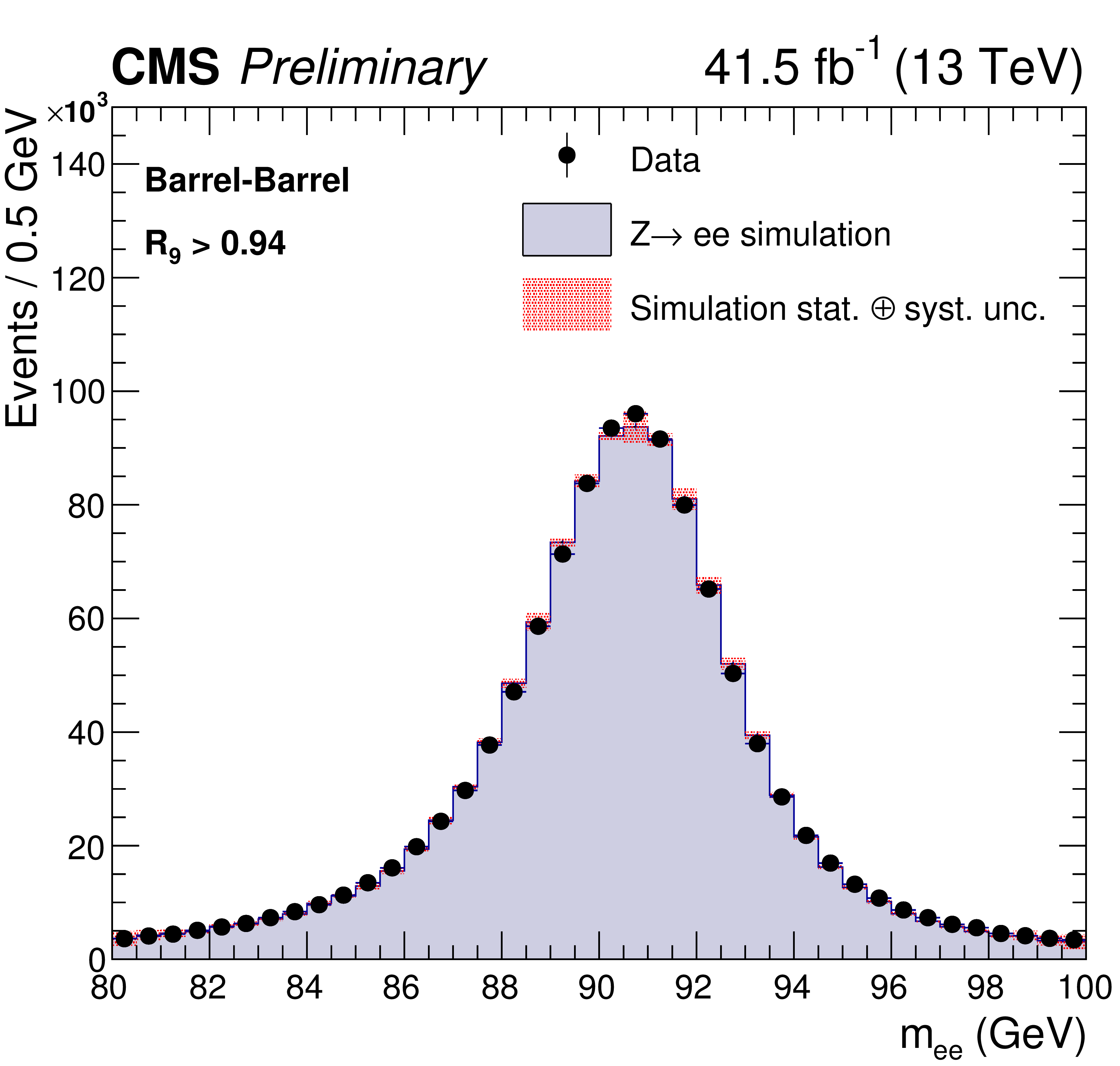
Comparison of the dielectron invariant mass spectra in data and simulation, after applying energy scale corrections to data and energy smearing to the simulation, for $ {\mathrm {Z}} \to {{\mathrm {e}^+} {\mathrm {e}^-}} $ events with electrons reconstructed as photons. The comparison is shown for events with both electrons in the ECAL barrel (left) and for all the remaining events (right). Electrons are required to satisfy $ {R_\mathrm {9}} > $ 0.94. |
png pdf |
Figure 1-a:
Comparison of the dielectron invariant mass spectra in data and simulation, after applying energy scale corrections to data and energy smearing to the simulation, for $ {\mathrm {Z}} \to {{\mathrm {e}^+} {\mathrm {e}^-}} $ events with electrons reconstructed as photons. The comparison is shown for events with both electrons in the ECAL barrel. |

png pdf |
Figure 1-b:
Comparison of the dielectron invariant mass spectra in data and simulation, after applying energy scale corrections to data and energy smearing to the simulation, for $ {\mathrm {Z}} \to {{\mathrm {e}^+} {\mathrm {e}^-}} $ events with electrons reconstructed as photons. The comparison is shown for events with at least one electron not in the ECAL barrel. Electrons are required to satisfy $ {R_\mathrm {9}} > $ 0.94. |

png pdf |
Figure 2:
Photon identification BDT score for $ {\mathrm {Z}} \to {{\mathrm {e}^+} {\mathrm {e}^-}} $ events in data and simulation, where the electrons are reconstructed as photons. Data (black markers) are compared to the Drell-Yan simulation (full histogram). The systematic uncertainty in the BDT output is shown in red. |
png pdf |
Figure 3:
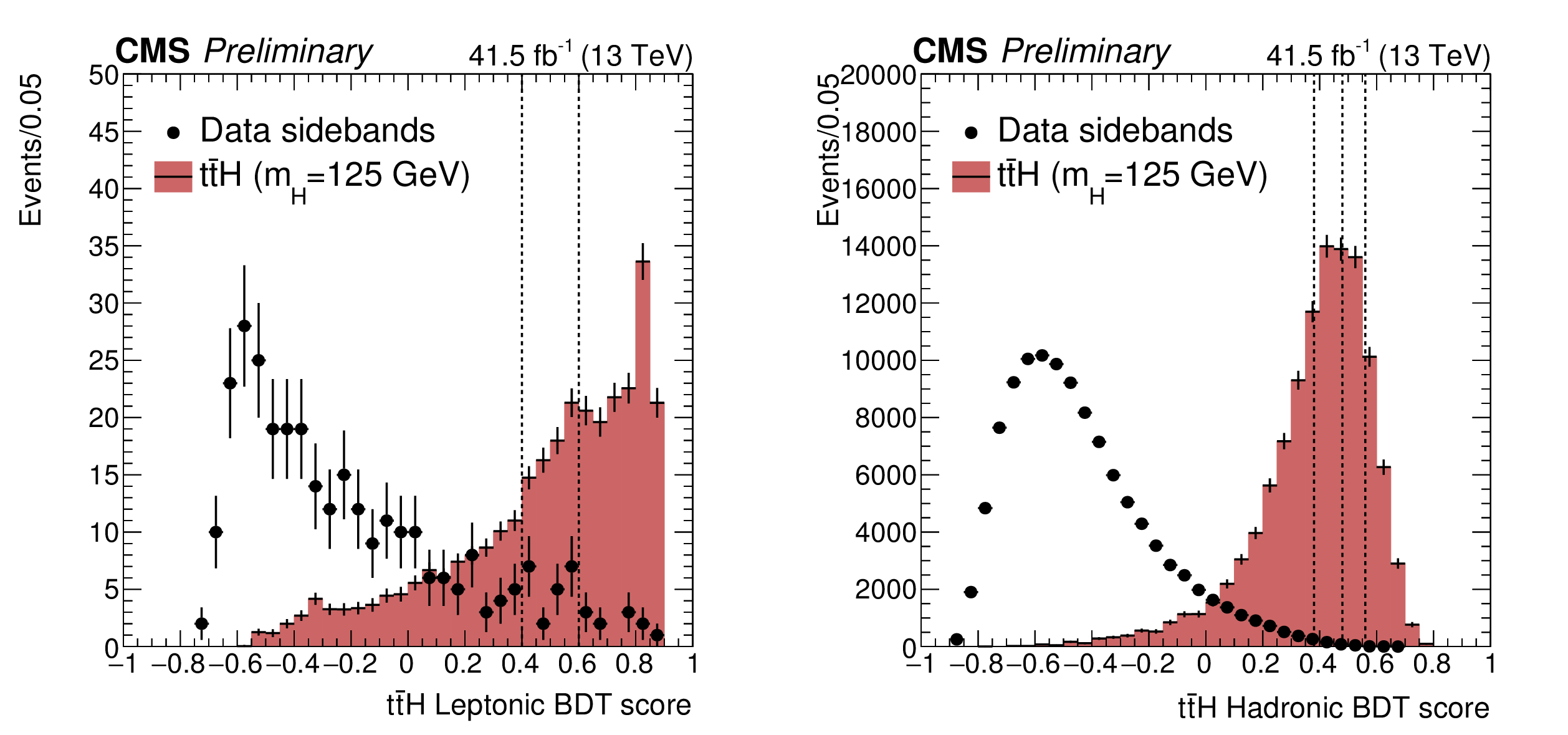
Distribution of the output of the $\mathrm{t\bar{t}H}$ BDTs for the leptonic categories (left) and the hadronic ones (right). Events are selected if the two photons have a photon identification score $ > -0.2$. At least one lepton and one b-tagged jet are required in the leptonic channel and no leptons and at least two jets in the hadronic one. Signal (red histogram) is compared to data sidebands (black markers), i.e. events in 100 $\leq \text {m}_{\gamma \gamma} < $ 115 GeV or 135 $\leq \text {m}_{\gamma \gamma} < $ 180 GeV, excluding the Higgs boson region. The signal histogram is scaled to match the area of the data one. Vertical lines represent the boundaries of the categories exploited in the analysis. |

png pdf |
Figure 3-a:
Distribution of the output of the $\mathrm{t\bar{t}H}$ BDTs for the leptonic categories. Events are selected if the two photons have a photon identification score $ > -0.2$. At least one lepton and one b-tagged jet are required in the leptonic channel and no leptons and at least two jets in the hadronic one. Signal (red histogram) is compared to data sidebands (black markers), i.e. events in 100 $\leq \text {m}_{\gamma \gamma} < $ 115 GeV or 135 $\leq \text {m}_{\gamma \gamma} < $ 180 GeV, excluding the Higgs boson region. The signal histogram is scaled to match the area of the data one. Vertical lines represent the boundaries of the categories exploited in the analysis. |

png pdf |
Figure 3-b:
Distribution of the output of the $\mathrm{t\bar{t}H}$ BDTs for the hadronic categories. Events are selected if the two photons have a photon identification score $ > -0.2$. At least one lepton and one b-tagged jet are required in the leptonic channel and no leptons and at least two jets in the hadronic one. Signal (red histogram) is compared to data sidebands (black markers), i.e. events in 100 $\leq \text {m}_{\gamma \gamma} < $ 115 GeV or 135 $\leq \text {m}_{\gamma \gamma} < $ 180 GeV, excluding the Higgs boson region. The signal histogram is scaled to match the area of the data one. Vertical lines represent the boundaries of the categories exploited in the analysis. |

png pdf |
Figure 4:
Parametrized signal shape for all categories, weighted by S/(S+B) as defined in the text. The open squares represent weighted simulation events and the blue line the corresponding model. Also shown is the $\sigma _{\text {eff}}$ value (half the width of the narrowest interval containing 68.3% of the invariant mass distribution), the full width at half of the maximum (FWHM) and the corresponding interval. |
png pdf |
Figure 5:
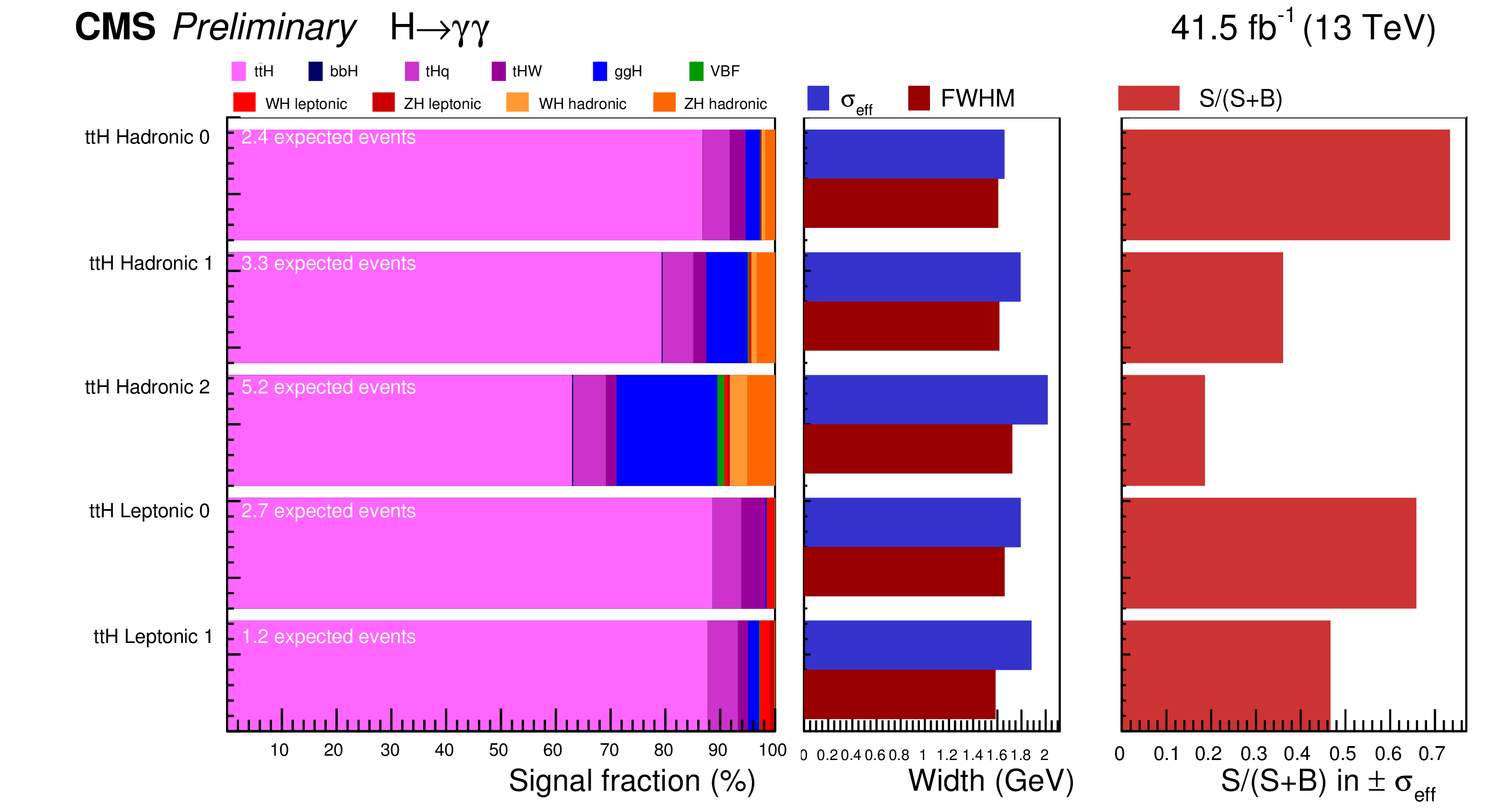
Expected fraction of signal events per production mode in the different categories. For each category, the $\sigma _{eff}$ and FWHM of the signal model, as described in the text, are given. The ratio of the number of signal events (S) to the number of signal plus background events (S+B) is shown on the right hand side. |

png pdf |
Figure 6:
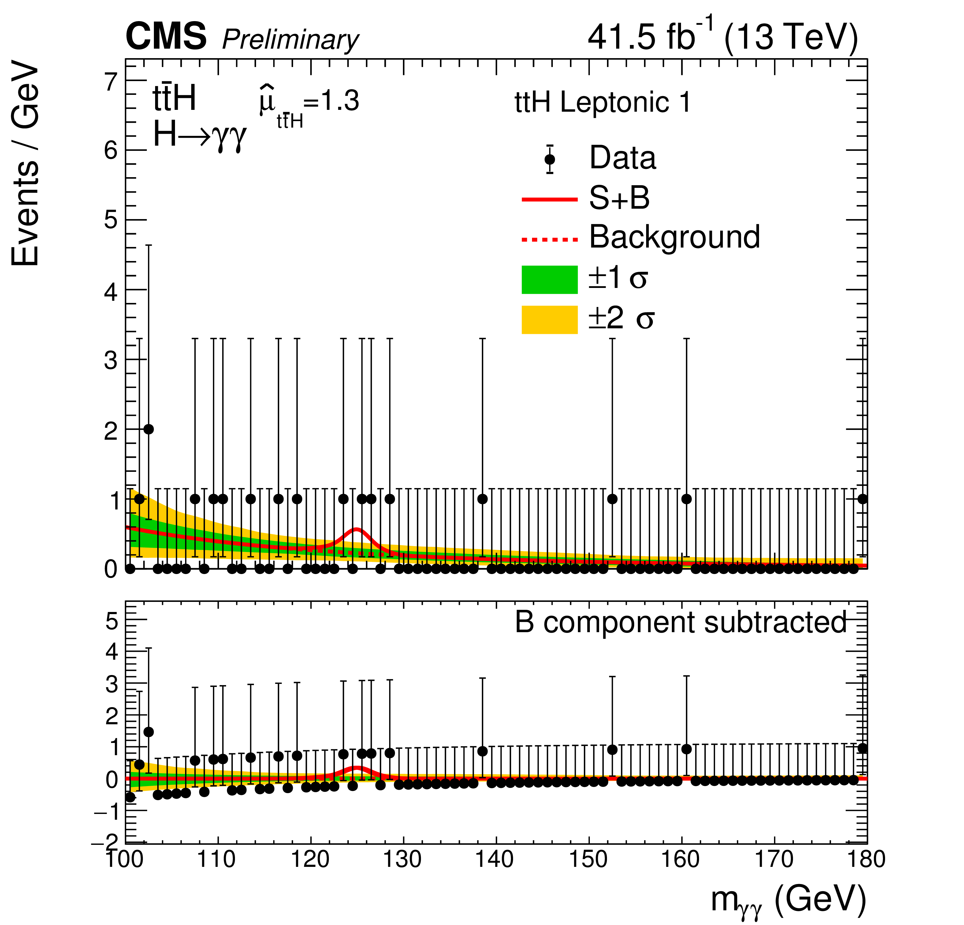
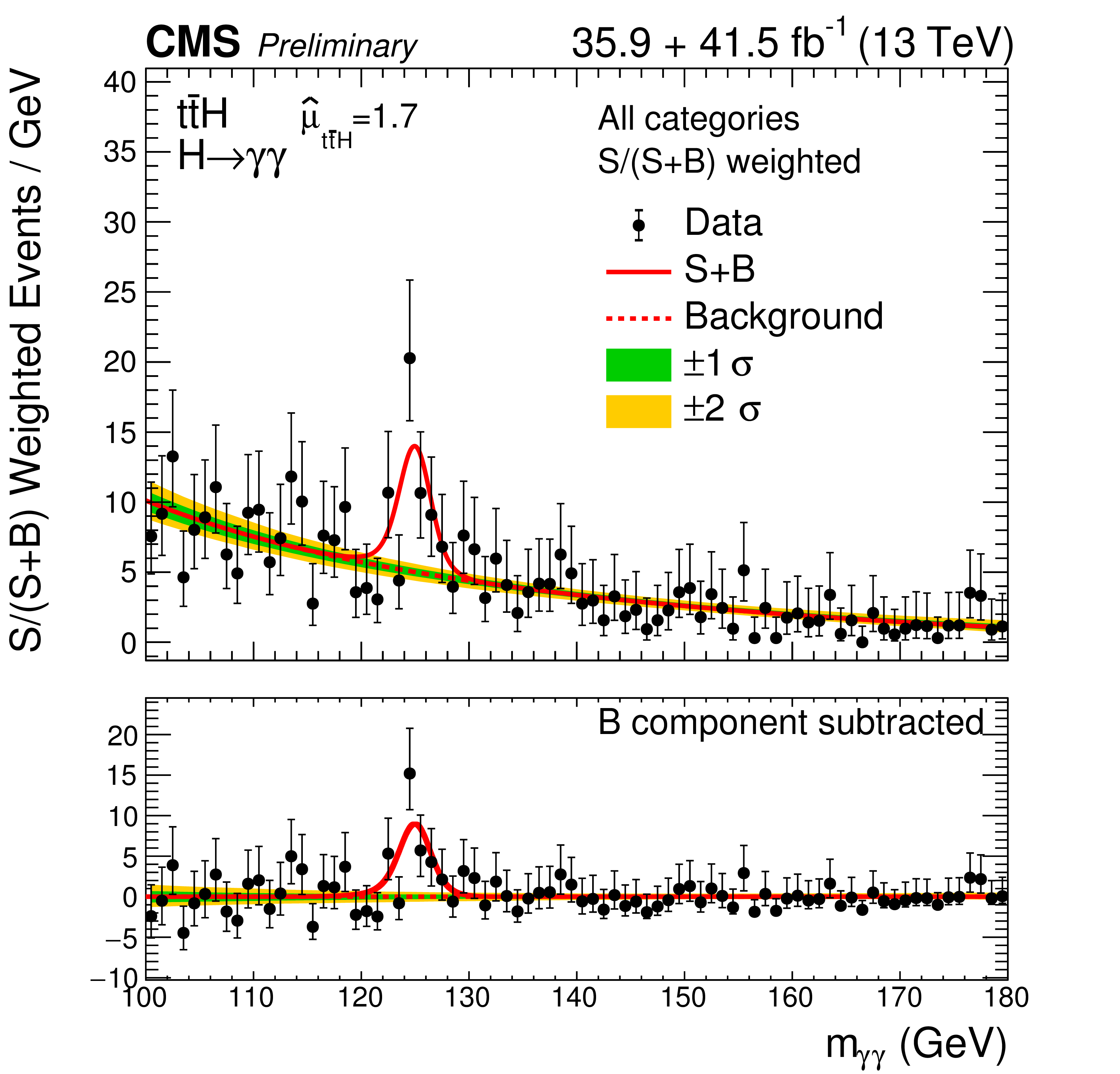
Data points (black) and signal plus background model fits in each category are shown. The $\mathrm{t\bar{t}H}$ signal strength reported in each plot is from the simultaneous fit to all 2017 categories. In the sum of all categories (bottom right), each category is weighted by S/(S + B), where S and B are the numbers of expected signal and background events, respectively, in a $ \pm $1$ \sigma _{eff}$ mass window centered on $m_{\textrm {H}}$. The one standard deviation (green) and two standard deviation (yellow) bands include the uncertainties in the background component of the fit. The solid red line shows the contribution from the total signal, plus the background contribution. The dashed red line shows the contribution from the background component of the fit. The bottom plot shows the residuals after subtraction of this background component. |

png pdf |
Figure 6-a:
Data points (black) and signal plus background model fit in the ttH Hadronic 0 category. The $\mathrm{t\bar{t}H}$ signal strength reported in each plot is from the simultaneous fit to all 2017 categories. In the sum of all categories (bottom right), each category is weighted by S/(S + B), where S and B are the numbers of expected signal and background events, respectively, in a $ \pm $1$ \sigma _{eff}$ mass window centered on $m_{\textrm {H}}$. The one standard deviation (green) and two standard deviation (yellow) bands include the uncertainties in the background component of the fit. The solid red line shows the contribution from the total signal, plus the background contribution. The dashed red line shows the contribution from the background component of the fit. The bottom plot shows the residuals after subtraction of this background component. |

png pdf |
Figure 6-b:
Data points (black) and signal plus background model fit in the ttH Hadronic 1 category. The $\mathrm{t\bar{t}H}$ signal strength reported in each plot is from the simultaneous fit to all 2017 categories. In the sum of all categories (bottom right), each category is weighted by S/(S + B), where S and B are the numbers of expected signal and background events, respectively, in a $ \pm $1$ \sigma _{eff}$ mass window centered on $m_{\textrm {H}}$. The one standard deviation (green) and two standard deviation (yellow) bands include the uncertainties in the background component of the fit. The solid red line shows the contribution from the total signal, plus the background contribution. The dashed red line shows the contribution from the background component of the fit. The bottom plot shows the residuals after subtraction of this background component. |

png pdf |
Figure 6-c:
Data points (black) and signal plus background model fit in the ttH Hadronic 2 category. The $\mathrm{t\bar{t}H}$ signal strength reported in each plot is from the simultaneous fit to all 2017 categories. In the sum of all categories (bottom right), each category is weighted by S/(S + B), where S and B are the numbers of expected signal and background events, respectively, in a $ \pm $1$ \sigma _{eff}$ mass window centered on $m_{\textrm {H}}$. The one standard deviation (green) and two standard deviation (yellow) bands include the uncertainties in the background component of the fit. The solid red line shows the contribution from the total signal, plus the background contribution. The dashed red line shows the contribution from the background component of the fit. The bottom plot shows the residuals after subtraction of this background component. |

png pdf |
Figure 6-d:
Data points (black) and signal plus background model fit in the ttH Leptonic 0 category. The $\mathrm{t\bar{t}H}$ signal strength reported in each plot is from the simultaneous fit to all 2017 categories. In the sum of all categories (bottom right), each category is weighted by S/(S + B), where S and B are the numbers of expected signal and background events, respectively, in a $ \pm $1$ \sigma _{eff}$ mass window centered on $m_{\textrm {H}}$. The one standard deviation (green) and two standard deviation (yellow) bands include the uncertainties in the background component of the fit. The solid red line shows the contribution from the total signal, plus the background contribution. The dashed red line shows the contribution from the background component of the fit. The bottom plot shows the residuals after subtraction of this background component. |
png pdf |
Figure 6-e:
Data points (black) and signal plus background model fit in the ttH Leptonic 1 category. The $\mathrm{t\bar{t}H}$ signal strength reported in each plot is from the simultaneous fit to all 2017 categories. In the sum of all categories (bottom right), each category is weighted by S/(S + B), where S and B are the numbers of expected signal and background events, respectively, in a $ \pm $1$ \sigma _{eff}$ mass window centered on $m_{\textrm {H}}$. The one standard deviation (green) and two standard deviation (yellow) bands include the uncertainties in the background component of the fit. The solid red line shows the contribution from the total signal, plus the background contribution. The dashed red line shows the contribution from the background component of the fit. The bottom plot shows the residuals after subtraction of this background component. |

png pdf |
Figure 6-f:
Data points (black) and signal plus background model fit for all categories, weighted by S/(S + B), where S and B are the numbers of expected signal and background events, respectively. The $\mathrm{t\bar{t}H}$ signal strength reported in each plot is from the simultaneous fit to all 2017 categories. In the sum of all categories (bottom right), each category is weighted by S/(S + B), where S and B are the numbers of expected signal and background events, respectively, in a $ \pm $1$ \sigma _{eff}$ mass window centered on $m_{\textrm {H}}$. The one standard deviation (green) and two standard deviation (yellow) bands include the uncertainties in the background component of the fit. The solid red line shows the contribution from the total signal, plus the background contribution. The dashed red line shows the contribution from the background component of the fit. The bottom plot shows the residuals after subtraction of this background component. |

png pdf |
Figure 7:
The likelihood scan for the $\mathrm{t\bar{t}H}$ signal strength where the value of the standard model Higgs boson mass is constrained to the Run I combination [9]. |

png pdf |
Figure 8:
Signal strength modifiers measured for each analysis category (black points), with the value of the standard model Higgs boson mass constrained to the Run I combination, compared to the overall signal strength (green band) and to the SM expectation (dashed red line). |

png pdf |
Figure 9:
The likelihood scan for the $\mathrm{t\bar{t}H}$ signal strength where the value of the SM Higgs boson mass is constrained to the Run I combination [9] in the fit combining 2016 and 2017 analysis. |
png pdf |
Figure 10:
Data points (black) and signal plus background model fits for all categories weighted by S/(S + B), where S and B are the numbers of expected signal and background events, respectively, in a $ \pm $1$ \sigma _{eff}$ mass window centered on $m_{\textrm {H}}$. The $\mathrm{t\bar{t}H}$ signal strength (top left) is from a simultaneous fit to all categories. The one standard deviation (green) and two standard deviation (yellow) bands include the uncertainties in the background component of the fit. The solid red line shows the contribution from the total signal, plus the background contribution. The dashed red line shows the contribution from the background component of the fit. The bottom plot shows the residuals after subtraction of this background component. |
| Tables | |

png pdf |
Table 1:
Schema of the photon preselection requirements. |
png pdf |
Table 2:
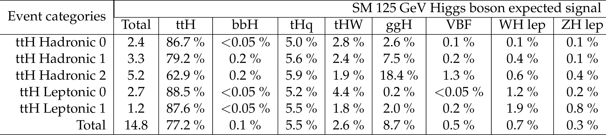
The expected number of signal events per category and the percentage breakdown per production mode in that category. The $\sigma _{eff}$, computed as the smallest interval containing 68.3% of the invariant mass distribution, and FWHM, computed as the width of the distribution at half of its highest point divided by 2.35 are also shown as an estimate of the $m_{\gamma \gamma}$ resolution in that category. The expected number of background events per $ GeV $ around $125 GeV $ is also listed. |
| Summary |
| This paper reports the measurement of the $\mathrm{t\bar{t}H}$ production rate, with the Higgs boson decaying into a pair of photons. The analysis is based on 41.5 fb$^{-1}$ collected in 2017 by the CMS detector. The measured signal strength is $\mu = $ 1.3$^{+0.7}_{-0.5}$, corresponding to a significance relative to the background-only hypothesis of 3.1$\sigma$. The measurement is limited by the statistical uncertainty and is in agreement with the SM expectation. The combination with the corresponding 2016 data analysis [16] is also reported. The combined measured signal strength is $\mu = $ 1.7$^{+0.6}_{-0.5}$, corresponding to a significance relative to the background-only hypothesis of 4.1$\sigma$. |
| References | ||||
| 1 | ATLAS Collaboration | Observation of a new particle in the search for the Standard Model Higgs boson with the detector at the LHC | PLB716 (2012) 1--29 | 1207.7214 |
| 2 | CMS Collaboration | Observation of a new boson at a mass of 125 GeV with the CMS experiment at the LHC | PLB716 (2012) 30--61 | CMS-HIG-12-028 1207.7235 |
| 3 | F. Englert and R. Brout | Broken Symmetry and the Mass of Gauge Vector Mesons | PRL 13 (1964) 321--323 | |
| 4 | P. W. Higgs | Broken symmetries, massless particles and gauge fields | PL12 (1964) 132--133 | |
| 5 | P. W. Higgs | Broken Symmetries and the Masses of Gauge Bosons | PRL 13 (1964) 508--509 | |
| 6 | G. S. Guralnik, C. R. Hagen, and T. W. B. Kibble | Global Conservation Laws and Massless Particles | PRL 13 (1964) 585--587 | |
| 7 | P. W. Higgs | Spontaneous Symmetry Breakdown without Massless Bosons | PR145 (1966) 1156--1163 | |
| 8 | T. W. B. Kibble | Symmetry breaking in nonAbelian gauge theories | PR155 (1967) 1554--1561 | |
| 9 | \relax ATLAS and CMS Collaborations | Combined Measurement of the Higgs Boson Mass in $ pp $ Collisions at $ \sqrt{s}= $ 7 and 8 TeV with the ATLAS and CMS Experiments | PRL 114 (2015) 191803 | 1503.07589 |
| 10 | \relax ATLAS and CMS Collaborations | Measurements of the Higgs boson production and decay rates and constraints on its couplings from a combined ATLAS and CMS analysis of the LHC pp collision data at $ \sqrt{s}= $ 7 and 8 TeV | JHEP 08 (2016) 045 | 1606.02266 |
| 11 | ATLAS Collaboration | Combined measurements of Higgs boson production and decay using up to 80 fb$ ^{-1} $ of proton--proton collision data at $ \sqrt{s}= $ 13 TeV collected with the ATLAS experiment | ATLAS-CONF-2018-031, CERN, Geneva, Jul | |
| 12 | CMS Collaboration | Combined measurements of Higgs boson couplings in proton-proton collisions at $ \sqrt{s}= $ 13 TeV | Submitted to: EPJ(2018) | CMS-HIG-17-031 1809.10733 |
| 13 | CMS Collaboration | Measurement of the top quark mass using proton-proton data at $ {\sqrt{s}} = $ 7 and 8 TeV | PRD93 (2016), no. 7, 072004 | CMS-TOP-14-022 1509.04044 |
| 14 | ATLAS Collaboration | Observation of Higgs boson production in association with a top quark pair at the LHC with the ATLAS detector | PLB784 (2018) 173--191 | 1806.00425 |
| 15 | CMS Collaboration | Observation of $ \mathrm{t\overline{t}} $H production | PRL 120 (2018), no. 23, 231801 | CMS-HIG-17-035 1804.02610 |
| 16 | CMS Collaboration | Measurements of Higgs boson properties in the diphoton decay channel in proton-proton collisions at $ \sqrt{s} = $ 13 TeV | CMS-HIG-16-040 1804.02716 |
|
| 17 | CMS Collaboration | Particle-flow reconstruction and global event description with the cms detector | JINST 12 (2017) P10003 | CMS-PRF-14-001 1706.04965 |
| 18 | M. Cacciari, G. P. Salam, and G. Soyez | The Anti-k(t) jet clustering algorithm | JHEP 04 (2008) 063 | 0802.1189 |
| 19 | M. Cacciari, G. P. Salam, and G. Soyez | FastJet user manual | EPJC 72 (2012) 1896 | 1111.6097 |
| 20 | CMS Collaboration | Description and performance of track and primary-vertex reconstruction with the CMS tracker | JINST 9 (2014), no. 10, P10009 | CMS-TRK-11-001 1405.6569 |
| 21 | CMS Collaboration | Identification of heavy-flavour jets with the CMS detector in pp collisions at 13 TeV | JINST 13 (2018), no. 05, P05011 | CMS-BTV-16-002 1712.07158 |
| 22 | CMS Collaboration | The CMS experiment at the CERN LHC | JINST 3 (2008) S08004 | CMS-00-001 |
| 23 | CMS Collaboration | Measurement of the Inclusive $ W $ and $ Z $ Production Cross Sections in $ pp $ Collisions at $ \sqrt{s}= $ 7 TeV | JHEP 10 (2011) 132 | CMS-EWK-10-005 1107.4789 |
| 24 | J. Alwall et al. | The automated computation of tree-level and next-to-leading order differential cross sections, and their matching to parton shower simulations | JHEP 07 (2014) 079 | 1405.0301 |
| 25 | T. Sjostrand et al. | An Introduction to PYTHIA 8.2 | CPC 191 (2015) 159--177 | 1410.3012 |
| 26 | LHC Higgs Cross Section Working Group Collaboration | Handbook of LHC Higgs Cross Sections: 4. Deciphering the Nature of the Higgs Sector | 1610.07922 | |
| 27 | P. Nason | A New method for combining NLO QCD with shower Monte Carlo algorithms | JHEP 11 (2004) 040 | hep-ph/0409146 |
| 28 | S. Frixione, P. Nason, and C. Oleari | Matching NLO QCD computations with Parton Shower simulations: the POWHEG method | JHEP 11 (2007) 070 | 0709.2092 |
| 29 | S. Alioli, P. Nason, C. Oleari, and E. Re | A general framework for implementing NLO calculations in shower Monte Carlo programs: the POWHEG BOX | JHEP 06 (2010) 043 | 1002.2581 |
| 30 | H. B. Hartanto, B. Jager, L. Reina, and D. Wackeroth | Higgs boson production in association with top quarks in the POWHEG BOX | PRD91 (2015), no. 9, 094003 | 1501.04498 |
| 31 | T. Gleisberg et al. | Event generation with SHERPA 1.1 | JHEP 02 (2009) 007 | 0811.4622 |
| 32 | GEANT4 Collaboration | GEANT4: A Simulation toolkit | NIMA506 (2003) 250--303 | |
| 33 | CMS Collaboration | Energy Calibration and Resolution of the CMS Electromagnetic Calorimeter in $ pp $ Collisions at $ \sqrt{s} = $ 7 TeV | JINST 8 (2013) P09009 | CMS-EGM-11-001 1306.2016 |
| 34 | CMS Collaboration | Performance of Photon Reconstruction and Identification with the CMS Detector in Proton-Proton Collisions at sqrt(s) = 8 TeV | JINST 10 (2015), no. 08, P08010 | CMS-EGM-14-001 1502.02702 |
| 35 | P. D. Dauncey, M. Kenzie, N. Wardle, and G. J. Davies | On the interpretation of $ \chi^2 $ from contingency tables, and the calculation of p | JINST 10 (2015), no. 04, P04015 | 1408.6865 |
| 36 | CMS Collaboration | Observation of the diphoton decay of the Higgs boson and measurement of its properties | EPJC74 (2014), no. 10 | CMS-HIG-13-001 1407.0558 |
| 37 | R. A. Fisher | Handling uncertainties in background shapes | Journal of the Royal Statistical Society 85 (1922), no. 87 | |
| 38 | J. Butterworth et al. | PDF4LHC recommendations for LHC Run II | JPG43 (2016) 023001 | 1510.03865 |
| 39 | LHC Higgs Cross Section Working Group Collaboration | Handbook of LHC Higgs Cross Sections: 3. Higgs Properties: Report of the LHC Higgs Cross Section Working Group | CERN-2013-004. CERN-2013-004, CERN, Jul, 2013 Comments: 404 pages, 139 figures, to be submitted to . Working Group web page: https://twiki.cern.ch/twiki/bin/view/LHCPhysics/CrossSections | |
| 40 | NNPDF Collaboration | Parton distributions for the LHC Run II | JHEP 04 (2015) 040 | 1410.8849 |
| 41 | S. Carrazza et al. | An Unbiased Hessian Representation for Monte Carlo PDFs | EPJC75 (2015), no. 8, 369 | 1505.06736 |
| 42 | CMS Collaboration | Measurement of the differential cross section for $ \mathrm{t \bar t} $ production in the dilepton final state at $ \sqrt{s}= $ 13 TeV | CMS-PAS-TOP-16-011 | CMS-PAS-TOP-16-011 |
| 43 | CMS Collaboration | Measurement of the cross section ratio ttbar+bbbar/ttbar+jj using dilepton final states in pp collisions at 13 TeV | CMS-PAS-TOP-16-010 | CMS-PAS-TOP-16-010 |
| 44 | CMS Collaboration | Jet algorithms performance in 13 TeV data | CMS-PAS-JME-16-003 | CMS-PAS-JME-16-003 |
| 45 | CMS Collaboration Collaboration | CMS luminosity measurement for the 2017 data-taking period at $ \sqrt{s} = $ 13 TeV | CMS-PAS-LUM-17-004, CERN, Geneva | |
| 46 | The ATLAS Collaboration, The CMS Collaboration, The LHC Higgs Combination Group Collaboration | Procedure for the LHC Higgs boson search combination in Summer 2011 | CMS-NOTE-2011-005 | |
| 47 | T. Junk | Confidence level computation for combining searches with small statistics | NIMA434 (1999) 435--443 | hep-ex/9902006 |
| 48 | A. L. Read | Modified frequentist analysis of search results (The CL(s) method) | in Workshop on confidence limits, CERN, Geneva, Switzerland, 17-18 Jan 2000: Proceedings, pp. 81--1012000 | |
| 49 | G. Cowan, K. Cranmer, E. Gross, and O. Vitells | Asymptotic formulae for likelihood-based tests of new physics | EPJC71 (2011) 1554 | 1007.1727 |
|
|
Compact Muon Solenoid LHC, CERN |
|

|

|

|

|

|