

Compact Muon Solenoid
LHC, CERN
| CMS-PAS-SUS-16-014 | ||
| Search for supersymmetry in events with jets and missing transverse momentum in proton-proton collisions at 13 TeV | ||
| CMS Collaboration | ||
| August 2016 | ||
| Abstract: A search for supersymmetry is performed in all-hadronic events with large missing transverse momentum produced in proton-proton collisions at $\sqrt{s}=$ 13 TeV. The data sample, corresponding to an integrated luminosity of 12.9 fb$^{-1}$, was collected with the CMS detector at the CERN LHC in 2016. The data are examined in search regions of jet multiplicity, tagged bottom quark jet multiplicity, missing transverse momentum, and the scalar sum of jet transverse momenta. The observed numbers of events in all search regions are found to be consistent with the expectations from standard model processes. Exclusion limits are presented for simplified supersymmetric models of gluino pair production and direct squark-antisquark production. For a massless, weakly interacting, lightest neutralino, lower limits on the gluino mass from around 1620 to 1750 GeV are obtained, depending on the assumed gluino decay mechanism. The corresponding limit on the squark mass varies between around 780 and 1150 GeV, depending on the assumed flavor of the squark. These results extend previous limits. | ||
| Links: CDS record (PDF) ; inSPIRE record ; CADI line (restricted) ; | ||
| Figures & Tables | Summary | Additional Figures & Tables | References | CMS Publications |
|---|
| Additional information on efficiencies needed for reinterpretation of these results are available here. |
| Figures | |
png pdf |
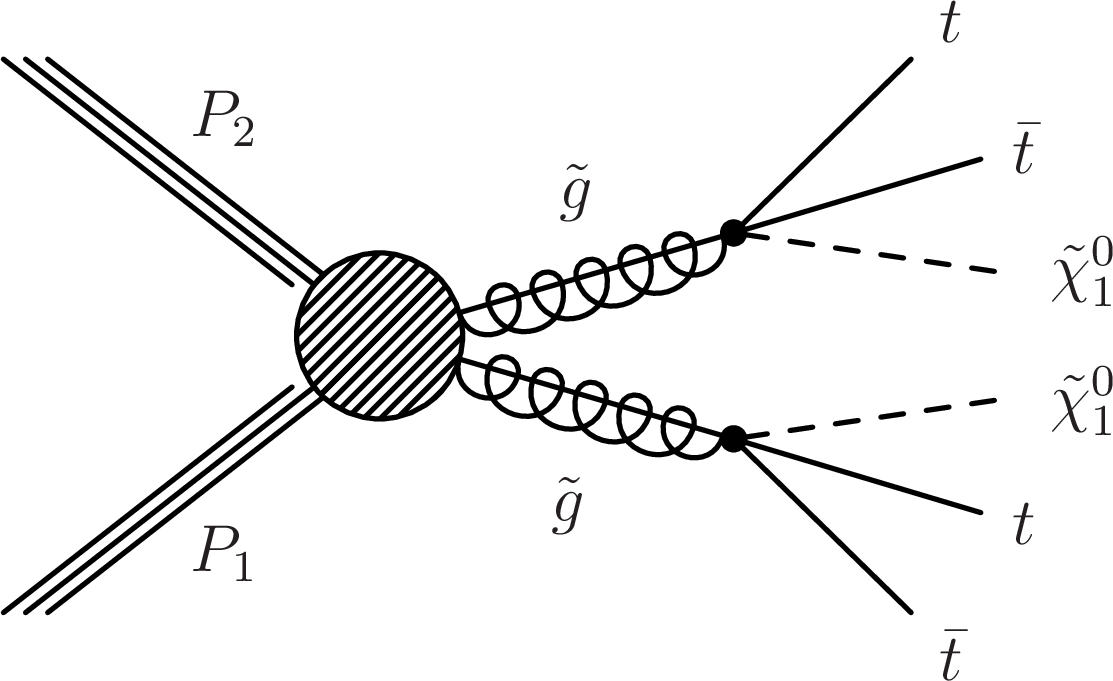
Figure 1-a:
Example event diagram for the signal scenarios considered in this study: the T1tttt simplified model. |
png pdf |
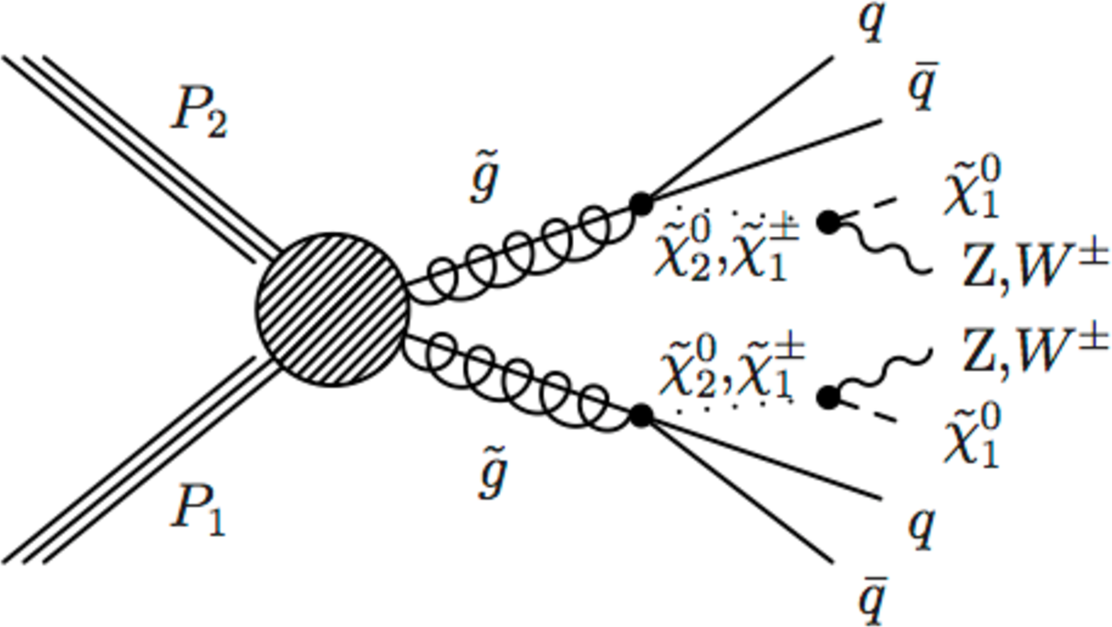
Figure 1-b:
Example event diagram for the signal scenarios considered in this study: the T5qqqqVV simplified model. The quark ${ {\mathrm {q}}}$ and antiquark ${ {\overline {\mathrm {q}}}}$ do not have the same flavor if the gluino $\tilde{g}$ decays as $ \tilde{g}\rightarrow {\mathrm {q}} {\overline {\mathrm {q}}} {\tilde{\chi}^{\pm}_{1}}$, where $ {\tilde{\chi}^{\pm}_{1}}$ is the lightest chargino. |
png pdf |
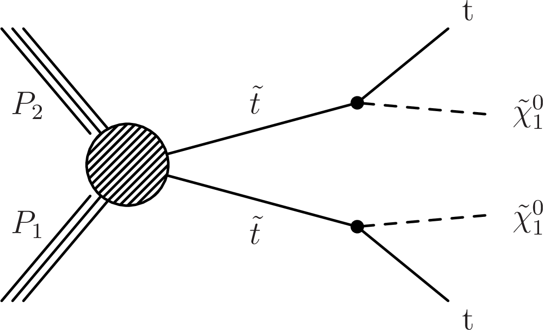
Figure 1-c:
Example event diagram for the signal scenarios considered in this study: the T2tt simplified model. |
png pdf |
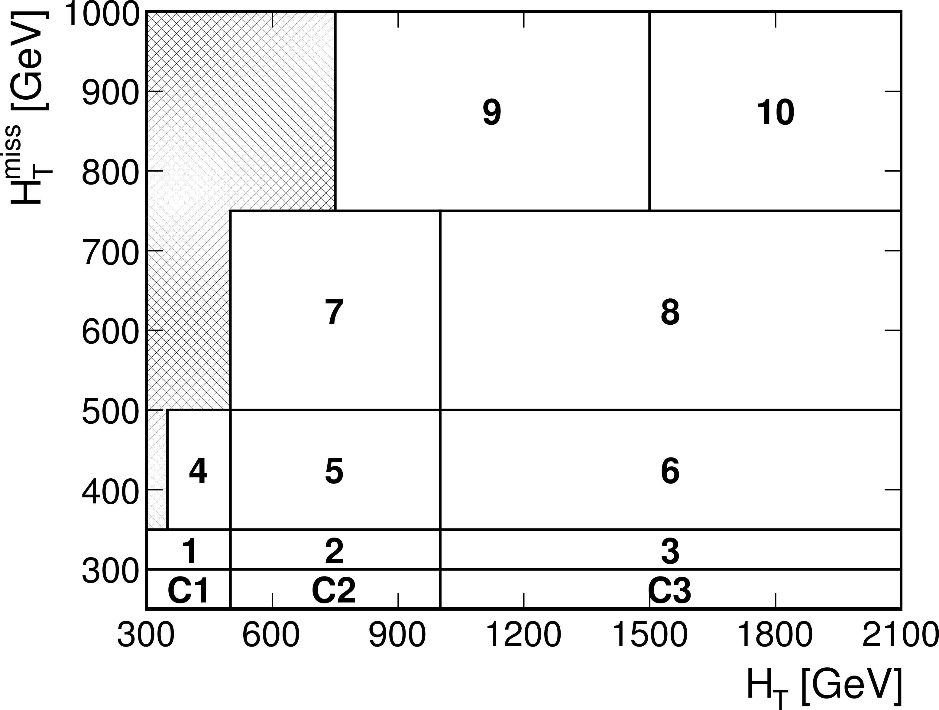
Figure 2:
Schematic illustration of the 10 search intervals in the ${H_{\mathrm T}^{\text {miss}}}$ versus ${H_{\mathrm {T}}}$ plane. Each of these intervals is examined in four ${N_{\text {jet}}} $ and four ${N_{{ {\mathrm {b}}}\text {-jet}}}$ bins, giving a total of 160 search regions. The intervals labeled C1, C2, and C3 are control regions used to evaluate the QCD multijet background. Note that the rightmost and topmost bins extend to $ {H_{\mathrm {T}}} =\infty $ and $ {H_{\mathrm T}^{\text {miss}}} =\infty $, respectively. |

png pdf |
Figure 3-a:
(a) The lost-lepton background in the 160 search regions of the analysis as determined directly from ${\mathrm {t}\overline {\mathrm {t}}}$ , single top quark, W+jets , diboson, and rare-event simulation (points, with statistical uncertainties) and as predicted by applying the lost-lepton background determination procedure to simulated electron and muon control samples (histograms, with statistical uncertainties). The lower panel shows the same results following division by the predicted value, where bins without markers have ratio values outside the scale of the plot. (b) The corresponding simulated results for the background from hadronically decaying $\tau $ leptons. For both plots, the 10 results within each region delineated by dashed lines correspond sequentially to the 10 regions of ${H_{\mathrm {T}}}$ and ${H_{\mathrm T}^{\text {miss}}}$ indicated in Table 1 and Fig. 2. |

png pdf |
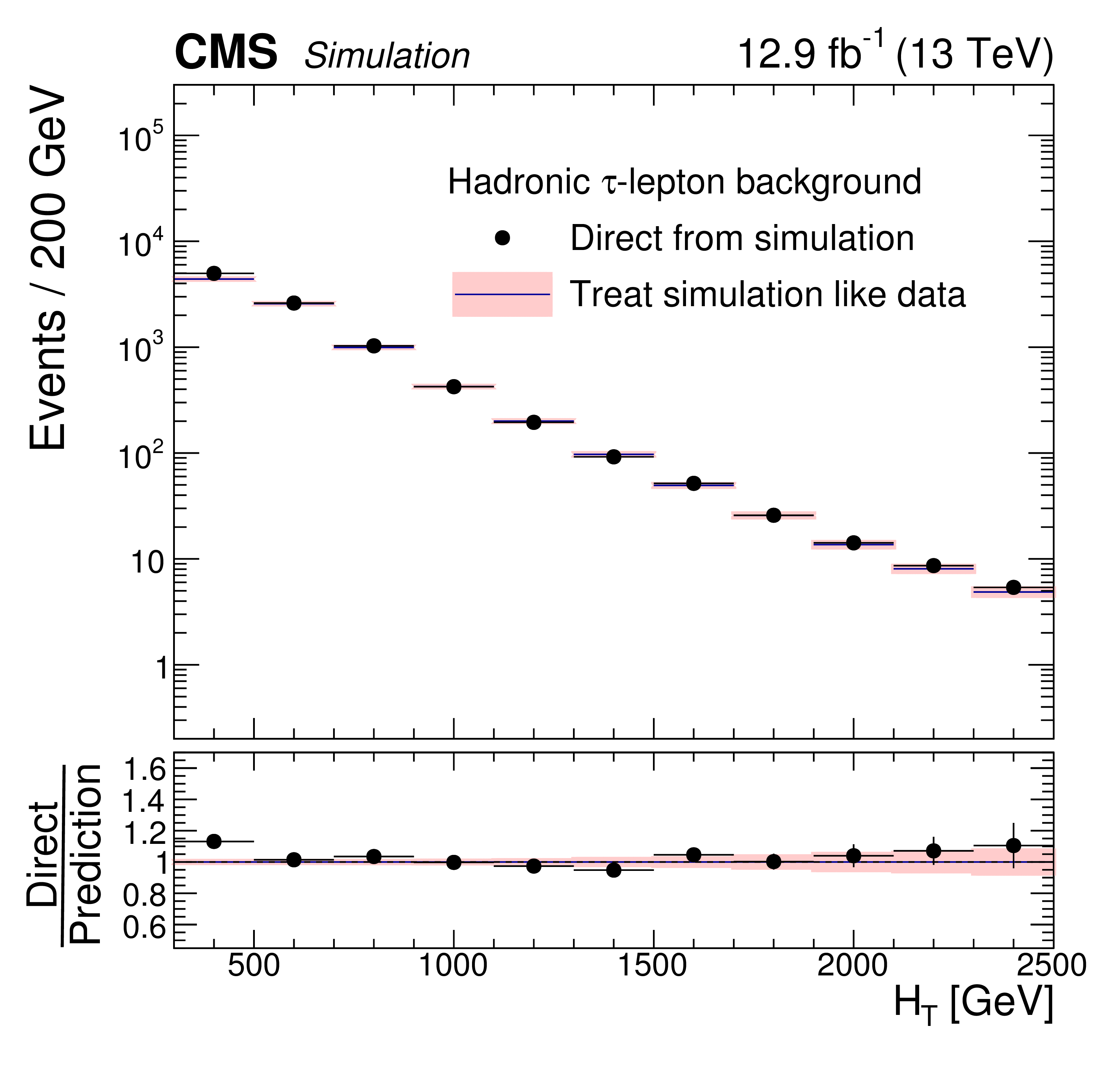
Figure 3-b:
(a) The lost-lepton background in the 160 search regions of the analysis as determined directly from ${\mathrm {t}\overline {\mathrm {t}}}$ , single top quark, W+jets , diboson, and rare-event simulation (points, with statistical uncertainties) and as predicted by applying the lost-lepton background determination procedure to simulated electron and muon control samples (histograms, with statistical uncertainties). The lower panel shows the same results following division by the predicted value, where bins without markers have ratio values outside the scale of the plot. (b) The corresponding simulated results for the background from hadronically decaying $\tau $ leptons. For both plots, the 10 results within each region delineated by dashed lines correspond sequentially to the 10 regions of ${H_{\mathrm {T}}}$ and ${H_{\mathrm T}^{\text {miss}}}$ indicated in Table 1 and Fig. 2. |
png pdf |
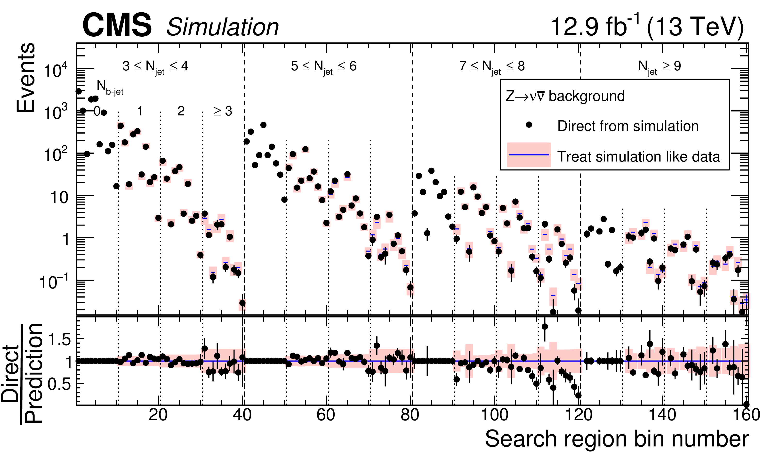
Figure 4:
The ${ {\mathrm {Z}}\to {\nu } {\overline {\nu }}}$ background in the 160 search regions of the analysis as determined directly from $ { {\mathrm {Z}}(\to {\nu } {\overline {\nu }})}$+jets and $ {\mathrm {t}\overline {\mathrm {t}}} {\mathrm {Z}}$ simulation (points), and as predicted by applying the ${ {\mathrm {Z}}\to {\nu } {\overline {\nu }}}$ background determination procedure to statistically independent $ { {\mathrm {Z}}(\to \ell ^{+} \ell ^{-} )}$+jets simulated event samples (histogram). For bins corresponding to $ {N_{{ {\mathrm {b}}}\text {-jet}}} =$ 0, the agreement is exact by construction. The lower panel shows the ratio between the true and predicted yields. For both the upper and lower panels, the shaded regions indicate the quadrature sum of the systematic uncertainty associated with the dependence of $\mathcal {F}$ on the kinematic parameters ( ${H_{\mathrm {T}}}$ and ${H_{\mathrm T}^{\text {miss}}}$ ) and the statistical uncertainty of the simulated sample. The labeling of the search regions is the same as in Fig. 3. |
png pdf |
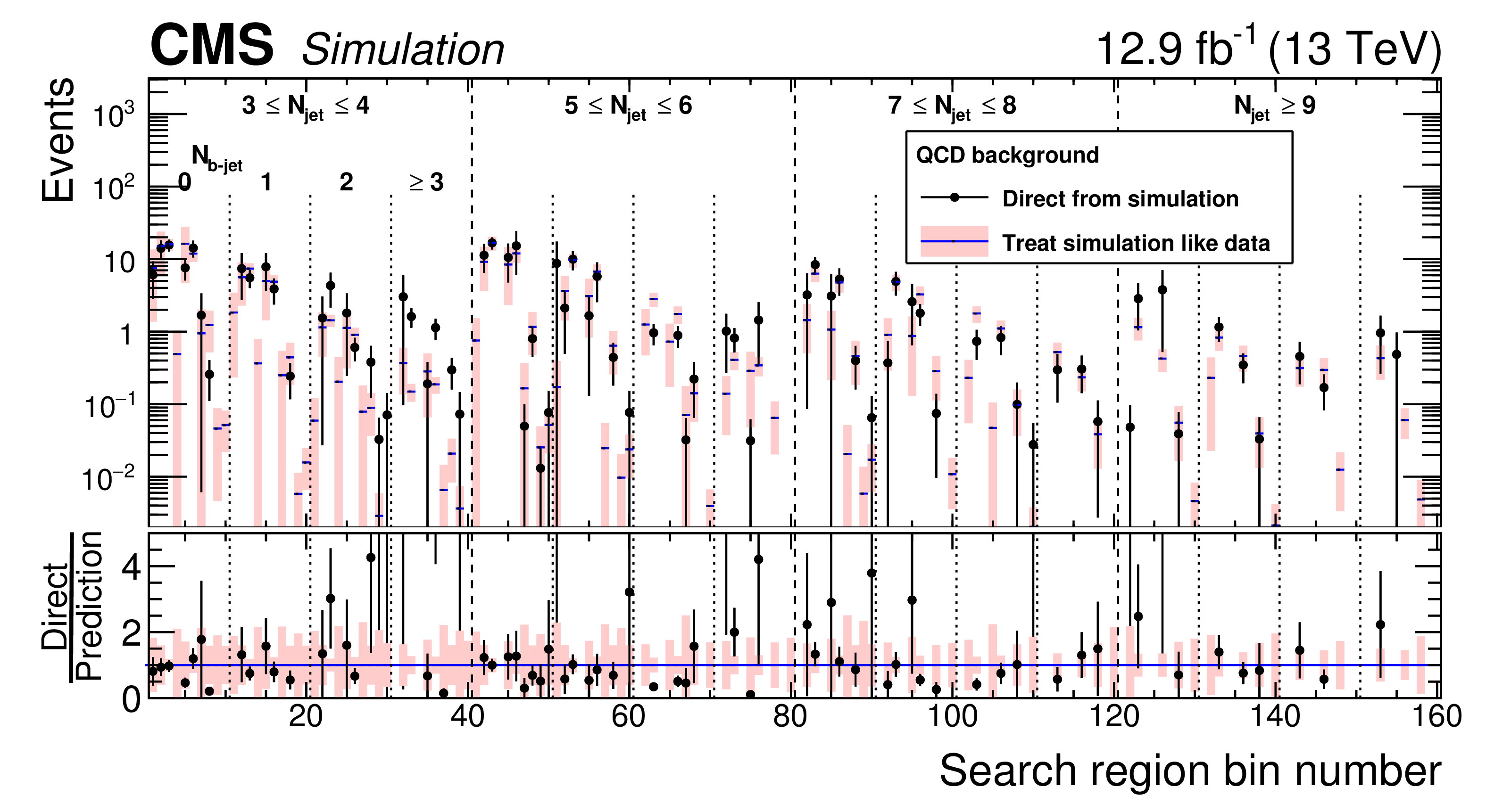
Figure 5:
The QCD multijet background in the 160 search regions of the analysis as determined directly from QCD multijet simulation (points, with statistical uncertainties) and as predicted by applying the QCD multijet background determination procedure to simulated event samples (histograms, with statistical and systematic uncertainties added in quadrature). The lower panel shows the same results following division by the predicted value. The labeling of the search regions is the same as in Fig. 3. Bins without markers have no events in the control regions. No result is given in the lower panel if the value of the prediction is zero. |
png pdf |
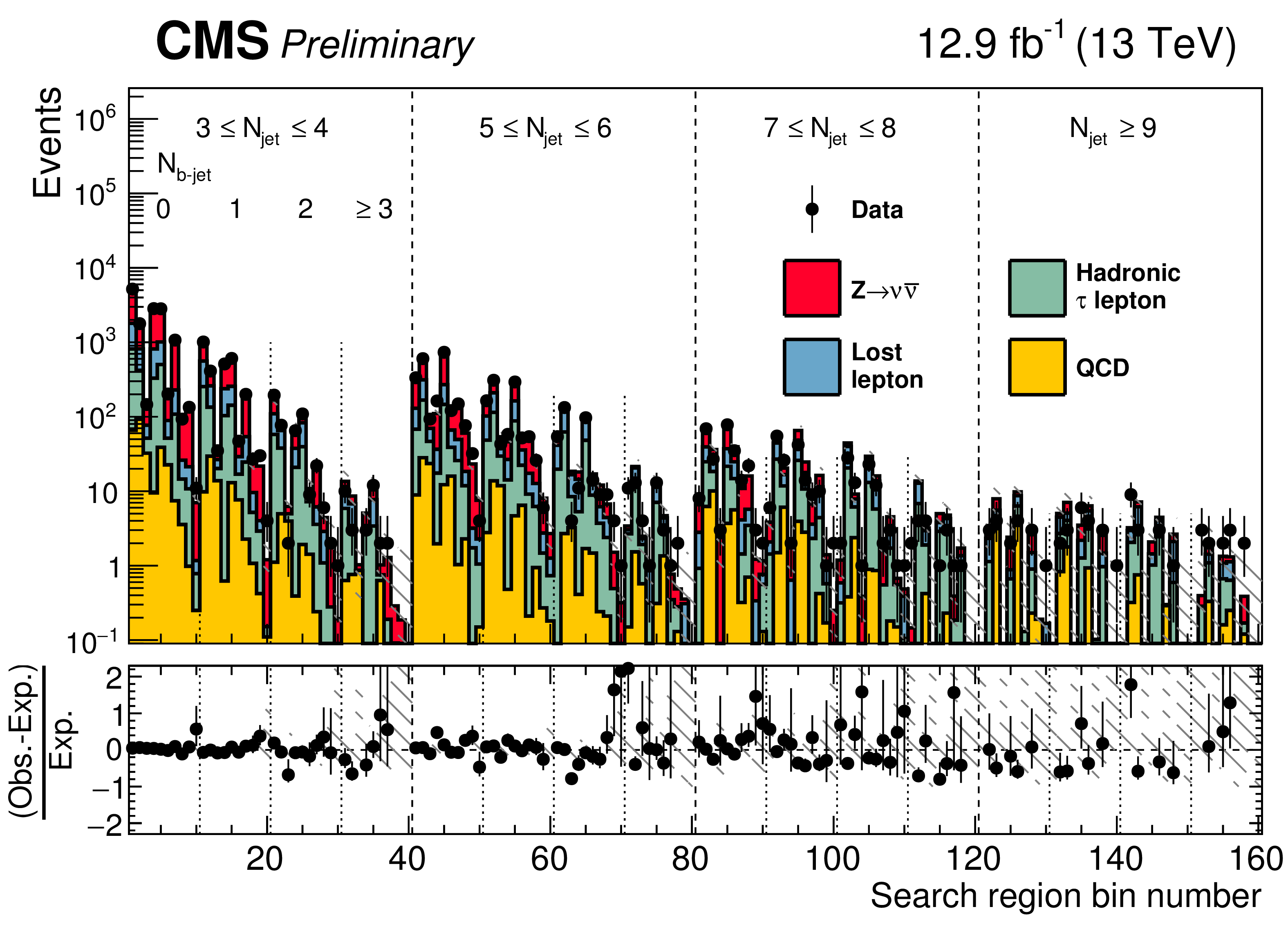
Figure 6:
Observed numbers of events and corresponding prefit SM background predictions in the 160 search regions of the analysis, with fractional differences shown in the lower panel. The shaded regions indicate the total uncertainties in the background predictions. The numerical values are tabulated in Appendix. The labeling of the search regions is the same as in Fig. 3. |
png pdf |
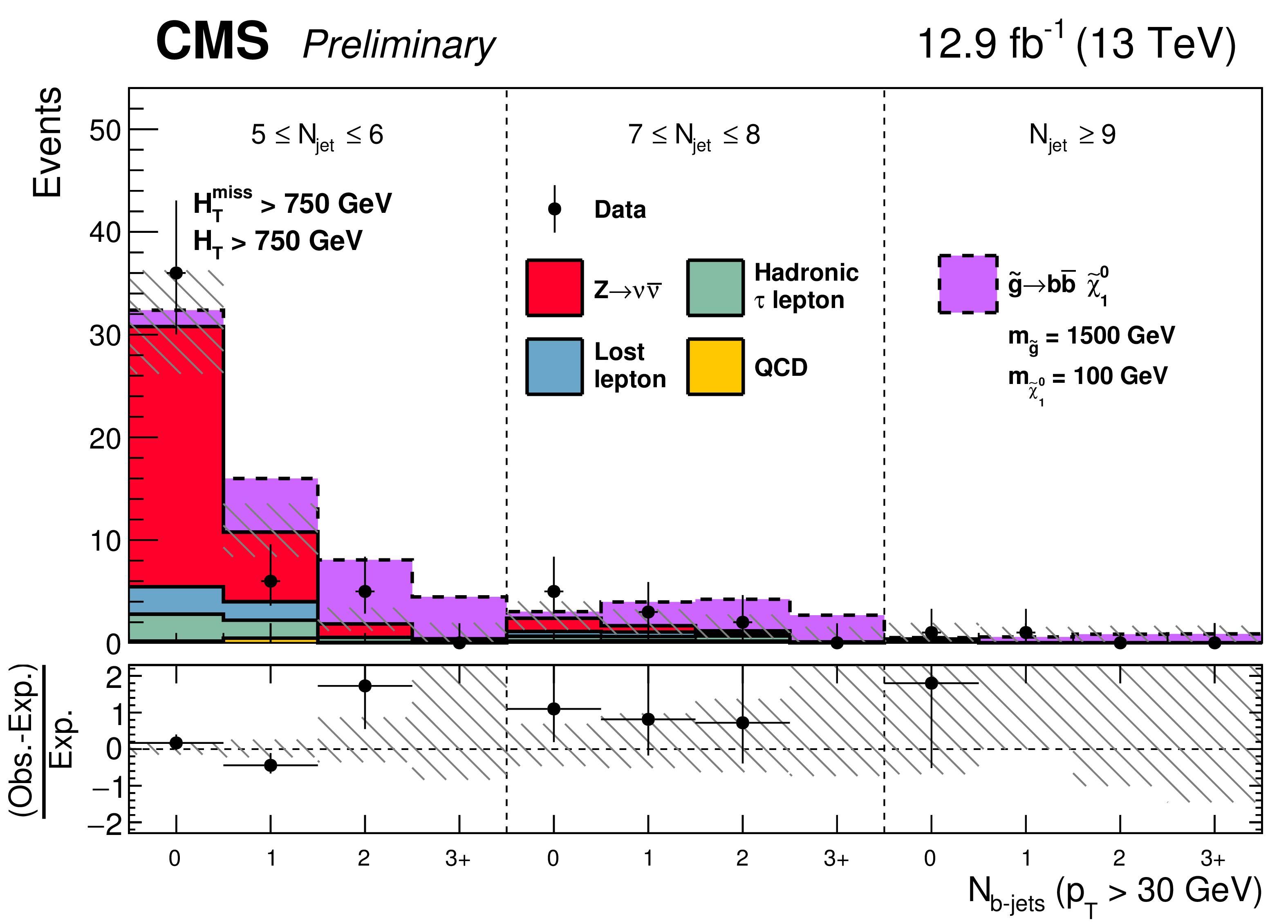
Figure 7:
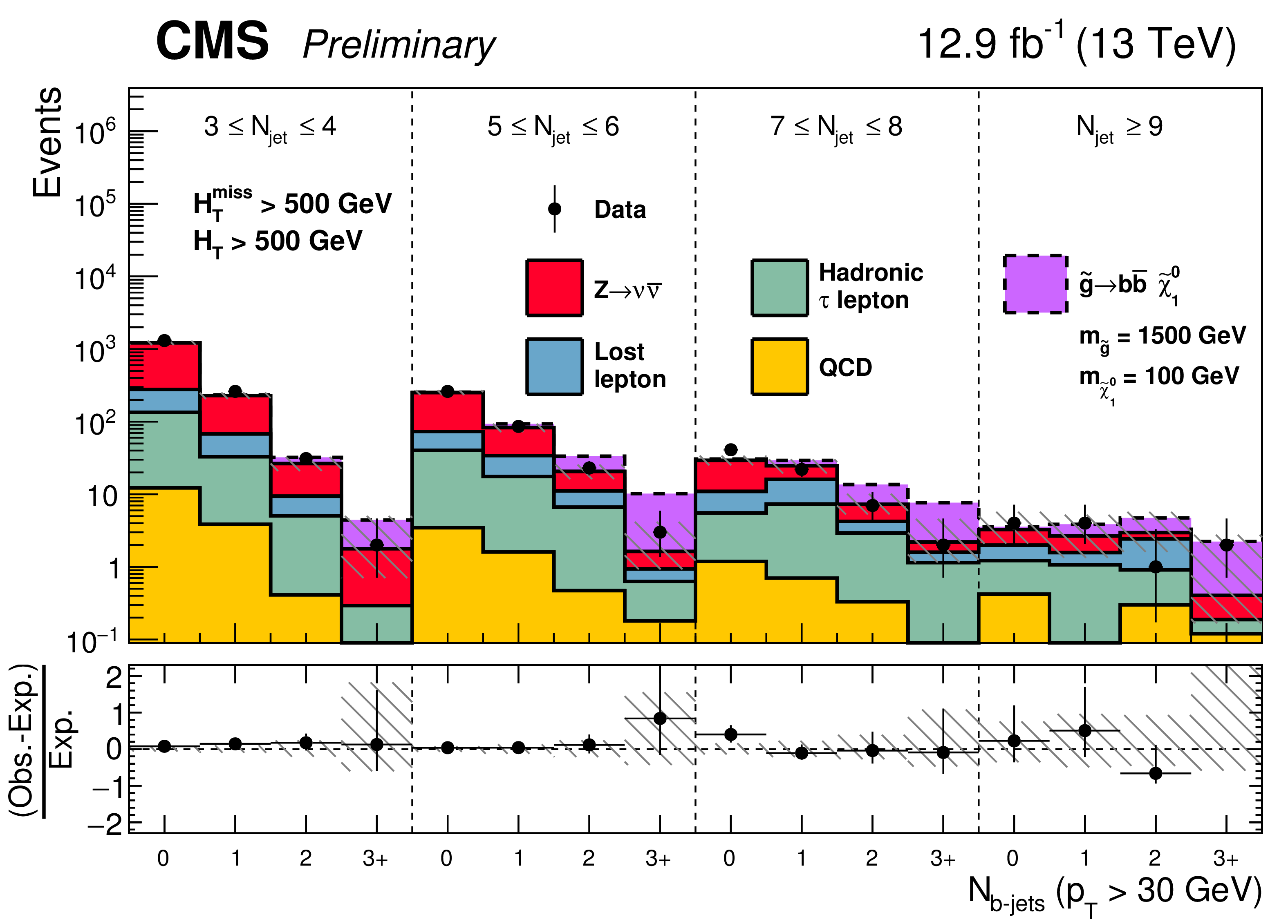
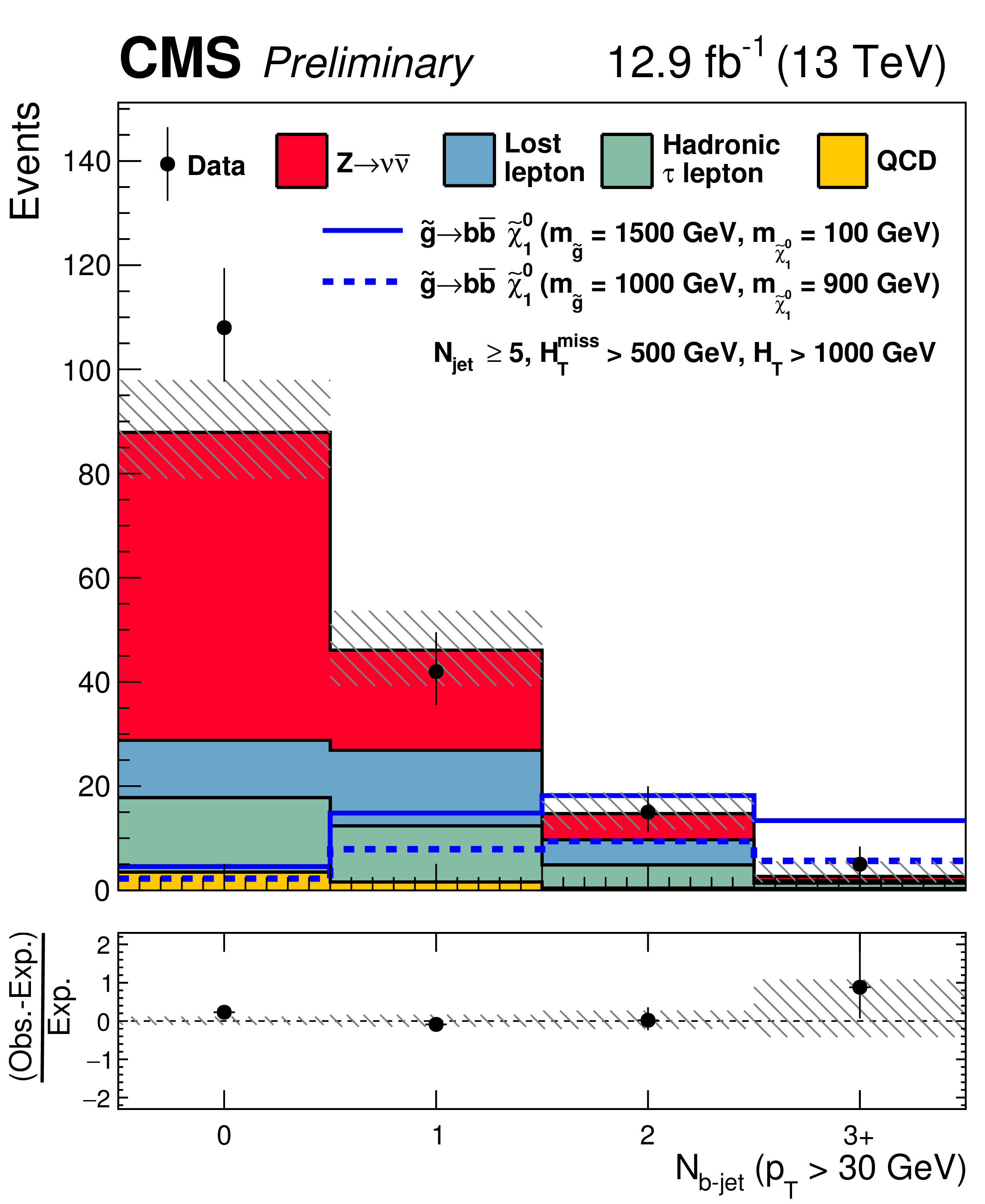
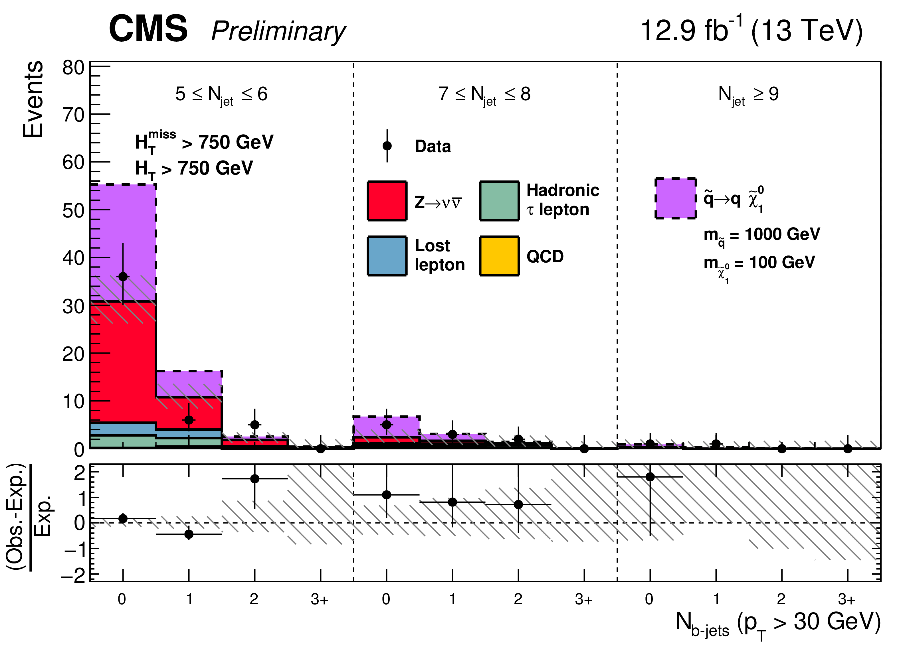
Observed numbers of events and corresponding SM background predictions in intervals of ${N_{\text {jet}}}$ and ${N_{{ {\mathrm {b}}}\text {-jet}}} $, integrated over all search regions with $ {H_{\mathrm T}^{\text {miss}}} > $ 500 GeV and $ {H_{\mathrm {T}}} > $ 500 GeV. An example T1bbbb signal scenario with ${ m_{\tilde{g}} } = $ 1500 GeV and $ m_{ {\tilde{\chi}^{0}_{1}} } = $ 100 GeV is shown by the (stacked) purple histogram. |

png pdf |
Figure 8-a:
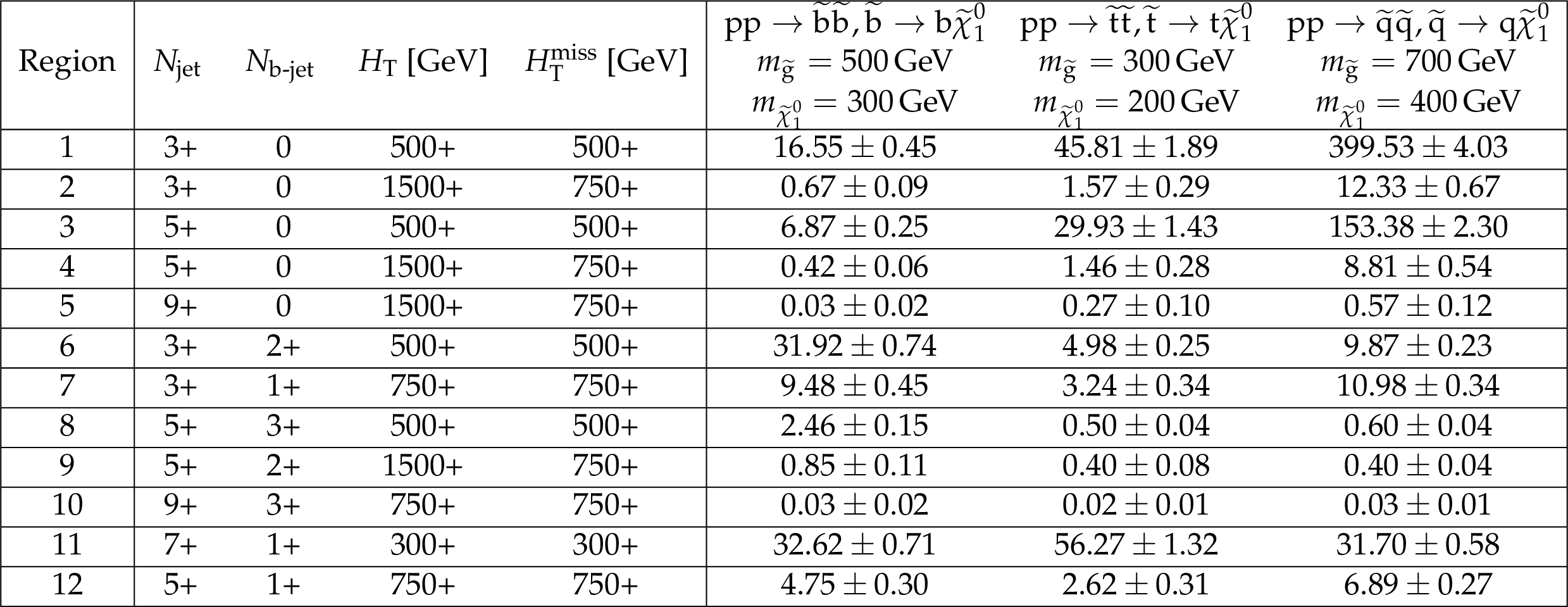
Observed numbers of events and corresponding SM background predictions for intervals of the search region parameter space particularly sensitive to the production of events in the (a) T1tttt, (b) T1bbbb, (c) T1qqqq, (d) T2tt, (e) T2bb, and (f) T2qq scenarios. The selection requirements are given in the figure legends. The hatched regions indicate the total uncertainties in the background predictions. The (unstacked) results for two example signal scenarios are shown in each instance, one with ${ m_{\tilde{g}} } $ or $ m_{ {\tilde{q}}} \gg m_{{\tilde{\chi}^{0}_{1}}} $ and the other with $ {m_{{\tilde{\chi}^{0}_{1}}} }\sim { m_{\tilde{g}} } $ or $ {m_{ {\tilde{q}} }} $. |
png pdf |
Figure 8-b:
Observed numbers of events and corresponding SM background predictions for intervals of the search region parameter space particularly sensitive to the production of events in the (a) T1tttt, (b) T1bbbb, (c) T1qqqq, (d) T2tt, (e) T2bb, and (f) T2qq scenarios. The selection requirements are given in the figure legends. The hatched regions indicate the total uncertainties in the background predictions. The (unstacked) results for two example signal scenarios are shown in each instance, one with ${ m_{\tilde{g}} } $ or $ m_{ {\tilde{q}}} \gg m_{{\tilde{\chi}^{0}_{1}}} $ and the other with $ {m_{{\tilde{\chi}^{0}_{1}}} }\sim { m_{\tilde{g}} } $ or $ {m_{ {\tilde{q}} }} $. |
png pdf |
Figure 8-c:
Observed numbers of events and corresponding SM background predictions for intervals of the search region parameter space particularly sensitive to the production of events in the (a) T1tttt, (b) T1bbbb, (c) T1qqqq, (d) T2tt, (e) T2bb, and (f) T2qq scenarios. The selection requirements are given in the figure legends. The hatched regions indicate the total uncertainties in the background predictions. The (unstacked) results for two example signal scenarios are shown in each instance, one with ${ m_{\tilde{g}} } $ or $ m_{ {\tilde{q}}} \gg m_{{\tilde{\chi}^{0}_{1}}} $ and the other with $ {m_{{\tilde{\chi}^{0}_{1}}} }\sim { m_{\tilde{g}} } $ or $ {m_{ {\tilde{q}} }} $. |

png pdf |
Figure 8-d:
Observed numbers of events and corresponding SM background predictions for intervals of the search region parameter space particularly sensitive to the production of events in the (a) T1tttt, (b) T1bbbb, (c) T1qqqq, (d) T2tt, (e) T2bb, and (f) T2qq scenarios. The selection requirements are given in the figure legends. The hatched regions indicate the total uncertainties in the background predictions. The (unstacked) results for two example signal scenarios are shown in each instance, one with ${ m_{\tilde{g}} } $ or $ m_{ {\tilde{q}}} \gg m_{{\tilde{\chi}^{0}_{1}}} $ and the other with $ {m_{{\tilde{\chi}^{0}_{1}}} }\sim { m_{\tilde{g}} } $ or $ {m_{ {\tilde{q}} }} $. |
png pdf |
Figure 8-e:
Observed numbers of events and corresponding SM background predictions for intervals of the search region parameter space particularly sensitive to the production of events in the (a) T1tttt, (b) T1bbbb, (c) T1qqqq, (d) T2tt, (e) T2bb, and (f) T2qq scenarios. The selection requirements are given in the figure legends. The hatched regions indicate the total uncertainties in the background predictions. The (unstacked) results for two example signal scenarios are shown in each instance, one with ${ m_{\tilde{g}} } $ or $ m_{ {\tilde{q}}} \gg m_{{\tilde{\chi}^{0}_{1}}} $ and the other with $ {m_{{\tilde{\chi}^{0}_{1}}} }\sim { m_{\tilde{g}} } $ or $ {m_{ {\tilde{q}} }} $. |
png pdf |
Figure 8-f:
Observed numbers of events and corresponding SM background predictions for intervals of the search region parameter space particularly sensitive to the production of events in the (a) T1tttt, (b) T1bbbb, (c) T1qqqq, (d) T2tt, (e) T2bb, and (f) T2qq scenarios. The selection requirements are given in the figure legends. The hatched regions indicate the total uncertainties in the background predictions. The (unstacked) results for two example signal scenarios are shown in each instance, one with ${ m_{\tilde{g}} } $ or $ m_{ {\tilde{q}}} \gg m_{{\tilde{\chi}^{0}_{1}}} $ and the other with $ {m_{{\tilde{\chi}^{0}_{1}}} }\sim { m_{\tilde{g}} } $ or $ {m_{ {\tilde{q}} }} $. |
png pdf root |
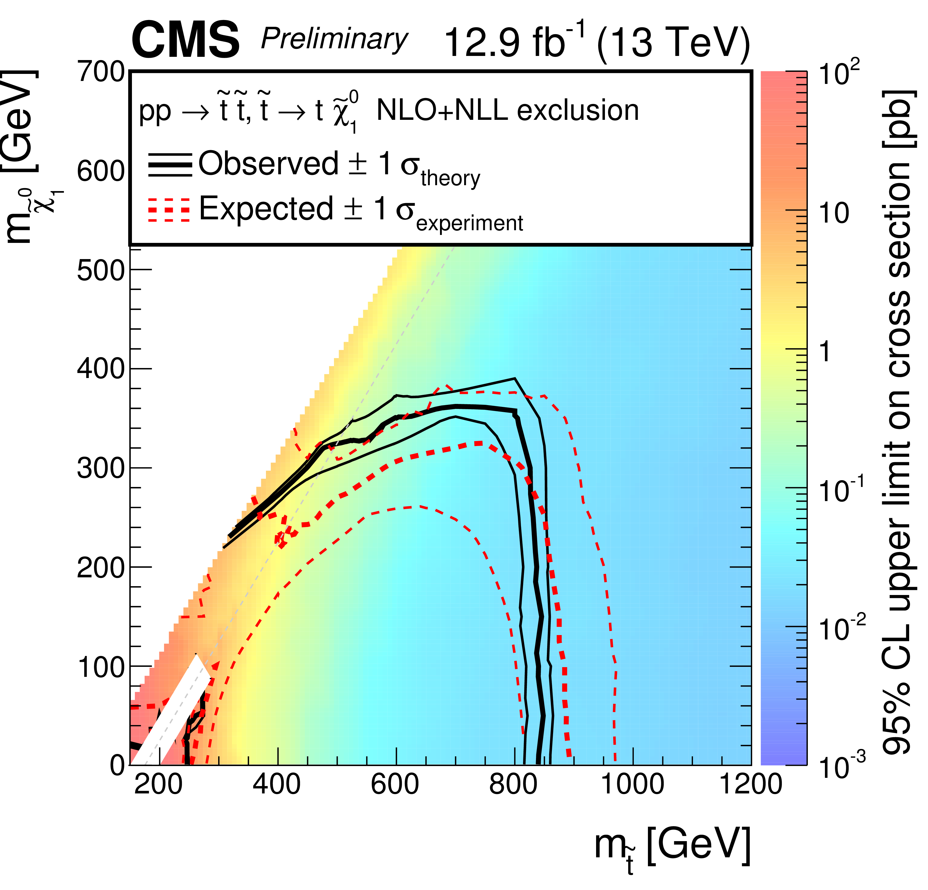
Figure 9-a:
The 95% CL upper limits on the production cross sections for the (a) T2tt, (b) T2bb, and (c) T2qq simplified models of supersymmetry, shown as a function of the squark and LSP masses ${m_{ {\tilde{q}}}}$ and $m_{{\tilde{\chi}^{0}_{1}}} $. The results labeled ``one light ${\tilde{q}}$ '' for the T2qq model are discussed in the text. The solid (black) curves show the observed exclusion contours assuming the NLO+NLL cross sections [50,51,52,53,54], with the corresponding $\pm $1standard deviation uncertainties [73]. The dashed (red) curves present the expected limits with $\pm $1 standard deviation experimental uncertainties. The dashed (grey) lines indicate the $ m_{{\tilde{\chi}^{0}_{1}}} = {m_{ {\tilde{q}}}}$ diagonal. |
png pdf root |
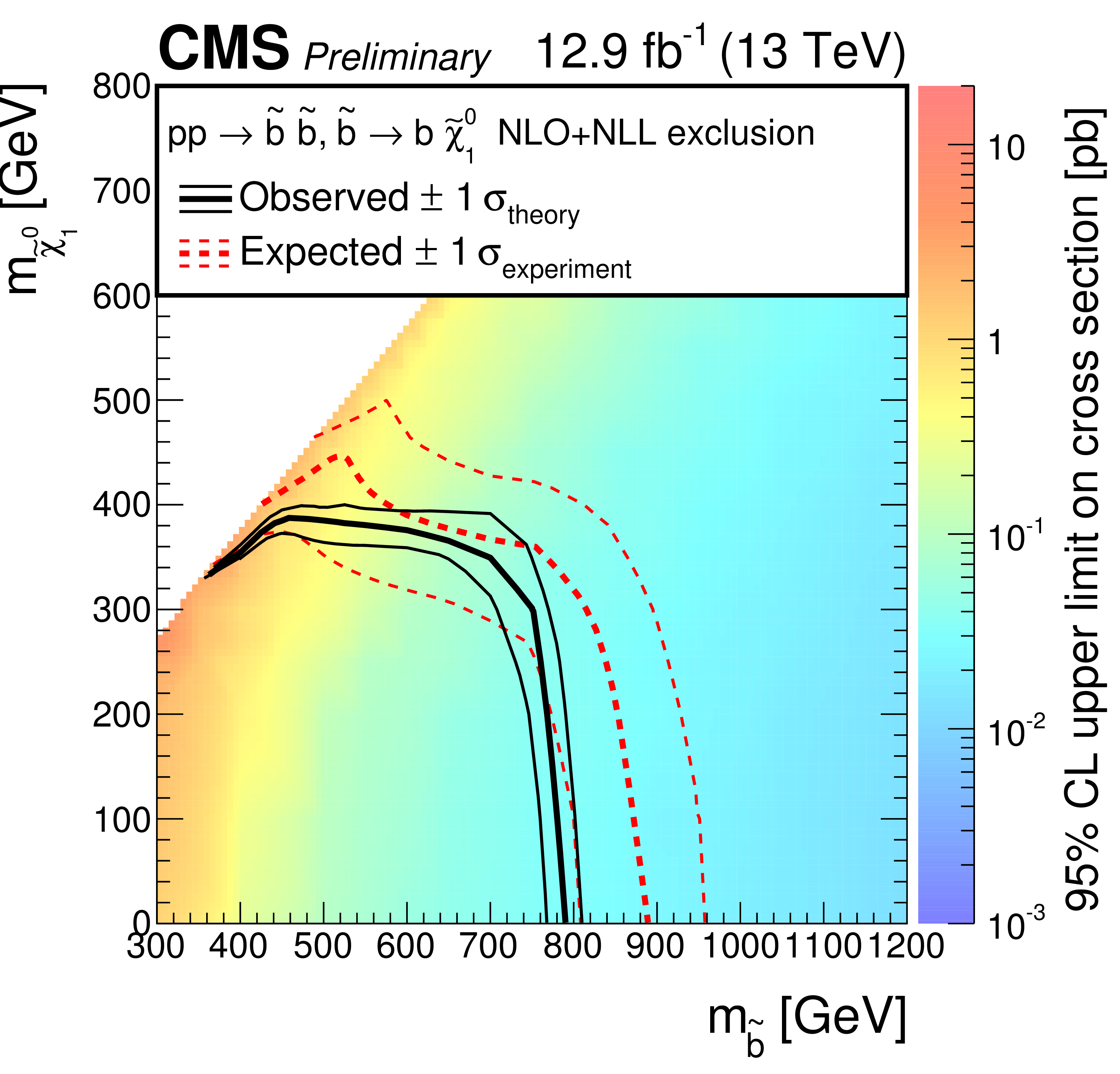
Figure 9-b:
The 95% CL upper limits on the production cross sections for the (a) T2tt, (b) T2bb, and (c) T2qq simplified models of supersymmetry, shown as a function of the squark and LSP masses ${m_{ {\tilde{q}}}}$ and $m_{{\tilde{\chi}^{0}_{1}}} $. The results labeled ``one light ${\tilde{q}}$ '' for the T2qq model are discussed in the text. The solid (black) curves show the observed exclusion contours assuming the NLO+NLL cross sections [50,51,52,53,54], with the corresponding $\pm $1standard deviation uncertainties [73]. The dashed (red) curves present the expected limits with $\pm $1 standard deviation experimental uncertainties. The dashed (grey) lines indicate the $ m_{{\tilde{\chi}^{0}_{1}}} = {m_{ {\tilde{q}}}}$ diagonal. |
png pdf root |
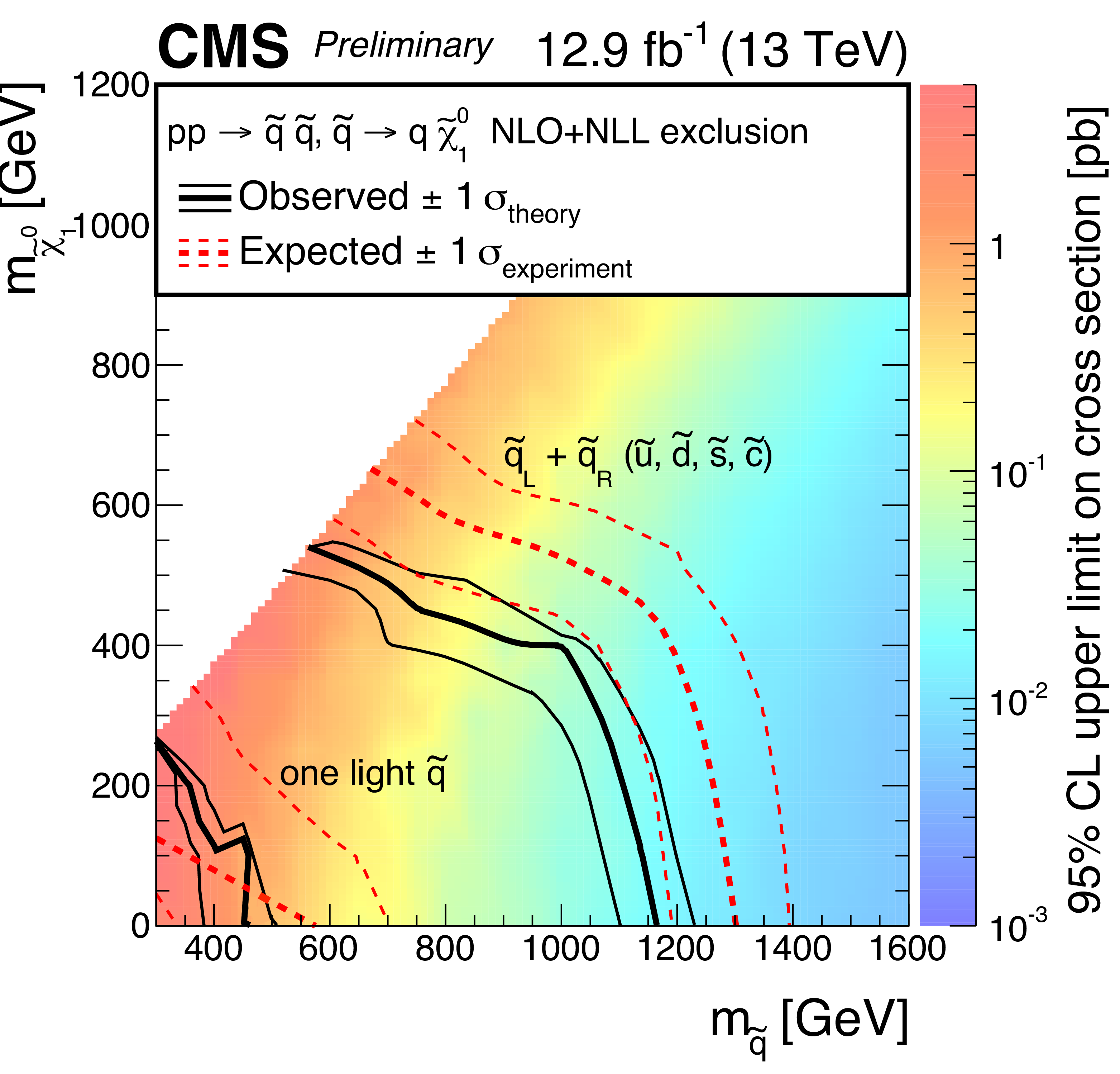
Figure 9-c:
The 95% CL upper limits on the production cross sections for the (a) T2tt, (b) T2bb, and (c) T2qq simplified models of supersymmetry, shown as a function of the squark and LSP masses ${m_{ {\tilde{q}}}}$ and $m_{{\tilde{\chi}^{0}_{1}}} $. The results labeled ``one light ${\tilde{q}}$ '' for the T2qq model are discussed in the text. The solid (black) curves show the observed exclusion contours assuming the NLO+NLL cross sections [50,51,52,53,54], with the corresponding $\pm $1standard deviation uncertainties [73]. The dashed (red) curves present the expected limits with $\pm $1 standard deviation experimental uncertainties. The dashed (grey) lines indicate the $ m_{{\tilde{\chi}^{0}_{1}}} = {m_{ {\tilde{q}}}}$ diagonal. |
png pdf root |
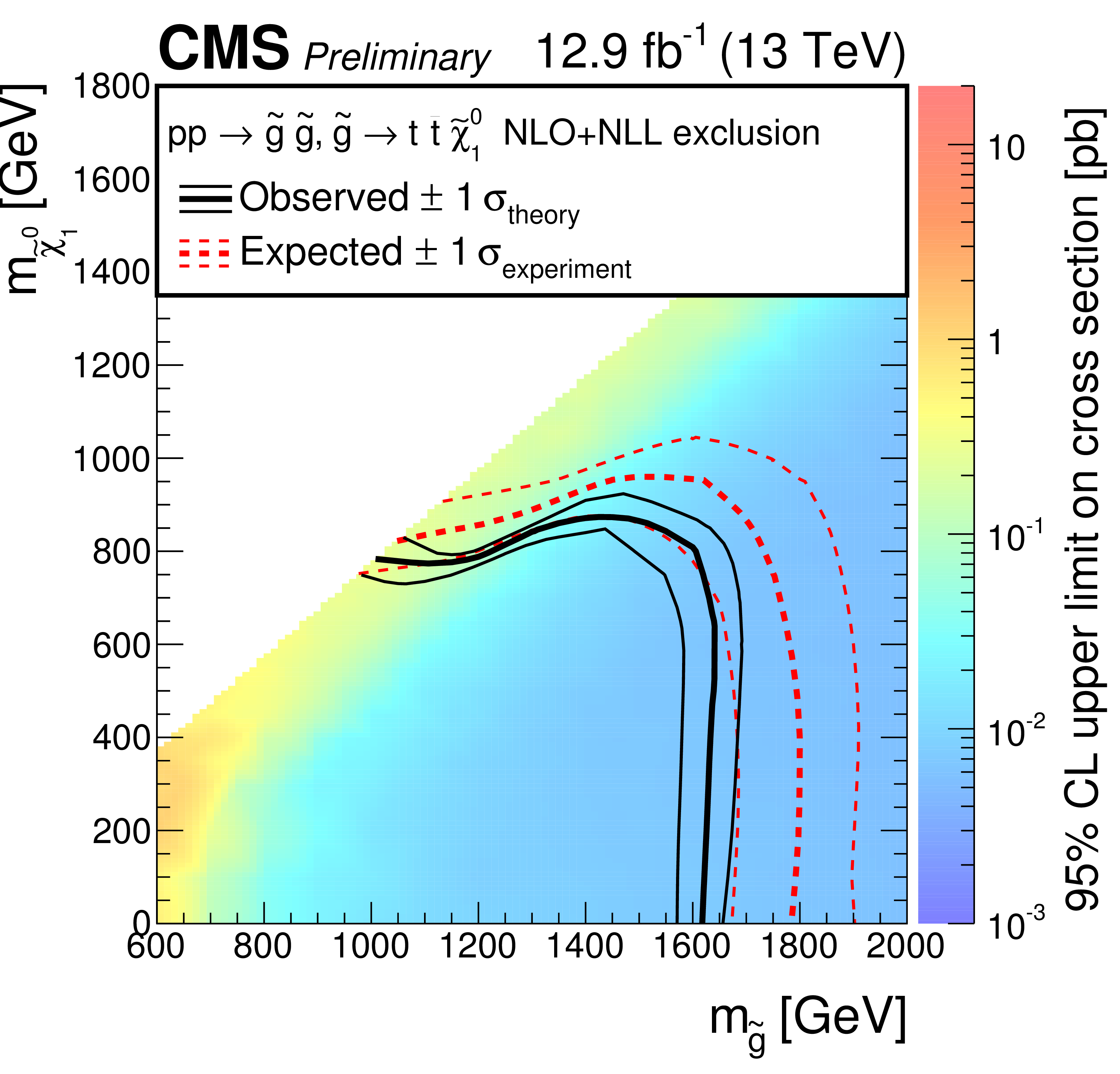
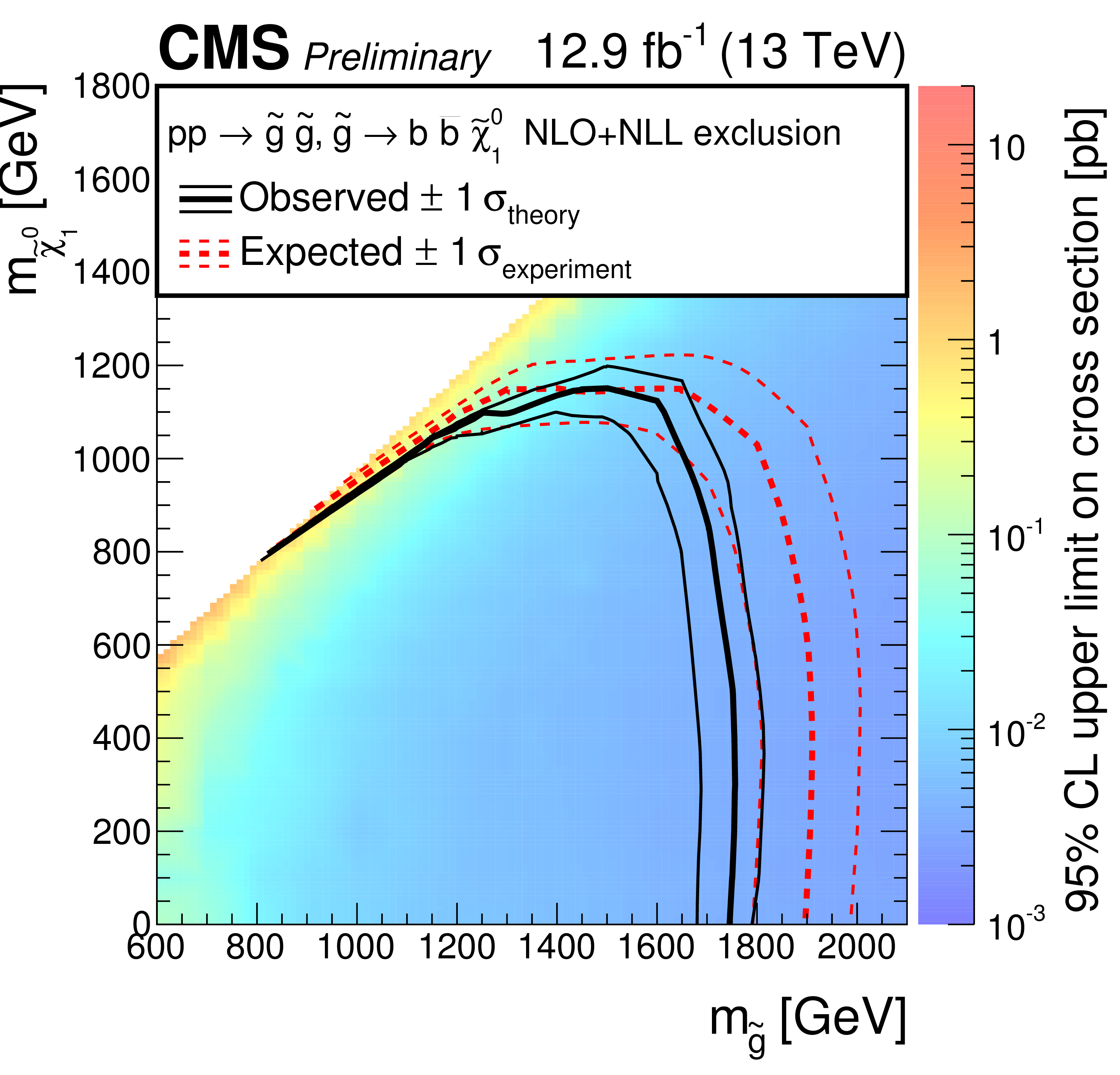
Figure 10-a:
The 95% CL upper limits on the production cross sections for the (a) T1tttt, (b) T1bbbb, (c) T1qqqq, and (d) T5qqqqVV simplified models of supersymmetry, shown as a function of the gluino and LSP masses $m_{\tilde{g}}$ and $ m_{{\tilde{\chi}^{0}_{1}}} $. For the T5qqqqVV model, the masses of the intermediate ${\tilde{\chi}^{0}_{2}}$ and $ {\tilde{\chi}^{\pm}_{1}}$ states are taken to be the mean of $ m_{{\tilde{\chi}^{0}_{1}}}$ and $ m_{\tilde{g}} $. The solid (black) curves show the observed exclusion contours assuming the NLO+NLL cross sections [50,51,52,53,54], with the corresponding $\pm $1standard deviation uncertainties [73]. The dashed (red) curves present the expected limits with $\pm $1 standard deviation experimental uncertainties. The dashed (grey) lines indicate the $ m_{{\tilde{\chi}^{0}_{1}}} = m_{\tilde{g}} $ diagonal. |
png pdf root |
Figure 10-b:
The 95% CL upper limits on the production cross sections for the (a) T1tttt, (b) T1bbbb, (c) T1qqqq, and (d) T5qqqqVV simplified models of supersymmetry, shown as a function of the gluino and LSP masses $m_{\tilde{g}}$ and $ m_{{\tilde{\chi}^{0}_{1}}} $. For the T5qqqqVV model, the masses of the intermediate ${\tilde{\chi}^{0}_{2}}$ and $ {\tilde{\chi}^{\pm}_{1}}$ states are taken to be the mean of $ m_{{\tilde{\chi}^{0}_{1}}}$ and $ m_{\tilde{g}} $. The solid (black) curves show the observed exclusion contours assuming the NLO+NLL cross sections [50,51,52,53,54], with the corresponding $\pm $1standard deviation uncertainties [73]. The dashed (red) curves present the expected limits with $\pm $1 standard deviation experimental uncertainties. The dashed (grey) lines indicate the $ m_{{\tilde{\chi}^{0}_{1}}} = m_{\tilde{g}} $ diagonal. |
png pdf root |
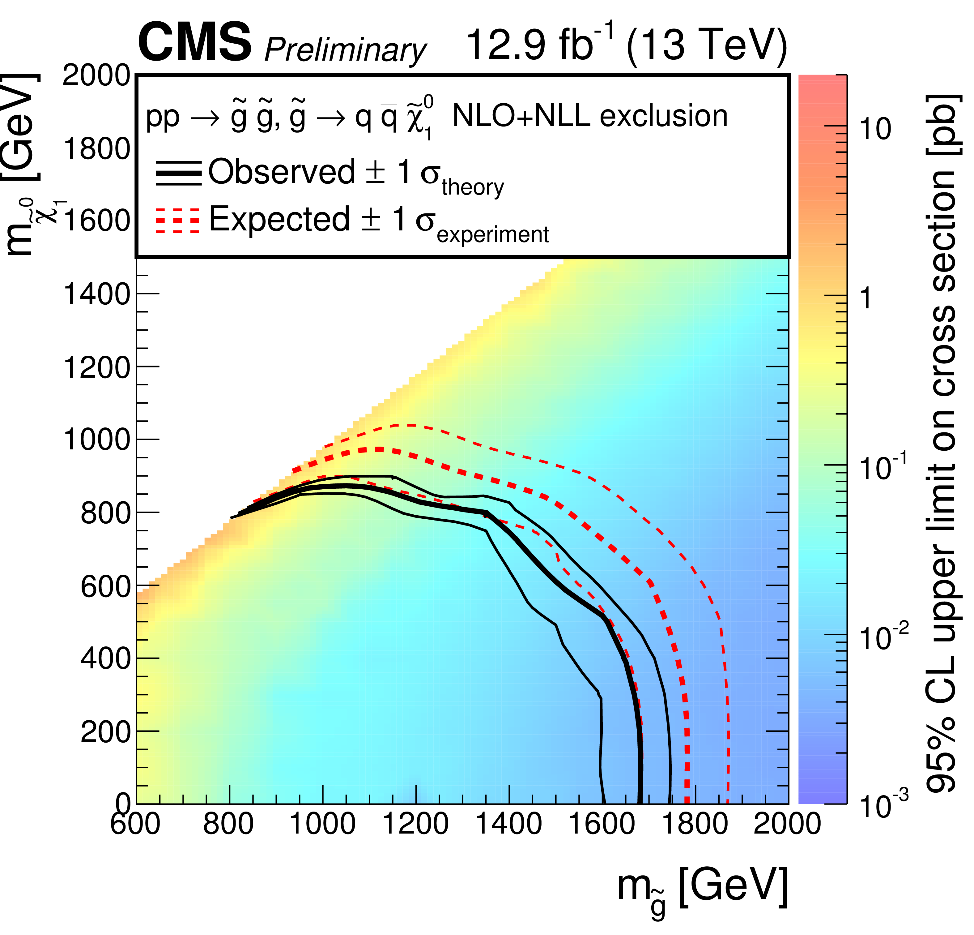
Figure 10-c:
The 95% CL upper limits on the production cross sections for the (a) T1tttt, (b) T1bbbb, (c) T1qqqq, and (d) T5qqqqVV simplified models of supersymmetry, shown as a function of the gluino and LSP masses $m_{\tilde{g}}$ and $ m_{{\tilde{\chi}^{0}_{1}}} $. For the T5qqqqVV model, the masses of the intermediate ${\tilde{\chi}^{0}_{2}}$ and $ {\tilde{\chi}^{\pm}_{1}}$ states are taken to be the mean of $ m_{{\tilde{\chi}^{0}_{1}}}$ and $ m_{\tilde{g}} $. The solid (black) curves show the observed exclusion contours assuming the NLO+NLL cross sections [50,51,52,53,54], with the corresponding $\pm $1standard deviation uncertainties [73]. The dashed (red) curves present the expected limits with $\pm $1 standard deviation experimental uncertainties. The dashed (grey) lines indicate the $ m_{{\tilde{\chi}^{0}_{1}}} = m_{\tilde{g}} $ diagonal. |
png pdf root |
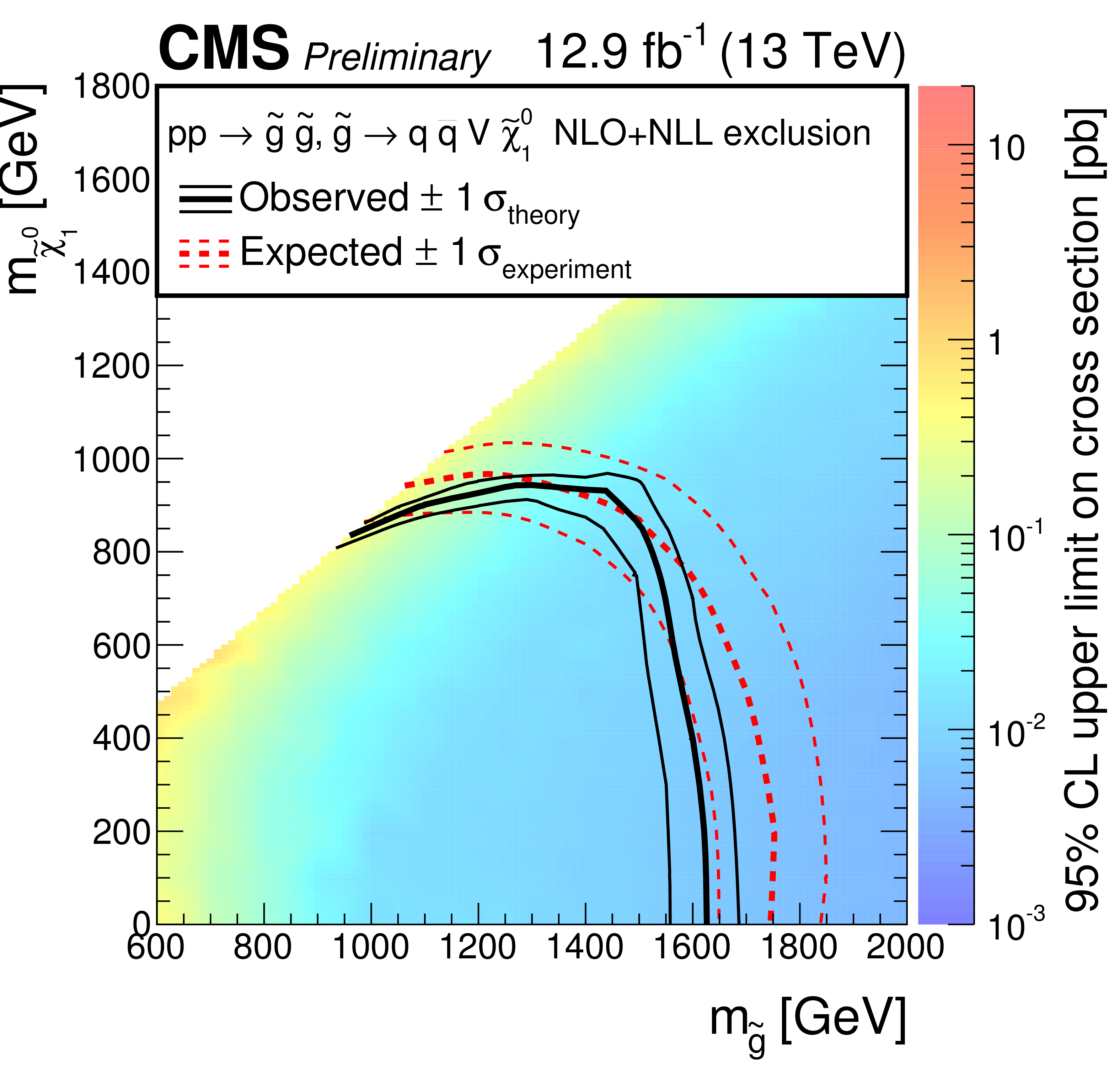
Figure 10-d:
The 95% CL upper limits on the production cross sections for the (a) T1tttt, (b) T1bbbb, (c) T1qqqq, and (d) T5qqqqVV simplified models of supersymmetry, shown as a function of the gluino and LSP masses $m_{\tilde{g}}$ and $ m_{{\tilde{\chi}^{0}_{1}}} $. For the T5qqqqVV model, the masses of the intermediate ${\tilde{\chi}^{0}_{2}}$ and $ {\tilde{\chi}^{\pm}_{1}}$ states are taken to be the mean of $ m_{{\tilde{\chi}^{0}_{1}}}$ and $ m_{\tilde{g}} $. The solid (black) curves show the observed exclusion contours assuming the NLO+NLL cross sections [50,51,52,53,54], with the corresponding $\pm $1standard deviation uncertainties [73]. The dashed (red) curves present the expected limits with $\pm $1 standard deviation experimental uncertainties. The dashed (grey) lines indicate the $ m_{{\tilde{\chi}^{0}_{1}}} = m_{\tilde{g}} $ diagonal. |
| Tables | |

png pdf |
Table 1:
Definition of the 10 search intervals in the ${H_{\mathrm T}^{\text {miss}}}$ and ${H_{\mathrm {T}}}$ variables. |

png pdf |
Table 2:
Summary of systematic uncertainties that affect the signal event selection efficiency. The results are averaged over all search regions. The variations correspond to different signal models and choices of the gluino and LSP masses. |
| Summary |
| A search is presented for an anomalously high rate of events with three or more jets, no identified isolated electron, muon, or charged track, large scalar sum $H_{\mathrm{T}}$ of jet transverse momenta, and large missing transverse momentum. The search is based on a sample of proton-proton collision data collected at $ \sqrt{s} = $ 13 TeV with the CMS detector at the CERN LHC in 2016, corresponding to an integrated luminosity of 12.9 fb$^{-1}$. The principal standard model backgrounds, from events with top quarks, W bosons and jets, Z bosons and jets, and QCD multijet production, are evaluated using control samples in the data. The study is performed in the framework of a global likelihood fit in which the observed numbers of events in 160 exclusive bins in a four-dimensional array of ${H_{\mathrm T}^{\text{miss}}} $, the number of jets, the number of tagged bottom quark jets, and $H_{\mathrm{T}}$, are compared to the standard model predictions. The standard model background estimates are found to agree with the observed numbers of events within the uncertainties. The results are interpreted with simplified models that, in the context of supersymmetry, correspond to gluino pair production and direct squark-antisquark production. Using the NLO+NLL production cross section as a reference, and for a massless LSP, we exclude gluinos with masses between around 1620 and 1750 GeV depending on the assumed gluino decay mode. The corresponding limit on the mass of directly produced squarks varies between around 780 and 1150 GeV depending on the squark flavor. These results extend the limits from previous searches. |
| Additional Figures | |

png pdf |
Additional Figure 1:
Observed number of events and pre-fit background predictions in all search bins. The lower panel of the plot shows the pull, defined as $(N_{\rm Obs.}-N_{\rm Pred.})/\sqrt {N_{\rm Pred.}+\delta N^{2}_{\rm Pred.}}$, where $\delta N_{\rm Pred.}$ is the total (STAT+SYST) uncertainty on the background prediction, for each bin. |
png pdf |
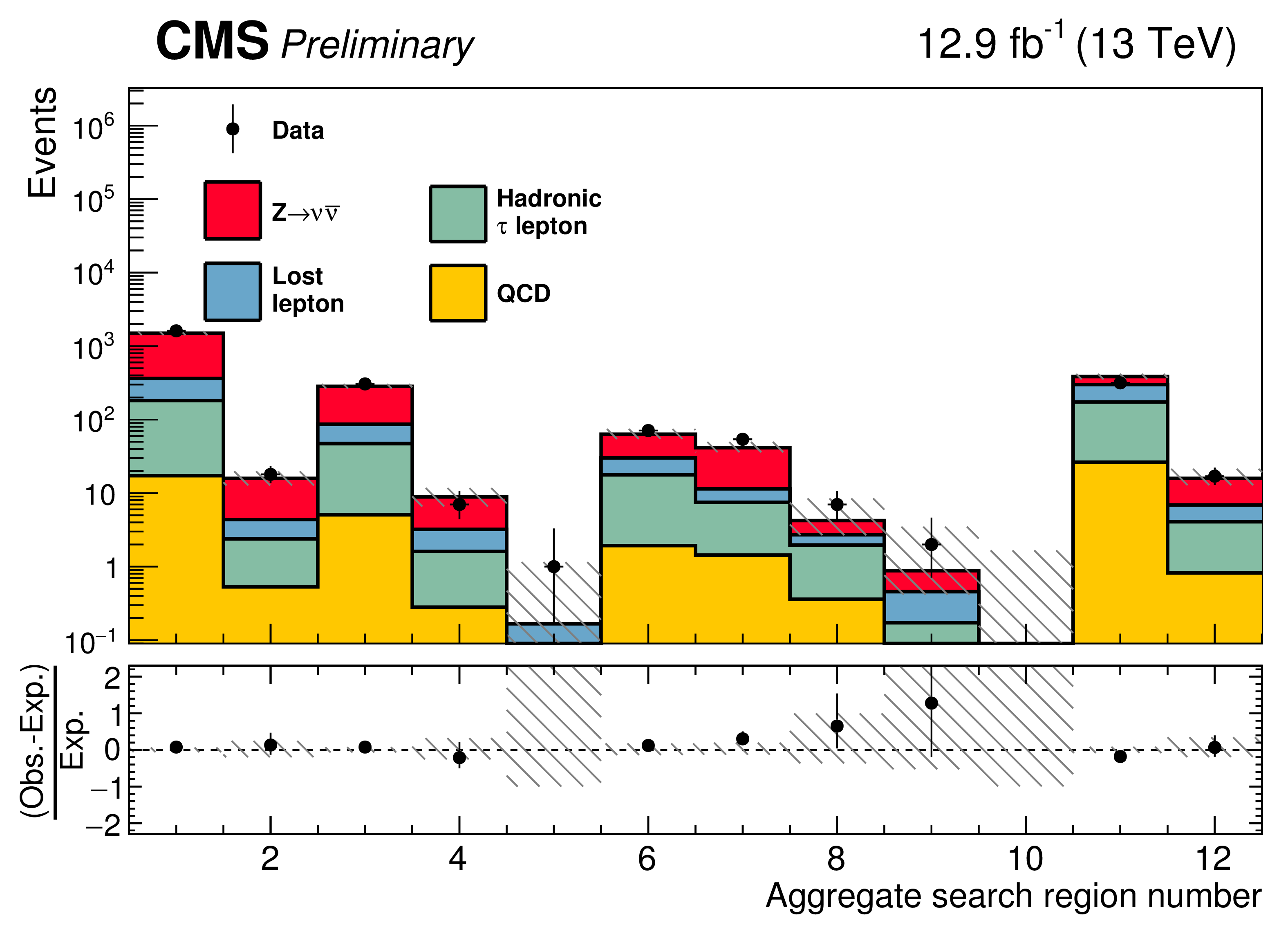
Additional Figure 2-a:
Observed number of events and pre-fit background predictions in the aggregate search regions. The lower panel of (a) shows the relative difference between the observed data and estimated background, while the lower panel of (b) shows the pull, defined as $(N_{\rm Obs.}-N_{\rm Pred.})/\sqrt {N_{\rm Pred.}+\delta N^{2}_{\rm Pred.}}$, where $\delta N_{\rm Pred.}$ is the total (STAT+SYST) uncertainty on the background prediction, for each bin. The selection, background predictions, and observed yields in each of these regions is summarized in Additional Table 5. |

png pdf |
Additional Figure 2-b:
Observed number of events and pre-fit background predictions in the aggregate search regions. The lower panel of (a) shows the relative difference between the observed data and estimated background, while the lower panel of (b) shows the pull, defined as $(N_{\rm Obs.}-N_{\rm Pred.})/\sqrt {N_{\rm Pred.}+\delta N^{2}_{\rm Pred.}}$, where $\delta N_{\rm Pred.}$ is the total (STAT+SYST) uncertainty on the background prediction, for each bin. The selection, background predictions, and observed yields in each of these regions is summarized in Additional Table 5. |
png pdf |
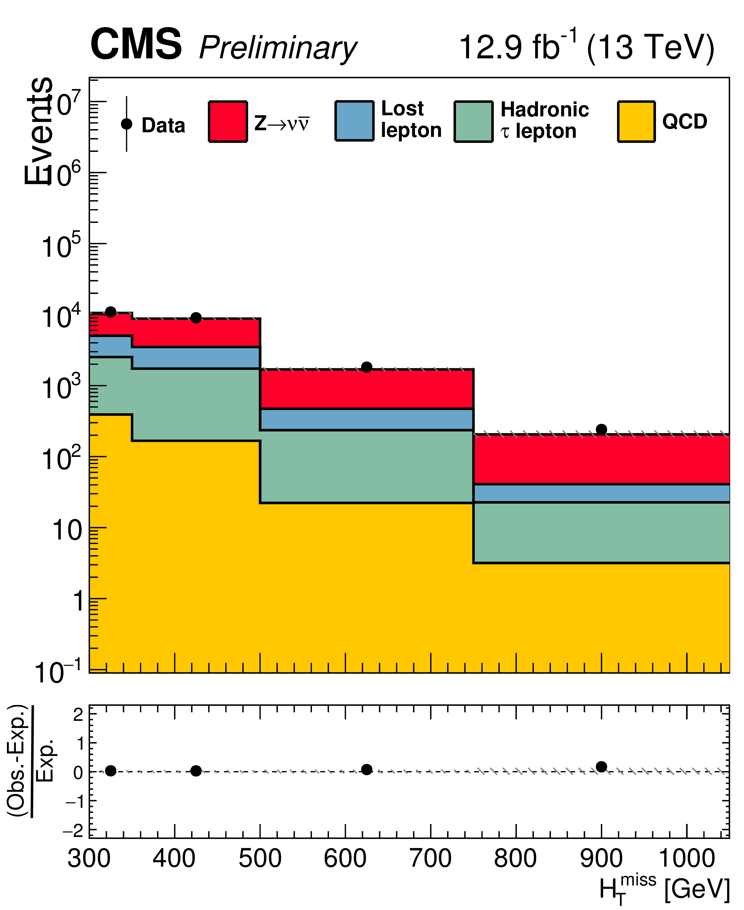
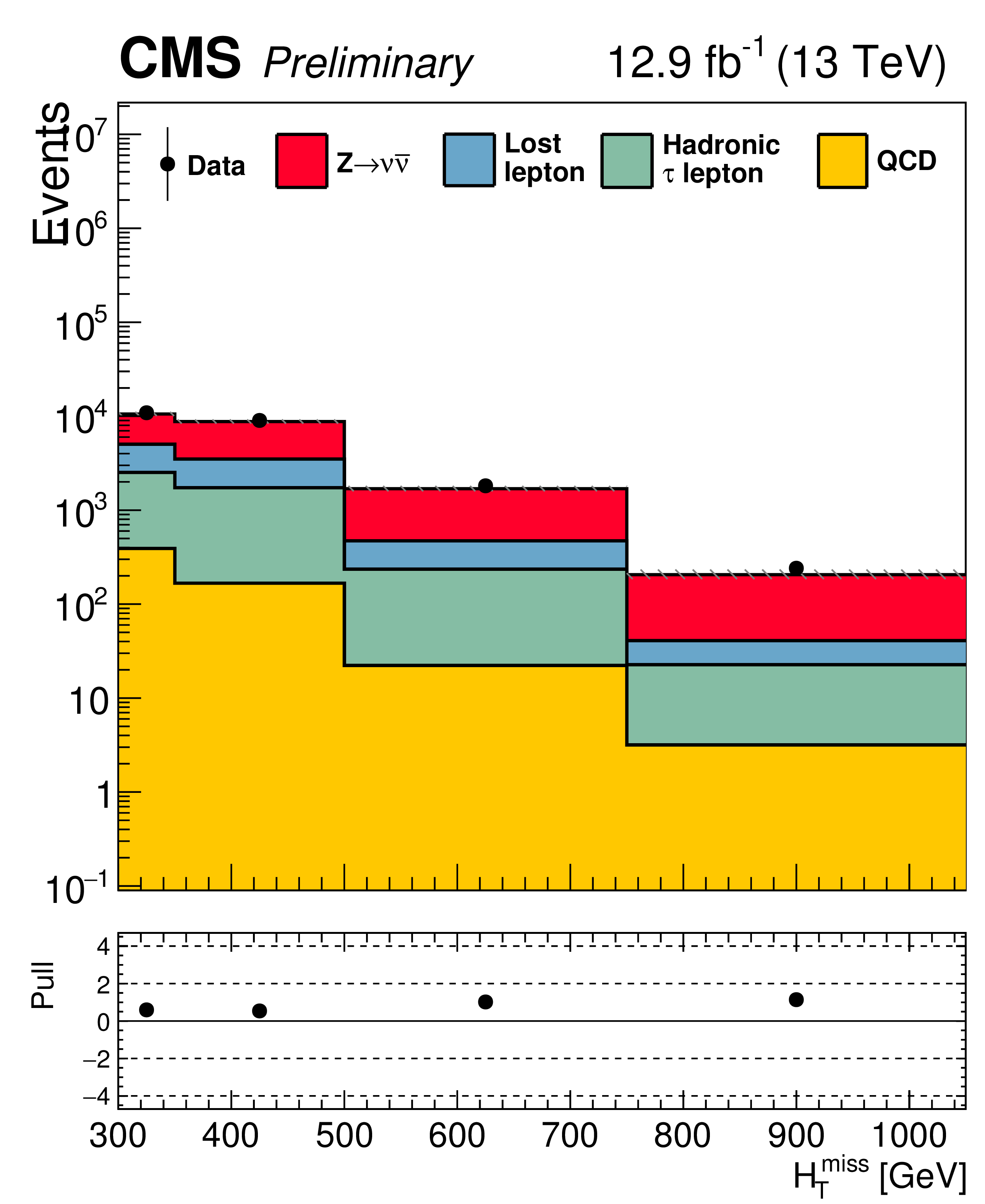
Additional Figure 3-a:
One-dimensional projections of observed number of events and pre-fit background predictions in the search region in (a) ${H_{\mathrm T}^{\text {miss}}} $, (b) ${N_{\text {jet}}} $, and (c) ${N_{{\mathrm{ b } }\text {-jet}}} $. The events in each distribution are integrated over the other three search variables. |

png pdf |
Additional Figure 3-b:
One-dimensional projections of observed number of events and pre-fit background predictions in the search region in (a) ${H_{\mathrm T}^{\text {miss}}} $, (b) ${N_{\text {jet}}} $, and (c) ${N_{{\mathrm{ b } }\text {-jet}}} $. The events in each distribution are integrated over the other three search variables. |

png pdf |
Additional Figure 3-c:
One-dimensional projections of observed number of events and pre-fit background predictions in the search region in (a) ${H_{\mathrm T}^{\text {miss}}} $, (b) ${N_{\text {jet}}} $, and (c) ${N_{{\mathrm{ b } }\text {-jet}}} $. The events in each distribution are integrated over the other three search variables. |
png pdf |
Additional Figure 4-a:
The same distributions shown in Add. Fig. 3, with the pull for each bin shown in the lower panel of each plot. |
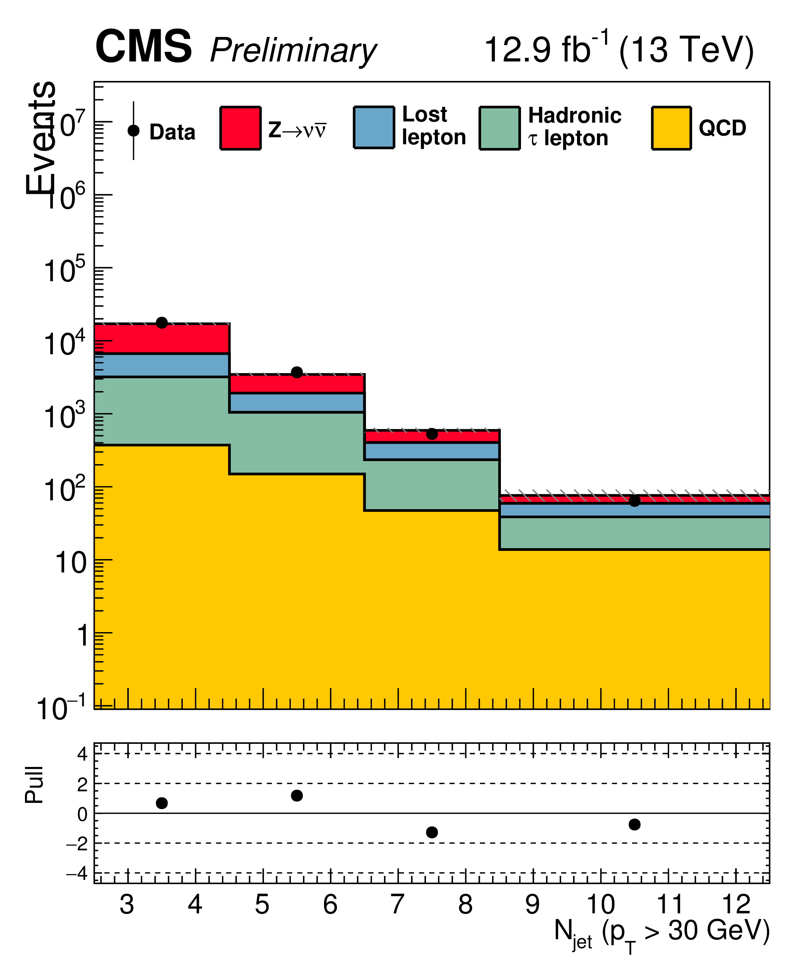
png pdf |
Additional Figure 4-b:
The same distributions shown in Add. Fig. 3, with the pull for each bin shown in the lower panel of each plot. |

png pdf |
Additional Figure 4-c:
The same distributions shown in Add. Fig. 3, with the pull for each bin shown in the lower panel of each plot. |

png pdf |
Additional Figure 5-a:
Observed numbers of events and corresponding SM background predictions in bins of $ {N_{\text {jet}}} $ and $ {N_{{\mathrm{ b } }\text {-jet}}} $ , integrated over all search bins with selection (a) $ {H_{\mathrm T}^{\text {miss}}} >500$ GeV and $ {H_{\mathrm {T}}} >500$ GeV or (b) $ {H_{\mathrm T}^{\text {miss}}} >750$ GeV, $ {H_{\mathrm {T}}} >750$ GeV, and $ {N_{\text {jet}}} \geq 5$. An example signal model, $\tilde{g} \rightarrow {\mathrm{ b \bar{b} } } \tilde{\chi}^0_1 $ with ${ {m_{\tilde{g} }} }=1500$ GeV and ${ {m_{\tilde{\chi}^{0}_{1}}} }=100$ GeV is stacked on top of the stacked background prediction to illustrate where a signal could lie in our search region phase space. |
png pdf |
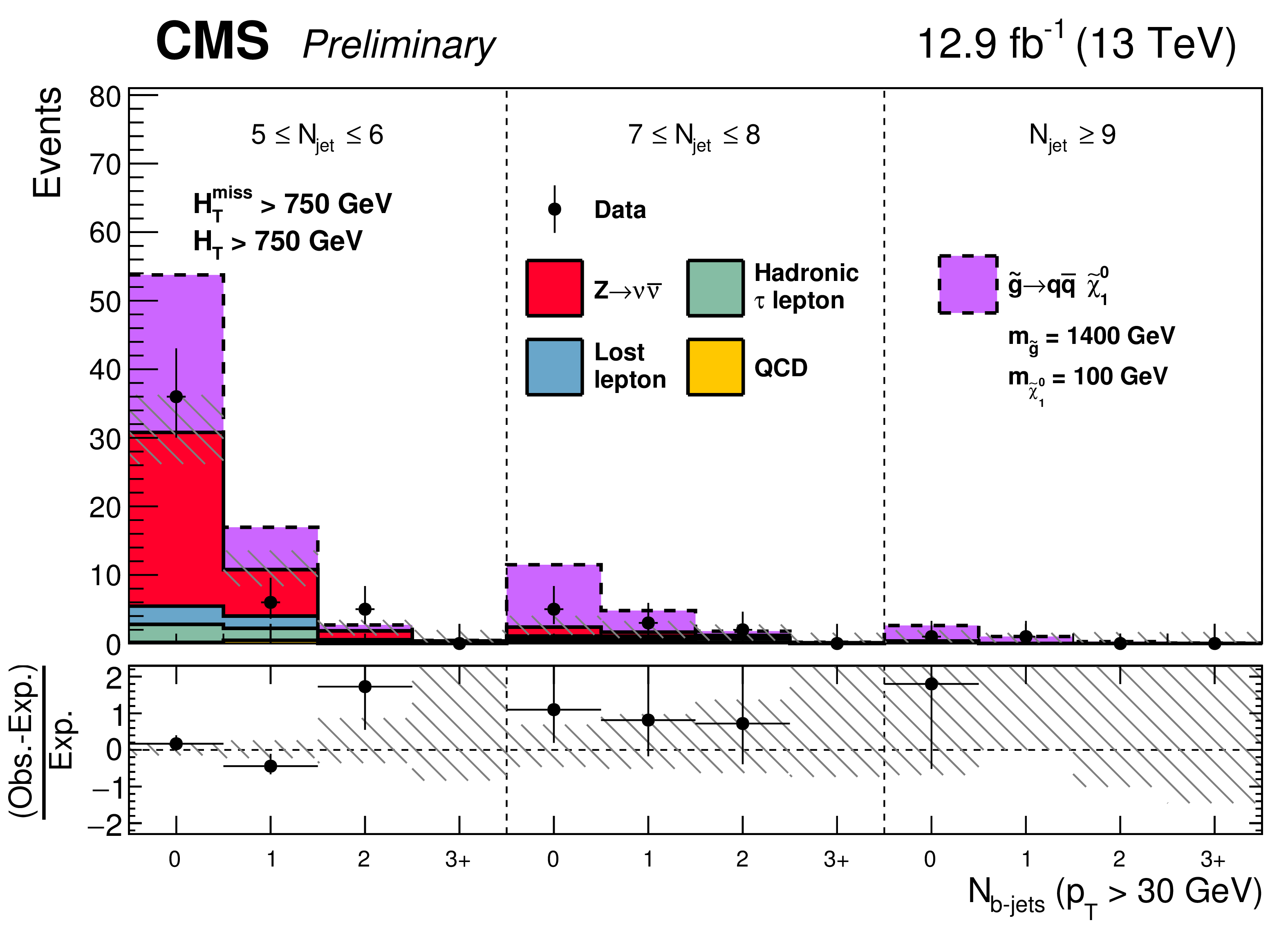
Additional Figure 5-b:
Observed numbers of events and corresponding SM background predictions in bins of $ {N_{\text {jet}}} $ and $ {N_{{\mathrm{ b } }\text {-jet}}} $ , integrated over all search bins with selection (a) $ {H_{\mathrm T}^{\text {miss}}} >500$ GeV and $ {H_{\mathrm {T}}} >500$ GeV or (b) $ {H_{\mathrm T}^{\text {miss}}} >750$ GeV, $ {H_{\mathrm {T}}} >750$ GeV, and $ {N_{\text {jet}}} \geq 5$. An example signal model, $\tilde{g} \rightarrow {\mathrm{ b \bar{b} } } \tilde{\chi}^0_1 $ with ${ {m_{\tilde{g} }} }=1500$ GeV and ${ {m_{\tilde{\chi}^{0}_{1}}} }=100$ GeV is stacked on top of the stacked background prediction to illustrate where a signal could lie in our search region phase space. |

png pdf |
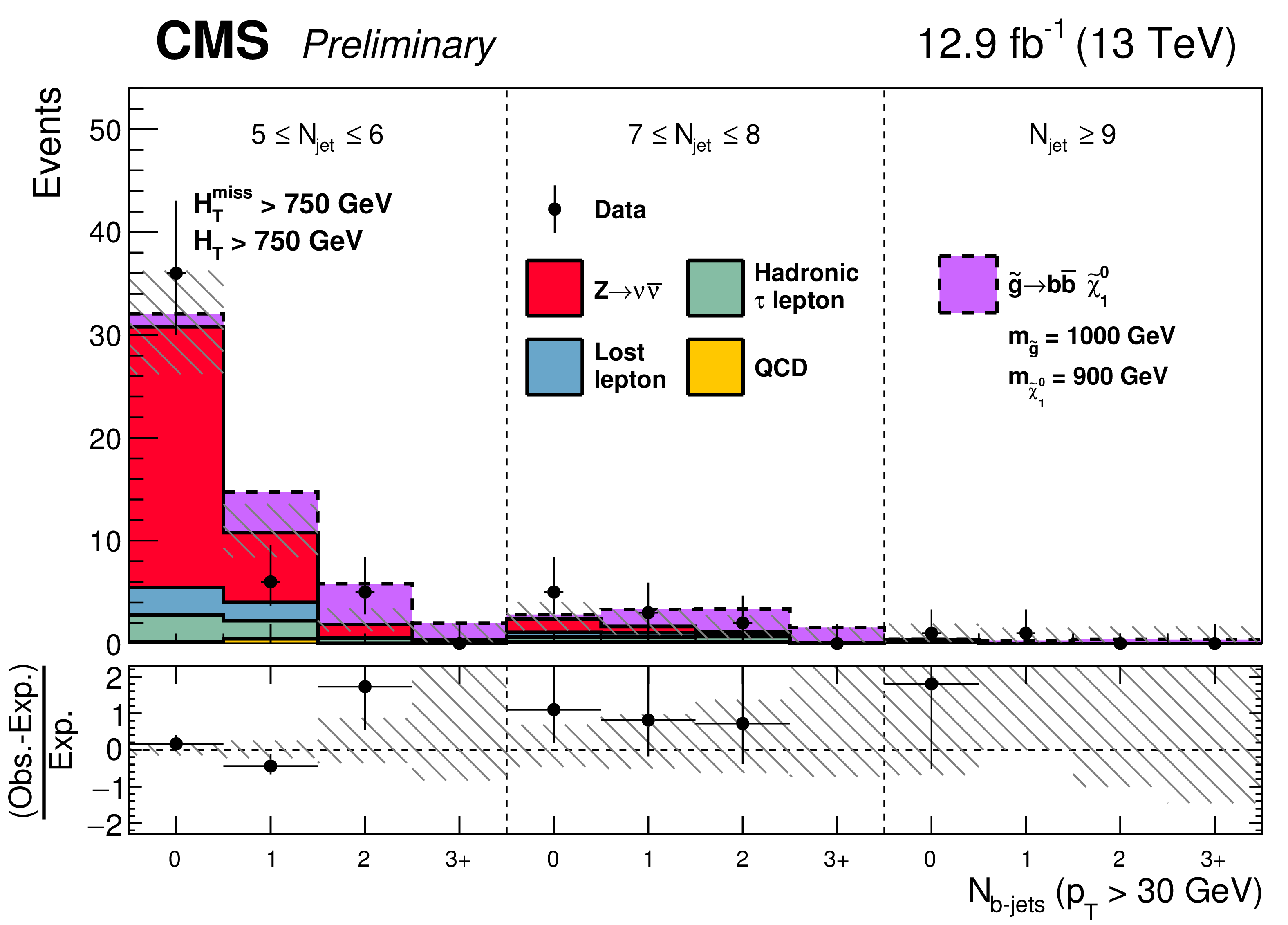
Additional Figure 6-a:
Observed numbers of events and corresponding SM background predictions in bins of $ {N_{\text {jet}}} $ and $ {N_{{\mathrm{ b } }\text {-jet}}} $ , integrated over all search bins with selection (a) $ {H_{\mathrm T}^{\text {miss}}} >500$ GeV and $ {H_{\mathrm {T}}} >500$ GeV or (b) $ {H_{\mathrm T}^{\text {miss}}} >750$ GeV, $ {H_{\mathrm {T}}} >750$ GeV, and $ {N_{\text {jet}}} \geq 5$. An example signal model, $\tilde{g} \rightarrow {\mathrm{ b \bar{b} } } \tilde{\chi}^0_1 $ with ${ {m_{\tilde{g} }} }=1000$ GeV and ${ {m_{\tilde{\chi}^{0}_{1}}} }=900$ GeV is stacked on top of the stacked background prediction to illustrate where a signal could lie in our search region phase space. |
png pdf |
Additional Figure 6-b:
Observed numbers of events and corresponding SM background predictions in bins of $ {N_{\text {jet}}} $ and $ {N_{{\mathrm{ b } }\text {-jet}}} $ , integrated over all search bins with selection (a) $ {H_{\mathrm T}^{\text {miss}}} >500$ GeV and $ {H_{\mathrm {T}}} >500$ GeV or (b) $ {H_{\mathrm T}^{\text {miss}}} >750$ GeV, $ {H_{\mathrm {T}}} >750$ GeV, and $ {N_{\text {jet}}} \geq 5$. An example signal model, $\tilde{g} \rightarrow {\mathrm{ b \bar{b} } } \tilde{\chi}^0_1 $ with ${ {m_{\tilde{g} }} }=1000$ GeV and ${ {m_{\tilde{\chi}^{0}_{1}}} }=900$ GeV is stacked on top of the stacked background prediction to illustrate where a signal could lie in our search region phase space. |
png pdf |
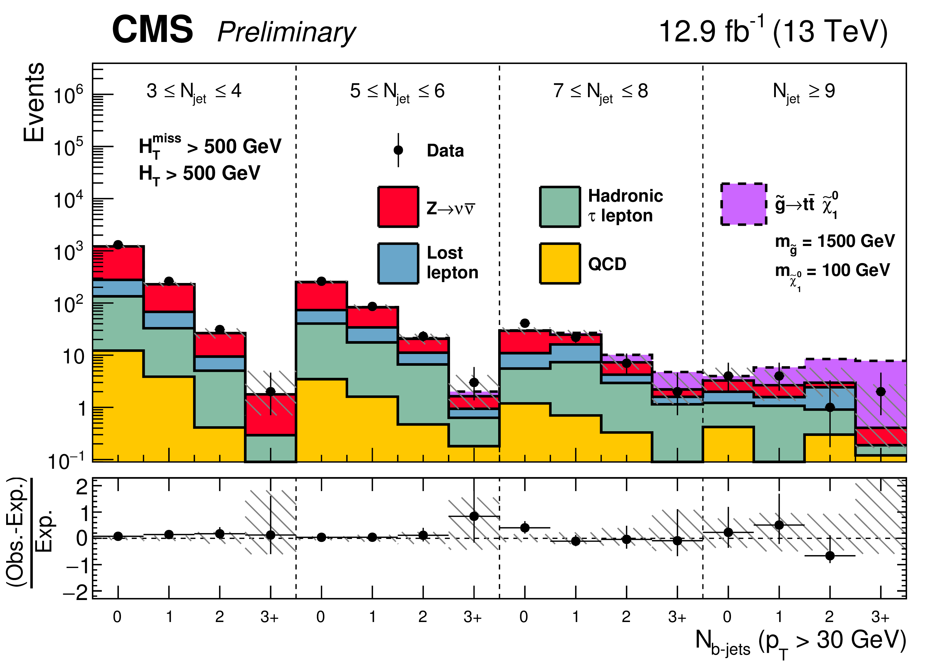
Additional Figure 7-a:
Observed numbers of events and corresponding SM background predictions in bins of $ {N_{\text {jet}}} $ and $ {N_{{\mathrm{ b } }\text {-jet}}} $ , integrated over all search bins with selection (a) $ {H_{\mathrm T}^{\text {miss}}} >500$ GeV and $ {H_{\mathrm {T}}} >500$ GeV or (b) $ {H_{\mathrm T}^{\text {miss}}} >750$ GeV, $ {H_{\mathrm {T}}} >750$ GeV, and $ {N_{\text {jet}}} \geq 5$. An example signal model, $\tilde{g} \rightarrow {\mathrm{ t } {}\mathrm{ \bar{t} } } \tilde{\chi}^0_1 $ with ${ {m_{\tilde{g} }} }=1500$ GeV and ${ {m_{\tilde{\chi}^{0}_{1}}} }=100$ GeV is stacked on top of the stacked background prediction to illustrate where a signal could lie in our search region phase space. |
png pdf |
Additional Figure 7-b:
Observed numbers of events and corresponding SM background predictions in bins of $ {N_{\text {jet}}} $ and $ {N_{{\mathrm{ b } }\text {-jet}}} $ , integrated over all search bins with selection (a) $ {H_{\mathrm T}^{\text {miss}}} >500$ GeV and $ {H_{\mathrm {T}}} >500$ GeV or (b) $ {H_{\mathrm T}^{\text {miss}}} >750$ GeV, $ {H_{\mathrm {T}}} >750$ GeV, and $ {N_{\text {jet}}} \geq 5$. An example signal model, $\tilde{g} \rightarrow {\mathrm{ t } {}\mathrm{ \bar{t} } } \tilde{\chi}^0_1 $ with ${ {m_{\tilde{g} }} }=1500$ GeV and ${ {m_{\tilde{\chi}^{0}_{1}}} }=100$ GeV is stacked on top of the stacked background prediction to illustrate where a signal could lie in our search region phase space. |
png pdf |
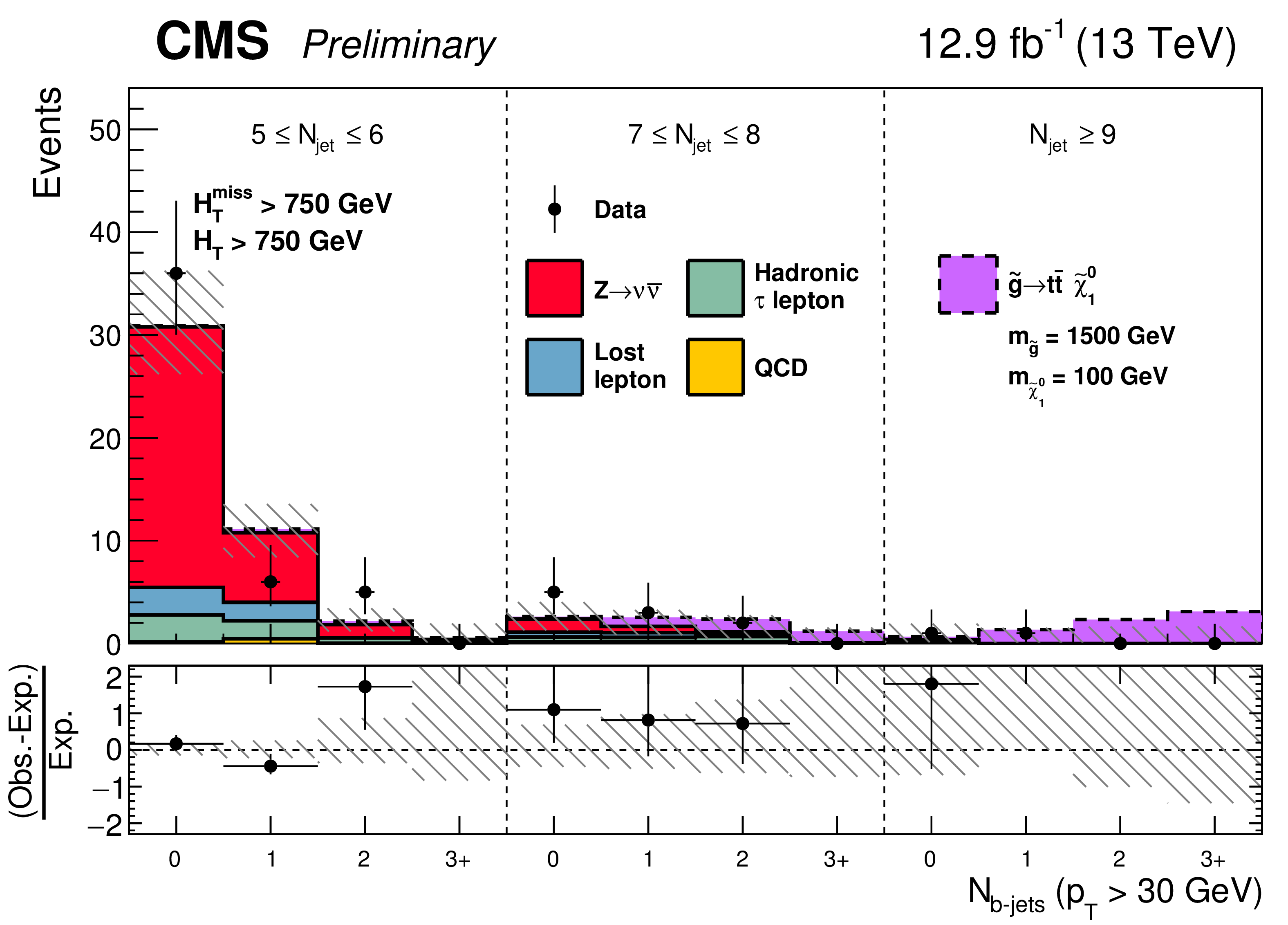
Additional Figure 8-a:
Observed numbers of events and corresponding SM background predictions in bins of $ {N_{\text {jet}}} $ and $ {N_{{\mathrm{ b } }\text {-jet}}} $ , integrated over all search bins with selection (a) $ {H_{\mathrm T}^{\text {miss}}} >500$ GeV and $ {H_{\mathrm {T}}} >500$ GeV or (b) $ {H_{\mathrm T}^{\text {miss}}} >750$ GeV, $ {H_{\mathrm {T}}} >750$ GeV, and $ {N_{\text {jet}}} \geq 5$. An example signal model, $\tilde{g} \rightarrow {\mathrm{ t } {}\mathrm{ \bar{t} } } \tilde{\chi}^0_1 $ with ${ {m_{\tilde{g} }} }=1200$ GeV and ${ {m_{\tilde{\chi}^{0}_{1}}} }=800$ GeV is stacked on top of the stacked background prediction to illustrate where a signal could lie in our search region phase space. |

png pdf |
Additional Figure 8-b:
Observed numbers of events and corresponding SM background predictions in bins of $ {N_{\text {jet}}} $ and $ {N_{{\mathrm{ b } }\text {-jet}}} $ , integrated over all search bins with selection (a) $ {H_{\mathrm T}^{\text {miss}}} >500$ GeV and $ {H_{\mathrm {T}}} >500$ GeV or (b) $ {H_{\mathrm T}^{\text {miss}}} >750$ GeV, $ {H_{\mathrm {T}}} >750$ GeV, and $ {N_{\text {jet}}} \geq 5$. An example signal model, $\tilde{g} \rightarrow {\mathrm{ t } {}\mathrm{ \bar{t} } } \tilde{\chi}^0_1 $ with ${ {m_{\tilde{g} }} }=1200$ GeV and ${ {m_{\tilde{\chi}^{0}_{1}}} }=800$ GeV is stacked on top of the stacked background prediction to illustrate where a signal could lie in our search region phase space. |

png pdf |
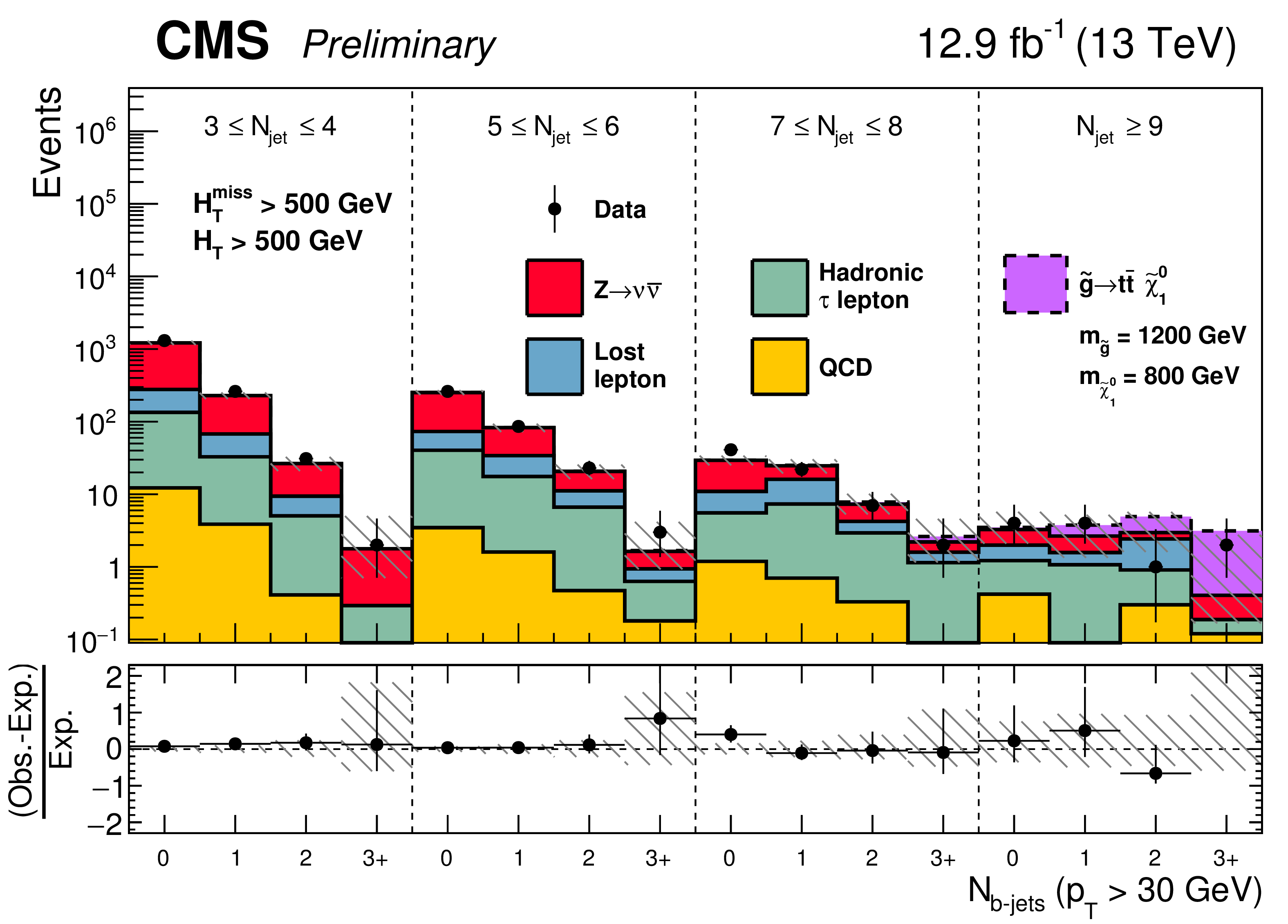
Additional Figure 9-a:
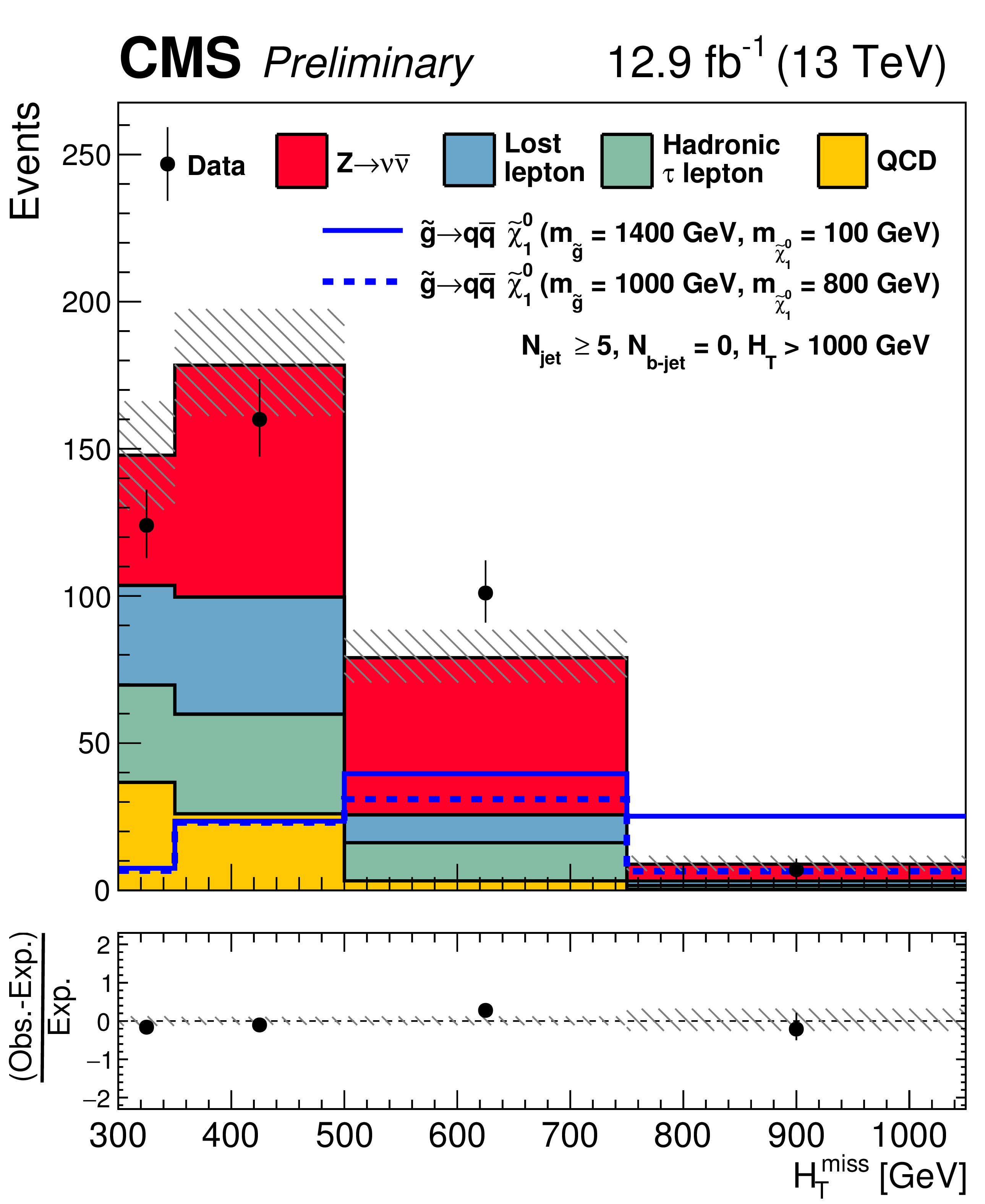
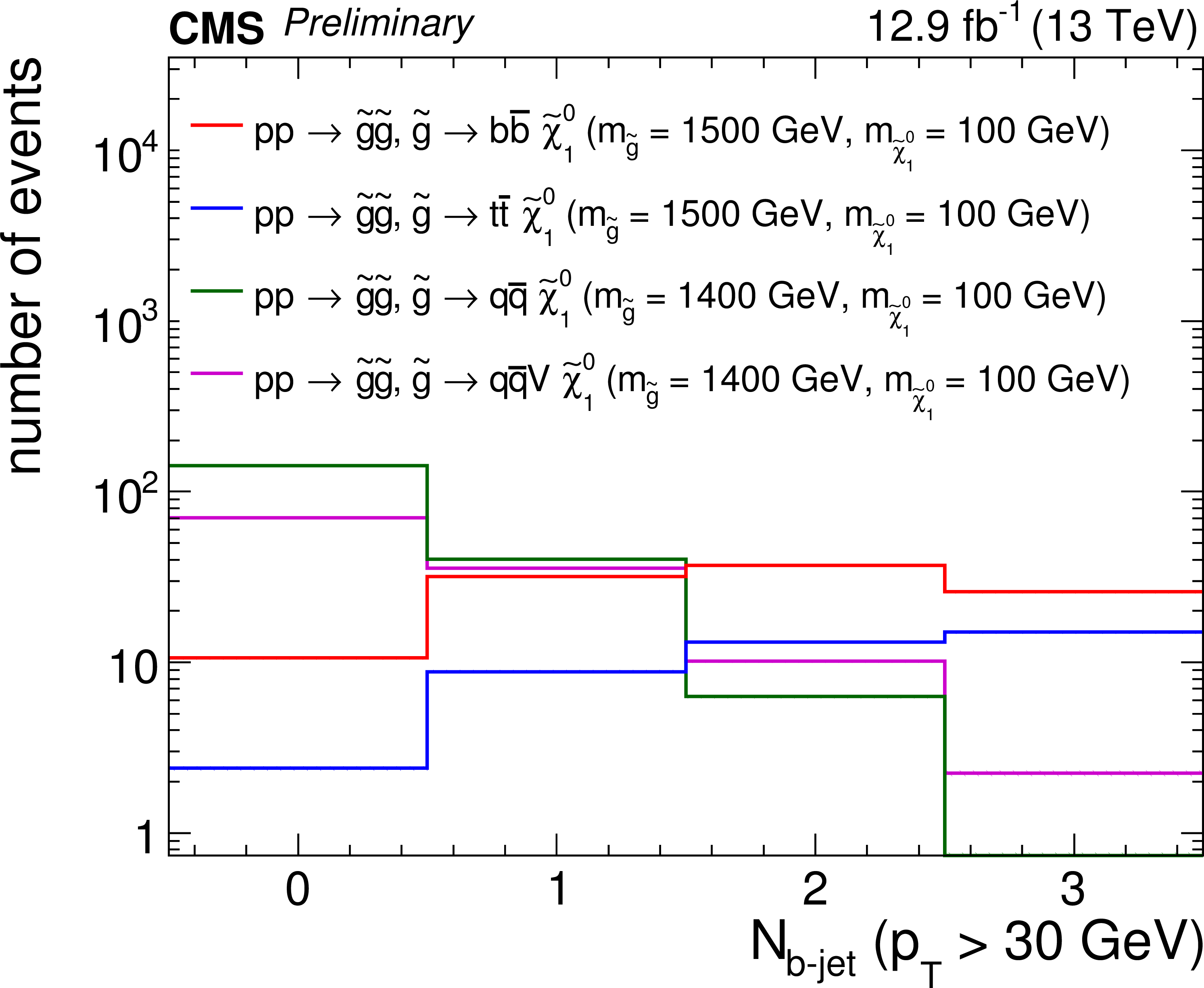
Observed numbers of events and corresponding SM background predictions in bins of $ {N_{\text {jet}}} $ and $ {N_{{\mathrm{ b } }\text {-jet}}} $ , integrated over all search bins with selection (a) $ {H_{\mathrm T}^{\text {miss}}} >500$ GeV and $ {H_{\mathrm {T}}} >500$ GeV or (b) $ {H_{\mathrm T}^{\text {miss}}} >750$ GeV, $ {H_{\mathrm {T}}} >750$ GeV, and $ {N_{\text {jet}}} \geq 5$. An example signal model, $\tilde{g} \rightarrow {\mathrm{ q } \mathrm{ \bar{q} } } \tilde{\chi}^0_1 $ with ${ {m_{\tilde{g} }} }=1400$ GeV and ${ {m_{\tilde{\chi}^{0}_{1}}} }=100$ GeV is stacked on top of the stacked background prediction to illustrate where a signal could lie in our search region phase space. |
png pdf |
Additional Figure 9-b:
Observed numbers of events and corresponding SM background predictions in bins of $ {N_{\text {jet}}} $ and $ {N_{{\mathrm{ b } }\text {-jet}}} $ , integrated over all search bins with selection (a) $ {H_{\mathrm T}^{\text {miss}}} >500$ GeV and $ {H_{\mathrm {T}}} >500$ GeV or (b) $ {H_{\mathrm T}^{\text {miss}}} >750$ GeV, $ {H_{\mathrm {T}}} >750$ GeV, and $ {N_{\text {jet}}} \geq 5$. An example signal model, $\tilde{g} \rightarrow {\mathrm{ q } \mathrm{ \bar{q} } } \tilde{\chi}^0_1 $ with ${ {m_{\tilde{g} }} }=1400$ GeV and ${ {m_{\tilde{\chi}^{0}_{1}}} }=100$ GeV is stacked on top of the stacked background prediction to illustrate where a signal could lie in our search region phase space. |

png pdf |
Additional Figure 10-a:
Observed numbers of events and corresponding SM background predictions in bins of $ {N_{\text {jet}}} $ and $ {N_{{\mathrm{ b } }\text {-jet}}} $ , integrated over all search bins with selection (a) $ {H_{\mathrm T}^{\text {miss}}} >500$ GeV and $ {H_{\mathrm {T}}} >500$ GeV or (b) $ {H_{\mathrm T}^{\text {miss}}} >750$ GeV, $ {H_{\mathrm {T}}} >750$ GeV, and $ {N_{\text {jet}}} \geq 5$. An example signal model, $\tilde{g} \rightarrow {\mathrm{ q } \mathrm{ \bar{q} } } \tilde{\chi}^0_1 $ with ${ {m_{\tilde{g} }} }=1000$ GeV and ${ {m_{\tilde{\chi}^{0}_{1}}} }=800$ GeV is stacked on top of the stacked background prediction to illustrate where a signal could lie in our search region phase space. |

png pdf |
Additional Figure 10-b:
Observed numbers of events and corresponding SM background predictions in bins of $ {N_{\text {jet}}} $ and $ {N_{{\mathrm{ b } }\text {-jet}}} $ , integrated over all search bins with selection (a) $ {H_{\mathrm T}^{\text {miss}}} >500$ GeV and $ {H_{\mathrm {T}}} >500$ GeV or (b) $ {H_{\mathrm T}^{\text {miss}}} >750$ GeV, $ {H_{\mathrm {T}}} >750$ GeV, and $ {N_{\text {jet}}} \geq 5$. An example signal model, $\tilde{g} \rightarrow {\mathrm{ q } \mathrm{ \bar{q} } } \tilde{\chi}^0_1 $ with ${ {m_{\tilde{g} }} }=1000$ GeV and ${ {m_{\tilde{\chi}^{0}_{1}}} }=800$ GeV is stacked on top of the stacked background prediction to illustrate where a signal could lie in our search region phase space. |
png pdf |
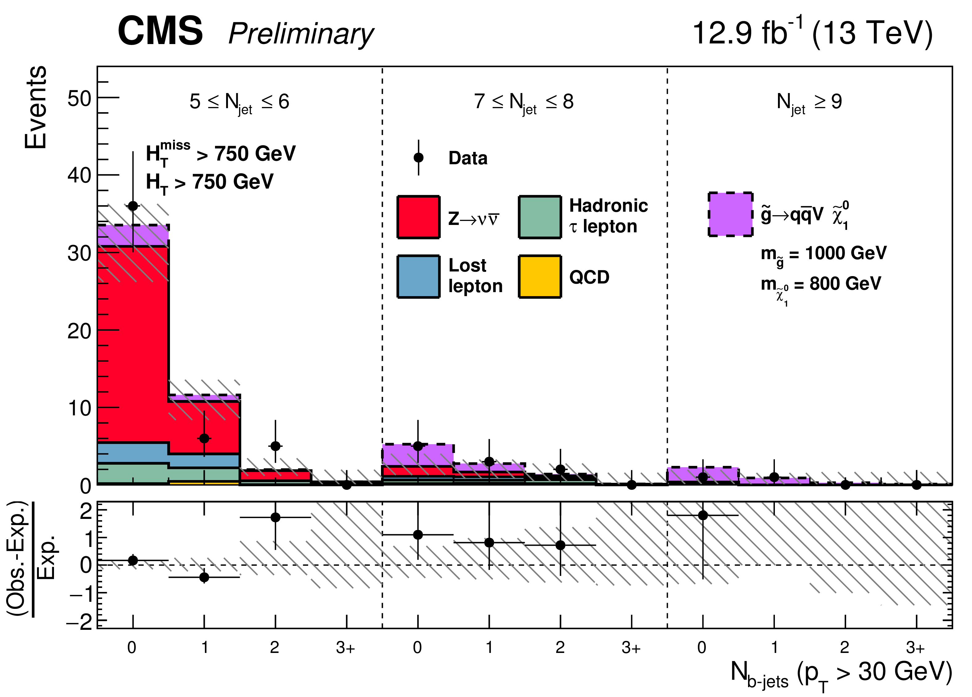
Additional Figure 11-a:
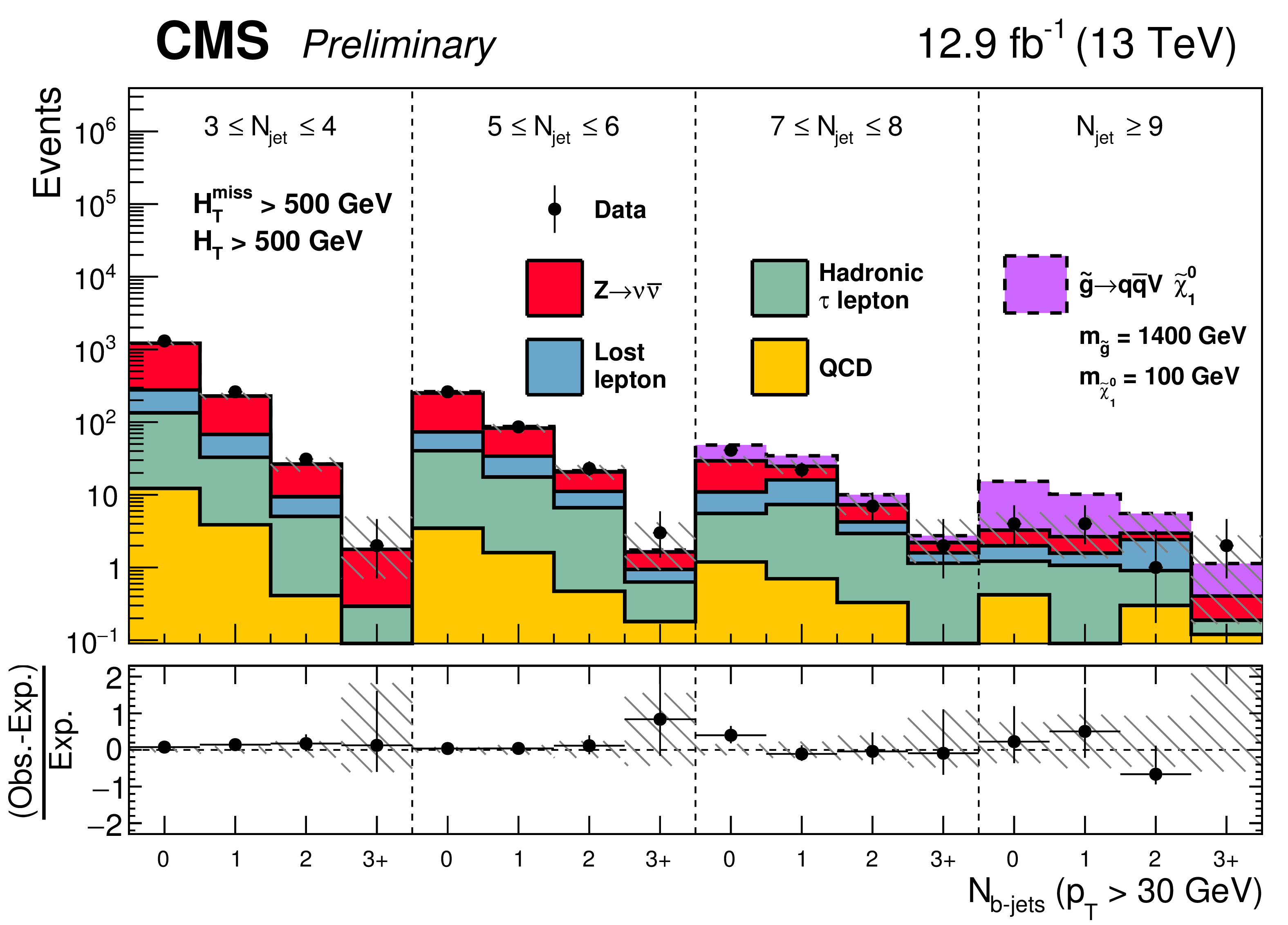
Observed numbers of events and corresponding SM background predictions in bins of $ {N_{\text {jet}}} $ and $ {N_{{\mathrm{ b } }\text {-jet}}} $ , integrated over all search bins with selection (a) $ {H_{\mathrm T}^{\text {miss}}} >500$ GeV and $ {H_{\mathrm {T}}} >500$ GeV or (b) $ {H_{\mathrm T}^{\text {miss}}} >750$ GeV, $ {H_{\mathrm {T}}} >750$ GeV, and $ {N_{\text {jet}}} \geq 5$. An example signal model, $\tilde{g} \rightarrow \mathrm{ q } \mathrm{ \bar{q} } \mathrm {V}\tilde{\chi}^0_1 $ with ${ {m_{\tilde{g} }} }=1400$ GeV and ${ {m_{\tilde{\chi}^{0}_{1}}} }=100$ GeV is stacked on top of the stacked background prediction to illustrate where a signal could lie in our search region phase space. |
png pdf |
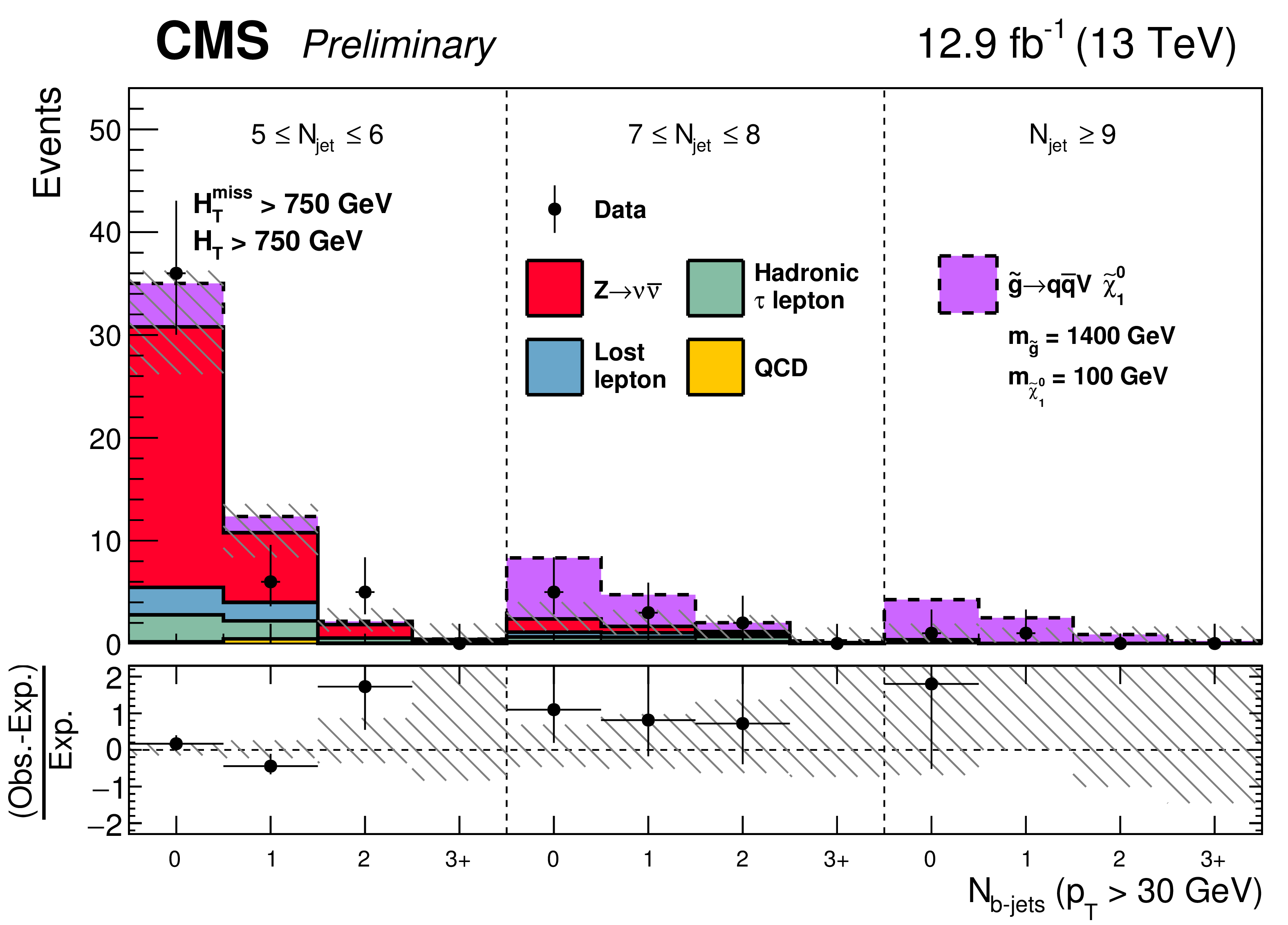
Additional Figure 11-b:
Observed numbers of events and corresponding SM background predictions in bins of $ {N_{\text {jet}}} $ and $ {N_{{\mathrm{ b } }\text {-jet}}} $ , integrated over all search bins with selection (a) $ {H_{\mathrm T}^{\text {miss}}} >500$ GeV and $ {H_{\mathrm {T}}} >500$ GeV or (b) $ {H_{\mathrm T}^{\text {miss}}} >750$ GeV, $ {H_{\mathrm {T}}} >750$ GeV, and $ {N_{\text {jet}}} \geq 5$. An example signal model, $\tilde{g} \rightarrow \mathrm{ q } \mathrm{ \bar{q} } \mathrm {V}\tilde{\chi}^0_1 $ with ${ {m_{\tilde{g} }} }=1400$ GeV and ${ {m_{\tilde{\chi}^{0}_{1}}} }=100$ GeV is stacked on top of the stacked background prediction to illustrate where a signal could lie in our search region phase space. |
png pdf |
Additional Figure 12-a:
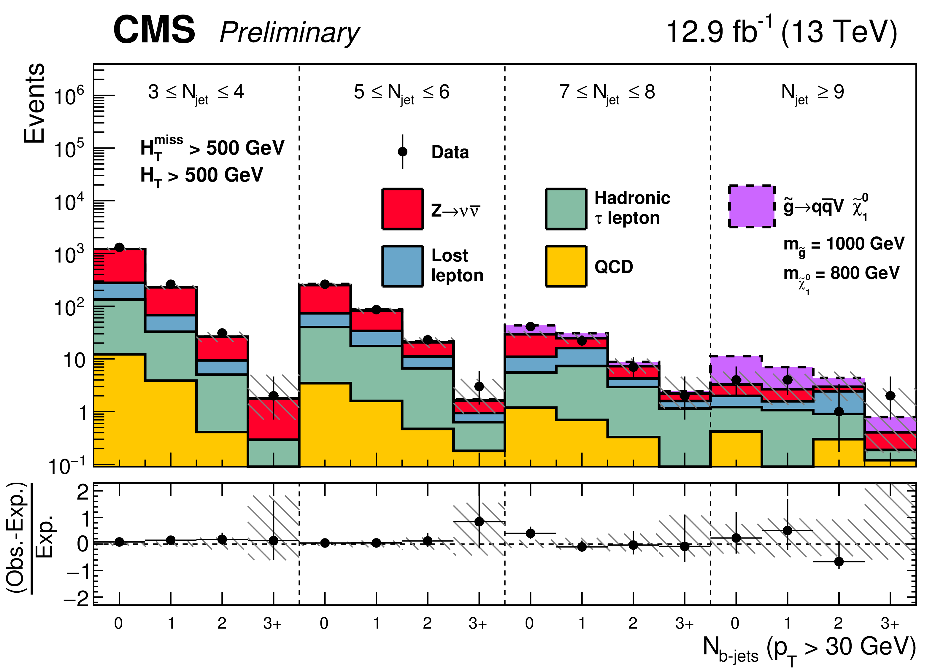
Observed numbers of events and corresponding SM background predictions in bins of $ {N_{\text {jet}}} $ and $ {N_{{\mathrm{ b } }\text {-jet}}} $ , integrated over all search bins with selection (a) $ {H_{\mathrm T}^{\text {miss}}} >500$ GeV and $ {H_{\mathrm {T}}} >500$ GeV or (b) $ {H_{\mathrm T}^{\text {miss}}} >750$ GeV, $ {H_{\mathrm {T}}} >750$ GeV, and $ {N_{\text {jet}}} \geq 5$. An example signal model, $\tilde{g} \rightarrow \mathrm{ q } \mathrm{ \bar{q} } \mathrm {V}\tilde{\chi}^0_1 $ with ${ {m_{\tilde{g} }} }=1000$ GeV and ${ {m_{\tilde{\chi}^{0}_{1}}} }=800$ GeV is stacked on top of the stacked background prediction to illustrate where a signal could lie in our search region phase space. |
png pdf |
Additional Figure 12-b:
Observed numbers of events and corresponding SM background predictions in bins of $ {N_{\text {jet}}} $ and $ {N_{{\mathrm{ b } }\text {-jet}}} $ , integrated over all search bins with selection (a) $ {H_{\mathrm T}^{\text {miss}}} >500$ GeV and $ {H_{\mathrm {T}}} >500$ GeV or (b) $ {H_{\mathrm T}^{\text {miss}}} >750$ GeV, $ {H_{\mathrm {T}}} >750$ GeV, and $ {N_{\text {jet}}} \geq 5$. An example signal model, $\tilde{g} \rightarrow \mathrm{ q } \mathrm{ \bar{q} } \mathrm {V}\tilde{\chi}^0_1 $ with ${ {m_{\tilde{g} }} }=1000$ GeV and ${ {m_{\tilde{\chi}^{0}_{1}}} }=800$ GeV is stacked on top of the stacked background prediction to illustrate where a signal could lie in our search region phase space. |

png pdf |
Additional Figure 13-a:
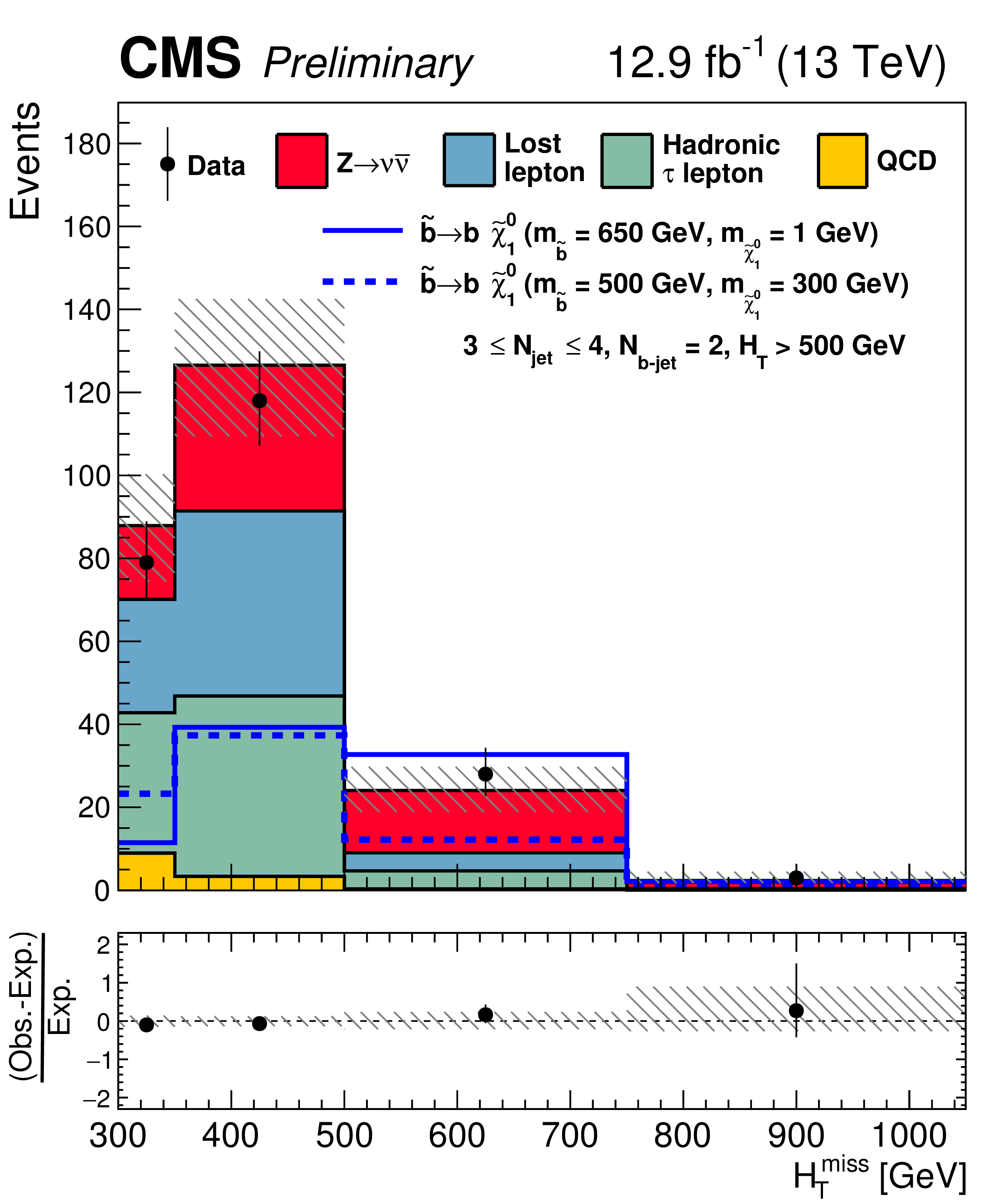
Observed numbers of events and corresponding SM background predictions in bins of $ {N_{\text {jet}}} $ and $ {N_{{\mathrm{ b } }\text {-jet}}} $ , integrated over all search bins with selection (a) $ {H_{\mathrm T}^{\text {miss}}} >500$ GeV and $ {H_{\mathrm {T}}} >500$ GeV or (b) $ {H_{\mathrm T}^{\text {miss}}} >750$ GeV, $ {H_{\mathrm {T}}} >750$ GeV, and $ {N_{\text {jet}}} \geq 5$. An example signal model, $\tilde{\mathrm{b}} \rightarrow \mathrm{ b } \tilde{\chi}^0_1 $ with $m_{\tilde{\mathrm{b}} }=650$ GeV and ${ {m_{\tilde{\chi}^{0}_{1}}} }=1$ GeV is stacked on top of the stacked background prediction to illustrate where a signal could lie in our search region phase space. |

png pdf |
Additional Figure 13-b:
Observed numbers of events and corresponding SM background predictions in bins of $ {N_{\text {jet}}} $ and $ {N_{{\mathrm{ b } }\text {-jet}}} $ , integrated over all search bins with selection (a) $ {H_{\mathrm T}^{\text {miss}}} >500$ GeV and $ {H_{\mathrm {T}}} >500$ GeV or (b) $ {H_{\mathrm T}^{\text {miss}}} >750$ GeV, $ {H_{\mathrm {T}}} >750$ GeV, and $ {N_{\text {jet}}} \geq 5$. An example signal model, $\tilde{\mathrm{b}} \rightarrow \mathrm{ b } \tilde{\chi}^0_1 $ with $m_{\tilde{\mathrm{b}} }=650$ GeV and ${ {m_{\tilde{\chi}^{0}_{1}}} }=1$ GeV is stacked on top of the stacked background prediction to illustrate where a signal could lie in our search region phase space. |

png pdf |
Additional Figure 14-a:
Observed numbers of events and corresponding SM background predictions in bins of $ {N_{\text {jet}}} $ and $ {N_{{\mathrm{ b } }\text {-jet}}} $ , integrated over all search bins with selection (a) $ {H_{\mathrm T}^{\text {miss}}} >500$ GeV and $ {H_{\mathrm {T}}} >500$ GeV or (b) $ {H_{\mathrm T}^{\text {miss}}} >750$ GeV, $ {H_{\mathrm {T}}} >750$ GeV, and $ {N_{\text {jet}}} \geq 5$. An example signal model, $\tilde{\mathrm{b}} \rightarrow \mathrm{ b } \tilde{\chi}^0_1 $ with $m_{\tilde{\mathrm{b}} }=500$ GeV and ${ {m_{\tilde{\chi}^{0}_{1}}} }=300$ GeV is stacked on top of the stacked background prediction to illustrate where a signal could lie in our search region phase space. |

png pdf |
Additional Figure 14-b:
Observed numbers of events and corresponding SM background predictions in bins of $ {N_{\text {jet}}} $ and $ {N_{{\mathrm{ b } }\text {-jet}}} $ , integrated over all search bins with selection (a) $ {H_{\mathrm T}^{\text {miss}}} >500$ GeV and $ {H_{\mathrm {T}}} >500$ GeV or (b) $ {H_{\mathrm T}^{\text {miss}}} >750$ GeV, $ {H_{\mathrm {T}}} >750$ GeV, and $ {N_{\text {jet}}} \geq 5$. An example signal model, $\tilde{\mathrm{b}} \rightarrow \mathrm{ b } \tilde{\chi}^0_1 $ with $m_{\tilde{\mathrm{b}} }=500$ GeV and ${ {m_{\tilde{\chi}^{0}_{1}}} }=300$ GeV is stacked on top of the stacked background prediction to illustrate where a signal could lie in our search region phase space. |

png pdf |
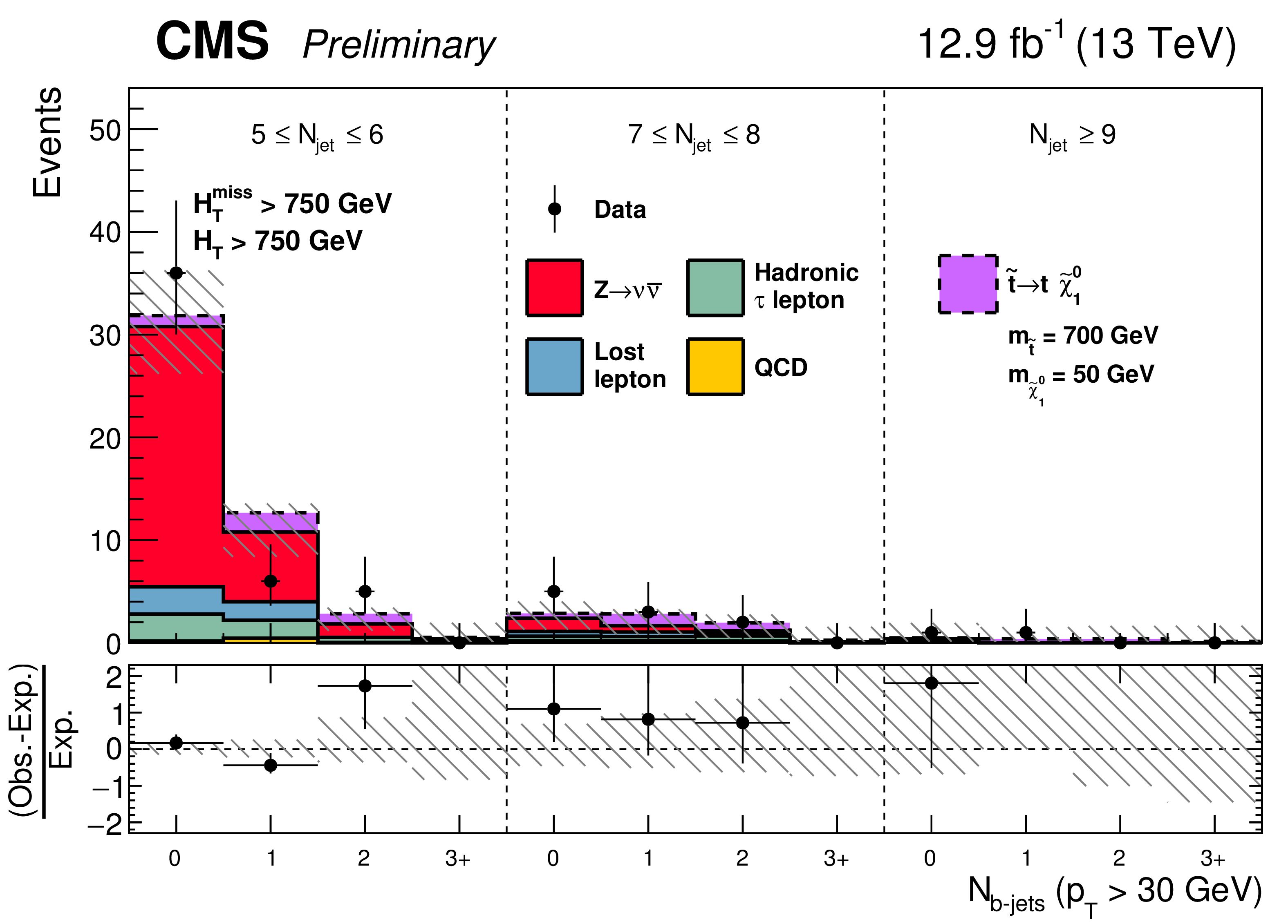
Additional Figure 15-a:
Observed numbers of events and corresponding SM background predictions in bins of $ {N_{\text {jet}}} $ and $ {N_{{\mathrm{ b } }\text {-jet}}} $ , integrated over all search bins with selection (a) $ {H_{\mathrm T}^{\text {miss}}} >500$ GeV and $ {H_{\mathrm {T}}} >500$ GeV or (b) $ {H_{\mathrm T}^{\text {miss}}} >750$ GeV, $ {H_{\mathrm {T}}} >750$ GeV, and $ {N_{\text {jet}}} \geq 5$. An example signal model, $\tilde{\mathrm{t}} \rightarrow \mathrm{ t } \tilde{\chi}^0_1 $ with $m_{\tilde{\mathrm{t}} }=700$ GeV and ${ {m_{\tilde{\chi}^{0}_{1}}} }=50$ GeV is stacked on top of the stacked background prediction to illustrate where a signal could lie in our search region phase space. |
png pdf |
Additional Figure 15-b:
Observed numbers of events and corresponding SM background predictions in bins of $ {N_{\text {jet}}} $ and $ {N_{{\mathrm{ b } }\text {-jet}}} $ , integrated over all search bins with selection (a) $ {H_{\mathrm T}^{\text {miss}}} >500$ GeV and $ {H_{\mathrm {T}}} >500$ GeV or (b) $ {H_{\mathrm T}^{\text {miss}}} >750$ GeV, $ {H_{\mathrm {T}}} >750$ GeV, and $ {N_{\text {jet}}} \geq 5$. An example signal model, $\tilde{\mathrm{t}} \rightarrow \mathrm{ t } \tilde{\chi}^0_1 $ with $m_{\tilde{\mathrm{t}} }=700$ GeV and ${ {m_{\tilde{\chi}^{0}_{1}}} }=50$ GeV is stacked on top of the stacked background prediction to illustrate where a signal could lie in our search region phase space. |

png pdf |
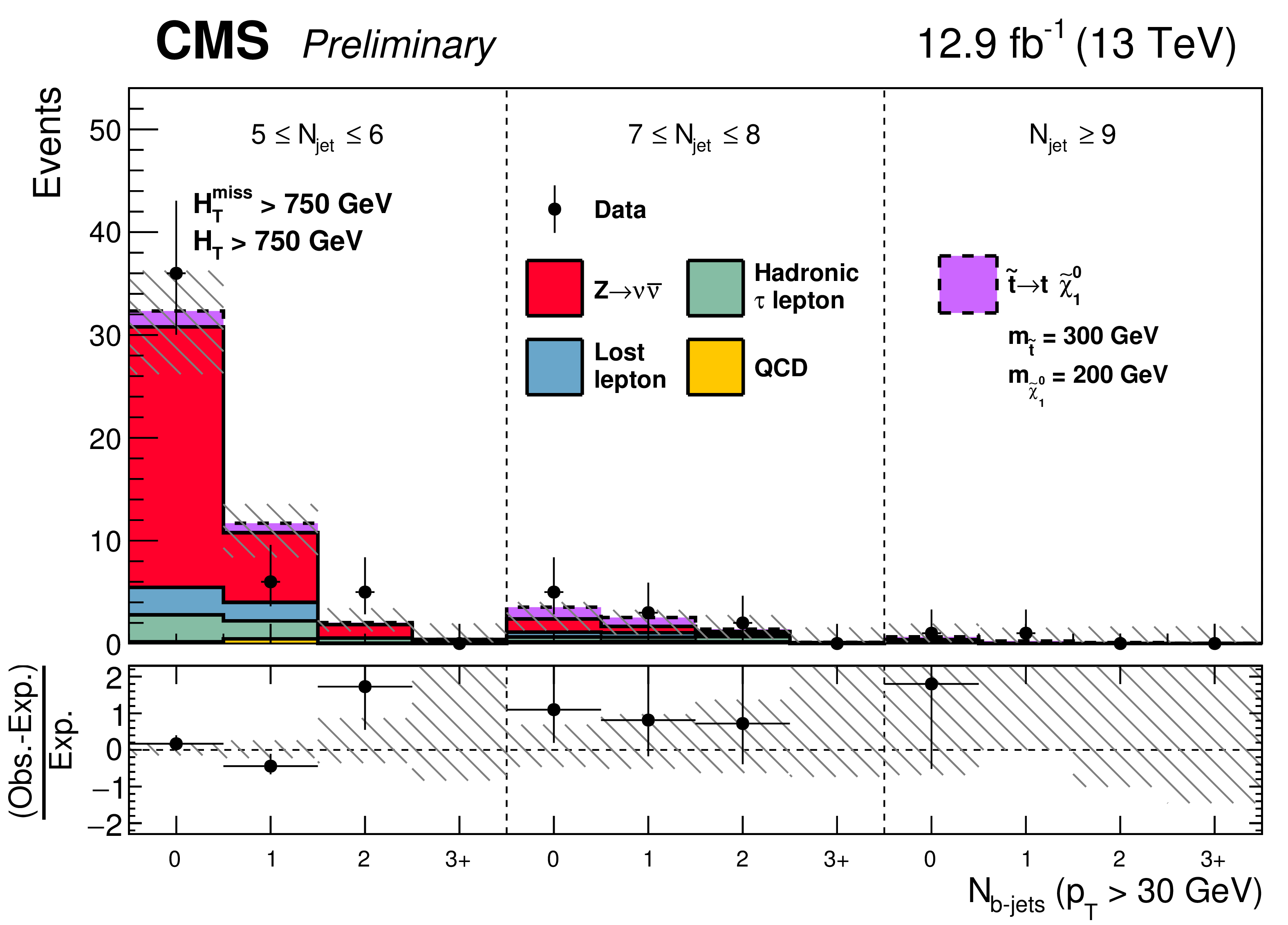
Additional Figure 16-a:
Observed numbers of events and corresponding SM background predictions in bins of $ {N_{\text {jet}}} $ and $ {N_{{\mathrm{ b } }\text {-jet}}} $ , integrated over all search bins with selection (a) $ {H_{\mathrm T}^{\text {miss}}} >500$ GeV and $ {H_{\mathrm {T}}} >500$ GeV or (b) $ {H_{\mathrm T}^{\text {miss}}} >750$ GeV, $ {H_{\mathrm {T}}} >750$ GeV, and $ {N_{\text {jet}}} \geq 5$. An example signal model, $\tilde{\mathrm{t}} \rightarrow \mathrm{ t } \tilde{\chi}^0_1 $ with $m_{\tilde{\mathrm{t}} }=300$ GeV and ${ {m_{\tilde{\chi}^{0}_{1}}} }=200$ GeV is stacked on top of the stacked background prediction to illustrate where a signal could lie in our search region phase space. |
png pdf |
Additional Figure 16-b:
Observed numbers of events and corresponding SM background predictions in bins of $ {N_{\text {jet}}} $ and $ {N_{{\mathrm{ b } }\text {-jet}}} $ , integrated over all search bins with selection (a) $ {H_{\mathrm T}^{\text {miss}}} >500$ GeV and $ {H_{\mathrm {T}}} >500$ GeV or (b) $ {H_{\mathrm T}^{\text {miss}}} >750$ GeV, $ {H_{\mathrm {T}}} >750$ GeV, and $ {N_{\text {jet}}} \geq 5$. An example signal model, $\tilde{\mathrm{t}} \rightarrow \mathrm{ t } \tilde{\chi}^0_1 $ with $m_{\tilde{\mathrm{t}} }=300$ GeV and ${ {m_{\tilde{\chi}^{0}_{1}}} }=200$ GeV is stacked on top of the stacked background prediction to illustrate where a signal could lie in our search region phase space. |
png pdf |
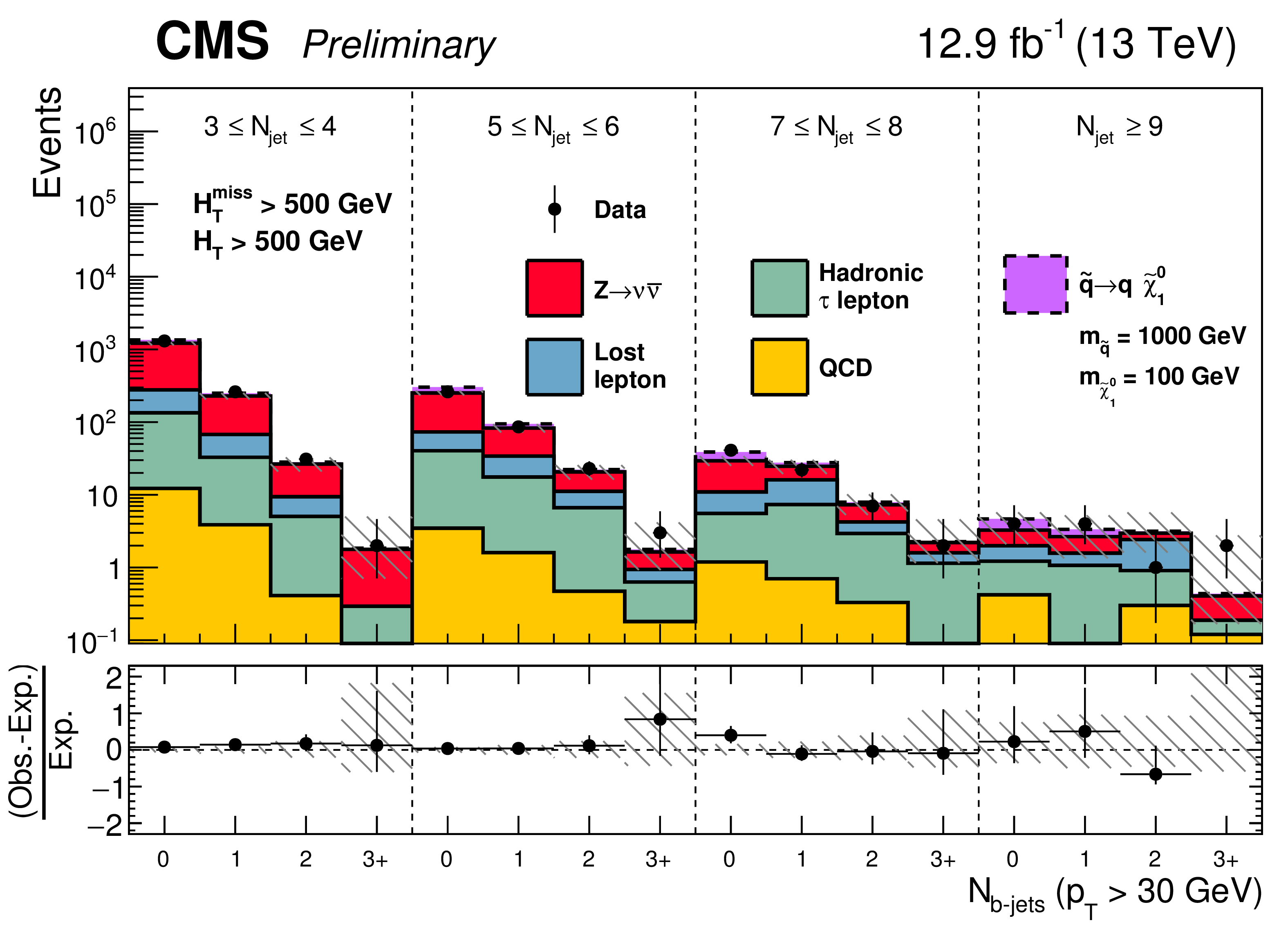
Additional Figure 17-a:
Observed numbers of events and corresponding SM background predictions in bins of $ {N_{\text {jet}}} $ and $ {N_{{\mathrm{ b } }\text {-jet}}} $ , integrated over all search bins with selection (a) $ {H_{\mathrm T}^{\text {miss}}} >500$ GeV and $ {H_{\mathrm {T}}} >500$ GeV or (b) $ {H_{\mathrm T}^{\text {miss}}} >750$ GeV, $ {H_{\mathrm {T}}} >750$ GeV, and $ {N_{\text {jet}}} \geq 5$. An example signal model, $\tilde{\mathrm{q}} \rightarrow \mathrm{ q } \tilde{\chi}^0_1 $ with $m_{\tilde{\mathrm{q}} }=1000$ GeV and ${ {m_{\tilde{\chi}^{0}_{1}}} }=100$ GeV is stacked on top of the stacked background prediction to illustrate where a signal could lie in our search region phase space. |
png pdf |
Additional Figure 17-b:
Observed numbers of events and corresponding SM background predictions in bins of $ {N_{\text {jet}}} $ and $ {N_{{\mathrm{ b } }\text {-jet}}} $ , integrated over all search bins with selection (a) $ {H_{\mathrm T}^{\text {miss}}} >500$ GeV and $ {H_{\mathrm {T}}} >500$ GeV or (b) $ {H_{\mathrm T}^{\text {miss}}} >750$ GeV, $ {H_{\mathrm {T}}} >750$ GeV, and $ {N_{\text {jet}}} \geq 5$. An example signal model, $\tilde{\mathrm{q}} \rightarrow \mathrm{ q } \tilde{\chi}^0_1 $ with $m_{\tilde{\mathrm{q}} }=1000$ GeV and ${ {m_{\tilde{\chi}^{0}_{1}}} }=100$ GeV is stacked on top of the stacked background prediction to illustrate where a signal could lie in our search region phase space. |

png pdf |
Additional Figure 18-a:
Observed numbers of events and corresponding SM background predictions in bins of $ {N_{\text {jet}}} $ and $ {N_{{\mathrm{ b } }\text {-jet}}} $ , integrated over all search bins with selection (a) $ {H_{\mathrm T}^{\text {miss}}} >500$ GeV and $ {H_{\mathrm {T}}} >500$ GeV or (b) $ {H_{\mathrm T}^{\text {miss}}} >750$ GeV, $ {H_{\mathrm {T}}} >750$ GeV, and $ {N_{\text {jet}}} \geq 5$. An example signal model, $\tilde{\mathrm{q}} \rightarrow \mathrm{ q } \tilde{\chi}^0_1 $ with $m_{\tilde{\mathrm{q}} }=700$ GeV and ${ {m_{\tilde{\chi}^{0}_{1}}} }=400$ GeV is stacked on top of the stacked background prediction to illustrate where a signal could lie in our search region phase space. |

png pdf |
Additional Figure 18-b:
Observed numbers of events and corresponding SM background predictions in bins of $ {N_{\text {jet}}} $ and $ {N_{{\mathrm{ b } }\text {-jet}}} $ , integrated over all search bins with selection (a) $ {H_{\mathrm T}^{\text {miss}}} >500$ GeV and $ {H_{\mathrm {T}}} >500$ GeV or (b) $ {H_{\mathrm T}^{\text {miss}}} >750$ GeV, $ {H_{\mathrm {T}}} >750$ GeV, and $ {N_{\text {jet}}} \geq 5$. An example signal model, $\tilde{\mathrm{q}} \rightarrow \mathrm{ q } \tilde{\chi}^0_1 $ with $m_{\tilde{\mathrm{q}} }=700$ GeV and ${ {m_{\tilde{\chi}^{0}_{1}}} }=400$ GeV is stacked on top of the stacked background prediction to illustrate where a signal could lie in our search region phase space. |

png pdf |
Additional Figure 19:
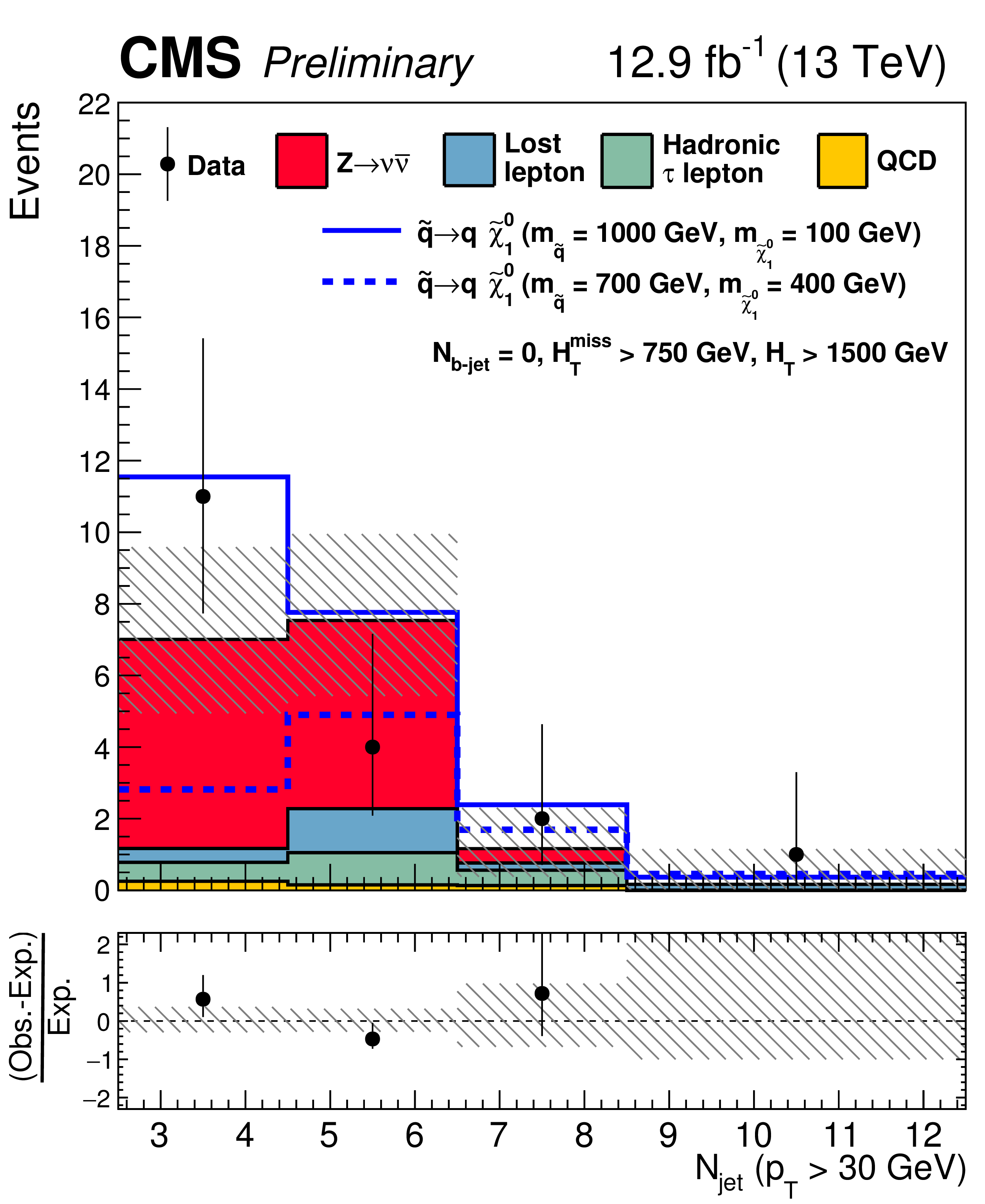
Observed numbers of events and corresponding SM background predictions for intervals of the search region parameter space particularly sensitive to the T5qqqqVV scenario. Additional selection requirements of $ {N_{{\mathrm{ b } }\text {-jet}}} =0$, $ {H_{\mathrm T}^{\text {miss}}} >750$ GeV, and $ {H_{\mathrm {T}}} >1500$ GeV are applied. The hatched regions indicate the total uncertainties in the background predictions. The (unstacked) results for two example signal scenarios are shown in each instance, one with ${ {m_{\tilde{g} }} } $ or $ {m_{\tilde{\mathrm{q}} }} \gg {m_{\tilde{\chi}^{0}_{1}}} $ and the other with ${ {m_{\tilde{\chi}^{0}_{1}}} }\sim {m_{\tilde{g} }} $ or $ {m_{\tilde{\mathrm{q}} }} $. |
png pdf |
Additional Figure 20:
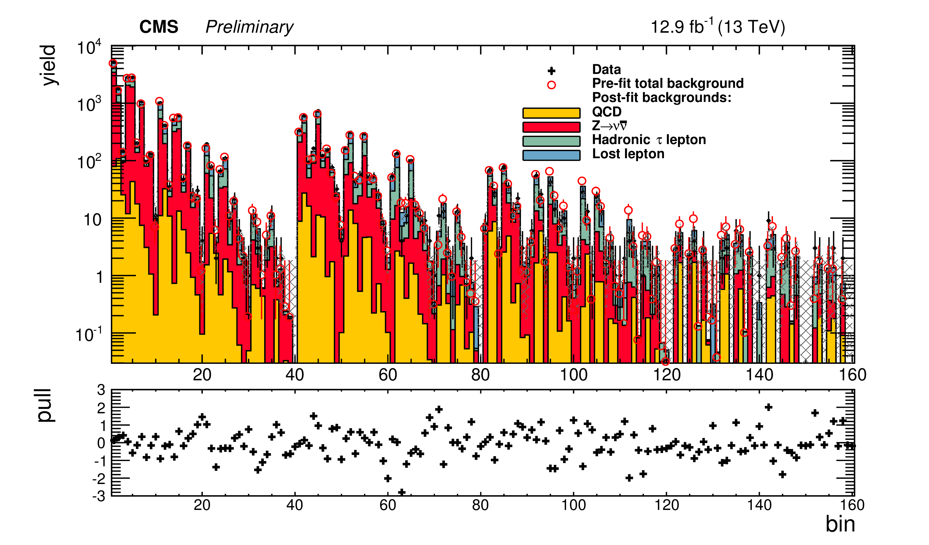
Observed number of events, post-fit background predictions, and pre-fit background predictions in all search bins. The lower panel of the plot shows the pull, defined as $\sqrt {-2\ln\left [{\rm Pois}(N_{\rm Obs.}|N_{\rm Pred.})/{\rm Pois}(N_{\rm Obs.}|N_{\rm Obs.})\right ]}$, where $N_{\rm Obs.}$ is the observed number of events in the bin, $N_{\rm Pred.}$ is the total post-fit background prediction for the bin, and ${\rm Pois}(a|b)$ is defined as the Poisson probability density function of mean $b$ evaluated at point $a$. |
png pdf |
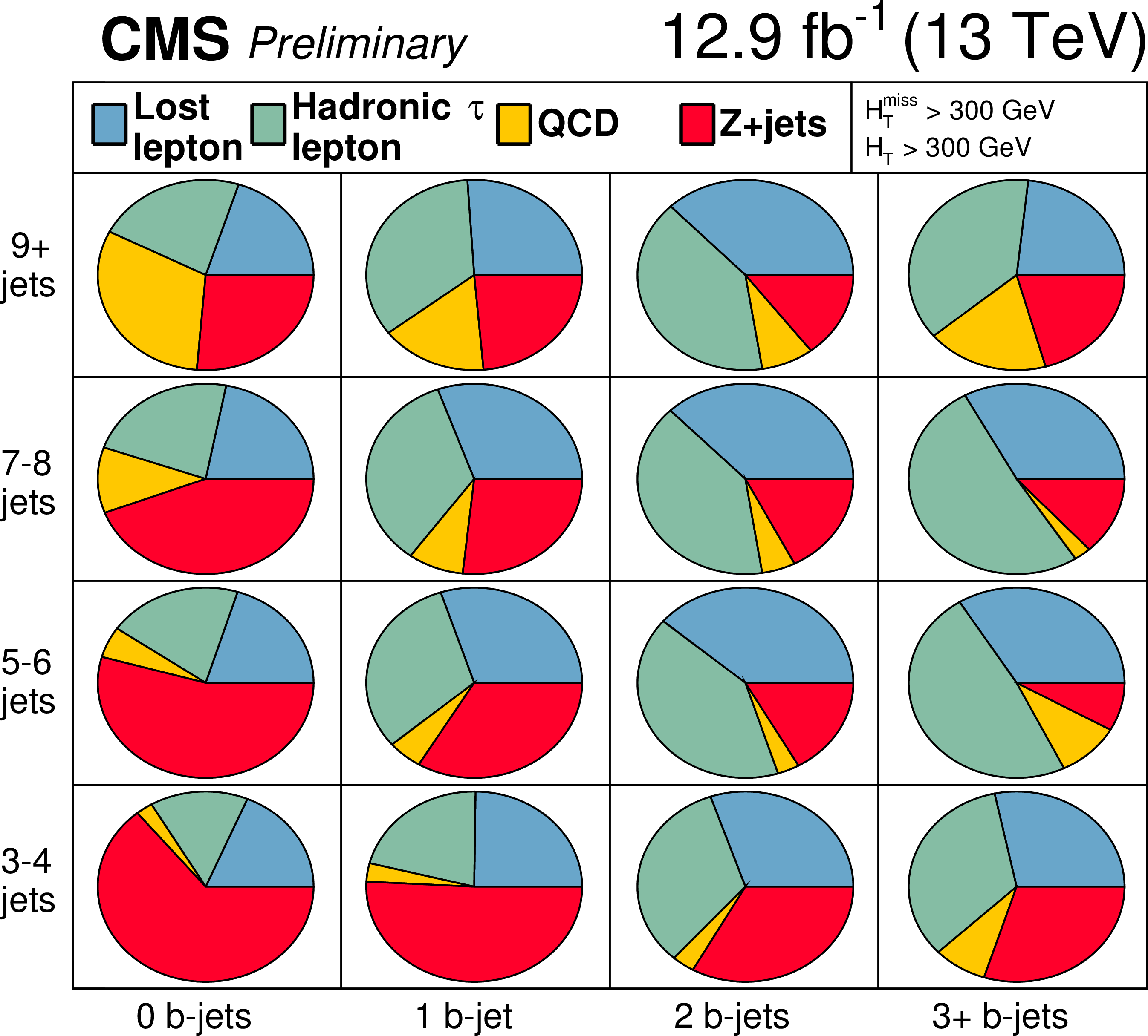
Additional Figure 21-a:
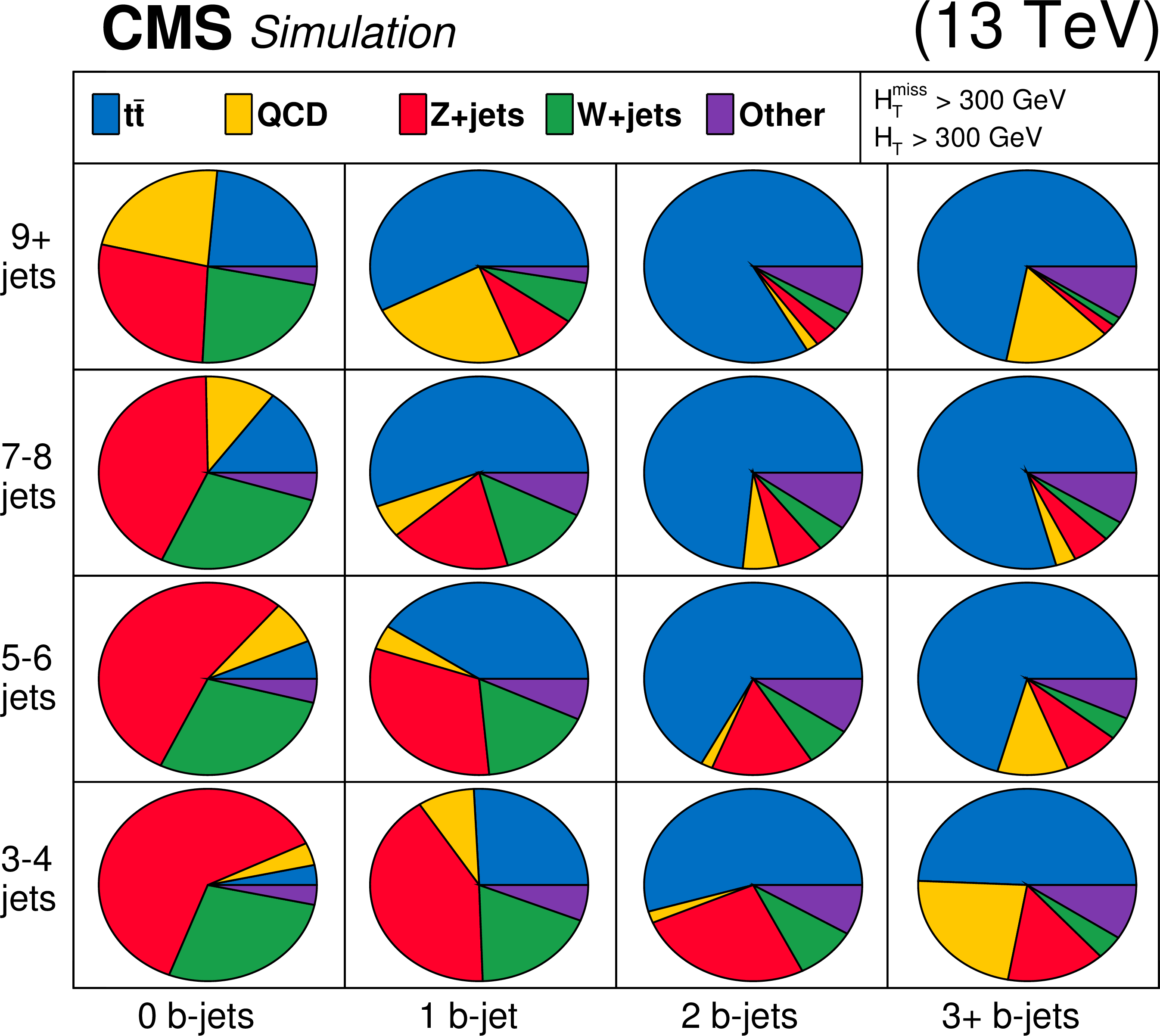
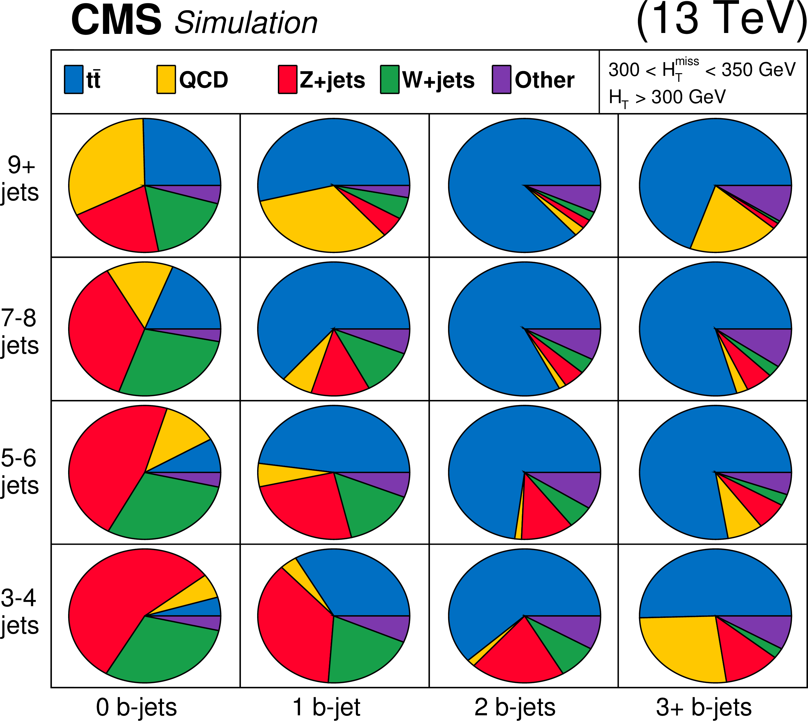
Background composition in zero-lepton search region in bins of the number of jets and the number of b-tagged jets. The expected contribution from each process is obtained from simulation after applying the full baseline selection, either inclusive in $ {H_{\mathrm T}^{\text {miss}}} $ and $ {H_{\mathrm {T}}} $ (a), or by also requiring $300< {H_{\mathrm T}^{\text {miss}}} <350$ GeV and $ {H_{\mathrm {T}}} >300$ GeV (b), $350< {H_{\mathrm T}^{\text {miss}}} <500$ GeV and $ {H_{\mathrm {T}}} >350$ GeV (c), or $ {H_{\mathrm T}^{\text {miss}}} >500$ GeV and $ {H_{\mathrm {T}}} >500$ GeV (d). |
png pdf |
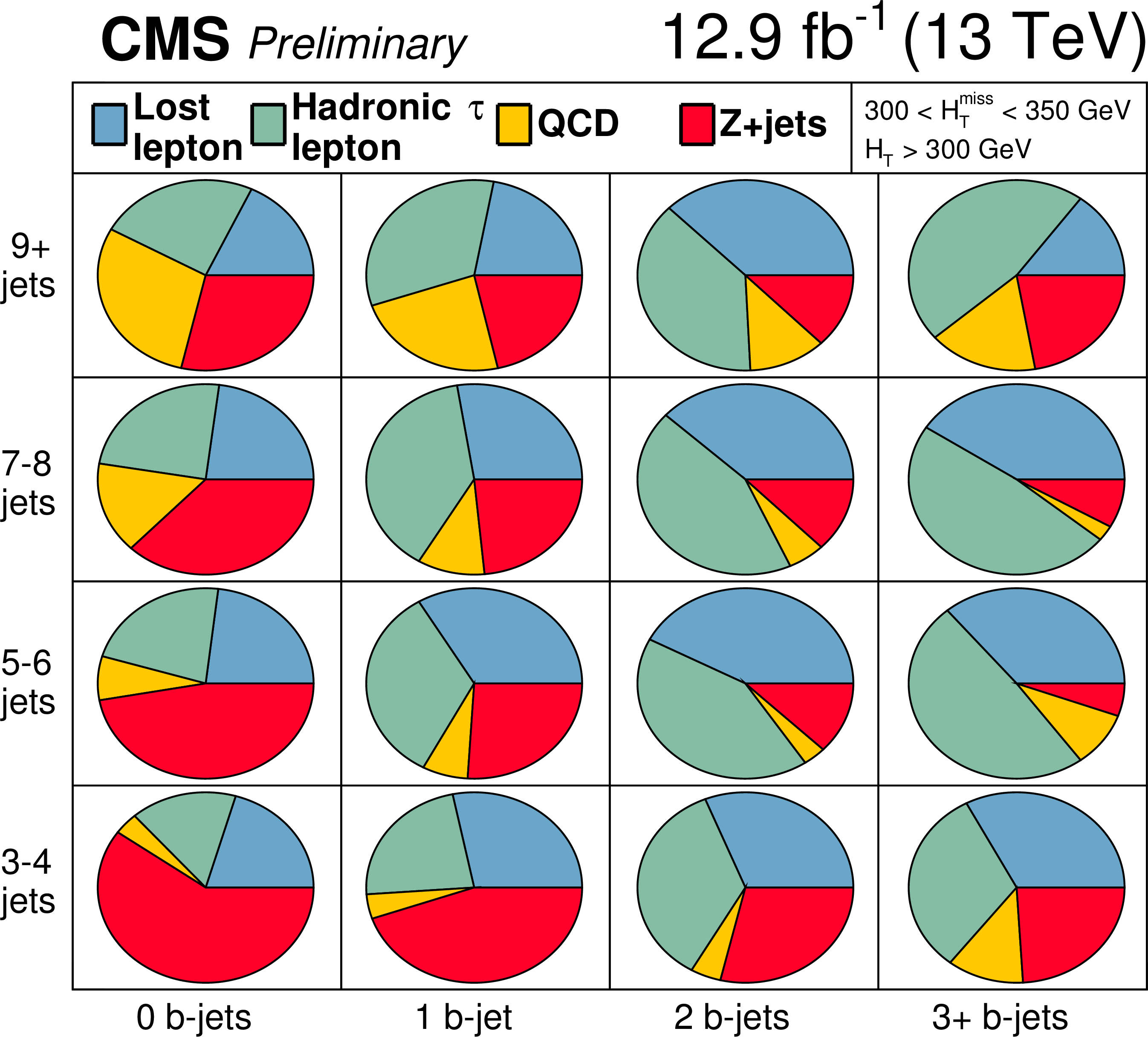
Additional Figure 21-b:
Background composition in zero-lepton search region in bins of the number of jets and the number of b-tagged jets. The expected contribution from each process is obtained from simulation after applying the full baseline selection, either inclusive in $ {H_{\mathrm T}^{\text {miss}}} $ and $ {H_{\mathrm {T}}} $ (a), or by also requiring $300< {H_{\mathrm T}^{\text {miss}}} <350$ GeV and $ {H_{\mathrm {T}}} >300$ GeV (b), $350< {H_{\mathrm T}^{\text {miss}}} <500$ GeV and $ {H_{\mathrm {T}}} >350$ GeV (c), or $ {H_{\mathrm T}^{\text {miss}}} >500$ GeV and $ {H_{\mathrm {T}}} >500$ GeV (d). |

png pdf |
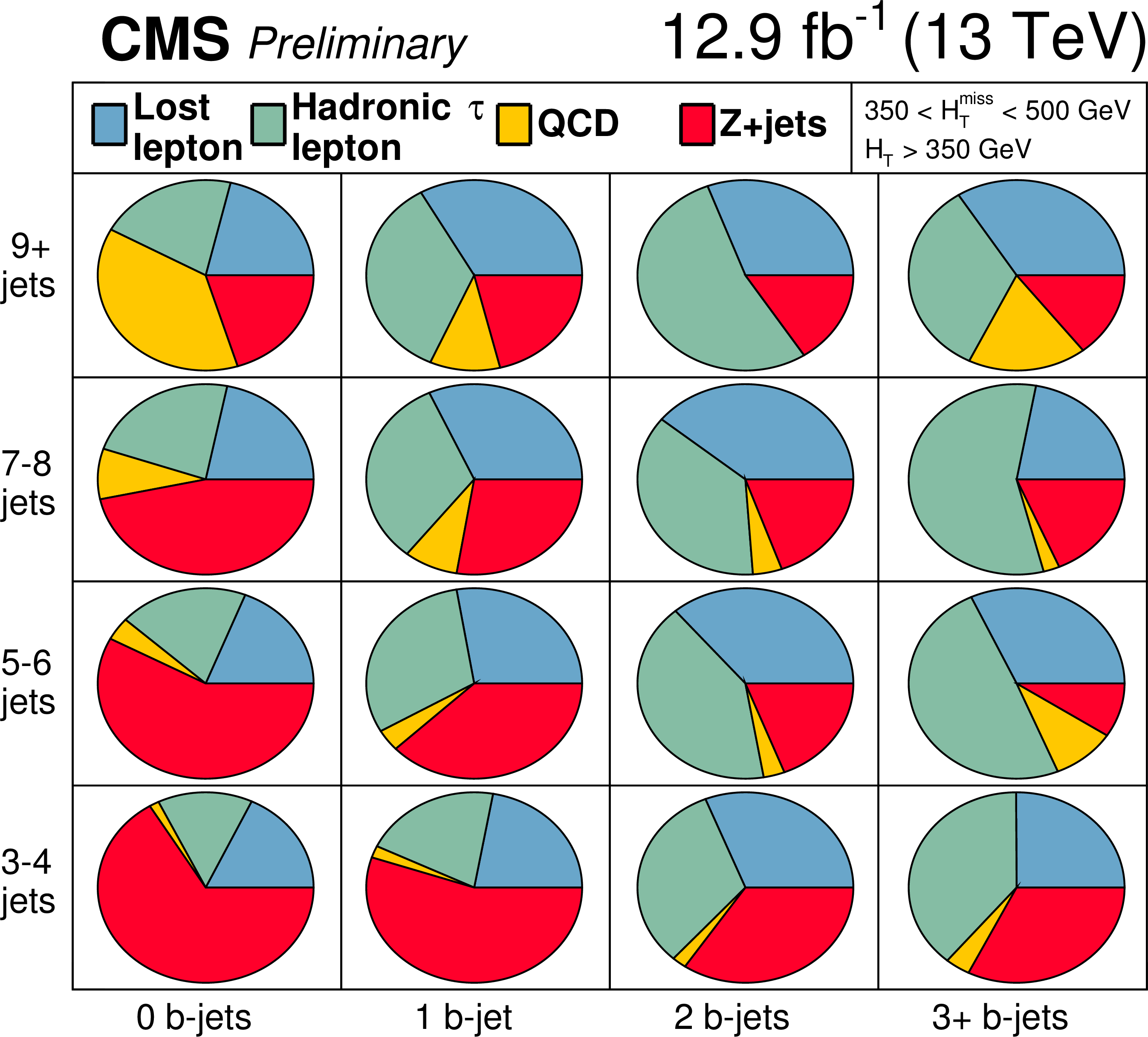
Additional Figure 21-c:
Background composition in zero-lepton search region in bins of the number of jets and the number of b-tagged jets. The expected contribution from each process is obtained from simulation after applying the full baseline selection, either inclusive in $ {H_{\mathrm T}^{\text {miss}}} $ and $ {H_{\mathrm {T}}} $ (a), or by also requiring $300< {H_{\mathrm T}^{\text {miss}}} <350$ GeV and $ {H_{\mathrm {T}}} >300$ GeV (b), $350< {H_{\mathrm T}^{\text {miss}}} <500$ GeV and $ {H_{\mathrm {T}}} >350$ GeV (c), or $ {H_{\mathrm T}^{\text {miss}}} >500$ GeV and $ {H_{\mathrm {T}}} >500$ GeV (d). |

png pdf |
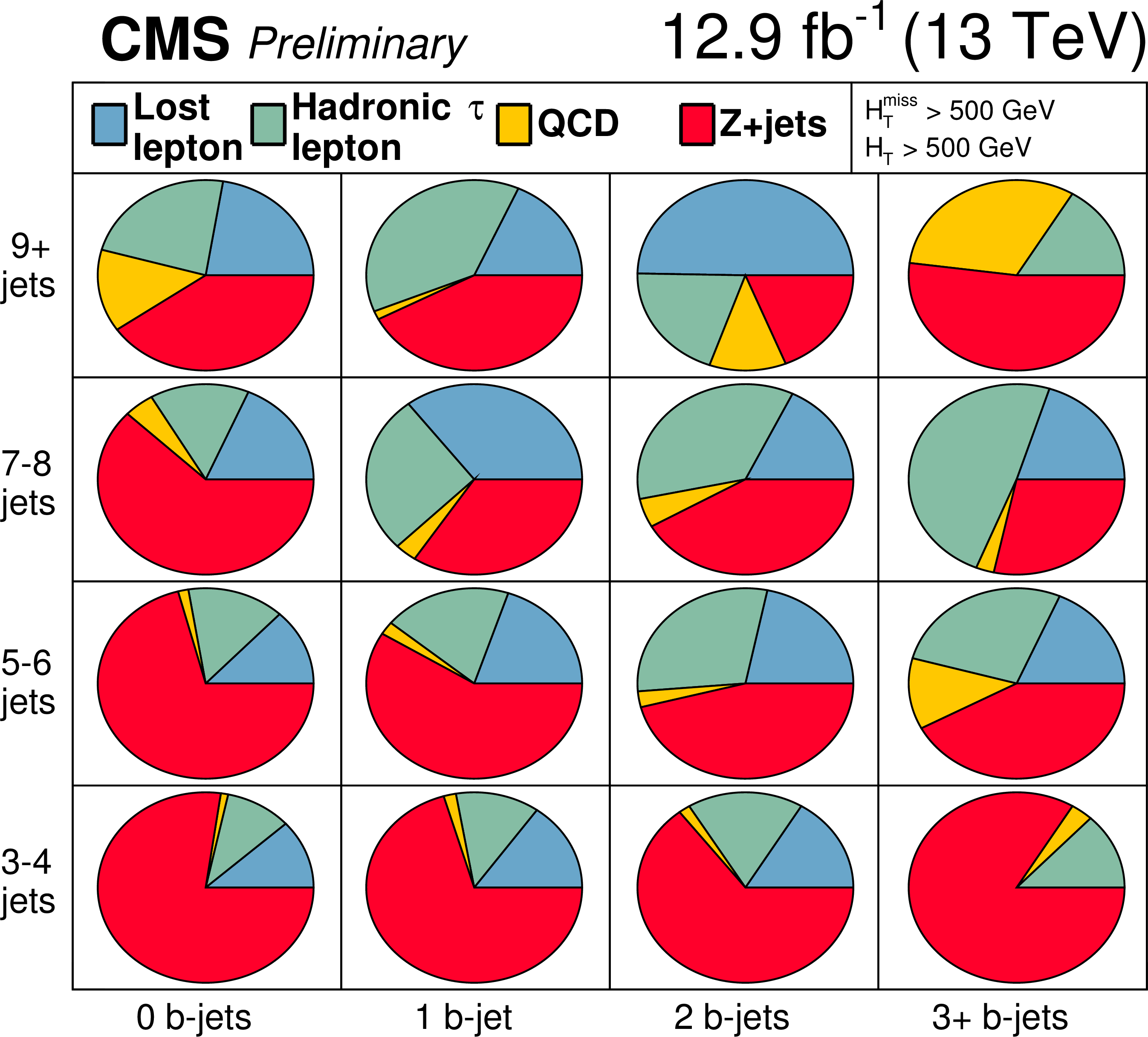
Additional Figure 21-d:
Background composition in zero-lepton search region in bins of the number of jets and the number of b-tagged jets. The expected contribution from each process is obtained from simulation after applying the full baseline selection, either inclusive in $ {H_{\mathrm T}^{\text {miss}}} $ and $ {H_{\mathrm {T}}} $ (a), or by also requiring $300< {H_{\mathrm T}^{\text {miss}}} <350$ GeV and $ {H_{\mathrm {T}}} >300$ GeV (b), $350< {H_{\mathrm T}^{\text {miss}}} <500$ GeV and $ {H_{\mathrm {T}}} >350$ GeV (c), or $ {H_{\mathrm T}^{\text {miss}}} >500$ GeV and $ {H_{\mathrm {T}}} >500$ GeV (d). |
png pdf |
Additional Figure 22-a:
Background composition in zero-lepton search region in bins of the number of jets and the number of b-tagged jets. The expected contribution from each process is obtained from our data-driven background measurement, either inclusive in $ {H_{\mathrm T}^{\text {miss}}} $ and $ {H_{\mathrm {T}}} $ (a), or integrating over bins with $300< {H_{\mathrm T}^{\text {miss}}} <350$ GeV and $ {H_{\mathrm {T}}} >300$ GeV (b), $350< {H_{\mathrm T}^{\text {miss}}} <500$ GeV and $ {H_{\mathrm {T}}} >350$ GeV (c), or $ {H_{\mathrm T}^{\text {miss}}} >500$ GeV and $ {H_{\mathrm {T}}} >500$ GeV (d). |
png pdf |
Additional Figure 22-b:
Background composition in zero-lepton search region in bins of the number of jets and the number of b-tagged jets. The expected contribution from each process is obtained from our data-driven background measurement, either inclusive in $ {H_{\mathrm T}^{\text {miss}}} $ and $ {H_{\mathrm {T}}} $ (a), or integrating over bins with $300< {H_{\mathrm T}^{\text {miss}}} <350$ GeV and $ {H_{\mathrm {T}}} >300$ GeV (b), $350< {H_{\mathrm T}^{\text {miss}}} <500$ GeV and $ {H_{\mathrm {T}}} >350$ GeV (c), or $ {H_{\mathrm T}^{\text {miss}}} >500$ GeV and $ {H_{\mathrm {T}}} >500$ GeV (d). |
png pdf |
Additional Figure 22-c:
Background composition in zero-lepton search region in bins of the number of jets and the number of b-tagged jets. The expected contribution from each process is obtained from our data-driven background measurement, either inclusive in $ {H_{\mathrm T}^{\text {miss}}} $ and $ {H_{\mathrm {T}}} $ (a), or integrating over bins with $300< {H_{\mathrm T}^{\text {miss}}} <350$ GeV and $ {H_{\mathrm {T}}} >300$ GeV (b), $350< {H_{\mathrm T}^{\text {miss}}} <500$ GeV and $ {H_{\mathrm {T}}} >350$ GeV (c), or $ {H_{\mathrm T}^{\text {miss}}} >500$ GeV and $ {H_{\mathrm {T}}} >500$ GeV (d). |
png pdf |
Additional Figure 22-d:
Background composition in zero-lepton search region in bins of the number of jets and the number of b-tagged jets. The expected contribution from each process is obtained from our data-driven background measurement, either inclusive in $ {H_{\mathrm T}^{\text {miss}}} $ and $ {H_{\mathrm {T}}} $ (a), or integrating over bins with $300< {H_{\mathrm T}^{\text {miss}}} <350$ GeV and $ {H_{\mathrm {T}}} >300$ GeV (b), $350< {H_{\mathrm T}^{\text {miss}}} <500$ GeV and $ {H_{\mathrm {T}}} >350$ GeV (c), or $ {H_{\mathrm T}^{\text {miss}}} >500$ GeV and $ {H_{\mathrm {T}}} >500$ GeV (d). |
png pdf |
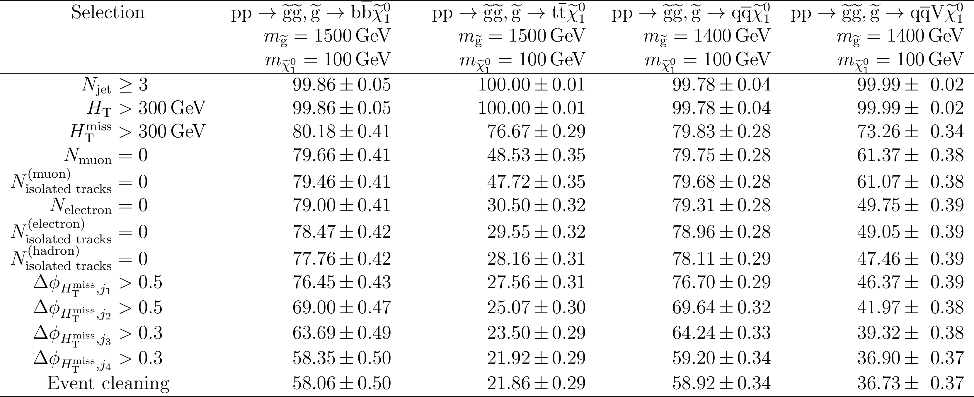
Additional Figure 23:
Absolute cumulative efficiencies in % for each step of the event selection process, listed for four representative gluino pair production signal models with ${m_{\tilde{g} } \gg m_{\tilde{\chi}^0_1 }}$. Only statistical uncertainties are shown. |

png pdf |
Additional Figure 24:
Absolute cumulative efficiencies in % for each step of the event selection process, listed for four representative gluino pair production signal models with ${m_{\tilde{g} } \sim m_{\tilde{\chi}^0_1 }}$. Only statistical uncertainties are shown. |
png pdf |
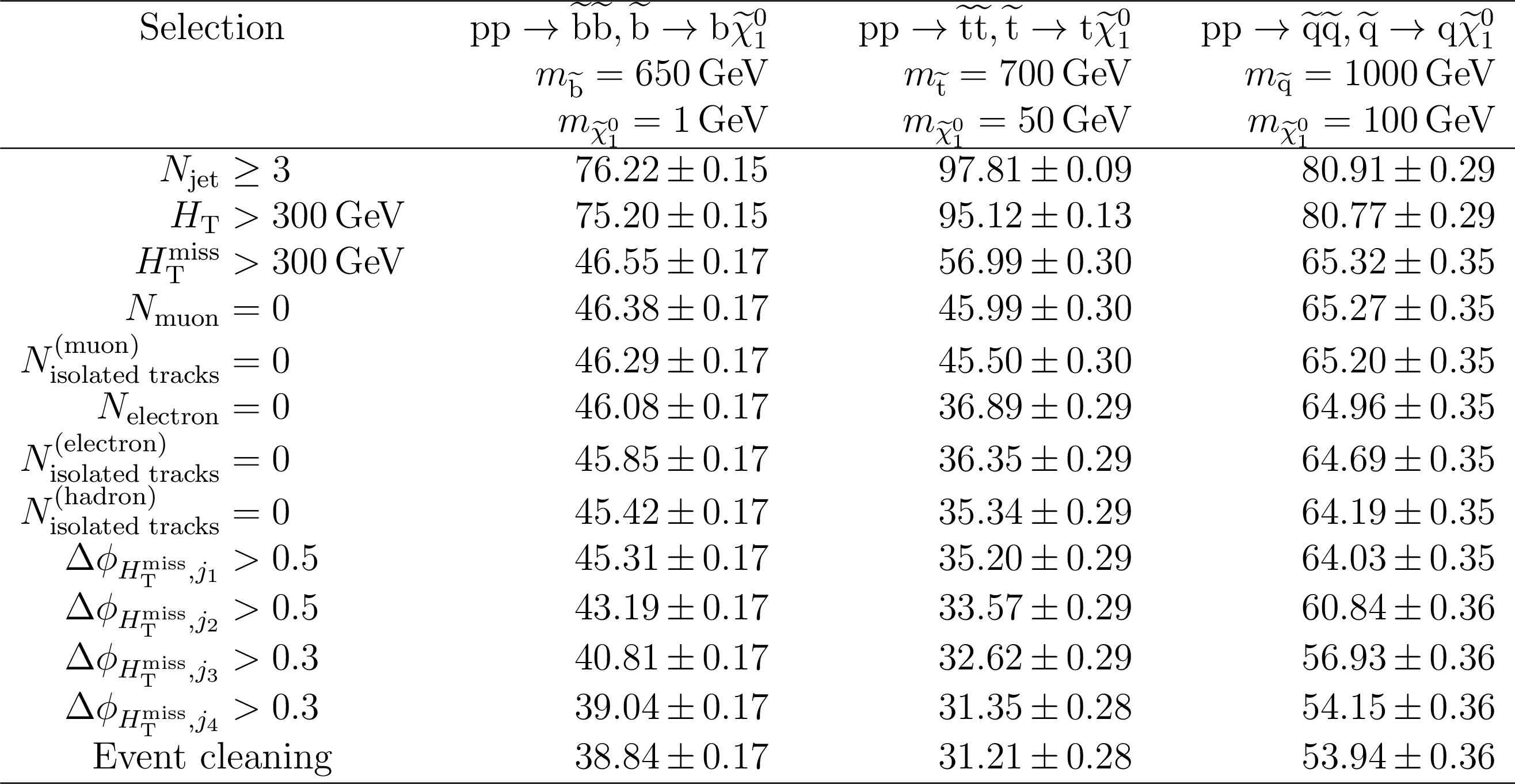
Additional Figure 25:
Absolute cumulative efficiencies in % for each step of the event selection process, listed for three representative squark pair production signal models with ${m_{\tilde{\mathrm{q}} } \gg m_{\tilde{\chi}^0_1 }}$. Only statistical uncertainties are shown. |

png pdf |
Additional Figure 26:
Absolute cumulative efficiencies in % for each step of the event selection process, listed for three representative squark pair production signal models with ${m_{\tilde{\mathrm{q}} } \sim m_{\tilde{\chi}^0_1 }}$. Only statistical uncertainties are shown. |

png pdf root |
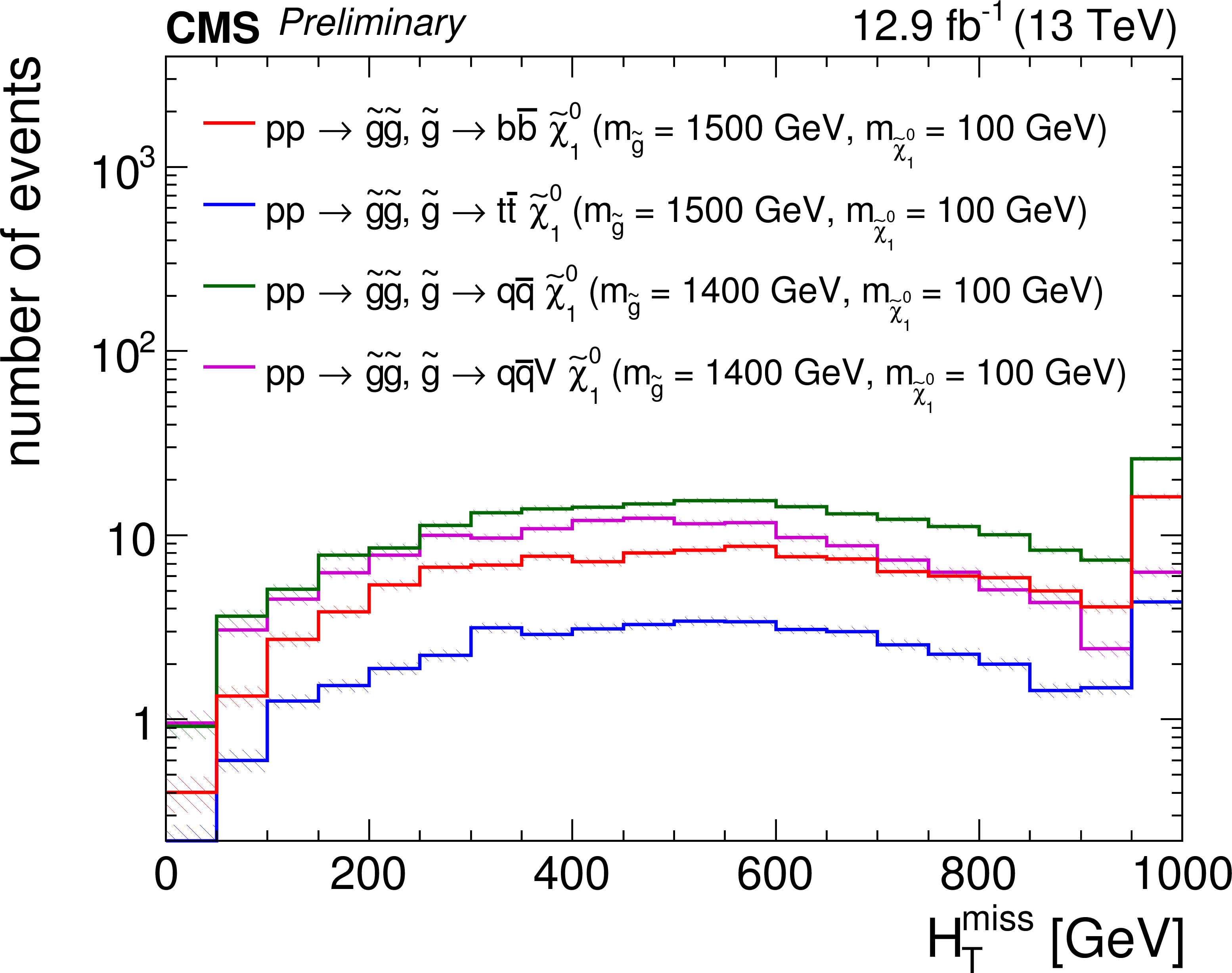
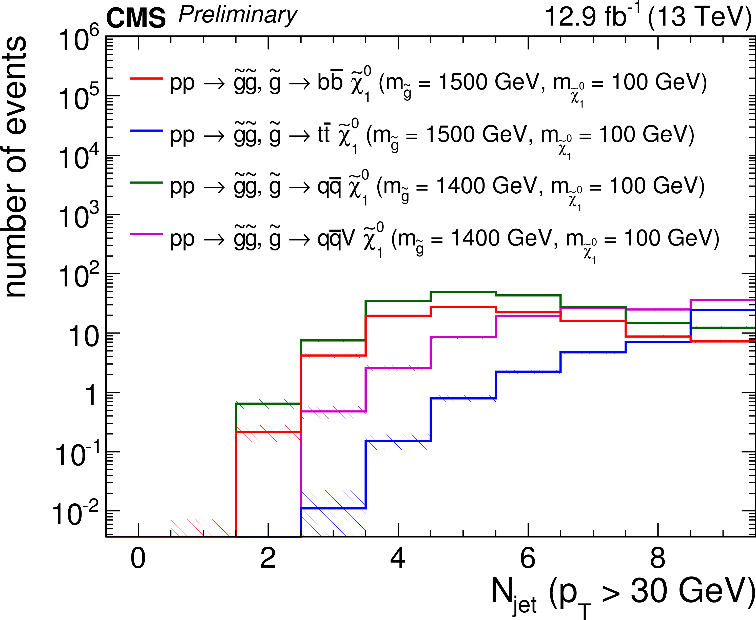
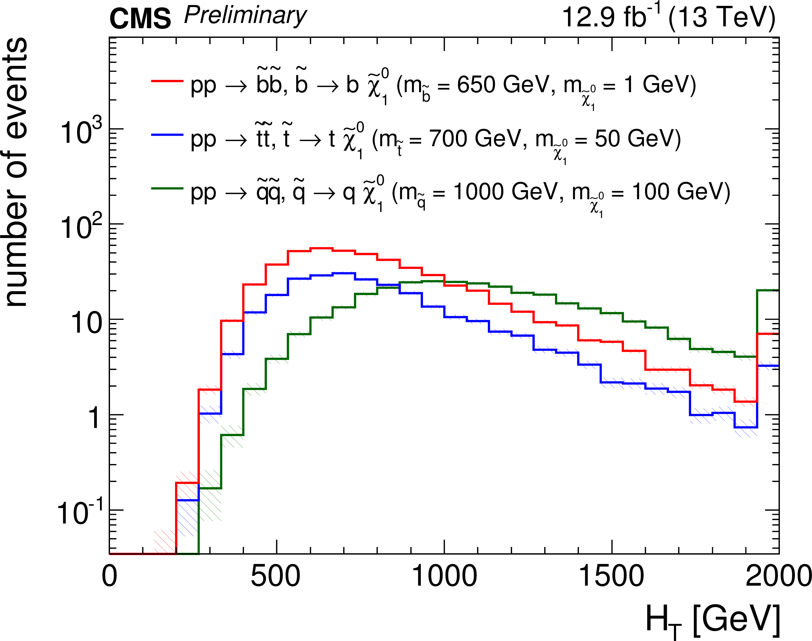
Additional Figure 27-a:
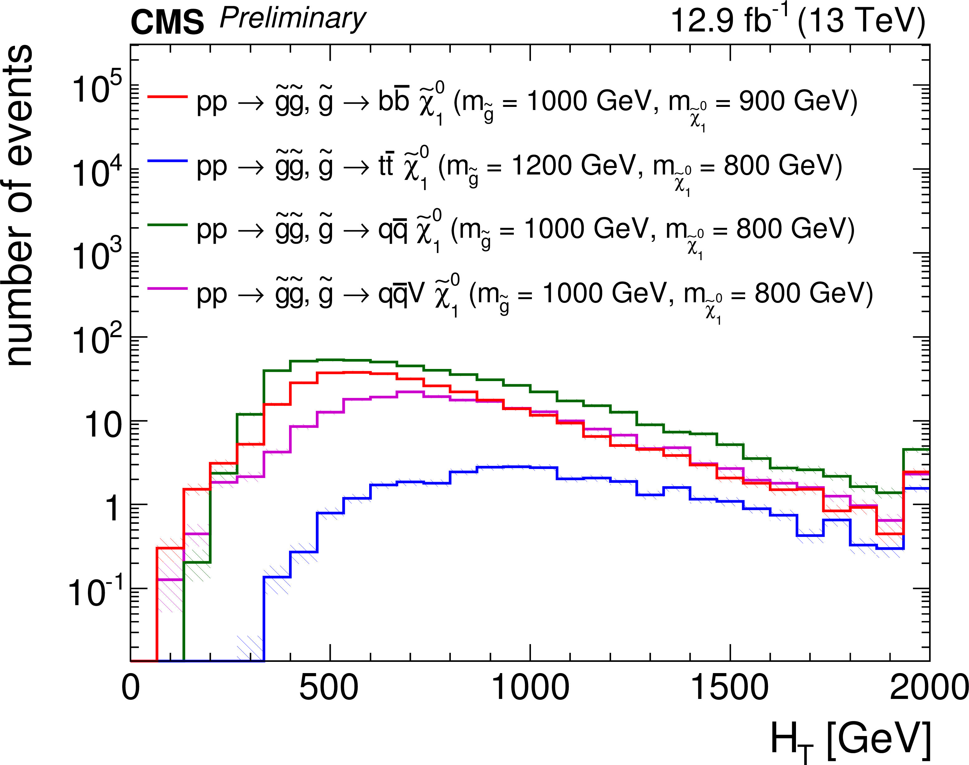
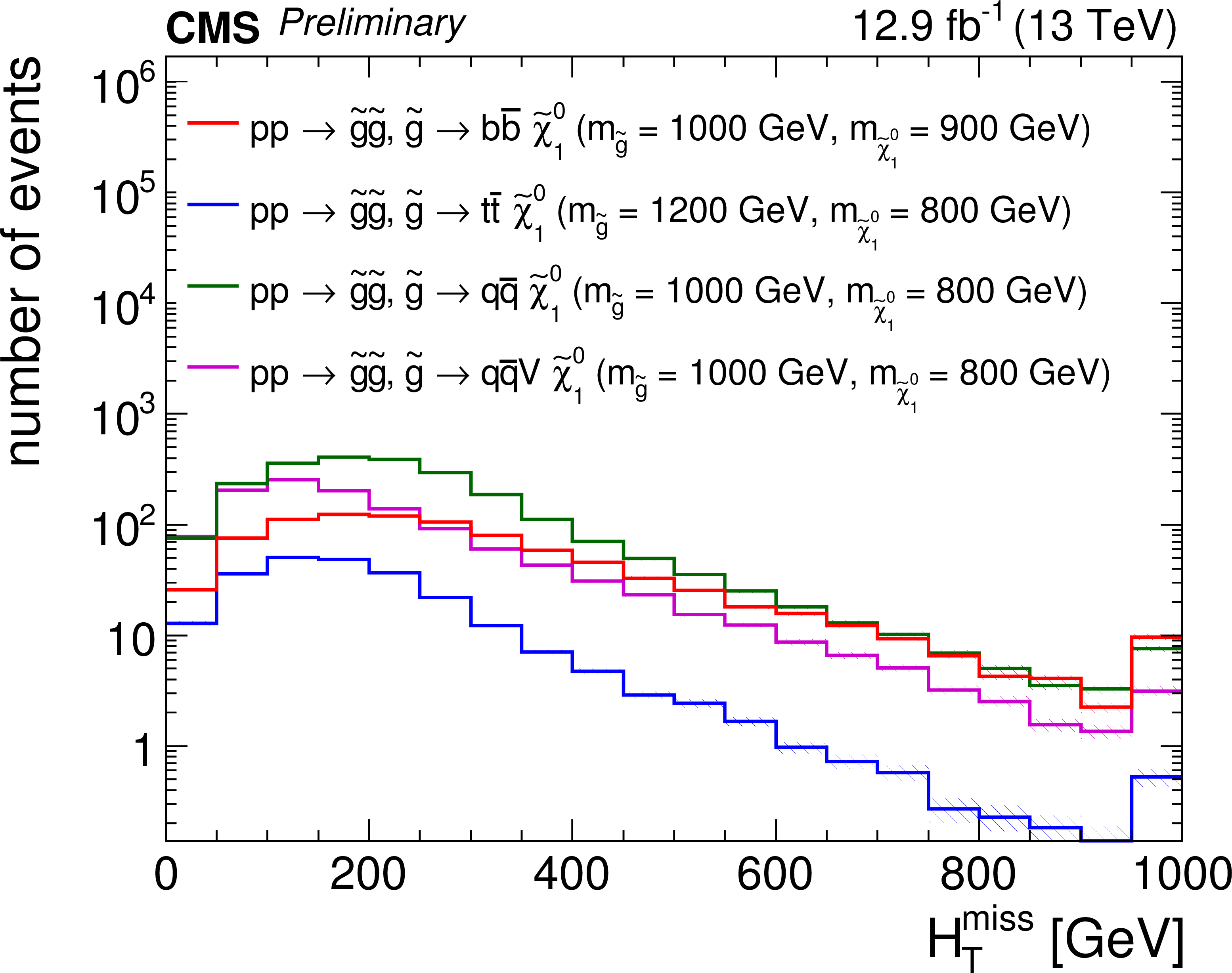
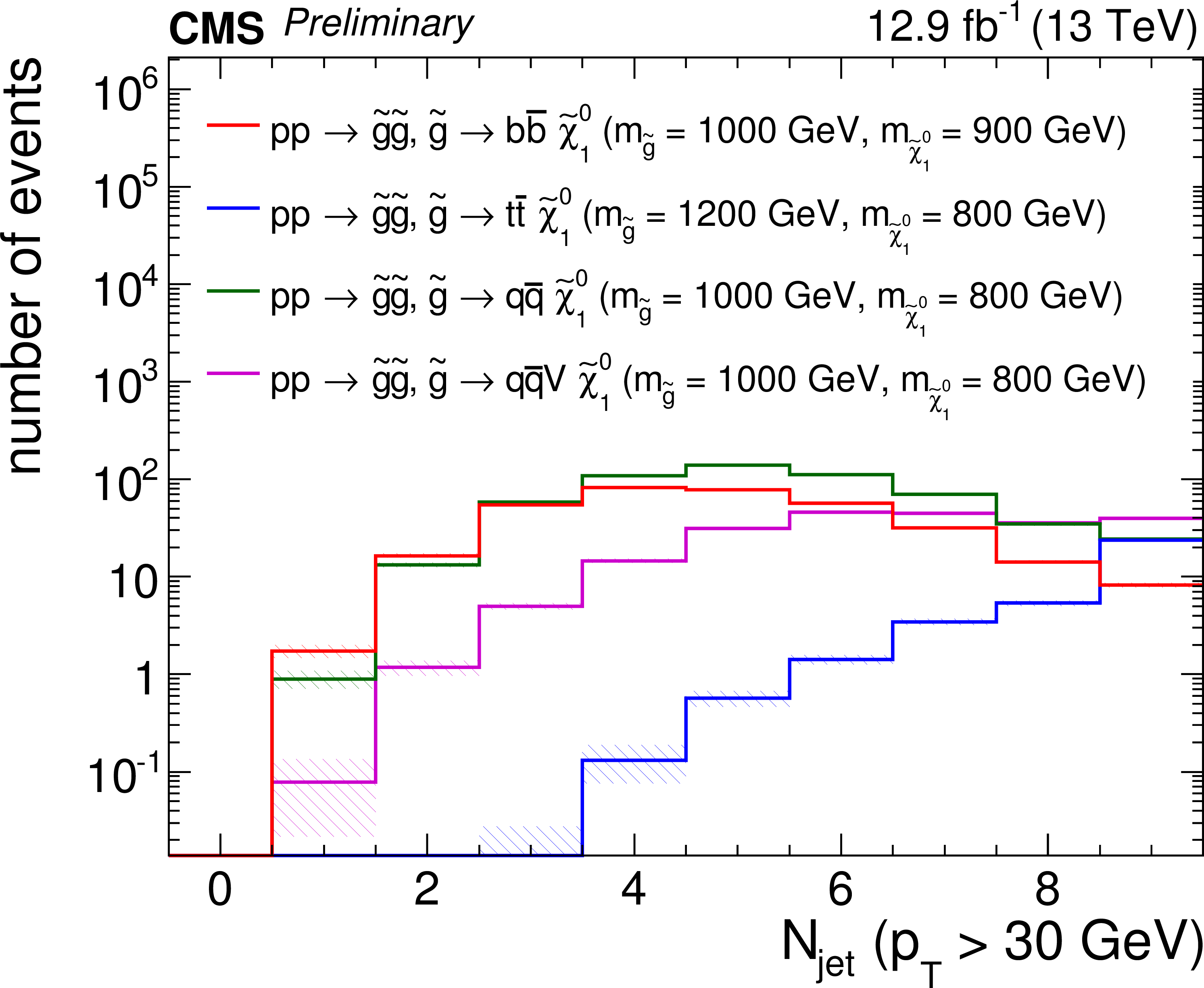
Distributions of (a) $H_{\rm T}$, (b) $H_{\rm T}^{\rm miss}$, (c) the number of b-tagged jets, and (d) the number of jets from four representative gluino pair production signal models with ${m_{\tilde{g} } \gg m_{\tilde{\chi}^0_1 }}$ after the baseline selection. Each plot ignores the baseline requirement (if any) for its respective variable. The last bin in each plot contains the overflow events. Only statistical uncertainties are shown. |
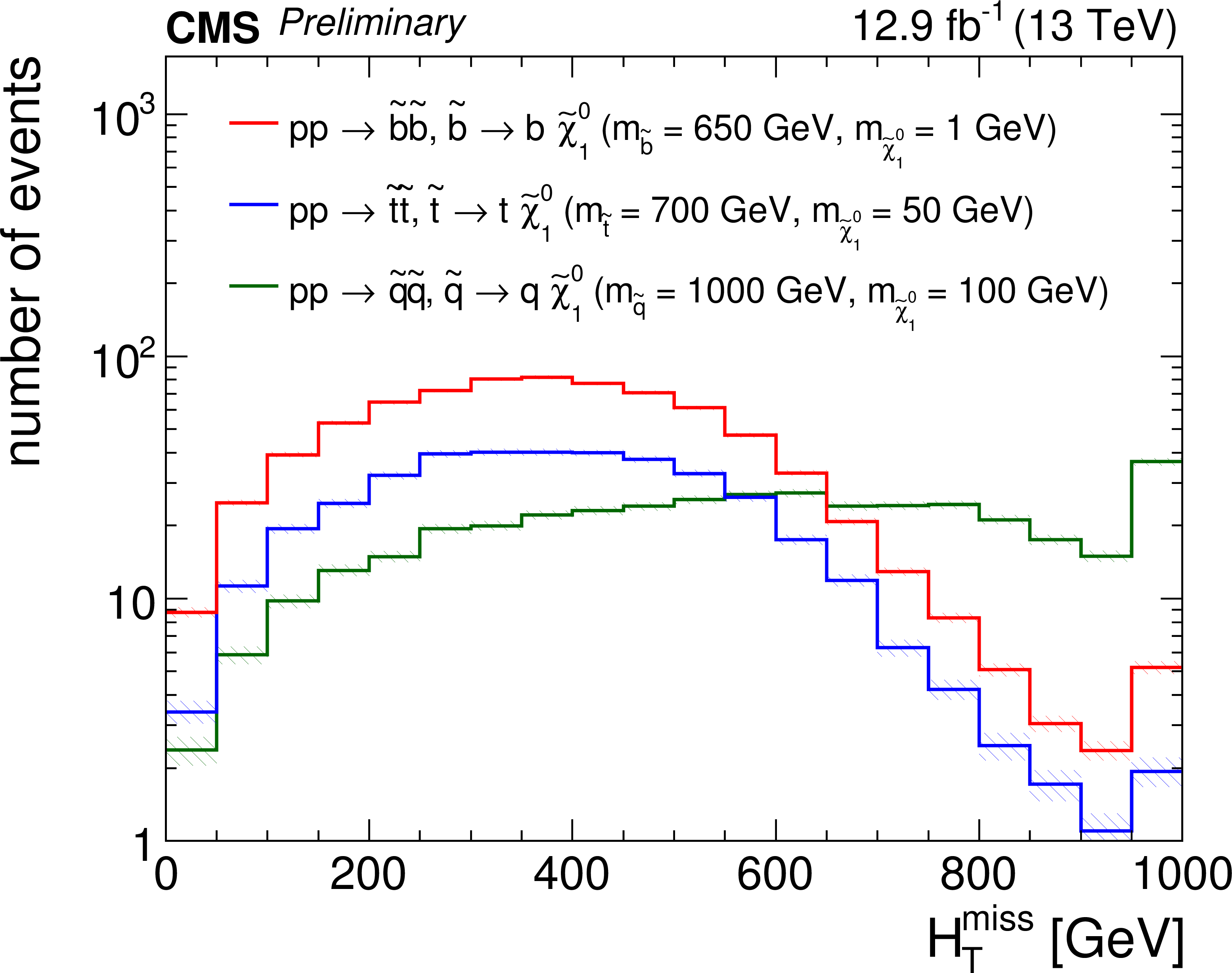
png pdf root |
Additional Figure 27-b:
Distributions of (a) $H_{\rm T}$, (b) $H_{\rm T}^{\rm miss}$, (c) the number of b-tagged jets, and (d) the number of jets from four representative gluino pair production signal models with ${m_{\tilde{g} } \gg m_{\tilde{\chi}^0_1 }}$ after the baseline selection. Each plot ignores the baseline requirement (if any) for its respective variable. The last bin in each plot contains the overflow events. Only statistical uncertainties are shown. |
png pdf root |
Additional Figure 27-c:
Distributions of (a) $H_{\rm T}$, (b) $H_{\rm T}^{\rm miss}$, (c) the number of b-tagged jets, and (d) the number of jets from four representative gluino pair production signal models with ${m_{\tilde{g} } \gg m_{\tilde{\chi}^0_1 }}$ after the baseline selection. Each plot ignores the baseline requirement (if any) for its respective variable. The last bin in each plot contains the overflow events. Only statistical uncertainties are shown. |
png pdf root |
Additional Figure 27-d:
Distributions of (a) $H_{\rm T}$, (b) $H_{\rm T}^{\rm miss}$, (c) the number of b-tagged jets, and (d) the number of jets from four representative gluino pair production signal models with ${m_{\tilde{g} } \gg m_{\tilde{\chi}^0_1 }}$ after the baseline selection. Each plot ignores the baseline requirement (if any) for its respective variable. The last bin in each plot contains the overflow events. Only statistical uncertainties are shown. |
png pdf root |
Additional Figure 28-a:
Distributions of (a) $H_{\rm T}$, (b) $H_{\rm T}^{\rm miss}$, (c) the number of b-tagged jets, and (d) the number of jets from four representative gluino pair production signal models with ${m_{\tilde{g} } \sim m_{\tilde{\chi}^0_1 }}$ after the baseline selection. Each plot ignores the baseline requirement (if any) for its respective variable. The last bin in each plot contains the overflow events. Only statistical uncertainties are shown. |
png pdf root |
Additional Figure 28-b:
Distributions of (a) $H_{\rm T}$, (b) $H_{\rm T}^{\rm miss}$, (c) the number of b-tagged jets, and (d) the number of jets from four representative gluino pair production signal models with ${m_{\tilde{g} } \sim m_{\tilde{\chi}^0_1 }}$ after the baseline selection. Each plot ignores the baseline requirement (if any) for its respective variable. The last bin in each plot contains the overflow events. Only statistical uncertainties are shown. |
png pdf root |
Additional Figure 28-c:
Distributions of (a) $H_{\rm T}$, (b) $H_{\rm T}^{\rm miss}$, (c) the number of b-tagged jets, and (d) the number of jets from four representative gluino pair production signal models with ${m_{\tilde{g} } \sim m_{\tilde{\chi}^0_1 }}$ after the baseline selection. Each plot ignores the baseline requirement (if any) for its respective variable. The last bin in each plot contains the overflow events. Only statistical uncertainties are shown. |

png pdf root |
Additional Figure 28-d:
Distributions of (a) $H_{\rm T}$, (b) $H_{\rm T}^{\rm miss}$, (c) the number of b-tagged jets, and (d) the number of jets from four representative gluino pair production signal models with ${m_{\tilde{g} } \sim m_{\tilde{\chi}^0_1 }}$ after the baseline selection. Each plot ignores the baseline requirement (if any) for its respective variable. The last bin in each plot contains the overflow events. Only statistical uncertainties are shown. |
png pdf root |
Additional Figure 29-a:
Distributions of (a) $H_{\rm T}$, (b) $H_{\rm T}^{\rm miss}$, (c) the number of b-tagged jets, and (d) the number of jets from three representative squark pair production signal models with ${m_{\tilde{\mathrm{q}} } \gg m_{\tilde{\chi}^0_1 }}$ after the baseline selection. Each plot ignores the baseline requirement (if any) for its respective variable. The last bin in each plot contains the overflow events. Only statistical uncertainties are shown. |
png pdf root |
Additional Figure 29-b:
Distributions of (a) $H_{\rm T}$, (b) $H_{\rm T}^{\rm miss}$, (c) the number of b-tagged jets, and (d) the number of jets from three representative squark pair production signal models with ${m_{\tilde{\mathrm{q}} } \gg m_{\tilde{\chi}^0_1 }}$ after the baseline selection. Each plot ignores the baseline requirement (if any) for its respective variable. The last bin in each plot contains the overflow events. Only statistical uncertainties are shown. |

png pdf root |
Additional Figure 29-c:
Distributions of (a) $H_{\rm T}$, (b) $H_{\rm T}^{\rm miss}$, (c) the number of b-tagged jets, and (d) the number of jets from three representative squark pair production signal models with ${m_{\tilde{\mathrm{q}} } \gg m_{\tilde{\chi}^0_1 }}$ after the baseline selection. Each plot ignores the baseline requirement (if any) for its respective variable. The last bin in each plot contains the overflow events. Only statistical uncertainties are shown. |

png pdf root |
Additional Figure 29-d:
Distributions of (a) $H_{\rm T}$, (b) $H_{\rm T}^{\rm miss}$, (c) the number of b-tagged jets, and (d) the number of jets from three representative squark pair production signal models with ${m_{\tilde{\mathrm{q}} } \gg m_{\tilde{\chi}^0_1 }}$ after the baseline selection. Each plot ignores the baseline requirement (if any) for its respective variable. The last bin in each plot contains the overflow events. Only statistical uncertainties are shown. |

png pdf root |
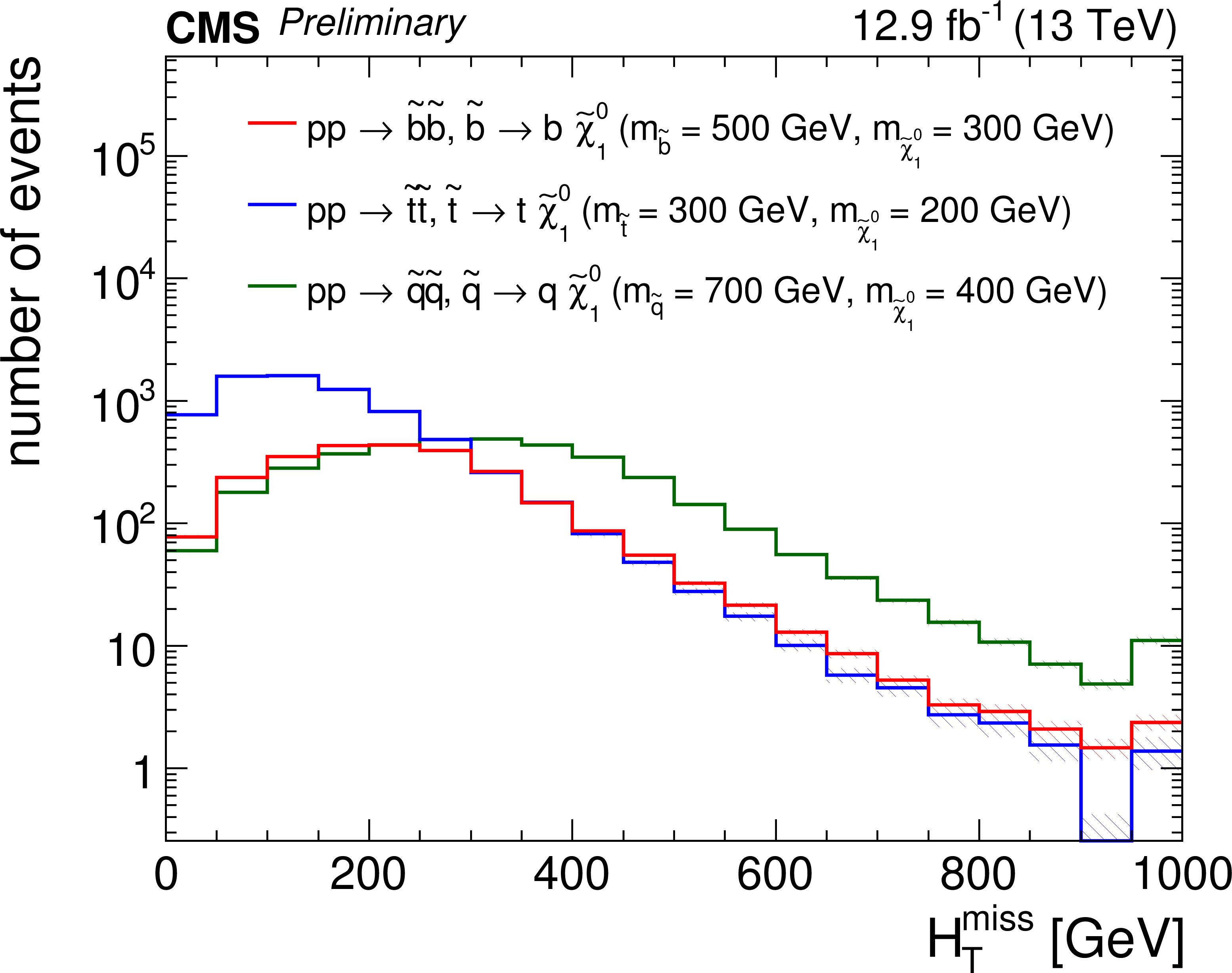
Additional Figure 30-a:
Distributions of (a) $H_{\rm T}$, (b) $H_{\rm T}^{\rm miss}$, (c) the number of b-tagged jets, and (d) the number of jets from three representative squark pair production signal models with ${m_{\tilde{\mathrm{q}} } \sim m_{\tilde{\chi}^0_1 }}$ after the baseline selection. Each plot ignores the baseline requirement (if any) for its respective variable. The last bin in each plot contains the overflow events. Only statistical uncertainties are shown. |
png pdf root |
Additional Figure 30-b:
Distributions of (a) $H_{\rm T}$, (b) $H_{\rm T}^{\rm miss}$, (c) the number of b-tagged jets, and (d) the number of jets from three representative squark pair production signal models with ${m_{\tilde{\mathrm{q}} } \sim m_{\tilde{\chi}^0_1 }}$ after the baseline selection. Each plot ignores the baseline requirement (if any) for its respective variable. The last bin in each plot contains the overflow events. Only statistical uncertainties are shown. |
png pdf root |
Additional Figure 30-c:
Distributions of (a) $H_{\rm T}$, (b) $H_{\rm T}^{\rm miss}$, (c) the number of b-tagged jets, and (d) the number of jets from three representative squark pair production signal models with ${m_{\tilde{\mathrm{q}} } \sim m_{\tilde{\chi}^0_1 }}$ after the baseline selection. Each plot ignores the baseline requirement (if any) for its respective variable. The last bin in each plot contains the overflow events. Only statistical uncertainties are shown. |

png pdf root |
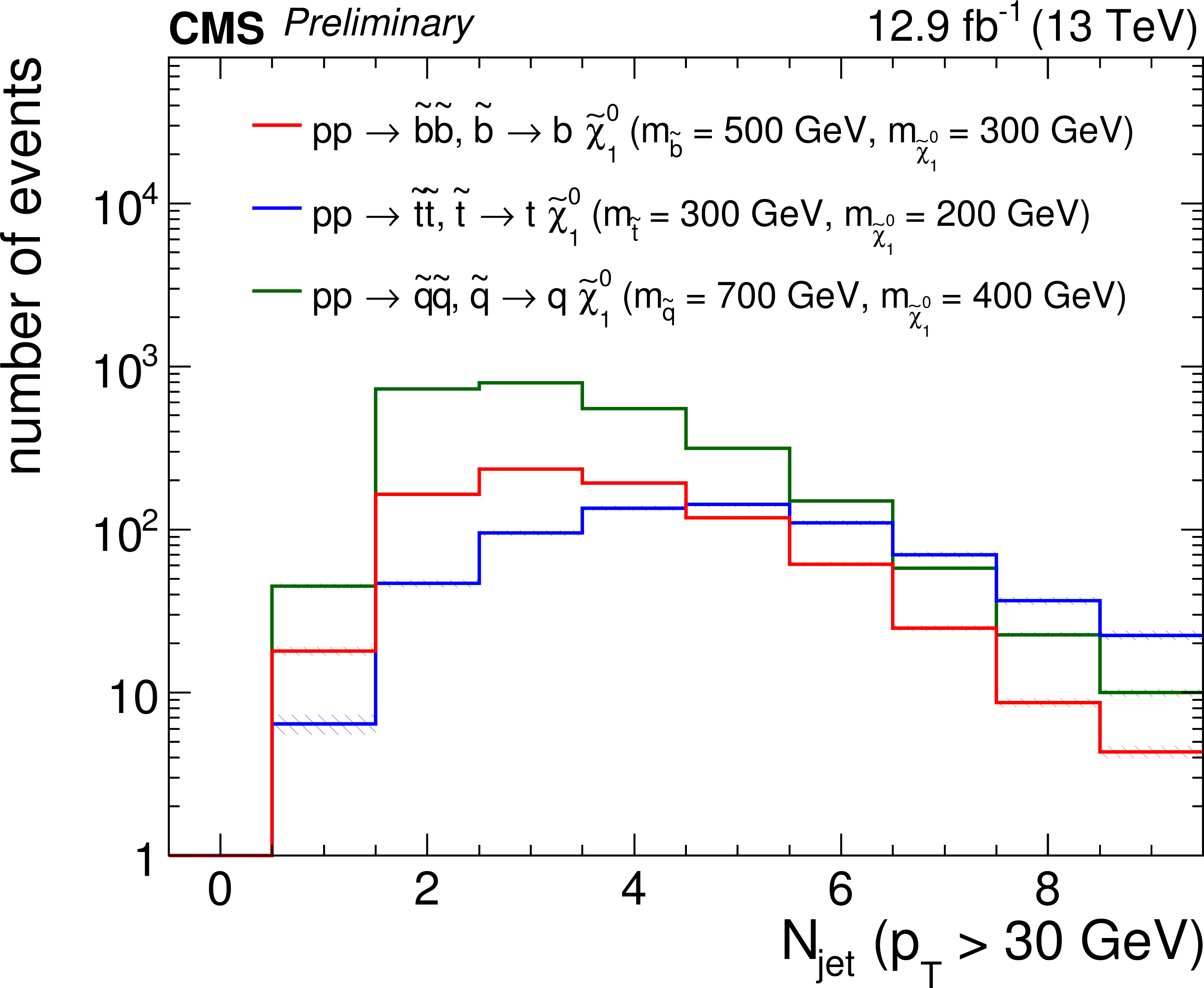
Additional Figure 30-d:
Distributions of (a) $H_{\rm T}$, (b) $H_{\rm T}^{\rm miss}$, (c) the number of b-tagged jets, and (d) the number of jets from three representative squark pair production signal models with ${m_{\tilde{\mathrm{q}} } \sim m_{\tilde{\chi}^0_1 }}$ after the baseline selection. Each plot ignores the baseline requirement (if any) for its respective variable. The last bin in each plot contains the overflow events. Only statistical uncertainties are shown. |
png pdf root |
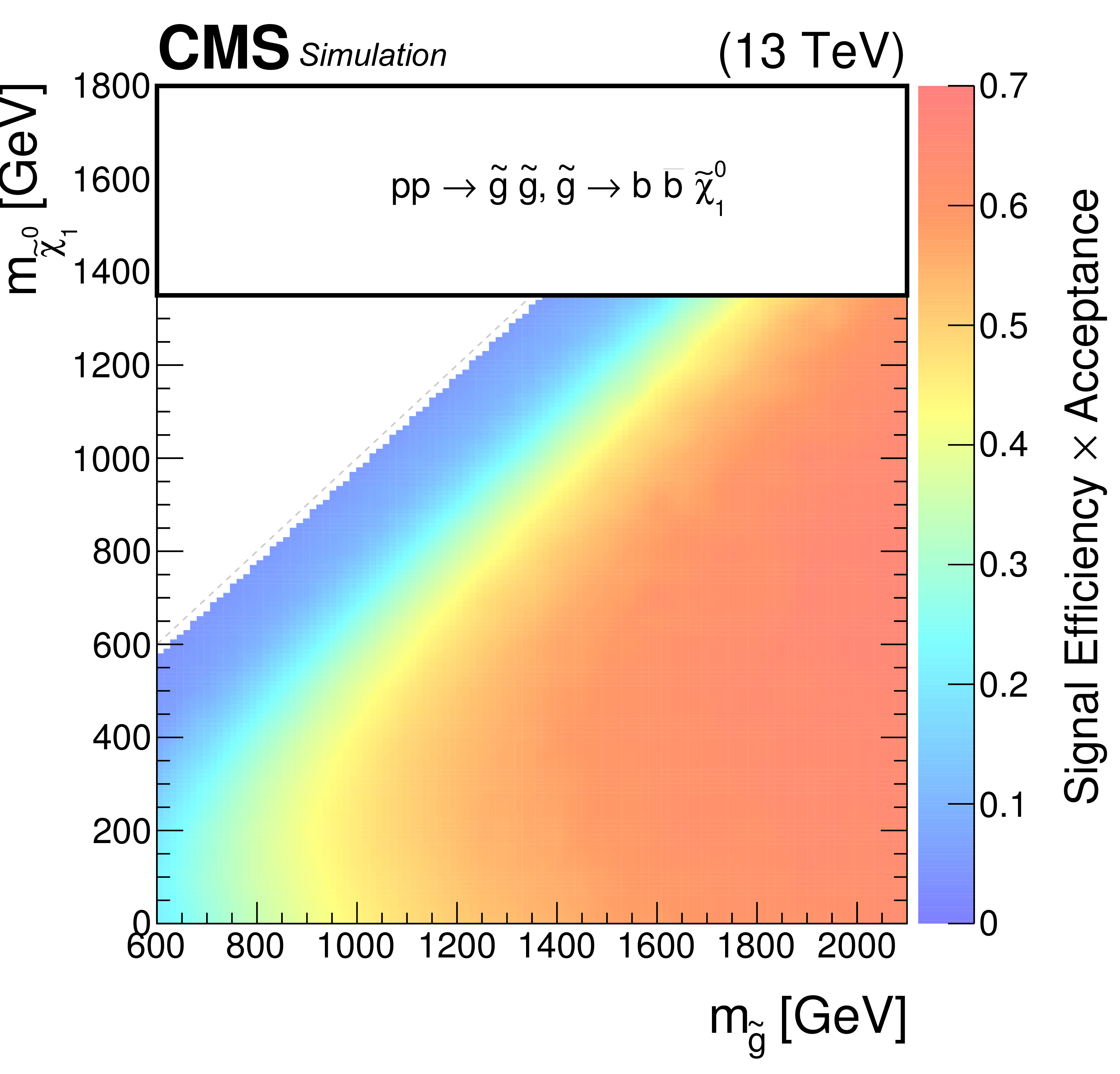
Additional Figure 31-a:
The signal efficiency for the baseline selection for the four SMS models of gluino pair production in the final states of (a) T1tttt (b) T1bbbb (c) T1qqqq (d) T5qqqqVV. |
png pdf root |
Additional Figure 31-b:
The signal efficiency for the baseline selection for the four SMS models of gluino pair production in the final states of (a) T1tttt (b) T1bbbb (c) T1qqqq (d) T5qqqqVV. |

png pdf root |
Additional Figure 31-c:
The signal efficiency for the baseline selection for the four SMS models of gluino pair production in the final states of (a) T1tttt (b) T1bbbb (c) T1qqqq (d) T5qqqqVV. |

png pdf root |
Additional Figure 31-d:
The signal efficiency for the baseline selection for the four SMS models of gluino pair production in the final states of (a) T1tttt (b) T1bbbb (c) T1qqqq (d) T5qqqqVV. |

png pdf root |
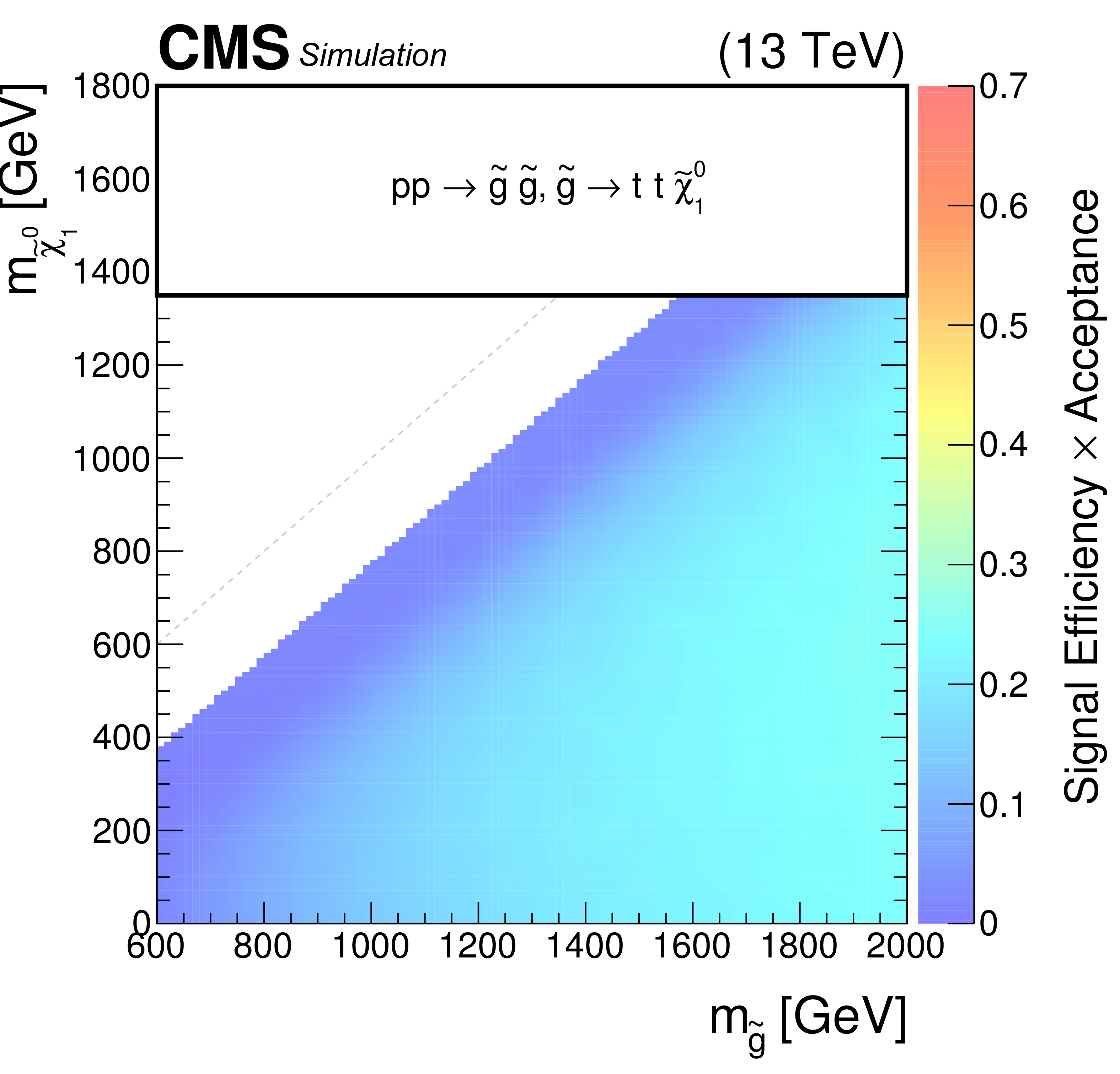
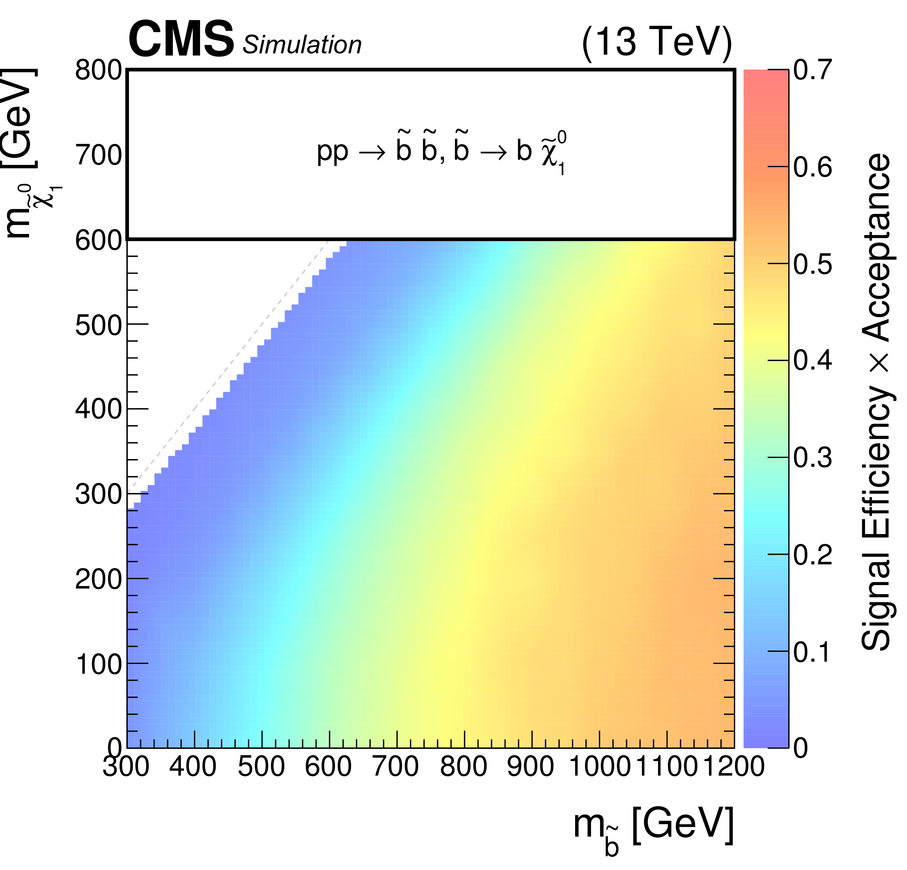
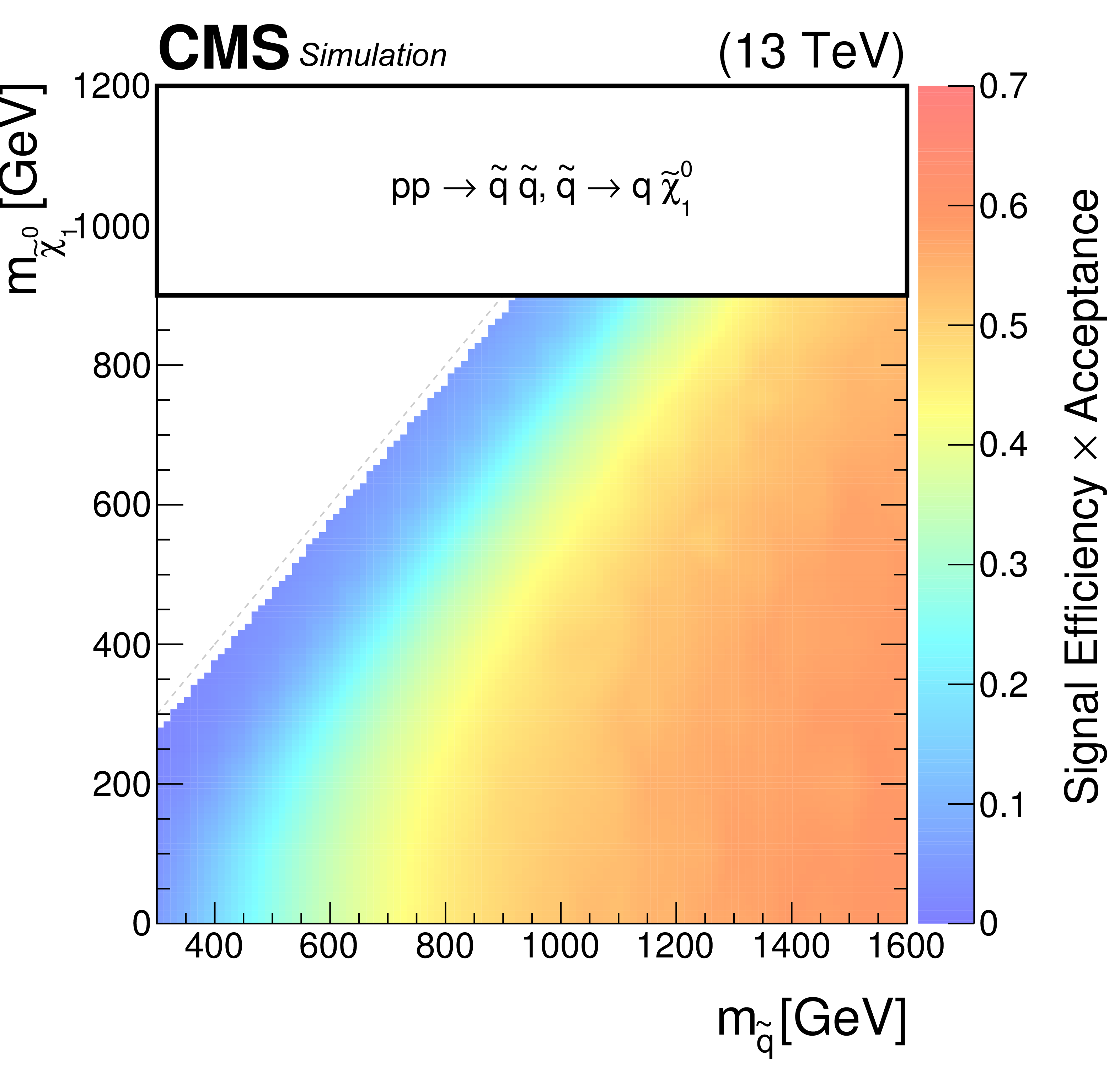
Additional Figure 32-a:
The signal efficiency for the baseline selection for the three SMS models of squark pair production in the final states of (a) T2tt (b) T2bb (c) T2qq. |
png pdf root |
Additional Figure 32-b:
The signal efficiency for the baseline selection for the three SMS models of squark pair production in the final states of (a) T2tt (b) T2bb (c) T2qq. |
png pdf root |
Additional Figure 32-c:
The signal efficiency for the baseline selection for the three SMS models of squark pair production in the final states of (a) T2tt (b) T2bb (c) T2qq. |
png pdf |
Additional Figure 33-a:
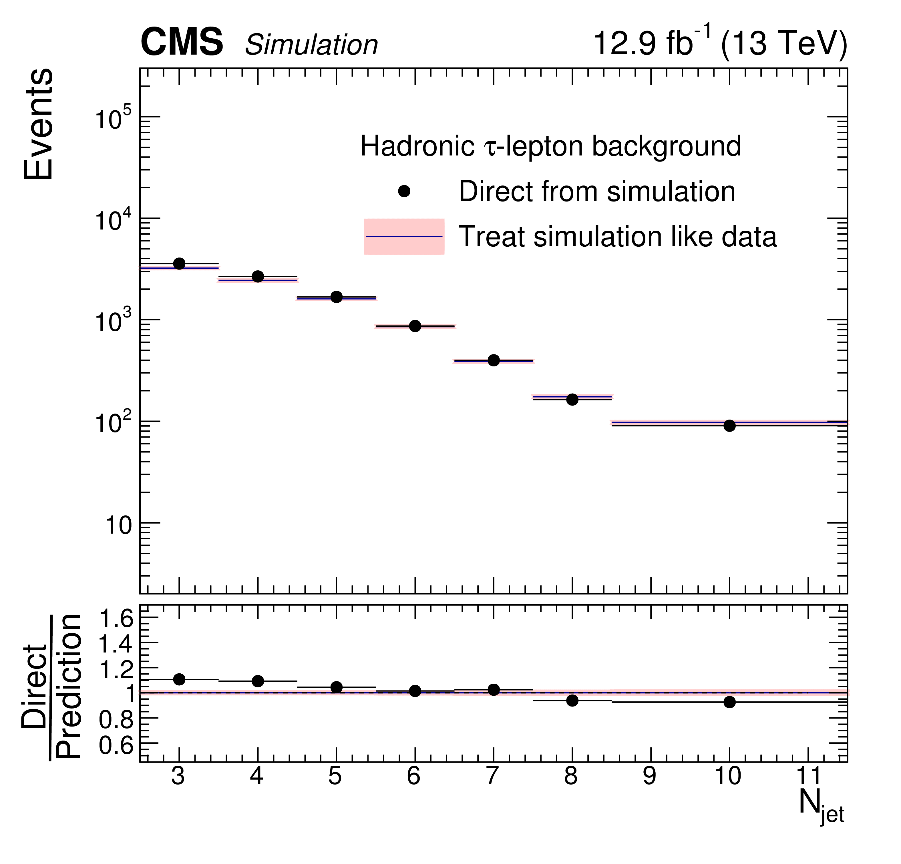
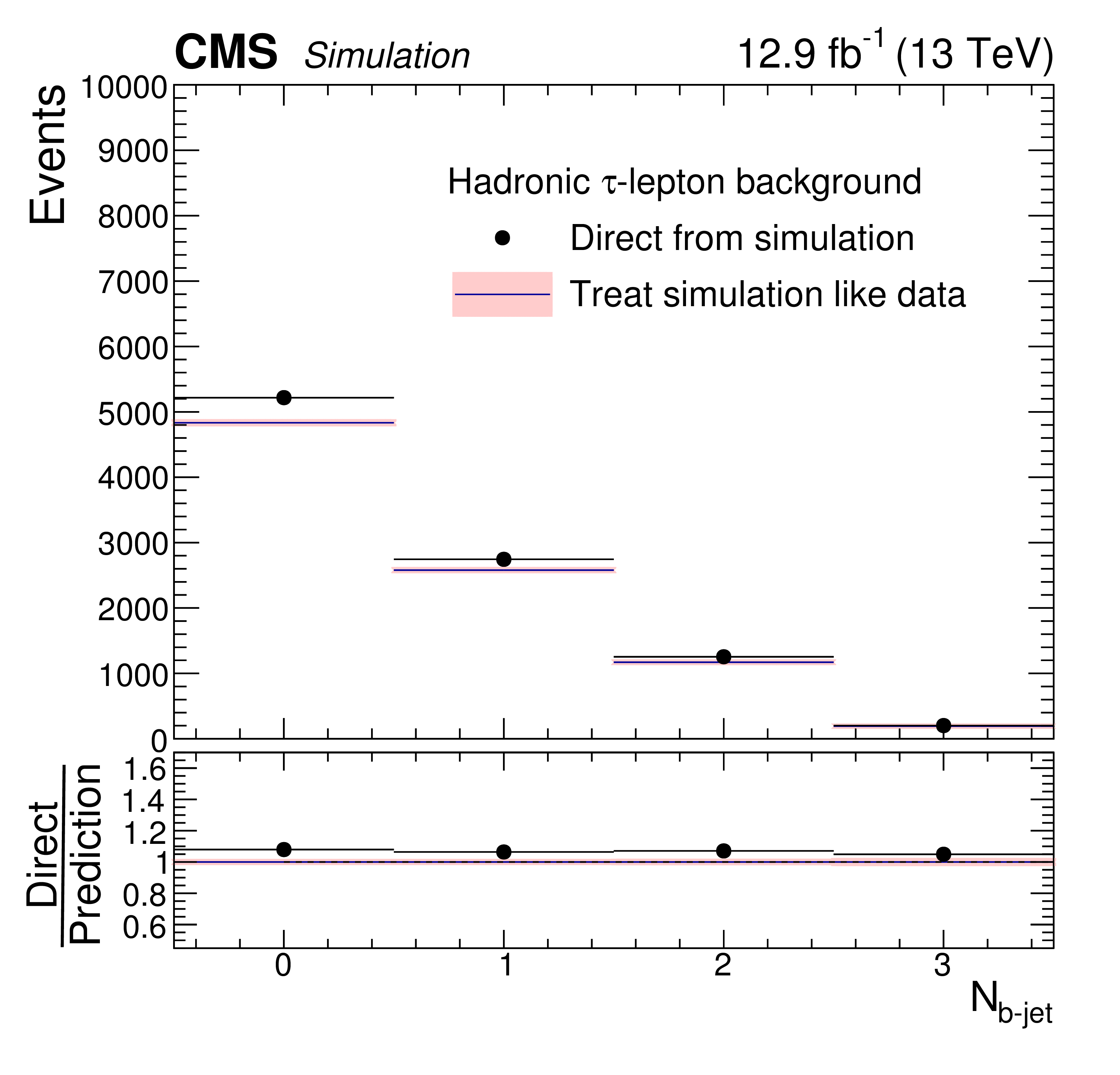
Distributions of $H_{\rm T}$, $H_{\rm T}^{\rm miss}$, the number of jets, and the number of b-tagged jets in background events with a hadronically decaying $\tau $ lepton as predicted directly from simulation (points, with statistical uncertainties) and as predicted by applying the hadronically decaying $\tau $ lepton background determination procedure to simulated muon control sample (shaded regions), for the baseline selection. The simulation includes $ \mathrm{ t \bar{t} } $, W+jets and single top quark process events. |

png pdf |
Additional Figure 33-b:
Distributions of $H_{\rm T}$, $H_{\rm T}^{\rm miss}$, the number of jets, and the number of b-tagged jets in background events with a hadronically decaying $\tau $ lepton as predicted directly from simulation (points, with statistical uncertainties) and as predicted by applying the hadronically decaying $\tau $ lepton background determination procedure to simulated muon control sample (shaded regions), for the baseline selection. The simulation includes $ \mathrm{ t \bar{t} } $, W+jets and single top quark process events. |
png pdf |
Additional Figure 33-c:
Distributions of $H_{\rm T}$, $H_{\rm T}^{\rm miss}$, the number of jets, and the number of b-tagged jets in background events with a hadronically decaying $\tau $ lepton as predicted directly from simulation (points, with statistical uncertainties) and as predicted by applying the hadronically decaying $\tau $ lepton background determination procedure to simulated muon control sample (shaded regions), for the baseline selection. The simulation includes $ \mathrm{ t \bar{t} } $, W+jets and single top quark process events. |
png pdf |
Additional Figure 33-d:
Distributions of $H_{\rm T}$, $H_{\rm T}^{\rm miss}$, the number of jets, and the number of b-tagged jets in background events with a hadronically decaying $\tau $ lepton as predicted directly from simulation (points, with statistical uncertainties) and as predicted by applying the hadronically decaying $\tau $ lepton background determination procedure to simulated muon control sample (shaded regions), for the baseline selection. The simulation includes $ \mathrm{ t \bar{t} } $, W+jets and single top quark process events. |
png pdf |
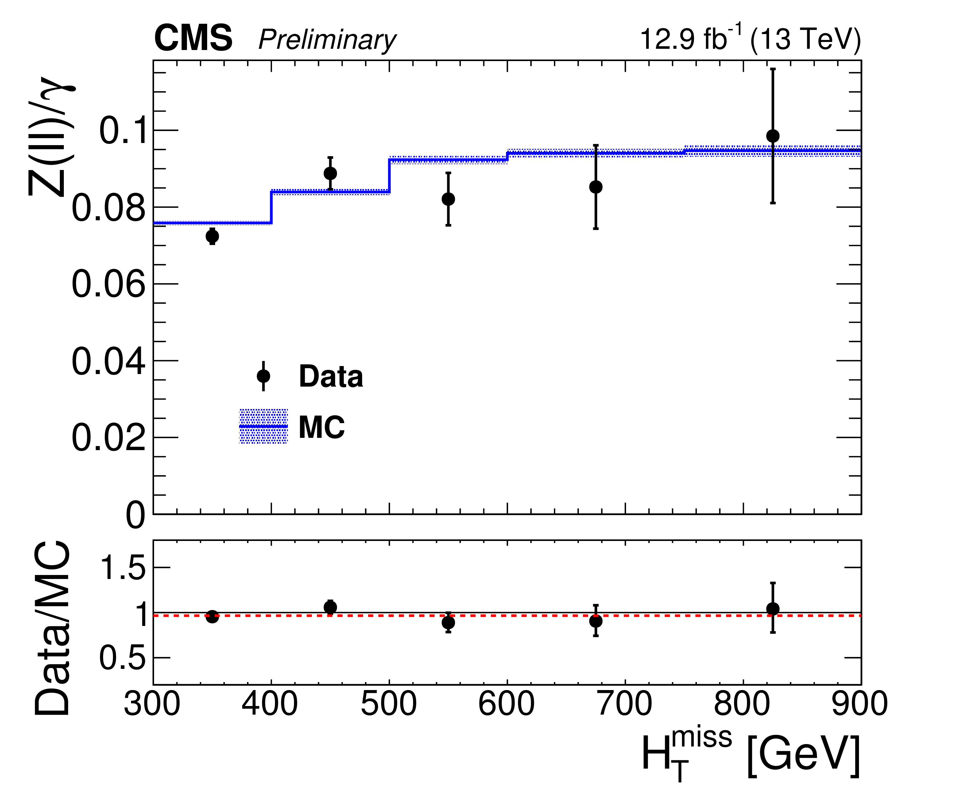
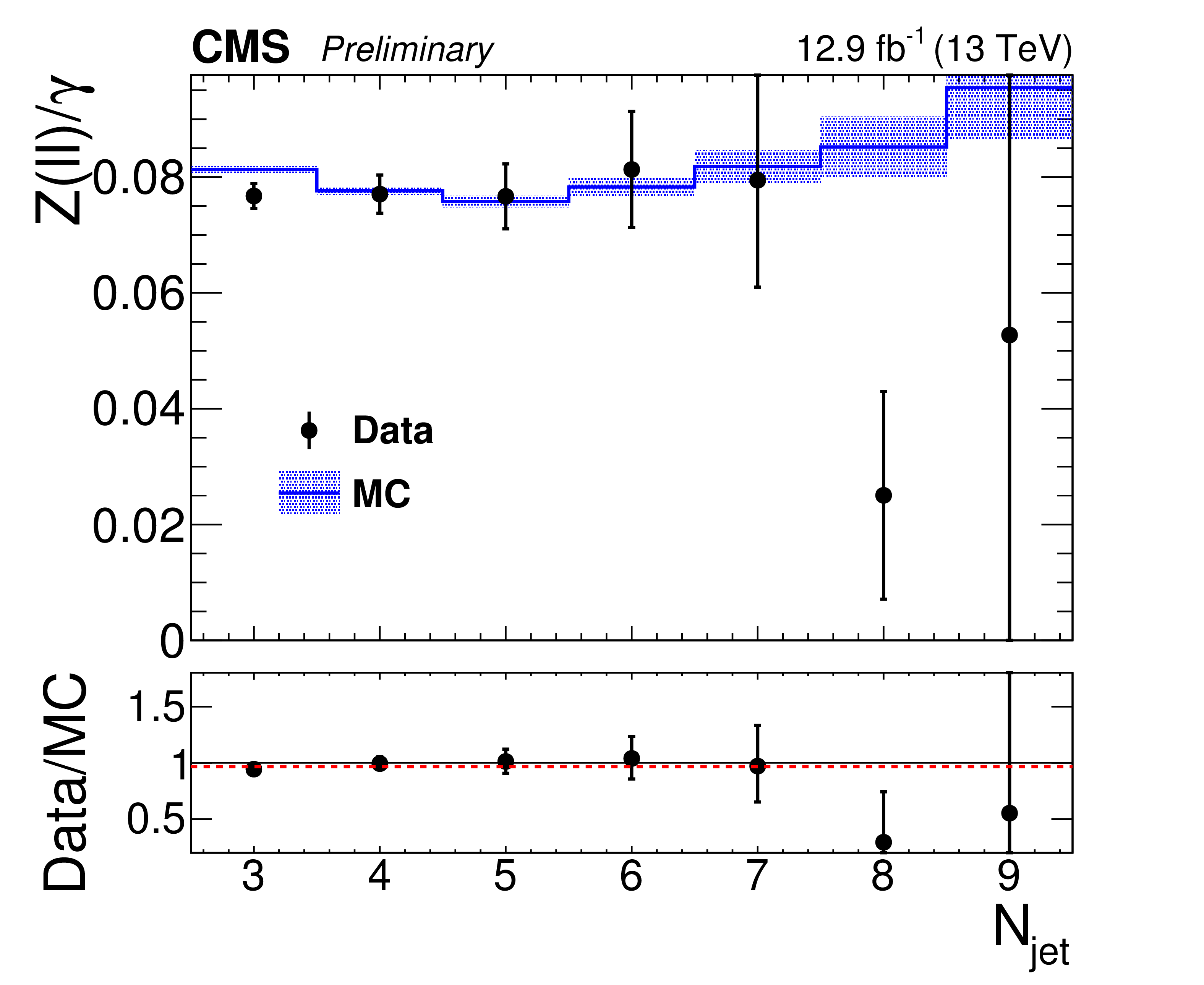
Additional Figure 34-a:
The $Z\rightarrow \ell ^{+}\ell ^{-}/\gamma $ ratio as a function of $ {H_{\mathrm T}^{\text {miss}}} $ (a), $ {H_{\mathrm {T}}} $ (b), and $ {N_{\text {jet}}} $ (c) after baseline selection for data (black) and simulation (blue). The $Z\rightarrow \nu \bar{\nu }/\gamma $ transfer factor is computed using simulated events and we check in one dimensional projections that data agree with simulation. The average value of the Double Ratio (bottom plot) of 0.966 is drawn as a red dashed line. |

png pdf |
Additional Figure 34-b:
The $Z\rightarrow \ell ^{+}\ell ^{-}/\gamma $ ratio as a function of $ {H_{\mathrm T}^{\text {miss}}} $ (a), $ {H_{\mathrm {T}}} $ (b), and $ {N_{\text {jet}}} $ (c) after baseline selection for data (black) and simulation (blue). The $Z\rightarrow \nu \bar{\nu }/\gamma $ transfer factor is computed using simulated events and we check in one dimensional projections that data agree with simulation. The average value of the Double Ratio (bottom plot) of 0.966 is drawn as a red dashed line. |
png pdf |
Additional Figure 34-c:
The $Z\rightarrow \ell ^{+}\ell ^{-}/\gamma $ ratio as a function of $ {H_{\mathrm T}^{\text {miss}}} $ (a), $ {H_{\mathrm {T}}} $ (b), and $ {N_{\text {jet}}} $ (c) after baseline selection for data (black) and simulation (blue). The $Z\rightarrow \nu \bar{\nu }/\gamma $ transfer factor is computed using simulated events and we check in one dimensional projections that data agree with simulation. The average value of the Double Ratio (bottom plot) of 0.966 is drawn as a red dashed line. |
png pdf |
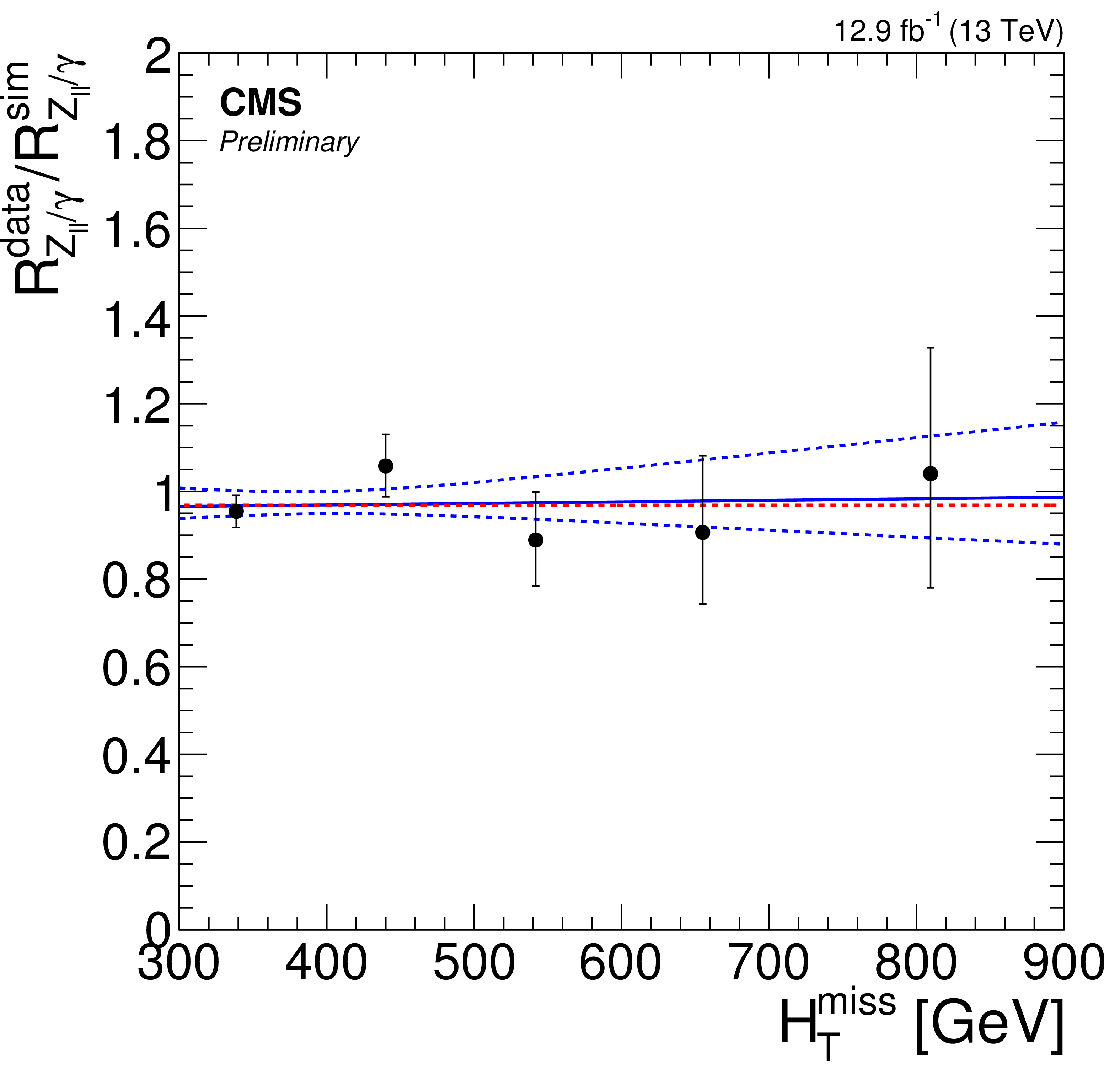
Additional Figure 35-a:
The $Z\rightarrow \ell ^{+}\ell ^{-}/\gamma $ Double Ratio and linear fit as a function of $ {H_{\mathrm T}^{\text {miss}}} $ (a), $ {H_{\mathrm {T}}} $ (b), and $ {N_{\text {jet}}} $ (c) after baseline selection. The average value of 0.966 is drawn as a red dashed line. |
png pdf |
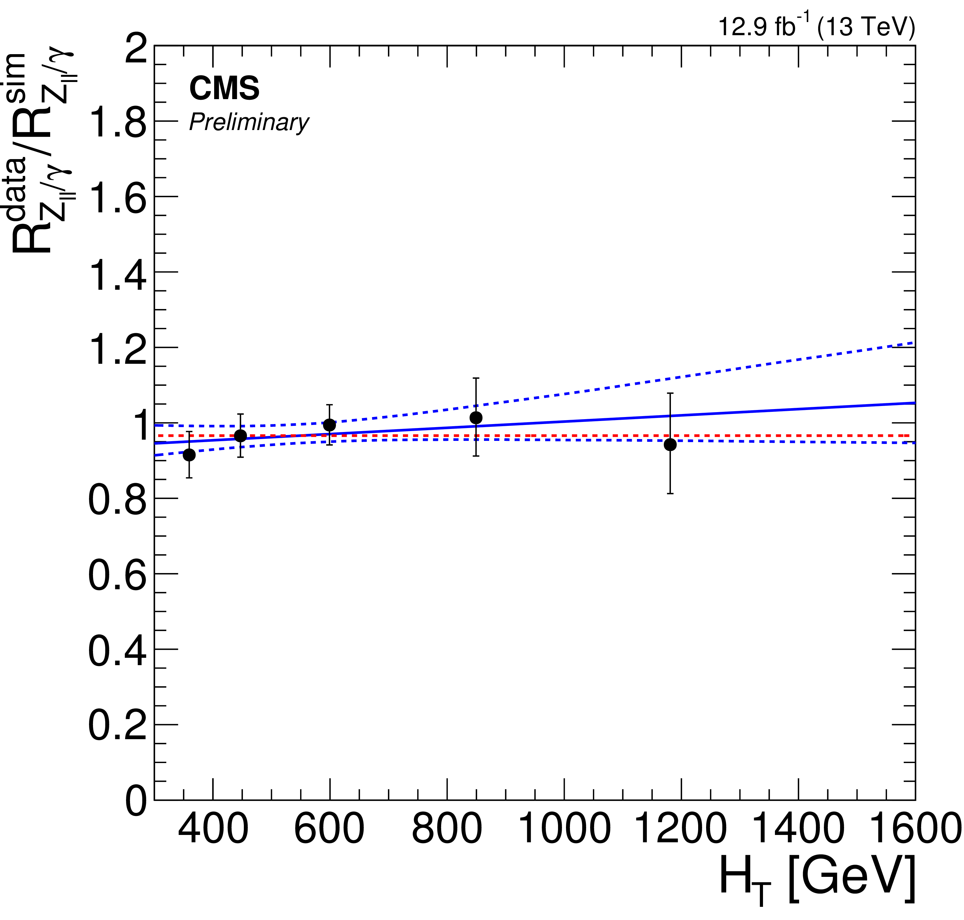
Additional Figure 35-b:
The $Z\rightarrow \ell ^{+}\ell ^{-}/\gamma $ Double Ratio and linear fit as a function of $ {H_{\mathrm T}^{\text {miss}}} $ (a), $ {H_{\mathrm {T}}} $ (b), and $ {N_{\text {jet}}} $ (c) after baseline selection. The average value of 0.966 is drawn as a red dashed line. |

png pdf |
Additional Figure 35-c:
The $Z\rightarrow \ell ^{+}\ell ^{-}/\gamma $ Double Ratio and linear fit as a function of $ {H_{\mathrm T}^{\text {miss}}} $ (a), $ {H_{\mathrm {T}}} $ (b), and $ {N_{\text {jet}}} $ (c) after baseline selection. The average value of 0.966 is drawn as a red dashed line. |
png pdf |
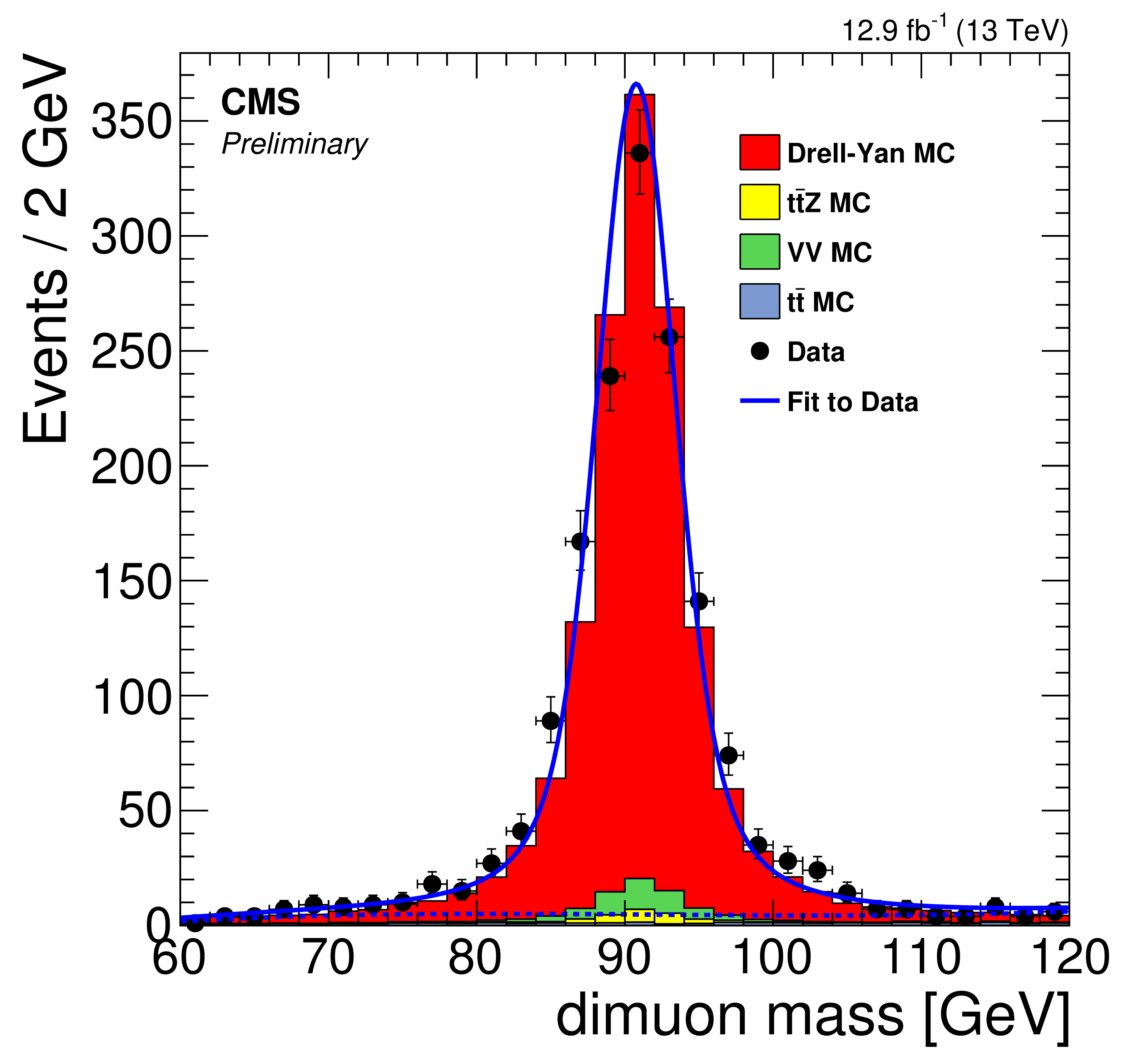
Additional Figure 36-a:
The dimuon (a) and dielectron (b) invariant mass distributions of the $Z\rightarrow \ell ^{+}\ell ^{-}$ control regions. Fit shapes are obtained from a data sample with baseline selection as shown. These shapes are then fixed and fit to a selection in $ {N_{{\mathrm{ b } }\text {-jet}}} $ to extract the purity. For comparison, we show Drell-Yan (red), ${\mathrm{ t } {}\mathrm{ \bar{t} } } {\mathrm{ Z } } $ (yellow), diboson (green), and ${\mathrm{ t } {}\mathrm{ \bar{t} } } $ (blue) simulation scaled to 12.9 fb$^{-1}$. |

png pdf |
Additional Figure 36-b:
The dimuon (a) and dielectron (b) invariant mass distributions of the $Z\rightarrow \ell ^{+}\ell ^{-}$ control regions. Fit shapes are obtained from a data sample with baseline selection as shown. These shapes are then fixed and fit to a selection in $ {N_{{\mathrm{ b } }\text {-jet}}} $ to extract the purity. For comparison, we show Drell-Yan (red), ${\mathrm{ t } {}\mathrm{ \bar{t} } } {\mathrm{ Z } } $ (yellow), diboson (green), and ${\mathrm{ t } {}\mathrm{ \bar{t} } } $ (blue) simulation scaled to 12.9 fb$^{-1}$. |

png pdf |
Additional Figure 37-a:
Event displays for a SUSY candidate event with the highest observed $ {H_{\mathrm T}^{\text {miss}}} $ in the search region, 275001:1026:1431223147 in (a) r-phi view, (b) 3D view with a black background, and (c) 3D view with a white background. |
png pdf |
Additional Figure 37-b:
Event displays for a SUSY candidate event with the highest observed $ {H_{\mathrm T}^{\text {miss}}} $ in the search region, 275001:1026:1431223147 in (a) r-phi view, (b) 3D view with a black background, and (c) 3D view with a white background. |

png pdf |
Additional Figure 37-c:
Event displays for a SUSY candidate event with the highest observed $ {H_{\mathrm T}^{\text {miss}}} $ in the search region, 275001:1026:1431223147 in (a) r-phi view, (b) 3D view with a black background, and (c) 3D view with a white background. |

png pdf |
Additional Figure 38-a:
Event displays for a SUSY candidate event, 274422:1149:1978921466, with 12 jets, 3 of which are b-tagged, in (a) r-phi view, (b) 3D view with a black background, and (c) 3D view with a white background. The b-tagged jets are marked in teal. |

png pdf |
Additional Figure 38-b:
Event displays for a SUSY candidate event, 274422:1149:1978921466, with 12 jets, 3 of which are b-tagged, in (a) r-phi view, (b) 3D view with a black background, and (c) 3D view with a white background. The b-tagged jets are marked in teal. |

png pdf |
Additional Figure 38-c:
Event displays for a SUSY candidate event, 274422:1149:1978921466, with 12 jets, 3 of which are b-tagged, in (a) r-phi view, (b) 3D view with a black background, and (c) 3D view with a white background. The b-tagged jets are marked in teal. |
png pdf |
Additional Figure 39-a:
Event displays for a SUSY candidate event, 274422:1961:3277333781, with 12 jets, 3 of which are b-tagged, in (a) r-phi view, (b) 3D view with a black background, (c) 3D view with a white background, and (d) eta-phi ``lego'' view. The b-tagged jets are marked in teal. |
png pdf |
Additional Figure 39-b:
Event displays for a SUSY candidate event, 274422:1961:3277333781, with 12 jets, 3 of which are b-tagged, in (a) r-phi view, (b) 3D view with a black background, (c) 3D view with a white background, and (d) eta-phi ``lego'' view. The b-tagged jets are marked in teal. |
png pdf |
Additional Figure 39-c:
Event displays for a SUSY candidate event, 274422:1961:3277333781, with 12 jets, 3 of which are b-tagged, in (a) r-phi view, (b) 3D view with a black background, (c) 3D view with a white background, and (d) eta-phi ``lego'' view. The b-tagged jets are marked in teal. |
png pdf |
Additional Figure 39-d:
Event displays for a SUSY candidate event, 274422:1961:3277333781, with 12 jets, 3 of which are b-tagged, in (a) r-phi view, (b) 3D view with a black background, (c) 3D view with a white background, and (d) eta-phi ``lego'' view. The b-tagged jets are marked in teal. |
png pdf |
Additional Figure 40-a:
Event displays for a SUSY candidate event, 273447:179:291867669, with 12 jets, 3 of which are b-tagged, in (a) r-phi view, (b) 3D view with a black background, (c) 3D view with a white background, and (d) eta-phi ``lego'' view. The b-tagged jets are marked in teal. |

png pdf |
Additional Figure 40-b:
Event displays for a SUSY candidate event, 273447:179:291867669, with 12 jets, 3 of which are b-tagged, in (a) r-phi view, (b) 3D view with a black background, (c) 3D view with a white background, and (d) eta-phi ``lego'' view. The b-tagged jets are marked in teal. |
png pdf |
Additional Figure 40-c:
Event displays for a SUSY candidate event, 273447:179:291867669, with 12 jets, 3 of which are b-tagged, in (a) r-phi view, (b) 3D view with a black background, (c) 3D view with a white background, and (d) eta-phi ``lego'' view. The b-tagged jets are marked in teal. |

png pdf |
Additional Figure 40-d:
Event displays for a SUSY candidate event, 273447:179:291867669, with 12 jets, 3 of which are b-tagged, in (a) r-phi view, (b) 3D view with a black background, (c) 3D view with a white background, and (d) eta-phi ``lego'' view. The b-tagged jets are marked in teal. |
png pdf |
Additional Figure 41-a:
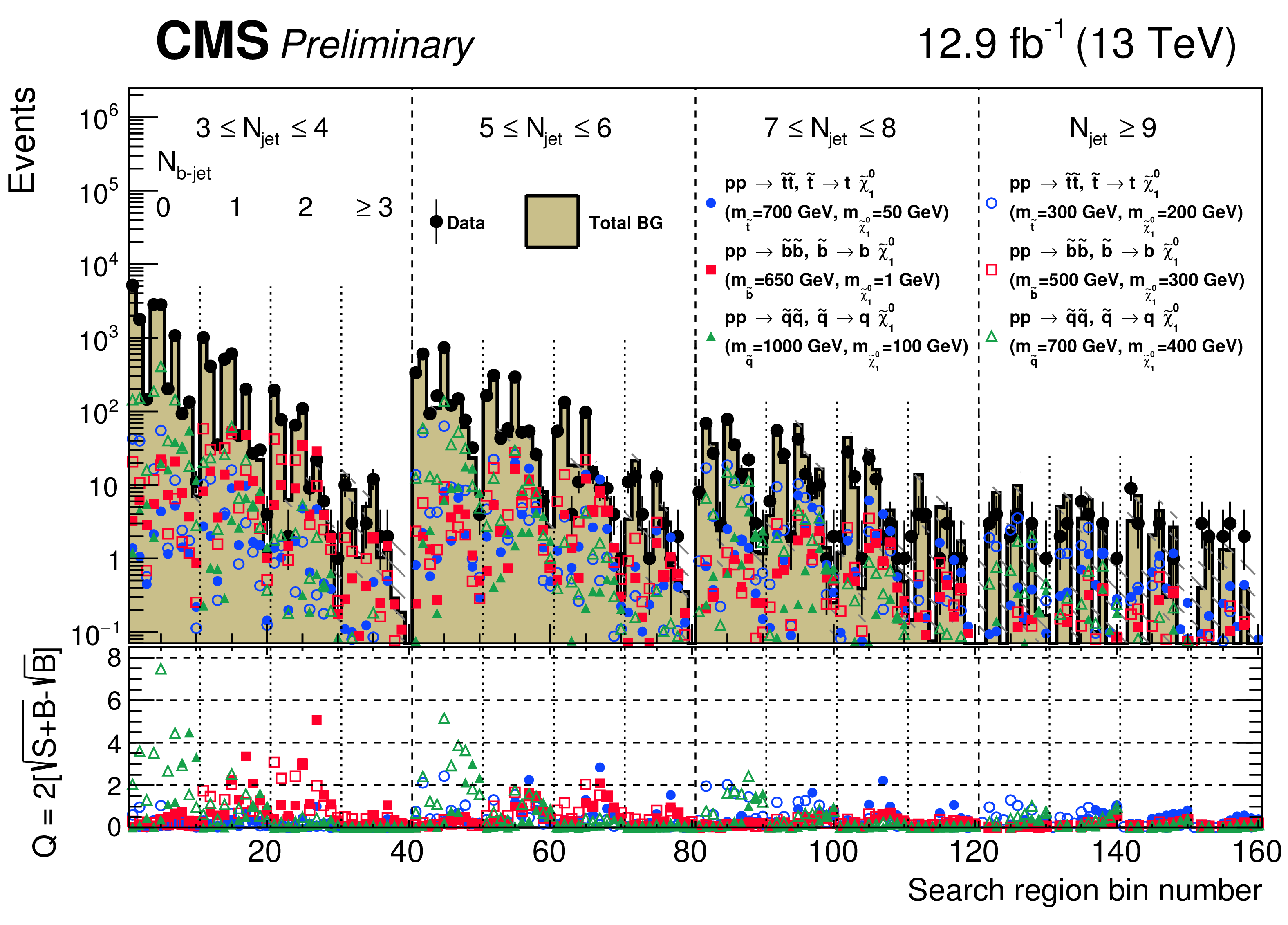
The sensitivity of the analysis to different direct gluino production signal models (a) and direct squark production signal models (b) as a function of the analysis binning. The upper panel shows the total predicted SM backgrounds and the expected number of signal events in 12.9 fb$^{-1}$ of data for six representative model points per analysis bin. The bottom panel shows the expected sensitivity, expressed in terms of the figure of merit Q, per analysis bin. |
png pdf |
Additional Figure 41-b:
The sensitivity of the analysis to different direct gluino production signal models (a) and direct squark production signal models (b) as a function of the analysis binning. The upper panel shows the total predicted SM backgrounds and the expected number of signal events in 12.9 fb$^{-1}$ of data for six representative model points per analysis bin. The bottom panel shows the expected sensitivity, expressed in terms of the figure of merit Q, per analysis bin. |
| Additional Tables | |

png pdf |
Additional Table 1:
Observed number of events and pre-fit background predictions in the $3\leq {N_{\text {jet}}} \leq 4$ search bins. |
png pdf |
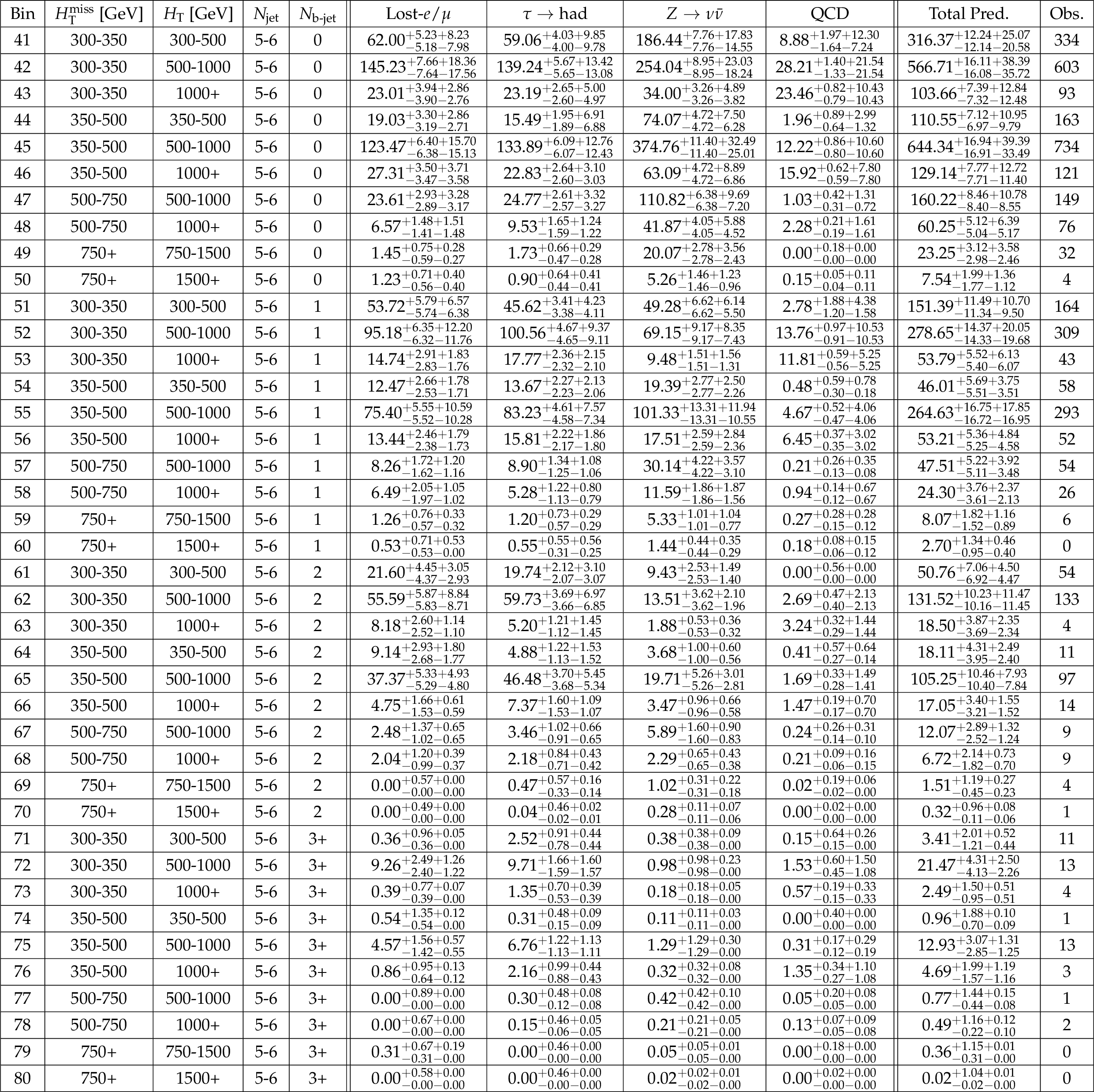
Additional Table 2:
Observed number of events and pre-fit background predictions in the $5\leq {N_{\text {jet}}} \leq 6$ search bins. |

png pdf |
Additional Table 3:
Observed number of events and pre-fit background predictions in the $7\leq {N_{\text {jet}}} \leq 8$ search bins. |
png pdf |
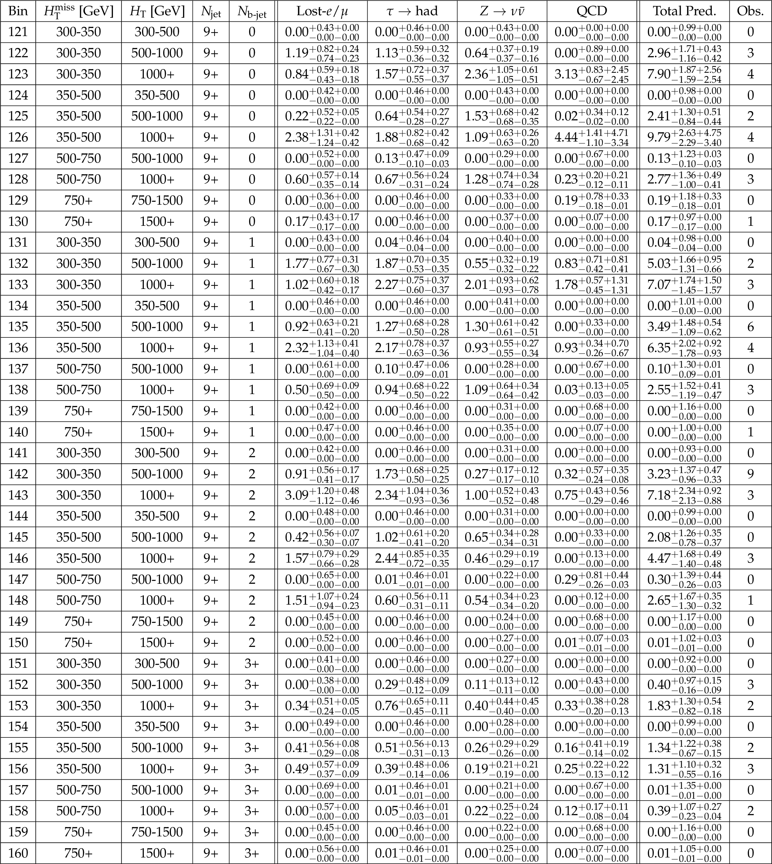
Additional Table 4:
Observed number of events and pre-fit background predictions in the $ {N_{\text {jet}}} \geq 9$ search bins. |

png pdf |
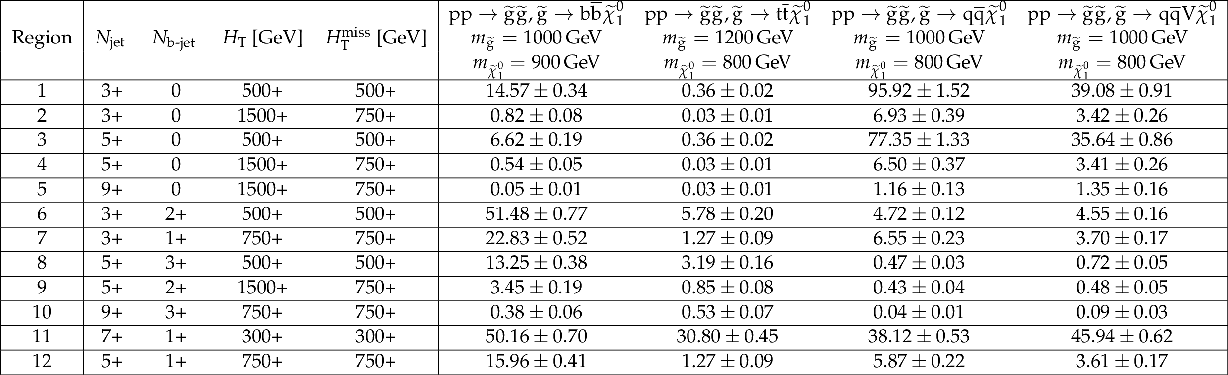
Additional Table 5:
Observed number of events and pre-fit background predictions in the aggregate search regions. |

png pdf |
Additional Table 6:
Expected number of signal events in 12.9 fb$^{-1}$ of data for four representative gluino pair production models with ${m_{\tilde{g} } \gg m_{\tilde{\chi}^0_1 }}$ in the aggregate search regions. Only statistical uncertainties are shown. |
png pdf |
Additional Table 7:
Expected number of signal events in 12.9 fb$^{-1}$ of data for four representative gluino pair production models with ${m_{\tilde{g} } \sim m_{\tilde{\chi}^0_1 }}$ in the aggregate search regions. Only statistical uncertainties are shown. |

png pdf |
Additional Table 8:
Expected number of signal events in 12.9 fb$^{-1}$ of data for three representative squark pair production models with ${m_{\tilde{\mathrm{q}} } \gg m_{\tilde{\chi}^0_1 }}$ in the aggregate search regions. Only statistical uncertainties are shown. |
png pdf |
Additional Table 9:
Expected number of signal events in 12.9 fb$^{-1}$ of data for three representative squark pair production models with ${m_{\tilde{\mathrm{q}} } \sim m_{\tilde{\chi}^0_1 }}$ in the aggregate search regions. Only statistical uncertainties are shown. |
| References | ||||
| 1 | P. Ramond | Dual theory for free fermions | PRD 3 (1971) 2415 | |
| 2 | Y. A. Golfand and E. P. Likhtman | Extension of the algebra of Poincare group generators and violation of P invariance | JEPTL 13 (1971)323 | |
| 3 | A. Neveu and J. H. Schwarz | Factorizable dual model of pions | Nucl. Phys. B 31 (1971) 86 | |
| 4 | D. V. Volkov and V. P. Akulov | Possible universal neutrino interaction | JEPTL 16 (1972)438 | |
| 5 | J. Wess and B. Zumino | A Lagrangian model invariant under supergauge transformations | PLB 49 (1974) 52 | |
| 6 | J. Wess and B. Zumino | Supergauge transformations in four dimensions | Nucl. Phys. B 70 (1974) 39 | |
| 7 | P. Fayet | Supergauge invariant extension of the Higgs mechanism and a model for the electron and its neutrino | Nucl. Phys. B 90 (1975) 104 | |
| 8 | H. P. Nilles | Supersymmetry, supergravity and particle physics | Phys. Rep. 110 (1984) 1 | |
| 9 | R. Barbieri and G. F. Giudice | Upper Bounds on Supersymmetric Particle Masses | Nucl. Phys. B 306 (1988) 63 | |
| 10 | S. Dimopoulos and G. F. Giudice | Naturalness constraints in supersymmetric theories with nonuniversal soft terms | PLB 357 (1995) 573 | hep-ph/9507282 |
| 11 | R. Barbieri and D. Pappadopulo | S-particles at their naturalness limits | JHEP 10 (2009) 061 | 0906.4546 |
| 12 | M. Papucci, J. T. Ruderman, and A. Weiler | Natural SUSY endures | JHEP 09 (2012) 035 | 1110.6926 |
| 13 | G. R. Farrar and P. Fayet | Phenomenology of the production, decay, and detection of new hadronic states associated with supersymmetry | PLB 76 (1978) 575 | |
| 14 | N. Arkani-Hamed et al. | MARMOSET: The path from LHC data to the new standard model via on-shell effective theories | hep-ph/0703088 | |
| 15 | J. Alwall, P. Schuster, and N. Toro | Simplified models for a first characterization of new physics at the LHC | PRD 79 (2009) 075020 | 0810.3921 |
| 16 | J. Alwall, M.-P. Le, M. Lisanti, and J. G. Wacker | Model-independent jets plus missing energy searches | PRD 79 (2009) 015005 | 0809.3264 |
| 17 | D. Alves et al. | Simplified models for LHC new physics searches | JPG 39 (2012) 105005 | 1105.2838 |
| 18 | CMS Collaboration | Interpretation of searches for supersymmetry with simplified models | PRD 88 (2013) 052017 | CMS-SUS-11-016 1301.2175 |
| 19 | CMS Collaboration | Search for supersymmetry in the multijet and missing transverse momentum final state in pp collisions at 13 TeV | PLB 758 (2016) 152 | CMS-SUS-15-002 1602.06581 |
| 20 | CMS Collaboration | The CMS experiment at the CERN LHC | JINST 3 (2008) S08004 | CMS-00-001 |
| 21 | CMS Collaboration | Particle flow event reconstruction in CMS and performance for jets, taus and $ E_{\mathrm{T}}^{\text{miss}} $ | CDS | |
| 22 | CMS Collaboration | Commissioning of the particle-flow event reconstruction with the first LHC collisions recorded in the CMS detector | CDS | |
| 23 | CMS Collaboration | Performance of electron reconstruction and selection with the CMS detector in proton-proton collisions at $ \sqrt{s} = $ 8 TeV | JINST 10 (2015) P06005 | CMS-EGM-13-001 1502.02701 |
| 24 | CMS Collaboration | The performance of the CMS muon detector in proton-proton collisions at $ \sqrt{s} = $ 7 TeV at the LHC | JINST 8 (2013) P11002 | CMS-MUO-11-001 1306.6905 |
| 25 | CMS Collaboration | Study of pileup removal algorithms for jets | CMS-PAS-JME-14-001 | CMS-PAS-JME-14-001 |
| 26 | M. Cacciari, G. P. Salam, and G. Soyez | The Anti-$ k_t $ jet clustering algorithm | JHEP 04 (2008) 063 | 0802.1189 |
| 27 | M. Cacciari, G. P. Salam, and G. Soyez | FastJet user manual | EPJC 72 (2012) 1896 | 1111.6097 |
| 28 | CMS Collaboration | Jet performance in pp collisions at $ \sqrt{s}=7 $ TeV | CDS | |
| 29 | M. Cacciari and G. P. Salam | Pileup subtraction using jet areas | PLB 659 (2008) 119 | 0707.1378 |
| 30 | CMS Collaboration | Determination of jet energy calibration and transverse momentum resolution in CMS | JINST 6 (2011) P11002 | CMS-JME-10-011 1107.4277 |
| 31 | CMS Collaboration | Identification of $ \mathrm{b } $ quark jets at the CMS experiment in the LHC Run 2 | CMS-PAS-BTV-15-001 | CMS-PAS-BTV-15-001 |
| 32 | UA1 Collaboration | Experimental Observation of Isolated Large Transverse Energy Electrons with Associated Missing Energy at $ \sqrt{s}= 540 $ GeV | PLB 122 (1983) 103 | |
| 33 | J. Alwall et al. | The automated computation of tree-level and next-to-leading order differential cross sections, and their matching to parton shower simulations | JHEP 07 (2014) 079 | 1405.0301 |
| 34 | P. Nason | A new method for combining NLO QCD with shower Monte Carlo algorithms | JHEP 11 (2004) 040 | hep-ph/0409146 |
| 35 | S. Frixione, P. Nason, and C. Oleari | Matching NLO QCD computations with Parton Shower simulations: the POWHEG method | JHEP 11 (2007) 070 | 0709.2092 |
| 36 | S. Alioli, P. Nason, C. Oleari, and E. Re | A general framework for implementing NLO calculations in shower Monte Carlo programs: the POWHEG BOX | JHEP 06 (2010) 043 | 1002.2581 |
| 37 | S. Alioli, P. Nason, C. Oleari, and E. Re | NLO single-top production matched with shower in POWHEG: $ s $- and $ t $-channel contributions | JHEP 09 (2009) 111, , [Erratum: \DOI10.1007/JHEP02(2010)011] | 0907.4076 |
| 38 | E. Re | Single-top Wt-channel production matched with parton showers using the POWHEG method | EPJC 71 (2011) 1547 | 1009.2450 |
| 39 | GEANT4 Collaboration | GEANT4---a simulation toolkit | NIMA 506 (2003) 250 | |
| 40 | T. Melia, P. Nason, R. Rontsch, and G. Zanderighi | W$ ^+ $W$ ^- $, WZ and ZZ production in the POWHEG BOX | JHEP 11 (2011) 078 | 1107.5051 |
| 41 | M. Beneke, P. Falgari, S. Klein, and C. Schwinn | Hadronic top-quark pair production with NNLL threshold resummation | Nucl. Phys. B 855 (2012) 695 | 1109.1536 |
| 42 | M. Cacciari et al. | Top-pair production at hadron colliders with next-to-next-to-leading logarithmic soft-gluon resummation | PLB 710 (2012) 612 | 1111.5869 |
| 43 | P. B\"arnreuther, M. Czakon, and A. Mitov | Percent Level Precision Physics at the Tevatron: First Genuine NNLO QCD Corrections to $ \mathrm{ q \bar{q} }\to\mathrm{ t \bar{t} } + X $ | PRL 109 (2012) 132001 | 1204.5201 |
| 44 | M. Czakon and A. Mitov | NNLO corrections to top-pair production at hadron colliders: the all-fermionic scattering channels | JHEP 12 (2012) 054 | 1207.0236 |
| 45 | M. Czakon and A. Mitov | NNLO corrections to top pair production at hadron colliders: the quark-gluon reaction | JHEP 01 (2013) 080 | 1210.6832 |
| 46 | M. Czakon, P. Fiedler, and A. Mitov | Total Top-Quark Pair-Production Cross Section at Hadron Colliders Through $ O(\alpha_S^4) $ | PRL 110 (2013) 252004 | 1303.6254 |
| 47 | R. Gavin, Y. Li, F. Petriello, and S. Quackenbush | W Physics at the LHC with FEWZ 2.1 | CPC 184 (2013) 208 | 1201.5896 |
| 48 | R. Gavin, Y. Li, F. Petriello, and S. Quackenbush | FEWZ 2.0: A code for hadronic Z production at next-to-next-to-leading order | CPC 182 (2011) 2388 | 1011.3540 |
| 49 | T. Sj\"ostrand et al. | An Introduction to PYTHIA 8.2 | CPC 191 (2015) 159 | 1410.3012 |
| 50 | W. Beenakker, R. H\"opker, M. Spira, and P. M. Zerwas | Squark and gluino production at hadron colliders | Nucl. Phys. B 492 (1997) 51 | hep-ph/9610490 |
| 51 | A. Kulesza and L. Motyka | Threshold resummation for squark-antisquark and gluino-pair production at the LHC | PRL 102 (2009) 111802 | 0807.2405 |
| 52 | A. Kulesza and L. Motyka | Soft gluon resummation for the production of gluino-gluino and squark-antisquark pairs at the LHC | PRD 80 (2009) 095004 | 0905.4749 |
| 53 | W. Beenakker et al. | Soft-gluon resummation for squark and gluino hadroproduction | JHEP 12 (2009) 041 | 0909.4418 |
| 54 | W. Beenakker et al. | Squark and gluino hadroproduction | Int. J. Mod. Phys. A 26 (2011) 2637 | 1105.1110 |
| 55 | CMS Collaboration | Fast simulation of the CMS detector | J. Phys. Conf. Ser. 219 (2010) 032053 | |
| 56 | CMS Collaboration | Comparison of the fast simulation of CMS with the first LHC data | CDS | |
| 57 | NNPDF Collaboration | Parton distributions for the LHC Run II | JHEP 04 (2015) 040 | 1410.8849 |
| 58 | S. Catani, D. de Florian, M. Grazzini, and P. Nason | Soft gluon resummation for Higgs boson production at hadron colliders | JHEP 07 (2003) 028 | hep-ph/0306211 |
| 59 | M. Cacciari et al. | The $ \mathrm{ t \bar{t} } $ cross-section at 1.8 TeV and 1.96 TeV: a study of the systematics due to parton densities and scale dependence | JHEP 04 (2004) 068 | hep-ph/0303085 |
| 60 | CMS Collaboration | Search for new physics in the multijet and missing transverse momentum final state in proton-proton collisions at $ \sqrt{s}= 8 $ TeV | JHEP 06 (2014) 055 | CMS-SUS-13-012 1402.4770 |
| 61 | CMS Collaboration | Search for new physics with jets and missing transverse momentum in pp collisions at $ \sqrt{s}=7 $ TeV | JHEP 08 (2011) 155 | CMS-SUS-10-005 1106.4503 |
| 62 | CMS Collaboration | Search for new physics in the multijet and missing transverse momentum final state in proton-proton collisions at $ \sqrt{s} = 7 $ TeV | PRL 109 (2012) 171803 | CMS-SUS-12-011 1207.1898 |
| 63 | J. Butterworth et al. | PDF4LHC recommendations for LHC Run II | JPG 43 (2016) 023001 | 1510.03865 |
| 64 | Particle Data Group, K. A. Olive et al. | Review of particle physics | CPC 38 (2014) 090001 | |
| 65 | CMS Collaboration | Observation of top quark pairs produced in association with a vector boson in pp collisions at $ \sqrt{s}= 8 $ TeV | JHEP 01 (2016) 096 | CMS-TOP-14-021 1510.01131 |
| 66 | CMS Collaboration | Search for gluino mediated bottom- and top-squark production in multijet final states in pp collisions at 8 TeV | PLB 725 (2013) 243 | CMS-SUS-12-024 1305.2390 |
| 67 | CMS Collaboration | Search for supersymmetry in events with b-quark jets and missing transverse energy in pp collisions at 7 TeV | PRD 86 (2012) 072010 | CMS-SUS-12-003 1208.4859 |
| 68 | G. Cowan, K. Cranmer, E. Gross, and O. Vitells | Asymptotic formulae for likelihood-based tests of new physics | EPJC 71 (2011) 1554, , [Erratum: \DOI10.1140/epjc/s10052-013-2501-z] | 1007.1727 |
| 69 | T. Junk | Confidence level computation for combining searches with small statistics | Nucl. Instr. and Meth. A 434 (1999) 435 | hep-ex/9902006 |
| 70 | A. L. Read | Presentation of search results: the $ {CL}_s $ technique | JPG 28 (2002) 2693 | |
| 71 | ATLAS and CMS Collaborations | Procedure for the LHC Higgs boson search combination in Summer 2011 | CMS-NOTE-2011-005 | |
| 72 | CMS Collaboration | Searches for supersymmetry using the M$ _{T2} $ variable in hadronic events produced in pp collisions at 8 TeV | JHEP 05 (2015) 078 | CMS-SUS-13-019 1502.04358 |
| 73 | C. Borschensky et al. | Squark and gluino production cross sections in pp collisions at $ \sqrt{s} $ = 13, 14, 33 and 100 TeV | EPJC 74 (2014) 3174 | 1407.5066 |
|
|
Compact Muon Solenoid LHC, CERN |
|

|

|

|

|

|