

Compact Muon Solenoid
LHC, CERN
| CMS-PAS-TAU-16-002 | ||
| Performance of reconstruction and identification of $\tau$ leptons in their decays to hadrons and $\nu_\tau$ in LHC Run-2 | ||
| CMS Collaboration | ||
| July 2016 | ||
| Abstract: The CMS hadrons-plus-strips (HPS) algorithm that was developed to reconstruct tau leptons in their hadronic decays demonstrated a good performance in the LHC Run-1; the algorithm achieves an identification efficiency of 50-60% with a probability for quark and gluon jets, electrons, and muons to be misidentified as $\tau$ lepton between per cent and per mille levels. In this paper improvements to the HPS algorithm for the LHC Run-2 are described. The performance is evaluated with a sample of proton-proton collisions recorded at a center-of-mass energy of $\sqrt{s} =$ 13 TeV in 2015. The data sample corresponds to a total integrated luminosity of 2.3 fb$^{-1}$. | ||
| Links: CDS record (PDF) ; inSPIRE record ; CADI line (restricted) ; | ||
| Figures & Tables | Summary | Additional Figures | References | CMS Publications |
|---|
| Figures | |

png pdf |
Figure 1-a:
Distance in $\eta $ (a) and in $\phi $ (b) between $ {\tau _\mathrm {h}} $ and $\mathrm{ e } / {\gamma } $, that are due to tau decay products, as a function of $\mathrm{ e } / {\gamma } $ $ {p_{\mathrm{T}}}$. A sample of simulated $ {\tau _\mathrm {h}} $ decays is used. The size of the window is larger in the $\phi $-direction due to magnetic bending. The dotted point shows 95% quantile for the given bin, and the dashed lines represent the fitted functions $f$ and $g$ given by Eq. 3. |

png pdf |
Figure 1-b:
Distance in $\eta $ (a) and in $\phi $ (b) between $ {\tau _\mathrm {h}} $ and $\mathrm{ e } / {\gamma } $, that are due to tau decay products, as a function of $\mathrm{ e } / {\gamma } $ $ {p_{\mathrm{T}}}$. A sample of simulated $ {\tau _\mathrm {h}} $ decays is used. The size of the window is larger in the $\phi $-direction due to magnetic bending. The dotted point shows 95% quantile for the given bin, and the dashed lines represent the fitted functions $f$ and $g$ given by Eq. 3. |

png pdf |
Figure 2-a:
Misidentification probability as a function of $ {\tau _\mathrm {h}} $ identification efficiency, evaluated using H $\to \tau \tau $ and QCD MC samples (a), and Z$^{'}$ (2TeV) and QCD MC samples (b). Four different configurations of reconstruction plus isolation method are compared (from top to bottom): Run-1 fixed size strip with $\Delta \beta = $ 0.46 , Run-1 fixed size strip with $\Delta \beta = $ 0.46 and $ {p_{\mathrm{T}}}^{\text {strip, outer}}$ cut, Run-1 fixed size strip with $\Delta \beta = $ 0.2 and $ {p_{\mathrm{T}}}^{\text {strip, outer}}$ cut, Run-2 dynamic strip with $\Delta \beta = $ 0.2 and $ {p_{\mathrm{T}}}^{\text {strip, outer}}$ cut. The three points on each curve correspond to, from left to right, the Tight, Medium and Loose working point. The misidentification probability is calculated with respect to jets, which pass minimal $\tau $ reconstruction requirements. |
png pdf |
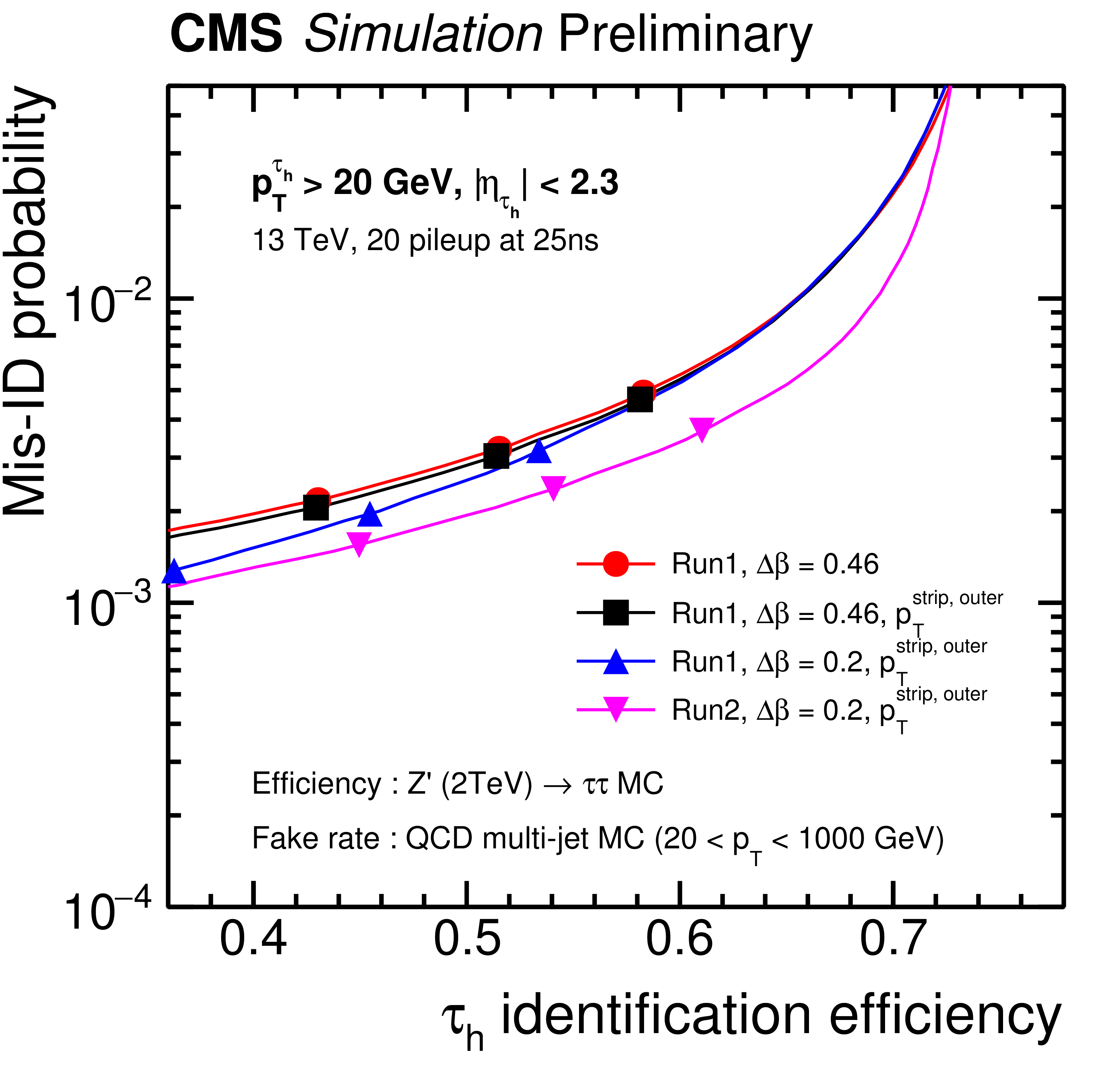
Figure 2-b:
Misidentification probability as a function of $ {\tau _\mathrm {h}} $ identification efficiency, evaluated using H $\to \tau \tau $ and QCD MC samples (a), and Z$^{'}$ (2TeV) and QCD MC samples (b). Four different configurations of reconstruction plus isolation method are compared (from top to bottom): Run-1 fixed size strip with $\Delta \beta = $ 0.46 , Run-1 fixed size strip with $\Delta \beta = $ 0.46 and $ {p_{\mathrm{T}}}^{\text {strip, outer}}$ cut, Run-1 fixed size strip with $\Delta \beta = $ 0.2 and $ {p_{\mathrm{T}}}^{\text {strip, outer}}$ cut, Run-2 dynamic strip with $\Delta \beta = $ 0.2 and $ {p_{\mathrm{T}}}^{\text {strip, outer}}$ cut. The three points on each curve correspond to, from left to right, the Tight, Medium and Loose working point. The misidentification probability is calculated with respect to jets, which pass minimal $\tau $ reconstruction requirements. |

png pdf |
Figure 3-a:
Misidentification probability as a function of $ {\tau _\mathrm {h}} $ identification efficiency, evaluated using H $\to \tau \tau $ and QCD MC samples (a), and Z$^{'}$ (2TeV) and QCD MC samples (b). The MVA-based discriminators are compared to that of the isolation sum discriminators. The points correspond to working points of the discriminators. The three working points of the isolation sum discriminator are Loose, Medium, and Tight working point. The six working points of the MVA-based discriminators are Very Loose, Loose, Medium, Tight, Very Tight, and Very Very Tight working point, respectively. The misidentification probability is calculated with respect to jets, which pass minimal $\tau $ reconstruction requirements. |
png pdf |
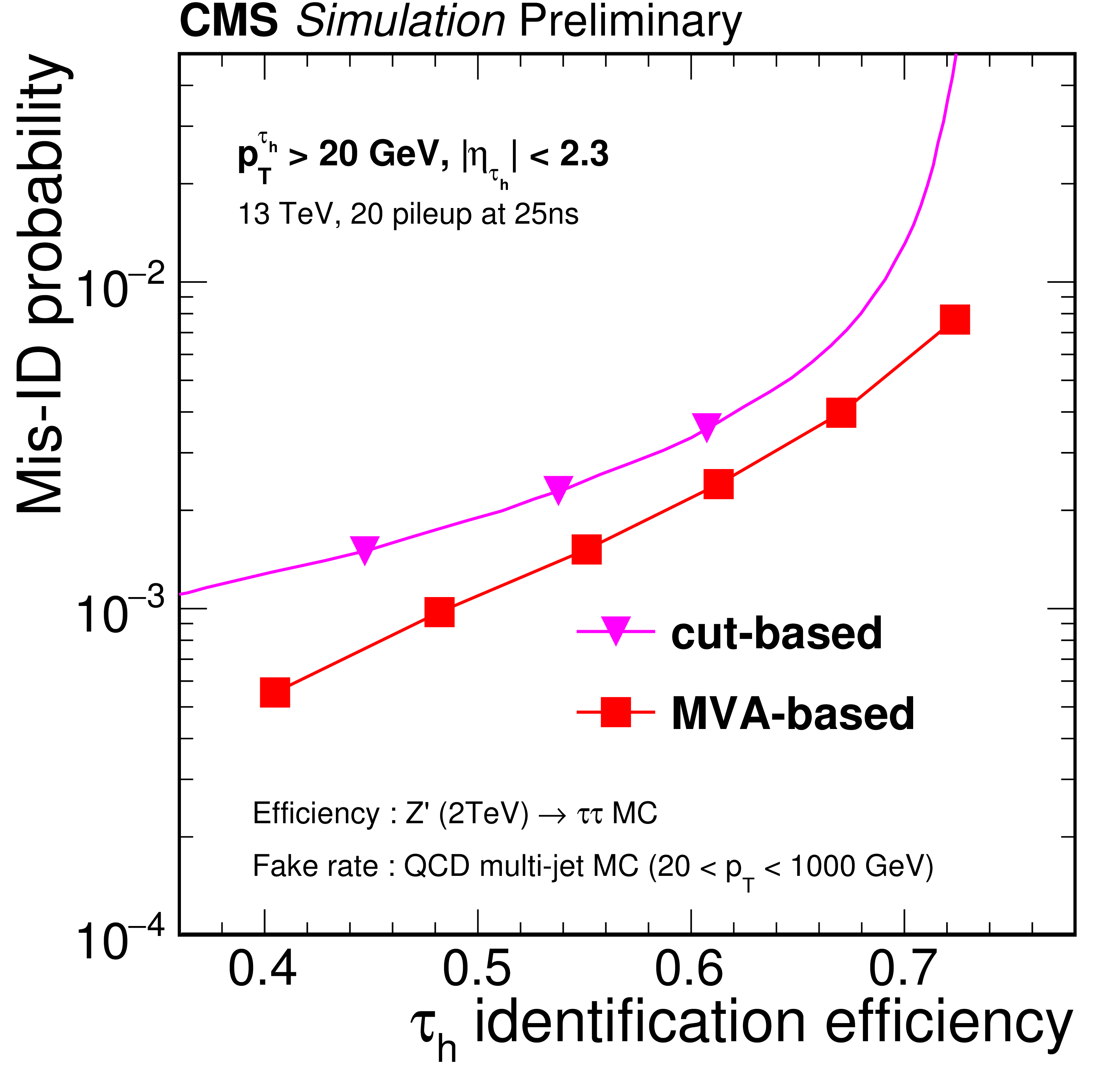
Figure 3-b:
Misidentification probability as a function of $ {\tau _\mathrm {h}} $ identification efficiency, evaluated using H $\to \tau \tau $ and QCD MC samples (a), and Z$^{'}$ (2TeV) and QCD MC samples (b). The MVA-based discriminators are compared to that of the isolation sum discriminators. The points correspond to working points of the discriminators. The three working points of the isolation sum discriminator are Loose, Medium, and Tight working point. The six working points of the MVA-based discriminators are Very Loose, Loose, Medium, Tight, Very Tight, and Very Very Tight working point, respectively. The misidentification probability is calculated with respect to jets, which pass minimal $\tau $ reconstruction requirements. |

png pdf |
Figure 4-a:
Efficiency of the $ {\tau _\mathrm {h}} $ identification estimated with simulated $\mathrm{ Z } / {\gamma ^{*}} \rightarrow \tau \tau $ events (a) and the misidentification probability estimated with simulated QCD multi-jet events (b) for the Very Loose, Loose, Medium, Tight, Very Tight, and Very Very Tight working points of the MVA based $ {\tau _\mathrm {h}} $ isolation algorithm. The efficiency is shown as a function of the $ {\tau _\mathrm {h}} $ transverse momentum while the misidentification probability is shown as a function of the jet transverse momentum. |

png pdf |
Figure 4-b:
Efficiency of the $ {\tau _\mathrm {h}} $ identification estimated with simulated $\mathrm{ Z } / {\gamma ^{*}} \rightarrow \tau \tau $ events (a) and the misidentification probability estimated with simulated QCD multi-jet events (b) for the Very Loose, Loose, Medium, Tight, Very Tight, and Very Very Tight working points of the MVA based $ {\tau _\mathrm {h}} $ isolation algorithm. The efficiency is shown as a function of the $ {\tau _\mathrm {h}} $ transverse momentum while the misidentification probability is shown as a function of the jet transverse momentum. |

png pdf |
Figure 5-a:
Efficiency of the $ {\tau _\mathrm {h}} $ identification estimated with simulated $\mathrm{ Z } / {\gamma ^{*}} \rightarrow \tau \tau $ events (a) and the $\mathrm{ e } \to {\tau _\mathrm {h}} $misidentification probability estimated with simulated $\mathrm{ Z } / {\gamma ^{*}} \rightarrow \mathrm{ e } \mathrm{ e } $ events (b) for the Very Loose, Loose, Medium, Tight and Very Tight working points of the MVA based anti-$\mathrm{ e } $ discrimination algorithm. The efficiency is shown as a function of the $ {\tau _\mathrm {h}} $ transverse momentum while the misidentification probability is shown as a function of the $\mathrm{ e } $ transverse momentum. Both efficiency and misidentification probability are calculated for $ {\tau _\mathrm {h}} $ candidates with a reconstructed decay mode and passing the Loose working point of the isolation sum discriminator. |

png pdf |
Figure 5-b:
Efficiency of the $ {\tau _\mathrm {h}} $ identification estimated with simulated $\mathrm{ Z } / {\gamma ^{*}} \rightarrow \tau \tau $ events (a) and the $\mathrm{ e } \to {\tau _\mathrm {h}} $misidentification probability estimated with simulated $\mathrm{ Z } / {\gamma ^{*}} \rightarrow \mathrm{ e } \mathrm{ e } $ events (b) for the Very Loose, Loose, Medium, Tight and Very Tight working points of the MVA based anti-$\mathrm{ e } $ discrimination algorithm. The efficiency is shown as a function of the $ {\tau _\mathrm {h}} $ transverse momentum while the misidentification probability is shown as a function of the $\mathrm{ e } $ transverse momentum. Both efficiency and misidentification probability are calculated for $ {\tau _\mathrm {h}} $ candidates with a reconstructed decay mode and passing the Loose working point of the isolation sum discriminator. |
png pdf |
Figure 6-a:
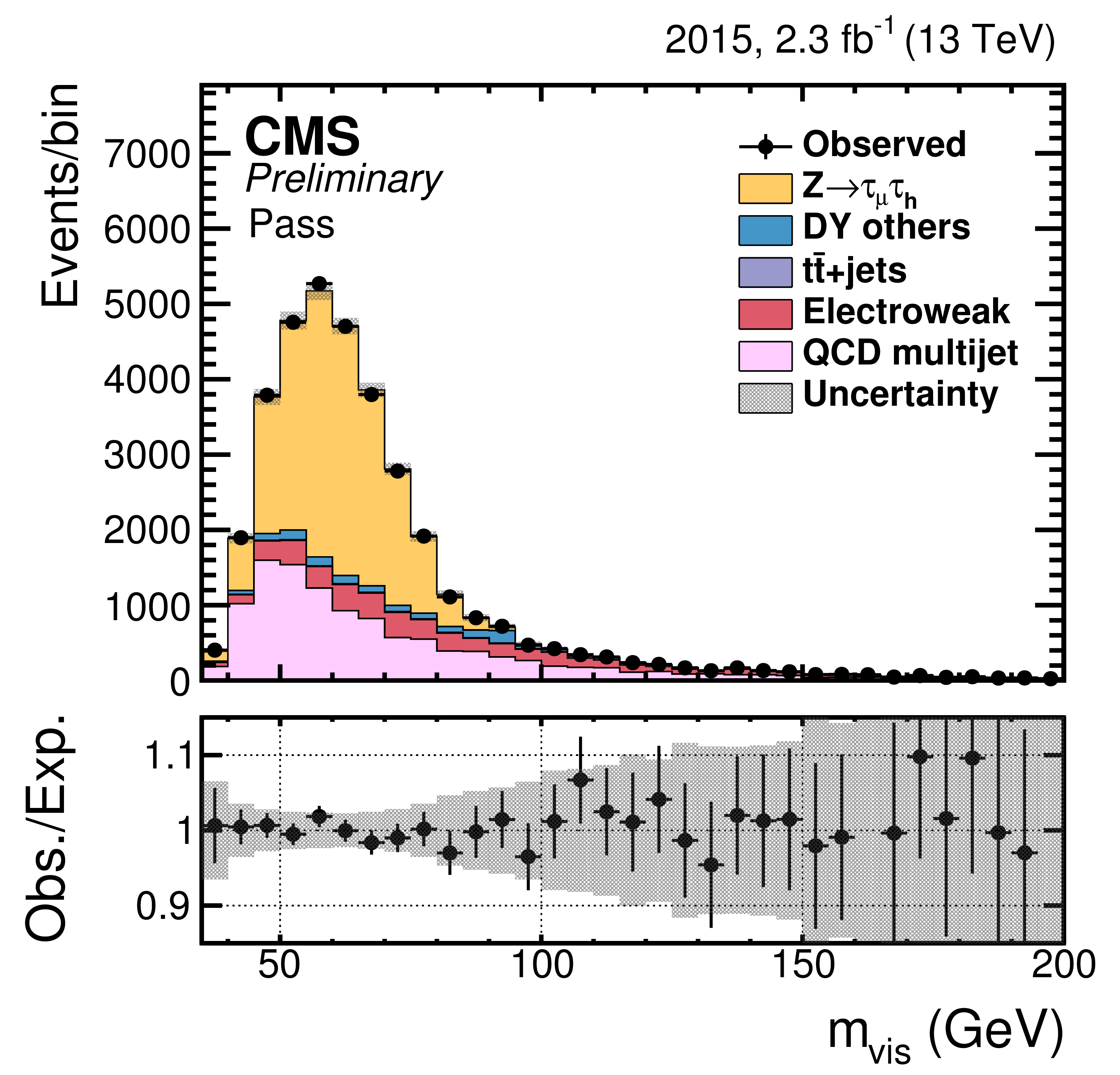
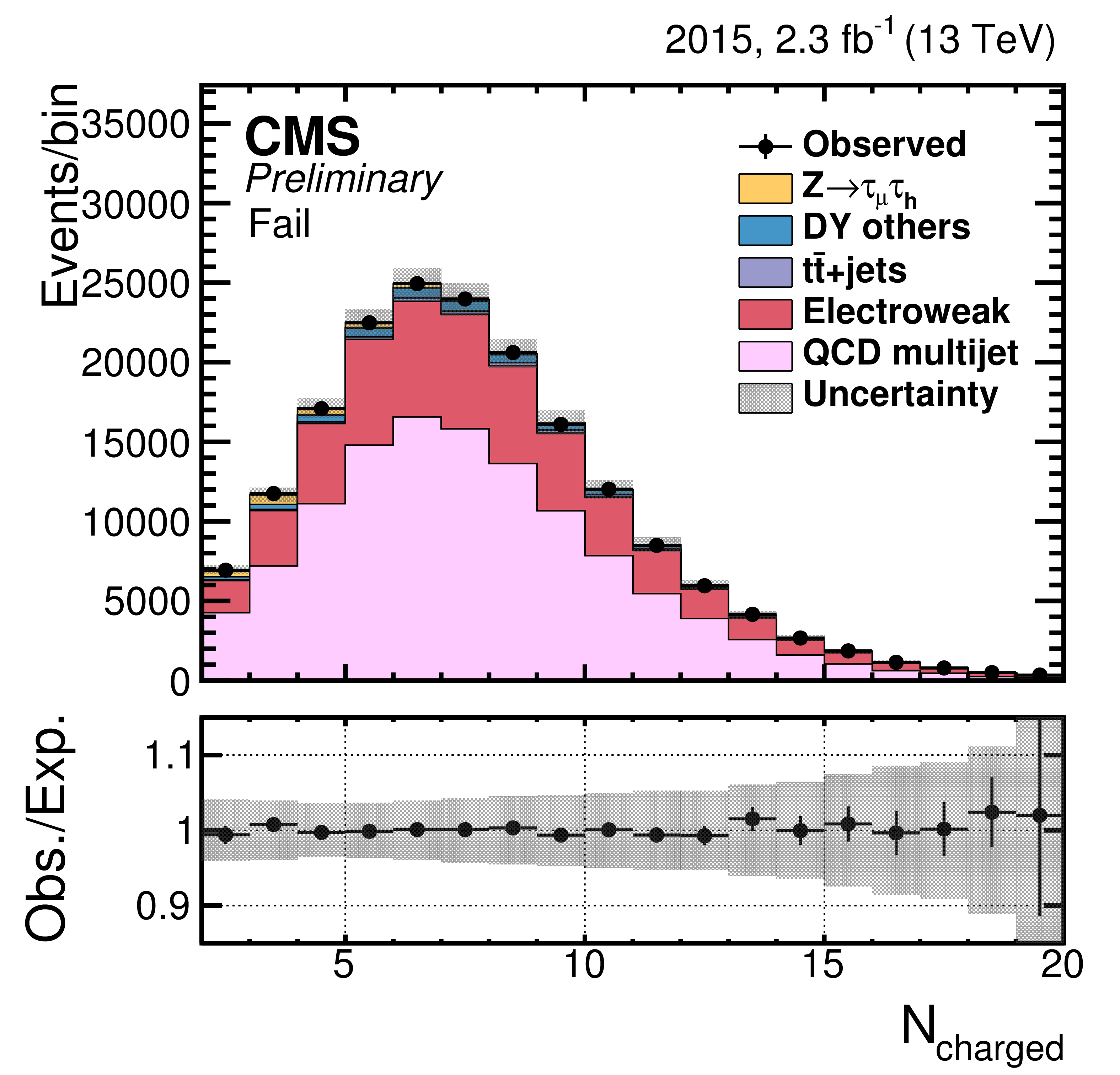
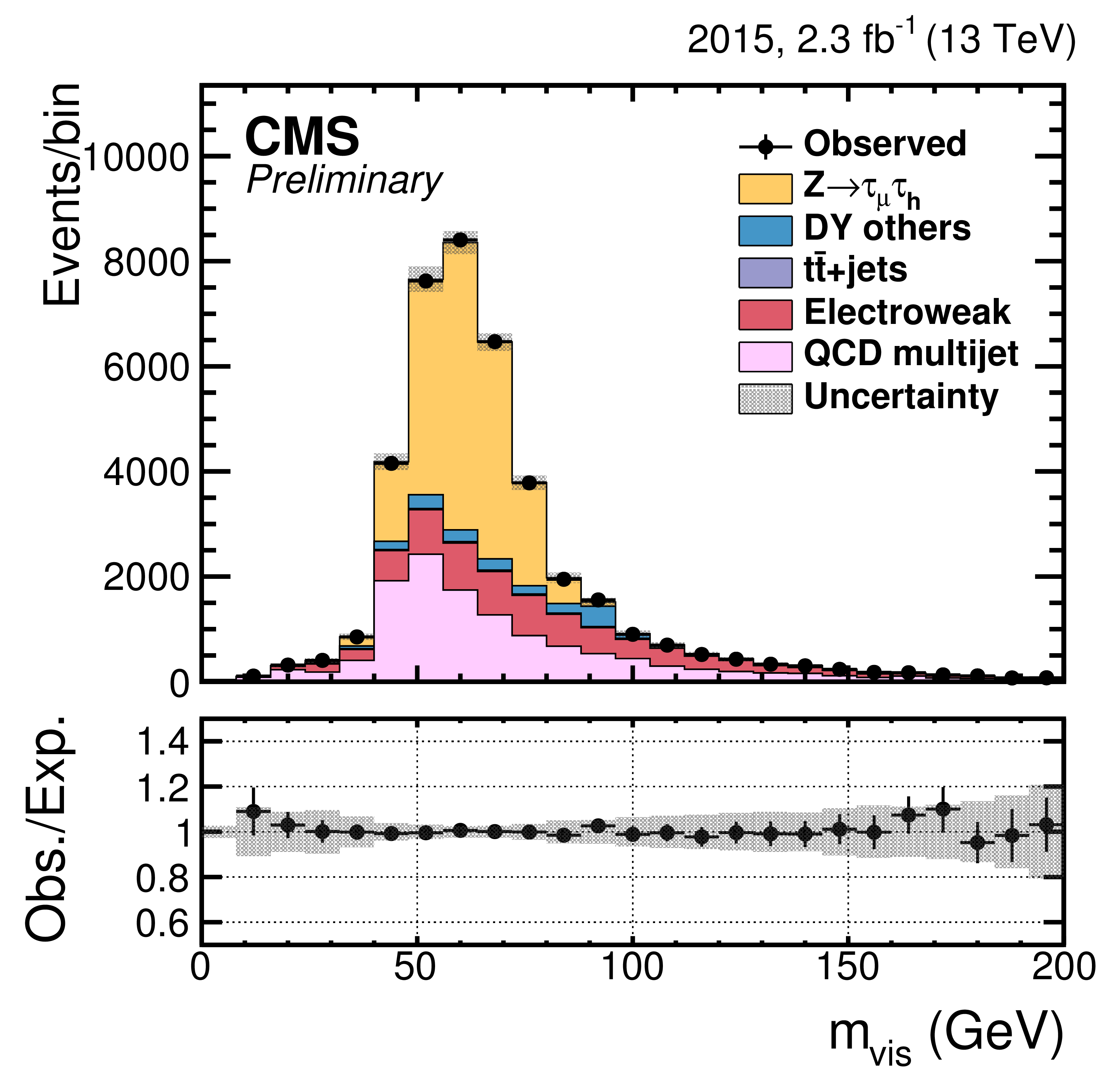
Postfit distributions in the $pass$ (a,c) and $fail$ (b,d) control regions, using $m_{vis}$ (a,b) or $N_{charged}$ (c,d) as observable, for the Loose working point of the MVA-based isolation. |
png pdf |
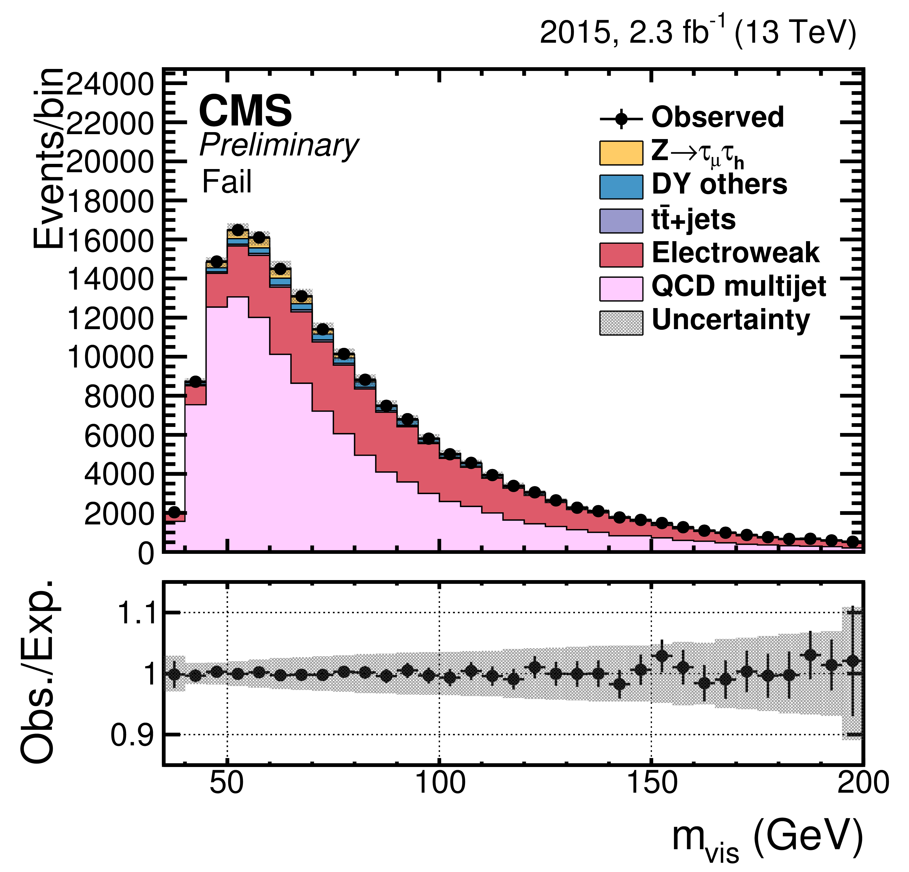
Figure 6-b:
Postfit distributions in the $pass$ (a,c) and $fail$ (b,d) control regions, using $m_{vis}$ (a,b) or $N_{charged}$ (c,d) as observable, for the Loose working point of the MVA-based isolation. |

png pdf |
Figure 6-c:
Postfit distributions in the $pass$ (a,c) and $fail$ (b,d) control regions, using $m_{vis}$ (a,b) or $N_{charged}$ (c,d) as observable, for the Loose working point of the MVA-based isolation. |
png pdf |
Figure 6-d:
Postfit distributions in the $pass$ (a,c) and $fail$ (b,d) control regions, using $m_{vis}$ (a,b) or $N_{charged}$ (c,d) as observable, for the Loose working point of the MVA-based isolation. |
png pdf |
Figure 7-a:
Postfit distributions in the $\mu \tau _h$ (a) and $\mu \mu $ (b) regions, for the Loose working point of the isolation-sum discriminator as derived using the $\mathrm{ Z } \to \tau \tau $/$\mathrm{ Z } \to \mu \mu $ ratio method. |

png pdf |
Figure 7-b:
Postfit distributions in the $\mu \tau _h$ (a) and $\mu \mu $ (b) regions, for the Loose working point of the isolation-sum discriminator as derived using the $\mathrm{ Z } \to \tau \tau $/$\mathrm{ Z } \to \mu \mu $ ratio method. |

png pdf |
Figure 8-a:
The transverse mass distribution in the selected sample of $\mathrm{ W } ^{*}\to \mu \nu $ events after applying maximum likelihood fit (a). The measured transverse mass distribution in the sample of selected $\mathrm{ W } ^{*}\to {\tau _\mathrm {h}} \nu $ events with Medium working point of isolation-sum discriminator. |

png pdf |
Figure 8-b:
The transverse mass distribution in the selected sample of $\mathrm{ W } ^{*}\to \mu \nu $ events after applying maximum likelihood fit (a). The measured transverse mass distribution in the sample of selected $\mathrm{ W } ^{*}\to {\tau _\mathrm {h}} \nu $ events with Medium working point of isolation-sum discriminator. |
png pdf |
Figure 9-a:
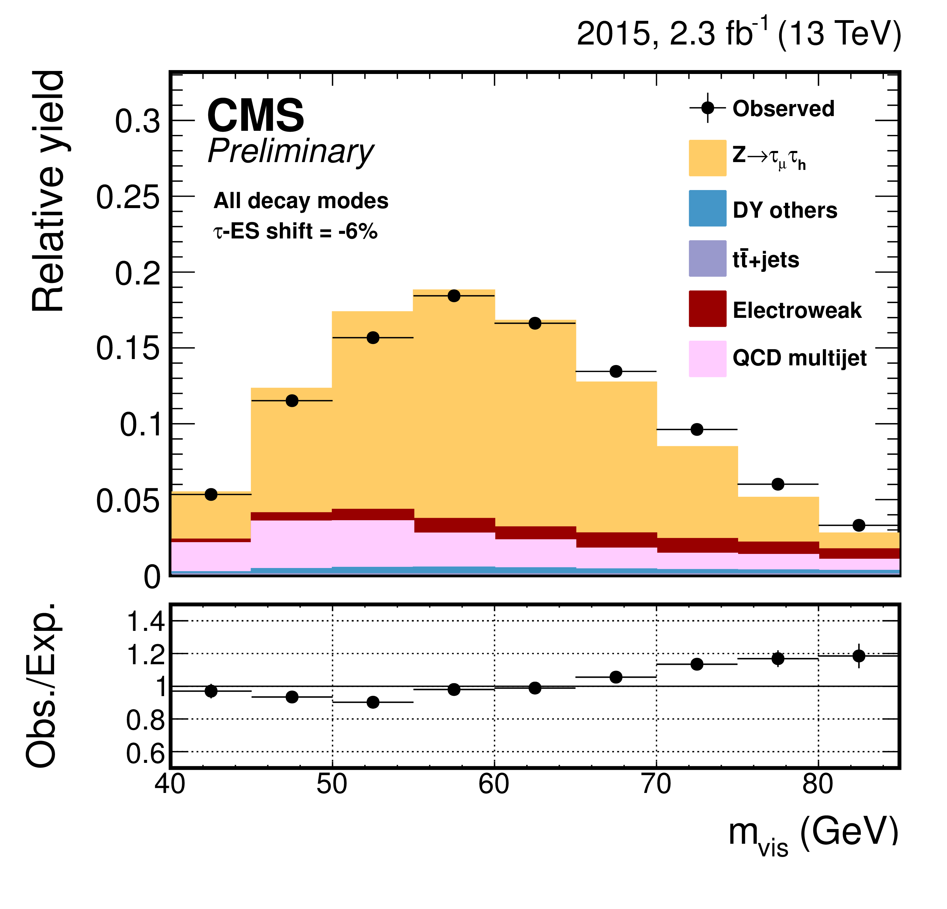
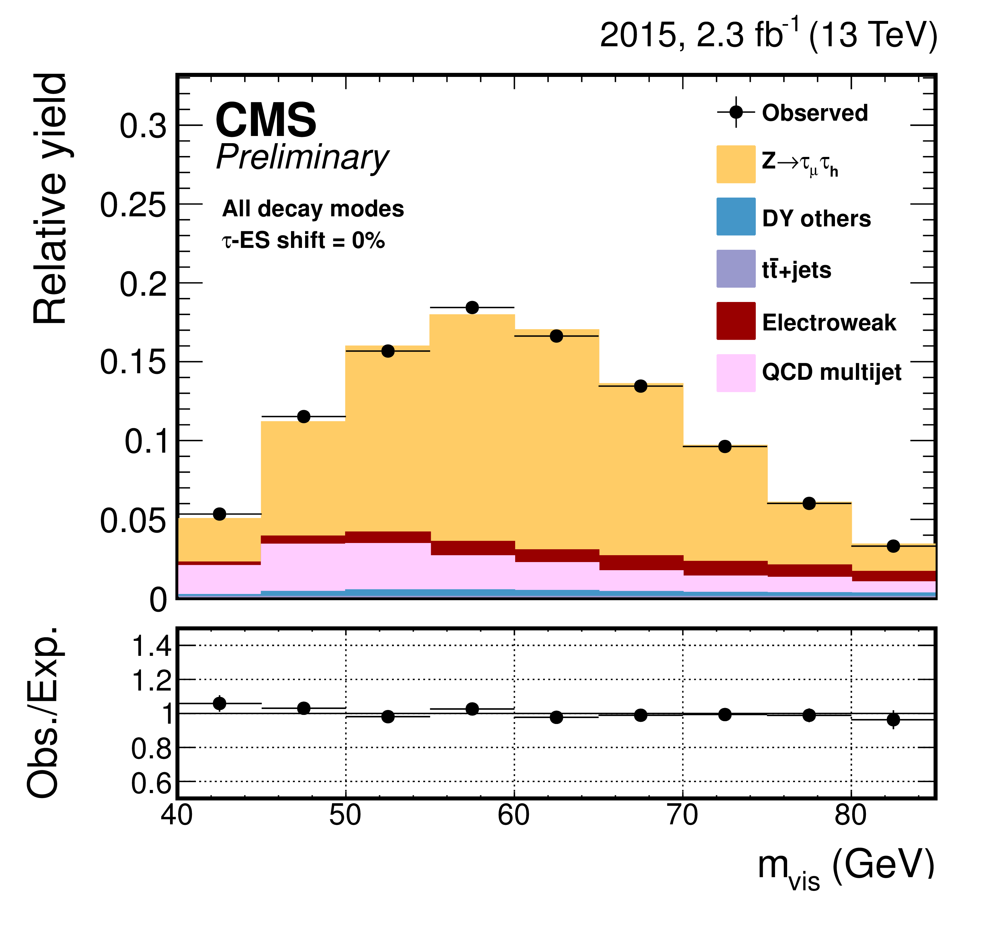
The distributions of $m_{vis}$ of the muon-$ {\tau _\mathrm {h}} $ system with all $ {\tau _\mathrm {h}} $ decay modes included. The observed data are compared to predictions with different shift applied to the energy scale: $-6%$ (a), $0%$ (b) and $+6%$ (c). |
png pdf |
Figure 9-b:
The distributions of $m_{vis}$ of the muon-$ {\tau _\mathrm {h}} $ system with all $ {\tau _\mathrm {h}} $ decay modes included. The observed data are compared to predictions with different shift applied to the energy scale: $-6%$ (a), $0%$ (b) and $+6%$ (c). |

png pdf |
Figure 9-c:
The distributions of $m_{vis}$ of the muon-$ {\tau _\mathrm {h}} $ system with all $ {\tau _\mathrm {h}} $ decay modes included. The observed data are compared to predictions with different shift applied to the energy scale: $-6%$ (a), $0%$ (b) and $+6%$ (c). |
png pdf |
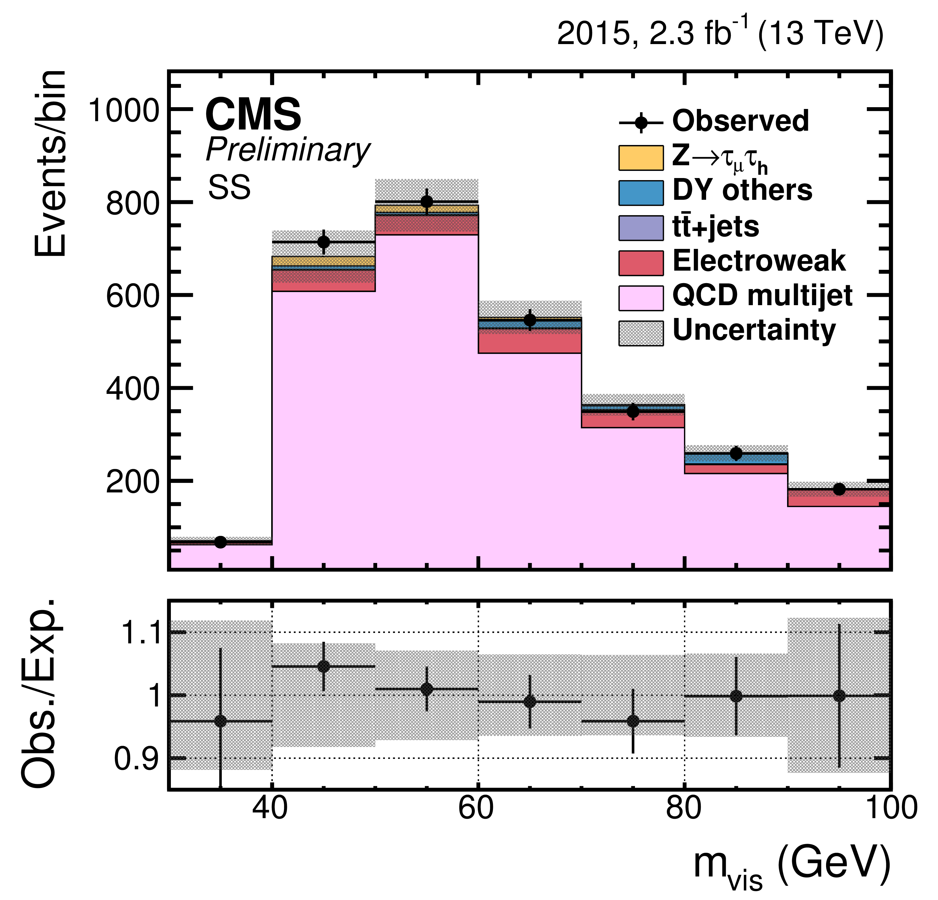
Figure 10-a:
Postfit distributions in the SS (a) and OS (b) regions for the charge misidentification probability measurement. |

png pdf |
Figure 10-b:
Postfit distributions in the SS (a) and OS (b) regions for the charge misidentification probability measurement. |

png pdf |
Figure 12-a:
Post-fit plots of the tag and probe mass in the pass category for the Loose (a), Medium (b), Tight (c) and Very Tight (d) working point of the anti-e discriminator in the barrel region. |
png pdf |
Figure 12-b:
Post-fit plots of the tag and probe mass in the pass category for the Loose (a), Medium (b), Tight (c) and Very Tight (d) working point of the anti-e discriminator in the barrel region. |
png pdf |
Figure 12-c:
Post-fit plots of the tag and probe mass in the pass category for the Loose (a), Medium (b), Tight (c) and Very Tight (d) working point of the anti-e discriminator in the barrel region. |

png pdf |
Figure 12-d:
Post-fit plots of the tag and probe mass in the pass category for the Loose (a), Medium (b), Tight (c) and Very Tight (d) working point of the anti-e discriminator in the barrel region. |
| Tables | |
png pdf |
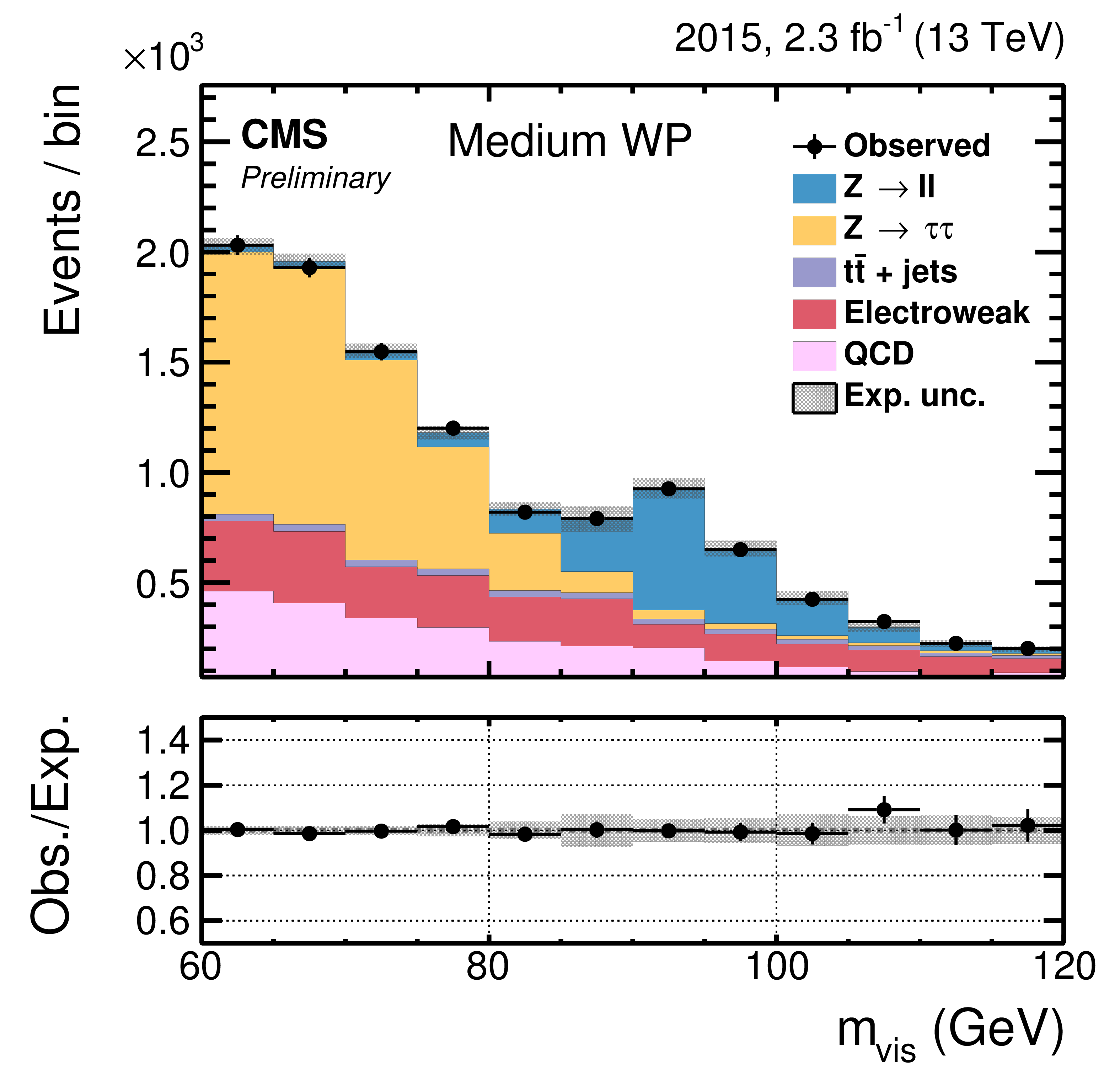
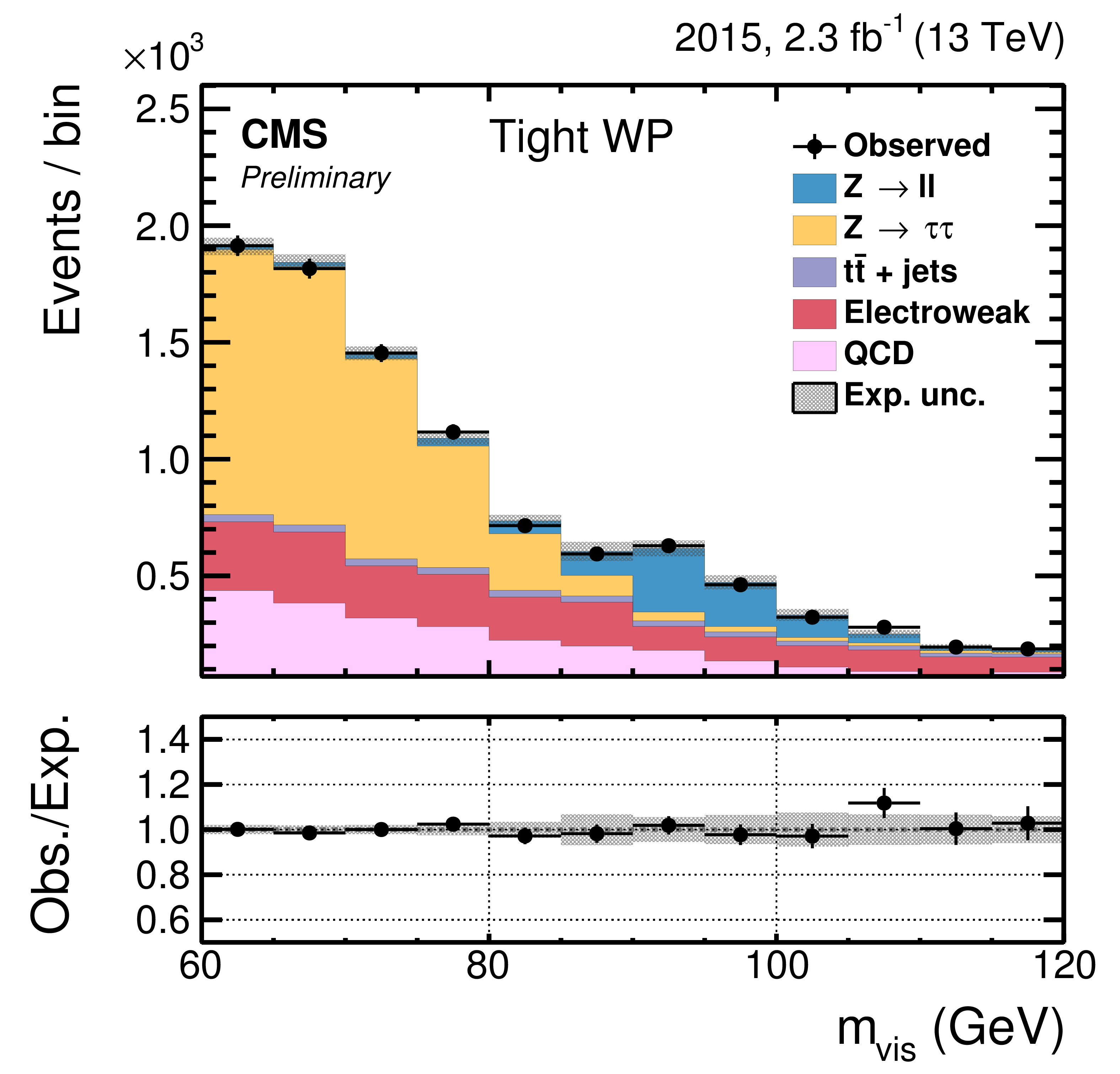
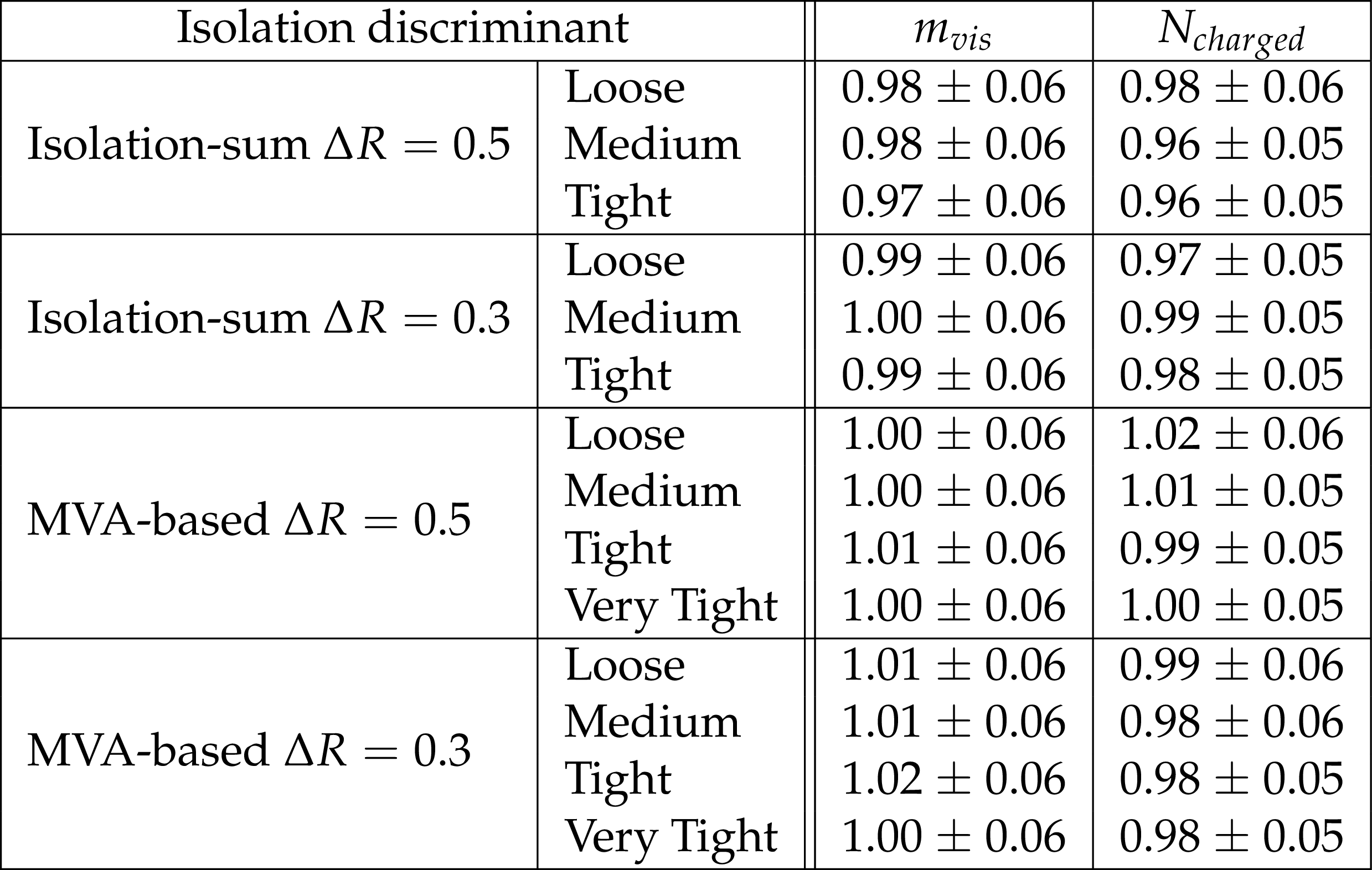
Table 1:
Data/MC scale factors for the different working points of the isolation-sum and MVA-based discriminator, and for two values of the isolation cone. An uncertainty of 3.9% has been added in quadrature to the uncertainty returned by the fit to account for the tracking efficiency uncertainty. Tag-and-probe method is used to measure the efficiency and its uncertainty. |

png pdf |
Table 2:
Data/MC scale factors for the different working points of the isolation-sum and MVA-based discriminator, and for two values of the isolation cone. The ratio, $\mathrm{ Z } \to \tau _{\mu } {\tau _\mathrm {h}} $/$\mathrm{ Z } \to \mu \mu $ is used as a discriminant variable. |
png pdf |
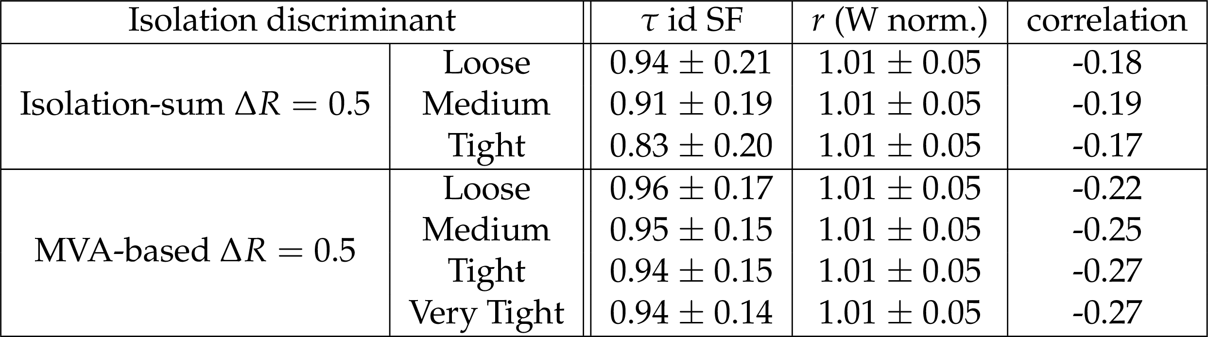
Table 3:
$ {\tau _\mathrm {h}} $ identification efficiency scale factor, the nomalization of $\sigma (pp\to \mathrm{ W } ^{*}+X|m_{\mathrm{ W } ^{*}}>200 {\text { GeV}} )$, $r$, and correlation coefficient between the two quantities obtained from the fit. The scale factors are measured for both isolation-sum and MVA-based discriminators. |

png pdf |
Table 4:
Energy scale corrections for $ {\tau _\mathrm {h}} $ measured in $\mathrm{Z} \to \tau \tau $ events for $ {\tau _\mathrm {h}} $ reconstructed in different decay modes. The inclusive result is obtained by means of an independent fit and hence may be different from the average of $ {\tau _\mathrm {h}} $ energy scale corrections measured for individual decay modes. |

png pdf |
Table 5:
Probability for electrons to pass the different working points of the MVA-based anti-e discriminator, splitted in barrel and endcap region. For each working point, the $\mathrm{ e } \to {\tau _\mathrm {h}} $ misidentification probability is defined as the fraction of probes passing the given discriminator with respect to the total number of probes. |
| Summary |
|
The algorithm used in Run-2 to reconstruct and identify hadronically decaying taus has been described in this note, with a particular emphasis on the changes with respect to Run-1. These changes include among others a dynamical strip reconstruction, and additional variables in the MVA-disriminators against jets and electrons. The performance has been measured in data collected in 2015 at a center-of-mass energy of $\sqrt{s} = $13 TeV. The tau identification and reconstruction techniques described are now fully commissioned and ready for use in CMS physics analyses for the remainder of Run-2. The performance in data of the $\tau_{\mathrm{h}}$ identification efficiency in both low and high $p_{\mathrm{T}}$ regions is similar to that in Monte Carlo simulation, while the performance of the jet $\to \tau_{\mathrm{h}}$ misidentification is found to be moderately different. The energy scale of $\tau_{\mathrm{h}}$ is measured and its response with respect to the Monte Carlo simulation is found to be close to 1. The reduction in electron $\to \tau_{\mathrm{h}}$ fake probability is seen to perform well in Run-2, and its scale factors have been measured. |
| Additional Figures | |

png pdf |
Additional Figure 1:
Input variable for the MVA-based anti-electron discriminator. Distribution, normalized to unity, of the ratio between the total ECAL energy and the inner track momentum, for hadronic $\tau $ decays (blue) and electrons (red). The $ {\tau _\mathrm {h}} $ candidates are required to have $ {p_{\mathrm{T}}}> $ 20 GeV, $|\eta | < $ 2.3, to pass the loose working point of the cut-based isolation and have to be reconstructed in one of the decay modes ${\mathrm{h}}^{\pm }$, ${\mathrm{h}}^{\pm }\pi ^{0}$, ${\mathrm{h}}^{\pm }\pi ^{0}\pi ^{0}$ or ${\mathrm{h}}^{\pm }{\mathrm{h}}^{\mp }{\mathrm{h}}^{\pm }$. |

png pdf |
Additional Figure 2:
Input variable for the MVA-based anti-electron discriminator. Distribution, normalized to unity, of $(N^{\text {GSF}}_{\text {hits}} - N^{\text {KF}}_{\text {hits}})/(N^{\text {GSF}}_{\text {hits}} + N^{\text {KF}}_{\text {hits}})$, for hadronic $\tau $ decays (blue) and electrons (red). The quantities $N^{\text {GSF}}_{\text {hits}}$ and $N^{\text {KF}}_{\text {hits}}$ are, respectively, the number of valid hits in the tracker detector which are associated with the track reconstructed by the GSF or Kalman filter (KF) algorithms. The $ {\tau _\mathrm {h}} $ candidates are required to have $ {p_{\mathrm{T}}}> $ 20 GeV, $|\eta | < $ 2.3, to pass the loose working point of the cut-based isolation and have to be reconstructed in one of the decay modes ${\mathrm{h}}^{\pm }$, ${\mathrm{h}}^{\pm }\pi ^{0}$, ${\mathrm{h}}^{\pm }\pi ^{0}\pi ^{0}$ or ${\mathrm{h}}^{\pm }{\mathrm{h}}^{\mp }{\mathrm{h}}^{\pm }$. |

png pdf |
Additional Figure 3:
Input variable for the MVA-based anti-electron discriminator. Distribution, normalized to unity, of the $\chi ^2$ per degree-of-freedom (DoF) of the track fit performed with the GSF algorithm, for hadronic $\tau $ decays (blue) and electrons (red). The $ {\tau _\mathrm {h}} $ candidates are required to have $ {p_{\mathrm{T}}}> $ 20 GeV, $|\eta | < $ 2.3, to pass the loose working point of the cut-based isolation and have to be reconstructed in one of the decay modes ${\mathrm{h}}^{\pm }$, ${\mathrm{h}}^{\pm }\pi ^{0}$, ${\mathrm{h}}^{\pm }\pi ^{0}\pi ^{0}$ or ${\mathrm{h}}^{\pm }{\mathrm{h}}^{\mp }{\mathrm{h}}^{\pm }$. |

png pdf |
Additional Figure 4:
Input variable for the MVA-based anti-electron discriminator. Distribution, normalized to unity, of $F_{\text {brem}} \equiv |p_{\text {in}}-p_{\text {out}}|/p_{\text {in}}$, for hadronic $\tau $ decays (blue) and electrons (red). The quantities $p_{\text {in}}$ and $p_{\text {out}}$ are the momenta, measured from the track curvature at the innermost and outermost position in the tracker, of the tracks reconstructed using the GSF algorithm. The $ {\tau _\mathrm {h}} $ candidates are required to have $ {p_{\mathrm{T}}}> $ 20 GeV, $|\eta | < $ 2.3, to pass the loose working point of the cut-based isolation and have to be reconstructed in one of the decay modes ${\mathrm{h}}^{\pm }$, ${\mathrm{h}}^{\pm }\pi ^{0}$, ${\mathrm{h}}^{\pm }\pi ^{0}\pi ^{0}$ or ${\mathrm{h}}^{\pm }{\mathrm{h}}^{\mp }{\mathrm{h}}^{\pm }$. |

png pdf |
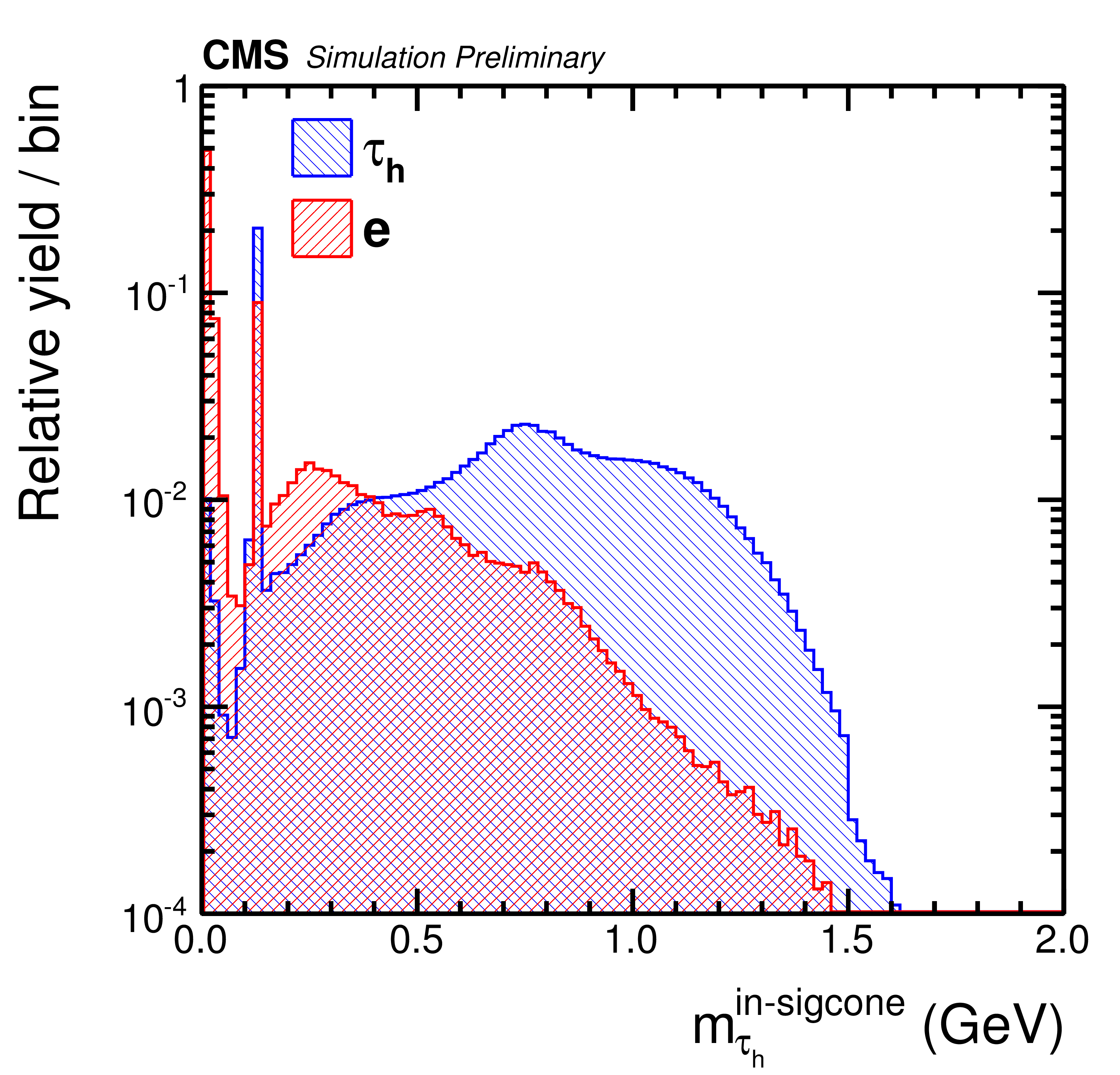
Additional Figure 5:
Input variable for the MVA-based anti-electron discriminator. Distribution, normalized to unity, of the ratio between the ECAL energy associated with the leading track of the $ {\tau _\mathrm {h}} $ candidate and the leading track momentum, for hadronic $\tau $ decays (blue) and electrons (red). The $ {\tau _\mathrm {h}} $ candidates are required to have $ {p_{\mathrm{T}}}> $ 20 GeV, $|\eta | < $ 2.3, to pass the loose working point of the cut-based isolation and have to be reconstructed in one of the decay modes ${\mathrm{h}}^{\pm }$, ${\mathrm{h}}^{\pm }\pi ^{0}$, ${\mathrm{h}}^{\pm }\pi ^{0}\pi ^{0}$ or ${\mathrm{h}}^{\pm }{\mathrm{h}}^{\mp }{\mathrm{h}}^{\pm }$. |

png pdf |
Additional Figure 6:
Input variable for the MVA-based anti-electron discriminator. Distribution, normalized to unity, of $\sqrt {\sum (\Delta \phi )^2 {p_{\mathrm {T}}} ^{\gamma \text { in-sigcone}}}$/GeV computed from the ${p_{\mathrm {T}}} $-weighted square of the distance in $\phi $ between each photon included in a strip and the leading track of the $ {\tau _\mathrm {h}} $ candidate, for hadronic $\tau $ decays (blue) and electrons (red). This variable is computed separately for photons inside and outside the $ {\tau _\mathrm {h}} $ candidate signal cone in order to increase its separation power. The $ {\tau _\mathrm {h}} $ candidates are required to have $ {p_{\mathrm{T}}}> $ 20 GeV, $|\eta | < $ 2.3, to pass the loose working point of the cut-based isolation and have to be reconstructed in one of the decay modes ${\mathrm{h}}^{\pm }$, ${\mathrm{h}}^{\pm }\pi ^{0}$, ${\mathrm{h}}^{\pm }\pi ^{0}\pi ^{0}$ or ${\mathrm{h}}^{\pm }{\mathrm{h}}^{\mp }{\mathrm{h}}^{\pm }$. |
png pdf |
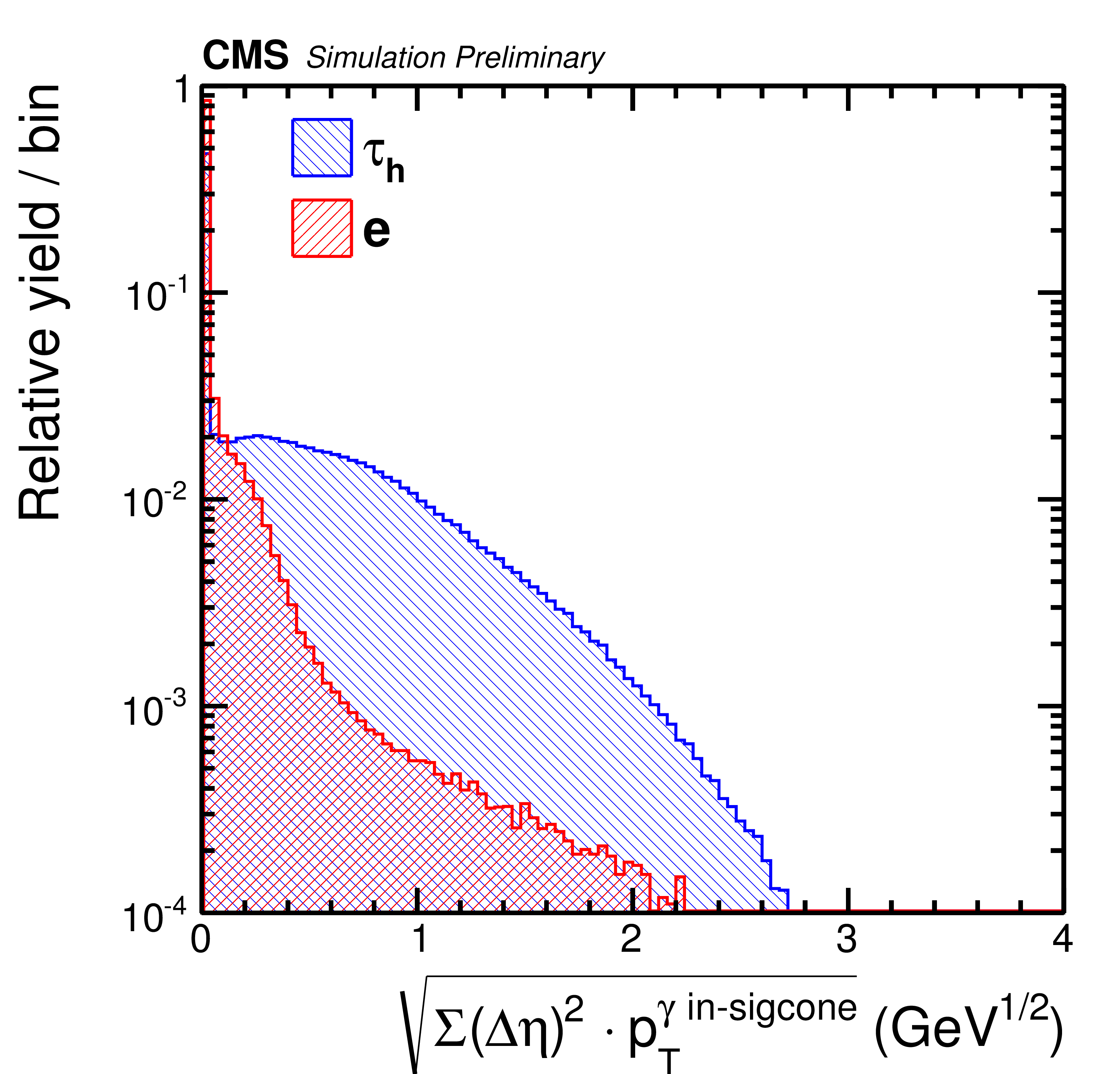
Additional Figure 7:
Input variable for the MVA-based anti-electron discriminator. Distribution, normalized to unity, of $\sqrt {\sum (\Delta \eta )^2 {p_{\mathrm {T}}} ^{\gamma \text { in-sigcone}}}$/GeV computed from the ${p_{\mathrm {T}}} $-weighted square of the distance in $\eta $ between each photon included in a strip and the leading track of the $ {\tau _\mathrm {h}} $ candidate, for hadronic $\tau $ decays (blue) and electrons (red). This variable is computed separately for photons inside and outside the $ {\tau _\mathrm {h}} $ candidate signal cone in order to increase its separation power. The $ {\tau _\mathrm {h}} $ candidates are required to have $ {p_{\mathrm{T}}}> $ 20 GeV, $|\eta | < $ 2.3, to pass the loose working point of the cut-based isolation and have to be reconstructed in one of the decay modes ${\mathrm{h}}^{\pm }$, ${\mathrm{h}}^{\pm }\pi ^{0}$, ${\mathrm{h}}^{\pm }\pi ^{0}\pi ^{0}$ or ${\mathrm{h}}^{\pm }{\mathrm{h}}^{\mp }{\mathrm{h}}^{\pm }$. |
png pdf |
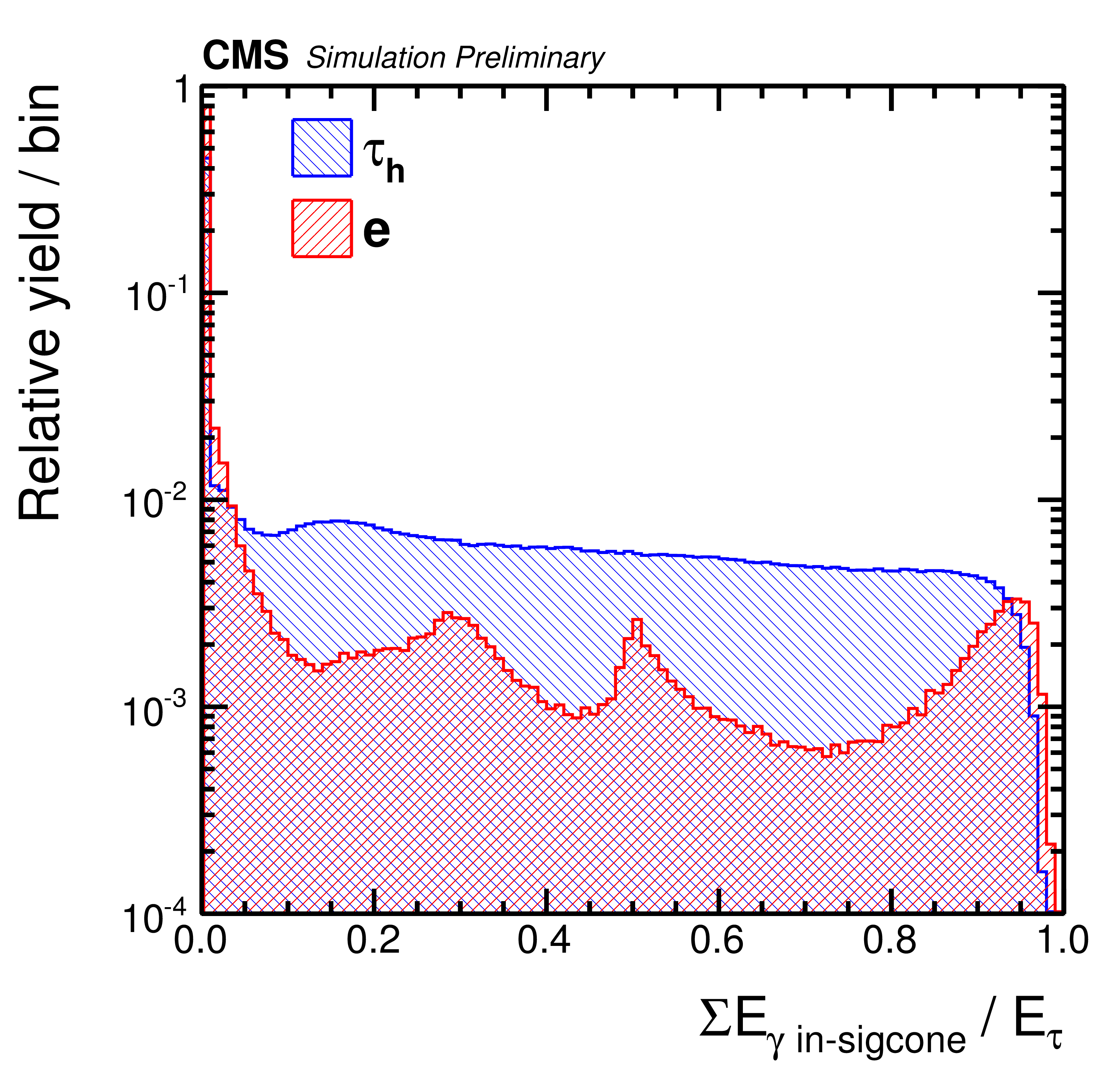
Additional Figure 8:
Input variable for the MVA-based anti-electron discriminator. Distribution, normalized to unity, of the fraction of $ {\tau _\mathrm {h}} $ energy carried by photons, for hadronic $\tau $ decays (blue) and electrons (red). This variable is computed separately for photons inside and outside the $ {\tau _\mathrm {h}} $ candidate signal cone in order to increase its separation power. The $ {\tau _\mathrm {h}} $ candidates are required to have $ {p_{\mathrm{T}}}> $ 20 GeV, $|\eta | < $ 2.3, to pass the loose working point of the cut-based isolation and have to be reconstructed in one of the decay modes ${\mathrm{h}}^{\pm }$, ${\mathrm{h}}^{\pm }\pi ^{0}$, ${\mathrm{h}}^{\pm }\pi ^{0}\pi ^{0}$ or ${\mathrm{h}}^{\pm }{\mathrm{h}}^{\mp }{\mathrm{h}}^{\pm }$. |

png pdf |
Additional Figure 9:
Input variable for the MVA-based anti-electron discriminator. Distribution, normalized to unity, of the ratio between the amount of energy deposited in the ECAL and the sum of the ECAL and HCAL energy deposits which are associated with the decay products of the $ {\tau _\mathrm {h}} $ candidate, for hadronic $\tau $ decays (blue) and electrons (red). The $ {\tau _\mathrm {h}} $ candidates are required to have $ {p_{\mathrm{T}}}> $ 20 GeV, $|\eta | < $ 2.3, to pass the loose working point of the cut-based isolation and have to be reconstructed in one of the decay modes ${\mathrm{h}}^{\pm }$, ${\mathrm{h}}^{\pm }\pi ^{0}$, ${\mathrm{h}}^{\pm }\pi ^{0}\pi ^{0}$ or ${\mathrm{h}}^{\pm }{\mathrm{h}}^{\mp }{\mathrm{h}}^{\pm }$. |
png pdf |
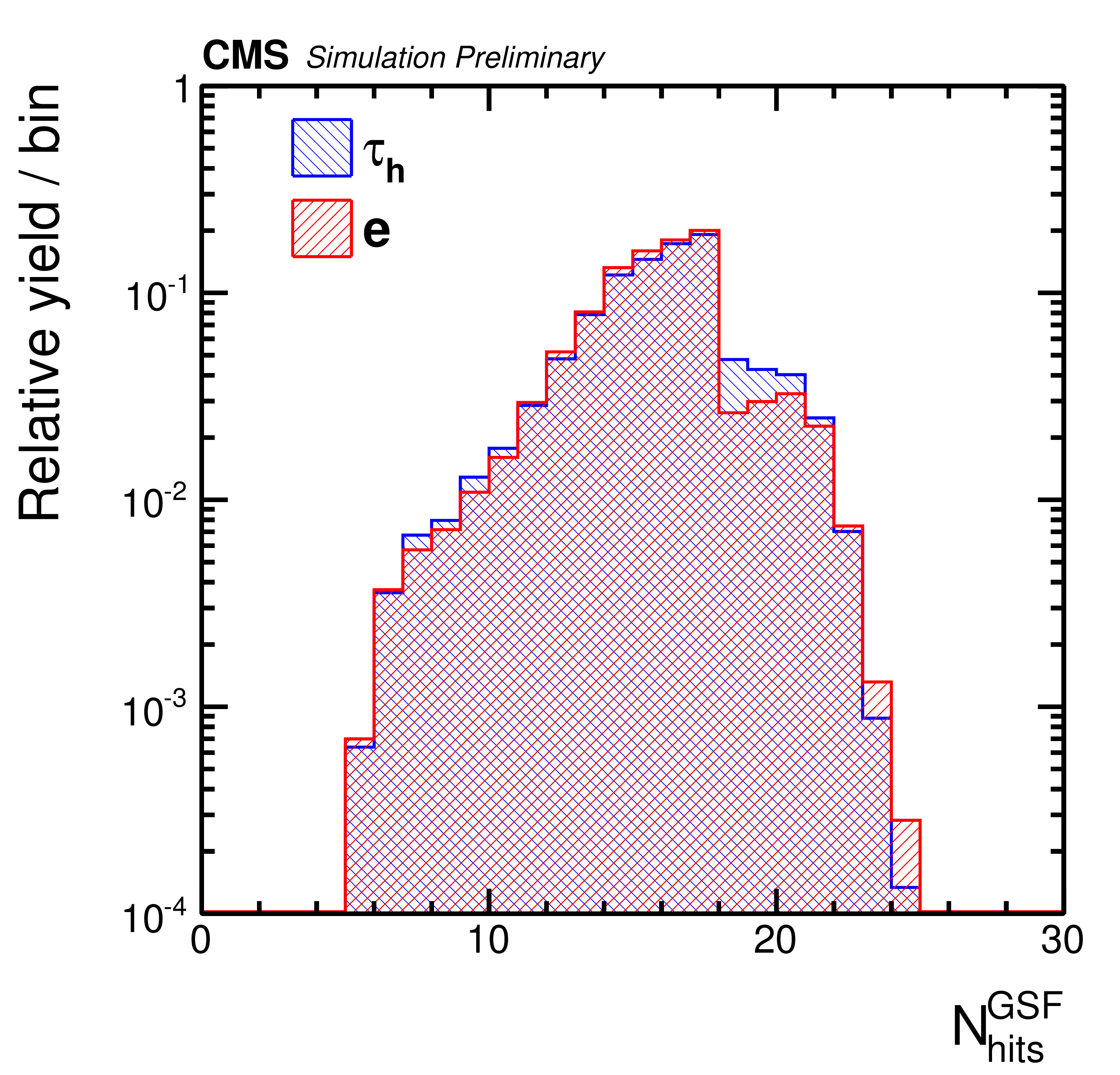
Additional Figure 10:
Input variable for the MVA-based anti-electron discriminator. Distribution, normalized to unity, of the number of valid hits of the track reconstructed by the GSF algorithm, for hadronic $\tau $ decays (blue) and electrons (red). The $ {\tau _\mathrm {h}} $ candidates are required to have $ {p_{\mathrm{T}}}> $ 20 GeV, $|\eta | < $ 2.3, to pass the loose working point of the cut-based isolation and have to be reconstructed in one of the decay modes ${\mathrm{h}}^{\pm }$, ${\mathrm{h}}^{\pm }\pi ^{0}$, ${\mathrm{h}}^{\pm }\pi ^{0}\pi ^{0}$ or ${\mathrm{h}}^{\pm }{\mathrm{h}}^{\mp }{\mathrm{h}}^{\pm }$. |
png pdf |
Additional Figure 11:
Input variable for the MVA-based anti-electron discriminator. Distribution, normalized to unity, of the $ {\tau _\mathrm {h}} $ candidate visible mass computed summing the four-momenta of photons and charged particles inside the $ {\tau _\mathrm {h}} $ candidate signal cone, for hadronic $\tau $ decays (blue) and electrons (red). The $ {\tau _\mathrm {h}} $ candidates are required to have $ {p_{\mathrm{T}}}> $ 20 GeV, $|\eta | < $ 2.3, to pass the loose working point of the cut-based isolation and have to be reconstructed in one of the decay modes ${\mathrm{h}}^{\pm }$, ${\mathrm{h}}^{\pm }\pi ^{0}$, ${\mathrm{h}}^{\pm }\pi ^{0}\pi ^{0}$ or ${\mathrm{h}}^{\pm }{\mathrm{h}}^{\mp }{\mathrm{h}}^{\pm }$. |

png pdf |
Additional Figure 12:
Input variable for the MVA-based anti-electron discriminator. Distribution, normalized to unity, of the ratio between the HCAL energy associated with the leading track of the $ {\tau _\mathrm {h}} $ candidate and the leading track momentum, for hadronic $\tau $ decays (blue) and electrons (red). The $ {\tau _\mathrm {h}} $ candidates are required to have $ {p_{\mathrm{T}}}> $ 20 GeV, $|\eta | < $ 2.3, to pass the loose working point of the cut-based isolation and have to be reconstructed in one of the decay modes ${\mathrm{h}}^{\pm }$, ${\mathrm{h}}^{\pm }\pi ^{0}$, ${\mathrm{h}}^{\pm }\pi ^{0}\pi ^{0}$ or ${\mathrm{h}}^{\pm }{\mathrm{h}}^{\mp }{\mathrm{h}}^{\pm }$. |

png pdf |
Additional Figure 13:
Distribution of the ${p_{\mathrm{T}}}$ sum of charged hadrons in the isolation cone, normalized to unity, which is used as an input variable for the MVA-based $ {\tau _\mathrm {h}} $-isolation discriminator, for hadronic $\tau $ decays (blue) and jets (red). The $ {\tau _\mathrm {h}} $ candidates are required to have $ {p_{\mathrm{T}}}> $ 20 GeV, $|\eta | < $ 2.3, and have to be reconstructed in one of the decay modes ${\mathrm{h}}^{\pm }$, ${\mathrm{h}}^{\pm }\pi ^{0}$, ${\mathrm{h}}^{\pm }\pi ^{0}\pi ^{0}$ or ${\mathrm{h}}^{\pm }{\mathrm{h}}^{\mp }{\mathrm{h}}^{\pm }$. |

png pdf |
Additional Figure 14:
Distribution of the ${p_{\mathrm{T}}}$ sum of Photons in the isolation cone, normalized to unity, which is used as an input variable for the MVA-based $ {\tau _\mathrm {h}} $-isolation discriminator, for hadronic $\tau $ decays (blue) and jets (red). The $ {\tau _\mathrm {h}} $ candidates are required to have $ {p_{\mathrm{T}}}> $ 20 GeV, $|\eta | < $ 2.3, and have to be reconstructed in one of the decay modes ${\mathrm{h}}^{\pm }$, ${\mathrm{h}}^{\pm }\pi ^{0}$, ${\mathrm{h}}^{\pm }\pi ^{0}\pi ^{0}$ or ${\mathrm{h}}^{\pm }{\mathrm{h}}^{\mp }{\mathrm{h}}^{\pm }$. |

png pdf |
Additional Figure 15:
Distribution of the signed transverse impact parameter of leading track, normalized to unity, which is used as an input variable for the MVA-based $ {\tau _\mathrm {h}} $-isolation discriminator, for hadronic $\tau $ decays (blue) and jets (red). The $ {\tau _\mathrm {h}} $ candidates are required to have $ {p_{\mathrm{T}}}> $ 20 GeV, $|\eta | < $ 2.3, and have to be reconstructed in one of the decay modes ${\mathrm{h}}^{\pm }$, ${\mathrm{h}}^{\pm }\pi ^{0}$, ${\mathrm{h}}^{\pm }\pi ^{0}\pi ^{0}$ or ${\mathrm{h}}^{\pm }{\mathrm{h}}^{\mp }{\mathrm{h}}^{\pm }$. |
png pdf |
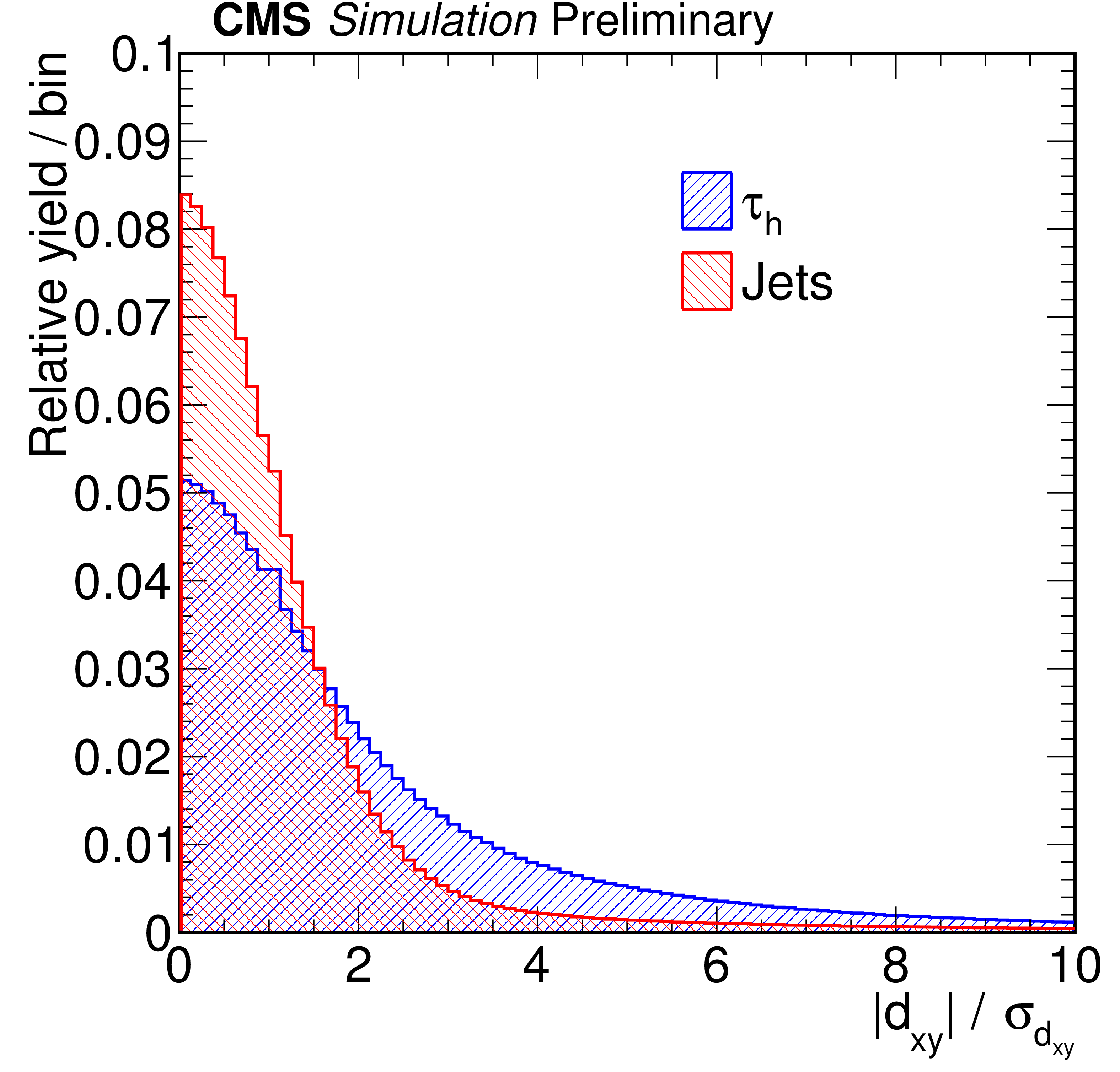
Additional Figure 16:
Distribution of the signed transverse impact parameter significance of leading track, normalized to unity, which is used as input variables for the MVA-based $ {\tau _\mathrm {h}} $-isolation discriminator, for hadronic $\tau $ decays (blue) and jets (red). The $ {\tau _\mathrm {h}} $ candidates are required to have $ {p_{\mathrm{T}}}> $ 20 GeV, $|\eta | < $ 2.3, and have to be reconstructed in one of the decay modes ${\mathrm{h}}^{\pm }$, ${\mathrm{h}}^{\pm }\pi ^{0}$, ${\mathrm{h}}^{\pm }\pi ^{0}\pi ^{0}$ or ${\mathrm{h}}^{\pm }{\mathrm{h}}^{\mp }{\mathrm{h}}^{\pm }$. |

png pdf |
Additional Figure 17:
Distribution of the Signed 3D impact parameter of the leading track, normalized to unity, which is used as an input variable for the MVA-based $ {\tau _\mathrm {h}} $-isolation discriminator, for hadronic $\tau $ decays (blue) and jets (red). The $ {\tau _\mathrm {h}} $ candidates are required to have $ {p_{\mathrm{T}}}> $ 20 GeV, $|\eta | < $ 2.3, and have to be reconstructed in one of the decay modes ${\mathrm{h}}^{\pm }$, ${\mathrm{h}}^{\pm }\pi ^{0}$, ${\mathrm{h}}^{\pm }\pi ^{0}\pi ^{0}$ or ${\mathrm{h}}^{\pm }{\mathrm{h}}^{\mp }{\mathrm{h}}^{\pm }$. |

png pdf |
Additional Figure 18:
Distribution of the Signed 3D impact parameter significance of the leading track, normalized to unity, which is used as an input variable for the MVA-based $ {\tau _\mathrm {h}} $-isolation discriminator, for hadronic $\tau $ decays (blue) and jets (red). The $ {\tau _\mathrm {h}} $ candidates are required to have $ {p_{\mathrm{T}}}> $ 20 GeV, $|\eta | < $ 2.3, and have to be reconstructed in one of the decay modes ${\mathrm{h}}^{\pm }$, ${\mathrm{h}}^{\pm }\pi ^{0}$, ${\mathrm{h}}^{\pm }\pi ^{0}\pi ^{0}$ or ${\mathrm{h}}^{\pm }{\mathrm{h}}^{\mp }{\mathrm{h}}^{\pm }$. |

png pdf |
Additional Figure 20:
Distribution of the flight distance significance for three-prong $\tau $s, normalized to unity, which is used as an input variable for the MVA-based $ {\tau _\mathrm {h}} $-isolation discriminator, for hadronic $\tau $ decays (blue) and jets (red). The $ {\tau _\mathrm {h}} $ candidates are required to have $ {p_{\mathrm{T}}}> $ 20 GeV, $|\eta | < $ 2.3, and have to be reconstructed in one of the decay modes ${\mathrm{h}}^{\pm }$, ${\mathrm{h}}^{\pm }\pi ^{0}$, ${\mathrm{h}}^{\pm }\pi ^{0}\pi ^{0}$ or ${\mathrm{h}}^{\pm }{\mathrm{h}}^{\mp }{\mathrm{h}}^{\pm }$. |
png pdf |
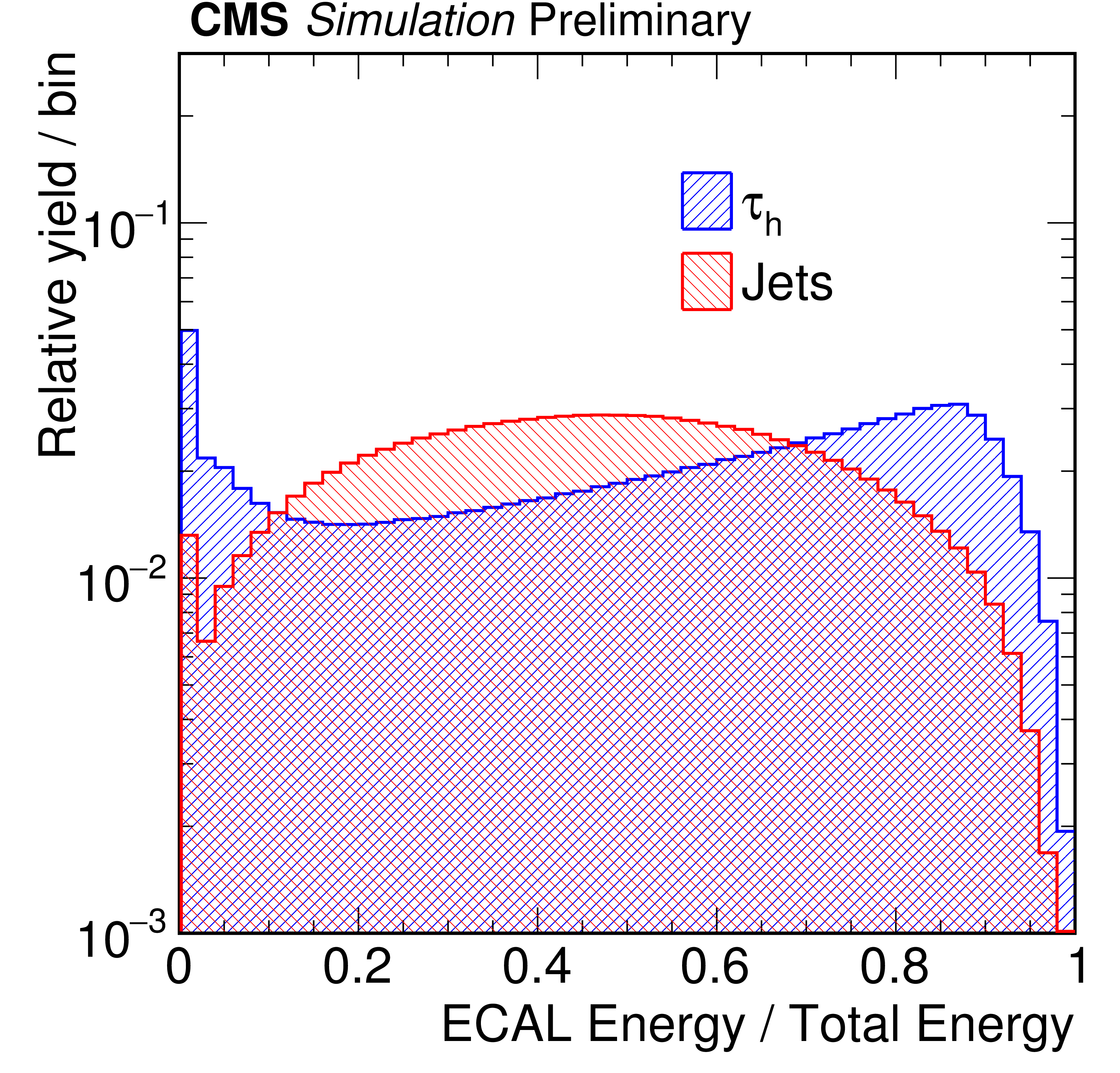
Additional Figure 22:
Fraction of electromagnetic energy in signal cone, normalized to unity, which is used as an input variable for the MVA-based $ {\tau _\mathrm {h}} $-isolation discriminator, for hadronic $\tau $ decays (blue) and jets (red). The $ {\tau _\mathrm {h}} $ candidates are required to have $ {p_{\mathrm{T}}}> $ 20 GeV, $|\eta | < $ 2.3, and have to be reconstructed in one of the decay modes ${\mathrm{h}}^{\pm }$, ${\mathrm{h}}^{\pm }\pi ^{0}$, ${\mathrm{h}}^{\pm }\pi ^{0}\pi ^{0}$ or ${\mathrm{h}}^{\pm }{\mathrm{h}}^{\mp }{\mathrm{h}}^{\pm }$. |

png pdf |
Additional Figure 24:
Distribution of the ${p_{\mathrm {T}}} $-weighted $\Delta R$ of photons within signal cone, normalized to unity, which is used as an input variable for the MVA-based $ {\tau _\mathrm {h}} $-isolation discriminator, for hadronic $\tau $ decays (blue) and jets (red). The $ {\tau _\mathrm {h}} $ candidates are required to have $ {p_{\mathrm{T}}}> $ 20 GeV, $|\eta | < $ 2.3, and have to be reconstructed in one of the decay modes ${\mathrm{h}}^{\pm }$, ${\mathrm{h}}^{\pm }\pi ^{0}$, ${\mathrm{h}}^{\pm }\pi ^{0}\pi ^{0}$ or ${\mathrm{h}}^{\pm }{\mathrm{h}}^{\mp }{\mathrm{h}}^{\pm }$. |
| References | ||||
| 1 | CMS Collaboration | Evidence for the 125 GeV Higgs boson decaying to a pair of $ \tau $ leptons | JHEP 1405 (2014) 104 | CMS-HIG-13-004 1401.5041 |
| 2 | CMS Collaboration | Evidence for the direct decay of the 125 GeV Higgs boson to fermions | Nature Phys. 10 (2014) 557 | CMS-HIG-13-033 1401.6527 |
| 3 | CMS Collaboration | Search for neutral MSSM Higgs bosons decaying to a pair of tau leptons in pp collisions | JHEP 10 (2014) 160 | CMS-HIG-13-021 1408.3316 |
| 4 | CMS Collaboration | Search for additional neutral Higgs bosons decaying to a pair of tau leptons in pp collisions at $ \sqrt{s} = 7 $ and 8 TeV | CMS-PAS-HIG-14-029 | CMS-PAS-HIG-14-029 |
| 5 | CMS Collaboration | Search for a charged Higgs boson in pp collisions at $ \sqrt{s}=8 $ TeV | JHEP 11 (2015) 018 | CMS-HIG-14-023 1508.07774 |
| 6 | CMS Collaboration | Updated search for a light charged Higgs boson in top quark decays in $ pp $ collisions at $ \sqrt{s}=7 $ TeV | CMS PAS HIG-12-052 (2012) | |
| 7 | CMS Collaboration | Search for charged Higgs bosons with the $ H^{+} \to \tau^{+}\nu_{\tau} $ decay channel in the fully hadronic final state at $ \sqrt{s}=8 $ TeV | CMS-PAS-HIG-14-020 | CMS-PAS-HIG-14-020 |
| 8 | CMS Collaboration | Measurement of the Inclusive Z Cross Section via Decays to Tau Pairs in $ pp $ Collisions at $ \sqrt{s}=7 $ TeV | JHEP 1108 (2011) 117 | CMS-EWK-10-013 1104.1617 |
| 9 | CMS Collaboration | Measurement of the $ W \rightarrow \tau\nu $ cross-–section in $ pp $ Collisions at $ \sqrt{s}=7 $ TeV | CDS | |
| 10 | CMS Collaboration | Measurement of the $ t\bar{t} $ production cross section in $ pp $ collisions at $ \sqrt{s} = 8 $ TeV in dilepton final states containing one $ \tau $ lepton | Phys.Lett. B739 (2014) 23 | CMS-TOP-12-026 1407.6643 |
| 11 | CMS Collaboration | Search for Supersymmetry with a single tau, jets and MET | CMS PAS SUS-12-008 (2012) | |
| 12 | CMS Collaboration | Search for charginos and neutralinos produced in vector boson fusion processes in $ pp $ collisions at $ \sqrt{s}=8 $ TeV | CMS PAS SUS-12-025 (2012) | |
| 13 | CMS Collaboration | Search for RPV supersymmetry with three or more leptons and b--tags | CMS PAS SUS-12-027 (2012) | |
| 14 | CMS Collaboration | A search for anomalous production of events with three or more leptons using $ 19.5 $ fb$ ^{−1} $ of $ \sqrt{s}=8 $ TeV LHC data | CMS PAS SUS-13-002 (2013) | |
| 15 | CMS Collaboration | Search for pair production of third generation leptoquarks and stops that decay to a tau and a b quark | CMS PAS EXO-12-002 (2012) | |
| 16 | CMS Collaboration | Search for high mass resonances decaying into $ \tau^- $ lepton pairs in $ pp $ collisions at $ \sqrt{s}=7 $ TeV | Phys.Lett. B716 (2012) 82 | CMS-EXO-11-031 1206.1725 |
| 17 | CMS Collaboration | Search for Third-Generation Scalar Leptoquarks in the t$ \tau $ Channel in Proton-Proton Collisions at $ \sqrt{s} $ = 8 TeV | JHEP 07 (2015) 042 | CMS-EXO-14-008 1503.09049 |
| 18 | CMS Collaboration | Search for pair production of third-generation scalar leptoquarks and top squarks in proton-proton collisions at $ \sqrt{s} $=8 TeV | PLB739 (2014) 229 | CMS-EXO-12-032 1408.0806 |
| 19 | CMS Collaboration | Search for W' decaying to tau lepton and neutrino in proton-proton collisions at $ \sqrt{s} $ = 8 TeV | CMS-EXO-12-011 1508.04308 |
|
| 20 | CMS Collaboration | Search for the exotic decay of the Higgs boson to two light pseudoscalar bosons with two taus and two muons in the final state at $ \sqrt{s} = 8 $ TeV | CMS-PAS-HIG-15-011 | CMS-PAS-HIG-15-011 |
| 21 | CMS Collaboration | Searches for a heavy scalar boson $ \mathrm{H} $ decaying to a pair of 125 GeV Higgs bosons $ \mathrm{ hh } $ or for a heavy pseudoscalar boson $ \mathrm{A} $ decaying to $ \mathrm{Zh} $, in the final states with $ \mathrm{h} \to \tau \tau $ | CMS-HIG-14-034 1510.01181 |
|
| 22 | CMS Collaboration | Search for a low-mass pseudoscalar Higgs boson produced in association with a $ \mathrm{ b \bar{b} } $ pair in pp collisions at $ \sqrt{s} = $ 8 TeV | CDS | |
| 23 | CMS Collaboration | A search for a doubly-charged Higgs boson in $ pp $ collisions at $ \sqrt{s}=7 $ TeV | Eur.Phys.J. C72 (2012) 2189 | CMS-HIG-12-005 1207.2666 |
| 24 | CMS Collaboration | Search for lepton-flavour-violating decays of the Higgs boson to etau and emu at sqrt(s)=8 TeV | CMS-PAS-HIG-14-040 | CMS-PAS-HIG-14-040 |
| 25 | CMS Collaboration | Search for Lepton-Flavour-Violating Decays of the Higgs Boson | PLB749 (2015) 337 | CMS-HIG-14-005 1502.07400 |
| 26 | Particle Data Group | Review of Particle Physics | Chin.Phys. C38 (2014) 090001 | |
| 27 | CMS Collaboration | Performance of CMS muon reconstruction in $ pp $ collision events at $ \sqrt{s}=7 $ TeV | JINST 7 (2012) P10002 | CMS-MUO-10-004 1206.4071 |
| 28 | CMS Collaboration | Performance of electron reconstruction and selection with the CMS detector in proton-proton collisions at $ \sqrt{s}=8 $$ TeV $ | JINST 10 (2015), no. 06, P06005 | CMS-EGM-13-001 1502.02701 |
| 29 | CMS Collaboration | Performance of tau-lepton reconstruction and identification in CMS | JINST 7 (2012) P01001 | CMS-TAU-11-001 1109.6034 |
| 30 | CMS Collaboration | Reconstruction and identification of $ \tau $ lepton decays to hadrons and $ \nu_\tau $ at CMS | JINST 11 (2016), no. 01, P01019 | CMS-TAU-14-001 1510.07488 |
| 31 | CMS Collaboration | The CMS experiment at the CERN LHC | JINST 3 (2008) S08004 | CMS-00-001 |
| 32 | CMS Collaboration | Description and performance of track and primary-vertex reconstruction with the CMS tracker | JINST 9 (2014), no. 10, P10009 | CMS-TRK-11-001 1405.6569 |
| 33 | CMS Collaboration | CMS Tracking Performance Results from early LHC Operation | EPJC 70 (2010) 1165 | CMS-TRK-10-001 1007.1988 |
| 34 | F. Maltoni and T. Stelzer | MadEvent: Automatic event generation with MadGraph | JHEP 0302 (2003) 027 | 0208.0156 |
| 35 | S. Frixione, P. Nason, and C. Oleari | Matching NLO QCD computations with Parton Shower simulations: the POWHEG method | JHEP 0711 (2007) 070 | 0709.2092 |
| 36 | T. Sj\"ostrand, S. Mrenna, and P. Z. Skands | A Brief Introduction to PYTHIA 8.1 | CPC 178 (2008) 852 | 0710.3820 |
| 37 | CMS Collaboration | Underlying Event Tunes and Double Parton Scattering | CDS | |
| 38 | K. Melnikov and F. Petriello | Electroweak gauge boson production at hadron colliders through O(alpha(s)**2) | Phys.Rev. D74 (2006) 114017 | hep-ph/0609070 |
| 39 | J. M. Campbell, R. K. Ellis, and C. Williams | Vector boson pair production at the LHC | JHEP 1107 (2011) 018 | 1105.0020 |
| 40 | NNPDF Collaboration | Parton distributions for the LHC Run II | JHEP 04 (2015) 040 | 1410.8849 |
| 41 | GEANT4 Collaboration | GEANT4: A Simulation toolkit | Nucl.Instrum.Meth. A506 (2003) 250 | |
| 42 | CMS Collaboration | Particle--Flow Event Reconstruction in CMS and Performance for Jets, Taus, and $ E_{\mathrm{T}}^{\text{miss}} $ | CDS | |
| 43 | CMS Collaboration | Commissioning of the Particle-flow Event Reconstruction with the first LHC collisions recorded in the CMS detector | CDS | |
| 44 | CMS Collaboration | Commissioning of the Particle-Flow reconstruction in Minimum-Bias and Jet Events from $ pp $ Collisions at 7 TeV | CDS | |
| 45 | CMS Collaboration | Particle-flow commissioning with muons and electrons from J/Psi and W events at 7 TeV | CDS | |
| 46 | M. Cacciari and G. P. Salam | Pileup subtraction using jet areas | PLB 659 (2008) 119 | 0707.1378 |
| 47 | M. Cacciari, G. P. Salam, and G. Soyez | The anti-$ k_t $ jet clustering algorithm | JHEP 04 (2008) 063 | 0802.1189 |
| 48 | CMS Collaboration | Determination of Jet Energy Calibration and Transverse Momentum Resolution in CMS | JINST 6 (2011) P11002 | CMS-JME-10-011 1107.4277 |
| 49 | CMS Collaboration | Identification of b-quark jets with the CMS experiment | JINST 8 (2013) P04013 | CMS-BTV-12-001 1211.4462 |
| 50 | CDF Collaboration | Search for neutral MSSM Higgs bosons decaying to tau pairs in $ p\bar{p} $ collisions at $ \sqrt{s} = 1.96 $ TeV | Phys.Rev.Lett. 96 (2006) 011802 | hep-ex/0508051 |
| 51 | CMS Collaboration | Measurement of the Underlying Event Activity at the LHC with $ \sqrt{s}= 7 $ TeV and Comparison with $ \sqrt{s} = 0.9 $ TeV | JHEP 1109 (2011) 109 | CMS-QCD-10-010 1107.0330 |
|
|
Compact Muon Solenoid LHC, CERN |
|

|

|

|

|

|