&OPTIMISE: FIELD-MAP

weighting_field

In the following example, we compare the weighting field for a strip in a cathode strip chamber as computed using ANSYS and the weighting field for the same strip neglecting the presence of the wire, using a z-strip on a cathode plane. The following command file illustrated how one can produce the finite-element weighting field: (refer to the ANSYS-solid-123 recipe for explanations)

FINISH /CLEAR,START /PREP7 ! No polynomial elements /PMETH,OFF,1

! Set electric preferences KEYW,PR_ELMAG,1 KEYW,MAGELC,1

! Select element ET,1,SOLID123

! Material properties MP,PERX,1,1e10 ! Metal MP,RSVX,1,0.0 ! MP,PERX,2,1.0 ! Gas MP,PERX,3,4.0 ! Permittivity of the FR4

! Construct the strips in mm w = 4 ! Strip width l = 10 ! Length modeled along the wire pitch = 2 ! Wire pitch h = 0.10 ! Strip thickness open = 0.500 ! Gap between strips gap = 2.5 ! Gap between strip and wire d = 0.050 ! Wire diameter sub = 2 ! Substrate thickness BLOCK, -pitch/2, pitch/2, 0, h, -w/2, w/2 ! 1: Strip to be read out BLOCK, -pitch/2, pitch/2, 0, h, -l/2, -w/2-open ! 2: Skirt 1 BLOCK, -pitch/2, pitch/2, 0, h, w/2+open, l/2 ! 3: Skirt 2 BLOCK, -pitch/2, pitch/2, -sub, 0, -l/2, l/2 ! 4: Substrate WPOFFS,,,-l/2 CYL4, 0, gap, d/2, , , ,l ! 5: Anode wire WPOFFS,,,l/2 BLOCK, -pitch/2, pitch/2, -sub, 2*gap, -l/2, l/2 ! 6: Gas

! Subtract the strips and wires from the gas VSEL, ALL VSBV,6,ALL,,,KEEP ! gas becomes 7

! Glue everything together, 1 = strip, 2 = skirt, 3 = skirt, 5 = wire, 6 = substrate, 7 = gas VSEL,ALL VGLUE, ALL

! Colour the parts /COLOR, VOLU, YELLOW, 1 ! Read-out strip /COLOR, VOLU, GREEN, 2 ! Skirt /COLOR, VOLU, GREEN, 3 ! Skirt /COLOR, VOLU, RED, 6 ! Substrate

! Assign material attributes VSEL, S, VOLU, , 6 ! FR4 VATT, 3 VSEL, S, VOLU, , 1 ! strip VSEL, A, VOLU, , 2 ! skirt VSEL, A, VOLU, , 3 ! skirt VSEL, A, VOLU, , 5 ! wire VATT, 1 VSEL, S, VOLU, , 7 ! gas VATT, 2

! Voltage boundaries for a weighting field VSEL,S,,,1 ASLV, S DA, ALL, VOLT, 1 ! Readout strip VSEL,S,,,2 VSEL,A,,,3 VSEL,A,,,5 ASLV, S DA, ALL, VOLT, 0 ! All other metal VSEL,S,,,7 ASLV, S ASEL, R, LOC, Y, 2*gap DA, ALL, VOLT, 0 ! Cathode plane without strips VSEL,S,,,7 ASLV, S ASEL, R, LOC, X, -pitch/2 DA, ALL, SYMM ! Continuity VSEL,S,,,7 ASLV, S ASEL, R, LOC, X, +pitch/2 DA, ALL, SYMM ! Continuity VSEL,S,,,7 ASLV, S ASEL, R, LOC, Z, -l/2 DA, ALL, SYMM ! Continuity VSEL,S,,,7 ASLV, S ASEL, R, LOC, Z, +l/2 DA, ALL, SYMM ! Continuity VSEL,S,,,6 ASLV, S ASEL, R, LOC, Y, -sub DA, ALL, VOLT, 0 ! Backplane

! Meshing VSEL, ALL ASLV, S

MSHKEY,0 SMRT, 6 VMESH, ALL

! Solve the field /SOLU SOLVE FINISH

! Display the solution /POST1 /EFACET,1 PLNSOL, VOLT,, 0

! Write the solution to files /OUTPUT, PRNSOL, lis PRNSOL /OUTPUT

/OUTPUT, NLIST, lis NLIST,,,,COORD /OUTPUT

/OUTPUT, ELIST, lis ELIST /OUTPUT

/OUTPUT, MPLIST, lis MPLIST /OUTPUT

The resultant field map of the weighting potential is called PRNSOL.lis and it is accompanied by an ELIST.lis file that contains the mesh structure, an NLIST.lis file with node coordinates and an MPLIST.lis file with material properties. These 3 files must be kept together in a directory from where they are read with the following Garfield commands:

&CELL
plane y=0 v=0 z-strip -0.2 0.2 gap 0.5 label b // Create a strip called "B"
plane y=0.5 v=0
rows
s 1 0.0050 0 0.25 1200

periodicity x=0.25

&OPTIMISE
Global bin `csc.bin`
If exist(bin) Then                // Read binary if it exists
   read-field-map {bin}
Else
   field-map files weighting-field "PRNSOL.lis" label A ... // Call this weighting field "A"
             units=mm ...
             ansys-solid-123 ...
             x-periodic z-periodic
   save-field-map {bin}           // Otherwise, create a binary
Endif

&GAS
get "Ar_80_CO2_20.gas" // Assumes the transport file exists
add ion-mobility 1.5e-6

&SIGNAL
select a b // Select both weighting fields
area -0.25 0 -0.5  0.25 0.5 0.5
window 0 0.025

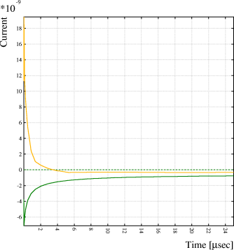
reset signals
Call drift_ion(0.0025, 0.26)
Call add_signals
Call get_signal(1,time1,dir1,cross1) // Retrieve the finite element signal ("A")
Call get_signal(2,time2,dir2,cross2) // Retrieve the no-wire signal ("B")

Call plot_frame(minimum(time1 & time2), minimum(dir1+cross1 & dir2+cross2), ...
   maximum(time1 & time2), maximum(dir1+cross1 & dir2+cross2), ...
   `Time [microsec]`, `Current`, `Comparing weighting fields`)
Call plot_line(minimum(time1 & time2), 0, maximum(time1 & time2), 0, `comment`)
Call plot_line(time1, dir1+cross1, `function-1`)
Call plot_line(time2, dir2+cross2, `function-2`)
Call plot_end

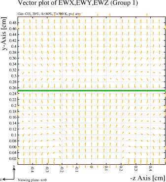
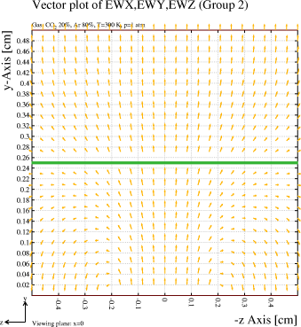
area view x=0
plot-field vector

In the above example, an ion is drifted from the vicinity of the anode wire towards the cathode plane that is not read out. The signal induced by this moving charge is computed twice:

in orange: using the finite element field map which takes the presence of the anode wire into account;
in green: using the weighting field for the strip neglecting the anode wire.

The comparison of these currents shows a clear difference: while the current computed with the finite element map is bipolar, as it should for a charge moving between electrodes that are not read out, the current computed neglecting the wire (in green) is unipolar:

The reason for this difference readily becomes apparent when comparing the weighting field maps (left: finite elements, including the wire, right: neglecting the wire):

space_charge

In this example, we show how to add, with the help of the finite element method, space charge or surface charge to a chamber. Space charge can, in a number of cases, also be added by analytic means using the CHARGES command but this method is not discussed here.

This example uses ANSYS, which is unit-free for what concerns distances. This affords flexibility as long as only symmetry and voltage boundary conditions are used - voltage and length units are decoupled. Charges in contrast are coupled to voltages both via \ε\<SUB\>0\</SUB\> and via an implicit length, as can be seen from the expression for a potential generated by a point charge:

       q
V = --------
    4 \&pi; \&epsilon;\<SUB\>0\</SUB\> r

\&epsilon;\<SUB\>0\</SUB\> ~ 8.854\&times;10\<SUP\>-14\</SUP\> C/(V.cm)

This leads to two scaling factors:

ANSYS apparently assumes \ε\<SUB\>0\</SUB\> to be expressed in units of C/(V.m). To be compatible with the Garfield unit of C/(V.cm), the charges need to be multiplied by 100.
Assume that the model is constructed using length-units of f\ \×\ cm (f equals 0.1 for mm, 1 for cm and 100 for m). When reading the field maps and using the unit information supplied in the FIELD-MAP command, Garfield scales all distances to cm, the length unit used by Garfield. This is sufficient for voltage and symmetry boundary conditions, but not for potentials that arise from charges. For these, inside ANSYS, unscaled distances (r in the above formula) are used. To compensate for this, a further factor of 1/f must be applied to the charges that are entered in ANSYS.

Combining these factors, the charges are entered as-is when native units of metre are used in ANSYS. Otherwise, the charges need to be scaled by a factor 100/f, i.e. a factor of 100 if cm is used and a factor 1000 for models in mm.

In ANSYS, charges can be entered as volume charge densities or as surface charge densities (amongst other possibilities). In case only the total charge is known, then this charge has to be divided by the volume or the surface area of the charge carrier. Example for a volume charge:

! Parameters of the device
unit = 1000            ! Units: 1000 for mm, 100 for cm, 1 for m
r  = 0.1               ! Radius [mm]
pi = 3.14159265        ! pi
qe = 1.60217646e-19    ! Electron charge [C]
charge = 12345*unit*qe ! Total charge in the device

! Create a ball which will act as charge carrier
SPH4,0,0,r

! Distribute charge in the volume of the ball
VSEL, S, VOLU, ,1
BFV,ALL,CHRG,charge/(4.0*pi*r*r*r/3.0)

When surface charges are used, an additional precaution needs to be taken in that the surface area for e.g. a sphere has to be multiplied by an ununderstood factor of 2:

! Distribute charges over the surfaces of the ball
VSEL, S, VOLU, ,1
ASLV, S
SFA,ALL,,CHRGS,charge/(2*4.0*pi*r*r)

It is therefore strongly recommended to verify the integral charge as follows:

Global r = 0.1             // sufficiently large to wrap around all charges
Global eps0 = 8.854e-14    // C/(V.cm)
Global qe = 1.60217646e-19 // C
Call integrate_charge(0, 0, 0, r, qi)
Say "Electron charges: {qi*4*pi*eps0/qe}"

Go to the top level, to &OPTIMISE, to FIELD-MAP, to the topic index, to the table of contents, or to the full text.

Formatted on 21/01/18 at 16:55.