Garfield input is subdivided in sections:
Garfield input can also contain rudimentary scripting:
Occasionally, you may wish to use the various utilities:
It is a program that can be run both interactively and in batch on a wide variety of computers without significant change in outwards appearance. The program is fully command driven but if you desire to add some pieces, you'll find no major obstacles (the program has been written in Fortran-77 and uses Patchy as pre-processor).
Although Garfield can be run in batch mode, it is easier to run it from a workstation or graphics terminal. You should be able to issue any combinations of commands without causing core dumps, abends etc. (please contact me if this nevertheless happens !).
A simple example:
&CELL plane x -1 plane y -1 rows S 5 * i i 1000*iThe program is structured in a set of so-called sections (cell, gas, magnetic, optimise, field, drift and signal) that each contain a set of instructions performing certain tasks. The cell section e.g. will read the cell description, the field section offers facilities for plotting the field etc. The sections are headed by a line starting with an ampersand (&), &CELL and &FIELD start sections in the above example. You may insert one or more blanks between the & and the section name.&FIELD plot-field surface V, contour V
There is one special header: &STOP (or &QUIT or &EXIT if you prefer) which will stop program execution. End-Of-File on input will have the same effect.
The instructions within the sections are free format lines. Input files can be both fixed and variable record length. The maximum record length is large, about 500\ characters.
An ellipsis (...) at the end of one physical line indicates that the instruction continues on the next. There can be only 1 instruction per input line.
The first word on each line is the command proper. The other words can be viewed as a set of parameters, with sometimes a value assigned to them.
The elements on the input are separated from each other by a blank ( ), a comma (,), a colon (:) or an equal sign (=). There is no difference in meaning between these separators. You may if you wish place several between the words.
Case is irrelevant in commands. Strings of which the case matters, such as file names on Unix systems and also in identifiers, should be delimited by double quotes.
Here is an example of a cell description:
&CELL
plane x=10, V=1000
plane x -10 ...
      V 1000
periodicity y 3
rows
S * * 0 0 5000

cell-identifier "Test cell"
The words PLANE, PERIODICITY, ROWS
and CELL-IDENTIFIER are the commands. The command "PLANE"
has two arguments with a value for each. You may if you wish invert their
order without affecting the meaning of the command:
PLANE V=1000 X=10This is true in general - exceptions are explicitly stated. PLANE, like most commands, can have more arguments. If no value is given, defaults are used for these, if a meaningful default is available.
The ROWS command has a slightly different syntax from the rest: apart from having arguments of its own (not shown in the example), it is followed by a series of lines (1 in this example) that contain the actual data. The end of the list is signalled by a blank line. There is one more such command in the cell section (SOLIDS) and there are also a few commands of this type in the gas section (CLUSTER and TABLE).
Nearly all words in the input may be abbreviated to some extent in each of the 'segments':
E-MOST-PROBABLE    & CELL      PLANE
E-MOST-PROB        &CELL       PLAN
E-M-PROB           &C          PL
Garfield does not pretend to be programmable, but Do loops and conditional execution of statements (If_lines and If_blocks) exist. For clarity, all control statements are shown with initial capital in the documentation. Here is an example:
Global ok False
Until ok Do
   Say "Please enter an integer number"
   Parse Terminal n
   If n<0 Then
      Say "The number you entered, {n}, is negative."
      Iterate
   Elseif entier(n)#n Then
      Say "The number you entered, {n}, is not an integer"
      Iterate
   Endif
   Global fac=1
   For i From 1 To n Do
      Global fac=fac*i
   Enddo
   Say "Factorial of {n} is {fac}."
   Global ok True
Enddo
A large collection of procedures, mainly in the areas of field
and drift-line calculation, are available - and they are more
and more widely used. They are described under Call.
After a little practice, you should become aware of the utility commands. They can be used to change the graphics settings, to issue commands to the shell (Aegis, DCL, Unix or VM/CMS), to take input from and to output data to files etc.
| Character | Description | Example |
|---|---|---|
& |
Start of a new section | & CELL |
! |
graphics commands | ! REP DR-L POLYL-COL RED |
% |
dataset commands | % DIR TEST.DAT |
< |
input from a file | < CELL.INPUT |
> |
output to a file | > OUTPUT.LIS |
>> |
recording of terminal input | >> record.dat |
$ |
shell commands | $ SHOW TIME |
* |
comment line | * Modified DC1 cell |
? |
Enter the help facility | ? &OPTIMISE SET |
@ |
algebra commands | @ |
Some characters have a special meaning when used inside commands:
| Character | Description | Example |
|---|---|---|
* |
Default value | AREA * -2 * 2 |
* |
Wildcard | GET CELL.DAT PL* |
@ |
Enter the algebra editor | PLOT CONT @ HIST E |
\\ |
Escape character | \\{abc\\} |
... |
Continuation lines | PLANE X ...\<BR\>2, V=1000 |
{ ... } |
Formula evaluation | Say "Two x pi={2*pi}" |
[ ... ] |
Matrix indexing | Global a=b[2;] |
' ... ' |
Keep string together | get 'cell lib d' |
" ... " |
Like '' but preserve case | get "/cell/lib/dc1" |
` ... ` |
Algebra string delimiters | Parse Input . `phi=` phi |
Examples:
Global a=cos(2*pi/3)
Call print(1+2*(3+4))
Example:
Global a=number(b[3;3])
Global argon=80
Global co2=20
Global gas_file=`Ar`/string(argon)/`CO2`/string(co2)
Call inquire_file(gas_file, exist)
If exist Then
   get {gas_file}
Else
   magboltz argon {argon} co2 {co2}
   heed argon {argon} co2 {co2}
   add mobility 1.5e-6
   write {gas_file}
Endif
Please note that curly brackets are used only in the GET, WRITE, MAGBOLTZ and HEED statements - these are commands, not control statements. Curly brackets are not used when the global variable GAS_FILE is used as argument of the INQUIRE_FILE procedure. Similarly, EXIST is not enclosed in curly brackets in the If-condition. When ARGON and CO2 are used without brackets in the Global statement, but with curly brackets in MAGBOLTZ and Heed.
Examples:
Say "Hello, how are you doing ?"
arrival dataset "arrival.dat"
Example:
Call threshold_crossing(1,-0.02,`rising,linear`,n,t1,t2)
If 'n=0' Then
   Say "Warning: No crossing found."
   Iterate
Endif
In earlier versions of Garfield, the condition of If_lines and If_blocks had to be a single word in upper case. In the example, an equal sign is used in the condition. Since equal signs are separators, like commata and blanks, the condition without quotes would be read as 2 words: "N" and "0".
Example:
Global argon=80
Global co2=20
Global gas_file=`Ar`/string(argon)/`CO2`/string(co2)
A file name is constructed from the percentages of Ar and CO\<SUB\>2\</SUB\>.
Text strings, such as formulae, that should not be broken up but which contain a word separator, should be put between single or double quotes. The string is converted to upper case when single quotes are used, while the case is preserved with double quotes.
Garfield is a fairly large drift chamber simulation program, it is a one person enterprise and the program changes rapidly. This has the advantage for the user that the program tries to track changes in the design considerations of gas detectors. The drawback is a lack of (complete) backwards compatibility of input files.
Please contact the author in case of trouble and if you need further information, have suggestions for extensions etc. In case you suspect an error, send the following:
A common source of problems is the use of a manual that is out of date. As a rule, it is better to consult the help file via WWW for up to date information concerning the commands:
http://cern.ch/garfield/cnl       for modifications
http://cern.ch/garfield/examples  for examples
http://cern.ch/garfield/files     for the files
http://cern.ch/garfield/help      for help
Magboltz is the work of Steve Biagi.
The TRIM interface has been contributed by James Butterworth.
Most of Garfield has been written by Rob Veenhof (referred to as 'I' or 'me' in the documentation). The best way to contact me is by electronic mail.
If you prefer more traditional means:
Rob Veenhof            Rob Veenhof
CERN / PH department   2, Rue du Reculet
CH-1211 Gen\ève 23      F-01630 St Genis-Pouilly
Suisse                 France
tel: + 41 22 7673222   tel: + 33 4 50421784
A prompt response can not be guaranteed because maintaining this program is not part of my regular work, but I do my best.
For technical questions and remarks about the control-C mechanism and other typical Vax features, please contact Carlo Mekenkamp directly (cmekenkamp@vx8000.nl).
G.A. Erskine contributed key ideas but he should not be called in case of problems. Please contact me in case of questions about his parts (theta functions, polygon mappings).
Since then, the program has grown enormously:
In 1984 the program had a length of 5000\ lines. By 2001, Garfield had grown to 127000\ lines (4.9\ Mb), while Magboltz and Heed count respectively 21800 and 19800\ lines (780\ kb and 507\ kb).
| Dimension | Input unit | Internal unit |
|---|---|---|
| angle | degree | radian |
| B field | user has the choice | 100\ G |
| charge | electron charge | 1.6 10\<SUP\>-19\</SUP\> C |
| current | \μA | 10\<SUP\>-18\</SUP\> A |
| energy | eV [Garfield] or MeV [Heed] | eV or MeV |
| length | centimetre | cm |
| potential | Volt | V |
| pressure | user has the choice | Torr |
| temperature | user has the choice | K |
| time | \μsec | \μsec |
| weight | grams | g |
| line charge | - | V |
| point charge | V.cm | V.cm |
When the input unit is shown as "user has the choice", then the quantity can, on input, be followed by a unit of the users choice. If no unit is indicated, then internal units are assumed.
To convert line charges into the more usual unit of C/cm, one should multiply the charge obtained from procedures such as GET_WIRE_DATA with 2\π\ε\<SUB\>0\</SUB\>, approximately 5.56\ 10\<SUP\>-13\</SUP\>\ C/V.cm. The wire charge shown in the table printed in response to the CELL-PRINT option and the PRINT-CELL command, includes this conversion factor.
Similarly, to convert point charges to C, one should multiply the charge expressed in V.cm with 4\π\ε\<SUB\>0\</SUB\>.
http://cern.ch/garfield/filesExecutables at CERN can be found on AFS in the PaRC area, and also in the author's private area:
/afs/cern.ch/user/r/rjd/Garfield/Files/garfield
Main \→ Cell section  \→ algebra sub-section
                       graphics sub-section
                       ...
       Gas section   \→ algebra sub-section
                       graphics sub-section
        ...
The &MAIN command moves you back to the top level of program input,
i.e. the level at which one enters the program. This is the normal
environment to execute procedure Calls which use cell or gas data,
e.g. in order to calculate drift-lines.
&MAIN can also be used as final statement in jobs that run Magboltz to produce electron transport plots. &MAIN is in this context approximately equivalent to &STOP.
The cell and gas sections produce plots, write data sets and make their data available to the procedures when the section is left. Leaving the section can be done in 3\ ways:
Example:
Global emin=100 Global emax=10000 &MAGNETIC components 0 0 0.4 TWithout the &MAIN statement, the GAS-PLOT option would have no effect, the WRITE statement would not be executed and the various procedure calls would be rejected.&GAS options gas-plot write "p10.gas" "b4000" magboltz argon 90 methane 10 coll 2 n-e 4 n-angle 2 ... e-range {emin,emax}
&MAIN Global n=100 Global e=emin*(emax/emin)^((row(n)-1)/(n-1)) Call transverse_diffusion(e, 0, 0, 0, 0, 0.4, dt) Call longitudinal_diffusion(e, 0, 0, 0, 0, 0.4, dl) Call plot_graph(e,(dt^2+dl^2),`E [V/cm]`, ... `sqrt(σ<SUB>T</SUB><SUP>2</SUP>+σ<SUB>L</SUB><SUP>2</SUP>)`, ... `Diffusion`) Call plot_end
Everything you enter, is simply stored. A comprehensive check of the input is only performed when leaving the section. That is also the time the compact format cell dataset is written, if requested, the layout is plotted, the cell description is printed etc.
Format:
&CELL
Creating a new cell:
| Command | Short description |
|---|---|
CELL-IDENTIFIER |
Provides a short description to the cell |
CUT-SOLIDS |
Removes parts of solids |
DEFINE |
Sets local parameters for use with ROWS |
DIELECTRICUM |
Enters a dielectric slab (do not use !) |
FIELD-MAP |
Reads a finite element field map |
OPTIONS |
Plotting of a layout etc |
PERIODICITY |
Makes the cell periodic |
PLANE |
Enters a plane |
RESET |
Cancels part of the cell description |
ROWS |
Header for the list of wires |
SAVE-FIELD-MAP |
Writes a field map in binary format |
SOLIDS |
Enters solid volumes for use with field maps |
TUBE |
Enters a tube surrounding the wires |
WRITE |
Writes a compact format dataset |
Retrieving a cell from a dataset:
| Command | Short description |
|---|---|
GET |
Retrieves a compact cell description |
READ-FIELD-MAP |
Reads a binary field map |
| Potential | Use |
|---|---|
| A | Non-periodic cells with at most 1 x- and 1 y-plane |
| B1X | x-Periodic cells without x-planes and at most 1 y-plane |
| B1Y | y-Periodic cells without y-planes and at most 1 x-plane |
| B2X | Cells with 2 x-planes and at at most 1 y-plane |
| B2Y | Cells with 2 y-planes and at at most 1 x-plane |
| C1 | Doubly periodic cells without planes |
| C2X | Doubly periodic cells with x-planes |
| C2Y | Doubly periodic cells with y-planes |
| C3 | Doubly periodic cells with x- and y-planes |
| D1 | Round tubes without axial periodicity |
| D2 | Round tubes with axial periodicity |
| D3 | Polygonal tubes without axial periodicity |
| D4 | Polygonal tubes with axial periodicity |
| BEM | Field calculated by neBEM |
| MAP | Finite element field maps |
Each chamber type has its own potential function. For numerical purposes, nearly all potential functions are further subdivided into a set of domains according to the aspect ratio of the periodicities, the distance between wires and planes etc.
Versions of most potential functions exist which take advantage of vector hardware. The choice between scalar and vector versions is made a compilation time.
Use GET_CELL_DATA to find out which potential function is in use. The cell type is also displayed when the CELL-PRINT option is active and in response to the PRINT-CELL command.
Garfield has shape functions to deal with various element types such as straight triangles, curved triangles, straight tetrahedra, curved tetrahedra, hexahedra etc. Use CELL-PRINT as described above to find the shape functions used for the current chamber.
neBEM has a range of Green's functions too: line elements, right-angled triangles and rectangles. Most models contain several of these elements at the same time.
| Coordinate system | Use |
|---|---|
| Cartesian | Cells described in (x,y) coordinates, field maps |
| Polar | Cells described in (r,\φ) coordinates |
| Tube | Cells which contain a TUBE |
One can use the GET_CELL_DATA to find out which system is in use.
Such a system is used for chambers constructed from wires and planes unless one of the following conditions is met:
Polar coordinates are internally dealt with by the conformal mapping:
(x,y) = exp(\ρ,\φ)
z     = \ζ
thanks to which the potential functions and drift-line integration procedures for Cartesian coordinates can be used. Most of the commands accept polar coordinates for input and translate the the output to polar coordinates. Procedures as a rule don't do this. A set of procedures is therefore provided for these transformations: CARTESIAN_TO_POLAR, CARTESIAN_TO_INTERNAL, INTERNAL_TO_CARTESIAN, INTERNAL_TO_POLAR, POLAR_TO_CARTESIAN and POLAR_TO_INTERNAL.
The tube coordinates are special in the sense that the wire locations are listed in Cartesian coordinates, while the tube is an object with a polar shape.
Garfield internally uses Cartesian coordinates for cells of this type. Potentials in round tubes are computed using the conformal mapping:
    z - z0
z = -----------
    1 - z0bar z
which maps z0 to 0 and which maps the unit circle onto itself.
Potentials in polygonal tubes are computed by mapping the centre of the tube to a round tube, while the edges are mapped with a local Schwarz-Christoffel expansion.
A. R. Mitchel and R. Wait, The finite element method in partial differential equations, Wiley (1977), in particular pp 108-110.
The string can be retrieved by means of the GET_CELL_DATA procedure.
The identification string is displayed in the plots using the COMMENT text representation.
Format:
CELL-IDENTIFIER string
Example:
CELL-ID "DC1 central cell"
After a cut operation, a solid will as a rule not be closed anymore. This does not pose a problem for neBEM field solutions provided that (mirror) periodicity conditions are applied.
This command is executed when preparing neBEM panels, i.e. on leaving the cell section. Any error will therefore only be reported at this stage and not when the command is issued. For the same reason, these commands can be placed anywhere in the cell section, even before the solids are defined.
When plotting the volumes, the outlines of solids do not reflect the cuts.
Example:
&CELL
Global r=0.2
solids
hole centre 0 0 -0.1 ...
half-lengths 2 2 0.1 ...
radius {r} ...
conductor-1 ...
label a ...
voltage -1
hole centre 0 0 0.5 ...
half-lengths 2 2 0.5 ...
radius {r} ...
epsilon 4 ...
label a ...
dielectric-1
hole centre 0 0 1.1 ...
half-lengths 2 2 0.1 ...
radius {r} ...
conductor-1 ...
label a ...
voltage 1
hole centre 1 {sqrt(3)} -0.1 ...
half-lengths 2 2 0.1 ...
radius {r} ...
conductor-1 ...
label b ...
voltage -1
hole centre 1 {sqrt(3)} 0.5 ...
half-lengths 2 2 0.5 ...
radius {r} ...
epsilon 4 ...
label b ...
dielectric-1
hole centre 1 {sqrt(3)} 1.1 ...
half-lengths 2 2 0.1 ...
radius {r} ...
conductor-1 ...
label b ...
voltage 1
cut plane x>0 solids all
cut plane y>0 solids all
cut plane x<1 solids all
cut plane y<{sqrt(3)} solids all
cut plane y<{sqrt(3)/2} solids a
cut plane y>{sqrt(3)/2} solids b
&FIELD
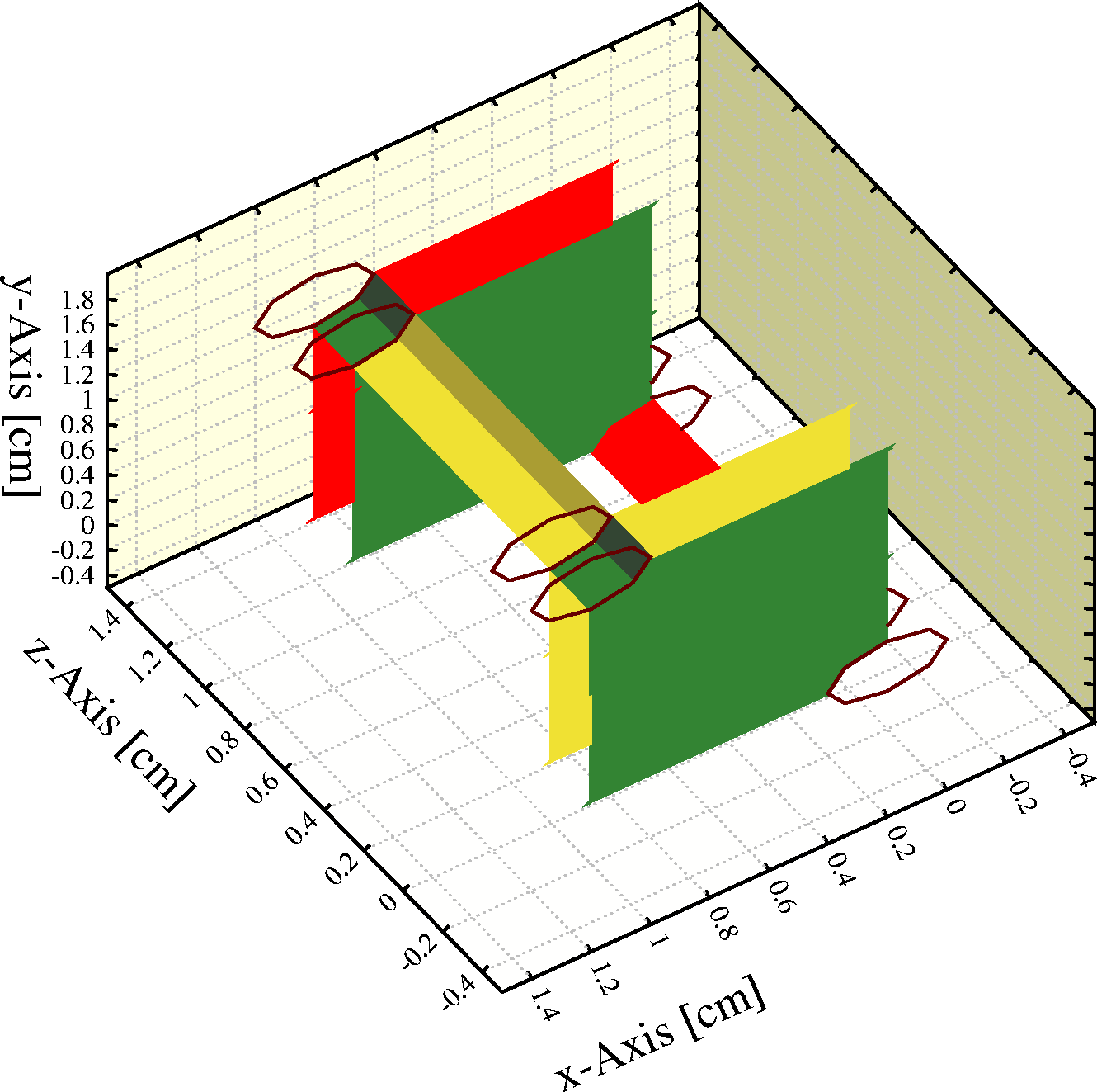
area -0.5 -0.5 -0.5 1.5 2 1.5 view 2*x+7*y-3*z=0 nebem
Call plot_field_area
Call plot_end
This example constructs the elementary cell of a GEM-like structure using 6 holes. The elementary cell contains 2 quarter-holes. The rest of the GEM is obtained by applying mirror symmetries in x and in y. Surface panels shown in red faced the inside (and were thus invisible) before the solids were cut.
As usual, the current value of a variable is displayed if no new value is provided. All variables are displayed if arguments are absent altogether.
Do not confuse DEFINE with Global: DEFINE defines local variables for the cell section. Global defines variables that you can use anywhere. Expressions using local variables and the loop-variable are evaluated automatically. Expressions in terms of global variables have to be enclosed by curly brackets to obtain substitution.
Format:
DEFINE variable value
Example:
def vp_1=1000
def vp_2=2000
def r_1=5000
def r_2=5000
def vp_between=(vp_1*r_2+vp_2*r_1)/(r_1+r_2)
def vp_between
A simple resistor chain, the last line displays the value. You could in principle also enter the whole formula in the ROWS lines.
Global resistor=5000
define r_1 {resistor}
define r_2 {resistor}
The global variable RESISTOR is copied to the local variables R_1 and R_2. Note the use of curly brackets.
The naming conventions for variable names should be observed.
The total number of variable names that can be stored is usually set to 100. If you need more, you'll have to recompile the program with a suitable value for MXVAR.
The variable name I is reserved as loop-variable.
Each variable may be defined in terms of previously defined variables and redefinition of variables is permitted at any time.
Adds a slab of dielectric material to your cell. The slab extends from -infinity to +infinity in one direction and has a range you choose in the other.
x-Slabs and y-slabs of dielectric material are allowed to overlap provided they have the same dielectric constant. Slabs in one direction are not allowed to overlap, even if they have the same dielectric constant.
Wire may be located inside dielectric media, but the media must be inside the equipotential planes, if there are any in your cell.
Dielectrics slow the program down significantly.
Format:
DIELECTRICUM {X-RANGE|Y-RANGE} min max EPSILON \ε
Example:
DIELECTRICUM X -10 10 EPS 5
This slab of dielectric material covers the -10\ <\ x\ <\ 10 part in x and the whole of y. The dielectric constant for the material is chosen to be 5.
Currently, field maps in the format generated by ANSYS, Maxwell Parameter Extractor 2D and 3D, Maxwell Field Simulator 2D and 3D as well as by Tosca can be read. Interfaces for files produced by other programs can be added on request (please contact the author).
When you read a field map in the cell section, any wire, plane, periodicity, dielectric medium and magnetic field that you entered sofar is deleted. Also field map components read with earlier FIELD-MAP commands are deleted.
The optimisation section has a FIELD-MAP command too. The field maps entered in the cell section serve as main field, i.e. this field map replaces the field generated by wires and planes. The field maps entered in the optimisation section are used e.g. when a finite element weighting field is needed in conjunction with a main field computed from wires and planes (see the weighting_field example), or when space charge computed with a finite element program is superimposed on a main field calculated for wires and planes. The two field maps share (for the moment) the same storage and can therefore not be used at the same time.
Reading large field maps is time consuming. To save time, you consider saving your field maps in binary format with SAVE-FIELD-MAP. Binary field maps are retrieved with READ-FIELD-MAP. Binary field maps are much smaller and much faster to read in, but they are not portable between computer systems.
The FIELD-MAP command can read magnetic fields computed by finite element programs. For the moment, there is no experience with such fields.
Format:
FIELD-MAP [FILES [contents_1] file_1 [LABEL label_1] ...
                 [contents_2] file_2 [LABEL label_2] ...
                 ...
                 [contents_n] file_n [LABEL label_n] ...
                 [format] ] ...
          [DRIFT-MEDIUM {SMALLEST-EPSILON | ...
                         SECOND-SMALLEST-EPSILON | ...
                         n | ...
                         SECOND-LARGEST-EPSILON | ...
                         LARGEST-EPSILON | ...
                         \ε}] ...
          [NOT-X-PERIODIC | X-PERIODIC | X-MIRROR-PERIODIC | X-AXIALLY-PERIODIC] ...
          [NOT-Y-PERIODIC | Y-PERIODIC | Y-MIRROR-PERIODIC | Y-AXIALLY-PERIODIC] ...
          [NOT-Z-PERIODIC | Z-PERIODIC | Z-MIRROR-PERIODIC | Z-AXIALLY-PERIODIC] ...
          [X-ROTATIONALLY-SYMMETRIC | Y-ROTATIONALLY-SYMMETRIC | Z-ROTATIONALLY-SYMMETRIC] ...
          [LINEAR | QUADRATIC | CUBIC] ...
          [INTERPOLATE-ELECTRIC-FIELD | COMPUTE-ELECTRIC-FIELD] ...
          [DELETE-BACKGROUND | KEEP-BACKGROUND] ...
          [UNIT {MICROMETRE | MILLIMETRE | CENTIMETRE | METRE}] ...
          [Z-RANGE zmin zmax] ...
          [OFFSET xoff yoff zoff] ...
          [PLOT-MAP | NOPLOT-MAP] ...
          [NOHISTOGRAM-MAP | HISTOGRAM-MAP] ...
          [RESET]
Example:
&CELL
field-map files "e_field.arg" "potential.arg" "epsilon.arg" ...
          drift-medium second-smallest ...
          x-periodic
(Maxwell Parameter Extractor 2D has been used to generate maps of the electric field, the potential and the dielectric constant. These maps are read in and the medium with the 2nd smallest dielectric constant is declared to be the drift medium. The map is also declared to be periodic in the x direction.)
Notes:
In case Maxwell Field Simulator has been used to generate the maps, identifying the mesh directory is recommended. The contents is optional for all other types of data written by Maxwell programs.
A warning is issued if the file contains other data than the declared contents.
Currently, the following contents types are recognised:
| Name | Synonyms | Used to compute |
|---|---|---|
B-FIELD |
MAGNETIC-FIELD | Drift-lines |
ELECTRIC-FIELD |
- | Drift-lines, various other plots |
D-FIELD |
- | \ε by comparing E and D |
MATERIAL |
D-FIELD | Drift-line termination |
MESH |
- | Mesh structure of Maxwell Field Simulator |
MODEL |
- | Problem domain in Maxwell 2D SV |
BACKGROUND |
- | Model vs background, Maxwell 11 |
POTENTIAL |
VOLTAGE | Contour maps |
WEIGHTING-FIELD |
- | Induced signals |
One reason is that the electric field is discontinuous across element boundaries. As a result, a node will typically have as many different electric field values associated with it, as there are elements of which the node is part. Potentials in contrast are unique.
Another reason is that the shape function method enables one to compute the electric field from the potential without need to take numerical derivatives. One does need the Jacobian of the coordinate transformation, but this is anyhow needed to compute the local isoparametric coordinates.
In other words, there is no significant gain in CPU time, and a major saving in memory, if one computes the electric field as needed, using the potentials.
The first finite element interfaces developed for Garfield were for programs that did output the electric field maps - and Garfield still allocates memory to store the electric field maps. All interfaces developed later arrange for the electric field to be computed from the potential map and it is expected that the stored electric field map will disappear in the foreseeable future.
See also the COMPUTE-ELECTRIC-FIELD and INTERPOLATE-ELECTRIC-FIELD options.
Since the current is a scalar and the velocity a vector, an intuitively plausible ansatz for the current reads:
I = factor Q Ew.vwhere Ew is a vectorial quantity called "weighting field". The formula can be derived using Green reciprocity and the factor turns out to be equal to -1. Such a calculation also shows that the weighting field Ew is obtained by setting the potential of all conductors to 0, except for the conductor (or set of conductors) that is read out. The potential of these conductors is to be set to 1.
Weighting fields resemble ordinary electric fields, and finite element programs do not distinguish them from electric fields. There are differences, though. For instance, as can be seen from the above formula, the unit of the weighting field is 1/cm, not V/cm.
Garfield stores only one mesh at the time and uses this mesh both for the ordinary field and for the weighting field. Care needs to be taken therefore that no mesh refinements occur between solving for the 2 types of field.
Finite element programs such as ANSYS output the weighting potential instead of the weighting field - Garfield computes the gradient internally.
These files are usually written by other programs than Garfield, and they therefore do not follow internally the Garfield format conventions. For notes on the way dataset names should be supplied to Garfield, see the guidelines for Garfield files.
For recipes for making these files, refer to the file format descriptions.
The label is a single upper case alphabetic character which serves two purposes:
In the absence of a match, e.g. because no solids have been entered, all signals on the weighting field map are classified as cross induced. Such signals are only computed if the CROSS-INDUCED option is active.
As for all finite element field maps, weighting field maps can be entered both in the cell section and in the optimisation section. When the main field is computed using a finite element program, then the weighting fields are entered, together with the main field, in the cell section. Entry of a weighting field in the optimisation section is used for weighting_field example when the main field can be calculated nearly exactly from wires and planes, while the shape of the read-out electrodes (typically pads) is such that the weighting field is more easily calculated using finite elements.
[By default, the label "S" is assigned to weighting field maps, which makes these maps are part of the initial, default, selection.]
The layout of the field maps for the various Maxwell versions is so similar that Garfield can only rarely tell which version has been used. As of version\ 11, the situation is even worse in that the layout of version\ 9 and version\ 11 files is identical, but the node numbering sequence is different. It is therefore advisable to systematically specify the format explicitly.
To generate your field maps with Maxwell Parameter Extractor 2D, you may wish to follow this recipe:
These steps should lead to a set files with names that end on .arg and that are located in the es.pjt sub-directory of your project.
Be sure to create the E, V, \ε or \σ and weighting field maps with identical meshes and the E, V and \εor \σ maps with identical boundary conditions.
The names of these 4 files should be placed after the FILES keyword of the FIELD-MAP command, the name of the weighting field maps should be preceded by the keyword "WEIGHTING-FIELD" to distinguish it from the regular electric field map. The order is not important. There is no need to specify that the files come from Maxwell Parameter Extractor 2D.
Maxwell documentation at CERN can be found in http://wwwinfo.cern.ch/ce/ae/Maxwell/documentation.html
(Instructions from Pawel Majewski)
To generate your field maps with Maxwell\ 2D Field Simulator, you may like to follow the following recipe:
These steps should lead to a set of files with names that end on .arg and that are located in your project directory.
Be sure to create the E, V, D, \ε or \σ and weighting field maps with identical meshes and in addition the E, V and D maps with identical boundary conditions.
The names of these 4 files should be placed after the FILES keyword of the FIELD-MAP command, the name of the weighting field maps should be preceded by the keyword "WEIGHTING-FIELD" to distinguish it from the regular electric field map. The order is not important. There is no need to specify that the files come from Maxwell 2D Field Simulator.
Information about using Maxwell at CERN can be found in http://wwwinfo.cern.ch/ce/ae/Maxwell/Maxwell.html
When generating your field maps with this program, you may wish to follow this recipe:
This procedure should create maps of the electrostatic potential, the E field, the D field and perhaps of a weighting field. The dielectric constants are computed by comparing E and D. These files will be located in the efs3d.pjt sub-directory of your project.
Be sure to create the E, V, D and weighting field maps with identical meshes and the E, V and D maps with identical boundary conditions.
Information about using Maxwell at CERN can be found in http://wwwinfo.cern.ch/ce/ae/Maxwell/Maxwell.html
Beware that files produced with Maxwell Version\ 11 can be read with the interface for earlier versions, and vice-versa, but the results will be incorrect. Be sure therefore to specify the correct Maxwell version on the FIELD-MAP command line.
When you use this program to create your field maps, you have to provide the following to Garfield:
The field maps can be created as follows: After having gone through the various steps, in the "Post Process" menu, select "Nominal Problem". From the "Data" menu, select "Calculator". In the "Input" column select the "Qty" menu where you pick "phi". In the "Output" column select "Write\ ..." and write out the field to a file called, for instance, "V.reg". Repeat the same steps replacing "phi" by "E" and "D".
Be sure to create the E, V, D and weighting field maps with identical meshes and the E, V and D maps in addition with identical boundary conditions.
Information about using Maxwell at CERN can be found in http://wwwinfo.cern.ch/ce/ae/Maxwell/Maxwell.html
After having worked your way through the various steps from model definition till problem solving, click on "Post\ Process\ ..." and enter "Data/Calculator". Then:
Alternatively, the electric field can be derived from the potential by selecting the COMPUTE-ELECTRIC-FIELD option. Several users have reported problems with the electric field maps as exported by Maxwell and this approach can therefore be recommended.
When using Maxwell SV, you have to feed the following files to Garfield:
An axis of rotational symmetry, if any, should be detected automatically and result in the Z-ROTATIONALLY-SYMMETRIC option being switched on.
(Procedure from Pawel Majewski.)
The files "username1.table" and "username2.table" (see item\ 6 and 10 above) are now ready for Garfield.
A Garfield input file that uses "username.table" and "username1.table" can be found in http://consult.cern.ch/writeup/garfield/examples/tosca/example
A single Tosca generated map can contain various kinds of data, such as the potential, the electric field and the D field. Since the file contains a description of the data, the contents field should only make clear that the file is not a mesh file. One can therefore set the contents field on the FIELD-MAP command to be any of the contained items.
It is advisable to use the INTERPOLATE-ELECTRIC-FIELD option when using Tosca field maps.
(Recipe from Guido Maria Urciuoli, INFN Gruppo Collegata Sanitá, Viale Regina Elena 299, 00161 Roma, Italia.)
The Tosca file, called a "simulation database" in Tosca-speak, should contain at least the following Tosca "datasets":
After the model has been created in the Modeller, create the simulation database with
To achieve this, enter at the console:
SOLVERS PROGRAM=&VF_ANALYSISTYPE& -SOLVENOW OPTION=NEW
        ELEMENT=QUADRATIC SURFACE=CURVED FILE='YourFileName.op3';
or follow the GUI path:
Model \→ Create Analysis Database...
In the post-processor export the results to an I-DEAS Universal File, where it important is to set BASIS=ELEMENT, i.e. write values at every node of every element:
As a console command:
IDEAS FILE='YourFileName.unv' MODE=CREATE TYPE=REAL
      BASIS=ELEMENT FIELD=SCALAR COMP=V;
or using the GUI:
Tables \→ SDRC I-DEAS Unv File...
(Recipe provided by Konstantin Klementiev <kklementiev@cells.es>.)
These elements have only 3 nodes, the potential is linear within each element and the local gradient is constant.
Although such field maps can be read, their use is not recommended. Use instead COMSOL-2D-QUADRATIC.
For the recipe to write such field maps, please refer to COMSOL-3D-QUADRATIC.
Garfield doesn't recognise this format automatically, be sure therefore to specify that your field map is in COMSOL-2D-QUADRATIC format.
You may specify a distance unit for such field maps, centimetres are assumed if no unit is given.
Example:
&CELL
field-map files potential "COMSOLFIELD2D.txt" ...
weighting-field "COMSOLFIELD2DElectrode1.txt" label s ...
comsol-2d
Two potential maps are read, the first contains the potential, the
second the weighting potential for one of the electrodes. The latter
is associated with label S which is later used in the signal section
to plot the weighting field map.
These elements have only 4 nodes, the potential is linear within each element and the local gradient is constant.
Although such field maps can be read, their use is not recommended. Use instead COMSOL-3D-QUADRATIC.
Garfield doesn't recognise this format automatically, be sure therefore to specify that your field map is in COMSOL-3D format.
You may specify a distance unit for such field maps, centimetres are assumed if no unit is given.
First, solve your problem in COMSOL. Take care to select 2nd order Lagrange elements. Then export the field map as follows:
To import the file in Garfield:
Example:
&CELL
field-map files "exported.txt" comsol-3d
save-field-map "exported.bin"
(Recipe written by Jeremy Janney <JJanneySG@hotmail.com> and Sven Lotze <lotze@physik.rwth-aachen.de>.)
ANSYS will occasionally generate degenerate quadrilaterals, which are curved quadratic triangles.
The recipe assumes that the command format is used. Most of the commands cited can of course also be run from the GUI.
FINISH
/CLEAR,START
/PREP7
KEYW,PR_ELMAG,1
KEYW,MAGELC,1
Disable the p-method solution options. This option leads to elements of higher polynomial order, which are a priori preferred, but Garfield does not yet have shape functions for these.
/PMETH,OFF,1
ET,1,PLANE121In case your chamber has rotational symmetry around an axis, a non-default element behaviour needs to be selected:
ET,1,PLANE121   ! Select plane quadrilaterals
KEYOPT,1,3,1    ! Declare the element to be axisymmetric
In ANSYS, the y-axis acts as axis of rotational symmetry and no part of the model should be located in x\ \<\ 0. When reading the field map with Garfield, you have to declare the symmetry again using X-ROTATIONALLY-SYMMETRIC, Y-ROTATIONALLY-SYMMETRIC or Z-ROTATIONALLY-SYMMETRIC.
For instance, to define a perfect conductor (material\ 1) and a dielectricum (material\ 2):
MP, PERX, 1, 1e10 ! Metal
MP, RSVX, 1, 0.0
MP, PERX, 2, 4.5  ! Bulk dielectric constant
! Define some dimensions, in microns halfpitch = 50 thickbulk = 200 halfstrip = 20 thickstrip = 5BLC4, 0, 0, halfpitch, thickbulk ! Area 1: dielectricum BLC4, 0, 0, halfstrip, thickstrip ! Area 2: conductor ASBA, 1, 2, , , KEEP ! Area 1 becomes area 3
AGLUE, ALL ! Glue everything
ASEL, S, , , 3             ! Select the dielectricum
AATT, 2                    ! Properties of material 2
ASEL, S, , , 2             ! Select the conductor
AATT, 1                    ! Properties of material 1
ASEL, S, , , 2 ! Select the metal LSLA, S ! Select all its border lines DL, ALL, 2, VOLT, 1000 ! Set the borders to 1000 VASEL, S, , , 3 ! Select the dielectricum LSLA, S ! Select all its border lines LSEL, R, LOC, Y, thickbulk ! Sub-select lines at y=thickbulk DL, ALL, 3, VOLT, 0 ! Set this line to 0 V
ASEL, S, , , 3 LSLA, S LSEL, R, LOC, X, 0 ! Select the lines at x=0 DL, ALL, 3, SYMM ! Impose a symmetry condition ASEL, S, , , 3 LSLA, S LSEL, R, LOC, X, halfpitch ! Idem for y=halfpitch DL, ALL, 3, SYMM
LSEL,ALL
ASEL, ALL
MSHKEY,0
SMRT, 3
AMESH, 2,3
It is not always necessary to mesh the metal parts of the device. Then solve the problem:
/SOLU
SOLVE
FINISH
Optionally visualise the solution:
/POST1
/EFACET,1
PLNSOL, VOLT,, 0
/OUTPUT, PRNSOL, lis
PRNSOL
/OUTPUT
There is no need to write the electric field to a file since the COMPUTE-ELECTRIC-FIELD option is implied when using ANSYS.
The PRNSOL file contains the potentials at the nodes. When interpolating between nodes, Garfield needs to know where each of these nodes is located in space. This information is contained in the output of the NLIST command, which should be written to a file called "NLIST.lis". Note the COORD option - without this option, the file would contain additional information which is not used in Garfield, at the price of reduced precision in the node coordinates. Garfield can read files in either format - but the COORD option is recommended.
/OUTPUT, NLIST, lis
NLIST,,,,COORD
/OUTPUT
Garfield also needs to know how the nodes are tied into elements. This structure is shown by the ELIST command, of which the output has to be written to a file called "ELIST.lis":
/OUTPUT, ELIST, lis
ELIST
/OUTPUT
Optionally, you may transmit the dielectric constants (permittivities) and the electric resistivities to Garfield. Only write this file if your material properties do not have a temperature dependence. The commands for writing the "MPLIST.lis" file are as follows:
/OUTPUT, MPLIST, lis
MPLIST
/OUTPUT
If you produce the field maps on operating systems like Windows, control-M will be appended to each line. These need to be removed before the field maps can be read with Garfield.
Since ANSYS allows the user to use any consistent system of units, the real size of the device can not be found in the field map files. The user therefore has to specify the distance UNIT.
&CELL field-map files "../scratch0/PRNSOL.lis" ansys-plane-121 ... x-mirror-periodic unit micron&FIELD area -0.0100 0 0.0100 0.0200 plot-field cont v
In order to compute signals, Garfield needs weighting fields. Refer to the ANSYS-solid-123 recipe.
The recipe assumes that the command format is used. Most of the commands cited can of course also be run from the GUI.
FINISH
/CLEAR,START
/PREP7
KEYW,PR_ELMAG,1
KEYW,MAGELC,1
Disable the p-method solution options. This option leads to elements of higher polynomial order, which are a priori preferred, but Garfield does not yet have shape functions for these.
/PMETH,OFF,1
ET,1,SOLID123
For instance, to define a perfect conductor (material\ 1), a gas (material 2) and a dielectricum (material\ 3):
MP,PERX,1,1e10  ! Metal
MP,RSVX,1,0     !
MP,PERX,2,1     ! Gas
MP,PERX,3,4.5   ! Dielectricum
VSEL, S, VOLU, , 2 ! Select volume 2
ASLV, S            ! Select all areas belonging to the selected volumes
DA, ALL, VOLT, 100 ! Set a voltage boundary on all selected areas
Similarly, a symmetry boundary on all selected areas can be set with the command:
DA, ALL, SYMM
SMRT, 2
MSHKEY,0
VMESH, 1, 3
VMESH, 15
It is not always necessary to mesh the metal parts of the device. Then solve the problem:
/SOLU
SOLVE
Optionally visualise the solution:
/POST1
/EFACET,1
PLNSOL, VOLT,, 0
/OUTPUT, PRNSOL, lis
PRNSOL
/OUTPUT
There is no need to write the electric field to a file since the COMPUTE-ELECTRIC-FIELD option is implied when using ANSYS.
The PRNSOL file contains the potentials at the nodes. When interpolating between nodes, Garfield needs to know where each of these nodes is located in space. This information is contained in the output of the NLIST command, which should be written to a file called "NLIST.lis". Note the COORD option - without this option, the file would contain additional information which is not used in Garfield, at the price of reduced precision in the node coordinates. Garfield can read files in either format - but the COORD option is recommended.
/OUTPUT, NLIST, lis
NLIST,,,,COORD
/OUTPUT
Garfield also needs to know how the nodes are tied into elements. This structure is shown by the ELIST command, of which the output has to be written to a file called "ELIST.lis":
/OUTPUT, ELIST, lis
ELIST
/OUTPUT
Optionally, you may transmit the dielectric constants (permittivities) and the electric resistivities to Garfield. Only write this file if your material properties do not have a temperature dependence. The commands for writing the "MPLIST.lis" file are as follows:
/OUTPUT, MPLIST, lis
MPLIST
/OUTPUT
If you produce the field maps on operating systems like Windows, control-M will be appended to each line. These need to be removed before the field maps can be read with Garfield.
Since ANSYS allows the user to use any consistent system of units, the real size of the device can not be found in the field map files. The user therefore has to specify the distance UNIT.
field-map files "PRNSOL.lis" units=mm ansys-solid-123
In order to compute signals, Garfield needs weighting fields. These are obtained by setting the read-out electrodes to a potential of\ 1 and all other electrodes to a potential of\ 0.
Garfield requires the weighting fields and the main field map to share one and the same mesh. To achieve this, follow the above recipe until the end, then clear the existing loads (LSCLEAR), apply new loads and solve without meshing again. This is illustrated in the following example of 3\ strips:
FINISH
/CLEAR,START
/PREP7
! No polynomial elements
/PMETH,OFF,1

! Set electric preferences
KEYW,PR_ELMAG,1
KEYW,MAGELC,1

! Select element
ET,1,SOLID123

! Material properties
MP,PERX,1,1e10  ! Metal
MP,RSVX,1,0.0   !
MP,PERX,2,1.0   ! Gas
MP,PERX,3,4.0   ! Permittivity of FR4

! Construct the structure
metal = 0.2
gas = 2
sub = -1
BLOCK, -10, -5, -10, 10,     0, metal ! 1: Wide side strip
BLOCK,  -2, -4, -10, 10,     0, metal ! 2: First signal
BLOCK,  -1,  1, -10, 10,     0, metal ! 3: 2nd signal
BLOCK,   2,  4, -10, 10,     0, metal ! 4: 3rd signal
BLOCK,   5, 10, -10, 10,     0, metal ! 5: Wide side strip
BLOCK, -10, 10, -10, 10,   sub,     0 ! 6: Substrate
BLOCK, -10, 10, -10, 10,     0,   gas ! 7: Gas

! Subtract the strips from the gas
VSBV,  7, 1, , , KEEP   ! 7 \→ 8
VSBV,  8, 2, , , KEEP   ! 8 \→ 7
VSBV,  7, 3, , , KEEP   ! 7 \→ 8
VSBV,  8, 4, , , KEEP   ! 8 \→ 7
VSBV,  7, 5, , , KEEP   ! 7 \→ 8

! Glue everything together 1 = left wide, 2, 3, 4, 5 = wide, 7 = sub, 8 = gas
VGLUE, ALL

! Assign material attributes
VSEL, S, VOLU, , 1, 5 ! Metal strips
VATT, 1, ,1
VSEL, S, VOLU, , 7    ! Gas volume
VATT, 3, ,1
VSEL, S, VOLU, , 8    ! Substrate
VATT, 2, ,1

! Voltage boundary conditions on the metal
VSEL, S, VOLU, , 1, 5 ! All strips at ground
ASLV, S
DA, ALL, VOLT, 0
ASEL, S, LOC, Z, gas  ! Drift electrode
DA, ALL, VOLT, -1000
ASEL, S, LOC, Z, sub  ! Back plane
DA, ALL, VOLT, 0

! Meshing options
VSEL, S, VOLU, , 8    ! Only mesh the gas
ASLV, S

MSHKEY,0
SMRT, 4
VMESH, 1,8

! Solve the field
/SOLU
SOLVE

! Write the solution
/POST1
/OUTPUT, field, lis
PRNSOL
/OUTPUT

! Change to weighting field boundary conditions for first narrow strip
/SOLU
LSCLEAR,ALL

VSEL, S, VOLU, , 1
VSEL, A, VOLU, , 3, 5
ASLV, S
DA, ALL, VOLT, 0

VSEL, S, VOLU, , 2
ASLV, S
DA, ALL, VOLT, 1

ASEL, S, LOC, Z, gas
DA, ALL, VOLT, 0
ASEL, S, LOC, Z, sub
DA, ALL, VOLT, 0

! Meshing options
VSEL, S, VOLU, , 1, 8
ASLV, S

! Solve the field
SOLVE

! Write the solution
/POST1
/OUTPUT, weight1, lis
PRNSOL
/OUTPUT

! Change to weighting field boundary conditions for 2nd narrow strip
/SOLU
LSCLEAR,ALL

VSEL, S, VOLU, , 1, 2
VSEL, A, VOLU, , 4, 5
ASLV, S
DA, ALL, VOLT, 0

VSEL, S, VOLU, , 3
ASLV, S
DA, ALL, VOLT, 1

ASEL, S, LOC, Z, gas
DA, ALL, VOLT, 0
ASEL, S, LOC, Z, sub
DA, ALL, VOLT, 0

! Meshing options
VSEL, S, VOLU, , 1, 8
ASLV, S

! Solve the field
SOLVE

! Write the solution
/POST1
/OUTPUT, weight2, lis
PRNSOL
/OUTPUT

! Change to weighting field boundary conditions for last narrow strip
/SOLU
LSCLEAR,ALL

VSEL, S, VOLU, , 1, 3
VSEL, A, VOLU, , 5
ASLV, S
DA, ALL, VOLT, 0

VSEL, S, VOLU, , 4
ASLV, S
DA, ALL, VOLT, 1

ASEL, S, LOC, Z, gas
DA, ALL, VOLT, 0
ASEL, S, LOC, Z, sub
DA, ALL, VOLT, 0

! Meshing options
VSEL, S, VOLU, , 1, 8
ASLV, S

! Solve the field
SOLVE

! Write the solution
/POST1
/OUTPUT, weight3, lis
PRNSOL
/OUTPUT

! Write the mesh to files
/OUTPUT, NLIST, lis
NLIST,,,,COORD
/OUTPUT

/OUTPUT, ELIST, lis
ELIST
/OUTPUT

/OUTPUT, MPLIST, lis
MPLIST
/OUTPUT

! Show the solution
/EFACET,1
PLNSOL, VOLT,, 0
After processing this, the following files should have been created:
These files can be processed in Garfield with the following commands:
&CELL
Global bin `strips.bin`
If exist(bin) Then                // Read binary if it exists
   read-field-map {bin}
Else
   field-map files potential "~/scratch0/field.lis" ...
                   weighting-field "~/scratch0/weight1.lis" label a ...
                   weighting-field "~/scratch0/weight2.lis" label b ...
                   weighting-field "~/scratch0/weight3.lis" label c ...
             units=cm ...
             ansys-solid-123
   save-field-map {bin}           // Otherwise, create a binary
Endif

&GAS
arg-50-eth-50                     // For demonstration only ...

&SIGNAL
area -5 -10 -2  5 10 8 x-z
window 0 0.0005                   // Sample signals every 0.5 nsec
select a b c                      // Read out all electrodes

grid 50                           // Improve granularity
plot-field vect ewx, ewy, ewz     // Plot the weighting fields

Call plot_drift_area
Call drift_electron_3(-2, 0, 1.8) // Drift one electron
Call plot_drift_line
Call add_signals
Call plot_end

plot-signals                      // Show signals
Please refer to http://www.quickfield.com/demo/manual.pdf
The recipe for making such field maps is similar to that for earlier versions like Field-Simulator-3D, with the exception that the solids file (with extension .shd) will be called "fields.shd", independent of the mesh iteration and it will be located in a different directory.
Beware that files produced with Maxwell Version\ 11 can be read with the interface for earlier versions, and vice-versa, but the results will be incorrect. Be sure therefore to specify the correct Maxwell version on the FIELD-MAP command line.
Use of the DELETE-BACKGROUND option is mandatory with this format.
There are 3 ways to select the drift medium:
Beware: DRIFT-MEDIUM\ 3 is not the same as DRIFT-MEDIUM\ 3.0\ ! In the first case, the medium with the 3rd dielectric constant or the 3rd conductivity will be selected. In the second case, the medium with the dielectric constant or the conductivity closest to 3 will be taken.
When using the DC conduction mode, it may be more natural to use the keywords SMALLEST-SIGMA, SECOND-SMALLEST-SIGMA, SECOND-LARGEST-SIGMA and LARGEST-SIGMA which are treated as synonyms of the keywords listed in the command description.
[By default, the medium with the lowest dielectric constant or the lowest conductivity is assumed to be the drift medium.]
[This is the default.]
The length of one period is taken to be the maximum extent in x of the field map.
A cell can not be both X-PERIODIC and X-MIRROR-PERIODIC, but can be X-AXIALLY-PERIODIC in addition to being translation periodic in the x-direction.
[By default, a field map is not assumed to be periodic.]
A cell can not be both X-PERIODIC and X-MIRROR-PERIODIC, but can be X-AXIALLY-PERIODIC in addition to being translation periodic in the x-direction.
[By default, a field map is not assumed to be periodic.]
The length of one period is deduced from the field map, and is therefore not specified on the FIELD-MAP statement.
The symmetry axis must pass through y=z=0.
A cell can not be both X-PERIODIC and X-MIRROR-PERIODIC, but can be X-AXIALLY-PERIODIC in addition to being translation periodic in the x-direction.
[By default, a field map is not assumed to be periodic.]
The field map has to be 2-dimensional. Elements must be used that are suitable for rotational symmetry. Currently, all interfaced finite element programs use the second field map coordinate axis, which we refer to as height, h, as axis of rotational symmetry. We call the first coordinate axis the radius, r. The field map must not contain any element or part of element at r\ \<\ 0.
The way the finite element program is informed about the rotational symmetry varies with the programs - consult the documentation.
The above is common for all 3 rotational symmetries. The difference is in the way the (r,h) field-map coordinates are computed from the chamber (x,y,z) coordinates. When using X-ROTATIONALLY-SYMMETRIC, the assignment is:
r = \√(y\² + z\²)
h = x
A chamber can have only one rotational symmetry at the time.
[By default, a field map is not assumed to be periodic.]
[This is the default.]
The length of one period is taken to be the maximum extent in y of the field map.
A cell can not be both Y-PERIODIC and Y-MIRROR-PERIODIC, but can be Y-AXIALLY-PERIODIC in addition to being translation periodic in the y-direction.
[By default, a field map is not assumed to be periodic.]
A cell can not be both Y-PERIODIC and Y-MIRROR-PERIODIC, but can be Y-AXIALLY-PERIODIC in addition to being translation periodic in the y-direction.
[By default, a field map is not assumed to be periodic.]
The length of one period is deduced from the field map, and is therefore not specified on the FIELD-MAP statement.
The symmetry axis must pass through x=z=0.
A cell can not be both Y-PERIODIC and Y-MIRROR-PERIODIC, but can be Y-AXIALLY-PERIODIC in addition to being translation periodic in the y-direction.
[By default, a field map is not assumed to be periodic.]
The field map has to be 2-dimensional. Elements must be used that are suitable for rotational symmetry. Currently, all interfaced finite element programs use the second field map coordinate axis, which we refer to as height, h, as axis of rotational symmetry. We call the first coordinate axis the radius, r. The field map must not contain any element or part of element at r\ \<\ 0.
The way the finite element program is informed about the rotational symmetry varies with the programs - consult the documentation.
The above is common for all 3 rotational symmetries. The difference is in the way the (r,h) field-map coordinates are computed from the chamber (x,y,z) coordinates. When using Y-ROTATIONALLY-SYMMETRIC, the assignment is:
r = \√(x\² + z\²)
h = y
A chamber can have only one rotational symmetry at the time.
[By default, a field map is not assumed to be periodic.]
[This is the default.]
The length of one period is taken to be the maximum extent in z of the field map.
A cell can not be both Z-PERIODIC and Z-MIRROR-PERIODIC, but can be Z-AXIALLY-PERIODIC in addition to being translation periodic in the z-direction.
[By default, a field map is not assumed to be periodic.]
A cell can not be both Z-PERIODIC and Z-MIRROR-PERIODIC, but can be Z-AXIALLY-PERIODIC in addition to being translation periodic in the z-direction.
[By default, a field map is not assumed to be periodic.]
The length of one period is deduced from the field map, and is therefore not specified on the FIELD-MAP statement.
The symmetry axis must pass through x=y=0.
A cell can not be both Z-PERIODIC and Z-MIRROR-PERIODIC, but can be Z-AXIALLY-PERIODIC in addition to being translation periodic in the z-direction.
[By default, a field map is not assumed to be periodic.]
The field map has to be 2-dimensional. Elements must be used that are suitable for rotational symmetry. Currently, all interfaced finite element programs use the second field map coordinate axis, which we refer to as height, h, as axis of rotational symmetry. We call the first coordinate axis the radius, r. The field map must not contain any element or part of element at r\ \<\ 0.
The way the finite element program is informed about the rotational symmetry varies with the programs - consult the documentation.
The above is common for all 3 rotational symmetries. The difference is in the way the (r,h) field-map coordinates are computed from the chamber (x,y,z) coordinates. When using Z-ROTATIONALLY-SYMMETRIC, the assignment is:
r = \√(x\² + y\²)
h = z
A chamber can have only one rotational symmetry at the time.
[By default, a field map is not assumed to be periodic.]
This method can be applied to all field maps.
[By default, the highest order method permitted by the field map will be used.]
This method can only be applied to field maps with additional nodes halfway the vertices. This information is present in for instance all Maxwell field maps.
[By default, the highest order method permitted by the field map will be used.]
This method can only be applied to field maps with additional nodes at 1 third and at 2 thirds between the vertices. There are currently no field map formats with which this interpolation order can be used.
[By default, the highest order method permitted by the field map will be used.]
This interpolation is meaningful only if the finite element program outputs, for a single node, as many electric field vectors as there are elements to which the node belongs. The reason for this is that, contrary to the potential, the electric field is as a rule discontinuous across element boundaries. This discontinuity exists even if \ε is the same on both sides. Many finite element programs output only one electric field vector per node. When using these, COMPUTE-ELECTRIC-FIELD should be selected.
This option is currently only active for hexahedral field maps. It is automatically set for several field map formats, such as those produced by Ansoft programs..
[This option is default.]
For elements with use isoparametric coordinates, which is nearly always the case, this calculation entails little or no overhead since the Jacobian is reused from the iterative calculation of the local coordinates.
These derivatives are reliable also in case the nodes happen to lie on an interface between materials of different \εs.
This option is automatically switched on when using ANSYS-solid-123, ANSYS-plane-121 and several other finite element programs.
[This option is not default.]
Option active with Maxwell Field Simulator 3D and ANSYS:
Note: this option is implicit with the MAXWELL-11 format.
[This option is on by default.]
This argument is ignored if the field map is 3-dimensional.
[By default, the cell is assumed to go from -50\ cm to +50\ cm in the z-direction.]
By default, Garfield uses the coordinate system from the finite element program. As a rule, this doesn't lead to limitations.
However, in case overlays an analytic field with a finite element field, it may happen that the fields need to be aligned. Such an alignment can be obtained with the OFFSET option.
If you specify an offset of (xoff,yoff,zoff), then Garfield will interpolate the field map at (x-xoff,y-yoff,z-zoff) when it needs a field at (x,y,z).
All 3\ coordinates should be specified, even if the field map is 2-dimensional.
[By default, the 3 offsets are set to 0. The offsets are saved with the binary field maps.]
[By default, the centimetre is assumed as length unit.]
Materials are distinguished by their dielectric constant or their conductivity. A map of either of these must therefore be available for this option to have effect. Maps of the dielectric constant an the conductivity can be supplied as such. A map of the dielectric constant will automatically be computed also if maps of both E and B are present.
The material with the smallest dielectric constant is shown with representation MATERIAL-1. The medium with the next highest dielectric constant with MATERIAL-2 etc. The drift medium is never shown.
Elements of a 2D field map are only shown in X-Y views and in CUT views at a constant z. The cross sections of the viewing plane with the elements of a 3D field map are shown in X-Y, X-Z, Y-Z and CUT views, but not in 3D views.
Field maps do not usually cover areas filled with conducting material since there is no field inside. To visualise these, one has to enter them manually with the SOLIDS command. SOLIDS doesn't interfere with PLOT-MAP.
This option can also be switched on and off with the PLOT-MAP option of the AREA command.
[By default, the map is shown.]
Elements with large aspect ratios can be a sign that the mesh is of poor quality. One should then consider using the so-called virtual-volumes technique to constrain the mesh elements.
Elements with a very large volume or surface are likely to cause problems when transporting particles since the finite element method only guarantees continuity of the potential, not of the electric field. With large elements, the discontinuity across element boundaries is likely to be large.
Switching on this option further enables checks on the elements to be carried out, in particular a search for irregular element degeneracy.
[These histograms are not made by default.]
This command is executed immediately and you may - with caution - replace some of the elements of the description after issuing the command.
Format:
GET file [member]
Examples:
get "~rjd/Garfield/Test/cell.dat"
get 'disk$zp:[veenhof.garfield]cell'
The first example is typical for a Unix system, note the use of double quotes to preserve the case. The second example, for Vax, will read the first member of type CELL from the library with file name "CELL.DAT". The extension .DAT is the default setting of the DEFAULT command, the upper case is the result of using single quotes. Libraries may contain members of other types - but only members of type CELL will be considered by GET.
The 3 arguments form a vector that indicates the direction in which gravity pulls on the wire. Only the direction of the vector is used, not its normalisation.
The default setting is (0,0,1) i.e. gravity works along the wires.
Format:
GRAVITY x y z
Example:
gravity 0 0 1
This makes the wires run vertical, the default. In this situation, gravity does not produce a wire sag.
Format:
NEBEM [ANGULAR-TOLERANCE eps_angle] ...
      [DISTANCE-TOLERANCE eps_distance] ...
      [LU-INVERSION | SVD-INVERSION] ...
      [MAXIMUM-ELEMENTS max] ...
      [MINIMUM-ELEMENTS min] ...
      [NEW-MODEL | REUSE-MODEL ] ...
      [NOKEEP-INVERTED-MATRIX | KEEP-INVERTED-MATRIX] ...
      [PERIODIC-COPIES copies] ...
      [QUALITY-THRESHOLD qthr] ...
      [SIZE-THRESHOLD sthr] ...
      [TARGET-ELEMENT-SIZE target] ...
      [X-PERIODIC-COPIES copies] ...
      [Y-PERIODIC-COPIES copies] ...
      [Z-PERIODIC-COPIES copies]
Example:
nebem min-elem 2 max-elem 10 target 0.1
[Default value: 10^-6 radian.]
Numerous warnings and error messages from the PLAOVL procedure are an indication that this parameter has an inappropriate value.
[Default value: 10^-6 cm.]
[The is default.]
This technique is superior where the charges on several panels have nearly identical effects. This seems to happen in cylindrical structures. The differences are marginal in box-like layouts.
SVD is substantially slower than LU. E.g. for a matrix size of 4000, SVD takes nearly ten times more time than LU. The difference is significant only for structures with several 1000 or more elements.
[The default is LU-INVERSION.]
Largest number of elements produced along either axis of a single primitive.
There is no upper limit but CPU time consumption and memory requirements rise faster than linear with the number of elements in the model. If the minimum exceeds the maximum, then the values will be interchanged.
[Default: 10]
Smallest number of elements produced along either axis of a single primitive.
The smallest value allowed is 1. If the minimum exceeds the maximum, then the values will be interchanged.
[Default: 1]
Instructs neBEM to obtain the geometric and potential data from Garfield, to calculate the influence matrix and to solve the capacitance equation.
[This is default]
Instructs neBEM to obtain the geometric and potential data from Garfield, but to recover the influence matrix and the element charges from files that have been written during an earlier run. The user must ensure that the geometry, influence matrix and charges are coherent. This means in practice that the calculations must be run in the same directory as an earlier run with the NEW-MODEL flag in effect, with identical boundary conditions.
There is no option or command to request storing the model: neBEM always stores the model.
If the inverted influence matrix (capacitance matrix) has been stored, in response to specifying the KEEP-INVERTED-MATRIX option.then it too will be retrieved when re-specifying this option.
[This is not default.]
This matrix is currently needed only for the calculation of weighting fields.
This matrix is large.
The flag must be set both during the initial run that computes and writes the element charges, and during the runs in which these charges are retrieved by means of the REUSE-MODEL option.
[By default, the inverted matrix is neither stored nor retrieved.]
neBEM currently does not have explicit periodic Green's functions for periodic configurations. It approximates these with the sum of a series of periodic copies of the non-periodic Green's function. The series runs from \<CODE\>-copies\</CODE\> to \<CODE\>copies\</CODE\>.
Since the Green's function are expensive to calculate, it is advisable to choose a low number of copies. In 3 dimensions, the series converges rapidly.
neBEM allows this parameter to be set individually for each primitive, but the Garfield interface stores only one value, common to all primitives.
The number of periodic copies can be set indivually along each axis, or collectively for all 3 axes.
[Default: 5, which corresponds to having in all 11 copies.]
This parameter currently only leads to reduction of the overall size of sharp-angled triangles, it does not yet stop them from being created.
The minimum quality must be larger than 1.
[Default setting: 150.]
This parameter has currently not effect. A similar effect can be obtained by setting discretisation sizes on the solids and also by using the TARGET-ELEMENT-SIZE, MINIMUM-ELEMENTS and MAXIMUM-ELEMENTS parameters.
[Default setting: 0.001]
Target linear size of the elements, measured along their edges, produced by neBEM's discretisation process. The element sizes are if needed increased or decreased to respect the MINIMUM-ELEMENTS and MAXIMUM-ELEMENTS parameters.
If specified before the SOLIDS command is issued, then the value will be used as default for all solids that are entered. The value can be overridden on any individual solid.
If specified after the SOLIDS command, then the value applies only to those faces for which the discretisation length has been is specified as "automatic".
[Default: 50 micron.]
neBEM currently does not have explicit periodic Green's functions for periodic configurations. It approximates these with the sum of a series of periodic copies of the non-periodic Green's function. The series runs from \<CODE\>-copies\</CODE\> to \<CODE\>copies\</CODE\>.
Since the Green's function are expensive to calculate, it is advisable to choose a low number of copies. In 3 dimensions, the series converges rapidly.
neBEM allows this parameter to be set individually for each primitive, but the Garfield interface stores only one value, common to all primitives.
The number of periodic copies can be set indivually along each axis, or collectively for all 3 axes.
[Default: 5, which corresponds to having in all 11 copies.]
Format:
OPTIONS [NOLAYOUT | LAYOUT] ...
        [NOCELL-PRINT | CELL-PRINT] ...
        [NOTISOMETRIC | ISOMETRIC] ...
        [NOWIRE-MARKERS | WIRE-MARKERS] ...
        [NOCHARGE-CHECK | CHARGE-CHECK] ...
        [NODIPOLE-TERMS | DIPOLE-TERMS]
Example:
OPT C-PR
Requests a summary of the elements present in the cell.
The same listing can be obtained in the optimisation section using the PRINT-CELL command.
[This option is initially off but its setting is remembered from one cell section to the next.]
Dipole terms are significant for thick wires that are nearly at the ambient potential, such as gate wires in TPCs. This can be investigated with the MULTIPOLE-MOMENTS command.
Currently, dipole terms are available only for potential types A, B1X, B1Y, B2X and B2Y. Contact the author if you need dipole terms for other potentials.
Example: A wire with no net charge is located half-way between 2 conduction planes. With the DIPOLE-TERMS option switched off (left), the wire has no influence on the field, whereas the field is distorted when the option is switched on (right).
&CELL plane y = -1 plane y = +1 v = 2000 rows s 1 1 0 0 1000opt nodipole // Switch dipole terms off
&FIELD area -1.1 -1.1 1.1 1.1 pl cont v
&CELL plane y = -1 plane y = +1 v = 2000 rows s 1 1 0 0 1000
opt dipole // Switch dipole terms on
&FIELD area -1.1 -1.1 1.1 1.1 pl cont v
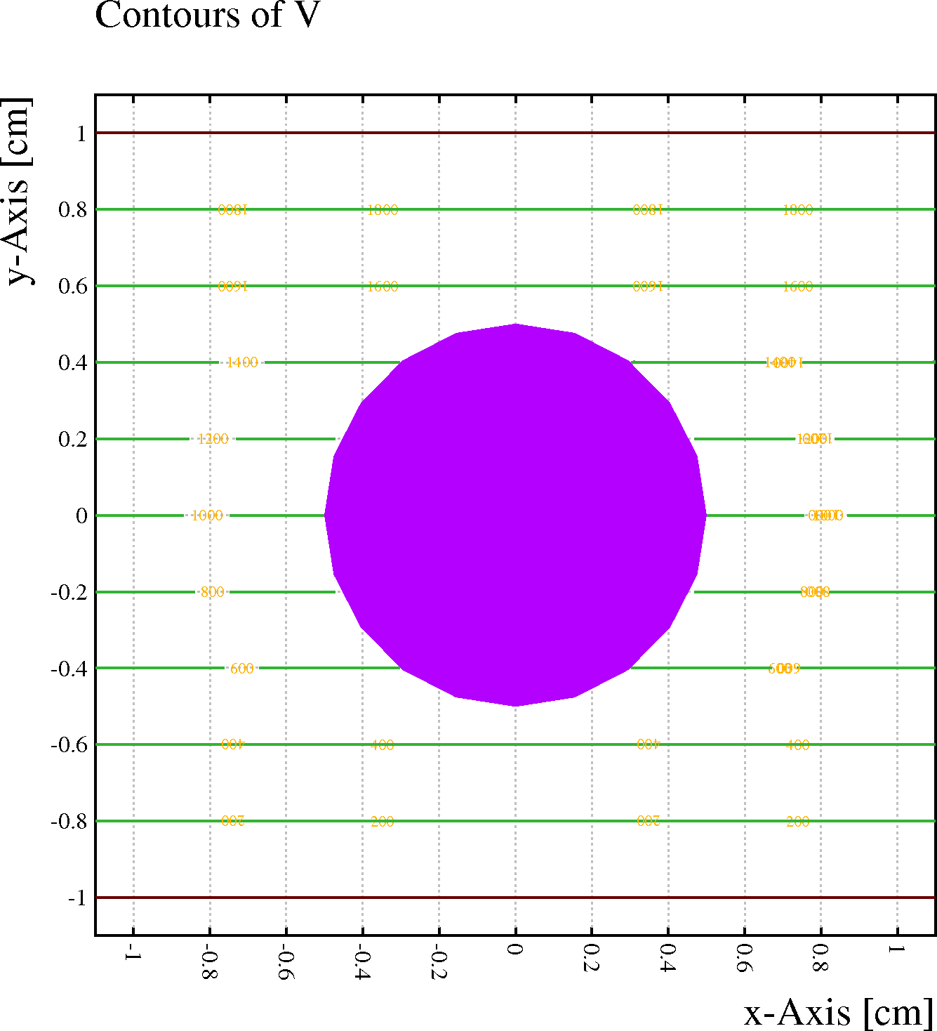
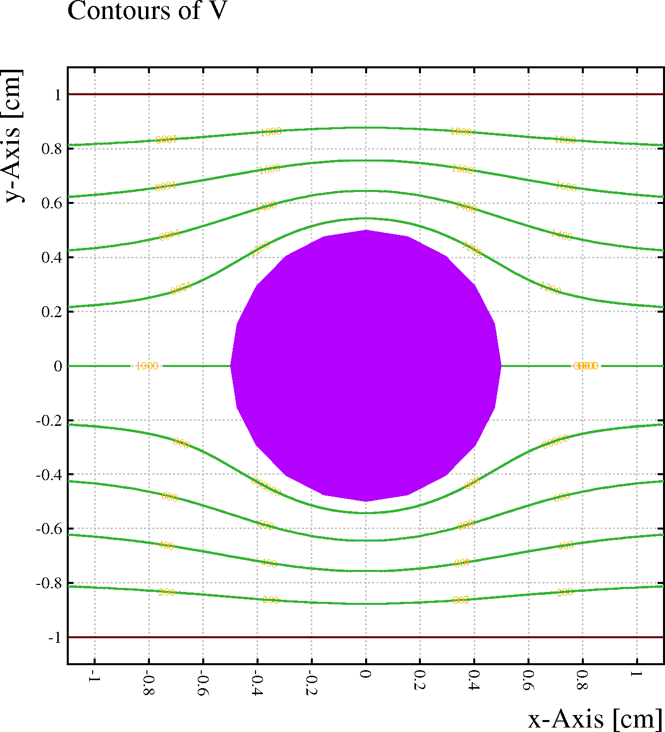
[Dipole terms are by default not included.]
The wire labels are shown next to the wires unless the WIRE-MARKERS option is active. The cell is plotted using the X-Y or R-PHI projection, as appropriate. To visualise the layout in other projections, use either the PLOT_FIELD_AREA or the PLOT_DRIFT_AREA procedure in the field respectively drift section.
Mainly used to check typing mistakes visually.
[This option is initially off but its setting is remembered from one cell section to the next.]
This option has only effect on the layout plot, not on plots made in for instance the field and drift sections - where the aspect ratio is determined by projection method specified in the AREA statements. In those sections, one can obtain an isometric view by using the 3D projection.
Using this option in conjunction with a non-square VIEWPORT is not meaningful.
[This option is initially off, but its setting is remembered from one cell section to the next.]
This option is shared between with the field, optimisation, drift and signal sections.
The type of marker used for a wire depends on the label that you have assigned to the wire in the ROWS listing. Each marker can be adjusted individually via the representations mechanism. The correspondence between labels and REPRESENTATION is as follows:
| Label | Representation |
|---|---|
S |
S-WIRES |
P |
P-WIRES |
C |
C-WIRES |
other |
OTHER-WIRES |
All wires are shown with the representation WIRES when the option is off.
The LAYOUT plot does not contain alphabetic wire labels if this option is active.
[This option is initially off, but its setting is remembered from one cell section to the next.]
Only meaningful if the capacitance matrix has indeed been inverted - in the vectorised executables, this is as a rule not done: the numerical quality of the charge calculation is higher if the capacitance equations are solved by other means than matrix inversion.
[This option is initially off but its setting is remembered from one cell section to the next.]
Chambers which have a repetitive structure over a considerable distance, as for instance in multiwire proportional chambers, should be declared periodic if you wish to enhance the numerical precision of the calculations. You will also gain CPU time by doing so. There are however instances where you may wish to enter explicit copies of the cell, increasing the periodicity length accordingly:
This statement is only used with chambers constructed from wires, planes and solids. If the field in the chamber is taken from a field map, options such as X-PERIODIC of the FIELD-MAP command should be used instead.
In chambers modelled using neBEM, periodicity-related parameters can be set using the NEBEM command.
Format:
PERIODICITY direction = length [REGULAR | MIRROR]
Example:
PERIOD X=1
| Direction | Meaning | Coordinate system |
|---|---|---|
X |
Cell repeats in x | Cartesian |
Y |
Cell repeats in y | Cartesian |
Z |
Cell repeats in z | - |
PHI |
Axial periodicity around the origin | Polar or Tube |
Repetition in r is not permitted because of the method used to calculate the potentials in cylindrical geometry.
Cylindrical geometries are handled via a conformal mapping onto a Cartesian coordinate system in which an r-periodicity would be equivalent to an x-periodicity with non-constant intervals. This is technically difficult to deal with. Contact the author if there is a genuine need for such a periodicity.
Periodicity in z is only allowed with neBEM field calculations, not in wire and planes chambers.
This is the only type of periodicity permitted in cells constructed of wires and planes. This type of periodicity is recognised by neBEM.
[If periodicity is requested, then it will by default have this type of periodicity.]
This is the type of periodicity is not permitted in cells constructed of wires and planes. This type of periodicity is recognised by neBEM.
[If periodicity is requested, then it will by default be regular.]
Note that one is not allowed to put a wire at the centre of a circular plane. Wires inside a circular plane, whether at the centre or not, are handled by TUBE geometries.
Planes are not compatible with a TUBE geometry. To generate a pie wedge, use a plane at constant r and two planes at constant \φ.
Format:
PLANE direction coordinate ...
      [V potential] ...
      [LABEL label] ...
      [{X-STRIP | Y-STRIP | R-STRIP | PHI-STRIP | Z-STRIP} strip_min strip_max ...
         [GAP gap] [LABEL strip_label]]
Examples:
pl x=-1, V=1000
plane phi=30
| Direction | Meaning | Coordinate system |
|---|---|---|
X |
Plane parallel with the y-axis | Cartesian |
Y |
Plane parallel with the x-axis | Cartesian |
R |
Circular plane | Polar |
PHI |
Plane through the origin | Polar |
The r coordinate must be strictly positive (non-zero).
[No default, the coordinate is mandatory.]
[Default: an earthed plane, at 0\ V.]
The label is a single alphabetic upper case character. You may type a longer string, but only the first character will be stored.
A label is not mandatory, but signals induced in a plane are only computed if the plane can be selected, and this can only be done if the plane has a label.
[By default, no label is assigned to a plane.]
Signals in strips are computed with weighting fields that are exclusively valid for parallel plate chambers without wires. This can perhaps most easily be seen in an MWPC where the weighting field (orange in the figure) of the strip (in red, covering -0.1\ <\ x\ <\ 0.1\ cm) is not influenced by the wires (purple) - while in reality, the influence of the wires is of course highly significant.
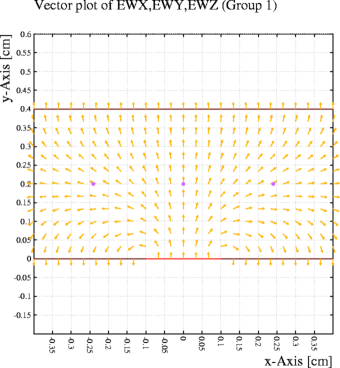
The reason for this limitation is that no exact weighting fields for strips are known for general wire-plane layouts. Should expressions be known for the particular case that interests you, then these can of course be added on demand.
See the weighting_field example for the FIELD-MAP command of the optimisation section for a method to address this using the finite element technique.
Subdivisions are permitted as follows:
| Subdivision | Permitted with | Unit |
|---|---|---|
R-STRIP |
PLANE PHI=... | cm |
PHI-STRIP |
PLANE R=... | degrees |
X-STRIP |
PLANE Y=... | cm |
Y-STRIP |
PLANE X=... | cm |
Z-STRIP |
all planes | cm |
The location should be given in degrees for \φ-sectors, in cm for all other strips.
[Mandatory parameter, no default provided.]
The location should be given in degrees for \φ-sectors, in cm for all other strips.
[Mandatory parameter, no default provided.]
The label is a single alphabetic upper case character. You may type a longer string, but only the first character will be stored.
A label is not mandatory, but signals induced in a strip are only computed if the strip can be selected, and this can only be done if the strip has a label.
[By default, no label is assigned to a strip.]
The gap is specified in cm for strips in x-, r- and y-planes, and in degrees for strips in \φ-planes.
[By default, this is taken to be the distance to the parallel plane, if there is one, otherwise the distance from the plane to which the strip belongs to the nearest electrode.]
Strips, if any, are shown with the STRIPS representation.
This command is executed immediately. Once the command has completed, you can use the FIELD-MAP command to modify for instance the selection of drift medium,
READ-FIELD-MAP has the same side effects as FIELD-MAP, i.e. the command deletes any wires, planes, periodicities, dielectric medium and magnetic field that may have been entered before the command is issued.
Reading binary field maps is, for most field map formats, much faster than reading the original files - but binary field maps are not portable. Files to be read with READ-FIELD-MAP must have been written on the same computer system.
Format:
READ-FIELD-MAP file ...
               [DRIFT-MEDIUM {SMALLEST-EPSILON | ...
                              SECOND-SMALLEST-EPSILON | ...
                              n | ...
                              SECOND-LARGEST-EPSILON | ...
                              LARGEST-EPSILON | ...
                              \ε}] ...
               [NOT-X-PERIODIC | X-PERIODIC | ...
                    X-MIRROR-PERIODIC | X-AXIALLY-PERIODIC] ...
               [NOT-Y-PERIODIC | Y-PERIODIC | ...
                    Y-MIRROR-PERIODIC | Y-AXIALLY-PERIODIC] ...
               [NOT-Z-PERIODIC | Z-PERIODIC | ...
                    Z-MIRROR-PERIODIC | Z-AXIALLY-PERIODIC] ...
               [LINEAR | QUADRATIC | CUBIC] ...
               [INTERPOLATE-ELECTRIC-FIELD | COMPUTE-ELECTRIC-FIELD] ...
               [PLOT-MAP | NOPLOT-MAP] ...
               [NOHISTOGRAM-MAP | HISTOGRAM-MAP]
Example:
&CELL
cell-identifier "Micromegas"
Global path=`/afs/cern.ch/exp/compass/scratch/d02/megas/Maxwell/mic3.pjt/`
Call inquire_file(path/`1000_400_0.1.bin`,exist)
If exist Then
   read-field-map {path/`1000_400_0.1.bin`}
Else
   field-map files potential "{path}/V_1000_400_0.1.arg" ...
                   e-field   "{path}/E_1000_400_0.1.arg" ...
             x-periodic y-mirror-periodic
Endif
If a binary field map exists, the map is read. Otherwise the field maps are read in their original format. The periodicity options need not be repeated: they are stored in the binary field map.
The order of the field map can not be increased when reading back a binary map.
The order of the field map can not be increased when reading back a binary map.
The order of the field map can not be increased when reading back a binary map.
Format:
RESET [COORDINATES] ...
      [DIELECTRICA] ...
      [DEFINITIONS] ...
      [FIELD-MAP] ...
      [PERIODICITIES] ...
      [PLANES] ...
      [ROWS or WIRES] ...
      [SOLIDS] ...
      [TUBE]
Example:
RESET
If the wires are thick, short or non-parallel, then neBEM should be used to compute the field. For thin wires, WIRE solids should be used while CYLINDER solids are appropriate for thick wires.
The following properties of the wires can be entered:
The coordinate system in which the wire position is specified can either be Cartesian or polar. The wires in a cell that has a tube, are listed in Cartesian coordinates. Polar coordinates will be assumed if you put the keyword POLAR after ROWS, if you have already entered a plane in polar coordinates and if you have already entered a \φ periodicity. Otherwise Cartesian coordinates are assumed. Once a coordinate system has been selected in the cell section, it has to be used throughout the section.
ROWS is a multi-line command because chambers sometimes contain many wires. You may enter one wire per line, but if your cell contains regularly spaced series of wires, you may prefer to enter these as a single "row" in which at least the position, but possibly also the other properties, depends on the so-called loop-variable I which automatically assumes a series of values.
One may use control structures (If_block, If_line, Do, Call) in the listing of wires. Please keep in mind that a blank line must be present to signal the end of the list, whether typed by hand or generated with a loop.
Format of the whole command:
ROWS [CARTESIAN | POLAR | TUBE]
row
...
row
(blank line)
Format of the rows:
label n diameter x y [V [weight [length [density]]]]
Examples:
ROWS
s * * 0 0 1000
p * * 0 1 -2000
p * * 0 -1 -2000
This is a very simple example in which 3 wires are entered at (0,0), (0,1) and (0,-1). Defaults are used for the number of wires and the diameter.
ROWS
S * * 0 0 1000
P 2 * -1+i*2 -1+i*2 -2000
This examples shows how the same cell can be entered using the loop variable.
rows
Global n=100
For i From 1 To n Do
   Global r=1+2*(i/n)
   Global phi=4*pi*i/n
   If i=2*entier(i/2) Then
       P * * {r*cos(phi), r*sin(phi), -i*10}
   Else
       S * * {r*cos(phi), r*sin(phi), +i*10}
   Endif
Enddo
This, artificial, example illustrates the use of Global variables, a Do loop and an If_block to generate a spiral. Do not forget the blank line to mark the end of the list of rows !
This keyword need not be specified if the cell is already established to be in Cartesian coordinates, for instance if a plane at constant x has already been entered. This keyword is not valid if the cell is already established to be in polar or in tube coordinates.
When Cartesian coordinates are used, you may enter planes at constant x and at constant y. Also both x and y periodicities are permitted.
[If no coordinate system has yet been established when ROWS is entered, then Cartesian coordinates are assumed by default.]
When the wires are listed in polar coordinates, the planes have to be entered in polar coordinates too. That is, the planes can be at constant r or at constant \φ.
Periodicity in \φ is permitted, but radial periodicity isn't.
These coordinates are transformed to an internal coordinates system which is a conformal map of a Cartesian system - but all frequently used instructions transform these internal coordinates back to polar coordinates when displaying the results.
This keyword need not be specified if the cell is already established to be in polar coordinates, for instance if a \φ periodicity has already been entered. This keyword is not valid if the cell is already established to be in Cartesian coordinates or in tube coordinates.
[If no coordinate system has been established yet when the ROWS command is entered, then Cartesian coordinates will be assumed by default.]
The tube itself and the \φ periodicity, if any, is specified in polar coordinates, but the wires are listed in Cartesian coordinates.
Like for polar coordinates, a coordinate transformation is applied to the wire location but the internal coordinates never appear on output.
This keyword need not be specified if the cell is already established to be in tube coordinates because a TUBE statement has already been entered. This keyword is not valid if the cell is already established to be in Cartesian or polar coordinates.
[If no coordinate system has been established yet when the ROWS command is entered, then Cartesian coordinates will be assumed by default.]
These labels are used by the SELECT statements to single out (groups of) wires from which particles should drift, for which arrival time distributions are to be computed, on which signals can be recorded, etc.
[Initially, all wires with a label of S are selected for such treatment.]
Each wire in such a row will have the same status as if it were entered on a separate line. Entering wires in the form of rows has no incidence on the choice of potential_function used for the chamber.
The number of wires may be a symbolic expression in terms of DEFINEd variables but you may, of course, not use the loop-variable I.
[Default: 1, i.e. a single wire].
Since the electric fields are currently computed in the thin wire approximation, i.e. neglecting dipole and other higher order terms, care has to be taken that the wire diameters are small compared to the inter-wire distances. One can use the MULTIPOLE-MOMENTS instruction to investigate the need for higher order terms to describe the field around the wire.
Consider using the DIPOLE-TERMS in case dipole terms are thought to be important.
This may be a symbolic expression in terms of DEFINEd variables and you may use the loop-variable I in the expression if you wish.
[Default: 0.01\ cm, i.e. 100\ \μm].
If the cell is described in Cartesian or Tube coordinates, then (x,y) coordinates should be used for the wire location. The wire coordinates should be given in (r,\φ) format for Polar cells.
This may be a symbolic expression in terms of DEFINEd variables and you may use the loop-variable I to construct symbolic expressions for the locations of the wires in the row. For instance, for a series of wires with coordinates 1, 2, 3 and 4 you could enter the expression
1+I
[Default: 0\ cm.]
If the cell is described in Cartesian or Tube coordinates, then (x,y) coordinates should be used for the wire location. The wire coordinates should be given in (r,\φ) format for Polar cells.
This may be a symbolic expression in terms of DEFINEd variables and you may use the loop-variable I to construct symbolic expressions for the locations of the wires in the row. For instance, for a series of wires with coordinates 1, 4, 9 and 16 you could enter the expression
(1+I)^2
[Default: 0\ cm, \φ should be in degrees.]
This may be a symbolic expression in terms of DEFINEd variables and you may use the loop-variable I to construct symbolic expressions for the locations of the wires in the row. For instance, for a series of wires with potentials 1000, 1000, 2000 and 2000, you could enter the expression
1000+entier(i/2)*1000
[Default: 0\ cm.]
Used by the FORCES command to estimate the wire displacement under gravitational and electrostatic forces.
This may be a symbolic expression in terms of DEFINEd variables and you may use the loop-variable I to construct symbolic expressions.
[Default: 50\ grams.]
Used by the FORCES command to estimate the wire displacement under gravitational and electrostatic forces.
This may be a symbolic expression in terms of DEFINEd variables and you may use the loop-variable I to construct symbolic expressions.
Note that the length of the wires has no impact on the fields in the chamber. Fields in chambers that are made up of wires and planes are truly 2-dimensional and are identical at all z, irrespective of the length of the wires. If you're interested in the end-effects of finite length wires, then you should use a finite element field map.
[Default: 100\ cm.]
Used by the FORCES command to estimate the wire displacement under gravitational and electrostatic forces. Not relevant if the wires are vertical.
For copper-beryllium wires, one can also enter CU-BE and for gold plated tungsten one can type TUNGSTEN or W.
This may be a symbolic expression in terms of DEFINEd variables and you may use the loop-variable I to construct symbolic expressions.
[Default: 19.3\ g/cm\³, i.e. 20\ \μm gold-plated tungsten wire]
This feature is less powerful than the method using the loop-variable and the increments have therefore been suppressed as of version\ 5.
This modification is not backwards compatible - input files prepared for Garfield\ 4 and earlier need to be modified.
This variable may be used for the diameter, the position, the potential, the stretching weight and the length of the wire.
The loop-variables can be used to construct non-standard electrode shapes using wires. Some examples are shown in the description of the wire position and voltage.
Note that the loop variable is not a Global variable: while substitution of expressions in terms of global variables has to be requested explicitly by means of curly brackets, expressions in terms of DEFINEd variables and the loop variable are automatically evaluated. Curly brackets should not be used with such variables.
This command is executed immediately, unlike the WRITE command which is only executed when the section is left. The field map must therefore be present (via a FIELD-MAP or a READ-FIELD-MAP) when you issue the SAVE-FIELD-MAP command.
Binary field maps tend to be much smaller than field maps in the original format. In addition, restoring field maps from binary files is usually much faster. However, binary files are not portable between computer systems.
Please the original field map files - the format of binary field maps changes whenever new elements are added to the field map.
Format:
SAVE-FIELD-MAP file
Example:
See READ-FIELD-MAP
Solids generate the field through an interface with neBEM if potentials, dielectric constants or other boundary conditions have been set for all of them. Otherwise, solids do not affect the field in the chamber, but they can nevertheless be useful for the following reasons:
Entering these volumes is not mandatory. The drift-line calculation routines for instance, can infer their presence in most cases from the dielectric constants in the field map.
If you do not enter any solids in a chambers composed of wires and planes, then all wires are automatically copied to cylindrical solids to ensure the wires are visible in 3D and CUT type plots. This copy is not performed if you enter at least 1 solid yourself.
SOLIDS is a multi-line command. Each line after SOLIDS describes one volume. The end of the list is signalled by a blank line.
Only a few shapes are currently provided, other shapes can be added on request - contact the author.
Format:
SOLIDS
{BOX | CYLINDER | EXTRUSION | HOLE | RIDGE | SPHERE | WIRE} parameters
...
(blank line)
Example 1, solids not affecting the field:
solids
For x From -0.02 Step 0.02 To 0.02 Do
   For y From -0.02 Step 0.02 To 0.02 Do
      hole centre {x,y} +0.0110 direction 0 0 1 ...
         half-lengths 0.0100 0.0100 0.0010 ...
         upper-radius 0.0080 lower-radius 0.0080 ...
         n = 5 ...
         conductor-3
      centre {x,y} +0.0050 direction 0 0 1 ...
         half-lengths 0.0100 0.0100 0.0050 ...
         upper-radius 0.0070 lower-radius 0.0040 ...
         n = 5 ...
         dielectric
      centre {x,y} -0.0050 direction 0 0 1 ...
         half-lengths 0.0100 0.0100 0.0050 ...
         upper-radius 0.0040 lower-radius 0.0070 ...
         n = 5 ...
         dielectric
      centre {x,y} -0.0110 direction 0 0 1 ...
         half-lengths 0.0100 0.0100 0.0010 ...
         upper-radius 0.0080 lower-radius 0.0080 ...
         n = 5 ...
         conductor-3
   Enddo
Enddo
This represents an array of 9\ double-tapered cylindrical holes in a copper clad foil of dielectric material,
similar to a GEM foil. These solids have no effect on the field.
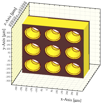
Example 2, dielectric materials:
&CELL
solids
box   centre 0 0 -1.2 ...
      half-lengths 5 5 0.2 ...
      conductor-1 ...
      voltage 1
box   centre 0 0 0 ...
      half-lengths 5 5 1 ...
      dielectricum-1 ...
      epsilon 2
ridge centre 0 0 1 ...
      half-lengths 2 5 ...
      notch 1 2 ...
      dir 0 0 1 ...
      epsilon 10 ...
      dielectricum-2
box   centre 0 0 8 ...
      half-lengths 5 5 0.2 ...
      conductor-1 ...
      voltage -1

nebem max-elem 2

&FIELD
// View the structure
area -9 -9 -2 9 9 9 ...
    nooutline ...
    light -20 -40 ...
    view -3*x+5*y-1*z=0 3d
Call plot_field_area
Call plot_end
// Contour plot
area -3 -1 -1  3 5 5 ...
    view y=0 cut rot 180
grid 25
plot-field cont
In this example, the solids define the field through the neBEM interface.
The field between 2 conducting plates is distorted by the presence of a
triangular piece of dielectric material.
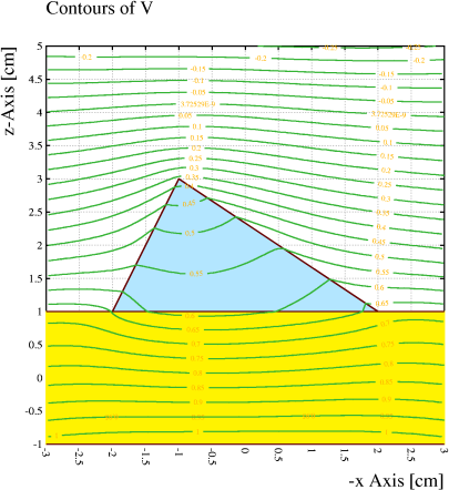
Example 3, importance of discretisation:
&CELL
solids
box      centre 0 0 0  ...
         half-lengths 5 5 0.1 ...
         voltage 1000 ...
         discretisation 10
box      centre 0 0 1  ...
         half-lengths 5 5 0.1 ...
         voltage 0 ...
         discretisation 10

&FIELD
area -7 -7 -1 7 7 2 view z=0.89
pl cont v n=50 range 0 500

&CELL
solids
box      centre 0 0 0  ...
         half-lengths 5 5 0.1 ...
         voltage 1000 ...
         discretisation 10
box      centre 0 0 1  ...
         half-lengths 5 5 0.1 ...
         voltage 0 ...
         discretisation 10 bottom-discretisation 1

&FIELD
area -7 -7 -1 7 7 2 view z=0.89
pl cont v n=50 range 0 500
This examples illustrates the impact of the discretisation of a face of a solid.
The first plot (left) shows the potential in a capacitor with just 1\ element
per plane, while the second plot (right) shows the potential when the plate has been
subdivided in 10\×10 elements.
Note that the boundary conditions are not strictly respected: in the boundary element approach, the fields are solutions of the Maxwell equations but they only satisfy the boundary conditions at the collocation points. In the finite element approach, the potentials are not solutions of the Maxwell equations, but they strictly respect the boundary conditions.
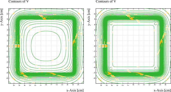
Example 4, selective discretisation:
&CELL
nebem target-element-size 0.1
solids
box      centre  0 0 0 half-lengths 1 1 1 voltage 1 ...
         discretisation 0.5
box      centre  3 0 0 half-lengths 1 2 2 voltage 1 ...
         front-discretisation 0.2 back-discretisation automatic
cylinder centre 10 0 0 half-length 1 radius 1 voltage -1 ...
         discretisation 0.5 top-discretisation 0.2

nebem target-element-size 0.8
opt cell-print
&MAIN
The default discretisation length is set to 1\ mm in the first NEBEM statement.
This value is only used for 4 of the faces of the second box.
All faces of the first box and the cylinder initially get a discretisation
size of 5\ mm, a value that is overruled for one of the faces of the cylinder.
The face of the second, larger, box that is in partial contact with the first,
smaller, box is given an AUTOMATIC discretisation length.
The part of this face that is in contact will inherit the discretisation
of the first box, which has been explicitely specified to be 5\ mm.
For other parts of this face a discretisation length of 8\ mm will be used,
as set in the second NEBEM statement.
Format:
BOX  CENTRE cx cy cz ...
     HALF-LENGTHS lx ly lz ...
     [DIRECTION dx dy dz] ...
     [VOLTAGE v] ...
     [FLOATING-CONDUCTOR] ...
     [CHARGE q] ...
     [EPSILON eps] ...
     [material] ...
     [LABEL label]
     [FRONT-DISCRETISATION discretisation] ...
     [BACK-DISCRETISATION discretisation] ...
     [RIGHT-DISCRETISATION discretisation] ...
     [LEFT-DISCRETISATION discretisation] ...
     [TOP-DISCRETISATION discretisation] ...
     [BOTTOM-DISCRETISATION discretisation]
Illustration:
A set of boxes that are intersecting each other. Shown using the default colour density table, with outlining.
[No default.]
[No default.]
The normalisation of the vector is not used. Zero-norm vectors are not acceptable.
[By default, the box is not rotated i.e. the half lengths are assumed to have been measured along x, y and z.]
The charge is added to the surface charges needed to satisfy the boundary conditions. The box can either be a dielectric or a conductor.
In the process of being implemented - initially, the charge is equally distributed over all surfaces, selection of surface panels is planned to be added later.
Specifying this option implies the use of neBEM to solve the field.
Specifying this option implies the use of neBEM to solve the field.
In the process of being implemented.
Specifying this option implies the use of neBEM to solve the field.
Specifying this option implies the use of neBEM to solve the field.
| Type | Representation | Notes |
|---|---|---|
CONDUCTOR |
CONDUCTORS-1 |
Equivalent to CONDUCTOR-1 |
CONDUCTOR-1 |
CONDUCTORS-1 |
- |
CONDUCTOR-2 |
CONDUCTORS-2 |
- |
CONDUCTOR-3 |
CONDUCTORS-3 |
- |
DIELECTRICUM |
DIELECTRICA-1 |
Equivalent to DIELECTRICUM-1 |
DIELECTRICUM-1 |
DIELECTRICA-1 |
- |
DIELECTRICUM-2 |
DIELECTRICA-2 |
- |
DIELECTRICUM-3 |
DIELECTRICA-3 |
- |
[Default: CONDUCTOR]
This label serves the same purpose as the wire label for wires, namely the selection of the solid as a place where signals can be measured, around which isochrons are drawn etc.
[By default, no label is assigned.]
Garfield generates, for each solid, a set of flat panels that together cover the faces. These panels, arbitrary convex polygons, are sub-divided when isolating contact areas between solids and also in order to comply with the neBEM requirement that it be given only rectangles and right-angled triangles. The triangles and rectangles handed to neBEM are called "primitives".
For reasons of accuracy neBEM as a rule sub-divides the primitives into "elements", in a process called "discretisation". The sub-divisions of the primitives are called "elements".
Discretisation will perhaps eventually be automated, but for the time being this remains the responsability of the user. In neBEM, the level of discretisation requested is described by 2 integers: the number of elements that is to be generated along each of 2 sides adjacent to a right angle. Since the shape, orientation and size of the primitives are non-trivial to predict, the level of discretisation is specified on the Garfield side as the desired length of the sides of the elements.
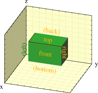
The designation of the surfaces is as follows:
The discretisation length can be set in several ways, see Example\ 4 for the SOLIDS command:
Discretisation lengths have to be given in cm.
[Default: the TARGET-ELEMENT-SIZE that is in effect at the time the solids are read.]
For many purposes, cylinders and wires are equivalent, but the differences are important when using neBEM to compute the field:
Mandatory parameters are the location of the centre, the radius and the length. The direction defaults to the z-axis.
Format:
CYLINDER  CENTRE cx cy cz ...
          RADIUS radius ... ...
          [OUTER-RADIUS | MEAN-RADIUS]
          HALF-LENGTH lz ...
          [DIRECTION dx dy dz] ...
          [VOLTAGE v] ...
          [FLOATING-CONDUCTOR] ...
          [CHARGE q] ...
          [EPSILON eps] ...
          [material] ...
          [LABEL label] ...
          [ROTATE angle] ...
          [N n] ...
          [TOP-LID-DISCRETISATION discretisation] ...
          [BODY-DISCRETISATION discretisation] ...
          [BOTTOM-LID-DISCRETISATION discretisation] ...
          [TOP-LID | NOTOP-LID] ...
          [BOTTOM-LID | NOBOTTOM-LID] ...
          [LIDS | NOLIDS]
Illustration:
A set of cylinders, partially hiding each other. Each cylinder is drawn with 50 panels, and 20 colour shades are used.
[No default.]
The decision whether a particle is inside or outside the cylinder, is made assuming a genuine cylinder. For plotting and neBEM field calculations however, a polygonal approximation is made and the precise interpretation of the radius is influenced by the MEAN-RADIUS and OUTER-RADIUS options.
[No default.]
2/(1 + arcsinh(tan(\α) cos(\α) / tan(\α)))where
\α = 1/4 \π / (N-1)
If you place a precisely fitting hole around the cylinder, then you should use the same option for the hole.
[This is not default.]
[No default.]
The normalisation of the vector is not used. Zero-norm vectors are not acceptable.
[By default, the central axis is aligned with the z-axis.]
The charge is added to the surface charges needed to satisfy the boundary conditions. The cylinder can either be a dielectric or a conductor.
In the process of being implemented - initially, the charge is equally distributed over all surfaces, selection of surface panels is planned to be added later.
Specifying this option implies the use of neBEM to solve the field.
Specifying this option implies the use of neBEM to solve the field.
In the process of being implemented.
Specifying this option implies the use of neBEM to solve the field.
Specifying this option implies the use of neBEM to solve the field.
| Type | Representation | Notes |
|---|---|---|
CONDUCTOR |
CONDUCTORS-1 |
Equivalent to CONDUCTOR-1 |
CONDUCTOR-1 |
CONDUCTORS-1 |
- |
CONDUCTOR-2 |
CONDUCTORS-2 |
- |
CONDUCTOR-3 |
CONDUCTORS-3 |
- |
DIELECTRICUM |
DIELECTRICA-1 |
Equivalent to DIELECTRICUM-1 |
DIELECTRICUM-1 |
DIELECTRICA-1 |
- |
DIELECTRICUM-2 |
DIELECTRICA-2 |
- |
DIELECTRICUM-3 |
DIELECTRICA-3 |
- |
[Default: CONDUCTOR]
This label serves the same purpose as the wire label for wires, namely the selection of the solid as a place where signals can be measured, around which isochrons are drawn etc.
[By default, no label is assigned.]
The interpretation of n is the same for holes and cylinders. Cylinders with a given n will precisely fit in holes with the same n, provided the radii and axes match.
Drift line termination assumes a perfect cylinder, the choice of n therefore has no importance for this purpose. However, the number of surface panels passed on to neBEM field calculations rises with n and the visual quality of 3D views improves with n.
[By default, N is chosen in function of the size occupied by the cylinder in the drawing. N must be larger than 1.]
This is equivalent to entering a WIRE.
[This is not default and mutually exclusive with specifying N.]
Such a rotation is meaningful only if N has been chosen small.
Rotations have only an optical effect. The algorithm which determines whether a point is inside or outside a cylinder, assumes a perfect cylinder and thus does not take rotations into account.
[Default: -\π/4\ radian]
Garfield generates, for each solid, a set of panels that together cover the faces. These panels, arbitrary convex polygons, are sub-divided when isolating contact areas between solids and also in order to comply with the neBEM requirement that it be given only rectangles and right-angled triangles. The triangles and rectangles handed to neBEM are called "primitives".
For reasons of accuracy neBEM as a rule sub-divides the primitives into "elements", in a process called "discretisation". The sub-divisions of the primitives are called "elements".
Discretisation will perhaps eventually be automated, but for the time being this remains the responsability of the user. In neBEM, the level of discretisation requested is described by 2 integers: the number of elements that is to be generated along each of 2 sides adjacent to a right angle. Since the shape, orientation and size of the primitives are non-trivial to predict, the level of discretisation is specified on the Garfield side as the desired length of the sides of the elements.
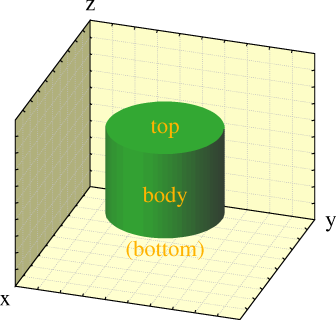
The designation of the surfaces is as follows:
The discretisation lengths can be set in several ways, see Example\ 4 for the SOLIDS command:
Discretisation lengths have to be given in cm.
[Default: the TARGET-ELEMENT-SIZE that is in effect at the time the solids are read.]
Not closing the cylinder results in smaller, more efficient neBEM models since polygonal lids are subdivided in a potentially large number of triangular elements, which are computationally less efficient. Leaving the cylinders open is therefore recommendable practice for periodic chambers.
The cylinder will appear closed for all visualisation techniques, except NEBEM.
This option has no effect on wire-type cylinders.
[This is default.]
Mandatory parameters are the extrusion profile and the half-length. The direction defaults to the z-axis and the central position to (0,0,0).
Format:
EXTRUSION  CENTRE cx cy cz ...
           HALF-LENGTH lz ...
           PROFILE x1 y1  x2 y2  x3 y3 ... xn yn ...
           [DIRECTION dx dy dz] ...
           [VOLTAGE v] ...
           [FLOATING-CONDUCTOR] ...
           [CHARGE q] ...
           [EPSILON eps] ...
           [material] ...
           [LABEL label] ...
           [TOP-LID-DISCRETISATION discretisation] ...
           [BODY-DISCRETISATION discretisation] ...
           [BOTTOM-LID-DISCRETISATION discretisation] ...
           [TOP-LID | NOTOP-LID] ...
           [BOTTOM-LID | NOBOTTOM-LID] ...
           [LIDS | NOLIDS]
Illustration:
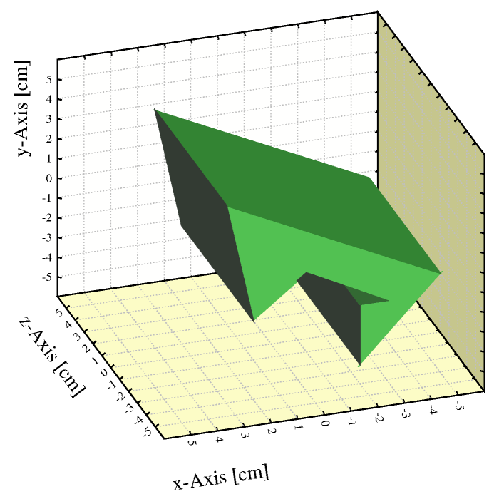
An extrusion
&CELL
nebem target-element-size 1
solids
box centre        0   0  10 ...
    half-lengths 10  10   0 ...
    volt          0
box centre        0   0 -10 ...
    half-lengths 10  10   0 ...
    volt          0
extrusion centre  0  0  0 ...
    half-length   4 ...
    profile       -5 -1   -2 -5   -2 -2  -3 -2   0 0    2 -2    3 4 ...
    voltage       1

opt cell-print
&FIELD
area -6 -6 -6 6 6 6 view x+2*y-3*z=0 nebem
Call plot_field_area
Call plot_end
[By default, (0,0,0).]
[No default.]
The normalisation of the vector is not used. Zero-norm vectors are not acceptable.
[By default, the central axis is aligned with the z-axis.]
The charge is added to the surface charges needed to satisfy the boundary conditions. The extrusion can either be a dielectric or a conductor.
In the process of being implemented - initially, the charge is equally distributed over all surfaces, selection of surface panels is planned to be added later.
Specifying this option implies the use of neBEM to solve the field.
Specifying this option implies the use of neBEM to solve the field.
In the process of being implemented.
Specifying this option implies the use of neBEM to solve the field.
Specifying this option implies the use of neBEM to solve the field.
| Type | Representation | Notes |
|---|---|---|
CONDUCTOR |
CONDUCTORS-1 |
Equivalent to CONDUCTOR-1 |
CONDUCTOR-1 |
CONDUCTORS-1 |
- |
CONDUCTOR-2 |
CONDUCTORS-2 |
- |
CONDUCTOR-3 |
CONDUCTORS-3 |
- |
DIELECTRICUM |
DIELECTRICA-1 |
Equivalent to DIELECTRICUM-1 |
DIELECTRICUM-1 |
DIELECTRICA-1 |
- |
DIELECTRICUM-2 |
DIELECTRICA-2 |
- |
DIELECTRICUM-3 |
DIELECTRICA-3 |
- |
[Default: CONDUCTOR]
This label serves the same purpose as the wire label for wires, namely the selection of the solid as a place where signals can be measured, around which isochrons are drawn etc.
[By default, no label is assigned.]
[Ny default, mandatory parameter.]
Garfield generates, for each solid, a set of panels that together cover the faces. These panels, arbitrary convex polygons, are sub-divided when isolating contact areas between solids and also in order to comply with the neBEM requirement that it be given only rectangles and right-angled triangles. The triangles and rectangles handed to neBEM are called "primitives".
For reasons of accuracy neBEM as a rule sub-divides the primitives into "elements", in a process called "discretisation". The sub-divisions of the primitives are called "elements".
Discretisation will perhaps eventually be automated, but for the time being this remains the responsability of the user. In neBEM, the level of discretisation requested is described by 2 integers: the number of elements that is to be generated along each of 2 sides adjacent to a right angle. Since the shape, orientation and size of the primitives are non-trivial to predict, the level of discretisation is specified on the Garfield side as the desired length of the sides of the elements.
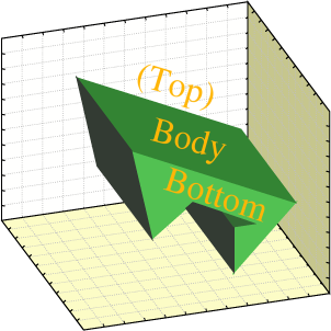
The designation of the surfaces is as follows:
The discretisation lengths can be set in several ways, see Example\ 4 for the SOLIDS command:
Discretisation lengths have to be given in cm.
[Default: the TARGET-ELEMENT-SIZE that is in effect at the time the solids are read.]
Not closing the extrusion results in smaller, more efficient neBEM models since polygonal lids are subdivided in a potentially large number of triangular elements, which are computationally less efficient. Leaving the extrusions open is therefore recommendable practice for periodic chambers.
The extrusion will appear closed for all visualisation techniques, except NEBEM.
This option has no effect on wire-type extrusions.
[This is default.]
Format:
HOLE  CENTRE cx cy cz ...
      RADIUS radius | UPPER-RADIUS r_up LOWER-RADIUS r_low ...
      [OUTER-RADII | MEAN-RADII]
      HALF-LENGTHS lx ly lz ...
      [DIRECTION dx dy dz] ...
      [VOLTAGE v] ...
      [FLOATING-CONDUCTOR] ...
      [CHARGE q] ...
      [EPSILON eps] ...
      [material] ...
      [LABEL label] ...
      [N n]
      [FRONT-DISCRETISATION discretisation] ...
      [BACK-DISCRETISATION discretisation] ...
      [RIGHT-DISCRETISATION discretisation] ...
      [LEFT-DISCRETISATION discretisation] ...
      [TOP-DISCRETISATION discretisation] ...
      [BOTTOM-DISCRETISATION discretisation] ...
      [CYLINDER-DISCRETISATION discretisation]
Illustration:
Two holes, on the left with N=2, on the right with N=20. Both are drawn with outlining.
[No default.]
The decision whether a particle is inside or outside the cylindric part of the hole is made assuming a genuine cylinder. For plotting and neBEM field calculations however, a polygonal approximation is made and the precise interpretation of the radius is influenced by the MEAN-RADII and OUTER-RADII options.
[No default.]
2/(1 + arcsinh(tan(\α) cos(\α) / tan(\α)))where
\α = 1/4 \π / (N-1)
If you insert a precisely fitting cylinder in the hole, then you should use the same option for the cylinder.
[This is not default.]
[No default.]
The normalisation of the vector is not used. Zero-norm vectors are not acceptable.
[By default, the central axis is aligned with the z-axis.]
The charge is added to the surface charges needed to satisfy the boundary conditions. The hole can either be a dielectric or a conductor.
In the process of being implemented - initially, the charge is equally distributed over all surfaces, selection of surface panels is planned to be added later.
Specifying this option implies the use of neBEM to solve the field.
Specifying this option implies the use of neBEM to solve the field.
In the process of being implemented.
Specifying this option implies the use of neBEM to solve the field.
Specifying this option implies the use of neBEM to solve the field.
| Type | Representation | Notes |
|---|---|---|
CONDUCTOR |
CONDUCTORS-1 |
Equivalent to CONDUCTOR-1 |
CONDUCTOR-1 |
CONDUCTORS-1 |
- |
CONDUCTOR-2 |
CONDUCTORS-2 |
- |
CONDUCTOR-3 |
CONDUCTORS-3 |
- |
DIELECTRICUM |
DIELECTRICA-1 |
Equivalent to DIELECTRICUM-1 |
DIELECTRICUM-1 |
DIELECTRICA-1 |
- |
DIELECTRICUM-2 |
DIELECTRICA-2 |
- |
DIELECTRICUM-3 |
DIELECTRICA-3 |
- |
[Default: CONDUCTOR]
The interpretation of n is the same for holes and cylinders. Cylinders with a given n will precisely fit in holes with the same n, provided the radii and axes match.
Drift line termination assumes a perfect cylinder, the choice of n therefore has no importance for this purpose. However, the number of surface panels passed on to neBEM field calculations rises with n and the visual quality of 3D views improves with n.
[By default, N is chosen in function of the size occupied by the cylinder in the drawing. N must be larger than 1.]
This label serves the same purpose as the wire label for wires, namely the selection of the solid as a place where signals can be measured, around which isochrons are drawn etc.
[By default, no label is assigned.]
Garfield generates, for each solid, a set of panels that together cover the faces. These panels, arbitrary convex polygons, are sub-divided when isolating contact areas between solids and also in order to comply with the neBEM requirement that it be given only rectangles and right-angled triangles. The triangles and rectangles handed to neBEM are called "primitives".
For reasons of accuracy neBEM as a rule sub-divides the primitives into "elements", in a process called "discretisation". The sub-divisions of the primitives are called "elements".
Discretisation will perhaps eventually be automated, but for the time being this remains the responsability of the user. In neBEM, the level of discretisation requested is described by 2 integers: the number of elements that is to be generated along each of 2 sides adjacent to a right angle. Since the shape, orientation and size of the primitives are non-trivial to predict, the level of discretisation is specified on the Garfield side as the desired length of the sides of the elements.
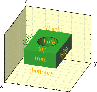
The designation of the surfaces is as follows:
The discretisation lengths can be set in several ways, see Example\ 4 for the SOLIDS command:
Discretisation lengths have to be given in cm. [Default: the TARGET-ELEMENT-SIZE that is in effect at the time the solids are read.]
The ridge proper is by default aligned with the y-axis, the (x,y) plane is taken to the floor of the construction.
Format:
RIDGE  CENTRE cx cy cz ...
       HALF-LENGTHS lx ly ...
       NOTCH rx rz ...
       [DIRECTION dx dy dz] ...
       [VOLTAGE v] ...
       [FLOATING-CONDUCTOR] ...
       [CHARGE q] ...
       [EPSILON eps] ...
       [material] ...
       [LABEL label]
       [FRONT-DISCRETISATION discretisation] ...
       [BACK-DISCRETISATION discretisation] ...
       [RIGHT-DISCRETISATION discretisation] ...
       [LEFT-DISCRETISATION discretisation] ...
       [FLOOR-DISCRETISATION discretisation]
Illustration:
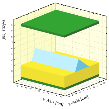
A ridge (blue) used to model a surface irregularity of a dielectric medium (yellow) between conductors (green).
[No default.]
[No default.]
If the offset is set to 0, then the ridge will be symmetric. This parameter is mandatory and is by default set to 0.
The height must be specified and must be positive (non-zero).
The normalisation of the vector is not used. Zero-norm vectors are not acceptable.
[By default, the box is not rotated i.e. the half lengths are assumed to have been measured along x, y and z.]
The charge is added to the surface charges needed to satisfy the boundary conditions. The box can either be a dielectric or a conductor.
In the process of being implemented - initially, the charge is equally distributed over all surfaces, selection of surface panels is planned to be added later.
Specifying this option implies the use of neBEM to solve the field.
Specifying this option implies the use of neBEM to solve the field.
In the process of being implemented.
Specifying this option implies the use of neBEM to solve the field.
Specifying this option implies the use of neBEM to solve the field.
| Type | Representation | Notes |
|---|---|---|
CONDUCTOR |
CONDUCTORS-1 |
Equivalent to CONDUCTOR-1 |
CONDUCTOR-1 |
CONDUCTORS-1 |
- |
CONDUCTOR-2 |
CONDUCTORS-2 |
- |
CONDUCTOR-3 |
CONDUCTORS-3 |
- |
DIELECTRICUM |
DIELECTRICA-1 |
Equivalent to DIELECTRICUM-1 |
DIELECTRICUM-1 |
DIELECTRICA-1 |
- |
DIELECTRICUM-2 |
DIELECTRICA-2 |
- |
DIELECTRICUM-3 |
DIELECTRICA-3 |
- |
[Default: CONDUCTOR]
This label serves the same purpose as the wire label for wires, namely the selection of the solid as a place where signals can be measured, around which isochrons are drawn etc.
[By default, no label is assigned.]
Garfield generates, for each solid, a set of panels that together cover the faces. These panels, arbitrary convex polygons, are sub-divided when isolating contact areas between solids and also in order to comply with the neBEM requirement that it be given only rectangles and right-angled triangles. The triangles and rectangles handed to neBEM are called "primitives".
For reasons of accuracy neBEM as a rule sub-divides the primitives into "elements", in a process called "discretisation". The sub-divisions of the primitives are called "elements".
Discretisation will perhaps eventually be automated, but for the time being this remains the responsability of the user. In neBEM, the level of discretisation requested is described by 2 integers: the number of elements that is to be generated along each of 2 sides adjacent to a right angle. Since the shape, orientation and size of the primitives are non-trivial to predict, the level of discretisation is specified on the Garfield side as the desired length of the sides of the elements.
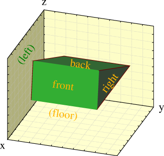
The designation of the surfaces is as follows:
The discretisation lengths can be set in several ways, see Example\ 4 for the SOLIDS command:
Discretisation lengths have to be given in cm.
[Default: the TARGET-ELEMENT-SIZE that is in effect at the time the solids are read.]
Format:
SPHERE  CENTRE cx cy cz ...
        RADIUS r ...
        [VOLTAGE v] ...
        [FLOATING-CONDUCTOR] ...
        [CHARGE q] ...
        [EPSILON eps] ...
        [material] ...
        [LABEL label] ...
        [N n]
        [DISCRETISATION discretisation] ...
Illustration:
A sphere with 50 by 50 panels, shown with a colour table of 50 elements.
[No default.]
[No default.]
The charge is added to the surface charges needed to satisfy the boundary conditions. The sphere can either be a dielectric or a conductor.
In the process of being implemented - initially, the charge is equally distributed over all surfaces, selection of surface panels is planned to be added later.
Specifying this option implies the use of neBEM to solve the field.
Specifying this option implies the use of neBEM to solve the field.
In the process of being implemented.
Specifying this option implies the use of neBEM to solve the field.
Specifying this option implies the use of neBEM to solve the field.
| Type | Representation | Notes |
|---|---|---|
CONDUCTOR |
CONDUCTORS-1 |
Equivalent to CONDUCTOR-1 |
CONDUCTOR-1 |
CONDUCTORS-1 |
- |
CONDUCTOR-2 |
CONDUCTORS-2 |
- |
CONDUCTOR-3 |
CONDUCTORS-3 |
- |
DIELECTRICUM |
DIELECTRICA-1 |
Equivalent to DIELECTRICUM-1 |
DIELECTRICUM-1 |
DIELECTRICA-1 |
- |
DIELECTRICUM-2 |
DIELECTRICA-2 |
- |
DIELECTRICUM-3 |
DIELECTRICA-3 |
- |
[Default: CONDUCTOR]
N must be equal to, or larger than, 3.
[By default, N is chosen in function of the size occupied by the sphere in the drawing. If you decide to specify N manually, then the that setting will be used no matter how large or small the sphere appears in the drawing.]
This label serves the same purpose as the wire label for wires, namely the selection of the solid as a place where signals can be measured, around which isochrons are drawn etc.
[By default, no label is assigned.]
Garfield generates, for each solid, a set of panels that together cover the faces. These panels, arbitrary convex polygons, are sub-divided when isolating contact areas between solids and also in order to comply with the neBEM requirement that it be given only rectangles and right-angled triangles. The triangles and rectangles handed to neBEM are called "primitives".
For reasons of accuracy neBEM as a rule sub-divides the primitives into "elements", in a process called "discretisation". The sub-divisions of the primitives are called "elements".
Discretisation will perhaps eventually be automated, but for the time being this remains the responsability of the user. In neBEM, the level of discretisation requested is described by 2 integers: the number of elements that is to be generated along each of 2 sides adjacent to a right angle. Since the shape, orientation and size of the primitives are non-trivial to predict, the level of discretisation is specified on the Garfield side as the desired length of the sides of the elements.
All panels covering the sphere are subject to the same discretisation.
The discretisation lengths can be set in several ways, see Example\ 4 for the SOLIDS command:
Discretisation lengths have to be given in cm. [Default: the TARGET-ELEMENT-SIZE that is in effect at the time the solids are read.]
These are to be used if the cell contains wires that are non-parallel or short compared to their length. If the cell can be described in terms rows of long and parallel wires, planes, a tube and periodicity, then it is preferable to do so.
Wire solids are treated as cylinders for most purposes, but neBEM handles them as charges distributed along the axis in such a manner that the surface is at the specified potential. This is equivalent to the thin-wire approximation used for wire and plane cells. This approach makes more efficient use of the elements than a solid cylinder in case the radius of the cylinder is small compared to its length and to the distance to other electrodes. A CYLINDER should be used if these conditions are not fulfilled.
Wires are always conductors.
Mandatory parameters are the location of the centre, the radius and the length. The direction defaults to the z-axis.
Format:
WIRE  CENTRE cx cy cz ...
      RADIUS r ...
      HALF-LENGTH lz ...
      [DIRECTION dx dy dz] ...
      [VOLTAGE v] ...
      [FLOATING-CONDUCTOR] ...
      [material] ...
      [LABEL label] ...
      [DISCRETISATION discretisation]
Example: Two perpendicular wires cross each other at a distance of 1\ mm.
&CELL
nebem target-element-size 0.01 maximum-elements 100
solids
wire centre      0      0   -0.05 ...
     half-length 1 ...
     radius      0.0100 ...
     direction   1      0    0 ...
     voltage    -1
wire centre      0      0   +0.05 ...
     half-length 1 ...
     radius      0.0100 ...
     direction   0      1    0 ...
     voltage    +1

&FIELD
area -0.25 -0.25 -0.25 0.25 0.25 0.25 view z=0
grid 50
plot-field surface e

area -1.2 -1.2 -1.2 1.2 1.2 1.2 view z=0
plot-field surface e

track -1 0.010001 -0.05   1 0.010001 -0.05
plot-field graph v range -1.01 -0.99
The first plot (reproduced below), like the second, shows how the field increases in the
area where the wires are nearest to each other. The third plot verifies the boundary condition.
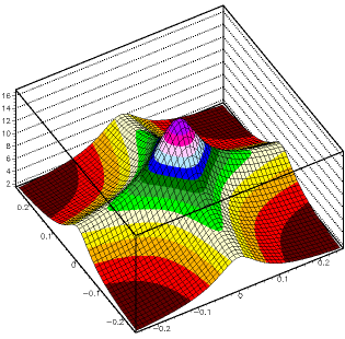
[No default.]
[No default.]
[No default.]
The normalisation of the vector is not used. Zero-norm vectors are not acceptable.
[By default, the central axis is aligned with the z-axis.]
Specifying this option implies the use of neBEM to solve the field.
In the process of being implemented.
Specifying this option implies the use of neBEM to solve the field.
| Type | Representation | Notes |
|---|---|---|
CONDUCTOR |
CONDUCTORS-1 |
Equivalent to CONDUCTOR-1 |
CONDUCTOR-1 |
CONDUCTORS-1 |
- |
CONDUCTOR-2 |
CONDUCTORS-2 |
- |
CONDUCTOR-3 |
CONDUCTORS-3 |
- |
[Default: CONDUCTOR]
This label serves the same purpose as the wire label for wires, namely the selection of the solid as a place where signals can be measured, around which isochrons are drawn etc.
[By default, no label is assigned.]
Garfield generates for each wire a single primitive: the centre line of the wire. neBEM sub-divides this primitive into "elements", in a process called "discretisation". The sub-divisions of the primitives are called "elements".
Discretisation will perhaps eventually be automated, but for the time being this remains the responsability of the user who has to indicate the length of the desired elements.
The discretisation length has to be given in cm. Also the value AUTOMATIC is allowed, in which case the TARGET-ELEMENT-SIZE will be used that is in effect when the cell section is being left.
[Default: the TARGET-ELEMENT-SIZE that is in effect at the time the solids are read.]
The main difference between a cell described in polar coordinates with a plane at constant r and a tube with radius r, is that one can put a wire at the centre of a tube, but not at the centre of a cell with a circular plane.
With Tube coordinates, you enter the wire location in Cartesian coordinates which you can combine with a \φ periodicity in degrees. Periodicities in x or y are not permitted, nor are planes in any direction.
The potential function for a square tube is expensive to compute compared to the equivalent potential which is used for a cell that has 2 planes at constant x and 2 planes at constant y.
Format:
TUBE  [RADIUS r] ...
      [VOLTAGE v] ...
      [EDGES n] ...
      [LABEL label] ...
      [{PHI-STRIP | Z-STRIP} strip_min strip_max ...
         [GAP gap] [LABEL strip_label]]
Examples:
tube r=2, v=2000
tube hexagonal r=5
In the first example, a circular tube (EDGES is not specified, one could also have added CIRCLE or EDGES=0) is defined with a radius of 2\ cm and at a potential of 2000\ V. In the second example, the tube is hexagonal and with radius 5\ cm. This tube is grounded.
[No default is provided.]
[By default 0\ V.]
| Shape | EDGES | Synonyms |
|---|---|---|
| Cylinder | 0 | CIRCLE, CIRCULAR, CYLINDER, CYLINDRICAL |
| Triangle | 3 | TRIANGLE, TRIANGULAR |
| Square | 4 | SQUARE |
| Pentagon | 5 | PENTAGON, PENTAGONAL |
| Hexagon | 6 | HEXAGON, HEXAGONAL |
| Heptagon | 7 | HEPTAGON, HEPTAGONAL |
| Octagon | 8 | OCTAGON, OCTAGONAL |
Polygons with a larger number of edges can be made available on request.
A label is not mandatory, but signals induced in the tube are only computed if the tube can be selected, and this can only be done if the tube has a label.
[By default, no label is assigned.]
Two kinds of sub-divisions are permitted: radial sectors and slices along the z-axis.
The location should be indicated in degrees for radial sectors and in cm for slices in z.
[Mandatory parameter, no default provided.]
The location should be indicated in degrees for radial sectors and in cm for slices in z.
[Mandatory parameter, no default provided.]
The label is a single alphabetic upper case character. You may type a longer string, but only the first character will be stored.
A label is not mandatory, but signals induced in a strip are only computed if the strip can be selected, and this can only be done if the strip has a label.
[By default, no label is assigned to a strip.]
The gap is specified in cm for z-slices and in degrees for \φ-sectors.
[By default, this is taken to be the distance to the central wire, if there is one.]
Strips, if any, are shown with the STRIPS representation.
This command has effect only if issued after a FIELD-MAP or READ-FIELD-MAP command.
Formats for 2D and 3D field maps respectively:
WINDOW xmin ymin xmax ymax
WINDOW xmin ymin zmin xmax ymax zmax
Example:
&CELL
Global bin `gabriele.bin`
If exist(bin) Then
   read-field-map {bin}
Else
   field-map files "e.reg" "v.reg" keep-background maxwell-11 ...
      x-mirror-periodic y-mirror-periodic
   save-field-map {bin}
Endif
window -0.0070 -0.0035 -10 0.0070 0.0035 10
opt cell-print
Although written in plain text, this kind of dataset is not meant to be human-readable. Use the LAYOUT option to visualise a cell and CELL-PRINT to obtain a table of the wire locations, charges etc. Compact format cells should not be edited.
The format is chosen to enable a fast restore of wire data. This is useful for chambers which contain large numbers of wires (several 1000s). Otherwise, the overhead is not worth the loss in flexibility. The capacitance matrix is not stored in compact format cell datasets.
Field maps are, because of their large size, not saved by the WRITE statement. If reading them with the FIELD-MAP command takes too much time, and if the size of the full field maps is a point of concern, then consider using SAVE-FIELD-MAP and READ-FIELD-MAP, which perform a binary (i.e. non-portable) save and retrieve.
The writing operation takes place when the section is left, not when the WRITE command is issued. The statement can appear at any place in the cell section.
Compact format cell datasets are written in a machine independent format - files written on one type of computer can be read on other computers.
Format:
WRITE DATASET file [member] [REMARK remark]
Examples:
WR DATA cell.dat cell1 REM "Some cell"
WR cell.dat cell1 "Some cell"
(These two examples are equivalent, they show that the keywords DATA and REMARK are not needed if the parameters are in the right order.)
The field is left blank by default.
The cell and gas descriptions are not touched when you enter a magnetic field, but commands like MAGBOLTZ will try and calculate a sensible default B-field range and range of E-B angles if a magnetic field is entered beforehand.
[Initially, the magnetic field is off.]
The radial and angular components of the magnetic field must be zero if your cell has been entered in polar coordinates. Only the z component may be non-zero in this case.
Format:
COMPONENTS  {value_Bx | vector_Bx VS {X|Y|Z} = vector_x | formula_Bx} ...
            {value_By | vector_By VS {X|Y|Z} = vector_y | formula_By} ...
            {value_Bz | vector_Bz VS {X|Y|Z} = vector_z | formula_Bz} ...
            [GAUSS | OERSTED | TESLA | V.MICROSEC/CM2]
Examples:
comp 0 0 5000 G
A constant magnetic field of 5000\ G, or 0.5\ T, along the z-axis.
comp -y x 0
A toroidal field specified with 2\ formulae and 1\ constant value.
If this format is used for all 3\ components of the magnetic field, then the PERMEABILITY is taken into account.
The magnetic field component should have the form of a Number.
If this format is used for 1 or more components of the magnetic field, then the PERMEABILITY is not taken into account.
Both the field vector and the coordinate vector have to be in the form of a 1-dimensional Matrix. These 2\ vectors must have the same length.
When you issue the COMPONENTS command, a copy of the vectors is made. You may therefore change the vectors afterwards - changes to the vectors do not, however, affect the magnetic field.
If this format is used for 1 or more components of the magnetic field, then the PERMEABILITY is not taken into account.
Components of the magnetic field that use this format should have the form of a String which uses the variables X, Y and Z when Cartesian coordinates are used, and R, PHI and Z when the cell is described in polar coordinates.
You have to express all components in the same unit, even if you use different formats.
You have to use this unit in calls to the various procedures which take magnetic fields as arguments, such as MAGNETIC_FIELD or DRIFT_VELOCITY.
The default unit for the COMPONENTS statement is the Tesla, if you wish to use other units, then you have to specify this.
The permeability is taken into account only in case all 3 COMPONENTS of the magnetic field have been entered as a constant value.
Format:
PERMEABILITY perm_wire perm_gas
Example:
PERM 1 0
Some of these properties can be computed: the Magboltz program will calculate the electron drift velocity, diffusion, Townsend and attachment coefficient for nearly arbitrary gas mixtures. The Heed program takes care of clustering, also for nearly arbitrary gas mixtures.
If you have measured gas properties, or have access to measurements you trust, you can enter this data in the form of tables. One can also replace parts of the Magboltz tables with measurements.
For rapid studies which do not require great accuracy, descriptions of a few common gas mixtures are built in to the program.
All existing gas information is cleared by entering the gas section.
Format:
&GAS
A couple of instructions can be used regardless of the origin.
Gas mixture prepared during the run:
| Command | Short description |
|---|---|
ADD |
Adds/replaces elements of the transport table |
CLUSTER |
Enters the cluster size distribution |
EXTRAPOLATIONS |
Extrapolation of the gas tables |
HEED |
Prepares cluster generation by Heed |
INTERPOLATIONS |
Interpolation method in the gas tables |
MAGBOLTZ |
Magboltz gas mixture (accurate) |
MIX |
Schultz-Gresser gas mixing (approximate) |
PARAMETERS |
Molecular parameters of the gas mixture |
PRESSURE |
Sets the pressure |
TEMPERATURE |
Sets the temperature |
WRITE |
Stores the gas description |
User specified gas mixture:
| Command | Short description |
|---|---|
ADD |
Adds/replaces elements of the transport table |
CLUSTER |
Enters the cluster size distribution |
EXTRAPOLATIONS |
Extrapolation of the gas tables |
GAS-IDENTIFIER |
Adds a label to the gas description |
INTERPOLATIONS |
Interpolation method in the gas tables |
PARAMETERS |
Molecular parameters of the gas mixture |
PRESSURE |
Sets the pressure |
RESET |
Erases gas data entered sofar |
TABLE |
Enters the gas tables |
TEMPERATURE |
Sets the temperature |
WRITE |
Stores the gas description |
Historically, Garfield contains a number of experiment-based gas tables. They remain available for backwards compatibility, but their use is not recommended for new applications:
| Command | Short description |
|---|---|
ARGON-20-ETHANE-80 |
Loads the mixture argon 20\ %, ethane 80\ % |
ARGON-50-ETHANE-50 |
Loads the mixture argon 50\ %, ethane 50\ % |
ARGON-80-ETHANE-20 |
Loads the mixture argon 80\ %, ethane 20\ % |
ARGON-73-METH-20-PROP-7 |
Loads argon 73\ %, CH\<SUB\>4\</SUB\> 20\ %, propanol 7\ % |
CO2 |
Loads data for almost pure CO\<SUB\>2\</SUB\> |
CO2-80-ETHANE-20 |
Loads the mixture CO\<SUB\>2\</SUB\> 80\ %, ethane 20\ % |
CO2-90-ETHANE-10 |
Loads the mixture CO\<SUB\>2\</SUB\> 90\ %, ethane 10\ % |
CO2-90-ISOBUTANE-10 |
Loads the mixture CO\<SUB\>2\</SUB\> 90\ %, isobutane 10\ % |
ETHANE |
Loads data for pure ethane |
ISOBUTANE |
Loads data for pure isobutane |
METHANE |
Loads data for pure methane |
Retrieval of a gas description previously stored:
| Command | Short description |
|---|---|
GET |
Retrieves gas data from a dataset |
General purpose instructions:
| Command | Short description |
|---|---|
OPTIONS |
Plotting and printing of the gas tables |
PLOT-OPTIONS |
Selects plots, sets ranges and log/lin axes |
For new applications, consider using HEED for ionisation of gas mixtures due to charged particles, MAGBOLTZ for the electron transport properties, and ADD to add ion mobility data, e.g. from the H.W. Ellis et al. papers.
Example:
ARG-50-ETH-50
(Until further notice, the program will use 50\ % argon, 50\ % ethane.)
This command is provided mainly for reasons of backwards compatibility. For new applications, consider using HEED for ionisation of gas mixtures due to charged particles, MAGBOLTZ for the electron transport properties, and ADD to add ion mobility data, e.g. from the H.W. Ellis et al. papers.
Source: Drift velocities taken from Jean-Marie et. al. (1979), diffusion from Ramanantsizehena (1979). Mobility and most probable energy loss are questionable. Supplied by Matthias Grosse Perdekamp (Freiburg, Germany).
This command is provided mainly for reasons of backwards compatibility. For new applications, consider using HEED for ionisation of gas mixtures due to charged particles, MAGBOLTZ for the electron transport properties, and ADD to add ion mobility data, e.g. from the H.W. Ellis et al. papers.
Source: Supplied by Manfred Guckes (transport properties) and Giorgio Sartori and Michela Giavedoni (Padova, parameters part).
This command is provided mainly for reasons of backwards compatibility. For new applications, consider using HEED for ionisation of gas mixtures due to charged particles, MAGBOLTZ for the electron transport properties, and ADD to add ion mobility data, e.g. from the H.W. Ellis et al. papers.
Source: Drift velocities taken from Jean-Marie et al. (1979), diffusion from Ramanantsizehena (1979). Mobility and most probable energy loss are questionable. Supplied by Matthias Grosse Perdekamp (Freiburg, Germany)
This command is provided mainly for reasons of backwards compatibility. For new applications, consider using HEED for ionisation of gas mixtures due to charged particles, MAGBOLTZ for the electron transport properties, and ADD to add ion mobility data, e.g. from the H.W. Ellis et al. papers.
Source: Drift velocities and diffusion from F. Piuz Cern-EF 82-11 and Fehlmann et. al. (1983). Clustering parameters with large, unknown errors. Supplied by Matthias Grosse Perdekamp (Freiburg).
This command is provided mainly for reasons of backwards compatibility. For new applications, consider using HEED for ionisation of gas mixtures due to charged particles, MAGBOLTZ for the electron transport properties, and ADD to add ion mobility data, e.g. from the H.W. Ellis et al. papers.
Source: Karl Dederichs and Fran\çois Piuz (drift velocity and diffusion) and Fran\çois Rohrbach (multiplication).
This command is provided mainly for reasons of backwards compatibility. For new applications, consider using HEED for ionisation of gas mixtures due to charged particles, MAGBOLTZ for the electron transport properties, and ADD to add ion mobility data, e.g. from the H.W. Ellis et al. papers.
Source: Data supplied by Diego Bettoni.
This command is provided mainly for reasons of backwards compatibility. For new applications, consider using HEED for ionisation of gas mixtures due to charged particles, MAGBOLTZ for the electron transport properties, and ADD to add ion mobility data, e.g. from the H.W. Ellis et al. papers.
Source: Data supplied by Diego Bettoni and Reyad Sawafti.
This command is provided mainly for reasons of backwards compatibility. For new applications, consider using HEED for ionisation of gas mixtures due to charged particles, MAGBOLTZ for the electron transport properties, and ADD to add ion mobility data, e.g. from the H.W. Ellis et al. papers.
Source: Data supplied Manfred Guckes (transport properties) and Helmut Boettcher (clustering properties).
This command is provided mainly for reasons of backwards compatibility. For new applications, consider using HEED for ionisation of gas mixtures due to charged particles, MAGBOLTZ for the electron transport properties, and ADD to add ion mobility data, e.g. from the H.W. Ellis et al. papers.
Source: Supplied by Ingo Herbst.
This command is provided mainly for reasons of backwards compatibility. For new applications, consider using HEED for ionisation of gas mixtures due to charged particles, MAGBOLTZ for the electron transport properties, and ADD to add ion mobility data, e.g. from the H.W. Ellis et al. papers.
Source: Supplied by Emile Schmoetter. Clustering properties from Helmut Boettcher.
This command is provided mainly for reasons of backwards compatibility. For new applications, consider using HEED for ionisation of gas mixtures due to charged particles, MAGBOLTZ for the electron transport properties, and ADD to add ion mobility data, e.g. from the H.W. Ellis et al. papers.
Source: Ingo Herbst, for the drift velocity and the diffusion and from "Basic data of plasma physics, 1966", Sanborn C. Brown.
The ADD command has 2 formats:
Beware that the WRITE command executes only when the section is left. Therefore, if you modify Magboltz computed gas tables with the ADD command, the modified tables will be written - not the original Magboltz data, no matter where you place the WRITE and ADD statements,
REPLACE is a synonym for ADD. The MERGE command should be used if you wish to combine the existing gas data with data from a gas file.
Format:
ADD  item_1 { function_1 | value_1 VS ep_1 [ORDER order_1] } ...
     item_2 { function_2 | value_2 VS ep_2 [ORDER order_2] } ...
     ...
Example:
Global pbar = 3 magboltz argon 91 nitrogen 4 methane 5 ... e/p-range 0.05 135 Vector E_Ar_Ar K_Ar_Ar 0 1.53 8 1.53 10 1.53 12 1.53 15 1.52 20 1.51 25 1.49 30 1.47 40 1.44 50 1.41 60 1.38 80 1.32 100 1.27 120 1.22 150 1.16 200 1.06 250 0.99 300 0.95 400 0.85 500 0.78 600 0.72 800 0.63 1000 0.56 1200 0.51 1500 0.46 2000 0.40Global E_Ar_Ar = E_Ar_Ar/(0.010354*300) Global K_Ar_Ar = K_Ar_Ar*1e-6/pbar add ion-mobility K_Ar_Ar vs E_Ar_Ar extrapolations low-ion-mobility constant high-ion-mobility linear
Magboltz is used to generate an electron transport table. This also sets the E/p scale.
Next, a file is read in that contains mobilities as function of E/N for Ar\<SUP\>+\</SUP\> ions in Ar at a pressure of 1 atm. The data is taken from the literature, in this case Hornbeck '51 and Beaty '68 (for an extensive compilation consult the H. W. Ellis et al. papers). The E/N values are stored in the matrix E_Ar_Ar, while the mobilities are kept in K_Ar_Ar.
The E/N vector is transformed to E/p. The mobility is divided by the pressure, and its units are changed from cm\²/sec.V to cm\²/\μsec.V.
Finally, the mobility is added to the gas tables using the ADD statement.
References:
| Item | Explanation | Unit |
|---|---|---|
ATTACHMENT-COEFFICIENT |
Attachment coefficient/pressure | 1/cm.Torr |
DRIFT-VELOCITY |
Drift velocity | cm/\μsec |
ION-DISSOCIATION |
Ion dissociation coefficient | 1/cm.Torr |
ION-MOBILITY |
Ion mobility | cm\²/\μsec.V |
LONGITUDINAL-DIFFUSION |
Longitudinal diffusion \√p | cm.\√Torr for 1\ cm |
LORENTZ-ANGLE |
Lorentz angle | degrees |
TOWNSEND-COEFFICIENT |
Townsend coefficient/pressure | 1/cm.Torr |
TRANSVERSE-DIFFUSION |
Transverse diffusion \√p | cm.\√Torr for 1\ cm |
Note that the same scalings have to be applied as for the TABLE.
| Variable | Meaning | Unit |
|---|---|---|
ANGLE_EB |
Angle between E and B | degrees |
ATTACHMENT |
Attachment coefficient / p | 1/cm.Torr |
B |
Magnetic field strength | Tesla |
BOLTZMANN |
Boltzmann constant | 1.380658 10\<SUP\>-23\</SUP\> J/K |
DISS |
Ion dissociation coefficient | 1/cm.Torr |
ECHARGE |
Electron charge | 1.60217733 10\<SUP\>-19\</SUP\> C |
EP |
Electric field / p | V/cm.Torr |
LORENTZ |
Lorentz angle | degrees |
MOBILITY |
Ion mobility | cm\²/\μsec.V |
P |
Pressure | Torr |
SIGMA_L |
Longitudinal diffusion \√ p | cm.\√Torr for 1\ cm |
SIGMA_T |
Transverse diffusion \√p | cm.\√Torr for 1\ cm |
T |
Temperature | K |
TOWNSEND |
Townsend coefficient / p | 1/cm.Torr |
VELOCITY |
Electron drift velocity | cm/\μsec |
The variable EP can always be used, ANGLE_EB and B can only be used in tables prepared for magnetic fields. The transport properties can be used only insofar as they have been entered already.
The E/p vector should in principle cover the entire range of the table. Values outside the range of the E/p vector are left untouched - no attempt is made to extrapolate. Since most items are initialised to values outside their permissible range, an error will in general be reported from the checks that are carried out while leaving the gas section. To avoid this, one can first set the item with an approximate function and then override in part with more precise values. This is illustrated here for He\<SUP\>+\</SUP\> in He:
// Experimental data Vector E_He_He K_He_He 0 10.5 6 10.3 8 10.2 10 10.2 12 10.1 15 10.0 20 9.90 25 9.74 30 9.60 40 9.28 50 8.97 60 8.67 80 8.12 100 7.67 120 7.25 150 6.78 200 6.12 250 5.60 300 5.19 400 4.58 500 4.17 600 3.81 700 3.57// Scaling from Td to V/cm.Torr and from V/cm\².sec to V/cm\².\μsec Global E_He_He = E_He_He/(0.010354*300) Global K_He_He = K_He_He*1e-6 // Fit an exponential to the shape Call fit_exponential(E_He_He,K_He_He,1e-8,p0,p1,p2,p3,ep0,ep1,ep2,ep3) // Provisionally set the mobility to the exponential function add ion-mobility exp({p0}+{p1}*ep+{p2}*ep^2+{p3}*ep^3) // Override the values that are in the range add ion-mobility K_He_He vs E_He_He
The E/p values in your vector do not have to coincide with the E/p values present in the table - your vectors will be interpolated at the values of the table and these interpolations are stored instead of the values from the vector.
When the data is smooth, a value of 2 (quadratic interpolation) is a good choice. This may however lead to intermediate points with a negative value in for instance Townsend coefficient tables that usually start at 0. For such tables, linear interpolation is advised.
Instead of ORDER 1, you may also type LINEAR. QUADRATIC is a synonym for ORDER 2, CUBIC for ORDER 3.
The cluster size distribution is not by itself enough to generate clusters along a track. The EXPONENTIAL-SPACING clustering model which uses the distribution entered here, also needs to know the mean number of clusters per cm.
If you use the HEED interface, then you neither need to enter a cluster size distribution nor the cluster spacing. Entering a cluster size distribution and initialising Heed is however allowed. It is only at the TRACK level that you decide which clustering model you are going to use.
In the areas between absorption shells, the distribution usually follows simple power laws, but the shell structure is in general not something which can be neglected.
Format:
CLUSTER FUNCTION cluster_function [N nmax]
Example:
cluster function 1/n^3 n 15
Doing this will produce a warning since, to compute probability to have a cluster size of 0, one would divide by zero.
This function will be evaluated between N=0 to N=nmax-1 at integer and half-integer values.
The cluster size distribution starts at a size of 0, not 1. The reason for this is that most interactions between charged particles and gas molecules result in excitation, rather than ionisation. In the absence of Penning transfers, these interactions will not lead to ionisation electrons. In case you enter a cluster spacing which only takes ionisations, and not excitations, into account, then you have to set the probability at N=0 to 0. This can most easily be done using the Mixed format.
Samples are taken at N, N+0.5 and N+1 and the probability that is assigned for a cluster size of N is the Simpson integral over these 3 points. The rationale for this approach is that it is anticipated that an energy transfer probability divided by work will be entered, so that the derived cluster size is the ratio truncated to the next lower integer, rather than the ratio rounded to the nearest integer.
You don't have to worry about the normalisation.
[There is no default function.]
Values between 1 and MXPAIR are permitted.
If set to 1, then only clusters of size 0 will ge generated. I.e. not a single ionisation electron will be produced.
[Default is MXPAIR, set to 2000 at the time of writing.]
Please note that the first number is the probability to have a cluster size of 0, i.e. a cluster without ionisation electrons. When a charged particle traverses a gas, most interactions result only in excitation, not in ionisation. If you set a mean number of clusters per cm which only takes clusters into account that contain at least 1 electron, then you have to set the first probability to 0.
Format:
CLUSTER
prob_size0 prob_size1
...
(blank line)
Example:
CLUSTER 0 0 0.1 0.2 0.5 0.2 0.1 0// Note that the preceding line is left blank
Format:
CLUSTER FUNCTION cluster_function [N nmax] OVERLAP-TABLE-AND-FUNCTION
prob_size0 prob_size1
...
(blank line)
Example:
CLUSTER FUNCTION 21.6/N^2 N=200 OVERLAP
0 86 20 10
There has to be a blank line after the cluster sizes. One can also simulate this format by using a Do loop:
cluster
0 86 20 10
For i From 4 To 200 Do
   {21.6/i^2}
Enddo

// Note that the previous line is left blank !
But this would be less efficient since the formula inside the loop (21.6/i^2) is translated each iteration of the loop. Note that there has to be a blank line after Enddo.
A more efficient version of the latter would be:
cluster
0 86 20 10 {21.6/row(200)^2}

// Note that the previous line is blank !
The composition is set by the MAGBOLTZ command and is preserved in gas files (written by WRITE and read with GET). There is therefore no need to use the COMPOSITION command when running Magboltz nor when retrieving Magboltz generated electron transport tables.
The information supplied by this command is only used by the microscopic electron tracking procedures such as DRIFT_MICROSCOPIC_ELECTRON and MICROSCOPIC_AVALANCHE.
This command does not provide the electron transport tables needed by the other electron tracking methods. You will therefore, in general, have to provide electron transport tables (e.g. using TABLE) when using the COMPOSITION statement.
All fractions must be strictly positive. The fractions may add up to any non-zero value - they will be normalised by Magboltz.
Format: see MAGBOLTZ
Example:
composition argon 80 co2 20This will set the gas composition to 80\ % Ar and 20\ % CO\<SUB\>2\</SUB\>.
The EXTRAPOLATIONS command has no effect on extrapolation in 2-dimensional tables, such as those produced by Magboltz when the B field is non-zero. For such tables, polynomial extrapolation is performed with the order set with the INTERPOLATIONS command.
EXTRAPOLATE can be used as synonym for this command.
Format:
EXTRAPOLATIONS item1 method1 item2 method2 ...
Examples:
extrapolate drift: linear, diff: const, town: const
extrapolate drift exp
| Item | Description |
|---|---|
[HIGH-]ATTACHMENT-COEFFICIENT |
Attachment coefficient beyond highest E/p |
[HIGH-]DIFFUSION-TENSOR |
Diffusion tensor beyond the highest E/p |
[HIGH-]DISSOCIATION |
Ion dissociation beyond the highest E/p |
[HIGH-]DRIFT-VELOCITY |
Drift velocity beyond the highest E/p |
[HIGH-]EXCITATION-RATES |
Excitation rates beyond the highest E/p |
[HIGH-]ION-MOBILITY |
Ion mobility beyond the highest E/p |
[HIGH-]IONISATION-RATES |
Ionisation rates beyond the highest E/p |
[HIGH-]LONGITUDINAL-DIFFUSION |
Long. diffusion beyond the highest E/p |
[HIGH-]LORENTZ-ANGLE |
Lorentz angle beyond the highest E/p |
[HIGH-]TOWNSEND-COEFFICIENT |
Townsend coefficient beyond highest E/p |
[HIGH-]TRANSVERSE-DIFFUSION |
Transv. diffusion beyond the highest E/p |
LOW-ATTACHMENT-COEFFICIENT |
Attachment coefficient below first E/p |
LOW-DIFFUSION-TENSOR |
Diffusion tensor below the first E/p |
LOW-DISSOCIATION |
Ion dissociation below the first E/p |
LOW-DRIFT-VELOCITY |
Drift velocity below the first E/p |
LOW-EXCITATION-RATES |
Excitation rates below the highest E/p |
LOW-ION-MOBILITY |
Ion mobility below the first E/p |
LOW-IONISATION-RATES |
Ionisation rates below the highest E/p |
LOW-LONGITUDINAL-DIFFUSION |
Long. diffusion below the first E/p |
LOW-LORENTZ-ANGLE |
Lorentz angle below the first E/p |
LOW-TOWNSEND-COEFFICIENT |
Townsend coefficient below first E/p |
LOW-TRANSVERSE-DIFFUSION |
Transv. diffusion below the first E/p |
The prefix HIGH- is optional for backwards compatibility. DIFFUSION can be used instead of LONGITUDINAL-DIFFUSION.
Constant extrapolation means values for any E/p outside the range of the table are set to the value for the first or last E/p in the table, as appropriate.
In the case of linear and exponential extrapolation the first or last two table points are used as basis for the extrapolation.
The MAGBOLTZ and MIX commands set an identification string that contains a description of the gas mixture. It is advisable not to override this string. Instead, one can use the GET_GAS_DATA procedure to obtain the identifier set by these commands, and then add further information to it.
The identification string is displayed in the plots using the COMMENT text representation.
Format:
GAS-IDENTIFIER string
Examples:
GAS-ID "Some gas"
Sets a simple identification string.
temperature 300 K magboltz argon 50 dme 50 *** Ar++ in Ar, T=300 K, error 1 % (Mason McDaniel I, Beaty 68) Vector E_Ar_Ar_2 K_Ar_Ar_2 40 2.49 50 2.47 60 2.45 70 2.42 80 2.39 90 2.37 100 2.34 120 2.28 140 2.23 160 2.19 180 2.15 200 2.11Call get_gas_data(p,t,gasid) Global E_Ar_Ar_2 = p*E_Ar_Ar_2/(0.010354*t) Global K_Ar_Ar_2 = K_Ar_Ar_2*1e-6 add ion-mobility K_Ar_Ar_2 vs E_Ar_Ar_2 extrapolations low-ion-mobility constant high-ion-mobility linear gas-id "{gasid} with Ar<SUP>++</SUP>"
Magboltz is used to compute electron transport properties, and these are complemented with experimental Ar mobility at the same temperature and pressure. The addition is registered in the gas identifier.
The compact gas description contains electron transport property tables, the ion mobility, cluster size and cluster spacing data, Heed initialisation information, SRIM energy loss, range and straggling tables, the pressure and the temperature. GET overwrites all of these.
Since format version\ 8, an attempt has been made to maintain backwards compatibility of file formats. Beware however that older formats will as a rule not contain as much information as the newer versions, which may result in the failure of certain newer commands.
Format:
GET file [member]
Example:
GET gas_data.dat gas2
The TEMPERATURE and the PRESSURE should be specified before issuing the HEED command. Defaults are assumed if they follow the HEED command.
Neither temperature nor pressure scaling is applied to the cluster information provided by HEED.
The author of Heed, Igor Smirnov, should be contacted for further information about this program.
Format:
HEED  [ HYDROGEN  fraction ]   [ HELIUM-4  fraction ] ...
      [ NEON  fraction ]       [ ARGON  fraction ] ...
      [ KRYPTON  fraction ]    [ XENON  fraction ] ...

      [ NITROGEN  fraction ]   [ OXYGEN  fraction ] ...

      [ METHANE   fraction ]   [ ETHANE  fraction ] ...
      [ ETHENE  fraction ]     [ ACETYLENE  fraction ]  ...
      [ PROPANE  fraction ]    [ ISOBUTANE  fraction ] ...
      [ NEOPENTANE  fraction ] ...

      [ WATER  fraction ]      [ CO2  fraction ] ...
      [ DME  fraction ]        [ NITROUS-OXIDE  fraction ] ...
      [ AMMONIA  fraction ]    [ SF6 fraction ] ...
      [ CS2 fraction ] ...

      [ CF4  fraction ]        [ C2F4H2  fraction ] ...
      [ C2F5H  fraction ]      [ C3F8 fraction ]
Example:
pressure {3*760}
Heed argon 50 ethane 50
(If you have a 3\ atm 50/50 argon-ethane mixture in your chamber.)
By default, the gas tables are interpolated using quadratic Newton polynomials. Use this statement if you wish to select splines, lower order polynomials or higher order polynomials.
The interpolation method is ignored if the gas table contains only a single electric field strength.
INTERPOLATE can be used as a synonym for this command.
Format:
INTERPOLATIONS item1 method1 item2 method2 ...
Examples:
interpolate drift-velocity newton 2, long-diffusion newton 1
int townsend spline
| Keyword | Meaning |
|---|---|
ATTACHMENT-COEFFICIENT |
Attachment coefficient of electrons |
DIFFUSION-TENSOR |
Diffusion tensor components |
DRIFT-VELOCITY |
Electron drift velocity |
EXCITATION-RATES |
Individual gas excitation rates |
ION-DISSOCIATION |
Ion dissociation coefficient |
ION-MOBILITY |
Ion mobility |
IONISATION-RATES |
Individual gas excitation rates |
LONGITUDINAL-DIFFUSION |
Longitudinal diffusion of electrons |
LORENTZ-ANGLE |
Lorentz angle of electrons |
TOWNSEND-COEFFICIENT |
Townsend coefficient of electrons |
TRANSVERSE-DIFFUSION |
Transverse diffusion of electrons |
Spline interpolation leads to smooth looking graphs, but tends to oscillate making the method less suited for numerical calculations. Spline interpolation can not be used on the 2-dimensional gas tables that are produced by programs like Magboltz when a magnetic field is present.
The order of polynomial interpolation must be between 1 and the smallest of the two numbers: 10 and number of table entries - 1. Orders larger than 2 are not recommended.
Formats:
INTERPOLATIONS item SPLINES
INTERPOLATIONS item NEWTON order
| Method | Effect | Use |
|---|---|---|
SPLINES |
Cubic spline interpolation | only 1-D |
NEWTON n |
Polynomial interpolation of order n | 1-D or 2-D |
LINEAR |
Linear interpolation (= NEWTON 1) | 1-D or 2-D |
QUADRATIC |
Parabolic interpolation (=NEWTON 2) | 1-D or 2-D |
CUBIC |
Cubic interpolation (=NEWTON 3) | 1-D or 2-D |
Contrary to the related MIX instruction, Magboltz takes cross sections for non-elastic processes into account. Furthermore, Magboltz is not limited to the 0th and 1st order terms of the spherical harmonics expansion used by MIX. Magboltz does need considerably more calculation time.
In Garfield up to version\ 8, this command gave access to both version\ 1 and version\ 2 of Magboltz. These programs differed by the integration technique use: ANALYTIC-INTEGRATION for version\ 1 and MONTE-CARLO-INTEGRATION for version\ 2. Version\ 1 was to be preferred for pure noble gases and mixtures of exclusively noble gases, without addition of quenchers or other additives. Version\ 2, which became default, was recommended for all other pure gases and for all gas mixtures. Even though these older versions of Magboltz did compute the Townsend and attachment coefficients, one used the Imonte program (from the same author) to compute these with better precision.
From Garfield version\ 9 on, Magboltz version\ 7 and higher is called. This Magboltz version only does Monte Carlo integration. It can be used for gas mixtures both with and without quenchers, even if the program will be slow for the latter. Magboltz version\ 7 includes the Imonte functionality - which is therefore no longer needed.
Since Magboltz takes the magnetic field into account to compute the transport properties, the &MAGNETIC section should precede the gas section. If there is a magnetic field, the program computes a drift velocity vector, otherwise a scalar.
Likewise, TEMPERATURE and PRESSURE statements should be issued before invoking Magboltz. If the temperature has not been specified when Magboltz runs, then a default temperature of 300\ K will be assumed. No scaling will be applied if the temperature is changed later on. The default pressure is 760\ Torr. The transport properties will be scaled according to simple scaling laws if the pressure is modified after the transport properties have been computed. It is not recommended, however, to rely on these scaling laws since these are very approximate.
The author of Magboltz, Steve Biagi, should be contacted for further information about this program.
Format:
MAGBOLTZ [ HYDROGEN frac ] ...
         [ DEUTERIUM frac ] ...
         [ HELIUM-3-ANISOTROPIC frac ] ...
         [ HELIUM-3-ISOTROPIC frac ] ...
         [ HELIUM-4-ANISOTROPIC frac ] ...
         [ HELIUM-4-ISOTROPIC frac ] ...
         [ NEON-ANISOTROPIC frac ] ...
         [ NEON-ISOTROPIC frac ] ...
         [ ARGON-ANISOTROPIC frac ] ...
         [ ARGON-ISOTROPIC frac ] ...
         [ KRYPTON-ANISOTROPIC frac ] ...
         [ KRYPTON-ISOTROPIC frac ] ...
         [ XENON-ANISOTROPIC frac ] ...
         [ XENON-ISOTROPIC frac ] ...
         [ NITROGEN-ANISOTROPIC frac ] ...
         [ NITROGEN-ISOTROPIC frac ] ...
         [ OXYGEN frac ] ...
         [ OZONE frac ] ...
         [ FLUORINE frac ] ...
         [ CAESIUM frac ] ...
         [ MERCURY frac ] ...
         [ METHANE frac ] ...
         [ DEUTERATED-METHANE frac ] ...
         [ ETHANE frac ] ...
         [ ETHENE frac ] ...
         [ ACETYLENE frac ] ...
         [ PROPANE frac ] ...
         [ CYCLOPROPANE frac ] ...
         [ PROPENE frac ] ...
         [ ISOBUTANE frac ] ...
         [ N-BUTANE frac ] ...
         [ NEOPENTANE frac ] ...
         [ N-PENTANE frac ] ...
         [ METHANOL frac ] ...
         [ ETHANOL frac ] ...
         [ PROPANOL frac ] ...
         [ CARBON-MONOXIDE frac ] ...
         [ CARBON-DIOXIDE frac ] ...
         [ WATER frac ] ...
         [ NITRIC-OXIDE frac ] ...
         [ NITROUS-OXIDE frac ] ...
         [ METHYLAL frac ] ...
         [ DME frac ] ...
         [ TRIFLUOROMETHANE frac ] ...
         [ TRIFLUOROBROMOMETHANE frac ] ...
         [ TETRAFLUOROMETHANE frac ] ...
         [ TETRAFLUOROETHANE frac ] ...
         [ HEXAFLUOROETHANE frac ] ...
         [ OCTAFLUOROPROPANE frac ] ...
         [ BORON-TRIFLUORIDE frac ] ...
         [ SULPHUR-HEXAFLUORIDE frac ] ...
         [ AMMONIA frac ] ...
         [ CARBON-DISULPHIDE frac ] ...
         [ CARBONYL-SULPHIDE frac ] ...
         [ HYDROGEN-SULPHIDE frac ] ...
         [ GERMANE frac ] ...
         [ SILANE frac ] ...
         [ REID-STEP frac ] ...
         [ MAXWELL-MODEL frac ] ...
         [ REID-RAMP frac ] ...


         [ [ ELECTRIC-FIELD-RANGE emin emax ] ...
              [ N-E ne ] ...
              [ LINEAR-E-SCALE | LOGARITHMIC-E-SCALE ] | ...
           [ ELECTRIC-FIELD {efield1 efield2 ... | vector} ] ] ...
         [ [ ANGLE-RANGE amin amax ] [ N-ANGLE nangle ] | ...
           [ ANGLE {angle1 angle2 ... | vector} ] ] ...
         [ [ B-FIELD-RANGE bmin bmax ] [ N-B nb ] | ...
           [ B-FIELD {bfield1 bfield2 ... | vector} ] ] ...

         [ NOPLOT-DISTRIBUTION-FUNCTIONS | PLOT-DISTRIBUTION-FUNCTIONS ] ...
         [ NOPLOT-CROSS-SECTIONS | PLOT-CROSS-SECTIONS ] ...
         [ NOKEEP | KEEP ] ...
         [ NOPRINT | PRINT ]

         [ ANALYTIC-INTEGRATION ...
            [ SECOND-ORDER-TERMS | FIRST-ORDER-TERMS | ORDERS n ] ...
            [ NOITERATE-ALPHA | ITERATE-ALPHA ] ...
            [ SWITCH [alpha/pressure] | NOSWITCH ] ...
            [ F0-TRANSVERSE-DIFFUSION | ...
              H1-TRANSVERSE-DIFFUSION | ...
              MEAN-ENERGY-TRANSVERSE-DIFFUSION ] ...
            [ F0-LONGITUDINAL-DIFFUSION | ...
              H1-LONGITUDINAL-DIFFUSION | ...
              G0-LONGITUDINAL-DIFFUSION ] | ...
         [ MONTE-CARLO-INTEGRATION ...
            [ COLLISIONS ncoll ] ] ] ...

         [ MOBILITY mob ]
Example:
magboltz argon 50 ethane 50
(You've a mixture of 50\ % argon and 50\ % ethane in your chamber, and you trust the default settings for the electric field range, for the magnetic field and for the angles between E and B field as well as the default precision.)
| Level description | Identifier | Energy [eV] |
|---|---|---|
| Triplet excitation | HYDROGEN-TRIPLET | 8.85 eV |
| Singlet excitation | HYDROGEN-SINGLET | 12.0 eV |
| Ionisation | HYDROGEN-IONISATION | 15.427 eV |
| Level description | Identifier | Energy [eV] |
|---|---|---|
| Triplet excitation | DEUTERIUM-TRIPLET | 8.85 eV |
| Singlet excitation | DEUTERIUM-SINGLET | 12.0 eV |
| Ionisation | DEUTERIUM-IONISATION | 15.427 eV |
| Level description | Identifier | Energy [eV] |
|---|---|---|
| Triplet excitation | HELIUM-3-TRIPLET | 19.82 eV |
| Singlet excitation | HELIUM-3-SINGLET | 20.61 eV |
| Ionisation | HELIUM-3-IONISATION | 24.587 eV |
| Level description | Identifier | Energy [eV] |
|---|---|---|
| Triplet excitation | HELIUM-3-ISOTROPIC-TRIPLET | 19.82 eV |
| Singlet excitation | HELIUM-3-ISOTROPIC-SINGLET | 20.6 eV |
| Ionisation | HELIUM-3-ISOTROPIC-IONISATION | 24.59 eV |
| Level description | Identifier | Energy [eV] |
|---|---|---|
| Triplet excitation | HELIUM-4-TRIPLET | 19.82 eV |
| Singlet excitation | HELIUM-4-SINGLET | 20.61 eV |
| Ionisation | HELIUM-4-IONISATION | 24.587 eV |
| Level description | Identifier | Energy [eV] |
|---|---|---|
| Triplet excitation | HELIUM-4-ISOTROPIC-TRIPLET | 19.82 eV |
| Singlet excitation | HELIUM-4-ISOTROPIC-SINGLET | 20.61 eV |
| Ionisation | HELIUM-4-ISOTROPIC-IONISATION | 24.587 eV |
| Level description | Identifier | Energy [eV] |
|---|---|---|
| 1s\<SUB\>5\</SUB\> excitation | NEON-1S5 | 16.618 eV |
| 1s\<SUB\>4\</SUB\> excitation | NEON-1S4 | 16.670 eV |
| 1s\<SUB\>3\</SUB\> excitation | NEON-1S3 | 16.715 eV |
| 1s\<SUB\>2\</SUB\> excitation | NEON-1S2 | 16.857 eV |
| 2p\<SUB\>2\</SUB\>-2p\<SUB\>10\</SUB\> excitations | NEON-2P2-2P10 | 18.381 eV |
| 2p\<SUB\>1\</SUB\> excitation | NEON-2P1 | 18.965 eV |
| 2s excitations | NEON-2S | 19.663 eV |
| 3d+3s excitations | NEON-3D-3S | 20.033 eV |
| 3p excitations | NEON-3P | 20.200 eV |
| Ionisation | NEON-IONISATION | 21.56 eV |
| Level description | Identifier | Energy [eV] |
|---|---|---|
| 1s\<SUB\>5\</SUB\> excitation | NEON-ISOTROPIC-1S5 | 16.618 eV |
| 1s\<SUB\>4\</SUB\> excitation | NEON-ISOTROPIC-1S4 | 16.670 eV |
| 1s\<SUB\>3\</SUB\> excitation | NEON-ISOTROPIC-1S3 | 16.715 eV |
| 1s\<SUB\>2\</SUB\> excitation | NEON-ISOTROPIC-1S2 | 16.857 eV |
| 2p\<SUB\>2\</SUB\>-2p\<SUB\>10\</SUB\> excitations | NEON-ISOTROPIC-2P2-2P10 | 18.381 eV |
| 2p\<SUB\>1\</SUB\> excitation | NEON-ISOTROPIC-2P1 | 18.965 eV |
| 2s excitations | NEON-ISOTROPIC-2S | 19.663 eV |
| 3d+3s excitations | NEON-ISOTROPIC-3D-3S | 20.033 eV |
| 3p excitations | NEON-ISOTROPIC-3P | 20.200 eV |
| Ionisation | NEON-ISOTROPIC-IONISATION | 21.56 eV |
| Level description | Identifier | Energy [eV] |
|---|---|---|
| s-level excitations | ARGON-S | 11.55 eV |
| p-level excitations | ARGON-P | 13.0 eV |
| d-level excitations | ARGON-D | 14.0 eV |
| Ionisation | ARGON-IONISATION | 15.70 eV |
| Level description | Identifier | Energy [eV] |
|---|---|---|
| s-level excitation | ARGON-ISOTROPIC-S | 11.55 eV |
| p-level excitation | ARGON-ISOTROPIC-P | 13.0 eV |
| d-level excitation | ARGON-ISOTROPIC-D | 14.0 eV |
| Ionisation | ARGON-ISOTROPIC-IONISATION | 15.70 eV |
| Level description | Identifier | Energy [eV] |
|---|---|---|
| s-level excitations | KRYPTON-S | 9.915 eV |
| p-level excitations | KRYPTON-P | 11.304 eV |
| d+p-level excitations | KRYPTON-D-P | 11.998 eV |
| Other excitations | KRYPTON-REST | 12.75 eV |
| Ionisation | KRYPTON-IONISATION | 13.996 eV |
| Level description | Identifier | Energy [eV] |
|---|---|---|
| s-level excitations | KRYPTON-ISOTROPIC-S | 9.915 eV |
| p-level excitations | KRYPTON-ISOTROPIC-P | 11.304 eV |
| d+p-level excitations | KRYPTON-ISOTROPIC-D-P | 11.998 eV |
| Other excitations | KRYPTON-ISOTROPIC-REST | 12.75 eV |
| Ionisation | KRYPTON-ISOTROPIC-IONISATION | 13.996 eV |
| Level description | Identifier | Energy [eV] |
|---|---|---|
| 8.315 eV excitation | XENON-1 | 8.315 eV |
| 9.447 eV excitation | XENON-2 | 9.447 eV |
| 9.917 eV excitation | XENON-3 | 9.917 eV |
| 11.70 eV excitation | XENON-4 | 11.70 eV |
| Ionisation | XENON-IONISATION | 12.13 eV |
| Level description | Identifier | Energy [eV] |
|---|---|---|
| 8.315 eV excitation | XENON-ISOTROPIC-1 | 8.315 eV |
| 9.447 eV excitation | XENON-ISOTROPIC-2 | 9.447 eV |
| 9.917 eV excitation | XENON-ISOTROPIC-3 | 9.917 eV |
| 11.70 eV excitation | XENON-ISOTROPIC-4 | 11.70 eV |
| Ionisation | XENON-ISOTROPIC-IONISATION | 12.13 eV |
| Level description | Identifier | Energy [eV] |
|---|---|---|
| Triplet 1 excitation | NITROGEN-TRIPLET-1 | 6.17 eV |
| Triplet 3 excitation | NITROGEN-TRIPLET-3 | 7.35 eV |
| Triplet 5 excitation | NITROGEN-TRIPLET-5 | 7.80 eV |
| Triplet 7 excitation | NITROGEN-TRIPLET-7 | 11.03 eV |
| Triplet 8 excitation | NITROGEN-TRIPLET-8 | 11.87 eV |
| Singlet 2 excitation | NITROGEN-SINGLET-2 | 8.55 eV |
| Singlet 5 excitation | NITROGEN-SINGLET-5 | 13.0 eV |
| Ionisation | NITROGEN-IONISATION | 15.60 eV |
| Level description | Identifier | Energy [eV] |
|---|---|---|
| Triplet 1 excitation | NITROGEN-ISOTROPIC-TRIPLET-1 | 6.17 eV |
| Triplet 3 excitation | NITROGEN-ISOTROPIC-TRIPLET-3 | 7.35 eV |
| Triplet 5 excitation | NITROGEN-ISOTROPIC-TRIPLET-5 | 7.80 eV |
| Triplet 7 excitation | NITROGEN-ISOTROPIC-TRIPLET-7 | 11.03 eV |
| Triplet 8 excitation | NITROGEN-ISOTROPIC-TRIPLET-8 | 11.87 eV |
| Singlet 2 excitation | NITROGEN-ISOTROPIC-SINGLET-2 | 8.55 eV |
| Singlet 5 excitation | NITROGEN-ISOTROPIC-SINGLET-5 | 13.0 eV |
| Ionisation | NITROGEN-ISOTROPIC-IONISATION | 15.60 eV |
| Level description | Identifier | Energy [eV] |
|---|---|---|
| Excitation A1 | OXYGEN-A1 | 0.977 eV |
| Excitation B1 | OXYGEN-B1 | 1.627 eV |
| Excitation C1+C3 | OXYGEN-C1-C3 | 4.50 eV |
| Dissociation A3 | OXYGEN-DISSOCIATION-A3 | 6.10 eV |
| Dissociation B3 | OXYGEN-DISSOCIATION-B3 | 8.40 eV |
| Other excitations | OXYGEN-REST | 9.30 eV |
| Ionisation | OXYGEN-IONISATION | 12.072 eV |
| Level description | Identifier | Energy [eV] |
|---|---|---|
| Excitation Chappuis | OZONE-CHAPPUIS | 1.50 eV |
| Excitation Hartley | OZONE-HARTLEY | 4.85 eV |
| Other excitations | OZONE-REST | 9.00 eV |
| Ionisation | OZONE-IONISATION | 12.75 eV |
| Level description | Identifier | Energy [eV] |
|---|---|---|
| 3.16 eV excitation | FLUORINE-1 | 3.16 eV |
| 4.34 eV excitation | FLUORINE-2 | 4.34 eV |
| 11.57 eV excitation | FLUORINE-3 | 11.57 eV |
| 13.08 eV excitation | FLUORINE-4 | 13.08 eV |
| Ionisation | FLUORINE-IONISATION | 15.69 eV |
| Level description | Identifier | Energy [eV] |
|---|---|---|
| P 1/2 excitation | CAESIUM-P12 | 1.3859 eV |
| P 3/2 excitation | CAESIUM-P32 | 1.4546 eV |
| D 3/2 + D 5/2 excitation | CAESIUM-D32-D52 | 1.7977 eV |
| S 1/2 excitation | CAESIUM-S12 | 2.2981 eV |
| Other excitations | CAESIUM-REST | 2.6986 eV |
| Ionisation | CAESIUM-IONISATION | 3.8926 eV |
| Level description | Identifier | Energy [eV] |
|---|---|---|
| Dimer super excitation | MERCURY-DIMER-SUPER | -0.040 eV |
| Dimer excitation | MERCURY-DIMER | 0.040 eV |
| 3P0 excitation | MERCURY-3P0 | 4.667 eV |
| 3P1 excitation | MERCURY-3P1 | 4.887 eV |
| 3P2 excitation | MERCURY-3P2 | 5.461 eV |
| 1P1 excitation | MERCURY-1P1 | 6.704 eV |
| 1S0 excitation | MERCURY-1S0 | 7.926 eV |
| Other excitations | MERCURY-REST | 8.60 eV |
| Ionisation | MERCURY-IONISATION | 10.4375 eV |
| Level description | Identifier | Energy [eV] |
|---|---|---|
| 9 eV dissociation | METHANE-DISSOCIATION-1 | 9.0 eV |
| 10 eV dissociation | METHANE-DISSOCIATION-2 | 10.0 eV |
| 11 eV dissociation | METHANE-DISSOCIATION-3 | 11.0 eV |
| 11.8 eV dissociation | METHANE-DISSOCIATION-4 | 11.8 eV |
| Ionisation | METHANE-IONISATION | 12.99 eV |
Structure:

Cross section:
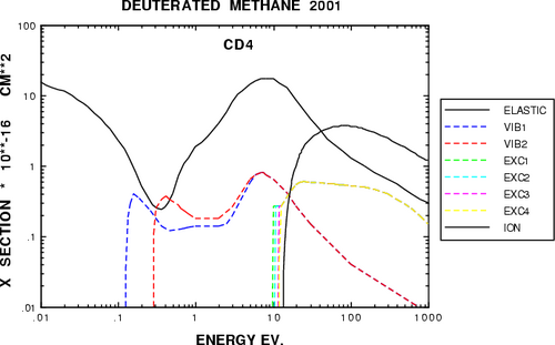
Alternative names:
Excited states:
| Level description | Identifier | Energy [eV] |
|---|---|---|
| 8.2 eV excitation | ETHANE-1 | 8.2 eV |
| 10.3 eV excitation | ETHANE-2 | 10.3 eV |
| 17.0 eV excitation | ETHANE-3 | 17.0 eV |
| Ionisation | ETHANE-IONISATION | 11.52 eV |
Structure:

Cross section:
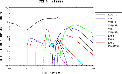
Alternative names:
Excited states:
Structure:

Cross section:
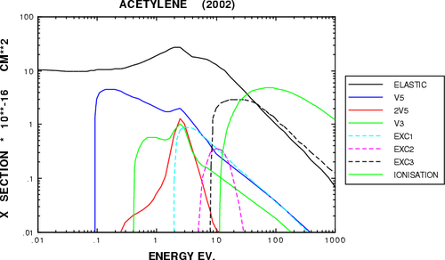
Alternative names:
Excited states:
| Level description | Identifier | Energy [eV] |
|---|---|---|
| 7.7 eV excitation | PROPANE-1 | 7.7 eV |
| 10.0 eV excitation | PROPANE-2 | 10.0 eV |
| 17.0 eV excitation | PROPANE-3 | 17.0 eV |
| Ionisation | PROPANE-IONISATION | 10.95 eV |
Structure:
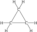
Cross section:
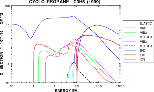
Alternative names:
Excited states:
Structure:

Cross section:
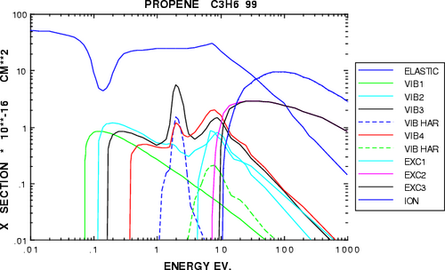
Alternative names:
Excited states:
| Level description | Identifier | Energy [eV] |
|---|---|---|
| 7.4 eV excitation | ISOBUTANE-1 | 7.40 eV |
| 9.7 eV excitation | ISOBUTANE-2 | 9.70 eV |
| 17 eV excitation | ISOBUTANE-3 | 17.0 eV |
| Ionisation | ISOBUTANE-IONISATION | 10.67 eV |
Structure:
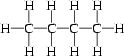
Cross section:
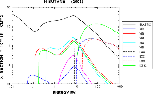
Alternative names:
Excited states:
Structure:
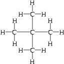
Cross section:
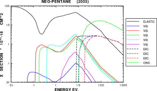
Alternative names:
Excited states:
Structure:
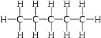
Cross section:
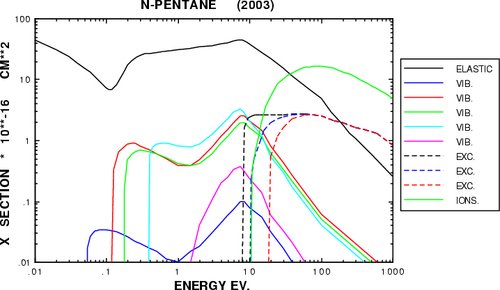
Alternative names:
Excited states:
Structure:

Cross section:
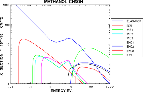
Alternative names:
Excited states:
Structure:

Cross section:
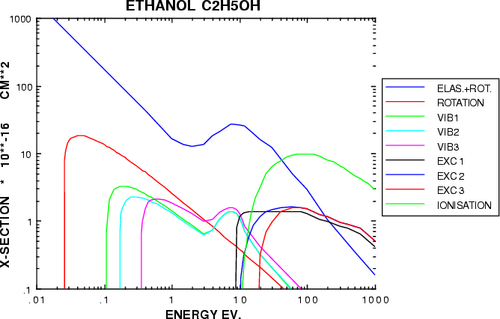
Alternative names:
Excited states:
Structure:
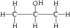
Cross section:
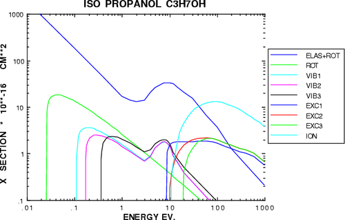
Alternative names:
Excited states:
Structure:

Cross section:
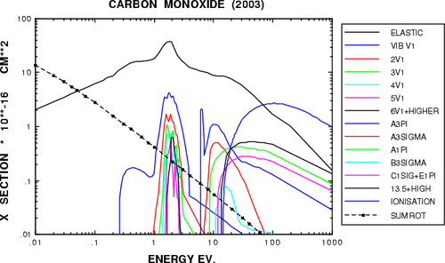
Alternative names:
Excited states:
| Level description | Identifier | Energy [eV] |
|---|---|---|
| 7.9 eV excitation | CO2-1 | 7.9 eV |
| 8.9 eV excitation | CO2-2 | 8.9 eV |
| 10.5 eV excitation | CO2-3 | 10.5 eV |
| 12.2 eV excitation | CO2-4 | 12.2 eV |
| 13.2 eV excitation | CO2-5 | 13.2 eV |
| 15.0 eV excitation | CO2-6 | 15.0 eV |
| Ionisation | CO2-IONISATION | 13.773 eV |
| Level description | Identifier | Energy [eV] |
|---|---|---|
| 4.20 eV excitation | H2O-1 | 4.20 eV |
| 7.40 eV excitation | H2O-2 | 7.40 eV |
| 13.1 eV excitation | H2O-3 | 13.1 eV |
| Ionisation | H2O-IONISATION | 12.61 eV |
| Level description | Identifier | Energy [eV] |
|---|---|---|
| 6.10 eV excitation | NITRIC-OXIDE-1 | 6.10 eV |
| Ionisation | NITRIC-OXIDE-IONISATION | 9.2644 eV |
| Level description | Identifier | Energy [eV] |
|---|---|---|
| 4.06 eV excitation | NITROUS-OXIDE-1 | 4.06 eV |
| 8.50 eV excitation | NITROUS-OXIDE-2 | 8.50 eV |
| 9.60 eV excitation | NITROUS-OXIDE-3 | 9.60 eV |
| Ionisation | NITROUS-OXIDE-IONISATION | 12.886 eV |
| Level description | Identifier | Energy [eV] |
|---|---|---|
| 6.3 eV excitation | METHYLAL-1 | 6.3 eV |
| 8.3 eV excitation | METHYLAL-2 | 8.3 eV |
| Ionisation | METHYLAL-IONISATION | 10.0 eV |
| Level description | Identifier | Energy [eV] |
|---|---|---|
| 7.7 eV excitation | DME-1 | 7.70 eV |
| 8.5 eV excitation | DME-2 | 8.50 eV |
| Ionisation | DME-IONISATION | 10.04 eV |
Structure:

Cross section:
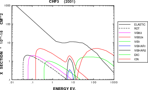
Alternative names:
Excited states:
Structure:

Cross section:
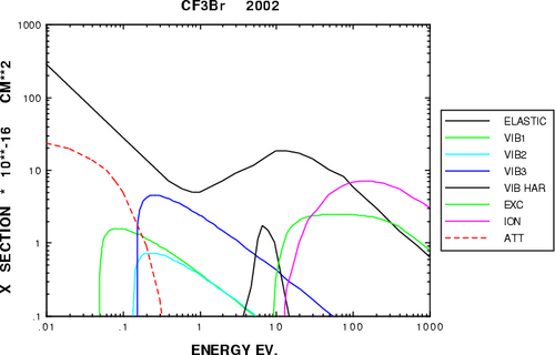
Alternative names:
Excited states:
| Level description | Identifier | Energy [eV] |
|---|---|---|
| Dissociation | CF4-DISSOCIATION | 12.5 eV |
| Ionisation | CF4-IONISATION | 15.90 eV |
Structure:
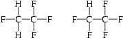
Cross section:
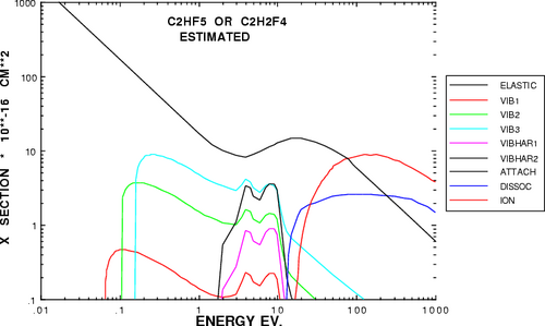
Alternative names:
Excited states:
Structure:

Cross section:
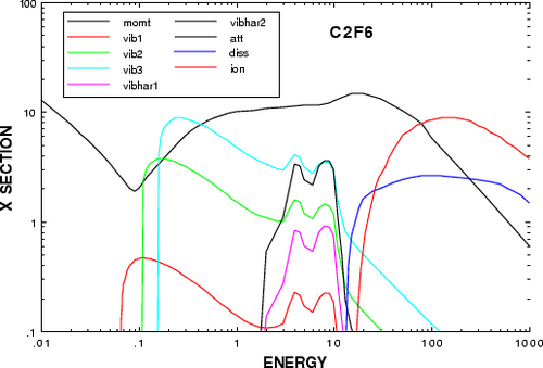
Alternative names:
Excited states:
Structure:

Cross section:
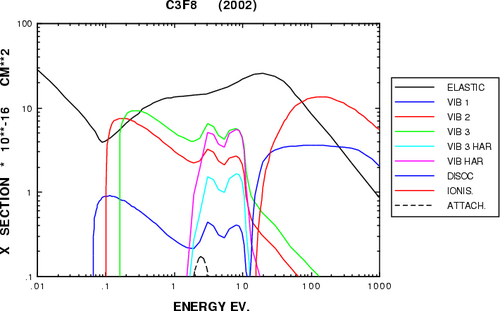
Alternative names:
Excited states:
| Level description | Identifier | Energy [eV] |
|---|---|---|
| Excitation | BF3-EXCITATION | 10.0 eV |
| Ionisation | BF3-IONISATION | 15.56 eV |
Structure:

Cross section:
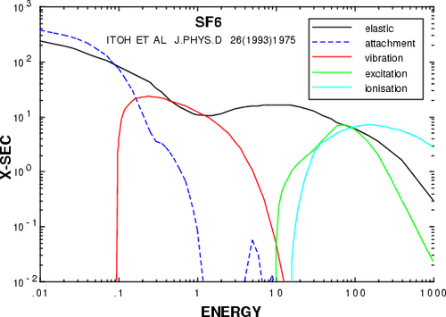
Alternative names:
Excited states:
Structure:

Cross section:
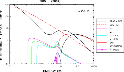
Alternative names:
Excited states:
Structure:

Cross section:
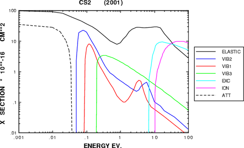
Alternative names:
Excited states:
Structure:

Cross section:
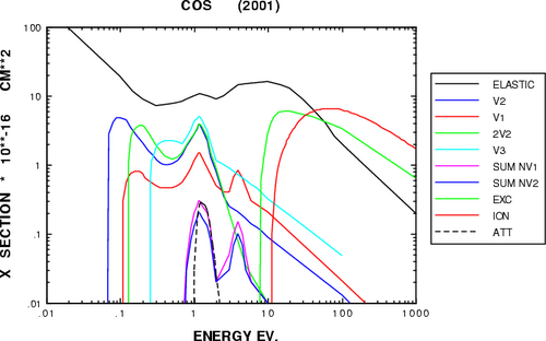
Alternative names:
Excited states:
Structure:

Cross section:
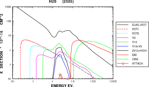
Alternative names:
Excited states:
Structure:

Cross section:
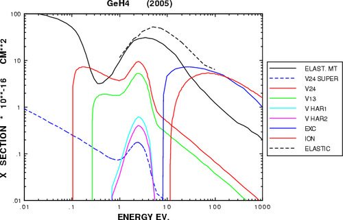
Alternative names:
Excited states:
Structure:

Cross section:
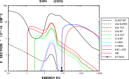
Alternative names:
Excited states:
The sum of the fractions is normalised - in the examples, fractions usually add up to 1 or to 100, but this is not mandatory.
[Each fraction is 0 by default.]
In either case, you can set the number of points with N-E or N-E/P (which are synonyms) and you have the choice between linear and logarithmic spacing of the points.
In either case, ensure that all fields are strictly positive and that they are in strictly increasing order.
Make sure that the all fields present in your chamber are covered by the table and do not rely on the EXTRAPOLATIONS. Pay particular attention to the region in the immediate vicinity of wires. Use e.g. the field section CHECK WIRES commands to determine the field there.
Try to be reasonable when selecting the number of electric fields at which you run Magboltz. On the one hand the number of points must be large enough so as to represent any fine structure that may be present in the transport properties. On the other hand, an excessively large number of points may lead to oscillations in the interpolation.
It is permissible to request transport properties for only a single field, for instance to study the dependence of the transverse diffusion on the magnetic field. The interpolation methods need not be specified in this case and only constant extrapolations can be used.
If you ask for a small number of points, e.g. 2, then you can only request low order INTERPOLATIONS.
[By default E ranges from 100\ V/cm to 100000\ V/cm in 20 logarithmically spaced steps.]
You can either ask Magboltz to compute the transport properties at evenly spaced magnetic fields within a range or for a set of magnetic fields that you specify.
You can set the number of points with N-B.
In either case, ensure that the fields are expressed in Tesla, also be sure that they are strictly positive.
If you ask for only 1 magnetic field strength and only 1 angle between E and B, then Magboltz will generate a 1-dimensional table for which you have greater control over the INTERPOLATIONS and EXTRAPOLATIONS methods.
These parameters can not be used if there is no magnetic field.
[If the magnetic field can be determined to be constant or zero, then Magboltz by default only computes a table for the magnetic field that is present in the chamber. If the B field is not constant, but of known range, then Magboltz will by default be run for 6 magnetic fields ranging from the minimum field to the maximum field present in the chamber. In all other cases, it will compute tables for 0, 1, 2, 3, 4 and 5 T.]
You can either ask Magboltz to compute the transport properties for angles between E and B that are evenly spaced over a range, or for a user-specified set of angles between the 2 fields:
Ensure that the range is entirely contained in [0\°,\ 90\°].
You can set the number of angles with N-ANGLES.
In either case, ensure that the angles are expressed in degrees, also be sure that they are in the range [0\°,\ 90\°].
It is advisable to use this format, with ANGLE=90, if your chamber is such that E is always perpendicular to B.
It is bad practice to set ANGLE=0 in TPCs where E is parallel with B in the drift volume. Other orientations occur in the read-out chambers, and these orientations have impact on the resolution of the TPC.
If you ask for only 1 magnetic field strength and only 1 angle between E and B, then Magboltz will generate a 1-dimensional table for which you have greater control over the INTERPOLATIONS and EXTRAPOLATIONS methods.
These parameters can not be used if there is no magnetic field.
[Magboltz will, if B is non-zero, by default be asked to compute tables for angles of 0\°, 30\°, 60\° and 90\° between the E and B field.]
Keep in mind that Magboltz only computes F2 and F3 on request: to get F2 and F3 you need to request SECOND-ORDER-TERMS (or ORDERS 2) and for a reasonably accurate F3 you should specify ORDERS 3. Both are incompatible with the option ITERATE-ALPHA which enables a more precise computation of the Townsend coefficient.
F0 is plotted with representation FUNCTION-1, F1 as FUNCTION-2, F2 as FUNCTION-3 and F3 as FUNCTION-4.
This function is plotted with representation FUNCTION-1,
[This option is off by default, but it is switched on automatically in case there are concerns about the validity of the energy range.]
Plotted is the quantity used inside Magboltz: the stp cross section scaled by pressure and temperature, multiplied with the Loschmidt number - a quantity that can be interpreted as the reciprocal of the mean free path.
This option is provided to enable a rapid inspection of the cross sections. The KEEP option is recommended to make better quality graphs.
The total cross section is plotted with representation FUNCTION-1, the elastic cross section with FUNCTION-2, the attachment cross section with FUNCTION-3 and the ionisation cross sections for the various components with FUNCTION-4.
[This option is off by default.]
The energy range over which these quantities are stored is set by the Magboltz program so as to obtain optimal accuracy for the calculation of the transport parameters. This range can not be set directly from the command line. However, the maximum energy is strongly influenced by the electric field, which can therefore be used to select the range.
The names of the global variables are shown in the table below. In order not to overwrite parameters from earlier calculations, a sequential number "n" is appended to the name. The names are displayed while the command executes.
| Name | Quantity | Unit |
|---|---|---|
| E_n | Energy | eV |
| F_n | Energy distribution function | Integral normalised to 1 |
| CST_n | Total cross section | cm\²/molecule |
| CSE_n | Elastic cross section | cm\²/molecule |
| CSA_n | Attachment cross section | cm\²/molecule |
| CSI_n | Ionisation cross section | cm\²/molecule |
Cross sections are given for the temperature and pressure that was specified in the gas section (or that was default).
For the conversion from cross section, given in cm\², to mean free path, one uses the relation (the constant is known as Loschmidt number):
\λ = 1 / (L \× \σ) L = 2.6867775 \× 10\<SUP\>19\</SUP\> molecules / cm\³
Example 1:
&GAS
magboltz argon 80 co2 1 coll 20 e-field 20000 keep
!options log-x log-y
Call plot_frame(0.01,1e-18,100,2e-15, ...
   `Electron energy [eV]`, ...
   `Cross section [cm2]`, ...
   `Cross section in argon 90 % CO2 20 %`)
Call plot_line(e_1,cst_1,`function-1`)       // Total
Call plot_line(e_1,cse_1,`function-2`)       // Elastic
Call plot_line(e_1,csa_1,`function-3`)       // Attachment
Call plot_line(e_1,csi_1,`function-4`)       // Ionisation
Call plot_end
This shows the various contributions to the cross section in an argon/CO\<SUB\>2\</SUB\> mixture.
Example 2:
&GAS
magboltz argon 100   co2   0   coll 20 e-field 200 keep
magboltz argon  99.5 co2   0.5 coll 20 e-field 200 keep
magboltz argon  99   co2   1   coll 20 e-field 200 keep
magboltz argon  98   co2   2   coll 20 e-field 200 keep
magboltz argon  95   co2   5   coll 20 e-field 200 keep
magboltz argon  90   co2  10   coll 20 e-field 200 keep
magboltz argon  50   co2  50   coll 20 e-field 200 keep
magboltz argon   0   co2 100   coll 20 e-field 200 keep
!options lin-x lin-y
Call plot_frame(0,0,6,1, ...
   `Electron energy [eV]`, ...
   `Energy distribution [normalised]`, ...
   `Electron energy in argon CO2 mixtures`)
Call plot_line(e_1,f_1,`function-1`)
Call plot_line(e_2,f_2,`function-2`)
Call plot_line(e_3,f_3,`function-3`)
Call plot_line(e_4,f_4,`function-4`)
Call plot_line(e_5,f_5,`function-5`)
Call plot_line(e_6,f_6,`function-6`)
Call plot_line(e_7,f_7,`function-7`)
Call plot_line(e_8,f_8,`function-1`)
Call plot_end
This shows the dramatic modification of the electron energy distribution that occurs when one adds tiny amounts of CO\<SUB\>2\</SUB\> to pure argon.
[This option is not on by default.]
This option, which is not default, is provided mainly for backwards compatibility, and only in Garfield up to version\ 8. Monte Carlo integration is currently believed to be superior for all gas mixtures. Analytic integration may still be the method of choice for a pure noble gas.
Several anisotropic gases can not be used when analytic integration is requested.
This option does not exist anymore in Garfield versions\ 9 and higher, which call Magboltz version\ 7 and higher. Magboltz version\ 7 can deal with pure noble gases - but it will be very slow.
Values larger than 1 are not compatible with ITERATE-ALPHA, this setting is overruled by the SWITCH option.
This option can only be used with ANALYTIC-INTEGRATION integration.
[Default: n=2, equivalent to SECOND-ORDER-TERMS.]
SWITCH overrules this selection.
HIGH-PRECISION is synonymous to SECOND-ORDER-TERMS.
This option can only be used with ANALYTIC-INTEGRATION integration, available only in Garfield version \ and earlier.
[This is the default order, but is overruled by SWITCH.]
LOW-PRECISION is synonymous to FIRST-ORDER-TERMS.
This option can only be used with ANALYTIC-INTEGRATION integration, available only in Garfield version\ 7 and earlier.
[The default is SECOND-ORDER-TERMS.]
This option can only be used with ANALYTIC-INTEGRATION integration, available only in Garfield version\ 7 and earlier.
[This is not default.]
If \α/pressure is smaller than the threshold, the quantities are computed with SECOND-ORDER-TERMS, NOITERATE-ALPHA
Otherwise, they are computed with FIRST-ORDER-TERMS, ITERATE-ALPHA.
This guarantees that the drift velocity, diffusion and Lorentz angle are accurate at low field values, which is where they matter most, whereas the Townsend coefficient is accurate at higher field values, at the price of a somewhat reduced accuracy for the other quantities.
This option can only be used with ANALYTIC-INTEGRATION integration, available only in Garfield version\ 7 and earlier.
[This option is default, \α/pressure is set to 50/pressure.]
These formulae are only valid when the approximation that the longitudinal and transverse diffusion are equal is true. This is of course never true, but one can get a correction to the longitudinal diffusion from the ratio of the longitudinal to transverse diffusion without the magnetic field in the given gas at the E-field of interest. [from Steve Biagi]
These diffusion coefficients are obtained when you specify F0-TRANSVERSE-DIFFUSION, H1-TRANSVERSE-DIFFUSION, F0-LONGITUDINAL-DIFFUSION and H1-LONGITUDINAL-DIFFUSION. The correction to the longitudinal diffusion is applied, using the G0 estimate of the longitudinal diffusion.
F0-TRANSVERSE-DIFFUSION is default.
These options can only be used with ANALYTIC-INTEGRATION integration, available only in Garfield version\ 7 and earlier.
This technique, which is believed to be more accurate than analytic integration for nearly all gas mixtures, is default. Pure noble gases seem to be the only exception to this rule.
Garfield up to version\ 8 maintained an interface to both the analytic integration method from Magboltz version\ 1 and the Monte Carlo method from Magboltz version\ 2. Garfield version\ 9 is interfaced only with Magboltz version\ 7, which uses Monte Carlo techniques, since the format of the gas descriptions used by this Magboltz version is no longer compatible with Magboltz version\ 1.
[Monte Carlo integration is default.]
Low values (e.g. 2-5) are suitable for mixtures than contain substantial amounts of quenchers. Nearly pure noble gases call for larger values (e.g. 10-20) while very large values (100 and more) are needed for pure noble gases. But in the latter case, it is preferable to use Magboltz\ 1 (see ANALYTIC-INTEGRATION).
The statistical accuracy of the drift velocity calculation improves with the square root of this parameter, while the CPU time consumption increases linearly. Since the accuracy depends on the gas mixture and on the field, it may be worthwhile in critical applications to estimate the statistical error of the Magboltz calculations for a given gas and a given field by repeatedly calculating the transport parameters:
Call book_histogram(vhist,50)
Call book_histogram(dlhist,50)
Call book_histogram(dthist,50)
Global nrndm=200
For irndm From 1 To nrndm Do
Say "Iteration {irndm}/{nrndm}"
&GAS
magboltz argon 90 methane 10 coll 5 e-field 125
&MAIN
Call drift_velocity(125,0,0,v)
Call fill_histogram(vhist,v)
Call transverse_diffusion(125,0,0,dt)
Call fill_histogram(dthist,10000*dt)
Call longitudinal_diffusion(125,0,0,dl)
Call fill_histogram(dlhist,10000*dl)
Enddo
Call plot_histogram(vhist,`v<SUB>D</SUB> [cm/microsec]`,`Drift velocity`)
Call plot_end
Call plot_histogram(dthist,`σ<SUB>T</SUB> [micron for 1 cm]`, ...
`Transverse diffusion`)
Call plot_end
Call plot_histogram(dlhist,`σ<SUB>L</SUB> [micron for 1 cm]`, ...
`Longitudinal diffusion`)
Call plot_end
From the histograms, one concludes that, for argon 90\ % methane 10\ % and E=125\ V/cm, COLLISION=5 leads to a statistical error of 0.4\ % on the drift velocity, 4.5\ % on the transverse diffusion and 7\ % on the longitudinal diffusion.
[By default: 10\ \×\ 960.000 collisions.]
This format only allows for mobilities that are constant or depend in a simple way on E/p. In the latter case, the argument of MOBILITY should be a function with EP as variable.
ADD provides a similar functionality, and can in addition be used if the mobility is available in tabular form.
The unit of mobility in Garfield is cm\²/\μsec.V.
[By default: no mobility.]
This output contains amongst others the ionisation, attachment and excitation rates which are needed if one wishes to correct the Townsend coefficients for Penning transfers. One also finds there the energy distribution.
This output tends to be long and it may therefore be advisable to write it to a file:
&GAS
pressure 3 bar
temperature 25 C
> magboltz.rates
magboltz argon 90 co2 10 ...
   e-field 100 200 500 1000 2000 5000 10000 20000 50000 100000 ...
   coll 3 ...
   print
>
[By default, this option is switched off.]
The MATERIAL command takes a chemical composition as argument,
Format:
MATERIAL  [ALUMINIUM n]    [ARGON n]     [CARBON n] ...
          [FLUORINE n]     [HELIUM n]    [HYDROGEN n] ...
          [KRYPTON n]      [LITHIUM n]   [NEON n] ...
          [NITROGEN n]     [OXYGEN n]    [SILICON n] ...
          [SULPHUR n]      [XENON n] ...
          DENSITY density ...
          WORK work ...
          [FANO fano]
Example:
material C 12 H 22 O 11 density 1.59 work 3
Which would fill your device with sucrose, ordinary sugar.
This number is mandatory, if you fill your chamber with pure silicon, for instance, you have to specify:
material Si 1 density 2.3 work 3.6
[No default]
[Mandatory parameter, no default.]
[Mandatory parameter, no default.]
[By default set to 0.19.]
This only works if the current data and the data in the file have at least 2 of the following 3 axes in common: the set of electric field values, the set of angles between E and B and the set of magnetic field values. This condition is trivially met if the current gas data and the data in the file both concern a zero magnetic field situation.
If precisely 2 of the 3 axes coincide, then the merged data will contain only the transport properties which are found in both the current data and in the file.
If all 3 axes coincide, then the merged data will contain all the transport properties that are found in either the current data or the file.
Also the ADD command adds transport properties to the gas tables, under somewhat different conditions.
Contrary to the GET command, MERGE can not read files written in earlier formats. The way out consists in reading old-format files with GET, writing them out using WRITE and then using the file thus obtained for the merge.
Format:
MERGE file [member] [KEEP-OLD | REPLACE-OLD]
Example:
get "low.gas"
merge "high.gas"
[This is default.]
[Default is to keep the existing data.]
The main limitation of this method is that it neglects ionisation effects and that it treats excitation inaccurately. This implies that the results are not valid for large E/p values, i.e. close to the electrodes.
Another limitation is that these calculations neglect the magnetic field - this is not an inherent limitation of the method, but there is no intention to invest further effort in this instruction. Garfield nowadays has an interface to the MAGBOLTZ program of Steve Biagi which is far superior in accuracy to this instruction.
Format:
MIX [ ARGON  frac ]          [ HELIUM  frac ] ...
    [ METHANE  frac ]        [ ETHANE  frac ] ...
    [ NEON  frac ]           [ NITROGEN  frac ] ...
    [ ISOBUTANE  frac ]      [ XENON  frac ] ...
    [ CO2  frac ]            [ METHYLAL  frac ] ...
    [ KRYPTON  frac ]        [ AMMONIA  frac ] ...

    [ MINIMUM-ENERGY emin ] ...
    [ MAXIMUM-ENERGY emax ] ...
    [ STEPSIZE-ENERGY estep ] ...

    [ CRITICAL-F0-FRACTION frcrit ] ...

    [ E/P-RANGE epmin epmax ] ...
    [ N-E/P n ] ...
    [ LINEAR-E/P-SCALE | LOGARITHMIC-E/P-SCALE ] ...

    [ PLOT-F0 | NOPLOT-F0 ] ...
    [ PLOT-ENERGY-LOSS | NOPLOT-ENERGY-LOSS ] ...
    [ PLOT-CROSS-SECTION | NOPLOT-CROSS-SECTION ] ...
    [ PLOT-PATH | NOPLOT-PATH ] ...

    [ PRINT-TABLES | NOPRINT-TABLES ] ...

    [ MOBILITY mob ] ...
    [ TOWNSEND-COEFFICIENT \α/p ] ...
    [ ATTACHMENT-COEFFICIENT \η/p ]
Example:
mix argon 50 ethane 50
The gas in your chamber will be 50\ % argon and 50\ % ethane.
The fractions do not necessarily have to add up to 1.
[Each fraction is 0 by default.]
[By default 0.01\ eV.]
This parameter should be chosen sufficiently large, otherwise the program might not be able to detect ionisation. The adverse effect of choosing this parameter too large is an increased CPU time consumption.
[By default 25\ eV.]
[By default 0.5\ eV.]
Also the energy distribution plot (see PLOT-F0) shows whether ionisation and excitation phenomena are likely to play a role.
[By default 0.01.]
[By default 0.5 to 50.]
[By default 20.]
[Logarithmic by default.]
The curve is plotted using polyline representation FUNCTION-1 if ionisation and excitation are not expected to be a problem, and using representation FUNCTION-2 if a fraction frcrit or more of the energy distribution exceeds the first ionisation or excitation threshold.
[This plot is made by default.]
The curve is plotted using polyline representation FUNCTION-1.
[This plot is by default not made.]
The curve is plotted using polyline representation FUNCTION-1.
[This plot is made by default.]
The curve is plotted using polyline representation FUNCTION-1.
[This plot is by default not made.]
[This table is by default not printed.]
This format only allows for mobilities that are constant or depend in a simple way on E/p. In the latter case, the argument of MOBILITY should be a function with EP as variable.
ADD provides similar functionality, and caters in addition for mobilities that are available in tabular form.
The Garfield unit for mobility is cm\²/V.\μsec.
[By default: no mobility.]
This format only allows for Townsend coefficients that depend in a simple way on E/p. The argument of TOWNSEND-COEFFICIENT should be a function with EP as variable. ADD is more flexible in that it provides similar functionality, but it caters in addition for Townsend coefficients that are available in tabular form.
Note that MAGBOLTZ can be used to compute Townsend coefficients.
The Townsend coefficient should be entered as \α/pressure, with \α in units 1/cm and the pressure in Torr.
[By default: no Townsend coefficient.]
This format only allows for attachment coefficients that depend in a simple way on E/p. The argument of ATTACHMENT-COEFFICIENT should be a function with EP as variable. ADD is more flexible in that it provides similar functionality, but it caters in addition for attachment coefficients that are available in tabular form.
Note that MAGBOLTZ can be used to compute attachment coefficients.
The attachment coefficient should be entered as \η/pressure, with eta in units 1/cm and the pressure in Torr.
[By default: no attachment coefficient.]
Format:
OPTIONS [NOGAS-PLOT | GAS-PLOT] ...
        [NOGAS-PRINT | GAS-PRINT]
Examples:
plot-options drift-velocity nodiffusion notownsend
opt gas-plot nogas-print
Requests a plot of the drift velocity. If cluster data has been entered, then also a cluster plot will be made (this is default) but diffusion and multiplication graphs are not shown. Using further PLOT-OPTIONS options, one could have fixed for instance the scale of the drift velocity plot.
&GAS
magboltz argon 70 dme 30
opt gas-print nogas-plot
>ArDME.print
&MAIN
>
MAGBOLTZ is called to compute transport properties for a 70/30 mixture of argon and DME. The transport tables are printed when leaving the section - note the use of the &MAIN command to close the gas section. They do not appear on the screen, but are output to the file ArDME.print.
If SRIM data has been entered, then in addition the energy loss, range and straggling parameters are plotted.
These plots are made when the gas section is left, not when the option is switched on. Use e.g. &MAIN to close the section. Once outside the gas section, the plots can be obtained by entering the &OPTIMISE section and issued a PLOT-GAS command.
The representations used in the graphs are the following:
[These graphs are not made by default.]
With the PLOT-OPTIONS command, you have further control over the axes (linear or logarithmic) and the vertical scale of these plots. This command also enables you to suppress one or more of the plots.
Use the ATTACHMENT, DRIFT_VELOCITY, GET_E/P_TABLE, ION_MOBILITY, LONGITUDINAL_DIFFUSION, LORENTZ_ANGLE, TOWNSEND, TRANSVERSE_DIFFUSION, VELOCITY_E, VELOCITY_BTRANSVERSE, VELOCITY_ExB, EXCITATION_RATE and IONISATION_RATE procedures for fully customised plots.
[This option is off initially, its setting is remembered from one gas section to the next.]
The tables are printed when the gas section is being left, not when the option is switched on. Use e.g. &MAIN to close the section. As a consequence, if you wish to output the tables to a file, then you have to start the re-routing just before leaving the section and revert to normal output once you are in the next section:
Once outside the gas section, this table can be obtained by entering the &OPTIMISE section and issued a PRINT-GAS command.
&GAS
magboltz argon 80 co2 20
opt gas-print
> Ar_80_CO2_20.print
&MAIN
>
The output can not be used directly as input to the program, use the WRITE instruction for that purpose.
[This option is off initially, its setting is remembered from one gas section to the next.]
Originally, most of this data was only used for a simple Landau-based backup estimate of the cluster size distribution if the CLUSTER size distribution is not known from data and if the HEED model can not be used.
Some of the parameters are however used for other purposes too:
Format:
PARAMETERS [ A a ] ...
           [ Z z ] ...
           [ RHO density ] ...
           [ E-PAIR epair ] ...
           [ E-MOST-PROBABLE emprob ] ...
           [ MEAN mean_number_of_clusters ] ...
           [ TRANSVERSE-ION-DIFFUSION {THERMAL | sigma_T} ] ...
           [ LONGITUDINAL-ION-DIFFUSION {THERMAL | sigma_L} ]
As shown in the format description, several lines may be used although a single line is perfectly acceptable as well.
Example:
PARA MEAN 20
This format could be used if you wish to compute arrival time spectra and enter the cluster size distribution with CLUSTER.
This parameter is used by (and mandatory for):
This parameter is used only to compute the cluster size distribution if you didn't enter such a distribution yourself with CLUSTER nor asked HEED to simulate the ionisation process.
You may also type MOST-PROBABLE-ENERGY-LOSS.
This parameter is used only to compute the cluster size distribution if you didn't enter such a distribution yourself with CLUSTER nor asked HEED to simulate the ionisation process.
You may also type PAIR-CREATION-ENERGY.
This parameter is not used when clustering is performed according to the HEED model, but it is required for the EXPONENTIAL-SPACING and EQUAL-SPACING clustering models. In the latter 2 cases, the parameter is required even if a cluster size distribution has been entered with a CLUSTER statement.
You may also type N-MEAN.
[No default setting.]
This parameter is used by:
SRIM files contain a density estimate and, when reading such a file with the SRIM command in the gas section, the gas density will be overwritten. It is therefore advisable to issue the PARAMETERS command after the SRIM command if you know the gas density.
This parameter is used by (and mandatory for):
.------
/ 2 k\<SUB\>B\</SUB\> T
\σ = \\ / ------
\\/ q\<SUB\>e\</SUB\> E
Where
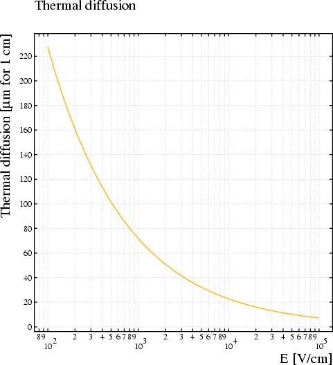
[By default, the diffusion is set to 0.]
These coefficients are used for Monte_Carlo drift-line integration of ion trajectories.
The diffusion coefficients should be expressed in cm of diffusion over 1\ cm of drift.
[Both diffusion coefficients default to 0.]
Several plots may be modified in a single statement.
Use DRIFT_VELOCITY and related procedures to have full control over the presentation of the plot.
Format:
PLOT-OPTIONS [plot [options]] ...
Example:
plot-options drift lin-x log-y nodiff nocluster
(Requests a linear E/p axis and a logarithmic drift velocity axis, the opposite of the default. The diffusion coefficients and the cluster size distribution are not plotted.)
The following are known, all of which can be negated to suppress the plot:
| Plot | Contains |
|---|---|
ATTACHMENT-COEFFICIENT-PLOT |
Synonym for TOWNSEND-COEFFICIENT-PLOT |
CLUSTER-SIZE-PLOT |
Cluster size distribution |
DIFFUSION-COEFFICIENTS-PLOT |
Transverse + longitudinal diffusion |
DRIFT-VELOCITY-PLOT |
Drift velocity of electrons |
EXCITATION-RATES-PLOT |
Excitation and ionisation rates |
ION-MOBILITY-PLOT |
Ion mobility |
IONISATION-RATES-PLOT |
Synonym for EXCITATION-RATES-PLOT |
LORENTZ-ANGLES-PLOT |
Lorentz angles for electrons |
MOBILITY-PLOT |
Synonym for ION-MOBILITY-PLOT |
TOWNSEND-COEFFICIENT-PLOT |
Townsend and attachment coefficients |
SRIM-PLOTS |
SRIM energy loss and straggling |
Notes:
| Option | Effect |
|---|---|
LINEAR-X |
Linear scale for the horizontal axes |
LINEAR-Y |
Linear scale for the vertical axes |
LOGARITHMIC-X |
Log scale for the horizontal axes |
LOGARITHMIC-Y |
Log scale for the vertical axes |
RANGE ymin ymax |
y Will range from ymin to ymax |
Notes:
The pressure is used by the gas mixing instructions MIX and MAGBOLTZ as well as by HEED. Please be sure to specify the pressure before issuing these commands.
If you specify the pressure after a mixing command, then the tables will be prepared for standard atmospheric pressure and the conversion to the pressure you specify will be done by relying on the simple scaling laws.
Format:
PRESSURE pressure [unit]
Example:
pressure 2 bar
[Initially set to 760\ Torr.]
Garfield internally stores the pressure in Torr and e.g. the E/p tables are therefore in V/cm.Torr, no matter the pressure unit you used on input. Also the unit with which the pressure is displayed is not affected by the unit with which you enter it.
The following pressure units are accepted:
| Unit | Equivalent of 1 atm | Notations |
|---|---|---|
| atmosphere | 1 atm | ATMOSPHERE |
| mm Hg | 760 mm Hg | MM-HG |
| Torricelli | 760 Torr | TORRICELLI |
| inch Hg | 29.9213 inch Hg | INCH-HG |
| Pa | 101325 Pa | Pascal, hPa, kPa |
| N/m2 | 101325 N/m\² | N/M2 |
| bar | 1.01325 bar | BAR |
| mbar | 1013.25 hPa | MBAR, MILLI-BAR |
[The default pressure input unit is the Torr.]
A selective reset is performed if any items are listed, otherwise all gas data is deleted.
Format:
RESET [item1] [item2] ...
In order to estimate electron deposition from the SRIM model, Garfield will need the A and Z of the gas to be entered with the PARAMETERS statement. The SRIM files do not seem to contain this information.
SRIM files contain a density estimate and, when reading such a file, the gas density, if entered on beforehand with the PARAMETERS statement, would be overwritten. It is therefore advisable to issue the PARAMETERS command after the SRIM command if the density as estimated by SRIM is not considered reliable. Please note that the a density entered with the PARAMETERS statement will not affect the range estimated by SRIM.
The energy loss, range and straggling parameters will be plotted, when the gas section is being left, if the GAS-PLOT option is switched on.
The SRIM tables are included in the files that are written by the WRITE command and read by the GET command.
Use the SRIM option of the TRACK command to produce clusters based on this model.
Comments, and in particular comparisons with experimental data, as well as suggestions for improvement are invited.
Format:
SRIM FILE file ...
     WORK-FUNCTION work ...
     FANO-FACTOR fano
Example:
srim file="SRIMHeInCF.dat" work=40A file with SRIM output for \α particles traversing He/CF\<SUB\>4\</SUB\> is read, and we assume a work function of 40\ eV.
The energy range of the table should at least extend up to the kinetic energy of the incoming particle, and should extend as far down as SRIM will allow so as to simulate the final absorption. The Garfield interface extrapolates to higher and lower energies by taking resp. the last and first tabulated values.
The file for \α particles traversing a mixture of He and CF\<SUB\>4\</SUB\> would look as follows:
 ==================================================================
              Calculation using SRIM-2003
              SRIM version ---> SRIM-2003.26
              Calc. date   ---> October 24, 2005
 ==================================================================

 Disk File Name = SRIM Outputs\\Helium in He- C- F

 Ion = Helium [2] , Mass = 4.003 amu

 Target Density =  1.9000E-03 g/cm3 = 1.1026E+20 atoms/cm3
 ======= Target  Composition ========
    Atom   Atom   Atomic    Mass
    Name   Numb   Percent   Percent
    ----   ----   -------   -------
     He      2    053.12    020.49
      C      6    009.38    010.86
      F      9    037.50    068.65
 ====================================
 Bragg Correction = 0.00%
 Stopping Units =  MeV / (mg/cm2)
 See bottom of Table for other Stopping units

   Ion        dE/dx      dE/dx     Projected  Longitudinal   Lateral
  Energy      Elec.      Nuclear     Range     Straggling   Straggling
-----------  ---------- ---------- ----------  ----------  ----------
  10.00 keV   2.629E-01  6.037E-02  128.41 um    52.40 um    46.05 um
  11.00 keV   2.760E-01  5.715E-02  140.80 um    55.57 um    49.42 um
  12.00 keV   2.885E-01  5.431E-02  153.00 um    58.53 um    52.63 um
(...)
   7.00 MeV   5.985E-01  3.596E-04   39.51 mm     1.44 mm   790.64 um
   8.00 MeV   5.416E-01  3.196E-04   48.75 mm     1.96 mm   931.02 um
   9.00 MeV   5.000E-01  2.879E-04   58.85 mm     2.44 mm     1.09 mm
  10.00 MeV   4.604E-01  2.622E-04   69.81 mm     2.91 mm     1.25 mm
-----------------------------------------------------------
 Multiply Stopping by        for Stopping Units
 -------------------        ------------------
  1.8999E-02                 eV / Angstrom
  1.8999E-01                keV / micron
  1.8999E-01                MeV / mm
  1.0000E+00                keV / (ug/cm2)
  1.0000E+00                MeV / (mg/cm2)
  1.0000E+03                keV / (mg/cm2)
  1.7231E+01                 eV / (1E15 atoms/cm2)
  1.5537E+00                L.S.S. reduced units
 ==================================================================
 (C) 1984,1989,1992,1998,2003 by J.P. Biersack and J.F. Ziegler
Recipe to be provided ... Berta !
[No default; mandatory argument.]
The work function depends on the gas and is typically a factor 2 larger than the ionisation energy.
[No default; mandatory argument.]
The Fano factor equals the RMS\²/average of the number of electrons produced by a given amount of electromagnetic energy. The factor depends on the electromagnetic energy - it tends to decrease from 1 at threshold to the asymptotic value which needs to be specified.
If set to NONE (or 0), the energy used for an electron will be equal to the work function, without fluctuations.
[By default: 0.17.]
Each of the table entries can either be tabulated or be computed from a parametrisation. In either case, the quantities that obey simple pressure scaling laws, have to be entered multiplied by the appropriate power of the pressure.
All tabulated entries must be specified at a common set of E/p values, which must itself be listed in the table if at least one transport property is tabulated. Use ADD if the data that you wish to use for one or more entries, is tabulated at a different set of E/p values.
The order of the tabulated entries is indicated on the TABLE line by listing the names of the entries in the same sequence as in the table. The entry names should not be followed by parametrisations. The place of the E/p values in the table should be indicated by 'E/P'. There is no preferred order of the entries.
If you opt for a parametrised form for one or more entries, then functions have to follow the names of the entries that are to be parametrised. The parametrisations that you enter are not stored as functions, rather they are evaluated at the E/p, angle(E,B) and B values of the table. The list thus obtained will be interpolated when transport properties are required, like for tabulated entries.
If all entries are entered in a parametrised form, then you can either establish the list of E/p values by tabulating them or by specifying an electric_field range.
You have the possibility to create tables with a dependence on the angle between E and B, as well as on the magnetic_field, provided a magnetic field is present in the chamber.
Format:
TABLE [ E/P ] ...
      [ DRIFT-VELOCITY [ function ] ] ...
      [ BTRANSVERSE-VELOCITY [ function ] ] ...
      [ ExB-VELOCITY [ function ] ] ...
      [ ION-MOBILITY [ function ] ] ...
      [ ION-DISSOCIATION-COEFFICIENT [ function ] ] ...
      [ LORENTZ-ANGLE [ function ] ] ...
      [ LONGITUDINAL-DIFFUSION-COEFFICIENT [ function ] ] ...
      [ TRANSVERSE-DIFFUSION-COEFFICIENT [ function ] ] ...
      [ TOWNSEND-COEFFICIENT [ function ] ] ...
      [ ATTACHMENT-COEFFICIENT [ function ] ] ...
      [ DUMMY [ function ] ] ...
      [ E/P-RANGE epmin epmax ] [ N-E/P nep ] ...
        [ LOGARITHMIC-E/P-SCALE | LINEAR-E/P-SCALE ] ...
      [ [ B-RANGE bmin bmax ] [ N-B nb ] | ...
        [ B-FIELD b ] ] ...
      [ [ ANGLE-RANGE amin amax ]  [ N-ANGLE nangle ] | ...
        [ ANGLE angle ] ]
This line is followed by tables for those items that are not functions. The end of the table is signalled by a blank line.
Example:
table drift=100*ep, diff, e/p 0.3 0.1 0.1 0.2 0.1 0.5 0.2 1.0 0.3 2.0// Note that the preceding line is intentionally left blank
The drift velocity is entered as the function 100*E/p which is evaluated at the E/p values listed in the second column. The longitudinal diffusion is listed in the first column. The ion mobility, the Lorentz angle and the Townsend and attachment coefficients are not specified. Note the blank line at the end of the table.
This is an optional keyword. If the E/P keyword is not used, then all transport properties must be specified by means of functions.
The attachment coefficients are computed from the function if the keyword is followed by a function. The coefficients should not be part of the listing in this case.
With a view to pressure scaling, one should in either case enter the attachment coefficients divided by the pressure. The quantity to be entered thus has the unit of 1/(cm.Torr).
Access to the data is provided with the ATTACHMENT procedure.
[Entering attachment coefficients is optional.]
This velocity component is computed from the function if the keyword is followed by a function. The velocity component should not be part of the listing in this case.
In either case, one should enter the velocity component in units of cm/\μsec.
This component should only be included in the table if a magnetic field has been defined. Although you do not have to enter this component if a magnetic field has been defined, you're strongly advised to do so if you dispose of the relevant data. If the component has not been entered, but is needed for a calculation, then the missing velocity components will be computed using the Lorentz angle, if available, otherwise from the Langevin equation.
Access to the data is provided with the VELOCITY_BTRANSVERSE procedure.
[Entering this component of the velocity is optional.]
If not followed by a function, the keyword indicates the location, in the listing that follows the command, of the component of the electron velocity parallel with E. If you do not enter both the component parallel with E\×B and the component parallel with the part of B that is transverse with respect to E, then you should enter here the norm of the drift velocity.
A function following this keyword should return the quantity described above. There should not be a corresponding item in the table if a function is specified.
If not followed by a function, the keyword indicates the location, in the listing that follows the command, of the norm of the electron drift velocity.
The velocity is computed from the function if the keyword is followed by a function. The velocity should not be part of the listing in this case.
The other components of the electron velocity vector should not be entered if there is no magnetic field.
In all cases, one should enter the velocity (component) in units of cm/\μsec.
The magnitude of the drift velocity can be accessed through the DRIFT_VELOCITY procedure. To obtain only the part parallel with E, one uses VELOCITY_E.
[Although entering the drift velocity is optional, one would normally do so since very few calculations can be performed if velocity data is absent.]
This velocity component is computed from the function if the keyword is followed by a function. The velocity component should not be part of the listing in this case.
In either case, one should enter the velocity component in units of cm/\μsec.
This component should only be included in the table if a magnetic field has been defined. Although you do not have to enter this component if a magnetic field has been defined, you're strongly advised to do so if you dispose of the relevant data. If the component has not been entered, but is needed for a calculation, then the missing velocity components will be computed using the Lorentz angle, if available, otherwise from the Langevin equation.
Access to the data is provided with the VELOCITY_ExB procedure.
[Entering this component of the velocity is optional.]
The dissociation coefficients are computed from the function if the keyword is followed by a function. The coefficients should not be part of the listing in this case.
With a view to pressure scaling, one should in either case enter the dissociation coefficients divided by the pressure. The quantity to be entered thus has the unit of 1/(cm.Torr).
Access to the data is provided with the ION_DISSOCIATION procedure.
[Entering dissociation coefficients is optional.]
The ion mobility is computed from the function if the keyword is followed by a function. The ion mobility should not be part of the listing in this case.
In either case, one should enter the ion mobility in units of cm\²/(\μsec.V).
Access to the data is provided with the ION_MOBILITY procedure.
[Entering the ion mobility is optional.]
The longitudinal diffusion coefficients are computed from the function if the keyword is followed by a function. The longitudinal diffusion coefficients should not be part of the listing in this case.
With a view to pressure scaling, one should in either case enter the amount of longitudinal diffusion over 1\ cm of drift, multiplied with the square root of the pressure. This quantity has the unit of \√(cm.Torr).
Access to the data is provided with the LONGITUDINAL_DIFFUSION procedure.
[Entering the longitudinal diffusion is optional.]
The Lorentz angle is computed from the function if the keyword is followed by a function. The Lorentz angle should not be part of the listing in this case.
In either case, the Lorentz angle should be entered in degrees.
This component can only be included in the table if a magnetic field has been defined. If you have included all 3\ components of the drift velocity vector, then you do not have to enter the Lorentz angle since this information will not be used. If however you enter only the velocity component parallel with E, then you're strongly advised to tabulate the Lorentz angle if you dispose of the relevant data. If neither Lorentz angles nor transverse velocity components are available, then the velocity vector will be computed using the Langevin equation.
Access to the data is provided with the LORENTZ_ANGLE procedure.
[Entering Lorentz angles is is optional.]
The Townsend coefficients are computed from the function if the keyword is followed by a function. The coefficients should not be part of the listing in this case.
With a view to pressure scaling, one should in either case enter the Townsend coefficient divided by the pressure. The quantity to be entered thus has the unit of 1/(cm.Torr).
Access to the data is provided with the TOWNSEND procedure.
[Entering Townsend coefficients is optional.]
The transverse diffusion coefficients are computed from the function if the keyword is followed by a function. The transverse diffusion coefficients should not be part of the listing in this case.
The coordinate_system aligns the longitudinal diffusion with the electric field, not necessarily with the drift velocity vector. The transverse diffusion is the average of the diffusion perpendicular to E.
With a view to pressure scaling, one should in either case enter the amount of transverse diffusion over 1\ cm of drift, multiplied with the square root of the pressure. This quantity has the unit of \√(cm.Torr).
Access to the data is provided with the TRANSVERSE_DIFFUSION procedure.
[Entering the transverse diffusion is optional.]
| Variable | Meaning | Value, Unit |
|---|---|---|
ANGLE_EB |
Angle between E and B | degrees |
B |
Magnetic field | Tesla |
BOLTZMANN |
Boltzmann constant | 1.380658 10\<SUP\>-23\</SUP\> J/K |
ECHARGE |
Electron charge | 1.60217733 10\<SUP\>-19\</SUP\> C |
EP |
E/p | V/cm.Torr |
P |
Pressure | Torr |
T |
Temperature | K |
The magnetic field related quantities, ANGLE_EB and B, are to be used only when there is a magnetic field.
Example:
See the FIT_EXPONENTIAL procedure.
| quantity | scaling | enter |
|---|---|---|
| drift velocity | v vs E/p | v |
| ion mobility | \μ vs E/p | \μ |
| diffusion coefficients | \σ.\√p vs E/p | \σ.\√p |
| Townsend coefficient | \α/p vs E/p | \α/p |
| Attachment coefficient | \η/p vs E/p | \η/p |
| Excitation rate | rate/p vs E/p | - |
| Lorentz angles | - | angle |
Example: the diffusion coefficient varies approximately with pressure according to the formula:
\σ(p=p1) = \σ(p=p0) \√p0/\√p1
hence \σ.\√p is approximately constant.
Assigning the transverse diffusion:
table e/p trans-diff long-diff
      1   0.1        0.1
      2   0.1        0.2
      3   0.1        0.3
Not assigning the transverse diffusion:
table e/p dummy long-diff
      1   0.1   0.1
      2   0.1   0.2
      3   0.1   0.3
Alternatively, you could have kept the original table followed by a RESET TRANS-DIFF command.
This parameter is relevant only if E/p is not tabulated i.e. if the table is composed exclusively of computed entries. There is in that case no E/P keyword on the TABLE instruction line.
You may specify that you wish linearly or logarithmically spaced points, and you may also select the number of points.
[By default: 100 to 100000\ V/cm in 20 logarithmic steps.]
Specifying such a range is valid only if there is a magnetic field.
Even though specifying an angle range is useful mainly if you have at least one computed table entry which depends on the angle, you may also specify the range for a tabulated table. Doing this forces the table to have room for B or angle dependent entries, which you can later add with the ADD command.
For defaults and further considerations, see the choice of ANGLE for the MAGBOLTZ command.
Specifying such a range is valid only if there is a magnetic field.
Even though specifying an magnetic field is useful mainly if you have at least one computed table entry which depends on this field, you may also specify the range for a tabulated table. Doing this forces the table to have room for B or angle dependent entries, which you can later add with the ADD command.
For defaults and further considerations, see the choice of B-FIELD for the MAGBOLTZ command.
The temperature is used by the gas mixing instructions (MIX and MAGBOLTZ) and also by HEED. Please be sure to specify the temperature before issuing these commands.
The temperature is not needed if both the transport properties and the clustering properties have been entered via tables.
Garfield applies, if required, pressure scaling of the transport properties but does not apply temperature scaling laws.
Format:
TEMPERATURE temp [unit]
Example:
TEMPERATURE 300 K
For room temperature.
[Initially set to 300\ K.]
Garfield internally stores the pressure in Kelvin. Temperatures are output in K or in C, the unit which is chosen for output doesn't depend on the unit you use for input.
Various temperature units are recognised, as listed in the table:
| Unit | Conversion from Kelvin | Notation, shortest |
|---|---|---|
| degree Celsius | T-273.15 | CELSIUS, C |
| degree Fahrenheit | (T-273.15)*9/5+32 | FAHRENHEIT, F |
| Kelvin | T | KELVIN, K |
| degree Rankine | (T-273.15)*9/5+32-459.67 | RANKINE, RA |
| degree Réaumur | (T-273.15)*4/5 | REAUMUR, RE |
[Default input unit is Kelvin.]
Interface written by James Butterworth.
Format:
TRIM LAYER layer ...
     ION ion ...
     WORK-FUNCTION work ...
     FANO-FACTOR fano ...
     RANGE-FILE range ...
     EXYZ-FILE exyz
The use of this instruction is strongly recommended when you compute the electron transport properties with MAGBOLTZ or with MIX, both of which consume a lot of CPU time. WRITE is not of interest if you enter the transport parameters of your gas description with a TABLE statement.
The dataset contains initialisation information for Heed, which will automatically be performed when re-reading the file with GET. Similarly, SRIM energy loss, range and straggling tables are included in the compact format gas datasets.
The format of the compact dataset is subject to modification and backwards compatibility is not guaranteed. Compact datasets that can no longer be read and that are of value, can be sent to the author of Garfield for recovery.
Files written with WRITE should in principle not be edited. These files are also not intended to serve as easily legible tables. Use the GAS-PRINT option or procedures like DRIFT_VELOCITY to obtain legible tables.
Writing takes place while the section is being left, not when the WRITE command is issued. Use e.g. &MAIN to close the section. The statement can appear at any place in the gas section.
Format:
WRITE [DATASET] file [member] [[REMARK] remark]
Example:
Global gas_file `Ar_70_iso_30.gas`
Global gas_member `exb`
Global p 760
&GAS
Call inquire_member(gas_file,gas_member,`gas`,exist)
If exist Then
   get {gas_file,gas_member}
Else
   write {gas_file,gas_member}
   pressure {p} Torr
   magboltz argon 70 isobutane 30 ...
         angle-range 0 10 n-angle 6 ...
         b-range 0.4 1.2 n-b 5 ...
         e-range 100 300000 n-e 25 ...
         coll 25
Endif
Since Magboltz consumes a large amount of CPU time, we use the WRITE command to store the gas tables. When the same input file is run next time, the INQUIRE_MEMBER procedure will detect that the gas tables already exist and a GET is issued instead of a MAGBOLTZ command.
You may prefix the dataset name with the keyword DATASET, but this is mandatory only if you wish to place a remark before the dataset name. If you use the DATASET keyword, then you must also use the REMARK keyword if you wish to add a remark to the member. If you do not use the DATASET keyword, then the first argument is interpreted as file name, the 2nd as member name and the 3rd and following arguments as remark.
[The file name is mandatory, no default is provided.]
The member name should follow the file name.
[The member name is by default set to "< none >".]
You may prefix the remark with the keyword REMARK, provided you also prefix the dataset name with DATASET. If you do not use these keywords, then the 3rd and following arguments are interpreted as remark.
[The field is left blank by default.]
Format:
&OPTIMISE
Optimisation of potential settings
| Command | Short description |
|---|---|
DISPLAY |
Displays potential settings |
FACTOR |
Factorises the potential |
FORCES |
Computes the forces on the wires |
PRINT-CELL |
Prints the cell data |
RESTORE |
Restores the original settings after a SET |
SAVE |
Saves the potential settings |
SET |
Optimises potential settings |
Modification of the cell structure:
| Command | Short description |
|---|---|
ADD |
Adds elements to the cell |
CHANGE-VOLTAGES |
Modifies the wire, plane and tube potentials |
DELETE |
Deletes elements from the cell |
Three dimensional charges:
| Command | Short description |
|---|---|
CHARGES |
Adds three dimensional charges to the cell |
DELETE-CHARGES |
Removes three dimensional charges from the cell |
LIST-CHARGES |
Lists the three dimensional charges |
Adding a background field:
| Command | Short description |
|---|---|
BACKGROUND-FIELD |
Adds a background field to the cell |
DELETE-FIELD-MAP |
Deletes a background field map |
DELETE-BACKGROUND-FIELD |
Removes the background field |
FIELD-MAP |
Reads a field map for use as background field |
READ-FIELD-MAP |
Reads a binary field map as background field |
SAVE-FIELD-MAP |
Saves a background field map in binary format |
Editing and inspecting the gas tables:
| Command | Short description |
|---|---|
LIST-EXCITATIONS |
List excitation and ionisation levels |
PENNING-TRANSFERS |
Enables and disables Penning transfers |
PLOT-GAS |
Makes the gas plots |
PRINT-GAS |
Prints the gas tables |
General purpose instructions:
| Command | Short description |
|---|---|
AREA |
Changes the part of the cell that is considered |
DRIFT-AREA |
Sets the part of the cell where electrons drift |
GRID |
Changes the grid density |
OPTIONS |
Switches options off and on |
POINTS |
Sets the number of points on the track |
SELECT |
Selects active wires |
TRACK |
Sets the track |
The coordinate system can not be changed by this instruction. This can only be done in the cell section.
The symbolic variables from the cell section as entered with the DEFINE command can not be used.
After each ADD instruction, the cell is checked, a new cell type is determined and the capacitance matrix is calculated. If you have several elements to add, it is advisable to group them in a single instruction. If you only wish to modify a wire voltage, use CHANGE-VOLTAGES instead.
An ADD statement causes the loss of the current electrode selection established with a SELECT statement.
Format:
ADD [PERIODICITY {X|Y|PHI} length] ...
    [PLANE {X|Y|R|PHI} coordinate ...
           [VOLTAGE voltage]] ...
           [LABEL label]
    [WIRE LABEL label ...
          AT position ...
          [VOLTAGE voltage] ...
          [DIAMETER diameter]] ...
          [TENSION tension]] ...
          [LENGTH length]] ...
          [DENSITY density]]
Periodicities in r are not permitted.
[This is a mandatory parameter; no default is provided.]
[Default: 0\ V].
The label 'S' has a special meaning in that electrodes with this label are by default selected.
[Planes are by default not given a label, a label is mandatory for wires.]
This is a set of two numbers (x,y) or (r,\φ) depending on coordinate_system used when the cell was entered.
The units of x, y and r is cm, \φ is in degrees.
[No default, these are mandatory parameters.]
[Default: 0.01\ cm.]
Used by the FORCES command to estimate the wire displacement under gravitational and electrostatic forces.
[Default: 50\ grams.]
Used by the FORCES command to estimate the wire displacement under gravitational and electrostatic forces.
[Default: 100\ cm.]
Used by the FORCES command to estimate the wire displacement under gravitational and electrostatic forces. Not relevant if the wires are vertical.
For copper-beryllium wires, one can also enter CU-BE and for gold plated tungsten one can type TUNGSTEN or W.
[Default: 19.3\ g/cm\³, i.e. 20\ \μm gold-plated tungsten wire.]
Please note that the AREA affected by this instruction is not the area in which electrons and ions are allowed to drift. The latter area, which is relevant when optimising the drift time, is set with the DRIFT-AREA command.
Format:
See the AREA command in the field section.
The background field is not checked for consistency between the field and potential, nor for compatibility with the boundary conditions. Such checks can be done in the field section using the CHECK instruction.
You have to supply at least 3 formulae: potential, x- component and y-component of the electric field. You may in addition supply the z-component of the electric field. The latter defaults to 0.
If the background field is to be derived from a field map, then the FIELD-MAP statement should precede the BACKGROUND-FIELD statement. The background field map is kept across optimisation and cell sections, as long as the storage occupied by this field is not claimed by a main field map in the cell section. It is therefore not necessary to read a field map again to modify the dependence of the background field map on the field map.
Since the background field map and the main field map occupy the same storage area, you can not apply a field map derived background field to a main field that is also supplied as a field map.
Format:
BACKGROUND-FIELD ...
     VOLTAGE formula  EX formula  EY formula  [EZ formula]
Example:
background-field voltage=   cos(2*x)*sin(2*y) ...
                 ex=      2*sin(2*x)*sin(2*y) ...
                 ey=     -2*cos(2*x)*cos(2*y)
| Variable | Meaning |
|---|---|
X (or R) |
x- or r-coordinate |
Y (or PHI) |
y- or \φ-coordinate |
Z |
z-coordinate |
EXMAP |
x-component of the background electric field map |
EYMAP |
y-component of the background electric field map |
EZMAP |
z-component of the background electric field map |
VMAP |
background potential field map |
This instruction does not recompute the capacitance matrix if the matrix is still in memory, and is therefore considerably faster than ADD for large cells. You must however use the latter if you need to modify other parameters than the potential, such as the location of a wire or a plane, the radius of the tube or the diameter of a wire.
Format:
CHANGE-VOLTAGES {WIRE wire | PLANE plane | TUBE} VOLTAGE voltage ...
Example:
ch-v w 1 v 1000 w 2 v 3000
Changes the voltage on wire\ 1 to 1000\ V and on wire\ 2 to 3000\ V.
[No default, this is a mandatory parameter.]
[No default, this is a mandatory parameter.]
[To be specified in Volt.]
Adds three dimensional point charges to the cell. These charges are not taken into account for the charge calculation on the wires, they therefore should be seen as, temporary, space charges.
Format:
CHARGES
x y z q
x y z q
...
(blank line)
Example:
charges
0 0 0 100
1 1 1 200
Places one space charge at (0,0,0) and one at (1,1,1). The first has a charge of 100 and the second a charge of 200.
V = q/rwhere r is the distance between the charge and the point where the potential is to be calculated.
It follows that the charge q should be expressed in units of V.cm. To convert from C to this unit, one should divide by 4\π\ε\<SUB\>0\</SUB\>.
Format:
DELETE-BACKGROUND-FIELD
Example:
del-backgr
Format:
DELETE-CHARGES
Example:
DELETE-CHARGES
Format:
DELETE-FIELD-MAP
Example:
DELETE-FIELD-MAP
Format:
DISPLAY
Please note that this command does not define the plane over which optimisation is carried out. To change this plane, use AREA.
Format:
See the AREA command in the field section.
Format:
FACTOR [GRID | WIRE | TRACK] ...
       [NOGROUP | GROUP]
Example:
factor
(All defaults, GRID and NOGROUP, are accepted.)
When computing a background field due to additional charges, all conductors in the chamber should be set to 0\ V. This ensures that the boundary conditions are respected when the basic field and the background field are superimposed.
Background fields usually need scaling since one wishes to study the perturbations as function of the amount of charge. This scaling is performed by the BACKGROUND-FIELD command. The field in the chamber is not modified until this command has been executed.
When computing signals, you identify each of the weighting fields that you have entered by their label to the SELECT command. Weighting fields have a fixed normalisation and the BACKGROUND-FIELD command should therefore not be used for weighting fields.
Also the cell section has a FIELD-MAP command. The field maps entered in the cell section serve as main field, i.e. the field map replaces the field due to wires and planes, while the field maps entered in the optimisation section are used for the computation of the background field. The two field maps share the same storage and can therefore not be used at the same time.
Format:
See the FIELD-MAP command in the cell section.
Example:
See the attached weighting_field example.
FINISH /CLEAR,START /PREP7 ! No polynomial elements /PMETH,OFF,1The resultant field map of the weighting potential is called PRNSOL.lis and it is accompanied by an ELIST.lis file that contains the mesh structure, an NLIST.lis file with node coordinates and an MPLIST.lis file with material properties. These 3 files must be kept together in a directory from where they are read with the following Garfield commands:! Set electric preferences KEYW,PR_ELMAG,1 KEYW,MAGELC,1
! Select element ET,1,SOLID123
! Material properties MP,PERX,1,1e10 ! Metal MP,RSVX,1,0.0 ! MP,PERX,2,1.0 ! Gas MP,PERX,3,4.0 ! Permittivity of the FR4
! Construct the strips in mm w = 4 ! Strip width l = 10 ! Length modeled along the wire pitch = 2 ! Wire pitch h = 0.10 ! Strip thickness open = 0.500 ! Gap between strips gap = 2.5 ! Gap between strip and wire d = 0.050 ! Wire diameter sub = 2 ! Substrate thickness BLOCK, -pitch/2, pitch/2, 0, h, -w/2, w/2 ! 1: Strip to be read out BLOCK, -pitch/2, pitch/2, 0, h, -l/2, -w/2-open ! 2: Skirt 1 BLOCK, -pitch/2, pitch/2, 0, h, w/2+open, l/2 ! 3: Skirt 2 BLOCK, -pitch/2, pitch/2, -sub, 0, -l/2, l/2 ! 4: Substrate WPOFFS,,,-l/2 CYL4, 0, gap, d/2, , , ,l ! 5: Anode wire WPOFFS,,,l/2 BLOCK, -pitch/2, pitch/2, -sub, 2*gap, -l/2, l/2 ! 6: Gas
! Subtract the strips and wires from the gas VSEL, ALL VSBV,6,ALL,,,KEEP ! gas becomes 7
! Glue everything together, 1 = strip, 2 = skirt, 3 = skirt, 5 = wire, 6 = substrate, 7 = gas VSEL,ALL VGLUE, ALL
! Colour the parts /COLOR, VOLU, YELLOW, 1 ! Read-out strip /COLOR, VOLU, GREEN, 2 ! Skirt /COLOR, VOLU, GREEN, 3 ! Skirt /COLOR, VOLU, RED, 6 ! Substrate
! Assign material attributes VSEL, S, VOLU, , 6 ! FR4 VATT, 3 VSEL, S, VOLU, , 1 ! strip VSEL, A, VOLU, , 2 ! skirt VSEL, A, VOLU, , 3 ! skirt VSEL, A, VOLU, , 5 ! wire VATT, 1 VSEL, S, VOLU, , 7 ! gas VATT, 2
! Voltage boundaries for a weighting field VSEL,S,,,1 ASLV, S DA, ALL, VOLT, 1 ! Readout strip VSEL,S,,,2 VSEL,A,,,3 VSEL,A,,,5 ASLV, S DA, ALL, VOLT, 0 ! All other metal VSEL,S,,,7 ASLV, S ASEL, R, LOC, Y, 2*gap DA, ALL, VOLT, 0 ! Cathode plane without strips VSEL,S,,,7 ASLV, S ASEL, R, LOC, X, -pitch/2 DA, ALL, SYMM ! Continuity VSEL,S,,,7 ASLV, S ASEL, R, LOC, X, +pitch/2 DA, ALL, SYMM ! Continuity VSEL,S,,,7 ASLV, S ASEL, R, LOC, Z, -l/2 DA, ALL, SYMM ! Continuity VSEL,S,,,7 ASLV, S ASEL, R, LOC, Z, +l/2 DA, ALL, SYMM ! Continuity VSEL,S,,,6 ASLV, S ASEL, R, LOC, Y, -sub DA, ALL, VOLT, 0 ! Backplane
! Meshing VSEL, ALL ASLV, S
MSHKEY,0 SMRT, 6 VMESH, ALL
! Solve the field /SOLU SOLVE FINISH
! Display the solution /POST1 /EFACET,1 PLNSOL, VOLT,, 0
! Write the solution to files /OUTPUT, PRNSOL, lis PRNSOL /OUTPUT
/OUTPUT, NLIST, lis NLIST,,,,COORD /OUTPUT
/OUTPUT, ELIST, lis ELIST /OUTPUT
/OUTPUT, MPLIST, lis MPLIST /OUTPUT
&CELL plane y=0 v=0 z-strip -0.2 0.2 gap 0.5 label b // Create a strip called "B" plane y=0.5 v=0 rows s 1 0.0050 0 0.25 1200In the above example, an ion is drifted from the vicinity of the anode wire towards the cathode plane that is not read out. The signal induced by this moving charge is computed twice:periodicity x=0.25
&OPTIMISE Global bin `csc.bin` If exist(bin) Then // Read binary if it exists read-field-map {bin} Else field-map files weighting-field "PRNSOL.lis" label A ... // Call this weighting field "A" units=mm ... ansys-solid-123 ... x-periodic z-periodic save-field-map {bin} // Otherwise, create a binary Endif
&GAS get "Ar_80_CO2_20.gas" // Assumes the transport file exists add ion-mobility 1.5e-6
&SIGNAL select a b // Select both weighting fields area -0.25 0 -0.5 0.25 0.5 0.5 window 0 0.025
reset signals Call drift_ion(0.0025, 0.26) Call add_signals Call get_signal(1,time1,dir1,cross1) // Retrieve the finite element signal ("A") Call get_signal(2,time2,dir2,cross2) // Retrieve the no-wire signal ("B")
Call plot_frame(minimum(time1 & time2), minimum(dir1+cross1 & dir2+cross2), ... maximum(time1 & time2), maximum(dir1+cross1 & dir2+cross2), ... `Time [microsec]`, `Current`, `Comparing weighting fields`) Call plot_line(minimum(time1 & time2), 0, maximum(time1 & time2), 0, `comment`) Call plot_line(time1, dir1+cross1, `function-1`) Call plot_line(time2, dir2+cross2, `function-2`) Call plot_end
area view x=0 plot-field vector
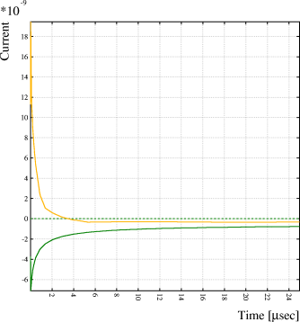
The reason for this difference readily becomes apparent when comparing the weighting field maps (left: finite elements, including the wire, right: neglecting the wire):
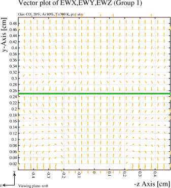
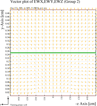
This example uses ANSYS, which is unit-free for what concerns distances. This affords flexibility as long as only symmetry and voltage boundary conditions are used - voltage and length units are decoupled. Charges in contrast are coupled to voltages both via \ε\<SUB\>0\</SUB\> and via an implicit length, as can be seen from the expression for a potential generated by a point charge:
q
V = --------
4 \π \ε\<SUB\>0\</SUB\> r
\ε\<SUB\>0\</SUB\> ~ 8.854\×10\<SUP\>-14\</SUP\> C/(V.cm)
This leads to two scaling factors:
In ANSYS, charges can be entered as volume charge densities or as surface charge densities (amongst other possibilities). In case only the total charge is known, then this charge has to be divided by the volume or the surface area of the charge carrier. Example for a volume charge:
! Parameters of the device unit = 1000 ! Units: 1000 for mm, 100 for cm, 1 for m r = 0.1 ! Radius [mm] pi = 3.14159265 ! pi qe = 1.60217646e-19 ! Electron charge [C] charge = 12345*unit*qe ! Total charge in the deviceWhen surface charges are used, an additional precaution needs to be taken in that the surface area for e.g. a sphere has to be multiplied by an ununderstood factor of 2:! Create a ball which will act as charge carrier SPH4,0,0,r
! Distribute charge in the volume of the ball VSEL, S, VOLU, ,1 BFV,ALL,CHRG,charge/(4.0*pi*r*r*r/3.0)
! Distribute charges over the surfaces of the ball
VSEL, S, VOLU, ,1
ASLV, S
SFA,ALL,,CHRGS,charge/(2*4.0*pi*r*r)
It is therefore strongly recommended to verify the integral charge as follows:
Global r = 0.1             // sufficiently large to wrap around all charges
Global eps0 = 8.854e-14    // C/(V.cm)
Global qe = 1.60217646e-19 // C
Call integrate_charge(0, 0, 0, r, qi)
Say "Electron charges: {qi*4*pi*eps0/qe}"
To obtain meaningful results, one should take care to supply, using the ROWS statement of the cell section, the wire length and the wire tension. If one is interested in the gravitational sag, then one should also enter the density of the wire material and the chamber orientation with the GRAVITY.
The wires on which this instruction operates are those selected by the SELECT instruction. These wires do not necessarily have to be located within the current AREA. When one uses the ITERATE option to study collective wire motion, then it is crucial to select all wires that are likely to move.
This instruction offer 2 levels of accuracy, called DETAILED and FAST.
All wires are restored to their nominal location once the calculations have been completed. To study the effect that sag has on the gain, one should displace the wires in the cell section.
Format:
FORCES [PRINT-SAG | NOPRINT-SAG] ...
       [PLOT-SAG | NOPLOT-SAG] ...
       [NOKEEP-SAG | KEEP-SAG] ...

       [PRINT-FORCES | NOPRINT-FORCES] ...
       [PLOT-FORCES | NOPLOT-FORCES] ...
       [NOKEEP-FORCES | KEEP-FORCES] ...

       [DETAILED | FAST] ...
       [SCANNING-GRID nx ny] ...
       [SCANNING-AREA {LARGEST | FIRST-ORDER | ...
                       FIRST-ORDER-ENLARGED-BY fact | ...
                       xmin ymin xmax ymax}] ...
       [SHOTS nshot] ...
       [STEPS-PER-SHOT nstep] ...
       [INTERPOLATION-ORDER order] ...
       [NOEXTRAPOLATE | EXTRAPOLATE] ...

       [ITERATE [n_iter] | NOITERATE] ...
       [TOLERANCE tolerance] ...
       [UPDATE-SCALING-FACTOR factor] ...
       [OFFSET wire x_offset y_offset] ...

       [ELECTROSTATICS | NOELECTROSTATICS] ...
       [GRAVITY | NOGRAVITY]
Example:
select s
forces detailed keep-sag
The forces acting on the S wires will be calculated in detail and the sag profiles will be stored in global variables.
Note:
This computation benefits greatly from vector processors and matrix algebra libraries tuned to the hardware (e.g. ESSL).
The wire sag that results from such a force is parabolic, since this it results from an elastic elongation. The shape is not a hyperbolic cosine, this would be the case of a freely hanging wire that is longer than the distance between the two (elongation negligible).
This approach is incorrect if the wire is nominally in an almost stable position while there are substantial forces acting on the wire in neighbouring positions.
In this mode, the program uses in its computations the force that acts on the wire if it is (artificially) offset. These forces are computed by solving the capacitance equations for every (set of) wire locations for which one needs a force. Since the force usually displays smooth variations with offset, the program computes the forces only for a number of locations (SCANNING-GRID) in the vicinity (SCANNING-AREA) of the nominal location and interpolates in this table (INTERPOLATION-ORDER) when a force is needed.
The boundaries of the grid are automatically computed from both the expected sag in the parabolic approximation and the largest area around each wire that is free of cell elements. One can also set the area manually with SCANNING-AREA.)
The number of grid lines can be controlled with the SCANNING-GRID option. Numbers can be specified separately for x and y and should be in the range 2 to MXGRID.
[Default is 11 for both nx and ny.]
If the scaling factor 2 doesn't appear suited, then use the keyword FIRST-ORDER-ENLARGED-BY followed by a scaling factor of your choice.
If the wire movements are expected to be very large, then one may wish to select LARGEST which will set the scanning area to the largest area around each wire which is free from other cell elements.
You may also manually set the scanning area by giving 4 numeric arguments: a lower x, a lower y, an upper x and an upper y which together describe a rectangular area relative to the nominal position of the wire under consideration. Note that a manually set scanning area is not checked to be located within the largest area free of other cell elements. The option is convenient for making plots of the force variations.
The number of shots can be chosen by the user and must be equal to 0, in which case the method becomes a single shot method.
Also the number of integration steps within each shot can be set by the user. This parameter must be at least equal to 1.
The interpolation is done by interpolating first along the rows of the table, then the interpolation results, in both cases by local polynomial interpolation of the selected order.
The order should be a number larger than or equal to 1, and small than or equal to the scanning grid size.
If you select EXTRAPOLATE, then the force on the wire at such a point, will be computed by extrapolating the force table.
It is usually a better strategy to pick a SCANNING-AREA that covers all wire positions - if this is not possible, then the wire is probably not in a stable position (i.e. it will move against other electrodes).
The iteration starts from the nominal position for all wires, and a set of wire offsets equal to (0,0) except for those wires for which the user has given an initial offset.
Then, a loop is started in which
The iteration is stopped when
ITERATE can be used both with the FAST and with the DETAILED method of calculating wire sags.
Output is only produced from the last iteration provided convergence has been achieved.
Iteration is done by default when the number of SELECTed wires is larger than 1. The default maximum number of iterations is set to 5, which may be insufficient if the TOLERANCE is set to a very small number, and also in case of an oscillatory systems. In the latter case it is preferable to adjust the UPDATE-SCALING-FACTOR.
In each iteration, the maximum of the differences between the current and the new wire offsets is computed. When this maximum drops below TOLERANCE, the iteration is declared to have converged.
[The parameter is by default set to 0.0010\ cm, 10\ \μm.]
To deal with such cases, you can manually set the initial offset of one or more wires.
The offsets you specify are applied to all wires except the one of which the sag is being computed.
[By default, all wires have an initial offset of (0,0).]
This option is meaningful only if the GRAVITY command has been used to set a direction in which gravity acts on the wires.
[This is default.]
[This is default.]
[This is default.]
The x-component of the sag is plotted with the representation FUNCTION-1 while the y-component is shown with the representation FUNCTION-2.
[This is default.]
The wire elongation is stored in STRETCH_n, a Number, in both cases.
In case these global variables are already in use, then their original contents will be lost.
These arrays can be used to obtain the sag at any point on the wire by such statements as:
Parse Terminal z
Call interpolate_2(z_1,sag_x_1,z,x)
Call interpolate_2(z_1,sag_y_1,z,y)
Say "Sag at z={z} is (x,y)=({x,y})."
You have to declare the Global variables before the loop if
The global variable OK is set to True if no error was detected during execution of the FORCES command, otherwise it is set to False. This variable can therefore be tested to decide whether further action on the output variables is meaningful.
[The wire sag is not kept by default.]
[This option is off by default.]
These graphs are meant to convey the absolute values of the forces, they are not meant to be particularly pleasing to the eye. For a more colourful presentation, use the KEEP-FORCES option and plot the forces with the PLOT_SURFACE or PLOT_CONTOURS procedure.
The x-component of the force is plotted with the representation FUNCTION-1 while the y-component is shown with the representation FUNCTION-2.
[This option is off by default.]
Note that only the electrostatic forces are stored - the gravitational force, if present, is assumed constant and can be computed from the wire density and chamber orientation.
In case these global variables are already in use, then their original contents will be lost.
This option can for instance be used to make a 3-dimensional graph of the electrostatic forces acting on the wire as function of the wire shift:
The plot shows the forces in a chamber with a planar and a wire cathode, as for instance used for the read-out of a TPC. The plot was made with the following set of commands: &CELL plane y -0.2 pl y 4 rows s * * 0 0 2000 p * * 0 0.2 0 p * * 0.2 0.2 0 |
One can also use this option to obtain the electrostatic forces acting on the wire in their final position:
* Get position at wire centre
Call interpolate_2(z_1,sag_x_1,0,xc)
Call interpolate_2(z_1,sag_y_1,0,yc)
Say "Position in the wire centre: ({xc,yc})."
* Get forces at wire centre
Call dimensions(x_f_1,ndim,dim)
Global nx=number(dim)
Call dimensions(y_f_1,ndim,dim)
Global ny=number(dim)
Call book_matrix(point,2,1)
Global point[1;1]=xc
Global point[2;1]=yc
Call interpolate(fx_1,x_f_1,y_f_1,point,out)
Global fxc=number(out)
Call interpolate(fy_1,x_f_1,y_f_1,point,out)
Global fyc=number(out)
Call delete_matrix(dim,point,out)
Say "Electrostatic forces in central position: ({fxc,fyc}) N/cm."
You have to declare the Global variables before the loop if
The variable OK is set to True if no error was detected during execution of the FORCES command, otherwise it is set to False. This variable can therefore be tested to decide whether further action on the output variables is meaningful.
[The force table is not kept by default.]
The grid is common to all sections.
Format:
GRID number_of_steps_in_x [number_of_steps_in_y]
Example:
GRID 5
You may supply either 1 or 2 arguments. If the 2nd argument is omitted the first value will be used for both the x (or r) and the y (or \φ) spacing.
[Default is 25 for both.]
Format:
LIST-CHARGES
Example:
LIST-CHARGES
The same list is shown when issues a PENNING-TRANSFERS command without arguments.
The Magboltz program contains, as part of its cross section catalogue, excitation and dissociative-excitation cross sections. Using these, the program computes for each electric field, and if applicable, also each magnetic field and (E,B) angle, the rates at which excited molecules are produced.
Some of these excited molecules can transfer their excess energy to other molecules, which become ionised as a result. This energy transfer is known as Penning effect. It leads to a, sometimes massive, increase of the gain.
The excited and ionised states are listed if no arguments are given, see LIST-EXCITATIONS.
This command requires the presence of excitation and ionisation rates in the gas tables. These can currently only be entered by running Magboltz version\ 7, called from Garfield version\ 7.22 or later.
Format:
PENNING-TRANSFERS state1 rate1 [PERMITTED | FORCED] [DELAY delay ] [RANGE range]...
     state2 rate2 [PERMITTED | FORCED] ...
Example: Let 50\ % of all excited neon states that have an energy above the ionisation energy of the admixture, cause ionisations
penning Ne* 50
This can be an explicit state. Their names are listed under the gas ingredient descriptions. For instance, NEON-1S2 corresponds to the 1s\<SUB\>2\</SUB\> excitation in the default description of neon, i.e. NEON-ANISOTROPIC.
This may be a wildcard in which a * can represent any string. For instance, specifying Ne* will select all excited states of neon.
The selection string may be entered in upper, lower or mixed case. Case is not significant.
Not all Magboltz excited states are accessible at present in this form. Please contact the author in case your favoured state needs to be added.
This number has to be given in the form of a percentage, from 0 to 100.
The actual time for each transfer is an exponentially distributed random number with the specified mean.
The actual ionisation location is Gaussian distributed with specified sigma.
These plots are the same as those made in response to the GAS-PLOT option in the &GAS section.
This table is the same as the one made in response to the GAS-PRINT option in the &GAS section.
Contrary to most other commands which take the number of sampling points from the TRACK command, SET uses the number set with POINTS.
This number is used nowhere else.
Format:
POINTS points_on_track
Example:
POINTS 50
[Default: 20]
Format:
PRINT-CELL
Example:
PRINT-CELL
Format:
RESTORE [reference_number]
Example:
save
(program replies with the reference number 5; next you try:)
set V to average on grid
display
(You notice you don't like the new settings and therefore\ ...)
restore 5
Format:
SAVE
In this section, the FORCES instruction will try to compute displacements for the wires that have been selected and the SET instruction will vary the voltages on such wires. Selection of other electrodes than wires has no effect.
Format:
See the SELECT command in the field section.
Example:
SEL (1 S) 2 F
(Put wire 1 together with all S wires in one group, make wire 2 a group of its own and do the same for each of the F wires.)
Only the potentials on the electrodes that have been subject to a SELECT will be touched during the process. Electrodes that are put together in a group, are shifted collectively.
The field and target functions are compared either over
The command is used e.g. to adjust the voltages on the anode wires such that the field in their proximity has a given value. One can also use SET to adjust the potentials on a drift electrode in a TPC to get the proper drift field. Another application could be improving the drift isochrony from a track.
The method used is that of repeated Householder steps minimising (in the Euclidean norm) the difference between the target and field function. Several conditions can cause the iteration to be stopped:
Format:
SET field_function ...
    TO {AVERAGE | target_function} ...
    [WEIGHT weight_function] ...
    [ON {TRACK | GRID | WIRES}] ...
    [DISTANCE distance] ...
    [EPSILON \ε] ...
    [ITERATE-LIMIT iterlim] ...
    [PRINT | NOPRINT]
Examples:
&CELL plane y=0 v=0 label=p plane y=2 v=-250 label=q rows s 1 0.0020 0 0.4 1400 f 1 0.0125 0.2 0.4 0 c 4 0.0067 0.1*i 0.8 0 g 2 0.0067 0.2*i 1.4 -67periodicity x=0.4
&OPTIMISE track -0.2 1.9 0.2 1.9 select q set e on track to 125
&FIELD track 0.05 0 0.05 2 plot-field graph e range 100 150
This is a TPC read-out cell similar to the one used by Aleph. It would not be practical to model the chamber with the membrane at its true location, i.e. several metres from the cell. It is therefore replaced by a plane at 2\ cm and we use to SET command to choose the voltage on this plane such that the drift field is 125\ V/cm. The graph verifies that the field has indeed reached the desired setting and that the plane is sufficiently far away from the cell to achieve a constant field.
[Initial default: 1, remembered from one SET command to the next]
Values smaller than 10\<SUP\>-4\</SUP\> are harmful on machines with a limited single precision accuracy, like Apollo, IBM and Vax, because the covariance matrix is effectively a set of second derivatives. On Cray one might consider moving to smaller values.
[The initial default setting is 10\<SUP\>-4\</SUP\>, the value is remembered from one SET command to the next.]
| Variable | Meaning | Notes |
|---|---|---|
X or R |
x- or r-Coordinate | - |
Y or PHI |
y- or \φ-Coordinate | - |
EX or ER |
x- or r-component of E | - |
EY or EPHI |
y- or \φ-component of E | - |
E |
norm of E | - |
V |
potential | - |
AVALANCHE |
integrated Townsend coefficient | Not compatible with WIRE |
DIFFUSION |
integrated diffusion | Not compatible with WIRE |
TIME |
drift time | Not compatible with WIRE |
When using drift related quantities (AVALANCHE, DIFFUSION and TIME), one should take care to define a proper drift area via the DRIFT-AREA command. These quantities can not be used when optimising on the surface of one or more WIRES.
More variables can be added on demand.
The density of the grid is set with the GRID command, please ensure that the number of grid points is not excessive.
Do not forget to set a proper DRIFT-AREA if you wish to optimise drift related quantities (AVALANCHE, DIFFUSION and TIME).
The alternative, AVERAGE, implies the field function is evaluated with the initial potential settings and that the resulting number is the target function for all points.
| Variable | Meaning | Notes |
|---|---|---|
X or R |
x- or r-Coordinate | - |
Y or PHI |
y- or \φ-Coordinate | - |
The number of track points can be set with POINTS.
Do not forget to set a proper DRIFT-AREA if you wish to optimise drift related quantities (AVALANCHE, DIFFUSION and TIME).
The default weight for all points is 1, a weight is allowed to be negative but may not be zero.
The weight function may depend only on the coordinates:
| Variable | Meaning | Notes |
|---|---|---|
X or R |
x- or r-Coordinate | - |
Y or PHI |
y- or \φ-Coordinate | - |
The number of points near the surface of each wire can be set with the POINTS command.
Drift related quantities (AVALANCHE, DIFFUSION and TIME) can not be used in conjunction with WIRES.
The TRACK command is shared between all sections and has therefore a rich format. In this section, only the geometrical aspects are used. Particle types and clustering models need not be specified.
Format:
See the TRACK command in the drift section.
Example:
TRACK 1 1 2 2
Format:
&FIELD
The use of this section is fairly straight-forward since it has only one frequently used instruction: PLOT-FIELD.
Setting parameters:
| Command | Short description |
|---|---|
AREA |
Sets the view and size of the plotting area |
GRID |
Sets the density of the plotting grid |
SELECT |
Establishes the list of sense wires |
TRACK |
Sets the track used for graphs |
Plotting and printing:
| Command | Short description |
|---|---|
PLOT-FIELD |
General purpose field plotting instruction |
PRINT |
General purpose field printing instruction |
Understanding:
| Command | Short description |
|---|---|
CHECK |
Verifies charges and boundary conditions |
MULTIPOLE-MOMENTS |
Computes the multipole moments for a wire |
Service instructions:
| Command | Short description |
|---|---|
SAMPLE |
Field value (see ELECTRIC_FIELD) |
TIME |
Times the field calculations |
Notes:
AREA commands are found in several sections:
The geometrical extent of the field and the drift area boxes are distinct, but the viewing plane is shared between the two.
Format:
AREA [xmin ymin xmax ymax | xmin ymin zmin xmax ymax zmax] ...
     [VIEW plane] ...
     [ROTATE angle] ...
     [X-Y | R-PHI | X-Z | Y-Z | 3D | CUT | NEBEM] ...
     [LIGHT-ORIGIN \φ_light \θ_light] ...
     [REFLECTED-FRACTION frac_refl] ...
     [ABSORBED-FRACTION frac_scat] ...
     [COLOURS ncol] ...
     [PARTIAL-BOX-TICKMARKS | FULL-BOX-TICKMARKS] ...
     [PARTIAL-TUBE | FULL-TUBE] ...
     [PARTIAL-PLANES | FULL-PLANES] ...
     [SPLIT-INTERSECTING-PLANES | NOSPLIT-INTERSECTING-PLANES] ...
     [NOSORT-PLANES | SORT-PLANES] ...
     [OUTLINE | NOOUTLINE] ...
     [PLOT-MAP | NOPLOT-MAP] ...
     [NOSTEP | STEP]
Example:
AREA -1 -1 1 1
Field plots are made only over the part of the viewing plane that is located inside the box.
Particles are allowed to drift inside the limits of the box.
[The initial default is taken from the cell dimensions.]
The viewing plane is defined by a formula in terms of the variables X, Y and Z that defines the points located in the plane. The formula should be linear in all 3\ variables. No particular format is required, the formula is not looked at token by token, but evaluated at 9 points to extract the parameters of the plane.
In 3-dimensional field plots, plane oriented commands such as PLOT-FIELD SURFACE, PLOT-FIELD VECTOR and PLOT-FIELD HISTOGRAM, compute the quantities that they plot in points of the viewing plane.
In 2-dimensional chambers, the plane would normally be chosen to coincide with the plane in which the chamber is described, i.e. the plane would be z=0 for a chamber in (x,y), but this is not mandatory. It is perfectly permissible, and it can also be meaningful, to define solids and view them in 3D perspective.
If you plan to issue field plotting commands after the AREA statement, then please ensure that the viewing plane crosses the limiting box of the area - points on the viewing plane, but outside the limiting box are not shown.
For drift plots, the viewing plane merely determines the plane onto which the drift-lines will be projected. Wires, tubes, planes and other materials are plotted as the cross section with the viewing plane.
Examples:
area view x+2*y+3*z=5
area view y=z
area view y=0 rotate 90
[The default setting is Z=0.]
a*x + b*y + c*z = d
Then N\ =\ (a,b,c) is a vector normal to the plane. The origin of the coordinates in the viewing plane is chosen to be:
Origin = N . d / (a\² + b\² + c\²)
If a and c are not both 0, then (c,0,-a) is normal to N and is used, after normalisation, as first coordinate. If a and c are both 0, then b is non-zero and (0,c,-b) is a non-zero vector normal to N which is used as second coordinate axis, also after normalisation. We call the first coordinate vector U, the second V.
The remaining coordinate vector is obtained as the external product of N and the already known coordinate vector. To ensure the system is right-handed, we define in the first case V\ =\ N\ \×\ U and in the second case U\ =\ V\ \×\ N.
These coordinates are chosen such that x is the first coordinate axis for a view in the y=0 plane and y the second coordinate axis for the x=0 plane. The default axes can be rotated by user specified angle.
This angle must not be specified with the X-Y, Y-Z, X-Z and R-PHI projections.
The angle should be given in degrees.
[Default rotation angle: 0\ \°.]
In this kind of view, any solids that may have been entered will not be shown. If the field is derived from a 2D or 3D field map, then the elements or the cross sections of the elements will be shown if the PLOT-MAP option is active.
This type of plot consists of
[This is the initial default for Cartesian cells and cells that have a tube, provided no VIEW is specified.]
In this kind of view, any solids that may have been entered will not be shown. If the field is derived from a 3D field map, then the cross sections of the elements of the field map will be shown if the PLOT-MAP option is active.
Beware that the coordinate system used for this view is left-handed. Trajectories of particles in a magnetic field will therefore appear to bend counter-naturally. To obtain a right-handed view of the same plane, use VIEW y=0 and request a CUT projection, optionally specifying a rotation angle.
This type of plot consists of
[X-Y is default]
In this kind of view, any solids that may have been entered will not be shown. If the field is derived from a 3D field map, then the cross sections of the elements of the field map will be shown if the PLOT-MAP option is active.
This type of plot consists of
[X-Y is default]
In this kind of view, any solids that may have been entered will not be shown, nor will cross sections of the elements of the field map appear.
This type of plot consists of
[This is the default in polar cells.]
The display will show the solids through which the viewing plane cuts, but will not show solids that are located fully above or below the viewing plane.
If displaying the solids is not desired, then the faster X-Y, X-Z or Y-Z options should be used. If on the other hand solids should be shown, then the 3D option might be preferable.
If the PLOT-MAP option is on and if the field is derived from a field map, then the elements or the cross sections of the elements with the viewing plane will be shown.
This projection, other than 3D, will usually lead to a view that is not isometric.
This type of plot consists of
A cut through the same GEM foil that illustrates the 3D view. Outlining is absent in this example.
[CUT becomes the default if a viewing plane is defined in the same AREA statement, unless 3D was set previously.]
The various solids present in the cell are coloured in shades of their basic colour, depending on the exposure with respect to the light source and the viewing plane, on the REFLECTED-FRACTION and on the ABSORBED-FRACTION of the light. The various shades of each colour can be examined with the SHADING-MAP graphics command.
Elements of the field map are not shown with this projection, even if the PLOT-MAP option is on.
This is the only projection that guarantees an isometric projection.
This option is highly CPU intensive and makes use of a much large number of colours than usual.
The plots consist of the following elements:
A three dimensional view of a GEM foil with staggered holes.
In this view, the outside of the solids is shown in the same colour shades as in the 3D view, while the inside is shown with colour 8, usually red. The inside should only be visible if:
This option is valid only when neBEM is used to calculate the field.
[Intended for debugging purposes.]
A panel can become visible in two ways:
Reflected light is assumed to be best visible when the normal vector of the panel is nearly equal to half the sum of the viewing direction and the light direction. A tolerance of 18\° (1\ \σ) is applied.
A surface illuminated by scattering is assumed visible if its normal vector and the viewing direction are less than 90\° apart. Diffusely scattered light is assumed to be fully random in direction. Surfaces on which the light falls with nearly normal incidence, are illuminated more (a Gaussian weighting with a 60\°\ \σ is assumed).
Garfield does not perform ray tracing - light reflected from one panel does not contribute to the illumination of another.
The shade used for a surface panel is therefore determined by the following factors:
Parts of panels that are hidden behind others are removed, see SPLIT-INTERSECTING-PLANES.
The light source is assumed to produce a broad beam of parallel light rays, similar to the sun - but unlike a light bulb in the immediate neighbourhood.
The location is expressed in polar angles \φ and \θ, both in degrees.
[Default is 30\° for \θ and \φ.]
Expressed as a percentage.
[Default: 10\ %]
Expressed as a percentage.
[Default: 3\ %]
The shades can be examined with the SHADING-MAP graphics instructions.
[Default: 10]
[By default, only the coordinate axes on the periphery of these 3 panels are shown so as to avoid ending up with an overcrowded plot, but you can obtain the 3 remaining axes by specifying the FULL-BOX-TICKMARKS option.]
On request, by specifying FULL-PLANES, the planes seen from the back will be shown fully,
This option is meaningful only with 3D impressions.
On request, by specifying FULL-TUBE, the parts seen from the back will be shown fully,
This option is meaningful only with 3D impressions.
Unfortunately, plots made with this option switched off are rarely acceptable. In rare cases, an reasonable result can be obtained with the SORT-PLANES option.
The cutting procedure is complex and presumably still contains errors. Please contact the author in case of poor results and warnings from the PLASPL procedure.
[This option is meaningful only with 3D impressions, where the option is on by default.]
A panel that is partially hidden by another panel will be plotted first. There is however no order relation for hiding: if A hides part of B, and B hides part of C, then C can very well hide part of A. Hence, only very simple cases can be treated with this option.
The main use of this option is to remedy cases where the SPLIT-INTERSECTING-PLANES procedure fails partially.
[The option is off by default.]
Meaningful with 3D plots. Can also be used with CUT plots although, in this kind of diagram, the outer lines of the solids and the borders of the cut through the solids do not as a rule match.
The lines are drawn according to the OUTLINE representation.
[Outlines are by default not drawn.]
The option has effect only if material properties have been entered, either as a map of dielectric constants or as maps of both D and E.
The materials are distinguished by their dielectric constant, which must therefore have been entered with the FIELD-MAP command. This can be done with an explicit map of dielectric constants, but also by a comparison of maps of E and D.
The material with the smallest dielectric constant is shown with representation MATERIAL-1. The medium with the next highest dielectric constant with MATERIAL-2 etc. The drift medium is never shown.
Elements of a 2D field map are only shown in X-Y views and in CUT views at a constant z. The cross sections of the viewing plane with the elements of a 3D field map are shown in X-Y, X-Z, Y-Z and CUT views, but not in 3D views.
Field maps do not usually cover areas filled with conducting material since there is no field inside these. To visualise these, one has to enter them manually with the SOLIDS command. SOLIDS doesn't interfere with PLOT-MAP.
This option can also be switched on or off with the PLOT-MAP option of the FIELD-MAP command.
[This option is by default on if the dielectric constants are known.]
Only active in 3D views.
This is a debugging option.
[This option is switched off initially.]
CHECK is mainly a debugging instruction, but the WIRE option is a convenient means to to determine the field at the surface of the wires. This quantity is of interest since it gives a rough feeling for the avalanche amplification.
The CHECK command is not meant to be used with finite element field maps. Even the MAXWELL option is not particularly useful since finite element fields are, by construction, not gradient-free. The finite element programs that are most commonly used with Garfield represent their potential as a 2nd order polynomials. Such potentials are gradient-free only if one imposes constraints on the coefficients, something that is in general not done. The finite element programs themselves are much better equipped to evaluate the quality of their field maps.
The CHECK command works in the z=0 plane and ignores the VIEW part of the AREA command - this is justified since chambers that are made of wires, planes and periodicity do not have structure in the z-direction. This point will have to be revisited when 3D point charges are introduced.
Format:
CHECK [WIRES] ...
           [EPSILON-WIRE \ε_wire] ...
      [CHARGES] ...
      [PLANES] ...
      [TUBE] ...
      [MAXWELL] ...
           [BINS bins] ...
           [EPSILON-MAXWELL \ε_Maxwell] ...
           [PRINT | NOPRINT] ...
           [PLOT | NOPLOT] ...
      [FULL] ...
      [NOKEEP-RESULTS | KEEP-RESULTS]
Example:
CH WIRE BINS 50
(This would be used to find the field on the surface of the wires and you'll get a few checks on the wire-charges for free.)
By default: 100\ bins.
This parameter is by default set to 10\<SUP\>-3\</SUP\>.
This parameter is by default set to 10\<SUP\>-5\</SUP\>.
The options PRINT and PLOT can be used to reduce the volume of output. The histograms produced via this option can be saved with the KEEP-RESULTS option.
If you wish to store these results in global variables, then use the KEEP-RESULTS option.
Also, the Histograms from the MAXWELL option are kept under the names EX_ERROR, EY_ERROR, EZ_ERROR, DIV_E, DIV_B.
In case these global variables are already in use, then their original contents will be lost after CHECK has executed.
You have to declare the Global variables before the loop if
[The output is not kept by default.]
In the field section, the grid determines the following:
The grid is common to all sections.
Format:
GRID number_of_steps_in_x [number_of_steps_in_y]
Example:
GRID 50
You may supply either 1 or 2 arguments. If the 2nd argument is omitted the first value will be used for both the x (or r) and the y (or \φ) spacing.
[Default is 25 for both.]
Dipole terms are available in Garfield for a few potential types via the DIPOLE-TERMS option. The absence of dipole terms for the remaining potential types, just like the absence of quadrupole etc. potentials in Garfield, is not a fundamental limitation. Such potentials can be added on request.
Format:
MULTIPOLE-MOMENTS ...
     WIRE wire ...
     [ORDER order] ...
     [RADIUS r] ...
     [NOPLOT | PLOT] ...
     [NOPRINT | PRINT] ...
     [EPSILON \ε] ...
     [ITERATE-MAXIMUM iter]
Example:
MULTIPOLE WIRE 1 PLOT
Will plot the multipole moments up to order 4 for wire 1.
[No default.]
Dipole moments are computed for ORDER=1 and higher, quadrupole moments for ORDER=2 and higher etc.
[Default: 4.]
[Default: 1, i.e. at the wire surface.]
[Default: 10\<SUP\>-4\</SUP\>.]
[Default: 20.]
The following representations are used:
[This plot is by default not made.]
[This information is by default not printed.]
Format:
OPTIONS [NOCHECK-MAP-INDICES | CHECK-MAP-INDICES] ...
        [CONTOUR-ALL-MEDIA | CONTOUR-DRIFT-MEDIUM] ...
        [NOWIRE-MARKERS | WIRE-MARKERS]
Example:
opt check-map contour-drift
When on, an explicit check is made for every point where a field interpolation is requested, that the point is located in one and only one triangle or tetrahedron.
This option is of interest only for debugging purposes. Switching the option on will usually increase CPU consumption considerably.
[This option is off by default.]
This option is ignored if the field is computed from wires and planes.
[This is default.]
This option is ignored if the field is computed from wires and planes. The option is honoured only if the dielectric constants are present in the field map.
[Contours are by default drawn in all media.]
For further information, see the WIRE-MARKERS option in the cell section.
Similar instructions exist in the drift and signal sections.
CPU time can be saved if several plots are combined in a single command.
Format:
PLOT-FIELD [CONTOUR [f1]   [RANGE {cmin cmax | AUTOMATIC}] ...
                           [N n] ...
                           [LABELS | NOLABELS] ] ...
           [GRAPH [f2]]    [ON f_curve] ...
                           [N n]] ...
                           [SCALE min max] ...
                           [NOPRINT | PRINT] ...
           [HISTOGRAM [f3] [RANGE {hmin hmax | AUTOMATIC}] ...
                           [BINS nbin]] ...
           [SURFACE [f4]   [ANGLES \φ \θ]] ...
           [VECTOR [f5 f6 [f7]]]
If you don't manage to fit all this on a single line, remember that lines that end on an ellipsis are continued on the next.
Examples:
PLOT HIST VECTOR SURF CONT
PLOT CONTOUR RANGE 500 550
PLOT GRAPH 'SIN X'
(The first example makes most of the plots using default functions and ranges - useful as a first call. The second example makes a more detailed contour plot and the third one shows that you can use this program also to produce graphs of arbitrary functions.)
Contours are drawn in the part of the viewing plane that is located within the current AREA box.
The contours are labelled with the function value if the LABEL option is active (which is by default the case).
If you request AUTOMATIC scaling of the range, contours are drawn at round values of the function over a range that covers the function values in the current AREA. The number of contours is used to compute a first estimate of the distance between two contours. This distance is rounded downwards to the first 10-fold multiple of 1, 2 or 5. The number of contours actually drawn is therefore usually larger than the number you requested.
Contours are plotted starting from their crossings with a regular GRID covering the AREA. Very small contours are not found if the grid is course. It is therefore usually preferable to use a fine grid for contours, even though plotting the contours takes more time.
You may also wish to optimise the CONTOUR-PARAMETERS, especially if your AREA is very small or highly non-isometric.
The contours are drawn with the representation CONTOUR-NORMAL and are labelled with CONTOUR-LABELS.
[The default function is V and the contours range by default from the highest to the lowest potential present in the cell. By default, 20 contours are plotted.]
The geometric aspects of the track, if used, should be set by means of the TRACK command before calling PLOT-FIELD. Other aspects of the track, such as the clustering model, are not used in the present context.
A curve should be parametrised in terms of T which will run from 0 to 1. All 3 coordinates of the curve should be specified. Note that ON expects only one argument, the parametrisation should therefore be enclosed in quotes, e.g.
on 'cos(pi*t),sin(pi*t),0'
would produce a graph over a semi-circle in the z=0 plane.
The SCALE option can be used to force a vertical scale in the plot, this can for instance be useful if you intend to overlay various graphs.
If you select the PRINT option, then the values plotted in the graph will also be printed out. Re-routing of the output (>\ file) can be used to write the values to a file.
The number of sampling points can be set with N, default is 200.
[The default function is V.]
This kind of plot can be useful to estimate the field homogeneity, provided the range has been tuned properly.
The automatic search for proper binning (AUTOMATIC) uses the first few entries to set the range. Since the grid is scanned in a regular sequence, these entries are not necessarily representative for the entire sample, in particular if the number of bins is small compared to the grid size. See AUTOSCALE for details on the automatic binning procedure.
[The default function is E. The number of bins is preset to 100 and the range is by default chosen automatically.]
The plot is first rotated by \φ degrees around the z-axis and then tilted by \θ degrees from the z-axis.
This plot is decorative but it is generally agreed upon that it is hard to extract any meaningful information from it\ ...
[The default function is V. The default viewing angles are 30\° and 60\°. The viewing angles are remembered from one call to the next.]
The z-component is set to 0, if not explicitly specified. For other than (x,y) views, this may give incorrect impressions.
The vectors are normalised in 3\ dimensions when they are plotted - the length of the vectors shown does not contain information on the magnitude of the quantity that is plotted. A vector that appears point like has no component in the viewing plane.
If used for (Ex,Ey,Ez), which is the default, one can pick out the location of the zeroes of the field and hence figure out roughly what the acceptance of a wire is.
It is advisable to have roughly equal ranges in view of the scaling that is performed on the vectors.
The vectors are plotted using the FUNCTION-1 representation. The appearance of the arrow is influence by the ARROW-TIP-ANGLE and ARROW-TIP-LENGTH settings.
[The default functions are EX, EY, EZ.]
| Name | Meaning | Unit |
|---|---|---|
X or R |
x- or r-Coordinate of a point | cm |
Y or PHI |
y- or \φ-Coordinate of a point | cm or degrees |
Z |
z-Coordinate of a point | cm |
EX or ER |
x- or r-Component of the electric field | V/cm |
EY or EPHI |
x- or \φ-Component of the electric field | V/cm |
EZ |
z-Component of the electric field | V/cm |
E |
Norm of the electric field | V/cm |
V |
Electrostatic potential | V |
BX |
x-Component of the magnetic field | 100 G = 0.01 T |
BY |
y-Component of the magnetic field | 100 G = 0.01 T |
BZ |
z-Component of the magnetic field | 100 G = 0.01 T |
B |
Norm of the magnetic field | 100 G = 0.01 T |
Note: The variables BX and BY should not be used with cells that have been described in polar coordinates.
This procedure, contrary to e.g. PLOT-FIELD still operates only in the z=0 plane.
A large number of functions may be given as argument but the tables are always for at most 4\ functions at the time. This instruction tends to produce a lot of output: one page per 10\×10 block of points on the current GRID.
Format:
PRINT f1 f2 ...
Example:
PR EX, EY, E, V
| Name | Meaning |
|---|---|
X or R |
x- or r-Coordinate of a point |
Y or PHI |
y- or \φ-Coordinate of a point |
EX or ER |
x- or r-Component of the electric field at (x/r,y/\φ) |
EY or EPHI |
x- or \φ-Component of the electric field at (x/r,y/\φ) |
E |
Norm of the electric field at (x/r,y/\φ) |
BX |
x-Component of the magnetic field at (x/r,y/\φ) |
BY |
y-Component of the magnetic field at (x/r,y/\φ) |
BZ |
z-Component of the magnetic field at (x/r,y/\φ) |
B |
Norm of the magnetic field at (x/r,y/\φ) |
V |
Electrostatic potential at (x/r,y/\φ) |
Note: The variables BX and BY should not be used with cells that have been described in polar coordinates.
This instruction was used for debugging, but is now superseded by the procedure calls ELECTRIC_FIELD and ELECTRIC_FIELD_3.
Format:
SAMPLE x y
Example:
SAMPLE 0.5 0.5
In this section, the selection determines which wires are checked by CHECK. The grouping is of no importance. Selection of other electrodes than wires has no effect.
Format:
SELECT selection
Example:
SEL (1 S) 2 F
(Put wire 1 together with all S wires in one group, make wire 2 a group of its own and do the same for each of the F wires.)
A wire, a plane, the tube, a strip and a weighting field map are selected if their label appears in the selection string.
Solids with a label identical to that of a weighting field map are associated with the weighting field map. When an electron or ion hits one of these solids, the signal is classified as "direct" by the SIGNAL command, otherwise the signal is classified as "cross induced" - and it would not be computed unless the CROSS-INDUCED option has been switched on.
One can also select solids with labels that do not match a weighting field map - such solids are not linked with a read-out group, but they are taken into account by such instructions as ARRIVAL-TIME-DISTRIBUTION and DRIFT SOLIDS.
Separators need to be placed only between numeric identifiers, not between labels.
Brackets are used to group electrodes that need collective treatment. For instance, signals are summed over groups of electrodes.
An electrode may be selected only once, further selections are ignored in order to avoid ambiguities in group assignment.
Wires, planes, the tube and weighting field maps can also be selected by numeric identifications as follows:
| Identifier | Meaning |
|---|---|
> 0 |
Wires |
0 |
Should not occur |
-1 |
Plane at lower x than the wires |
-2 |
Plane at higher x than the wires |
-3 |
Plane at lower y than the wires |
-4 |
Plane at higher y than the wires |
-5 |
Tube |
< -5 |
Field maps |
[An initial selection is made in which all electrodes with an "S" label are assigned to a group of their own.]
Format:
TIME [n]
Example:
TIME 10000
[Default: 1000\ times]
The TRACK command is shared between all sections and has therefore a rich format. In this section, only the geometrical aspects are used. Particle types and clustering models need not be specified.
Format:
See the TRACK command in the drift section.
Example:
TR -1 -1 -1 1
The central instruction is the DRIFT command, but also ARRIVAL and XT-PLOT can be useful for a coarse chamber calibration.
This is probably the most intensively used section of Garfield. Before loops and procedure calls became available, many requests for instructions that are variations on existing instructions were made. This has lead to a fair amount of duplication among the instructions.
Setting parameters:
| Command | Short description |
|---|---|
AREA |
Sets the size and view of the drift area |
GRID |
Grid density for tables and contour plots |
INTEGRATION-PARAMETERS |
Accuracy of diffusion, Townsend integration |
LINES |
Number of drift-lines used by x(t) etc. |
OPTIONS |
Debugging options |
SELECT |
Selection of sense wires |
TRACK |
Sets the particle trajectory |
Calibration:
| Command | Short description |
|---|---|
ARRIVAL-TIME-DISTRIBUTION |
x(t) Relations, detailed calculation |
MINIMISE |
Search for the minimum of a function |
TABLE |
Produces a drift time table |
TIMING |
Arrival time distributions for 2D areas |
XT-PLOT |
x(t) Relations, simple variant |
Display drift behaviour:
| Command | Short description |
|---|---|
CLUSTERING-HISTOGRAMS |
Makes histograms of the cluster statistics |
DRIFT |
Plots drift-lines and isochrons |
GRAPHICS-INPUT |
Graphics menu driven drift-line plotting |
LORENTZ-ANGLE |
Prints the Lorentz angle at a given point |
PLOT-FIELD |
Plots drift related quantities |
SINGLE |
Graphs for a single drift-line |
SPEED |
Prints the drift speed at a given point |
TIME |
Timing of drift-line calculation |
Service instructions:
| Command | Short description |
|---|---|
GET-TRACK |
Retrieves a prepared track from a file |
PREPARE-TRACK |
Prepares a track of interpolation |
WRITE-ISOCHRONS |
Writes the set of isochrons to a file |
WRITE-TRACK |
Writes a prepared track to a file |
Note: There are procedures that perform drift related tasks: AVALANCHE, DRIFT_ELECTRON, DRIFT_ELECTRON_3, DRIFT_MC_ELECTRON, DRIFT_POSITRON, DRIFT_POSITRON_3, DRIFT_MC_POSITRON, DRIFT_ION, DRIFT_ION_3, DRIFT_MC_ION, DRIFT_MC_NEGATIVE_ION, DRIFT_NEGATIVE_ION, DRIFT_NEGATIVE_ION_3, DRIFT_INFORMATION, GET_CLUSTER, GET_DRIFT_LINE, NEW_TRACK, PLOT_DRIFT_AREA, PLOT_DRIFT_LINE, PLOT_TRACK, PRINT_DRIFT_LINE and RND_MULTIPLICATION.
The FIT_GAUSSIAN procedure can be of use when studying the output of the ARRIVAL-TIME-DISTRIBUTION instruction.
The above plot illustrates the difference between Monte Carlo and Runge Kutta Fehlberg drifting. In this symmetric chamber, 20\ electrons are drifted, from a point, using the Monte Carlo algorithm in the upper half and using Runge Kutta Fehlberg integration in the lower half.
The plot has been made with the following commands:
area -0.11 -0.11 0.11 0.11
int-par mc-dist-int 0.001
Call plot_drift_area
For i From 1 To 20 Do
   Call drift_mc_electron(0.005,0.09,0)
   Call plot_drift_line
Enddo
Call drift_electron(0.005,-0.09)
Call plot_drift_line
Call plot_end
The magnitude of the drift velocity vector is taken from the gas tables. Mainly for historic reasons, the tables list the velocity for electrons and the velocity divided by the field (usually called mobility) for ions, a difference that is of a merely formal nature.
The magnitude of the drift velocity of electrons and the mobility of ions can be entered with the TABLE and ADD gas section commands. Electron velocities can in addition be computed with MAGBOLTZ and MIX.
In the presence of a magnetic field, both electrons and ions experience a force which is perpendicular to both the E field and the local velocity. In vacuum, particles will follow a spiraling trajectory. In chamber gases however, both electrons and ions undergo frequent scattering as a result of which they move in a straight line.
This motion can be described in 3 ways in Garfield:
        \μ       /                          \\
v = ---------- | E  +  \μ E\×B  +  \μ\² B (E.B) |
    1 + (\μ B)\²  \\                          /
where \μ stands for the mobility with the sign of the charge.
I.e. \μ is negative for electrons. The mobility is computed by
dividing the velocity entered via DRIFT-VELOCITY
by the electric field E.
Since the Lorentz angle for ions can currently not be entered in the gas tables, the latter formula is always used for ions.
The method iterates over the following steps:
            accuracy
dt' =  dt \√ ---------
            |z\<SUB\>2\</SUB\> - z\<SUB\>3\</SUB\>|
The iteration ends when any of the following conditions is satisfied:
The strength of this algorithm is that it takes very long steps in areas where the field is nearly constant and small steps in areas with a varying field. This saves computation time and improves the overall accuracy of the calculation.
The method is well adapted to fields that are smooth, such as analytic potentials. Field maps in contrast are sometimes not even continuous. This algorithm has difficulties coping with such rough maps - the Monte Carlo method is then a better choice.
\½ m v\² = t Ethen drawing an exponentially distributed time interval with the collision time as mean and multiplying this with a user specified number of collisions to be skipped.
The method iterates over the following steps:
The iteration ends when any of the following conditions is satisfied:
The most striking difference between Monte Carlo and Runge Kutta integration is that the latter will, for a given starting point, always compute the same path while Monte Carlo integration will lead to different trajectories (provided lateral diffusion is appreciable).
Monte Carlo integration is intrinsically robust and is therefore well suited when integrating non-smooth fields such as those encountered in field maps.
The Monte Carlo method is also to be preferred for very small scale detectors at the scale of the diffusion.
However, care must be taken to adjust the step size. If the steps are too large, the method is inaccurate. If they are too small, the maximum number of steps will be reached before the particle has reached an electrode.
This method relies heavily on the Magboltz procedures and should give results which are statistically compatible with Magboltz tables.
Between collisions with gas molecules, the electron follows a vacuum trajectory. The path length between collisions is drawn from an exponential distribution around the mean free path that corresponds to the electron energy. The null-collision technique [H.R. Skullerud, Brit. J. Appl. Phys. series 2 volume 1 (1968) 1567-1577] is used to correct for the variations of the mean free path as a result of the change in electron kinetic energy between collisions.
Each collision is classified as one of the following with one of the molecule species present in the gas:
The choice is made according to the relative cross sections of these processes at the energy of the electron just prior to the collision. Magboltz contains for each gas ingredient separate cross sections for each type of interaction. It is not unusual that several tens or even hundreds of processes take part.
Procedures which perform microscopic tracking include DRIFT_MICROSCOPIC_ELECTRON and MICROSCOPIC_AVALANCHE.
Runge-Kutta-Nystr\öm integration is used to solve the second order equation of motion numerically:
  .    q   /                              \\
  v = --- | E  +  v/c \× B  -  v/c  v/c \⋅ E |
      \γ m  \\                              /
where q is the charge, m the mass, v the velocity, E the electric field
and B the magnetic field.
An automatic step size update is performed by comparing the RKN step, accurate to fourth order, with a simple trapezoid estimate. The integration accuracy must therefore be set to a larger value than with RKF integration.
Tracking in vacuum is provided by the procedures DRIFT_ELECTRON_VACUUM and DRIFT_ION_VACUUM.
The relativistic character of the calculations is illustrated by the following examples:
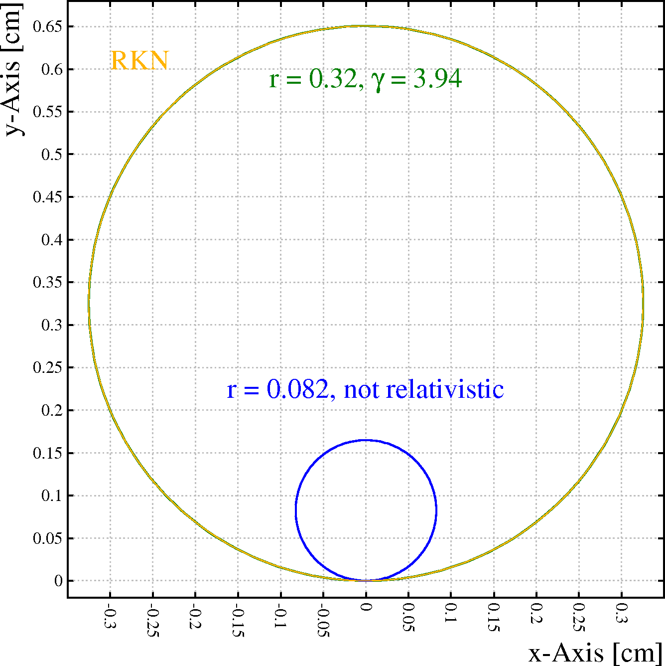
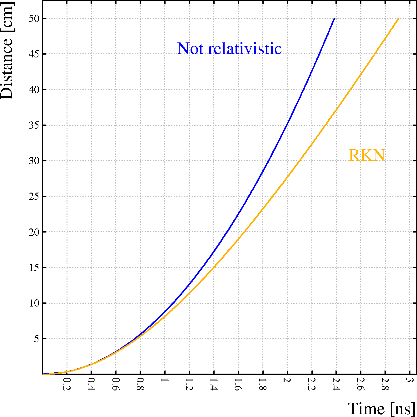
Left: the orange line represents a relativistic electron (\γ nearly 4) moving through a uniform B field of 2\ T perpendicular to the plane of view. It starts from (0,0) with an initial velocity pointing along the positive x-axis. There is no electric field. The green line (partially hidden by the orange line) is a circle with a radius\ =\ p/(B\ q) where p is the momentum and q the charge. For the blue line, the momentum is replaced by m\ v, i.e. this is the result of a non-relativistic calculation.
Right: an electron, initially at rest, accelerates in a uniform electric field of 10\ kV/cm over a distance of 50\ /cm. As in the figure on the left, the blue line shows the non-relativistic calculation.
The transverse component of diffusion, usually the largest of the two, will make a particle follow a trajectory that differs from the mean. Longitudinal diffusion will only have an effect on the drift time.
If diffusion does not cause the particles starting at one and the same point to reach different electrodes, the dominant effect of diffusion is a fluctuation in arrival time. One should note that this fluctuation is not only due to the longitudinal part of diffusion - also the transverse part plays a role.
Garfield offers several methods to estimate the effect of diffusion:
When the transport properties of a gas have been computed with MAGBOLTZ, then transverse diffusion coefficients are stored - unless they have subsequently been deleted with the RESET command of the gas section.
Such integration can explicitly be requested by calling procedures like DRIFT_ELECTRON after having deleted the transverse diffusion data, if needed. Since the DRIFT command by default uses Runge-Kutta-Fehlberg integration, the diffusion graph made by the DRIFT TRACK command, is computed with this technique if the transverse diffusion is absent.
The computed quantity, the spread in arrival time, is estimated by integrating quadratically the ratio of longitudinal diffusion coefficient and drift velocity over the drift path:
spread\² = \∫ (\σ/speed)\² dzThe integration is performed using the Newton-Raphson technique over each step of the drift-line, repeatedly bisecting a step until either the maximum stack depth has been reached, or until the difference between the trapezoidal and the quadratic estimate over a section becomes less than a fraction \ε of the trapezoidal estimate without bisection of the integral over the entire path.
Starting from a \δ-distribution at the starting point, the cloud is adjusted at each step according to the following phenomena:
The cloud is considered Gaussian at every stage.
When the centre of the cloud comes closer than ncloud wire radii to a wire, the cloud is projected onto the wire using one of several methods.
M = e\<SUP\>\∫ \α dz\</SUP\>The integration is performed using the Newton-Raphson technique over each step of the drift-line, repeatedly bisecting a step until either the maximum stack depth has been reached, or until the difference between the trapezoidal and the quadratic estimate over a section becomes less than a fraction \ε of the trapezoidal estimate without bisection of the integral over the entire path.
The integral of the Townsend coefficient over a drift path computed with the Monte_Carlo technique is larger than the integral over a drift path from the same point computed with the Runge_Kutta_Fehlberg method. The reason for this difference is that the path length for Monte Carlo integration is larger than for RKF integration.
Magboltz computes Townsend coefficients which are suitable for use with an Runge-Kutta path. The PROJECTED-PATH-INTEGRATION integration parameter can in certain contexts be used to reduce the step size dependence of the integral over Monte Carlo paths.
Attachment, even at a rate which is orders of magnitude smaller than the gain, profoundly modifies the avalanche fluctuations. Usually, the effect of combined gain and attachment is a loss of energy resolution. The reason for this effect is that the attachment rate, in many gas mixtures, exceeds the gain at the onset of the avalanche. Thus, there is a non-negligible probability that an electron is lost before it can start an avalanche while attachment after the avalanche has reached a certain size has virtually no effect anymore. Fluctuations of the avalanche size can be estimated by using the AVALANCHE and RND_MULTIPLICATION procedures.
L = e\<SUP\>- \∫ η dz\</SUP\>The integration is performed using the Newton-Raphson technique over each step of the drift-line, repeatedly bisecting a step until either the maximum stack depth has been reached, or until the difference between the trapezoidal and the quadratic estimate over a section becomes less than a fraction \ε of the trapezoidal estimate without bisection of the integral over the entire path.
The integral of the attachment coefficient over a drift path computed with the Monte_Carlo technique is larger than the integral over a drift path from the same point computed with the Runge_Kutta_Fehlberg method. The reason for this difference is that the path length for Monte Carlo integration is larger than for RKF integration.
Magboltz computes attachment coefficients for use with an RKF path. The PROJECTED-PATH-INTEGRATION integration parameter can in certain contexts be used to reduce the step size dependence of the integral over Monte Carlo paths.
When the integration routines are called through commands, the status is, on request, printed as part of the output. If the routines are called via procedures, then the status is usually one of the output arguments.
The status is usually shown or returned as a string, shown in the second column of the table below. Occasionally however, a numeric status code is returned, shown in the third column.
The DRIFT_INFORMATION procedure returns on request the status of the last drift-line that has been computed in either of these 2 formats.
| Drift-line ended because ... | Status string | Numeric status code |
|---|---|---|
| Particle left the drift area | Left the drift area |
-1 |
| More than MXLIST steps | Too many steps |
-2 |
| Various faults | Calculations abandoned |
-3 |
| Hit an equipotential plane | Hit a plane |
-4 |
| Entered a dielectricum | Left drift medium |
-5 |
| Left the finite element mesh | Left the mesh |
-6 |
| Attached by a gas molecule | Attached |
-7 |
| Drift-line makes sharp kink | Bend sharper than pi/2 |
-8 |
| Electron energy too high | Energy exceeds E_maximum |
-9 |
| Hit the plane on the left | Hit the minimum x plane |
-11 |
| Hit the plane on the right | Hit the maximum x plane |
-12 |
| Hit the plane on the bottom | Hit the minimum y plane |
-13 |
| Hit the plane on the top | Hit the maximum y plane |
-14 |
| Hit the tube wall | Hit the tube |
-15 |
| Below transport energy | Below transport cut |
-16 |
| Maximum total MC time reached | Maximum MC time reached |
-18 |
| Hit a wire of type X | Hit X wire N |
1 ... MXWIRE |
| Hit a replica of an X-wire | Hit a replica of X wire N |
MXWIRE+1 ... 2*MXWIRE |
| Ended in a solid of type X | Hit X solid N |
2*MXWIRE+1 ... 2*MXWIRE+MXSOLI |
| Other cases (shouldn't occur) | Unknown |
other |
Notes:
Formats:
See the AREA command in the field section.
Before issuing this command, you should take care of the following:
By default, this command operates in the x-y plane, but it can also work in the y-z and z-x planes. The choice is controlled with the STEP and SCAN keywords.
Another important argument is ELECTRON.
Format:
ARRIVAL-TIME-DISTRIBUTION ...
     [ELECTRON {electron | LAST | ONE-BUT-LAST | ... }] ...
     [THRESHOLD threshold] ...
     [TIME-WINDOW {AUTOMATIC | FULL-RANGE | tmin tmax }] ...
     [STEP {X | Y | Z} ...
           [RANGE umin umax] ...
           [INCREMENT ustep]] ...
     [SCAN {X | Y | Z} ...
           [RANGE vmin vmax] ...
           [ANGLE phi]] ...
     [OFFSET w] ...
     [LINES lines] ...
     [DIFFUSION | NODIFFUSION] ...
     [ATTACHMENT | NOATTACHMENT] ...
     [DATASET file [member]] [REMARK remark] ...
     [BINS bins] ...
     [ITERATIONS iterations] ...
     [POLYNOMIAL-ORDER order] ...
     [NOKEEP-HISTOGRAMS | KEEP-HISTOGRAMS] ...
     [NOKEEP-RESULTS | KEEP-RESULTS] ...
     [NOPLOT-ALL-ELECTRONS | PLOT-ALL-ELECTRONS] ...
     [NOPLOT-SELECTED-ELECTRONS | PLOT-SELECTED-ELECTRONS] ...
     [NOPRINT-ALL-ELECTRONS | PRINT-ALL-ELECTRONS] ...
     [NOPRINT-SELECTED-ELECTRONS | PRINT-SELECTED-ELECTRONS] ...
     [PLOT-OVERVIEW | NOPLOT-OVERVIEW]
     [PRINT-OVERVIEW | NOPRINT-OVERVIEW]
If you don't manage to fit all this on a single line, remember that an instruction can be split over several lines by putting an ellipsis at the end of each line but the last.
Example:
track exponential
arrival electron 5 last dataset "arrival/electron.5" thresh 0.8
The track type is set to EXPONENTIAL-SPACING, i.e. the mean number of clusters per cm and the cluster size distribution from the gas section are used. One could also ask for HEED, to simulate a particle. The arrival time distribution of the 5th and of the last electron are computed. A file is written that contains the the time by which 80\ % of these electrons have reached the electrode.
In all 3 cases, one of the 2 axes of the plane, the one that we call here "stepping axis" serves as coordinate in the calibration curve. The tracks cross a line through the centre of the electrode being studied and parallel to the stepping axis at multiples of a user-defined INCREMENT.
The axis which should serve as stepping axis is identified with the STEP keyword. You can set the RANGE of coordinates along the stepping axis for which tracks should be generated.
The other axis in the plane is called "scanning axis". The tracks can be at an ANGLE to this axis, but will usually be parallel to it.
The axis which should serve as stepping axis is identified with the SCAN keyword. Like for the stepping axis, You can limit the RANGE of coordinates along the stepping axis.
|
In the rest of the descriptions, these electrons are referred to as the 'selected electrons'.
If a value is negative, then the electrons will be counted from the back, the last electron corresponds to a value of 0. For the 4 last electrons, you can also type LAST, ONE-BUT-LAST, TWO-BUT-LAST and THREE-BUT-LAST.
[Default: initially, only the 25th electron is selected. The set of selected is remembered as default for the next call.]
[Default: initially 0.5, the median of the distribution. The value set is kept as default for the next call.]
You have, for these histograms, the choice between:
If you specify an explicit time window, then this time window is also used for the all-electrons arrival time histogram. Otherwise, these histograms are booked with the full time range of the track.
Setting a time window is most useful in conjunction with the KEEP-HISTOGRAMS option when you wish to study the histograms in more detail by other programs.
[Default: by default the time range of the selected electron histogram is computed from the first 100 entries of this histogram, whereas the range of the all-electron histogram is set to the time range for the track under study.]
Automatic range calculation means that the first entries are used to compute a suitable range.
The number of entries used to set the scale is equal to half the number of bins of the histograms. You should ensure that the number of track iterations is at least equal to half the number of bins.
Keep in mind, if you do so, that the accuracy of the median arrival time of the selected electron can be reduced because the arrival time distribution is likely to cover only a small fraction of the range of the histogram.
Tracks are usually perpendicular to the stepping axis and at regularly spaced distances from the centre of the electrode. The distance between 2 successive tracks, measured along the stepping axis, can be set with INCREMENT. The part of the stepping axis for which tracks are to be generated can be set with RANGE.
The stepping axis must be either the x-, the y- or the z-axis and must be distinct from the scanning axis.
[By default: X]
The range is specified in the usual coordinate system, not relative to the electrodes.
[Default: the entire stepping axis as given by AREA.]
[Default: approximately 5\ % of the stepping range.]
Tracks are usually parallel to the scanning axis, or at a small ANGLE to it.
The scanning axis must be either the x-, the y- or the z-axis and must be distinct from the stepping axis.
[By default: Y]
The range is specified in the usual coordinate system, not relative to the electrodes.
If the scanning range does not cover the full acceptance of an electrode, some of the electrons to reach the electrode in the real chamber, will be absent in the simulation.
If the range is chosen too large, the accuracy suffers unless the LINES parameter is set to a high value. Moreover, considerable waste of CPU time occurs.
[Default: the entire scanning range as given by AREA.]
[Default: initially 0\°. The angle that you set is kept as default for the next call.]
If you wish to compute arrival time distributions in a parallel plane, then specify OFFSET followed by the 3rd coordinate of the plane.
The parameter lines is the total amount of drift-lines that are calculated this way: 75\ % in the first step and 25\ % in the second.
[Default: the LINES parameter from the drift section.]
[Default: initially half of MXLIST, usually 100-500 bins. The value that you set is kept as default for the next call.]
A common application of this option seems to be the Gaussian fit of the arrival time histograms. This can be done using the FIT_GAUSSIAN procedure, or by a user program after writing the histograms out with the WRITE_HISTOGRAM procedure.
You have to declare the Global variables before the loop if
[Default: histograms are not kept. The setting is kept across calls of ARRIVAL.]
| Global | Description | Type |
|---|---|---|
[X|Y|Z]_<electrode> |
Distance from electrode | Matrix |
MEAN_<electrode> |
mean time all electrons | Matrix |
MEDIAN_<electrode> |
median time all electrons | Matrix |
RMS_<electrode> |
RMS time all electrons | Matrix |
MEAN<electron>_<electrode> |
mean time selected electron | Matrix |
MEDIAN<electron_<electrode> |
median time selected electron | Matrix |
RMS<electron>_<electrode> |
RMS time selected electron | Matrix |
E_<electron> |
sequence # selected electron | Number |
The string "<electrode>" in the global variable name is set to 1 for the first selected electrode, 2 for the next etc.
The string "<electron>" is an index that runs from 1 to the number of selected electrons. E_<electron> shows which electron a given index corresponds to. This can be zero or a negative number: 0 means the last electron, -1 the one but last etc.
You have to declare the Global variables before the loop if
[This option is not on by default, but its setting is remembered from one call to the next.]
It seems therefore tempting to select a large value for this parameter. When saving the distributions (KEEP-HISTOGRAMS) and then using them in a fit, this may indeed be a good approach. However, when extracting information from the MC process with means and RMS, the accuracy tends to degrade for large values of loop, mainly because of single entries with are far from the mean.
When specifying SINGLE-CLUSTER, only one cluster is generated per track, as a result the default value will be low and you are advised to choose a larger value in this case.
[Default: initially 1000. Each ARRIVAL statement has as default the value set in the previous invocation.]
For the lower orders, you may also specify the keywords LINEAR, QUADRATIC or PARABOLIC and CUBIC.
Although values between 1 and 10 are accepted, orders larger than 2 are not recommended since they tend to lead to oscillation.
[Default: 2, parabolic interpolation. The setting will be remembered from one call to the next.]
[Dataset output is only done on request.]
Garfield uses by default a string specifying the electrode as remark for the member header. You may override this.
The PLOT-SELECTED-ELECTRONS and PLOT-ALL-ELECTRONS options tend to lead to very bulky output, but these plots can be instructive.
The time range of these histograms can be controlled with TIME-WINDOW.
You can request printouts of these histograms with PRINT-SELECTED-ELECTRONS or ask the histogram to stay in memory with the KEEP-HISTOGRAMS option.
[These plots are not made by default. The default setting of each call is the setting of the previous call.]
The time range of these histograms can be controlled by TIME-WINDOW, provided you set an explicit time window.
You can request printouts of these histograms with PRINT-ALL-ELECTRONS or ask the histogram to stay in memory with the KEEP-HISTOGRAMS option.
[These plots are not made by default. The default setting of each call is the setting of the previous call.]
This graph is a more refined version of the x(t) relation as calculated by the XT-PLOT instruction.
Since the threshold is usually set to 50\ %, this probability is in practice equivalent to the median.
The spread in shown in this graph is the standard deviation of the arrival time histogram. This measure is sensitive to outliers, and should not be used for delicate studies of the resolution. The KEEP-HISTOGRAMS option can be used to store the histograms, more robust techniques can then be applied outside Garfield.
In all plots, the all-electron graphs are plotted with the graphics representation FUNCTION-1, while the graphs for the selected electrons are plotted as FUNCTION-2.
The results are kept in memory if you specify the KEEP-RESULTS option.
[These plots are initially made by default. The default setting of each call is the setting of the previous call.]
[The setting is remembered from one call to the next.]
The time range of these histograms can be controlled with TIME-WINDOW.
You can request plots of these histograms with PLOT-SELECTED-ELECTRONS or ask the histogram to stay in memory with the KEEP-HISTOGRAMS option.
[These printouts are not made by default. The default setting of each call is the setting of the previous call.]
The time range of these histograms can be controlled by TIME-WINDOW, provided you set an explicit time window.
You can request plots of these histograms with PLOT-ALL-ELECTRONS or ask the histogram to stay in memory with the KEEP-HISTOGRAMS option.
[These printouts are not made by default. The default setting of each call is the setting of the previous call.]
To obtain a printout, use DATASET output.
These histograms are of use mainly if Heed is used to generate tracks. Keep the following in mind in this respect:
When you use the NODELTA-ELECTRONS option of TRACK, then all electrons that stem from a single virtual photon are placed at the location where the virtual photon was absorbed, thus creating a cluster. Such a cluster will usually be located very close to the track. With this option, the cluster size distribution is of interest, but the distance between track and electrons is meaningless.
When you use the DELTA-ELECTRONS option of TRACK, then each electron generated by Heed is dealt with as a cluster of size 1. The electrons will usually be located further from the track than the virtual photons. With this option, the cluster size distribution is of no interest, while the distribution between track and electrons reflects the range of \δ-electrons.
Format:
CLUSTERING-HISTOGRAMS ...
     [ITERATIONS  iter] ...
     [BINS  bins] ...
     [CLUSTER-SIZE-BINS  bins] ...
          [CLUSTER-SIZE-RANGE  {AUTOMATIC | min max}] ...
     [CLUSTER-COUNT-BINS  bins] ...
          [CLUSTER-COUNT-RANGE  {AUTOMATIC | min max}] ...
     [CLUSTER-ENERGY-BINS  bins] ...
          [CLUSTER-ENERGY-RANGE  {AUTOMATIC | min max}] ...
     [DELTA-RANGE-BINS  bins] ...
          [DELTA-RANGE-RANGE  {AUTOMATIC | min max}] ...
     [TRACK-RANGE-BINS  bins] ...
          [TRACK-RANGE-RANGE  {AUTOMATIC | min max}] ...
     [ENERGY-LOSS-BINS  bins] ...
          [ENERGY-LOSS-RANGE  {AUTOMATIC | min max}] ...
     [NOKEEP-HISTOGRAMS | KEEP-HISTOGRAMS] ...
     [PLOT-HISTOGRAMS | NOPLOT-HISTOGRAMS]
[By default 200]
One can either set the same number of bins for all histograms using the BINS keyword, or set a different number for each of the 6 histograms that are produced.
[By default 100]
You may, e.g. for comparison purposes, wish to set the same range for all histograms. This can be accomplished with the various RANGE options.
[By default automatic range selection for all histograms.]
| Name | Description |
|---|---|
SIZE |
Number of electrons in a cluster |
CLUSTERS |
Number of clusters on the track |
DELTA |
Distance between track and electrons [cm] |
RANGE |
Distance between track start and last electron [cm] |
DE |
Total energy loss [MeV] |
ECLUSTER |
Energy per cluster [eV] |
You have to declare the Global variables before the loop if
[The histograms are not kept by default, the setting of this option is remembered from one call to the next.]
[The plots are made by default, the setting is remembered from one call to the next.]
The main choice is between the 5 kinds of starting points:
Format:
DRIFT {EDGES  [LEFT | NOTLEFT] ...
              [RIGHT | NOTRIGHT] ...
              [UP | NOTUP] ...
              [DOWN | NOTDOWN] ...
              [LINES lines]                                    | ...
       TRACK  [NOTIME-GRAPH | TIME-GRAPH] ...
              [NOVELOCITY-GRAPH | VELOCITY-GRAPH] ...
              [NODIFFUSION-GRAPH | DIFFUSION-GRAPH] ...
              [NOAVALANCHE-GRAPH | AVALANCHE-GRAPH] ...
              [NOFUNCTION-GRAPH | FUNCTION-GRAPH function] ...
              [MARKER | SOLID]                                 | ...
       SOLIDS [LINES lines]                                    | ...
       WIRES  [LINES lines] ...
              [ANGLE-RANGE amin amax]                          | ...
       ZEROES                                                    } ...

       [RUNGE-KUTTA-DRIFT | MONTE-CARLO-DRIFT] ...
       [NOISOCHRONS | ISOCHRONS delta_t] ...
       [REVERSE-ISOCHRONS | NOREVERSE-ISOCHRONS] ...
       [LINE-PLOT | NOLINE-PLOT] ...
       [NOLINE-PRINT | LINE-PRINT] ...
       [ELECTRON | ION] ...
       [NEGATIVE | POSITIVE]
If you don't manage to fit all this on one line, remember you are allowed to abbreviate. A line that ends on an ellipsis continues on the next line.
Examples:
drift wires lines=25 isochrons 0.1 nol-pl
drift track function-graph time+5*diffusion nol-pl l-pr
drift zero
(The first example will plot only a set of isochrons computed using 25 drift-lines from each of the selected wires. The second example prints a table of drift times etc. and plots the drift time plus five times the diffusion. The last example shows the acceptance boundaries.)
You can select the edges from which drift-lines should start and you can also set the number of drift-lines from each edge with the LINES keyword.
Although other projections are permitted, this plot type is designed to work in the X-Y projection.
An example of an EDGES drift-line plot, made with the following command: drift edge left right notup notdown isochron 0.02 |
You can select the sides with one or more of the keywords listed in the table below. The keywords are processed in sequence, to obtain drift-lines only from the top, one could specify NONE DOWN.
| Options | Negation | Meaning |
|---|---|---|
LEFT |
NOTLEFT |
From the right to the left |
RIGHT |
NOTRIGHT |
From the left to the right |
UP |
NOTUP |
Upwards from the bottom |
DOWN |
NOTDOWN |
Downwards from the top |
HORIZONTAL |
NOTHORIZONTAL |
From the left and the right |
VERTICAL |
NOTVERTICAL |
From the top and bottom |
ALL |
NONE |
From all 4 borders |
[Default: HORIZONTAL.]
A similar option exists for WIRES and SOLIDS, but separate settings are maintained for each type of plot.
Please note that this LINES option has no link anymore with the LINES command in the drift and signal sections.
[Default: initially set to 20, the setting is remembered from one call of DRIFT to the next.]
You can control the number of drift-lines from each solid with the LINES keyword.
ELECTRONs are usually not produced near the electrodes and they are therefore drifted by default 'in reverse', i.e. with a positive charge. The resulting plot shows the origin of all electrons that can end up on the electrode.
Since IONs are normally produced near the electrode surface, they are drifted in their usual mode, i.e. with a positive charge. The resulting plot therefore shows where ions go that are produced in an avalanche at the electrode.
To modify this behaviour, i.e. to study electrons drifting away from electrodes that repel electrons and ions drifting away from electrodes that attract ions, use the POSITIVE and NEGATIVE options.
A SOLIDS drift-line plot made with a finite element field map of the read-out structure of a TPC. drift solid lines 50 ion positive contour 10 l-pl nol-prSolids have been defined to represent the octagonal cathode, the gating structure (top of the figure) and the avalanche wire, at the origin. The drift-lines start from the wire. The plot has been made with the default isochron settings. |
A similar option exists for EDGES and SOLIDS, but separate settings are maintained for each type of plot.
Please note that this LINES option has no link anymore with the LINES command in the drift and signal sections.
[Default: initially set to 20. The setting is remembered from one call to the next.]
You can control the number of drift-lines from each wire with the LINES keyword.
ELECTRONs are not usually produced near the wires. If the absence of a B field component perpendicular to the E field, this command will drift the particles 'in reverse' so that the resulting plot shows the origin of all electrons that can end up on the wire. This interpretation does not apply should there be an E-perpendicular component of the B field.
Since IONs are normally produced near the wire surface, they are drifted in their usual mode, i.e. with a positive charge. The resulting plot therefore shows where ions go that are produced in an avalanche at the wire.
To modify this behaviour, i.e. to study electrons drifting away from wires that repel electrons and ions drifting away from wires that attract ions, use the POSITIVE and NEGATIVE options.
An example of a WIRES drift-line plot, made with the following command: int-par iso-connect 0.1 drift wire lines 30 isochron 0.02The distance over which isochron segments are connected has been limited in this example for clarity, See ISOCHRON-CONNECTION-THRESHOLD for more information on this. |
The angle range should be specified in degrees. The x-axis is at 0\° while the y-axis is at 90\°.
[Drift-lines are by default started from regularly spaced points around the wire. The setting is kept from one call to the next.]
A similar option exists for EDGES and SOLIDS, but separate settings are maintained for each type of plot.
Please note that this LINES option has no link anymore with the LINES command in the drift and signal sections.
[Default: initially set to 20. The setting is remembered from one call to the next.]
The resulting plot depends to a large extent on the clustering model you have selected with the TRACK command:
Unlike drifting from solids, edges or wires, DRIFT TRACK does not take its number of lines from a LINES keyword.
An example of a TRACK drift-line plot, made with the following command: track -2.9 0.9 2.9 0.9 muon energy 1 GeV drift track noisochronsThis figure shows a HEED simulation of a 1 GeV muon in argon 50\ %, ethane 50\ % mixture. |
The graphs can be customised with the FUNCTION-GRAPH option which takes as argument a function of the following parameters:
| Variable | Meaning | Unit |
|---|---|---|
AVALANCHE |
Gain over the drift path | numeric |
LENGTH |
Drift-line path length | cm |
DIFFUSION |
Integrated diffusion | \μsec |
LOSS |
Survival probability | numeric |
TIME |
Total drift time | \μsec |
X_END or R_END |
x Or r at drift-line end | cm |
Y_END or PHI_END |
y Or \φ at drift-line end | cm or degrees |
Z_END |
z At drift-line end | cm |
X_START or R_START |
x Or r at drift-line start | cm |
Y_START or PHI_START |
y Or \φ at drift-line start | cm or degrees |
Z_START |
z At drift-line start | cm |
Further details on the survival probability can be found under the method used to integrate the attachment coefficients.
Care should be taken that the AREA is chosen sufficiently large to let the particles reach their target.
You may switch off the printing and plotting of both drift-lines and the plotting of isochrons if you're only interested in the graph.
The graph is drawn either as a line or as a set of markers, depending on the setting of the MARKER and SOLID options.
[By default, no graphs are produced. The set of requested graphs is remembered from one call to the next.]
MARKER means that all points are represented by small symbols, e.g. crosses. The symbol that is chosen, as well as its size and colour are taken from polymarker representation FUNCTION-1.
SOLID means that points for drift-lines that reach the same end point are joined by straight line segments. The line type, width and colour are taken from polyline representation FUNCTION-1. Sections of the graph where the drift-lines reach a different end point are separated by vertical lines drawn with the COMMENT polyline representation.
[The initial default is SOLID.]
The ELECTRON/ION and POSITIVE/NEGATIVE settings are ignored. This choice is useful when you're determining the precise acceptance boundaries for each of the wires.
Note: zero finding is not available yet in the default version of Garfield.
Runge Kutta integration is easier to use than Monte Carlo stepping in that the integration parameters are more tolerant.
The parameters controlling the accuracy are adjusted for chambers that are several centimetres large. When studying much smaller structures, at the micron scale, one may wish to request more accuracy.
The Runge Kutta algorithm is well suited for smooth fields, such as those obtained with analytic potentials. The field computed from field maps is sometimes not even continuous, and one should in such cases prefer the Monte Carlo algorithm.
[The initial default is RUNGE-KUTTA-DRIFT.]
This option is particularly interesting used in conjunction with drifting from a TRACK and on which clusters are generated with HEED.
When using this option, care has to be taken that the step_size has been set to a value appropriate to the chamber.
[The initial default is RUNGE-KUTTA-DRIFT.]
The appearance of the isochrons is affected by:
Plotting isochrons can be a CPU intensive operation, depending on the number of drift-lines, the number of isochrons and the options that have been chosen.
In order to plot only the isochrons and not the drift-lines, one uses ISOCHRONS in conjunction with NOLINE-PLOT.
The drift time used for the isochrons is by default measured from the wire or the solid where the electron or ion ends up. This can be changed by using the REVERSE-ISOCHRONS option. Isochrons are only plotted for electrons and ions that do reach a wire, a solid, a plane or the tube. Isochrons are not plotted for particles that reach a replica of a wire (in case of periodic chambers).
Note that isochrons can also be obtained with TABLE CONTOUR and with PLOT-FIELD CONTOUR TIME. These commands do not take the end-point of the electrons into account, and as a result may produce isochrons joining points leading to different wires or solids.
[Isochrons are by default not plotted.]
Thus, the drift-lines starting from the track or the edges are by default reversed when isochrons are computed. This behaviour can be changed by using NOREVERSE-ISOCHRONS.
If you wish the drift time to be measured from the end point of the drift-line in DRIFT WIRES and DRIFT SOLIDS plot, then you should specify the REVERSE-ISOCHRONS option.
[This setting of this option is, like all other DRIFT options, kept from one call to the next.]
Electron drift-lines are plotted with the representation E-DRIFT-LINE and ion drift-lines with ION-DRIFT-LINE.
[This option is initially on.]
This option is not compatible with LINE-PLOT in interactive VM/CMS (because of system shortcomings) unless the output has been re-routed (> file).
This option is initially off.
The POSITIVE option forces the charge to be positive, no matter whether the particle is an electron or an ion.
[The default setting of this option depends on the context.]
The NEGATIVE option forces the charge to be negative, no matter whether the particle is an electron or an ion.
[The default setting of this option depends on the context.]
Format:
GET-TRACK file [member]
Example:
get-tr lib
(This call will retrieve the first prepared track in the dataset LIB.DAT, which may contain members of different type as well.)
You have some control over the graphics input mode with the options listed below.
Format:
GRAPHICS-INPUT [CHOICE-PET chpet] [LOCATOR-PET locpet1 locpet2] ...
               [PICK-PET pickpet] [VALUATOR-PET valpet] ...
               [CHOICE-DEVICE chdev] [LOCATOR-DEVICE locdev] ...
               [PICK-DEVICE pickdev] [VALUATOR-DEVICE valdev] ...
               [WORK-STATION wkid]
Example:
gra loc-pet 1 4
Chooses rubber band for the second point.
The PET can be chosen independently for each input mode.
The grid is common to all sections.
Format:
GRID number_of_steps_in_x [number_of_steps_in_y]
Example:
grid 10 20
You may supply either 1 or 2 arguments. If the 2nd argument is omitted the first value will be used for both the x (or r) and the y (or \φ) spacing.
[Default is 25 for both.]
These parameters are used both in this section and in the signal section.
Format:
INTEGRATION-PARAMETERS ...
     [INTEGRATION-ACCURACY accuracy ] ...
     [ MAXIMUM-STEP-LENGTH maximum_step | ...
       NOMAXIMUM-STEP-LENGTH ] ...
     [ MONTE-CARLO-MAXIMUM-TIME maximum_time | ...
       NOMONTE-CARLO-MAXIMUM-TIME ] ...
     [ MONTE-CARLO-TIME-INTERVAL step_size ...
       MONTE-CARLO-DISTANCE-INTERVAL step_size ...
       MONTE-CARLO-COLLISIONS step_size ] ...
     [ DIFFUSION-SCALING-RANGE scale_min scale_max ] ...
     [ CHECK-ATTRACTING-WIRES | ...
       CHECK-ALL-WIRES ] ...
     [ REJECT-KINKS | ...
       NOREJECT-KINKS ] ...
     [TRAP-RADIUS ntrap] ...
     [INTERPOLATION-ORDER order] ...
     [ COMPUTE-IF-INTERPOLATION-FAILS | ...
       ABANDON-IF-INTERPOLATION-FAILS ] ...
     [CLOUD-PROJECTION-DISTANCE ncloud] ...
     [CLOUD-PROJECTION-METHOD ...
         { CENTRAL-VELOCITY-INTEGRATION | ...
           INTEGRATION | ...
           LONGITUDINAL-DIMENSION | ...
           LARGEST-DIMENSION | ...
           NO-PROJECTION } ...
     [DIFFUSION-ACCURACY \ε_diff] ...
     [TOWNSEND-ACCURACY \ε_Town] ...
     [ATTACHMENT-ACCURACY \ε_att] ...
     [DIFFUSION-STACK-DEPTH stack_diff] ...
     [TOWNSEND-STACK-DEPTH stack_Town] ...
     [ATTACHMENT-STACK-DEPTH stack_att] ...
     [PROJECTED-PATH-INTEGRATION | ...
       TRUE-PATH-INTEGRATION ] ...
     [ DRAW-ISOCHRONS | ...
       MARK-ISOCHRONS ] ...
     [ SORT-ISOCHRONS | ...
       NOSORT-ISOCHRONS ] ...
     [ ISOCHRON-CONNECTION-THRESHOLD iso_thr | ...
       NOISOCHRON-CONNECTION-THRESHOLD ] ...
     [ISOCHRON-ASPECT-RATIO-SWITCH iso_aspect] ...
     [ISOCHRON-LOOP-THRESHOLD iso_loop] ...
     [ CHECK-ISOCHRON-CROSSINGS | ...
       NOCHECK-ISOCHRON-CROSSINGS ]
Example:
int diff-st 5, diff-acc 1.0e-3
Will limit the number of subdivisions to 32 per drift-line step (the default is usually 2\<SUP\>20\</SUP\>) and asks for a relative precision per step of one per mille.
This parameter enters in the update of the step size used in drift line integration. The initial value of this parameter is suitable for chambers with a size of several cm's which have a reasonably complicated field structure. If the field is very simple, or if the chamber is very small, then a smaller value should be chosen.
This parameter has no effect on Monte_Carlo integration and microscopic tracking.
[This parameter is initially set to 10\<SUP\>-8\</SUP\>.]
The Runge_Kutta_Fehlberg drift-line integration method automatically updates the step length at each step. When traversing a large area with a very smooth field, the step size becomes large. If this is not desired, for instance because there is a fine structure behind the smooth area, then one should limit the step size with this option.
Recommended value: a maximum step length of order 1/10th-1/20th of the distance to be traversed.
This parameter has no effect on Monte_Carlo integration and microscopic tracking..
[By default, there is no limit to the step size.]
&CELL &CELL -> plane" y = 0 v = 0 &CELL -> plane" y = 1 v = 1000&GAS co2 add ion-mobility 2e-6 parameters ... transverse-ion-diffusion thermal ... longitudinal-ion-diffusion thermal
&DRIFT int-par monte-carlo-time 0.01 ... monte-carlo-maximum-time 8 area -0.0100 0 0.0100 0.0200
Call plot_drift_area For i From 1 To 5 Do Call drift_ion_mc(0, 0.0190, 0, status, time) Say "{status} {time} microsec" Call plot_drift_line Enddo Call plot_end
Call plot_drift_area For i From 1 To 1000 Do Call drift_ion_mc(0, 0.0190, 0, status, time) Say "{status} {time} microsec" Call get_drift_line(xd, yd, zd, td) Call plot_marker(number(xd[size(xd)]), number(yd[size(yd)]), `function-1`) Enddo Call plot_end
The first plot shows trajectories of 5 ions while the second plot shows the point reached when the cut-off time was reached.
[By default: no maximum]
Steps will have a constant duration in time. Since electrons move much faster than ions, and since the same duration will be used for both, this option is of little practical use in situations where both types of particles are drifting.
[Default: 20 psec]
An approximately constant spatial length will be used for each step. The steps will as a rule not have exactly the requested length as a result of the diffusion process and to a lesser extent also through non-linearities in the field.
This is the most commonly used method since the same settings can be used for both electrons and ions.
[Default: 10 \μm]
When using microscopic tracking, the parameter determines how many collisions occur between 2 collisions which are recorded in the drift path. The parameter does not in any way influence tracking.
[Default: 100 steps]
None of these parameters has an effect on Runge_Kutta_Fehlberg integration.
Excessively small and large scaling factors are indicative of a locally too large step_size. This is commonly the case in the vicinity of small electrodes such as wires. Garfield therefore reduces the step size locally if the scaling is found to lie outside the range given.
The minimum of the scaling range has to be larger than or equal to 0. The maximum has to be larger than 1.
Using the default range, one effectively uses the expressions for diffusion spread in the limit of infinitely small steps. This is not appropriate in case the mean free path is substantially larger than a few \μm.
[Default: 0.95 as minimum and 1.05 as maximum.]
ntrap*radiusthen the electron or ion is considered to be caught by the wire.
When using microscopic tracking, it is advisable to set the radius to 1, i.e. not to consider an electron caught until it tries to enter the wire.
From the moment a wire is considered caught by a wire, a dedicated integration algorithm takes over which is better at estimating the residual drift time than the default algorithm.
[This parameter is preset to a value of the order of 2-5 (depending on program version). This can be too large if the wires are very thick but it may as well be too small for very thin wires.]
For the lower orders, you may also specify the keywords LINEAR, QUADRATIC or PARABOLIC and CUBIC.
Although values between 1 and 10 are accepted, orders larger than 2 are not recommended since they tend to lead to oscillation.
[Default: 2, parabolic interpolation.]
Reasons why a track can't be interpolated for a point are:
Computation time can increase dramatically if many points need to be computed.
If you specify ABANDON-IF-INTERPOLATION-FAILS, then such points are assigned a status of "Abandoned", a drift time, diffusion, multiplication, loss and incidence angle of 0.
[By default, drift-lines are computed when needed.]
If the CHECK-ALL-WIRES option is in effect, then all wires, no matter their charge, are considered able to catch a particle. As soon as a particle comes closer to any wire than the TRAP-RADIUS, an attempt will be made to drift it to the wire.
This is meaningful if you have e.g. dipole (q=0) type wires, but this is harmful if you particles pass near repelling wires, such as gating grids. This option also interferes with calculation of signals due to ions drifting from the neighbourhood of the sense wires.
When not needed, this option also wastes a lot of CPU time.
[By default, only attracting wires are checked.]
This is usually the recommended mode but there are cases, such as the presence of wires with almost no net charge, but with a multipole moment, where the alternative is better suited.
[This option is on by default.]
Drift-lines that are terminated because of this condition, are given the status "Bend sharper than pi/2".
Since fields obtained with finite element methods occasionally have areas with very uneven fields, it may be advisable in such cases to switch the option off.
This option has effect when drift-line integration is performed using the Runge_Kutta_Fehlberg method, but not when the Monte_Carlo or microscopic method is used.
[The option is on by default.]
[This parameter is preset to a value of the order of 2-5.]
When the drift-line approaches the wire, the cloud as a whole is projected onto the wire. For this phase, various algorithms are put at your disposal:
Complete integration over the cloud of the local distance to the wire divided by the local drift velocity.
The longitudinal diffusion over the remaining distance to the wire is added to the estimate.
The longitudinal diffusion over the remaining distance to the wire is added to the estimate.
[This is currently the default method.]
The longitudinal diffusion over the remaining distance to the wire is added to the estimate.
The longitudinal dimension is in principle the dimension that matters, but in the presence of a strong magnetic field, the cloud rapidly rotates near the wire. At the same time, the cloud stretches to the point of becoming almost one-dimensional. A small rounding error in the cloud alignment, can make the dimension along the axis pointing to the wire, very small.
For this reason, this method is not recommended, unless the cloud trap radius is very large (in which case the velocity estimates are likely to be inaccurate).
The longitudinal diffusion over the remaining distance to the wire is added to the estimate.
For reasons explained under LONGITUDINAL-DIMENSION, this method must be considered superior, provided the cloud-trap radius is small.
[The default is 10\<SUP\>-3\</SUP\>.]
This parameter should be set to a small value (1 or 2) if the field is interpolated in a finite element map because the electric field, and hence the quantity to be integrated, is usually discontinuous across element boundaries.
If the field is computed from analytic formulae, then the maximum stack depth has usually little impact on the integration of the diffusion coefficients, since the latter are normally fairly smoothly varying quantities.
For the integration of the Townsend coefficient however, which suddenly grows from 0 to an appreciable value, the stack depth is a critical parameter in the accuracy of the computation. Although CPU time can go up rapidly with stack depth, it is a good idea to keep a large value: when not needed, no use of the stack is made.
[Default is 2, the maximum is given by MXSTCK, usually set to 5. The smallest permitted value is 1 and this setting will usually already give a reasonable accuracy. The default stack depth is large and may result in excessively lengthy computations.]
As a result, integrating the Townsend and the attachment coefficient over Monte Carlo paths leads to larger multiplications and larger losses than are obtained integrating over Runge Kutta Fehlberg paths. In addition, the integral over Monte Carlo paths is ill-defined since it depends on the step size.
To bypass this problem, programs such as Magboltz compute the Townsend coefficient by counting the number of electrons produced in a unit of projected path length measured along the average direction of motion, not in a unit of distance effectively covered by an electron during its random walk motion.
When the PROJECTED-PATH-INTEGRATION integration parameter is active, Garfield replicates this approach by integrating the Townsend and attachment coefficients over path segments projected on the local drift velocity vector. This ensures that the path length integral doesn't depend on the step size used in Monte Carlo integration.
Since electrons occasionally move backwards with respect to the average motion, without this leading to electron losses, the procedure tries to cancel backwards steps against nearby forward steps. A warning message is printed in case of net backwards motion (backscatter).
This option has effect on
[Default is TRUE-PATH-INTEGRATION.]
When this option is selected, you may also wish to inspect the settings of the other isochron related options.
This action of this option can reversed with the MARK-ISOCHRONS option.
Isochrons are drawn using the ISOCHRON polyline representation.
[By default, isochrons are drawn as lines.]
If this option is active, no sorting needs to be done. Hence, the other isochron options are ignored. Plotting isochrons is fast with this option switched on.
This action of this option can reversed with the DRAW-ISOCHRONS option.
Isochrons are marked using the ISOCHRON polymarker representation.
[By default, isochrons are drawn as lines.]
By setting SORT-ISOCHRONS, an attempt is made to order the points in such a manner that the isochrons appear as reasonably smooth lines. Any attempt to do so is likely to fail for certain cases. Moreover, sorting can take a large amount of computing time - the problem is related to the notorious "travelling salesperson problem (TSP)".
Garfield, for these reasons uses a simple algorithm to sort the points on a contour: each contour is classified as being either linear or arcs. Linear contours are sorted along the main axis, points on arcs by angle with respect to the centre of gravity. Arcs that appear to be nearly full loops are drawn as closed contours, otherwise as an open arc. Whether an isochron is sorted as a line or as an arc depends on the setting of ISOCHRON-ASPECT-RATIO-SWITCH. Whether 2 points on an isochron are connected or not depends on the setting of ISOCHRON-CONNECTION-THRESHOLD.
The sorting algorithm by itself is fast - the check on intersects between isochrons and drift-lines in contrast is fairly time consuming.
Sorting is not useful (hence potentially harmful) when the drift-lines come from a track on which the points are ordered - which is usually the case. The sort is useful on the other hand for drift-lines starting from wires or other electrodes.
The SORT-ISOCHRONS option is ignored when MARK-ISOCHRONS is in effect.
[By default: sort done]
The fraction iso_thr can be set to any value between 0 (only markers) and 1 (isochrons are only interrupted by drift-line crossings).
Selecting NOISOCHRON-CONNECTION-THRESHOLD is tantamount to setting iso_thr to 1.
[Initial setting: 0.2]
Whether the set is circular or linear is decided by computing the RMS in the two principal axes of the point distribution. If the ratio of these two RMS's exceeds iso_aspect, then the isochron is assumed to be linear, otherwise circular.
This switch has effect only when SORT-ISOCHRONS has been switched on.
[Initial setting: 3]
[Initial setting: 0.2]
Such crossings can for instance occur if the drift-lines from a track flow left or right of an intermediate object, which itself also attracts some electrons, to a wire located behind the object.
This check is fairly time consuming.
[By default: check done]
Please note that LINES has no effect anymore on the DRIFT command. For DRIFT TRACK, use the TRACK command to set a clustering model. For DRIFT EDGES, DRIFT SOLIDS and DRIFT WIRES, use the respective LINES option on the DRIFT command line.
Format:
LINES lines
Example:
lines 50
This command is now superseded by the LORENTZ_ANGLE procedure.
Format:
LORENTZ-ANGLE x y z
Example:
lorentz 0.5 0.5 1
Format:
MINIMISE f_min ...
         [SELECTION-FUNCTION f_select] ...
         ON f_curve ...
         RANGE t_min t_max ...
         [N n] ...
         [ELECTRON | ION] ...
         [NEGATIVE | POSITIVE] ...
         [FUNCTION-PRECISION \ε_f] ...
         [POSITIONAL-RESOLUTION \ε_pos] ...
         [ITERATE-LIMIT itermax] ...
         [PRINT | NOPRINT] ...
         [DATASET dataset [member] [REMARK remark]]
Example:
minimise time on '5*cos(t), 5*sin(t)' range {pi/4,3*pi/4}
This instruction asks for a minimisation of the drift time over an arc with radius 5 and in the angular range pi/4 to 3 pi/4. Note that quotes are used to specify the curve: a comma has to be placed between the two coordinates, but since the comma is one of the separators and since ON expects only one element, quotes are used. RANGE on the other hand expects two elements and quotes should therefore not be used !
| Symbol | Meaning | Unit |
|---|---|---|
TIME |
Total drift time | \μsec |
LENGTH |
Length of the drift-line | cm |
DIFFUSION |
Integrated diffusion coefficient | \μsec |
AVALANCHE |
exp(\∫ Townsend dz) | probability |
LOSS |
exp(-\∫ attachment dz) | probability |
Further details can be found under the methods used to integrate the diffusion, the multiplication and the attachment.
[The default function to be minimised is TIME.]
The following variables can be used:
| Symbol | Meaning | Unit |
|---|---|---|
TIME |
Total drift time | \μsec |
LENGTH |
Length of the drift-line | cm |
DIFFUSION |
Integrated diffusion coefficient | \μsec |
AVALANCHE |
exp(\∫ Townsend dz) | probability |
LOSS |
exp(-\∫ attachment dz) | probability |
STATUS |
What happened to the particle | see below |
All variables are of type Number except for STATUS which is a String and which can have one of the following values: `Left_Area`, `Too_Many_Steps`, `Abandoned`, `Hit_Plane`, `Left_Drift_Medium`, `Left_Mesh`, `Hit_X_Wire`, `Hit_X_Replica` and `Hit_X_Solid`. `X` is the label that you have assigned to the wire or solid.
Further details can be found under the methods used to integrate the diffusion, the multiplication and the attachment.
[The default selection curve returns always True.]
The range of T can be specified via RANGE.
[No default curve is provided.]
[No default RANGE is provided.]
[The default value for N is 20.]
[This is the default.]
[By default, minimisation is done for electrons.]
[The default is NEGATIVE.]
[This is the default.]
[The default value is 10\<SUP\>-4\</SUP\>, which is also the smallest reasonable value on computers like Vax and IBM. On Cray and other computers with 64-bit precision, \ε_f can be made smaller.]
[The default value is 10\<SUP\>-4\</SUP\>, which is also the smallest reasonable value on computers like Vax and IBM. On Cray and other computers with 64-bit precision, \ε_pos can be made smaller.]
[By default 20.]
[This is default.]
[No such output is produced by default.]
You may also change global options in the same statement, see the top level OPTIONS command for further information.
Format:
OPTIONS [DRIFT-PRINT | NODRIFT-PRINT] ...
        [DRIFT-PLOT | NO-DRIFT-PLOT] ...
        [KEY | NOKEY] ...
        [CONTOUR-ALL-MEDIA | CONTOUR-DRIFT-MEDIUM] ...
        [NOWIRE-MARKERS | WIRE-MARKERS] ...
        [NOCHECK-MAP-INDICES | CHECK-MAP-INDICES]
Example:
opt dr-pl nodr-pr
Most commands have their local print option.
The option is particularly useful to verify that prepared tracks are interpolated with a reasonable order, and to judge whether there is a need to set the COMPUTE-IF-INTERPOLATION-FAILS option.
[The option is by default off.]
This option is ignored if the field is computed from wires and planes.
[This is default.]
This option is ignored if the field is computed from wires and planes. The option is honoured only if the dielectric constants are present in the field map.
[Contours are by default drawn in all media.]
For further information, see the WIRE-MARKERS option in the cell section.
See the CHECK-MAP-INDICES option in the field section for further information.
Similar instructions exist in the field and signal sections.
CPU time can be saved if several plots are combined in a single command.
Format:
PLOT-FIELD [CONTOUR [f1]   [RANGE {cmin cmax | AUTOMATIC}] ...
                           [N n] ...
                           [LABELS | NOLABELS]] ...
           [GRAPH [f2]     [ON f_curve] ...
                           [N n]] ...
                           [SCALE min max] ...
                           [NOPRINT | PRINT] ...
           [HISTOGRAM [f3] [RANGE {hmin hmax | AUTOMATIC}] ...
                           [BINS nbin]] ...
           [SURFACE [f4]   [ANGLES \φ \θ]] ...
           [VECTOR [f5 f6 [f7]]] ...
           [RUNGE-KUTTA-DRIFT | MONTE-CARLO-DRIFT] ...
           [ELECTRON | ION] ...
           [POSITIVE | NEGATIVE]
If you don't manage to fit all this on a single line, remember that lines that end on an ellipsis are continued on the next.
Examples:
plot hist diffusion vector vdx, vdy surf cont
plot contour time range 0.1 0.3
(The first example makes most of the plots using default functions and ranges - useful as a first call. The second example makes a more detailed contour plot.)
| Symbol | Meaning | Note |
|---|---|---|
X, Y, Z |
Position | R, PHI for polar cells |
EX, EY, EZ, E |
E-field at (x,y,z) | ER, EPHI for polar cells |
BX, BY, BZ, B |
B-field at (x,y,z) | only if there is a B-field |
VDX, VDY, VDZ, VD |
Local drift velocity | VDR, VDPHI for polar cells |
LORENTZ |
Local Lorentz angle | - |
TIME |
Total drift time | - |
PATH |
Total drift path length | - |
DIFFUSION |
Integrated diffusion | only if data is available |
AVALANCHE |
Avalanche multiplication | only if data is available |
LOSS |
Survival probability | only if data is available |
STATUS |
Numeric status code | See below |
P |
Pressure of the gas | - |
Further details can be found under the methods used to integrate the diffusion, the multiplication and the attachment. The numeric status code is a Number, not a string.
Other variables can be added on request.
Contours are drawn in the part of the viewing plane that is located within the current AREA box.
The contours are labelled with the function value if the LABEL option is on (which is by default the case).
If you request AUTOMATIC scaling of the range, contours are drawn at decent function heights covering the range of the function on the AREA. The number of contours is used to compute a rough distance between two contours; the distance is rounded downwards. The number of contours actually drawn may therefore be larger than the number you request.
Note that much better equal time contours can be obtained with the DRIFT WIRES ISOCHRONS=delta NODRIFT-PLOT instruction which takes the end-point of the drift-lines into account when deciding which points of the contours are to be joined with a line.
Contours are plotted starting from their crossings with a regular GRID covering the AREA. Very small contours are not found if the grid is course. It is therefore usually preferable to use a fine grid for contours, even though plotting the contours takes more time.
You may also wish to optimise the CONTOUR-PARAMETERS, especially if your AREA is very small or highly non-isometric.
The contours are drawn with the representation CONTOUR-NORMAL and are labelled with CONTOUR-LABELS.
[The default function is VD, the drift velocity, and the contour range is by default adjusted automatically. By default, about 20 contours are plotted.]
The geometric aspects of the track, if used, should be set by means of the TRACK command before calling PLOT-FIELD. Other aspects of the track, such as the clustering model, are not used in the present context.
A curve should be parametrised in terms of T which will run from 0 to 1. All 3 coordinates of the curve should be specified. Note that ON expects only one argument, the parametrisation should therefore be enclosed in quotes, e.g.
'cos(pi*t),sin(pi*t),0'would be appropriate to describe a semi-circle in the z=0 plane.
The SCALE option can be used to force a vertical scale in the plot, this can for instance be useful if you intend to overlay various graphs.
If you select the PRINT option, then the values plotted in the graph will also be printed out. Re-routing of the output (> file) can be used to write the values to a file.
The number of sampling points can be set with N, default is 200.
[The default function is VD, the drift velocity.]
This kind of plot can be useful to estimate for instance the spread in drift time over a given region.
The automatic search for proper binning (AUTOMATIC) uses the first few entries to set the range. Since the grid is scanned in a regular sequence, these entries are not necessarily representative for the entire sample, in particular if the number of bins is small compared to the grid size. See AUTOSCALE for details on the automatic binning procedure.
[The default function is VD. The number of bins is preset to 100 and the range is by default chosen automatically.]
The plot is first rotated by \φ degrees around the z-axis and then tilted by \θ degrees from the z-axis.
This plot is decorative but it is generally agreed upon that it is hard to extract any meaningful information from it\ ...
[The default function is VD, i.e. the magnitude of the drift velocity. The default viewing angles are 30\° and 60\°. The viewing angles are remembered from one call to the next.]
The z-component is set to 0, if not explicitly specified. For other than (x,y) views, this may give incorrect impressions.
The vectors are normalised in 3 dimensions when they are plotted - the length of the vectors shown does not contain information on the magnitude of the quantity that is plotted. A vector that appears point like has no component in the viewing plane.
It is advisable to have roughly equal ranges in view of the scaling that is performed on the vectors.
The vectors are plotted using the FUNCTION-1 representation. The appearance of the arrow is influence by the ARROW-TIP-ANGLE and ARROW-TIP-LENGTH settings.
[The default functions are VDX, VDY, VDZ, i.e. the drift velocity.]
[This is default.]
[This is not default.]
The POSITIVE option forces the charge to be positive, no matter whether the particle is an electron or an ion.
The NEGATIVE option forces the charge to be negative, no matter whether the particle is an electron or an ion.
Runge Kutta integration is easier to use than Monte Carlo stepping in that the integration parameters are more tolerant.
The parameters controlling the accuracy are adjusted for chambers that are several centimetres large. When studying much smaller structures, at the \μm scale, one may wish to request more accuracy.
The Runge Kutta algorithm is well suited for smooth fields, such as those obtained with analytic potentials. The field computed from field maps is sometimes not even continuous, and one should in such cases prefer the Monte Carlo algorithm.
[The initial default is RUNGE-KUTTA-DRIFT.]
When using this option, care has to be taken that the step size has been set to a value appropriate to the chamber, see in particular the step_size as set with the INTEGRATION-PARAMETERS command.
[The initial default is RUNGE-KUTTA-DRIFT.]
Interpolation of tracks is currently done in 3 cases:
The track thus prepared, can be saved in a dataset with WRITE-TRACK from where it can be retrieved in subsequent runs with GET-TRACK.
Format:
PREPARE-TRACK ...
     [ATTACHMENT-COEFFICIENT | NOATTACHMENT-COEFFICIENT] ...
     [DIFFUSION-COEFFICIENT | NODIFFUSION-COEFFICIENT] ...
     [TOWNSEND-COEFFICIENT | NOTOWNSEND-COEFFICIENT] ...
     [LINES n]
Example:
prep-tr
(Accept all defaults, usually adequate.)
In a first step, 75\ % of the drift-lines are distributed uniformly over the track. The remaining 25\ % of the points are chosen in a matter that tries to optimise the accuracy of the interpolation table.
When interpolation is requested for a point which is located between 2 tabulated points from where electrons reach different electrodes, Garfield either computes the drift-line (if the integration parameter COMPUTE-IF-INTERPOLATION-FAILS has been selected) or returns a drift-line status of Abandoned. In case electrons starting from the track reach several different electrodes, LINES should therefore be chosen large so as to minimise the regions where explicit calculation is required.
[By default, the number set with LINES.]
The grouping is of no importance in this section. The selection determines for instance which wires are processed by DRIFT WIRES, ARRIVAL-TIME-DISTRIBUTION and XT-PLOT.
Format:
See SELECT
Example:
sel (1 s) 2 f
(Put wire 1 together with all S wires in one group, make wire 2 a group of its own and do the same for each of the F wires.)
Similar plots can be obtained by first computing a drift-line with the DRIFT_ELECTRON, DRIFT_ELECTRON_3, DRIFT_MC_ELECTRON, DRIFT_POSITRON, DRIFT_POSITRON_3, DRIFT_MC_POSITRON, DRIFT_ION, DRIFT_ION_3, DRIFT_MC_ION, DRIFT_MC_NEGATIVE_ION, DRIFT_NEGATIVE_ION or DRIFT_NEGATIVE_ION_3 procedure, then retrieving it with GET_DRIFT_LINE and finally making the graph with PLOT_GRAPH.
Format:
SINGLE  FROM  x y ...
        [PLOT f1 VS f2 | NOPLOT] ...
        [PRINT f3 | NOPRINT] ...
        [NEGATIVE | POSITIVE] ...
        [ELECTRON | ION]
Examples:
single from 0.5 0.3 plot diffusion vs path
single from 0.1 0.2 print vdx
| Symbol | Meaning | Note |
|---|---|---|
X, Y, Z |
Position | R, PHI for polar cells |
EX, EY, EZ, E |
E-field at (x,y,z) | ER, EPHI for polar cells |
BX, BY, BZ, B |
B-field at (x,y,z) | only if there is a B-field |
VDX, VDY, VDZ, VD |
Local drift velocity | VDR, VDPHI for polar cells |
TIME |
Cumulative drift time | - |
PATH |
Cumulative path length | - |
DIFFUSION |
Local long. diffusion | only if data is available |
TOWNSEND |
Local Townsend coeff. | only if data is available |
ATTACHMENT |
Local attachment coeff. | only if data is available |
STATUS |
Drift-line status code | numeric status code |
The numeric status code is a number which tells where the particle ended. These codes have a 1-1 correspondence with the status strings which are displayed in regular program output.
[No meaningful default functions are provided.]
[The table is by default not produced.]
[By default, a graph is not made.]
Similar functionality is provided by the ELECTRON_VELOCITY and ION_VELOCITY procedures.
Format:
SPEED x y z [ELECTRON | ION] [NEGATIVE | POSITIVE]
Example:
speed 0.5 1.5 0
The POSITIVE or NEGATIVE keyword should, if used, be at the end of the command.
Format:
TABLE [TABLE | NOTABLE] ...
      [NOCONTOUR | CONTOUR] ...
      [ELECTRON | ION] ...
      [NEGATIVE | POSITIVE]
This command must be entered on a single line !
Example:
table
(Only produce the table, no contours.)
Format:
TIME [n]
Example:
time 5
This instruction overwrites the geometrical part of the track description, but uses the clustering type entered via the TRACK statement.
Format:
TIMING [ELECTRONS {electron | LAST | ONE-BUT-LAST | ... }] ...
       [TIME-WINDOW tmin tmax ] ...
       [X-RANGE xmin xmax]
       [Y-RANGE ymin ymax] ...
       [ANGLE-RANGE phimin phimax] ...
       [BINS bins] ...
       [ITERATIONS loops] ...
       [RUNGE-KUTTA-DRIFT | MONTE-CARLO-DRIFT] ...
       [NOATTACHMENT | ATTACHMENT] ...
       [WEIGHTING-FUNCTION weight] ...
       [NOKEEP-HISTOGRAMS | KEEP-HISTOGRAMS] ...
       [NOPLOT-OVERALL | PLOT-OVERALL] ...
       [NOPLOT-SELECTED-ELECTRON | PLOT-SELECTED-ELECTRON] ...
       [NOPRINT-OVERALL | PRINT-OVERALL] ...
       [NOPRINT-SELECTED-ELECTRON | PRINT-SELECTED-ELECTRON]
If you don't manage to fit all this on a single line, remember that lines that end on an ellipsis are continued on the next.
The PROGRESS-PRINT global option enables you to follow the progress of the computations.
Example:
track muon energy 20 GeV
timing electron 3 last y-range -0.3 +0.3
Computes the arrival time distribution of the 3rd and the last electron for random vertical Heed-generated tracks of 20\ GeV muons in the y range [-0.3,+0.3]. The x-range is default, i.e. the x-portion of the AREA.
This should be approximately the threshold of the electronics, but since electronics usually doesn't trigger on a well defined electron, one can't obtain a too accurate resolution from this kind of instruction. If resolution estimates are required, one should compute signals and process these by an electronics simulation program.
[Default: only the 5th electron.]
Tracks are generated uniformly over this x-range. The WEIGHTING-FUNCTION can be used to assign probabilities to the various x values.
[Default: the entire x-range of the AREA.]
[Default: the entire y-range of the AREA.]
Tracks will be generated according to a uniform distribution over this angular range. The WEIGHTING-FUNCTION can be used to attribute a probability to each angle.
One may also enter a single angle if tracks are to be generated only at that angle.
[Default: only vertical tracks are generated.]
Each electron of a cluster is in this case drifted separately.
When using this option, you have to be sure that the time or distance interval for Monte Carlo integration has been set to a reasonable value with INTEGRATION-PARAMETERS.
[Default: Runge-Kutta-Fehlberg integration is used.]
[Default: attachment data is not taken into account.]
Tracks are generated uniformly within the X-RANGE and the ANGLE-RANGE.
[Default: a weight of 1 is assigned to each track.]
[Default: half of MXLIST, usually 100\ bins.]
You have to declare the Global variables before the loop if
[Default: histograms are not kept.]
[Default: 1000.]
The track definition command has an elaborate format that stems from its broad use. For field plotting and potential optimisation, it is sufficient to enter the track location - for most other applications you should specify a clustering model too:
Tracks are 3-dimensional objects. You may omit the z-component of the track, to indicate that the track is located in the (x,y) plane. However, multiple scattering may cause the track to leave this plane and \δ-electrons, Auger electrons and photons are generated irrespective of whether you specify a track located in the (x,y) plane or not.
The model to be used is determined by the last keyword that is found on the line. You may, in a single TRACK statement, set parameters for several models. To avoid ambiguity it is then advisable to type one of the model names (FIXED-NUMBER, EQUAL-SPACING etc) at the end of the line.
Format:
TRACK  [ x0 y0 | x0 y0 x1 y1 | ...
         x0 y0 z0 | x0 y0 z0 x1 y1 z1 | ...
         FROM x0 y0 [z0] | ...
         { TO x1 y1 [z1] | DIRECTION dx dy [dz] RANGE range } ] ...
       [ FIXED-NUMBER ]  ...
            [ LINES nline ]                    | ...
       [ EQUAL-SPACING ]                       | ...
       [ EXPONENTIAL-SPACING ]                 | ...
       [ SINGLE-CLUSTER ]                      | ...
       [ WEIGHTED-DISTRIBUTION ] ...
            [ WEIGHTING-FUNCTION { f | weight vs coordinate } ] ...
            [ SAMPLES nsample ]                | ...
       [ HEED ] ...
            [ DELTA-ELECTRONS | NODELTA-ELECTRONS ] ...
            [ TRACE-DELTA-ELECTRONS | NOTRACE-DELTA-ELECTRONS ] ...
            [ NOMULTIPLE-SCATTERING | MULTIPLE-SCATTERING ] ...
            [ NOENERGY-CUT | ENERGY-CUT ] ...
            [ SWITCH-ELECTRON-TO-CHARGED eswitch ] ...
            [ particle | MASS mass CHARGE charge ] ...
            [ ENERGY energy ]                  | ...
       [ SRIM ] ...
            ENERGY energy ...
            [ particle | MASS mass CHARGE charge ] ...
            [ FLUCTUATION-MODEL model ] ...
            [ LATERAL-STRAGGLING | NOLATERAL-STRAGGLING] ...
            [ LONGITUDINAL-STRAGGLING | NOLONGITUDINAL-STRAGGLING] ...
            [ FAST-VAVILOV | PRECISE-VAVILOV] ...
            [ GROUPING [AUTOMATIC | NONE | n_e ]]     | ...
       [ TRIM ] ...
       [ EQUAL-FLUX-INTERVALS ] ...
            [ FLUX-LINES n]                    | ...
       [ CONSTANT-FLUX-INTERVALS ] ...
            [ FLUX-INTERVAL dv]
Examples:
track * * * 5
Keep all old values except the y coordinate of the end point.
track 1 1 1 2 2 2
Defines a track from (1,1,1) to (2,2,2).
track from 1 1 1 direction 0 0 1 range 5
track mu+ energy 10 GeV lines 10 multiple-scattering nodelta
track fixed
drift track
track heed
drift track
In a first TRACK statement, the location of the track is described. The length of the track projected onto the DIRECTION is limited to 5\ cm. The second TRACK statement provides HEED with a description of the particle, indicates that multiple scattering should be taken into account, but not \δ-electrons. The same line changes the default number of deposits for the FIXED-NUMBER model to 10. The third TRACK statement selects the model to be used, a plot is made with this model, the model is then changed to HEED and another plot is produced.
This would usually be a set of 3\ numbers. If you omit the z-coordinate, 0 is assumed.
[No default, in cm.]
When both TO is used and DIRECTION and RANGE, then the information provided with TO is taken.
This would usually be a set of 3\ numbers. If you omit the z-coordinate, 0 is assumed.
[No default, in cm.]
When using DIRECTION, you must also use RANGE. You should not use TO however in this case, since TO overrules the information from DIRECTION and RANGE.
This would usually be a set of 3\ numbers. If you omit the z-coordinate, 0 is assumed.
[No default, in cm.]
The RANGE should be chosen sufficiently large to avoid having the particle cut prematurely, but not too large either - this would cause overflow in HEED's internal buffers.
[No default, in cm.]
The number of points can be specified after the LINES keyword. The number of clusters per cm, which can be entered in the gas section with PARAMETERS, is not used.
Each deposit contains a single electron or ion, a cluster size distribution, if entered, is not used by this model.
The track is straight in this model.
If this keyword is used, it should be the last keyword on the command line. The model is implied by the use of the LINES keyword.
Used only with the FIXED-NUMBER model.
Note that for a track of length 0, and (e.g.) LINES=25, one would get 25 deposits in the same point. This can be meaningful if you ask for Monte Carlo drifting from that point.
[Default: 20]
1 / meanwhere "mean" is the mean number of clusters per cm as entered with the MEAN option of the PARAMETERS statement in the gas section.
The cluster size distribution will usually be taken from a CLUSTER statement, but can also be derived from data entered with PARAMETERS.
Both the cluster size distribution and the number of clusters must be specified as described above. Heed is not called to fill in missing data.
If this keyword is used, it should be the last keyword on the command line.
mean * lengthwhere "mean" is the mean number of clusters per cm as entered with the MEAN option of the PARAMETERS statement in the gas section and where "length" is the distance between the start and end points of the track.
The spacing between the clusters is exponentially distributed.
The cluster size distribution will usually be taken from a CLUSTER statement, but can also be derived from data entered with PARAMETERS.
Both the cluster size distribution and the number of clusters must be specified as described above. Heed is not called to fill in missing data.
If this keyword is used, it should be the last keyword on the command line.
The deposits are generated in random sequence.
If this keyword is used, it should be the last keyword on the command line. The use of this model is implied by the keywords WEIGHTING-FUNCTION and SAMPLES.
The function should return only non-negative values with a total contents larger than zero. The function need not be normalised.
This model differs from FIXED-NUMBER with a number of samples set to 1 in that the cluster of SINGLE-CLUSTER is at a random location while it would be in the middle of the track when using FIXED-NUMBER.
This model can be seen as a rough approximation to photon from e.g. an \<SUP\>55\</SUP\>Fe source, provided an adequate cluster size distribution is entered.
If this keyword is used, it should be the last keyword on the command line.
The particle knocks an electron out of an atom. The electron may have sufficient energy to cause further ionisations (in that case we speak of a \δ-electron) or it may start drifting towards the anode. The atom returns to its ground state by either emitting an Auger electron or by fluorescence photons. The Auger electrons are treated like the ionisation electrons. The photons can be absorbed in other atoms.
When using the Heed interface, you must define the gas mixture with a HEED command in the gas section. You should specify on the TRACK statement what kind of particle traverses the chamber. Clustering information entered in the gas section through the PARAMETERS and CLUSTER statements is not used when clustering is performed hy Heed.
Since Heed will occasionally generate \δ-electrons, which are not located on the track, it is advisable to switch on the COMPUTE-IF-INTERPOLATION-FAILS integration parameter if you intend to use commands that perform track preparation.
If this keyword is used, it should be the last keyword on the command line. The use of this model is implied by the specification of a particle type, charge or kinetic energy and by the options related to multiple scattering and \δ-electrons.
Reference: I.B.\ Smirnov, NIM\ A\ 554 (2005) 474.
| Name | Particle | Mass [MeV] | Charge |
|---|---|---|---|
ELECTRON |
e\<SUP\>-\</SUP\> | 0.51099907 | -1 |
POSITRON |
e\<SUP\>+\</SUP\> | 0.51099907 | +1 |
MU-MINUS |
\μ\<SUP\>-\</SUP\> | 105.658389 | -1 |
MU-PLUS |
\μ\<SUP\>+\</SUP\> | 105.658389 | +1 |
TAU-MINUS |
\τ\<SUP\>-\</SUP\> | 1777.00 | -1 |
TAU-PLUS |
\τ\<SUP\>+\</SUP\> | 1777.00 | +1 |
GAMMA |
photon | 0 | 0 |
PION-MINUS |
\π\<SUP\>-\</SUP\> | 139.56995 | -1 |
PION-0 |
\π\<SUP\>0\</SUP\> | 134.9764 | 0 |
PION-PLUS |
\π\<SUP\>+\</SUP\> | 139.56995 | +1 |
KAON-MINUS |
K\<SUP\>-\</SUP\> | 493.677 | -1 |
KAON-0 |
neutral K or anti-K | 497.672 | 0 |
KAON-PLUS |
K\<SUP\>+\</SUP\> | 493.677 | +1 |
PROTON |
proton (p) | 938.27231 | +1 |
ANTI-PROTON |
anti-proton (p-bar) | 938.27231 | -1 |
NEUTRON |
neutron (n) | 939.56563 | 0 |
ANTI-NEUTRON |
anti-neutron (n-bar) | 939.56563 | 0 |
Although some neutral particles are included in this list, their use is, with the exception of photons, not meaningful since these particles do not cause ionisation losses in the Heed model.
\δ-Electrons with an energy less than twice the cuteneBdel compilation parameter of Heed, usually set to 1\ keV, do not undergo scattering during their absorption into ionisation electrons.
When using electrons as primary particle, it is advisable not to use the ENERGY-CUT option.
Mass: 0.51099907\ MeV, charge: -1
Mass: 0.51099907\ MeV, charge: +1
Mass: 105.658389\ MeV, charge: -1
Mass: 105.658389\ MeV, charge: +1
Mass: 1777.00\ MeV, charge: -1
Mass: 1777.00\ MeV, charge: +1
Mass: 0, charge: 0.
Example:
&CELL plane x=-10 plane x=+10 v=2000Simulation of the absorption of an \<SUP\>55\</SUP\>Fe photon.&GAS arg-50-eth-50 heed argon 70 co2 30
&DRIFT area -10 -10 -9 10 track -10 5 10 5 gamma energy 5.9 kev Global done Call book_histogram(xhist,100,-10,-5) Call book_histogram(nhist,100,50,250) For i From 1 To 1000 Do If entier(i/100)*100=i Then Say "Iteration {i} ..." Call new_track Global nelec=0 Do Call get_cluster(x,y,z,e,n,done) If done Then Leave Call fill_histogram(xhist,x) Global nelec=nelec+1 Enddo Call fill_histogram(nhist,nelec) Enddo Call plot_histogram(nhist) Call plot_end Call plot_histogram(xhist) Call plot_end
Mass: 139.56995\ MeV, charge: -1
Mass: 139.56995\ MeV, charge: +1
Mass: 493.677\ MeV, charge: -1
Mass: 493.677\ MeV, charge: +1
Mass: 938.27231\ MeV, charge: +1
Mass: 938.27231\ MeV, charge: -1
The mass can either be a number, in which case it is assumed to be in MeV, or a number followed by a unit (eV, keV, MeV or GeV).
[Default: muon mass]
The charge of the particle should be in proton charges, i.e. an electron would have charge -1, a K+ would have +1.
Currently, only charges of +1 and -1 are accepted by Heed, but for SRIM purposes, all non-zero charges are permitted.
The Heed program is designed for GeV-energy charged particles, not for low energy particles which stop in the gas. For these, the SRIM program might be more suitable.
The kinetic energy Ekin is related to the energy E by the relation E\ =\ Ekin\ +\ m, where m is the mass of the particle. In high energy physics, it is usual to quote the energy E of a particle, not the kinetic energy.
The kinetic energy can either be a number, in which case it is assumed to be in MeV, or a number followed by a unit (eV, keV, MeV or GeV).
For reasons of numerical stability, Heed requires the kinetic energy of the particle to be larger than 10\<SUP\>-3\</SUP\> times the particle mass.
[Default: 1 GeV]
Keep in mind that multiple scattering will slow Heed down.
Track preparation is compatible with multiple scattering but such a combination is not meaningful since the drift path of electrons produced far from the prepared track has to be computed without interpolation.
[Multiple scattering is off by default.]
The DELTA-ELECTRONS option is compatible with track preparation, e.g. in the context of signal calculations, but the drift path of electrons produced far from the prepared track will be computed rather than interpolated.
Apart from this, there is no substantial gain in time by switching \δ-electrons off.
[\δ-Electrons are by default kept as they come out of Heed.]
When this option is switched on, they are traced from one collision to the next following the E and B field. Since this is a time consuming operation, you may wish to switch tracing off when studying only the cluster statistics.
\δ-Electrons are not traced either when the NODELTA-ELECTRONS option is specified.
[Tracing is on by default.]
The interface will, on demand by setting the ENERGY-CUT option, remove ionisation electrons after the primary particle has lost all its energy.
Bear in mind that simulations are inherently inaccurate if this option has an effect.
This option will occasionally lead to the loss of an ionisation electron when the primary particle is an ELECTRON.
[This option is off by default.]
This option sets the energy at which this switch-over takes place.
The energy is to be specified in MeV.
[Default: 0.1 MeV = 100 keV.]
The number of points can be set with the FLUX-LINES keyword.
The flux is computed by integrating the electric field component that is in viewing plane and perpendicular to the track.
If the flux changes sign over the track, then points are only generated over the parts of the track where the flux is positive if the total flux over the track is positive. Conversely, if the total flux is negative, points are generated only in areas where the flux is negative.
The cluster size is set to 1 and the cluster energy to 0 in this model.
If this keyword is used, it should be the last keyword on the command line. The use of this model is implied by the presence of the FLUX-LINES keyword.
Segments of the track over which no points are generated because of a change of sign in the flux, do not consume points.
This keyword is only used by the EQUAL-FLUX-INTERVALS model.
[Default: 20 lines]
When using this clustering model, you have to specify the kinetic energy. You may also specify the mass, and charge, of the particle that traverses the chamber, even though this data is contained in, and extracted from, the SRIM tables.
The SRIM tables contain in addition the following data:
Note that these tables contain only average quantities, not their distributions. The interface tries to generate individual tracks which statistically reproduce the above quantities. It does this by starting with a particle with the given energy and a direction derived from the beginning and ending point of the track.
Then, iteratively,
Example: displaying the Bragg curve
&DRIFT
area -1 -10 30 10
track 0 0 20 0 ...
    energy 10 MeV ...
    charge 2 ...
    grouping=auto ...
    fluctuation-model=gaussian

Call book_histogram(hx,100,0,8)
For i From 1 To 100 Do
   Call new_track
   Do
      Call get_cluster(x,y,z,n,e,done)
      If done Then Leave
      Call fill_histogram(hx,x,n)
   Enddo
Enddo
Call plot_histogram(hx,`x [cm]`,`Deposits vs x`)
Call plot_end
The histogram hx is booked for a range of [0\ cm, 8\ cm] - we can't use an automatic range here since the range will be determined from the first few entries and the x-coordinates will come in sequence.
[By default, switched on.]
Since longitudinal straggling is SRIMs way to introduce energy loss fluctuations, this option should be switched off when energy loss fluctuations are introduced by other means. See for this the FLUCTUATION-MODEL options.
[By default, switched on.]
The alternative is the use of the precise Vavilov generator, which internally is the same as RND_VAVILOV.
In most cases, the additional precision afforded by using the precise generator is not justified by the overall precision of the energy loss generator.
[Default is the fast generator.]
You may override this by manually specifying a grouping size.
[Automatic grouping is default.]
The kinetic energy Ekin is related to the energy E by the relation E\ =\ Ekin\ +\ m, where m is the mass of the particle. In high energy physics, it is usual to quote the energy E of a particle, not the kinetic energy.
The kinetic energy can either be a number, in which case it is assumed to be in MeV, or a number followed by a unit (eV, keV, MeV or GeV).
[No default; mandatory parameter]
[By default, the mass found in the SRIM table.]
[By default, the charge found in the SRIM table.]
By default, Garfield uses a combined model which is described in http://cern.ch/rjd/Garfield/vavilov.ps This model uses the Landau distribution for small steps, the Vavilov distribution for medium steps and the Gaussian distribution for long steps. The parameters of these distributions are automatically updated according to the particle properties (mass, charge and kinetic energy) and the gas properties (A, Z and the density rho).
The following models are available:
Whenever using a Vavilov distribution, whether by using the "combined" model or by requesting the Vavilov distribution explicitly, you have the choice between two generators, a fast one (FAST-VAVILOV) and a more precise one (PRECISE-VAVILOV).
When explicitly requesting the use of the Vavilov distribution, beware of the limitations in applicability which are explained in the note cited above. The permissible parameter range is that of the RND_VAVILOV or RND_VAVILOV_FAST procedure, depending on the choice of generator.
Please note that range fluctuations should be switched off with the NOLONGITUDINAL-STRAGGLING option if energy loss fluctuations are introduced.
[Default: the combined model.]
Interface written by James Butterworth.
The flux between 2 points can be specified following the FLUX-INTERVAL keyword.
The flux is computed by integrating the electric field component that is in viewing plane and perpendicular to the track.
If the flux changes sign over the track, then points are only generated over the parts of the track where the flux is positive if the total flux over the track is positive. Conversely, if the total flux is negative, points are generated only in areas where the flux is negative.
The cluster size is set to 1 and the cluster energy to 0 in this model.
If this keyword is used, it should be the last keyword on the command line. The use of this model is implied by the presence of the FLUX-INTERVAL keyword.
The flux interval is specified in units of V.
This keyword is only used by the CONSTANT-FLUX-INTERVALS model.
[Default: 10\ V.]
The track location and, when using the Heed model also the clusters, are shown usually as last elements of a figure to ensure that they are not hidden under drift-lines.
In other models than Heed, the track location is plotted but the cluster locations are not marked.
The XT-PLOT algorithm works as follows:
Note that there is another instruction in Garfield, ARRIVAL-TIME-DISTRIBUTION, that serves approximately the same purpose. The differences between XT-PLOT and ARRIVAL are summarised in the table below. As can be seen from the table, ARRIVAL provides more detail than XT-PLOT, which in return is faster.
For accurate calibration, the use of signals is recommended. This permits, in addition to all the features ARRIVAL, processing of the signals by electronics and the setting of a true threshold.
-----------------------------------------------------------------------
Aspect    ARRIVAL                        XT-PLOT
-----------------------------------------------------------------------
input     complete gas tables,           drift velocity and optionally
          clustering properties          diffusion and Lorentz angle
          (spacing, cluster size)        tables
method    Monte Carlo generation of      parabolic minimisation of the
          tracks with clusters           drift time over lines
included  drift velocity, Lorentz        drift velocity, Lorentz angle,
          angle, diffusion, attachment,  optionally also diffusion
          cluster spacing and size       over the fastest drift-line
output    mean, median and RMS of        minimum drift time, diffusion
          selected electrons             over the fastest drift-line
-----------------------------------------------------------------------
Format:
XT-PLOT [DATASET file [member] [REMARK remark] ...
        [ANGLE angle] ...
        [X-RANGE xmin xmax] ...
        [X-STEP xstep] ...
        [JUMP jump] ...
        [ITERATIONS {YES|NO|itermax}] ...
        [PRECISION \ε] ...
        [LEFT-ANGLE-RANGE lmin lmax] ...
        [RIGHT-ANGLE-RANGE rmin rmax] ...
        [PRINT-XT-RELATION | NOPRINT-XT-RELATION] ...
        [PLOT-XT-RELATION | NOPLOT-XT-RELATION] ...
        [KEEP-RESULTS | NOKEEP-RESULTS] ...
        [SCALE min max]
Examples:
xt-plot
xt dataset lib.dat xt1 precision 1e-2
(The second example will produce fairly quickly a crude x(t).)
The default remark for x(t) relations states the wire number and the angle.
[Default: 0\°.]
[By default the whole x-range of the drift area is taken.]
[By default the whole x-range of the drift area is taken.]
[By default chosen such that the step size is a reasonable number for about 20 data points.]
[By default, no point is interpolated.]
[Default: 5.]
[Default: 10\<SUP\>-4\</SUP\>.]
This option should be used with great caution if a magnetic field is present since the drift-lines in this case normally approach the wire at a (substantial) angle.
[The default range is +90\° to -90\° both left and right.]
[On by default.]
The graph usually shows 2 curves:
Both curves are interrupted if the procedure has doubts about the accuracy of a neighbouring point - markers are used if both neighbours of a reliable point are considered unreliable.
[On by default.]
| Global | Description | Units | Type |
|---|---|---|---|
X_<n> |
Distance from electrode | cm | Matrix |
T_<n> |
Distance from electrode | \μsec | Matrix |
S_<n> |
Distance from electrode | \μsec | Matrix |
The string "<n>" in the global variable name is set to 1 for the first x(t) relation, 2 for the next etc.
You have to declare the Global variables before the loop if
[This option is not on by default, but its setting is remembered from one call to the next.]
This statement should be issued after the DRIFT command.
Format:
WRITE-ISOCHRONS DATASET file [member] [REMARK remark]
Example:
wr-iso 'test data b'
(Writes the isochrons to the VM/CMS dataset TEST DATA on the users B disk.)
The field is left blank by default.
Format:
WRITE-TRACK DATASET file [member] [REMARK remark]
Example:
wr-tr 'disk$scratch:[pubzh.work.garfield]track.dat'
The field is left blank by default.
Since signal calculation and processing is strongly experiment dependent, this section consists only of a series of building blocks with which you can hopefully build a detailed simulation. A series of procedure calls, listed at the end of the overview, form an integral part of this section.
Setting parameters:
| Command | Short description |
|---|---|
AREA |
Sets the size of the plotting area |
AVALANCHE |
Sets the avalanche model |
FOURIER |
Number of Fourier terms (periodic cells) |
GRID |
Grid density for PLOT-FIELD |
INTEGRATION-PARAMETERS |
Drift-line integration parameters |
OPTIONS |
Various printing and plotting options |
RESET |
Resets one or more aspects of the signals |
SELECT |
Establishes the list of sense wires |
SIGNAL-PARAMETERS |
Signal calculation parameters |
TRACK |
Sets the track for which a signal is generated |
WINDOW |
Sets the time window of the signals |
Computing and processing a signal:
| Command | Short description |
|---|---|
ADD-NOISE |
Adds noise to the signals |
CONVOLUTE-SIGNALS |
Convolutes signals with a transfer function |
PLOT-SIGNALS |
Plots the signals |
SIGNAL |
Simulates a signal |
WRITE-SIGNALS |
Stores a signal in a dataset |
Service instructions:
| Command | Short description |
|---|---|
PREPARE-TRACK |
Prepare a track for interpolation |
GET-TRACK |
Retrieve a a prepared track from a dataset |
WRITE-TRACK |
Save a prepared track in a dataset |
Debugging instructions:
| Command | Short description |
|---|---|
CHECK |
Verify proper functioning |
PLOT-FIELD |
Plots the signal induction field |
Procedure calls:
| Procedure | Short description |
|---|---|
Call ADD_SIGNALS |
Computes signals for current drift-line |
Call GET_RAW_SIGNAL |
Retrieves raw signals for an electrode |
Call GET_SIGNAL |
Retrieves the signals for an electrode |
Call INDUCED_CHARGE |
Computes integrated induced charge |
Call LIST_RAW_SIGNALS |
Lists raw signals currently in memory |
Call STORE_SIGNAL |
Stores a signal |
Call THRESHOLD_CROSSING |
Computes threshold crossing times |
Call WEIGHTING_FIELD |
Returns the weighting field |
Call WEIGHTING_FIELD_3 |
Returns the weighting field |
The noise function is evaluated separately for each wire, but the same noise is added on demand both to the direct and cross-induced parts of the signals.
It is permissible to use the ADD-NOISE command before any signal has been computed, but the time WINDOW must have been set beforehand.
Format:
ADD-NOISE NOISE-FUNCTION function ...
          [NOCROSS-INDUCED | CROSS-INDUCED]
Example:
add-noise noise-function -0.01*rnd_poisson(30)
In this example, the RND_POISSON generator is used to add to each of the sampling points a Poisson distributed number with mean 30, multiplied by -0.01.
There is no default function, but the function is remembered
If the noise is added both to the cross-induced signal and to direct signal, then these signals must not be summed later: the noise would be added twice.
[Option off by default]
Formats:
See the AREA command of the field section.
No default type of avalanche is set - you must issue an AVALANCHE command prior to any signal calculation, each time you enter the &SIGNAL section.
Only avalanches generated by electrons that hit an electrode (a wire, a plane, the tube, a solid) are affected by this statement. In particular, this command has no influence on avalanches in a field map for which no solids have been defined.
This statement takes effect on SIGNAL commands that follow. Issuing the AVALANCHE command does reset the signals that may have computed earlier.
Format:
AVALANCHE {EXPONENTIAL mean | ...
           FIXED factor | ...
           FIXED-TOWNSEND | ...
           GAUSSIAN mean relative_sigma | ...
           NONE | ...
           POLYA-FIXED [mean [theta]] | ...
           POLYA-TOWNSEND [theta] | ...
           TOWNSEND}
Examples:
aval exp 1e4
aval townsend
For large mean multiplications, significant deviations are observed, especially at the low end high ends of the distribution. These can empirically be modeled with the Polya distribution which can be obtained by using POLYA-FIXED or POLYA-TOWNSEND
Although the exponential distribution has a non-zero probability at 0, the multiplication factor used in Garfield is always equal to at least 1: if a factor less than 1 is drawn, it is rejected and a new number is drawn.
The mean multiplication factor has to be strictly positive.
[Default: you have to specify the mean multiplication.]
The factor has to be larger than or equal to 1, the latter being equivalent to specifying NONE.
[Default: none, you have to specify the multiplication factor.]
The multiplications obtained with this option are constant for a given drift path. They may vary when the Monte Carlo drift line integration routines are used since these introduce variations in the drift path.
This option is accessible only if Townsend data has been entered in the gas section.
Please note that the 2nd argument is a relative, not an absolute, standard deviation. If you use for instance
avalanche gaussian 20000 0.5
then you'll end up with a normally distributed multiplication with a mean of 20000 and a sigma of 10000.
The Gaussian distribution has non-zero probability for factors less than 0. Since the multiplication factor as defined here has to be equal to 1 at least, Garfield will if needed repeatedly draw a random number until an acceptable number is found.
The mean is allowed to be negative, but the width must be strictly positive - a width of zero would be equivalent to using the FIXED option.
[Default: none, you have to specify both the mean and the relative standard deviation.]
The Polya distribution is a \Γ-distribution that matches reasonably well the fluctuations in a cylindrically symmetric amplification region. A physical interpretation of the parameter \θ is given in G.\ D.\ Alkhazov, NIM\ 89 (1970) 155-165.
When \θ is set to 0, an exponential distribution is obtained. If \θ\ <\ 0, the distribution is "concave", while for \θ\ >\ 0 the distribution assumes the more usual shape with a maximum.
The properties of this distribution can be examined using the RND_POLYA function, as shown in the following example:
Say "Please enter theta"
Parse Terminal theta
Call book_histogram(ref,100,0.0,5.0)
For i From 1 To 50000 Do
   Call fill_histogram(ref,rnd_polya(theta))
Enddo
!options log-y
Call plot_histogram(ref,`Multiplication`,`Polya distribution`)
Call plot_end
Although the Polya distribution has a non-zero probability at 0, the multiplication factor used in Garfield is always equal to at least 1. If a factor less than 1 is drawn, it is rejected and a new number is drawn.
The mean multiplication factor has to be strictly positive,
[The default value for the mean multiplication is 1, the default setting of the \θ parameter is 0.5.]
See POLYA-FIXED for comments on the Polya distribution.
Additional fluctuations are obtained when the Monte Carlo drift line integration routines are used since these introduce variations in the drift path.
Although the Polya distribution has a non-zero probability at 0, the multiplication factor used in Garfield is always equal to at least 1. If a factor less than 1 is drawn, it is rejected and a new number is drawn.
This option is accessible only if Townsend data has been entered in the gas section.
[The default value for \θ is 0.5.]
This is similar to the EXPONENTIAL option, but here the mean of the distribution may be different for each ionisation cluster. Additional fluctuations are obtained when the Monte Carlo drift-line integration routines are used since these introduce variations in the drift path.
Although the exponential distribution has a non-zero probability at 0, the multiplication factor used in Garfield is always equal to at least 1. If a factor less than 1 is drawn, it is rejected and a new number is drawn.
This option is accessible only if Townsend data has been entered in the gas section.
Format:
CHECK [AVALANCHE] ...
      [DIFFUSION] ...
      [CLUSTER] ...
      [RANGE min max] ...
      [FROM x y] ...
      [N n] ...
      [BINS nbin]
Example:
ch avalanche from 5 6 bins 50
Signal processing in Garfield is limited to convoluting the induced currents with transfer functions and to addition of certain types of noise with ADD-NOISE.
The CONVOLUTE-SIGNALS command convolutes all signals that are available at the moment the command is issued, with the transfer function that is specified. You may issue several of these commands in succession.
The transfer function is only evaluated once for all signals. The transfer function should therefore not depend on random number generators.
It is permissible to use the CONVOLUTE-SIGNALS command before any signal has been computed, e.g. in order to process noise, but the time WINDOW must have been set beforehand.
Format:
CONVOLUTE-SIGNALS ...
     TRANSFER-FUNCTION { function  |  transfer VS time } ...
     [ADD-ON-FUNCTION add] ...
     RANGE tmin tmax
Example:
convolute-signals ...
     transfer-function 250*(6*t/0.025)^6*exp(-6*t/0.025) ...
     range 0 2000
(This example, taken from an Atlas muon tube study, simulates the response of a pre-amplifier.)
There is no default transfer function, but the transfer function is remembered from one call to the next.
       s + 1/t1
F(s) = -------- ,   F(t) = (1/t1 - 1/t2) * exp(-t/t2) + \δ(t)
       s + 1/t2
To simulate such a filter, one would convolute with exp(-t/t2)
and add the original signal on top.
The function to be added is allowed to be a function of the time, written as T, and of the signal, written as SIGNAL. In the case of the example, one would therefore type
convolute transfer-function 0.2*exp(-t/0.012) add signal
[By default, no function is added.]
[By default, the range extends from 0 to 10\<SUP\>10\</SUP\>\ \μsec.]
Garfield will, by default, compute the weighting fields by considering only the basic cell - suppressing all periodicities. This is a good approximation if the wires that are read-out are surrounded by many other wires in the basic cell.
If this is not the case, then the FOURIER command can be used to request inclusion of a number of copies of the basic cell. For technical reasons related to the Fourier transforms needed for such calculations, the number of copies to be considered must be an integral power of 2.
Signal calculations with a large number of copies of the basic cell requires considerable memory - temporary files on disk will be used for the purpose.
Requesting a large number of copies is meaningful only in chambers which contain equipotential planes - convergence is poor otherwise.
In addition to numeric arguments, the value NONE can be specified. This is to be used in the exceptional case where all copies of the read-out wires are interconnected. The weighting field will then be computed using the same potential functions that are used for the electric field. In addition, avalanches will be started from the copy in the basic cell, of the wire where an electron ends. As a result, the plot produced in response to the CLUSTER-PLOT option, may be surprising.
This statement takes effect on SIGNAL commands that follow. Issuing the FOURIER command does reset the signals that may have computed earlier.
Format:
FOURIER [ copies | NONE ]
Example:
fourier 16
(Note that this setting may require a fantastic amount of disk I/O !)
Format:
See the GET-TRACK command in the drift section.
The grid is common to all sections.
Format:
GRID number_of_steps_in_x [number_of_steps_in_y]
Example:
grid 25 15
You may supply either 1 or 2 arguments. If the 2nd argument is omitted the first value will be used for both the x (or r) and the y (or \φ) spacing.
[Default is 25 for both.]
Format:
OPTIONS [ CLUSTER-PRINT | NOCLUSTER-PRINT ] ...
        [ CLUSTER-PLOT | NOCLUSTER-PLOT ] ...
        [ CONTOUR-ALL-MEDIA | CONTOUR-DRIFT-MEDIUM ] ...
        [ NOWIRE-MARKERS | WIRE-MARKERS ] ...
        [ NOCHECK-MAP-INDICES | CHECK-MAP-INDICES ]
Example:
opt nocluster-print
When FOURIER is set to NONE, ions may appear to start from another periodic copy of a wires than the copy where the electrons arrive.
The electron drift-lines are plotted with representation E-DRIFT-LINE, the ions with ION-DRIFT-LINE.
The various elements of the track are shown with their respective representations.
[This option is initially on.]
On certain systems, the graphics and printed output appear on the same screen. If both CLUSTER-PLOT and CLUSTER-PRINT are desired, it is on such systems advisable to redirect the printed output since the output of these 2 options is produced simultaneously.
[This option is initially on.]
This option is ignored if the field is computed from wires and planes.
[This is default.]
This option is ignored if the field is computed from wires and planes. The option is honoured only if the dielectric constants are present in the field map.
[Contours are by default drawn in all media.]
For further information, see the WIRE-MARKERS option in the cell section.
See the CHECK-MAP-INDICES option in the field section for further information.
The main quantities of interest in this context are the so-called weighting_field and the charges induced in an electrode by electrons and ions drifting from a given point.
The weighting field and the induced charge are plotted separately for each electrode that is read out. You can however limit the set of plots to a subset of electrodes.
There are related instructions in the field and drift sections.
Format:
PLOT-FIELD [CONTOUR [f1]   [RANGE {cmin cmax | AUTOMATIC}] ...
                           [N n] ...
                           [LABELS | NOLABELS]] ...
           [GRAPH [f2]     [ON f_curve] ...
                           [N n]] ...
                           [SCALE min max] ...
                           [NOPRINT | PRINT] ...
           [HISTOGRAM [f3] [RANGE {hmin hmax | AUTOMATIC}] ...
                           [BINS nbin]] ...
           [SURFACE [f4]   [ANGLES \φ \θ]] ...
           [VECTOR [f5 f6]] ...
           [GROUP {ALL | sense }] ...
           [TIME-WINDOW tmin tmax] ...
           [RUNGE-KUTTA-DRIFT-LINES | MONTE-CARLO-DRIFT-LINES]
If you don't manage to fit all this on a single line, remember that lines that end on an ellipsis are continued on the next.
Examples:
plot-field hist status_e vector surf cont
plot-field contour time_ion range 1000 3000
(The first example makes most of the plots using default functions and ranges\ - useful as a first call. The result will be an histogram that shows where electrons end up, a vector plot of the weighting field and a contour plot of the currents induced by single electrons released from the various locations. The second example makes a contour plot of the ion drift time.)
| Symbol | Meaning | Note |
|---|---|---|
X, Y, Z |
Position | R, PHI for polar cells |
EX, EY, EZ, E |
E-field at (x,y,z) | ER, EPHI for polar cells |
EWX, EWY, EWZ, EW |
Weighting at (x,y,z) | EWR, EWPHI for polar cells |
BX, BY, BZ, B |
B-field at (x,y,z) | only if there is a B-field |
VDX, VDY, VDZ, VD |
Local e- drift velocity | VDR, VDPHI for polar cells |
TIME_E |
Drift time for electrons | - |
TIME_ION |
Drift time for ions | - |
STATUS_E |
Drift status for electrons | a number, not a string |
STATUS_ION |
Drift status for ions | a number, not a string |
Q_E |
Charge induced by an e- | - |
Q_ION |
Charge induced by an ion | - |
Other variables can be added on request.
The charge should be +1 or -1 for a particle drifting from the read-out electrode to another conductor and 0 for a particle that drifts between conductors that are not read out.
The charge induced over a given path should, apart from the sign, should not depend on the type of particle that drifts. However, in the presence of a magnetic field, electrons and ions will in general follow different paths, may therefore end up at different points, and hence induce different charges.
Charges are expressed in multiples of the electron charge.
The electrode whose weighting field is to be used can be set with the GROUP keyword. You can limit the charge integration to a time window by means of the TIME-WINDOW keyword.
The times are expressed in \μsec.
There is one such field per electrode or per group of sense wires.
This field is computed by setting the read-out electrode to unit voltage and earthing all other conductors.
The unit of the weighting field is 1/cm.
Contours are drawn in the part of the viewing plane that is located within the current AREA box.
The contours are labelled with the function value if the LABEL option is on (which is by default the case).
If you request AUTOMATIC scaling of the range, contours are drawn at decent function heights covering the range of the function on the AREA. The number of contours is used to compute a rough distance between two contours; the distance is rounded downwards. The number of contours actually drawn may therefore be larger than the number you request.
Contours are plotted starting from their crossings with a regular GRID covering the AREA. Very small contours are not found if the grid is course. It is therefore usually preferable to use a fine grid for contours, even though plotting the contours takes more time.
You may also wish to optimise the CONTOUR-PARAMETERS, especially if your AREA is very small or highly non-isometric.
The contours are drawn with the representation CONTOUR-NORMAL and are labelled with CONTOUR-LABELS.
[The default function is Q_E, the charge induced on the read-out electrode by an electron drifting from (x,y,z). The contour range is by default adjusted automatically. By default, about 20 contours are plotted.]
The geometric aspects of the track, if used, should be set by means of the TRACK command before calling PLOT-FIELD. Other aspects of the track, such as the clustering model, are not used in the present context.
A curve should be parametrised in terms of T which will run from 0 to 1. All 3 coordinates of the curve should be specified. Note that ON expects only one argument, the parametrisation should therefore be enclosed in quotes, e.g.
'cos(pi*t),sin(pi*t),0'would be appropriate to describe a semi-circle in the z=0 plane.
The SCALE option can be used to force a vertical scale in the plot, this can for instance be useful if you intend to overlay various graphs.
If you select the PRINT option, then the values plotted in the graph will also be printed out. Re-routing of the output (> file) can be used to write the values to a file.
The number of sampling points can be set with N.
[The default function is Q_E, the charge induced on the read out electrode by an electron drifting from (x,y,z). The default number of sampling points is MXLIST, 200 or 1000 depending on the compilation parameters.]
This kind of plot can be useful to estimate for instance the spread in drift time over a given region.
The automatic search for proper binning (AUTOMATIC) uses the first few entries to set the range. Since the grid is scanned in a regular sequence, these entries are not necessarily representative for the entire sample, in particular if the number of bins is small compared to the grid size. See AUTOSCALE for details on the automatic binning procedure.
[The default function is Q_E, the charge induced on the read out electrode by an electron drifting from (x,y,z). The default preset to 100 and the range is by default chosen automatically.]
The plot is first rotated by \φ degrees around the z-axis and then tilted by \θ degrees from the z-axis.
This plot is decorative but it is generally agreed upon that it is hard to extract any meaningful information from it ...
[The default function is Q_E, the charge induced on the read out electrode by an electron drifting from (x,y,z). The default viewing angles are 30\° and 60\°. The viewing angles are remembered from one call to the next.]
The z-component is set to 0, if not explicitly specified. For other than (x,y) views, this may give incorrect impressions.
The vectors are normalised in 3 dimensions when they are plotted - the length of the vectors shown does not contain information on the magnitude of the quantity that is plotted. A vector that appears point like has no component in the viewing plane.
It is advisable to have roughly equal ranges in view of the scaling that is performed on the vectors.
The vectors are plotted using the FUNCTION-1 representation. The appearance of the arrow is influence by the ARROW-TIP-ANGLE and ARROW-TIP-LENGTH settings.
[The default functions are EWX, EWY, EWZ, i.e. the weighting field.]
Read-out groups are formed with the SELECT command. SELECT without arguments will show how the groups are composed.
[By default, all sense wire groups are plotted.]
The lower time limit may be specified as START, the upper time limit as END (or INFINITY).
[When no time window is given, the charge is integrated from the moment the particle starts to drift until the moment it stops. The time window is reset each time PLOT-FIELD is called.]
Runge Kutta integration is easier to use than Monte Carlo stepping in that the integration parameters are more tolerant.
The parameters controlling the accuracy are adjusted for chambers that are several centimetres large. When studying much smaller structures, at the \μm scale, one may wish to request more accuracy.
The Runge Kutta algorithm is well suited for smooth fields, such as those obtained with analytic potentials. The field computed from field maps is sometimes not even continuous, and one should in such cases prefer the Monte Carlo algorithm.
[The initial default is RUNGE-KUTTA-DRIFT-LINES.]
This option is particularly interesting used in conjunction with drifting from a TRACK and on which clusters are generated with HEED.
When using this option, care has to be taken that the step size has been set to a value appropriate to the chamber, see in particular the step_size as set with the INTEGRATION-PARAMETERS command.
[The initial default is RUNGE-KUTTA-DRIFT-LINES.]
The graphs contain either one or two curves, distinguished by their representations, depending on whether cross induced currents have been computed or not.
Use the SELECT statement without arguments to find out which electrodes are concerned by each of the signals.
Format:
PLOT-SIGNALS [TIME-WINDOW {AUTOMATIC | tmin tmax}] ...
             [RANGE {AUTOMATIC | smin smax}] ...
             [WIRES {ALL | ACTIVE | numbers, labels}] ...
             [CROSS-INDUCED-SIGNALS | NOCROSS-INDUCED-SIGNALS] ...
             [DIRECT-SIGNALS | NODIRECT-SIGNALS]
Example:
pl-sig time 2.7 3.1 wire 1
Plots the signal on wire 1 in the time window [2.7,3.1]\ \μsec.
If you select AUTOMATIC, then only the part of the signals that is non-zero will be plotted.
By default: the entire time range is shown.
[By default, the signal within the time window establishes the full scale of the graphs. This is also what is done if you ask for AUTOMATIC.]
If you're interested in only a subset of these, then list them either by wire number or by wire label after WIRES.
[By default, these currents are shown if available.]
[This is the case, by default.]
Format:
See PREPARE-TRACK in the drift section.
The REPEAT statement used to tell the SIGNAL command that you wish to repeat the calculation several times.
Old format: New format:REPEAT 100 For i From 1 To 100 Do SIGNAL SIGNAL Enddo
If the statement is issued without arguments, then all elements are reset.
Format:
RESET   [AVALANCHE-MODEL] ...
        [MATRICES] ...
        [SIGNALS] ...
        [WINDOW]
Further signal calculations can only be performed after an AVALANCHE statement has been issued.
A new set of matrices will be computed when needed.
This option is intended for debugging purposes only, the signal matrices normally do not change during signal calculations and are normally updated when a change in parameters makes this mandatory.
Further signal calculations can only be performed after a WINDOW statement has been issued.
This command, and the resulting selection of electrodes, is common throughout Garfield, but the interpretation of the selection is left to the individual instructions. In this section, the grouping is relevant: the signals for electrodes in a single group are summed.
This command takes effect at the next signal calculation. Issuing a SELECT causes all previously computed signals to be deleted. Similarly, the ADD option of the SIGNAL command can not be used on the first signal that is computed after a SELECT command.
A SELECT command without arguments will display the contents of the electrode groups. This is helpful when figuring out what the signals produced by PLOT-SIGNALS correspond to. It is also useful in conjunction with the GET_SIGNAL procedure.
The cell section establishes an initial selection of all electrodes which have a label S, without grouping.
Format:
See SELECT
Example:
sel (1 s) 2 f
(Put wire 1 together with all S wires in one group, make wire 2 a group of its own and do the same for each of the F wires.)
Before issuing a SIGNAL instruction, one has to
Further, it is advisable to use the CLUSTER-PLOT option for the first few signals to inspect the electron and ion trajectories. This will tell you whether the AREA is sufficiently large and whether the INTEGRATION-PARAMETERS are properly set.
Signals can be further processed externally with electronics simulation programs (WRITE-SIGNALS). Inside Garfield, one can do basic signal manipulations such as convolution with transfer functions (CONVOLUTE-SIGNALS), adding noise (ADD-NOISE) and determining threshold crossings (THRESHOLD_CROSSING).
Garfield distinguishes two kinds of signals: the "direct" and the "cross induced" signals. Direct signals arise from an avalanche on a read-out electrode. These signals are always computed. Cross induced (or indirect) signals are all other currents induced by moving charges anywhere in the chamber. These signals are only computed on request.
Procedure calls should be used if greater flexible is required. ADD_SIGNALS is the key procedure: it computes the currents induced by a single charged particle.
Use INDUCED_CHARGE to compute the charge (as opposed to current) induced by a single charged particle.
Format:
SIGNAL [ANGULAR-INTEGRATION-POINTS n_angle] ...
       [ANGULAR-SPREAD {f_angle | FLAT} | NOANGULAR-SPREAD] ...
       [ATTACHMENT | NOATTACHMENT] ...
       [AVALANCHE | NOAVALANCHE] ...
       [AVERAGE-SIGNAL n_average | SAMPLE-SIGNAL | SUM-SIGNAL] ...
       [DIFFUSION | NODIFFUSION] ...
       [ELECTRON-PULSE | NOELECTRON-PULSE] ...
       [ION-PULSE | NOION-PULSE] ...
       [INTERPOLATION-ORDER n_order] ...
       [ION-ANGLES {n_ion | NOSAMPLING}] ...
       [ION-TAIL | DETAILED-ION-TAIL | ...
        NONSAMPLED-ION-TAIL | NOION-TAIL] ...
       [ION-THRESHOLD thr] ...
       [RUNGE-KUTTA-DRIFT-LINES | MONTE-CARLO-DRIFT-LINES] ...
       [NEW | ADD] ...
       [NOCROSS-INDUCED | CROSS-INDUCED] ...
       [NOINTERPOLATE-TRACK | INTERPOLATE-TRACK]
Example:
signal cross-induced
This option can for instance be used to study two-track resolution.
In order to prevent summing of signals computed with different characteristics, one may not use the ADD option with the first signal after:
[By default, signals are not summed. The option is reset to NEW at each signal calculation.]
Use of this keyword implies the ION-TAIL model of ion tail calculation.
[By default, n_angle is set to 2.]
The spread is to be provided as a probability distribution in terms of the angle PHI (in radians) between the incidence angle of the electron and the angle at which the ions start to drift away from the wire.
In the ION-TAIL model, ions start only from discrete angles around the wire. The number of such angles can be set with ION-ANGLES. The function that you specify is integrated around the nearest angles using Newton-Raphson integration with ANGULAR-INTEGRATION-POINTS sampling points.
The spread function may be specified as FLAT, in which case the avalanche is assumed to wrap uniformly around the wire. You may also specify NOANGULAR-SPREAD, in which case the ions will be drifted back from the nearest angular sampling point only.
Use of this keyword implies the ION-TAIL model of ion tail calculation.
Example:
Global sigma 30
signal cross ion-angles 1000 ang-spread 'exp(-((phi*180/(pi*{sigma}))^2))'
This example assumes a Gaussian angular spread with a sigma of 30\°. The number of discretisation points is set to 1000 in this example.
References:
Attachment coefficients are taken into account by simply multiplying the multiplication factor computed from Townsend coefficients with the loss factor computed from attachment coefficients. This leads to incorrect statistics: an electron lost through attachment will not be able to multiply later, while an electron that has already multiplied will usually only be partially lost through attachment. This asymmetry is important since in many gas mixtures the attachment coefficients dominate the Townsend coefficient at fields slightly smaller than those found at the onset of multiplication. For gas mixtures in which attachment is important, it is therefore advisable to use the AVALANCHE_SIGNAL procedure instead of the SIGNAL command.
This option can only be specified if attachment data has been entered in the gas section.
[This option is initially on and is remembered from one SIGNAL statement to the next.]
[This option is initially on and is remembered from one SIGNAL statement to the next.]
The averaging is done with an 2*n_average+1 point Newton-Raphson integration over a time bin centred at the point in time indicated in the output, interpolating the signal vector with a polynomial order set with INTERPOLATION-ORDER.
This parameter can also be set with the SIGNAL-PARAMETERS command.
[By default, 5 points are used, i.e. n_average is set to 2.]
Direct and indirect signals are shown separately by PLOT-SIGNALS, they can also separately be retrieved by the GET_SIGNAL procedure.
When the CROSS-INDUCED option is on, Garfield computes both the direct and the indirect currents in all electrodes that are currently SELECTed for read-out. When CROSS-INDUCED is off, then Garfield computes only the direct signals.
[The option is initially switch on.]
In this model, the avalanche develops along the path of the primary electron. A mean avalanche profile is computed from the Townsend and attachment coefficients. This profile is scaled to a size as given by the AVALANCHE command, which also determines the fluctuations. Point-to-point correlations in the avalanche size are absent in this model.
This model is to be preferred in case the avalanche region is substantial or when the integrated charge is important. This model must also be used in case the electrons hit other electrodes than wires (planes, tube, solids). Otherwise, the simpler ION-TAIL and NONSAMPLED-ION-TAIL models will be faster.
Ion tail calculation requires the possibility of drifting ions from the vicinity of electrodes. To enable this, one may have to switch CHECK-ALL-WIRES off.
Use the AVALANCHE_SIGNAL procedure if the lateral extent of the avalanche is of importance and if you wish to have a more accurate growth model.
[The default is ION-TAIL.]
[Diffusion is included by default, if diffusion data is present.]
The electron pulse is computed by following the avalanche process along the electron drift-line, this option therefore requires the presence of Townsend coefficients. Attachment coefficients, if present, will also be taken into account. Also the INTERPOLATE-TRACK option is not compatible with ELECTRON-PULSE.
[An electron pulse is by default not included.]
The ion pulse is computed by tracing the ionisation electrons from their production point. The model currently doesn't foresee multiplication processes along the ion path. As a result, the signal due to this process is negligibly small in all chambers where amplification of the primary electrons occurs.
Signals due to primary ions are classified as cross-induced and you therefore have to ensure the CROSS-INDUCED flag is on when setting the ION-PULSE option.
[An ion pulse is by default included.]
This option can not be used together with ELECTRON-PULSE nor with DETAILED-ION-TAIL.
[Default: Even if a prepared track is available, it will by default not be used for the signal calculation.]
The parameter n_order should not be chosen large since especially electron pulses rise very fast. This can easily give rise to interpolated values of the wrong sign.
This parameter can also be set with the SIGNAL-PARAMETERS command.
[A value of 1 is therefore recommended, and is also default.]
The number of electron incidence angles for which a separate ion tail is calculated can be chosen with this keyword. A value of 1 would be suitable for cylindrically symmetric detectors, while a value of order 10-50 would be appropriate if one wishes to study stereo effects.
You may specify the number of angles as NOSAMPLING (or INFINITE) to indicate that ions should start from the point where the electron hit the wire. This choice implies the use of the NONSAMPLED-ION-TAIL model. Otherwise, using this keyword implies the use of the ION-TAIL model.
Separate ion tails are kept for the different wires on which avalanches are occurring and for the different wires on which the induced current is measured. A large setting therefore implies that a large volume of data has to be stored.
[Default: 50]
You may in this model choose to spread the ions that are produced in the avalanche around the wire of. This can be achieved via the ANGULAR-SPREAD keyword.
This model, for efficiency reasons, keeps ion tails from a set of angles in memory. The number of such angles can be set with ION-ANGLES. If such sampling is not desired, then you should opt for the NONSAMPLED-ION-TAIL model, which however does not offer the possibility of spreading the avalanche around a wire.
Only electrons that hit a wire and some selected solids generate a current (direct or cross induced) in this model. DETAILED-ION-TAIL should be used if the electrons hit other electrodes such as planes, the tube and solids in general.
Ion tail calculation requires the possibility of drifting ions from the vicinity of electrodes. To enable this, one may have to switch CHECK-ALL-WIRES off.
[This is the default.]
To save CPU time, only steps are considered in which at least a certain fraction of the total number of ions is produced.
This fraction should be set to 0 for chambers filled with, for instance, liquid Helium where the avalanche develops over a large part of the electron drift-line.
For conventional gaseous counters, 10\<SUP\>-3\</SUP\> to 10\<SUP\>-4\</SUP\> would be a more appropriate choice.
Using this keyword implies the use of the DETAILED-ION-TAIL model.
[The fraction is initially set to 0.]
Since all electrons from a cluster are treated independently, and since options like INTERPOLATE-TRACK can not be used in conjunction with MONTE-CARLO-DRIFT-LINES, use of this option tends to make the computations longer.
You may have to adjust the Monte Carlo parameters in the INTEGRATION-PARAMETERS statement when using this option.
[Default is RUNGE-KUTTA-DRIFT-LINES]
This option is the reverse of ADD.
[This is default.]
This model does not take the spatial extent of the avalanche into account, for which the DETAILED-ION-TAIL model should be used, nor does it provide angular spread of the ions around a wire.
Ion tail calculation requires the possibility of drifting ions from the vicinity of electrodes. To enable this, one may have to switch CHECK-ALL-WIRES off.
[The default is ION-TAIL.]
Runge Kutta integration is easier to use than Monte Carlo stepping in that the integration parameters are more tolerant.
The parameters controlling the accuracy are adjusted for chambers that are several centimetres large. When studying much smaller structures, at the \μm scale, one may wish to request more accuracy.
The Runge Kutta algorithm is well suited for smooth fields, such as those obtained with analytic potentials. The field computed from field maps is sometimes not even continuous, and one should in such cases prefer the Monte Carlo algorithm.
[The initial default is RUNGE-KUTTA-DRIFT-LINES.]
This parameter can also be set with the SIGNAL-PARAMETERS command.
[By default, AVERAGE-SIGNAL is used with 5-point integration.]
[By default, AVERAGE-SIGNAL is used with 5-point integration.]
Format:
SIGNAL-PARAMETERS [AVERAGE-SIGNAL n_average | SAMPLE-SIGNAL | SUM-SIGNAL] ...
[INTERPOLATION-ORDER n_order] ...
[INTEGRATE-WEIGHTING-FIELD | SAMPLE-WEIGHTING-FIELD]
The averaging is done with an 2*n_average+1 point Newton-Raphson integration over a time bin centred at the point in time indicated in the output, interpolating the signal vector with a polynomial order set with INTERPOLATION-ORDER.
[By default, 5 points are used, i.e. n_average is set to 2.]
The parameter n_order should not be chosen large since especially electron pulses rise very fast. This can easily give rise to interpolated values of the wrong sign.
[A value of 1 is therefore recommended, and is also default.]
[By default, AVERAGE-SIGNAL is used with 5-point integration.]
[By default, AVERAGE-SIGNAL is used with 5-point integration.]
Requests 6-point Gaussian integration of the weighting field over a drift-path segment when computing the induced current. This is considerably more precise in case long steps are taken because of sparse drift-line sampling as set with the step_size option of the INTEGRATION-PARAMETERS command. The only disadvantage of this over the alternative SAMPLE-WEIGHTING-FIELD, is that the calculation time is larger.
[Default is 6-point Gaussian integration.]
Requests mid-point sampling of the weighting field over a drift-path segment when computing the induced current.
[Default is 6-point Gaussian integration.]
The track is shared between commands from nearly all sections.
Please verify both the location and the clustering model before starting a signal calculation. Some clustering models used elsewhere, e.g. a fixed number of single-electron deposits on each track, are not meaningful in the signal section.
Format:
See TRACK
Examples:
track 0 1 2 0 2 4 exp track 0 1 2 0 2 4 muon energy 10 GeV
The track in both examples runs from (0,1,2) to (0,2,4). In the first example, the cluster spacing will be exponential and the cluster size will be derived from the data entered in the gas section. In the second example, Heed takes care of generating the clusters. Enters the size and granularity of time window in which you want to study the signals.
The WINDOW command resets the signals to zero. The ADD option of the SIGNAL command can not be used on the first signal that is computed after a WINDOW command.
The time window is reset when entering the &SIGNAL section. Each signal section must therefore contain, at its start, a WINDOWS statement.
Format:
WINDOW t_start t_step [n_step]
Example:
window 0.5 0.01 200
(This is a proper setting if your signals never start before 0.5\ \μsec and decay almost fully before 0.5+200\×0.01=2.5\ \μsec.)
Writing is done when the command is executed, not while the SIGNAL command runs as in versions of Garfield prior to 5.20.
Format:
WRITE-SIGNALS [FILE-NAME file [member]] [REMARK remark] ...
[FORMAT {SPICE | SCEPTRE | SORIN}] ...
[WRITE-IF condition] ...
[UNITS units]
If you don't manage to fit all this on a single line, remember that lines that end on an ellipsis are continued on the next.
Example:
wr-sig file-name "/home/garfield/signal.dat"
One alternative is the Sceptre format, i.e. a comma between time and current but neither a heading nor a closing line.
In the above 2 cases, the file contains records indicating the wires on which the signal was induced and the number of records that have been written out.
With the Sorin format, the files do not contain any header. Instead, to identify the signals, the global variables EVENT and GROUP can be used in the file name. Note the use of escaped curly brackets:
For event From 1 To 5 Do
// Compute signals
...
// Write to a file for off-line processing
write-signals file="sorin_\\{event\\}_\\{group\\}.sig" ...
units ampere second ...
format sorin
Enddo
The EVENT variable is expected to be set by the user,
the GROUP variable is automatically set to the number of the
read-out group. In this format, the direct and cross-induced
signals are added - they are not written to separate files.
Other formats can be added - please contact the author.
The condition is an expression in terms of the following variables:
| Variable | Meaning |
|---|---|
SAMPLE |
the sample number, 1 to MXLIST |
SIGNAL |
in case of a pure signal, the current in \μA |
TIME |
the time corresponding to the sample in \μsec |
The condition must evaluate to a Logical.
The condition is remembered, and re-used, by default from one call to the next - the initial default is 'True'.
Examples:
write-signal dataset "signal.list" wr-if 'time>0.5&time<1'write-signal dataset "signal.list" wr-if 'signal<-0.02'
Call threshold_crossing(1,-0.02,`falling,plot`,n1,t1_fall) Call threshold_crossing(1,-0.02,`rising,plot`,n2,t1_rise) If n1<1 | n2<1 Then Say "Didn't find both a falling and a rising edge." Elseif t1_fall > t1_rise Then Say "Rising edge precedes falling edge." Else write-signal dataset "signal.list" ... write-if 'time>{t1_fall}&time<{t1_rise}' Say "Writing out the signal for {t1_fall} < t < {t1_rise}" Endif
The first 2 examples are simple applications of the write condition: writing out only the signal within a fixed time range and writing out only the portions of the signal that are below a threshold of -0.02\ \μA.
The 3rd example illustrates how one can obtain the times at which the signal passes a threshold in a given direction and to write out the signal between the rising and falling edges.
This argument may also be prefixed with the keyword DATASET for backwards compatibility.
By default, the remark field will contain the read-out electrode number and an indication whether the signal is direct or cross induced,
| Keyword | Meaning | Keyword | Meaning |
|---|---|---|---|
- |
- | KILO-AMPERE |
10\<SUP\>3\</SUP\> A |
SECOND |
sec | AMPERE |
A |
MILLI-SECOND |
10\<SUP\>-3\</SUP\> sec | MILLI-AMPERE |
10\<SUP\>-3\</SUP\> A |
MICRO-SECOND |
10\<SUP\>-6\</SUP\> sec | MICRO-AMPERE |
10\<SUP\>-6\</SUP\> A |
NANO-SECOND |
10\<SUP\>-9\</SUP\> sec | NANO-AMPERE |
10\<SUP\>-9\</SUP\> A |
PICO-SECOND |
10\<SUP\>-12\</SUP\> sec | PICO-AMPERE |
10\<SUP\>-12\</SUP\> A |
FEMTO-SECOND |
10\<SUP\>-15\</SUP\> sec | FEMTO-AMPERE |
10\<SUP\>-15\</SUP\> A |
ATTO-SECOND |
10\<SUP\>-18\</SUP\> sec | ATTO-AMPERE |
10\<SUP\>-18\</SUP\> A |
Some commonly abbreviations of these units are recognised (e.g. nsec).
Format:
See the WRITE-TRACK command in the drift section.
&STOP has an advantage over an end-of-file condition in that &STOP closes the current section before ending program execution. This does not happen with end-of-file. Data that is output when the section is closed, such as gas files and gas plots, are therefore lost when end-of-file is used instead of &STOP.
A section can be closed without stopping Garfield by means of the &MAIN command.
Program execution can also terminate because errors are encountered while the ON-ERROR-TERMINATE option is in effect. Such termination is equivalent to issuing a &STOP command.
Some options can also be set from the command line.
Format:
OPTIONS [NODEBUG | DEBUG] ...
[NOIDENTIFY | IDENTIFICATION] ...
[NOINPUT-LISTING | INPUT-LISTING] ...
[RECORDING | NORECORDING] ...
[PROGRESS-PRINT | NOPROGRESS-PRINT] ...
[ON-ERROR-CONTINUE | ON-ERROR-SKIP | ON-ERROR-TERMINATE] ...
[NODUMP-ON-GRAPHICS-ERROR | DUMP-ON-GRAPHICS-ERROR] ...
[WARN-BUT-WRITE | WARN-AND-NOWRITE | DELETE-OLD-MEMBER ]
Example:
opt id
Note: Actions depending on the setting of the ON-ERROR-... options are only gradually being introduced.
This option can be set from the command line on most systems.
[Initially off by default.]
This option can be set from the command line on most systems.
[Initially off by default.]
This option can be set from the command line on most systems.
[This option is initially on by default in batch and initially off in interactive mode.]
This option can be set from the command line on most systems.
[This option is initially off by default in batch and initially on in interactive mode.]
This option can be set from the command line on most systems.
[This option is initially off by default in batch and initially on in interactive mode.]
In case repairable execution time errors are detected, whatever action needed to complete the command is taken. The command is aborted if no fix can be applied but program execution continues.
[This option is default.]
In case of an execution time error, the command is aborted but program execution continues. Thus for instance a cell that contains 2 wires that overlap, is flagged as not usable - and subsequent sections using cell data are skipped.
This setting is useful in batch and also interactively on machines that do not allow control-C type interrupts (stopping a command but not the program).
Note that this option has effect on some CPU intensive instructions only - the effect can, on demand, be extended to other instructions.
[ON-ERROR-CONTINUE is default.]
Note that this option has effect on some CPU intensive instructions only - the effect can, on demand, be extended to other instructions.
[ON-ERROR-CONTINUE is default.]
This is a debugging option.
[This option is switched off initially.]
Attempts to read such a member will in general lead to unexpected results: the member that already existed will be seen first and will be read instead of the newly written member.
[This is default.]
Moreover, an error condition is raised and certain instructions that generate dataset output as they proceed, such as ARRIVAL and MINIMISE, will not be executed if the ON-ERROR-SKIP option is active. Program execution will be terminated if ON-ERROR-TERMINATE has been selected.
[WARN-BUT-WRITE is default.]
As a result, a read will be successful.
The members marked for deletion are not physically removed from the file and can be recovered with the RECOVER dataset command. They can be removed from the file with the PURGE dataset command.
This option requires more extensive dataset access and is therefore slower than its alternatives. Use of this option is nevertheless recommended since dataset access in Garfield is usually a marginal CPU time consumer.
[WARN-BUT-WRITE is default.]
Call gives access to a wide variety of routines and data inside Garfield. Although originally intended as a debugging aid, procedure calls are now widely used whenever the commands do not provide sufficient flexibility.
Input arguments can be Global variables, constants or expressions in terms of global variables and/or constants. Output variables are simple global variables - not constants nor expressions. An output variables which does not exist at the time of the procedure call, will be declared automatically. An existing global variable will be overwritten by the procedure.
Procedure arguments which are used as input, must have (one of) the types shown in the description. Some procedures can accept arguments of several types. Fits, for instance, can usually be done on matrices and on histograms. The descriptions of such procedures show two or more formats - one of which must be chosen, the formats should not be mixed.
To ensure that the procedures that rely on cell and gas data work, one should call them only after the cell and gas sections have been left (e.g. via &MAIN) - it is not enough to have entered the cell and gas data, cell and gas data become available to the procedures only when the sections have been left.
Format:
CALL procedure(arg1, arg2, ... )
Examples are given in the descriptions of most procedures.
Service calls:
| Procedure name | Purpose |
|---|---|
INQUIRE_FILE |
Tells whether a file exists |
INQUIRE_MEMBER |
Tells whether a member of a library exists |
INQUIRE_TYPE |
Returns the type of a global variables |
LIST_OBJECTS |
Lists the current booking state of objects |
PRINT |
Prints its arguments |
SLEEP |
Pause for a number of seconds |
TIME_LOGGING |
Enters a timing record |
Numeric procedures:
| Procedure name | Purpose |
|---|---|
CARTESIAN_TO_POLAR |
Converts Cartesian to polar coordinates |
CARTESIAN_TO_INTERNAL |
Converts Cartesian to internal coordinates |
EXTREMUM |
Searches for an extremum of a function |
INTERNAL_TO_CARTESIAN |
Converts internal to Cartesian coordinates |
INTERNAL_TO_POLAR |
Converts internal to polar coordinates |
POLAR_TO_CARTESIAN |
Converts polar to Cartesian coordinates |
POLAR_TO_INTERNAL |
Converts polar to internal coordinates |
PREPARE_RND_FUNCTION |
Prepares random number generation for functions |
RND_IONISATION_ENERGY |
Generates an ionisation energy for 1 electron |
RND_VAVILOV |
Generates Vavilov-distributed random numbers |
RND_VAVILOV_FAST |
Generates Vavilov-distributed random numbers |
VAVILOV |
Computes Vavilov probabilities |
ZEROES |
Searches for zeroes of a function |
Cell related procedures:
| Procedure name | Purpose |
|---|---|
GET_CELL_DATA |
Returns # of wires, coordinate system etc |
GET_CELL_SIZE |
Returns the size of the cell |
GET_PERIODS |
Returns the periodicities |
GET_X_PLANE_DATA |
Returns the x-plane descriptions |
GET_Y_PLANE_DATA |
Returns the y-plane descriptions |
GET_WIRE_DATA |
Returns information on a wire |
GET_SOLID_DATA |
Returns information on a solid |
Gas related procedures:
| Procedure name | Purpose |
|---|---|
ATTACHMENT |
Returns the attachment coeff. for a given (E,B) |
CROSS_SECTION_IDENTIFIER |
Identifies a Magboltz cross section term. |
DIFFUSION_TENSOR |
Returns the diffusion tensor for a given (E,B) |
DRIFT_DIVERGENCE |
Returns the local divergence of the drift field. |
DRIFT_ROTATION |
Returns the drift field rotation matrices. |
DRIFT_VELOCITY |
Returns the drift velocity for a given (E,B) |
EXCITATION_IDENTIFIER |
Returns the identification string of a state. |
GAS_AVAILABILITY |
Tells which gas description elements are present |
GET_GAS_DATA |
Returns pressure, temperature and gas identifier |
GET_E/P_TABLE |
Returns the list of E/p values in the table |
IONISATION_IDENTIFIER |
Returns the identification string of a state. |
ION_MOBILITY |
Returns the ion mobility for a given (E,B) |
LEVEL_COUNT |
Returns the number of excitations and ionisations. |
LONGITUDINAL_DIFFUSION |
Returns sigma_L for a given (E,B) |
LORENTZ_ANGLE |
Returns the Lorentz angle for a given (E,B) |
TOWNSEND |
Returns the Townsend coeff. for a given (E,B) |
TRANSVERSE_DIFFUSION |
Returns sigma_T for a given (E,B) |
VELOCITY_BTRANSVERSE |
Returns the drift velocity component || Btrans |
VELOCITY_E |
Returns the drift velocity component || E |
VELOCITY_ExB |
Returns the drift velocity component || E\×B |
Electric field calculation:
| Procedure name | Purpose |
|---|---|
ELECTRIC_FIELD |
Computes the electric field for a given (x,y) |
ELECTRIC_FIELD_3 |
Computes the electric field for a given (x,y,z) |
FORCE_FIELD |
Electrostatic force component (debugging only) |
INTEGRATE_CHARGE |
Integrates the charge contained in an area. |
INTEGRATE_FLUX |
Integrates the E flux over a parallelogram |
MAGNETIC_FIELD |
Computes the magnetic field for a given (x,y) |
MAGNETIC_FIELD_3 |
Computes the magnetic field for a given (x,y,z) |
MAP_ELEMENT |
Returns a field map element description |
MAP_INDEX |
Returns a field map element index |
MAP_MATERIAL |
Returns a field map material reference |
PLOT_FIELD_AREA |
Plots the current field area |
Drift-line related procedures:
| Procedure name | Purpose |
|---|---|
AVALANCHE |
Simulates an electron induced avalanche |
DRIFT_ELECTRON |
Drifts an electron from a given (x,y) |
DRIFT_ELECTRON_3 |
Drifts an electron from a given (x,y,z) |
DRIFT_INFORMATION |
Returns information about the current drift-line |
DRIFT_ION |
Drifts a positive ion from a given (x,y) |
DRIFT_ION_3 |
Drifts a positive ion from a given (x,y,z) |
DRIFT_MC_ELECTRON |
MC drift of an electron from a given (x,y,z) |
DRIFT_MC_ION |
MC drift of a positive ion from a given (x,y,z) |
DRIFT_MC_NEGATIVE_ION |
MC drift of a negative ion from a given (x,y,z) |
DRIFT_MC_POSITRON |
MC drift of a positron from a given (x,y,z) |
DRIFT_NEGATIVE_ION |
Drifts a negative ion from a given (x,y) |
DRIFT_NEGATIVE_ION_3 |
Drifts a negative ion from a given (x,y,z) |
DRIFT_POSITRON |
Drifts a positron from a given (x,y) |
DRIFT_POSITRON_3 |
Drifts a positron from a given (x,y,z) |
ELECTRON_VELOCITY |
Returns the electron velocity vector at (x,y,z) |
ION_VELOCITY |
Returns the ion velocity vector at (x,y,z) |
GET_CLUSTER |
Returns a new cluster position |
GET_DRIFT_LINE |
Copies the current drift-line to vectors |
INTERPOLATE_TRACK |
Performs interpolation on prepared tracks |
NEW_TRACK |
Re-initialises the track |
PLOT_DRIFT_AREA |
Plots the current drift area |
PLOT_DRIFT_LINE |
Plots projections of the current drift-line |
PLOT_TRACK |
Plots the current track with clusters |
PRINT_DRIFT_LINE |
Prints the current drift-line |
RND_MULTIPLICATION |
Simulates multiplication over a drift-line |
Signal related procedures:
| Procedure name | Purpose |
|---|---|
ADD_SIGNALS |
Computes signals for the current drift-line |
GET_RAW_SIGNAL |
Stores a raw signal in a 1-dimensional matrix |
GET_SIGNAL |
Copies a signal to a 1-dimensional matrix |
INDUCED_CHARGE |
Computes total charges induced in electrodes |
LIST_RAW_SIGNALS |
Lists the raw signals currently in store |
STORE_SIGNAL |
Copies a 1-dimensional matrix to a signal |
THRESHOLD_CROSSING |
Returns threshold crossings in a signal |
WEIGHTING_FIELD |
Computes single electrode ("weighting") fields |
WEIGHTING_FIELD_3 |
Same as WEIGHTING_FIELD for (x,y,z) coordinates |
Histogramming:
| Procedure name | Purpose |
|---|---|
BARYCENTRE |
Computes the barycentre of an histogram |
BOOK_HISTOGRAM |
Books an histogram |
CONVOLUTE |
Convolutes two histograms |
CUT_HISTOGRAM |
Returns a sub-range of an histogram |
DELETE_HISTOGRAM |
Deletes one or more histograms |
FILL_HISTOGRAM |
Fills an histogram |
GET_HISTOGRAM |
Retrieves an histogram from a file |
INQUIRE_HISTOGRAM |
Returns information about an histogram |
LIST_HISTOGRAMS |
Lists the histograms currently in memory |
PLOT_HISTOGRAM |
Plots an histogram |
PRINT_HISTOGRAM |
Prints an histogram |
REBIN_HISTOGRAM |
Rebins an histogram |
RESET_HISTOGRAM |
Resets the contents of an histogram |
SKIP_HISTOGRAM |
Skips one or more histogram representations |
WRITE_HISTOGRAM |
Writes an histogram to a Garfield library |
WRITE_HISTOGRAM_RZ |
Writes an histogram to an RZ file |
HISTOGRAM_TO_MATRIX |
Copies an histogram to a matrix |
MATRIX_TO_HISTOGRAM |
Copies a matrix to an histogram |
Matrix manipulation:
| Procedure name | Purpose |
|---|---|
ADJUST_MATRIX |
Modifies on or more dimensions of a matrix |
BOOK_MATRIX |
Creates a new matrix |
DELETE_MATRIX |
Deletes one or more matrices |
DERIVATIVE |
Computes numerically a derivative |
DIMENSIONS |
Returns the dimensions of a matrix |
EXTRACT_SUBMATRIX |
Returns a sub-matrix of a matrix (internal) |
GET_MATRIX |
Retrieves a matrix from a file |
INTERPOLATE |
Linear interpolation in an n-dimensional matrix |
INTERPOLATE_i |
Local polynomial interpolation in a vector |
LIST_MATRICES |
Lists the matrices currently in memory |
LOCATE_MAXIMUM |
Returns the indices of the maximum of a matrix |
LOCATE_MINIMUM |
Returns the indices of the minimum of a matrix |
MULTIPLY_MATRICES |
Multiplies 2 matrices |
PRINT_MATRIX |
Prints a matrix |
RESHAPE_MATRIX |
Changes the format of a matrix |
SOLVE_EQUATION |
Solves a matrix equation |
SORT_MATRIX |
Sorts a matrix |
STORE_SUBMATRIX |
Stores a sub-matrix in a matrix (internal) |
WRITE_MATRIX |
Writes a matrix to a file |
Fitting:
| Procedure name | Purpose |
|---|---|
FIT_EXPONENTIAL |
Fits a exponential to an histogram or to vectors |
FIT_FUNCTION |
Fits an arbitrary function |
FIT_GAUSSIAN |
Fits a Gaussian to an histogram or to vectors |
FIT_MATHIESON |
Fits a Mathieson distribution to an histogram |
FIT_POLYA |
Fits a Polya distribution |
FIT_POLYNOMIAL |
Fits a polynomial to an histogram or to vectors |
String manipulation:
| Procedure name | Purpose |
|---|---|
DELETE_STRING |
Deletes one or more strings |
LIST_STRINGS |
Lists the currently known strings |
STRING_DELETE |
Deletes a portion from a string |
STRING_INDEX |
Returns the start position of a sub-string |
STRING_LENGTH |
Returns the length of a string |
STRING_LOWER |
Converts a string to lower case |
STRING_MATCH |
Tells whether 2 strings match |
STRING_PORTION |
Returns a sub-string |
STRING_REPLACE |
Replaces parts of a string |
STRING_UPPER |
Converts a string to upper case |
STRING_WORDS |
Counts the number of words in a string |
STRING_WORD |
Returns a selected word from a string |
Graphics:
| Procedure name | Purpose |
|---|---|
GKS_AREA |
Plots an area |
GKS_POLYLINE |
Plots a polyline |
GKS_POLYMARKER |
Plots a polymarker |
GKS_SELECT_NT |
Selects a normalisation transformation |
GKS_SET_CHARACTER_EXPANSION |
Sets the character expansion factor |
GKS_SET_CHARACTER_HEIGHT |
Sets the character height |
GKS_SET_CHARACTER_SPACING |
Sets the character spacing |
GKS_SET_CHARACTER_UP_VECTOR |
Sets the character up vector |
GKS_SET_TEXT_ALIGNMENT |
Sets the text alignment |
GKS_SET_TEXT_COLOUR |
Sets the text colour index |
GKS_SET_TEXT_FONT_PRECISION |
Sets the text font and precision |
GKS_TEXT |
Plots a text string |
GKS_VIEWPORT |
Sets a viewport |
GKS_WINDOW |
Sets a window |
PLOT_AREA |
Plots a fill-area |
PLOT_ARROW |
Plots an arrow |
PLOT_BARCHART |
Plots a bar chart |
PLOT_COMMENT |
Places a comment on the current plot |
PLOT_CONTOURS |
Plots 2-matrix as a set of contours |
PLOT_END |
Closes the current plot |
PLOT_ERROR_BAND |
Plots an error band |
PLOT_ERROR_BAR |
Plots a series of error bars |
PLOT_FRAME |
Plots a set of coordinate axes |
PLOT_GRAPH |
Plots a graph |
PLOT_LINE |
Plots a line |
PLOT_MARKERS |
Plots a series of markers |
PLOT_OBLIQUE_ERROR_BAR |
Plots a series of oblique error bars |
PLOT_START |
Starts a plot |
PLOT_SURFACE |
Plots a 2-matrix as a 3D surface plot |
PLOT_TEXT |
Plots a text string |
PLOT_TITLE |
Plots a string in the title area |
PLOT_X_LABEL |
Plots a string in the x-label area |
PLOT_Y_LABEL |
Plots a string in the y-label area |
PROJECT_LINE |
Projects a line |
PROJECT_MARKERS |
Projects a set of markers |
SET_LINE_ATTRIBUTES |
Selects the representation to use next |
SET_MARKER_ATTRIBUTES |
Selects the representation to use next |
SET_TEXT_ATTRIBUTES |
Selects the representation to use next |
SET_AREA_ATTRIBUTES |
Selects the representation to use next |
This call should be issued from the signal section and it should be preceded by:
A RESET SIGNALS command should be issued prior to the procedure call if you do not wish to add the new signals to signals computed earlier.
Use INDUCED_CHARGE instead of ADD_SIGNALS if you wish to compute the charge induced in the various electrodes.
Format:
CALL ADD_SIGNALS([shift [,weight [,options]]])
Example:
&SIGNAL
area -1 -1 1 1
select s
resolution 0 0.001
Call drift_ion(0, 0.001001)
Call add_signals
Call get_signal(1,time,direct,cross)
Global qe 1.60217733E-19
Say "Summed signal: {sum(cross)*0.001*1e-12/qe}"
Call induced_charge(0, 0.001001, 0, `ion`, 1, 0, 1, q)
Say "Induced charge: {q}"
After setting the time window and selecting the read-out electrode, we compute an ion drift-line from a point near a wire, located at (0,0). We then use the ADD_SIGNALS procedure to compute the signals induced by this ion and compare the integral of the current with the more accurate estimate from INDUCED_CHARGE over the same time window [0,1]\ \μsec.
The electron signal naturally starts at the time it starts to drift. The signal will initially be small, but it will become larger as the avalanche grows. This part is easy to simulate: you drift an electron using one of the procedures designed for this and use ADD_SIGNALS to compute the currents that are induced in the electrodes.
There is a subtlety when it comes to the ions: the signals induced by the ions should not start at the time they start to drift, but at the time the electron started to drift. To account for this delay, you specify the electron drift time as first argument of the ADD_SIGNALS procedure.
[By default, this delay is set to 0.]
[By default, the signals are given a weight of 1.]
| Option | Meaning | Default |
|---|---|---|
CROSS-INDUCED |
Requests cross induced signals | Is default |
DIRECT |
Only direct signals are computed | Not default |
The options have the same effect as the CROSS-INDUCED option of the SIGNAL command.
ADJUST_MATRIX changes the size of a matrix in one or more dimensions, without changing the place the elements occupy. If you wish to change the number of dimensions of a matrix, then use RESHAPE_MATRIX.
ADJUST_MATRIX operates by creating a new matrix of the requested dimensions, then copying the elements from the old matrix to the same place in the new matrix. If the new matrix is smaller in any dimension, some elements are lost, even if the overall size of the matrix is larger. If a dimension of the new matrix is larger than the corresponding dimension of the old matrix, then the new elements are filled with pad.
The procedure sets the OK global variable to True if the matrix is successfully adjusted, and to False in case of a problem.
Format:
CALL ADJUST_MATRIX(matrix, size_1, size_2, ... size_n, pad)
Examples:
Global n=3
Call book_matrix(a,2,n)
For i From 1 To 2 Do
Say "How many elements do you need in row {i} ?"
Global n_new=n
Parse Terminal n_new
If n_new>n Then
Call adjust_matrix(a,2,n_new,pi)
Global n=n_new
Endif
For j From 1 To n Do
Global a[i;j]=i*j
Enddo
Enddo
Call print_matrix(a)
A matrix is initially booked as 2\×3, but since the amount of data to be stored in the matrix is not a priori known, the matrix may have to be extended. This is the approach followed by the Vector command. The PAD argument is compulsory in ADJUST_MATRIX, and is likely to be used in this example.
Global a=row(1) Call adjust_matrix(a,1000,1)
A trick to create a vector which contains everywhere the value 1, an alternative to using the ONES function.
The adjusted matrix replaces the matrix given as input. This argument should therefore be modifiable, i.e. a simple name of a matrix, not an expression.
[This is a mandatory argument, no default is supplied.]
These arguments should in principle be integers, if they are not, then they are rounded to the nearest integer.
The number of dimensions of the adjusted matrix is equal to the number of size arguments.
[These are mandatory arguments, there must at least be one of them and there can be at most MXMDIM, usually 10, dimensions. No defaults are supplied.]
[This argument is mandatory, even if the adjusted matrix is smaller than the original matrix. No default is supplied.]
In the absence of a magnetic field, the orientation of the electric field is immaterial. The electric field may be specified either by the norm or as a vector, of which only the norm matters.
In the presence of a magnetic field, the transport parameters depend on the relative orientation of the electric and magnetic field vectors. Both fields therefore have to be specified as vectors.
If the magnetic field is omitted, then all 3\ components are assumed to be zero, irrespective of the magnetic field settings that may be in effect.
Each of the field components can either be a Number or a Matrix. It is permissible to specify 1 or 2 components of the field as Numbers and the other(s) as Matrices.
All components which are specified as Matrix, must have the same total size - they do not have to be 1-dimensional. If at least one component is specified as Matrix, then the output will be a 1-dimensional Matrix with length equal to the overall size of the arguments of type Matrix. Otherwise the result will be a Number.
The electric field should be in V/cm. The magnetic field, if present, should be expressed in native units of 0.01\ T or 100\ G. The attachment coefficient is returned in 1/cm.
Formats:
CALL ATTACHMENT(e, attachment) CALL ATTACHMENT(ex, ey, ez, attachment) CALL ATTACHMENT(ex, ey, ez, bx, by, bz, attachment)
A simplified version of this procedure, which neglects the spatial development of the avalanche, is available as RND_MULTIPLICATION.
A more detailed version, which uses microscopic tracking, is available as MICROSCOPIC_AVALANCHE.
This procedure can produce 3\ kinds of output:
The procedure first drifts an initial electron from the specified starting point. At each step, a number of secondary electrons and ions is drawn according to the local Townsend and attachment coefficients and the newly produced electrons are traced like the initial electron.
Ion drift-lines are computed only if needed, i.e. when their start or end point has to be histogrammed, and when their path has to be plotted.
Drifting of both electrons and ions is performed using the Monte_Carlo technique. Care has to be taken therefore that the step_size is set properly. The use of the PROJECTED-PATH-INTEGRATION integration parameter is recommended in order to avoid a dependence of the multiplication on the step size.
Format:
CALL AVALANCHE(x, y, z, options, n_electron, n_ion, ... formula_1, histogram_1, formula_2, histogram_2 ...)
Example:
&DRIFT
area -0.02 -0.02 0.02 0.02
integration-parameters m-c-dist-int 0.0002
Call book_histogram(elec,50,0,2500)
Call book_histogram(ion,50,0,2500)
Call book_histogram(created,50,-0.02,+0.02)
Call book_histogram(lost,50,-0.02,+0.02)
Call book_histogram(end_e,50,-0.02,+0.02)
Call book_histogram(end_ion,50,-0.02,+0.02)
For i From 1 To 100 Do
Call plot_drift_area
Call avalanche(0.010,0.019,0,`plot-electron,plot-ion`,ne,ni,...
`y_created`,created,`y_lost`,lost,`y_e`,end_e,`y_ion`,end_ion)
Say "Electrons: {ne}, ions: {ni} (avalanche {i})"
Call fill_histogram(elec,ne)
Call fill_histogram(ion,ni)
Call plot_end
Enddo
Call fit_exponential(elec,a,b,ea,eb,`plot`)
Say "Slope: {-1/b}"
!options log-y
Call plot_histogram(elec,`Electrons`,`Number of electrons after avalanche`)
Call plot_end
Call hplot(ion,`Ions`,`Number of ions produced in avalanche`)
Call plot_end
Call hplot(created,`y [cm]`,`Production point of electrons`)
Call plot_end
Call hplot(lost,`y [cm]`,`Absorption point of electrons`)
Call plot_end
Call hplot(end_e,`y [cm]`,`End point of electrons`)
Call plot_end
Call hplot(end_ion,`y [cm]`,`End point of ions`)
Call plot_end
After setting the AREA, the parameters for Monte Carlo drift line integration are set such that there are about 100 steps on each drift-line. The output histograms are booked beforehand so as to ensure they have a common scale. Then, 100 avalanches are produced, all of which are fully plotted, after which the overview statistics are shown.
| Option | Meaning | Default |
|---|---|---|
ABORT-100 |
Kills an avalanche at size 100 | No |
ABORT-1000 |
Kills an avalanche at size 1000 | No |
ABORT-10000 |
Kills an avalanche at size 10000 | No |
ATTACHMENT |
Include attachment | If data present |
NOATTACHMENT |
Don't include attachment | If data absent |
NOPLOT-ELECTRON |
Don't plot electron drift-lines | Yes |
NOPLOT-ION |
Don't plot ion drift-lines | Yes |
NOTOWNSEND |
Don't include multiplication | If data absent |
PLOT-ELECTRON |
Plot electron drift-lines | No |
PLOT-ION |
Plot ion drift-lines | No |
TOWNSEND |
Include multiplication | If data present |
The TOWNSEND and ATTACHMENT options can only be selected if the corresponding data has been entered in the gas section.
A plot frame (e.g. with PLOT_DRIFT_AREA) has to be opened before the call to AVALANCHE if you wish to use the PLOT-ELECTRON or PLOT-ION options.
This is an optional output parameter. If present, it must be modifiable. The value assigned to this parameter on entry is not used and will be lost after the call.
This is an optional output parameter. If present, it must be modifiable. The value assigned to this parameter on entry is not used and will be lost after the call.
If you wish to have an histogram filled only under certain conditions, then use format: `value,condition` where "value" is the quantity to be entered in the histogram and "condition" the condition under which the quantity should be entered. The "value" part should evaluate to a Number while "condition" should be a Logical.
This argument should be provided in the form of a String. The string is not modified in the call.
If this argument is of a type other than Histogram, then any storage associated with it is liberated and a new histogram is created with 100 bins and an automatically adjusted range.
You may also give an existing histogram as argument, in which case new entries will be added to it.
This is an optional parameter. Since it is used for output, it should be modifiable.
This procedure can be used to add e.g. ion-induced currents to a signal, as is illustrated with an example for the AVALANCHE_SIGNAL procedure.
Format:
CALL AVALANCHE_INFORMATION(item1, [index1,] value1, item2, [index2,], value2 ...)
| item | index | value |
|---|---|---|
| ELECTRONS | - | Number of electrons in the avalanche |
| X-START | electron number | x-Coordinate of the production point |
| Y-START | electron number | y-Coordinate of the production point |
| Z-START | electron number | z-Coordinate of the production point |
| T-START | electron number | Production time |
| X-END | electron number | x-Coordinate of the end of the trajectory |
| Y-END | electron number | y-Coordinate of the end of the trajectory |
| Z-END | electron number | z-Coordinate of the end of the trajectory |
| STATUS-CODE | electron number | Numeric status of the electron drift-line |
| STATUS-STRING | electron number | Status string of the electron drift-line |
| T-END | electron number | Time at which the electron ends |
STATUS-STRING and STATUS-CODE return the same status information in a different form. While the String provided by STATUS-STRING is convenient for printing, the Number given by STATUS-CODE is better suited for use in scripts.
The procedure first drifts an initial electron from the specified starting point. The currents induced by the electron are added to the signals if requested. At each step, a number of secondary electrons and ions is drawn according to the local Townsend and attachment coefficients. Trajectories, signals and secondaries are computed for the newly produced electrons as for the initial electron. Start and end points of all electrons can be histogrammed.
Ion drift-lines are computed if needed, i.e. when ion induced currents have been requested, when their start or end point has to be histogrammed, and when their path has to be plotted. Ions do not generate secondaries in this procedure.
This call should be issued from the signal section and it should be preceded by:
Drifting of both electrons and ions is performed using the Monte_Carlo technique. Care has to be taken therefore that the step_size is set properly. The use of the PROJECTED-PATH-INTEGRATION integration parameter is recommended in order to avoid a dependence of the multiplication on the step size. Ion tail calculation requires the possibility of drifting ions from the vicinity of electrodes. To enable this, one may have to switch CHECK-ALL-WIRES off. If electron induced currents are to be computed in chambers with wires, then you have to reduce the TRAP-RADIUS considerably.
This procedure adds the newly computed signals to the signal banks. A RESET SIGNALS command should therefore be issued prior to the procedure call if you wish to obtain only the newly computed signals.
Format:
CALL AVALANCHE_SIGNAL(x, y, z, options, n_electron, n_ion, ... formula_1, histogram_1, formula_2, histogram_2 ...)
Example 1:
&SIGNAL area -0.2 -0.2 0.2 0.2 integration-parameters max-step 0.01 int-acc 1e-10 m-c-dist-int 0.0002 projected ... trap-radius 1.01 select s window 0 0.001 Call plot_drift_area Call avalanche_signal(0.01,0.01,0,`plot-electron`,ne,ni) Call plot_end plot-signals
The integration parameters are set such that very small steps are taken, for higher accuracy. Also, the trap radius is made small to avoid avalanche truncation near the wire. Then. we use the AVALANCHE_SIGNAL procedure to generate an avalanche, which is plotted, and to compute the signal its electrons (but not its ions !) induces.
To add the ion signals, one would use the AVALANCHE_INFORMATION and DRIFT_ION_3 procedures, as illustrated below:
Call avalanche_information(`electrons`,ne)
For ie From 1 To ne Do
Call avalanche_information( `x-start`, ie, xe, `y-start`, ie, ye, ...
`z-start`, ie, ze, `t-start`, ie, te)
Call drift_ion_3(xe, ye, ze, status, tion)
Call add_signals(te)
Enddo
Example 2:
Global sumaval=0
Global sumdetail=0
For i From 1 To 10 Do
reset signals
Call avalanche_signal(0.01,0.01,0,`noplot-electron,ion-tail`,ne,ni)
Say "Avalanche {i}, electrons/ions: {ne}/{ni}"
Call get_signal(1,time,direct,cross)
Global sumaval=sumaval+cross
reset signals
signal detailed-ion-tail cross-induced mc-drift
Call get_signal(1,time,direct,cross)
Global sumdetail=sumdetail+direct
Enddo
Global sumaval=sumaval/sum(sumaval)
Global sumdetail=sumdetail/sum(sumdetail)
Call plot_graph(time,sumaval,`Time [microsec]`,`Signal`, ...
`Comparison`)
Call plot_line(time,sumdetail,`function-2`)
Call plot_end
This example demonstrates a comparison with the DETAILED-ION-TAIL method of calculating a signal.
| Option | Meaning | Default |
|---|---|---|
ABORT-100 |
Kills an avalanche at size 100 | No |
ABORT-1000 |
Kills an avalanche at size 1000 | No |
ABORT-10000 |
Kills an avalanche at size 10000 | No |
ATTACHMENT |
Include attachment | If data present |
CROSS-INDUCED |
Requests cross induced signals | Yes |
DIRECT |
Computes only direct signals | No |
ELECTRON-PULSE |
Add signals due to electrons | No |
NOATTACHMENT |
Don't include attachment | If data absent |
NOELECTRON-PULSE |
Do not compute electron signals | Yes |
NOPLOT-ELECTRON |
Don't plot electron drift-lines | Yes |
NOPLOT-ION |
Don't plot ion drift-lines | Yes |
NOTOWNSEND |
Don't include multiplication | If data absent |
PLOT-ELECTRON |
Plot electron drift-lines | No |
PLOT-ION |
Plot ion drift-lines | No |
TOWNSEND |
Include multiplication | If data present |
The TOWNSEND and ATTACHMENT options can only be selected if the corresponding data has been entered in the gas section.
See the CROSS-INDUCED option of the SIGNAL command for the distinction between direct and cross induced signals.
A plot frame (e.g. with PLOT_DRIFT_AREA) has to be opened before the call to AVALANCHE_SIGNAL if you wish to use the PLOT-ELECTRON or PLOT-ION options.
The procedure works by sliding a window of width NBIN over the histogram to locate a maximum (if several peaks have the same maximum, then the first peak is taken). Then, the weighted mean of the entries within the window is computed and returned.
If the calculation fails (no maximum), then the global variable OK will be set to False, otherwise to True.
Format:
CALL BARYCENTRE(histogram, barycentre [, nbin])
Histograms are normally linked to global variables, they can be created via BOOK_HISTOGRAM, read from a file with GET_HISTOGRAM, by operations between other existing histograms, or obtained from some commands with a KEEP-HISTOGRAM option.
[No default]
This argument must be a modifiable global variable, not an expression, a constant etc. If the variable exists prior to the procedure call, then the associated value will be lost.
[Default is 3]
Histograms can be filled with FILL_HISTOGRAM, plotted with PLOT_HISTOGRAM, fitted with a variety of functions (e.g. FIT_POLYA) and written to a file with WRITE_HISTOGRAM. One can also apply arithmetic to them.
Garfield histograms can either be created with a user determined range, or can be declared with the AUTOSCALE option. In the latter case, the first few entries are used to set a range.
Only the histogram reference argument is mandatory, all other arguments are optional.
The procedure sets the OK global variable to True if the histogram is successfully booked, and to False in case of a problem.
Format:
CALL BOOK_HISTOGRAM(reference, [number of bins, ...
[minimum, maximum]] [, options]])
Example:
Call book_histogram(ref,10,2,3) Call book_histogram(ref,10,`integer`)
The first example books an histogram of 10 bins for the range [2,3]. The second example books an histogram with 10 bins each spanning an integer range with an automatically chosen scale.
See also FILL_HISTOGRAM.
This parameter should have the format of a normal variable name (e.g. A, REF, B_1) not of e.g. a constant number, string or logical. This parameter can either be a new, unused, variable or one that is already in use. In the latter case, the object related to the global variable will be deleted. Hence, when you issue a BOOK_HISTOGRAM call for an histogram which already exists, you effectively reset the histogram.
This argument is mandatory.
The maximum number of bins is set at compilation time and equals MXLIST/2, where MXLIST is usually 1000.
This argument is optional, default value is 100 bins.
The AUTOSCALE option is implied if these arguments are omitted. The range is ignored if the autoscaling is explicitly requested as one of the options. If you specify the minimum, you must also specify the maximum.
You can later modify the horizontal range of the histogram: CUT_HISTOGRAM will extract a piece of an histogram, and HISTOGRAM_TO_MATRIX combined with MATRIX_TO_HISTOGRAM permits multiplying the horizontal scale by a factor.
| Option | Meaning |
|---|---|
AUTOSCALE |
Requests automatic scaling, ignoring min and max |
INTEGER |
Entries will be integers |
MANUAL |
Manual scaling, minimum and maximum respected |
REAL |
Entries will be reals or integers |
When this option is in effect, a rough range is set to
[mean - 3*RMS, mean + 3*RMS]
where the mean and the RMS are computed from the first n_bin/2 entries, with n_bin is the number of bins.
The range is then enlarged a bit by rounding the limits to 1, 2 or 5 times a power of 10. If in addition the INTEGER option has been set, then the range limits are rounded to integer numbers.
An histogram can not be used in arithmetic operations as long as the range has not been set.
The options MANUAL and AUTOSCALE are mutually exclusive.
[Default: The automatic range option is off by default but is implied if minimum and maximum are not specified.]
The INTEGER/REAL setting only has effect when the range is established automatically.
[Default is REAL]
When MANUAL is in effect, the histogram can be used in arithmetic expressions from the moment it has been booked.
The options MANUAL and AUTOSCALE are mutually exclusive.
[This is default if a range is specified.]
The INTEGER/REAL setting only has effect when the range is established automatically.
[This is default.]
The procedure sets the OK global variable to True if the matrix is successfully created, and to False in case of a problem.
Format:
CALL BOOK_MATRIX(reference, size_1, size_2, ...)
Example:
Call book_matrix(cube,3,3,3)
Books a 3\×3\×3 matrix which can be accessed via the global variable CUBE.
This argument should be a simple variable name, not an expression. It must also be modifiable, hence it can't be a constant.
If the global variable is already in use, anything attached to it at the moment BOOK_MATRIX is called will be deleted. In particular, if the global variable is already a matrix, then the matrix is first deleted before a newly created matrix is associated with the global variable.
This argument is mandatory.
Each parameter of this kind should be of type Number. One such argument is mandatory. These arguments are not modified by the procedure.
\ρ = 0.5*log(x\²+y\²) [dimension not defined] \φ = arctan(y/x) [\φ in radians]
The input arguments of this procedure can be either of type Number or of type Matrix. If the input type is Matrix, then the two input matrices must have the same total number of elements. The output matrices will have the same structure as the first input matrix.
The abbreviated procedure name CTR is also accepted.
Format:
CALL CARTESIAN_TO_INTERNAL(x,y,\ρ,\φ)
The input arguments of this procedure can be either of type Number or of type Matrix. If the input type is Matrix, then the two input matrices must have the same total number of elements. The output matrices will have the same structure as the first input matrix.
The abbreviated procedure name CTP is also accepted.
Format:
CALL CARTESIAN_TO_POLAR(x,y,r,\φ)
The range of the output histogram is chosen as the combined range of the two input histograms. The bin width of the output histogram is the same as the bin width of the input histograms.
If the calculation fails (different bin widths, not enough memory), then the global variable OK will be set to False, otherwise to True.
Format:
CALL CONVOLUTE(hist1, hist2, hist3)
Format:
CALL CROSS_SECTION_IDENTIFIER(number, identifier, type)
Example: listing only the ionisation cross sections and counting the total number of ionisations
Call drift_microscopic_electron(x, y, z, status, time, ``, ...
100.0, 4.0, 0,0,0, histe, vec)
Global sum=0
For i From 1 To size(vec) Do
Call cross_section_identifier(i, level, type)
If type#`Ionisation` Then Iterate
Say "Level {i} = {level}, count = {number(vec[i])}, type = {type}"
Global sum=sum+number(vec[i])
Enddo
Say "Total number of ionisations: {sum}"
Use the SIZE function to find the length of the rates vector.
[Mandatory argument, no default.]
Usually, the first 15 characters contain the Magboltz name of the gas while the last 45 characters are the Magboltz cross section description.
Any contents of this argument on input will be lost after the call.
[Mandatory argument.]
[This argument is optional.]
The procedure sets the OK global variable to True if the operation was successful and to False if it wasn't.
Format:
CALL CUMULATE_HISTOGRAM(refin, refout)
Example:
Vector a 1 2 3 2 1Call matrix_to_histogram(a,1,6,aa)
Call plot_histogram(aa) Call plot_end
Call cumulate_histogram(aa,bb)
Call plot_histogram(bb) Call plot_end
An histogram is created from a Vector and a call to MATRIX_TO_HISTOGRAM. We then call CUMULATE_HISTOGRAM and verify the result with PLOT_HISTOGRAM.
Format:
CALL CUMULATE_MATRIX(matrixin, matrixout)
Example:
Global a = row(20)
Call cumulate_matrix(a, acum)
Say {acum}
This procedure does not change the bin width - use the REBIN_HISTOGRAM for that purpose.
This procedure may be called while filling is in progress, but should not be called for AUTOSCALE histograms before the range has been established.
If the calculation fails (sub-range doesn't overlap with the histogram, input histogram doesn't exist etc), then the global variable OK will be set to False, otherwise to True.
Format:
CALL CUT_HISTOGRAM(ref_in, xmin, xmax, ref_out)
Example:
Call book_histogram(gauss,500,-50,50) For i From 1 To 500 Do Call fill_histogram(gauss,rnd_gauss) Enddo Call plot_histogram(gauss) Call plot_endCall cut_histogram(gauss,-5,5,new) Call plot_histogram(new) Call plot_end
Gaussian random numbers are entered in an histogram which is much wider than the spread of the entries. Using the CUT_HISTOGRAM procedure, the central part of the histogram is isolated.
This histogram is not modified by the procedure.
[No default, this is a mandatory argument.]
If xmin is located outside the range of the histogram, then the first bins of the output and input histograms coincide.
This argument should be of type Number.
[No default, this is a mandatory argument]
If xmax is located outside the range of the histogram, then the last bins of the output and input histograms coincide.
This argument should be of type Number.
[No default, this is a mandatory argument]
The value that ref_out has when the procedure is called, is lost after the procedure call.
This argument must be modifiable, i.e. this must be a simple variable name, not an expression.
The memory associated with the histograms is only released at the next histogram garbage collect, usually only carried out when there are no free histogram slots left.
If the histograms were known via a Global variable, as is usually the case, then the global variables will exist after this call but their type will have changed to Undefined.
Format:
CALL DELETE_HISTOGRAM(reference_1, reference_2, ...)
If a DELETE_MATRIX call is issued without arguments, then all existing matrices are deleted, whether associated with a global variable or not, whether in use as a constant of an active instruction or not. The use of this procedure in a loop is therefore not recommended.
DELETE_MATRICES may be used as a synonym for DELETE_MATRIX.
Format:
CALL DELETE_MATRIX(matrix_1, matrix_2, ...)
Example:
Call book_matrix(a,2,3,4,5) Call delete_matrix(a) Call list_matrices
If called without arguments, then all global variables of type String are deleted, but strings not associated with a global variable are left in peace - strings are used also outside the context global variables.
This procedure is almost never used since liberating string storage can also be achieved by assigning e.g. a number to global variables representing strings.
Format:
CALL DELETE_STRING(string_1, string_2, ...)
Example:
Global a=`test`
Call delete_string(a)
Say {a}
The calculation is using an interpolation between y and x of an order that can be specified as an option and which is by default quadratic.
Format:
CALL DERIVATIVE(x, y, x_int, dy [, option])
Example:
Vector x -3,-2.3,-1,0,1,2,5,7,8,12Global y=x^2 Say "Please enter a value" Parse Terminal xint Call derivative(x,y,xint,dy) Say "Derivative: {dy} should be {2*xint}."
This example verifies that the derivative is approximately correct. If y had been set to x\<SUP\>3\</SUP\>, the derivative would be inaccurate unless one adds the option `cubic`.
This array must be strictly in increasing order and must have the same length as y.
This array must have the same length as x.
| Keyword | Meaning | Notes |
|---|---|---|
LINEAR |
Linear interpolation | Rarely useful |
PARABOLIC |
Quadratic interpolation | Default |
CUBIC |
Cubic interpolation | Risk of oscillation |
In the absence of a magnetic field, the orientation of the electric field is immaterial. The electric field may be specified either by the norm or as a vector, of which only the norm matters.
In the presence of a magnetic field, the transport parameters depend on the relative orientation of the electric and magnetic field vectors. Both fields therefore have to be specified as vectors.
Each of the field components can either be a Number or a Matrix. It is permissible to specify 1 or 2 components of the field as Numbers and the other(s) as Matrices.
All components which are specified as Matrix, must have the same total size - they do not have to be 1-dimensional. If at least one component is specified as Matrix, then the output will be a 1-dimensional Matrix with length equal to the overall size of the arguments of type Matrix. Otherwise the result will be a Number.
The electric field should be in V/cm. The magnetic field, if present, should be expressed in native units of 0.01\ T or 100\ G. The tensor, contrary to the convention used for the diffusion coefficients, is returned in cm. The diagonal components correspond to \σ\<SUB\>E\</SUB\>\², \σ\<SUB\>Btrans\</SUB\>\² and \σ\<SUB\>E\×B\</SUB\>\² and while the off-diagonal elements are the covariances between the diffusion along (E, Btrans, E\×B). The tensor is a 3\×3 Matrix if all input arguments are Numbers, otherwise it will be an n\×3\×3 Matrix.
Formats:
CALL DIFFUSION_TENSOR(e, covariance) CALL DIFFUSION_TENSOR(ex, ey, ez, covariance) CALL DIFFUSION_TENSOR(ex, ey, ez, bx, by, bz, covariance)
Example:
Call diffusion_tensor(100,0,0, 0,0,100, cov)
Say "Diffusion along E: {10000*sqrt(cov[1;1])} micron"
Say "Diffusion along Btrans: {10000*sqrt(cov[2;2])} micron"
Say "Diffusion along ExB: {10000*sqrt(cov[3;3])} micron"
Say "Correlation E vs Btrans: {100*cov[1;2]/sqrt(cov[1;1]*cov[2;2])} %"
Say "Correlation E vs ExB: {100*cov[1;3]/sqrt(cov[1;1]*cov[3;3])} %"
Say "Correlation Btrans vs ExB: {100*cov[2;3]/sqrt(cov[2;2]*cov[3;3])} %"
This example shows the interpretation of the components of the diffusion tensor.
Use the SIZE function if you only need to know the overall size of the matrix.
Format:
CALL DIMENSIONS(matrix, n_dimensions, dimension_vector)
Example:
Call get_matrix(abc,`abc.mat`)
Call dimensions(abc,n_dim,dim_abc)
For i From 1 To n_dim Do
If i=1 Then
Global shape=string(number(dim_abc[i]))
Else
Global shape=shape/` x `/string(number(dim_abc[i]))
Endif
Enddo
Say "Matrix abc has {n_dim} dimensions and its shape is {shape}."
A matrix is read from a file, and the example shows how one can find out what the structure of the object is. The NUMBER function is used to convert the 1-dimensional matrices dim_abc[i] into numbers - this is purely aesthetic: Say would place parentheses around the individual dimensions.
This procedure should be called only from within the drift or signal sections, after the cell and the gas have been entered.
The integrated diffusion, the multiplication and the attachment losses can only be computed if resp. longitudinal diffusion, Townsend and attachment data have been supplied in the &GAS section. The integrated diffusion takes the transverse diffusion into account if both transverse and longitudinal diffusion coefficients have been entered.
This procedure uses the Runge_Kutta_Fehlberg integration method.
Format:
CALL DRIFT_ELECTRON(x, y [, status [, time [, diffusion ...
[, multiplication [, attachment]]]]])
The coordinates should be specified as constants, variables or expressions that are or evaluate to Numbers.
The time is expressed in \μsec.
This parameter should be a global variable, not a constant nor an expression. The global may exist prior to the call, but doesn't have to. If the global exists, the value it has before the call will be lost.
This parameter should be a global variable, not a constant nor an expression. The global may exist prior to the call, but doesn't have to. If the global exists, the value it has before the call will be lost.
This argument is optional. The diffusion is not integrated if the argument is omitted, you should therefore leave it out if you do not need the value.
This parameter should be a global variable, not a constant nor an expression. The global may exist prior to the call, but doesn't have to. If the global exists, the value it has before the call will be lost.
This argument is optional. The multiplication is not computed if the argument is omitted, you should therefore leave it out if you do not need the value.
This parameter should be a global variable, not a constant nor an expression. The global may exist prior to the call, but doesn't have to. If the global exists, the value it has before the call will be lost.
This argument is optional. The attachment losses are not computed if the argument is omitted, you should therefore leave it out if you do not need the value.
This procedure should be called only from within the drift or signal sections, after the cell and the gas have been entered.
The integrated diffusion, the multiplication and the attachment losses can only be computed if resp. longitudinal diffusion, Townsend and attachment data have been supplied in the &GAS section. The integrated diffusion takes the transverse diffusion into account if both transverse and longitudinal diffusion coefficients have been entered.
This procedure uses the Runge_Kutta_Fehlberg integration method.
Format:
CALL DRIFT_ELECTRON_3(x, y, z [, status [, time [, diffusion ...
[, multiplication [, attachment]]]]])
This procedure is intended for testing the inter-molecular tracking algorithm used in microscopic simulation. For this reason, a gas must be entered before the procedure can be called, even though no gas properties are used by this procedure.
Format:
CALL DRIFT_ELECTRON_VACUUM(x, y, z, vx, vy, vz[, status [, time]])
Example:
&CELL plane x -1 v=0 plane x +1 v=0 rows s * * 0 0 200000A strong radial electric field in a tube combined with an axial magnetic field of 0.2\ T, makes a relavistic electron with a velocity of 0.33\ c describe a flower-like trajectory:&MAG comp 0 0 0.2 T
&GAS arg-50-eth-50 // Mandatory, but not used gas-id "Vacuum"
&DRIFT integration-parameters integration-accuracy 1e-4 area -1 -1 -1 1 1 1 Call plot_drift_area Call drift_electron_vacuum(0.5,0,0, -10000,0,0, status, time) Say {status, time} Call plot_drift_line Call plot_end
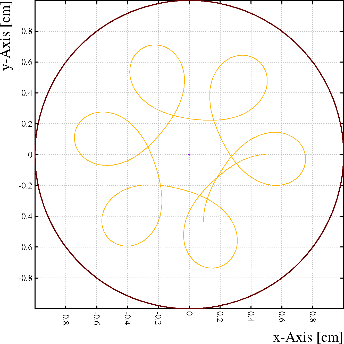
[Mandatory argument, no default.]
[Mandatory argument, no default.]
[Mandatory argument, no default.]
[Mandatory argument, no default.]
[Mandatory argument, no default.]
[Mandatory argument, no default.]
[Optional argument]
[Optional argument]
This procedure can be called after any of the drift-line computation procedures has been called (e.g. DRIFT_ELECTRON).
Format:
CALL DRIFT_INFORMATION( ...
[ `CHARGE`, q ] , ...
[ `DRIFT-TIME`, time ] , ...
[ `ELECTRODE`, electrode ] , ...
[ `PARTICLE`, particle ] , ...
[ `PATH-LENGTH`, path ] , ...
[ `STATUS-CODE`, istat ] , ...
[ `STATUS-STRING`, status ] , ...
[ `STEPS`, nsteps ] , ...
[ `TECHNIQUE`, technique ] , ...
[ `X-START`, coordinate ] , ...
[ `Y-START`, coordinate ] , ...
[ `Z-START`, coordinate ] , ...
[ `X-END`, coordinate ] , ...
[ `Y-END`, coordinate ] , ...
[ `Z-END`, coordinate ])
Example:
Call plot_drift_area
Call drift_electron_3(2.5,3.5,4.5,status,time)
Call plot_drift_line
Call plot_end
Say "Status: {status}"
Call string_index(status,`wire`,index1)
Call string_index(status,`replica`,index2)
If index1>0 & index2=0 Then
Call drift_information('status-code',wire)
Say "The particle hit wire {wire}."
Endif
An electron drift-line is computed using the Runge Kutta method with DRIFT_ELECTRON_3 which returns a formatted status string. This string has, if the electron hits a wire, the format "Hit X wire n" or "Hit a replica of X wire n". With the help of the STRING_INDEX procedure, we search for the strings "wire" and "replica" to determine whether an original copy of a wire has been hit. If so, DRIFT_INFORMATION is called to find the number of the wire that has been hit.
This argument must be modifiable. It will be of type Number after the call. Any value this argument may have before the procedure call is lost.
This argument must be modifiable. It will be of type Number after the call. Any value this argument may have before the procedure call is lost.
Read-out group numbers are assigned by the SELECT statement.
This argument must be modifiable. Any value this argument may have before the procedure call is lost.
| particle | Meaning |
|---|---|
electron |
An electron or a positron has been drifted |
ion |
An ion with charge +1 or -1 has been drifted |
unknown |
Neither electron nor ion |
This argument must be modifiable. Any value this argument may have before the procedure call is lost.
This argument must be modifiable. It will be of type Number after the call. Any value this argument may have before the procedure call is lost.
This argument must be modifiable. It will be of type Number after the call. Any value this argument may have before the procedure call is lost.
This argument must be modifiable. Any value this argument may have before the procedure call is lost.
This argument must be modifiable. It will be of type Number after the call. Any value this argument may have before the procedure call is lost.
| particle | Meaning |
|---|---|
Runge-Kutta-Fehlberg |
Analytic integration of the mean trajectory |
Monte-Carlo |
Integration taking diffusion into account |
vacuum |
Integration in vacuum |
microscopic |
Molecular level tracking |
unknown |
None of the above |
This argument must be modifiable. Any value this argument may have before the procedure call is lost.
The internal coordinate system is used - for Cartesian cells, this system coincides with the user coordinates, for polar cells, the INTERNAL_TO_POLAR procedure can be used to convert the coordinates.
These arguments must be modifiable. They will be of type Number after the call. Any value these arguments may have before the procedure call is lost.
The integrated diffusion, the multiplication and the attachment losses are not computed.
This procedure should be called only from within the drift or signal sections, after the cell and the gas have been entered.
This procedure uses the Runge_Kutta_Fehlberg integration method.
Format:
CALL DRIFT_ION(x, y [, status [, time]])
This procedure should be called only from within the drift or signal sections, after the cell and the gas have been entered.
The integrated diffusion, the multiplication and the attachment losses are not computed.
This procedure uses the Runge_Kutta_Fehlberg integration method.
Format:
CALL DRIFT_ION_3(x, y , z [, status [, time]])
This procedure is intended for testing the inter-molecular tracking algorithm used in microscopic simulation. For this reason, a gas must be entered before the procedure can be called, even though no gas properties are used by this procedure.
Format:
CALL DRIFT_ION_VACUUM(x, y, z, vx, vy, vz, charge, mass [, status [, time]])
Example:
&CELL plane x -1 v=0 plane x +1 v=0 rows s * * 0 0 -100000000A fully stripped Ar nucleus starts from (0.5 , 0.5) with a velocity slightly in excess of 2000 cm/\μs, approximately 0.07\ c. It is subject to an electric and a magnetic field. The example should produce the following figure:&MAG comp 0 0 0.2 T
&GAS arg-50-eth-50 // Dummy gas-id "Vacuum"
&DRIFT integration-parameters integration-accuracy 1e-4 area -1 -1 -1 1 1 1 Call plot_drift_area Call drift_vacuum_ion(0.5,0.5,0, -2e3,-1e2,0, 18, 39.948*931.494, status, time) Say {status, time} Call plot_drift_line Call plot_end
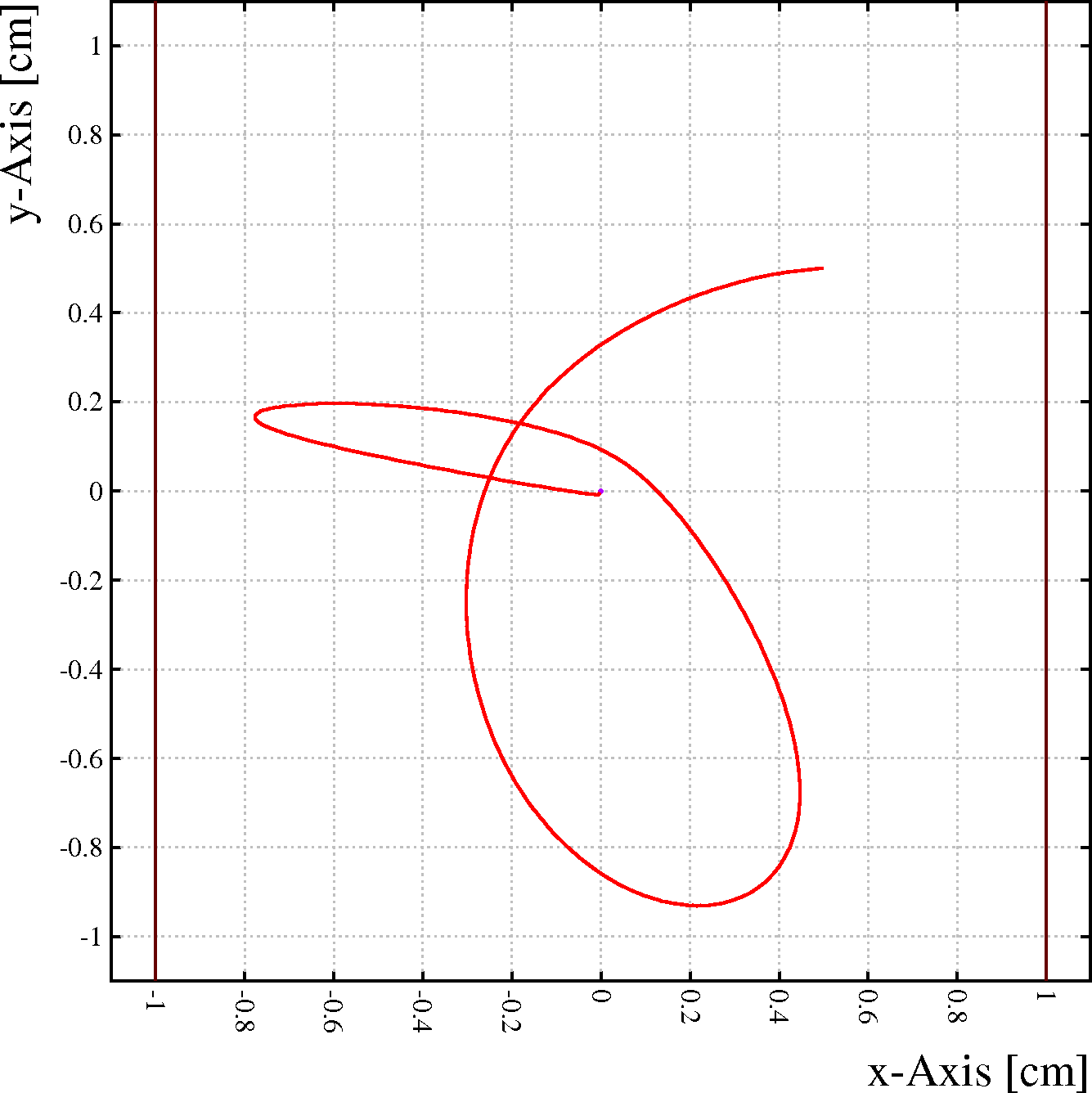
[Mandatory argument, no default.]
[Mandatory argument, no default.]
[Mandatory argument, no default.]
[Mandatory argument, no default.]
[Mandatory argument, no default.]
[Mandatory argument, no default.]
[Mandatory argument, no default.]
[Mandatory argument, no default.]
[Optional argument]
[Optional argument]
This procedure should be called only from within the drift or signal sections, after the cell and the gas have been entered.
This procedure can only meaningfully be used if both the transverse and the longitudinal diffusion have been supplied in the gas section. The multiplication and the attachment losses can only be computed if Townsend and attachment data have been entered.
The Monte Carlo integration method is described in the drift section under Monte_Carlo.
Format:
CALL DRIFT_MC_ELECTRON(x, y, z [, status [, time ...
[, multiplication [, attachment]]]])
This procedure should be called only from within the drift or signal sections, after the cell and the gas have been entered.
It should be noted that MC drift of electrons and ions uses the same set of integration parameters (step size in particular). Care should be taken to set these parameters to reasonable values for ions before this procedure is called.
Diffusion coefficients for ions can be set with the PARAMETERS statement in the gas section (see sigma).
Multiplication and attachment losses are not evaluated.
The Monte Carlo integration method is described in the drift section under Monte_Carlo.
Format:
CALL DRIFT_MC_ION(x, y, z [, status [, time]])
This procedure should be called only from within the drift or signal sections, after the cell and the gas have been entered.
It should be noted that MC drift of electrons and ions uses the same set of integration parameters (step size in particular). Care should be taken to set these parameters to reasonable values for ions before this procedure is called.
Diffusion coefficients for ions can be set with the PARAMETERS statement in the gas section (see sigma).
Multiplication and attachment losses are not evaluated.
The Monte Carlo integration method is described in the drift section under Monte_Carlo.
Format:
CALL DRIFT_MC_NEGATIVE_ION(x, y, z [, status [, time]])
Note that the drift velocity vector is not anti-symmetric under charge inversion is there is a non-zero E-perpendicular component of the B field.
This procedure should be called only from within the drift or signal sections, after the cell and the gas have been entered.
This procedure can only meaningfully be used if both the transverse and the longitudinal diffusion have been supplied in the &GAS section.
The Monte Carlo integration method is described in the drift section under Monte_Carlo.
Format:
CALL DRIFT_MC_POSITRON(x, y, z [, status [, time]])
This procedure relies extensively on Magboltz. Before using this procedure, the Magboltz gas composition must be set - by running MAGBOLTZ, by retrieving using GET gas tables that have been computed with Magboltz and which have been written in gas file format 10, or by using the COMPOSITION command.
The step size in this procedure is the free path, as in the real gas, with its natural (exponential) distribution. A typical drift path therefore proceeds through millions of collisions and it is rarely practical to store each step individually. Instead, the electron location is recorded every n'th collision, where n is specified with the MONTE-CARLO-COLLISIONS parameters of the INTEGRATION-PARAMETERS command - n may be set to 1 if desired.
In order to profit fully from the detailed nature of these calculations, it is advisable, in case the electrons head for a wire, to set the TRAP-RADIUS to 1.
Each collision is classified as either elastic, inelastic, super-elastic, attachment or ionisation, with one of the species of molecules present in the gas mixture. In case of attachment, the electron is not tracked any further and the status is set accordingly. In this procedure, additional electrons produced through ionisation are not tracked. Use MICROSCOPIC_AVALANCHE if this is desired.
Format:
CALL DRIFT_MICROSCOPIC_ELECTRON(x, y, z ... [, status [, time [, options ... [, e_maximum [, e_start [, dir_x, dir_y, dir_z ... [, distribution, [, rates]]]]]]]])
Note: switching on any of the MARK options presumes that you have already opened a graphics window suitable for plotting the drift-line. Example:
Call plot_drift_area
Call new_track
Do
Call get_cluster(x,y,z,n,e,done)
If done Then Leave
Call drift_microscopic(x, y, z, status, time, ...
`mark-ion mark-att`, ...
5.0, 0.1, 0,0,0, histe)
Say "Status = {status}, Drift time = {time} microsec"
Call plot_drift_line
Enddo
Call plot_track
Call plot_end
In this example, all electrons generated along a track are traced and plotted, marking locations where ionisation and attachment occurs.
The calculation of the electron trajectory is aborted with status "Energy exceeds E_maximum" if at any point the electron energy exceeds this value.
The trajectory will be inaccurate if the maximum energy is chosen too large.
The simplest way to find suitable values for this parameter is running MAGBOLTZ with the PLOT-DISTRIBUTION-FUNCTIONS option switched on. Beware that e_maximum must be suitable over the entire drift path of the electron, which may include a high field region in the vicinity of an anode.
[Default: 5 eV]
This energy must be strictly positive (non-zero) and less than e_maximum.
[Default: 2\ % of e_maximum.]
The norm of the initial velocity is taken from e_start, not from the direction vector. The normalisation is arbitrary.
All three components must be specified. If all 3\ components of the direction vector are zero, then an isotropic random vector will be generated.
[A random direction is assumed if no direction is specified.]
If this argument is on entry an existing histogram, then new entries will be added to it. This can be used to force a scale and also to accumulate statistics across multiple calls.
If this argument is of another type on entry, then the current value will be deleted and a new histogram will be booked with 100\ bins and ranging from 0 to e_maximum.
The cross sections present in the vector vary with e_maximum since Magboltz eliminates, for reasons of efficiency, negligibly small cross section terms.
The various terms can be identified with the help of the CROSS_SECTION_IDENTIFIER procedure:
Call drift_microscopic(x, y, z, status, time, ``, ...
100.0, 4.0, 0,0,0, histe, vec)
For i From 1 To size(vec) Do
Call cross_section_identifier(i, level, type)
Say "Level {i} = {level}, count = {number(vec[i])}, type = {type}"
Enddo
The integrated diffusion, the multiplication and the losses through attachment are not computed.
This procedure should be called only from within the drift or signal sections, after the cell and the gas have been entered.
This procedure uses the Runge_Kutta_Fehlberg integration method.
Format:
CALL DRIFT_NEGATIVE_ION(x, y [, status [, time]])
This procedure should be called only from within the drift or signal sections, after the cell and the gas have been entered.
The integrated diffusion, the multiplication and the losses through attachment are not computed.
This procedure uses the Runge_Kutta_Fehlberg integration method.
Format:
CALL DRIFT_NEGATIVE_ION_3(x, y, z [, status [, time]])
Note that the drift velocity vector is not anti-symmetric under charge inversion is there is a non-zero E-perpendicular component of the B field.
This procedure should be called only from within the drift or signal sections, after the cell and the gas have been entered.
This procedure uses the Runge_Kutta_Fehlberg integration method.
Format:
CALL DRIFT_POSITRON(x, y [, status [, time]])
Note that the drift velocity vector is not anti-symmetric under charge inversion is there is a non-zero E-perpendicular component of the B field.
This procedure should be called only from within the drift or signal sections, after the cell and the gas have been entered.
This procedure uses the Runge_Kutta_Fehlberg integration method.
Format:
CALL DRIFT_POSITRON_3(x, y, z [, status [, time]])
This is a instruction used to debug the diffusion calculation, the procedure is not of much general use.
Format:
CALL DRIFT_DIVERGENCE(x, y, z, f1, f2, f3 [, options])
Example:
&CELL tube r=1 rows s 1 0.01 0 0 1000This example computes the divergence of the drift field in a round tube with a gas of constant mobility. The product of f1 and f2 should be equal to 1 in this case. With a gas of constant drift velocity, f1 should be constant but not f2.&GAS table drift-velocity=ep/100
&DRIFT Global step=0.0010 integration-parameters m-c-dist {step} Call book_matrix(xv,100) Call book_matrix(f1v,100) Call book_matrix(f2v,100) Global n=0 Global phi=335*pi/180 For x From 0.01 Step 0.02 To 0.99 Do Call drift_divergence(x*cos(phi), x*sin(phi), 0, ... f1, f2, f3, `positive,electron`) Global n=n+1 Global xv[n]=x Global f1v[n]=f1 Global f2v[n]=f2 Enddo Call adjust_matrix(xv,n,0) Call adjust_matrix(f1v,n,0) Call adjust_matrix(f2v,n,0) Global min=minimum(f1v&f2v) Global max=maximum(f1v&f2v) Call plot_frame(0,0.95*min,1,1.05*max,`r`,`f`,`Divergence`) Call plot_line(xv,f1v,`function-1`) Call plot_line(xv,f2v,`function-2`) Call plot_line(xv,1+step/xv,`function-3`) Call plot_end
The curve drawn with representation FUNCTION-3 shows the exact expression of the transverse divergence.
Although there can be correlations between these divergences, they are not computed.
| option | Meaning | Default |
|---|---|---|
ELECTRON |
Divergence for electrons | Default |
ION |
Divergence for ions | Electron is default |
POSITIVE |
Positive charge | Negative is default |
NEGATIVE |
Negative charge | Default |
This is a instruction used to debug the diffusion calculation, the procedure is not of much general use.
Format:
CALL DRIFT_ROTATION(x, y, z, Rvc, Rmc, Rvm [, options])
Example:
&CELL tube r=1 rows s 1 0.01 0 0 1000&MAGNETIC components 0 0 1 T
&DRIFT integration-parameters m-c-dist 0.001 Call drift_rotation(0.1, 0.0, 0,rvc,rmc,rvm,`electron,positive`) Call print_matrix(rvc,rmc,rvm)
All coordinate systems are right-handed. The rotation matrices are written as follows:
These arguments do not need to be initialised before the procedure is called. Any value assigned to the arguments before the call will be lost afterwards.
| option | Meaning | Default |
|---|---|---|
ELECTRON |
Rotation for electrons | Default |
ION |
Rotation for ions | Electron is default |
POSITIVE |
Positive charge | Negative is default |
NEGATIVE |
Negative charge | Default |
In the absence of a magnetic field, the orientation of the electric field is immaterial. The electric field may be specified either by the norm or as a vector, of which only the norm matters. In this case, the values returned by this procedure coincide with those returned by VELOCITY_E.
In the presence of a magnetic field, the transport parameters depend on the relative orientation of the electric and magnetic field vectors. Both fields therefore have to be specified as vectors. The velocity that is returned is equal to the vectorial sum of VELOCITY_E, VELOCITY_BTRANSVERSE and VELOCITY_ExB.
Each of the field components can either be a Number or a Matrix. It is permissible to specify some components of the field as Numbers and the other(s) as Matrices.
All components which are specified as Matrix, must have the same total size - they do not have to be 1-dimensional. If at least one component is specified as Matrix, then the output will be a 1-dimensional Matrix with length equal to the overall size of the arguments of type Matrix. Otherwise the result will be a Number.
The electric field should be in V/cm, the magnetic field has to be in native units of 100\ G or 0.01\ T, and the drift velocity is returned in cm/\μsec.
Formats:
CALL DRIFT_VELOCITY(e, drift) CALL DRIFT_VELOCITY(ex, ey, ez, drift) CALL DRIFT_VELOCITY(ex, ey, ez, bx, by, bz, drift)
Example:
Global emin=100
Global emax=10000
Global e=emin*(emax/emin)^((row(200)-1)/199)
&GAS
mix argon 95 methane 5 noplot-f0 noplot-cross-section e/p-range {emin/760,emax/760}
&MAIN
Call drift_velocity(0,0,e,vd5)
&GAS
mix argon 90 methane 10 noplot-f0 noplot-cross-section e/p-range {emin/760,emax/760}
&MAIN
Call drift_velocity(0,0,e,vd10)
&GAS
mix argon 80 methane 20 noplot-f0 noplot-cross-section e/p-range {emin/760,emax/760}
&MAIN
Call drift_velocity(0,0,e,vd20)
Call plot_frame(emin,0,emax,10,`E [V/cm]`, ...
`v<SUB>D</SUB> [cm/microsec]`, ...
`Drift velocity in Ar/CH4 mixtures`)
Call plot_line(e,vd5,`function-1`)
Call plot_line(e,vd10,`function-2`)
Call plot_line(e,vd20,`function-3`)
Call plot_end
The arguments ex, ey, ez, e, v and status are optional.
Format:
CALL ELECTRIC_FIELD(x, y, ex, ey, ez, e, v, status)
Example:
&CELL plane x=-1 plane y=-1 rows s * * 1 1 1000&FIELD Global n=6 Call book_matrix(x,n,n) Call book_matrix(y,n,n) For i From 1 To n Do For j From 1 To n Do Global x[i;j]=(i-1)/(n-1) Global y[i;j]=(j-1)/(n-1) Enddo Enddo Call efield(x,y,ex,ey,ez,e,v,stat) Call print_matrix(x,y,ex,ey,ez,e,v,stat) area 0 0 1 1 grid {n} print ex ey e v
In a simple chamber, one uses on the one hand the ELECTRIC_FIELD procedure to compute the field on a 6x6 grid, on the other hand the PRINT command is used to verify the result.
If at least one of the input arguments x and y is of type Matrix, then all output arguments are of type Matrix, with the dimensions of the first input argument of type Matrix. If one input argument is of type Number and the other of type Matrix, then the Number type argument is "expanded" to become a Matrix filled uniformly with the value of the Number.
The coordinates system expected by ELECTRIC_FIELD is the internal frame. If you describe your cell in Cartesian coordinates, then the internal frame is simply the Cartesian coordinate system. If polar coordinates are used however, then you should supply the following parameters:
for x: log(r) for y: \φ, in radians
These mappings can be performed with the POLAR_TO_INTERNAL procedure.
Er = Ex/r Ephi = Ey/r Ez is invariant
This argument must be modifiable and its value prior to the call will be overwritten.
On return, the argument will be of type Matrix if either of the coordinates is of that type, otherwise it will be of type Number.
See also ex.
| Status | Location string | Numeric |
|---|---|---|
In a material |
Inside the mesh, but not in a drift medium | -5 |
In X-wire N |
Inside wire number N of type X | 1-MXWIRE |
In X-solid N |
Inside solid number N of type X | > 2*MXWIRE |
Normal |
In the active part of the cell | 0 |
Outside mesh |
Not in any mesh triangle or tetrahedron | -6 |
Outside plane |
On the side of a plane where no wires are | -4 to -1 |
Unknown potential |
Unknown potential type (shouldn't occur) | -10 |
Unknown |
Other cases (shouldn't occur) | other |
The arguments ex, ey, ez, e, v and status are optional.
Format:
CALL ELECTRIC_FIELD_3(x, y, z, ex, ey, ez, e, v, status)
Example:
See ELECTRIC_FIELD.
If at least one of the input arguments x, y, z is of type Matrix, then all output arguments are of type Matrix, with the dimensions of the first input argument of type Matrix. If one or more input arguments are of type Number and one or more others of type Matrix, then the Number type arguments are "expanded" to become Matrices filled uniformly with the value of the Numbers.
The coordinates system expected by ELECTRIC_FIELD_3 is the internal frame. If you describe your cell in Cartesian coordinates, then the internal frame is simply the Cartesian coordinate system. If polar coordinates are used however, then you should supply the following parameters:
for x: log(r) for y: \φ, in radians for z: z
The z-coordinate is not affected by any of the conformal mappings currently in use by the program.
These mappings can be performed with the POLAR_TO_INTERNAL procedure.
Er = Ex/r Ephi = Ey/r Ez is invariant
This procedure needs electron drift velocity data, which can be computed with the MAGBOLTZ gas section command. The magnetic field, if present, is taken into account. Diffusion data is not used, even if present - the vector that is returned represents the mean electron drift velocity at a given point.
This procedure provides functionality similar to the SPEED command.
Format:
CALL ELECTRON_VELOCITY(x, y, z, vx, vy, vz [, status])
Example:
Call electron_velocity(2,3,0,vx,vy,vz,status)
Say "Velocity: ({vx,vy,vz}), Status: {status}"
The coordinates are expected to refer to the internal frame. If you describe your cell in Cartesian coordinates, then the internal frame is simply the Cartesian coordinate system. If polar coordinates are used however, then you should supply the following parameters:
for x: log(r) for y: \φ, in radians for z: z
The z-coordinate is not affected by any of the conformal mappings currently in use by the program.
These mappings can be performed with the POLAR_TO_INTERNAL procedure.
vr = vx/r vphi = vy/r vz is invariant
The first argument is the level number, the index of the vector given by INTEGRATE_EXCITATIONS. The second argument contains on return a string with the level identifier, which is described in somewhat more detail in the gas ingredients. The optional third argument contains on return the threshold energy of the level (in eV).
The number of levels can be obtained with LEVEL_COUNT.
Format:
CALL EXCITATION_IDENTIFIER(level_number, level_identifier [, level_energy])
For examples, see INTEGRATE_EXCITATIONS and LEVEL_COUNT.
In the absence of a magnetic field, the orientation of the electric field is immaterial. The electric field may be specified either by the norm or as a vector, of which only the norm matters.
In the presence of a magnetic field, the rates (at least in principle) depend on the relative orientation of the electric and magnetic field vectors. Both fields therefore have to be specified as vectors.
Each of the field components can either be a Number or a Matrix. It is permissible to specify some components of the field as Numbers and the other(s) as Matrices.
All components which are specified as Matrix must have the same total size - they do not have to be 1-dimensional. If at least one component is specified as Matrix, then the output will be a 1-dimensional Matrix with length equal to the overall size of the arguments of type Matrix. Otherwise the result will be a Number.
The first argument is a Number which identifies the level. The number of available levels can be found with the LEVEL_COUNT procedure and further information can be obtained with EXCITATION_IDENTIFIER.
The electric field should be in V/cm, the magnetic field has to be in native units of 100\ G or 0.01\ T, and the rate is returned in THz.
Formats:
CALL EXCITATION_RATE(level, e, rate) CALL EXCITATION_RATE(level, ex, ey, ez, rate) CALL EXCITATION_RATE(level, ex, ey, ez, bx, by, bz, rate)
Example:
Global emin=5000
Global emax=25000
Global e=emin*(emax/emin)^((row(200)-1)/199)
Call plot_frame(emin/1000, 0, emax/1000, 2, `E [kV/cm]`, ...
`Excitation rate [GHz]`, `Excitations and Dissociations`)
Call level_count(nexc, nion)
For id From 1 To nexc Do
Call excitation_rate(id,e,exc)
Call excitation_identifier(id, name, ethresh)
Say "{id}: {name}, Emin = {ethresh}"
Call string_index(name,`DISS`,ind)
If ind>0 Then
Call plot_line(e/1000,exc*1e3, `function-2`)
Else
Call plot_line(e/1000,exc*1e3, `function-3`)
Endif
Enddo
Call plot_end
This examples plots all excitation rates, and marks the dissociations using a different line type.
The matrix from which elements are to be extracted should exist prior to the call, the receiving matrix should not exist prior to the call.
This procedure is used to process array indexing on the right hand side of formulae, in procedure calls etc. This procedure is not meant to called by the user. It is much simpler to get sub-matrices using indexing expressions.
Format:
CALL EXTRACT_SUBMATRIX(ndim, nsel_1, nsel_2, ... , ...
isel_1_1, isel_1_2, ..., isel_2_1, isel_2_2, ... , ...
isel_n_1, isel_n_2, ref_submatrix, ref_matrix)
When the search is successful, the global variable OK is set to True, otherwise to False. The following conditions can lead to un unsuccessful search:
This procedure works by parabolic iteration over a set of 3 near-extreme values, which is initialised with a random search. If the boundary values are better, than the result of the random search, then the parabolic search is skipped.
Format for functions:
CALL EXTREMUM(function, extremum, minimum, maximum, ...
[ options [, \ε_loc [, \ε_fun [, itermax ]]]])
Format for matrices:
CALL EXTREMUM(ordinates, values, extremum, ...
[ options [, \ε_loc [, \ε_fun [, itermax ]]]])
Examples:
Call extremum(`1+5*x-(x-2)^3`,x,-1,4,`plot,print,minimum`)
Global min=x
Call extremum(`1+5*x-(x-2)^3`,x,-1,4,`plot,print,maximum`)
Global max=x
Say "Extrema: {min,max}"
The function 1+5*x-(x-2)^3 has a local minimum near x=0.7 and a local maximum near x=3.3. The first call will indeed find the local minimum, while the second call will set x to -1 since the function value on this boundary is higher than in the local maximum.
Global a=2
Global b=3
Call extremum(`1+cosh(a-b)`,b,-1,4,`plot,print,minimum`)
Say "Minimum found is {b}, should be {a}."
This example shows a function of two global variables, A and B. The function is minimised as function of B in this example. During the minimisation, A retains its value.
This argument is mandatory and should be of the type String.
This argument is mandatory.
This argument is mandatory.
The variable doesn't have to have a value before the procedure is called. Any value associated with it before the procedure is called will be lost, if the search is successful.
On successful completion, the value of the variable is set to the abscissa of the extremum and it will then have the type Number.
The variable may be modified even if the search fails.
This argument should be a global variable, not an expression nor a constant.
This argument is mandatory for an extremum search on a function and must then be of the type Number. The argument should not be specified when searching vectors.
This argument is mandatory for an extremum search on a function and must then be of the type Number. The argument should not be specified when searching vectors.
| Option | Effect | Notes |
|---|---|---|
CUBIC |
Cubic vector interpolation | Only with vectors |
LINEAR |
Linear vector interpolation | Only with vectors |
MAXIMUM |
Searches for a maximum | Not default |
MINIMUM |
Searches for a minimum | Default |
NOPLOT |
No plot of the function | Default |
NOPRINT |
No printout | Default |
PLOT |
Makes a plot of the function | Not default |
PRINT |
Prints a progress report | Not default |
QUADRATIC |
Quadratic vector interpolation | Only with vectors |
The search is declared to have converged when, between 2 iterations, the location of the extremum changes relatively by less than a fraction \ε_loc or absolutely by less than an amount \ε_loc.
This is an optional parameter of type Number.
Since the function is evaluated in single precision arithmetic, values less than 10\<SUP\>-6\</SUP\> are not meaningful on most computers.
[By default 10\<SUP\>-4\</SUP\>.]
The search is declared to have converged when, between 2 iterations, the extreme function value changes relatively by less than a fraction \ε_fun or absolutely by less than an amount \ε_fun.
This is an optional parameter of type Number.
Since the function is evaluated in single precision arithmetic, values less than 10\<SUP\>-6\</SUP\> are not meaningful on most computers.
[By default 10\<SUP\>-4\</SUP\>.]
The search is abandoned if it has not converged on the basis of \ε_loc or \ε_fun within the specified number of iterations,
This is an optional parameter of type Number.
[By default 20.]
The procedure sets the OK global variable to True if filling was successful and to False if it wasn't, usually because the histogram to be filled didn't exist. OK is not set to False if the entry is out of range.
Format:
CALL FILL_HISTOGRAM(histogram, entry [, weight])
Example:
Call book_histogram(ref,100) For i From 1 To 10000 Do Call fill_histogram(ref,rnd_landau) Enddo Call plot_histogram(ref,`Energy loss`,`Landau distribution`) Call plot_end
This example could be used to check that the Landau random number generator does indeed work.
Such variables are of Histogram. Usually, they are created by calling BOOK_HISTOGRAM to explicitly create a new histogram, or by calling GET_HISTOGRAM to retrieve an existing histogram from a file. They can also be the result of arithmetic between histograms.
This argument should not be an expression since this would result in adding entries to a temporary histogram.
[This is a mandatory argument]
If you supply a Matrix type argument, then ensure that the weight is either a Number or a Matrix of the same overall length as the entries. All Matrix shapes are permitted. The shapes of the entry and weight matrices do not have to be the same.
[This argument is mandatory.]
If you supply a Matrix type argument, then ensure that the entry is either a Number or a Matrix of the same length as the weights. All Matrix shapes are permitted. Moreover, the shapes of the entries and the weights do not have to be the same,
[This argument is mandatory is optional and defaults to 1.]
In addition to the parameters, the global variable OK is set by this procedure. Its value is True is the fit converged, and False otherwise.
Format for histograms:
CALL FIT_EXPONENTIAL(reference, a0, a1, a2, ..., an, ...
err_a0, err_a1, err_a2, ..., err_an [, options])
Format for matrices:
CALL FIT_EXPONENTIAL(x, y, err_y, a0, a1, a2, ..., an, ...
err_a0, err_a1, err_a2, ..., err_an [, options])
Examples:
&SIGNAL
avalanche polya-townsend 0.5
check avalanche from 0 0.5 range 0.1 10000 keep-histograms
Call fit_exponential(avalanche,a0,a1,ea0,ea1,`print,plot`)
Say "a0 = {a0}+/-{ea0}, a1 = {a1}+/-{ea1}."
In this example, the user wishes to see how well a Polya distribution with parameter \θ=0.5, can be reproduced by an exponential.
Vector ep ap
0.13158 0
0.65789 0
1.31579 0
2.63158 0
6.57895 0
13.1579 0.0089211
19.7368 0.10592
26.3158 0.24737
39.4737 0.62105
52.6316 0.97995
78.9474 1.86895
105.263 2.74474
131.579 3.605
197.368 5.515
230.263 6.39237
300 8.07711
Global epfit=ep[6,7,8,9]
Global apfit=ap[6,7,8,9]
Global p=760
Call fit_exponential(1/epfit,apfit,0.1*apfit,a0,a1,ea0,ea1, ...
`noplot,noprint`)
Global emin=5000
Global emax=300000
Global ne=100
Global ekorff=emin*(emax/emin)^((row(ne)-1)/(ne-1))
Global akorff=exp(a0+a1*p/ekorff)*p
!options log-x log-y
Call plot_frame(emin,0.1,emax,8000,`E [V/cm]`,`α [1/cm]`, ...
`Korff fit`)
Call plot_error_bar(ep*p,ap*p)
Call plot_line(ekorff,akorff,`function-1`)
Global a=exp(a0)
Global ea=ea0*a
Global a=entier(a*10)/10
Global ea=entier(ea*10)/10
Global b=-entier(a1)
Global eb=entier(ea1)
Call plot_text(40000,100,`A = `/string(a)/` ± `/string(ea), ...
`title`)
Call plot_text(40000,60,`B = `/string(b)/` ± `/string(eb), ...
`title`)
Call plot_end
The Townsend coefficients are sometimes approximated using the Rose-Korff formula:
\α/p = A.exp(-B.p/E)This example performs such a fit on Townsend coefficients that have been computed by the Imonte program for a mixture of 90\ % argon and 10\ % isobutane. Imonte is a precursor program for Magboltz version\ 7 and is no longer used.
The argument is not modified on return.
The vectors x, y and err_y must have the same length, unless err_y is given as a scalar.
Not changed on exit.
The vectors x, y and err_y must have the same length, unless err_y is given as a scalar.
In the initial estimate, the data points where y\ \≤\ 0 are skipped. If there are many such points which should be taken into account for the fit, then convergence is not guaranteed.
Not changed on exit.
This argument can also be a scalar, which is then used as error for all points. If this argument is a vector, then it must have the same length as x and y.
Not changed on exit.
function = exp(polynomial)where
polynomial = a\<SUB\>0\</SUB\> + a\<SUB\>1\</SUB\>*x + a\<SUB\>2\</SUB\>*x\<SUP\>2\</SUP\> + a\<SUB\>3\</SUB\>*x\<SUP\>3\</SUP\> + ... + a\<SUB\>n\</SUB\>*x\<SUP\>n\</SUP\>The arguments a\<SUB\>0\</SUB\>, a\<SUB\>1\</SUB\> etc. are the terms in this expansion.
The input values for the terms are not used in the fitting procedure. Initial values are obtained from an unweighted maximum likelihood fit neglecting the data points where y=0.
This argument must be modifiable, i.e. it can not be a constant nor an expression.
\√(\χ\²/(#points - #parameters))
This correction factor is equal to 1 if the errors to the data points have been assigned correctly.
These arguments must be modifiable, that is, they can neither be constants nor expressions.
| Option | Meaning | Defaults |
|---|---|---|
EQUAL |
Assume equal weight of all points | Not default |
NOPLOT |
Don't plot the histogram and fit | Default |
NOPRINT |
Don't print details during the fit | Default |
PLOT |
Plot the histogram with fit | Not default |
POISSON |
Assume Poisson errors | Default |
PRINT |
Print details during the fit | Not default |
Notes:
This procedure, unlike the other fitting procedures, does not try to find suitable starting values for the fitting parameters. A starting value for each parameter must therefore be supplied by the user.
Since this procedure uses the symbolic evaluation procedures of Garfield, the fit works essentially in single precision. In order to have a chance to be successful, the problem must therefore be well conditioned.
In addition to the parameters, the global variable OK is set by this procedure. Its value is True is the fit converged, and False otherwise.
Format for histograms:
CALL FIT_FUNCTION(reference, function, ...
par1, par2, par3, ... , err1, err2, err3, ... [, options])
Format for matrices:
CALL FIT_FUNCTION(x, y, err_y, function, ...
par1, par2, par3, ... , err1, err2, err3, ... [, options])
Example:
Call book_histogram(ref,50,-1,3)
For i From 1 To 500 Do
Global x=-1+4*rnd_uniform
Global w=x^2+1
Call fill_histogram(ref,x,w)
Enddo
Global c=100
Global a=2
Global b=1
Call fit_function(ref,`c+a*(1+b*x^2)`,a,b,ea,eb,`plot,print`)
Say "Function: {c}+{a}*(1+{b}*x^2), errors {ea,eb}"
Say "{a+c} +/- {abs(ea)} should be equal to"
Say "{a*b} +/- {a*b*sqrt((ea/a)^2+(eb/b)^2)}"
This is a simple test of the FIT_FUNCTION procedure in which the function depends on 3 global variables A, B and C of which A and B are varied while C is kept fixed.
Another example can be found in the description of the RND_POISSON random number generator.
The global variables that are to be varied are those that appear in the argument list of the procedure call. The other globals are not changed.
The argument is not modified on return.
The vectors x, y and err_y must have the same length, unless err_y is given as a scalar.
Not changed on exit.
The vectors x, y and err_y must have the same length, unless err_y is given as a scalar.
In the initial estimate, the data points where y\ \≤\ 0 are skipped. If there are many such points which should be taken into account for the fit, then convergence is not guaranteed.
Not changed on exit.
This argument can also be a scalar, which is then used as error for all points. If this argument is a vector, then it must have the same length as x and y.
Not changed on exit.
These parameters must be given a suitable initial value of type Number, for instance by using the Global statement.
On return of a successful fit, the global variables are set equal to the optimum value found. The global variables are of type Undefined if the fit fails.
\√(\χ\²/(#points - #parameters))
This correction factor is equal to 1 if the errors to the data points have been assigned correctly.
These arguments must be modifiable, that is, they can neither be constants nor expressions.
| Option | Meaning | Defaults |
|---|---|---|
EQUAL |
Assume equal weight of all points | Not default |
NOPLOT |
Don't plot the histogram and fit | Default |
NOPRINT |
Don't print details during the fit | Default |
PLOT |
Plot the histogram with fit | Not default |
POISSON |
Assume Poisson errors | Default |
PRINT |
Print details during the fit | Not default |
Note:
In addition to the parameters, the global variable OK is set by this procedure. Its value is True is the fit converged, and False otherwise.
Format for histograms:
CALL FIT_GAUSSIAN(reference, integral, mean, sigma ...
[, error_int [, error_mean [, error_sigma [, options]]]])
Format for matrices:
CALL FIT_GAUSSIAN(x, y, err_y, integral, mean, sigma ...
[, error_int [, error_mean [, error_sigma [, options]]]])
Example 1:
Call get_histogram(sel_5,`arrival.hist`,`sel_5`)
Call fit_gaussian(sel_5,dum,dum,sigma,dum,dum,esigma,`PLOT`)
Say "Gaussian width is {sigma} +/- {esigma}."
The ARRIVAL-TIME-DISTRIBUTION instruction returns the RMS of the arrival time distributions. To obtain Gaussian fits in addition, you can specify the KEEP-HISTOGRAMS option and then use FIT_GAUSSIAN. You can also do the fit in a separate job as explained in http://cern.ch/garfield/examples/
Example 2:
Call book_histogram(hist)
For i From 1 To 10000 Do
Global sum=0
For j From 1 To 12 Do
Global sum=sum+rnd_uniform
Enddo
Call fill_histogram(hist,sum)
Enddo
Call fit_gaussian(hist,a,b,c,ea,eb,ec,`print,plot`)
(This verifies the approximation of a Gaussian distribution by the sum of 12 uniformly distributed random numbers.)
This is usually a global variable that has been returned by a call to BOOK_HISTOGRAM or to GET_HISTOGRAM. This argument may also be an expression that results in a histogram.
The argument is not modified by the procedure.
[Mandatory argument.]
This vector should have the same size as y.
The argument is not modified by the procedure.
[Mandatory argument.]
This vector should have the same size as x.
The argument is not modified by the procedure.
[Mandatory argument.]
If a Matrix type argument is used, then it must have the same length as x and y.
The argument is not modified by the procedure.
[Mandatory argument.]
There is no need to initialise this argument - the initial value for the fitting procedure is set to the sum of the histogram or Y array.
This argument must be modifiable, i.e. it can not be a constant nor an expression. The argument will be of type Number.
[Mandatory argument.]
There is no need to initialise this argument - the initial value for the fitting procedure is set to the mean of the histogram or arrays.
This argument must be modifiable, i.e. it can not be a constant nor an expression. The argument will be of type Number.
[Mandatory argument.]
There is no need to initialise this argument - the initial value for the fitting procedure is set to the RMS of the histogram or arrays.
This argument must be modifiable, i.e. it can not be a constant nor an expression. The argument will be of type Number.
[Mandatory argument.]
\√(\χ\²/(#points - #parameters))
This correction factor is equal to 1 if the errors to the data points have been assigned correctly.
Errors are only returned upon request. The corresponding arguments must be modifiable, that is, they can neither be constants nor expressions. All errors are of type Number.
| Option | Meaning | Defaults |
|---|---|---|
EQUAL |
Assume equal weight of all points | Not default |
NOPLOT |
Don't plot the histogram and fit | Default |
NOPRINT |
Don't print details during the fit | Default |
PLOT |
Plot the histogram with fit | Not default |
POISSON |
Assume Poisson errors | Default |
PRINT |
Print details during the fit | Not default |
The Mathieson distribution depends on a shape parameter, called K3, which is a function of the geometrical structure of the chamber, and on the ratio of strip width and anode-cathode distance. The distribution assumes that the avalanche is localised on anode wires placed centrally with respect to the cathode strips.
The procedure derives the strip width from the bin width of the input histogram, the anode-cathode distance has to be entered as an argument. The K3 parameter can be fitted, but may optionally also be kept constant during the fit at a user-specified value.
In addition to the parameters, the global variable OK is set by this procedure. Its value is True is the fit converged, and False otherwise.
Formats:
CALL FIT_MATHIESON(x, y, err_y, distance, norm, centre, k3, ...
error_norm, error_centre, error_k3, [, options])
CALL FIT_MATHIESON(reference, distance, norm, centre, k3, ...
error_norm, error_centre, error_k3, [, options])
Example:
Call book_histogram(ref_m,50)
Call book_histogram(ref_b,50)
For i From 1 To 65 Do
Call get_histogram(hist,`profile.hist`,string(i))
Global k3=0.1
Global s=0.254
Call fit_mathieson(hist,s,f,xc,k3,ef,exc,ek3,...
`noplot,noprint,equal,fitk3`)
Call fill_histogram(ref_m,xc)
Call barycentre(hist,b,5)
Call fill_histogram(ref_b,b)
Say "Centre: {xc} +/- {exc}"
Say "Barycentre: {b}"
Say "K3: {k3} +/- {ek3}"
Enddo
Call plot_histogram(ref_m,`Reconstructed x [cm]`,`Mathieson fits`)
Call plot_end
Call plot_histogram(ref_b,`Reconstructed x [cm]`,`Barycentre`)
Call plot_end
(We have already produced a file that contains for 65 events a distribution of induced charges in the pads, and now we fit each of these with a Mathieson distribution and compare these fits with barycentres. The K3 parameter is left free.)
References:
[Mandatory argument if the histogram format is used.]
This vector should have the same size as y.
The argument is not modified by the procedure.
[Mandatory argument if the matrix format is used.]
This vector should have the same size as x.
The argument is not modified by the procedure.
[Mandatory argument if the matrix format is used.]
If a Matrix type argument is used, then it must have the same length as x and y.
The argument is not modified by the procedure.
[Mandatory argument if the matrix format is used.]
This parameter is mandatory, and should be entered in cm.
This parameter should be modifiable and its value prior to the call is not used. Any matrix, histogram or string associated with it before the call is lost.
This parameter should be modifiable and its value prior to the call is not used. Any matrix, histogram or string associated with it before the call is lost.
The argument must in this case be modifiable. Any matrix, histogram or string associated with it before the call is lost.
If the NOFITK3 option is specified, then this argument must contain on entry your preferred value of K3. The argument is then not modified and the corresponding error is set to 0.
\√(\χ\²/(#points - #parameters))
This correction factor is equal to 1 if the errors to the data points have been assigned correctly.
These arguments must be modifiable, that is, they can neither be constants nor expressions.
| Option | Meaning | Defaults |
|---|---|---|
EQUAL |
Assume equal weight of all points | Default |
FITK3 |
Fits the K3 parameter | Default |
NOFITK3 |
Keep the K3 parameter fixed | Not default |
NOPLOT |
Don't plot the histogram and fit | Default |
NOPRINT |
Don't print details during the fit | Default |
PLOT |
Plot the histogram with fit | Not default |
POISSON |
Assume Poisson errors | Not default |
PRINT |
Print details during the fit | Not default |
This procedure optionally tries to determine the a linear horizontal scale correction for which the fit is optimal. But, fitting a Polya distribution with a free scale is a numerically poorly conditioned problem because of the high correlation between the Polya parameter and the scale parameters. If the scale is known, then it is preferable to fix the scale.
Similarly, the routine will make an attempt to estimate the Polya parameter if no starting value is known, but it is better to provide a starting value if one is known with reasonable accuracy.
In addition to the parameters, the global variable OK is set by this procedure. Its value is True is the fit converged, and False otherwise.
Format for histograms:
CALL FIT_POLYA(reference, factor, offset, slope, \θ, ...
error_factor, error_offset, error_slope, error_theta [, options])
Format for matrices:
CALL FIT_POLYA(x, y, err_y, factor, offset, slope, \θ, ...
error_factor, error_offset, error_slope, error_theta [, options])
Example:
Call book_histogram(ref,100,0,10)
For i From 1 To 2000 Do
Call fill_histogram(ref,1+2*rnd_polya(1))
Enddo
Global o=-1/2
Global s=1/2
Global t=500
Global f=200
Call fit_polya(ref,f,o,s,t,ef,eo,es,et,`plot,print,poisson,auto`)
Say "Scaling X={o}+{s}*x, theta={t}+/-{et}, contents={f}."
(First we fill a histogram with a Polya distribution of which we know the \θ parameter and the scale, then we check whether the fit finds the input values back. We don't need to give initial values in this case since the AUTO option is specified.)
The argument is not modified on return.
The vectors x, y and err_y must have the same length, unless err_y is given as a scalar.
Not changed on exit.
The vectors x, y and err_y must have the same length, unless err_y is given as a scalar.
In the initial estimate, the data points where y\ \≤\ 0 are skipped. If there are many such points which should be taken into account for the fit, then convergence is not guaranteed.
Not changed on exit.
This argument can also be a scalar, which is then used as error for all points. If this argument is a vector, then it must have the same length as x and y.
Not changed on exit.
function = factor slope (\θ+1)\<SUP\>\θ+1\</SUP\>/\Γ(\θ+1) (offset+slope*x)\<SUP\>\θ\</SUP\> e\<SUP\>-(\θ+1)*(offset+slope*x)\</SUP\>i.e. a Polya distribution with argument offset+slope*x and with Polya parameter \θ.
The input values for the terms are used as initial values for the fit if the MANUAL option is used (this is not default). The parameters "offset" and "slope" are fitted if the option FIT is specified, otherwise the values have to be specified on input.
Parameters of which the value on input is to be used, must be of type Number.
All arguments except "offset" and "slope" when using the FIX option, must be modifiable, i.e. it can not be a constant nor an expression.
\√(\χ\²/(#points - #parameters))
This correction factor is equal to 1 if the errors to the data points have been assigned correctly.
These arguments must be modifiable, that is, they can neither be constants nor expressions.
| Option | Meaning | Defaults |
|---|---|---|
AUTO |
Determine suitable starting values | Default |
EQUAL |
Assume equal weight of all points | Not default |
FIT |
Fit the scale of the distribution | Default |
FIX |
Don't modify the scale parameters | Not default |
MANUAL |
Start from given initial values | Not default |
NOPLOT |
Don't plot the histogram and fit | Default |
NOPRINT |
Don't print details during the fit | Default |
PLOT |
Plot the histogram with fit | Not default |
POISSON |
Assume Poisson errors | Default |
PRINT |
Print details during the fit | Not default |
Notes:
In addition to the parameters, the global variable OK is set by this procedure. Its value is True is the fit converged, and False otherwise.
Format for histograms:
CALL FIT_POLYNOMIAL(reference, a0, a1, a2, ..., an, ...
err_a0, err_a1, err_a2, ..., err_an [, options])
Format for matrices:
CALL FIT_POLYNOMIAL(x, y, err_y, a0, a1, a2, ..., an, ...
err_a0, err_a1, err_a2, ..., err_an [, options])
Example:
Call hdelete(ref)
Call hbook(ref,100,-2,2)
For i From 1 To 10000 Do
Global x=(rnd_uniform-0.5)*4
Global dy=0.01*(rnd_uniform-0.5)
Call hfill(ref,x,1+2*x+x^2+dy)
Enddo
Call fit_polynomial(ref,a0,a1,a2,ea0,ea1,ea2,`print,plot`)
Say "a0 = {a0}+/-{ea0}, a1 = {a1}+/-{ea1}, a2 = {a2}+/-{ea2}."
This example is a test to verify that the fit works. In the procedure calls, HDELETE is short for DELETE_HISTOGRAM, HBOOK for BOOK_HISTOGRAM and HFILL for FILL_HISTOGRAM.
The argument is not modified on return.
The vectors x, y and err_y must have the same length, unless err_y is given as a scalar.
Not changed on exit.
The vectors x, y and err_y must have the same length, unless err_y is given as a scalar.
Not changed on exit.
This argument can also be a scalar, which is then used as error for all points. If this argument is a vector, then it must have the same length as x and y.
Not changed on exit.
polynomial = a\<SUB\>0\</SUB\> + a\<SUB\>1\</SUB\>*x + a\<SUB\>2\</SUB\>*x\<SUP\>2\</SUP\> + a\<SUB\>3\</SUB\>*x\<SUP\>3\</SUP\> + ... + a\<SUB\>n\</SUB\>*x\<SUP\>n\</SUP\>
The input values for the terms are not used in the fitting procedure. Initial values are obtained from an unweighted maximum likelihood fit.
This argument must be modifiable, i.e. it can not be a constant nor an expression.
\√(\χ\²/(#points - #parameters))
This correction factor is equal to 1 if the errors to the data points have been assigned correctly.
These arguments must be modifiable, that is, they can neither be constants nor expressions.
| Option | Meaning | Defaults |
|---|---|---|
EQUAL |
Assume equal weight of all points | Not default |
NOPLOT |
Don't plot the histogram and fit | Default |
NOPRINT |
Don't print details during the fit | Default |
PLOT |
Plot the histogram with fit | Not default |
POISSON |
Assume Poisson errors | Default |
PRINT |
Print details during the fit | Not default |
Note: the EQUAL and POISSON options are ignored for matrix fits since the errors on the points are explicitly provided in that case.
This procedure is only of use for debugging, and must be used with caution since it is on purpose not protected for locations inside wires (the call can result in a division by zero).
Format:
CALL FORCE_FIELD(x, y, ex, ey)
for x: log(r) for y: \φ, in radians
Er = Ex/r Ephi = Ey/r
Format:
CALL GAS_AVAILABILITY(object, available)
Can be any of the following:
| Object | GASOK bit |
|---|---|
ATTACHMENT-COEFFICIENT |
6 |
CLUSTERING-DATA |
5 |
DIFFUSION-TENSOR |
11 |
DRIFT-VELOCITY or VELOCITY-E |
1 |
ION-DISSOCIATION-COEFFICIENT |
12 |
ION-MOBILITY |
2 |
LONGITUDINAL-DIFFUSION-COEFFICIENT |
3 |
LORENTZ-ANGLE |
7 |
TOWNSEND-COEFFICIENT |
4 |
TRANSVERSE-DIFFUSION-COEFFICIENT |
8 |
VELOCITY-BTRANSVERSE |
9 |
VELOCITY-E or DRIFT-VELOCITY |
1 |
VELOCITY-EXB |
10 |
All arguments are optional.
Format:
CALL GET_CELL_DATA([number_of_wires [, cell_type [, ...
coordinates [, identifier]]]])
Three values can be returned, Cartesian, Polar and Tube.
If the cell has been entered in polar coordinates, then the dimensions are returned in internal coordinates. These can be converted to Cartesian or polar coordinates with the INTERNAL_TO_CARTESIAN and INTERNAL_TO_POLAR procedures.
If 4 arguments are provided, only the (x,y) part of the cell dimensions is returned. If 6 arguments are present, also the z part is set.
Formats:
CALL GET_CELL_SIZE(xmin, ymin, zmin, xmax, ymax, zmax) CALL GET_CELL_SIZE(xmin, ymin, xmax, ymax)
Example: see GET_WIRE_DATA
In addition to the parameters, the global variable OK is set by this procedure. Its value is True if generating the clusters worked properly, otherwise it will be set to False. OK is set to False if the done flag has been set to True.
Before using the cluster location and energy, the value of the done argument and of the OK global variable should be checked. The parameters should not be used if either of these two has been set to True.
Format:
CALL GET_CLUSTER(xcls, ycls, zcls, npair, ecls, [extra1,] done)
Example:
track 0 1 1 1 muon energy 10000 nodelta
Call book_histogram(size,100)
For i From 1 To 100 Do
Call new_track
Until done Do
Call get_cluster(xcls,ycls,zcls,npair,ecls,done)
If done Then Iterate
Call fill_histogram(size,npair)
Enddo
Enddo
!options log-y
Call plot_histogram(size,`Cluster size`,...
`Cluster size distribution`)
Call plot_end
This example shows how one can obtain the cluster size distribution for tracks generated by the Heed program. Since Heed doesn't generate clusters but always \δ-electrons (they usually have a very short range), we use the NODELTA-ELECTRONS option on the TRACK command. This compresses the \δ-electrons into clusters.
These arguments should not be used if done has been set to True or OK to False.
This 3 arguments should be a simple global variables, not formulae or constants. The global variables may already exist before the procedure is called, in which case their contents will be lost, but they may also be an variables that have sofar not been used.
The coordinates are returned as Numbers with unit cm, no matter the coordinate system that is used.
This argument should not be used if done has been set to True or OK to False.
The precise interpretation of the energy that is returned depends on the clustering model that is in effect:
This argument should be a simple global variable, not a formula or a constant. The global variable may already exist before the procedure is called, in which case its contents will be lost, but it may also be an variable that has sofar not been used. The argument is of type Number after the call.
This argument should not be used if done has been set to True or OK to False.
This argument should be a simple global variable, not a formula or a constant. The global variable may already exist before the procedure is called, in which case its contents will be lost, but it may also be an variable that has sofar not been used.
This argument is optional. If it is present, then it must be the one-but-last argument of the procedure. That is, if 6 arguments are passed, then the 6th will be considered to be done and extra will not be returned.
This argument should be a simple global variable, not a formula or a constant. The global variable may already exist before the procedure is called, in which case its contents will be lost, but it may also be an variable that has sofar not been used.
It is set to True if the present call didn't result in a cluster because:
Note the difference between this parameter and OK. The latter is set to False if an error has been detected generating the clusters, for instance because of buffer overflow in Heed.
This argument should be a simple global variable, not a formula or a constant. The global variable may already exist before the procedure is called, in which case its contents will be lost, but it may also be an variable that has sofar not been used.
If you wish to retrieve e.g. the length or the coordinates of the end point of the drift path, then DRIFT_INFORMATION provides easier access to the information.
The drift time is expressed in \μsec and the z-component of the drift path in cm. Also the (x,y) part of the path is in cm if Cartesian or tube coordinates are used. If the cell has been described in polar coordinates, then (x,y) is represented in internal coordinates:
(\ρ,\φ)=(log(\√(x\²+y\²),arctan(y/x))
These can be converted to Cartesian or polar coordinates with the INTERNAL_TO_CARTESIAN and INTERNAL_TO_POLAR procedures.
Format:
CALL GET_DRIFT_LINE(x [, y [, z [, t]]])
Example:
Say "Please enter (x,y) of the starting point" Parse Terminal x_start y_start Call drift_electron(1,1,status,time) Call get_drift_line(x,y,z,t) Call plot_graph(t,x,`Time [microsec]`,`x [cm]`,`x vs time`) Call plot_comment(`UP-LEFT`,`Status: `/status) Call plot_comment(`DOWN-LEFT`,`Drift time: `/string(time)/` [microsec]`) Call plot_comment(`UP-RIGHT`, `From (x,y)=(`/string(x_start)/`,`/... string(y_start)/`)`) Call plot_end
A way to plot the relation between the x-coordinate of a drift line and the drift time.
After the call, the argument is a 1-dimensional Matrix. Any value this argument has before the procedure call, is lost after the call.
Format:
CALL GET_E/P_TABLE(ep)
Example:
Call get_e/p_table(ep) Call get_gas_data(p) Call townsend(ep*p,0,0,a) Call plot_graph(ep*p,a,`E [V/cm]`,`α [1/cm]`, ... `Townsend coefficient`) Call plot_error_bar(ep*p,a,0,0.1*a) Call plot_end
Retrieves the set of E/p points, the pressure and the Townsend coefficients, and then makes a plot showing 10\ % error bars for the values.
Format:
CALL GET_GAS_DATA(pressure [, temperature [, identifier]])
Example:
Call get_gas_data(p, t, gasid)
Say "Gas identifier is {gasid}."
The pressure of the gas is established with the PRESSURE command.
This value of this argument on entry is not used, and is lost after the procedure has completed. On return, this argument is of type Number.
The temperature of the gas is established with the TEMPERATURE command.
This value of this argument on entry is not used, and is lost after the procedure has completed. On return, this argument is of type Number.
This argument is optional.
This value of this argument on entry is not used, and is lost after the procedure has completed. On return, this argument is of type String.
This argument is optional.
The procedure sets the OK global variable to True if the histogram has successfully been retrieved and to False if a problem occurred.
Format:
CALL GET_HISTOGRAM(reference, file [, member])
This argument plays the same role as the reference argument of BOOK_HISTOGRAM.
If this variable is already associated with a string, histogram or matrix, then this string, histogram or matrix is lost after the call to GET_HISTOGRAM.
This argument should be of type String.
This is in many cases a meaningful default and there is therefore rarely a need to specify a member.
This argument should be of type String.
The procedure sets the OK global variable to True if the matrix is successfully retrieved, and to False in case of a problem.
Format:
CALL GET_MATRIX(matrix, file [, member])
Example:
See WRITE_MATRIX.
This argument should be of type String.
This argument should be of type String.
Format:
CALL GET_PERIODS(yesno_x, length_x, yesno_y, length_y)
Internal coordinates are used if the cell has been described in polar coordinates,
Raw signals are obtained by computing drift trajectories, and multiplying at each step, the local velocity with the weighting field. Raw signals do not, as a rule, have equal time intervals.
Use the LIST_RAW_SIGNALS procedure to find out which raw signals currently are in memory.
Format:
CALL GET_RAW_SIGNAL(type, electrode, avalanche_wire, angle, ...
time, signal)
Read-out groups are formed with the SELECT command. SELECT without arguments will show how the groups are composed.
[No default, this is a mandatory parameter.]
This wire can be the same as the sense wire but this is not necessarily the case. Note that you must have asked for cross-induced signals in order to have signals computed that are due to avalanches on other wires than the sense wire.
The avalanche wire doesn't have to be SELECT'ed.
This argument should be a Number.
This argument should be a global variable, not a constant or an expression. The global may exist before the call is issued, but doesn't have to. If it exists, then its contents will be lost.
Signal currents are expressed in \μA when they are computed, but their units can change as a result of convolutions.
This argument should be a global variable, not a constant or an expression. The global may exist before the call is issued, but doesn't have to. If it exists, then its contents will be lost.
Format:
CALL GET_SIGNAL(electrode, time, direct [, cross])
Example:
Read-out groups are formed with the SELECT command. SELECT without arguments will show how the groups are composed.
[No default, this is a mandatory parameter.]
This argument should be a global variable, not a constant or an expression. The global may exist before the call is issued, but doesn't have to. If it exists, then its contents will be lost.
Signals are expressed in \μA when they are computed, but their units can change as a result of convolutions.
This argument should be a global variable, not a constant or an expression. The global may exist before the call is issued, but doesn't have to. If it exists, then its contents will be lost.
This argument is optional.
Signals are expressed in \μA when they are computed, but their units can change as a result of convolutions.
This argument should be a global variable, not a constant or an expression. The global may exist before the call is issued, but doesn't have to. If it exists, then its contents will be lost.
Format:
CALL GET_SOLID_DATA(solid, qsolid)
Example: see INTEGRATE_CHARGE.
Solids are numbered sequentially, starting from 1.
The charge is expressed in units of V.cm and thus needs to be multiplied by 4\π\ε\<SUB\>0\</SUB\> for conversion to Coulomb. See the example.
Internal coordinates are used for the plane locations. Use the INTERNAL_TO_POLAR procedure to convert to, for instance, polar coordinates.
All arguments are mandatory.
Format:
CALL GET_X_PLANE_DATA(yn_1, x_1, V_1, label_1, ...
yn_2, x_2, V_2, label_2)
Example:
Call get_cell_data(wires,type,coord,id)
Call get_x_plane_data(yn1,x1,V1,lab1, yn2,x2,V2,lab2)
If coord="Polar" Then
If yn1 Then Say "There is a plane at r={exp(x1)} and with V={V1}."
If yn2 Then Say "There is a plane at r={exp(x2)} and with V={V2}."
Else
If yn1 Then Say "There is a plane at x={x1} and with V={V1}."
If yn2 Then Say "There is a plane at x={x2} and with V={V2}."
Endif
Internal coordinates are used for the plane locations, use the INTERNAL_TO_POLAR procedure to convert to polar coordinates.
All arguments are mandatory.
Format:
CALL GET_Y_PLANE_DATA(yn_1, y_1, V_1, label1, ...
yn_2, y_2, V_2, label2)
Example:
Call get_cell_data(wires,type,coord,id)
Call get_y_plane_data(yn1,y1,V1,lab1, yn2,y2,V2,lab2)
If coord="Polar" Then
If yn1 Then Say "There is a plane at phi={180*y1/pi} and with V={V1}."
If yn2 Then Say "There is a plane at phi={180*y2/pi} and with V={V2}."
Else
If yn1 Then Say "There is a plane at y={y1} and with V={V1}."
If yn2 Then Say "There is a plane at y={y2} and with V={V2}."
Endif
All arguments are optional.
Format:
CALL GET_WIRE_DATA(wire [, x [, y [, V [, d [, q [, label [, ... length [, weight [, density]]]]]]]]])
Example:
Call get_cell_data(nwire,dummy,dummy,id)
Say "List of wires with a negative charge:"
For i From 1 To nwire Do
Call get_wire_data(i,xw,yw,vw,dw,qw,labelw)
If qw>0 Then Iterate
Say "Wire {i} at (x,y)=({xw,yw}), type {labelw}"
Enddo
This example shows how one can produce a list of the wires that have a negative charge. One could also select a sense wire and store its coordinates using this technique.
This argument is mandatory and is not modified.
[No default.]
If the cell has been entered in polar coordinates, then the wire location is returned in internal coordinates. These can be converted to Cartesian or polar coordinates with the INTERNAL_TO_CARTESIAN and INTERNAL_TO_POLAR procedures.
This argument is optional. The argument should be a global variable, not a constant nor an expression. The global may have been declared prior to the call, but doesn't have to. The value an existing variable had before the call will be lost. The argument will be of type Number on return.
This argument is optional. The argument should be a global variable, not a constant nor an expression. The global may have been declared prior to the call, but doesn't have to. The value an existing variable had before the call will be lost. The argument will be of type Number on return.
The CHECK instruction can display the potential that is computed for the neighbourhood of the wire.
This argument is optional. The argument should be a global variable, not a constant nor an expression. The global may have been declared prior to the call, but doesn't have to. The value an existing variable had before the call will be lost. The argument will be of type Number on return.
Also the INTEGRATE_CHARGE procedure returns charges in V. It is, however, more usual to express wire charges in pC/cm, as is for instance done by the CELL-PRINT option. To convert from V to C/cm, multiply by 2\π\ε\<SUB\>0\</SUB\>, approximately 5.56\ 10\<SUP\>-13\</SUP\>\ C/V.cm.
This argument is optional. The argument should be a global variable, not a constant nor an expression. The global may have been declared prior to the call, but doesn't have to. The value an existing variable had before the call will be lost. The argument will be of type Number on return.
This argument is optional. The argument should be a global variable, not a constant nor an expression. The global may have been declared prior to the call, but doesn't have to. The value an existing variable had before the call will be lost.
This argument is optional. The argument should be a global variable, not a constant nor an expression. The global may have been declared prior to the call, but doesn't have to. The value an existing variable had before the call will be lost. The argument will be of type Number on return.
This argument is optional. The argument should be a global variable, not a constant nor an expression. The global may have been declared prior to the call, but doesn't have to. The value an existing variable had before the call will be lost. The argument will be of type Number on return.
This argument is optional. The argument should be a global variable, not a constant nor an expression. The global may have been declared prior to the call, but doesn't have to. The value an existing variable had before the call will be lost. The argument will be of type Number on return.
This procedure is a direct interface to the GKS routine GFA. The first argument of GFA, the vector length, is absent.
The area is plotted with the area attributes, and using the normalisation transformation that are in effect at the time the procedure is called.
Format:
CALL GKS_AREA(x,y)
The vectors should have a minimum length of 3.
[No defaults, these are mandatory parameters.]
This procedure is a direct interface to the GKS routine GPL. The first argument of GPL, the vector length, is absent.
The polyline is plotted with the polyline attributes, and using the normalisation transformation that are in effect at the time the procedure is called.
Format:
CALL GKS_POLYLINE(x,y)
The vectors should have a minimum length of 2.
[No defaults, these are mandatory parameters.]
This procedure is a direct interface to the GKS routine GPM. The first argument of GPM, the vector length, is absent.
The polymarker is plotted with the polymarker attributes, and using the normalisation transformation that are in effect at the time the procedure is called.
Format:
CALL GKS_POLYMARKER(x,y)
The vectors should have a minimum length of 1.
[No defaults, these are mandatory parameters.]
This procedure is equivalent to the GKS routine GSELNT.
Format:
CALL GKS_SELECT_NT(nt)Example:
See PLOT_START.
A normalisation transformation is composed of a window and a viewport, and is referenced via an integer number.
Normalisation transformation 0 is pre-defined by GKS and corresponds to window limits of (0,0) and (1,1).
[No default, this is a mandatory parameter.]
This procedure is an interface to the GKS routine GSCHXP.
Format:
CALL GKS_SET_CHARACTER_EXPANSION(expansion)
An expansion of 1 corresponds to normal text.
This procedure is an interface to the GKS routine GSCHH.
Format:
CALL GKS_SET_CHARACTER_HEIGHT(height)
This procedure is an interface to the GKS routine GSCHSP.
Format:
CALL GKS_SET_CHARACTER_SPACING(spacing)
A spacing of 0 corresponds to normal text.
This procedure is an interface to the GKS routine GSCHUP.
Format:
CALL GKS_SET_CHARACTER_UP_VECTOR(x, y)
The text alignments specify where a piece of text is to placed with respect to its anchor point.
This procedure is an interface to the GKS routine GSTXAL.
Format:
CALL GKS_SET_TEXT_ALIGNMENT(hor, vert)
| Alignment | Numeric | Meaning | Notes |
|---|---|---|---|
NORMAL |
0 | Depends on system | Usually LEFT |
LEFT |
1 | Left aligned | - |
CENTRE |
2 | Centre aligned | - |
RIGHT |
3 | Right aligned | - |
and v one of the vert
| Alignment | Numeric | Meaning | Notes |
|---|---|---|---|
NORMAL |
0 | Depends on system | Usually BASE |
TOP |
1 | Highest point of "l" | - |
CAP |
2 | Highest point of "o" | - |
HALF |
3 | Centre aligned | - |
BASE |
4 | Lowest point of "o" | Not in HIGZ |
BOTTOM |
5 | Lowest point of "y" | Not in HIGZ |
[No defaults, these are mandatory arguments.]
This procedure is a direct interface to the GKS routine GSTXCI.
Format:
CALL GKS_SET_TEXT_COLOUR(colour)
Colour names are established with the COLOUR command.
This procedure is a direct interface to the GKS routine GSTXFP.
CALL GKS_SET_TEXT_FONT_PRECISION(font, precision)
| Precision | Meaning |
|---|---|
STROKE |
Highest precision, all attributes respected |
CHARACTER |
Standard precision |
STRING |
Low precision, suited for fast rendering |
This procedure is a direct interface to the GKS routine GTX.
The text is plotted with the polyline attributes, the alignment, the up-vector and using the normalisation transformation that are in effect at the time the procedure is called. These attributes can either be set at the GKS level by calling GKS_SET_CHARACTER_EXPANSION, GKS_SET_CHARACTER_HEIGHT, GKS_SET_CHARACTER_SPACING, GKS_SET_CHARACTER_UP_VECTOR, GKS_SET_TEXT_ALIGNMENT, GKS_SET_TEXT_COLOUR and GKS_SET_TEXT_FONT_PRECISION, or at the Garfield level by calling SET_TEXT_ATTRIBUTES.
Format:
CALL GKS_TEXT(x,y,text)
Where the text will appear with respect to the anchor point depends on the text alignment.
[No defaults, these are mandatory parameters.]
[No default, this is a mandatory parameter.]
Specifying a viewport doesn't entail an automatic change of normalisation transformation. For this, one needs to call the GKS_SELECT_NT procedure.
A call to a procedure like PLOT_FRAME overrides the viewport setting for normalisation transformation number 1 with the parameters that can be set with the VIEWPORT graphics command. Also, all regular Garfield plots will modify these viewport settings.
This procedure is equivalent to the GKS routine GSVP.
Format:
CALL GKS_VIEWPORT(nt, xmin, xmax, ymin, ymax)Example:
See PLOT_START.
A normalisation transformation is composed of a window and a viewport, and is referenced via an integer number.
Normalisation transformation 0 is pre-defined by GKS and corresponds to window limits of (0,0) and (1,1).
[No default, this is a mandatory parameter.]
The limits are expressed in normalised device coordinates, i.e. the system in which (0,0) is the lower left hand corner and (1,1) the upper right hand corner.
Note the order of the arguments, which is different from the usual order of window specifications in Garfield.
[No default, these are mandatory parameters.]
Specifying a window doesn't entail an automatic change of normalisation transformation. For this, one needs to call the GKS_SELECT_NT procedure.
A call to a procedure like PLOT_FRAME overrides the window setting for normalisation transformation number 1 with the dimensions specified in the argument. Also all regular Garfield plots will modify these window settings.
This procedure is equivalent to the GKS routine GSWN.
Format:
CALL GKS_WINDOW(nt, xmin, xmax, ymin, ymax)Example:
See PLOT_START.
A normalisation transformation is composed of a window and a viewport, and is referenced via an integer number.
Normalisation transformation 0 is pre-defined by GKS and corresponds to window limits of (0,0) and (1,1).
[No default, this is a mandatory parameter.]
The limits are expressed in the coordinate system in which you perform your calculations.
Note the order of the arguments, which is different from the usual order of window specifications in Garfield.
[No default, these are mandatory parameters.]
The histogram is not affected by this operation.
Format:
CALL HISTOGRAM_TO_MATRIX(hist, matrix [, min [, max]])
Example:
Call book_histogram(ref1,10,0,1) For i From 1 To 1000 Do Call fill_histogram(ref1,rnd_uniform) Enddo Call plot_histogram(ref1) Call plot_end Call histogram_to_matrix(ref1,a,min,max) Call matrix_to_histogram(a,min,max,ref2) Call plot_histogram(ref2) Call plot_end
First, we book an histogram and fill it with uniformly distributed random numbers. The histogram is then copied to a matrix A, and then copied back to a histogram. Both histograms are plotted to check they are indeed the same.
To take the effect of electronics into account, one should calculate pure signals with the SIGNAL command or with the ADD_SIGNALS procedure, process them (e.g. with CONVOLUTE-SIGNALS), recuperate the electronics output with GET_SIGNAL and integrate the signal using the SUM function.
The procedure first drifts a particle of the desired kind from the starting point. Next, the routine integrates the internal product of the weighting field for the electrode that is read out and the drift velocity between the time limits over the drift path. The result is multiplied with minus the charge of the particle that has been drifting.
Contrary to appearances, the total induced charge (i.e. integrated over the entire drift path) thus computed is a surprisingly boring quantity. A charged particle that moves from one electrode to another can only induce a total charge of +1, 0 or -1. The total charge is +1 or -1 in case the particles moves from an electrode that is read out to one that is not, or vv. The total charge is 0 if the particle moves between electrodes which are both read out or are both not read out.
The sum of charges induced on all electrodes vanishes: the effect of a moving charge in a chamber is a reshuffling of the charges on the conductors, charges are not created and do not vanish.
Format:
CALL INDUCED_CHARGE(x, y, z, particle, electrode ... [, tmin, tmax], q)
Example:
&CELL pl y -1 label p pl y +1 label q rows a * * +0.5 0 -1000 s * * 0 0 1000 b * * -0.5 0 -1000&GAS co2
&SIG area -1.1 -1.1 1.1 1.1 sel (pq)s(ab) Call induced_charge(-0.4,-0.5,0,`e-`,2,q1) Call induced_charge(-0.4,-0.5,0,`e+`,2,q2) Say "Status e-: {stat1}, e+: {stat2}" Say "Charge between wire and plane: {q1+q2}"
Verifies that the total charge induced by a particle moving between two conductors (the B wire and a plane) other than the one that is read out (the S wire), is indeed 0.
A more elaborate application of this procedure can be found in http://cern.ch/garfield/examples/charge
| Value | Meaning |
|---|---|
`E-` |
electron |
`E+` |
positron |
`ION-` |
negatively charged ion |
`ION+` |
positively charged ion |
[No default, this is a mandatory parameter.]
Read-out groups are formed with the SELECT command. SELECT without arguments will show how the groups are composed.
[No default, this is a mandatory parameter.]
These arguments are optional. If they are omitted, the charge is integrated over the entire drift path.
This argument should be a global variable, not an expression nor a constant. The variable doesn't have to be declared. Any value the variable has before the call, is lost after the call.
The charge is expressed in multiples of the electron charge.
This procedure is used to control the starting point in the random number generator sequences. By default, the random number generators are, at the start of the calculations, called a number of times that depends on the time of the day (product of the hours, minutes and seconds).
If reproducible, yet different, sequences are required, then specify the -noRNDM_initialisation command line option and use this procedure to set a starting point.
Format:
CALL INITIALISE_GENERATORS(ncalls)
Example:
garfield -noRNDM_init (start) Call initialise_generators(1234)
The file does not have to be a Garfield library. If you wish to test the presence of, for instance, a gas description in a given library, then you should use INQUIRE_MEMBER.
The EXIST function performs the same tasks as this procedure.
Format:
CALL INQUIRE_FILE(file, exists)
Example:
&CELL Call inquire_file(`new_cell`,exist) If exist Then % delete "dc1.lib" cell < new_cell write "dc1.lib" cell Else get "dc1.lib" cell Endif
In this example a cell description is retrieved from a library called dc1.lib, unless a file called new_cell is found. In that case, the cell description is deleted from the library, the new description is read and stored in compact format in the library.
This parameter should be a String or an expression that evaluates to a character string.
[This argument is mandatory, no default is supplied.]
This argument should be modifiable, any object associated with it at the time the call is made, will be deleted. The value of the variable on input, if any, is not used.
[This is a mandatory argument.]
Calling this procedure does not interfere with the filling process.
The first 2 arguments are mandatory, the rest is optional.
Format:
CALL INQUIRE_HISTOGRAM(reference, exists, set, channels, ...
minimum, maximum, entries, mean, rms)
[No default, this is a mandatory argument.]
This argument is in practice always True since the first argument has to be a valid histogram reference. The argument's main application is in the area of debugging where it is used in conjunction with the REF_HISTOGRAM function via which one can address directly the entire histogram storage area, also those parts for which no pointer in the form of a Global variable exists.
This argument must me modifiable, i.e. it must be a simple variable name and not an expression. The argument is optional. The value of this argument on entry is not used, and is lost after the procedure call.
This argument must me modifiable, i.e. it must be a simple variable name and not an expression. The argument is optional. The value of this argument on entry is not used, and is lost after the procedure call.
This argument must me modifiable, i.e. it must be a simple variable name and not an expression. The argument is optional. The value of this argument on entry is not used, and is lost after the procedure call.
This argument must me modifiable, i.e. it must be a simple variable name and not an expression. The argument is on return of type Number. This is an optional argument. The value of this argument on entry is not used, and is lost after the procedure call.
This number can also be obtained with the MINIMUM function.
This argument must me modifiable, i.e. it must be a simple variable name and not an expression. The argument is on return of type Number. This is an optional argument. The value of this argument on entry is not used, and is lost after the procedure call.
This number can also be obtained with the MAXIMUM function.
This argument must me modifiable, i.e. it must be a simple variable name and not an expression. The argument is optional.
The value of this argument on entry is not used, and is lost after the procedure call.
This argument must me modifiable, i.e. it must be a simple variable name and not an expression. The argument is on return of type Number. This is an optional argument. The value of this argument on entry is not used, and is lost after the procedure call.
The mean of an histogram can also be obtained with the MEAN function.
This argument must me modifiable, i.e. it must be a simple variable name and not an expression. The argument is on return of type Number. This is an optional argument. The value of this argument on entry is not used, and is lost after the procedure call.
The RMS of an histogram can also be obtained with the RMS function.
The exists argument is set to True only if all of the following conditions are fulfilled:
Otherwise exists is set to False and the arguments member, remark, date and time are not touched.
Use the INQUIRE_FILE procedure if you only wish to find out whether a file exists.
Format:
CALL INQUIRE_MEMBER(file, member, type, exists ...
[,remark [, date [, time]]])
Example:
&GAS Call inquire_member(`straw.gas`,`xe50e50`,`gas`,exist) If exist Then get gas.dat xe50e50 Else pressure 500 temperature 300 magboltz xenon 50 ethane 50 write gas.dat xe50e50 Endif
In this example the existence of a member called XE50E50 in a library called straw.gas is checked. Since the type is set to GAS, only compact gas descriptions are considered. If the member exists, the data is read, otherwise a new table is prepared and is then written to the file.
This parameter should be a String or an expression that evaluates to a character string.
[This argument is mandatory, no default is supplied.]
This parameter can be a wildcard, for instance `*` would search for the first occurrence of a member of the given type. If this argument is modifiable, it will be overwritten by the member type found.
This argument should be a String or an expression that evaluates to a character string. Member names have a length of 8 at most.
[This argument is mandatory, no default is supplied.]
This argument can not be a wildcard.
The argument should be a String of up to 8 characters, and may also be an expression that evaluates to such a string.
[This argument is mandatory, no default is supplied.]
This argument should be modifiable, any object associated with it at the time the call is made, will be deleted. The value of the variable on input, if any, is not used.
[This is a mandatory argument.]
This argument should be modifiable, any object associated with it at the time the call is made, will be deleted.
[This is an optional argument.]
This argument should be modifiable, any object associated with it at the time the call is made, will be deleted.
[This is an optional argument.]
This argument should be modifiable, any object associated with it at the time the call is made, will be deleted.
[This is an optional argument.]
The return parameter, type, can have the following values: `String`, `Number`, `Logical`, `Histogram`, `Matrix`, `Undefined` and `# Invalid`.
This procedure provides a functionality which is similar to that of the TYPE function. The main difference is that it is permissible to give the INQUIRE_TYPE procedure as first argument a variable that does not yet exist while this is not allowed with the TYPE function. The reason for this is that the arguments of procedures are automatically declared if they do not yet exist, while the arguments of functions must be existing variables.
Format:
CALL INQUIRE_TYPE(variable, type)
Example:
Call book_histogram(hist,10,0,10)
Call inquire_type(hist,type)
Say "Type is {type}"
Line charges are returned in units of V and point charges in units of V.cm. The reason for these unusual charge units is that Garfield uses potential functions without scaling factors that cancel between the charge and field calculations.
The potential function used for line charges reads:
V = q log(x\² + y\²)The procedure applied to a 2-dimensional area surrounding such a line charge, and no other charges, should return the value q. Charges expressed in V need to be scaled, as illustrated in the example, before the charge can be compared with the values shown by the CELL-PRINT option, which uses the pC/cm unit. GET_WIRE_DATA returns charges expressed in V, which can be compared directly.
Similarly, in the 3-dimensional case, integrating the a point charge over a field with potential function
_____________ -1
V = q \\/ x\² + y\² + z\²
should yield a charge of q. To convert from V.cm to C, one should multiply
with 4\π\ε\<SUB\>0\</SUB\>.
Integration is performed using 6-point Gaussian quadrature over 50\ equal intervals for the 2-dimensional case, and over 20\ equal intervals both in \φ and in \θ for the 3-dimensional case.
ANSYS field calculations are unit-independent when only voltage and periodicity boundary conditions are used. But a choice of distance unit needs to be made when charges are added because of the presence of \ε\<SUB\>0\</SUB\> in the expressions for potentials and fields. When the ANSYS model is prepared in the native distance unit of metre, no precautions need to be taken. For all other distance units, the charge needs to be adjusted as explained in the space_charge example.
Format:
CALL INTEGRATE_CHARGE(x, y, [z,] r, q)
Example 1: Verify the line and point charges.
&CELL rows s * * 1 1 1000 // Wire 1 s * * -1 -1 -1000 // Wire 2&OPTIMISE charges 2 2 2 1 3 2 3 4.5
&FIELD Call integrate_charge(1.1, 0.5, 0.8, q) // Integrate around wire 1 Global eps0=8.854187817e-14 // Vacuum dielectric constant [C/V.cm] Call get_wire_data(1,xw,yw,vw,dw,ew) // Retrieve internal wire charge Say "Charge on wire 1:" Say " as calculated by integrate_charge: {q} V," Say " should be equal to the get_wire_data charge: {ew} V," Say " the cell-print option should give: {2*pi*eps0*q * 1e12} pC/cm." Call integrate_charge(5, 2, 2.5, 3.5, q) Say "Both point charges:" Say " as calculated by integrate_charge: {q} V.cm" Say " in conventional units: {4*pi*eps0*q * 1e12} pC"
Example 2: Verify solid charges as computed by neBEM
&CELL
solids
box centre 0 0 -1 ...
half-lengths 0.01 0.01 0.01 ...
voltage 1000 ...
label a
box centre 0 0 +1 ...
half-lengths 0.01 0.01 0.01 ...
voltage -1000 ...
label b
&FIELD
track 0 0 -1.1 0 0 1.1
plot-field graph v
Call integrate_charge(0, 0, -1, 0.3, q1) // Integrate around box 1
Call integrate_charge(0, 0, +1, 0.3, q2) // Integrate around box 2
Call get_solid_data(1, qbox1) // Obtain charge of box 1 from neBEM
Call get_solid_data(2, qbox2) // Obtain charge of box 2 from neBEM
Global eps0=8.854187817e-14 // Vacuum dielectric constant [C/V.cm]
Say "Charge on first box:"
Say " as calculated by integrate_charge: {q1} V.cm,"
Say " should be equal to the get_solid_data charge: {qbox1} V.cm,"
Say " the cell-print option should show: {q1 * 4*pi*eps0 * 1e12} pC."
Say "Charge on second box:"
Say " as calculated by integrate_charge: {q2} V.cm,"
Say " should be equal to the get_solid_data charge: {qbox2} V.cm,"
Say " the cell-print option should show: {q2 * 4*pi*eps0 * 1e12} pC."
Example 3: ANSYS finite element surface charges
First, we prepare a model of a small box of dielectric material between two conductor plates at different voltages. A charge equivalent to 1234567 electrons is distributed over the 6 faces of the small box:
FINISH /CLEAR,START /PREP7 ! No polynomial elements /PMETH,OFF,1! Set electric preferences KEYW,PR_ELMAG,1 KEYW,MAGELC,1
! Select element ET,1,SOLID123
! Material properties MP,PERX,1,1e10 ! Metal MP,RSVX,1,0.0 ! MP,PERX,2,1.0 ! Gas MP,PERX,3,5.0 ! Permittivity of the box
! Parameters of the device unit = 1000 ! Units: 1000 for mm, 100 for cm, 1 for m r = 10 ! Radius [mm] box = 50 ! Surrounding box qe = 1.60217646e-19 ! Electron charge [C] charge = 1234567*unit*qe ! Total charge in the device
! Model a box in a block BLOCK, -box, box, -box, box, -box, box BLOCK, -r, r, -r, r, -r, r
! Subtract the small box from the block VSBV, 1, 2, , , KEEP ! 1 -> 3
! Glue everything together VGLUE, ALL
! Assign material attributes VSEL, S,,, 3 VATT, 2 VSEL, S,,, 2 VATT, 3
! Voltage boundaries on the planes VSEL, ALL ASEL, S, LOC, Z, box DA, ALL, VOLT, 100 ASEL, S, LOC, Z, -box DA, ALL, VOLT, 200
! Distribute charges over the surfaces of the small box VSEL, S,,,2 ASLV, S SFA,ALL,,CHRGS,charge/(2*6*4*r*r)
! Meshing VSEL, S,,, 2, 3 ASLV, S MSHKEY,0 SMRT, 1 VMESH, ALL
! Solve the field /SOLU SOLVE FINISH
! Plot /POST1 /EFACET,1 PLNSOL, VOLT,, 0
! Write the solution to files /OUTPUT, PRNSOL, lis PRNSOL /OUTPUT
/OUTPUT, NLIST, lis NLIST,,,,COORD /OUTPUT
/OUTPUT, ELIST, lis ELIST /OUTPUT
/OUTPUT, MPLIST, lis MPLIST /OUTPUT
Next we read the field maps and integrate the charge around the small box.
The model has been prepared in units of mm, as shown by the charge correction factor ("unit" in the above script). We need to inform Garfield about this choice when reading the field maps.
&CELL field-map files "~/scratch0/PRNSOL.lis" ansys-solid-123 unit mm&MAIN Global r = 4 // sufficiently large to wrap around all charges Global eps0 = 8.854e-14 // C/(V.cm) Global qe = 1.60217646e-19 // C Call integrate_charge(0, 0, 0, r, qi) Say "Electron charges: {qi*4*pi*eps0/qe}"
It is worth trying the above example for a smaller charge to observe that the field generated by a small charge is invisible in a finite element map.
This procedure was written with classic (i.e. diffusion-free) estimates of the transparency of e.g. meshes in mind. More realistic estimates of such transparencies can be obtained with microscopic tracking techniques.
Although this procedure can be used to determine the charge contained in a box, the INTEGRATE_CHARGE procedure is easier to use in case the integration can also be performed over a sphere. Note that there is a difference of 4\ \π between the normalisations of these two procedures (see Example 2).
The parallelogram has (x0,y0,z0) as one of its corners while the two adjacent corners are (x0+dx1,y0+dy1,z1+dz1) and (x0+dx2,y0+dy2,z1+dz2).
Integration is performed using 6-point Gaussian quadrature over (nu\ \×\ nv) equal intervals along the two sides of the rectangle. The arguments nu and nv are optional. They are by default set to 20.
The flux is returned in Volt.cm.
Format:
CALL INTEGRATE_FLUX(x0,y0,z0, dx1,dy1,dz1, dx2,dy2,dz2, flux [, nu [, nv]])
Example 1: Flux in a parallel plate device
&CELL plane x=-1 v=-1000 plane x=+1 v=+1000&FIELD Call flux(0,-1,-1, 0,2,0, 0,0,2, flux) Say "Flux={flux} [V.cm]"
In a parallel plate chamber, with a field of 1\ kV/cm, we compute the flux through a rectangle of 2\ cm by 2\ cm. The flux is equal to 1000\ V/cm\ \×\ 4\ cm\²\ =\ 4000\ V.cm
Example 2: Relation with charge
&CELL field-map files "~/scratch0/PRNSOL.lis" ansys-solid-123 unit mm&MAIN Global r = 4 // sufficiently large to wrap around all charges Global eps0 = 8.854e-14 // C/(V.cm) Global qe = 1.60217646e-19 // C Call integrate_charge(0, 0, 0, r, qi) Say "Electron charges: {qi*4*pi*eps0/qe}"
Global r=4 Global n=30 Call integrate_flux(-r,-r,-r, 2*r,0,0, 0,2*r,0, f1, n, n) Call integrate_flux(-r,-r,-r, 0,2*r,0, 0,0,2*r, f2, n, n) Call integrate_flux(-r,-r,-r, 0,0,2*r, 2*r,0,0, f3, n, n) Call integrate_flux( r, r, r, 0,0,-2*r, 0,-2*r,0, f4, n, n) Call integrate_flux( r, r, r, 0,-2*r,0, -2*r,0,0, f5, n, n) Call integrate_flux( r, r, r, -2*r,0,0, 0,0,-2*r, f6, n, n) Say {f1,f2,f3,f4,f5,f6} Global qj = f1+f2+f3+f4+f5+f6 Say "Electron charges: {-qj*eps0/qe}"
This example computes the total charge for the field map used in Example 3 for INTEGRATE_CHARGE by summing the flux through the 6 faces of a box enclosing the charges. Note that INTEGRATE_FLUX, contrary to INTEGRATE_CHARGE does not divide the flux by a factor 4\ \π. The difference in sign is due to the orientation of the panels.
An electron drift-line must be computed before the present procedure is called. Currently, only Runge_Kutta_Fehlberg integrated electron drift-lines can be processed, pending validation of the integration method. Such drift-lines can be calculated using the DRIFT_ELECTRON and DRIFT_ELECTRON_3 procedures.
Excitation rates are computed by Magboltz as a side product of the calculation of the transport parameters. These rates can be visualised and printed using the GAS-PLOT and GAS-PRINT options of the gas section.
The integration of these rates takes the underlying avalanche into account. Since both the excitation rates and the Townsend coefficients rise fast on approach of electrodes, the leading terms in the integrand are differences between terms of order exp(x\²) resp. exp(-x\²). To maintain precision, integration is split over 6 different regimes while the special functions that are used (the error function erf, the complement of error function erfc, the reduced complement of error function erfcr, the imaginary error function erfi and the reduced imaginary error function erfir) all have internally a set of approximations according to argument value. Although tested for a wide range of parameters, users are advised to carefully check the results that are obtained with this procedure.
The accuracy of this procedure is controlled by the setting of the TOWNSEND-ACCURACY and TOWNSEND-STACK-DEPTH INTEGRATION-PARAMETERS
Format:
CALL INTEGRATE_EXCITATIONS(rates)
Example:
Call drift_electron(-0.3,0.2,status,time,diff,gain)
Call level_count(nexc, nion)
Call integrate_excitations(ex)
For i From 1 To nexc Do
Call excitation_identifier(i,name)
Say "Level {i}: {number(ex[i])} ({name})."
Enddo
This example calculates an electron drift-line from (-0.3,0.2) and lists the total number of excited molecules produced along the path.
An electron drift-line must be computed before the present procedure is called. Currently, only Runge_Kutta_Fehlberg integrated electron drift-lines can be processed, pending validation of the integration method. Such drift-lines can be calculated using the DRIFT_ELECTRON and DRIFT_ELECTRON_3 procedures.
Ionisation rates are computed by Magboltz as a side product of the calculation of the transport parameters. These rates can be visualised and printed using the GAS-PLOT and GAS-PRINT options of the gas section.
A priori, the number of ionised molecules should be the same as the number of avalanche electrons. As can easily be checked, this is not really the case. This is related to the way the velocity is computed when determining the Townsend coefficient.
The integration of these rates takes the underlying avalanche into account. Since both the ionisation rates and the Townsend coefficients rise fast on approach of electrodes, the leading terms in the integrand are differences between terms of order exp(x\²) resp. exp(-x\²). To maintain precision, integration is split over 6 different regimes while the special functions that are used (the error function erf, the complement of error function erfc, the reduced complement of error function erfcr, the imaginary error function erfi and the reduced imaginary error function erfir) all have internally a set of approximations according to argument value. Although tested for a wide range of parameters, users are advised to carefully check the results that are obtained with this procedure.
The accuracy of this procedure is controlled by the setting of the TOWNSEND-ACCURACY and TOWNSEND-STACK-DEPTH INTEGRATION-PARAMETERS
Format:
CALL INTEGRATE_IONISATIONS(rates)
Example:
Call drift_electron(-0.3,0.2,status,time,diff,gain)
Call level_count(nexc, nion)
Call integrate_ionisations(ion)
For i From 1 To nion Do
Call ionisation_identifier(i,name)
Say "Level {i}: {number(ion[i])} ({name})."
Enddo
Internal coordinates are related to Cartesian coordinates by:
x = cos(\φ)*exp(\ρ) [\φ in radian, x in cm] y = sin(\φ)*exp(\ρ) [\φ in radian, y in cm]
The input arguments of this procedure can be either of type Number or of type Matrix. If the input type is Matrix, then the two input matrices must have the same total number of elements. The output matrices will have the same structure as the first input matrix.
The abbreviated procedure name RTC is also accepted.
Format:
CALL INTERNAL_TO_CARTESIAN(\ρ,\φ,x,y)
Internal coordinates are related to polar coordinates by:
r = exp(\ρ) [dimensions not defined] \φ' = 180*\φ/\π [\φ' in degrees]
The input arguments of this procedure can be either of type Number or of type Matrix. If the input type is Matrix, then the two input matrices must have the same total number of elements. The output matrices will have the same structure as the first input matrix.
The abbreviated procedure name RTP is also accepted.
Format:
CALL INTERNAL_TO_CARTESIAN(\ρ,\φ,x,y)
This procedure is intended for interpolations in multi-dimensional matrices for a series of points at the time. For single-point interpolations in 1-dimensional arrays, it is easier to use the INTERPOLATE_i (i = 1, 2, 3 or 4) procedures which furthermore permit higher order polynomial interpolation.
The procedure is based on the CERN library routine FINT and in addition verifies that the points at which interpolations are requested, are within the ranges of the ordinate vectors. If a point is located outside these ranges, then a value of 0 is returned, without warning message.
Format:
CALL INTERPOLATE(matrix, ord_1, ... ord_n, points, out)
Example:
Call get_matrix(time,`transfer.mat`) Call get_matrix(z,`transfer.mat`) Call get_matrix(delta,`transfer.mat`)Say "Please enter the value of z for which you wish the transfer function:" Global OK=False Global z_hit=-1 While ^OK Do Parse Terminal z_hit Global OK=z_hit>=0 & z_hit<=6 If ^OK Then Say "Please enter a value between 0 and 6 m." Enddo
Call dimensions(time,ndim_time,dim_time) Call book_matrix(point,2,dim_time[1]) Call delete_matrix(dim_time) Global point[1;]=z_hit Global point[2;]=time
Call interpolate(delta,z,time,point,trans) Call delete_matrix(point)
The matrix delta contains the \δ-responses of a tube measured at various points along the tube (written z) and as function of time (written time). The purpose of the example is to show how one can compute the \δ-response for intermediate values of z by interpolation.
In the description of this routine, n is used for the number of dimensions of this matrix.
This argument should be a global variable. If the variable is already in use, then any string, histogram or matrix associated with it will be deleted.
For (linear) interpolation in higher-dimensional matrices, use the INTERPOLATE procedure.
Format:
CALL INTERPOLATE_i(x_vector, y_vector, x, y)
Example:
&FIELD
select 1
check wire keep-results
Call interpolate_2(phi_1, e_1, pi/2, e90)
Call interpolate_2(phi_1, e_1, 3*pi/2, e270)
Say "Electric field at 90 degrees is {e90} and at 270 degrees {e270}."
In this example, one computes the field at the surface of wire 1 and asks to save the results in a series of vectors. Since the values at 90\° and 270\° are not present in these vectors, one uses one of the INTERPOLATE_i procedures to interpolate for these angles.
The vector x_vector should be in strictly increasing or in strictly decreasing order, i.e. an element may not be equal to the element preceding or following it.
[These are mandatory arguments, no defaults are supplied.]
If a coordinate is outside this range, then 0 is returned. No error condition is raised in this case.
[This is a mandatory argument, no default is supplied.]
Any value associated with this argument at the time the procedure is called, is lost after execution of the procedure.
[This is a mandatory argument.]
Track preparation is a means to obtain rapidly, mainly for the sake of Monte Carlo calculations, numerous drift times, integrated diffusions and multiplications for a single track.
Format:
CALL INTERPOLATE_TRACK(x, y, z, status [, time [, ... diffusion [, multiplication [, attachment [, angle]]]]])
Example:
Global n 20
track 0.5 -0.9 0.5 0.9 lines {n}
prepare-track
Call book_matrix(yvec,n)
Call book_matrix(tvec,n)
Call book_matrix(dvec,n)
Call book_matrix(avec,n)
Call book_matrix(bvec,n)
Call new_track
For i From 1 To n Do
Call get_cluster(x,y,z,npair,e,done)
Call interpolate_track(x,y,z,status,time,diff,aval,loss)
Say "From ({x,y,z}), t={time}, status={status}"
Global yvec[i]=y
Global tvec[i]=time
Global dvec[i]=diff
Global avec[i]=aval
Global bvec[i]=loss
Enddo
Call plot_graph(yvec,tvec,`y [cm]`,`Time [microsec]`, ...
`Drift time`)
Call plot_end
Call plot_graph(yvec,dvec,`y [cm]`,`Diffusion [microsec]`, ...
`Diffusion`)
Call plot_end
Call plot_graph(yvec,avec*bvec,`y [cm]`,`Electron`, ...
`Multiplication and loss`)
Call plot_end
A track is defined by its location and its clustering model. In this example, the clustering model is chosen to be a fixed number of regularly spaced points along the track, a convenient choice for making the drift time, diffusion and multiplication graphs.
The incidence angle is defined for wires and cylindrical solids. The angle is set to 0 for all other electrodes. Electrons in principle hit planes perpendicularly, but the actual angle is not computed.
[Expressed in radians.]
The first argument is the level number, the index of the vector given by INTEGRATE_IONISATIONS. The second argument contains on return a string with the level identifier, which is described in somewhat more detail in the gas ingredients. The optional third argument contains on return the threshold energy of the level (in eV).
The number of levels can be obtained with LEVEL_COUNT.
Format:
CALL IONISATION_IDENTIFIER(level_number, level_identifier [, level_energy])
For examples, see INTEGRATE_IONISATIONS and LEVEL_COUNT.
In the absence of a magnetic field, the orientation of the electric field is immaterial. The electric field may be specified either by the norm or as a vector, of which only the norm matters.
In the presence of a magnetic field, the rates (at least in principle) depend on the relative orientation of the electric and magnetic field vectors. Both fields therefore have to be specified as vectors.
Each of the field components can either be a Number or a Matrix. It is permissible to specify some components of the field as Numbers and the other(s) as Matrices.
All components which are specified as Matrix must have the same total size - they do not have to be 1-dimensional. If at least one component is specified as Matrix, then the output will be a 1-dimensional Matrix with length equal to the overall size of the arguments of type Matrix. Otherwise the result will be a Number.
The first argument is a Number which identifies the level. The number of available levels can be found with the LEVEL_COUNT procedure and further information can be obtained with IONISATION_IDENTIFIER.
The electric field should be in V/cm, the magnetic field has to be in native units of 100\ G or 0.01\ T, and the rate is returned in THz.
Formats:
CALL IONISATION_RATE(level, e, rate) CALL IONISATION_RATE(level, ex, ey, ez, rate) CALL IONISATION_RATE(level, ex, ey, ez, bx, by, bz, rate)
Example:
Global emin=5000 Global emax=25000 Global e=emin*(emax/emin)^((row(200)-1)/199) Call plot_frame(emin/1000, 0, emax/1000, 100, `E [kV/cm]`, ... `Ionisation rate [MHz]`, `Ionisations`) Call level_count(nexc, nion) For id From 1 To nion Do Call ionisation_rate(id,e,ion) Call plot_line(e/1000,ion*1e6, `function-1`) Enddo Enddo Call plot_end
This examples makes a simple plot of all ionisation rates, similar to the one obtained when using the GAS-PLOT option, but with a customised range.
In the absence of a magnetic field, the orientation of the electric field is immaterial. The electric field may be specified either by the norm or as a vector, of which only the norm matters.
In the presence of a magnetic field, the transport parameters depend on the relative orientation of the electric and magnetic field vectors. Both fields therefore have to be specified as vectors.
Each of the field components can either be a Number or a Matrix. It is permissible to specify 1 or 2 components of the field as Numbers and the other(s) as Matrices.
All components which are specified as Matrix, must have the same total size - they do not have to be 1-dimensional. If at least one component is specified as Matrix, then the output will be a 1-dimensional Matrix with length equal to the overall size of the arguments of type Matrix. Otherwise the result will be a Number.
The electric field should be in V/cm. The magnetic field, if present, should be expressed in native units of 0.01\ T or 100\ G. The dissociation coefficient is returned in 1/cm.
Formats:
CALL ION_DISSOCIATION(e, dissociation) CALL ION_DISSOCIATION(ex, ey, ez, dissociation) CALL ION_DISSOCIATION(ex, ey, ez, bx, by, bz, dissociation)
In the absence of a magnetic field, the orientation of the electric field is immaterial. The electric field may be specified either by the norm or as a vector, of which only the norm matters.
Although to my knowledge not yet measured, the ion mobility may depend on the magnetic field as well as on the angle between the electric and magnetic field. If such dependence has been entered in the gas tables, then it can be retrieved with this procedure. Both fields then have to be specified as vectors.
Each of the field components can either be a Number or a Matrix. It is permissible to specify 1 or 2 components of the field as Numbers and the other(s) as Matrices.
All components which are specified as Matrix, must have the same total size - they do not have to be 1-dimensional. If at least one component is specified as Matrix, then the output will be a 1-dimensional Matrix with length equal to the overall size of the arguments of type Matrix. Otherwise the result will be a Number.
The electric field should be in V/cm, the magnetic field, if present, in native units of 0.01\ T or 100\ G. The ion mobility is returned in cm\²/V.\μsec.
Formats:
CALL ION_MOBILITY(e, mobility) CALL ION_MOBILITY(ex, ey, ez, mobility) CALL ION_MOBILITY(ex, ey, ez, bx, by, bz, mobility)
This procedure needs ion mobility data, which can for instance be entered with the TABLE and ADD gas section commands. The magnetic field, if present, is taken into account for the calculation of the vector. Diffusion data is not used, even if present - the vector that is returned represents the mean ion drift velocity at a given point.
This procedure provides functionality similar to the SPEED command.
Format:
CALL ION_VELOCITY(x, y, z, vx, vy, vz [, status])
Example:
Call ion_velocity(2,3,0,vx,vy,vz,status)
Say "Velocity: ({vx,vy,vz}), Status: {status}"
The coordinates are expected to refer to the internal frame. If you describe your cell in Cartesian coordinates, then the internal frame is simply the Cartesian coordinate system. If polar coordinates are used however, then you should supply the following parameters:
for x: log(r) for y: \φ, in radians for z: z
The z-coordinate is not affected by any of the conformal mappings currently in use by the program.
These mappings can be performed with the POLAR_TO_INTERNAL procedure.
vr = vx/r vphi = vy/r vz is invariant
Excitation and ionisation rates are computed by Magboltz as a side product when generating transport tables. Magboltz distinguishes a large number of individual levels. The list of gas mixture ingredients contains a brief descriptions of these levels.
The INTEGRATE_EXCITATIONS and INTEGRATE_IONISATIONS procedures integrate the rates, returning vectors of integrated rates. The correspondence between the indices of these vectors and the level identifiers is established by the EXCITATION_IDENTIFIER and IONISATION_IDENTIFIER procedures.
Format:
CALL LEVEL_COUNT(n_excitations, n_ionisations)
Example:
Call level_count(nexc, nion)
For i From 1 To nexc Do
Call excitation_identifier(i,name, e)
Say "Excitation {i}: {name}, threshold energy = {e} eV"
Enddo
For i From 1 To nion Do
Call ionisation_identifier(i,name, e)
Say "Ionisation {i}: {name}, threshold energy = {e} eV"
Enddo
Histograms should in principle always be associated with a global variable. Memory leaks can occur however because of incomplete garbage collects. If all available memory is occupied by orphan histograms, then memory can be freed with the DELETE_HISTOGRAM procedure.
Format:
CALL LIST_HISTOGRAMS
Example:
Call book_histogram(hist,50,`integer`) Call list_histograms For i From 1 To 10000 Do Call fill_histogram(hist,rnd_poisson(10)) Enddo Call list_histograms
An histogram is booked in autorange mode with integer bins. The listing will indicate this, adding that there are no entries yet. During filling, the range of the histogram is set, as is revealed in the second listing.
Matrices should in principle always be associated with a global variable. Memory leaks can occur however because of incomplete garbage collects. If all available memory is occupied by orphan matrices, then memory can be freed with the DELETE_MATRIX procedure.
Format:
CALL LIST_MATRICES
Example:
Call book_matrix(a,2,3,4,5) Call list_matrices Call delete_matrix(a) Call list_matrices
Objects are e.g. memory areas which can be shared by various calculations. Some procedures can proceed faster if some area of memory contains data of a certain kind, and they test this by looking into the object booking list.
Usually, you do not need to worry about this.
CALL LIST_OBJECTS
Example:
&CELL rows s 5 * i i 1000*i&FIELD Call list_objects plot surf v Call list_objects
Will show that the area called MATRIX is first used for the capacitance matrix. Once the charges have been computed, the area is released. It is claimed again for making the surface plot, and released once this plot has been made. The capacitance matrix is lost at this point, and e.g. CHANGE-VOLTAGES would now recompute the capacitance matrix.
Raw signals can be retrieved using the GET_RAW_SIGNAL procedure.
Format:
CALL LIST_RAW_SIGNALS
Example:
&SIGNAL track 0.5 -0.5 0.5 0.5 ava exp 10000 res 0 0.01 200 opt nocl-pr nocl-pl sel 1 signal Call list_raw_signals Call get_raw_signal(`ion`,1,1,0,time,sig) Call plot_frame(0,0,4,10,` `,` `,` `) Call plot_line(time,sig) Call plot_end
In this example, the LIST_RAW_SIGNALS call is used to determine which raw signals are currently available. Then, one of them is retrieved and plotted.
Unlike histograms and matrices, not all strings are associated with a global. For instance, names of metafiles are kept in the string buffer.
Format:
CALL LIST_STRINGS
Example:
Global a=`This is a string` Call string_listing
Use the MAXIMUM function instead if you only need to know the value, and not the location, of the maximum.
Format:
CALL LOCATE_MAXIMUM(matrix, index_1,index_2, ... , index_n)
Example:
Call book_matrix(a,3,3,3)
For i From 1 To 3 Do
For j From 1 To 3 Do
For k From 1 To 3 Do
Global a[i;j;k]=(i-1)*(j-2)*(k-3)
Enddo
Enddo
Enddo
Call locate_maximum(a,imax,jmax,kmax)
Say "Maximum is at A[{imax};{jmax};{kmax}] = {a[imax;jmax;kmax]},"
Say "which should be equal to {maximum(a)}."
This argument is mandatory and is not modified by the procedure.
There should be as many arguments of this type as the matrix has dimensions.
The value of this argument on input is not used and is lost after the procedure call.
Use the MINIMUM function instead if you only need to know the value, and not the location, of the minimum.
Format:
CALL LOCATE_MINIMUM(matrix, index_1,index_2, ... , index_n)
Example:
Call book_matrix(a,3,3,3)
For i From 1 To 3 Do
For j From 1 To 3 Do
For k From 1 To 3 Do
Global a[i;j;k]=(i-1)*(j-2)*(k-3)
Enddo
Enddo
Enddo
Call locate_minimum(a,imin,jmin,kmin)
Say "Minimum is at A[{imin};{jmin};{kmin}] = {a[imin;jmin;kmin]},"
Say "which should be equal to {minimum(a)}."
This argument is mandatory and is not modified by the procedure.
There should be as many arguments of this type as the matrix has dimensions.
The value of this argument on input is not used and is lost after the procedure call.
In the absence of a magnetic field, the orientation of the electric field is immaterial. The electric field may be specified either by the norm or as a vector, of which only the norm matters.
In the presence of a magnetic field, the transport parameters depend on the relative orientation of the electric and magnetic field vectors. Both fields therefore have to be specified as vectors.
Each of the field components can either be a Number or a Matrix. It is permissible to specify 1 or 2 components of the field as Numbers and the other(s) as Matrices.
All components which are specified as Matrix, must have the same total size - they do not have to be 1-dimensional. If at least one component is specified as Matrix, then the output will be a 1-dimensional Matrix with length equal to the overall size of the arguments of type Matrix. Otherwise the result will be a Number.
The electric field should be in V/cm. The magnetic field, if present, should be expressed in native units of 0.01\ T or 100\ G. The diffusion is returned in \√cm.
The coordinate_system aligns the longitudinal diffusion with the electric field, not necessarily with the drift velocity vector. The transverse diffusion is the average of the diffusion perpendicular to E.
SIGMA_L can be typed as a synonym to LONGITUDINAL_DIFFUSION.
Formats:
CALL LONGITUDINAL_DIFFUSION(e, sigma_l) CALL LONGITUDINAL_DIFFUSION(ex, ey, ez, sigma_l) CALL LONGITUDINAL_DIFFUSION(ex, ey, ez, bx, by, bz, sigma_l)
If the fields are specified with vectors, then the result will also be a vector. Otherwise the result will be a scalar. It is permitted to specify 1 or 2 components of the fields with scalars and the other(s) with vectors. The result will still be a vector in that case.
The electric field should be in V/cm, the magnetic field in native units of 0.01\ T or 100\ G. The Lorentz angles are returned in radians.
Format:
CALL LORENTZ_ANGLE(ex, ey, ez, bx, by, bz, angle)
The arguments bx, by, bz, and b are optional.
Format:
CALL MAGNETIC_FIELD(x, y, bx, by, bz [, b])
If at least one of the input arguments x and y is of type Matrix, then all output arguments are of type Matrix, with the dimensions of the first input argument of type Matrix. If one input argument is of type Number and the other of type Matrix, then the Number type argument is "expanded" to become a Matrix filled uniformly with the value of the Number.
The coordinates system expected by MAGNETIC_FIELD is the internal frame. If you describe your cell in Cartesian coordinates, then the internal frame is simply the Cartesian coordinate system. If use polar coordinates however, then you should supply the following parameters:
for x: log(r) for y: \φ, in radians
These mappings can be performed with the POLAR_TO_INTERNAL procedure.
The internal coordinates system is Cartesian when the cell is described in Cartesian coordinates, but when you describe the cell in polar coordinates, you've to apply the following mapping:
Br = Bx/r Bphi = By/r Bz = Bz
The internal units for the magnetic field are 100\ G or 0.01\ T.
The arguments bx, by, bz and b are optional.
Format:
CALL MAGNETIC_FIELD_3(x, y, z, bx, by, bz [, b])
If at least one of the input arguments x, y, z is of type Matrix, then all output arguments are of type Matrix, with the dimensions of the first input argument of type Matrix. If one or more input arguments are of type Number and one or more others of type Matrix, then the Number type arguments are "expanded" to become Matrices filled uniformly with the value of the Numbers.
The coordinates system expected by MAGNETIC_FIELD_3 is the internal frame. If you describe your cell in Cartesian coordinates, then the internal frame is simply the Cartesian coordinate system. If use polar coordinates however, then you should supply the following parameters:
for x: log(r) for y: \φ, in radians for z: z
The z-coordinate is not affected by any of the conformal mappings currently in use by the program.
These mappings can be performed with the POLAR_TO_INTERNAL procedure.
The internal coordinates system is Cartesian when the cell is described in Cartesian coordinates, but when you describe the cell in polar coordinates, you've to apply the following mapping:
Br = Bx/r Bphi = By/r Bz = Bz
The internal units for the magnetic field are 100\ G or 0.01\ T.
The input argument is an element number which, for a given location, can be obtained with the related MAP_INDEX procedure. The dielectric constant of the element can be found with MAP_MATERIAL.
The output arguments depend on the elements used in the field map:
If the element does not exist, then a warning is printed, the global variable OK is set to False and the return arguments are not touched.
This procedure is meaningful only when the field is generated by a field map. This procedure is used for debugging such maps.
Formats:
CALL MAP_ELEMENT(element, x1, y1, x2, y2, x3, y3) CALL MAP_ELEMENT(element, x1, y1, x2, y2, x3, y3, x4, y4) CALL MAP_ELEMENT(element, x1, y1, z1, x2, y2, z1, x3, y3, z3, ... x4, y4, z4) CALL MAP_ELEMENT(element, x1, y1, z1, x2, y2, z1, x3, y3, z3, ... x4, y4, z4, x5, y5, z5, x6, y6, z6, x7, y7, z7, x8, y8, z8)
Example:
Call plot_frame(-1.6,-1.6,1.6,1.6,`x [cm]`,`y [cm]`,`Mesh structure`) For i From 1 Step 1 Until ^OK To 10000 Do Call map_element(i,x1,y1,x2,y2,x3,y3) If ^OK Then Leave Call plot_area(x1,y1,x2,y2,x3,y3,`material-2`) Enddo Call plot_end
This example assumes a triangular map of less than 10000 elements. It fetches one element at the time, then plots it.
The arguments to be provided depend on the elements used in the field map:
Use the MAP_ELEMENT procedure to obtain geometric information about the field map element. The MAP_MATERIAL procedure supplies information on the material with which the element is filled.
This procedure does not reduce the input coordinates to the elementary cell, even if the cell has been declared to have symmetries.
If the point is not located in any element, then a warning is printed, the global variable OK is set to False and the return arguments of the procedure are not touched.
Due to numerical rounding errors, points which are located in the immediate vicinity of the boundaries of the field map, are sometimes mistakenly declared to be outside the map. One should therefore test on OK.
This procedure is meaningful only when the field is generated by a field map. This procedure is used for debugging such maps.
Format:
CALL MAP_INDEX(x, y [, z], element, [t1, t2, t3 [,t4]])
The first argument of the procedure is the element number which, for a given location, can be obtained with the MAP_INDEX procedure. The geometric aspects of the element can be found with MAP_ELEMENT.
If the element does not exist, then a warning is printed, the global variable OK is set to False and the return arguments of the procedure are not touched.
Format:
CALL MAP_MATERIAL(element, material, \ε)
Example:
Global xmin=-0.0100
Global xmax=+0.0100
Global ymin=-0.0180
Global ymax=+0.01800
Global z=0.0032
Global n=50
!rep function-1 polymarker-colour green marker-type circle marker-size 0.2
!rep function-2 polymarker-colour blue marker-type circle marker-size 0.2
!rep function-3 polymarker-colour red marker-type circle marker-size 0.2
Call plot_field_area
For i From 1 Step 1 To n Do
Global x=xmin+(i-1)*(xmax-xmin)/(n-1)
For j From 1 Step 1 To n Do
Global y=ymin+(j-1)*(ymax-ymin)/(n-1)
Call map_index(x,y,0,index)
Call map_material(index,ieps,eps)
If eps<4 Then Iterate
Call electric_field_3(x,y,z,ex,ey,ez,e)
If ez<0 Then
Call plot_markers(x,y,`function-1`)
Elseif ez>5000 Then
Call plot_markers(x,y,`function-3`)
Else
Call plot_markers(x,y,`function-2`)
Endif
Enddo
Enddo
Call plot_end
This example shows how one can find areas of a GEM foil that attract electrons, and thus can cause inefficiencies. A scan is made just above the foil (at z=32\ \μm) over a grid of n\ \×\ n points. A green marker is plotted in places where the z-component of the field is negative (i.e. areas where the foil will not attract electrons), a red marker shows spots where electrons are attracted and a blue marker is used for the transition regions. To exclude the hole in the GEM, which should not be shown in red since this area attracts electrons when the GEM operates properly, the dielectric constant at z=0, i.e. in the middle of the kapton layer, is checked.
The matrix should be 1-dimensional, if you give a matrix with a higher number of dimensions, then it will be unfolded.
The procedure sets the OK global variable to True if the conversion has been performed and to False if it hasn't.
Format:
CALL MATRIX_TO_HISTOGRAM(matrix, min, max, hist)
Example:
Call histogram_to_matrix(heheed,mat,x0,x1) Call matrix_to_histogram(mat,1e6*x0,1e6*x1,heheed)
This example illustrates how one can change the horizontal scale of a matrix. With the help of a call to HISTOGRAM_TO_MATRIX, the range of the histogram HEHEED is obtained and stored in the variables X0 and X1. The contents is stored in the vector MAT. The subsequent call to MATRIX_TO_HISTOGRAM overwrites the original histogram by one that has the same bin contents, but an horizontal scale increased by a factor 1e6.
This procedure will optionally also compute signals.
Refer to DRIFT_MICROSCOPIC_ELECTRON for a description of the techniques used and the precautions to be taken.
After a call to this procedure, one can obtain the start and end location of all electrons in the avalanche with the AVALANCHE_INFORMATION procedure. This feature can e.g. be used to compute the ion trajectories.
Format:
CALL MICROSCOPIC_AVALANCHE(x, y, z, options, e_maximum, e_start, ...
dir_x, dir_y, dir_z, distribution, rates, n_electron, n_ion, delay)
Example:
Call plot_drift_area
Call new_track
Do
Call get_cluster(x,y,z,n,e,done)
If done Then Leave
Call microscopic_avalanche(x, y, z, ...
`mark-ion nomark-super mark-att print plot-electron abort-10000`, ...
200.0, 1.0, 0,0,0, histe, rates, ne, ni)
Say "Electrons: {ne}, Ions: {ni}"
Enddo
Call plot_track
Call plot_end
In this example, all electrons generated along a track, as well as the avalanches they generate are traced up to a size of 10000. The electron trajectories are plotted and locations where ionisation and attachment occurs are marked.
Note: switching on any of the MARK and PLOT options presumes that you have already opened a graphics window suitable for plotting the drift-line.
Example:
// Options and arguments Global options = `plot-electron, abort-100` Global emax = 200 Global estart = 0.1 Global xstart = -0.2+0.4*rnd_uniform Global ystart = 0.8// Open a plot frame Call plot_drift_area // Microscopic avalanche Call microscopic_avalanche(xstart, ystart, 0, options, emax, estart, ... 0, 0, 0, edist, rates, n_electron, n_ion) Say "Electrons: {n_electron}, ions: {n_ion}"
// Retrieve the ion production point Call avalanche_information(`electrons`, ne) For ie From 2 To ne Do // No ion from the drift line starting point Call avalanche_information( ... `x-start`, ie, xion, `y-start`, ie, yion, `z-start`, ie, zion, ... `t-start`, ie, tion) Call drift_ion_3(xion, yion, zion) Call plot_drift_line Call add_signals(tion) // Offset with production time Enddo
// Close the plot Call plot_end
The locations where ions are produced are retrieved using AVALANCHE_INFORMATION and the ions are drifted with DRIFT_ION_3. The ion-induced signals are computed and added with ADD_SIGNALS.
The calculation of the avalanche as a whole is aborted when at any point an electron energy exceeds this value. The global variable OK will be set to False should this occur.
The trajectory will be inaccurate if the maximum energy is chosen too large.
A simple way to find suitable values for this parameter is running MAGBOLTZ with the PLOT-DISTRIBUTION-FUNCTIONS option switched on. Beware that e_maximum must be suitable over the entire drift path of the electron, including the avalanche region.
[Default: 200 eV]
This energy must be strictly positive (non-zero) and less than e_maximum.
[Default: 2\ % of e_maximum.]
The norm of the initial velocity is taken from e_start, not from the direction vector. The normalisation is arbitrary.
All three components must be specified. If all 3\ components of the direction vector are zero, then an isotropic random vector will be generated.
[A random direction is assumed if no direction is specified.]
If this argument is on entry an existing histogram, then new entries will be added to it. This can be used to force a scale and also to accumulate statistics across multiple calls.
If this argument is of another type on entry, then the current value will be deleted and a new histogram will be booked with 100\ bins and ranging from 0 to e_maximum.
The cross sections present in the vector vary with e_maximum since Magboltz eliminates, for reasons of efficiency, negligibly small cross section terms.
The various terms can be identified with the help of the CROSS_SECTION_IDENTIFIER procedure:
See the rates argument of the DRIFT_MICROSCOPIC_ELECTRON procedure for an example.
This is an optional output parameter. If present, it must be modifiable. The value assigned to this parameter on entry is not used and will be lost after the call.
This is an optional output parameter. If present, it must be modifiable. The value assigned to this parameter on entry is not used and will be lost after the call.
This option is used in conjuction with signal calculation, to offset the signals in time.
[Default: 0 microsec.]
The track location and the clustering model should be specified on beforehand with the TRACK command.
Once NEW_TRACK has been called, cluster positions and cluster sizes can be obtained from GET_CLUSTER.
Format:
CALL NEW_TRACK
Example:
See GET_CLUSTER.
This procedure should only be called after a call to PLOT_FRAME.
Two formats are accepted: one takes a series of (x,y) coordinates, the other takes a pair of vectors as arguments.
Formats:
CALL PLOT_AREA(x1, y1, x2, y2, ..., x_n, y_n [, representation]) CALL PLOT_AREA(x_vector, y_vector [, representation])
Example:
!rep times-roman character-height 0.075 ch-exp {1.2/8.5}
!rep box-tickmarks polyline-col background
!rep grid polyline-col background
!rep numbers text-col background
Call plot_frame(0,0,1.2,8.5,` `,` `,` `)
For i from 0 to 1.01 step 0.2 do
For j from 0 to 1.01 step 0.2 do
For k from 0 to 1.01 step 0.2 do
!colour a red {i} green {j} blue {k}
!rep wires fill-area-colour a fill-area-int-style solid
Call plot_area(j,7*i+k, j,7*i+k+0.2, j+0.2,7*i+k+0.2, ...
j+0.2,7*i+k, j,7*i+k, `WIRES`)
Call plot_text(j+0.1,7*i+k+0.1, ...
`R=`/string(i)/`, B=`/string(k)/`, G=`/string(j), ...
`TIMES-ROMAN`,`CENTRE-HALF`)
Enddo
Enddo
Enddo
Call plot_end
This example illustrates how one can generate an RGB colour map. The colour A is repeatedly redefined in the loop and is used to modify also the representation of WIRES (one of the few pre-defined FILL-AREA representations). In each box with a given colour, the RGB value is plotted in TIMES-ROMAN. You may have to change this name depending on the graphics system that you are using.
There should be at least 3 pairs of (x,y) coordinates if you use this format.
The vector and scalar formats can not be mixed.
[These are mandatory arguments, no default is supplied.]
The vector and scalar formats can not be mixed.
[These are mandatory arguments, no default is supplied.]
The appearance of the arrow is affected by the representation used to draw the lines, and also by the settings of ARROW-TIP-ANGLE and ARROW-TIP-LENGTH.
The start and end point of the arrow are interpreted in the user coordinate system even if a call to GKS_SELECT_NT has been issued prior to the PLOT_ARROW call.
Format:
CALL PLOT_ARROW(x0, y0, x1, y1 [, representation])
Example:
Call plot_arrow(0,0,1,1,`function-1`)
This argument is not modified by the call and should be of type Number.
[No default, this is a mandatory argument.]
This argument is not modified by the call and should be of type Number.
[No default, this is a mandatory argument.]
This argument is not modified by the call and should be of type Number.
[No default, this is a mandatory argument.]
This argument is not modified by the call and should be of type Number.
[No default, this is a mandatory argument.]
This argument is not modified by the call and should be of type String.
[By default, the currently active polyline representation.]
This procedure, by default, plots the bar chart in a frame with dimensions adjusted to the range of the points. If you wish to control the axes yourself, then use the PLOT_FRAME procedure to plot the axes and use the NOFRAME option of PLOT_BARCHART. This option can also be used to superimpose several charts.
The width of the bars can be adjusted with the BARCHART-WIDTH graphics command. This is useful when overlaying several charts, as shown in the example.
The procedure leaves the plot open for further additions, the PLOT_END procedure should be called when the plot is complete.
Format:
CALL PLOT_BARCHART(x, y [, x_label [, y_label [, title [, options]]]])
Example:
!colour red red 1 blue 0 green 0 !col blue red 0 blue 1 green 0 !representation barchart-1 fill-area-colour blue fill-area-int-style solid !rep barchart-2 fill-area-colour red fill-area-int-style solidGlobal x=row(20)/3 Global y=sin(x) Global z=cos(x) !barchart-width 0.9 Call plot_barchart(x,y,`x`,`f(x)`,`sin(x) and cos(x)`) !bar-w 0.7 Call plot_barchart(x,z,``,``,``,`noframe`) Call plot_end
This example shows 2 overlaid bar charts, distinguished by colour.
This argument does not have to be 1-dimensional - the structure of the argument matrix is ignored - but the overall length has to be the same as that of the coordinate vector y.
[This argument is mandatory. No default is supplied.]
This argument does not have to be 1-dimensional - the structure of the argument matrix is ignored - but the overall length has to be the same as that of the ordinate vector x.
[This argument is mandatory. No default is supplied.]
The label is shown using the text representation LABELS.
If omitted or if specified as `*`, the name of the global variable associated with the ordinate vector x will be used, unless this vector is the result of an operation, in which case the string `Ordinate` will be shown.
This argument is ignored if the NOFRAME option is in effect.
The label is shown using the text representation LABELS.
If omitted or if specified as `*`, the name of the global variable associated with the coordinate vector y will be used, unless this vector is the result of an operation, in which case the string `Coordinate` will be shown.
This argument is ignored if the NOFRAME option is in effect.
The title is shown using the text representation TITLE.
If omitted or if specified as `*`, a name will be constructed from the global variables from which the plot is made. If one of these is the result of an operation, then the string `Title` will be used.
This argument is ignored if the NOFRAME option is in effect.
| Option | Effect | Notes |
|---|---|---|
FRAME |
Plots the bar chart with a frame | Default |
NOFRAME |
Reuses the existing frame | Not default |
The counter is reset each time a plot is started or completed.
Format:
CALL PLOT_COMMENT(place, text)
Example:
Call plot_frame(1,1,2,2,`x`,`y`,`Title`)
Call plot_comment(`up-left`,`Made on `/machine)
Call plot_comment('down-right`,`Time left: `/string(time_left))
Call plot_end
Will place a comment string on the left in the top row that reads (on a Vax) "Made on Vax".
`h-v`
Where
h = LEFT or RIGHT v = UP or DOWN
The comment string is plotted with the text representation COMMENT.
Format:
CALL PLOT_CONTOURS(matrix [, n_contours [, options ...
[, x-vector [, y-vector ...
[, x-label [, y-label [, title ]]]]]]])
Example:
Call book_matrix(a,30,30) Call plot_contours(a)
This matrix should be 2-dimensional, and have a length of at least 2 in both directions. In the descriptions, the first index of the matrix will be written x, the second y.
The overall size of the matrix is limited to an amount that depends on the graphics system used (NAG or HIGZ) but is in both cases very large (around 10000 words at least).
The permissible range depends on the underlying graphics system, but usually covers [2,50].
| Option | Effect | Notes |
|---|---|---|
POLAR |
Polar coordinate system | Not with HIGZ |
CARTESIAN |
Cartesian coordinate system | - |
ROUND |
Select nearest round numbers for contour heights | - |
LABEL |
Labels the contours | Not with HIGZ |
COLOUR |
Produces a colour map, or colours the contours | Not with NAG |
TYPE |
Distinguish the contours by line type | Not with NAG |
Only the first and last element are used to set the scale along the x-axis of the plot.
If omitted, a range of [0, 1] is assumed.
Only the first and last element are used to set the scale along the x-axis of the plot.
If omitted, a range of [0, 1] is assumed.
This label will be shown using the text representation LABELS.
If omitted, the name of the global variable associated with x-vector is used, if there is one, otherwise the string 'x-axis' is taken.
This label will be shown using the text representation LABELS.
If omitted, the name of the global variable associated with y-vector is used, if there is one, otherwise the string 'y-axis' is taken.
The title will be shown using the text representation TITLE.
If omitted, the name of the global variable associated with matrix is used, if there is one, otherwise the title is left blank.
Use PLOT_FIELD_AREA to plot the field area.
Format:
CALL PLOT_DRIFT_AREA([title])
Example:
area -1 -1 -2 1 1 2 view x+2*y+3*z=5 Call plot_drift_area
The title will be shown using the text representation TITLE.
If omitted, the CELL-IDENTIFIER is used provided the latter is not blank. If the cell identifier is blank, then the title will be `Layout of the cell`.
The desired projection should be set on beforehand with the AREA command and coordinate axes should have been plotted before, with e.g. PLOT_DRIFT_AREA.
Format:
CALL PLOT_DRIFT_LINE
Example:
Global x0=0.001 Global y0=0.028 Call plot_drift_area For i From 1 To 50 Do Call drift_mc_electron(x0, y0, 0, status, time) Call plot_drift_line Enddo Call plot_end
This examples makes a plot of 50 Monte Carlo integrated drift-lines all starting from the same point (x0,y0). One would use a similar construction to histogram e.g. the drift time or the arrival point.
Ion drift-lines are plotted using the ION-DRIFT-LINE polyline representation.
The procedure empties the graphics buffer to ensure that the plot is complete. If the WAIT-AFTER-PLOT option is in effect, a prompt is displayed before proceeding with the next plot.
You may optionally specify a string as argument. The string will be entered in the list of plots that is printed at the end of the job output.
Format:
CALL PLOT_END( [string] )
This call would typically be combined with PLOT_ERROR_BAR.
Format:
CALL PLOT_ERROR_BAND(x, y1, y2)
Example:
Call plot_frame(0,0,5,5,`x`,`y`,`title`) Global x1=(row(51)-1)/10 Global y1=1+x1^2/10 Global y2=y1*1.2 Call plot_error_band(x1,y1,y2) Call plot_end
First, we create a vector X1 that contains 50 numbers regularly spaced between 0 and 5. Using X1, an error band between Y1 and Y2 is constructed with 20\ % uncertainty.
The arguments should contain respectively the x-coordinate, the lower y of the band for this x and the higher y bound of the band for this x.
The minimum permissible length of the vectors is 2, the maximum depends on the compilation parameter MXLIST (usually set either to 200 or to 1000 depending on the Patchy flag LONGLIST) and is equal to (MXLIST-1)/2.
The vectors should be 1-dimensional; matrices with another number of dimensions are unfolded before use.
This procedure does not accept scalar arguments.
Filling the area with yellow, gives good results when the plot is included in a black and white PostScript document: the area then appears as light grey.
Format:
CALL PLOT_ERROR_BAR(x, y [, ex-, ey- [, ex+, ey+]] [, type [, size]])
Example:
Vector x y ex1 ey1 ex2 ey2 1 1 0.5 0.5 0.25 0.25 2 2 0.5 0.25 0.5 0.25Call plot_frame(0,0,5,5,`x`,`y`,`title`) Call plot_error_bar(x,y,ex1,ey1,`circle`,0.02) Call plot_error_bar(x+2,y,ex1,ey1,ex2,ey2,`square`) Call plot_end
The 2 do not need to have the same type: if at least one of the coordinates of the centre or one of the error components is a Matrix, then all arguments of type Number are expanded to type Matrix.
All arguments of type Matrix must have the same length, but they do not have to be 1-dimensional.
[The location of the centre is a mandatory argument for which no default value is provided.]
One can either specify only one set of error bars, in which case the error bar will be symmetric, or two sets, in which case the first set is taken to be the left resp. lower error whereas the second set becomes the right resp. upper error.
All components of the error bar can be of type Number or of type Matrix.
The components do not need to have the same type: if at least one of the coordinates of the centre or one of the error components is a Matrix, then all arguments of type Number are expanded to type Matrix.
All arguments of type Matrix must have the same length, but they do not have to be 1-dimensional.
[Error components that are missing default to 0. The error components may be omitted altogether.]
|
More error bar types can be added on request.
[The default error bar type is CIRCLE.]
By selecting a fill area interior style of HOLLOW one gets "empty" markers, while SOLID gives "filled" markers of a chosen colour. The colour of "empty" markers is determined by the colour of the polyline representation rather than the fill area representation since the polyline is drawn last.
The size is measured in the Normalised Device Coordinates, i.e. the coordinate system in which the plot has a range of (0,0) to (1,1).
[The default size is 1\ % of the NDC frame.]
Use PLOT_DRIFT_AREA to plot the drift area.
Format:
CALL PLOT_FIELD_AREA([title])
Example:
area -1 -1 -2 1 1 2 view x+2*y+3*z=5 cut Call plot_field_area
This argument is optional. If present, it should be of type String.
If omitted, the CELL-IDENTIFIER is used provided the latter is not blank. If the cell identifier is blank, then the title will be `Layout of the cell`.
Call PLOT_END to end the plot.
Format:
CALL PLOT_FRAME(xmin, ymin, xmax, ymax ...
[, x_label [, y_label [, title]]])
This argument is should be a variable, constant or expression that evaluates to a Number.
[A mandatory parameter, no default.]
This argument is should be a variable, constant or expression that evaluates to a Number.
[A mandatory parameter, no default.]
This argument is should be a variable, constant or expression that evaluates to a Number.
[A mandatory parameter, no default.]
This argument is should be a variable, constant or expression that evaluates to a Number.
[A mandatory parameter, no default.]
This label will be shown using the text representation LABELS.
This argument is should be a variable, constant or expression that evaluates to a String.
[By default: `x`]
This label will be shown using the text representation LABELS.
This argument is should be a variable, constant or expression that evaluates to a String.
[By default: `y`]
This label will be shown using the text representation TITLE.
This argument is should be a variable, constant or expression that evaluates to a String.
[By default left empty.]
The scales are chosen automatically on the basis of the range of the vectors and axes are plotted accordingly. The procedure PLOT_FRAME should not be called prior to PLOT_GRAPH.
The graph is left open after the call and further elements can be added to the plot. PLOT_END should be called to end the plot.
Format:
CALL PLOT_GRAPH(x_vector, y_vector [, x_label [, y_label, [,title]]])
Example:
Global n=20 Call book_matrix(x,n) Call book_matrix(y,n) Global m=3 For i From 1 To n Do Global x[i]=cos(m*2*pi*i/(n-1)) Global y[i]=sin(m*2*pi*i/(n-1)) Enddo Call plot_graph(x,y) !representation circle polymarker-colour green Call plot_markers(x,y,`circle`) Call plot_end
The plot in this example is a kind of star pattern. The axis labels are omitted and will therefore be replaced by X and Y, the names of the variables that have been plotted.
If the arguments are not 1-dimensional, then they are unravelled. Use the PLOT_CONTOURS and PLOT_SURFACE procedures if you wish to plot 2-dimensional matrices.
[These arguments are mandatory. No default is supplied.]
If they are omitted, they will be replaced by the name of the global variable that corresponds to x_vector and y_vector, if these vectors are simple variables. Otherwise, they are set to `x` and `y`.
To leave the label field blank, you need to specify ` ` as label.
[The title is left blank if omitted.]
The labels are shown using the text representation LABELS.
The title is shown using the text representation TITLE.
Calling this procedure does not interfere with filling of the histogram but an autorange histogram will only be shown if the range has been set.
This procedure, by default, plots the histogram in a frame with dimensions adjusted to the histogram. If you wish to control the axes yourself, then use the PLOT_FRAME procedure to plot the axes and use the NOFRAME option of PLOT_HISTOGRAM. This option can also be used to superimpose several histograms.
The procedure leaves the plot open for further additions, the PLOT_END procedure should be called when the plot is complete.
The procedure sets the OK global variable to True if the histogram has been plotted and to False if it hasn't. OK is set to True even if the range has not yet been established.
Format:
CALL PLOT_HISTOGRAM(histogram [, x_label [, title [, options]]])
Example:
!colour red red 1 blue 0 green 0 !col blue red 0 blue 1 green 0 !col green red 0 blue 0 green 1 !representation histogram-1 polyline-colour green !rep histogram-2 polyline-colour red !rep histogram-3 polyline-colour blue Call plot_histogram(all_1,`Time [microsec]`,`Arrival time spectrum`) Call plot_histogram(sel_1,` `,` `,`noframe`) Call plot_histogram(sel_2,` `,` `,`noframe`) Call plot_end
In this example, the overall arrival time spectrum is plotted together with the arrival time distributions for a number of selected electron. The 3 histograms are distinguished by colour.
[This argument is mandatory. No default is supplied.]
The label is shown using the text representation LABELS.
This argument is ignored if the NOFRAME option is in effect.
[By default, this will be `Coordinate`]
The title is shown using the text representation TITLE.
If omitted or if specified as `*`, the name of the global variable associated with the histogram will be used as title. If the histogram is the result of an operation, the string `Title` will be used.
This argument is ignored if the NOFRAME option is in effect.
| Option | Effect | Notes |
|---|---|---|
FRAME |
Plots the histogram with a frame | Default |
NOFRAME |
Reuses the existing frame | Not default |
The counter is reset each time a plot is started or completed.
Use the SKIP_HISTOGRAM procedure if you wish to skip one or more representations from this sequence.
If you wish to make a graph, then using the PLOT_GRAPH procedure is probably simpler. If the curve you wish to plot is in fact a projection of a line in 3 dimensions, then consider using PROJECT_LINE.
Two formats are accepted: one takes a series of (x,y) coordinates, the other takes a pair of vectors as arguments.
Formats:
CALL PLOT_LINE(x1, y1, x2, y2, ..., x_n, y_n [, option]) CALL PLOT_LINE(x_vector, y_vector [, option])
Example 1:
!colour cyan red 0 green 1 blue 1 !representation function-4 polyline-colour cyan Call plot_frame(-1,-1,2,2) Call plot_line(0,0, 1,0, 0,1, 1,1, 0,0, `function-4`) Call plot_end
A colour called CYAN is defined with the COLOUR graphics command. Tis colour is used to modify the appearance of FUNCTION-4, polylines. This polyline representation is used to produce a figure.
Example 2:
Global time=row(20) Call plot_frame(0,-1.1,21,1.1,`Time`,`Sinus`,`A curve`) Call plot_line(time,sin(time/3),`FUNCTION-1`) Call plot_end
This example shows how one can plot a simple curve: the vector TIME is declared and initialised with the numbers 1 through 20 using the ROW function. Then, a plot is made of TIME vs sin(TIME/3). A slightly simpler way to achieve this result would have been to use PLOT_GRAPH.
Example 3:
Global r=0.2 Global phi=2*pi*row(21)/20 Call plot_line(r*cos(phi),r*sin(phi),`FUNCTION-1`)
Plots a circle.
There should be at least 2 pairs of (x,y) coordinates if you use this format.
The vector and scalar formats can not be mixed.
[These are mandatory arguments, no default is supplied.]
The vector and scalar formats can not be mixed.
[These are mandatory arguments, no default is supplied.]
The following polyline representations can be used: SOLID, DASHED, DOTTED, DASH-DOTTED, FUNCTION-1, FUNCTION-2, FUNCTION-3, FUNCTION-4, FUNCTION-5, FUNCTION-6, FUNCTION-7, COMMENT, ERROR-BAR and BOX-TICKMARKS.
Use the REPRESENTATION graphics command to adjust the line width, the line type and the colour.
To obtain smoothened lines, add the option SMOOTH. Line smoothing is performed with cubic splines. Cubic splines tend to oscillate if there are jumps in the data points.
[Default: representation SOLID and no smoothing.]
If the markers you wish to plot are in fact located in 3-dimensional space, then consider using PROJECT_MARKERS.
Formats:
CALL PLOT_MARKERS(x1, y1, x2, y2, x3, y3, ... [, marker_type]) CALL PLOT_MARKERS(x_vector, y_vector [, marker_type])
Example:
Global n=50 Call book_matrix(x,n) Call book_matrix(y,n) For i From 1 To n Do Global x[i]=i Global y[i]=rnd_gauss Enddo Call plot_frame(number(x[1]),-3,number(x[n]),3,... `Time`,`Random`,`Scattered points`) !representation circle polymarker-colour orange Call plot_markers(x,y,`CIRCLE`) Call plot_end
First, 2 matrices are created. One is filled with the numbers 1-n, the other with Gaussian distributed random numbers. Then, the pairs are plotted as orange circles.
If you supply (x,y) pairs, then the arguments must be of type Number, otherwise they should be of type Matrix.
[These are mandatory arguments, no default is supplied.]
Examples in the standard graphics representation tables are CROSS, DOT, PLUS and CIRCLE.
Use the REPRESENTATION graphics command to adjust the size of the marker, the colour and the marker type.
Please note that other marker types are available with the PLOT_ERROR_BAR procedure. By giving errors of size zero to the latter procedure, or by omitting the error arguments, one gets the same appearance as with PLOT_MARKERS.
[By default, the CIRCLE representation will be used.]
The format and collection of symbols is identical to that of PLOT_ERROR_BAR, but the appearance differs. This procedure plots a symbol and a single oblique error bar from
(x - ex\<SUP\>-\</SUP\>, y - ey\<SUP\>-\</SUP\>) - (x + ex\<SUP\>+\</SUP\>, y + ey\<SUP\>+\</SUP\>)
Format:
CALL PLOT_OBLIQUE_ERROR_BAR(x, y [, ex-, ey- [, ex+, ey+]] [, type [, size]])
You only need to call this procedure if you wish to set window, viewport and normalisation transformation manually. All plot routines do this automatically.
Format:
CALL PLOT_STARTExample:
// Start graphics Call plot_start// Set a viewport for normalisation transformation 1 and show the border Call GKS_viewport(1, 0.25, 0.75, 0.25, 0.75) Call GKS_select_nt(0) Call plot_line(0.25,0.25, 0.25,0.75, 0.75,0.75, 0.75,0.25, 0.25,0.25, `box-tickmarks`)
// Set a window for normalisation transformation 1 and select it Call GKS_window (1, 0, 2, -1, 3) Call GKS_select_nt(1)
// Plot some elements Call plot_line(0,0,1,1,`function-1`) Call plot_markers(0,0,`function-2`) Call plot_text(1,1,`abc`,`function-3`)
// Close the plot Call plot_end
Format:
CALL PLOT_SURFACE(matrix ...
[, \θ [, \φ ...
[, x-vector [, y-vector ...
[, x-label [, y-label [, title]]]]]]])
Example:
Call book_matrix(a,30,30) Call plot_surface(a)
This matrix should be 2-dimensional, and have a length of at least 2 in both directions. In the descriptions, the first index of the matrix will be written x, the second y.
The overall size of the matrix is limited to an amount that depends on the graphics system used (NAG or HIGZ) but is in both cases very large (around 10000 words at least).
The ordinates of the matrix have to be equidistant because of limitations in the underlying graphics packages.
This argument is of type Number.
Default: 60\°.
This argument is of type Number.
Default: 60\°.
Only the first and last element are used to set the scale along the x-axis of the plot. Hence, a function value matrix with non-equidistant ordinates will not be rendered correctly.
Whether a scale is actually plotted along the axes depends on the graphics system that is used.
If omitted, a range of [0, 1] is assumed.
Only the first and last element are used to set the scale along the y-axis of the plot. Hence, a function value matrix with non-equidistant ordinates will not be rendered correctly.
Whether a scale is actually plotted along the axes depends on the graphics system that is used.
If omitted, a range of [0, 1] is assumed.
Whether a label is actually plotted along the axes depends on the graphics system that is used.
The label is shown using the LABELS text representation.
If omitted, the name of the global variable associated with x-vector is used, if there is one, otherwise the string 'x-axis' is taken.
Whether a label is actually plotted along the axes depends on the graphics system that is used.
The label is shown using the LABELS text representation.
If omitted, the name of the global variable associated with y-vector is used, if there is one, otherwise the string 'y-axis' is taken.
The title is shown using the TITLE text representation.
If omitted, the name of the global variable associated with matrix is used, if there is one, otherwise the title is left blank.
The text string is plotted near the point (x,y). Whether this point is the centre of the box enclosing the string, the lower left corner, or the middle of the upper edge etc. is determined by the alignment. The orientation of the string will by default be horizontal. The appearance of the text string is determined by the representation which is used.
Provided the graphics option DISPLAY-CONTROL-CHARACTERS is on, which is by default the case, special symbols are available with some graphics system through the following mechanisms:
Format:
CALL PLOT_TEXT(x, y, string [, representation [, alignment [, orientation]]])
Example:
Call plot_text(0.5, 0.5, `Some text`, `TIMES-ROMAN`, `LEFT-BASE`)
The string "Some text" will be plotted horizontally with its lower left corner at (0.5,0.5).
This argument is mandatory and should be of type Number.
This argument is mandatory and should be of type Number.
For convenience, a few text representations are provided that are not used by the program and that can therefore be modified at will. These include some commonly used fonts: Times Roman (TIMES-ROMAN) and Prestige Elite (PRESTIGE), but also Greek characters (GREEK), gothic characters (GOTHIC) and the italics for most of these (e.g. GOTHIC-ITALIC). Not all of these are available with all graphics systems.
The font should be specified with a variable of the type String.
[By default, the COMMENT text representation is used.]
[By default, the alignment is assumed to be `NORMAL-NORMAL`.]
The orientation is a Number and should be specified in degrees.
[By default: 0\°.]
This procedure is used if you wish to replace the default title of a plot with your own.
The title is shown according to the TITLE representation. The location is determined with the LAYOUT command.
Format:
CALL PLOT_TITLE(title)
Example:
!representation title text-colour background drift track !rep title text-colour red Call plot_title(`Track at 1 m from the membrane`) Call plot_end
To make the default title invisible, the text colour of the title is set to BACKGROUND before the drift-line plot is made. Once this plot is finished, the title colour is restored and a new title is put in place. The PLOT_END procedure is used to close the graph.
For most track models, this will simply be a line from the starting point of the track to the end point.
To plot a track that has been generated with Heed, you must first call NEW_TRACK and then at least once GET_CLUSTER, even if you don't use the data returned by the latter procedure.
Format:
CALL PLOT_TRACK
Example:
For i From 1 To nstat Do
If i=10*entier(i/10) Then Say "Iteration {i}"
Call plot_drift_area
Call new_track
Do
Call get_cluster(xcls,ycls,zcls,npair,done)
If done Then
Leave
Else
For n From 1 To npair Do
Call drift_mc_electron(xcls, ycls, zcls, status, time)
Call plot_drift_line
Enddo
Endif
Enddo
Call plot_track
Call plot_end
Enddo
(This example shows how one can make the same kind of plot as DRIFT TRACK by calling procedures.)
This procedure is used if you wish to replace the default label of a plot with your own.
The label is shown according to the LABELS representation. The location is determined with the LAYOUT command.
Format:
CALL PLOT_X_LABEL(label)
Example:
See PLOT_TITLE
This procedure is used if you wish to replace the default label of a plot with your own.
The label is shown according to the LABELS representation. The location is determined with the LAYOUT command.
Format:
CALL PLOT_Y_LABEL(label)
Example:
See PLOT_TITLE
The input arguments of this procedure can be either of type Number or of type Matrix. If the input type is Matrix, then the two input matrices must have the same total number of elements. The output matrices will have the same structure as the first input matrix.
The abbreviated procedure name PTC is also accepted.
Format:
CALL POLAR_TO_CARTESIAN(r,\φ,x,y)
If the condition r>0 is not met, then the global variable OK is set to False, otherwise to True.
Internal coordinates are related to polar coordinates by:
\ρ = log(r) [dimension not defined] \φ' = \π \φ/180 [radians]
The input arguments of this procedure can be either of type Number or of type Matrix. If the input type is Matrix, then the two input matrices must have the same total number of elements. The output matrices will have the same structure as the first input matrix.
The abbreviated procedure name PTR is also accepted.
Format:
CALL POLAR_TO_INTERNAL(r,\φ,\ρ,\φ')
If the distribution to be generated originates from an histogram, then the RND_HISTOGRAM function should be used.
RND_FUNCTION is based on the FUNLUX routine from the CERN program library.
Format:
CALL PREPARE_RND_FUNCTION(function, min, max)
Example:
Call book_histogram(hist,100,-1,2) Call prepare_rnd_function(`1.5+sin(6*x)`,-1,2) For i From 1 To 10000 Do Call fill_histogram(hist,rnd_function) Enddo Call plot_histogram(hist) Call plot_end
The function should use X as variable. If the function does not depend on X, then RND_UNIFORM is a more appropriate random number generator to use.
The function is allowed to be zero at individual points, but must not be negative anywhere over the specified range.
[No default, this is a mandatory argument.]
Both are Numbers.
[No default, these arguments are mandatory.]
Format:
CALL PRINT(any number of arguments)
Format:
CALL PRINT_DRIFT_LINE
Example:
Call drift_electron(1,2) Call print_drift_line
Format:
CALL PRINT_HISTOGRAM(reference [, x-title [, title]])
You may also supply an expression that evaluates to an Histogram.
Format:
CALL PRINT_MATRIX(matrix_1, matrix2, ...)
Example:
Call book_matrix(a,2,3) Call print_matrix(a)
A matrix called A is booked, and is then immediately printed. This shows how matrices are initialised.
The procedure should be only be called after a plot frame has been opened, e.g. with PLOT_FIELD_AREA or PLOT_DRIFT_AREA.
Format:
CALL PROJECT_LINE(vector_1, vector_2, vector_3 [, representation])
Example:
&DRIFT
Global n=20
Global nmax=5000
Call delete_matrix
Call book_matrix(xbuf,nmax)
Call book_matrix(ybuf,nmax)
Call book_matrix(zbuf,nmax)
Call book_matrix(nbuf,n)
Call book_matrix(ibuf,n)
Global i0=1
For i From 1 Step 1 To n Do
Global y=4*(i-1)/(n-1)-0.5
Call drift_electron_3(-0.5,y,1.5,status,time)
Call get_drift_line(xd,yd,zd,t)
Call drift_information(`steps`,nd)
If i0+nd>nmax Then
Say "Buffer overflow, reducing n to {i-1}."
Global n=i-1
Leave
Endif
Call book_matrix(ind,nd)
Global xbuf[i0+ind]=xd
Global ybuf[i0+ind]=yd
Global zbuf[i0+ind]=zd
Global ibuf[i]=i0
Global nbuf[i]=nd
Global i0=i0+nd
Enddo
Do
Global a
Global b
Global c
Say "Please enter the normal vector of the viewing plane:"
Parse Terminal a b c
If type(a)=`Undefined` Then
Leave
Elseif type(a)#`Number` | type(b)#`Number` | type(c)#`Number` Then
Say "The vector is not fully numeric"
Iterate
Endif
area -1.5 -1.5 -1.5 4.5 4.5 4.5 view {a}*x+{b}*y+{c}*z=0 3d
Call plot_drift_area
For i From 1 Step 1 To n Do
Call book_matrix(ind,nbuf[i])
Global i0=number(ibuf[i])
Global xd=xbuf[i0+ind]
Global yd=ybuf[i0+ind]
Global zd=zbuf[i0+ind]
Call project_line(xd,yd,zd,`e-drift-line`)
Enddo
Call plot_end
Enddo
This shows how one can compute a set of drift-lines and then look at them from various angles - probably more interesting for drift-lines computed with the MC procedures, where the method ensures that the drift-lines are the same in all projections.
These arguments should be of type Matrix.
[Default is SOLID.]
The procedure should be only be called after a plot frame has been opened, e.g. with PLOT_FIELD_AREA or PLOT_DRIFT_AREA.
Format:
CALL PROJECT_MARKERS(vector_1, vector_2, vector_3 [, representation])
If you use vectors as argument, then ensure that the vectors all have the same length, in the range [1,MXLIST].
[Default is CROSS.]
Format:
CALL RAINBOW(wavelength, red, green, blue)Example:
// Wave length range
Global wlmin = 350
Global wlmax = 801
// Start graphics
Call plot_start
Call GKS_viewport(1, 0.1, 0.9, 0.1, 0.9)
Call GKS_window (1, wlmin, wlmax, 0, 2)
Call GKS_select_nt(1)
// Axis, tickmarks and labels
Call plot_line(wlmin, 1, wlmax, 1,`box-tickmarks`)
For wl From wlmin To wlmax Step 50 Do
Call plot_line(wl,1,wl,0.95,`box-tickmarks`)
Call plot_text(wl,0.90,string(wl),`numbers`,`centre-top`)
Enddo
// Colours
For wl From wlmin Step 1 To wlmax Do
Call rainbow(wl,r,g,b)
If r=0 & g=0 & b=0 Then Iterate
!colour rainbow red {r} green {g} blue {b}
!representation function-1 polyline-colour rainbow
Call plot_line(wl,1.1,wl,2,`function-1`)
Enddo
// Close the plot
Call plot_end
This is an input argument which is not modified.
See http://www.physics.sfasu.edu/astro/color.html for the expressions used.
This argument must be modifiable, i.e. a simple global variable, not a constant or an expression. Any value associated with the variable before the call, will be lost. On return, the variable has type Number.
See http://www.physics.sfasu.edu/astro/color.html for the expressions used.
This argument must be modifiable, i.e. a simple global variable, not a constant or an expression. Any value associated with the variable before the call, will be lost. On return, the variable has type Number.
See http://www.physics.sfasu.edu/astro/color.html for the expressions used.
This argument must be modifiable, i.e. a simple global variable, not a constant or an expression. Any value associated with the variable before the call, will be lost. On return, the variable has type Number.
This procedure does not change the range of the histogram. To reduce the range, use CUT_HISTOGRAM.
This procedure may be called while filling is in progress, but should not be called for AUTOSCALE histograms before the range has been established.
If the calculation fails (invalid arguments etc), then the global variable OK will be set to False, otherwise to True.
Format:
CALL REBIN_HISTOGRAM(ref_in, ngroup, ref_out)
Example:
Call book_histogram(gauss,200,-10,10) For i From 1 To 500 Do Call fill_histogram(gauss,rnd_gauss) Enddo Call plot_histogram(gauss) Call plot_endCall rebin_histogram(gauss,5,new) Call hplot(new) Call plot_end
An histogram is filled with fine binning, and then rebinned for better readability.
This histogram is not modified by the procedure.
[No default, this is a mandatory argument.]
If ngroup does not divide the number of bins in the input histogram, the incomplete set of bins at the upper end of the histogram range will be added to the overflow.
This argument should be an integer Number larger than 0 and smaller than, or equal to, the number of bins in the input histogram.
[No default, this is a mandatory argument.]
The value of this parameter on entry is not used and is lost after the procedure call.
This argument must be modifiable, i.e. this must be a simple variable name and not an expression.
It is permissible that ref_out and ref_in coincide.
The range, if set, and number of bins is not touched.
If the range has not been established for an histogram of the AUTOSCALE type, then the range will eventually be computed from only those entries that were entered after the call to RESET_HISTOGRAM. In case the range of such an histogram has already been established, and you wish the histogram to regain its auto scale status, then you should book the histogram anew with BOOK_HISTOGRAM.
If arguments are omitted altogether, then all histograms currently stored as global variables are reset.
Format:
CALL RESET_HISTOGRAM(hist1, hist2, ...)
RESHAPE_MATRIX first unpacks the matrix in a string of numbers, then fills these numbers in a new matrix of the specified dimensions. This procedure can therefore be used to change the number of dimensions of a matrix. If you wish to truncate or expand a matrix keeping the elements in place, then use ADJUST_MATRIX.
If the new matrix contains more elements than the old matrix did, then the remaining elements are assigned the value PAD (the last argument of the procedure).
If the new matrix is smaller than the old matrix, then the remaining elements are simply lost.
The procedure sets the OK global variable to True if the matrix is successfully reshaped, and to False in case of a problem.
Format:
CALL RESHAPE_MATRIX(matrix, size_1, size_2, ..., size_n, pad)
Example:
(assume that B is a 3\×4 matrix) Global a=b[2;] Call reshape_matrix(b,4,0.0)
The 2nd row of the matrix B is extracted with the Global statement. At this point, A is a 1x4 matrix. In order to reduce A to a 4-matrix, RESHAPE_MATRIX is used. The PAD argument is compulsory, but its value is not used here.
The reshaped matrix replaces the matrix given as input. This argument should therefore be modifiable, i.e. a simple name of a matrix, not an expression.
[This is a mandatory argument, no default is supplied.]
These arguments should in principle be integers, if they are not, then they are rounded to the nearest integer.
The number of dimensions of the reshaped matrix is equal to the number of size arguments.
[These are mandatory arguments, there must at least be one of them and there can be at most MXMDIM, usually 10, dimensions. No defaults are supplied.]
[This argument is mandatory, even if the reshaped matrix is smaller than the original matrix. No default is supplied.]
This distribution, empirical in nature and introduced by I.B. Smirnov [NIM A 554 (2005) 474-493] is used by the Heed program to convert electromagnetic energy loss into electron-ion pairs. It is generated from a standardised distribution with parameters w=30 eV and F=0.174 which is zero below w/2, flat from w/2 to w, falling with the 4th power of the energy until 3.064 w and zero beyond. It is scaled to the desired work function and Fano factor settings. As a result of this scaling, especially when F>0.174, values below w/2 can occur.
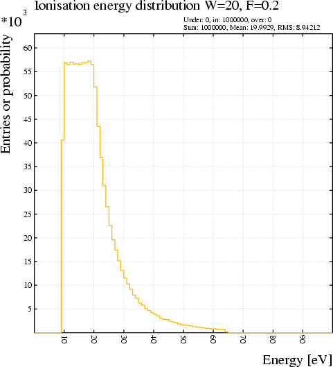
|
Format:
CALL RND_IONISATION_ENERGY(work_function, fano_factor, random_energy)
Example: Verification that the generator indeed asymptotically produces the specified work function and Fano factor.
Global emin=10 Global emax=500 Global npoint=50 Call book_matrix(evec,npoint) Call book_matrix(rmsvec,npoint) Call book_matrix(meanvec,npoint) Call book_histogram(nhist,100,-0.5,99.5)Global w=20 Global f=0.2
For ie From 1 To npoint Do Call book_histogram(nhist,100,-0.5,99.5) Global estart=emin*(emax/emin)^((ie-1)/(npoint-1)) For irndm From 1 To 100000 Do Global ne=0 Global etot=estart Do Call rnd_ionisation_energy(w,f,eloss) If etot-eloss>0 Then Global etot=etot-eloss Global ne=ne+1 Else Leave Endif Enddo Call fill_histogram(nhist,ne) Enddo Global evec[ie]=estart Global rmsvec[ie]=rms(nhist) Global meanvec[ie]=mean(nhist) Enddo
!options log-x Call plot_frame(emin,0,emax,80,`Energy [eV]`, ... `Energy deposited per electron [eV]`, ... `Energy used per electron`) Call plot_line(evec,evec/meanvec,`function-1`) Global v=70 Call plot_line(50,v,80,v,`function-1`) Call plot_text(100,v,`Heed model`,`function-1`,`left-half`)
Global fvec=w/(1-0.45*w/evec) Call plot_line(evec[2+row(size(evec)-2)],fvec[2+row(size(evec)-2)], ... `function-2`) Global v=v-5 Call plot_line(50,v,80,v,`function-2`) Call plot_text(100,v,`W/(1-V/E)`,`function-2`,`left-half`) Call plot_line(emin,w,emax,w,`comment`) Call plot_text(15,22,`w<SUB>s</SUB>`,`title`) Call plot_end
Call plot_frame(emin,0,emax,0.5,`Energy [eV]`, ... `RMS<SUP>2</SUP>/mean`,`Fano factor`) Call plot_line(evec,rmsvec^2/meanvec,`function-1`) Call plot_line(emin,f,emax,f,`comment`) Call plot_text(50,0.16,`Asymptotic Fano factor`,`title`) !rep comment linetype solid Call plot_arrow(w,0.03,w,0,`comment`) !rep comment linetype dashed Call plot_text(w,0.042,`Mean work`,`title`,`centre,half`) Call plot_end
For each step of the drift-line, the procedure uses the Townsend coefficients to compute the probability that an electron is produced, and the attachment coefficients to compute the probability that an electron is lost.
According to these probabilities, electrons are created or absorbed at each step.
The procedure can be applied both to drift-lines computed with the Runge_Kutta_Fehlberg and with Monte_Carlo methods. In the latter case, the use of the PROJECTED-PATH-INTEGRATION integration parameter is recommended in order to avoid a step size dependence in the multiplication.
The procedure can be called repeatedly for the same drift line.
Format:
CALL RND_MULTIPLICATION(ne, [ni])
Example:
&DRIFT
integration-parameters projected m-c-dist-int 0.0002
Call drift_electron_3(0.15,0,0,status,time,diff,aval,att)
Say "Mean RKF aval: {aval}, loss: {att}, product: {aval*att}, status {status}"
Call book_histogram(hist,50,0,2*aval*att)
Global nrndm=500
For i From 1 To nrndm Do
Call drift_mc_electron(0.15,0,0)
Call rnd_multiplication(a)
Call fill_histogram(hist,a)
If entier(i/100)*100=i Then
!options log-y
Call plot_histogram(hist)
Call plot_end
Endif
Enddo
Format:
CALL RND_UNIT_SPHERE(x, y, z)
Example:
Call book_histogram(h, 100, -1, 1) For i From 1 To 1000000 Do Call rnd_unit_sphere(x, y, z) Call fill_histogram(h, x) Enddo Call plot_histogram(h,`Projected coordinate`) Call plot_endThis verifies that one of the projections is uniformly distributed. The other projections should be similarly distributed.
This procedure relies on the G116 procedures of the CERN program library, a high-precision evaluation of the Vavilov distribution, typically 5 decimal are correct. Random numbers are generated using the V152 procedures. See the writeups http://consult.cern.ch/shortwrups/g116/top.html and http://consult.cern.ch/shortwrups/v152/top.html for particulars.
The following restrictions apply: 0.01\ \≤\ \κ\ \≤\ 10 and 0\ \≤\ \β\²\ \≤\ 1
The procedure seems to have difficulty coping with a few narrow ranges of \κ values (around 0.35 and 0.92), for broad ranges of \β\². In those cases, a value of 0 is returned.
A faster, but considerably less accurate, version is available with the RND_VAVILOV_FAST procedure.
Format:
CALL RND_VAVILOV(\κ, \β\², random_number)
This procedure relies on the G115 procedures in the CERN program library. This is a low-precision evaluation of the Vavilov distribution, typically only 1-2 decimal places are correct. See the writeup for particulars: http://consult.cern.ch/shortwrups/g115/top.html for particulars.
The following restrictions apply: 0.01\ \≤\ \κ\ \≤\ 12 and 0\ \≤\ \β\²\ \≤\ 1
A much slower, but considerably more accurate, version is available with the RND_VAVILOV procedure.
Format:
CALL RND_VAVILOV(\κ, \β\², random_number)
Calling this procedure is useful only if you draw the next fill area with GKS_AREA, most other procedures set the attributes before plotting.
Format:
CALL SET_AREA_ATTRIBUTES(representation)
This argument is a text string.
[No default, this is a mandatory parameter.]
Calling this procedure is useful only if you draw the next polyline with GKS_POLYLINE, most other procedures set the attributes before plotting.
Format:
CALL SET_LINE_ATTRIBUTES(representation)
This argument is a text string.
[No default, this is a mandatory parameter.]
Calling this procedure is useful only if you draw the next polymarker with GKS_POLYMARKER, most other procedures set the attributes before plotting.
Format:
CALL SET_MARKER_ATTRIBUTES(representation)
This argument is a text string.
[No default, this is a mandatory parameter.]
Calling this procedure is useful only if you draw the next text with GKS_TEXT, most other procedures set the attributes before plotting.
Format:
CALL SET_TEXT_ATTRIBUTES(representation)
This argument is a text string.
[No default, this is a mandatory parameter.]
Format:
CALL SKIP_HISTOGRAM([number_to_be_skipped])
Example: Suppose, we usually plot 3 histograms in a row and now wish to comment one of these out, without changing the representations of the others. Then we could do this:
Call plot_histogram(hnheed,`n<SUM>e</SUB>`,`Electron count`) * Call plot_histogram(hnexp,``,``,`noframe`) Call skip_histogram Call plot_histogram(hnsrim,``,``,`noframe`) Call plot_end
The points in the array are supposed to be equidistant and in sequence. Each element is replaced by the Gaussian average of the surrounding points:
+n_w
x_i := Sum w_j x_i+j
j = -n_w
-(j/sigma)^2/2
w_j = e
Near the end-points of the array, the sum is truncated symmetrically to prevent an asymmetric bias.
Thus, the first and last point are not changed.
The integral of the array is automatically conserved.
Format:
CALL SMOOTH(x[, n_w[, sigma]])Example: a string of Gaussian random numbers is smoothed.
Global n=10000 Call book_matrixx, n) For i From 1 To n Do Global x[i] = rnd_gauss Enddo Call plot_frame(0, -5, n+1, +5) Call plot_markers(row(n), x, `function-1`) Call smooth(x) Call plot_markers(row(n), x, `function-2`) Call plot_end
Although smoothing is not particularly meaningful on other than 1-dimensional matrices, there is no requirement of the kind.
The matrix is overwritten on return.
[No default, this is a mandatory argument.]
Near the extremities, n_w is reduced symmetrically to avoid bias and addressing outside the array boundaries. As a result, the fluctuations in the extremities will be larger.
[By default, 1 % of the number of points.
[By default, n_w/3.]
Sorting a matrix of higher dimensionality than 1 is equivalent to first unravelling the matrix, sorting its elements and then restoring the original shape of the matrix.
Format:
CALL SORT_MATRIX(matrix)
This procedure is available only in Lunix compilations.
Format:
CALL SLEEP(seconds)
The vectors to be stored must have the same length as the other signals currently stored. The time vector can not be changed with this command.
Format:
CALL STORE_SIGNAL(electrode, direct [, cross-induced])
Read-out groups are formed with the SELECT command. SELECT without arguments will show how the groups are composed and will display the numbers by which they are identified.
[No default, this is a mandatory parameter.]
The matrix should contain the signal directly induced into the electrode specified with the first argument, at time intervals established with the WINDOW command.
[This is a mandatory argument.]
The matrix should contain the cross induced signal of the electrode specified with the first argument, at time intervals established with the WINDOW command.
[This is a mandatory argument.]
Both matrices should exist prior to the call and the size of the selected area should match the size of the matrix which is to be stored.
This procedure is used to process array indexing on the left hand side of Global statements. The procedure is not intended to be called by the user. Using the Global statement is much simpler.
Format:
CALL STORE_SUBMATRIX(ndim, nsel_1, nsel_2, ..., isel_1_1, ...
isel_1_2, ..., isel_2_1, isel_2_2, ... , isel_n_1, isel_n_2, ...
ref_submatrix, ref_matrix)
Format:
CALL STRING_DELETE(string, istart, iend, output)
Example:
Call string_delete(`abc def ghi`,4,8,out)
A mandatory argument, not modified by the procedure.
A mandatory argument, not modified by the procedure.
A mandatory argument, not modified by the procedure.
Should be a modifiable argument. Any data contained in this argument before the procedure is called, is lost after the procedure call.
The first character of a string is numbered 1. Returns 0 if the substring is not found within the string.
Format:
CALL STRING_INDEX(string, substring, index)
Example:
Call string_index(`abc def`,`def`,pos)
Say "`def` starts at character {pos} in `abc def`"
Format:
CALL STRING_LENGTH(string, length)
Example:
Call string_length(`abc`,n)
Say "Length of string is {n} characters."
Format:
CALL STRING_LOWER(string)
Example:
Global str=`ABCDEF`
Call string_lower(str)
Say {str}
Format:
CALL STRING_MATCH(string, pattern, match)
Example:
Call string_match(`abc-def`,`ab#cdef-de#fghi-#ghijkl`,match) If match Then Say "The strings match." Else Say "The strings do not match." Endif
Format:
CALL STRING_PORTION(string, istart, iend, portion)
Example:
Call string_portion(`abc def ghi`,5,7,out)
Say "Characters 5 through 7 of `abc def ghi` are: {out}"
This procedure does not replace characters that stem from earlier replacements.
Format:
CALL STRING_REPLACE(string, search, replace)
Examples:
Global mixture=`argon 90 methane 10`
Global gas_file=mixture/`.gas`
Call string_replace(gas_file,` `,`_`)
Say "|{gas_file}|"
In order to create a file name without blanks from a gas mixture, the blanks are replaced by underscores.
Vector a 1.23 2.34 3.45 4.56Global b=string(a) Call string_replace(b,`, `,` `) Call string_replace(b,`(`,``) Call string_replace(b,`)`,``) Say "-{b}-"
Prints the vector A without parentheses and commata.
Global a=`baaaaa`
Call string_replace(a,`ba`,`bbb`)
Say "|{a}|"
After the call, a will be equal to `bbbaaaa` and not `bbbbbbbbbbb`.
Format:
CALL STRING_UPPER(string)
Example:
Global str=`abcdef`
Call string_upper(str)
Say {str}
Format:
CALL STRING_WORD(string, i, word)
Example:
Global str=`abc def ghi`
Call string_words(str,n)
Say "The string contains {n} words."
For i From 1 To n Do
Call string_word(str,i,out)
Say "Word {i} is {out}."
Enddo
Format:
CALL STRING_WORDS(string, n)
Example:
See STRING_WORD
The entire buffer is printed out at job completion.
Format:
CALL TIME_LOGGING( string )
Example:
Call time_logging(`Until timing test`) Global x0=0.5 Global y0=1.5 Call plot_drift_area For i From 1 To 100 Do Call drift_mc_electron(x0, y0, 0, status, time) Call plot_drift_line Enddo Call time_logging(`MC drifting`)
The TIME_LOGGING routine is called a first time to ensure that in the end we will record only the time spent in MC drifting will be recorded.
Format:
CALL THRESHOLD_CROSSING(electrode, threshold, options, ... ntime, time1 [,time2 [,time3 ...]])
Example:
For i From 1 To 100 Do
signal
convolute-signals range 0 1000 ...
transfer-function (5*t/0.01)^5*exp(-5*t/0.01)
Call threshold_crossing(1,-0.02,`rising,linear`,n,t1,t2)
Say "Found {n} threshold crossings, 1st at {t1} nsec."
Enddo
Read-out groups are formed with the SELECT command. SELECT without arguments will show how the groups are composed.
[No default, this is a mandatory parameter.]
| Option | Meaning |
|---|---|
RISING |
Detect rising edges crossing the threshold |
FALLING |
Detect falling edges crossing the threshold |
LINEAR |
Use linear interpolation (default) |
QUADRATIC |
Use quadratic interpolation |
CUBIC |
Use cubic interpolation |
PLOT |
Plot a graph detailing the fits and the results |
NOPLOT |
Do not plot the results |
DIRECT |
Consider the direct component (default) |
NODIRECT |
Do not consider the direct component |
CROSS |
Consider the cross-induced component |
NOCROSS |
Do not consider the cross-induced component |
Notes:
[This is a mandatory argument which must be modifiable.]
If there are more return arguments than threshold crossings, then the excess arguments are set to Nill, which is of type Undefined.
If more threshold crossings are found than return arguments are provided, then the excess crossing are not returned.
The threshold crossings are returned in increasing order,
[One such argument is mandatory, all these arguments must be modifiable.]
In the absence of a magnetic field, the orientation of the electric field is immaterial. The electric field may be specified either by the norm or as a vector, of which only the norm matters.
In the presence of a magnetic field, the transport parameters depend on the relative orientation of the electric and magnetic field vectors. Both fields therefore have to be specified as vectors.
If the magnetic field is omitted, then all 3\ components are assumed to be zero, irrespective of the magnetic field settings that may be in effect.
Each of the field components can either be a Number or a Matrix. It is permissible to specify 1 or 2 components of the field as Numbers and the other(s) as Matrices.
All components which are specified as Matrix, must have the same total size - they do not have to be 1-dimensional. If at least one component is specified as Matrix, then the output will be a 1-dimensional Matrix with length equal to the overall size of the arguments of type Matrix. Otherwise the result will be a Number.
The electric field should be in V/cm. The magnetic field, if present, should be expressed in native units of 0.01\ T or 100\ G. The Townsend coefficient is returned in 1/cm.
Formats:
CALL TOWNSEND(e, townsend) CALL TOWNSEND(ex, ey, ez, townsend) CALL TOWNSEND(ex, ey, ez, bx, by, bz, townsend)
In the absence of a magnetic field, the orientation of the electric field is immaterial. The electric field may be specified either by the norm or as a vector, of which only the norm matters.
In the presence of a magnetic field, the transport parameters depend on the relative orientation of the electric and magnetic field vectors. Both fields therefore have to be specified as vectors.
Each of the field components can either be a Number or a Matrix. It is permissible to specify 1 or 2 components of the field as Numbers and the other(s) as Matrices.
All components which are specified as Matrix, must have the same total size - they do not have to be 1-dimensional. If at least one component is specified as Matrix, then the output will be a 1-dimensional Matrix with length equal to the overall size of the arguments of type Matrix. Otherwise the result will be a Number.
The electric field should be in V/cm. The magnetic field, if present, should be expressed in native units of 0.01\ T or 100\ G. The diffusion is returned in \√cm.
SIGMA_T can be used as a synonym for TRANSVERSE_DIFFUSION.
Formats:
CALL TRANSVERSE_DIFFUSION(e, sigma_t) CALL TRANSVERSE_DIFFUSION(ex, ey, ez, sigma_t) CALL TRANSVERSE_DIFFUSION(ex, ey, ez, bx, by, bz, sigma_t)
This procedure accepts both a Number and a Matrix as 3rd argument. The value that is returned will be of the same type and shape.
This procedure relies on the G116 procedures in the CERN program library. This is a higher-precision evaluation of the Vavilov distribution than the one used for RND_VAVILOV, and is typically correct to 5 decimal places. See the writeup for particulars: http://consult.cern.ch/shortwrups/g116/top.html for particulars.
The following restrictions apply: 0.01\ \≤\ \κ\ \≤\ 10 and 0\ \≤\ \β\²\ \≤\ 1
Format:
CALL VAVILOV(\κ, \β\², \λ, probability)
This component is zero when there is no magnetic field.
Each of the field components can either be a Number or a Matrix. It is permissible to specify some components of the field as Numbers and the other(s) as Matrices.
All components which are specified as Matrix, must have the same total size - they do not have to be 1-dimensional. If at least one component is specified as Matrix, then the output will be a 1-dimensional Matrix with length equal to the overall size of the arguments of type Matrix. Otherwise the result will be a Number.
The electric field should be in V/cm, the magnetic field has to be in native units of 100\ G or 0.01\ T, and the drift velocity is returned in cm/\μsec.
Format:
CALL VELOCITY_BTRANSVERSE(ex, ey, ez, bx, by, bz, drift)
If there is no magnetic field, then the magnetic field must not be specified. In this case, the values returned by this procedure coincide with those returned by DRIFT_VELOCITY.
Each of the field components can either be a Number or a Matrix. It is permissible to specify some components of the field as Numbers and the other(s) as Matrices.
All components which are specified as Matrix, must have the same total size - they do not have to be 1-dimensional. If at least one component is specified as Matrix, then the output will be a 1-dimensional Matrix with length equal to the overall size of the arguments of type Matrix. Otherwise the result will be a Number.
The electric field should be in V/cm, the magnetic field has to be in native units of 100\ G or 0.01\ T, and the drift velocity is returned in cm/\μsec.
Format:
CALL VELOCITY_E(ex, ey, ez, bx, by, bz, drift)
Example:
&GAS magboltz argon 92 co2 8 e/p-range 0.05 8&MAIN Global emin=60 Global emax=7000 Global n=200 Global e=emin*(emax/emin)^((row(n)-1)/(n-1)) Call velocity_e(0,0,e,v) !options log-x Call plot_graph(e,v,`E [V/cm]`,`Drift velocity [cm/microsec]`, ... `Magboltz vs Zhao et al.`) Vector ezhao 0.07 0.14 0.21 0.28 0.35 0.42 0.49 0.559 0.629 0.699 0.769 0.839 0.909 0.979 1.049 1.119 1.189 1.259 1.329 1.399 1.573 1.748 1.923 2.098 2.448 2.797 3.147 3.497 3.846 4.196 4.545 4.895 5.245 5.735
Vector vzhao 0.52 1.15 1.89 2.77 3.56 4.18 4.57 4.78 4.82 4.79 4.71 4.62 4.53 4.43 4.35 4.3 4.26 4.23 4.2 4.2 4.2 4.24 4.29 4.36 4.49 4.57 4.59 4.58 4.56 4.5 4.47 4.44 4.4 4.4
Call plot_error_bar(ezhao*1000,vzhao,`circle`) Call plot_end
Magboltz is used to compute the drift velocity in a mixture of 92\ % argon and 8\ % CO\<SUB\>2\</SUB\>. The results are compared with the measurements of T. Zhao et al., NIM A340 (1994) 485. The E > 3000 V/cm region is controversial, apart from that the two are in good agreement. This is an abridged version of http://cern.ch/garfield/examples/gas/ArCO2_detail.html
This component is zero when there is no magnetic field.
Each of the field components can either be a Number or a Matrix. It is permissible to specify some components of the field as Numbers and the other(s) as Matrices.
All components which are specified as Matrix, must have the same total size - they do not have to be 1-dimensional. If at least one component is specified as Matrix, then the output will be a 1-dimensional Matrix with length equal to the overall size of the arguments of type Matrix. Otherwise the result will be a Number.
The electric field should be in V/cm, the magnetic field has to be in native units of 100\ G or 0.01\ T, and the drift velocity is returned in cm/\μsec.
Format:
CALL VELOCITY_ExB(ex, ey, ez, bx, by, bz, drift)
This routine differs from WEIGHTING_FIELD_3 in that it expects only the (x,y) part of the location, assuming z=0.
This procedure should be called from within the signal section.
Format:
CALL WEIGHTING_FIELD(x, y, ex, ey, ez, electrode)
for x: log(r) for y: \φ, in radians for z: assumed to be 0
The transformation from (x,y) to (\ρ,\φ) can be performed by the CARTESIAN_TO_INTERNAL procedure.
Er = Ex/r Ephi = Ey/r Ez = Ez
[This argument is compulsory.]
This procedure differs from WEIGHTING_FIELD in that it expects an (x,y,z) set of coordinates.
This procedure should be called from within the signal section.
Format:
CALL WEIGHTING_FIELD_3(x, y, z, ex, ey, ez, electrode)
for x: log(r) for y: \φ, in radians for z: z
The transformation from (x,y) to (\ρ,\φ) can be performed by the CARTESIAN_TO_INTERNAL procedure.
Er = Ex/r Ephi = Ey/r Ez = Ez
This argument is mandatory.
Histograms can, by means of the WRITE_HISTOGRAM_RZ procedure, also be written out in a format suitable for use with PAW. Using the h2root program, such files can be converted for use with root, see http://root.cern.ch/root/HowtoConvert.html
Calling this procedure does not interfere with filling of the histogram and an autorange histogram can be written to disk before the range has been set.
This procedure is for instance used when one job fills a set of histograms which are, probably repeatedly, fitted by another job. Another application is a found in calculations where statistics are accumulated over a series of jobs. The first job would create the histogram and fill it, all successive jobs read the existing histogram, continue filling it, and write it back to the file at the end of the job. Care should be taken that the global option DELETE-OLD-MEMBER has been switched on before doing this.
The procedure sets the OK global variable to True if the histogram has been written and to False if it hasn't.
Format:
CALL WRITE_HISTOGRAM(reference, file [, member [, remark]])
Example:
Global chamber=1(calculation of e.g. arrival time histograms for chamber 1)
Global hfile `CHAMBER`/string(chamber)/`.HIST` Global i=0 Global exist=True Global n=0 While exist Do Global i=i+1 Call inquire_histogram(reference(i),exist) If exist Then Call write_histogram(reference(i),hfile) Global n=n+1 Endif Enddo Say "Have written {n} histograms."
In this example, the input file is assumed to contain a cell section that enters the elements for chambers 1, 2, etc depending on the setting of the global variable "chamber".
At the end of the run, the user wishes to keep all histograms for further examination. The loop in the example writes all histograms to a file (hfile) the name of which is CHAMBER1.HIST, CHAMBER2.HIST etc. depending on the setting of the global variable "chamber".
All histograms are written to the same file, but they will be distinguished by their member names which are defaulted to the name of the global variables associated with the histogram.
This example assumes that no histograms have been deleted during the run, as it assumes the histograms are numbered from 1 on.
Histogram references can be created with calls to BOOK_HISTOGRAM or GET_HISTOGRAM. Histogram references are also created by arithmetic between existing histograms.
If this argument is an expression which results in an histogram, the member name should be specified.
This argument should be of type String.
If the member name is omitted, a default member name equal to the name of the global variable associated with the histogram, will be assigned to the histogram. This is in many cases a meaningful default and there is therefore rarely a need to specify a member.
This argument should be of type String.
[By default, set to "none".]
RZ files can be converted for use by root with the h2root program, see http://root.cern.ch/root/HowtoConvert.html
An autorange histogram can only be written out to an RZ file once its range has been established. Use the WRITE_HISTOGRAM and GET_HISTOGRAM procedures to save and recover such an histogram.
The procedure sets the OK global variable to True if the histogram has been written and to False if it hasn't.
Format:
CALL WRITE_HISTOGRAM_RZ([reference [, file [, title]]])
Example:
Call book_histogram(a,200) For i From 1 To 10000 Do Call fill_histogram(a,rnd_landau) Enddo Call plot_histogram(a,`Energy`,`Landau`) Call plot_end Call write_histogram_rz(a,`hist.rz`,`Landau distribution`)
This generates an histogram with a Landau distribution and writes the histogram to a file called "hist.rz". Garfield replies telling that the histogram has been written with PAW identifier 1 and cycle number 1. To read it back with PAW, one would type:
h/file 20 hist.rz h/pl 1
Histogram references can be created with calls to BOOK_HISTOGRAM or GET_HISTOGRAM. Histogram references are also created by arithmetic between existing histograms.
This parameter may be omitted, or be set to `ALL`, in which case all histograms are written to the RZ file.
[Default: all histograms are written.]
For this reason, Garfield prints the identifier when the histogram is written.
Garfield also prints the cycle number assigned by PAW. The cycle number will be 1 if the histogram identifier is not yet in use in the RZ file. The first cycle of a histogram can be accessed from PAW without special precautions:
h/pl 5
In case, however, that the RZ file already contains an histogram with the same identifier, then the newly written histogram will be assigned a higher cycle number. The histogram now has to be accessed as follows, assuming the cycle number is 3:
h/pl 5;3
The file may exist before the call is issued, but doesn't have to. If the file already exists, then it must be an RZ file formatted with a record length of 1024. The file may already contain other histograms.
[Default: `garfield.rz`.]
The title is ignored if all histograms are to be written out. In that case, the histograms are given the name of the variable with which they are associated, as title.
[Default: the name of the global variable if the histogram is associated with a global variable, otherwise the field is left blank.]
The Garfield WWW example pages contain a Matlab function that reads a file written by WRITE_MATRIX (contributed by Guy Garty): http://cern.ch/garfield/examples/load_garf.m
The procedure sets the OK global variable to True if the matrix is successfully written, and to False in case of a problem.
Format:
CALL WRITE_MATRIX(matrix, file [, member])
Example:
If type(global(`ABC`))#`Matrix` Then
Call inquire_member(`abc.mat`,`abc`,`matrix`,exist)
If exist Then
Call get_matrix(abc,`abc.mat`)
Call dimensions(abc,n_dim,dim_abc)
Global nx=number(dim_abc[1])
Global ny=number(dim_abc[2])
Call delete_matrix(dim_abc)
Else
Global nx=20
Global ny=30
Call book_matrix(abc,nx,ny)
For i From 1 To nx Do
For j From 1 To ny Do
Global abc[i;j]=sin(i)*exp(j/10)
Enddo
Enddo
Call write_matrix(abc,`abc.mat`)
Endif
Endif
First, one checks whether ABC is already in memory. If it is, nothing is done. Otherwise, an attempt is made to recuperate the matrix from a file. If this doesn't work, then the matrix is generated and stored in the file so that next time, the matrix can be recuperated from there.
A matrix reference is usually created with a call to BOOK_MATRIX, using the ROW function or by arithmetic between existing matrices.
If this argument is an expression which results in a matrix, then the member name should be specified.
This argument should be of type String.
If the member name is omitted, a default member name equal to the name of the global variable associated with the matrix, will be assigned to the histogram. This is in many cases a meaningful default and there is therefore rarely a need to specify a member.
This argument should be of type String.
The procedure searches for zero crossings between 2 adjacent tabulated values, then performs a linear or quadratic interpolation over the neighbouring range.
Do not confuse this procedure with the ZEROES function.
Format:
CALL ZEROES(x_vector, y_vector, nzero, zero1, zero2, ...)
Examples:
Call get_signal(1,time,direct,cross)
Global signal=direct+cross
Call zeroes(time,signal/maximum(signal)-0.5,nz,t1,t2)
If nz<2 Then
Say "Time range not long enough to determine FWHM."
Else
Say "FWHM of the signal: {t2-t1}"
Endif
Global r=row(200)/10
Global v=sin(r)
Call zeroes(r,v,nz,z1,z2,z3)
Say "Zeroes: {nz} - {z1,z2,z3}"
The first example computes the FWHM of a signal, the second
example finds the zeroes of the sine function.
If the arguments are not 1-dimensional, then they are unravelled.
[These arguments are mandatory. No default is supplied.]
If there are more return arguments than zeroes found, then the excess arguments are set to Nill, which is of type Undefined.
If more zeroes are found than return arguments are provided, then the excess zeroes are not returned.
The zeroes are returned in numerically increasing order, irrespective of the order of the ordinate vector.
Do loops are used to repeatedly execute a set of lines.
There are 3 types of loops in Garfield:
Do not attempt to input a file with < while in a Do loop.
Format of a "From-Step-To" loop:
For var From from [Step step] To to [While while] [Until until] Do [statement | Leave [var] | Iterate [var]] ... Enddo
Example:
For i From 1 To 5 Do
Say "Now I has the value {I}."
Enddo
Say "Finished !"
Format of an "In" loop:
For var In in [While while] [Until until] Do [statement | Leave [var] | Iterate [var]] ... Enddo
Example:
Vector angles 0 1 2 5 10 30 60 90For angle In angles Do &SIGNAL (various signal settings required here) track 0.2 2 0.2 {2+0.4*tan(pi*angle/180)} pion energy 5 GeV signal Enddo
Signals are computed for tracks at various inclinations.
Format for a "Leave" loop:
[While while] [Until until] Do [statement | Leave [var] | Iterate [var]] ... Enddo
Example:
Do
Say "Please enter a number"
Parse Terminal x
If type(x)=`Number` Then Leave
Say "{x} is not a number, try again"
Enddo
Say "You entered {x}"
This fragment will keep asking for a value to be given to x until what the user types can be identified as being numeric.
You may change the value of this variable inside the loop. If you do so in a "From-Step-To" loop, then the increment for the next iteration will be added to the modified value. Such a modification has no effect on the next iteration in a "In" loop, nor does it affect the contents of the matrix from which the values are taken.
The loop variable can be used anywhere inside the body of the loop to perform calculations. It can also be referenced in the Leave and Iterate statements.
The loop variable is a Global of type Number. It does not have to be declared before the loop. Its name should obey the naming conventions for global variables.
[This is an optional parameter.]
This parameter must be a Global variable of type Number or an expression that evaluates to a Number.
"From-Step-Do" loops should not have an In clause.
[This argument is mandatory for "From-Step-To" loops. No default is provided.]
This parameter must be a Global variable of type Number or an expression that evaluates to a Number.
This expression is evaluated anew at each iteration.
"From-Step-Do" loops should not have an In clause.
[This argument is permitted only in "From-Step-To" loops. If no step size is indicated, a default value of 1 is assumed.]
This parameter must be a Global variable of type Number or an expression that evaluates to a Number.
This expression is evaluated anew each iteration.
"From-Step-Do" loops should not have an In clause.
[This argument is mandatory for "From-Step-To" loops. No default is provided.]
This expression is evaluated anew at each iteration. It is permissible to modify the matrix in the body of the loop.
From, Step and To must not be used in "In" loops, but you may use While and Until.
[This argument is mandatory for "In" loops. There is no default matrix.]
This parameter must be a Global variable of type Logical or an expression that evaluates to a Logical.
This expression is evaluated anew each iteration.
[This optional parameter is by default set to True.]
This parameter must be a Global variable of type Logical or an expression that evaluates to a Logical.
[This optional parameter is by default set to False.]
You may specify as an argument the name of the loop variable associated with the loop you wish to leave.
Leave is the Garfield equivalent of the break statement in C, "break" may be used instead of "Leave" if preferred.
[Use of a Leave statement is optional.]
You may specify as an argument the name of the loop variable associated with the loop you wish to leave.
Iterate is the Garfield equivalent of the continue statement in C, "continue" may be used instead of "Iterate" if preferred.
[Use of an Iterate statement is optional.]
Assigns a value to a global variable, declares a global variable or lists the currently known global variables, depending on the number of arguments.
Global variables are used for the substitution of an expression in input statements and they play a key role in Do loops, procedure Calls and in conditionally executed If_lines and If_blocks.
This statement has up to 2 arguments:
If there are no arguments: All currently defined globals are listed with their type and value. You will see that the list includes a few predefined globals. Occasionally, you will find globals with names that do not comply with the naming conventions for variables. These are copies of globals which must be kept even if you modify the original. If you wish to see the value of only a single variable, then use Say. To list all currently known strings, matrices and histograms, use the LIST_STRINGS, LIST_MATRICES, and LIST_HISTOGRAMS procedures.
When the value is omitted:
When both a variable name and a value are supplied:
If you wish to use the type of a global variable in a formula, then use either the TYPE function or the INQUIRE_TYPE procedure.
Format:
Global variable [value]
Examples:
Global my_name=`abc DEF`Global argon=80 Global ethane=20 Global member=`a`/string(argon)/`e`/string(ethane)
The first example assigns the character string "abc DEF" to the variable my_name. In the second example, a suitable member name of a compact gas description is constructed from the argon and ethane contents. Note that no curly brackets are used.
This argument should not be an expression. If you really need to update a variable of which the name can only be constructed at run time, then use a construction like the following:
For i From 1 To n Do
Global {`M`/string(i)}=i
Enddo
Note that this will considerably slow down execution of the loop since the expression will be translated at every iteration rather than just once.
To enter a set of numbers into a Matrix, one would normally use the Vector statement even though one can also use the Global command as illustrated in one of the examples below.
Examples:
Global abc `abc` // Assigns a string to ABC Global abc 2<3 // Assigns a logical to ABC Global abc string(2+3)/abc // Updates the ABC string Global abc 1 & 5 & 7 // Assigns a vector to ABC
If blocks are used to conditionally execute a group of statements and to execute only one of a set of groups of statements depending on a series of conditions. If blocks may be nested and may also contain entire Do loops in their branches.
Format:
If condition Then
statements
[Elseif condition Then
statements]
[Else
statements]
Endif
Example:
If vax Then
get 'disk$food:[garfield]lasagne.dat'
Elseif cray|apollo|sun Then
If Cray Then $ fetch //food/garfield/lasagne.dat ...
-t'fn=FOOD,ft=LASAGNE'
get "//food/garfield/lasagne.dat"
Elseif cms Then
get food.lasagne.*
Else
Say "No GET for this machine; stopping."
& stop
Endif
In this example, a cell (or gas) compact description is fetched from a file - the name depends on the machine. In the case of the Cray, the file is first read from the IBM.
The statements of the branch are executed if the condition evaluates to True, otherwise they are skipped.
The nesting level of If blocks is limited by a compilation parameter which is usually set to 10.
The If line is used to execute conditionally only one line, for instance a &STOP if the amount of CPU time left to the job is less than a few seconds. An If line is also used to conditionally execute an entire Do loop.
Format 1:
If condition Then statement
Format 2:
If cond Then ... Dostatement | Leave [var] | Iterate [var]
Enddo
Examples:
If time_left < 10 Then &stop If vax Then Say "Running on a Vax."If x>10 Then For i From 10 To 1 Step -1 Do If entier(i/3+0.001)=3 Then Iterate Say "x+i/3 = {x+i/3}" Enddo
The statements of the branch are executed if the condition evaluates to True, otherwise they are skipped.
The statement of an If line may not be itself an If line.
This instruction enables you to make input files that prompt for parameters. For instance, in a magnetic field section, you could ask for the value of the magnetic field and then issue a COMPONENTS instruction with the B-field the user specifies. You could also ask the user to enter the name of a cell description and then load it from a library of such descriptions.
If you're familiar with REXX, you'll note the similarity with the REXX command by the same name, even if the REXX syntax is far richer than what is offered here.
By default, the values found on input are assigned Literally to the Global. You can also request evaluation of the input prior to assignment by using the Evaluate option.
Format:
Parse [Literal | Evaluate] ...
{Argument | Global var | Input | Terminal | Value expression} ...
template
Example 1: Get the piece before and after the decimal dot of pi².
Parse Val pi^2 int'.'frac
Example 2: Ask for a yes/no answer
&FIELD
Global yes=True
Global no=False
Say "Make a 3D plot ? (yes/no)"
Until OK Do
Parse Evaluate Terminal plot_3D
Call inquire_type(plot_3D,type)
If type=`Logical` Then
Global OK=True
Else
Say "Please give an answer that evaluates to True or False."
Global OK=False
Endif
Enddo
If plot_3D Then plot-field surface
The usual initialisation files set the global variables YES and NO to respectively True and False. Since we use the Evaluate option, one can simply reply with "yes" or "no" (without typing the quotes), but one may also answer with any expression that evaluates to a Logical such as 3>4. If the default Literal mode were used, only True and False would be accepted.
Example 3: Ask for a cell name
Say "Please enter the name of the cell to be read:"
Parse Terminal cell
(The user responds with e.g. DC1)
get cell.lib {cell}
Here we use the default Literal mode - the response, DC1, will be classified as string and there is no need for quotes. We could also use the Evaluate mode but then reverse quotes would be required around the user response since we do not want DC1 to be evaluated as if it were a global.
Example 4: An argument to an input file
Assume we have the following input file called "plot_gas":
Parse Arg gas
Call inquire_file(gas/`.gas`,exist)
If ~exist Then
Say "{gas}.gas does not exist."
Else
&GAS
get "{gas}.gas"
opt gas-plot
&MAIN
Endif
and a set of gas files with such names as "p10.gas", then we could plot the gas data with a command like:
< plot_gas p10
In most cases, this is what you would intuitively expect to happen.
If you use the Literal or Evaluate option, then the option must be placed immediately after the Parse command. Literal and Evaluate are mutually exclusive options.
Example:
Global hello `Hello Peter !`
Parse Literal Value hello . name .
Say "Person greeted: {name}"
Here, we have to use Literal since the string can not be evaluated: for that, "Hello" would have to be a function, "Peter" an argument hence a Global variable, and the exclamation mark would have to have some algebraic meaning, which it doesn't.
[This is default.]
If you use the Literal or Evaluate option, then the option must be placed immediately after the Parse command. Literal and Evaluate are mutually exclusive options.
Example:
Say "Open a metafile (yes/no) ?"
Global yes True
Global no False
Global y True
Global n False
Parse Evaluate Terminal metafile
If metafile Then
Say "Opening metafile {input}.ps ..."
!add meta type PostScript file-name "{input}.ps"
!open meta
!act meta
Else
Say "No metafile opened."
Endif
The If statement expects a Logical as condition. We would however like to offer the user the possibility to reply with "yes" or "no". Therefore, we define Global variables by those names which have the values True and False. With the Evaluate option, a reply of "yes" therefore results in the assignment of Logical value True to the global variable METAFILE. With the Literal option, METAFILE would become a String with value `YES`.
[This is not default.]
Examples:
Garfield is started by issuing a command like:
garfield -arg "Hello !"The double quotes around the argument string are needed only in case of special characters, such as the exclamation mark. Once the program is running, you can access the string "Hello !" with the Parse command:
Parse Arg greeting
Say {greeting}
Imagine you've an input file called factorial which looks like this:
Parse Arg n
If type(n)#`Number` Then
Say "Please supply a numeric argument."
Elseif n<1 | abs(entier(n+0.5)-n)>1e-4 Then
Say "Please supply a strictly positive, integer argument."
Else
Global fac=1
For i From 2 To n Do
Global fac=fac*i
Enddo
Say "Factorial of {n} is {fac}."
Endif
One would run this file as follows:
<factorial 5
Parsing should not give surprising results with Globals that are of type Number or String. Globals of type Logical will result in the string `True` or `False` while variables of type Undefined yield the string `Nill`.
If the Global variable is an Histogram, then the resulting string will be `Histogram`, which is not useful.
Similarly, a Matrix with more than 1 dimension gives the string `n-Matrix` where n is the number of dimensions. Only for 1-dimensional matrices will the string contain a formatted portion of the matrix. This can be parsed, although not trivially:
Call book_matrix(a,4) Parse Global a `(` a `,` b `,` c `,` d `)`
which is equivalent to:
Parse Value row(4) `(` a `,` b `,` c `,` d `)`
This format is only offered for completeness - the Terminal input format is probably more useful. See there for further details.
The input line is treated like all other input, i.e. text outside single and reverse quotes is converted to upper case.
This is a frequently used format since it permits obtaining user input while a file is being input.
This format can also be used to pause execution of an input file, while waiting for the user to hit the return key:
&FIELD grid 5 print ex,ey Parse Terminal dummy print v
The first table will be printed, then the program waits for a response from the user and the 2nd table is printed only after the return key has been pressed.
This format is similar to Parse Global, see there for examples and further comments.
A template can contain the following elements:
| Element | Purpose |
|---|---|
`string` |
Locate string in the input, resume from there |
var |
Global variable to which the field is assigned |
. |
Ignore the corresponding input field. |
All elements can be repeated many times.
Instead of reverse quotes (`), one can also use single and double quotes to delimit search strings. Keep in mind however that the quote is a syntax element - the quote must therefore still be visible after the Parse statement has been processed by the usual input routines.
If there are more variables in the template than elements in the input, then the variables to which no value can be assigned will be set to have type Undefined. Conversely, if there are more elements than variables, then all variables will together, with their separators, be assigned to the last variable. This operation is likely to fail in the Evaluate mode.
Examples with option Literal:
| Input | Template | Result |
|---|---|---|
1 2 3 |
x y z |
x=1, y=2, z=3 |
1 2 x+1 |
x y z |
x=1, y=2, z=`x+1` |
1 2 3 4 |
x y . |
x=1, y=2 |
1 2 |
x y z |
x=1, y=2, z=Nill |
1 2 3 |
x y |
x=1, y=`2 3` |
1 2 A 3 |
x . `A` y |
x=1, y=3 |
1 2 A 3 |
x `A` y |
x=`1 2`, y=3 |
1 `abc` 2 |
x y . |
x=1, y=`abc` |
1>2 |
z . |
z=`1>2` |
Examples with option Evaluate:
| Input | Template | Result |
|---|---|---|
1 2 3 |
x y z |
x=1, y=2, z=3 |
1 2 x+1 |
x y z |
x=1, y=2, z=2 |
1 2 3 4 |
x y . |
x=1, y=2 |
1 2 |
x y z |
x=1, y=2, z=Nill |
1 2 3 |
x y |
Error: y := 2 3 is incorrect syntax |
1 2 A 3 |
x . `A` y |
x=1, y=3 |
1 2 A 3 |
x `A` y |
Error: x := 1 2 is incorrect syntax |
1 `abc` 2 |
x y . |
x=1, y=`abc` |
1>2 |
z . |
z=False |
Format:
SAY string
Example:
Say "Only {time_left} seconds left !"
Prints the value of a predefined
global variable.
Newly created Matrices are 1-dimensional and have a length that is equal to the number of elements entered. Matrices can be given another shape with the RESHAPE_MATRIX procedure.
For existing 1-dimensional Matrices, the new elements replace the existing elements, keeping existing elements if the number of new elements is smaller than the size of the vector, and skipping new elements if there are more than the size of the matrix.
For higher dimensional already existing Matrices, the number of dimensions and the size are kept as they were, and new elements replace old elements in the order in which the Matrix is internally stored (opposite to the Fortran convention).
Use the DELETE_MATRIX procedure to delete the matrix if this way of re-using existing matrices is not as desired.
The Vector statement can read data into one or more Matrices at the time. If more than one Matrix is present, then the statement should be followed by a series of lines which contain precisely one new element of each of the Matrices. If only one Matrix is present, then one may type an arbitrary number of elements on an arbitrary number of lines following the statement. In either case, there should be a blank line to signal that all elements have been entered.
Fields which are to be ignored, for instance because they do not contain numeric data, are to be identified as DUMMY.
Format:
Vector x y z ... Vector x x1 y1 z1 ... x1 x2 x3 ... x2 y2 z2 ... ... ... ... xn yn zn ... ... xn (blank line) (blank line)
Example 1:
Vector zzz 0 1 2 3 4 5 6The Vector statement results in a 1-dimensional matrix of length 7, called ZZZ, which contains the numbers 0 to 6. The RESHAPE_MATRIX procedure call re-arranges this vector to a 2\×4 matrix. This matrix has one element more than the original vector, which is filled with the value PI, which is one of the pre-defined constants.Call reshape_matrix(zzz,2,4,pi)
We could have written the Vector statement using the concatenation operator & and the ROW function:
Global zzz = 0 & row(6)
Example 2:
Vector Z dummy wK wL1 wL2 wL3 f12 f13 f23
48 Cd 0.842 0.018 0.056 0.056 0.10 0.59 0.155
49 In 0.851 0.020 0.061 0.060 0.10 0.59 0.157
50 Sn 0.860 0.037 0.065 0.064 0.17 0.27 0.157
51 Sb 0.868 0.039 0.069 0.069 0.17 0.28 0.156
52 Te 0.875 0.041 0.074 0.074 0.18 0.28 0.155
53 I 0.882 0.044 0.079 0.079 0.18 0.28 0.154
54 Xe 0.888 0.046 0.083 0.085 0.19 0.28 0.154
55 Cs 0.894 0.049 0.090 0.091 0.19 0.28 0.154
56 Ba 0.900 0.052 0.096 0.097 0.19 0.28 0.153
57 La 0.905 0.055 0.103 0.104 0.19 0.29 0.153
// Note the empty line
Here, we enter a table (an extract from the Krause fluorescence
and Coster-Kronig yields tables) copied from a paper, without having to
manually remove the names of the elements. This is done by declaring
the field of the element name as "dummy".
If the name of the variable is already in use for a variable of another data type, then the value the variable had before the Vector statement is lost.
Formulae can be typed as usual in Fortran or C, with some exceptions:
Evaluation is not as quick as compiled routines but since the formulae are preprocessed and translated into an instruction_list, the losses for repeated evaluations are small compared to what would otherwise be needed in terms of human time.
The translation of the formula into an instruction list, is done independent of the data type. It may also be possible that the resulting instruction list can be executed for several data types.
Instruction lists can be edited in the algebra editor which is entered by typing a @ instead of a formula. The editor behaves like a subsection. On exit of the editor, the function is used by the calling routine to perform its task.
PLOT CONTOUR V
The "V" in this statement is a local variable of the PLOT-FIELD command which equals the electrostatic potential at a given point. The name and value of these variables is not under your control. Moreover, you usually only have access to them in the context of the command being executed.
Garfield also has variables which are entirely under your control: you choose their name and value, you determine when expressions are to be evaluated, and you decide when and how to display their values. These are called global variables, or Globals for short. The name has been chosen to reflect the broader scope of globals, as compared to the local variables mentioned above. Local variables have a scope limited to one command, while global variables can be used across sections.
Global variables can be used for a variety of things:
In contrast, you can create and (in most cases) modify Global variables. There are many methods to create them:
Also some global variables are defined by the program:
Examples:
Global a_1 = 5 Global abc = `This is a string` Global v=row(20)
Although permitted, it is not advisable to force variable names to contain lower case characters as in the following:
// Not recommended Global "Abc" 123
If the formula evaluates to a Number, Logical or String, then the value is simply substituted. If the result is an Histogram, then the string "Histogram" is substituted for the formula. For a 1-dimensional Matrix, the first portion of the matrix is substituted but for higher dimensional matrices, the string "n-Matrix" will appear, where n is the dimension of the matrix.
Curly brackets { } are very often misused, in particular they should never be used in Do loops, in the conditions of If_lines and If_blocks, in the arguments of procedure Calls, in Parse and Global statements.
The contents of { } is evaluated and substituted before the statement is interpreted, while you would probably expect evaluation to happen only when the control statements are executed. For an overview of the use of round, square and curly brackets.
Format:
any text {formula} more text
Example:
Global a=60
Say "Tangent of {a} degrees is {tan(pi*a/180)}."
The global variable A is assigned the value 60. In the following SAY statement, A is converted from degrees to radians and its tangent is displayed.
Further examples of this use of global variables can be found in the examples given for many other commands.
// What one should not do
Global n=5 For i From 1 To 5 Do
For i From 1 To {n} Do For j From 1 To {i} Do
... Say "j={j}"
Enddo Enddo
Enddo
The example on the left would still work if the value of n doesn't change during execution, the example on the right would fail. A priori, I is not defined at the time the loop on J is read. If it is, then the loop on J would be executed a fixed number of times that has no relation with the value of I in the outer loop.
Garfield variables know their own type. Garfield takes care that a version of the operators and the functions appropriate for the given data type or combination of data types is called. The type of the argument propagates to the result for most operators and functions.
Global variables come in the following types:
| Type | Explanation | Mode |
|---|---|---|
| Undefined | Declared but not initialised | 0 |
| String | Character strings | 1 |
| Number | A real or integer number | 2 |
| Logical | Can be either True or False | 3 |
| Histogram | 1-Dimensional histogram | 4 |
| Matrix | n-dimensional matrices made up of numbers | 5 |
The mode is a numeric equivalent of the type, the mode is used only internally for quick reference.
All arithmetic is permitted between variables of this type and a variable of any other type. All such operations result in a variable of the type Undefined, with the exception of the TYPE function.
One of the pre-defined constants is of this type: NILL.
Strings are usually created by enclosing a series of characters in reverse quotes, as illustrated in the examples below.
Strings can be concatenated with the / operator and can be lexically compared with each other using the >, < and = operator. The functions NUMBER and STRING convert Strings to Numbers and vv. There is also a series of procedures that act on Strings: STRING_DELETE, STRING_INDEX, STRING_LENGTH, STRING_LOWER, STRING_MATCH, STRING_PORTION, STRING_REPLACE, STRING_UPPER, STRING_WORD and STRING_WORDS.
Strings are internally stored in a dynamic buffer which has a fixed maximum total size. The buffer remembers the length of each string. One does not declare the length of Strings since the length is implied by the initialisation and operations the string has undergone. The length of a string can vary in time.
There are no constant strings, but there are predefined globals of type String.
Examples:
Global gas_file `gas.dat`Global p=1 Global gas_file `gas_p`/string(p)/`.gas`
The numbers 0, 1, 2 and PI are constants, there are also predefined globals of this type.
Both True and False are stored as constants and there are several predefined globals of this type. Logicals can also be created by applying a comparison operator to variables of other data types:
Global equal `aaa`=`a`/`aa` Global bigger 5>2^2
Logicals can be acted upon with operators, as & (and) and | (or) as well as with the NOT, STRING and TYPE functions.
Logicals are commonly used in the conditions of If_lines, If_blocks and Do loops:
Do
Say "Quit ? Please reply with True or False"
Parse terminal quit
If type(quit)#`Logical` Then
Say "Please answer with True or False"
Elseif quit Then
Say "Quit"
Leave
Endif
Enddo
Logicals in Garfield are not equivalent to numbers, i.e. one can not normally replace True by 1. Similarly, one can not apply mixed arithmetic between Logicals and Numbers.
Garfield histograms are currently 1-dimensional only, and they have adjacent, equal size bins. They come in 2 flavours:
Histograms are usually created with a call to BOOK_HISTOGRAM. Several instructions can generate histograms as part of their output.
Histograms can be subject of most of the ordinary arithmetic operators and functions. Mixed arithmetic between Numbers and histograms is permitted and results in histograms.
Example:
Call get_histogram(part1,`file1.hist`,`delay`) Call get_histogram(part2,`file2,hist`,`delay`) Call get_histogram(part3,`file3,hist`,`delay`) Global delay=(part1+part2+part3)/3Each of a series of jobs, run in parallel, has created an histogram called DELAY, filled it, and written it to a file. The histograms from the 3 files are retrieved and averaged.
Histograms can also be operated on by a series of procedures, For instance, histograms can, by means of the WRITE_HISTOGRAM_RZ procedure, be written out to an RZ file for further processing with PAW.
There are no predefined constant histograms, nor globals of this type.
Matrices can be created in a variety of ways:
The usual arithmetic operators and functions can be applied to matrices as if they were numbers. Mixed arithmetic between Numbers and matrices is permitted and results in matrices. Applying arithmetic to entire matrices is much faster than looping over the elements.
Parts of matrices can be addressed with the following syntax:
Some examples for a 1-dimensional matrix:
A = (9 8 7) A[1,2,3,1] = (9 8 7 9) A[1+ROW(2)] = (8 7)The ROW function returns a 1-dimensional Matrix that contains the numbers 1 to the value of the argument, in this case the numbers 1 and 2. Indexing using 1-dimensional matrices is particularly convenient to extract a large sub-matrix, such as in the following example where one only fits the central portion of a cosine curve with a parabola:
Global x=-pi+2*pi*(row(500)-1)/499 Global y=cos(x) Call fit_polynomial(x[200+row(100)],y[200+row(100)],0.001, ... a0,a1,a2,ea0,ea1,ea2,`plot`)
When indexing a 2-dimensional matrix, one needs a semi-colon to separate the indices along the 1st and 2nd dimension. Remember that an empty indexing part selects that entire dimension:
( 1 2 3 ) ( 3 2 )
A = ( 2 4 6 ) A[3,2;] = ( 6 4 ) A[;1] = ( 1 2 3 )
( 3 6 9 ) ( 9 6 )
Notes:
The value of Numbers and Logicals is stored directly in R, while for Histograms, Matrices and Strings a reference number is kept in R.
Each element of R has type information attached to it.
All R's from R(0) downwards are assumed to be constants that are not affected by the execution of the instruction list.
Although changing the values of the registers R(0) to R(-6) is not by itself prevented, the "jump always" code will for instance not work if R(-1) is set to something else than the value\ 1. Similar trouble can arise from changing the other constants in this range.
The space below R(-7) can be used for constants present in user entry points. These constants are deleted when the list is deleted with which they are associated.
The values of the constants which can be used in all lists are:
| Location | Name | Value | Type |
|---|---|---|---|
R(0) |
0 |
0 | Number |
R(-1) |
1 |
1 | Number |
R(-2) |
2 |
2 | Number |
R(-3) |
PI |
3.14159265 | Number |
R(-4) |
FALSE |
False | Logical |
R(-5) |
TRUE |
True | Logical |
R(-6) |
NILL |
Nill | Undefined |
Notes:
| Global | Type | Explanation |
|---|---|---|
BATCH |
Logical | True if running in batch, False otherwise. |
FRAME |
Number | Sequential number of the plot frame |
INPUT |
String | Name of the current input stream. |
INTERACT |
Logical | True if running interactively, False otherwise. |
MACHINE |
String | The type of computer on which you're running. |
OK |
Logical | True if last algebra instruction was successful. |
OUTPUT |
String | Name of the current output stream. |
TIME_LEFT |
Number | The amount of CPU time that remains [sec]. |
X |
Number | Used for fitting |
A program is said to run in batch if the standard input stream is anything else than terminal input. For instance, running under Unix with input taken from a file (e.g. by typing garfield < input) will result in BATCH being set to True.
This variable is meant to be used in conjunction with the SINGLE-FRAME-FILE option when opening a workstation which should only receive one frame per file, such as an Encapsulated PostScript file.
You may change the value of this variable, but not its type.
The variable has a value of "Standard input" when input comes from standard input. The value changes while an initialisation file is read, and also whenever you use input redirection.
This variable can be used to construct automatically a name for a metafile:
If input#`Standard input` Then
!add meta type PostScript file-name "{input}.ps"
!open meta
!act meta
Else
!add meta type PostScript file-name "garfield.ps"
!open meta
!act meta
Endif
A program is said to run interactively if the standard input stream is terminal input. INTERACT will be set to True if you start Garfield by simply typing the name of the executable, but INTERACT will be set to False if input is taken from a file (e.g. by typing garfield < input).
Currently, the following values can be returned:
| Value | Meaning |
|---|---|
Apollo |
Apollo systems running SR 10 |
CMS |
VM/CMS, an IBM operating system |
Cray |
Cray running UNICOS |
MVS |
MVS, an IBM operating system |
Vax |
Vax or Alpha systems running VMS or OpenVMS |
Unix |
Various Unix systems, including Linux |
< not known > |
Unidentified system |
Most procedures and also several regular commands set this variable depending on the success of the calculations requested.
The variable has a value of "Standard output" when output is sent to the standard output stream. The value changes whenever you use output redirection.
Time limits are relevant mostly while running in batch and checking this variable permits graceful termination of iterative calculations.
This variable is of type Number.
This is a Number which may be modified by the user, but its value can at any moment be overwritten by the program.
There are also operators for certain kinds of mixed arithmetic, such as between numbers and histograms and between numbers and matrices. Mixed arithmetic of logicals and numbers is not permitted.
Garfield recognises the following binary operators:
| Operator | Acts on | Gives | Effect |
|---|---|---|---|
+ |
-N-HM |
same |
addition |
+ |
--L-- |
--L-- |
or |
+ |
S---- |
S---- |
commutative concatenation |
- |
-N-HM |
same |
subtraction |
- |
--L-- |
--L-- |
exclusive or |
* |
-N-HM |
same |
multiplication |
* |
--L-- |
--L-- |
and |
/ |
-N-HM |
same |
division |
/ |
S---- |
S---- |
concatenate strings |
**, ^ |
-N-HM |
same |
exponentiation |
& |
--L-- |
--L-- |
and |
& |
-N--M |
----M |
concatenate matrices |
& |
S---- |
S---- |
concatenate strings |
| |
--L-- |
--L-- |
or |
= |
SN-HM |
--L-- |
equality |
= |
--L-- |
--L-- |
equivalence |
#, <>, >< |
SN-HM |
--L-- |
non-equality |
#, <>, >< |
--L-- |
--L-- |
non-equivalence |
> |
SN-HM |
--L-- |
greater than |
>=, => |
SN-HM |
--L-- |
greater than or equal to |
< |
SN-HM |
--L-- |
less than |
<=, =< |
SN-HM |
--L-- |
less than or equal to |
Unary operators are treated like functions, and therefore have higher precedence than binary operators. As a result, '-x^2' is always positive. The following unary operators are currently known:
| Operator | Acts on | Gives | Effect |
|---|---|---|---|
+ |
-N-HM |
same |
assignment |
- |
-N-HM |
same |
negative |
^, ~ |
--L-- |
--L-- |
not |
Notes:
| Function | Acts on | Gives | Effect |
|---|---|---|---|
ABS |
-N-HM |
same |
absolute value |
ARCCOS |
-N-HM |
same |
arc cosine |
ARCCOSH |
-N-HM |
same |
arc hyperbolic cosine |
ARCSIN |
-N-HM |
same |
arc sine |
ARCSINH |
-N-HM |
same |
arc hyperbolic sine |
ARCTAN |
-N-HM |
same |
arc tangent |
ARCTANH |
-N-HM |
same |
arc hyperbolic tangent |
COS |
-N-HM |
same |
cosine |
COSH |
-N-HM |
same |
hyperbolic cosine |
ENTIER |
-N-HM |
same |
integer part |
EXIST |
S---- |
--L-- |
existence of a file |
EXP |
-N-HM |
same |
exponential |
GAMMA |
-N-HM |
same |
\Γ-function |
GLOBAL |
S---- |
any |
global with name of the string |
LANDAU |
-N-HM |
same |
Landau density function |
LOG |
-N-HM |
same |
logarithm |
LOG_GAMMA |
-N-HM |
same |
logarithm of \Γ-function |
MAXIMUM |
---HM |
-N--- |
maximum of matrix or histogram |
MEAN |
---HM |
-N--- |
mean of a matrix or histogram |
MINIMUM |
---HM |
-N--- |
minimum of matrix or histogram |
NOT |
--L-- |
--L-- |
negation of logical value |
NUMBER |
S---M |
-N--- |
conversion to a number |
ONES |
-N--- |
----M |
row of 1's |
PRODUCT |
---HM |
-N--- |
product of matrix or histogram |
REFERENCE |
S--HM |
-N--- |
reference of a given string etc |
REF_HISTOGRAM |
-N--- |
---H- |
histogram with given reference |
REF_MATRIX |
-N--- |
----M |
matrix with given reference |
REF_STRING |
-N--- |
S---- |
string with given reference |
REVERSE |
----M |
----M |
reverse order in a matrix |
RMS |
---HM |
-N--- |
RMS of a matrix or histogram |
ROW |
-N--- |
----M |
row of number 1 to argument |
SIN |
-N-HM |
same |
sine |
SINH |
-N-HM |
same |
hyperbolic sine |
SIZE |
----M |
-N--- |
total number of elements |
SQRT |
-N-HM |
same |
square root |
STRING |
SNLHM |
S---- |
conversion to string |
SUM |
---HM |
-N--- |
sum of matrix or histogram |
TAN |
-N-HM |
same |
tangent |
TANH |
-N-HM |
same |
hyperbolic tangent |
TRAILING |
-N-HM |
same |
complement of ENTIER |
TYPE |
SNLHM |
S---- |
type of the argument |
ZEROES |
-N--- |
----M |
row of 0's |
In addition, the following random number generators are known:
| Function | Argument | Effect |
|---|---|---|
RND_EXPONENTIAL |
mean | Exponential distribution with given mean |
RND_FUNCTION |
- | Random number according to a function |
RND_GAMMA |
mean | \Γ-distribution with given mean |
RND_GAUSS |
- | Normal distribution N(0,1) |
RND_HISTOGRAM |
histogram | Random number according to an histogram |
RND_LANDAU |
- | Landau distribution |
RND_LAPLACE |
width | Laplace distribution |
RND_POISSON |
mean | Poisson distribution with given mean |
RND_POLYA |
\θ | Polya distribution with given \θ |
RND_UNIFORM |
scaling | Uniform distribution |
Notes:
This function can take either an Histogram, a Matrix or a Number as argument. The function acts bin-by-bin on Histograms and element-by-element on Matrices and returns a value of the same type as the argument.
The angle is expressed in radians.
The absolute value of the argument, or of each element of the argument, should be less than or equal to 1.
This function can take either an Histogram, a Matrix or a Number as argument. The function acts bin-by-bin on Histograms and element-by-element on Matrices and returns a value of the same type as the argument.
The argument, or each element of the argument, should be equal to or larger than 1.
This function can take either an Histogram, a Matrix or a Number as argument. The function acts bin-by-bin on Histograms and element-by-element on Matrices and returns a value of the same type as the argument.
The angle is expressed in radians.
The absolute value of the argument, or of each element of the argument, should be less than or equal to 1.
This function can take either an Histogram, a Matrix or a Number as argument. The function acts bin-by-bin on Histograms and element-by-element on Matrices and returns a value of the same type as the argument.
This function can take either an Histogram, a Matrix or a Number as argument. The function acts bin-by-bin on Histograms and element-by-element on Matrices and returns a value of the same type as the argument.
The angle is expressed in radians.
This function can take either an Histogram, a Matrix or a Number as argument. The function acts bin-by-bin on Histograms and element-by-element on Matrices and returns a value of the same type as the argument.
The absolute value of the argument, or of each element of the argument, should be less than 1.
This function can take either an Histogram, a Matrix or a Number as argument. The function acts bin-by-bin on Histograms and element-by-element on Matrices and returns a value of the same type as the argument.
This function can take either an Histogram, a Matrix or a Number as argument. The function acts bin-by-bin on Histograms and element-by-element on Matrices and returns a value of the same type as the argument.
This function can take either an Histogram, a Matrix or a Number as argument. The function acts bin-by-bin on Histograms and element-by-element on Matrices and returns a value of the same type as the argument.
This function can take either an Histogram, a Matrix or a Number as argument. The function acts bin-by-bin on Histograms and element-by-element on Matrices and returns a value of the same type as the argument.
This function is equivalent to the INQUIRE_FILE procedure call.
The argument must be of type String.
The argument, or, in case of an argument of type matrix or histogram, all elements of the argument, should be less than the compilation parameter EXPMAX. An exponential overflow error condition is raised if this condition is not fulfilled. The exponential of an argument or an element of the argument less than -EXPMAX will be set to 0 if the IGNORE-EXPONENTIAL-UNDERFLOW option has been set. Otherwise an exponential underflow error condition is raised.
This function can take either an Histogram, a Matrix or a Number as argument. The function acts bin-by-bin on Histograms and element-by-element on Matrices and returns a value of the same type as the argument.
The argument, or each element of the argument, should be larger than 10\<SUP\>-20\</SUP\> and smaller than 25. In expressions where the \Γ-function is cancelled in part by other exponentials, and in which arguments larger than 25 are required, one should use the LOG_GAMMA function.
This function can take either an Histogram, a Matrix or a Number as argument. The function acts bin-by-bin on Histograms and element-by-element on Matrices and returns a value of the same type as the argument.
The function returns Nill, of type Undefined, if there is no such global variable.
Example:
Global i=1 Do If type(global(`SEL_`/string(i)))#`Histogram` Then Leave Call write_histogram_rz(global(`SEL_`/string(i)),`arrival.rz`) Global i=i+1 Enddo
The ARRIVAL-TIME-DISTRIBUTION command can create a set of histograms which are numbered SEL_1, SEL_2 etc. These histograms are written to an RZ file by the above set of instructions. The TYPE and GLOBAL functions are used to stop the loop as soon as the last histogram has been written.
This function can take either an Histogram, a Matrix or a Number as argument. The function acts bin-by-bin on Histograms and element-by-element on Matrices and returns a value of the same type as the argument.
The argument, or each element of the argument, should be larger than 0.
This function can take either an Histogram, a Matrix or a Number as argument. The function acts bin-by-bin on Histograms and element-by-element on Matrices and returns a value of the same type as the argument.
This function is used when the \Γ-function itself can't be evaluated without numerical overflow, but when the overflow in the expression as a whole is cancelled by other terms. If the argument is in the range [10\<SUP\>-20\</SUP\>,25], then one would normally use the GAMMA function directly.
The argument, or each element of the argument, should be strictly positive.
This function can take either an Histogram, a Matrix or a Number as argument. The function acts bin-by-bin on Histograms and element-by-element on Matrices and returns a value of the same type as the argument.
When given an Histogram, it will return the coordinate of the upper edge for the last bin. Using this function with an Histogram is equivalent to calling the INQUIRE_HISTOGRAM procedure and using its maximum argument.
When given a Matrix as argument, it will return the largest value found in the Matrix. To obtain the indices of the maximum, use the LOCATE_MAXIMUM procedure call.
The function returns in either case a value of type Number.
Using this function with an Histogram is equivalent to calling the INQUIRE_HISTOGRAM procedure and using its mean argument.
This function accepts Matrices with any number of dimensions.
The mean is for both Histograms and Matrices defined as:
\Σ x
mean = ---
n
The function returns in either case a value of type Number.
Example:
See the RMS function.
When given an Histogram, it will return the coordinate of the lower edge for the first bin. Using this function with an Histogram is equivalent to calling the INQUIRE_HISTOGRAM procedure and using its minimum argument.
When given a Matrix as argument, it will return the smallest value found in the Matrix. To obtain the indices of the minimum, use the LOCATE_MINIMUM procedure call.
The function returns in either case a value of type Number.
Example: finding the smallest of a set of numbers
Global x1 = 2
Global x2 = 3
Global x3 = 1
Global x4 = 1.5
Global xmin = minimum(x1 & x2 & x3 & x4)
Say "The smallest of the numbers ({x1,x2,x3,x4}) is {xmin}."
The function takes a Logical are argument and returns a Logical.
If the argument is a String, it should contain a simple number, not an expression.
If the argument is a Matrix, then its first element will be returned.
Use the ZEROES function to create a vector than contains 0 everywhere and the ROW function if you wish to create a vector that contains the numbers 1, 2, 3 ...
The function returns in either case a value of type Number.
This is the reverse operation of the REF_HISTOGRAM, REF_MATRIX and REF_STRING.
Internally however, the bookkeeping of histograms and of global variables are separated, and it is common that histograms exist which have no associated global. In the rare event that one wishes to access these histograms one uses REF_HISTOGRAM.
REF_HISTOGRAM takes a Number as argument which is interpreted as the number of the histogram in the histogram buffer. The numbers of the histograms can be found in the first column of the output of the LIST_HISTOGRAMS procedure.
Example:
Call delete_histogram Call book_histogram(a,25,`integer`) For i From 1 To 10000 Do Call fill_histogram(a,rnd_poisson(3)) Enddo Call plot_histogram(ref_histogram(1)) Call plot_end
By first calling DELETE_HISTOGRAM, we are sure that the next histogram to be booked will have number 1. This histogram is in this case also known as A. It is filled and then plotted, using its number rather than its associated global.
Such access is rarely required since all user-relevant Matrices can in principle be accessed via a Global variable.
Such access is rarely required since all user-relevant Strings can in principle be accessed via a Global variable.
Example:
Global evec = 10000 & 15000 & 25000 & 50000
For e In reverse(evec) Do
Say {e}
Enddo
In this example, a vector EVEC is filled with 4 elements. The loop
over this vector starts from the last element.
Using this function with an Histogram is equivalent to calling the INQUIRE_HISTOGRAM procedure and using its rms argument.
This function accepts Matrices with any number of dimensions.
The RMS is for both Histograms and Matrices defined as:
\Σ(x\²) - \Σ\²(x)/n
RMS\² = ---------------
n
The function returns in either case a value of type Number.
Example:
Call book_histogram(a,100)
Call book_matrix(b,10000)
For i From 1 To 10000 Do
Global entry=rnd_gauss
Call fill_histogram(a,entry)
Global b[i]=entry
Enddo
Say "Histogram mean: {mean(a)}, rms: {rms(a)}"
Say "Matrix mean: {mean(b)}, rms: {rms(b)}"
A test to verify that the mean and RMS for matrices and histograms coincide. This should be numerically exact since the mean and RMS for histograms are computed from the entries, not from the bin contents.
The optional argument specifies the mean (and the standard deviation) of the distribution to be generated. If the argument is omitted, a mean of 1 is assumed.
The mean is usually specified as a Number but may also be of type Histogram and Matrix. In the latter two cases, variables of the same type will be returned, taking for each output element as mean the corresponding element of the argument.
A random number sequences according to only one function can be generated at the time.
This generator has no arguments.
This function has no arguments.
\Γ(x,p) = x\<SUP\>p-1\</SUP\> e\<SUP\>-x\</SUP\> / (p-1)!Three special cases deserve to be mentioned:
The shape parameter p is usually specified as a Number but may also be of type Histogram and Matrix. In the latter two cases, variables of the same type will be returned, taking for each output element as shape parameter the corresponding element of the argument.
Example:
Call book_histogram(hrnd,100,0,5) For i From 1 To 100000 Do Call fill_histogram(hrnd,rnd_gamma(2)) Enddo Call plot_histogram(hrnd) Call plot_end
This function has no arguments.
A companion random number generator, RND_VAVILOV, is available as a procedure call. This generator is to be used when typical single-interaction energy losses are small compared with the kinematic maximum energy loss.
P = exp(-x/w)/(2w) for x>0
exp(+x/w)/(2w) for x<0
The optional argument w acts as a multiplicative scaling.
Example:
Call book_histogram(hl,100,-8,8) For i From 1 To 100000 Do Call fill_histogram(hl,rnd_laplace(1)) Enddo Call plot_histogram(hl,`x`,`Laplace distribution`) Call plot_endWhich should produce this plot:
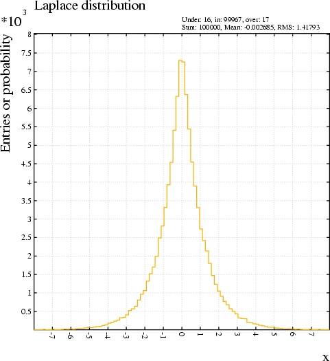
Separate random number sequences according to different histograms can be generated concurrently.
The procedure works by creating a cumulative histogram and reverse-interpolating it for a uniformly distributed random number. Failures can occur for the following reasons:
The argument is mandatory.
Example:
// Generate an electron energy spectrum. magboltz xenon 90 co2 10 e-field 250 coll 1 keep// This results in a set of arrays, E_1 and F_1 in particular. // These arrays are typically too long to be used directly as // histograms and need therefore to be rebinned. Global bin=5 Call book_matrix(he,entier(size(f_1)/bin)) Call book_matrix(hf,entier(size(f_1)/bin)) For i From 1 To size(hf) Do Global he[i]=0 Global hf[i]=0 For j From 1 To bin Do Global he[i]=he[i]+e_1[bin*(i-1)+j] Global hf[i]=hf[i]+f_1[bin*(i-1)+j] Enddo Global he[i]=he[i]/bin Global hf[i]=hf[i]/bin Enddo
// Convert the rebinned array to a histogram Call matrix_to_histogram(hf, number(he[1]), number(he[size(he)]), histf)
// Book an histogram with identical parameters Call book_histogram(check, size(hf), number(he[1]), number(he[size(he)]))
// And generate 10000 samples For i From 1 To 10000 Do Call fill_histogram(check, rnd_histogram(histf)) Enddo Global check = check * sum(histf)/sum(check)
// Compare Call plot_graph(he,hf) Call plot_line(e_1,f_1,`function-2`) Call plot_histogram(histf, ``,``, `noframe`) Call plot_histogram(check, ``,``, `noframe`) Call plot_end
-mean n
e mean
P(n) = -------------
n!
The optional argument of this generator specifies the mean of the distribution to be generated. If the argument is omitted, a mean of 1 is assumed.
This procedure calls the CERN library routine RNPSSN.
The mean is usually specified as a Number but may also be of type Histogram and Matrix. In the latter two cases, variables of the same type will be returned, taking for each output element as mean the corresponding element of the argument.
Example:
Global mean=4.2 Global nrndm=10000Call book_histogram(p,20,-0.5,19.5) For i From 1 To nrndm Do Call fill_histogram(p,rnd_poisson(mean)) Enddo
Global mu=mean(p) Global scale=sum(p)
Call fit_function(p,`scale*exp(-mu)*mu^x/gamma(x+1)`, ... mu,scale,emu,escale,`plot,print`)
Say "Fitted mean: {mu} +/- {emu}, Histogram mean: {mean}, True: {mean}" Say "Contents: {scale} +/- {escale}, True: {nrndm}"
After having filled an histogram (note the binning) with Poisson random numbers, we wish to verify the generator. This we do by computing the MEAN and we also do a fit using FIT_FUNCTION. For the initial guess of the parameters we use the mean and the SUM.
This example only works for small values of the mean since the GAMMA function does not accept large arguments. To make it work for larger means, one uses the LOG_GAMMA function:
Global mean=50 Global nrndm=10000Call book_histogram(p,100,-0.5,99.5) For i From 1 To nrndm Do Call fill_histogram(p,rnd_poisson(mean)) Enddo
Global mu=mean(p) Global scale=sum(p)
Call fit_function(p,`scale*exp(x*log(mu)-log_gamma(x+1)-mu)`, ... mu,scale,emu,escale,`plot,print`)
Say "Fitted mean: {mu} +/- {emu}, Histogram mean: {mean}, True: {mean}" Say "Contents: {scale} +/- {escale}, True: {nrndm}"
The argument specifies the \θ parameter of the distribution to be generated. If the argument is omitted, a \θ of 1 is assumed.
This procedure calls the CERN library routine RNGAMA.
The \θ parameter is usually specified as a Number but may also be of type Histogram and Matrix. In the latter two cases, variables of the same type will be returned, taking for each output element as \θ the corresponding element of the argument.
This procedure calls the CERN library routine RANLUX.
The scaling factor is usually specified as a Number but may also be of type Histogram and Matrix. In the latter two cases, variables of the same type will be returned, taking for each output element as mean the corresponding element of the argument.
The description of the FIT_GAUSSIAN procedure shows an example of the use of RND_UNIFORM.
[The default scaling factor is 1.]
Use the ZEROES and ONES functions if you wish to create a vector that contains only 0 or only 1.
Examples:
Global xmin=2 Global xmax=23 Global nx=200 Global xlin=xmin+(xmax-xmin)*(row(nx)-1)/(nx-1) Global xlog=xmin*(xmax-xmin)^((row(nx)-1)/(nx-1))
This generates series of nx equally and logarithmically spaced points between xmin and xmax.
This function can take either an Histogram, a Matrix or a Number as argument. The function acts bin-by-bin on Histograms and element-by-element on Matrices and returns a value of the same type as the argument.
This function can take either an Histogram, a Matrix or a Number as argument. The function acts bin-by-bin on Histograms and element-by-element on Matrices and returns a value of the same type as the argument.
Use the DIMENSIONS procedure to obtain more detailed information about the structure of the matrix.
This function is of use if you need to loop over the elements of a 1-dimensional matrix in order to apply an operation which is not available via the operators and procedure calls, e.g.:
For i From 1 To size(a) Do
If a[i]>0 Then
Global i0=i
Leave
Endif
Enddo
This finds the first strictly positive element in a matrix.
The argument, or each element of the argument, should be equal to or larger than 0.
This function can take either an Histogram, a Matrix or a Number as argument. The function acts bin-by-bin on Histograms and element-by-element on Matrices and returns a value of the same type as the argument.
The STRING function is for instance used to create file names that depend on parameters of the chamber being studied:
Global argon 70
Global co2 30
Global gas_file `argon_`/string(argon)/`_CO2_`/string(co2)/`.gas`
Call inquire_file(gas_file,exist)
If exist Then
get {gas_file}
Else
write {gas_file}
magboltz argon {argon} co2 {co2}
Endif
The function returns in either case a value of type Number.
This function can take either an Histogram, a Matrix or a Number as argument. The function acts bin-by-bin on Histograms and element-by-element on Matrices and returns a value of the same type as the argument.
This function can take either an Histogram, a Matrix or a Number as argument. The function acts bin-by-bin on Histograms and element-by-element on Matrices and returns a value of the same type as the argument.
This function can take either an Histogram, a Matrix or a Number as argument. The function acts bin-by-bin on Histograms and element-by-element on Matrices and returns a value of the same type as the argument.
This function provides a functionality which is similar to the INQUIRE_TYPE procedure. The main difference is that it is permissible to give the INQUIRE_TYPE procedure as first argument a variable that does not yet exist while this is not allowed with the TYPE function. The reason for this is that the arguments of procedures are automatically declared if they do not yet exist, while the arguments of functions must be existing variables. If you wish to use the TYPE function and are not sure the variable exists, then use the GLOBAL function.
Examples:
Global a `Hello !`
Say {type(a)}
Say {type(global(`A`))}
Say {type(global(`does not exist`))}
Both Say statements in the first example will display "String", which is the type the variable A gets by executing the Global statement.
The argument of the GLOBAL function in the second example is not a valid name for a global variable, GLOBAL will therefore return Nill, of type Undefined.
Use the ONES function to create a vector than contains 1 everywhere and the ROW function if you wish to create a vector that contains the numbers 1, 2, 3 ...
Do not confuse this function with the ZEROES procedure.
The instruction list usually contains many pieces, identified by entry_points which can be executed independently.
The instruction list consists, as the name says, of a list of instructions.
Each instruction is made up of 4 integers:
| Description | Codes |
|---|---|
| R(j) \→ Arg(k) | i 8 j k |
The first code (i) can have the values 0 and 1, 1 requests the originating register not to be changed on return from the call.
Numerical binary arithmetic:
| Description | Codes |
|---|---|
| R(i) + R(j) \→ R(k) | i 1 j k |
| R(i) - R(j) \→ R(k) | i 2 j k |
| R(i) * R(j) \→ R(k) | i 3 j k |
| R(i) / R(j) \→ R(k) | i 4 j k |
| R(i) ^ R(j) \→ R(k) | i 5 j k |
Comparisons resulting in a logical, where numeric equality and non-equality are tested at a precision of 10\<SUP\>-5\</SUP\> or 10\<SUP\>-10\</SUP\> depending on the machine precision:
| Description | Codes |
|---|---|
| R(i) = R(j) \→ R(k) | i 10 j k |
| R(i) \≠ R(j) \→ R(k) | i 11 j k |
| R(i) \< R(j) \→ R(k) | i 12 j k |
| R(i) \≤ R(j) \→ R(k) | i 13 j k |
| R(i) \> R(j) \→ R(k) | i 14 j k |
| R(i) \≥ R(j) \→ R(k) | i 15 j k |
Logical binary arithmetic:
| Description | Codes |
|---|---|
| R(i) and R(j) \→ R(k) | i 16 j k |
| R(i) or R(j) \→ R(k) | i 17 j k |
| Description | Codes |
|---|---|
| Call procedure m with n args m 9 | n 0 |
The procedures are listed separately, see Call.
Numerical functions:
| Description | Codes | Name |
|---|---|---|
| trailing R(i) \→ R(j) | -11 6 i j |
TRAILING |
| arctanh R(i) \→ R(j) | -9 6 i j |
ARCTANH |
| arccosh R(i) \→ R(j) | -8 6 i j |
ARCCOSH |
| arcsinh R(i) \→ R(j) | -7 6 i j |
ARCSINH |
| - R(i) \→ R(j) | -6 6 i j |
- |
| \√ R(i) \→ R(j) | -5 6 i j |
SQRT |
| arctan R(i) \→ R(j) | -4 6 i j |
ARCTAN |
| arccos R(i) \→ R(j) | -3 6 i j |
ARCCOS |
| arcsin R(i) \→ R(j) | -2 6 i j |
ARCSIN |
| log R(i) \→ R(j) | -1 6 i j |
LOG |
| exp R(i) \→ R(j) | 1 6 i j |
EXP |
| sin R(i) \→ R(j) | 2 6 i j |
SIN |
| cos R(i) \→ R(j) | 3 6 i j |
COS |
| tan R(i) \→ R(j) | 4 6 i j |
TAN |
| | R(i) | \→ R(j) | 5 6 i j |
ABS |
| + R(i) \→ R(j) | 6 6 i j |
- |
| sinh R(i) \→ R(j) | 7 6 i j |
SINH |
| cosh R(i) \→ R(j) | 8 6 i j |
COSH |
| tanh R(i) \→ R(j) | 9 6 i j |
TANH |
| entier R(i) \→ R(j) | 11 6 i j |
ENTIER |
| \Σ R(i) \→ R(j) | 13 6 i j |
SUM |
| \Π R(i) \→ R(j) | 14 6 i j |
PRODUCT |
| Landau R(i) \→ R(j) | 18 6 i j |
LANDAU |
| Minimum of R(i) \→ R(j) | 19 6 i j |
MINIMUM |
| Maximum of R(i) \→ R(j) | 20 6 i j |
MAXIMUM |
| Row of 1 to R(i) \→ R(j) | 40 6 i j |
ROW |
| Mean of R(i) \→ R(j) | 41 6 i j |
MEAN |
| RMS of R(i) \→ R(j) | 42 6 i j |
RMS |
| Size of R(i) \→ R(j) | 43 6 i j |
SIZE |
| Row of R(i) zeroes \→ R(j) | 44 6 i j |
ZEROES |
| Row of R(i) ones \→ R(j) | 45 6 i j |
ONES |
| Existence of file R(i) \→ R(j) | 46 6 i j |
EXIST |
| \Γ R(i) \→ R(j) | 47 6 i j |
GAMMA |
Logical functions:
| Description | Codes | Name |
|---|---|---|
| not R(i) \→ R(j) | 10 6 i j |
NOT |
Type conversions:
| Description | Codes | Name |
|---|---|---|
| string R(i) \→ number R(j) | -12 6 i j |
NUMBER |
| formatted R(i) \→ R(j) | 12 6 i j |
STRING |
| number R(i) \→ string R(j) | 51 6 i j |
REF_STRING |
| number R(i) \→ histogram R(j) | 54 6 i j |
REF_HISTOGRAM |
| number R(i) \→ matrix R(j) | 55 6 i j |
REF_MATRIX |
| name global R(i) \→ string R(j) | 16 6 i j |
GLOBAL |
| type of R(i) \→ string R(j) | 17 6 i j |
TYPE |
Random numbers:
| Description | Codes | Name |
|---|---|---|
| Uniform random number \→ R(j) | 21 6 - j |
RND_UNIFORM |
| Gaussian random number \→ R(j) | 22 6 - j |
RND_GAUSS, RND_NORMAL |
| Exp. random number \→ R(j) | 23 6 i j |
RND_EXPONENTIAL, RND_EXP |
| Poisson random number \→ R(j) | 24 6 i j |
RND_POISSON |
| Landau random number \→ R(j) | 25 6 i j |
RND_LANDAU |
| Polya, \θ R(i) \→ R(j) | 26 6 i j |
RND_POLYA |
| Function random number \→ R(j) | 27 6 i j |
RND_FUNCTION |
| Histogram random R(i) \→ R(j) | 28 6 i j |
RND_HISTOGRAM |
The random number generators RND_EXPONENTIAL and RND_POISSON have the mean of the distribution as argument. The argument of RND_POLYA is the "theta" parameter. These arguments are optional, they default to 1. They can generate random number sequences of different data types.
RND_HISTOGRAM takes an Histogram as argument and always returns a single random number.
| Description | Codes |
|---|---|
| If R(i) Goto Ins(R(j)) | i 7 j 0 |
A direct jumps are obtained by setting R(i) to 1 (i.e. i=-1). Setting R(i) to 0 (i.e. i=0) is a no-operation code because the jump would never occur.
A value out of range for R(j) (typically 0) is a alternative for return. You are allowed to modify the value of R(j) during execution.
| Description | Codes |
|---|---|
| R(i) \→ output variable (j) | 0 0 i j |
| Description | Codes |
|---|---|
| Return to calling procedure | i -9 0 0 |
| Stop procedure execution | i -9 1 0 |
| Stop program execution | i -9 2 0 |
These instructions are referred to as Return, Exit and Quit. The statement is executed if R(i) has the value 1, if R(i) is 0, the statement is skipped, otherwise an error condition is raised.
Each time you ask a function to be translated, this will be done in a new entry point. Similarly, when you enter the editor, you are assigned an entry point to store your instructions in. The entry point description for en edited entry point is updated when leaving the editor.
You can not change the description of an entry point but you can delete entry points, add new ones and see the description of one.
Format:
ADD-ENTRY-POINT
Format:
CL-ENTRY [entry_reference]
Examples:
CL-ENTRY CL-ENTRY 5
In the first example, the current entry point (the one you are editing) is dropped. You may continue to modify it etc. and it can also be executed as long as no garbage collect is done.
In the second example, the entry point with reference number 5 is dropped. The reference number can be obtained from the MEMORY command, details about an entry point are provided by the DISPLAY-ENTRY-POINT command.
Format:
DELETE [from [to|LAST]]
Example:
DEL DEL 1 LAST
(Both examples delete all instructions.)
Note that the description of an entry point that is being edited is not always entirely up to date.
Format:
DISPLAY-ENTRY-POINT [entry_reference]
Example:
DISP-ENTRY
Shows details about your current entry point.
Format:
EXECUTE [from [to|LAST]]
Example:
EXEC
(Execute the whole instruction list, skipping branching statements.)
Format:
EXIT
Format:
FUNCTION function
Example:
F ARCTAN (EX/EY)
Format:
GARBAGE-COLLECT
Format:
INSERT before
Format:
LIST [from [to|LAST]]
Example:
LIST 5
(Lists line 5 only.)
This command can be used both in the algebra editor, which is entered by typing @ instead of a formula, or as part of regular input, provided the command is prefixed by a @ symbol.
Formats:
MEMORY @ MEMORY
The algebra OPTIONS can be set via a single-line command as shown in the example, and also from within the algebra editor which is entered by typing @ instead of a formula.
Format:
OPTIONS [NO-SYNTAX-CHECK | ALGEBRA-SYNTAX-CHECK | ...
PROCEDURE-SYNTAX-CHECK] ...
[SIGNAL-EXPONENTIAL-UNDERFLOW | IGNORE-EXPONENTIAL-UNDERFLOW]
Examples:
&SIGNAL
// insert avalanche, time resolution and other settings
Global phi0=10*pi/180
@opt ignore-exponential-underflow
signal ion-tail cross-induced noelectron-pulse ...
ion-angles 20 angular-spread exp(-((phi/{phi0})^2))
Avalanches are spread around the wire with a standard deviation of 10\°. This would lead to many underflows in the calculation and the spread would be rejected as a result. This is why the IGNORE-EXPONENTIAL-UNDERFLOW option is used.
OPTION NO-SYNTAX-CHECK DEBUG
If you are confident you won't make typing errors\ ...
The instruction codes for return, goto, argument and call are processed at a higher level. Such instruction codes are used for instance when addressing elements of matrices. These codes are accepted only if you have set PROCEDURE-SYNTAX-CHECK.
You may change also switch syntax checking off altogether.
To have such exponentials set to 0 and to continue evaluating the formula, the IGNORE-EXPONENTIAL-UNDERFLOW option is used. When IGNORE-EXPONENTIAL-UNDERFLOW is in effect, underflows are not counted.
Note that this option applies only to exponentials evaluated by algebraic expressions, not to exponentials computed by regular Garfield commands.
These options may also be written IGNORE-UNDERFLOW and SIGNAL-UNDERFLOW.
[By default, exponential underflows are not signalled.]
This does not apply to results of calculations, for which other limits apply, as explained for the IGNORE-EXPONENTIAL-UNDERFLOW option.
[By default, underflow on input is ignored.]
Format:
PRINT [from [to|LAST]]
Example:
PRINT 2 10
(Prints lines 2 through 10.)
You have access to the entire storage area, constant elements included.
Format:
REGISTER array_index value
Examples:
REG 5 10 REG 5
(First assign the value 10 to R(5), then check the value.)
Format:
RESET
Format:
RESULTS
During the simplification, constants are evaluated, complementary operations are cancelled, assignments are propagated and removed, equal subexpressions are identified and stored, steps that are not executed are dropped from the instruction list.
Some of these simplifications are skipped if the instruction list contains (un)conditional jumps since the jump address can not a priori be assumed to be known.
Format:
SIMPLIFY
This instruction differs from EXECUTE in that goto is executed. Loops, jumps and if's therefore work as usual.
Format:
TEST var1 var2 ...
Example:
TEST 2 3 6 10
(Execute the instruction list after substituting 2 for R(1), 3 for R(2), 6 for R(3) and 10 for R(4).)
Format:
VARIABLES
The program ignores the portion of a physical input line that follows a double slash (//). If the line has a continuation mark (...) preceding the //, then the following physical input line will be concatenated with what preceded the ellipsis.
Format:
statement // comment
Examples:
Global a=5 // initialise AGarfield ignores an entire input line that begins with an asterisk (*). Also all continuation lines, as signalled with an ellipsis (...), are considered as comment.box centre -1.3 1.39 0 ... // Centre of strip 1 half-lengths 0.01 0.65 0.1 ... // Dimensions conductors-2 // Material
Format:
* comment
Example:
* this is a comment ... that spans several ... lines
An interrupt mechanism that will stop the current computation but not the program has not yet been implemented for Apollo.
Control-Z is interpreted as an EOF by the Fortran run time I/O library. Program execution is terminated after this control.
The program can be stopped if necessary by hitting the CP key and then typing IPL CMS. There is no elegant interrupt when a plot is being produced in interactive mode.
The standard EOF mark in VM (a blank return) is intercepted and is treated like a blank input line.
The line separation character (#) is switched off during startup of the program since the symbol has a meaning in Garfield.
Lengthy loops can be interrupted by checking for the existence of a file. For example, the following loop
For i From 1 To 10000 Do If exist(`stop_loop`) Then Leave // Lengthy calculation Enddochecks each iteration whether a file called "stop_loop" exists and ends the loop iteration if this is the case. To stop the loop, the user would type (to the Unix command prompt):
touch stop_loopThere is currently no elegant built-in interrupt to stop lengthy calculations without terminating program execution.
Control-Z will place the program in the background, you will need to type "bg" in addition to make it continue to run.
Control-C on a Vax will terminate execution of the command that is being executed and then return control to the command reading routine. The graphics buffers are emptied if plotting is in progress, to make sure GKS is in a well defined state. The terminal printing buffer is flushed. Other I/O channels are left untouched, hence a dataset attached to logical unit 12 (used for short term sequential dataset access) may be left open. This is harmless since the dataset will be closed when a new dataset has to be opened. The same goes for dataset access that is transparent to the user.
The RTL I/O routines have to be replaced so as to avoid blocking of the terminal I/O channel when the AST occurs in an RTL routine. The reason for this is that AST intercepting routine simply unwinds the stack until the routine which has been LIB$ESTABLISH'ed, usually the command reading routine.
Control-Z is interpreted as an EOF by the Fortran run time I/O library. Program execution is terminated after this control.
Although Garfield datasets are sequential files for the operating system, they have for Garfield purposes the structure of libraries composed of one or more members. A member can for instance be a compact cell description, a piece of program output or a signal in Spice readable format.
Garfield datasets can be moved between machines, you may also operate on such datasets on other computers if the OS allows.
Garfield libraries are things you would not normally wish to edit except to extract an x(t)-relation or a piece of output. Instead, the program provides a set of instructions that make directory listings, list individual members and delete members.
All dataset commands start with a % sign. If you have lots of dataset commands to do, you may prefer to enter the dataset subsection by typing only the % sign, without arguments. In the dataset subsection no % has to be prefixed to the commands. You may not enter other subsections from within the dataset subsection. EXIT will get you back to the section you came from.
In general, the file name should be entered the way it is usually entered on system where you run Garfield. There are however a few points to keep in mind:
When you access a file via a procedure Call, then the file name is contained in a String and no further precautions need to be taken.
Garfield libraries are on most computers variable record length sequential files to the operating system. On IBM, the datasets are opened with a fixed record length of 133.
The first record is a line of length 133 which is only there to make sure the operating system doesn't reduce the record length between successive accesses. This record is written automatically when a new file is opened.
Each member is identified through a name, a string of 8 characters. As a rule, the user can chose the member name but users tend to leave the field empty (in which case it will be set to "< none >").
Since the various GET commands will by default search for the first member of the appropriate type, you can leave the member name blank if the file contains only one member of each type.
New members are appended to a file, they do not replace existing members.
Although a single file is allowed to contain several members with the same name and the same type, this is to be avoided since only the first of these members can be accessed. Problems of this kind occur for instance if you have a dataset that contains histograms which are retrieved, updated, and then written back to the file. The use of the DELETE-OLD-MEMBER global option is recommended in such cases.
The INDEX dataset command and the INQUIRE_MEMBER procedure can be used to find out which members are present in a dataset. The dataset command DELETE will mark members for deletion and PURGE will remove deleted members from a dataset.
Case is not relevant in member names. If, when writing, you surround the member name with double quotes, then the member will have the exact name that you entered. However, when reading, all case variations will be declared to match. For instance, a member called "ExB" in the file can be retrieved as "exb", "eXb", "EXB" etc.
Each member starts with a header record formatted as follows:
| Character | Contents | Length |
|---|---|---|
| 1 | a percent sign (%) | 1 |
| 2 | a blank, changed to 'X' if the member is deleted | 1 |
| 3-10 | the string "Created " | 8 |
| 11-18 | day (dd/mm/yy) on which the member was written | 8 |
| 19-22 | the string " at " | 4 |
| 23-30 | time (hh.mm.ss) at which the member was written | 8 |
| 31 | is blank | 1 |
| 32-39 | member name | 8 |
| 40 | is blank | 1 |
| 41-48 | type of the member | 8 |
| 49 | is blank | 1 |
| 50 | double quote (") | 1 |
| 51-79 | remark | 29 |
| 80 | double quote (") | 1 |
The type given to a member is chosen by the program according to the following scheme:
| Type | Description | Main user |
|---|---|---|
| ARRIVAL | Output of the ARRIVAL instruction | User |
| CELL | Compact format cell description | Internal |
| ISOCHRON | Equal time contours (isochrons) | User |
| GAS | Compact format gas description | Internal |
| GRAPHCOL | Colour table | Internal |
| GRAPHREP | Representation table | Internal |
| HIST | Histograms | Both |
| MATRIX | Matrices | Internal |
| MINIMUM | Output from the MINIMISE instruction | User |
| OUTPUT | General output | User |
| SIGNAL | Signals | User |
| TRACK | Prepared tracks | Internal |
| TRANSLAT | Input translation table | Internal |
| XTPLOT | Output from the XT-PLOT instruction | User |
Types marked "User" are intended for use by the user and can freely be modified. Types marked "Internal" are not meant to be of use to the user, and should also not be modified.
The remark has a length of 1 to 29 characters.
This command can not be issued from within a dataset subsection.
Format:
% DEFAULT file_specification
Examples:
% DEF % DEF 'VAXODIE::' %default .GARFLIB
The first example shows the current default, the second tells Garfield that it should try to find the files on the node called VAXODIE (note the quotes, the colons are separators and would be discarded without the quotes). The last example ensures that the libraries to be read and written have extension GARFLIB.
Removing members physically from a dataset is done by PURGE . RECOVER will undo a %DELETE.
Both the member and the type may be wildcards (a * matches every string).
Format:
%DELETE file member [type]
Beware ... this command will generate a huge amount of output !
Format:
EXIT
The member and type, if you enter them at all, may be wildcards, i.e. a * matches any number of every character. Only the members that match both will be in the list.
Also the INQUIRE_MEMBER procedure can be used to determine whether a member exists in a dataset.
Format:
%INDEX file [member] [type]
One can re-rout the output of this command to a file.
Both the member and the type may be of the wildcard type (a * matches any string).
Format:
%LIST file [member] [type]
The VMS help utility is used on Vax computers. This instruction will therefore create a help library rather than a direct access dataset on such devices.
Before this command is executed, one has to ensure that the readable (or raw) help file is available. It is distributed as:
This command is not executed if a direct access help file exists when the command is entered, except on Vax where a new version of the library is generated.
Member and type are not specified on this command.
Format:
%PURGE file
Both the member and the type may be wildcards (a * matches every string).
Format:
%RECOVER file member [type]
You should not normally see KERNLIB error messages, the instruction described below is therefore mainly useful for debugging the program.
Format:
ERROR-HANDLING MESSAGE mess-id ...
[PRINT {ALWAYS | NEVER | nprint}] ...
[ABEND {NEVER | nabend}]
mess-id Is the identifier of the message as listed in the 'green book' of CERN program library writeups. Both nprint and nabend are meaningful only in the range 0 to 100. Execution is terminated at the nabend+1 occurrence of the error.
For further details, see short writeup N001: http://consult.cern.ch/shortwrups/n001/top.html
Settings that are common for most of your runs can be placed more conveniently in your initialisation file. This is for instance the case of the colours and the representations.
All graphics commands start with a ! sign. If you have lots of graphics things to do, you may prefer to enter the graphics subsection by typing only the ! sign, without arguments. In the graphics subsection no ! has to be prefixed to the commands. You may not enter other subsections from within the graphics subsection. EXIT will get you back to the section you came from.
Examples are an X-terminal, a printer, a PostScript file, a mouse or a set of crosshairs.
In interactive jobs, Garfield by default usually has only X-terminal output, while in batch it will have only PostScript output.
These defaults can be changed both with the command line line arguments -terminal and -metafile and from the running program via the commands described below.
Workstations can be in 3 states in Garfield, 2 of which are also in the GKS definition:
Moving between the 3 states is accomplished with the following set of commands:
| state | reached from previous by | to return to previous |
|---|---|---|
| defined | ADD-WORKSTATION |
DELETE-WORKSTATION |
| open | OPEN-WORKSTATION |
CLOSE-WORKSTATION |
| active | ACTIVATE-WORKSTATION |
DEACTIVATE-WORKSTATION |
A workstation that is to be activated, must already be "open". If you try to activate a workstation that is "defined" but not "open", then an implicit !OPEN-WORKSTATION is performed.
After this operation, the workstation is in the GKS state "active" which means that it will receive graphics output. The workstation can then be deactivated with !DEACTIVATE-WORKSTATION.
The argument is an alphanumeric string designating the workstation, Usually, this will be the name that you gave to the workstation when issuing a !ADD-WORKSTATION command, but this can also be one of the two workstations that can be predefined: TERMINAL and METAFILE. Whether these 2 are defined or not depends on the mode in which you run Garfield.
Format:
! ACTIVATE-WORKSTATION workstation
Example:
! deact metafile (make some plots) ! act metafile (make final version of plots again)
You do not wish to fill the metafile with useless plots. Therefore, you first make a few tests without metafile active and once you are happy with them, you activate the metafile and make the plots again.
Up to two workstations can be predefined in Garfield: TERMINAL and/or METAFILE. You can manipulate them like any other workstation.
After !ADD-WORKSTATION, the workstation is in the state 'defined', which in GKS terminology means that the workstation is neither 'open' nor 'active'. Thus, the workstation will not receive any graphics output until you have used !OPEN-WORKSTATION and !ACTIVATE-WORKSTATION to first open and then activate the newly defined workstation.
A workstation displays can as a rule handle both input and output, and the output that is sent there will as a rule not be stored. The first format below deals with this situation.
Output-only workstations, second format, are associated with a graphics file which will store the images. By default, it is assumed that one file can contain any number of images. Use the SINGLE-FRAME-FILE option in case the output format you wish to use can only deal with a single image per file.
In both formats, either the type (e.g. "inquire" for X-windows inquiry at startup, or "EPS" for Encapsulated PostScript ) or the GKS identifier (the driver number) must be specified, but not both.
Format for input/output workstations:
! ADD-WORKSTATION name [TYPE type | GKS-IDENTIFIER identifier] ...
[CONNECTION-IDENTIFIER connection]
Format for output (metafile, PostScript etc) workstations:
! ADD-WORKSTATION name [TYPE type | GKS-IDENTIFIER identifier] ...
FILE-NAME file ...
[OFFSET offset] ...
[MULTIPLE-FRAME-FILE | SINGLE-FRAME-FILE]
Examples:
!add postscript type ps file-name garfield.ps
This instruction adds a PostScript formatted metafile.
Global quencher `CH4`
Global ps True
If ps Then
!add meta type PostScript file-name "gain_{quencher}.ps"
!open meta
!act meta
Endif
...
If ps Then
!deact meta
!close meta
!del meta
Endif
The name of the PostScript file is made to depend on the quencher gas which is used. Note the use of substitution using curly brackets.
This should be a character string of 20 characters or less.
[No default, this is a mandatory argument.]
You've to specify either a type or a GKS identifier, but not both.
| Type | GKS identifier | Offset | Class | Description |
|---|---|---|---|---|
| DN300_bw | 10002 | 1 | in/out | Apollo DN300 |
| DN3000_bw | 10002 | 1 | in/out | Apollo DN3000 B/W |
| DN3000_colour | 10004 | 1 | in/out | Apollo DN3000 colour |
| DN550_colour | 10003 | 1 | in/out | Apollo DN550 B/W |
| DN660_colour | 10003 | 1 | in/out | Apollo DN660 B/W |
| GSR_1 | 9701 | 1 | in/out | - |
| GSR_2 | 9702 | 1 | in/out | - |
| GSR_3 | 9703 | 1 | in/out | - |
| GSR_4 | 9704 | 1 | in/out | - |
| GSR_5 | 9705 | 1 | in/out | - |
| GSR_6 | 9706 | 1 | in/out | - |
| GSR_7 | 9707 | 1 | in/out | - |
| GSR_8 | 9708 | 1 | in/out | - |
| X_windows_0 | 32120 | 1 | in/out | X windows screen 0 |
| X_windows_1 | 32121 | 1 | in/out | X windows screen 1 |
| X_windows_2 | 32122 | 1 | in/out | X windows screen 2 |
| X_windows_3 | 32123 | 1 | in/out | X windows screen 3 |
| X_windows_4 | 32124 | 1 | in/out | X windows screen 4 |
| X_windows_5 | 32125 | 1 | in/out | X windows screen 5 |
| X_windows_6 | 32126 | 1 | in/out | X windows screen 6 |
| X_windows_7 | 32127 | 1 | in/out | X windows screen 7 |
| X_windows_8 | 32128 | 1 | in/out | X windows screen 8 |
| X_windows_9 | 32129 | 1 | in/out | X windows screen 9 |
| X_windows | 32120 | 1 | in/out | X windows |
| APPENDIX_E | 4 | 0 | output | Appendix E metafile |
| PS_portrait_colour | 12201 | 100 | output | PostScript metafile |
| PS_landscape_colour | 12202 | 100 | output | PostScript metafile |
| PS_landscape_bw | 12204 | 100 | output | PostScript metafile |
| PS_portrait_bw | 12203 | 100 | output | PostScript metafile |
| PostScript | 12203 | 100 | output | PostScript metafile |
| EPS_portrait_colour | 12201 | 200 | output | Encapsulated PostScript |
| EPS_landscape_colour | 12202 | 200 | output | Encapsulated PostScript |
| EPS_landscape_bw | 12204 | 200 | output | Encapsulated PostScript |
| EPS_portrait_bw | 12203 | 200 | output | Encapsulated PostScript |
| Encapsulated_PS | 12203 | 200 | output | Encapsulated PostScript |
Interactive default: DN3000_bw. Batch default: PS_portrait_bw.
Other than Apollo:
| Type | GKS identifier | Offset | Class | Description |
|---|---|---|---|---|
| VT100_RETROGRAPHICS | 1001 | 1 | in/out | Digital |
| VT100_SELENAR | 1002 | 1 | in/out | Digital |
| VT125_REGIS | 1010 | 1 | in/out | Digital |
| VT240_REGIS | 1020 | 1 | in/out | Digital |
| VT241_REGIS | 1021 | 1 | in/out | Digital |
| VT340 | 1030 | 1 | in/out | Digital |
| VAXSTATION | 8601 | 1 | in/out | Digital |
| PG7800 | 7878 | 1 | in/out | Pericom |
| MG600 | 7800 | 1 | in/out | Pericom |
| MX2000 | 221 | 1 | in/out | Pericom |
| MX7000 | 221 | 1 | in/out | Pericom |
| MX8000 | 227 | 1 | in/out | Pericom |
| 4010 | 101 | 1 | in/out | Tektronix |
| 4012 | 102 | 1 | in/out | Tektronix |
| 4014 | 101 | 1 | in/out | Tektronix |
| 4015 | 103 | 1 | in/out | Tektronix |
| 4105 | 110 | 1 | in/out | Tektronix |
| 4107 | 121 | 1 | in/out | Tektronix |
| 4109 | 122 | 1 | in/out | Tektronix |
| 4207 | 121 | 1 | in/out | Tektronix |
| 4209 | 122 | 1 | in/out | Tektronix |
| 4111 | 123 | 1 | in/out | Tektronix |
| 4113 | 125 | 1 | in/out | Tektronix |
| 4114 | 127 | 1 | in/out | Tektronix |
| 4115 | 127 | 1 | in/out | Tektronix |
| FALCO | 114 | 1 | in/out | Falco |
| X_WINDOWS_0 | 32120 | 1 | in/out | X-windows screen 0 |
| X_WINDOWS_1 | 32121 | 1 | in/out | X-windows screen 1 |
| X_WINDOWS_2 | 32122 | 1 | in/out | X-windows screen 2 |
| X_WINDOWS_3 | 32123 | 1 | in/out | X-windows screen 3 |
| X_WINDOWS_4 | 32124 | 1 | in/out | X-windows screen 4 |
| X_WINDOWS_5 | 32125 | 1 | in/out | X-windows screen 5 |
| X_WINDOWS_6 | 32126 | 1 | in/out | X-windows screen 6 |
| X_WINDOWS_7 | 32127 | 1 | in/out | X-windows screen 7 |
| X_WINDOWS_8 | 32128 | 1 | in/out | X-windows screen 8 |
| X_WINDOWS_9 | 32129 | 1 | in/out | X-windows screen 9 |
| X_WINDOWS | 32120 | 1 | in/out | X-windows |
| PT-100G | 112 | 1 | in/out | - |
| APPENDIX_E | 4 | 0 | output | Appendix E metafile |
| PS_PORTRAIT_COLOUR | 12201 | 100 | output | PostScript metafile |
| PS_LANDSCAPE_COLOUR | 12202 | 100 | output | PostScript metafile |
| PS_LANDSCAPE_BW | 12204 | 100 | output | PostScript metafile |
| PS_PORTRAIT_BW | 12203 | 100 | output | PostScript metafile |
| POSTSCRIPT | 12203 | 100 | output | PostScript metafile |
| EPS_PORTRAIT_COLOUR | 12201 | 200 | output | Encapsulated PostScript |
| EPS_LANDSCAPE_COLOUR | 12202 | 200 | output | Encapsulated PostScript |
| EPS_LANDSCAPE_BW | 12204 | 200 | output | Encapsulated PostScript |
| EPS_PORTRAIT_BW | 12203 | 200 | output | Encapsulated PostScript |
| ENCAPSULATED_PS | 12203 | 200 | output | Encapsulated PostScript |
Interactive_default: PG7800 Batch_default: APPENDIX_E
| Type | GKS identifier | Offset | Class | Description |
|---|---|---|---|---|
| LOGICAL | 0 | 0 | in/out | defined by a logical |
| VT125_COLOUR | 11 | 0 | in/out | Digital |
| VT125_BW | 12 | 0 | in/out | Digital |
| VT240_COLOUR | 13 | 0 | in/out | Digital |
| VT240_BW | 14 | 0 | in/out | Digital |
| VT330 | 16 | 0 | in/out | Digital |
| VT340 | 17 | 0 | in/out | Digital |
| VAXSTATION_1 | 42 | 0 | in/out | Digital |
| VAXSTATION_2 | 41 | 0 | in/out | Digital |
| VS_1 | 42 | 0 | in/out | Digital |
| VS_2 | 41 | 0 | in/out | Digital |
| VS_2000 | 41 | 0 | in/out | Digital |
| DECWINDOWS | 211 | 0 | in/out | Digital |
| 4014 | 72 | 0 | in/out | Tektronix |
| 4017 | 82 | 0 | in/out | Tektronix |
| POSTSCRIPT | 61 | 0 | output | PostScript metafile |
| PS | 61 | 0 | output | PostScript metafile |
| METAFILE | 2 | 0 | output | Appendix E metafile |
| DECGKS_MO | 2 | 0 | output | Metafile output |
| CGM | 7 | 0 | output | Computer graphics metafile |
| LCP01 | 15 | 0 | output | - |
| LCG01 | 15 | 0 | output | - |
| LN03 | 38 | 0 | output | - |
| HP7475 | 51 | 0 | output | Hewlett-Packard |
| HP7550 | 53 | 0 | output | Hewlett-Packard |
| HP7580 | 54 | 0 | output | Hewlett-Packard |
| HP7585 | 56 | 0 | output | Hewlett-Packard |
| LBP8A2 | 531 | 0 | output | Canon |
| L880 | 532 | 0 | output | Kyocera |
Interactive default: 4014 Batch default: POSTSCRIPT
| Type | GKS identifier | Offset | Class | Description |
|---|---|---|---|---|
| 4014_NOTABLET | 401400 | -2 | in/out | Tektronix |
| 4014_TABLET | 401401 | -2 | in/out | Tektronix |
| 4105 | 410500 | -2 | in/out | Tektronix |
| 4107 | 410700 | -2 | in/out | Tektronix |
| 4109 | 410900 | -2 | in/out | Tektronix |
| PERICOM | 301400 | -2 | in/out | Pericom |
| PLOT10_MO | 100000 | 0 | output | Metafile output |
Interactive default: PERICOM Batch default : PLOT10_MO
| Type | GKS identifier | Offset | Class | Description |
|---|---|---|---|---|
| borrow | 300009 | 1 | in/out | - |
| frame | 300010 | 1 | in/out | - |
| direct | 300011 | 1 | in/out | - |
| 4014 | 401400 | 1 | in/out | Tektronix |
| PERICOM | 301400 | 1 | in/out | Pericom |
| APPENDIX_E | 300018 | 0 | output | Appendix E metafile |
Interactive default: PERICOM. Batch default: APPENDIX_E.
| Type | GKS identifier | Offset | Class | Description |
|---|---|---|---|---|
| Console | 4 | 1 | in/out | Workstation console |
| Appendix_E | 7 | 0 | output | Appendix E metafile |
Interactive_default: Console. Batch_default: Appendix_E.
| Type | GKS identifier | Offset | Class | Description |
|---|---|---|---|---|
| Console | 1 | 1 | in/out | Workstation console |
| X_windows | 6 | -1 | in/out | X windows |
| GDF | 5 | 0 | output | - |
| MO | 3 | 0 | output | Metafile output |
Interactive default: X_windows Batch default: MO
| Type | GKS identifier | Offset | Class | Description |
|---|---|---|---|---|
| VT125_REGIS | 2600 | 1 | in/out | Digital |
| VT240_REGIS | 2601 | 1 | in/out | Digital |
| VT241_REGIS | 2602 | 1 | in/out | Digital |
| VT330 | 2603 | 1 | in/out | Digital |
| VT340 | 2604 | 1 | in/out | Digital |
| VT340_COLOUR | 2505 | 1 | in/out | Digital |
| 4010 | 2500 | 1 | in/out | Tektronix |
| COMP_4010 | 2501 | 1 | in/out | Tektronix |
| 4014 | 2400 | 1 | in/out | Tektronix |
| 4105 | 2300 | 1 | in/out | Tektronix |
| PIX_4105 | 2301 | 1 | in/out | Tektronix |
| COMP_4105 | 2302 | 1 | in/out | Tektronix |
| 4107 | 3100 | 1 | in/out | Tektronix |
| 12B_4107 | 3101 | 1 | in/out | Tektronix |
| 4205 | 3102 | 1 | in/out | Tektronix |
| 12B_4205 | 3103 | 1 | in/out | Tektronix |
| 4208 | 3104 | 1 | in/out | Tektronix |
| 12B_4208 | 3105 | 1 | in/out | Tektronix |
| 4111 | 3200 | 1 | in/out | Tektronix |
| 32B_4111 | 3201 | 1 | in/out | Tektronix |
| 4115 | 3202 | 1 | in/out | Tektronix |
| 32B_4115 | 3203 | 1 | in/out | Tektronix |
| 4125 | 3204 | 1 | in/out | Tektronix |
| 32B_4125 | 3205 | 1 | in/out | Tektronix |
| CIT_414A | 2502 | 1 | in/out | C-ITOH 414A |
| GRAPHON | 2506 | 1 | in/out | Graphon 140, 230 |
| LAND_IMG | 6300 | 1 | in/out | Imagen landscape |
| PORT_IMG | 6301 | 1 | in/out | Imagen portrait |
| RETRO | 3203 | 1 | in/out | Retrographics VT640 |
| X11 | 5300 | 1 | in/out | X windows |
| X_WINDOWS | 5300 | 1 | in/out | X windows |
| BS_X11 | 5350 | 1 | in/out | X11 (back and store) |
| CGM_BIN | 10100 | 100 | output | Computer graphics metafile |
| CGM_MBIN | 10101 | 100 | output | Computer graphics metafile |
| CGM_CHAR | 10110 | 200 | output | Computer graphics metafile |
| CGM_TEXT | 10120 | 300 | output | Computer graphics metafile |
| CGM_LBIN | 10150 | 100 | output | Computer graphics metafile |
| CGM_LCHAR | 10160 | 200 | output | Computer graphics metafile |
| CGM_LTEXT | 10170 | 300 | output | Computer graphics metafile |
| PS_PORTRAIT_COLOUR | 1900 | 400 | output | PostScript |
| PS_LANDSCAPE_COLOUR | 1901 | 400 | output | PostScript |
| PS_LANDSCAPE_BW | 1901 | 400 | output | PostScript |
| PS_PORTRAIT_BW | 1900 | 400 | output | PostScript |
| POSTSCRIPT | 1900 | 400 | output | PostScript |
| EPS_PORTRAIT_COLOUR | 1900 | 400 | output | Encapsulated PostScript |
| EPS_LANDSCAPE_COLOUR | 1901 | 400 | output | Encapsulated PostScript |
| EPS_LANDSCAPE_BW | 1901 | 400 | output | Encapsulated PostScript |
| EPS_PORTRAIT_BW | 1900 | 400 | output | Encapsulated PostScript |
| ENCAPSULATED_PS | 1900 | 400 | output | Encapsulated PostScript |
Interactive default: VT241_REGIS Batch_default: PS_PORTRAIT_COLOUR
| Type | GKS identifier | Offset | Class | Description |
|---|---|---|---|---|
| 0 | 0 | 0 | - | No terminal output |
| NONE | 0 | 0 | - | No terminal output |
| none | 0 | 0 | - | No terminal output |
| INQUIRE | -1 | 0 | unknown | Inquire at startup |
| inquire | -1 | 0 | unknown | Inquire at startup |
| 1 | 1 | 0 | in/out | HIGZ window 1 |
| 2 | 2 | 0 | in/out | HIGZ window 1 |
| 3 | 3 | 0 | in/out | HIGZ window 1 |
| 4 | 4 | 0 | in/out | HIGZ window 1 |
| 5 | 5 | 0 | in/out | HIGZ window 1 |
| 6 | 6 | 0 | in/out | HIGZ window 1 |
| 7 | 7 | 0 | in/out | HIGZ window 1 |
| 8 | 8 | 0 | in/out | HIGZ window 1 |
| 9 | 9 | 0 | in/out | HIGZ window 1 |
| 7878 | 7878 | 0 | in/out | Falco |
| FALCO | 7878 | 0 | in/out | Falco |
| Falco | 7878 | 0 | in/out | Falco |
| XTERM | 7879 | 0 | in/out | X terminal |
| PS_LANDSCAPE | -112 | 0 | output | PostScript |
| PS_landscape | -112 | 0 | output | PostScript |
| PS_PORTRAIT | -111 | 0 | output | PostScript |
| PS_portrait | -111 | 0 | output | PostScript |
| POSTSCRIPT | -111 | 0 | output | PostScript |
| PostScript | -111 | 0 | output | PostScript |
| EPS | -113 | 0 | output | Encapsulated PostScript |
| ENCAPSULATED_PS | -113 | 0 | output | Encapsulated PostScript |
| encapsulated_PS | -113 | 0 | output | Encapsulated PostScript |
| ENCAPSULATED_POSTSCR | -113 | 0 | output | Encapsulated PostScript |
| encapsulated_PostScr | -113 | 0 | output | Encapsulated PostScript |
| LATEX | -777 | 0 | output | LaTeX |
| LaTeX | -777 | 0 | output | LaTeX |
Interactive default: inquire. Batch default: PostScript.
You've to specify either a type or a GKS identifier, but not both.
Workstations associated with a file are connected via a logical unit which is chosen by Garfield, and the connection identifier is in this case given by the logical unit number plus an offset.
[This parameter is optional and defaults to 1.]
This parameter should not be specified when you are adding a workstation that is not associated with a file.
This parameter is used by certain GKS systems to distinguish closely related workstation types. Details should be contained in the GKS documentation.
[If you describe the workstation by type, you do not have to specify the offset. Specifying the parameter is optional if you describe the workstation by GKS identifier. In the latter case it defaults to 0.]
This file is opened at the time the OPEN-WORKSTATION command is issued and it is closed by CLOSE-WORKSTATION.
The file name is allowed to be an expression in terms of Global variables, to be evaluated at the time the workstation is opened. This is useful if the SINGLE-FRAME-FILE option is specified.
[This parameter is mandatory for workstations which are output-only.]
[This option is default except if the file name contains curly brackets.]
This option is default if the file name associated with the workstation is constructed such that it depends on Global variables, as in the following example:
!add epsfig type EPS file-name "fig\\{frame\\}.eps"
Here, the file name depends on the predefined variable FRAME which is automatically incremented for each new frame, but any expression in terms of global variables can be used.
Note the use of the ESCAPE character (a backslash in this example): without backslash, the expression would be substituted using the value of FRAME at the time the command is issued and subsequent changes in the value of FRAME would not be reflected in the file name. With the backslash, the { and } are preserved as part of the string and substitution of the value of FRAME is done only when the file is opened.
If you select this option and specify a static file name, then the file will be overwritten each time a new plot is made.
[This option is default if the file name contains curly brackets.]
The angle should be entered in degrees.
Format:
!ARROW-TIP-ANGLE angle
Example:
!arrow-angle 60
This would make the tip angles twice the default.
[The default setting is 30\°.]
The length should be specified either as an absolute length in normalised device coordinates (in which the screen has a width and height of 1) or as a fraction of the total length of the arrow, in the range 0 (excluded) to 1 (included).
Format:
!ARROW-TIP-LENGTH length [RELATIVE | ABSOLUTE]
Example:
!arrow-length 0.2
This would make the tip a bit shorter than the default.
[The default setting is 0.3, relative.]
The width should be specified as a fraction of the maximum bin width, in the range 0 (excluded) to 1 (included). The bars touch if set to 1, effectively producing an histogram.
Format:
!BARCHART-WIDTH fraction
Example:
!bar-w 0.5
This would make the bars much more narrow than default.
[The default setting is 0.9.]
Format:
!CLEAR-SCREEN
Before !CLOSE-WORKSTATION, the workstation should be in the state 'open', afterwards it is in the state 'defined'. It can be re-opened with !OPEN-WORKSTATION and then be activated with !ACTIVATE-WORKSTATION.
Any metafile attached to the workstation being closed, will first be completed with any data that might still be buffered and then the file will be closed. The file will be overwritten if you perform an !OPEN-WORKSTATION on the same workstation.
If !CLOSE-WORKSTATION is invoked for a workstation that is still in the state "active", then !DEACTIVATE-WORKSTATION will automatically be called before closing the workstation.
Format:
! CLOSE-WORKSTATION workstation
Example:
!close metafile
This will deactivate workstation METAFILE if still active, then close the workstation and close the file receiving the graphics output.
Each workstation has (at least) two predefined colours: the colour used by default for all items: FOREGROUND and the screen which is in BACKGROUND, items plotted with this colour are therefore normally invisible.
For each additional colour, you have to state how much red, blue and green there is in it.
Use the MAP-COLOURS graphics command to inspect graphically the colours which are currently defined.
Format:
! COLOUR colour_name {RED red BLUE blue GREEN green | ...
RGB hex} ...
[WORKSTATION wkid]
Examples:
! COL RED BLUE 0 GREEN 0 RED 1 ! COL LIGHT_BLUE BLUE 1 RED 0 GREEN 1
If the colour has already been defined, then its colour composition will be modified. On workstations which permit this, the change will be visible in currently displayed graphics that use the colour.
If the colour has not yet been defined, then it will be added to the colour table (provided there is still room).
The current definition of a colour will be shown if only a colour name is specified. All currently defined colours are listed if no arguments are given.
For the FOREGROUND colour, the red fraction is 1, for the BACKGROUND colour it is 0.
[No default, the amount of red must be specified.]
For the FOREGROUND colour, the green fraction is 1, for the BACKGROUND colour it is 0.
[No default, the amount of green must be specified.]
For the FOREGROUND colour, the blue fraction is 1, for the BACKGROUND colour it is 0.
[No default, the amount of blue must be specified.]
Red would be specified as FF0000, green as 00FF00 and blue as 0000FF.
[No default, all colour components must be specified.]
However, if the area over which the contours are to plotted is much smaller than 1, then contours will occasionally be "jumping" from one contour segment to another, with the default set of parameters. This can be cured by lowering the \ε parameters by a factor of 10.
Contour plotting works as follows:
Format:
! CONTOUR-PARAMETERS [ BISECTION-ITERATIONS n_bisection ] ...
[ EPSILON-GRADIENT \ε-gradient ] ...
[ EPSILON-TRACING \ε_tracing ] ...
[ GRID-TOLERANCE tol ] ...
[ NEWTON-ITERATIONS n_Newton ] ...
[ STEP-MAXIMUM steps ]
Example:
area -0.01 -0.01 0.01 0.01 !cont-par eps-gra 1e-4 eps-tra 1e-4 plot cont V
Since the area is small, the step size scaling factor for computing gradients and for making steps perpendicular to the gradient are reduced to 10\<SUP\>-4\</SUP\>.
Small values are recommended since a Newton search anyhow refines the starting point.
[Default: 10]
For coordinates near 0, this is the absolute sampling size. For large coordinates, the parameter is taken relative.
When the area is very small (e.g. around 10\<SUP\>-3\</SUP\>) or when there is a lot of structure in the contours, then it is a good idea to reduce the value of this parameter to e.g. 10\<SUP\>-4\</SUP\>.
[Default: 10\<SUP\>-3\</SUP\>]
For coordinates near 0, this is the absolute step size. For large coordinates, the parameter is taken relative.
When the area is very small (e.g. around 10\<SUP\>-3\</SUP\>) or when the contours make sharp bends, then it is a good idea to reduce the value of this parameter to e.g. 10\<SUP\>-4\</SUP\>.
[Default: 10\<SUP\>-3\</SUP\>]
In such cases, the algorithm checks whether the contour passes near a grid point within a certain fraction of the grid size, set with this option.
This parameter rarely needs updating. If the parameter is too small, then some contours will be drawn twice. Contours are not missed due to a poor setting of this parameter.
[Default: 0.1]
[Default: 10]
If this parameter is too small, then the contours will be drawn as a series of overlapping pieces.
[Default: 500]
After this operation, the workstation is in the GKS state 'open'. This means that it will still be known to Garfield and GKS, but it will not receive any graphics output. The workstation can then be closed via !CLOSE-WORKSTATION or re-activated by !ACTIVATE-WORKSTATION.
A workstation can only be deactivated if it is in the "active" state.
This instruction is used to disable temporarily graphics output to the metafile (e.g. when you wish to optimise some parameters without getting a huge metafile) or to the terminal.
Format:
! DEACTIVATE-WORKSTATION workstation
Example:
! deact terminal
Temporarily suspends graphics output to the terminal.
Before this operation, the workstation should be in the state "open". If !DELETE-WORKSTATION is invoked for a workstation that is still in the state "open" or "active", then !CLOSE-WORKSTATION will automatically be called before deleting the workstation.
After this operation, all information about the workstation is lost. A workstation can therefore not be re-opened or re-activated after a !DELETE-WORKSTATION - it would first have to be re-added to the workstation table with !ADD-WORKSTATION.
!DELETE-WORKSTATION does not delete a metafile that might be attached to the workstation.
Format:
! DELETE-WORKSTATION workstation
Example:
!delete metafile
You opened the metafile by accident and decide you don't need a metafile at all during this run.
Format:
EXIT
The representation and colour tables are closely connected. When retrieving representations and colours, the recommended approach is to first read the colours and then the representations. Since the representations contain a colour sequence number (assigned on the basis of the colour table present when processing REPRESENTATION statements) rather than a colour name, reading a new colour table without updating the colour references in the representation table, can create incorrect colour references. Representation files do contain colour names, ensuring correct references.
You may modify colours after having retrieved them from a file - modifications of colours do not change their sequence number.
Format:
! GET-COLOURS file [member]
Examples:
!GET-COL TEST PARROT
Picks up the member PARROT on dataset TEST.
Be sure that all colours that are referenced by the representations in the file, are defined before issuing a !GET-REPRESENTATION command. In practice, this means that GET-COLOURS commands should precede !GET-REPRESENTATION commands. Items that reference an undefined colour will be shown with a colour set to FOREGROUND.
Format:
! GET-REPRESENTATION file [member]
Example:
!GET-REP TEST MG*
Picks up the first member that matches MG*, presumably MG600.
Format:
! INQUIRE-DEFERRAL-UPDATE-STATE
Example:
!inq-def
Format:
!INQUIRE-LEVEL
Format:
!INQUIRE-OPERATING-STATE
Format:
!INQUIRE-WORKSTATIONS
All distances are measured in Normalised Device Coordinates (NDC) which cover the graphics screen from 0 to 1 both in x and in y.
By default, Garfield plots occupy the entire NDC frame: the actual image covers both in x and in y the range [0.1, 0.9] leaving the margins for labels, numbers, comments, the time stamp and the title. The so-called viewport, or the part of the NDC frame occupied by the image, labels, numbers, comments, stamp and title can be reduced with the VIEWPORT graphics command.
Format:
!LAYOUT [ X-NUMBER x_number ] ...
[ Y-NUMBER y_number ] ...
[ X-DECADE x_decade ] ...
[ Y-DECADE y_decade ] ...
[ X-LABEL x_label ] ...
[ Y-LABEL x_label ] ...
[ TITLE title ]
The parameters are graphically illustrated in the diagram.
The diagram has been made with a viewport covering the entire NDC space and using the following layout settings:
!layout x-number = 0.015, x-decade = 0.025, ...
y-number = 0.007, y-decade = 0.015, ...
x-label = 0.010, y-label = 0.010, ...
title = 0.010
|
The numbers are plotted centred horizontally at the coordinate they represent.
The size of the numbers can be controlled with the NUMBERS representation.
[Initial setting: 0.007]
The numbers are plotted centred vertically at the coordinate they represent.
The size of the numbers can be controlled with the NUMBERS representation.
[Initial setting: 0.007]
The "10" or "1" is plotted centred horizontally at the coordinate it represents, the exponent is plotted such that its lower left edge coincides with the upper right edge of the "10".
The size of the numbers, both the "10" or "1" and the exponent, can be controlled with the NUMBERS representation.
[Initial setting: 0.015]
The "10" or "1" is plotted centred vertically at the coordinate it represents, the exponent is plotted such that its lower left edge coincides with the upper right edge of the "10".
The size of the numbers, both the "10" or "1" and the exponent, can be controlled with the NUMBERS representation.
[Initial setting: 0.015]
The label is plotted right-aligned with the coordinate frame.
The size of the characters can be controlled with the LABELS representation.
[Initial setting: 0.01]
The label is plotted right-aligned with the coordinate frame.
The size of the characters can be controlled with the LABELS representation.
[Initial setting: 0.01]
The title is plotted left-aligned with the coordinate frame.
The size of the characters can be controlled with the TITLE representation.
[Initial setting: 0.01]
Format:
!MAP-COLOURS
A workstation to be opened must already have been defined, for instance via !ADD-WORKSTATION. After !OPEN-WORKSTATION, the workstation is in the GKS state 'open' and can be activated by means of !ACTIVATE-WORKSTATION.
Format:
! OPEN-WORKSTATION workstation
Example:
!add falco type falco !open falco !act falco
This example shows how to add, open and activate a workstation named FALCO of type FALCO.
Format:
! OPTIONS [GRID | NOGRID] ...
[DECADES-ONLY | COMPLETE-GRID] ...
[TIME-STAMP | NOTIME-STAMP] ...
[LOGARITHMIC-X | LINEAR-X] ...
[LOGARITHMIC-Y | LINEAR-Y] ...
[CLEAR-BEFORE-PLOT | NOCLEAR-BEFORE-PLOT] ...
[CLEAR-AFTER-PLOT | NOCLEAR-AFTER-PLOT] ...
[WAIT-BEFORE-PLOT | NOWAIT-BEFORE-PLOT] ...
[WAIT-AFTER-PLOT | NOWAIT-AFTER-PLOT] ...
[DISPLAY-CONTROL-CHARACTERS | EXECUTE-CONTROL-CHARACTERS] ...
[CLIP-AREAS | NOCLIP-AREAS] ...
[CLIP-LINES | NOCLIP-LINES] ...
[CLIP-MARKERS | NOCLIP-MARKERS] ...
[CLIP-TEXT | NOCLIP-TEXT]
Example:
!options grid
(The plots that follow will have a grid overlaid.)
This option is also set by various commands - it may therefore happen that your request is overruled. E.g. some gas plots have forced logarithmic scales, the logarithmic and linear options are reset when these plots are produced.
This option is also set by various commands - it may therefore happen that your request is overruled. E.g. some gas plots have forced logarithmic scales, the logarithmic and linear options are reset when these plots are produced.
The grid is plotted with the representation GRID.
In Cartesian log scale plots covering more than 1 decade, you can further choose whether you wish to have only the decade grid lines (DECADES-ONLY) or all grid lines (COMPLETE-GRID).
[By default, no grid is displayed.]
The opposite, COMPLETE-GRID, requests all grid lines to be shown.
This option has effect only when the GRID option is in effect.
[Initially, COMPLETE-GRID is selected.]
[By default, a time stamp is displayed and the stamp indicated by default the version of Garfield used for making the plot.]
The NOCLEAR-AFTER-PLOT option is primarily used when one wishes to add elements to a plot. This option can, in combination with CLEAR-BEFORE-PLOT, also be used to overlay two consecutive plots.
When overlaying plots, it is advisable to use the REPRESENTATION command to set the colours of the TITLE, the LABELS and the NUMBERS to BACKGROUND in all but the last plot.
Example:
!options noclear-after nowait-after-plot !representation title text-colour background !rep numbers text-colour background !rep labels text-colour background&FIELD area -1 -1 1 1 plot-field cont v
!options noclear-before-plot !rep numbers text-colour foreground !rep labels text-colour foreground
&DRIFT area -1 -1 1 1 drift wire
!rep title text-colour red !options wait-after-plot Call GKS_select_nt(0) Call plot_text(0.1,0.95,`My own title`,`title`) Call plot_end
This is useful on ordinary terminals, but less so on workstations, and you may wish to switch this option off on such devices.
This behaviour is not meaningful on workstations and it might therefore be a good idea to switch this option off on such devices.
If you wish special characters to be interpreted this way, then specify the option EXECUTE-CONTROL-CHARACTERS. But many of the built-in plots contain special characters, e.g. [ and ] are used as delimiters of the units. These plots will therefore not come out right if you switch this option on. In practice, this option is only useful if you wish to have full control, in user plots, over the special characters that a specific graphics system offers.
If on the other hand you select DISPLAY-CONTROL-CHARACTERS, then [ and ] are displayed as such. Furthermore, on some graphics systems, several special symbols are easily accessible:
[The default is DISPLAY-CONTROL-CHARACTERS.]
[This option is on by default.]
If you wish to plot lines in these areas, then you've to switch this option off - otherwise plots will look more clean if you leave the option switched on.
[This option is on by default.]
If you wish to plot markers in these areas, then you've to switch this option off - otherwise plots will look more clean if you leave the option switched on.
Note that markers are either plotted entirely or not at all. This option does not control removing parts of a marker that are outside the main plot window.
[This option is on by default.]
[This option is on by default.]
Per REPRESENTATION statement, you may modify only one item; if an item consists of more than one primitive, you are further restricted to the attributes of only one of these primitives.
Each item has a preset representation in black and white. These are usually overwritten at startup by the various initialisation files.
If the attributes are omitted, the current representation is shown. If the item is omitted, all representations are displayed.
Format:
! REPRESENT item attribute value attribute value ...
Examples:
!rep title text-font -7, text-precision stroke, text-colour red, ...
character-height 0.03
This ensures the title is plotted in the locally defined (font number is negative) font -7, using the colour RED (which you are supposed to have defined beforehand). The characters will be a bit larger than default.
!rep isochron linetype solid polyline-colour blue !rep isochron polymarker-colour blue !rep isochron
This shows how isochrons can be plotted in blue. Isochrons consist both of lines segments and single points, hence two statements are needed: polyline and polymarker. The last line inquires the representation of the isochrons. Both the polyline and polymarker attributes are shown.
Most items (e.g. the title of the plot) are drawn using only 1 primitive (in this case, text). Some items however (e.g. an error bar) are drawn using several primitives (fill area and polyline, in this case).
In the list below, no distinction is made between the primitives via which the items are plotted. You're not allowed though, to update in a single REPRESENTATION statement, attributes belonging to different primitives.
Is initialised to be an asterisk, of which you can change the size and colour.
This representation is used by the DRIFT_MICROSCOPIC_ELECTRON procedure.
If an Auger electron generates secondary electrons, then a line is drawn showing its trajectory. Otherwise a marker indicates the point where it was produced.
The fill area item should in principle have an interior style of SOLID and a light colour. The colour will not be used as such - rather, various shades will be used depending on the exposition of the panel with respect to the light source.
Is initialised to be a circle, of which you can change the size and colour.
The text item is used for
The latter 4 areas are used for:
This representation is used as such if the chamber is shown as a CUT view.
For 3D impressions, the interior style should in principle be set to SOLID. The colour is not used as such, rather various shades of it will be used depending on the exposition of the various surface panels with respect to the light source. The shades can be seen with the SHADING-MAP graphics command.
The elements of the field map are shown with a separate set of representations: MATERIAL-1, MATERIAL-2, MATERIAL-3, MATERIAL-4 and MATERIAL-5.
Is initialised to be a cross, of which you can change the size and colour.
If this option is not active, then the wires will be shown with WIRES.
The representation is not used by normal Garfield commands.
The representation is not used by normal Garfield commands.
If the \δ-electron generates several further electrons, then it will be drawn as a line, otherwise as a marker.
This representation is used as such if the chamber is shown as a CUT view.
For 3D impressions, the interior style should in principle be set to SOLID. The colour is not used as such, rather various shades of it will be used depending on the exposition of the various surface panels with respect to the light source. The shades can be seen with the SHADING-MAP graphics command.
The elements of the field map are shown with a separate set of representations: MATERIAL-1, MATERIAL-2, MATERIAL-3, MATERIAL-4 and MATERIAL-5.
Is initialised to be a dot, of which you can change the representation.
The representation is not used by normal Garfield commands.
This representation is used by the DRIFT_MICROSCOPIC_ELECTRON procedure.
Colour combinations offering good contrast include:
Inelastic interactions that do not lead to an excited state are plotted with the INELASTIC representation.
This representation is used by the DRIFT_MICROSCOPIC_ELECTRON procedure.
The polyline and polymarker items are used for the primary graph in almost every graph that Garfield makes.
The text and fill area items are not used by Garfield, and are mainly provided for use with user procedure calls. Usually, all items are set to share the same colour so as to make it clear that they belong together.
This representation is commonly used in scripts.
The polyline and polymarker types are used for the secondary graph in a plot, for instance the integrated diffusion in the x(t) plot or the transverse diffusion in the gas plots.
The text and fill area items are not used by Garfield, and are mainly provided for use with user procedure calls. Usually, all items are set to share the same colour so as to make it clear that they belong together.
This representation is commonly used in scripts.
The polyline and polymarker types are used in a few plots where one needs 3 graphs in the same plot, such as the drift velocity graphs.
The text and fill area items are not used by Garfield, and are mainly provided for use with user procedure calls. Usually, all items are set to share the same colour so as to make it clear that they belong together.
This representation is commonly used in scripts.
The polyline type is used for the cross section and energy distribution plots of Magboltz. The other types are not used by Garfield.
This representation is commonly used in scripts.
Not all graphics systems will recognise this representation.
Not all graphics systems will recognise this representation.
Not all graphics systems will recognise this representation.
The grid is shown only if the GRID graphics option is in effect.
Inelastic interactions that lead to an excited state are plotted with the EXCITATION representation.
This representation is used by the DRIFT_MICROSCOPIC_ELECTRON procedure.
This representation is used by the DRIFT_MICROSCOPIC_ELECTRON procedure.
With the initial default settings, i.e. when the DRAW-ISOCHRONS option is on, an attempt is made to link the points on an isochron with lines.
When a point on an isochron can not be linked to another point of the same contour, and also when the MARK-ISOCHRONS option is on, a marker is plotted on the drift-line.
The location of the labels can be adjusted using the LAYOUT command.
All graphs produced with normal commands have labels along their axes. Usually, you have no influence on the text shown there. However, you can make these labels invisible by setting the text colour to BACKGROUND and put other labels in place with the help of the PLOT_X_LABEL and PLOT_Y_LABEL procedures.
The materials are only shown when PLOT-MAP has been requested in the FIELD-MAP command.
Solids are shown with a separate set of representations: DIELECTRICA-1, DIELECTRICA-2, DIELECTRICA-3, CONDUCTORS-1, CONDUCTORS-2 and CONDUCTORS-3.
The materials are only shown when PLOT-MAP has been requested in the FIELD-MAP command.
Solids are shown with a separate set of representations: DIELECTRICA-1, DIELECTRICA-2, DIELECTRICA-3, CONDUCTORS-1, CONDUCTORS-2 and CONDUCTORS-3.
The materials are only shown when PLOT-MAP has been requested in the FIELD-MAP command.
Solids are shown with a separate set of representations: DIELECTRICA-1, DIELECTRICA-2, DIELECTRICA-3, CONDUCTORS-1, CONDUCTORS-2 and CONDUCTORS-3.
The materials are only shown when PLOT-MAP has been requested in the FIELD-MAP command.
Solids are shown with a separate set of representations: DIELECTRICA-1, DIELECTRICA-2, DIELECTRICA-3, CONDUCTORS-1, CONDUCTORS-2 and CONDUCTORS-3.
The materials are only shown when PLOT-MAP has been requested in the FIELD-MAP command.
Solids are shown with a separate set of representations: DIELECTRICA-1, DIELECTRICA-2, DIELECTRICA-3, CONDUCTORS-1, CONDUCTORS-2 and CONDUCTORS-3.
If this option is not active, then the wires will be shown with WIRES.
Strips on the planes, if defined, are shown using the STRIPS representation.
The fill area representation should in principle be set to SOLID. The colour is not used as such, rather various shades of it will be used depending on the exposition of the various surface panels with respect to the light source. The shades can be examined with the SHADING-MAP graphics command.
Is initialised to be a plus sign, of which you can change the size and colour.
Not all graphics systems will recognise this representation.
If this option is not active, then the wires will be shown with WIRES.
The representation is not used by normal Garfield commands, but serves as default for several procedures.
The planes themselves and the tube are shown using the PLANES and TUBE representation.
The fill area representation should in principle be set to SOLID. The colour is not used as such, rather various shades of it will be used depending on the exposition of the various surface panels with respect to the light source. The shades can be examined with the SHADING-MAP graphics command.
This representation is used by the DRIFT_MICROSCOPIC_ELECTRON procedure.
If this option is not active, then the wires will be shown with WIRES.
Not all graphics systems will recognise this representation.
Not all graphics systems will recognise this representation.
All graphs produced with normal commands have a title at the top. Usually, you have no influence on the text shown there. However, you can make the title invisible by setting the text colour to BACKGROUND and put another title in place with the help of the PLOT_TITLE procedure.
The location of the title can be adjusted using the LAYOUT command.
The two kinds of tracks coincide unless
In both cases, the track can be a point in some circumstances. In that event, a marker is used rather than a line.
Strips on the tube, if defined, are shown using the STRIPS representation.
The fill area representation should in principle be set to SOLID. The colour is not used as such, rather various shades of it will be used depending on the exposition of the various surface panels with respect to the light source. The shades can be examined with the SHADING-MAP graphics command.
If the WIRE-MARKERS option is active, then wires are shown using C-WIRES, OTHER-WIRES, P-WIRES or S-WIRES as appropriate.
Two colours are known on every workstation: BACKGROUND and FOREGROUND. If your workstation allows, you may add further colours with the COLOUR command.
Polylines can be coloured (POLYLINE-COLOUR), can be thick or thin (LINEWIDTH-SCALE-FACTOR) and can be dashed, dotted, dash-dotted etc. (LINETYPE).
[Default is SOLID.]
These implementation dependent line types should have a negative number.
[Default is 1.]
Two colours are known on every workstation: BACKGROUND and FOREGROUND. If your workstation has colour facilities, you can add further colours with the COLOUR command.
[Default is FOREGROUND.]
You could also envisage using the PLOT_ERROR_BAR procedure.
Two colours are known on every workstation: BACKGROUND and FOREGROUND. If your workstation allows, you may add further colours yourself with the COLOUR command.
This attribute is ignored by some graphics systems, such as HIGZ.
This attribute is ignored by some graphics systems, such as HIGZ.
Two colours are known on every workstation: BACKGROUND and FOREGROUND. If your workstation allows, you may add further colours with the COLOUR command.
Moreover, provided one selects a PostScript font and provided that the DISPLAY-CONTROL-CHARACTERS graphics option is in effect, one can use SGML entities for symbols without keyboard equivalent.
Also, effects like super and sub scripts can be obtained with SGML-like tags.
Information on HIGZ can be found in http://cern.ch/higz
Example:
!rep title text-font times-roman text-precision high ch-height 0.05 Call plot_frame(0,0,10,10,` `,` `,` `) Call plot_text(1,6,`élève`,`title`) Call plot_text(1,4,`Τροχια`/... ` Μυονιου`,`title`) Call plot_end
(The representation of the TITLE is changed from the default HIGZ-SOFTWARE font to large TIMES-ROMAN characters, and then used to write the French word for "student" and the Greek for "muon track" on the screen.)
| Font name | Font | Notes |
|---|---|---|
HIGZ-SOFTWARE |
0 | Used by default |
TIMES-ITALIC |
-1 | Italic Times |
TIMES-BOLD |
-2 | Bold Times |
TIMES-BOLD-ITALIC |
-3 | Bold-italic Times |
HELVETICA |
-4 | Helvetica |
HELVETICA-OBLIQUE |
-5 | Oblique Helvetica |
HELVETICA-BOLD |
-6 | Bold Helvetica |
HELVETICA-BOLD-OBLIQUE |
-7 | Bold-oblique Helvetica |
COURIER |
-8 | Courier |
COURIER-OBLIQUE |
-9 | Oblique Courier |
COURIER-BOLD |
-10 | Bold Courier |
COURIER-BOLD-OBLIQUE |
-11 | Bold-oblique Courier |
SYMBOL |
-12 | Mainly Greek characters |
TIMES-ROMAN |
-13 | Roman Times |
ZAPF-DINGBAT |
-14 | Stars, phones, hearts etc |
HOLLOW-TIMES-ITALIC |
-15 | Hollow forms of the above |
HOLLOW-TIMES-BOLD |
-16 | idem |
HOLLOW-TIMES-BOLD-ITALIC |
-17 | idem |
HOLLOW-HELVETICA |
-18 | idem |
HOLLOW-HELVETICA-OBLIQUE |
-19 | idem |
HOLLOW-HELVETICA-BOLD |
-20 | idem |
HOLLOW-HELVETICA-BOLD-OBLIQUE |
-21 | idem |
HOLLOW-SYMBOL |
-22 | idem |
HOLLOW-TIMES-ROMAN |
-23 | idem |
HOLLOW-ZAPF-DINGBAT |
-24 | idem |
These fonts have the following appearance:
|
Notes:
|
When using the PS code, remember that the backslash that precedes the symbol number is by default an escape character in Garfield. You must therefore set the escape character to something else before using these codes. It is therefore probably easier to use the SGML entities.
The correspondence for some symbols commonly used in French, German and Polish is listed in the table below. The SGML entity names for most Greek characters are easy to guess: α, β, Ζ etc. The terminal \σ and alternative \θ are in the table, accented Greek characters (dialytica and tonos) are currently not available via entities (they are not in the standard Greek PostScript fonts).
PostScript characters are as a rule not visible on the screen.
| PostScript | SGML entity | Symbol |
|---|---|---|
| \\366 | á | \á |
| \\367 | Á | \Á |
| \\276 | â | \â |
| \\300 | Â | \Â |
| \\260 | à | \à |
| \\265 | À | \À |
| \\357 | å | \å |
| \\362 | Å | \Å |
| \\311 | ä | \ä |
| \\314 | Ä | \Ä |
| ? | ã | \ã |
| ? | Ã | \Ã |
| \\321 | ç | \ç |
| \\322 | Ç | \Ç |
| \\323 | é | \é |
| \\324 | É | \É |
| \\327 | ê | \ê |
| \\330 | Ê | \Ê |
| \\325 | è | \è |
| \\326 | È | \È |
| \\331 | ë | \ë |
| \\332 | Ë | \Ë |
| \\333 | î | \î |
| \\334 | Î | \Î |
| \\335 | ï | \ï |
| \\336 | Ï | \Ï |
| \\370 | ł | \ł, lower case l with stroke, not in HTML 3 |
| \\350 | Ł | \Ł, upper case L with stroke, not in HTML 3 |
| \\337 | ñ | \ñ |
| \\340 | Ñ | \Ñ |
| \\342 | ô | \ô |
| \\344 | Ô | \Ô |
| \\371 | ø | \ø |
| \\351 | Ø | \Ø |
| \\345 | ö | \ö |
| \\346 | Ö | \Ö |
| \\347 | û | \û |
| \\354 | Û | \Û |
| \\374 | ù | \ù |
| \\375 | Ù | \Ù |
| \\355 | ü | \ü |
| \\356 | Ü | \Ü |
| \\361 | æ | \æ, "ae" ligature |
| \\341 | Æ | \Æ, "AE" ligature |
| \\256 | fi | fi ligature, not in HTML 3 |
| \\257 | fl | fl ligature, not in HTML 3 |
| \\372 | œ | \œ, "oe" ligature, not in HTML 3 |
| \\352 | Œ | \œ, "OE" ligature, not in HTML 3 |
| \\373 | ß | \ß, German sharp "s" |
| \\126 G | ς | \ς, final \σ, not in HTML 3 |
| \\112 G | ϑ | alternative \θ, not in HTML 3 |
| \\302 | ´ | \´, acute accent, not in HTML 3 |
| \\046 | & | \&, ampersand |
| \\047 | ' | \', apostrophe, not in HTML 3 |
| \\145 S | ≈ | \≈, approximately equal |
| \\100 | @ | \@, commercial at |
| \\323 S | © | \©, copyright symbol |
| \\360 S | € | \€, euro sign |
| \\257 S | ← | \↓, down arrow |
| \\312 | ° | \° degrees, not in HTML 3 |
| \\044 | $ | $, dollar |
| \\041 | ! | !, exclamation mark |
| \\263 S | ≥ | \≥, greater or equal, not in HTML 3 |
| \\301 | ` | \`, grave accent, not in HTML 3 |
| \\076 S | > | \>, greater than |
| \\071 S | ↔ | \↔, horizontal double arrow |
| \\111 S | ∫ | \∫, integral sign, not in HTML 3 |
| \\067 S | ← | \←, left arrow |
| \\243 S | ≤ | \≤, less or equal, not in HTML 3 |
| \\133 | [ | [, left bracket |
| \\074 S | < | \<, less than |
| \\043 | # | #, hash |
| \\144 S | ∂ | \∂, partial derivative |
| \\045 | % | %, percent |
| \\275 | ‰ | \‰, parts per thousand, not in HTML 3 |
| \\261 S | ± | \± plus-minus, not in HTML 3 |
| \\122 S | √ | \√, radical sign, not in HTML 3 |
| \\065 S | → | \→, right arrow |
| \\322 S | ® | \®, superscript registered trademark symbol |
| \\135 | ] | ], right bracket |
| \\122 S | &sqrt; | \√, square root, not in HTML 3 |
| \\264 S | × | \×, product, not in HTML 3 |
| \\324 S | ™ | \™, superscript trademark symbol |
| \\255 S | ↑ | \↑, up arrow |
Notes:
| Tag | Meaning |
|---|---|
<BACK> |
Backspace one character |
<SUB> |
Go to subscript |
</SUB> |
End of subscript |
<SUP> |
Go to superscript |
</SUP> |
End of superscript |
Note: tags are case sensitive.
Garfield does not provide support for diacritical marks with GTS-GRAL/GKS.
| Font name | Font | Notes |
|---|---|---|
PRESTIGE |
-2 | Prestige Elite |
TIMES-ROMAN |
-3 | Roman Times |
TIMES-ITALIC |
-104 | Italic Times |
GREEK |
-13 | Greek characters |
ITALIC-GREEK |
-113 | Italic Greek characters |
GOTHIC |
-9 | Gothic characters |
ITALIC-GOTHIC |
-109 | Italic gothic characters |
High quality representations are normally only meaningful when a suitable font has been selected.
A synonym for STROKE is HIGH.
A synonym for CHARACTER is MEDIUM.
Usually hardware fonts are used and most attributes are ignored, such as the orientation and size of the characters.
Format:
!RESET-COLOURS
Format:
!SET-DEFERRAL-STATE ...
{ AS-SOON-AS-POSSIBLE | BEFORE-NEXT-INTERACTION-GLOBALLY | ...
BEFORE-NEXT-INTERACTION-LOCALLY | AT-SOME-TIME } ...
{ SUPPRESSED | ALLOWED}
The map contains the shaded variations of the colours of the fill area representations BOX-TICKMARKS, PLANES, CONDUCTORS-1, CONDUCTORS-2, CONDUCTORS-3, DIELECTRICA-1, DIELECTRICA-2 and DIELECTRICA-3 representations that are used for one or more solids.
These shades are only generated during execution of the AREA statement. No colour memory is allocated for representations that are not in use - it can therefore be that parts of the shading map are left empty.
The number of shades of each colour can be set with the COLOURS option of the AREA command.
This string may contain expressions in terms of global variables, as explained in the example below.
Whether the time stamp appears at all is controlled with the TIME-STAMP graphics option.
The string is displayed using the MESSAGE representation.
Format:
! STAMP string
Examples:
!stampGlobal vc=2000 ... !stamp "Vc=\\{vc\\}"
In the first example, you ask the program to display the current time stamp comment string. In the second example, you first set a global variable VC, probably in the cell section. You then include the value of this variable in the stamp. Note the use of the escape character (backslash, see ESCAPE): without backslash, VC would be substituted and subsequent changes in the value of VC would not be reflected in the string that is plotted. With the backslash, the { and } are preserved as part of the string and substitution of the value of VC is done only when the string is plotted.
The viewport is the part of the output surface that is used for displaying graphics. In the GKS model, the output surface is a square with corners (0,0) and (1,1). The viewport is specified using the coordinate system of the output surface, a system that is known as "normalised device coordinates" or NDC for short.
Since Garfield allocates 0.1\ NDC units all around the actual graph in order to place labels, numbers and titles, the viewport must have a width of at least 0.2\ NDC units in x and in y.
Some plots assume that the viewport is square, this is for instance the case for 3D plots of the drift and field area which may be distorted.
The current viewport settings are displayed if all arguments are omitted.
This command should not be confused with the GKS_VIEWPORT procedure.
Format:
! VIEWPORT xmin ymin xmax ymax
Initial settings: (0,0) to (1,1).
Format:
! WRITE-COLOURS DATASET file [member] [REMARK remark]
Example:
! WR-COL TEST.DAT PARROT "Lots of bright colours"
The field is left blank by default.
Representation datasets are read with GET-REPRESENTATION.
Format:
! WRITE-REPRESENTATION DATASET file [member] [REMARK remark]
Example:
! WR-REP TEST.DAT MG600 "For Monterey terminals"
The field is left blank by default.
If, on the other hand, it is likely that you will re-run a given set of commands several times, changing perhaps a few parameters, then it is probably more convenient to place the set of commands in a file to be read by Garfield.
To prepare such a file,
Reading a file that contains input statements, is achieved with the "<" command. The file will be read until its end, unless a label is specified and seen. While the file is being read, the global variable INPUT contains the name of the new input file. Items that follow the label, if present, are made available to the Parse Argument statement and can thus be used as arguments of the input file.
Format:
< file [<< label] [arguments]
Example:
< rpc
To read the file called "rpc" until the end of the file.
Although this file should contain ordinary Garfield input statements, the file naming conventions for Garfield libraries should be followed.
The main exception is that there is no need to put the file name between quotes for the sole purpose of preventing case conversion. Like with output re-routing, the case of the file name is preserved.
If this string is found at the start of a line in the input file, the file is closed and reading continues from the previously opened file.
Specifying EOF as label implies the file is read until the end of the physical file.
["EOF" is default]
[By default, a blank string.]
Output to datasets is buffered on some systems. The output file is therefore complete only when the buffer is emptied, i.e. when the file is closed. The file is closed when you type > without file name and also when you end program execution with the &STOP command.
This command is taken care of by the low-level input reading routine. The section doesn't see it and doesn't know either where the output is being sent. You can find out whether output is being re-routing by examining the OUTPUT global variable.
Format to start re-routing:
> file [member [remark]]
Format to stop re-routing:
>
Example:
> field.map print ex,ey,e,v >
This example works in the field section. First the output is re-routed to the dataset FIELD.MAP, this file captures the long printout from the PRINT command and then output is sent to the terminal again.
Contrary to what is usual in other commands, case is preserved and there is therefore no need to use quotes for the sole purpose of preventing case conversion.
[This is a mandatory parameter when starting to re-rout. No default is provided.]
Like for the file name, the case of this argument is preserved, and quotes are not normally needed therefore.
[This field is by default left blank.]
Like for the file name, the case of this argument is preserved, and quotes are not normally needed therefore.
[The field is by default set to "Printed output".]
On systems which permit multiple versions of a file (e.g. VMS and OpenVMS), a separate copy of the recording file will be generated for each run. On other systems, the previous recording file (if any) is renamed with extension .bak, and the one-but-last recording file is deleted.
The recorded input is commonly used as input for subsequent runs.
The command to start recording is:
>> file
To stop recording, type:
>>
Example:
>> a.b Say "Recording on a.b" >> c.d Say "Recording on c.d" >> Say "Not recording anymore"
[The recording file is by default called garflast.dat or similar.]
The case of the command following the $ is preserved, hence there is normally no need to use quotes. One may perform substitution of expressions using curly brackets.
Format for a single line command:
$ [Aegis, DCL, Unix or VM/CMS instruction]
Format for an excursion:
$ $ $ $ (Aegis commands) (Vax commands) (Unix commands) (CMS commands) return LOGOUT exit RETURN
Examples:
$ emacs layout &Global gas_file `Ar_DME.gas` $ ls -l {gas_file}
Starts an emacs editing session and list the characteristics of the gas file.
The PGM_$INVOKE system call is used to invoke /com/sh with your command as argument.
To return to Garfield, type:
return
The LIB$SPAWN system call is used.
To return from the subprocess to Garfield, type:
LOGOUT
Trips to the outside world are safe since they employ SUBSET mode, in which no illegal commands - in the above sense - are permitted. This mode of use is therefore recommended.
The CERN library routine VMCMS is used, see its documentation for details about the restrictions.
To get back into Garfield, type:
RETURN
SHELL "csh"
in your initialisation file.
Note the double quotes around the shell name. As for most parameter setting commands, one can type SHELL without arguments to find out what the current setting is.
The shell is called via a C language interface to the "system" procedure, and there are no restriction on the commands you can issue from sub-shell.
To return to Garfield, type:
exit
Your terminal may also lack some keys.
The initial translation table converts tabulation characters to spaces on Vax, Alpha and Unix computers.
You may occasionally also have to bypass the translation mechanism by using or modifying the escape character.
The escape character prevents the character that follows it from being translated, even if there is an entry for it in the translation table.
The escape character prefixed to curly brackets also inhibits evaluation of a formula enclosed in a pair curly brackets.
Format:
ESCAPE character
Example:
esc ^
(Replaces the current escape character by a caret.)
To avoid interference with low level input processing, the escape character may not be set to any of the following symbols:
| Description | Symbol | Reserved as |
|---|---|---|
| single quote | ' |
Word delimiter |
| double quote | " |
Word delimiter |
| reverse quote | ` |
Character string |
| blank | ( ) |
Word separator |
| comma | , |
Word separator |
| equal sign | = |
Word separator |
| ampersand | & |
Section header |
| commercial at | @ |
Algebra sub-header |
| percent sign | % |
Dataset sub-header |
| question mark | ? |
Help |
| exclamation mark | ! |
Graphics sub-header |
| dollar sign | $ |
Shell commands |
| number sign | # |
Minimal abbreviation |
| asterisk | * |
Comment lines |
| smaller than | < |
Input redirection |
| larger than | > |
Output redirection |
| round brackets | () |
Formulae |
| square brackets | [] |
Matrix indices |
| curly brackets | {} |
Formula evaluation |
[The escape character is initially set to \\.]
Input translation is carried out immediately after reading the line, before case conversion and also before substitution of expressions enclosed by curly brackets.
Characters preceded by the escape character (by default set to backslash: \\, see also ESCAPE) are not translated.
If arguments are omitted altogether, the current translation table is displayed.
Format:
TRANSLATE [CYCLES ncycle] ...
[INTEGER | HEXADECIMAL] char_in [INTEGER | HEXADECIMAL] char_out
Example:
TRANSLATE "." "&", X Y
From this point onwards, you can type .CELL in addition to &CELL to enter the cell section. In addition, all characters X found in the input are changed into Y. The number of translation cycles is not changed.
Format:
GET-TRANSLATION-TABLE file [member]
Example:
GET-TRANS garflib.dat vax
Reads a member called VAX from the library GARFLIB.DAT.
Format:
WRITE-TRANSLATION-TABLE DATASET file [member] [REMARK remark]
Example:
WR-TRANS trans.dat vax
The field is left blank by default.