Service calls:
| Procedure name | Purpose |
|---|---|
INQUIRE_FILE |
Tells whether a file exists |
INQUIRE_MEMBER |
Tells whether a member of a library exists |
INQUIRE_TYPE |
Returns the type of a global variables |
LIST_OBJECTS |
Lists the current booking state of objects |
PRINT |
Prints its arguments |
SLEEP |
Pause for a number of seconds |
TIME_LOGGING |
Enters a timing record |
Numeric procedures:
| Procedure name | Purpose |
|---|---|
CARTESIAN_TO_POLAR |
Converts Cartesian to polar coordinates |
CARTESIAN_TO_INTERNAL |
Converts Cartesian to internal coordinates |
EXTREMUM |
Searches for an extremum of a function |
INTERNAL_TO_CARTESIAN |
Converts internal to Cartesian coordinates |
INTERNAL_TO_POLAR |
Converts internal to polar coordinates |
POLAR_TO_CARTESIAN |
Converts polar to Cartesian coordinates |
POLAR_TO_INTERNAL |
Converts polar to internal coordinates |
PREPARE_RND_FUNCTION |
Prepares random number generation for functions |
RND_IONISATION_ENERGY |
Generates an ionisation energy for 1 electron |
RND_VAVILOV |
Generates Vavilov-distributed random numbers |
RND_VAVILOV_FAST |
Generates Vavilov-distributed random numbers |
VAVILOV |
Computes Vavilov probabilities |
ZEROES |
Searches for zeroes of a function |
Cell related procedures:
| Procedure name | Purpose |
|---|---|
GET_CELL_DATA |
Returns # of wires, coordinate system etc |
GET_CELL_SIZE |
Returns the size of the cell |
GET_PERIODS |
Returns the periodicities |
GET_X_PLANE_DATA |
Returns the x-plane descriptions |
GET_Y_PLANE_DATA |
Returns the y-plane descriptions |
GET_WIRE_DATA |
Returns information on a wire |
GET_SOLID_DATA |
Returns information on a solid |
Gas related procedures:
| Procedure name | Purpose |
|---|---|
ATTACHMENT |
Returns the attachment coeff. for a given (E,B) |
CROSS_SECTION_IDENTIFIER |
Identifies a Magboltz cross section term. |
DIFFUSION_TENSOR |
Returns the diffusion tensor for a given (E,B) |
DRIFT_DIVERGENCE |
Returns the local divergence of the drift field. |
DRIFT_ROTATION |
Returns the drift field rotation matrices. |
DRIFT_VELOCITY |
Returns the drift velocity for a given (E,B) |
EXCITATION_IDENTIFIER |
Returns the identification string of a state. |
GAS_AVAILABILITY |
Tells which gas description elements are present |
GET_GAS_DATA |
Returns pressure, temperature and gas identifier |
GET_E/P_TABLE |
Returns the list of E/p values in the table |
IONISATION_IDENTIFIER |
Returns the identification string of a state. |
ION_MOBILITY |
Returns the ion mobility for a given (E,B) |
LEVEL_COUNT |
Returns the number of excitations and ionisations. |
LONGITUDINAL_DIFFUSION |
Returns sigma_L for a given (E,B) |
LORENTZ_ANGLE |
Returns the Lorentz angle for a given (E,B) |
TOWNSEND |
Returns the Townsend coeff. for a given (E,B) |
TRANSVERSE_DIFFUSION |
Returns sigma_T for a given (E,B) |
VELOCITY_BTRANSVERSE |
Returns the drift velocity component || Btrans |
VELOCITY_E |
Returns the drift velocity component || E |
VELOCITY_ExB |
Returns the drift velocity component || E\×B |
Electric field calculation:
| Procedure name | Purpose |
|---|---|
ELECTRIC_FIELD |
Computes the electric field for a given (x,y) |
ELECTRIC_FIELD_3 |
Computes the electric field for a given (x,y,z) |
FORCE_FIELD |
Electrostatic force component (debugging only) |
INTEGRATE_CHARGE |
Integrates the charge contained in an area. |
INTEGRATE_FLUX |
Integrates the E flux over a parallelogram |
MAGNETIC_FIELD |
Computes the magnetic field for a given (x,y) |
MAGNETIC_FIELD_3 |
Computes the magnetic field for a given (x,y,z) |
MAP_ELEMENT |
Returns a field map element description |
MAP_INDEX |
Returns a field map element index |
MAP_MATERIAL |
Returns a field map material reference |
PLOT_FIELD_AREA |
Plots the current field area |
Drift-line related procedures:
| Procedure name | Purpose |
|---|---|
AVALANCHE |
Simulates an electron induced avalanche |
DRIFT_ELECTRON |
Drifts an electron from a given (x,y) |
DRIFT_ELECTRON_3 |
Drifts an electron from a given (x,y,z) |
DRIFT_INFORMATION |
Returns information about the current drift-line |
DRIFT_ION |
Drifts a positive ion from a given (x,y) |
DRIFT_ION_3 |
Drifts a positive ion from a given (x,y,z) |
DRIFT_MC_ELECTRON |
MC drift of an electron from a given (x,y,z) |
DRIFT_MC_ION |
MC drift of a positive ion from a given (x,y,z) |
DRIFT_MC_NEGATIVE_ION |
MC drift of a negative ion from a given (x,y,z) |
DRIFT_MC_POSITRON |
MC drift of a positron from a given (x,y,z) |
DRIFT_NEGATIVE_ION |
Drifts a negative ion from a given (x,y) |
DRIFT_NEGATIVE_ION_3 |
Drifts a negative ion from a given (x,y,z) |
DRIFT_POSITRON |
Drifts a positron from a given (x,y) |
DRIFT_POSITRON_3 |
Drifts a positron from a given (x,y,z) |
ELECTRON_VELOCITY |
Returns the electron velocity vector at (x,y,z) |
ION_VELOCITY |
Returns the ion velocity vector at (x,y,z) |
GET_CLUSTER |
Returns a new cluster position |
GET_DRIFT_LINE |
Copies the current drift-line to vectors |
INTERPOLATE_TRACK |
Performs interpolation on prepared tracks |
NEW_TRACK |
Re-initialises the track |
PLOT_DRIFT_AREA |
Plots the current drift area |
PLOT_DRIFT_LINE |
Plots projections of the current drift-line |
PLOT_TRACK |
Plots the current track with clusters |
PRINT_DRIFT_LINE |
Prints the current drift-line |
RND_MULTIPLICATION |
Simulates multiplication over a drift-line |
Signal related procedures:
| Procedure name | Purpose |
|---|---|
ADD_SIGNALS |
Computes signals for the current drift-line |
GET_RAW_SIGNAL |
Stores a raw signal in a 1-dimensional matrix |
GET_SIGNAL |
Copies a signal to a 1-dimensional matrix |
INDUCED_CHARGE |
Computes total charges induced in electrodes |
LIST_RAW_SIGNALS |
Lists the raw signals currently in store |
STORE_SIGNAL |
Copies a 1-dimensional matrix to a signal |
THRESHOLD_CROSSING |
Returns threshold crossings in a signal |
WEIGHTING_FIELD |
Computes single electrode ("weighting") fields |
WEIGHTING_FIELD_3 |
Same as WEIGHTING_FIELD for (x,y,z) coordinates |
Histogramming:
| Procedure name | Purpose |
|---|---|
BARYCENTRE |
Computes the barycentre of an histogram |
BOOK_HISTOGRAM |
Books an histogram |
CONVOLUTE |
Convolutes two histograms |
CUT_HISTOGRAM |
Returns a sub-range of an histogram |
DELETE_HISTOGRAM |
Deletes one or more histograms |
FILL_HISTOGRAM |
Fills an histogram |
GET_HISTOGRAM |
Retrieves an histogram from a file |
INQUIRE_HISTOGRAM |
Returns information about an histogram |
LIST_HISTOGRAMS |
Lists the histograms currently in memory |
PLOT_HISTOGRAM |
Plots an histogram |
PRINT_HISTOGRAM |
Prints an histogram |
REBIN_HISTOGRAM |
Rebins an histogram |
RESET_HISTOGRAM |
Resets the contents of an histogram |
SKIP_HISTOGRAM |
Skips one or more histogram representations |
WRITE_HISTOGRAM |
Writes an histogram to a Garfield library |
WRITE_HISTOGRAM_RZ |
Writes an histogram to an RZ file |
HISTOGRAM_TO_MATRIX |
Copies an histogram to a matrix |
MATRIX_TO_HISTOGRAM |
Copies a matrix to an histogram |
Matrix manipulation:
| Procedure name | Purpose |
|---|---|
ADJUST_MATRIX |
Modifies on or more dimensions of a matrix |
BOOK_MATRIX |
Creates a new matrix |
DELETE_MATRIX |
Deletes one or more matrices |
DERIVATIVE |
Computes numerically a derivative |
DIMENSIONS |
Returns the dimensions of a matrix |
EXTRACT_SUBMATRIX |
Returns a sub-matrix of a matrix (internal) |
GET_MATRIX |
Retrieves a matrix from a file |
INTERPOLATE |
Linear interpolation in an n-dimensional matrix |
INTERPOLATE_i |
Local polynomial interpolation in a vector |
LIST_MATRICES |
Lists the matrices currently in memory |
LOCATE_MAXIMUM |
Returns the indices of the maximum of a matrix |
LOCATE_MINIMUM |
Returns the indices of the minimum of a matrix |
MULTIPLY_MATRICES |
Multiplies 2 matrices |
PRINT_MATRIX |
Prints a matrix |
RESHAPE_MATRIX |
Changes the format of a matrix |
SOLVE_EQUATION |
Solves a matrix equation |
SORT_MATRIX |
Sorts a matrix |
STORE_SUBMATRIX |
Stores a sub-matrix in a matrix (internal) |
WRITE_MATRIX |
Writes a matrix to a file |
Fitting:
| Procedure name | Purpose |
|---|---|
FIT_EXPONENTIAL |
Fits a exponential to an histogram or to vectors |
FIT_FUNCTION |
Fits an arbitrary function |
FIT_GAUSSIAN |
Fits a Gaussian to an histogram or to vectors |
FIT_MATHIESON |
Fits a Mathieson distribution to an histogram |
FIT_POLYA |
Fits a Polya distribution |
FIT_POLYNOMIAL |
Fits a polynomial to an histogram or to vectors |
String manipulation:
| Procedure name | Purpose |
|---|---|
DELETE_STRING |
Deletes one or more strings |
LIST_STRINGS |
Lists the currently known strings |
STRING_DELETE |
Deletes a portion from a string |
STRING_INDEX |
Returns the start position of a sub-string |
STRING_LENGTH |
Returns the length of a string |
STRING_LOWER |
Converts a string to lower case |
STRING_MATCH |
Tells whether 2 strings match |
STRING_PORTION |
Returns a sub-string |
STRING_REPLACE |
Replaces parts of a string |
STRING_UPPER |
Converts a string to upper case |
STRING_WORDS |
Counts the number of words in a string |
STRING_WORD |
Returns a selected word from a string |
Graphics:
| Procedure name | Purpose |
|---|---|
GKS_AREA |
Plots an area |
GKS_POLYLINE |
Plots a polyline |
GKS_POLYMARKER |
Plots a polymarker |
GKS_SELECT_NT |
Selects a normalisation transformation |
GKS_SET_CHARACTER_EXPANSION |
Sets the character expansion factor |
GKS_SET_CHARACTER_HEIGHT |
Sets the character height |
GKS_SET_CHARACTER_SPACING |
Sets the character spacing |
GKS_SET_CHARACTER_UP_VECTOR |
Sets the character up vector |
GKS_SET_TEXT_ALIGNMENT |
Sets the text alignment |
GKS_SET_TEXT_COLOUR |
Sets the text colour index |
GKS_SET_TEXT_FONT_PRECISION |
Sets the text font and precision |
GKS_TEXT |
Plots a text string |
GKS_VIEWPORT |
Sets a viewport |
GKS_WINDOW |
Sets a window |
PLOT_AREA |
Plots a fill-area |
PLOT_ARROW |
Plots an arrow |
PLOT_BARCHART |
Plots a bar chart |
PLOT_COMMENT |
Places a comment on the current plot |
PLOT_CONTOURS |
Plots 2-matrix as a set of contours |
PLOT_END |
Closes the current plot |
PLOT_ERROR_BAND |
Plots an error band |
PLOT_ERROR_BAR |
Plots a series of error bars |
PLOT_FRAME |
Plots a set of coordinate axes |
PLOT_GRAPH |
Plots a graph |
PLOT_LINE |
Plots a line |
PLOT_MARKERS |
Plots a series of markers |
PLOT_OBLIQUE_ERROR_BAR |
Plots a series of oblique error bars |
PLOT_START |
Starts a plot |
PLOT_SURFACE |
Plots a 2-matrix as a 3D surface plot |
PLOT_TEXT |
Plots a text string |
PLOT_TITLE |
Plots a string in the title area |
PLOT_X_LABEL |
Plots a string in the x-label area |
PLOT_Y_LABEL |
Plots a string in the y-label area |
PROJECT_LINE |
Projects a line |
PROJECT_MARKERS |
Projects a set of markers |
SET_LINE_ATTRIBUTES |
Selects the representation to use next |
SET_MARKER_ATTRIBUTES |
Selects the representation to use next |
SET_TEXT_ATTRIBUTES |
Selects the representation to use next |
SET_AREA_ATTRIBUTES |
Selects the representation to use next |
This call should be issued from the signal section and it should be preceded by:
A RESET SIGNALS command should be issued prior to the procedure call if you do not wish to add the new signals to signals computed earlier.
Use INDUCED_CHARGE instead of ADD_SIGNALS if you wish to compute the charge induced in the various electrodes.
Format:
CALL ADD_SIGNALS([shift [,weight [,options]]])
Example:
&SIGNAL
area -1 -1 1 1
select s
resolution 0 0.001
Call drift_ion(0, 0.001001)
Call add_signals
Call get_signal(1,time,direct,cross)
Global qe 1.60217733E-19
Say "Summed signal: {sum(cross)*0.001*1e-12/qe}"
Call induced_charge(0, 0.001001, 0, `ion`, 1, 0, 1, q)
Say "Induced charge: {q}"
After setting the time window and selecting the read-out electrode, we compute an ion drift-line from a point near a wire, located at (0,0). We then use the ADD_SIGNALS procedure to compute the signals induced by this ion and compare the integral of the current with the more accurate estimate from INDUCED_CHARGE over the same time window [0,1]\ \μsec.
Additional information on:
ADJUST_MATRIX changes the size of a matrix in one or more dimensions, without changing the place the elements occupy. If you wish to change the number of dimensions of a matrix, then use RESHAPE_MATRIX.
ADJUST_MATRIX operates by creating a new matrix of the requested dimensions, then copying the elements from the old matrix to the same place in the new matrix. If the new matrix is smaller in any dimension, some elements are lost, even if the overall size of the matrix is larger. If a dimension of the new matrix is larger than the corresponding dimension of the old matrix, then the new elements are filled with pad.
The procedure sets the OK global variable to True if the matrix is successfully adjusted, and to False in case of a problem.
Format:
CALL ADJUST_MATRIX(matrix, size_1, size_2, ... size_n, pad)
Examples:
Global n=3
Call book_matrix(a,2,n)
For i From 1 To 2 Do
   Say "How many elements do you need in row {i} ?"
   Global n_new=n
   Parse Terminal n_new
   If n_new>n Then
      Call adjust_matrix(a,2,n_new,pi)
      Global n=n_new
   Endif
   For j From 1 To n Do
      Global a[i;j]=i*j
   Enddo
Enddo
Call print_matrix(a)
A matrix is initially booked as 2\×3, but since the amount of data to be stored in the matrix is not a priori known, the matrix may have to be extended. This is the approach followed by the Vector command. The PAD argument is compulsory in ADJUST_MATRIX, and is likely to be used in this example.
Global a=row(1)
Call adjust_matrix(a,1000,1)
A trick to create a vector which contains everywhere the value 1, an alternative to using the ONES function.
Additional information on:
In the absence of a magnetic field, the orientation of the electric field is immaterial. The electric field may be specified either by the norm or as a vector, of which only the norm matters.
In the presence of a magnetic field, the transport parameters depend on the relative orientation of the electric and magnetic field vectors. Both fields therefore have to be specified as vectors.
If the magnetic field is omitted, then all 3\ components are assumed to be zero, irrespective of the magnetic field settings that may be in effect.
Each of the field components can either be a Number or a Matrix. It is permissible to specify 1 or 2 components of the field as Numbers and the other(s) as Matrices.
All components which are specified as Matrix, must have the same total size - they do not have to be 1-dimensional. If at least one component is specified as Matrix, then the output will be a 1-dimensional Matrix with length equal to the overall size of the arguments of type Matrix. Otherwise the result will be a Number.
The electric field should be in V/cm. The magnetic field, if present, should be expressed in native units of 0.01\ T or 100\ G. The attachment coefficient is returned in 1/cm.
Formats:
CALL ATTACHMENT(e, attachment)
CALL ATTACHMENT(ex, ey, ez, attachment)
CALL ATTACHMENT(ex, ey, ez, bx, by, bz, attachment)
A simplified version of this procedure, which neglects the spatial development of the avalanche, is available as RND_MULTIPLICATION.
A more detailed version, which uses microscopic tracking, is available as MICROSCOPIC_AVALANCHE.
This procedure can produce 3\ kinds of output:
The procedure first drifts an initial electron from the specified starting point. At each step, a number of secondary electrons and ions is drawn according to the local Townsend and attachment coefficients and the newly produced electrons are traced like the initial electron.
Ion drift-lines are computed only if needed, i.e. when their start or end point has to be histogrammed, and when their path has to be plotted.
Drifting of both electrons and ions is performed using the Monte_Carlo technique. Care has to be taken therefore that the step_size is set properly. The use of the PROJECTED-PATH-INTEGRATION integration parameter is recommended in order to avoid a dependence of the multiplication on the step size.
Format:
CALL AVALANCHE(x, y, z, options, n_electron, n_ion, ...
   formula_1, histogram_1, formula_2, histogram_2 ...)
Example:
&DRIFT
area -0.02 -0.02 0.02 0.02
integration-parameters m-c-dist-int 0.0002
Call book_histogram(elec,50,0,2500)
Call book_histogram(ion,50,0,2500)
Call book_histogram(created,50,-0.02,+0.02)
Call book_histogram(lost,50,-0.02,+0.02)
Call book_histogram(end_e,50,-0.02,+0.02)
Call book_histogram(end_ion,50,-0.02,+0.02)
For i From 1 To 100 Do
   Call plot_drift_area
   Call avalanche(0.010,0.019,0,`plot-electron,plot-ion`,ne,ni,...
      `y_created`,created,`y_lost`,lost,`y_e`,end_e,`y_ion`,end_ion)
   Say "Electrons: {ne}, ions: {ni} (avalanche {i})"
   Call fill_histogram(elec,ne)
   Call fill_histogram(ion,ni)
   Call plot_end
Enddo
Call fit_exponential(elec,a,b,ea,eb,`plot`)
Say "Slope: {-1/b}"
!options log-y
Call plot_histogram(elec,`Electrons`,`Number of electrons after avalanche`)
Call plot_end
Call hplot(ion,`Ions`,`Number of ions produced in avalanche`)
Call plot_end
Call hplot(created,`y [cm]`,`Production point of electrons`)
Call plot_end
Call hplot(lost,`y [cm]`,`Absorption point of electrons`)
Call plot_end
Call hplot(end_e,`y [cm]`,`End point of electrons`)
Call plot_end
Call hplot(end_ion,`y [cm]`,`End point of ions`)
Call plot_end
After setting the AREA, the parameters for Monte Carlo drift line integration are set such that there are about 100 steps on each drift-line. The output histograms are booked beforehand so as to ensure they have a common scale. Then, 100 avalanches are produced, all of which are fully plotted, after which the overview statistics are shown.
Additional information on:
This procedure can be used to add e.g. ion-induced currents to a signal, as is illustrated with an example for the AVALANCHE_SIGNAL procedure.
Format:
CALL AVALANCHE_INFORMATION(item1, [index1,] value1, item2, [index2,], value2 ...)
Additional information on:
The procedure first drifts an initial electron from the specified starting point. The currents induced by the electron are added to the signals if requested. At each step, a number of secondary electrons and ions is drawn according to the local Townsend and attachment coefficients. Trajectories, signals and secondaries are computed for the newly produced electrons as for the initial electron. Start and end points of all electrons can be histogrammed.
Ion drift-lines are computed if needed, i.e. when ion induced currents have been requested, when their start or end point has to be histogrammed, and when their path has to be plotted. Ions do not generate secondaries in this procedure.
This call should be issued from the signal section and it should be preceded by:
Drifting of both electrons and ions is performed using the Monte_Carlo technique. Care has to be taken therefore that the step_size is set properly. The use of the PROJECTED-PATH-INTEGRATION integration parameter is recommended in order to avoid a dependence of the multiplication on the step size. Ion tail calculation requires the possibility of drifting ions from the vicinity of electrodes. To enable this, one may have to switch CHECK-ALL-WIRES off. If electron induced currents are to be computed in chambers with wires, then you have to reduce the TRAP-RADIUS considerably.
This procedure adds the newly computed signals to the signal banks. A RESET SIGNALS command should therefore be issued prior to the procedure call if you wish to obtain only the newly computed signals.
Format:
CALL AVALANCHE_SIGNAL(x, y, z, options, n_electron, n_ion, ...
   formula_1, histogram_1, formula_2, histogram_2 ...)
Example 1:
&SIGNAL
area -0.2 -0.2 0.2 0.2
integration-parameters max-step 0.01 int-acc 1e-10 m-c-dist-int 0.0002 projected ...
   trap-radius 1.01
select s
window 0 0.001
Call plot_drift_area
Call avalanche_signal(0.01,0.01,0,`plot-electron`,ne,ni)
Call plot_end
plot-signals
The integration parameters are set such that very small steps are taken, for higher accuracy. Also, the trap radius is made small to avoid avalanche truncation near the wire. Then. we use the AVALANCHE_SIGNAL procedure to generate an avalanche, which is plotted, and to compute the signal its electrons (but not its ions !) induces.
To add the ion signals, one would use the AVALANCHE_INFORMATION and DRIFT_ION_3 procedures, as illustrated below:
Call avalanche_information(`electrons`,ne)
For ie From 1 To ne Do
   Call avalanche_information( `x-start`, ie, xe, `y-start`, ie, ye, ...
      `z-start`, ie, ze, `t-start`, ie, te)
   Call drift_ion_3(xe, ye, ze, status, tion)
   Call add_signals(te)
Enddo
Example 2:
Global sumaval=0
Global sumdetail=0
For i From 1 To 10 Do
   reset signals
   Call avalanche_signal(0.01,0.01,0,`noplot-electron,ion-tail`,ne,ni)
   Say "Avalanche {i}, electrons/ions: {ne}/{ni}"
   Call get_signal(1,time,direct,cross)
   Global sumaval=sumaval+cross
   reset signals
   signal detailed-ion-tail cross-induced mc-drift
   Call get_signal(1,time,direct,cross)
   Global sumdetail=sumdetail+direct
Enddo

Global sumaval=sumaval/sum(sumaval)
Global sumdetail=sumdetail/sum(sumdetail)
Call plot_graph(time,sumaval,`Time [microsec]`,`Signal`, ...
   `Comparison`)
Call plot_line(time,sumdetail,`function-2`)
Call plot_end
This example demonstrates a comparison with the DETAILED-ION-TAIL method of calculating a signal.
Additional information on:
The procedure works by sliding a window of width NBIN over the histogram to locate a maximum (if several peaks have the same maximum, then the first peak is taken). Then, the weighted mean of the entries within the window is computed and returned.
If the calculation fails (no maximum), then the global variable OK will be set to False, otherwise to True.
Format:
CALL BARYCENTRE(histogram, barycentre [, nbin])
Additional information on:
Histograms can be filled with FILL_HISTOGRAM, plotted with PLOT_HISTOGRAM, fitted with a variety of functions (e.g. FIT_POLYA) and written to a file with WRITE_HISTOGRAM. One can also apply arithmetic to them.
Garfield histograms can either be created with a user determined range, or can be declared with the AUTOSCALE option. In the latter case, the first few entries are used to set a range.
Only the histogram reference argument is mandatory, all other arguments are optional.
The procedure sets the OK global variable to True if the histogram is successfully booked, and to False in case of a problem.
Format:
CALL BOOK_HISTOGRAM(reference, [number of bins, ...
     [minimum, maximum]] [, options]])
Example:
Call book_histogram(ref,10,2,3)
Call book_histogram(ref,10,`integer`)
The first example books an histogram of 10 bins for the range [2,3]. The second example books an histogram with 10 bins each spanning an integer range with an automatically chosen scale.
See also FILL_HISTOGRAM.
Additional information on:
The procedure sets the OK global variable to True if the matrix is successfully created, and to False in case of a problem.
Format:
CALL BOOK_MATRIX(reference, size_1, size_2, ...)
Example:
Call book_matrix(cube,3,3,3)
Books a 3\×3\×3 matrix which can be accessed via the global variable CUBE.
Additional information on:
\ρ = 0.5*log(x\²+y\²) [dimension not defined] \φ = arctan(y/x) [\φ in radians]
The input arguments of this procedure can be either of type Number or of type Matrix. If the input type is Matrix, then the two input matrices must have the same total number of elements. The output matrices will have the same structure as the first input matrix.
The abbreviated procedure name CTR is also accepted.
Format:
CALL CARTESIAN_TO_INTERNAL(x,y,\ρ,\φ)
The input arguments of this procedure can be either of type Number or of type Matrix. If the input type is Matrix, then the two input matrices must have the same total number of elements. The output matrices will have the same structure as the first input matrix.
The abbreviated procedure name CTP is also accepted.
Format:
CALL CARTESIAN_TO_POLAR(x,y,r,\φ)
The range of the output histogram is chosen as the combined range of the two input histograms. The bin width of the output histogram is the same as the bin width of the input histograms.
If the calculation fails (different bin widths, not enough memory), then the global variable OK will be set to False, otherwise to True.
Format:
CALL CONVOLUTE(hist1, hist2, hist3)
Format:
CALL CROSS_SECTION_IDENTIFIER(number, identifier, type)
Example: listing only the ionisation cross sections and counting the total number of ionisations
Call drift_microscopic_electron(x, y, z, status, time, ``, ...
   100.0, 4.0, 0,0,0, histe, vec)
Global sum=0
For i From 1 To size(vec) Do
   Call cross_section_identifier(i, level, type)
   If type#`Ionisation` Then Iterate
   Say "Level {i} = {level}, count = {number(vec[i])}, type = {type}"
   Global sum=sum+number(vec[i])
Enddo
Say "Total number of ionisations: {sum}"
Additional information on:
The procedure sets the OK global variable to True if the operation was successful and to False if it wasn't.
Format:
CALL CUMULATE_HISTOGRAM(refin, refout)
Example:
Vector a 1 2 3 2 1Call matrix_to_histogram(a,1,6,aa)
Call plot_histogram(aa) Call plot_end
Call cumulate_histogram(aa,bb)
Call plot_histogram(bb) Call plot_end
An histogram is created from a Vector and a call to MATRIX_TO_HISTOGRAM. We then call CUMULATE_HISTOGRAM and verify the result with PLOT_HISTOGRAM.
Format:
CALL CUMULATE_MATRIX(matrixin, matrixout)
Example:
Global a = row(20)
Call cumulate_matrix(a, acum)
Say {acum}
Additional information on:
This procedure does not change the bin width - use the REBIN_HISTOGRAM for that purpose.
This procedure may be called while filling is in progress, but should not be called for AUTOSCALE histograms before the range has been established.
If the calculation fails (sub-range doesn't overlap with the histogram, input histogram doesn't exist etc), then the global variable OK will be set to False, otherwise to True.
Format:
CALL CUT_HISTOGRAM(ref_in, xmin, xmax, ref_out)
Example:
Call book_histogram(gauss,500,-50,50) For i From 1 To 500 Do Call fill_histogram(gauss,rnd_gauss) Enddo Call plot_histogram(gauss) Call plot_endCall cut_histogram(gauss,-5,5,new) Call plot_histogram(new) Call plot_end
Gaussian random numbers are entered in an histogram which is much wider than the spread of the entries. Using the CUT_HISTOGRAM procedure, the central part of the histogram is isolated.
Additional information on:
The memory associated with the histograms is only released at the next histogram garbage collect, usually only carried out when there are no free histogram slots left.
If the histograms were known via a Global variable, as is usually the case, then the global variables will exist after this call but their type will have changed to Undefined.
Format:
CALL DELETE_HISTOGRAM(reference_1, reference_2, ...)
Additional information on:
If a DELETE_MATRIX call is issued without arguments, then all existing matrices are deleted, whether associated with a global variable or not, whether in use as a constant of an active instruction or not. The use of this procedure in a loop is therefore not recommended.
DELETE_MATRICES may be used as a synonym for DELETE_MATRIX.
Format:
CALL DELETE_MATRIX(matrix_1, matrix_2, ...)
Example:
Call book_matrix(a,2,3,4,5)
Call delete_matrix(a)
Call list_matrices
If called without arguments, then all global variables of type String are deleted, but strings not associated with a global variable are left in peace - strings are used also outside the context global variables.
This procedure is almost never used since liberating string storage can also be achieved by assigning e.g. a number to global variables representing strings.
Format:
CALL DELETE_STRING(string_1, string_2, ...)
Example:
Global a=`test`
Call delete_string(a)
Say {a}
The calculation is using an interpolation between y and x of an order that can be specified as an option and which is by default quadratic.
Format:
CALL DERIVATIVE(x, y, x_int, dy [, option])
Example:
Vector x -3,-2.3,-1,0,1,2,5,7,8,12Global y=x^2 Say "Please enter a value" Parse Terminal xint Call derivative(x,y,xint,dy) Say "Derivative: {dy} should be {2*xint}."
This example verifies that the derivative is approximately correct. If y had been set to x\<SUP\>3\</SUP\>, the derivative would be inaccurate unless one adds the option `cubic`.
Additional information on:
In the absence of a magnetic field, the orientation of the electric field is immaterial. The electric field may be specified either by the norm or as a vector, of which only the norm matters.
In the presence of a magnetic field, the transport parameters depend on the relative orientation of the electric and magnetic field vectors. Both fields therefore have to be specified as vectors.
Each of the field components can either be a Number or a Matrix. It is permissible to specify 1 or 2 components of the field as Numbers and the other(s) as Matrices.
All components which are specified as Matrix, must have the same total size - they do not have to be 1-dimensional. If at least one component is specified as Matrix, then the output will be a 1-dimensional Matrix with length equal to the overall size of the arguments of type Matrix. Otherwise the result will be a Number.
The electric field should be in V/cm. The magnetic field, if present, should be expressed in native units of 0.01\ T or 100\ G. The tensor, contrary to the convention used for the diffusion coefficients, is returned in cm. The diagonal components correspond to \σ\<SUB\>E\</SUB\>\², \σ\<SUB\>Btrans\</SUB\>\² and \σ\<SUB\>E\×B\</SUB\>\² and while the off-diagonal elements are the covariances between the diffusion along (E, Btrans, E\×B). The tensor is a 3\×3 Matrix if all input arguments are Numbers, otherwise it will be an n\×3\×3 Matrix.
Formats:
CALL DIFFUSION_TENSOR(e, covariance)
CALL DIFFUSION_TENSOR(ex, ey, ez, covariance)
CALL DIFFUSION_TENSOR(ex, ey, ez, bx, by, bz, covariance)
Example:
Call diffusion_tensor(100,0,0,  0,0,100, cov)
Say "Diffusion along E:         {10000*sqrt(cov[1;1])} micron"
Say "Diffusion along Btrans:    {10000*sqrt(cov[2;2])} micron"
Say "Diffusion along ExB:       {10000*sqrt(cov[3;3])} micron"
Say "Correlation E vs Btrans:   {100*cov[1;2]/sqrt(cov[1;1]*cov[2;2])} %"
Say "Correlation E vs ExB:      {100*cov[1;3]/sqrt(cov[1;1]*cov[3;3])} %"
Say "Correlation Btrans vs ExB: {100*cov[2;3]/sqrt(cov[2;2]*cov[3;3])} %"
This example shows the interpretation of the components of the diffusion tensor.
Use the SIZE function if you only need to know the overall size of the matrix.
Format:
CALL DIMENSIONS(matrix, n_dimensions, dimension_vector)
Example:
Call get_matrix(abc,`abc.mat`)
Call dimensions(abc,n_dim,dim_abc)
For i From 1 To n_dim Do
   If i=1 Then
      Global shape=string(number(dim_abc[i]))
   Else
      Global shape=shape/` x `/string(number(dim_abc[i]))
   Endif
Enddo
Say "Matrix abc has {n_dim} dimensions and its shape is {shape}."
A matrix is read from a file, and the example shows how one can find out what the structure of the object is. The NUMBER function is used to convert the 1-dimensional matrices dim_abc[i] into numbers - this is purely aesthetic: Say would place parentheses around the individual dimensions.
This procedure should be called only from within the drift or signal sections, after the cell and the gas have been entered.
The integrated diffusion, the multiplication and the attachment losses can only be computed if resp. longitudinal diffusion, Townsend and attachment data have been supplied in the &GAS section. The integrated diffusion takes the transverse diffusion into account if both transverse and longitudinal diffusion coefficients have been entered.
This procedure uses the Runge_Kutta_Fehlberg integration method.
Format:
CALL DRIFT_ELECTRON(x, y [, status [, time [, diffusion ...
     [, multiplication [, attachment]]]]])
Additional information on:
This procedure should be called only from within the drift or signal sections, after the cell and the gas have been entered.
The integrated diffusion, the multiplication and the attachment losses can only be computed if resp. longitudinal diffusion, Townsend and attachment data have been supplied in the &GAS section. The integrated diffusion takes the transverse diffusion into account if both transverse and longitudinal diffusion coefficients have been entered.
This procedure uses the Runge_Kutta_Fehlberg integration method.
Format:
CALL DRIFT_ELECTRON_3(x, y, z [, status [, time [, diffusion ...
     [, multiplication [, attachment]]]]])
Additional information on:
This procedure is intended for testing the inter-molecular tracking algorithm used in microscopic simulation. For this reason, a gas must be entered before the procedure can be called, even though no gas properties are used by this procedure.
Format:
CALL DRIFT_ELECTRON_VACUUM(x, y, z, vx, vy, vz[, status [, time]])
Example:
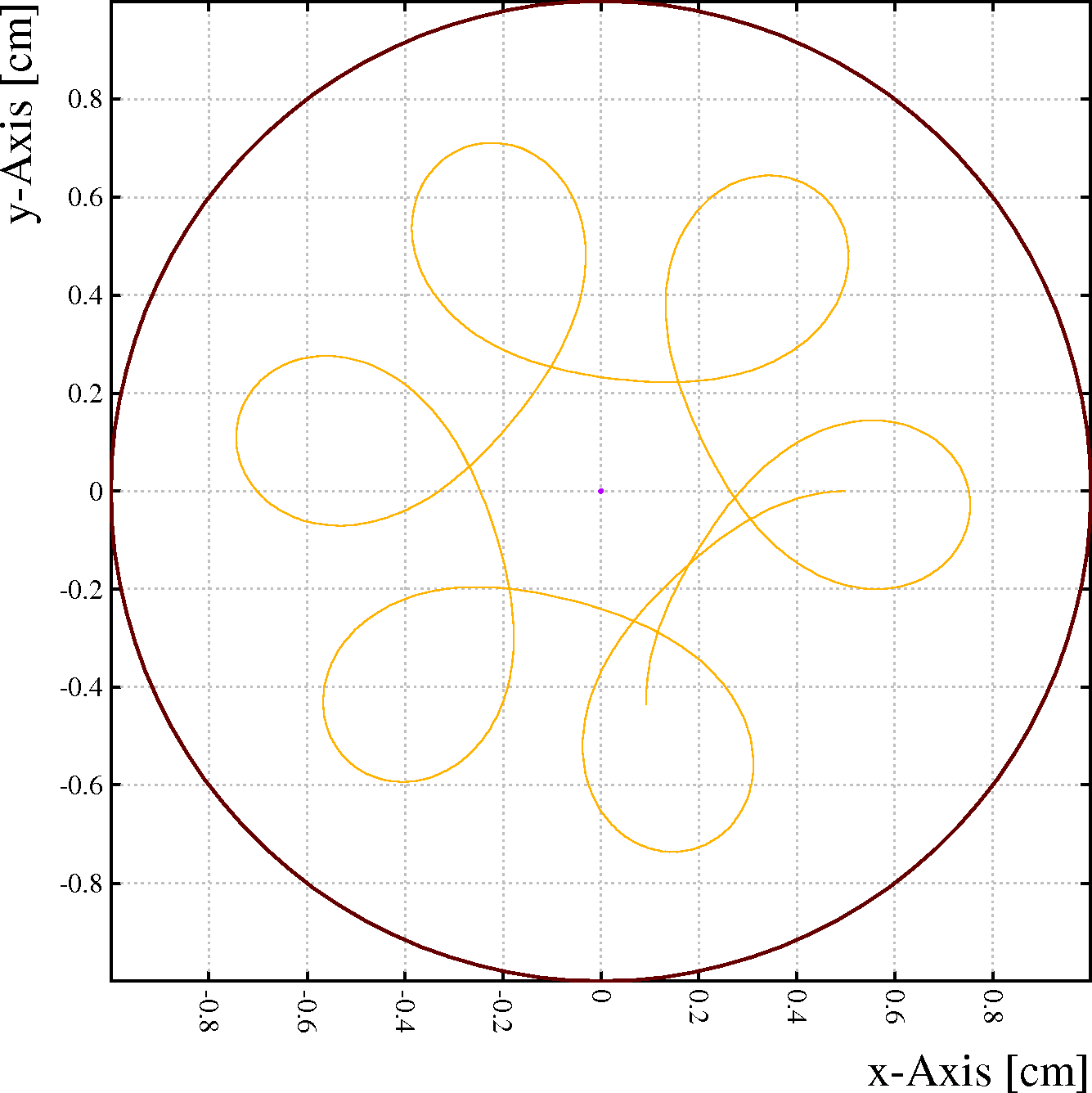
&CELL plane x -1 v=0 plane x +1 v=0 rows s * * 0 0 200000A strong radial electric field in a tube combined with an axial magnetic field of 0.2\ T, makes a relavistic electron with a velocity of 0.33\ c describe a flower-like trajectory:&MAG comp 0 0 0.2 T
&GAS arg-50-eth-50 // Mandatory, but not used gas-id "Vacuum"
&DRIFT integration-parameters integration-accuracy 1e-4 area -1 -1 -1 1 1 1 Call plot_drift_area Call drift_electron_vacuum(0.5,0,0, -10000,0,0, status, time) Say {status, time} Call plot_drift_line Call plot_end
Additional information on:
This procedure can be called after any of the drift-line computation procedures has been called (e.g. DRIFT_ELECTRON).
Format:
CALL DRIFT_INFORMATION(             ...
     [ `CHARGE`, q ] ,              ...
     [ `DRIFT-TIME`, time ] ,       ...
     [ `ELECTRODE`, electrode ] ,   ...
     [ `PARTICLE`, particle ] ,     ...
     [ `PATH-LENGTH`, path ] ,      ...
     [ `STATUS-CODE`, istat ] ,     ...
     [ `STATUS-STRING`, status ] ,  ...
     [ `STEPS`, nsteps ] ,          ...
     [ `TECHNIQUE`, technique ] ,   ...
     [ `X-START`, coordinate ] ,    ...
     [ `Y-START`, coordinate ] ,    ...
     [ `Z-START`, coordinate ] ,    ...
     [ `X-END`, coordinate ] ,      ...
     [ `Y-END`, coordinate ] ,      ...
     [ `Z-END`, coordinate ])
Example:
Call plot_drift_area
Call drift_electron_3(2.5,3.5,4.5,status,time)
Call plot_drift_line
Call plot_end
Say "Status: {status}"
Call string_index(status,`wire`,index1)
Call string_index(status,`replica`,index2)
If index1>0 & index2=0 Then
   Call drift_information('status-code',wire)
   Say "The particle hit wire {wire}."
Endif
An electron drift-line is computed using the Runge Kutta method with DRIFT_ELECTRON_3 which returns a formatted status string. This string has, if the electron hits a wire, the format "Hit X wire n" or "Hit a replica of X wire n". With the help of the STRING_INDEX procedure, we search for the strings "wire" and "replica" to determine whether an original copy of a wire has been hit. If so, DRIFT_INFORMATION is called to find the number of the wire that has been hit.
Additional information on:
The integrated diffusion, the multiplication and the attachment losses are not computed.
This procedure should be called only from within the drift or signal sections, after the cell and the gas have been entered.
This procedure uses the Runge_Kutta_Fehlberg integration method.
Format:
CALL DRIFT_ION(x, y [, status [, time]])
Additional information on:
This procedure should be called only from within the drift or signal sections, after the cell and the gas have been entered.
The integrated diffusion, the multiplication and the attachment losses are not computed.
This procedure uses the Runge_Kutta_Fehlberg integration method.
Format:
CALL DRIFT_ION_3(x, y , z [, status [, time]])
Additional information on:
This procedure is intended for testing the inter-molecular tracking algorithm used in microscopic simulation. For this reason, a gas must be entered before the procedure can be called, even though no gas properties are used by this procedure.
Format:
CALL DRIFT_ION_VACUUM(x, y, z, vx, vy, vz, charge, mass [, status [, time]])
Example:
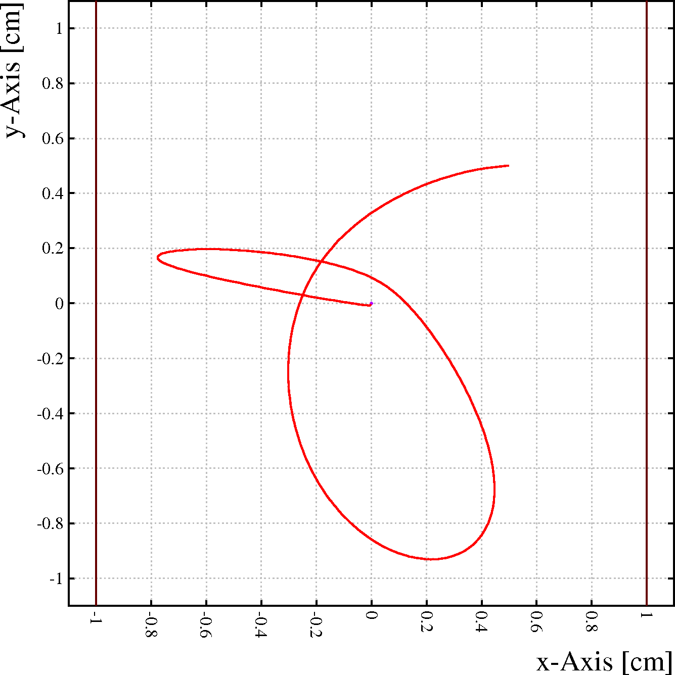
&CELL plane x -1 v=0 plane x +1 v=0 rows s * * 0 0 -100000000A fully stripped Ar nucleus starts from (0.5 , 0.5) with a velocity slightly in excess of 2000 cm/\μs, approximately 0.07\ c. It is subject to an electric and a magnetic field. The example should produce the following figure:&MAG comp 0 0 0.2 T
&GAS arg-50-eth-50 // Dummy gas-id "Vacuum"
&DRIFT integration-parameters integration-accuracy 1e-4 area -1 -1 -1 1 1 1 Call plot_drift_area Call drift_vacuum_ion(0.5,0.5,0, -2e3,-1e2,0, 18, 39.948*931.494, status, time) Say {status, time} Call plot_drift_line Call plot_end
Additional information on:
This procedure should be called only from within the drift or signal sections, after the cell and the gas have been entered.
This procedure can only meaningfully be used if both the transverse and the longitudinal diffusion have been supplied in the gas section. The multiplication and the attachment losses can only be computed if Townsend and attachment data have been entered.
The Monte Carlo integration method is described in the drift section under Monte_Carlo.
Format:
CALL DRIFT_MC_ELECTRON(x, y, z [, status [, time ...
     [, multiplication [, attachment]]]])
Additional information on:
This procedure should be called only from within the drift or signal sections, after the cell and the gas have been entered.
It should be noted that MC drift of electrons and ions uses the same set of integration parameters (step size in particular). Care should be taken to set these parameters to reasonable values for ions before this procedure is called.
Diffusion coefficients for ions can be set with the PARAMETERS statement in the gas section (see sigma).
Multiplication and attachment losses are not evaluated.
The Monte Carlo integration method is described in the drift section under Monte_Carlo.
Format:
CALL DRIFT_MC_ION(x, y, z [, status [, time]])
Additional information on:
This procedure should be called only from within the drift or signal sections, after the cell and the gas have been entered.
It should be noted that MC drift of electrons and ions uses the same set of integration parameters (step size in particular). Care should be taken to set these parameters to reasonable values for ions before this procedure is called.
Diffusion coefficients for ions can be set with the PARAMETERS statement in the gas section (see sigma).
Multiplication and attachment losses are not evaluated.
The Monte Carlo integration method is described in the drift section under Monte_Carlo.
Format:
CALL DRIFT_MC_NEGATIVE_ION(x, y, z [, status [, time]])
Additional information on:
Note that the drift velocity vector is not anti-symmetric under charge inversion is there is a non-zero E-perpendicular component of the B field.
This procedure should be called only from within the drift or signal sections, after the cell and the gas have been entered.
This procedure can only meaningfully be used if both the transverse and the longitudinal diffusion have been supplied in the &GAS section.
The Monte Carlo integration method is described in the drift section under Monte_Carlo.
Format:
CALL DRIFT_MC_POSITRON(x, y, z [, status [, time]])
Additional information on:
This procedure relies extensively on Magboltz. Before using this procedure, the Magboltz gas composition must be set - by running MAGBOLTZ, by retrieving using GET gas tables that have been computed with Magboltz and which have been written in gas file format 10, or by using the COMPOSITION command.
The step size in this procedure is the free path, as in the real gas, with its natural (exponential) distribution. A typical drift path therefore proceeds through millions of collisions and it is rarely practical to store each step individually. Instead, the electron location is recorded every n'th collision, where n is specified with the MONTE-CARLO-COLLISIONS parameters of the INTEGRATION-PARAMETERS command - n may be set to 1 if desired.
In order to profit fully from the detailed nature of these calculations, it is advisable, in case the electrons head for a wire, to set the TRAP-RADIUS to 1.
Each collision is classified as either elastic, inelastic, super-elastic, attachment or ionisation, with one of the species of molecules present in the gas mixture. In case of attachment, the electron is not tracked any further and the status is set accordingly. In this procedure, additional electrons produced through ionisation are not tracked. Use MICROSCOPIC_AVALANCHE if this is desired.
Format:
CALL DRIFT_MICROSCOPIC_ELECTRON(x, y, z ...
   [, status [, time [, options ...
   [, e_maximum [, e_start [, dir_x, dir_y, dir_z ...
   [, distribution, [, rates]]]]]]]])
Additional information on:
The integrated diffusion, the multiplication and the losses through attachment are not computed.
This procedure should be called only from within the drift or signal sections, after the cell and the gas have been entered.
This procedure uses the Runge_Kutta_Fehlberg integration method.
Format:
CALL DRIFT_NEGATIVE_ION(x, y [, status [, time]])
Additional information on:
This procedure should be called only from within the drift or signal sections, after the cell and the gas have been entered.
The integrated diffusion, the multiplication and the losses through attachment are not computed.
This procedure uses the Runge_Kutta_Fehlberg integration method.
Format:
CALL DRIFT_NEGATIVE_ION_3(x, y, z [, status [, time]])
Additional information on:
Note that the drift velocity vector is not anti-symmetric under charge inversion is there is a non-zero E-perpendicular component of the B field.
This procedure should be called only from within the drift or signal sections, after the cell and the gas have been entered.
This procedure uses the Runge_Kutta_Fehlberg integration method.
Format:
CALL DRIFT_POSITRON(x, y [, status [, time]])
Additional information on:
Note that the drift velocity vector is not anti-symmetric under charge inversion is there is a non-zero E-perpendicular component of the B field.
This procedure should be called only from within the drift or signal sections, after the cell and the gas have been entered.
This procedure uses the Runge_Kutta_Fehlberg integration method.
Format:
CALL DRIFT_POSITRON_3(x, y, z [, status [, time]])
Additional information on:
This is a instruction used to debug the diffusion calculation, the procedure is not of much general use.
Format:
CALL DRIFT_DIVERGENCE(x, y, z, f1, f2, f3 [, options])
Example:
&CELL tube r=1 rows s 1 0.01 0 0 1000This example computes the divergence of the drift field in a round tube with a gas of constant mobility. The product of f1 and f2 should be equal to 1 in this case. With a gas of constant drift velocity, f1 should be constant but not f2.&GAS table drift-velocity=ep/100
&DRIFT Global step=0.0010 integration-parameters m-c-dist {step} Call book_matrix(xv,100) Call book_matrix(f1v,100) Call book_matrix(f2v,100) Global n=0 Global phi=335*pi/180 For x From 0.01 Step 0.02 To 0.99 Do Call drift_divergence(x*cos(phi), x*sin(phi), 0, ... f1, f2, f3, `positive,electron`) Global n=n+1 Global xv[n]=x Global f1v[n]=f1 Global f2v[n]=f2 Enddo Call adjust_matrix(xv,n,0) Call adjust_matrix(f1v,n,0) Call adjust_matrix(f2v,n,0) Global min=minimum(f1v&f2v) Global max=maximum(f1v&f2v) Call plot_frame(0,0.95*min,1,1.05*max,`r`,`f`,`Divergence`) Call plot_line(xv,f1v,`function-1`) Call plot_line(xv,f2v,`function-2`) Call plot_line(xv,1+step/xv,`function-3`) Call plot_end
The curve drawn with representation FUNCTION-3 shows the exact expression of the transverse divergence.
Additional information on:
This is a instruction used to debug the diffusion calculation, the procedure is not of much general use.
Format:
CALL DRIFT_ROTATION(x, y, z, Rvc, Rmc, Rvm [, options])
Example:
&CELL tube r=1 rows s 1 0.01 0 0 1000&MAGNETIC components 0 0 1 T
&DRIFT integration-parameters m-c-dist 0.001 Call drift_rotation(0.1, 0.0, 0,rvc,rmc,rvm,`electron,positive`) Call print_matrix(rvc,rmc,rvm)
Additional information on:
In the absence of a magnetic field, the orientation of the electric field is immaterial. The electric field may be specified either by the norm or as a vector, of which only the norm matters. In this case, the values returned by this procedure coincide with those returned by VELOCITY_E.
In the presence of a magnetic field, the transport parameters depend on the relative orientation of the electric and magnetic field vectors. Both fields therefore have to be specified as vectors. The velocity that is returned is equal to the vectorial sum of VELOCITY_E, VELOCITY_BTRANSVERSE and VELOCITY_ExB.
Each of the field components can either be a Number or a Matrix. It is permissible to specify some components of the field as Numbers and the other(s) as Matrices.
All components which are specified as Matrix, must have the same total size - they do not have to be 1-dimensional. If at least one component is specified as Matrix, then the output will be a 1-dimensional Matrix with length equal to the overall size of the arguments of type Matrix. Otherwise the result will be a Number.
The electric field should be in V/cm, the magnetic field has to be in native units of 100\ G or 0.01\ T, and the drift velocity is returned in cm/\μsec.
Formats:
CALL DRIFT_VELOCITY(e, drift)
CALL DRIFT_VELOCITY(ex, ey, ez, drift)
CALL DRIFT_VELOCITY(ex, ey, ez, bx, by, bz, drift)
Example:
Global emin=100
Global emax=10000
Global e=emin*(emax/emin)^((row(200)-1)/199)
&GAS
mix argon 95 methane 5 noplot-f0 noplot-cross-section e/p-range {emin/760,emax/760}
&MAIN
Call drift_velocity(0,0,e,vd5)
&GAS
mix argon 90 methane 10 noplot-f0 noplot-cross-section e/p-range {emin/760,emax/760}
&MAIN
Call drift_velocity(0,0,e,vd10)
&GAS
mix argon 80 methane 20 noplot-f0 noplot-cross-section e/p-range {emin/760,emax/760}
&MAIN
Call drift_velocity(0,0,e,vd20)

Call plot_frame(emin,0,emax,10,`E [V/cm]`, ...
   `v<SUB>D</SUB> [cm/microsec]`, ...
   `Drift velocity in Ar/CH4 mixtures`)
Call plot_line(e,vd5,`function-1`)
Call plot_line(e,vd10,`function-2`)
Call plot_line(e,vd20,`function-3`)
Call plot_end
The arguments ex, ey, ez, e, v and status are optional.
Format:
CALL ELECTRIC_FIELD(x, y, ex, ey, ez, e, v, status)
Example:
&CELL plane x=-1 plane y=-1 rows s * * 1 1 1000&FIELD Global n=6 Call book_matrix(x,n,n) Call book_matrix(y,n,n) For i From 1 To n Do For j From 1 To n Do Global x[i;j]=(i-1)/(n-1) Global y[i;j]=(j-1)/(n-1) Enddo Enddo Call efield(x,y,ex,ey,ez,e,v,stat) Call print_matrix(x,y,ex,ey,ez,e,v,stat) area 0 0 1 1 grid {n} print ex ey e v
In a simple chamber, one uses on the one hand the ELECTRIC_FIELD procedure to compute the field on a 6x6 grid, on the other hand the PRINT command is used to verify the result.
Additional information on:
The arguments ex, ey, ez, e, v and status are optional.
Format:
CALL ELECTRIC_FIELD_3(x, y, z, ex, ey, ez, e, v, status)
Example:
See ELECTRIC_FIELD.
Additional information on:
This procedure needs electron drift velocity data, which can be computed with the MAGBOLTZ gas section command. The magnetic field, if present, is taken into account. Diffusion data is not used, even if present - the vector that is returned represents the mean electron drift velocity at a given point.
This procedure provides functionality similar to the SPEED command.
Format:
CALL ELECTRON_VELOCITY(x, y, z, vx, vy, vz [, status])
Example:
Call electron_velocity(2,3,0,vx,vy,vz,status)
Say "Velocity: ({vx,vy,vz}), Status: {status}"
Additional information on:
The first argument is the level number, the index of the vector given by INTEGRATE_EXCITATIONS. The second argument contains on return a string with the level identifier, which is described in somewhat more detail in the gas ingredients. The optional third argument contains on return the threshold energy of the level (in eV).
The number of levels can be obtained with LEVEL_COUNT.
Format:
CALL EXCITATION_IDENTIFIER(level_number, level_identifier [, level_energy])
For examples, see INTEGRATE_EXCITATIONS and LEVEL_COUNT.
In the absence of a magnetic field, the orientation of the electric field is immaterial. The electric field may be specified either by the norm or as a vector, of which only the norm matters.
In the presence of a magnetic field, the rates (at least in principle) depend on the relative orientation of the electric and magnetic field vectors. Both fields therefore have to be specified as vectors.
Each of the field components can either be a Number or a Matrix. It is permissible to specify some components of the field as Numbers and the other(s) as Matrices.
All components which are specified as Matrix must have the same total size - they do not have to be 1-dimensional. If at least one component is specified as Matrix, then the output will be a 1-dimensional Matrix with length equal to the overall size of the arguments of type Matrix. Otherwise the result will be a Number.
The first argument is a Number which identifies the level. The number of available levels can be found with the LEVEL_COUNT procedure and further information can be obtained with EXCITATION_IDENTIFIER.
The electric field should be in V/cm, the magnetic field has to be in native units of 100\ G or 0.01\ T, and the rate is returned in THz.
Formats:
CALL EXCITATION_RATE(level, e, rate)
CALL EXCITATION_RATE(level, ex, ey, ez, rate)
CALL EXCITATION_RATE(level, ex, ey, ez, bx, by, bz, rate)
Example:
Global emin=5000
Global emax=25000
Global e=emin*(emax/emin)^((row(200)-1)/199)
Call plot_frame(emin/1000, 0, emax/1000, 2, `E [kV/cm]`, ...
   `Excitation rate [GHz]`, `Excitations and Dissociations`)
Call level_count(nexc, nion)
For id From 1 To nexc Do
   Call excitation_rate(id,e,exc)
   Call excitation_identifier(id, name, ethresh)
   Say "{id}: {name}, Emin = {ethresh}"
   Call string_index(name,`DISS`,ind)
   If ind>0 Then
      Call plot_line(e/1000,exc*1e3, `function-2`)
   Else
      Call plot_line(e/1000,exc*1e3, `function-3`)
   Endif
Enddo
Call plot_end
This examples plots all excitation rates, and marks the dissociations using a different line type.
The matrix from which elements are to be extracted should exist prior to the call, the receiving matrix should not exist prior to the call.
This procedure is used to process array indexing on the right hand side of formulae, in procedure calls etc. This procedure is not meant to called by the user. It is much simpler to get sub-matrices using indexing expressions.
Format:
CALL EXTRACT_SUBMATRIX(ndim, nsel_1, nsel_2, ... , ...
     isel_1_1, isel_1_2, ..., isel_2_1, isel_2_2, ... , ...
     isel_n_1, isel_n_2, ref_submatrix, ref_matrix)
When the search is successful, the global variable OK is set to True, otherwise to False. The following conditions can lead to un unsuccessful search:
This procedure works by parabolic iteration over a set of 3 near-extreme values, which is initialised with a random search. If the boundary values are better, than the result of the random search, then the parabolic search is skipped.
Format for functions:
CALL EXTREMUM(function, extremum, minimum, maximum, ...
     [ options [, \ε_loc [, \ε_fun [, itermax ]]]])
Format for matrices:
CALL EXTREMUM(ordinates, values, extremum, ...
     [ options [, \ε_loc [, \ε_fun [, itermax ]]]])
Examples:
Call extremum(`1+5*x-(x-2)^3`,x,-1,4,`plot,print,minimum`)
Global min=x
Call extremum(`1+5*x-(x-2)^3`,x,-1,4,`plot,print,maximum`)
Global max=x
Say "Extrema: {min,max}"
The function 1+5*x-(x-2)^3 has a local minimum near x=0.7 and a local maximum near x=3.3. The first call will indeed find the local minimum, while the second call will set x to -1 since the function value on this boundary is higher than in the local maximum.
Global a=2
Global b=3
Call extremum(`1+cosh(a-b)`,b,-1,4,`plot,print,minimum`)
Say "Minimum found is {b}, should be {a}."
This example shows a function of two global variables, A and B. The function is minimised as function of B in this example. During the minimisation, A retains its value.
Additional information on:
The procedure sets the OK global variable to True if filling was successful and to False if it wasn't, usually because the histogram to be filled didn't exist. OK is not set to False if the entry is out of range.
Format:
CALL FILL_HISTOGRAM(histogram, entry [, weight])
Example:
Call book_histogram(ref,100)
For i From 1 To 10000 Do
   Call fill_histogram(ref,rnd_landau)
Enddo
Call plot_histogram(ref,`Energy loss`,`Landau distribution`)
Call plot_end
This example could be used to check that the Landau random number generator does indeed work.
Additional information on:
In addition to the parameters, the global variable OK is set by this procedure. Its value is True is the fit converged, and False otherwise.
Format for histograms:
CALL FIT_EXPONENTIAL(reference, a0, a1, a2, ..., an, ...
     err_a0, err_a1, err_a2, ..., err_an [, options])
Format for matrices:
CALL FIT_EXPONENTIAL(x, y, err_y, a0, a1, a2, ..., an, ...
     err_a0, err_a1, err_a2, ..., err_an [, options])
Examples:
&SIGNAL
avalanche polya-townsend 0.5
check avalanche from 0 0.5 range 0.1 10000 keep-histograms
Call fit_exponential(avalanche,a0,a1,ea0,ea1,`print,plot`)
Say "a0 = {a0}+/-{ea0}, a1 = {a1}+/-{ea1}."
In this example, the user wishes to see how well a Polya distribution with parameter \θ=0.5, can be reproduced by an exponential.
Vector ep      ap
       0.13158 0
       0.65789 0
       1.31579 0
       2.63158 0
       6.57895 0
      13.1579  0.0089211
      19.7368  0.10592
      26.3158  0.24737
      39.4737  0.62105
      52.6316  0.97995
      78.9474  1.86895
     105.263   2.74474
     131.579   3.605
     197.368   5.515
     230.263   6.39237
     300       8.07711

Global epfit=ep[6,7,8,9]
Global apfit=ap[6,7,8,9]

Global p=760
Call fit_exponential(1/epfit,apfit,0.1*apfit,a0,a1,ea0,ea1, ...
   `noplot,noprint`)

Global emin=5000
Global emax=300000
Global ne=100
Global ekorff=emin*(emax/emin)^((row(ne)-1)/(ne-1))
Global akorff=exp(a0+a1*p/ekorff)*p
!options log-x log-y
Call plot_frame(emin,0.1,emax,8000,`E [V/cm]`,`α [1/cm]`, ...
   `Korff fit`)
Call plot_error_bar(ep*p,ap*p)
Call plot_line(ekorff,akorff,`function-1`)
Global a=exp(a0)
Global ea=ea0*a
Global a=entier(a*10)/10
Global ea=entier(ea*10)/10
Global b=-entier(a1)
Global eb=entier(ea1)
Call plot_text(40000,100,`A = `/string(a)/` ± `/string(ea), ...
   `title`)
Call plot_text(40000,60,`B = `/string(b)/` ± `/string(eb), ...
   `title`)
Call plot_end
The Townsend coefficients are sometimes approximated using the Rose-Korff formula:
\α/p = A.exp(-B.p/E)This example performs such a fit on Townsend coefficients that have been computed by the Imonte program for a mixture of 90\ % argon and 10\ % isobutane. Imonte is a precursor program for Magboltz version\ 7 and is no longer used.
Additional information on:
This procedure, unlike the other fitting procedures, does not try to find suitable starting values for the fitting parameters. A starting value for each parameter must therefore be supplied by the user.
Since this procedure uses the symbolic evaluation procedures of Garfield, the fit works essentially in single precision. In order to have a chance to be successful, the problem must therefore be well conditioned.
In addition to the parameters, the global variable OK is set by this procedure. Its value is True is the fit converged, and False otherwise.
Format for histograms:
CALL FIT_FUNCTION(reference, function, ...
     par1, par2, par3, ... , err1, err2, err3, ... [, options])
Format for matrices:
CALL FIT_FUNCTION(x, y, err_y, function, ...
     par1, par2, par3, ... , err1, err2, err3, ... [, options])
Example:
Call book_histogram(ref,50,-1,3)
For i From 1 To 500 Do
   Global x=-1+4*rnd_uniform
   Global w=x^2+1
   Call fill_histogram(ref,x,w)
Enddo
Global c=100
Global a=2
Global b=1
Call fit_function(ref,`c+a*(1+b*x^2)`,a,b,ea,eb,`plot,print`)
Say "Function: {c}+{a}*(1+{b}*x^2), errors {ea,eb}"
Say "{a+c} +/- {abs(ea)} should be equal to"
Say "{a*b} +/- {a*b*sqrt((ea/a)^2+(eb/b)^2)}"
This is a simple test of the FIT_FUNCTION procedure in which the function depends on 3 global variables A, B and C of which A and B are varied while C is kept fixed.
Another example can be found in the description of the RND_POISSON random number generator.
Additional information on:
In addition to the parameters, the global variable OK is set by this procedure. Its value is True is the fit converged, and False otherwise.
Format for histograms:
CALL FIT_GAUSSIAN(reference, integral, mean, sigma ...
     [, error_int [, error_mean [, error_sigma [, options]]]])
Format for matrices:
CALL FIT_GAUSSIAN(x, y, err_y, integral, mean, sigma ...
     [, error_int [, error_mean [, error_sigma [, options]]]])
Example 1:
Call get_histogram(sel_5,`arrival.hist`,`sel_5`)
Call fit_gaussian(sel_5,dum,dum,sigma,dum,dum,esigma,`PLOT`)
Say "Gaussian width is {sigma} +/- {esigma}."
The ARRIVAL-TIME-DISTRIBUTION instruction returns the RMS of the arrival time distributions. To obtain Gaussian fits in addition, you can specify the KEEP-HISTOGRAMS option and then use FIT_GAUSSIAN. You can also do the fit in a separate job as explained in http://cern.ch/garfield/examples/
Example 2:
Call book_histogram(hist)
For i From 1 To 10000 Do
   Global sum=0
   For j From 1 To 12 Do
      Global sum=sum+rnd_uniform
   Enddo
   Call fill_histogram(hist,sum)
Enddo
Call fit_gaussian(hist,a,b,c,ea,eb,ec,`print,plot`)
(This verifies the approximation of a Gaussian distribution by the sum of 12 uniformly distributed random numbers.)
Additional information on:
The Mathieson distribution depends on a shape parameter, called K3, which is a function of the geometrical structure of the chamber, and on the ratio of strip width and anode-cathode distance. The distribution assumes that the avalanche is localised on anode wires placed centrally with respect to the cathode strips.
The procedure derives the strip width from the bin width of the input histogram, the anode-cathode distance has to be entered as an argument. The K3 parameter can be fitted, but may optionally also be kept constant during the fit at a user-specified value.
In addition to the parameters, the global variable OK is set by this procedure. Its value is True is the fit converged, and False otherwise.
Formats:
CALL FIT_MATHIESON(x, y, err_y, distance, norm, centre, k3, ...
     error_norm, error_centre, error_k3, [, options])
CALL FIT_MATHIESON(reference, distance, norm, centre, k3, ...
     error_norm, error_centre, error_k3, [, options])
Example:
Call book_histogram(ref_m,50)
Call book_histogram(ref_b,50)
For i From 1 To 65 Do
   Call get_histogram(hist,`profile.hist`,string(i))
   Global k3=0.1
   Global s=0.254
   Call fit_mathieson(hist,s,f,xc,k3,ef,exc,ek3,...
      `noplot,noprint,equal,fitk3`)
   Call fill_histogram(ref_m,xc)
   Call barycentre(hist,b,5)
   Call fill_histogram(ref_b,b)
   Say "Centre:     {xc} +/- {exc}"
   Say "Barycentre: {b}"
   Say "K3:         {k3} +/- {ek3}"
Enddo
Call plot_histogram(ref_m,`Reconstructed x [cm]`,`Mathieson fits`)
Call plot_end
Call plot_histogram(ref_b,`Reconstructed x [cm]`,`Barycentre`)
Call plot_end
(We have already produced a file that contains for 65 events a distribution of induced charges in the pads, and now we fit each of these with a Mathieson distribution and compare these fits with barycentres. The K3 parameter is left free.)
References:
Additional information on:
This procedure optionally tries to determine the a linear horizontal scale correction for which the fit is optimal. But, fitting a Polya distribution with a free scale is a numerically poorly conditioned problem because of the high correlation between the Polya parameter and the scale parameters. If the scale is known, then it is preferable to fix the scale.
Similarly, the routine will make an attempt to estimate the Polya parameter if no starting value is known, but it is better to provide a starting value if one is known with reasonable accuracy.
In addition to the parameters, the global variable OK is set by this procedure. Its value is True is the fit converged, and False otherwise.
Format for histograms:
CALL FIT_POLYA(reference, factor, offset, slope, \θ, ...
     error_factor, error_offset, error_slope, error_theta [, options])
Format for matrices:
CALL FIT_POLYA(x, y, err_y, factor, offset, slope, \θ, ...
     error_factor, error_offset, error_slope, error_theta [, options])
Example:
Call book_histogram(ref,100,0,10)
For i From 1 To 2000 Do
   Call fill_histogram(ref,1+2*rnd_polya(1))
Enddo
Global o=-1/2
Global s=1/2
Global t=500
Global f=200
Call fit_polya(ref,f,o,s,t,ef,eo,es,et,`plot,print,poisson,auto`)
Say "Scaling X={o}+{s}*x, theta={t}+/-{et}, contents={f}."
(First we fill a histogram with a Polya distribution of which we know the \θ parameter and the scale, then we check whether the fit finds the input values back. We don't need to give initial values in this case since the AUTO option is specified.)
Additional information on:
In addition to the parameters, the global variable OK is set by this procedure. Its value is True is the fit converged, and False otherwise.
Format for histograms:
CALL FIT_POLYNOMIAL(reference, a0, a1, a2, ..., an, ...
     err_a0, err_a1, err_a2, ..., err_an [, options])
Format for matrices:
CALL FIT_POLYNOMIAL(x, y, err_y, a0, a1, a2, ..., an, ...
     err_a0, err_a1, err_a2, ..., err_an [, options])
Example:
Call hdelete(ref)
Call hbook(ref,100,-2,2)
For i From 1 To 10000 Do
   Global x=(rnd_uniform-0.5)*4
   Global dy=0.01*(rnd_uniform-0.5)
   Call hfill(ref,x,1+2*x+x^2+dy)
Enddo
Call fit_polynomial(ref,a0,a1,a2,ea0,ea1,ea2,`print,plot`)
Say "a0 = {a0}+/-{ea0}, a1 = {a1}+/-{ea1}, a2 = {a2}+/-{ea2}."
This example is a test to verify that the fit works. In the procedure calls, HDELETE is short for DELETE_HISTOGRAM, HBOOK for BOOK_HISTOGRAM and HFILL for FILL_HISTOGRAM.
Additional information on:
This procedure is only of use for debugging, and must be used with caution since it is on purpose not protected for locations inside wires (the call can result in a division by zero).
Format:
CALL FORCE_FIELD(x, y, ex, ey)
Additional information on:
Format:
CALL GAS_AVAILABILITY(object, available)
Additional information on:
All arguments are optional.
Format:
CALL GET_CELL_DATA([number_of_wires [, cell_type [, ...
     coordinates [, identifier]]]])
Additional information on:
If the cell has been entered in polar coordinates, then the dimensions are returned in internal coordinates. These can be converted to Cartesian or polar coordinates with the INTERNAL_TO_CARTESIAN and INTERNAL_TO_POLAR procedures.
If 4 arguments are provided, only the (x,y) part of the cell dimensions is returned. If 6 arguments are present, also the z part is set.
Formats:
CALL GET_CELL_SIZE(xmin, ymin, zmin, xmax, ymax, zmax)
CALL GET_CELL_SIZE(xmin, ymin, xmax, ymax)
Example: see GET_WIRE_DATA
In addition to the parameters, the global variable OK is set by this procedure. Its value is True if generating the clusters worked properly, otherwise it will be set to False. OK is set to False if the done flag has been set to True.
Before using the cluster location and energy, the value of the done argument and of the OK global variable should be checked. The parameters should not be used if either of these two has been set to True.
Format:
CALL GET_CLUSTER(xcls, ycls, zcls, npair, ecls, [extra1,] done)
Example:
track 0 1 1 1 muon energy 10000 nodelta
Call book_histogram(size,100)
For i From 1 To 100 Do
   Call new_track
   Until done Do
      Call get_cluster(xcls,ycls,zcls,npair,ecls,done)
      If done Then Iterate
      Call fill_histogram(size,npair)
   Enddo
Enddo
!options log-y
Call plot_histogram(size,`Cluster size`,...
   `Cluster size distribution`)
Call plot_end
This example shows how one can obtain the cluster size distribution for tracks generated by the Heed program. Since Heed doesn't generate clusters but always \δ-electrons (they usually have a very short range), we use the NODELTA-ELECTRONS option on the TRACK command. This compresses the \δ-electrons into clusters.
Additional information on:
If you wish to retrieve e.g. the length or the coordinates of the end point of the drift path, then DRIFT_INFORMATION provides easier access to the information.
The drift time is expressed in \μsec and the z-component of the drift path in cm. Also the (x,y) part of the path is in cm if Cartesian or tube coordinates are used. If the cell has been described in polar coordinates, then (x,y) is represented in internal coordinates:
(\ρ,\φ)=(log(\√(x\²+y\²),arctan(y/x))
These can be converted to Cartesian or polar coordinates with the INTERNAL_TO_CARTESIAN and INTERNAL_TO_POLAR procedures.
Format:
CALL GET_DRIFT_LINE(x [, y [, z [, t]]])
Example:
Say "Please enter (x,y) of the starting point"
Parse Terminal x_start y_start
Call drift_electron(1,1,status,time)
Call get_drift_line(x,y,z,t)
Call plot_graph(t,x,`Time [microsec]`,`x [cm]`,`x vs time`)
Call plot_comment(`UP-LEFT`,`Status: `/status)
Call plot_comment(`DOWN-LEFT`,`Drift time: `/string(time)/` [microsec]`)
Call plot_comment(`UP-RIGHT`, `From (x,y)=(`/string(x_start)/`,`/...
   string(y_start)/`)`)
Call plot_end
A way to plot the relation between the x-coordinate of a drift line and the drift time.
After the call, the argument is a 1-dimensional Matrix. Any value this argument has before the procedure call, is lost after the call.
Format:
CALL GET_E/P_TABLE(ep)
Example:
Call get_e/p_table(ep)
Call get_gas_data(p)
Call townsend(ep*p,0,0,a)
Call plot_graph(ep*p,a,`E [V/cm]`,`α [1/cm]`, ...
   `Townsend coefficient`)
Call plot_error_bar(ep*p,a,0,0.1*a)
Call plot_end
Retrieves the set of E/p points, the pressure and the Townsend coefficients, and then makes a plot showing 10\ % error bars for the values.
Format:
CALL GET_GAS_DATA(pressure [, temperature [, identifier]])
Example:
Call get_gas_data(p, t, gasid)
Say "Gas identifier is {gasid}."
Additional information on:
The procedure sets the OK global variable to True if the histogram has successfully been retrieved and to False if a problem occurred.
Format:
CALL GET_HISTOGRAM(reference, file [, member])
Additional information on:
The procedure sets the OK global variable to True if the matrix is successfully retrieved, and to False in case of a problem.
Format:
CALL GET_MATRIX(matrix, file [, member])
Example:
See WRITE_MATRIX.
Additional information on:
Format:
CALL GET_PERIODS(yesno_x, length_x, yesno_y, length_y)
Additional information on:
Raw signals are obtained by computing drift trajectories, and multiplying at each step, the local velocity with the weighting field. Raw signals do not, as a rule, have equal time intervals.
Use the LIST_RAW_SIGNALS procedure to find out which raw signals currently are in memory.
Format:
CALL GET_RAW_SIGNAL(type, electrode, avalanche_wire, angle, ...
     time, signal)
Additional information on:
Format:
CALL GET_SIGNAL(electrode, time, direct [, cross])
Example:
Additional information on:
Format:
CALL GET_SOLID_DATA(solid, qsolid)
Example: see INTEGRATE_CHARGE.
Additional information on:
Internal coordinates are used for the plane locations. Use the INTERNAL_TO_POLAR procedure to convert to, for instance, polar coordinates.
All arguments are mandatory.
Format:
CALL GET_X_PLANE_DATA(yn_1, x_1, V_1, label_1, ...
                      yn_2, x_2, V_2, label_2)
Example:
Call get_cell_data(wires,type,coord,id)
Call get_x_plane_data(yn1,x1,V1,lab1, yn2,x2,V2,lab2)
If coord="Polar" Then
   If yn1 Then Say "There is a plane at r={exp(x1)} and with V={V1}."
   If yn2 Then Say "There is a plane at r={exp(x2)} and with V={V2}."
Else
   If yn1 Then Say "There is a plane at x={x1} and with V={V1}."
   If yn2 Then Say "There is a plane at x={x2} and with V={V2}."
Endif
Internal coordinates are used for the plane locations, use the INTERNAL_TO_POLAR procedure to convert to polar coordinates.
All arguments are mandatory.
Format:
CALL GET_Y_PLANE_DATA(yn_1, y_1, V_1, label1, ...
                      yn_2, y_2, V_2, label2)
Example:
Call get_cell_data(wires,type,coord,id)
Call get_y_plane_data(yn1,y1,V1,lab1, yn2,y2,V2,lab2)
If coord="Polar" Then
   If yn1 Then Say "There is a plane at phi={180*y1/pi} and with V={V1}."
   If yn2 Then Say "There is a plane at phi={180*y2/pi} and with V={V2}."
Else
   If yn1 Then Say "There is a plane at y={y1} and with V={V1}."
   If yn2 Then Say "There is a plane at y={y2} and with V={V2}."
Endif
All arguments are optional.
Format:
CALL GET_WIRE_DATA(wire [, x [, y [, V [, d [, q [, label [, ...
   length [, weight [, density]]]]]]]]])
Example:
Call get_cell_data(nwire,dummy,dummy,id)
Say "List of wires with a negative charge:"
For i From 1 To nwire Do
   Call get_wire_data(i,xw,yw,vw,dw,qw,labelw)
   If qw>0 Then Iterate
   Say "Wire {i} at (x,y)=({xw,yw}), type {labelw}"
Enddo
This example shows how one can produce a list of the wires that have a negative charge. One could also select a sense wire and store its coordinates using this technique.
Additional information on:
This procedure is a direct interface to the GKS routine GFA. The first argument of GFA, the vector length, is absent.
The area is plotted with the area attributes, and using the normalisation transformation that are in effect at the time the procedure is called.
Format:
CALL GKS_AREA(x,y)
Additional information on:
This procedure is a direct interface to the GKS routine GPL. The first argument of GPL, the vector length, is absent.
The polyline is plotted with the polyline attributes, and using the normalisation transformation that are in effect at the time the procedure is called.
Format:
CALL GKS_POLYLINE(x,y)
Additional information on:
This procedure is a direct interface to the GKS routine GPM. The first argument of GPM, the vector length, is absent.
The polymarker is plotted with the polymarker attributes, and using the normalisation transformation that are in effect at the time the procedure is called.
Format:
CALL GKS_POLYMARKER(x,y)
Additional information on:
This procedure is equivalent to the GKS routine GSELNT.
Format:
CALL GKS_SELECT_NT(nt)Example:
See PLOT_START.
Additional information on:
This procedure is an interface to the GKS routine GSCHXP.
Format:
CALL GKS_SET_CHARACTER_EXPANSION(expansion)
Additional information on:
This procedure is an interface to the GKS routine GSCHH.
Format:
CALL GKS_SET_CHARACTER_HEIGHT(height)
This procedure is an interface to the GKS routine GSCHSP.
Format:
CALL GKS_SET_CHARACTER_SPACING(spacing)
Additional information on:
This procedure is an interface to the GKS routine GSCHUP.
Format:
CALL GKS_SET_CHARACTER_UP_VECTOR(x, y)
Additional information on:
The text alignments specify where a piece of text is to placed with respect to its anchor point.
This procedure is an interface to the GKS routine GSTXAL.
Format:
CALL GKS_SET_TEXT_ALIGNMENT(hor, vert)
Additional information on:
This procedure is a direct interface to the GKS routine GSTXCI.
Format:
CALL GKS_SET_TEXT_COLOUR(colour)
Additional information on:
This procedure is a direct interface to the GKS routine GSTXFP.
CALL GKS_SET_TEXT_FONT_PRECISION(font, precision)
Additional information on:
This procedure is a direct interface to the GKS routine GTX.
The text is plotted with the polyline attributes, the alignment, the up-vector and using the normalisation transformation that are in effect at the time the procedure is called. These attributes can either be set at the GKS level by calling GKS_SET_CHARACTER_EXPANSION, GKS_SET_CHARACTER_HEIGHT, GKS_SET_CHARACTER_SPACING, GKS_SET_CHARACTER_UP_VECTOR, GKS_SET_TEXT_ALIGNMENT, GKS_SET_TEXT_COLOUR and GKS_SET_TEXT_FONT_PRECISION, or at the Garfield level by calling SET_TEXT_ATTRIBUTES.
Format:
CALL GKS_TEXT(x,y,text)
Additional information on:
Specifying a viewport doesn't entail an automatic change of normalisation transformation. For this, one needs to call the GKS_SELECT_NT procedure.
A call to a procedure like PLOT_FRAME overrides the viewport setting for normalisation transformation number 1 with the parameters that can be set with the VIEWPORT graphics command. Also, all regular Garfield plots will modify these viewport settings.
This procedure is equivalent to the GKS routine GSVP.
Format:
CALL GKS_VIEWPORT(nt, xmin, xmax, ymin, ymax)Example:
See PLOT_START.
Additional information on:
Specifying a window doesn't entail an automatic change of normalisation transformation. For this, one needs to call the GKS_SELECT_NT procedure.
A call to a procedure like PLOT_FRAME overrides the window setting for normalisation transformation number 1 with the dimensions specified in the argument. Also all regular Garfield plots will modify these window settings.
This procedure is equivalent to the GKS routine GSWN.
Format:
CALL GKS_WINDOW(nt, xmin, xmax, ymin, ymax)Example:
See PLOT_START.
Additional information on:
The histogram is not affected by this operation.
Format:
CALL HISTOGRAM_TO_MATRIX(hist, matrix [, min [, max]])
Example:
Call book_histogram(ref1,10,0,1)
For i From 1 To 1000 Do
   Call fill_histogram(ref1,rnd_uniform)
Enddo
Call plot_histogram(ref1)
Call plot_end
Call histogram_to_matrix(ref1,a,min,max)
Call matrix_to_histogram(a,min,max,ref2)
Call plot_histogram(ref2)
Call plot_end
First, we book an histogram and fill it with uniformly distributed random numbers. The histogram is then copied to a matrix A, and then copied back to a histogram. Both histograms are plotted to check they are indeed the same.
To take the effect of electronics into account, one should calculate pure signals with the SIGNAL command or with the ADD_SIGNALS procedure, process them (e.g. with CONVOLUTE-SIGNALS), recuperate the electronics output with GET_SIGNAL and integrate the signal using the SUM function.
The procedure first drifts a particle of the desired kind from the starting point. Next, the routine integrates the internal product of the weighting field for the electrode that is read out and the drift velocity between the time limits over the drift path. The result is multiplied with minus the charge of the particle that has been drifting.
Contrary to appearances, the total induced charge (i.e. integrated over the entire drift path) thus computed is a surprisingly boring quantity. A charged particle that moves from one electrode to another can only induce a total charge of +1, 0 or -1. The total charge is +1 or -1 in case the particles moves from an electrode that is read out to one that is not, or vv. The total charge is 0 if the particle moves between electrodes which are both read out or are both not read out.
The sum of charges induced on all electrodes vanishes: the effect of a moving charge in a chamber is a reshuffling of the charges on the conductors, charges are not created and do not vanish.
Format:
CALL INDUCED_CHARGE(x, y, z, particle, electrode ...
   [, tmin, tmax], q)
Example:
&CELL pl y -1 label p pl y +1 label q rows a * * +0.5 0 -1000 s * * 0 0 1000 b * * -0.5 0 -1000&GAS co2
&SIG area -1.1 -1.1 1.1 1.1 sel (pq)s(ab) Call induced_charge(-0.4,-0.5,0,`e-`,2,q1) Call induced_charge(-0.4,-0.5,0,`e+`,2,q2) Say "Status e-: {stat1}, e+: {stat2}" Say "Charge between wire and plane: {q1+q2}"
Verifies that the total charge induced by a particle moving between two conductors (the B wire and a plane) other than the one that is read out (the S wire), is indeed 0.
A more elaborate application of this procedure can be found in http://cern.ch/garfield/examples/charge
Additional information on:
This procedure is used to control the starting point in the random number generator sequences. By default, the random number generators are, at the start of the calculations, called a number of times that depends on the time of the day (product of the hours, minutes and seconds).
If reproducible, yet different, sequences are required, then specify the -noRNDM_initialisation command line option and use this procedure to set a starting point.
Format:
CALL INITIALISE_GENERATORS(ncalls)
Example:
garfield -noRNDM_init
(start)
Call initialise_generators(1234)
The file does not have to be a Garfield library. If you wish to test the presence of, for instance, a gas description in a given library, then you should use INQUIRE_MEMBER.
The EXIST function performs the same tasks as this procedure.
Format:
CALL INQUIRE_FILE(file, exists)
Example:
&CELL
Call inquire_file(`new_cell`,exist)
If exist Then
   % delete "dc1.lib" cell
   < new_cell
   write "dc1.lib" cell
Else
   get "dc1.lib" cell
Endif
In this example a cell description is retrieved from a library called dc1.lib, unless a file called new_cell is found. In that case, the cell description is deleted from the library, the new description is read and stored in compact format in the library.
Additional information on:
Calling this procedure does not interfere with the filling process.
The first 2 arguments are mandatory, the rest is optional.
Format:
CALL INQUIRE_HISTOGRAM(reference, exists, set, channels, ...
     minimum, maximum, entries, mean, rms)
Additional information on:
The exists argument is set to True only if all of the following conditions are fulfilled:
Otherwise exists is set to False and the arguments member, remark, date and time are not touched.
Use the INQUIRE_FILE procedure if you only wish to find out whether a file exists.
Format:
CALL INQUIRE_MEMBER(file, member, type, exists ...
     [,remark [, date [, time]]])
Example:
&GAS
Call inquire_member(`straw.gas`,`xe50e50`,`gas`,exist)
If exist Then
   get gas.dat xe50e50
Else
   pressure 500
   temperature 300
   magboltz xenon 50 ethane 50
   write gas.dat xe50e50
Endif
In this example the existence of a member called XE50E50 in a library called straw.gas is checked. Since the type is set to GAS, only compact gas descriptions are considered. If the member exists, the data is read, otherwise a new table is prepared and is then written to the file.
Additional information on:
The return parameter, type, can have the following values: `String`, `Number`, `Logical`, `Histogram`, `Matrix`, `Undefined` and `# Invalid`.
This procedure provides a functionality which is similar to that of the TYPE function. The main difference is that it is permissible to give the INQUIRE_TYPE procedure as first argument a variable that does not yet exist while this is not allowed with the TYPE function. The reason for this is that the arguments of procedures are automatically declared if they do not yet exist, while the arguments of functions must be existing variables.
Format:
CALL INQUIRE_TYPE(variable, type)
Example:
Call book_histogram(hist,10,0,10)
Call inquire_type(hist,type)
Say "Type is {type}"
Line charges are returned in units of V and point charges in units of V.cm. The reason for these unusual charge units is that Garfield uses potential functions without scaling factors that cancel between the charge and field calculations.
The potential function used for line charges reads:
V = q log(x\² + y\²)The procedure applied to a 2-dimensional area surrounding such a line charge, and no other charges, should return the value q. Charges expressed in V need to be scaled, as illustrated in the example, before the charge can be compared with the values shown by the CELL-PRINT option, which uses the pC/cm unit. GET_WIRE_DATA returns charges expressed in V, which can be compared directly.
Similarly, in the 3-dimensional case, integrating the a point charge over a field with potential function
        _____________ -1
V = q \\/ x\² + y\² + z\²
should yield a charge of q. To convert from V.cm to C, one should multiply
with 4\π\ε\<SUB\>0\</SUB\>.
Integration is performed using 6-point Gaussian quadrature over 50\ equal intervals for the 2-dimensional case, and over 20\ equal intervals both in \φ and in \θ for the 3-dimensional case.
ANSYS field calculations are unit-independent when only voltage and periodicity boundary conditions are used. But a choice of distance unit needs to be made when charges are added because of the presence of \ε\<SUB\>0\</SUB\> in the expressions for potentials and fields. When the ANSYS model is prepared in the native distance unit of metre, no precautions need to be taken. For all other distance units, the charge needs to be adjusted as explained in the space_charge example.
Format:
CALL INTEGRATE_CHARGE(x, y, [z,] r, q)
Example 1: Verify the line and point charges.
&CELL rows s * * 1 1 1000 // Wire 1 s * * -1 -1 -1000 // Wire 2&OPTIMISE charges 2 2 2 1 3 2 3 4.5
&FIELD Call integrate_charge(1.1, 0.5, 0.8, q) // Integrate around wire 1 Global eps0=8.854187817e-14 // Vacuum dielectric constant [C/V.cm] Call get_wire_data(1,xw,yw,vw,dw,ew) // Retrieve internal wire charge Say "Charge on wire 1:" Say " as calculated by integrate_charge: {q} V," Say " should be equal to the get_wire_data charge: {ew} V," Say " the cell-print option should give: {2*pi*eps0*q * 1e12} pC/cm." Call integrate_charge(5, 2, 2.5, 3.5, q) Say "Both point charges:" Say " as calculated by integrate_charge: {q} V.cm" Say " in conventional units: {4*pi*eps0*q * 1e12} pC"
Example 2: Verify solid charges as computed by neBEM
&CELL
solids
box centre 0 0 -1 ...
half-lengths 0.01 0.01 0.01 ...
voltage 1000 ...
label a
box centre 0 0 +1 ...
half-lengths 0.01 0.01 0.01 ...
voltage -1000 ...
label b
&FIELD
track 0 0 -1.1 0 0 1.1
plot-field graph v
Call integrate_charge(0, 0, -1, 0.3, q1) // Integrate around box 1
Call integrate_charge(0, 0, +1, 0.3, q2) // Integrate around box 2
Call get_solid_data(1, qbox1) // Obtain charge of box 1 from neBEM
Call get_solid_data(2, qbox2) // Obtain charge of box 2 from neBEM
Global eps0=8.854187817e-14 // Vacuum dielectric constant [C/V.cm]
Say "Charge on first box:"
Say " as calculated by integrate_charge: {q1} V.cm,"
Say " should be equal to the get_solid_data charge: {qbox1} V.cm,"
Say " the cell-print option should show: {q1 * 4*pi*eps0 * 1e12} pC."
Say "Charge on second box:"
Say " as calculated by integrate_charge: {q2} V.cm,"
Say " should be equal to the get_solid_data charge: {qbox2} V.cm,"
Say " the cell-print option should show: {q2 * 4*pi*eps0 * 1e12} pC."
Example 3: ANSYS finite element surface charges
First, we prepare a model of a small box of dielectric material between two conductor plates at different voltages. A charge equivalent to 1234567 electrons is distributed over the 6 faces of the small box:
FINISH /CLEAR,START /PREP7 ! No polynomial elements /PMETH,OFF,1! Set electric preferences KEYW,PR_ELMAG,1 KEYW,MAGELC,1
! Select element ET,1,SOLID123
! Material properties MP,PERX,1,1e10 ! Metal MP,RSVX,1,0.0 ! MP,PERX,2,1.0 ! Gas MP,PERX,3,5.0 ! Permittivity of the box
! Parameters of the device unit = 1000 ! Units: 1000 for mm, 100 for cm, 1 for m r = 10 ! Radius [mm] box = 50 ! Surrounding box qe = 1.60217646e-19 ! Electron charge [C] charge = 1234567*unit*qe ! Total charge in the device
! Model a box in a block BLOCK, -box, box, -box, box, -box, box BLOCK, -r, r, -r, r, -r, r
! Subtract the small box from the block VSBV, 1, 2, , , KEEP ! 1 -> 3
! Glue everything together VGLUE, ALL
! Assign material attributes VSEL, S,,, 3 VATT, 2 VSEL, S,,, 2 VATT, 3
! Voltage boundaries on the planes VSEL, ALL ASEL, S, LOC, Z, box DA, ALL, VOLT, 100 ASEL, S, LOC, Z, -box DA, ALL, VOLT, 200
! Distribute charges over the surfaces of the small box VSEL, S,,,2 ASLV, S SFA,ALL,,CHRGS,charge/(2*6*4*r*r)
! Meshing VSEL, S,,, 2, 3 ASLV, S MSHKEY,0 SMRT, 1 VMESH, ALL
! Solve the field /SOLU SOLVE FINISH
! Plot /POST1 /EFACET,1 PLNSOL, VOLT,, 0
! Write the solution to files /OUTPUT, PRNSOL, lis PRNSOL /OUTPUT
/OUTPUT, NLIST, lis NLIST,,,,COORD /OUTPUT
/OUTPUT, ELIST, lis ELIST /OUTPUT
/OUTPUT, MPLIST, lis MPLIST /OUTPUT
Next we read the field maps and integrate the charge around the small box.
The model has been prepared in units of mm, as shown by the charge correction factor ("unit" in the above script). We need to inform Garfield about this choice when reading the field maps.
&CELL field-map files "~/scratch0/PRNSOL.lis" ansys-solid-123 unit mm&MAIN Global r = 4 // sufficiently large to wrap around all charges Global eps0 = 8.854e-14 // C/(V.cm) Global qe = 1.60217646e-19 // C Call integrate_charge(0, 0, 0, r, qi) Say "Electron charges: {qi*4*pi*eps0/qe}"
It is worth trying the above example for a smaller charge to observe that the field generated by a small charge is invisible in a finite element map.
This procedure was written with classic (i.e. diffusion-free) estimates of the transparency of e.g. meshes in mind. More realistic estimates of such transparencies can be obtained with microscopic tracking techniques.
Although this procedure can be used to determine the charge contained in a box, the INTEGRATE_CHARGE procedure is easier to use in case the integration can also be performed over a sphere. Note that there is a difference of 4\ \π between the normalisations of these two procedures (see Example 2).
The parallelogram has (x0,y0,z0) as one of its corners while the two adjacent corners are (x0+dx1,y0+dy1,z1+dz1) and (x0+dx2,y0+dy2,z1+dz2).
Integration is performed using 6-point Gaussian quadrature over (nu\ \×\ nv) equal intervals along the two sides of the rectangle. The arguments nu and nv are optional. They are by default set to 20.
The flux is returned in Volt.cm.
Format:
CALL INTEGRATE_FLUX(x0,y0,z0, dx1,dy1,dz1, dx2,dy2,dz2, flux [, nu [, nv]])
Example 1: Flux in a parallel plate device
&CELL plane x=-1 v=-1000 plane x=+1 v=+1000&FIELD Call flux(0,-1,-1, 0,2,0, 0,0,2, flux) Say "Flux={flux} [V.cm]"
In a parallel plate chamber, with a field of 1\ kV/cm, we compute the flux through a rectangle of 2\ cm by 2\ cm. The flux is equal to 1000\ V/cm\ \×\ 4\ cm\²\ =\ 4000\ V.cm
Example 2: Relation with charge
&CELL field-map files "~/scratch0/PRNSOL.lis" ansys-solid-123 unit mm&MAIN Global r = 4 // sufficiently large to wrap around all charges Global eps0 = 8.854e-14 // C/(V.cm) Global qe = 1.60217646e-19 // C Call integrate_charge(0, 0, 0, r, qi) Say "Electron charges: {qi*4*pi*eps0/qe}"
Global r=4 Global n=30 Call integrate_flux(-r,-r,-r, 2*r,0,0, 0,2*r,0, f1, n, n) Call integrate_flux(-r,-r,-r, 0,2*r,0, 0,0,2*r, f2, n, n) Call integrate_flux(-r,-r,-r, 0,0,2*r, 2*r,0,0, f3, n, n) Call integrate_flux( r, r, r, 0,0,-2*r, 0,-2*r,0, f4, n, n) Call integrate_flux( r, r, r, 0,-2*r,0, -2*r,0,0, f5, n, n) Call integrate_flux( r, r, r, -2*r,0,0, 0,0,-2*r, f6, n, n) Say {f1,f2,f3,f4,f5,f6} Global qj = f1+f2+f3+f4+f5+f6 Say "Electron charges: {-qj*eps0/qe}"
This example computes the total charge for the field map used in Example 3 for INTEGRATE_CHARGE by summing the flux through the 6 faces of a box enclosing the charges. Note that INTEGRATE_FLUX, contrary to INTEGRATE_CHARGE does not divide the flux by a factor 4\ \π. The difference in sign is due to the orientation of the panels.
An electron drift-line must be computed before the present procedure is called. Currently, only Runge_Kutta_Fehlberg integrated electron drift-lines can be processed, pending validation of the integration method. Such drift-lines can be calculated using the DRIFT_ELECTRON and DRIFT_ELECTRON_3 procedures.
Excitation rates are computed by Magboltz as a side product of the calculation of the transport parameters. These rates can be visualised and printed using the GAS-PLOT and GAS-PRINT options of the gas section.
The integration of these rates takes the underlying avalanche into account. Since both the excitation rates and the Townsend coefficients rise fast on approach of electrodes, the leading terms in the integrand are differences between terms of order exp(x\²) resp. exp(-x\²). To maintain precision, integration is split over 6 different regimes while the special functions that are used (the error function erf, the complement of error function erfc, the reduced complement of error function erfcr, the imaginary error function erfi and the reduced imaginary error function erfir) all have internally a set of approximations according to argument value. Although tested for a wide range of parameters, users are advised to carefully check the results that are obtained with this procedure.
The accuracy of this procedure is controlled by the setting of the TOWNSEND-ACCURACY and TOWNSEND-STACK-DEPTH INTEGRATION-PARAMETERS
Format:
CALL INTEGRATE_EXCITATIONS(rates)
Example:
Call drift_electron(-0.3,0.2,status,time,diff,gain)
Call level_count(nexc, nion)
Call integrate_excitations(ex)
For i From 1 To nexc Do
   Call excitation_identifier(i,name)
   Say "Level {i}: {number(ex[i])} ({name})."
Enddo
This example calculates an electron drift-line from (-0.3,0.2) and lists the total number of excited molecules produced along the path.
An electron drift-line must be computed before the present procedure is called. Currently, only Runge_Kutta_Fehlberg integrated electron drift-lines can be processed, pending validation of the integration method. Such drift-lines can be calculated using the DRIFT_ELECTRON and DRIFT_ELECTRON_3 procedures.
Ionisation rates are computed by Magboltz as a side product of the calculation of the transport parameters. These rates can be visualised and printed using the GAS-PLOT and GAS-PRINT options of the gas section.
A priori, the number of ionised molecules should be the same as the number of avalanche electrons. As can easily be checked, this is not really the case. This is related to the way the velocity is computed when determining the Townsend coefficient.
The integration of these rates takes the underlying avalanche into account. Since both the ionisation rates and the Townsend coefficients rise fast on approach of electrodes, the leading terms in the integrand are differences between terms of order exp(x\²) resp. exp(-x\²). To maintain precision, integration is split over 6 different regimes while the special functions that are used (the error function erf, the complement of error function erfc, the reduced complement of error function erfcr, the imaginary error function erfi and the reduced imaginary error function erfir) all have internally a set of approximations according to argument value. Although tested for a wide range of parameters, users are advised to carefully check the results that are obtained with this procedure.
The accuracy of this procedure is controlled by the setting of the TOWNSEND-ACCURACY and TOWNSEND-STACK-DEPTH INTEGRATION-PARAMETERS
Format:
CALL INTEGRATE_IONISATIONS(rates)
Example:
Call drift_electron(-0.3,0.2,status,time,diff,gain)
Call level_count(nexc, nion)
Call integrate_ionisations(ion)
For i From 1 To nion Do
   Call ionisation_identifier(i,name)
   Say "Level {i}: {number(ion[i])} ({name})."
Enddo
Internal coordinates are related to Cartesian coordinates by:
x = cos(\φ)*exp(\ρ)        [\φ in radian, x in cm]
y = sin(\φ)*exp(\ρ)        [\φ in radian, y in cm]
The input arguments of this procedure can be either of type Number or of type Matrix. If the input type is Matrix, then the two input matrices must have the same total number of elements. The output matrices will have the same structure as the first input matrix.
The abbreviated procedure name RTC is also accepted.
Format:
CALL INTERNAL_TO_CARTESIAN(\ρ,\φ,x,y)
Internal coordinates are related to polar coordinates by:
r  = exp(\ρ)      [dimensions not defined]
\φ' = 180*\φ/\π     [\φ' in degrees]
The input arguments of this procedure can be either of type Number or of type Matrix. If the input type is Matrix, then the two input matrices must have the same total number of elements. The output matrices will have the same structure as the first input matrix.
The abbreviated procedure name RTP is also accepted.
Format:
CALL INTERNAL_TO_CARTESIAN(\ρ,\φ,x,y)
This procedure is intended for interpolations in multi-dimensional matrices for a series of points at the time. For single-point interpolations in 1-dimensional arrays, it is easier to use the INTERPOLATE_i (i = 1, 2, 3 or 4) procedures which furthermore permit higher order polynomial interpolation.
The procedure is based on the CERN library routine FINT and in addition verifies that the points at which interpolations are requested, are within the ranges of the ordinate vectors. If a point is located outside these ranges, then a value of 0 is returned, without warning message.
Format:
CALL INTERPOLATE(matrix, ord_1, ... ord_n, points, out)
Example:
Call get_matrix(time,`transfer.mat`) Call get_matrix(z,`transfer.mat`) Call get_matrix(delta,`transfer.mat`)Say "Please enter the value of z for which you wish the transfer function:" Global OK=False Global z_hit=-1 While ^OK Do Parse Terminal z_hit Global OK=z_hit>=0 & z_hit<=6 If ^OK Then Say "Please enter a value between 0 and 6 m." Enddo
Call dimensions(time,ndim_time,dim_time) Call book_matrix(point,2,dim_time[1]) Call delete_matrix(dim_time) Global point[1;]=z_hit Global point[2;]=time
Call interpolate(delta,z,time,point,trans) Call delete_matrix(point)
The matrix delta contains the \δ-responses of a tube measured at various points along the tube (written z) and as function of time (written time). The purpose of the example is to show how one can compute the \δ-response for intermediate values of z by interpolation.
Additional information on:
For (linear) interpolation in higher-dimensional matrices, use the INTERPOLATE procedure.
Format:
CALL INTERPOLATE_i(x_vector, y_vector, x, y)
Example:
&FIELD
select 1
check wire keep-results
Call interpolate_2(phi_1, e_1, pi/2, e90)
Call interpolate_2(phi_1, e_1, 3*pi/2, e270)
Say "Electric field at 90 degrees is {e90} and at 270 degrees {e270}."
In this example, one computes the field at the surface of wire 1 and asks to save the results in a series of vectors. Since the values at 90\° and 270\° are not present in these vectors, one uses one of the INTERPOLATE_i procedures to interpolate for these angles.
Additional information on:
Track preparation is a means to obtain rapidly, mainly for the sake of Monte Carlo calculations, numerous drift times, integrated diffusions and multiplications for a single track.
Format:
CALL INTERPOLATE_TRACK(x, y, z, status [, time [, ...
   diffusion [, multiplication [, attachment [, angle]]]]])
Example:
Global n 20
track 0.5 -0.9 0.5 0.9 lines {n}
prepare-track
Call book_matrix(yvec,n)
Call book_matrix(tvec,n)
Call book_matrix(dvec,n)
Call book_matrix(avec,n)
Call book_matrix(bvec,n)
Call new_track
For i From 1 To n Do
   Call get_cluster(x,y,z,npair,e,done)
   Call interpolate_track(x,y,z,status,time,diff,aval,loss)
   Say "From ({x,y,z}), t={time}, status={status}"
   Global yvec[i]=y
   Global tvec[i]=time
   Global dvec[i]=diff
   Global avec[i]=aval
   Global bvec[i]=loss
Enddo
Call plot_graph(yvec,tvec,`y [cm]`,`Time [microsec]`, ...
   `Drift time`)
Call plot_end
Call plot_graph(yvec,dvec,`y [cm]`,`Diffusion [microsec]`, ...
   `Diffusion`)
Call plot_end
Call plot_graph(yvec,avec*bvec,`y [cm]`,`Electron`, ...
   `Multiplication and loss`)
Call plot_end
A track is defined by its location and its clustering model. In this example, the clustering model is chosen to be a fixed number of regularly spaced points along the track, a convenient choice for making the drift time, diffusion and multiplication graphs.
Additional information on:
The first argument is the level number, the index of the vector given by INTEGRATE_IONISATIONS. The second argument contains on return a string with the level identifier, which is described in somewhat more detail in the gas ingredients. The optional third argument contains on return the threshold energy of the level (in eV).
The number of levels can be obtained with LEVEL_COUNT.
Format:
CALL IONISATION_IDENTIFIER(level_number, level_identifier [, level_energy])
For examples, see INTEGRATE_IONISATIONS and LEVEL_COUNT.
In the absence of a magnetic field, the orientation of the electric field is immaterial. The electric field may be specified either by the norm or as a vector, of which only the norm matters.
In the presence of a magnetic field, the rates (at least in principle) depend on the relative orientation of the electric and magnetic field vectors. Both fields therefore have to be specified as vectors.
Each of the field components can either be a Number or a Matrix. It is permissible to specify some components of the field as Numbers and the other(s) as Matrices.
All components which are specified as Matrix must have the same total size - they do not have to be 1-dimensional. If at least one component is specified as Matrix, then the output will be a 1-dimensional Matrix with length equal to the overall size of the arguments of type Matrix. Otherwise the result will be a Number.
The first argument is a Number which identifies the level. The number of available levels can be found with the LEVEL_COUNT procedure and further information can be obtained with IONISATION_IDENTIFIER.
The electric field should be in V/cm, the magnetic field has to be in native units of 100\ G or 0.01\ T, and the rate is returned in THz.
Formats:
CALL IONISATION_RATE(level, e, rate)
CALL IONISATION_RATE(level, ex, ey, ez, rate)
CALL IONISATION_RATE(level, ex, ey, ez, bx, by, bz, rate)
Example:
Global emin=5000
Global emax=25000
Global e=emin*(emax/emin)^((row(200)-1)/199)
Call plot_frame(emin/1000, 0, emax/1000, 100, `E [kV/cm]`, ...
   `Ionisation rate [MHz]`, `Ionisations`)
Call level_count(nexc, nion)
For id From 1 To nion Do
   Call ionisation_rate(id,e,ion)
   Call plot_line(e/1000,ion*1e6, `function-1`)
Enddo
Enddo
Call plot_end
This examples makes a simple plot of all ionisation rates, similar to the one obtained when using the GAS-PLOT option, but with a customised range.
In the absence of a magnetic field, the orientation of the electric field is immaterial. The electric field may be specified either by the norm or as a vector, of which only the norm matters.
In the presence of a magnetic field, the transport parameters depend on the relative orientation of the electric and magnetic field vectors. Both fields therefore have to be specified as vectors.
Each of the field components can either be a Number or a Matrix. It is permissible to specify 1 or 2 components of the field as Numbers and the other(s) as Matrices.
All components which are specified as Matrix, must have the same total size - they do not have to be 1-dimensional. If at least one component is specified as Matrix, then the output will be a 1-dimensional Matrix with length equal to the overall size of the arguments of type Matrix. Otherwise the result will be a Number.
The electric field should be in V/cm. The magnetic field, if present, should be expressed in native units of 0.01\ T or 100\ G. The dissociation coefficient is returned in 1/cm.
Formats:
CALL ION_DISSOCIATION(e, dissociation)
CALL ION_DISSOCIATION(ex, ey, ez, dissociation)
CALL ION_DISSOCIATION(ex, ey, ez, bx, by, bz, dissociation)
In the absence of a magnetic field, the orientation of the electric field is immaterial. The electric field may be specified either by the norm or as a vector, of which only the norm matters.
Although to my knowledge not yet measured, the ion mobility may depend on the magnetic field as well as on the angle between the electric and magnetic field. If such dependence has been entered in the gas tables, then it can be retrieved with this procedure. Both fields then have to be specified as vectors.
Each of the field components can either be a Number or a Matrix. It is permissible to specify 1 or 2 components of the field as Numbers and the other(s) as Matrices.
All components which are specified as Matrix, must have the same total size - they do not have to be 1-dimensional. If at least one component is specified as Matrix, then the output will be a 1-dimensional Matrix with length equal to the overall size of the arguments of type Matrix. Otherwise the result will be a Number.
The electric field should be in V/cm, the magnetic field, if present, in native units of 0.01\ T or 100\ G. The ion mobility is returned in cm\²/V.\μsec.
Formats:
CALL ION_MOBILITY(e, mobility)
CALL ION_MOBILITY(ex, ey, ez, mobility)
CALL ION_MOBILITY(ex, ey, ez, bx, by, bz, mobility)
This procedure needs ion mobility data, which can for instance be entered with the TABLE and ADD gas section commands. The magnetic field, if present, is taken into account for the calculation of the vector. Diffusion data is not used, even if present - the vector that is returned represents the mean ion drift velocity at a given point.
This procedure provides functionality similar to the SPEED command.
Format:
CALL ION_VELOCITY(x, y, z, vx, vy, vz [, status])
Example:
Call ion_velocity(2,3,0,vx,vy,vz,status)
Say "Velocity: ({vx,vy,vz}), Status: {status}"
Additional information on:
Excitation and ionisation rates are computed by Magboltz as a side product when generating transport tables. Magboltz distinguishes a large number of individual levels. The list of gas mixture ingredients contains a brief descriptions of these levels.
The INTEGRATE_EXCITATIONS and INTEGRATE_IONISATIONS procedures integrate the rates, returning vectors of integrated rates. The correspondence between the indices of these vectors and the level identifiers is established by the EXCITATION_IDENTIFIER and IONISATION_IDENTIFIER procedures.
Format:
CALL LEVEL_COUNT(n_excitations, n_ionisations)
Example:
Call level_count(nexc, nion)
For i From 1 To nexc Do
   Call excitation_identifier(i,name, e)
   Say "Excitation {i}: {name}, threshold energy = {e} eV"
Enddo
For i From 1 To nion Do
   Call ionisation_identifier(i,name, e)
   Say "Ionisation {i}: {name}, threshold energy = {e} eV"
Enddo
Histograms should in principle always be associated with a global variable. Memory leaks can occur however because of incomplete garbage collects. If all available memory is occupied by orphan histograms, then memory can be freed with the DELETE_HISTOGRAM procedure.
Format:
CALL LIST_HISTOGRAMS
Example:
Call book_histogram(hist,50,`integer`)
Call list_histograms
For i From 1 To 10000 Do
   Call fill_histogram(hist,rnd_poisson(10))
Enddo
Call list_histograms
An histogram is booked in autorange mode with integer bins. The listing will indicate this, adding that there are no entries yet. During filling, the range of the histogram is set, as is revealed in the second listing.
Matrices should in principle always be associated with a global variable. Memory leaks can occur however because of incomplete garbage collects. If all available memory is occupied by orphan matrices, then memory can be freed with the DELETE_MATRIX procedure.
Format:
CALL LIST_MATRICES
Example:
Call book_matrix(a,2,3,4,5)
Call list_matrices
Call delete_matrix(a)
Call list_matrices
Objects are e.g. memory areas which can be shared by various calculations. Some procedures can proceed faster if some area of memory contains data of a certain kind, and they test this by looking into the object booking list.
Usually, you do not need to worry about this.
CALL LIST_OBJECTS
Example:
&CELL rows s 5 * i i 1000*i&FIELD Call list_objects plot surf v Call list_objects
Will show that the area called MATRIX is first used for the capacitance matrix. Once the charges have been computed, the area is released. It is claimed again for making the surface plot, and released once this plot has been made. The capacitance matrix is lost at this point, and e.g. CHANGE-VOLTAGES would now recompute the capacitance matrix.
Raw signals can be retrieved using the GET_RAW_SIGNAL procedure.
Format:
CALL LIST_RAW_SIGNALS
Example:
&SIGNAL
track 0.5 -0.5 0.5 0.5
ava exp 10000
res 0 0.01 200
opt nocl-pr nocl-pl
sel 1
signal
Call list_raw_signals
Call get_raw_signal(`ion`,1,1,0,time,sig)
Call plot_frame(0,0,4,10,` `,` `,` `)
Call plot_line(time,sig)
Call plot_end
In this example, the LIST_RAW_SIGNALS call is used to determine which raw signals are currently available. Then, one of them is retrieved and plotted.
Unlike histograms and matrices, not all strings are associated with a global. For instance, names of metafiles are kept in the string buffer.
Format:
CALL LIST_STRINGS
Example:
Global a=`This is a string`
Call string_listing
Use the MAXIMUM function instead if you only need to know the value, and not the location, of the maximum.
Format:
CALL LOCATE_MAXIMUM(matrix, index_1,index_2, ... , index_n)
Example:
Call book_matrix(a,3,3,3)
For i From 1 To 3 Do
   For j From 1 To 3 Do
      For k From 1 To 3 Do
         Global a[i;j;k]=(i-1)*(j-2)*(k-3)
      Enddo
   Enddo
Enddo
Call locate_maximum(a,imax,jmax,kmax)
Say "Maximum is at A[{imax};{jmax};{kmax}] = {a[imax;jmax;kmax]},"
Say "which should be equal to {maximum(a)}."
Additional information on:
Use the MINIMUM function instead if you only need to know the value, and not the location, of the minimum.
Format:
CALL LOCATE_MINIMUM(matrix, index_1,index_2, ... , index_n)
Example:
Call book_matrix(a,3,3,3)
For i From 1 To 3 Do
   For j From 1 To 3 Do
      For k From 1 To 3 Do
         Global a[i;j;k]=(i-1)*(j-2)*(k-3)
      Enddo
   Enddo
Enddo
Call locate_minimum(a,imin,jmin,kmin)
Say "Minimum is at A[{imin};{jmin};{kmin}] = {a[imin;jmin;kmin]},"
Say "which should be equal to {minimum(a)}."
Additional information on:
In the absence of a magnetic field, the orientation of the electric field is immaterial. The electric field may be specified either by the norm or as a vector, of which only the norm matters.
In the presence of a magnetic field, the transport parameters depend on the relative orientation of the electric and magnetic field vectors. Both fields therefore have to be specified as vectors.
Each of the field components can either be a Number or a Matrix. It is permissible to specify 1 or 2 components of the field as Numbers and the other(s) as Matrices.
All components which are specified as Matrix, must have the same total size - they do not have to be 1-dimensional. If at least one component is specified as Matrix, then the output will be a 1-dimensional Matrix with length equal to the overall size of the arguments of type Matrix. Otherwise the result will be a Number.
The electric field should be in V/cm. The magnetic field, if present, should be expressed in native units of 0.01\ T or 100\ G. The diffusion is returned in \√cm.
The coordinate_system aligns the longitudinal diffusion with the electric field, not necessarily with the drift velocity vector. The transverse diffusion is the average of the diffusion perpendicular to E.
SIGMA_L can be typed as a synonym to LONGITUDINAL_DIFFUSION.
Formats:
CALL LONGITUDINAL_DIFFUSION(e, sigma_l)
CALL LONGITUDINAL_DIFFUSION(ex, ey, ez, sigma_l)
CALL LONGITUDINAL_DIFFUSION(ex, ey, ez, bx, by, bz, sigma_l)
If the fields are specified with vectors, then the result will also be a vector. Otherwise the result will be a scalar. It is permitted to specify 1 or 2 components of the fields with scalars and the other(s) with vectors. The result will still be a vector in that case.
The electric field should be in V/cm, the magnetic field in native units of 0.01\ T or 100\ G. The Lorentz angles are returned in radians.
Format:
CALL LORENTZ_ANGLE(ex, ey, ez, bx, by, bz, angle)
The arguments bx, by, bz, and b are optional.
Format:
CALL MAGNETIC_FIELD(x, y, bx, by, bz [, b])
Additional information on:
The arguments bx, by, bz and b are optional.
Format:
CALL MAGNETIC_FIELD_3(x, y, z, bx, by, bz [, b])
Additional information on:
The input argument is an element number which, for a given location, can be obtained with the related MAP_INDEX procedure. The dielectric constant of the element can be found with MAP_MATERIAL.
The output arguments depend on the elements used in the field map:
If the element does not exist, then a warning is printed, the global variable OK is set to False and the return arguments are not touched.
This procedure is meaningful only when the field is generated by a field map. This procedure is used for debugging such maps.
Formats:
CALL MAP_ELEMENT(element, x1, y1, x2, y2, x3, y3)
CALL MAP_ELEMENT(element, x1, y1, x2, y2, x3, y3, x4, y4)
CALL MAP_ELEMENT(element, x1, y1, z1, x2, y2, z1, x3, y3, z3, ...
   x4, y4, z4)
CALL MAP_ELEMENT(element, x1, y1, z1, x2, y2, z1, x3, y3, z3, ...
   x4, y4, z4, x5, y5, z5, x6, y6, z6, x7, y7, z7, x8, y8, z8)
Example:
Call plot_frame(-1.6,-1.6,1.6,1.6,`x [cm]`,`y [cm]`,`Mesh structure`)
For i From 1 Step 1 Until ^OK To 10000 Do
   Call map_element(i,x1,y1,x2,y2,x3,y3)
   If ^OK Then Leave
   Call plot_area(x1,y1,x2,y2,x3,y3,`material-2`)
Enddo
Call plot_end
This example assumes a triangular map of less than 10000 elements. It fetches one element at the time, then plots it.
The arguments to be provided depend on the elements used in the field map:
Use the MAP_ELEMENT procedure to obtain geometric information about the field map element. The MAP_MATERIAL procedure supplies information on the material with which the element is filled.
This procedure does not reduce the input coordinates to the elementary cell, even if the cell has been declared to have symmetries.
If the point is not located in any element, then a warning is printed, the global variable OK is set to False and the return arguments of the procedure are not touched.
Due to numerical rounding errors, points which are located in the immediate vicinity of the boundaries of the field map, are sometimes mistakenly declared to be outside the map. One should therefore test on OK.
This procedure is meaningful only when the field is generated by a field map. This procedure is used for debugging such maps.
Format:
CALL MAP_INDEX(x, y [, z], element, [t1, t2, t3 [,t4]])
The first argument of the procedure is the element number which, for a given location, can be obtained with the MAP_INDEX procedure. The geometric aspects of the element can be found with MAP_ELEMENT.
If the element does not exist, then a warning is printed, the global variable OK is set to False and the return arguments of the procedure are not touched.
Format:
CALL MAP_MATERIAL(element, material, \ε)
Example:
Global xmin=-0.0100
Global xmax=+0.0100
Global ymin=-0.0180
Global ymax=+0.01800
Global z=0.0032
Global n=50
!rep function-1 polymarker-colour green marker-type circle marker-size 0.2
!rep function-2 polymarker-colour blue  marker-type circle marker-size 0.2
!rep function-3 polymarker-colour red   marker-type circle marker-size 0.2
Call plot_field_area
For i From 1 Step 1 To n Do
   Global x=xmin+(i-1)*(xmax-xmin)/(n-1)
   For j From 1 Step 1 To n Do
      Global y=ymin+(j-1)*(ymax-ymin)/(n-1)
      Call map_index(x,y,0,index)
      Call map_material(index,ieps,eps)
      If eps<4 Then Iterate
      Call electric_field_3(x,y,z,ex,ey,ez,e)
      If ez<0 Then
         Call plot_markers(x,y,`function-1`)
      Elseif ez>5000 Then
         Call plot_markers(x,y,`function-3`)
      Else
         Call plot_markers(x,y,`function-2`)
      Endif
   Enddo
Enddo
Call plot_end
This example shows how one can find areas of a GEM foil that attract electrons, and thus can cause inefficiencies. A scan is made just above the foil (at z=32\ \μm) over a grid of n\ \×\ n points. A green marker is plotted in places where the z-component of the field is negative (i.e. areas where the foil will not attract electrons), a red marker shows spots where electrons are attracted and a blue marker is used for the transition regions. To exclude the hole in the GEM, which should not be shown in red since this area attracts electrons when the GEM operates properly, the dielectric constant at z=0, i.e. in the middle of the kapton layer, is checked.
The matrix should be 1-dimensional, if you give a matrix with a higher number of dimensions, then it will be unfolded.
The procedure sets the OK global variable to True if the conversion has been performed and to False if it hasn't.
Format:
CALL MATRIX_TO_HISTOGRAM(matrix, min, max, hist)
Example:
Call histogram_to_matrix(heheed,mat,x0,x1)
Call matrix_to_histogram(mat,1e6*x0,1e6*x1,heheed)
This example illustrates how one can change the horizontal scale of a matrix. With the help of a call to HISTOGRAM_TO_MATRIX, the range of the histogram HEHEED is obtained and stored in the variables X0 and X1. The contents is stored in the vector MAT. The subsequent call to MATRIX_TO_HISTOGRAM overwrites the original histogram by one that has the same bin contents, but an horizontal scale increased by a factor 1e6.
This procedure will optionally also compute signals.
Refer to DRIFT_MICROSCOPIC_ELECTRON for a description of the techniques used and the precautions to be taken.
After a call to this procedure, one can obtain the start and end location of all electrons in the avalanche with the AVALANCHE_INFORMATION procedure. This feature can e.g. be used to compute the ion trajectories.
Format:
CALL MICROSCOPIC_AVALANCHE(x, y, z, options, e_maximum, e_start, ...
     dir_x, dir_y, dir_z, distribution, rates, n_electron, n_ion, delay)
Example:
Call plot_drift_area
Call new_track
Do
   Call get_cluster(x,y,z,n,e,done)
   If done Then Leave
   Call microscopic_avalanche(x, y, z, ...
      `mark-ion nomark-super mark-att print plot-electron abort-10000`, ...
      200.0, 1.0, 0,0,0, histe, rates, ne, ni)
   Say "Electrons: {ne}, Ions: {ni}"
Enddo
Call plot_track
Call plot_end
In this example, all electrons generated along a track, as well as the avalanches they generate are traced up to a size of 10000. The electron trajectories are plotted and locations where ionisation and attachment occurs are marked.
Additional information on:
The track location and the clustering model should be specified on beforehand with the TRACK command.
Once NEW_TRACK has been called, cluster positions and cluster sizes can be obtained from GET_CLUSTER.
Format:
CALL NEW_TRACK
Example:
See GET_CLUSTER.
This procedure should only be called after a call to PLOT_FRAME.
Two formats are accepted: one takes a series of (x,y) coordinates, the other takes a pair of vectors as arguments.
Formats:
CALL PLOT_AREA(x1, y1, x2, y2, ..., x_n, y_n [, representation])
CALL PLOT_AREA(x_vector, y_vector [, representation])
Example:
!rep times-roman character-height 0.075 ch-exp {1.2/8.5}
!rep box-tickmarks polyline-col background
!rep grid polyline-col background
!rep numbers text-col background
Call plot_frame(0,0,1.2,8.5,` `,` `,` `)
For i from 0 to 1.01 step 0.2 do
   For j from 0 to 1.01 step 0.2 do
      For k from 0 to 1.01 step 0.2 do
         !colour a red {i} green {j} blue {k}
         !rep wires fill-area-colour a fill-area-int-style solid
         Call plot_area(j,7*i+k, j,7*i+k+0.2, j+0.2,7*i+k+0.2, ...
              j+0.2,7*i+k, j,7*i+k, `WIRES`)
         Call plot_text(j+0.1,7*i+k+0.1, ...
              `R=`/string(i)/`, B=`/string(k)/`, G=`/string(j), ...
              `TIMES-ROMAN`,`CENTRE-HALF`)
      Enddo
   Enddo
Enddo
Call plot_end
This example illustrates how one can generate an RGB colour map. The colour A is repeatedly redefined in the loop and is used to modify also the representation of WIRES (one of the few pre-defined FILL-AREA representations). In each box with a given colour, the RGB value is plotted in TIMES-ROMAN. You may have to change this name depending on the graphics system that you are using.
Additional information on:
The appearance of the arrow is affected by the representation used to draw the lines, and also by the settings of ARROW-TIP-ANGLE and ARROW-TIP-LENGTH.
The start and end point of the arrow are interpreted in the user coordinate system even if a call to GKS_SELECT_NT has been issued prior to the PLOT_ARROW call.
Format:
CALL PLOT_ARROW(x0, y0, x1, y1 [, representation])
Example:
Call plot_arrow(0,0,1,1,`function-1`)
Additional information on:
This procedure, by default, plots the bar chart in a frame with dimensions adjusted to the range of the points. If you wish to control the axes yourself, then use the PLOT_FRAME procedure to plot the axes and use the NOFRAME option of PLOT_BARCHART. This option can also be used to superimpose several charts.
The width of the bars can be adjusted with the BARCHART-WIDTH graphics command. This is useful when overlaying several charts, as shown in the example.
The procedure leaves the plot open for further additions, the PLOT_END procedure should be called when the plot is complete.
Format:
CALL PLOT_BARCHART(x, y [, x_label [, y_label [, title [, options]]]])
Example:
!colour red red 1 blue 0 green 0 !col blue red 0 blue 1 green 0 !representation barchart-1 fill-area-colour blue fill-area-int-style solid !rep barchart-2 fill-area-colour red fill-area-int-style solidGlobal x=row(20)/3 Global y=sin(x) Global z=cos(x) !barchart-width 0.9 Call plot_barchart(x,y,`x`,`f(x)`,`sin(x) and cos(x)`) !bar-w 0.7 Call plot_barchart(x,z,``,``,``,`noframe`) Call plot_end
This example shows 2 overlaid bar charts, distinguished by colour.
Additional information on:
Format:
CALL PLOT_COMMENT(place, text)
Example:
Call plot_frame(1,1,2,2,`x`,`y`,`Title`)
Call plot_comment(`up-left`,`Made on `/machine)
Call plot_comment('down-right`,`Time left: `/string(time_left))
Call plot_end
Will place a comment string on the left in the top row that reads (on a Vax) "Made on Vax".
Additional information on:
Format:
CALL PLOT_CONTOURS(matrix [, n_contours [, options ...
     [, x-vector [, y-vector ...
     [, x-label [, y-label [, title ]]]]]]])
Example:
Call book_matrix(a,30,30)
Call plot_contours(a)
Additional information on:
Use PLOT_FIELD_AREA to plot the field area.
Format:
CALL PLOT_DRIFT_AREA([title])
Example:
area -1 -1 -2 1 1 2 view x+2*y+3*z=5
Call plot_drift_area
Additional information on:
The desired projection should be set on beforehand with the AREA command and coordinate axes should have been plotted before, with e.g. PLOT_DRIFT_AREA.
Format:
CALL PLOT_DRIFT_LINE
Example:
Global x0=0.001
Global y0=0.028
Call plot_drift_area
For i From 1 To 50 Do
   Call drift_mc_electron(x0, y0, 0, status, time)
   Call plot_drift_line
Enddo
Call plot_end
This examples makes a plot of 50 Monte Carlo integrated drift-lines all starting from the same point (x0,y0). One would use a similar construction to histogram e.g. the drift time or the arrival point.
Additional information on:
The procedure empties the graphics buffer to ensure that the plot is complete. If the WAIT-AFTER-PLOT option is in effect, a prompt is displayed before proceeding with the next plot.
You may optionally specify a string as argument. The string will be entered in the list of plots that is printed at the end of the job output.
Format:
CALL PLOT_END( [string] )
This call would typically be combined with PLOT_ERROR_BAR.
Format:
CALL PLOT_ERROR_BAND(x, y1, y2)
Example:
Call plot_frame(0,0,5,5,`x`,`y`,`title`)
Global x1=(row(51)-1)/10
Global y1=1+x1^2/10
Global y2=y1*1.2
Call plot_error_band(x1,y1,y2)
Call plot_end
First, we create a vector X1 that contains 50 numbers regularly spaced between 0 and 5. Using X1, an error band between Y1 and Y2 is constructed with 20\ % uncertainty.
Additional information on:
Format:
CALL PLOT_ERROR_BAR(x, y [, ex-, ey- [, ex+, ey+]] [, type [, size]])
Example:
Vector x y ex1 ey1 ex2 ey2 1 1 0.5 0.5 0.25 0.25 2 2 0.5 0.25 0.5 0.25Call plot_frame(0,0,5,5,`x`,`y`,`title`) Call plot_error_bar(x,y,ex1,ey1,`circle`,0.02) Call plot_error_bar(x+2,y,ex1,ey1,ex2,ey2,`square`) Call plot_end
Additional information on:
Use PLOT_DRIFT_AREA to plot the drift area.
Format:
CALL PLOT_FIELD_AREA([title])
Example:
area -1 -1 -2 1 1 2 view x+2*y+3*z=5 cut
Call plot_field_area
Additional information on:
Call PLOT_END to end the plot.
Format:
CALL PLOT_FRAME(xmin, ymin, xmax, ymax ...
     [, x_label [, y_label [, title]]])
Additional information on:
The scales are chosen automatically on the basis of the range of the vectors and axes are plotted accordingly. The procedure PLOT_FRAME should not be called prior to PLOT_GRAPH.
The graph is left open after the call and further elements can be added to the plot. PLOT_END should be called to end the plot.
Format:
CALL PLOT_GRAPH(x_vector, y_vector [, x_label [, y_label, [,title]]])
Example:
Global n=20
Call book_matrix(x,n)
Call book_matrix(y,n)
Global m=3
For i From 1 To n Do
   Global x[i]=cos(m*2*pi*i/(n-1))
   Global y[i]=sin(m*2*pi*i/(n-1))
Enddo
Call plot_graph(x,y)
!representation circle polymarker-colour green
Call plot_markers(x,y,`circle`)
Call plot_end
The plot in this example is a kind of star pattern. The axis labels are omitted and will therefore be replaced by X and Y, the names of the variables that have been plotted.
Additional information on:
Calling this procedure does not interfere with filling of the histogram but an autorange histogram will only be shown if the range has been set.
This procedure, by default, plots the histogram in a frame with dimensions adjusted to the histogram. If you wish to control the axes yourself, then use the PLOT_FRAME procedure to plot the axes and use the NOFRAME option of PLOT_HISTOGRAM. This option can also be used to superimpose several histograms.
The procedure leaves the plot open for further additions, the PLOT_END procedure should be called when the plot is complete.
The procedure sets the OK global variable to True if the histogram has been plotted and to False if it hasn't. OK is set to True even if the range has not yet been established.
Format:
CALL PLOT_HISTOGRAM(histogram [, x_label [, title [, options]]])
Example:
!colour red red 1 blue 0 green 0
!col blue red 0 blue 1 green 0
!col green red 0 blue 0 green 1
!representation histogram-1 polyline-colour green
!rep histogram-2 polyline-colour red
!rep histogram-3 polyline-colour blue
Call plot_histogram(all_1,`Time [microsec]`,`Arrival time spectrum`)
Call plot_histogram(sel_1,` `,` `,`noframe`)
Call plot_histogram(sel_2,` `,` `,`noframe`)
Call plot_end
In this example, the overall arrival time spectrum is plotted together with the arrival time distributions for a number of selected electron. The 3 histograms are distinguished by colour.
Additional information on:
If you wish to make a graph, then using the PLOT_GRAPH procedure is probably simpler. If the curve you wish to plot is in fact a projection of a line in 3 dimensions, then consider using PROJECT_LINE.
Two formats are accepted: one takes a series of (x,y) coordinates, the other takes a pair of vectors as arguments.
Formats:
CALL PLOT_LINE(x1, y1, x2, y2, ..., x_n, y_n [, option])
CALL PLOT_LINE(x_vector, y_vector [, option])
Example 1:
!colour cyan red 0 green 1 blue 1
!representation function-4 polyline-colour cyan
Call plot_frame(-1,-1,2,2)
Call plot_line(0,0, 1,0, 0,1, 1,1, 0,0, `function-4`)
Call plot_end
A colour called CYAN is defined with the COLOUR graphics command. Tis colour is used to modify the appearance of FUNCTION-4, polylines. This polyline representation is used to produce a figure.
Example 2:
Global time=row(20)
Call plot_frame(0,-1.1,21,1.1,`Time`,`Sinus`,`A curve`)
Call plot_line(time,sin(time/3),`FUNCTION-1`)
Call plot_end
This example shows how one can plot a simple curve: the vector TIME is declared and initialised with the numbers 1 through 20 using the ROW function. Then, a plot is made of TIME vs sin(TIME/3). A slightly simpler way to achieve this result would have been to use PLOT_GRAPH.
Example 3:
Global r=0.2
Global phi=2*pi*row(21)/20
Call plot_line(r*cos(phi),r*sin(phi),`FUNCTION-1`)
Plots a circle.
Additional information on:
If the markers you wish to plot are in fact located in 3-dimensional space, then consider using PROJECT_MARKERS.
Formats:
CALL PLOT_MARKERS(x1, y1, x2, y2, x3, y3, ... [, marker_type])
CALL PLOT_MARKERS(x_vector, y_vector [, marker_type])
Example:
Global n=50
Call book_matrix(x,n)
Call book_matrix(y,n)
For i From 1 To n Do
   Global x[i]=i
   Global y[i]=rnd_gauss
Enddo
Call plot_frame(number(x[1]),-3,number(x[n]),3,...
   `Time`,`Random`,`Scattered points`)
!representation circle polymarker-colour orange
Call plot_markers(x,y,`CIRCLE`)
Call plot_end
First, 2 matrices are created. One is filled with the numbers 1-n, the other with Gaussian distributed random numbers. Then, the pairs are plotted as orange circles.
Additional information on:
The format and collection of symbols is identical to that of PLOT_ERROR_BAR, but the appearance differs. This procedure plots a symbol and a single oblique error bar from
(x - ex\<SUP\>-\</SUP\>, y - ey\<SUP\>-\</SUP\>) - (x + ex\<SUP\>+\</SUP\>, y + ey\<SUP\>+\</SUP\>)
Format:
CALL PLOT_OBLIQUE_ERROR_BAR(x, y [, ex-, ey- [, ex+, ey+]] [, type [, size]])
You only need to call this procedure if you wish to set window, viewport and normalisation transformation manually. All plot routines do this automatically.
Format:
CALL PLOT_STARTExample:
// Start graphics Call plot_start// Set a viewport for normalisation transformation 1 and show the border Call GKS_viewport(1, 0.25, 0.75, 0.25, 0.75) Call GKS_select_nt(0) Call plot_line(0.25,0.25, 0.25,0.75, 0.75,0.75, 0.75,0.25, 0.25,0.25, `box-tickmarks`)
// Set a window for normalisation transformation 1 and select it Call GKS_window (1, 0, 2, -1, 3) Call GKS_select_nt(1)
// Plot some elements Call plot_line(0,0,1,1,`function-1`) Call plot_markers(0,0,`function-2`) Call plot_text(1,1,`abc`,`function-3`)
// Close the plot Call plot_end
Format:
CALL PLOT_SURFACE(matrix ...
     [, \θ [, \φ ...
     [, x-vector [, y-vector ...
     [, x-label [, y-label [, title]]]]]]])
Example:
Call book_matrix(a,30,30)
Call plot_surface(a)
Additional information on:
The text string is plotted near the point (x,y). Whether this point is the centre of the box enclosing the string, the lower left corner, or the middle of the upper edge etc. is determined by the alignment. The orientation of the string will by default be horizontal. The appearance of the text string is determined by the representation which is used.
Provided the graphics option DISPLAY-CONTROL-CHARACTERS is on, which is by default the case, special symbols are available with some graphics system through the following mechanisms:
Format:
CALL PLOT_TEXT(x, y, string [, representation [, alignment [, orientation]]])
Example:
Call plot_text(0.5, 0.5, `Some text`, `TIMES-ROMAN`, `LEFT-BASE`)
The string "Some text" will be plotted horizontally with its lower left corner at (0.5,0.5).
Additional information on:
This procedure is used if you wish to replace the default title of a plot with your own.
The title is shown according to the TITLE representation. The location is determined with the LAYOUT command.
Format:
CALL PLOT_TITLE(title)
Example:
!representation title text-colour background
drift track
!rep title text-colour red
Call plot_title(`Track at 1 m from the membrane`)
Call plot_end
To make the default title invisible, the text colour of the title is set to BACKGROUND before the drift-line plot is made. Once this plot is finished, the title colour is restored and a new title is put in place. The PLOT_END procedure is used to close the graph.
For most track models, this will simply be a line from the starting point of the track to the end point.
To plot a track that has been generated with Heed, you must first call NEW_TRACK and then at least once GET_CLUSTER, even if you don't use the data returned by the latter procedure.
Format:
CALL PLOT_TRACK
Example:
For i From 1 To nstat Do
   If i=10*entier(i/10) Then Say "Iteration {i}"
   Call plot_drift_area
   Call new_track
   Do
      Call get_cluster(xcls,ycls,zcls,npair,done)
      If done Then
         Leave
      Else
         For n From 1 To npair Do
           Call drift_mc_electron(xcls, ycls, zcls, status, time)
           Call plot_drift_line
         Enddo
      Endif
   Enddo
   Call plot_track
   Call plot_end
Enddo
(This example shows how one can make the same kind of plot as DRIFT TRACK by calling procedures.)
Additional information on:
This procedure is used if you wish to replace the default label of a plot with your own.
The label is shown according to the LABELS representation. The location is determined with the LAYOUT command.
Format:
CALL PLOT_X_LABEL(label)
Example:
See PLOT_TITLE
This procedure is used if you wish to replace the default label of a plot with your own.
The label is shown according to the LABELS representation. The location is determined with the LAYOUT command.
Format:
CALL PLOT_Y_LABEL(label)
Example:
See PLOT_TITLE
The input arguments of this procedure can be either of type Number or of type Matrix. If the input type is Matrix, then the two input matrices must have the same total number of elements. The output matrices will have the same structure as the first input matrix.
The abbreviated procedure name PTC is also accepted.
Format:
CALL POLAR_TO_CARTESIAN(r,\φ,x,y)
If the condition r>0 is not met, then the global variable OK is set to False, otherwise to True.
Internal coordinates are related to polar coordinates by:
\ρ  = log(r)     [dimension not defined]
\φ' = \π \φ/180    [radians]
The input arguments of this procedure can be either of type Number or of type Matrix. If the input type is Matrix, then the two input matrices must have the same total number of elements. The output matrices will have the same structure as the first input matrix.
The abbreviated procedure name PTR is also accepted.
Format:
CALL POLAR_TO_INTERNAL(r,\φ,\ρ,\φ')
If the distribution to be generated originates from an histogram, then the RND_HISTOGRAM function should be used.
RND_FUNCTION is based on the FUNLUX routine from the CERN program library.
Format:
CALL PREPARE_RND_FUNCTION(function, min, max)
Example:
Call book_histogram(hist,100,-1,2)
Call prepare_rnd_function(`1.5+sin(6*x)`,-1,2)
For i From 1 To 10000 Do
   Call fill_histogram(hist,rnd_function)
Enddo
Call plot_histogram(hist)
Call plot_end
Additional information on:
Format:
CALL PRINT(any number of arguments)
Format:
CALL PRINT_DRIFT_LINE
Example:
Call drift_electron(1,2)
Call print_drift_line
Format:
CALL PRINT_HISTOGRAM(reference [, x-title [, title]])
Additional information on:
Format:
CALL PRINT_MATRIX(matrix_1, matrix2, ...)
Example:
Call book_matrix(a,2,3)
Call print_matrix(a)
A matrix called A is booked, and is then immediately printed. This shows how matrices are initialised.
The procedure should be only be called after a plot frame has been opened, e.g. with PLOT_FIELD_AREA or PLOT_DRIFT_AREA.
Format:
CALL PROJECT_LINE(vector_1, vector_2, vector_3 [, representation])
Example:
&DRIFT
Global n=20
Global nmax=5000
Call delete_matrix
Call book_matrix(xbuf,nmax)
Call book_matrix(ybuf,nmax)
Call book_matrix(zbuf,nmax)
Call book_matrix(nbuf,n)
Call book_matrix(ibuf,n)
Global i0=1
For i From 1 Step 1 To n Do
   Global y=4*(i-1)/(n-1)-0.5
   Call drift_electron_3(-0.5,y,1.5,status,time)
   Call get_drift_line(xd,yd,zd,t)
   Call drift_information(`steps`,nd)
   If i0+nd>nmax Then
      Say "Buffer overflow, reducing n to {i-1}."
      Global n=i-1
      Leave
   Endif
   Call book_matrix(ind,nd)
   Global xbuf[i0+ind]=xd
   Global ybuf[i0+ind]=yd
   Global zbuf[i0+ind]=zd
   Global ibuf[i]=i0
   Global nbuf[i]=nd
   Global i0=i0+nd
Enddo

Do
   Global a
   Global b
   Global c
   Say "Please enter the normal vector of the viewing plane:"
   Parse Terminal a b c
   If type(a)=`Undefined` Then
       Leave
   Elseif type(a)#`Number` | type(b)#`Number` | type(c)#`Number` Then
       Say "The vector is not fully numeric"
       Iterate
   Endif
   area -1.5 -1.5 -1.5 4.5 4.5 4.5 view {a}*x+{b}*y+{c}*z=0 3d
   Call plot_drift_area
   For i From 1 Step 1 To n Do
      Call book_matrix(ind,nbuf[i])
      Global i0=number(ibuf[i])
      Global xd=xbuf[i0+ind]
      Global yd=ybuf[i0+ind]
      Global zd=zbuf[i0+ind]
      Call project_line(xd,yd,zd,`e-drift-line`)
   Enddo
   Call plot_end
Enddo
This shows how one can compute a set of drift-lines and then look at them from various angles - probably more interesting for drift-lines computed with the MC procedures, where the method ensures that the drift-lines are the same in all projections.
Additional information on:
The procedure should be only be called after a plot frame has been opened, e.g. with PLOT_FIELD_AREA or PLOT_DRIFT_AREA.
Format:
CALL PROJECT_MARKERS(vector_1, vector_2, vector_3 [, representation])
Additional information on:
Format:
CALL RAINBOW(wavelength, red, green, blue)Example:
// Wave length range
Global wlmin = 350
Global wlmax = 801
// Start graphics
Call plot_start
Call GKS_viewport(1, 0.1, 0.9, 0.1, 0.9)
Call GKS_window  (1, wlmin, wlmax, 0, 2)
Call GKS_select_nt(1)
// Axis, tickmarks and labels
Call plot_line(wlmin, 1, wlmax, 1,`box-tickmarks`)
For wl From wlmin To wlmax Step 50 Do
   Call plot_line(wl,1,wl,0.95,`box-tickmarks`)
   Call plot_text(wl,0.90,string(wl),`numbers`,`centre-top`)
Enddo
// Colours
For wl From wlmin Step 1 To wlmax Do
   Call rainbow(wl,r,g,b)
   If r=0 & g=0 & b=0 Then Iterate
   !colour rainbow red {r} green {g} blue {b}
   !representation function-1 polyline-colour rainbow
   Call plot_line(wl,1.1,wl,2,`function-1`)
Enddo
// Close the plot
Call plot_end
Additional information on:
This procedure does not change the range of the histogram. To reduce the range, use CUT_HISTOGRAM.
This procedure may be called while filling is in progress, but should not be called for AUTOSCALE histograms before the range has been established.
If the calculation fails (invalid arguments etc), then the global variable OK will be set to False, otherwise to True.
Format:
CALL REBIN_HISTOGRAM(ref_in, ngroup, ref_out)
Example:
Call book_histogram(gauss,200,-10,10) For i From 1 To 500 Do Call fill_histogram(gauss,rnd_gauss) Enddo Call plot_histogram(gauss) Call plot_endCall rebin_histogram(gauss,5,new) Call hplot(new) Call plot_end
An histogram is filled with fine binning, and then rebinned for better readability.
Additional information on:
The range, if set, and number of bins is not touched.
If the range has not been established for an histogram of the AUTOSCALE type, then the range will eventually be computed from only those entries that were entered after the call to RESET_HISTOGRAM. In case the range of such an histogram has already been established, and you wish the histogram to regain its auto scale status, then you should book the histogram anew with BOOK_HISTOGRAM.
If arguments are omitted altogether, then all histograms currently stored as global variables are reset.
Format:
CALL RESET_HISTOGRAM(hist1, hist2, ...)
RESHAPE_MATRIX first unpacks the matrix in a string of numbers, then fills these numbers in a new matrix of the specified dimensions. This procedure can therefore be used to change the number of dimensions of a matrix. If you wish to truncate or expand a matrix keeping the elements in place, then use ADJUST_MATRIX.
If the new matrix contains more elements than the old matrix did, then the remaining elements are assigned the value PAD (the last argument of the procedure).
If the new matrix is smaller than the old matrix, then the remaining elements are simply lost.
The procedure sets the OK global variable to True if the matrix is successfully reshaped, and to False in case of a problem.
Format:
CALL RESHAPE_MATRIX(matrix, size_1, size_2, ..., size_n, pad)
Example:
(assume that B is a 3\×4 matrix)
Global a=b[2;]
Call reshape_matrix(b,4,0.0)
The 2nd row of the matrix B is extracted with the Global statement. At this point, A is a 1x4 matrix. In order to reduce A to a 4-matrix, RESHAPE_MATRIX is used. The PAD argument is compulsory, but its value is not used here.
Additional information on:
This distribution, empirical in nature and introduced by I.B. Smirnov [NIM A 554 (2005) 474-493] is used by the Heed program to convert electromagnetic energy loss into electron-ion pairs. It is generated from a standardised distribution with parameters w=30 eV and F=0.174 which is zero below w/2, flat from w/2 to w, falling with the 4th power of the energy until 3.064 w and zero beyond. It is scaled to the desired work function and Fano factor settings. As a result of this scaling, especially when F>0.174, values below w/2 can occur.
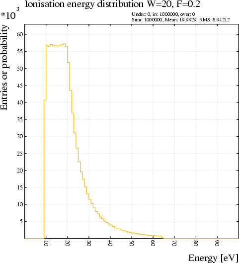
|
Format:
CALL RND_IONISATION_ENERGY(work_function, fano_factor, random_energy)
Example: Verification that the generator indeed asymptotically produces the specified work function and Fano factor.
Global emin=10 Global emax=500 Global npoint=50 Call book_matrix(evec,npoint) Call book_matrix(rmsvec,npoint) Call book_matrix(meanvec,npoint) Call book_histogram(nhist,100,-0.5,99.5)Global w=20 Global f=0.2
For ie From 1 To npoint Do Call book_histogram(nhist,100,-0.5,99.5) Global estart=emin*(emax/emin)^((ie-1)/(npoint-1)) For irndm From 1 To 100000 Do Global ne=0 Global etot=estart Do Call rnd_ionisation_energy(w,f,eloss) If etot-eloss>0 Then Global etot=etot-eloss Global ne=ne+1 Else Leave Endif Enddo Call fill_histogram(nhist,ne) Enddo Global evec[ie]=estart Global rmsvec[ie]=rms(nhist) Global meanvec[ie]=mean(nhist) Enddo
!options log-x Call plot_frame(emin,0,emax,80,`Energy [eV]`, ... `Energy deposited per electron [eV]`, ... `Energy used per electron`) Call plot_line(evec,evec/meanvec,`function-1`) Global v=70 Call plot_line(50,v,80,v,`function-1`) Call plot_text(100,v,`Heed model`,`function-1`,`left-half`)
Global fvec=w/(1-0.45*w/evec) Call plot_line(evec[2+row(size(evec)-2)],fvec[2+row(size(evec)-2)], ... `function-2`) Global v=v-5 Call plot_line(50,v,80,v,`function-2`) Call plot_text(100,v,`W/(1-V/E)`,`function-2`,`left-half`) Call plot_line(emin,w,emax,w,`comment`) Call plot_text(15,22,`w<SUB>s</SUB>`,`title`) Call plot_end
Call plot_frame(emin,0,emax,0.5,`Energy [eV]`, ... `RMS<SUP>2</SUP>/mean`,`Fano factor`) Call plot_line(evec,rmsvec^2/meanvec,`function-1`) Call plot_line(emin,f,emax,f,`comment`) Call plot_text(50,0.16,`Asymptotic Fano factor`,`title`) !rep comment linetype solid Call plot_arrow(w,0.03,w,0,`comment`) !rep comment linetype dashed Call plot_text(w,0.042,`Mean work`,`title`,`centre,half`) Call plot_end
For each step of the drift-line, the procedure uses the Townsend coefficients to compute the probability that an electron is produced, and the attachment coefficients to compute the probability that an electron is lost.
According to these probabilities, electrons are created or absorbed at each step.
The procedure can be applied both to drift-lines computed with the Runge_Kutta_Fehlberg and with Monte_Carlo methods. In the latter case, the use of the PROJECTED-PATH-INTEGRATION integration parameter is recommended in order to avoid a step size dependence in the multiplication.
The procedure can be called repeatedly for the same drift line.
Format:
CALL RND_MULTIPLICATION(ne, [ni])
Example:
&DRIFT
integration-parameters projected m-c-dist-int 0.0002
Call drift_electron_3(0.15,0,0,status,time,diff,aval,att)
Say "Mean RKF aval: {aval}, loss: {att}, product: {aval*att}, status {status}"
Call book_histogram(hist,50,0,2*aval*att)
Global nrndm=500
For i From 1 To nrndm Do
   Call drift_mc_electron(0.15,0,0)
   Call rnd_multiplication(a)
   Call fill_histogram(hist,a)
   If entier(i/100)*100=i Then
      !options log-y
      Call plot_histogram(hist)
      Call plot_end
   Endif
Enddo
Format:
CALL RND_UNIT_SPHERE(x, y, z)
Example:
Call book_histogram(h, 100, -1, 1)
For i From 1 To 1000000 Do
   Call rnd_unit_sphere(x, y, z)
   Call fill_histogram(h, x)
Enddo
Call plot_histogram(h,`Projected coordinate`)
Call plot_end
This verifies that one of the projections is uniformly distributed. The other projections should be similarly distributed.
This procedure relies on the G116 procedures of the CERN program library, a high-precision evaluation of the Vavilov distribution, typically 5 decimal are correct. Random numbers are generated using the V152 procedures. See the writeups http://consult.cern.ch/shortwrups/g116/top.html and http://consult.cern.ch/shortwrups/v152/top.html for particulars.
The following restrictions apply: 0.01\ \≤\ \κ\ \≤\ 10 and 0\ \≤\ \β\²\ \≤\ 1
The procedure seems to have difficulty coping with a few narrow ranges of \κ values (around 0.35 and 0.92), for broad ranges of \β\². In those cases, a value of 0 is returned.
A faster, but considerably less accurate, version is available with the RND_VAVILOV_FAST procedure.
Format:
CALL RND_VAVILOV(\κ, \β\², random_number)
This procedure relies on the G115 procedures in the CERN program library. This is a low-precision evaluation of the Vavilov distribution, typically only 1-2 decimal places are correct. See the writeup for particulars: http://consult.cern.ch/shortwrups/g115/top.html for particulars.
The following restrictions apply: 0.01\ \≤\ \κ\ \≤\ 12 and 0\ \≤\ \β\²\ \≤\ 1
A much slower, but considerably more accurate, version is available with the RND_VAVILOV procedure.
Format:
CALL RND_VAVILOV(\κ, \β\², random_number)
Calling this procedure is useful only if you draw the next fill area with GKS_AREA, most other procedures set the attributes before plotting.
Format:
CALL SET_AREA_ATTRIBUTES(representation)
Additional information on:
Calling this procedure is useful only if you draw the next polyline with GKS_POLYLINE, most other procedures set the attributes before plotting.
Format:
CALL SET_LINE_ATTRIBUTES(representation)
Additional information on:
Calling this procedure is useful only if you draw the next polymarker with GKS_POLYMARKER, most other procedures set the attributes before plotting.
Format:
CALL SET_MARKER_ATTRIBUTES(representation)
Additional information on:
Calling this procedure is useful only if you draw the next text with GKS_TEXT, most other procedures set the attributes before plotting.
Format:
CALL SET_TEXT_ATTRIBUTES(representation)
Additional information on:
Format:
CALL SKIP_HISTOGRAM([number_to_be_skipped])
Example: Suppose, we usually plot 3 histograms in a row and now wish to comment one of these out, without changing the representations of the others. Then we could do this:
Call plot_histogram(hnheed,`n<SUM>e</SUB>`,`Electron count`)
* Call plot_histogram(hnexp,``,``,`noframe`)
Call skip_histogram
Call plot_histogram(hnsrim,``,``,`noframe`)
Call plot_end
The points in the array are supposed to be equidistant and in sequence. Each element is replaced by the Gaussian average of the surrounding points:
       +n_w
x_i := Sum       w_j x_i+j
       j = -n_w

        -(j/sigma)^2/2
w_j = e
Near the end-points of the array, the sum is truncated symmetrically to prevent an asymmetric bias.
Thus, the first and last point are not changed.
The integral of the array is automatically conserved.
Format:
CALL SMOOTH(x[, n_w[, sigma]])Example: a string of Gaussian random numbers is smoothed.
Global n=10000
Call book_matrixx, n)
For i From 1 To n Do
   Global x[i] = rnd_gauss
Enddo
Call plot_frame(0, -5, n+1, +5)
Call plot_markers(row(n), x, `function-1`)
Call smooth(x)
Call plot_markers(row(n), x, `function-2`)
Call plot_end
Additional information on:
Sorting a matrix of higher dimensionality than 1 is equivalent to first unravelling the matrix, sorting its elements and then restoring the original shape of the matrix.
Format:
CALL SORT_MATRIX(matrix)
This procedure is available only in Lunix compilations.
Format:
CALL SLEEP(seconds)
The vectors to be stored must have the same length as the other signals currently stored. The time vector can not be changed with this command.
Format:
CALL STORE_SIGNAL(electrode, direct [, cross-induced])
Additional information on:
Both matrices should exist prior to the call and the size of the selected area should match the size of the matrix which is to be stored.
This procedure is used to process array indexing on the left hand side of Global statements. The procedure is not intended to be called by the user. Using the Global statement is much simpler.
Format:
CALL STORE_SUBMATRIX(ndim, nsel_1, nsel_2, ..., isel_1_1, ...
     isel_1_2, ..., isel_2_1, isel_2_2, ... , isel_n_1, isel_n_2, ...
     ref_submatrix, ref_matrix)
Format:
CALL STRING_DELETE(string, istart, iend, output)
Example:
Call string_delete(`abc def ghi`,4,8,out)
Additional information on:
The first character of a string is numbered 1. Returns 0 if the substring is not found within the string.
Format:
CALL STRING_INDEX(string, substring, index)
Example:
Call string_index(`abc def`,`def`,pos)
Say "`def` starts at character {pos} in `abc def`"
Format:
CALL STRING_LENGTH(string, length)
Example:
Call string_length(`abc`,n)
Say "Length of string is {n} characters."
Format:
CALL STRING_LOWER(string)
Example:
Global str=`ABCDEF`
Call string_lower(str)
Say {str}
Format:
CALL STRING_MATCH(string, pattern, match)
Example:
Call string_match(`abc-def`,`ab#cdef-de#fghi-#ghijkl`,match)
If match Then
   Say "The strings match."
Else
   Say "The strings do not match."
Endif
Format:
CALL STRING_PORTION(string, istart, iend, portion)
Example:
Call string_portion(`abc def ghi`,5,7,out)
Say "Characters 5 through 7 of `abc def ghi` are: {out}"
This procedure does not replace characters that stem from earlier replacements.
Format:
CALL STRING_REPLACE(string, search, replace)
Examples:
Global mixture=`argon 90 methane 10`
Global gas_file=mixture/`.gas`
Call string_replace(gas_file,` `,`_`)
Say "|{gas_file}|"
In order to create a file name without blanks from a gas mixture, the blanks are replaced by underscores.
Vector a 1.23 2.34 3.45 4.56Global b=string(a) Call string_replace(b,`, `,` `) Call string_replace(b,`(`,``) Call string_replace(b,`)`,``) Say "-{b}-"
Prints the vector A without parentheses and commata.
Global a=`baaaaa`
Call string_replace(a,`ba`,`bbb`)
Say "|{a}|"
After the call, a will be equal to `bbbaaaa` and not `bbbbbbbbbbb`.
Format:
CALL STRING_UPPER(string)
Example:
Global str=`abcdef`
Call string_upper(str)
Say {str}
Format:
CALL STRING_WORD(string, i, word)
Example:
Global str=`abc def ghi`
Call string_words(str,n)
Say "The string contains {n} words."
For i From 1 To n Do
    Call string_word(str,i,out)
    Say "Word {i} is {out}."
Enddo
Format:
CALL STRING_WORDS(string, n)
Example:
See STRING_WORD
The entire buffer is printed out at job completion.
Format:
CALL TIME_LOGGING( string )
Example:
Call time_logging(`Until timing test`)
Global x0=0.5
Global y0=1.5
Call plot_drift_area
For i From 1 To 100 Do
   Call drift_mc_electron(x0, y0, 0, status, time)
   Call plot_drift_line
Enddo
Call time_logging(`MC drifting`)
The TIME_LOGGING routine is called a first time to ensure that in the end we will record only the time spent in MC drifting will be recorded.
Format:
CALL THRESHOLD_CROSSING(electrode, threshold, options, ...
   ntime, time1 [,time2 [,time3 ...]])
Example:
For i From 1 To 100 Do
   signal
   convolute-signals range 0 1000 ...
      transfer-function (5*t/0.01)^5*exp(-5*t/0.01)
   Call threshold_crossing(1,-0.02,`rising,linear`,n,t1,t2)
   Say "Found {n} threshold crossings, 1st at {t1} nsec."
Enddo
Additional information on:
In the absence of a magnetic field, the orientation of the electric field is immaterial. The electric field may be specified either by the norm or as a vector, of which only the norm matters.
In the presence of a magnetic field, the transport parameters depend on the relative orientation of the electric and magnetic field vectors. Both fields therefore have to be specified as vectors.
If the magnetic field is omitted, then all 3\ components are assumed to be zero, irrespective of the magnetic field settings that may be in effect.
Each of the field components can either be a Number or a Matrix. It is permissible to specify 1 or 2 components of the field as Numbers and the other(s) as Matrices.
All components which are specified as Matrix, must have the same total size - they do not have to be 1-dimensional. If at least one component is specified as Matrix, then the output will be a 1-dimensional Matrix with length equal to the overall size of the arguments of type Matrix. Otherwise the result will be a Number.
The electric field should be in V/cm. The magnetic field, if present, should be expressed in native units of 0.01\ T or 100\ G. The Townsend coefficient is returned in 1/cm.
Formats:
CALL TOWNSEND(e, townsend)
CALL TOWNSEND(ex, ey, ez, townsend)
CALL TOWNSEND(ex, ey, ez, bx, by, bz, townsend)
In the absence of a magnetic field, the orientation of the electric field is immaterial. The electric field may be specified either by the norm or as a vector, of which only the norm matters.
In the presence of a magnetic field, the transport parameters depend on the relative orientation of the electric and magnetic field vectors. Both fields therefore have to be specified as vectors.
Each of the field components can either be a Number or a Matrix. It is permissible to specify 1 or 2 components of the field as Numbers and the other(s) as Matrices.
All components which are specified as Matrix, must have the same total size - they do not have to be 1-dimensional. If at least one component is specified as Matrix, then the output will be a 1-dimensional Matrix with length equal to the overall size of the arguments of type Matrix. Otherwise the result will be a Number.
The electric field should be in V/cm. The magnetic field, if present, should be expressed in native units of 0.01\ T or 100\ G. The diffusion is returned in \√cm.
SIGMA_T can be used as a synonym for TRANSVERSE_DIFFUSION.
Formats:
CALL TRANSVERSE_DIFFUSION(e, sigma_t)
CALL TRANSVERSE_DIFFUSION(ex, ey, ez, sigma_t)
CALL TRANSVERSE_DIFFUSION(ex, ey, ez, bx, by, bz, sigma_t)
This procedure accepts both a Number and a Matrix as 3rd argument. The value that is returned will be of the same type and shape.
This procedure relies on the G116 procedures in the CERN program library. This is a higher-precision evaluation of the Vavilov distribution than the one used for RND_VAVILOV, and is typically correct to 5 decimal places. See the writeup for particulars: http://consult.cern.ch/shortwrups/g116/top.html for particulars.
The following restrictions apply: 0.01\ \≤\ \κ\ \≤\ 10 and 0\ \≤\ \β\²\ \≤\ 1
Format:
CALL VAVILOV(\κ, \β\², \λ, probability)
This component is zero when there is no magnetic field.
Each of the field components can either be a Number or a Matrix. It is permissible to specify some components of the field as Numbers and the other(s) as Matrices.
All components which are specified as Matrix, must have the same total size - they do not have to be 1-dimensional. If at least one component is specified as Matrix, then the output will be a 1-dimensional Matrix with length equal to the overall size of the arguments of type Matrix. Otherwise the result will be a Number.
The electric field should be in V/cm, the magnetic field has to be in native units of 100\ G or 0.01\ T, and the drift velocity is returned in cm/\μsec.
Format:
CALL VELOCITY_BTRANSVERSE(ex, ey, ez, bx, by, bz, drift)
If there is no magnetic field, then the magnetic field must not be specified. In this case, the values returned by this procedure coincide with those returned by DRIFT_VELOCITY.
Each of the field components can either be a Number or a Matrix. It is permissible to specify some components of the field as Numbers and the other(s) as Matrices.
All components which are specified as Matrix, must have the same total size - they do not have to be 1-dimensional. If at least one component is specified as Matrix, then the output will be a 1-dimensional Matrix with length equal to the overall size of the arguments of type Matrix. Otherwise the result will be a Number.
The electric field should be in V/cm, the magnetic field has to be in native units of 100\ G or 0.01\ T, and the drift velocity is returned in cm/\μsec.
Format:
CALL VELOCITY_E(ex, ey, ez, bx, by, bz, drift)
Example:
&GAS magboltz argon 92 co2 8 e/p-range 0.05 8&MAIN Global emin=60 Global emax=7000 Global n=200 Global e=emin*(emax/emin)^((row(n)-1)/(n-1)) Call velocity_e(0,0,e,v) !options log-x Call plot_graph(e,v,`E [V/cm]`,`Drift velocity [cm/microsec]`, ... `Magboltz vs Zhao et al.`) Vector ezhao 0.07 0.14 0.21 0.28 0.35 0.42 0.49 0.559 0.629 0.699 0.769 0.839 0.909 0.979 1.049 1.119 1.189 1.259 1.329 1.399 1.573 1.748 1.923 2.098 2.448 2.797 3.147 3.497 3.846 4.196 4.545 4.895 5.245 5.735
Vector vzhao 0.52 1.15 1.89 2.77 3.56 4.18 4.57 4.78 4.82 4.79 4.71 4.62 4.53 4.43 4.35 4.3 4.26 4.23 4.2 4.2 4.2 4.24 4.29 4.36 4.49 4.57 4.59 4.58 4.56 4.5 4.47 4.44 4.4 4.4
Call plot_error_bar(ezhao*1000,vzhao,`circle`) Call plot_end
Magboltz is used to compute the drift velocity in a mixture of 92\ % argon and 8\ % CO\<SUB\>2\</SUB\>. The results are compared with the measurements of T. Zhao et al., NIM A340 (1994) 485. The E > 3000 V/cm region is controversial, apart from that the two are in good agreement. This is an abridged version of http://cern.ch/garfield/examples/gas/ArCO2_detail.html
This component is zero when there is no magnetic field.
Each of the field components can either be a Number or a Matrix. It is permissible to specify some components of the field as Numbers and the other(s) as Matrices.
All components which are specified as Matrix, must have the same total size - they do not have to be 1-dimensional. If at least one component is specified as Matrix, then the output will be a 1-dimensional Matrix with length equal to the overall size of the arguments of type Matrix. Otherwise the result will be a Number.
The electric field should be in V/cm, the magnetic field has to be in native units of 100\ G or 0.01\ T, and the drift velocity is returned in cm/\μsec.
Format:
CALL VELOCITY_ExB(ex, ey, ez, bx, by, bz, drift)
This routine differs from WEIGHTING_FIELD_3 in that it expects only the (x,y) part of the location, assuming z=0.
This procedure should be called from within the signal section.
Format:
CALL WEIGHTING_FIELD(x, y, ex, ey, ez, electrode)
Additional information on:
This procedure differs from WEIGHTING_FIELD in that it expects an (x,y,z) set of coordinates.
This procedure should be called from within the signal section.
Format:
CALL WEIGHTING_FIELD_3(x, y, z, ex, ey, ez, electrode)
Additional information on:
Histograms can, by means of the WRITE_HISTOGRAM_RZ procedure, also be written out in a format suitable for use with PAW. Using the h2root program, such files can be converted for use with root, see http://root.cern.ch/root/HowtoConvert.html
Calling this procedure does not interfere with filling of the histogram and an autorange histogram can be written to disk before the range has been set.
This procedure is for instance used when one job fills a set of histograms which are, probably repeatedly, fitted by another job. Another application is a found in calculations where statistics are accumulated over a series of jobs. The first job would create the histogram and fill it, all successive jobs read the existing histogram, continue filling it, and write it back to the file at the end of the job. Care should be taken that the global option DELETE-OLD-MEMBER has been switched on before doing this.
The procedure sets the OK global variable to True if the histogram has been written and to False if it hasn't.
Format:
CALL WRITE_HISTOGRAM(reference, file [, member [, remark]])
Example:
Global chamber=1(calculation of e.g. arrival time histograms for chamber 1)
Global hfile `CHAMBER`/string(chamber)/`.HIST` Global i=0 Global exist=True Global n=0 While exist Do Global i=i+1 Call inquire_histogram(reference(i),exist) If exist Then Call write_histogram(reference(i),hfile) Global n=n+1 Endif Enddo Say "Have written {n} histograms."
In this example, the input file is assumed to contain a cell section that enters the elements for chambers 1, 2, etc depending on the setting of the global variable "chamber".
At the end of the run, the user wishes to keep all histograms for further examination. The loop in the example writes all histograms to a file (hfile) the name of which is CHAMBER1.HIST, CHAMBER2.HIST etc. depending on the setting of the global variable "chamber".
All histograms are written to the same file, but they will be distinguished by their member names which are defaulted to the name of the global variables associated with the histogram.
This example assumes that no histograms have been deleted during the run, as it assumes the histograms are numbered from 1 on.
Additional information on:
RZ files can be converted for use by root with the h2root program, see http://root.cern.ch/root/HowtoConvert.html
An autorange histogram can only be written out to an RZ file once its range has been established. Use the WRITE_HISTOGRAM and GET_HISTOGRAM procedures to save and recover such an histogram.
The procedure sets the OK global variable to True if the histogram has been written and to False if it hasn't.
Format:
CALL WRITE_HISTOGRAM_RZ([reference [, file [, title]]])
Example:
Call book_histogram(a,200)
For i From 1 To 10000 Do
   Call fill_histogram(a,rnd_landau)
Enddo
Call plot_histogram(a,`Energy`,`Landau`)
Call plot_end
Call write_histogram_rz(a,`hist.rz`,`Landau distribution`)
This generates an histogram with a Landau distribution and writes the histogram to a file called "hist.rz". Garfield replies telling that the histogram has been written with PAW identifier 1 and cycle number 1. To read it back with PAW, one would type:
h/file 20 hist.rz
h/pl 1
Additional information on:
The Garfield WWW example pages contain a Matlab function that reads a file written by WRITE_MATRIX (contributed by Guy Garty): http://cern.ch/garfield/examples/load_garf.m
The procedure sets the OK global variable to True if the matrix is successfully written, and to False in case of a problem.
Format:
CALL WRITE_MATRIX(matrix, file [, member])
Example:
If type(global(`ABC`))#`Matrix` Then
   Call inquire_member(`abc.mat`,`abc`,`matrix`,exist)
   If exist Then
      Call get_matrix(abc,`abc.mat`)
      Call dimensions(abc,n_dim,dim_abc)
      Global nx=number(dim_abc[1])
      Global ny=number(dim_abc[2])
      Call delete_matrix(dim_abc)
   Else
      Global nx=20
      Global ny=30
      Call book_matrix(abc,nx,ny)
      For i From 1 To nx Do
         For j From 1 To ny Do
            Global abc[i;j]=sin(i)*exp(j/10)
         Enddo
      Enddo
      Call write_matrix(abc,`abc.mat`)
   Endif
Endif
First, one checks whether ABC is already in memory. If it is, nothing is done. Otherwise, an attempt is made to recuperate the matrix from a file. If this doesn't work, then the matrix is generated and stored in the file so that next time, the matrix can be recuperated from there.
Additional information on:
The procedure searches for zero crossings between 2 adjacent tabulated values, then performs a linear or quadratic interpolation over the neighbouring range.
Do not confuse this procedure with the ZEROES function.
Format:
CALL ZEROES(x_vector, y_vector, nzero, zero1, zero2, ...)
Examples:
Call get_signal(1,time,direct,cross)
Global signal=direct+cross
Call zeroes(time,signal/maximum(signal)-0.5,nz,t1,t2)
If nz<2 Then
   Say "Time range not long enough to determine FWHM."
Else
   Say "FWHM of the signal: {t2-t1}"
Endif

Global r=row(200)/10
Global v=sin(r)
Call zeroes(r,v,nz,z1,z2,z3)
Say "Zeroes: {nz} - {z1,z2,z3}"
The first example computes the FWHM of a signal, the second
example finds the zeroes of the sine function.
Additional information on:
Formatted on 21/01/18 at 16:55.