

Compact Muon Solenoid
LHC, CERN
| CMS-BPH-15-001 ; CERN-EP-2018-125 | ||
| Angular analysis of the decay ${\mathrm{B^{+}} \to \mathrm{K^{+}} \mu^{+} \mu^{-}}$ in proton-proton collisions at $\sqrt{s} = $ 8 TeV | ||
| CMS Collaboration | ||
| 2 June 2018 | ||
| Phys. Rev. D 98 (2018) 112011 | ||
| Abstract: The angular distribution of the flavor-changing neutral current decay ${\mathrm{B^{+}} \to \mathrm{K^{+}} \mu^{+} \mu^{-}}$ is studied in proton-proton collisions at a center-of-mass energy of 8 TeV. The analysis is based on data collected with the CMS detector at the LHC, corresponding to an integrated luminosity of 20.5 fb$^{-1}$. The forward-backward asymmetry $A_{\mathrm{FB}}$ of the dimuon system and the contribution $F_{\mathrm{H}}$ from the pseudoscalar, scalar, and tensor amplitudes to the decay width are measured as a function of the dimuon mass squared. The measurements are consistent with the standard model expectations. | ||
| Links: e-print arXiv:1806.00636 [hep-ex] (PDF) ; CDS record ; inSPIRE record ; HepData record ; CADI line (restricted) ; | ||
| Figures & Tables | Summary | Additional Figures | References | CMS Publications |
|---|
| Figures | |
png pdf |
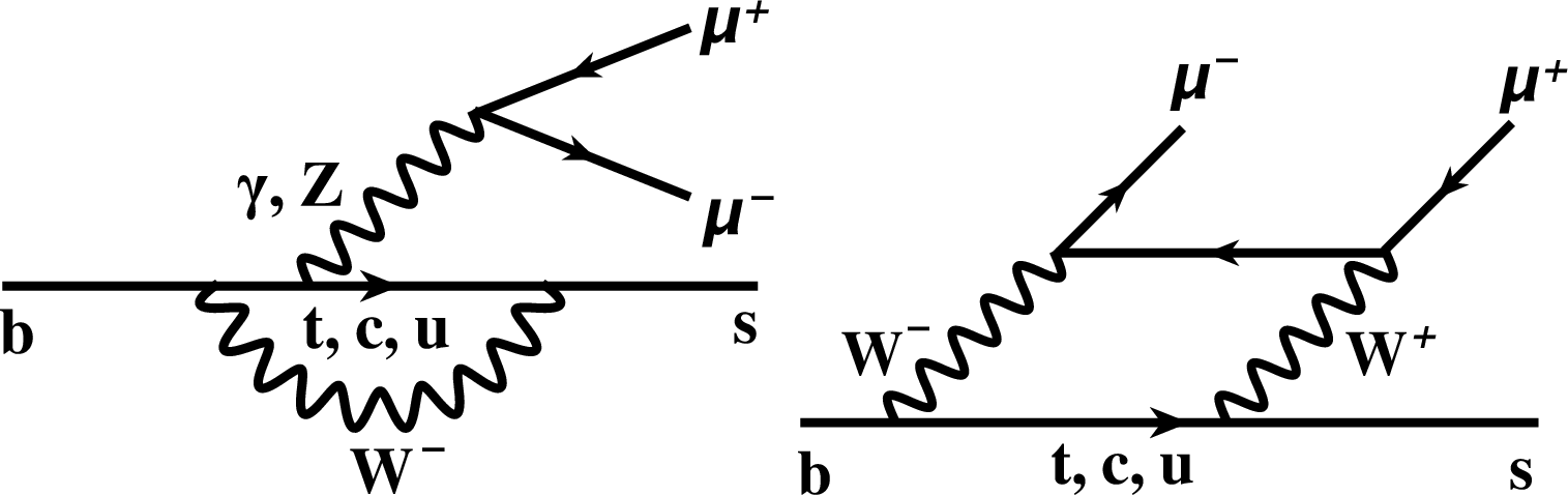
Figure 1:
The SM electroweak $ {\mathrm {Z}} / {\gamma}$ penguin (left) and $ {\mathrm {W^+}} {\mathrm {W^-}}$ box (right) diagrams for the decay process ${{{\mathrm {B}^{+}}}\to {\mathrm {K^+}} {{\mu ^+}} {{\mu ^-}}}$. |
png pdf |
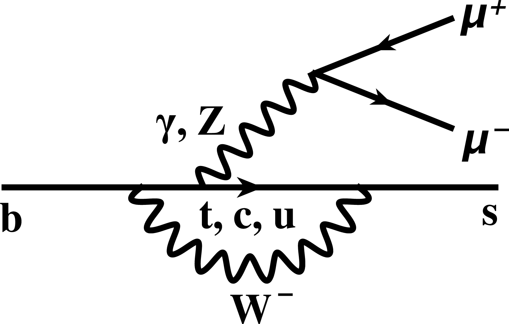
Figure 1-a:
The SM electroweak $ {\mathrm {Z}} / {\gamma}$ penguin diagram for the decay process ${{{\mathrm {B}^{+}}}\to {\mathrm {K^+}} {{\mu ^+}} {{\mu ^-}}}$. |
png pdf |
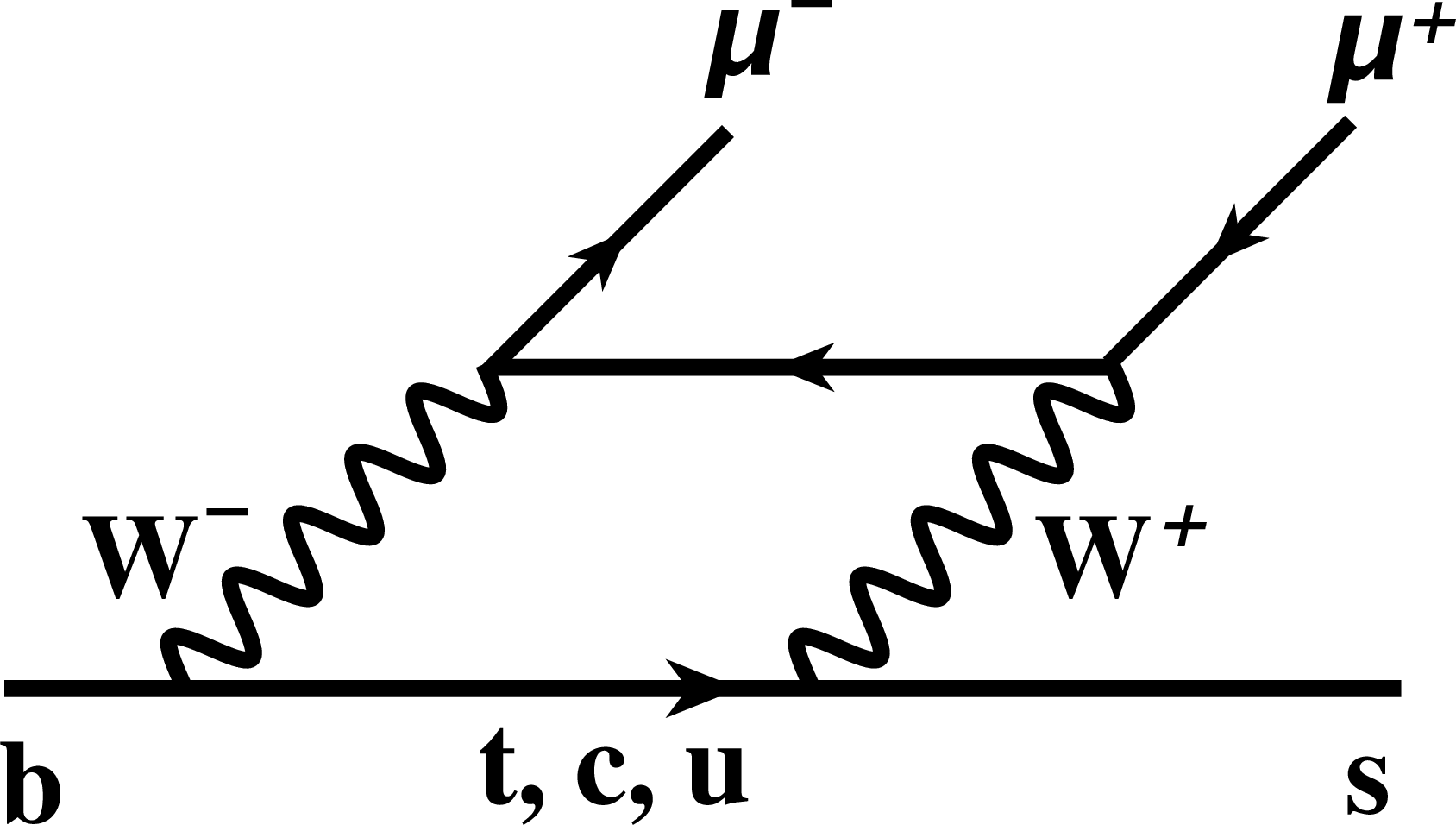
Figure 1-b:
The SM electroweak $ {\mathrm {W^+}} {\mathrm {W^-}}$ box diagram for the decay process ${{{\mathrm {B}^{+}}}\to {\mathrm {K^+}} {{\mu ^+}} {{\mu ^-}}}$. |
png pdf |
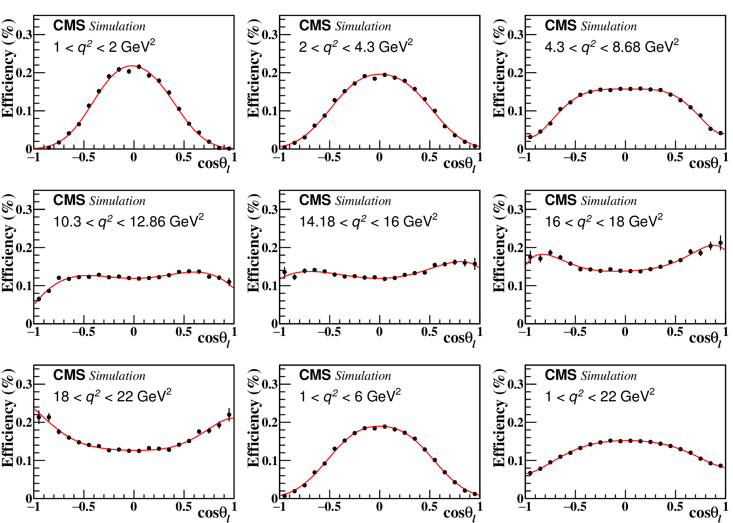
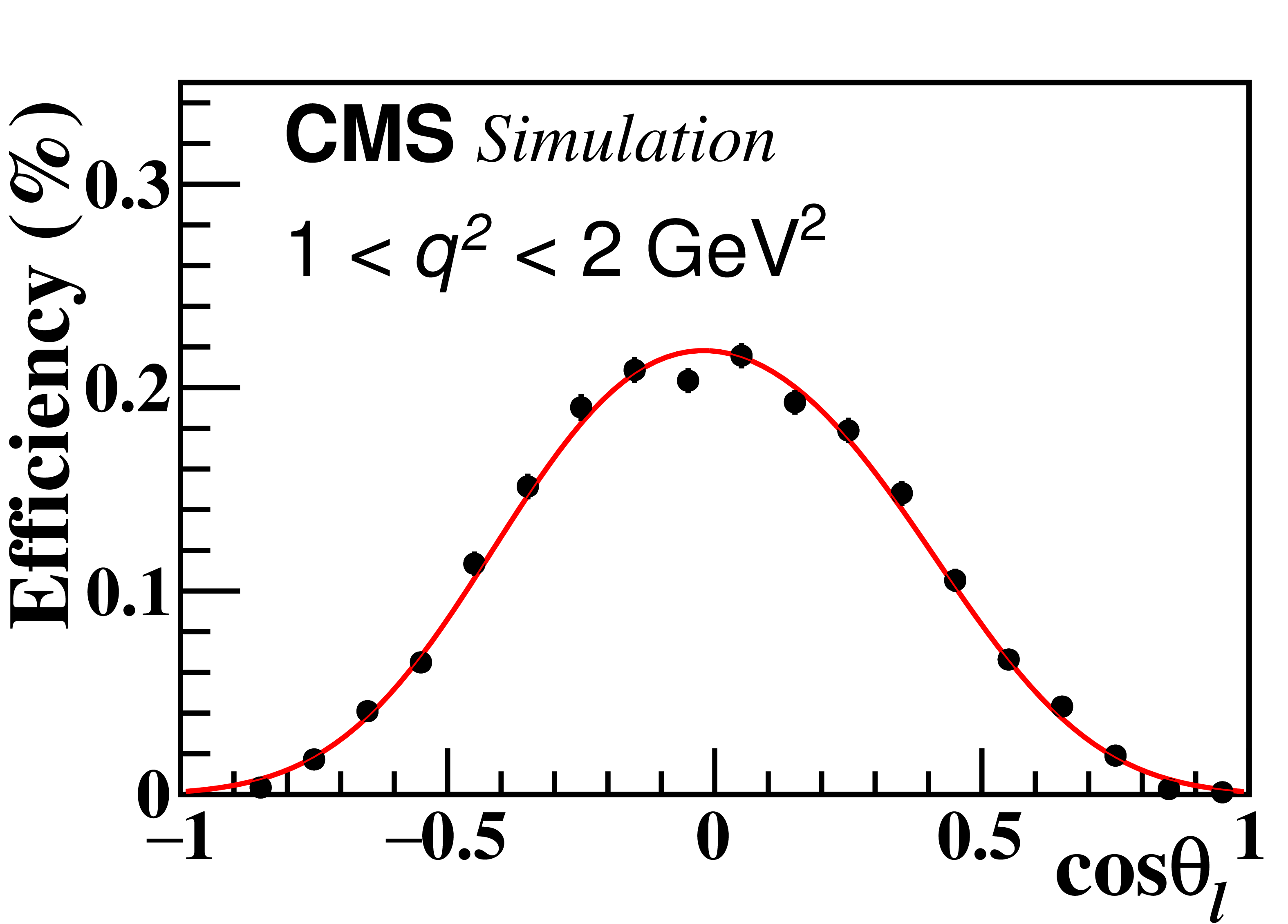
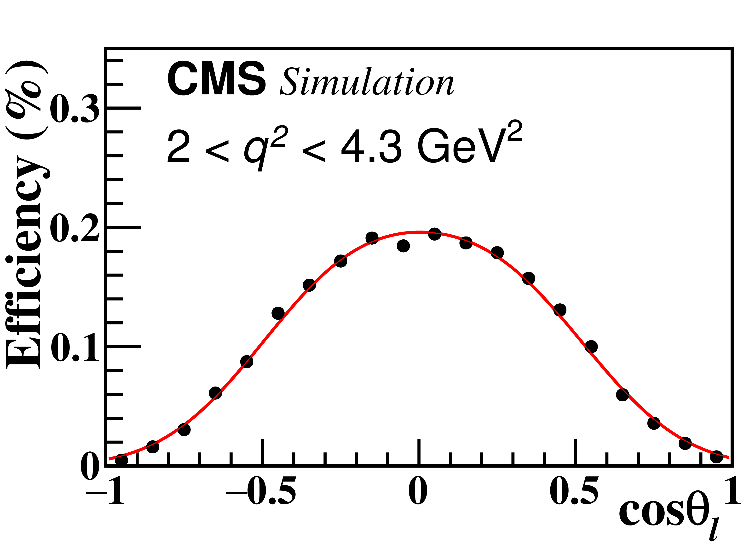
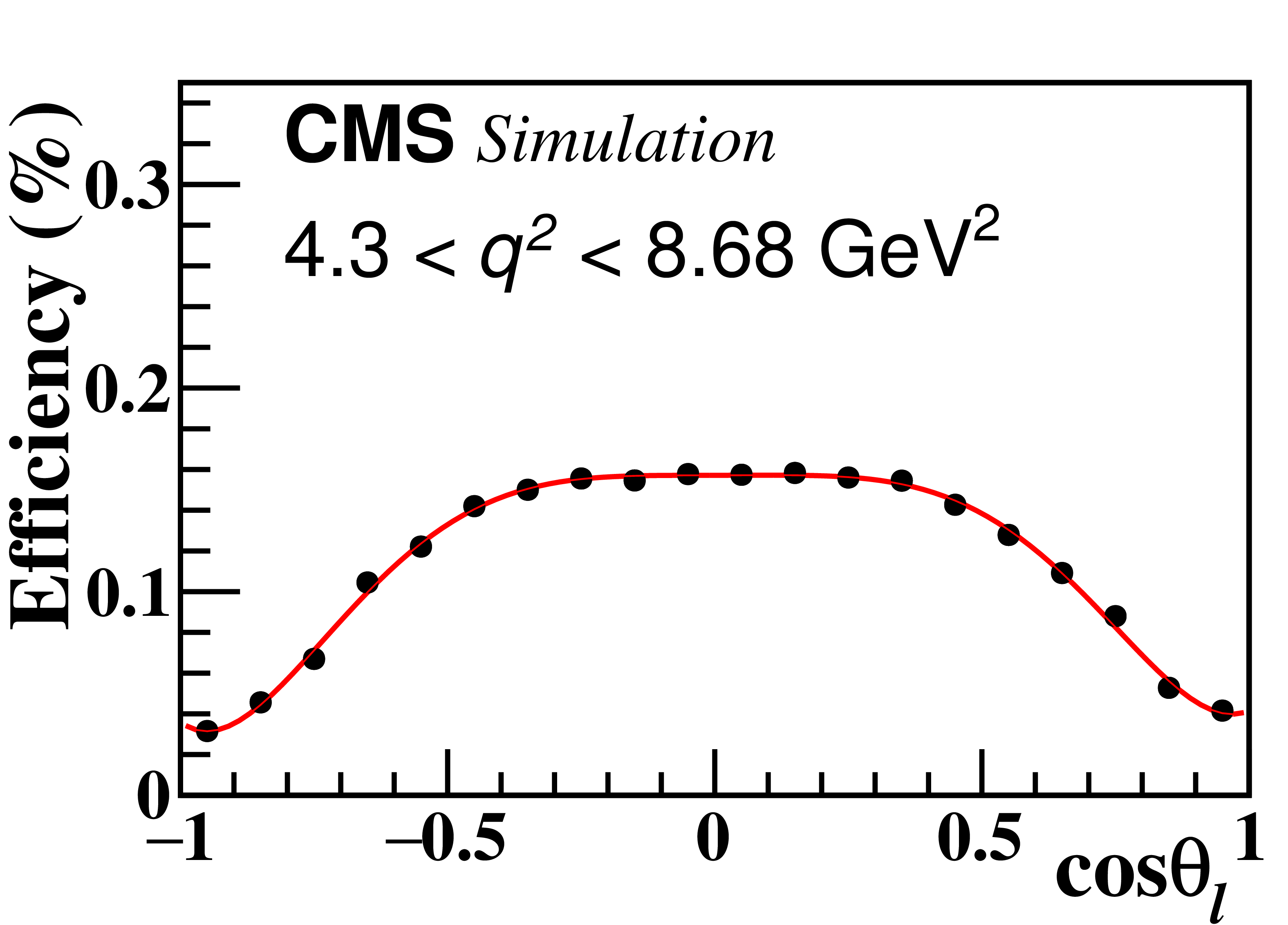
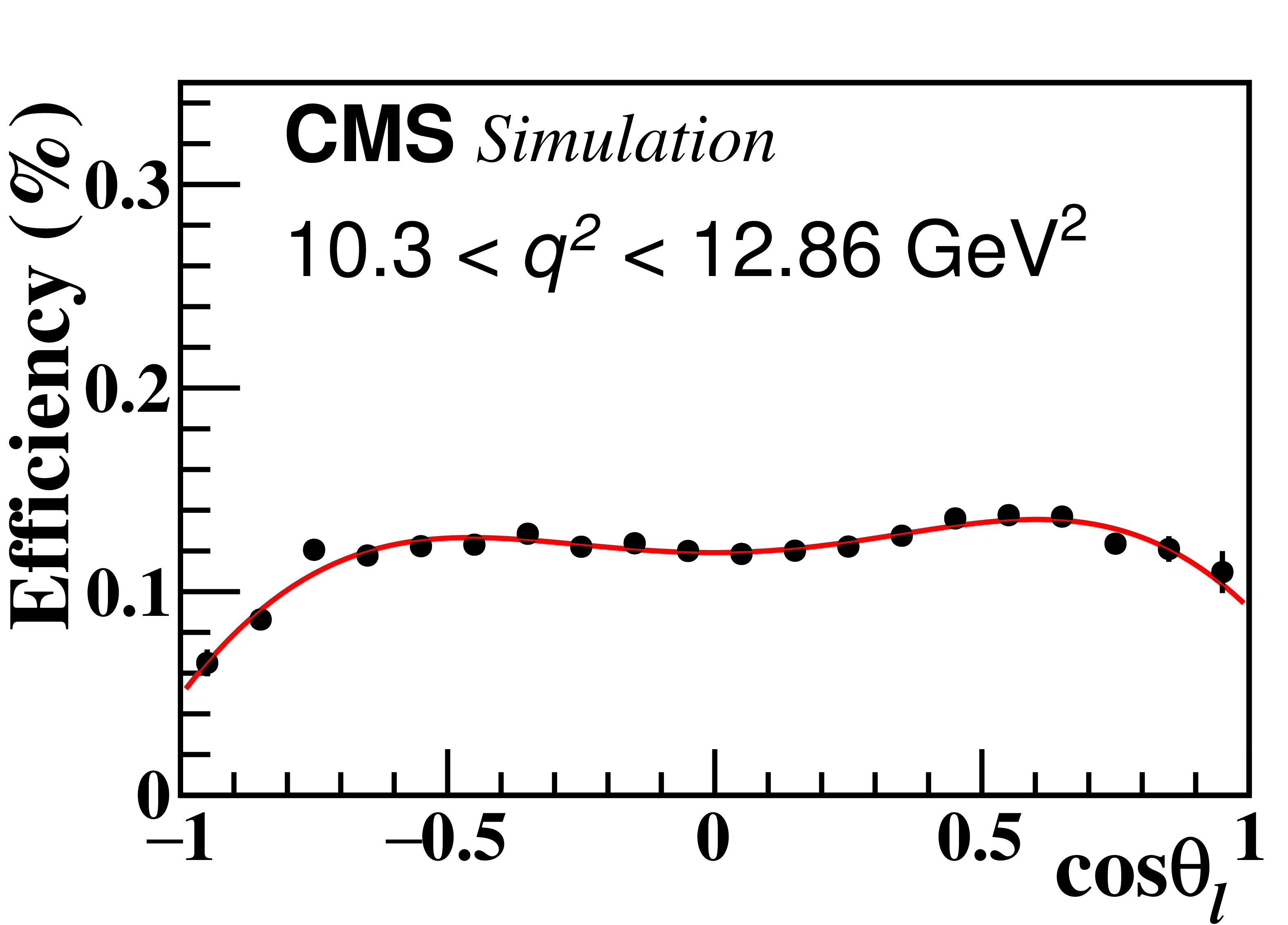
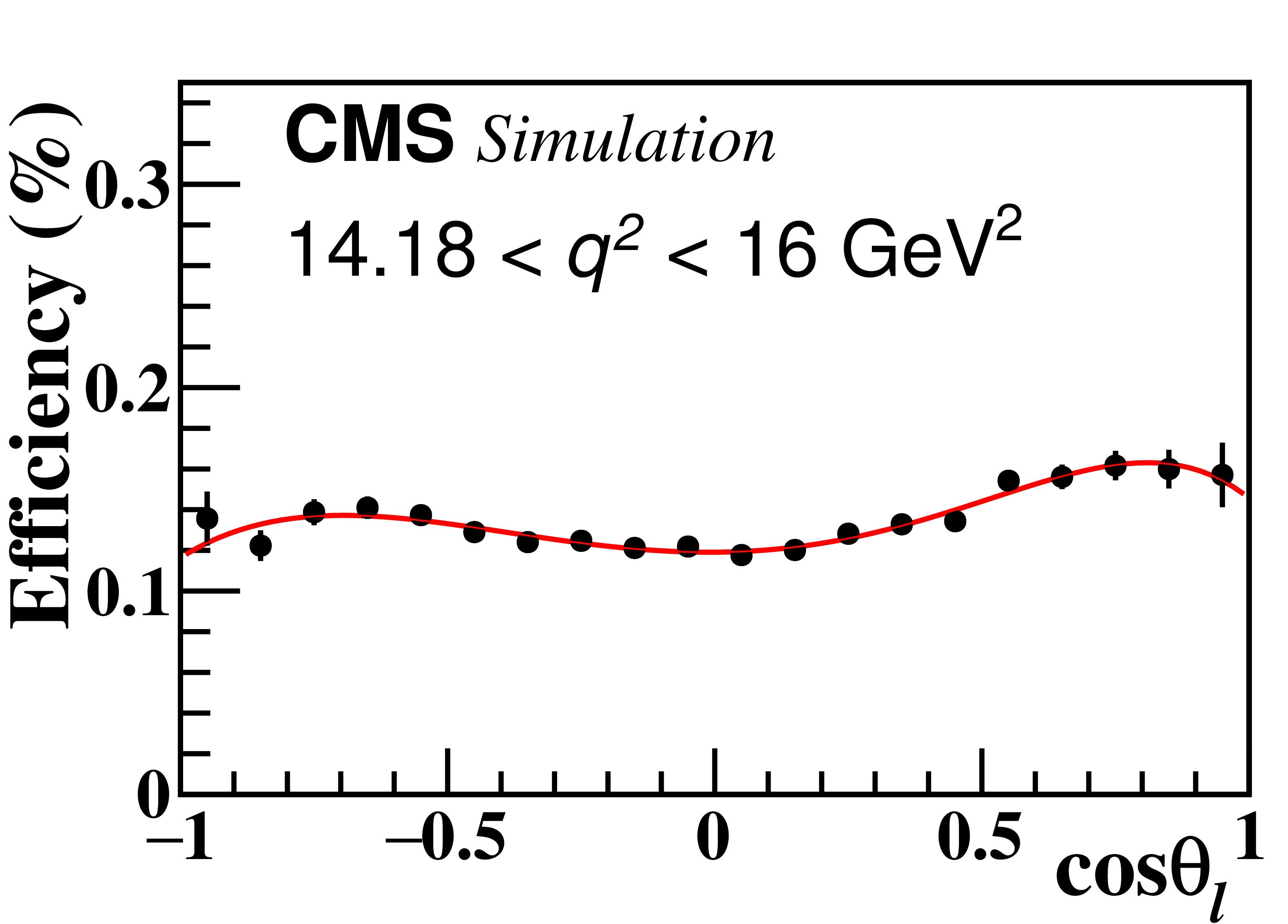
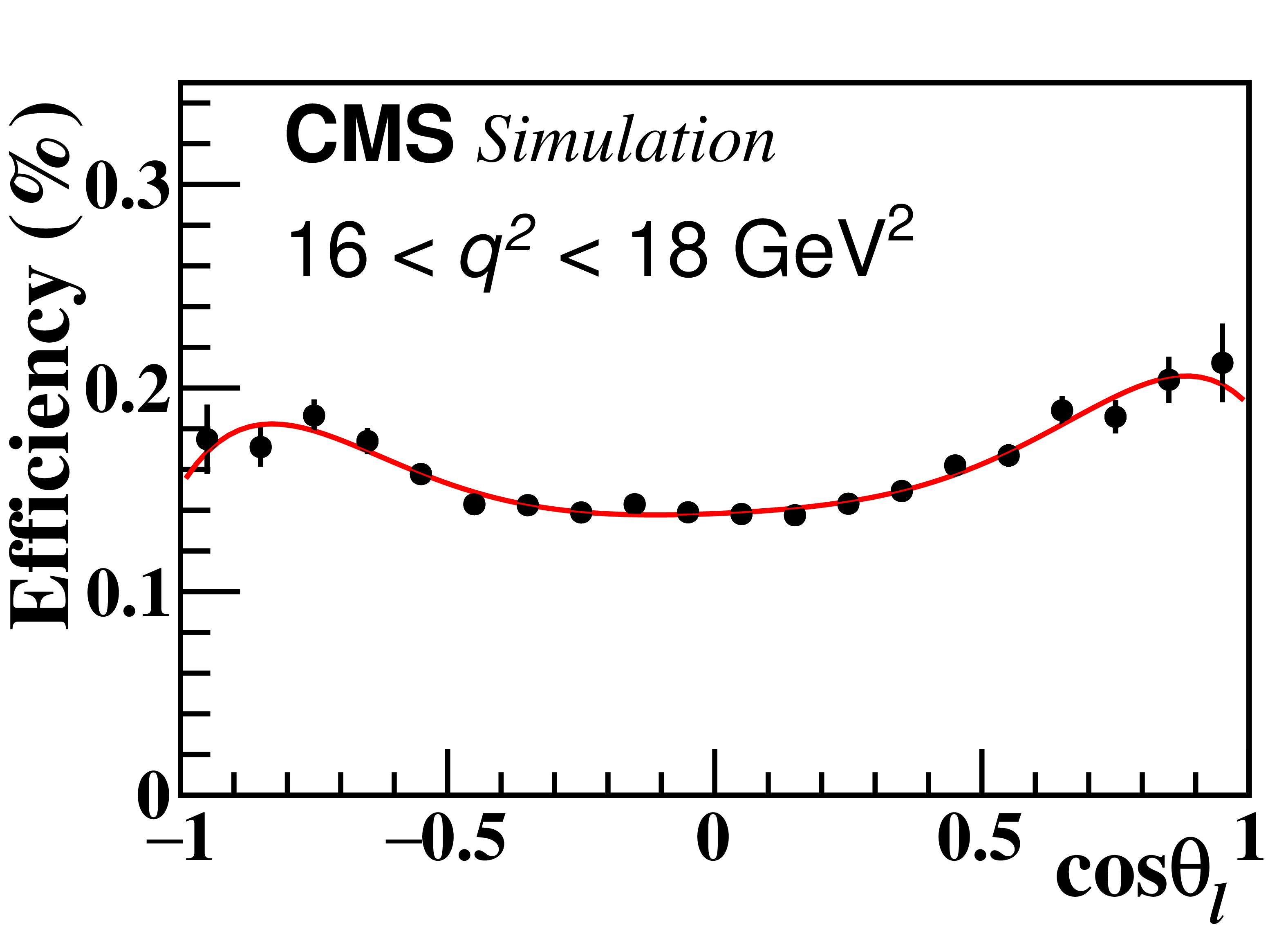
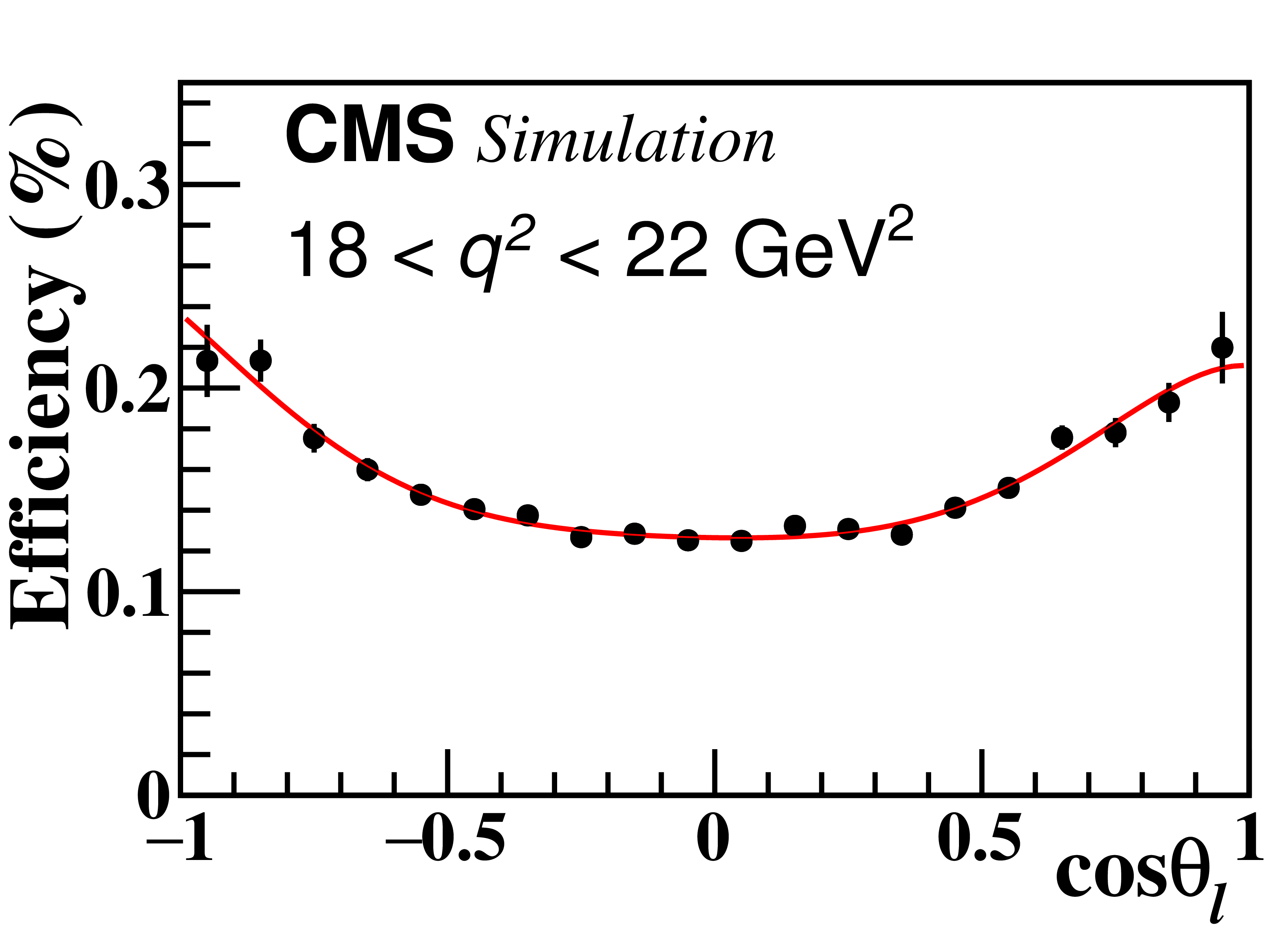
Figure 2:
The signal efficiency determined from simulated events as a function of $\cos\theta _{\ell}$ for the different $q^2$ ranges (points). The vertical bars indicate the statistical uncertainty. The curves show the sixth-order polynomial fits to the points. |
png pdf |
Figure 2-a:
The signal efficiency determined from simulated events as a function of $\cos\theta _{\ell}$ for 1 $ < q^2 < $ 2 GeV$^2$ (points). The vertical bars indicate the statistical uncertainty. The curves show the sixth-order polynomial fits to the points. |
png pdf |
Figure 2-b:
The signal efficiency determined from simulated events as a function of $\cos\theta _{\ell}$ for 2 $ < q^2 < $ 4.3 GeV$^2$ (points). The vertical bars indicate the statistical uncertainty. The curves show the sixth-order polynomial fits to the points. |
png pdf |
Figure 2-c:
The signal efficiency determined from simulated events as a function of $\cos\theta _{\ell}$ for 4.3 $ < q^2 < $ 8.68 GeV$^2$ (points). The vertical bars indicate the statistical uncertainty. The curves show the sixth-order polynomial fits to the points. |
png pdf |
Figure 2-d:
The signal efficiency determined from simulated events as a function of $\cos\theta _{\ell}$ for 10.3 $ < q^2 < $ 12.86 GeV$^2$ (points). The vertical bars indicate the statistical uncertainty. The curves show the sixth-order polynomial fits to the points. |
png pdf |
Figure 2-e:
The signal efficiency determined from simulated events as a function of $\cos\theta _{\ell}$ for 14.18 $ < q^2 < $ 16 GeV$^2$ (points). The vertical bars indicate the statistical uncertainty. The curves show the sixth-order polynomial fits to the points. |
png pdf |
Figure 2-f:
The signal efficiency determined from simulated events as a function of $\cos\theta _{\ell}$ for 16 $ < q^2 < $ 18 GeV$^2$ (points). The vertical bars indicate the statistical uncertainty. The curves show the sixth-order polynomial fits to the points. |
png pdf |
Figure 2-g:
The signal efficiency determined from simulated events as a function of $\cos\theta _{\ell}$ for 18 $ < q^2 < $ 22 GeV$^2$ (points). The vertical bars indicate the statistical uncertainty. The curves show the sixth-order polynomial fits to the points. |

png pdf |
Figure 2-h:
The signal efficiency determined from simulated events as a function of $\cos\theta _{\ell}$ for 1 $ < q^2 < $ 6 GeV$^2$ (points). The vertical bars indicate the statistical uncertainty. The curves show the sixth-order polynomial fits to the points. |

png pdf |
Figure 2-i:
The signal efficiency determined from simulated events as a function of $\cos\theta _{\ell}$ for 1 $ < q^2 < $ 22 GeV$^2$ (points). The vertical bars indicate the statistical uncertainty. The curves show the sixth-order polynomial fits to the points. |

png pdf |
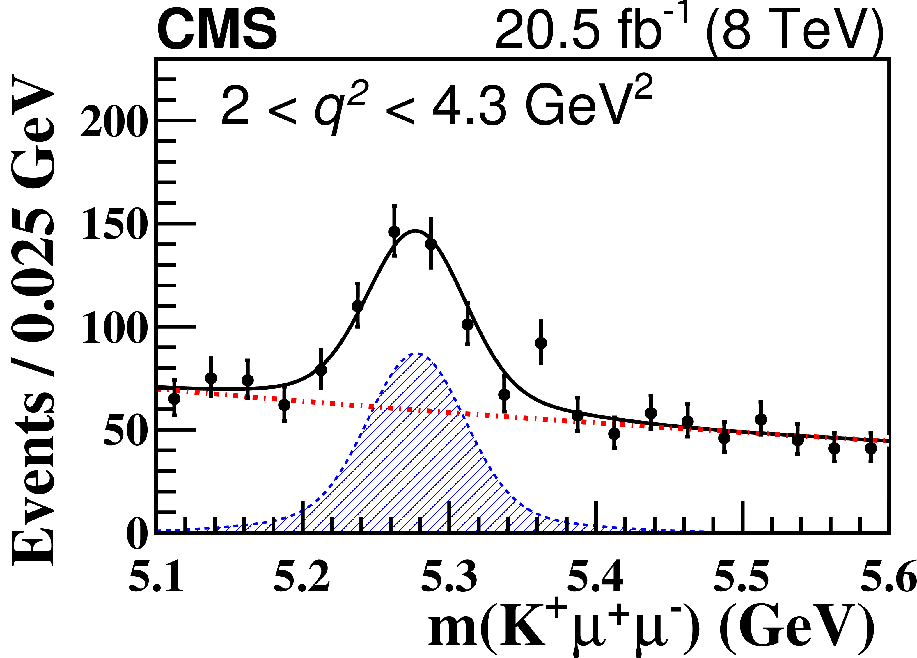
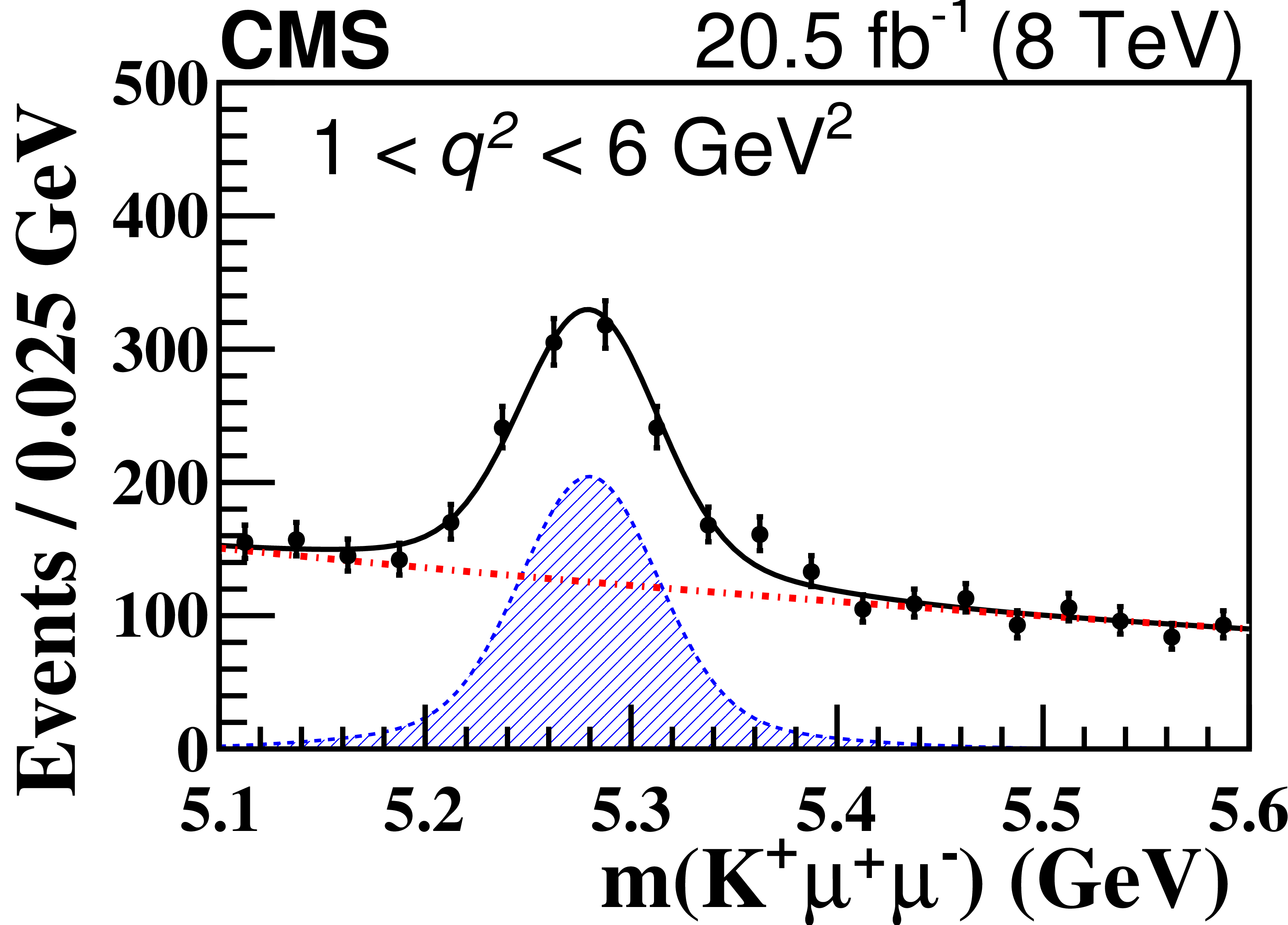
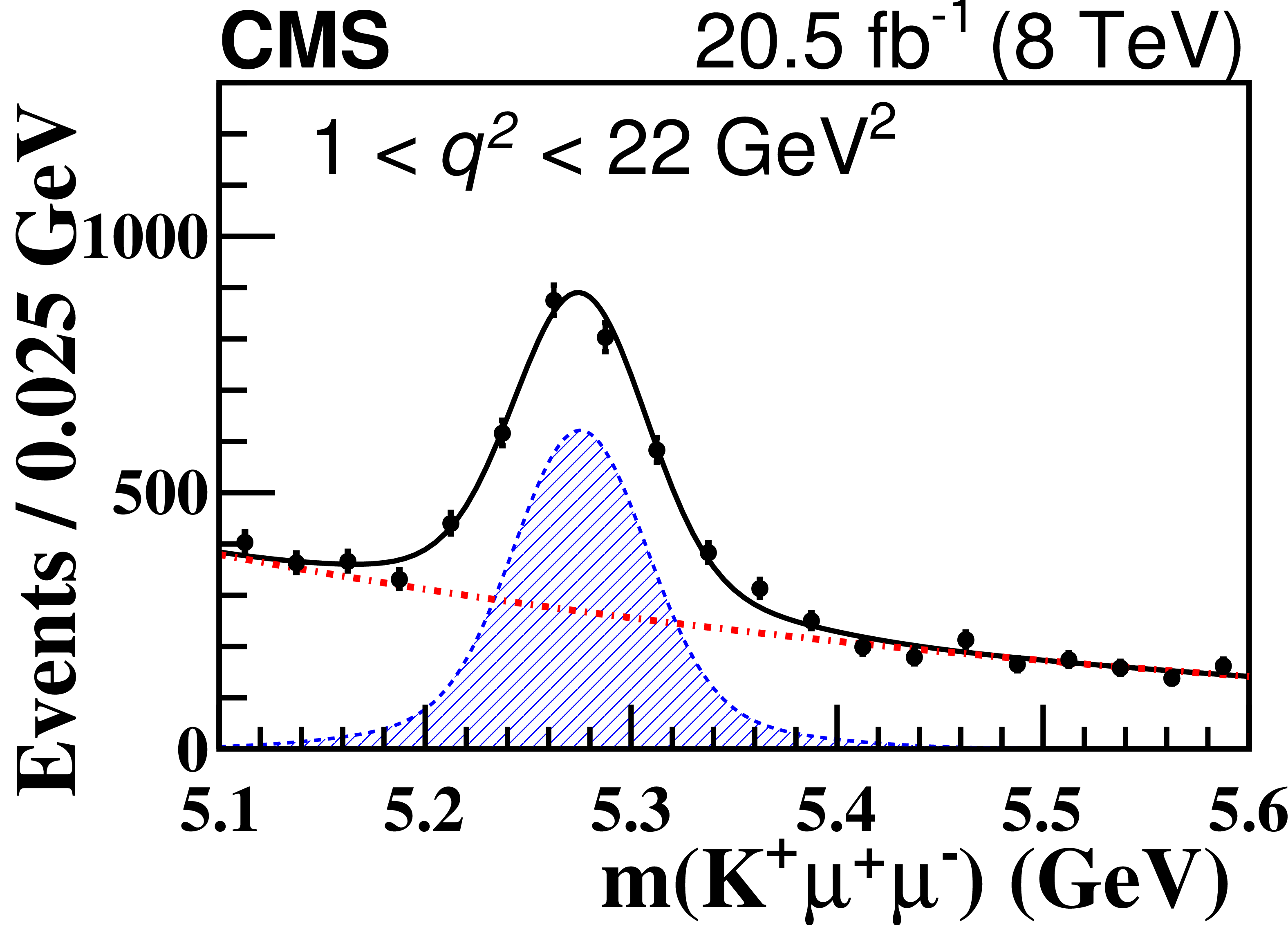
Figure 3:
Projections of the $ {\mathrm {K^+}} {{\mu ^+}} {{\mu ^-}}$ invariant mass distributions for each $q^2$ range from the two-dimensional fit of data. The solid lines show the total fit, the shaded area the signal contribution, and the dash-dotted lines the background. The vertical bars on the points represent the statistical uncertainty in data. |

png pdf |
Figure 3-a:
Projection of the $ {\mathrm {K^+}} {{\mu ^+}} {{\mu ^-}}$ invariant mass distribution for 1 $ < q^2 < $ 2 GeV$^2$ from the two-dimensional fit of data. The solid lines show the total fit, the shaded area the signal contribution, and the dash-dotted lines the background. The vertical bars on the points represent the statistical uncertainty in data. |
png pdf |
Figure 3-b:
Projection of the $ {\mathrm {K^+}} {{\mu ^+}} {{\mu ^-}}$ invariant mass distribution for 2 $ < q^2 < $ 4.3 GeV$^2$ from the two-dimensional fit of data. The solid lines show the total fit, the shaded area the signal contribution, and the dash-dotted lines the background. The vertical bars on the points represent the statistical uncertainty in data. |

png pdf |
Figure 3-c:
Projection of the $ {\mathrm {K^+}} {{\mu ^+}} {{\mu ^-}}$ invariant mass distribution for 4.3 $ < q^2 < $ 8.68 GeV$^2$ from the two-dimensional fit of data. The solid lines show the total fit, the shaded area the signal contribution, and the dash-dotted lines the background. The vertical bars on the points represent the statistical uncertainty in data. |
png pdf |
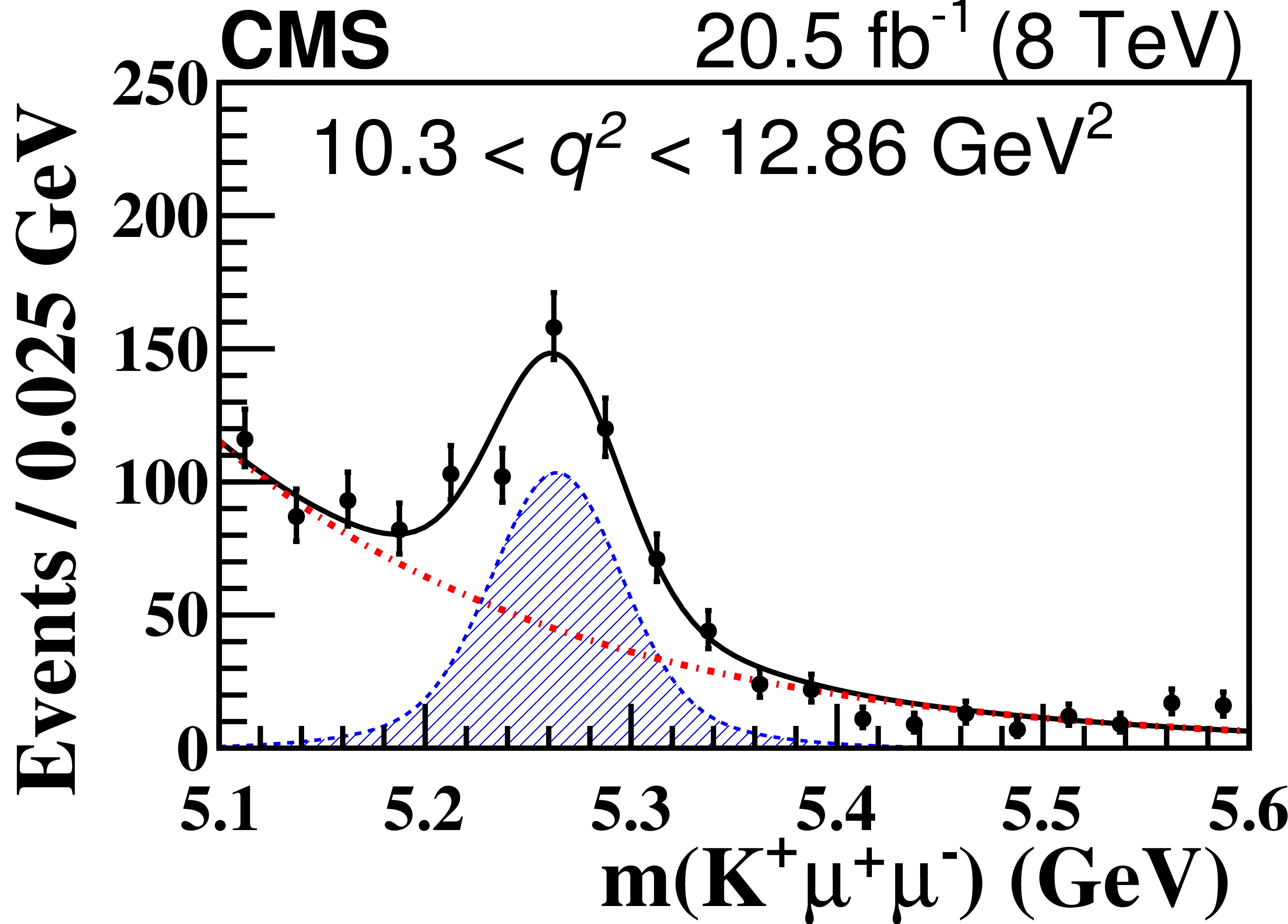
Figure 3-d:
Projection of the $ {\mathrm {K^+}} {{\mu ^+}} {{\mu ^-}}$ invariant mass distribution for 10.3 $ < q^2 < $ 12.86 GeV$^2$ from the two-dimensional fit of data. The solid lines show the total fit, the shaded area the signal contribution, and the dash-dotted lines the background. The vertical bars on the points represent the statistical uncertainty in data. |
png pdf |
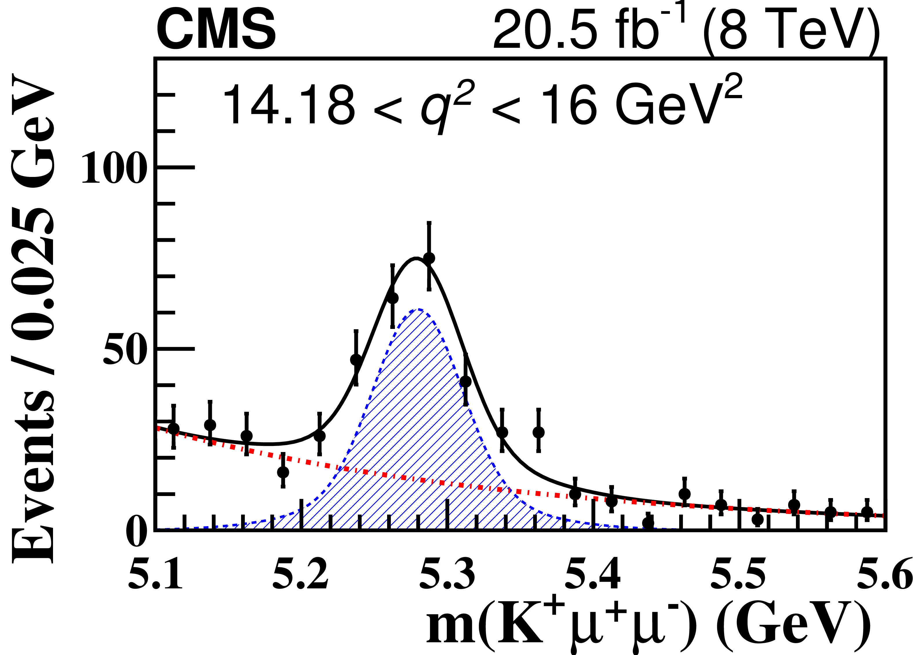
Figure 3-e:
Projection of the $ {\mathrm {K^+}} {{\mu ^+}} {{\mu ^-}}$ invariant mass distribution for 14.18 $ < q^2 < $ 16 GeV$^2$ from the two-dimensional fit of data. The solid lines show the total fit, the shaded area the signal contribution, and the dash-dotted lines the background. The vertical bars on the points represent the statistical uncertainty in data. |
png pdf |
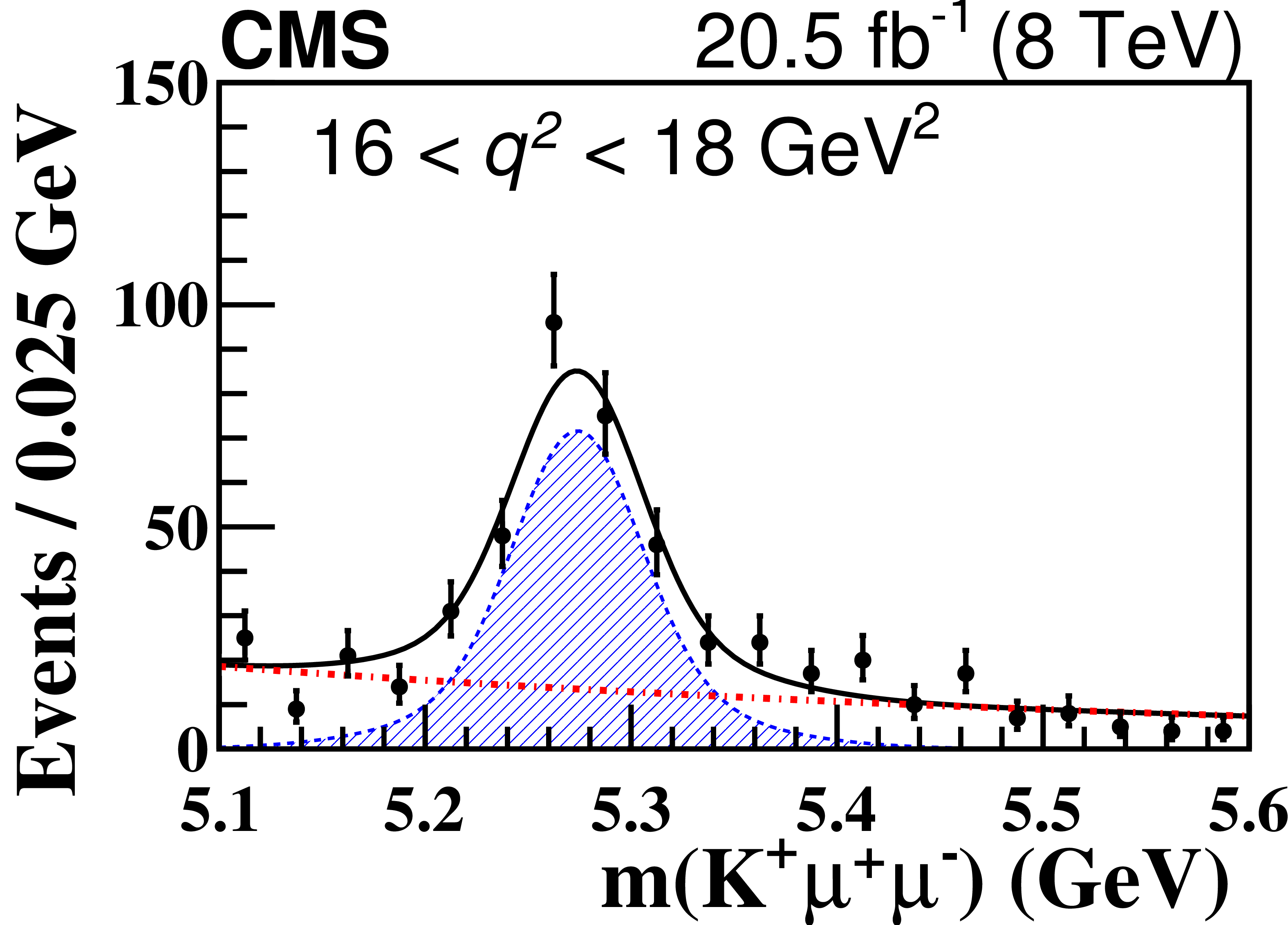
Figure 3-f:
Projection of the $ {\mathrm {K^+}} {{\mu ^+}} {{\mu ^-}}$ invariant mass distribution for 16 $ < q^2 < $ 18 GeV$^2$ from the two-dimensional fit of data. The solid lines show the total fit, the shaded area the signal contribution, and the dash-dotted lines the background. The vertical bars on the points represent the statistical uncertainty in data. |
png pdf |
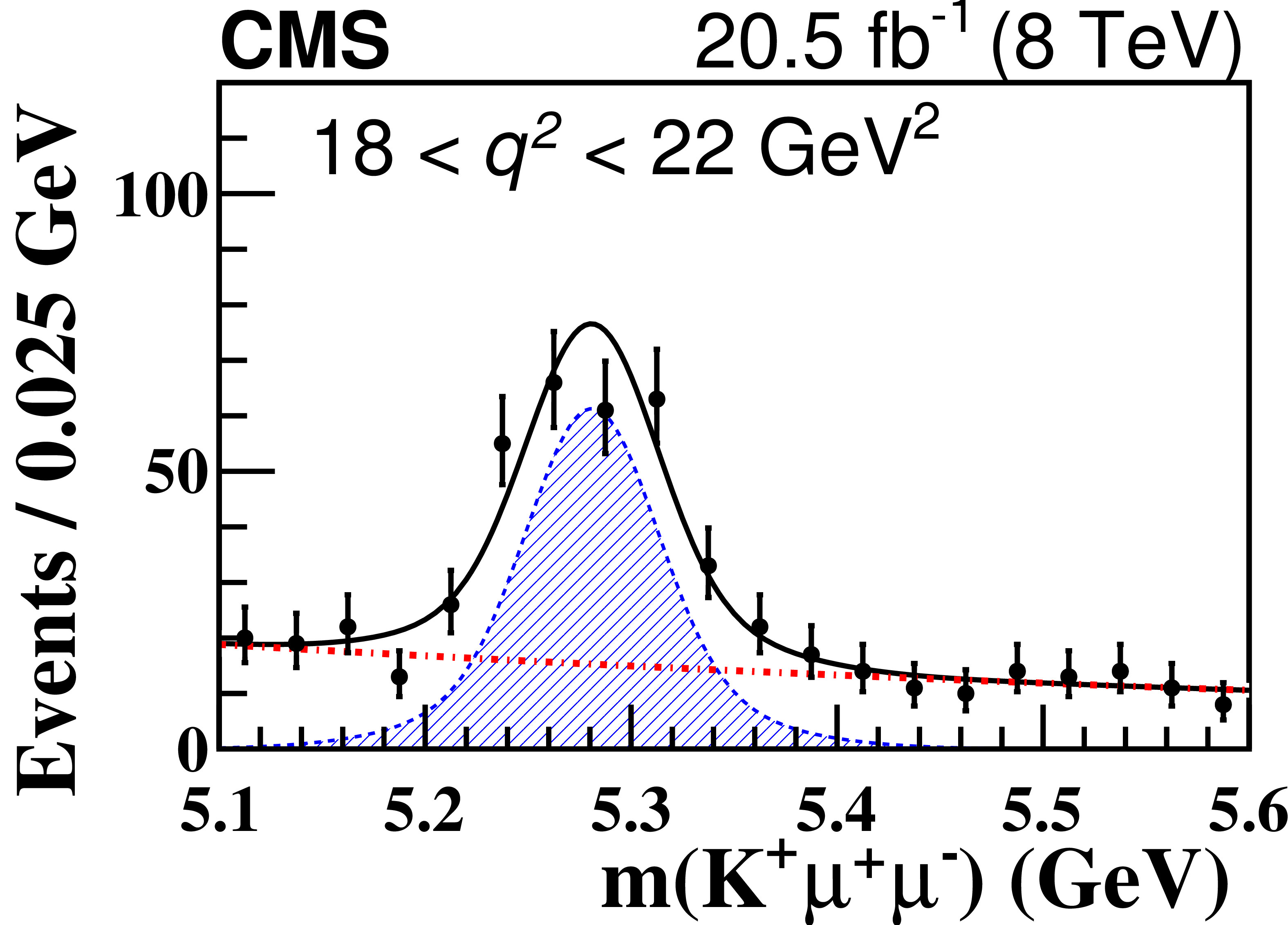
Figure 3-g:
Projection of the $ {\mathrm {K^+}} {{\mu ^+}} {{\mu ^-}}$ invariant mass distribution for 18 $ < q^2 < $ 22 GeV$^2$ from the two-dimensional fit of data. The solid lines show the total fit, the shaded area the signal contribution, and the dash-dotted lines the background. The vertical bars on the points represent the statistical uncertainty in data. |
png pdf |
Figure 3-h:
Projection of the $ {\mathrm {K^+}} {{\mu ^+}} {{\mu ^-}}$ invariant mass distribution for 1 $ < q^2 < $ 6 GeV$^2$ from the two-dimensional fit of data. The solid lines show the total fit, the shaded area the signal contribution, and the dash-dotted lines the background. The vertical bars on the points represent the statistical uncertainty in data. |
png pdf |
Figure 3-i:
Projection of the $ {\mathrm {K^+}} {{\mu ^+}} {{\mu ^-}}$ invariant mass distribution for 1 $ < q^2 < $ 22 GeV$^2$ from the two-dimensional fit of data. The solid lines show the total fit, the shaded area the signal contribution, and the dash-dotted lines the background. The vertical bars on the points represent the statistical uncertainty in data. |

png pdf |
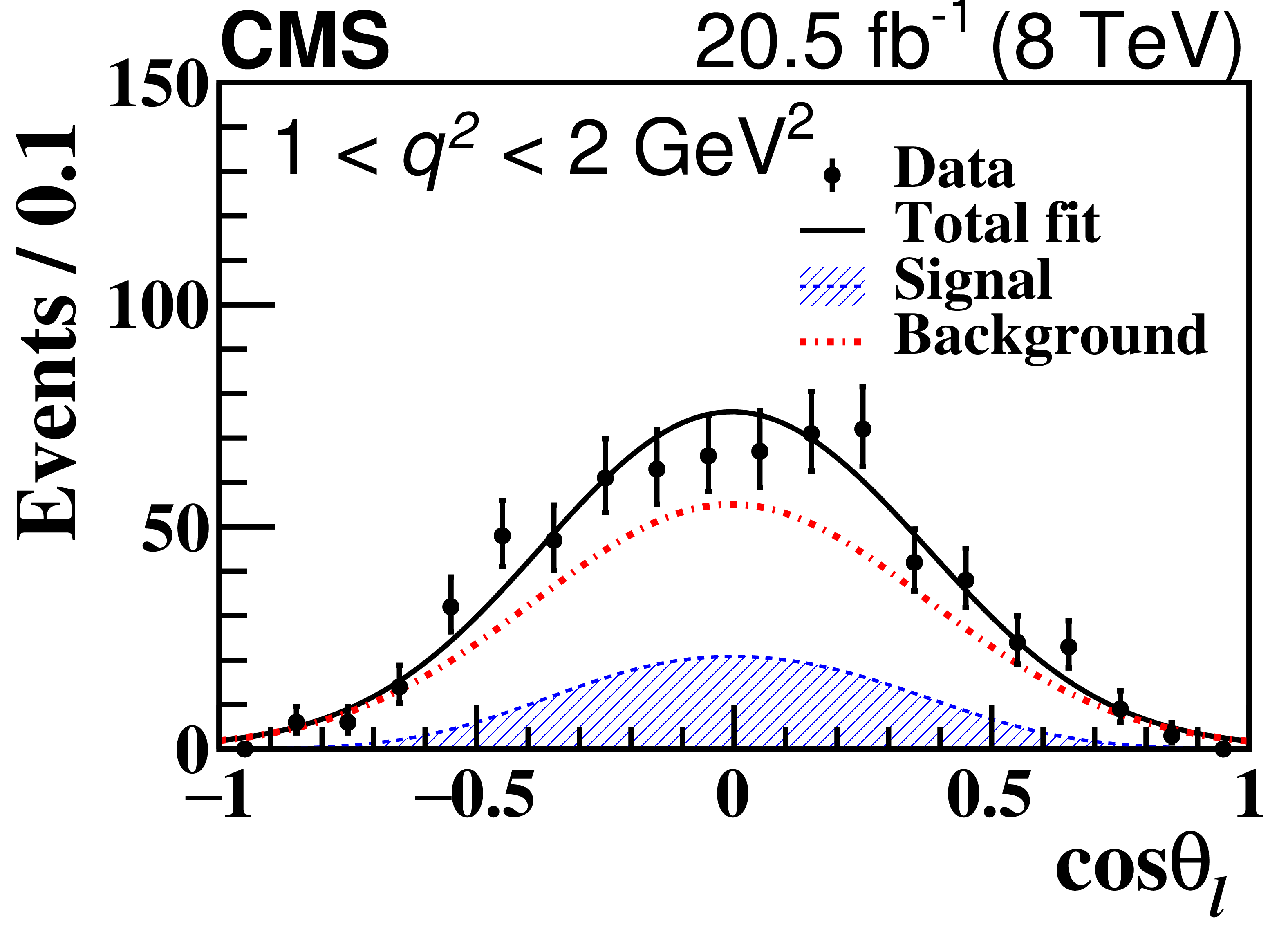
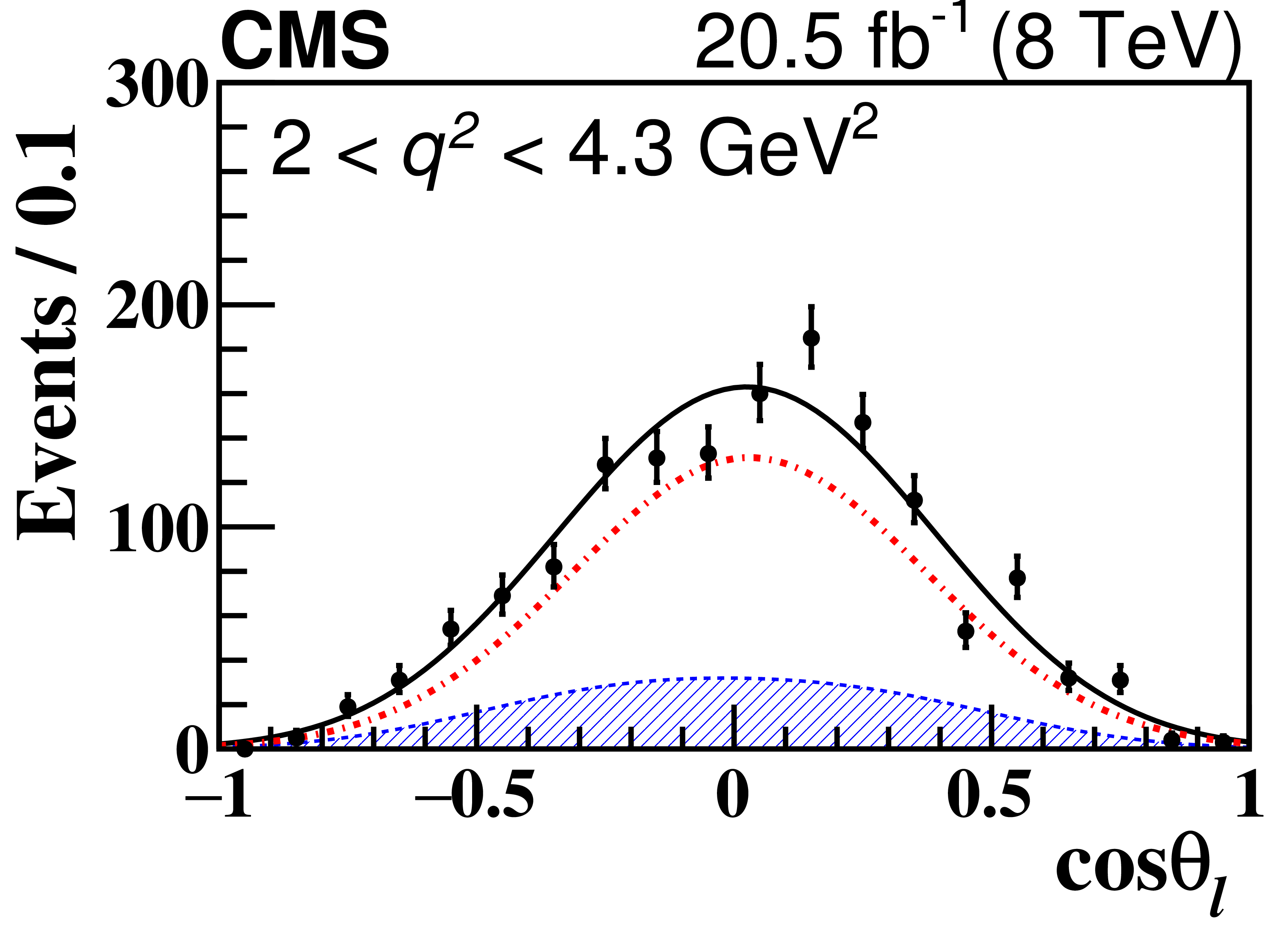
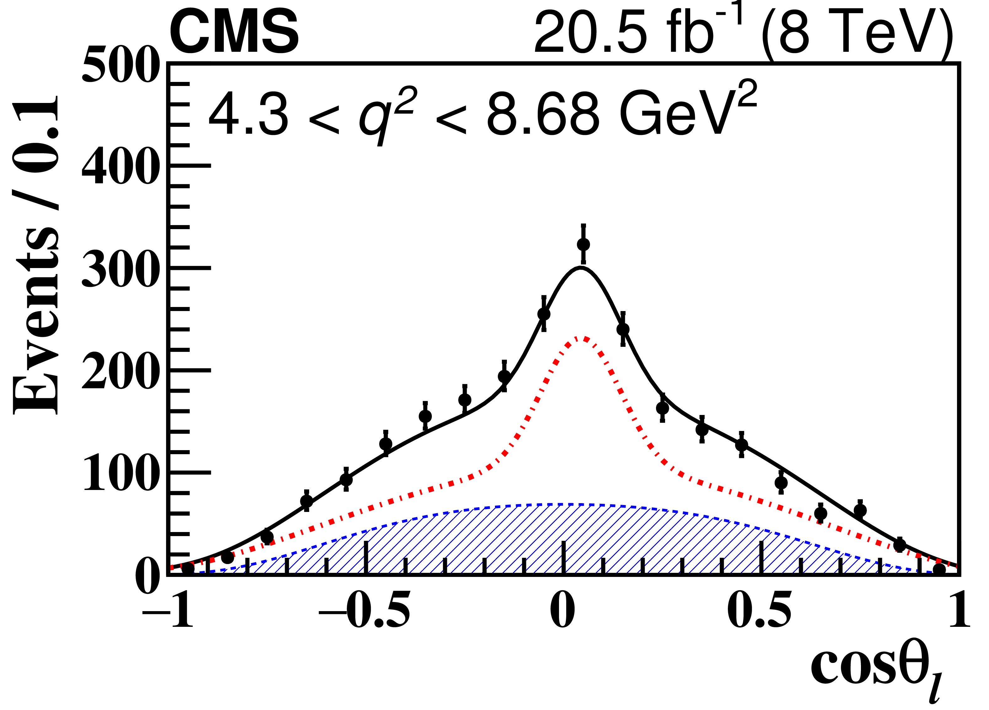
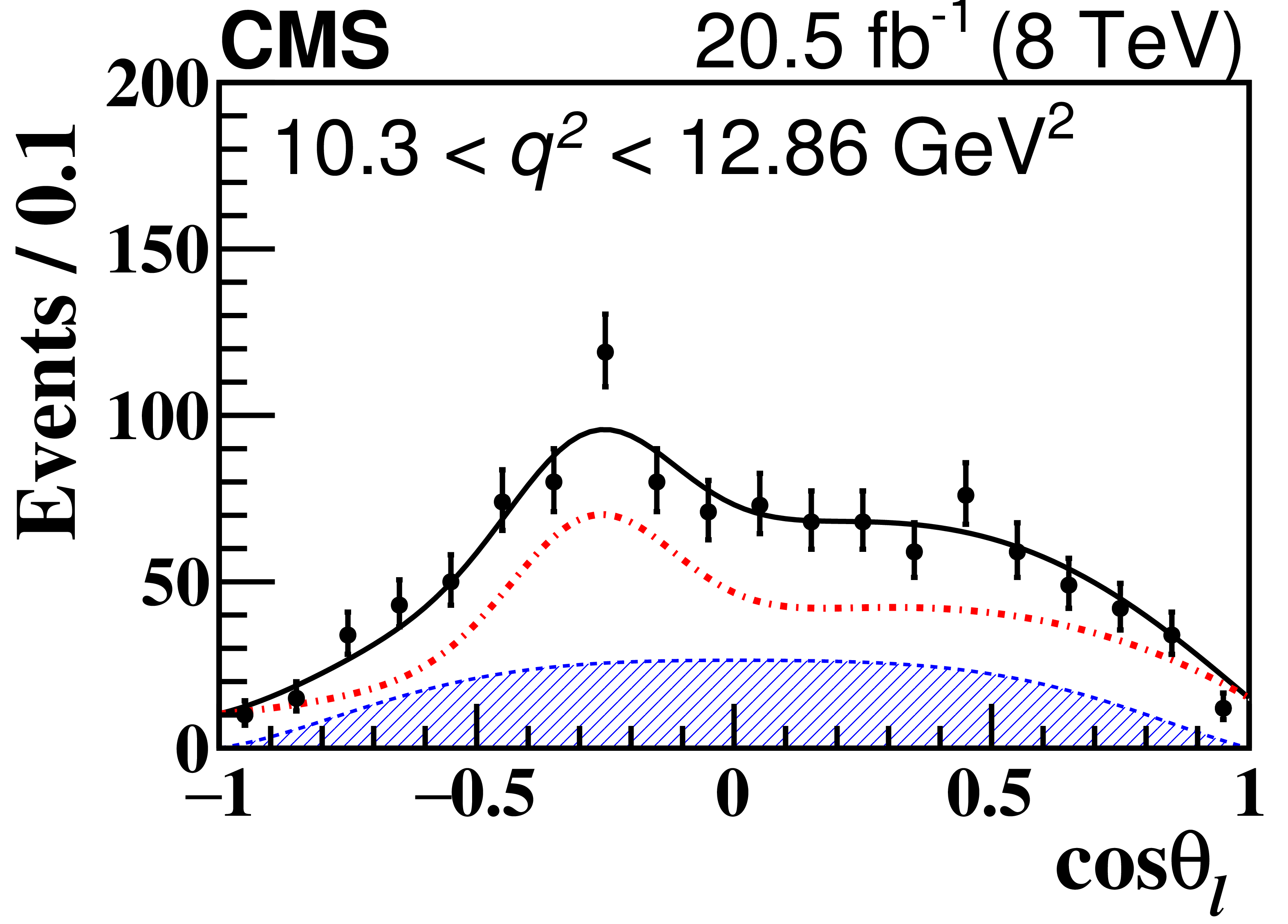
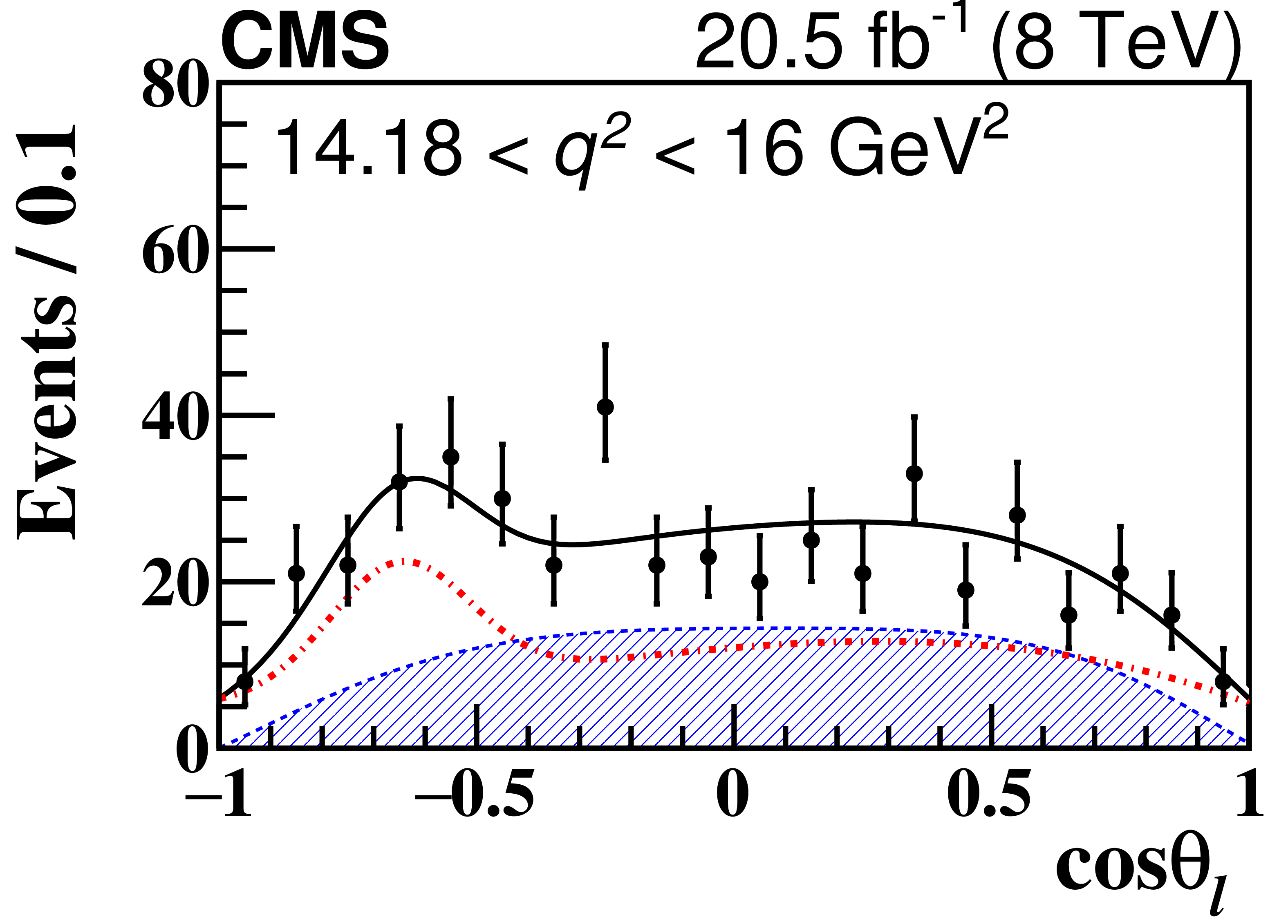
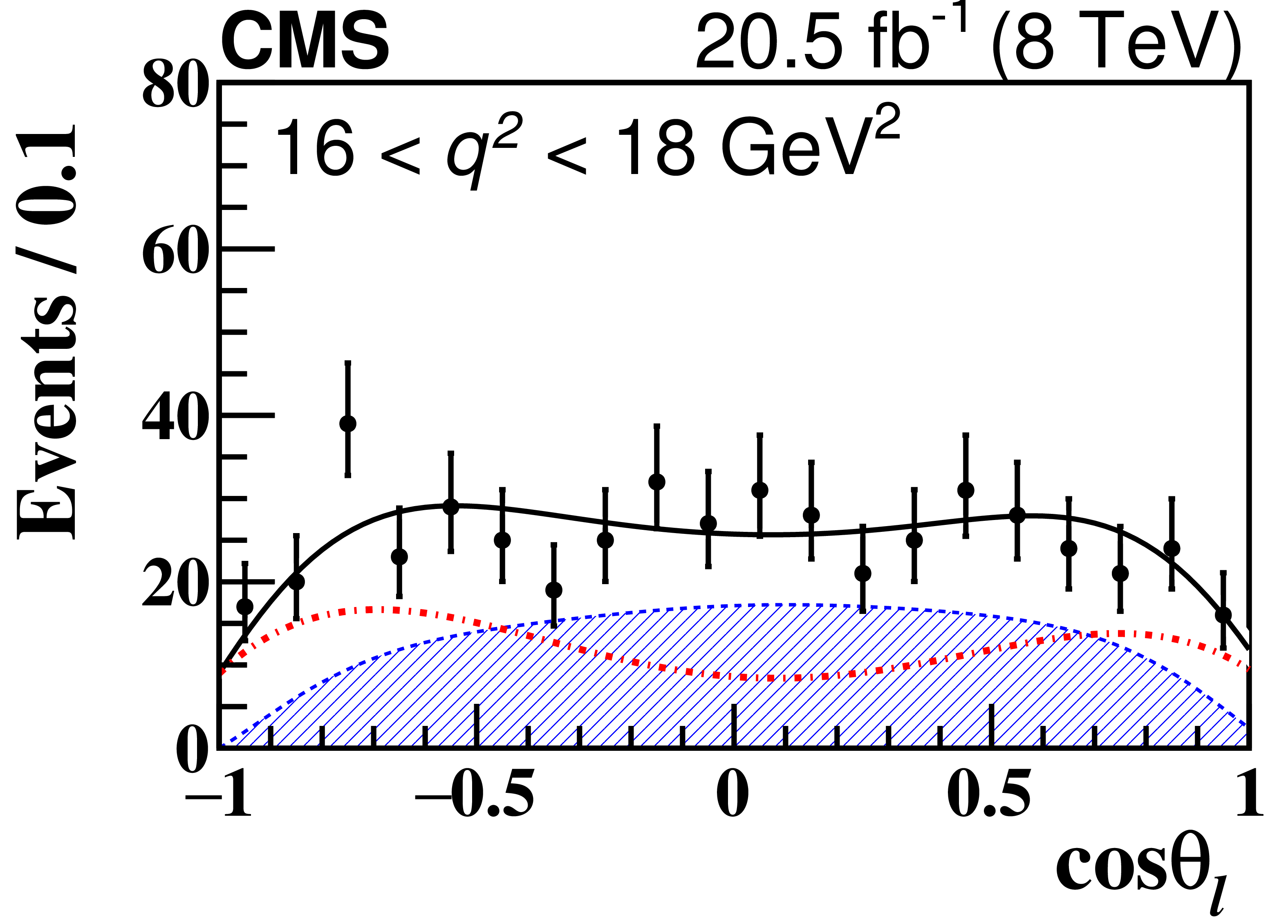
Figure 4:
Projections of the $\cos\theta _{\ell}$ distributions for each $q^2$ range from the two-dimensional fit of data. The solid lines show the total fit, the shaded area the signal contribution, and the dash-dotted lines the background. The vertical bars on the points represent the statistical uncertainty in data. |
png pdf |
Figure 4-a:
Projection of the $\cos\theta _{\ell}$ distribution for 1 $ < q^2 < $ 2 GeV$^2$ from the two-dimensional fit of data. The solid lines show the total fit, the shaded area the signal contribution, and the dash-dotted lines the background. The vertical bars on the points represent the statistical uncertainty in data. |
png pdf |
Figure 4-b:
Projection of the $\cos\theta _{\ell}$ distribution for 2 $ < q^2 < $ 4.3 GeV$^2$ from the two-dimensional fit of data. The solid lines show the total fit, the shaded area the signal contribution, and the dash-dotted lines the background. The vertical bars on the points represent the statistical uncertainty in data. |
png pdf |
Figure 4-c:
Projection of the $\cos\theta _{\ell}$ distribution for 4.3 $ < q^2 < $ 8.68 GeV$^2$ from the two-dimensional fit of data. The solid lines show the total fit, the shaded area the signal contribution, and the dash-dotted lines the background. The vertical bars on the points represent the statistical uncertainty in data. |
png pdf |
Figure 4-d:
Projection of the $\cos\theta _{\ell}$ distribution for 10.3 $ < q^2 < $ 12.86 GeV$^2$ from the two-dimensional fit of data. The solid lines show the total fit, the shaded area the signal contribution, and the dash-dotted lines the background. The vertical bars on the points represent the statistical uncertainty in data. |
png pdf |
Figure 4-e:
Projection of the $\cos\theta _{\ell}$ distribution for 14.18 $ < q^2 < $ 16 GeV$^2$ from the two-dimensional fit of data. The solid lines show the total fit, the shaded area the signal contribution, and the dash-dotted lines the background. The vertical bars on the points represent the statistical uncertainty in data. |
png pdf |
Figure 4-f:
Projection of the $\cos\theta _{\ell}$ distribution for 16 $ < q^2 < $ 18 GeV$^2$ from the two-dimensional fit of data. The solid lines show the total fit, the shaded area the signal contribution, and the dash-dotted lines the background. The vertical bars on the points represent the statistical uncertainty in data. |
png pdf |
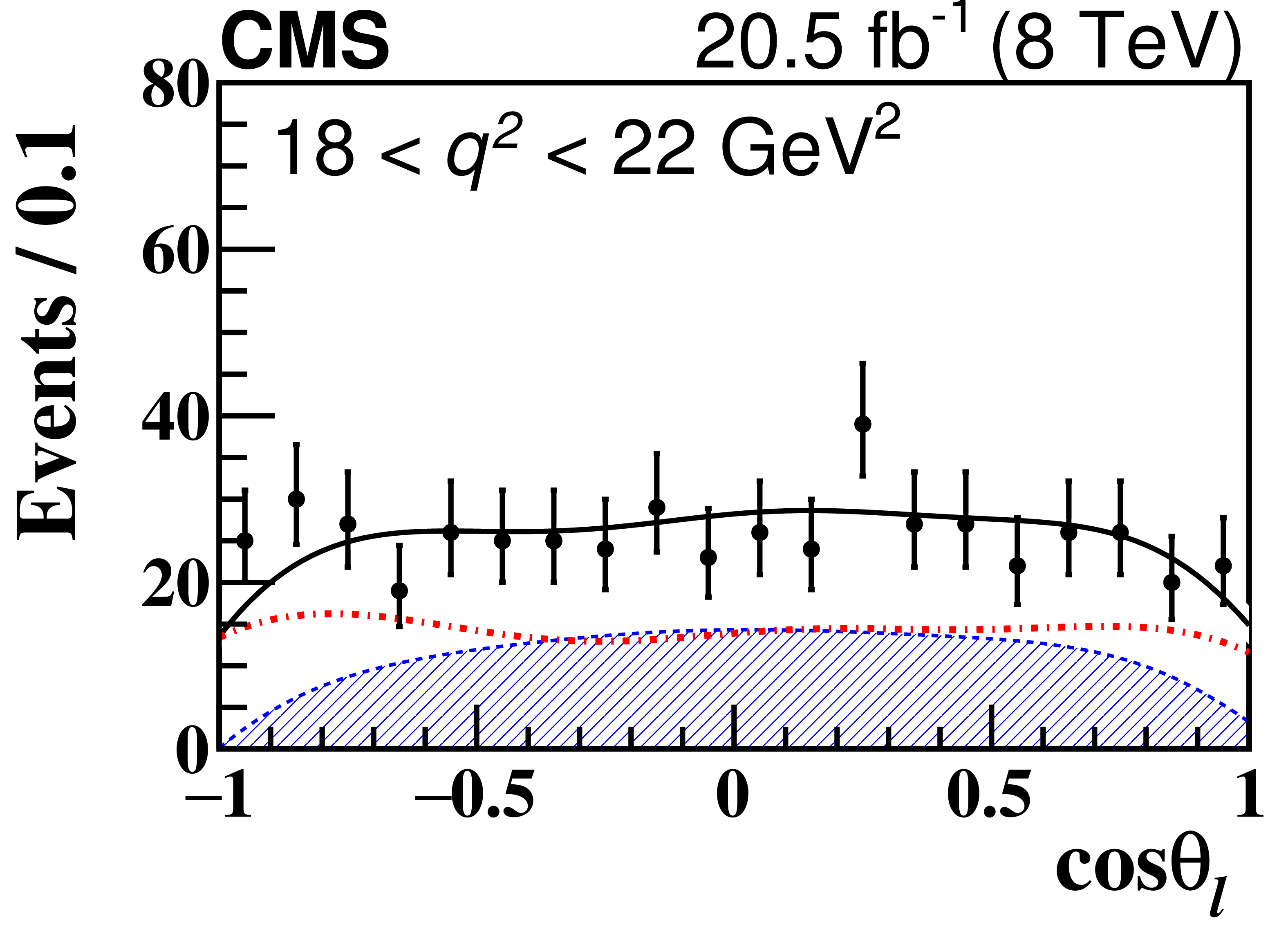
Figure 4-g:
Projection of the $\cos\theta _{\ell}$ distribution for 18 $ < q^2 < $ 22 GeV$^2$ from the two-dimensional fit of data. The solid lines show the total fit, the shaded area the signal contribution, and the dash-dotted lines the background. The vertical bars on the points represent the statistical uncertainty in data. |
png pdf |
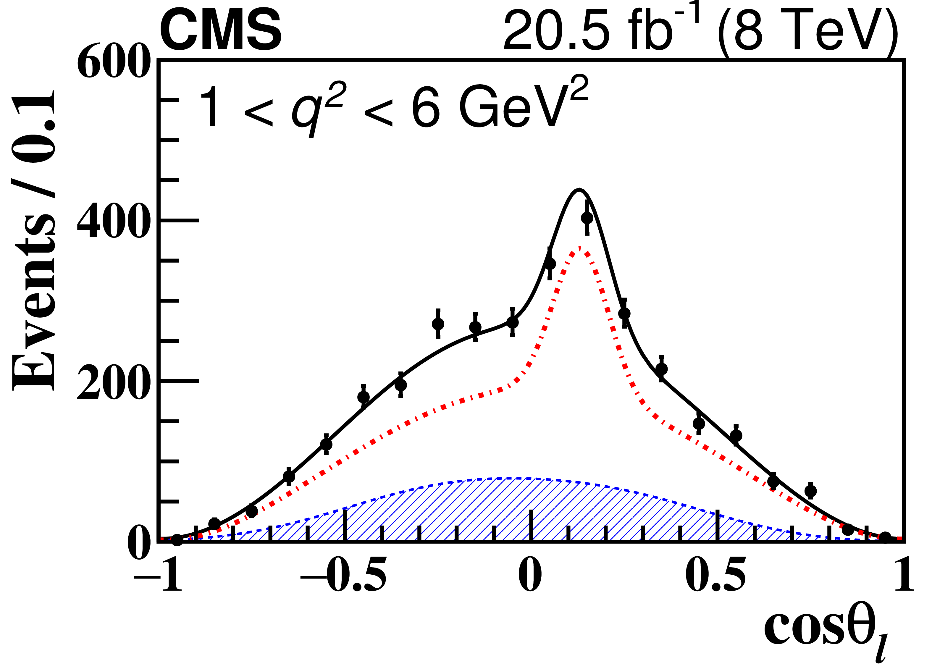
Figure 4-h:
Projection of the $\cos\theta _{\ell}$ distribution for 1 $ < q^2 < $ 6 GeV$^2$ from the two-dimensional fit of data. The solid lines show the total fit, the shaded area the signal contribution, and the dash-dotted lines the background. The vertical bars on the points represent the statistical uncertainty in data. |
png pdf |
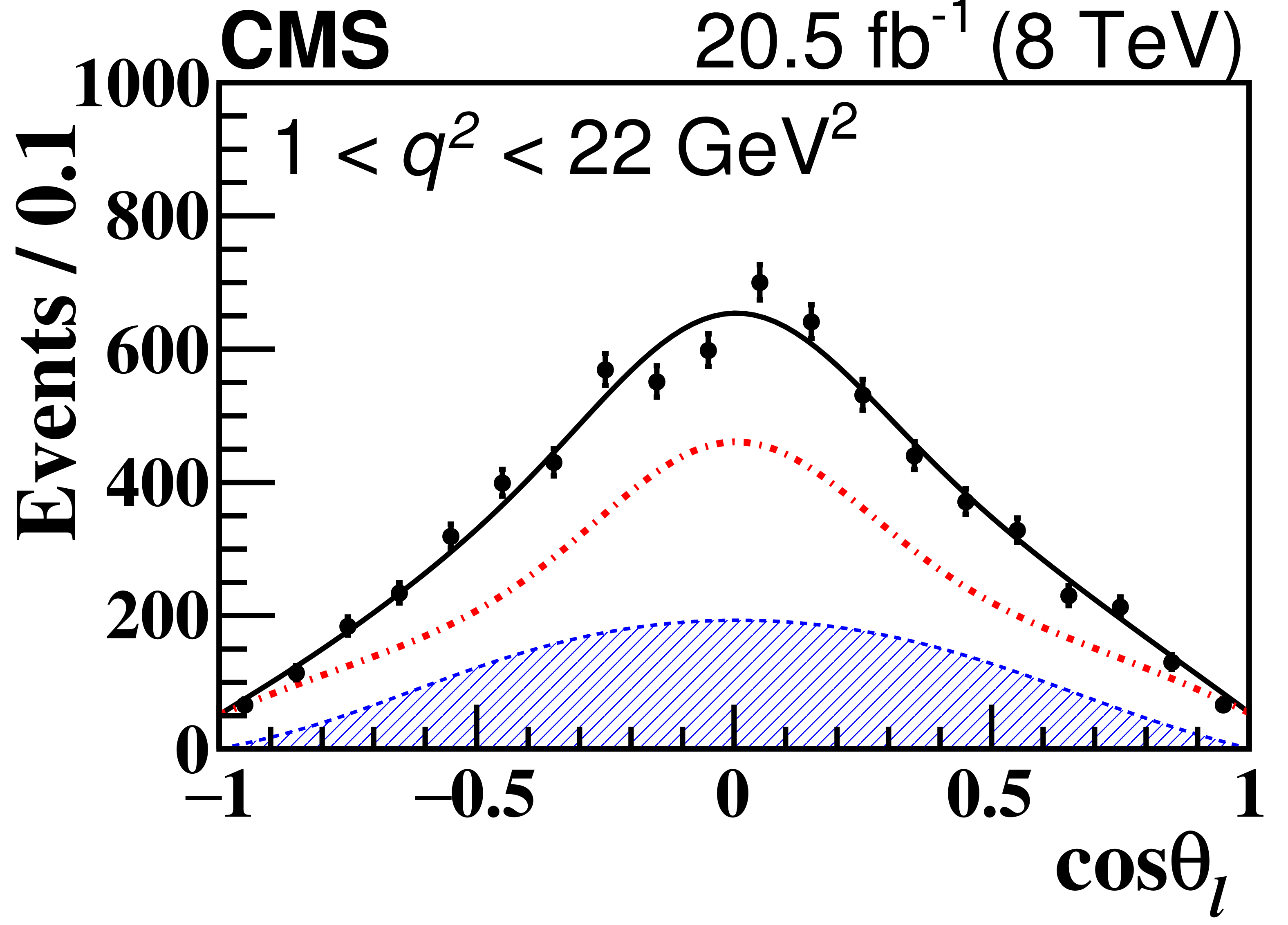
Figure 4-i:
Projection of the $\cos\theta _{\ell}$ distribution for 1 $ < q^2 < $ 22 GeV$^2$ from the two-dimensional fit of data. The solid lines show the total fit, the shaded area the signal contribution, and the dash-dotted lines the background. The vertical bars on the points represent the statistical uncertainty in data. |
png pdf |
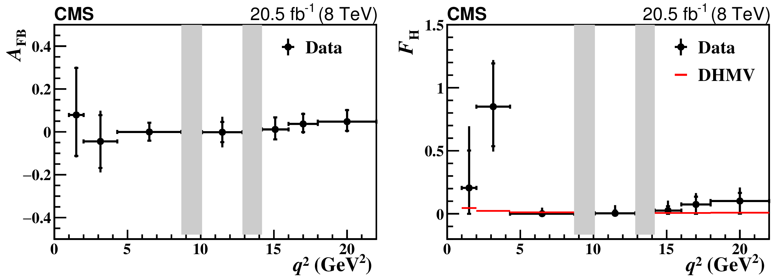
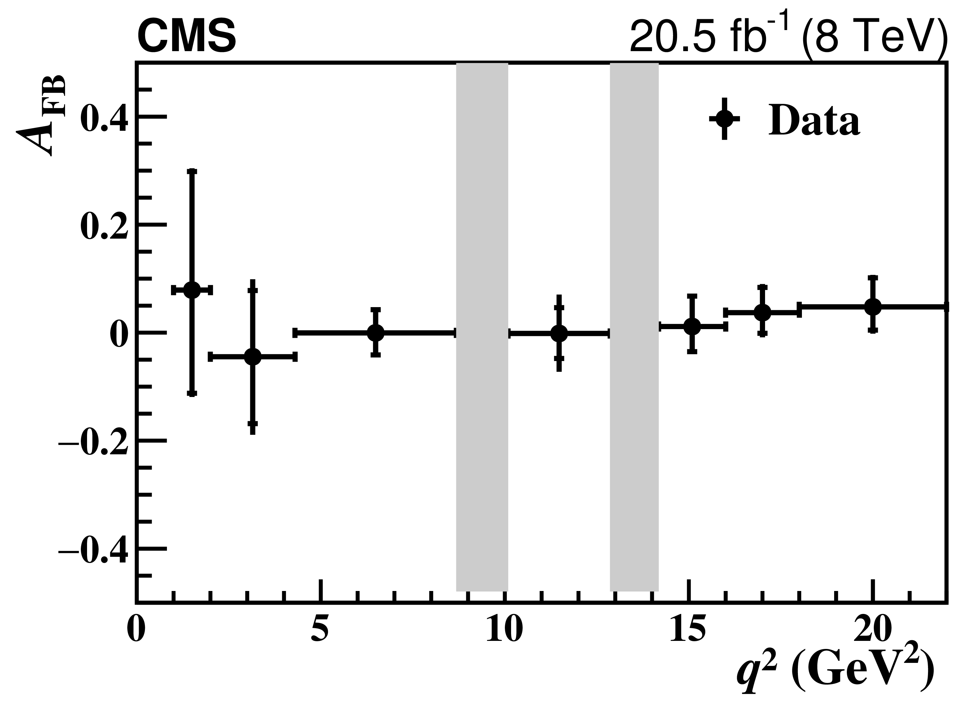
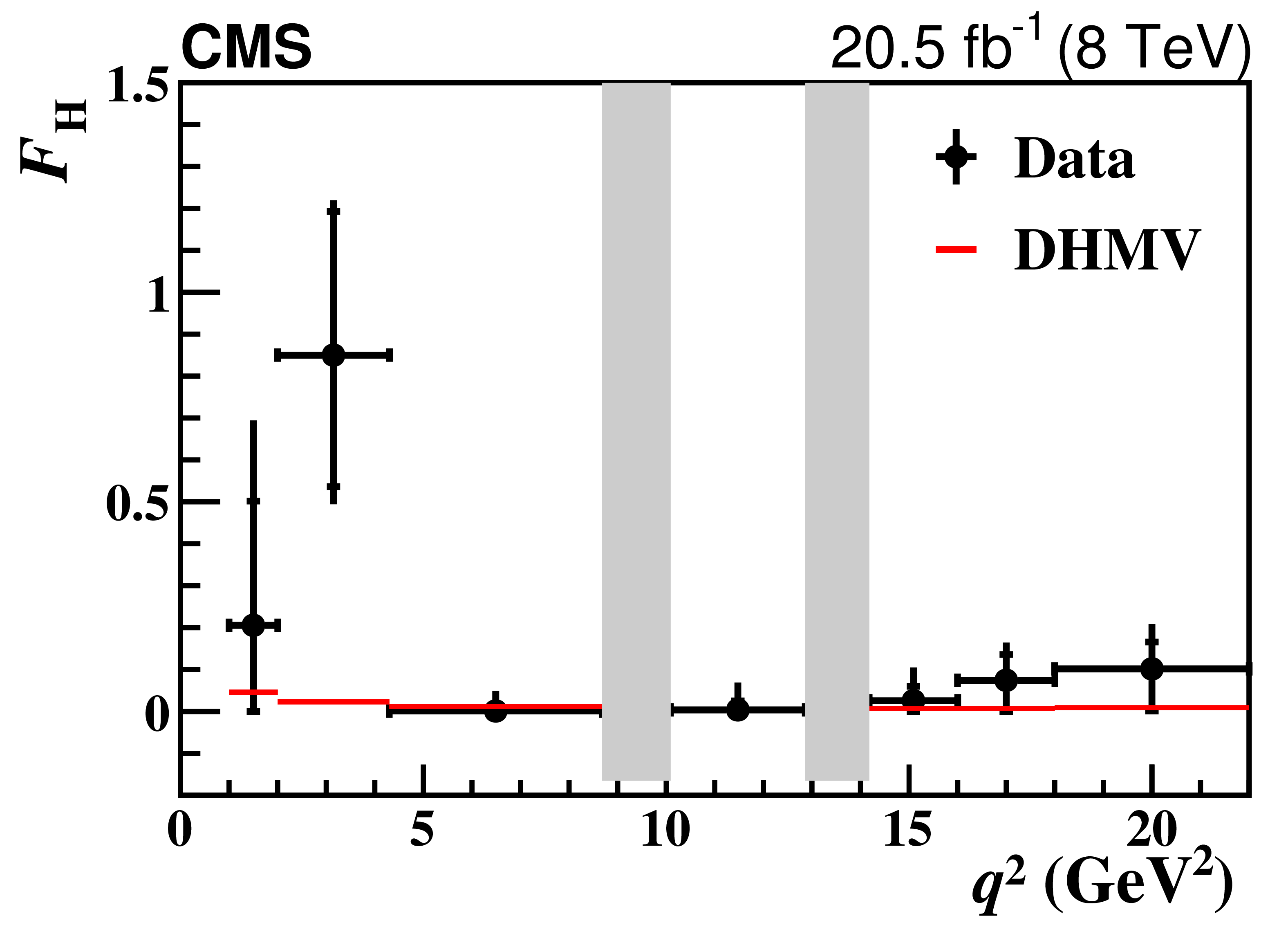
Figure 5:
Results of the $A_{\mathrm {FB}}$ (left) and $F_{{\mathrm {H}}}$ (right) measurements in ranges of $q^2$. The statistical uncertainties are shown by the inner vertical bars, while the outer vertical bars give the total uncertainties. The horizontal bars show the $q^2$ range widths. The vertical shaded regions are 8.68-10.09 and 12.86-14.18 GeV$ ^2$, corresponding to the $ {{\mathrm {J}/\psi}}$ - and $ {\psi \mathrm {(2S)}} $-dominated control regions, respectively. The horizontal lines in the right plot show the DHMV SM theoretical predictions [31,32], whose uncertainties are smaller than the line width. |
png pdf |
Figure 5-a:
Results of the $A_{\mathrm {FB}}$ measurements in ranges of $q^2$. The statistical uncertainties are shown by the inner vertical bars, while the outer vertical bars give the total uncertainties. The horizontal bars show the $q^2$ range widths. The vertical shaded regions are 8.68-10.09 and 12.86-14.18 GeV$ ^2$, corresponding to the $ {{\mathrm {J}/\psi}}$ - and $ {\psi \mathrm {(2S)}} $-dominated control regions, respectively. The horizontal lines in the right plot show the DHMV SM theoretical predictions [31,32], whose uncertainties are smaller than the line width. |
png pdf |
Figure 5-b:
Results of the $F_{{\mathrm {H}}}$ measurements in ranges of $q^2$. The statistical uncertainties are shown by the inner vertical bars, while the outer vertical bars give the total uncertainties. The horizontal bars show the $q^2$ range widths. The vertical shaded regions are 8.68-10.09 and 12.86-14.18 GeV$ ^2$, corresponding to the $ {{\mathrm {J}/\psi}}$ - and $ {\psi \mathrm {(2S)}} $-dominated control regions, respectively. The horizontal lines in the right plot show the DHMV SM theoretical predictions [31,32], whose uncertainties are smaller than the line width. |
| Tables | |
png pdf |
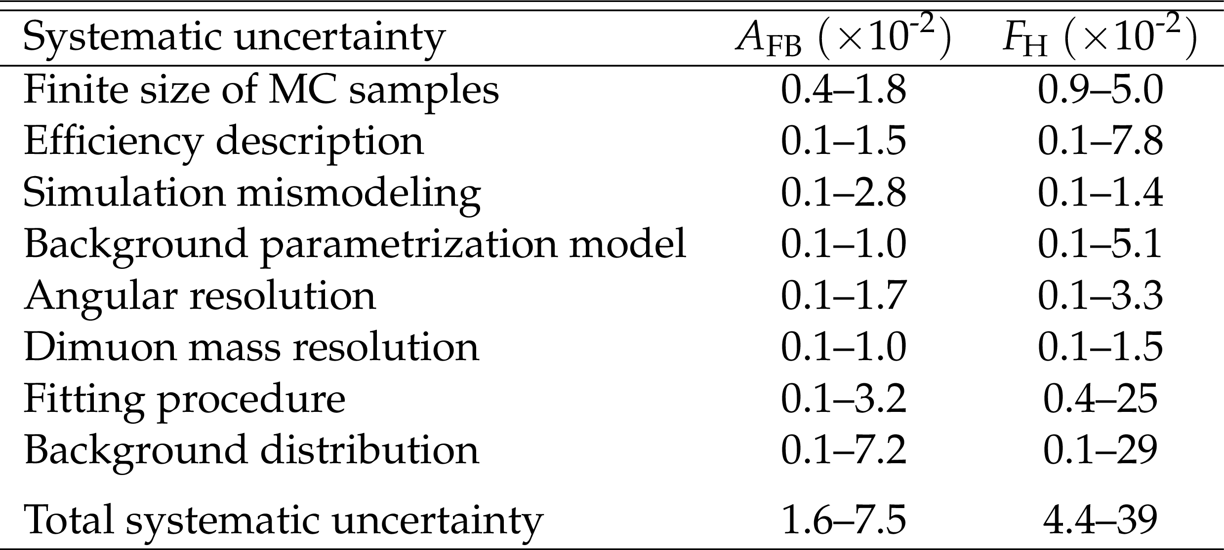
Table 1:
Absolute values of the uncertainty contributions in the measurements of $A_{\mathrm {FB}}$ and $F_{{\mathrm {H}}}$. For each item, the range indicates the variation of the uncertainty in the signal $q^2$ ranges. |
png pdf |
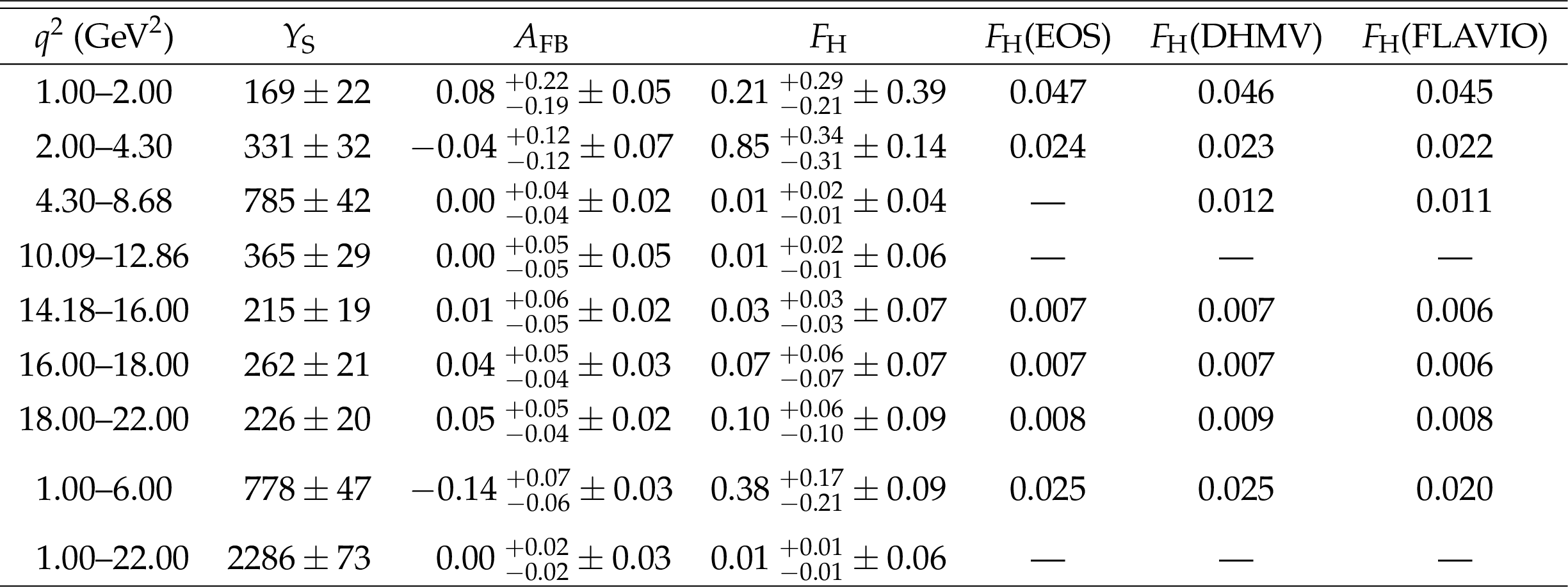
Table 2:
Results of the fit for each $q^2$ range, together with several SM predictions. The inclusive $q^2=$ 1.00-22.00 GeV$ ^2$ range in the bottom line does not include events from the $ {{\mathrm {J}/\psi}}$ and $ {\psi \mathrm {(2S)}}$ resonance regions. The signal yield $Y_{\mathrm {S}}$ is given, along with its statistical uncertainty. The measured values of $A_{\mathrm {FB}}$ and $F_{{\mathrm {H}}}$ are presented, where the first uncertainties are statistical and the second are systematic. The fifth column is a theoretical prediction by C. Bobeth et al. [1,3] using the EOS package [33] with the form factors from Refs. [34,35,2]. The sixth column is the calculation from S. Descotes-Genon et al. (DHMV) based on Refs. [31,32]. The last column is the prediction using the FLAVIO package [36] with the form factors from Ref. [37]. Only the central values of the theoretical predictions are shown, since their uncertainties are insignificant compared to those in the measurements. |
| Summary |
| An angular analysis of the decay ${\mathrm{B^{+}} \to \mathrm{K^{+}} \mu^{+} \mu^{-}} $ has been performed using a data sample of proton-proton collisions corresponding to an integrated luminosity of 20.5 fb$^{-1}$ recorded with the CMS detector at $ \sqrt{s} = $ 8 TeV. The forward-backward asymmetry $A_{\mathrm{FB}}$ of the muon system and the contribution $F_{\mathrm{H}}$ of the pseudoscalar, scalar, and tensor amplitudes to the decay width are measured as a function of the dimuon mass squared. The results are consistent with previous measurements, and are also compatible with three different standard model predictions. |
| Additional Figures | |

png pdf |
Additional Figure 1:
Spectrum of the dimuon invariant mass. The two peaks correspond to the $ \mathrm{J}/\psi $ and ${\psi \mathrm {(2S)}}$ resonances used as control samples. |
png pdf |
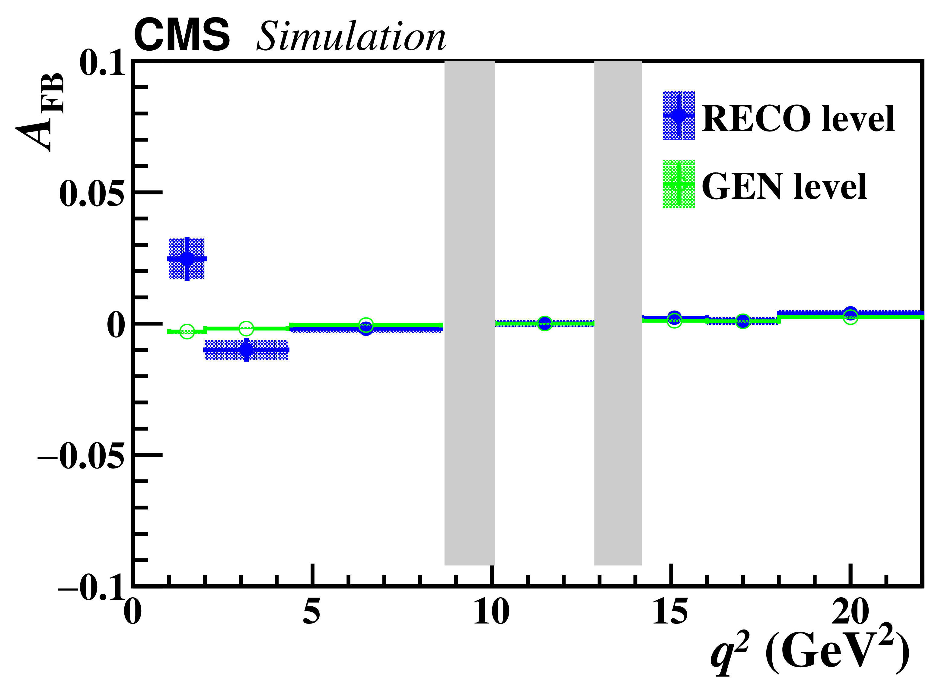
Additional Figure 2:
Closure test of the fitting results of $A_{\text {FB}}$ for each $q^{2}$ bin on simulated data. The results of the fit on reconstructed events (blue dots) are compared with the fit on the generated events (green circles). The vertical shaded regions correspond to the $ \mathrm{J}/\psi $ and ${\psi \mathrm {(2S)}}$ resonances. |
png pdf |
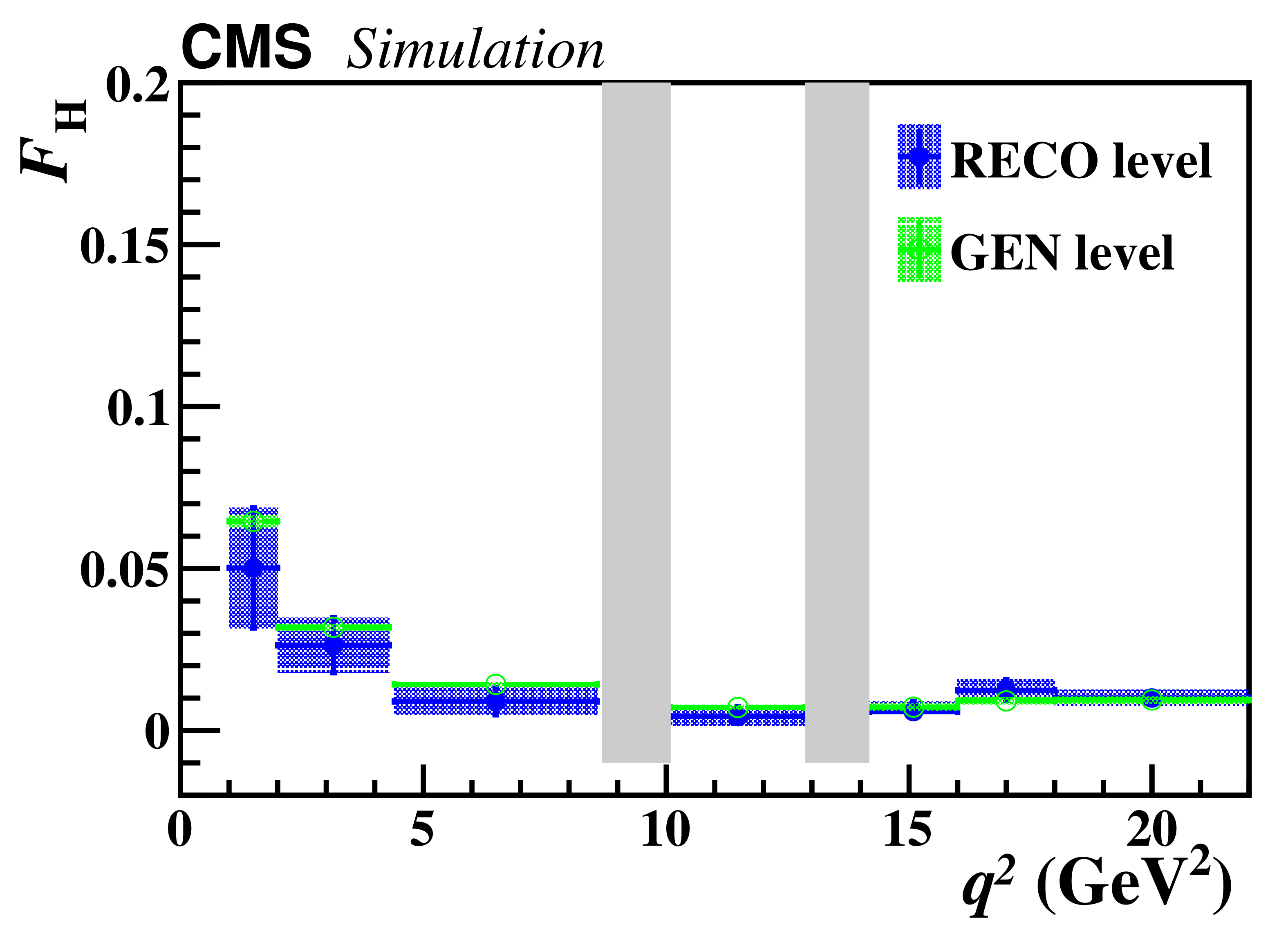
Additional Figure 3:
Closure test of the fitting results of $F_{\text {H}}$ for each $q^{2}$ bin on simulated data. The results of the fit on reconstructed events (blue dots) are compared with the fit on the generated events (green circles). The vertical shaded regions correspond to the $ \mathrm{J}/\psi $ and ${\psi \mathrm {(2S)}}$ resonances. |

png pdf |
Additional Figure 4:
Measured values of the differential branching fraction of ${{{\mathrm {B}^{+}}}\to {\mathrm {K^+}} {{\mu ^+}} {{\mu ^-}}}$ in each of the $q^2$ bins from CMS, compared with standard model prediction [18] and LHCb [18,19] results. The uncertainties of CMS values are statistical only. |
png pdf |
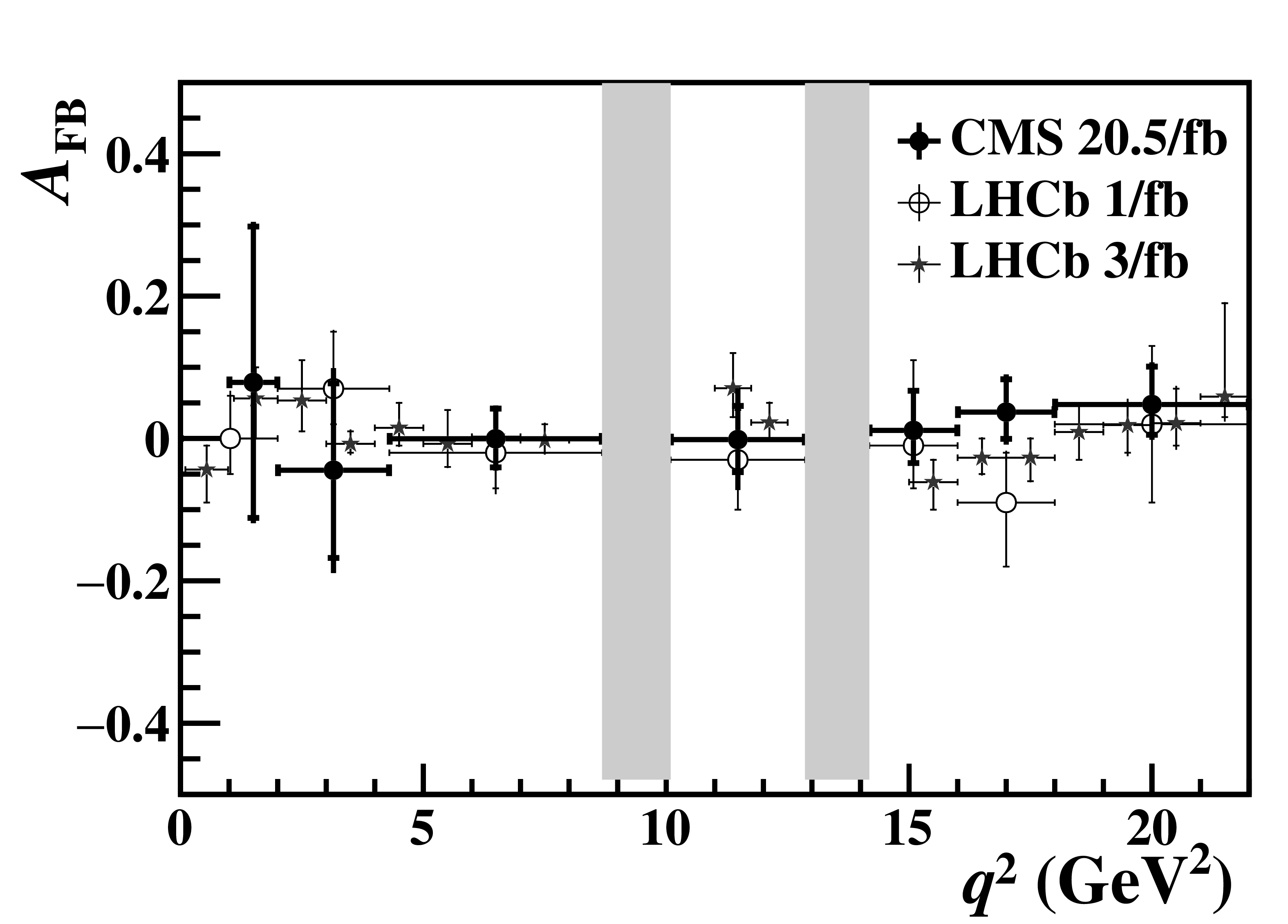
Additional Figure 5:
Measured values of $A_{\text {FB}}$ versus $q^2$ for ${{{\mathrm {B}^{+}}}\to {\mathrm {K^+}} {{\mu ^+}} {{\mu ^-}}}$ from CMS, compared with LHCb [18,19] results. The statistical uncertainty is shown by the inner vertical bars, while the outer vertical bars give the total uncertainty. The horizontal bars show the bin widths. The vertical shaded regions correspond to the $ \mathrm{J}/\psi $ and ${\psi \mathrm {(2S)}}$ resonances. |
png pdf |
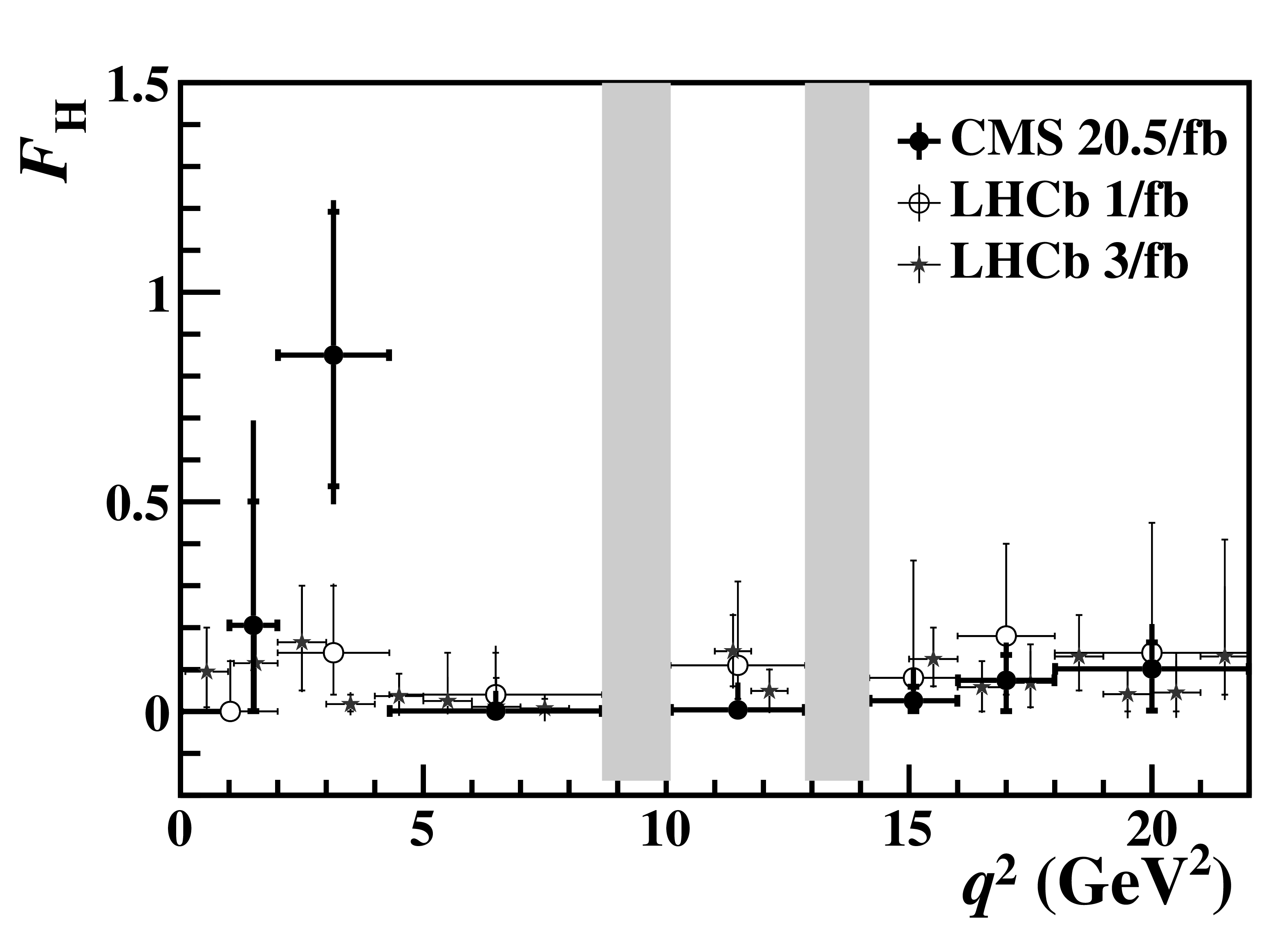
Additional Figure 6:
Measured values of $F_{\text {H}}$ versus $q^2$ for ${{{\mathrm {B}^{+}}}\to {\mathrm {K^+}} {{\mu ^+}} {{\mu ^-}}}$ from CMS, compared with LHCb [18,19] results. The statistical uncertainty is shown by the inner vertical bars, while the outer vertical bars give the total uncertainty. The horizontal bars show the bin widths. The vertical shaded regions correspond to the $ \mathrm{J}/\psi $ and ${\psi \mathrm {(2S)}}$ resonances. |
png pdf |
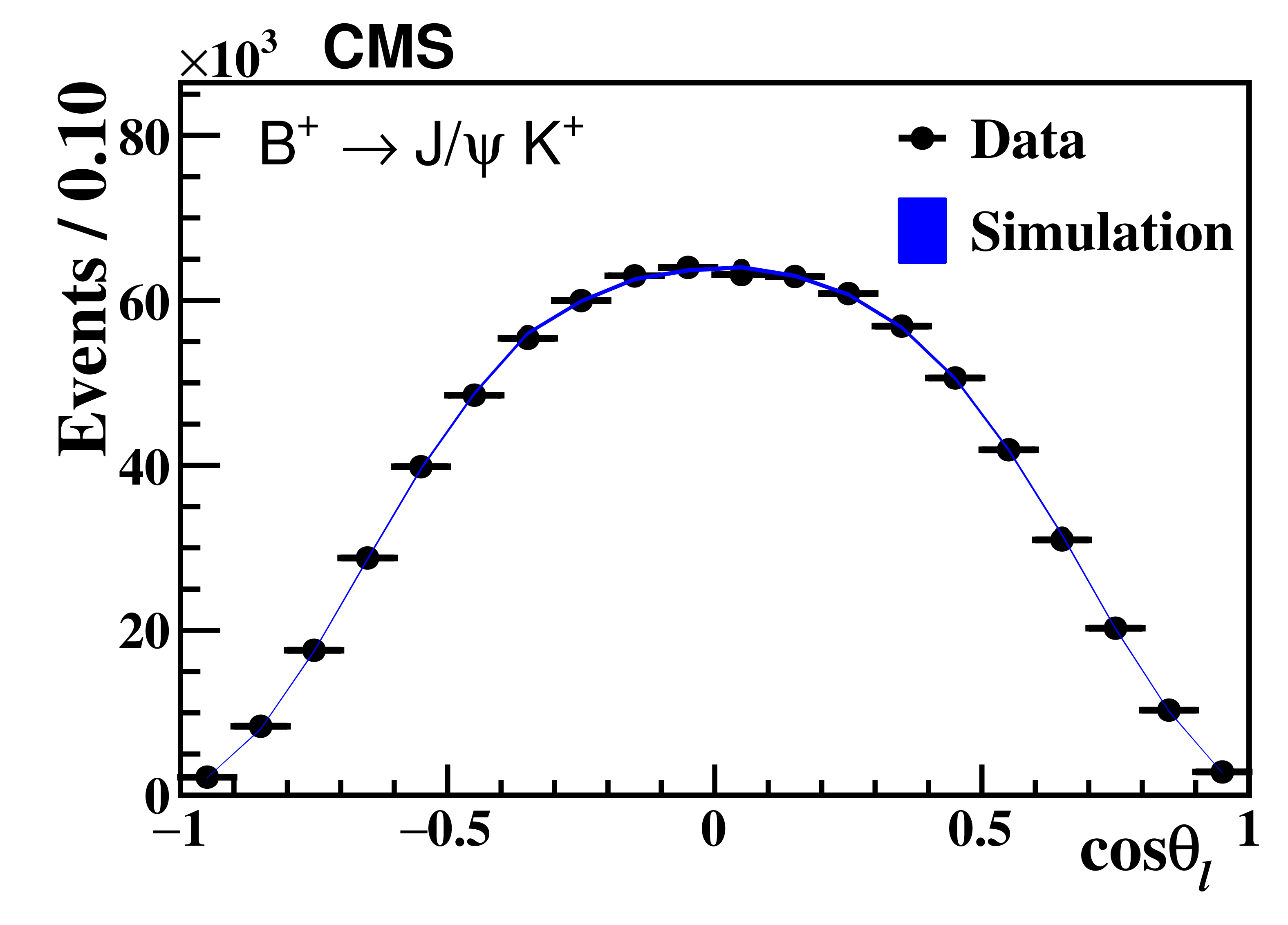
Additional Figure 7:
The angular distributions of ${{{\mathrm {B}^{+}}}\to {\mathrm {K^+}} \mathrm{J}/\psi ({{\mu ^+}} {{\mu ^-}})}$ control channel. The black points are data, the blue band is MC simulation. |
png pdf |
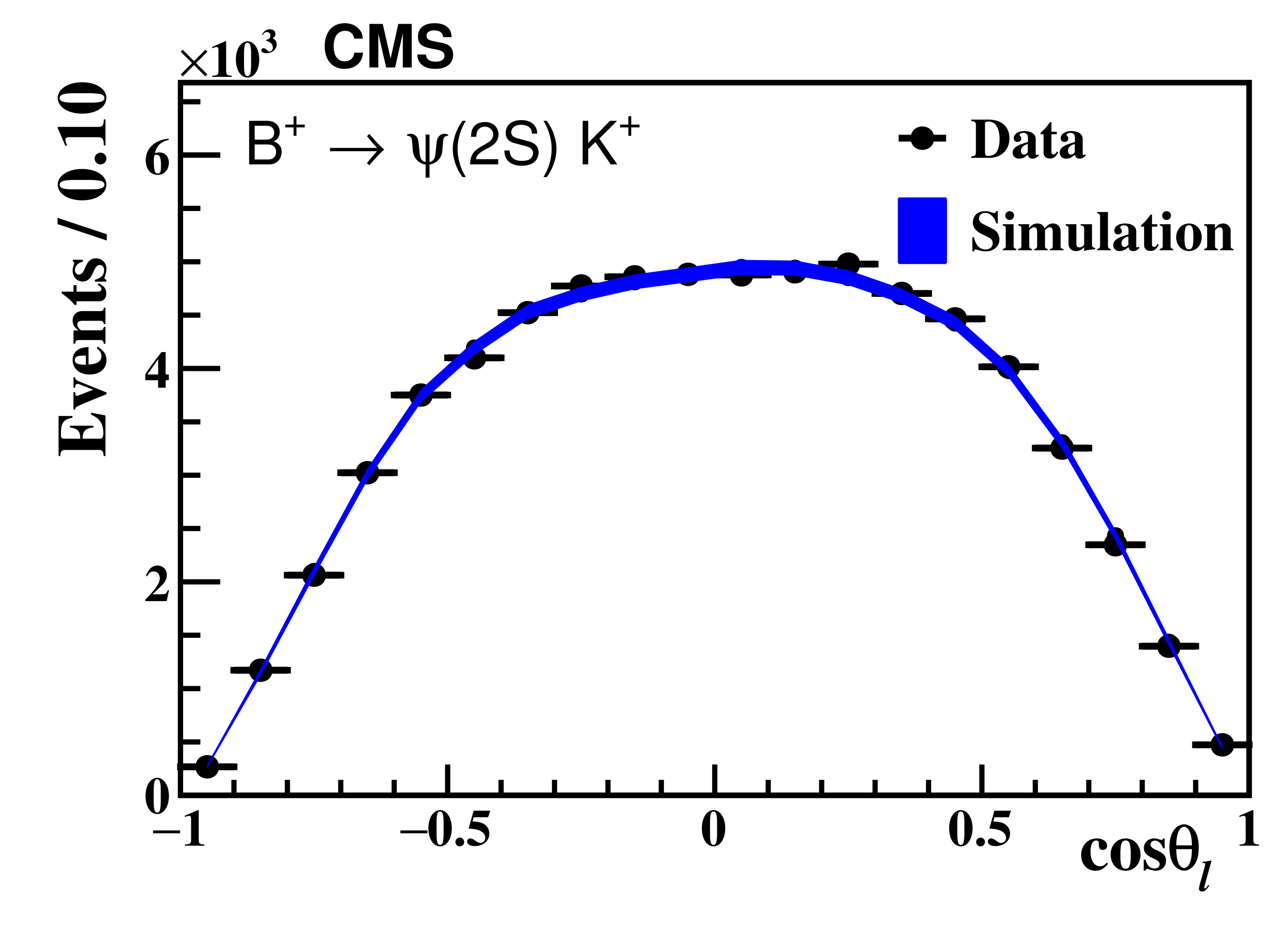
Additional Figure 8:
The angular distributions of ${{{\mathrm {B}^{+}}}\to {\mathrm {K^+}} {\psi \mathrm {(2S)}} ({{\mu ^+}} {{\mu ^-}})}$ control channel. The black points are data, the blue band is MC simulation. |
| References | ||||
| 1 | C. Bobeth, G. Hiller, and G. Piranishvili | Angular distributions of $ \mathrm{B} \to \mathrm{K} \ell^+ \ell^- $ decays | JHEP 12 (2007) 040 | 0709.4174 |
| 2 | A. Khodjamirian, T. Mannel, A. A. Pivovarov, and Y. M. Wang | Charm-loop effect in $ \mathrm{B} \to \mathrm{K}^{(*)} \ell^{+} \ell^{-} $ and $ \mathrm{B} \to \mathrm{K}^* \gamma $ | JHEP 09 (2010) 089 | 1006.4945 |
| 3 | C. Bobeth, G. Hiller, D. van Dyk, and C. Wacker | The decay $ \mathrm{B} \to \mathrm{K} \ell^+ \ell^- $ at low hadronic recoil and model-independent $ {^\circ}lta \mathrm{B} = $ 1 constraints | JHEP 01 (2012) 107 | 1111.2558 |
| 4 | A. Ali, T. Mannel, and T. Morozumi | Forward-backward asymmetry of dilepton angular distribution in the decay $ \mathrm{b} \to \mathrm{s} \ell^+ \ell^- $ | PLB 273 (1991) 505 | |
| 5 | F. Beaujean, C. Bobeth, and S. Jahn | Constraints on tensor and scalar couplings from $ \mathrm{B} \to \mathrm{K} \overline{\mu} \mu $ and $ \mathrm{B}_{\mathrm{s}} \to \overline{\mu} \mu $ | EPJC 75 (2015) 456 | 1508.01526 |
| 6 | W. Altmannshofer, C. Niehoff, P. Stangl, and D. M. Straub | Status of the $ \mathrm{B} \to \mathrm{K}^{*} \mu^{+} \mu^{-} $ anomaly after Moriond 2017 | EPJC 77 (2017) 377 | 1703.09189 |
| 7 | W. Altmannshofer, P. Paradisi, and D. M. Straub | Model-independent constraints on new physics in $ \mathrm{b} \to \mathrm{s} $ transitions | JHEP 04 (2012) 008 | 1111.1257 |
| 8 | A. Ali, P. Ball, L. T. Handoko, and G. Hiller | A comparative study of the decays $ \mathrm{B} \to \mathrm{K}^{(\ast)} \ell^+ \ell^- $ in standard model and supersymmetric theories | PRD 61 (2000) 074024 | hep-ph/9910221 |
| 9 | C. Bobeth, T. Ewerth, F. Kruger, and J. Urban | Analysis of neutral Higgs-boson contributions to the decays $ \mathrm{B}_{\mathrm{s}} \to \ell^+ \ell^- $ and $ \mathrm{B} \to \mathrm{K} \ell^+ \ell^- $ | PRD 64 (2001) 074014 | hep-ph/0104284 |
| 10 | A. K. Alok, A. Dighe, and S. U. Sankar | Large forward-backward asymmetry in $ \mathrm{B} \to \mathrm{K} \mu^{+} \mu^{-} $ from new physics tensor operators | PRD 78 (2008) 114025 | 0810.3779 |
| 11 | F. Sala and D. M. Straub | A new light particle in $ \mathrm{B} $ decays? | PLB 774 (2017) 205 | 1704.06188 |
| 12 | W. Altmannshofer and D. M. Straub | New physics in $ \mathrm{b} \to \mathrm{s} $ transitions after LHC 1 | EPJC 75 (2015) 382 | 1411.3161 |
| 13 | D. Ghosh, M. Nardecchia, and S. A. Renner | Hint of lepton flavour non-universality in $ \mathrm{B} $ meson decays | JHEP 12 (2014) 131 | 1408.4097 |
| 14 | CMS Collaboration | CMS luminosity based on pixel cluster counting---summer 2013 update | CMS-PAS-LUM-13-001 | CMS-PAS-LUM-13-001 |
| 15 | BABAR Collaboration | Measurements of branching fractions, rate asymmetries, and angular distributions in the rare decays $ \mathrm{B} \to \mathrm{K} \ell^+ \ell^- $ and $ \mathrm{B} \to \mathrm{K}^{\ast} \ell^+ \ell^- $ | PRD 73 (2006) 092001 | hep-ex/0604007 |
| 16 | Belle Collaboration | Measurement of the differential branching fraction and forward-backward asymmetry for $ \mathrm{B} \to \mathrm{K}^{(\ast)} \ell^+ \ell^- $ | PRL 103 (2009) 171801 | 0904.0770 |
| 17 | CDF Collaboration | Measurements of the angular distributions in the decays $ \mathrm{B} \to \mathrm{K}^{(\ast)} \mu^+ \mu^- $ at CDF | PRL 108 (2012) 081807 | 1108.0695 |
| 18 | LHCb Collaboration | Differential branching fraction and angular analysis of the $ \mathrm{B}^+ \to \mathrm{K}^+ \mu^+ \mu^- $ decay | JHEP 02 (2013) 105 | 1209.4284 |
| 19 | LHCb Collaboration | Angular analysis of charged and neutral $ \mathrm{B} \to \mathrm{K} \mu^+ \mu^- $ decays | JHEP 05 (2014) 082 | 1403.8045 |
| 20 | CMS Collaboration | The CMS experiment at the CERN LHC | JINST 3 (2008) S08004 | CMS-00-001 |
| 21 | CMS Collaboration | The CMS trigger system | JINST 12 (2017) P01020 | CMS-TRG-12-001 1609.02366 |
| 22 | T. Sjostrand, S. Mrenna, and P. Skands | $ PYTHIA $ 6.4 physics and manual | JHEP 05 (2006) 026 | hep-ph/0603175 |
| 23 | D. J. Lange | The EvtGen particle decay simulation package | NIMA 462 (2001) 152 | |
| 24 | GEANT4 Collaboration | $ GEANT4--a $ simulation toolkit | NIMA 506 (2003) 250 | |
| 25 | CMS Collaboration | Performance of CMS muon reconstruction in pp collision events at $ \sqrt{s} = $ 7 TeV | JINST 7 (2012) P10002 | CMS-MUO-10-004 1206.4071 |
| 26 | CMS Collaboration | Muon ID performance: low-$ p_{\mathrm{t}} $ muon efficiencies | CDS | |
| 27 | CMS Collaboration | Angular analysis and branching fraction measurement of the decay $ \mathrm{B}^0 \to \mathrm{K}^{*0} \mu^+\mu^- $ | PLB 727 (2013) 77 | CMS-BPH-11-009 1308.3409 |
| 28 | Particle Data Group, C. Patrignani et al. | Review of particle physics | CPC 40 (2016) 100001 | |
| 29 | CMS Collaboration | Angular analysis of the decay $ \mathrm{B}^0 \to \mathrm{K}^{*0} \mu^+ \mu^- $ from pp collisions at $ \sqrt{s} = $ 8 TeV | PLB 753 (2016) 424 | CMS-BPH-13-010 1507.08126 |
| 30 | G. J. Feldman and R. D. Cousins | A unified approach to the classical statistical analysis of small signals | PRD 57 (1998) 3873 | physics/9711021 |
| 31 | S. Descotes-Genon, L. Hofer, J. Matias, and J. Virto | On the impact of power corrections in the prediction of $ \mathrm{B} \to \mathrm{K}^* \mu^+ \mu^- $ observables | JHEP 12 (2014) 125 | 1407.8526 |
| 32 | S. Descotes-Genon, L. Hofer, J. Matias, and J. Virto | Global analysis of $ \mathrm{b} \to \mathrm{s} \ell \ell $ anomalies | JHEP 06 (2016) 092 | 1510.04239 |
| 33 | D. van Dyk, C. Bobeth, F. Beaujean, and T. Blake | EOS (lambda-polarised release) | 2017 | |
| 34 | HPQCD Collaboration | Rare decay $ \mathrm{B} \to \mathrm{K} \ell^+ \ell^- $ form factors from lattice QCD | PRD 88 (2013) 054509 | 1306.2384 |
| 35 | P. Ball and R. Zwicky | New results on $ \mathrm{B} {\to} {\pi}, \mathrm{K}, {\eta} $ decay form factors from light-cone sum rules | PRD 71 (2005) 014015 | hep-ph/0406232 |
| 36 | D. Straub et al. | flav-io/flavio v0.15.1 | 2016 | |
| 37 | Fermilab Lattice and MILC Collaborations | $ \mathrm{B} \to \mathrm{K} \ell^ + \ell^- $ decay form factors from three-flavor lattice QCD | PRD 93 (2016) 025 | 1509.06235 |
|
|
Compact Muon Solenoid LHC, CERN |
|

|

|

|

|

|