

Compact Muon Solenoid
LHC, CERN
| CMS-TRG-12-001 ; CERN-EP-2016-160 | ||
| The CMS trigger system | ||
| CMS Collaboration | ||
| 4 September 2016 | ||
| JINST 12 (2017) P01020 | ||
| Abstract: This paper describes the CMS trigger system and its performance during Run 1 of the LHC. The trigger system consists of two levels designed to select events of potential physics interest from a GHz (MHz) interaction rate of proton-proton (heavy ion) collisions. The first level of the trigger is implemented in hardware, and selects events containing detector signals consistent with an electron, photon, muon, $\tau$ lepton, jet, or missing transverse energy. A programmable menu of up to 128 object-based algorithms is used to select events for subsequent processing. The trigger thresholds are adjusted to the LHC instantaneous luminosity during data taking in order to restrict the output rate to 100 kHz, the upper limit imposed by the CMS readout electronics. The second level, implemented in software, further refines the purity of the output stream, selecting an average rate of 400 Hz for offline event storage. The objectives, strategy and performance of the trigger system during the LHC Run 1 are described. | ||
| Links: e-print arXiv:1609.02366 [physics.ins-det] (PDF) ; CDS record ; inSPIRE record ; CADI line (restricted) ; | ||
| Figures | |
png pdf |
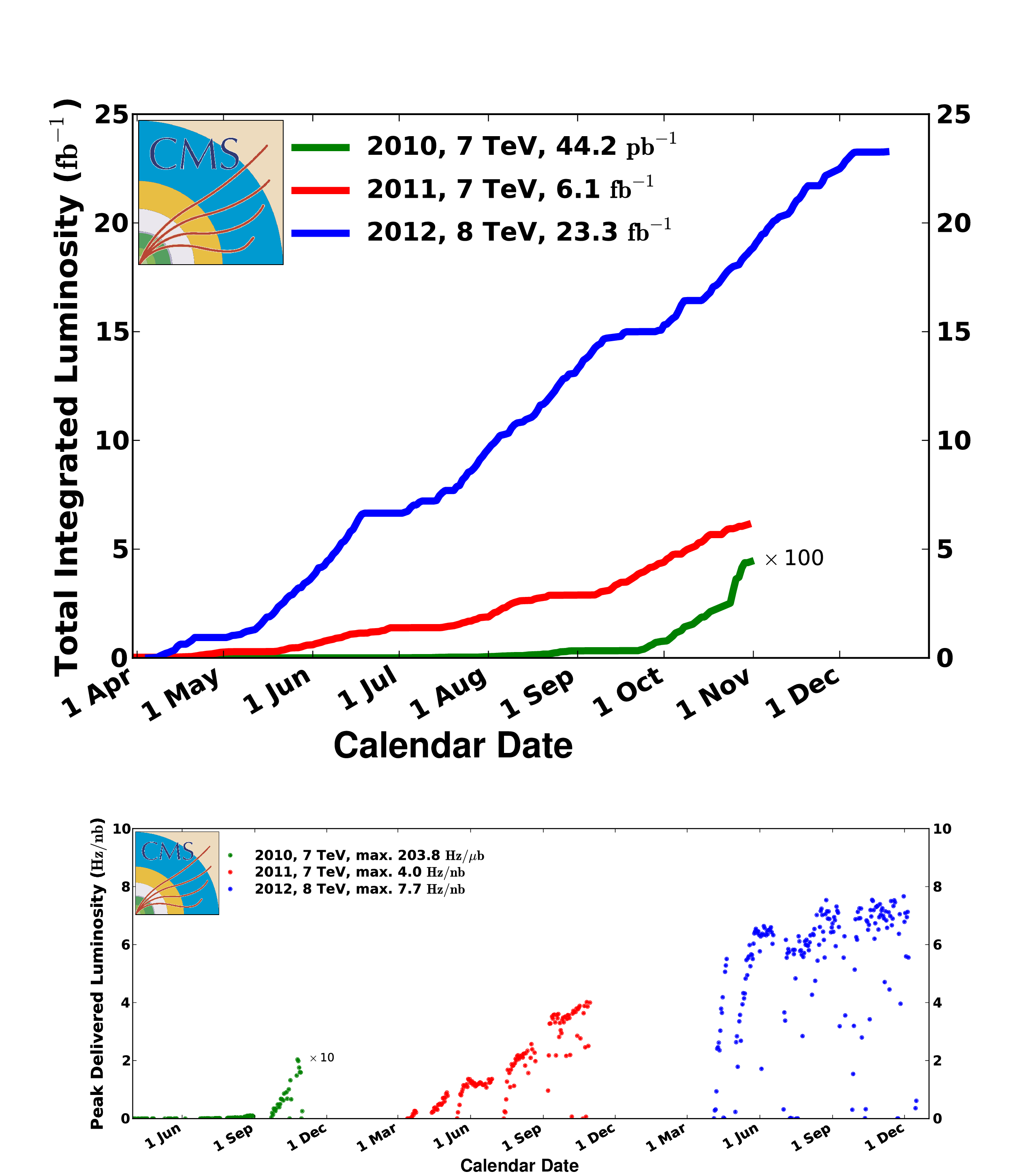
Figure 1:
Integrated (top) and peak (bottom) proton-proton luminosities as a function of time for calendar years 2010-2012. The 2010 integrated (instantaneous) luminosity is multiplied by a factor of 100 (10). In the lower plot, 1 Hz/nb corresponds to 10$^{33}$ cm$^{-2}$s$^{-1}$. |

png pdf |
Figure 1-a:
Integrated proton-proton luminosities as a function of time for calendar years 2010-2012. The 2010 integrated luminosity is multiplied by a factor of 100. |

png pdf |
Figure 1-b:
Peak proton-proton luminosities as a function of time for calendar years 2010-2012. The 2010 instantaneous luminosity is multiplied by a factor of 10. In this plot, 1 Hz/nb corresponds to 10$^{33}$ cm$^{-2}$s$^{-1}$. |
png pdf |
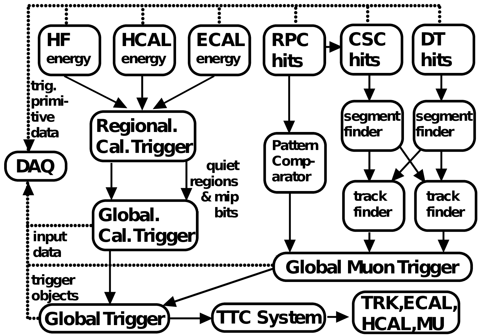
Figure 2:
Overview of the CMS L1 trigger system. Data from the forward (HF) and barrel (HCAL) hadronic calorimeters, and from the electromagnetic calorimeter (ECAL), are processed first regionally (RCT) and then globally (GCT). Energy deposits (hits) from the resistive-plate chambers (RPC), cathode strip chambers (CSC), and drift tubes (DT) are processed either via a pattern comparator or via a system of segment- and track-finders and sent onwards to a global muon trigger (GMT). The information from the GCT and GMT is combined in a global trigger (GT), which makes the final trigger decision. This decision is sent to the tracker (TRK), ECAL, HCAL or muon systems (MU) via the trigger, timing and control (TTC) system. The data acquisition system (DAQ) reads data from various subsystems for offline storage. MIP stands for minimum-ionizing particle. |

png pdf |
Figure 3:
Block diagram of the regional calorimeter trigger (RCT) system showing the data flow through the different cards in a RCT crate. At the top is the input from the calorimeters; at the bottom is the data transmitted to the global calorimeter trigger (GCT). Data exchanged on the backplane is shown as arrows between cards. Data from neighboring towers come via the backplane, but may come over cables from adjoining crates. |

png pdf |
Figure 4:
A schematic of the global calorimeter trigger (GCT) system, showing the data flow through the various component cards. |
png pdf |
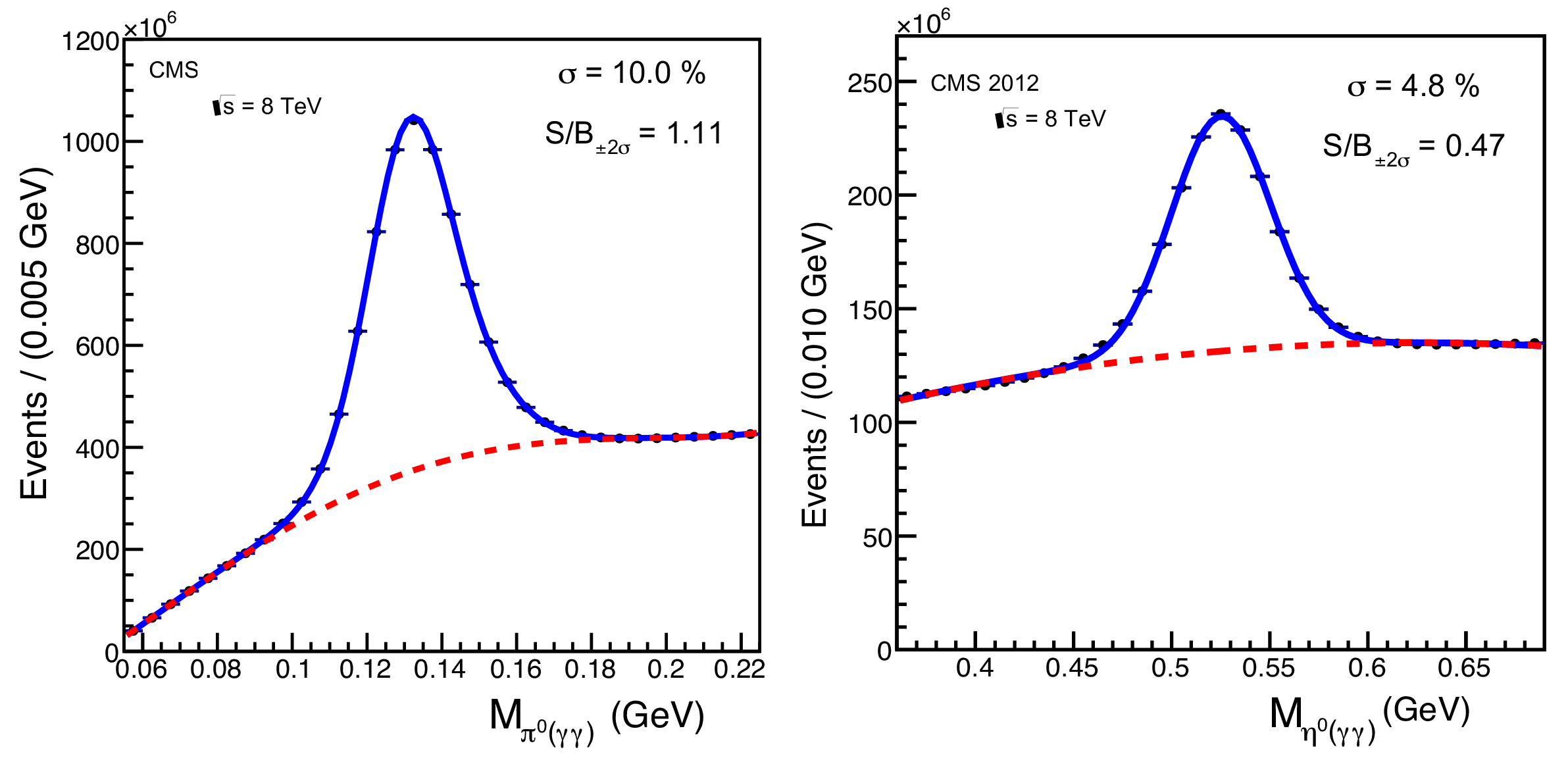
Figure 5:
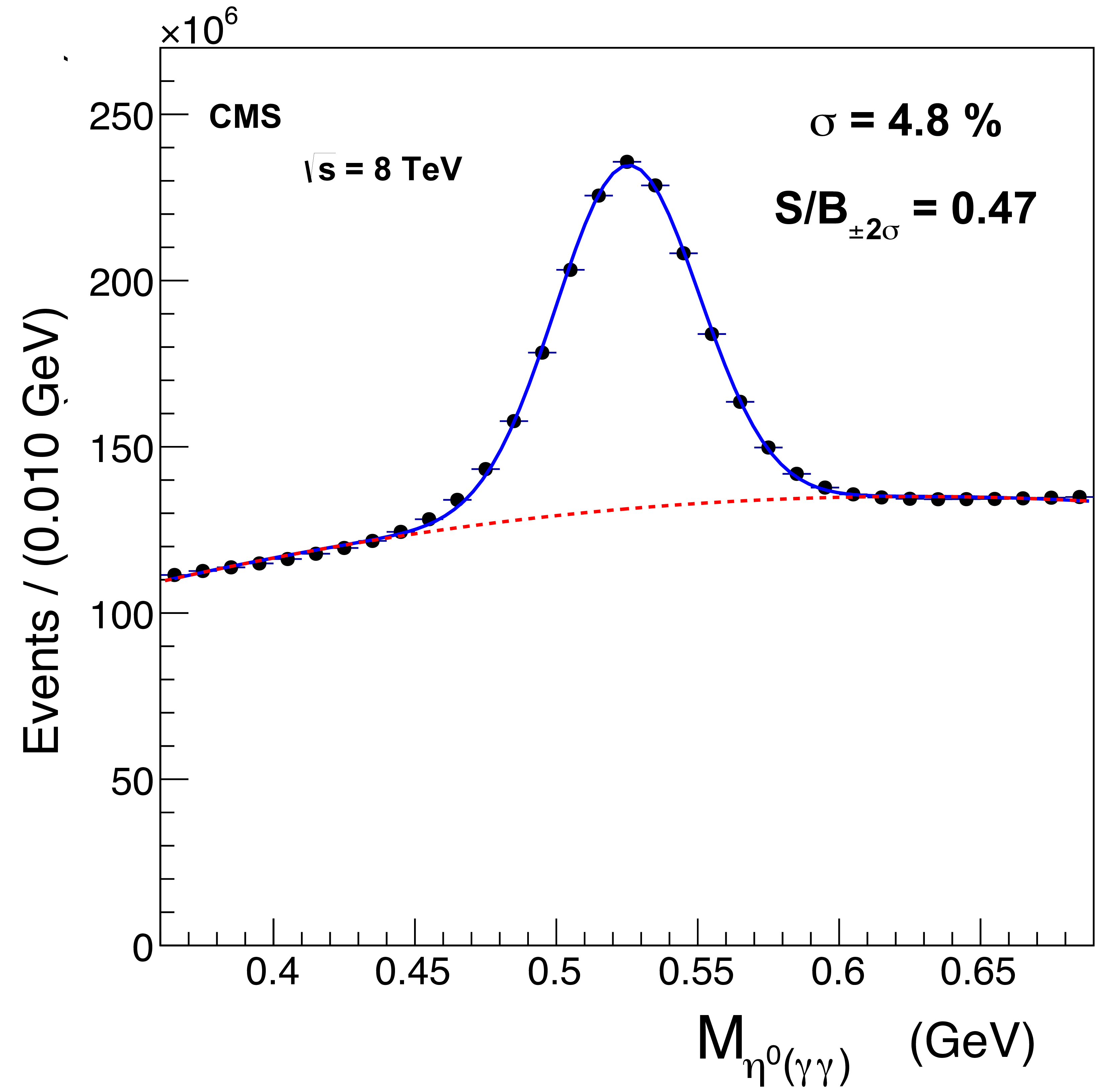
Neutral pion (left) and $\eta $ (right) invariant mass peaks reconstructed in the barrel with 2012 data. The spectra are fitted with a combination of a double (single) Gaussian for the signal and a 4th (2nd) order polynomial for the background. The entire 2012 data set is used, using special online $\pi ^0/\eta $ calibration streams. The sample size is determined by the rate of this calibration stream. Signal over background (S/B) and the fitted resolution are indicated on the plots. The fitted peak positions are not exactly at the nominal $\pi ^0/\eta $ mass values mainly due to the effects of selective readout and leakage outside the 3${\times }$3 clusters used in the mass reconstruction; however, the absolute mass values are not used in the inter-calibration. |
png pdf |
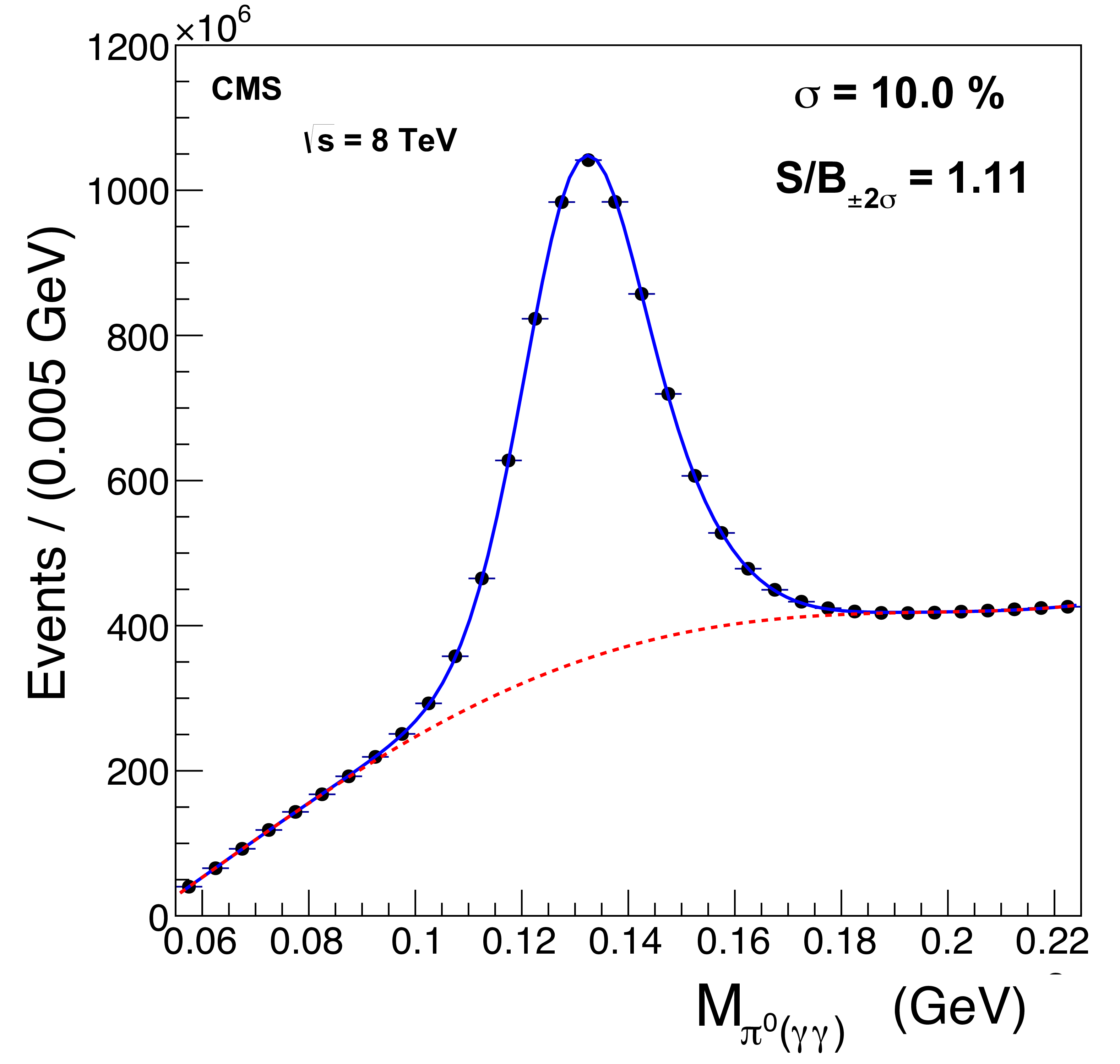
Figure 5-a:
Neutral pion invariant mass peak reconstructed in the barrel with 2012 data. The spectra are fitted with a combination of a double Gaussian for the signal and a 4th order polynomial for the background. The entire 2012 data set is used, using special online $\pi ^0/\eta $ calibration streams. The sample size is determined by the rate of this calibration stream. Signal over background (S/B) and the fitted resolution are indicated on the plots. The fitted peak position is not exactly at the nominal $\pi ^0$ mass value mainly due to the effects of selective readout and leakage outside the 3${\times }$3 clusters used in the mass reconstruction; however, the absolute mass value is not used in the inter-calibration. |
png pdf |
Figure 5-b:
$\eta $ invariant mass peak reconstructed in the barrel with 2012 data. The spectra are fitted with a combination of a single Gaussian for the signal and a 2nd order polynomial for the background. The entire 2012 data set is used, using special online $\pi ^0/\eta $ calibration streams. The sample size is determined by the rate of this calibration stream. Signal over background (S/B) and the fitted resolution are indicated on the plots. The fitted peak position is not exactly at the nominal $\eta $ mass value mainly due to the effects of selective readout and leakage outside the 3${\times }$3 clusters used in the mass reconstruction; however, the absolute mass value is not used in the inter-calibration. |
png pdf |
Figure 6:
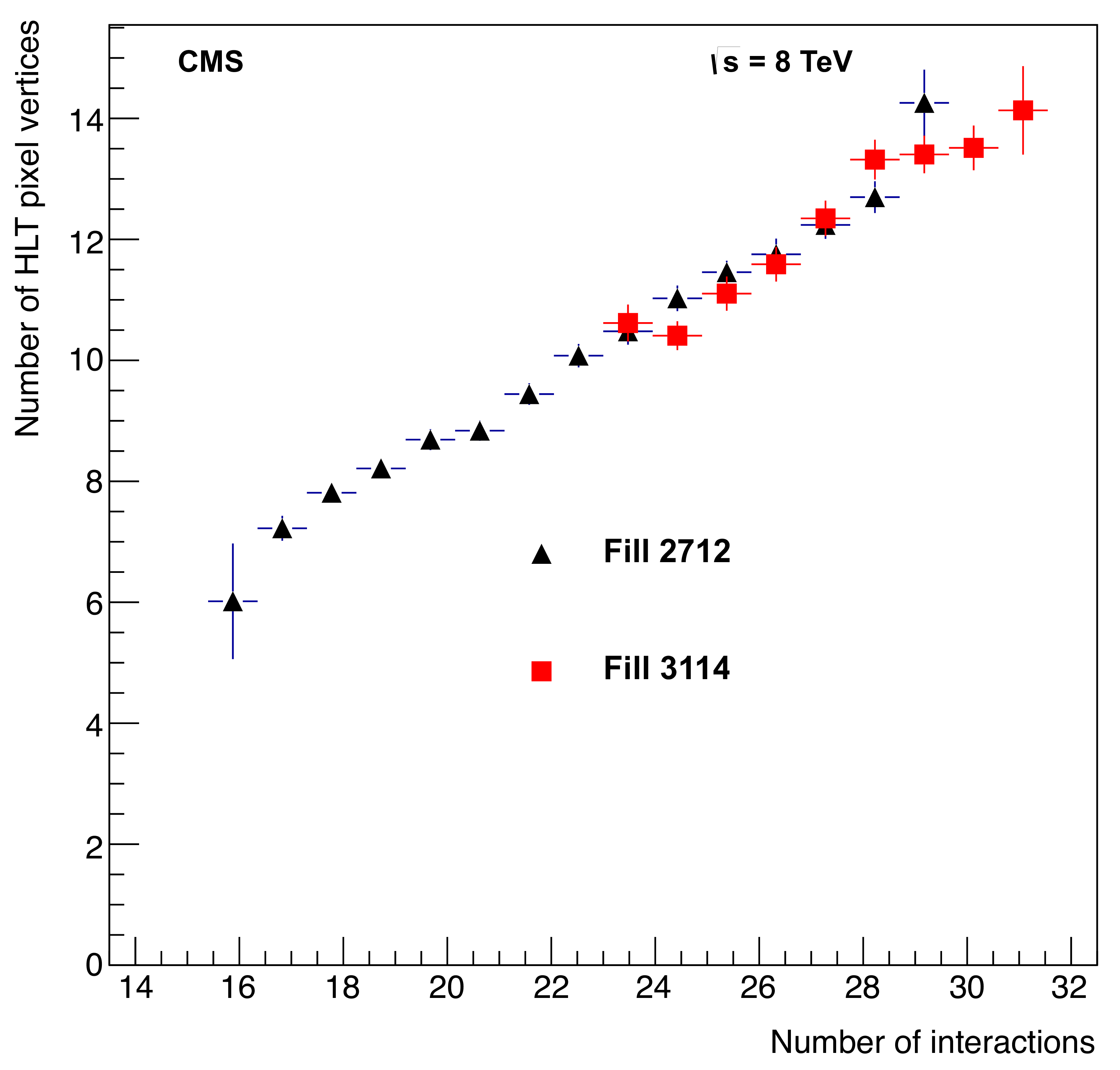
Number of vertices as a function of the number of pp interactions as measured by the forward calorimeter, for fills taken in two different periods of the 2012 pp run. A linear relation can be seen between the two quantities, demonstrating good performance of the HLT pixel vertex algorithm. |

png pdf |
Figure 7:
Tracking efficiency as a function of the momentum of the reconstructed particle, for the HLT and offline tracking, as determined from simulated $ {\mathrm{ t } \mathrm{ \bar{t} } } $ events. Above 0.9 GeV, the online efficiency is above 80% and plateaus at around 90%. |

png pdf |
Figure 8:
The CPU time spent in the tracking reconstruction as a function of the average pileup, as measured in pp data taken during the 2012 run. The red line shows a fit to data with a second-order polynomial. On average, about 30% of the total CPU time of the HLT was devoted to tracking during this run. |

png pdf |
Figure 9:
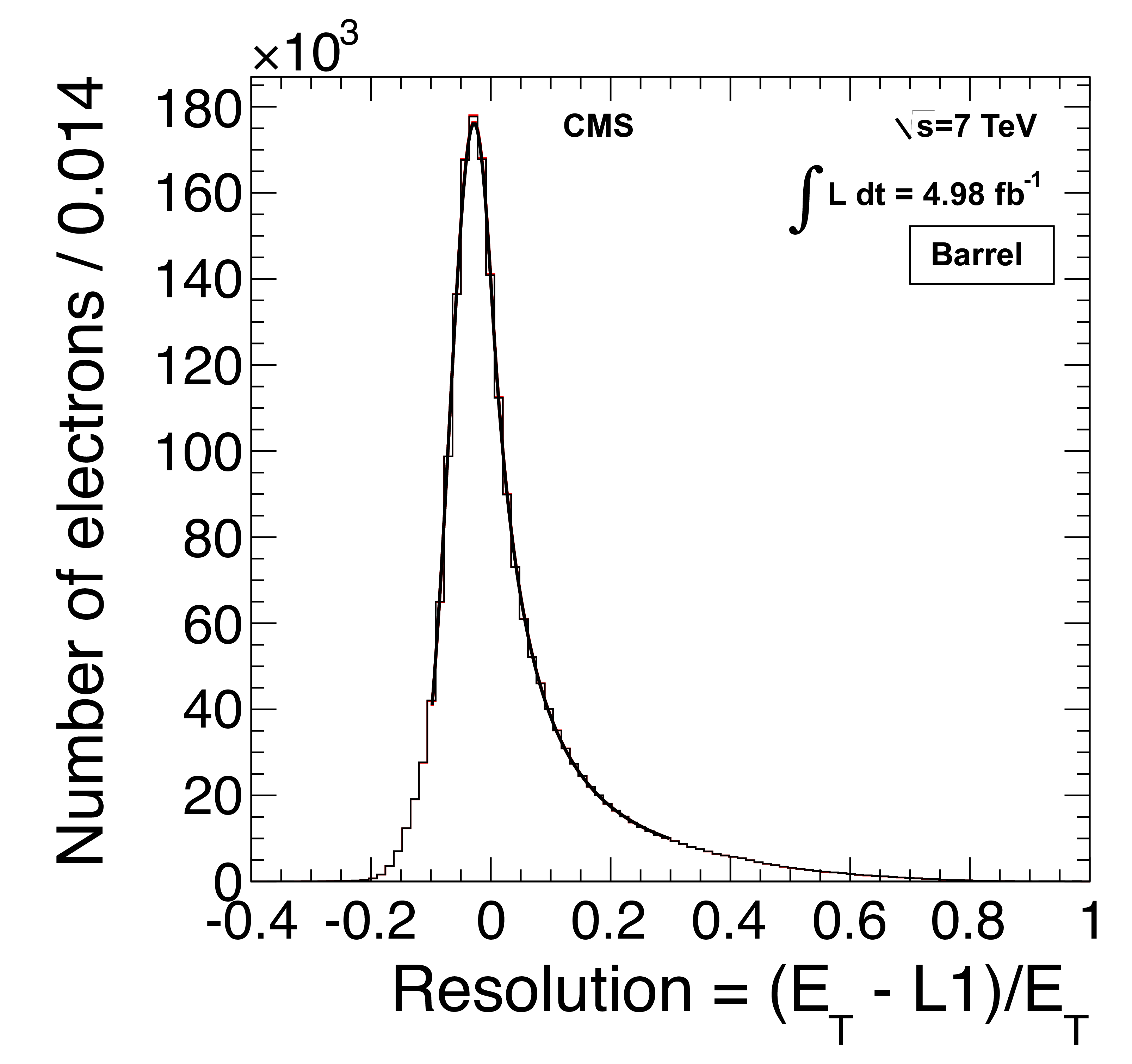
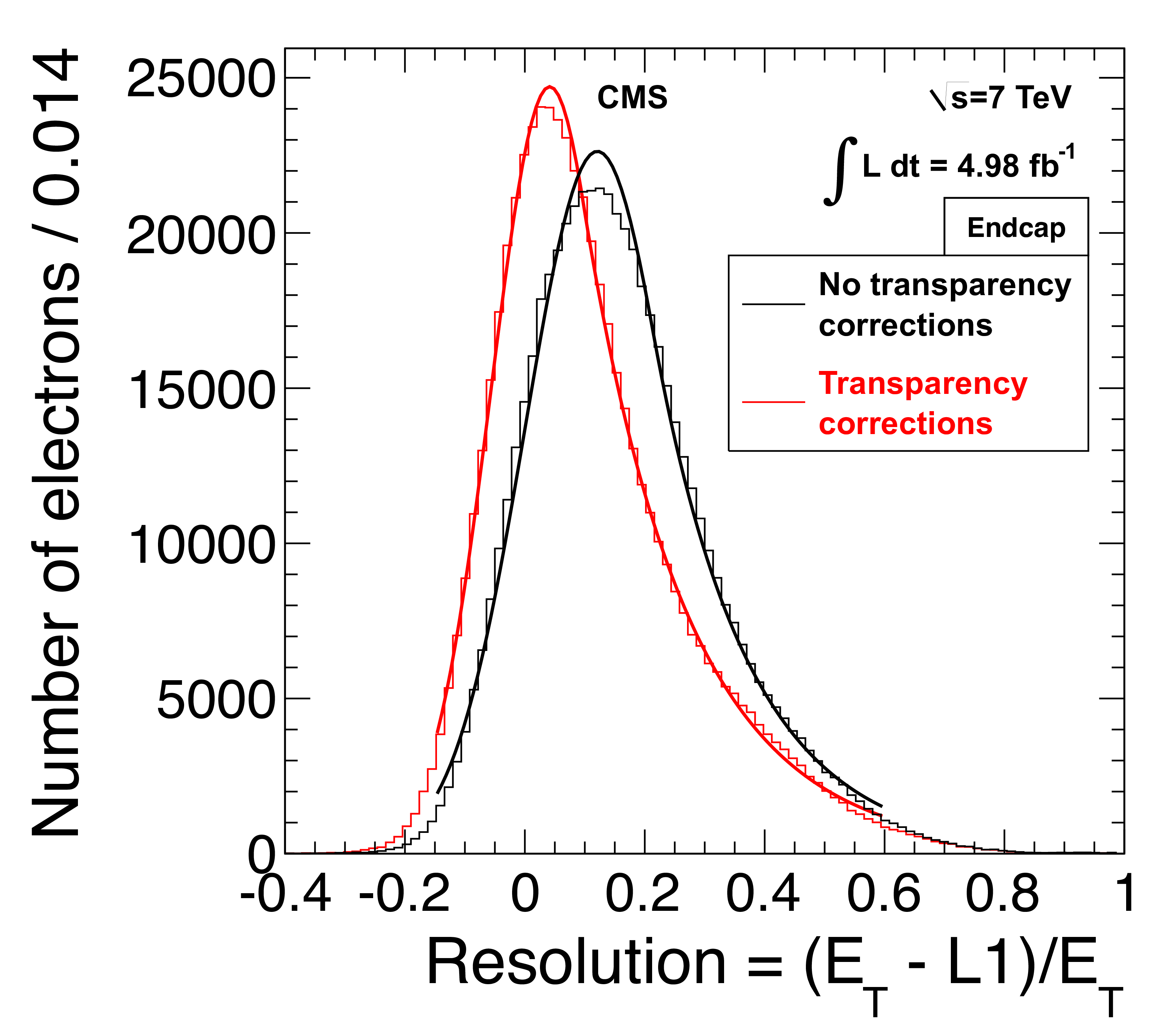
The L1 EG resolution, reconstructed offline $ {E_{\mathrm {T}}} $ minus L1 $ {E_{\mathrm {T}}} $ divided by reconstructed offline $ {E_{\mathrm {T}}} $, in the barrel (left) and endcap (right) regions. For both distributions, a fit to a Crystal Ball function is performed. On the right curve, the red solid line shows the result after applying the transparency corrections (as discussed in Sec. 2.2.1.1) For EB, the resolution after transparency correction is unchanged. |
png pdf |
Figure 9-a:
The L1 EG resolution, reconstructed offline $ {E_{\mathrm {T}}} $ minus L1 $ {E_{\mathrm {T}}} $ divided by reconstructed offline $ {E_{\mathrm {T}}} $, in the barrel region. A fit to a Crystal Ball function is performed. |
png pdf |
Figure 9-b:
The L1 EG resolution, reconstructed offline $ {E_{\mathrm {T}}} $ minus L1 $ {E_{\mathrm {T}}} $ divided by reconstructed offline $ {E_{\mathrm {T}}} $, in the endcap regions. A fit to a Crystal Ball function is performed. The red solid line shows the result after applying the transparency corrections (as discussed in Sec. 2.2.1.1). |
png pdf |
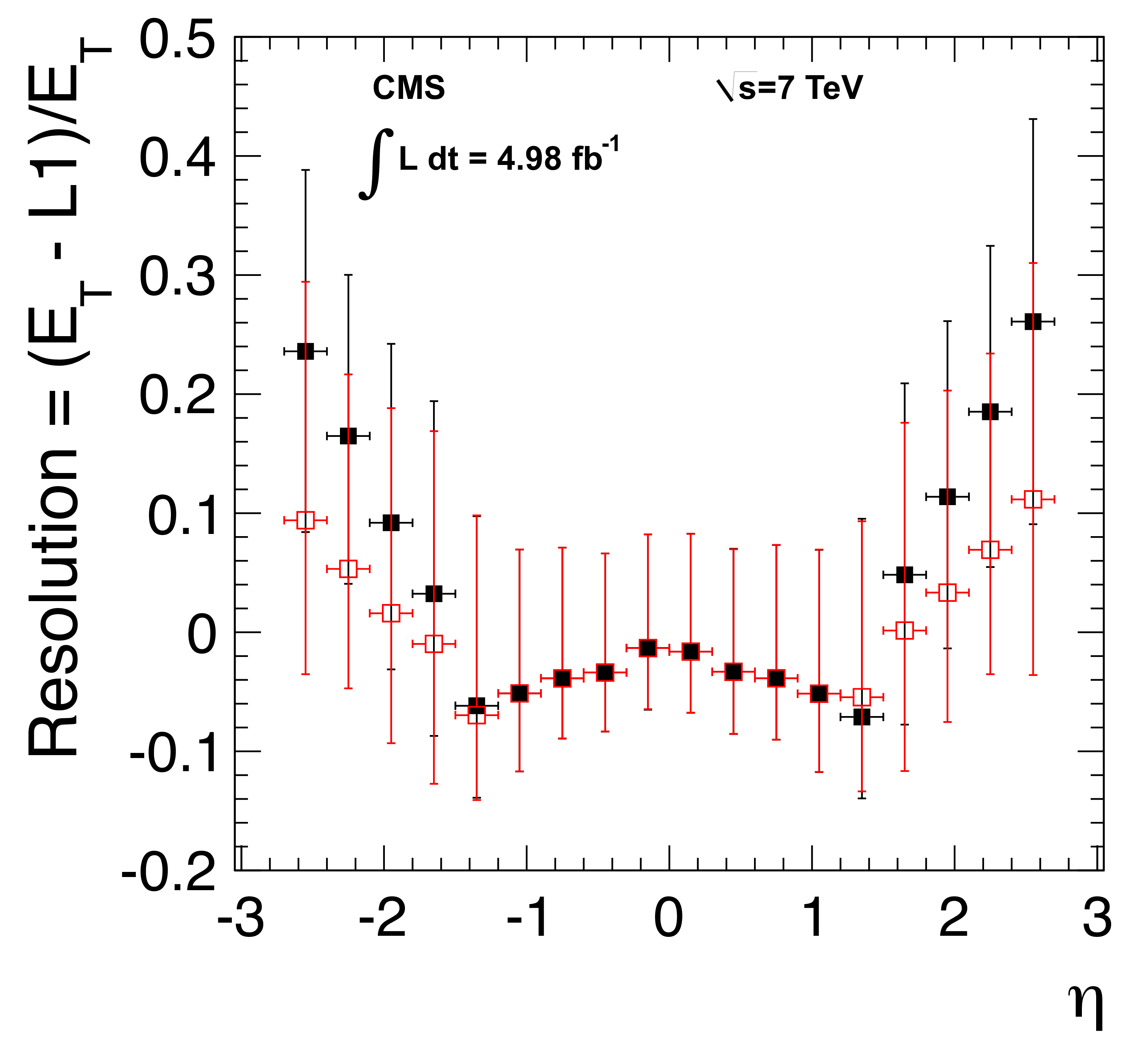
Figure 10:
The L1 EG resolution for all electron $ {p_{\mathrm {T}}} $ as a function of pseudorapidity $\eta $. For each $\eta $ bin, a fit to a Crystal Ball function was used to model the data distribution. The vertical bars on each point represent the sigma of each fitted function which is defined as the width of the 68% area. The red points show the improved resolution after applying transparency corrections (as discussed in Sec. 2.2.1.1). |
png pdf |
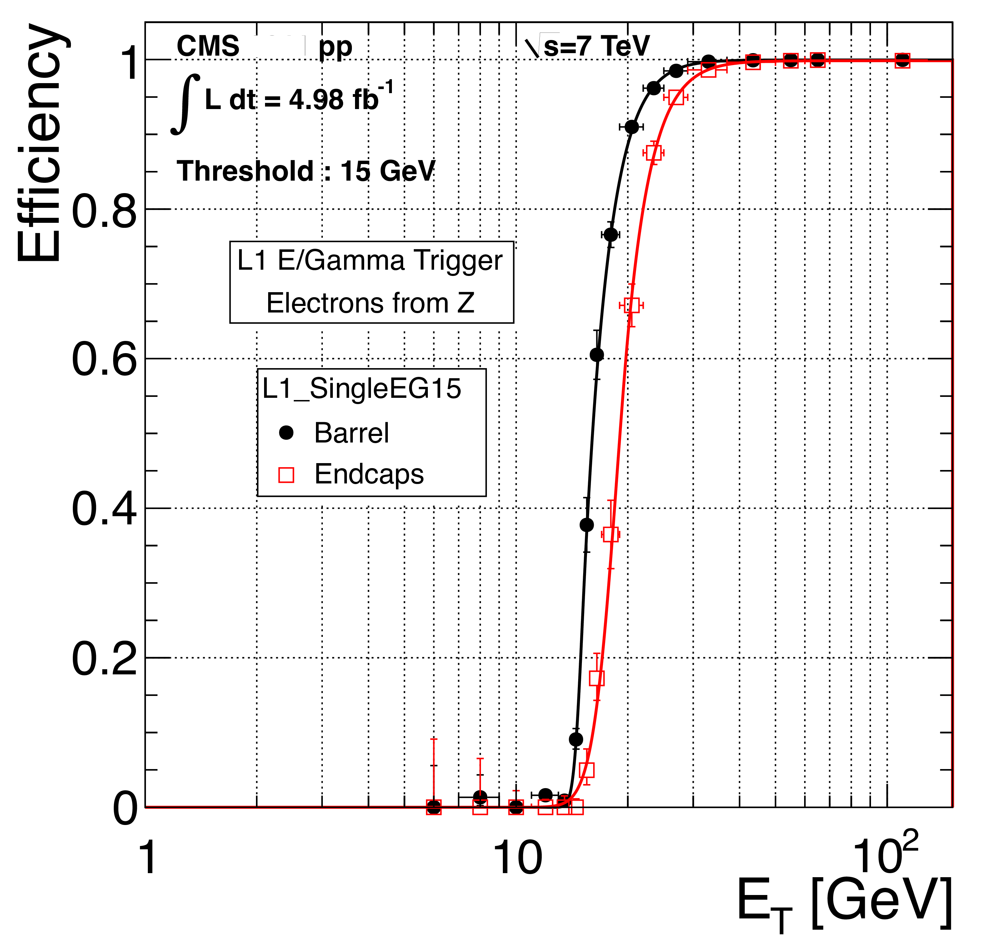
Figure 11:
The electron trigger efficiency at L1 as a function of offline reconstructed $ {E_{\mathrm {T}}} $ for electrons in the EB (black dots) and EE (red dots), with an EG threshold: $ {E_{\mathrm {T}}} = $ 15 GeV. The curves show unbinned likelihood fits. |
png pdf |
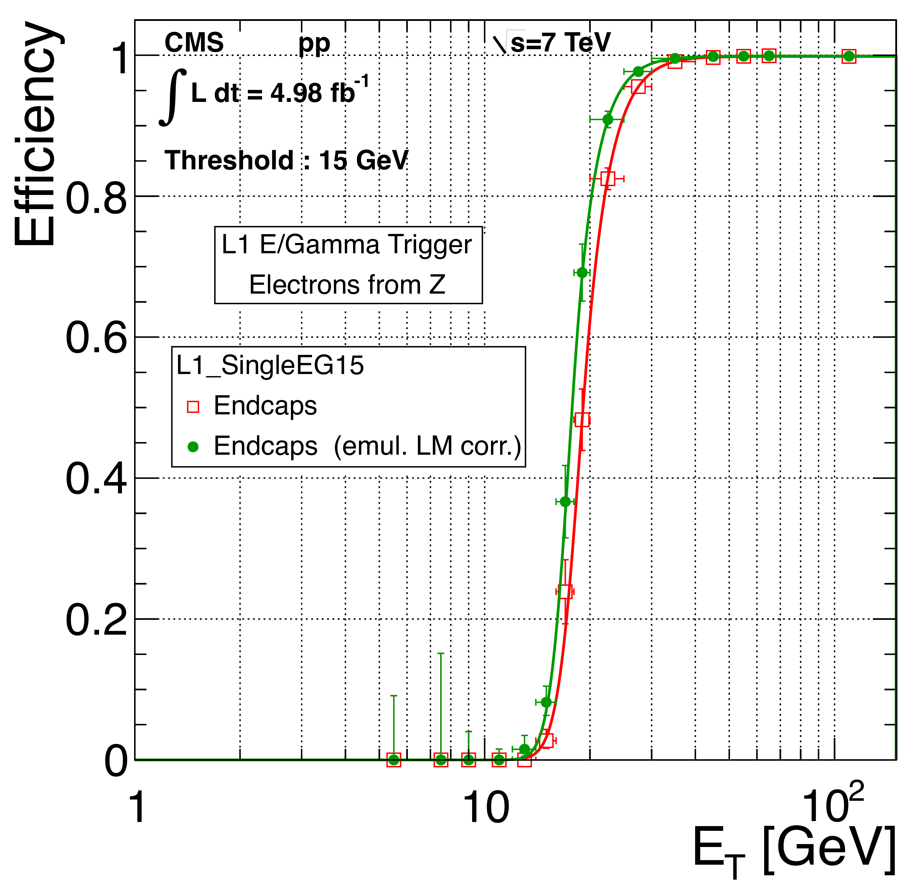
Figure 12:
The EE L1 electron trigger efficiency as a function of offline reconstructed $ {E_{\mathrm {T}}} $ before (red) and after (green) transparency corrections are applied at the ECAL TP level. The curves show unbinned likelihood fits. |

png pdf |
Figure 13:
The L1 electron triggering efficiency as a function of the reconstructed offline electron $ {E_{\mathrm {T}}} $ for barrel (left) and endcap (right). The efficiency is shown for the EG12, EG15, EG20 and EG30 L1 trigger algorithms. The curves show unbinned likelihood fits. |

png pdf |
Figure 13-a:
The L1 electron triggering efficiency as a function of the reconstructed offline electron $ {E_{\mathrm {T}}} $ for barrel. The efficiency is shown for the EG12, EG15, EG20 and EG30 L1 trigger algorithms. The curves show unbinned likelihood fits. |
png pdf |
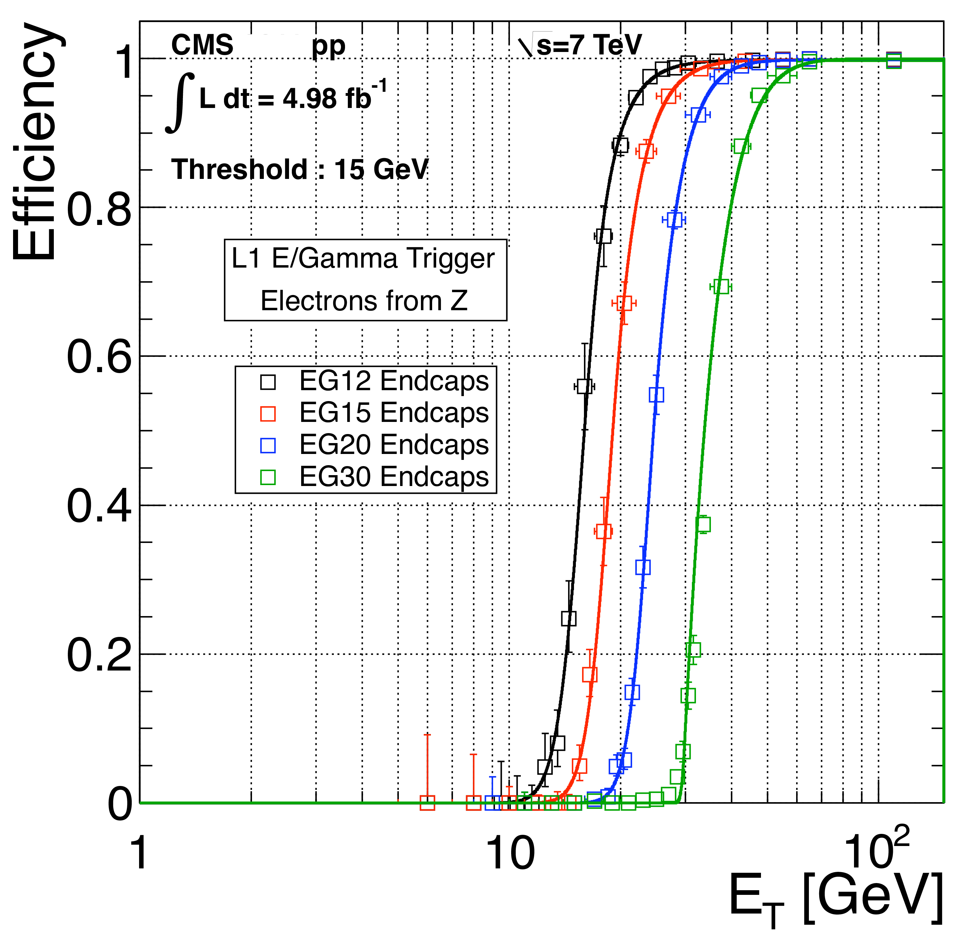
Figure 13-b:
The L1 electron triggering efficiency as a function of the reconstructed offline electron $ {E_{\mathrm {T}}} $ for endcap. The efficiency is shown for the EG12, EG15, EG20 and EG30 L1 trigger algorithms. The curves show unbinned likelihood fits. |

png pdf |
Figure 14:
Electron trigger efficiency at L1, as a function of offline reconstructed $ {E_{\mathrm {T}}} $ for electrons in the EB (black dots) and EE (red squares) using the 2011 data set (EG threshold: $ {E_{\mathrm {T}}} =$ 20 GeV). The curves show unbinned likelihood fits. |

png pdf |
Figure 15:
Electron trigger efficiency at L1 as a function of offline reconstructed $ {E_{\mathrm {T}}} $ for electrons in the EB (black dots) and EE (red squares) using the 2012 data set (EG threshold: $ {E_{\mathrm {T}}} =$ 20 GeV). The curves show unbinned likelihood fits. |
png pdf |
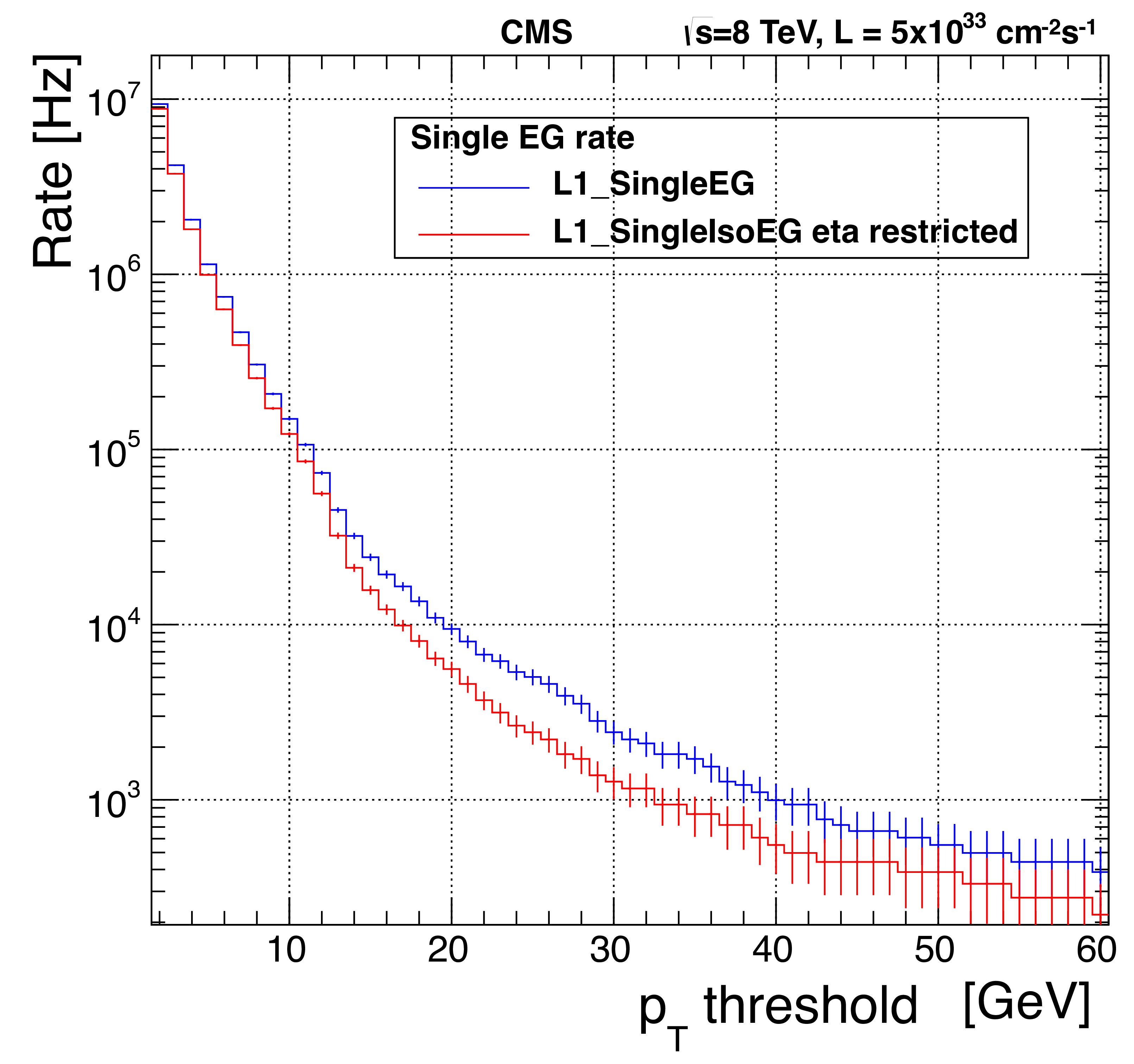
Figure 16:
Rates of the isolated and nonisolated versions of the single-EG trigger versus the transverse energy threshold rescaled to an instantaneous luminosity of 5$ \times $10$^{33}$ cm$^{-2}$s$^{-1}$. Isolated EG rates are computed within a pseudorapidity range of $ {| \eta | }< $ 2.172 to reflect the configuration of the L1 isolated EG algorithms used in 2012. |

png pdf |
Figure 17:
Electron trigger efficiency as a function of the spike rejection at L1. Each point corresponds to a different spike removal trigger sFGVB threshold. The trigger killing threshold is set to 8 GeV. The data were taken in 2010. |
png pdf |
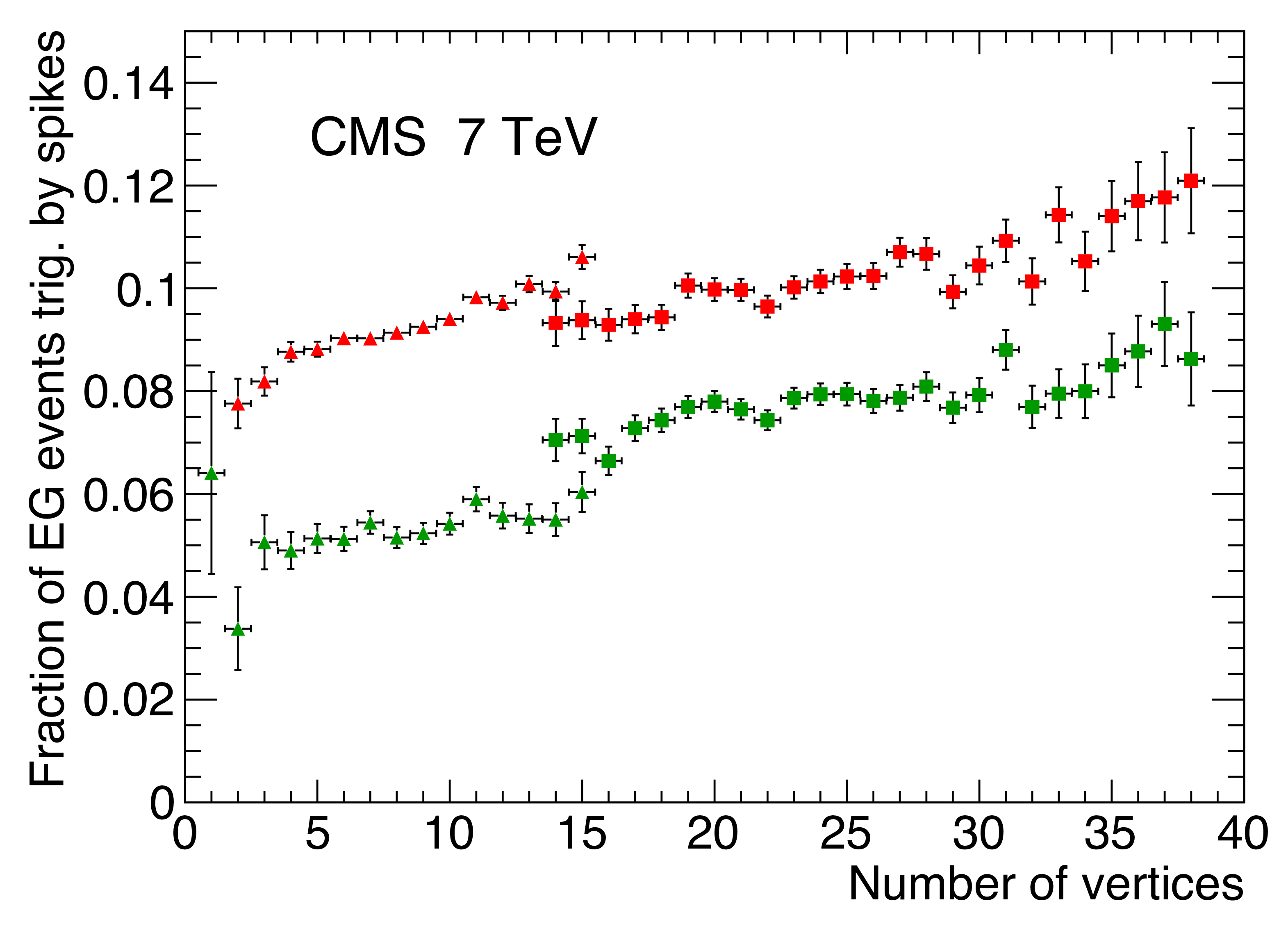
Figure 18:
Fraction of spike-induced EG triggers as a function of the number of reconstructed vertices. The red points represent the spike removal working point used in 2011, and the green points the optimized working point for 2012. The squares (triangles) correspond to higher (lower) pileup data. |
png pdf |
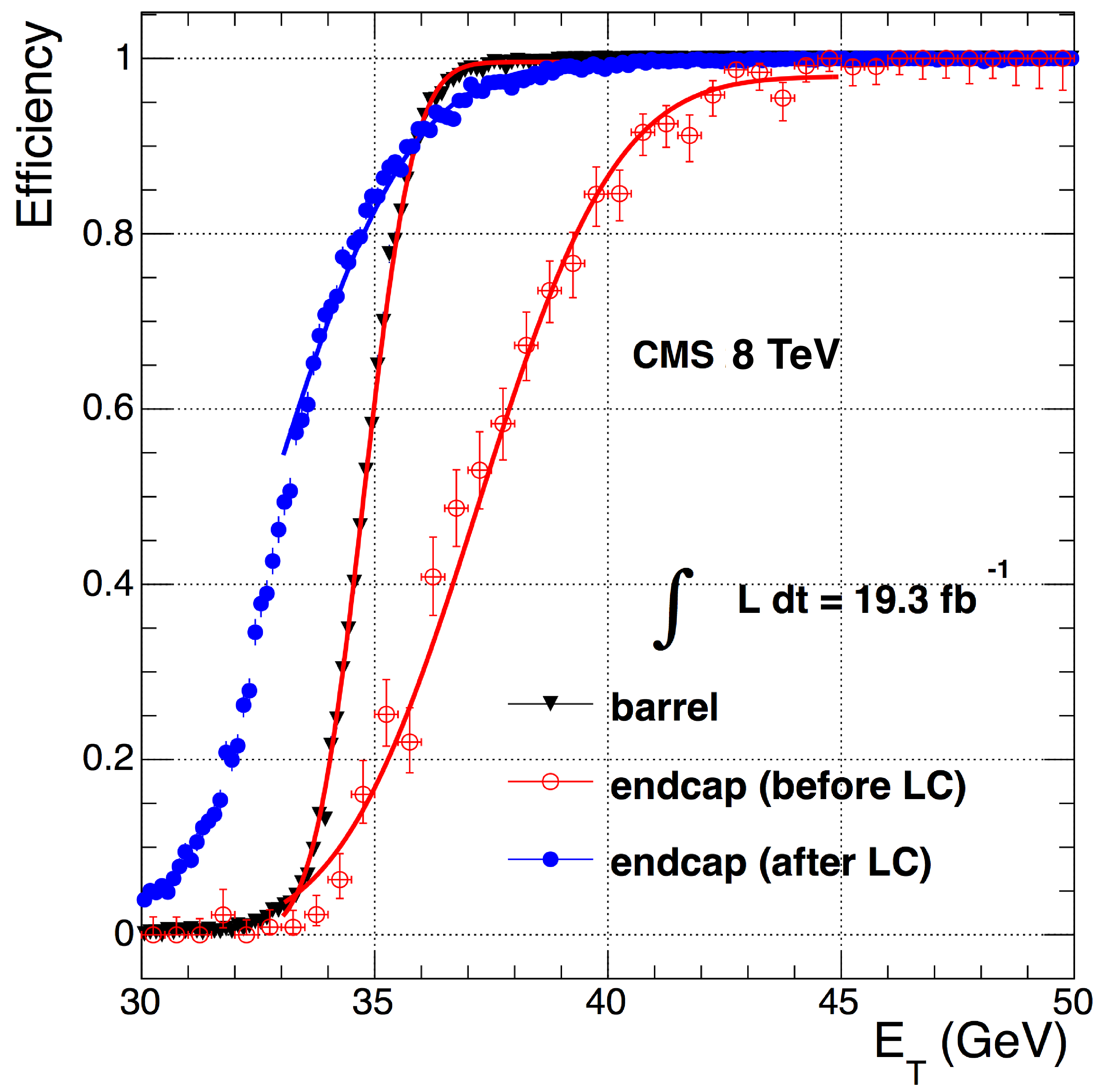
Figure 19:
Efficiency of the online $ {E_{\mathrm {T}}} $ selection as a function of the offline electron $ {E_{\mathrm {T}}} $, in barrel and endcap regions, before and after the deployment of online transparency corrections. The data depicts the results of a double-electron trigger requiring $ {p_{\mathrm {T}}} > $ 33 GeV for both legs, and shows that applying the corrections causes a significant improvement of the online turn-on curve. |

png pdf |
Figure 20:
Efficiencies of the leading leg for the double-photon trigger as a function of the photon transverse energy (left) and pseudorapidity (right), as described in the text. The red symbols show the efficiency of the isolation plus calorimeter identification requirement, and the blue symbols show the efficiency of the $ {\mathrm {R}_\mathrm {9}} $ selection criteria. The black symbols show the combined efficiency. |

png pdf |
Figure 20-a:
Efficiencies of the leading leg for the double-photon trigger as a function of the photon transverse energy, as described in the text. The red symbols show the efficiency of the isolation plus calorimeter identification requirement, and the blue symbols show the efficiency of the $ {\mathrm {R}_\mathrm {9}} $ selection criteria. The black symbols show the combined efficiency. |

png pdf |
Figure 20-b:
Efficiencies of the leading leg for the double-photon trigger as a function of the photon pseudorapidity, as described in the text. The red symbols show the efficiency of the isolation plus calorimeter identification requirement, and the blue symbols show the efficiency of the $ {\mathrm {R}_\mathrm {9}} $ selection criteria. The black symbols show the combined efficiency. |
png pdf |
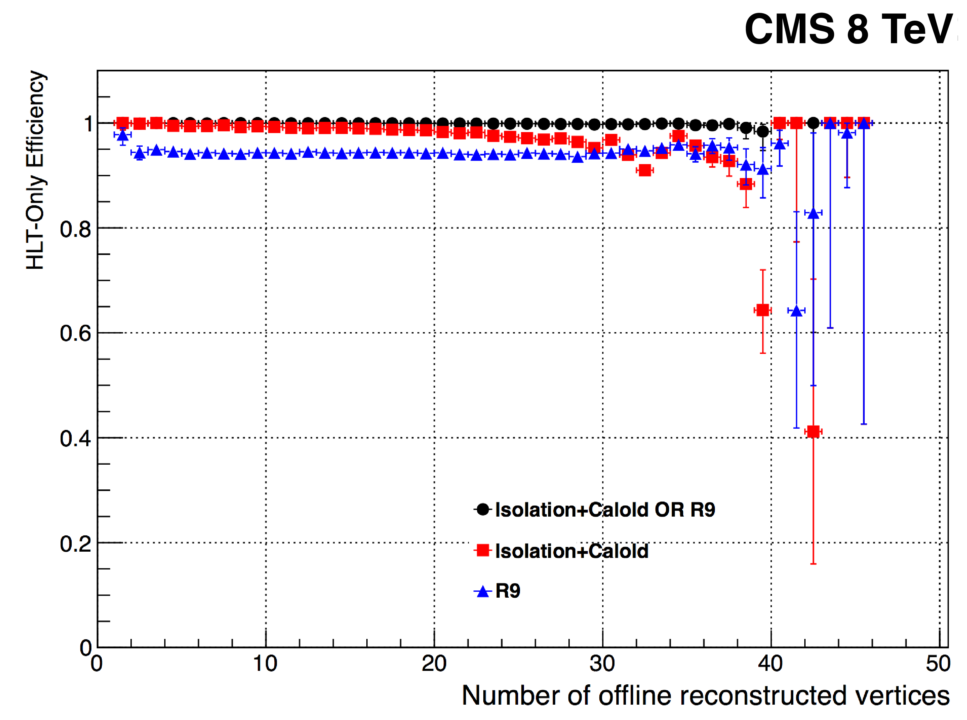
Figure 21:
Efficiencies of the leading leg of the double-photon trigger described in the text as a function of the number of offline reconstructed vertices. The red symbols show the efficiency of the isolation plus calorimeter identification requirement, and the blue symbols show the efficiency of the $ {\mathrm {R}_\mathrm {9}} $ selection. The black symbols show the combined efficiency. |
png pdf |
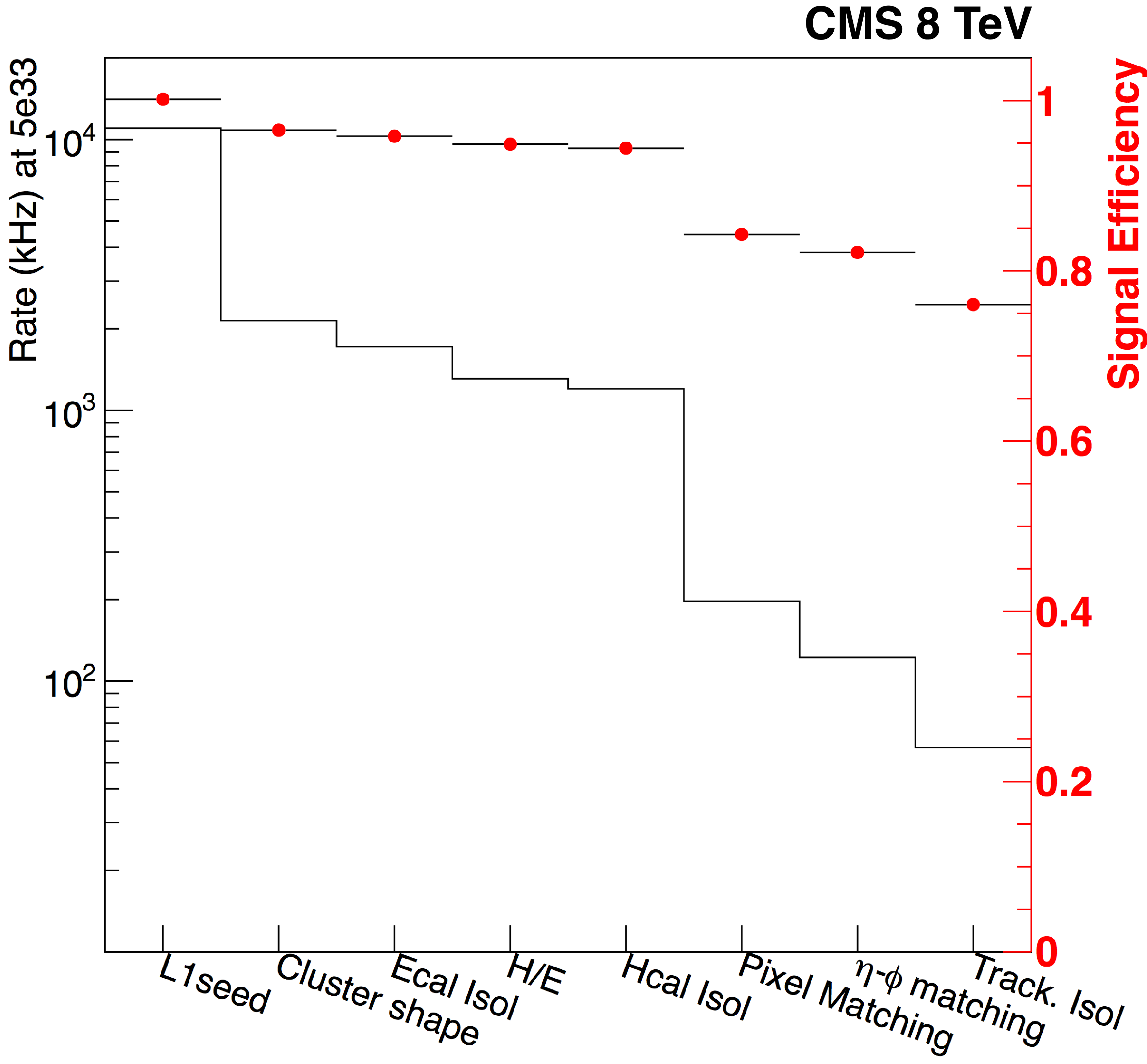
Figure 22:
Performance of the internal stages of the lowest-$ {E_{\mathrm {T}}} $ unprescaled single-electron trigger. The rate is shown as the black histogram (left scale); the red symbols show the efficiency for electron selection (right scale). |

png pdf |
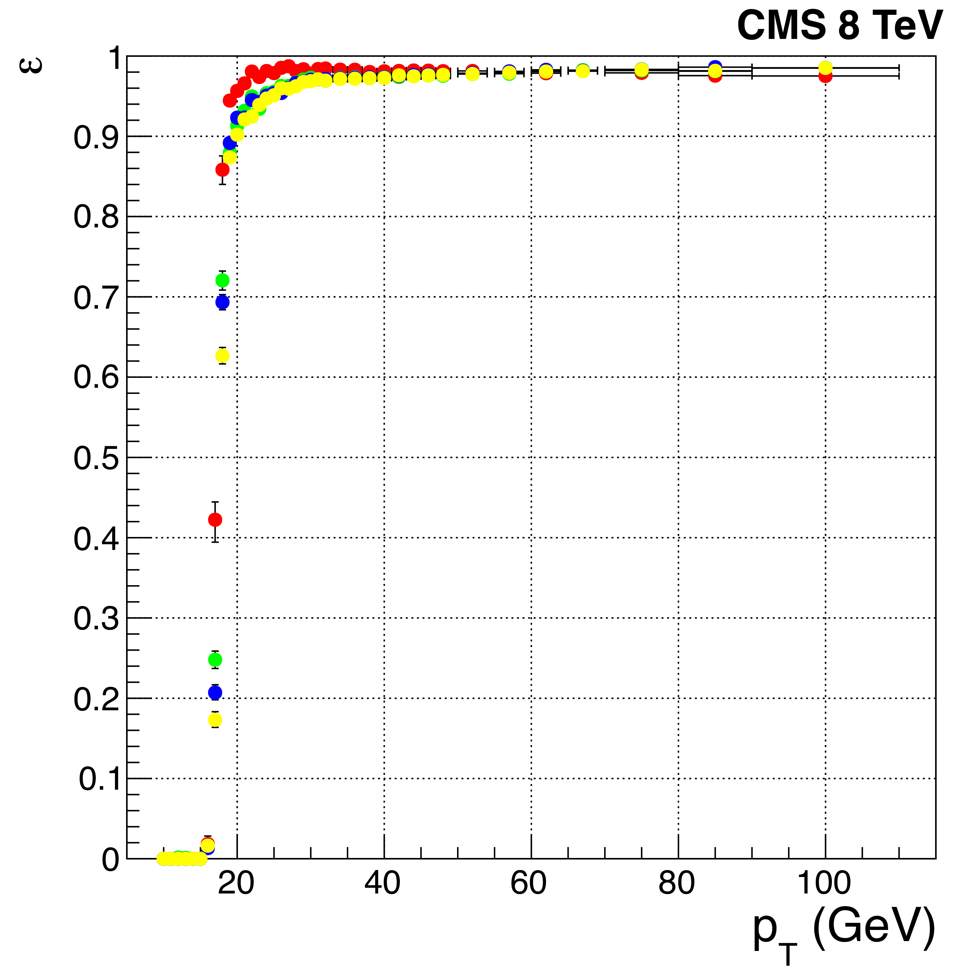
Figure 23:
Efficiencies of the leading leg for the double-electron trigger described in the text as a function of the offline electron momentum. The trigger uses identical selection for both legs, so the other leg just has a different threshold. Efficiencies are shown for different running periods (red May, green June, blue August, and yellow November of 2012) and separately for electron reconstructed in barrel (left) and endcap (right). |
png pdf |
Figure 23-a:
Efficiencies of the leading leg for the double-electron trigger described in the text as a function of the offline electron momentum. The trigger uses identical selection for both legs, so the other leg just has a different threshold. Efficiencies are shown for different running periods (red May, green June, blue August, and yellow November of 2012) for electron reconstructed in barrel. |

png pdf |
Figure 23-b:
Efficiencies of the leading leg for the double-electron trigger described in the text as a function of the offline electron momentum. The trigger uses identical selection for both legs, so the other leg just has a different threshold. Efficiencies are shown for different running periods (red May, green June, blue August, and yellow November of 2012) for electron reconstructed endcap. |

png pdf |
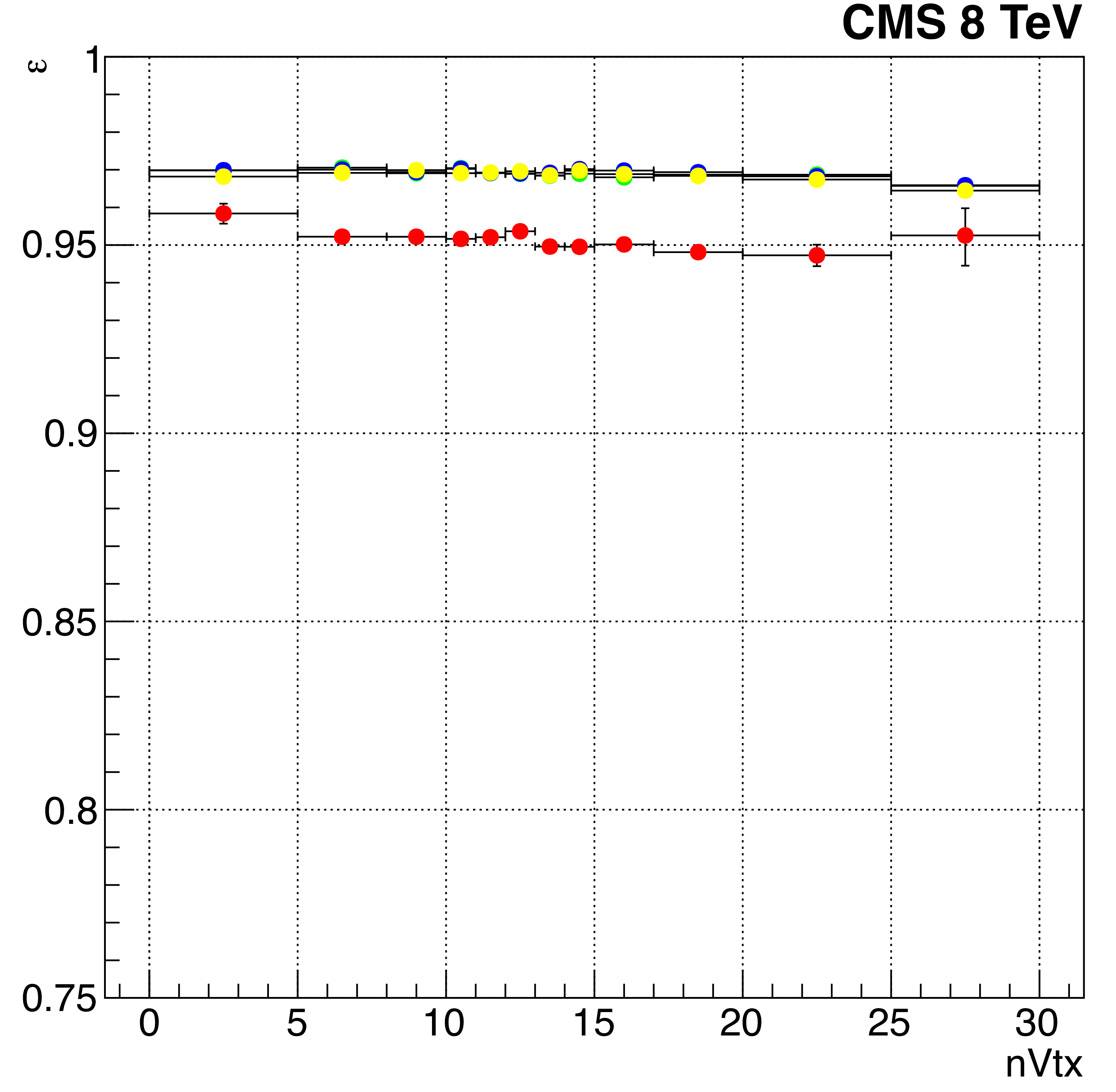
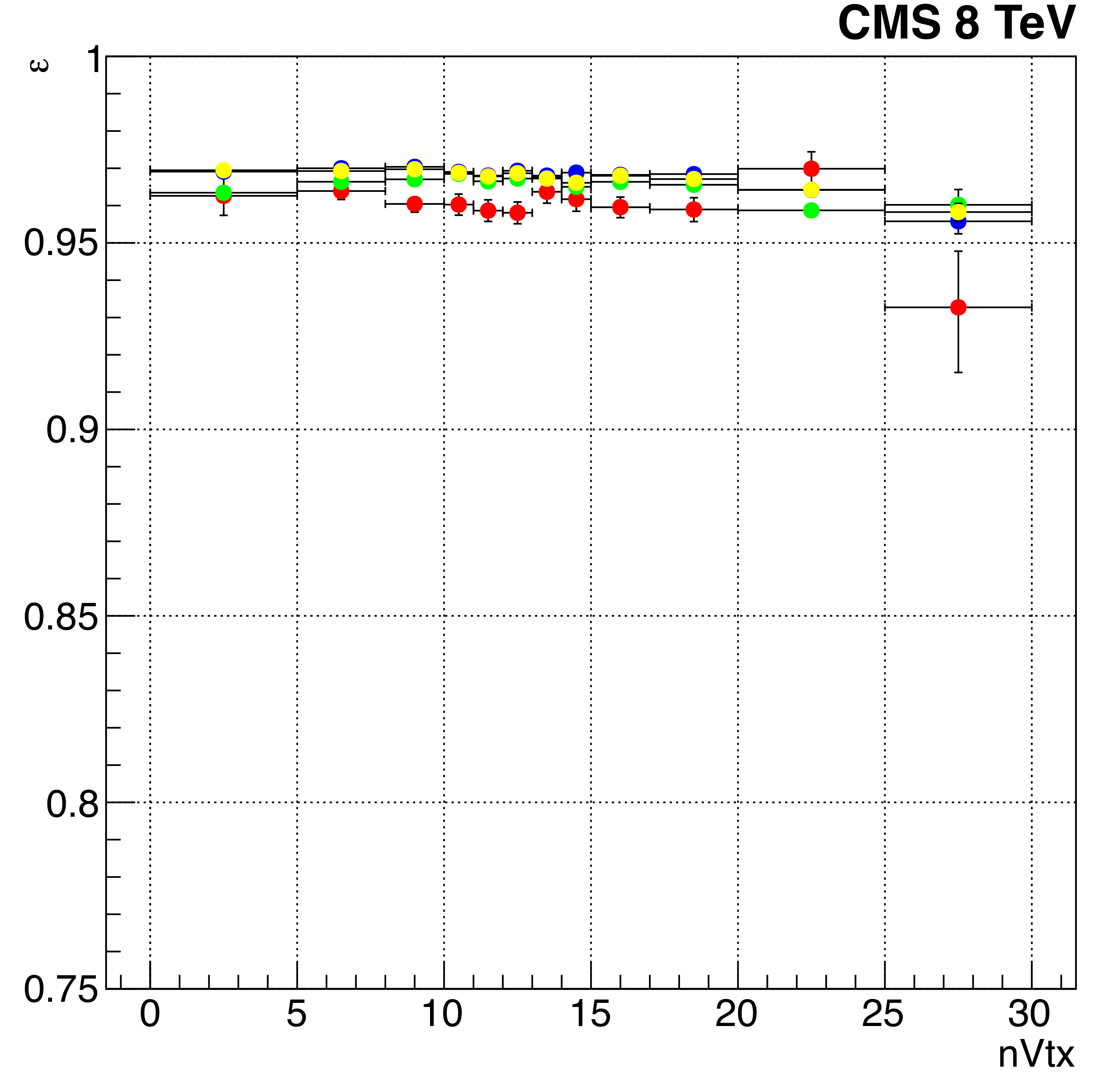
Figure 24:
Efficiencies of the leading leg for the double-electron trigger described in the text as a function of the number of reconstructed vertices. The trigger uses identical selection for both legs, so the other leg just has a different threshold. Efficiencies are shown for different running periods (red May, green June, blue August, and yellow November of 2012) and separately for electron reconstructed in barrel (left) and endcap (right). |
png pdf |
Figure 24-a:
Efficiencies of the leading leg for the double-electron trigger described in the text as a function of the number of reconstructed vertices. The trigger uses identical selection for both legs, so the other leg just has a different threshold. Efficiencies are shown for different running periods (red May, green June, blue August, and yellow November of 2012) for electron reconstructed in barrel. |
png pdf |
Figure 24-b:
Efficiencies of the leading leg for the double-electron trigger described in the text as a function of the number of reconstructed vertices. The trigger uses identical selection for both legs, so the other leg just has a different threshold. Efficiencies are shown for different running periods (red May, green June, blue August, and yellow November of 2012) for electron reconstructed in endcap. |
png pdf |
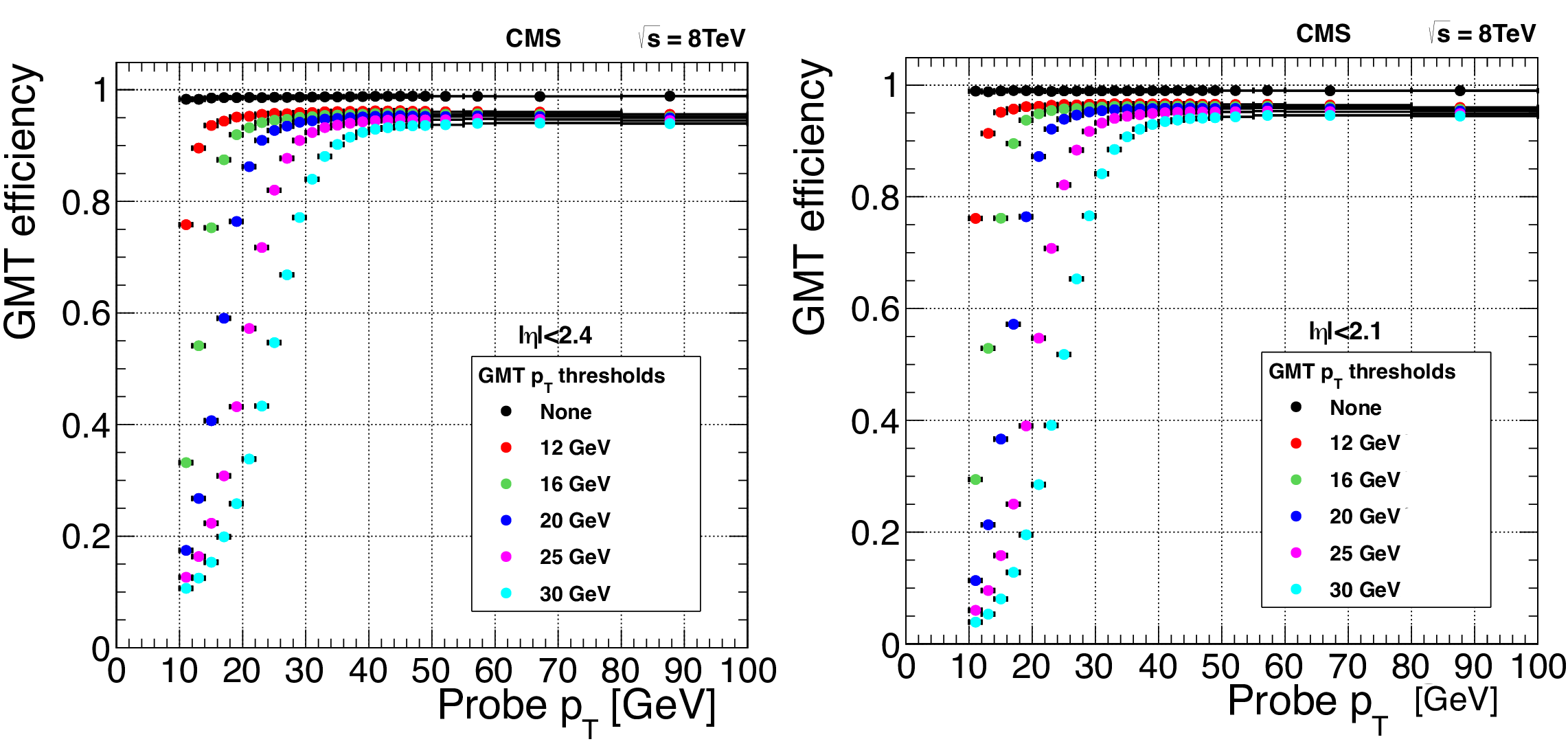
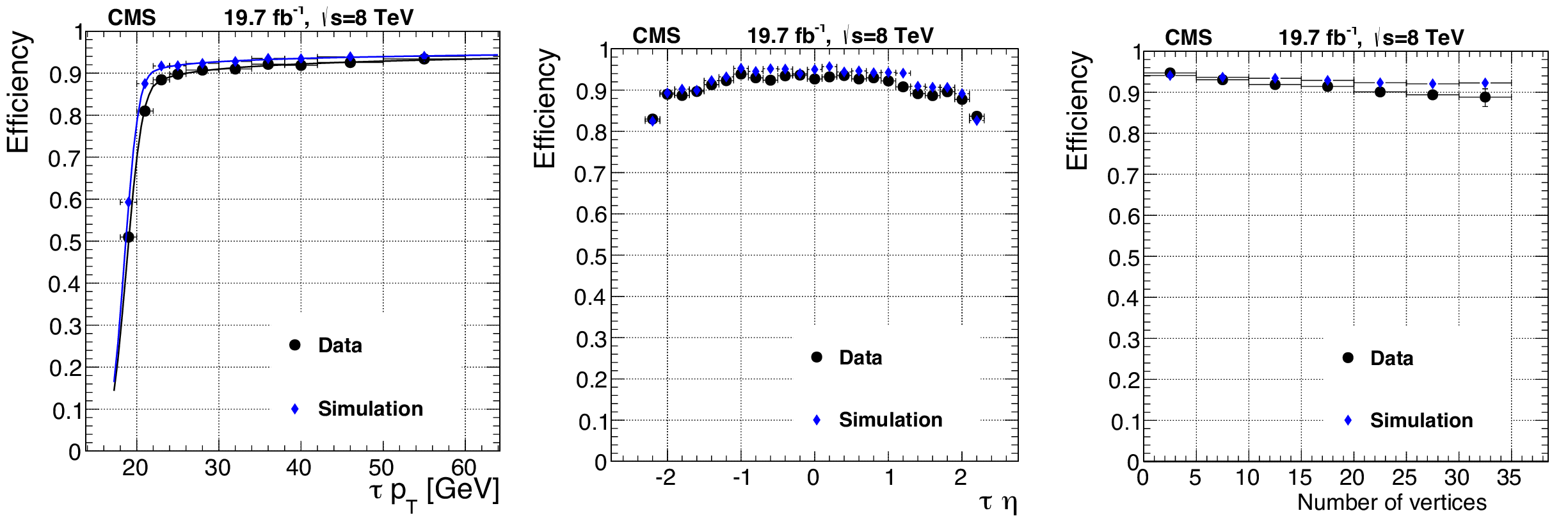
Figure 25:
The efficiency of the single-muon trigger versus the reconstructed transverse momentum of the muon for different thresholds applied on the trigger candidate $ {p_{\mathrm {T}}} $ for the full pseudorapidity range $ {| \eta | } < $ 2.4 (left), and limited to the range $ {| \eta | }< $ 2.1 (right). The quality requirement used in the single-muon trigger algorithms (see text) was applied. Results are computed using the tag-and-probe method applied on a Z boson enriched sample. |

png pdf |
Figure 25-a:
The efficiency of the single-muon trigger versus the reconstructed transverse momentum of the muon for different thresholds applied on the trigger candidate $ {p_{\mathrm {T}}} $ for the full pseudorapidity range $ {| \eta | } < $ 2.4. The quality requirement used in the single-muon trigger algorithms (see text) was applied. Results are computed using the tag-and-probe method applied on a Z boson enriched sample. |

png pdf |
Figure 25-b:
The efficiency of the single-muon trigger versus the reconstructed transverse momentum of the muon for different thresholds applied on the trigger candidate $ {p_{\mathrm {T}}} $ limited to the range $ {| \eta | }< $ 2.1. The quality requirement used in the single-muon trigger algorithms (see text) was applied. Results are computed using the tag-and-probe method applied on a Z boson enriched sample. |

png pdf |
Figure 26:
The efficiency of the single-muon trigger as a function of $\eta $ for the threshold of 16 GeV (black) for muons with reconstructed $ {p_{\mathrm {T}}} > $ 24 GeV. The contribution of the muon trigger subsystems to this efficiency is also presented: the red/green/blue points show the fraction of the GMT events based on the RPC/DTTF/CSCTF candidates, respectively. Results are computed using the tag-and-probe method applied to a Z boson enriched sample. |

png pdf |
Figure 27:
The efficiency of the double-muon trigger versus the reconstructed transverse momentum of the muon for different thresholds applied on the trigger candidate $ {p_{\mathrm {T}}} $. Results are computed using the tag-and-probe method applied to a $ \mathrm{J}/\psi $ enriched sample. |

png pdf |
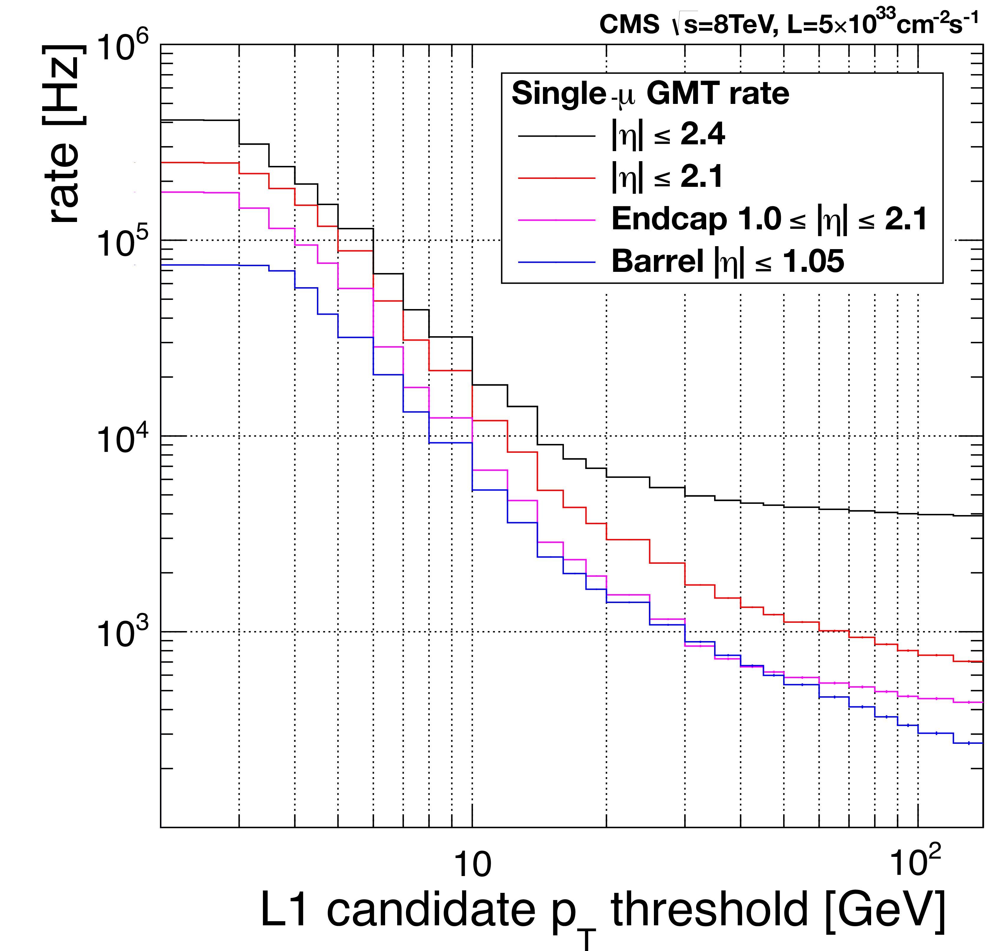
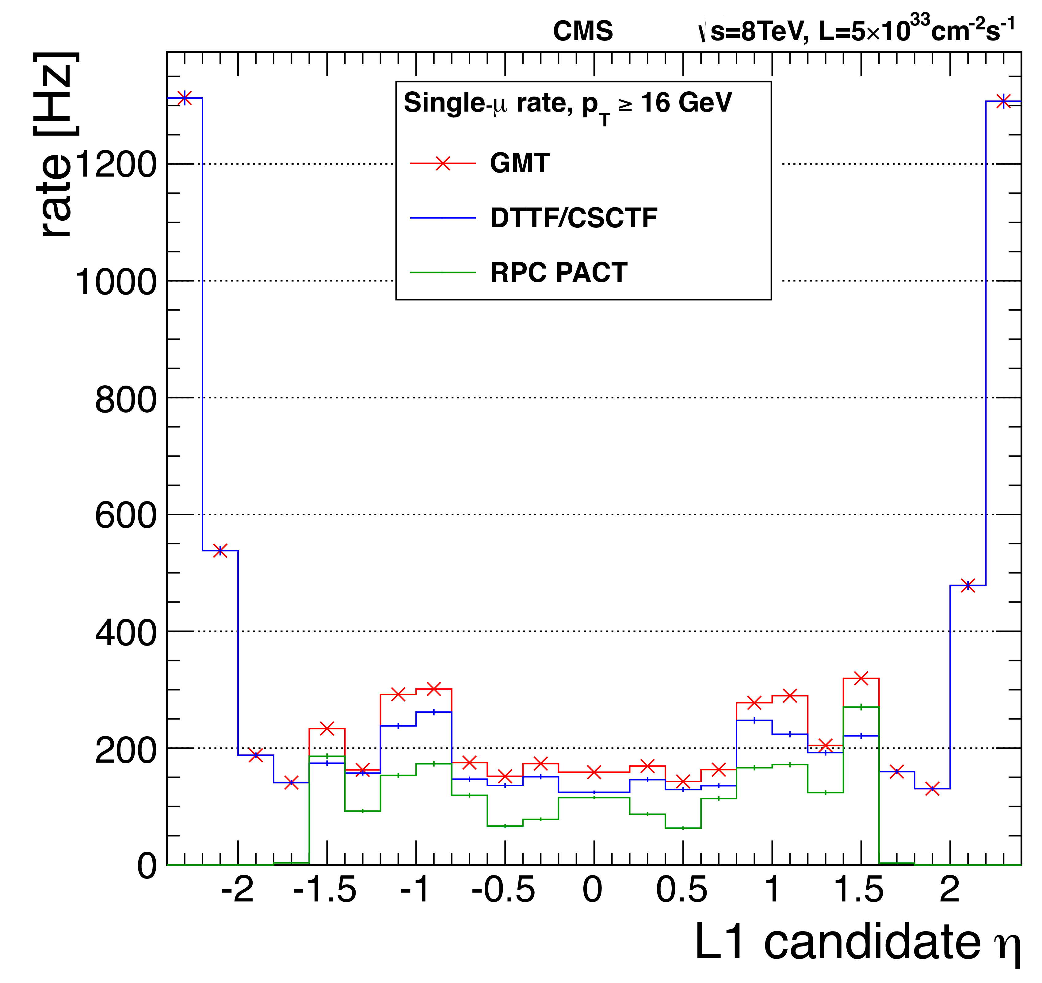
Figure 28:
Left: rate of the single-muon trigger versus the transverse momentum threshold for the full pseudorapidity range $ {| \eta | }< $ 2.4 and for pseudorapidity limited to $ {| \eta | }< $ 2.1. Additionally the curves for pure endcap and barrel regions are presented. Right: the rate of the single-muon trigger GMT candidates as a function of $\eta $ for the $ {p_{\mathrm {T}}} $ threshold of 16 GeV (blue histogram). The contribution of the muon trigger subsystems to this rate is also presented: the green and blue histograms show how often the above GMT candidates built using RPC or DTTF/CSCTF candidates. On both plots the rates are rescaled to an instantaneous luminosity of 5$ \times $10$^{33}$ cm$^{-2}$s$^{-1}$. The quality requirement used for single-muon trigger algorithms (see text) was applied. |
png pdf |
Figure 28-a:
Left: rate of the single-muon trigger versus the transverse momentum threshold for the full pseudorapidity range $ {| \eta | }< $ 2.4 and for pseudorapidity limited to $ {| \eta | }< $ 2.1. Additionally the curves for pure endcap and barrel regions are presented. The rates are rescaled to an instantaneous luminosity of 5$ \times $10$^{33}$ cm$^{-2}$s$^{-1}$. The quality requirement used for single-muon trigger algorithms (see text) was applied. |
png pdf |
Figure 28-b:
The rate of the single-muon trigger GMT candidates as a function of $\eta $ for the $ {p_{\mathrm {T}}} $ threshold of 16 GeV (blue histogram). The contribution of the muon trigger subsystems to this rate is also presented: the green and blue histograms show how often the above GMT candidates built using RPC or DTTF/CSCTF candidates. The rates are rescaled to an instantaneous luminosity of 5$ \times $10$^{33}$ cm$^{-2}$s$^{-1}$. The quality requirement used for single-muon trigger algorithms (see text) was applied. |

png pdf |
Figure 29:
The rate of the double-muon trigger versus the threshold applied to the first and second muon. The rates are rescaled to the instantaneous luminosity 5$ \times $10$^{33}$ cm$^{-2}$s$^{-1}$. |
png pdf |
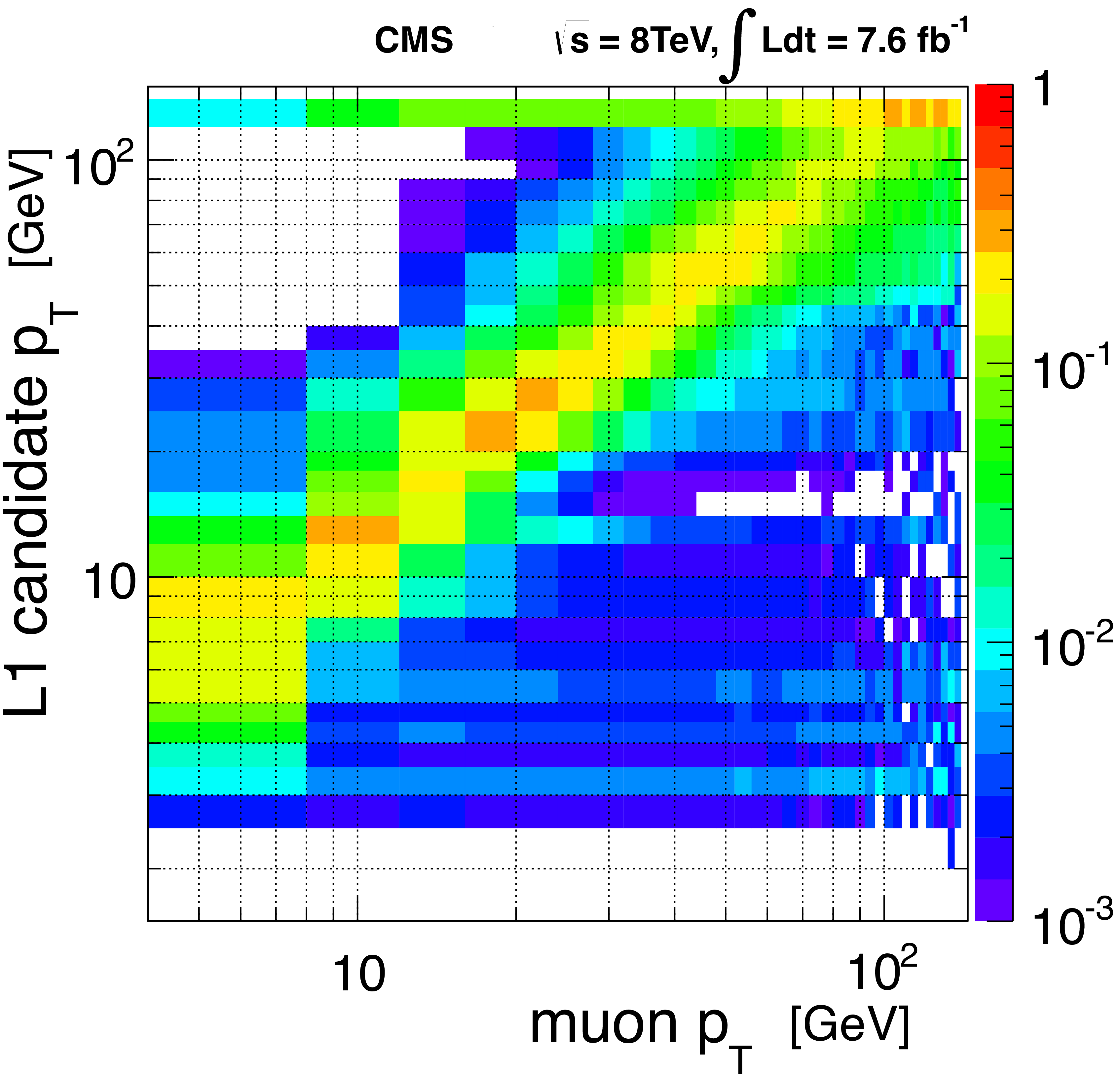
Figure 30:
The distribution of the momentum of the L1 muon candidates versus the momentum of the corresponding reconstructed muon (``tight''identification criteria). Events with both Z boson and $ \mathrm{J}/\psi $ resonances contribute. Offline muons in the full acceptance region ($ {| \eta | }< $ 2.4) are used. |

png pdf |
Figure 31:
The overall timing distribution of L1 muon triggers. The distribution of GMT candidates is shown as a shaded histogram. The contributions from regional muon triggers (DT, CSC, RPC) are given. In addition, the GMT and RPC distributions for heavy stable charged particle trigger configurations are labeled separately. |
png pdf |
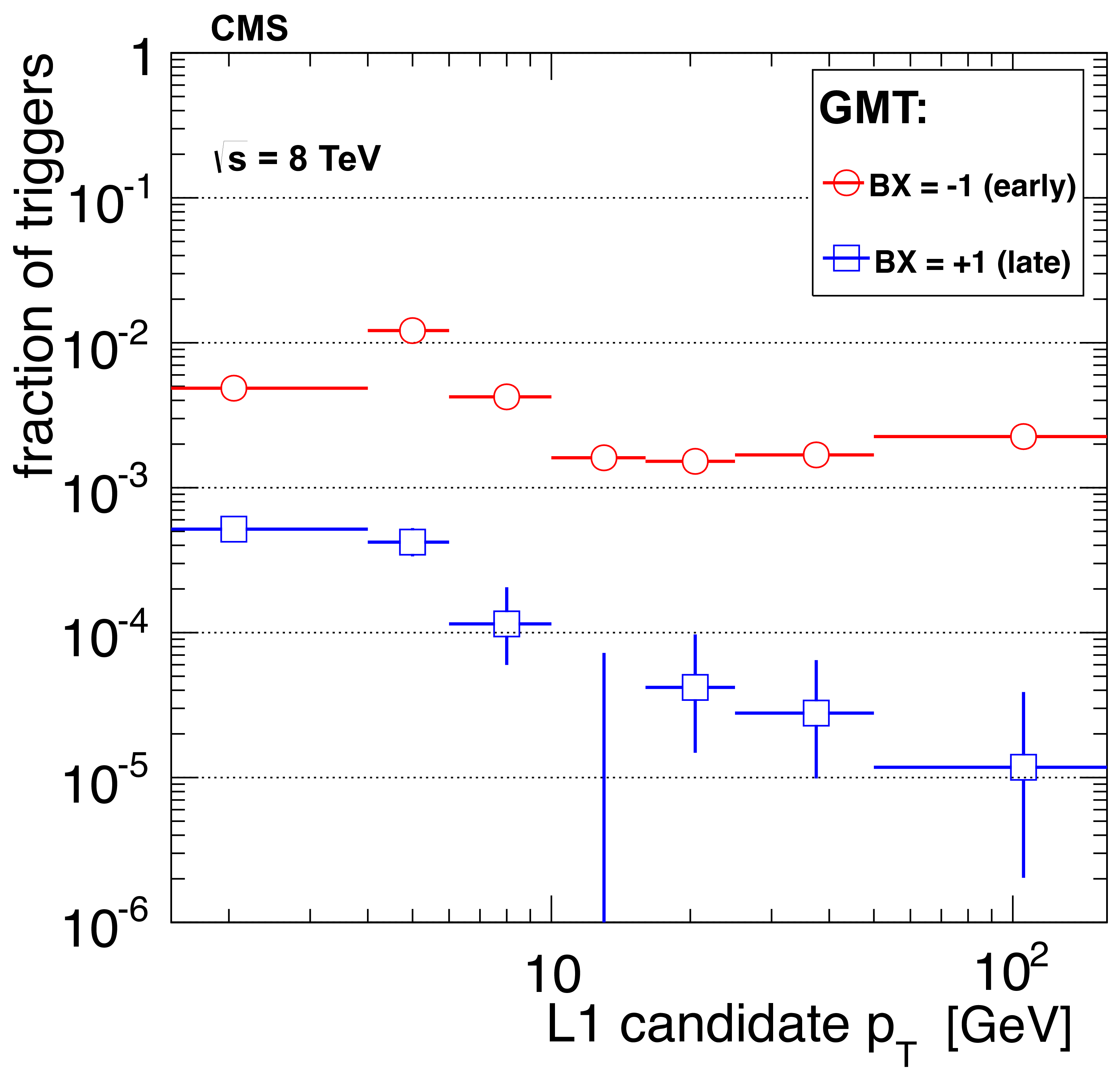
Figure 32:
The fractions of GMT candidates in early and late bunch crossings as a function of L1 muon candidate transverse momentum. |
png pdf |
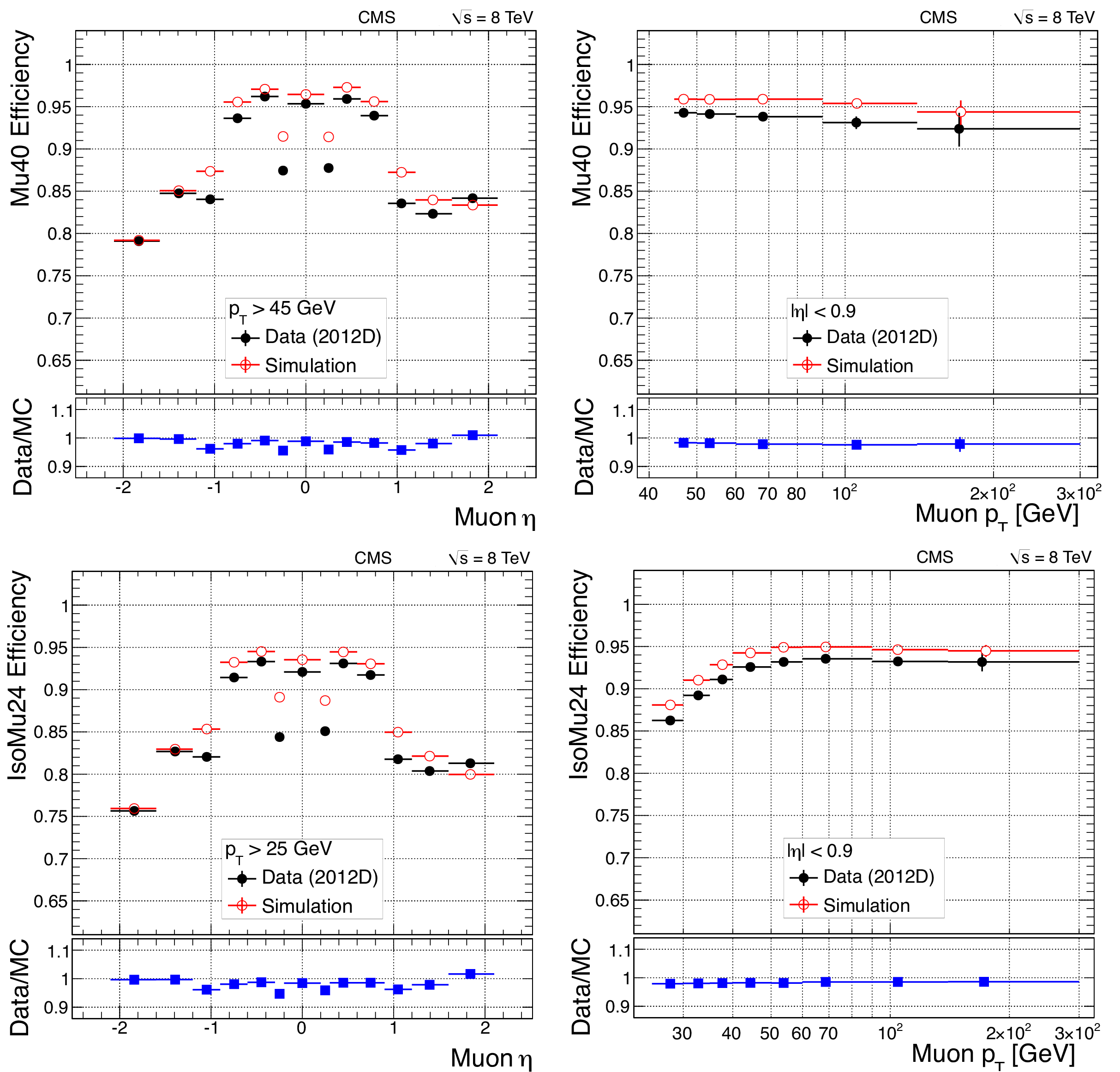
Figure 33:
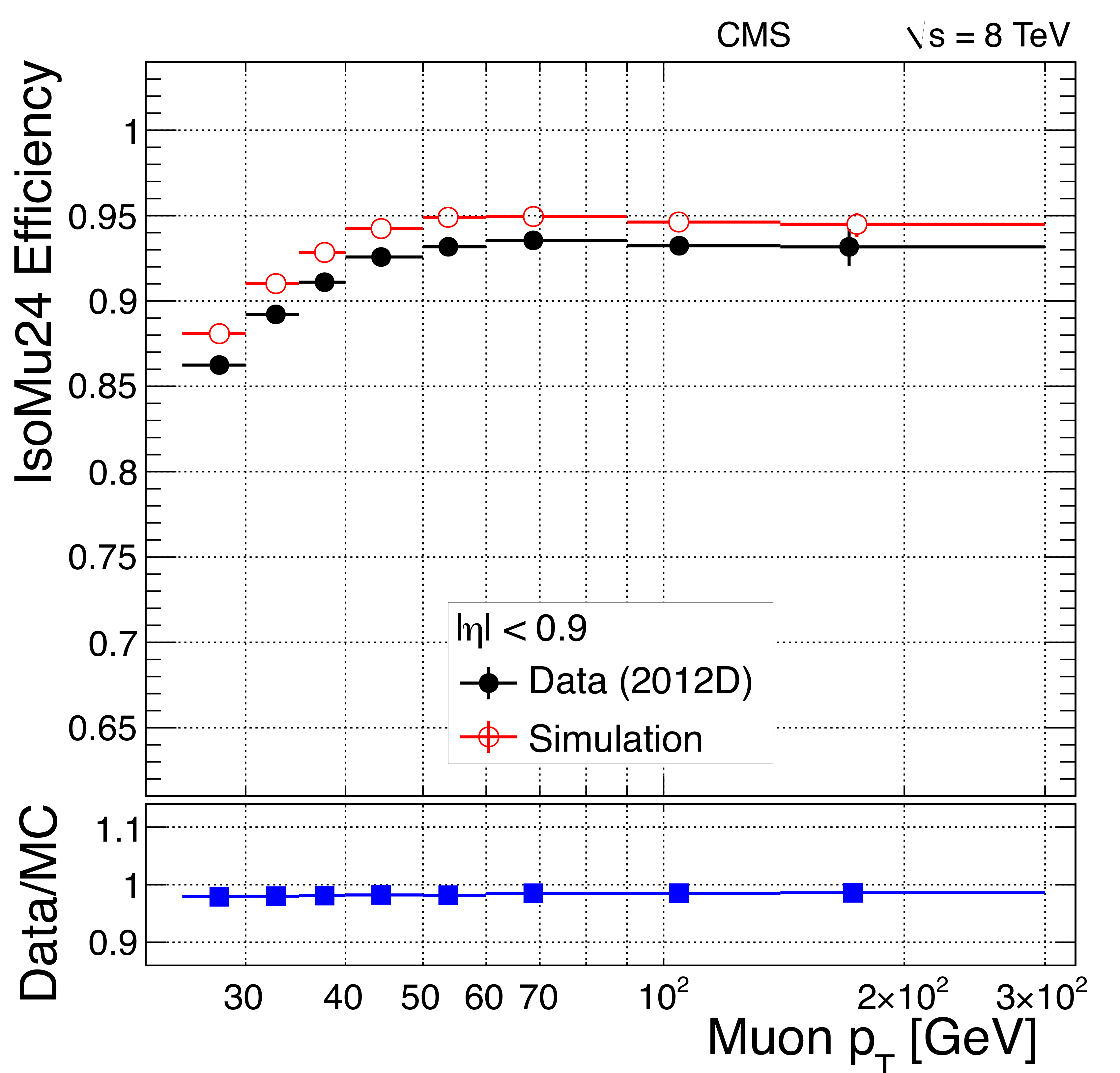
Efficiency of single-muon triggers without isolation (top) and with isolation (bottom) in 2012 data collected at 8 TeV, as functions of $\eta $ (left) and $ {p_{\mathrm {T}}} $, for $ {| \eta | } < 0.9$ (right). |
png pdf |
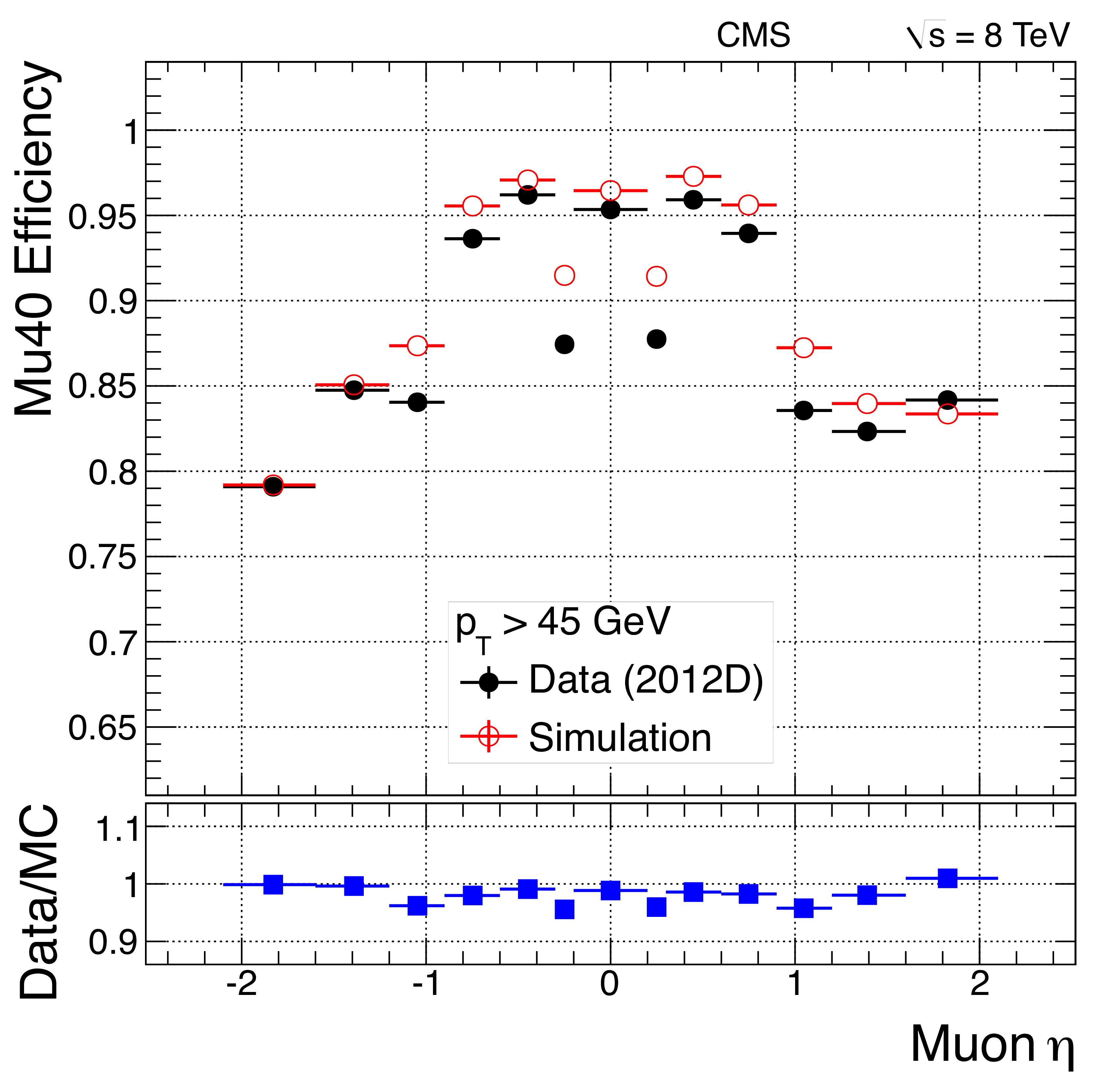
Figure 33-a:
Efficiency of single-muon triggers without isolation in 2012 data collected at 8 TeV, as functions of $\eta $. |
png pdf |
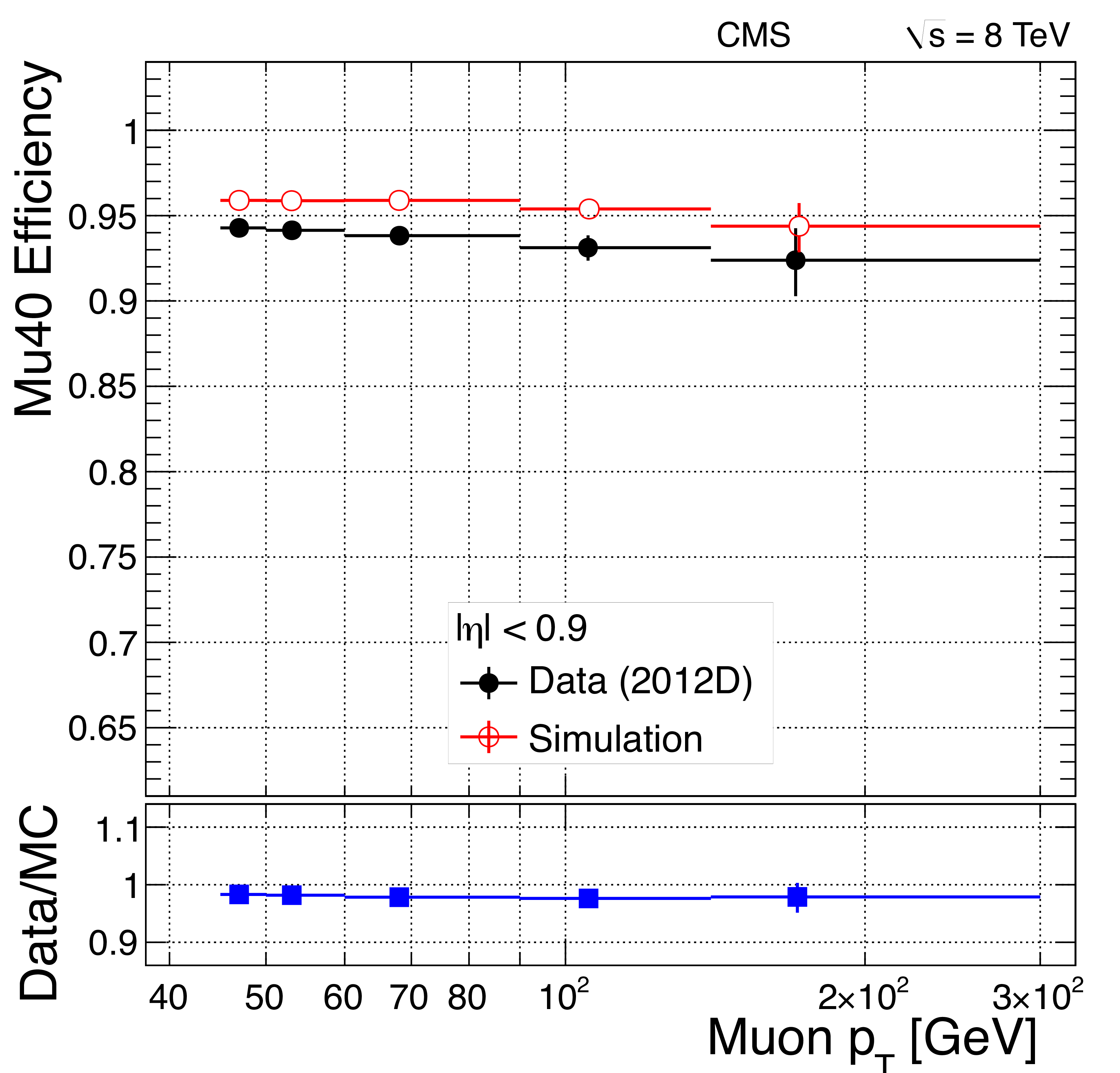
Figure 33-b:
Efficiency of single-muon triggers without isolation in 2012 data collected at 8 TeV, as functions of $ {p_{\mathrm {T}}} $, for $ {| \eta | } < 0.9$. |

png pdf |
Figure 33-c:
Efficiency of single-muon triggers with isolation in 2012 data collected at 8 TeV, as functions of $\eta $ (left). |
png pdf |
Figure 33-d:
Efficiency of single-muon triggers with isolation in 2012 data collected at 8 TeV, as functions of $ {p_{\mathrm {T}}} $, for $ {| \eta | } < 0.9$. |
png pdf |
Figure 34:
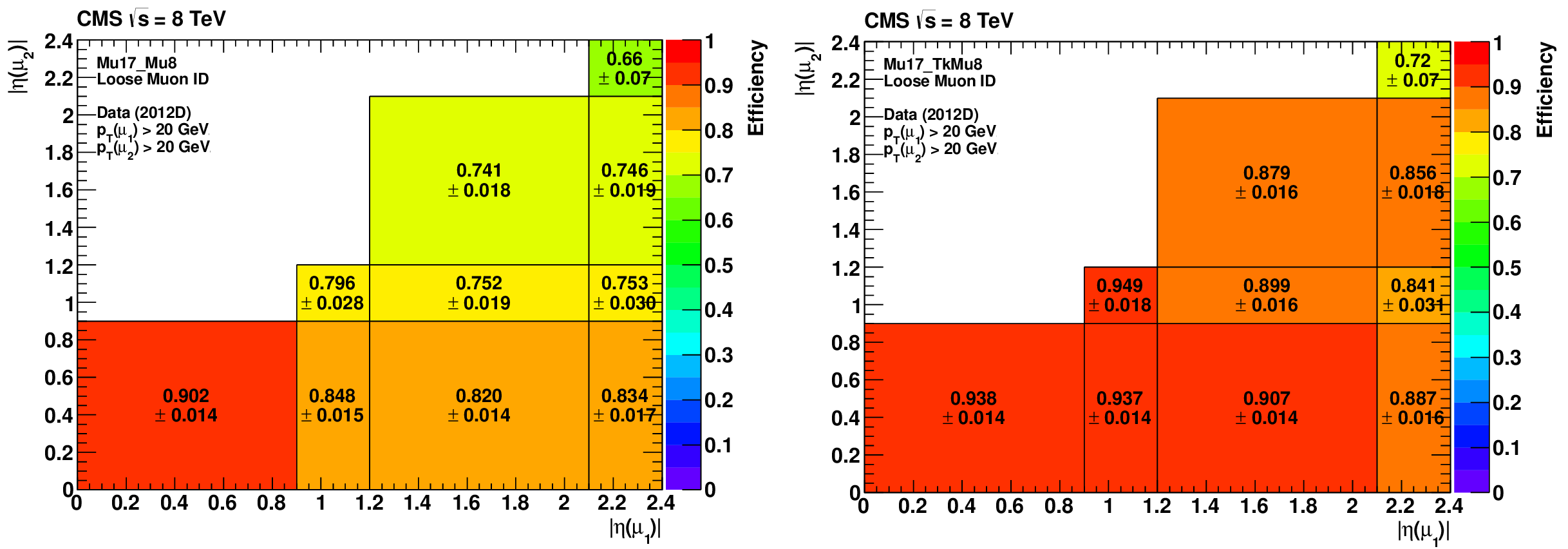
Efficiencies of double-muon triggers without (left) and with (right) the tracker muon requirement in 2012 data collected at 8 TeV as functions of the pseudorapidities $ {| \eta | }$ of the two muons, for loose muons with $ {p_{\mathrm {T}}} > 20$ GeV. |

png pdf |
Figure 34-a:
Efficiencies of double-muon triggers without (left) and with (right) the tracker muon requirement in 2012 data collected at 8 TeV as functions of the pseudorapidities $ {| \eta | }$ of the two muons, for loose muons with $ {p_{\mathrm {T}}} > 20$ GeV. |

png pdf |
Figure 34-b:
Efficiencies of double-muon triggers without (left) and with (right) the tracker muon requirement in 2012 data collected at 8 TeV as functions of the pseudorapidities $ {| \eta | }$ of the two muons, for loose muons with $ {p_{\mathrm {T}}} > 20$ GeV. |
png pdf |
Figure 35:
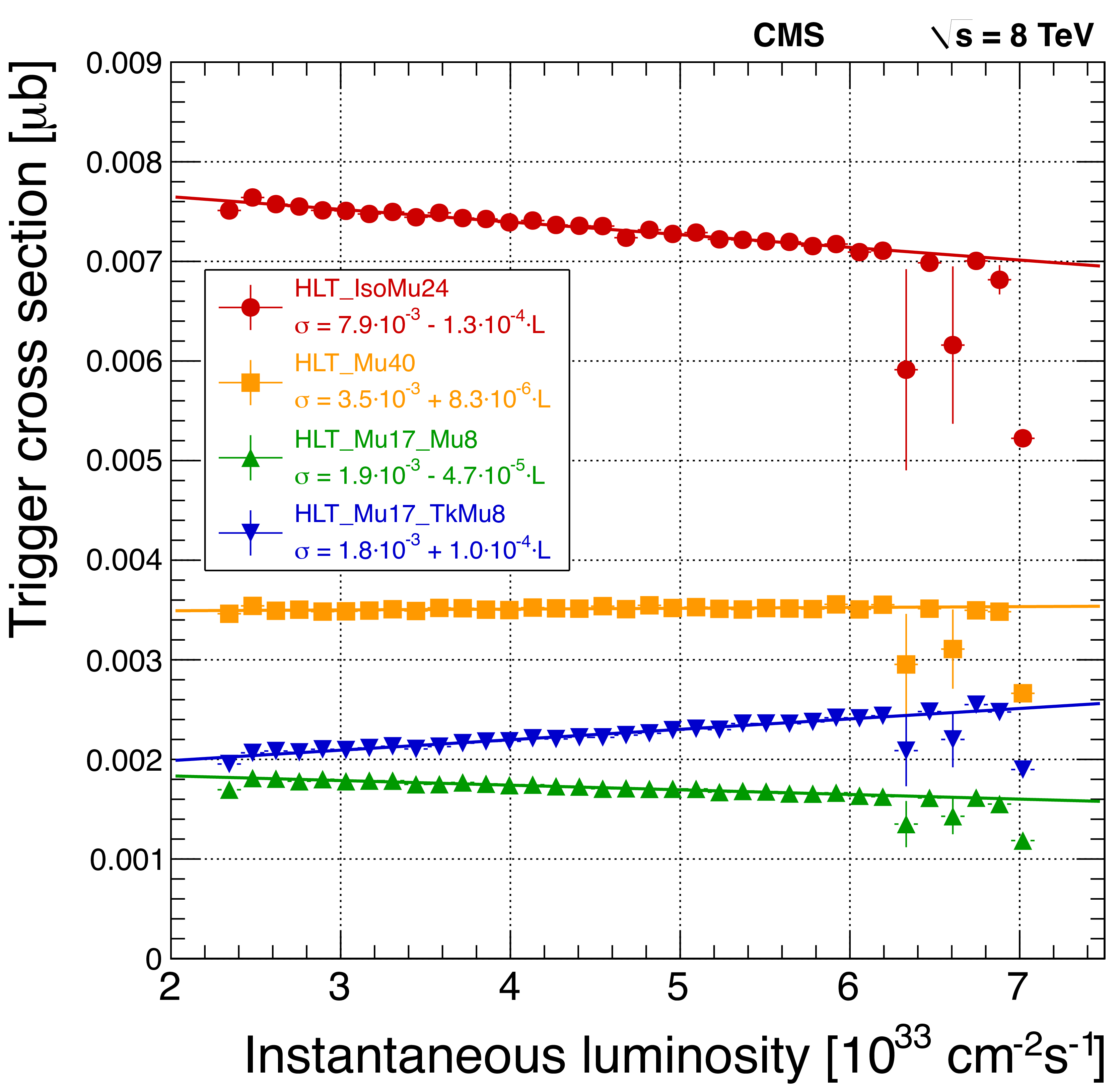
Cross sections of the four main single- and double-muon triggers used in 2012 data taking, described in the text, as a function of the LHC instantaneous luminosity. Mild pileup dependencies are visible. |

png pdf |
Figure 36:
Illustration of the available tower granularity for the L1 jet finding algorithm in the central region, $ {| \eta | } < 3$ (left). The jet trigger uses a $3{\times }3$ calorimeter region sliding window technique which spans the full $(\eta, \phi )$ coverage of the calorimeter. The active tower patterns allowed for L1 $\tau $ jet candidates are shown on the right. |

png pdf |
Figure 37:
Left: The L1 jet trigger efficiency as a function of the offline CaloJet transverse momentum. Right: The L1 jet trigger efficiencies as a function of the PF jet transverse momentum. In both cases, three L1 thresholds ($ E_{mathrm{T}} > $ 16, 36, 92 GeV) are shown. |

png |
Figure 37-a:
The L1 jet trigger efficiency as a function of the offline CaloJet transverse momentum. Three L1 thresholds ($ E_{mathrm{T}} > $ 16, 36, 92 GeV) are shown. |

png |
Figure 37-b:
The L1 jet trigger efficiencies as a function of the PF jet transverse momentum. Three L1 thresholds ($ E_{mathrm{T}} > $ 16, 36, 92 GeV) are shown. |

png pdf |
Figure 38:
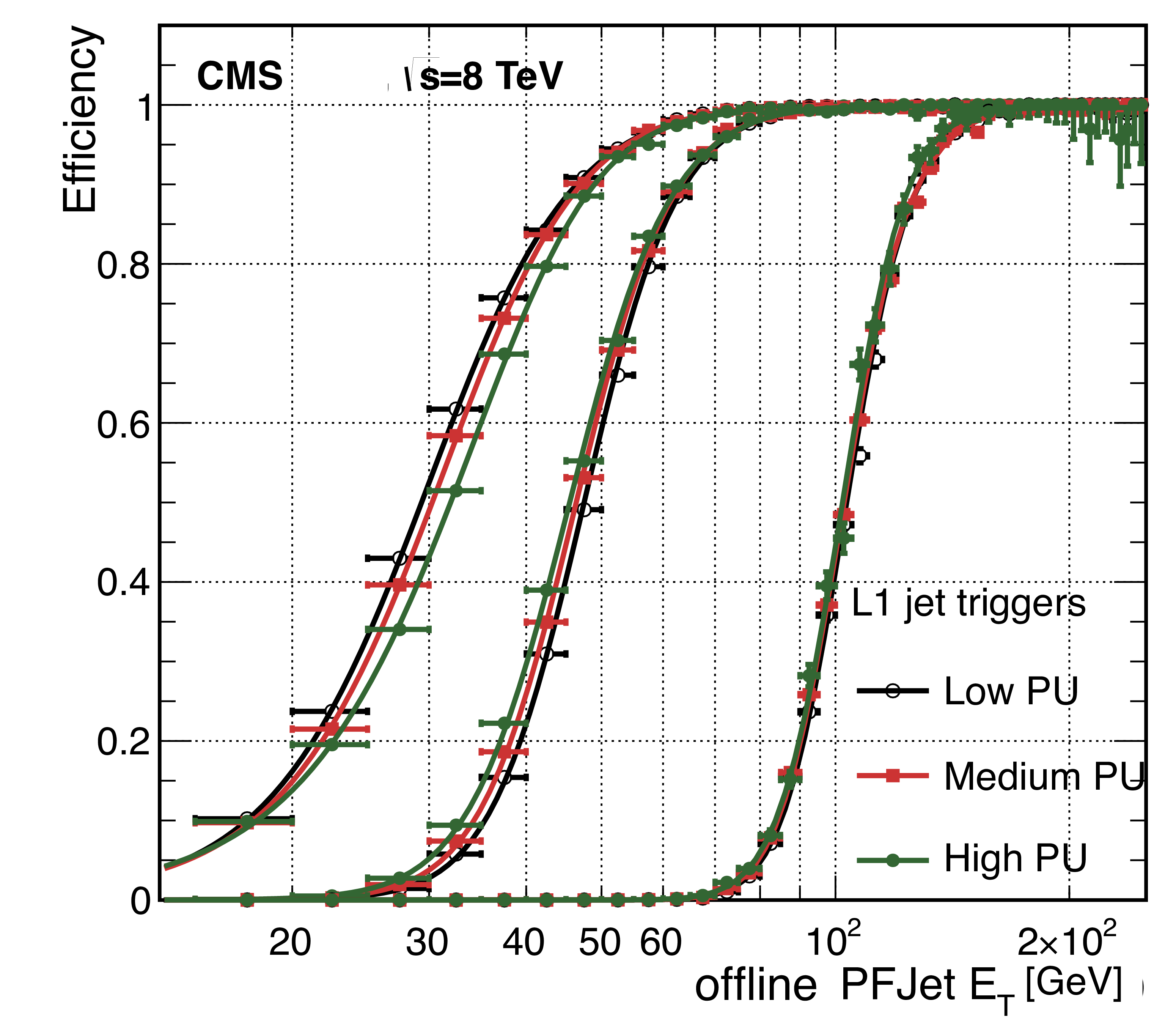
The L1 jet efficiency turn-on curves as a function of the leading offline CaloJet $ {E_{\mathrm {T}}} $ (left) and as a function of the leading offline PF jet $ {E_{\mathrm {T}}} $ (right), for low-, medium-, and high-pileup scenarios for three different thresholds: $ {E_{\mathrm {T}}} > $ 16, 36, and 92 GeV. |

png pdf |
Figure 38-a:
The L1 jet efficiency turn-on curves as a function of the leading offline CaloJet $ {E_{\mathrm {T}}} $, for low-, medium-, and high-pileup scenarios for three different thresholds: $ {E_{\mathrm {T}}} > $ 16, 36, and 92 GeV. |
png pdf |
Figure 38-b:
The L1 jet efficiency turn-on curves as a function of the leading offline PF jet $ {E_{\mathrm {T}}} $, for low-, medium-, and high-pileup scenarios for three different thresholds: $ {E_{\mathrm {T}}} > $ 16, 36, and 92 GeV. |
png pdf |
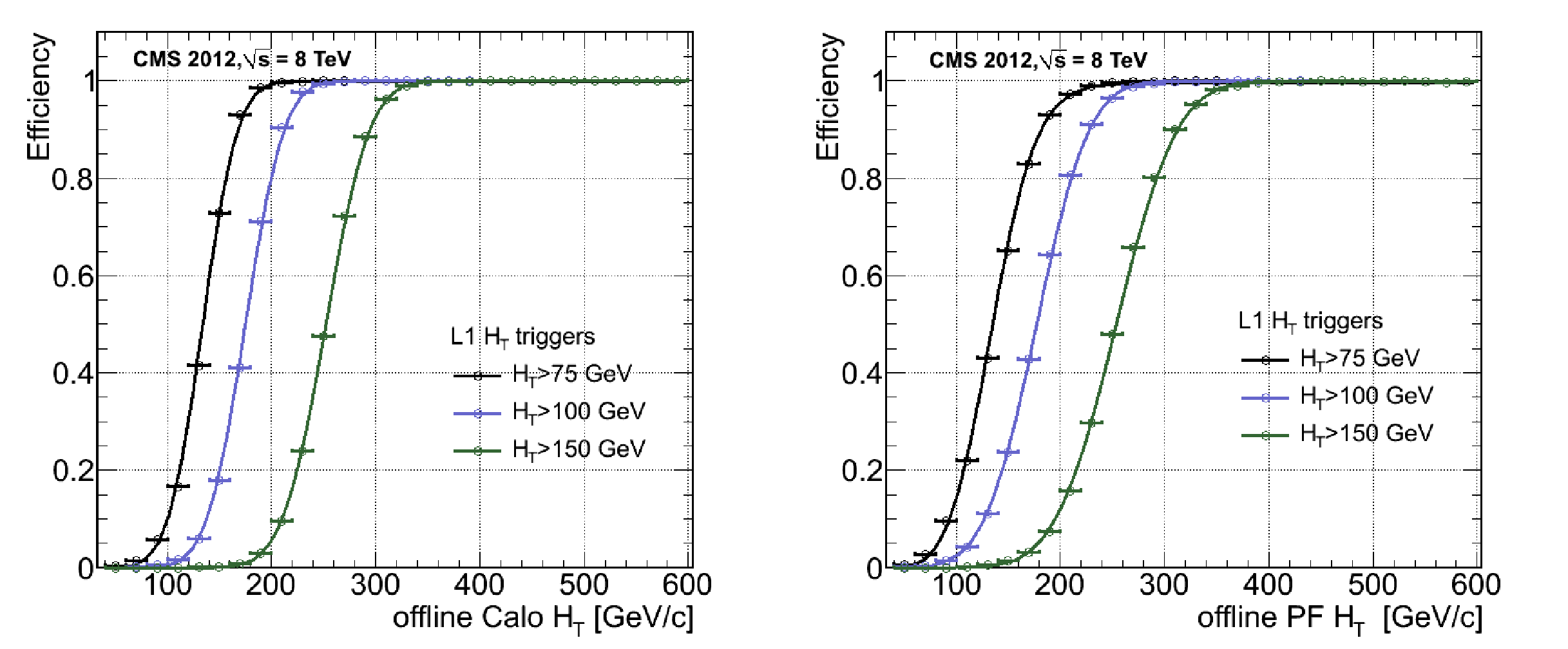
Figure 39:
The L1 $ H_{\mathrm{T}} $ efficiency turn-on curves as a function of the offline CaloJet (left) and PF (right) $ H_{\mathrm{T}} $, for three thresholds ($ H_{\mathrm{T}} > $ 75, 100, 150 GeV). |
png |
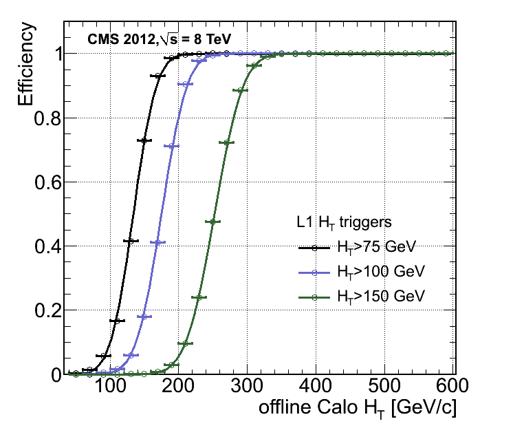
Figure 39-a:
The L1 $ H_{\mathrm{T}} $ efficiency turn-on curves as a function of the offline CaloJet $ H_{\mathrm{T}} $, for three thresholds ($ H_{\mathrm{T}} > $ 75, 100, 150 GeV). |

png |
Figure 39-b:
The L1 $ H_{\mathrm{T}} $ efficiency turn-on curves as a function of the offline PF $ H_{\mathrm{T}} $, for three thresholds ($ H_{\mathrm{T}} > $ 75, 100, 150 GeV). |
png pdf |
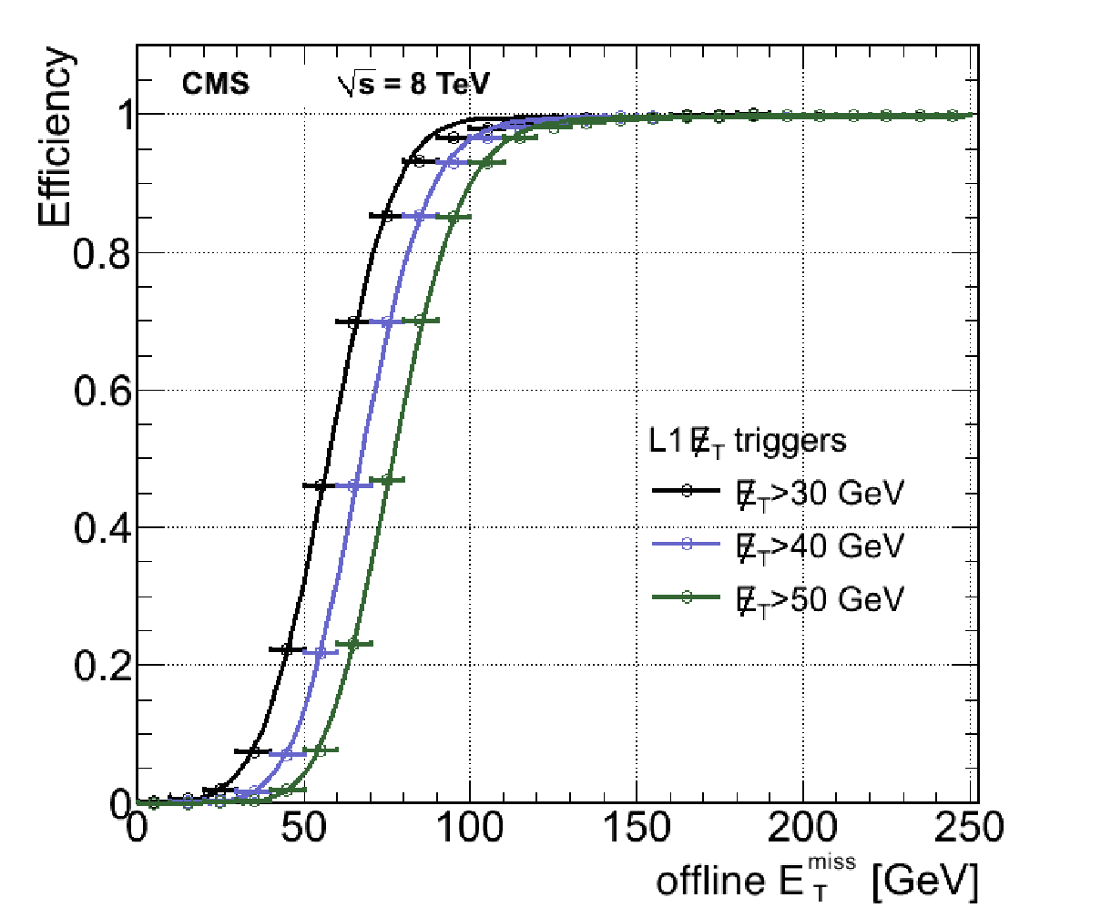
Figure 40:
The L1 $ {E_{\mathrm {T}}^{\text {miss}}} $ efficiency turn-on curve as a function of the offline calorimeter $ {E_{\mathrm {T}}^{\text {miss}}} $, for three thresholds ($ {E_{\mathrm {T}}^{\text {miss}}} >$ 30, 40, 50 GeV). |

png pdf |
Figure 41:
The rate of the L1 single-jet trigger as a function of the $ {E_{\mathrm {T}}} $ threshold. The rates are rescaled to the instantaneous luminosity 5$\times $10$^{33}$ cm$^{-2}$s$^{-1}$. |
png pdf |
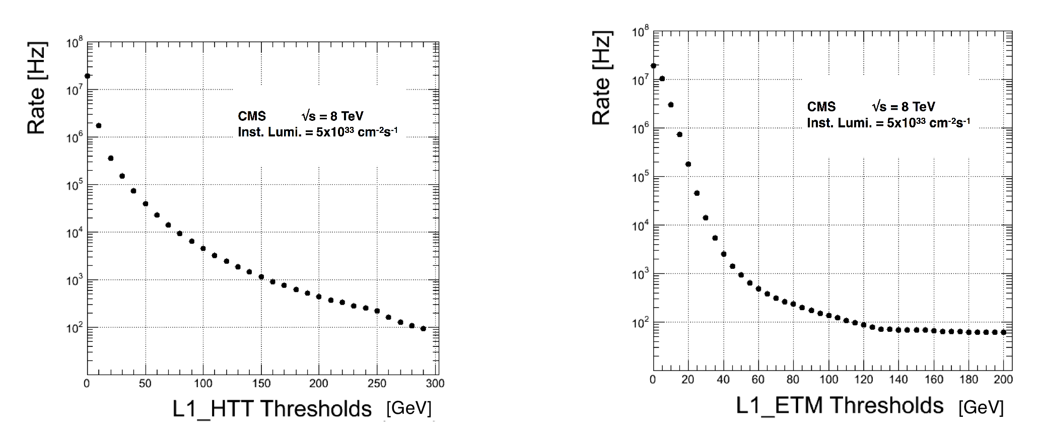
Figure 42:
Left: Rate of the L1-HTT trigger versus the L1-HTT threshold. Right: Rate of the L1-ETM missing transverse energy trigger as a function of the L1-ETM threshold. On both plots, the rates are rescaled to the instantaneous luminosity 5$\times $10$^{33}$ cm$^{-2}$s$^{-1}$. |

png pdf |
Figure 42-a:
Rate of the L1-HTT trigger versus the L1-HTT threshold. The rates are rescaled to the instantaneous luminosity 5$\times $10$^{33}$ cm$^{-2}$s$^{-1}$. |
png pdf |
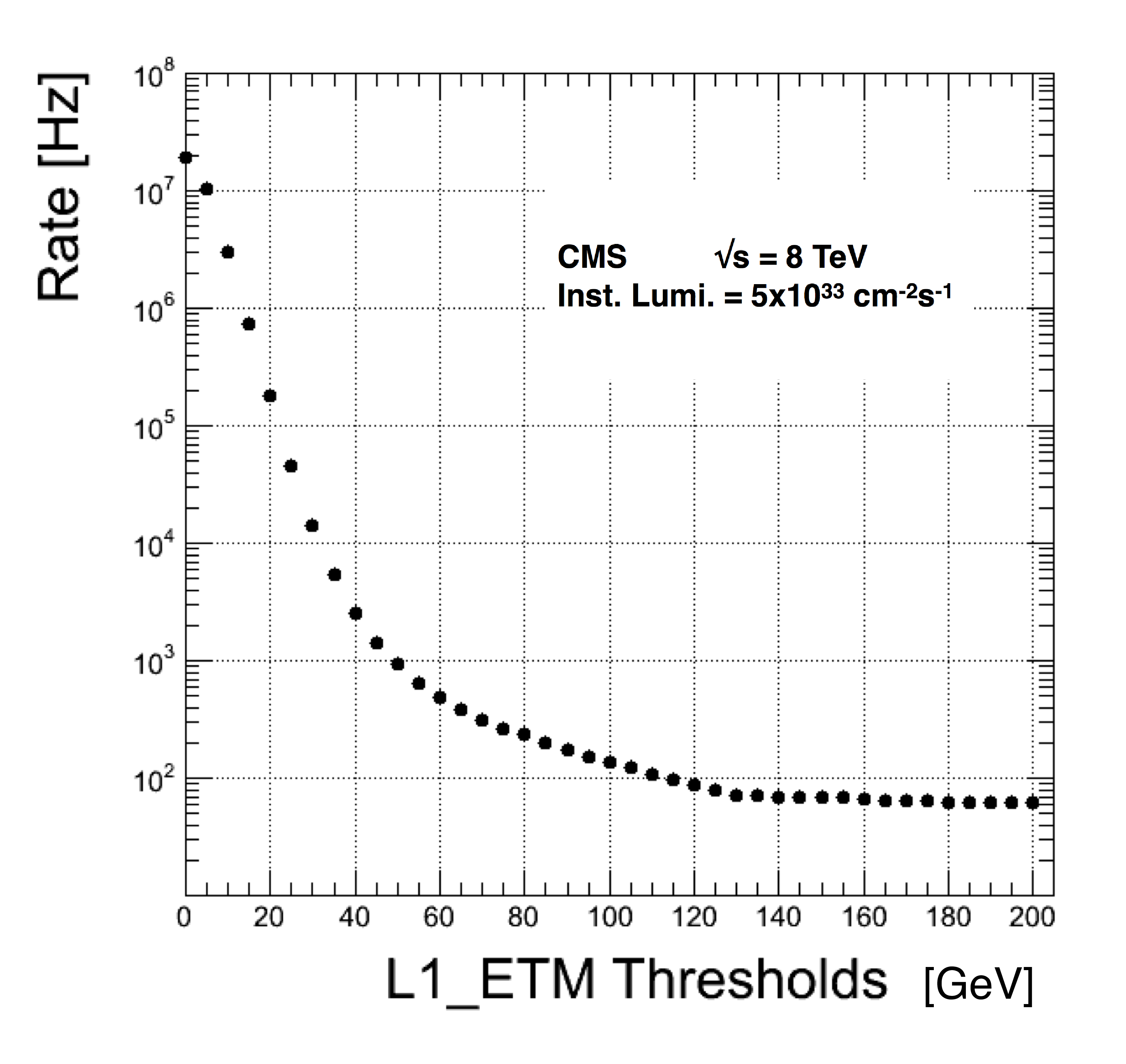
Figure 42-b:
Rate of the L1-ETM missing transverse energy trigger as a function of the L1-ETM threshold. The rates are rescaled to the instantaneous luminosity 5$\times $10$^{33}$ cm$^{-2}$s$^{-1}$. |
png pdf |
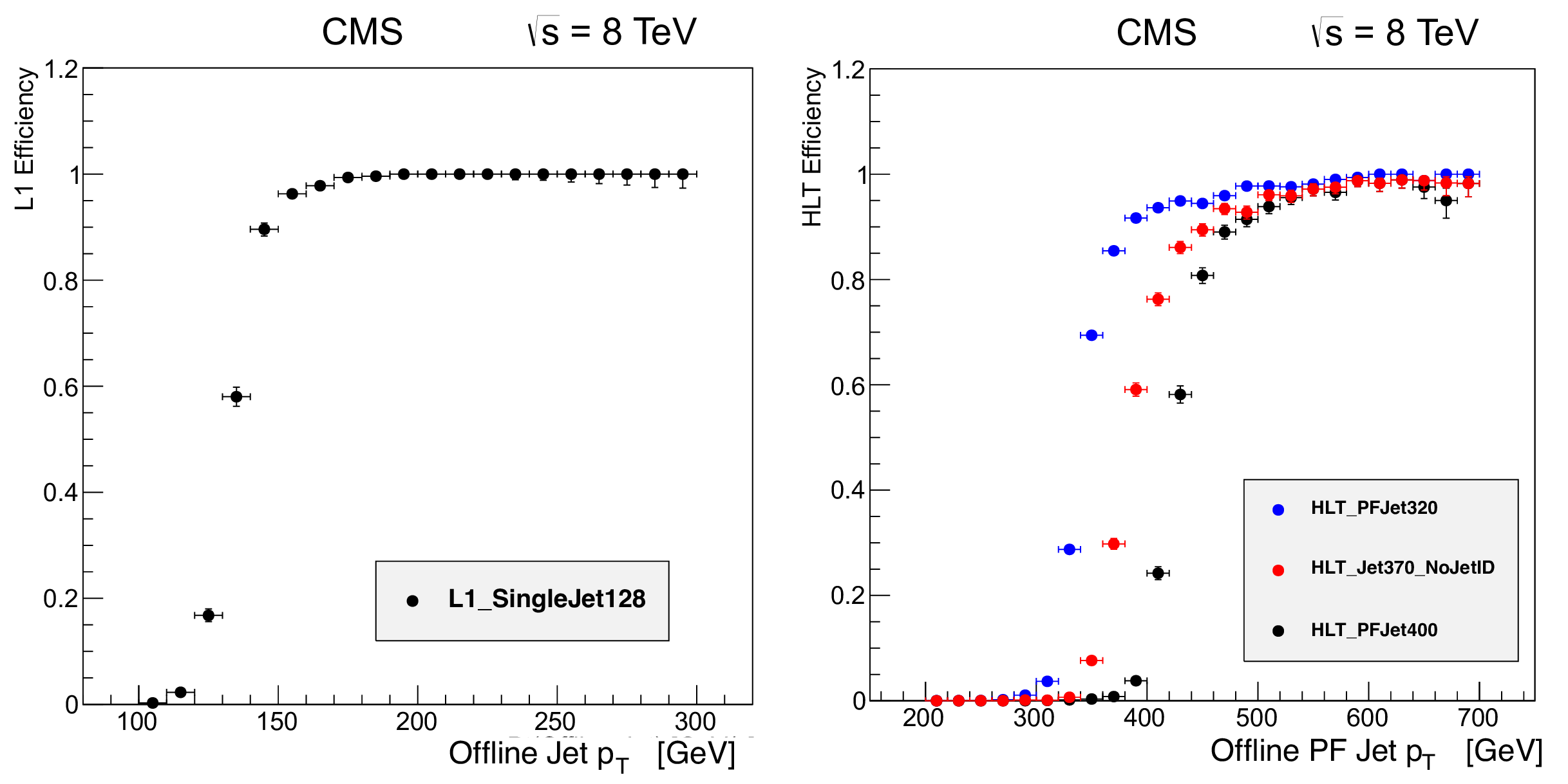
Figure 43:
Left: Efficiency of the L1 single-jet trigger with an $ E_{\mathrm{T}} $ threshold of 128 GeV as a function of the offline jet transverse momentum. Right: The HLT efficiencies as a function of transverse momentum for a calorimeter jet trigger with a 370 GeV threshold and no jet identification requirements, and two PF jet triggers with 320 and 400 GeV thresholds. |

png pdf |
Figure 43-a:
Efficiency of the L1 single-jet trigger with an $ E_{\mathrm{T}} $ threshold of 128 GeV as a function of the offline jet transverse momentum. |

png pdf |
Figure 43-b:
The HLT efficiencies as a function of transverse momentum for a calorimeter jet trigger with a 370 GeV threshold and no jet identification requirements, and two PF jet triggers with 320 and 400 GeV thresholds. |

png pdf |
Figure 44:
The HLT efficiencies as a function of the offline PF $ E_{\mathrm{T}}^{\text{miss}} $ for different $ E_{\mathrm{T}}^{\text{miss}} $ thresholds ($ E_{\mathrm{T}}^{\text{miss}} = $ 80-400 GeV). |

png pdf |
Figure 45:
Examples of trigger regions, where trigger towers with energy deposits $ {E_{\mathrm {T}}} ^\mathrm {ECAL}> $ 4 GeV or $ {E_{\mathrm {T}}} ^\mathrm {HCAL}> $ 4 GeV, are shown as shaded squares. The L1 $\tau $ veto bit is not set if the energy is contained in a square of 2${\times }$2 trigger towers (a). Otherwise, the $\tau $ veto bit is set (b). |

png pdf |
Figure 46:
Rate of L1 double-$\tau $ and double-jet seeds as a function of the $ {p_{\mathrm {T}}} $ threshold on the two objects. The double-$\tau $ objects are restricted to $ {| \eta | }< $ 2.17, while the double-jet requires two seed objects (either $\tau $ or jet) within $ {| \eta | }< $ 3.0. The given rates are scaled to an instantaneous luminosity of 5$ \times $10$^{33}$ cm$^{-2}$s$^{-1}$. |

png pdf |
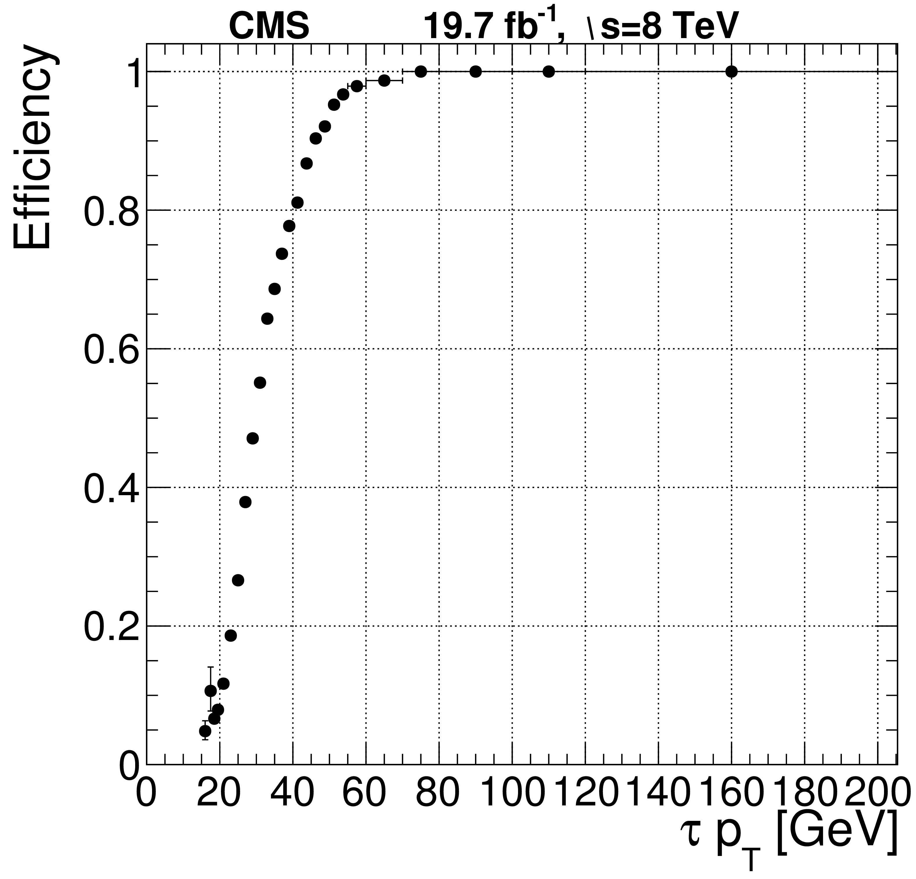
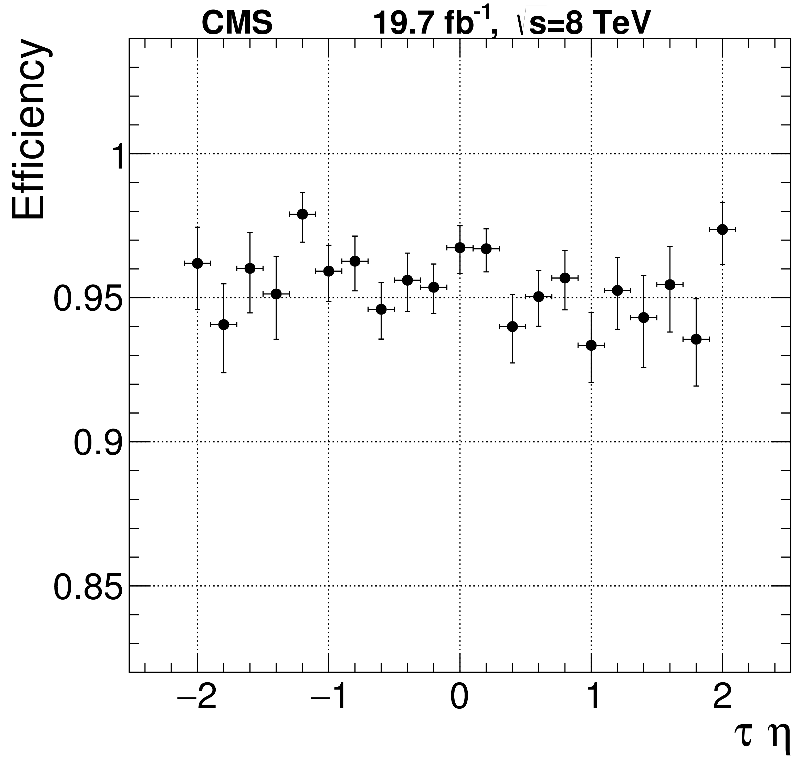
Figure 47:
Efficiency of the double-$\tau _\mathrm {h}$ L1 trigger with a threshold of 44 and 64 GeV on the L1 $\tau $ and jet objects, respectively. Presented is the efficiency of one $\tau $ lepton candidate as a function of transverse momentum (left) and pseudorapidity (right). |
png pdf |
Figure 47-a:
Efficiency of the double-$\tau _\mathrm {h}$ L1 trigger with a threshold of 44 and 64 GeV on the L1 $\tau $ and jet objects, respectively. Presented is the efficiency of one $\tau $ lepton candidate as a function of transverse momentum. |
png pdf |
Figure 47-b:
Efficiency of the double-$\tau _\mathrm {h}$ L1 trigger with a threshold of 44 and 64 GeV on the L1 $\tau $ and jet objects, respectively. Presented is the efficiency of one $\tau $ lepton candidate as a function of pseudorapidity. |
png pdf |
Figure 48:
Efficiency of the L2 and L2.5 $\tau $ trigger with a 35 GeV threshold as a function of the offline reconstructed $\tau $ transverse momentum (left) and pseudorapidity (right). |
png pdf |
Figure 48-a:
Efficiency of the L2 and L2.5 $\tau $ trigger with a 35 GeV threshold as a function of the offline reconstructed $\tau $ transverse momentum. |
png pdf |
Figure 48-b:
Efficiency of the L2 and L2.5 $\tau $ trigger with a 35 GeV threshold as a function of the offline reconstructed $\tau $ pseudorapidity. |
png pdf |
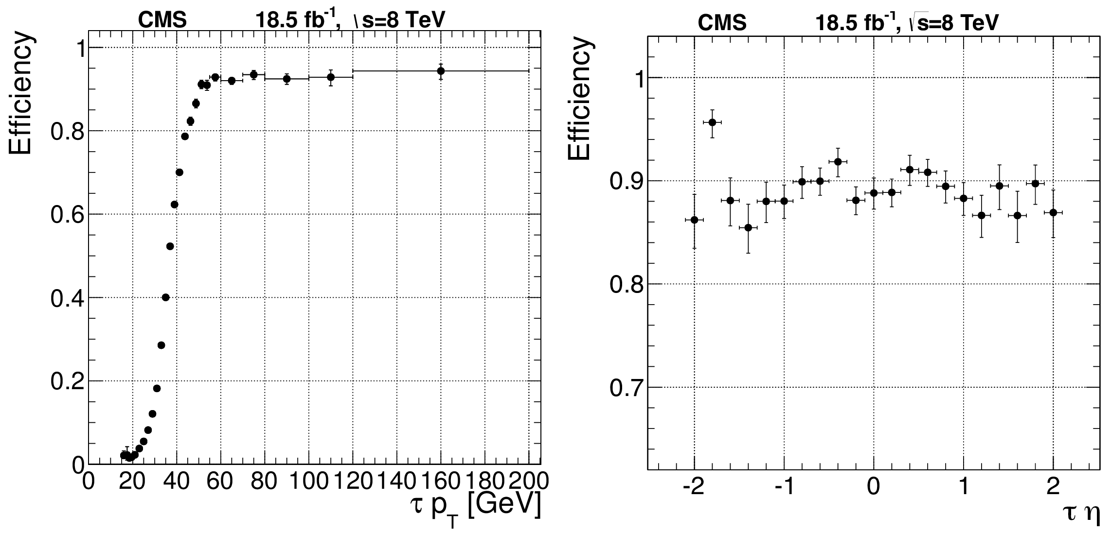
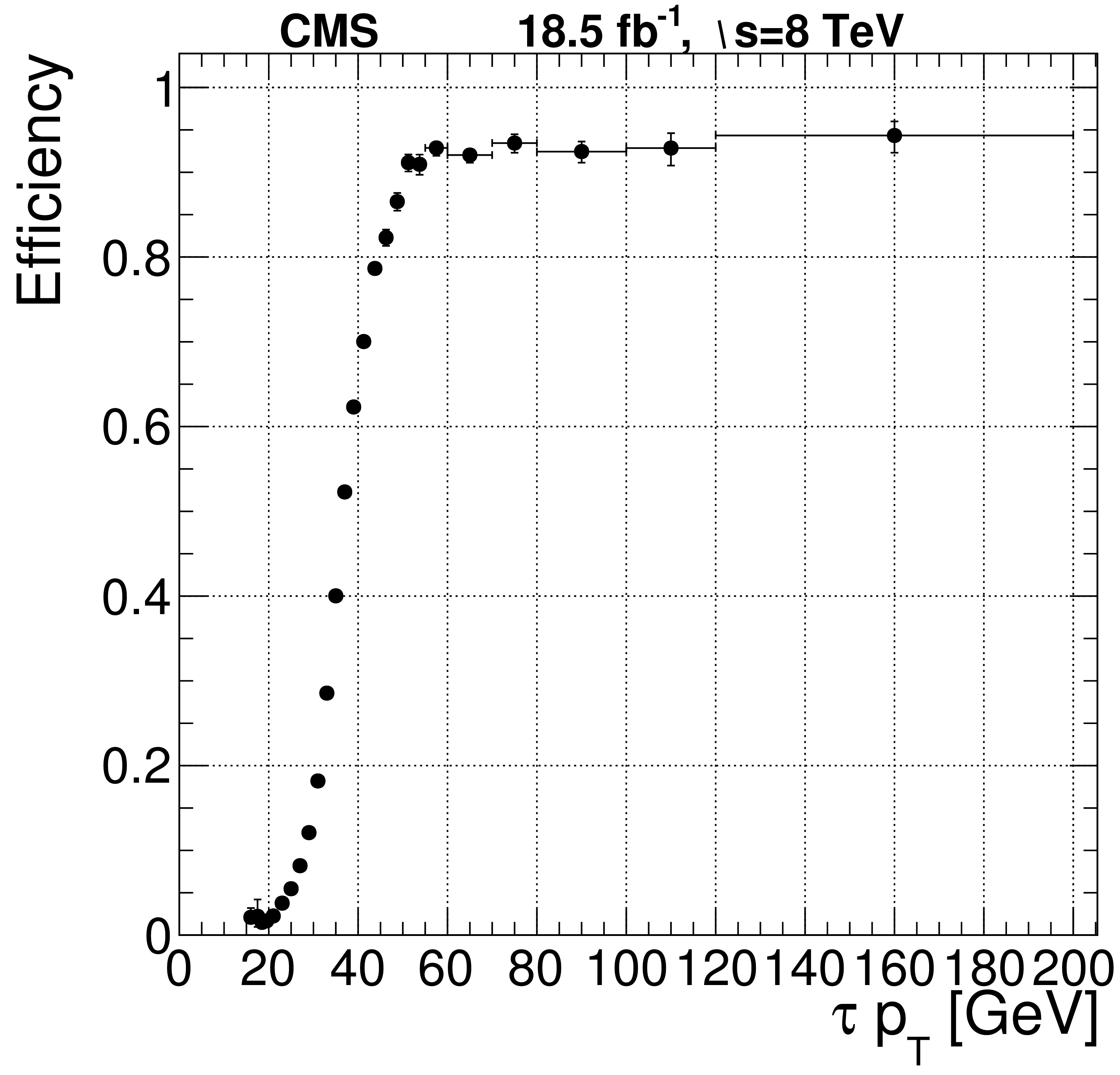
Figure 49:
Efficiency of the loose L3 $\tau $ algorithm from the $\tau _h\tau _\mu $ events plotted as a function of offline $\tau _h$ transverse momentum (left), pseudorapidity (center), and number of vertices (right). |

png pdf |
Figure 49-a:
Efficiency of the loose L3 $\tau $ algorithm from the $\tau _h\tau _\mu $ events plotted as a function of offline $\tau _h$ transverse momentum. |

png pdf |
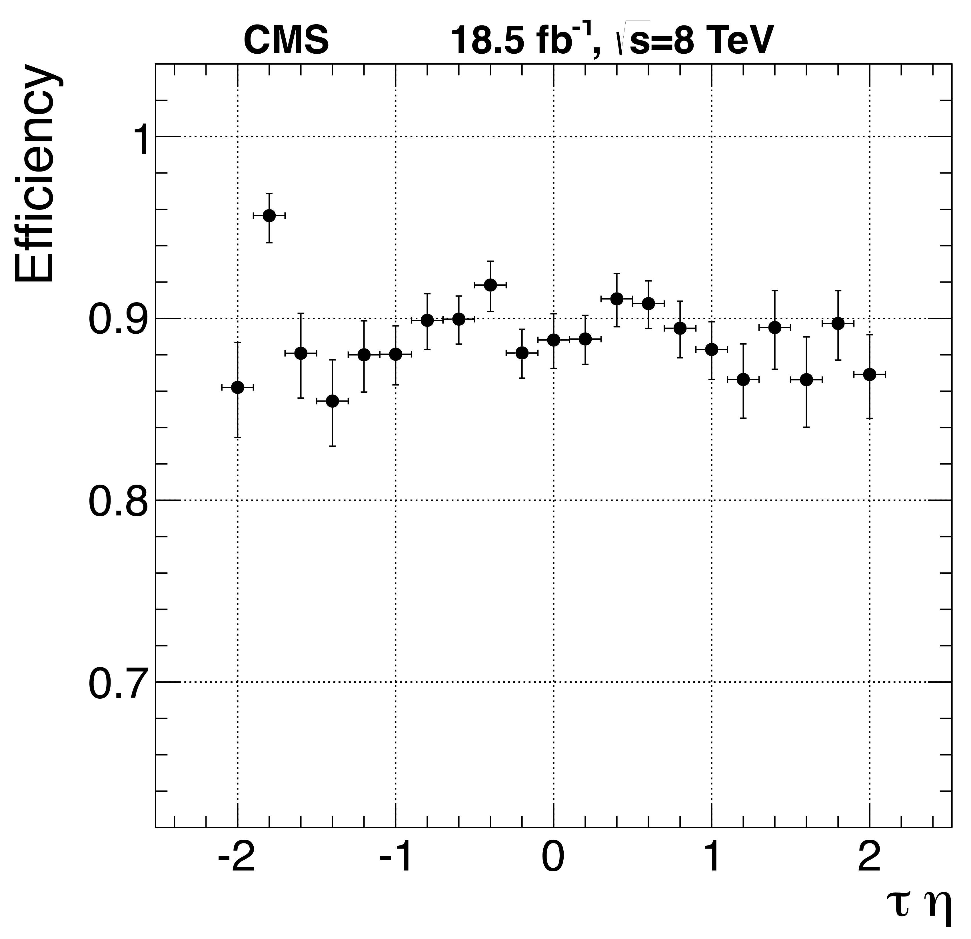
Figure 49-b:
Efficiency of the loose L3 $\tau $ algorithm from the $\tau _h\tau _\mu $ events plotted as a function of offline $\tau _h$ pseudorapidity. |
png pdf |
Figure 49-c:
Efficiency of the loose L3 $\tau $ algorithm from the $\tau _h\tau _\mu $ events plotted as a function of offline number of vertices. |
png pdf |
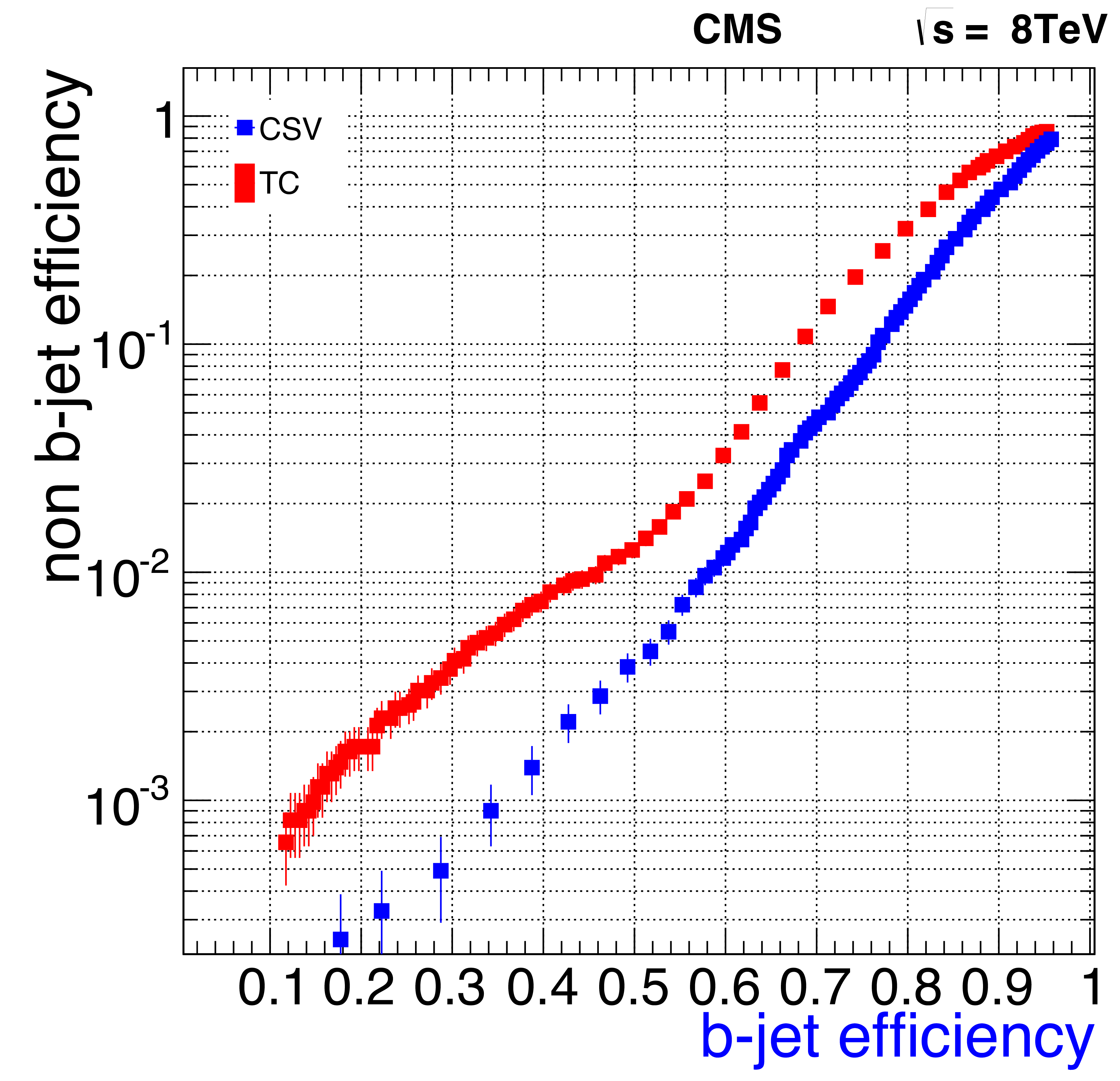
Figure 50:
The efficiency to tag b quark jets versus the mistag rate, obtained from Monte Carlo simulations, for the track counting (TC) and for the combined secondary vertex (CSV) algorithms. As expected from offline studies, the CSV algorithm performs better than the TC algorithm. |
png pdf |
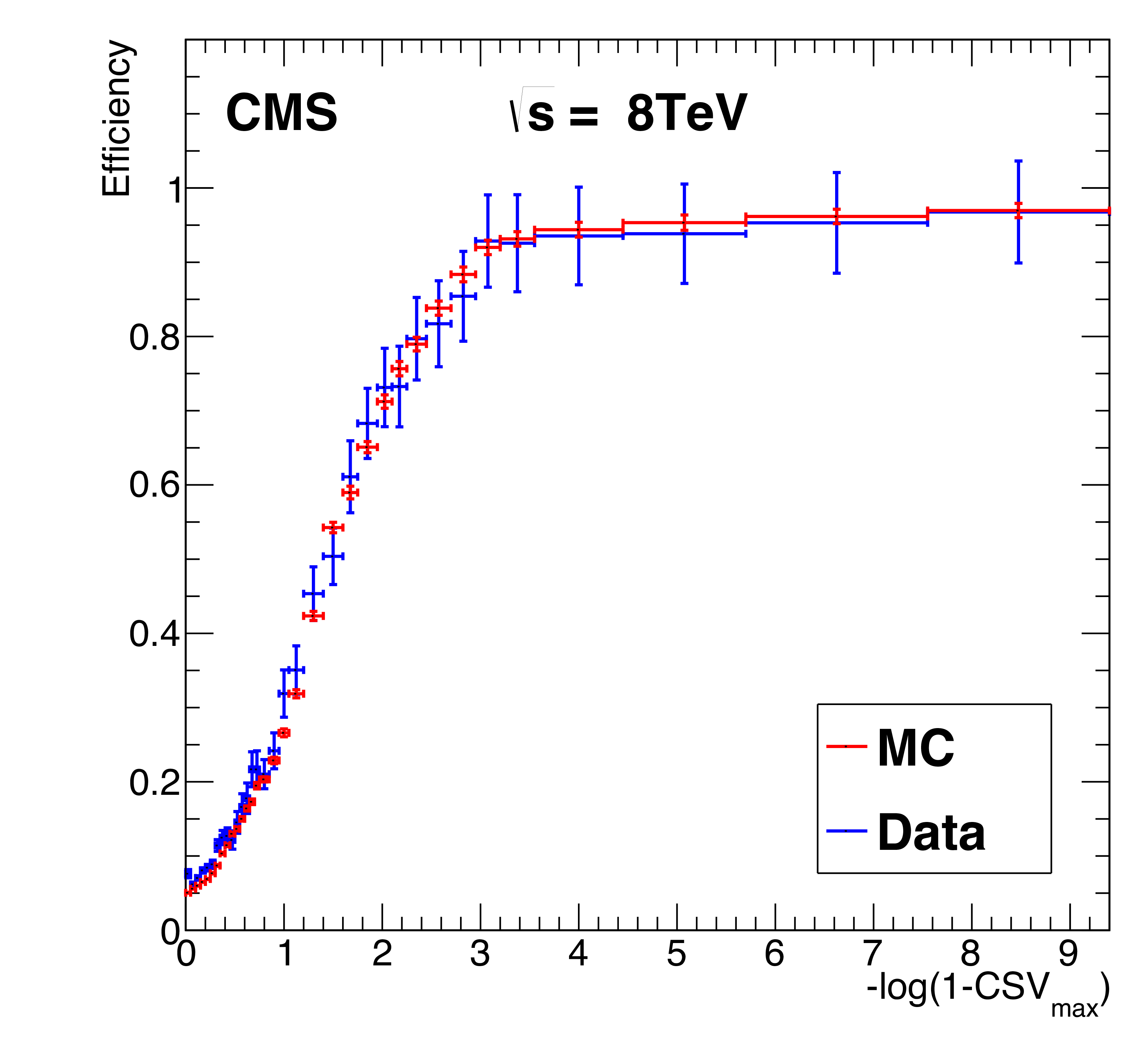
Figure 51:
The efficiency of the online CSV trigger as a function of the offline CSV tagger discriminant, obtained from the data and from Monte Carlo simulations. Good agreement between the two is observed. |
png pdf |
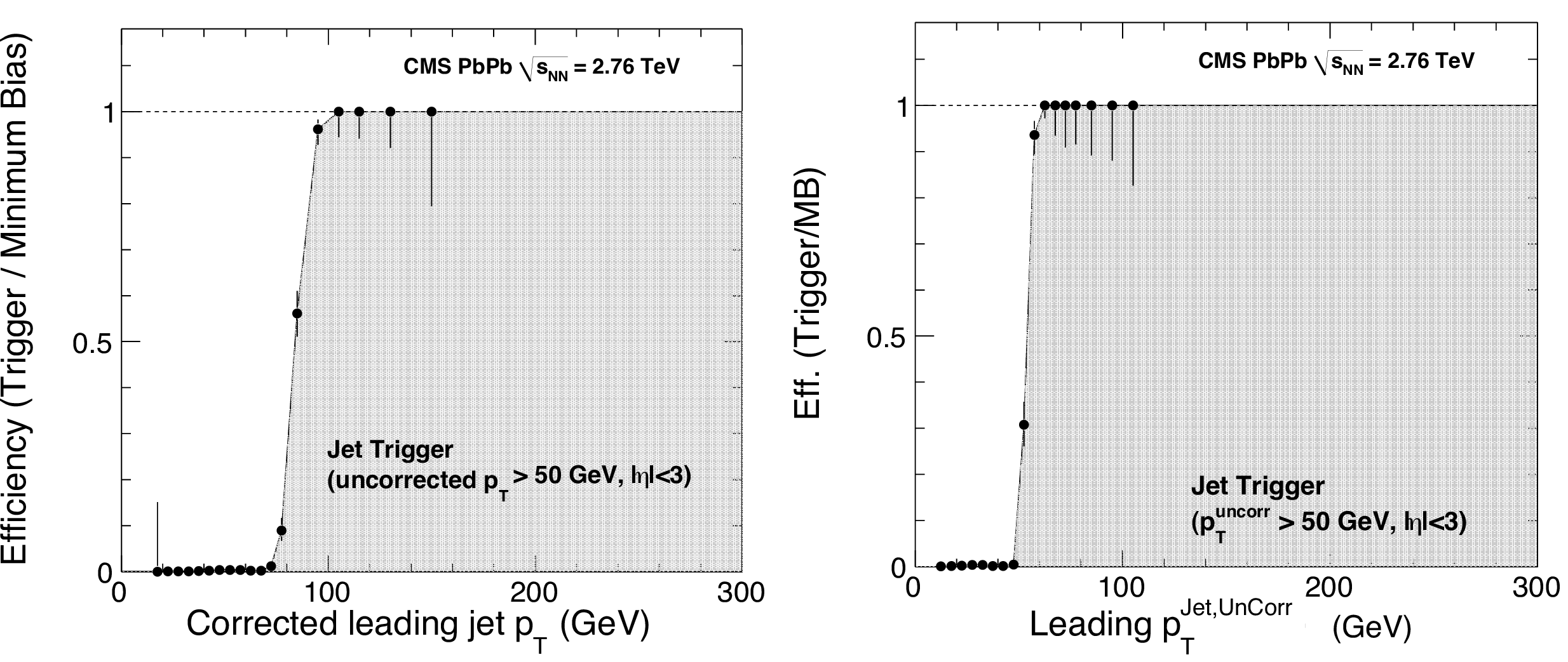
Figure 52:
Efficiency curves for the Jet50U trigger in PbPb at $\sqrt {s_\mathrm {NN}}=$ 2.76 TeV, as a function of the corrected (left) and uncorrected (right) leading jet transverse momentum. |

png pdf |
Figure 52-a:
Efficiency curves for the Jet50U trigger in PbPb at $\sqrt {s_\mathrm {NN}}=$ 2.76 TeV, as a function of the corrected leading jet transverse momentum. |

png pdf |
Figure 52-b:
Efficiency curves for the Jet50U trigger in PbPb at $\sqrt {s_\mathrm {NN}}=$ 2.76 TeV, as a function of the uncorrected leading jet transverse momentum. |

png pdf |
Figure 53:
Efficiency curves for the Jet80 trigger in PbPb at $\sqrt {s_\mathrm {NN}}= $ 2.76 TeV, as a function of the leading jet transverse momentum in the $ {| \eta | }< $ 2 region evaluated from minimum bias sample. The red, black, and blue points correspond to anti-$ {k_{\mathrm {T}}}$ jets with cone size of 0.2, 0.3, and 0.4, respectively. |

png pdf |
Figure 54:
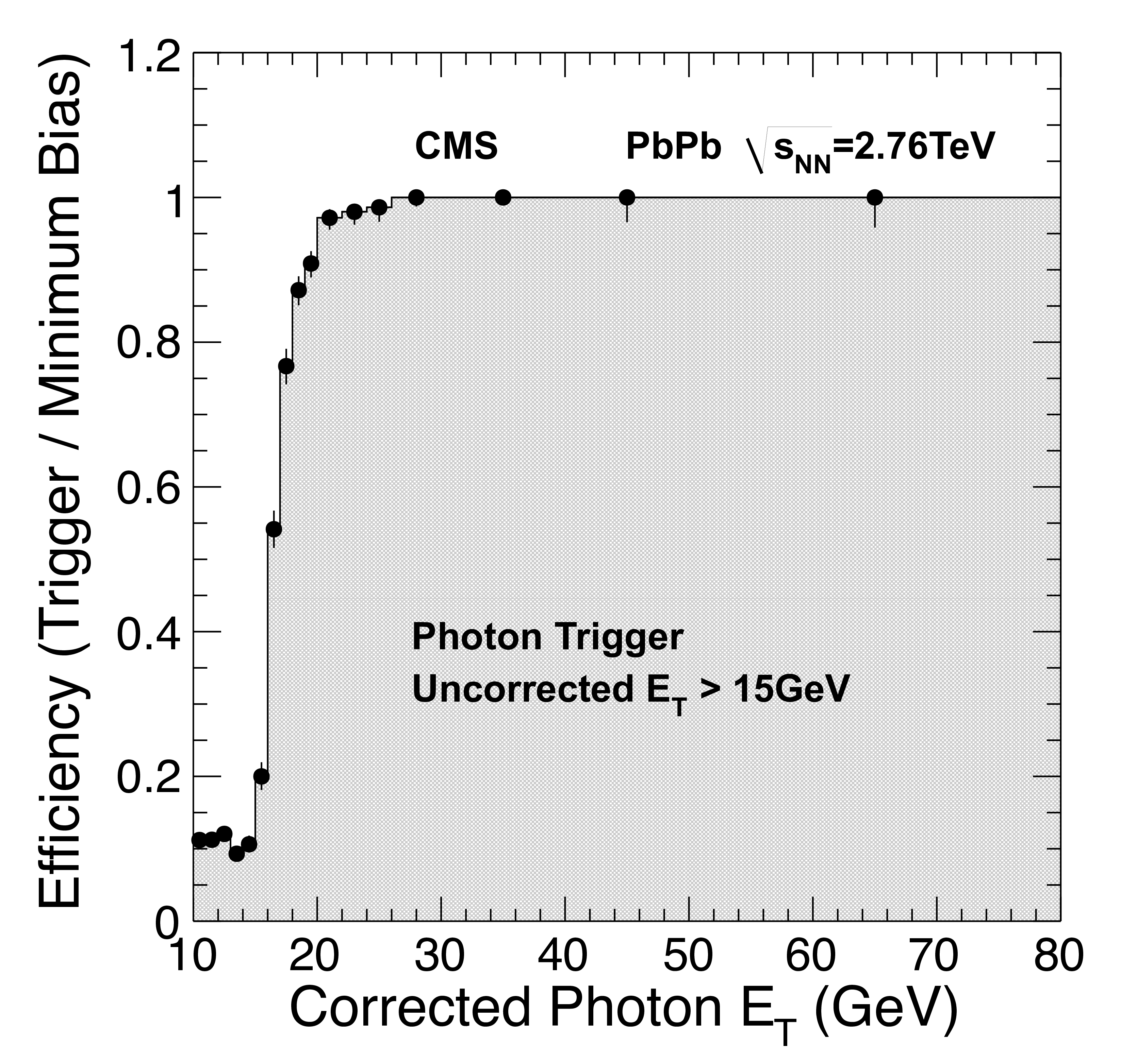
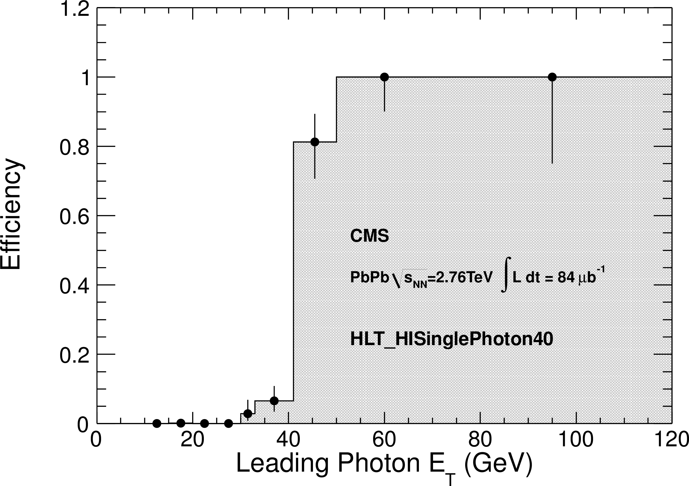
Trigger efficiency of the uncorrected Photon15 (left) and the corrected Photon40 (right) triggers as a function of corrected offline photon transverse momentum, in PbPb collisions at $\sqrt {s_{\rm NN}}= $ 2.76 TeV. |
png pdf |
Figure 54-a:
Trigger efficiency of the uncorrected Photon15 trigger as a function of corrected offline photon transverse momentum, in PbPb collisions at $\sqrt {s_{\rm NN}}= $ 2.76 TeV. |
png pdf |
Figure 54-b:
Trigger efficiency of the corrected Photon40 trigger as a function of corrected offline photon transverse momentum, in PbPb collisions at $\sqrt {s_{\rm NN}}= $ 2.76 TeV. |

png pdf |
Figure 55:
Per-muon triggering efficiency of the HLT HI double-muon trigger as a function of $ {p_{\mathrm {T}}} $ (left), $\eta $ (center), and average number of participant nucleons (right). Z bosons in data (red) are compared to simulated Z bosons embedded in HI background simulated with hydjet (blue). |
png pdf |
Figure 55-a:
Per-muon triggering efficiency of the HLT HI double-muon trigger as a function of $ {p_{\mathrm {T}}} $. Z bosons in data (red) are compared to simulated Z bosons embedded in HI background simulated with hydjet (blue). |
png pdf |
Figure 55-b:
Per-muon triggering efficiency of the HLT HI double-muon trigger as a function of $\eta $. Z bosons in data (red) are compared to simulated Z bosons embedded in HI background simulated with hydjet (blue). |
png pdf |
Figure 55-c:
Per-muon triggering efficiency of the HLT HI double-muon trigger as a function of the average number of participant nucleons. Z bosons in data (red) are compared to simulated Z bosons embedded in HI background simulated with hydjet (blue). |

png pdf |
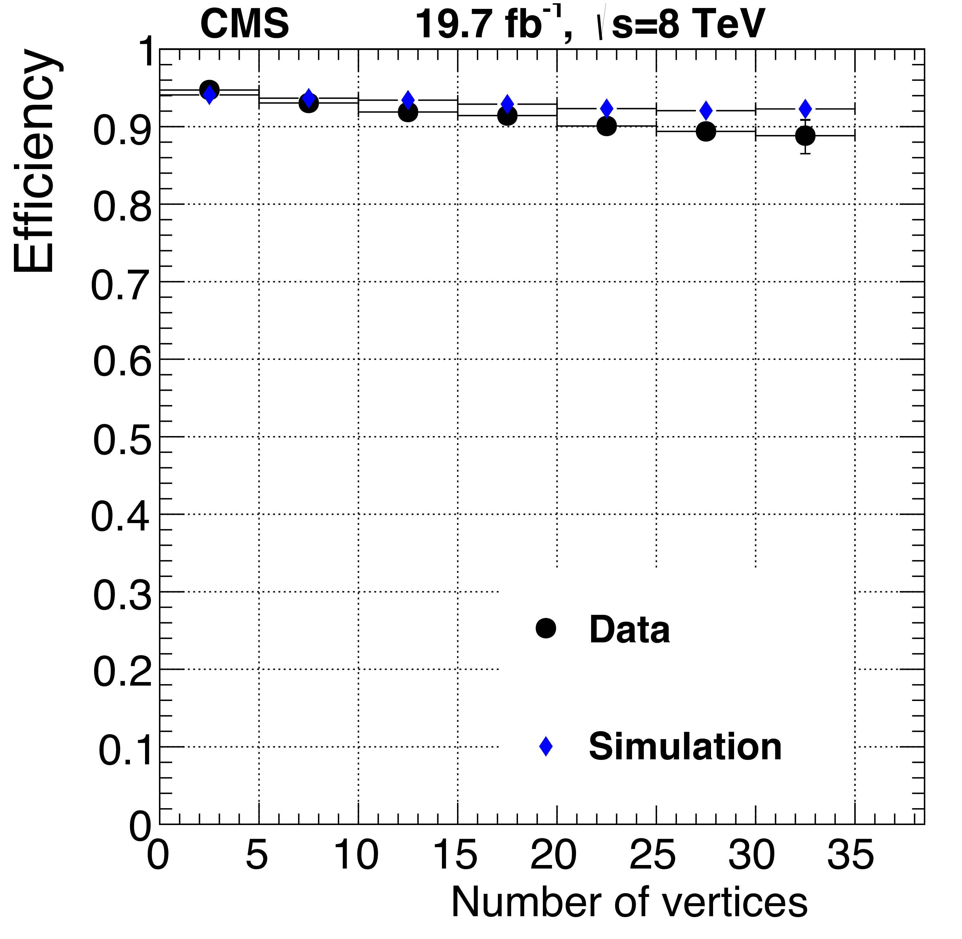
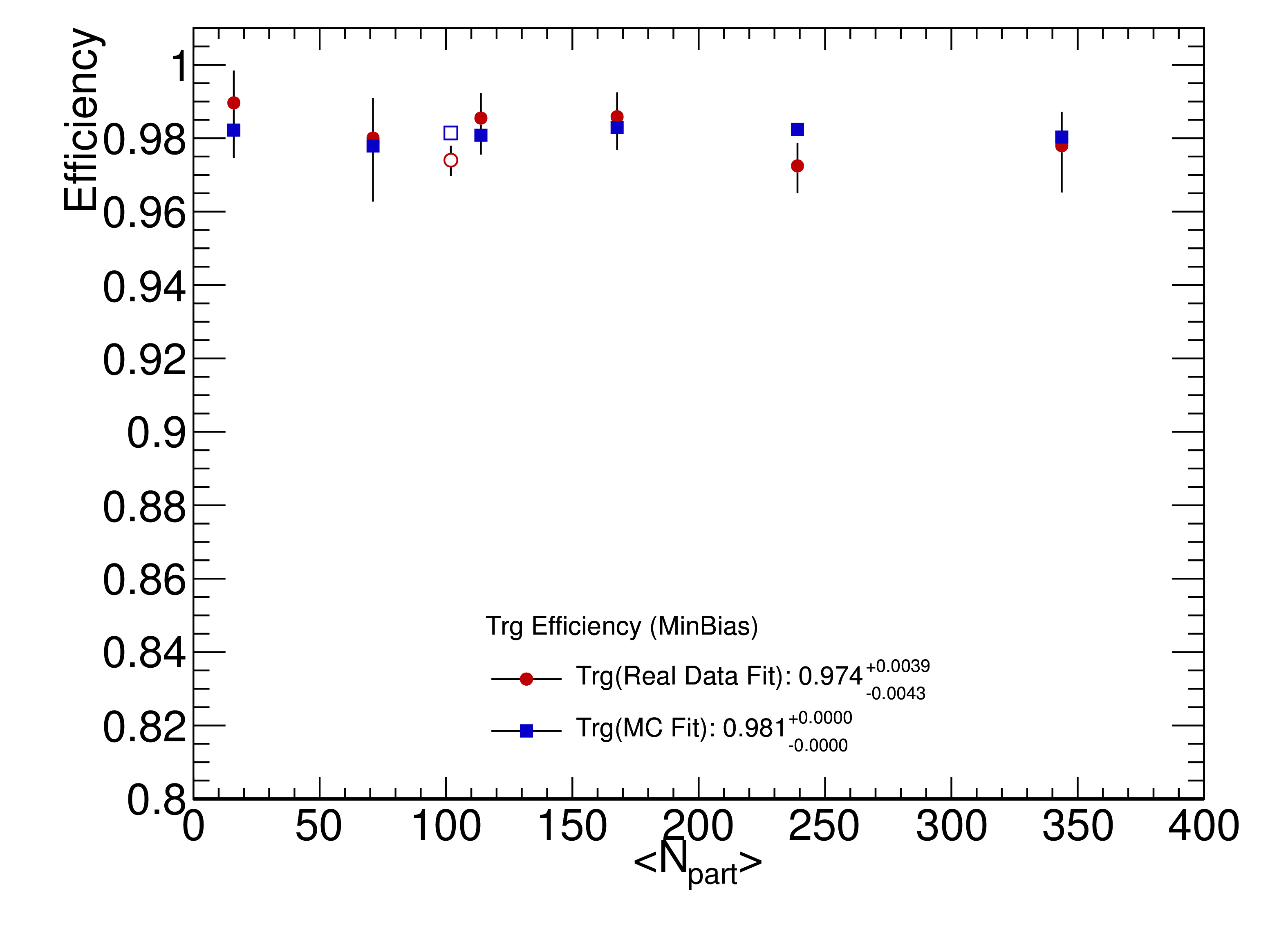
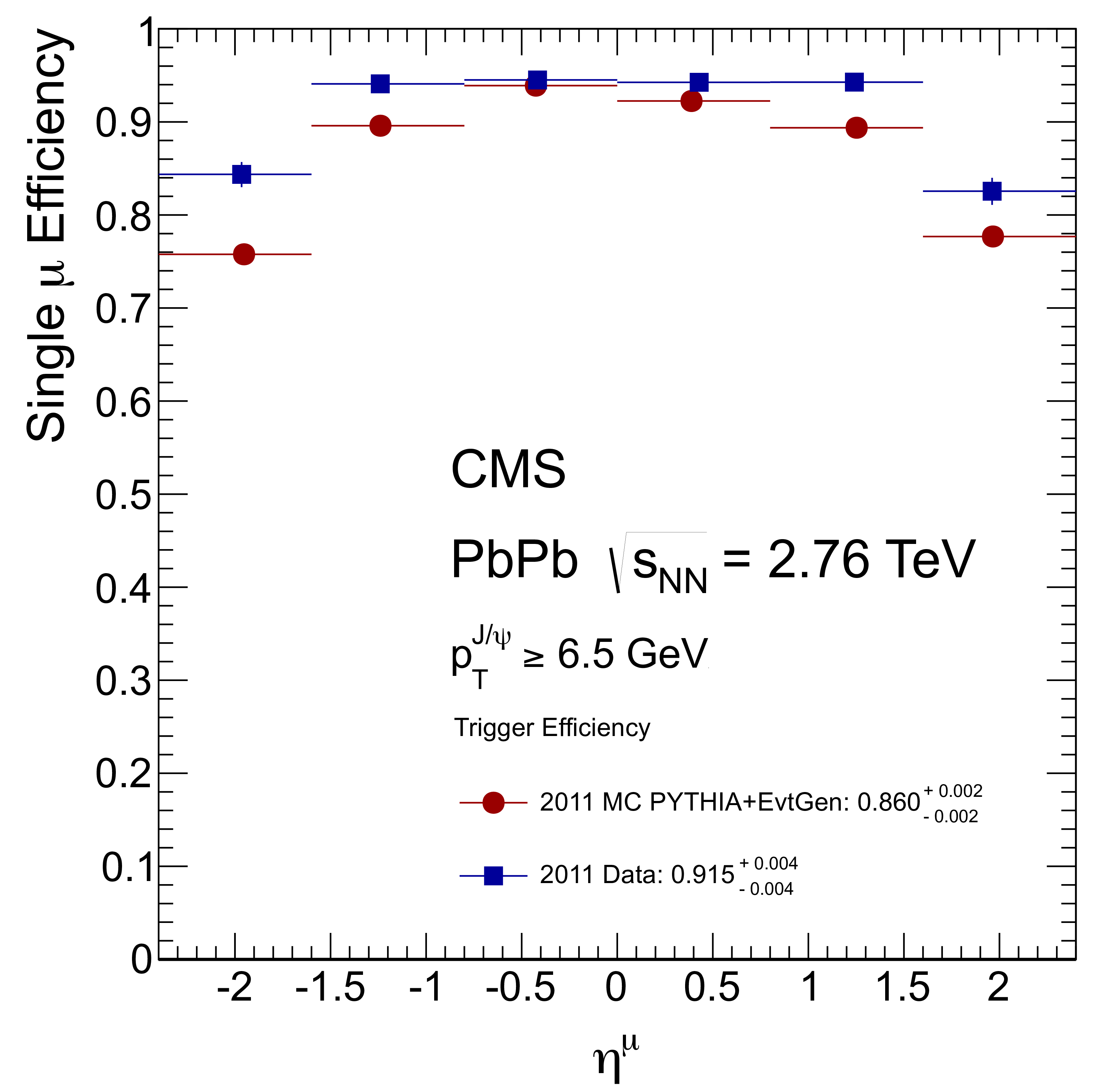
Figure 56:
Single-muon trigger efficiencies as functions of probe muon transverse momentum, pseudorapidity, and number of participants in the 2011 PbPb data. Red full circles are simulation and blue full squares are data. The numbers quoted in the legends of the figures are the integrated efficiencies. |

png pdf |
Figure 56-a:
Single-muon trigger efficiencies as functions of probe muon transverse momentum, pseudorapidity, and number of participants in the 2011 PbPb data. Red full circles are simulation and blue full squares are data. The numbers quoted in the legends of the figures are the integrated efficiencies. |
png pdf |
Figure 56-b:
Single-muon trigger efficiencies as functions of probe muon transverse momentum, pseudorapidity, and number of participants in the 2011 PbPb data. Red full circles are simulation and blue full squares are data. The numbers quoted in the legends of the figures are the integrated efficiencies. |

png pdf |
Figure 56-c:
Single-muon trigger efficiencies as functions of probe muon transverse momentum, pseudorapidity, and number of participants in the 2011 PbPb data. Red full circles are simulation and blue full squares are data. The numbers quoted in the legends of the figures are the integrated efficiencies. |
png pdf |
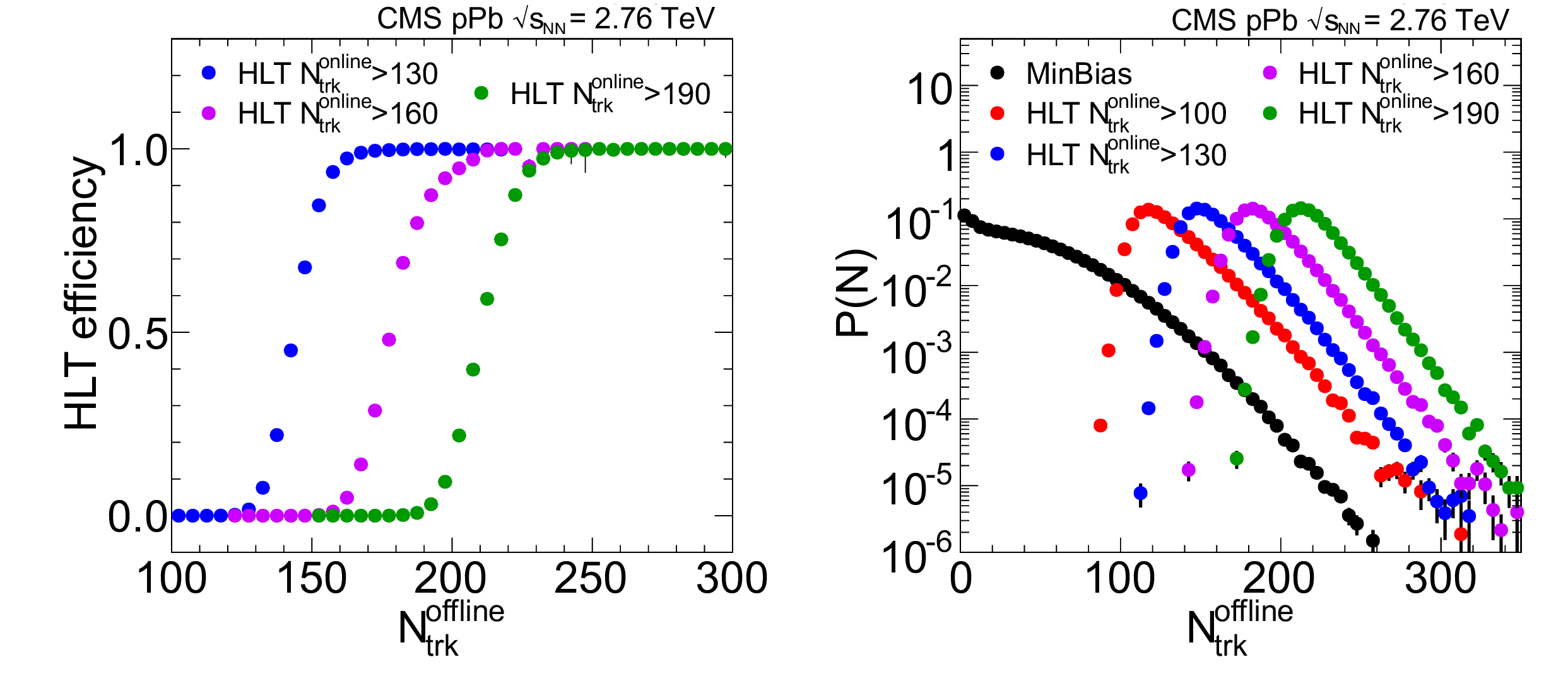
Figure 57:
Left: Trigger efficiency as a function of the offline track multiplicity, for the three most selective high-multiplicity triggers. Right: The spectrum of the offline tracks for minimum bias and for all the different track-based high-multiplicity triggers in the 2013 pPb data. |

png pdf |
Figure 57-a:
Trigger efficiency as a function of the offline track multiplicity, for the three most selective high-multiplicity triggers. |

png pdf |
Figure 57-b:
The spectrum of the offline tracks for minimum bias and for all the different track-based high-multiplicity triggers in the 2013 pPb data. |
png pdf |
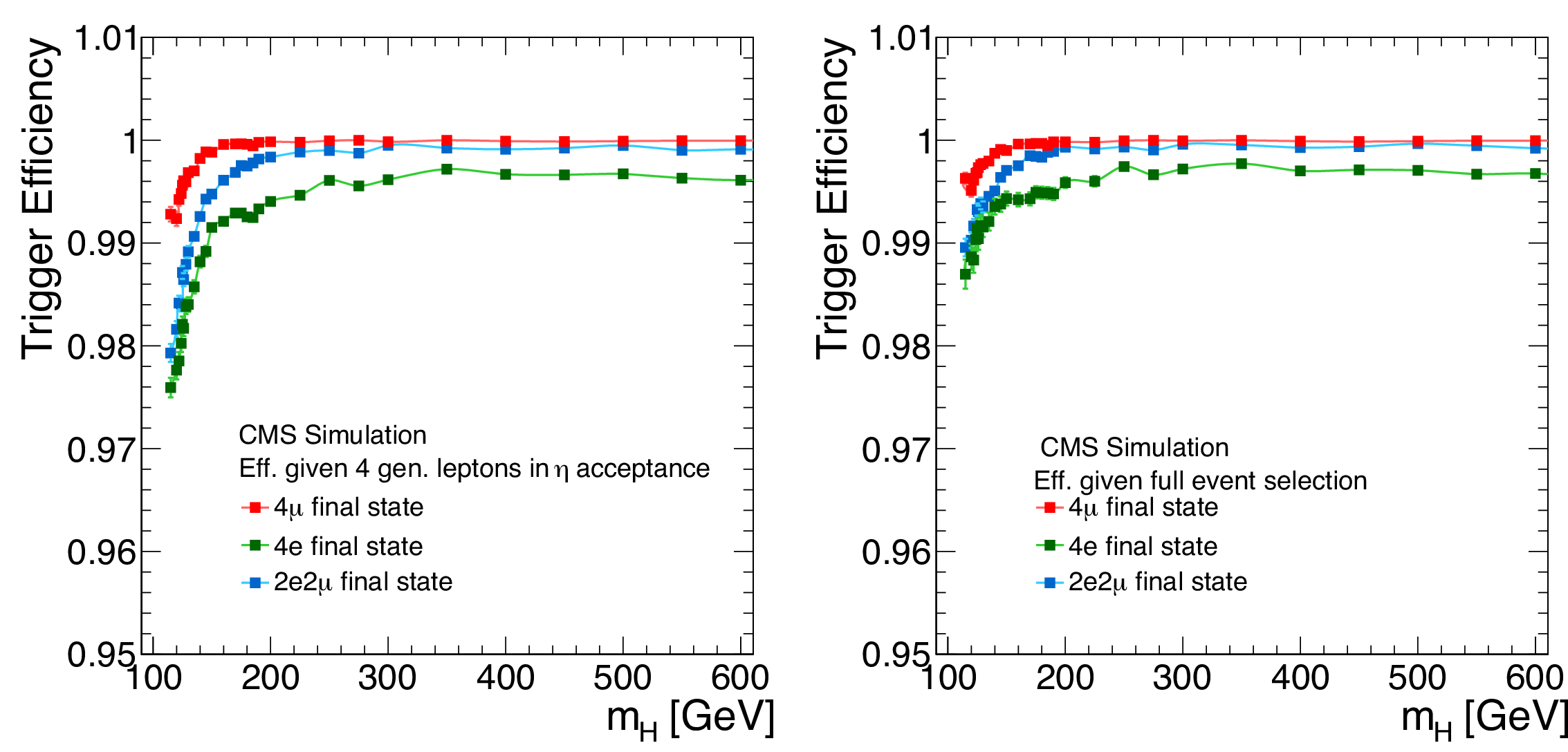
Figure 58:
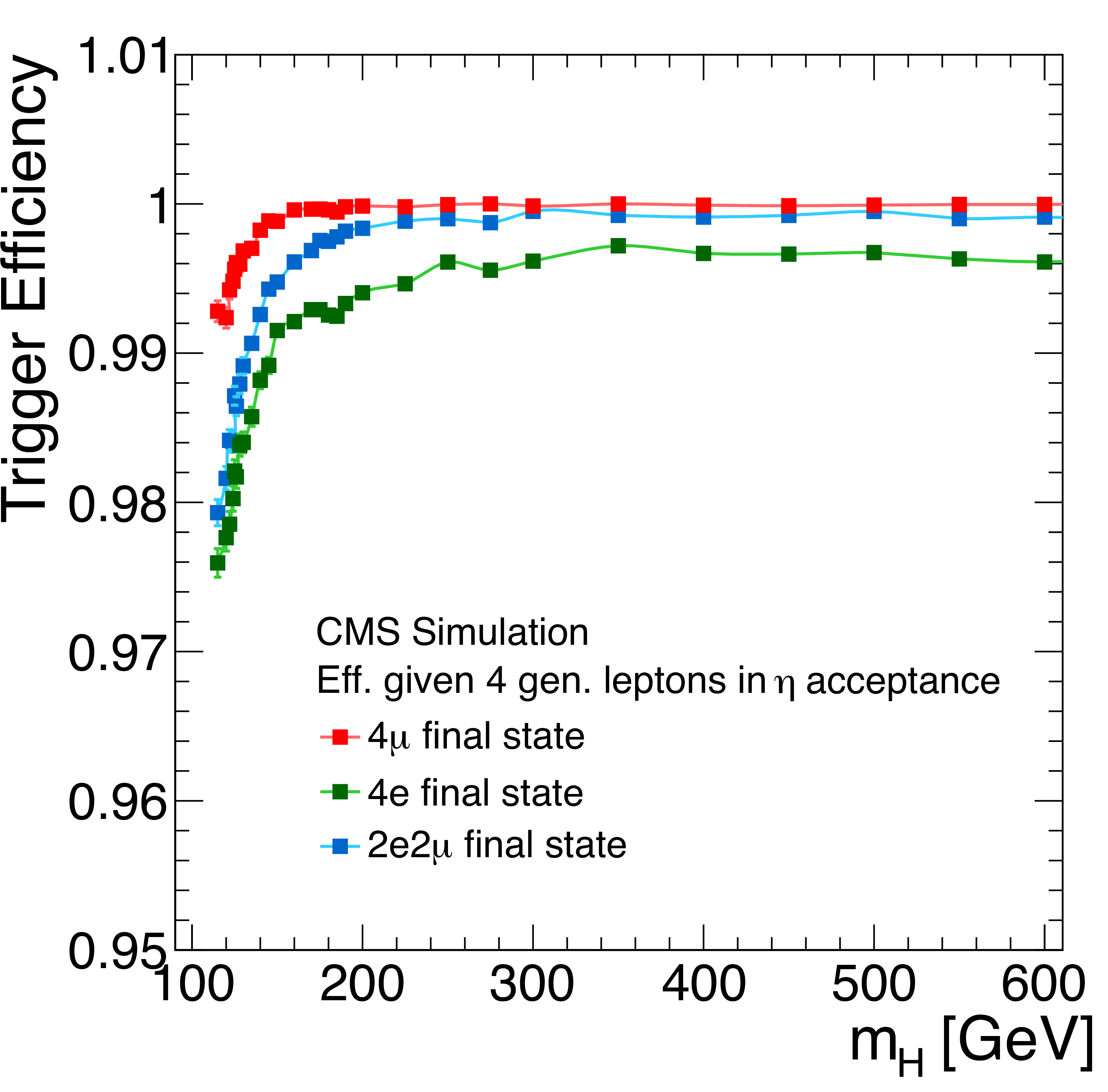
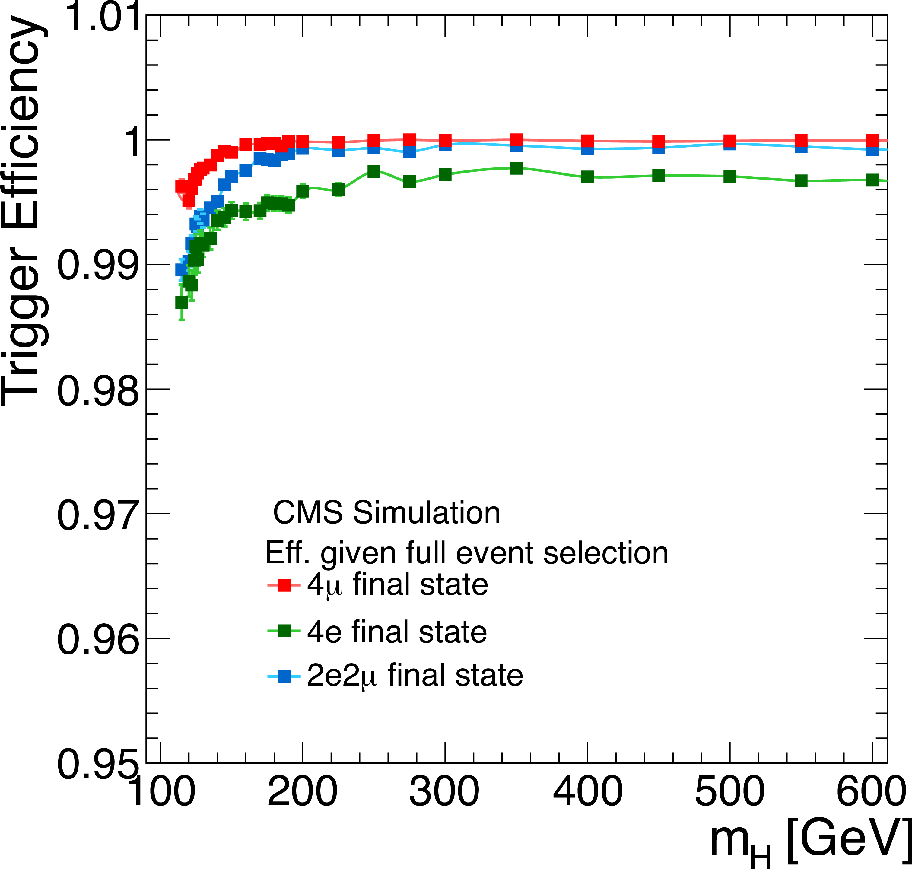
Trigger efficiency for simulated signal events with four generated leptons in the pseudorapidity acceptance (left), and for simulated signal events that have passed the full $\mathrm{ H } \to 4\ell $ analysis selection (right). |
png pdf |
Figure 58-a:
Trigger efficiency for simulated signal events with four generated leptons in the pseudorapidity acceptance. |
png pdf |
Figure 58-b:
Trigger efficiency for simulated signal events that have passed the full $\mathrm{ H } \to 4\ell $ analysis selection. |
png pdf |
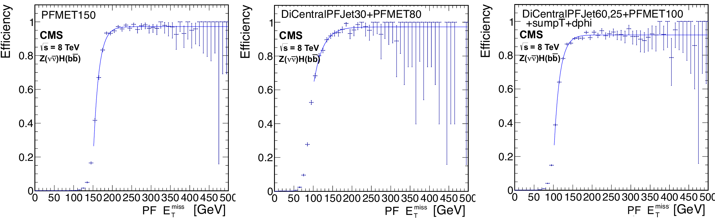
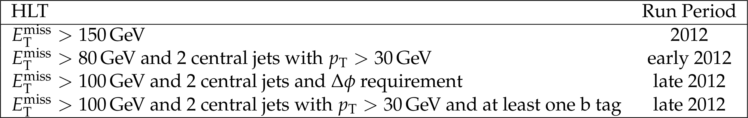
Figure 59:
Trigger efficiencies for the ${\mathrm{ Z } } (\nu \bar{\nu} )\mathrm{ H } ( {\mathrm{ b \bar{b} } } )$ analysis, as a function of offline PF $ {E_{\mathrm {T}}^{\text {miss}}} $ for the pure $ {E_{\mathrm {T}}^{\text {miss}}} > $ 150 GeV trigger (left) using late 2012 data, dijet and $ {E_{\mathrm {T}}^{\text {miss}}} $ trigger (center) using early 2012 data, and dijet, $ {E_{\mathrm {T}}^{\text {miss}}} $ and $\Delta \phi $ requirement trigger (right) using 2012 late data, as described in the text. |

png pdf |
Figure 59-a:
Trigger efficiencies for the ${\mathrm{ Z } } (\nu \bar{\nu} )\mathrm{ H } ( {\mathrm{ b \bar{b} } } )$ analysis, as a function of offline PF $ {E_{\mathrm {T}}^{\text {miss}}} $ for the pure $ {E_{\mathrm {T}}^{\text {miss}}} > $ 150 GeV trigger using late 2012 data, dijet and $ {E_{\mathrm {T}}^{\text {miss}}} $ trigger. |

png pdf |
Figure 59-b:
Trigger efficiencies for the ${\mathrm{ Z } } (\nu \bar{\nu} )\mathrm{ H } ( {\mathrm{ b \bar{b} } } )$ analysis, as a function of offline PF $ {E_{\mathrm {T}}^{\text {miss}}} $ for the pure $ {E_{\mathrm {T}}^{\text {miss}}} > $ 150 GeV trigger using early 2012 data, and dijet, $ {E_{\mathrm {T}}^{\text {miss}}} $ and $\Delta \phi $ requirement trigger. |
png pdf |
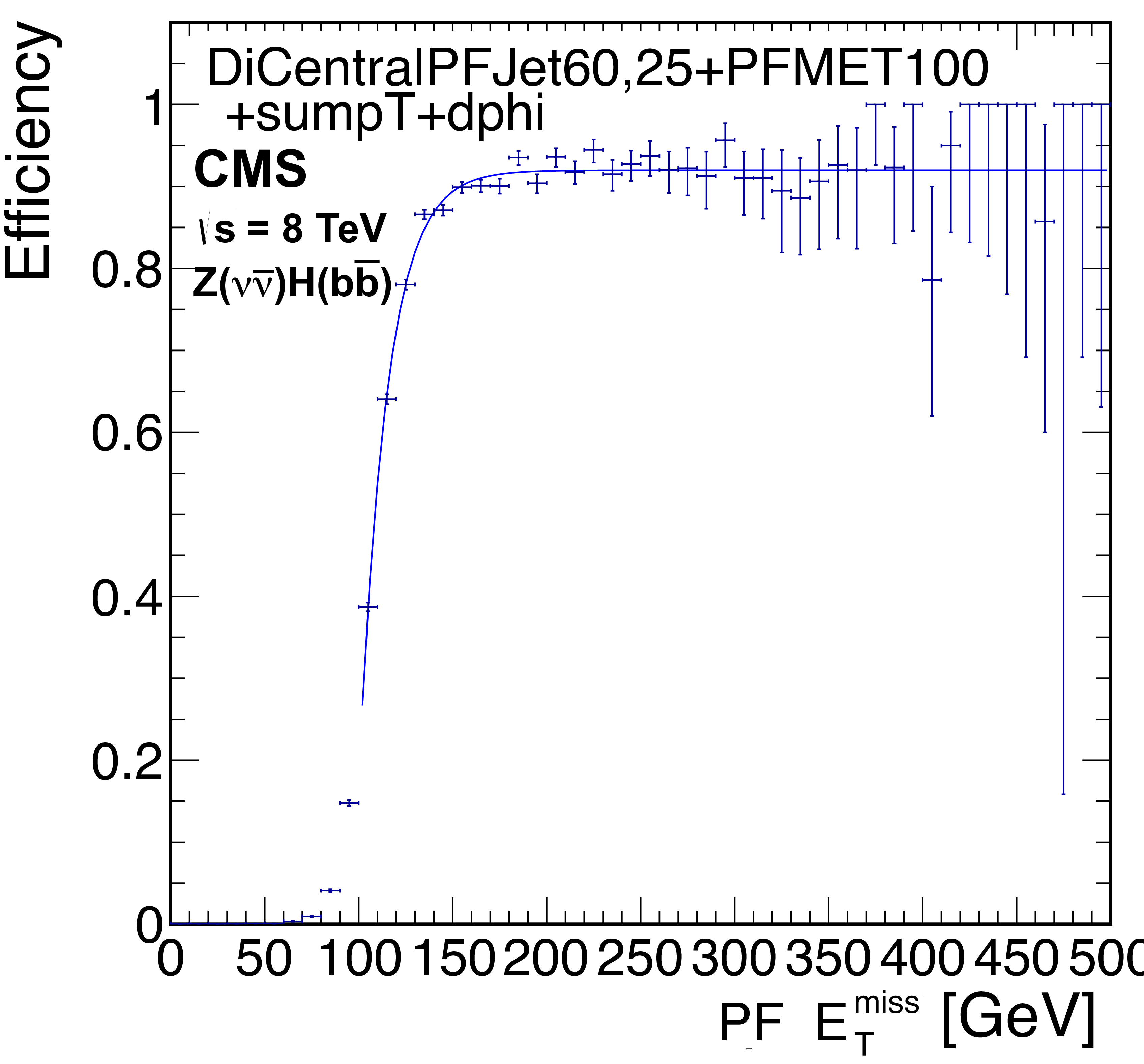
Figure 59-c:
Trigger efficiencies for the ${\mathrm{ Z } } (\nu \bar{\nu} )\mathrm{ H } ( {\mathrm{ b \bar{b} } } )$ analysis, as a function of offline PF $ {E_{\mathrm {T}}^{\text {miss}}} $ for the pure $ {E_{\mathrm {T}}^{\text {miss}}} > $ 150 GeV trigger using 2012 late data. |
png pdf |
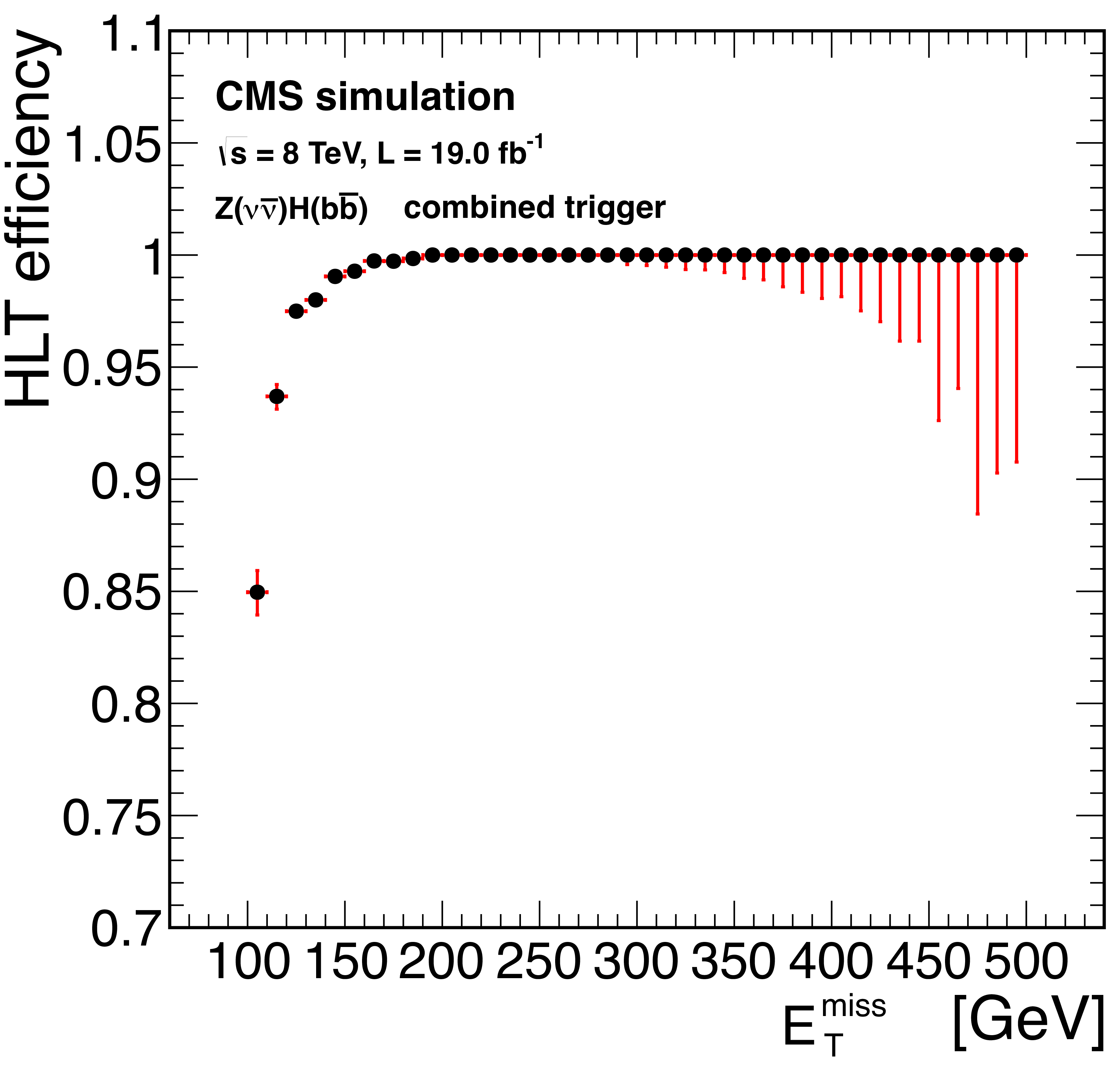
Figure 60:
Efficiency as function of $ {E_{\mathrm {T}}^{\text {miss}}} $ for the ${\mathrm{ Z } } (\nu \bar{\nu} )\mathrm{ H } ( {\mathrm{ b \bar{b} } } )$ signal events. An efficiency greater than 99% is obtained for $ {E_{\mathrm {T}}^{\text {miss}}} > $ 170 GeV. |

png pdf |
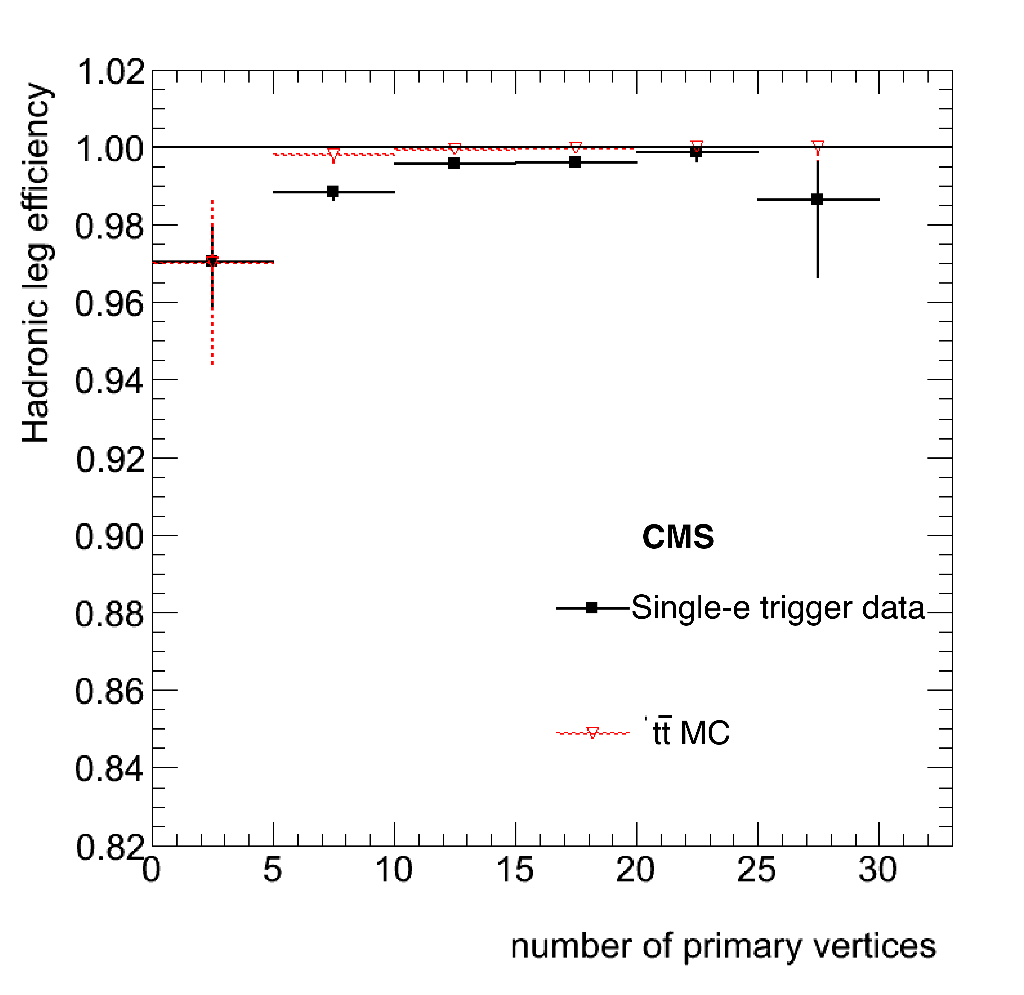
Figure 61:
Top quark triggers: Efficiency of the hadronic leg for the electron plus jets paths in 2012 as a function of the $ {p_{\mathrm {T}}} $ of the 4th jet (left) and of the number of reconstructed vertices (right). |

png pdf |
Figure 61-a:
Top quark triggers: Efficiency of the hadronic leg for the electron plus jets paths in 2012 as a function of the $ {p_{\mathrm {T}}} $ of the 4th jet. |
png pdf |
Figure 61-b:
Top quark triggers: Efficiency of the hadronic leg for the electron plus jets paths in 2012 as a function of the $ {p_{\mathrm {T}}} $ of the number of reconstructed vertices. |
png pdf |
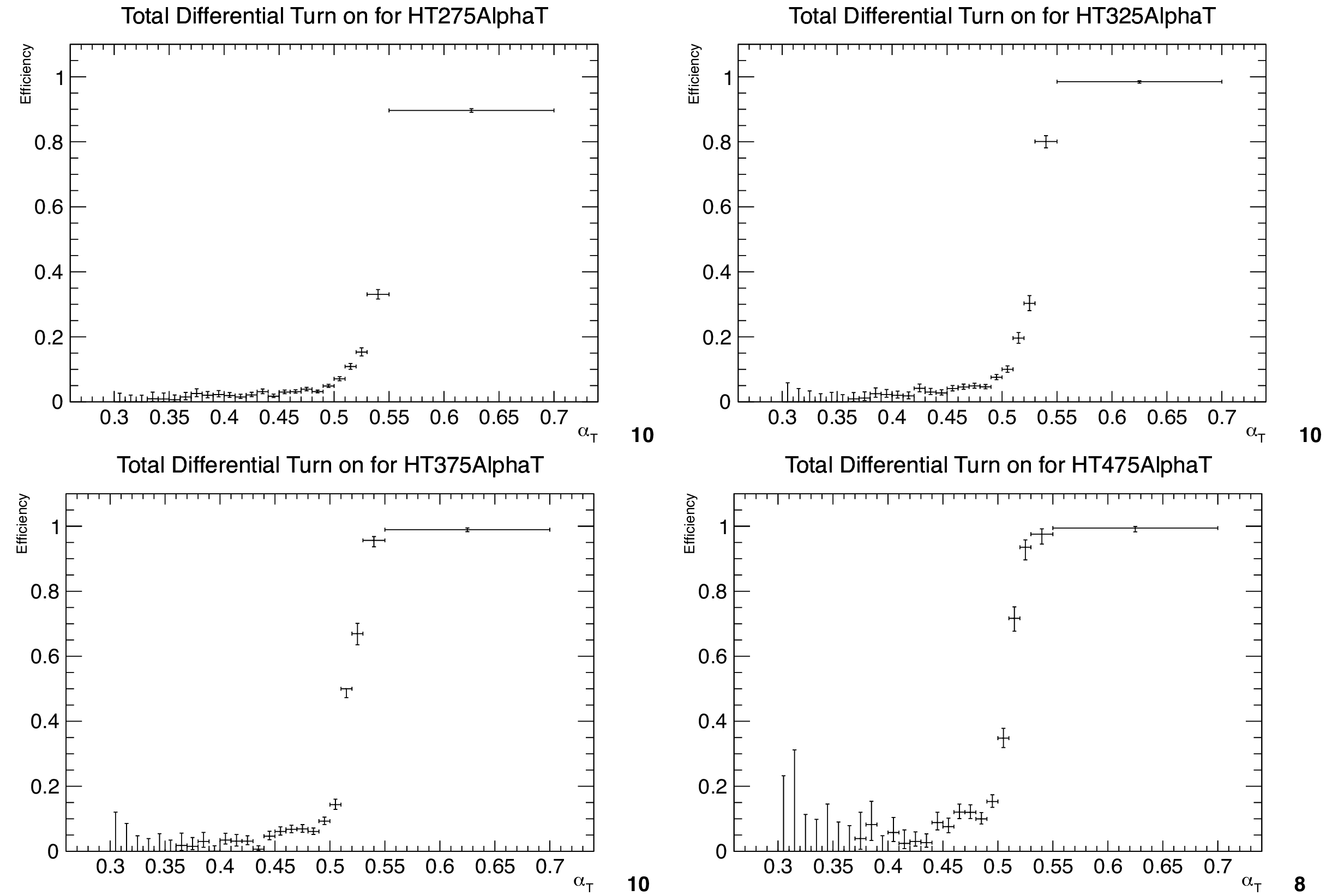
Figure 62:
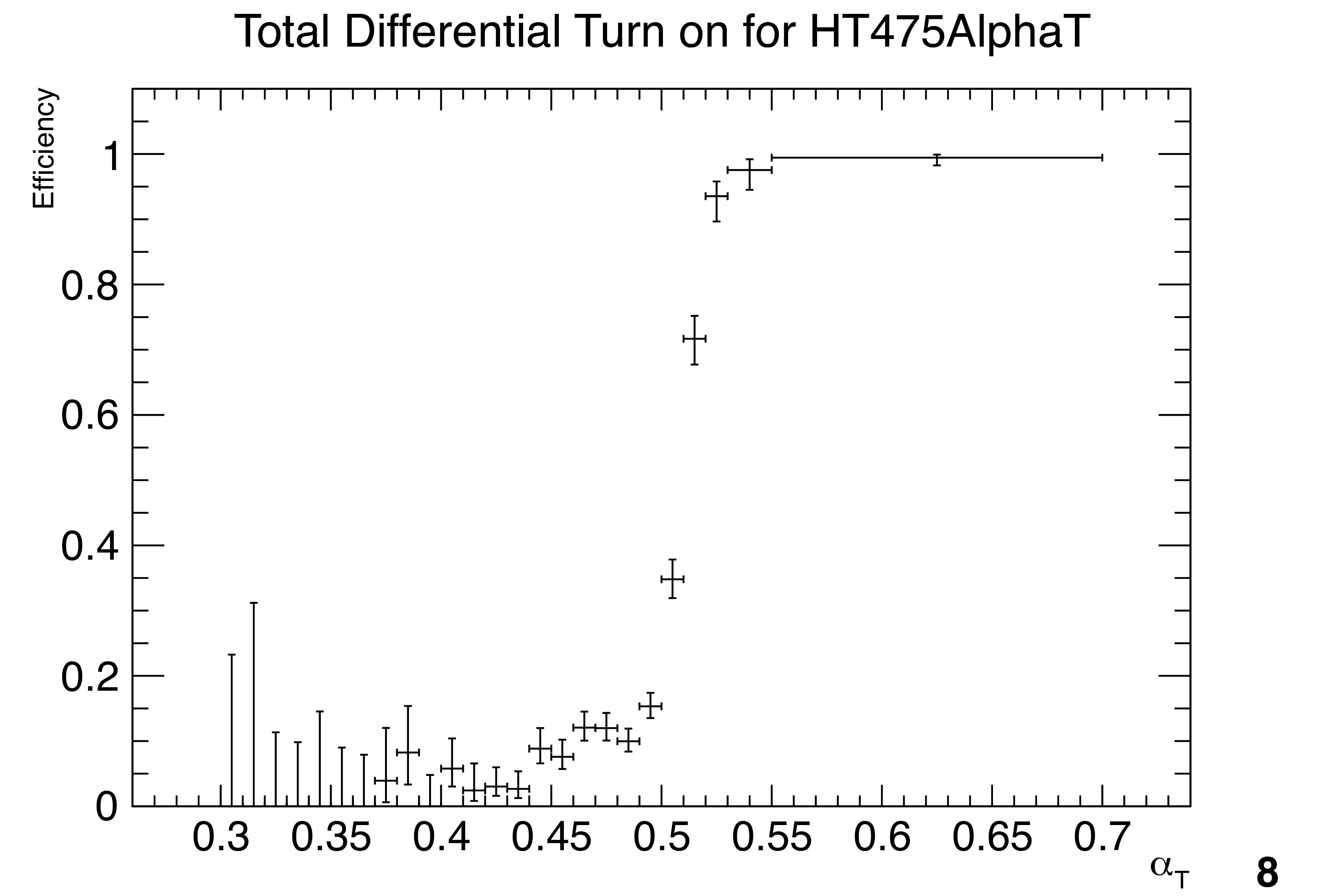
Efficiency turn-on curves for the $\alpha _T$ triggers used to collect events for four different ${H_{\mathrm {T}}}$ regions: 275 $ < {H_{\mathrm {T}}} < $ 325 GeV (upper left), 325 $ < {H_{\mathrm {T}}} < $ 375 GeV (upper right), 375 $ < {H_{\mathrm {T}}} < $ 475 GeV (lower left), and $ {H_{\mathrm {T}}} > $ 475 GeV (lower right). |

png pdf |
Figure 62-a:
Efficiency turn-on curves for the $\alpha _T$ triggers used to collect events for 275 $ < {H_{\mathrm {T}}} < $ 325 GeV. |
png pdf |
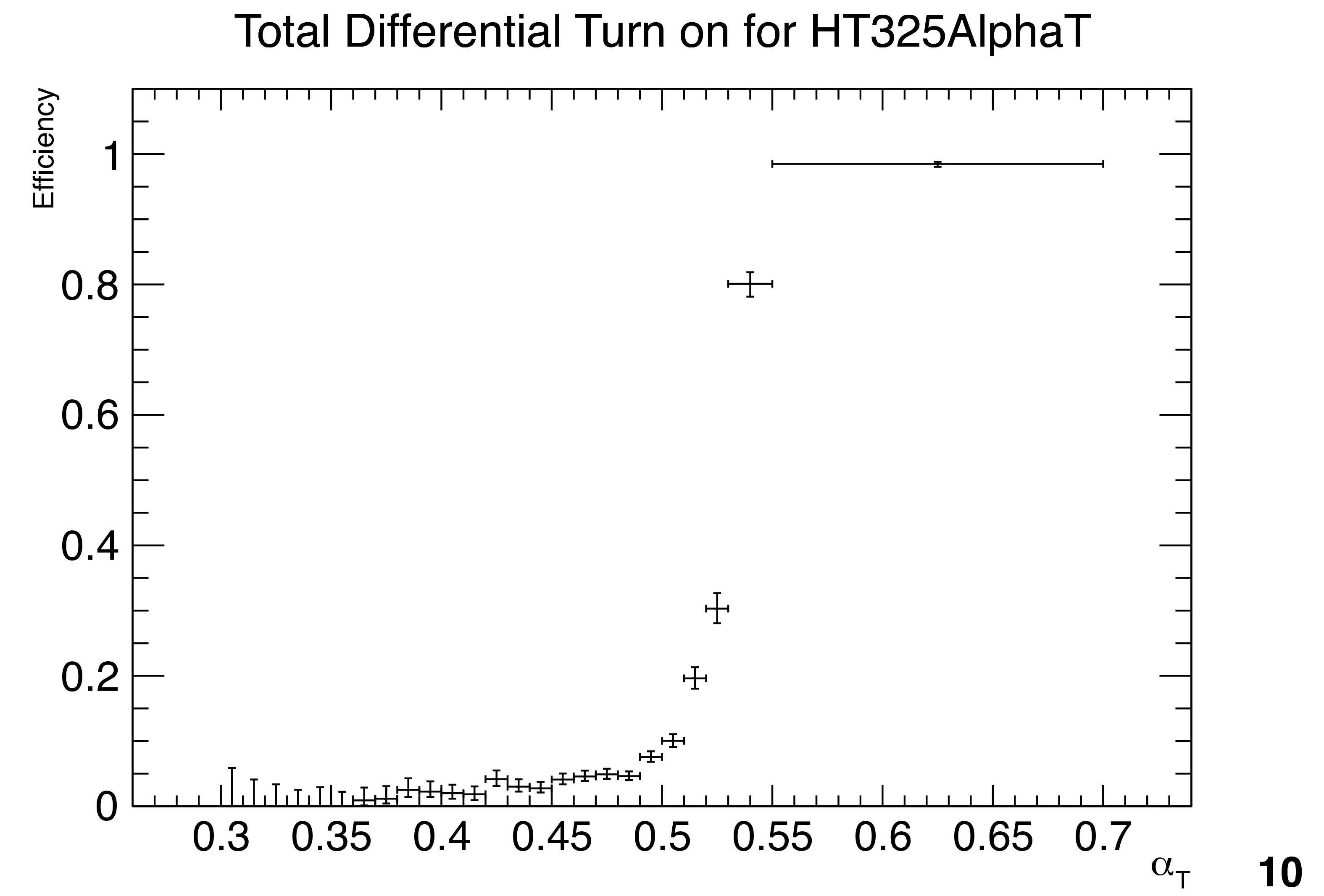
Figure 62-b:
Efficiency turn-on curves for the $\alpha _T$ triggers used to collect events for 325 $ < {H_{\mathrm {T}}} < $ 375 GeV. |

png pdf |
Figure 62-c:
Efficiency turn-on curves for the $\alpha _T$ triggers used to collect events for four different 375 $ < {H_{\mathrm {T}}} < $ 475 GeV. |
png pdf |
Figure 62-d:
Efficiency turn-on curves for the $\alpha _T$ triggers used to collect events for $ {H_{\mathrm {T}}} > $ 475 GeV. |

png pdf |
Figure 63:
Turn-on curve for $M_R$ (left) and $R^2$ (right) for the inclusive Razor trigger, after requiring $R^2> $ 0.25 (left) and $M_R> $ 400 GeV (right). Events passing the single-electron triggers are selected to define the denominator of the efficiency, together with the dijet requirement. The requirement of satisfying the Razor trigger defines the numerator. |

png pdf |
Figure 63-a:
Turn-on curve for $M_R$ for the inclusive Razor trigger, after requiring $R^2> $ 0.25. Events passing the single-electron triggers are selected to define the denominator of the efficiency, together with the dijet requirement. The requirement of satisfying the Razor trigger defines the numerator. |

png pdf |
Figure 63-b:
Turn-on curve for $R^2$ for the inclusive Razor trigger, after requiring $M_R> $ 400 GeV. Events passing the single-electron triggers are selected to define the denominator of the efficiency, together with the dijet requirement. The requirement of satisfying the Razor trigger defines the numerator. |
png pdf |
Figure 64:
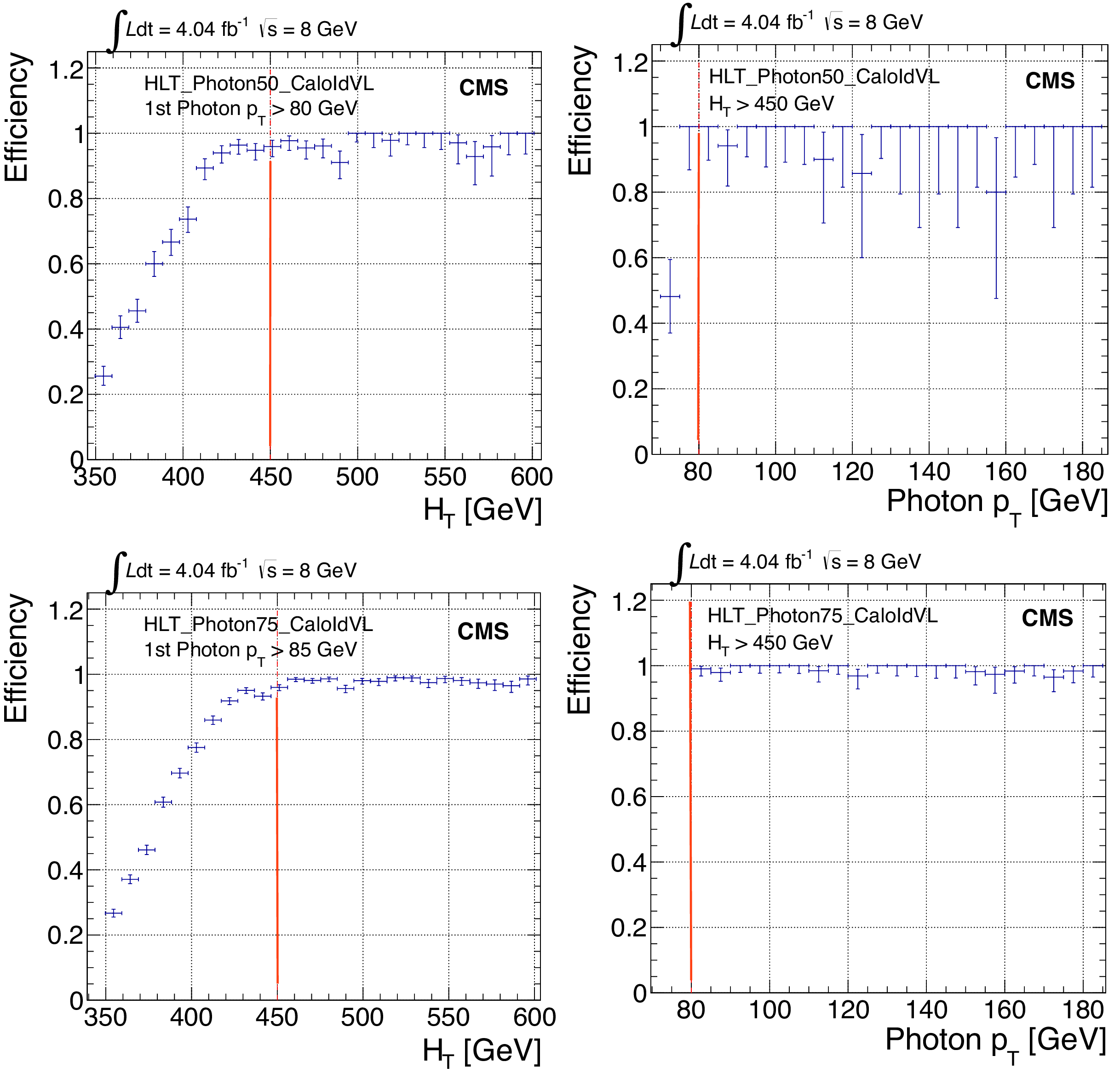
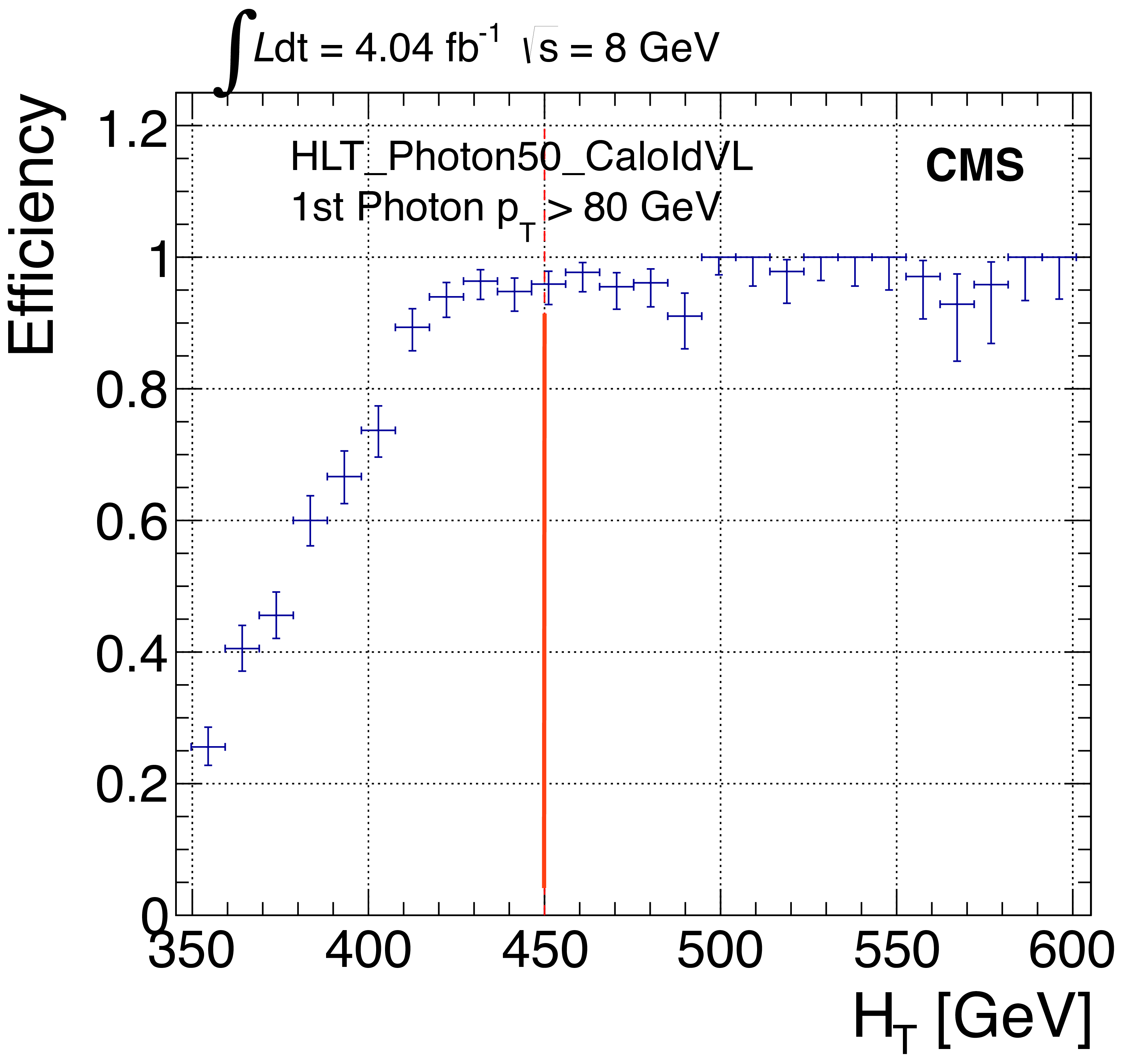
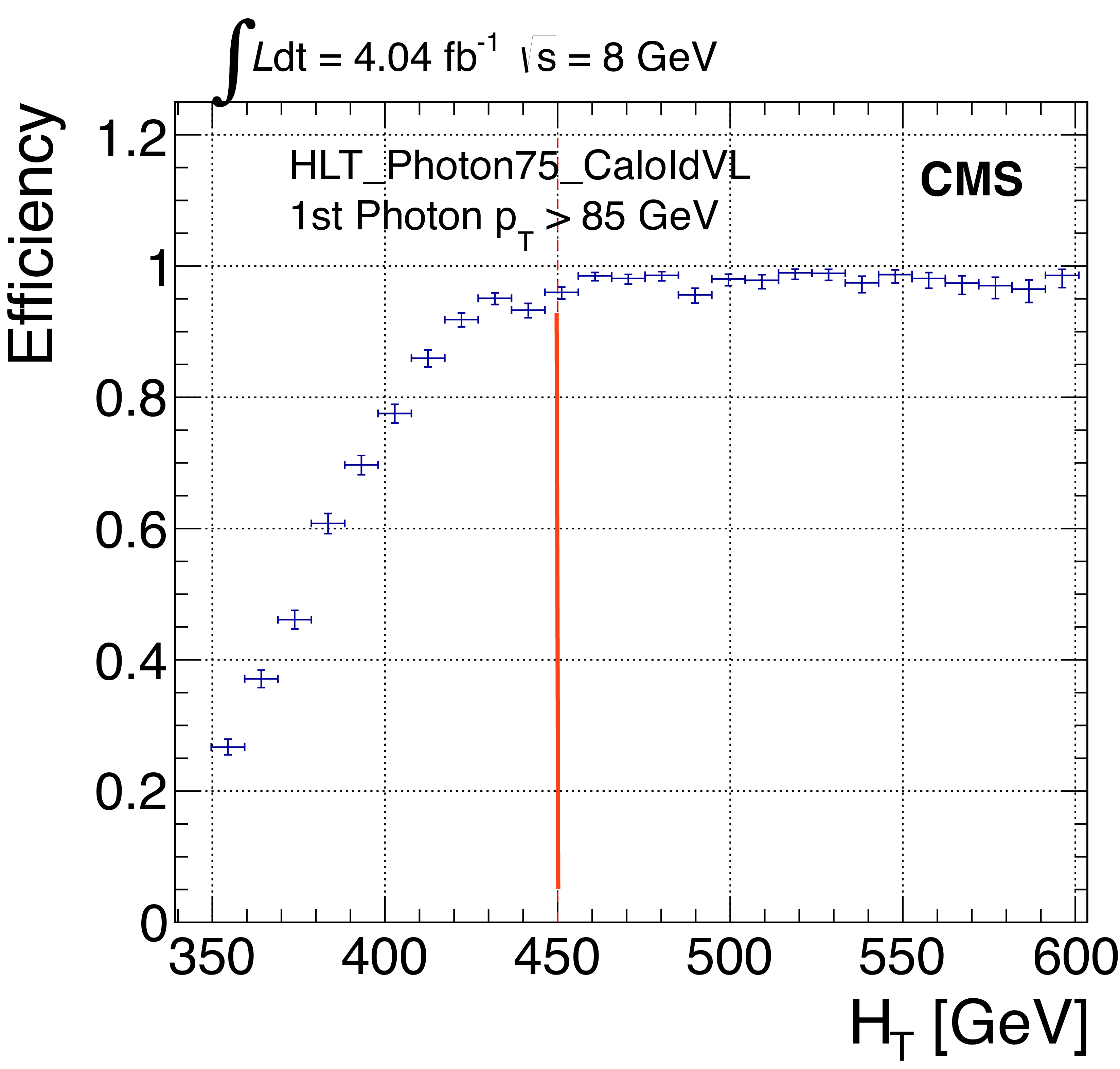
Supersymmetry search in the $\gamma $ + $ {E_{\mathrm {T}}^{\text {miss}}} $ channel: trigger efficiency of the $ {H_{\mathrm {T}}} $ leg (left column), and the photon leg (right column), using as a reference the single-photon trigger with $ {p_{\mathrm {T}}} > $ 50 GeV (top row) and $ {p_{\mathrm {T}}} > $ 75 GeV (bottom row). The red lines indicate offline requirements. |
png pdf |
Figure 64-a:
Supersymmetry search in the $\gamma $ + $ {E_{\mathrm {T}}^{\text {miss}}} $ channel: trigger efficiency of the $ {H_{\mathrm {T}}} $ leg using as a reference the single-photon trigger with $ {p_{\mathrm {T}}} > $ 50 GeV. The red lines indicate offline requirements. |

png pdf |
Figure 64-b:
Supersymmetry search in the $\gamma $ + $ {E_{\mathrm {T}}^{\text {miss}}} $ channel: trigger efficiency of the photon leg, using as a reference the single-photon trigger with $ {p_{\mathrm {T}}} > $ 50 GeV. The red lines indicate offline requirements. |
png pdf |
Figure 64-c:
Supersymmetry search in the $\gamma $ + $ {E_{\mathrm {T}}^{\text {miss}}} $ channel: trigger efficiency of the $ {H_{\mathrm {T}}} $ leg using as a reference the single-photon trigger with $ {p_{\mathrm {T}}} > $ 75 GeV. The red lines indicate offline requirements. |

png pdf |
Figure 64-d:
Supersymmetry search in the $\gamma $ + $ {E_{\mathrm {T}}^{\text {miss}}} $ channel: trigger efficiency of the photon leg, using as a reference the single-photon trigger with $ {p_{\mathrm {T}}} > $ 75 GeV. The red lines indicate offline requirements. |
png pdf |
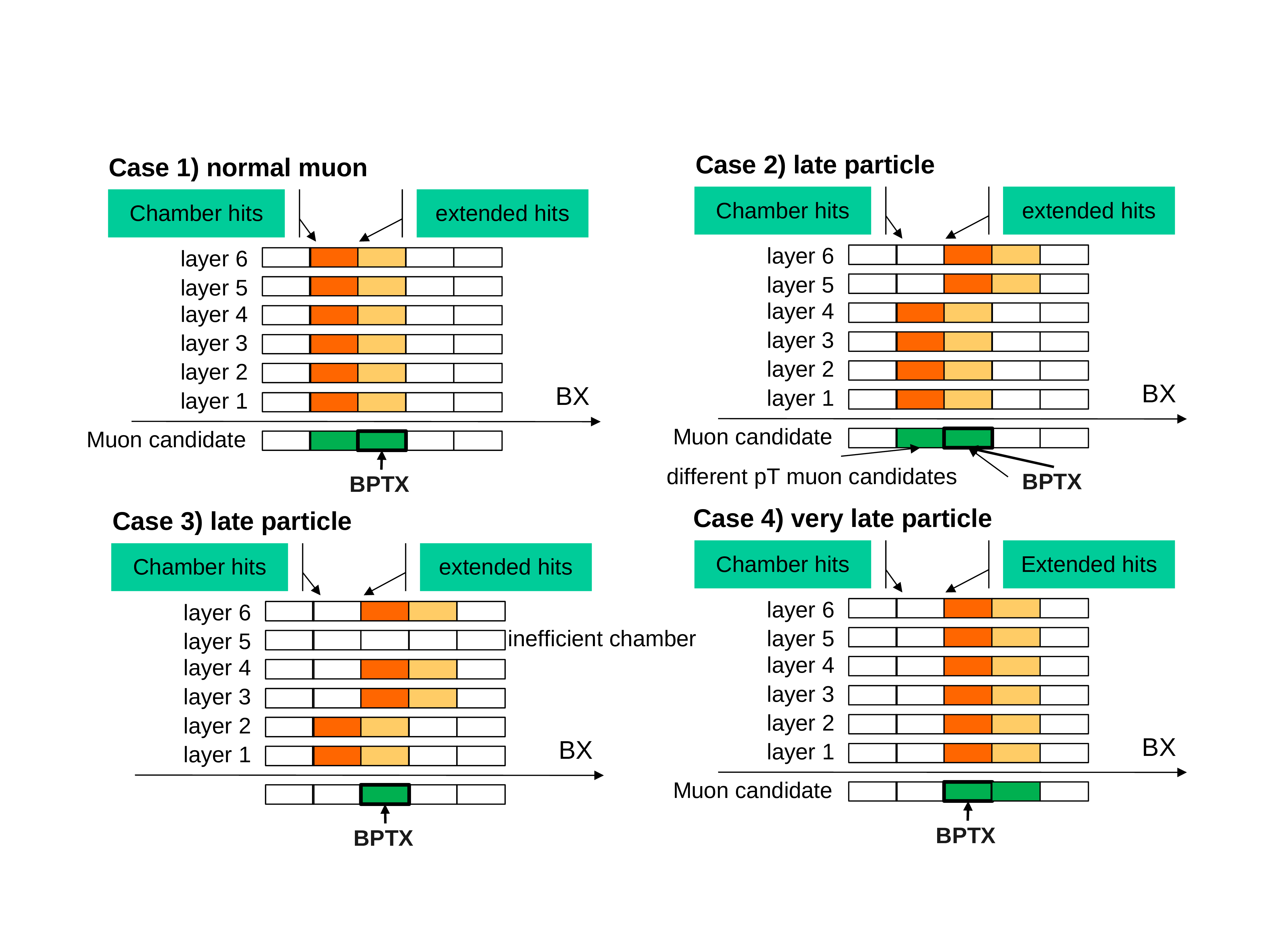
Figure 65:
The principle of operation of the RPC HSCP trigger for an ordinary muon (case 1), and a slow minimum ionizing particle, which produces hits across two consecutive bunch crossings (cases 2, 3) or in the next BX (case 4). Hits that would be seen in the standard PAC configuration are effectively those shown in pale orange; additionally observed hits in the HSCP configuration are those shown in dark orange. In case 1 the output of both configurations is identical, in case 2 the HSCP configuration uses the full detector information, in case 3 only the HSCP configuration can issue a trigger, and in case 4 the HSCP configuration brings back the event to the correct BX. |
png pdf |
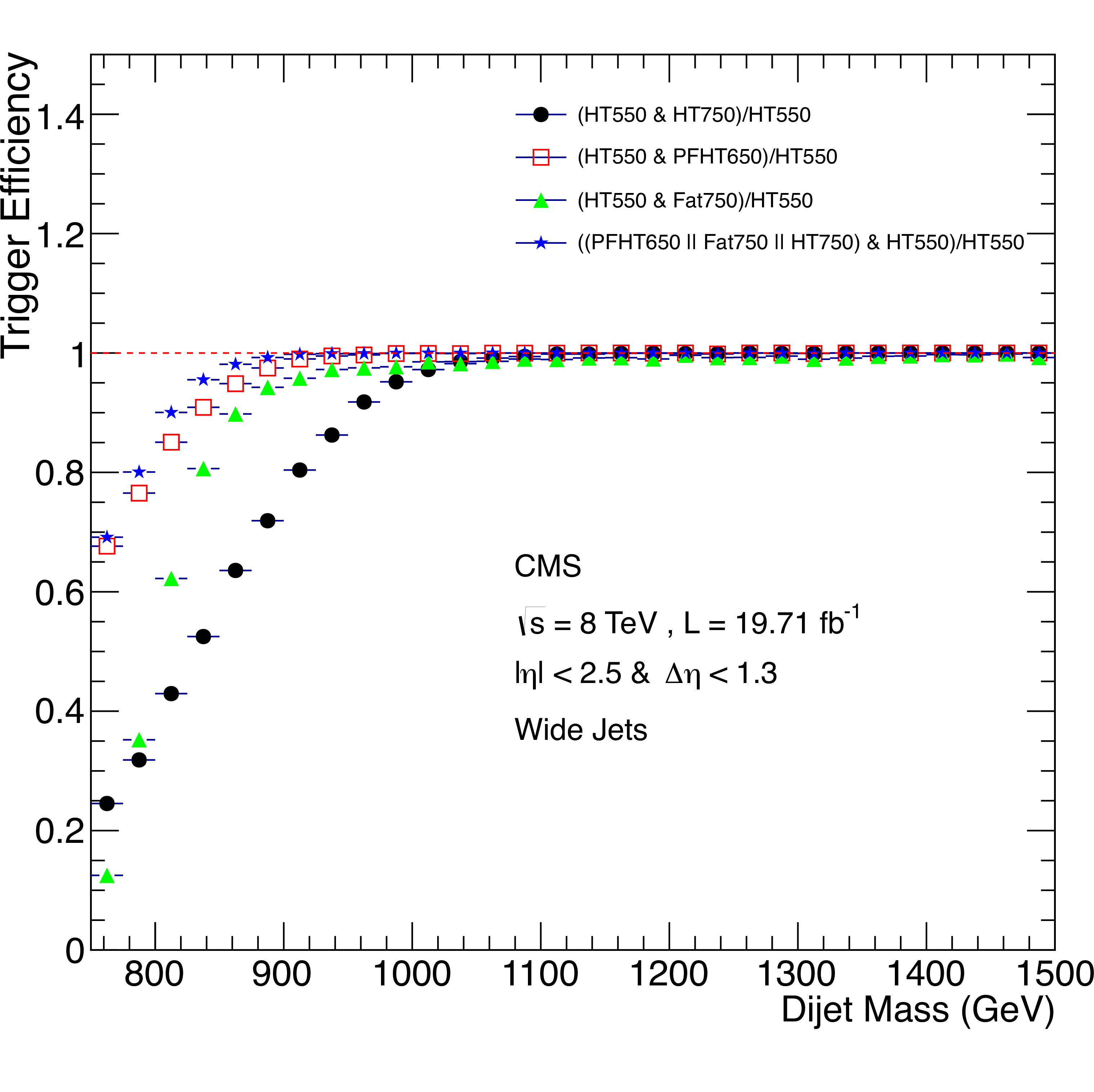
Figure 66:
Dijet resonance search triggers. The HLT efficiency of $ {H_{\mathrm {T}}} > $ 650 GeV, $ {H_{\mathrm {T}}} > $ 750 GeV, and Fat750 triggers individually, and their logical OR as a function of the offline dijet mass. The efficiency is measured with the data sample collected with a trigger path that requires $ {H_{\mathrm {T}}} > $ 550 GeV. The horizontal dashed line marks the trigger efficiency ${\geq } $99%. |

png pdf |
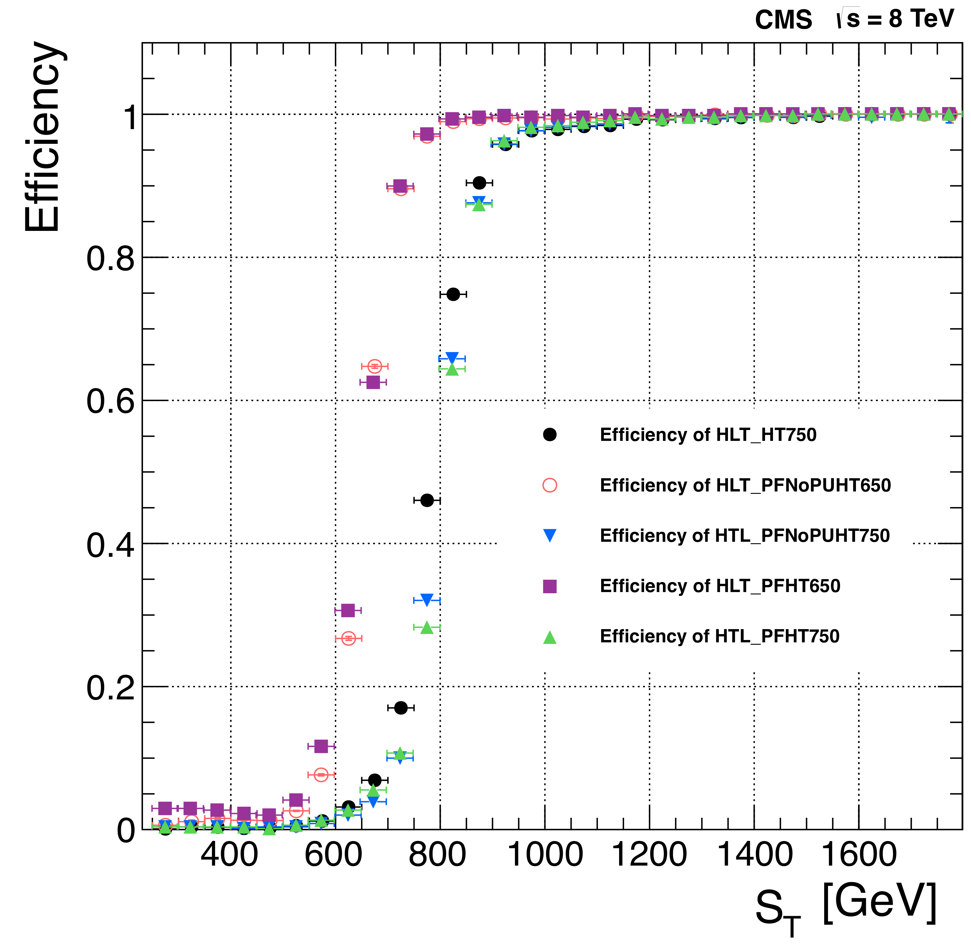
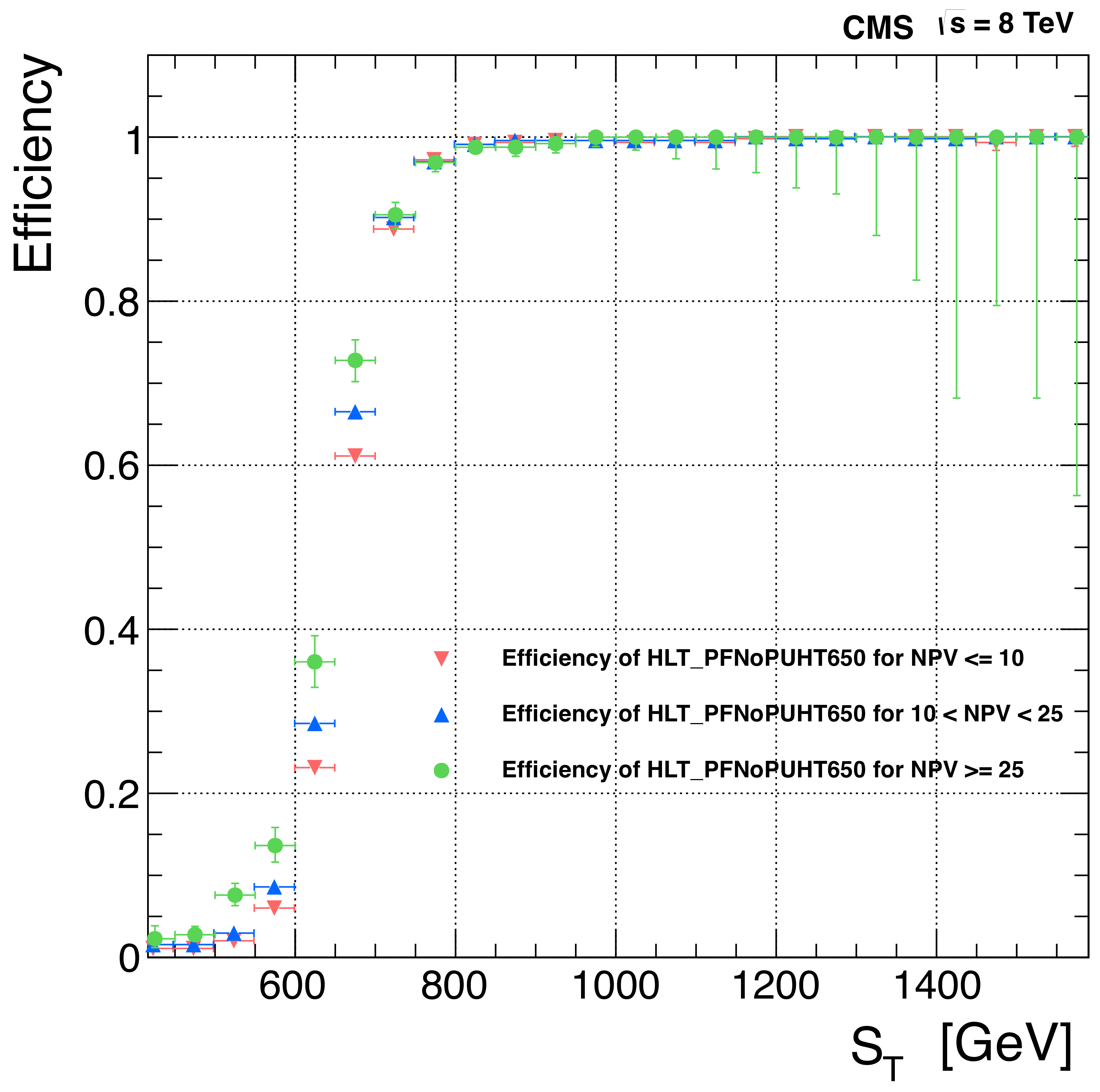
Figure 67:
Left: Efficiency of unscaled total jet activity HLT paths as a function of $ {S_\mathrm {T}} $. Right: Efficiency of HLT-PFNoPUHT650 as a function of $ {S_\mathrm {T}} $ in three bins of number of primary vertices, $N_\mathrm {PV}$: (i) $N_\mathrm {PV} \le 10$, (ii) 10 $ < N_\mathrm {PV} < $ 25, and (iii) $N_\mathrm {PV} \ge $ 25. All efficiencies are calculated with respect to a prescaled total activity path with $ {H_{\mathrm {T}}} = $ 450 GeV threshold. |
png pdf |
Figure 67-a:
Efficiency of unscaled total jet activity HLT paths as a function of $ {S_\mathrm {T}} $. All efficiencies are calculated with respect to a prescaled total activity path with $ {H_{\mathrm {T}}} = $ 450 GeV threshold. |
png pdf |
Figure 67-b:
Efficiency of HLT-PFNoPUHT650 as a function of $ {S_\mathrm {T}} $ in three bins of number of primary vertices, $N_\mathrm {PV}$: (i) $N_\mathrm {PV} \le 10$, (ii) 10 $ < N_\mathrm {PV} < $ 25, and (iii) $N_\mathrm {PV} \ge $ 25. All efficiencies are calculated with respect to a prescaled total activity path with $ {H_{\mathrm {T}}} = $ 450 GeV threshold. |
png pdf |
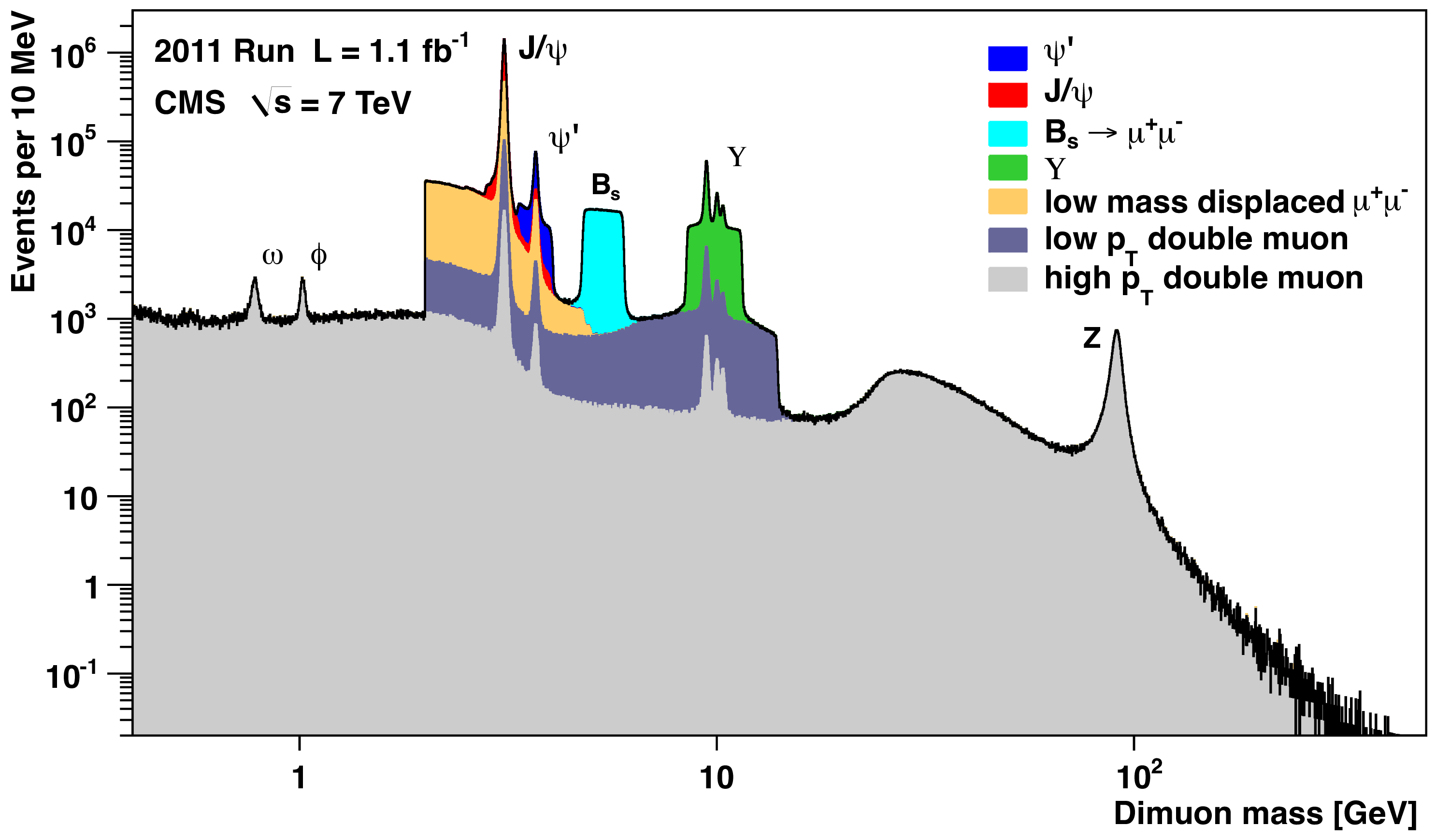
Figure 68:
Dimuon mass distributions collected with the inclusive double-muon trigger used during early data taking in 2011. The colored areas correspond to triggers requiring dimuons in specific mass windows, while the dark gray area represents a trigger only operated during the first 0.2 fb$^{-1}$ of the 2011 run. |

png pdf |
Figure 69:
Single-muon detection efficiencies (convolving trigger, reconstruction, and selection requirements) as a function of $ {p_{\mathrm {T}}} $, as obtained from the data, using the tag-and-probe method. Data points are shown for the pseudorapidity range $ {| \eta | } < $ 0.2, while the curves (depicting a parametrization of the measured efficiencies) correspond to the three ranges indicated in the legend. |
png pdf |
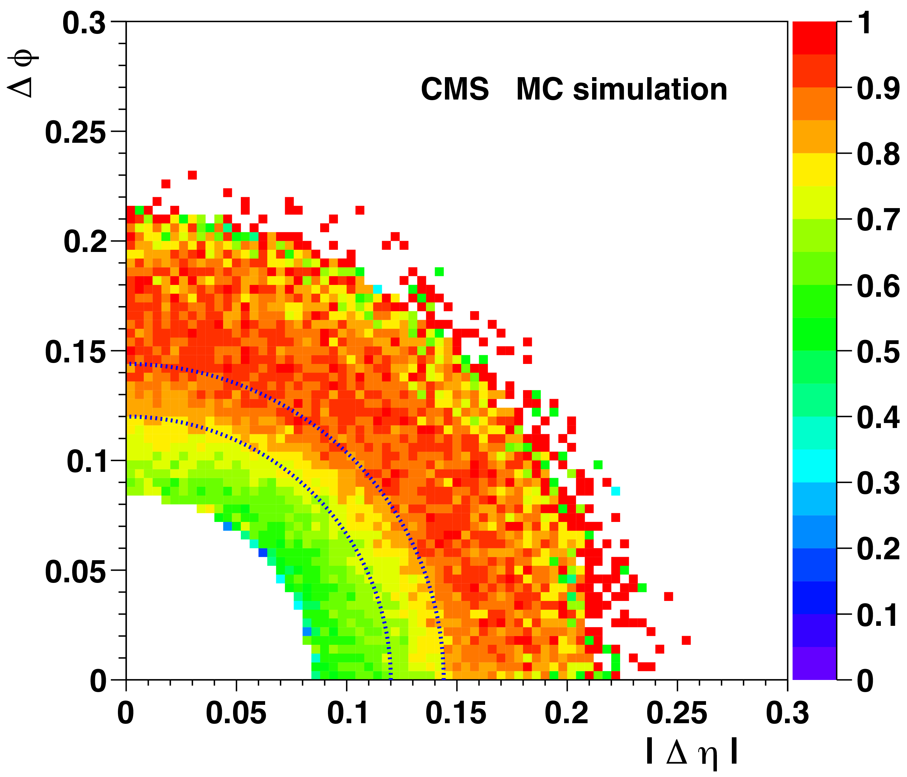
Figure 70:
Dimuon trigger efficiencies in the $\Delta \phi $ versus $\Delta \eta $ plane for $ \mathrm{J}/\psi $ events generated in the kinematic region $ {p_{\mathrm {T}}} > $ 50 GeV and $ {| y | }< $ 1.2, illustrating the efficiency drop when the two muons are too close to each other. |

png pdf |
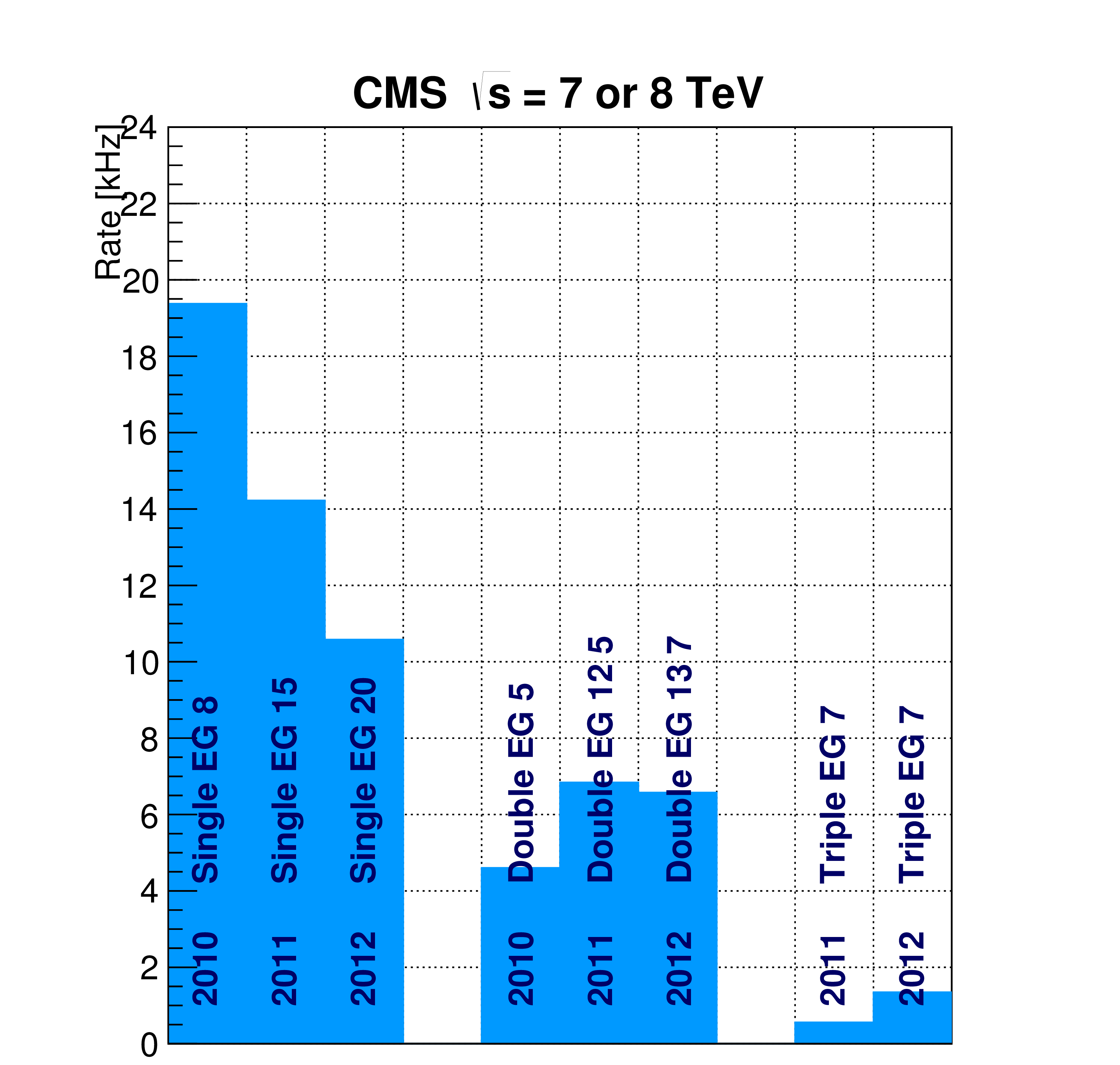
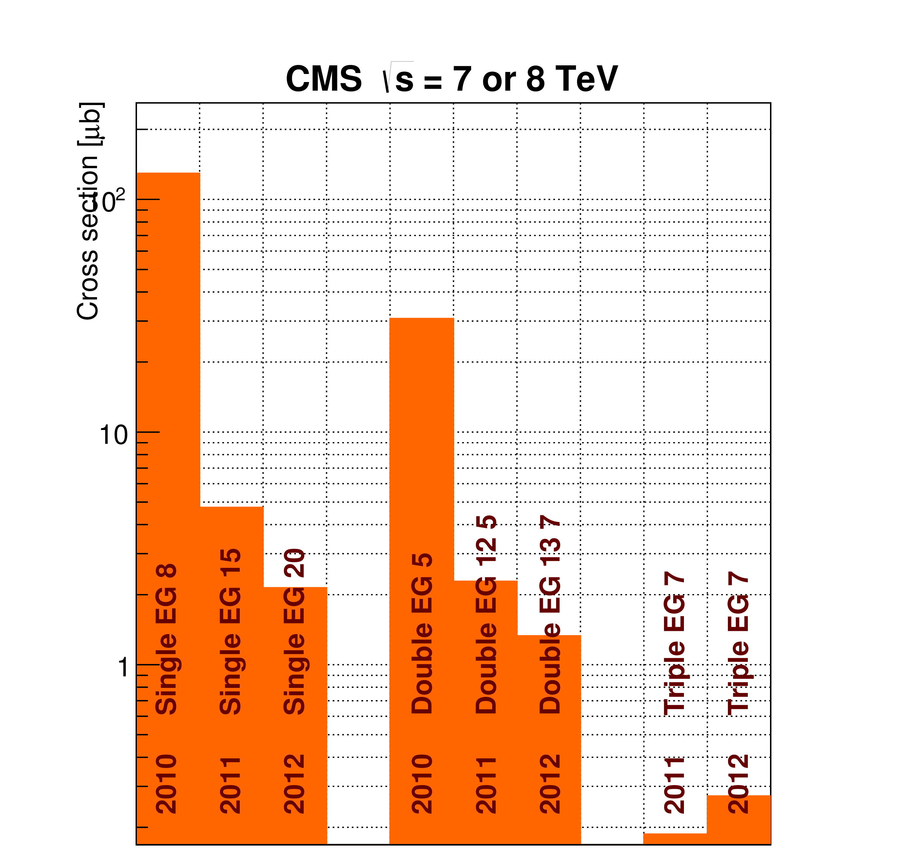
Figure 71:
Rates (left) and cross sections (right) for a significant sample of L1 $\mathrm{ e } /\gamma $ triggers from 2010, 2011, and 2012 sample menus. |
png pdf |
Figure 71-a:
Rates for a significant sample of L1 $\mathrm{ e } /\gamma $ triggers from 2010, 2011, and 2012 sample menus. |
png pdf |
Figure 71-b:
Cross sections for a significant sample of L1 $\mathrm{ e } /\gamma $ triggers from 2010, 2011, and 2012 sample menus. |
png pdf |
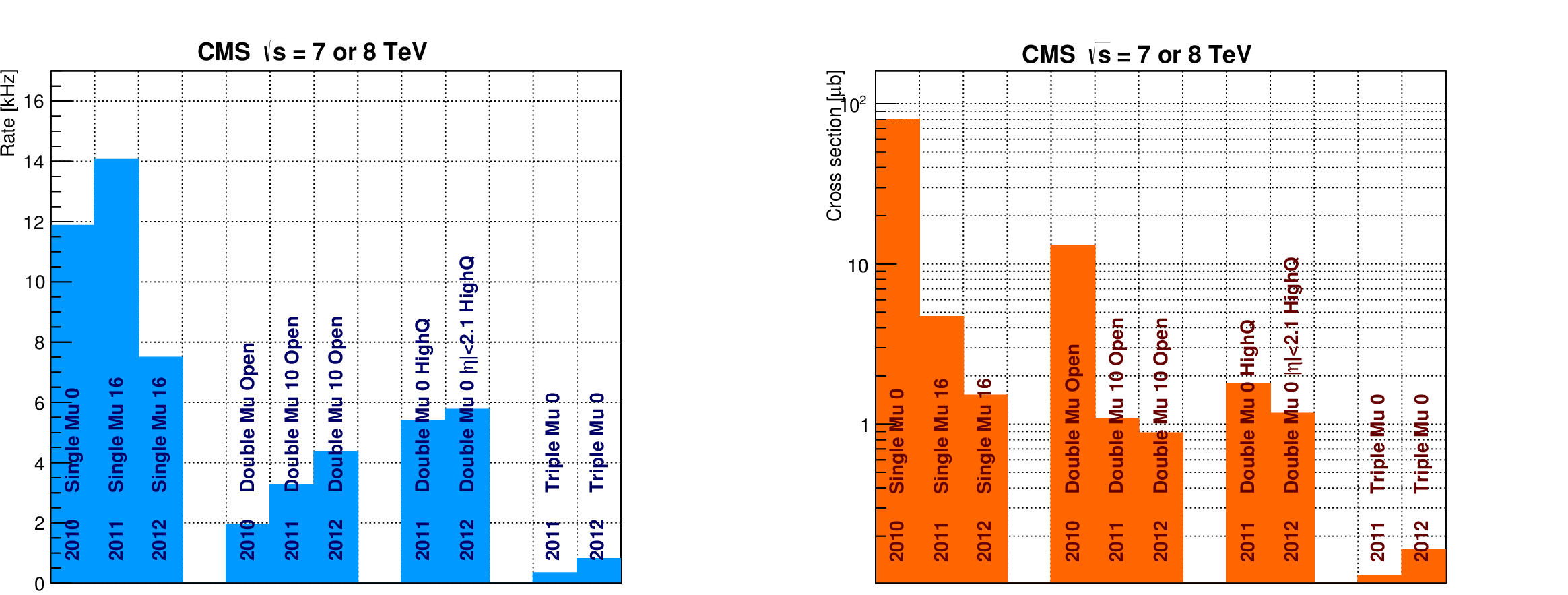
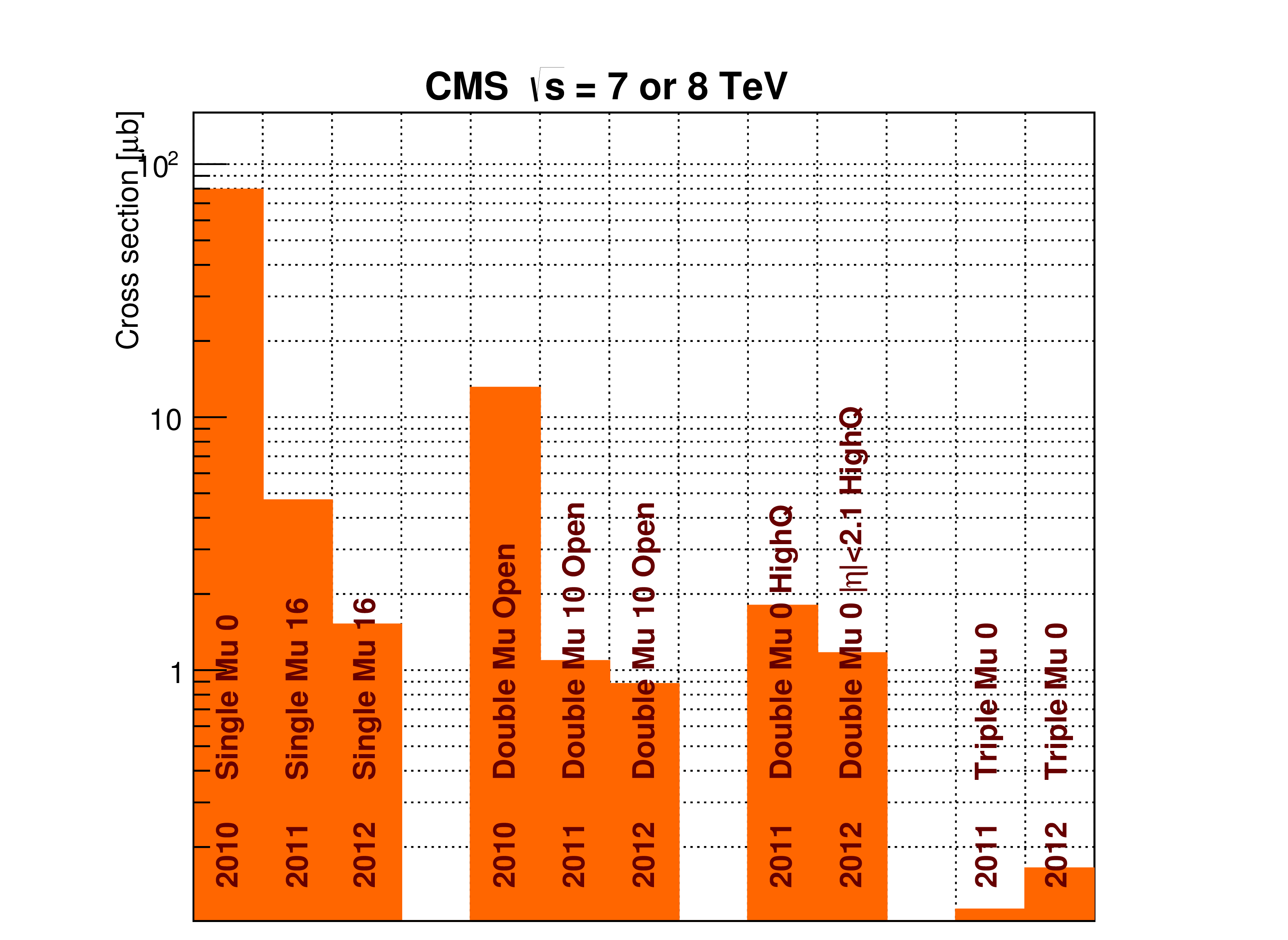
Figure 72:
Rates (left) and cross sections (right) for a significant sample of L1 muon triggers from 2010, 2011, and 2012 sample menus. |

png pdf |
Figure 72-a:
Rates for a significant sample of L1 muon triggers from 2010, 2011, and 2012 sample menus. |
png pdf |
Figure 72-b:
Cross sections for a significant sample of L1 muon triggers from 2010, 2011, and 2012 sample menus. |

png pdf |
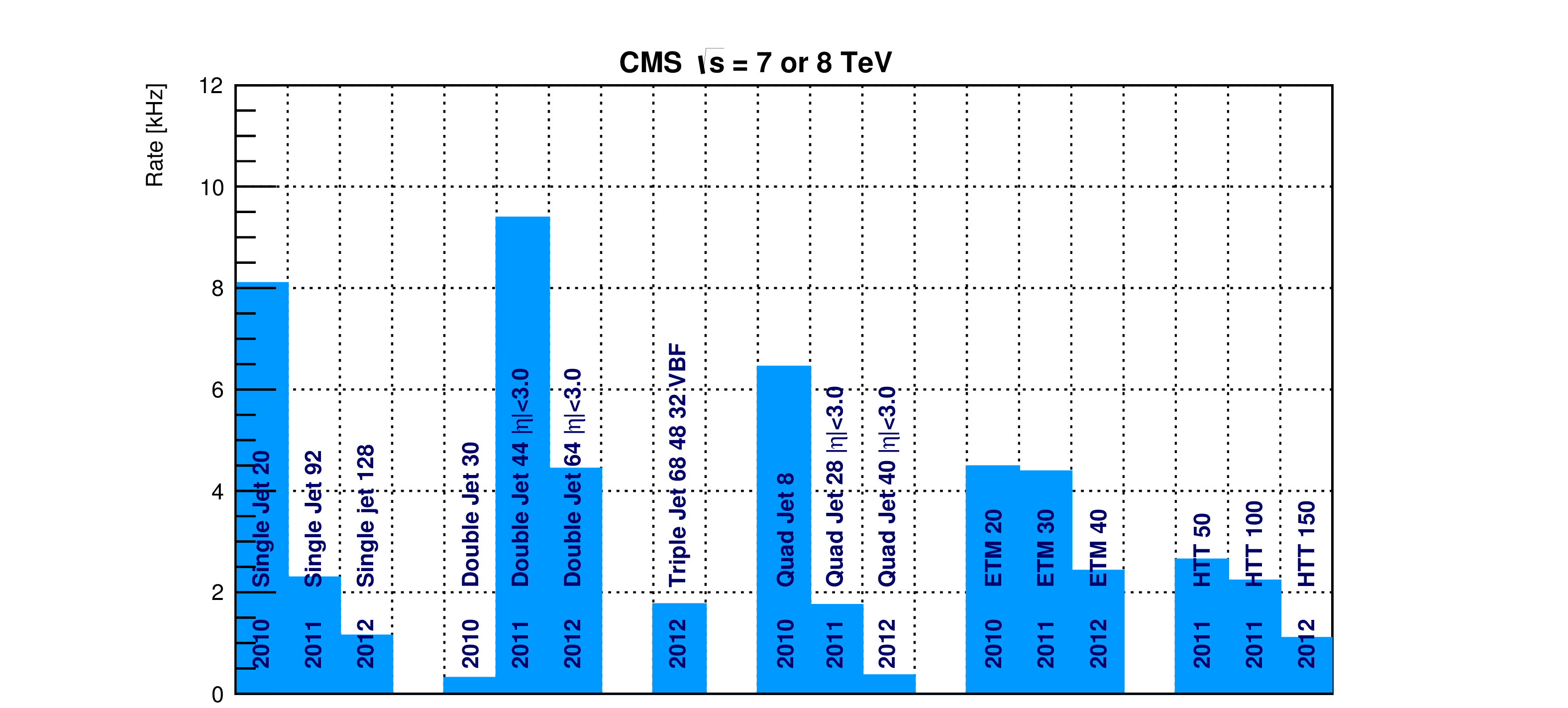
Figure 73:
Rates (top) and cross sections (bottom) for a significant sample of L1 jet triggers from 2010, 2011, and 2012 sample menus. |
png pdf |
Figure 73-a:
Rates for a significant sample of L1 jet triggers from 2010, 2011, and 2012 sample menus. |

png pdf |
Figure 73-b:
Cross sections for a significant sample of L1 jet triggers from 2010, 2011, and 2012 sample menus. |
png pdf |
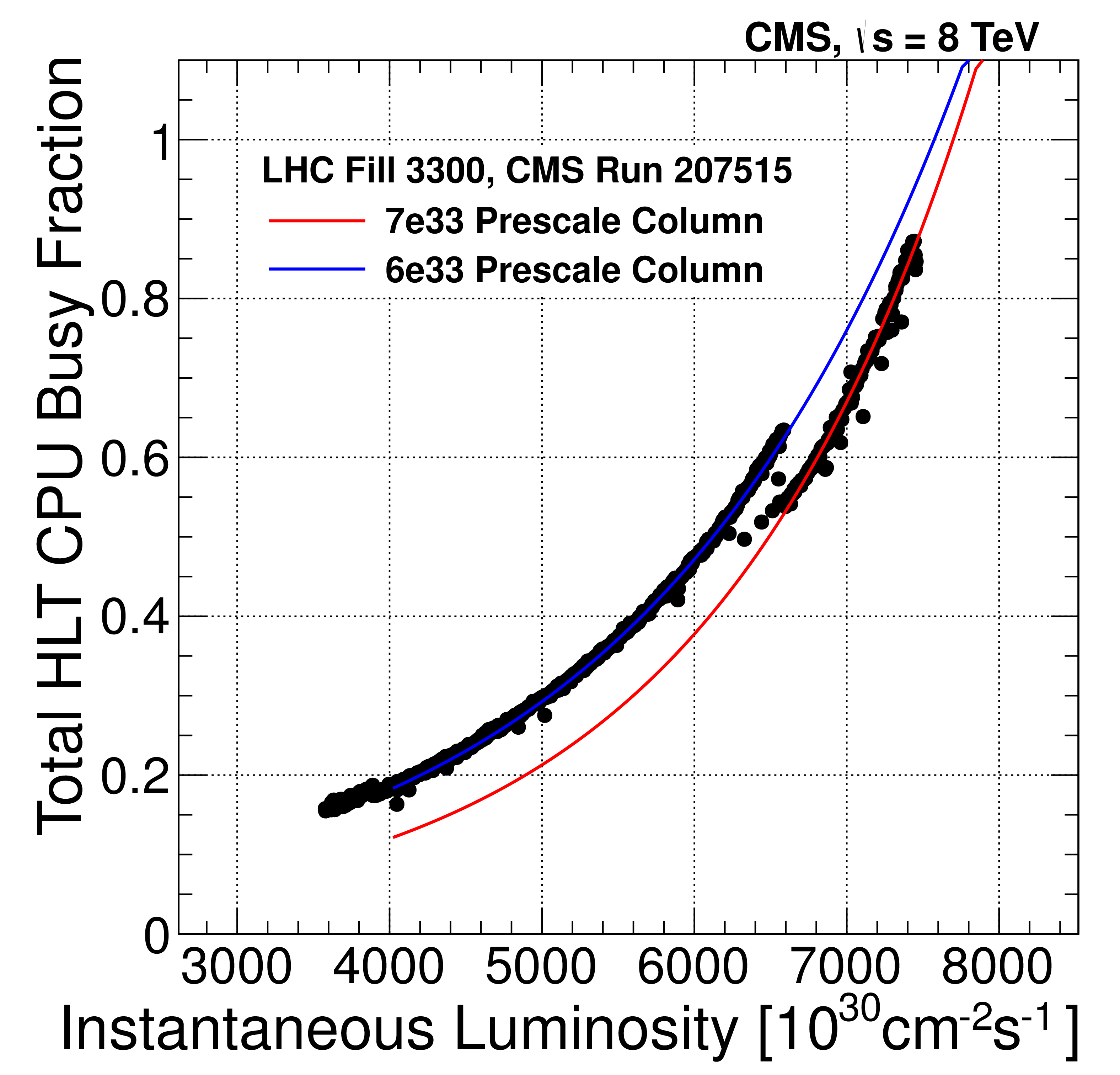
Figure 74:
The average CPU busy fraction as a function of instantaneous luminosity for one LHC fill. Luminosity sections with data-taking deadtime $>$40% are removed. |
png pdf |
Figure 75:
The HLT processing time per event as a function of instantaneous luminosity for the three different machine types used in the filter farm. |

png pdf |
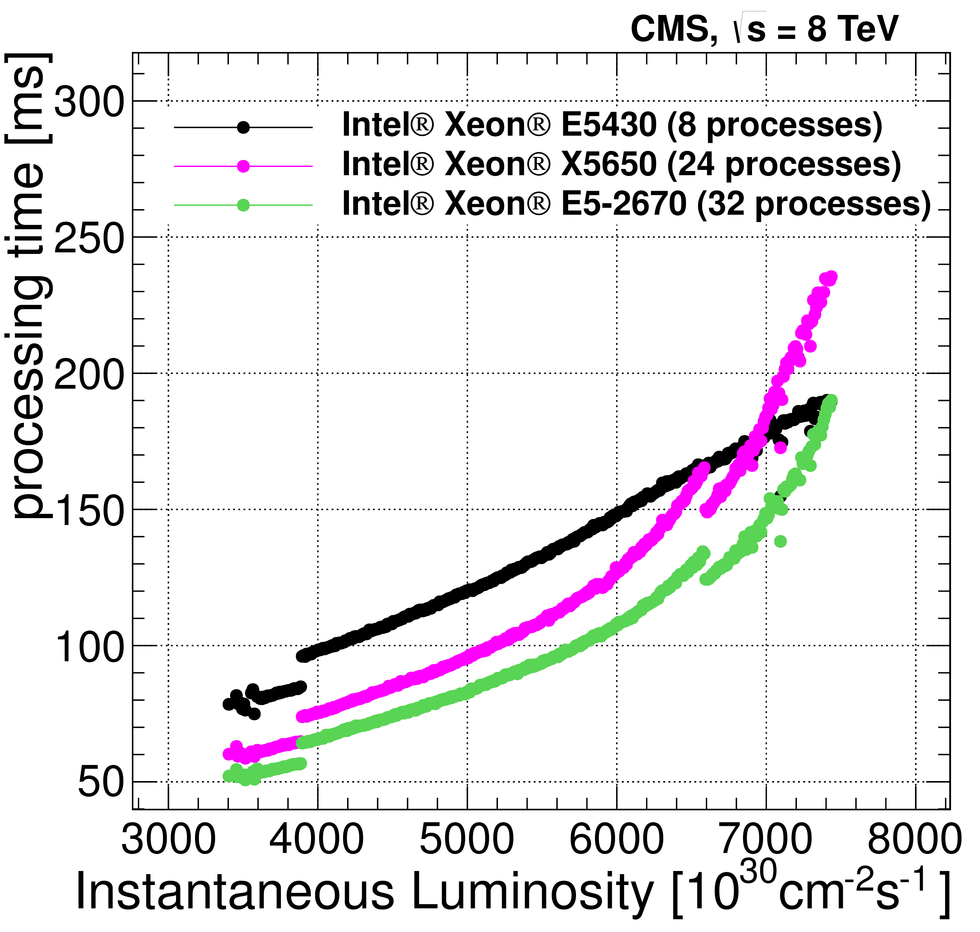
Figure 76:
Comparison of the time per event measured for two different HLT menus using a validation machine outside of the event filter farm. |
| Tables | |

png pdf |
Table 1:
The L1 electron trigger turn-on curve parameters. This table gives the electron $ {E_{\mathrm {T}}} $ thresholds for which an efficiency of 50%, 95% and 99% are reached for EB and EE separately. The last entry corresponds to the efficiency obtained at the plateau of each curve shown in Figure 11. |

png pdf |
Table 2:
The EE L1 electron trigger turn-on curve parameters. This table gives the electron $ {E_{\mathrm {T}}} $ thresholds for which an efficiency of 50%, 95% and 99% are reached before and after transparency corrections are applied. The last entry corresponds to the efficiency obtained at the plateau of each curve shown in Figure 12. |

png pdf |
Table 3:
Turn-on points for the EG12, EG15, EG20, and EG30 L1 trigger algorithms shown in Fig. 13. |

png pdf |
Table 4:
Rate reduction factors obtained for L1 EG algorithms (considering a 258 MeV sFGVB threshold and an 8 GeV killing threshold on the ECAL Trigger Primitives) for various EG thresholds. |

png pdf |
Table 5:
Single-jet triggers used for $ {\mathcal {L}} = $ 7$\times $10$^{33}$ cm$^{-2}$s$^{-1}$ (pileup ${\approx }$32), their prescales, and trigger rates at that instantaneous luminosity. |
png pdf |
Table 6:
Dijet-triggers used at $ {\mathcal {L}} =$ 7$\times $10$^{33}$ cm$^{-2}$s$^{-1}$ (pileup ${\approx }$ 32), their prescales, and trigger rates. The main purpose of these triggers is the $\eta $-dependent calibration of the calorimeter. |
png pdf |
Table 7:
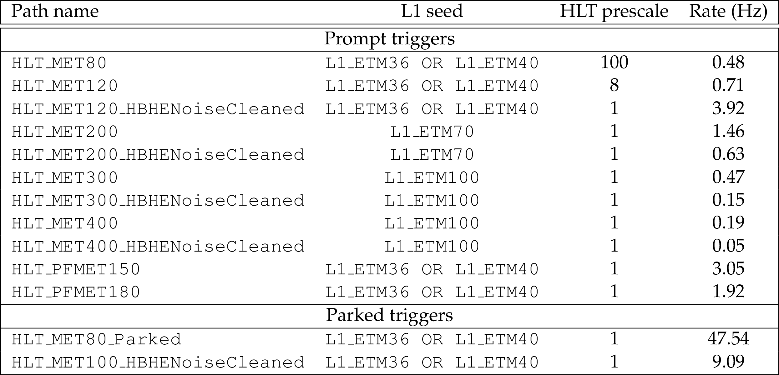
The $ {E_{\mathrm {T}}^{\text {miss}}} $ triggers used for $ {\mathcal {L}} =$ 7$\times $10$^{33}$ cm$^{-2}$s$^{-1}$ (pileup ${\approx }$32), their prescales, and rates at that luminosity. Note that the L1 $ {E_{\mathrm {T}}^{\text {miss}}} > $ 36 GeV trigger (L1-ETM36) was highly prescaled starting at this luminosity and hence the need to use an OR with the L1 $ {E_{\mathrm {T}}^{\text {miss}}} > $ 40 GeV trigger (L1-ETM40). The parked HLT $ {E_{\mathrm {T}}^{\text {miss}}} > $ 80 GeV trigger (HLT-MET80-Parked) was also anticipated to be highly prescaled starting from $ {\mathcal {L}} = $ 8$\times $10$^{33}$ cm$^{-2}$s$^{-1}$. The $ {E_{\mathrm {T}}^{\text {miss}}} $ parking triggers were available at the end of 2012. ``Cleaned'' refers to application of dedicated algorithms to remove noise events. |
png pdf |
Table 8:
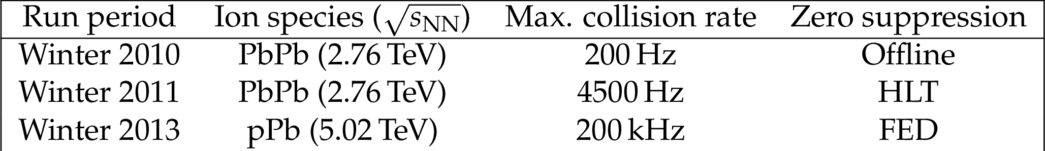
Summary of the heavy ion running conditions in various data-taking periods. |

png pdf |
Table 9:
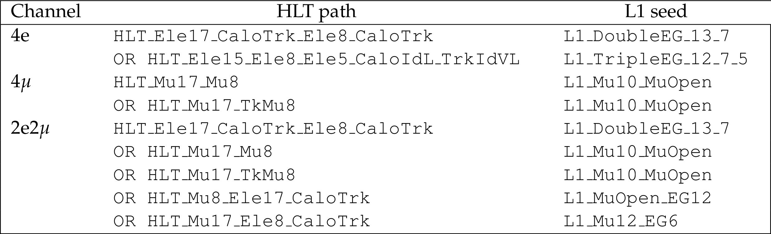
Triggers used in the $\mathrm{ H } \to 4\ell $ event selection (2012 data and simulation). No prescaling is applied to these triggers. |
png pdf |
Table 10:
Triggers used for tag-and-probe (T&P) efficiency measurements of four-lepton events in 2012 data and simulation: CaloTrk = CaloIdT-CaloIsoVL-TrkIdVL-TrkIsoVL, CaloTrkVT = CaloIdVT-CaloIsoVT-TrkIdT-TrkIsoVT |

png pdf |
Table 11:
List of L1 and HLT used for 2012 data for the ${\mathrm{ Z } } (\nu \bar{\nu} )\mathrm{ H } ( {\mathrm{ b \bar{b} } } )$ channel. We use PF $ {E_{\mathrm {T}}^{\text {miss}}} $. All triggers are combined to maximize acceptance. In all cases, an OR of the L1 $ {E_{\mathrm {T}}^{\text {miss}}} > $ 36 GeV and $ {E_{\mathrm {T}}^{\text {miss}}} > $ 40 GeV are used as the L1 seed. |
png pdf |
Table 12:
Unscaled cross-triggers used for the $ {\mathrm{ t } \mathrm{ \bar{t} } } $ (lepton plus jets) cross section measurement in 2012. All leptons use tight or very tight identification, and lepton and calorimeter isolation requirements. All jets are PF jets and restricted to the central region. At L1, single electrons or muons are required with the denoted thresholds and the L1 muons are required to be central ($ {| \eta | }< $ 2.1). When two thresholds are listed at L1, they include a lower (possibly prescaled) threshold and a higher unscaled threshold. |
png pdf |
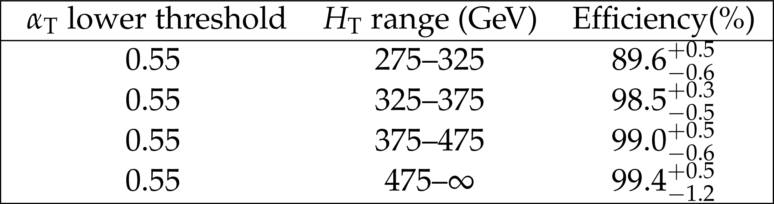
Table 13:
Measured efficiencies of the $ {H_{\mathrm {T}}} $ and $ {H_{\mathrm {T}}} $-$ {\alpha _\mathrm {T}} $ triggers, as a function of $ {\alpha _\mathrm {T}} $ and $ {H_{\mathrm {T}}} $, as measured with respect to the offline selection used in the $\alpha _\mathrm {T}$ analysis. |
png pdf |
Table 14:
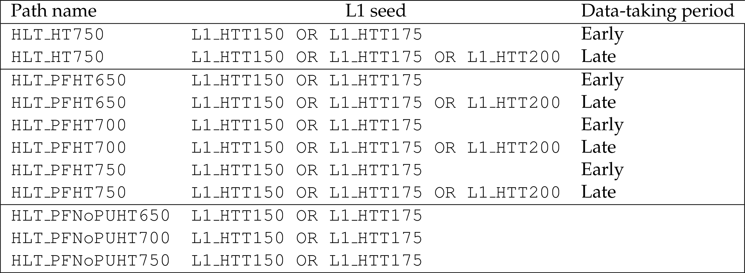
Black Hole trigger: Unprescaled total jet activity HLT paths and their respective L1 seeds. The L1 seeds for a number of the HLT paths were revised during the data taking to account for higher instantaneous luminosity. |

png pdf |
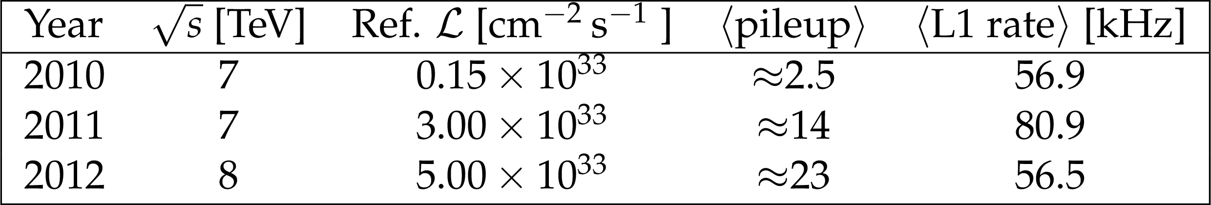
Table 15:
Machine operational conditions, target instantaneous luminosity used for rate estimation, and approximate overall L1 rate for three sample L1 menus, representative of the end of the year data-taking conditions for 2010, 2011, and 2012. |
| Summary |
| The CMS trigger system consists of two levels: an L1 custom hardware trigger, and an HLT system with custom c++ software routines running on commodity CPUs. The L1 trigger takes input from the calorimeters and the muon system to select the events of physics interest. To do this, it uses identified leptons, photons, and jet candidates, as well as event-level information such as missing transverse energy. Trigger primitives are generated on the front-ends of the subdetectors and then processed in several steps before a final decision is rendered in the global trigger. The L1 calorimeter trigger comprises two stages, a regional calorimeter trigger (RCT) and a global calorimeter trigger (GCT). The RCT processes the regional information in parallel and sends as output $\mathrm{ e }/\gamma$ candidates and regional $ E_{\mathrm{T}} $ sums. The GCT sorts the $\mathrm{ e }/\gamma$ candidates further, finds jets (classified as central, forward, and tau) using the $ E_{\mathrm{T}} $ sums, and calculates global quantities such as $ E_{\mathrm{T}}^{\text{miss}} $. Each of the three muon detector systems in CMS participates in the L1 muon trigger to ensure good coverage and redundancy. For the DT and CSC systems, the front-end trigger electronics identifies track segments from the hit information registered in multiple detector planes. Track finders apply pattern recognition algorithms which identify muon candidates, and measure their momenta from the amount of their bending in the magnetic field of the return yoke between measurement locations. The RPC hits are directly sent from the front-end electronics to pattern-comparator logic boards which identify muon candidates. The global muon trigger merges muon candidates, applies quality criteria, and sends the muon candidates to the global trigger. The global trigger implements the menu of selection requirements applied to all objects. A maximum of 128 separate selections can be implemented simultaneously. Overall, the L1 decision is rendered within 4 $\mu$s after the collision. At most 100 kHz of events are sent to the HLT for processing. The HLT is implemented in software, and further refines the purity of the physics objects. Events are selected for offline storage at an average rate of 400 Hz. The HLT event selection is performed in a similar way to that used in the offline processing. For each event, objects such as leptons, photons, and jets are reconstructed and identification criteria are applied in order to select only those events which are of possible interest for data analysis. The HLT hardware consists of a processor farm using commodity PCs running Scientific Linux. The subunits are called builder and filter units. In the builder units, event fragments are assembled to complete events. Filter units then unpack the raw data and perform event reconstruction and trigger filtering. Both the L1 triggers and HLT include prescaling of events passing defined selection criteria. The performance of the CMS trigger system has been evaluated in two stages. First, the performance of the L1 and HLT systems has been evaluated for individual trigger objects such as electrons, muons, photons, or jets, using tag-and-probe techniques. Most of the measurements considered come from the 2012 CMS data set, where data have been collected at $\sqrt{s} =$ 8 TeV. Performance has been evaluated in terms of efficiency with respect to offline quantities and to the appropriate trigger rate. Both L1 and HLT performance have been studied, showing the high selection efficiency of the CMS trigger system. Second, the performance of the trigger system has been demonstrated by considering key examples across different physics analyses. In CMS, the HLT decisions often are derived from complex correlated combinations of single objects such as electrons, muons, or $\tau$ leptons. The broad range of capabilities of the trigger system has been shown through examples in Higgs boson, top-quark, and B physics, as well as in searches for new physics. The trigger system has been instrumental in the successful collection of data for physics analyses in Run 1 of the CMS experiment at the LHC. Efficiencies were measured in data and compared to simulation, and shown to be high and well-understood. Many physics signals were collected with high efficiency and flexibility under rapidly-changing conditions, enabling a diverse and rich physics program, which has led to hundreds of publications based on the Run 1 data samples. |
| References | ||||
| 1 | CMS Collaboration | The CMS experiment at the CERN LHC | JINST 3 (2008) S08004 | CMS-00-001 |
| 2 | L. Evans and P. Bryant | LHC Machine | JINST 3 (2008) S08001 | |
| 3 | CMS Collaboration | CMS The TRIDAS Project, Technical Design Report Vol. 2: Data Acquisition and High-Level Trigger | CDS | |
| 4 | ATLAS Collaboration | Performance of the ATLAS Trigger System in 2010 | EPJC 72 (2012) 1849 | |
| 5 | CMS Collaboration | CMS The TRIDAS Project, Technical Design Report Vol. 1: The Trigger Systems | CDS | |
| 6 | M. Anfreville et al. | Laser monitoring system for the CMS lead tungstate crystal calorimeter | NIMA 594 (2008) 292 | |
| 7 | CMS Collaboration | Energy calibration and resolution of the CMS electromagnetic calorimeter in pp collisions at $ \sqrt{s} $ = 7 TeV | JINST 8 (2013) P09009 | CMS-EGM-11-001 1306.2016 |
| 8 | P. Klabbers et al. | Integration of the CMS Regional Calorimeter Trigger Hardware into the CMS Level-1 Trigger | in Topical Workshop on Electronics for Particle Physics (TWEPP 2007), p. 241 | |
| 9 | P. Klabbers et al. | Operation and Monitoring of the CMS Regional Calorimeter Trigger Hardware | in Topical Workshop on Electronics for Particle Physics (TWEPP 2008), p. 133 | |
| 10 | P. Klabbers et al. | Performance of the CMS Regional Calorimeter Trigger | in Topical Workshop on Electronics for Particle Physics (TWEPP 2009), p. 191 | |
| 11 | W. H. Smith et al. | CMS Regional Calorimeter Trigger High Speed ASICs | in Proceedings of the Sixth Workshop on Electronics for LHC Experiments CERN | |
| 12 | M. Stettler et al. | The CMS Global Calorimeter Trigger Hardware Design | in Proceedings for the 12th Workshop on Electronics for LHC and Future Experiments CERN | |
| 13 | G. Iles et al. | Revised CMS Global Calorimeter Trigger Functionality $ \& $ Algorithms | in Proceedings for the 12th Workshop on Electronics for LHC and Future Experiments, p. 465 2006 | |
| 14 | C. Foudas et al. | First Results on the Performance of the CMS Global Calorimeter Trigger | in Topical Workshop on Electronics for Particle Physics (TWEPP 2007), p. 246 2007 | |
| 15 | G. Iles et al. | Performance and lessons of the CMS Global Calorimeter Trigger | in Topical Workshop on Electronics for Particle Physics (TWEPP 2008), p. 129 2008 | |
| 16 | A. Tapper et al. | Commissioning and Performance of the CMS Global Calorimeter Trigger | in Conference Record, IEEE Nuclear Science Symposium, p. 1871 IEEE | |
| 17 | J. Brooke et al. | Performance of the CMS Global Calorimeter Trigger | in Proceedings for the 1st International Conference on Technology and Instrumentation in Particle Physics, p. 546 2010 | |
| 18 | J. J. Brooke et al. | The design of a flexible Global Calorimeter Trigger system for the Compact Muon Solenoid experiment | JINST 2 (2007) P10002 | |
| 19 | M. De Giorgi et al. | Test results of the ASIC front end trigger prototypes for the muon barrel detector of CMS at LHC | NIMA 438 (1999) 302 | |
| 20 | CMS Collaboration | Design of the Track Correlator for the DTBX Trigger | CDS | |
| 21 | CMS Collaboration | Antifuse-FPGAs for the Track-Sorter-Master of the CMS Muon Barrel Drift Tubes: Design Issues and Irradiation Test | CDS | |
| 22 | P. Arce et al. | Bunched beam test of the CMS drift tubes local muon trigger | NIMA 534 (2004) 441 | |
| 23 | M. Aldaya et al. | Fine synchronization of the muon drift tubes local trigger | NIMA 564 (2006) 169 | |
| 24 | CMS Collaboration | Fine synchronization of the CMS muon drift-tube local trigger using cosmic rays | JINST 5 (2009) T03004 | |
| 25 | L. Guiducci et al. | DT sector collector electronics design and construction | in Topical Workshop on Electronics for Particle Physics (TWEPP 2007), p. 85 2007 | |
| 26 | CMS Collaboration | The performance of the CMS muon detector in proton-proton collisions at $ \sqrt{s} = $ 7 TeV at the LHC | JINST 8 (2013) P11002 | CMS-MUO-11-001 1306.6905 |
| 27 | J. Ero et al. | The CMS drift tube trigger track finder | JINST 3 (2008) P08006 | |
| 28 | L. Guiducci et al. | Design and test of the off-detector electronics for the CMS barrel muon trigger | in Proceedings for the 12th Workshop on Electronics for LHC and Future Experiments, p. 289 2006 | |
| 29 | D. Acosta et al. | Development and test of a prototype regional track-finder for the Level-1 trigger of the cathode strip chamber muon system of CMS | NIMA 496 (2003) 64 | |
| 30 | CMS Collaboration | Performance of CMS muon reconstruction in pp collision events at $ \sqrt{s} = 7 $$ TeV $ | JINST 7 (2012) P10002 | |
| 31 | M. Andlinger et al. | Pattern Comparator Trigger (PACT) for the muon system of the CMS experiment | NIMA 370 (1996) 389 | |
| 32 | K. Banzuzi et al. | Link System and Crate Layout of the RPC Pattern Comparator Trigger for the CMS detector | CMS IN 2002/065 | |
| 33 | H. Sakulin and A. Taurok | The Level-1 Global Muon Trigger for the CMS Experiment | in Proceedings for the 9th Workshop on Electronics for LHC Experiments, p. 245 Amsterdam | |
| 34 | M. Jeitler et al. | The Level-1 global trigger for the CMS experiment at LHC | JINST 2 (2007) P01006 | |
| 35 | A. Taurok et al. | The Central Trigger Control System of the CMS Experiment at CERN | CMS-NOTE-2010-017 | |
| 36 | J. Varela | CMS L1 Trigger Control System | CMS-NOTE-2002-033 | |
| 37 | TOTEM Collaboration | The TOTEM Experiment at the CERN Large Hadron Collider | JINST 3 (2008) S08007 | |
| 38 | G. Bauer et al. | Recent experience and future evolution of the CMS High Level Trigger System | in Real Time Conference (RT), 2012 18th IEEE-NPSS, p. 1 2012 | |
| 39 | CMS Collaboration | Commissioning of the CMS High-Level Trigger with cosmic rays | JINST 5 (2010) T03005 | |
| 40 | CMS Collaboration | The CMS high level trigger | EPJC 46 (2006) 605 | |
| 41 | CMS Collaboration | Data Parking and Data Scouting at the CMS Experiment | CDS | |
| 42 | CMS Collaboration | Particle-Flow Event Reconstruction in CMS and Performance for Jets, Taus, and $ E_{\rm T}^{\rm miss} $ | ||
| 43 | CMS Collaboration | Commissioning of the Particle FLow Event Reconstruction With the First LHC Collisions Recorded in the CMS Detector | ||
| 44 | CMS Collaboration | Description and performance of track and primary-vertex reconstruction with the CMS tracker | JINST 9 (2014) P10009 | CMS-TRK-11-001 1405.6569 |
| 45 | R. Fruehwirth | Application of Kalman filtering to track and vertex fitting | NIMA 262 (1987) 444 | |
| 46 | CMS Collaboration | Electron reconstruction and identification at $ \sqrt{s} $ = 7 TeV | ||
| 47 | CMS Collaboration | Performance of electron reconstruction and selection with the CMS detector in proton-proton collisions at $ \sqrt{s} = 8 $$ TeV $ | JINST 10 (2015) P06005 | |
| 48 | M. J. Oreglia | A study of the reactions $\psi' \to \gamma\gamma \psi$ | PhD thesis, Stanford University, 1980 SLAC Report SLAC-R-236, see Appendix D | |
| 49 | CMS Collaboration | Measurement of the inclusive W and Z production cross sections in pp collisions at $ \sqrt{s} = $ 7 TeV with the CMS experiment | JHEP 10 (2011) 132 | |
| 50 | W. Bialasa and D. A. Petyt | Mitigation of anomalous APD signals in the CMS ECAL | JINST 8 (2013) C03020 | |
| 51 | CMS Collaboration | Anomalous APD signals in the CMS Electromagnetic Calorimeter | NIMA 695 (2012) 293 | |
| 52 | CMS Collaboration | Measurement of the $ {B}_{s}^{0} {\rightarrow}{ {\mu}}^{\mathbf{+}}{ {\mu}}^{\mathbf{-}} $ Branching Fraction and Search for $ {B}^{0} {\rightarrow}{ {\mu}}^{\mathbf{+}}{ {\mu}}^{\mathbf{-}} $ with the CMS Experiment | PRL 111 (2013) 101804 | CMS-BPH-13-004 1307.5025 |
| 53 | CMS Collaboration and LHCb Collaboration | Observation of the rare $ B^0_s\to\mu^+\mu^- $ decay from the combined analysis of CMS and LHCb data | Nature 522 (2015) 68 | 1411.4413 |
| 54 | M. Cacciari, G. P. Salam, and G. Soyez | FastJet user manual | EPJC 72 (2012) 1896 | 1111.6097 |
| 55 | CMS Collaboration | Determination of jet energy calibration and transverse momentum resolution in CMS | JINST 6 (2011) P11002 | |
| 56 | M. Cacciari, G. P. Salam, and G. Soyez | The anti-$ k_t $ jet clustering algorithm | JHEP 04 (2008) 063 | 0802.1189 |
| 57 | CMS Collaboration | Calorimeter Jet Quality Criteria for the First CMS Collision Data | CDS | |
| 58 | CMS Collaboration | Evidence for the 125$ GeV $ Higgs boson decaying to a pair of $ \tau $ leptons | JHEP 05 (2014) 104 | |
| 59 | CMS Collaboration | Performance of tau-lepton reconstruction and identification in CMS | JINST 7 (2012) P01001 | CMS-TAU-11-001 1109.6034 |
| 60 | CMS Collaboration | Identification of b-quark jets with the CMS experiment | JINST 8 (2013) P04013 | CMS-BTV-12-001 1211.4462 |
| 61 | I. P. Lokhtin and A. M. Snigirev | A model of jet quenching in ultrarelativistic heavy ion collisions and high-p$ _{T} $ hadron spectra at RHIC | EPJC 45 (2006) 211 | hep-ph/0506189 |
| 62 | O. Kodolova, I. Vardanian, A. Nikitenko, and A. Oulianov | The performance of the jet identification and reconstruction in heavy ions collisions with CMS detector | EPJC 50 (2007) 117 | |
| 63 | CMS Collaboration | Observation of a new boson at a mass of 125 GeV with the CMS experiment at the LHC | PLB 716 (2012) 30 | CMS-HIG-12-028 1207.7235 |
| 64 | CMS Collaboration | Observation of a new boson with mass near 125 GeV in pp collisions at $ \sqrt{s} $ = 7 and 8 TeV | JHEP 06 (2013) 081 | CMS-HIG-12-036 1303.4571 |
| 65 | CMS Collaboration | Measurement of the properties of a Higgs boson in the four-lepton final state | PRD 89 (2014) 092007 | CMS-HIG-13-002 1312.5353 |
| 66 | CMS Collaboration | Search for the standard model Higgs boson decaying to bottom quarks in $ pp $ collisions at $ \sqrt{s}=7 $~TeV | PLB 710 (2012) 284 | |
| 67 | CMS Collaboration | Measurement of the production cross section in pp collisions at with lepton plus jets final states | PLB 720 (2013) 83 | |
| 68 | CMS Collaboration | Measurement of the $ \mathrm{ t \bar{t} } $ production cross section in the dilepton channel in pp collisions at $ \sqrt{s} = 8 $ TeV | JHEP 02 (2014) 024 | |
| 69 | CMS Collaboration | Pileup Removal Algorithms | CMS-PAS-JME-14-001 | CMS-PAS-JME-14-001 |
| 70 | J. Alwall, P. Schuster, and N. Toro | Simplified Models for a First Characterization of New Physics at the LHC | PRD 79 (2009) 075020 | |
| 71 | G. R. Farrar and P. Feyet | Phenomenology of the production, decay, and detection of new hadronic states associated with supersymmetry | PLB 76 (1978) 675 | |
| 72 | CMS Collaboration | Search for supersymmetry in hadronic final states with missing transverse energy using the variables $ \alpha_{\rm T} $ and b-quark multiplicity in pp collisions at 8 TeV | EPJC 73 (2013) 2568 | CMS-SUS-12-028 1303.2985 |
| 73 | CMS Collaboration | Inclusive search for squarks and gluinos in $ pp $ collisions at $ \sqrt{s}=7 $ TeV | PRD 85 (2012) 012004 | CMS-SUS-10-009 1107.1279 |
| 74 | CMS Collaboration | Inclusive search for supersymmetry using the Razor variables in $ pp $ collisions at $ \sqrt{s}=7 $ TeV | PRL 111 (2013) 081802 | CMS-SUS-11-024 1212.6961 |
| 75 | S. Dimopoulos and G. L. Landsberg | Black holes at the LHC | PRL 87 (2001) 161602 | hep-ph/0106295 |
| 76 | S. B. Giddings and S. D. Thomas | High-energy colliders as black hole factories: The end of short distance physics | PRD 65 (2002) 056010 | hep-ph/0106219 |
| 77 | S. Dimopoulos and R. Emparan | String balls at the LHC and beyond | PLB 526 (2002) 393 | hep-ph/0108060 |
| 78 | CMS Collaboration | Search for microscopic black holes in pp collisions at $ \sqrt{s} $ = 8~$ TeV $ | JHEP 07 (2013) 1 | CMS-EXO-12-009 1303.5338 |
| 79 | CMS Collaboration | Search for microscopic black hole signatures at the Large Hadron Collider | PLB 697 (2011) 434 | CMS-EXO-10-017 1012.3375 |
| 80 | CMS Collaboration | Search for microscopic black holes in pp collisions at $ \sqrt{s} $ = 7~$ TeV $ | JHEP 04 (2012) 061 | CMS-EXO-11-071 1202.6396 |
| 81 | D0 Collaboration | Evidence for an anomalous like-sign dimuon charge asymmetry | PRL 105 (2010) 081801 | 1007.0395 |
| 82 | L. Tuura, A. Meyer, I. Segoni, and G. Della Ricca | CMS data quality monitoring: systems and experiences | in Proceedings of the 17th International Conference on Computing in High Energy and Nuclear Physics (CHEP09), volume 219, p. 072020 2010 | |
|
|
Compact Muon Solenoid LHC, CERN |
|

|

|

|

|

|