

Compact Muon Solenoid
LHC, CERN
| CMS-PAS-HIG-16-038 | ||
| Search for $\mathrm{t\overline{t}H}$ production in the $\mathrm{H}\rightarrow \mathrm{b\overline{b}}$ decay channel with 2016 pp collision data at $\sqrt{s}= $ 13 TeV | ||
| CMS Collaboration | ||
| November 2016 | ||
| Abstract: The results of the search for the associated production of a Higgs boson with a top quark-antiquark pair ($\mathrm{t\overline{t}H}$) in proton-proton collisions at a center-of-mass energy of $\sqrt{s} = $ 13 TeV are presented. The data correspond to an integrated luminosity of up to 12.9 fb$^{-1}$ recorded with the CMS experiment in 2016. Candidate $\mathrm{t\overline{t}H}$ events are selected with criteria enhancing the lepton+jets or dilepton decay-channels of the $\mathrm{t\overline{t}}$ system and the decay of the Higgs boson into a bottom quark-antiquark pair ($\mathrm{H}\rightarrow \mathrm{b\overline{b}}$). In order to increase the sensitivity of the search, selected events are split into several categories with different expected signal and background rates. In each category signal and background events are separated using a multivariate approach that combines a matrix element method with boosted decision trees. The results are characterized by an observed $\mathrm{t\overline{t}H}$ signal strength relative to the standard model cross section, $\mu = \sigma/\sigma_{{\rm SM}}$, under the assumption of $m_{H} = $ 125 GeV. A combined fit of multivariate discriminant distributions in all categories results in an observed (expected) upper limit of $\mu < $ 1.5 (1.7) at the 95% confidence level, and a best fit value of $\mu = -0.19\,^{+0.45}_{-0.44}\,(\text{stat.})\,^{+0.66}_{-0.68}\,(\text{syst.})$. | ||
| Links: CDS record (PDF) ; inSPIRE record ; CADI line (restricted) ; | ||
| Figures & Tables | Summary | Additional Figures | References | CMS Publications |
|---|
| Figures | |
png pdf |
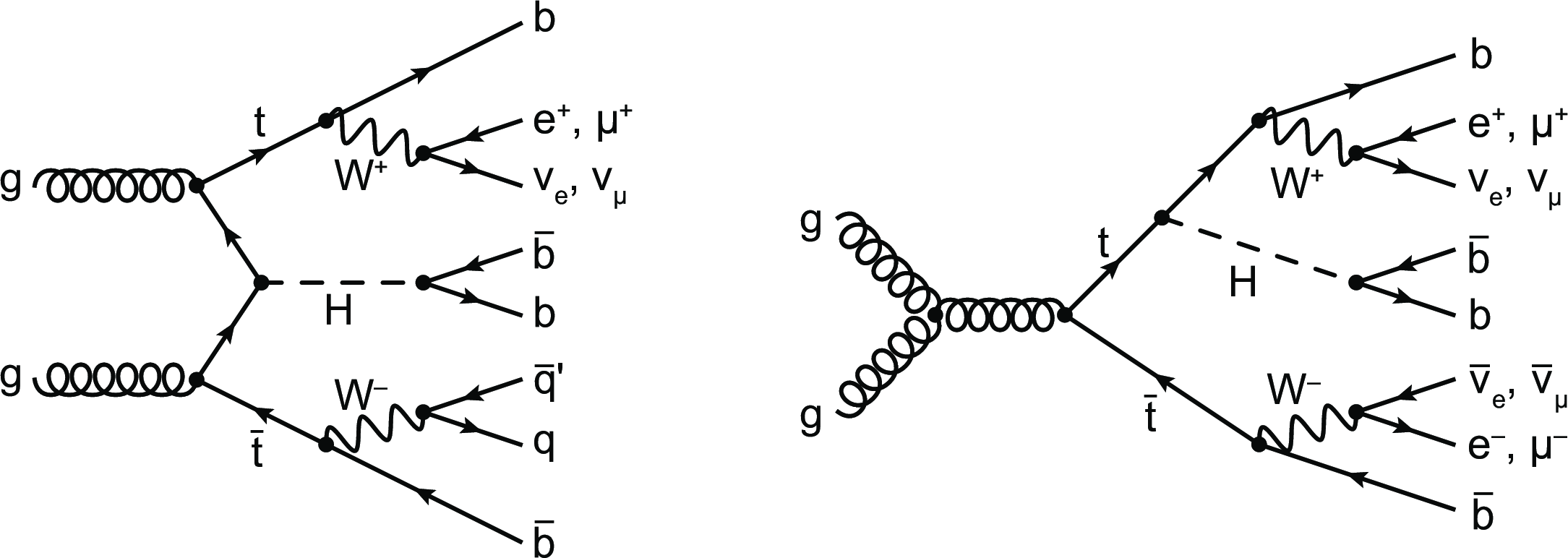
Figure 1:
Exemplary leading-order Feynman diagrams for $\mathrm{t \bar{t} H} $ production, including the subsequent decays of the top quark-antiquark pair in the lepton+jets channel (left) and the dilepton channel (right) as well as the decay of the Higgs boson into a bottom quark-antiquark pair. |

png pdf |
Figure 1-a:
Exemplary leading-order Feynman diagram for $\mathrm{t \bar{t} H} $ production, with the subsequent decays of the top quark-antiquark pair in the lepton+jets channel, as well as the decay of the Higgs boson into a bottom quark-antiquark pair. |

png pdf |
Figure 1-b:
Exemplary leading-order Feynman diagram for $\mathrm{t \bar{t} H} $ production, with the subsequent decays of the top quark-antiquark pair in the dilepton channel, as well as the decay of the Higgs boson into a bottom quark-antiquark pair. |

png pdf |
Figure 2:
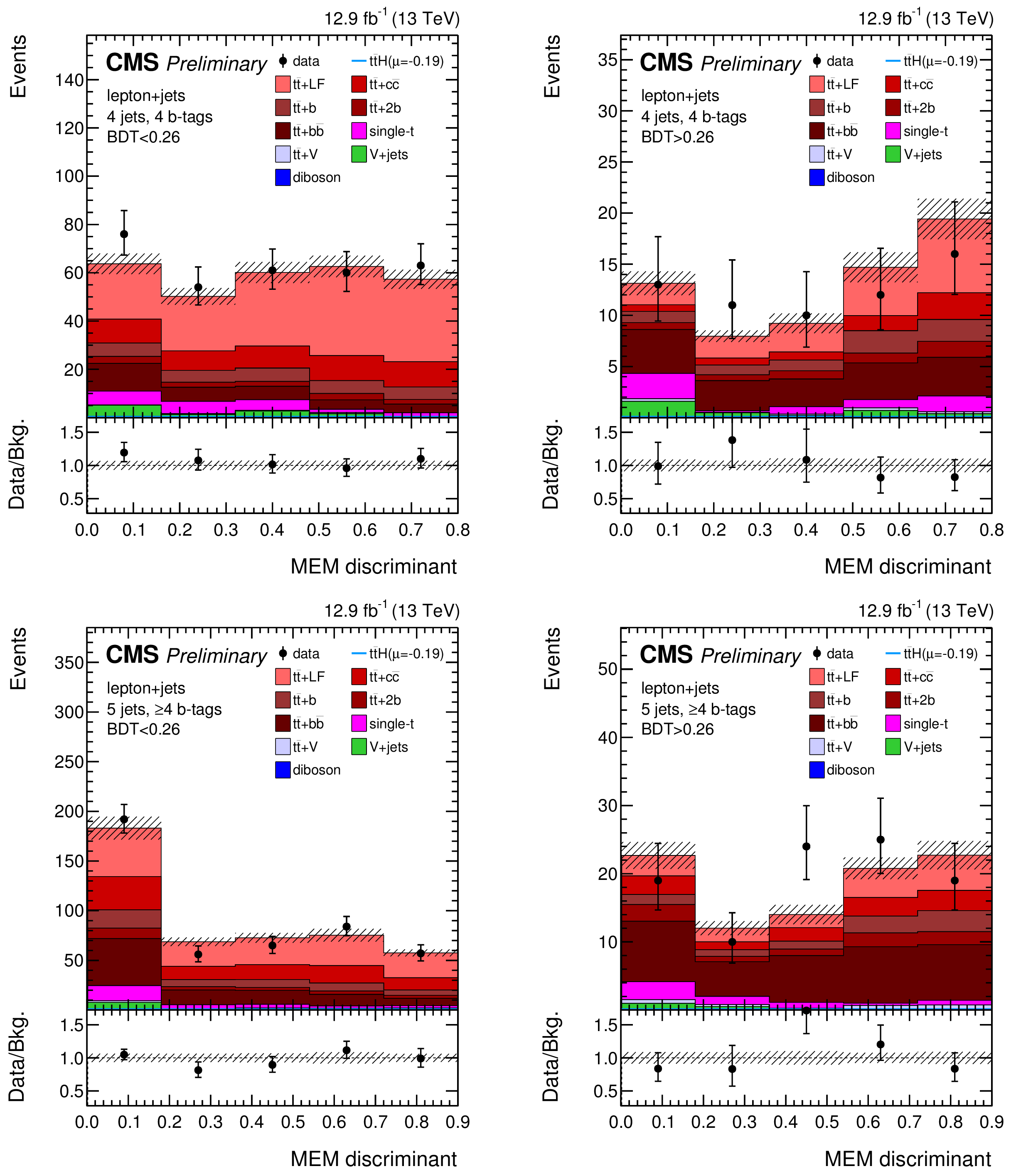
Final discriminant (MEM) shapes in the lepton+jets channel before the fit to data, in the analysis categories with 4 jets, 4 b-tags (top row) and 5 jets, $\geq $4 b-tags (bottom row) with low (left) and high (right) BDT output. The expected background contributions (filled histograms) are stacked, and the expected signal distribution (line) for a Higgs-boson mass of $ m_{\mathrm{H}} = $ 125 GeV is superimposed. Each contribution is normalized to an integrated luminosity of 12.9 fb$^{-1}$, and the signal distribution is additionally scaled by a factor of 15 for better readability. The error bands include the total uncertainty of the fit model. The distributions observed in data (markers) are also shown. |

png pdf |
Figure 2-a:
Final discriminant (MEM) shapes in the lepton+jets channel before the fit to data, in the analysis categories with 4 jets, 4 b-tags with low BDT output. The expected background contributions (filled histograms) are stacked, and the expected signal distribution (line) for a Higgs-boson mass of $ m_{\mathrm{H}} = $ 125 GeV is superimposed. Each contribution is normalized to an integrated luminosity of 12.9 fb$^{-1}$, and the signal distribution is additionally scaled by a factor of 15 for better readability. The error bands include the total uncertainty of the fit model. The distributions observed in data (markers) are also shown. |

png pdf |
Figure 2-b:
Final discriminant (MEM) shapes in the lepton+jets channel before the fit to data, in the analysis categories with 4 jets, 4 b-tags with high BDT output. The expected background contributions (filled histograms) are stacked, and the expected signal distribution (line) for a Higgs-boson mass of $ m_{\mathrm{H}} = $ 125 GeV is superimposed. Each contribution is normalized to an integrated luminosity of 12.9 fb$^{-1}$, and the signal distribution is additionally scaled by a factor of 15 for better readability. The error bands include the total uncertainty of the fit model. The distributions observed in data (markers) are also shown. |

png pdf |
Figure 2-c:
Final discriminant (MEM) shapes in the lepton+jets channel before the fit to data, in the analysis categories with 5 jets, $\geq $4 b-tags with low BDT output. The expected background contributions (filled histograms) are stacked, and the expected signal distribution (line) for a Higgs-boson mass of $ m_{\mathrm{H}} = $ 125 GeV is superimposed. Each contribution is normalized to an integrated luminosity of 12.9 fb$^{-1}$, and the signal distribution is additionally scaled by a factor of 15 for better readability. The error bands include the total uncertainty of the fit model. The distributions observed in data (markers) are also shown. |
png pdf |
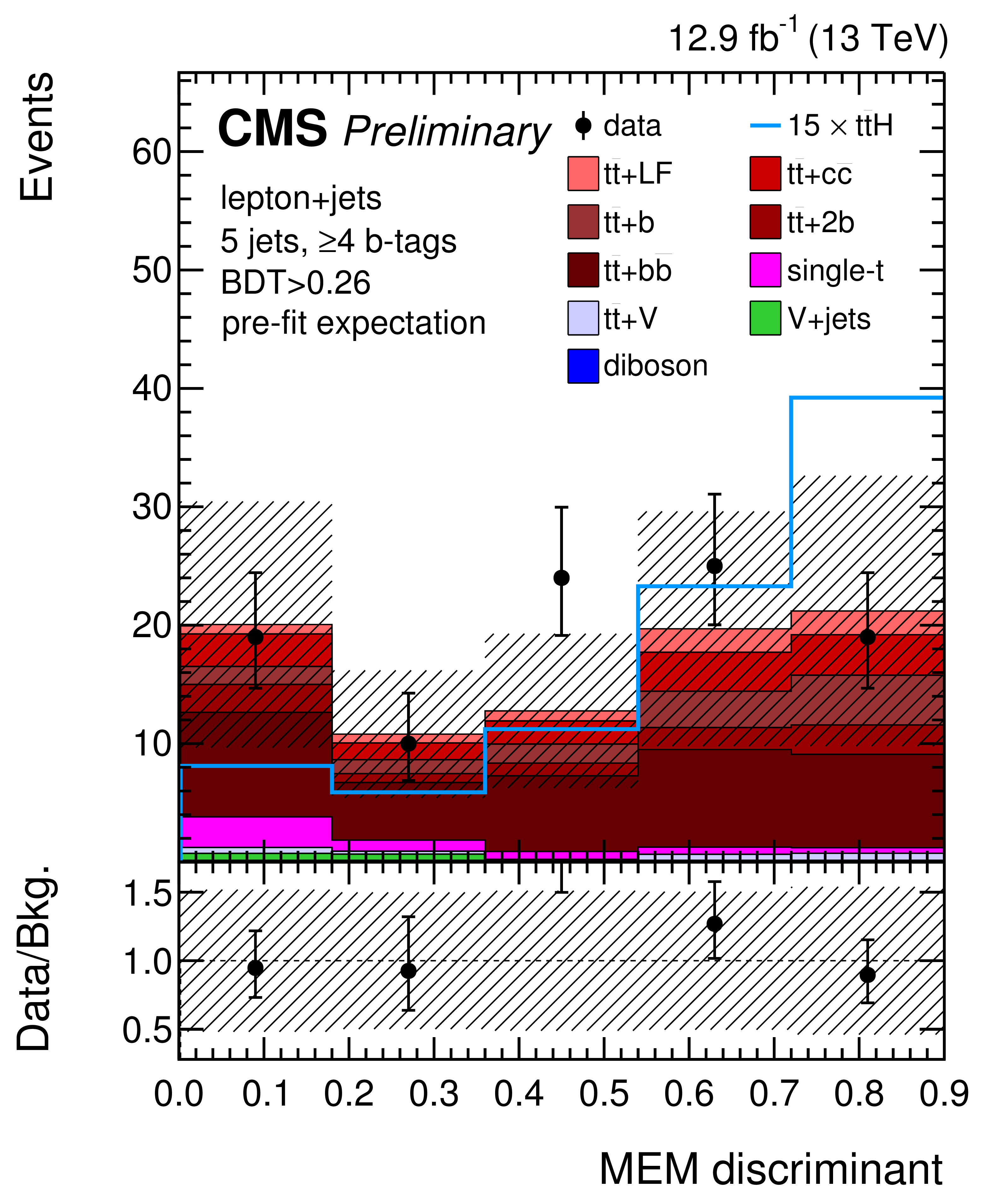
Figure 2-d:
Final discriminant (MEM) shapes in the lepton+jets channel before the fit to data, in the analysis categories with 5 jets, $\geq $4 b-tags with high BDT output. The expected background contributions (filled histograms) are stacked, and the expected signal distribution (line) for a Higgs-boson mass of $ m_{\mathrm{H}} = $ 125 GeV is superimposed. Each contribution is normalized to an integrated luminosity of 12.9 fb$^{-1}$, and the signal distribution is additionally scaled by a factor of 15 for better readability. The error bands include the total uncertainty of the fit model. The distributions observed in data (markers) are also shown. |

png pdf |
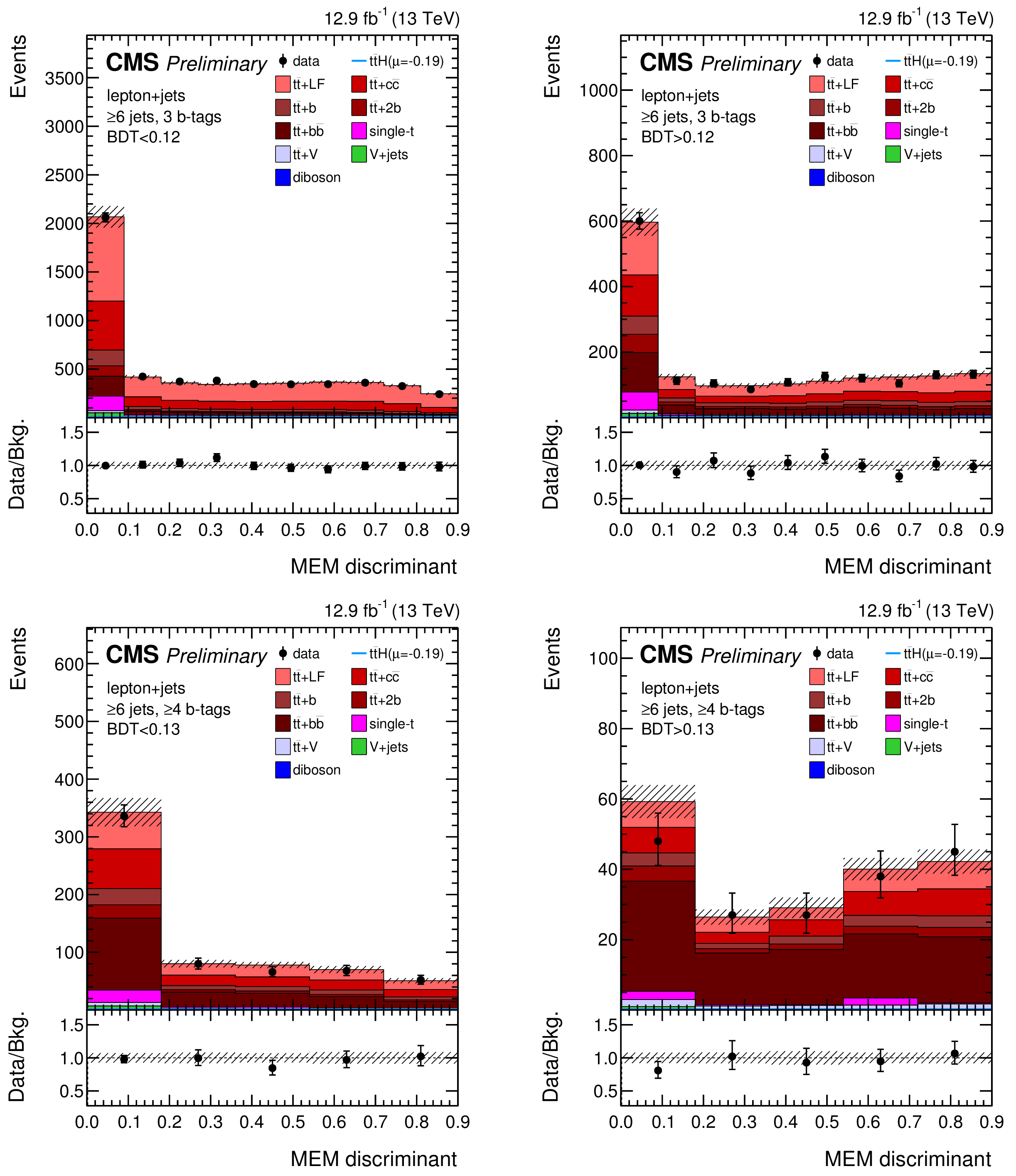
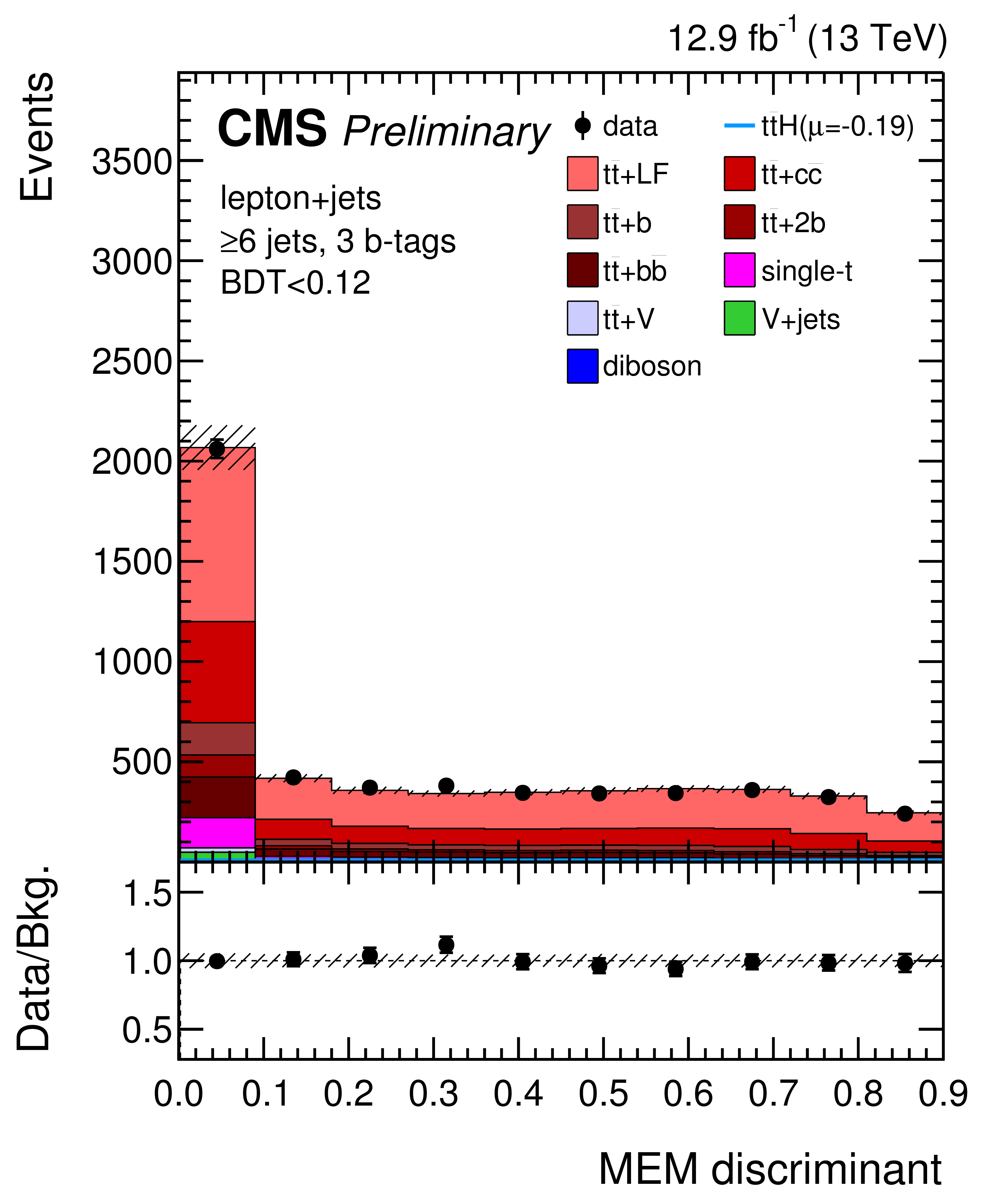
Figure 3:
Final discriminant (MEM) shapes in the lepton+jets channel before the fit to data, in the analysis categories with $\geq $6 jets, 3 b-tags (top row) and $\geq $6 jets, $\geq $4 b-tags (bottom row) with low (left) and high (right) BDT output (continued from Fig. 2). |
png pdf |
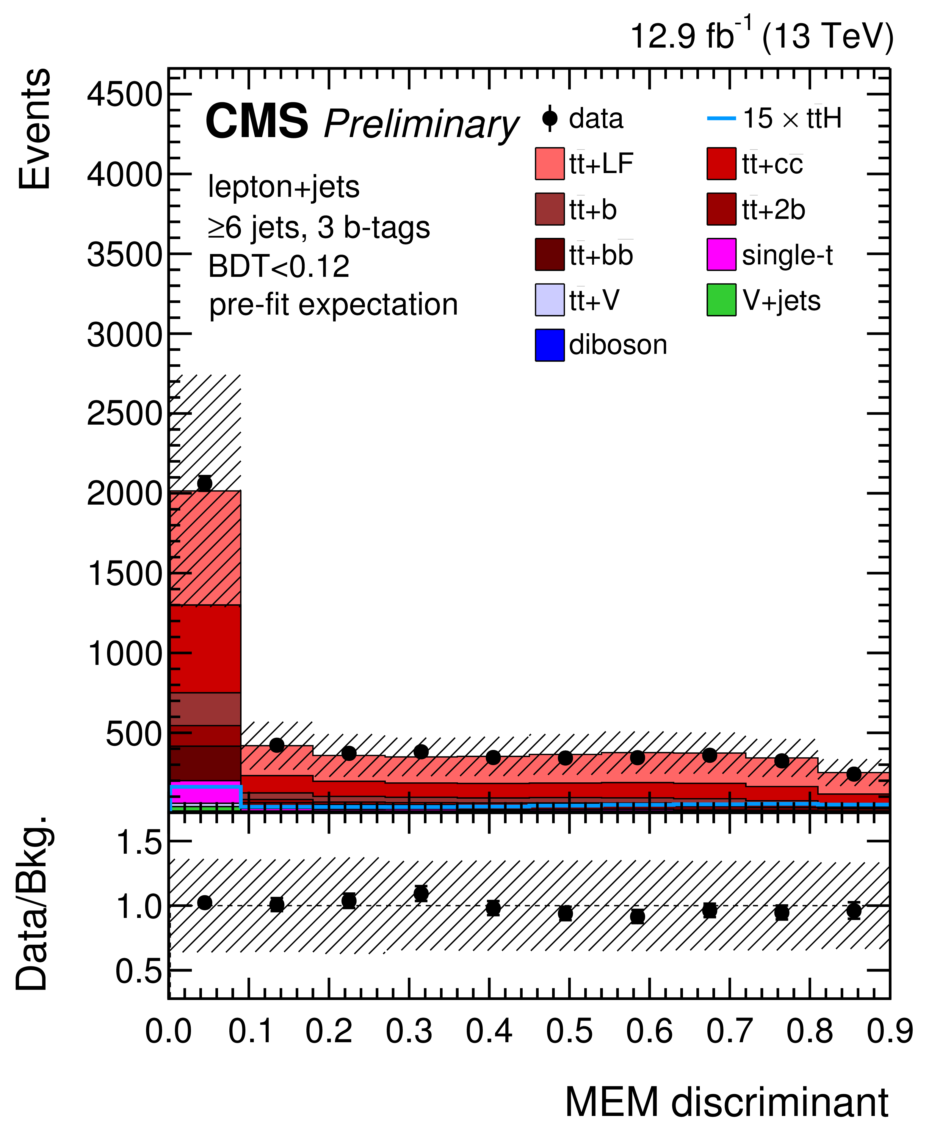
Figure 3-a:
Final discriminant (MEM) shapes in the lepton+jets channel before the fit to data, in the analysis category with $\geq $6 jets, 3 b-tags with low BDT output (continued from Fig. 2). |

png pdf |
Figure 3-b:
Final discriminant (MEM) shapes in the lepton+jets channel before the fit to data, in the analysis category with $\geq $6 jets, 3 b-tags with high BDT output (continued from Fig. 2). |

png pdf |
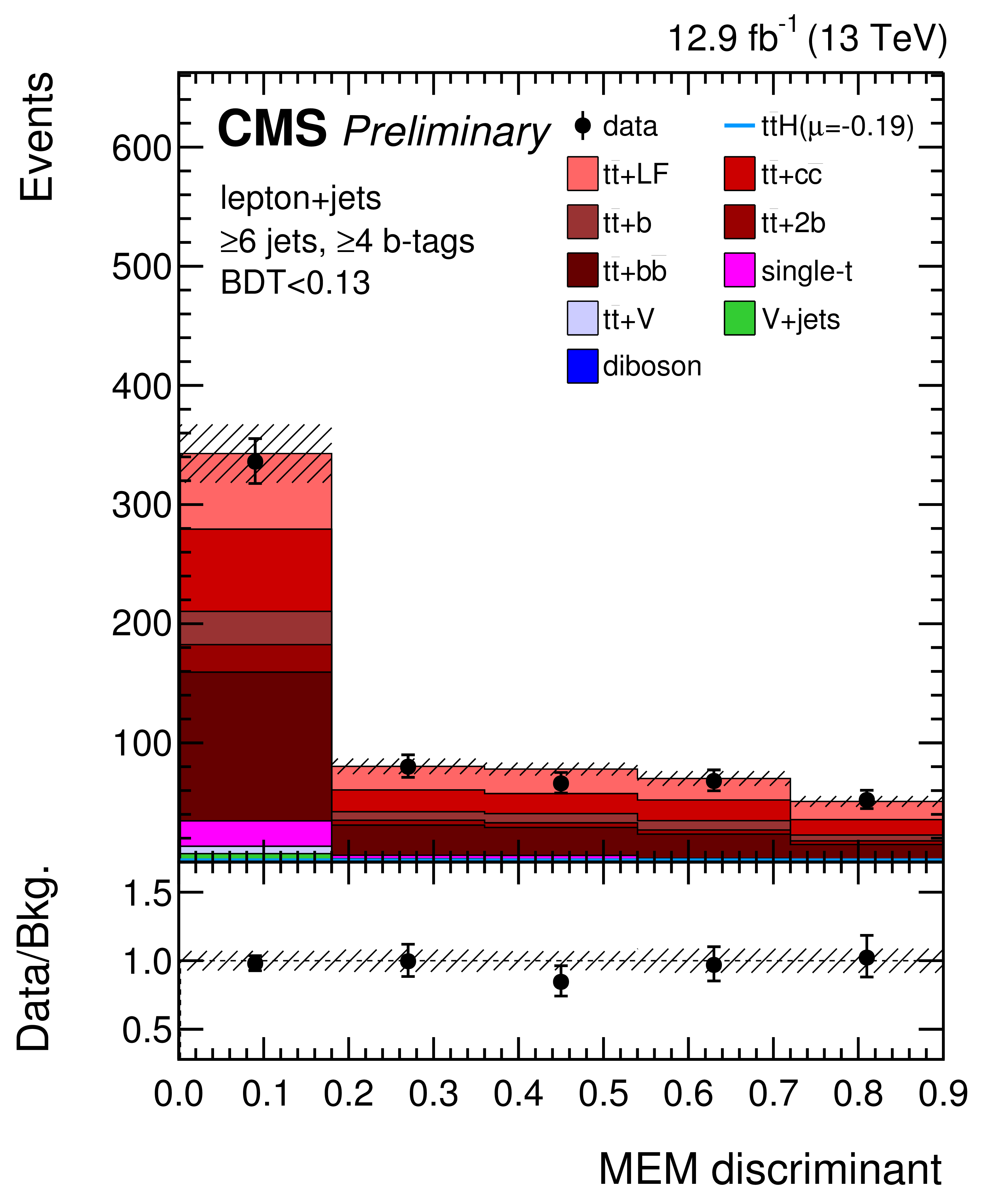
Figure 3-c:
Final discriminant (MEM) shapes in the lepton+jets channel before the fit to data, in the analysis category with $\geq $6 jets, $\geq $4 b-tags with low BDT output (continued from Fig. 2). |
png pdf |
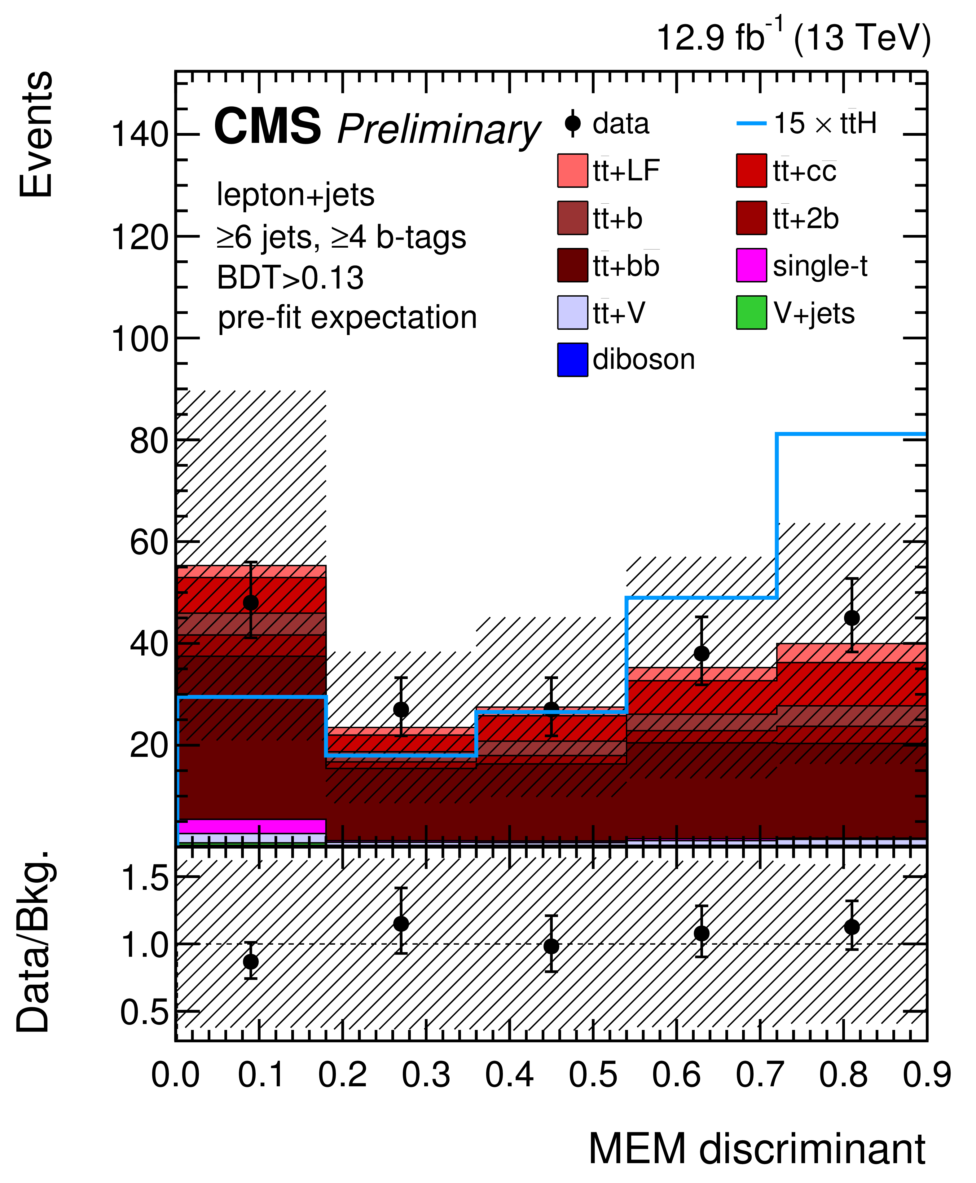
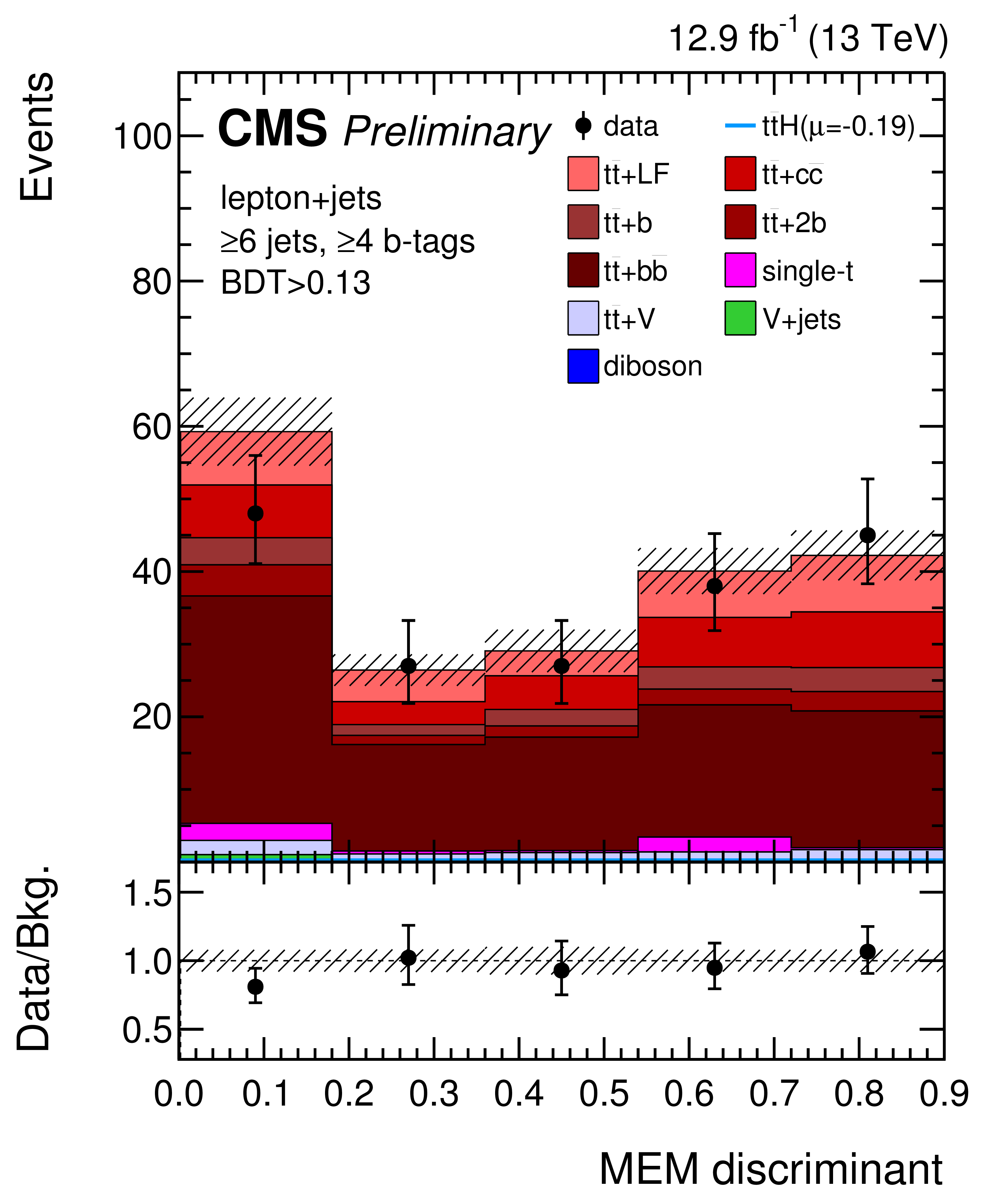
Figure 3-d:
Final discriminant (MEM) shapes in the lepton+jets channel before the fit to data, in the analysis category with $\geq $6 jets, $\geq $4 b-tags with high BDT output (continued from Fig. 2). |
png pdf |
Figure 4:
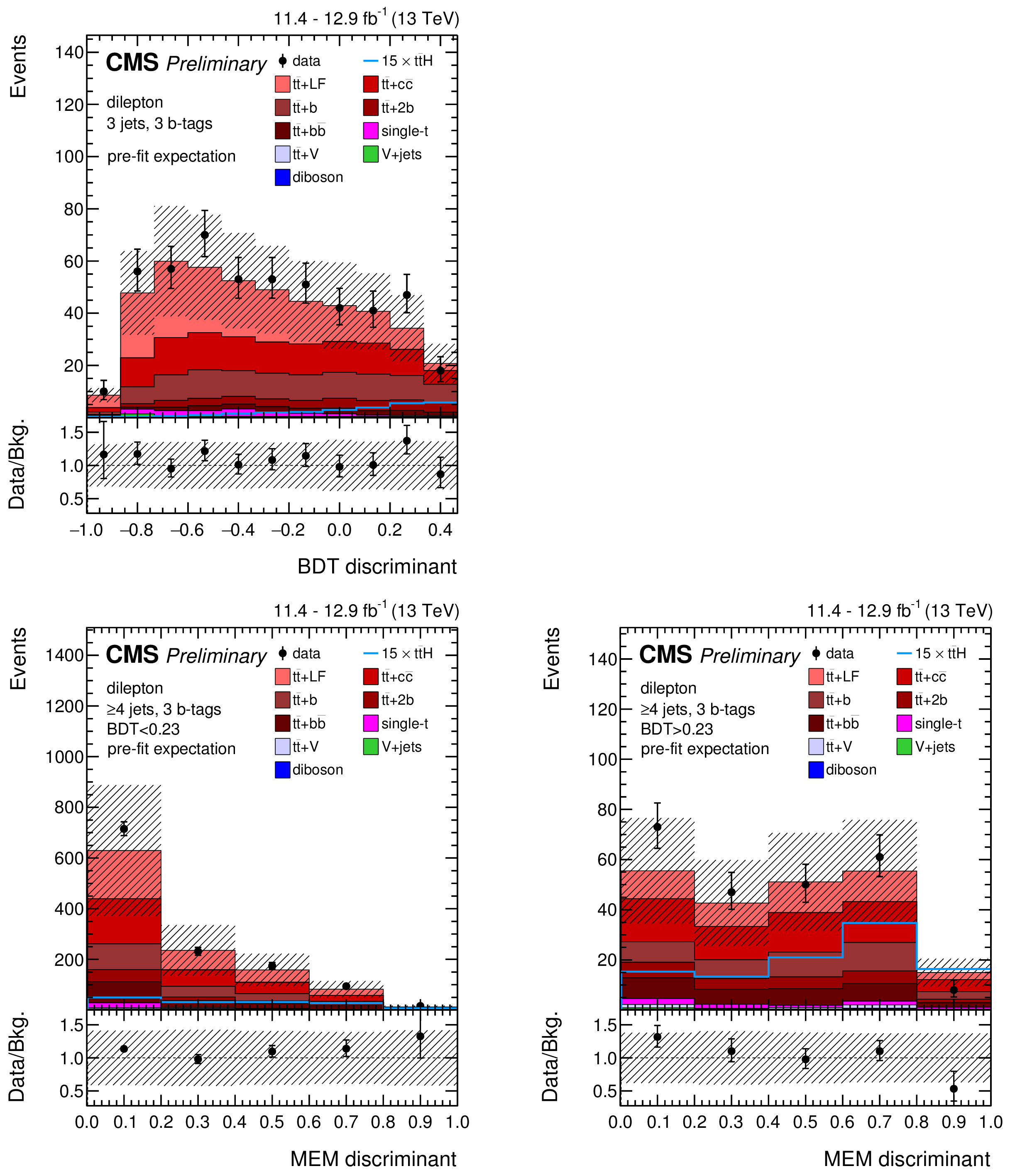
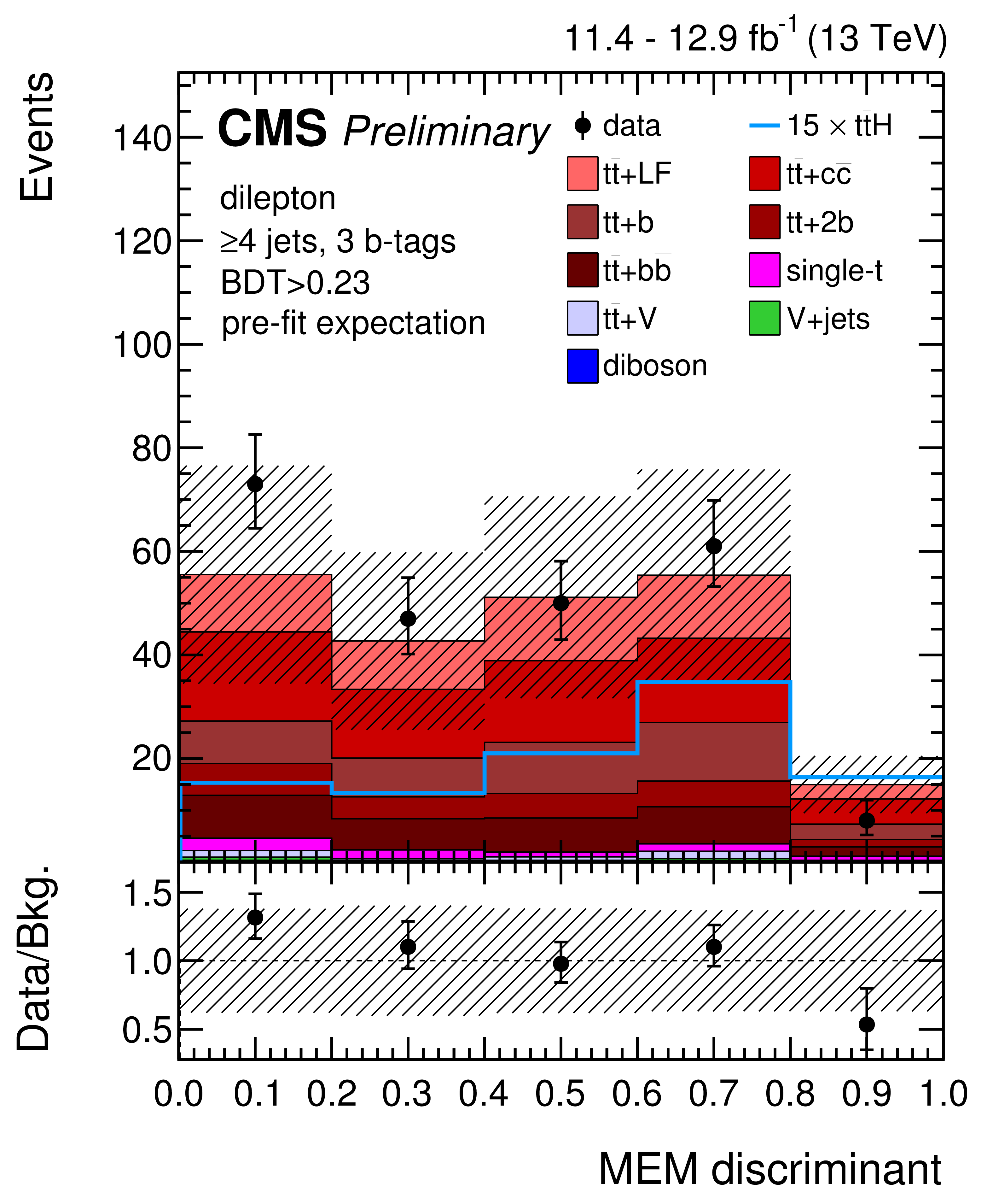
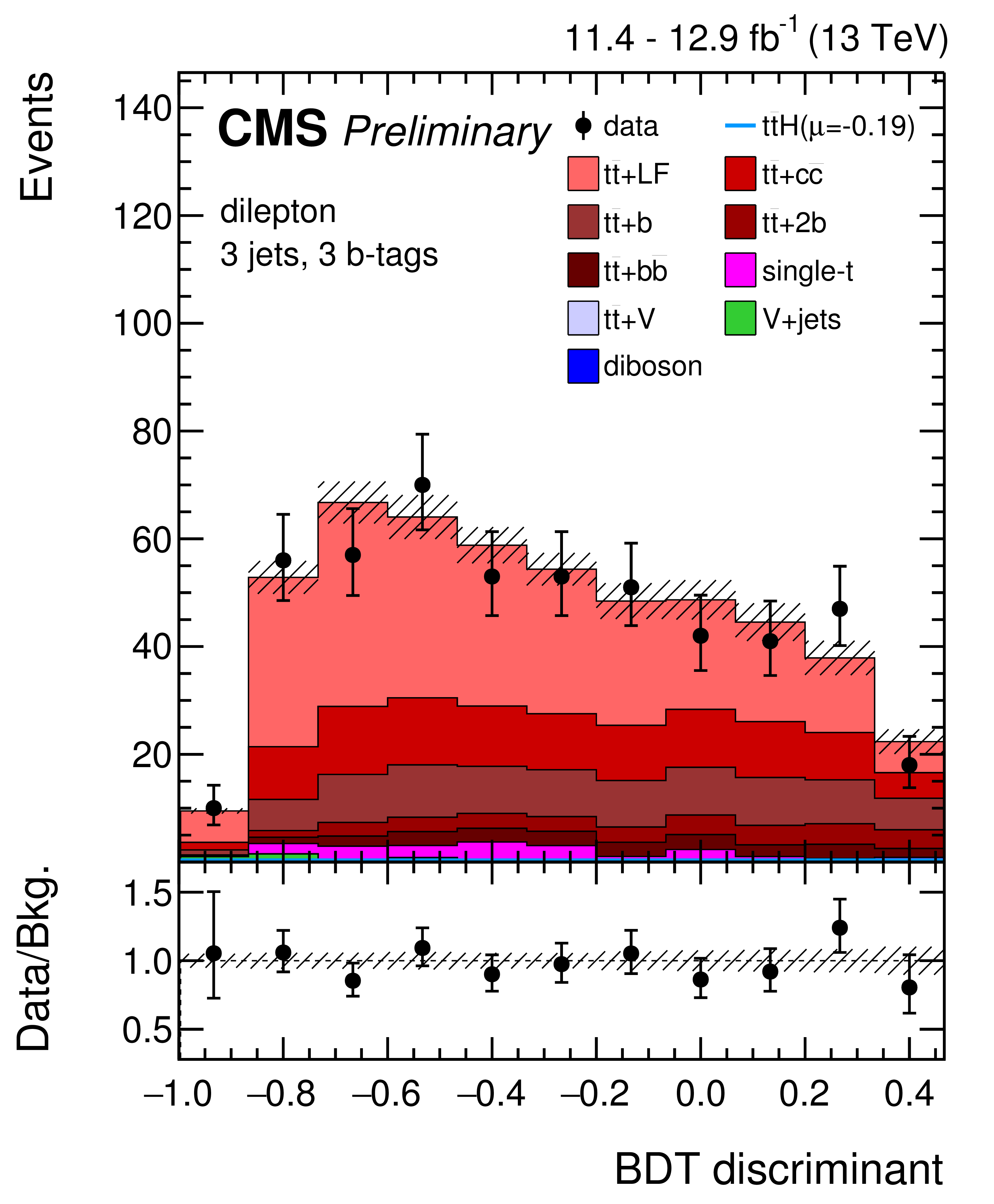
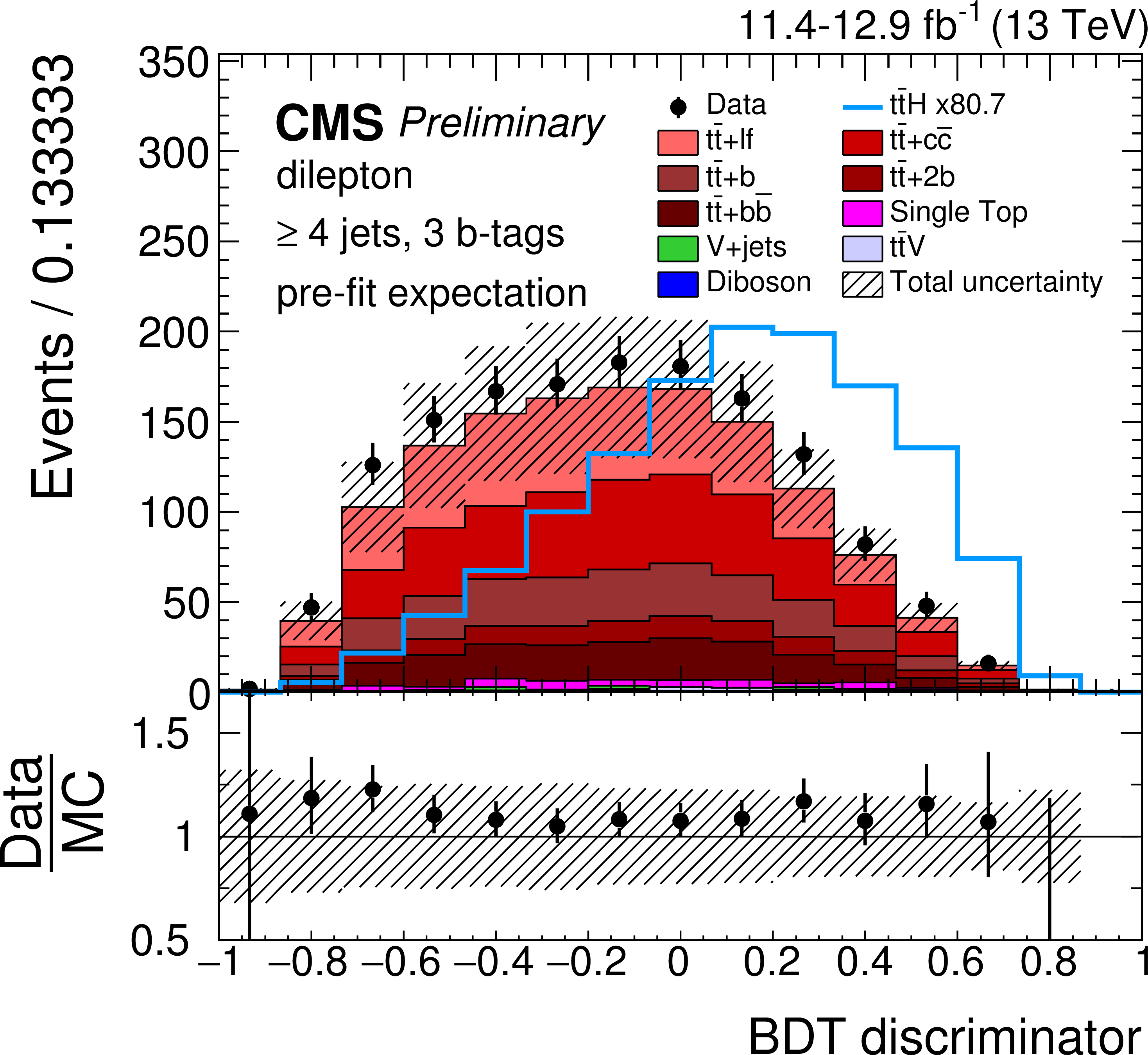
Final discriminant shapes (BDT or MEM) in the dilepton channel before the fit to data, in the analysis categories with 3 jets, 3 b-tags (top row) and $\geq $4 jets, 3 b-tags (bottom row) with low (left) and high (right) BDT output. The expected background contributions (filled histograms) are stacked, and the expected signal distribution (line) for a Higgs-boson mass of $ m_{\mathrm{H}} = $ 125 GeV is superimposed. Each contribution is normalized to an integrated luminosity of 11.4-12.9 fb$^{-1}$, and the signal distribution is additionally scaled by a factor of 15 for better readability. The error bands include the total uncertainty of the fit model. The distributions observed in data (markers) are also shown. |

png pdf |
Figure 4-a:
Final discriminant shapes (BDT or MEM) in the dilepton channel before the fit to data, in the analysis category with 3 jets, 3 b-tags. The expected background contributions (filled histograms) are stacked, and the expected signal distribution (line) for a Higgs-boson mass of $ m_{\mathrm{H}} = $ 125 GeV is superimposed. Each contribution is normalized to an integrated luminosity of 11.4-12.9 fb$^{-1}$, and the signal distribution is additionally scaled by a factor of 15 for better readability. The error band includes the total uncertainty of the fit model. The distribution observed in data (markers) is also shown. |

png pdf |
Figure 4-b:
Final discriminant shapes (BDT or MEM) in the dilepton channel before the fit to data, in the analysis category with $\geq $4 jets, 3 b-tags with low BDT output. The expected background contributions (filled histograms) are stacked, and the expected signal distribution (line) for a Higgs-boson mass of $ m_{\mathrm{H}} = $ 125 GeV is superimposed. Each contribution is normalized to an integrated luminosity of 11.4-12.9 fb$^{-1}$, and the signal distribution is additionally scaled by a factor of 15 for better readability. The error band includes the total uncertainty of the fit model. The distribution observed in data (markers) is also shown. |
png pdf |
Figure 4-c:
Final discriminant shapes (BDT or MEM) in the dilepton channel before the fit to data, in the analysis category with $\geq $4 jets, 3 b-tags with high BDT output. The expected background contributions (filled histograms) are stacked, and the expected signal distribution (line) for a Higgs-boson mass of $ m_{\mathrm{H}} = $ 125 GeV is superimposed. Each contribution is normalized to an integrated luminosity of 11.4-12.9 fb$^{-1}$, and the signal distribution is additionally scaled by a factor of 15 for better readability. The error band includes the total uncertainty of the fit model. The distribution observed in data (markers) is also shown. |

png pdf |
Figure 5:
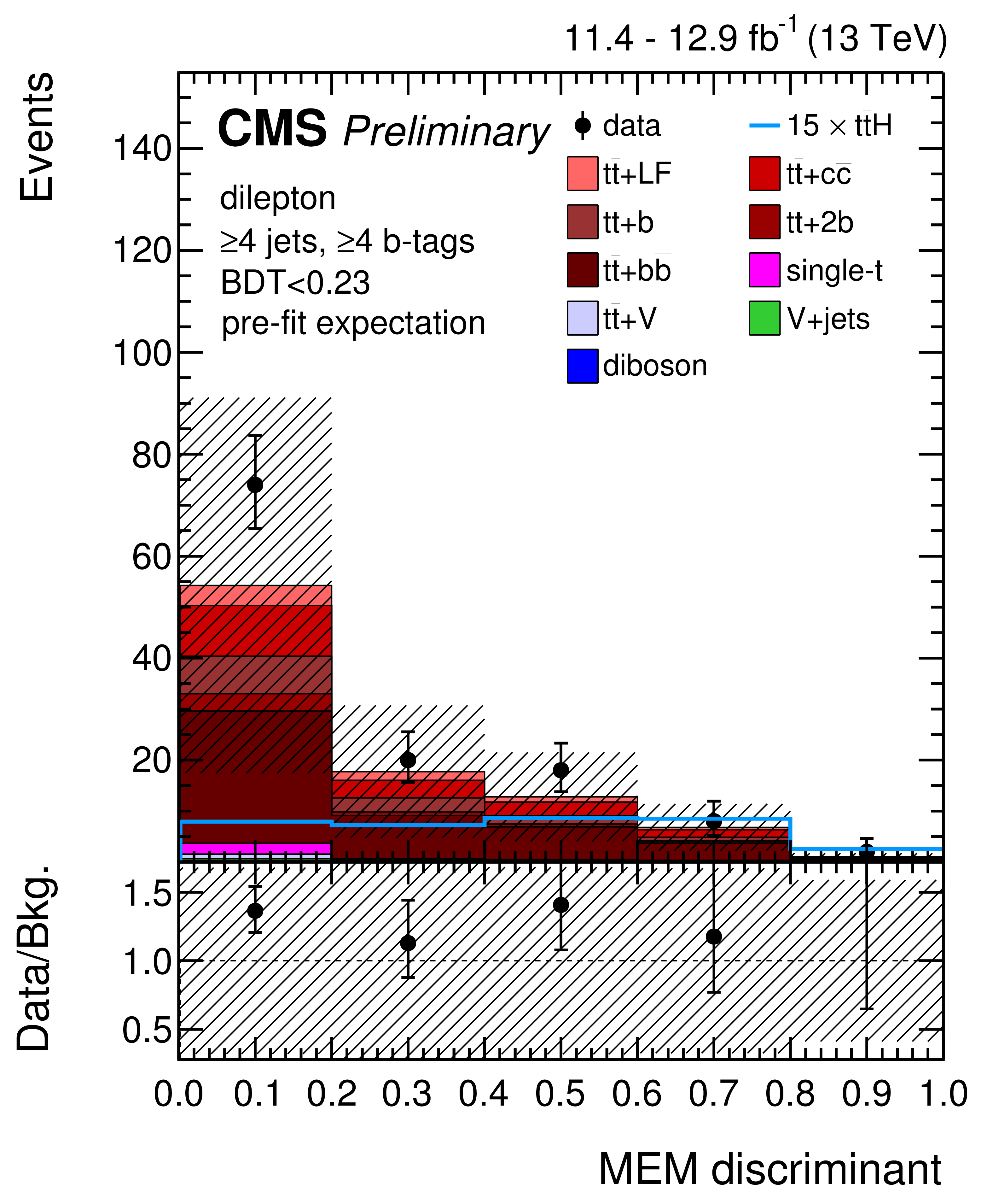
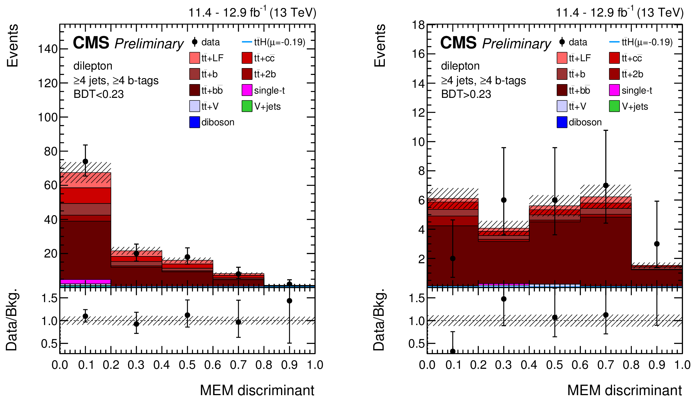
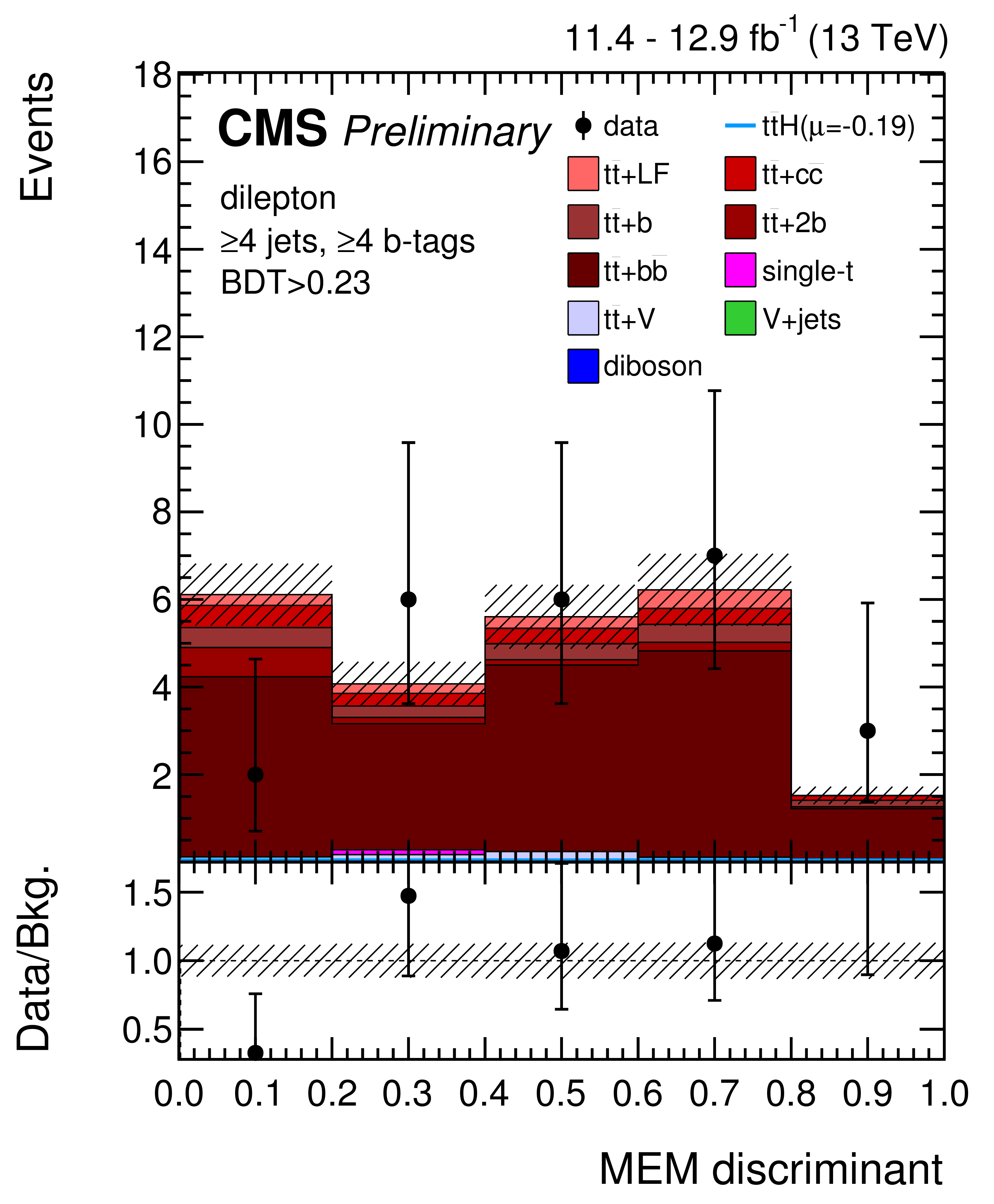
Final discriminant (MEM) shapes in the dilepton channel before the fit to data, in the analysis categories with $\geq $4 jets, $\geq $4 b-tags with low (left) and high (right) BDT output (continued from Fig. 4). |
png pdf |
Figure 5-a:
Final discriminant (MEM) shapes in the dilepton channel before the fit to data, in the analysis category with $\geq $4 jets, $\geq $4 b-tags with low BDT output (continued from Fig. 4). |

png pdf |
Figure 5-b:
Final discriminant (MEM) shapes in the dilepton channel before the fit to data, in the analysis category with $\geq $4 jets, $\geq $4 b-tags with high BDT output (continued from Fig. 4). |
png pdf |
Figure 6:
Final discriminant shapes (MEM) in the analysis categories with 4 jets, 4 b-tags (top row) and 5 jets, $\geq $4 b-tags (bottom row) with low (left) and high (right) BDT output in the lepton+jets channel after the fit to data. |

png pdf |
Figure 6-a:
Final discriminant shapes (MEM) in the analysis category with 4 jets, 4 b-tags with low BDT output in the lepton+jets channel after the fit to data. |

png pdf |
Figure 6-b:
Final discriminant shapes (MEM) in the analysis category with 4 jets, 4 b-tags with high BDT output in the lepton+jets channel after the fit to data. |

png pdf |
Figure 6-c:
Final discriminant shapes (MEM) in the analysis category with 5 jets, $\geq $4 b-tags with low BDT output in the lepton+jets channel after the fit to data. |

png pdf |
Figure 6-d:
Final discriminant shapes (MEM) in the analysis category with 5 jets, $\geq $4 b-tags with low high BDT output in the lepton+jets channel after the fit to data. |
png pdf |
Figure 7:
Final discriminant shapes (MEM) in the analysis categories with $\geq $6 jets, 3 b-tags (top row) and $\geq $6 jets, $\geq $4 b-tags (bottom row) with low (left) and high (right) BDT output in the lepton+jets channel after the fit to data (continued from Fig. 6). |
png pdf |
Figure 7-a:
Final discriminant shapes (MEM) in the analysis category with $\geq $6 jets, 3 b-tags with low BDT output in the lepton+jets channel after the fit to data (continued from Fig. 6). |

png pdf |
Figure 7-b:
Final discriminant shapes (MEM) in the analysis category with $\geq $6 jets, 3 b-tags with low BDT output in the lepton+jets channel after the fit to data (continued from Fig. 6). |
png pdf |
Figure 7-c:
Final discriminant shapes (MEM) in the analysis category with $\geq $6 jets, $\geq $4 b-tags with low BDT output in the lepton+jets channel after the fit to data (continued from Fig. 6). |
png pdf |
Figure 7-d:
Final discriminant shapes (MEM) in the analysis category with $\geq $6 jets, $\geq $4 b-tags with high BDT output in the lepton+jets channel after the fit to data (continued from Fig. 6). |

png pdf |
Figure 8:
Final discriminant shapes (BDT or MEM) in the analysis categories with 3 jets, 3 b-tags (top row) and $\geq $4 jets, 3 b-tags (bottom row) with low (left) and high (right) BDT output in the dilepton channel after the fit to data. |
png pdf |
Figure 8-a:
Final discriminant shapes (BDT or MEM) in the analysis category with 3 jets, 3 b-tags in the dilepton channel after the fit to data. |

png pdf |
Figure 8-b:
Final discriminant shapes (BDT or MEM) in the analysis category with $\geq $4 jets, 3 b-tags with low BDT output in the dilepton channel after the fit to data. |

png pdf |
Figure 8-c:
Final discriminant shapes (BDT or MEM) in the analysis categories with $\geq $4 jets, 3 b-tags with high BDT output in the dilepton channel after the fit to data. |
png pdf |
Figure 9:
Final discriminant shapes (MEM) in the analysis categories with $\geq $4 jets, $\geq $4 b-tags with low (left) and high (right) BDT output in the dilepton channel after the fit to data (continued from Fig. togodo). |

png pdf |
Figure 9-a:
Final discriminant shapes (MEM) in the analysis categories with $\geq $4 jets, $\geq $4 b-tags with low (left) and high (right) BDT output in the dilepton channel after the fit to data (continued from Fig. togodo). |
png pdf |
Figure 9-b:
Final discriminant shapes (MEM) in the analysis categories with $\geq $4 jets, $\geq $4 b-tags with low (left) and high (right) BDT output in the dilepton channel after the fit to data (continued from Fig. togodo). |

png pdf |
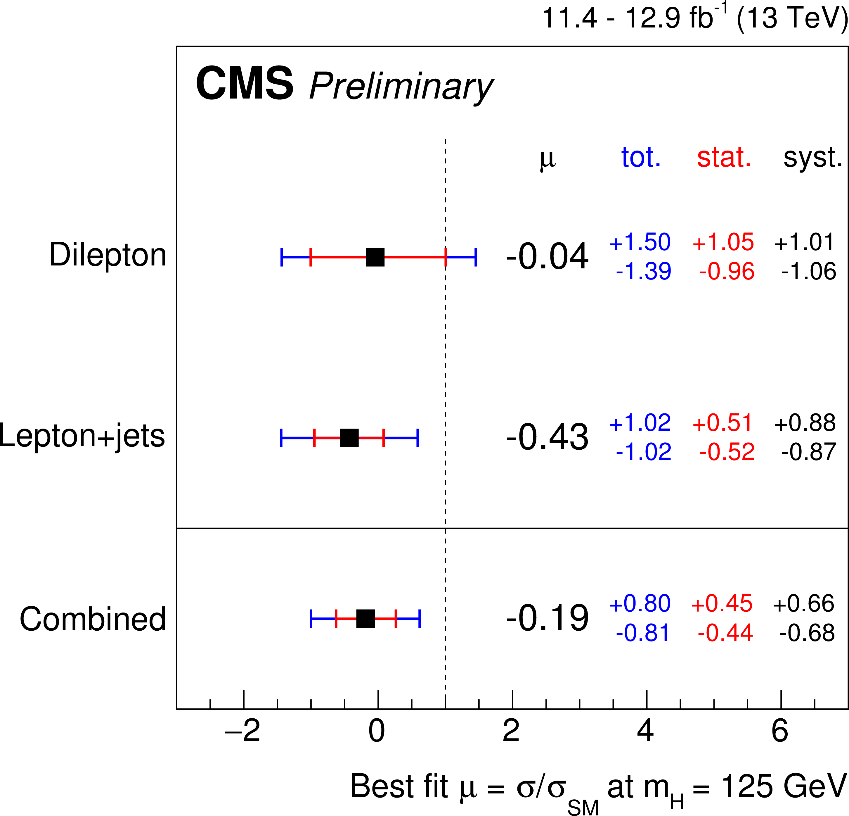
Figure 10:
Best-fit values of the signal strength modifiers $\mu $ with their $\pm$1$ \sigma $ confidence intervals, also split into their statistical and systematic components (left), and median expected and observed 95% CL upper limits on $\mu $ (right). The expected limits are displayed together with $\pm$1$ \sigma $ and $\pm$2$ \sigma $ confidence intervals. Also shown are the limits in case of an injected signal of $\mu =$ 1. |
png pdf |
Figure 10-a:
Best-fit values of the signal strength modifiers $\mu $ with their $\pm$1$ \sigma $ confidence intervals, also split into their statistical and systematic components. |

png pdf |
Figure 10-b:
Median expected and observed 95% CL upper limits on $\mu $. The expected limits are displayed together with $\pm$1$ \sigma $ and $\pm$2$ \sigma $ confidence intervals. Also shown are the limits in case of an injected signal of $\mu =$ 1. |

png pdf |
Figure 11:
Observed and expected upper limits at 95% CL on $\mu $ in the lepton+jets channel. The limits are calculated with the asymptotic method. |

png pdf |
Figure 12:
Observed and expected and upper limits at 95% CL on $\mu $ in the dilepton channel. The limits are calculated with the asymptotic method. |
| Tables | |

png pdf |
Table 1:
$\mathrm{t \bar{t} H} $ and background event yields for lepton+jets categories. The processes and the separation of the $\mathrm{t \bar{t} } $+jets sample are described in Section 3. The uncertainties in the expected yields include the statistical as well as all the systematic contributions. Cases where no events pass the event selection are marked as ``--''. |

png pdf |
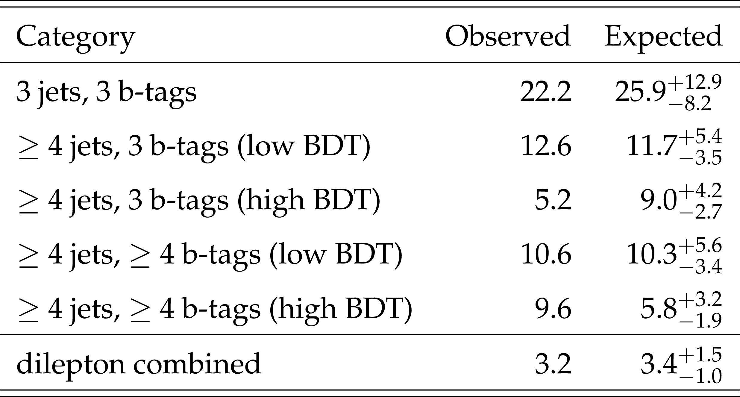
Table 2:
$\mathrm{t \bar{t} H} $ and background event yields for dilepton categories. The processes and the separation of the $\mathrm{t \bar{t} } $+jets sample are described in Section 3. The uncertainties in the expected yields include the statistical as well as all the systematic contributions. Cases where no events pass the event selection are marked as ``--''. |

png pdf |
Table 3:
Systematic uncertainties considered in the analysis. |

png pdf |
Table 4:
Specific effect of systematic uncertainties that affect the discriminant shape on the predicted background and signal yields for events in the $\geq $6 jets, 3 b-tags category of the lepton+jets channel. Here, only the sum of the largest background processes,$ \mathrm{ t \bar{t} } $+LF, $ \mathrm{ t \bar{t} } $+b, $ \mathrm{ t \bar{t} } $+2b, $ \mathrm{ t \bar{t} } $+$\mathrm{b\bar{b}}$, and $ \mathrm{ t \bar{t} } $+$\mathrm{c\bar{c}}$, are considered. |

png pdf |
Table 5:
Best-fit value of the signal strength modifier $\mu $ and the median expected and observed 95% CL upper limits (UL) in the dilepton and the lepton+jets channels as well as the combined results. The one standard deviation ($\pm$1$ \sigma $) confidence intervals of the expected limit and the best-fit value are also quoted, split into the statistical and systematic components in the latter case. Expected limits are calculated with the asymptotic method [79]. |

png pdf |
Table 6:
Variables used in the BDT training in the lepton+jets channel. |

png pdf |
Table 7:
BDT input variable assignment per category in the lepton+jets channel. |
png pdf |
Table 8:
Observed and median expected 95% CLs upper limits on $\mu $ in the lepton+jets channel, calculated with the asymptotic method. The upper and lower range of the 1$\sigma $ confidence interval is also quoted. |
png pdf |
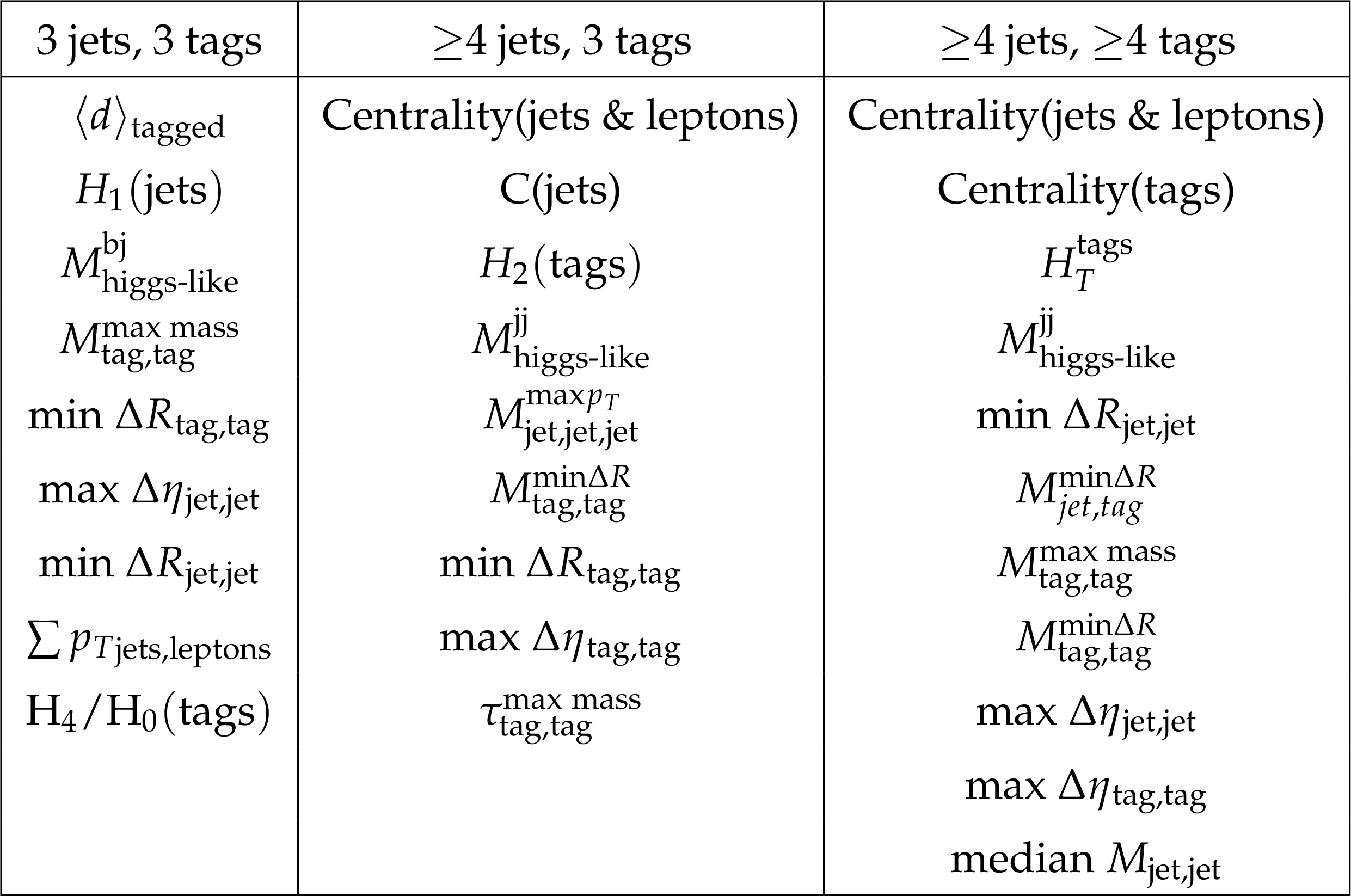
Table 9:
Variables used in the BDT training in the dilepton channel. |
| Summary |
| A search for the associated production of a Higgs boson and a top quark-antiquark pair is performed using up to 12.9 fb$^{-1}$ of pp collision data recorded with the CMS detector at a center-of-mass energy of 13 TeV in 2016. Candidate events are selected in final states compatible with the Higgs boson decay ${\mathrm{H\to\mathrm{ b \bar{b} }}} $ and the lepton+jets or dilepton decay channel of the $\mathrm{ t \bar{t} } $ pair. Selected events are split into mutually exclusive categories according to their $\mathrm{ t \bar{t} }$ decay channel and jet content. In each category a powerful discriminant is constructed to separate the $\mathrm{t \bar{t} H} $ signal from the $\mathrm{ t \bar{t} }$-dominated background, based on boosted decision trees and the matrix element method. An observed (expected) upper limit on the $\mathrm{t \bar{t} H} $ production cross section relative to the SM expectations of $\mu = 1.5\,(1.7)$ at the 95% confidence level is obtained. The best-fit value of $\mu$ is \mbox{$-0.19\,^{+0.45}_{-0.44}\,(\text{stat.})\,^{+0.66}_{-0.68}\,(\text{syst.})$}. These results are compatible with SM expectations at the level of 1.5 standard deviations. |
| Additional Figures | |

png pdf |
Additional Figure 1:
Jet (left) and b-tagged jet (right) multiplicity observed in data (markers) and expected for the SM background processes (stacked histograms) in a control region with $\geq$4 jets, $\geq$2 of which are b-tagged, in the lepton+jets channel. The expected signal distribution (line) is superimposed and scaled to the total background yield for better readability. The uncertainty bands include all uncertainties, treated as fully uncorrelated, that affect the shape of the distributions. |

png pdf |
Additional Figure 1-a:
Jet multiplicity observed in data (markers) and expected for the SM background processes (stacked histograms) in a control region with $\geq$4 jets, $\geq$2 of which are b-tagged, in the lepton+jets channel. The expected signal distribution (line) is superimposed and scaled to the total background yield for better readability. The uncertainty bands include all uncertainties, treated as fully uncorrelated, that affect the shape of the distributions. |
png pdf |
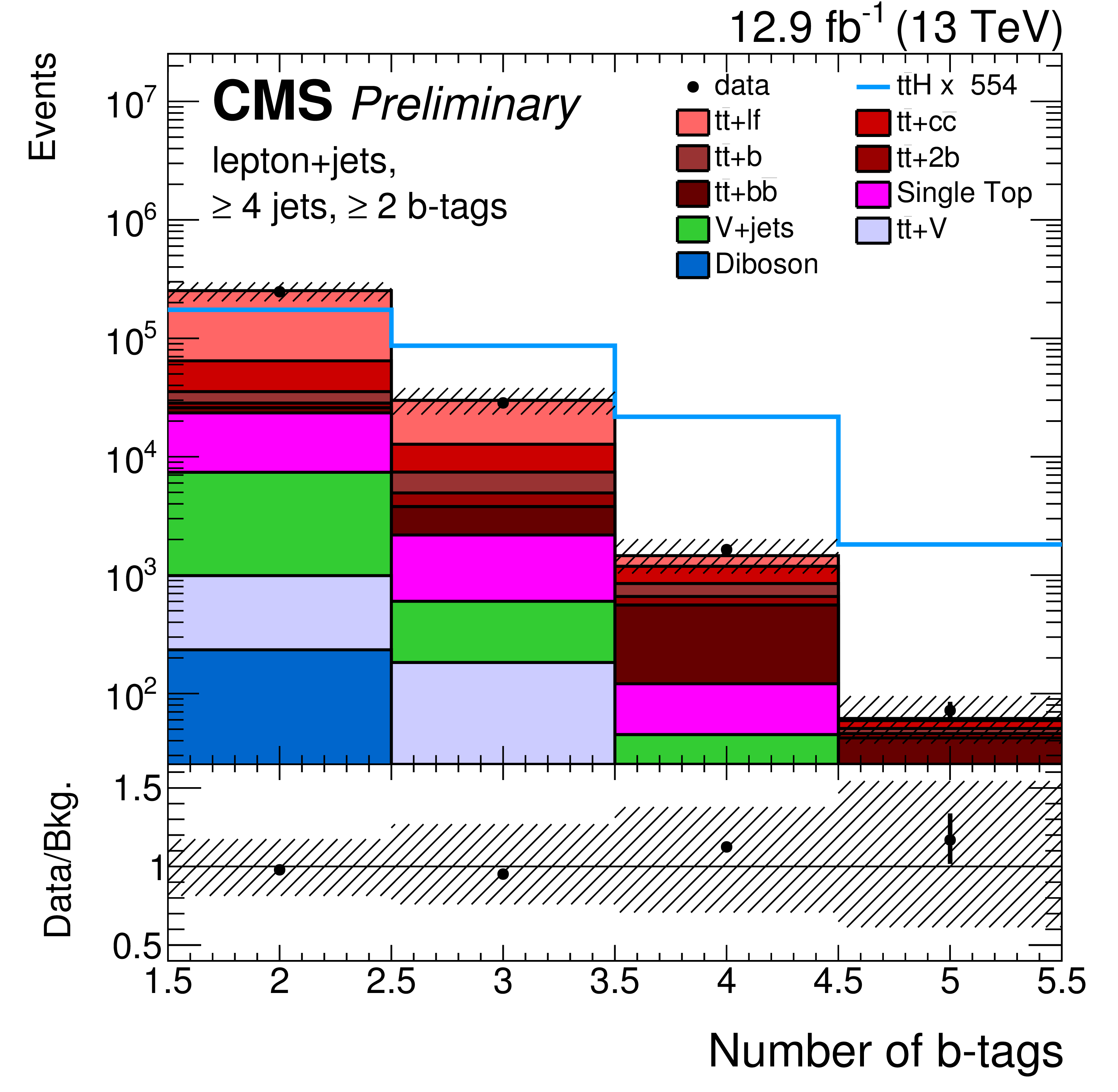
Additional Figure 1-b:
b-tagged jet multiplicity observed in data (markers) and expected for the SM background processes (stacked histograms) in a control region with $\geq$4 jets, $\geq$2 of which are b-tagged, in the lepton+jets channel. The expected signal distribution (line) is superimposed and scaled to the total background yield for better readability. The uncertainty bands include all uncertainties, treated as fully uncorrelated, that affect the shape of the distributions. |

png pdf |
Additional Figure 2:
Jet (left) and lepton (right) $ {p_{\mathrm {T}}} $ observed in data (markers) and expected for the SM background processes (stacked histograms) in a control region with $\geq$4 jets, $\geq$2 of which are b-tagged, in the lepton+jets channel. The expected signal distribution (line) is superimposed and scaled to the total background yield for better readability. The uncertainty bands include all uncertainties, treated as fully uncorrelated, that affect the shape of the distributions. |

png pdf |
Additional Figure 2-a:
Jet $ {p_{\mathrm {T}}} $ observed in data (markers) and expected for the SM background processes (stacked histograms) in a control region with $\geq$4 jets, $\geq$2 of which are b-tagged, in the lepton+jets channel. The expected signal distribution (line) is superimposed and scaled to the total background yield for better readability. The uncertainty bands include all uncertainties, treated as fully uncorrelated, that affect the shape of the distributions. |
png pdf |
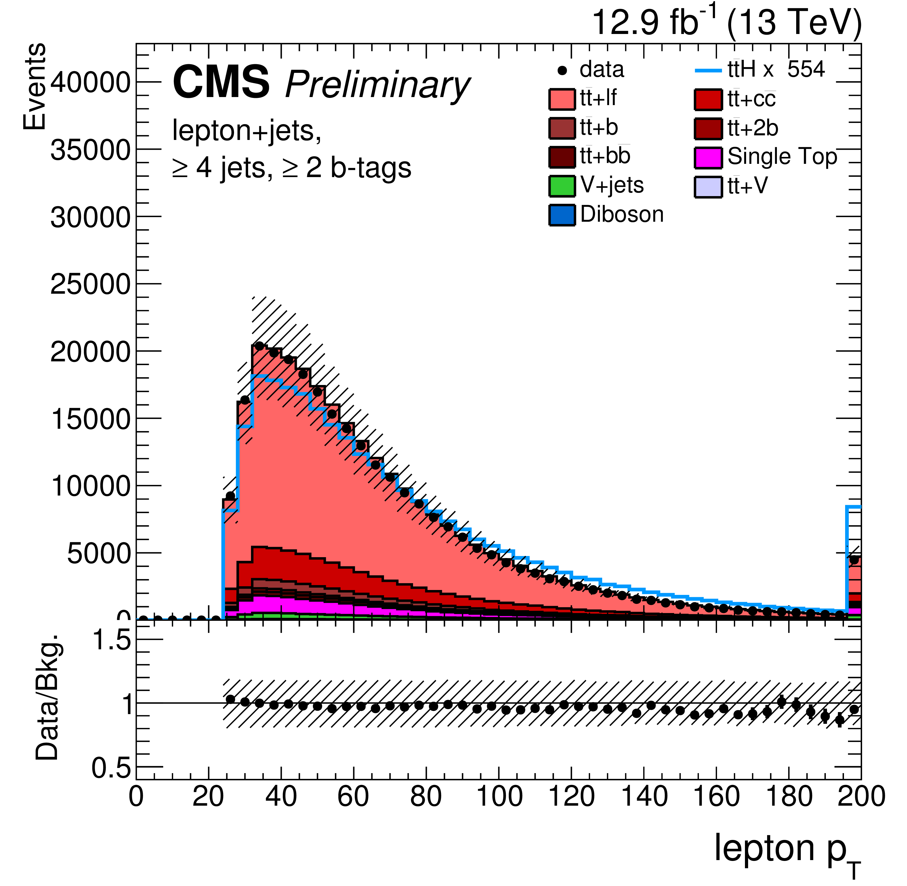
Additional Figure 2-b:
Lepton $ {p_{\mathrm {T}}} $ observed in data (markers) and expected for the SM background processes (stacked histograms) in a control region with $\geq$4 jets, $\geq$2 of which are b-tagged, in the lepton+jets channel. The expected signal distribution (line) is superimposed and scaled to the total background yield for better readability. The uncertainty bands include all uncertainties, treated as fully uncorrelated, that affect the shape of the distributions. |

png pdf |
Additional Figure 3:
The b-tagging discriminant (left) and ratio of the likelihoods (right) that an event contains four b jets or two b jets, computed from the jets' b-tagging discriminant values, of the jets observed in data (markers) and expected for the SM background processes (stacked histograms) in a control region with $\geq$4 jets, $\geq$2 of which are b-tagged, in the lepton+jets channel. The expected signal distribution (line) is superimposed and scaled to the total background yield for better readability. The uncertainty bands include all uncertainties, treated as fully uncorrelated, that affect the shape of the distributions. |

png pdf |
Additional Figure 3-a:
The b-tagging discriminant that an event contains four b jets or two b jets, computed from the jets' b-tagging discriminant values, of the jets observed in data (markers) and expected for the SM background processes (stacked histograms) in a control region with $\geq$4 jets, $\geq$2 of which are b-tagged, in the lepton+jets channel. The expected signal distribution (line) is superimposed and scaled to the total background yield for better readability. The uncertainty bands include all uncertainties, treated as fully uncorrelated, that affect the shape of the distributions. |

png pdf |
Additional Figure 3-b:
Ratio of the likelihoods that an event contains four b jets or two b jets, computed from the jets' b-tagging discriminant values, of the jets observed in data (markers) and expected for the SM background processes (stacked histograms) in a control region with $\geq$4 jets, $\geq$2 of which are b-tagged, in the lepton+jets channel. The expected signal distribution (line) is superimposed and scaled to the total background yield for better readability. The uncertainty bands include all uncertainties, treated as fully uncorrelated, that affect the shape of the distributions. |
png pdf |
Additional Figure 4:
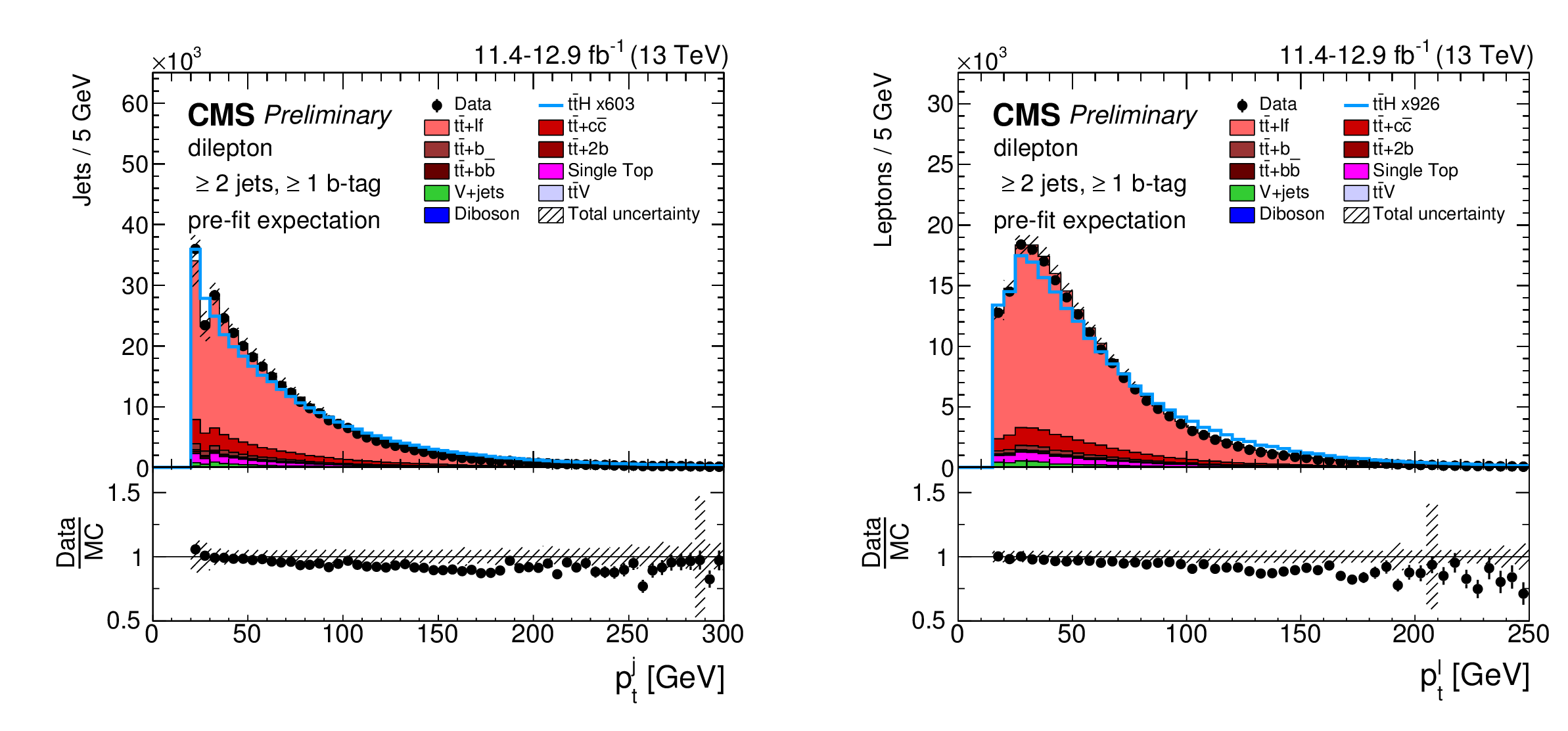
Jet (left) and lepton (right) $ {p_{\mathrm {T}}} $ observed in data (markers) and expected for the SM background processes (stacked histograms) in a control region with $\geq$2 jets, $\geq$1 of which are b-tagged, in the dilepton channel. The expected signal distribution (line) is superimposed and scaled to the total background yield for better readability. The uncertainty bands include all uncertainties, treated as fully uncorrelated, that affect the shape of the distributions. |

png pdf |
Additional Figure 4-a:
Jet $ {p_{\mathrm {T}}} $ observed in data (markers) and expected for the SM background processes (stacked histograms) in a control region with $\geq$2 jets, $\geq$1 of which are b-tagged, in the dilepton channel. The expected signal distribution (line) is superimposed and scaled to the total background yield for better readability. The uncertainty bands include all uncertainties, treated as fully uncorrelated, that affect the shape of the distributions. |

png pdf |
Additional Figure 4-b:
Lepton $ {p_{\mathrm {T}}} $ observed in data (markers) and expected for the SM background processes (stacked histograms) in a control region with $\geq$2 jets, $\geq$1 of which are b-tagged, in the dilepton channel. The expected signal distribution (line) is superimposed and scaled to the total background yield for better readability. The uncertainty bands include all uncertainties, treated as fully uncorrelated, that affect the shape of the distributions. |
png pdf |
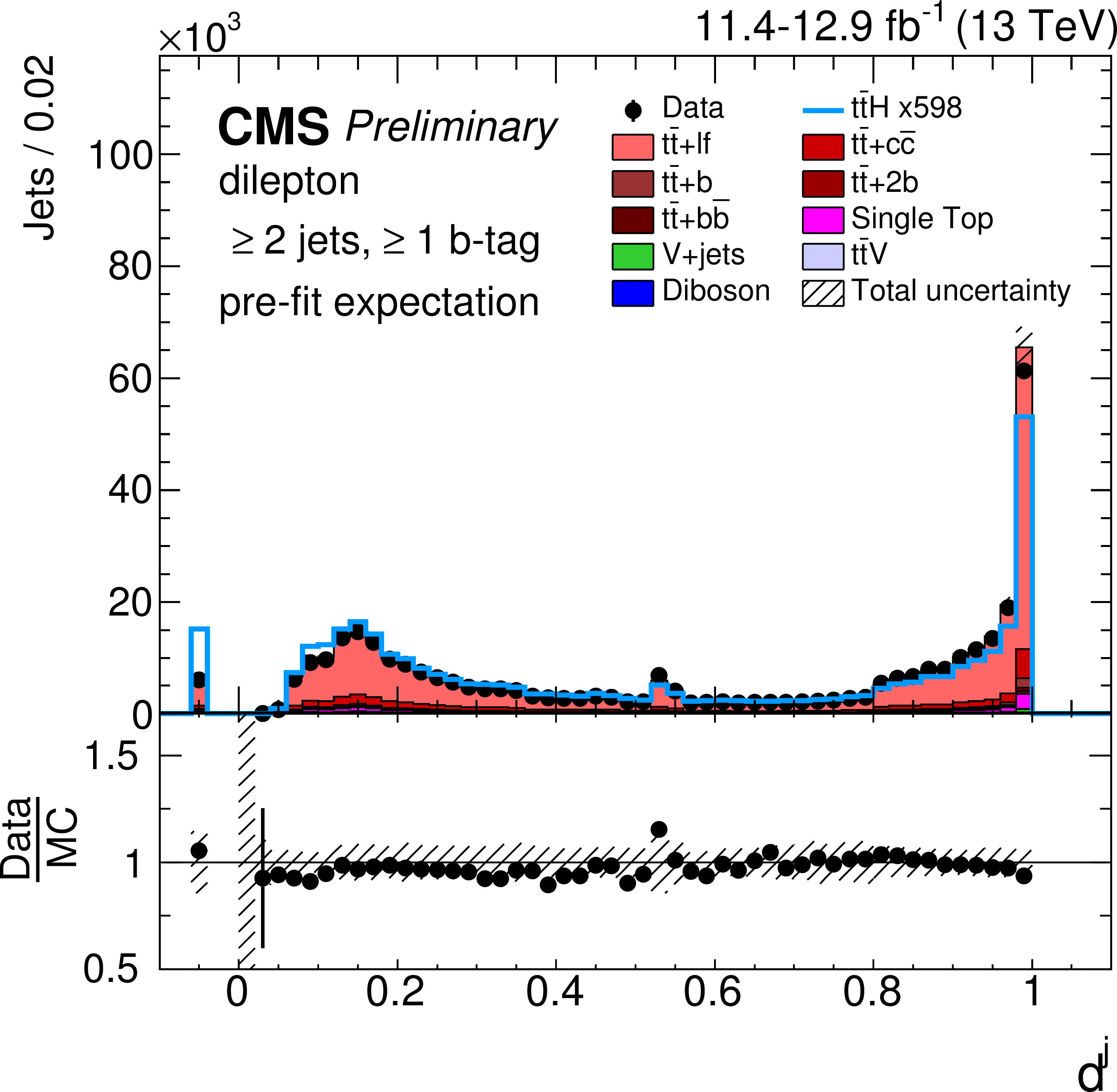
Additional Figure 5:
The b-tagging discriminant computed from the jets' b-tagging discriminant values, of the jets observed in data (markers) and expected for the SM background processes (stacked histograms) in a control region with $\geq$2 jets, $\geq$1 of which are b-tagged, in the dilepton channel. The expected signal distribution (line) is superimposed and scaled to the total background yield for better readability. The uncertainty bands include all uncertainties, treated as fully uncorrelated, that affect the shape of the distributions. |
png pdf |
Additional Figure 6:
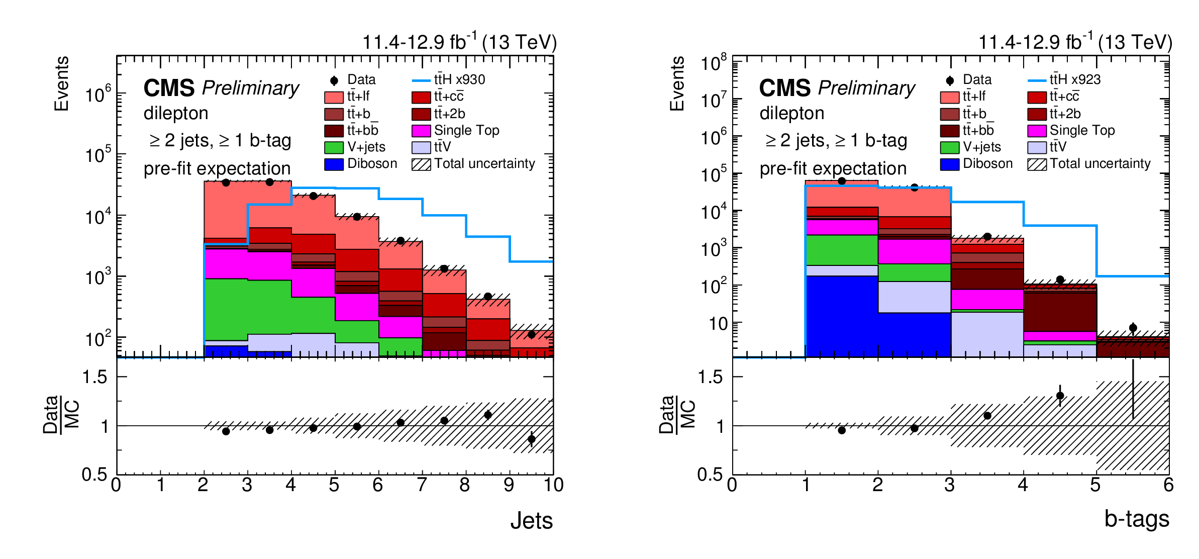
Jet (left) and b-tagged jet (right) multiplicity observed in data (markers) and expected for the SM background processes (stacked histograms) in a control region with $\geq$2 jets, $\geq$1 of which are b-tagged, in the dilepton channel. The expected signal distribution (line) is superimposed and scaled to the total background yield for better readability. The uncertainty bands include all uncertainties, treated as fully uncorrelated, that affect the shape of the distributions. |
png pdf |
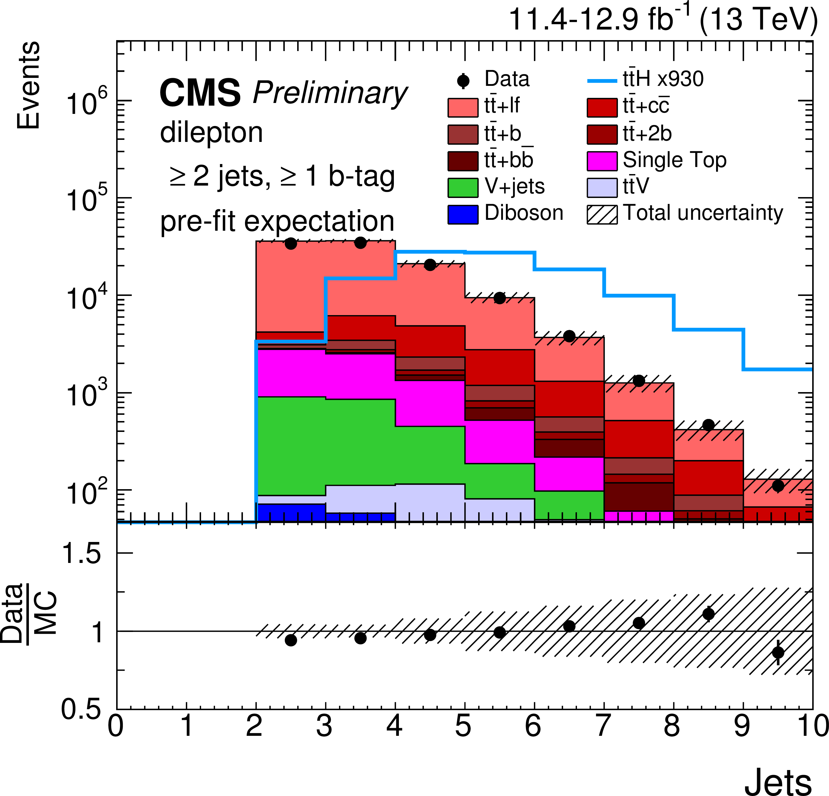
Additional Figure 6-a:
Jet multiplicity observed in data (markers) and expected for the SM background processes (stacked histograms) in a control region with $\geq$2 jets, $\geq$1 of which are b-tagged, in the dilepton channel. The expected signal distribution (line) is superimposed and scaled to the total background yield for better readability. The uncertainty bands include all uncertainties, treated as fully uncorrelated, that affect the shape of the distributions. |
png pdf |
Additional Figure 6-b:
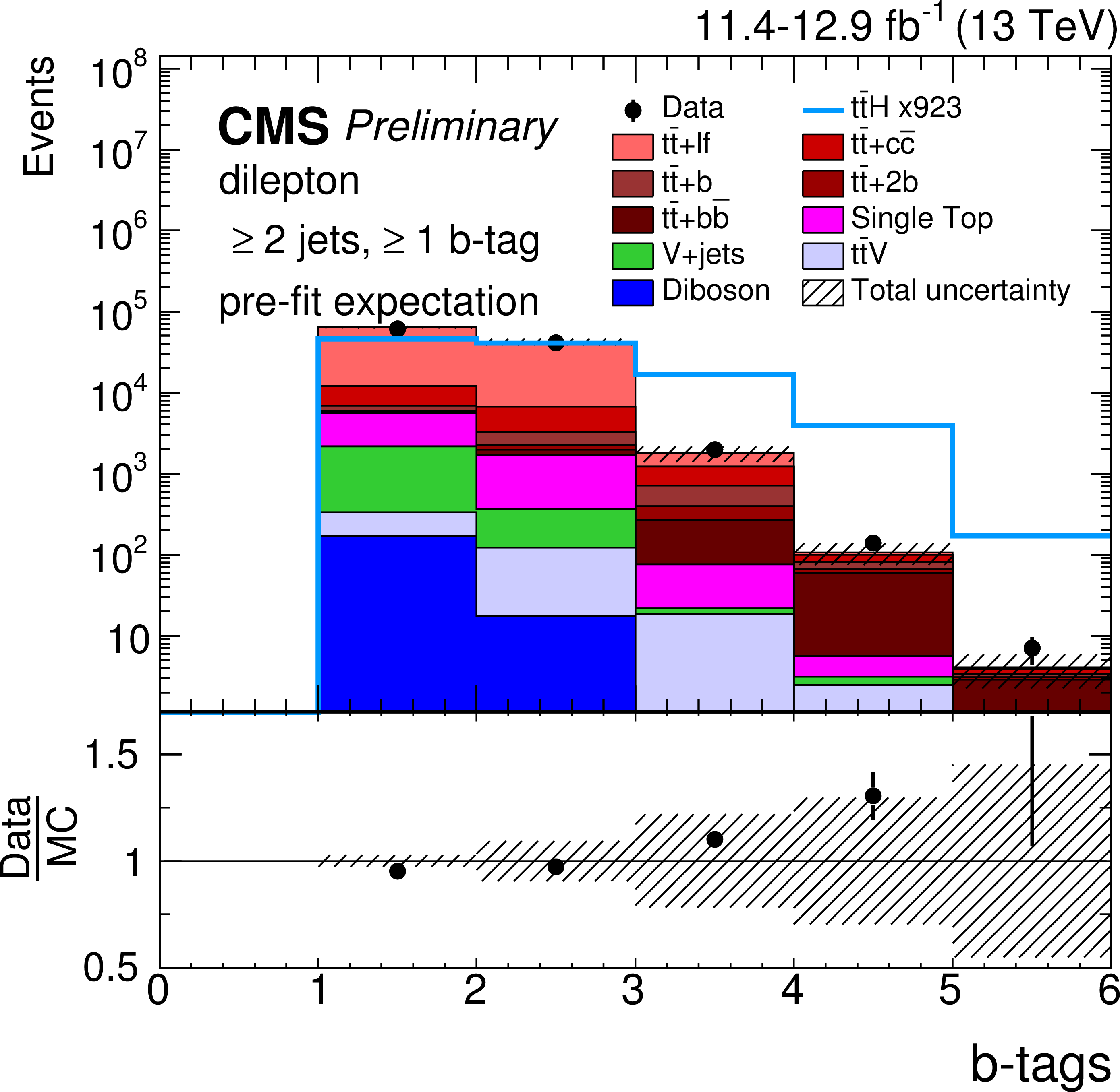
b-tagged jet multiplicity observed in data (markers) and expected for the SM background processes (stacked histograms) in a control region with $\geq$2 jets, $\geq$1 of which are b-tagged, in the dilepton channel. The expected signal distribution (line) is superimposed and scaled to the total background yield for better readability. The uncertainty bands include all uncertainties, treated as fully uncorrelated, that affect the shape of the distributions. |

png pdf |
Additional Figure 7:
Expected fraction of signal and background processes contributing to the analysis categories of the lepton+jets (top row) and dilepton (bottom row) channels. |
png pdf |
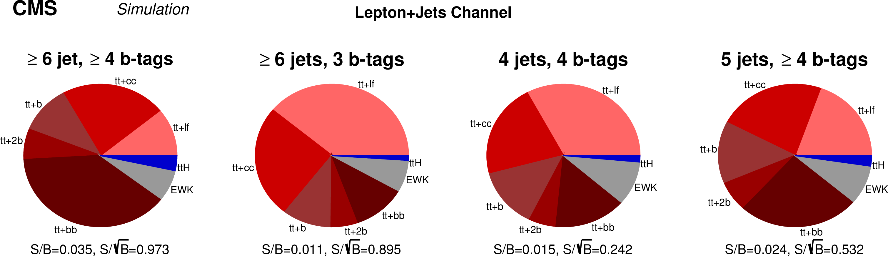
Additional Figure 7-a:
Expected fraction of signal and background processes contributing to the analysis categories of the lepton+jets channel. |
png pdf |
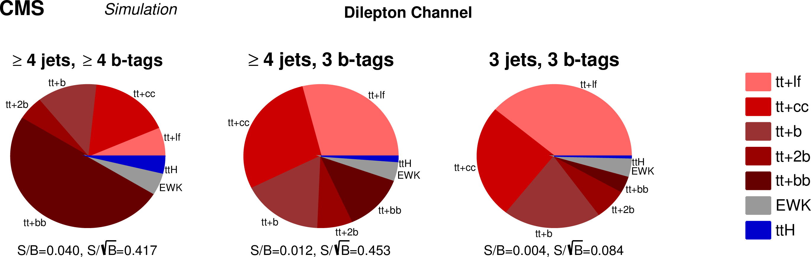
Additional Figure 7-b:
Expected fraction of signal and background processes contributing to the analysis categories of the dilepton channel. |
png pdf |
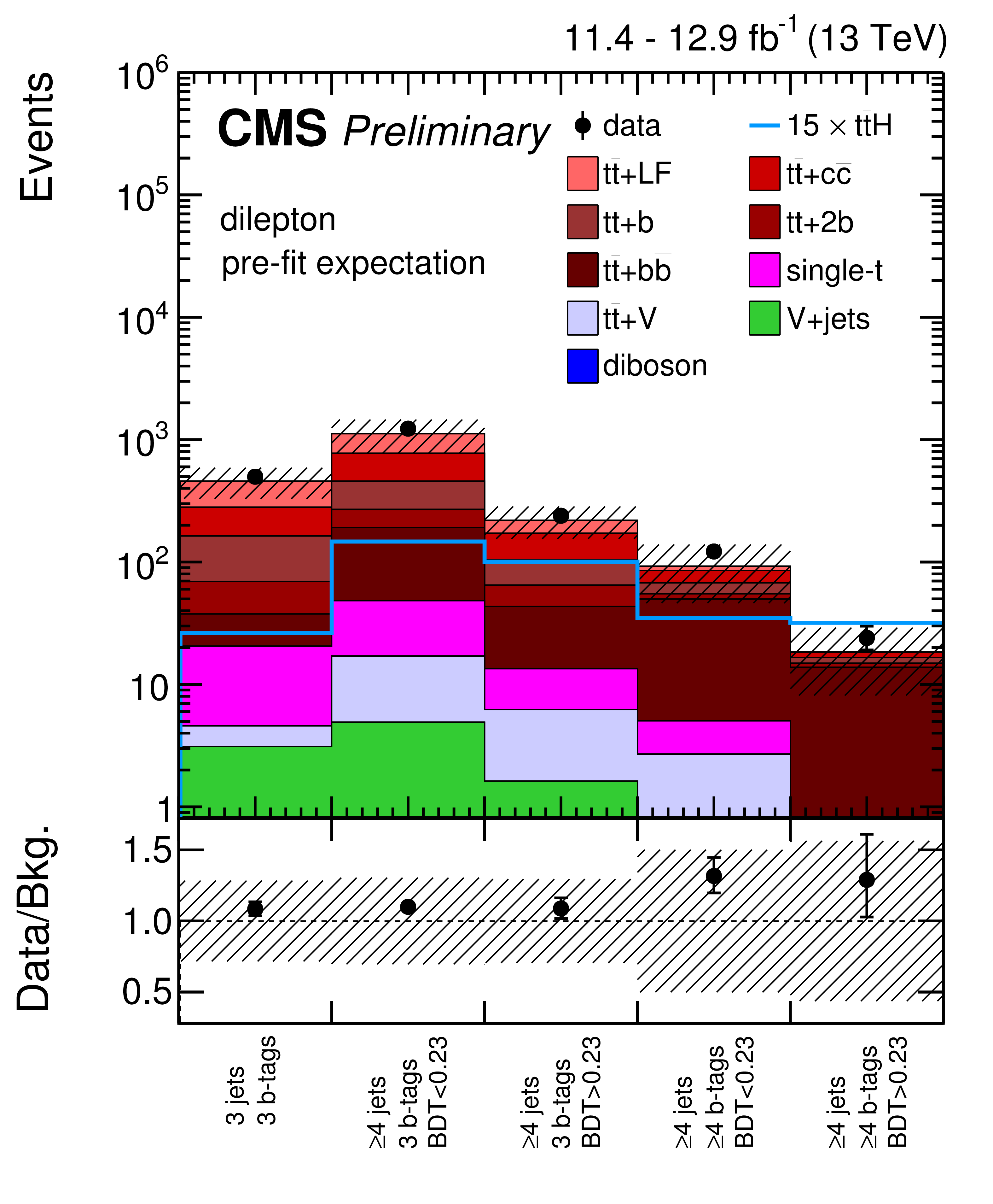
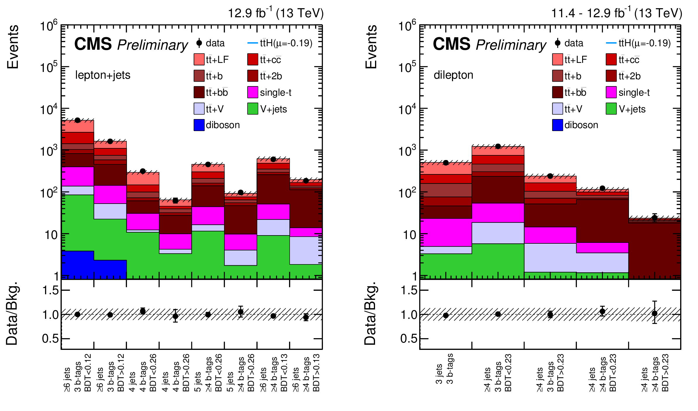
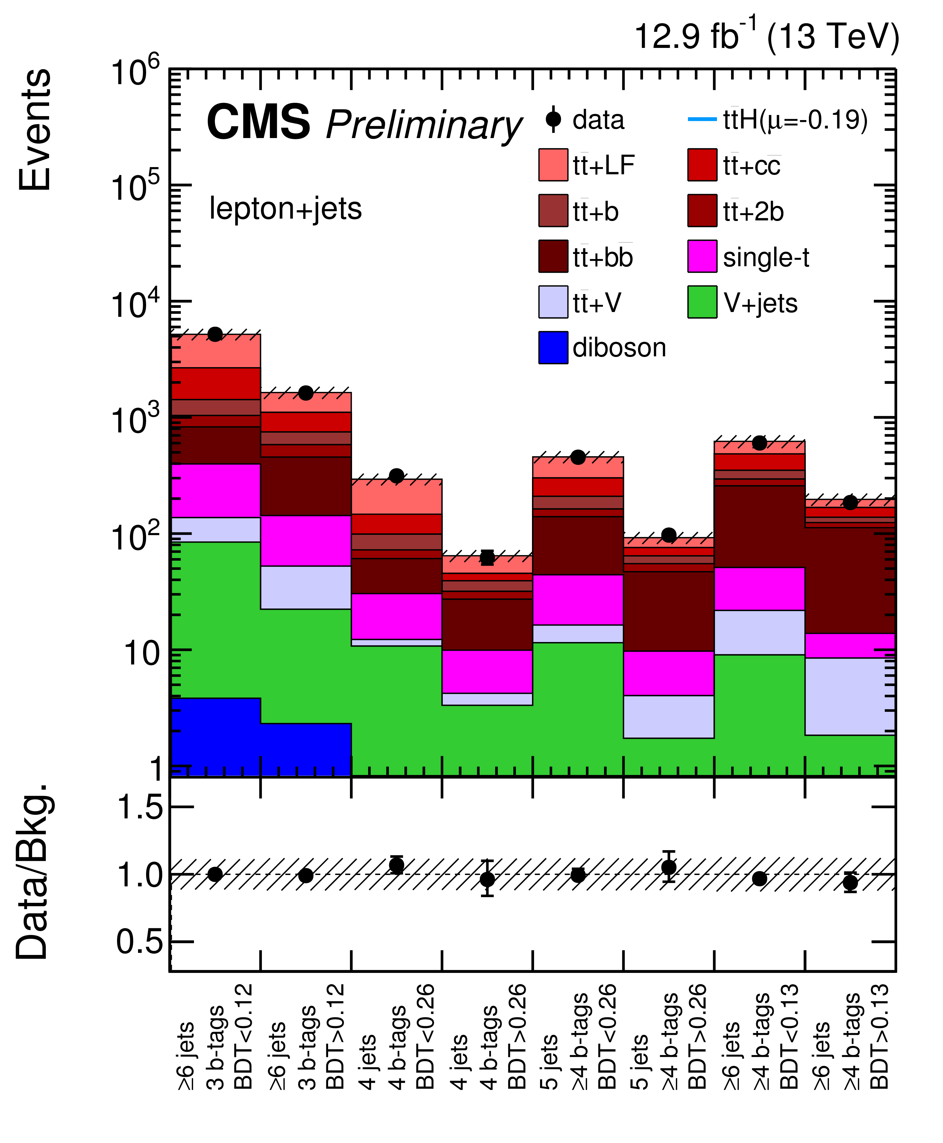
Additional Figure 8:
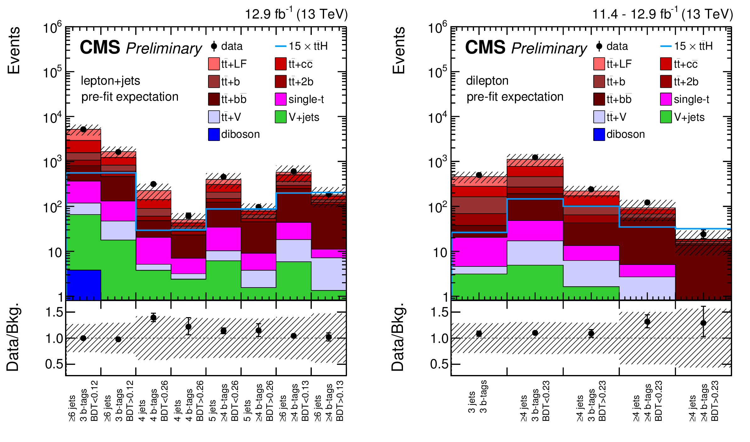
Event yields observed in data (markers) and expected for the SM background processes (stacked histograms) in the different analysis categories in the lepton+jets (left) and dilepton (right) channels prior to the fit to data. The expected signal yield (line) is superimposed and scaled by a factor of 15 for better readability. The uncertainty bands approximate the pre-fit uncertainties of the model. |

png pdf |
Additional Figure 8-a:
Event yields observed in data (markers) and expected for the SM background processes (stacked histograms) in the different analysis categories in the lepton+jets channel prior to the fit to data. The expected signal yield (line) is superimposed and scaled by a factor of 15 for better readability. The uncertainty bands approximate the pre-fit uncertainties of the model. |
png pdf |
Additional Figure 8-b:
Event yields observed in data (markers) and expected for the SM background processes (stacked histograms) in the different analysis categories in the dilepton channel prior to the fit to data. The expected signal yield (line) is superimposed and scaled by a factor of 15 for better readability. The uncertainty bands approximate the pre-fit uncertainties of the model. |
png pdf |
Additional Figure 9:
Event yields observed in data (markers) and expected for the SM background processes (stacked histograms) in the different analysis categories in the lepton+jets (left) and dilepton (right) channels after the fit to data. The uncertainty bands approximate the post-fit uncertainties of the model. |
png pdf |
Additional Figure 9-a:
Event yields observed in data (markers) and expected for the SM background processes (stacked histograms) in the different analysis categories in the lepton+jets channel after the fit to data. The uncertainty bands approximate the post-fit uncertainties of the model. |

png pdf |
Additional Figure 9-b:
Event yields observed in data (markers) and expected for the SM background processes (stacked histograms) in the different analysis categories in the dilepton channel after the fit to data. The uncertainty bands approximate the post-fit uncertainties of the model. |
png pdf |
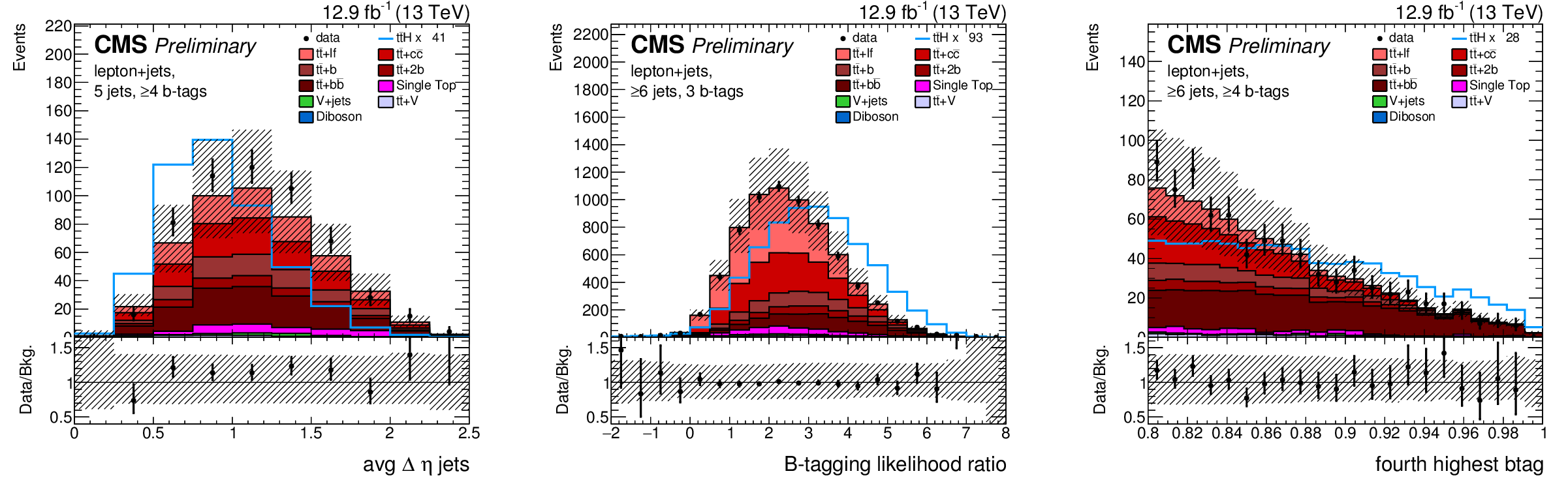
Additional Figure 10:
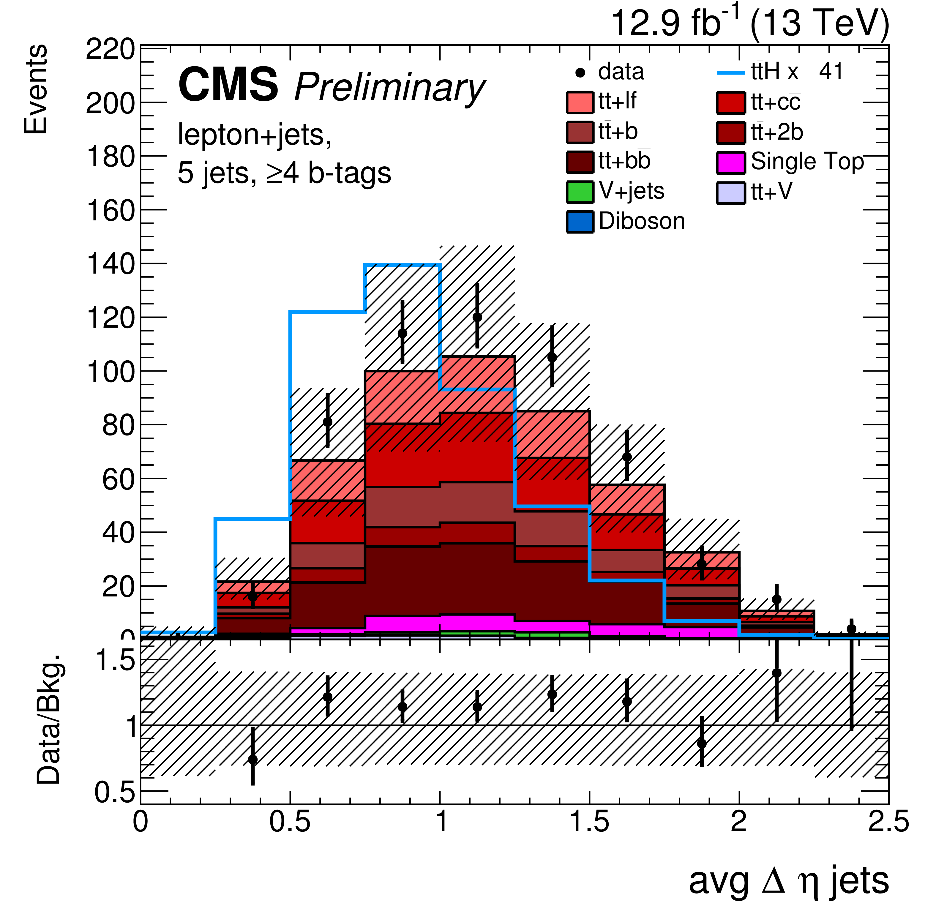
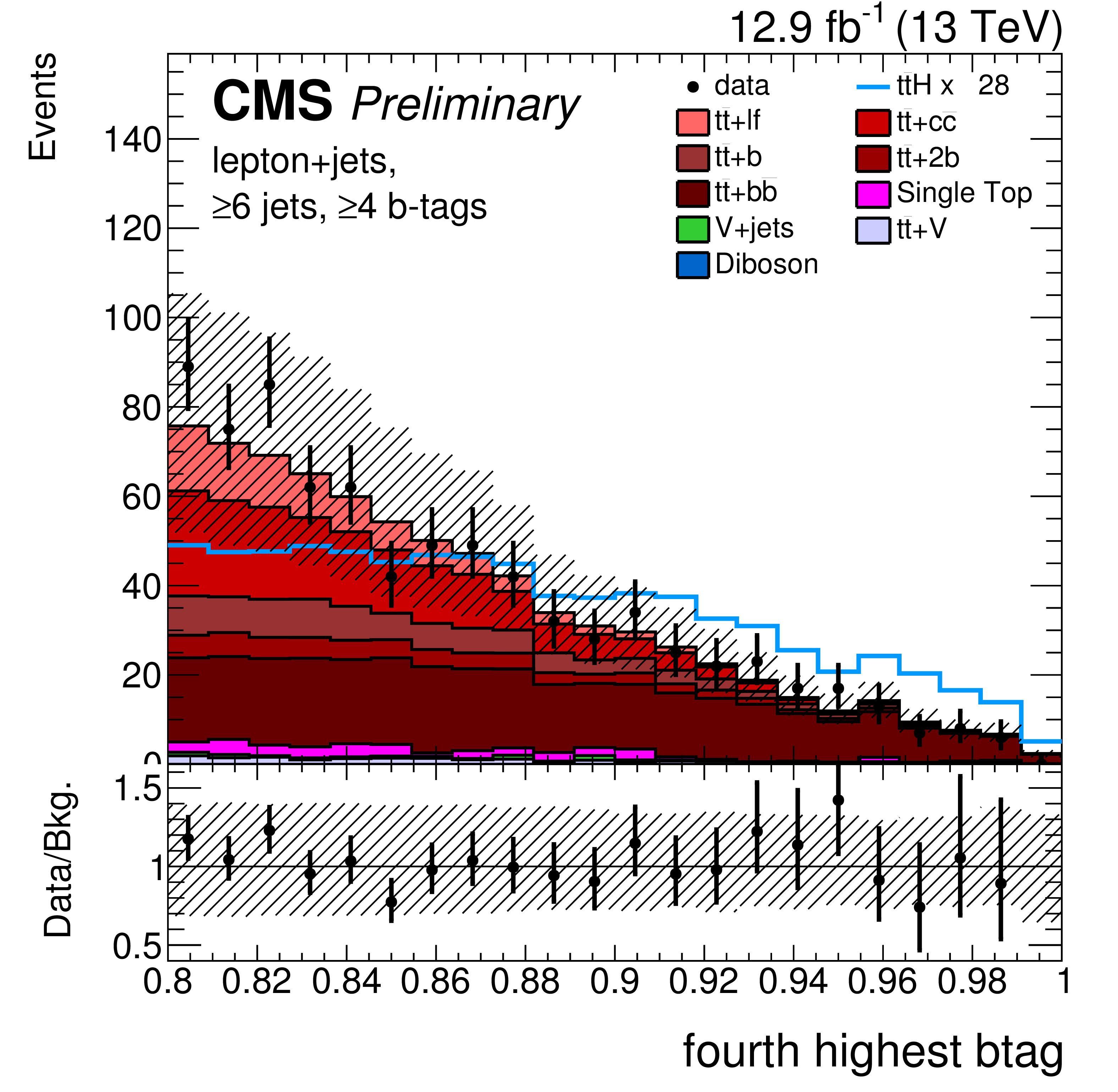
Examples of BDT input variables in three different analysis categories in the lepton+jets channel: average difference in $\eta $ between any two jets in the 5 jets, $\geq $4 b-tags category (left); ratio of the likelihoods that an event contains four b jets or two b jets, computed from the jets' b-tagging discriminant values, in the $\geq $6 jets, 3 b-jet category (middle); and fourth highest b-tagging discriminant value per event in the $\geq $6 jets, $\geq $4 b-tags category (right). Shown are the distributions observed in data (markers) and expected for the SM background processes (stacked histograms) and for the signal (line). The signal distribution is scaled to the total background yield for better readability. The uncertainty bands approximate the post-fit uncertainties of the model. |
png pdf |
Additional Figure 10-a:
Example of BDT input variable in the lepton+jets channel: average difference in $\eta $ between any two jets in the 5 jets, $\geq $4 b-tags category. Shown is the distribution observed in data (markers) and expected for the SM background processes (stacked histogram) and for the signal (line). The signal distribution is scaled to the total background yield for better readability. The uncertainty bands approximate the post-fit uncertainties of the model. |

png pdf |
Additional Figure 10-b:
Example of BDT input variable in the lepton+jets channel: ratio of the likelihoods that an event contains four b jets or two b jets, computed from the jets' b-tagging discriminant values, in the $\geq $6 jets, 3 b-jet category. Shown is the distribution observed in data (markers) and expected for the SM background processes (stacked histogram) and for the signal (line). The signal distribution is scaled to the total background yield for better readability. The uncertainty bands approximate the post-fit uncertainties of the model. |
png pdf |
Additional Figure 10-c:
Example of BDT input variable in the lepton+jets channel: fourth highest b-tagging discriminant value per event in the $\geq $6 jets, $\geq $4 b-tags category. Shown is the distribution observed in data (markers) and expected for the SM background processes (stacked histogram) and for the signal (line). The signal distribution is scaled to the total background yield for better readability. The uncertainty bands approximate the post-fit uncertainties of the model. |

png pdf |
Additional Figure 11:
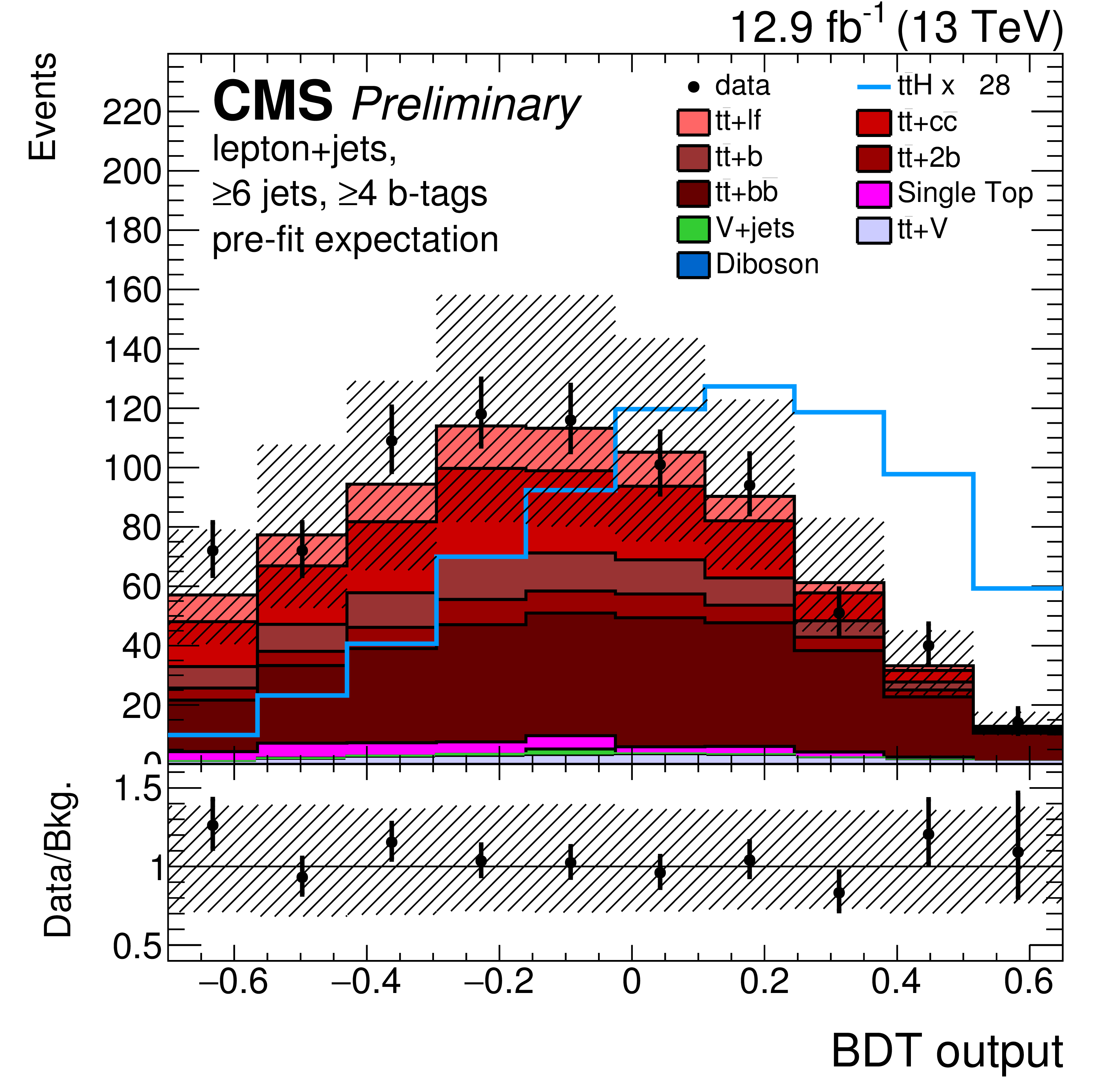
BDT output distributions observed in data (markers) and expected for the SM background processes (stacked histograms) in the four different jet and b-tag multiplicity categories of the lepton+jets channel. The expected signal distribution (line) is superimposed and scaled to the total background yield for better readability. The uncertainty bands include all uncertainties, treated as fully uncorrelated, that affect the shape of the distributions. Based on these distributions, events are further separated into categories with low and high BDT output. |

png pdf |
Additional Figure 11-a:
BDT output distribution observed in data (markers) and expected for the SM background processes (stacked histograms) in the 4 jets, 4 b-tags category of the lepton+jets channel. The expected signal distribution (line) is superimposed and scaled to the total background yield for better readability. The uncertainty band includes all uncertainties, treated as fully uncorrelated, that affect the shape of the distributions. |

png pdf |
Additional Figure 11-b:
BDT output distribution observed in data (markers) and expected for the SM background processes (stacked histograms) in the 5 jets, $\geq$4 b-tags b-tags category of the lepton+jets channel. The expected signal distribution (line) is superimposed and scaled to the total background yield for better readability. The uncertainty band includes all uncertainties, treated as fully uncorrelated, that affect the shape of the distributions. |

png pdf |
Additional Figure 11-c:
BDT output distribution observed in data (markers) and expected for the SM background processes (stacked histograms) in the $\geq$6 jets, 3 b-tags category of the lepton+jets channel. The expected signal distribution (line) is superimposed and scaled to the total background yield for better readability. The uncertainty band includes all uncertainties, treated as fully uncorrelated, that affect the shape of the distributions. |
png pdf |
Additional Figure 11-d:
BDT output distribution observed in data (markers) and expected for the SM background processes (stacked histograms) in the $\geq$6 jets, $\geq$4 b-tags category of the lepton+jets channel. The expected signal distribution (line) is superimposed and scaled to the total background yield for better readability. The uncertainty band includes all uncertainties, treated as fully uncorrelated, that affect the shape of the distributions. |

png pdf |
Additional Figure 12:
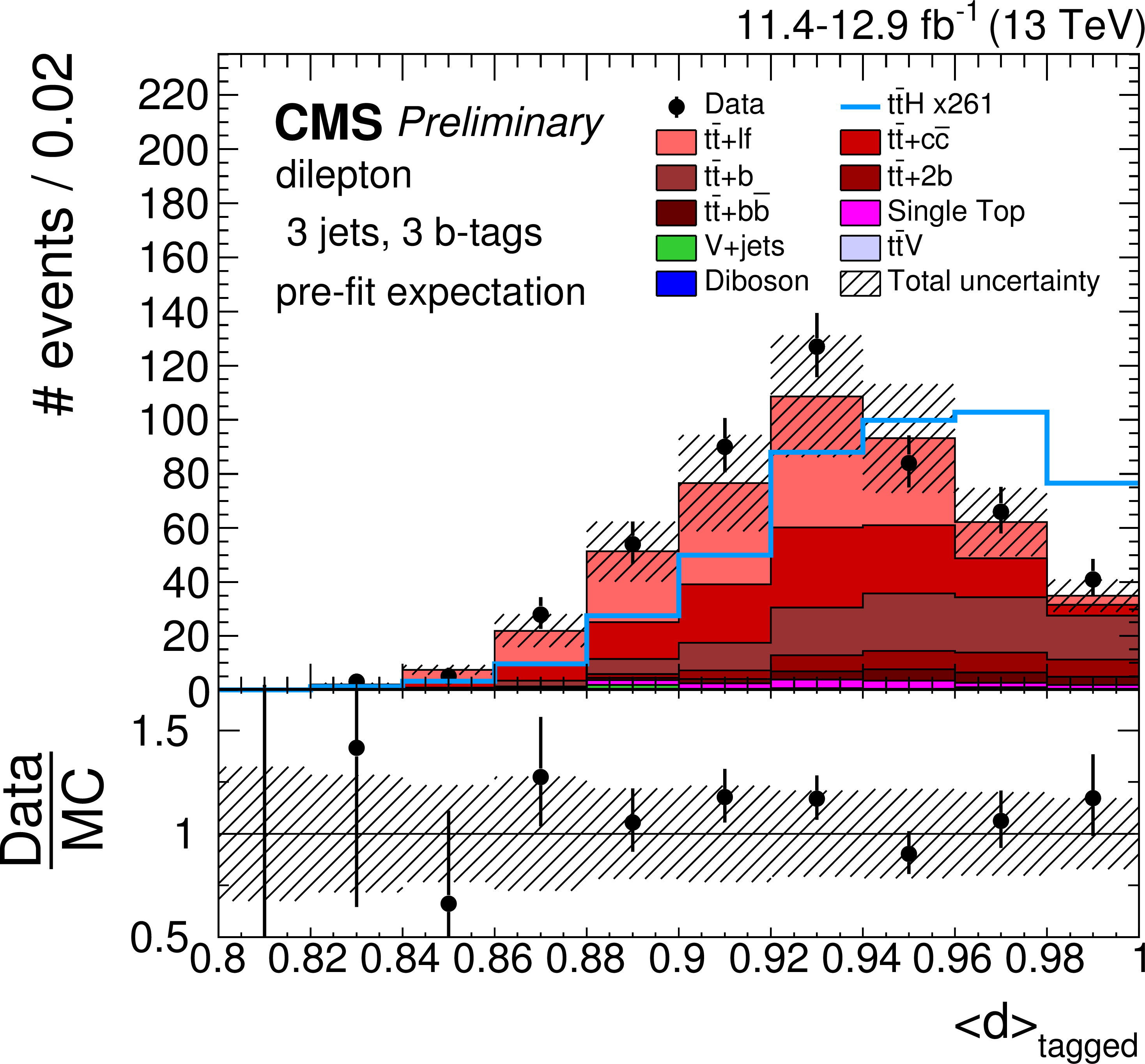
Examples of BDT input variables in three different analysis categories in the dilepton channel: average b-tag discriminant value of all jets passing the medium b-tagging working point selection in the 3 jets, 3 b-tags category (left); twist angle ($\tau $) in the $\geq $4 jets, 3 b-tags category (middle), defined as the inverse tangent of the ratio of the $\Delta \phi $ to $\Delta \eta $ of the b-tagged jets with the maximum mass combination in the event; and centrality of the events in the $\geq $4 jets, $\geq $4 b-tags category (right), defined as the ratio of the sum of the transverse momentum of all b-tagged jets and their total energy. Shown are the distributions observed in data (markers) and expected for the SM background processes (stacked histograms) and for the signal (line). The signal distribution is scaled to the total background yield for better readability. The uncertainty bands approximate the post-fit uncertainties of the model. |
png pdf |
Additional Figure 12-a:
Example of BDT input variable in the 3 jets, 3 b-tags category of the dilepton channel: average b-tag discriminant value of all jets passing the medium b-tagging working point selection. Shown is the distribution observed in data (markers) and expected for the SM background processes (stacked histograms) and for the signal (line). The signal distribution is scaled to the total background yield for better readability. The uncertainty band approximates the post-fit uncertainties of the model. |

png pdf |
Additional Figure 12-b:
Example of BDT input variable in the $\geq $4 jets, 3 b-tags category of the dilepton channel: twist angle ($\tau $), defined as the inverse tangent of the ratio of the $\Delta \phi $ to $\Delta \eta $ of the b-tagged jets with the maximum mass combination in the event. Shown is the distribution observed in data (markers) and expected for the SM background processes (stacked histograms) and for the signal (line). The signal distribution is scaled to the total background yield for better readability. The uncertainty band approximates the post-fit uncertainties of the model. |

png pdf |
Additional Figure 12-c:
Example of BDT input variable in the $\geq $4 jets, $\geq $4 b-tags category of the dilepton channel: centrality of the events, defined as the ratio of the sum of the transverse momentum of all b-tagged jets and their total energy. Shown is the distribution observed in data (markers) and expected for the SM background processes (stacked histograms) and for the signal (line). The signal distribution is scaled to the total background yield for better readability. The uncertainty band approximates the post-fit uncertainties of the model. |

png pdf |
Additional Figure 13:
BDT output distributions observed in data (markers) and expected for the SM background processes (stacked histograms) in the two $\geq$4 jets categories of the dilepton channel. The expected signal distribution (line) is superimposed and scaled to the total background yield for better readability. The uncertainty bands include all uncertainties, treated as fully uncorrelated, that affect the shape of the distributions. Based on these distributions, events are further separated into categories with low and high BDT output. |
png pdf |
Additional Figure 13-a:
BDT output distribution observed in data (markers) and expected for the SM background processes (stacked histograms) in the $\geq$4 jets, 3 b-tags category of the dilepton channel. The expected signal distribution (line) is superimposed and scaled to the total background yield for better readability. The uncertainty band includes all uncertainties, treated as fully uncorrelated, that affect the shape of the distributions. |

png pdf |
Additional Figure 13-b:
BDT output distribution observed in data (markers) and expected for the SM background processes (stacked histograms) in the $\geq$4 jets, $\geq$4 b-tags category of the dilepton channel. The expected signal distribution (line) is superimposed and scaled to the total background yield for better readability. The uncertainty band includes all uncertainties, treated as fully uncorrelated, that affect the shape of the distributions. |
png pdf |
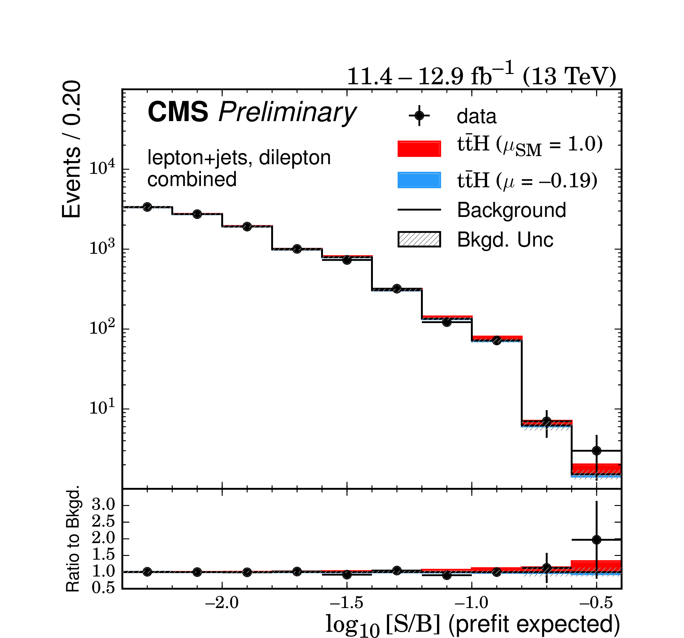
Additional Figure 14:
The bins of the final discriminants as used in the fit, reordered by the pre-fit expected signal over background ratio (S/B). Each bin on this plot includes multiple bins of the final discriminants with similar S/B. The background is shown post-fit (S+B), with the fitted signal in azure. The SM signal expectation is shown in red for comparison. |
| References | ||||
| 1 | ATLAS Collaboration | Observation of a new particle in the search for the Standard Model Higgs boson with the ATLAS detector at the LHC | PLB 716 (2012) 1, 1--29 | 1207.7214 |
| 2 | CMS Collaboration | Observation of a new boson at a mass of 125 GeV with the CMS experiment at the LHC | PLB 716 (2012) 1, 30--61 | CMS-HIG-12-028 1207.7235 |
| 3 | CMS Collaboration | Evidence for the direct decay of the 125 GeV Higgs boson to fermions | Nature Phys. 10 (2014) 5, 557--560 | CMS-HIG-13-033 1401.6527 |
| 4 | ATLAS Collaboration | Evidence for the Higgs-boson Yukawa coupling to tau leptons with the ATLAS detector | JHEP 04 (2015) 117 | 1501.04943 |
| 5 | ATLAS Collaboration | Measurements of Higgs boson production and couplings in diboson final states with the ATLAS detector at the LHC | PLB 726 (2013) 1-3, 88 | 1307.1427 |
| 6 | CMS Collaboration | Precise determination of the mass of the Higgs boson and tests of compatibility of its couplings with the standard model predictions using proton collisions at 7 and 8 TeV | EPJC. 75 (2015) 5, 212 | CMS-HIG-14-009 1412.8662 |
| 7 | ATLAS Collaboration | Evidence for the spin-0 nature of the Higgs boson using ATLAS data | PLB 726 (2013) 1-3, 120--144 | 1307.1432 |
| 8 | CMS Collaboration | Constraints on the spin-parity and anomalous HVV couplings of the Higgs boson in proton collisions at 7 and 8 TeV | PRD 92 (2015) 1, 012004 | CMS-HIG-14-018 1411.3441 |
| 9 | LHC Higgs Cross Section Working Group Collaboration | Handbook of LHC Higgs Cross Sections: 4. Deciphering the Nature of the Higgs Sector | 1610.07922 | |
| 10 | G. Burdman, M. Perelstein, and A. Pierce | Large Hadron Collider tests of a little Higgs model | PRL 90 (2003) 24, 241802 | hep-ph/0212228 |
| 11 | T. Han, H. E. Logan, B. McElrath, and L.-T. Wang | Phenomenology of the little Higgs model | PRD 67 (2003) 9, 095004 | hep-ph/0301040 |
| 12 | M. Perelstein, M. E. Peskin, and A. Pierce | Top quarks and electroweak symmetry breaking in little Higgs models | PRD 69 (2004) 7, 075002 | hep-ph/0310039 |
| 13 | H.-C. Cheng, I. Low, and L.-T. Wang | Top partners in little Higgs theories with T-parity | PRD 74 (2006) 5, 055001 | hep-ph/0510225 |
| 14 | H.-C. Cheng, B. A. Dobrescu, and C. T. Hill | Electroweak symmetry breaking and extra dimensions | Nucl. Phys. B. 589 (2000) 1-3, 249--268 | hep-ph/9912343 |
| 15 | M. Carena, E. Ponton, J. Santiago, and C. E. M. Wagner | Light Kaluza Klein States in Randall-Sundrum Models with Custodial SU(2) | Nucl. Phys. B. 759 (2006) 1-2, 202--227 | hep-ph/0607106 |
| 16 | R. Contino, L. Da Rold, and A. Pomarol | Light custodians in natural composite Higgs models | PRD 75 (2007) 5, 055014 | hep-ph/0612048 |
| 17 | G. Burdman and L. Da Rold | Electroweak Symmetry Breaking from a Holographic Fourth Generation | JHEP 12 (2007) 086 | 0710.0623 |
| 18 | C. T. Hill | Topcolor: Top quark condensation in a gauge extension of the standard model | PLB 266 (1991) 3, 419--424 | |
| 19 | A. Carmona, M. Chala, and J. Santiago | New Higgs Production Mechanism in Composite Higgs Models | JHEP 07 (2012) 049 | 1205.2378 |
| 20 | CMS Collaboration | Search for the associated production of the Higgs boson with a top-quark pair | JHEP 09 (2014) 087 | CMS-HIG-13-029 1408.1682 |
| 21 | ATLAS Collaboration | Search for the associated production of the Higgs boson with a top quark pair in multilepton final states with the ATLAS detector | PLB 749 (2015) 519--541 | 1506.05988 |
| 22 | J. M. Campbell et al. | The Matrix Element Method at Next-to-Leading Order | JHEP 11 (2012) 043 | |
| 23 | CMS Collaboration | Search for a standard model Higgs boson produced in association with a top-quark pair and decaying to bottom quarks using a matrix element method | EPJC. 75 (2015) 6, 251 | CMS-HIG-14-010 1502.02485 |
| 24 | ATLAS Collaboration | Search for the Standard Model Higgs boson produced in association with top quarks and decaying into $ b\bar{b} $ in pp collisions at $ \sqrt{s} $ = 8 TeV with the ATLAS detector | EPJC. 75 (2015) 7, 349 | 1503.05066 |
| 25 | LHC Higgs Cross Section Working Group Collaboration | Handbook of LHC Higgs Cross Sections: 1. Inclusive Observables | 1101.0593 | |
| 26 | CMS Collaboration | Updated measurements of Higgs boson production in the diphoton decay channel at $ \sqrt{s}= $ 13 TeV in pp collisions at CMS. | ||
| 27 | CMS Collaboration | Search for associated production of Higgs bosons and top quarks in multilepton final states at $ \sqrt{s}= $ 13 TeV | ||
| 28 | ATLAS Collaboration | Measurement of fiducial, differential and production cross sections in the $ H\to\gamma\gamma $ decay channel with 13.3 fb$ ^{-1} $ of 13 TeV proton-proton collision data with the ATLAS detector | ATLAS-CONF-2016-067 | |
| 29 | ATLAS Collaboration | Search for the Associated Production of a Higgs Boson and a Top Quark Pair in Multilepton Final States with the ATLAS Detector | ATLAS-CONF-2016-058 | |
| 30 | CMS Collaboration | Search for $ \mathrm{t\overline{t}H} $ production in the $ \mathrm{H}\rightarrow \mathrm{b\overline{b}} $ decay channel with $ \sqrt{s}= $ 13 TeV pp collisions at the CMS experiment | CMS-PAS-HIG-16-004 | CMS-PAS-HIG-16-004 |
| 31 | T. J. Hastie, R. J. Tibshirani, and J. H. Friedman | The elements of statistical learning : data mining, inference, and prediction | Springer series in statistics. Springer, New York, 2013 | |
| 32 | P. C. Bhat | Multivariate Analysis Methods in Particle Physics | Annual Review of Nuclear and Particle Science 61 (2011) 1, 281 | |
| 33 | A. Hocker et al. | TMVA: Toolkit for Multivariate Data Analysis | PoS ACAT (2007) 040 | physics/0703039 |
| 34 | K. Kondo | Dynamical Likelihood Method for Reconstruction of Events With Missing Momentum. 1: Method and Toy Models | J. Phys. Soc. Jap. 57 (1988) 4126--4140 | |
| 35 | D0 Collaboration | A precision measurement of the mass of the top quark | Nature 429 (2004) 638--642 | hep-ex/0406031 |
| 36 | CMS Collaboration | The CMS experiment at the CERN LHC | JINST 3 (2008) 8, S08004 | CMS-00-001 |
| 37 | GEANT4 Collaboration | GEANT4---a simulation toolkit | NIMA 506 (2003) 3, 250 | |
| 38 | S. Frixione, P. Nason, and C. Oleari | Matching NLO QCD computations with parton shower simulations: the POWHEG method | JHEP 11 (2007) 070 | 0709.2092 |
| 39 | E. Re | Single-top Wt-channel production matched with parton showers using the POWHEG method | EPJC 71 (2011) 1547 | 1009.2450 |
| 40 | NNPDF Collaboration | Parton distributions for the LHC Run II | JHEP 04 (2015) 040 | 1410.8849 |
| 41 | T. Sjostrand et al. | An introduction to PYTHIA 8.2 | CPC 191 (2015) 159 | 1410.3012 |
| 42 | J. Alwall et al. | The automated computation of tree-level and next-to-leading order differential cross sections, and their matching to parton shower simulations | JHEP 07 (2014) 079 | 1405.0301 |
| 43 | R. Frederix and S. Frixione | Merging meets matching in MC@NLO | JHEP 12 (2012) 061 | 1209.6215 |
| 44 | CMS Collaboration | Underlying event tunes and double parton scattering | CDS | |
| 45 | P. Skands, S. Carrazza, and J. Rojo | Tuning PYTHIA 8.1: the Monash 2013 Tune | EPJC 74 (2014) 8 | 1404.5630 |
| 46 | N. Kidonakis | Two-loop soft anomalous dimensions for single top quark associated production with $ \mathrm{W^-} $ or $ \mathrm{H^-} $ | PRD 82 (2010) 5, 054018 | hep-ph/1005.4451 |
| 47 | J. M. Campbell, R. K. Ellis, and C. Williams | Vector boson pair production at the LHC | JHEP 07 (2011) 018 | 1105.0020 |
| 48 | F. Maltoni, D. Pagani, and I. Tsinikos | Associated production of a top-quark pair with vector bosons at NLO in QCD: impact on $ t \bar{t} H $ searches at the LHC | 1507.05640 | |
| 49 | W. Beenakker et al. | Higgs radiation off top quarks at the Tevatron and the LHC | PRL 87 (2001) 20, 201805 | hep-ph/0107081 |
| 50 | W. Beenakker et al. | NLO QCD corrections to $ \mathrm{ t \bar{t} }\mathrm{ H } $ production in hadron collisions | Nucl. Phys. B 653 (2003) 1-2, 151 | hep-ph/0211352 |
| 51 | S. Dawson, L. H. Orr, L. Reina, and D. Wackeroth | Associated top quark Higgs boson production at the LHC | PRD 67 (2003) 7, 071503 | hep-ph/0211438 |
| 52 | S. Dawson et al. | Associated Higgs production with top quarks at the large hadron collider: NLO QCD corrections | PRD 68 (2003) 3, 034022 | hep-ph/0305087 |
| 53 | A. Djouadi, J. Kalinowski, and M. Spira | HDECAY: A program for Higgs boson decays in the standard model and its supersymmetric extension | CPC 108 (1998) 1, 56 | hep-ph/9704448 |
| 54 | A. Djouadi, M. M. Muhlleitner, and M. Spira | Decays of supersymmetric particles: The Program SUSY-HIT (SUspect-SdecaY-Hdecay-InTerface) | Acta Phys. Polon. B 38 (2007) 635 | hep-ph/0609292 |
| 55 | A. Bredenstein, A. Denner, S. Dittmaier, and M. M. Weber | Precise predictions for the Higgs-boson decay $ \mathrm{ H } \to \mathrm{ W }\mathrm{ W }/\mathrm{ Z }\mathrm{ Z } \to 4 $ leptons | PRD 74 (2006) 1, 013004 | hep-ph/0604011 |
| 56 | A. Bredenstein, A. Denner, S. Dittmaier, and M. M. Weber | Radiative corrections to the semileptonic and hadronic Higgs-boson decays $ \mathrm{ H } \to \mathrm{ W }\mathrm{ W }/\mathrm{ Z }\mathrm{ Z } \to 4 $ fermions | JHEP 02 (2007) 080 | hep-ph/0611234 |
| 57 | M. Cacciari et al. | Top-pair production at hadron colliders with next-to-next-to-leading logarithmic soft-gluon resummation | PLB 710 (2012) 4-5, 612 | 1111.5869 |
| 58 | P. Baernreuther et al. | Percent Level Precision Physics at the Tevatron: First Genuine NNLO QCD Corrections to $ q\bar{q}\rightarrow t\bar{t} +X $ | PRL 109 (2012) 13, 132001 | 1204.5201 |
| 59 | M. Czakon and A. Mitov | NNLO corrections to top-pair production at hadron colliders: the all-fermionic scattering channels | JHEP 12 (2012) 054 | 1207.0236 |
| 60 | M. Czakon and A. Mitov | NNLO corrections to top-pair production at hadron colliders: the quark-gluon reaction | JHEP 01 (2013) 080 | 1210.6832 |
| 61 | M. Beneke et al. | Hadronic top-quark pair production with NNLL threshold resummation | Nucl. Phys. B 855 (2012) 3, 695 | 1109.1536 |
| 62 | M. Czakon, P. Fiedler, and A. Mitov | Total Top-Quark Pair-Production Cross Section at Hadron Colliders Through $ O({\alpha_S}^4) $ | PRL 110 (2013) 25, 252004 | 1303.6254 |
| 63 | M. Czakon and A. Mitov | Top++: A Program for the Calculation of the Top-Pair Cross-Section at Hadron Colliders | CPC 185 (2014) 11 | 1112.5675 |
| 64 | CMS Collaboration | Particle--flow event reconstruction in CMS and performance for jets, taus, and $ E_{\mathrm{T}}^{\text{miss}} $ | CDS | |
| 65 | CMS Collaboration | Commissioning of the particle-flow event reconstruction with the first LHC collisions recorded in the CMS detector | CDS | |
| 66 | M. Cacciari, G. P. Salam, and G. Soyez | The anti-$ k_t $ jet clustering algorithm | JHEP 04 (2008) 063 | 0802.1189 |
| 67 | M. Cacciari, G. P. Salam, and G. Soyez | FastJet User Manual | EPJC72 (2012) 1896 | 1111.6097 |
| 68 | M. Cacciari, G. P. Salam, and G. Soyez | The catchment area of jets | JHEP 04 (2008) 005 | 0802.1188 |
| 69 | CMS Collaboration | Determination of jet energy calibration and transverse momentum resolution in CMS | JINST 6 (2011) 11, P11002 | CMS-JME-10-011 1107.4277 |
| 70 | CMS Collaboration | Identification of b-quark jets with the CMS experiment | JINST 8 (2013) 4, P04013 | CMS-BTV-12-001 1211.4462 |
| 71 | CMS Collaboration | Identification of b quark jets at the CMS Experiment in the LHC Run 2 | CMS-PAS-BTV-15-001 | CMS-PAS-BTV-15-001 |
| 72 | J. H. Friedman | Stochastic gradient boosting | Computational Statistics \& Data Analysis 38 (2002) 4, 367, . Nonlinear Methods and Data Mining | |
| 73 | J. Kennedy and R. Eberhart | Particle swarm optimization | in Proceedings of the IEEE International Conference on neural networks, volume 4, 1995 | |
| 74 | CMS Collaboration | CMS Luminosity Measurement for the 2015 Data Taking Period | CMS-PAS-LUM-15-001 | CMS-PAS-LUM-15-001 |
| 75 | R. J. Barlow and C. Beeston | Fitting using finite Monte Carlo samples | CPC 77 (1993) 2, 219--228 | |
| 76 | J. S. Conway | Incorporating Nuisance Parameters in Likelihoods for Multisource Spectra | in Proceedings, PHYSTAT 2011 Workshop on Statistical Issues Related to Discovery Claims in Search Experiments and Unfolding, CERN, 2011 | 1103.0354 |
| 77 | A. Read | Modified frequentist analysis of search results (the $ {CL}_s $ method) | CERN-OPEN-2000-005, CERN | |
| 78 | T. Junk | Confidence level computation for combining searches with small statistics | NIMA 434 (1999) 2-3, 435 | hep-ex/9902006 |
| 79 | G. Cowan, K. Cranmer, E. Gross, and O. Vitells | Asymptotic formulae for likelihood-based tests of new physics | EPJC71 (2011) 1554 | 1007.1727 |
| 80 | J. D. Bjorken and S. J. Brodsky | Statistical Model for Electron-Positron Annihilation into Hadrons | PRD 1 (Mar, 1970) 1416--1420 | |
| 81 | G. Fox and S. Wolfram | Event shapes in $ e^{+}e^{-} $ annihilation | Nuclear Physics B 157 (1979) 3, 543--544 | |
|
|
Compact Muon Solenoid LHC, CERN |
|

|

|

|

|

|