

Compact Muon Solenoid
LHC, CERN
| CMS-PAS-HIG-19-011 | ||
| Measurement of the ttH and tH production rates in the H $ \to\mathrm{b\overline{b}} $ decay channel with 138 fb$ ^{-1} $ of proton-proton collision data at $ \sqrt{s}= $ 13 TeV | ||
| CMS Collaboration | ||
| 22 August 2023 | ||
| Abstract: An analysis of the production of a Higgs boson (H) in association with a top quark-antiquark pair (ttH) or a single top quark (tH) in the channel where the Higgs boson decays into a bottom quark-antiquark pair (H $\to\mathrm{b\overline{b}} $) is presented. The analysis utilises proton-proton collision data collected at the CERN LHC with the CMS experiment at $ \sqrt{s}= $ 13 TeV between 2016 and 2018, which correspond to an integrated luminosity of 138 fb$ ^{-1} $. All three decay channels of the $ \mathrm{t\overline{t}} $ system are considered. Various signal interpretations are performed. The observed ttH production rate relative to the standard model (SM) expectation is 0.33 $ \pm $ 0.26 $ = $ 0.33 $ \pm $ 0.17 (stat) $ \pm $ 0.21 (syst). Additionally, the ttH production rate is determined in intervals of Higgs boson $ p_{\mathrm{T}} $. An upper limit at 95% confidence level on the tH production rate of 14.6 times the SM expectation is observed, with an expectation of 19.3 $ ^{+9.2}_{-6.0} $. Finally, constraints are derived on the strength and structure of the coupling between the Higgs boson and the top quark from simultaneous extraction of the ttH and tH production rates. | ||
| Links: CDS record (PDF) ; CADI line (restricted) ; | ||
| Figures & Tables | Summary | Additional Figures & Tables | References | CMS Publications |
|---|
| Figures | |

png pdf |
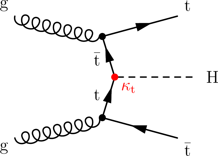
Figure 1:
Representative leading-order Feynman diagrams for the associated production of a Higgs boson and a top quark-antiquark pair (left) and for the associated production of a single top quark and a Higgs boson in the $ t $ channel, where the Higgs boson couples to the top quark (centre) or the W boson (right). |
png pdf |
Figure 1-a:
Representative leading-order Feynman diagrams for the associated production of a Higgs boson and a top quark-antiquark pair (left) and for the associated production of a single top quark and a Higgs boson in the $ t $ channel, where the Higgs boson couples to the top quark (centre) or the W boson (right). |

png pdf |
Figure 1-b:
Representative leading-order Feynman diagrams for the associated production of a Higgs boson and a top quark-antiquark pair (left) and for the associated production of a single top quark and a Higgs boson in the $ t $ channel, where the Higgs boson couples to the top quark (centre) or the W boson (right). |

png pdf |
Figure 1-c:
Representative leading-order Feynman diagrams for the associated production of a Higgs boson and a top quark-antiquark pair (left) and for the associated production of a single top quark and a Higgs boson in the $ t $ channel, where the Higgs boson couples to the top quark (centre) or the W boson (right). |

png pdf |
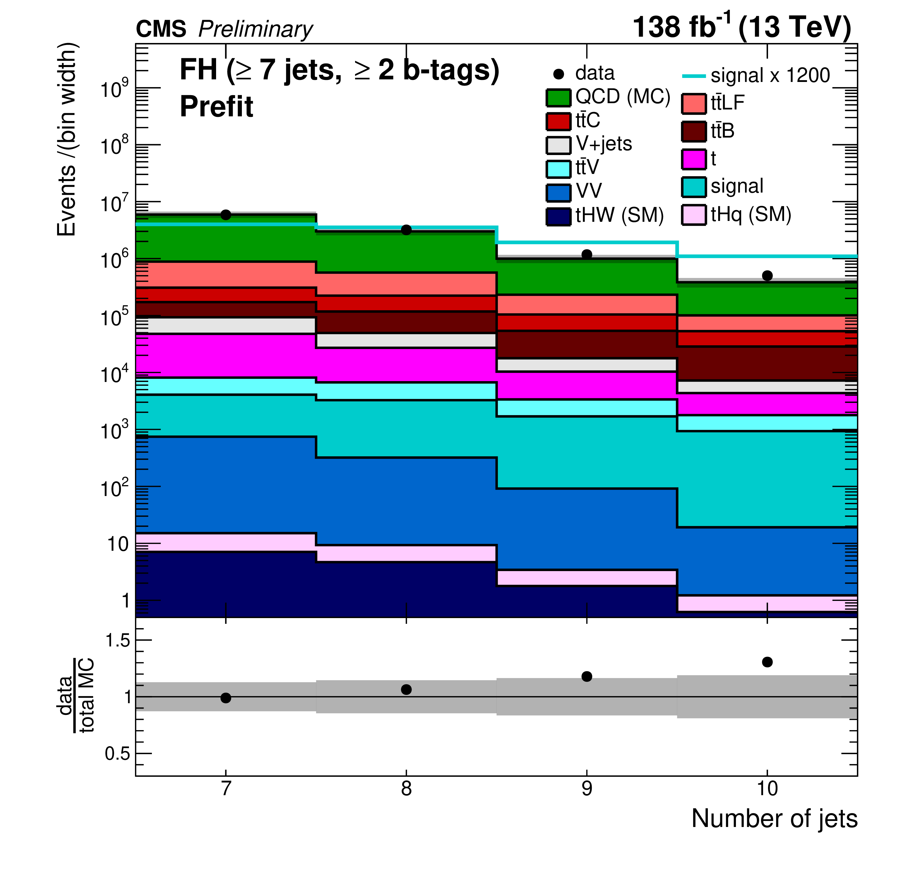
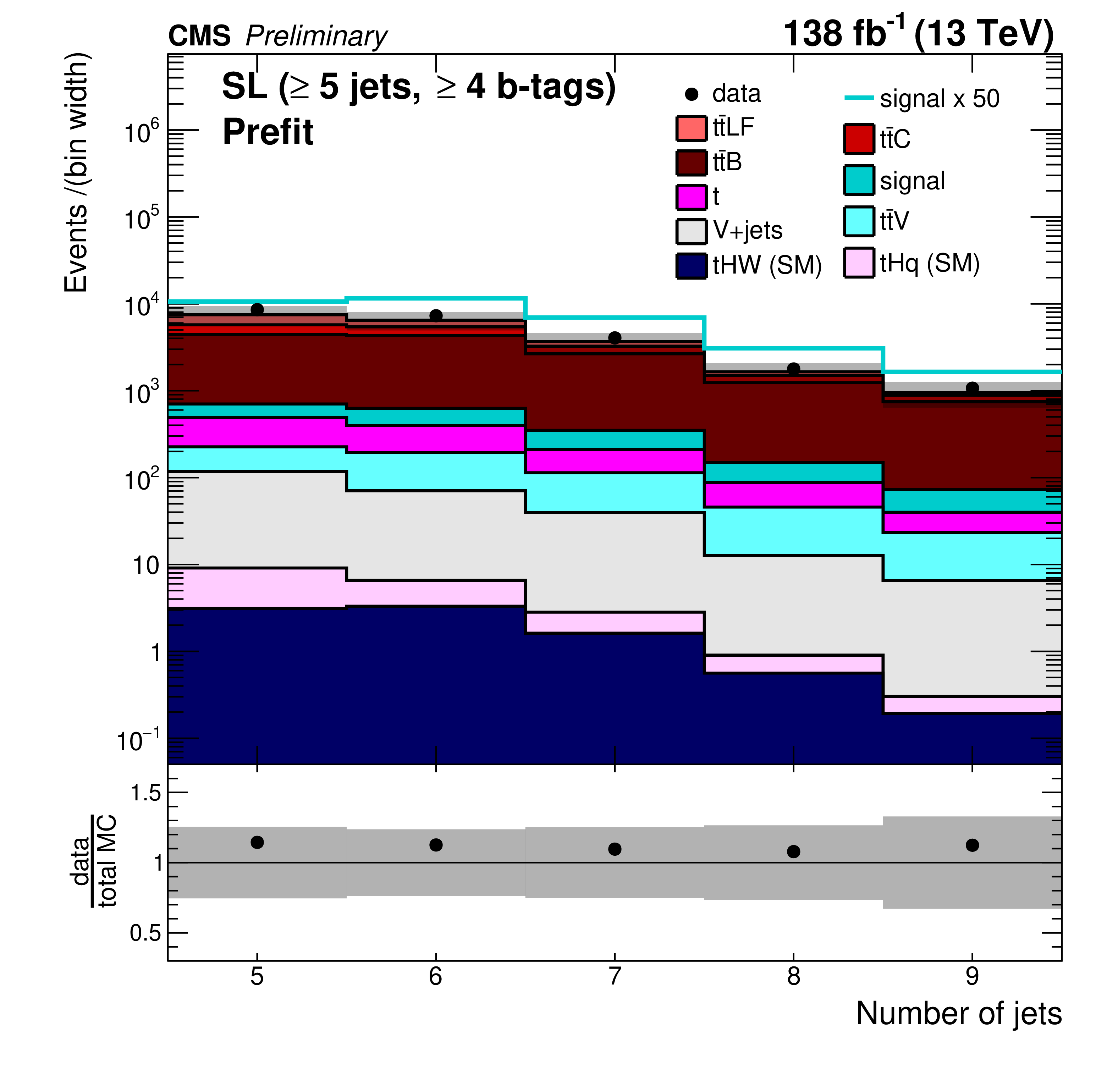
Figure 2:
Jet multiplicity distribution in the FH (upper left), SL (upper right), and DL (lower) channels, after the baseline selection and prior to the fit to the data. Here, the QCD background prediction is taken from simulation. The expected ttH signal contribution, scaled as indicated in the legend for better visibility, is also overlayed (line). The uncertainty band represents the total uncertainty. The last bins include overflow events. |
png pdf |
Figure 2-a:
Jet multiplicity distribution in the FH (upper left), SL (upper right), and DL (lower) channels, after the baseline selection and prior to the fit to the data. Here, the QCD background prediction is taken from simulation. The expected ttH signal contribution, scaled as indicated in the legend for better visibility, is also overlayed (line). The uncertainty band represents the total uncertainty. The last bins include overflow events. |
png pdf |
Figure 2-b:
Jet multiplicity distribution in the FH (upper left), SL (upper right), and DL (lower) channels, after the baseline selection and prior to the fit to the data. Here, the QCD background prediction is taken from simulation. The expected ttH signal contribution, scaled as indicated in the legend for better visibility, is also overlayed (line). The uncertainty band represents the total uncertainty. The last bins include overflow events. |

png pdf |
Figure 2-c:
Jet multiplicity distribution in the FH (upper left), SL (upper right), and DL (lower) channels, after the baseline selection and prior to the fit to the data. Here, the QCD background prediction is taken from simulation. The expected ttH signal contribution, scaled as indicated in the legend for better visibility, is also overlayed (line). The uncertainty band represents the total uncertainty. The last bins include overflow events. |

png pdf |
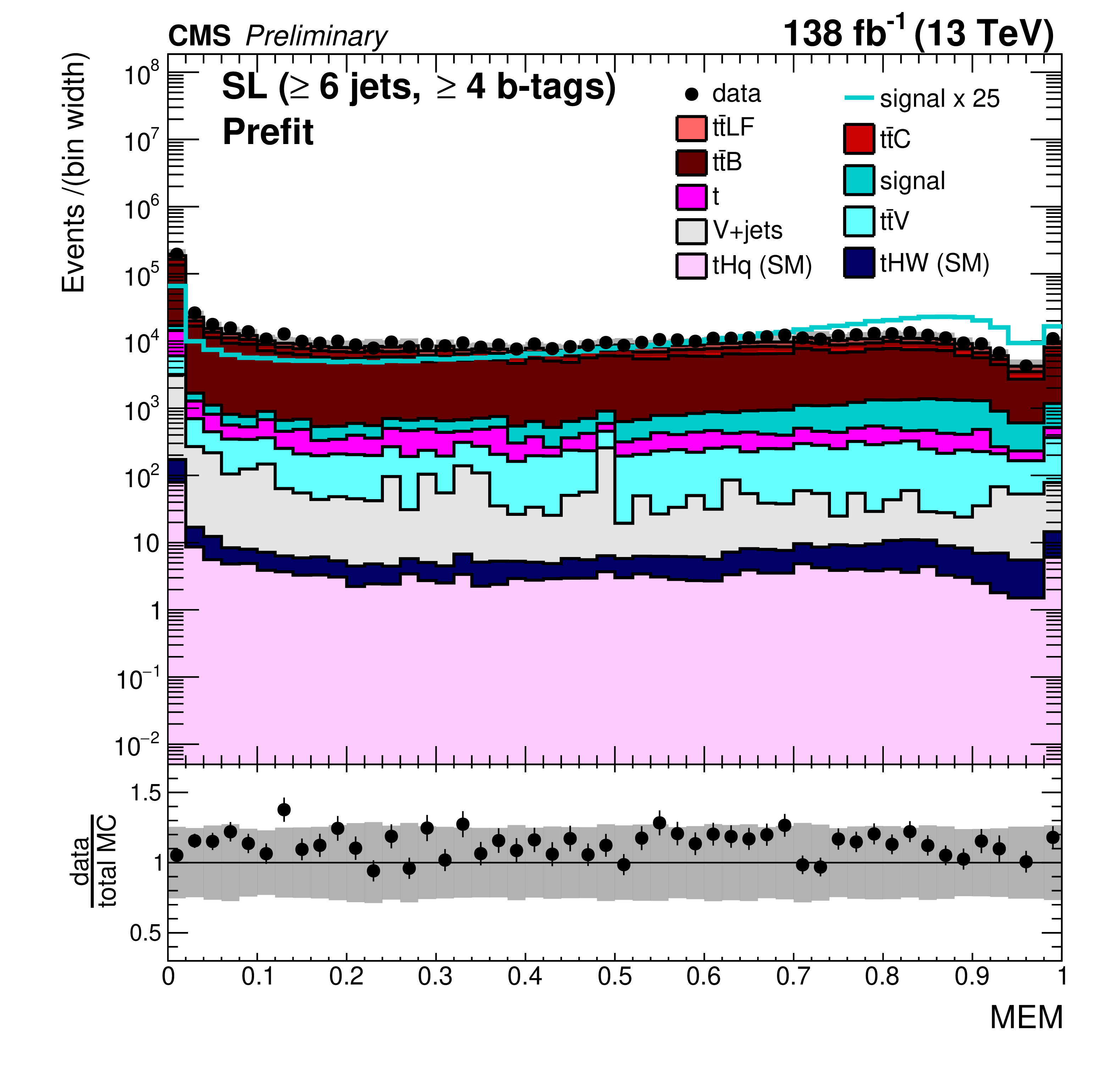
Figure 3:
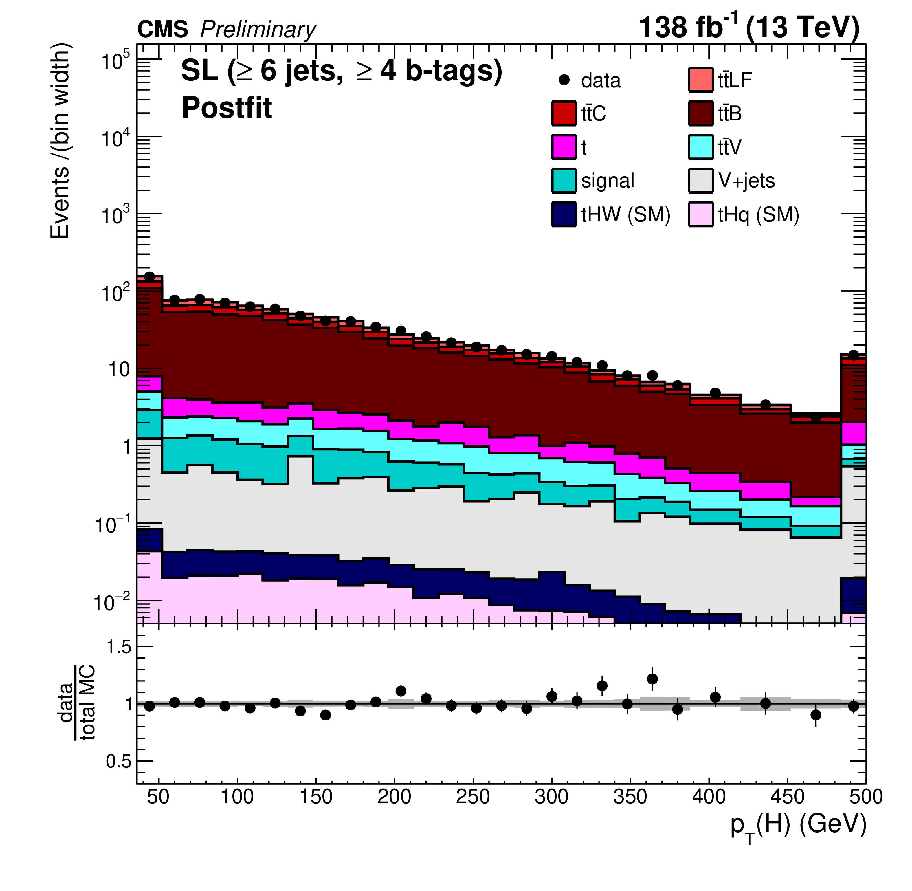
Average $ \Delta\eta $ between any two b-tagged jets (upper), MEM discriminant output (middle), and $ p_{\mathrm{T}} $ of the Higgs boson candidate identified with reconstruction BDT (lower) for events passing the baseline selection requirements and additionally $ \geq $ 6 jets in the SL channel prefit (left) and with the postfit background model (right) obtained from the fit to data described in Section 10. In the prefit case, the ttH signal contribution, scaled by a factor 25 for better visibility, is also overlayed (line). Where applicable, the last bins include overflow events. |

png pdf |
Figure 3-a:
Average $ \Delta\eta $ between any two b-tagged jets (upper), MEM discriminant output (middle), and $ p_{\mathrm{T}} $ of the Higgs boson candidate identified with reconstruction BDT (lower) for events passing the baseline selection requirements and additionally $ \geq $ 6 jets in the SL channel prefit (left) and with the postfit background model (right) obtained from the fit to data described in Section 10. In the prefit case, the ttH signal contribution, scaled by a factor 25 for better visibility, is also overlayed (line). Where applicable, the last bins include overflow events. |

png pdf |
Figure 3-b:
Average $ \Delta\eta $ between any two b-tagged jets (upper), MEM discriminant output (middle), and $ p_{\mathrm{T}} $ of the Higgs boson candidate identified with reconstruction BDT (lower) for events passing the baseline selection requirements and additionally $ \geq $ 6 jets in the SL channel prefit (left) and with the postfit background model (right) obtained from the fit to data described in Section 10. In the prefit case, the ttH signal contribution, scaled by a factor 25 for better visibility, is also overlayed (line). Where applicable, the last bins include overflow events. |
png pdf |
Figure 3-c:
Average $ \Delta\eta $ between any two b-tagged jets (upper), MEM discriminant output (middle), and $ p_{\mathrm{T}} $ of the Higgs boson candidate identified with reconstruction BDT (lower) for events passing the baseline selection requirements and additionally $ \geq $ 6 jets in the SL channel prefit (left) and with the postfit background model (right) obtained from the fit to data described in Section 10. In the prefit case, the ttH signal contribution, scaled by a factor 25 for better visibility, is also overlayed (line). Where applicable, the last bins include overflow events. |

png pdf |
Figure 3-d:
Average $ \Delta\eta $ between any two b-tagged jets (upper), MEM discriminant output (middle), and $ p_{\mathrm{T}} $ of the Higgs boson candidate identified with reconstruction BDT (lower) for events passing the baseline selection requirements and additionally $ \geq $ 6 jets in the SL channel prefit (left) and with the postfit background model (right) obtained from the fit to data described in Section 10. In the prefit case, the ttH signal contribution, scaled by a factor 25 for better visibility, is also overlayed (line). Where applicable, the last bins include overflow events. |

png pdf |
Figure 3-e:
Average $ \Delta\eta $ between any two b-tagged jets (upper), MEM discriminant output (middle), and $ p_{\mathrm{T}} $ of the Higgs boson candidate identified with reconstruction BDT (lower) for events passing the baseline selection requirements and additionally $ \geq $ 6 jets in the SL channel prefit (left) and with the postfit background model (right) obtained from the fit to data described in Section 10. In the prefit case, the ttH signal contribution, scaled by a factor 25 for better visibility, is also overlayed (line). Where applicable, the last bins include overflow events. |
png pdf |
Figure 3-f:
Average $ \Delta\eta $ between any two b-tagged jets (upper), MEM discriminant output (middle), and $ p_{\mathrm{T}} $ of the Higgs boson candidate identified with reconstruction BDT (lower) for events passing the baseline selection requirements and additionally $ \geq $ 6 jets in the SL channel prefit (left) and with the postfit background model (right) obtained from the fit to data described in Section 10. In the prefit case, the ttH signal contribution, scaled by a factor 25 for better visibility, is also overlayed (line). Where applicable, the last bins include overflow events. |
png pdf |
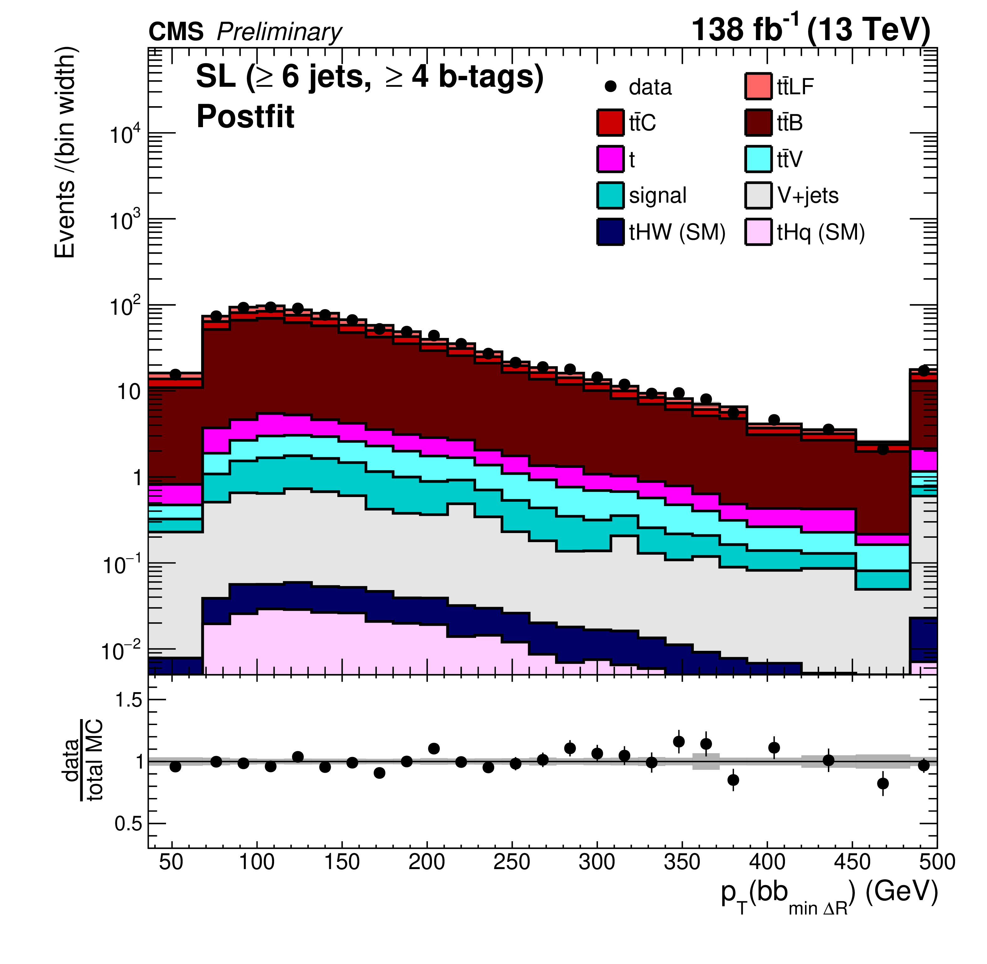
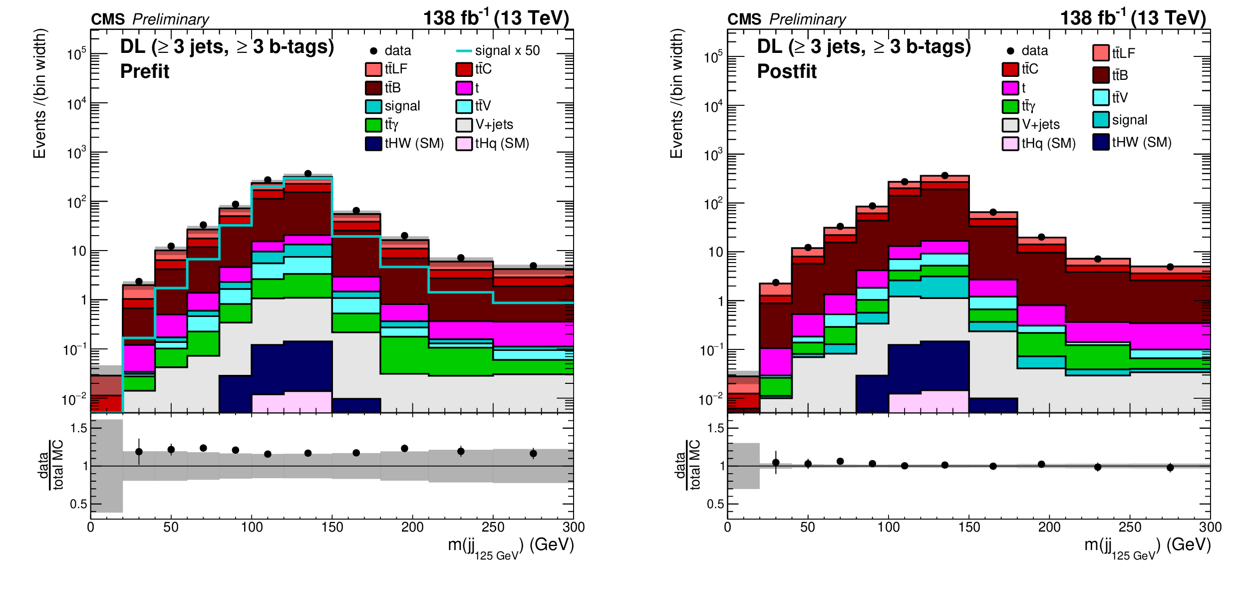
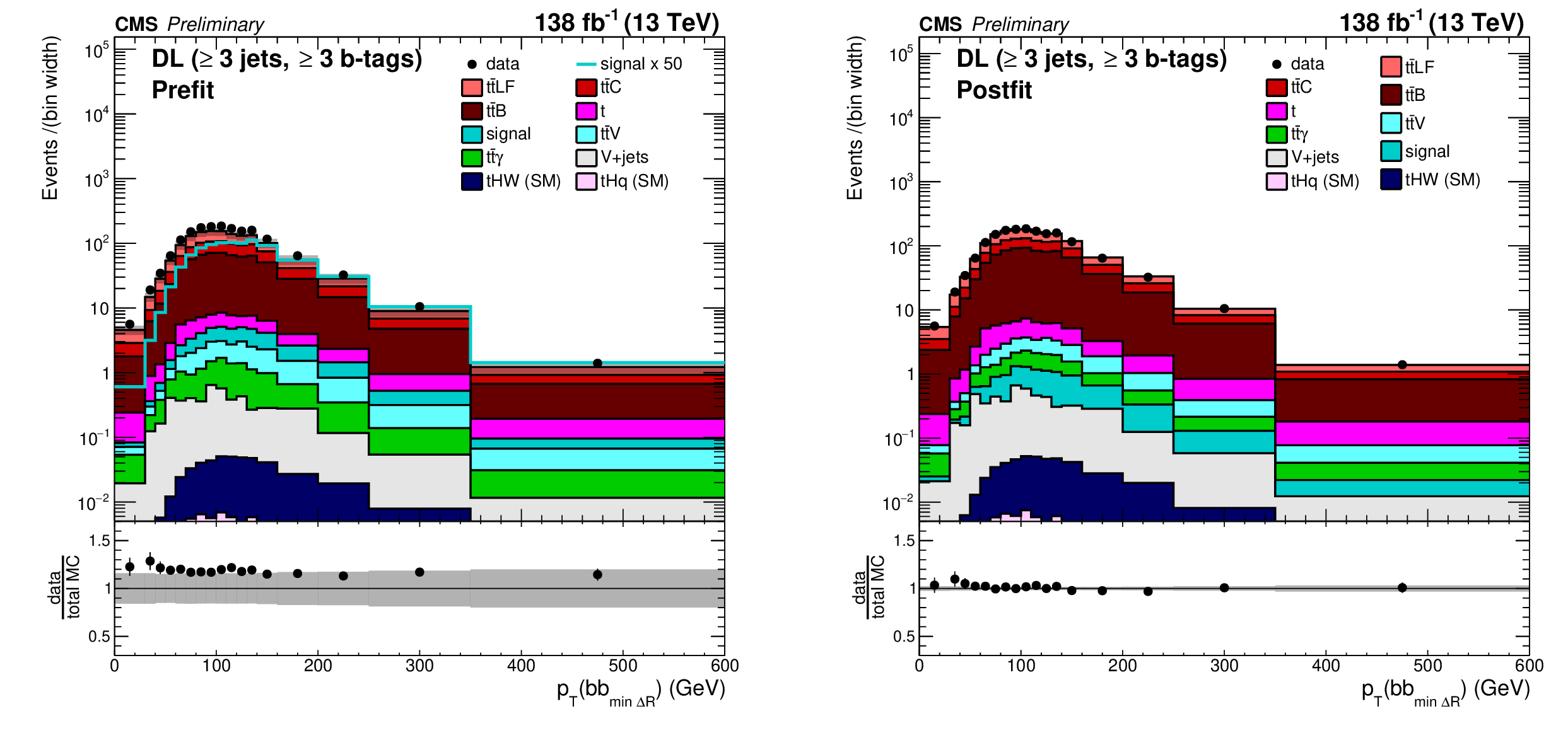
Figure 4:
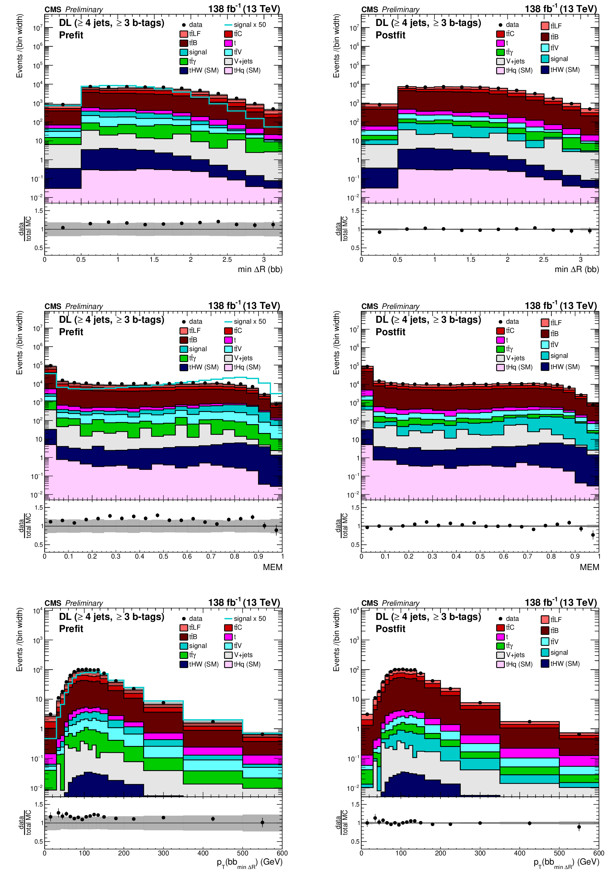
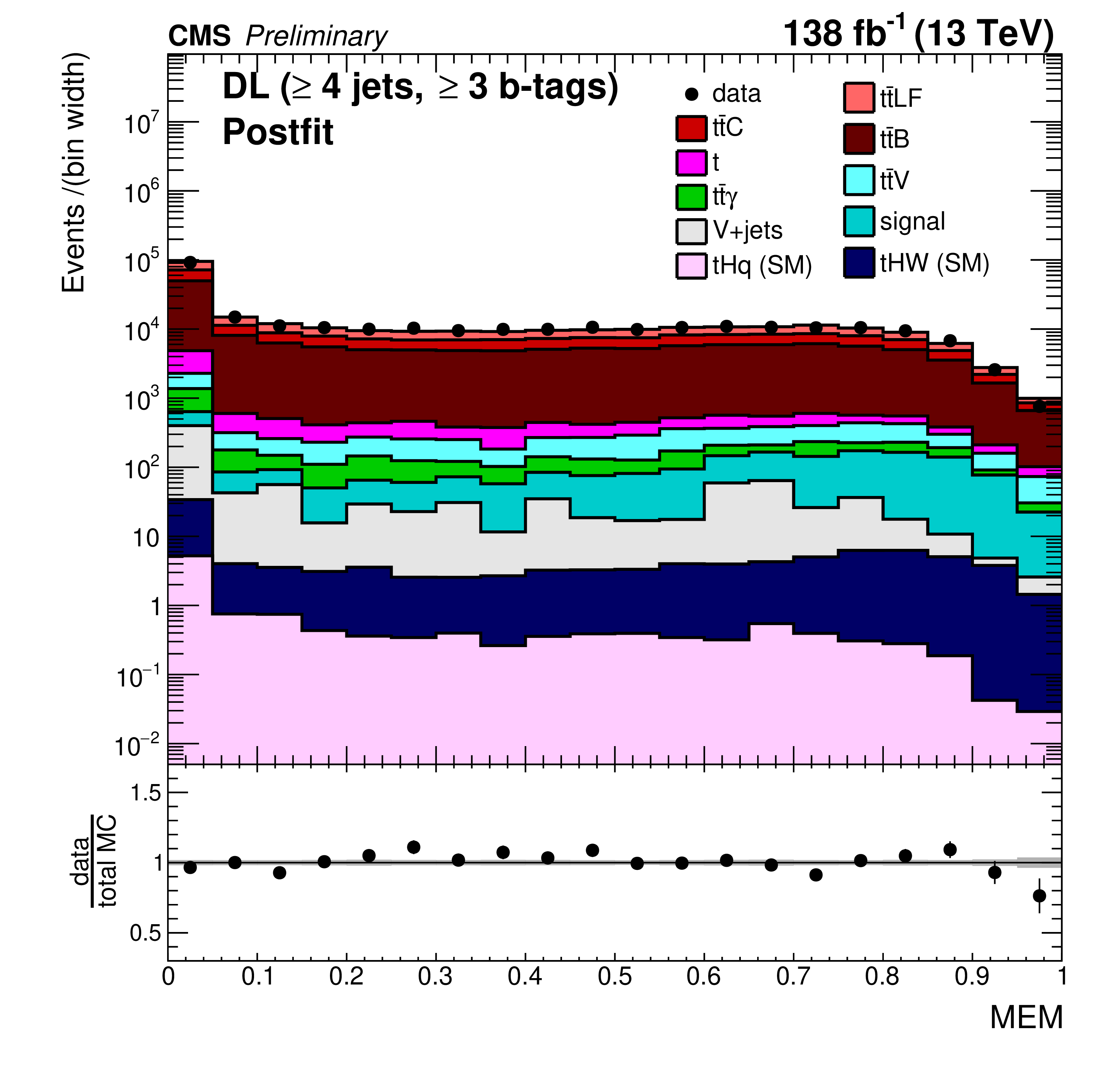
Minimum $ \Delta R $ between any two b-tagged jets (upper), MEM discriminant output (middle), and $ p_{\mathrm{T}} $ of the Higgs boson candidate identified as pair of b-tagged jets closest in $ \Delta R $ (lower) for events passing the baseline selection requirements and additionally $ \geq $ 4 jets in the DL channel prefit (left) and with the postfit background model (right) obtained from the fit to data described in Section 10. In the prefit case, the ttH signal contribution, scaled by a factor 50 for better visibility, is also overlayed (line). Where applicable, the last bins include overflow events. |

png pdf |
Figure 4-a:
Minimum $ \Delta R $ between any two b-tagged jets (upper), MEM discriminant output (middle), and $ p_{\mathrm{T}} $ of the Higgs boson candidate identified as pair of b-tagged jets closest in $ \Delta R $ (lower) for events passing the baseline selection requirements and additionally $ \geq $ 4 jets in the DL channel prefit (left) and with the postfit background model (right) obtained from the fit to data described in Section 10. In the prefit case, the ttH signal contribution, scaled by a factor 50 for better visibility, is also overlayed (line). Where applicable, the last bins include overflow events. |

png pdf |
Figure 4-b:
Minimum $ \Delta R $ between any two b-tagged jets (upper), MEM discriminant output (middle), and $ p_{\mathrm{T}} $ of the Higgs boson candidate identified as pair of b-tagged jets closest in $ \Delta R $ (lower) for events passing the baseline selection requirements and additionally $ \geq $ 4 jets in the DL channel prefit (left) and with the postfit background model (right) obtained from the fit to data described in Section 10. In the prefit case, the ttH signal contribution, scaled by a factor 50 for better visibility, is also overlayed (line). Where applicable, the last bins include overflow events. |

png pdf |
Figure 4-c:
Minimum $ \Delta R $ between any two b-tagged jets (upper), MEM discriminant output (middle), and $ p_{\mathrm{T}} $ of the Higgs boson candidate identified as pair of b-tagged jets closest in $ \Delta R $ (lower) for events passing the baseline selection requirements and additionally $ \geq $ 4 jets in the DL channel prefit (left) and with the postfit background model (right) obtained from the fit to data described in Section 10. In the prefit case, the ttH signal contribution, scaled by a factor 50 for better visibility, is also overlayed (line). Where applicable, the last bins include overflow events. |
png pdf |
Figure 4-d:
Minimum $ \Delta R $ between any two b-tagged jets (upper), MEM discriminant output (middle), and $ p_{\mathrm{T}} $ of the Higgs boson candidate identified as pair of b-tagged jets closest in $ \Delta R $ (lower) for events passing the baseline selection requirements and additionally $ \geq $ 4 jets in the DL channel prefit (left) and with the postfit background model (right) obtained from the fit to data described in Section 10. In the prefit case, the ttH signal contribution, scaled by a factor 50 for better visibility, is also overlayed (line). Where applicable, the last bins include overflow events. |

png pdf |
Figure 4-e:
Minimum $ \Delta R $ between any two b-tagged jets (upper), MEM discriminant output (middle), and $ p_{\mathrm{T}} $ of the Higgs boson candidate identified as pair of b-tagged jets closest in $ \Delta R $ (lower) for events passing the baseline selection requirements and additionally $ \geq $ 4 jets in the DL channel prefit (left) and with the postfit background model (right) obtained from the fit to data described in Section 10. In the prefit case, the ttH signal contribution, scaled by a factor 50 for better visibility, is also overlayed (line). Where applicable, the last bins include overflow events. |

png pdf |
Figure 4-f:
Minimum $ \Delta R $ between any two b-tagged jets (upper), MEM discriminant output (middle), and $ p_{\mathrm{T}} $ of the Higgs boson candidate identified as pair of b-tagged jets closest in $ \Delta R $ (lower) for events passing the baseline selection requirements and additionally $ \geq $ 4 jets in the DL channel prefit (left) and with the postfit background model (right) obtained from the fit to data described in Section 10. In the prefit case, the ttH signal contribution, scaled by a factor 50 for better visibility, is also overlayed (line). Where applicable, the last bins include overflow events. |

png pdf |
Figure 5:
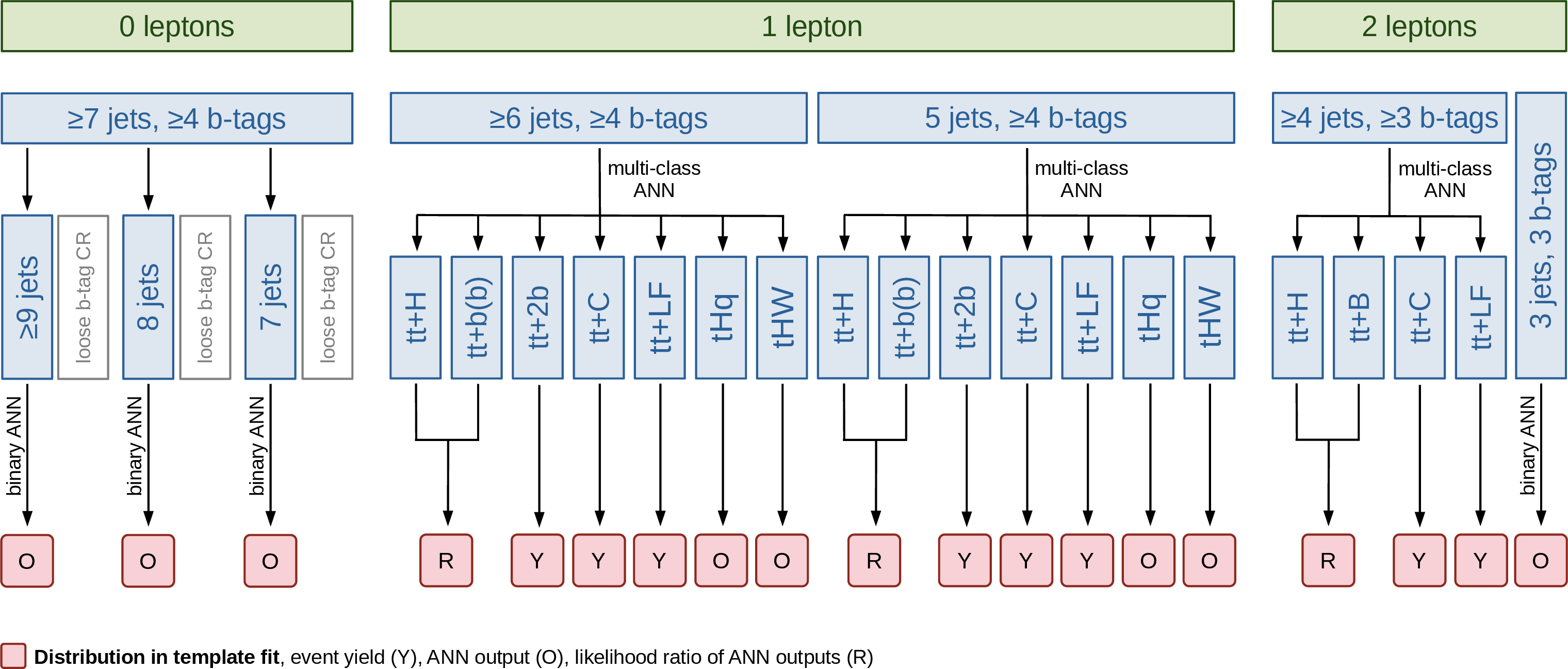
Illustration of the analysis strategy for the inclusive ttH and tH signal-strength modifier and coupling and CP measurements (upper) and for the ttH STXS measurement (lower). The procedure is applied separately for the three years of data taking. |
png pdf |
Figure 5-a:
Illustration of the analysis strategy for the inclusive ttH and tH signal-strength modifier and coupling and CP measurements (upper) and for the ttH STXS measurement (lower). The procedure is applied separately for the three years of data taking. |

png pdf |
Figure 5-b:
Illustration of the analysis strategy for the inclusive ttH and tH signal-strength modifier and coupling and CP measurements (upper) and for the ttH STXS measurement (lower). The procedure is applied separately for the three years of data taking. |
png pdf |
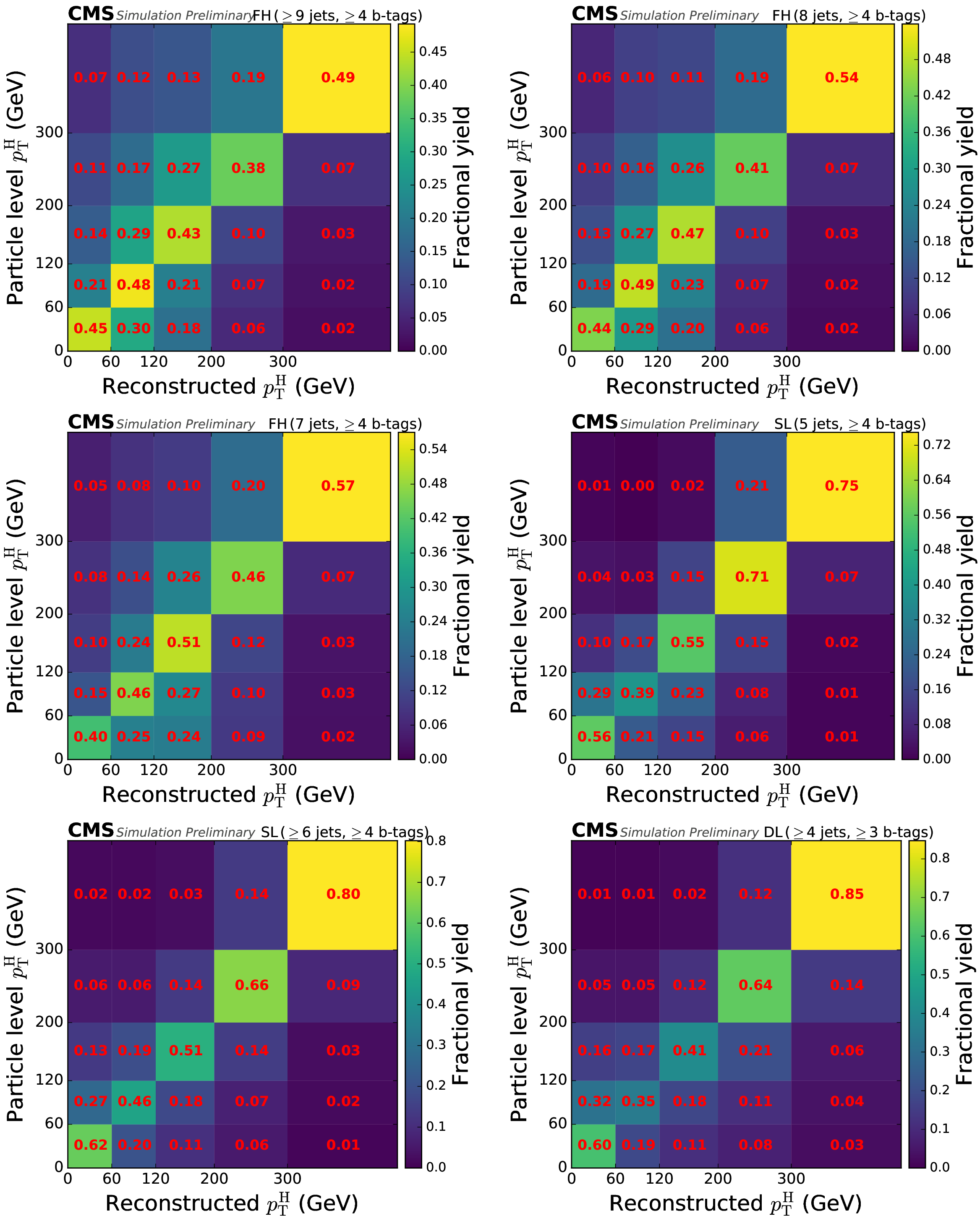
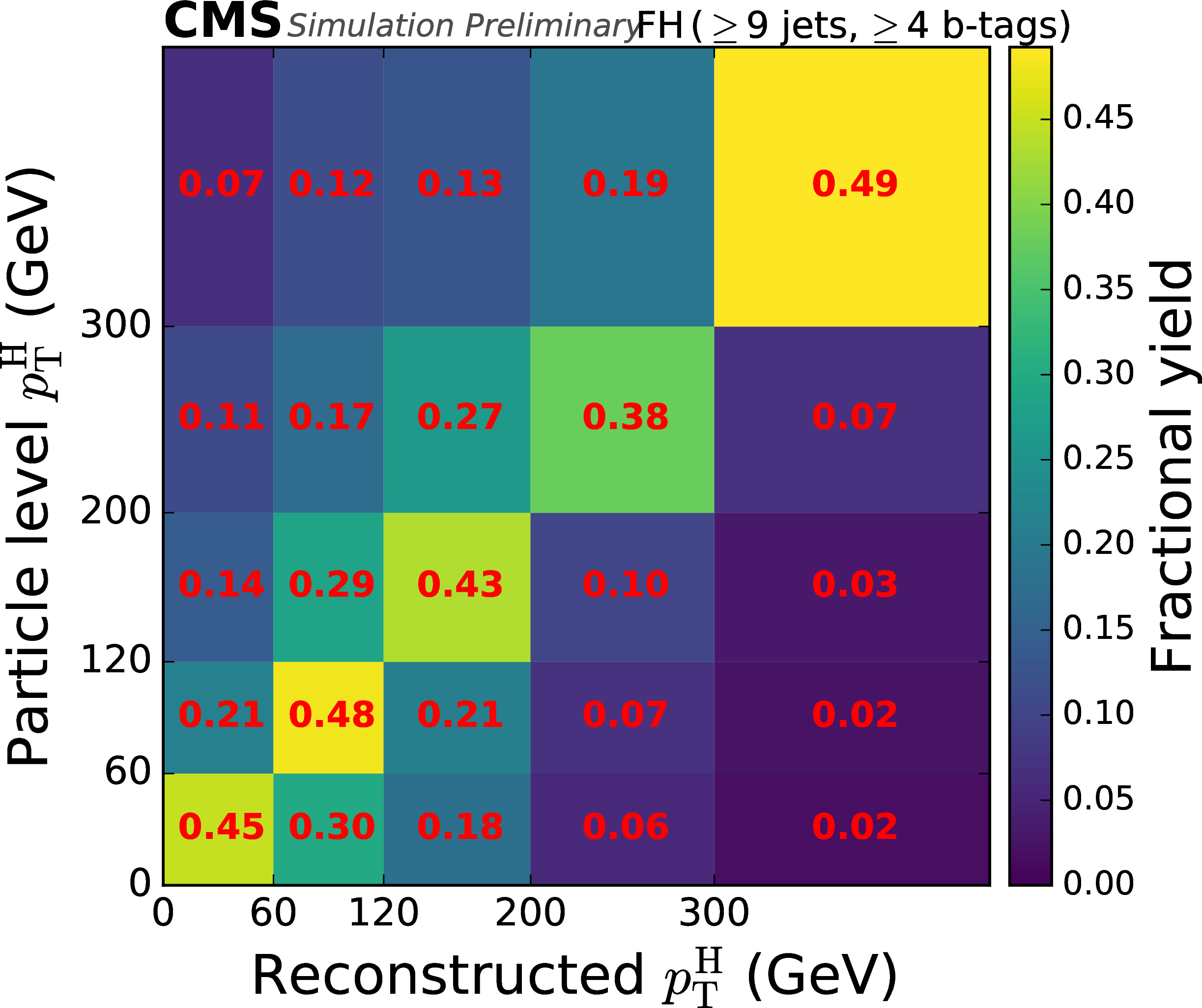
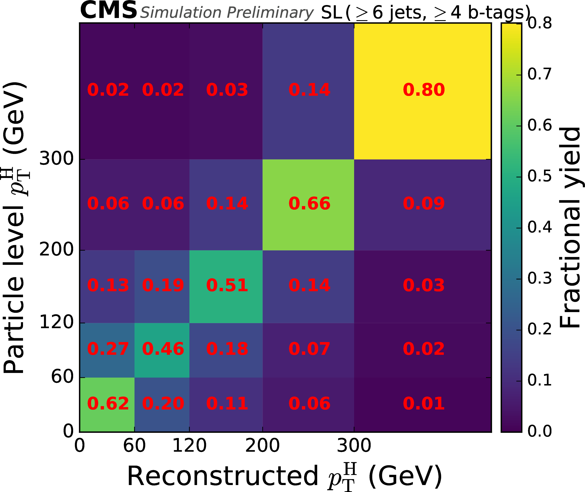
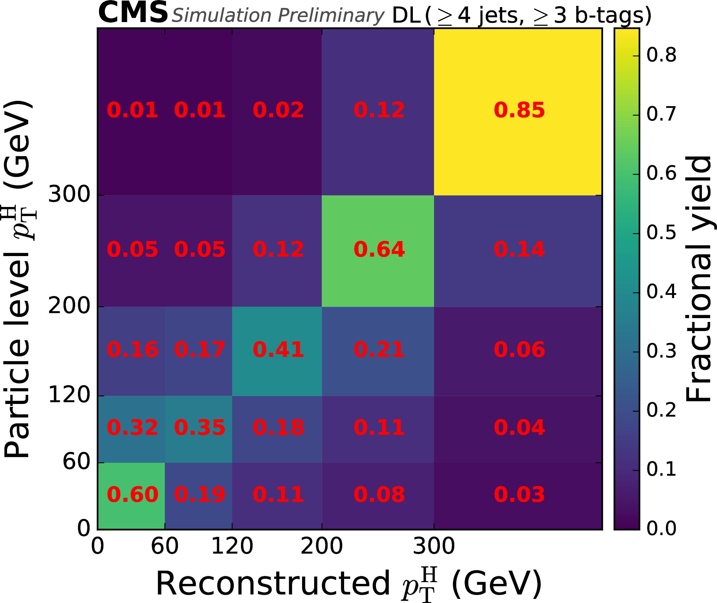
Figure 6:
Categorisation efficiency of the ttH signal events in the STXS analysis in the different categories of the FH channel (upper row, middle row left), the SL channel (middle row right, lower row left), and the DL channel (lower row right). |
png pdf |
Figure 6-a:
Categorisation efficiency of the ttH signal events in the STXS analysis in the different categories of the FH channel (upper row, middle row left), the SL channel (middle row right, lower row left), and the DL channel (lower row right). |

png pdf |
Figure 6-b:
Categorisation efficiency of the ttH signal events in the STXS analysis in the different categories of the FH channel (upper row, middle row left), the SL channel (middle row right, lower row left), and the DL channel (lower row right). |

png pdf |
Figure 6-c:
Categorisation efficiency of the ttH signal events in the STXS analysis in the different categories of the FH channel (upper row, middle row left), the SL channel (middle row right, lower row left), and the DL channel (lower row right). |

png pdf |
Figure 6-d:
Categorisation efficiency of the ttH signal events in the STXS analysis in the different categories of the FH channel (upper row, middle row left), the SL channel (middle row right, lower row left), and the DL channel (lower row right). |
png pdf |
Figure 6-e:
Categorisation efficiency of the ttH signal events in the STXS analysis in the different categories of the FH channel (upper row, middle row left), the SL channel (middle row right, lower row left), and the DL channel (lower row right). |
png pdf |
Figure 6-f:
Categorisation efficiency of the ttH signal events in the STXS analysis in the different categories of the FH channel (upper row, middle row left), the SL channel (middle row right, lower row left), and the DL channel (lower row right). |

png pdf |
Figure 7:
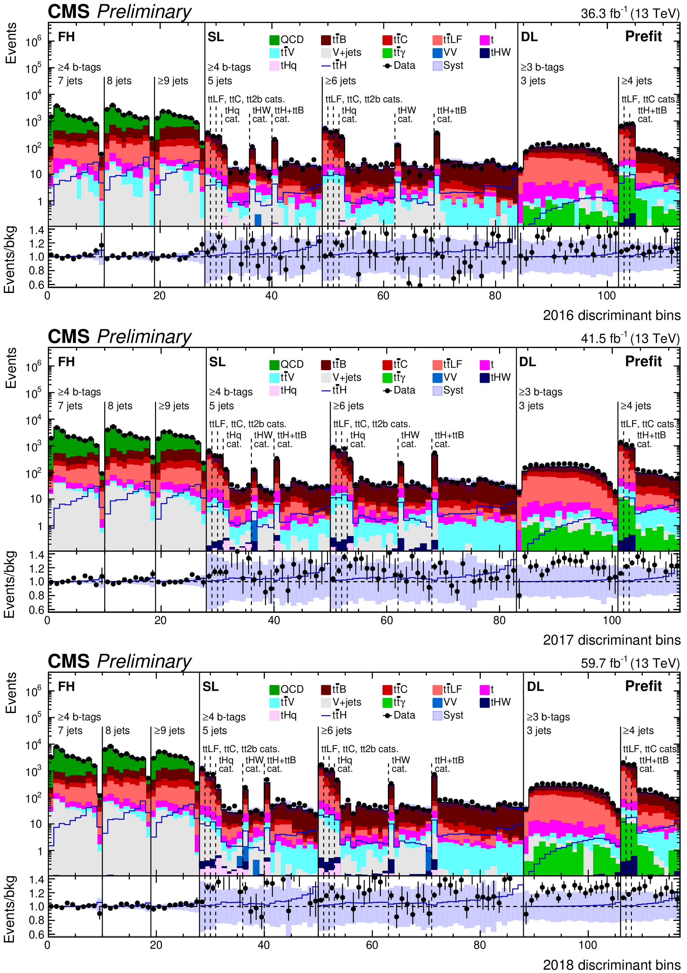
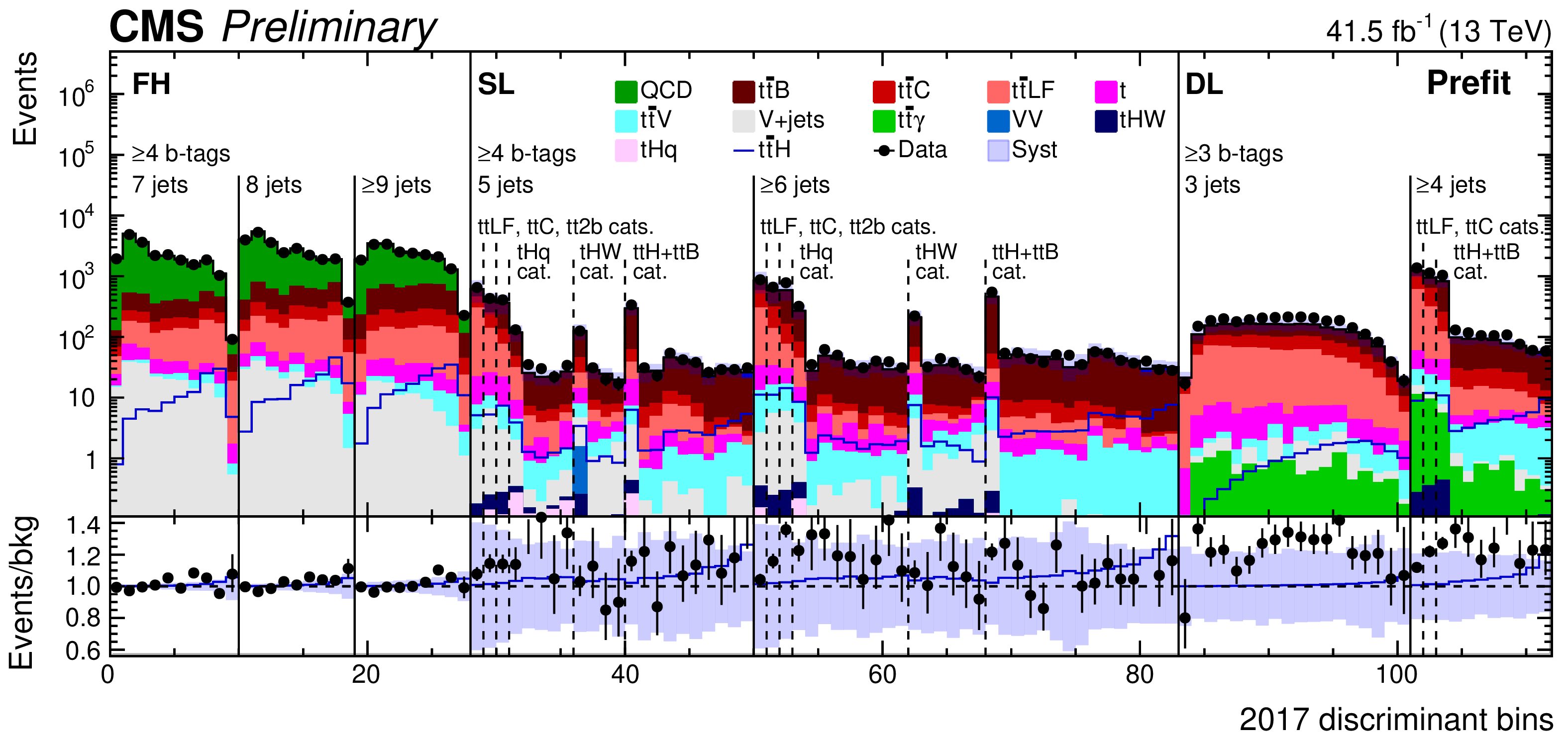
Observed (points) and postfit expected (filled histograms) yields in each discriminant (category yield, ANN score, or ratio of ANN scores) bin for the 2016 (upper), 2017 (middle), and 2018 (lower) data-taking periods. The uncertainty bands include the total uncertainty of the fit model. The lower pads show the ratio of the data to the background (points) and of the postfit expected signal+background to the background-only contribution (line). |

png pdf |
Figure 7-a:
Observed (points) and postfit expected (filled histograms) yields in each discriminant (category yield, ANN score, or ratio of ANN scores) bin for the 2016 (upper), 2017 (middle), and 2018 (lower) data-taking periods. The uncertainty bands include the total uncertainty of the fit model. The lower pads show the ratio of the data to the background (points) and of the postfit expected signal+background to the background-only contribution (line). |

png pdf |
Figure 7-b:
Observed (points) and postfit expected (filled histograms) yields in each discriminant (category yield, ANN score, or ratio of ANN scores) bin for the 2016 (upper), 2017 (middle), and 2018 (lower) data-taking periods. The uncertainty bands include the total uncertainty of the fit model. The lower pads show the ratio of the data to the background (points) and of the postfit expected signal+background to the background-only contribution (line). |

png pdf |
Figure 7-c:
Observed (points) and postfit expected (filled histograms) yields in each discriminant (category yield, ANN score, or ratio of ANN scores) bin for the 2016 (upper), 2017 (middle), and 2018 (lower) data-taking periods. The uncertainty bands include the total uncertainty of the fit model. The lower pads show the ratio of the data to the background (points) and of the postfit expected signal+background to the background-only contribution (line). |

png pdf |
Figure 8:
Best-fit results of the ttH signal-strength modifier $ \mu_{{\mathrm{t}\overline{\mathrm{t}}} \mathrm{H}} $ in each channel (upper three rows), in each year (middle three rows), and in the combination of all channels and years (lower row). Uncertainties are correlated between the channels and years. |

png pdf |
Figure 9:
Observed likelihood-ratio test statistic (blue shading) as a function of the ttH signal-strength modifier $ \mu_{{\mathrm{t}\overline{\mathrm{t}}} \mathrm{H}} $ and the $ {\mathrm{t}\overline{\mathrm{t}}} \text{B} $ background normalisation, together with the observed (blue) and SM expected (black) best-fit points (cross and diamond markers) as well as the 68% (solid lines) and 95% (dashed lines) CL regions. The $ {\mathrm{t}\overline{\mathrm{t}}} \text{C} $ background normalisation and all other nuisance parameters are profiled such that the likelihood attains its minimum at each point in the plane. |

png pdf |
Figure 10:
Postfit values of the nuisance parameters (black markers), shown as the difference of their best-fit values, $ \hat{\theta} $, and prefit values, $ \theta_{0} $, relative to the prefit uncertainties $ \Delta\theta $. The impact $ \Delta\hat{\mu} $ of the nuisance parameters on the signal strength $ \mu_{{\mathrm{t}\overline{\mathrm{t}}} \mathrm{H}} $ is computed as the difference of the nominal best fit value of $ \mu $ and the best fit value obtained when fixing the nuisance parameter under scrutiny to its best fit value $ \hat{\theta} $ plus/minus its postfit uncertainty (coloured areas). The nuisance parameters are ordered by their impact, and only the 20 highest ranked parameters are shown. |

png pdf |
Figure 11:
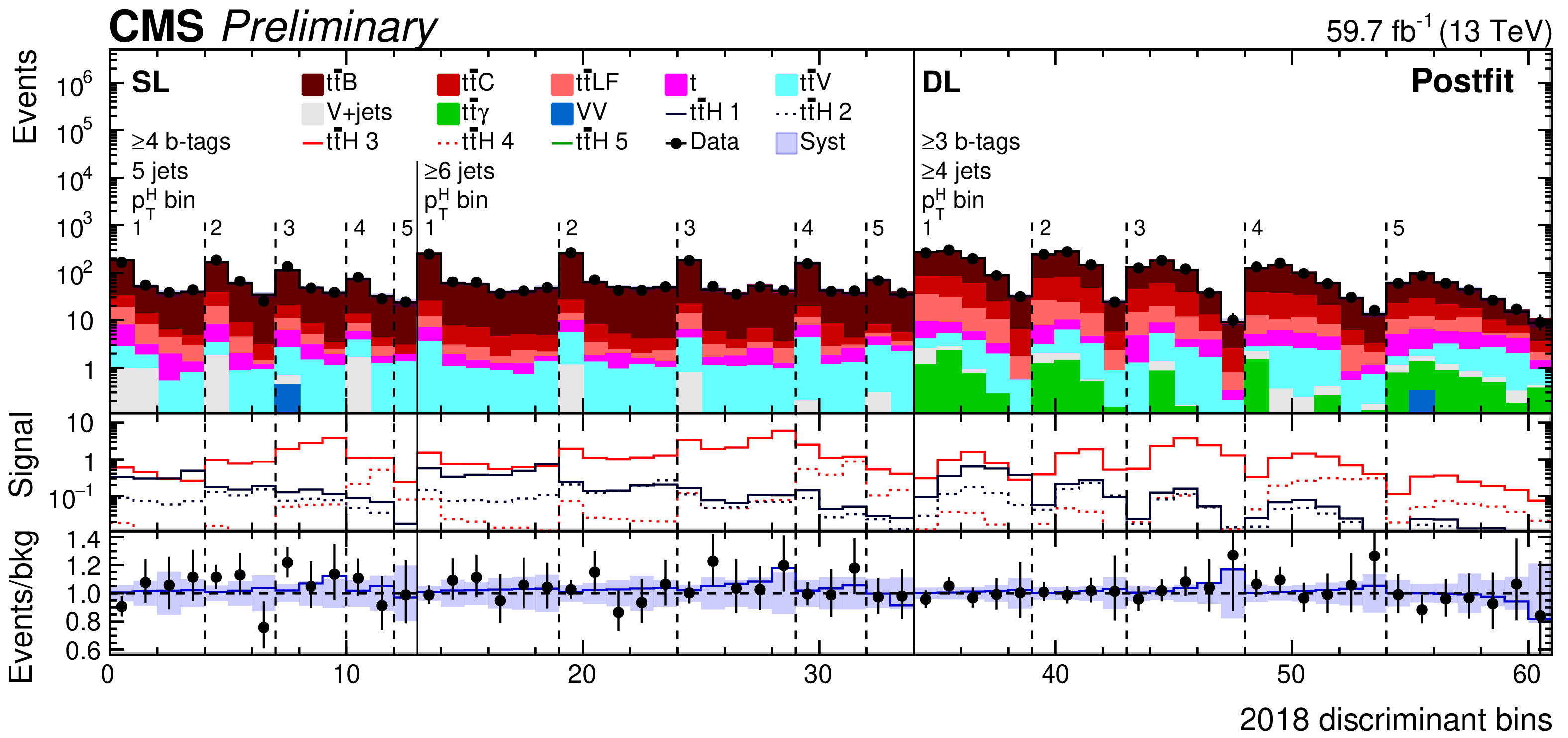
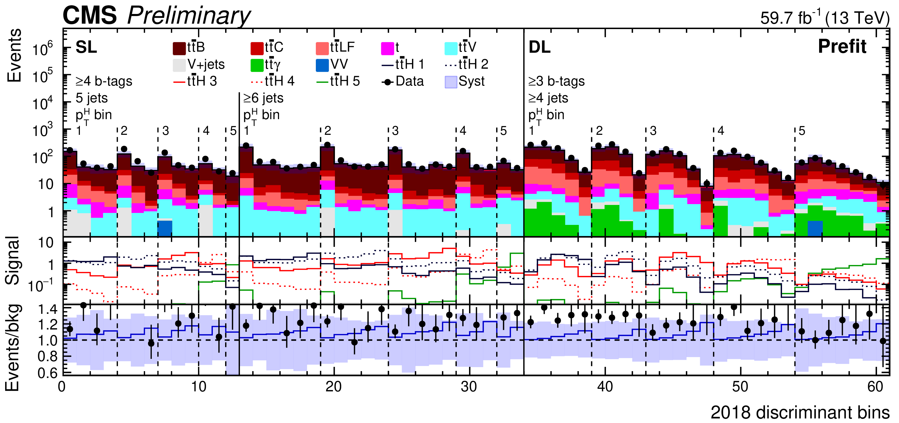
Observed (points) and postfit expected (filled histograms) yields in each STXS analysis discriminant bin in the signal regions of the SL and DL channels for the 2016 (upper), 2017 (middle), and 2018 (lower) data-taking periods. The fitted signal distributions (lines labelled ttH 1 to 5) in each Higgs boson $ p_{\mathrm{T}} $ bin are shown in the middle pads. The lower pads show the ratio of the data to the background (points) and of the postfit expected total signal+background to the background-only contribution (line). The uncertainty bands include the total uncertainty of the fit model. |

png pdf |
Figure 11-a:
Observed (points) and postfit expected (filled histograms) yields in each STXS analysis discriminant bin in the signal regions of the SL and DL channels for the 2016 (upper), 2017 (middle), and 2018 (lower) data-taking periods. The fitted signal distributions (lines labelled ttH 1 to 5) in each Higgs boson $ p_{\mathrm{T}} $ bin are shown in the middle pads. The lower pads show the ratio of the data to the background (points) and of the postfit expected total signal+background to the background-only contribution (line). The uncertainty bands include the total uncertainty of the fit model. |

png pdf |
Figure 11-b:
Observed (points) and postfit expected (filled histograms) yields in each STXS analysis discriminant bin in the signal regions of the SL and DL channels for the 2016 (upper), 2017 (middle), and 2018 (lower) data-taking periods. The fitted signal distributions (lines labelled ttH 1 to 5) in each Higgs boson $ p_{\mathrm{T}} $ bin are shown in the middle pads. The lower pads show the ratio of the data to the background (points) and of the postfit expected total signal+background to the background-only contribution (line). The uncertainty bands include the total uncertainty of the fit model. |
png pdf |
Figure 11-c:
Observed (points) and postfit expected (filled histograms) yields in each STXS analysis discriminant bin in the signal regions of the SL and DL channels for the 2016 (upper), 2017 (middle), and 2018 (lower) data-taking periods. The fitted signal distributions (lines labelled ttH 1 to 5) in each Higgs boson $ p_{\mathrm{T}} $ bin are shown in the middle pads. The lower pads show the ratio of the data to the background (points) and of the postfit expected total signal+background to the background-only contribution (line). The uncertainty bands include the total uncertainty of the fit model. |

png pdf |
Figure 12:
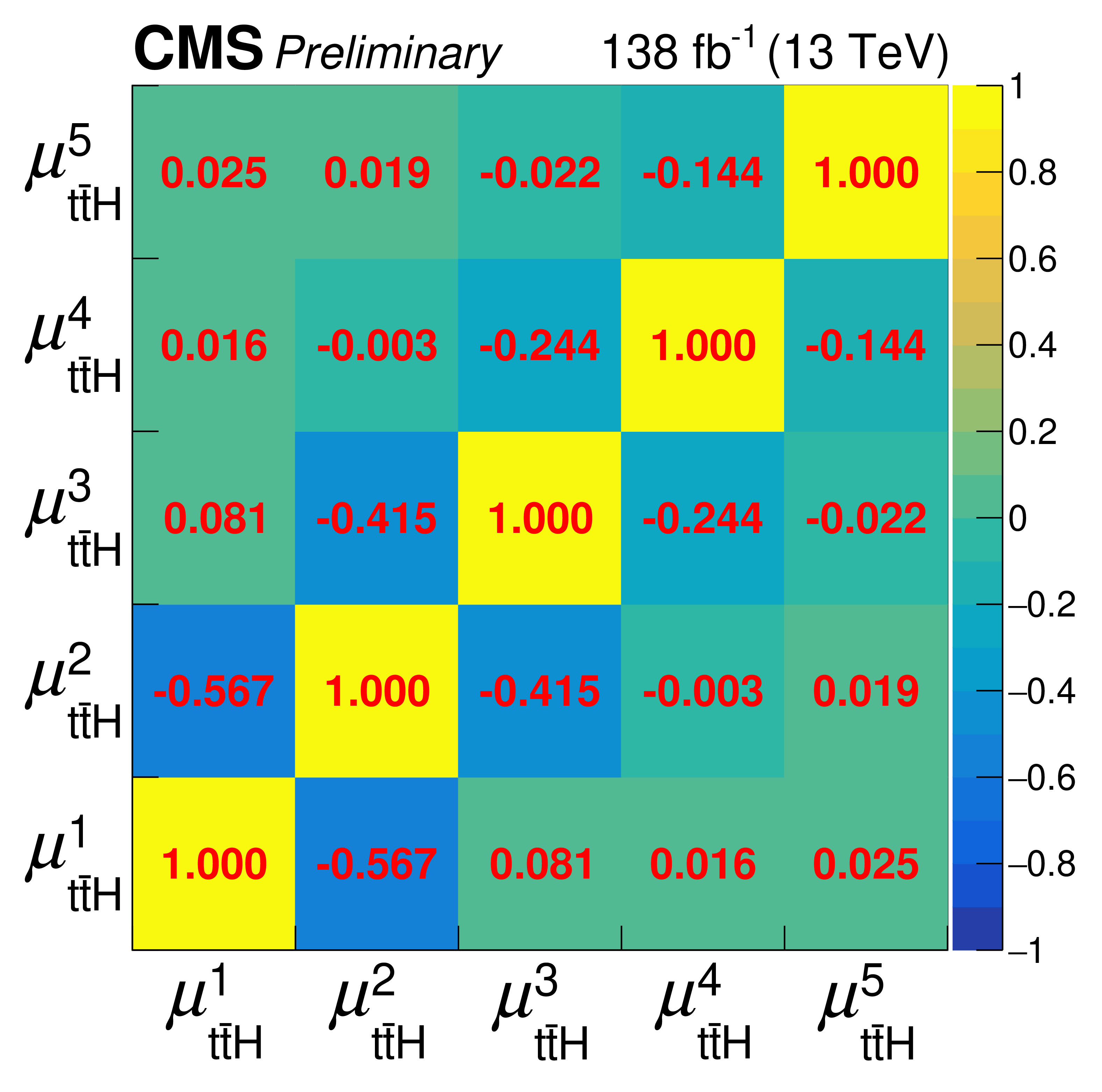
Best-fit results of the ttH signal-strength modifiers $ \mu_{{\mathrm{t}\overline{\mathrm{t}}} \mathrm{H}} $ in the different bins of Higgs boson $ p_{\mathrm{T}} $ (left) and their correlations (right) of the STXS measurement. |

png pdf |
Figure 12-a:
Best-fit results of the ttH signal-strength modifiers $ \mu_{{\mathrm{t}\overline{\mathrm{t}}} \mathrm{H}} $ in the different bins of Higgs boson $ p_{\mathrm{T}} $ (left) and their correlations (right) of the STXS measurement. |
png pdf |
Figure 12-b:
Best-fit results of the ttH signal-strength modifiers $ \mu_{{\mathrm{t}\overline{\mathrm{t}}} \mathrm{H}} $ in the different bins of Higgs boson $ p_{\mathrm{T}} $ (left) and their correlations (right) of the STXS measurement. |

png pdf |
Figure 13:
Observed (solid vertical line) and expected (dashed vertical line) upper 95% CL limit on the tH signal strength modifier $ \mu_{\mathrm{t}\mathrm{H}} $ for different channels and years, where the uncertainties are uncorrelated between the channels and years, and in their combination. The green (yellow) areas indicate the one (two) standard deviation confidence intervals on the expected limit. |

png pdf |
Figure 14:
Observed likelihood-ratio test statistic (blue shading) as a function of the ttH and tH signal strength modifiers $ \mu_{{\mathrm{t}\overline{\mathrm{t}}} \mathrm{H}} $ and $ \mu_{\mathrm{t}\mathrm{H}} $, together with the observed (blue) and SM expected (black) best-fit points (cross and diamond markers) as well as the 68% (solid lines) and 95% (dashed lines) CL regions. |

png pdf |
Figure 15:
Observed likelihood ratio test statistic (blue shading) as a function of $ \kappa_{\mathrm{t}} $ and $ \kappa_{\text{V}} $, together with the observed (blue) and SM expected (black) best-fit points (cross and diamond markers) as well as the 68% (solid lines) and 95% (dashed lines) CL regions (left). The observed (solid blue line) and expected (dotted black line) values of the likelihood ratio for $ \kappa_{\text{V}}= $ 1 are also shown (right), together with the 1 (green area) and 2 (yellow area) standard deviations confidence intervals. |

png pdf |
Figure 15-a:
Observed likelihood ratio test statistic (blue shading) as a function of $ \kappa_{\mathrm{t}} $ and $ \kappa_{\text{V}} $, together with the observed (blue) and SM expected (black) best-fit points (cross and diamond markers) as well as the 68% (solid lines) and 95% (dashed lines) CL regions (left). The observed (solid blue line) and expected (dotted black line) values of the likelihood ratio for $ \kappa_{\text{V}}= $ 1 are also shown (right), together with the 1 (green area) and 2 (yellow area) standard deviations confidence intervals. |

png pdf |
Figure 15-b:
Observed likelihood ratio test statistic (blue shading) as a function of $ \kappa_{\mathrm{t}} $ and $ \kappa_{\text{V}} $, together with the observed (blue) and SM expected (black) best-fit points (cross and diamond markers) as well as the 68% (solid lines) and 95% (dashed lines) CL regions (left). The observed (solid blue line) and expected (dotted black line) values of the likelihood ratio for $ \kappa_{\text{V}}= $ 1 are also shown (right), together with the 1 (green area) and 2 (yellow area) standard deviations confidence intervals. |

png pdf |
Figure 16:
Observed likelihood ratio test statistic (blue shading) as a function of $ \kappa_{\mathrm{t}} $ and $ \tilde{\kappa}_{\mathrm{t}} $, where $ \kappa_{\text{V}}= $ 1, together with the observed (blue) and SM expected (black) best-fit points (cross and diamond markers) as well as the 68% (solid lines) and 95% (dashed lines) CL regions (left). |

png pdf |
Figure 17:
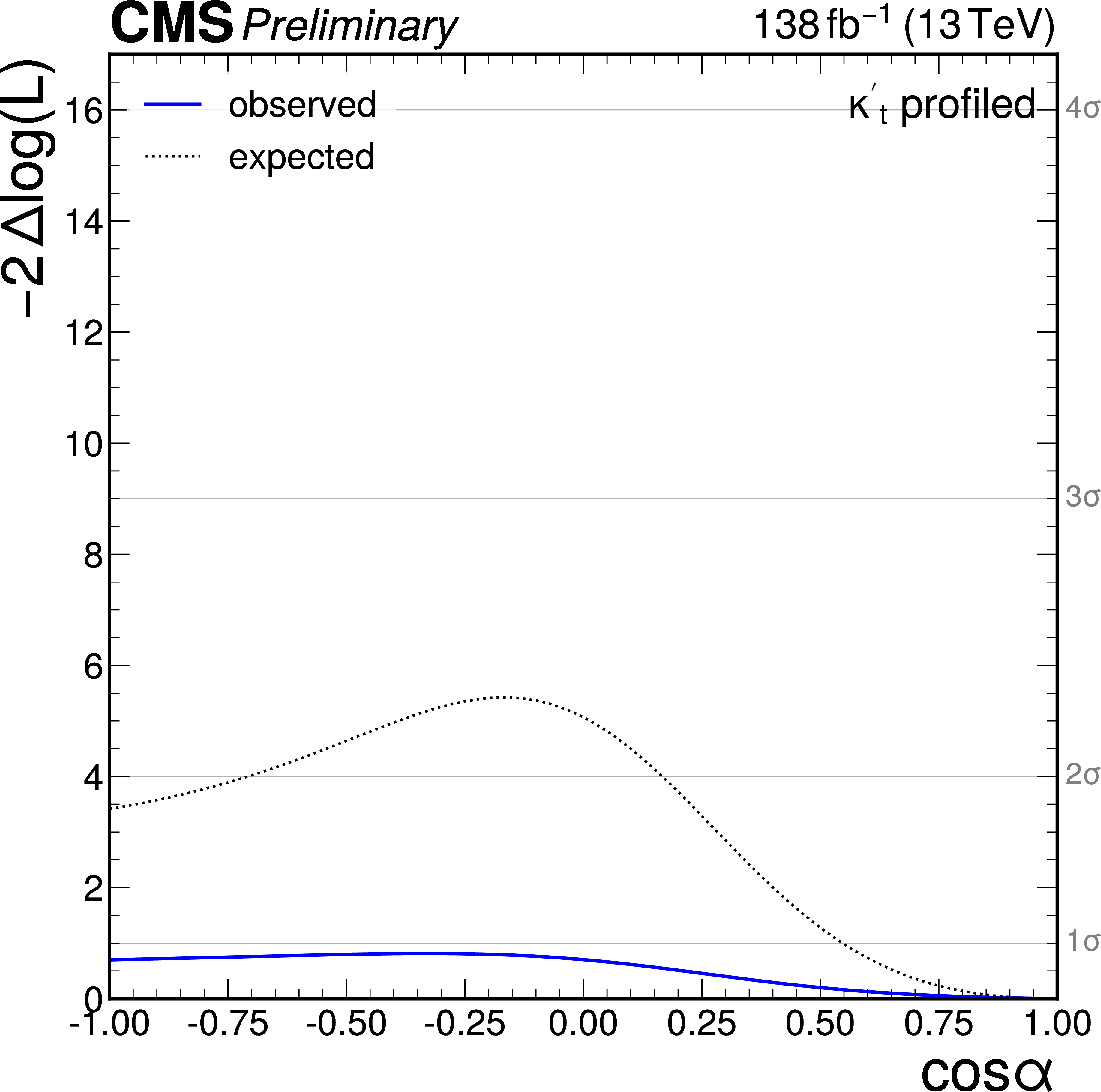
The observed (solid blue line) and expected (dotted black line) likelihood ratio test statistic as a function of $ f_{\text{CP}} $ (left) and $ \cos\alpha $ (right), where $ \kappa_{\text{V}} $ is 1 and $ \kappa^{\prime}_{\mathrm{t}}=\sqrt{\tilde{\kappa}_{\mathrm{t}}^{2}+\kappa_{\mathrm{t}}^{2}} $, the overall modifier of the top-Higgs coupling strength, is profiled such that the likelihood attains its minimum at each point in the plane. |

png pdf |
Figure 17-a:
The observed (solid blue line) and expected (dotted black line) likelihood ratio test statistic as a function of $ f_{\text{CP}} $ (left) and $ \cos\alpha $ (right), where $ \kappa_{\text{V}} $ is 1 and $ \kappa^{\prime}_{\mathrm{t}}=\sqrt{\tilde{\kappa}_{\mathrm{t}}^{2}+\kappa_{\mathrm{t}}^{2}} $, the overall modifier of the top-Higgs coupling strength, is profiled such that the likelihood attains its minimum at each point in the plane. |
png pdf |
Figure 17-b:
The observed (solid blue line) and expected (dotted black line) likelihood ratio test statistic as a function of $ f_{\text{CP}} $ (left) and $ \cos\alpha $ (right), where $ \kappa_{\text{V}} $ is 1 and $ \kappa^{\prime}_{\mathrm{t}}=\sqrt{\tilde{\kappa}_{\mathrm{t}}^{2}+\kappa_{\mathrm{t}}^{2}} $, the overall modifier of the top-Higgs coupling strength, is profiled such that the likelihood attains its minimum at each point in the plane. |
| Tables | |

png pdf |
Table 1:
Trigger selection criteria in the fully-hadronic (FH) channel. Multiple triggers, each represented by one row, are used per year and combined with a logical OR. In the case of the four-jet trigger, the minimum jet $ p_{\mathrm{T}} $ is different for each jet and separated by a slash (/). |

png pdf |
Table 2:
Generator version and configuration of the $ {\mathrm{t}\overline{\mathrm{t}}} $ and $ {\mathrm{t}\overline{\mathrm{t}}} \mathrm{b}\overline{\mathrm{b}} $ samples. The parameters $m_{\mathrm{t}}$ and $m_{\mathrm{b}}$ denote the top quark and bottom quark mass, respectively, $m_{\mathrm{T},\mathrm{t}}$, $m_{\mathrm{T},\mathrm{b}}$, and $m_{\mathrm{T},\mathrm{g}}$ the transverse mass of the top quark, the bottom quark, and additional gluons, respectively, and $ h_{\text{damp}} $ the parton-shower matching scale. |
png pdf |
Table 3:
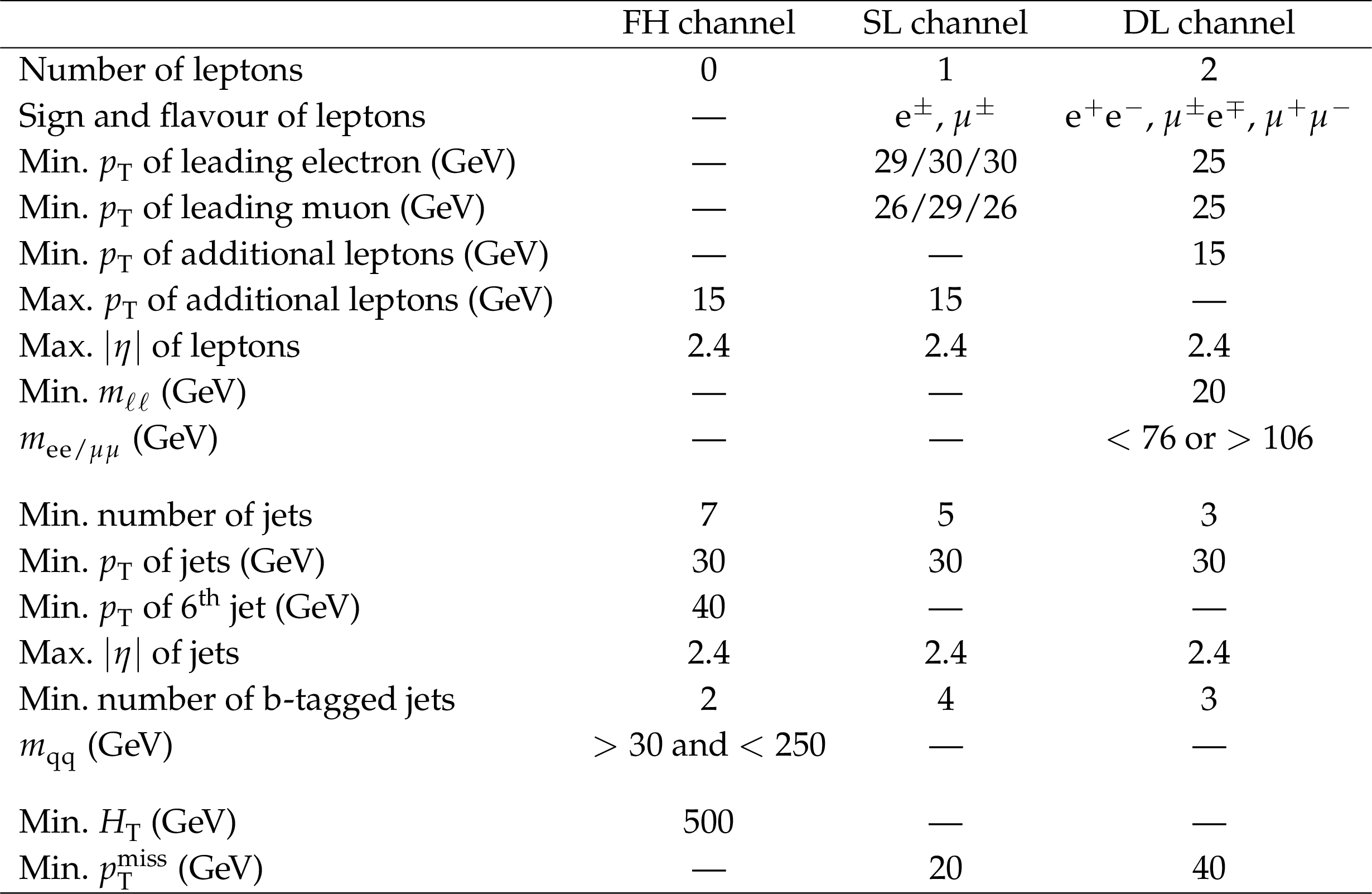
Baseline selection criteria in the fully-hadronic (FH), single-lepton (SL), and dilepton (DL) channels based on the observables defined in the text. Where the criteria differ per year of data taking, they are quoted as three values, corresponding to 2016/2017/2018, respectively. |
png pdf |
Table 4:
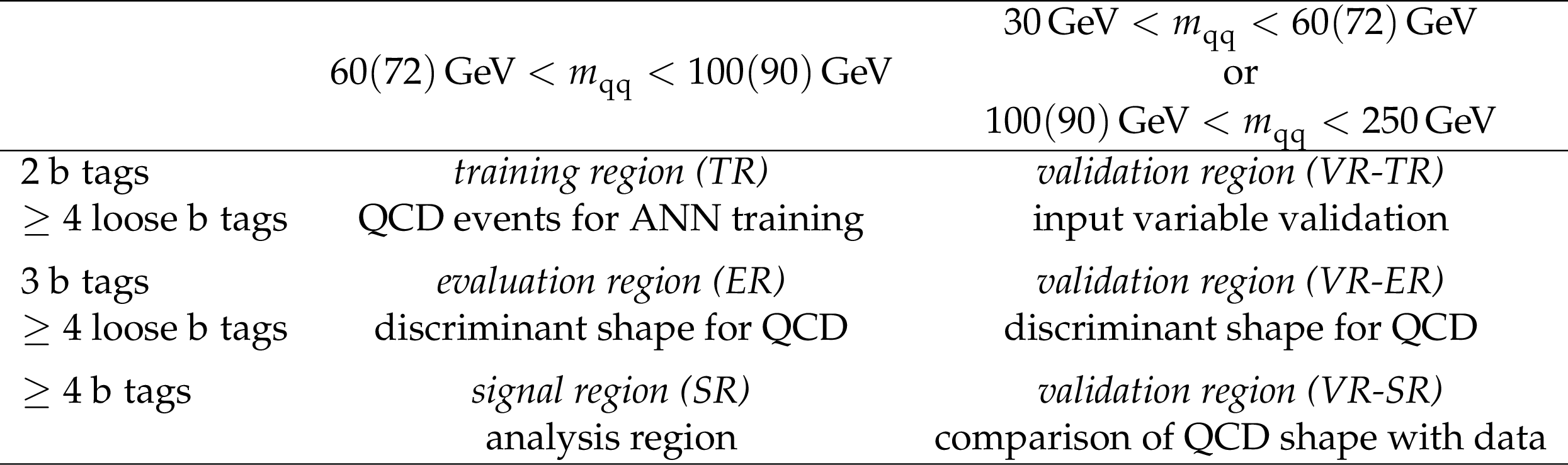
Categorisation scheme in the FH channel, applied independently in each jet-multiplicity category. The $m_{\mathrm{qq}}$ selection criteria refer to events with 7 or 8 ($ \geq $ 9) jets. |

png pdf |
Table 5:
Observables used as input variables to the ANN per channel. Observables marked with a $ ^{\dagger} $ are constructed using information from the BDT-based event reconstruction. |

png pdf |
Table 6:
Systematic uncertainties considered in the analysis. ``Type'' refers to rate (R) or rate and shape (S) altering uncertainties. ``Correlation'' indicates whether the uncertainty is treated as correlated, partially correlated (as detailed in the text), or uncorrelated across the years 2016--18. Uncertainties for $ {\mathrm{t}\overline{\mathrm{t}}} $+jets events marked with a $ ^{\dagger} $ are treated as partially correlated between each of the STXS categories and the other categories in the STXS analysis. |

png pdf |
Table 7:
Best-fit results of the ttH signal-strength modifier $ \mu_{{\mathrm{t}\overline{\mathrm{t}}} \mathrm{H}} $ in each channel and in their combination. Uncertainties are correlated between the channels. |

png pdf |
Table 8:
Contributions of different sources of uncertainty to the result for the fit to the data (observed) and to the expectation from simulation (expected). The quoted uncertainties $ \Delta\mu_{{\mathrm{t}\overline{\mathrm{t}}} \mathrm{H}} $ in $ \mu_{{\mathrm{t}\overline{\mathrm{t}}} \mathrm{H}} $ are obtained by fixing the listed sources of uncertainties to their postfit values in the fit and subtracting the obtained result in quadrature from the result of the full fit. The statistical uncertainty is evaluated by fixing all nuisance parameters to their postfit values and repeating the fit. The quadratic sum of the contributions is different from the total uncertainty because of correlations between the nuisance parameters. |

png pdf |
Table 9:
Best-fit results of the ttH signal-strength modifier $ \mu_{{\mathrm{t}\overline{\mathrm{t}}} \mathrm{H}} $ in the different bins of Higgs boson $ p_{\mathrm{T}} $ of the STXS measurement. |
| Summary |
| A combined analysis of the associated production of a Higgs boson (H) with a top quark-antiquark pair (ttH) or a single top quark (tH) with the Higgs boson decaying into a bottom quark-antiquark pair has been presented. The analysis has been performed using pp collision data recorded with the CMS detector at a centre-of-mass energy of 13 TeV, corresponding to an integrated luminosity of $ \mathcal{L} $. Candidate events are selected in mutually exclusive categories according to the lepton and jet multiplicity, targeting all decay channels of the $ \mathrm{t} \overline{\mathrm{t}} $ system. Neural network discriminants are used to further categorise the events according to the most probable process, targeting the signal and different topologies of the dominant $ {\mathrm{t}\overline{\mathrm{t}}} $+jets background, as well as to separate the signal from the background. Compared to previous CMS results in this channel, several updates of the analysis strategy as well as modelling of the $ {\mathrm{t}\overline{\mathrm{t}}} $+jets background based on state-of-the art $ {\mathrm{t}\overline{\mathrm{t}}} \mathrm{b}\overline{\mathrm{b}} $ simulations have been adopted, and an extended set of interpretations is performed. A best-fit value of the ttH production cross section relative to the standard model (SM) expectation of 0.33 $ \pm $ 0.26 $ = $ 0.33 $ \pm $ 0.17 (stat) $ \pm $ 0.21 (syst) is obtained. The analysis is additionally performed within the Simplified Template Cross Section framework in five intervals of Higgs boson $ p_{\mathrm{T}} $, probing potential $ p_{\mathrm{T}} $ dependent deviations from the SM expectation. An observed (expected) upper limit on the tH production cross section relative to the SM expectation of 14.6 (19.3) at 95% confidence level is derived. Information on the Higgs boson coupling strength is furthermore inferred from a simultaneous fit of the ttH and tH production rates, probing either the coupling strength of the Higgs boson to top quarks and to heavy vector bosons, or possible CP-odd admixtures in the coupling between the Higgs boson and top quarks. |
| Additional Figures | |

png pdf |
Additional Figure 1:
Transverse momentum of leading jet, ranked in $ p_{\mathrm{T}} $, for events in the SL channel after the baseline selection in the The last bins include overflow events. category, prefit (left) and with the postfit background model obtained from the fit of the final classifier distributions to data (right). The uncertainty band represents the total uncertainty. The last bins include overflow events. |

png pdf |
Additional Figure 1-a:
Transverse momentum of leading jet, ranked in $ p_{\mathrm{T}} $, for events in the SL channel after the baseline selection in the The last bins include overflow events. category, prefit (left) and with the postfit background model obtained from the fit of the final classifier distributions to data (right). The uncertainty band represents the total uncertainty. The last bins include overflow events. |

png pdf |
Additional Figure 1-b:
Transverse momentum of leading jet, ranked in $ p_{\mathrm{T}} $, for events in the SL channel after the baseline selection in the The last bins include overflow events. category, prefit (left) and with the postfit background model obtained from the fit of the final classifier distributions to data (right). The uncertainty band represents the total uncertainty. The last bins include overflow events. |
png pdf |
Additional Figure 2:
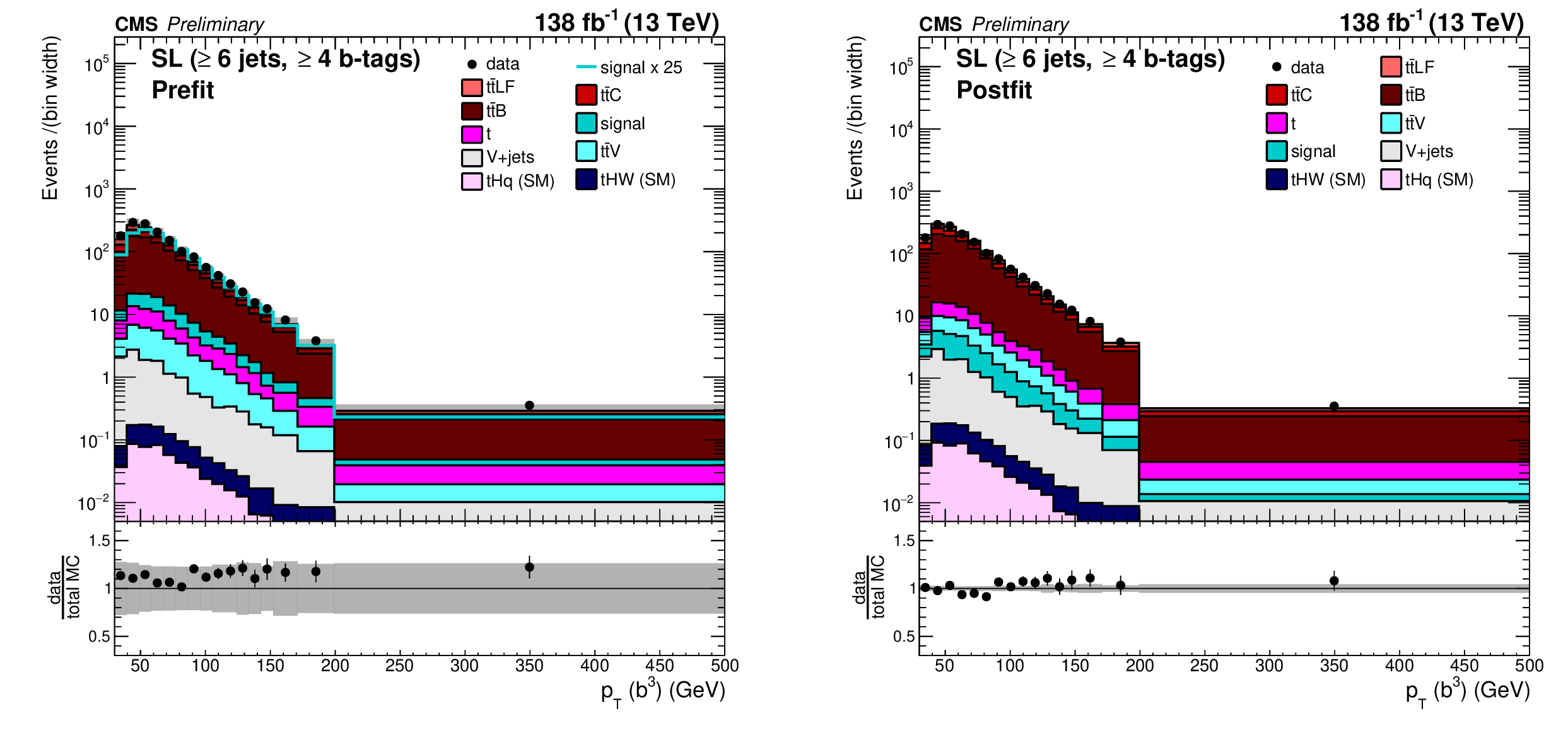
Transverse momentum of third leading b-tagged jet, ranked in $ p_{\mathrm{T}} $, for events in the SL channel after the baseline selection in the ($\geq$6 jets, $\geq$4 b tags) category, prefit (left) and with the postfit background model obtained from the fit of the final classifier distributions to data (right). The uncertainty band represents the total uncertainty. The last bins include overflow events. |

png pdf |
Additional Figure 2-a:
Transverse momentum of third leading b-tagged jet, ranked in $ p_{\mathrm{T}} $, for events in the SL channel after the baseline selection in the ($\geq$6 jets, $\geq$4 b tags) category, prefit (left) and with the postfit background model obtained from the fit of the final classifier distributions to data (right). The uncertainty band represents the total uncertainty. The last bins include overflow events. |

png pdf |
Additional Figure 2-b:
Transverse momentum of third leading b-tagged jet, ranked in $ p_{\mathrm{T}} $, for events in the SL channel after the baseline selection in the ($\geq$6 jets, $\geq$4 b tags) category, prefit (left) and with the postfit background model obtained from the fit of the final classifier distributions to data (right). The uncertainty band represents the total uncertainty. The last bins include overflow events. |
png pdf |
Additional Figure 3:
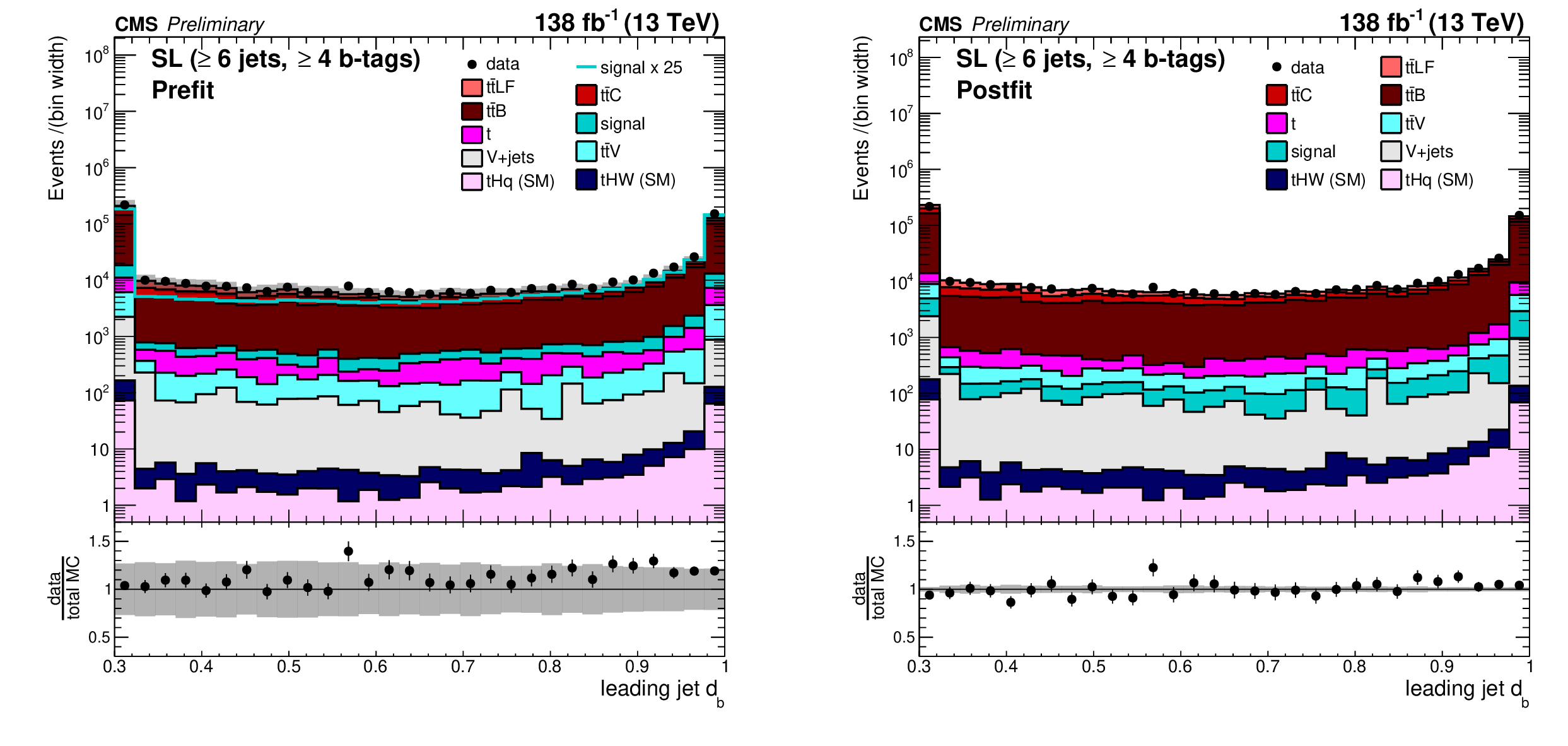
b tagging discriminant value of leading jet, ranked in $ p_{\mathrm{T}} $, for events in the SL channel after the baseline selection in the ($\geq$6 jets, $\geq$4 b tags) category, prefit (left) and with the postfit background model obtained from the fit of the final classifier distributions to data (right). The uncertainty band represents the total uncertainty. |

png pdf |
Additional Figure 3-a:
b tagging discriminant value of leading jet, ranked in $ p_{\mathrm{T}} $, for events in the SL channel after the baseline selection in the ($\geq$6 jets, $\geq$4 b tags) category, prefit (left) and with the postfit background model obtained from the fit of the final classifier distributions to data (right). The uncertainty band represents the total uncertainty. |

png pdf |
Additional Figure 3-b:
b tagging discriminant value of leading jet, ranked in $ p_{\mathrm{T}} $, for events in the SL channel after the baseline selection in the ($\geq$6 jets, $\geq$4 b tags) category, prefit (left) and with the postfit background model obtained from the fit of the final classifier distributions to data (right). The uncertainty band represents the total uncertainty. |

png pdf |
Additional Figure 4:
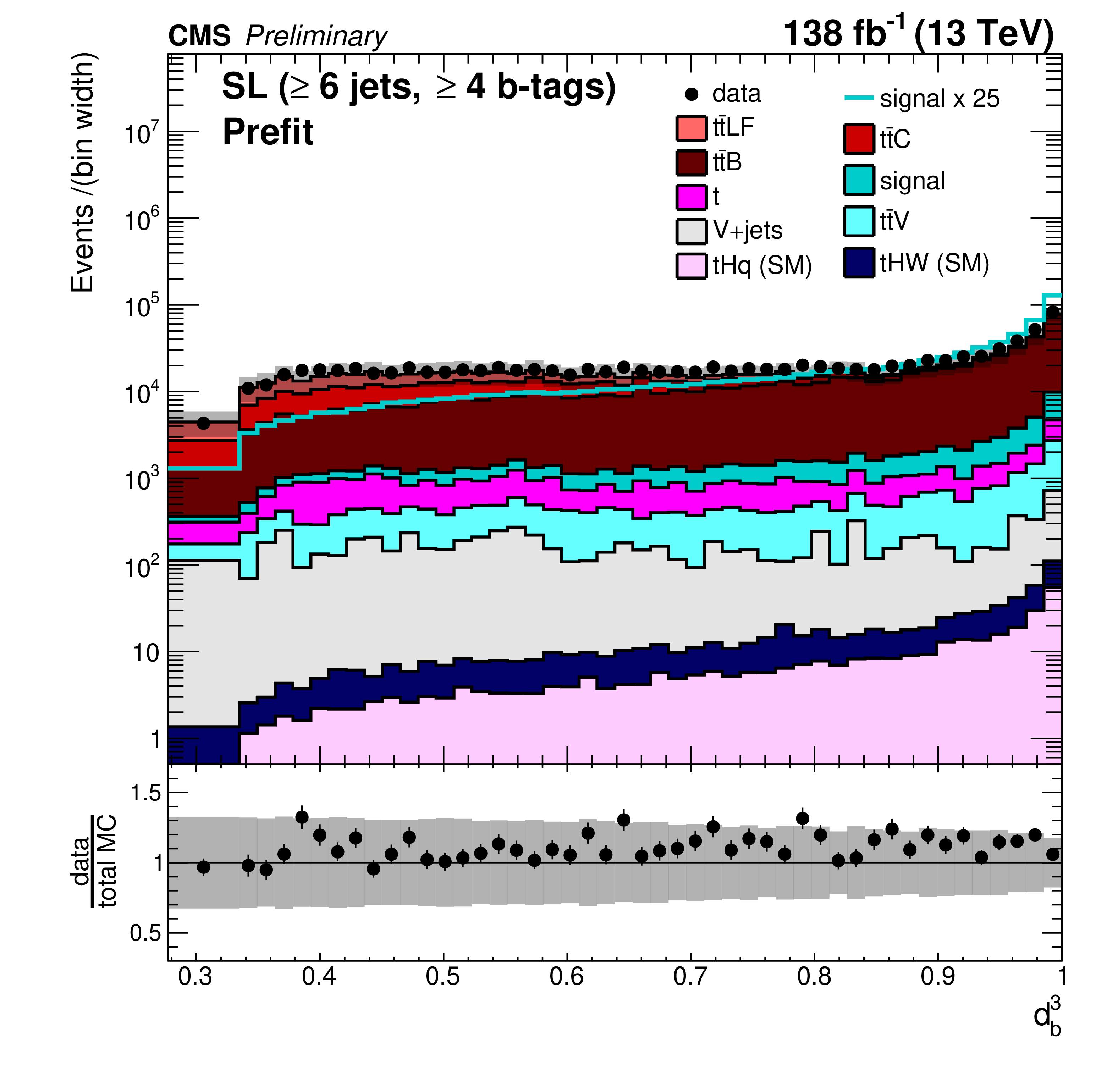
Third highest b tagging discriminant value of all jets for events in the SL channel after the baseline selection in the ($\geq$6 jets, $\geq$4 b tags) category, prefit (left) and with the postfit background model obtained from the fit of the final classifier distributions to data (right). The uncertainty band represents the total uncertainty. |
png pdf |
Additional Figure 4-a:
Third highest b tagging discriminant value of all jets for events in the SL channel after the baseline selection in the ($\geq$6 jets, $\geq$4 b tags) category, prefit (left) and with the postfit background model obtained from the fit of the final classifier distributions to data (right). The uncertainty band represents the total uncertainty. |

png pdf |
Additional Figure 4-b:
Third highest b tagging discriminant value of all jets for events in the SL channel after the baseline selection in the ($\geq$6 jets, $\geq$4 b tags) category, prefit (left) and with the postfit background model obtained from the fit of the final classifier distributions to data (right). The uncertainty band represents the total uncertainty. |

png pdf |
Additional Figure 5:
Transverse momentum of pair of b-tagged jets closest in $ \Delta R $ for events in the SL channel after the baseline selection in the ($\geq$6 jets, $\geq$4 b tags) category, prefit (left) and with the postfit background model obtained from the fit of the final classifier distributions to data (right). The uncertainty band represents the total uncertainty. The last bins include overflow events. |

png pdf |
Additional Figure 5-a:
Transverse momentum of pair of b-tagged jets closest in $ \Delta R $ for events in the SL channel after the baseline selection in the ($\geq$6 jets, $\geq$4 b tags) category, prefit (left) and with the postfit background model obtained from the fit of the final classifier distributions to data (right). The uncertainty band represents the total uncertainty. The last bins include overflow events. |
png pdf |
Additional Figure 5-b:
Transverse momentum of pair of b-tagged jets closest in $ \Delta R $ for events in the SL channel after the baseline selection in the ($\geq$6 jets, $\geq$4 b tags) category, prefit (left) and with the postfit background model obtained from the fit of the final classifier distributions to data (right). The uncertainty band represents the total uncertainty. The last bins include overflow events. |
png pdf |
Additional Figure 6:
Invariant mass of pair of b-tagged jets with mass closest to 125 GeV for events in the DL channel after the baseline selection, prefit (left) and with the postfit background model obtained from the fit of the final classifier distributions to data (right). The uncertainty band represents the total uncertainty. The last bins include overflow events. |

png pdf |
Additional Figure 6-a:
Invariant mass of pair of b-tagged jets with mass closest to 125 GeV for events in the DL channel after the baseline selection, prefit (left) and with the postfit background model obtained from the fit of the final classifier distributions to data (right). The uncertainty band represents the total uncertainty. The last bins include overflow events. |

png pdf |
Additional Figure 6-b:
Invariant mass of pair of b-tagged jets with mass closest to 125 GeV for events in the DL channel after the baseline selection, prefit (left) and with the postfit background model obtained from the fit of the final classifier distributions to data (right). The uncertainty band represents the total uncertainty. The last bins include overflow events. |

png pdf |
Additional Figure 7:
Transverse momentum of pair of b-tagged jets with mass closest to 125 GeV for events in the DL channel after the baseline selection, prefit (left) and with the postfit background model obtained from the fit of the final classifier distributions to data (right). The uncertainty band represents the total uncertainty. The last bins include overflow events. |

png pdf |
Additional Figure 7-a:
Transverse momentum of pair of b-tagged jets with mass closest to 125 GeV for events in the DL channel after the baseline selection, prefit (left) and with the postfit background model obtained from the fit of the final classifier distributions to data (right). The uncertainty band represents the total uncertainty. The last bins include overflow events. |

png pdf |
Additional Figure 7-b:
Transverse momentum of pair of b-tagged jets with mass closest to 125 GeV for events in the DL channel after the baseline selection, prefit (left) and with the postfit background model obtained from the fit of the final classifier distributions to data (right). The uncertainty band represents the total uncertainty. The last bins include overflow events. |
png pdf |
Additional Figure 8:
Transverse momentum of pair of b-tagged jets closest in $ \Delta R $ for events in the DL channel after the baseline selection, prefit (left) and with the postfit background model obtained from the fit of the final classifier distributions to data (right). The uncertainty band represents the total uncertainty. The last bins include overflow events. |

png pdf |
Additional Figure 8-a:
Transverse momentum of pair of b-tagged jets closest in $ \Delta R $ for events in the DL channel after the baseline selection, prefit (left) and with the postfit background model obtained from the fit of the final classifier distributions to data (right). The uncertainty band represents the total uncertainty. The last bins include overflow events. |

png pdf |
Additional Figure 8-b:
Transverse momentum of pair of b-tagged jets closest in $ \Delta R $ for events in the DL channel after the baseline selection, prefit (left) and with the postfit background model obtained from the fit of the final classifier distributions to data (right). The uncertainty band represents the total uncertainty. The last bins include overflow events. |

png pdf |
Additional Figure 9:
Average $ \Delta\eta $ between any two b-tagged jets for events in the SL channel after the baseline selection in the ($\geq$6 jets, $\geq$4 b tags) category prior to the fit to data, where the $ {\mathrm{t}\overline{\mathrm{t}}} \text{B} $ background contribution has been estimated using the $ {\mathrm{t}\overline{\mathrm{t}}} $ 5 FS sample. The uncertainty band represents the total uncertainty. The last bin includes overflow events. |
png pdf |
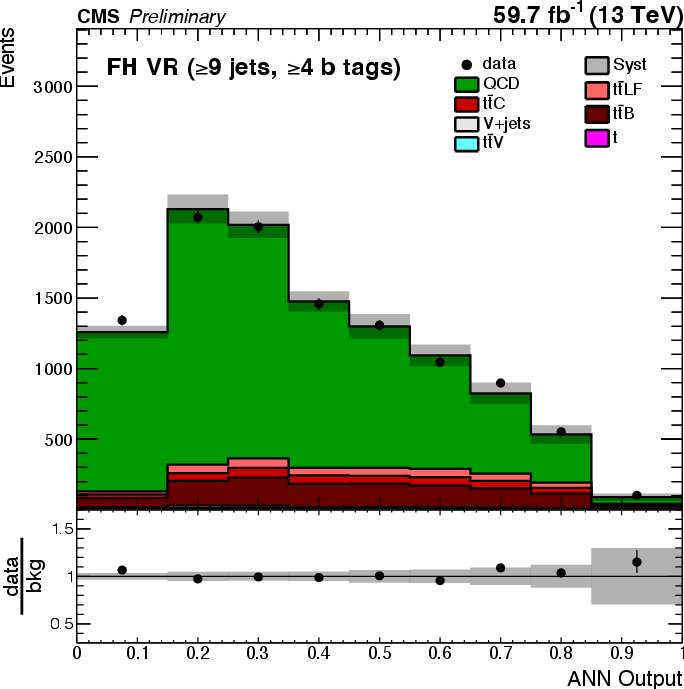
Additional Figure 10:
Validation of the QCD background estimation procedure: ANN output distribution observed in data compared to the predicted contributions from QCD (from data-driven procedure) and from other background processes (from simulation) in the ($\geq$9 jets, $\geq$4 b tags) validation region of the FH channel. |
png pdf |
Additional Figure 11:
Prefit expected (filled histograms) and observed (points) yields in each discriminant bin for the 2016 (top), 2017 (middle), and 2018 (bottom) data-taking periods. The uncertainty bands include the total uncertainty of the fit model. The lower pads show the ratio of the data to the background (points) and of the prefit expected signal+background to the background-only contribution (line). |

png pdf |
Additional Figure 11-a:
Prefit expected (filled histograms) and observed (points) yields in each discriminant bin for the 2016 (top), 2017 (middle), and 2018 (bottom) data-taking periods. The uncertainty bands include the total uncertainty of the fit model. The lower pads show the ratio of the data to the background (points) and of the prefit expected signal+background to the background-only contribution (line). |
png pdf |
Additional Figure 11-b:
Prefit expected (filled histograms) and observed (points) yields in each discriminant bin for the 2016 (top), 2017 (middle), and 2018 (bottom) data-taking periods. The uncertainty bands include the total uncertainty of the fit model. The lower pads show the ratio of the data to the background (points) and of the prefit expected signal+background to the background-only contribution (line). |

png pdf |
Additional Figure 11-c:
Prefit expected (filled histograms) and observed (points) yields in each discriminant bin for the 2016 (top), 2017 (middle), and 2018 (bottom) data-taking periods. The uncertainty bands include the total uncertainty of the fit model. The lower pads show the ratio of the data to the background (points) and of the prefit expected signal+background to the background-only contribution (line). |

png pdf |
Additional Figure 12:
Observed (points) and prefit expected (filled histograms) yields in each STXS analysis discriminant bin in the signal regions of the SL and DL channels for the 2016 (top), 2017 (middle), and 2018 (bottom) data-taking periods. The signal distributions in each Higgs boson $ p_{\mathrm{T}} $ bin are also overlayed (lines labelled $ {\mathrm{t}\overline{\mathrm{t}}} \mathrm{H} $ 1 to 5). The uncertainty bands include the total uncertainty of the fit model. The lower pads show the ratio of the data to the background (points) and of the prefit expected signal+background to the background-only contribution (lines). |

png pdf |
Additional Figure 12-a:
Observed (points) and prefit expected (filled histograms) yields in each STXS analysis discriminant bin in the signal regions of the SL and DL channels for the 2016 (top), 2017 (middle), and 2018 (bottom) data-taking periods. The signal distributions in each Higgs boson $ p_{\mathrm{T}} $ bin are also overlayed (lines labelled $ {\mathrm{t}\overline{\mathrm{t}}} \mathrm{H} $ 1 to 5). The uncertainty bands include the total uncertainty of the fit model. The lower pads show the ratio of the data to the background (points) and of the prefit expected signal+background to the background-only contribution (lines). |

png pdf |
Additional Figure 12-b:
Observed (points) and prefit expected (filled histograms) yields in each STXS analysis discriminant bin in the signal regions of the SL and DL channels for the 2016 (top), 2017 (middle), and 2018 (bottom) data-taking periods. The signal distributions in each Higgs boson $ p_{\mathrm{T}} $ bin are also overlayed (lines labelled $ {\mathrm{t}\overline{\mathrm{t}}} \mathrm{H} $ 1 to 5). The uncertainty bands include the total uncertainty of the fit model. The lower pads show the ratio of the data to the background (points) and of the prefit expected signal+background to the background-only contribution (lines). |
png pdf |
Additional Figure 12-c:
Observed (points) and prefit expected (filled histograms) yields in each STXS analysis discriminant bin in the signal regions of the SL and DL channels for the 2016 (top), 2017 (middle), and 2018 (bottom) data-taking periods. The signal distributions in each Higgs boson $ p_{\mathrm{T}} $ bin are also overlayed (lines labelled $ {\mathrm{t}\overline{\mathrm{t}}} \mathrm{H} $ 1 to 5). The uncertainty bands include the total uncertainty of the fit model. The lower pads show the ratio of the data to the background (points) and of the prefit expected signal+background to the background-only contribution (lines). |

png pdf |
Additional Figure 13:
Postfit values of the nuisance parameters (black markers) in the STXS analysis, shown as the difference of their best-fit values, $ \hat{\theta} $, and prefit values, $ \theta_{0} $, relative to the prefit uncertainties $ \Delta\theta $. The impact $ \Delta\hat{\mu}_{{\mathrm{t}\overline{\mathrm{t}}} \mathrm{H}}^{i} $ of the nuisance parameters on the signal strength $ \mu_{{\mathrm{t}\overline{\mathrm{t}}} \mathrm{H}}^{i} $ in the $ i $-th STXS bin is computed as the difference of the nominal best fit value of $ \mu_{{\mathrm{t}\overline{\mathrm{t}}} \mathrm{H}}^{i} $ and the best fit value obtained when fixing the nuisance parameter under scrutiny to its best fit value $ \hat{\theta} $ plus/minus its postfit uncertainty (coloured areas). The nuisance parameters are ordered by the quadratic sum of their relative impacts on all five $ \mu_{{\mathrm{t}\overline{\mathrm{t}}} \mathrm{H}}^{i} $, and only the 20 highest ranked parameters are shown. |

png pdf |
Additional Figure 14:
Correlations of the best-fit $ {\mathrm{t}\overline{\mathrm{t}}} \mathrm{H} $ signal-strength modifiers $ \mu_{{\mathrm{t}\overline{\mathrm{t}}} \mathrm{H}}^{i} $ in the different STXS bins $ i $ and the global ($ {\mathrm{t}\overline{\mathrm{t}}} \text{B} $) and per-bin ($ {\mathrm{t}\overline{\mathrm{t}}} \text{B}\;i $) $ {\mathrm{t}\overline{\mathrm{t}}} \text{B} $ background normalisation parameters. |
| Additional Tables | |

png pdf |
Additional Table 1:
Results of background model robustness tests performed in the SL+DL channels. For the tests, pseudo data are generated sampling the $ {\mathrm{t}\overline{\mathrm{t}}} \text{B} $ component from alternative $ {\mathrm{t}\overline{\mathrm{t}}} \text{B} $ predictions, and fitted using the nominal signal+background model. The injected signal corresponds to the SM expectation ($ \mu_{{\mathrm{t}\overline{\mathrm{t}}} \mathrm{H}} = $ 1). Pseudo data are sampled in different scenarios. First, the data are sampled from the nominal background model used in the analysis, as a cross-check. Second, the $ {\mathrm{t}\overline{\mathrm{t}}} \text{B} $ yield from the $ {\mathrm{t}\overline{\mathrm{t}}} \mathrm{b}\overline{\mathrm{b}} $ sample is scaled by a factor 1.2. In the next two tests, the $ {\mathrm{t}\overline{\mathrm{t}}} \text{B} $ component is taken from the $ {\mathrm{t}\overline{\mathrm{t}}} $ sample, once at its nominal value and once scaling its yield up by a factor 1.2. The table lists the mean values of the best-fit signal strength modifier, as well as the $ {\mathrm{t}\overline{\mathrm{t}}} \text{B} $ and $ {\mathrm{t}\overline{\mathrm{t}}} \text{C} $ background normalisation parameters obtained in the fits to the pseudo data. The quoted uncertainty corresponds to the RMS of the distributions. The statistical uncertainty on the mean values is below 1%. In all cases the fitted signal strength is compatible with the injected value of 1, showing that the fit is robust against potential mismodelling of the $ {\mathrm{t}\overline{\mathrm{t}}} \text{B} $ component. Also the $ {\mathrm{t}\overline{\mathrm{t}}} \text{B} $ and $ {\mathrm{t}\overline{\mathrm{t}}} \text{C} $ normalisations are compatible with the injected values within. |
| References | ||||
| 1 | ATLAS Collaboration | Observation of Higgs boson production in association with a top quark pair at the LHC with the ATLAS detector | PLB 784 (2018) 159 | 1806.00425 |
| 2 | CMS Collaboration | Observation of $ \mathrm{t}\overline{\mathrm{t}}\mathrm{H} $ production | PRL 120 (2018) 231801 | CMS-HIG-17-035 1804.02610 |
| 3 | ATLAS Collaboration | Observation of $ \mathrm{H}\to\mathrm{b}\overline{\mathrm{b}} $ decays and VH production with the ATLAS detector | PLB 786 (2018) 59 | 1808.08238 |
| 4 | CMS Collaboration | Observation of Higgs boson decay to bottom quarks | PRL 121 (2018) 121801 | CMS-HIG-18-016 1808.08242 |
| 5 | F. Maltoni, K. Paul, T. Stelzer, and S. Willenbrock | Associated production of Higgs and single top at hadron colliders | PRD 64 (2001) 094023 | hep-ph/0106293 |
| 6 | M. Farina et al. | Lifting degeneracies in Higgs couplings using single top production in association with a Higgs boson | JHEP 05 (2013) 022 | 1211.3736 |
| 7 | P. Agrawal, S. Mitra, and A. Shivaji | Effect of anomalous couplings on the associated production of a single top quark and a Higgs boson at the LHC | JHEP 12 (2013) 077 | 1211.4362 |
| 8 | F. Demartin, F. Maltoni, K. Mawatari, and M. Zaro | Higgs production in association with a single top quark at the LHC | EPJC 75 (2015) 267 | 1504.00611 |
| 9 | LHC Higgs Cross Section Working Group | Handbook of LHC Higgs cross sections: 4. deciphering the nature of the Higgs sector | 1610.07922 | |
| 10 | ATLAS Collaboration | Measurement of Higgs boson decay into b-quarks in associated production with a top-quark pair in pp collisions at $ \sqrt{s}= $ 13 TeV with the ATLAS detector | JHEP 06 (2022) 097 | 2111.06712 |
| 11 | CMS Collaboration | Search for $ \mathrm{t}\overline{\mathrm{t}}\mathrm{H} $ production in the $ \mathrm{H}\to\mathrm{b}\overline{\mathrm{b}} $ decay channel with leptonic $ \mathrm{t}\overline{\mathrm{t}} $ decays in proton-proton collisions at $ \sqrt{s}= $ 13 TeV | JHEP 03 (2019) 026 | CMS-HIG-17-026 1804.03682 |
| 12 | CMS Collaboration | Search for $ \mathrm{t}\overline{\mathrm{t}}\mathrm{H} $ production in the all-jet final state in proton-proton collisions at $ \sqrt{s}= $ 13 TeV | JHEP 06 (2018) | CMS-HIG-17-022 1803.06986 |
| 13 | CMS Collaboration | Search for associated production of a Higgs boson and a single top quark in proton-proton collisions at $ \sqrt{s}= $ 13 TeV | PRD 99 (2019) 092005 | CMS-HIG-18-009 1811.09696 |
| 14 | ATLAS Collaboration | Probing the $ CP $ nature of the top-Higgs Yukawa coupling in $ \mathrm{t}\overline{\mathrm{t}}\mathrm{H} $ and $ \mathrm{t}\mathrm{H} $ events with $ \mathrm{H}\to\mathrm{b}\overline{\mathrm{b}} $ decays using the ATLAS detector at the LHC | Submitted to PLB, 2023 | 2303.05974 |
| 15 | CMS Collaboration | The CMS experiment at the CERN LHC | JINST 3 (2008) S08004 | |
| 16 | CMS Collaboration | Performance of the CMS level-1 trigger in proton-proton collisions at $ \sqrt{s}= $ 13 TeV | JINST 15 (2020) P10017 | CMS-TRG-17-001 2006.10165 |
| 17 | CMS Collaboration | The CMS trigger system | JINST 12 (2017) P01020 | CMS-TRG-12-001 1609.02366 |
| 18 | CMS Collaboration | Precision luminosity measurement in proton-proton collisions at $ \sqrt{s}= $ 13 TeV in 2015 and 2016 at CMS | EPJC 81 (2021) 800 | CMS-LUM-17-003 2104.01927 |
| 19 | CMS | CMS luminosity measurement for the 2017 data-taking period at $ \sqrt{s}= $ 13 TeV | CMS Physics Analysis Summary, 2017 CMS-PAS-LUM-17-004 |
CMS-PAS-LUM-17-004 |
| 20 | CMS | CMS luminosity measurement for the 2018 data-taking period at $ \sqrt{s}= $ 13 TeV | CMS Physics Analysis Summary, 2018 CMS-PAS-LUM-18-002 |
CMS-PAS-LUM-18-002 |
| 21 | GEANT4 Collaboration | GEANT 4---a simulation toolkit | NIM A 506 (2003) 250 | |
| 22 | P. Nason | A new method for combining NLO QCD with shower Monte Carlo algorithms | JHEP 11 (2004) 040 | hep-ph/0409146 |
| 23 | S. Frixione, P. Nason, and C. Oleari | Matching NLO QCD computations with parton shower simulations: the POWHEG method | JHEP 11 (2007) 070 | 0709.2092 |
| 24 | S. Alioli, P. Nason, C. Oleari, and E. Re | A general framework for implementing NLO calculations in shower Monte Carlo programs: the POWHEG BOX | JHEP 06 (2010) 043 | 1002.2581 |
| 25 | T. Je žo and P. Nason | On the treatment of resonances in next-to-leading order calculations matched to a parton shower | JHEP 12 (2015) 065 | 1509.09071 |
| 26 | H. B. Hartanto, B. Jager, L. Reina, and D. Wackeroth | Higgs boson production in association with top quarks in the POWHEG BOX | PRD 91 (2015) 094003 | 1501.04498 |
| 27 | J. Alwall et al. | The automated computation of tree-level and next-to-leading order differential cross sections, and their matching to parton shower simulations | JHEP 07 (2014) 079 | 1405.0301 |
| 28 | T. Sjöstrand et al. | An introduction to PYTHIA 8.2 | Comput. Phys. Commun. 191 (2015) 159 | 1410.3012 |
| 29 | NNPDF Collaboration | Parton distributions from high-precision collider data | EPJC 77 (2017) 663 | 1706.00428 |
| 30 | CMS Collaboration | Extraction and validation of a new set of CMS PYTHIA 8 tunes from underlying-event measurements | EPJC 80 (2020) 4 | CMS-GEN-17-001 1903.12179 |
| 31 | CMS Collaboration | Event generator tunes obtained from underlying event and multiparton scattering measurements | EPJC 76 (2016) 155 | CMS-GEN-14-001 1512.00815 |
| 32 | F. Maltoni, G. Ridolfi, and M. Ubiali | b-initiated processes at the LHC: a reappraisal | JHEP 07 (2012) 022 | 1203.6393 |
| 33 | F. Demartin et al. | $ \mathrm{t}\mathrm{W}\mathrm{H} $ associated production at the LHC | EPJC 77 (2017) 34 | 1607.05862 |
| 34 | J. S. Gainer et al. | Exploring theory space with Monte Carlo reweighting | JHEP 10 (2014) 078 | 1404.7129 |
| 35 | O. Mattelaer | On the maximal use of Monte Carlo samples: re-weighting events at NLO accuracy | EPJC 76 (2016) 674 | 1607.00763 |
| 36 | T. Ježo, J. M. Lindert, N. Moretti, and S. Pozzorini | New NLOPS predictions for $ \mathrm{t}\overline{\mathrm{t}}+\mathrm{b} $-jet production at the LHC | EPJC 78 (2018) 502 | 1802.00426 |
| 37 | F. Buccioni et al. | OpenLoops 2 | EPJC 79 (2019) 866 | 1907.13071 |
| 38 | F. Cascioli et al. | NLO matching for $ \mathrm{t}\overline{\mathrm{t}}\mathrm{b}\overline{\mathrm{b}} $ production with massive b-quarks | PLB 734 (2014) 210 | 1309.5912 |
| 39 | F. Buccioni, S. Kallweit, S. Pozzorini, and M. F. Zoller | NLO QCD predictions for $ \mathrm{t}\overline{\mathrm{t}}\mathrm{b}\overline{\mathrm{b}} $ production in association with a light jet at the LHC | JHEP 12 (2019) 015 | 1907.13624 |
| 40 | S. Alioli, P. Nason, C. Oleari, and E. Re | NLO single-top production matched with shower in POWHEG: $ s $- and $ t $-channel contributions | JHEP 09 (2009) 111 | 0907.4076 |
| 41 | E. Re | Single-top Wt-channel production matched with parton showers using the POWHEG method | EPJC 71 (2011) 1547 | 1009.2450 |
| 42 | R. Frederix and S. Frixione | Merging meets matching in MC@NLO | JHEP 12 (2012) 061 | 1209.6215 |
| 43 | J. Alwall et al. | Comparative study of various algorithms for the merging of parton showers and matrix elements in hadronic collisions | EPJC 53 (2008) 473 | 0706.2569 |
| 44 | CMS Collaboration | A measurement of the Higgs boson mass in the diphoton decay channel | PLB 805 (2020) 135425 | CMS-HIG-19-004 2002.06398 |
| 45 | M. Cacciari et al. | Top-pair production at hadron colliders with next-to-next-to-leading logarithmic soft-gluon resummation | PLB 710 (2012) 612 | 1111.5869 |
| 46 | P. Bärnreuther, M. Czakon, and A. Mitov | Percent-level-precision physics at the Tevatron: next-to-next-to-leading order QCD corrections to $ \mathrm{q}\overline{\mathrm{q}}\to\mathrm{t}\overline{\mathrm{t}}\text{+X} $ | PRL 109 (2012) 132001 | 1204.5201 |
| 47 | M. Czakon and A. Mitov | NNLO corrections to top-pair production at hadron colliders: the all-fermionic scattering channels | JHEP 12 (2012) 054 | 1207.0236 |
| 48 | M. Czakon and A. Mitov | NNLO corrections to top pair production at hadron colliders: the quark-gluon reaction | JHEP 01 (2013) 080 | 1210.6832 |
| 49 | M. Beneke, P. Falgari, S. Klein, and C. Schwinn | Hadronic top-quark pair production with NNLL threshold resummation | NPB 855 (2012) 695 | 1109.1536 |
| 50 | M. Czakon, P. Fiedler, and A. Mitov | Total top-quark pair-production cross section at hadron colliders through $ o({\alpha_s}^4) $ | PRL 110 (2013) 252004 | 1303.6254 |
| 51 | M. Czakon and A. Mitov | Top++: a program for the calculation of the top-pair cross-section at hadron colliders | Comput. Phys. Commun. 185 (2014) 2930 | 1112.5675 |
| 52 | N. Kidonakis | Two-loop soft anomalous dimensions for single top quark associated production with $ \mathrm{W^-} $ or $ \mathrm{H}^{-} $ | PRD 82 (2010) 054018 | 1005.4451 |
| 53 | M. Aliev et al. | HATHOR: HAdronic Top and Heavy quarks crOss section calculatoR | Comput. Phys. Commun. 182 (2011) 1034 | 1007.1327 |
| 54 | P. Kant et al. | HatHor for single top-quark production: Updated predictions and uncertainty estimates for single top-quark production in hadronic collisions | Comput. Phys. Commun. 191 (2015) 74 | 1406.4403 |
| 55 | F. Maltoni, D. Pagani, and I. Tsinikos | Associated production of a top-quark pair with vector bosons at NLO in QCD: impact on $ \mathrm{t}\overline{\mathrm{t}}\mathrm{H} $ searches at the LHC | JHEP 02 (2016) 113 | 1507.05640 |
| 56 | J. M. Campbell, R. K. Ellis, and C. Williams | Vector boson pair production at the LHC | JHEP 07 (2011) 018 | 1105.0020 |
| 57 | CMS Collaboration | Particle-flow reconstruction and global event description with the CMS detector | JINST 12 (2017) P10003 | CMS-PRF-14-001 1706.04965 |
| 58 | CMS Collaboration | Technical proposal for the phase-2 upgrade of the Compact Muon Solenoid | CMS Technical Proposal CERN-LHCC-2015-010, CMS-TDR-15-02, 2015 CDS |
|
| 59 | CMS Collaboration | Performance of the CMS muon detector and muon reconstruction with proton-proton collisions at $ \sqrt{s}= $ 13 TeV | JINST 13 (2018) P06015 | CMS-MUO-16-001 1804.04528 |
| 60 | CMS Collaboration | Electron and photon reconstruction and identification with the CMS experiment at the CERN LHC | JINST 16 (2021) P05014 | CMS-EGM-17-001 2012.06888 |
| 61 | CMS Collaboration | ECAL 2016 refined calibration and Run2 summary plots | CMS Detector Performance Summary CMS-DP-2020-021, 2020 CDS |
|
| 62 | M. Cacciari, G. P. Salam, and G. Soyez | The anti-$ k_{\mathrm{T}} $ jet clustering algorithm | JHEP 04 (2008) 063 | 0802.1189 |
| 63 | M. Cacciari, G. P. Salam, and G. Soyez | FastJet user manual | EPJC 72 (2012) 1896 | 1111.6097 |
| 64 | M. Cacciari, G. P. Salam, and G. Soyez | The catchment area of jets | JHEP 04 (2008) 005 | 0802.1188 |
| 65 | CMS Collaboration | Jet energy scale and resolution in the CMS experiment in pp collisions at 8 TeV | JINST 12 (2017) P02014 | CMS-JME-13-004 1607.03663 |
| 66 | CMS Collaboration | Identification of heavy-flavour jets with the CMS detector in pp collisions at 13 TeV | JINST 13 (2018) P05011 | CMS-BTV-16-002 1712.07158 |
| 67 | E. Bols et al. | Jet flavour classification using DeepJet | JINST 15 (2020) P12012 | 2008.10519 |
| 68 | CMS Collaboration | B-tagging performance of the CMS legacy dataset 2018 | CMS Detector Performance Summary CMS-DP-2021-004, 2021 CDS |
|
| 69 | CMS Collaboration | Performance of missing transverse momentum reconstruction in proton-proton collisions at $ \sqrt{s} = $ 13 TeV using the CMS detector | JINST 14 (2019) P07004 | CMS-JME-17-001 1903.06078 |
| 70 | K. Kondo | Dynamical likelihood method for reconstruction of events with missing momentum. 1: Method and toy models | J. Phys. Soc. Jap. 57 (1988) 4126 | |
| 71 | CMS Collaboration | Inclusive and differential cross section measurements of $ \mathrm{t}\overline{\mathrm{t}}\mathrm{b}\overline{\mathrm{b}} $ production in the lepton+jets channel at $ \sqrt{s}= $ 13 TeV with the CMS detector | CMS Physics Analysis Summary, 2023 CMS-PAS-TOP-22-009 |
CMS-PAS-TOP-22-009 |
| 72 | CMS Collaboration | Measurement of the cross section for $ \mathrm{t}\overline{\mathrm{t}} $ production with additional jets and b jets in pp collisions at $ \sqrt{s}= $ 13 TeV | JHEP 07 (2020) 125 | CMS-TOP-18-002 2003.06467 |
| 73 | CMS Collaboration | Measurement of the $ \mathrm{t}\overline{\mathrm{t}}\mathrm{b}\overline{\mathrm{b}} $ production cross section in the all-jet final state in pp collisions at $ \sqrt{s}= $ 13 TeV | PLB 803 (2020) 135285 | CMS-TOP-18-011 1909.05306 |
| 74 | ATLAS and CMS Collaborations, and the LHC Higgs Combination Group | Procedure for the LHC Higgs boson search combination in summer 2011 | ATL-PHYS-PUB-2011-011, CMS NOTE-2011/005, 2011 link |
|
| 75 | J. S. Conway | Incorporating nuisance parameters in likelihoods for multisource spectra | PHYSTAT 201 (2011) 1 | 1103.0354 |
| 76 | J. D. Bjorken and S. J. Brodsky | Statistical model for electron-positron annihilation into hadrons | PRD 1 (1970) 1416 | |
| 77 | G. C. Fox and S. Wolfram | Event shapes in $ \mathrm{e}^+\mathrm{e}^- $ annihilation | Nuclear Physics B 157 (1979) 543 | |
| 78 | I. Goodfellow, Y. Bengio, and A. Courville | Deep Learning | MIT Press, 2016 link |
|
| 79 | J. K. Lindsey | Parametric statistical inference | Clarendon Press, Oxford, England, 1996 | |
| 80 | CMS Collaboration | Performance of deep tagging algorithms for boosted double quark jet topology in proton-proton collisions at 13 TeV with the phase-0 CMS detector | CMS Detector Performance Summary CMS-DP-2018-046, 2018 CDS |
|
| 81 | F. Chollet et al. | Keras | link | |
| 82 | S. Jasper, L. Hugo, and P. A. Ryan | Practical bayesian optimization of machine learning algorithms | 1206.2944 | |
| 83 | F. Luca, D. Michele, F. Paolo, and P. Massimiliano | Forward and reverse gradient-based hyperparameter optimization | in 34th International Conference on Machine Learning, Proceedings of Machine Learning Research, vol. 70. PMLR, 2017 | |
| 84 | NNPDF Collaboration | Parton distributions for the LHC Run II | JHEP 04 (2015) 040 | 1410.8849 |
| 85 | P. Skands, S. Carrazza, and J. Rojo | Tuning PYTHIA 8.1: the Monash 2013 tune | EPJC 74 (2014) 3024 | 1404.5630 |
| 86 | CMS Collaboration | Measurement of differential cross sections for the production of top quark pairs and of additional jets in lepton+jets events from pp collisions at $ \sqrt{s}= $ 13 TeV | PRD 97 (2018) 112003 | CMS-TOP-17-002 1803.08856 |
| 87 | J. R. Andersen et al. | Les Houches 2017: Physics at TeV colliders standard model working group report | 1803.07977 | |
| 88 | CMS Tracker Group Collaboration | The CMS phase-1 pixel detector upgrade | JINST 16 (2021) P02027 | 2012.14304 |
| 89 | R. Barlow and C. Beeston | Fitting using finite Monte Carlo samples | Comp. Phys. Commun. 77 (1993) 219 | |
| 90 | CMS Collaboration | First measurement of the cross section for top quark pair production with additional charm jets using dileptonic final states in pp collisions at $ \sqrt{s}= $ 13 TeV | PLB 820 (2021) 136565 | CMS-TOP-20-003 2012.09225 |
| 91 | LHC Higgs Cross Section Working Group | Handbook of LHC Higgs cross sections: 3. Higgs properties | 1307.1347 | |
| 92 | A. V. Gritsan, R. Röntsch, M. Schulze, and M. Xiao | Constraining anomalous Higgs boson couplings to the heavy flavor fermions using matrix element techniques | PRD 94 (2016) 055023 | 1606.03107 |
| 93 | F. Demartin et al. | Higgs characterisation at NLO in QCD: CP properties of the top-quark Yukawa interaction | EPJC 74 (2014) 3065 | 1407.5089 |
|
|
Compact Muon Solenoid LHC, CERN |
|

|

|

|

|

|