

Compact Muon Solenoid
LHC, CERN
| CMS-PAS-HIG-20-016 | ||
| Search for high mass resonances decaying into W$^{+}$W$^{-}$ in the dileptonic final state with 138 fb$^{-1}$ of proton-proton collisions at $\sqrt{s}=$ 13 TeV | ||
| CMS Collaboration | ||
| March 2022 | ||
| Abstract: A search for high mass resonances decaying into a pair of W bosons is performed. The analysis considers the fully leptonic final state (e$\mu$, $\mu\mu$, ee). New techniques are implemented in the analysis to improve the sensitivity of the search, especially in the very high mass range. The search is performed in a mass range from 115 GeV to 5 TeV, and for various width hypotheses. Both the gluon-gluon-fusion and vector-boson-fusion signal production processes are considered. Interference effects between signal and background are also taken into account. The results are presented as 95% confidence level upper limits on the product of the cross section and branching ratio on the production of a high mass resonance, and exclusion limits are derived on various two-higgs-doublet models and minimal supersymmetric standard model benchmark scenarios. | ||
| Links: CDS record (PDF) ; CADI line (restricted) ; | ||
| Figures & Tables | Summary | Additional Figures | References | CMS Publications |
|---|
| Figures | |

png pdf |
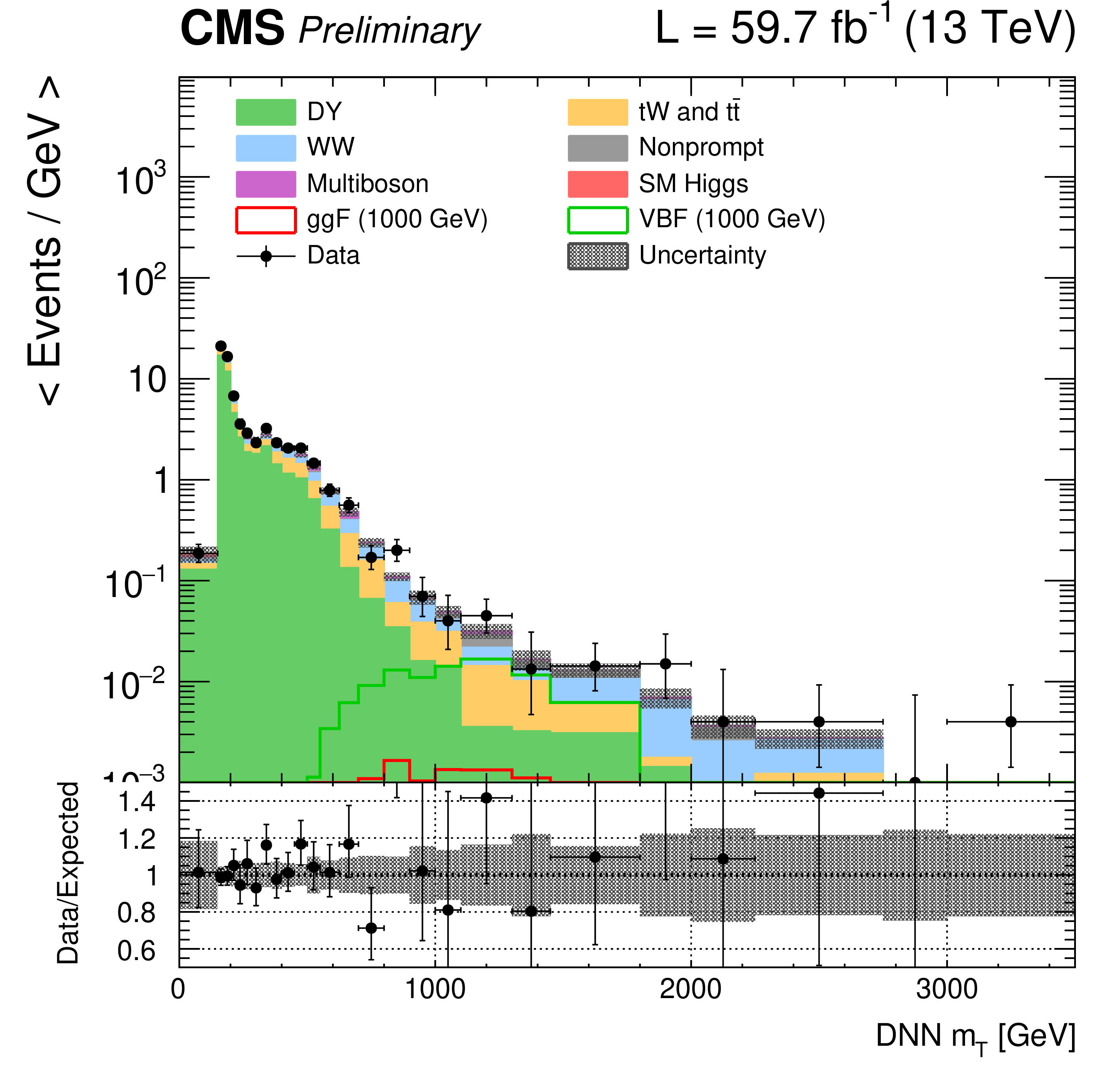
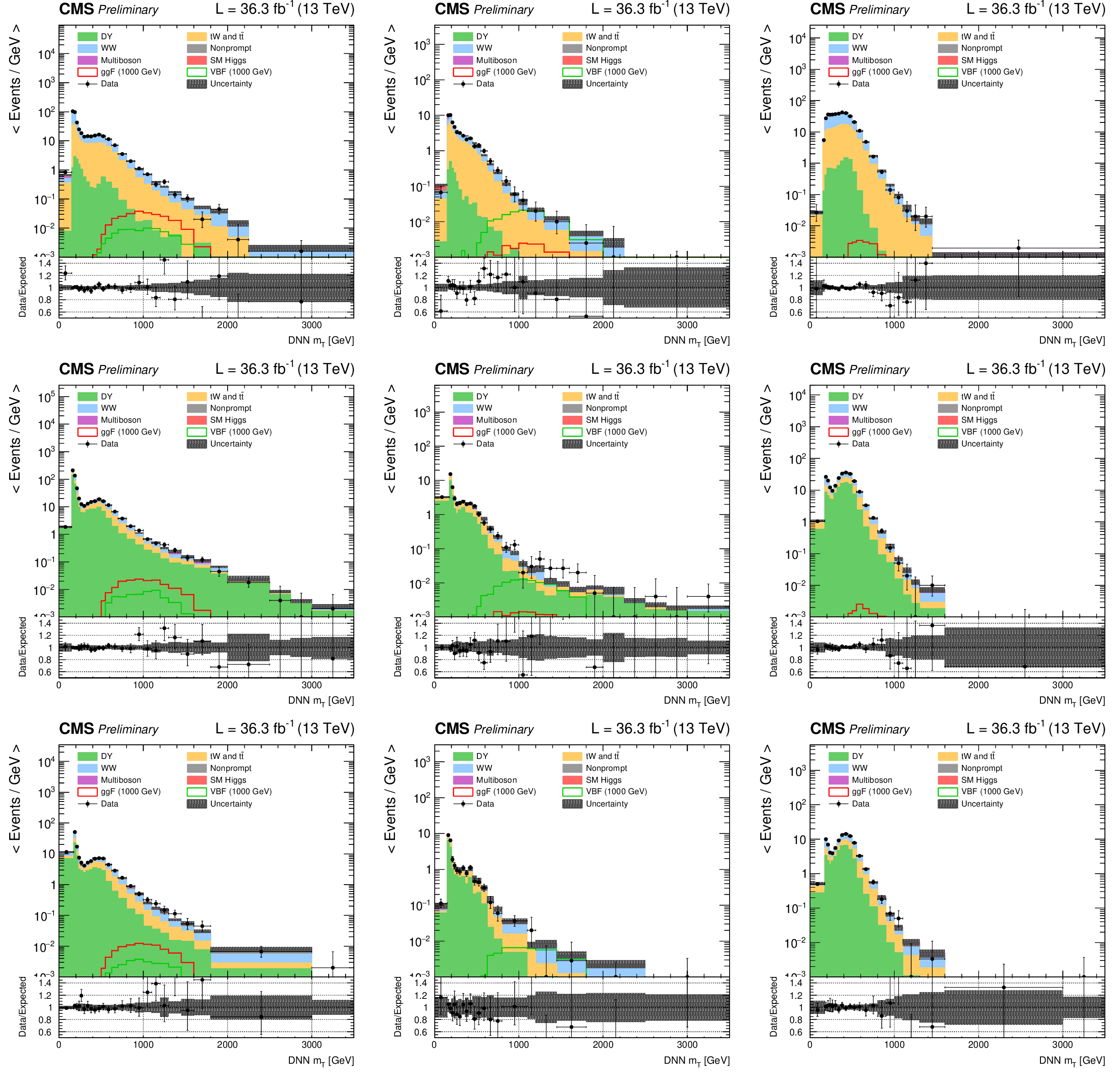
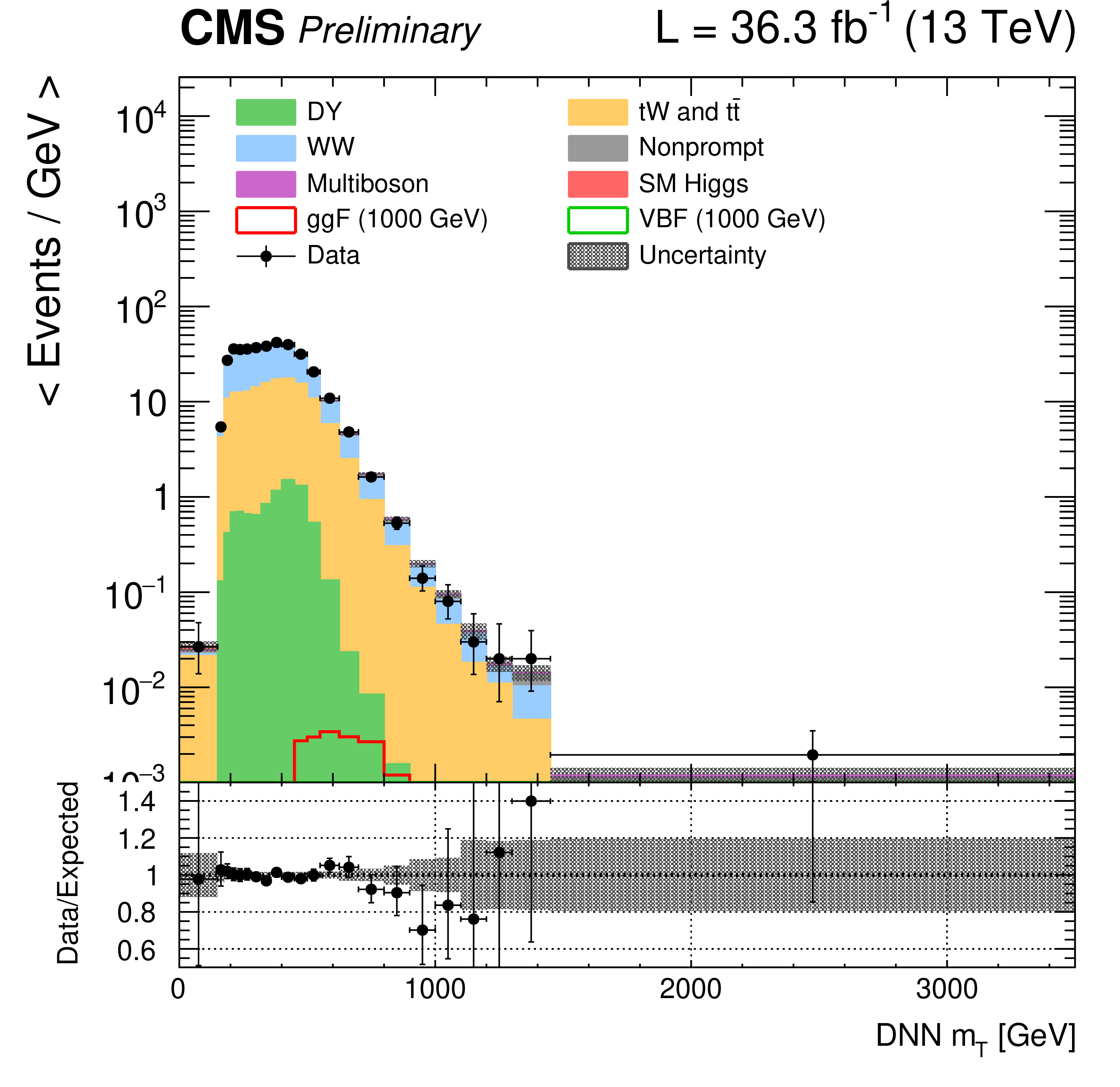
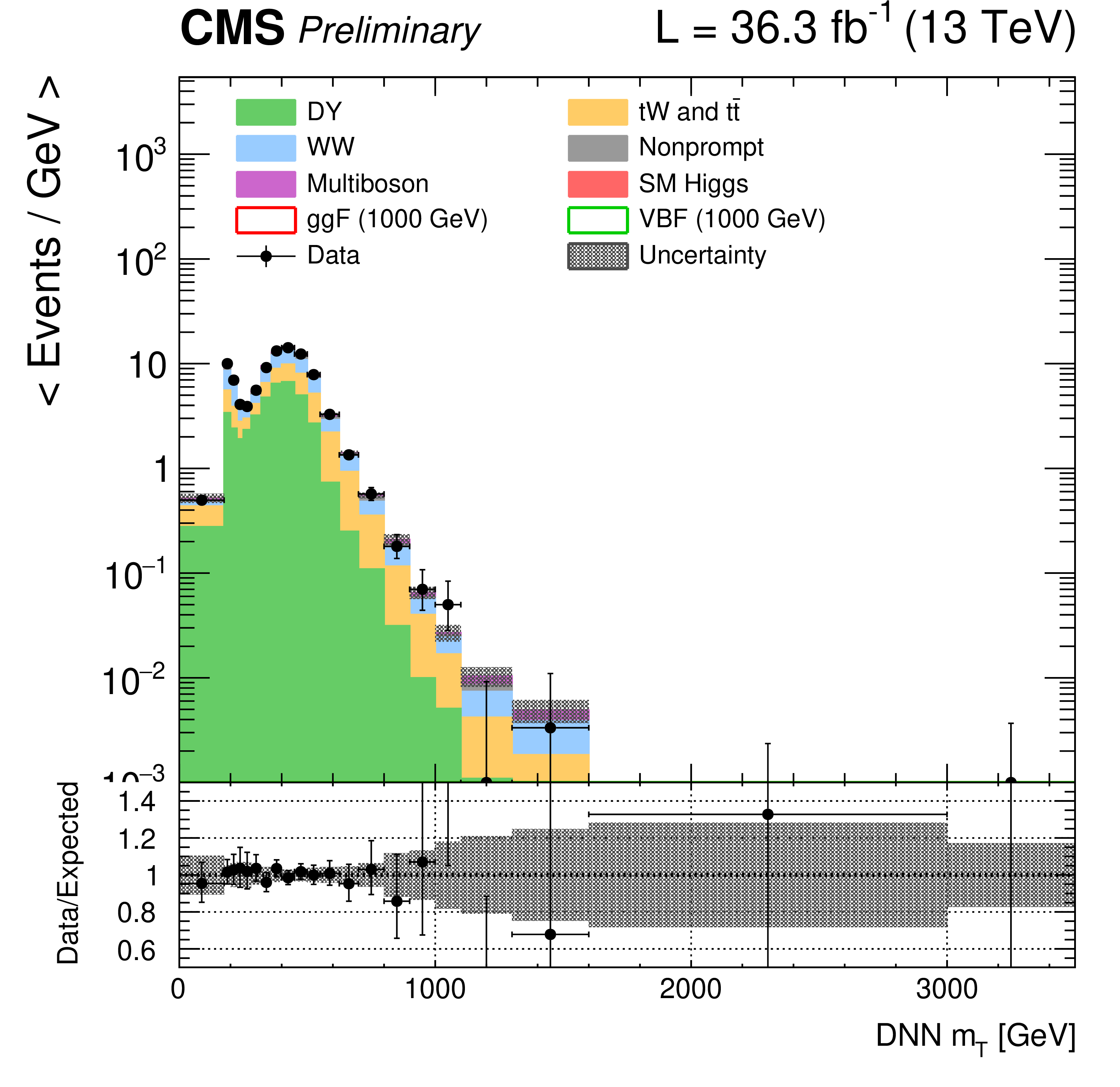
Figure 1:
DNN $m_{\mathrm{T}}$ distributions for the 2018 data set along with the background estimation and the prediction of a 1000 GeV signal, for events passing the e$ \mu $ (top), $\mu \mu $ (middle) and ee (bottom) signal region selections and entering the ggF (left), VBF (middle) and background (right) categories. |

png pdf |
Figure 1-a:
DNN $m_{\mathrm{T}}$ distributions for the 2018 data set along with the background estimation and the prediction of a 1000 GeV signal, for events passing the e$ \mu $ (top), $\mu \mu $ (middle) and ee (bottom) signal region selections and entering the ggF (left), VBF (middle) and background (right) categories. |

png pdf |
Figure 1-b:
DNN $m_{\mathrm{T}}$ distributions for the 2018 data set along with the background estimation and the prediction of a 1000 GeV signal, for events passing the e$ \mu $ (top), $\mu \mu $ (middle) and ee (bottom) signal region selections and entering the ggF (left), VBF (middle) and background (right) categories. |

png pdf |
Figure 1-c:
DNN $m_{\mathrm{T}}$ distributions for the 2018 data set along with the background estimation and the prediction of a 1000 GeV signal, for events passing the e$ \mu $ (top), $\mu \mu $ (middle) and ee (bottom) signal region selections and entering the ggF (left), VBF (middle) and background (right) categories. |

png pdf |
Figure 1-d:
DNN $m_{\mathrm{T}}$ distributions for the 2018 data set along with the background estimation and the prediction of a 1000 GeV signal, for events passing the e$ \mu $ (top), $\mu \mu $ (middle) and ee (bottom) signal region selections and entering the ggF (left), VBF (middle) and background (right) categories. |

png pdf |
Figure 1-e:
DNN $m_{\mathrm{T}}$ distributions for the 2018 data set along with the background estimation and the prediction of a 1000 GeV signal, for events passing the e$ \mu $ (top), $\mu \mu $ (middle) and ee (bottom) signal region selections and entering the ggF (left), VBF (middle) and background (right) categories. |

png pdf |
Figure 1-f:
DNN $m_{\mathrm{T}}$ distributions for the 2018 data set along with the background estimation and the prediction of a 1000 GeV signal, for events passing the e$ \mu $ (top), $\mu \mu $ (middle) and ee (bottom) signal region selections and entering the ggF (left), VBF (middle) and background (right) categories. |

png pdf |
Figure 1-g:
DNN $m_{\mathrm{T}}$ distributions for the 2018 data set along with the background estimation and the prediction of a 1000 GeV signal, for events passing the e$ \mu $ (top), $\mu \mu $ (middle) and ee (bottom) signal region selections and entering the ggF (left), VBF (middle) and background (right) categories. |
png pdf |
Figure 1-h:
DNN $m_{\mathrm{T}}$ distributions for the 2018 data set along with the background estimation and the prediction of a 1000 GeV signal, for events passing the e$ \mu $ (top), $\mu \mu $ (middle) and ee (bottom) signal region selections and entering the ggF (left), VBF (middle) and background (right) categories. |

png pdf |
Figure 1-i:
DNN $m_{\mathrm{T}}$ distributions for the 2018 data set along with the background estimation and the prediction of a 1000 GeV signal, for events passing the e$ \mu $ (top), $\mu \mu $ (middle) and ee (bottom) signal region selections and entering the ggF (left), VBF (middle) and background (right) categories. |

png pdf |
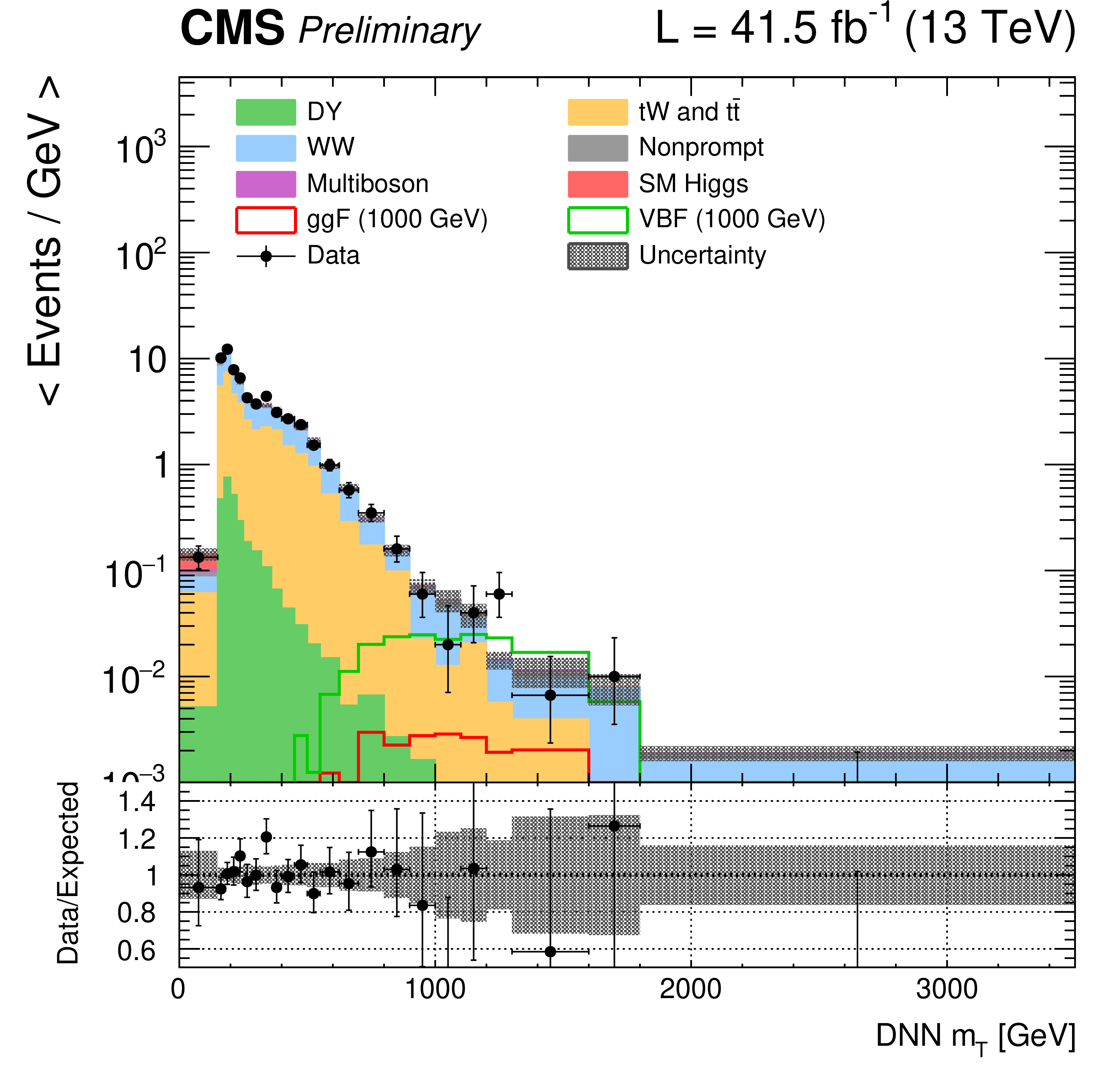
Figure 2:
DNN $m_{\mathrm{T}}$ distributions for the 2017 data set along with the background estimation and the prediction of a 1000 GeV signal, for events passing the e$ \mu $ (top), $\mu \mu $ (middle) and ee (bottom) signal region selections and entering the ggF (left), VBF (middle) and background (right) categories. |

png pdf |
Figure 2-a:
DNN $m_{\mathrm{T}}$ distributions for the 2017 data set along with the background estimation and the prediction of a 1000 GeV signal, for events passing the e$ \mu $ (top), $\mu \mu $ (middle) and ee (bottom) signal region selections and entering the ggF (left), VBF (middle) and background (right) categories. |
png pdf |
Figure 2-b:
DNN $m_{\mathrm{T}}$ distributions for the 2017 data set along with the background estimation and the prediction of a 1000 GeV signal, for events passing the e$ \mu $ (top), $\mu \mu $ (middle) and ee (bottom) signal region selections and entering the ggF (left), VBF (middle) and background (right) categories. |

png pdf |
Figure 2-c:
DNN $m_{\mathrm{T}}$ distributions for the 2017 data set along with the background estimation and the prediction of a 1000 GeV signal, for events passing the e$ \mu $ (top), $\mu \mu $ (middle) and ee (bottom) signal region selections and entering the ggF (left), VBF (middle) and background (right) categories. |

png pdf |
Figure 2-d:
DNN $m_{\mathrm{T}}$ distributions for the 2017 data set along with the background estimation and the prediction of a 1000 GeV signal, for events passing the e$ \mu $ (top), $\mu \mu $ (middle) and ee (bottom) signal region selections and entering the ggF (left), VBF (middle) and background (right) categories. |

png pdf |
Figure 2-e:
DNN $m_{\mathrm{T}}$ distributions for the 2017 data set along with the background estimation and the prediction of a 1000 GeV signal, for events passing the e$ \mu $ (top), $\mu \mu $ (middle) and ee (bottom) signal region selections and entering the ggF (left), VBF (middle) and background (right) categories. |

png pdf |
Figure 2-f:
DNN $m_{\mathrm{T}}$ distributions for the 2017 data set along with the background estimation and the prediction of a 1000 GeV signal, for events passing the e$ \mu $ (top), $\mu \mu $ (middle) and ee (bottom) signal region selections and entering the ggF (left), VBF (middle) and background (right) categories. |

png pdf |
Figure 2-g:
DNN $m_{\mathrm{T}}$ distributions for the 2017 data set along with the background estimation and the prediction of a 1000 GeV signal, for events passing the e$ \mu $ (top), $\mu \mu $ (middle) and ee (bottom) signal region selections and entering the ggF (left), VBF (middle) and background (right) categories. |
png pdf |
Figure 2-h:
DNN $m_{\mathrm{T}}$ distributions for the 2017 data set along with the background estimation and the prediction of a 1000 GeV signal, for events passing the e$ \mu $ (top), $\mu \mu $ (middle) and ee (bottom) signal region selections and entering the ggF (left), VBF (middle) and background (right) categories. |

png pdf |
Figure 2-i:
DNN $m_{\mathrm{T}}$ distributions for the 2017 data set along with the background estimation and the prediction of a 1000 GeV signal, for events passing the e$ \mu $ (top), $\mu \mu $ (middle) and ee (bottom) signal region selections and entering the ggF (left), VBF (middle) and background (right) categories. |
png pdf |
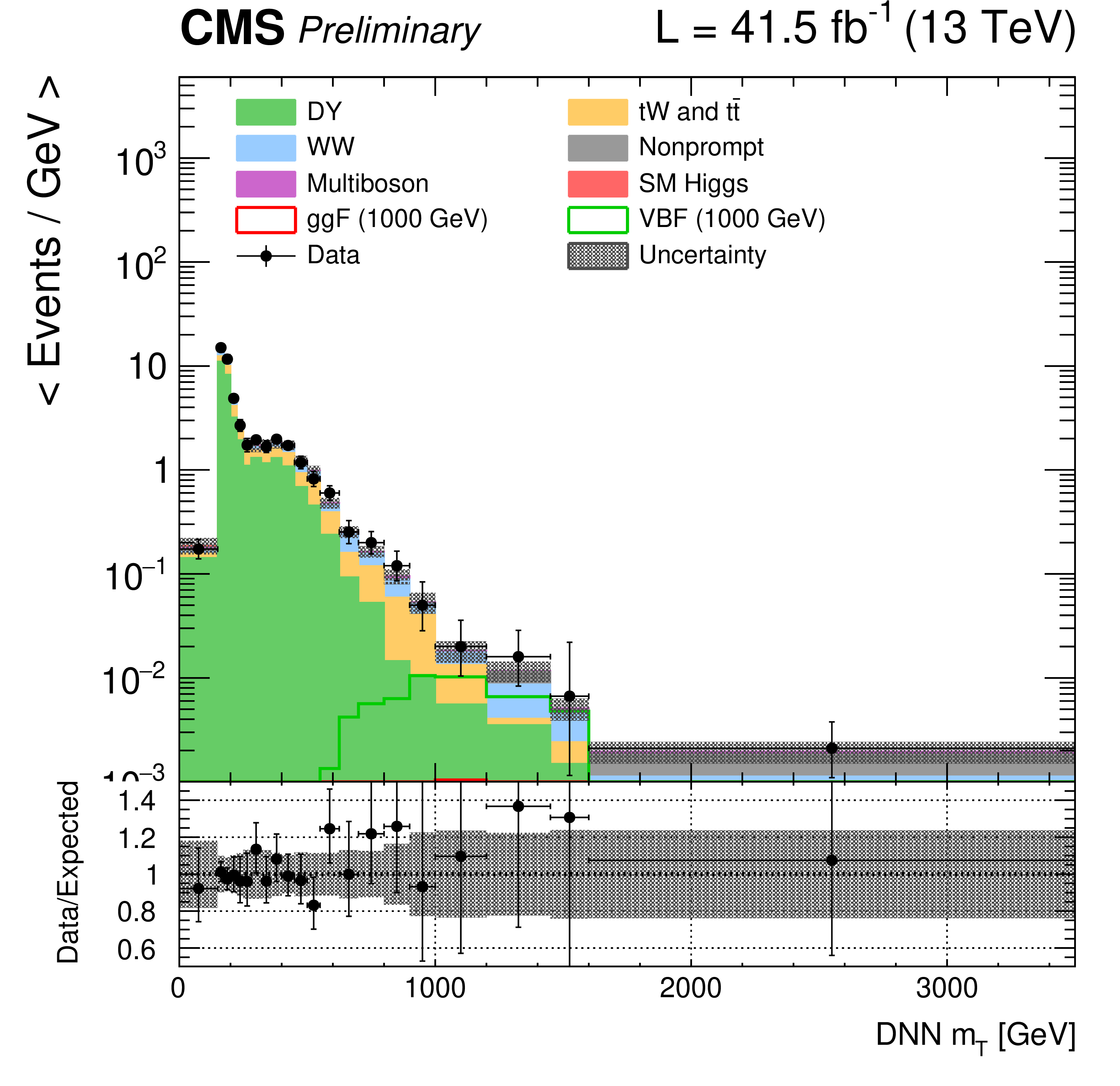
Figure 3:
DNN $m_{\mathrm{T}}$ distributions for the 2016 data set along with the background estimation and the prediction of a 1000 GeV signal, for events passing the e$ \mu $ (top), $\mu \mu $ (middle) and ee (bottom) signal region selections and entering the ggF (left), VBF (middle) and background (right) categories. |

png pdf |
Figure 3-a:
DNN $m_{\mathrm{T}}$ distributions for the 2016 data set along with the background estimation and the prediction of a 1000 GeV signal, for events passing the e$ \mu $ (top), $\mu \mu $ (middle) and ee (bottom) signal region selections and entering the ggF (left), VBF (middle) and background (right) categories. |

png pdf |
Figure 3-b:
DNN $m_{\mathrm{T}}$ distributions for the 2016 data set along with the background estimation and the prediction of a 1000 GeV signal, for events passing the e$ \mu $ (top), $\mu \mu $ (middle) and ee (bottom) signal region selections and entering the ggF (left), VBF (middle) and background (right) categories. |
png pdf |
Figure 3-c:
DNN $m_{\mathrm{T}}$ distributions for the 2016 data set along with the background estimation and the prediction of a 1000 GeV signal, for events passing the e$ \mu $ (top), $\mu \mu $ (middle) and ee (bottom) signal region selections and entering the ggF (left), VBF (middle) and background (right) categories. |

png pdf |
Figure 3-d:
DNN $m_{\mathrm{T}}$ distributions for the 2016 data set along with the background estimation and the prediction of a 1000 GeV signal, for events passing the e$ \mu $ (top), $\mu \mu $ (middle) and ee (bottom) signal region selections and entering the ggF (left), VBF (middle) and background (right) categories. |

png pdf |
Figure 3-e:
DNN $m_{\mathrm{T}}$ distributions for the 2016 data set along with the background estimation and the prediction of a 1000 GeV signal, for events passing the e$ \mu $ (top), $\mu \mu $ (middle) and ee (bottom) signal region selections and entering the ggF (left), VBF (middle) and background (right) categories. |

png pdf |
Figure 3-f:
DNN $m_{\mathrm{T}}$ distributions for the 2016 data set along with the background estimation and the prediction of a 1000 GeV signal, for events passing the e$ \mu $ (top), $\mu \mu $ (middle) and ee (bottom) signal region selections and entering the ggF (left), VBF (middle) and background (right) categories. |

png pdf |
Figure 3-g:
DNN $m_{\mathrm{T}}$ distributions for the 2016 data set along with the background estimation and the prediction of a 1000 GeV signal, for events passing the e$ \mu $ (top), $\mu \mu $ (middle) and ee (bottom) signal region selections and entering the ggF (left), VBF (middle) and background (right) categories. |

png pdf |
Figure 3-h:
DNN $m_{\mathrm{T}}$ distributions for the 2016 data set along with the background estimation and the prediction of a 1000 GeV signal, for events passing the e$ \mu $ (top), $\mu \mu $ (middle) and ee (bottom) signal region selections and entering the ggF (left), VBF (middle) and background (right) categories. |
png pdf |
Figure 3-i:
DNN $m_{\mathrm{T}}$ distributions for the 2016 data set along with the background estimation and the prediction of a 1000 GeV signal, for events passing the e$ \mu $ (top), $\mu \mu $ (middle) and ee (bottom) signal region selections and entering the ggF (left), VBF (middle) and background (right) categories. |
png pdf |
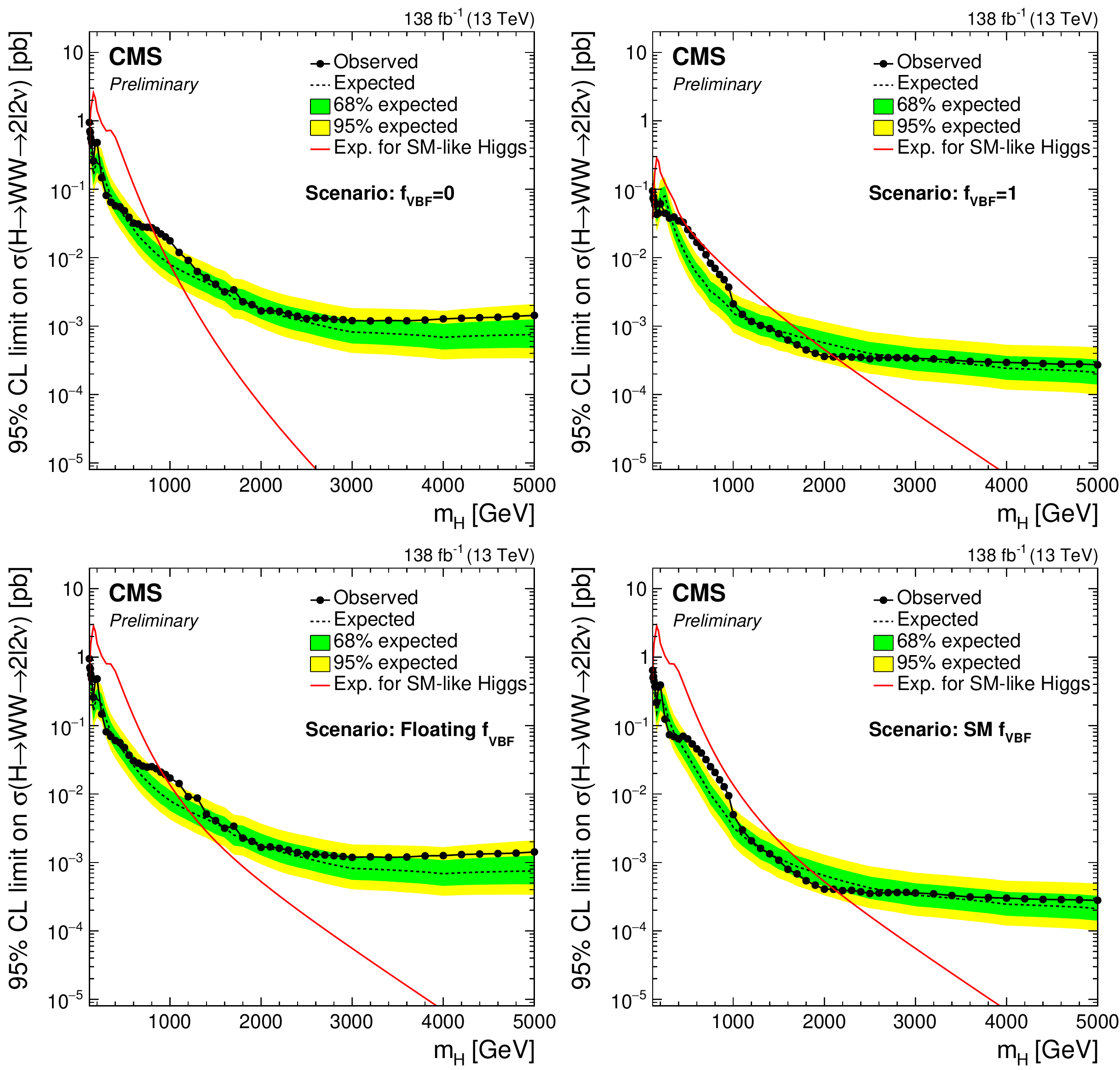
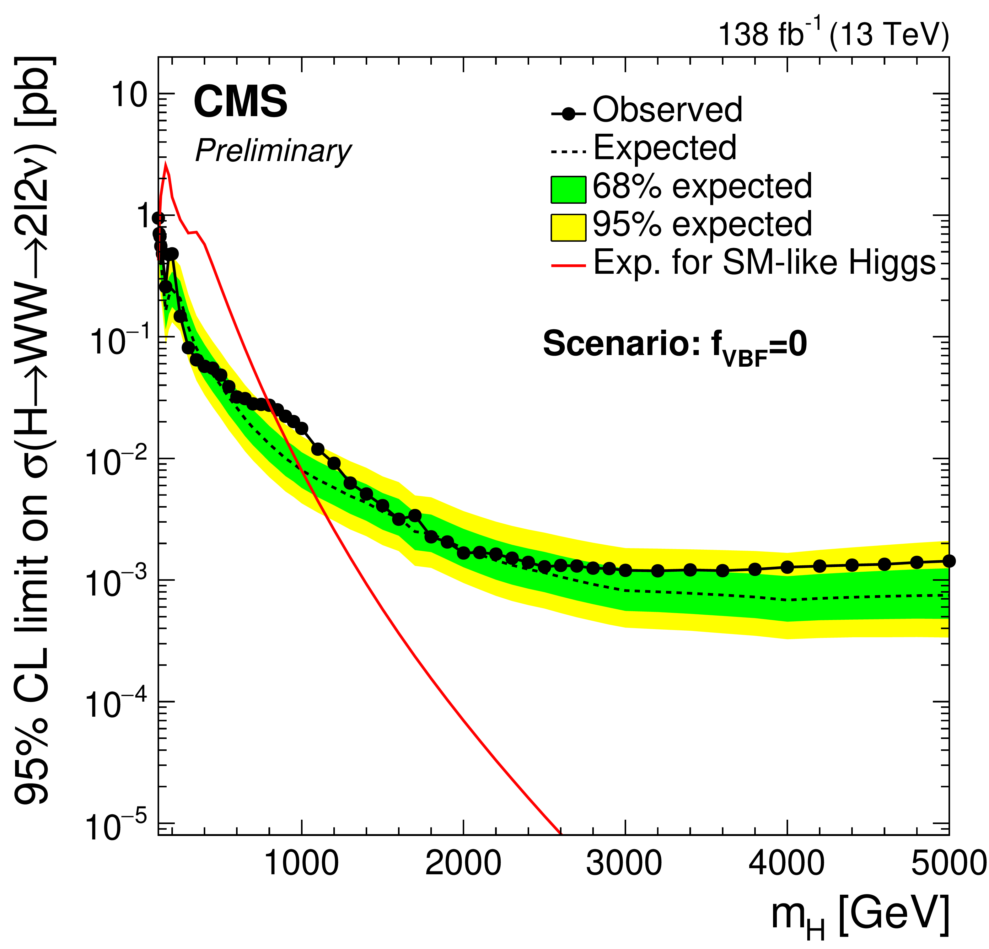
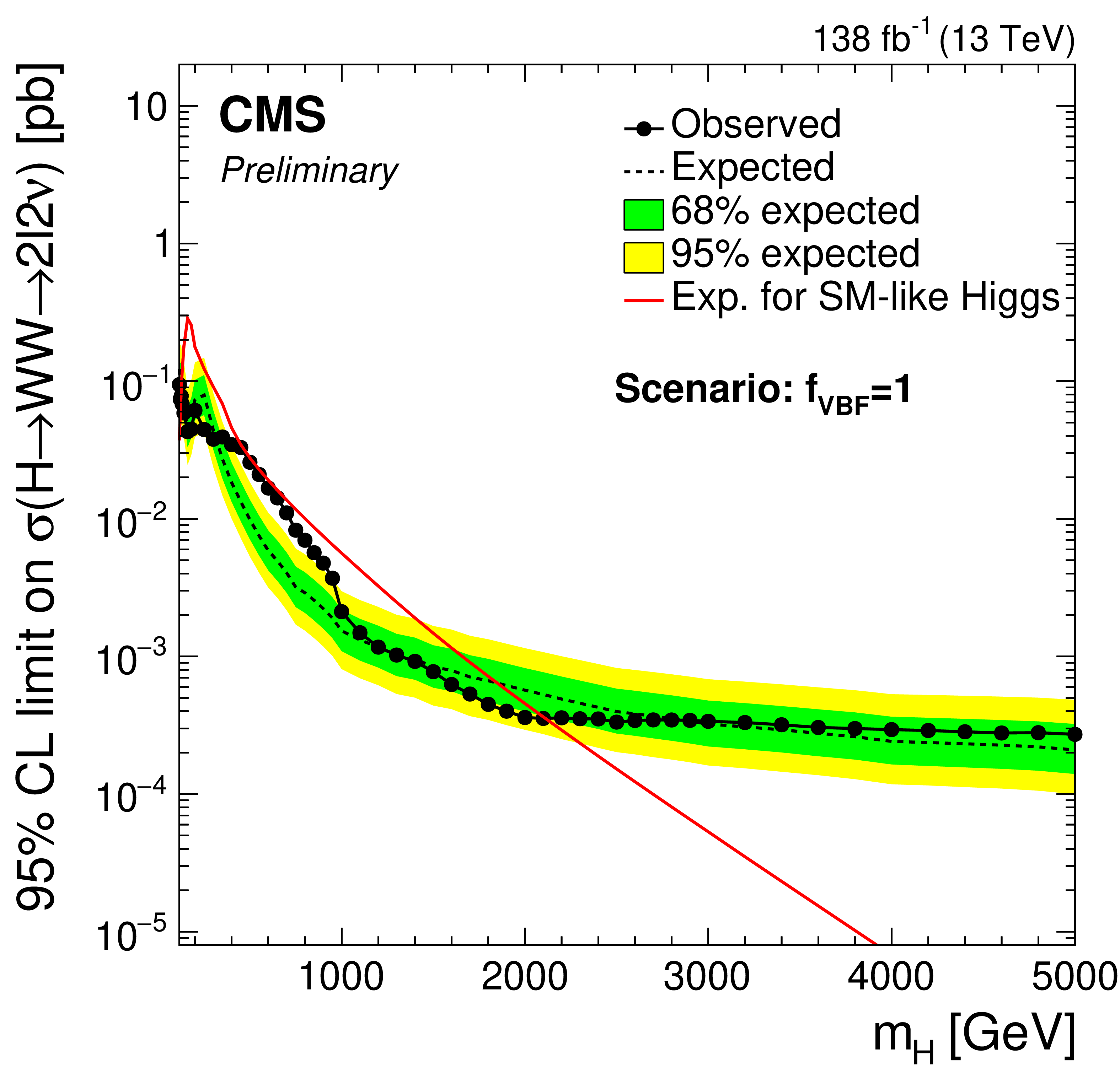
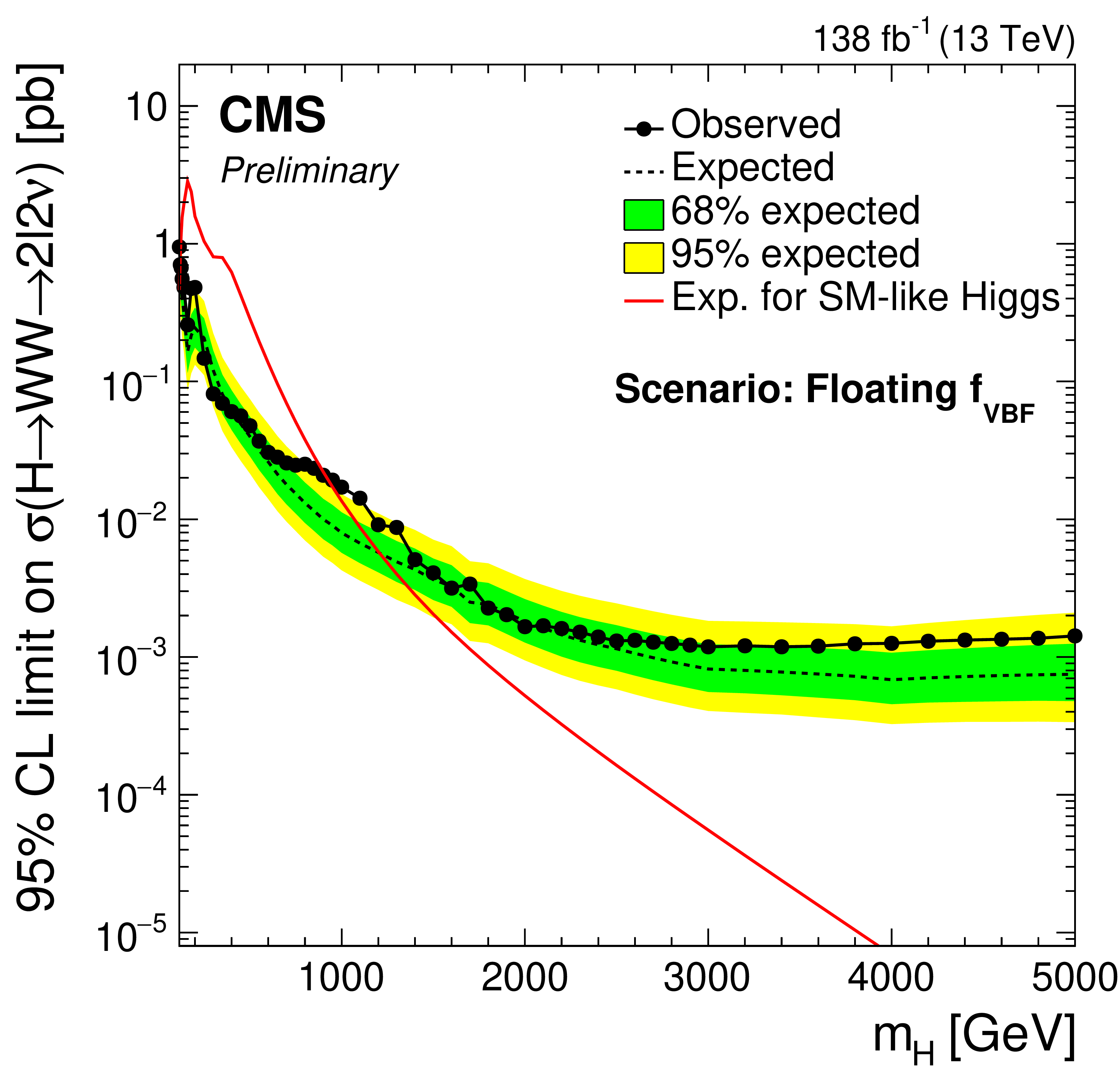
Figure 4:
Limits using the combined Run 2 data set for the $f_{VBF}=$ 0 (top left), $f_{VBF}=$ 1 (top right), floating $f_{VBF}$ (bottom left) and the SM $f_{VBF}$ scenarios (bottom right). |
png pdf |
Figure 4-a:
Limits using the combined Run 2 data set for the $f_{VBF}=$ 0 (top left), $f_{VBF}=$ 1 (top right), floating $f_{VBF}$ (bottom left) and the SM $f_{VBF}$ scenarios (bottom right). |
png pdf |
Figure 4-b:
Limits using the combined Run 2 data set for the $f_{VBF}=$ 0 (top left), $f_{VBF}=$ 1 (top right), floating $f_{VBF}$ (bottom left) and the SM $f_{VBF}$ scenarios (bottom right). |
png pdf |
Figure 4-c:
Limits using the combined Run 2 data set for the $f_{VBF}=$ 0 (top left), $f_{VBF}=$ 1 (top right), floating $f_{VBF}$ (bottom left) and the SM $f_{VBF}$ scenarios (bottom right). |

png pdf |
Figure 4-d:
Limits using the combined Run 2 data set for the $f_{VBF}=$ 0 (top left), $f_{VBF}=$ 1 (top right), floating $f_{VBF}$ (bottom left) and the SM $f_{VBF}$ scenarios (bottom right). |

png pdf |
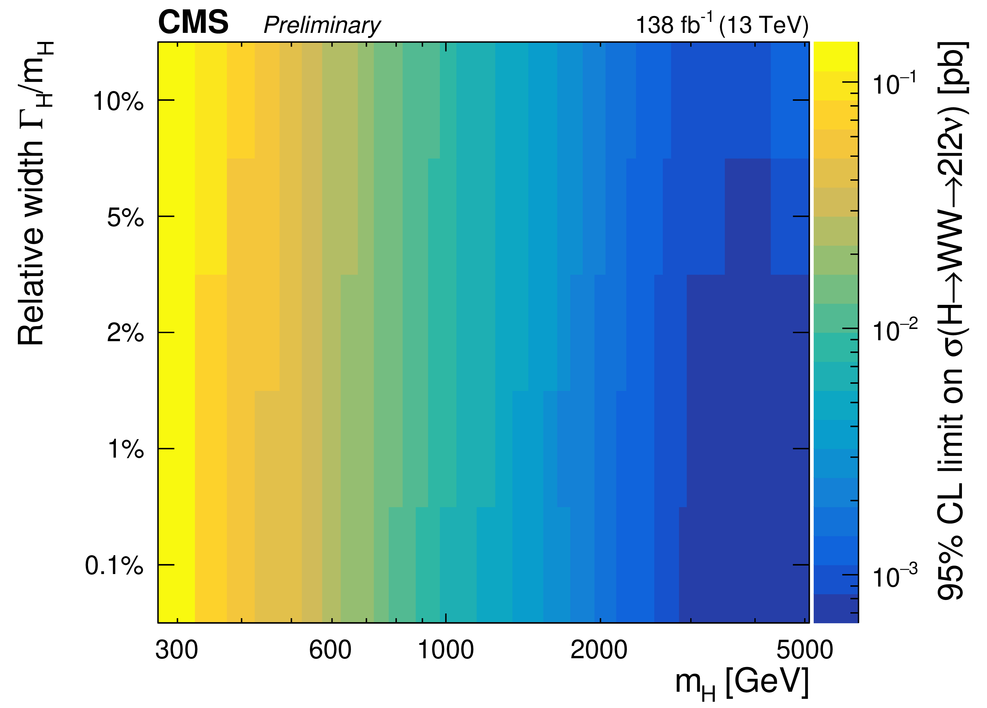
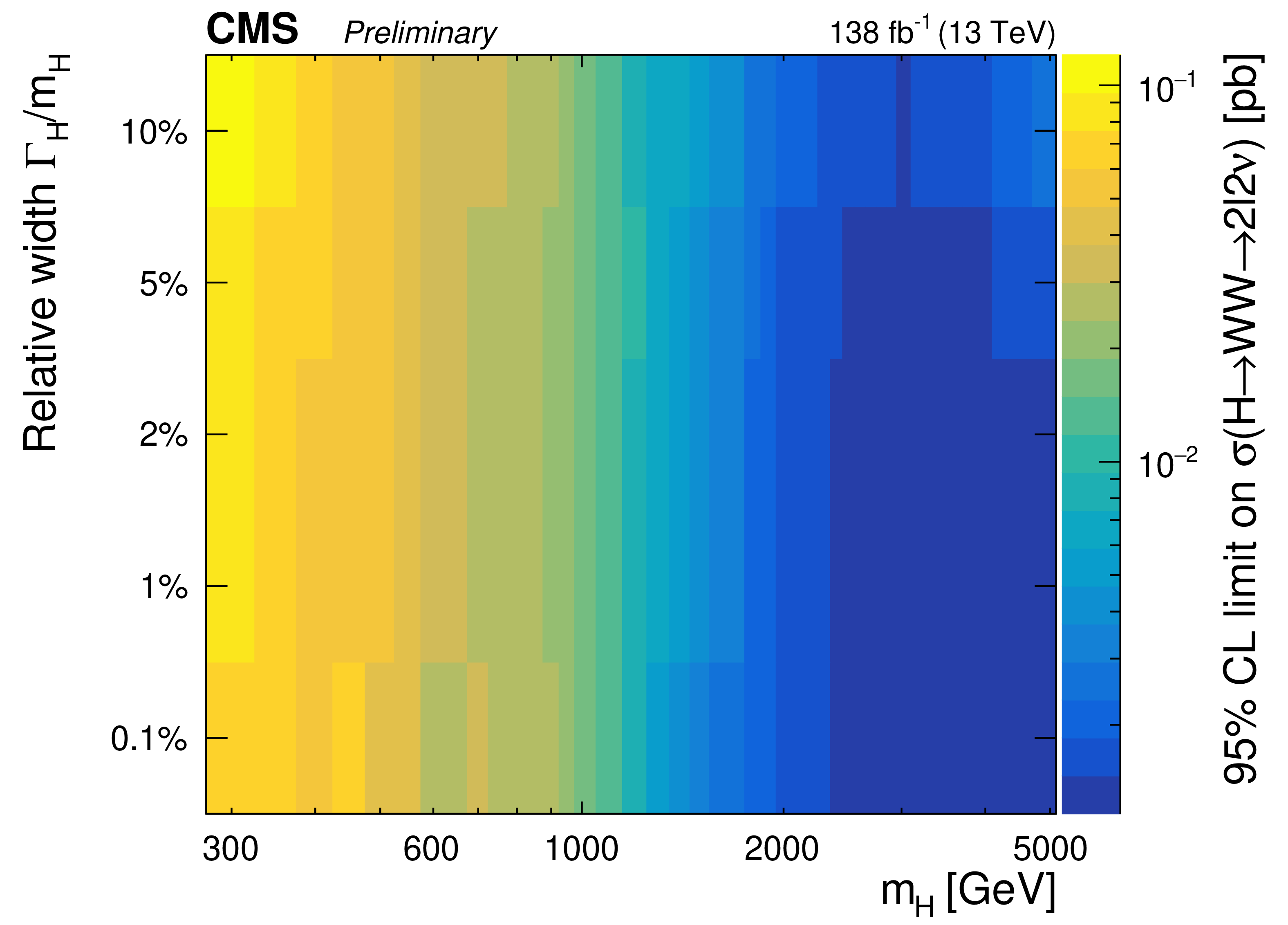
Figure 5:
Expected (left) and observed (right) upper limits as a function of the signal mass and the relative width. From top to bottom, the limits are shown for the $f_{VBF}=$ 0, $f_{VBF}=$ 1, floating $f_{VBF}$ and the SM $f_{VBF}$ scenarios. |
png pdf |
Figure 5-a:
Expected (left) and observed (right) upper limits as a function of the signal mass and the relative width. From top to bottom, the limits are shown for the $f_{VBF}=$ 0, $f_{VBF}=$ 1, floating $f_{VBF}$ and the SM $f_{VBF}$ scenarios. |
png pdf |
Figure 5-b:
Expected (left) and observed (right) upper limits as a function of the signal mass and the relative width. From top to bottom, the limits are shown for the $f_{VBF}=$ 0, $f_{VBF}=$ 1, floating $f_{VBF}$ and the SM $f_{VBF}$ scenarios. |
png pdf |
Figure 5-c:
Expected (left) and observed (right) upper limits as a function of the signal mass and the relative width. From top to bottom, the limits are shown for the $f_{VBF}=$ 0, $f_{VBF}=$ 1, floating $f_{VBF}$ and the SM $f_{VBF}$ scenarios. |

png pdf |
Figure 5-d:
Expected (left) and observed (right) upper limits as a function of the signal mass and the relative width. From top to bottom, the limits are shown for the $f_{VBF}=$ 0, $f_{VBF}=$ 1, floating $f_{VBF}$ and the SM $f_{VBF}$ scenarios. |

png pdf |
Figure 5-e:
Expected (left) and observed (right) upper limits as a function of the signal mass and the relative width. From top to bottom, the limits are shown for the $f_{VBF}=$ 0, $f_{VBF}=$ 1, floating $f_{VBF}$ and the SM $f_{VBF}$ scenarios. |

png pdf |
Figure 5-f:
Expected (left) and observed (right) upper limits as a function of the signal mass and the relative width. From top to bottom, the limits are shown for the $f_{VBF}=$ 0, $f_{VBF}=$ 1, floating $f_{VBF}$ and the SM $f_{VBF}$ scenarios. |

png pdf |
Figure 5-g:
Expected (left) and observed (right) upper limits as a function of the signal mass and the relative width. From top to bottom, the limits are shown for the $f_{VBF}=$ 0, $f_{VBF}=$ 1, floating $f_{VBF}$ and the SM $f_{VBF}$ scenarios. |
png pdf |
Figure 5-h:
Expected (left) and observed (right) upper limits as a function of the signal mass and the relative width. From top to bottom, the limits are shown for the $f_{VBF}=$ 0, $f_{VBF}=$ 1, floating $f_{VBF}$ and the SM $f_{VBF}$ scenarios. |

png pdf |
Figure 6:
Expected exclusion limits for the MSSM scenarios. The limits are shown for the $ {M_{\mathrm{h}}^{125}} $ (top left), $ {M_{\mathrm{h}}^{125}(\tilde{\chi})} $ (top right), $ {M_{\mathrm{h}}^{125}(\tilde{\tau})} $ (middle left), $ {M_{\mathrm{h}}^{125}\text {(alignment)}} $ (middle right), $ {M_{\mathrm{h},\text {EFT}}^{125}} $ (bottom left) and $ {M_{\mathrm{h},\text {EFT}}^{125}(\tilde{\chi})} $ (bottom right) scenarios. |

png pdf |
Figure 6-a:
Expected exclusion limits for the MSSM scenarios. The limits are shown for the $ {M_{\mathrm{h}}^{125}} $ (top left), $ {M_{\mathrm{h}}^{125}(\tilde{\chi})} $ (top right), $ {M_{\mathrm{h}}^{125}(\tilde{\tau})} $ (middle left), $ {M_{\mathrm{h}}^{125}\text {(alignment)}} $ (middle right), $ {M_{\mathrm{h},\text {EFT}}^{125}} $ (bottom left) and $ {M_{\mathrm{h},\text {EFT}}^{125}(\tilde{\chi})} $ (bottom right) scenarios. |

png pdf |
Figure 6-b:
Expected exclusion limits for the MSSM scenarios. The limits are shown for the $ {M_{\mathrm{h}}^{125}} $ (top left), $ {M_{\mathrm{h}}^{125}(\tilde{\chi})} $ (top right), $ {M_{\mathrm{h}}^{125}(\tilde{\tau})} $ (middle left), $ {M_{\mathrm{h}}^{125}\text {(alignment)}} $ (middle right), $ {M_{\mathrm{h},\text {EFT}}^{125}} $ (bottom left) and $ {M_{\mathrm{h},\text {EFT}}^{125}(\tilde{\chi})} $ (bottom right) scenarios. |
png pdf |
Figure 6-c:
Expected exclusion limits for the MSSM scenarios. The limits are shown for the $ {M_{\mathrm{h}}^{125}} $ (top left), $ {M_{\mathrm{h}}^{125}(\tilde{\chi})} $ (top right), $ {M_{\mathrm{h}}^{125}(\tilde{\tau})} $ (middle left), $ {M_{\mathrm{h}}^{125}\text {(alignment)}} $ (middle right), $ {M_{\mathrm{h},\text {EFT}}^{125}} $ (bottom left) and $ {M_{\mathrm{h},\text {EFT}}^{125}(\tilde{\chi})} $ (bottom right) scenarios. |

png pdf |
Figure 6-d:
Expected exclusion limits for the MSSM scenarios. The limits are shown for the $ {M_{\mathrm{h}}^{125}} $ (top left), $ {M_{\mathrm{h}}^{125}(\tilde{\chi})} $ (top right), $ {M_{\mathrm{h}}^{125}(\tilde{\tau})} $ (middle left), $ {M_{\mathrm{h}}^{125}\text {(alignment)}} $ (middle right), $ {M_{\mathrm{h},\text {EFT}}^{125}} $ (bottom left) and $ {M_{\mathrm{h},\text {EFT}}^{125}(\tilde{\chi})} $ (bottom right) scenarios. |

png pdf |
Figure 6-e:
Expected exclusion limits for the MSSM scenarios. The limits are shown for the $ {M_{\mathrm{h}}^{125}} $ (top left), $ {M_{\mathrm{h}}^{125}(\tilde{\chi})} $ (top right), $ {M_{\mathrm{h}}^{125}(\tilde{\tau})} $ (middle left), $ {M_{\mathrm{h}}^{125}\text {(alignment)}} $ (middle right), $ {M_{\mathrm{h},\text {EFT}}^{125}} $ (bottom left) and $ {M_{\mathrm{h},\text {EFT}}^{125}(\tilde{\chi})} $ (bottom right) scenarios. |
png pdf |
Figure 6-f:
Expected exclusion limits for the MSSM scenarios. The limits are shown for the $ {M_{\mathrm{h}}^{125}} $ (top left), $ {M_{\mathrm{h}}^{125}(\tilde{\chi})} $ (top right), $ {M_{\mathrm{h}}^{125}(\tilde{\tau})} $ (middle left), $ {M_{\mathrm{h}}^{125}\text {(alignment)}} $ (middle right), $ {M_{\mathrm{h},\text {EFT}}^{125}} $ (bottom left) and $ {M_{\mathrm{h},\text {EFT}}^{125}(\tilde{\chi})} $ (bottom right) scenarios. |

png pdf |
Figure 7:
Exclusion limits for a Type-II THDM (left) and a Type-I THDM (right) over the $m_\mathrm{H} $-$\tan\beta $-plane for $\cos(\beta -\alpha)=$ 0.1. |

png pdf |
Figure 7-a:
Exclusion limits for a Type-II THDM (left) and a Type-I THDM (right) over the $m_\mathrm{H} $-$\tan\beta $-plane for $\cos(\beta -\alpha)=$ 0.1. |

png pdf |
Figure 7-b:
Exclusion limits for a Type-II THDM (left) and a Type-I THDM (right) over the $m_\mathrm{H} $-$\tan\beta $-plane for $\cos(\beta -\alpha)=$ 0.1. |
png pdf |
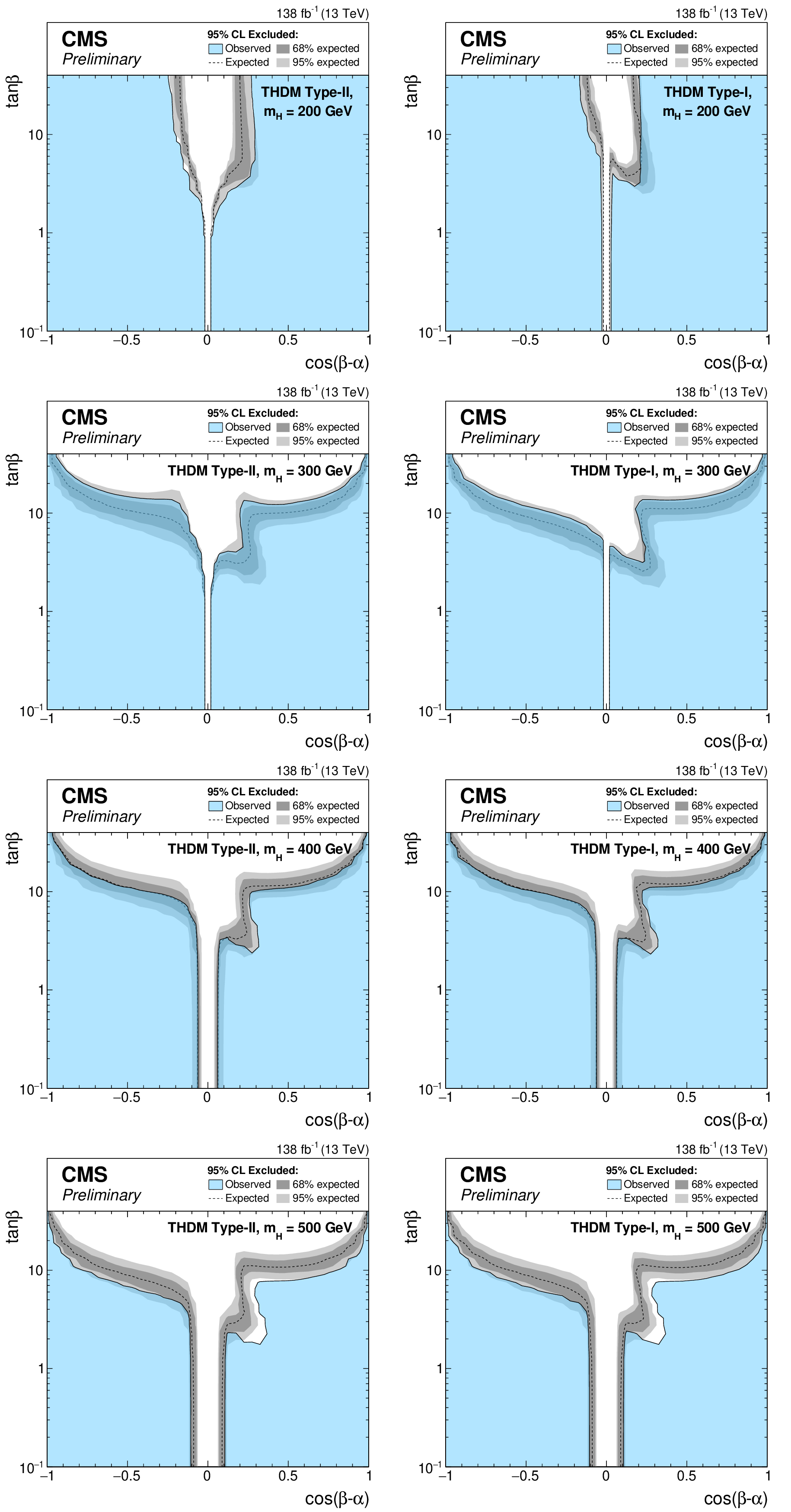
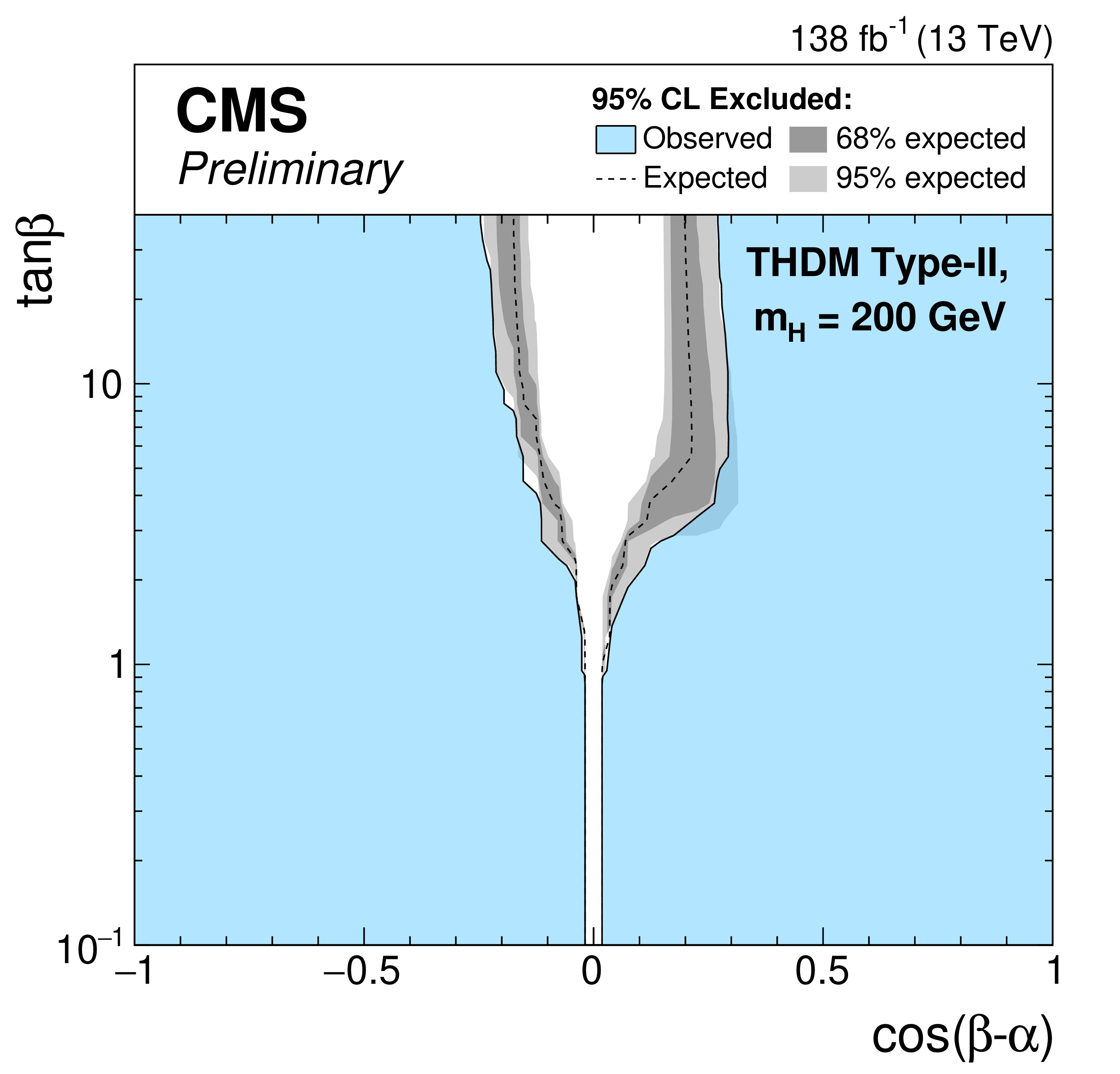
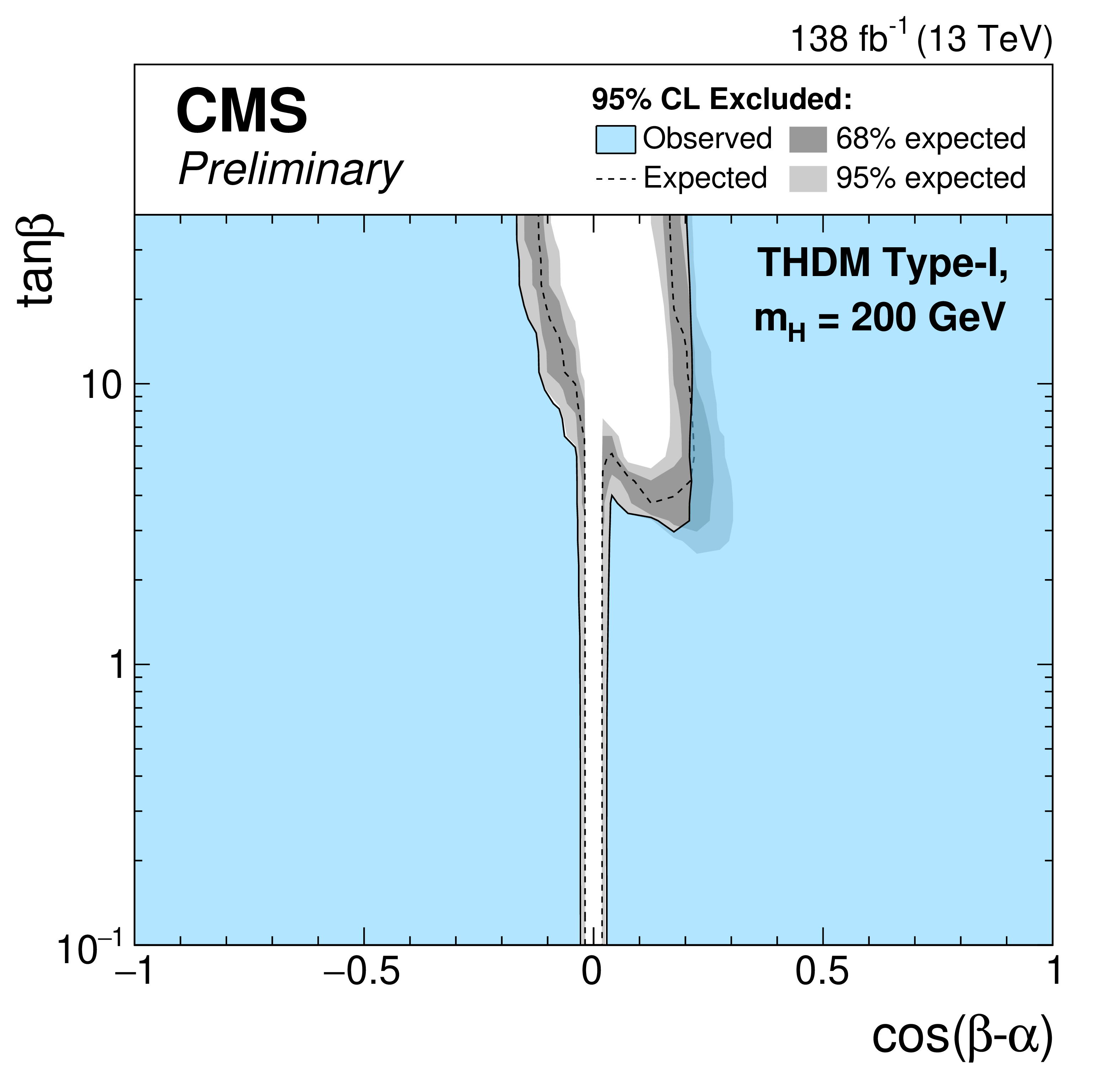
Figure 8:
Exclusion limits for a Type-II THDM (left) and a Type-I THDM (right) over the $\cos(\beta -\alpha)$-$\tan\beta $-plane. The limits are shown from top to bottom for $m_\mathrm{H} = $ 200 GeV, $m_\mathrm{H} = $ 300 GeV, $m_\mathrm{H} = $ 400 GeV and $m_\mathrm{H} = $ 500 GeV. |
png pdf |
Figure 8-a:
Exclusion limits for a Type-II THDM (left) and a Type-I THDM (right) over the $\cos(\beta -\alpha)$-$\tan\beta $-plane. The limits are shown from top to bottom for $m_\mathrm{H} = $ 200 GeV, $m_\mathrm{H} = $ 300 GeV, $m_\mathrm{H} = $ 400 GeV and $m_\mathrm{H} = $ 500 GeV. |
png pdf |
Figure 8-b:
Exclusion limits for a Type-II THDM (left) and a Type-I THDM (right) over the $\cos(\beta -\alpha)$-$\tan\beta $-plane. The limits are shown from top to bottom for $m_\mathrm{H} = $ 200 GeV, $m_\mathrm{H} = $ 300 GeV, $m_\mathrm{H} = $ 400 GeV and $m_\mathrm{H} = $ 500 GeV. |

png pdf |
Figure 8-c:
Exclusion limits for a Type-II THDM (left) and a Type-I THDM (right) over the $\cos(\beta -\alpha)$-$\tan\beta $-plane. The limits are shown from top to bottom for $m_\mathrm{H} = $ 200 GeV, $m_\mathrm{H} = $ 300 GeV, $m_\mathrm{H} = $ 400 GeV and $m_\mathrm{H} = $ 500 GeV. |

png pdf |
Figure 8-d:
Exclusion limits for a Type-II THDM (left) and a Type-I THDM (right) over the $\cos(\beta -\alpha)$-$\tan\beta $-plane. The limits are shown from top to bottom for $m_\mathrm{H} = $ 200 GeV, $m_\mathrm{H} = $ 300 GeV, $m_\mathrm{H} = $ 400 GeV and $m_\mathrm{H} = $ 500 GeV. |

png pdf |
Figure 8-e:
Exclusion limits for a Type-II THDM (left) and a Type-I THDM (right) over the $\cos(\beta -\alpha)$-$\tan\beta $-plane. The limits are shown from top to bottom for $m_\mathrm{H} = $ 200 GeV, $m_\mathrm{H} = $ 300 GeV, $m_\mathrm{H} = $ 400 GeV and $m_\mathrm{H} = $ 500 GeV. |

png pdf |
Figure 8-f:
Exclusion limits for a Type-II THDM (left) and a Type-I THDM (right) over the $\cos(\beta -\alpha)$-$\tan\beta $-plane. The limits are shown from top to bottom for $m_\mathrm{H} = $ 200 GeV, $m_\mathrm{H} = $ 300 GeV, $m_\mathrm{H} = $ 400 GeV and $m_\mathrm{H} = $ 500 GeV. |

png pdf |
Figure 8-g:
Exclusion limits for a Type-II THDM (left) and a Type-I THDM (right) over the $\cos(\beta -\alpha)$-$\tan\beta $-plane. The limits are shown from top to bottom for $m_\mathrm{H} = $ 200 GeV, $m_\mathrm{H} = $ 300 GeV, $m_\mathrm{H} = $ 400 GeV and $m_\mathrm{H} = $ 500 GeV. |
png pdf |
Figure 8-h:
Exclusion limits for a Type-II THDM (left) and a Type-I THDM (right) over the $\cos(\beta -\alpha)$-$\tan\beta $-plane. The limits are shown from top to bottom for $m_\mathrm{H} = $ 200 GeV, $m_\mathrm{H} = $ 300 GeV, $m_\mathrm{H} = $ 400 GeV and $m_\mathrm{H} = $ 500 GeV. |
png pdf |
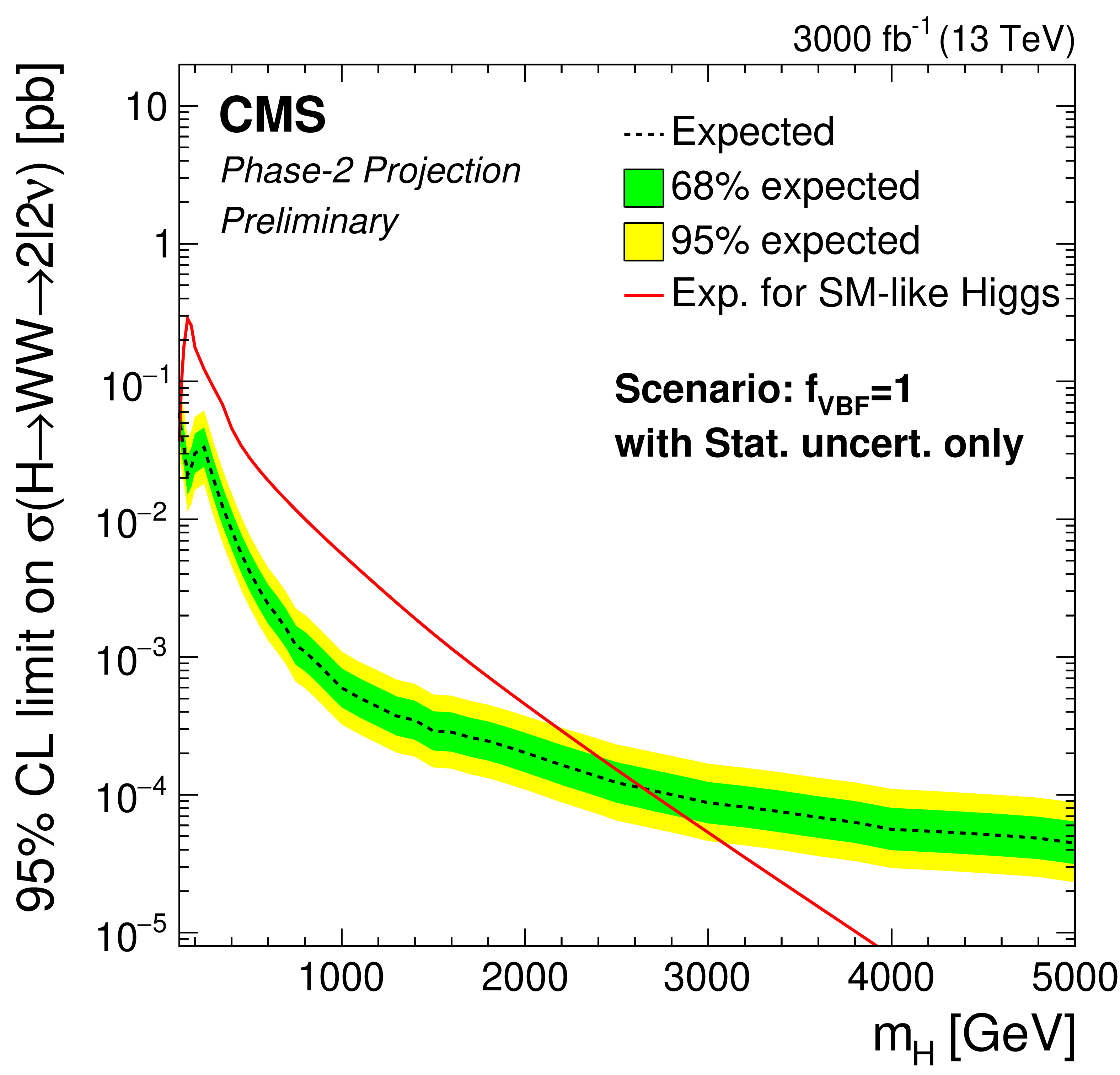
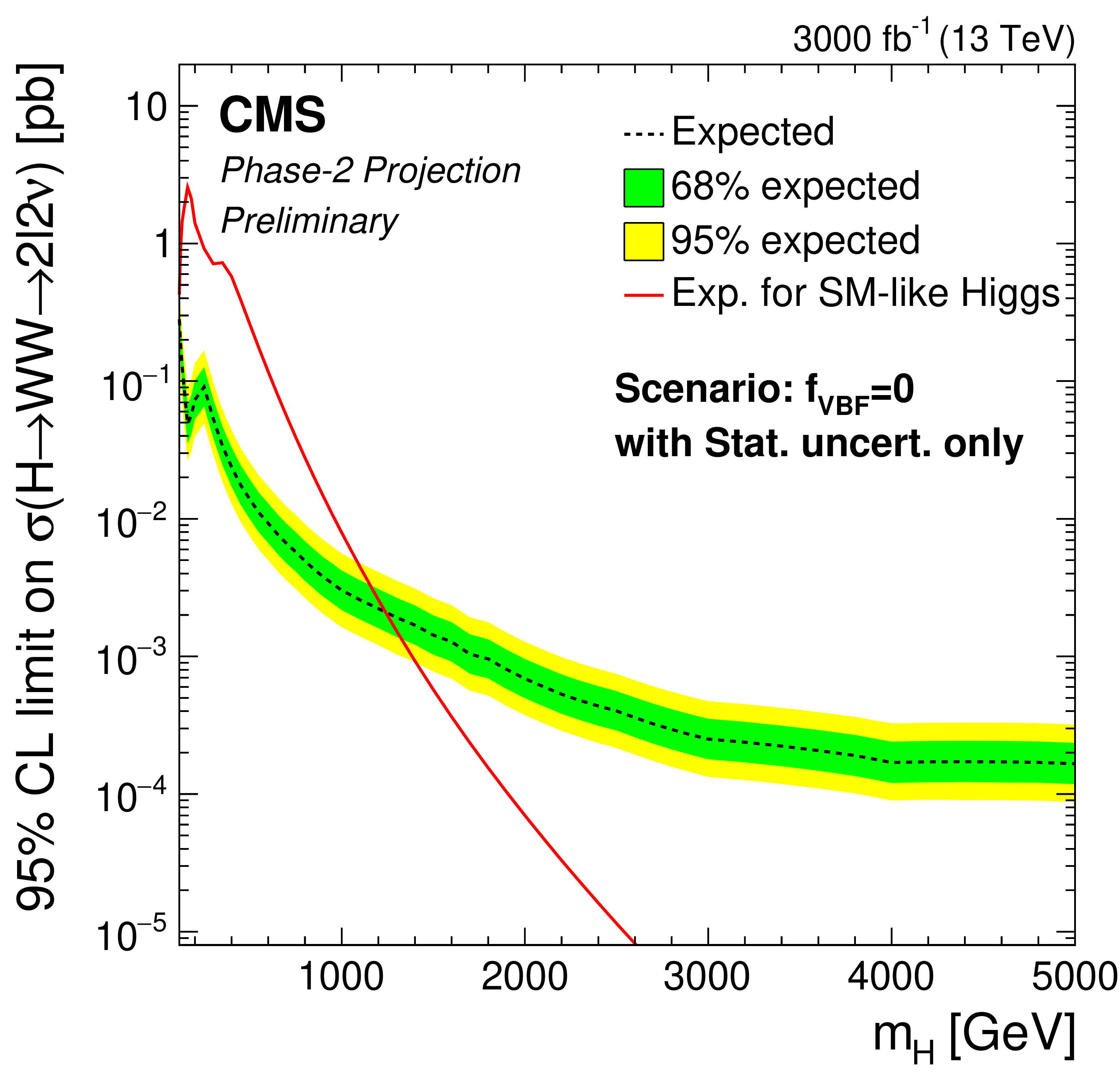
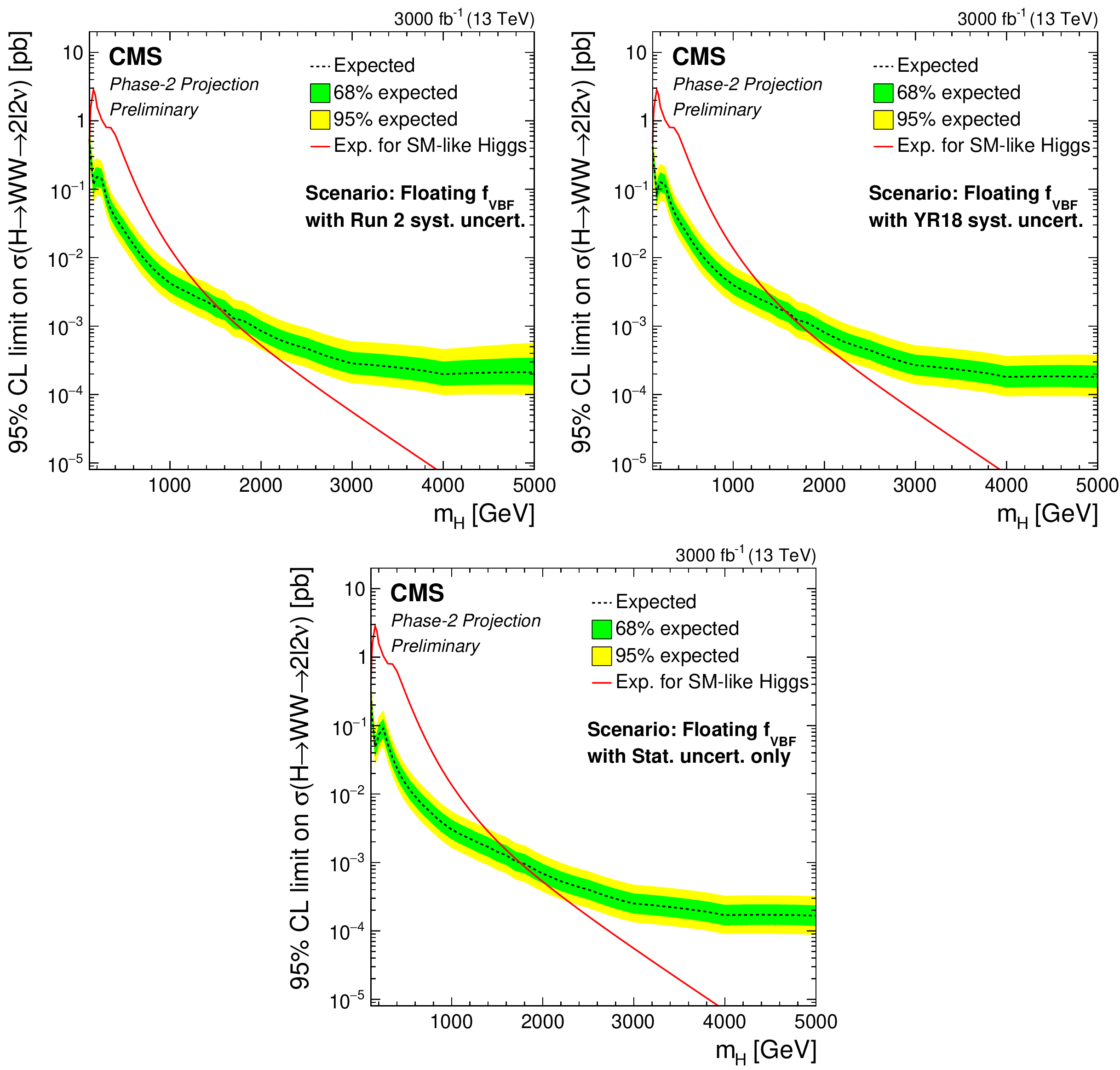
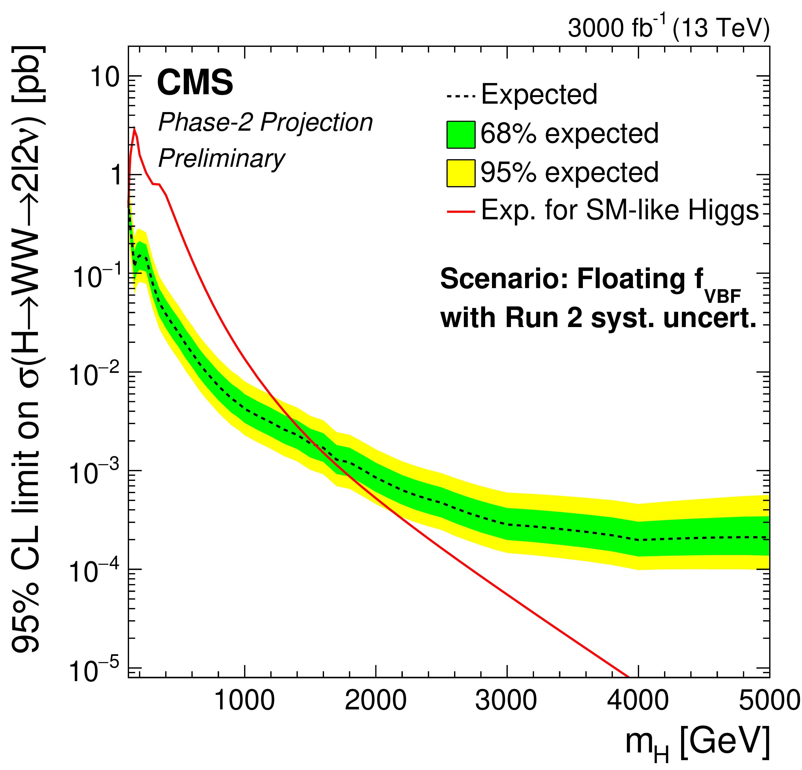
Figure 9:
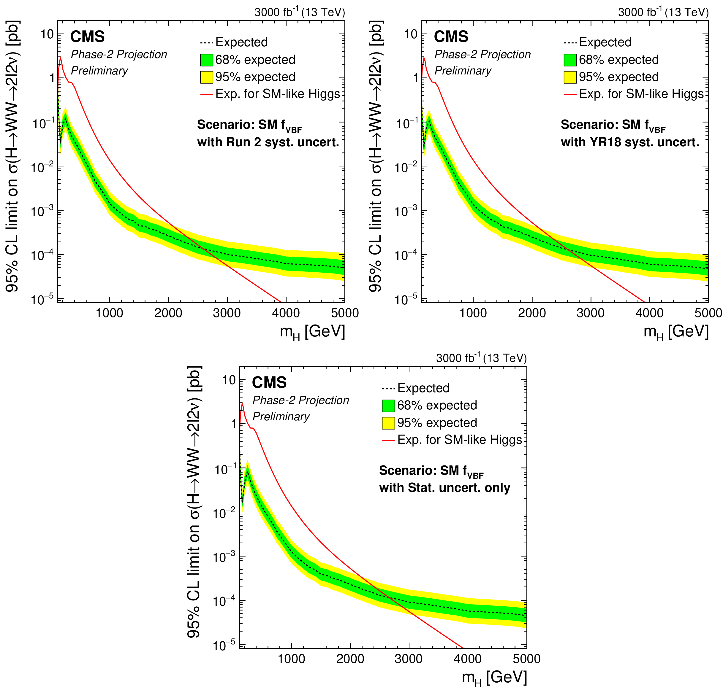
Phase-2 extrapolated limits for the SM VBF fraction scenario, using the Run 2 uncertainties scenario (top left), the YR18 uncertainties scenario (top right) and the statistical uncertainties only scenario (bottom). |

png pdf |
Figure 9-a:
Phase-2 extrapolated limits for the SM VBF fraction scenario, using the Run 2 uncertainties scenario (top left), the YR18 uncertainties scenario (top right) and the statistical uncertainties only scenario (bottom). |

png pdf |
Figure 9-b:
Phase-2 extrapolated limits for the SM VBF fraction scenario, using the Run 2 uncertainties scenario (top left), the YR18 uncertainties scenario (top right) and the statistical uncertainties only scenario (bottom). |

png pdf |
Figure 9-c:
Phase-2 extrapolated limits for the SM VBF fraction scenario, using the Run 2 uncertainties scenario (top left), the YR18 uncertainties scenario (top right) and the statistical uncertainties only scenario (bottom). |

png pdf |
Figure 10:
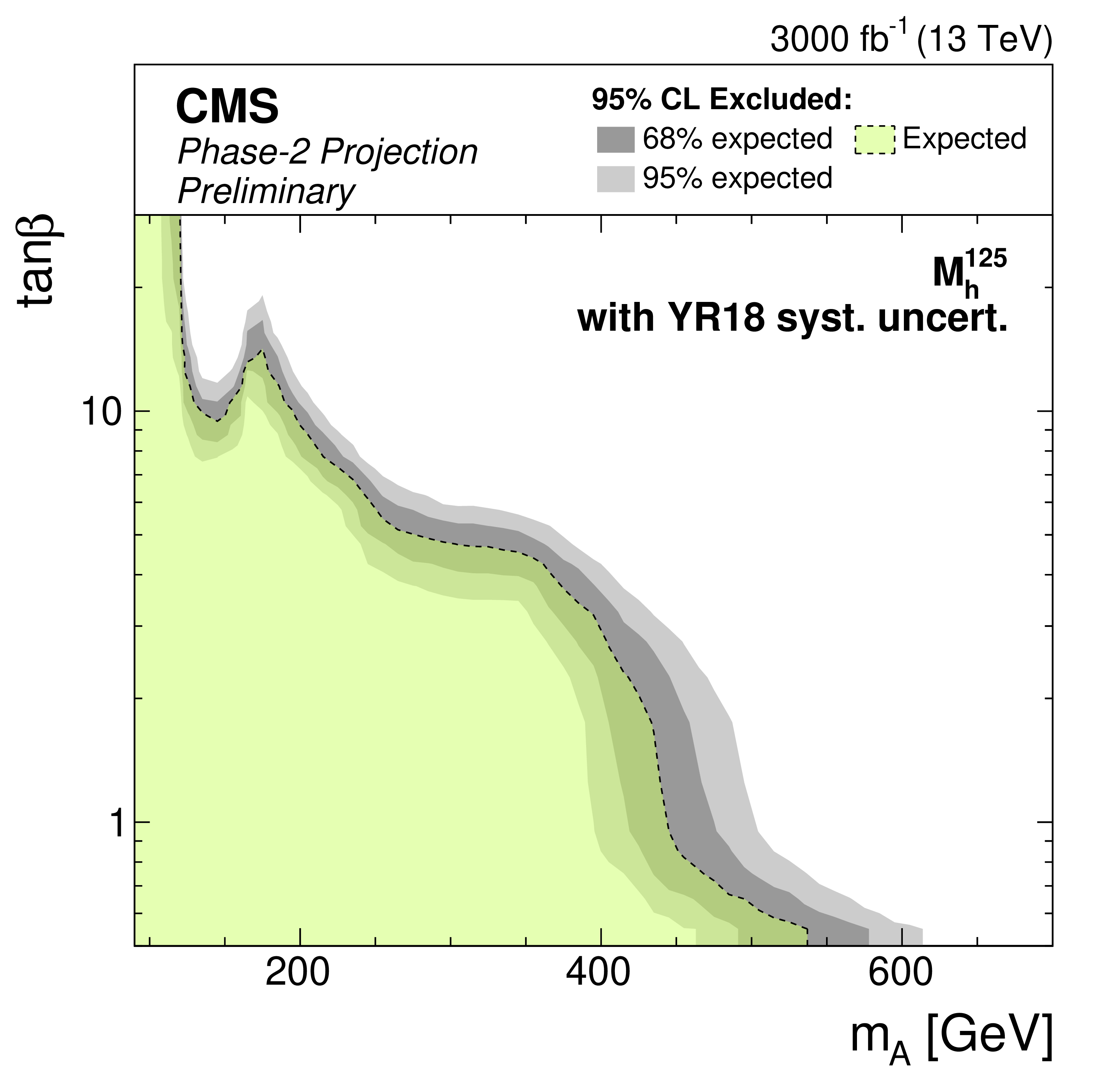
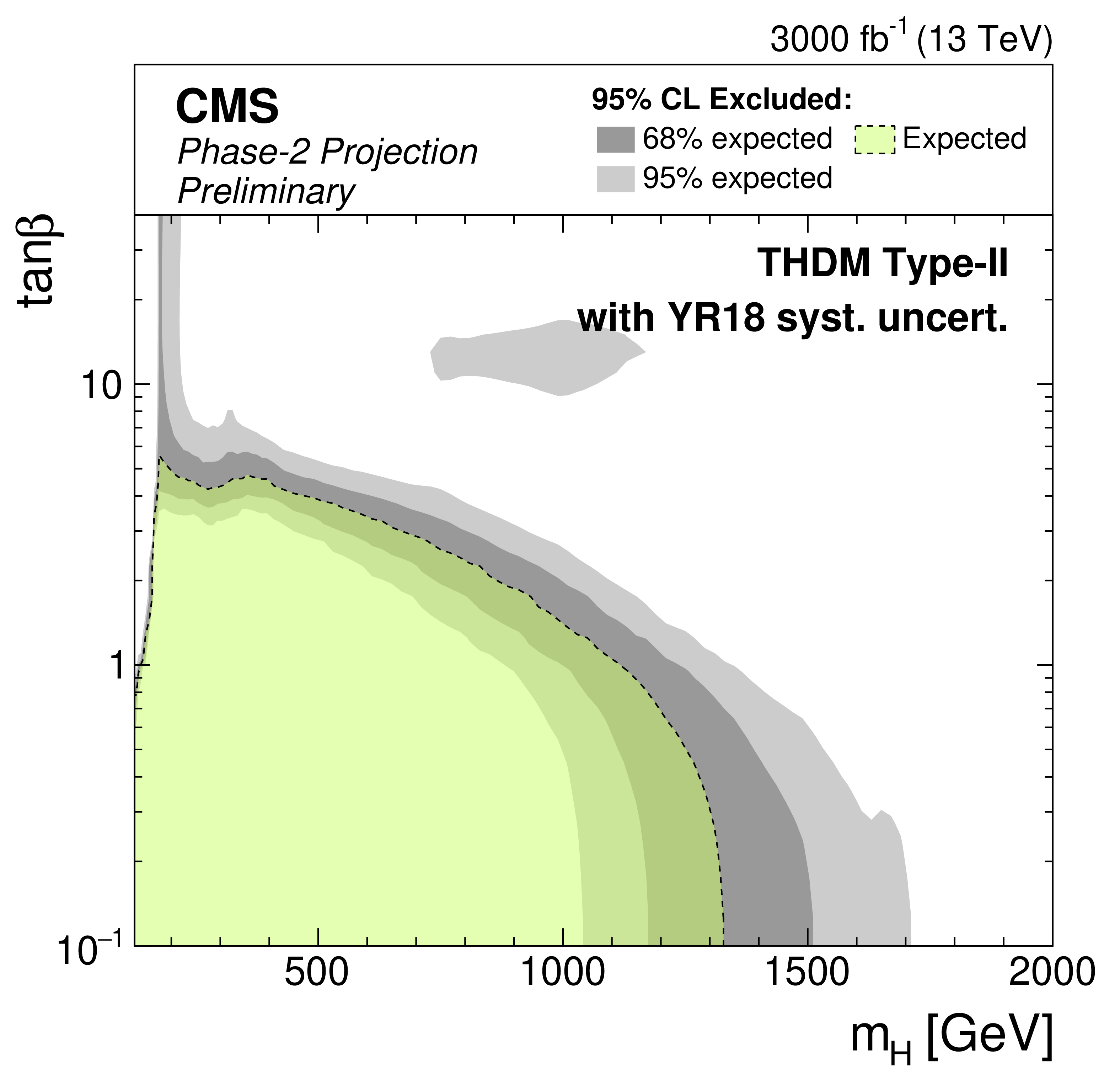
Phase-2 extrapolated limits for the MSSM $ {M_{\mathrm{h}}^{125}} $ scenario (left) and a Type-II THDM over the $m_\mathrm{H} $-$\tan\beta $-plane (right). The limits are shown using the Run 2 uncertainties scenario (top), the YR18 uncertainties scenario (middle) and the statistical uncertainties only scenario (bottom). |

png pdf |
Figure 10-a:
Phase-2 extrapolated limits for the MSSM $ {M_{\mathrm{h}}^{125}} $ scenario (left) and a Type-II THDM over the $m_\mathrm{H} $-$\tan\beta $-plane (right). The limits are shown using the Run 2 uncertainties scenario (top), the YR18 uncertainties scenario (middle) and the statistical uncertainties only scenario (bottom). |

png pdf |
Figure 10-b:
Phase-2 extrapolated limits for the MSSM $ {M_{\mathrm{h}}^{125}} $ scenario (left) and a Type-II THDM over the $m_\mathrm{H} $-$\tan\beta $-plane (right). The limits are shown using the Run 2 uncertainties scenario (top), the YR18 uncertainties scenario (middle) and the statistical uncertainties only scenario (bottom). |
png pdf |
Figure 10-c:
Phase-2 extrapolated limits for the MSSM $ {M_{\mathrm{h}}^{125}} $ scenario (left) and a Type-II THDM over the $m_\mathrm{H} $-$\tan\beta $-plane (right). The limits are shown using the Run 2 uncertainties scenario (top), the YR18 uncertainties scenario (middle) and the statistical uncertainties only scenario (bottom). |
png pdf |
Figure 10-d:
Phase-2 extrapolated limits for the MSSM $ {M_{\mathrm{h}}^{125}} $ scenario (left) and a Type-II THDM over the $m_\mathrm{H} $-$\tan\beta $-plane (right). The limits are shown using the Run 2 uncertainties scenario (top), the YR18 uncertainties scenario (middle) and the statistical uncertainties only scenario (bottom). |

png pdf |
Figure 10-e:
Phase-2 extrapolated limits for the MSSM $ {M_{\mathrm{h}}^{125}} $ scenario (left) and a Type-II THDM over the $m_\mathrm{H} $-$\tan\beta $-plane (right). The limits are shown using the Run 2 uncertainties scenario (top), the YR18 uncertainties scenario (middle) and the statistical uncertainties only scenario (bottom). |

png pdf |
Figure 10-f:
Phase-2 extrapolated limits for the MSSM $ {M_{\mathrm{h}}^{125}} $ scenario (left) and a Type-II THDM over the $m_\mathrm{H} $-$\tan\beta $-plane (right). The limits are shown using the Run 2 uncertainties scenario (top), the YR18 uncertainties scenario (middle) and the statistical uncertainties only scenario (bottom). |
| Tables | |

png pdf |
Table 1:
Summary of the selection criteria. |

png pdf |
Table 2:
Considered systematic uncertainties and their year-by-year correlations. |
png pdf |
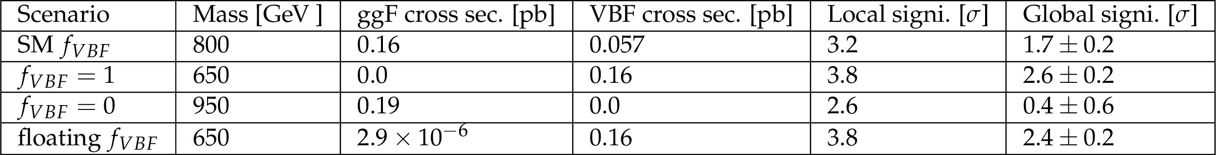
Table 3:
Summary of the signal hypotheses with highest local significance for each $f_{VBF}$ scenario. For each signal hypothesis the resonance mass, production cross sections, and the local and global significances are given. |
| Summary |
|
We performed a search for a high mass Higgs boson decaying into a pair of W bosons in the dileptonic channel. We observe an upward fluctuation of data compared to the expected background. The signal hypothesis with the highest significance corresponds to a resonance mass of 650 GeV in the scenario where only VBF production is considered. The global significance of this excess is 2.6$\sigma$. The presence of a heavy SM-like Higgs boson is excluded at 95% CL up to 2100 GeV, assuming the relative contribution of ggF and VBF production is SM-like and also assuming only VBF production. The exclusion is up to about 800 GeV when considering only ggF production. In the case where the ratio between ggF and VBF production is left floating in the fit, an exclusion of up to 900 GeV is observed. In MSSM scenarios the analysis is sensitive at low values of $m_{\mathrm{A} }$ and $\tan\beta$ and the exclusion limits extend up to $m_{\mathrm{A} } = $ 450 GeV. For $m_{\mathrm{A} }$ between 150 GeV and 400 GeV, we exclude values of $\tan\beta$ between 10 and 3. The sensitivity is similar between the mmodh, mmodc, mmodt, mmodhEFT and mmodcEFT scenarios. In the mmoda scenario, the exclusion limits reach to about $m_{\mathrm{A} } = $ 400 GeV. In THDM scenarios, the limits show an exclusion of up to 750 GeV in THDMs of both Type-I and Type-II. For $\cos(\beta-\alpha)=$ 0.1, the limits in $\tan\beta$ extend up to 4 in Type-II and up to 5 in Type-I, with the sensitivity generally becoming lower for higher masses of H. The sensitivity over $\tan\beta$ varies more strongly as a function of $\cos(\beta-\alpha)$. Extrapolation studies were performed to evaluate the expected gain in sensitivity for the Phase-2 operations of the HL-LHC. The upper limits on the product of the cross section and branching ratio of a new resonance are expected to be improved by almost one order of magnitude. The expected exclusion range in MSSM scenarios increases by only about 50 GeV along the $m_{\mathrm{A} }$ axis. The increase in sensitivity is more noticeable for a general THDM, with the exclusion extending from 1000 GeV up to 1500 GeV for low values of $\tan\beta$. |
| Additional Figures | |

png pdf |
Additional Figure 1:
Phase-2 extrapolated limits for the VBF-only scenario, using the Run 2 uncertainties scenario (top left), the YR18 uncertainties scenario (top right) and the statistical uncertainties only scenario (bottom). |

png pdf |
Additional Figure 1-a:
Phase-2 extrapolated limits for the VBF-only scenario, using the Run 2 uncertainties scenario. |

png pdf |
Additional Figure 1-b:
Phase-2 extrapolated limits for the VBF-only scenario, using the YR18 uncertainties scenario. |
png pdf |
Additional Figure 1-c:
Phase-2 extrapolated limits for the VBF-only scenario, using the statistical uncertainties only scenario. |

png pdf |
Additional Figure 2:
Phase-2 extrapolated limits for the ggF-only scenario, using the Run 2 uncertainties scenario (top left), the YR18 uncertainties scenario (top right) and the statistical uncertainties only scenario (bottom). |

png pdf |
Additional Figure 2-a:
Phase-2 extrapolated limits for the ggF-only scenario, using the Run 2 uncertainties scenario. |

png pdf |
Additional Figure 2-b:
Phase-2 extrapolated limits for the ggF-only scenario, using the YR18 uncertainties scenario. |
png pdf |
Additional Figure 2-c:
Phase-2 extrapolated limits for the ggF-only scenario, using the statistical uncertainties only scenario. |
png pdf |
Additional Figure 3:
Phase-2 extrapolated limits for the floating VBF fraction scenario, using the Run 2 uncertainties scenario (top left), the YR18 uncertainties scenario (top right) and the statistical uncertainties only scenario (bottom). |
png pdf |
Additional Figure 3-a:
Phase-2 extrapolated limits for the floating VBF fraction scenario, using the Run 2 uncertainties scenario. |

png pdf |
Additional Figure 3-b:
Phase-2 extrapolated limits for the floating VBF fraction scenario, using the YR18 uncertainties scenario. |

png pdf |
Additional Figure 3-c:
Phase-2 extrapolated limits for the floating VBF fraction scenario, using the statistical uncertainties only scenario. |

png pdf |
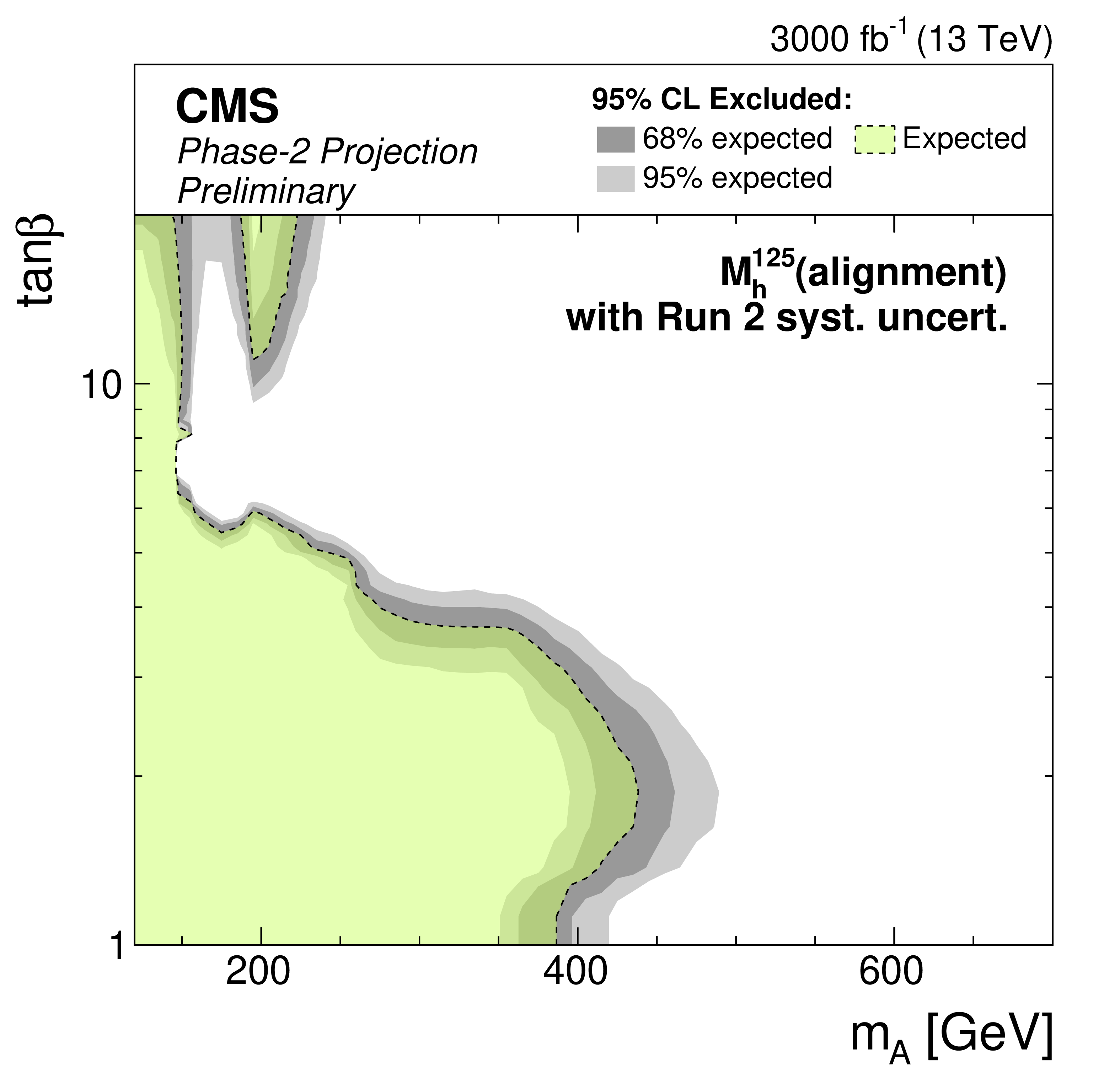
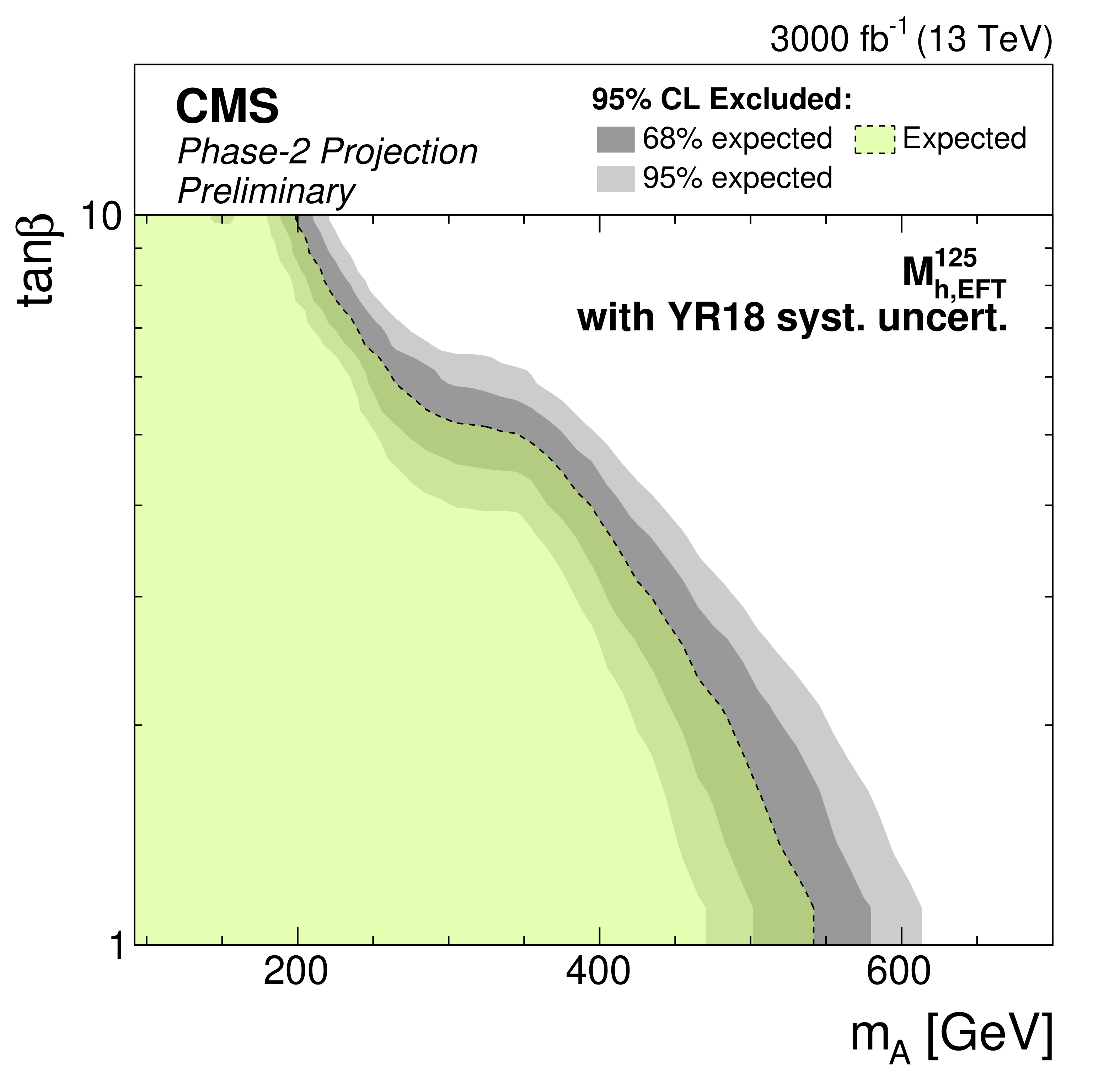
Additional Figure 4:
Phase-2 extrapolated limits for the MSSM $M_{\mathrm{h}}^{125}$(alignment) scenario (left) and $M_{\mathrm{h},\text {EFT}}^{125}$ scenario (right). The limits are shown using the Run 2 uncertainties scenario (top), the YR18 uncertainties scenario (middle) and the statistical uncertainties only scenario (bottom). |
png pdf |
Additional Figure 4-a:
Phase-2 extrapolated limits for the MSSM $M_{\mathrm{h}}^{125}$(alignment) scenario. The limits are shown using the Run 2 uncertainties scenario. |

png pdf |
Additional Figure 4-b:
Phase-2 extrapolated limits for the MSSM $M_{\mathrm{h},\text {EFT}}^{125}$ scenario. The limits are shown using the Run 2 uncertainties scenario. |

png pdf |
Additional Figure 4-c:
Phase-2 extrapolated limits for the MSSM $M_{\mathrm{h}}^{125}$(alignment) scenario. The limits are shown using the YR18 uncertainties scenario. |
png pdf |
Additional Figure 4-d:
Phase-2 extrapolated limits for the MSSM $M_{\mathrm{h},\text {EFT}}^{125}$ scenario. The limits are shown using the YR18 uncertainties scenario. |

png pdf |
Additional Figure 4-e:
Phase-2 extrapolated limits for the MSSM $M_{\mathrm{h}}^{125}$(alignment) scenario. The limits are shown using the statistical uncertainties only scenario. |

png pdf |
Additional Figure 4-f:
Phase-2 extrapolated limits for the MSSM $M_{\mathrm{h},\text {EFT}}^{125}$ scenario. The limits are shown using the statistical uncertainties only scenario. |
| References | ||||
| 1 | CMS Collaboration | Observation of a New Boson at a Mass of 125 GeV with the CMS Experiment at the LHC | PLB 716 (2012) 30 | CMS-HIG-12-028 1207.7235 |
| 2 | ATLAS Collaboration | Observation of a new particle in the search for the Standard Model Higgs boson with the ATLAS detector at the LHC | PLB 716 (2012) 1 | 1207.7214 |
| 3 | V. Barger et al. | LHC Phenomenology of an Extended Standard Model with a Real Scalar Singlet | PRD 77 (2008) 035005 | 0706.4311 |
| 4 | G. C. Branco et al. | Theory and phenomenology of two-Higgs-doublet models | PR 516 (2012) 1 | 1106.0034 |
| 5 | S. P. Martin | A Supersymmetry primer | Adv. Ser. Direct. High Energy Phys. 18 (1998) 1 | hep-ph/9709356 |
| 6 | J. E. Kim | Light Pseudoscalars, Particle Physics and Cosmology | PR 150 (1987) 1 | |
| 7 | E. Bagnaschi et al. | MSSM Higgs Boson Searches at the LHC: Benchmark Scenarios for Run 2 and Beyond | EPJC 79 (2019), no. 7, 617 | 1808.07542 |
| 8 | H. Bahl, S. Liebler, and T. Stefaniak | MSSM Higgs benchmark scenarios for Run 2 and beyond: the low $ \tan \beta $ region | EPJC 79 (2019), no. 3, 279 | 1901.05933 |
| 9 | CMS Collaboration | The CMS experiment at the CERN LHC | JINST 3 (2008) S08004 | CMS-00-001 |
| 10 | CMS Collaboration | Performance of the CMS Level-1 trigger in proton-proton collisions at $ \sqrt{s} = $ 13 TeV | JINST 15 (2020) P10017 | CMS-TRG-17-001 2006.10165 |
| 11 | CMS Collaboration | The CMS trigger system | JINST 12 (2017) P01020 | CMS-TRG-12-001 1609.02366 |
| 12 | CMS Collaboration | Performance of electron reconstruction and selection with the CMS detector in proton-proton collisions at $ \sqrt{s} = $ 8 TeV | JINST 10 (2015) P06005 | CMS-EGM-13-001 1502.02701 |
| 13 | CMS Collaboration | Performance of the CMS muon detector and muon reconstruction with proton-proton collisions at $ \sqrt{s}= $ 13 TeV | JINST 13 (2018) P06015 | CMS-MUO-16-001 1804.04528 |
| 14 | CMS Collaboration | Performance of photon reconstruction and identification with the CMS detector in proton-proton collisions at sqrt(s) = 8 TeV | JINST 10 (2015) P08010 | CMS-EGM-14-001 1502.02702 |
| 15 | CMS Collaboration | Description and performance of track and primary-vertex reconstruction with the CMS tracker | JINST 9 (2014) P10009 | CMS-TRK-11-001 1405.6569 |
| 16 | CMS Collaboration | Particle-flow reconstruction and global event description with the CMS detector | JINST 12 (2017) P10003 | CMS-PRF-14-001 1706.04965 |
| 17 | CMS Collaboration | Performance of reconstruction and identification of $ \tau $ leptons decaying to hadrons and $ \nu_\tau $ in pp collisions at $ \sqrt{s}= $ 13 TeV | JINST 13 (2018), no. 10, P10005 | CMS-TAU-16-003 1809.02816 |
| 18 | CMS Collaboration | Jet energy scale and resolution in the CMS experiment in pp collisions at 8 TeV | JINST 12 (2017) P02014 | CMS-JME-13-004 1607.03663 |
| 19 | CMS Collaboration | Performance of missing transverse momentum reconstruction in proton-proton collisions at $ \sqrt{s} = $ 13 TeV using the CMS detector | JINST 14 (2019) P07004 | CMS-JME-17-001 1903.06078 |
| 20 | P. Nason | A New method for combining NLO QCD with shower Monte Carlo algorithms | JHEP 11 (2004) 040 | hep-ph/0409146 |
| 21 | S. Frixione, P. Nason, and C. Oleari | Matching NLO QCD computations with Parton Shower simulations: the POWHEG method | JHEP 11 (2007) 070 | 0709.2092 |
| 22 | S. Alioli, P. Nason, C. Oleari, and E. Re | A general framework for implementing NLO calculations in shower Monte Carlo programs: the POWHEG BOX | JHEP 06 (2010) 043 | 1002.2581 |
| 23 | E. Bagnaschi, G. Degrassi, P. Slavich, and A. Vicini | Higgs production via gluon fusion in the POWHEG approach in the SM and in the MSSM | JHEP 02 (2012) 088 | 1111.2854 |
| 24 | P. Nason and C. Oleari | NLO Higgs boson production via vector-boson fusion matched with shower in POWHEG | JHEP 02 (2010) 037 | 0911.5299 |
| 25 | JHU generator and MELA package | Manual for the JHU generator and MELA package | ``Manual for the JHU generator and MELA package'' | |
| 26 | Y. Gao et al. | Spin Determination of Single-Produced Resonances at Hadron Colliders | PRD 81 (2010) 075022 | 1001.3396 |
| 27 | S. Bolognesi et al. | On the spin and parity of a single-produced resonance at the LHC | PRD 86 (2012) 095031 | 1208.4018 |
| 28 | I. Anderson et al. | Constraining Anomalous HVV Interactions at Proton and Lepton Colliders | PRD 89 (2014), no. 3, 035007 | 1309.4819 |
| 29 | A. V. Gritsan, R. Rontsch, M. Schulze, and M. Xiao | Constraining anomalous Higgs boson couplings to the heavy flavor fermions using matrix element techniques | PRD 94 (2016), no. 5, 055023 | 1606.03107 |
| 30 | J. Alwall et al. | The automated computation of tree-level and next-to-leading order differential cross sections, and their matching to parton shower simulations | JHEP 07 (2014) 079 | 1405.0301 |
| 31 | J. Alwall et al. | Comparative study of various algorithms for the merging of parton showers and matrix elements in hadronic collisions | EPJC 53 (2008) 473 | 0706.2569 |
| 32 | R. Frederix and S. Frixione | Merging meets matching in MC@NLO | JHEP 12 (2012) 061 | 1209.6215 |
| 33 | P. Artoisenet, R. Frederix, O. Mattelaer, and R. Rietkerk | Automatic spin-entangled decays of heavy resonances in Monte Carlo simulations | JHEP 03 (2013) 015 | 1212.3460 |
| 34 | J. M. Campbell, R. K. Ellis, and C. Williams | Bounding the Higgs Width at the LHC: Complementary Results from $ H \to WW $ | PRD 89 (2014), no. 5, 053011 | 1312.1628 |
| 35 | J. M. Campbell and R. K. Ellis | An Update on vector boson pair production at hadron colliders | PRD 60 (1999) 113006 | hep-ph/9905386 |
| 36 | J. M. Campbell, R. K. Ellis, and C. Williams | Vector boson pair production at the LHC | JHEP 07 (2011) 018 | 1105.0020 |
| 37 | J. M. Campbell, R. K. Ellis, and W. T. Giele | A Multi-Threaded Version of MCFM | EPJC 75 (2015), no. 6, 246 | 1503.06182 |
| 38 | GEANT4 Collaboration | GEANT4--a simulation toolkit | NIMA 506 (2003) 250 | |
| 39 | T. Sjostrand et al. | An introduction to PYTHIA 8.2 | CPC 191 (2015) 159 | 1410.3012 |
| 40 | CMS Collaboration | Event generator tunes obtained from underlying event and multiparton scattering measurements | EPJC 76 (2016), no. 3, 155 | CMS-GEN-14-001 1512.00815 |
| 41 | NNPDF Collaboration | Parton distributions for the LHC Run II | JHEP 04 (2015) 040 | 1410.8849 |
| 42 | CMS Collaboration | Extraction and validation of a new set of CMS PYTHIA8 tunes from underlying-event measurements | EPJC 80 (2020), no. 1, 4 | CMS-GEN-17-001 1903.12179 |
| 43 | NNPDF Collaboration | Parton distributions from high-precision collider data | EPJC 77 (2017), no. 10, 663 | 1706.00428 |
| 44 | BSM Higgs production cross sections at $\sqrt{s}$ = 13 TeV (update in CERN Report4 2016) | link | ||
| 45 | R. V. Harlander, S. Liebler, and H. Mantler | SusHi: A program for the calculation of Higgs production in gluon fusion and bottom-quark annihilation in the Standard Model and the MSSM | CPC 184 (2013) 1605 | 1212.3249 |
| 46 | R. V. Harlander, S. Liebler, and H. Mantler | SusHi Bento: Beyond NNLO and the heavy-top limit | CPC 212 (2017) 239 | 1605.03190 |
| 47 | M. Spira, A. Djouadi, D. Graudenz, and P. M. Zerwas | Higgs boson production at the LHC | NPB 453 (1995) 17 | hep-ph/9504378 |
| 48 | R. V. Harlander and W. B. Kilgore | Next-to-next-to-leading order Higgs production at hadron colliders | PRL 88 (2002) 201801 | hep-ph/0201206 |
| 49 | C. Anastasiou and K. Melnikov | Higgs boson production at hadron colliders in NNLO QCD | NPB 646 (2002) 220 | hep-ph/0207004 |
| 50 | V. Ravindran, J. Smith, and W. L. van Neerven | NNLO corrections to the total cross-section for Higgs boson production in hadron hadron collisions | NPB 665 (2003) 325 | hep-ph/0302135 |
| 51 | U. Aglietti, R. Bonciani, G. Degrassi, and A. Vicini | Two loop light fermion contribution to Higgs production and decays | PLB 595 (2004) 432 | hep-ph/0404071 |
| 52 | R. Bonciani, G. Degrassi, and A. Vicini | On the Generalized Harmonic Polylogarithms of One Complex Variable | CPC 182 (2011) 1253 | 1007.1891 |
| 53 | J. F. Gunion, H. E. Haber, G. L. Kane, and S. Dawson | The Higgs Hunter's Guide | volume 80 Front. Phys. | |
| 54 | D. Eriksson, J. Rathsman, and O. Stal | 2HDMC: Two-Higgs-Doublet Model Calculator Physics and Manual | CPC 181 (2010) 189 | 0902.0851 |
| 55 | R. Harlander et al. | Interim recommendations for the evaluation of Higgs production cross sections and branching ratios at the LHC in the Two-Higgs-Doublet Model | arXiv e-prints (12, 2013) | 1312.5571 |
| 56 | CMS Collaboration | Summary results of high mass BSM Higgs searches using CMS run-I data | CMS-PAS-HIG-16-007 | CMS-PAS-HIG-16-007 |
| 57 | J. Lorenzo D\'\iaz-Cruz | The Higgs profile in the standard model and beyond | Rev. Mex. Fis. 65 (2019), no. 5, 419 | 1904.06878 |
| 58 | S. Heinemeyer, W. Hollik, and G. Weiglein | FeynHiggs: A Program for the calculation of the masses of the neutral CP even Higgs bosons in the MSSM | CPC 124 (2000) 76 | hep-ph/9812320 |
| 59 | S. Heinemeyer, W. Hollik, and G. Weiglein | The Masses of the neutral CP - even Higgs bosons in the MSSM: Accurate analysis at the two loop level | EPJC 9 (1999) 343 | hep-ph/9812472 |
| 60 | G. Degrassi et al. | Towards high precision predictions for the MSSM Higgs sector | EPJC 28 (2003) 133 | hep-ph/0212020 |
| 61 | M. Frank et al. | The Higgs Boson Masses and Mixings of the Complex MSSM in the Feynman-Diagrammatic Approach | JHEP 02 (2007) 047 | hep-ph/0611326 |
| 62 | T. Hahn et al. | High-Precision Predictions for the Light CP -Even Higgs Boson Mass of the Minimal Supersymmetric Standard Model | PRL 112 (2014), no. 14, 141801 | 1312.4937 |
| 63 | H. Bahl and W. Hollik | Precise prediction for the light MSSM Higgs boson mass combining effective field theory and fixed-order calculations | EPJC 76 (2016), no. 9, 499 | 1608.01880 |
| 64 | H. Bahl, S. Heinemeyer, W. Hollik, and G. Weiglein | Reconciling EFT and hybrid calculations of the light MSSM Higgs-boson mass | EPJC 78 (2018), no. 1, 57 | 1706.00346 |
| 65 | A. Djouadi, J. Kalinowski, and M. Spira | HDECAY: A Program for Higgs boson decays in the standard model and its supersymmetric extension | CPC 108 (1998) 56 | hep-ph/9704448 |
| 66 | A. Djouadi, J. Kalinowski, M. Muehlleitner, and M. Spira | HDECAY: Twenty$ _{++} $ years after | CPC 238 (2019) 214 | 1801.09506 |
| 67 | A. Bredenstein, A. Denner, S. Dittmaier, and M. M. Weber | Precise predictions for the Higgs-boson decay H ---$ > $ WW/ZZ ---$ > $ 4 leptons | PRD 74 (2006) 013004 | hep-ph/0604011 |
| 68 | A. Bredenstein, A. Denner, S. Dittmaier, and M. M. Weber | Radiative corrections to the semileptonic and hadronic Higgs-boson decays H ---$ > $ W W / Z Z ---$ > $ 4 fermions | JHEP 02 (2007) 080 | hep-ph/0611234 |
| 69 | R. Harlander and P. Kant | Higgs production and decay: Analytic results at next-to-leading order QCD | JHEP 12 (2005) 015 | hep-ph/0509189 |
| 70 | G. Degrassi and P. Slavich | NLO QCD bottom corrections to Higgs boson production in the MSSM | JHEP 11 (2010) 044 | 1007.3465 |
| 71 | G. Degrassi, S. Di Vita, and P. Slavich | On the NLO QCD Corrections to the Production of the Heaviest Neutral Higgs Scalar in the MSSM | EPJC 72 (2012) 2032 | 1204.1016 |
| 72 | E. Bagnaschi et al. | Benchmark scenarios for low $ \tan \beta $ in the MSSM | LHCHXSWG-2015-002, CERN, Geneva, Aug | |
| 73 | M. Czakon et al. | Top-pair production at the LHC through NNLO QCD and NLO EW | JHEP 10 (2017) 186 | 1705.04105 |
| 74 | P. Meade, H. Ramani, and M. Zeng | Transverse momentum resummation effects in $ W^+W^- $ measurements | PRD 90 (2014), no. 11, 114006 | 1407.4481 |
| 75 | P. Jaiswal and T. Okui | Explanation of the $ WW $ excess at the LHC by jet-veto resummation | PRD 90 (2014), no. 7, 073009 | 1407.4537 |
| 76 | F. Caola et al. | QCD corrections to vector boson pair production in gluon fusion including interference effects with off-shell Higgs at the LHC | JHEP 07 (2016) 087 | 1605.04610 |
| 77 | CMS Collaboration | An embedding technique to determine $ \tau\tau $ backgrounds in proton-proton collision data | JINST 14 (2019), no. 06, P06032 | CMS-TAU-18-001 1903.01216 |
| 78 | MET recoil corrections and uncertainties | link | ||
| 79 | M. Grazzini, S. Kallweit, D. Rathlev, and M. Wiesemann | $ W^{\pm}Z $ production at hadron colliders in NNLO QCD | PLB 761 (2016) 179 | 1604.08576 |
| 80 | CMS Collaboration | Measurements of properties of the Higgs boson decaying to a W boson pair in pp collisions at $ \sqrt{s}= $ 13 TeV | PLB 791 (2019) 96 | CMS-HIG-16-042 1806.05246 |
| 81 | D. Bertolini, P. Harris, M. Low, and N. Tran | Pileup Per Particle Identification | JHEP 10 (2014) 059 | 1407.6013 |
| 82 | CMS Collaboration | Identification of heavy-flavour jets with the CMS detector in pp collisions at 13 TeV | JINST 13 (2018), no. 05, P05011 | CMS-BTV-16-002 1712.07158 |
| 83 | CMS Collaboration | Precision luminosity measurement in proton-proton collisions at $ \sqrt{s} = $ 13 TeV in 2015 and 2016 at CMS | EPJC 81 (2021) 800 | CMS-LUM-17-003 2104.01927 |
| 84 | CMS Collaboration | CMS luminosity measurement for the 2017 data-taking period at $ \sqrt{s} = $ 13 TeV | CMS-PAS-LUM-17-004 | CMS-PAS-LUM-17-004 |
| 85 | CMS Collaboration | CMS luminosity measurement for the 2018 data-taking period at $ \sqrt{s} = $ 13 TeV | CMS-PAS-LUM-18-002 | CMS-PAS-LUM-18-002 |
| 86 | A. Bodek et al. | Extracting Muon Momentum Scale Corrections for Hadron Collider Experiments | EPJC 72 (2012) 2194 | 1208.3710 |
| 87 | CMS Collaboration | Pileup mitigation at CMS in 13 TeV data | JINST 15 (2020), no. 09, P09018 | CMS-JME-18-001 2003.00503 |
| 88 | ATLAS, CMS, LHC Higgs Combination Group Collaboration | Procedure for the LHC Higgs boson search combination in Summer 2011 | technical report, CERN, Geneva, Aug | |
| 89 | E. Gross and O. Vitells | Trial factors for the look elsewhere effect in high energy physics | EPJC 70 (2010) 525 | 1005.1891 |
|
|
Compact Muon Solenoid LHC, CERN |
|

|

|

|

|

|