

Compact Muon Solenoid
LHC, CERN
| CMS-PAS-SUS-16-015 | ||
| Search for new physics in the all-hadronic final state with the $M_{T2}$ variable | ||
| CMS Collaboration | ||
| August 2016 | ||
| Abstract: A search for new physics is performed using events with jets and the $M_{T2}$ variable, which is a measure of the transverse momentum imbalance in an event. The results are based on the same kinematic variable as a search with the 2015 dataset, here with a sample of proton-proton collisions collected in 2016 at a center-of-mass energy of 13 TeV with the CMS detector and corresponding to an integrated luminosity of 12.9 fb$^{-1}$. No excess above the standard model background is observed. The results are interpreted as limits on the masses of potential new colored particles in a variety of simplified models of supersymmetry. | ||
| Links: CDS record (PDF) ; inSPIRE record ; CADI line (restricted) ; | ||
| Figures & Tables | Summary | Additional Figures & Tables | References | CMS Publications |
|---|
| Additional information on efficiencies needed for reinterpretation of these results are available here. |
| Figures | |
png pdf |
Figure 1-a:
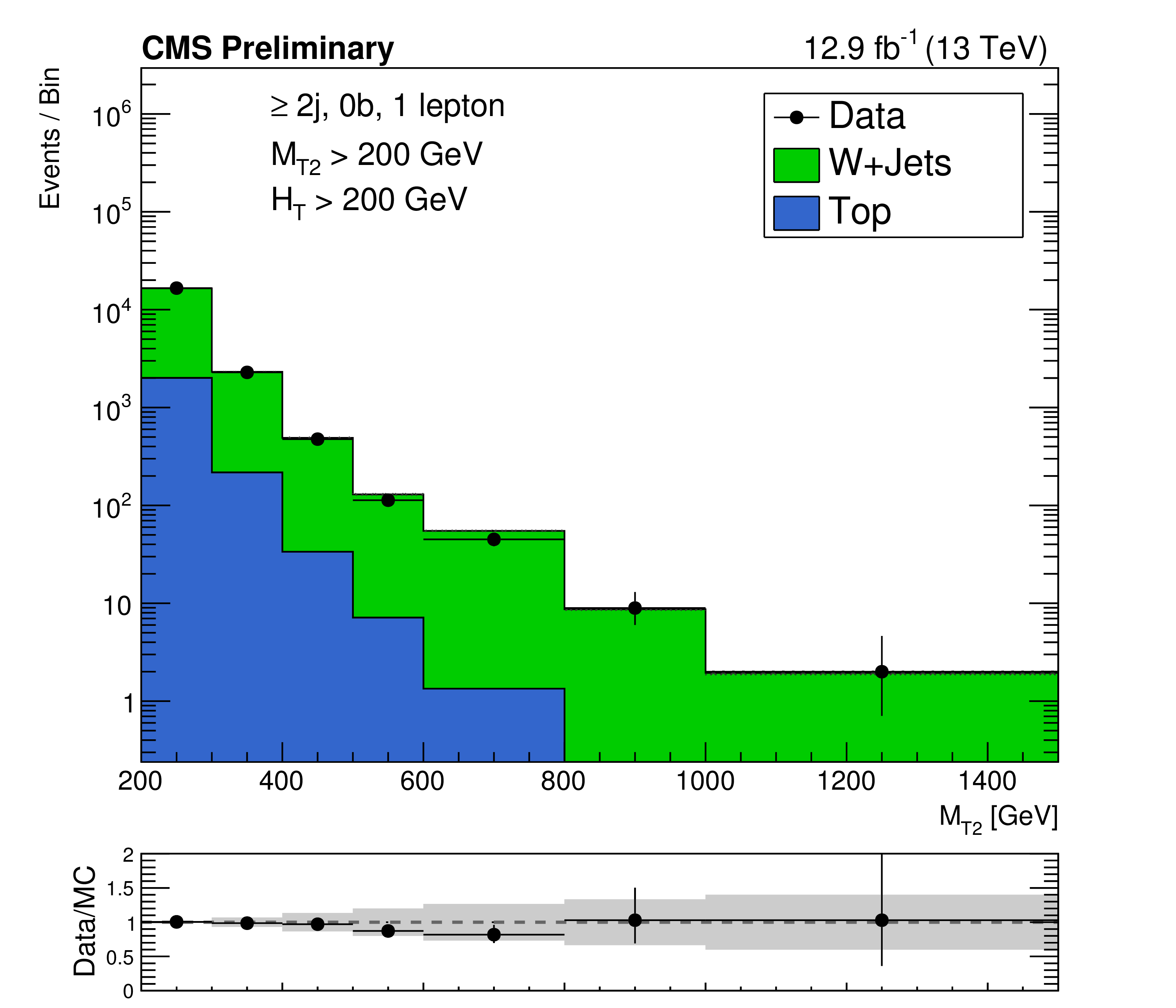
Shape comparison between simulation and data for the ${M_{T2}}$ observable, after the simulation has been normalized to data in each of the control region bins. The left and right panels correspond to W+jets and $\mathrm{ t \bar{t} }$+jets enriched control samples, respectively. |
png pdf |
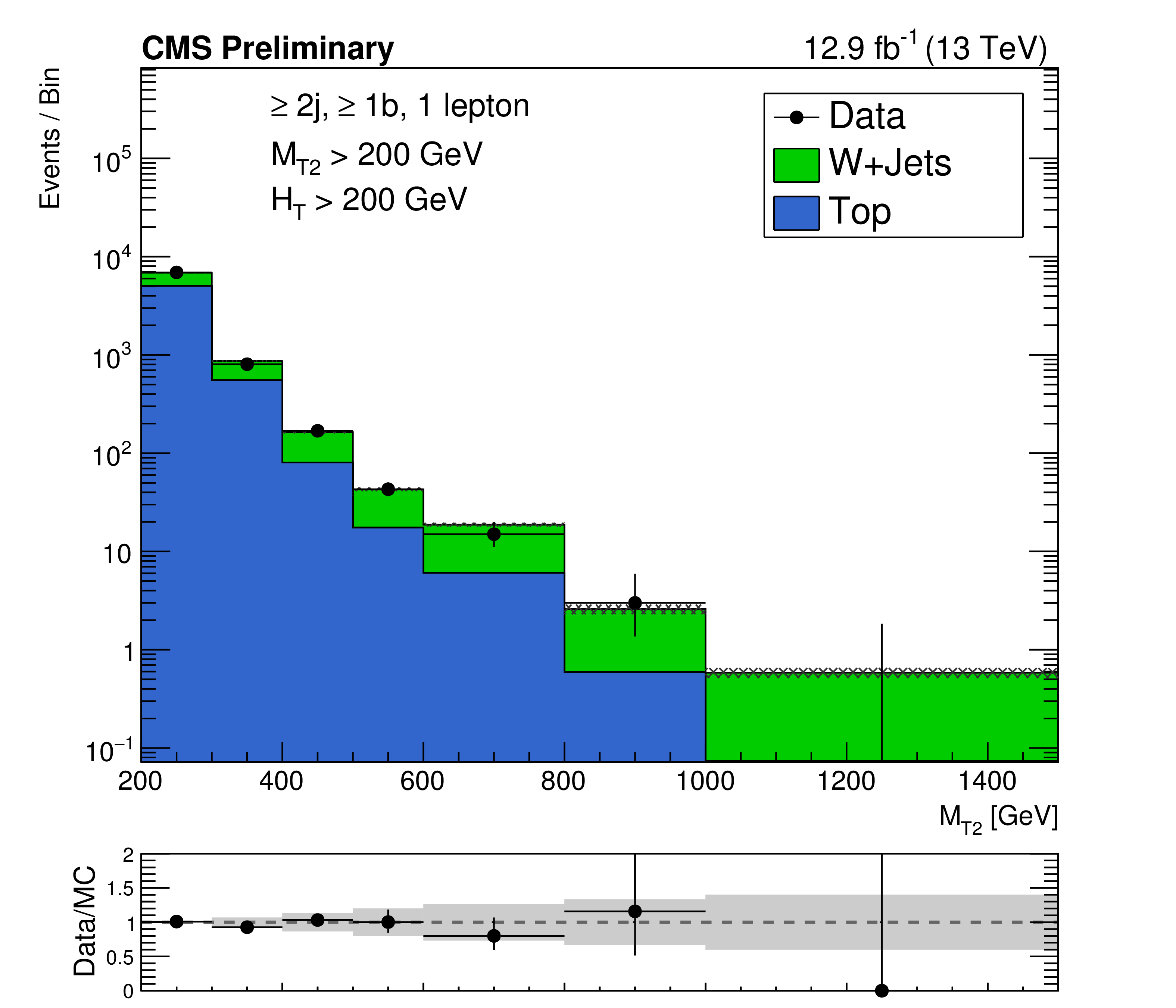
Figure 1-b:
Shape comparison between simulation and data for the ${M_{T2}}$ observable, after the simulation has been normalized to data in each of the control region bins. The left and right panels correspond to W+jets and $\mathrm{ t \bar{t} }$+jets enriched control samples, respectively. |
png pdf |
Figure 2-a:
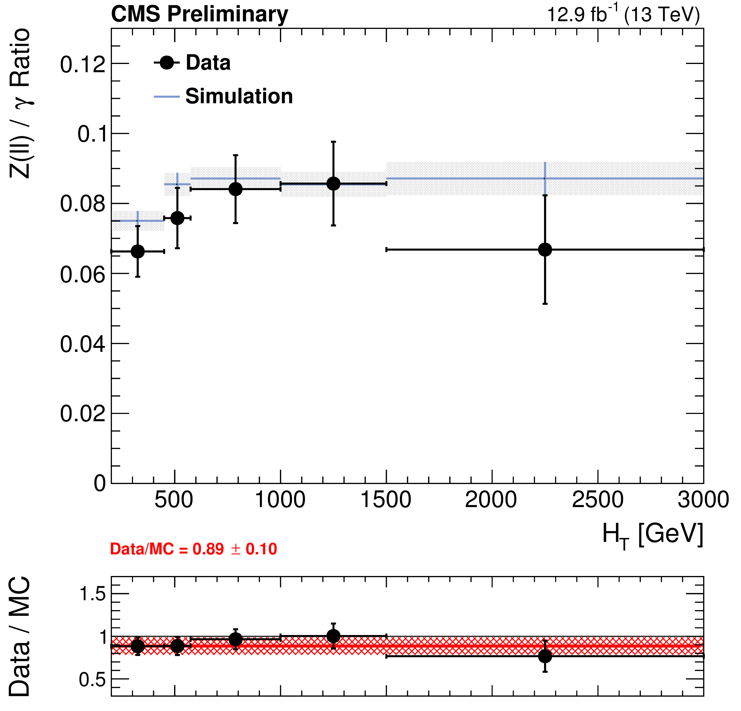
(a) Ratio $R^{Z\rightarrow \ell \ell /\gamma }$ in simulation and data as a function of ${H_{\mathrm {T}}}$ , and the corresponding double ratio (bottom panel). The red line and uncertainty corresponds to the overall correction of 0.89 $\pm$ 0.10 as measured inclusively. (b) The shape of the ${M_{T2}}$distribution from ${Z\rightarrow \nu \overline {\nu }}$ simulation compared to shapes from $\gamma $ and W data control samples in the high ${H_{\mathrm {T}}}$ region. |

png pdf |
Figure 2-b:
(a) Ratio $R^{Z\rightarrow \ell \ell /\gamma }$ in simulation and data as a function of ${H_{\mathrm {T}}}$ , and the corresponding double ratio (bottom panel). The red line and uncertainty corresponds to the overall correction of 0.89 $\pm$ 0.10 as measured inclusively. (b) The shape of the ${M_{T2}}$distribution from ${Z\rightarrow \nu \overline {\nu }}$ simulation compared to shapes from $\gamma $ and W data control samples in the high ${H_{\mathrm {T}}}$ region. |

png pdf |
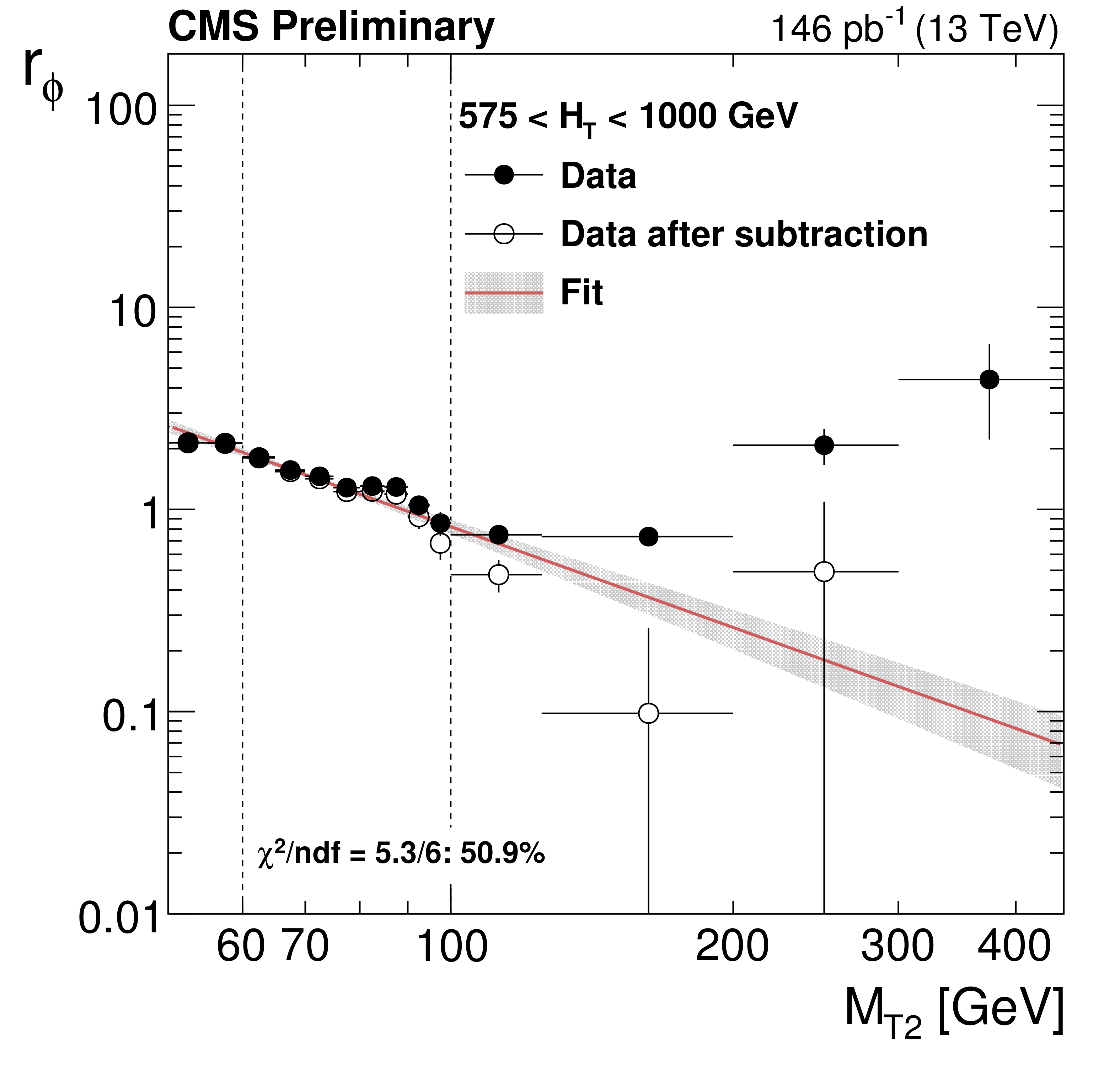
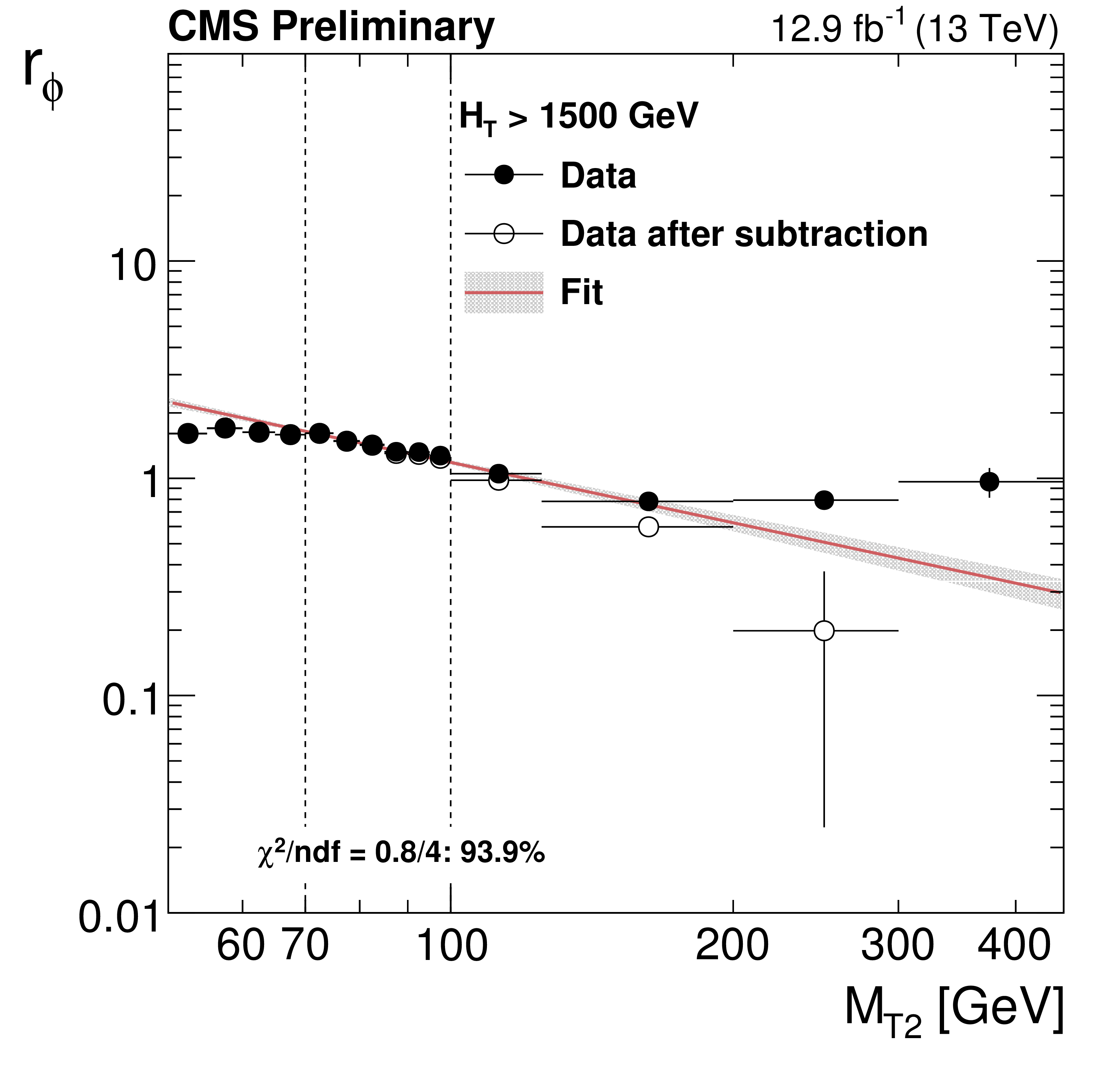
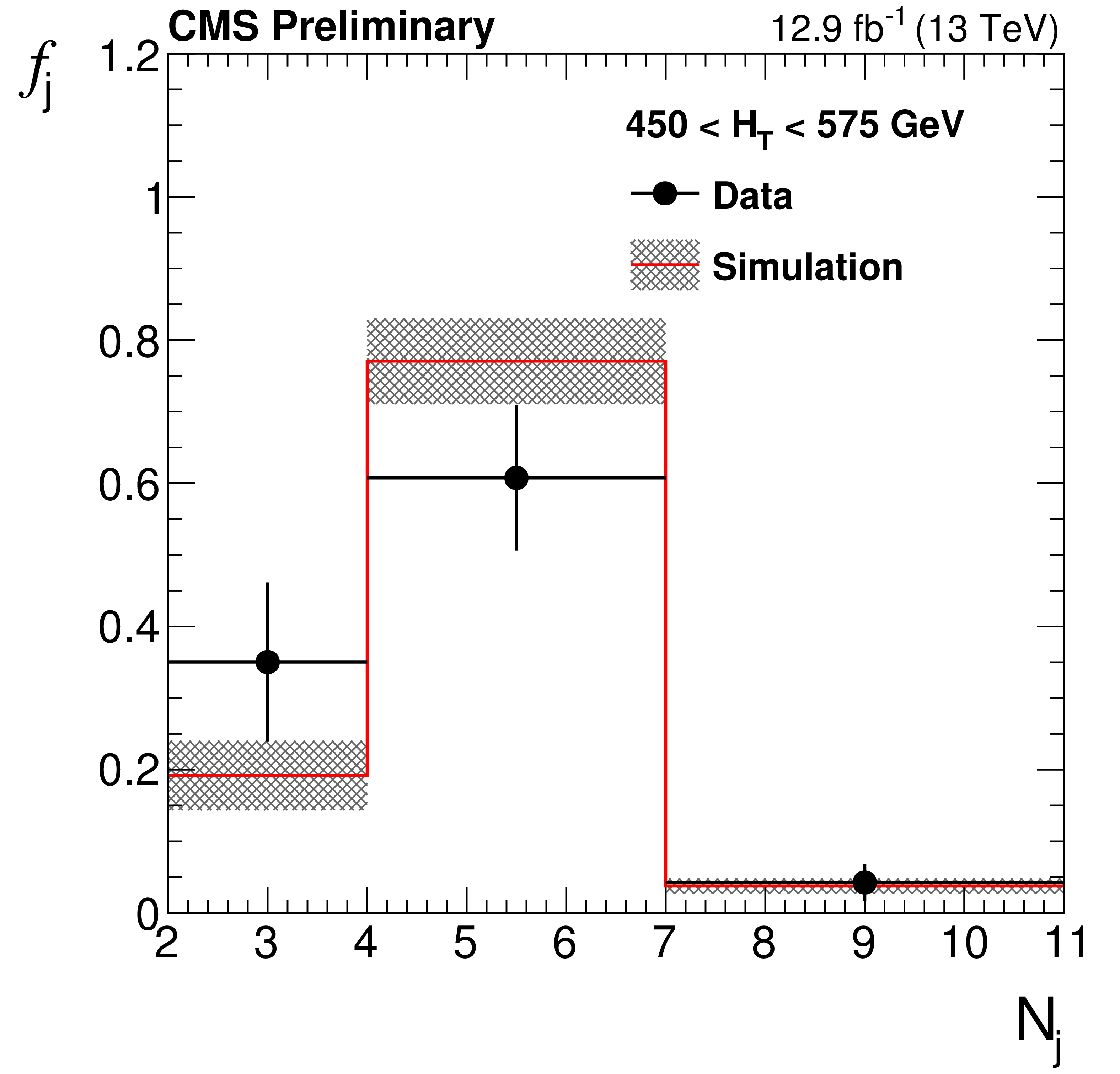
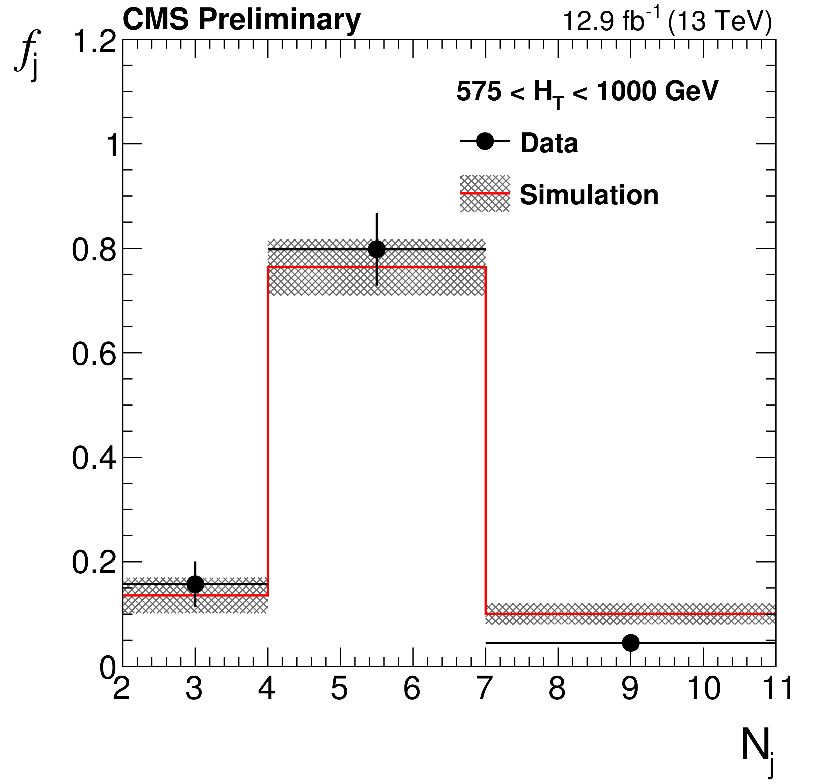
Figure 3-a:
Distribution of the ratio $r_{\phi }$ as a function of ${M_{T2}}$ for the high $ H_{\mathrm{T}}$ region (a). The fit is performed to the hollow, background-subtracted data points. The full points represent the data before subtracting non-QCD backgrounds using simulation. Data point uncertainties are statistical only. The red line and the band around it show the fit to a power-law function perfomed in the window 70 $ {<} {M_{T2}} {<} $ 100 GeV and the associated fit uncertainty. Values of $f_j$ (b) and $r_b$ (c) measured in data after requiring ${\Delta \phi _{\mathrm {min}}}{<} $ 0.3 radians and 100 $ {<}\ {M_{T2}}{<} $ 200 GeV. The bands represent both statistical and systematic uncertainties. |

png pdf |
Figure 3-b:
Distribution of the ratio $r_{\phi }$ as a function of ${M_{T2}}$ for the high $ H_{\mathrm{T}}$ region (a). The fit is performed to the hollow, background-subtracted data points. The full points represent the data before subtracting non-QCD backgrounds using simulation. Data point uncertainties are statistical only. The red line and the band around it show the fit to a power-law function perfomed in the window 70 $ {<} {M_{T2}} {<} $ 100 GeV and the associated fit uncertainty. Values of $f_j$ (b) and $r_b$ (c) measured in data after requiring ${\Delta \phi _{\mathrm {min}}}{<} $ 0.3 radians and 100 $ {<}\ {M_{T2}}{<} $ 200 GeV. The bands represent both statistical and systematic uncertainties. |
png pdf |
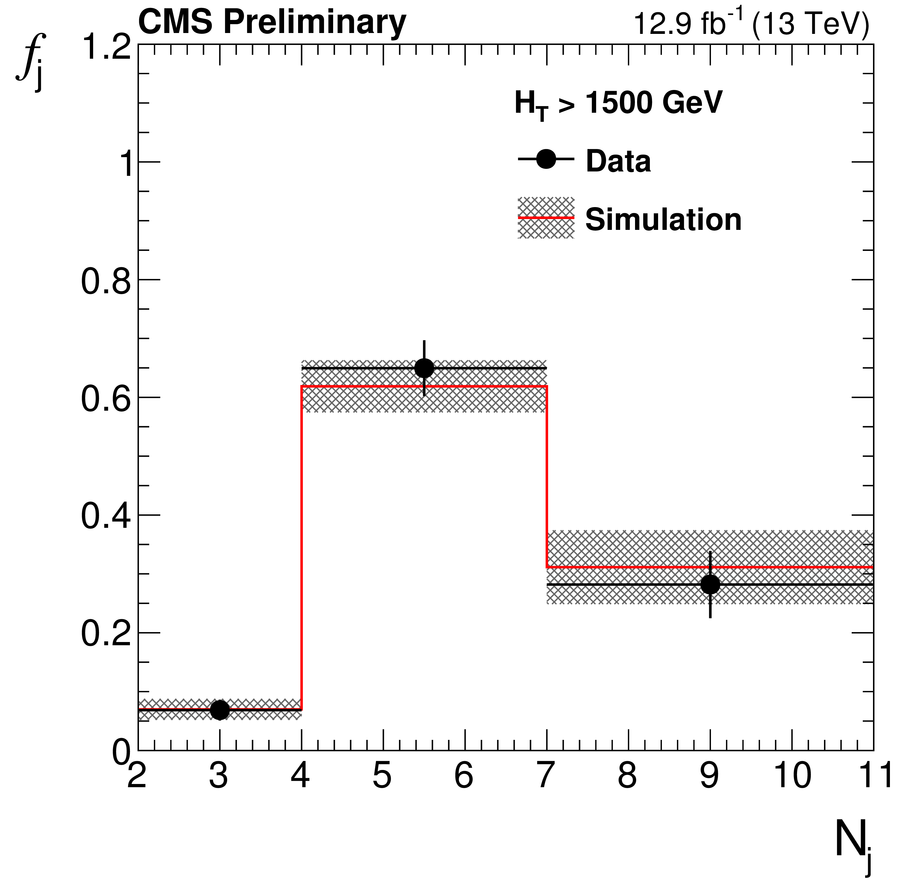
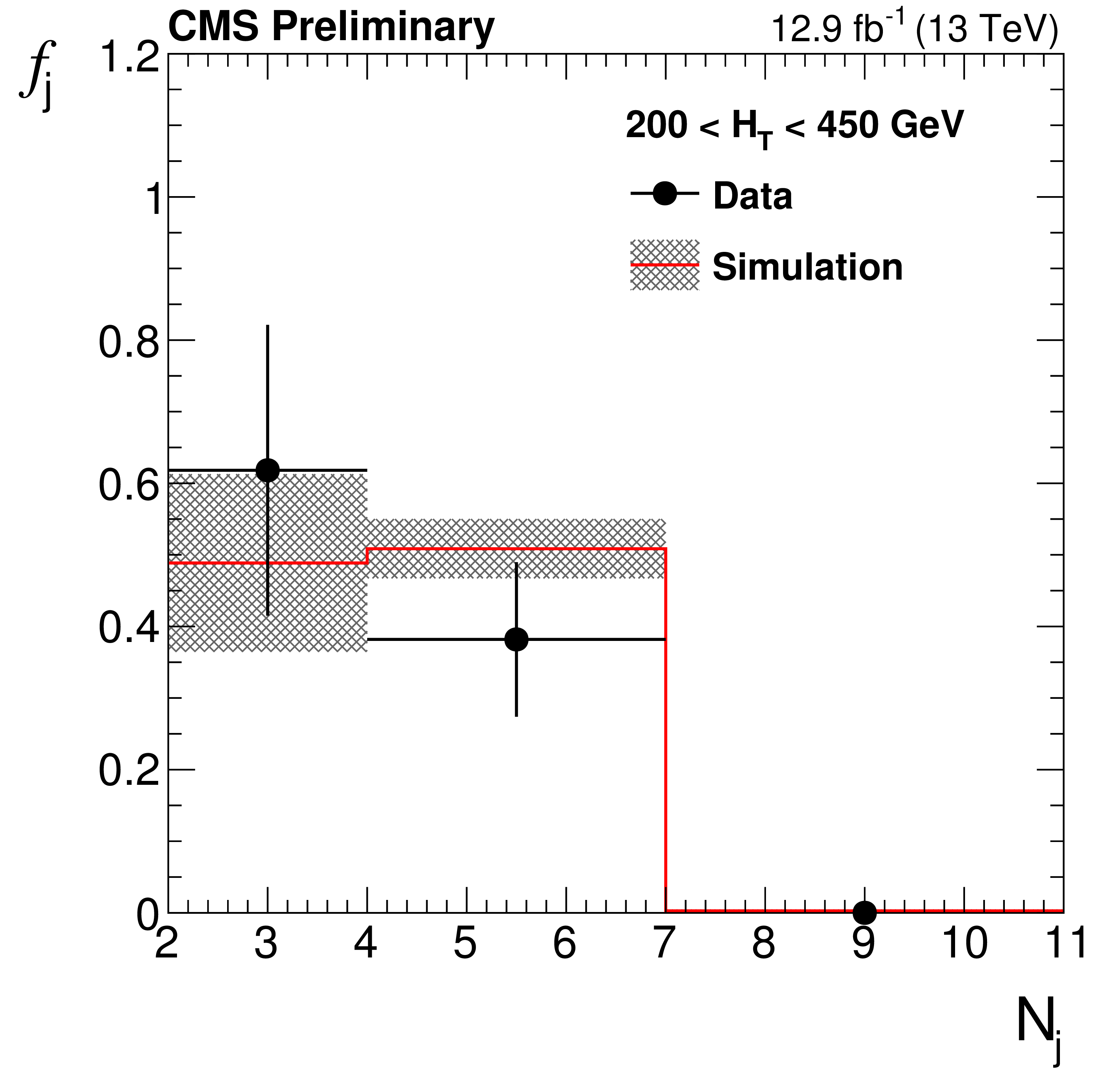
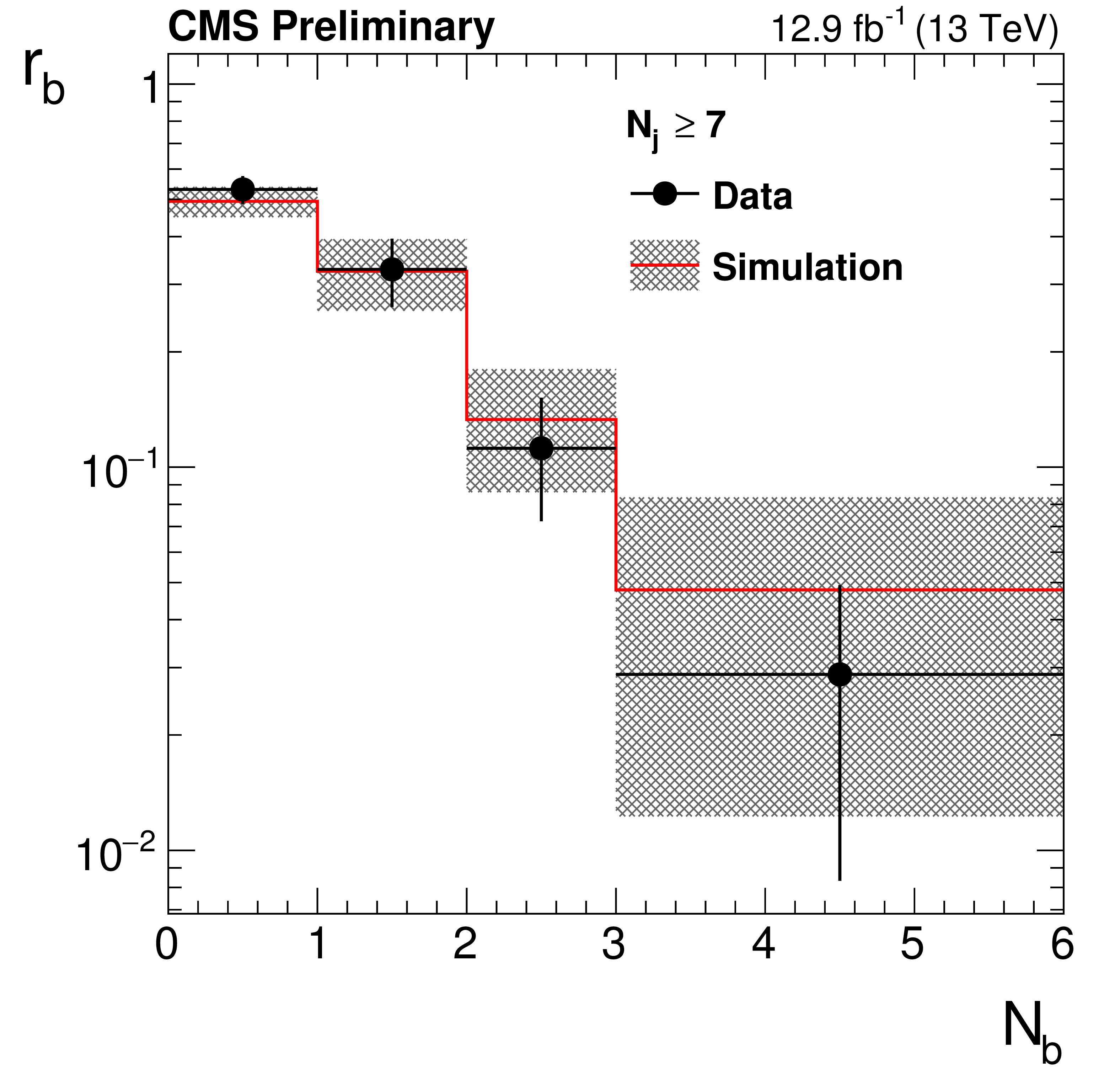
Figure 3-c:
Distribution of the ratio $r_{\phi }$ as a function of ${M_{T2}}$ for the high $ H_{\mathrm{T}}$ region (a). The fit is performed to the hollow, background-subtracted data points. The full points represent the data before subtracting non-QCD backgrounds using simulation. Data point uncertainties are statistical only. The red line and the band around it show the fit to a power-law function perfomed in the window 70 $ {<} {M_{T2}} {<} $ 100 GeV and the associated fit uncertainty. Values of $f_j$ (b) and $r_b$ (c) measured in data after requiring ${\Delta \phi _{\mathrm {min}}}{<} $ 0.3 radians and 100 $ {<}\ {M_{T2}}{<} $ 200 GeV. The bands represent both statistical and systematic uncertainties. |
png pdf |
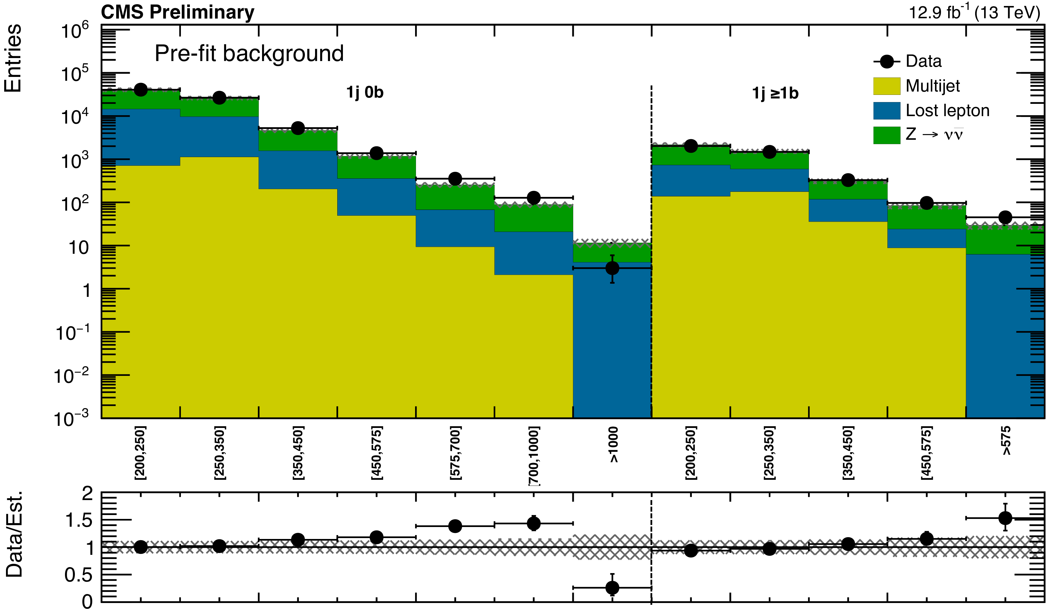
Figure 4-a:
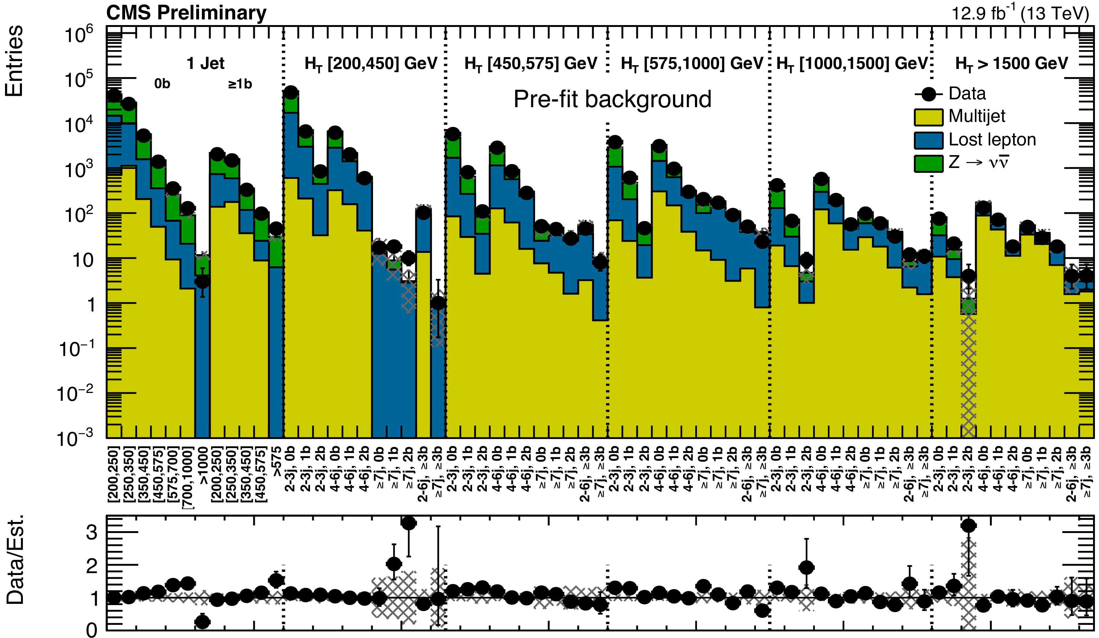
(a) Comparison of estimated (pre-fit) background and observed data events in each topological region. Hatched bands represent the full uncertainty on the background estimate. The results shown for $ {\mathrm {N}_{\mathrm {j}}} =$ 1 correspond to the monojet search regions binned in jet $ p_{\mathrm{T}}$ , whereas for the multijet signal regions, the notations j, b indicate ${\mathrm {N}_{\mathrm {j}}} $, ${\mathrm {N}_{\mathrm {b}}}$ labeling. (b) Same for individual ${M_{T2}}$ signal bins in the medium $ H_{\mathrm{T}}$ region. On the $x$-axis, the ${M_{T2}}$ binning is shown (in GeV). Bins with no entry for data have an observed count of 0. |
png pdf |
Figure 4-b:
(a) Comparison of estimated (pre-fit) background and observed data events in each topological region. Hatched bands represent the full uncertainty on the background estimate. The results shown for $ {\mathrm {N}_{\mathrm {j}}} =$ 1 correspond to the monojet search regions binned in jet $ p_{\mathrm{T}}$ , whereas for the multijet signal regions, the notations j, b indicate ${\mathrm {N}_{\mathrm {j}}} $, ${\mathrm {N}_{\mathrm {b}}}$ labeling. (b) Same for individual ${M_{T2}}$ signal bins in the medium $ H_{\mathrm{T}}$ region. On the $x$-axis, the ${M_{T2}}$ binning is shown (in GeV). Bins with no entry for data have an observed count of 0. |
png pdf |
Figure 5-a:
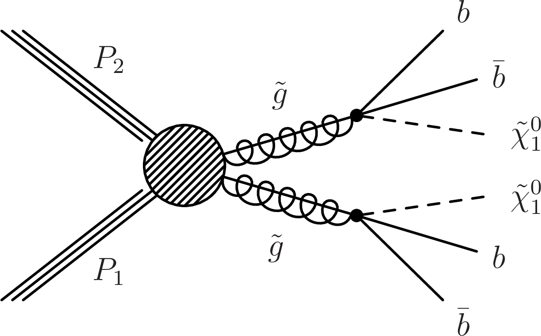
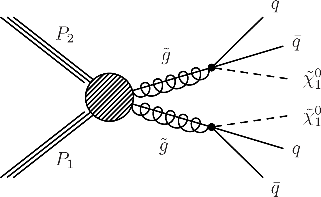
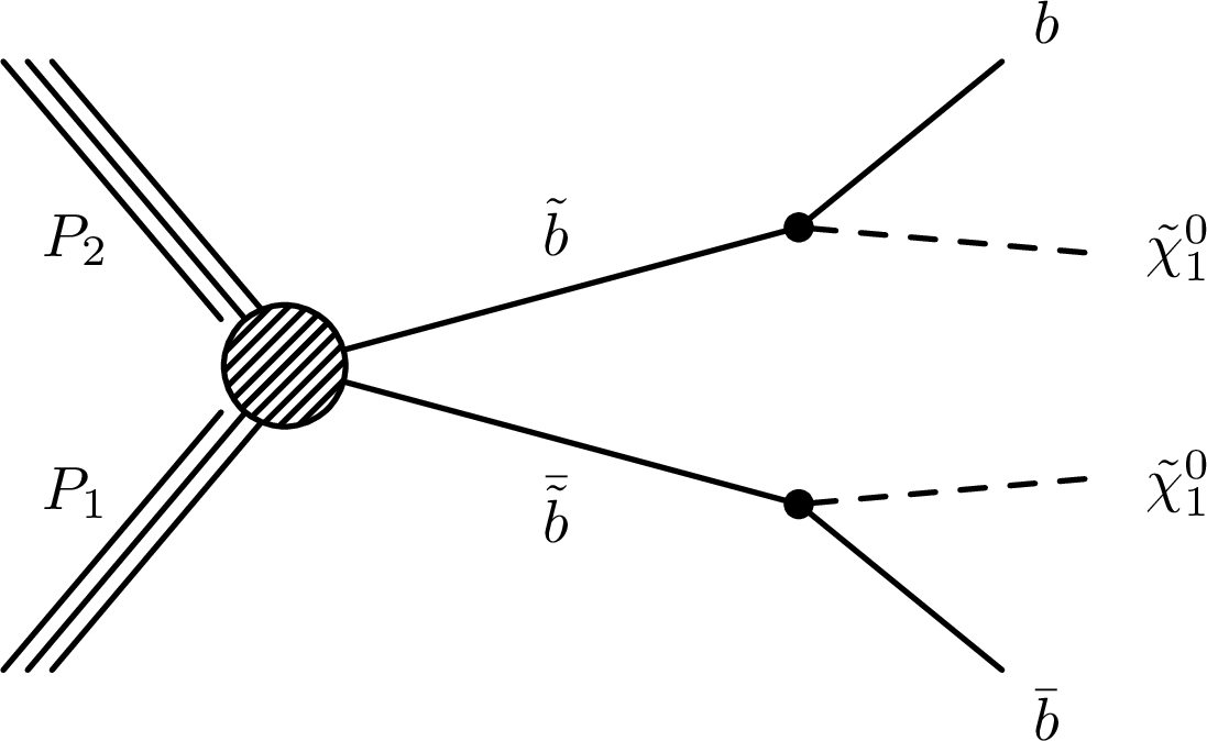
(a,b,c) Diagrams for the three scenarios of gluino mediated bottom squark, top squark and light flavor squark production considered. (d,e,f) Similar diagrams for the direct production of bottom, top and light flavor squark pairs. |

png pdf |
Figure 5-b:
(a,b,c) Diagrams for the three scenarios of gluino mediated bottom squark, top squark and light flavor squark production considered. (d,e,f) Similar diagrams for the direct production of bottom, top and light flavor squark pairs. |
png pdf |
Figure 5-c:
(a,b,c) Diagrams for the three scenarios of gluino mediated bottom squark, top squark and light flavor squark production considered. (d,e,f) Similar diagrams for the direct production of bottom, top and light flavor squark pairs. |
png pdf |
Figure 5-d:
(a,b,c) Diagrams for the three scenarios of gluino mediated bottom squark, top squark and light flavor squark production considered. (d,e,f) Similar diagrams for the direct production of bottom, top and light flavor squark pairs. |

png pdf |
Figure 5-e:
(a,b,c) Diagrams for the three scenarios of gluino mediated bottom squark, top squark and light flavor squark production considered. (d,e,f) Similar diagrams for the direct production of bottom, top and light flavor squark pairs. |

png pdf |
Figure 5-f:
(a,b,c) Diagrams for the three scenarios of gluino mediated bottom squark, top squark and light flavor squark production considered. (d,e,f) Similar diagrams for the direct production of bottom, top and light flavor squark pairs. |
png pdf root |
Figure 6-a:
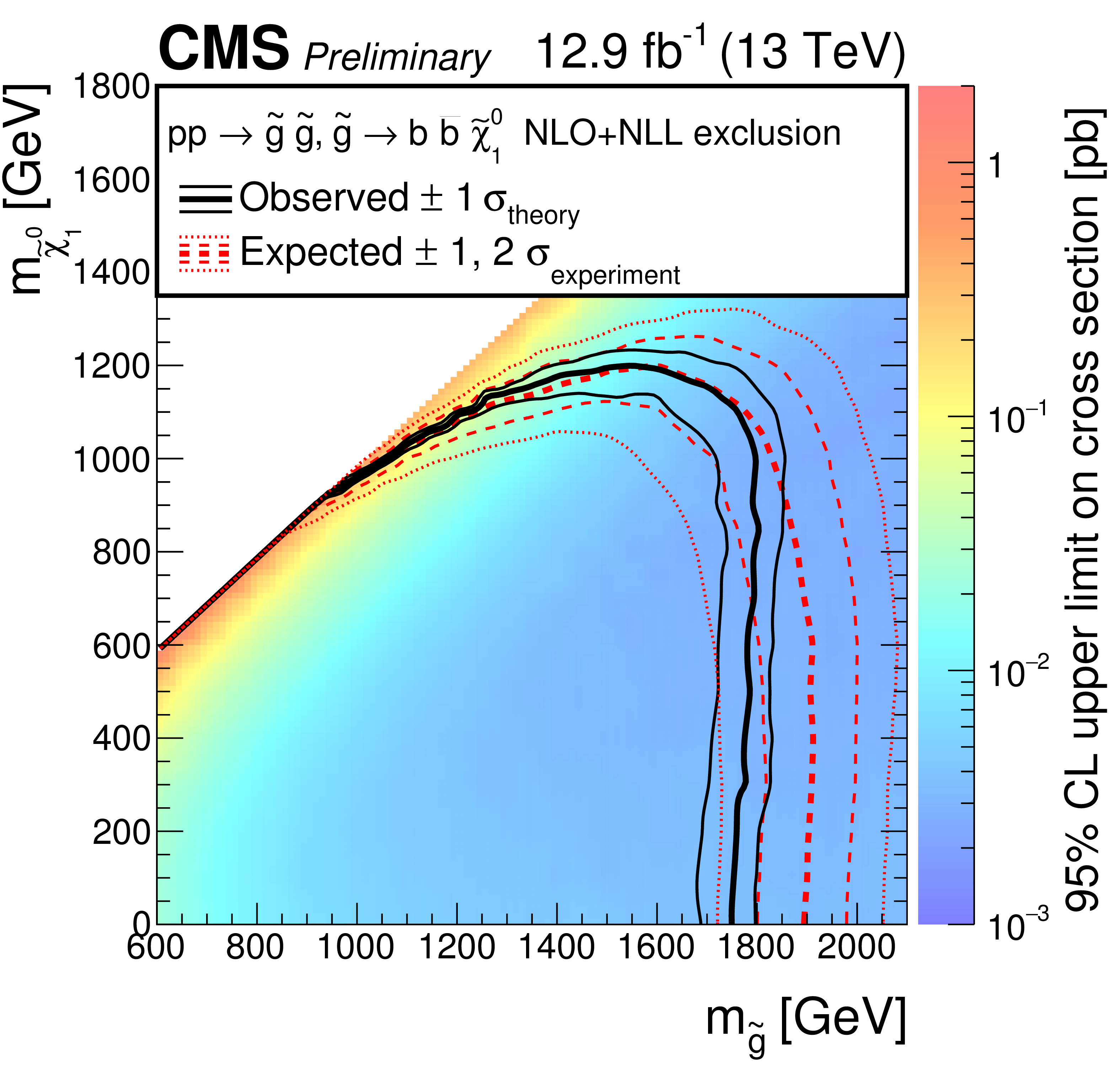
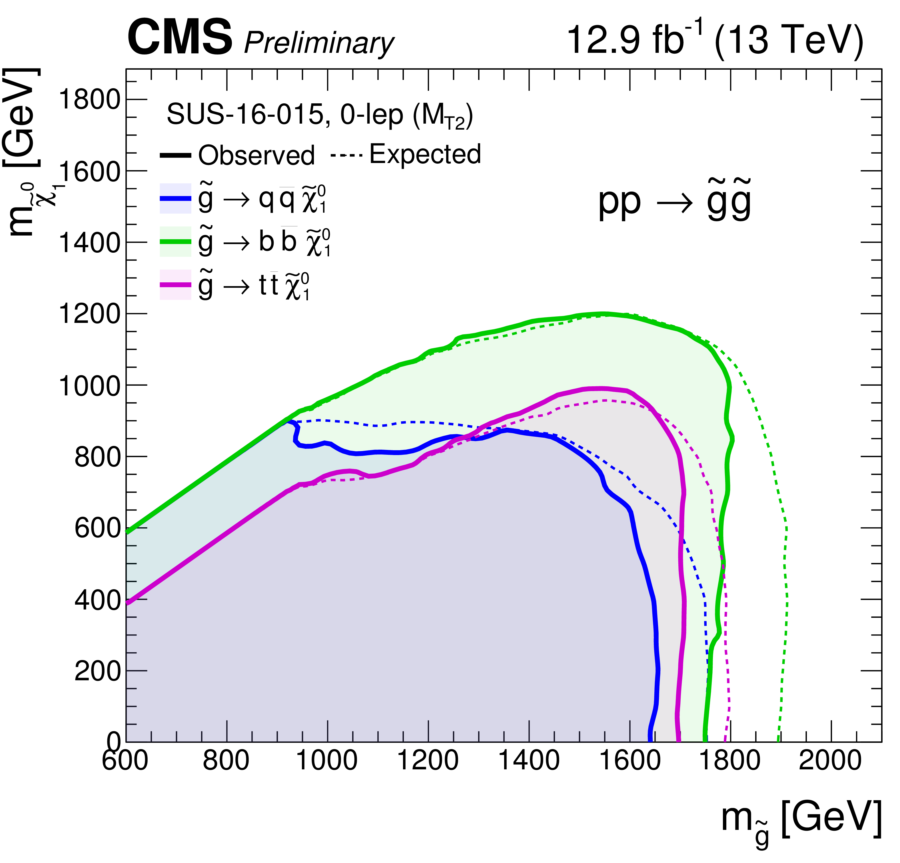
Exclusion limits at 95% CL on the cross sections for gluino-mediated bottom squark production (a), gluino-mediated top squark production (b), and gluino-mediated light-flavor squark production (c). The area to the left of and below the thick black curve represents the observed exclusion region, while the dashed red lines indicate the expected limits and their $\pm $1 $\sigma _{\mathrm {experiment}}$ standard deviation uncertainties. For the squark-pair production plot, the $\pm $2 standard deviation uncertainties are also shown. The thin black lines show the effect of the theoretical uncertainties $\sigma _{\mathrm {theory}}$ on the signal cross section. |

png pdf root |
Figure 6-b:
Exclusion limits at 95% CL on the cross sections for gluino-mediated bottom squark production (a), gluino-mediated top squark production (b), and gluino-mediated light-flavor squark production (c). The area to the left of and below the thick black curve represents the observed exclusion region, while the dashed red lines indicate the expected limits and their $\pm $1 $\sigma _{\mathrm {experiment}}$ standard deviation uncertainties. For the squark-pair production plot, the $\pm $2 standard deviation uncertainties are also shown. The thin black lines show the effect of the theoretical uncertainties $\sigma _{\mathrm {theory}}$ on the signal cross section. |

png pdf root |
Figure 6-c:
Exclusion limits at 95% CL on the cross sections for gluino-mediated bottom squark production (a), gluino-mediated top squark production (b), and gluino-mediated light-flavor squark production (c). The area to the left of and below the thick black curve represents the observed exclusion region, while the dashed red lines indicate the expected limits and their $\pm $1 $\sigma _{\mathrm {experiment}}$ standard deviation uncertainties. For the squark-pair production plot, the $\pm $2 standard deviation uncertainties are also shown. The thin black lines show the effect of the theoretical uncertainties $\sigma _{\mathrm {theory}}$ on the signal cross section. |
png pdf root |
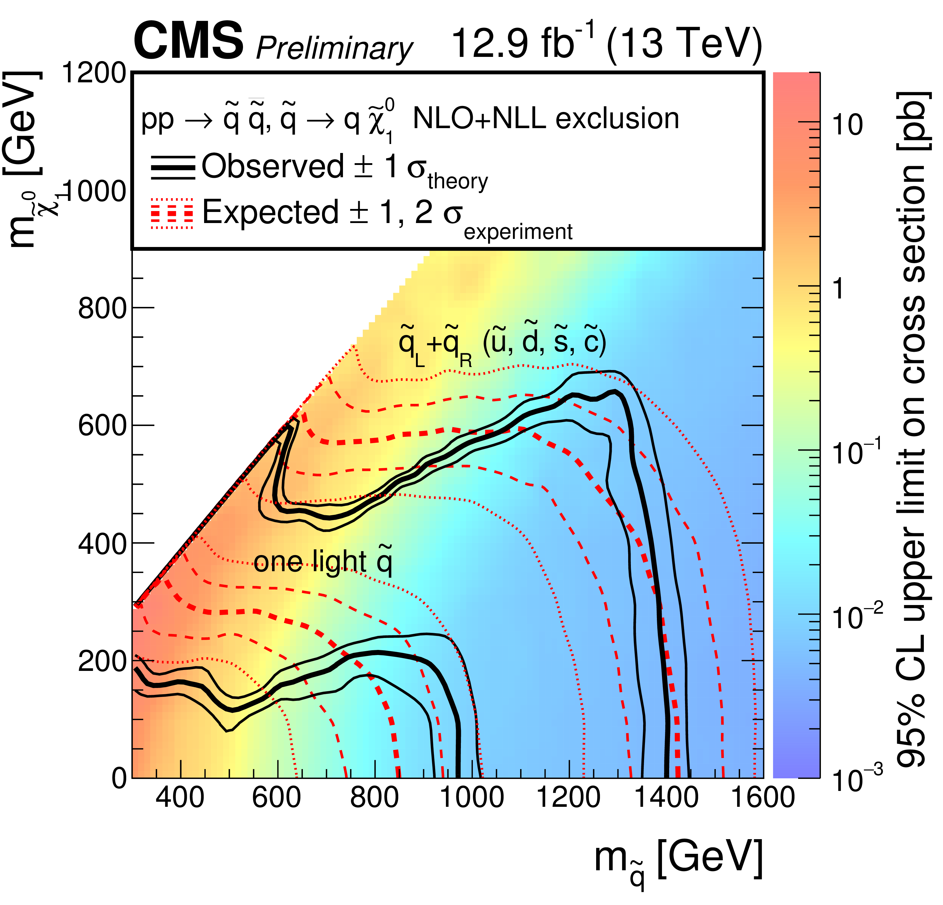
Figure 7-a:
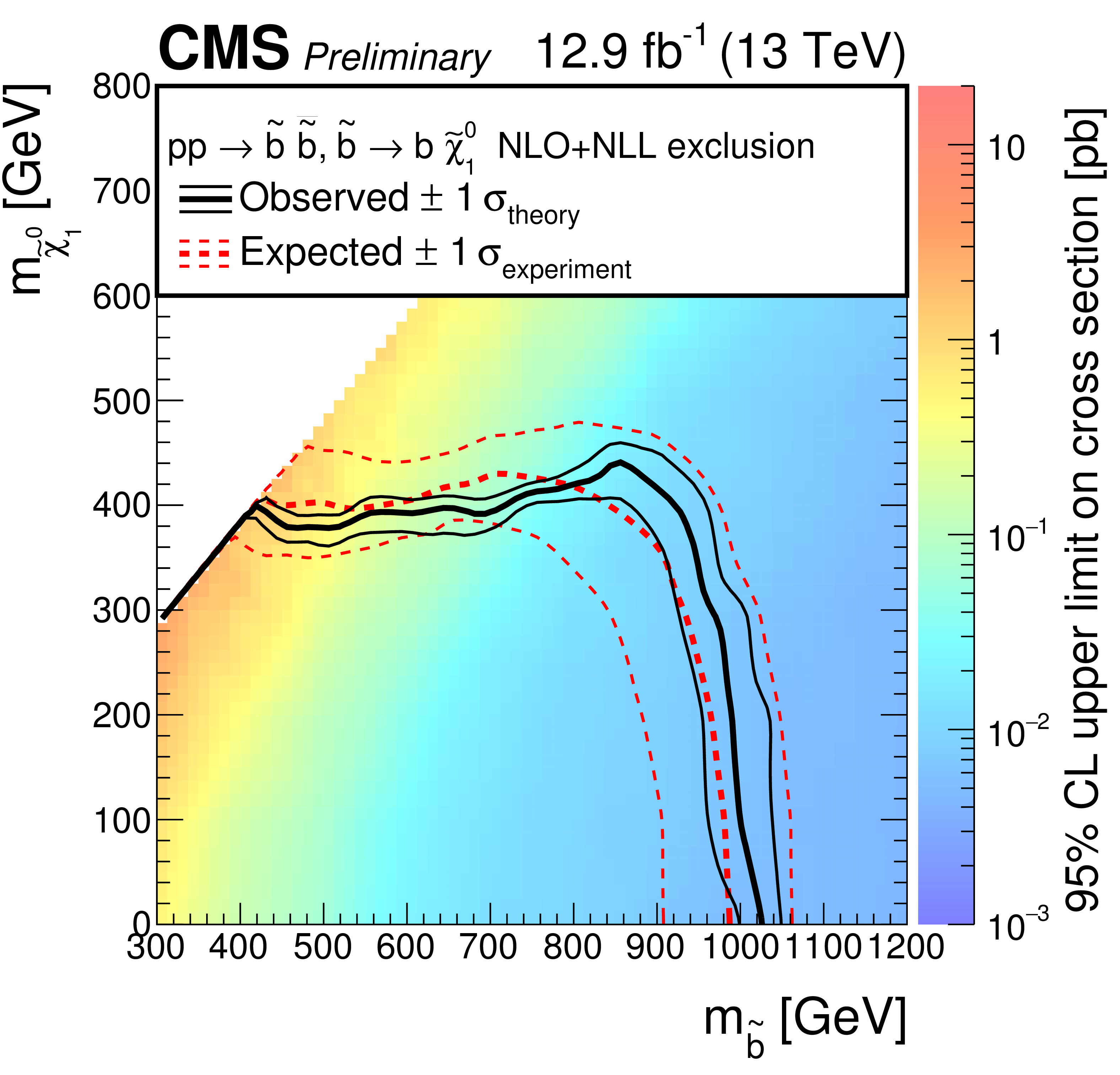
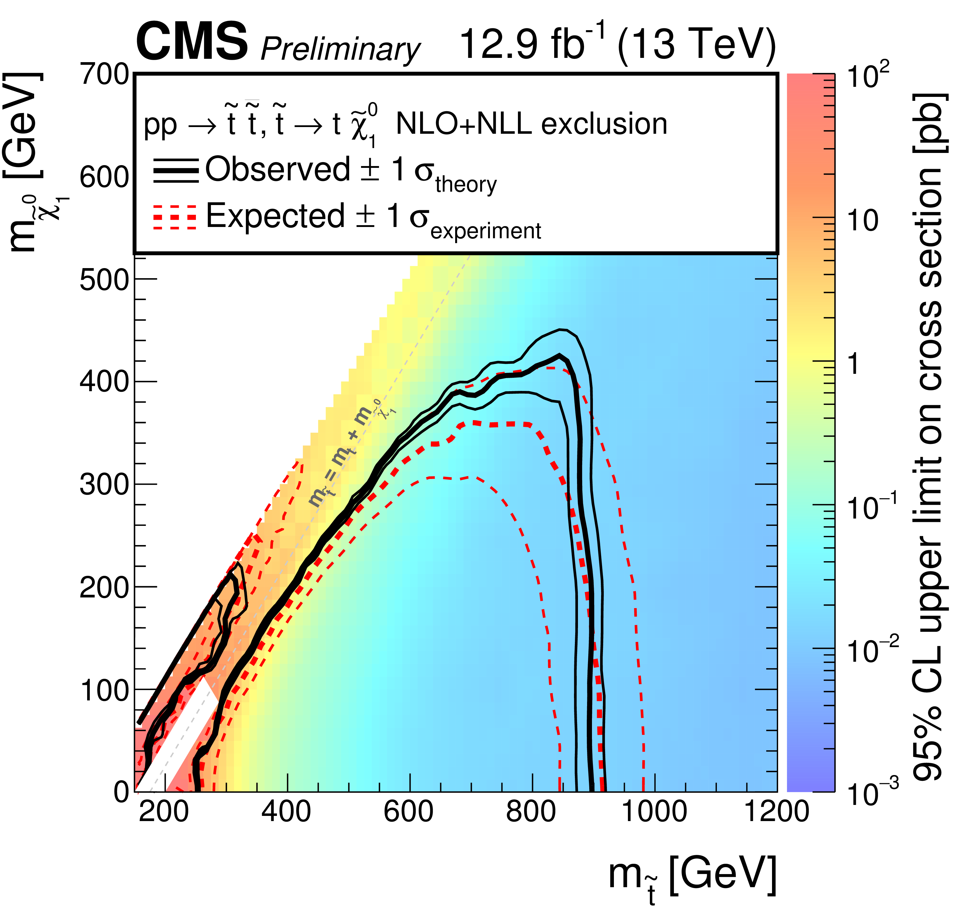
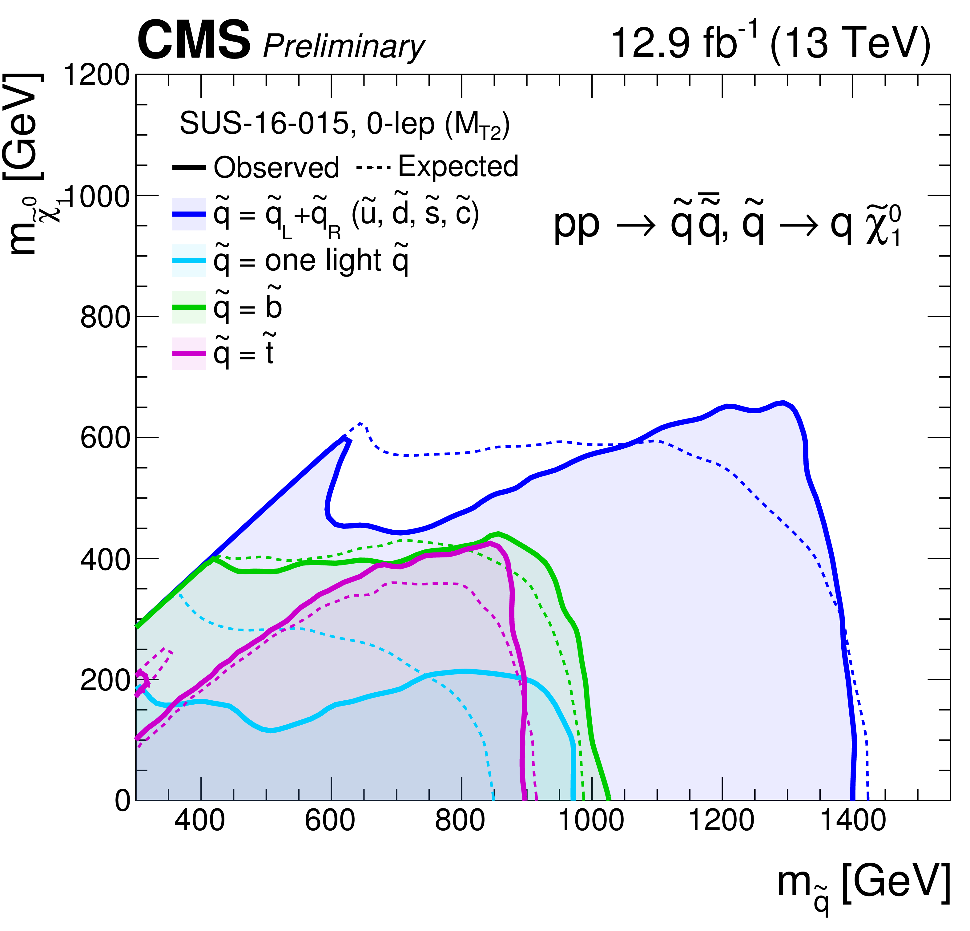
Exclusion limit at 95% CL on the cross sections for bottom squark pair production (a), top squark pair production (b), and light-flavor squark pair production (c). The area to the left of and below the thick black curve represents the observed exclusion region, while the dashed red lines indicate the expected limits and their $\pm $1 $\sigma _{\mathrm {experiment}}$ standard deviation uncertainties. The thin black lines show the effect of the theoretical uncertainties $\sigma _{\mathrm {theory}}$ on the signal cross section. The white diagonal band in the upper right plot corresponds to the region $ {| m_{\tilde{\mathrm {t}}}-m_{\mathrm {t}}-m_{\mathrm {LSP}} | } {<} $ 25 GeV , and small $m_{\mathrm {LSP}}$. Here the efficiency of the selection is a strong function of $m_{\tilde{\mathrm {t}}}-m_{\mathrm {LSP}}$, and as a result the precise determination of the cross section upper limit is uncertain because of the finite granularity of the available MC samples in this region of the ($m_{\tilde{\mathrm {t}}}$, $m_{\mathrm {LSP}}$) plane. |
png pdf root |
Figure 7-b:
Exclusion limit at 95% CL on the cross sections for bottom squark pair production (a), top squark pair production (b), and light-flavor squark pair production (c). The area to the left of and below the thick black curve represents the observed exclusion region, while the dashed red lines indicate the expected limits and their $\pm $1 $\sigma _{\mathrm {experiment}}$ standard deviation uncertainties. The thin black lines show the effect of the theoretical uncertainties $\sigma _{\mathrm {theory}}$ on the signal cross section. The white diagonal band in the upper right plot corresponds to the region $ {| m_{\tilde{\mathrm {t}}}-m_{\mathrm {t}}-m_{\mathrm {LSP}} | } {<} $ 25 GeV , and small $m_{\mathrm {LSP}}$. Here the efficiency of the selection is a strong function of $m_{\tilde{\mathrm {t}}}-m_{\mathrm {LSP}}$, and as a result the precise determination of the cross section upper limit is uncertain because of the finite granularity of the available MC samples in this region of the ($m_{\tilde{\mathrm {t}}}$, $m_{\mathrm {LSP}}$) plane. |
png pdf root |
Figure 7-c:
Exclusion limit at 95% CL on the cross sections for bottom squark pair production (a), top squark pair production (b), and light-flavor squark pair production (c). The area to the left of and below the thick black curve represents the observed exclusion region, while the dashed red lines indicate the expected limits and their $\pm $1 $\sigma _{\mathrm {experiment}}$ standard deviation uncertainties. The thin black lines show the effect of the theoretical uncertainties $\sigma _{\mathrm {theory}}$ on the signal cross section. The white diagonal band in the upper right plot corresponds to the region $ {| m_{\tilde{\mathrm {t}}}-m_{\mathrm {t}}-m_{\mathrm {LSP}} | } {<} $ 25 GeV , and small $m_{\mathrm {LSP}}$. Here the efficiency of the selection is a strong function of $m_{\tilde{\mathrm {t}}}-m_{\mathrm {LSP}}$, and as a result the precise determination of the cross section upper limit is uncertain because of the finite granularity of the available MC samples in this region of the ($m_{\tilde{\mathrm {t}}}$, $m_{\mathrm {LSP}}$) plane. |
png pdf |
Figure 8-a:
(a) Comparison of the estimated background and observed data events in each signal bin in the mono-jet region. On the $x$-axis, the ${ {p_{\mathrm {T}}} ^{\mathrm {jet1}}}$ binning is shown (in GeV). Hatched bands represent the full uncertainty on the background estimate. (b) Same for the very low $ H_{\mathrm{T}}$ region. On the $x$-axis, the ${M_{T2}}$ binning is shown (in GeV). Bins with no entry for data have an observed count of 0. |

png pdf |
Figure 8-b:
(a) Comparison of the estimated background and observed data events in each signal bin in the mono-jet region. On the $x$-axis, the ${ {p_{\mathrm {T}}} ^{\mathrm {jet1}}}$ binning is shown (in GeV). Hatched bands represent the full uncertainty on the background estimate. (b) Same for the very low $ H_{\mathrm{T}}$ region. On the $x$-axis, the ${M_{T2}}$ binning is shown (in GeV). Bins with no entry for data have an observed count of 0. |
png pdf |
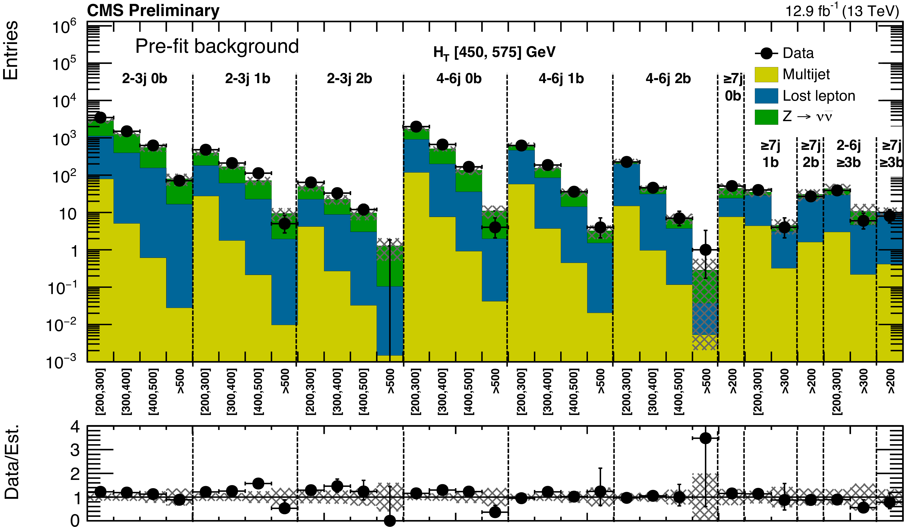
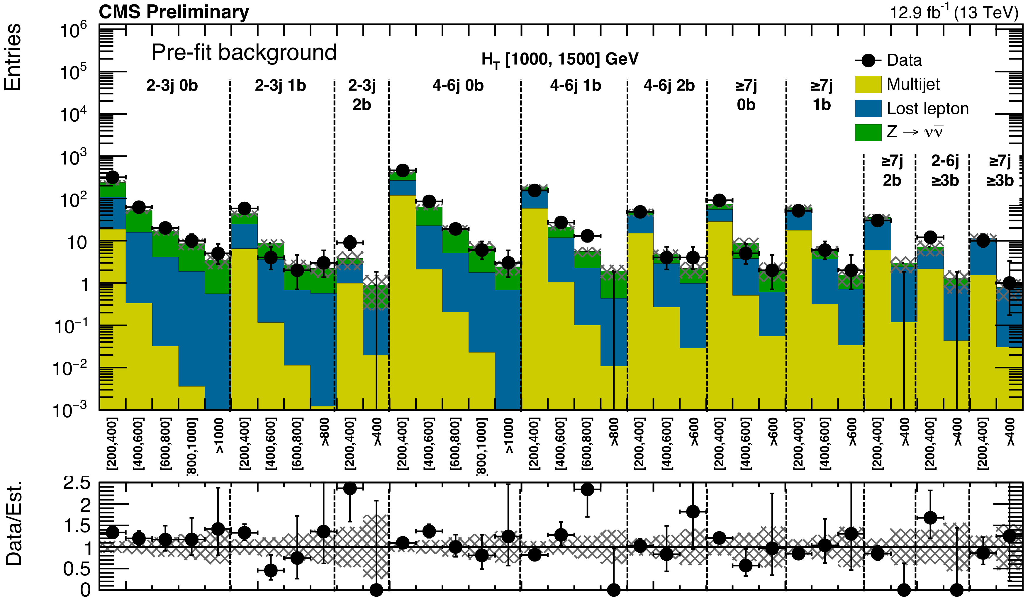
Figure 9-a:
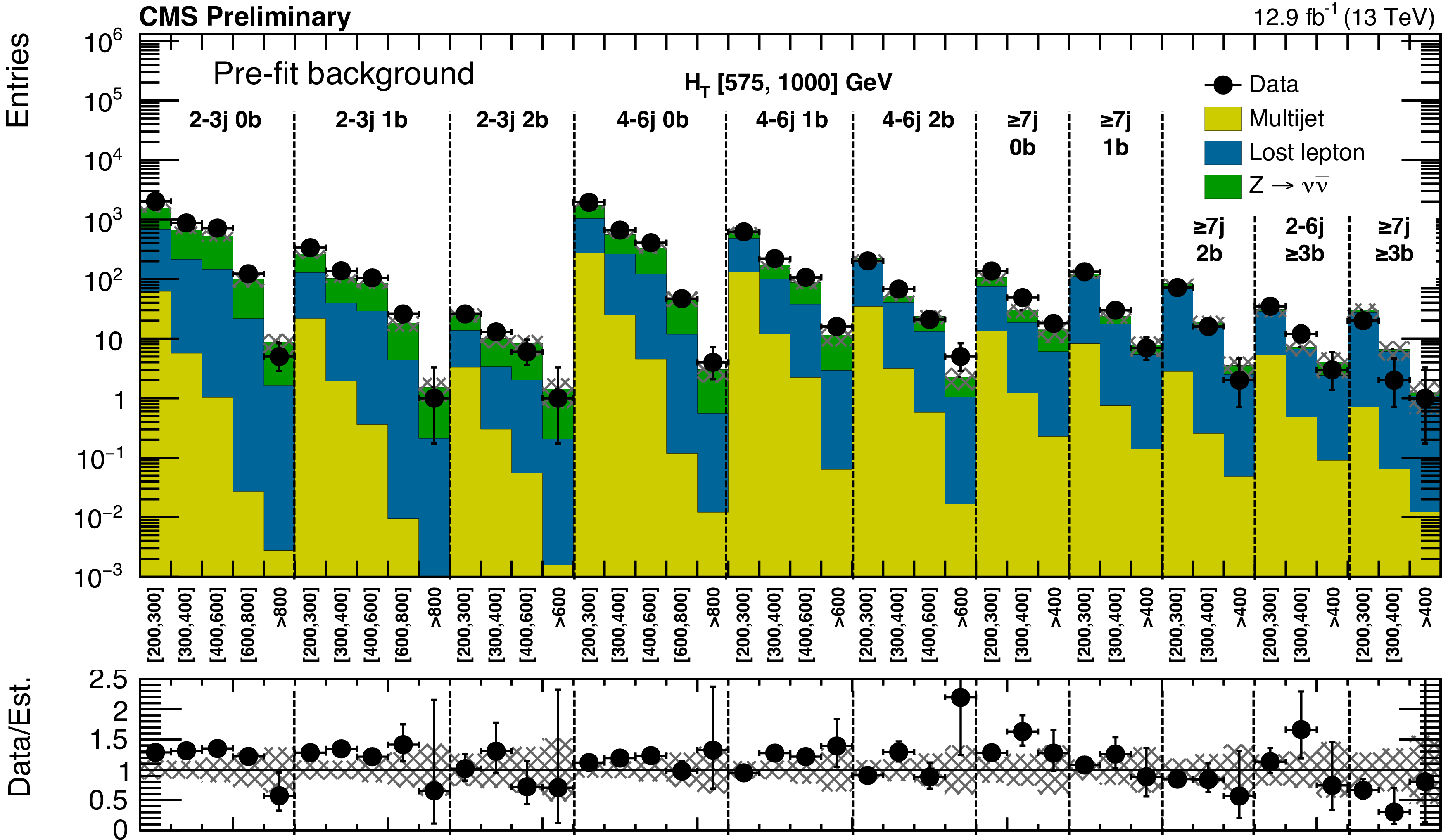
(a) Comparison of the estimated background and observed data events in each signal bin in the low $ H_{\mathrm{T}}$ region. Hatched bands represent the full uncertainty on the background estimate. Same for the high (b) and extreme (c) $ H_{\mathrm{T}}$ regions. On the $x$-axis, the ${M_{T2}}$ binning is shown (in GeV). Bins with no entry for data have an observed count of 0. |
png pdf |
Figure 9-b:
(a) Comparison of the estimated background and observed data events in each signal bin in the low $ H_{\mathrm{T}}$ region. Hatched bands represent the full uncertainty on the background estimate. Same for the high (b) and extreme (c) $ H_{\mathrm{T}}$ regions. On the $x$-axis, the ${M_{T2}}$ binning is shown (in GeV). Bins with no entry for data have an observed count of 0. |

png pdf |
Figure 9-c:
(a) Comparison of the estimated background and observed data events in each signal bin in the low $ H_{\mathrm{T}}$ region. Hatched bands represent the full uncertainty on the background estimate. Same for the high (b) and extreme (c) $ H_{\mathrm{T}}$ regions. On the $x$-axis, the ${M_{T2}}$ binning is shown (in GeV). Bins with no entry for data have an observed count of 0. |

png pdf |
Figure 10:
Comparison of post-fit background prediction and observed data events in each topological region. Hatched bands represent the post-fit uncertainty on the background prediction. For the monojet, on the $x$-axis the ${ {p_{\mathrm {T}}} ^{\mathrm {jet1}}}$ binning is shown (in GeV), whereas for the multijet signal regions, the notations j, b indicate$ {\mathrm {N}_{\mathrm {j}}} $, ${\mathrm {N}_{\mathrm {b}}}$ labeling. |

png pdf |
Figure 11-a:
(a) Comparison of the estimated background (post-fit) and observed data events in each signal bin in the mono-jet region. On the $x$-axis, the ${ {p_{\mathrm {T}}} ^{\mathrm {jet1}}}$ binning is shown (in GeV). (b) and (c): Same for the very low and low $ H_{\mathrm{T}}$ region. On the $x$-axis, the ${M_{T2}}$ binning is shown (in GeV). Bins with no entry for data have an observed count of 0. In these Figures, the uncertainty band represents the full uncertainty band associated to the data-driven estimate, a-posteriori.-a |
png pdf |
Figure 11-b:
(a) Comparison of the estimated background (post-fit) and observed data events in each signal bin in the mono-jet region. On the $x$-axis, the ${ {p_{\mathrm {T}}} ^{\mathrm {jet1}}}$ binning is shown (in GeV). (b) and (c): Same for the very low and low $ H_{\mathrm{T}}$ region. On the $x$-axis, the ${M_{T2}}$ binning is shown (in GeV). Bins with no entry for data have an observed count of 0. In these Figures, the uncertainty band represents the full uncertainty band associated to the data-driven estimate, a-posteriori.-b |

png pdf |
Figure 11-c:
(a) Comparison of the estimated background (post-fit) and observed data events in each signal bin in the mono-jet region. On the $x$-axis, the ${ {p_{\mathrm {T}}} ^{\mathrm {jet1}}}$ binning is shown (in GeV). (b) and (c): Same for the very low and low $ H_{\mathrm{T}}$ region. On the $x$-axis, the ${M_{T2}}$ binning is shown (in GeV). Bins with no entry for data have an observed count of 0. In these Figures, the uncertainty band represents the full uncertainty band associated to the data-driven estimate, a-posteriori.-c |
png pdf |
Figure 12-a:
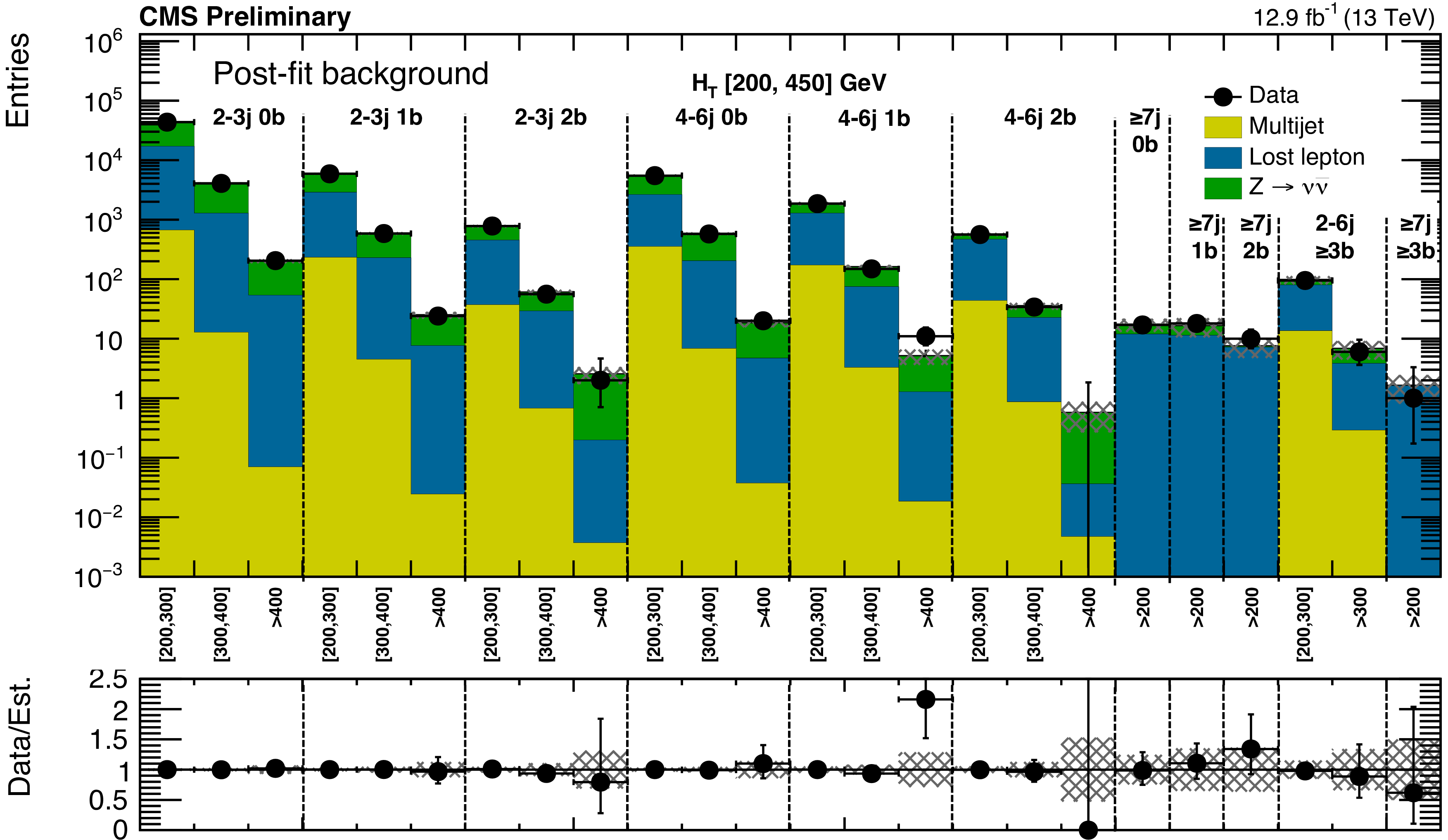
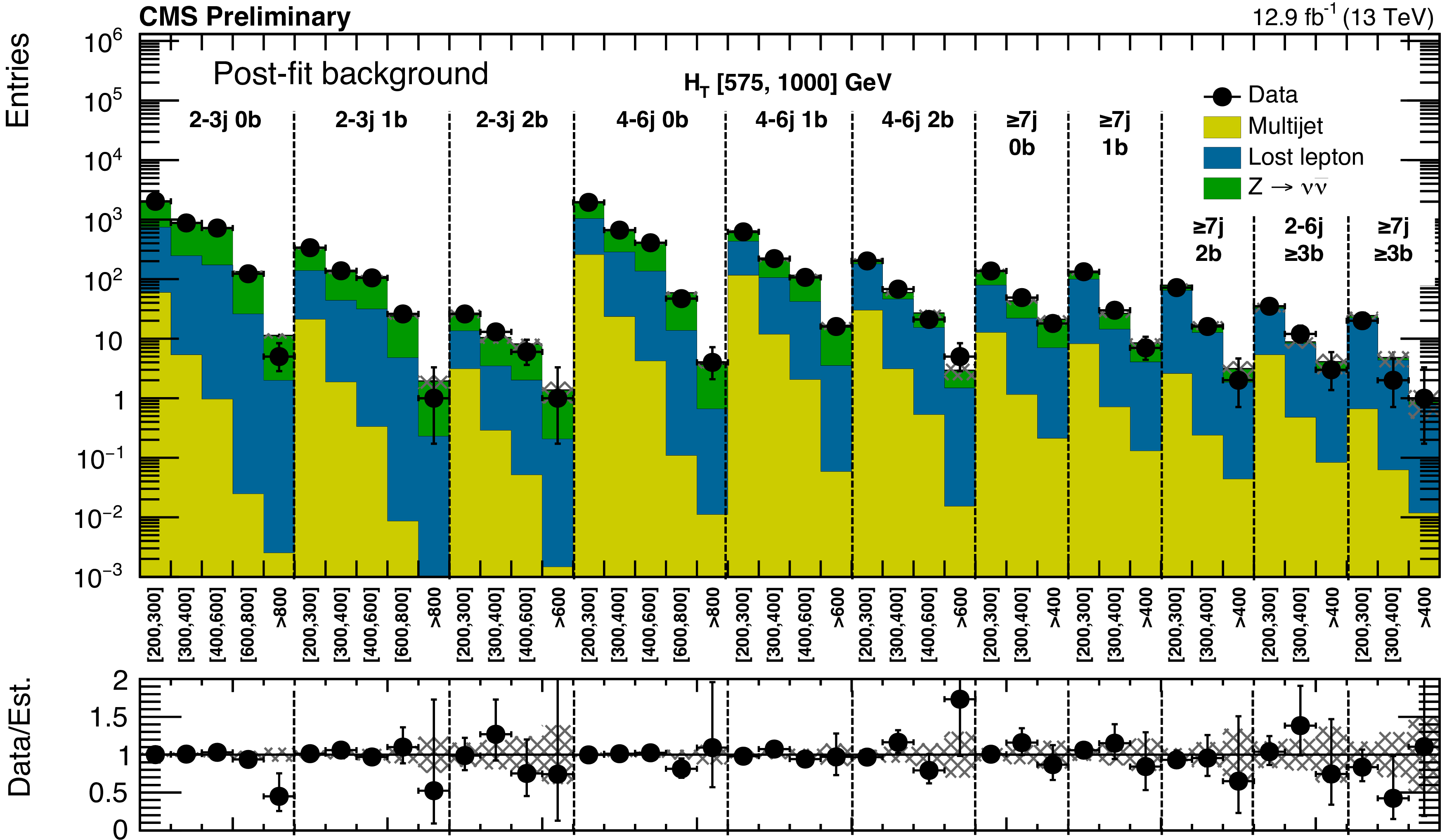
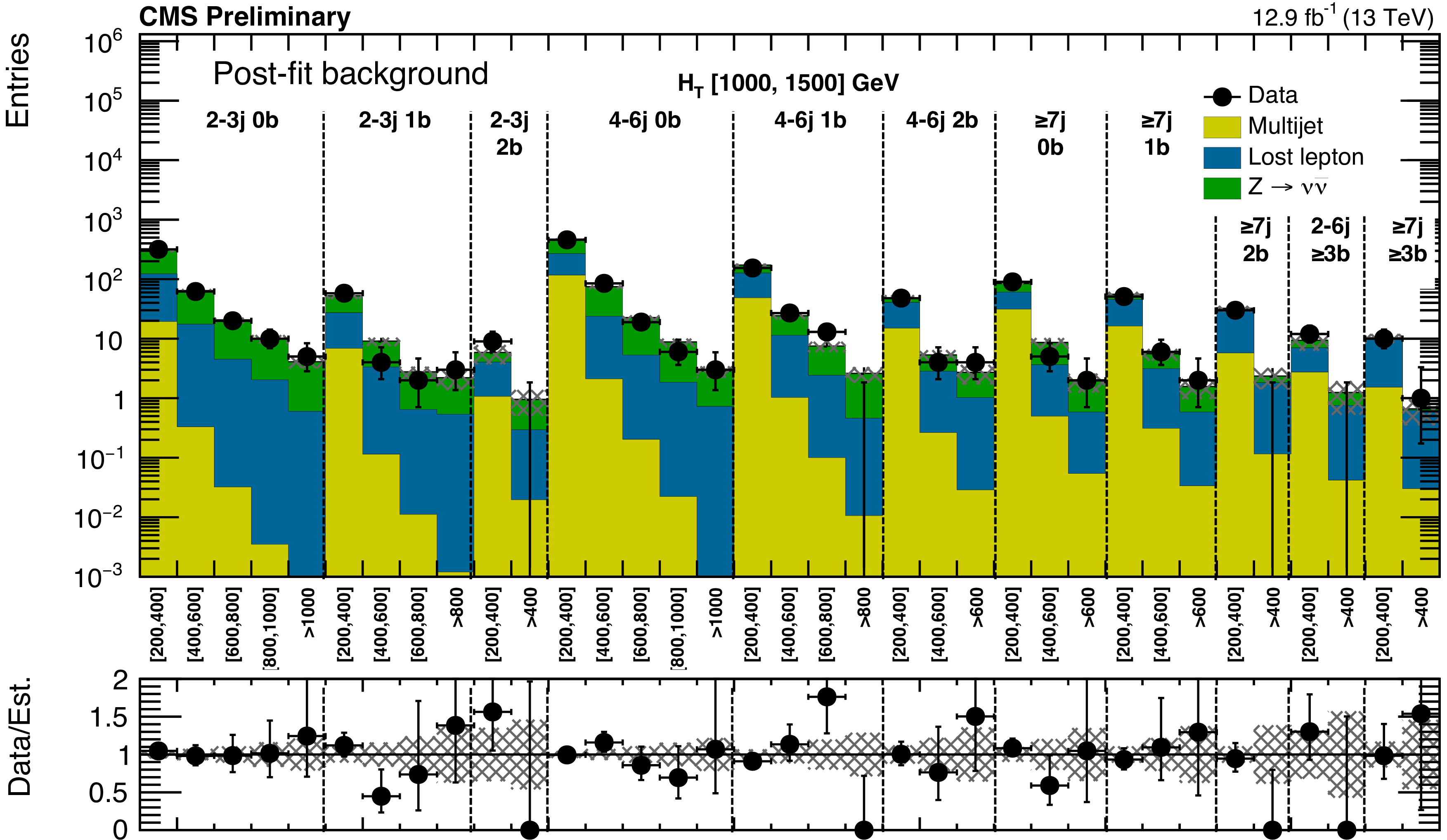
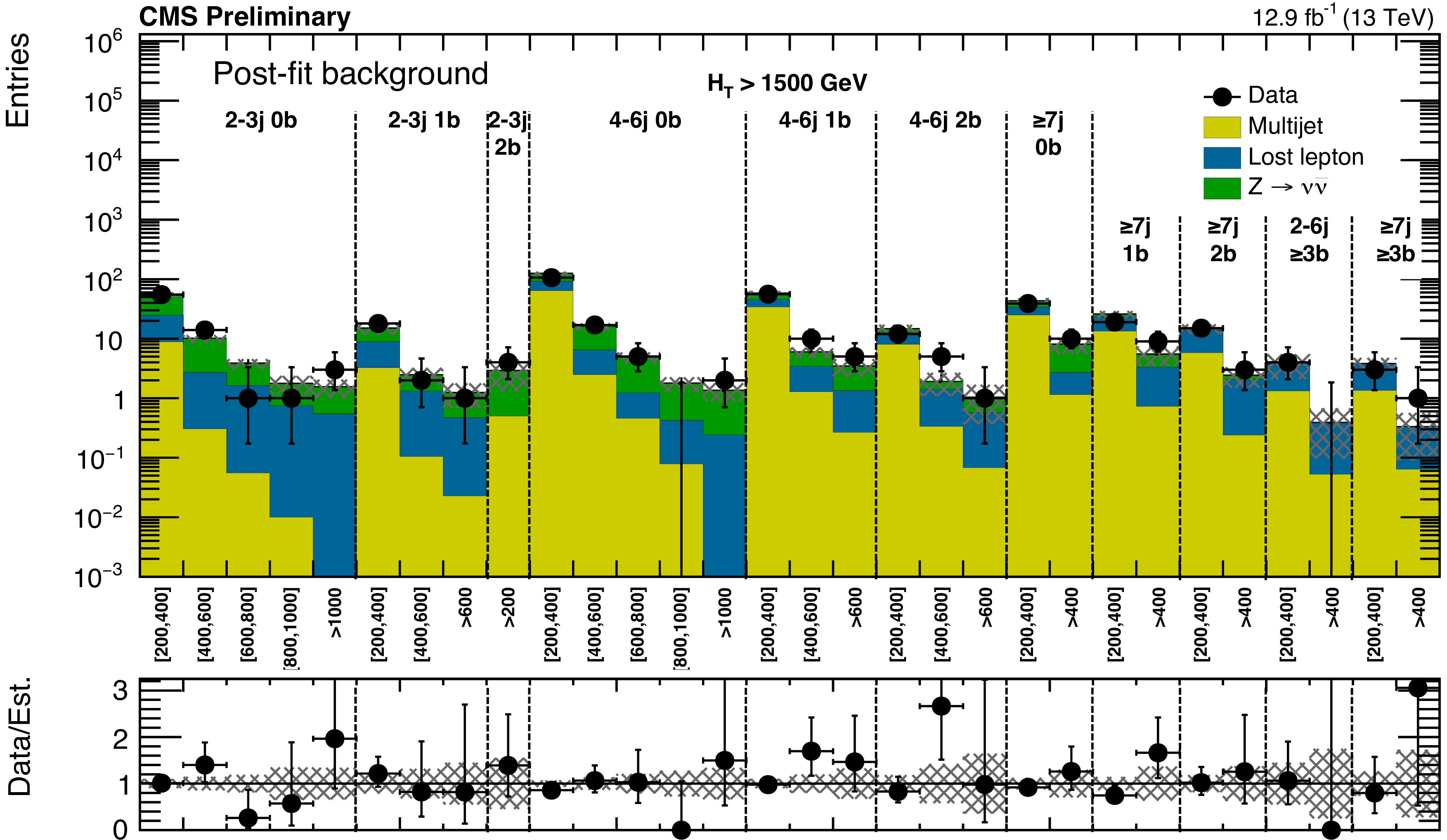
(a) Comparison of the estimated background (post-fit) and observed data events in each signal bin in the medium $ H_{\mathrm{T}}$ region. Same for the high (b) and extreme (c) $ H_{\mathrm{T}}$ regions. On the $x$-axis, the ${M_{T2}}$ binning is shown (in GeV). Bins with no entry for data have an observed count of 0. In these Figures, the uncertainty band represents the full uncertainty band associated to the data-driven estimate, a-posteriori.-a |
png pdf |
Figure 12-b:
(a) Comparison of the estimated background (post-fit) and observed data events in each signal bin in the medium $ H_{\mathrm{T}}$ region. Same for the high (b) and extreme (c) $ H_{\mathrm{T}}$ regions. On the $x$-axis, the ${M_{T2}}$ binning is shown (in GeV). Bins with no entry for data have an observed count of 0. In these Figures, the uncertainty band represents the full uncertainty band associated to the data-driven estimate, a-posteriori.-b |
png pdf |
Figure 12-c:
(a) Comparison of the estimated background (post-fit) and observed data events in each signal bin in the medium $ H_{\mathrm{T}}$ region. Same for the high (b) and extreme (c) $ H_{\mathrm{T}}$ regions. On the $x$-axis, the ${M_{T2}}$ binning is shown (in GeV). Bins with no entry for data have an observed count of 0. In these Figures, the uncertainty band represents the full uncertainty band associated to the data-driven estimate, a-posteriori.-c |

png pdf |
Figure 13-a:
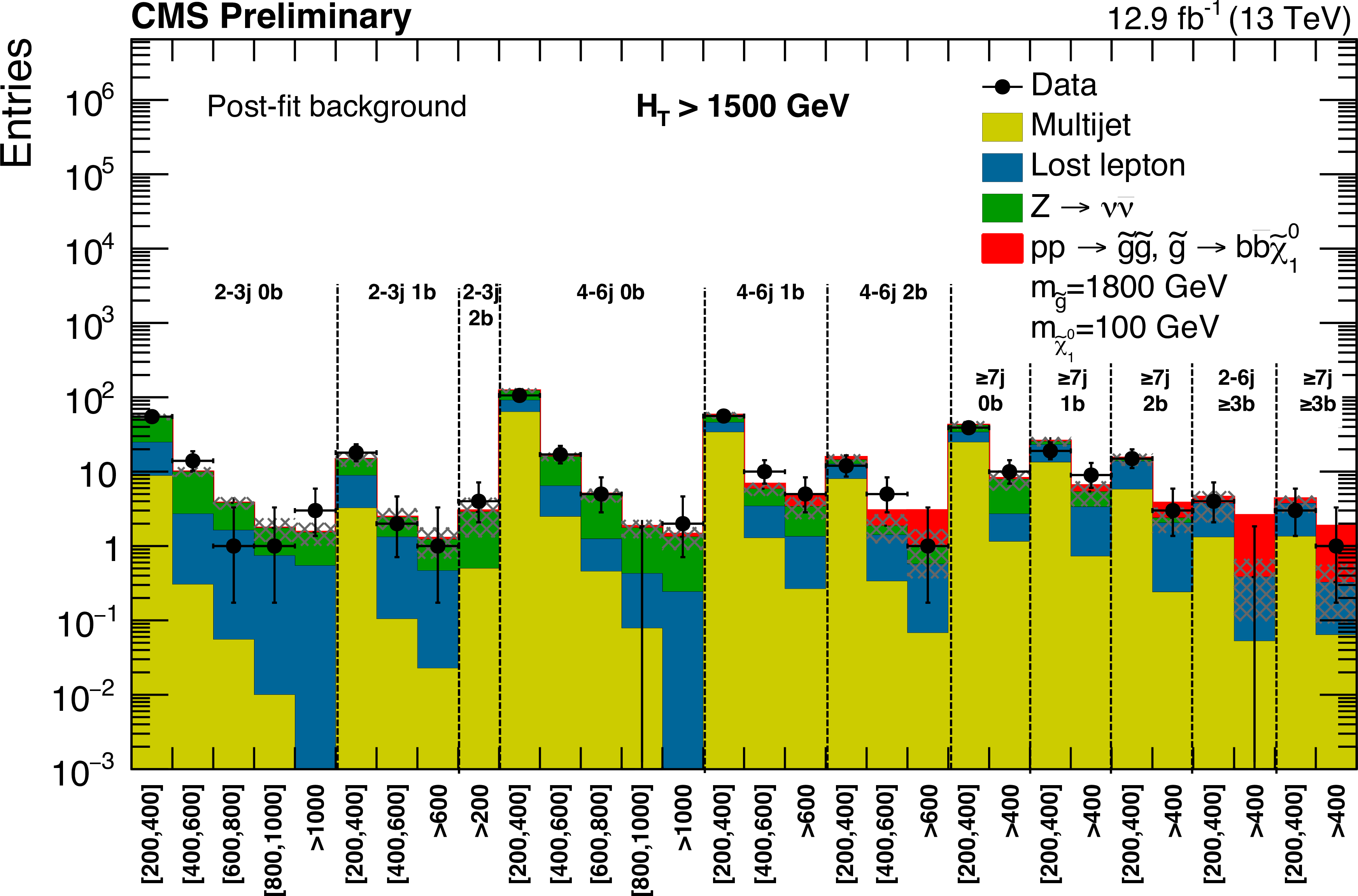
(a) Expected (post-fit) and observed yields in the analysis binning, for all topological regions with the expected yield for the signal model of gluino mediated bottom-squark production ($m_{ {\mathrm {\tilde{g}}}}=$ 1000 GeV , $m_{ {\tilde{\chi}^{0}_{1}} }=$ 800 GeV) stacked on top of the expected background. For the monojet regions, on the $x$-axis is shown the ${ {p_{\mathrm {T}}} ^{\mathrm {jet1}}}$ binning (in GeV). (b) Same for the extreme $ H_{\mathrm{T}}$ region for the same signal with ($m_{ {\mathrm {\tilde{g}}}}=$ 1800 GeV $m_{ {\tilde{\chi}^{0}_{1}} }=$ 100 GeV ). In these Figures, the uncertainty band represents the full uncertainty band associated to the data-driven estimate, a-posteriori.-a |
png pdf |
Figure 13-b:
(a) Expected (post-fit) and observed yields in the analysis binning, for all topological regions with the expected yield for the signal model of gluino mediated bottom-squark production ($m_{ {\mathrm {\tilde{g}}}}=$ 1000 GeV , $m_{ {\tilde{\chi}^{0}_{1}} }=$ 800 GeV) stacked on top of the expected background. For the monojet regions, on the $x$-axis is shown the ${ {p_{\mathrm {T}}} ^{\mathrm {jet1}}}$ binning (in GeV). (b) Same for the extreme $ H_{\mathrm{T}}$ region for the same signal with ($m_{ {\mathrm {\tilde{g}}}}=$ 1800 GeV $m_{ {\tilde{\chi}^{0}_{1}} }=$ 100 GeV ). In these Figures, the uncertainty band represents the full uncertainty band associated to the data-driven estimate, a-posteriori.-b |
| Tables | |
png pdf |
Table 1:
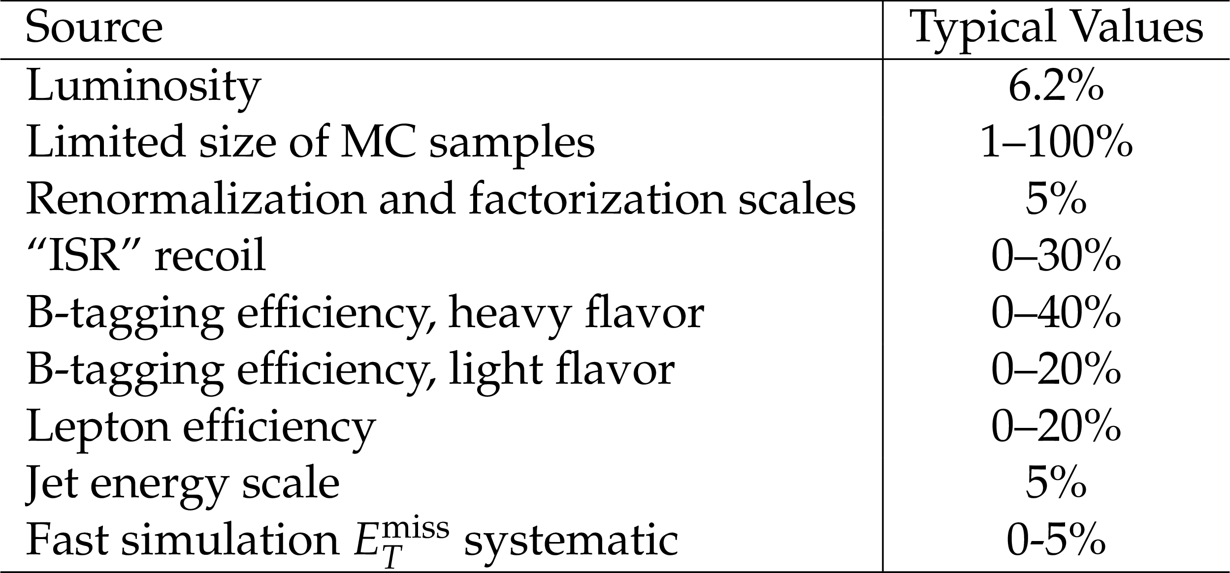
Typical values of the signal systematic uncertainties as evaluated for the simplified signal model of gluino mediated bottom squark production, $ {\mathrm {p}} {\mathrm {p}}\to {\mathrm {\tilde{g}}} {\mathrm {\tilde{g}}}, {\mathrm {\tilde{g}}}\to { {\mathrm {b}} {\overline {\mathrm {b}}} } {\tilde{\chi}^{0}_{1}} $. Uncertainties evaluated on other signal models are consistent with these ranges of values. |
png pdf |
Table 2:
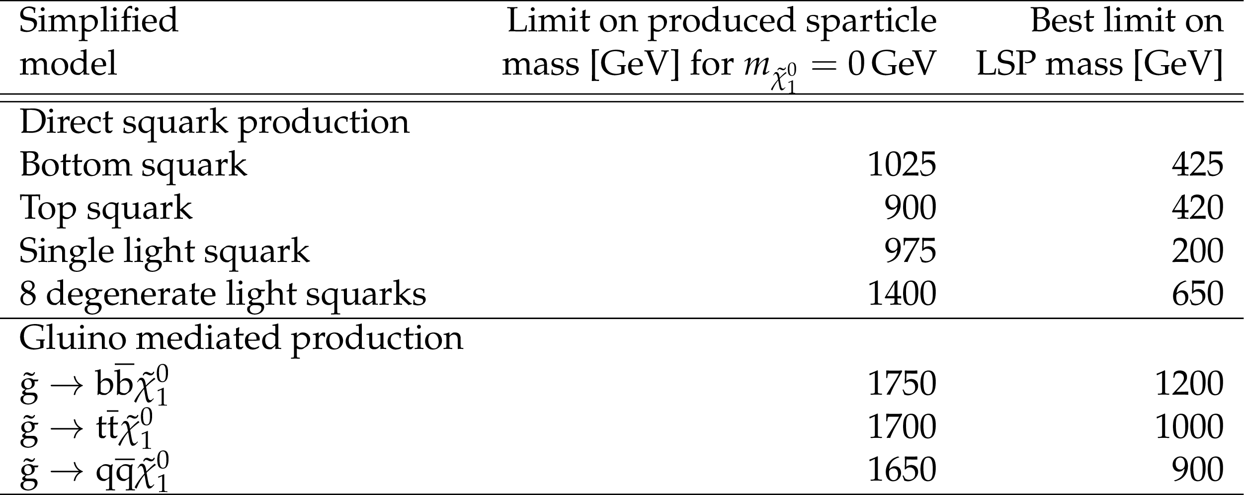
Summary of 95% CL observed exclusion limits for different SUSY simplified model scenarios. The limit on the mass of the produced sparticle is quoted for a massless LSP, while for the lightest neutralino the best limit on its mass is quoted. |

png pdf |
Table 3:
Definitions of aggregate regions. All selections listed for a given region are considered in a logical OR. |

png pdf |
Table 4:
Predictions and observations for the aggregated regions defined in Table 3, together with the observed 95% CL limit on the number of signal events contributing to each region ($N_{95}^{\text {obs}}$). An uncertainty of either 15 or 30% in the signal efficiency is assumed for calculating the limits. |
png pdf |
Table 5:
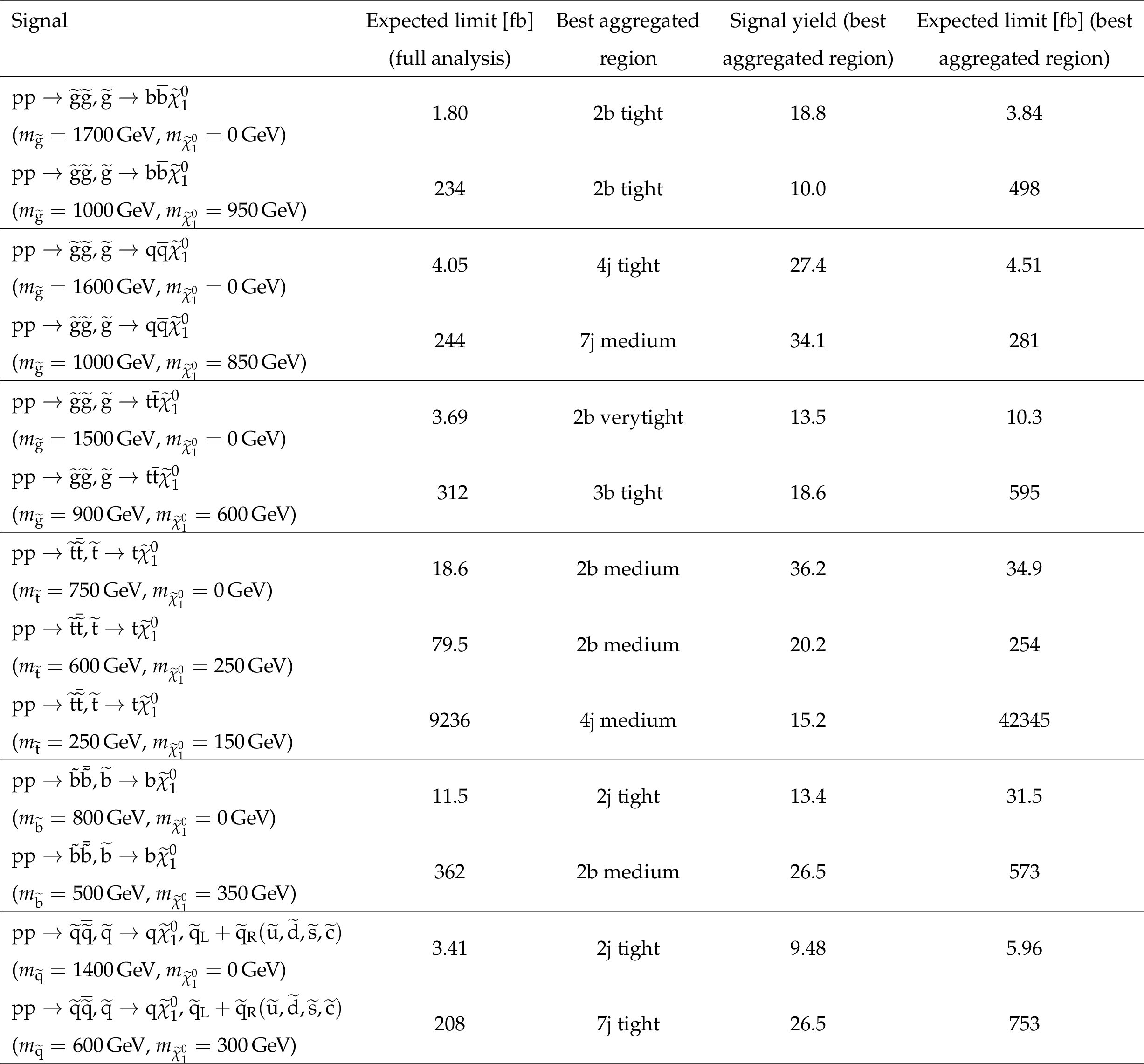
Expected upper limits on the cross section of several signal models, as determined from the full binned analysis, are compared to the upper limits obtained using only the aggregated region that has the best sensitivity to each considered signal model. A 15% uncertainty in the signal selection efficiency is assumed for calculating these limits. The signal yields expected for an integrated luminosity of 12.9 fb$^{-1}$ are also shown. |
| Summary |
| This note presents the result of a search for new physics using events with jets and the ${M_{T2}} $variable. Results are based on a 12.9 fb$^{-1}$ data sample of proton-proton collisions at $\sqrt{s} =$ 13 TeV collected in 2016 with the CMS detector. No significant deviations from the standard model expectations are observed. The results are interpreted as limits on the production of new, massive colored particles. We probe gluino masses up to 1750 GeV and LSP masses up to 1200 GeV. Additional interpretations in the context of the pair production of light flavor, bottom, and top squarks are performed, probing masses up to 1400, 1025, and 900 GeV, respectively, and LSP masses up to 650, 425, and 420 GeV in each scenario. |
| Additional Figures | |
png pdf |
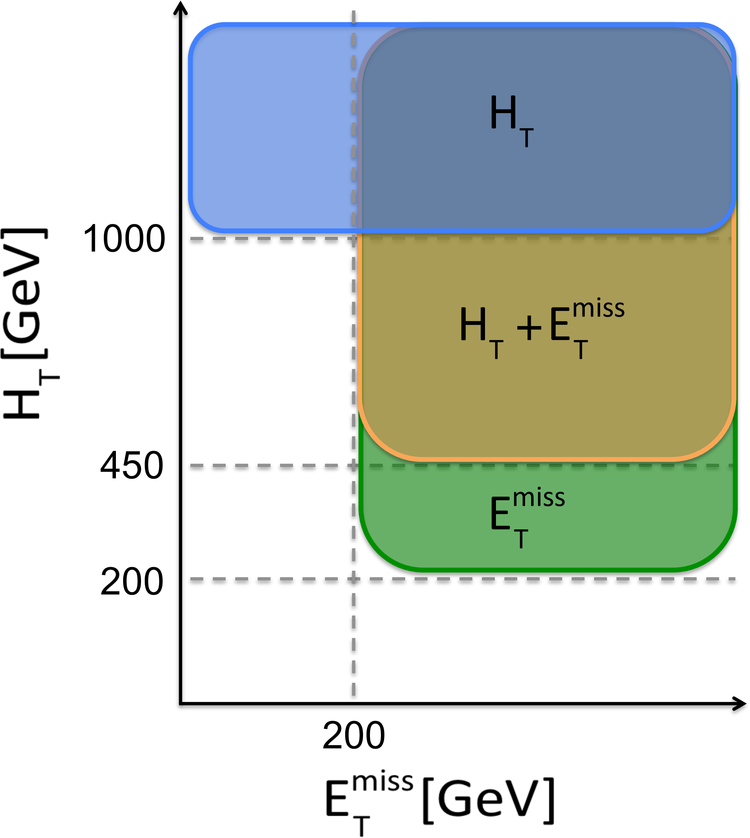
Additional Figure 1-a:
Diagrams of the analysis coverage in the plane of ${H_{\mathrm{T}}}$ and ${E_{T}^{\mathrm {miss}}}$ , showing (a) the coverage of the triggers used and (b) the ${H_{\mathrm{T}}}$ binning used. |
png pdf |
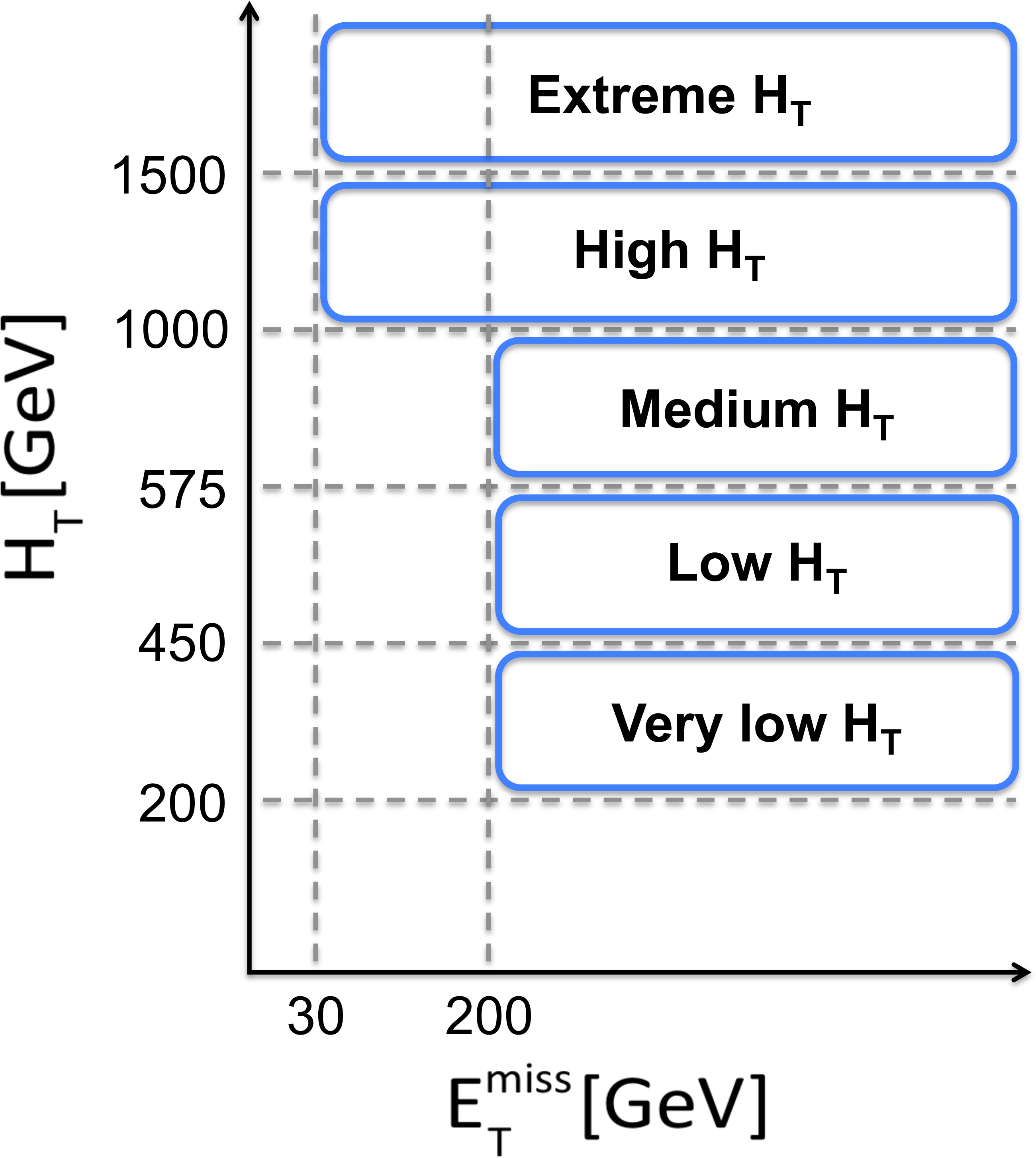
Additional Figure 1-b:
Diagrams of the analysis coverage in the plane of ${H_{\mathrm{T}}}$ and ${E_{T}^{\mathrm {miss}}}$ , showing (a) the coverage of the triggers used and (b) the ${H_{\mathrm{T}}}$ binning used. |

png pdf |
Additional Figure 2:
Diagram of the ${\mathrm {N}_{\mathrm {j}}}$ and ${\mathrm {N}_{\mathrm {b}}}$ binning used in the analysis. The background composition from simulation for the medium-${H_{\mathrm{T}}}$ bin is shown in each bin with a pie chart. |

png pdf |
Additional Figure 3:
Diagram of the maximal analysis binning in the plane of ${H_{\mathrm{T}}}$ and ${M_{T2}}$ for multijet bins. In each bin of ( ${H_{\mathrm{T}}}$ , ${\mathrm {N}_{\mathrm {j}}}$, ${\mathrm {N}_{\mathrm {b}}}$ ), the bins with highest ${M_{T2}}$ values are merged to have at least one expected background event. |
png pdf |
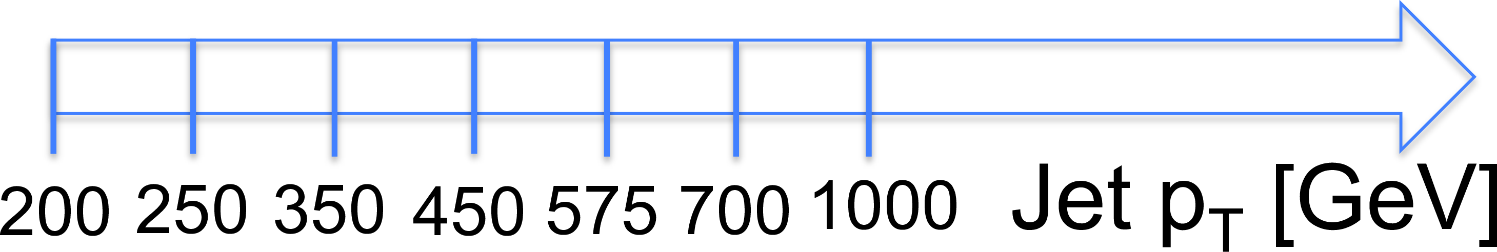
Additional Figure 4:
Diagram of the maximal analysis binning in the jet ${p_{\mathrm{T}}}$ dimension for monojet bins. Within each ${\mathrm {N}_{\mathrm {b}}}$ category, the highest bins in jet ${p_{\mathrm{T}}}$ are merged to have at least one expected background event. |
png pdf |
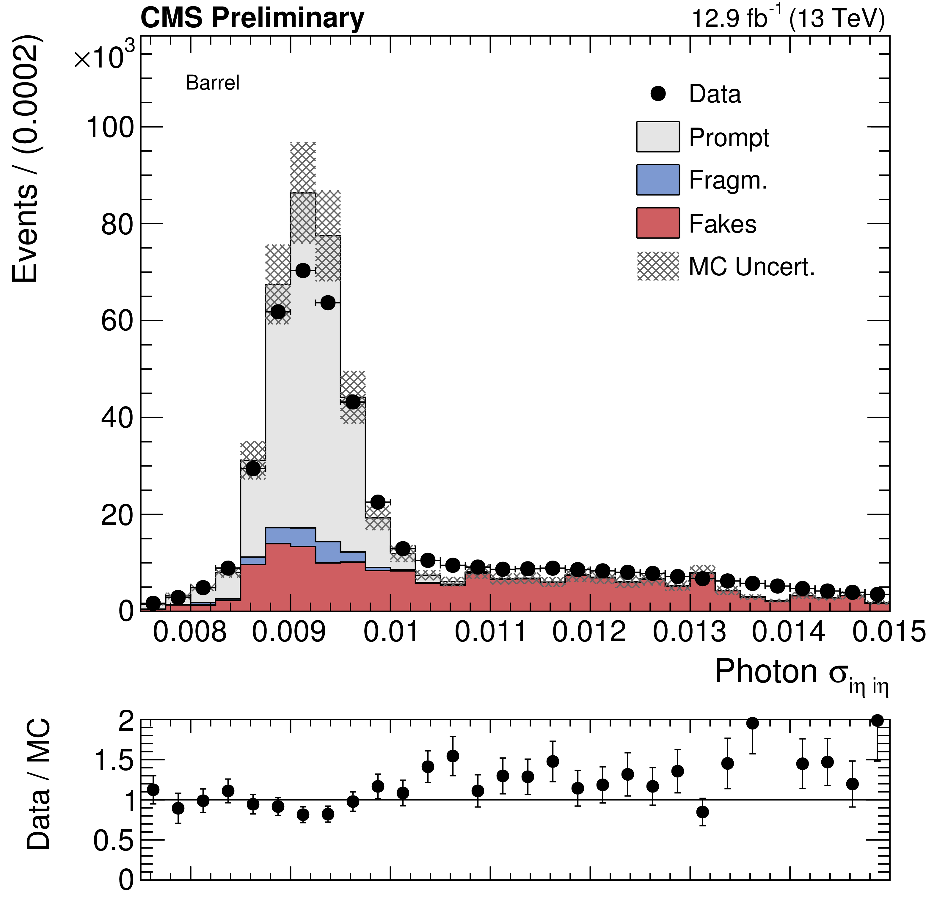
Additional Figure 5-a:
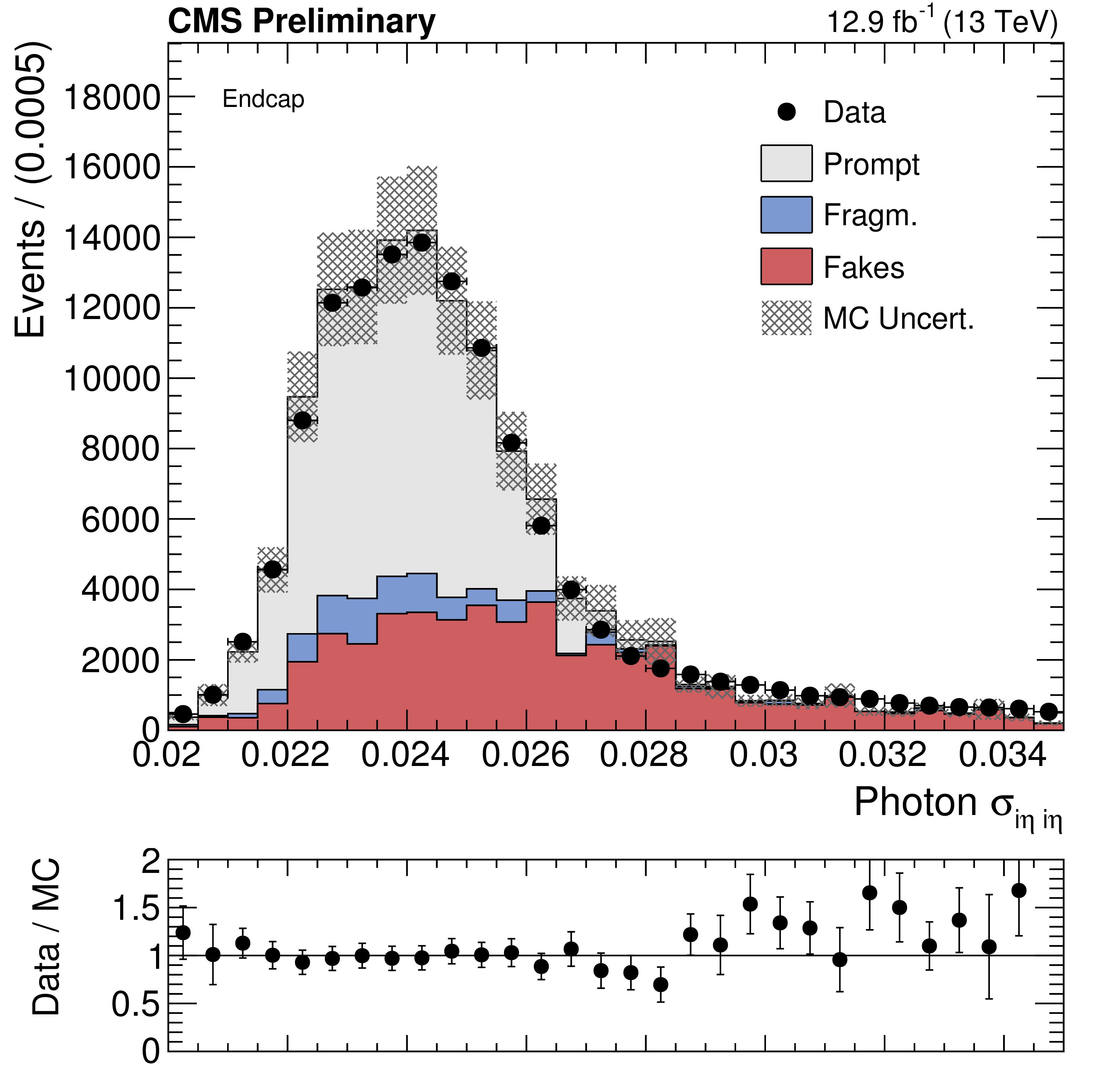
Data-MC shape comparison of ${\sigma _{i\eta i\eta }}$ for photon candidates reconstructed in the ECAL barrel(left) and endcaps(right). Prompt photons are shown in grey, fragmentation photons in blue and fake photons in red. These events have been selected with a very loose isolation requirement, in order to increase the yield of fake photons. The fragmentation (``Fragm.'') category is obtained from Madraph+Pythia QCD samples, and it includes prompt photons that fail the $\Delta R > $ 0.4 requirement between the prompt photon and the nearest parton. |
png pdf |
Additional Figure 5-b:
Data-MC shape comparison of ${\sigma _{i\eta i\eta }}$ for photon candidates reconstructed in the ECAL barrel(left) and endcaps(right). Prompt photons are shown in grey, fragmentation photons in blue and fake photons in red. These events have been selected with a very loose isolation requirement, in order to increase the yield of fake photons. The fragmentation (``Fragm.'') category is obtained from Madraph+Pythia QCD samples, and it includes prompt photons that fail the $\Delta R > $ 0.4 requirement between the prompt photon and the nearest parton. |
png pdf |
Additional Figure 6:
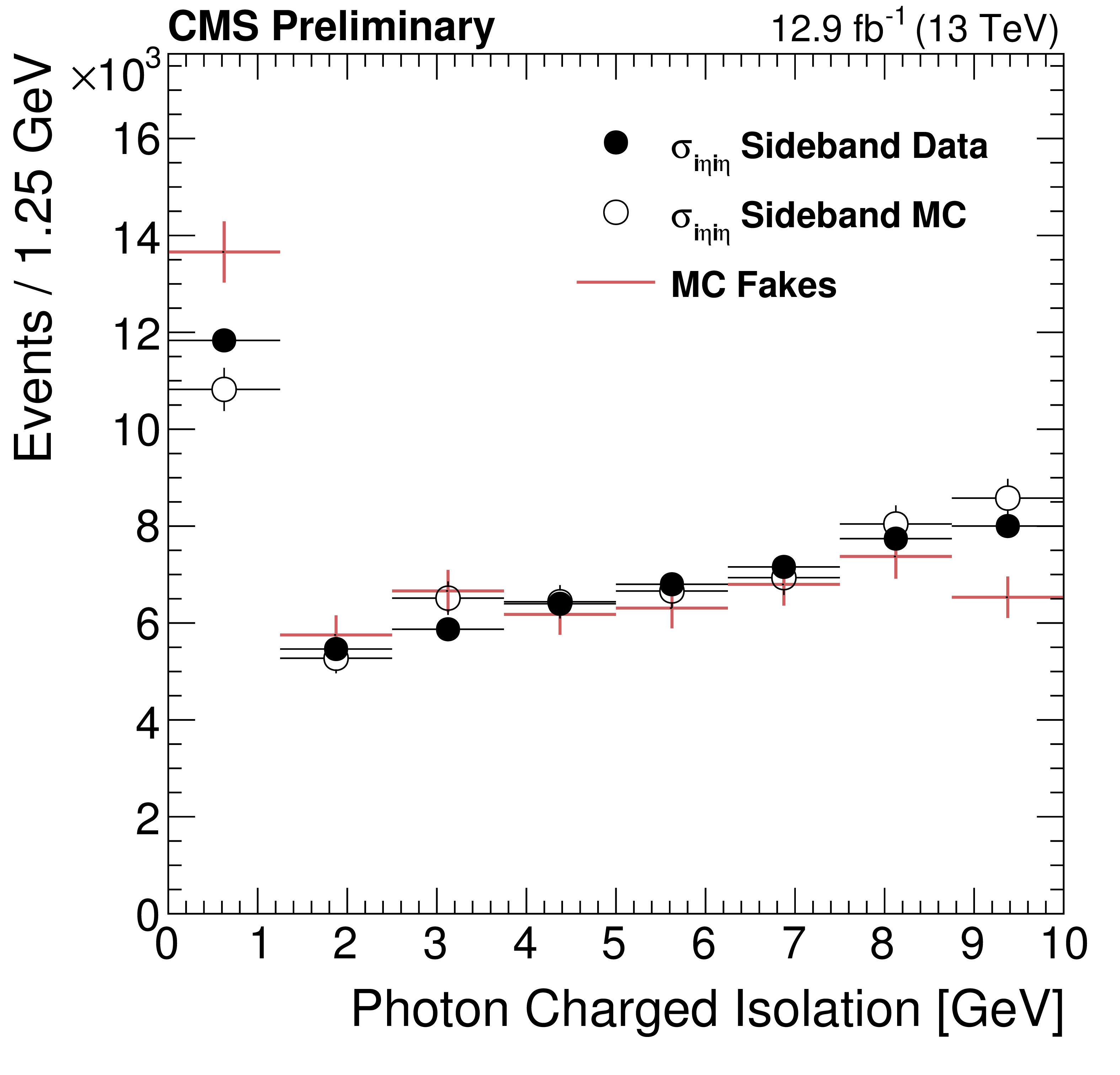
Comparison between the fake photon isolation template obtained from the ${\sigma _{i\eta i\eta }}$ sidebands(black markers) and the one obtained by selecting MC-matched fake photons that pass the nominal selection(red crosses). |

png pdf |
Additional Figure 7:
Results of the purity template fits in data (yellow markers) compared to the MC truth purity (hollow markers), as a function of ${H_{\mathrm {T}}} $. |
png pdf |
Additional Figure 8-a:
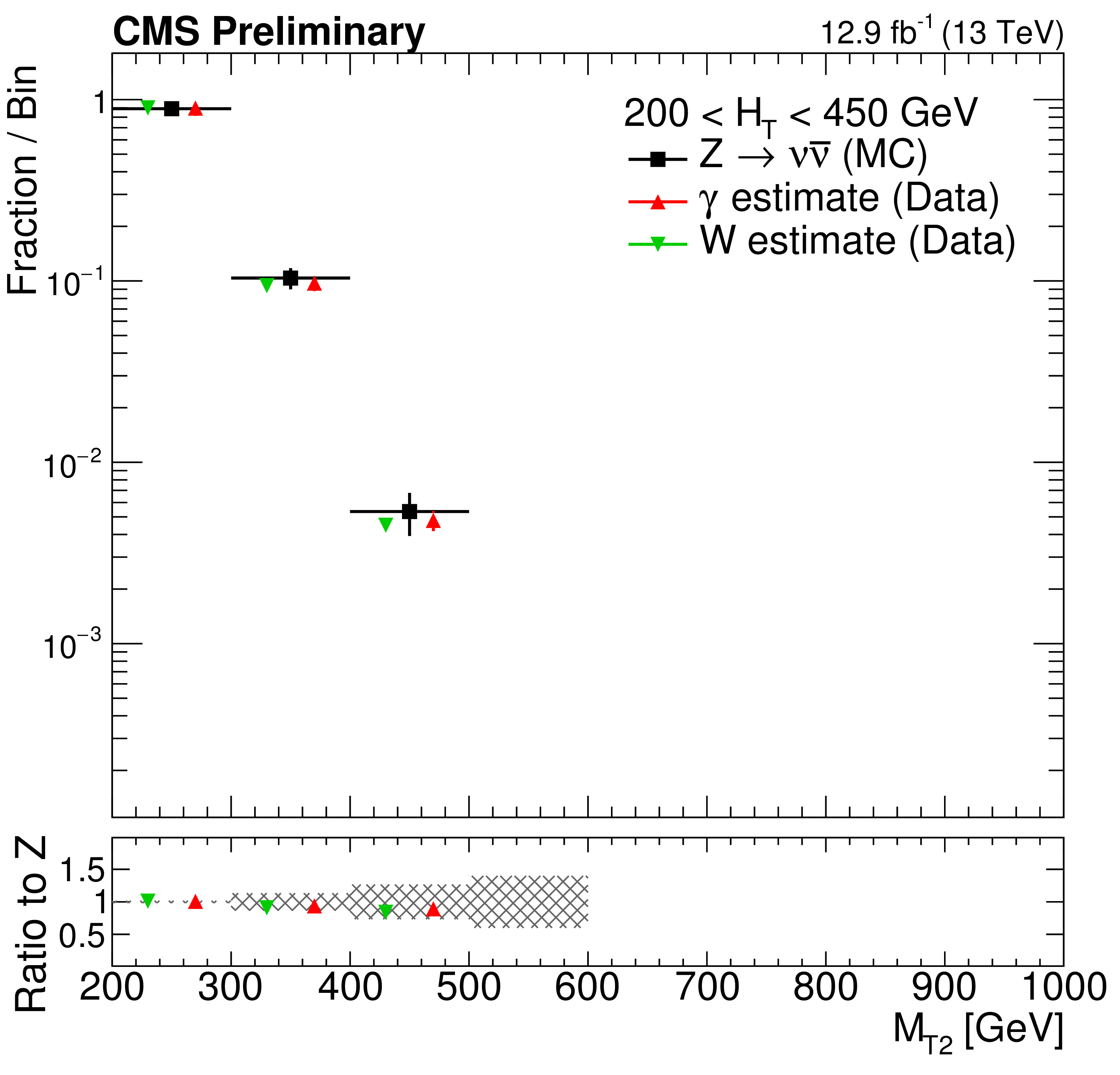
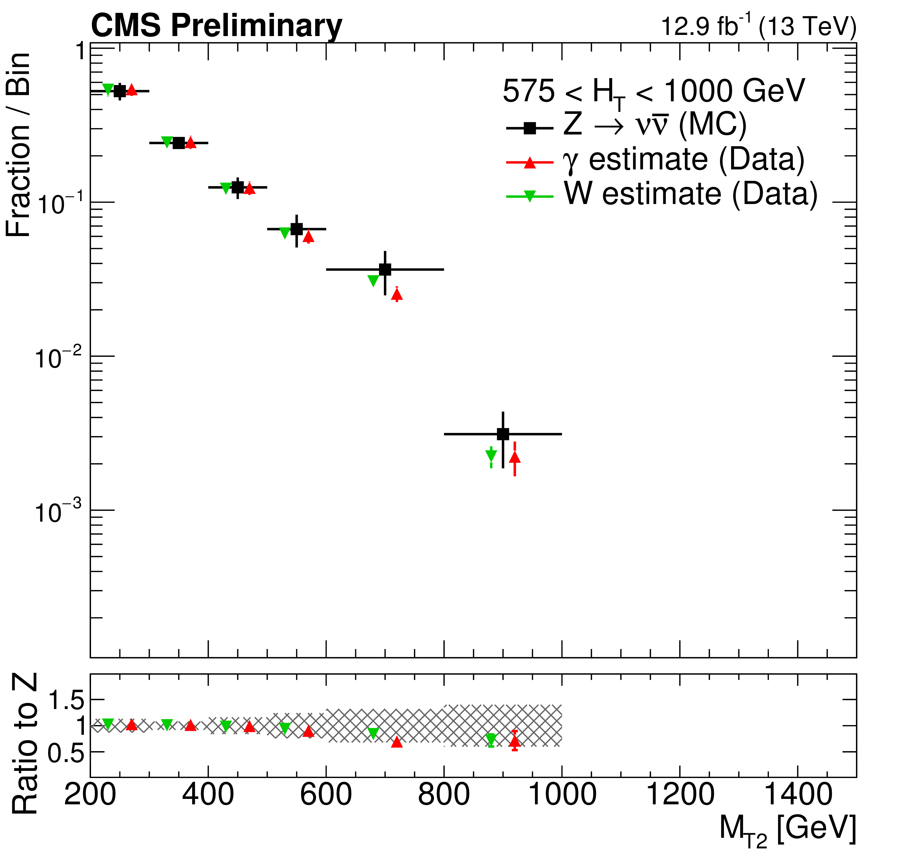
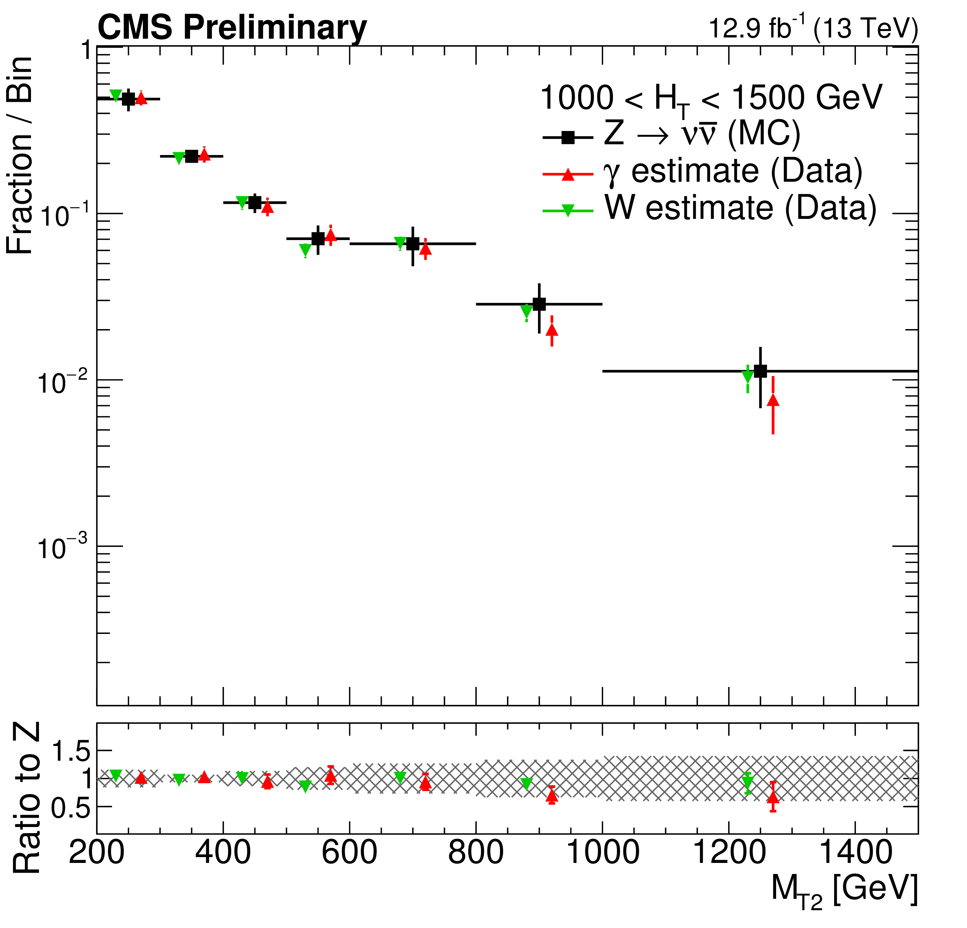
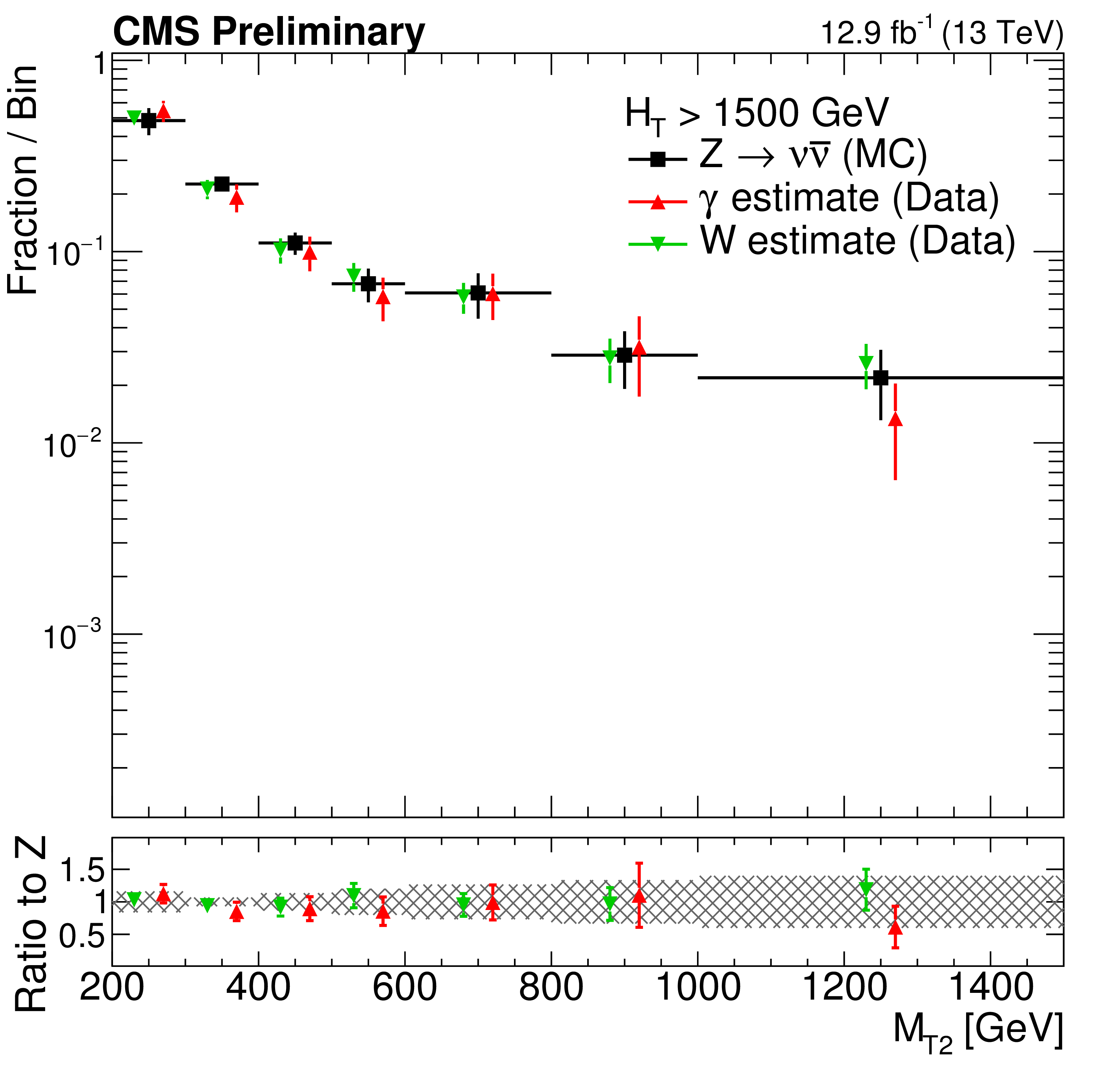
Shape comparison of the ${M_{T2}}$ distribution in the $\gamma $+jets (red markers) and $ \mathrm{ W }^{\pm} \to \ell \nu $ control(green markers) regions in data, compared to the expected shape of the simulated $ \mathrm{Z} \rightarrow \nu \overline {\nu } $ process(black markers), in different ${H_{\mathrm{T}}}$ regions: 200 $ < {H_{\mathrm{T}}} < $ 450 GeV (top left), 450 $ < {H_{\mathrm{T}}} < $ 575 GeV(top right), 575 $ < {H_{\mathrm{T}}} < $ 1000 GeV (center left), 1000 $ < {H_{\mathrm{T}}} < $ 1500 GeV (center right) and finally ${H_{\mathrm{T}}} > $ 1500 GeV (bottom). The shaded band in the ratio histogram includes experimental and theoretical uncertainties on the $ \mathrm{Z} \rightarrow \nu \overline {\nu } $ background ${M_{T2}}$ distribution. |

png pdf |
Additional Figure 8-b:
Shape comparison of the ${M_{T2}}$ distribution in the $\gamma $+jets (red markers) and $ \mathrm{ W }^{\pm} \to \ell \nu $ control(green markers) regions in data, compared to the expected shape of the simulated $ \mathrm{Z} \rightarrow \nu \overline {\nu } $ process(black markers), in different ${H_{\mathrm{T}}}$ regions: 200 $ < {H_{\mathrm{T}}} < $ 450 GeV (top left), 450 $ < {H_{\mathrm{T}}} < $ 575 GeV(top right), 575 $ < {H_{\mathrm{T}}} < $ 1000 GeV (center left), 1000 $ < {H_{\mathrm{T}}} < $ 1500 GeV (center right) and finally ${H_{\mathrm{T}}} > $ 1500 GeV (bottom). The shaded band in the ratio histogram includes experimental and theoretical uncertainties on the $ \mathrm{Z} \rightarrow \nu \overline {\nu } $ background ${M_{T2}}$ distribution. |
png pdf |
Additional Figure 8-c:
Shape comparison of the ${M_{T2}}$ distribution in the $\gamma $+jets (red markers) and $ \mathrm{ W }^{\pm} \to \ell \nu $ control(green markers) regions in data, compared to the expected shape of the simulated $ \mathrm{Z} \rightarrow \nu \overline {\nu } $ process(black markers), in different ${H_{\mathrm{T}}}$ regions: 200 $ < {H_{\mathrm{T}}} < $ 450 GeV (top left), 450 $ < {H_{\mathrm{T}}} < $ 575 GeV(top right), 575 $ < {H_{\mathrm{T}}} < $ 1000 GeV (center left), 1000 $ < {H_{\mathrm{T}}} < $ 1500 GeV (center right) and finally ${H_{\mathrm{T}}} > $ 1500 GeV (bottom). The shaded band in the ratio histogram includes experimental and theoretical uncertainties on the $ \mathrm{Z} \rightarrow \nu \overline {\nu } $ background ${M_{T2}}$ distribution. |
png pdf |
Additional Figure 8-d:
Shape comparison of the ${M_{T2}}$ distribution in the $\gamma $+jets (red markers) and $ \mathrm{ W }^{\pm} \to \ell \nu $ control(green markers) regions in data, compared to the expected shape of the simulated $ \mathrm{Z} \rightarrow \nu \overline {\nu } $ process(black markers), in different ${H_{\mathrm{T}}}$ regions: 200 $ < {H_{\mathrm{T}}} < $ 450 GeV (top left), 450 $ < {H_{\mathrm{T}}} < $ 575 GeV(top right), 575 $ < {H_{\mathrm{T}}} < $ 1000 GeV (center left), 1000 $ < {H_{\mathrm{T}}} < $ 1500 GeV (center right) and finally ${H_{\mathrm{T}}} > $ 1500 GeV (bottom). The shaded band in the ratio histogram includes experimental and theoretical uncertainties on the $ \mathrm{Z} \rightarrow \nu \overline {\nu } $ background ${M_{T2}}$ distribution. |
png pdf |
Additional Figure 8-e:
Shape comparison of the ${M_{T2}}$ distribution in the $\gamma $+jets (red markers) and $ \mathrm{ W }^{\pm} \to \ell \nu $ control(green markers) regions in data, compared to the expected shape of the simulated $ \mathrm{Z} \rightarrow \nu \overline {\nu } $ process(black markers), in different ${H_{\mathrm{T}}}$ regions: 200 $ < {H_{\mathrm{T}}} < $ 450 GeV (top left), 450 $ < {H_{\mathrm{T}}} < $ 575 GeV(top right), 575 $ < {H_{\mathrm{T}}} < $ 1000 GeV (center left), 1000 $ < {H_{\mathrm{T}}} < $ 1500 GeV (center right) and finally ${H_{\mathrm{T}}} > $ 1500 GeV (bottom). The shaded band in the ratio histogram includes experimental and theoretical uncertainties on the $ \mathrm{Z} \rightarrow \nu \overline {\nu } $ background ${M_{T2}}$ distribution. |
png pdf |
Additional Figure 9-a:
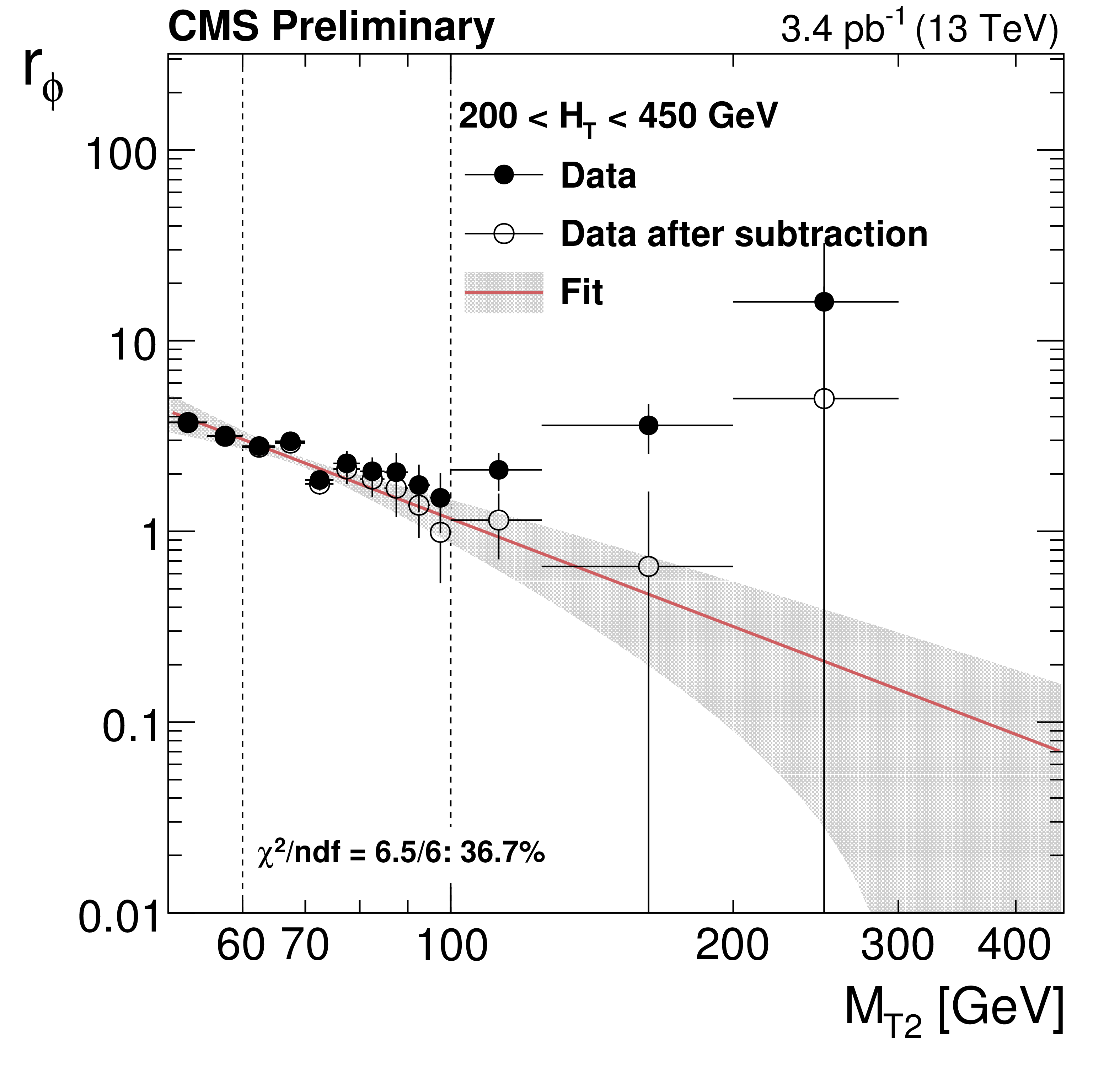
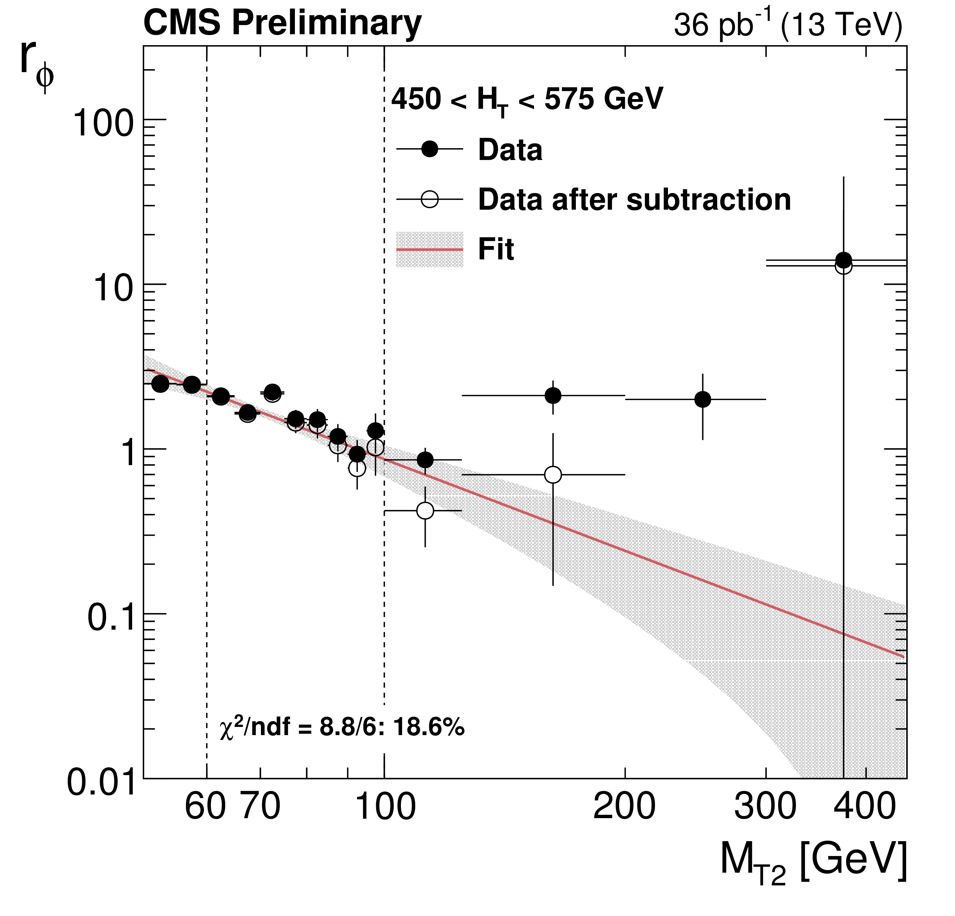
Distributions from data of the ratio $r_\phi ( {M_{T2}} ) = N(\Delta \phi _{\text{min}} > 0.3) / N(\Delta \phi _{\text{min}} < 0.3)$ as a function of ${M_{T2}}$ , for the very low (top left), low (top right), medium (bottom left), extreme (bottom right) ${H_{\mathrm{T}}}$ regions. The full points are the ratio from data before subtracting the non-multijet component, while the hollow points represent the data after the non-multijet contribution has been subtracted. The data in the high and extreme ${H_{\mathrm{T}}}$ regions has been collected with an unprescaled HLT trigger with an online ${H_{\mathrm{T}}}$ threshold of 800 GeV, while for the very low, low and the medium ${H_{\mathrm{T}}}$ regions prescaled HLT triggers have been used, with an online ${H_{\mathrm{T}}}$ threshold of 125 GeV (prescale $\approx $ 3800), 350 GeV (prescale $\approx $ 350) and of 475 GeV (prescale $\approx$ 90) respectively. The luminosity in each figure corresponds to the effective luminosity given the trigger prescales of each ${H_{\mathrm {T}}}$ region. The red line and the band around it show the fit to a power law function perfomed in the fit window, with its associated fit uncertainties. |
png pdf |
Additional Figure 9-b:
Distributions from data of the ratio $r_\phi ( {M_{T2}} ) = N(\Delta \phi _{\text{min}} > 0.3) / N(\Delta \phi _{\text{min}} < 0.3)$ as a function of ${M_{T2}}$ , for the very low (top left), low (top right), medium (bottom left), extreme (bottom right) ${H_{\mathrm{T}}}$ regions. The full points are the ratio from data before subtracting the non-multijet component, while the hollow points represent the data after the non-multijet contribution has been subtracted. The data in the high and extreme ${H_{\mathrm{T}}}$ regions has been collected with an unprescaled HLT trigger with an online ${H_{\mathrm{T}}}$ threshold of 800 GeV, while for the very low, low and the medium ${H_{\mathrm{T}}}$ regions prescaled HLT triggers have been used, with an online ${H_{\mathrm{T}}}$ threshold of 125 GeV (prescale $\approx $ 3800), 350 GeV (prescale $\approx $ 350) and of 475 GeV (prescale $\approx$ 90) respectively. The luminosity in each figure corresponds to the effective luminosity given the trigger prescales of each ${H_{\mathrm {T}}}$ region. The red line and the band around it show the fit to a power law function perfomed in the fit window, with its associated fit uncertainties. |
png pdf |
Additional Figure 9-c:
Distributions from data of the ratio $r_\phi ( {M_{T2}} ) = N(\Delta \phi _{\text{min}} > 0.3) / N(\Delta \phi _{\text{min}} < 0.3)$ as a function of ${M_{T2}}$ , for the very low (top left), low (top right), medium (bottom left), extreme (bottom right) ${H_{\mathrm{T}}}$ regions. The full points are the ratio from data before subtracting the non-multijet component, while the hollow points represent the data after the non-multijet contribution has been subtracted. The data in the high and extreme ${H_{\mathrm{T}}}$ regions has been collected with an unprescaled HLT trigger with an online ${H_{\mathrm{T}}}$ threshold of 800 GeV, while for the very low, low and the medium ${H_{\mathrm{T}}}$ regions prescaled HLT triggers have been used, with an online ${H_{\mathrm{T}}}$ threshold of 125 GeV (prescale $\approx $ 3800), 350 GeV (prescale $\approx $ 350) and of 475 GeV (prescale $\approx$ 90) respectively. The luminosity in each figure corresponds to the effective luminosity given the trigger prescales of each ${H_{\mathrm {T}}}$ region. The red line and the band around it show the fit to a power law function perfomed in the fit window, with its associated fit uncertainties. |
png pdf |
Additional Figure 9-d:
Distributions from data of the ratio $r_\phi ( {M_{T2}} ) = N(\Delta \phi _{\text{min}} > 0.3) / N(\Delta \phi _{\text{min}} < 0.3)$ as a function of ${M_{T2}}$ , for the very low (top left), low (top right), medium (bottom left), extreme (bottom right) ${H_{\mathrm{T}}}$ regions. The full points are the ratio from data before subtracting the non-multijet component, while the hollow points represent the data after the non-multijet contribution has been subtracted. The data in the high and extreme ${H_{\mathrm{T}}}$ regions has been collected with an unprescaled HLT trigger with an online ${H_{\mathrm{T}}}$ threshold of 800 GeV, while for the very low, low and the medium ${H_{\mathrm{T}}}$ regions prescaled HLT triggers have been used, with an online ${H_{\mathrm{T}}}$ threshold of 125 GeV (prescale $\approx $ 3800), 350 GeV (prescale $\approx $ 350) and of 475 GeV (prescale $\approx$ 90) respectively. The luminosity in each figure corresponds to the effective luminosity given the trigger prescales of each ${H_{\mathrm {T}}}$ region. The red line and the band around it show the fit to a power law function perfomed in the fit window, with its associated fit uncertainties. |
png pdf |
Additional Figure 10-a:
Fraction $f_{\mathrm {j}}$ of multijet events falling in bins of number of jets ${\mathrm {N}_{\mathrm {j}}}$ as measured in data using $\Delta \phi < $ 0.3 and 100 $ < {M_{T2}} < $ 200 GeV, compared to the prediction from QCD multijet simulation. The uncertainties shown include both statistical and systematic sources. |
png pdf |
Additional Figure 10-b:
Fraction $f_{\mathrm {j}}$ of multijet events falling in bins of number of jets ${\mathrm {N}_{\mathrm {j}}}$ as measured in data using $\Delta \phi < $ 0.3 and 100 $ < {M_{T2}} < $ 200 GeV, compared to the prediction from QCD multijet simulation. The uncertainties shown include both statistical and systematic sources. |
png pdf |
Additional Figure 10-c:
Fraction $f_{\mathrm {j}}$ of multijet events falling in bins of number of jets ${\mathrm {N}_{\mathrm {j}}}$ as measured in data using $\Delta \phi < $ 0.3 and 100 $ < {M_{T2}} < $ 200 GeV, compared to the prediction from QCD multijet simulation. The uncertainties shown include both statistical and systematic sources. |
png pdf |
Additional Figure 10-d:
Fraction $f_{\mathrm {j}}$ of multijet events falling in bins of number of jets ${\mathrm {N}_{\mathrm {j}}}$ as measured in data using $\Delta \phi < $ 0.3 and 100 $ < {M_{T2}} < $ 200 GeV, compared to the prediction from QCD multijet simulation. The uncertainties shown include both statistical and systematic sources. |

png pdf |
Additional Figure 11-a:
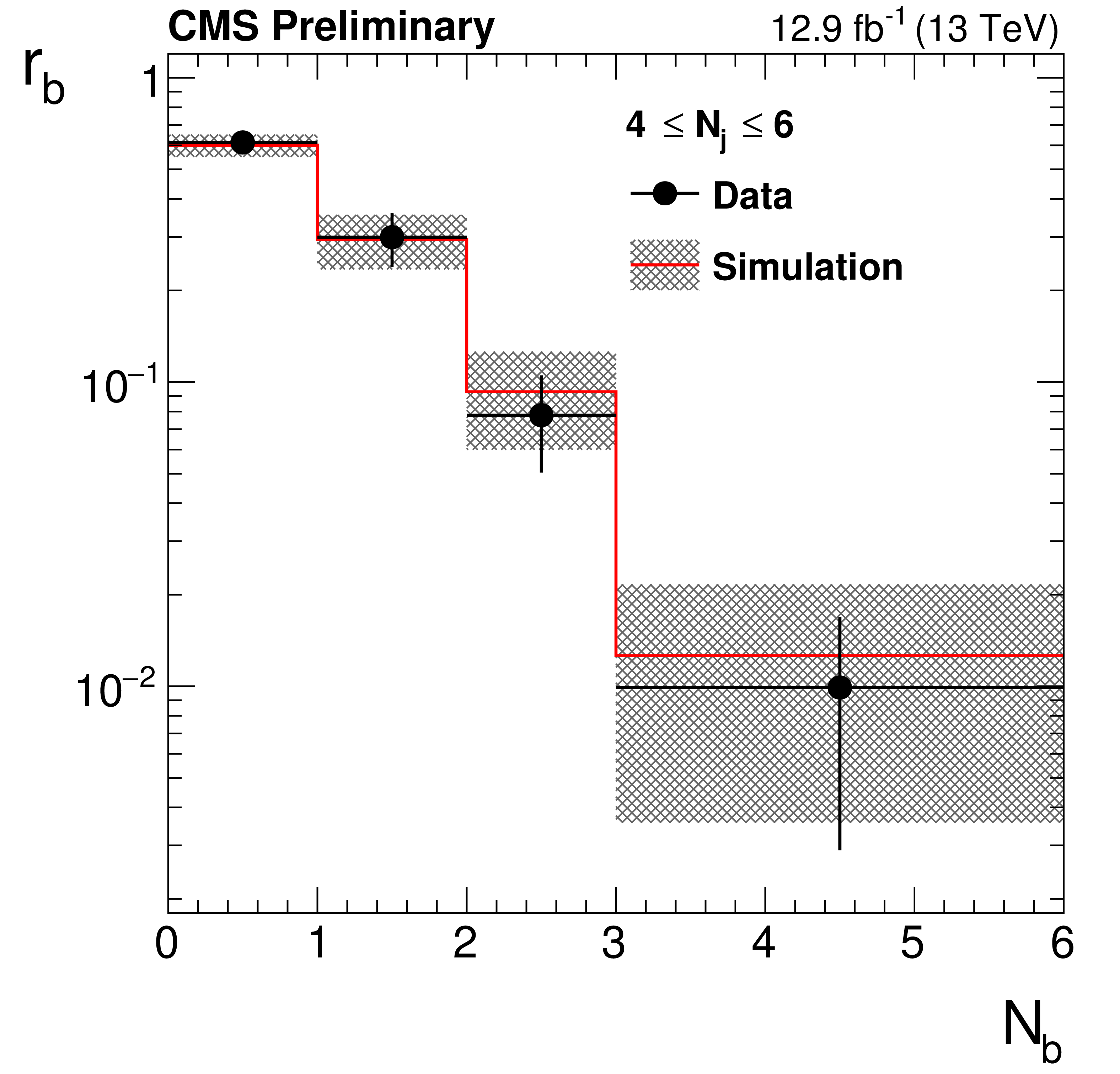
Fraction $r_{\mathrm {b}}$ of events falling in bins of number of b-tagged jets ${\mathrm {N}_{\mathrm {b}}}$ as measured in data using $\Delta \phi < $ 0.3 and 100 $ < {M_{T2}} < $ 200 GeV, compared to the prediction from QCD multijet simulation. The uncertainties shown include both statistical and systematic sources. |
png pdf |
Additional Figure 11-b:
Fraction $r_{\mathrm {b}}$ of events falling in bins of number of b-tagged jets ${\mathrm {N}_{\mathrm {b}}}$ as measured in data using $\Delta \phi < $ 0.3 and 100 $ < {M_{T2}} < $ 200 GeV, compared to the prediction from QCD multijet simulation. The uncertainties shown include both statistical and systematic sources. |

png pdf |
Additional Figure 12:
Validation of the data-driven multijet estimate in the region 100 $ < {M_{T2}} < $ 200 GeV. The points are data with $\Delta \phi < $ 0.3, triggered by the ${H_{\mathrm{T}}}$-only triggers (prescaled for every regions with ${H_{\mathrm{T}}} <$ 1000GeV). The green histogram is the non-multijet contribution as expected from simulation, while the yellow histogram is the multijet estimation using the data-driven method on 12.9 fb$^{-1}$ of data. |

png pdf |
Additional Figure 13:
Distribution of subleading jet $ {p_{\mathrm {T}}} $ for dijet events with leading jet ${p_{\mathrm{T}}} > $ 200 GeV. The simulation is normalized to the data yield. |

png pdf |
Additional Figure 14:
Observed significance for all the signal regions for which the observed yield is larger than the pre-fit background estimate. The significance distribution is also fitted with a one-sided Gaussian function centered at zero. Because the background estimates are correlated for groups of signal regions, the distribution is not expected to be exactly Gaussian. |

png pdf |
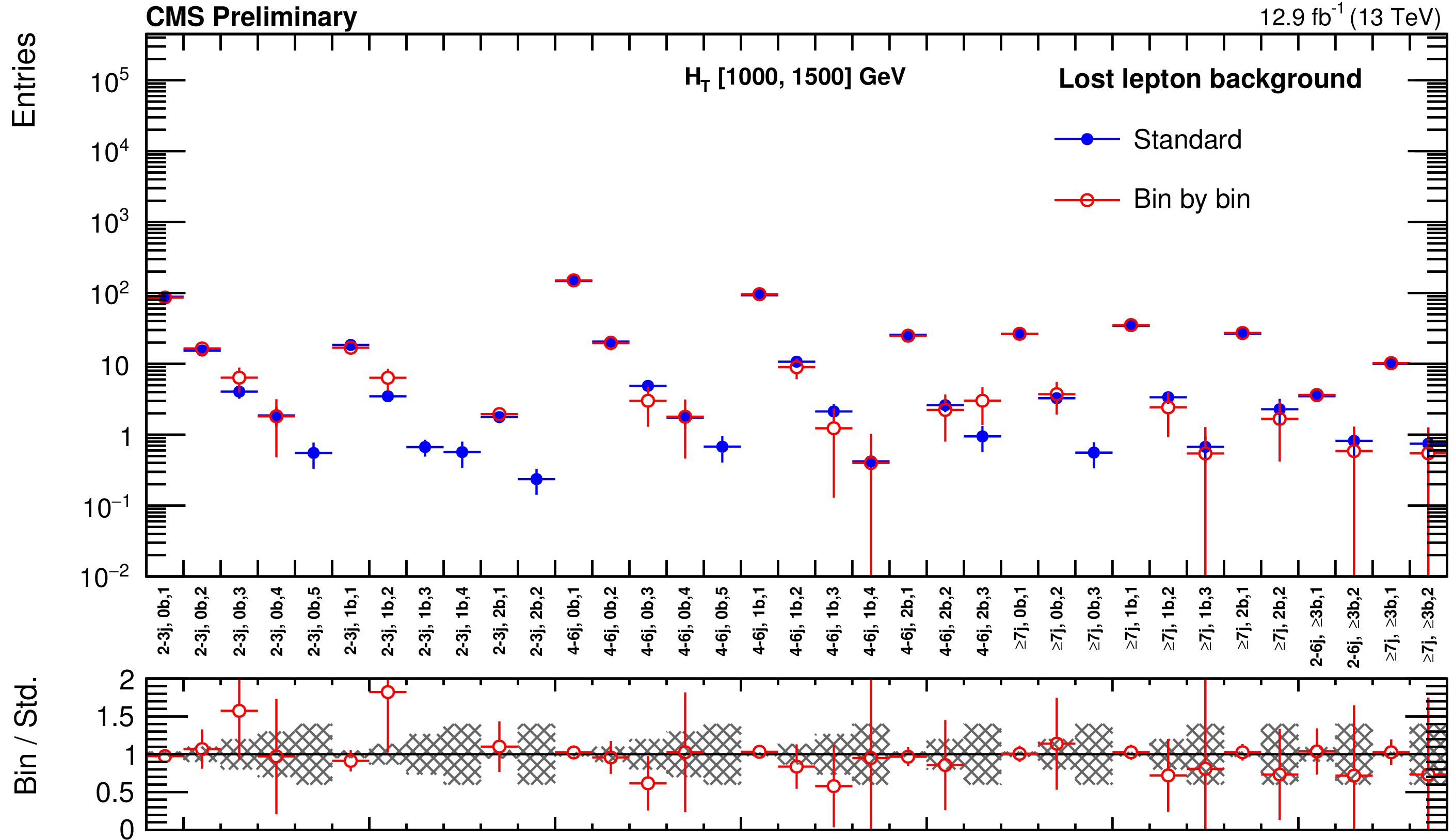
Additional Figure 15:
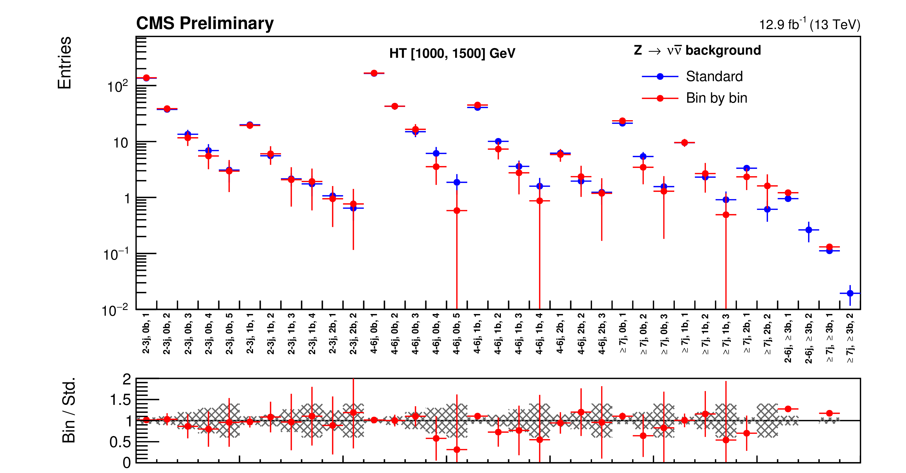
The standard lost lepton predictions based on the single lepton yields in bins of ( ${H_{\mathrm{T}}}$ , ${\mathrm {N}_{\mathrm {j}}}$ , ${\mathrm {N}_{\mathrm {b}}}$ ) and combined with the MC shape along ${M_{T2}}$ are compared with the bin-by-bin predictions obtained using single lepton yields in bins of ( ${H_{\mathrm{T}}}$ , ${\mathrm {N}_{\mathrm {j}}}$ , ${\mathrm {N}_{\mathrm {b}}}$ , ${M_{T2}}$ ), for the medium- ${H_{\mathrm{T}}}$ region. The MC sum of $ {\mathrm{ t } {}\mathrm{ \bar{t} } } $ , W+jets , single top, $ {\mathrm{ t } {}\mathrm{ \bar{t} } } \mathrm{ W } $, $ {\mathrm{ t } {}\mathrm{ \bar{t} } } {\mathrm{ Z } } $, and $ {\mathrm{ t } {}\mathrm{ \bar{t} } } \mathrm{ H } $ processes is used. Bins with no entry for data have an observed count of 0 events. |
png pdf |
Additional Figure 16:
The standard lost lepton predictions based on the single lepton yields in bins of ( ${H_{\mathrm{T}}}$ , ${\mathrm {N}_{\mathrm {j}}}$ , ${\mathrm {N}_{\mathrm {b}}}$ ) and combined with the MC shape along ${M_{T2}}$ are compared with the bin-by-bin predictions obtained using single lepton yields in bins of ( ${H_{\mathrm{T}}}$ , ${\mathrm {N}_{\mathrm {j}}}$ , ${\mathrm {N}_{\mathrm {b}}}$ , ${M_{T2}}$ ), for the high- ${H_{\mathrm{T}}}$ region. The MC sum of $ {\mathrm{ t } {}\mathrm{ \bar{t} } } $ , W+jets , single top, $ {\mathrm{ t } {}\mathrm{ \bar{t} } } \mathrm{ W } $ , $ {\mathrm{ t } {}\mathrm{ \bar{t} } } {\mathrm{ Z } }$ , and $ {\mathrm{ t } {}\mathrm{ \bar{t} } } \mathrm{ H } $ processes is used. Bins with no entry for data have an observed count of 0 events. |

png pdf |
Additional Figure 17:
The standard $ \mathrm{Z} \rightarrow \nu \overline {\nu } $ predictions based on the $\gamma $+jets yields in bins of ( ${H_{\mathrm{T}}}$ , ${\mathrm {N}_{\mathrm {j}}}$ , ${\mathrm {N}_{\mathrm {b}}}$ ) and combined with the $ \mathrm{Z} \rightarrow \nu \overline {\nu } $ MC shape along ${M_{T2}}$ are compared with the bin-by-bin predictions obtained using $\gamma $+jets yields in bins of ( ${H_{\mathrm{T}}}$ , ${\mathrm {N}_{\mathrm {j}}}$ , ${\mathrm {N}_{\mathrm {b}}}$ , ${M_{T2}}$ ), for the medium- ${H_{\mathrm{T}}}$ region. Bins with no entry for data have an observed count of 0 events. |
png pdf |
Additional Figure 18:
The standard $ \mathrm{Z} \rightarrow \nu \overline {\nu } $ predictions based on the $\gamma $+jets yields in bins of ( ${H_{\mathrm{T}}}$ , ${\mathrm {N}_{\mathrm {j}}}$ , ${\mathrm {N}_{\mathrm {b}}}$ ) and combined with the $ \mathrm{Z} \rightarrow \nu \overline {\nu } $ MC shape along ${M_{T2}}$ are compared with the bin-by-bin predictions obtained using $\gamma $+jets yields in bins of ( ${H_{\mathrm{T}}}$ , ${\mathrm {N}_{\mathrm {j}}}$ , ${\mathrm {N}_{\mathrm {b}}}$ , ${M_{T2}}$ ), for the high- ${H_{\mathrm{T}}}$ region. Bins with no entry for data have an observed count of 0 events. |
png pdf |
Additional Figure 19-a:
Summary of exclusion limits at 95% CL on the cross-section for gluino-mediated models (top), and for direct squark pair production models (bottom). |
png pdf |
Additional Figure 19-b:
Summary of exclusion limits at 95% CL on the cross-section for gluino-mediated models (top), and for direct squark pair production models (bottom). |

png |
Additional Figure 20-a:
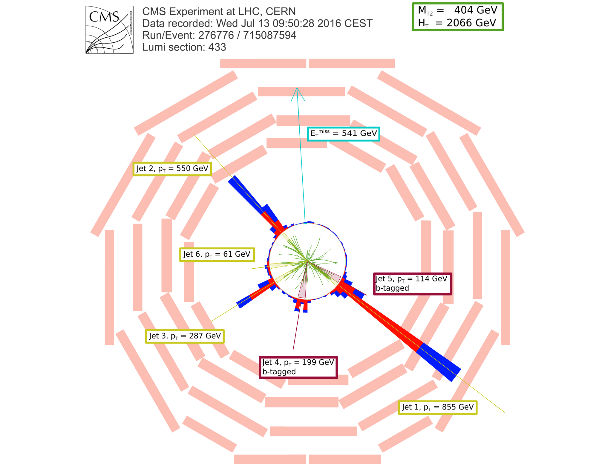
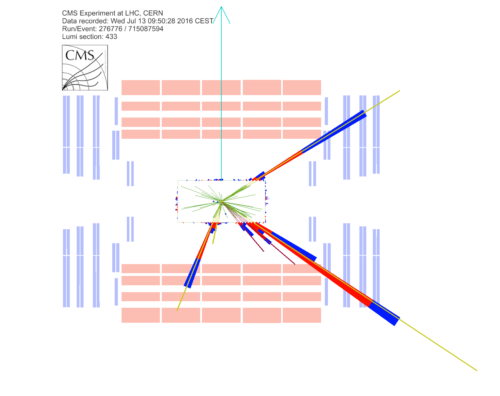
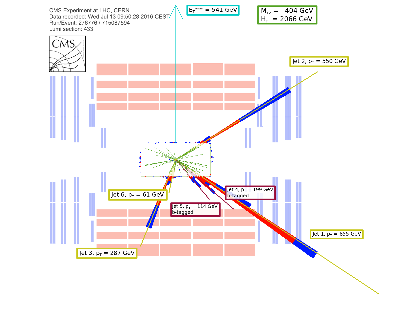
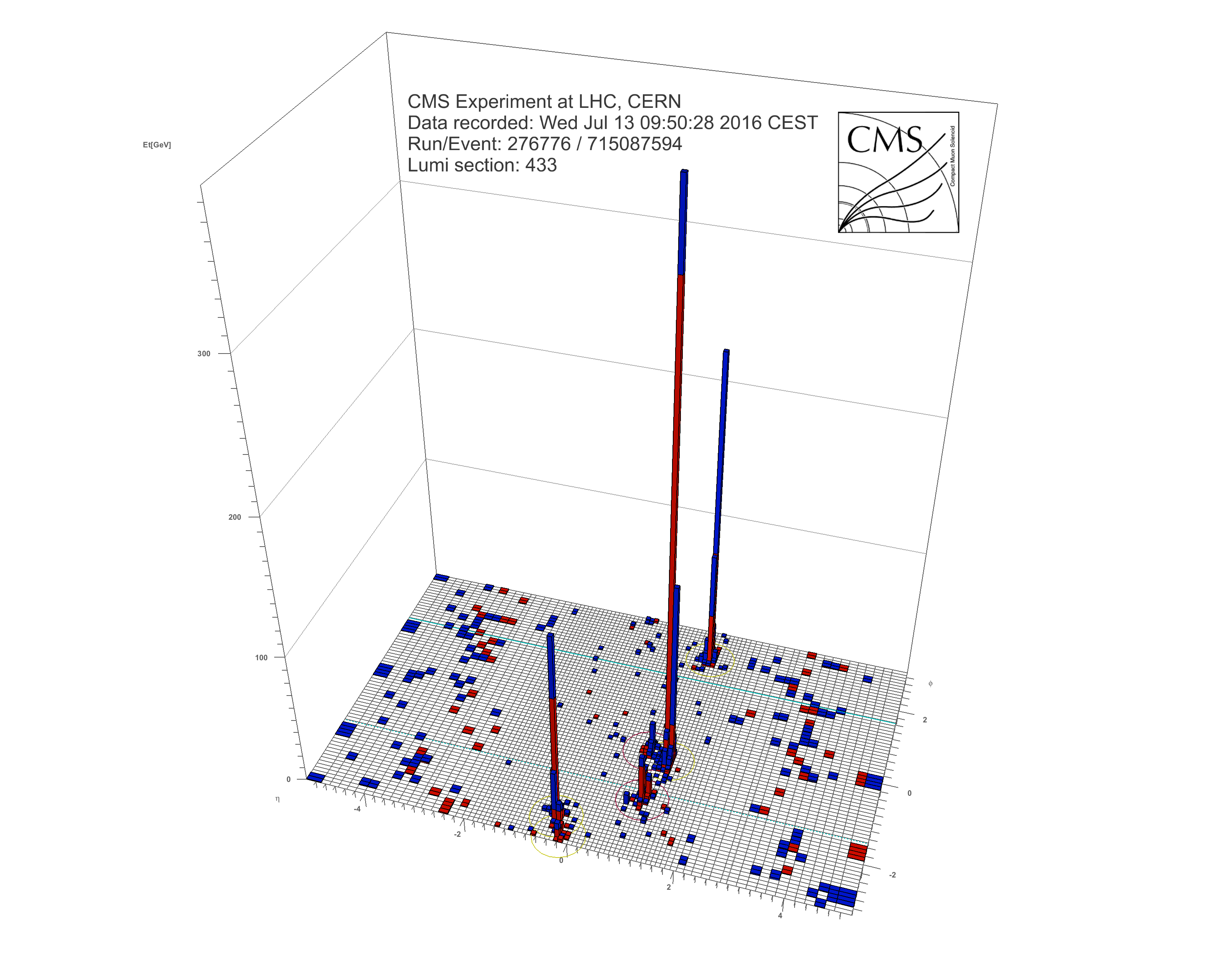
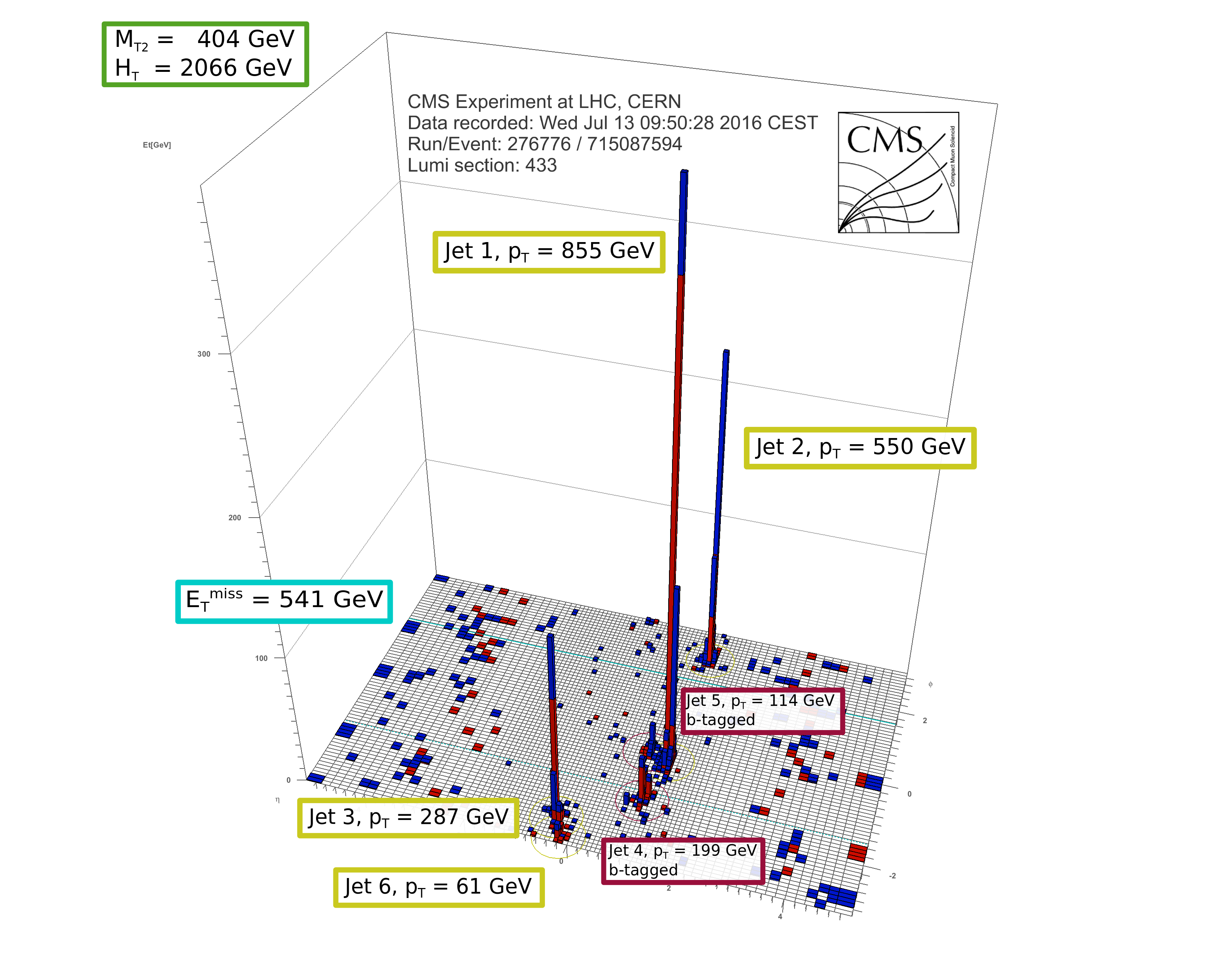
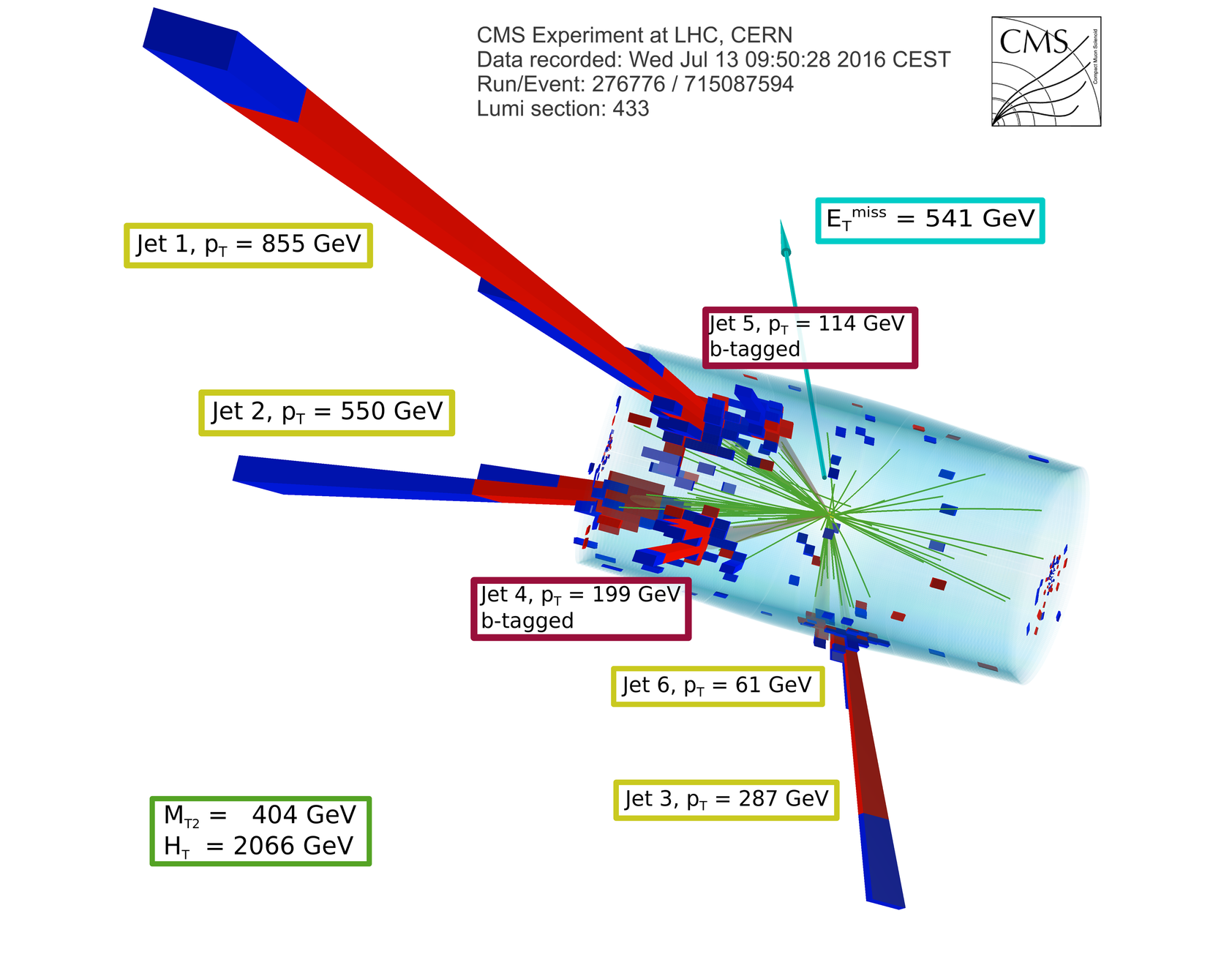
Display of a candidate event at event:run:lumi=715087594:276776:433, with ${M_{T2}} = $ 404 GeV, ${H_{\mathrm{T}}} =$ 2066 GeV, ${E_{T}^{\mathrm {miss}}} =$ 541 GeV, 6 jets and 2 b-jets. |
png |
Additional Figure 20-b:
Display of a candidate event at event:run:lumi=715087594:276776:433, with ${M_{T2}} = $ 404 GeV, ${H_{\mathrm{T}}} =$ 2066 GeV, ${E_{T}^{\mathrm {miss}}} =$ 541 GeV, 6 jets and 2 b-jets. |
png |
Additional Figure 20-c:
Display of a candidate event at event:run:lumi=715087594:276776:433, with ${M_{T2}} = $ 404 GeV, ${H_{\mathrm{T}}} =$ 2066 GeV, ${E_{T}^{\mathrm {miss}}} =$ 541 GeV, 6 jets and 2 b-jets. |
png |
Additional Figure 20-d:
Display of a candidate event at event:run:lumi=715087594:276776:433, with ${M_{T2}} = $ 404 GeV, ${H_{\mathrm{T}}} =$ 2066 GeV, ${E_{T}^{\mathrm {miss}}} =$ 541 GeV, 6 jets and 2 b-jets. |
png |
Additional Figure 20-e:
Display of a candidate event at event:run:lumi=715087594:276776:433, with ${M_{T2}} = $ 404 GeV, ${H_{\mathrm{T}}} =$ 2066 GeV, ${E_{T}^{\mathrm {miss}}} =$ 541 GeV, 6 jets and 2 b-jets. |
png |
Additional Figure 20-f:
Display of a candidate event at event:run:lumi=715087594:276776:433, with ${M_{T2}} = $ 404 GeV, ${H_{\mathrm{T}}} =$ 2066 GeV, ${E_{T}^{\mathrm {miss}}} =$ 541 GeV, 6 jets and 2 b-jets. |

png |
Additional Figure 20-g:
Display of a candidate event at event:run:lumi=715087594:276776:433, with ${M_{T2}} = $ 404 GeV, ${H_{\mathrm{T}}} =$ 2066 GeV, ${E_{T}^{\mathrm {miss}}} =$ 541 GeV, 6 jets and 2 b-jets. |
png |
Additional Figure 20-h:
Display of a candidate event at event:run:lumi=715087594:276776:433, with ${M_{T2}} = $ 404 GeV, ${H_{\mathrm{T}}} =$ 2066 GeV, ${E_{T}^{\mathrm {miss}}} =$ 541 GeV, 6 jets and 2 b-jets. |
| Additional Tables | |
png pdf |
Additional Table 1:
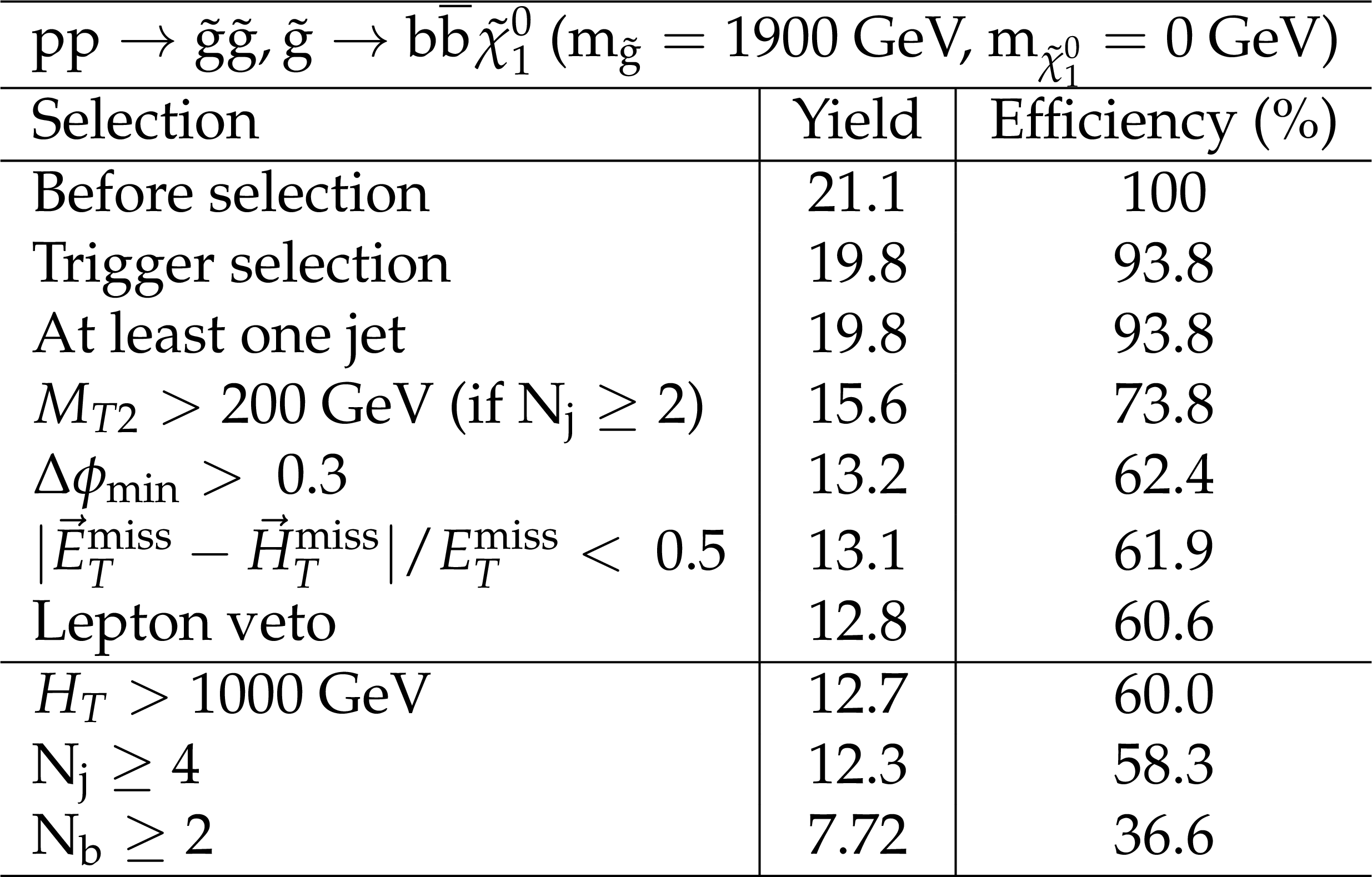
Cut flow table for baseline selection and several sample additional kinematic selections for a signal model of gluino-mediated bottom squark production with the mass of the gluino and the LSP equal to 1900 and 0 GeV, respectively. Theory cross section for this signal is 0.0016 pb. |
png pdf |
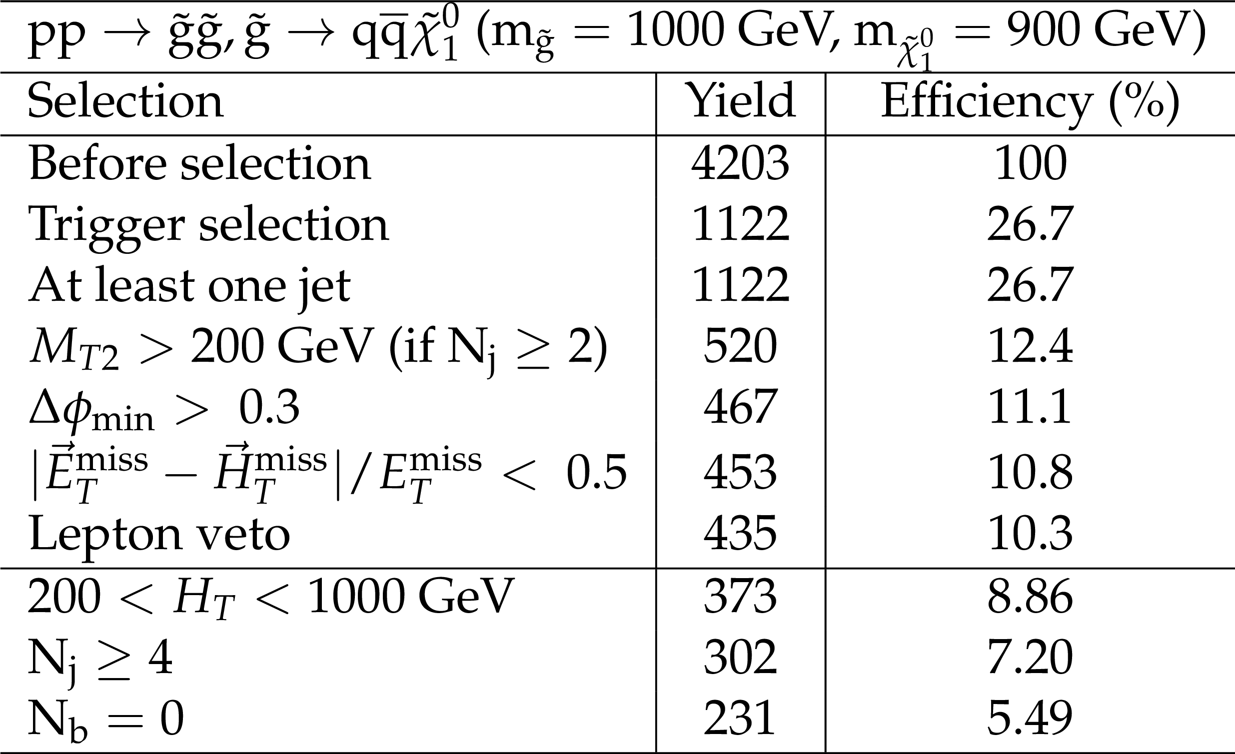
Additional Table 2:
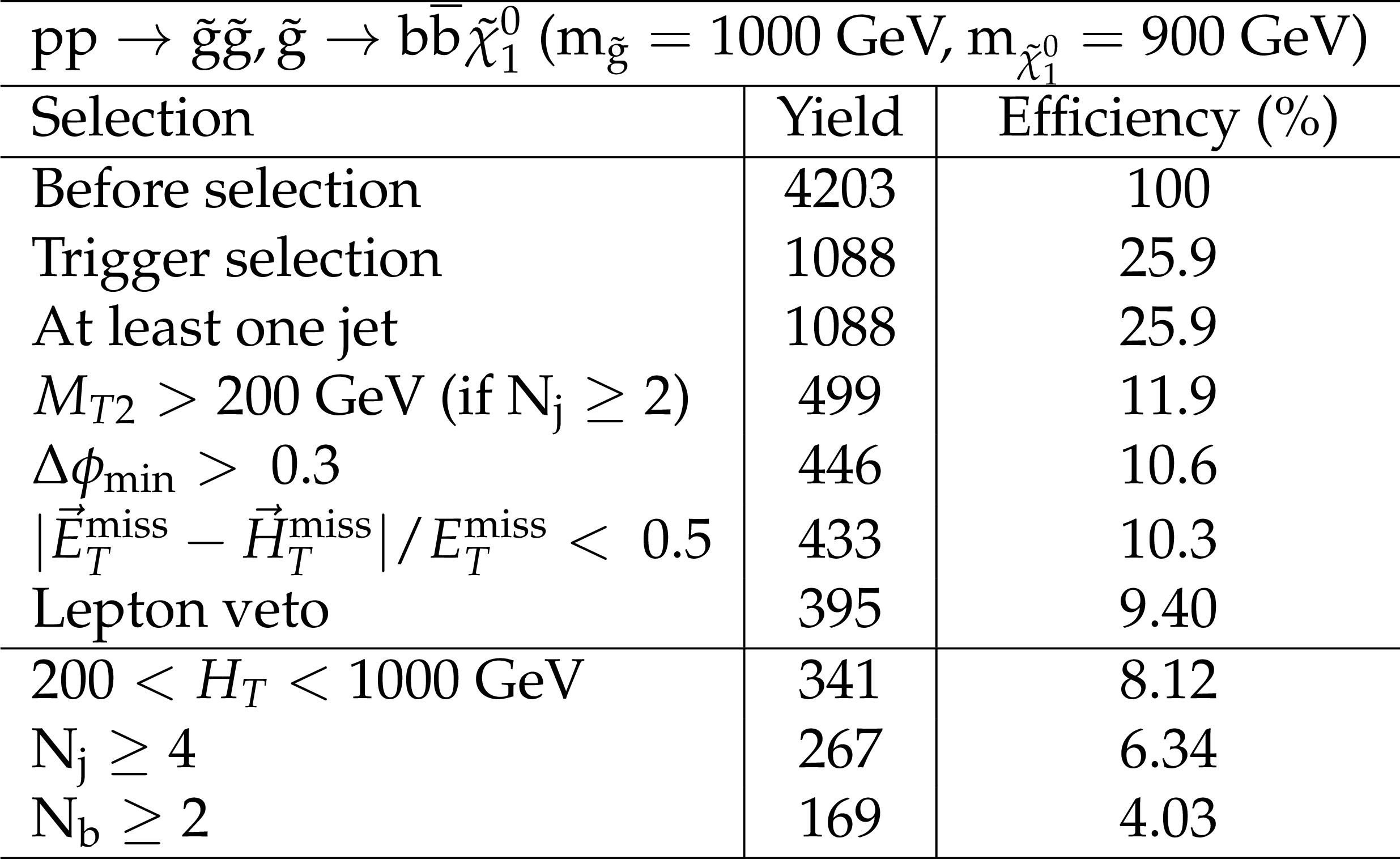
Cut flow table for baseline selection and several sample additional kinematic selections for a signal model of gluino-mediated bottom squark production with the mass of the gluino and the LSP equal to 1000 and 900 GeV, respectively. Theory cross section for this signal is 0.33 pb. |

png pdf |
Additional Table 3:
Cut flow table for baseline selection and several sample additional kinematic selections for a signal model of gluino-mediated top squark production with the mass of the gluino and the LSP equal to 1800 and 0 GeV, respectively. Theory cross section for this signal is 0.0028 pb. |
png pdf |
Additional Table 4:
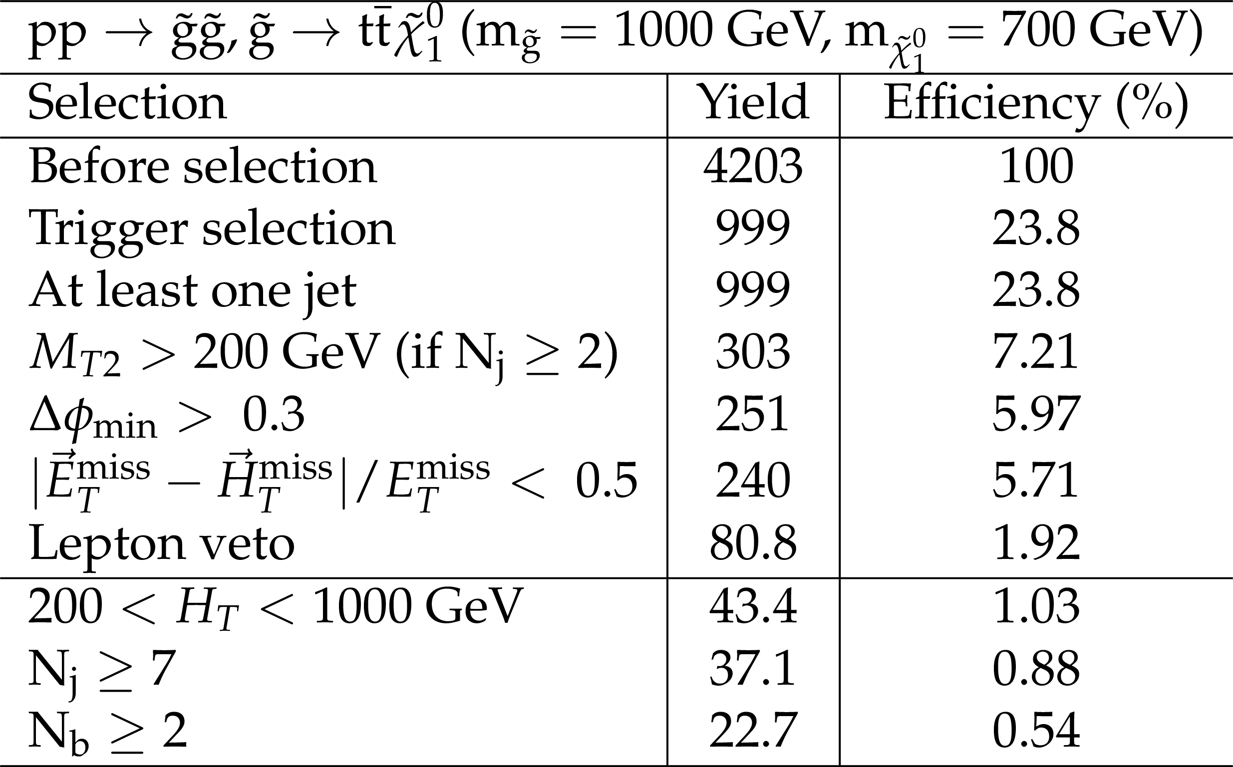
Cut flow table for baseline selection and several sample additional kinematic selections for a signal model of gluino-mediated top squark production with the mass of the gluino and the LSP equal to 1000 and 700 GeV, respectively. Theory cross section for this signal is 0.33 pb. |

png pdf |
Additional Table 5:
Cut flow table for baseline selection and several sample additional kinematic selections for a signal model of gluino-mediated light squark production with the mass of the gluino and the LSP equal to 1700 and 0 GeV, respectively. Theory cross section for this signal is 0.0047 pb. |
png pdf |
Additional Table 6:
Cut flow table for baseline selection and several sample additional kinematic selections for a signal model of gluino-mediated light squark production with the mass of the gluino and the LSP equal to 1000 and 900 GeV, respectively. Theory cross section for this signal is 0.33 pb. |
png pdf |
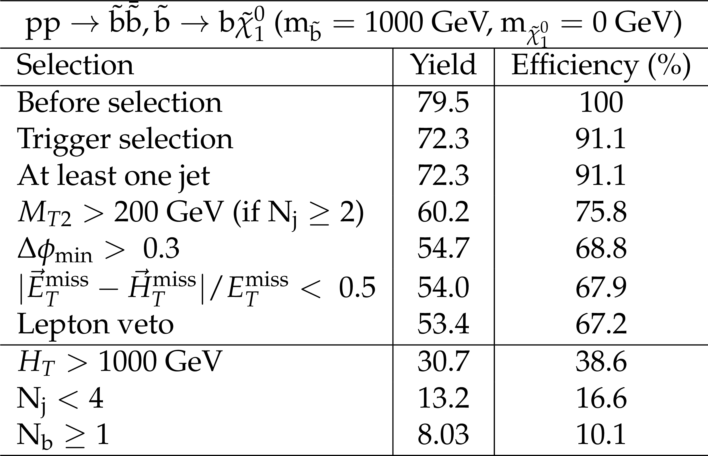
Additional Table 7:
Cut flow table for baseline selection and several sample additional kinematic selections for a signal model of direct bottom squark production with the mass of the squark and the LSP equal to 1000 and 0 GeV, respectively. Theory cross section for this signal is 0.0062 pb. |
png pdf |
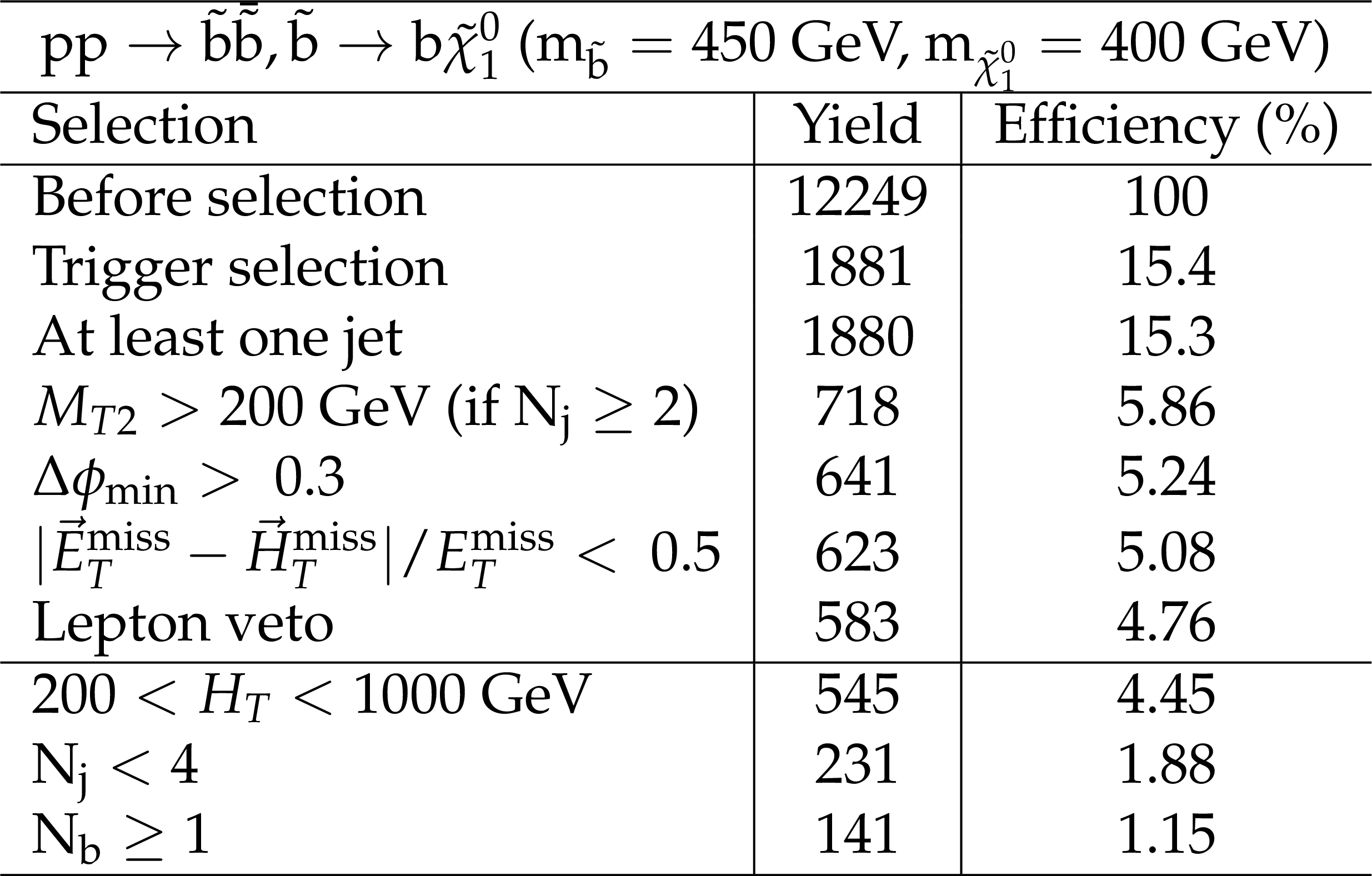
Additional Table 8:
Cut flow table for baseline selection and several sample additional kinematic selections for a signal model of direct bottom squark production with the mass of the squark and the LSP equal to 450 and 400 GeV, respectively. Theory cross section for this signal is 0.95 pb. |

png pdf |
Additional Table 9:
Cut flow table for baseline selection and several sample additional kinematic selections for a signal model of direct top squark production with the mass of the squark and the LSP equal to 900 and 0 GeV, respectively. Theory cross section for this signal is 0.013 pb. |

png pdf |
Additional Table 10:
Cut flow table for baseline selection and several sample additional kinematic selections for a signal model of direct top squark production with the mass of the squark and the LSP equal to 350 and 250 GeV, respectively. Theory cross section for this signal is 3.79 pb. |
png pdf |
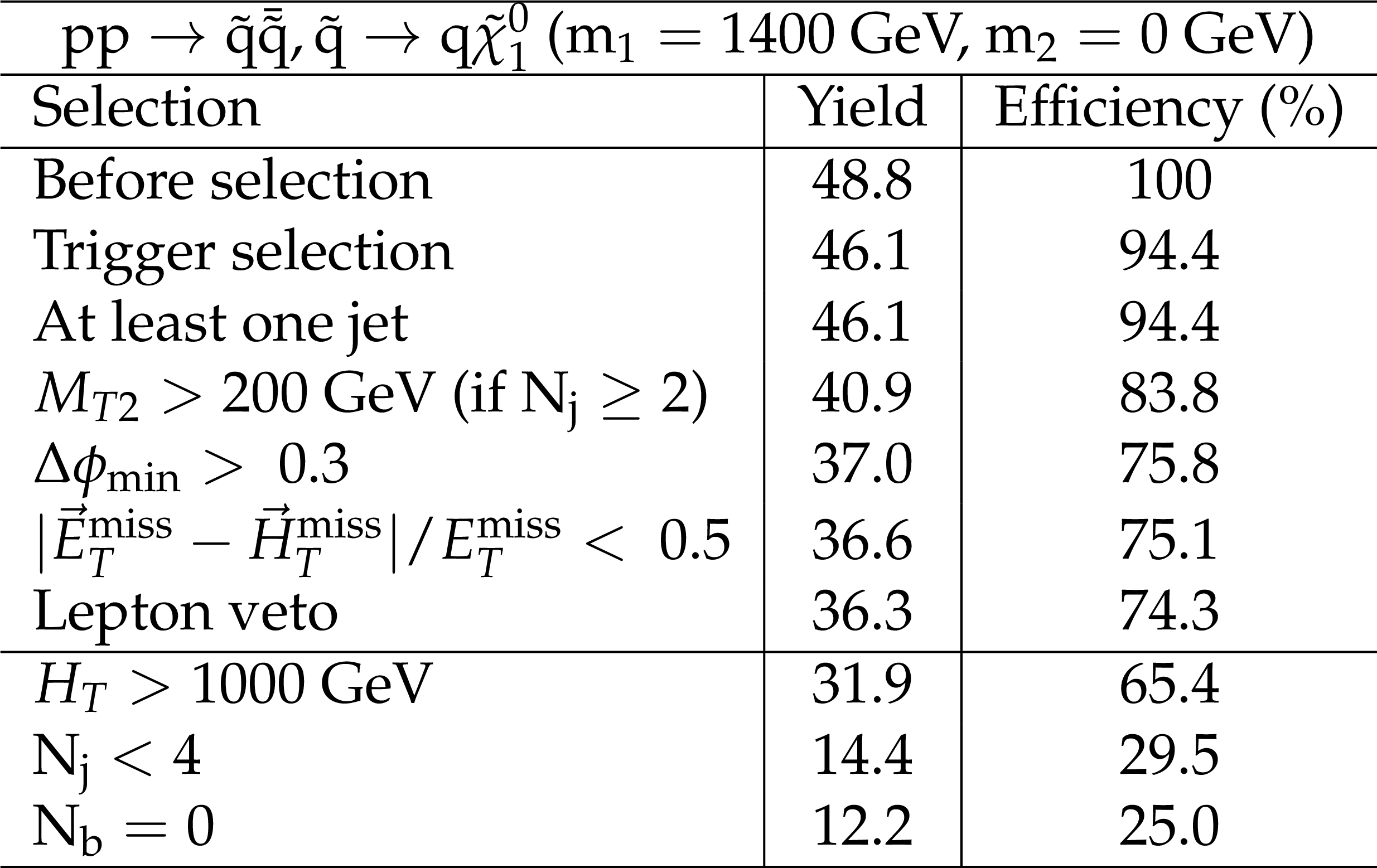
Additional Table 11:
Cut flow table for baseline selection and several sample additional kinematic selections for a signal model of direct light squark production with the mass of the squark and the LSP equal to 1400 and 0 GeV, respectively. Theory cross section for this signal is 0.0038 pb. |
png pdf |
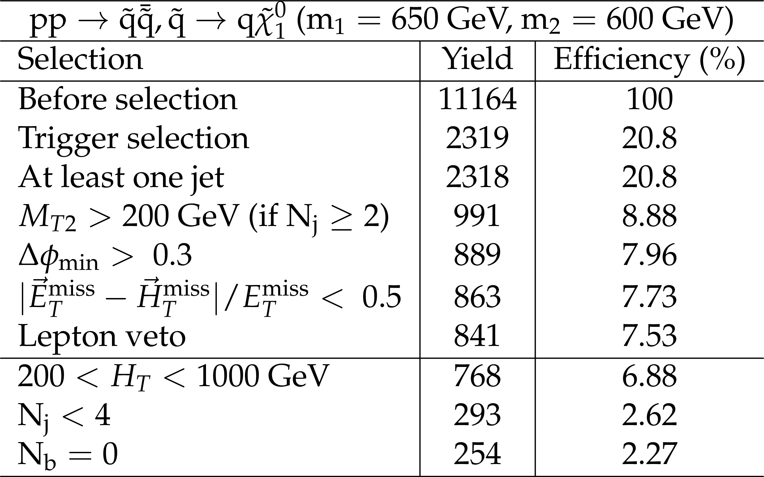
Additional Table 12:
Cut flow table for baseline selection and several sample additional kinematic selections for a signal model of direct light squark production with the mass of the squark and the LSP equal to 650 and 600 GeV, respectively. Theory cross section for this signal is 0.86 pb. |
png pdf |
Additional Table 13:
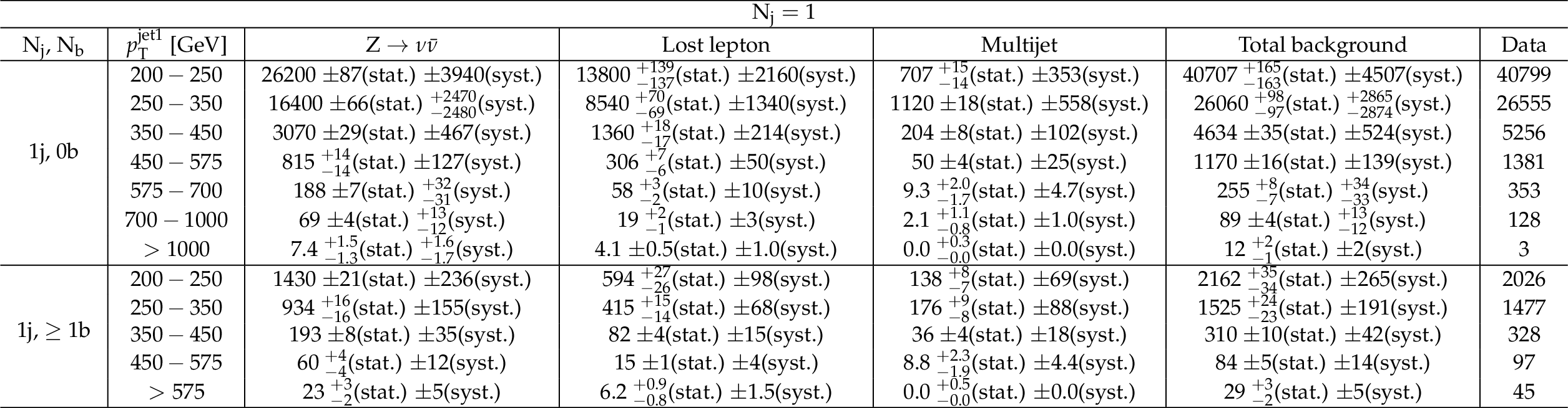
Background estimate and observation in bins of $ { {p_{\mathrm {T}}} ^{\mathrm {jet1}}} $ for the monojet regions. The yields correspond to an integrated luminosity of 12.9 fb$^{-1}$. |
png pdf |
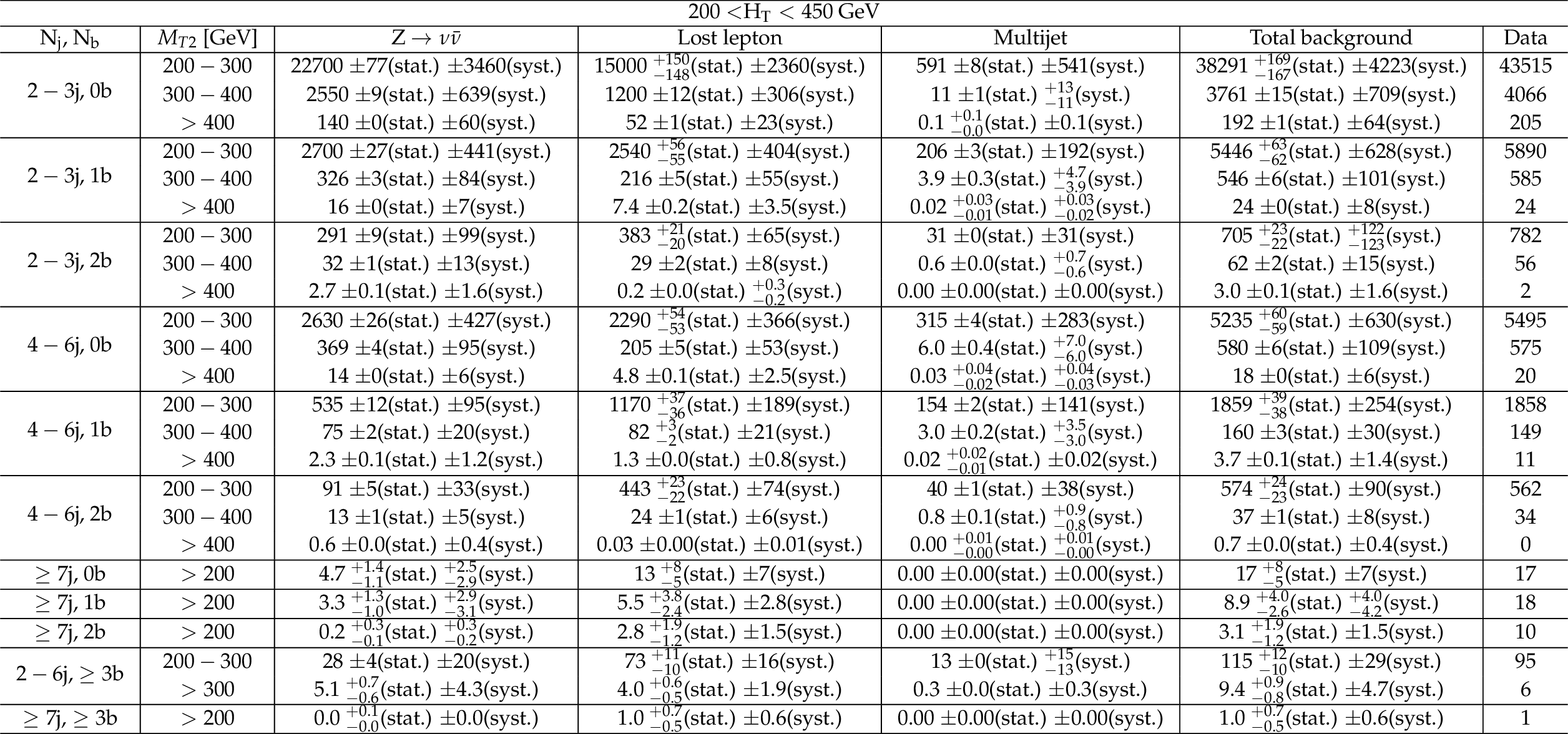
Additional Table 14:
Background estimate and observation in bins of ${M_{T2}}$ for 200 $ < H_{\mathrm {T}} < $ 450 GeV. The yields correspond to an integrated luminosity of 12.9 fb$^{-1}$. |
png pdf |
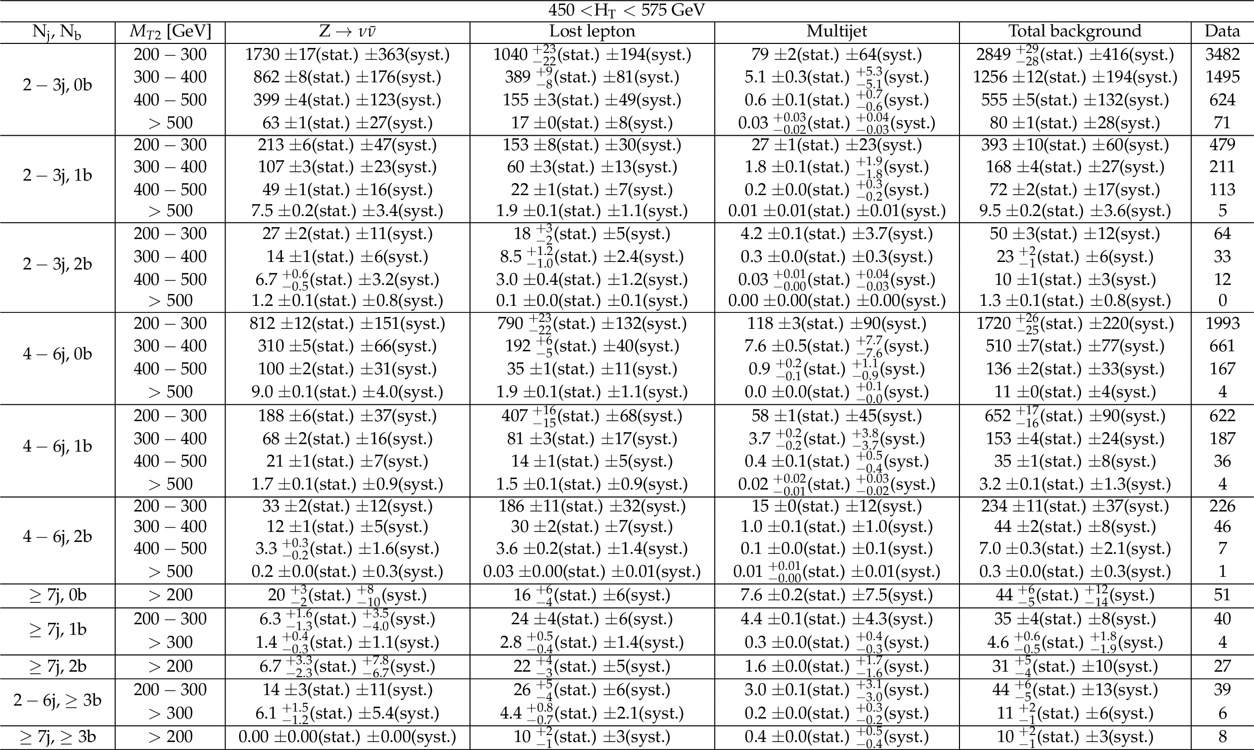
Additional Table 15:
Background estimate and observation in bins of ${M_{T2}}$ for 450 $ < H_{\mathrm {T}} < $ 575 GeV. The yields correspond to an integrated luminosity of 12.9 fb$^{-1}$. |
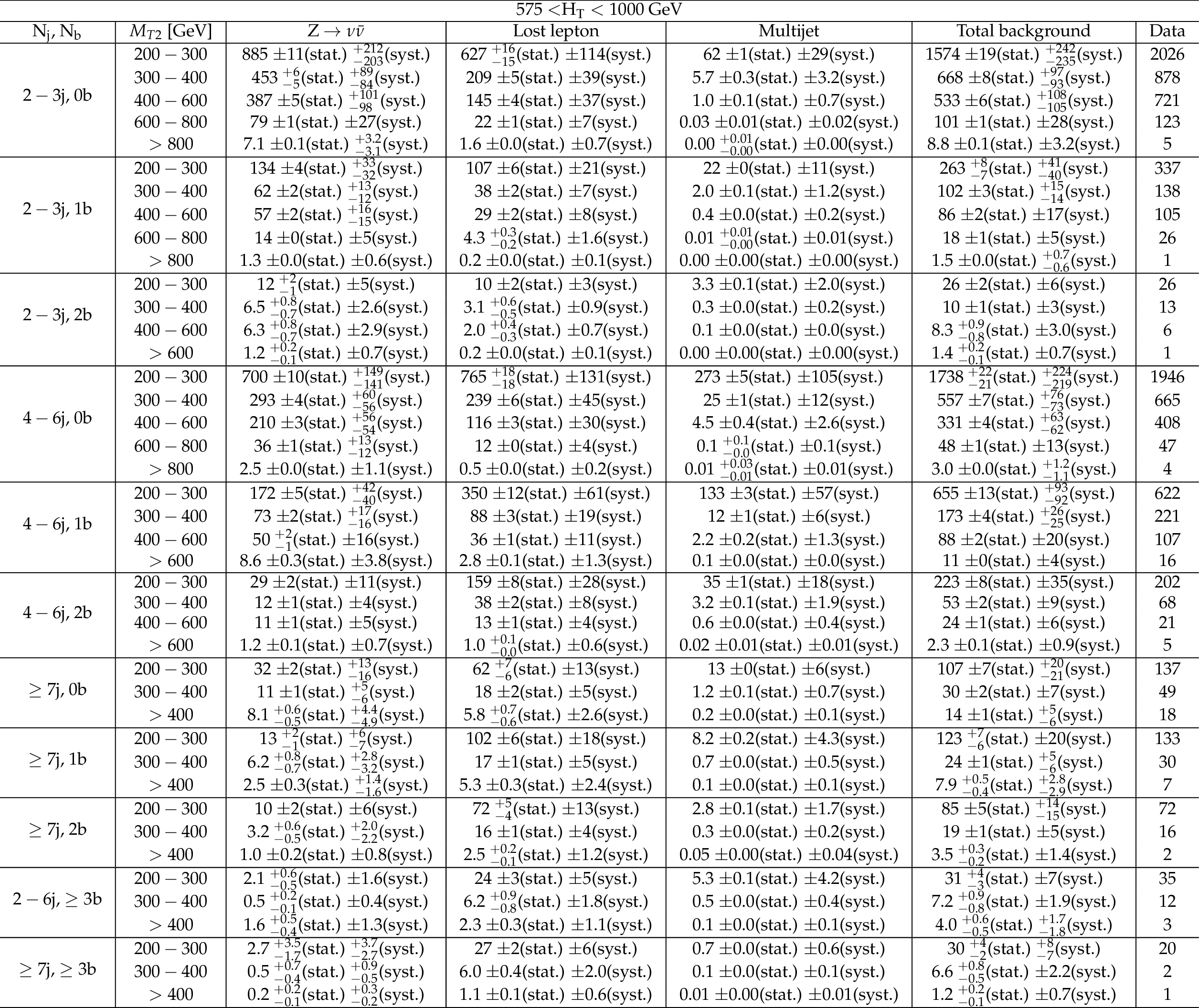
png pdf |
Additional Table 16:
Background estimate and observation in bins of ${M_{T2}}$ for 575 $ < H_{\mathrm {T}} < $ 1000 GeV. The yields correspond to an integrated luminosity of 12.9 fb$^{-1}$. |

png pdf |
Additional Table 17:
Background estimate and observation in bins of ${M_{T2}}$ for 1000 $ < H_{\mathrm {T}} < $ 1500 GeV. The yields correspond to an integrated luminosity of 12.9 fb$^{-1}$. |

png pdf |
Additional Table 18:
Background estimate and observation in bins of ${M_{T2}}$ for $H_{\mathrm {T}} > $ 1500 GeV. The yields correspond to an integrated luminosity of 12.9 fb$^{-1}$. |
| Additional code to compute hemispheres and MT2 and an example of usage is available here. |
| References | ||||
| 1 | ATLAS Collaboration | Search for new phenomena in final states with large jet multiplicities and missing transverse momentum with ATLAS using $ \sqrt{s} = $ 13 TeV proton-proton collisions | PLB757 (2016) 334--355 | 1602.06194 |
| 2 | ATLAS Collaboration | Search for new phenomena in final states with an energetic jet and large missing transverse momentum in $ pp $ collisions at $ \sqrt{s}=13 $ TeV using the ATLAS detector | 1604.07773 | |
| 3 | ATLAS Collaboration | Search for squarks and gluinos in final states with jets and missing transverse momentum at $ \sqrt{s}= $ 13 TeV with the ATLAS detector | 1605.03814 | |
| 4 | ATLAS Collaboration | Search for pair production of gluinos decaying via stop and sbottom in events with $ b $-jets and large missing transverse momentum in $ pp $ collisions at $ \sqrt{s} = 13 $ TeV with the ATLAS detector | 1605.09318 | |
| 5 | CMS Collaboration | Search for new physics with the MT2 variable in all-jets final states produced in pp collisions at sqrt(s) = 13 TeV | CMS-SUS-15-003 1603.04053 |
|
| 6 | CMS Collaboration | Search for supersymmetry in the multijet and missing transverse momentum final state in pp collisions at 13 TeV | PLB758 (2016) 152--180 | CMS-SUS-15-002 1602.06581 |
| 7 | CMS Collaboration Collaboration | Inclusive search for supersymmetry using the razor variables at sqrt(s) = 13 TeV | Technical Report CMS-PAS-SUS-15-004, CERN, Geneva | |
| 8 | CMS Collaboration Collaboration | Search for new physics in final states with jets and missing transverse momentum in $ \sqrt{s} $ = 13 TeV pp collisions with the $ \alpha_{\text{T}} $ variable | Technical Report CMS-PAS-SUS-15-005, CERN, Geneva | |
| 9 | C. G. Lester and D. J. Summers | Measuring masses of semiinvisibly decaying particles pair produced at hadron colliders | PLB 463 (1999) 99 | hep-ph/9906349 |
| 10 | CMS Collaboration | Performance of Electron Reconstruction and Selection with the CMS Detector in Proton-Proton Collisions at √s = 8 TeV | JINST 10 (2015), no. 06, P06005 | CMS-EGM-13-001 1502.02701 |
| 11 | A. L. Read | Presentation of search results: The $ CL_{s} $ technique | JPG 28 (2002) 2693 | |
| 12 | A. L. Read | Modified frequentist analysis of search results (The $ CL_{s} $ method) | CERN-OPEN 205(2000) | |
| 13 | G. Cowan, K. Cranmer, E. Gross, and O. Vitells | Asymptotic formulae for likelihood-based tests of new physics | EPJC 71 (2011) 1554 | 1007.1727 |
| 14 | ATLAS and CMS Collaborations | Procedure for the LHC Higgs boson search combination in summer 2011 | CMS-NOTE-2011-005 | |
| 15 | CMS Collaboration | Search for top-squark pair production in the single-lepton final state in pp collisions at $ \sqrt{s} $ = 8 TeV | EPJC73 (2013), no. 12 | CMS-SUS-13-011 1308.1586 |
|
|
Compact Muon Solenoid LHC, CERN |
|

|

|

|

|

|