

Compact Muon Solenoid
LHC, CERN
| CMS-SUS-15-003 ; CERN-EP-2016-067 | ||
| Search for new physics with the $M_{\mathrm{T2}}$ variable in all-jets final states produced in pp collisions at $\sqrt{s} =$ 13 TeV | ||
| CMS Collaboration | ||
| 13 March 2016 | ||
| J. High Energy Phys. 10 (2016) 006 | ||
| Abstract: A search for new physics is performed using events that contain one or more jets, no isolated leptons, and a large transverse momentum imbalance, as measured through the $M_{\mathrm{T2}}$ variable, which is an extension of the transverse mass in events with two invisible particles. The results are based on a sample of proton-proton collisions collected at a center-of-mass energy of 13 TeV with the CMS detector at the LHC, and that corresponds to an integrated luminosity of 2.3 fb$^{-1}$. The observed event yields in the data are consistent with predictions for the standard model backgrounds. The results are interpreted using simplified models of supersymmetry and are expressed in terms of limits on the masses of potential new colored particles. Assuming that the lightest neutralino is stable and has a mass less than about 500 GeV, gluino masses up to 1550-1750 GeV are excluded at 95% confidence level, depending on the gluino decay mechanism. For the scenario of direct production of squark-antisquark pairs, top squarks with masses up to 800 GeV are excluded, assuming a 100% branching fraction for the decay to a top quark and neutralino. Similarly, bottom squark masses are excluded up to 880 GeV, and masses of light-flavor squarks are excluded up to 600-1260 GeV, depending on the degree of degeneracy of the squark masses. | ||
| Links: e-print arXiv:1603.04053 [hep-ex] (PDF) ; CDS record ; inSPIRE record ; CADI line (restricted) ; | ||
| Figures & Tables | Summary | Additional Figures & Tables | References | CMS Publications |
|---|
| Figures | |
png pdf |
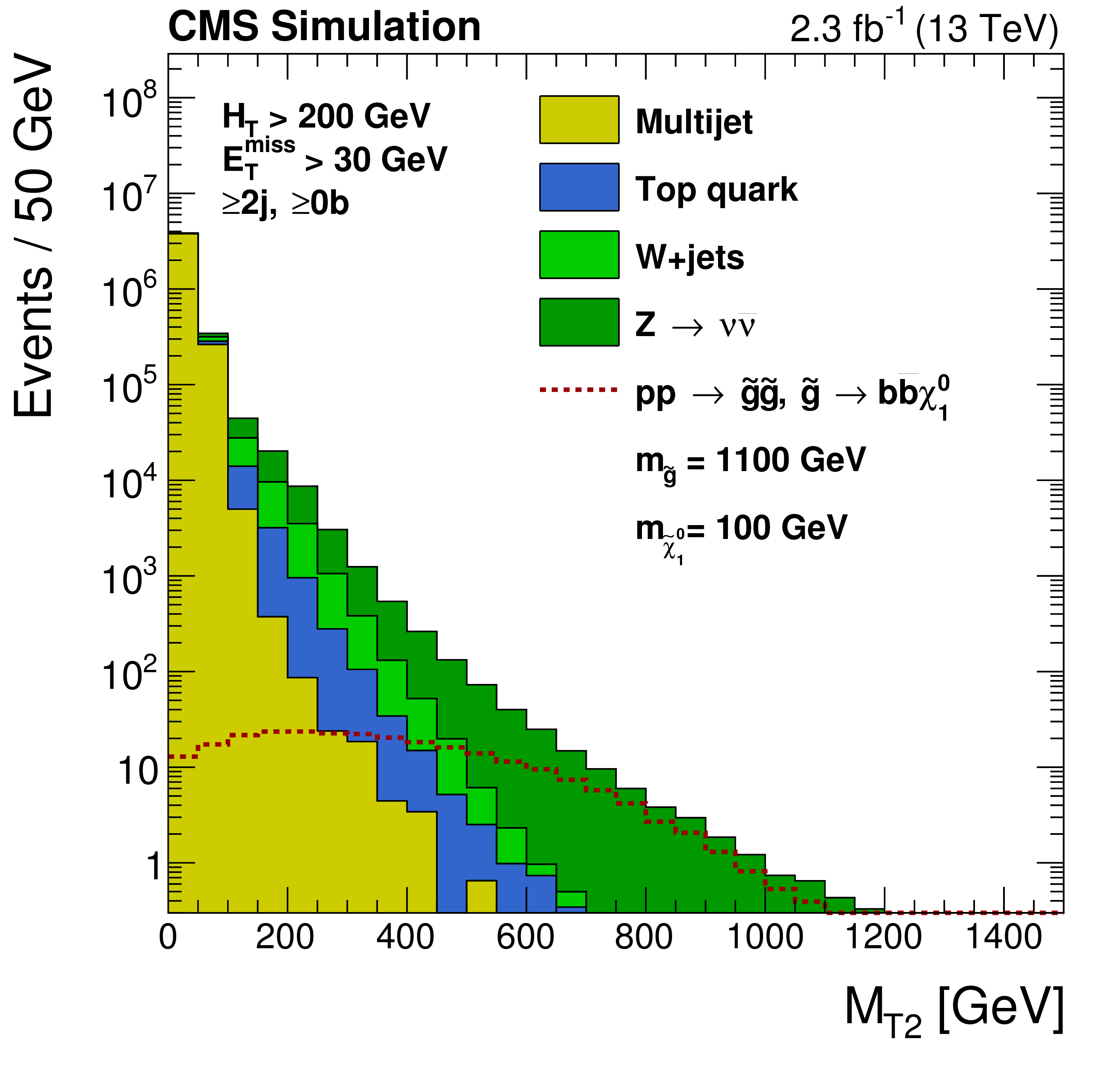
Figure 1:
Distribution of the $ {M_{\mathrm {T2}}} $ variable in simulated background and signal event samples after the baseline selection is applied. The line shows the expected $ {M_{\mathrm {T2}}} $ distribution for a signal model of gluino-mediated bottom squark production with the masses of gluino and lightest neutralino equal to 1100 and 100 GeV, respectively. |
png pdf |
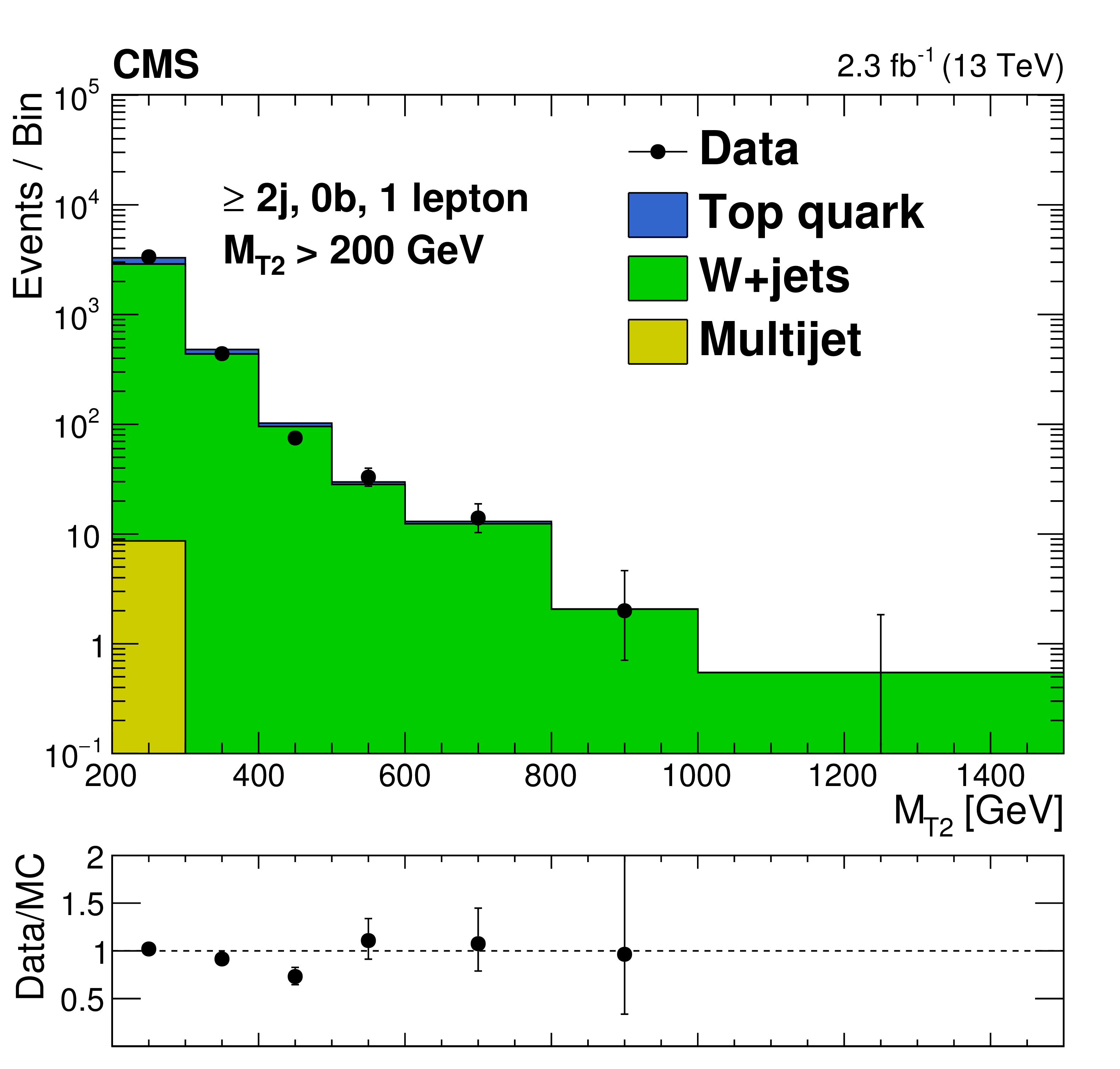
Figure 2-a:
Comparison between simulation and data in the $ {M_{\mathrm {T2}}} $ observable. The (a) and (b) plots correspond to control samples enriched in W+jets and $ \mathrm{ t \bar{t} } $+jets, respectively. The sum of two distributions from simulation is scaled to have the same integral as the corresponding histograms from data. The uncertainties shown are statistical only. |
png pdf |
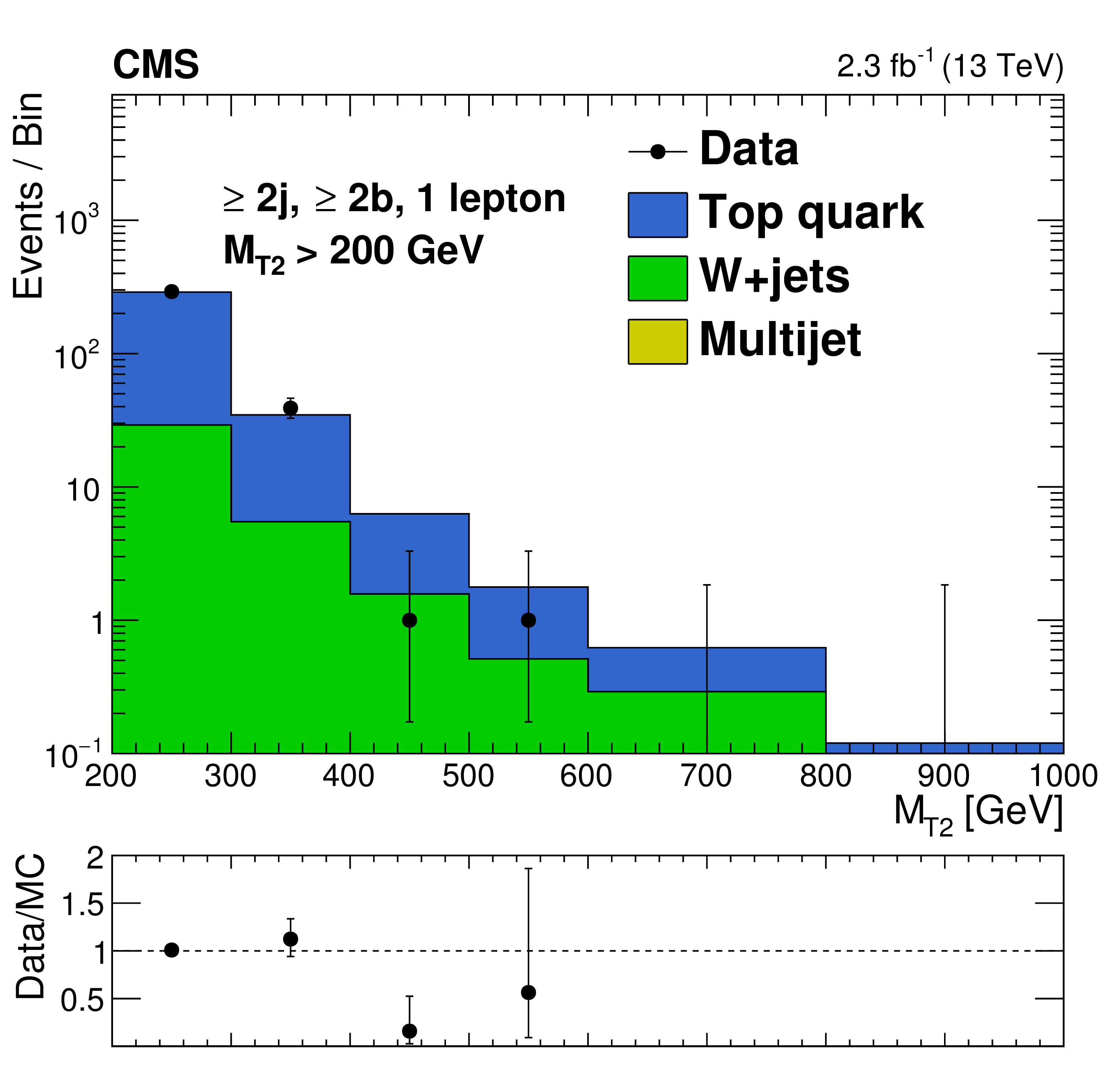
Figure 2-b:
Comparison between simulation and data in the $ {M_{\mathrm {T2}}} $ observable. The (a) and (b) plots correspond to control samples enriched in W+jets and $ \mathrm{ t \bar{t} } $+jets, respectively. The sum of two distributions from simulation is scaled to have the same integral as the corresponding histograms from data. The uncertainties shown are statistical only. |

png pdf |
Figure 3-a:
The (a) plot shows the photon purity, $P_{\gamma }$, measured in data for the single-photon control sample compared with the values extracted from simulation. The (b) plots show the $\mathrm{ Z } /\gamma $ ratio in simulation and data as a function of $ {H_{\mathrm {T}}} $ (upper plot), and the corresponding double ratio (lower plot). |
png pdf |
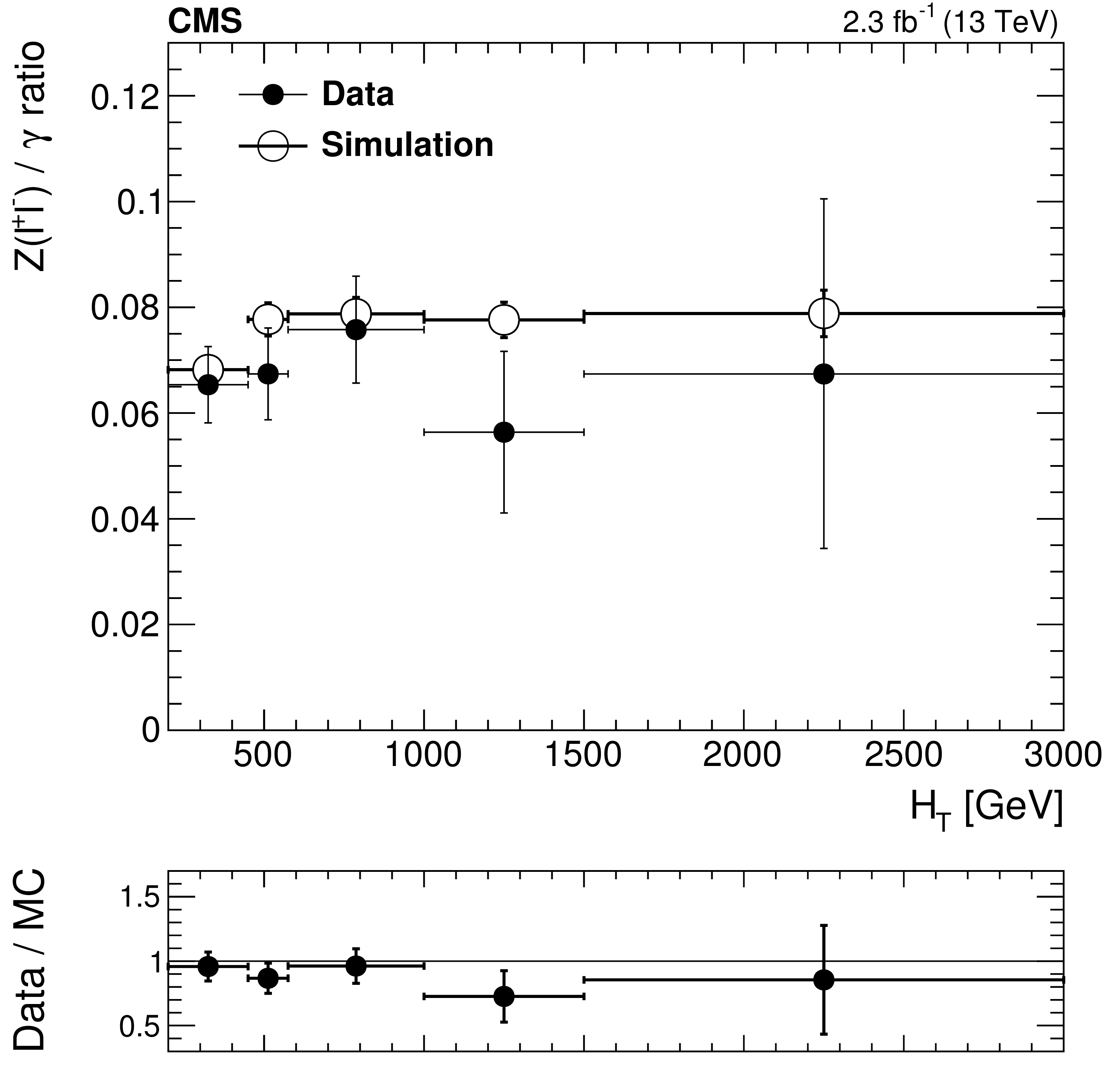
Figure 3-b:
The (a) plot shows the photon purity, $P_{\gamma }$, measured in data for the single-photon control sample compared with the values extracted from simulation. The (b) plots show the $\mathrm{ Z } /\gamma $ ratio in simulation and data as a function of $ {H_{\mathrm {T}}} $ (upper plot), and the corresponding double ratio (lower plot). |
png pdf |
Figure 4-a:
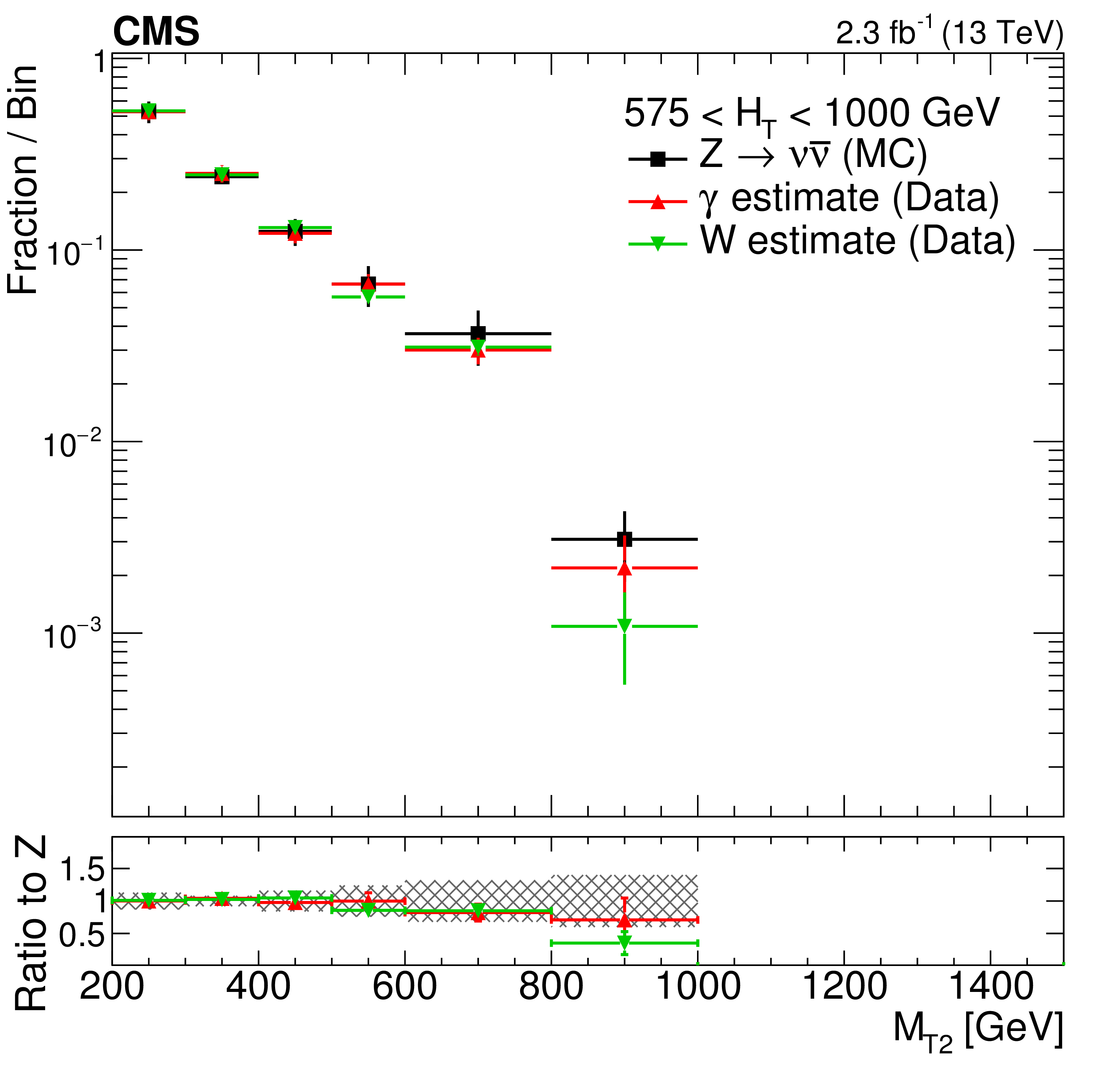
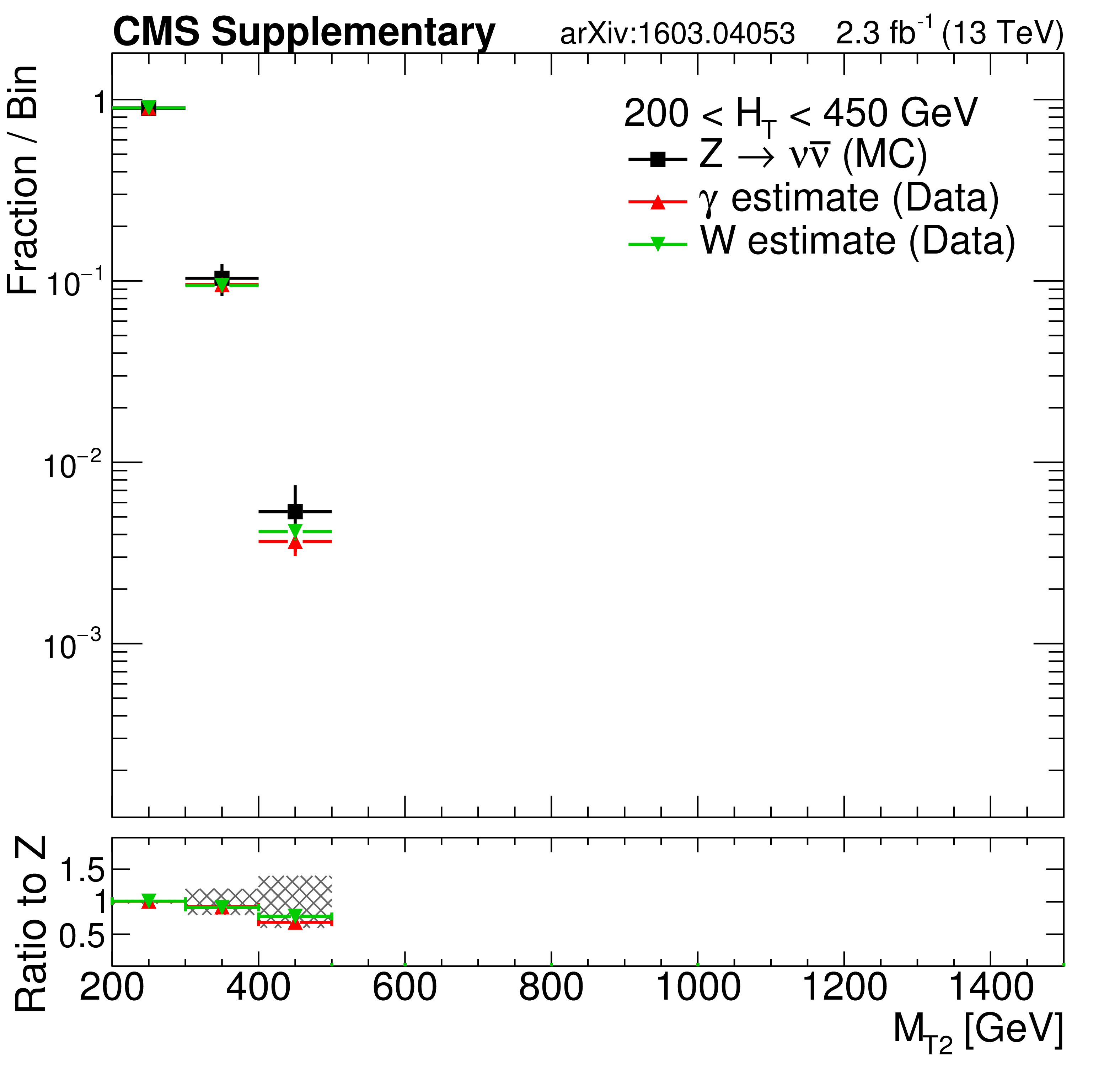
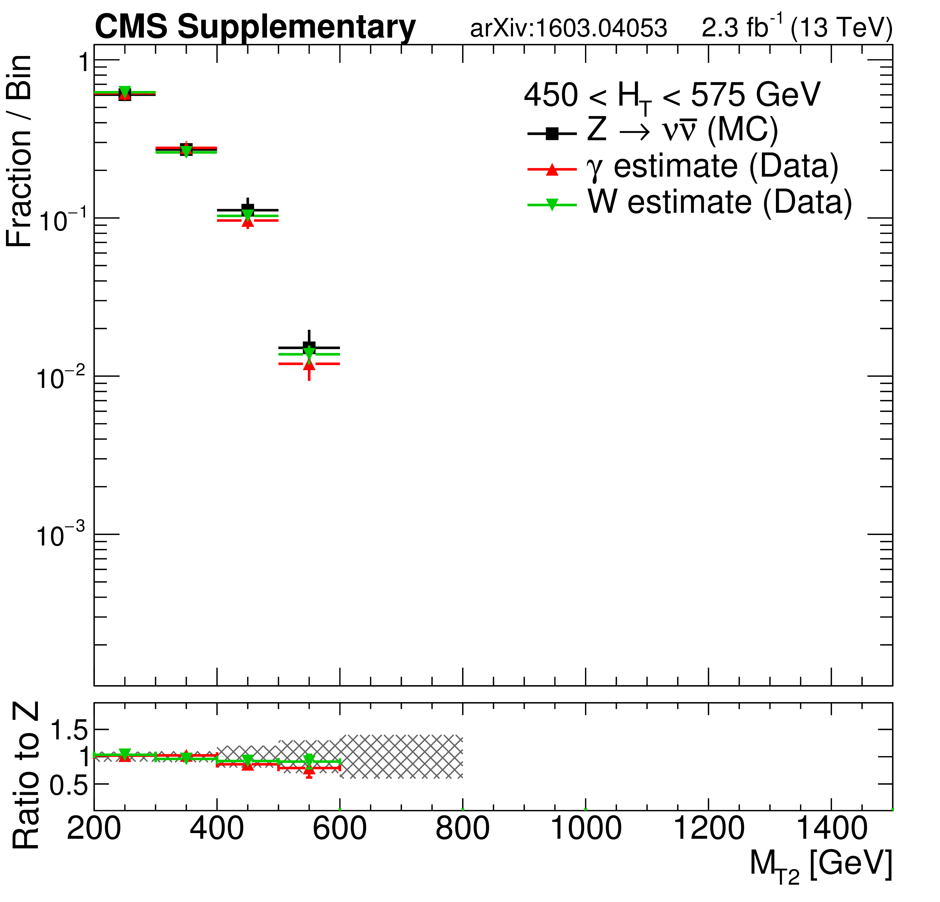
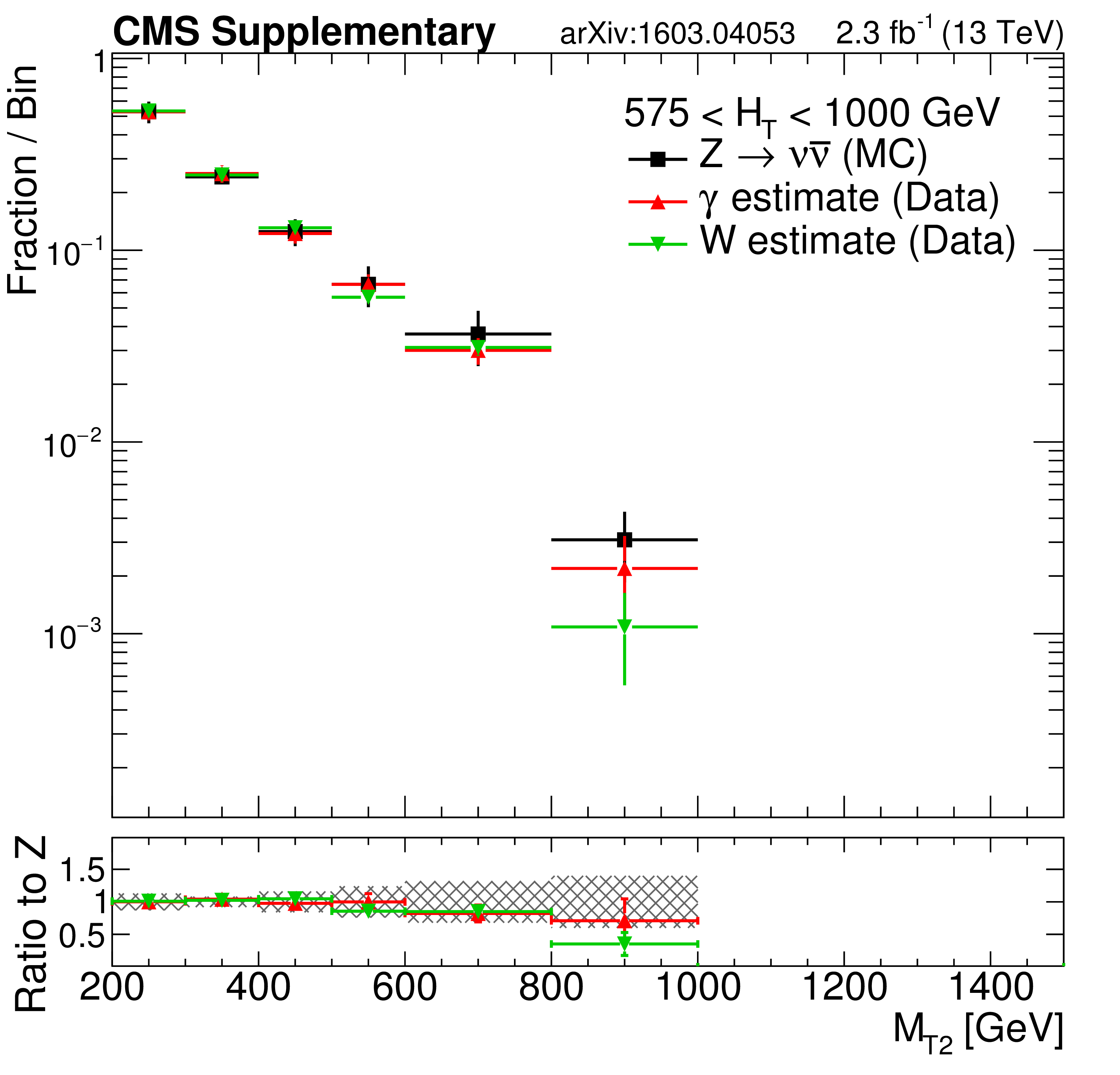
The shape of the $ {M_{\mathrm {T2}}} $ distribution from $ {\mathrm{ Z } \to \nu \bar{ \nu } } $ simulation compared to shapes extracted from $\gamma $ and W data control samples in the medium- (a plot) and high-$ {H_{\mathrm {T}}} $ regions (b plot). The $ {M_{\mathrm {T2}}} $ distributions in the data control samples are obtained after removing the reconstructed $\gamma $ or lepton from the event, to replicate the kinematics of $ {\mathrm{ Z } \to \nu \bar{ \nu } } $. The ratio of the shapes derived from data to the $ {\mathrm{ Z } \to \nu \bar{ \nu } } $ simulation shape is shown in the lower plots, where the shaded band represents the uncertainty in the MC modeling of the $ {M_{\mathrm {T2}}} $ variable. |

png pdf |
Figure 4-b:
The shape of the $ {M_{\mathrm {T2}}} $ distribution from $ {\mathrm{ Z } \to \nu \bar{ \nu } } $ simulation compared to shapes extracted from $\gamma $ and W data control samples in the medium- (a plot) and high-$ {H_{\mathrm {T}}} $ regions (b plot). The $ {M_{\mathrm {T2}}} $ distributions in the data control samples are obtained after removing the reconstructed $\gamma $ or lepton from the event, to replicate the kinematics of $ {\mathrm{ Z } \to \nu \bar{ \nu } } $. The ratio of the shapes derived from data to the $ {\mathrm{ Z } \to \nu \bar{ \nu } } $ simulation shape is shown in the lower plots, where the shaded band represents the uncertainty in the MC modeling of the $ {M_{\mathrm {T2}}} $ variable. |
png pdf |
Figure 5:
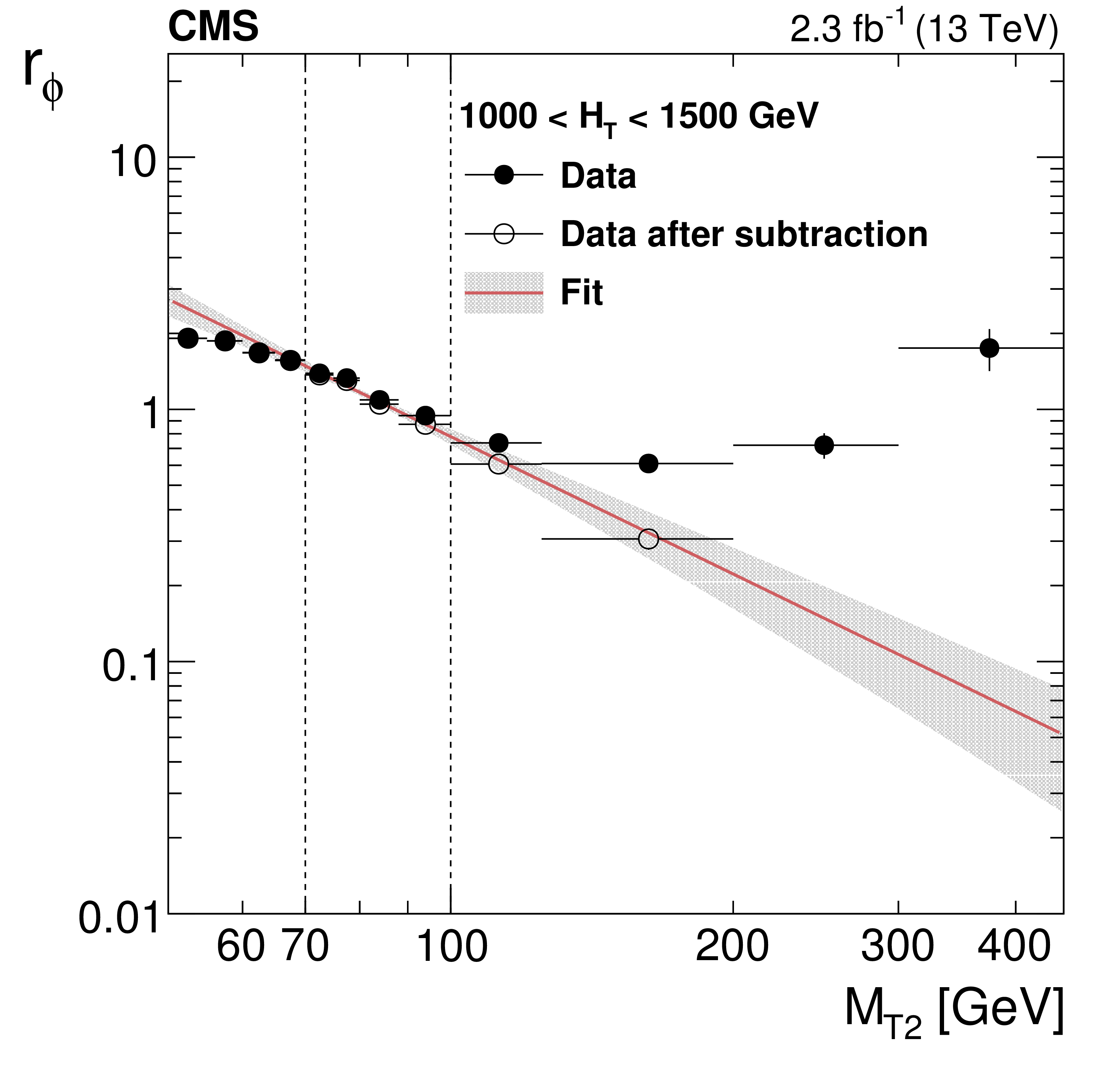
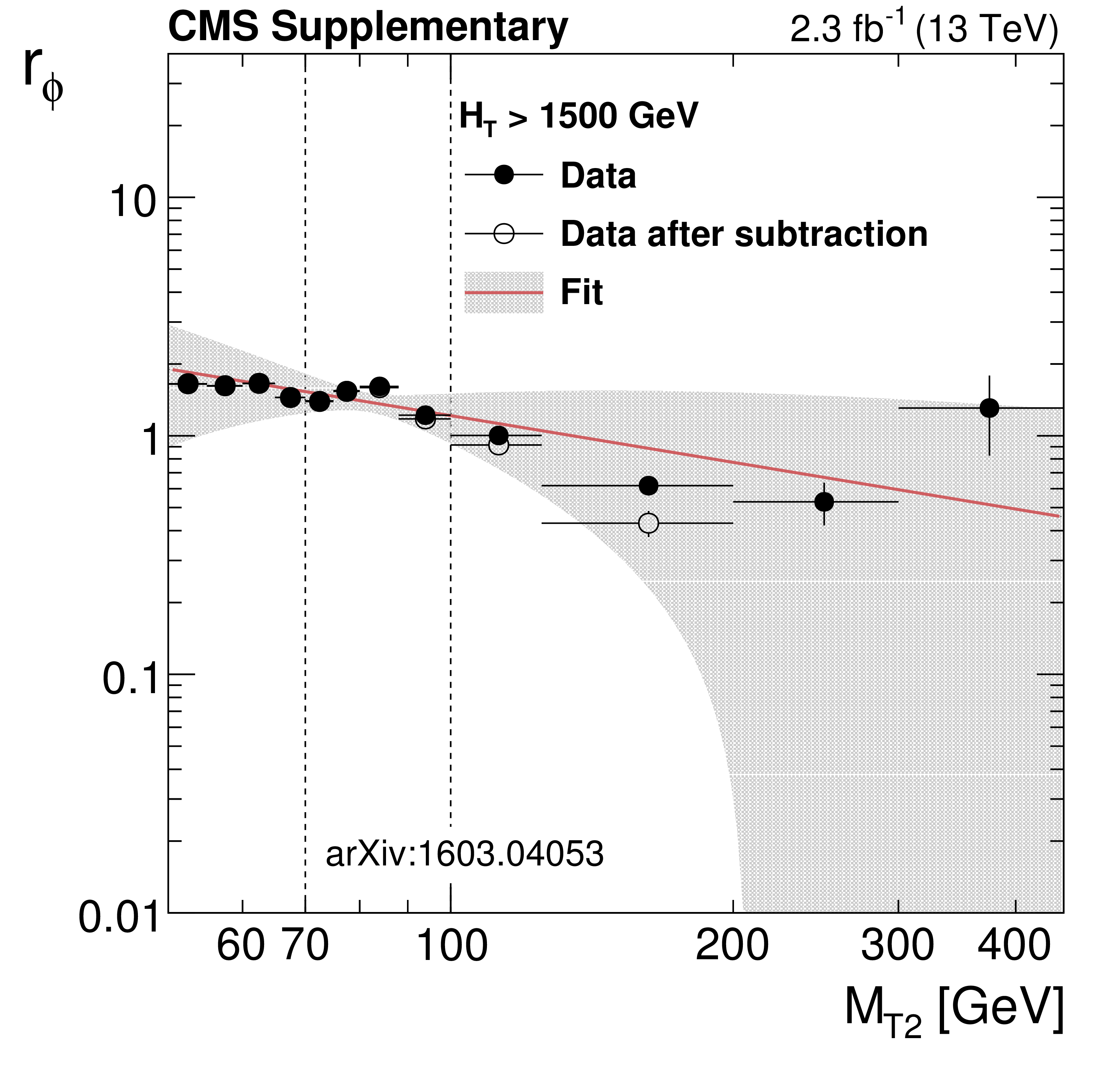
Distribution of the ratio $r_{\phi }$ as a function of $ {M_{\mathrm {T2}}} $ for the high-$ {H_{\mathrm {T}}} $ region. The fit is performed on the background-subtracted data points (open markers) in the interval 70 $< {M_{\mathrm {T2}}} <$ 100 GeV delimited by the two vertical dashed lines. The solid points represent the data before subtracting non-multijet backgrounds using simulation. Data point uncertainties are statistical only. The line and the band around it show the fit to a power-law function and the associated uncertainty. |
png pdf |
Figure 6-a:
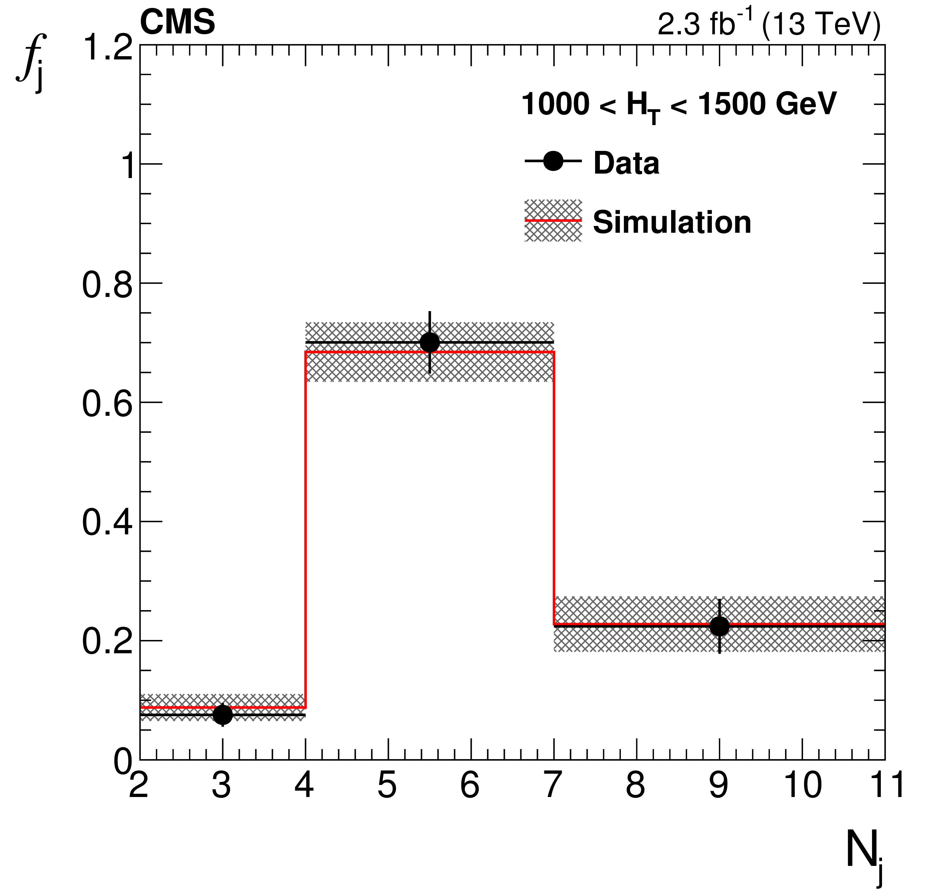
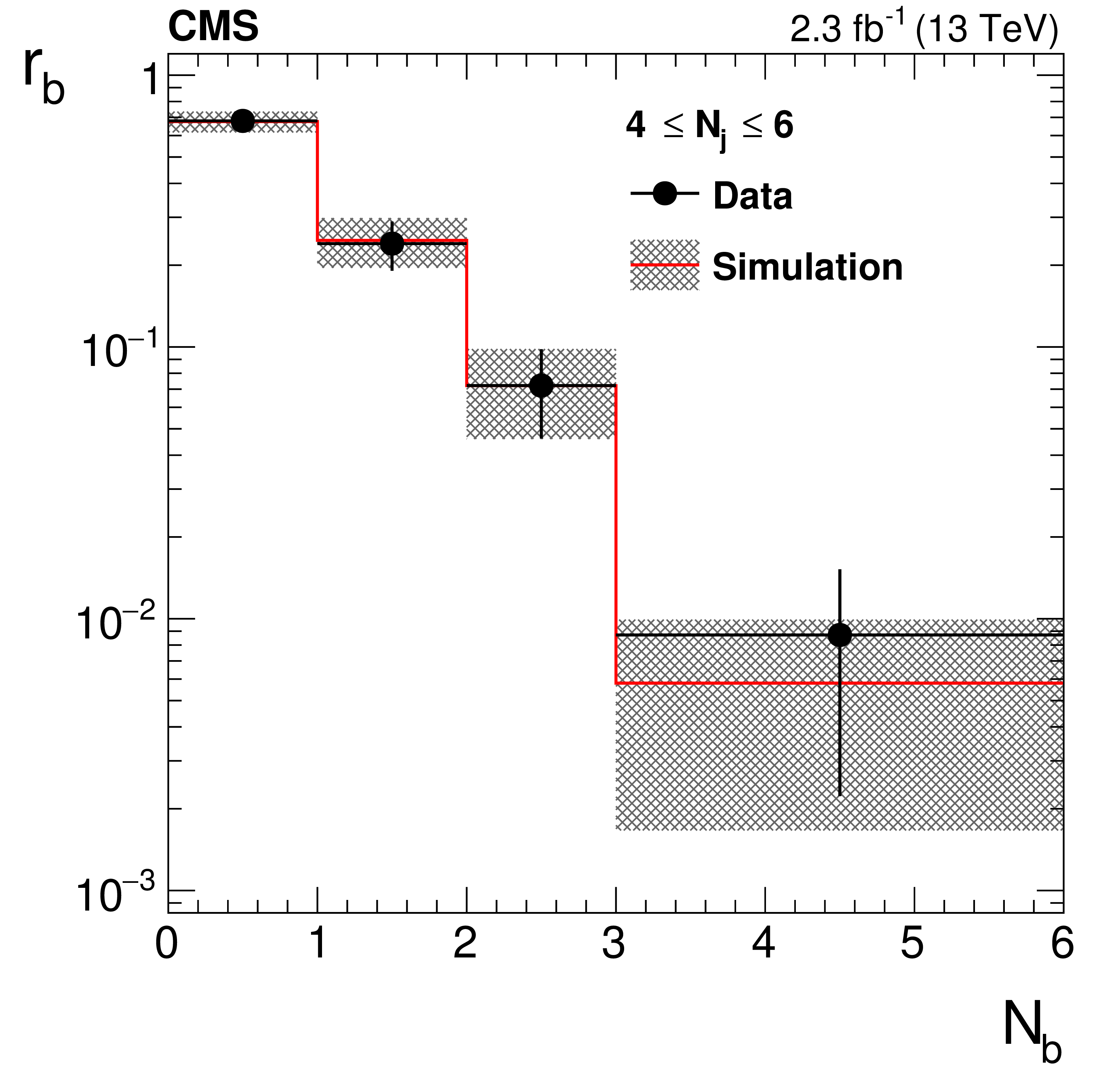
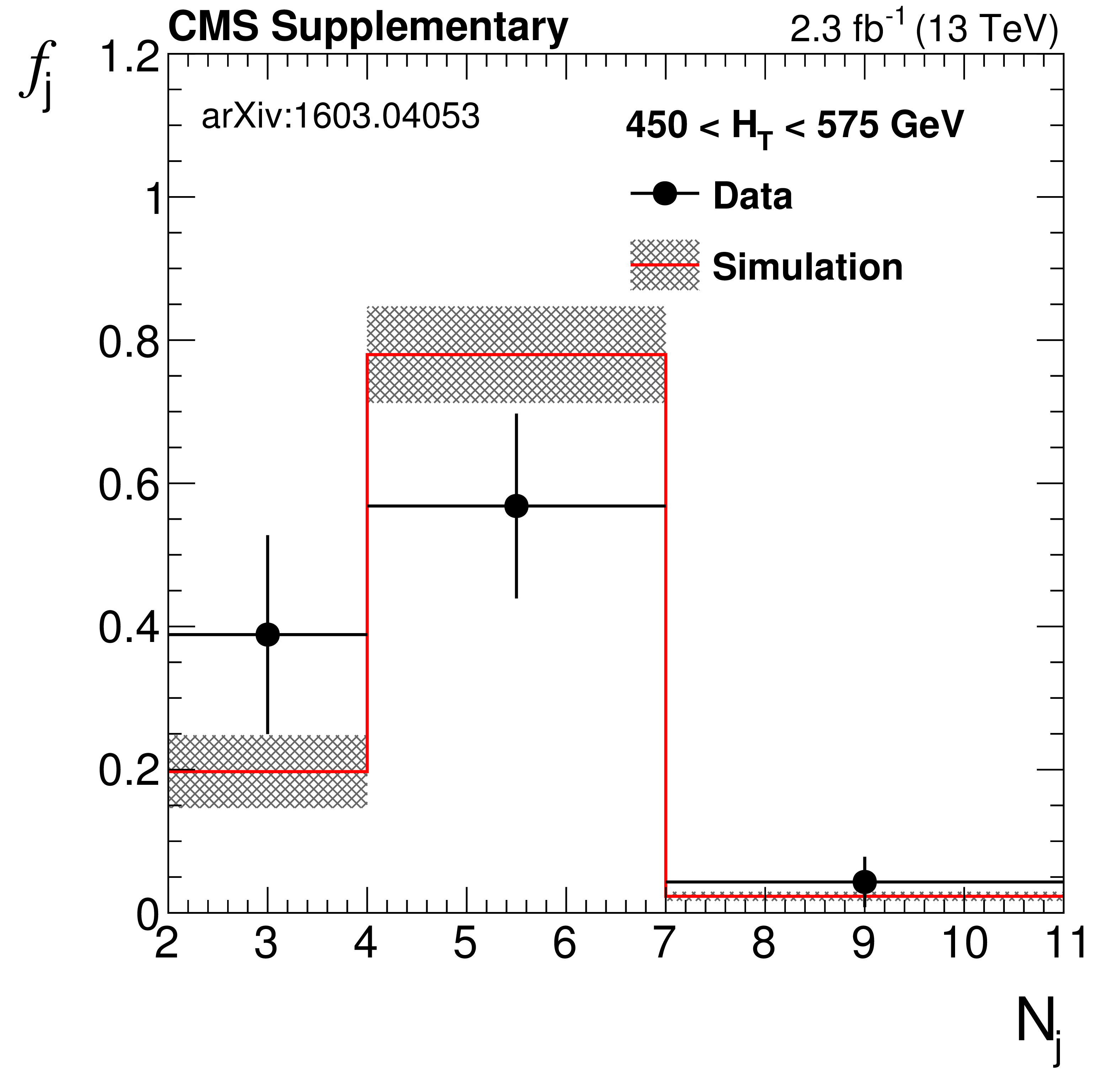
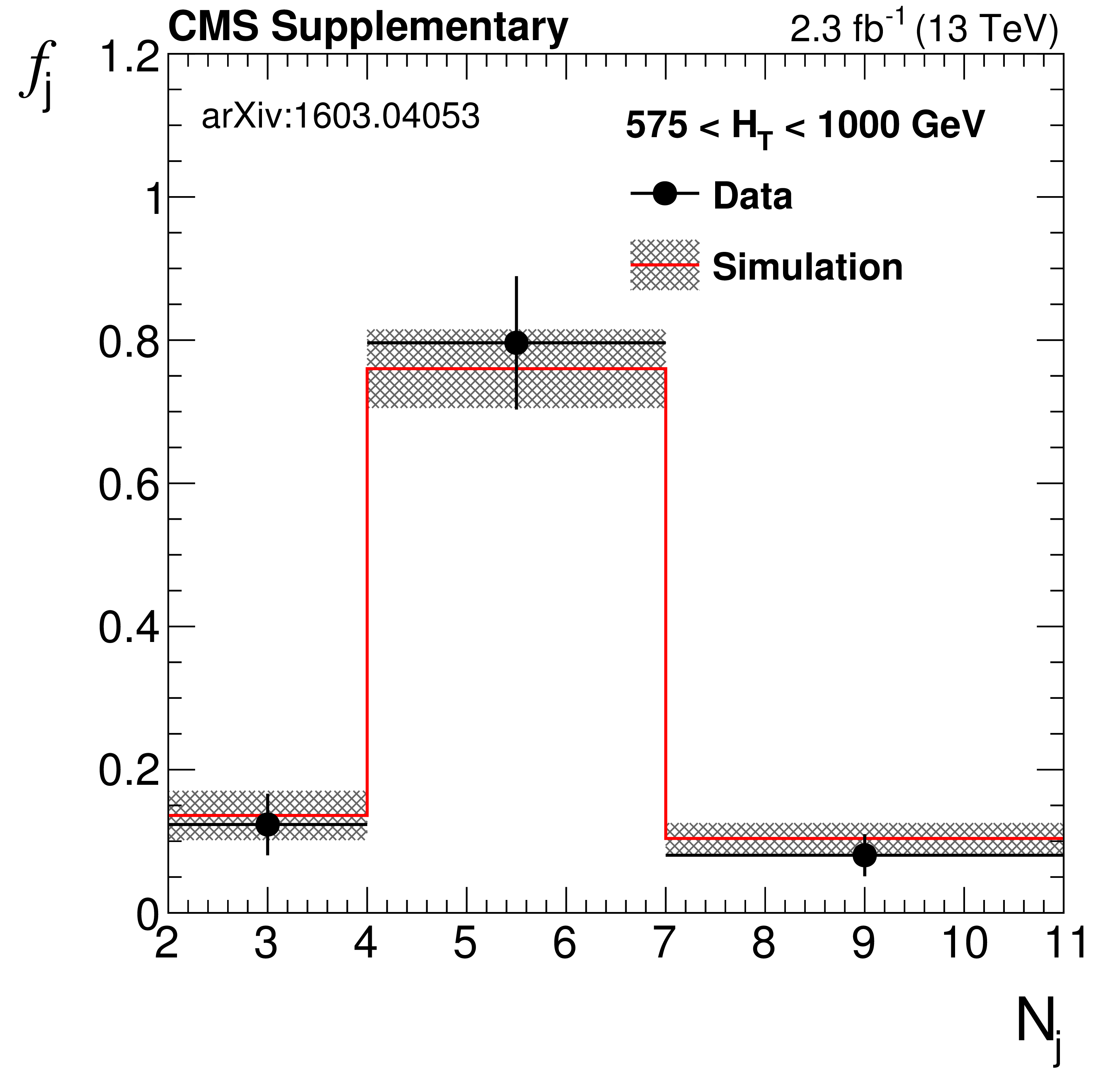
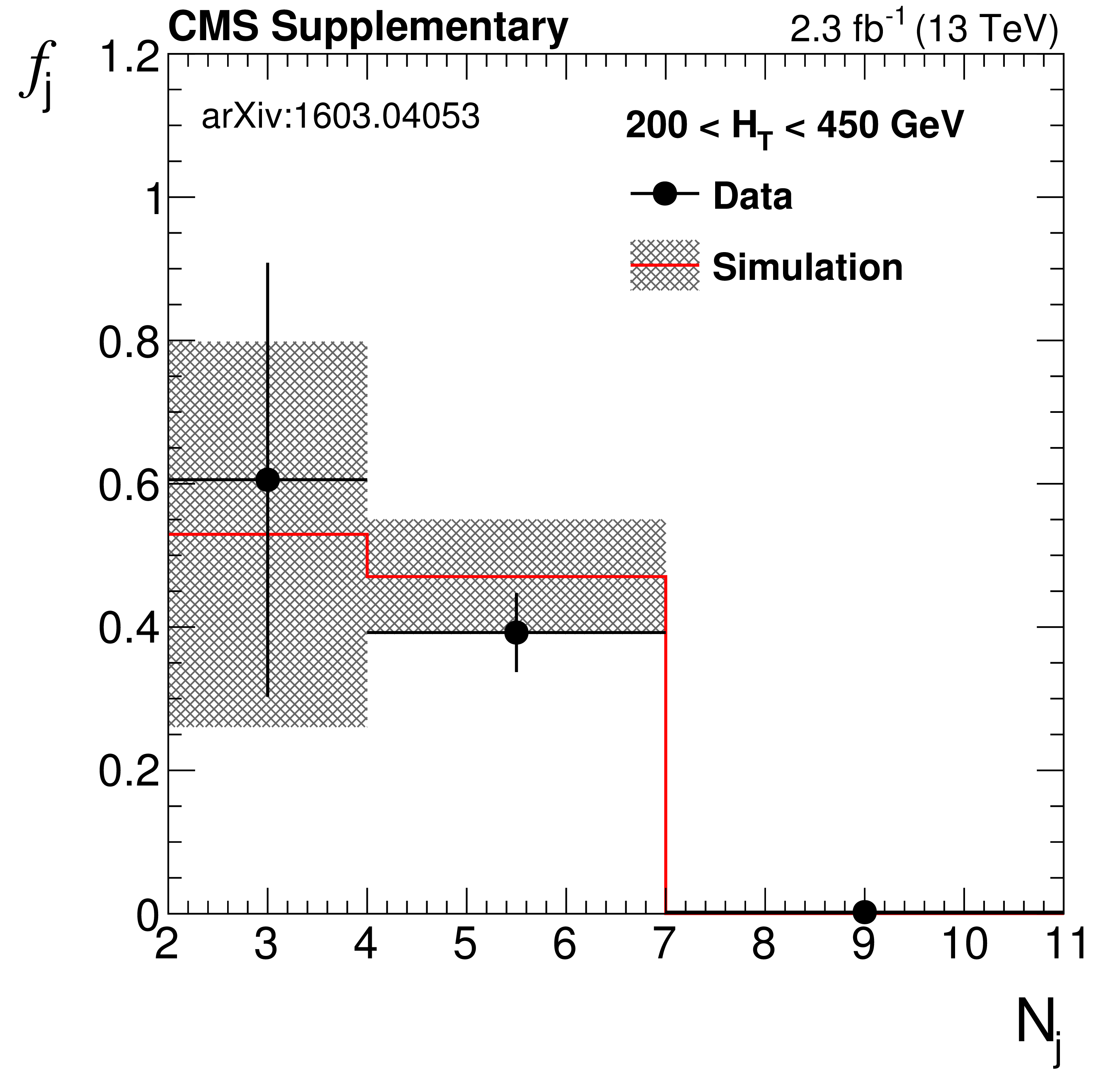
Fraction $f_{\mathrm {j}}$ of multijet events falling in bins of number of jets $ {N_{\mathrm {j}}} $ (a) and fraction $r_{\mathrm{ b} }$ of events falling in bins of number of b-tagged jets $ {N_{\mathrm{ b} }} $ (b). Values of $f_{\mathrm {j}}$ and $r_{\mathrm{ b} }$ are measured in data, after requiring $ {\Delta \phi _{\text {min}}} <$ 0.3 and 100 $< {M_{\mathrm {T2}}} <$ 200 GeV. The bands represent both statistical and systematic uncertainties of the estimate from simulation. |
png pdf |
Figure 6-b:
Fraction $f_{\mathrm {j}}$ of multijet events falling in bins of number of jets $ {N_{\mathrm {j}}} $ (a) and fraction $r_{\mathrm{ b} }$ of events falling in bins of number of b-tagged jets $ {N_{\mathrm{ b} }} $ (b). Values of $f_{\mathrm {j}}$ and $r_{\mathrm{ b} }$ are measured in data, after requiring $ {\Delta \phi _{\text {min}}} <$ 0.3 and 100 $< {M_{\mathrm {T2}}} <$ 200 GeV. The bands represent both statistical and systematic uncertainties of the estimate from simulation. |
png pdf |
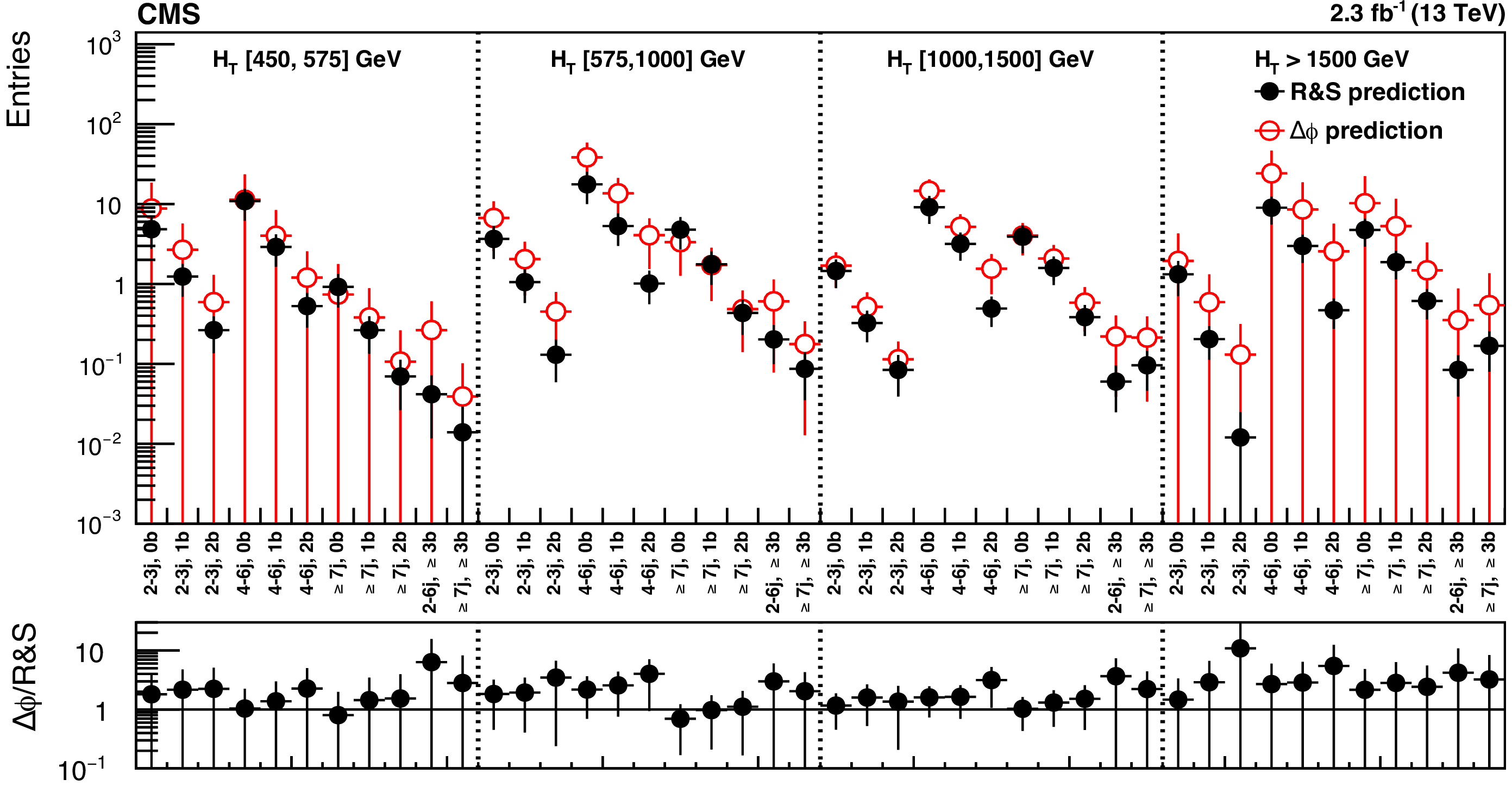
Figure 7:
Comparison of the predictions of the multijet background in the topological regions ($ {M_{\mathrm {T2}}} >$ 200 GeV) from the R&S method and the $ {\Delta \phi _{\text {min}}} $ ratio method. The uncertainties are combined statistical and systematic. Within each of the four $ {H_{\mathrm {T}}} $ categories, the estimates from the $ {\Delta \phi _{\text {min}}} $ ratio method are correlated as they are derived from the same fit to the $ {\Delta \phi _{\text {min}}} $ ratio data. |
png pdf |
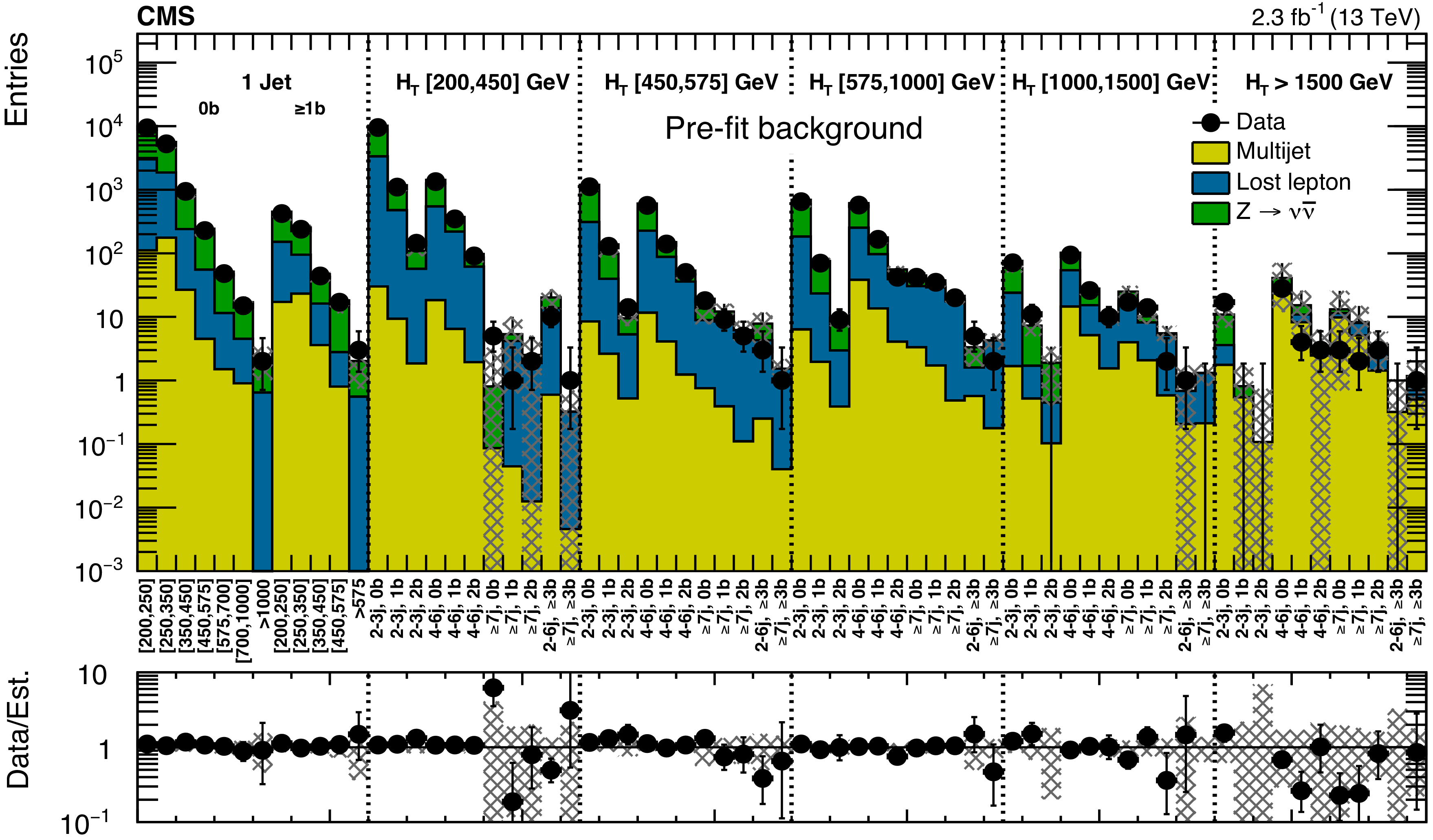
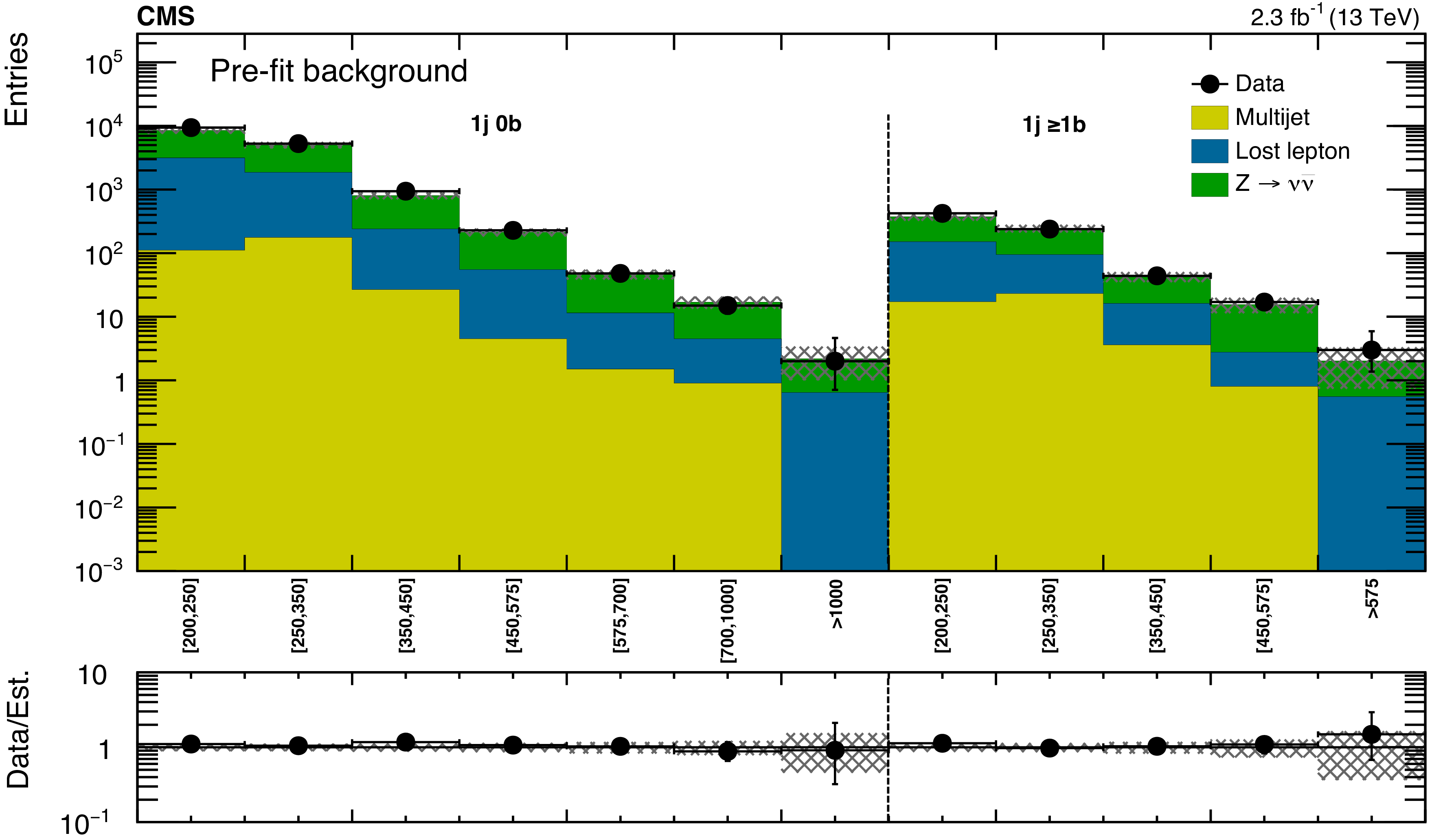
Figure 8-a:
(a) Comparison of estimated background (pre-fit) and observed data events in each topological region. The results shown for $ {N_{\mathrm {j}}} =$ 1 correspond to the monojet search regions binned in jet $ {p_{\mathrm {T}}} $. Hatched bands represent the full uncertainty in the background estimate. (b) Comparison for individual $ {M_{\mathrm {T2}}} $ signal bins in the medium $ {H_{\mathrm {T}}} $ region. On the $x$-axis, the $ {M_{\mathrm {T2}}} $ bin of each signal region is shown (in GeV), except where the notations j, b indicate $ {N_{\mathrm {j}}} $, $ {N_{\mathrm{ b} }} $ labeling. Bins with no entry for data have an observed count of 0 events. |

png pdf |
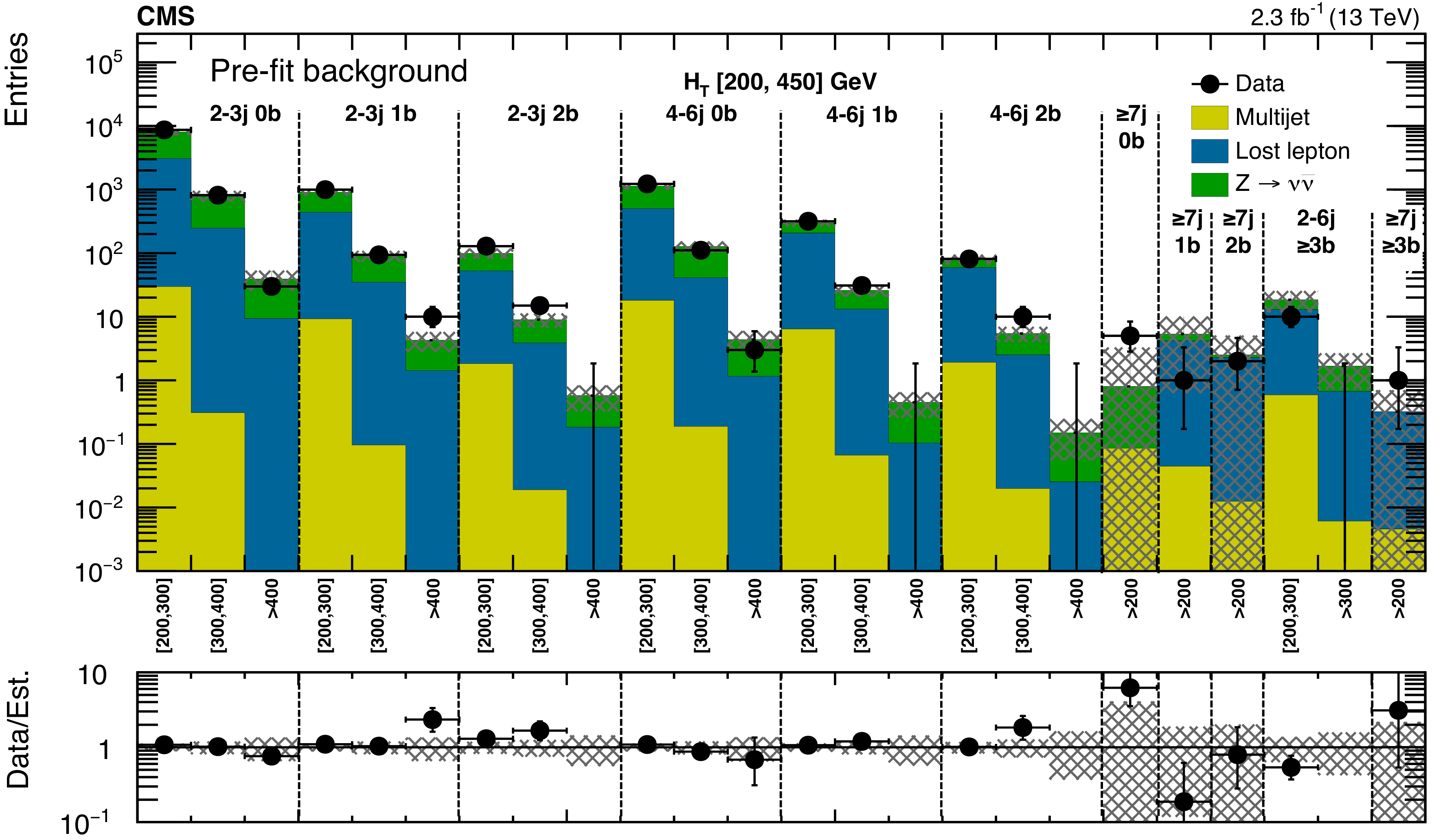
Figure 8-b:
(a) Comparison of estimated background (pre-fit) and observed data events in each topological region. The results shown for $ {N_{\mathrm {j}}} =$ 1 correspond to the monojet search regions binned in jet $ {p_{\mathrm {T}}} $. Hatched bands represent the full uncertainty in the background estimate. (b) Comparison for individual $ {M_{\mathrm {T2}}} $ signal bins in the medium $ {H_{\mathrm {T}}} $ region. On the $x$-axis, the $ {M_{\mathrm {T2}}} $ bin of each signal region is shown (in GeV), except where the notations j, b indicate $ {N_{\mathrm {j}}} $, $ {N_{\mathrm{ b} }} $ labeling. Bins with no entry for data have an observed count of 0 events. |

png pdf |
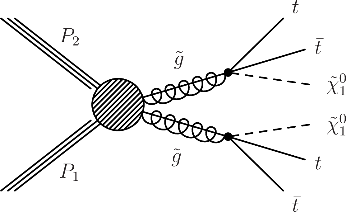
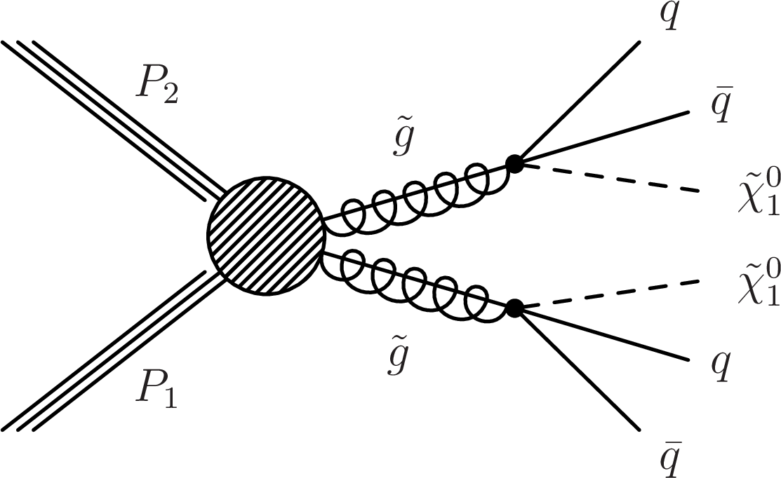
Figure 9-a:
(a,b,c) Diagrams for the three considered scenarios of gluino-mediated bottom squark, top squark, and light flavor squark production. The depicted three-body decays are assumed to proceed through off-shell squarks. |
png pdf |
Figure 9-b:
(a,b,c) Diagrams for the three considered scenarios of gluino-mediated bottom squark, top squark, and light flavor squark production. The depicted three-body decays are assumed to proceed through off-shell squarks. |
png pdf |
Figure 9-c:
(a,b,c) Diagrams for the three considered scenarios of gluino-mediated bottom squark, top squark, and light flavor squark production. The depicted three-body decays are assumed to proceed through off-shell squarks. |

png pdf |
Figure 9-d:
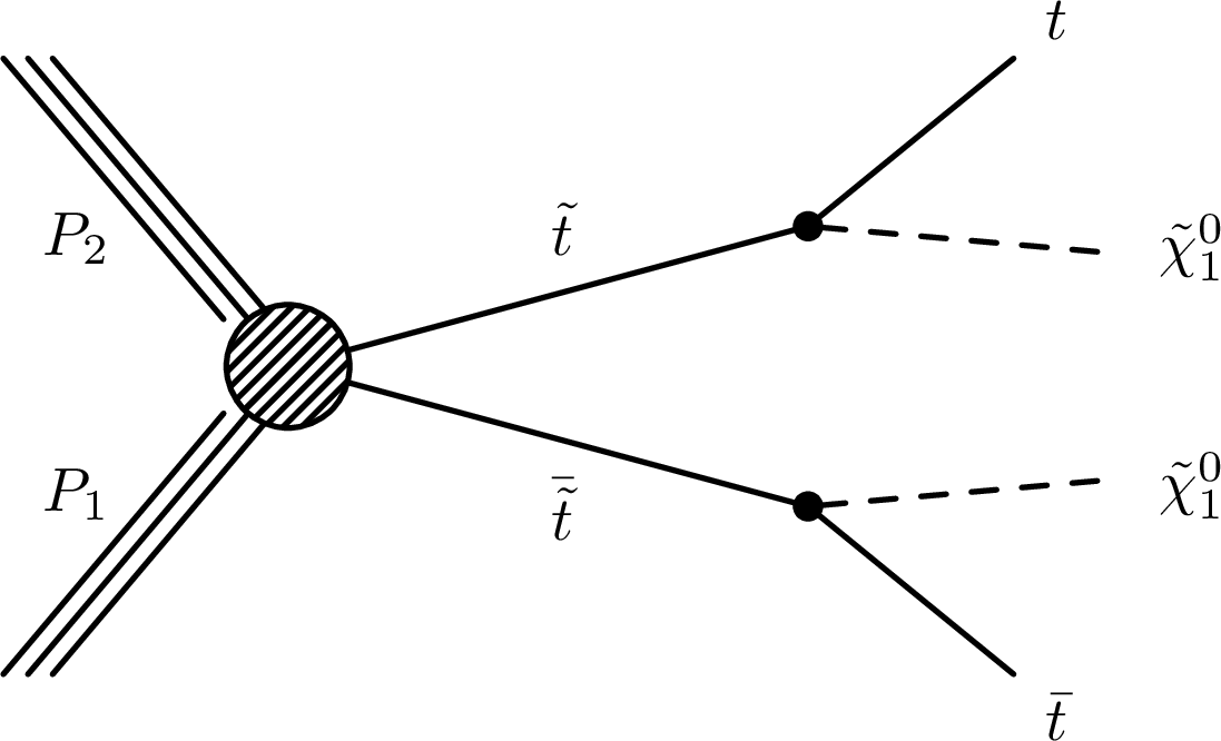
(d,e,f) The results of this search are also used to constrain simplified models of bottom squark, top squark, and light flavor squark pair production. |
png pdf |
Figure 9-e:
(d,e,f) The results of this search are also used to constrain simplified models of bottom squark, top squark, and light flavor squark pair production. |

png pdf |
Figure 9-f:
(d,e,f) The results of this search are also used to constrain simplified models of bottom squark, top squark, and light flavor squark pair production. |
png pdf |
Figure 10-a:
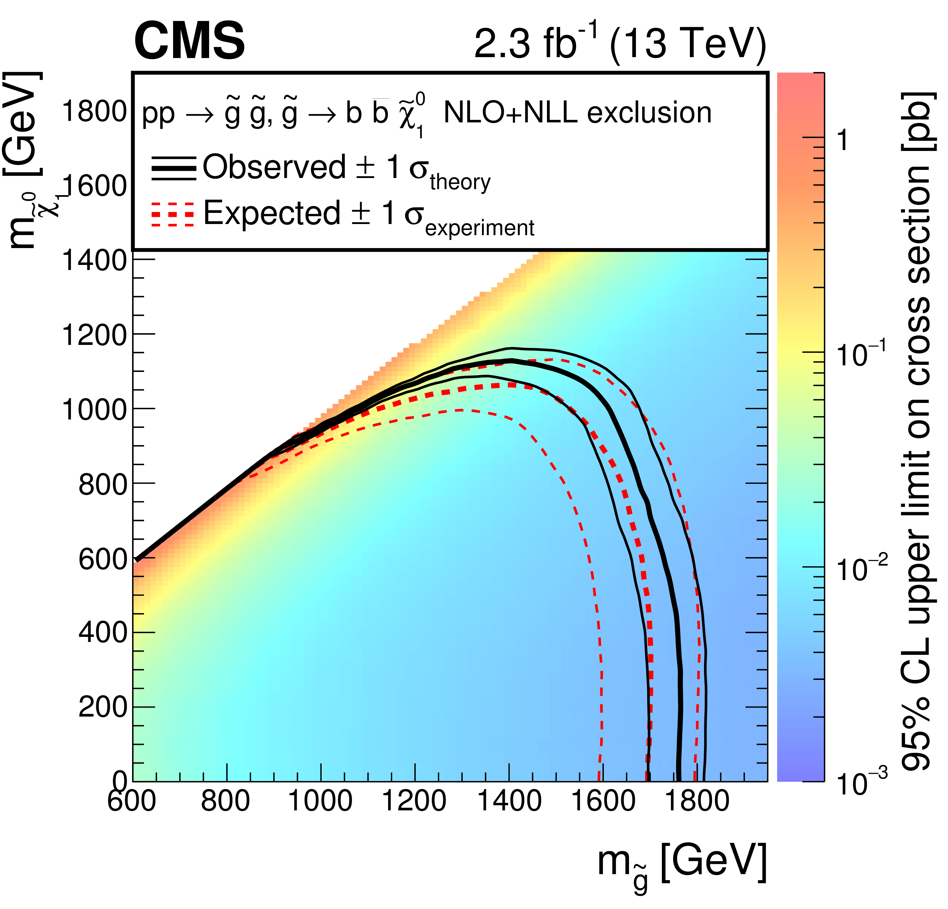
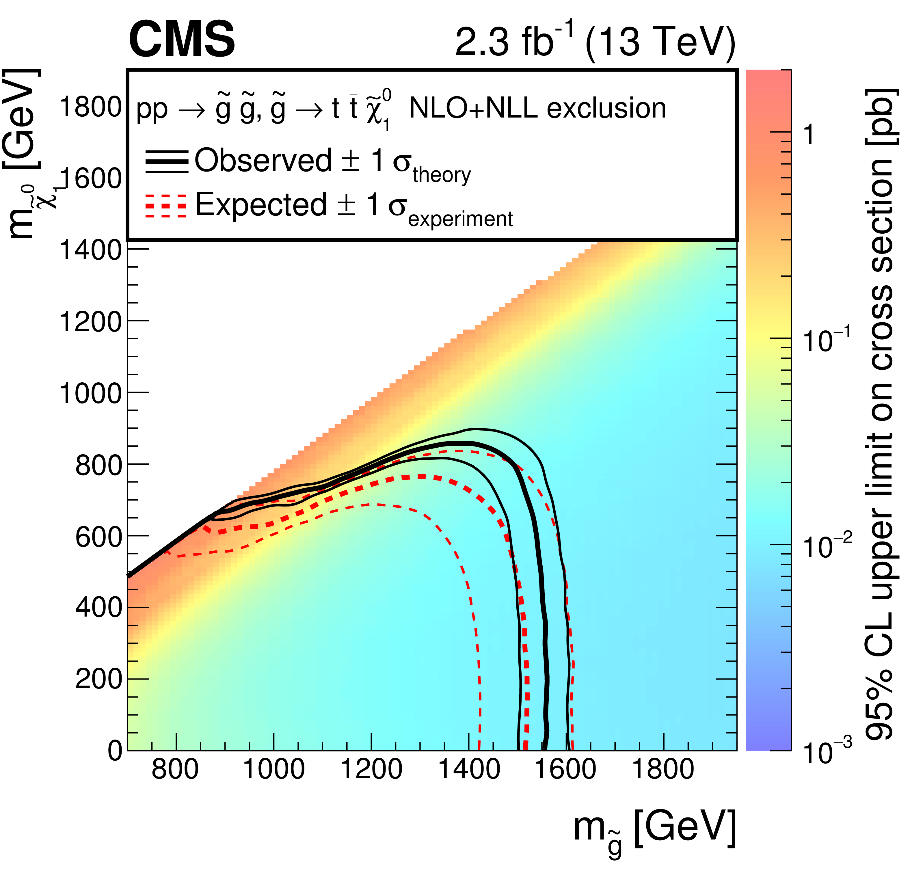
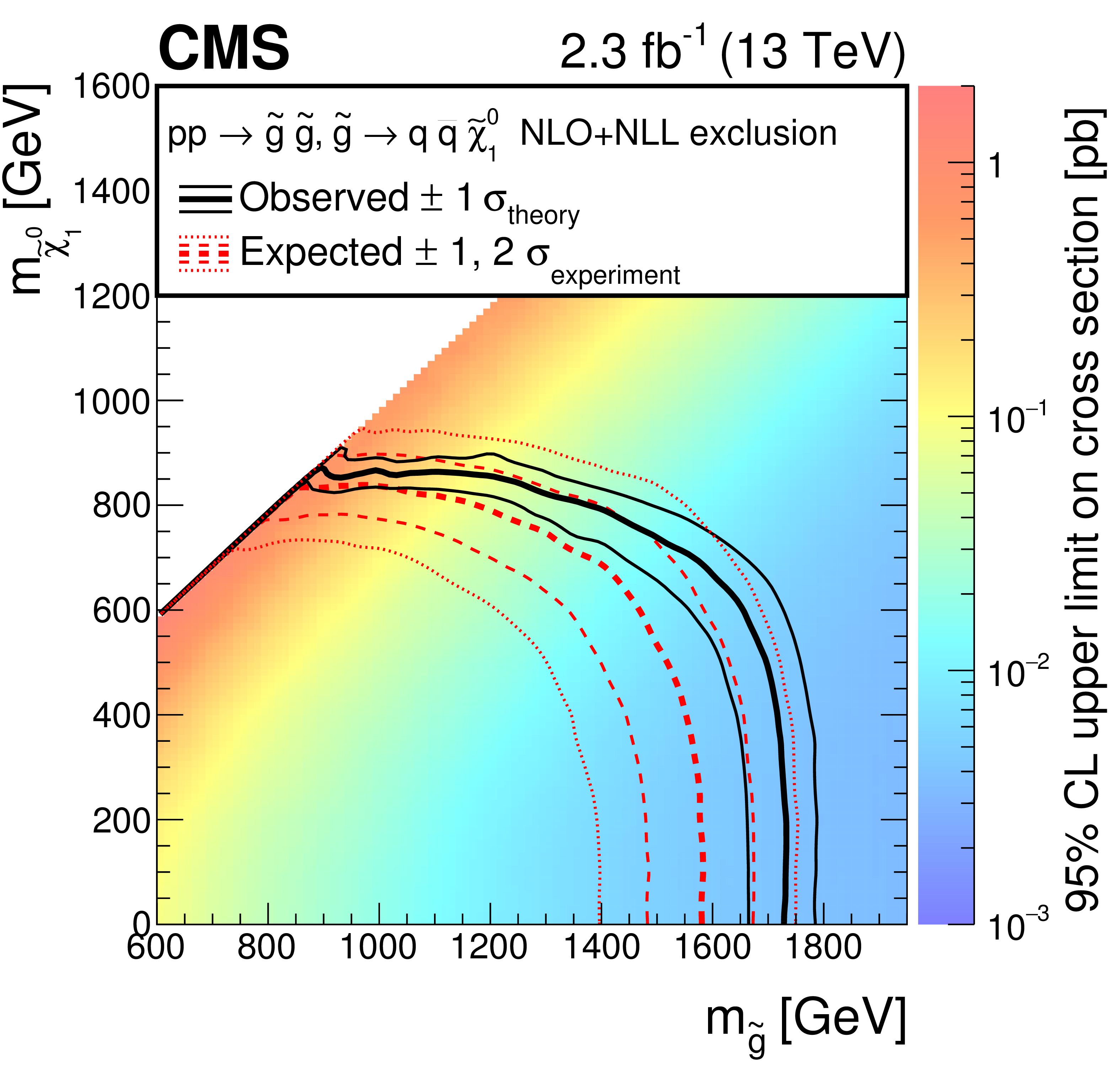
Exclusion limits at 95% CL on the cross sections for gluino-mediated bottom squark production (a), gluino-mediated top squark production (b), and gluino-mediated light-flavor squark production (c). The area to the left of and below the thick black curve represents the observed exclusion region, while the dashed red lines indicate the expected limits and their $\pm $1 $\sigma _{\text {experiment}}$ standard deviation uncertainties. For the squark-pair production plot, the $\pm $2 standard deviation uncertainties are also shown. The thin black lines show the effect of the theoretical uncertainties $\sigma _{\text {theory}}$ on the signal cross section. |
png pdf |
Figure 10-b:
Exclusion limits at 95% CL on the cross sections for gluino-mediated bottom squark production (a), gluino-mediated top squark production (b), and gluino-mediated light-flavor squark production (c). The area to the left of and below the thick black curve represents the observed exclusion region, while the dashed red lines indicate the expected limits and their $\pm $1 $\sigma _{\text {experiment}}$ standard deviation uncertainties. For the squark-pair production plot, the $\pm $2 standard deviation uncertainties are also shown. The thin black lines show the effect of the theoretical uncertainties $\sigma _{\text {theory}}$ on the signal cross section. |
png pdf |
Figure 10-c:
Exclusion limits at 95% CL on the cross sections for gluino-mediated bottom squark production (a), gluino-mediated top squark production (b), and gluino-mediated light-flavor squark production (c). The area to the left of and below the thick black curve represents the observed exclusion region, while the dashed red lines indicate the expected limits and their $\pm $1 $\sigma _{\text {experiment}}$ standard deviation uncertainties. For the squark-pair production plot, the $\pm $2 standard deviation uncertainties are also shown. The thin black lines show the effect of the theoretical uncertainties $\sigma _{\text {theory}}$ on the signal cross section. |
png pdf |
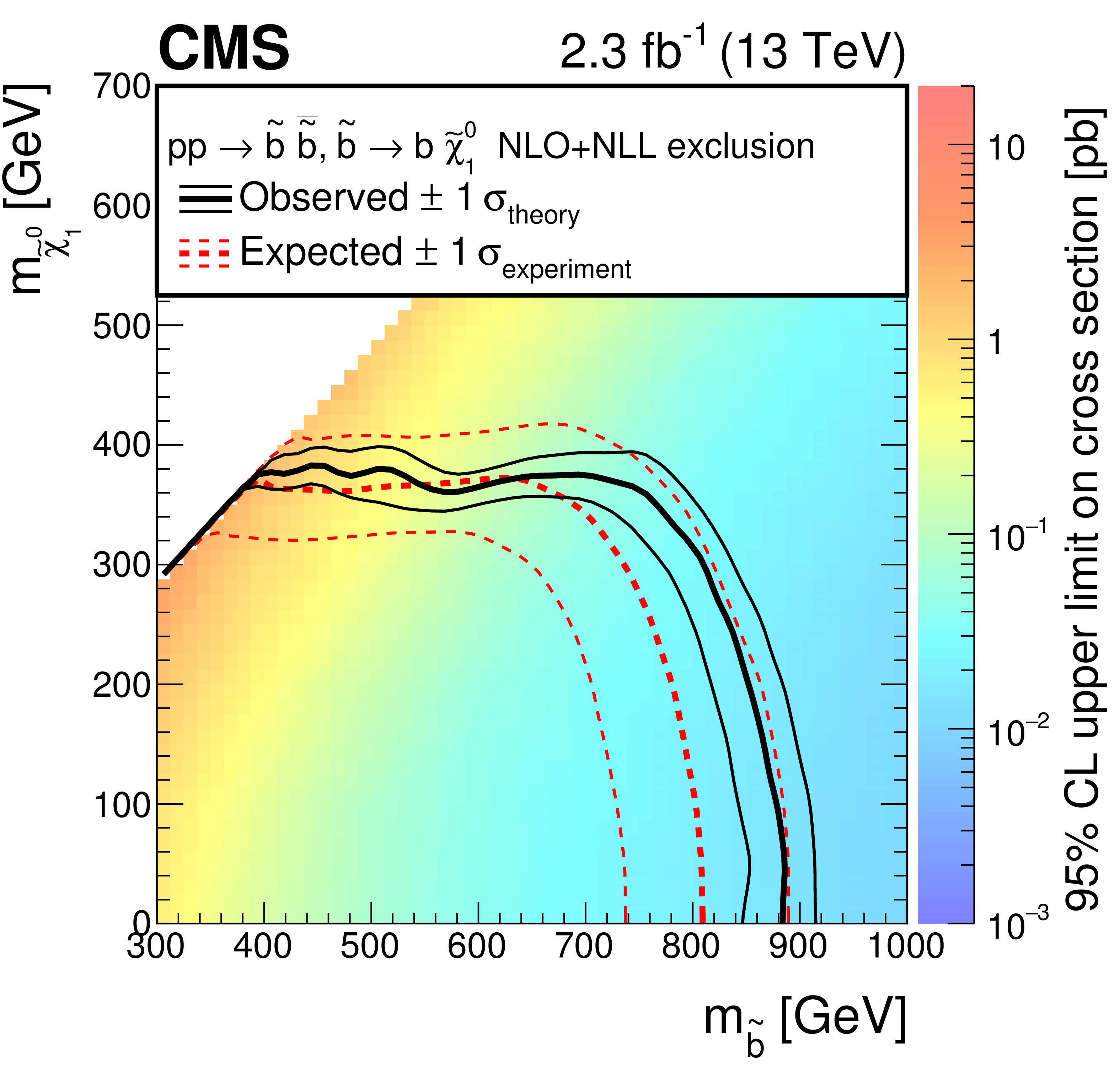
Figure 11-a:
Exclusion limit at 95% CL on the cross sections for bottom squark pair production (a), top squark pair production (b), and light-flavor squark pair production (c). The area to the left of and below the thick black curve represents the observed exclusion region, while the dashed red lines indicate the expected limits and their $\pm $1 $\sigma _{\text {experiment}}$ standard deviation uncertainties. The thin black lines show the effect of the theoretical uncertainties $\sigma _{\text {theory}}$ on the signal cross section. The white diagonal band in the upper right plot corresponds to the region $ {| m_{\mathrm{ \tilde{t}} }-m_{\mathrm{ t } }-m_{\mathrm {LSP}} | }< 25$ GeV . Here the efficiency of the selection is a strong function of $m_{\mathrm{ \tilde{t}} }-m_{\mathrm {LSP}}$, and as a result the precise determination of the cross section upper limit is uncertain because of the finite granularity of the available MC samples in this region of the ($m_{\mathrm{ \tilde{t}} }$, $m_{\mathrm {LSP}}$) plane. |

png pdf |
Figure 11-b:
Exclusion limit at 95% CL on the cross sections for bottom squark pair production (a), top squark pair production (b), and light-flavor squark pair production (c). The area to the left of and below the thick black curve represents the observed exclusion region, while the dashed red lines indicate the expected limits and their $\pm $1 $\sigma _{\text {experiment}}$ standard deviation uncertainties. The thin black lines show the effect of the theoretical uncertainties $\sigma _{\text {theory}}$ on the signal cross section. The white diagonal band in the upper right plot corresponds to the region $ {| m_{\mathrm{ \tilde{t}} }-m_{\mathrm{ t } }-m_{\mathrm {LSP}} | }< 25$ GeV . Here the efficiency of the selection is a strong function of $m_{\mathrm{ \tilde{t}} }-m_{\mathrm {LSP}}$, and as a result the precise determination of the cross section upper limit is uncertain because of the finite granularity of the available MC samples in this region of the ($m_{\mathrm{ \tilde{t}} }$, $m_{\mathrm {LSP}}$) plane. |
png pdf |
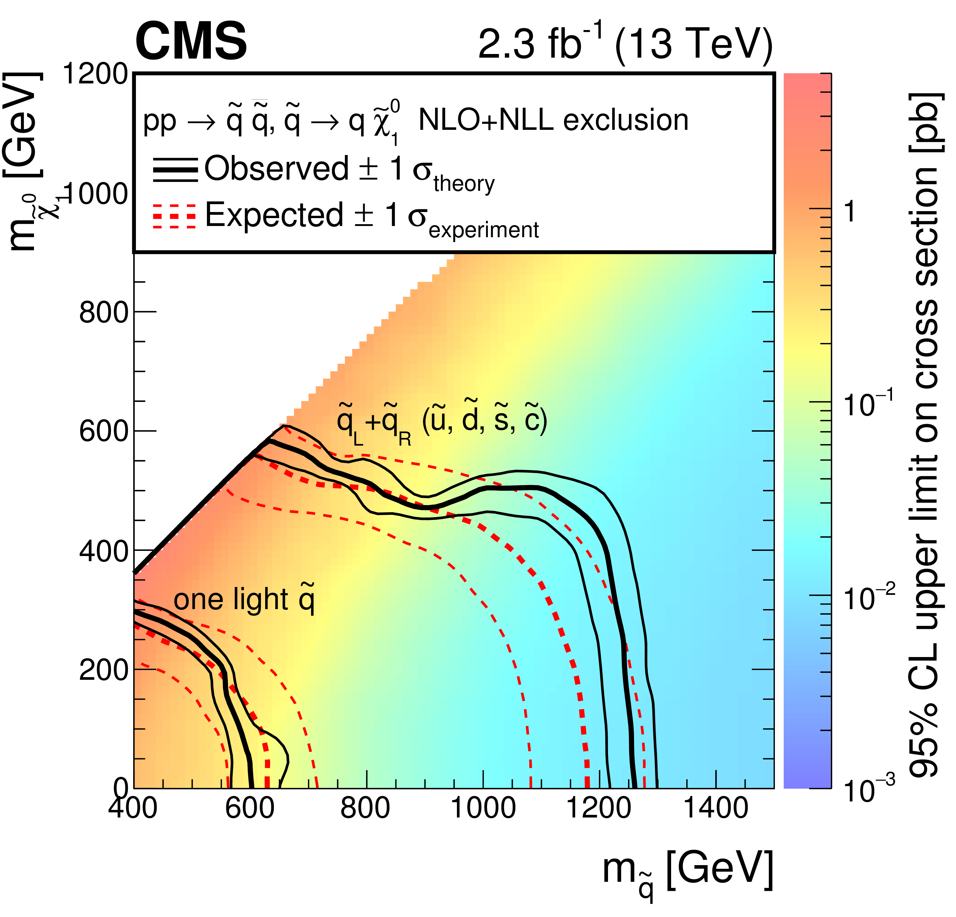
Figure 11-c:
Exclusion limit at 95% CL on the cross sections for bottom squark pair production (a), top squark pair production (b), and light-flavor squark pair production (c). The area to the left of and below the thick black curve represents the observed exclusion region, while the dashed red lines indicate the expected limits and their $\pm $1 $\sigma _{\text {experiment}}$ standard deviation uncertainties. The thin black lines show the effect of the theoretical uncertainties $\sigma _{\text {theory}}$ on the signal cross section. The white diagonal band in the upper right plot corresponds to the region $ {| m_{\mathrm{ \tilde{t}} }-m_{\mathrm{ t } }-m_{\mathrm {LSP}} | }< 25$ GeV . Here the efficiency of the selection is a strong function of $m_{\mathrm{ \tilde{t}} }-m_{\mathrm {LSP}}$, and as a result the precise determination of the cross section upper limit is uncertain because of the finite granularity of the available MC samples in this region of the ($m_{\mathrm{ \tilde{t}} }$, $m_{\mathrm {LSP}}$) plane. |
png pdf |
Figure A1-a:
(a) Comparison of the estimated background (pre-fit) and observed data events in each signal bin in the monojet region. On the $x$-axis, the jet $ p_{\mathrm{T}} $ binning is shown (in GeV). Hatched bands represent the full uncertainty in the background estimate. (b) Same for the very-low-$ H_{\mathrm{T}} $ region. On the $x$-axis, the $M_{\mathrm{T2}}$ binning is shown (in GeV). Bins with no entry for data have an observed count of 0 events. |
png pdf |
Figure A1-b:
(a) Comparison of the estimated background (pre-fit) and observed data events in each signal bin in the monojet region. On the $x$-axis, the jet $ p_{\mathrm{T}} $ binning is shown (in GeV). Hatched bands represent the full uncertainty in the background estimate. (b) Same for the very-low-$ H_{\mathrm{T}} $ region. On the $x$-axis, the $M_{\mathrm{T2}}$ binning is shown (in GeV). Bins with no entry for data have an observed count of 0 events. |
png pdf |
Figure A2-a:
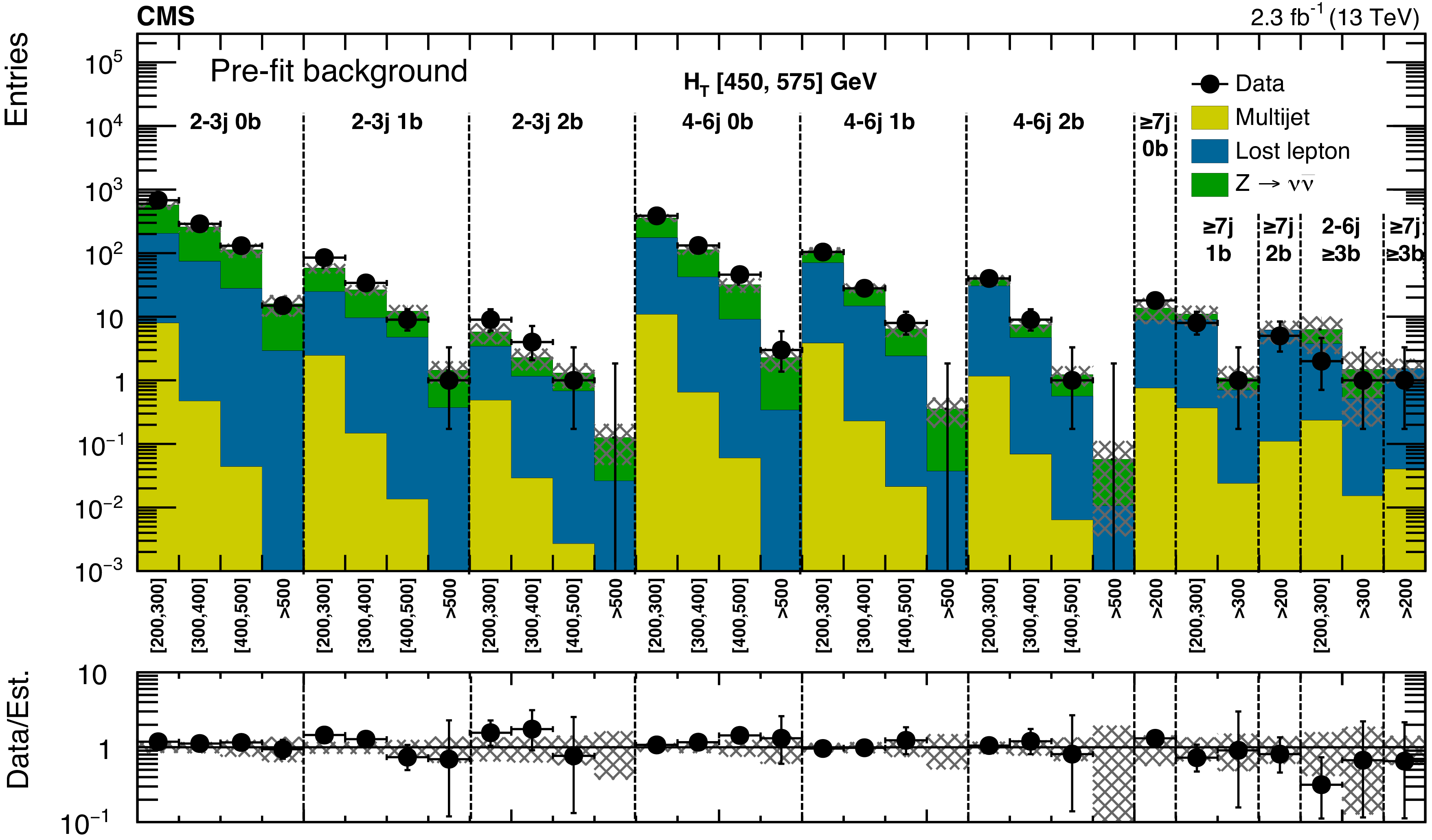
(a) Comparison of the estimated background (pre-fit) and observed data events in each signal bin in the low-$ H_{\mathrm{T}} $ region. Hatched bands represent the full uncertainty in the background estimate. (b) Same for the medium-$ H_{\mathrm{T}} $ region. On the $x$-axis, the $M_{\mathrm{T2}}$ binning is shown (in GeV). Bins with no entry for data have an observed count of 0 events. |
png pdf |
Figure A2-b:
(a) Comparison of the estimated background (pre-fit) and observed data events in each signal bin in the low-$ H_{\mathrm{T}} $ region. Hatched bands represent the full uncertainty in the background estimate. (b) Same for the medium-$ H_{\mathrm{T}} $ region. On the $x$-axis, the $M_{\mathrm{T2}}$ binning is shown (in GeV). Bins with no entry for data have an observed count of 0 events. |
png pdf |
Figure A3-a:
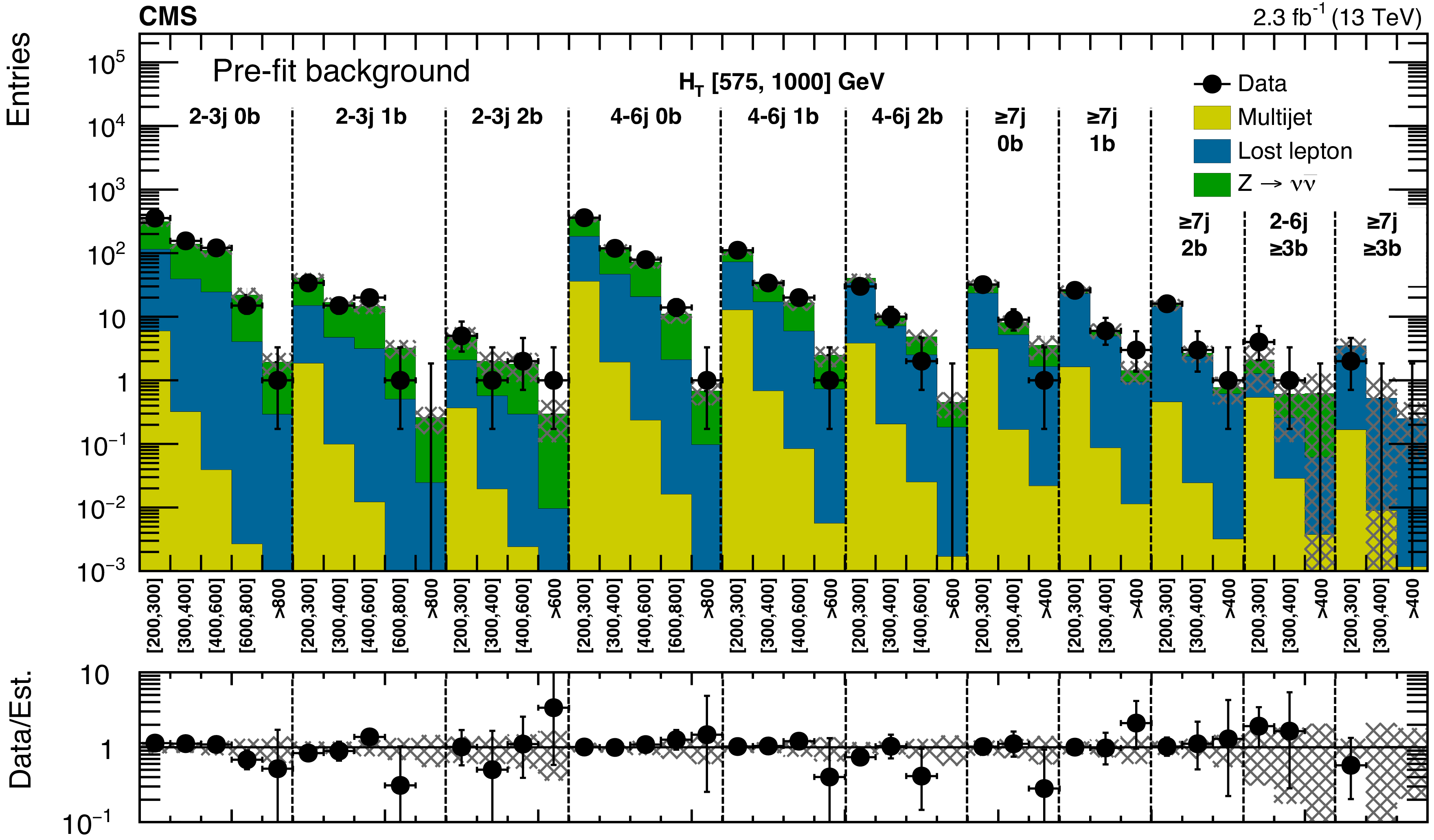
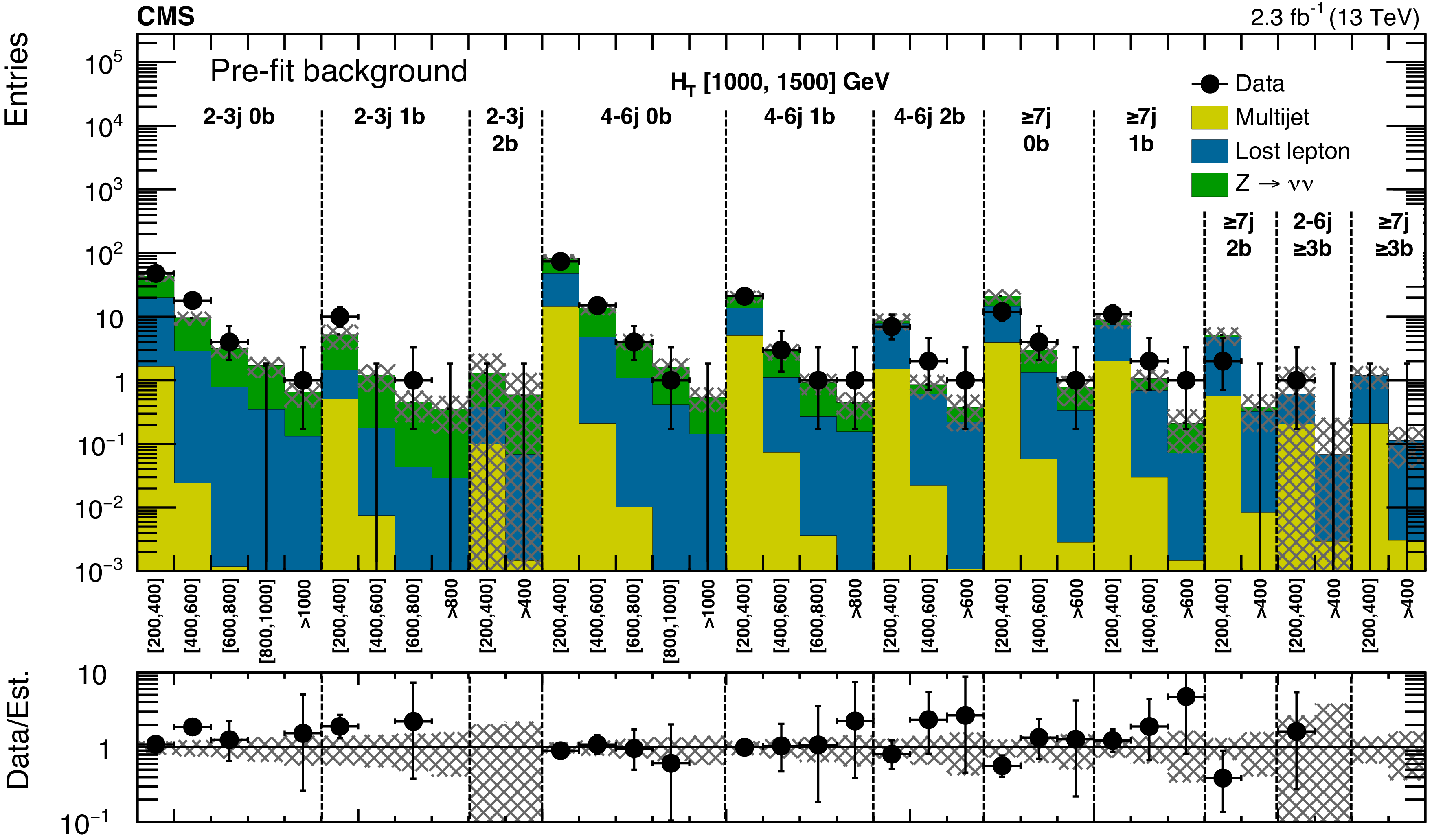
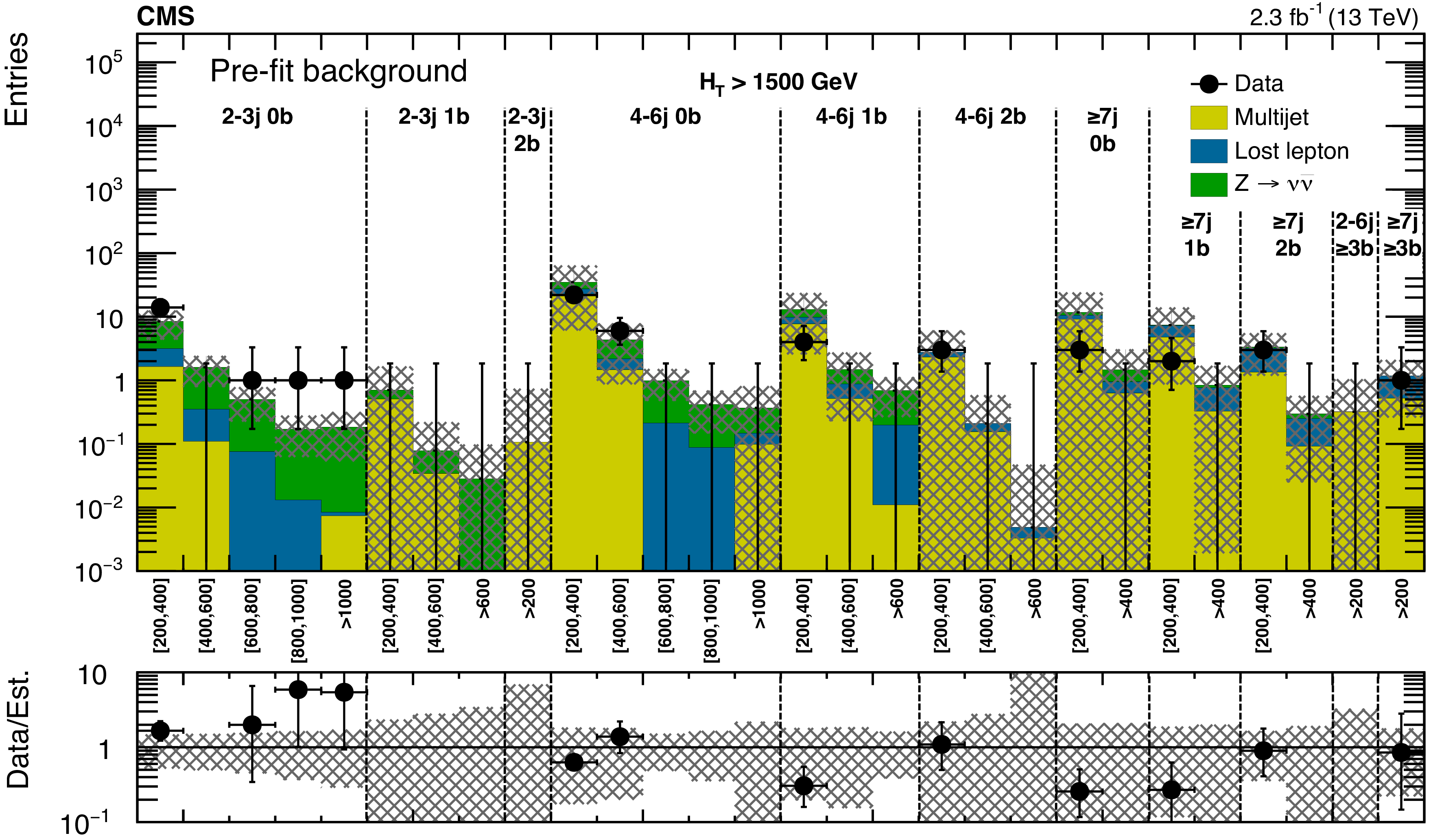
(a) Comparison of the estimated background (pre-fit) and observed data events in each signal bin in the high-$ H_{\mathrm{T}} $ region. Hatched bands represent the full uncertainty in the background estimate. (b) Same for the extreme-$ H_{\mathrm{T}} $ region. On the $x$-axis, the $M_{\mathrm{T2}}$ binning is shown (in GeV). Bins with no entry for data have an observed count of 0 events. |
png pdf |
Figure A3-b:
(a) Comparison of the estimated background (pre-fit) and observed data events in each signal bin in the high-$ H_{\mathrm{T}} $ region. Hatched bands represent the full uncertainty in the background estimate. (b) Same for the extreme-$ H_{\mathrm{T}} $ region. On the $x$-axis, the $M_{\mathrm{T2}}$ binning is shown (in GeV). Bins with no entry for data have an observed count of 0 events. |
png pdf |
Figure A4:
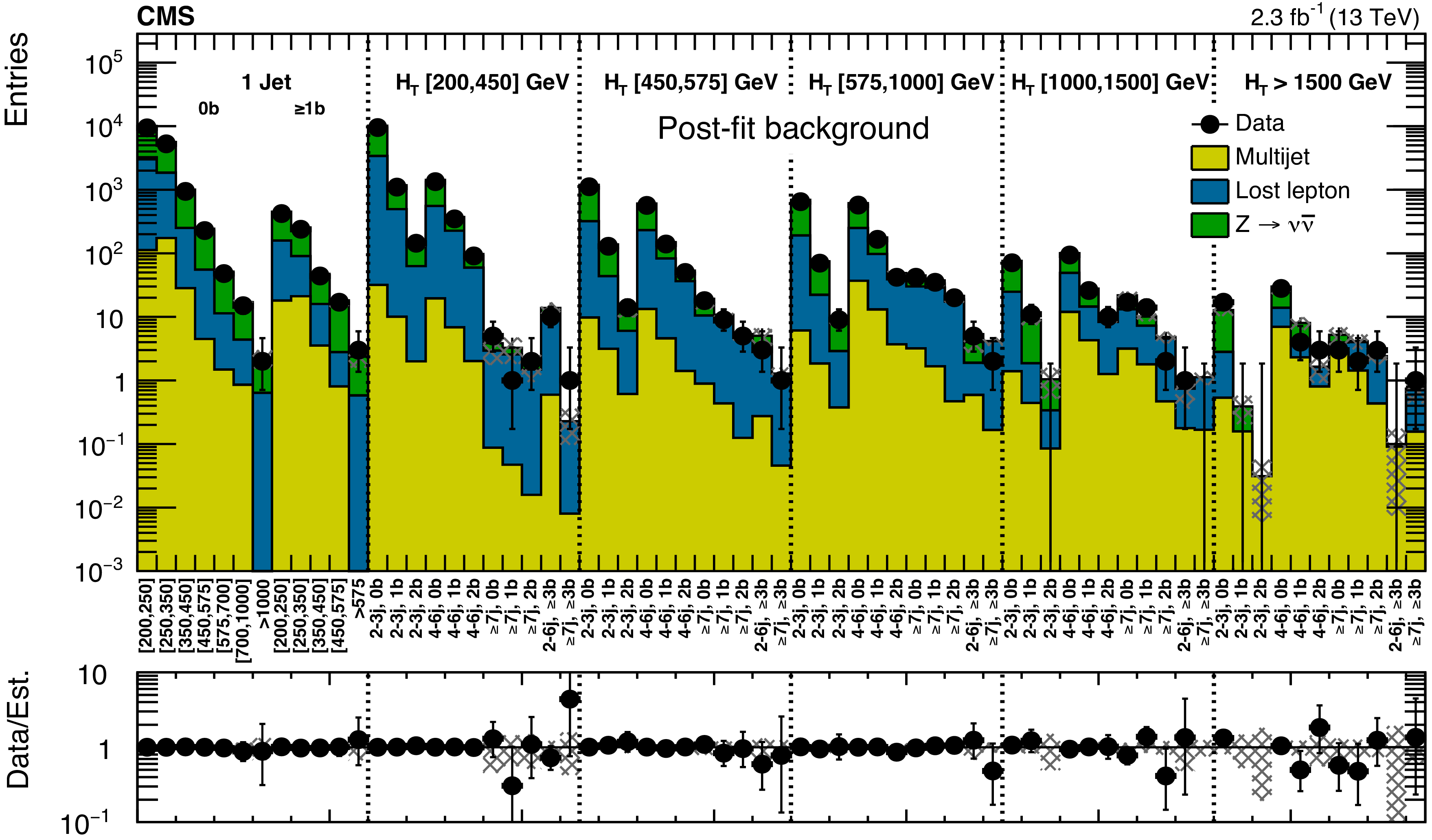
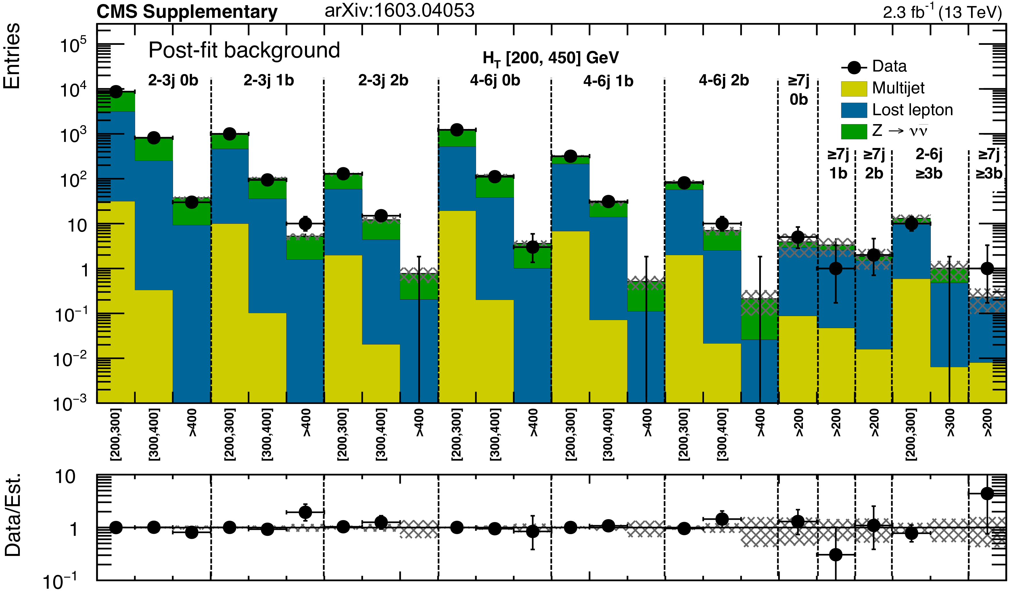
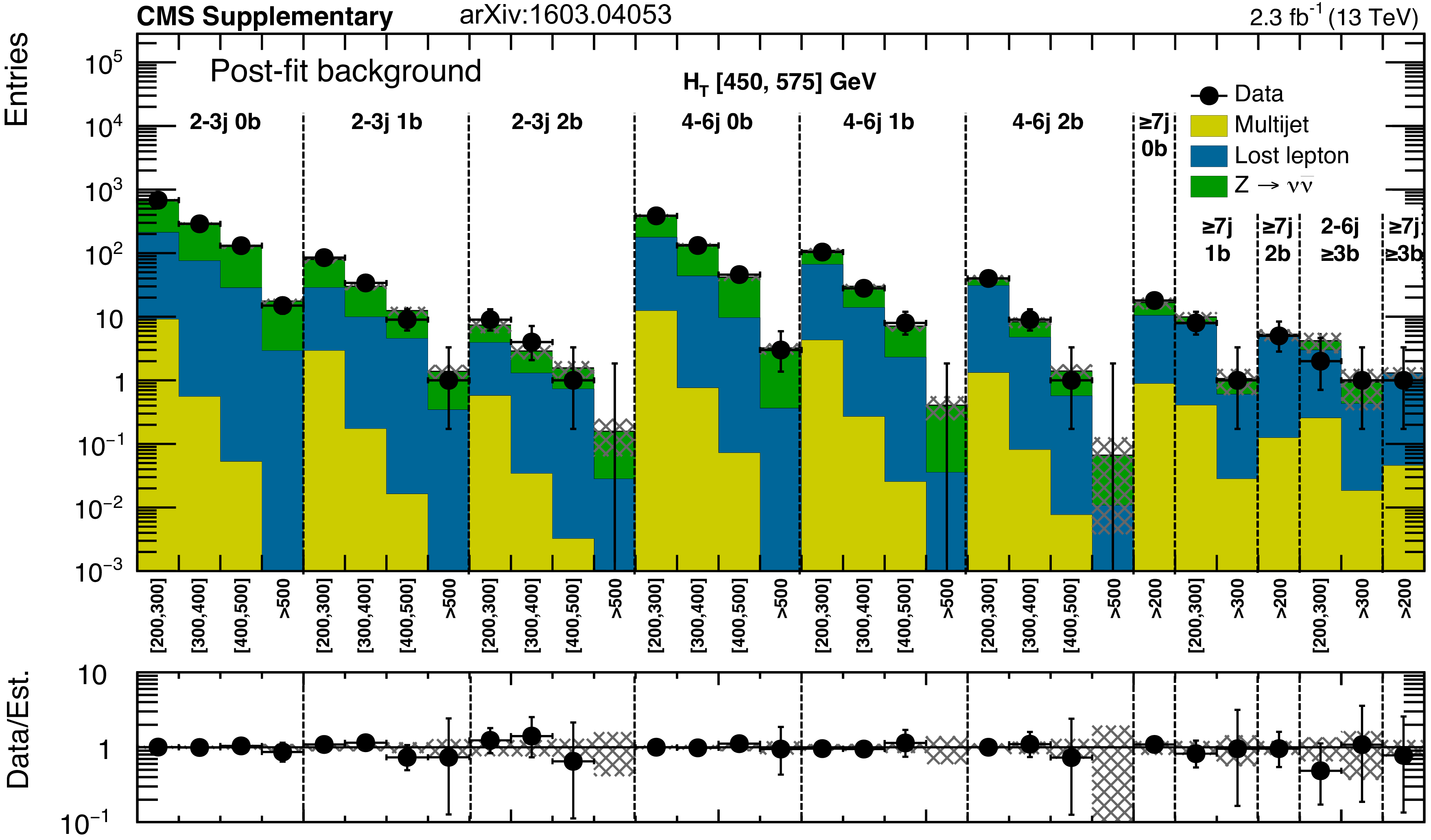
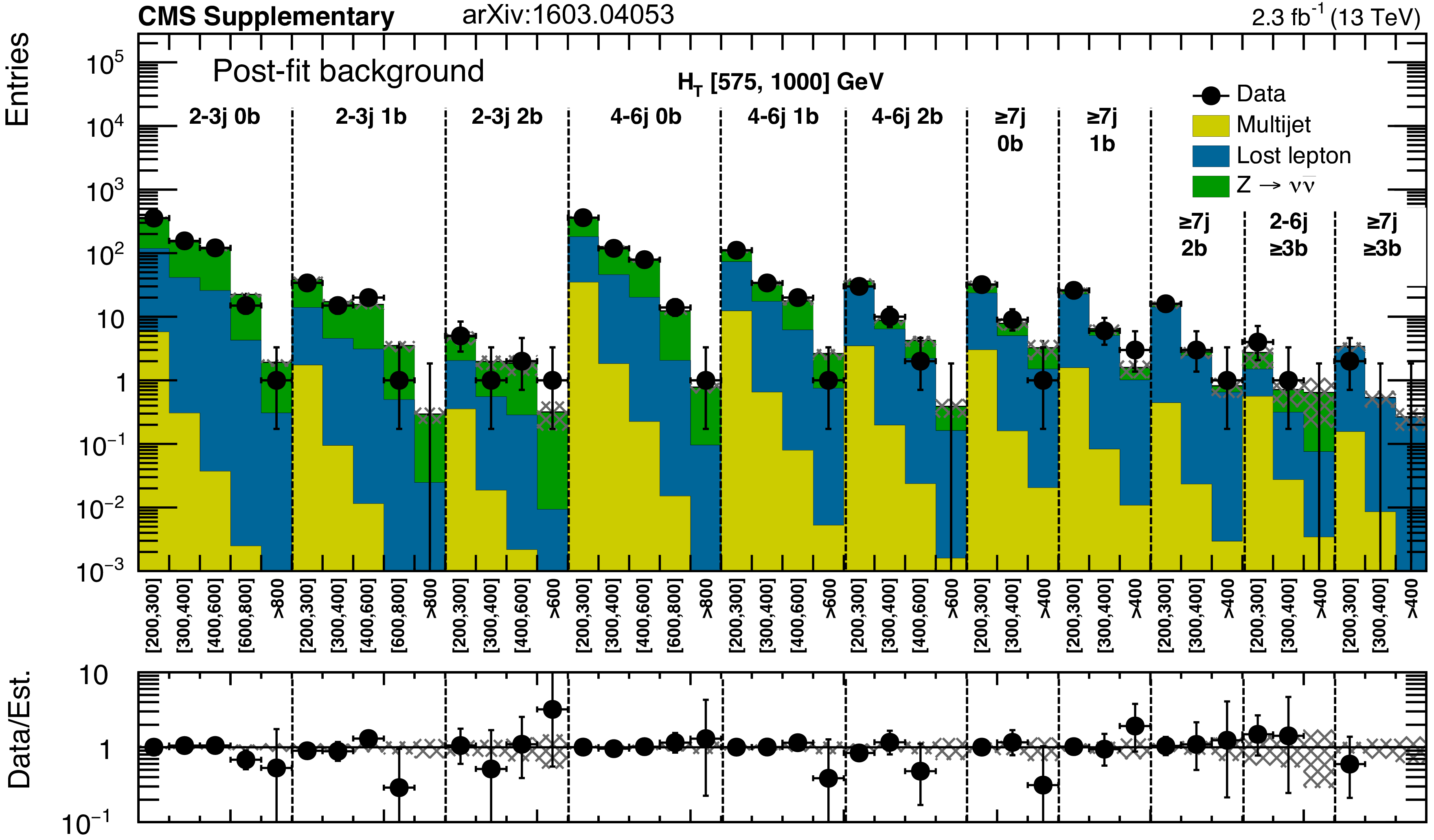
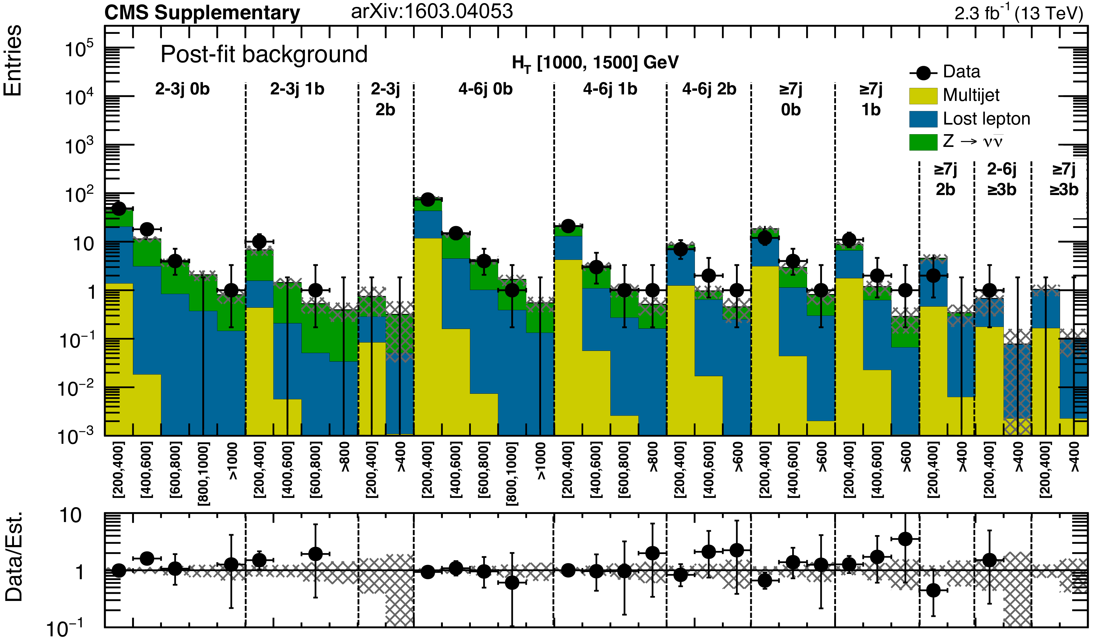
Comparison of post-fit background prediction and observed data events in each topological region. Hatched bands represent the post-fit uncertainty in the background prediction. For the monojet region, on the $x$-axis, the $ H_{\mathrm{T}} $ binning is shown in GeV. |
png pdf |
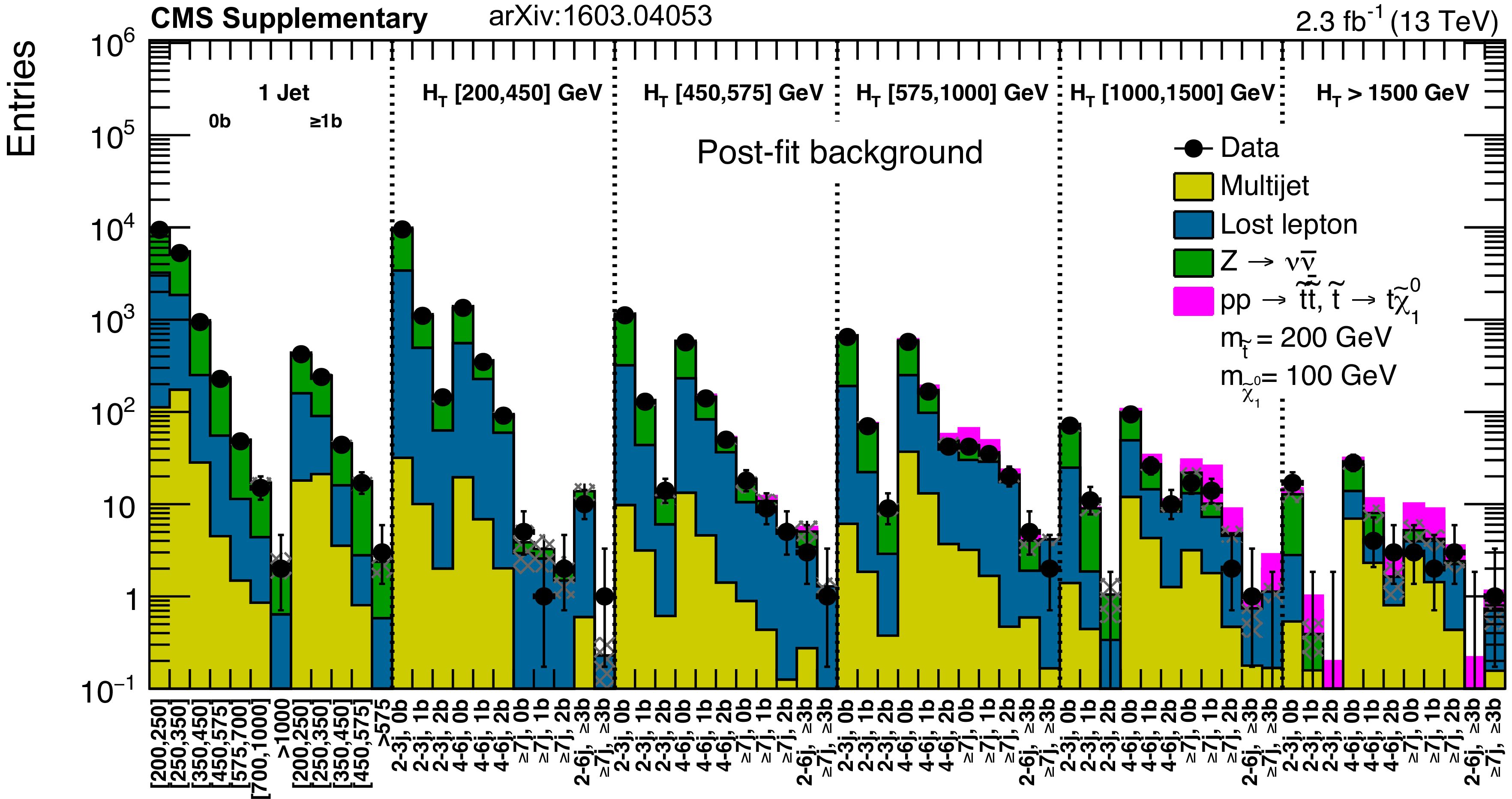
Figure A5:
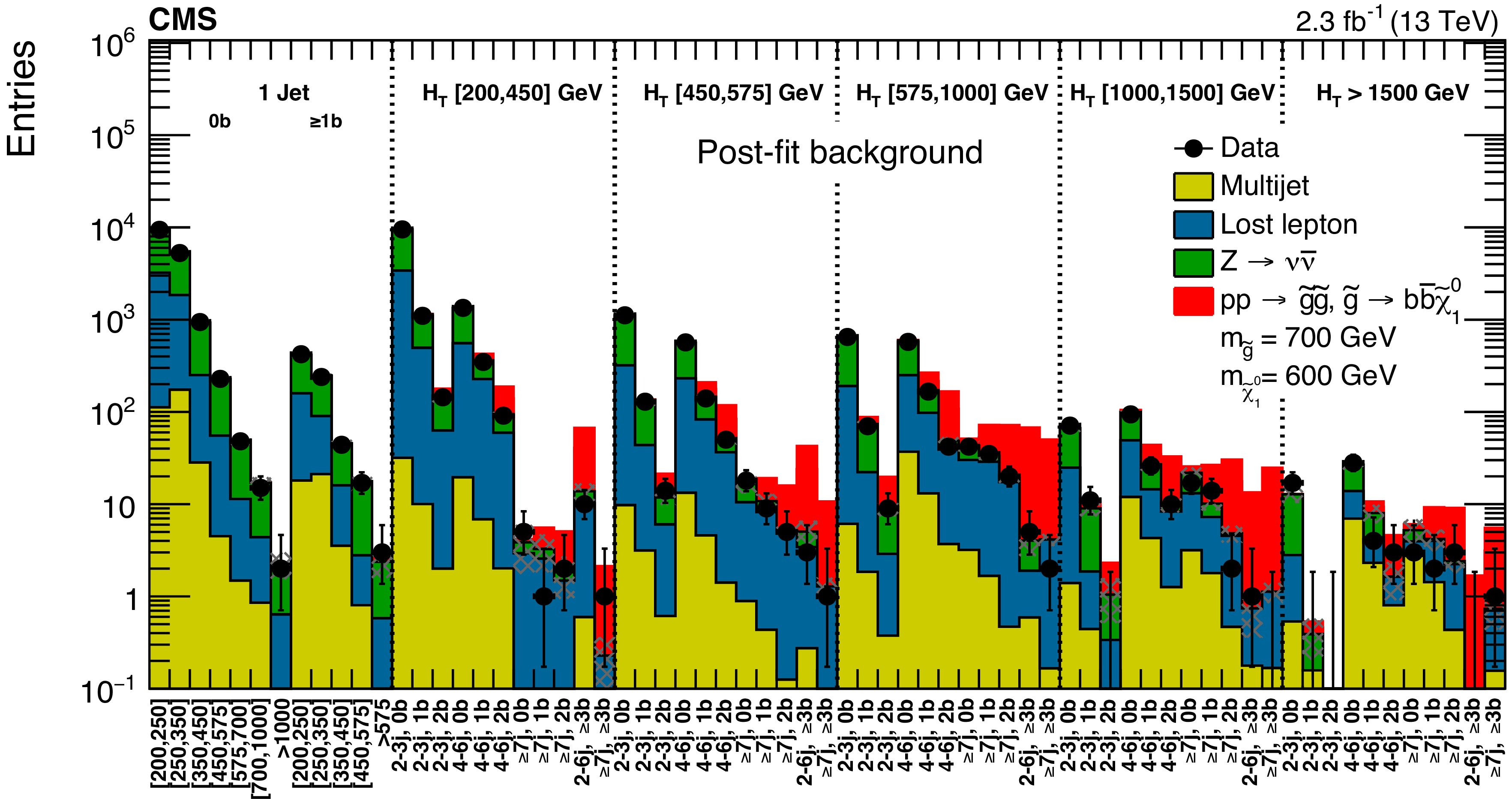
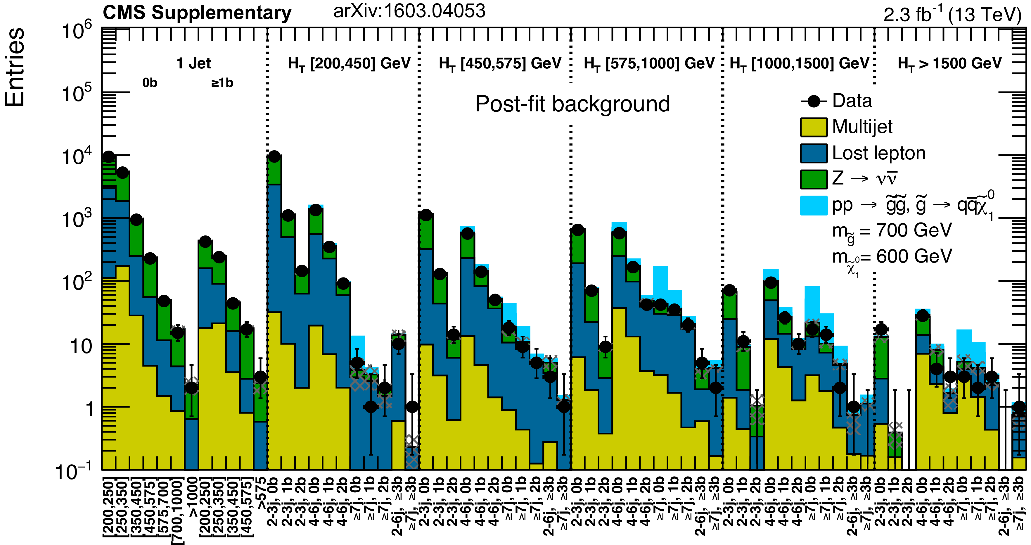
Post-fit background prediction, expected signal yields, and observed data events in each topological region. Hatched bands represent the post-fit uncertainty in the background prediction. For the monojet region, on the $x$-axis, the jet $ p_{\mathrm{T}} $ binning is shown (in GeV). The red histogram shows the expected contribution from a compressed-spectrum signal model of gluino-mediated bottom squark production with the mass of the gluino and the LSP equal to 700 and 600 GeV, respectively. |
png pdf |
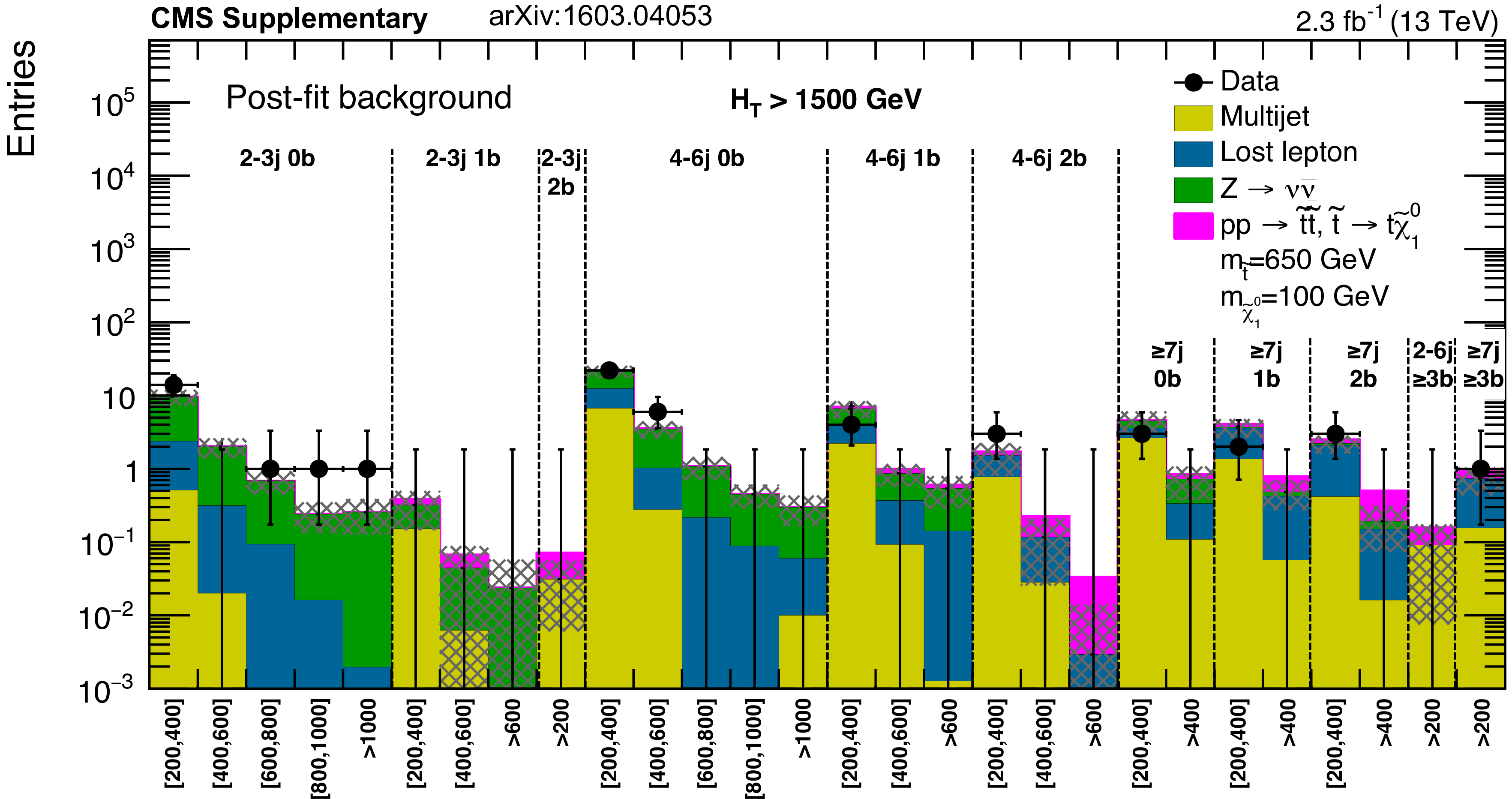
Figure A6:
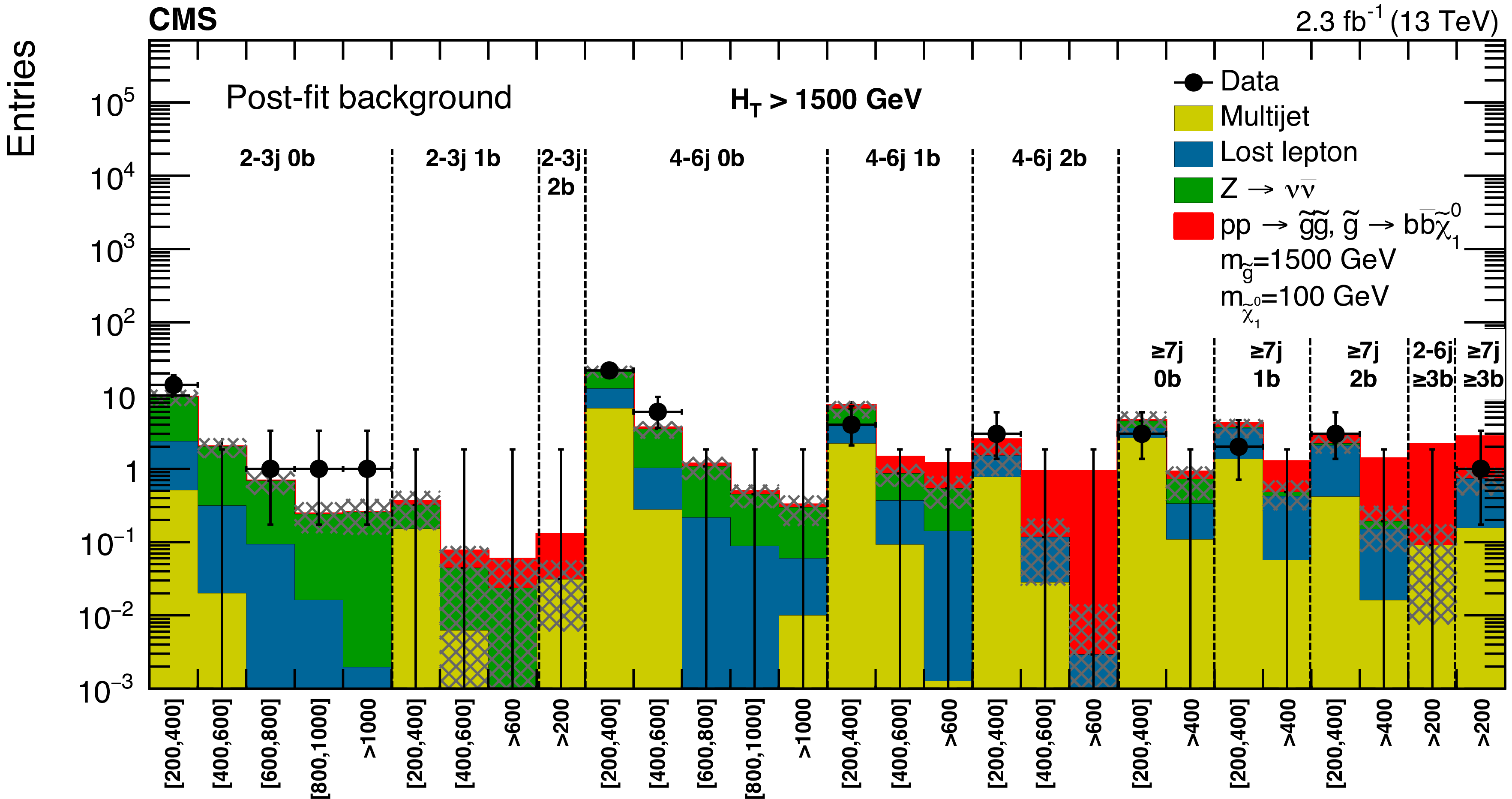
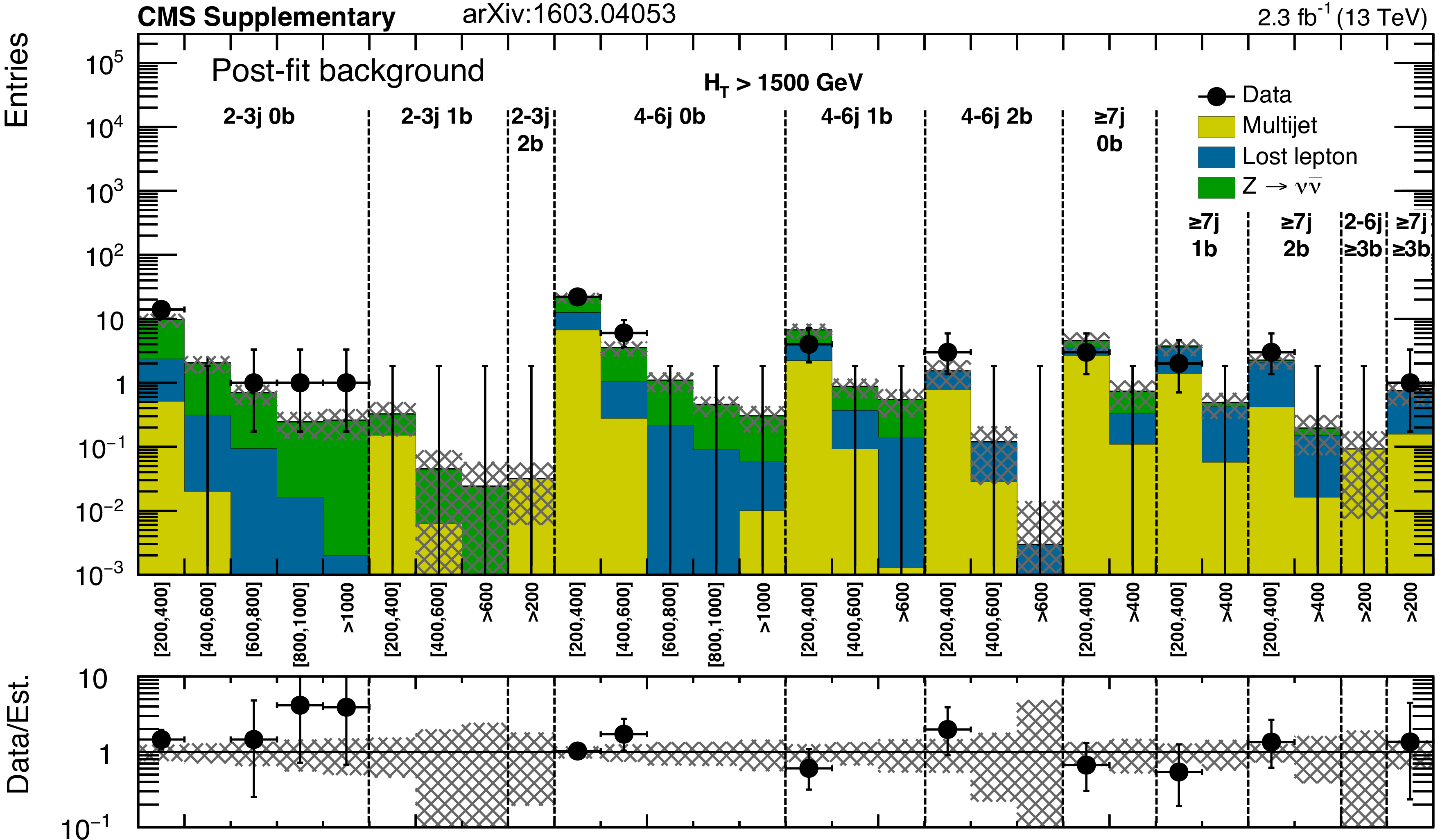
Post-fit background prediction, expected signal yields, and observed data events in each signal bin in the extreme-$ H_{\mathrm{T}} $ region. Hatched bands represent the post-fit uncertainty in the background prediction. On the $x$-axis, the $M_{\mathrm{T2}}$ binning is shown (in GeV). The red histogram shows the expected contribution from an open-spectra signal model of gluino-mediated bottom squark production with the mass of the gluino and the LSP equal to 1500 and 100 GeV, respectively. |
png pdf |
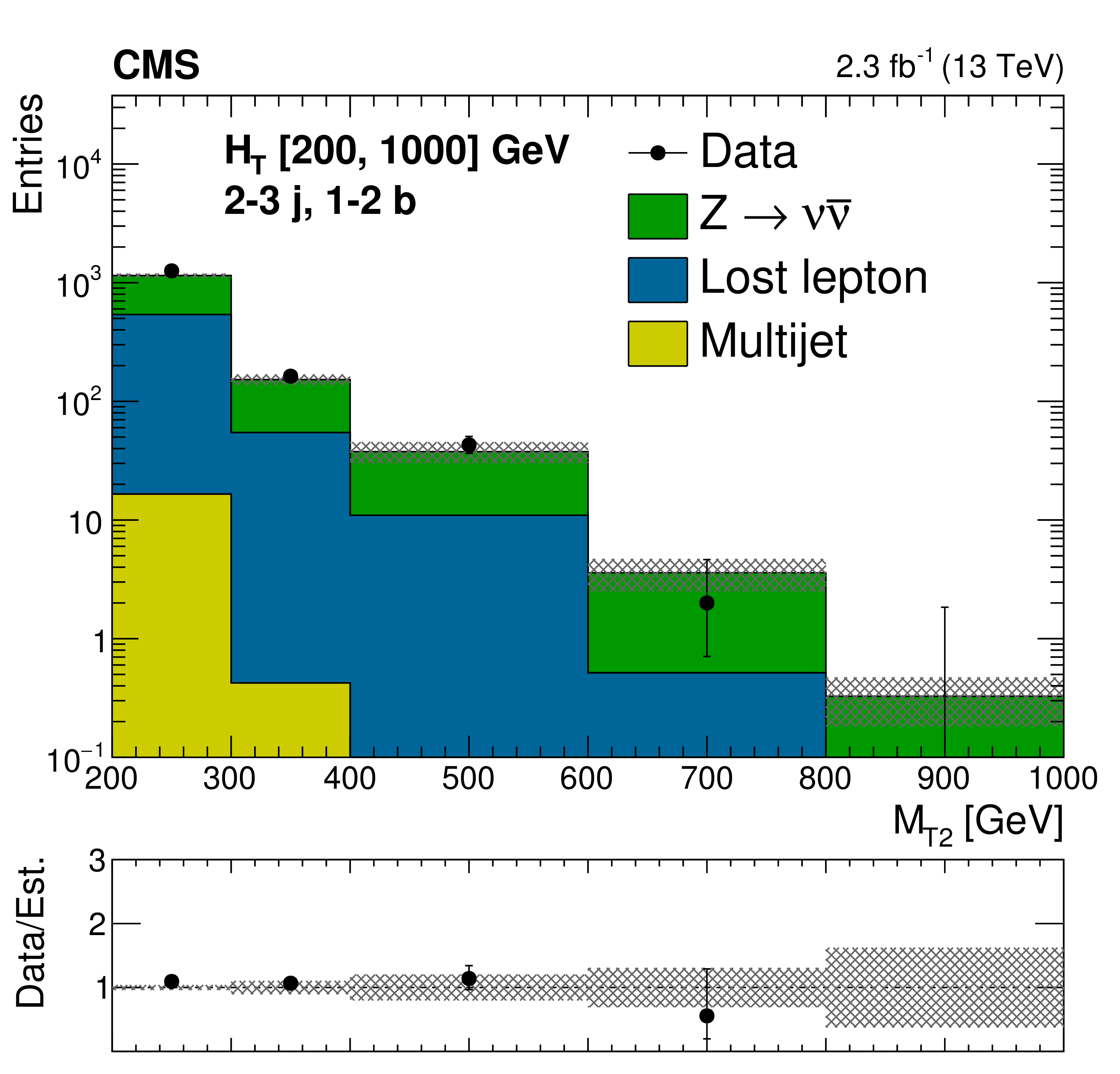
Figure C1-a:
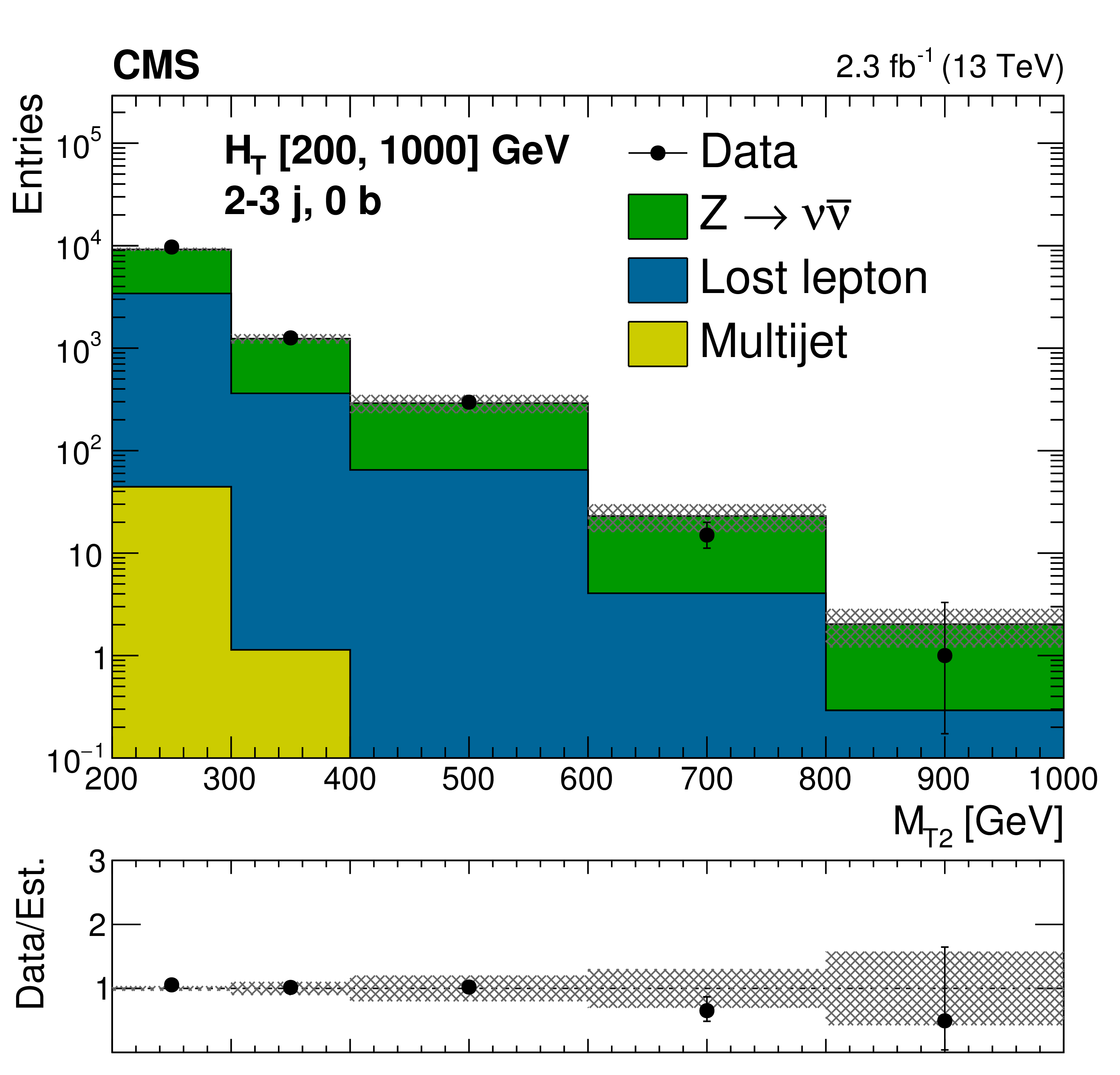
Comparison of estimated background and observed data events in inclusive topological regions, as labeled in the legends, as a function of $M_{\mathrm{T2}}$, for events with 200 $< H_{\mathrm{T}} <$ 1000 GeV. The background prediction is formed by summing pre-fit values for all signal regions included in each plot. Hatched bands represent the full uncertainty in the background estimate. |
png pdf |
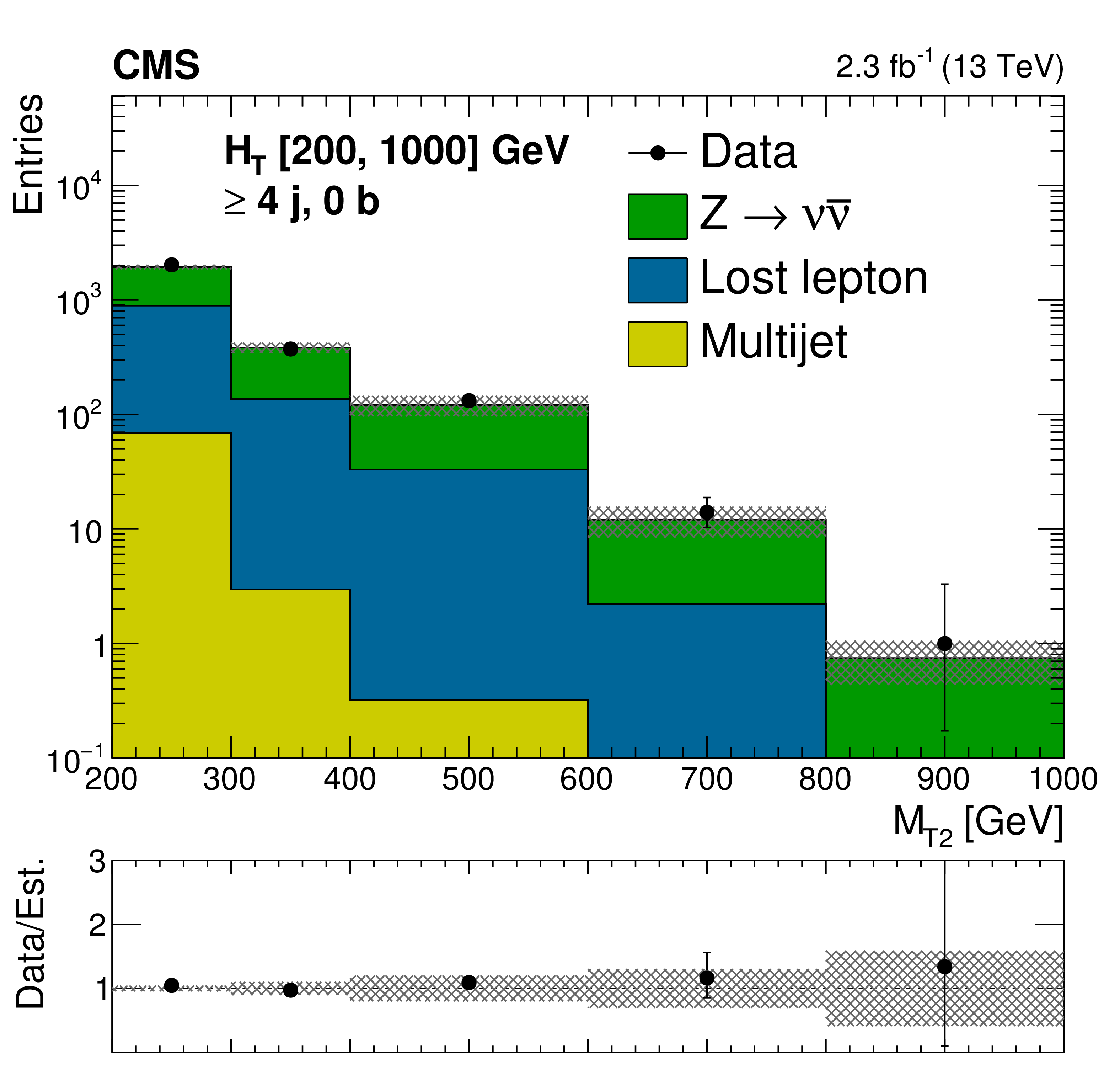
Figure C1-b:
Comparison of estimated background and observed data events in inclusive topological regions, as labeled in the legends, as a function of $M_{\mathrm{T2}}$, for events with 200 $< H_{\mathrm{T}} <$ 1000 GeV. The background prediction is formed by summing pre-fit values for all signal regions included in each plot. Hatched bands represent the full uncertainty in the background estimate. |
png pdf |
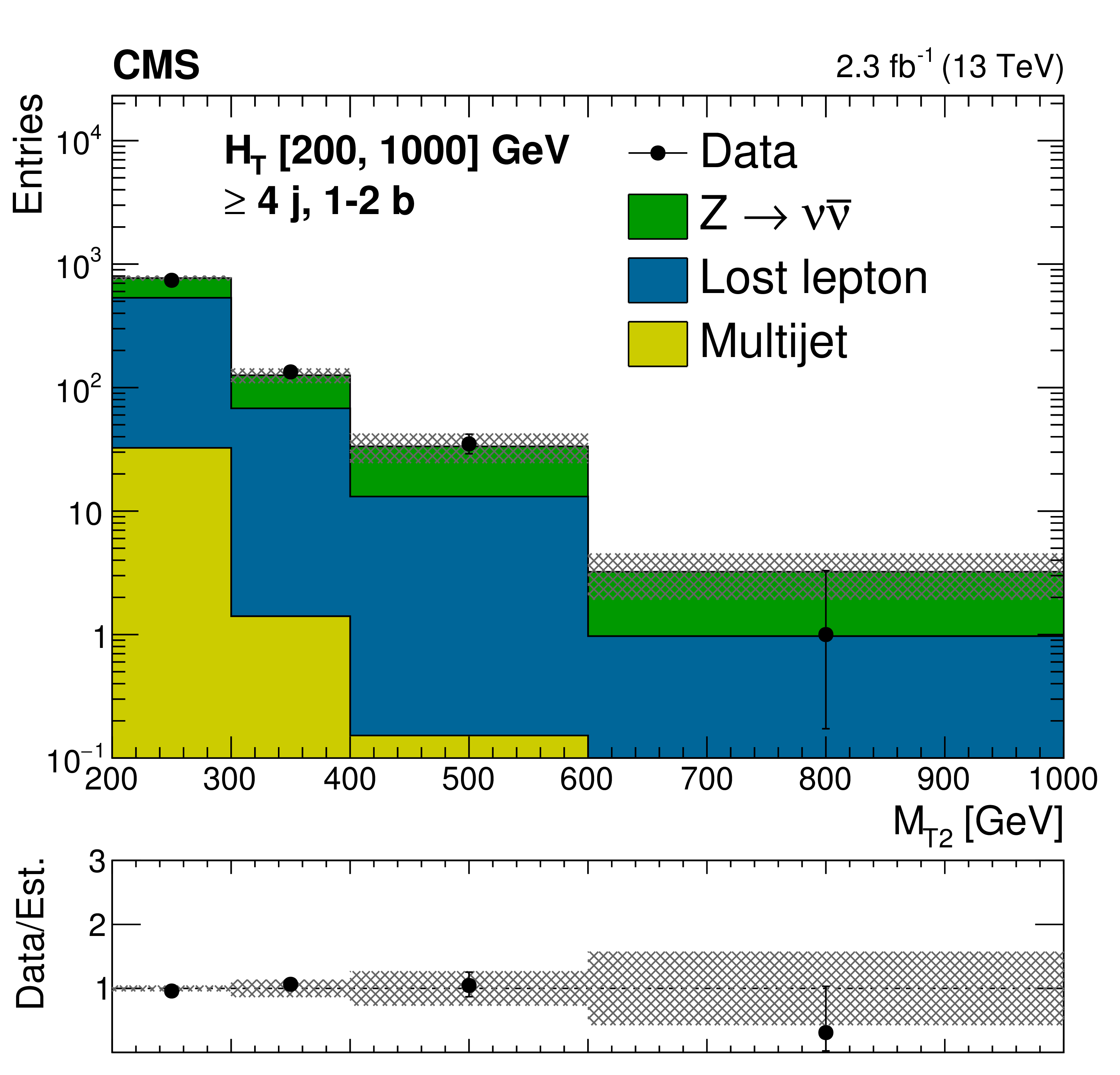
Figure C1-c:
Comparison of estimated background and observed data events in inclusive topological regions, as labeled in the legends, as a function of $M_{\mathrm{T2}}$, for events with 200 $< H_{\mathrm{T}} <$ 1000 GeV. The background prediction is formed by summing pre-fit values for all signal regions included in each plot. Hatched bands represent the full uncertainty in the background estimate. |
png pdf |
Figure C1-d:
Comparison of estimated background and observed data events in inclusive topological regions, as labeled in the legends, as a function of $M_{\mathrm{T2}}$, for events with 200 $< H_{\mathrm{T}} <$ 1000 GeV. The background prediction is formed by summing pre-fit values for all signal regions included in each plot. Hatched bands represent the full uncertainty in the background estimate. |
png pdf |
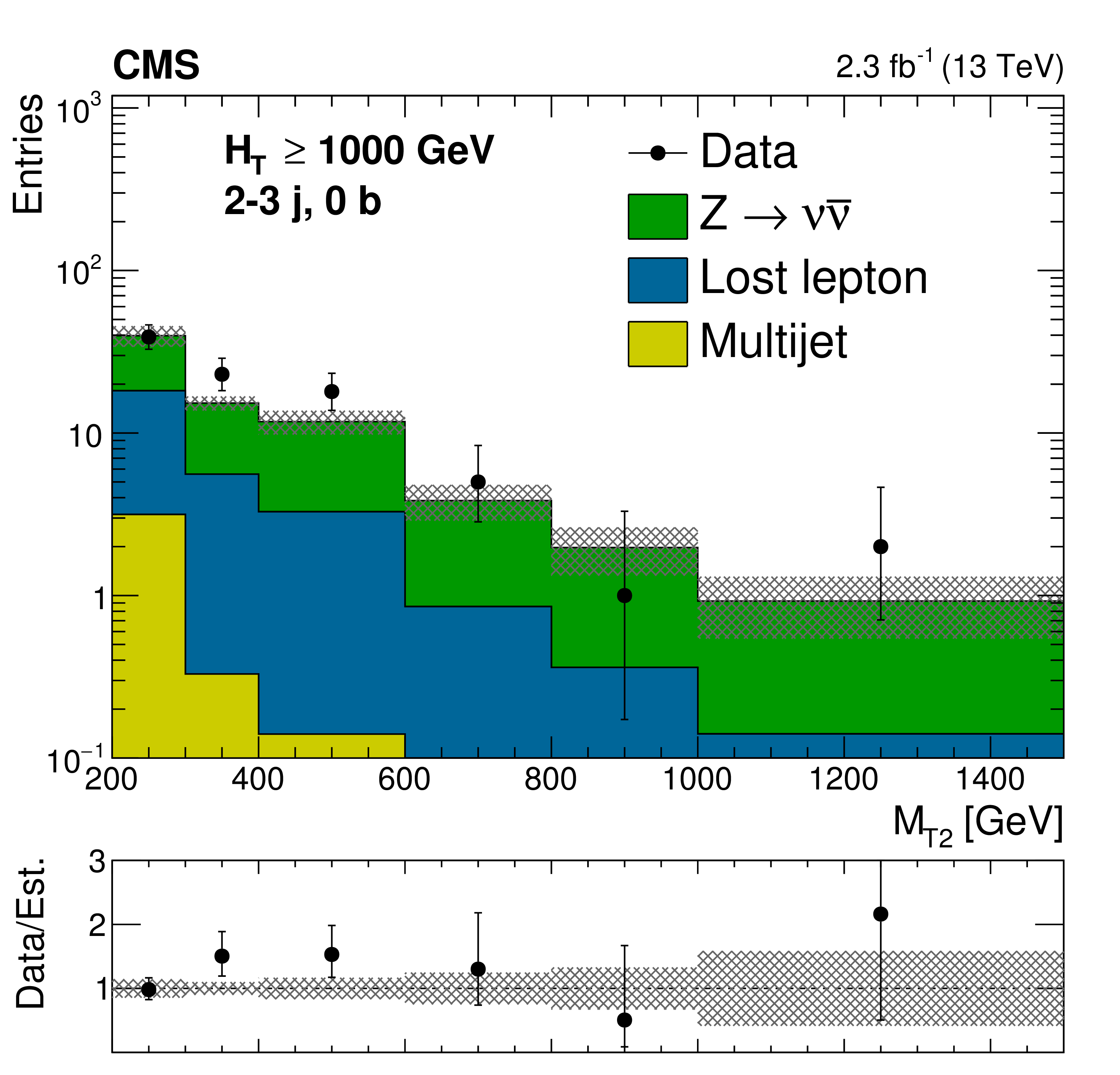
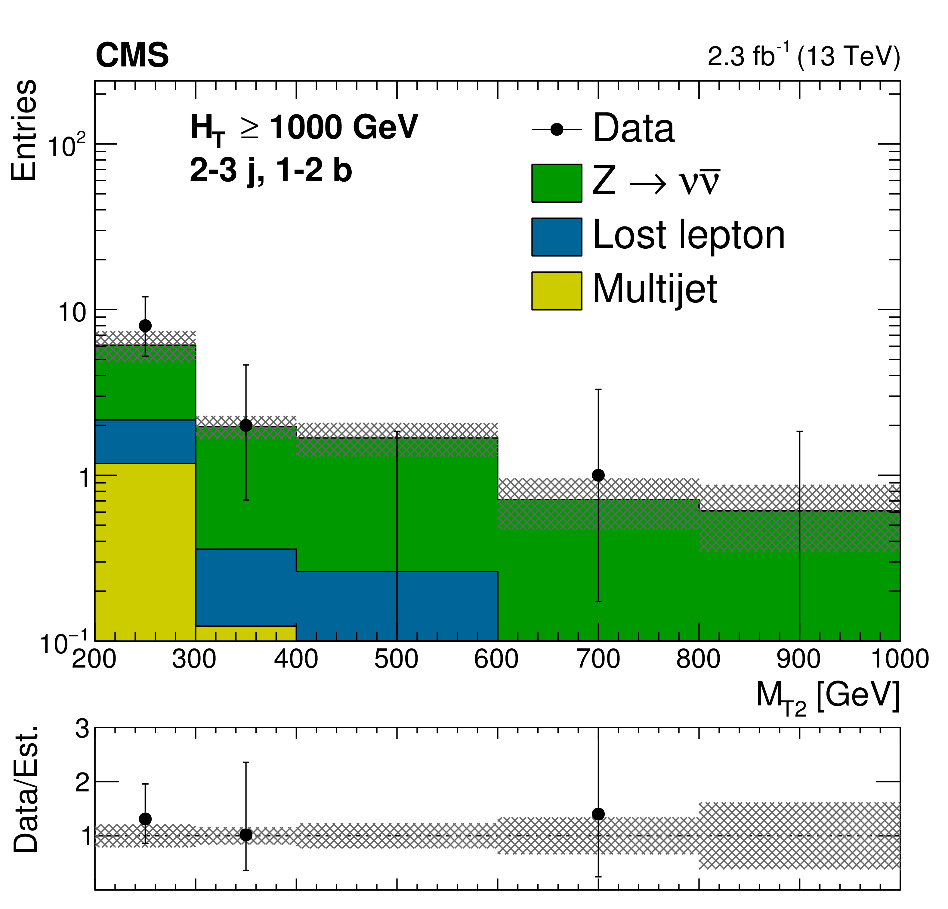
Figure C2-a:
Comparison of estimated background and observed data events in inclusive topological regions, as labeled in the legends, as a function of $M_{\mathrm{T2}}$, for events with $ H_{\mathrm{T}} >$ 1000 GeV. The background prediction is formed by summing pre-fit values for all signal regions included in each plot. Hatched bands represent the full uncertainty in the background estimate. |
png pdf |
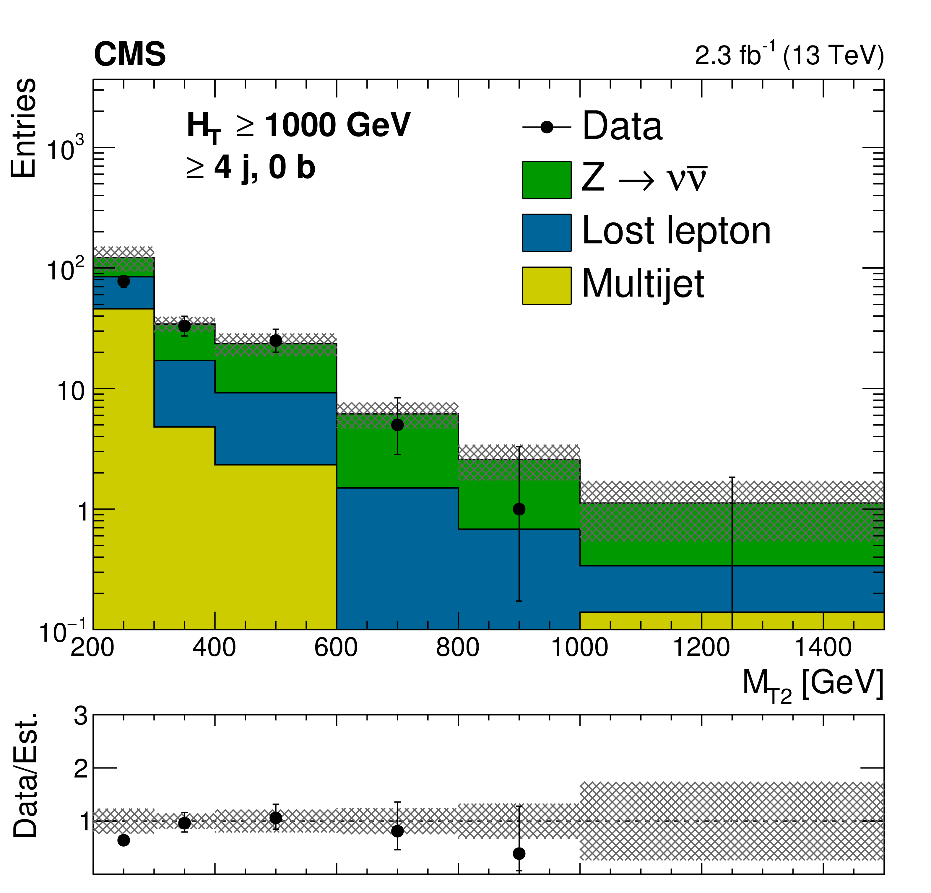
Figure C2-b:
Comparison of estimated background and observed data events in inclusive topological regions, as labeled in the legends, as a function of $M_{\mathrm{T2}}$, for events with $ H_{\mathrm{T}} >$ 1000 GeV. The background prediction is formed by summing pre-fit values for all signal regions included in each plot. Hatched bands represent the full uncertainty in the background estimate. |
png pdf |
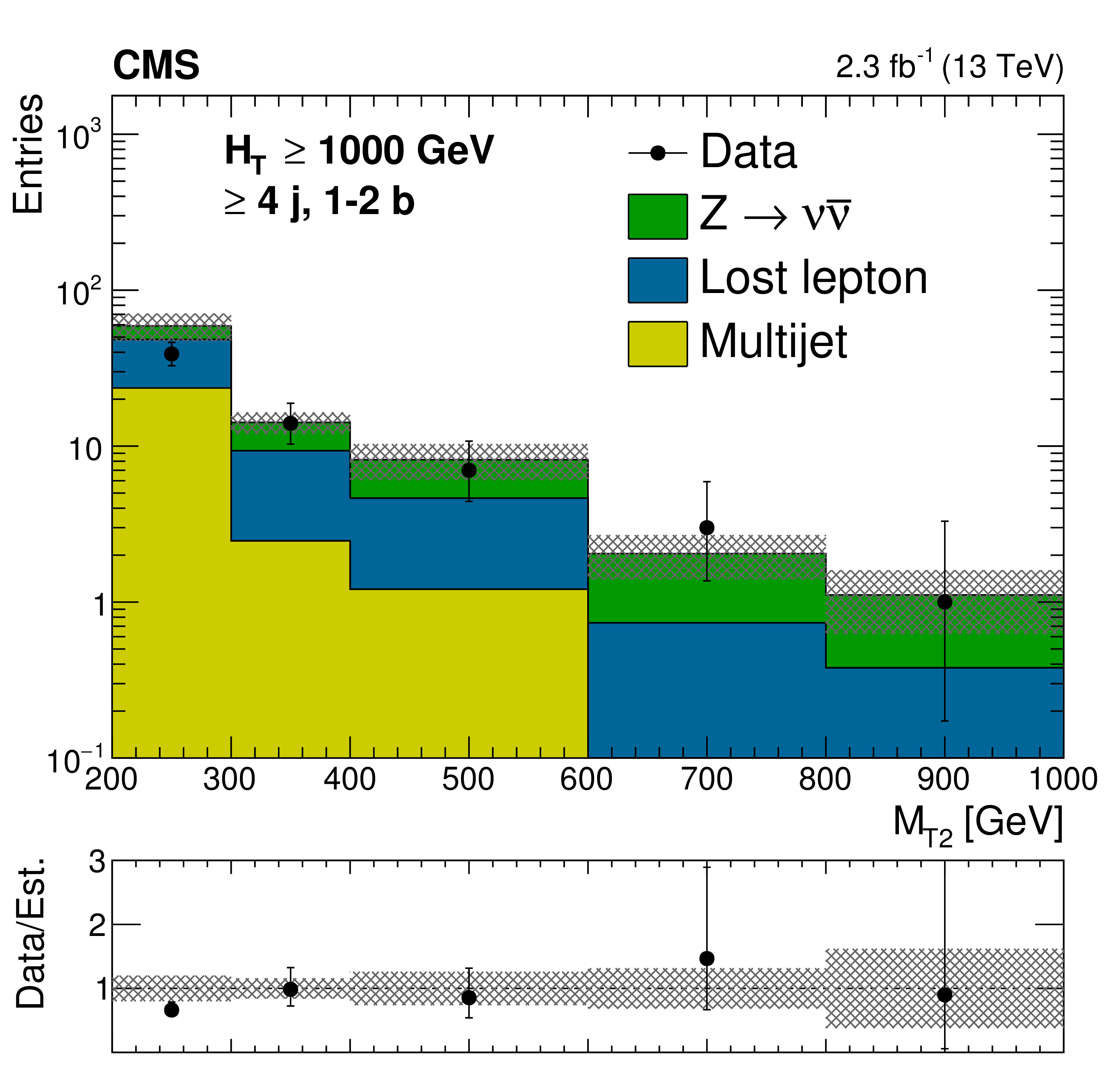
Figure C2-c:
Comparison of estimated background and observed data events in inclusive topological regions, as labeled in the legends, as a function of $M_{\mathrm{T2}}$, for events with $ H_{\mathrm{T}} >$ 1000 GeV. The background prediction is formed by summing pre-fit values for all signal regions included in each plot. Hatched bands represent the full uncertainty in the background estimate. |
png pdf |
Figure C2-d:
Comparison of estimated background and observed data events in inclusive topological regions, as labeled in the legends, as a function of $M_{\mathrm{T2}}$, for events with $ H_{\mathrm{T}} >$ 1000 GeV. The background prediction is formed by summing pre-fit values for all signal regions included in each plot. Hatched bands represent the full uncertainty in the background estimate. |
| Tables | |

png pdf |
Table 1:
The three signal triggers and the corresponding offline selections. |

png pdf |
Table 2:
Ranges of typical values of the signal systematic uncertainties as evaluated for the $\mathrm{ \tilde{g} \to b \bar{b} \tilde{\chi}^0_1 } $ signal model. Uncertainties evaluated on other signal models are consistent with these ranges of values. A large uncertainty from the limited size of the simulated sample only occurs for a small number of model points for which a small subset of search regions have very low efficiency. |

png pdf |
Table 3:
Summary of 95% CL observed exclusion limits for different SUSY simplified model scenarios. The limit on the mass of the produced sparticle is quoted for a massless LSP, while for the lightest neutralino the best limit on its mass is quoted. |
png pdf |
Table A1:
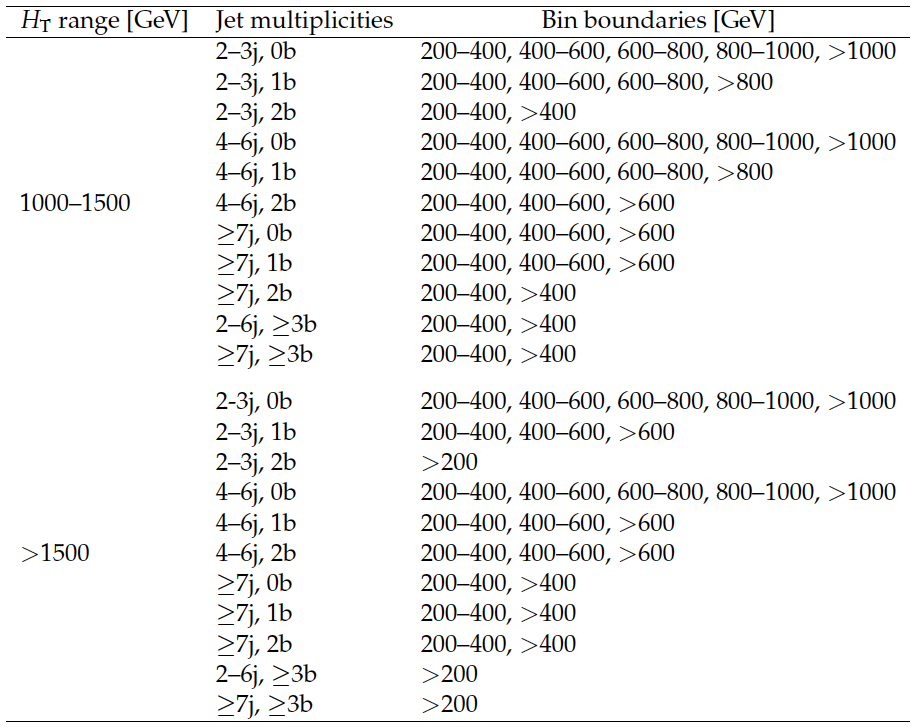
Binning in $M_{\mathrm{T2}}$ for each topological region of the multijet search regions with very low, low, and medium $ H_{\mathrm{T}} $. Within each topological or $ N_{\mathrm{b}} $ categorization, we merge $M_{\mathrm{T2}}$ bins that are expected to contain fewer than one background event. |
png pdf |
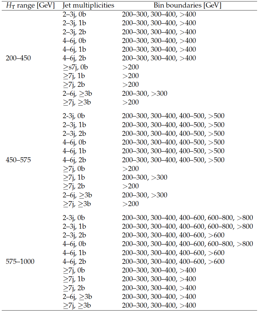
Table A2:
Binning in $M_{\mathrm{T2}}$ for each topological region of the multijet search regions with high and extreme $ H_{\mathrm{T}} $. Within each topological or $ N_{\mathrm{b}} $ categorization, we merge $M_{\mathrm{T2}}$ bins that are expected to contain fewer than one background event. |
png pdf |
Table A3:
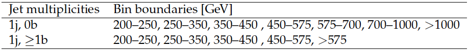
Binning in jet $ p_{\mathrm{T}} $ for the monojet regions. Within each $ N_{\mathrm{b}} $ categorization, we merge jet $ p_{\mathrm{T}} $ bins that are expected to contain fewer than one background event. |

png pdf |
Table B1:
Definitions of aggregated regions. Each aggregated region is obtained by selecting all events that pass the logical OR of the listed selections. |

png pdf |
Table B2:
Predictions and observations for the aggregated regions defined in Table B1, together with the observed 95\% CL limit on the number of signal events contributing to each region ($N_{95}^{\text{obs}}$). An uncertainty of either 15 or 30\% in the signal efficiency is assumed for calculating the limits. |

png pdf |
Table B3:
Expected upper limits on the cross section of several signal models, as determined from the full binned analysis, are compared to the upper limits obtained using only the aggregated region that has the best sensitivity to each considered signal model. A 15% uncertainty in the signal selection efficiency is assumed for calculating these limits. The signal yields expected for an integrated luminosity of 2.3 fb$^{-1}$ are also shown. |
| Summary |
| A search for new physics using events containing hadronic jets with transverse momentum imbalance as measured by the $M_{\mathrm{T2}}$ variable has been presented. Results are based on a data sample of proton-proton collisions at $\sqrt{s}=$ 13 TeV collected with the CMS detector and corresponding to an integrated luminosity of 2.3 fb$^{-1}$. No significant deviations from the standard model expectations are observed. In the limit of a massless LSP, gluino masses of up to 1750 GeV are excluded, extending the reach of Run 1 searches by more than 300 GeV. For lighter gluinos, LSP masses up to 1125 GeV in the most favorable models are excluded, also increasing previous limits by more than 300 GeV. Among the three gluino decays considered, the strongest limits on gluino pair production are generally achieved for the $ \tilde{g} \to \mathrm{ b \bar{b} } \tilde{\chi}^0_1 $ channel. Improved sensitivity is obtained in this scenario as selections requiring at least two b-tagged jets in the final state retain a significant fraction of gluino-mediated bottom squark events, while strongly suppressing the background from W+jets, Z+jets, and multijet processes. Also, unlike for models with $ \tilde{g} \to \mathrm{ t \bar{t} } \tilde{\chi}^0_1 $ decays, which include leptonic decays, gluino-mediated bottom squark events do not suffer from an efficiency loss due to the lepton veto. For direct pair production of first- and second-generation squarks, each assumed to decay exclusively to a quark of the same flavor and the lightest neutralino, squark masses of about 1260 GeV and LSP masses up to 580 GeV are excluded. If only a single squark is assumed to be light, the limit on the squark and LSP masses is relaxed to 600 and 300 GeV, respectively. For the pair production of third-generation squarks, each assumed to decay with 100% branching fraction to a quark of the same flavor and the lightest neutralino, a bottom (top) squark mass up to 880 (800) GeV is excluded. For gluino-induced and direct squark production models, the observed exclusion limits on the masses of the sparticles are from 200 to about 300 GeV higher than those obtained by a similar analysis performed on 8 TeV data [13]. In relative terms, the largest difference is in the limit on the mass of the top squark, which moves from about 500 GeV to 800 GeV for a massless LSP. This is mostly due to a fluctuation in the 8 TeV data that is not present in the13 TeV data. |
| Additional Figures | |
png pdf |
Additional Figure 1-a:
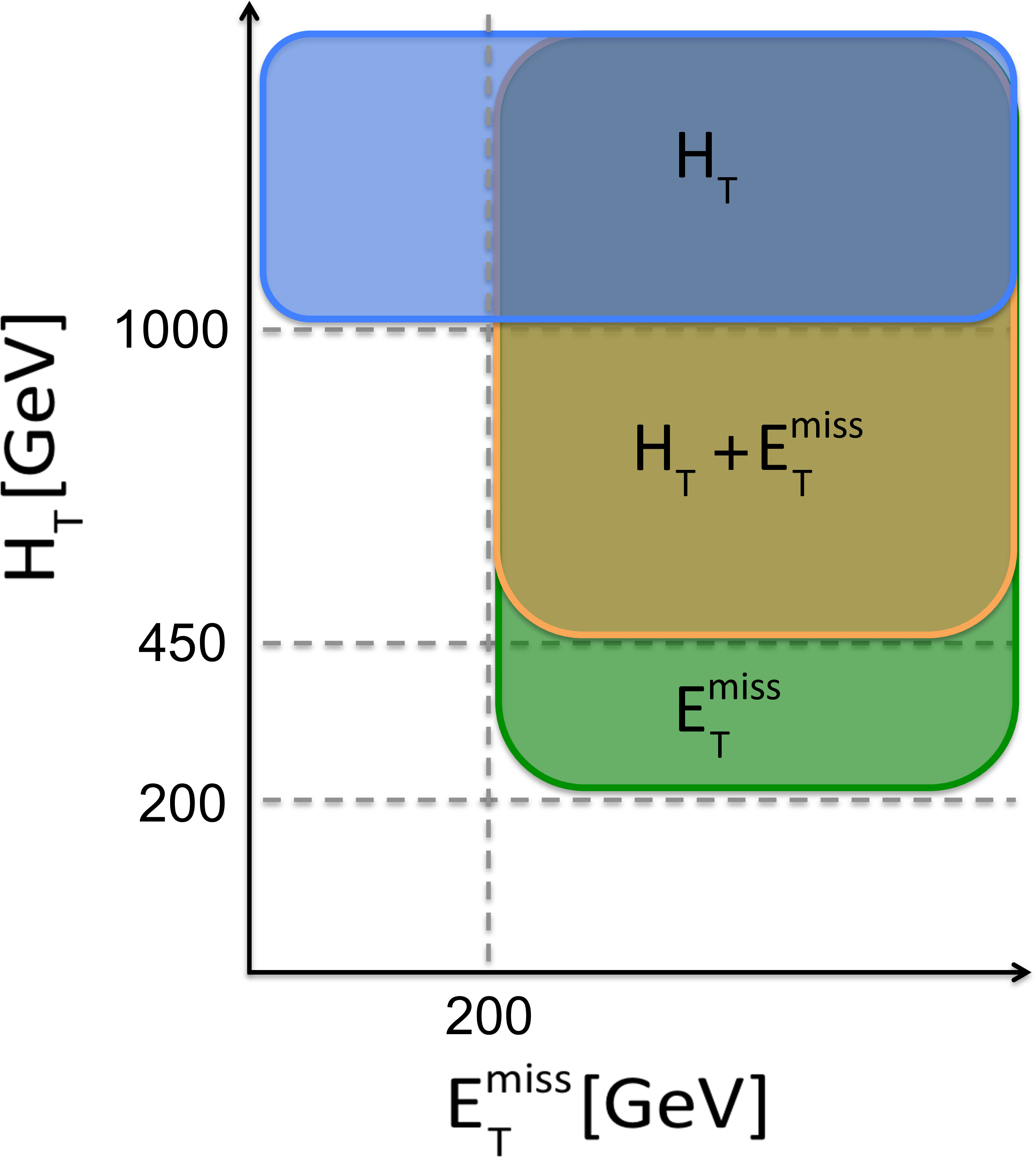
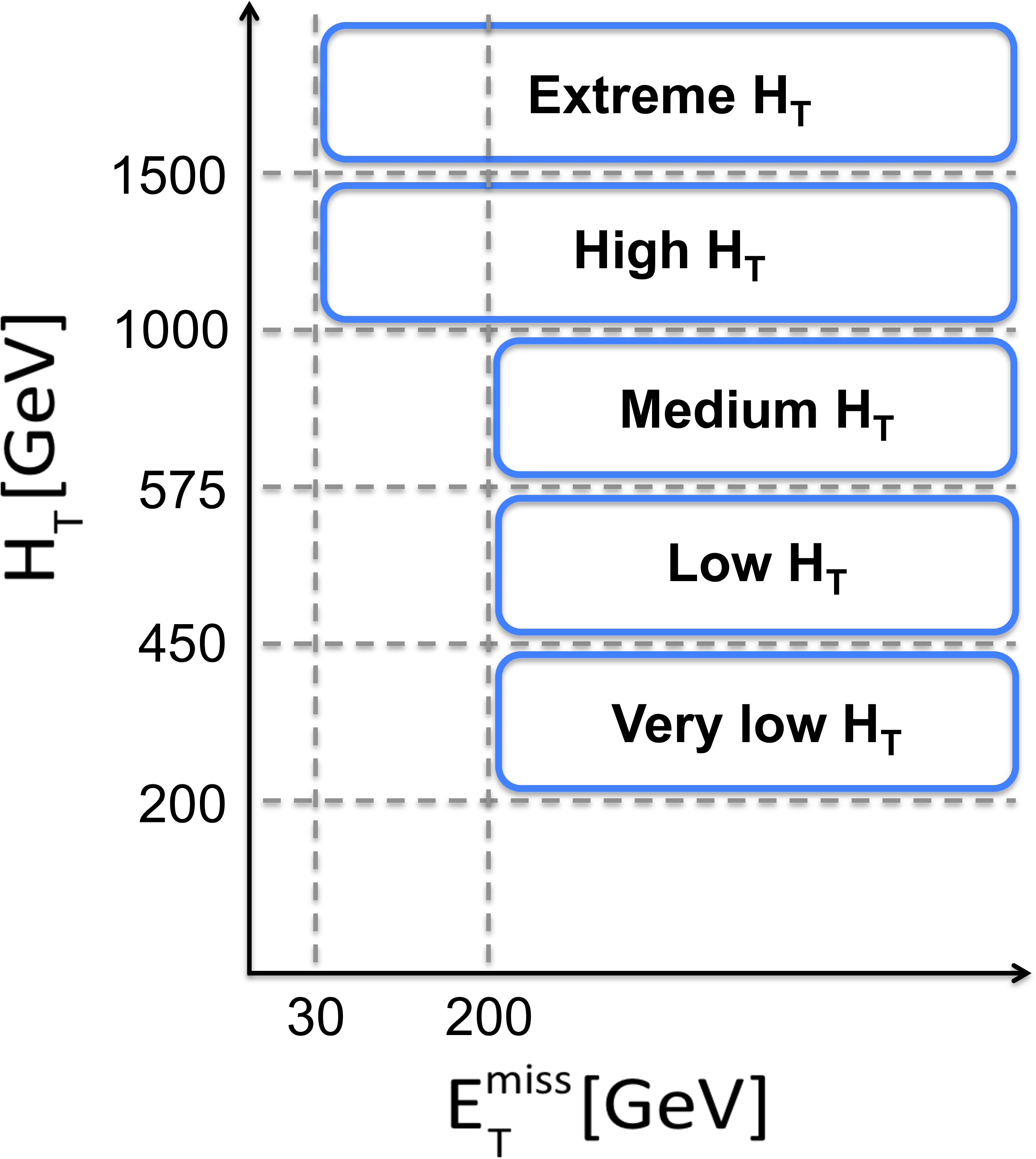
Diagrams of the analysis coverage in the plane of $ {H_{\mathrm {T}}} $ and $ {E_{\mathrm {T}}^{\text {miss}}} $, showing (a) the coverage of the triggers used and (b) the $ {H_{\mathrm {T}}} $ binning used. |
png pdf |
Additional Figure 1-b:
Diagrams of the analysis coverage in the plane of $ {H_{\mathrm {T}}} $ and $ {E_{\mathrm {T}}^{\text {miss}}} $, showing (a) the coverage of the triggers used and (b) the $ {H_{\mathrm {T}}} $ binning used. |

png pdf |
Additional Figure 2:
Diagram of the $ {N_{\mathrm {j}}} $ and $ {N_{\mathrm {b}}} $ binning used in the analysis. The background composition from simulation for the medium-$ {H_{\mathrm {T}}} $ bin is shown in each bin with a pie chart. |
png pdf |
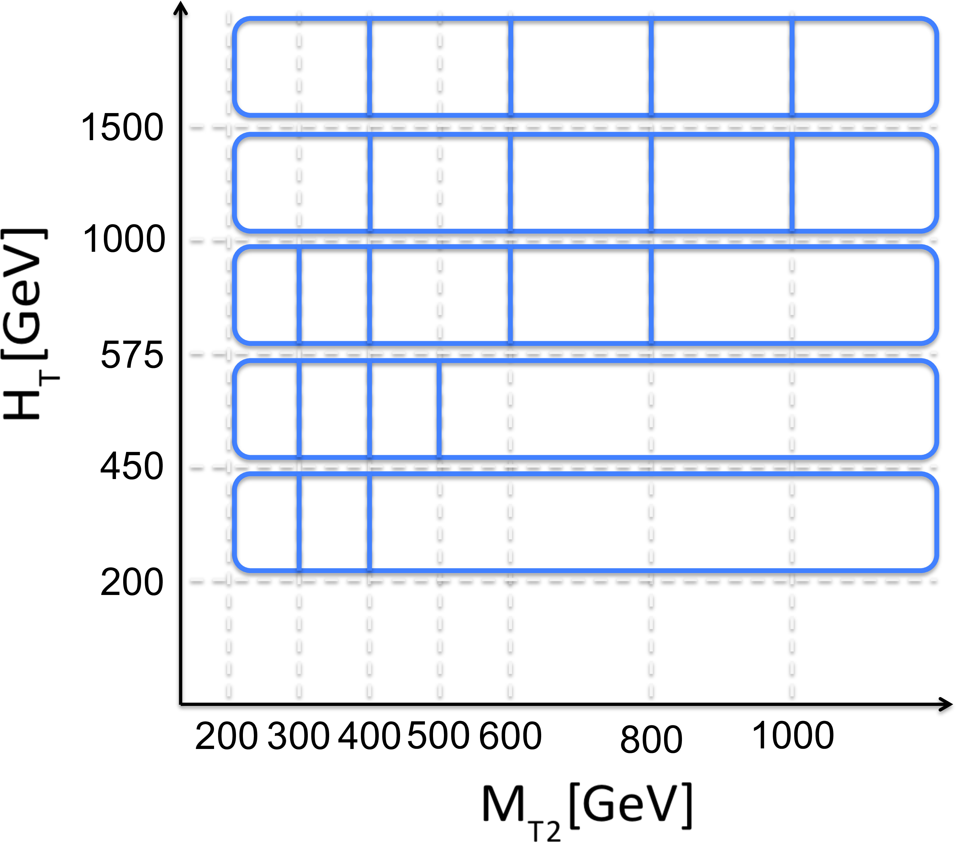
Additional Figure 3:
Diagram of the maximal analysis binning in the plane of $ {H_{\mathrm {T}}} $ and $ {M_{\mathrm {T2}}} $ for multijet bins. In each bin of ($ {H_{\mathrm {T}}} $, $ {N_{\mathrm {j}}} $, $ {N_{\mathrm {b}}} $), the bins with highest $ {M_{\mathrm {T2}}} $ values are merged to have at least one expected background event. |
png pdf |
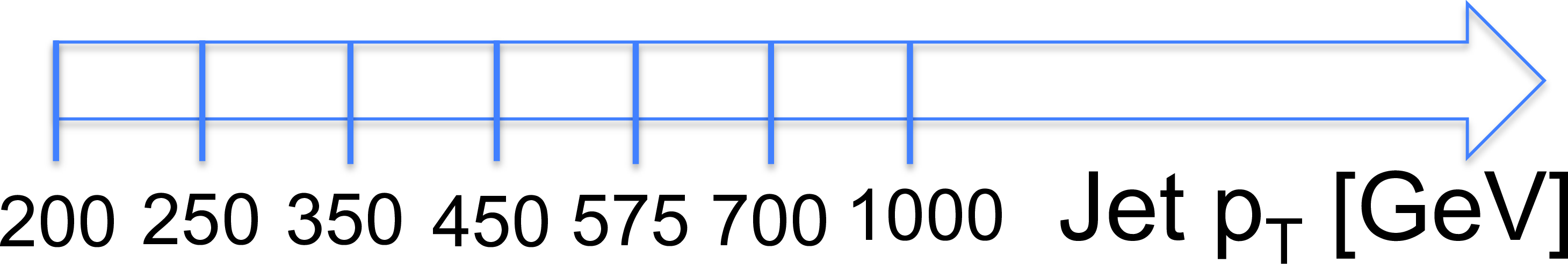
Additional Figure 4:
Diagram of the maximal analysis binning in the jet $ {p_{\mathrm {T}}} $ dimension for monojet bins. Within each $ {N_{\mathrm {b}}} $ category, the highest bins in jet $ {p_{\mathrm {T}}} $ are merged to have at least one expected background event. |
png pdf |
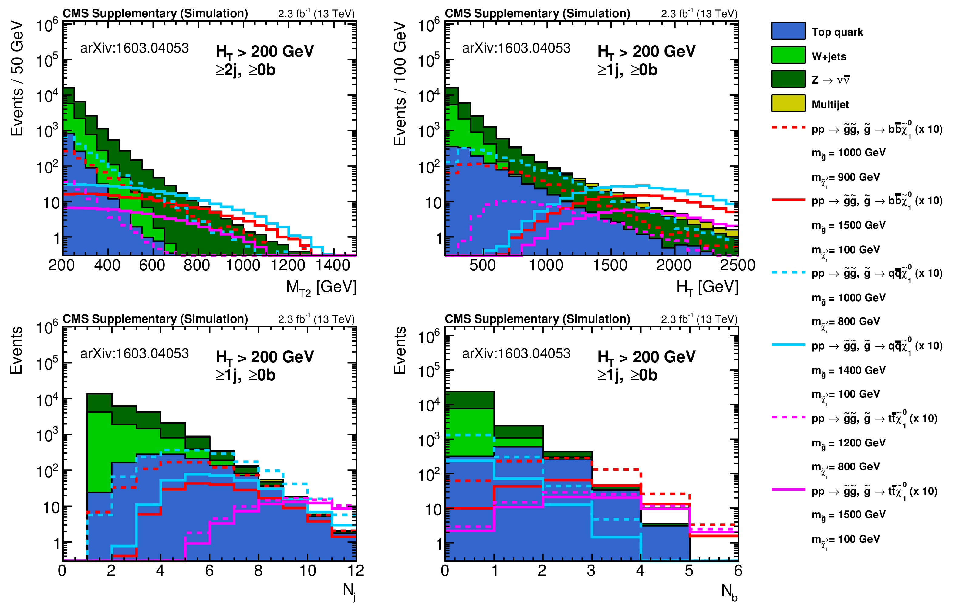
Additional Figure 5:
Distributions of the variables used for binning the signal regions after the baseline selection. The SM backgrounds are stacked and example signal points are overlaid with their cross sections scaled up by a factor of 10. For the $ {M_{\mathrm {T2}}} $ plot, only events with at least two jets are selected. |
png pdf |
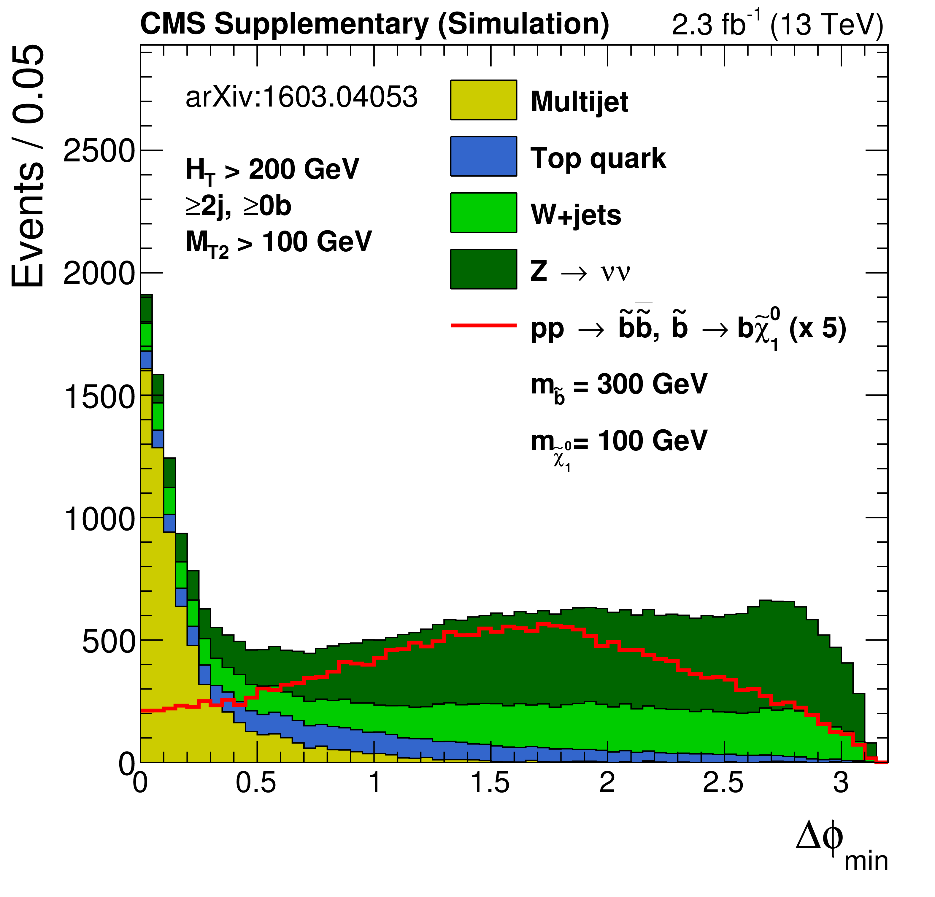
Additional Figure 6:
Distribution of the $ {\Delta \phi _{\mathrm {min}}} $ variable used in the baseline selection. The SM backgrounds are stacked and an example signal point is overlaid with its cross sections scaled up by a factor of 5. |
png pdf |
Additional Figure 7-a:
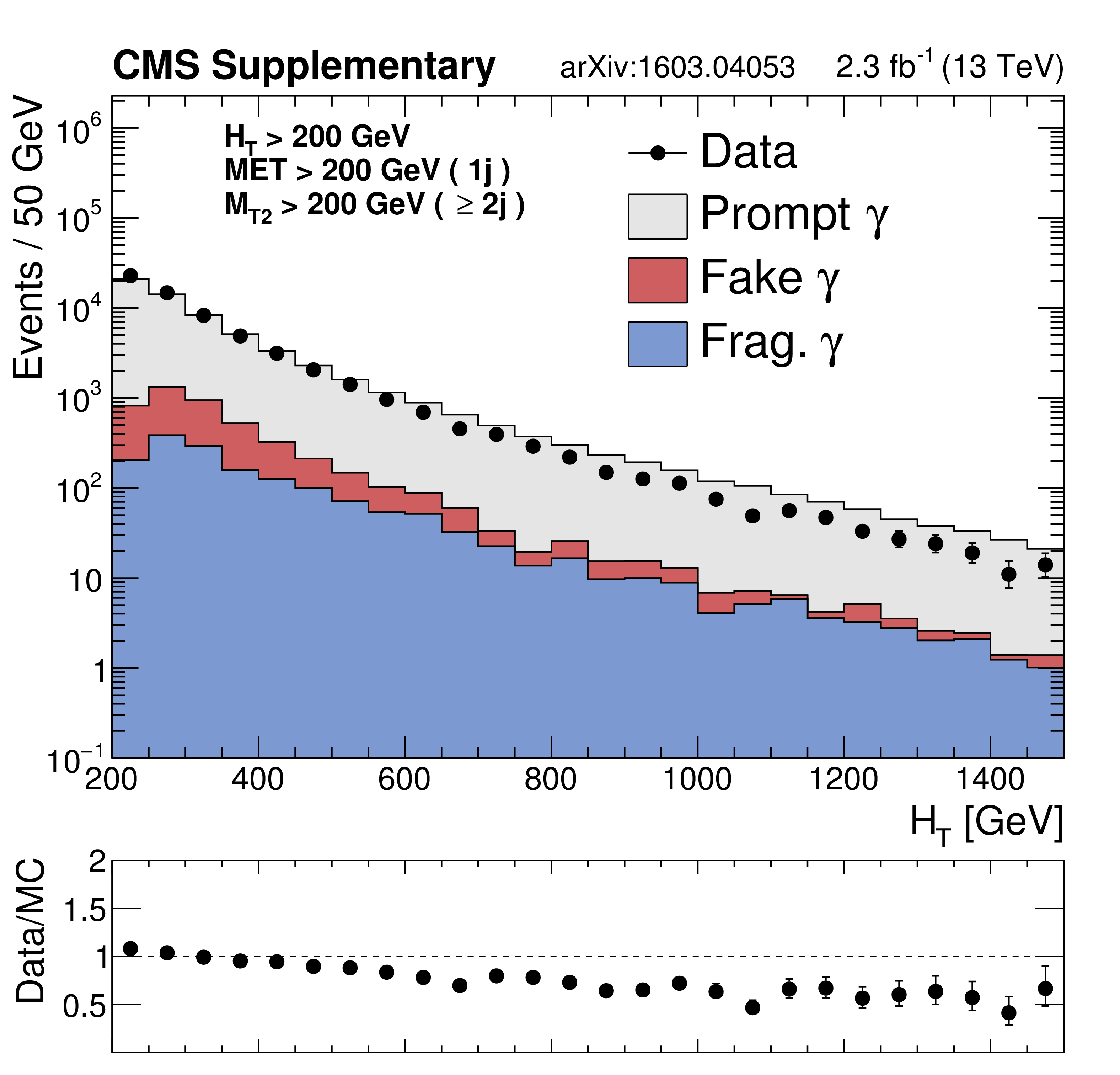
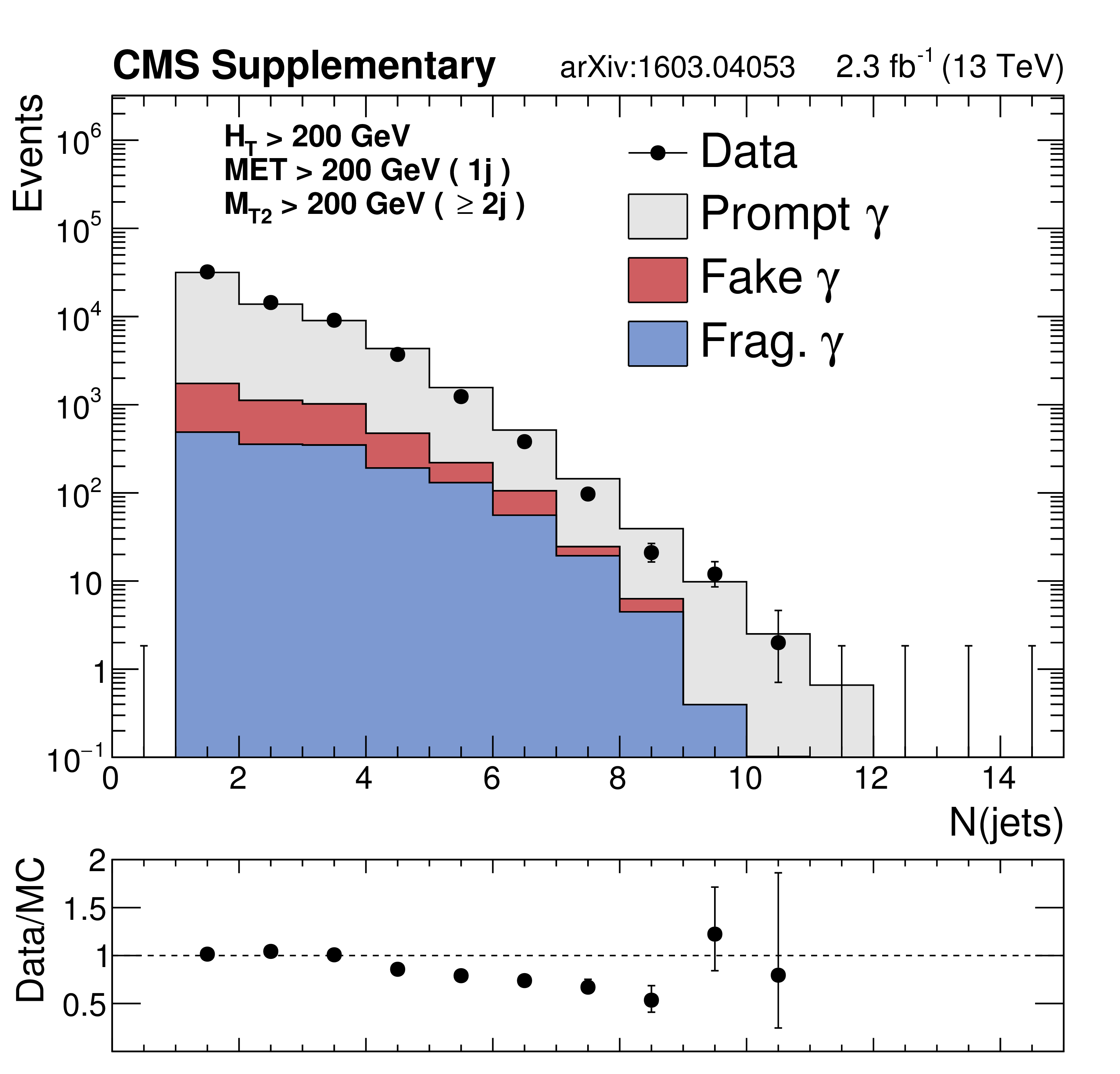
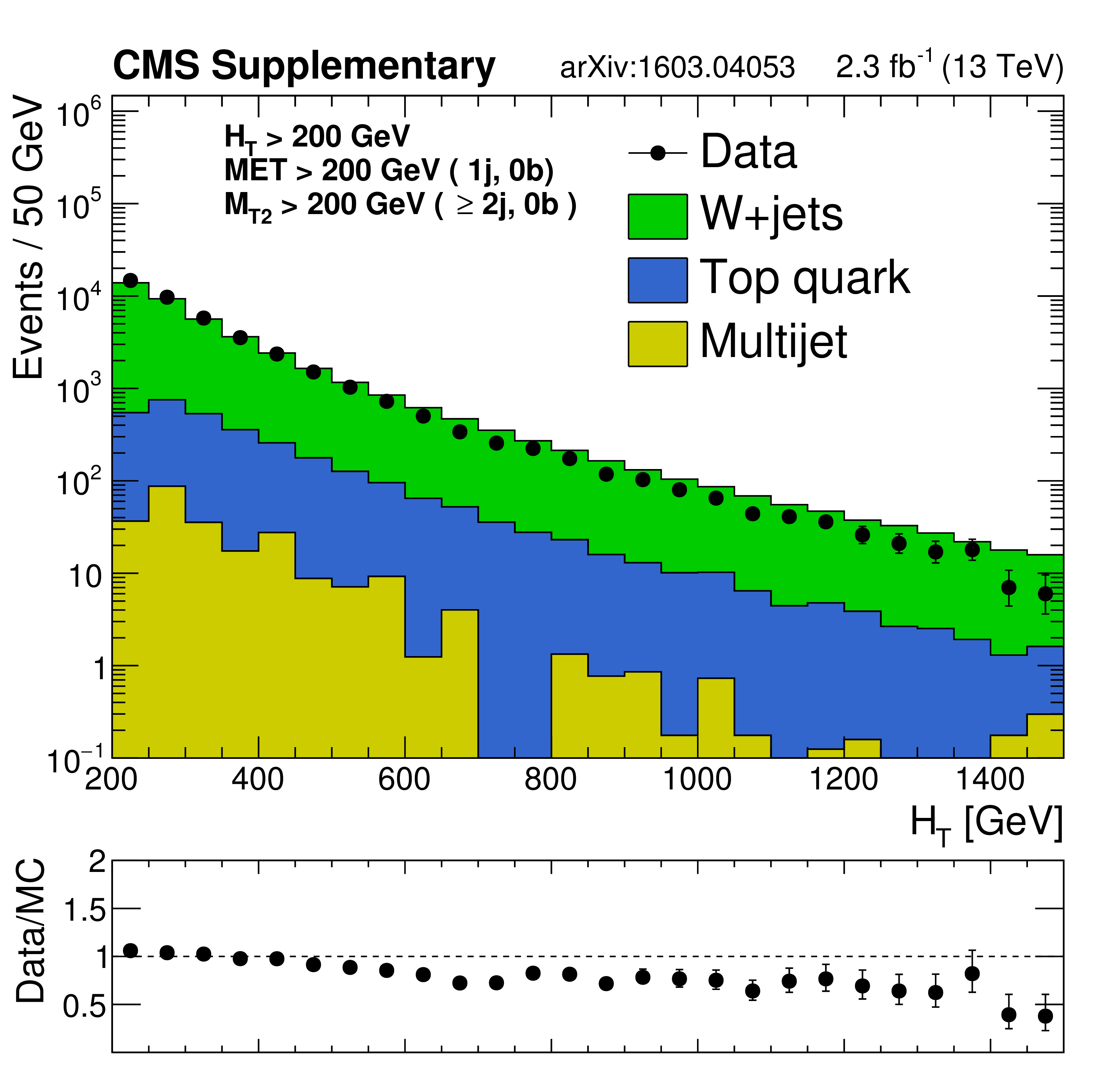
Data and MC comparison in the $ {\gamma +\mathrm {jets}} $ control region for $ {\mathrm {Z}\rightarrow \nu \bar{\nu} } $ background after the baseline selections, as a function of $ {H_{\mathrm {T}}} $, $ {N_{\mathrm {j}}} $, $ {N_{\mathrm {b}}} $. An $ {M_{\mathrm {T2}}} $ requirement is applied for events with 2 or more jets, while an $ {E_{\mathrm {T}}^{\text {miss}}} $ requirement is applied to events with exactly one jet. The fragmentation (''Frag.'') category is obtained from Madraph+Pythia QCD samples, and it includes prompt photons that fail the $\Delta R > 0.4$ requirement between the prompt photon and the nearest parton. In the analysis, data-driven background estimates binned in $ {H_{\mathrm {T}}} $, $ {N_{\mathrm {j}}} $ and $ {N_{\mathrm {b}}} $ are used to account for trends in Data/MC ratios, which are similar to those observed in the $ {\mathrm {Z}\rightarrow \ell ^+\ell ^-} $ and $ {\mathrm{ W }^{\pm} \to \ell^{\pm} \nu } $ control regions. |
png pdf |
Additional Figure 7-b:
Data and MC comparison in the $ {\gamma +\mathrm {jets}} $ control region for $ {\mathrm {Z}\rightarrow \nu \bar{\nu} } $ background after the baseline selections, as a function of $ {H_{\mathrm {T}}} $, $ {N_{\mathrm {j}}} $, $ {N_{\mathrm {b}}} $. An $ {M_{\mathrm {T2}}} $ requirement is applied for events with 2 or more jets, while an $ {E_{\mathrm {T}}^{\text {miss}}} $ requirement is applied to events with exactly one jet. The fragmentation (''Frag.'') category is obtained from Madraph+Pythia QCD samples, and it includes prompt photons that fail the $\Delta R > 0.4$ requirement between the prompt photon and the nearest parton. In the analysis, data-driven background estimates binned in $ {H_{\mathrm {T}}} $, $ {N_{\mathrm {j}}} $ and $ {N_{\mathrm {b}}} $ are used to account for trends in Data/MC ratios, which are similar to those observed in the $ {\mathrm {Z}\rightarrow \ell ^+\ell ^-} $ and $ {\mathrm{ W }^{\pm} \to \ell^{\pm} \nu } $ control regions. |

png pdf |
Additional Figure 7-c:
Data and MC comparison in the $ {\gamma +\mathrm {jets}} $ control region for $ {\mathrm {Z}\rightarrow \nu \bar{\nu} } $ background after the baseline selections, as a function of $ {H_{\mathrm {T}}} $, $ {N_{\mathrm {j}}} $, $ {N_{\mathrm {b}}} $. An $ {M_{\mathrm {T2}}} $ requirement is applied for events with 2 or more jets, while an $ {E_{\mathrm {T}}^{\text {miss}}} $ requirement is applied to events with exactly one jet. The fragmentation (''Frag.'') category is obtained from Madraph+Pythia QCD samples, and it includes prompt photons that fail the $\Delta R > 0.4$ requirement between the prompt photon and the nearest parton. In the analysis, data-driven background estimates binned in $ {H_{\mathrm {T}}} $, $ {N_{\mathrm {j}}} $ and $ {N_{\mathrm {b}}} $ are used to account for trends in Data/MC ratios, which are similar to those observed in the $ {\mathrm {Z}\rightarrow \ell ^+\ell ^-} $ and $ {\mathrm{ W }^{\pm} \to \ell^{\pm} \nu } $ control regions. |

png pdf |
Additional Figure 8-a:
Data-MC shape comparison of $ {\sigma _{i\eta i\eta }} $ for photon candidates reconstructed in the ECAL barrel (a) and endcaps (b). Prompt photons are shown in grey, fragmentation photons in blue and fake photons in red. These events have been selected with a very loose isolation requirement, in order to increase the yield of fake photons. The fragmentation (``Fragm.'') category is obtained from Madraph+Pythia QCD samples, and it includes prompt photons that fail the $\Delta R > 0.4$ requirement between the prompt photon and the nearest parton. |
png pdf |
Additional Figure 8-b:
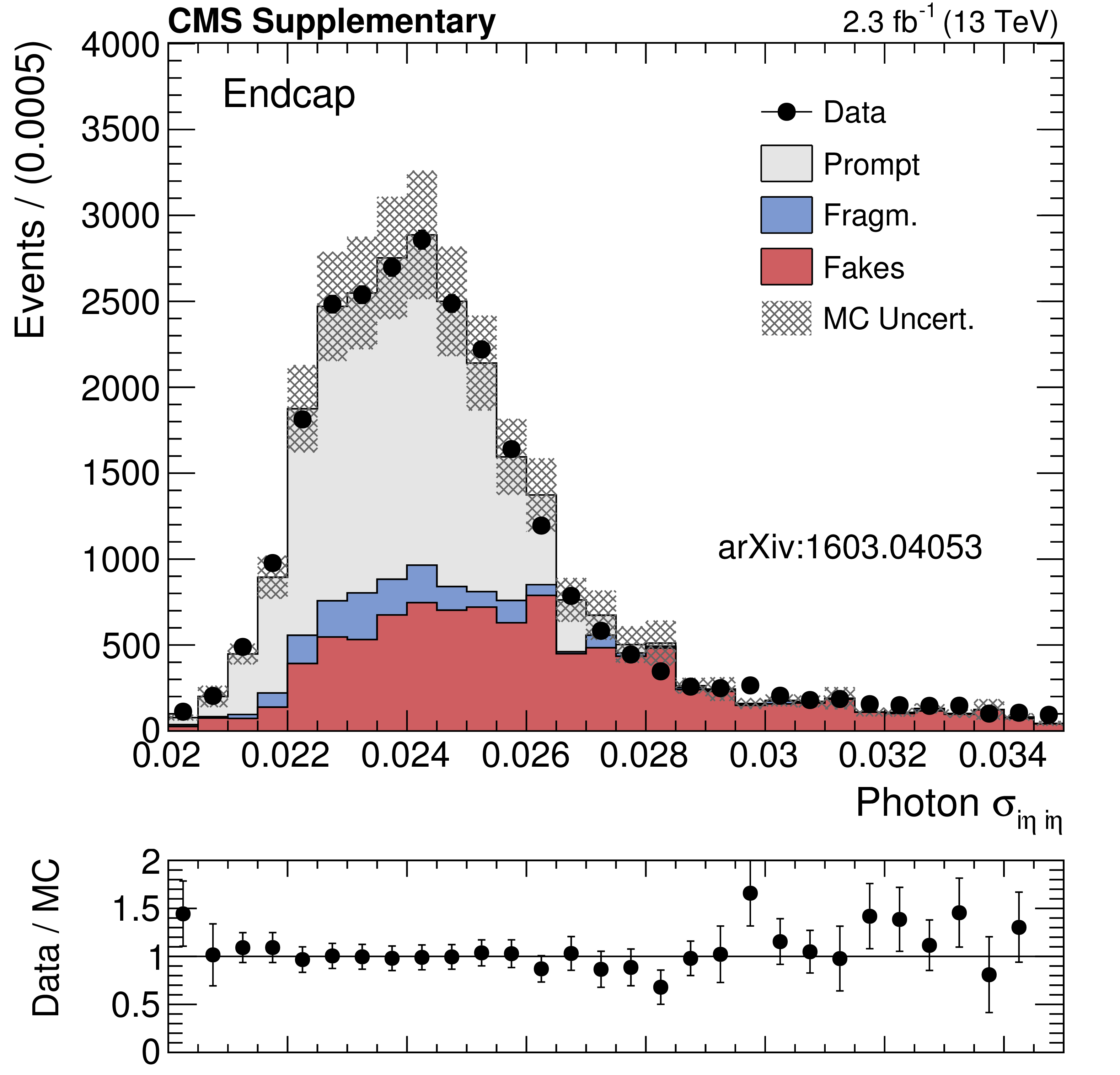
Data-MC shape comparison of $ {\sigma _{i\eta i\eta }} $ for photon candidates reconstructed in the ECAL barrel (a) and endcaps (b). Prompt photons are shown in grey, fragmentation photons in blue and fake photons in red. These events have been selected with a very loose isolation requirement, in order to increase the yield of fake photons. The fragmentation (``Fragm.'') category is obtained from Madraph+Pythia QCD samples, and it includes prompt photons that fail the $\Delta R > 0.4$ requirement between the prompt photon and the nearest parton. |
png pdf |
Additional Figure 9:
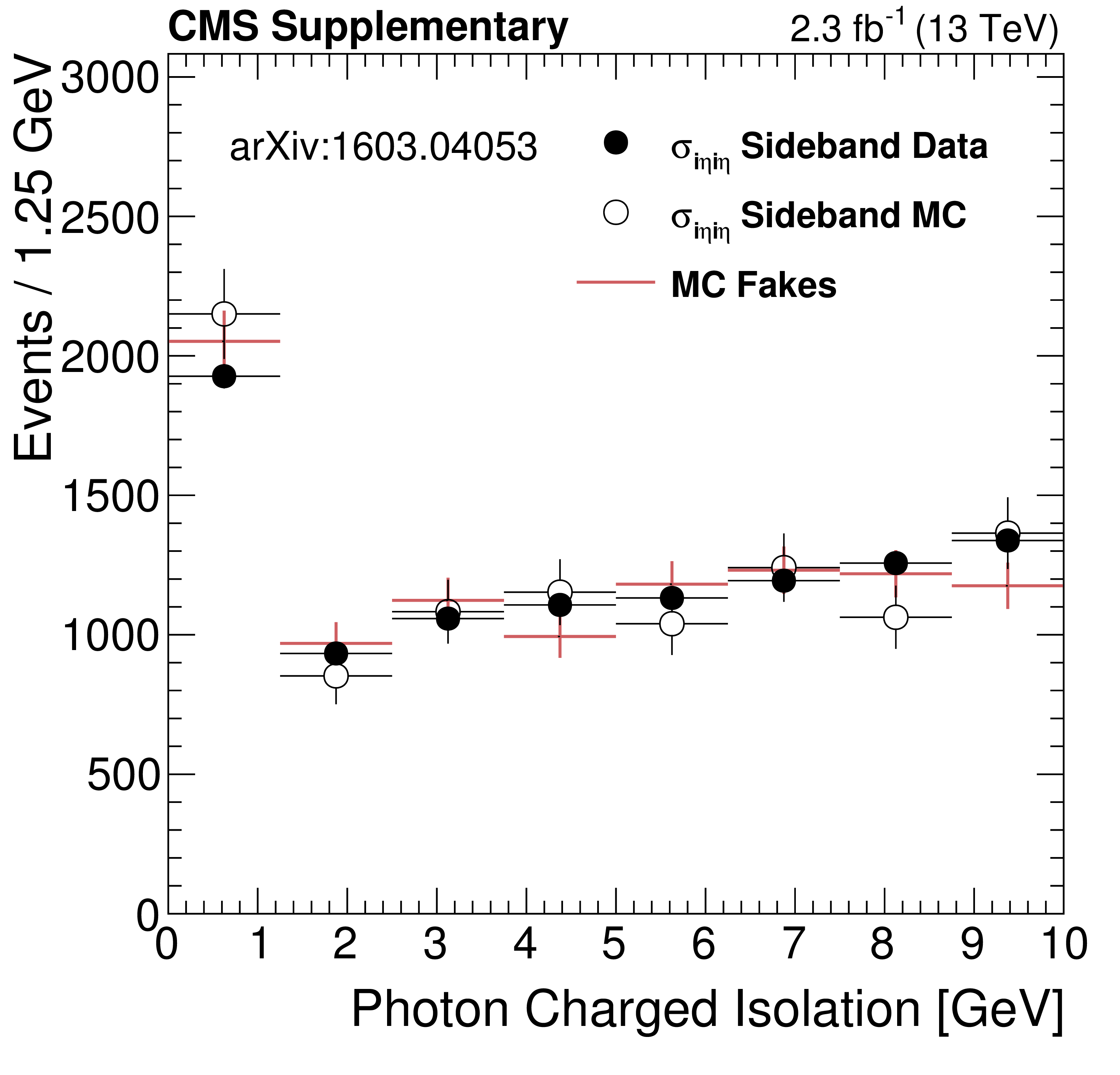
Comparison between the fake photon isolation template obtained from the $ {\sigma _{i\eta i\eta }} $ sidebands (black markers) and the one obtained by selecting MC-matched fake photons that pass the nominal selection (red crosses). |
png pdf |
Additional Figure 10-a:
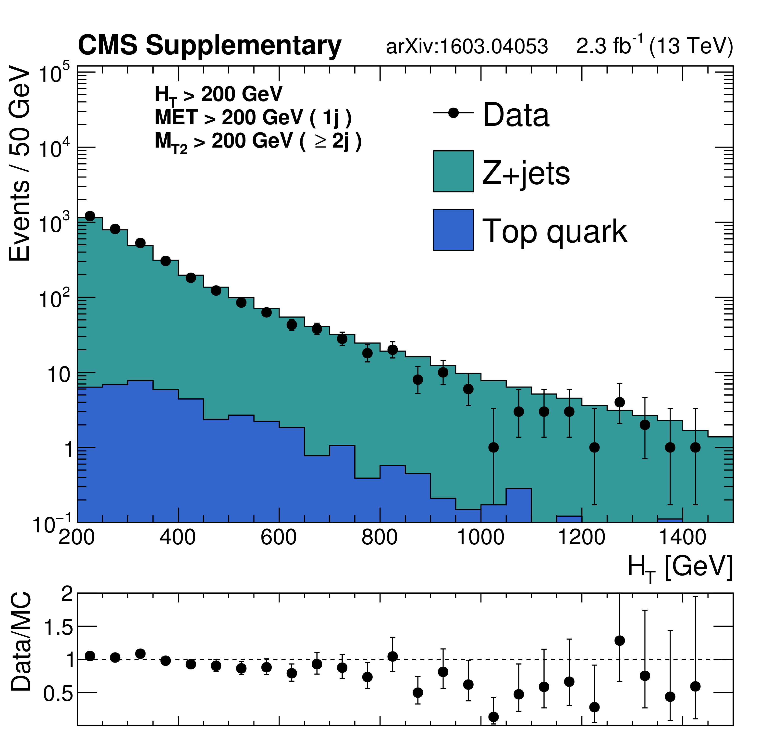
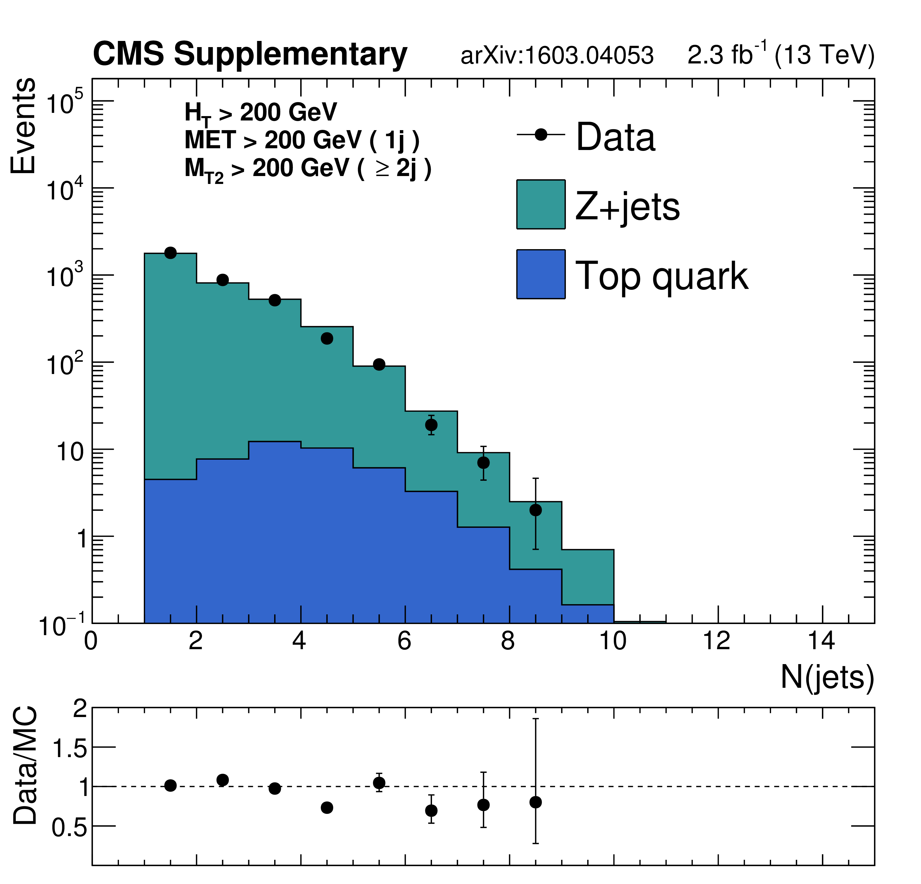
Data and MC comparison in the $ {\mathrm {Z}\rightarrow \ell ^+\ell ^-} $ control region for $ {\mathrm {Z}\rightarrow \nu \bar{\nu} } $ background after the baseline selections, as a function of $ {H_{\mathrm {T}}} $, $ {N_{\mathrm {j}}} $, $ {N_{\mathrm {b}}} $. An $ {M_{\mathrm {T2}}} $ requirement is applied for events with 2 or more jets, while an $ {E_{\mathrm {T}}^{\text {miss}}} $requirement is applied to events with exactly one jet. The trends in the Data/MC ratios are similar to those observed in the $ {\gamma +\mathrm {jets}} $ and $ {\mathrm{ W }^{\pm} \to \ell^{\pm} \nu } $ control regions. |
png pdf |
Additional Figure 10-b:
Data and MC comparison in the $ {\mathrm {Z}\rightarrow \ell ^+\ell ^-} $ control region for $ {\mathrm {Z}\rightarrow \nu \bar{\nu} } $ background after the baseline selections, as a function of $ {H_{\mathrm {T}}} $, $ {N_{\mathrm {j}}} $, $ {N_{\mathrm {b}}} $. An $ {M_{\mathrm {T2}}} $ requirement is applied for events with 2 or more jets, while an $ {E_{\mathrm {T}}^{\text {miss}}} $requirement is applied to events with exactly one jet. The trends in the Data/MC ratios are similar to those observed in the $ {\gamma +\mathrm {jets}} $ and $ {\mathrm{ W }^{\pm} \to \ell^{\pm} \nu } $ control regions. |

png pdf |
Additional Figure 10-c:
Data and MC comparison in the $ {\mathrm {Z}\rightarrow \ell ^+\ell ^-} $ control region for $ {\mathrm {Z}\rightarrow \nu \bar{\nu} } $ background after the baseline selections, as a function of $ {H_{\mathrm {T}}} $, $ {N_{\mathrm {j}}} $, $ {N_{\mathrm {b}}} $. An $ {M_{\mathrm {T2}}} $ requirement is applied for events with 2 or more jets, while an $ {E_{\mathrm {T}}^{\text {miss}}} $requirement is applied to events with exactly one jet. The trends in the Data/MC ratios are similar to those observed in the $ {\gamma +\mathrm {jets}} $ and $ {\mathrm{ W }^{\pm} \to \ell^{\pm} \nu } $ control regions. |
png pdf |
Additional Figure 11-a:
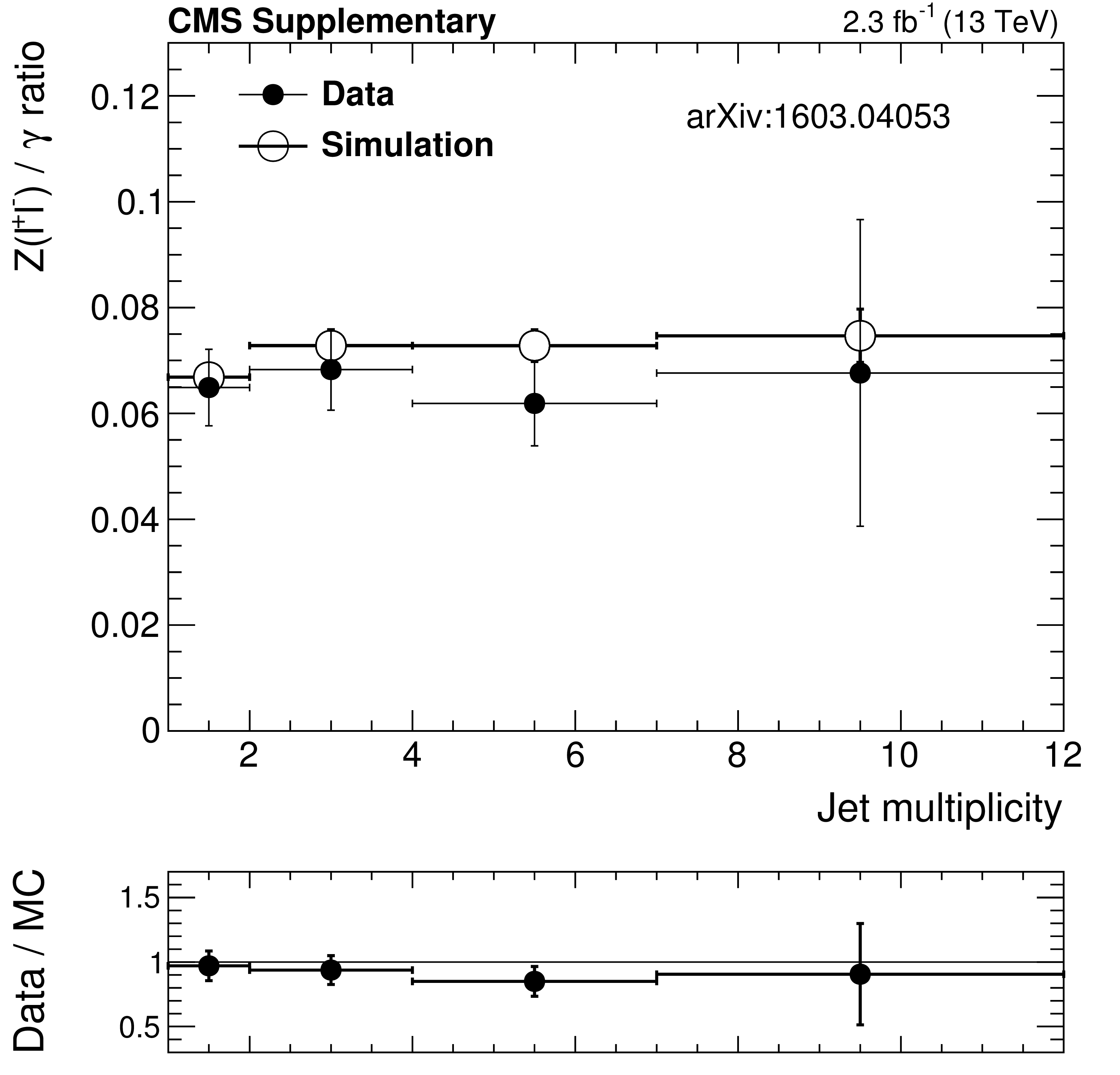
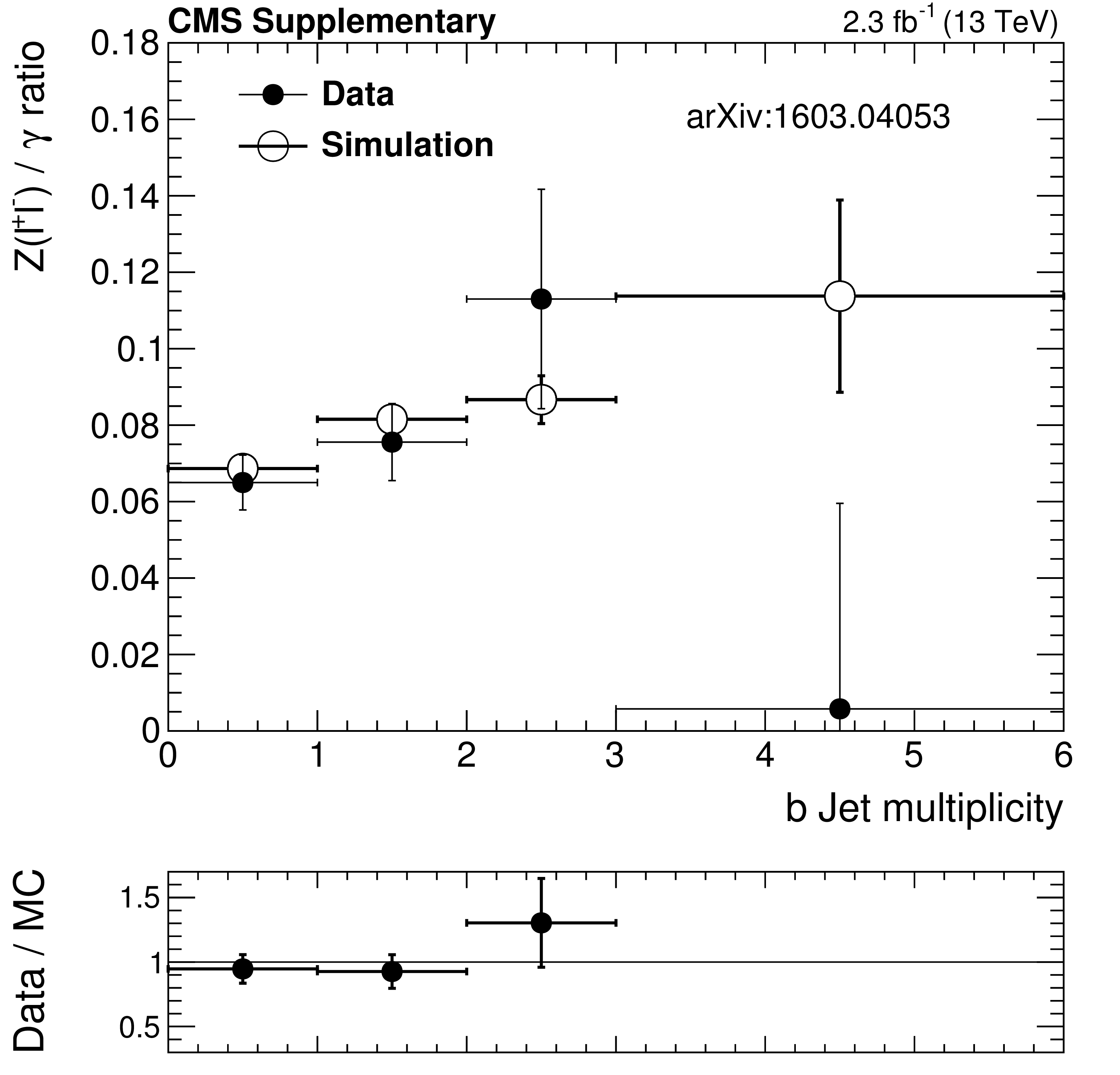
$R( {\mathrm {Z}\rightarrow \ell ^+\ell ^-} /\gamma )$ ratio in data (black markers) and in the simulation (black open markers) as a function of $ {N_{\mathrm {j}}} $ (a) and $ {N_{\mathrm {b}}} $ (b) after baseline selection. The $ {H_{\mathrm {T}}} $ plot is shown with a finer binning, corresponding to the $ {H_{\mathrm {T}}} $ bins of the monojet analysis region, in (c). |
png pdf |
Additional Figure 11-b:
$R( {\mathrm {Z}\rightarrow \ell ^+\ell ^-} /\gamma )$ ratio in data (black markers) and in the simulation (black open markers) as a function of $ {N_{\mathrm {j}}} $ (a) and $ {N_{\mathrm {b}}} $ (b) after baseline selection. The $ {H_{\mathrm {T}}} $ plot is shown with a finer binning, corresponding to the $ {H_{\mathrm {T}}} $ bins of the monojet analysis region, in (c). |

png pdf |
Additional Figure 11-c:
$R( {\mathrm {Z}\rightarrow \ell ^+\ell ^-} /\gamma )$ ratio in data (black markers) and in the simulation (black open markers) as a function of $ {N_{\mathrm {j}}} $ (a) and $ {N_{\mathrm {b}}} $ (b) after baseline selection. The $ {H_{\mathrm {T}}} $ plot is shown with a finer binning, corresponding to the $ {H_{\mathrm {T}}} $ bins of the monojet analysis region, in (c). |

png pdf |
Additional Figure 12:
Flavor composition of the leading two $b$-tagged jets in signal regions with at least 2 $b$-tags in the $ {\mathrm {Z}\rightarrow \nu \bar{\nu} } $ and $ {\gamma +\mathrm {jets}} $ samples. |
png pdf |
Additional Figure 13-a:
Data and MC comparison in the $ {\mathrm{ W }^{\pm} \to \ell^{\pm} \nu } $ control region for $ {\mathrm {Z}\rightarrow \nu \bar{\nu} } $ background after the baseline selections, as a function of $ {H_{\mathrm {T}}} $ and $ {N_{\mathrm {j}}} $. An $ {M_{\mathrm {T2}}} $ requirement is applied for events with 2 or more jets, while an $ {E_{\mathrm {T}}^{\text {miss}}} $requirement is applied to events with exactly one jet. The trends in the Data/MC ratios are similar to those observed in the $ {\gamma +\mathrm {jets}} $ and $ {\mathrm {Z}\rightarrow \ell ^+\ell ^-} $ control regions. |

png pdf |
Additional Figure 13-b:
Data and MC comparison in the $ {\mathrm{ W }^{\pm} \to \ell^{\pm} \nu } $ control region for $ {\mathrm {Z}\rightarrow \nu \bar{\nu} } $ background after the baseline selections, as a function of $ {H_{\mathrm {T}}} $ and $ {N_{\mathrm {j}}} $. An $ {M_{\mathrm {T2}}} $ requirement is applied for events with 2 or more jets, while an $ {E_{\mathrm {T}}^{\text {miss}}} $requirement is applied to events with exactly one jet. The trends in the Data/MC ratios are similar to those observed in the $ {\gamma +\mathrm {jets}} $ and $ {\mathrm {Z}\rightarrow \ell ^+\ell ^-} $ control regions. |
png pdf |
Additional Figure 14-a:
Shape comparison of the $ {M_{\mathrm {T2}}} $ distribution in the $ {\gamma +\mathrm {jets}} $ (red markers) and $ {\mathrm{ W }^{\pm} \to \ell^{\pm} \nu } $ control (green markers) regions in data, compared to the expected shape of the simulated $ {\mathrm {Z}\rightarrow \nu \bar{\nu} } $ process(black markers), in different $ {H_{\mathrm {T}}} $ regions: $200 < {H_{\mathrm {T}}} < 450$ GeV (a), $450 < {H_{\mathrm {T}}} < 575$ GeV (b), $575 < {H_{\mathrm {T}}} < 1000$ GeV(c), $1000 < {H_{\mathrm {T}}} < 1500$ GeV (d) and finally $ {H_{\mathrm {T}}} > 1500$ GeV (e). The shaded band in the ratio histogram includes experimental and theoretical uncertainties on the $ {\mathrm {Z}\rightarrow \nu \bar{\nu} } $ background $ {M_{\mathrm {T2}}} $ distribution. |
png pdf |
Additional Figure 14-b:
Shape comparison of the $ {M_{\mathrm {T2}}} $ distribution in the $ {\gamma +\mathrm {jets}} $ (red markers) and $ {\mathrm{ W }^{\pm} \to \ell^{\pm} \nu } $ control (green markers) regions in data, compared to the expected shape of the simulated $ {\mathrm {Z}\rightarrow \nu \bar{\nu} } $ process(black markers), in different $ {H_{\mathrm {T}}} $ regions: $200 < {H_{\mathrm {T}}} < 450$ GeV (a), $450 < {H_{\mathrm {T}}} < 575$ GeV (b), $575 < {H_{\mathrm {T}}} < 1000$ GeV(c), $1000 < {H_{\mathrm {T}}} < 1500$ GeV (d) and finally $ {H_{\mathrm {T}}} > 1500$ GeV (e). The shaded band in the ratio histogram includes experimental and theoretical uncertainties on the $ {\mathrm {Z}\rightarrow \nu \bar{\nu} } $ background $ {M_{\mathrm {T2}}} $ distribution. |
png pdf |
Additional Figure 14-c:
Shape comparison of the $ {M_{\mathrm {T2}}} $ distribution in the $ {\gamma +\mathrm {jets}} $ (red markers) and $ {\mathrm{ W }^{\pm} \to \ell^{\pm} \nu } $ control (green markers) regions in data, compared to the expected shape of the simulated $ {\mathrm {Z}\rightarrow \nu \bar{\nu} } $ process(black markers), in different $ {H_{\mathrm {T}}} $ regions: $200 < {H_{\mathrm {T}}} < 450$ GeV (a), $450 < {H_{\mathrm {T}}} < 575$ GeV (b), $575 < {H_{\mathrm {T}}} < 1000$ GeV(c), $1000 < {H_{\mathrm {T}}} < 1500$ GeV (d) and finally $ {H_{\mathrm {T}}} > 1500$ GeV (e). The shaded band in the ratio histogram includes experimental and theoretical uncertainties on the $ {\mathrm {Z}\rightarrow \nu \bar{\nu} } $ background $ {M_{\mathrm {T2}}} $ distribution. |

png pdf |
Additional Figure 14-d:
Shape comparison of the $ {M_{\mathrm {T2}}} $ distribution in the $ {\gamma +\mathrm {jets}} $ (red markers) and $ {\mathrm{ W }^{\pm} \to \ell^{\pm} \nu } $ control (green markers) regions in data, compared to the expected shape of the simulated $ {\mathrm {Z}\rightarrow \nu \bar{\nu} } $ process(black markers), in different $ {H_{\mathrm {T}}} $ regions: $200 < {H_{\mathrm {T}}} < 450$ GeV (a), $450 < {H_{\mathrm {T}}} < 575$ GeV (b), $575 < {H_{\mathrm {T}}} < 1000$ GeV(c), $1000 < {H_{\mathrm {T}}} < 1500$ GeV (d) and finally $ {H_{\mathrm {T}}} > 1500$ GeV (e). The shaded band in the ratio histogram includes experimental and theoretical uncertainties on the $ {\mathrm {Z}\rightarrow \nu \bar{\nu} } $ background $ {M_{\mathrm {T2}}} $ distribution. |
png pdf |
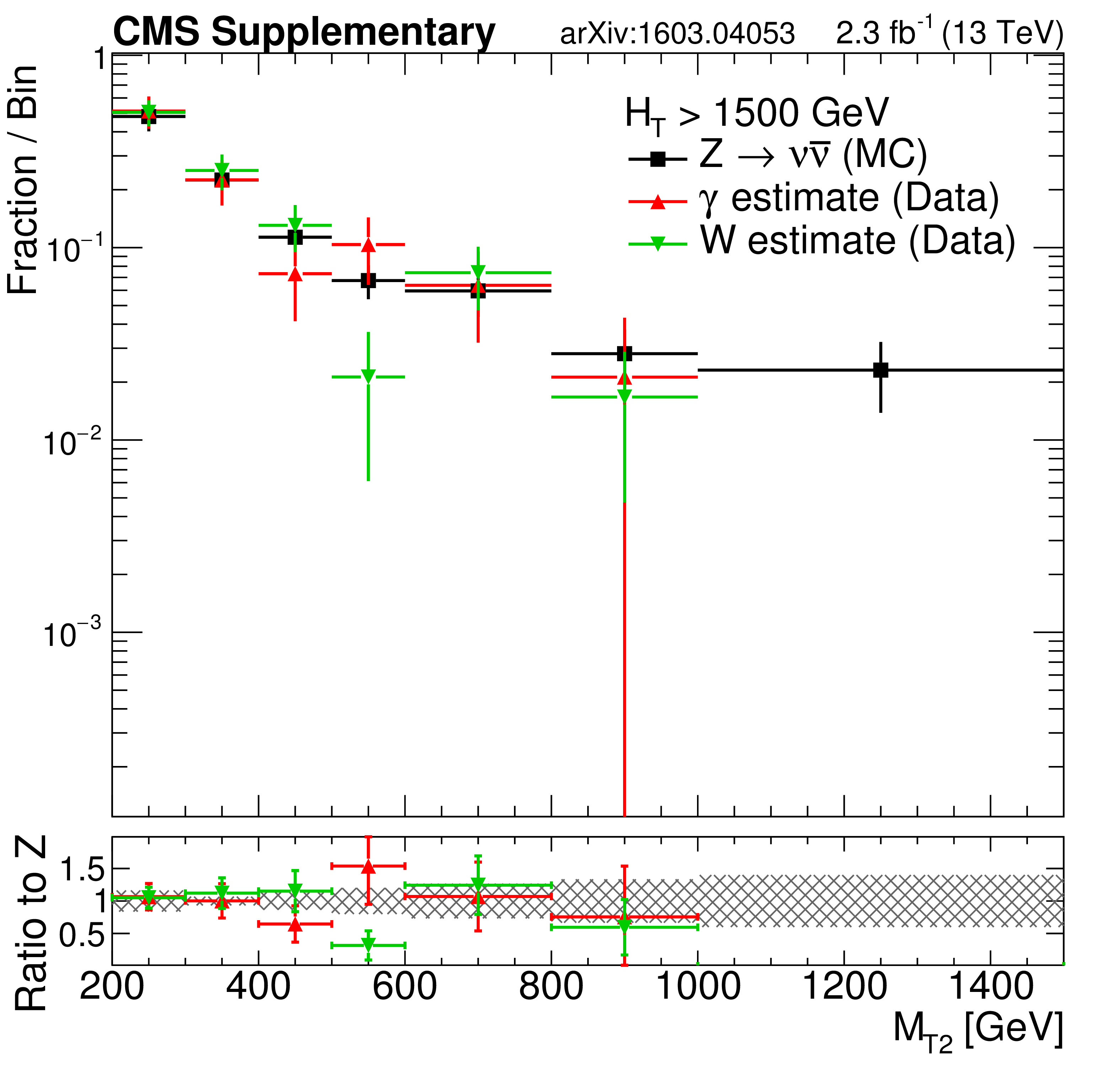
Additional Figure 14-e:
Shape comparison of the $ {M_{\mathrm {T2}}} $ distribution in the $ {\gamma +\mathrm {jets}} $ (red markers) and $ {\mathrm{ W }^{\pm} \to \ell^{\pm} \nu } $ control (green markers) regions in data, compared to the expected shape of the simulated $ {\mathrm {Z}\rightarrow \nu \bar{\nu} } $ process(black markers), in different $ {H_{\mathrm {T}}} $ regions: $200 < {H_{\mathrm {T}}} < 450$ GeV (a), $450 < {H_{\mathrm {T}}} < 575$ GeV (b), $575 < {H_{\mathrm {T}}} < 1000$ GeV(c), $1000 < {H_{\mathrm {T}}} < 1500$ GeV (d) and finally $ {H_{\mathrm {T}}} > 1500$ GeV (e). The shaded band in the ratio histogram includes experimental and theoretical uncertainties on the $ {\mathrm {Z}\rightarrow \nu \bar{\nu} } $ background $ {M_{\mathrm {T2}}} $ distribution. |
png pdf |
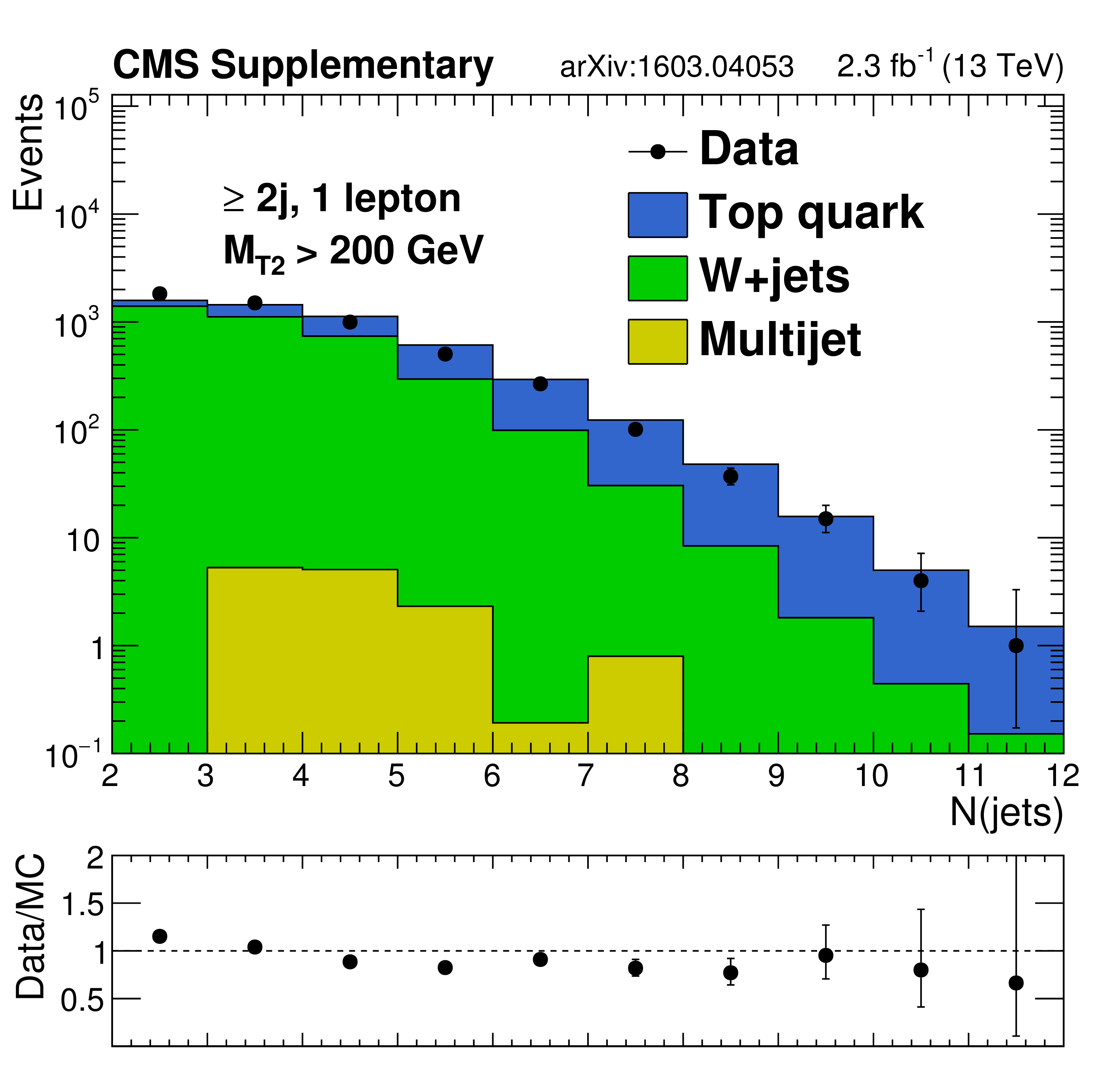
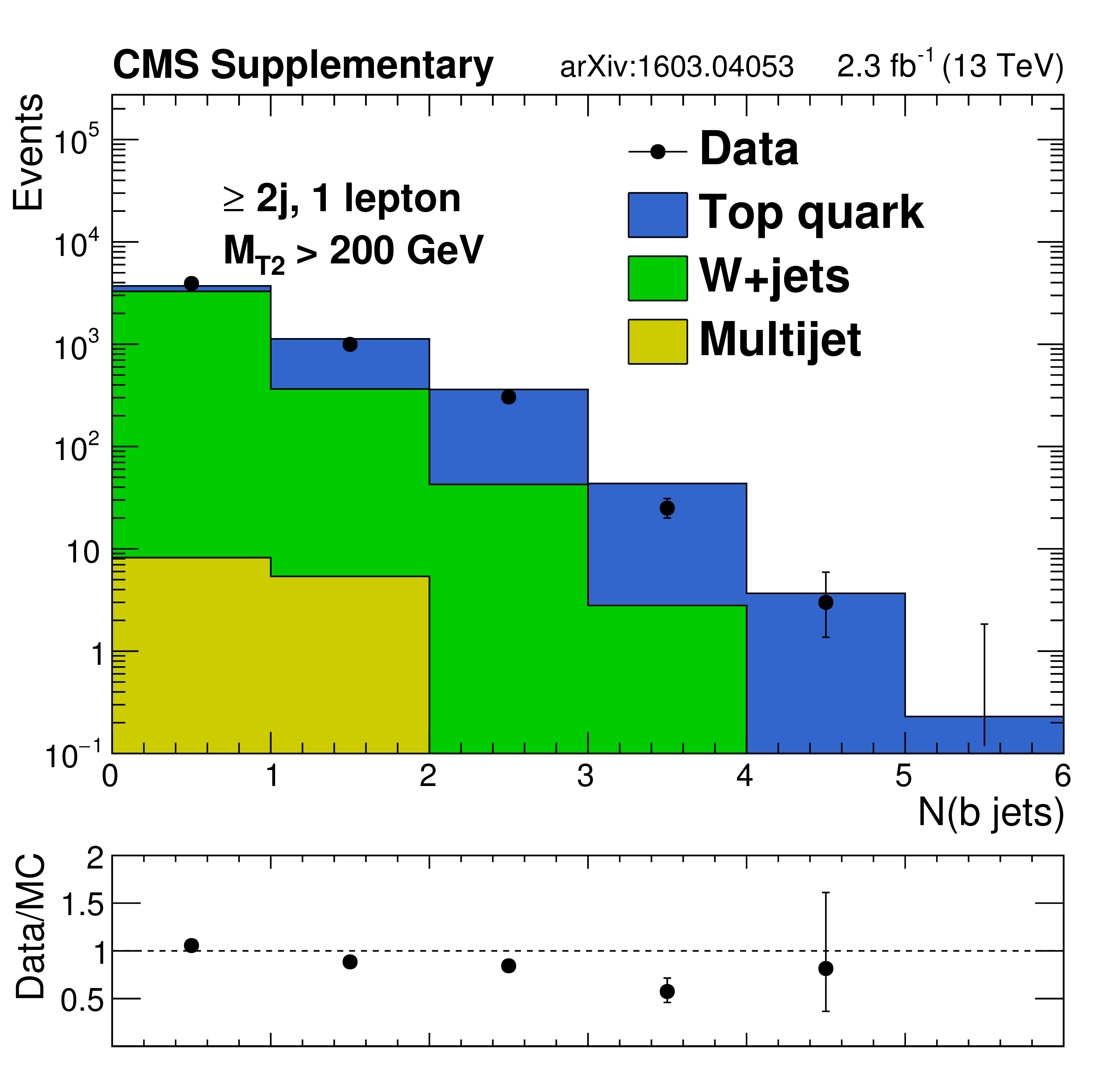
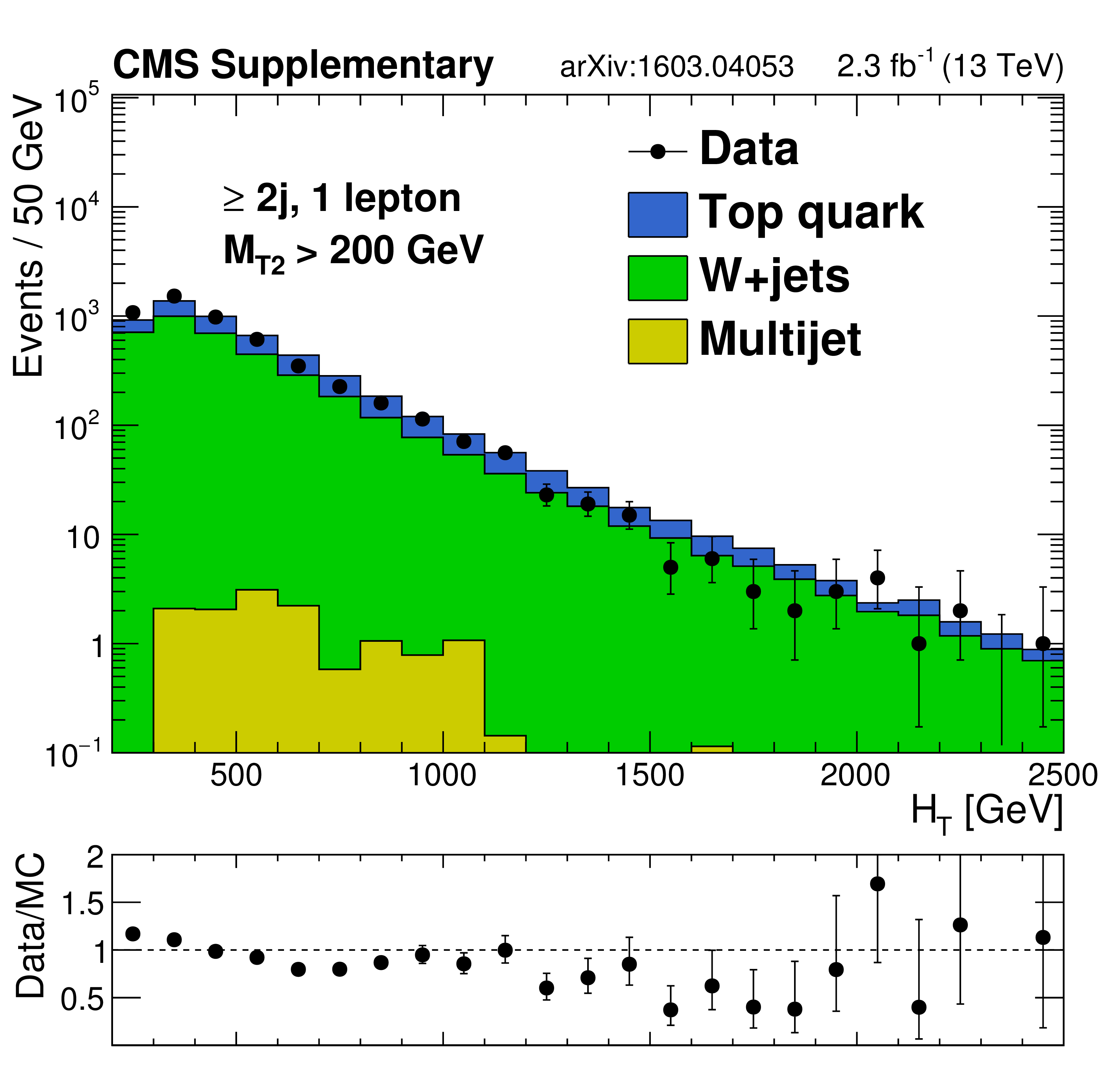
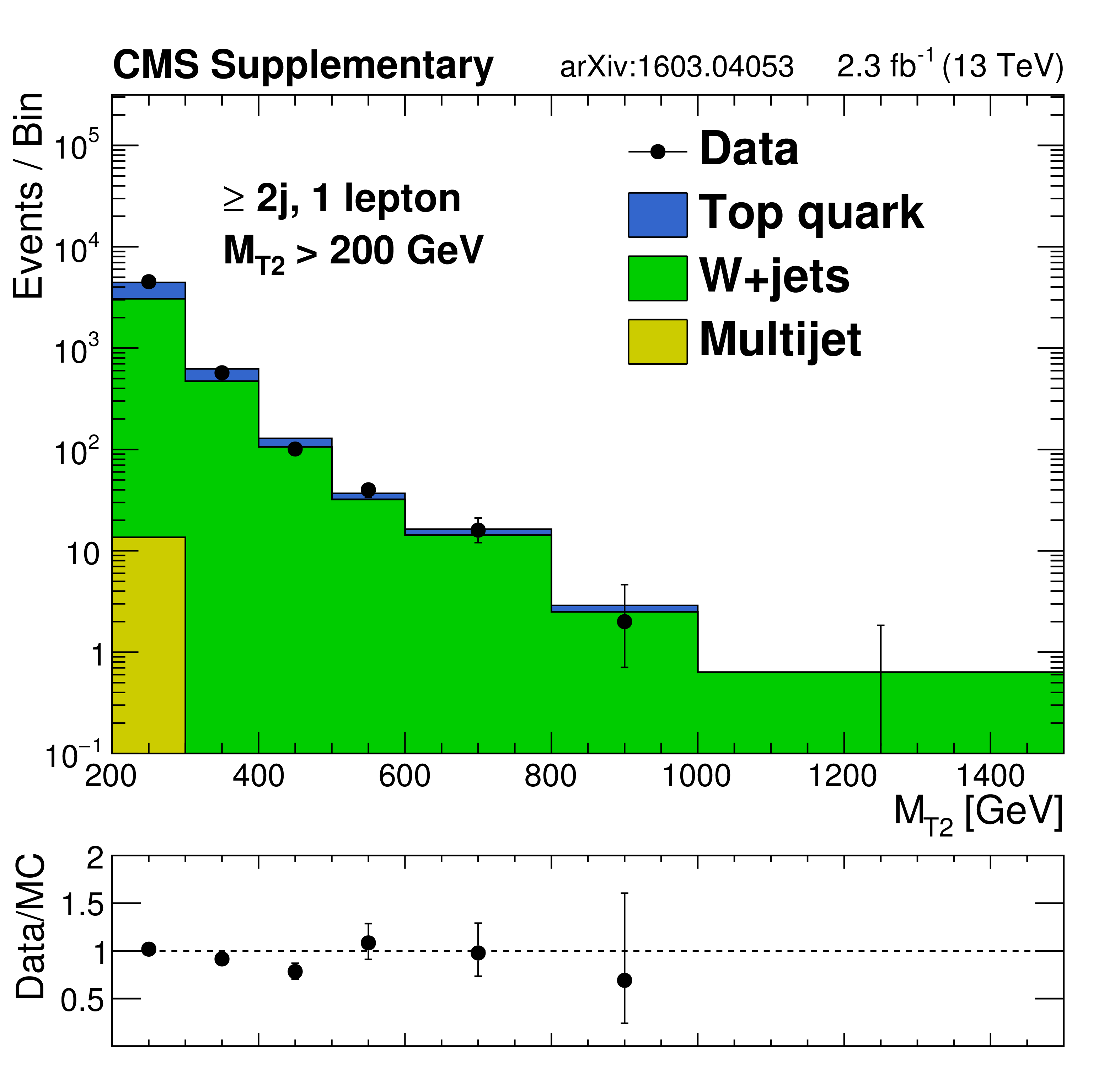
Additional Figure 15-a:
Distributions of data and MC predictions for the baseline single lepton control region selection with at least 2 jets and $ {H_{\mathrm {T}}} > 200$ GeV. Shown are (a) $ {N_{\mathrm {j}}} $, (b) $ {N_{\mathrm {b}}} $ , (c) $ {H_{\mathrm {T}}} $, and (d) $ {M_{\mathrm {T2}}} $. MC is normalized to data in each plot to compare the shapes. |
png pdf |
Additional Figure 15-b:
Distributions of data and MC predictions for the baseline single lepton control region selection with at least 2 jets and $ {H_{\mathrm {T}}} > 200$ GeV. Shown are (a) $ {N_{\mathrm {j}}} $, (b) $ {N_{\mathrm {b}}} $ , (c) $ {H_{\mathrm {T}}} $, and (d) $ {M_{\mathrm {T2}}} $. MC is normalized to data in each plot to compare the shapes. |
png pdf |
Additional Figure 15-c:
Distributions of data and MC predictions for the baseline single lepton control region selection with at least 2 jets and $ {H_{\mathrm {T}}} > 200$ GeV. Shown are (a) $ {N_{\mathrm {j}}} $, (b) $ {N_{\mathrm {b}}} $ , (c) $ {H_{\mathrm {T}}} $, and (d) $ {M_{\mathrm {T2}}} $. MC is normalized to data in each plot to compare the shapes. |
png pdf |
Additional Figure 15-d:
Distributions of data and MC predictions for the baseline single lepton control region selection with at least 2 jets and $ {H_{\mathrm {T}}} > 200$ GeV. Shown are (a) $ {N_{\mathrm {j}}} $, (b) $ {N_{\mathrm {b}}} $ , (c) $ {H_{\mathrm {T}}} $, and (d) $ {M_{\mathrm {T2}}} $. MC is normalized to data in each plot to compare the shapes. |
png pdf |
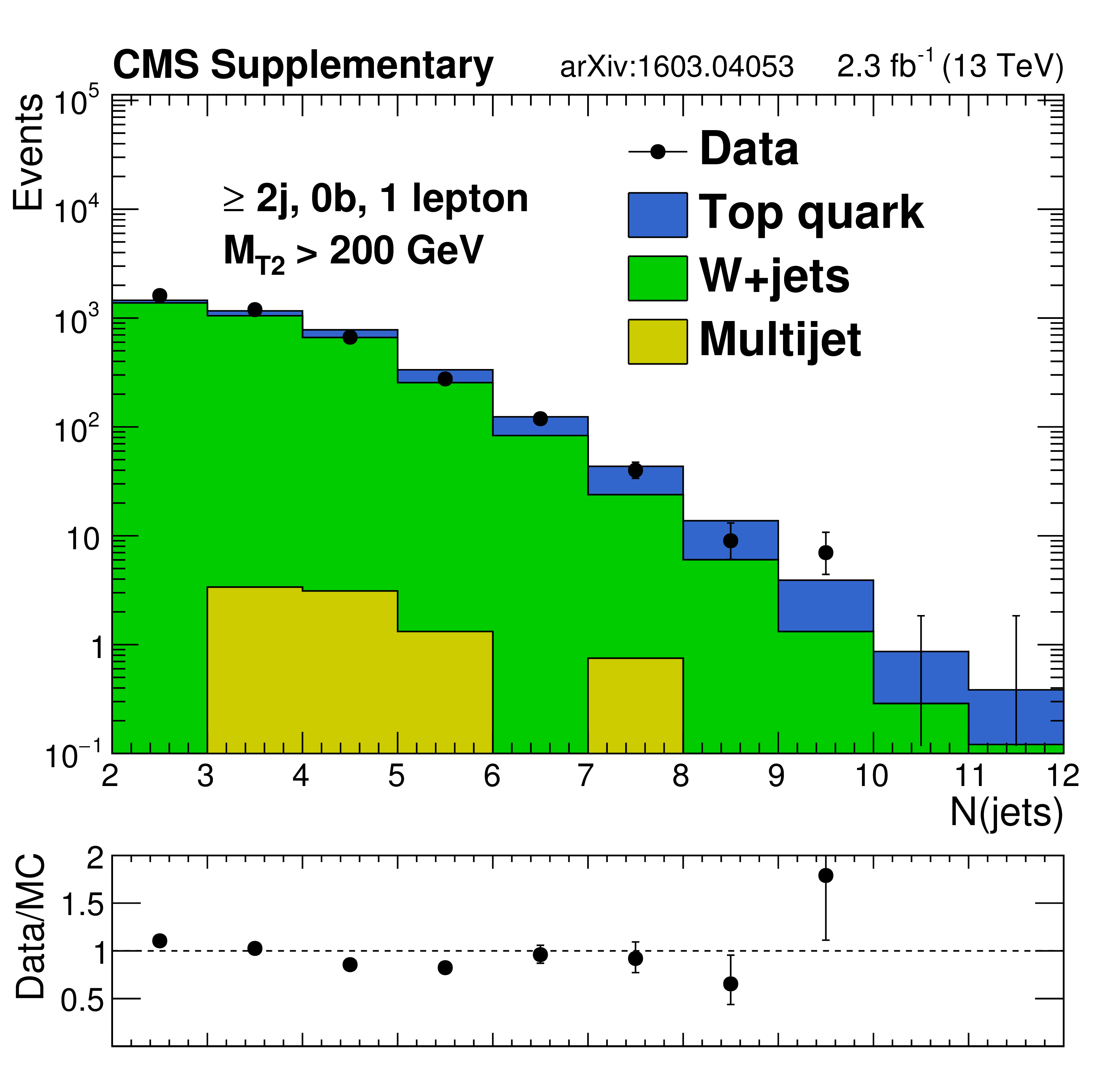
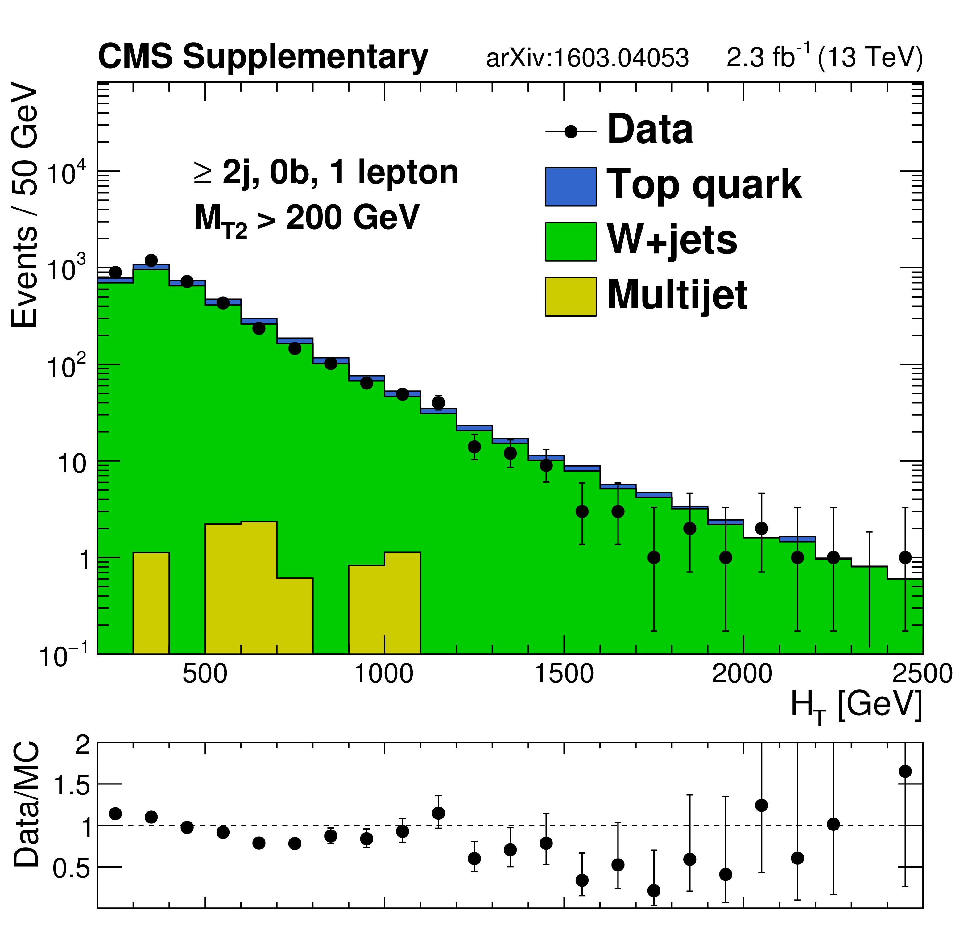
Additional Figure 16-a:
Distributions of data and MC predictions for the single lepton control region selection enhanced in $ {\mathrm {W}\mathrm {+jets}} $: at least 2 jets, no b-tagged jets, and $ {H_{\mathrm {T}}} > 200$ GeV. Shown are (a) $ {N_{\mathrm {j}}} $, (b) $ {H_{\mathrm {T}}} $, and (c) $ {M_{\mathrm {T2}}} $. MC is normalized to data in each plot to compare the shapes. |
png pdf |
Additional Figure 16-b:
Distributions of data and MC predictions for the single lepton control region selection enhanced in $ {\mathrm {W}\mathrm {+jets}} $: at least 2 jets, no b-tagged jets, and $ {H_{\mathrm {T}}} > 200$ GeV. Shown are (a) $ {N_{\mathrm {j}}} $, (b) $ {H_{\mathrm {T}}} $, and (c) $ {M_{\mathrm {T2}}} $. MC is normalized to data in each plot to compare the shapes. |
png pdf |
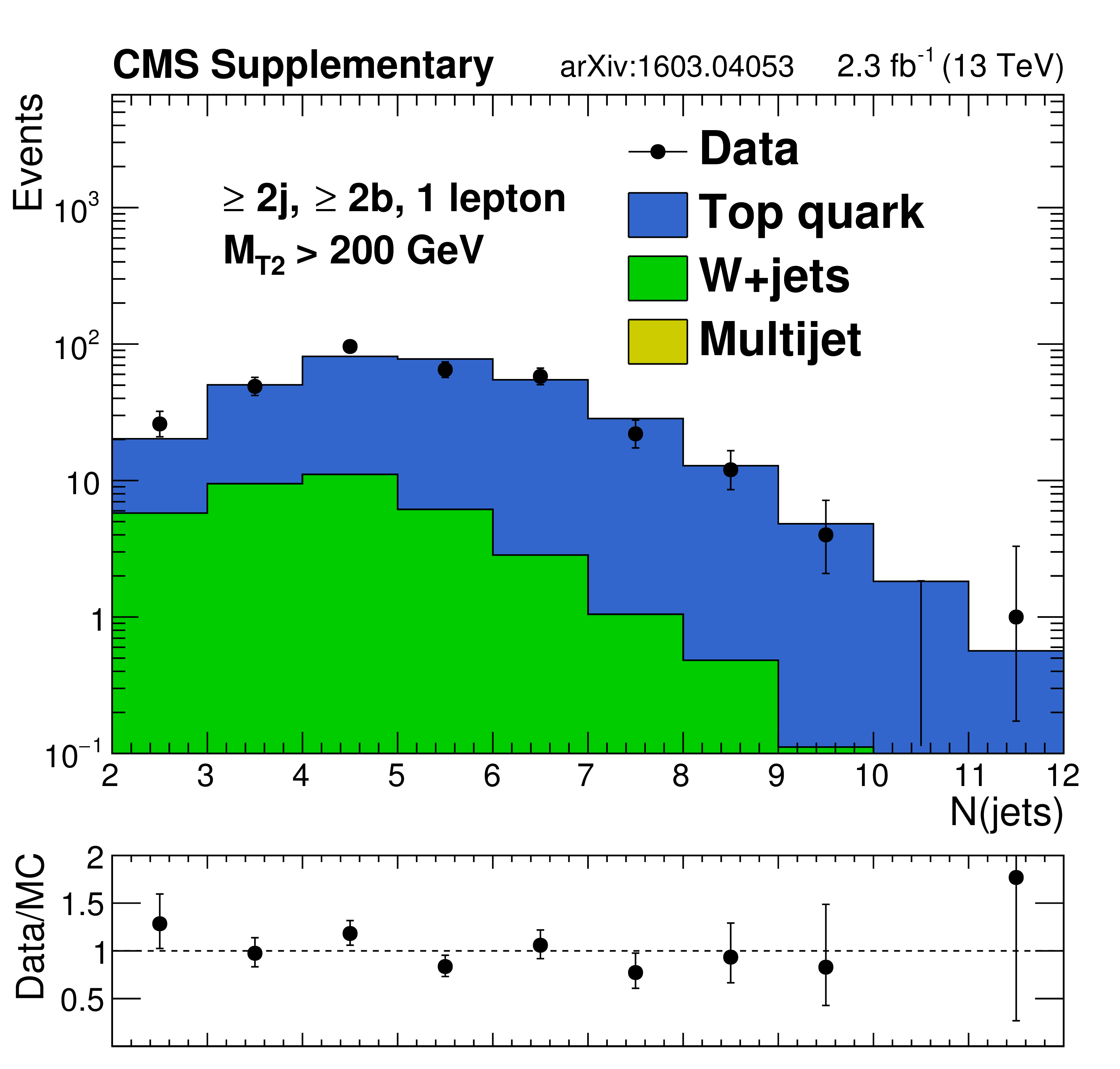
Additional Figure 17-a:
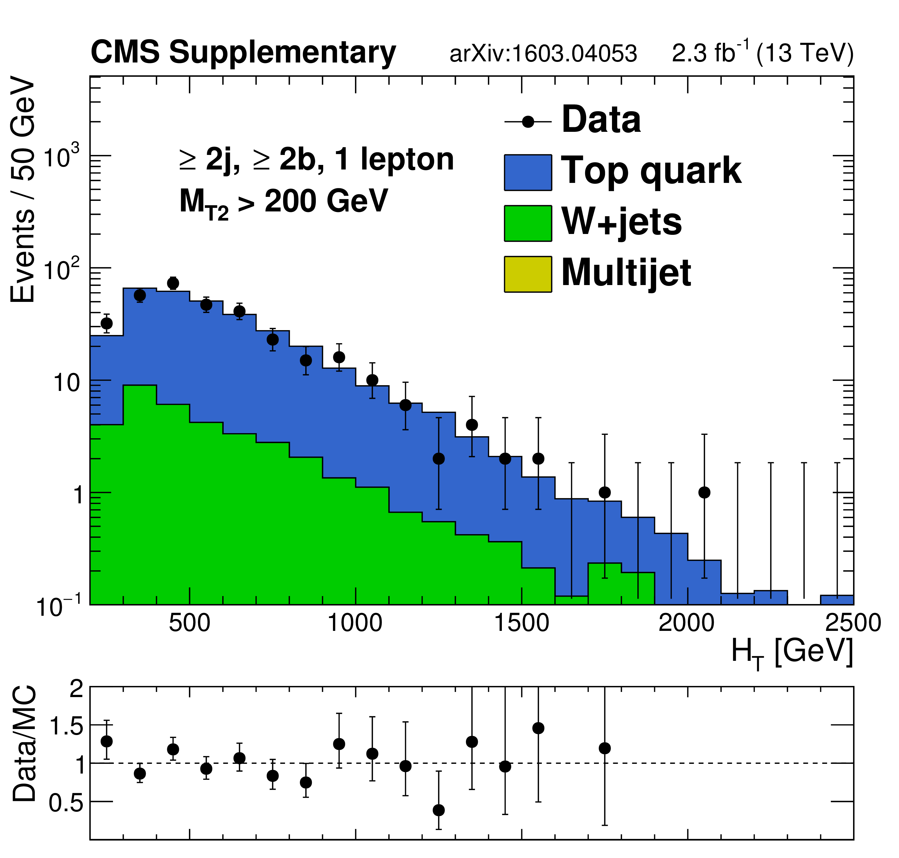
Distributions of data and MC predictions for the single lepton control region selection enhanced in $ {\mathrm{ t \bar{t} } } $: at least 2 jets, at least 2 b-tagged jets, and $ {H_{\mathrm {T}}} > 200$ GeV. Shown are (a) $ {N_{\mathrm {j}}} $, (b) $ {H_{\mathrm {T}}} $, and (c) $ {M_{\mathrm {T2}}} $. MC is normalized to data in each plot to compare the shapes. |
png pdf |
Additional Figure 17-b:
Distributions of data and MC predictions for the single lepton control region selection enhanced in $ {\mathrm{ t \bar{t} } } $: at least 2 jets, at least 2 b-tagged jets, and $ {H_{\mathrm {T}}} > 200$ GeV. Shown are (a) $ {N_{\mathrm {j}}} $, (b) $ {H_{\mathrm {T}}} $, and (c) $ {M_{\mathrm {T2}}} $. MC is normalized to data in each plot to compare the shapes. |
png pdf |
Additional Figure 18-a:
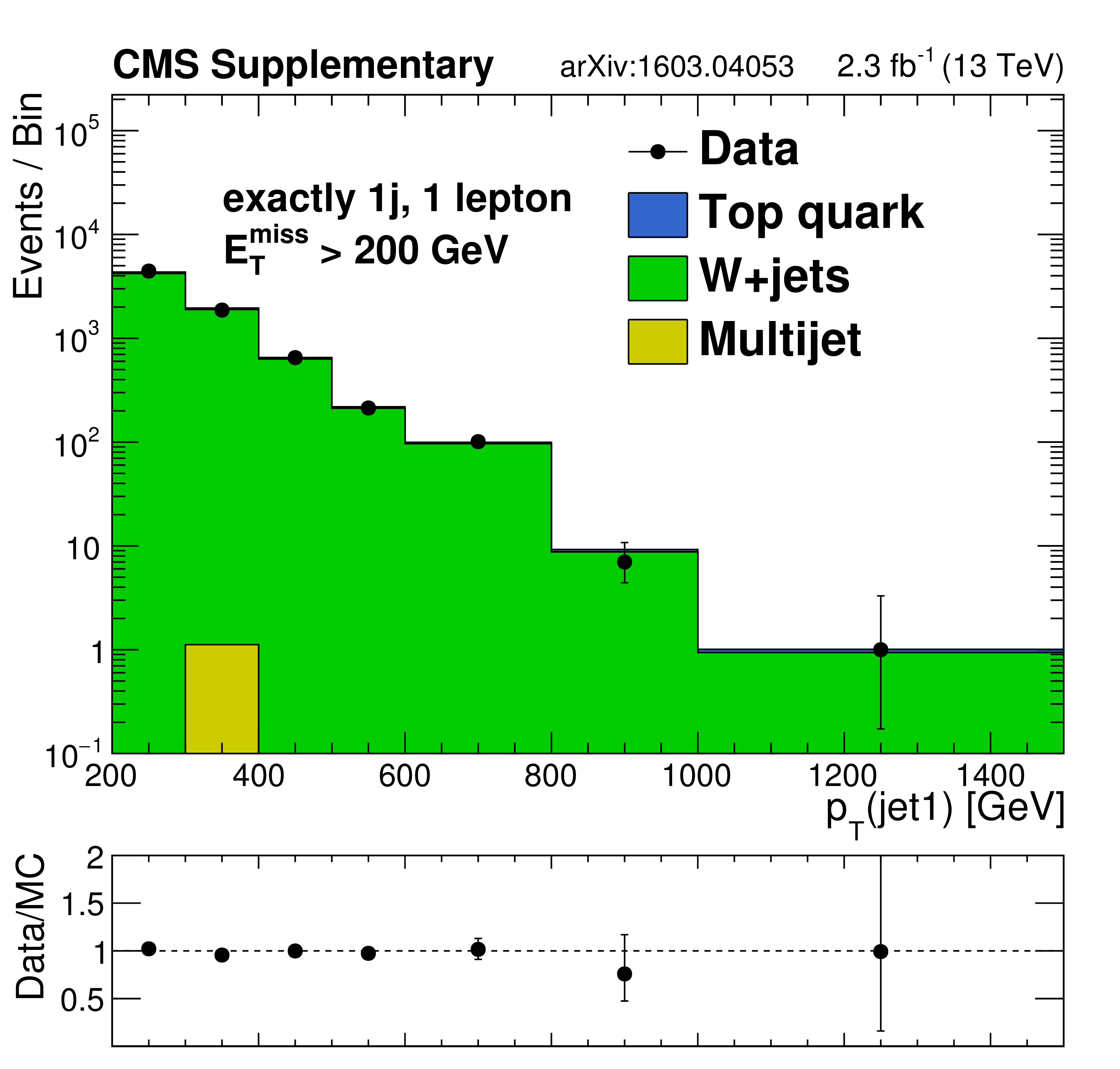
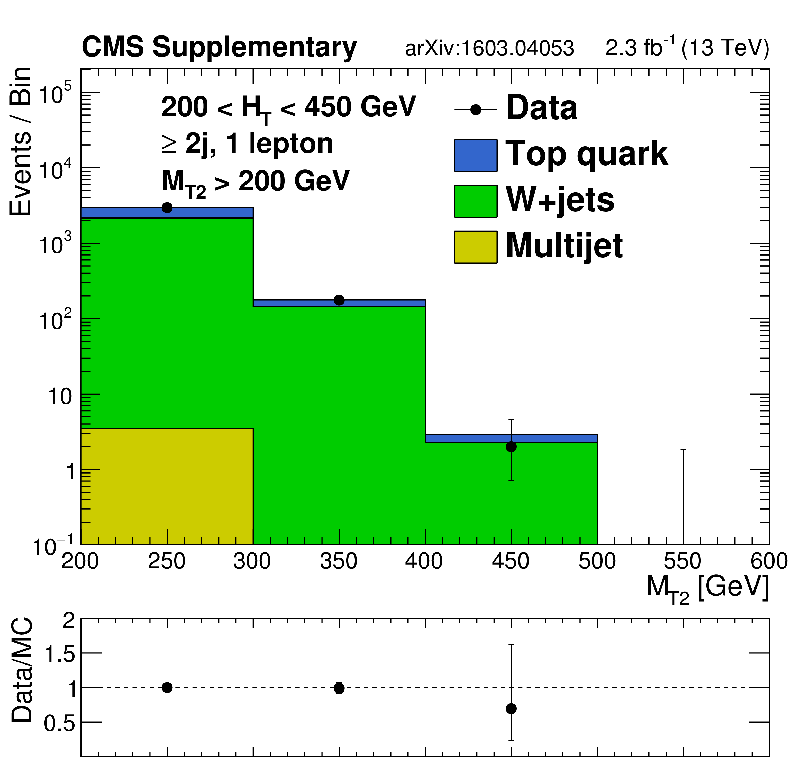
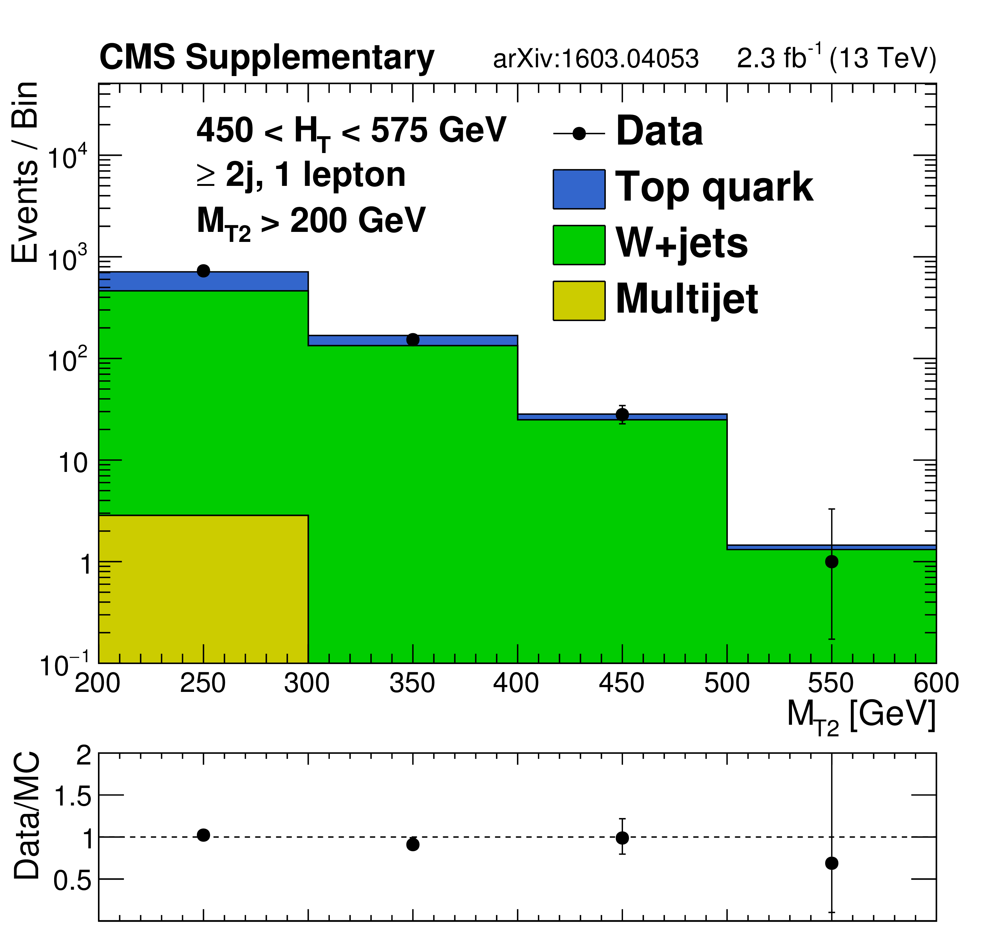
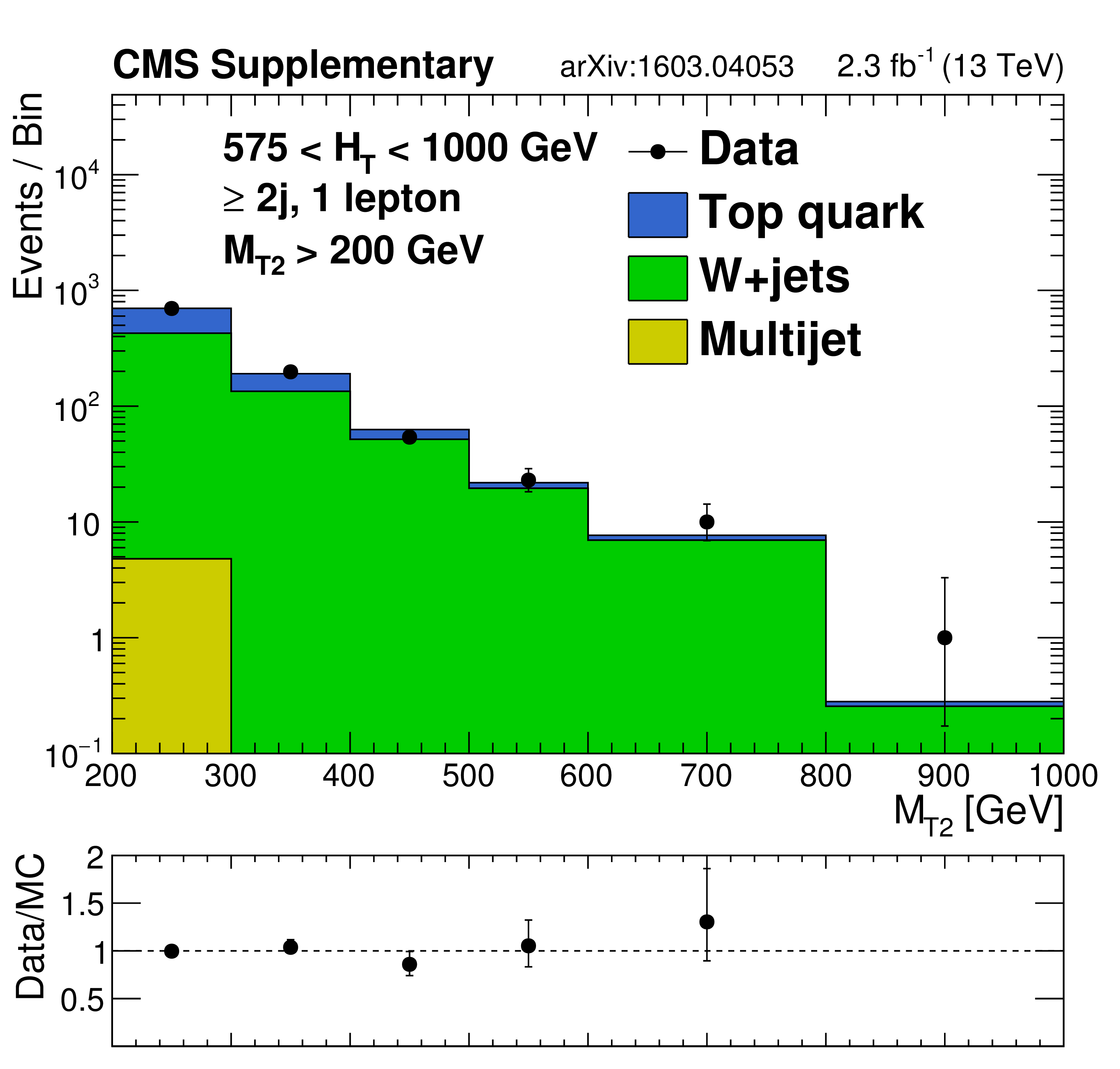
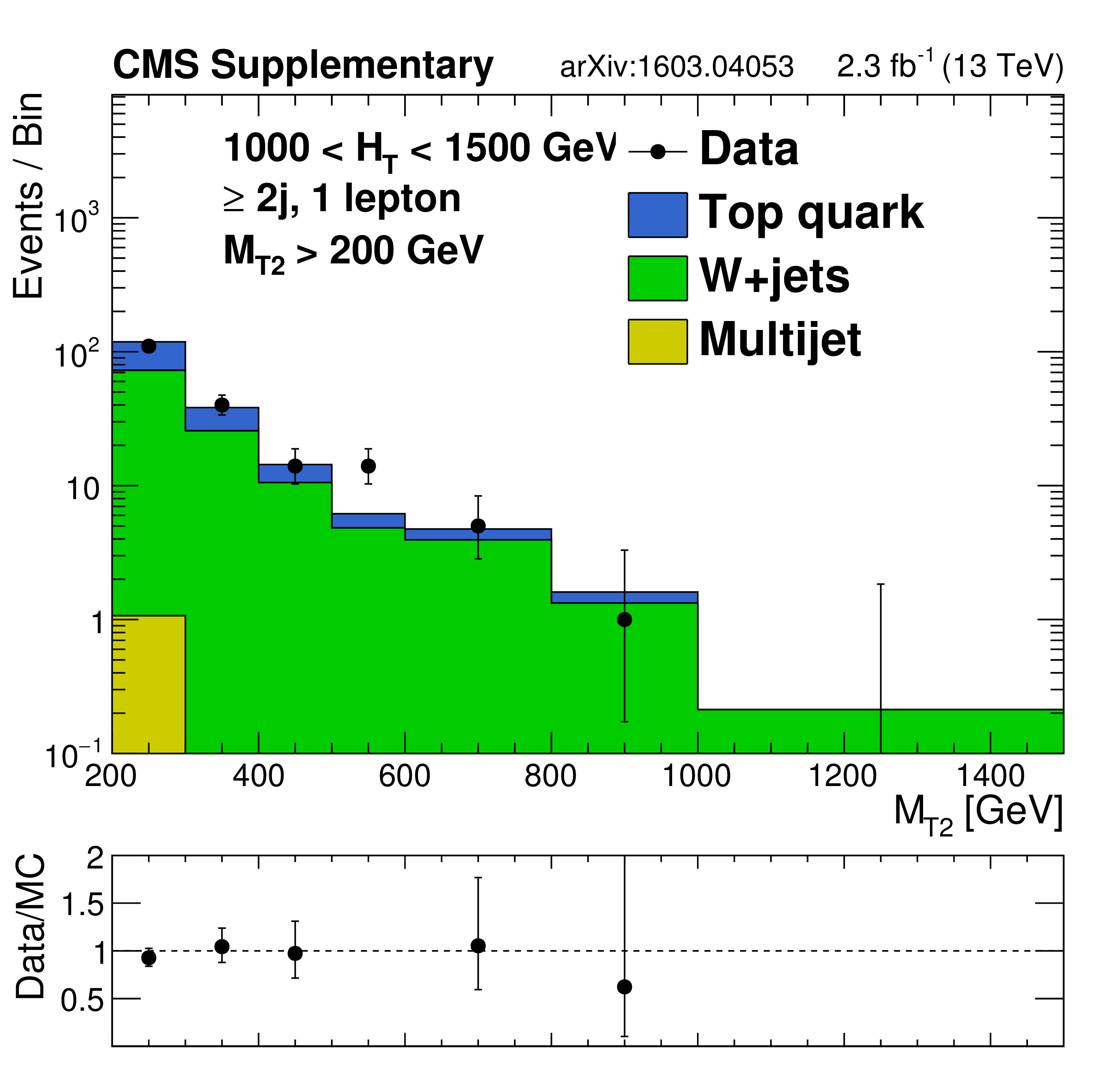
Distributions of jet $ {p_{\mathrm {T}}} $ or $ {M_{\mathrm {T2}}} $ data and MC predictions for the single lepton control regions in the monojet region (top left) or in the analysis $ {H_{\mathrm {T}}} $ bins for regions with at least 2 jets. MC is normalized to data in each plot to compare the shapes. |
png pdf |
Additional Figure 18-b:
Distributions of jet $ {p_{\mathrm {T}}} $ or $ {M_{\mathrm {T2}}} $ data and MC predictions for the single lepton control regions in the monojet region (top left) or in the analysis $ {H_{\mathrm {T}}} $ bins for regions with at least 2 jets. MC is normalized to data in each plot to compare the shapes. |
png pdf |
Additional Figure 18-c:
Distributions of jet $ {p_{\mathrm {T}}} $ or $ {M_{\mathrm {T2}}} $ data and MC predictions for the single lepton control regions in the monojet region (top left) or in the analysis $ {H_{\mathrm {T}}} $ bins for regions with at least 2 jets. MC is normalized to data in each plot to compare the shapes. |
png pdf |
Additional Figure 18-d:
Distributions of jet $ {p_{\mathrm {T}}} $ or $ {M_{\mathrm {T2}}} $ data and MC predictions for the single lepton control regions in the monojet region (top left) or in the analysis $ {H_{\mathrm {T}}} $ bins for regions with at least 2 jets. MC is normalized to data in each plot to compare the shapes. |
png pdf |
Additional Figure 18-e:
Distributions of jet $ {p_{\mathrm {T}}} $ or $ {M_{\mathrm {T2}}} $ data and MC predictions for the single lepton control regions in the monojet region (top left) or in the analysis $ {H_{\mathrm {T}}} $ bins for regions with at least 2 jets. MC is normalized to data in each plot to compare the shapes. |

png pdf |
Additional Figure 18-f:
Distributions of jet $ {p_{\mathrm {T}}} $ or $ {M_{\mathrm {T2}}} $ data and MC predictions for the single lepton control regions in the monojet region (top left) or in the analysis $ {H_{\mathrm {T}}} $ bins for regions with at least 2 jets. MC is normalized to data in each plot to compare the shapes. |
png pdf |
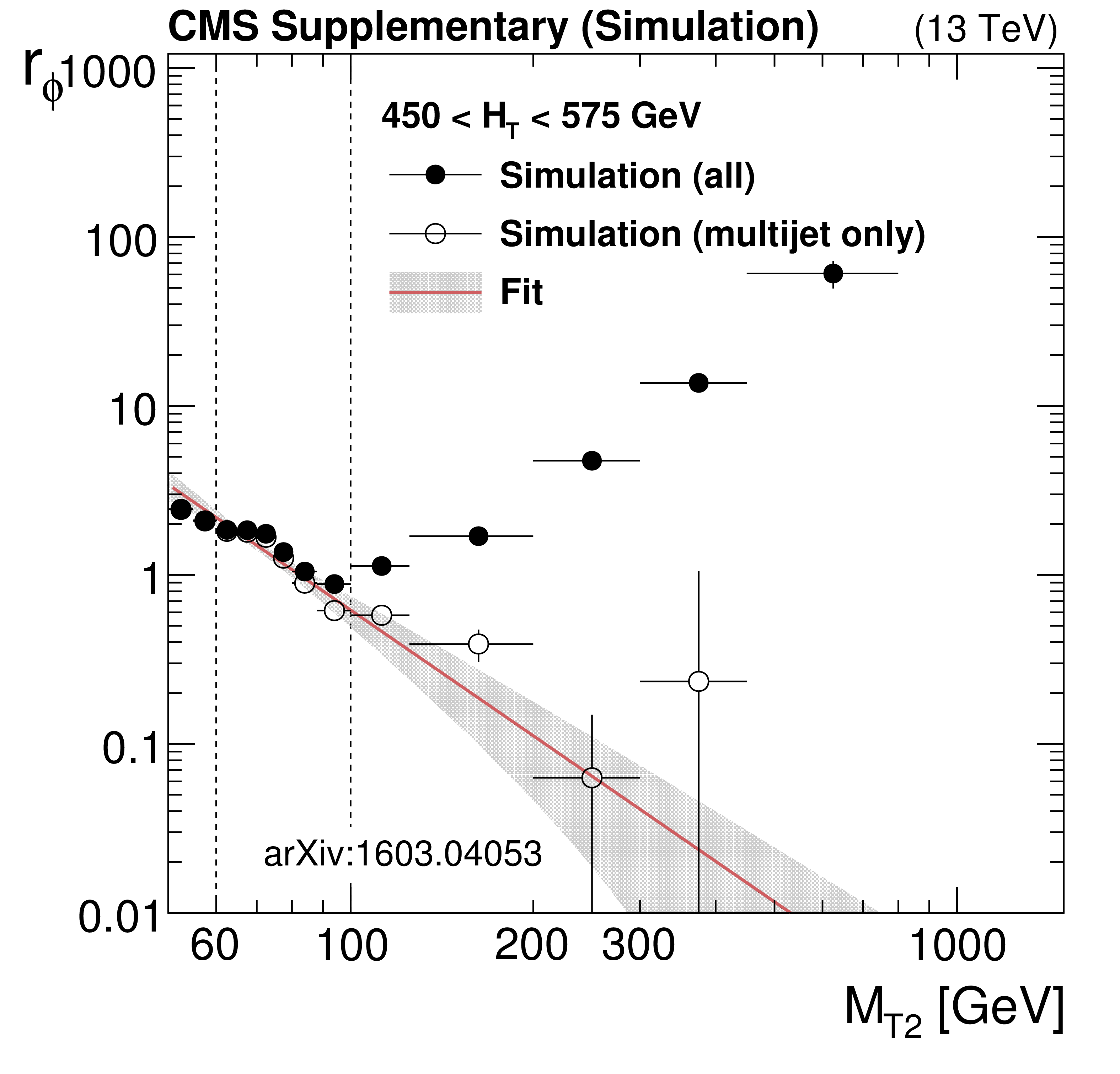
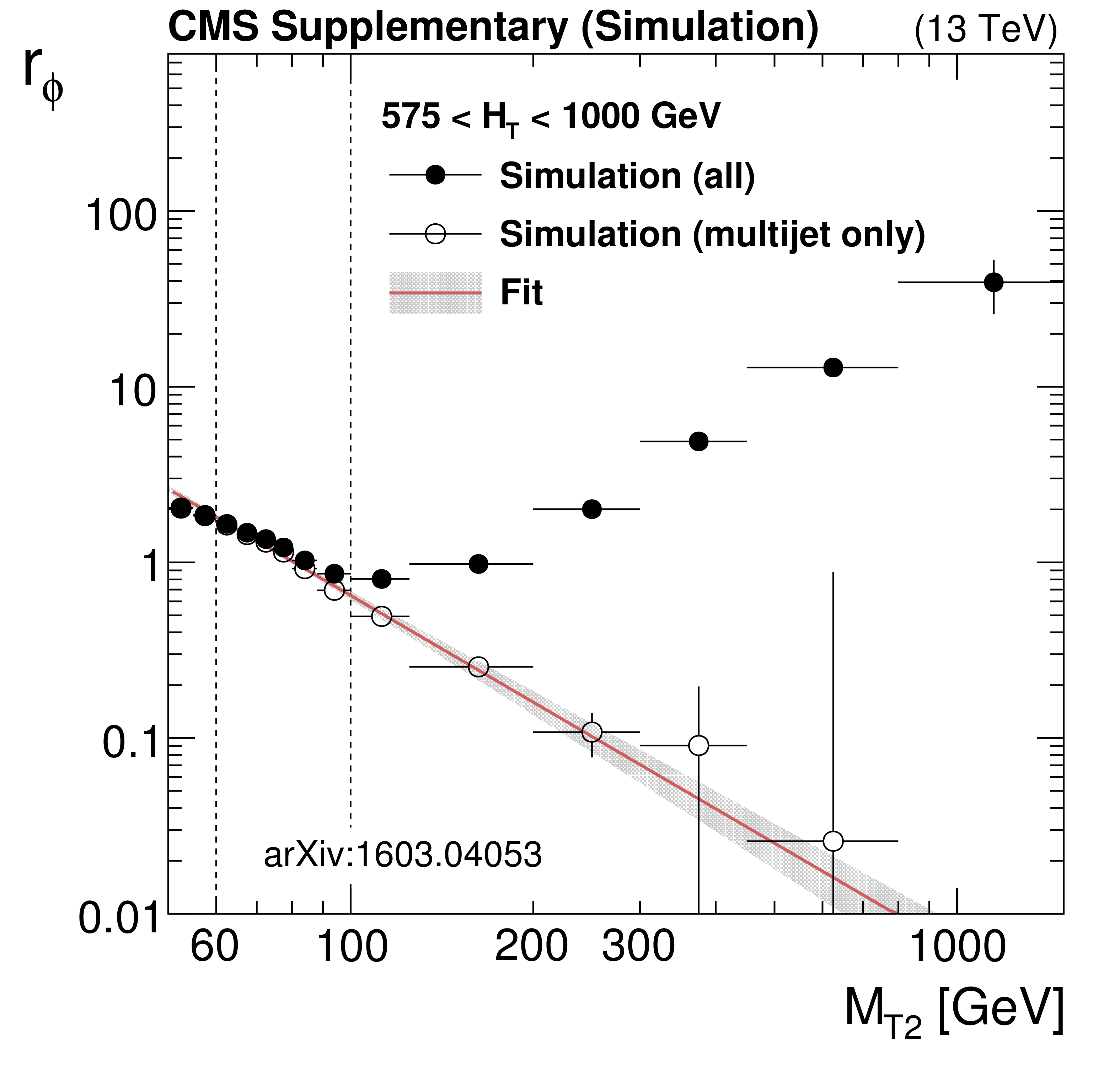
Additional Figure 19-a:
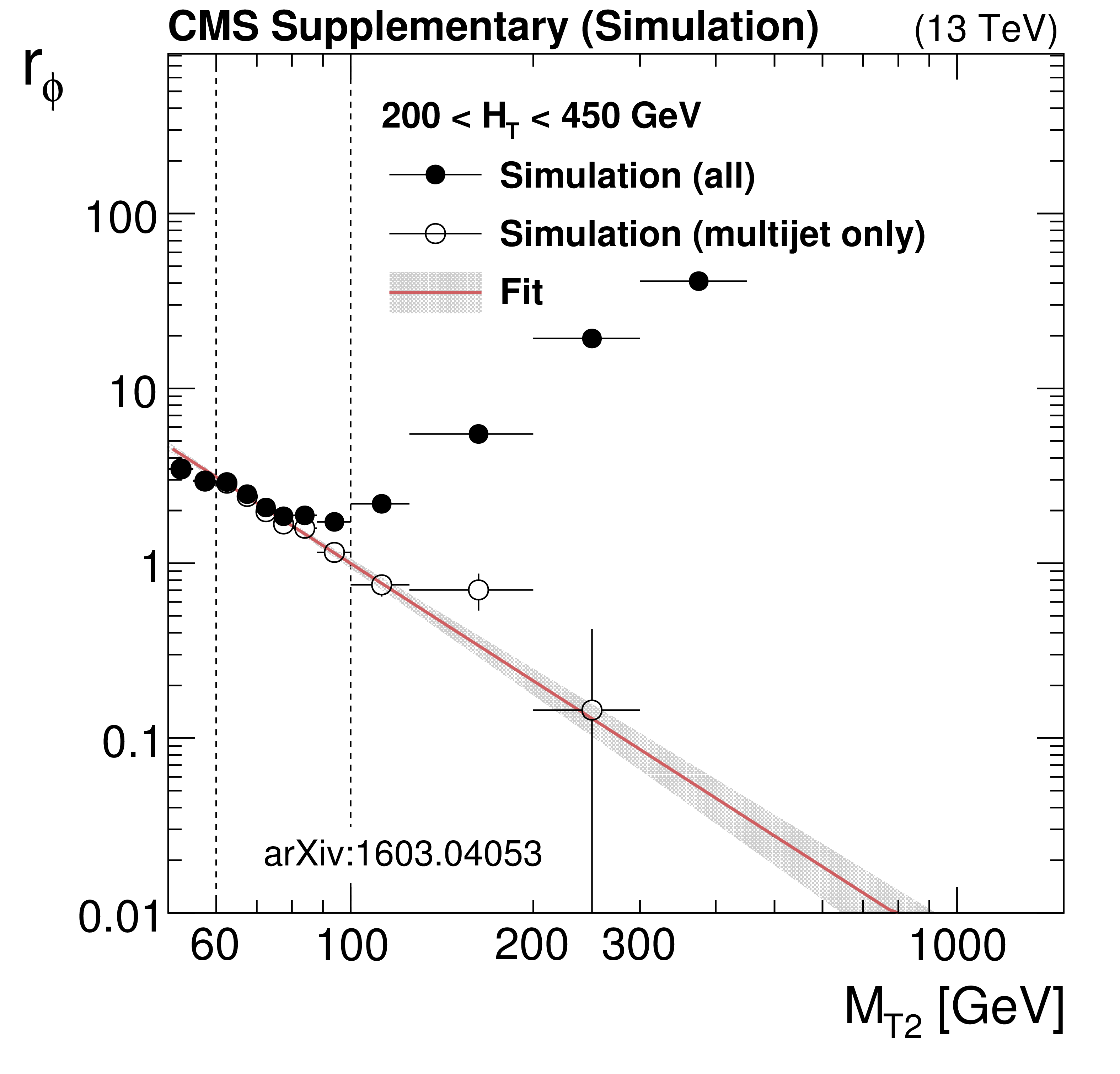
Expected distributions from simulation of the ratio $r_\phi ( {M_{\mathrm {T2}}} ) = N(\Delta \phi _{\text{min}} > 0.3) / N(\Delta \phi _{\text{min}} < 0.3)$ as a function of $ {M_{\mathrm {T2}}} $ , for the low (top left), medium (top right), high (medium left), extreme (medium right) and very low (bottom) $ {H_{\mathrm {T}}} $ regions. The full points represent the ratio as predicted from simulation using all background components, while the hollow points represent the expected ratio from QCD multijet. The errors are MC statistics. The red line and the band around it show the fit to a power law function perfomed in the fit window, with its associated fit uncertainties. |
png pdf |
Additional Figure 19-b:
Expected distributions from simulation of the ratio $r_\phi ( {M_{\mathrm {T2}}} ) = N(\Delta \phi _{\text{min}} > 0.3) / N(\Delta \phi _{\text{min}} < 0.3)$ as a function of $ {M_{\mathrm {T2}}} $ , for the low (top left), medium (top right), high (medium left), extreme (medium right) and very low (bottom) $ {H_{\mathrm {T}}} $ regions. The full points represent the ratio as predicted from simulation using all background components, while the hollow points represent the expected ratio from QCD multijet. The errors are MC statistics. The red line and the band around it show the fit to a power law function perfomed in the fit window, with its associated fit uncertainties. |

png pdf |
Additional Figure 19-c:
Expected distributions from simulation of the ratio $r_\phi ( {M_{\mathrm {T2}}} ) = N(\Delta \phi _{\text{min}} > 0.3) / N(\Delta \phi _{\text{min}} < 0.3)$ as a function of $ {M_{\mathrm {T2}}} $ , for the low (top left), medium (top right), high (medium left), extreme (medium right) and very low (bottom) $ {H_{\mathrm {T}}} $ regions. The full points represent the ratio as predicted from simulation using all background components, while the hollow points represent the expected ratio from QCD multijet. The errors are MC statistics. The red line and the band around it show the fit to a power law function perfomed in the fit window, with its associated fit uncertainties. |
png pdf |
Additional Figure 19-d:
Expected distributions from simulation of the ratio $r_\phi ( {M_{\mathrm {T2}}} ) = N(\Delta \phi _{\text{min}} > 0.3) / N(\Delta \phi _{\text{min}} < 0.3)$ as a function of $ {M_{\mathrm {T2}}} $ , for the low (top left), medium (top right), high (medium left), extreme (medium right) and very low (bottom) $ {H_{\mathrm {T}}} $ regions. The full points represent the ratio as predicted from simulation using all background components, while the hollow points represent the expected ratio from QCD multijet. The errors are MC statistics. The red line and the band around it show the fit to a power law function perfomed in the fit window, with its associated fit uncertainties. |
png pdf |
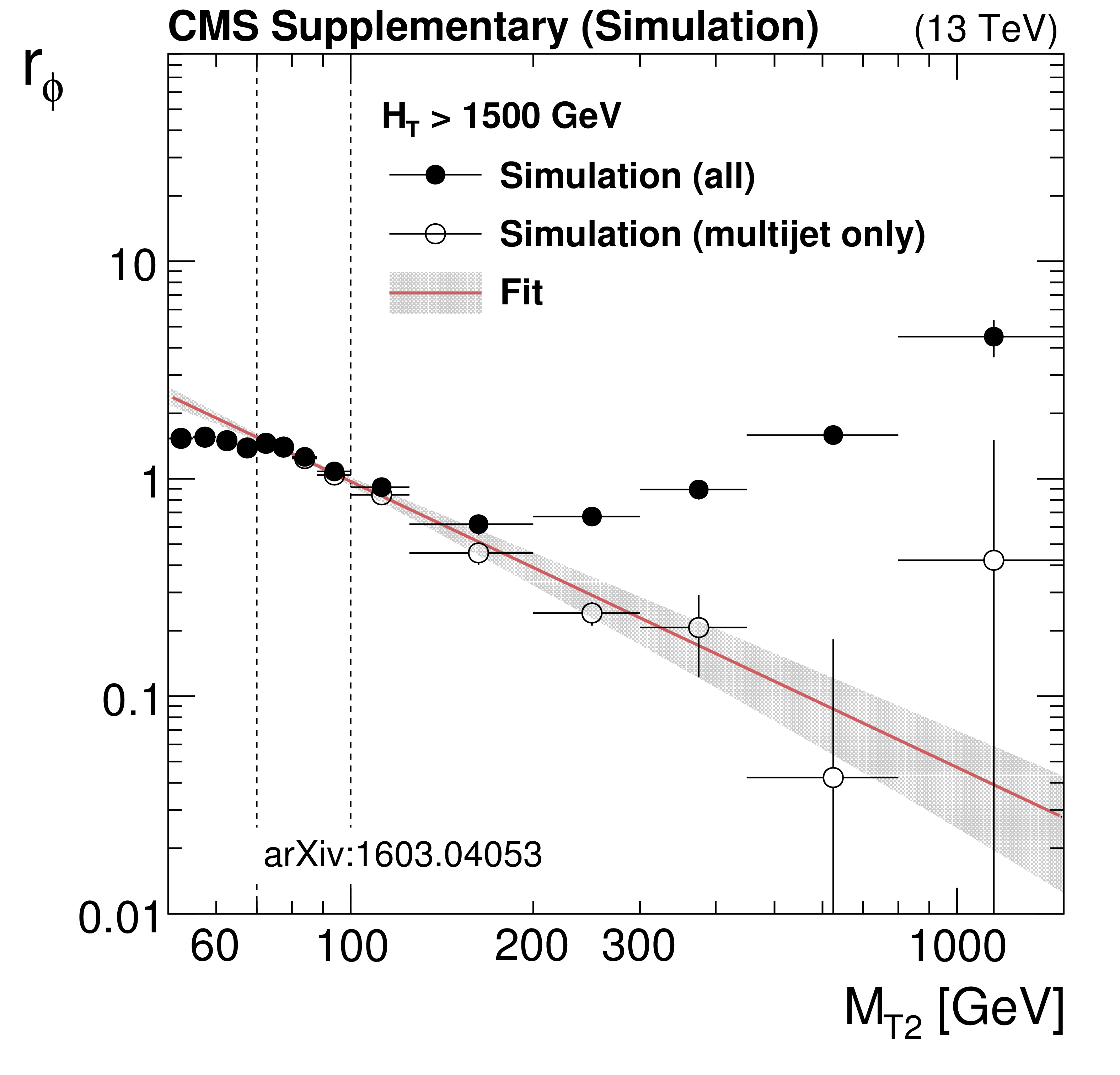
Additional Figure 19-e:
Expected distributions from simulation of the ratio $r_\phi ( {M_{\mathrm {T2}}} ) = N(\Delta \phi _{\text{min}} > 0.3) / N(\Delta \phi _{\text{min}} < 0.3)$ as a function of $ {M_{\mathrm {T2}}} $ , for the low (top left), medium (top right), high (medium left), extreme (medium right) and very low (bottom) $ {H_{\mathrm {T}}} $ regions. The full points represent the ratio as predicted from simulation using all background components, while the hollow points represent the expected ratio from QCD multijet. The errors are MC statistics. The red line and the band around it show the fit to a power law function perfomed in the fit window, with its associated fit uncertainties. |
png pdf |
Additional Figure 20-a:
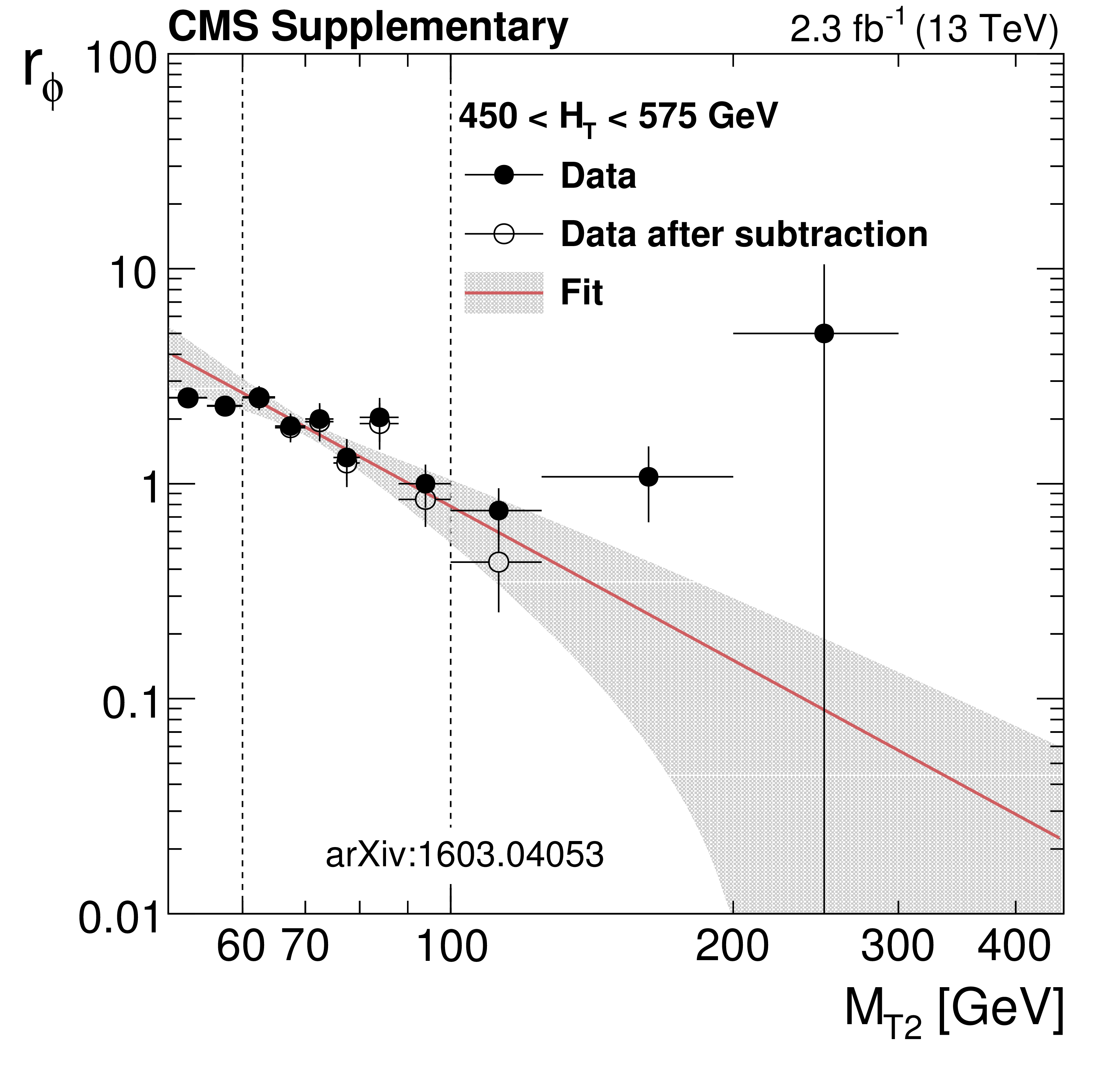
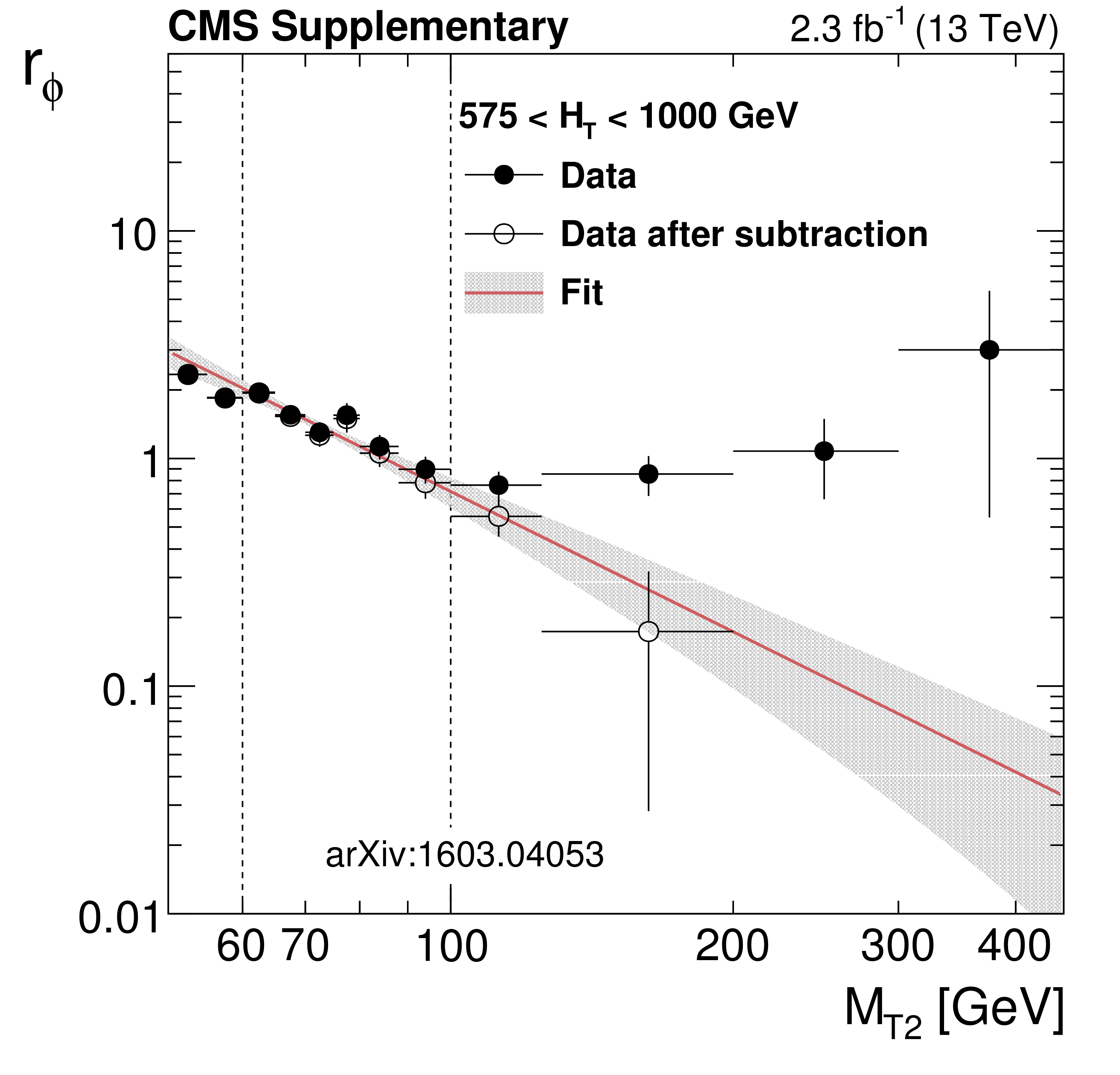
Distributions from data of the ratio $r_\phi ( {M_{\mathrm {T2}}} ) = N(\Delta \phi _{\text{min}} > 0.3) / N(\Delta \phi _{\text{min}} < 0.3)$ as a function of $ {M_{\mathrm {T2}}} $ , for the low (top left), medium (top right), high (bottom left), extreme (bottom right) $ {H_{\mathrm {T}}} $ regions. The full points are the ratio from data before subtracting the non-multijet component, while the hollow points represent the data after the non-multijet contribution has been subtracted. The data in the high and extreme $ {H_{\mathrm {T}}} $ regions has been collected with an unprescaled HLT trigger with an online $ {H_{\mathrm {T}}} $ threshold of 800 GeV, while for the low and the medium $ {H_{\mathrm {T}}} $ regions prescaled HLT triggers have been used, with an online $ {H_{\mathrm {T}}} $ threshold of 350 GeV (prescale 180) and of 475 GeV (prescale 60) respectively. The red line and the band around it show the fit to a power law function performed in the fit window, with its associated fit uncertainties. |
png pdf |
Additional Figure 20-b:
Distributions from data of the ratio $r_\phi ( {M_{\mathrm {T2}}} ) = N(\Delta \phi _{\text{min}} > 0.3) / N(\Delta \phi _{\text{min}} < 0.3)$ as a function of $ {M_{\mathrm {T2}}} $ , for the low (top left), medium (top right), high (bottom left), extreme (bottom right) $ {H_{\mathrm {T}}} $ regions. The full points are the ratio from data before subtracting the non-multijet component, while the hollow points represent the data after the non-multijet contribution has been subtracted. The data in the high and extreme $ {H_{\mathrm {T}}} $ regions has been collected with an unprescaled HLT trigger with an online $ {H_{\mathrm {T}}} $ threshold of 800 GeV, while for the low and the medium $ {H_{\mathrm {T}}} $ regions prescaled HLT triggers have been used, with an online $ {H_{\mathrm {T}}} $ threshold of 350 GeV (prescale 180) and of 475 GeV (prescale 60) respectively. The red line and the band around it show the fit to a power law function performed in the fit window, with its associated fit uncertainties. |
png pdf |
Additional Figure 20-c:
Distributions from data of the ratio $r_\phi ( {M_{\mathrm {T2}}} ) = N(\Delta \phi _{\text{min}} > 0.3) / N(\Delta \phi _{\text{min}} < 0.3)$ as a function of $ {M_{\mathrm {T2}}} $ , for the low (top left), medium (top right), high (bottom left), extreme (bottom right) $ {H_{\mathrm {T}}} $ regions. The full points are the ratio from data before subtracting the non-multijet component, while the hollow points represent the data after the non-multijet contribution has been subtracted. The data in the high and extreme $ {H_{\mathrm {T}}} $ regions has been collected with an unprescaled HLT trigger with an online $ {H_{\mathrm {T}}} $ threshold of 800 GeV, while for the low and the medium $ {H_{\mathrm {T}}} $ regions prescaled HLT triggers have been used, with an online $ {H_{\mathrm {T}}} $ threshold of 350 GeV (prescale 180) and of 475 GeV (prescale 60) respectively. The red line and the band around it show the fit to a power law function performed in the fit window, with its associated fit uncertainties. |
png pdf |
Additional Figure 21-a:
Fraction $f_{\mathrm {j}}$ of multijet events falling in bins of number of jets $ {N_{\mathrm {j}}} $ as measured in data using $\Delta \phi <0.3$ and $100< {M_{\mathrm {T2}}} <200$ GeV, compared to the prediction from QCD multijet simulation. The uncertainties shown include both statistical and systematic sources. |
png pdf |
Additional Figure 21-b:
Fraction $f_{\mathrm {j}}$ of multijet events falling in bins of number of jets $ {N_{\mathrm {j}}} $ as measured in data using $\Delta \phi <0.3$ and $100< {M_{\mathrm {T2}}} <200$ GeV, compared to the prediction from QCD multijet simulation. The uncertainties shown include both statistical and systematic sources. |

png pdf |
Additional Figure 21-c:
Fraction $f_{\mathrm {j}}$ of multijet events falling in bins of number of jets $ {N_{\mathrm {j}}} $ as measured in data using $\Delta \phi <0.3$ and $100< {M_{\mathrm {T2}}} <200$ GeV, compared to the prediction from QCD multijet simulation. The uncertainties shown include both statistical and systematic sources. |
png pdf |
Additional Figure 21-d:
Fraction $f_{\mathrm {j}}$ of multijet events falling in bins of number of jets $ {N_{\mathrm {j}}} $ as measured in data using $\Delta \phi <0.3$ and $100< {M_{\mathrm {T2}}} <200$ GeV, compared to the prediction from QCD multijet simulation. The uncertainties shown include both statistical and systematic sources. |
png pdf |
Additional Figure 22-a:
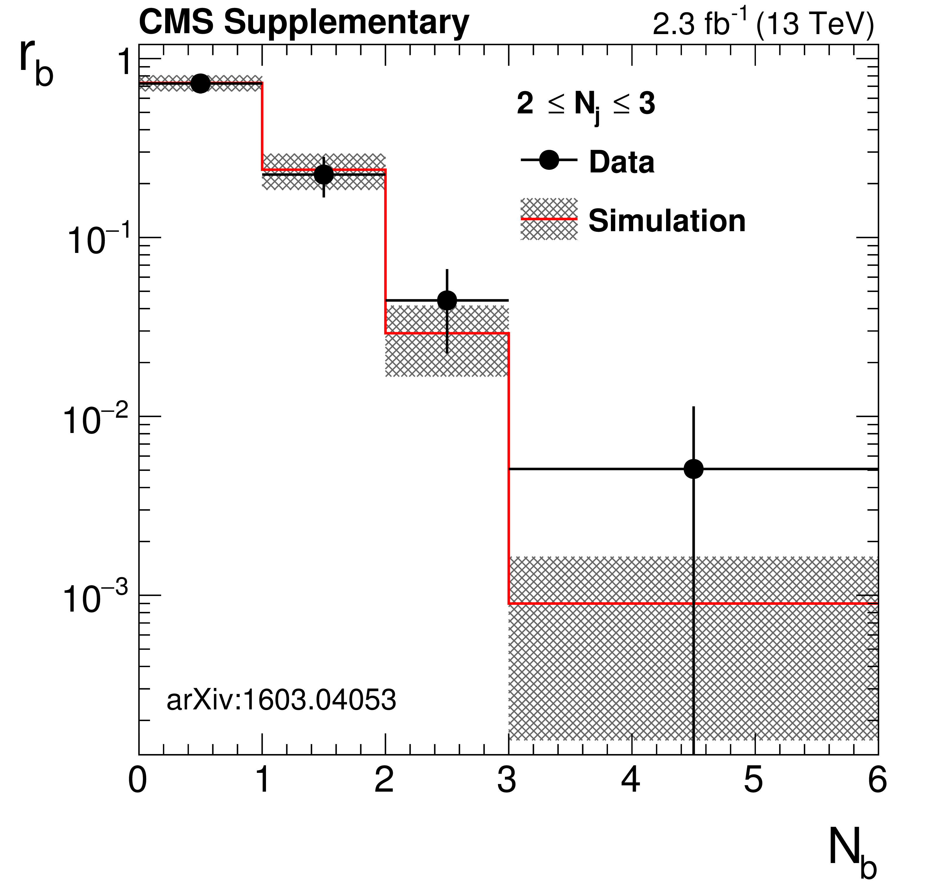
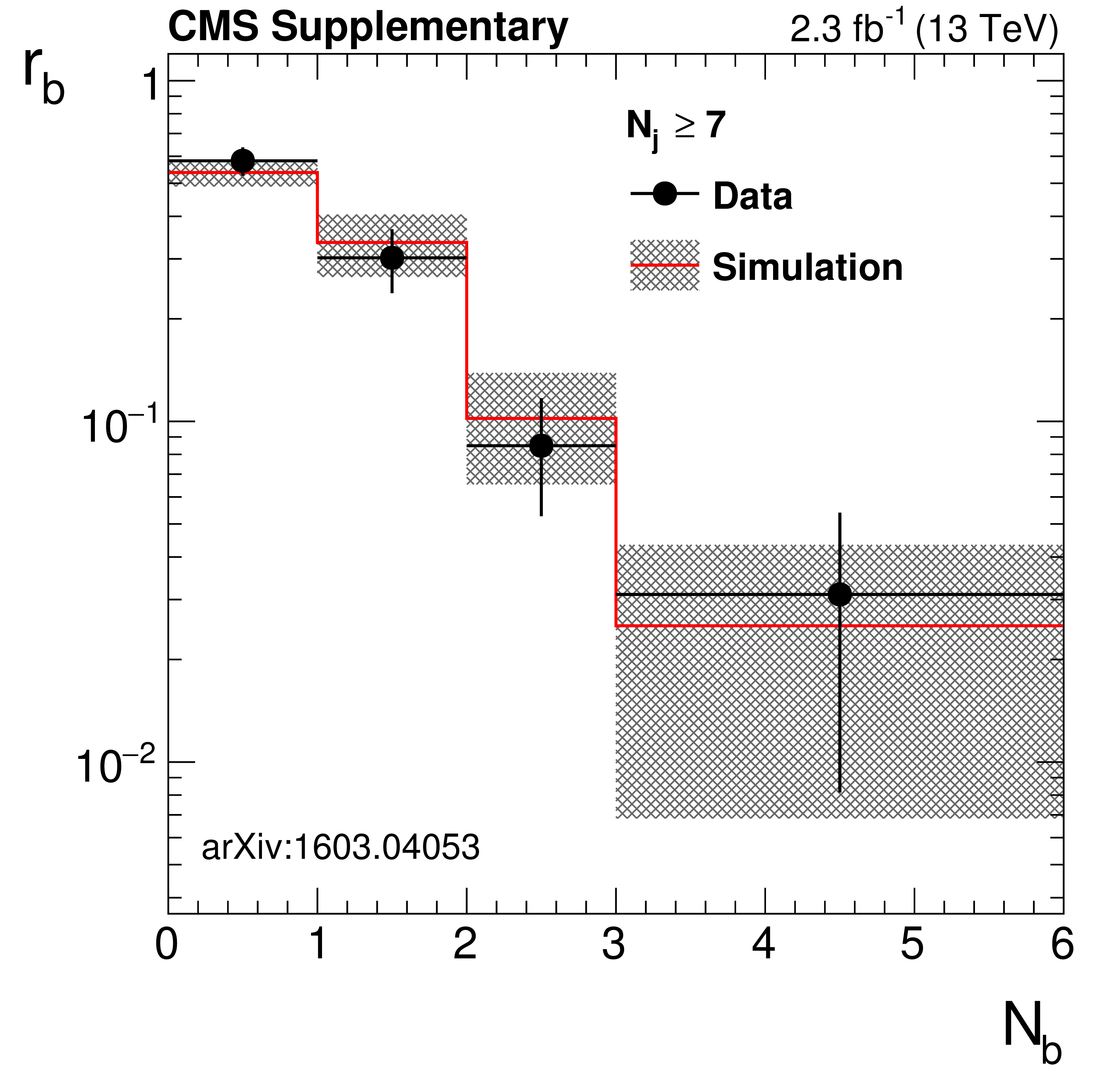
Fraction $r_{\mathrm {b}}$ of events falling in bins of number of b-tagged jets $ {N_{\mathrm {b}}} $ as measured in data using $\Delta \phi <0.3$ and $100< {M_{\mathrm {T2}}} <200$ GeV, compared to the prediction from QCD multijet simulation. The uncertainties shown include both statistical and systematic sources. |
png pdf |
Additional Figure 22-b:
Fraction $r_{\mathrm {b}}$ of events falling in bins of number of b-tagged jets $ {N_{\mathrm {b}}} $ as measured in data using $\Delta \phi <0.3$ and $100< {M_{\mathrm {T2}}} <200$ GeV, compared to the prediction from QCD multijet simulation. The uncertainties shown include both statistical and systematic sources. |
png pdf |
Additional Figure 23:
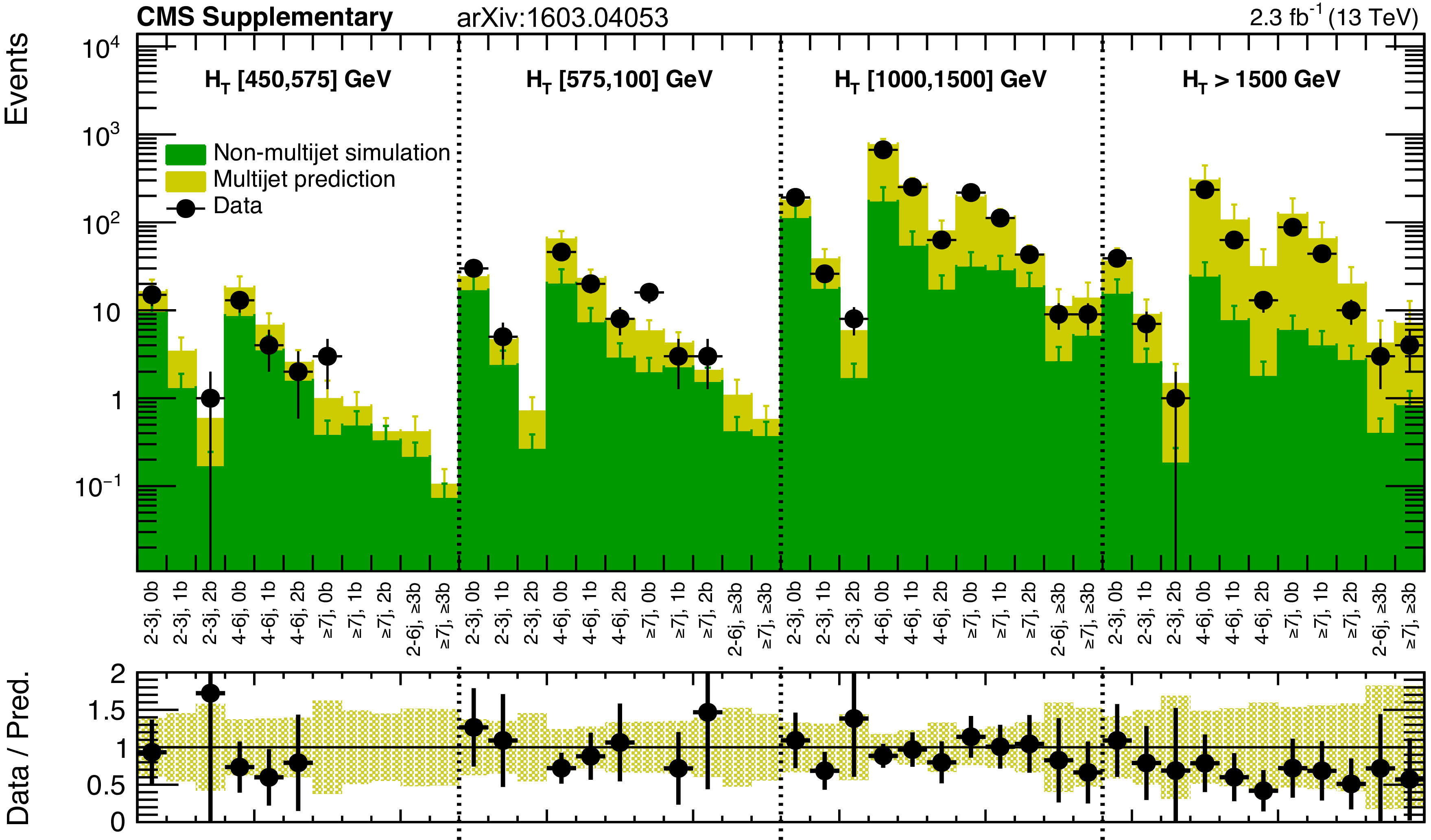
Validation of the data-driven multijet estimate in the region $100< {M_{\mathrm {T2}}} <200$ GeV. The points are data with $\Delta \phi >0.3$, triggered by the $ {H_{\mathrm {T}}} $-only triggers (prescaled for low and medium $ {H_{\mathrm {T}}} $). The green histogram is the non-multijet contribution as expected from simulation, while the yellow histogram is the multijet estimation using the data-driven method on 2.3 fb${^{-1}}$ of data. |

png pdf |
Additional Figure 24:
Distribution of subleading jet $ {p_{\mathrm {T}}} $ for dijet events with leading jet $ {p_{\mathrm {T}}} > 200$ GeV. The simulation is normalized to the data yield. |
png pdf |
Additional Figure 25:
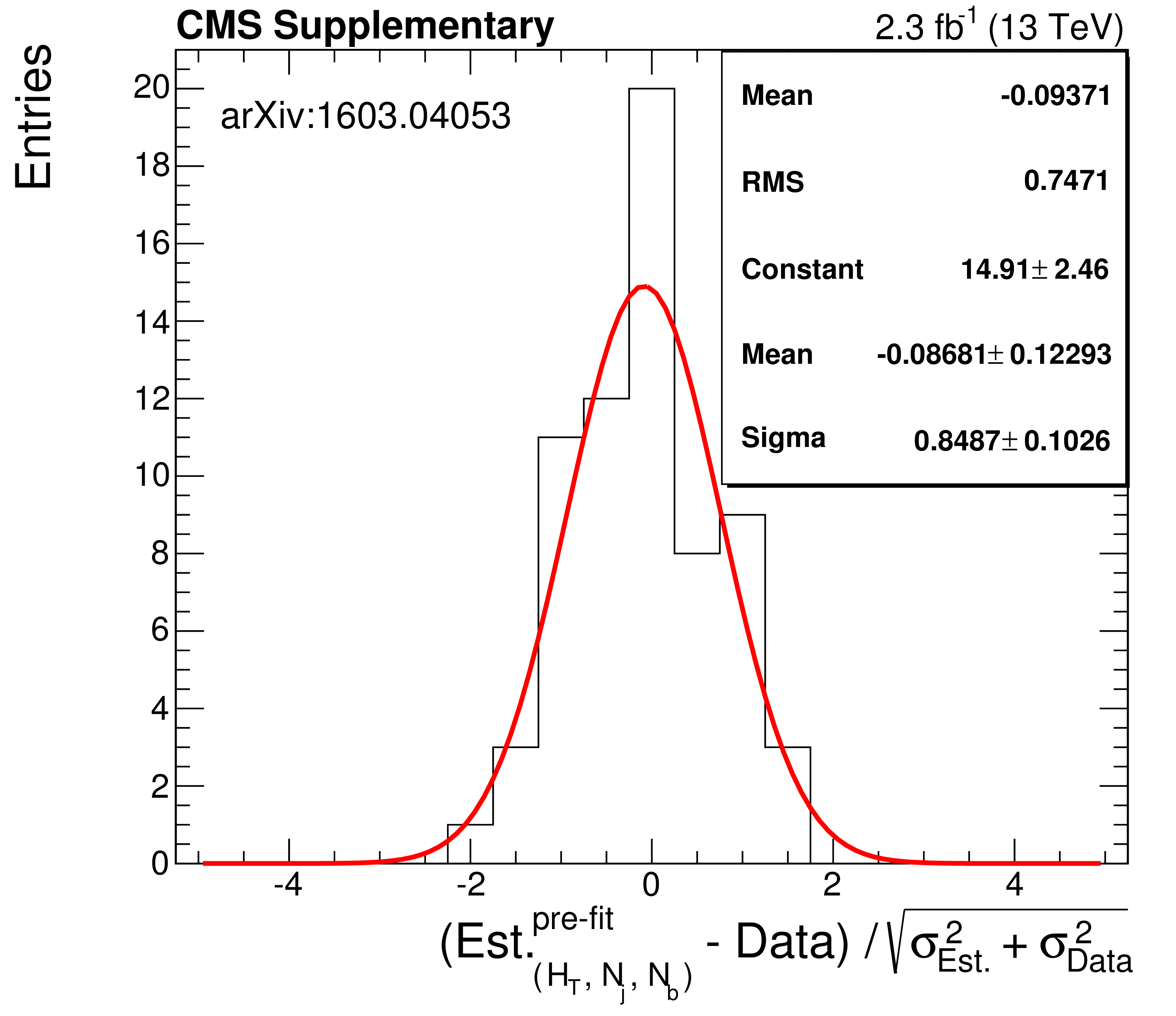
Pull distribution for all topological regions (integrated over $ {M_{\mathrm {T2}}} $ for the multijet regions). The pull is defined as the difference between the estimated background (pre-fit) and the observation, relative to the total uncertainty. The red curve shows the result of a gaussian fit to the pull distribution. |

png pdf |
Additional Figure 26:
Expected (post-fit) and observed yields in the analysis binning, for the monojet region, with jet $ {p_{\mathrm {T}}} > 200$ GeV, in each of the $ {N_{\mathrm {b}}} $ bins. On the $x$-axis, the jet $ {p_{\mathrm {T}}} $ binning is shown (in GeV). |
png pdf |
Additional Figure 27:
Expected (post-fit) and observed yields in the analysis binning, for the very-low-$ {H_{\mathrm {T}}} $ region and each of the $ {N_{\mathrm {j}}} $ and $ {N_{\mathrm {b}}} $ bins. On the $x$-axis, the $ {M_{\mathrm {T2}}} $ binning is shown (in GeV). |
png pdf |
Additional Figure 28:
Expected (post-fit) and observed yields in the analysis binning, for the low-$ {H_{\mathrm {T}}} $ region and each of the $ {N_{\mathrm {j}}} $ and $ {N_{\mathrm {b}}} $ bins. On the $x$-axis, the $ {M_{\mathrm {T2}}} $ binning is shown (in GeV). |
png pdf |
Additional Figure 29:
Expected (post-fit) and observed yields in the analysis binning, for the medium-$ {H_{\mathrm {T}}} $ region and each of the $ {N_{\mathrm {j}}} $ and $ {N_{\mathrm {b}}} $ bins. On the $x$-axis, the $ {M_{\mathrm {T2}}} $ binning is shown (in GeV). |
png pdf |
Additional Figure 30:
Expected (post-fit) and observed yields in the analysis binning, for the high-$ {H_{\mathrm {T}}} $ region and each of the $ {N_{\mathrm {j}}} $ and $ {N_{\mathrm {b}}} $ bins. On the $x$-axis, the $ {M_{\mathrm {T2}}} $ binning is shown (in GeV). |
png pdf |
Additional Figure 31:
Expected (post-fit) and observed yields in the analysis binning, for the extreme-$ {H_{\mathrm {T}}} $ region and each of the $ {N_{\mathrm {j}}} $ and $ {N_{\mathrm {b}}} $ bins. On the $x$-axis, the $ {M_{\mathrm {T2}}} $ binning is shown (in GeV). |
png pdf |
Additional Figure 32:
Expected (post-fit) and observed yields in the analysis binning, for all regions and integrated over $ {M_{\mathrm {T2}}} $ , with the expected contribution from a signal model of gluino-mediated light squark production with the mass of the gluino and the LSP equal to 700 and 600 GeV, respectively. For the monojet, on the $x$-axis the jet $ {p_{\mathrm {T}}} $ binning is shown (in GeV). |

png pdf |
Additional Figure 33:
Expected (post-fit) and observed yields in the analysis binning, for all regions and integrated over $ {M_{\mathrm {T2}}} $ , with the expected contribution from a signal model of gluino-mediated top squark production with the mass of the gluino and the LSP equal to 700 and 400 GeV, respectively. For the monojet, on the $x$-axis the jet $ {p_{\mathrm {T}}} $ binning is shown (in GeV). |
png pdf |
Additional Figure 34:
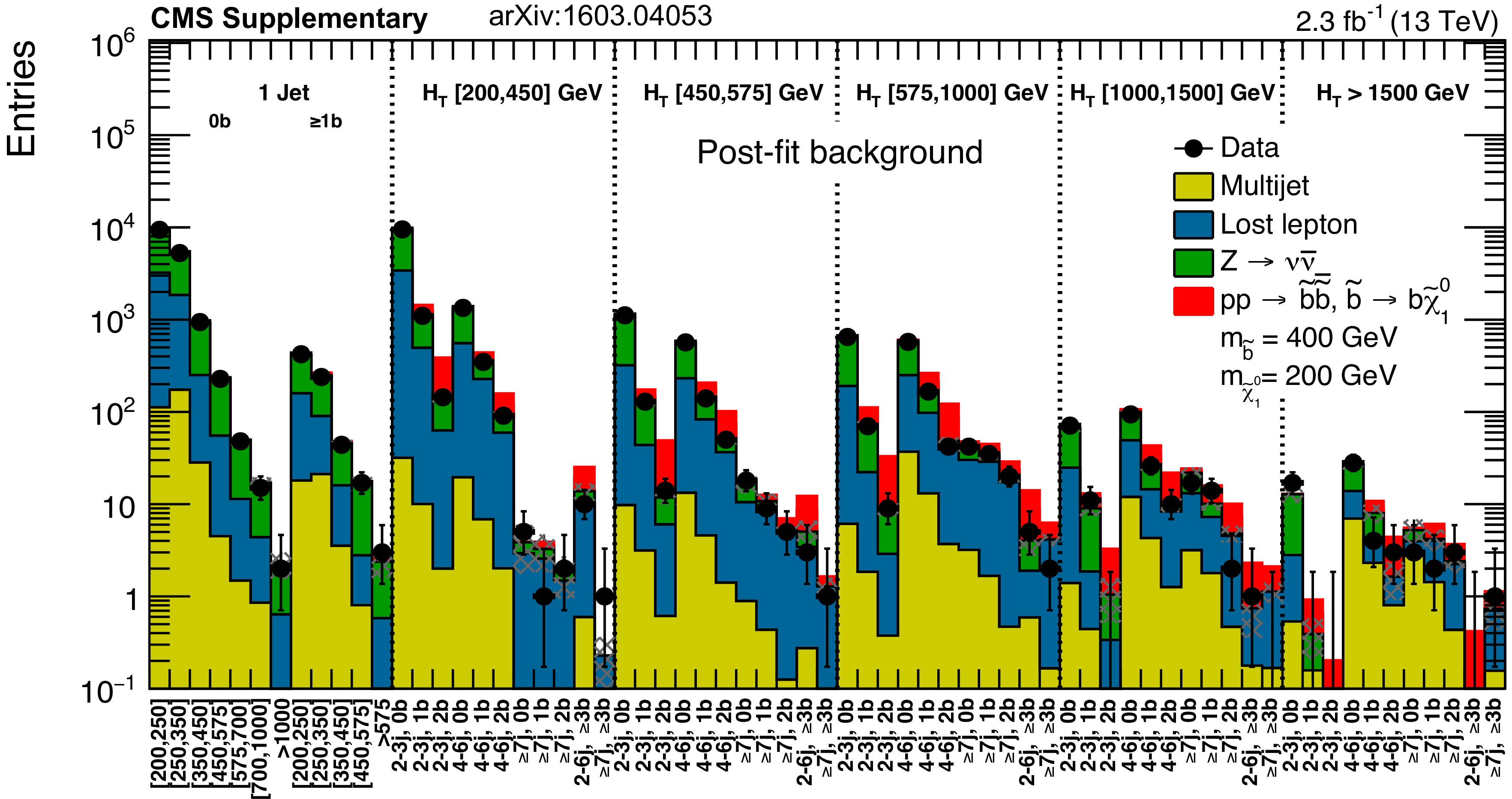
Expected (post-fit) and observed yields in the analysis binning, for all regions and integrated over $ {M_{\mathrm {T2}}} $ , with the expected contribution from a signal model of direct bottom squark production with the mass of the bottom squark and the LSP equal to 400 and 200 GeV, respectively. For the monojet, on the $x$-axis the jet $ {p_{\mathrm {T}}} $ binning is shown (in GeV). |
png pdf |
Additional Figure 35:
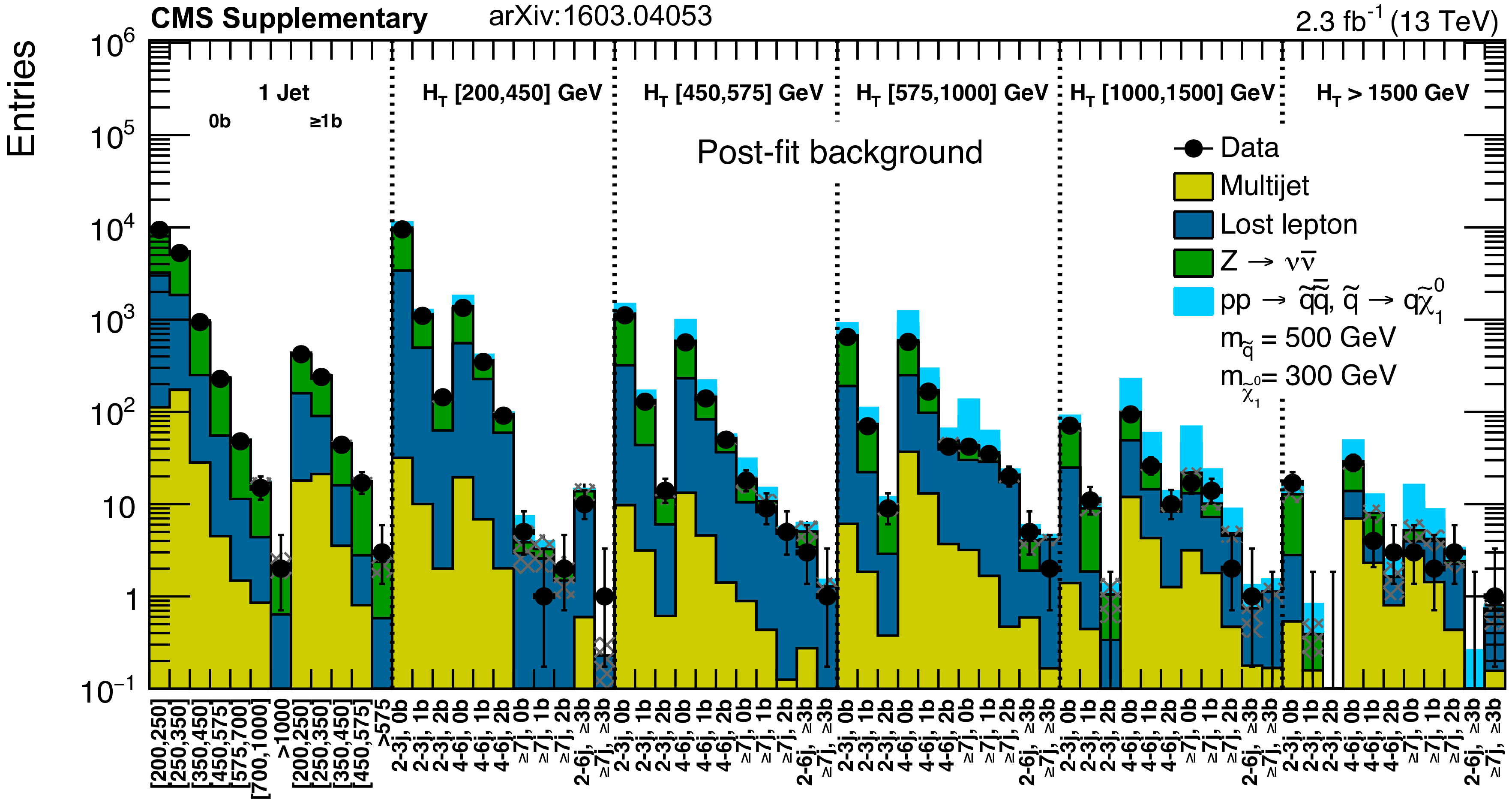
Expected (post-fit) and observed yields in the analysis binning, for all regions and integrated over $ {M_{\mathrm {T2}}} $ , with the expected contribution from a signal model of direct light squark production with the mass of the squark and the LSP equal to 500 and 300 GeV, respectively. For the monojet, on the $x$-axis the jet $ {p_{\mathrm {T}}} $ binning is shown (in GeV). |
png pdf |
Additional Figure 36:
Expected (post-fit) and observed yields in the analysis binning, for all regions and integrated over $ {M_{\mathrm {T2}}} $ , with the expected contribution from a signal model of direct top squark production with the mass of the top squark and the LSP equal to 200 and 100 GeV, respectively. For the monojet, on the $x$-axis the jet $ {p_{\mathrm {T}}} $ binning is shown (in GeV). |
png pdf |
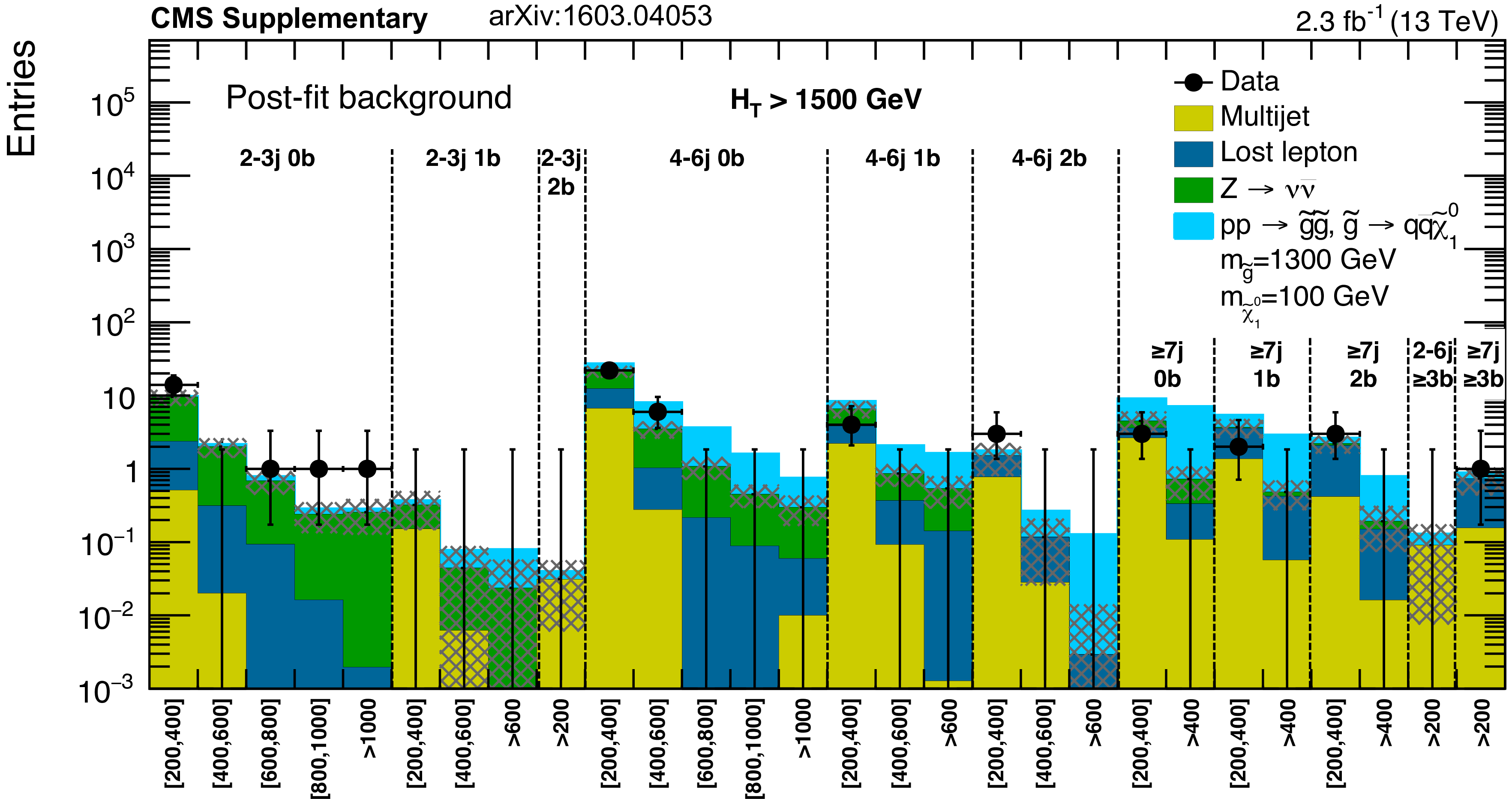
Additional Figure 37:
Expected (post-fit) and observed yields in the analysis binning, for the extreme-$ {H_{\mathrm {T}}} $ region and each of the $ {N_{\mathrm {j}}} $ and $ {N_{\mathrm {b}}} $ bins, with the expected contribution from a signal model of gluino-mediated light squark production with the mass of the gluino and the LSP equal to 1300 and 100 GeV, respectively. On the $x$-axis the $ {M_{\mathrm {T2}}} $ binning is shown (in GeV). |
png pdf |
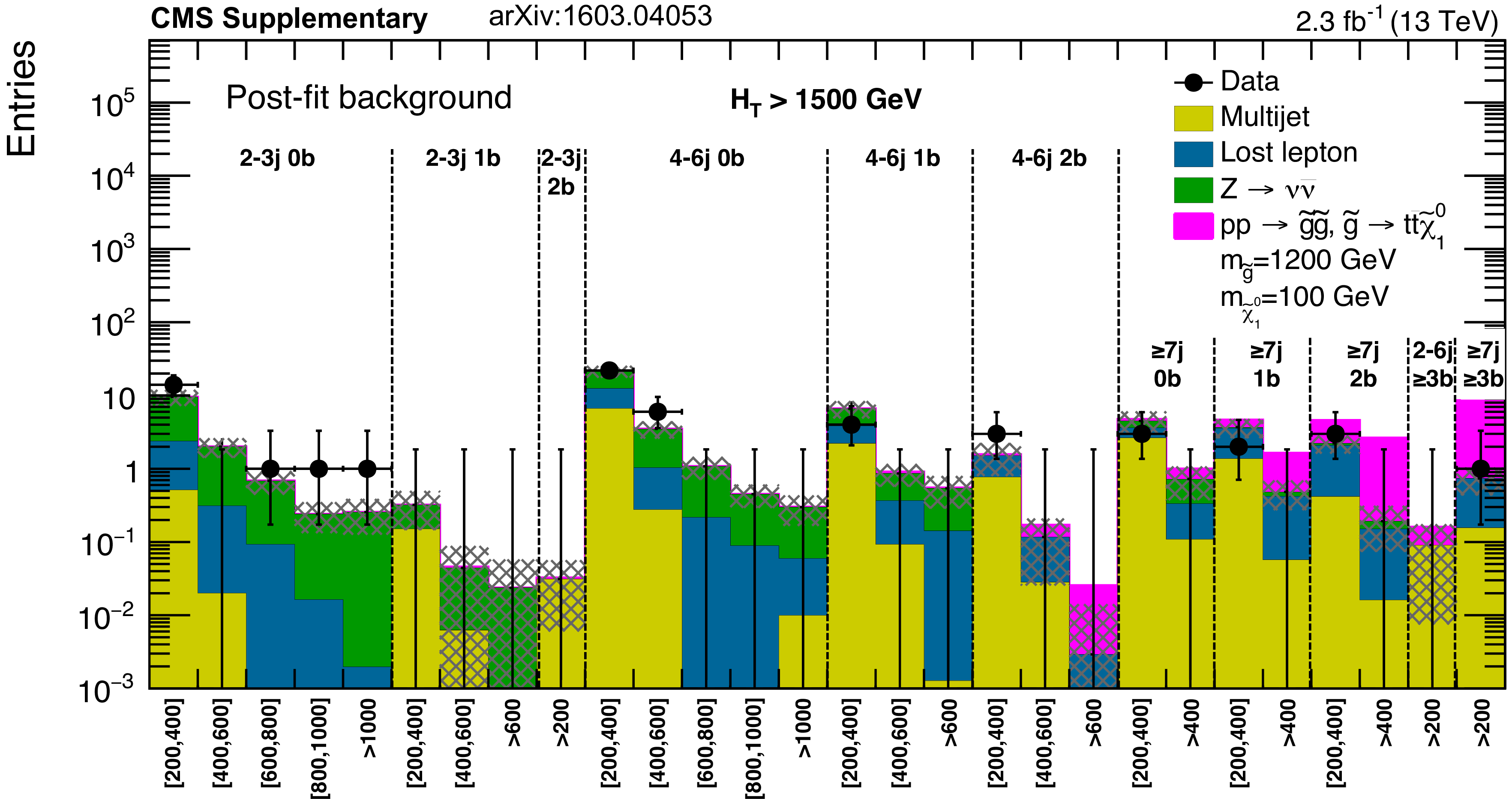
Additional Figure 38:
Expected (post-fit) and observed yields in the analysis binning, for the extreme-$ {H_{\mathrm {T}}} $ region and each of the $ {N_{\mathrm {j}}} $ and $ {N_{\mathrm {b}}} $ bins, with the expected contribution from a signal model of gluino-mediated top squark production with the mass of the gluino and the LSP equal to 1200 and 100 GeV, respectively. On the $x$-axis the $ {M_{\mathrm {T2}}} $ binning is shown (in GeV). |

png pdf |
Additional Figure 39:
Expected (post-fit) and observed yields in the analysis binning, for the extreme-$ {H_{\mathrm {T}}} $ region and each of the $ {N_{\mathrm {j}}} $ and $ {N_{\mathrm {b}}} $ bins, with the expected contribution from a signal model of direct bottom squark production with the mass of the bottom squark and the LSP equal to 700 and 100 GeV, respectively. On the $x$-axis the $ {M_{\mathrm {T2}}} $ binning is shown (in GeV). |
png pdf |
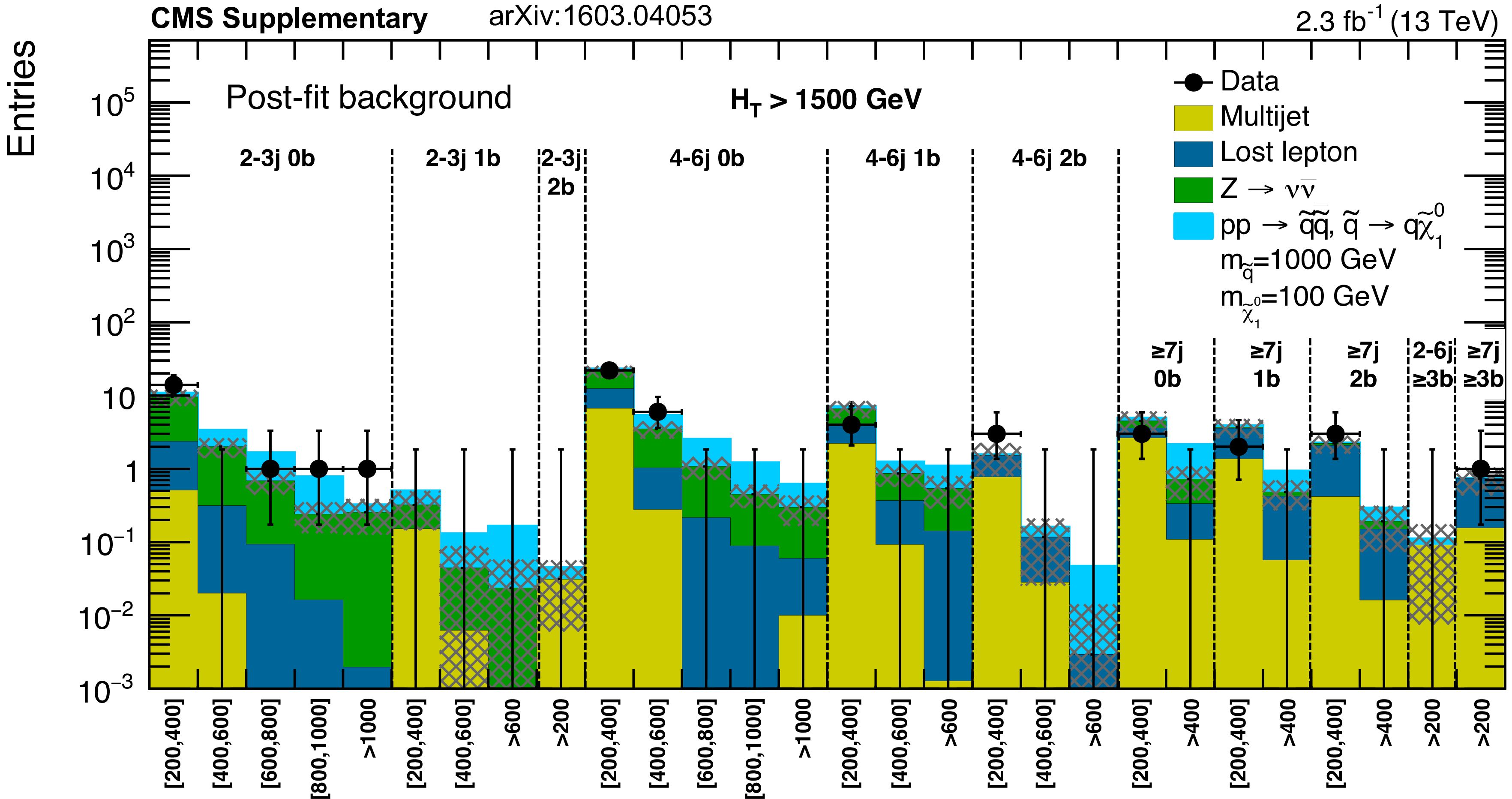
Additional Figure 40:
Expected (post-fit) and observed yields in the analysis binning, for the extreme-$ {H_{\mathrm {T}}} $ region and each of the $ {N_{\mathrm {j}}} $ and $ {N_{\mathrm {b}}} $ bins, with the expected contribution from a signal model of direct light squark production with the mass of the squark and the LSP equal to 1000 and 100 GeV, respectively. On the $x$-axis the $ {M_{\mathrm {T2}}} $ binning is shown (in GeV). |
png pdf |
Additional Figure 41:
Expected (post-fit) and observed yields in the analysis binning, for the extreme-$ {H_{\mathrm {T}}} $ region and each of the $ {N_{\mathrm {j}}} $ and $ {N_{\mathrm {b}}} $ bins, with the expected contribution from a signal model of direct top squark production with the mass of the top squark and the LSP equal to 650 and 100 GeV, respectively. On the $x$-axis the $ {M_{\mathrm {T2}}} $ binning is shown (in GeV). |
png pdf |
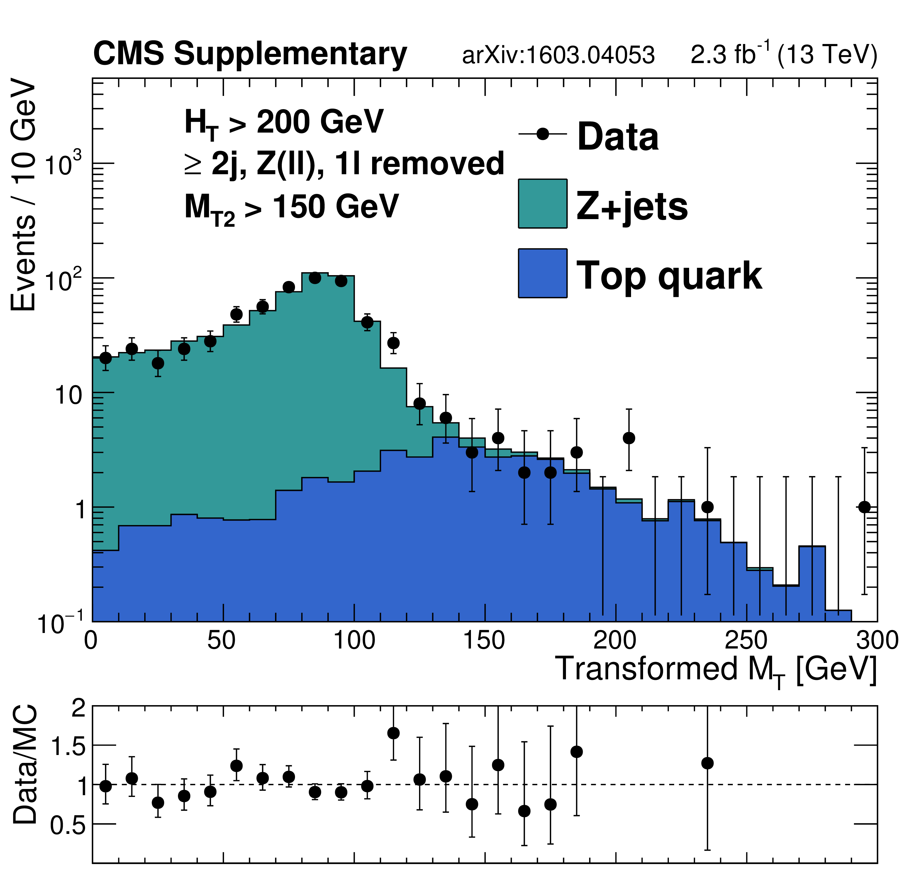
Additional Figure 42:
Distribution of $ {M_{\mathrm {T}}} $ in $ {\mathrm {Z}\rightarrow \ell ^+\ell ^-} $ events with one lepton treated as ``missing,'' comparing data to MC simulation. The requirement on $ {M_{\mathrm {T2}}} $ has been relaxed to $ {M_{\mathrm {T2}}} > 150$ GeV to preserve statistics. The sum of the MC prediction is normalized to data. |
png pdf |
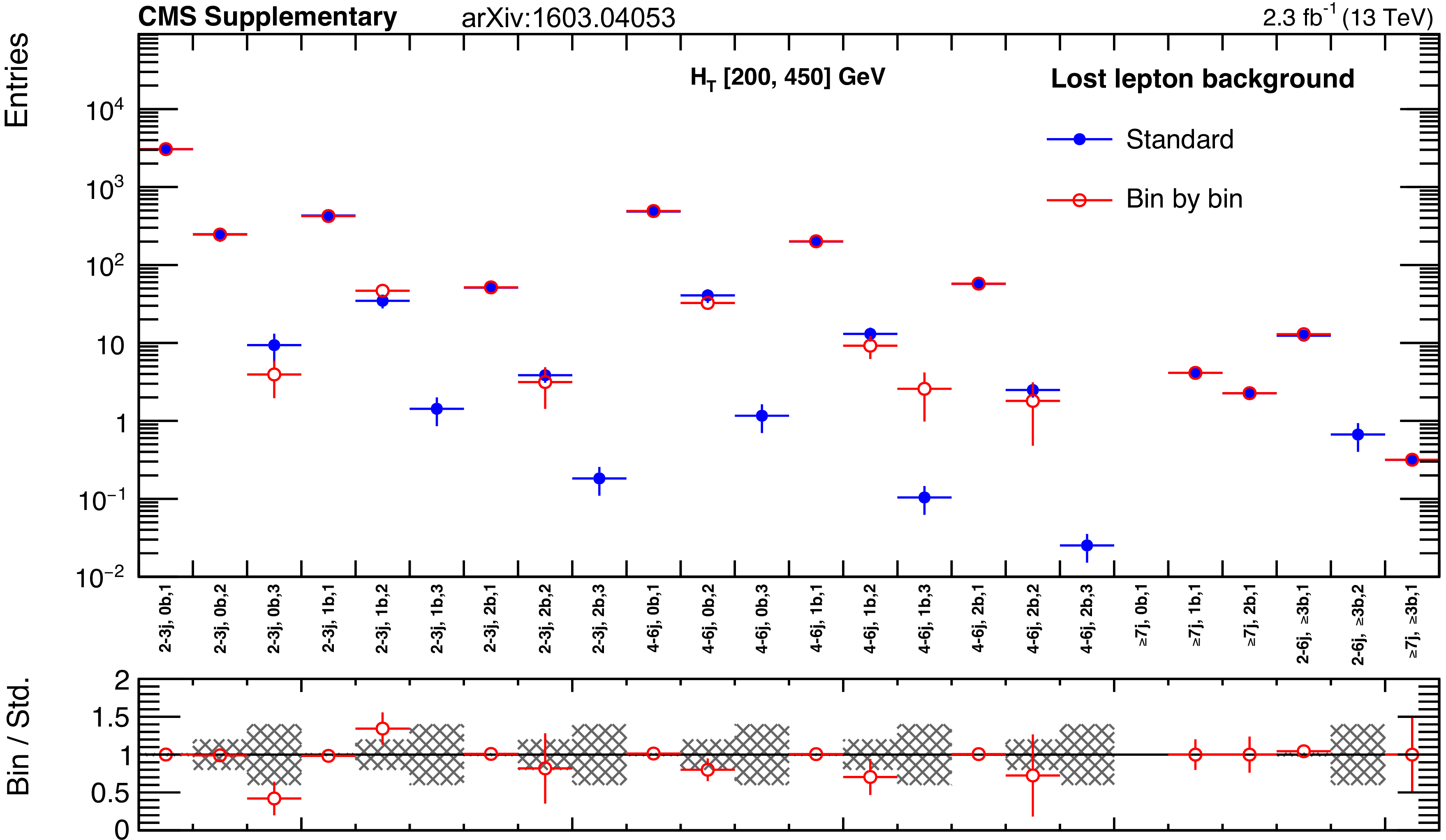
Additional Figure 43:
The standard lost lepton predictions based on the single lepton yields in bins of ($ {H_{\mathrm {T}}} $, $ {N_{\mathrm {j}}} $, $ {N_{\mathrm {b}}} $) and combined with the MC shape along $ {M_{\mathrm {T2}}} $ are compared with the bin-by-bin predictions obtained using single lepton yields in bins of ($ {H_{\mathrm {T}}} $, $ {N_{\mathrm {j}}} $, $ {N_{\mathrm {b}}} $ , $ {M_{\mathrm {T2}}} $), for the very-low-$ {H_{\mathrm {T}}} $ region. The MC sum of $ {\mathrm{ t \bar{t} } } $, $ {\mathrm {W}\mathrm {+jets}} $, single top, $ {\mathrm{ t \bar{t} } } \mathrm{ W } $, $ {\mathrm{ t \bar{t} } } {\mathrm{ Z } } $, and $ {\mathrm{ t \bar{t} } } \mathrm{ H } $ processes is used. Bins with no entry for data have an observed count of 0 events. |
png pdf |
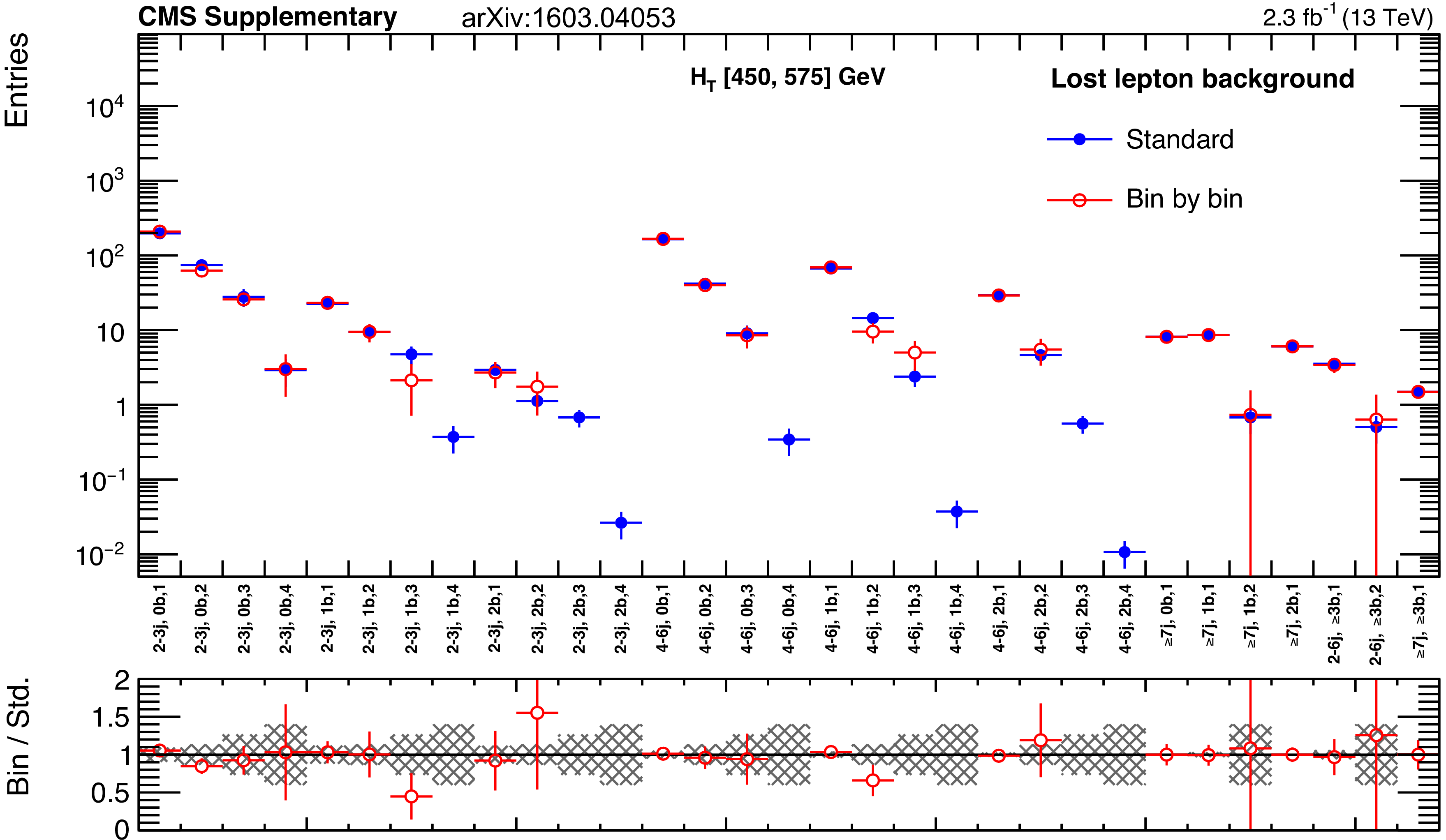
Additional Figure 44:
The standard lost lepton predictions based on the single lepton yields in bins of ($ {H_{\mathrm {T}}} $, $ {N_{\mathrm {j}}} $, $ {N_{\mathrm {b}}} $) and combined with the MC shape along $ {M_{\mathrm {T2}}} $ are compared with the bin-by-bin predictions obtained using single lepton yields in bins of ($ {H_{\mathrm {T}}} $, $ {N_{\mathrm {j}}} $, $ {N_{\mathrm {b}}} $ , $ {M_{\mathrm {T2}}} $), for the low- $ {H_{\mathrm {T}}} $ region. The MC sum of $ {\mathrm{ t \bar{t} } } $, $ {\mathrm {W}\mathrm {+jets}} $, single top, $ {\mathrm{ t \bar{t} } } \mathrm{ W } $, $ {\mathrm{ t \bar{t} } } {\mathrm{ Z } } $, and $ {\mathrm{ t \bar{t} } } \mathrm{ H } $ processes is used. Bins with no entry for data have an observed count of 0 events. |
png pdf |
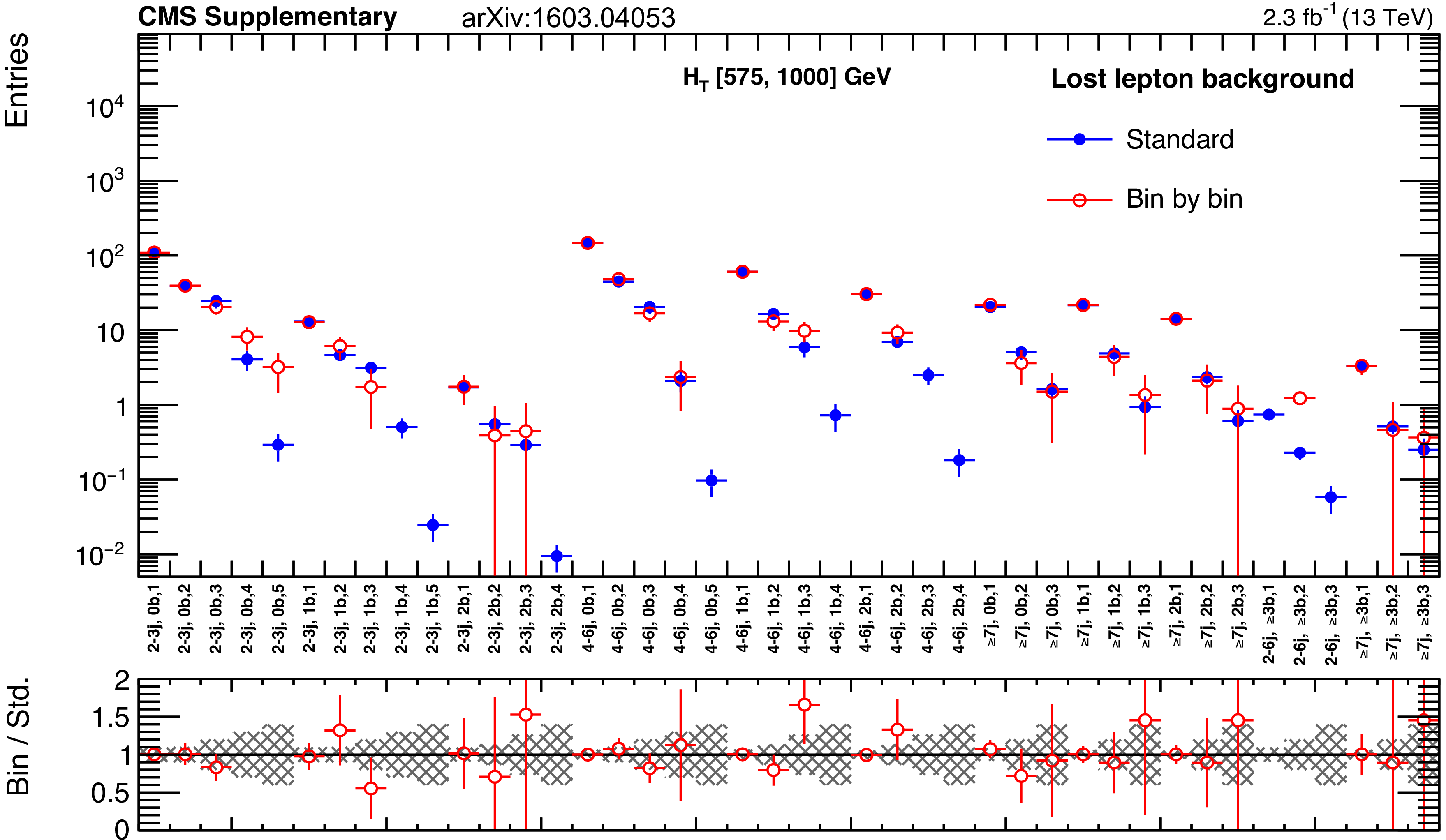
Additional Figure 45:
The standard lost lepton predictions based on the single lepton yields in bins of ($ {H_{\mathrm {T}}} $, $ {N_{\mathrm {j}}} $, $ {N_{\mathrm {b}}} $) and combined with the MC shape along $ {M_{\mathrm {T2}}} $ are compared with the bin-by-bin predictions obtained using single lepton yields in bins of ($ {H_{\mathrm {T}}} $, $ {N_{\mathrm {j}}} $, $ {N_{\mathrm {b}}} $ , $ {M_{\mathrm {T2}}} $), for the medium-$ {H_{\mathrm {T}}} $ region. The MC sum of $ {\mathrm{ t \bar{t} } } $, $ {\mathrm {W}\mathrm {+jets}} $, single top, $ {\mathrm{ t \bar{t} } } \mathrm{ W } $, $ {\mathrm{ t \bar{t} } } {\mathrm{ Z } } $, and $ {\mathrm{ t \bar{t} } } \mathrm{ H } $ processes is used. Bins with no entry for data have an observed count of 0 events. |
png pdf |
Additional Figure 46:
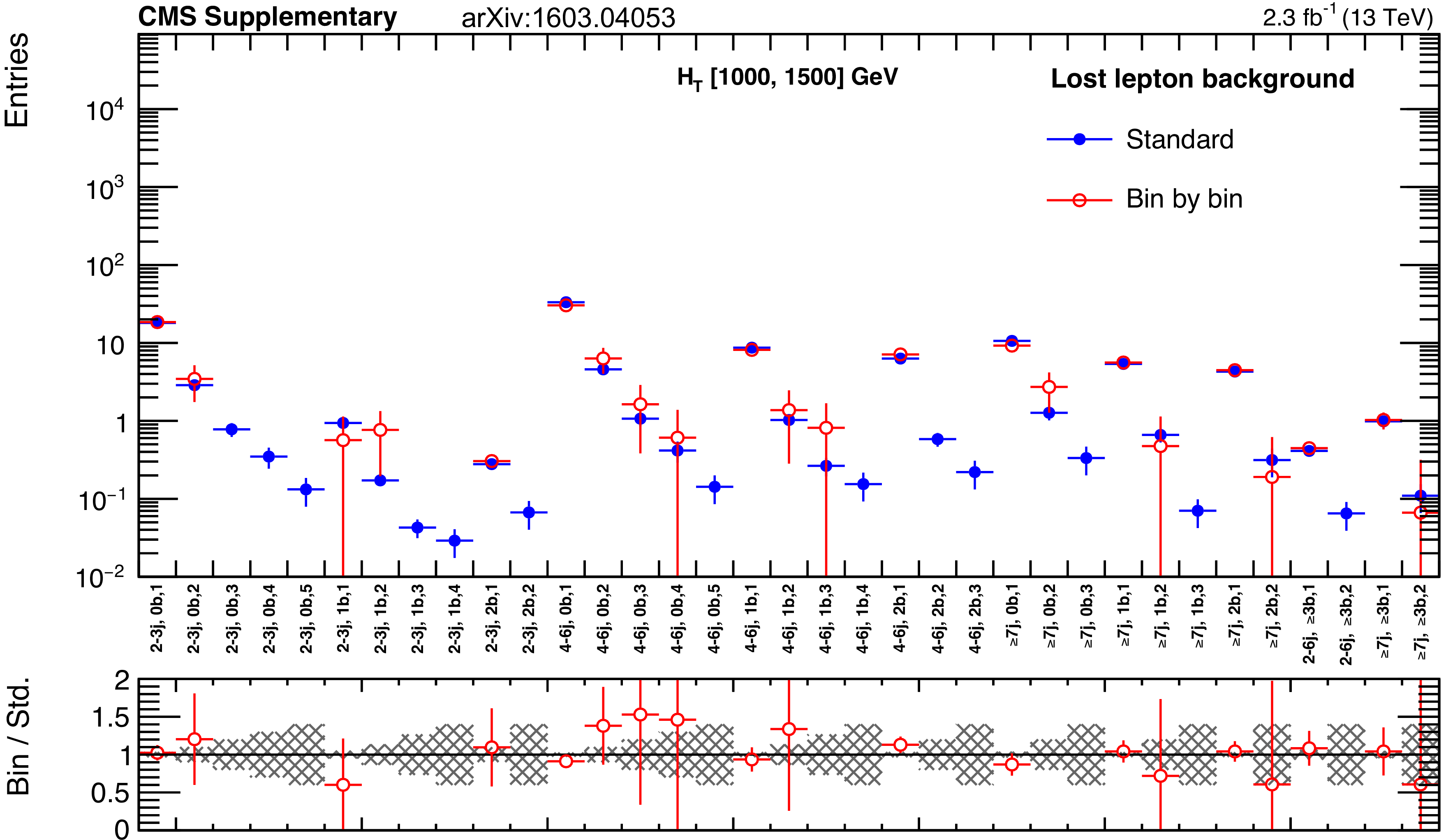
The standard lost lepton predictions based on the single lepton yields in bins of ($ {H_{\mathrm {T}}} $, $ {N_{\mathrm {j}}} $, $ {N_{\mathrm {b}}} $) and combined with the MC shape along $ {M_{\mathrm {T2}}} $ are compared with the bin-by-bin predictions obtained using single lepton yields in bins of ($ {H_{\mathrm {T}}} $, $ {N_{\mathrm {j}}} $, $ {N_{\mathrm {b}}} $ , $ {M_{\mathrm {T2}}} $), for the high-$ {H_{\mathrm {T}}} $ region. The MC sum of $ {\mathrm{ t \bar{t} } } $, $ {\mathrm {W}\mathrm {+jets}} $, single top, $ {\mathrm{ t \bar{t} } } \mathrm{ W } $, $ {\mathrm{ t \bar{t} } } {\mathrm{ Z } } $, and $ {\mathrm{ t \bar{t} } } \mathrm{ H } $ processes is used. Bins with no entry for data have an observed count of 0 events. |
png pdf |
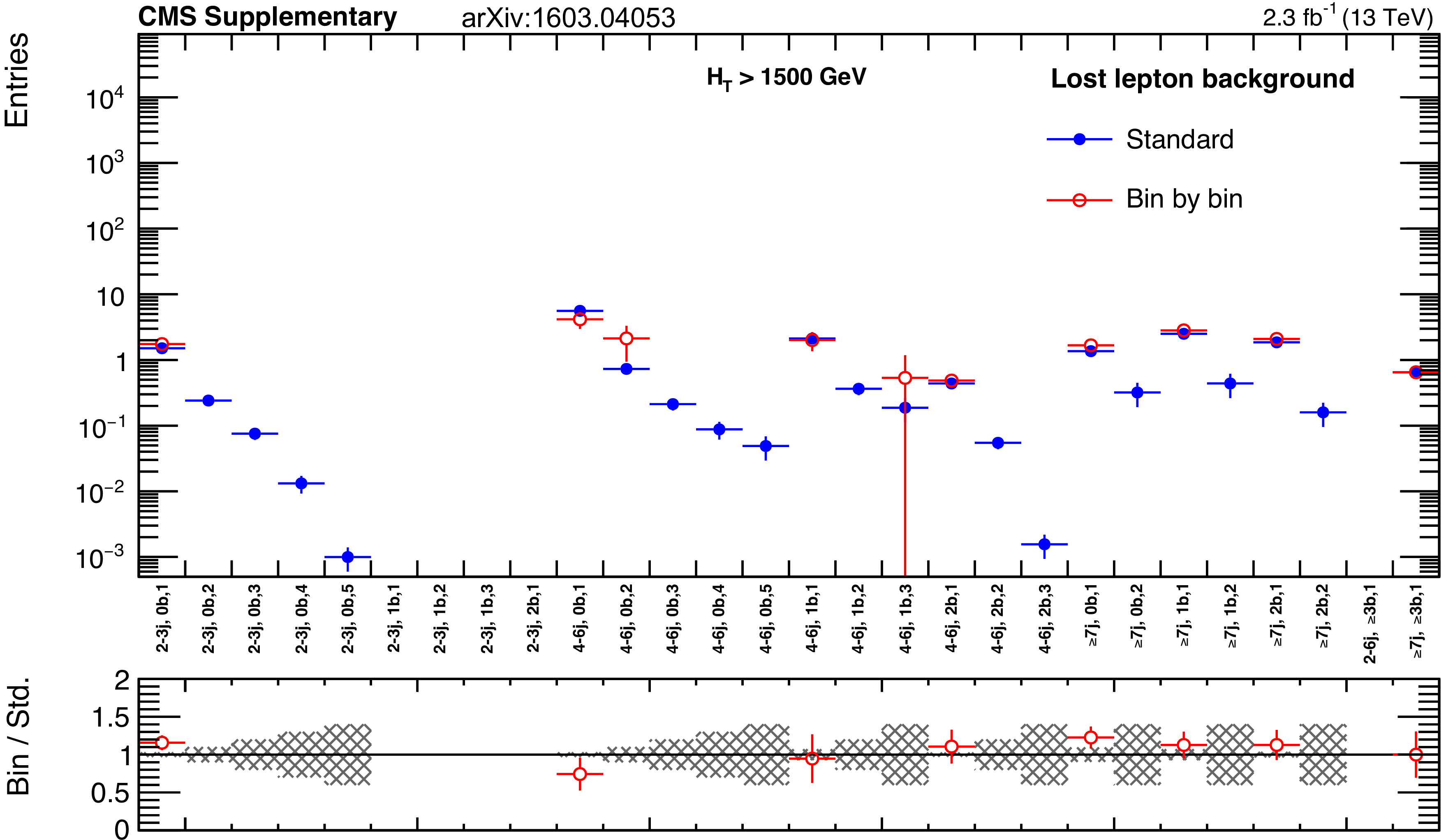
Additional Figure 47:
The standard lost lepton predictions based on the single lepton yields in bins of ($ {H_{\mathrm {T}}} $, $ {N_{\mathrm {j}}} $, $ {N_{\mathrm {b}}} $) and combined with the MC shape along $ {M_{\mathrm {T2}}} $ are compared with the bin-by-bin predictions obtained using single lepton yields in bins of ($ {H_{\mathrm {T}}} $, $ {N_{\mathrm {j}}} $, $ {N_{\mathrm {b}}} $ , $ {M_{\mathrm {T2}}} $), for the extreme-$ {H_{\mathrm {T}}} $ region. The MC sum of $ {\mathrm{ t \bar{t} } } $, $ {\mathrm {W}\mathrm {+jets}} $, single top, $ {\mathrm{ t \bar{t} } } \mathrm{ W } $, $ {\mathrm{ t \bar{t} } } {\mathrm{ Z } } $, and $ {\mathrm{ t \bar{t} } } \mathrm{ H } $ processes is used. Bins with no entry for data have an observed count of 0 events. |

png pdf |
Additional Figure 48:
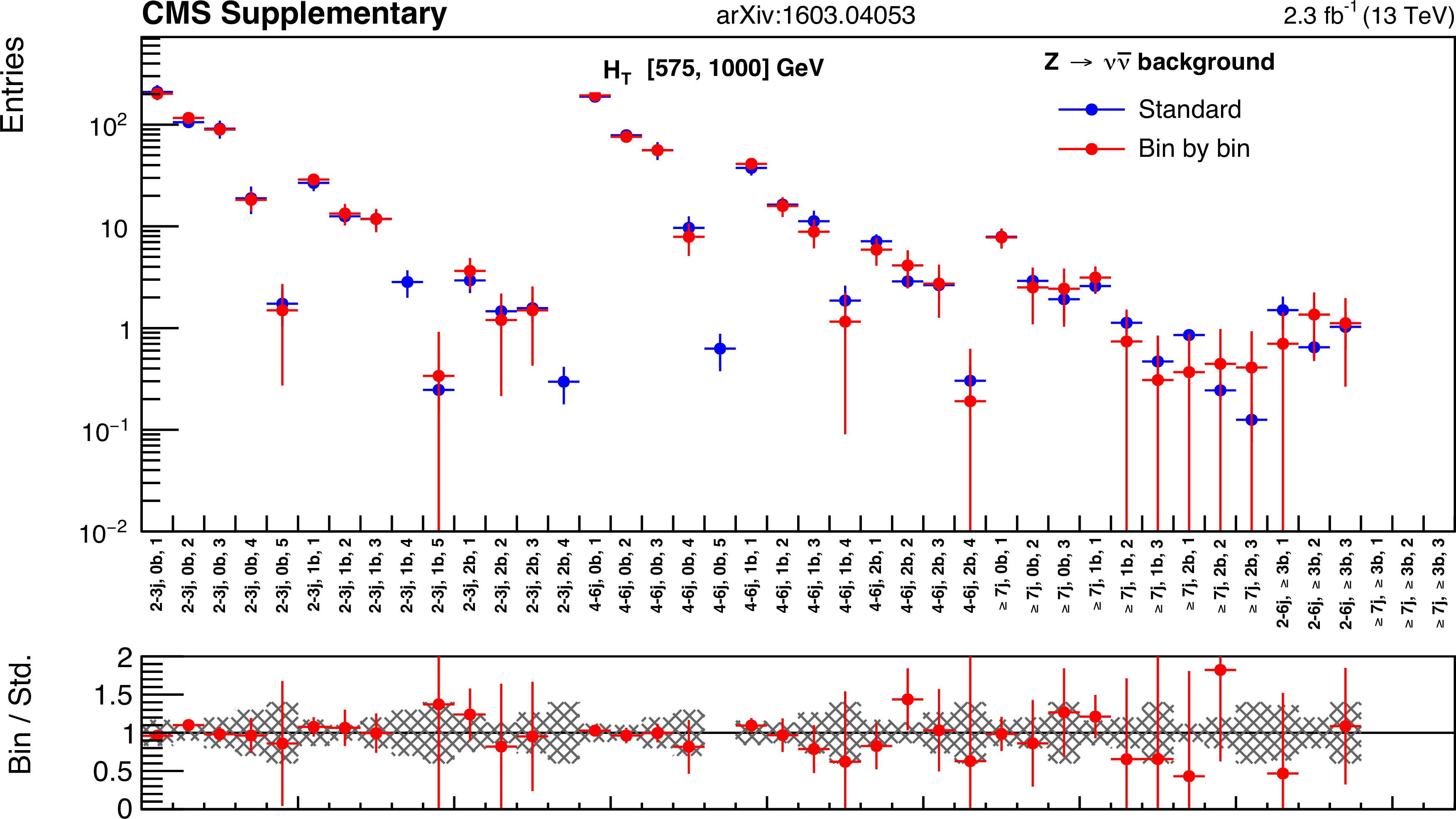
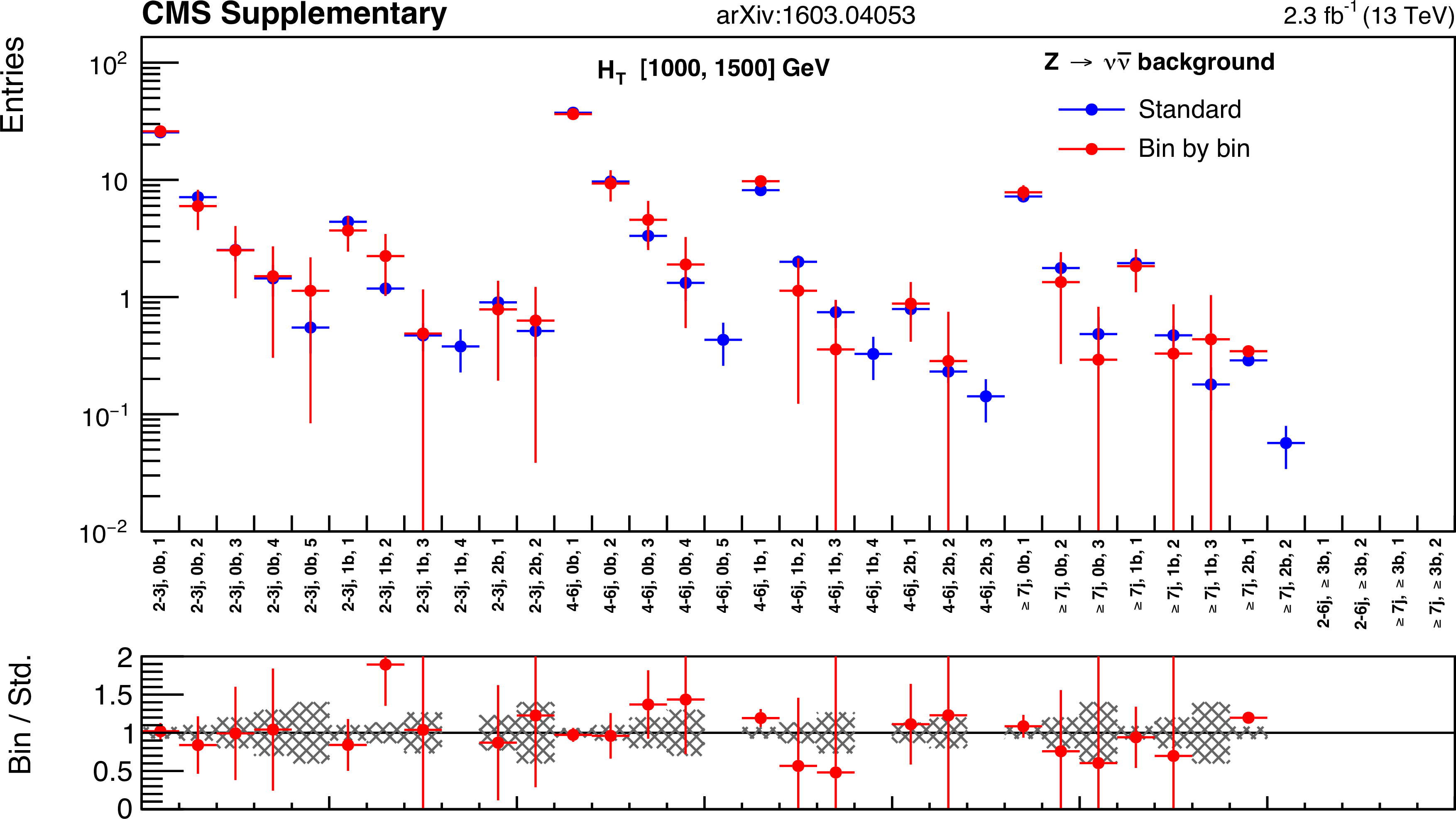
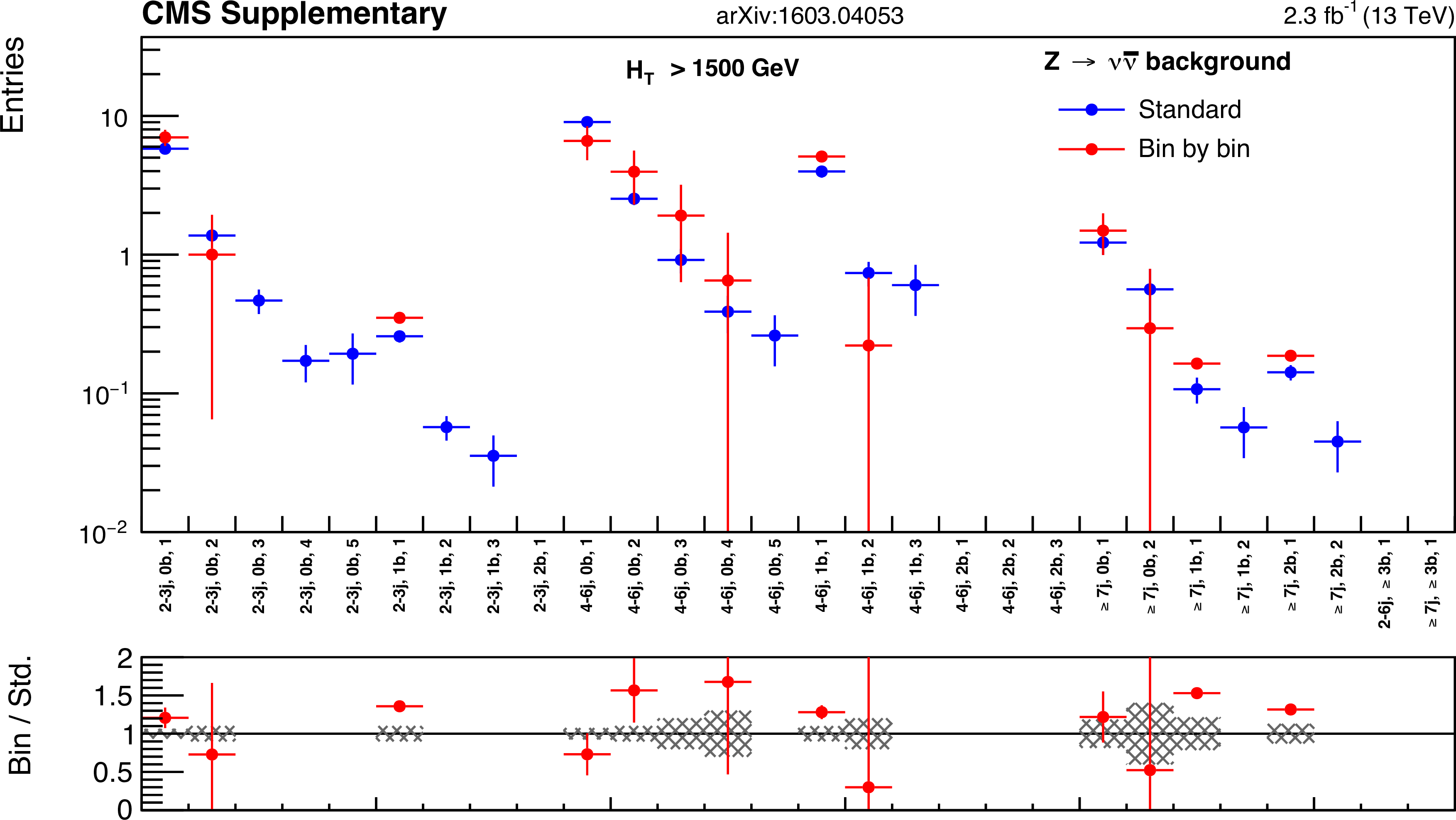
The standard $ {\mathrm {Z}\rightarrow \nu \bar{\nu} } $ predictions based on the $ {\gamma +\mathrm {jets}} $ yields in bins of ($ {H_{\mathrm {T}}} $, $ {N_{\mathrm {j}}} $, $ {N_{\mathrm {b}}} $) and combined with the $ {\mathrm {Z}\rightarrow \nu \bar{\nu} } $ MC shape along $ {M_{\mathrm {T2}}} $ are compared with the bin-by-bin predictions obtained using $ {\gamma +\mathrm {jets}} $ yields in bins of ($ {H_{\mathrm {T}}} $, $ {N_{\mathrm {j}}} $, $ {N_{\mathrm {b}}} $ , $ {M_{\mathrm {T2}}} $), for the very-low-$ {H_{\mathrm {T}}} $ region. Bins with no entry for data have an observed count of 0 events. |
png pdf |
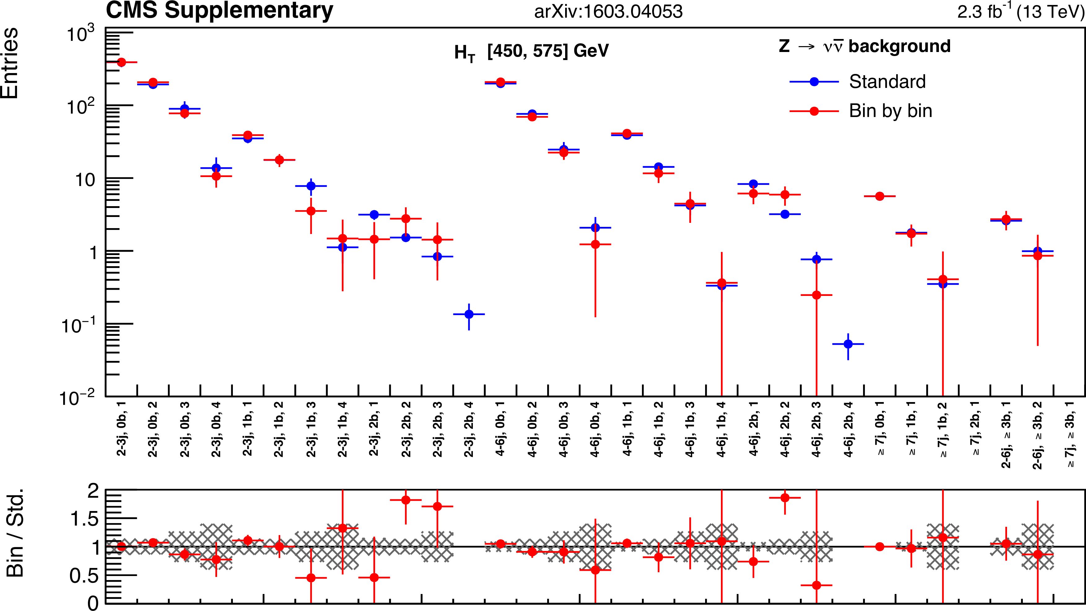
Additional Figure 49:
The standard $ {\mathrm {Z}\rightarrow \nu \bar{\nu} } $ predictions based on the $ {\gamma +\mathrm {jets}} $ yields in bins of ($ {H_{\mathrm {T}}} $, $ {N_{\mathrm {j}}} $, $ {N_{\mathrm {b}}} $) and combined with the $ {\mathrm {Z}\rightarrow \nu \bar{\nu} } $ MC shape along $ {M_{\mathrm {T2}}} $ are compared with the bin-by-bin predictions obtained using $ {\gamma +\mathrm {jets}} $ yields in bins of ($ {H_{\mathrm {T}}} $, $ {N_{\mathrm {j}}} $, $ {N_{\mathrm {b}}} $ , $ {M_{\mathrm {T2}}} $), for the low-$ {H_{\mathrm {T}}} $ region. Bins with no entry for data have an observed count of 0 events. |
png pdf |
Additional Figure 50:
The standard $ {\mathrm {Z}\rightarrow \nu \bar{\nu} } $ predictions based on the $ {\gamma +\mathrm {jets}} $ yields in bins of ($ {H_{\mathrm {T}}} $, $ {N_{\mathrm {j}}} $, $ {N_{\mathrm {b}}} $) and combined with the $ {\mathrm {Z}\rightarrow \nu \bar{\nu} } $ MC shape along $ {M_{\mathrm {T2}}} $ are compared with the bin-by-bin predictions obtained using $ {\gamma +\mathrm {jets}} $ yields in bins of ($ {H_{\mathrm {T}}} $, $ {N_{\mathrm {j}}} $, $ {N_{\mathrm {b}}} $ , $ {M_{\mathrm {T2}}} $), for the medium-$ {H_{\mathrm {T}}} $ region. Bins with no entry for data have an observed count of 0 events. |
png pdf |
Additional Figure 51:
The standard $ {\mathrm {Z}\rightarrow \nu \bar{\nu} } $ predictions based on the $ {\gamma +\mathrm {jets}} $ yields in bins of ($ {H_{\mathrm {T}}} $, $ {N_{\mathrm {j}}} $, $ {N_{\mathrm {b}}} $) and combined with the $ {\mathrm {Z}\rightarrow \nu \bar{\nu} } $ MC shape along $ {M_{\mathrm {T2}}} $ are compared with the bin-by-bin predictions obtained using $ {\gamma +\mathrm {jets}} $ yields in bins of ($ {H_{\mathrm {T}}} $, $ {N_{\mathrm {j}}} $, $ {N_{\mathrm {b}}} $ , $ {M_{\mathrm {T2}}} $), for the high-$ {H_{\mathrm {T}}} $ region. Bins with no entry for data have an observed count of 0 events. |
png pdf |
Additional Figure 52:
The standard $ {\mathrm {Z}\rightarrow \nu \bar{\nu} } $ predictions based on the $ {\gamma +\mathrm {jets}} $ yields in bins of ($ {H_{\mathrm {T}}} $, $ {N_{\mathrm {j}}} $, $ {N_{\mathrm {b}}} $) and combined with the $ {\mathrm {Z}\rightarrow \nu \bar{\nu} } $ MC shape along $ {M_{\mathrm {T2}}} $ are compared with the bin-by-bin predictions obtained using $ {\gamma +\mathrm {jets}} $ yields in bins of ($ {H_{\mathrm {T}}} $, $ {N_{\mathrm {j}}} $, $ {N_{\mathrm {b}}} $ , $ {M_{\mathrm {T2}}} $), for the extreme-$ {H_{\mathrm {T}}} $ region. Bins with no entry for data have an observed count of 0 events. |
png pdf |
Additional Figure 53:
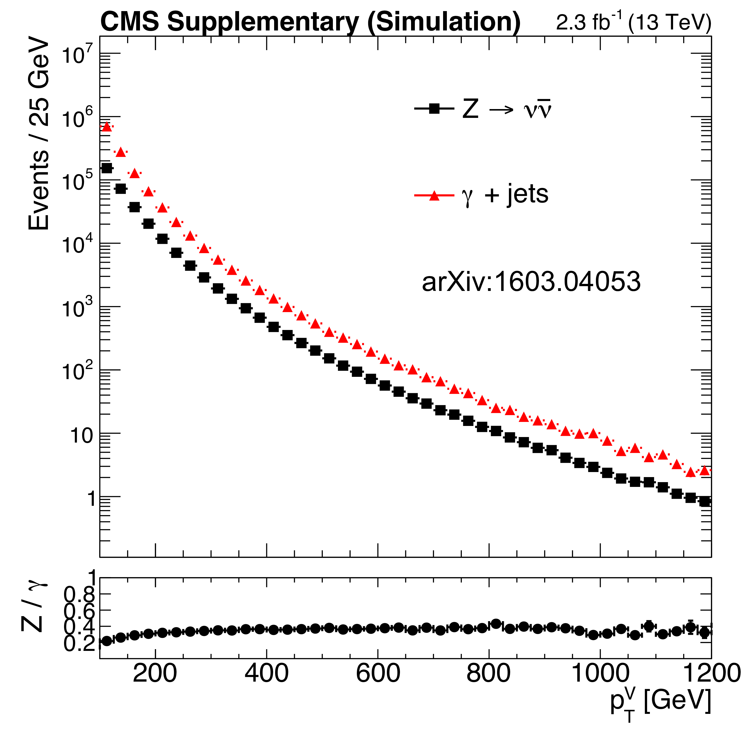
Expected number of events with $ {H_{\mathrm {T}}} > 100$ GeV as a function of the transverse momentum of the boson($p_{\mathrm {T}}(V)$) for $ {\gamma +\mathrm {jets}} $ (red markers) and $ {\mathrm {Z}\rightarrow \nu \bar{\nu} } $ (black markers). The $Z/\gamma $ ratio as a function of $p_{\mathrm {T}}(V)$ is shown at the bottom, flattening out as the transverse momentum becomes larger than the $Z$ mass. |
png |
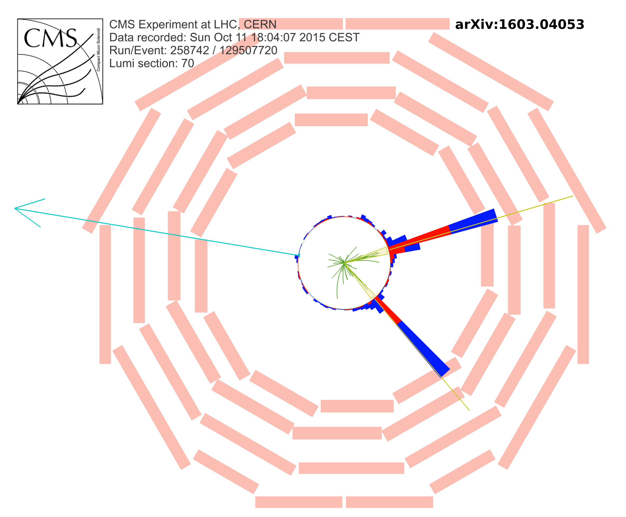
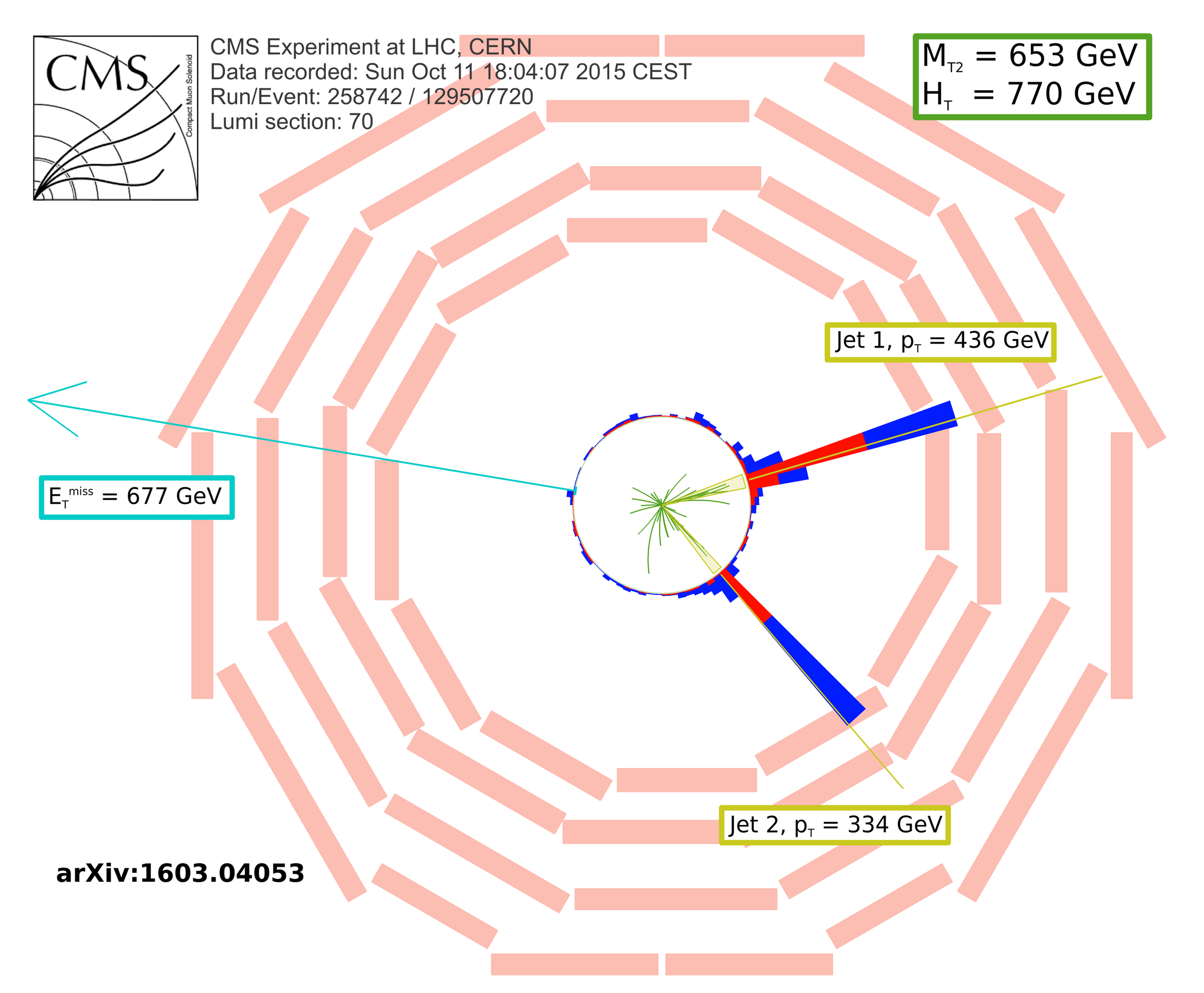
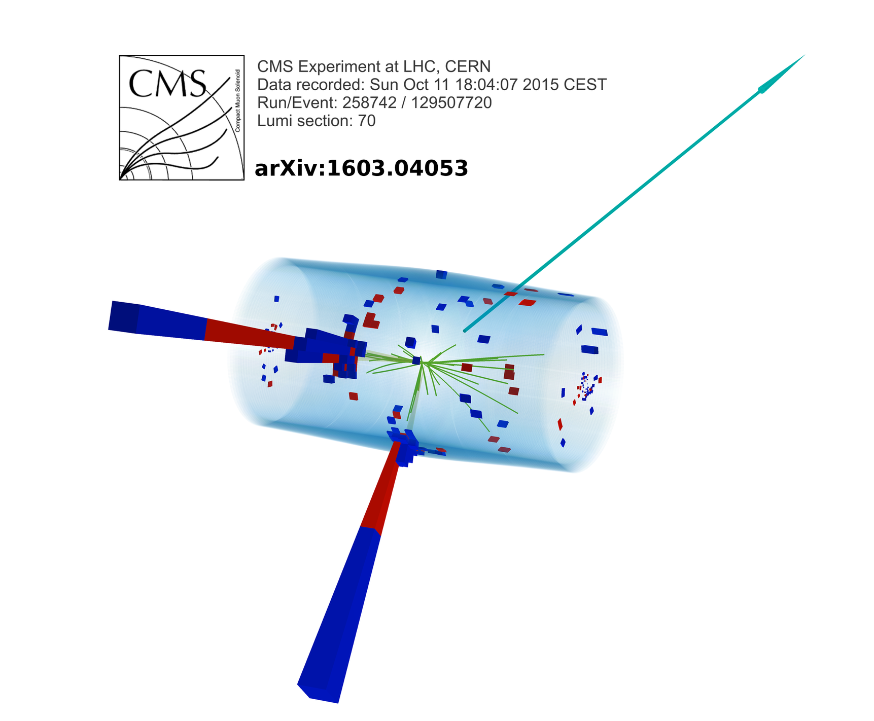
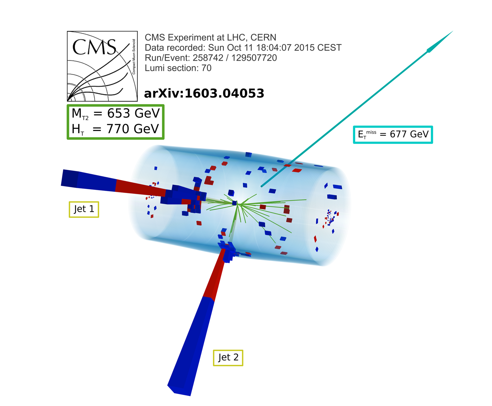
Additional Figure 54-a:
Display of a candidate event at event:run:lumi=129507720:70:258742, with $ {M_{\mathrm {T2}}} =653$ GeV, $ {H_{\mathrm {T}}} =770$ GeV, $ {E_{\mathrm {T}}^{\text {miss}}} =677$ GeV, 2 jets and 0 b-jets. |
png |
Additional Figure 54-b:
Display of a candidate event at event:run:lumi=129507720:70:258742, with $ {M_{\mathrm {T2}}} =653$ GeV, $ {H_{\mathrm {T}}} =770$ GeV, $ {E_{\mathrm {T}}^{\text {miss}}} =677$ GeV, 2 jets and 0 b-jets. |
png |
Additional Figure 54-c:
Display of a candidate event at event:run:lumi=129507720:70:258742, with $ {M_{\mathrm {T2}}} =653$ GeV, $ {H_{\mathrm {T}}} =770$ GeV, $ {E_{\mathrm {T}}^{\text {miss}}} =677$ GeV, 2 jets and 0 b-jets. |
png |
Additional Figure 54-d:
Display of a candidate event at event:run:lumi=129507720:70:258742, with $ {M_{\mathrm {T2}}} =653$ GeV, $ {H_{\mathrm {T}}} =770$ GeV, $ {E_{\mathrm {T}}^{\text {miss}}} =677$ GeV, 2 jets and 0 b-jets. |
png |
Additional Figure 55-a:
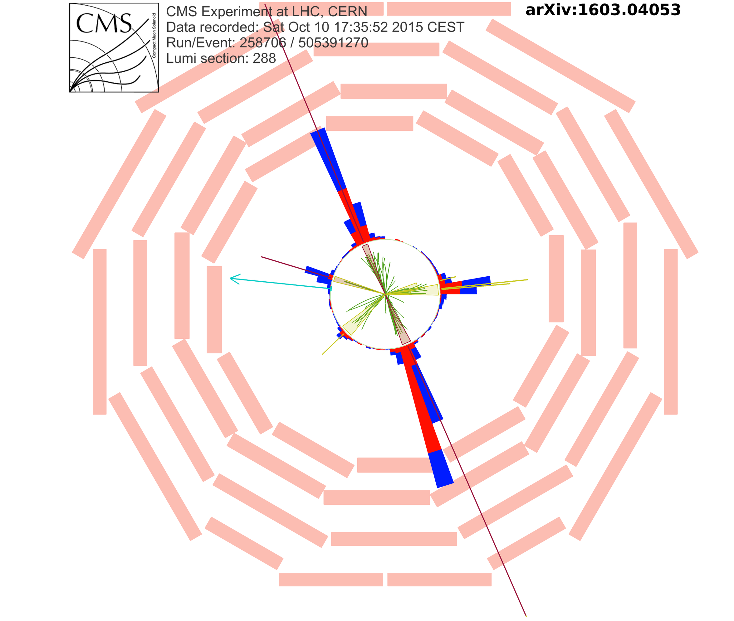
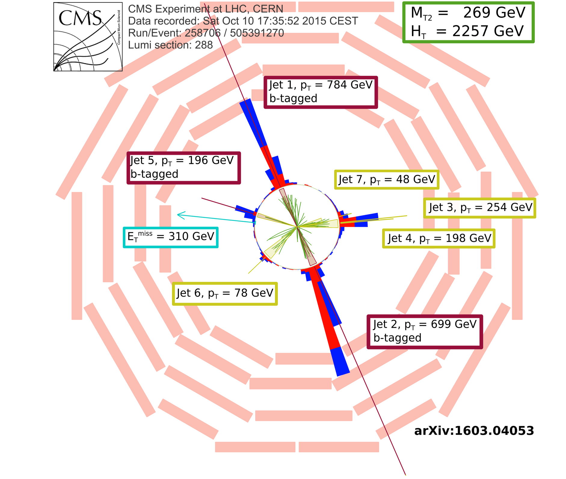
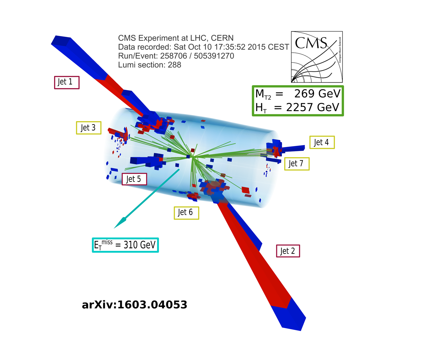
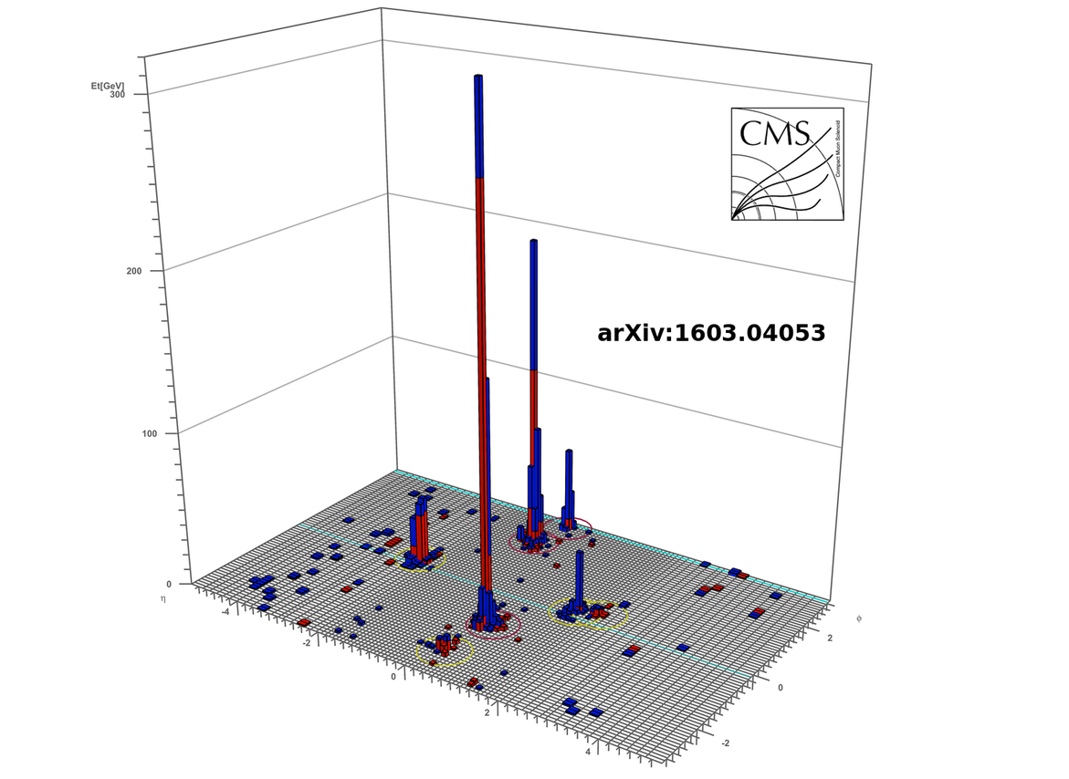
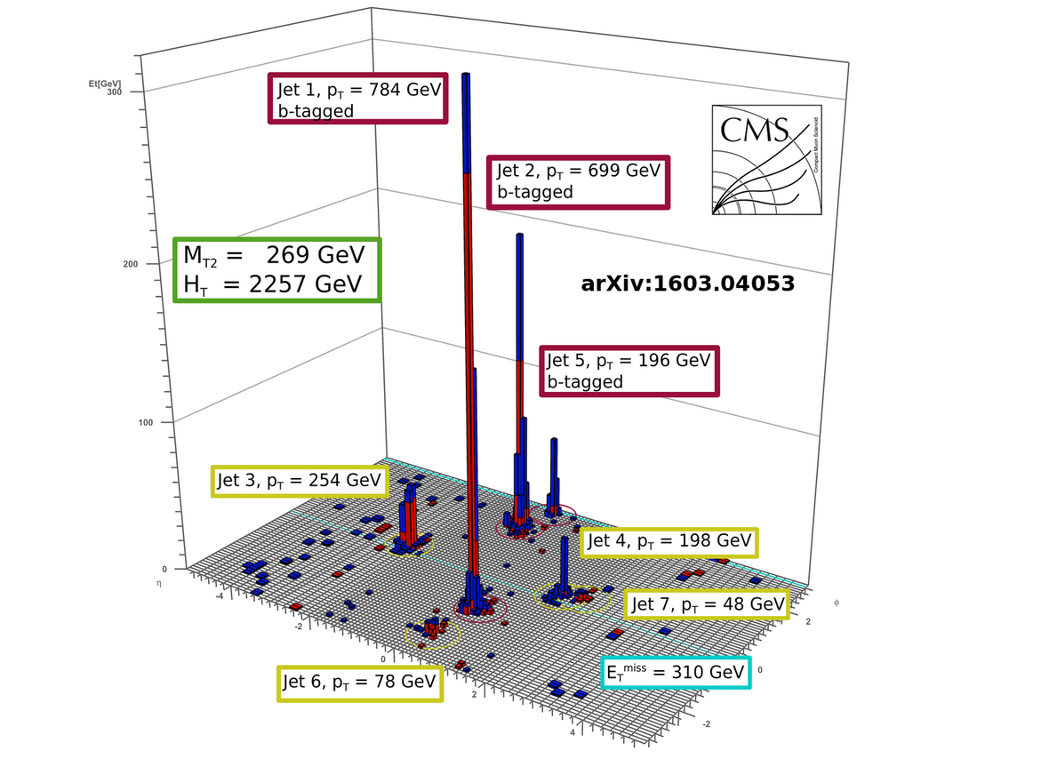
Display of a candidate event at event:run:lumi=505391270:288:258706, with $ {M_{\mathrm {T2}}} =269$ GeV, $ {H_{\mathrm {T}}} =2257$ GeV, $ {E_{\mathrm {T}}^{\text {miss}}} =310$ GeV, 7 jets and 3 b-jets. |
png |
Additional Figure 55-b:
Display of a candidate event at event:run:lumi=505391270:288:258706, with $ {M_{\mathrm {T2}}} =269$ GeV, $ {H_{\mathrm {T}}} =2257$ GeV, $ {E_{\mathrm {T}}^{\text {miss}}} =310$ GeV, 7 jets and 3 b-jets. |

png |
Additional Figure 55-c:
Display of a candidate event at event:run:lumi=505391270:288:258706, with $ {M_{\mathrm {T2}}} =269$ GeV, $ {H_{\mathrm {T}}} =2257$ GeV, $ {E_{\mathrm {T}}^{\text {miss}}} =310$ GeV, 7 jets and 3 b-jets. |
png |
Additional Figure 55-d:
Display of a candidate event at event:run:lumi=505391270:288:258706, with $ {M_{\mathrm {T2}}} =269$ GeV, $ {H_{\mathrm {T}}} =2257$ GeV, $ {E_{\mathrm {T}}^{\text {miss}}} =310$ GeV, 7 jets and 3 b-jets. |
png |
Additional Figure 55-e:
Display of a candidate event at event:run:lumi=505391270:288:258706, with $ {M_{\mathrm {T2}}} =269$ GeV, $ {H_{\mathrm {T}}} =2257$ GeV, $ {E_{\mathrm {T}}^{\text {miss}}} =310$ GeV, 7 jets and 3 b-jets. |
png |
Additional Figure 55-f:
Display of a candidate event at event:run:lumi=505391270:288:258706, with $ {M_{\mathrm {T2}}} =269$ GeV, $ {H_{\mathrm {T}}} =2257$ GeV, $ {E_{\mathrm {T}}^{\text {miss}}} =310$ GeV, 7 jets and 3 b-jets. |
| Additional Tables | |
png pdf |
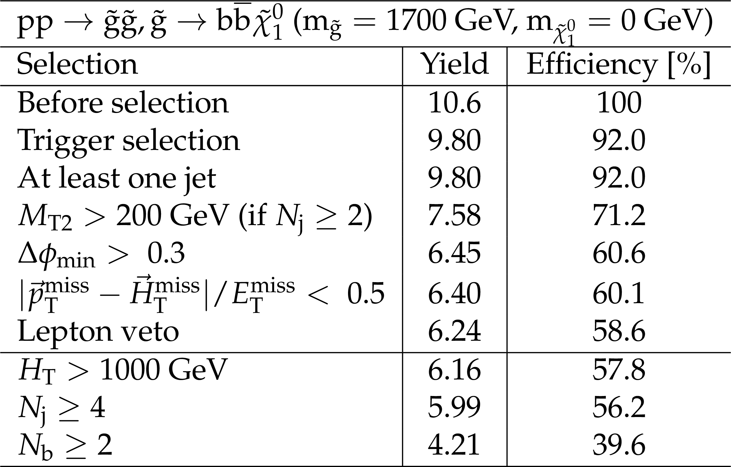
Additional Table 1:
Cut flow table, for a signal model of gluino-mediated bottom squark production with the mass of the gluino and the LSP equal to 1700 and 0 GeV, respectively. Theory cross section for this signal is 0.0047 pb. |
png pdf |
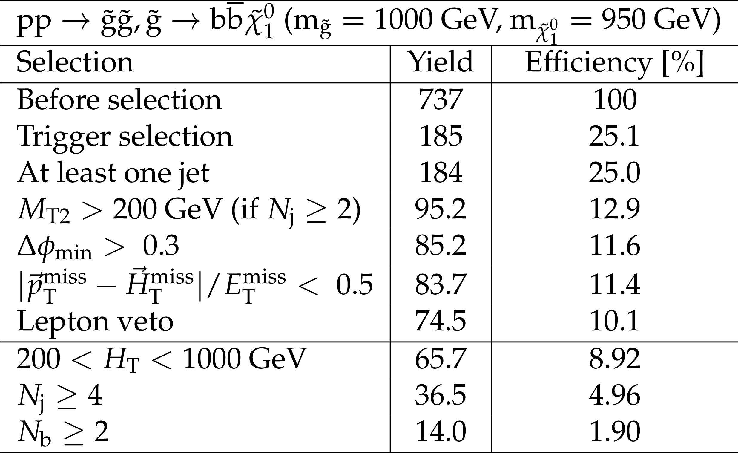
Additional Table 2:
Cut flow table, for a signal model of gluino-mediated bottom squark production with the mass of the gluino and the LSP equal to 1000 and 950 GeV, respectively. Theory cross section for this signal is 0.33 pb. |

png pdf |
Additional Table 3:
Cut flow table, for a signal model of gluino-mediated light squark production with the mass of the gluino and the LSP equal to 1600 and 0 GeV, respectively. Theory cross section for this signal is 0.0081 pb. |
png pdf |
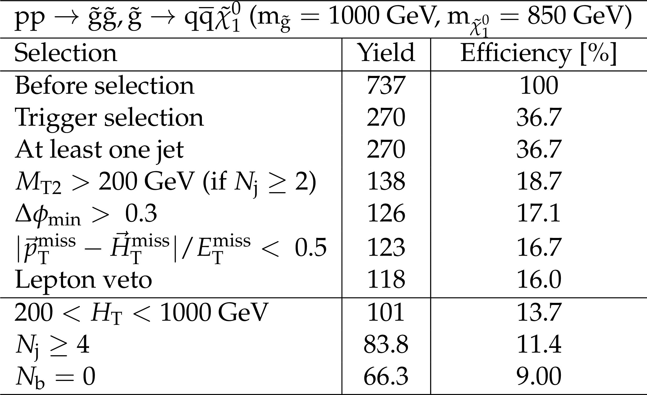
Additional Table 4:
Cut flow table, for a signal model of gluino-mediated light squark production with the mass of the gluino and the LSP equal to 1000 and 850 GeV, respectively . Theory cross section for this signal is 0.33 pb. |
png pdf |
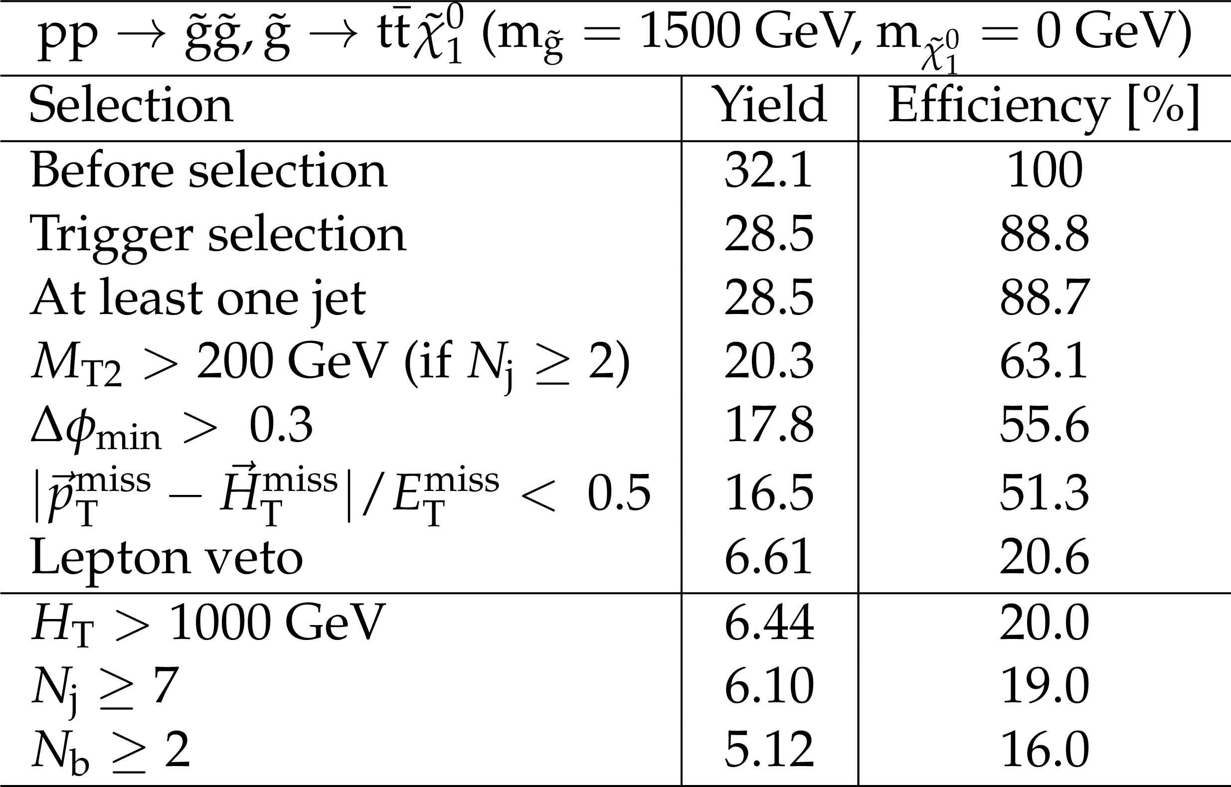
Additional Table 5:
Cut flow table, for a signal model of gluino-mediated top squark production with the mass of the gluino and the LSP equal to 1500 and 0 GeV, respectively. Theory cross section for this signal is 0.014 pb. |
png pdf |
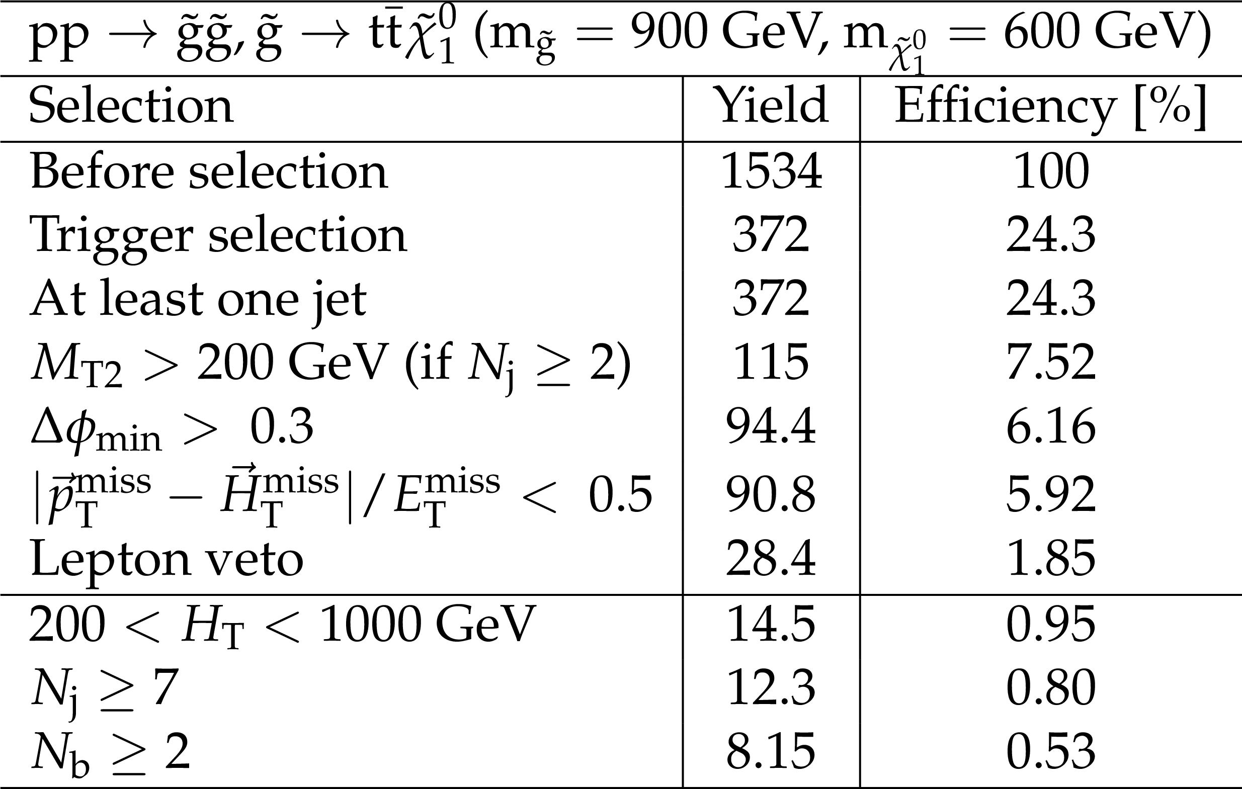
Additional Table 6:
Cut flow table, for a signal model of gluino-mediated top squark production with the mass of the gluino and the LSP equal to 900 and 600 GeV, respectively. Theory cross section for this signal is 0.68 pb. |
png pdf |
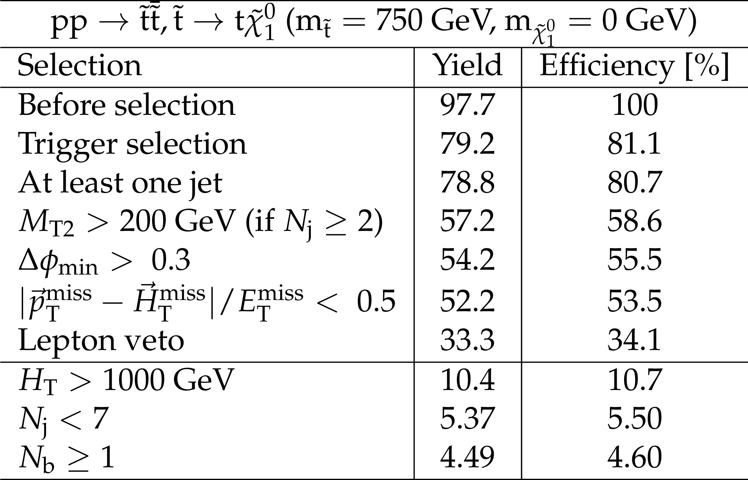
Additional Table 7:
Cut flow table, for a signal model of direct top squark production with the mass of the squark and the LSP equal to 750 and 0 GeV, respectively. Theory cross section for this signal is 0.043 pb. |
png pdf |
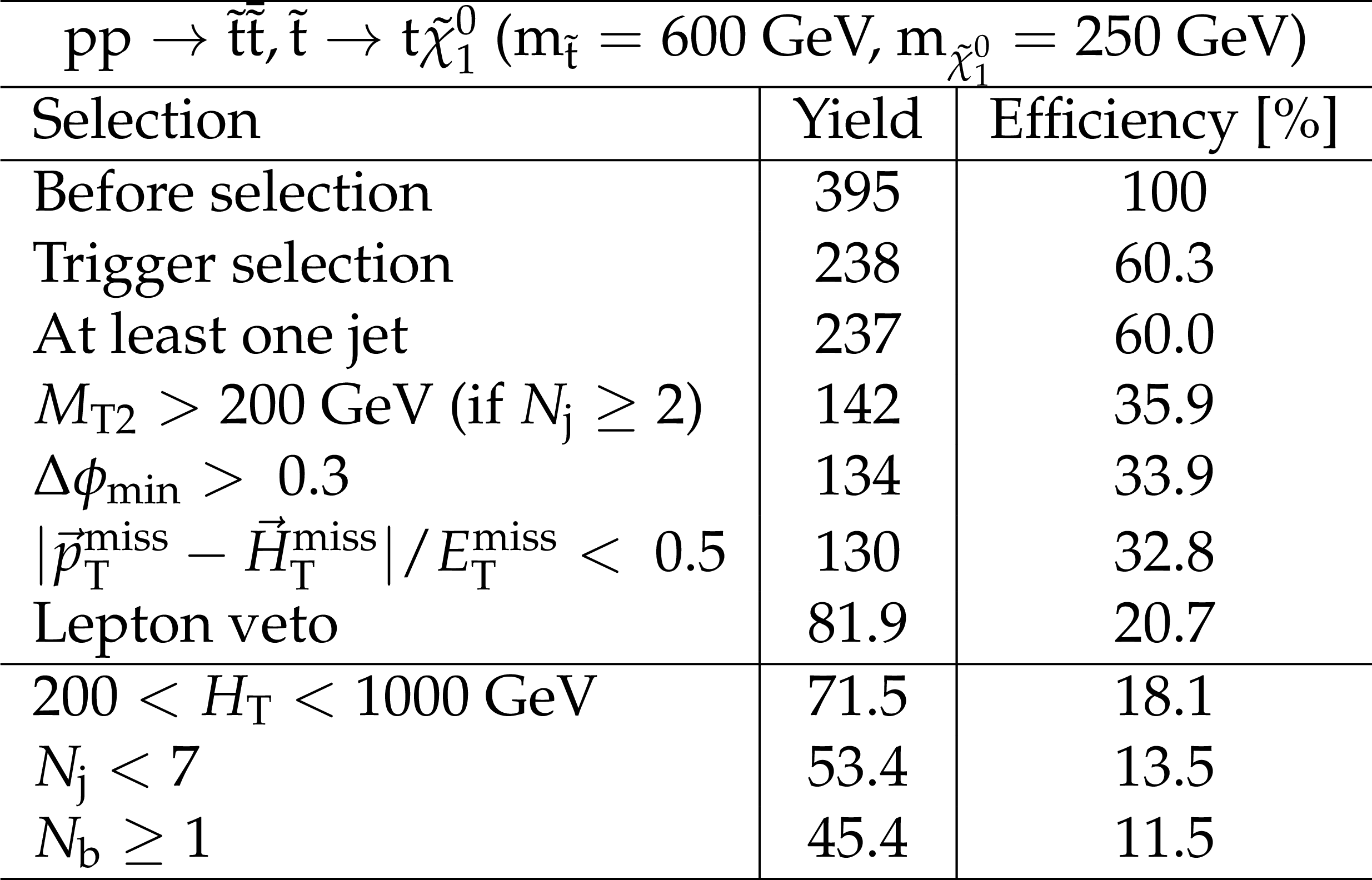
Additional Table 8:
Cut flow table, for a signal model of direct top squark production with the mass of the squark and the LSP equal to 600 and 250 GeV, respectively. Theory cross section for this signal is 0.17 pb. |
png pdf |
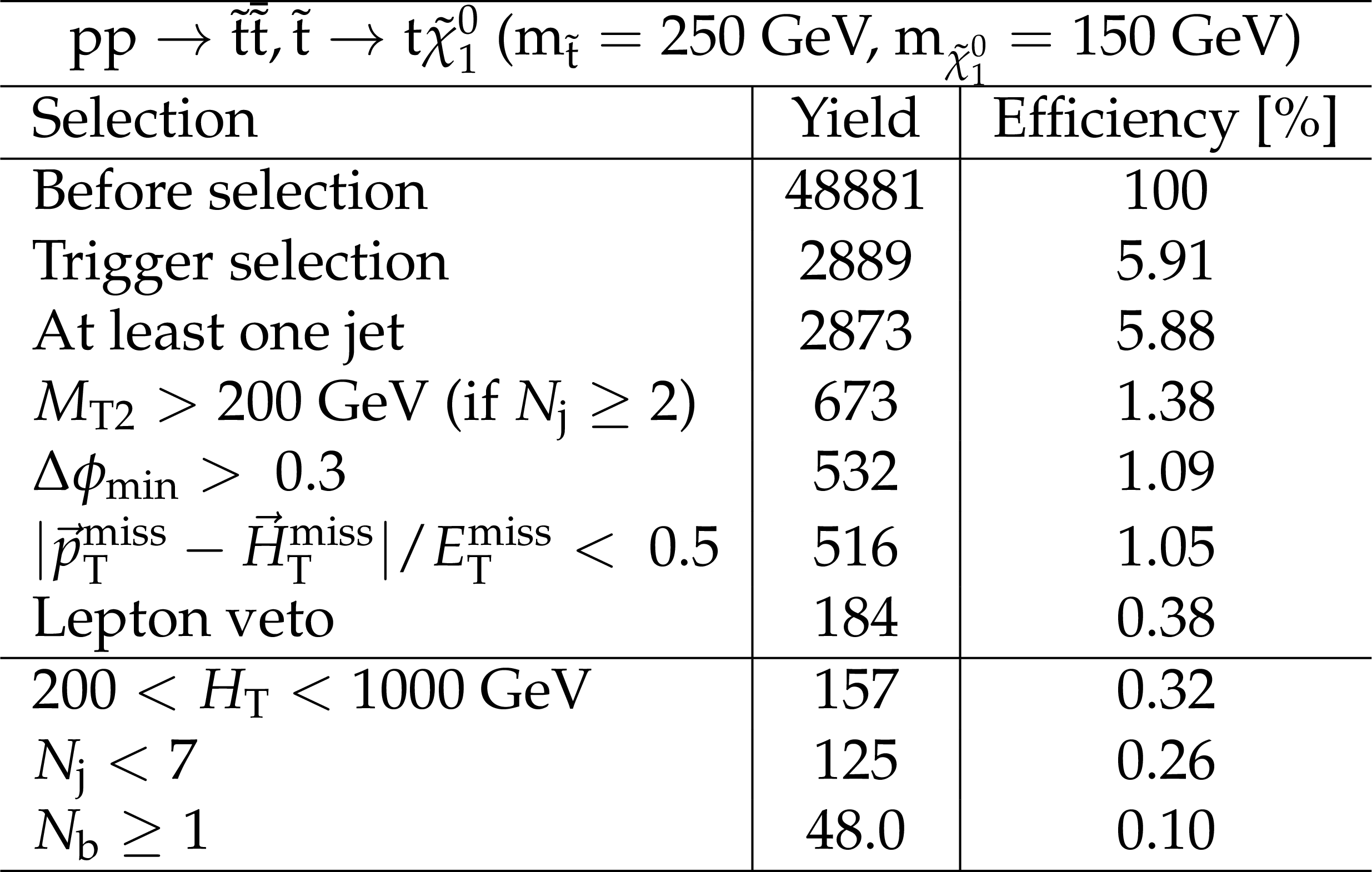
Additional Table 9:
Cut flow table, for a signal model of direct top squark production with the mass of the squark and the LSP equal to 250 and 150 GeV, respectively. Theory cross section for this signal is 21.6 pb. |

png pdf |
Additional Table 10:
Cut flow table, for a signal model of direct bottom squark production with the mass of the squark and the LSP equal to 800 and 0 GeV, respectively. Theory cross section for this signal is 0.028 pb. |
png pdf |
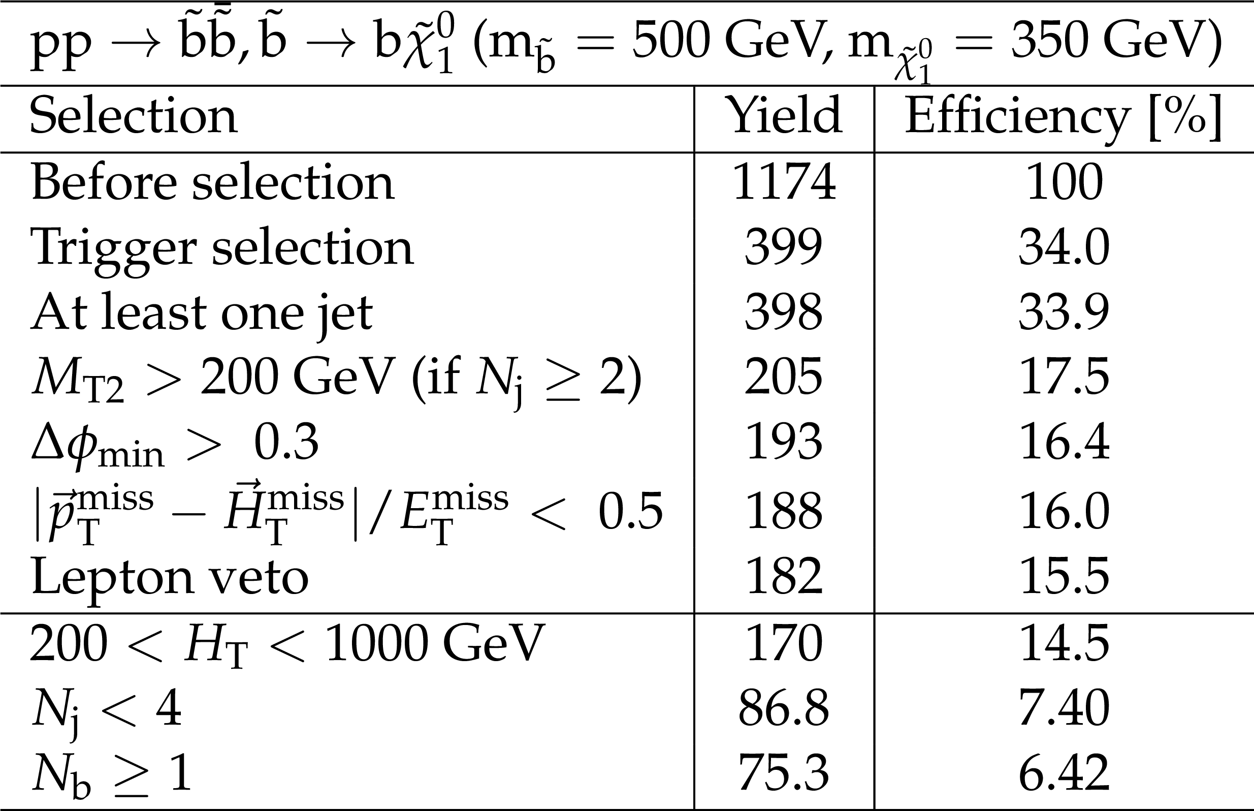
Additional Table 11:
Cut flow table, for a signal model of direct bottom squark production with the mass of the squark and the LSP equal to 500 and 350 GeV, respectively. Theory cross section for this signal is 0.52 pb. |

png pdf |
Additional Table 12:
Cut flow table, for a signal model of direct light squark production with the mass of the squark and the LSP equal to 1200 and 0 GeV, respectively. Theory cross section for this signal is 0.013 pb. |

png pdf |
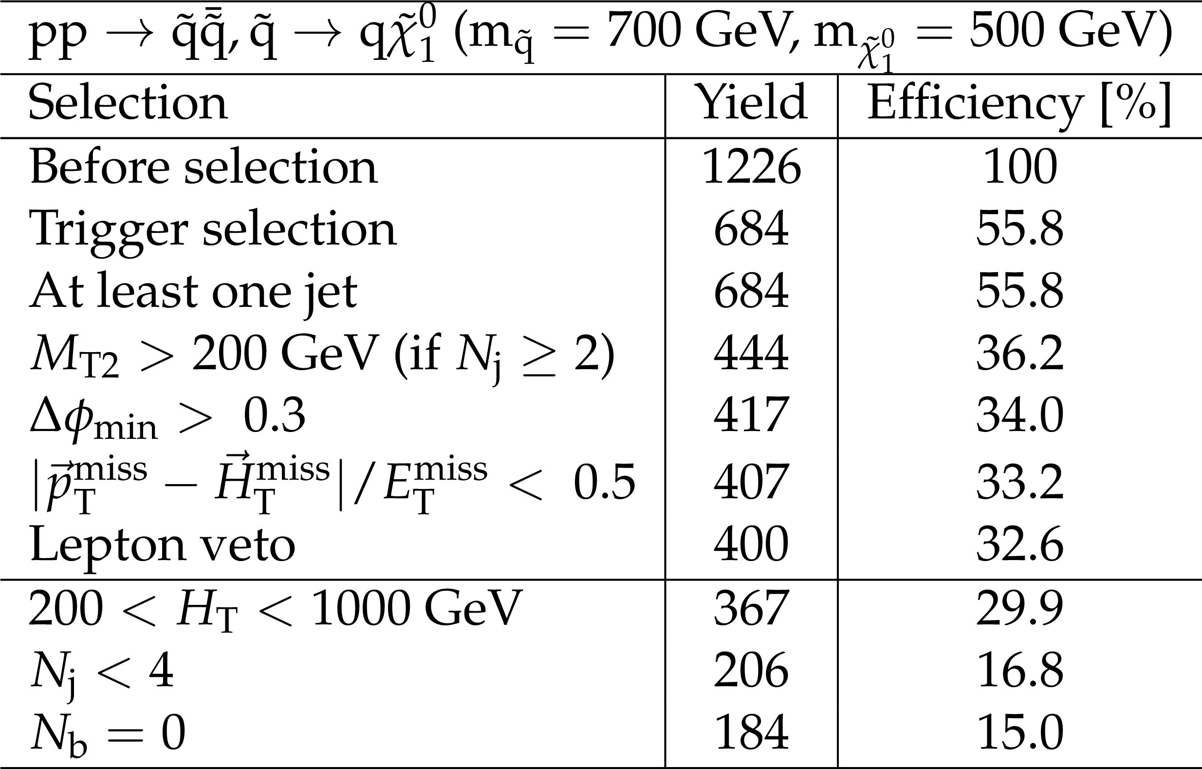
Additional Table 13:
Cut flow table, for a signal model of direct light squark production with the mass of the squark and the LSP equal to 600 and 0 GeV, respectively. Theory cross section for this signal is 1.41 pb. |
png pdf |
Additional Table 14:
Cut flow table, for a signal model of direct light squark production with the mass of the squark and the LSP equal to 700 and 500 GeV, respectively. Theory cross section for this signal is 0.54 pb. |
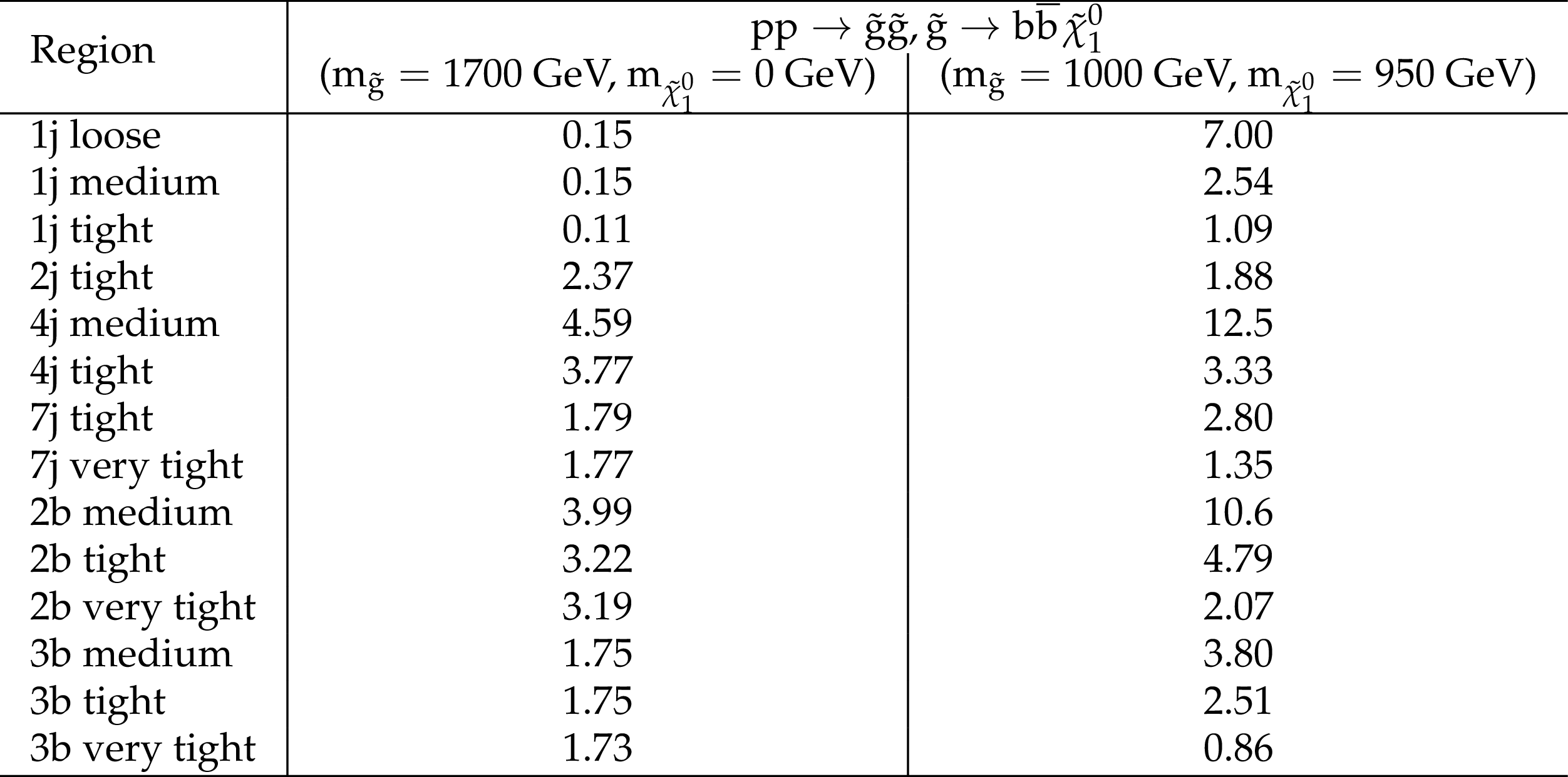
png pdf |
Additional Table 15:
Expected yields in aggregate regions, for a signal model of gluino-mediated bottom squark production. |
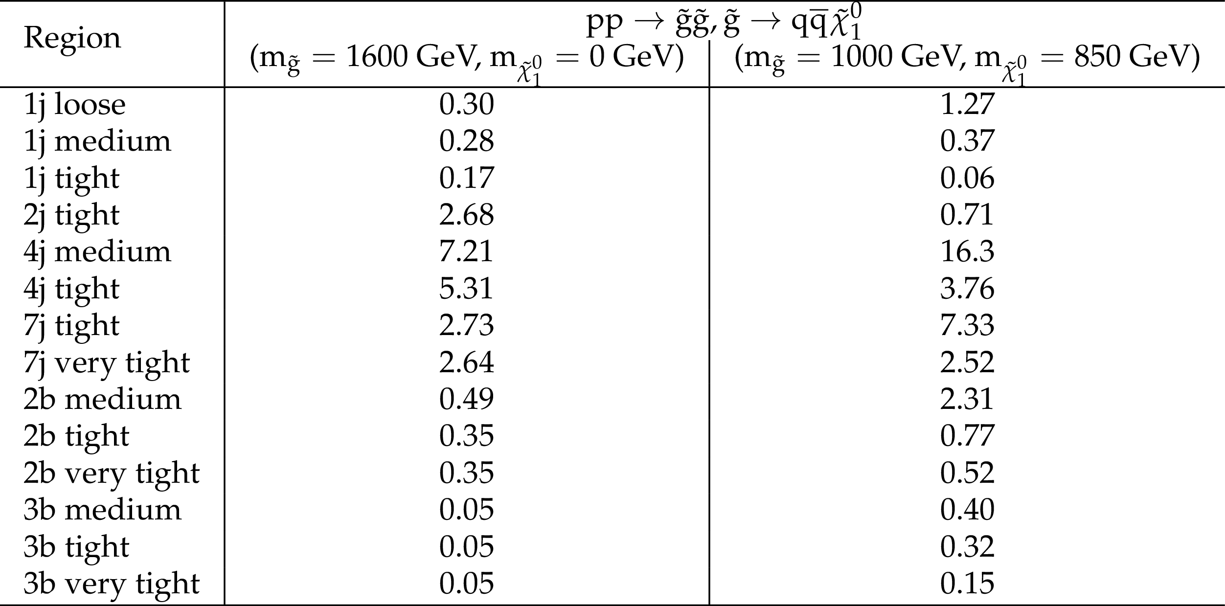
png pdf |
Additional Table 16:
Expected yields in aggregate regions, for a signal model of gluino-mediated light squark production. |
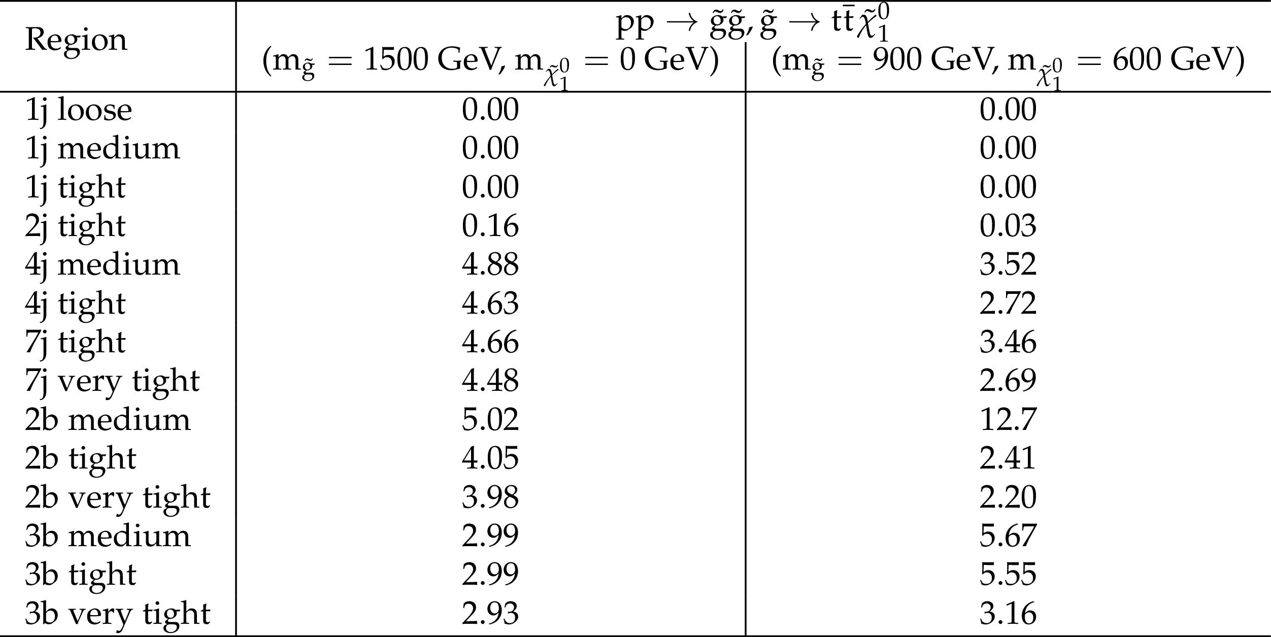
png pdf |
Additional Table 17:
Expected yields in aggregate regions, for a signal model of gluino-mediated top squark production. |
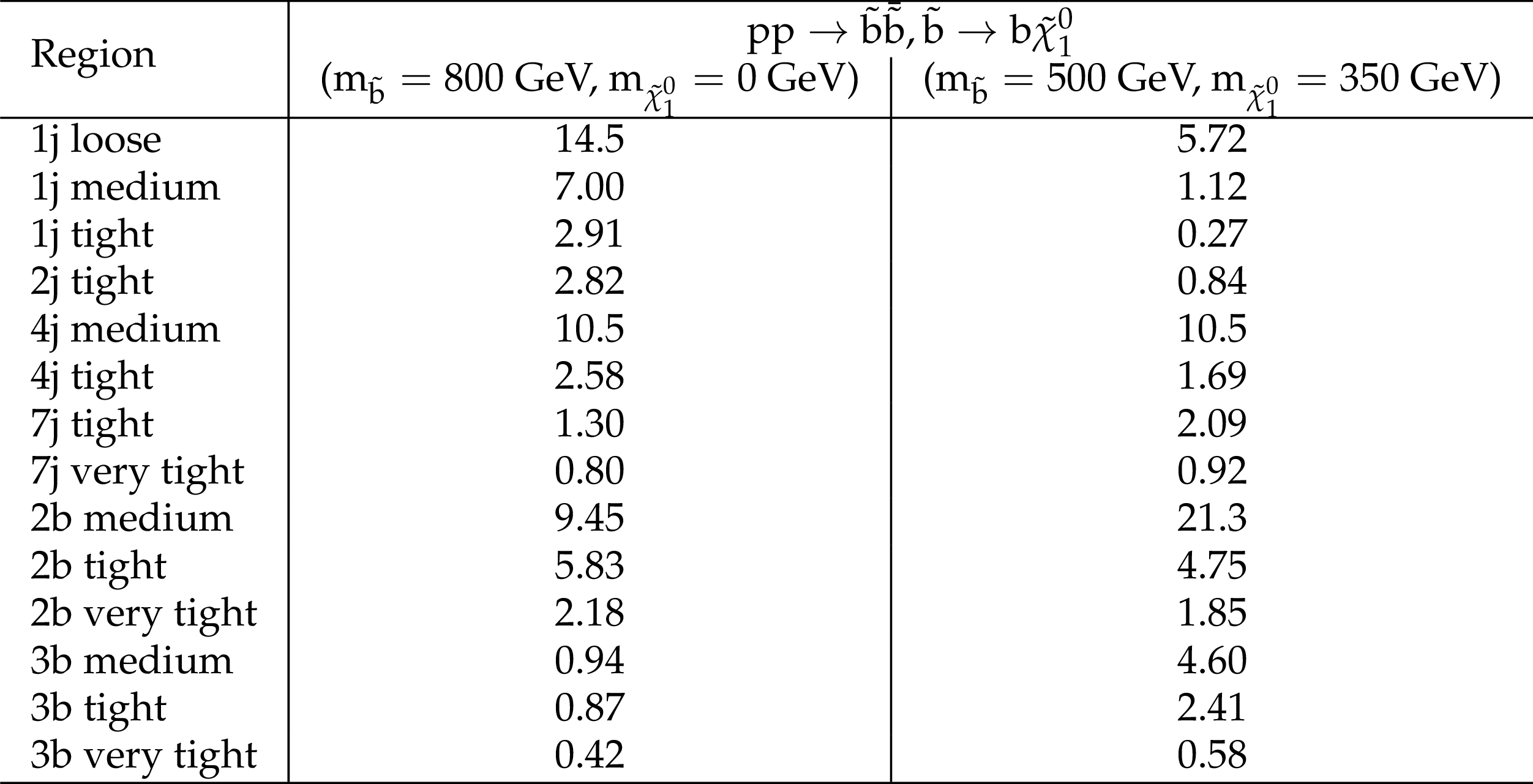
png pdf |
Additional Table 18:
Expected yields in aggregate regions, for a signal model of direct bottom squark production. |
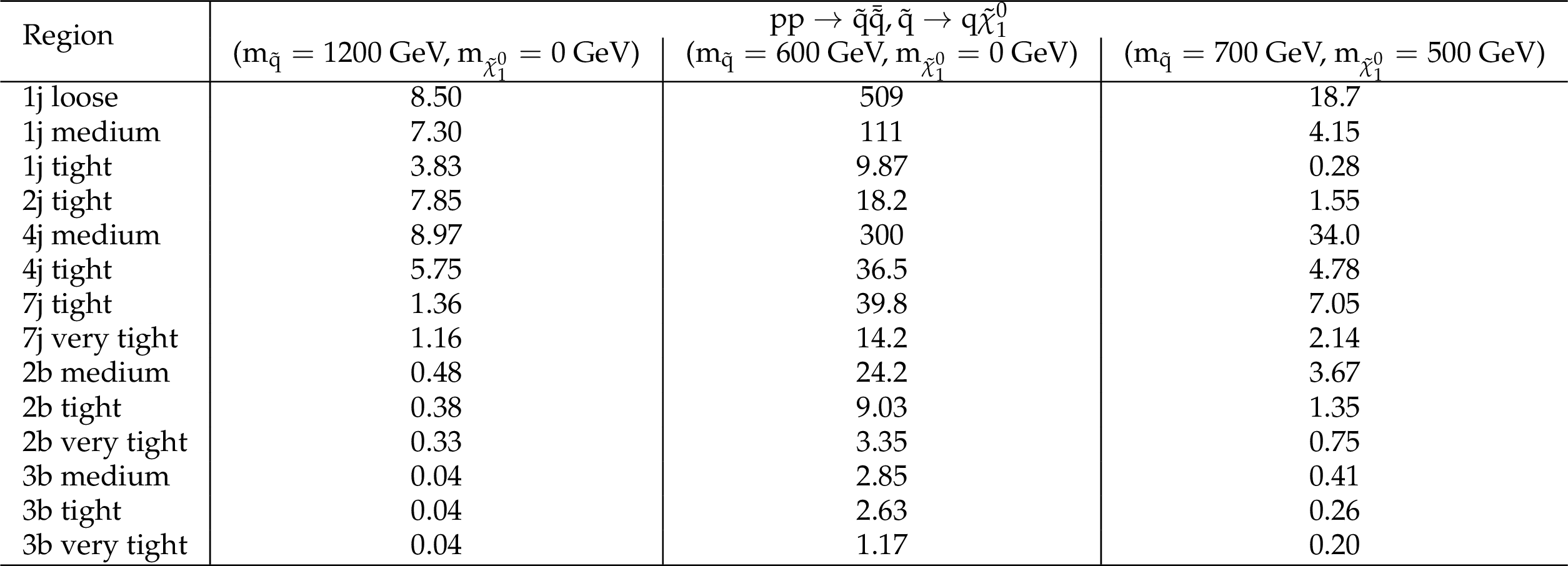
png pdf |
Additional Table 19:
Expected yields in aggregate regions, for a signal model of light squark production. |

png pdf |
Additional Table 20:
Expected yields in aggregate regions, for a signal model of direct top squark production. |

png pdf |
Additional Table 21:
Background estimate and observation in bins of jet ${p_{\mathrm {T}}}$ for the monojet regions. The yields are normalized to 2.3 fb$^{-1}$. |

png pdf |
Additional Table 22:
Background estimate and observation in bins of ${M_{\mathrm {T2}}}$ for 200 $ < H_{\mathrm {T}} < $ 450 GeV. The yields are normalized to 2.3 fb$^{-1}$. |
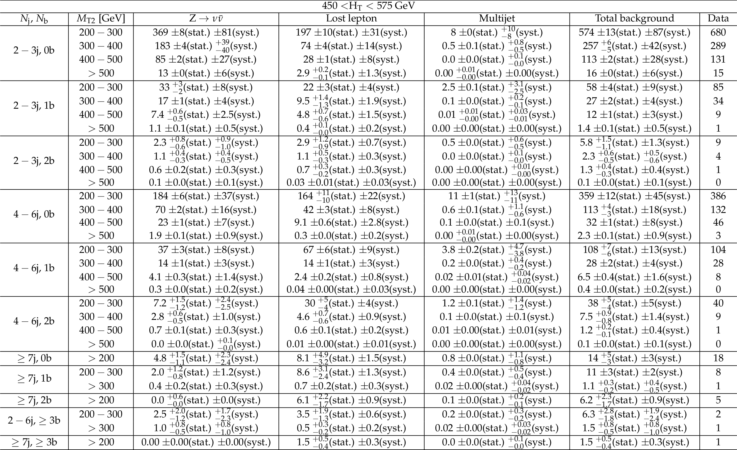
png pdf |
Additional Table 23:
Background estimate and observation in bins of ${M_{\mathrm {T2}}}$ for 450 $ < H_{\mathrm {T}} < $ 575 GeV. The yields are normalized to 2.3 fb$^{-1}$. |
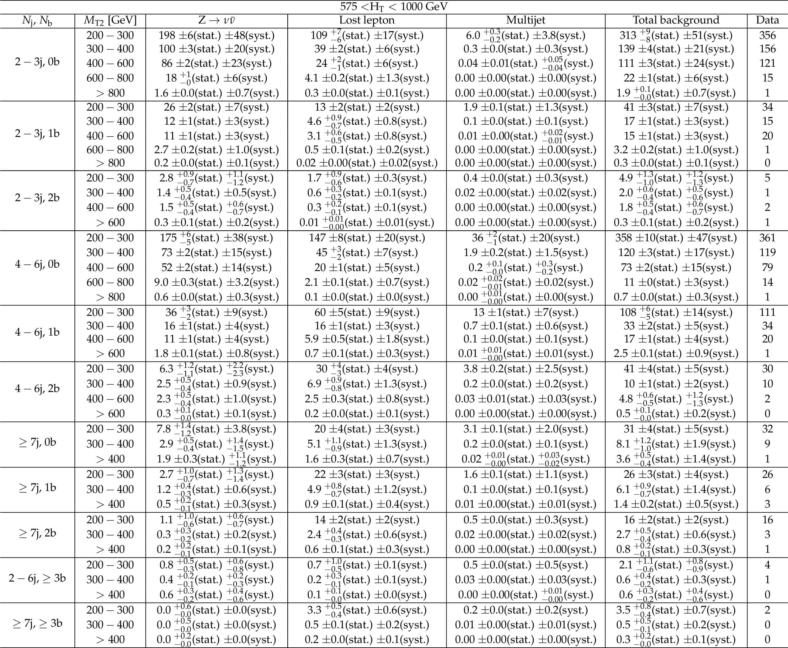
png pdf |
Additional Table 24:
Background estimate and observation in bins of ${M_{\mathrm {T2}}}$ for 575 $ < H_{\mathrm {T}} < $ 1000 GeV. The yields are normalized to 2.3 fb$^{-1}$. |

png pdf |
Additional Table 25:
Background estimate and observation in bins of ${M_{\mathrm {T2}}}$ for 1000 $ < H_{\mathrm {T}} < $ 1500 GeV. The yields are normalized to 2.3 fb$^{-1}$. |

png pdf |
Additional Table 26:
Background estimate and observation in bins of ${M_{\mathrm {T2}}}$ for $H_{\mathrm {T}} > $ 1500 GeV. The yields are normalized to 2.3 fb$^{-1}$. |
| References | ||||
| 1 | P. Ramond | Dual theory for free fermions | PRD 3 (1971) 2415 | |
| 2 | Y. A. Golfand and E. P. Likhtman | Extension of the algebra of Poincar$ \'e $ group generators and violation of P invariance | JEPTL 13 (1971)323 | |
| 3 | A. Neveu and J. H. Schwarz | Factorizable dual model of pions | Nucl. Phys. B 31 (1971) 86 | |
| 4 | D. V. Volkov and V. P. Akulov | Possible universal neutrino interaction | JEPTL 16 (1972)438 | |
| 5 | J. Wess and B. Zumino | A Lagrangian model invariant under supergauge transformations | PLB 49 (1974) 52 | |
| 6 | J. Wess and B. Zumino | Supergauge transformations in four dimensions | Nucl. Phys. B 70 (1974) 39 | |
| 7 | P. Fayet | Supergauge invariant extension of the Higgs mechanism and a model for the electron and its neutrino | Nucl. Phys. B 90 (1975) 104 | |
| 8 | H. P. Nilles | Supersymmetry, supergravity and particle physics | Phys. Rep. 110 (1984) 1 | |
| 9 | CMS Collaboration | Search for supersymmetry in hadronic final states with missing transverse energy using the variables $ \alpha_\mathrm{T} $ and b-quark multiplicity in pp collisions at $ \sqrt{s} = 8 $ TeV | EPJC 73 (2013) 2568 | CMS-SUS-12-028 1303.2985 |
| 10 | CMS Collaboration | Search for gluino mediated bottom- and top-squark production in multijet final states in pp collisions at 8 TeV | PLB 725 (2013) 243 | CMS-SUS-12-024 1305.2390 |
| 11 | CMS Collaboration | Search for new physics in the multijet and missing transverse momentum final state in proton-proton collisions at $ \sqrt{s} = 8 $ TeV | JHEP 06 (2014) 055 | CMS-SUS-13-012 1402.4770 |
| 12 | CMS Collaboration | Search for Supersymmetry using razor variables in events with $ b $-tagged jets in $ pp $ collisions at $ \sqrt{s} = 8 $ TeV | PRD 91 (2015) 052018 | CMS-SUS-13-004 1502.00300 |
| 13 | CMS Collaboration | Searches for supersymmetry using the $ M_{\mathrm{T2}} $ variable in hadronic events produced in pp collisions at 8 TeV | JHEP 05 (2015) 078 | CMS-SUS-13-019 1502.04358 |
| 14 | ATLAS Collaboration | ATLAS Run 1 searches for direct pair production of third-generation squarks at the Large Hadron Collider | EPJC 75 (2015) 510 | 1506.08616 |
| 15 | ATLAS Collaboration | Summary of the searches for squarks and gluinos using $ \sqrt{s} = 8 $ TeV pp collisions with the ATLAS experiment at the LHC | JHEP 10 (2015) 054 | 1507.05525 |
| 16 | ATLAS Collaboration | Search for new phenomena in final states with large jet multiplicities and missing transverse momentum with ATLAS using $ \sqrt{s} = 13 $ TeV proton--proton collisions | Submitted to PLB | 1602.06194 |
| 17 | CMS Collaboration | Search for supersymmetry in the multijet and missing transverse momentum final state in pp collisions at 13 TeV | Submitted to PLB | CMS-SUS-15-002 1602.06581 |
| 18 | C. G. Lester and D. J. Summers | Measuring masses of semiinvisibly decaying particles pair produced at hadron colliders | PLB 463 (1999) 99 | hep-ph/9906349 |
| 19 | A. Barr, C. Lester, and P. Stephens | m(T2): The truth behind the glamour | JPG 29 (2003) 2343 | hep-ph/0304226 |
| 20 | CMS Collaboration | Search for supersymmetry in hadronic final states using $ M_\mathrm{T2} $ in pp collisions at $ \sqrt{s} = 7 $ TeV | JHEP 10 (2012) 018 | CMS-SUS-12-002 1207.1798 |
| 21 | N. Arkani-Hamed et al. | MARMOSET: The path from LHC data to the new standard model via on-shell effective theories | hep-ph/0703088 | |
| 22 | J. Alwall, P. Schuster, and N. Toro | Simplified models for a first characterization of new physics at the LHC | PRD 79 (2009) 075020 | 0810.3921 |
| 23 | J. Alwall, M.-P. Le, M. Lisanti, and J. G. Wacker | Model-independent jets plus missing energy searches | PRD 79 (2009) 015005 | 0809.3264 |
| 24 | D. Alves et al. | Simplified models for LHC new physics searches | JPG 39 (2012) 105005 | 1105.2838 |
| 25 | CMS Collaboration | Interpretation of searches for supersymmetry with simplified models | PRD 88 (2013) 052017 | CMS-SUS-11-016 1301.2175 |
| 26 | CMS Collaboration | The CMS experiment at the CERN LHC | JINST 3 (2008) S08004 | CMS-00-001 |
| 27 | J. Alwall et al. | MadGraph 5: going beyond | JHEP 06 (2011) 128 | 1106.0522 |
| 28 | T. Sj\"ostrand, S. Mrenna, and P. Z. Skands | A brief introduction to PYTHIA 8.1 | CPC 178 (2008) 852 | 0710.3820 |
| 29 | J. Alwall et al. | The automated computation of tree-level and next-to-leading order differential cross sections, and their matching to parton shower simulations | JHEP 07 (2014) 079 | 1405.0301 |
| 30 | S. Alioli, P. Nason, C. Oleari, and E. Re | NLO single-top production matched with shower in POWHEG: $ s $- and $ t $-channel contributions | JHEP 09 (2009) 111, , [Erratum: \DOI10.1007/JHEP02(2010)011] | 0907.4076 |
| 31 | E. Re | Single-top Wt-channel production matched with parton showers using the POWHEG method | EPJC 71 (2011) 1547 | 1009.2450 |
| 32 | R. Gavin, Y. Li, F. Petriello, and S. Quackenbush | FEWZ 2.0: A code for hadronic Z production at next-to-next-to-leading order | CPC 182 (2011) 2388 | 1011.3540 |
| 33 | R. Gavin, Y. Li, F. Petriello, and S. Quackenbush | W Physics at the LHC with FEWZ 2.1 | CPC 184 (2013) 208 | 1201.5896 |
| 34 | M. Czakon and A. Mitov | Top++: A program for the calculation of the top-pair cross-section at hadron colliders | CPC 185 (2014) 2930 | 1112.5675 |
| 35 | C. Borschensky et al. | Squark and gluino production cross sections in $ pp $ collisions at $ \sqrt{s} = 13 $, 14, 33 and 100 TeV | EPJC 74 (2014) 3174 | 1407.5066 |
| 36 | NNPDF Collaboration | Parton distributions for the LHC Run II | JHEP 04 (2015) 040 | 1410.8849 |
| 37 | GEANT4 Collaboration | GEANT4---a simulation toolkit | NIMA 506 (2003) 250 | |
| 38 | S. Abdullin et al. | The fast simulation of the CMS detector at LHC | J. Phys. Conf. Ser. 331 (2011) 032049 | |
| 39 | CMS Collaboration | Particle--flow event reconstruction in CMS and performance for jets, taus, and $ E_{\mathrm{T}}^{\text{miss}} $ | CDS | |
| 40 | CMS Collaboration | Commissioning of the particle-flow event reconstruction with the first LHC collisions recorded in the CMS detector | CDS | |
| 41 | M. Cacciari, G. P. Salam, and G. Soyez | The anti-k$ _\mathrm{t} $ jet clustering algorithm | JHEP 04 (2008) 063 | 0802.1189 |
| 42 | CMS Collaboration | Determination of jet energy calibration and transverse momentum resolution in CMS | JINST 6 (2011) P11002 | CMS-JME-10-011 1107.4277 |
| 43 | CMS Collaboration | Performance of b-tagging algorithms in 25 ns data at 13 TeV | CDS | |
| 44 | CMS Collaboration | Jet performance in pp collisions at $ \sqrt{s} = 7 $ TeV | CDS | |
| 45 | CMS Collaboration | Performance of electron reconstruction and selection with the CMS detector in proton-proton collisions at $ \sqrt{s} = 8 $~TeV | JINST 10 (2015) P06005 | CMS-EGM-13-001 1502.02701 |
| 46 | CMS Collaboration | Performance of CMS muon reconstruction in pp collision events at $ \sqrt{s} = 7 $ TeV | JINST 7 (2012) P10002 | CMS-MUO-10-004 1206.4071 |
| 47 | CMS Collaboration | Study of pileup removal algorithms for jets | CMS-PAS-JME-14-001 | CMS-PAS-JME-14-001 |
| 48 | CMS Collaboration | Performance of photon reconstruction and identification with the CMS detector in proton-proton collisions at $ \sqrt{s} = 8 $~TeV | JINST 10 (2015) P08010 | CMS-EGM-14-001 1502.02702 |
| 49 | T. Sj\"ostrand | The Lund Monte Carlo for e$ ^{+} $e$ ^{-} $ jet physics | CPC 28 (1983) 229 | |
| 50 | T. Sj\"ostrand, S. Mrenna, and P. Skands | PYTHIA 6.4 physics and manual | JHEP 05 (2006) 026 | hep-ph/0603175 |
| 51 | UA1 Collaboration | Experimental observation of isolated large transverse energy electrons with associated missing energy at $ \sqrt{s} = 540 $ GeV | PLB 122 (1983) 103 | |
| 52 | CMS Collaboration | Missing transverse energy performance of the CMS detector | JINST 6 (2011) P09001 | CMS-JME-10-009 1106.5048 |
| 53 | J. Butterworth et al. | PDF4LHC recommendations for LHC Run II | JPG 43 (2016) 023001 | 1510.03865 |
| 54 | CMS Collaboration | Search for new physics with same-sign isolated dilepton events with jets and missing transverse energy at the LHC | JHEP 06 (2011) 077 | CMS-SUS-10-004 1104.3168 |
| 55 | CMS Collaboration | Search for new physics with jets and missing transverse momentum in pp collisions at $ \sqrt{s} = 7 $ TeV | JHEP 08 (2011) 155 | CMS-SUS-10-005 1106.4503 |
| 56 | A. L. Read | Presentation of search results: The CL$ _\mathrm{s} $ technique | JPG 28 (2002) 2693 | |
| 57 | T. Junk | Confidence level computation for combining searches with small statistics | NIMA 434 (1999) 435 | hep-ex/9902006 |
| 58 | G. Cowan, K. Cranmer, E. Gross, and O. Vitells | Asymptotic formulae for likelihood-based tests of new physics | EPJC 71 (2011) 1554 | 1007.1727 |
| 59 | ATLAS and CMS Collaborations | Procedure for the LHC Higgs boson search combination in summer 2011 | CMS-NOTE-2011-005 | |
| 60 | CMS Collaboration | Search for top-squark pair production in the single-lepton final state in pp collisions at $ \sqrt{s} = 8 $ TeV | EPJC 73 (2013) 2677 | CMS-SUS-13-011 1308.1586 |
| 61 | W. Beenakker, R. H\"opker, M. Spira, and P. M. Zerwas | Squark and gluino production at hadron colliders | Nucl. Phys. B 492 (1997) 51 | hep-ph/9610490 |
| 62 | A. Kulesza and L. Motyka | Threshold resummation for squark-antisquark and gluino-pair production at the LHC | PRL 102 (2009) 111802 | 0807.2405 |
| 63 | A. Kulesza and L. Motyka | Soft gluon resummation for the production of gluino-gluino and squark-antisquark pairs at the LHC | PRD 80 (2009) 095004 | 0905.4749 |
| 64 | W. Beenakker et al. | Soft-gluon resummation for squark and gluino hadroproduction | JHEP 12 (2009) 041 | 0909.4418 |
| 65 | W. Beenakker et al. | Squark and gluino hadroproduction | Int. J. Mod. Phys. A 26 (2011) 2637 | 1105.1110 |
|
|
Compact Muon Solenoid LHC, CERN |
|

|

|

|

|

|