

Compact Muon Solenoid
LHC, CERN
| CMS-PAS-TOP-15-008 | ||
| Measurement of the top-quark mass in the dileptonic $\mathrm{ t \bar{t} }$ decay channel using the $M_{\mathrm{b}\ell}$, $M_{\mathrm{T}2}$, and $M_{\mathrm{b}\ell\nu}$ observables | ||
| CMS Collaboration | ||
| August 2016 | ||
| Abstract: We report on a measurement of the top-quark mass ($M_{\mathrm{t}}$) in the dileptonic $\mathrm{t}\overline{\mathrm{t}}$ decay channel using events selected from a data sample corresponding to an integrated luminosity of 19.7 $\pm$ 0.5 fb$^{-1}$. The events were recorded by the CMS detector at the LHC in proton-proton collisions at $\sqrt{s} =$ 8 TeV. The analysis is based on three observables whose distribution shapes are sensitive to the value of $M_{\mathrm{t}}$. The $M_{\mathrm{b}\ell}$ invariant mass and $M_{\mathrm{T}2}^{\mathrm{bb}}$ `stransverse mass' observables are employed in a simultaneous fit to determine the value of $M_{\mathrm{t}}$ and an overall jet energy scale factor (JSF). In a complementary approach, the $M_{\mathrm{T}2}$-Assisted On-Shell reconstruction technique is used to construct an $M_{\mathrm{b}\ell\nu}$ invariant mass observable that is combined with $M_{\mathrm{T}2}^{\mathrm{bb}}$ to measure $M_{\mathrm{t}}$. The shapes of the observables, along with their evolutions in $M_{\mathrm{t}}$ and JSF, are modeled by a non-parametric Gaussian Process regression technique. The top-quark mass is measured to be 172.22 $\pm$ 0.18 (stat) $^{+0.89}_{-0.93}$ (syst) GeV. | ||
|
Links:
CDS record (PDF) ;
inSPIRE record ;
CADI line (restricted) ;
These preliminary results are superseded in this paper, PRD 96 (2017) 032002. The superseded preliminary plots can be found here. |
||
| Figures | |
png pdf |
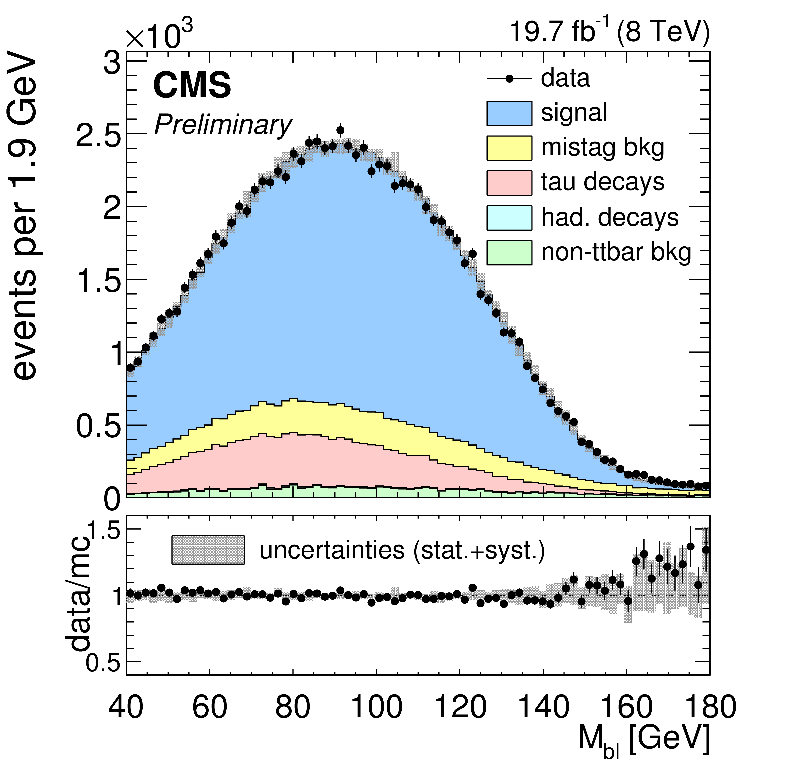
Figure 1-a:
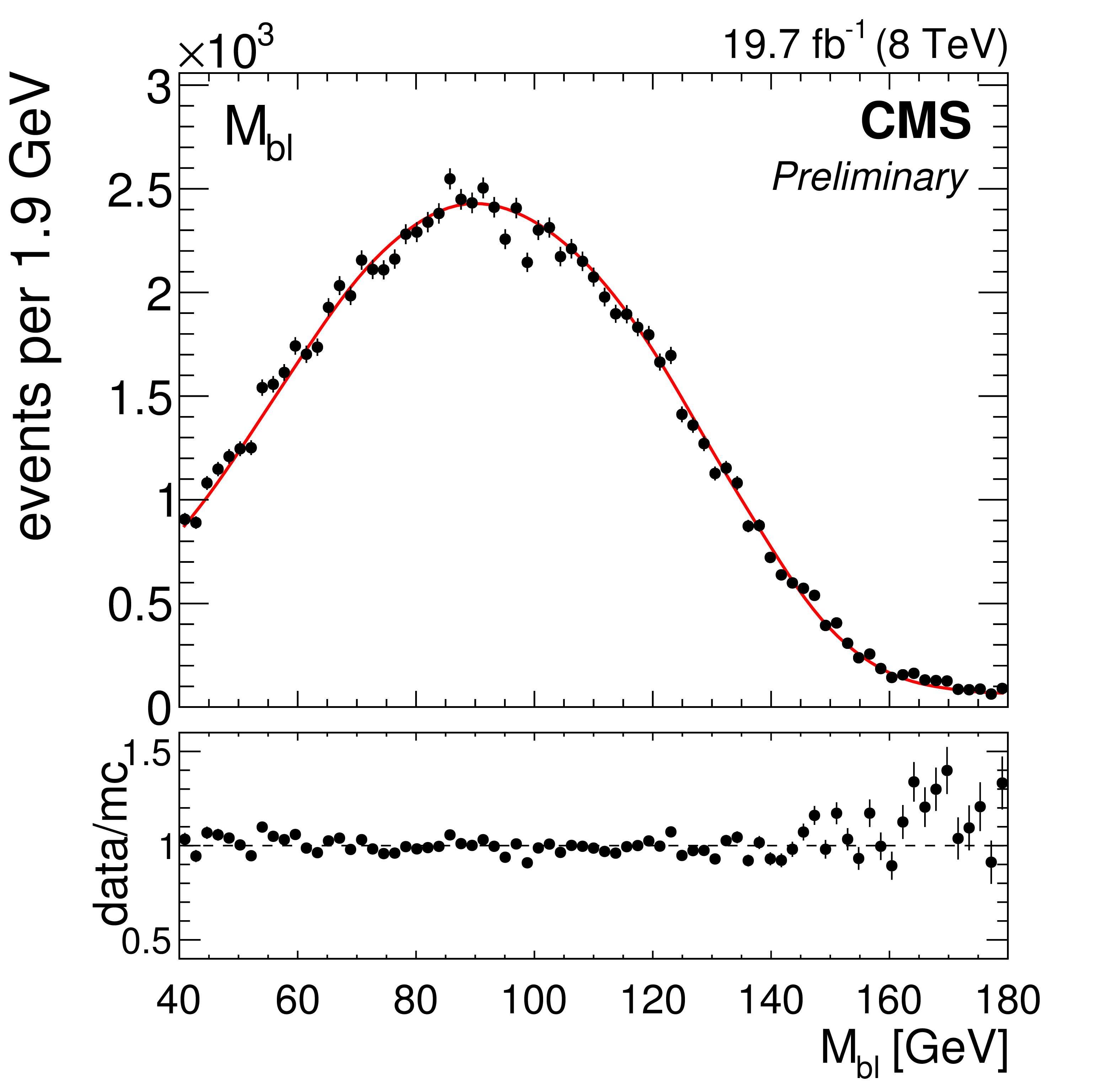
(a) the ${\mathrm {M}_{\mathrm {b}\ell }}$ distribution in data and simulation with $ {\mathrm {M}_{\mathrm {t}}^{\text {MC}}}= $ 172.5 GeV, normalized to the number of events in the 8 TeV dataset corresponding to an integrated luminosity of 19.7 $\pm$ 0.5 fb$^{-1}$. Statistical and systematic uncertainties on the distribution in simulation are represented by the grey shaded area. A description of the systematic uncertainties is given in Section 8. (b) the ${\mathrm {M}_{\mathrm {b}\ell }}$ distribution shapes in simulation corresponding to three values of ${\mathrm {M}_{\mathrm {t}}^{\text {MC}}}$ are shown in grey. The `local shape sensitivity' function, described in Appendix A, is shown in red. |
png pdf |
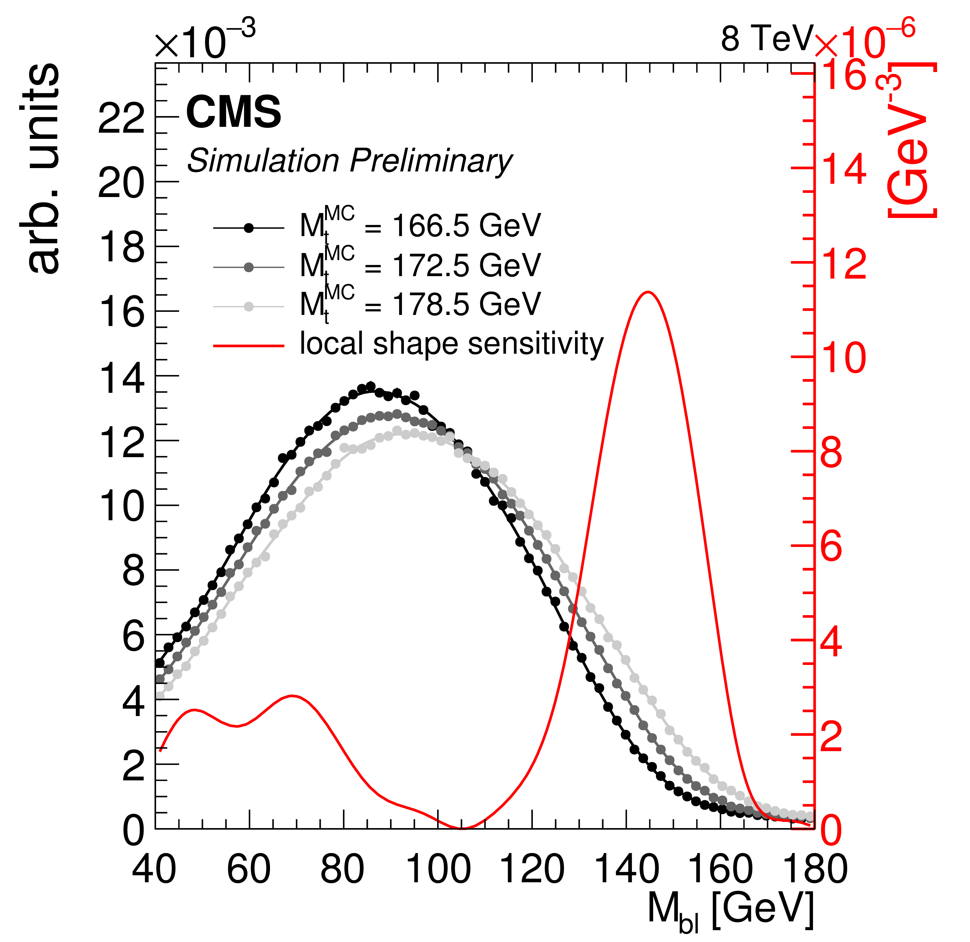
Figure 1-b:
(a) the ${\mathrm {M}_{\mathrm {b}\ell }}$ distribution in data and simulation with $ {\mathrm {M}_{\mathrm {t}}^{\text {MC}}}= $ 172.5 GeV, normalized to the number of events in the 8 TeV dataset corresponding to an integrated luminosity of 19.7 $\pm$ 0.5 fb$^{-1}$. Statistical and systematic uncertainties on the distribution in simulation are represented by the grey shaded area. A description of the systematic uncertainties is given in Section 8. (b) the ${\mathrm {M}_{\mathrm {b}\ell }}$ distribution shapes in simulation corresponding to three values of ${\mathrm {M}_{\mathrm {t}}^{\text {MC}}}$ are shown in grey. The `local shape sensitivity' function, described in Appendix A, is shown in red. |
png pdf |
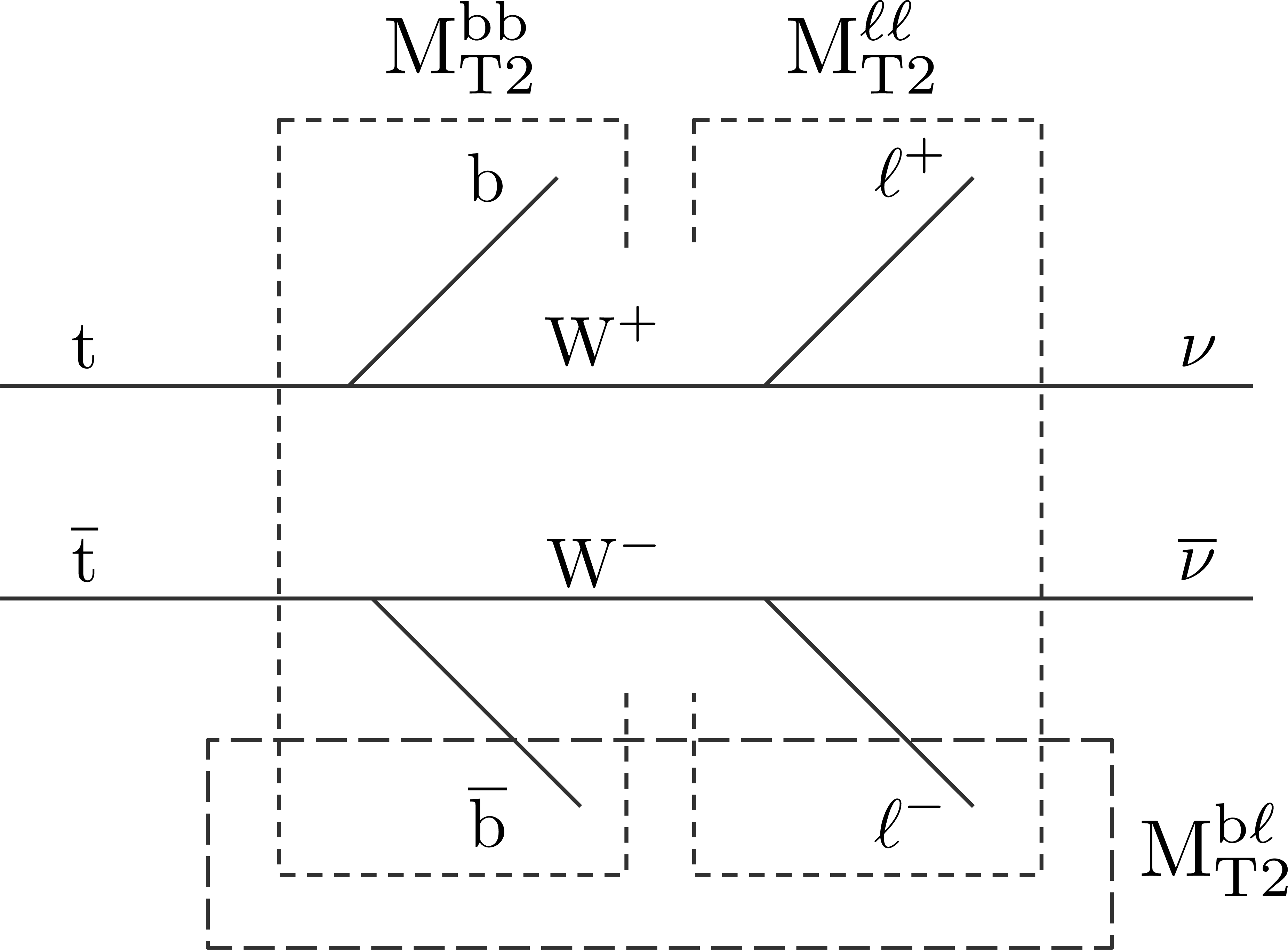
Figure 2:
${\mathrm {M}_{\mathrm {T}2}}$ subsystems in the dileptonic ${\mathrm {t}\overline {\mathrm {t}}} $ event topology. |
png pdf |
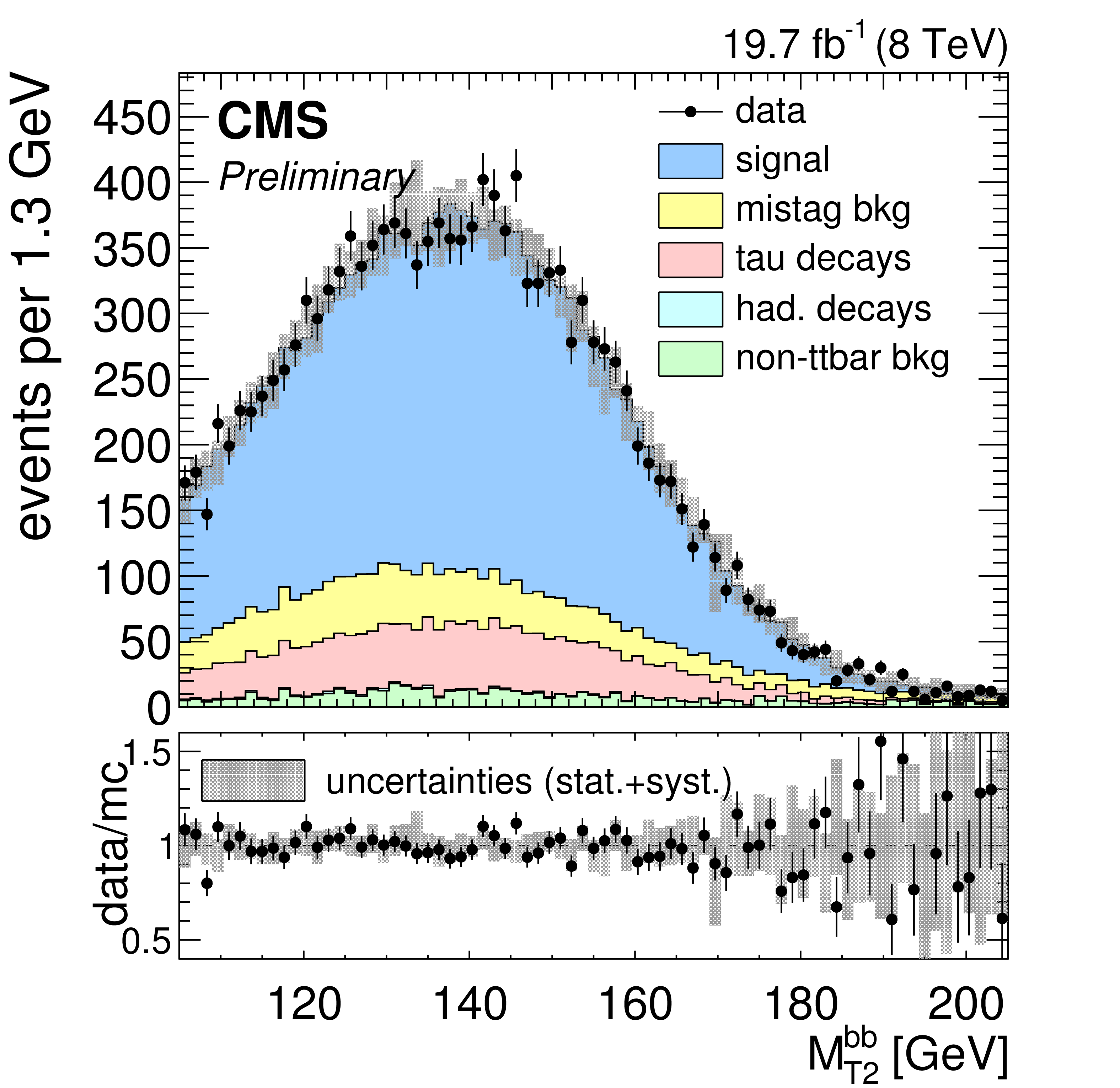
Figure 3-a:
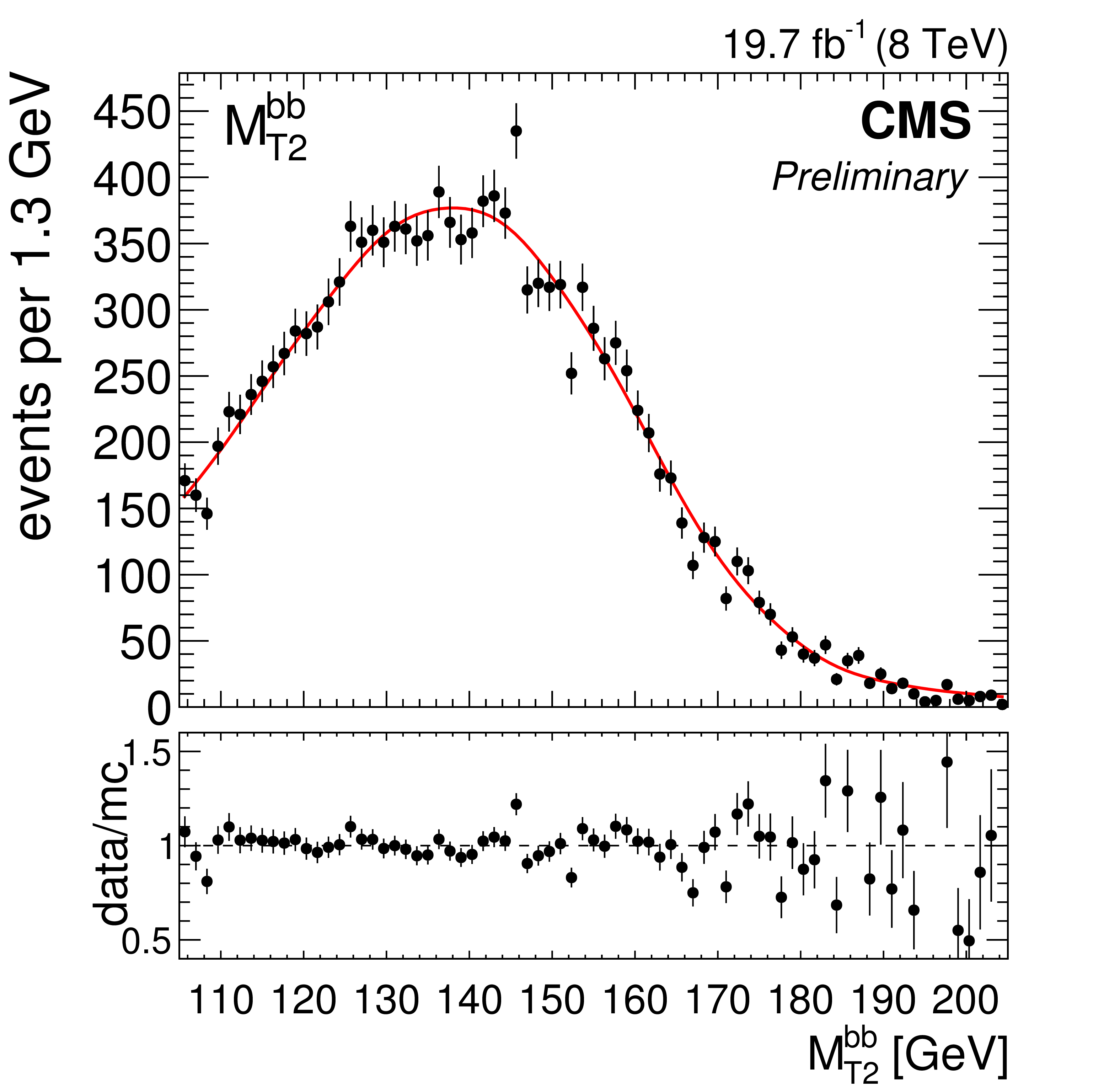
(a) the ${\mathrm {M}_{\mathrm {T}2}^{\mathrm {bb}}}$ distribution in data and simulation with $ {\mathrm {M}_{\mathrm {t}}^{\text {MC}}}=$ 172.5 GeV, normalized to the number of events in the 8 TeV dataset corresponding to an integrated luminosity of 19.7 $\pm$ 0.5 fb$^{-1}$. Statistical and systematic uncertainties on the distribution in simulation are represented by the grey shaded area. (b) the ${\mathrm {M}_{\mathrm {T}2}^{\mathrm {bb}}}$ distribution shapes in simulation corresponding to three values of ${\mathrm {M}_{\mathrm {t}}^{\text {MC}}}$ are shown in grey. The `local shape sensitivity' function is shown in red. |

png pdf |
Figure 3-b:
(a) the ${\mathrm {M}_{\mathrm {T}2}^{\mathrm {bb}}}$ distribution in data and simulation with $ {\mathrm {M}_{\mathrm {t}}^{\text {MC}}}=$ 172.5 GeV, normalized to the number of events in the 8 TeV dataset corresponding to an integrated luminosity of 19.7 $\pm$ 0.5 fb$^{-1}$. Statistical and systematic uncertainties on the distribution in simulation are represented by the grey shaded area. (b) the ${\mathrm {M}_{\mathrm {T}2}^{\mathrm {bb}}}$ distribution shapes in simulation corresponding to three values of ${\mathrm {M}_{\mathrm {t}}^{\text {MC}}}$ are shown in grey. The `local shape sensitivity' function is shown in red. |

png pdf |
Figure 4-a:
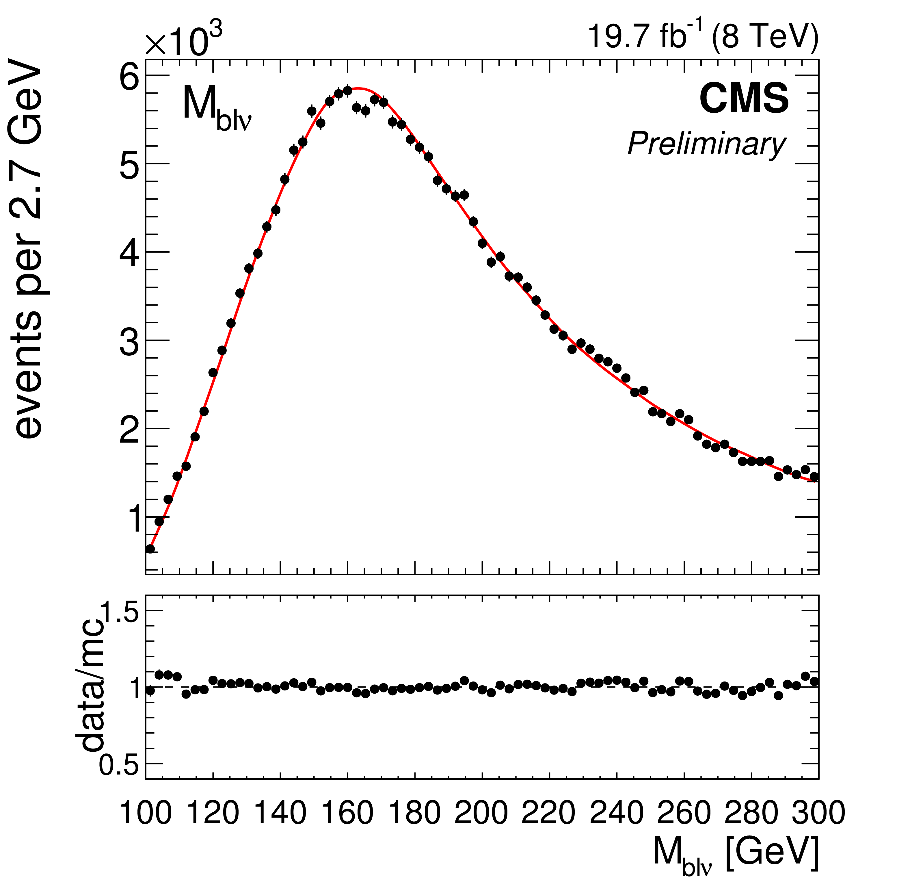
(a) the MAOS ${\mathrm {M}_{\mathrm {b}\ell \nu }}$ distribution in data and simulation with $ {\mathrm {M}_{\mathrm {t}}^{\text {MC}}}=$ 172.5 GeV, normalized to the number of events in the 8 TeV dataset corresponding to an integrated luminosity of 19.7 $\pm$ 0.5 fb$^{-1}$. Statistical and systematic uncertainties on the distribution in simulation are represented by the grey shaded area. (b) the MAOS ${\mathrm {M}_{\mathrm {b}\ell \nu }}$ distribution shapes in simulation corresponding to three values of ${\mathrm {M}_{\mathrm {t}}^{\text {MC}}}$ are shown in grey. The `local shape sensitivity' function is shown in red. |

png pdf |
Figure 4-b:
(a) the MAOS ${\mathrm {M}_{\mathrm {b}\ell \nu }}$ distribution in data and simulation with $ {\mathrm {M}_{\mathrm {t}}^{\text {MC}}}=$ 172.5 GeV, normalized to the number of events in the 8 TeV dataset corresponding to an integrated luminosity of 19.7 $\pm$ 0.5 fb$^{-1}$. Statistical and systematic uncertainties on the distribution in simulation are represented by the grey shaded area. (b) the MAOS ${\mathrm {M}_{\mathrm {b}\ell \nu }}$ distribution shapes in simulation corresponding to three values of ${\mathrm {M}_{\mathrm {t}}^{\text {MC}}}$ are shown in grey. The `local shape sensitivity' function is shown in red. |
png pdf |
Figure 5-a:
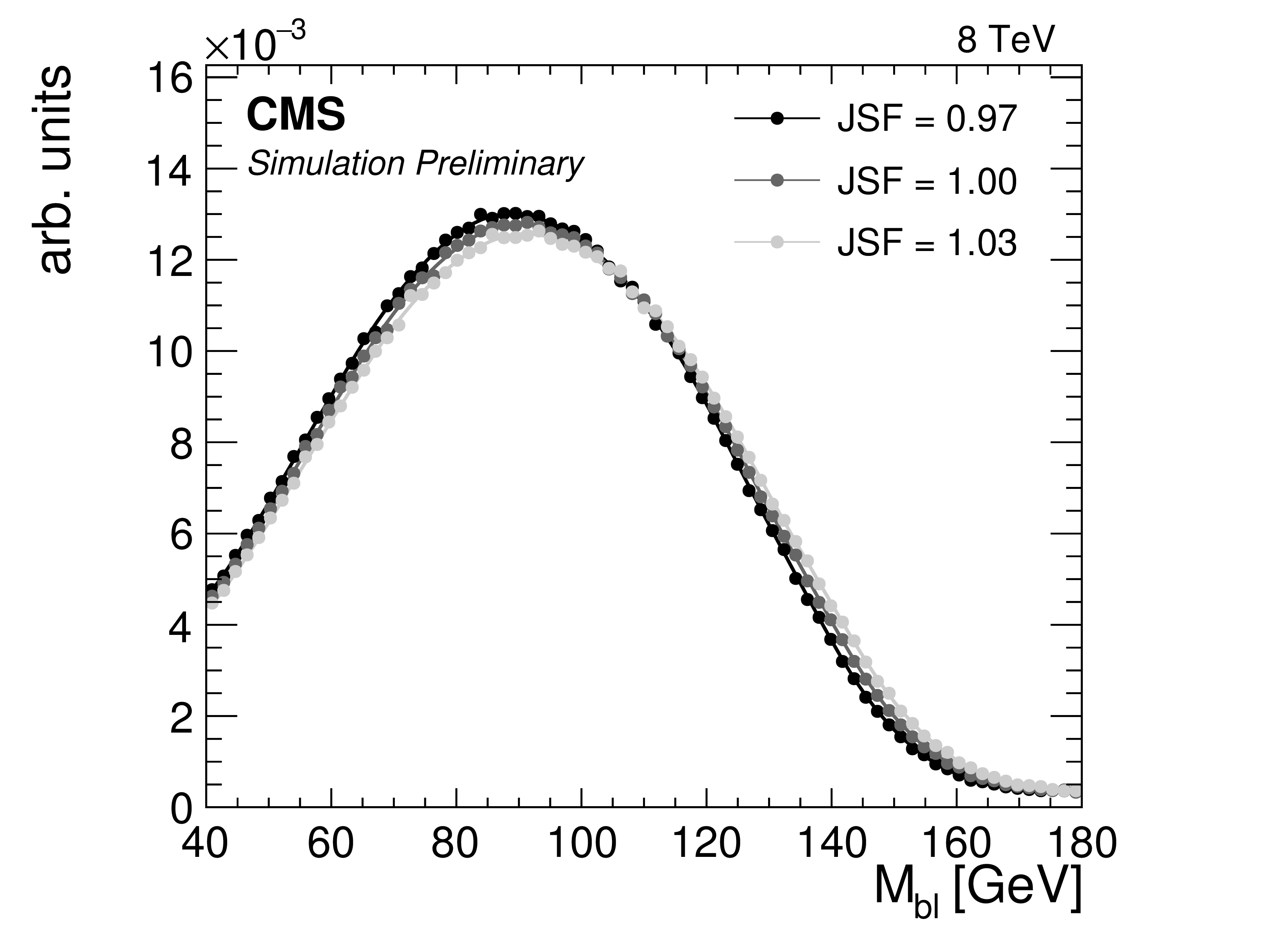
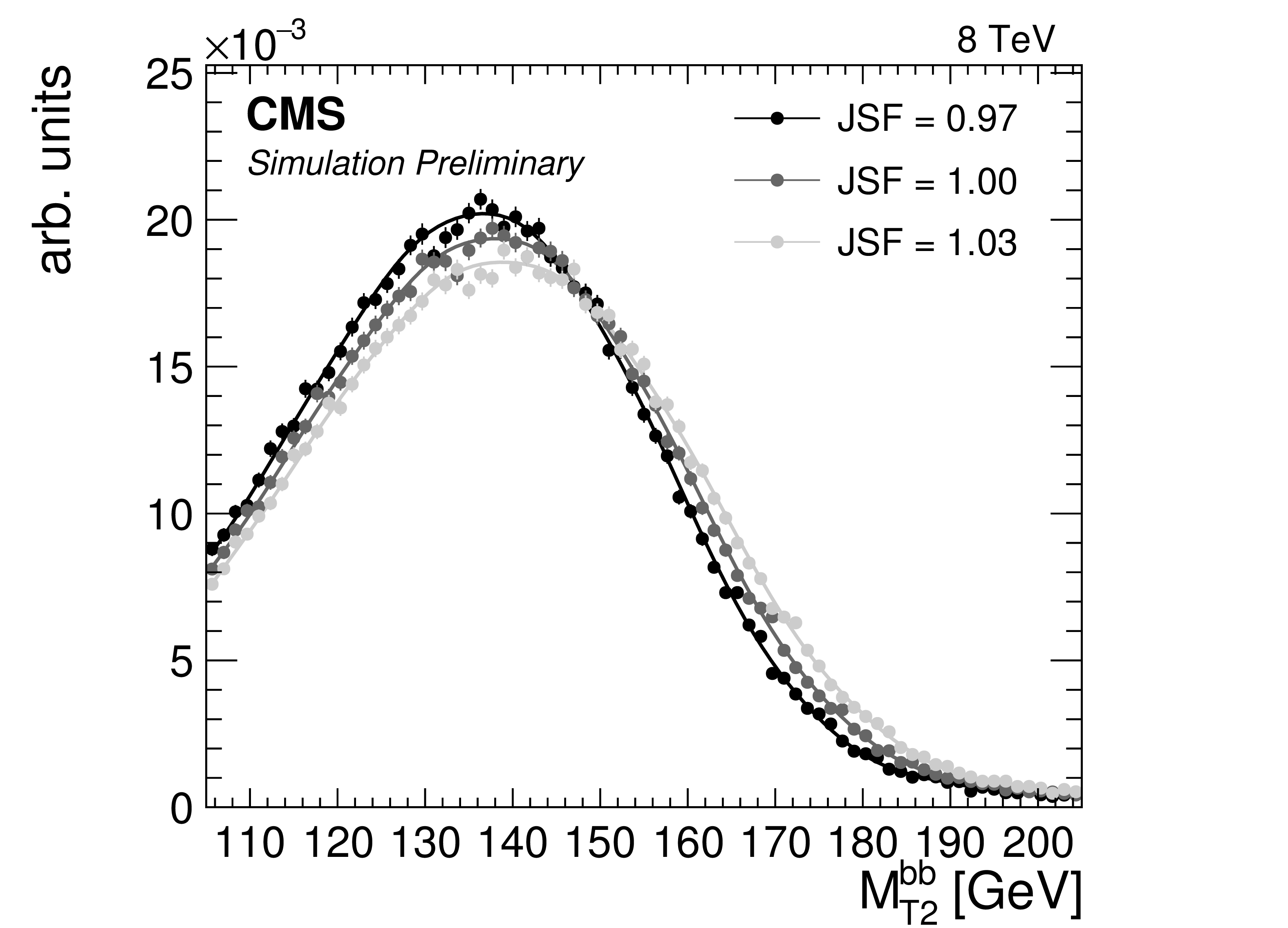
The (left) ${\mathrm {M}_{\mathrm {b}\ell }}$ and (right) ${\mathrm {M}_{\mathrm {T}2}^{\mathrm {bb}}}$ distributions in MC with $ {\mathrm {M}_{\mathrm {t}}}= 172.5$ GeV for several values of JSF. |
png pdf |
Figure 5-b:
The (left) ${\mathrm {M}_{\mathrm {b}\ell }}$ and (right) ${\mathrm {M}_{\mathrm {T}2}^{\mathrm {bb}}}$ distributions in MC with $ {\mathrm {M}_{\mathrm {t}}}= 172.5$ GeV for several values of JSF. |
png pdf |
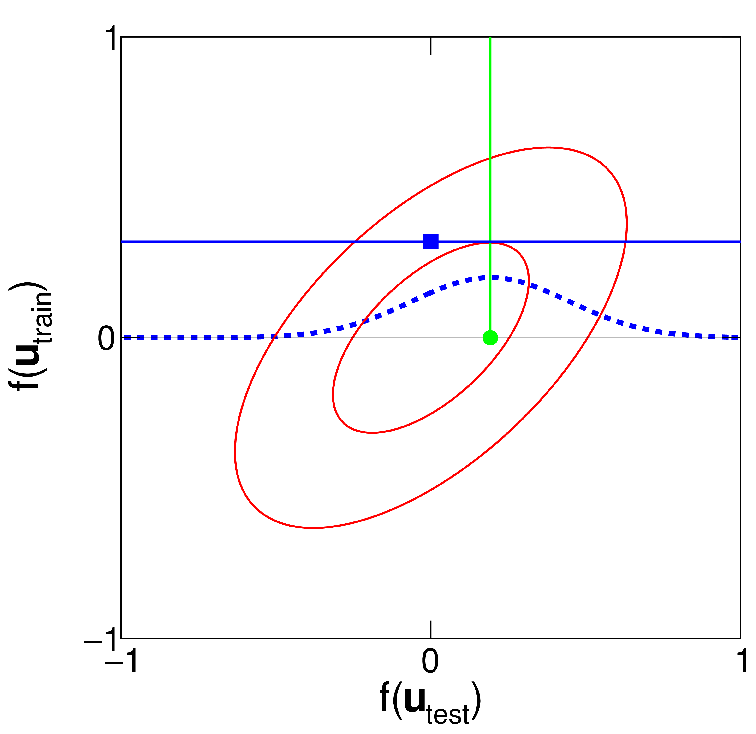
Figure 6:
Demonstration of the GP conditioning process (Eqs. (9) et (10)) for one training point and one test point. The covariance between the value of the shape at the training and test point is represented by the red ellipse. The known value of the shape at the training point (blue square) determines the mean value of the shape at the test point (green circle). |

png pdf |
Figure 7-a:
Likelihood fit results using 50 pseudo-experiments in MC simulation, with values of ${\mathrm {M}_{\mathrm {t}}^{\text {MC}}}$ ranging from 166.5 to 178.5 GeV. A calibration curve of the form $y=ax + b$ is determined for each fit configuration. Measured values of (a) ${\mathrm {M}_{\mathrm {t}}}$ and (b) JSF are shown for the 2D fit, and measured values of ${\mathrm {M}_{\mathrm {t}}}$ are shown for the (c) 1D, (d) MAOS, and (e) hybrid fits. |
png pdf |
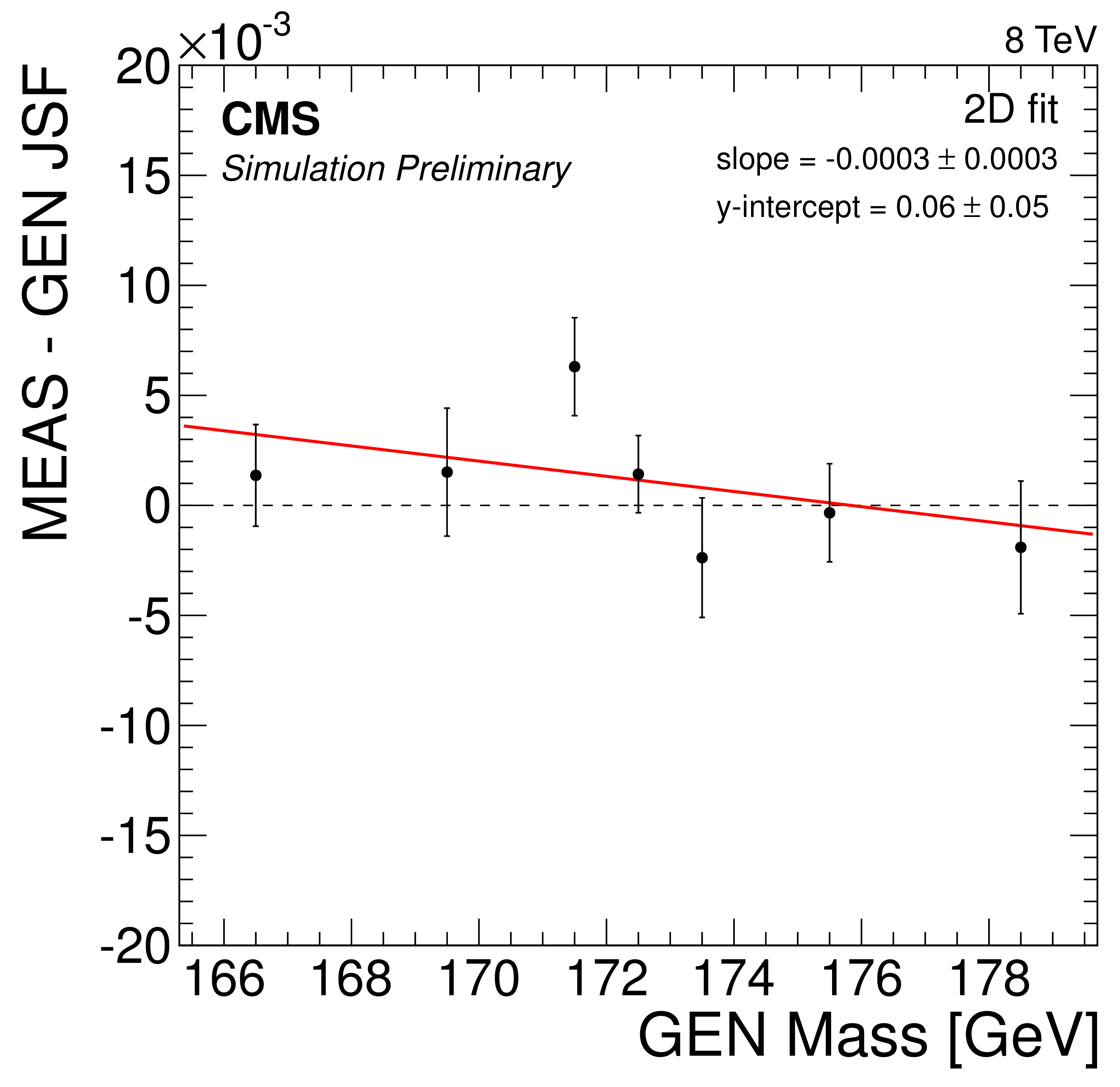
Figure 7-b:
Likelihood fit results using 50 pseudo-experiments in MC simulation, with values of ${\mathrm {M}_{\mathrm {t}}^{\text {MC}}}$ ranging from 166.5 to 178.5 GeV. A calibration curve of the form $y=ax + b$ is determined for each fit configuration. Measured values of (a) ${\mathrm {M}_{\mathrm {t}}}$ and (b) JSF are shown for the 2D fit, and measured values of ${\mathrm {M}_{\mathrm {t}}}$ are shown for the (c) 1D, (d) MAOS, and (e) hybrid fits. |

png pdf |
Figure 7-c:
Likelihood fit results using 50 pseudo-experiments in MC simulation, with values of ${\mathrm {M}_{\mathrm {t}}^{\text {MC}}}$ ranging from 166.5 to 178.5 GeV. A calibration curve of the form $y=ax + b$ is determined for each fit configuration. Measured values of (a) ${\mathrm {M}_{\mathrm {t}}}$ and (b) JSF are shown for the 2D fit, and measured values of ${\mathrm {M}_{\mathrm {t}}}$ are shown for the (c) 1D, (d) MAOS, and (e) hybrid fits. |
png pdf |
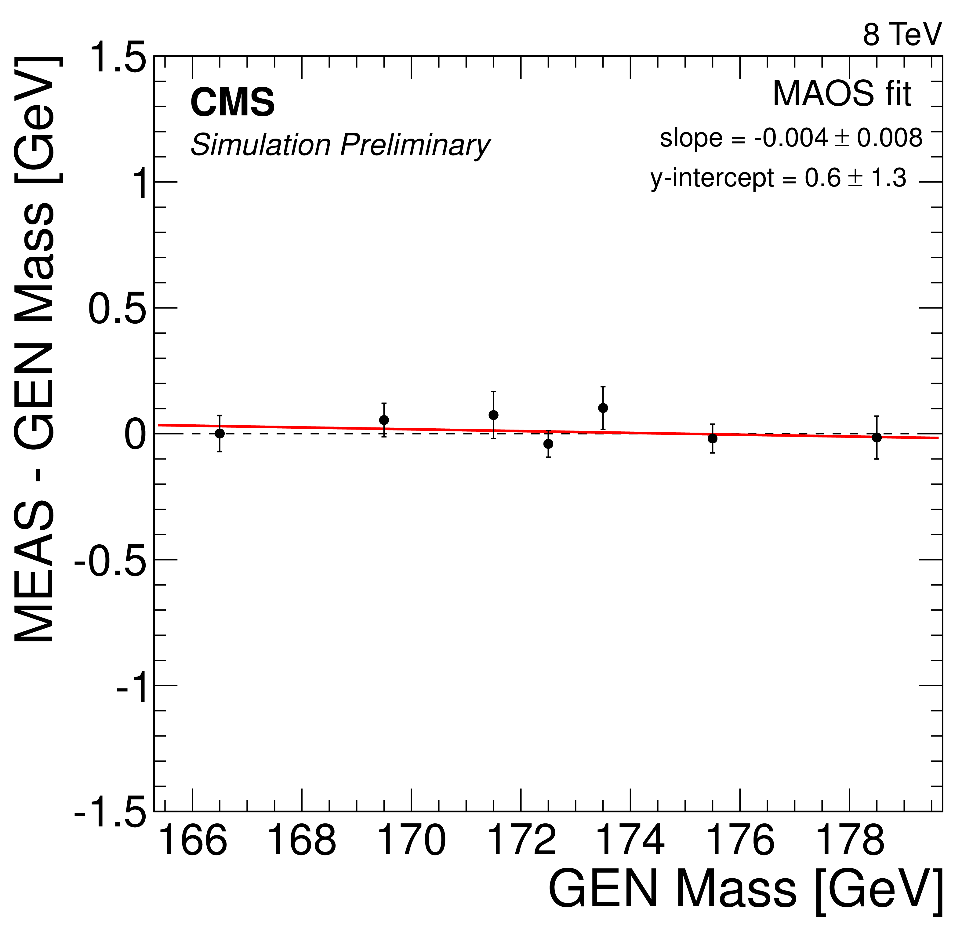
Figure 7-d:
Likelihood fit results using 50 pseudo-experiments in MC simulation, with values of ${\mathrm {M}_{\mathrm {t}}^{\text {MC}}}$ ranging from 166.5 to 178.5 GeV. A calibration curve of the form $y=ax + b$ is determined for each fit configuration. Measured values of (a) ${\mathrm {M}_{\mathrm {t}}}$ and (b) JSF are shown for the 2D fit, and measured values of ${\mathrm {M}_{\mathrm {t}}}$ are shown for the (c) 1D, (d) MAOS, and (e) hybrid fits. |
png pdf |
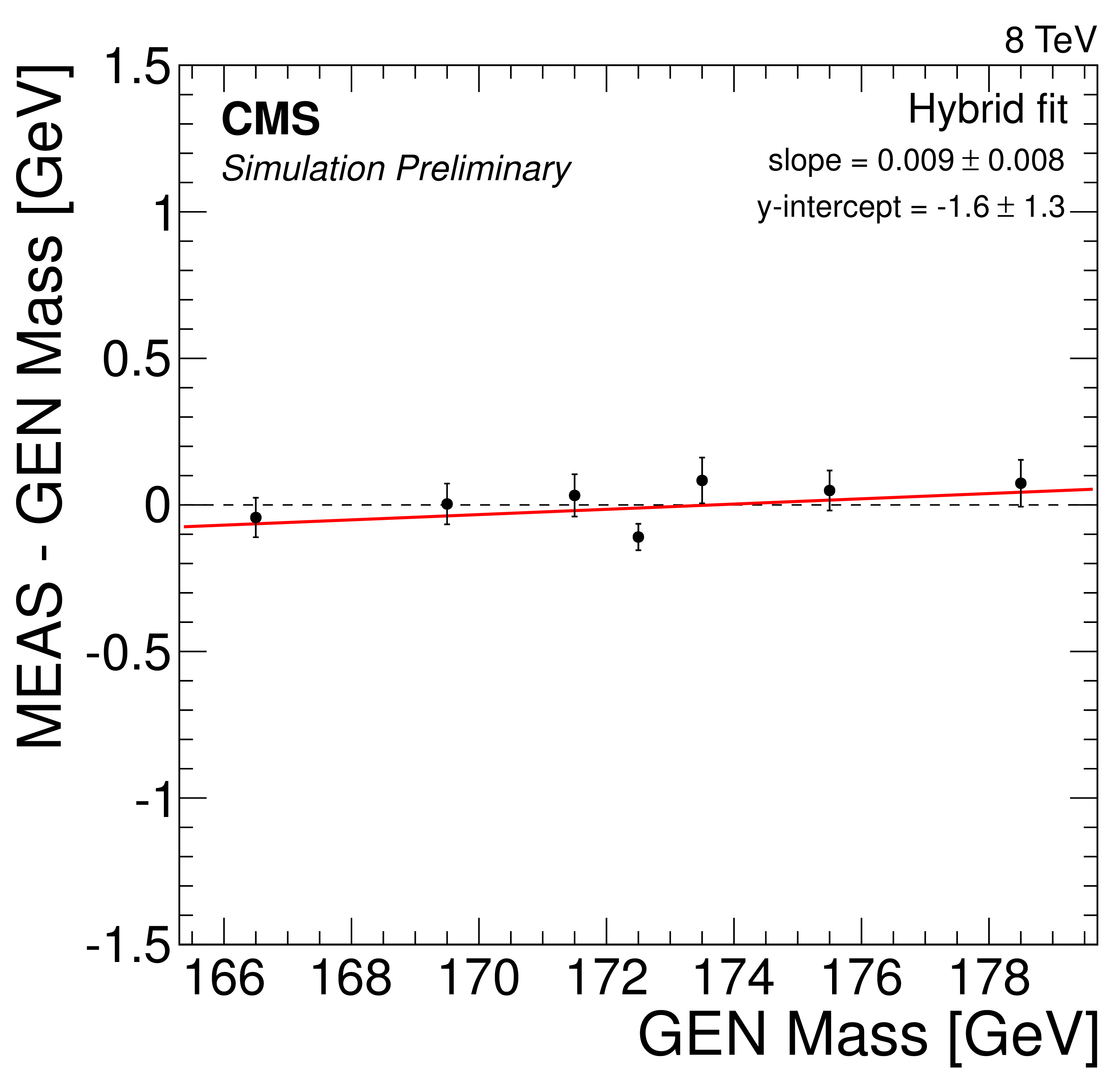
Figure 7-e:
Likelihood fit results using 50 pseudo-experiments in MC simulation, with values of ${\mathrm {M}_{\mathrm {t}}^{\text {MC}}}$ ranging from 166.5 to 178.5 GeV. A calibration curve of the form $y=ax + b$ is determined for each fit configuration. Measured values of (a) ${\mathrm {M}_{\mathrm {t}}}$ and (b) JSF are shown for the 2D fit, and measured values of ${\mathrm {M}_{\mathrm {t}}}$ are shown for the (c) 1D, (d) MAOS, and (e) hybrid fits. |
png pdf |
Figure 8-a:
Likelihood fit results using 1k bootstrap pseudo-experiments for the (a,b) 2D fit, (c) 1D fit, (d) MAOS fit. (e) hybrid fit results given by a linear combination of the 1D and 2D fits (Eq. (4)). |
png pdf |
Figure 8-b:
Likelihood fit results using 1k bootstrap pseudo-experiments for the (a,b) 2D fit, (c) 1D fit, (d) MAOS fit. (e) hybrid fit results given by a linear combination of the 1D and 2D fits (Eq. (4)). |
png pdf |
Figure 8-c:
Likelihood fit results using 1k bootstrap pseudo-experiments for the (a,b) 2D fit, (c) 1D fit, (d) MAOS fit. (e) hybrid fit results given by a linear combination of the 1D and 2D fits (Eq. (4)). |
png pdf |
Figure 8-d:
Likelihood fit results using 1k bootstrap pseudo-experiments for the (a,b) 2D fit, (c) 1D fit, (d) MAOS fit. (e) hybrid fit results given by a linear combination of the 1D and 2D fits (Eq. (4)). |

png pdf |
Figure 8-e:
Likelihood fit results using 1k bootstrap pseudo-experiments for the (a,b) 2D fit, (c) 1D fit, (d) MAOS fit. (e) hybrid fit results given by a linear combination of the 1D and 2D fits (Eq. (4)). |
png pdf |
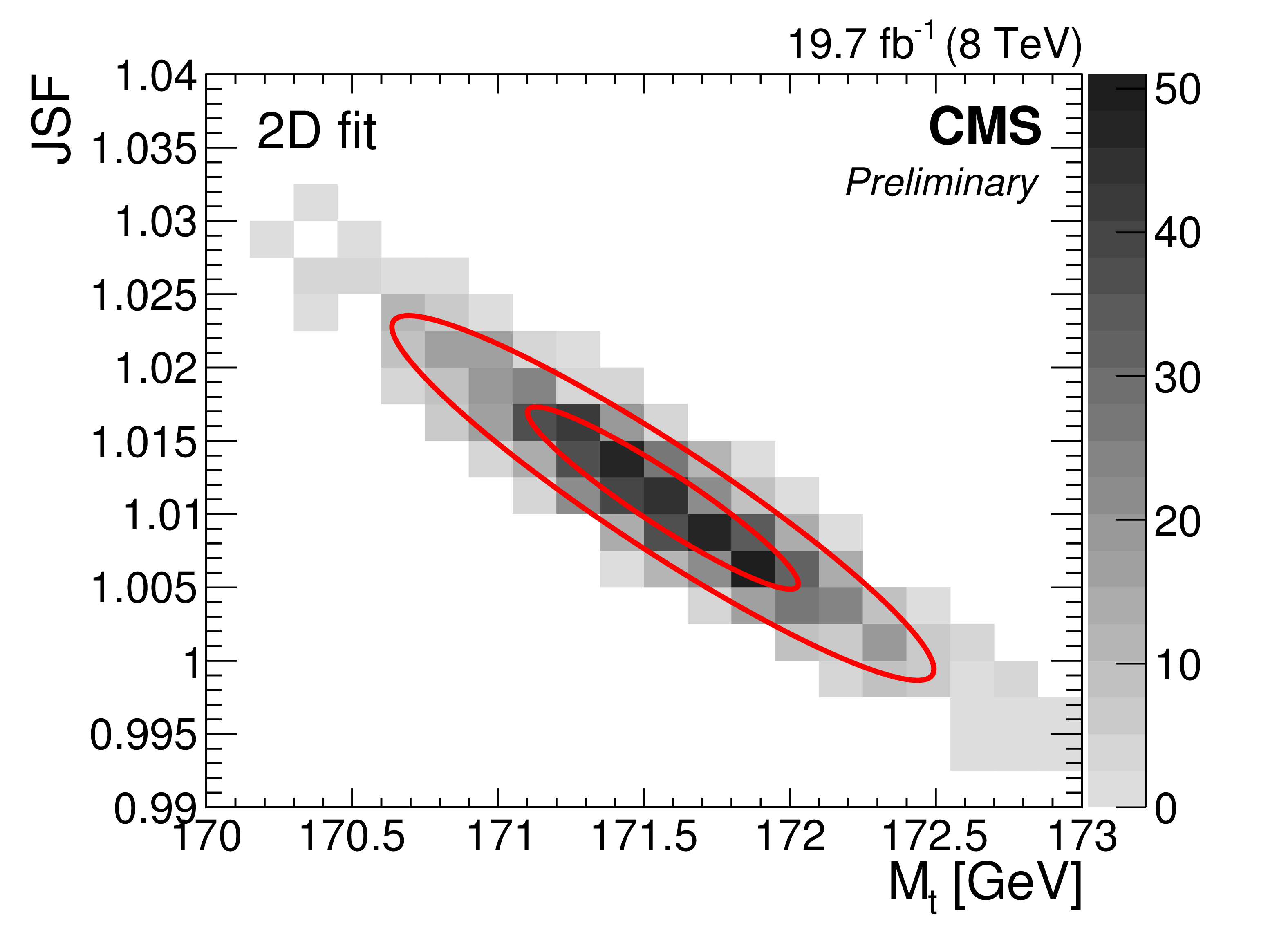
Figure 9-a:
Likelihood fit results corresponding to the 2D fit (a) and hybrid fit (b), obtained using 1k pseudo-experiments constructed with the bootstrapping technique. The shaded gray histogram represents the number of pseudo-experiments in each bin of ${\mathrm {M}_{\mathrm {t}}}$ and JSF. Two-dimensional contours corresponding to $-2\Delta \log(\mathcal {L})=1(4)$ are shown in red to indicate the one (two) sigma statistical intervals in ${\mathrm {M}_{\mathrm {t}}}$ and JSF. The hybrid fit results are given by a linear combination of the 1D and 2D fit results using Eq. (14). The correlation coefficient between the ${\mathrm {M}_{\mathrm {t}}}$ and JSF parameters is $-0.94$ in the 2D fit and $-0.40$ in the hybrid fit. |
png pdf |
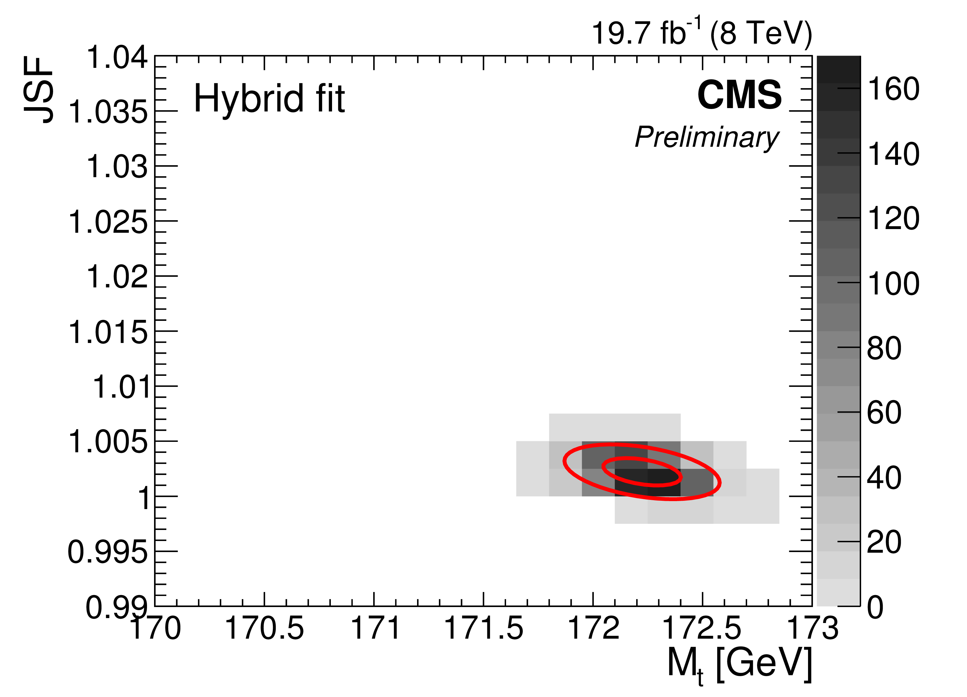
Figure 9-b:
Likelihood fit results corresponding to the 2D fit (a) and hybrid fit (b), obtained using 1k pseudo-experiments constructed with the bootstrapping technique. The shaded gray histogram represents the number of pseudo-experiments in each bin of ${\mathrm {M}_{\mathrm {t}}}$ and JSF. Two-dimensional contours corresponding to $-2\Delta \log(\mathcal {L})=1(4)$ are shown in red to indicate the one (two) sigma statistical intervals in ${\mathrm {M}_{\mathrm {t}}}$ and JSF. The hybrid fit results are given by a linear combination of the 1D and 2D fit results using Eq. (14). The correlation coefficient between the ${\mathrm {M}_{\mathrm {t}}}$ and JSF parameters is $-0.94$ in the 2D fit and $-0.40$ in the hybrid fit. |
png pdf |
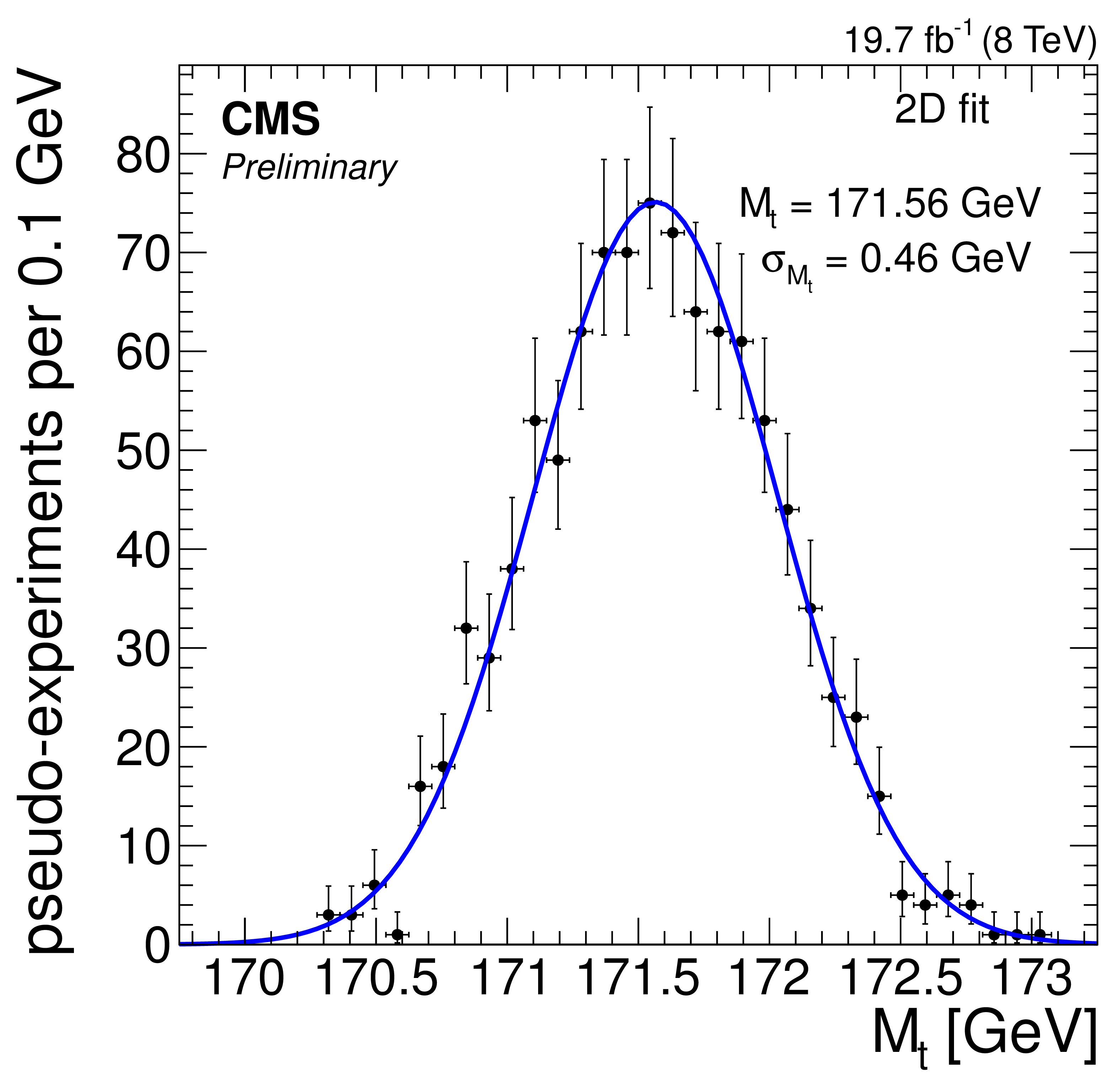
Figure 10-a:
Maximum likelihood fit result in a typical pseudo-experiment of the 2D likelihood fit. The best-fit parameter values for this pseudo-experiment are $ {\mathrm {M}_{\mathrm {t}}}=$ 171.99 GeV and $ {\mathrm {JSF}}=$ 1.007. |

png pdf |
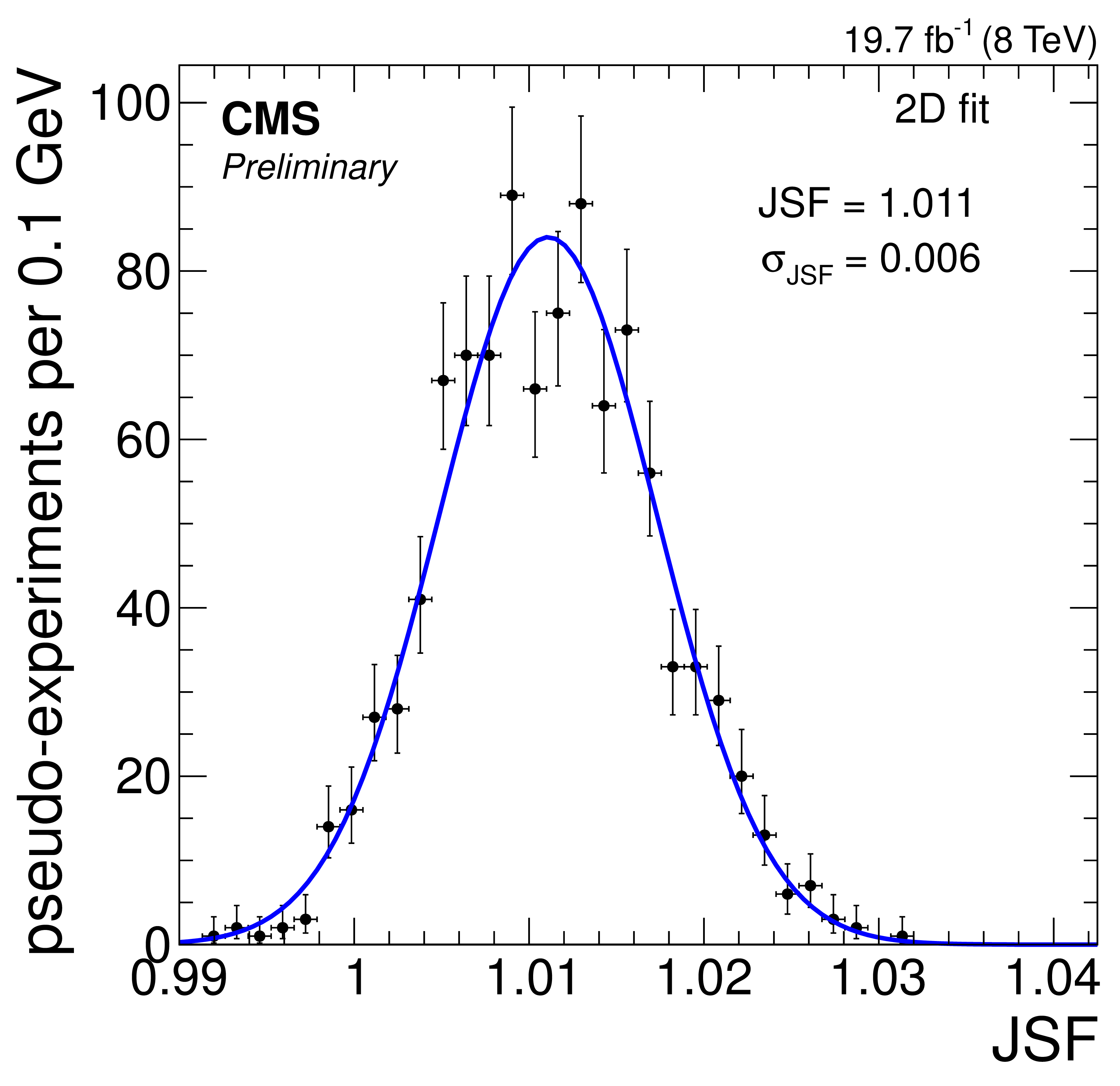
Figure 10-b:
Maximum likelihood fit result in a typical pseudo-experiment of the 2D likelihood fit. The best-fit parameter values for this pseudo-experiment are $ {\mathrm {M}_{\mathrm {t}}}=$ 171.99 GeV and $ {\mathrm {JSF}}=$ 1.007. |

png pdf |
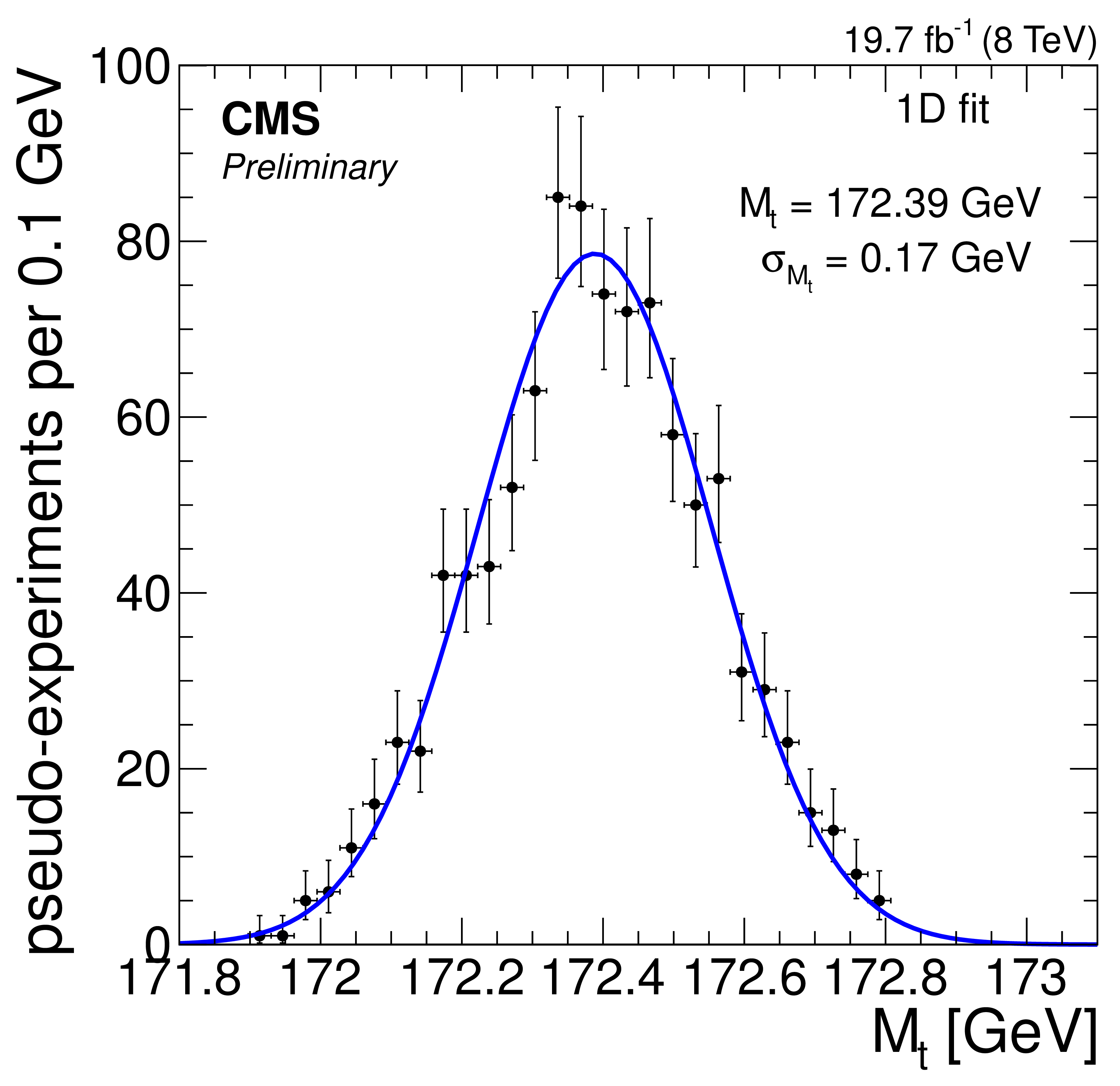
Figure 11-a:
Maximum likelihood fit result in a typical pseudo-experiment of the 1D likelihood fit. The best-fit value of ${\mathrm {M}_{\mathrm {t}}}$ for this pseudo-experiment is 172.48 GeV. |
png pdf |
Figure 11-b:
Maximum likelihood fit result in a typical pseudo-experiment of the 1D likelihood fit. The best-fit value of ${\mathrm {M}_{\mathrm {t}}}$ for this pseudo-experiment is 172.48 GeV. |
png pdf |
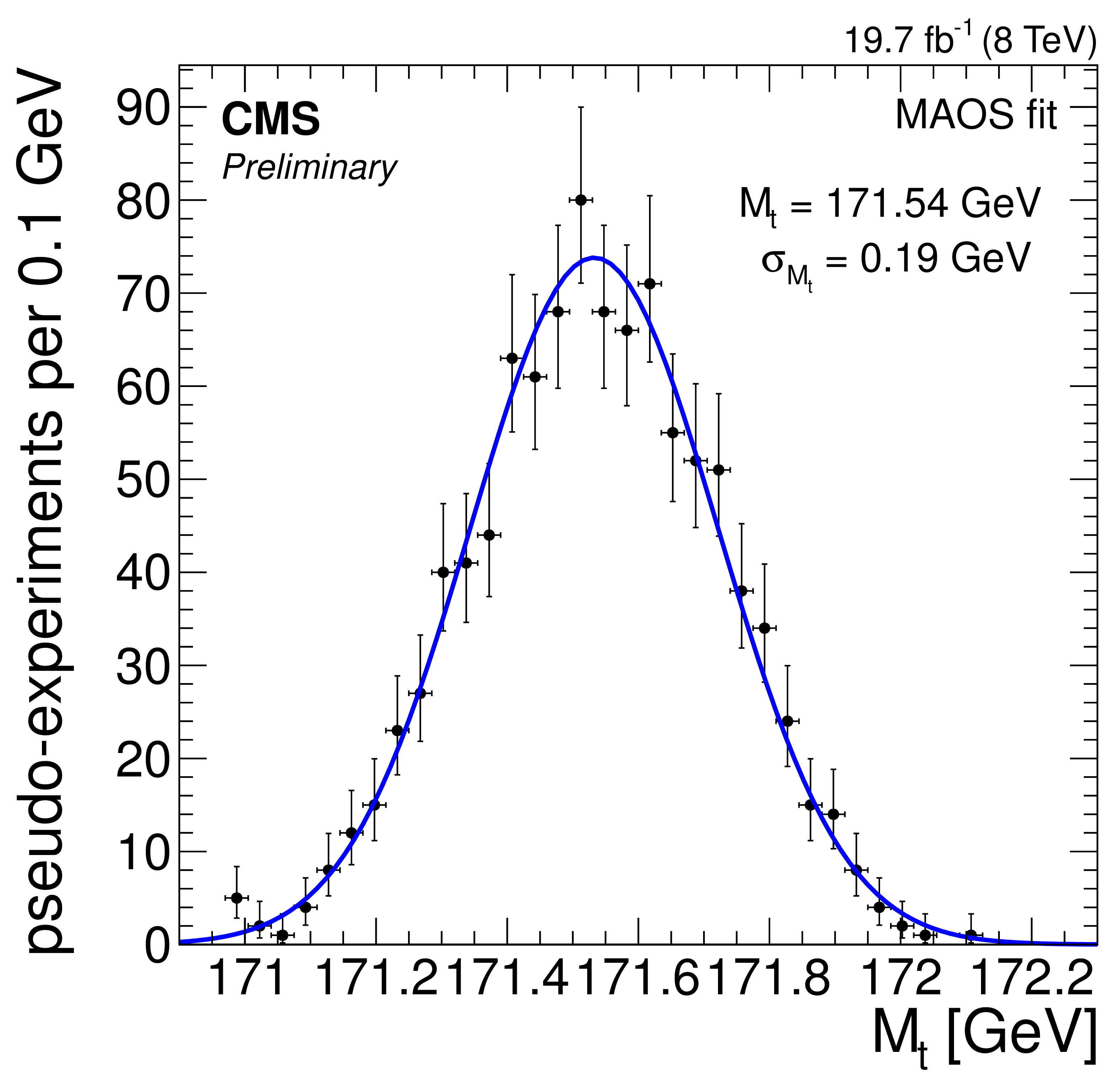
Figure 12-a:
Maximum likelihood fit result in a typical pseudo-experiment of the MAOS likelihood fit. The best-fit value of ${\mathrm {M}_{\mathrm {t}}}$ for this pseudo-experiment is 171.54 GeV. |

png pdf |
Figure 12-b:
Maximum likelihood fit result in a typical pseudo-experiment of the MAOS likelihood fit. The best-fit value of ${\mathrm {M}_{\mathrm {t}}}$ for this pseudo-experiment is 171.54 GeV. |

png pdf |
Figure 13:
Summary of the 1D, 2D, hybrid, and MAOS likelihood fit results using the CMS 2012 dataset corresponding to an integrated luminosity of 19.7 $\pm$ 0.5 fb$^{-1}$ and $ \sqrt{s} = $ 8 TeV. The most recent combination of ${\mathrm {M}_{\mathrm {t}}}$ measurements by CMS [5] is shown for reference. |
| Tables | |
png pdf |
Table 1:
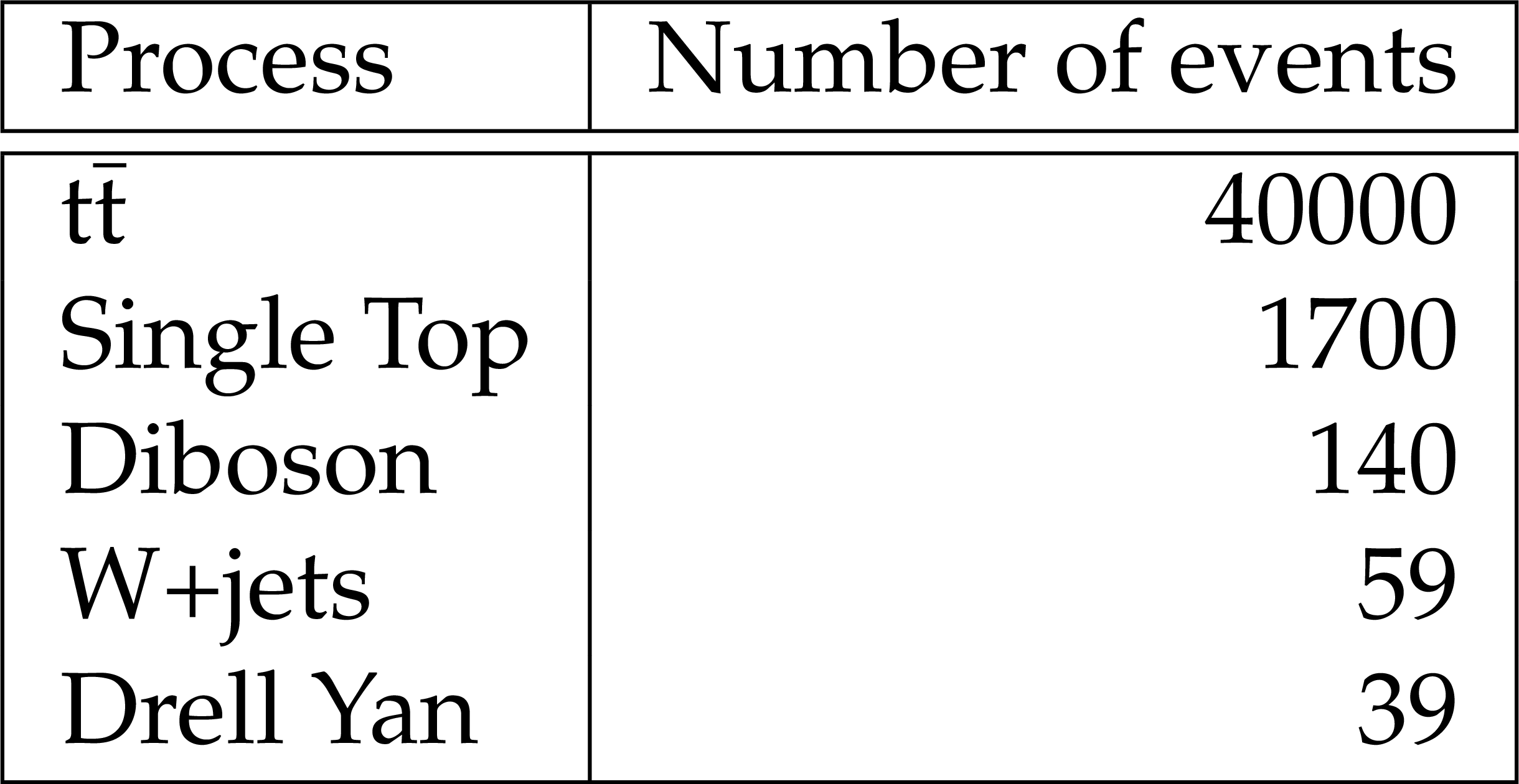
Estimate of signal and background composition in MC simulation, normalized to the number of events observed in the full dataset corresponding to an integrated luminosity of 19.7 $\pm$ 0.5 fb$^{-1}$ and $ sqrt {s}= $ 8 TeV . The contributions of these processes to the distribution shapes are shown in Figs. 1, 3, and 4, where the single top, diboson, W+jets, and Drell Yan processes are included in the `non-ttbar bkg' category. The ${\mathrm {t}\overline {\mathrm {t}}} $ category includes: `signal' dilepton events; `mistag' where a light quark or gluon jet is incorrectly selected by the b tagging algorithm; `tau decays' where dilepton events include one $\tau $ in the final state subsequently decaying leptonically; and `hadronic decays' that include events where one of the top quarks decays hadronically. |
png pdf |
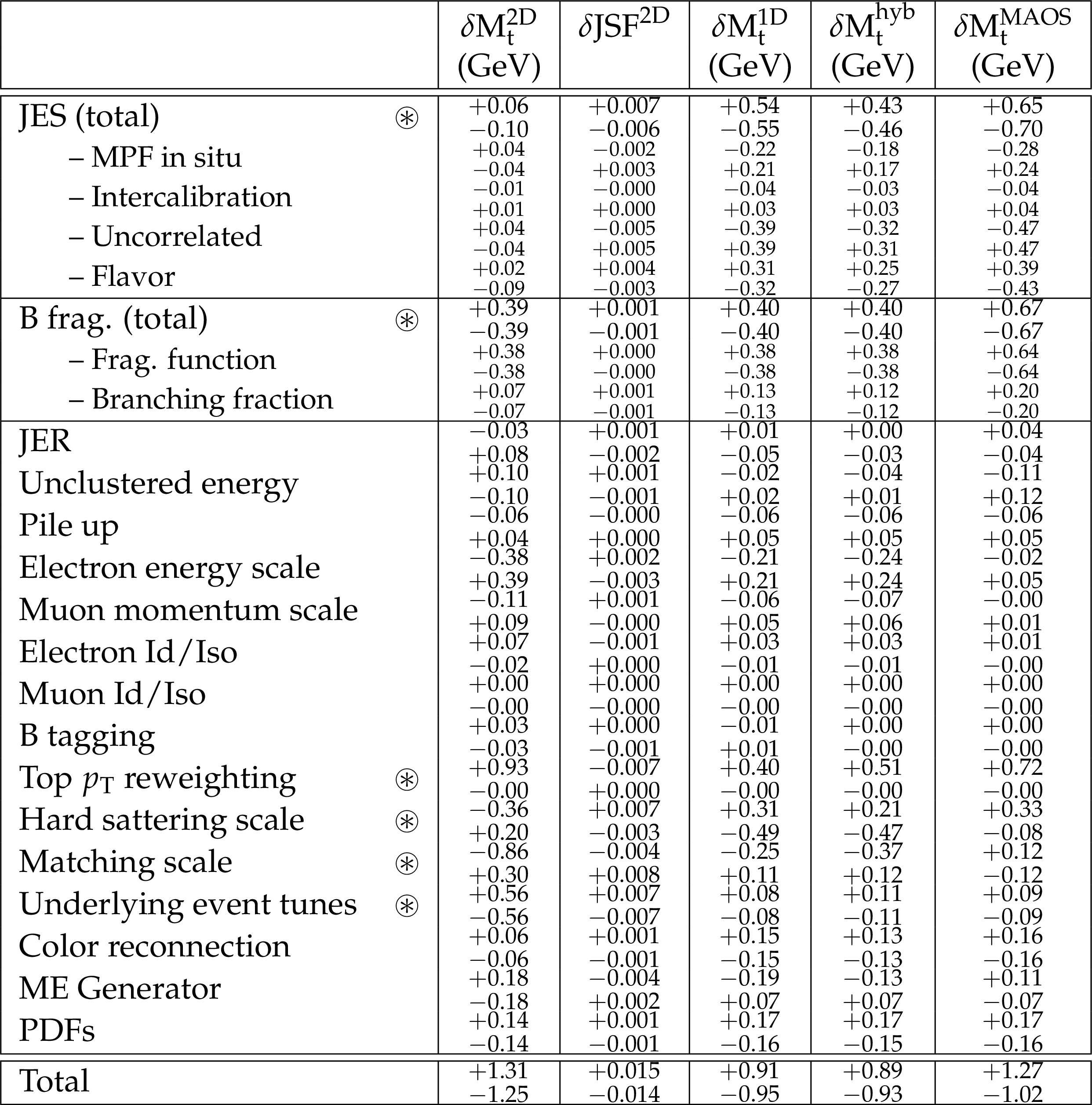
Table 2:
Systematic uncertainties for the 2D, 1D, hybrid, and MAOS likelihood fits. The breakdown of JES uncertainties into four separate components is shown, where the components are added in quadrature to obtain the total. The `up' and `down' variations are given separately, with the sign of each variation indicating the direction of the corresponding shift in ${\mathrm {M}_{\mathrm {t}}}$ or JSF. The $\star$ character highlights the uncertainty sources that are large in at least one of the likelihood fits. |
| Summary |
| We have presented a measurement of the top-quark mass using events in the dileptonic $\mathrm{ t \bar{t} }$ decay channel selected from a dataset corresponding to an integrated luminosity of (lumi)inosity and center of mass energy $ \sqrt{s} = $ 8 TeV. The measurement is based on the ${M_{\mathrm{b}}\ell}$, ${M_{\mathrm{T}2}^{\mathrm{bb}}}$, and MAOS ${M_{\mathrm{b}\ell\nu}}$ observables, which allow for mass reconstruction in decay topologies that are kinematically underconstrained. These observables are employed in three versions of an event-by-event likelihood fit, where a GP technique is used to model the corresponding distribution shapes and their evolution in the ${M_{\mathrm{t}}}$ and JSF parameters. The GP shapes are non-parametric, and allow for a likelihood fitting framework that gives unbiased results. The results for each version of the likelihood fit are summarized in Fig. 13. The 2D fit provides a measurement of ${M_{\mathrm{t}}}$ that is robust against uncertainties due to the determination of JES, yielding 171.56 $\pm$ 0.46 (stat) $^{+1.31}_{-1.25}$ (syst) GeV and 1.011 $\pm$ 0.006 (stat) $^{+0.015}_{-0.014}$ (syst). The most precise measurement of the top quark mass is given by the hybrid fit, which gives 172.22 $\pm$ 0.18 (stat) $^{+0.89}_{-0.93}$ (syst) GeV. |
| References | ||||
| 1 | Gfitter Group Collaboration | The global electroweak fit at NNLO and prospects for the LHC and ILC | EPJC 74 (2014) 3046 | 1407.3792 |
| 2 | G. Degrassi et al. | Higgs mass and vacuum stability in the Standard Model at NNLO | JHEP 08 (2012) 098 | 1205.6497 |
| 3 | A. H. Hoang and I. W. Stewart | Top Mass Measurements from Jets and the Tevatron Top-Quark Mass | NPPS 185 (2008) 220 | 0808.0222 |
| 4 | ATLAS Collaboration | Measurement of the top quark mass in the $ t\bar{t}\to $ dilepton channel from $ \sqrt{s}=8 $ TeV ATLAS data | 1606.02179 | |
| 5 | CMS Collaboration | Measurement of the top quark mass using proton-proton data at $ {\sqrt{s}} $ = 7 and 8 TeV | PRD 93 (2016) 072004 | CMS-TOP-14-022 1509.04044 |
| 6 | ATLAS, CDF, CMS, D0 Collaboration | First combination of Tevatron and LHC measurements of the top-quark mass | 1403.4427 | |
| 7 | A. J. Barr and C. G. Lester | A Review of the Mass Measurement Techniques proposed for the Large Hadron Collider | JPG 37 (2010) 123001 | 1004.2732 |
| 8 | C. G. Lester and D. J. Summers | Measuring masses of semi-invisibly decaying particles pair produced at hadron colliders | PLB 463 (1999) 99 | hep-ph/9906349 |
| 9 | H.-C. Cheng and Z. Han | Minimal Kinematic Constraints and m(T2) | JHEP 12 (2008) 063 | 0810.5178 |
| 10 | W. S. Cho, K. Choi, Y. G. Kim, and C. B. Park | M(T2)-assisted on-shell reconstruction of missing momenta and its application to spin measurement at the LHC | PRD 79 (2009) 031701 | 0810.4853 |
| 11 | CMS Collaboration | Measurement of masses in the $ t \bar{t} $ system by kinematic endpoints in pp collisions at $ \sqrt{s} $ = 7 TeV | EPJC 73 (2013) 2494 | CMS-TOP-11-027 1304.5783 |
| 12 | C. Rasmussen and C. Williams | MIT Press, 2006 ISBN 026218253X | ||
| 13 | C. Bishop | Springer-Verlag, New York, 1 edition, 2006 ISBN 978-0-387-31073-2 | ||
| 14 | CMS Collaboration | The CMS experiment at the CERN LHC | JINST 3 (2008) S08004 | CMS-00-001 |
| 15 | CMS Collaboration | Commissioning of the Particle-Flow reconstruction in Minimum-Bias and Jet Events from pp Collisions at 7 TeV | CDS | |
| 16 | CMS Collaboration | Performance of electron reconstruction and selection with the CMS detector in proton-proton collisions at $ \sqrt{s} = 8 $$ TeV $ | JINST 10 (2015) P06005 | CMS-EGM-13-001 1502.02701 |
| 17 | CMS Collaboration | Performance of CMS muon reconstruction in $ pp $ collision events at $ \sqrt{s}=7 $ TeV | JINST 7 (2012) P10002 | CMS-MUO-10-004 1206.4071 |
| 18 | M. Cacciari, G. P. Salam, and G. Soyez | The anti-$ k_t $ jet clustering algorithm | JHEP 04 (2008) 063 | 0802.1189 |
| 19 | M. Cacciari, G. P. Salam, and G. Soyez | FastJet User Manual | EPJC 72 (2012) 1896 | 1111.6097 |
| 20 | CMS Collaboration | Determination of jet energy calibration and transverse momentum resolution in CMS | JINST 6 (2011) P11002 | CMS-JME-10-011 1107.4277 |
| 21 | CMS Collaboration | Identification of b-quark jets with the CMS experiment | JINST 8 (2013) P04013 | CMS-BTV-12-001 1211.4462 |
| 22 | J. Alwall et al. | The automated computation of tree-level and next-to-leading order differential cross sections, and their matching to parton shower simulations | JHEP 07 (2014) 079 | 1405.0301 |
| 23 | P. Artoisenet, R. Frederix, O. Mattelaer, and R. Rietkerk | Automatic spin-entangled decays of heavy resonances in Monte Carlo simulations | JHEP 03 (2013) 015 | 1212.3460 |
| 24 | T. Sjostrand, S. Mrenna, and P. Skands | PYTHIA 6.4 physics and manual | JHEP 05 (2006) 026 | hep-ph/0603175 |
| 25 | S. Jadach, Z. Was, R. Decker, and J. H. Kuhn | The tau decay library TAUOLA: Version 2.4 | CPC 76 (1993) 361 | |
| 26 | W.-K. Tung | New generation of parton distributions with uncertainties from global QCD analysis | Acta Phys. Polon. B 33 (2002) 2933 | hep-ph/0206114 |
| 27 | S. Alioli, P. Nason, C. Oleari, and E. Re | NLO single-top production matched with shower in POWHEG: s- and t-channel contributions | JHEP 09 (2009) 111, , [Erratum: JHEP02,011(2010)] | 0907.4076 |
| 28 | E. Re | Single-top Wt-channel production matched with parton showers using the POWHEG method | EPJC 71 (2011) 1547 | 1009.2450 |
| 29 | S. Frixione, P. Nason, and C. Oleari | Matching NLO QCD computations with Parton Shower simulations: the POWHEG method | JHEP 11 (2007) 070 | 0709.2092 |
| 30 | S. Alioli, P. Nason, C. Oleari, and E. Re | A general framework for implementing NLO calculations in shower Monte Carlo programs: the POWHEG BOX | JHEP 06 (2010) 043 | 1002.2581 |
| 31 | GEANT4 Collaboration | GEANT4: A Simulation toolkit | NIMA 506 (2003) 250 | |
| 32 | N. Kidonakis | Next-to-next-to-leading soft-gluon corrections for the top quark cross section and transverse momentum distribution | PRD 82 (2010) 114030 | 1009.4935 |
| 33 | N. Kidonakis | Differential and total cross sections for top pair and single top production | in Proceedings, 20th International Workshop on Deep-Inelastic Scattering and Related Subjects (DIS 2012) | 1205.3453 |
| 34 | K. Melnikov and F. Petriello | Electroweak gauge boson production at hadron colliders through O(alpha(s)**2) | PRD 74 (2006) 114017 | hep-ph/0609070 |
| 35 | J. M. Campbell and R. K. Ellis | MCFM for the Tevatron and the LHC | NPPS 205-206 (2010) 10 | 1007.3492 |
| 36 | M. Czakon, P. Fiedler, and A. Mitov | Total Top-Quark Pair-Production Cross Section at Hadron Colliders Through $ O(α\frac{4}{S}) $ | PRL 110 (2013) 252004 | 1303.6254 |
| 37 | M. Burns, K. Kong, K. T. Matchev, and M. Park | Using Subsystem MT2 for Complete Mass Determinations in Decay Chains with Missing Energy at Hadron Colliders | JHEP 03 (2009) 143 | 0810.5576 |
| 38 | B. Efron and R. Tibshirani | Monographs on Statistics and Applied Probability. Chapman & Hall | ||
| 39 | CMS and ATLAS Collaboration | Jet energy scale uncertainty correlations between ATLAS and CMS at 8 TeV | CMS-PAS-JME-15-001, ATL-PHYS-PUB-2015-049 | |
| 40 | M. Bahr et al. | Herwig++ Physics and Manual | EPJC 58 (2008) 639 | 0803.0883 |
| 41 | CMS Collaboration | Identification of b-quark jets with the CMS experiment | JINST 8 (2013) P04013 | CMS-BTV-12-001 1211.4462 |
| 42 | CMS Collaboration | Measurement of the differential cross section for top quark pair production in pp collisions at $ \sqrt{s} = 8\,\text {TeV} $ | EPJC 75 (2015) 542 | CMS-TOP-12-028 1505.04480 |
| 43 | P. Z. Skands | Tuning Monte Carlo Generators: The Perugia Tunes | PRD 82 (2010) 074018 | 1005.3457 |
| 44 | H.-L. Lai et al. | New parton distributions for collider physics | PRD 82 (2010) 074024 | 1007.2241 |
| 45 | ALEPH Collaboration | Study of the fragmentation of b quarks into B mesons at the Z peak | PLB 512 (2001) 30 | hep-ex/0106051 |
| 46 | DELPHI Collaboration | A study of the b-quark fragmentation function with the DELPHI detector at LEP I and an averaged distribution obtained at the Z Pole | EPJC 71 (2011) 1557 | 1102.4748 |
| 47 | H. Cr\'amer | Princeton University Press | ||
| 48 | A. DasGupta | Springer | ||
|
|
Compact Muon Solenoid LHC, CERN |
|

|

|

|

|

|