Studying HLT efficiencies, rates and overlaps

Whether you are a line developer or you’re just interested in the current status of LHCb’s high level trigger, you might like to study the efficiencies, rates and overlaps of a particular line or subset of lines. HltEfficiencyChecker is a package designed to help you do just that.

In earlier sections of this documentation, you’ve seen how to run Moore on some MC samples. HltEfficiencyChecker extends this functionality and writes the trigger decisions to a ROOT nTuple. The package then also provides configurable analysis scripts that take the tuple and give you information on the rates, efficiencies and overlaps of the line(s) you’re interested in. In the case of efficiencies, some MC truth information of the kinematics of each event will have also been saved, allowing a configurable set of plots, console and text file output to be created that characterise the response of the trigger line(s) that were run as a function of the decay’s kinematics. There is also functionality to calculate the inclusive and exclusive rates of multiple lines in one run.

In the same way that you would provide an options file to gaudirun.py when running Moore, you interface with HltEfficiencyChecker by providing a configuration file (what lines you’re interested in, what MC input files to use, whether you want to see efficiencies/rates/overlaps, what plots to make etc.). You can then run the trigger and tupling sequence from the command line in a similar way that you would run Moore.

In this tutorial we will first see how to set up the package in addition to the usual LHCb software stack. This is followed by a set of examples, which increase in complexity. All of these examples are closely based on scripts that live in the directory DaVinci/HltEfficiencyChecker/options/.

Note

HltEfficiencyChecker is best suited to running either a single trigger line, or a small group of lines. If you wish to run more than O(100) lines, the tool will become slow and the amount of output overwhelming. In some cases, it may even fail with so many lines. If you wish to do studies of the status of the entire trigger, please take a look at the UpgradeRateTest.

Note

Since late July 2020, HltEfficiencyChecker uses Allen as the default HLT1 option, to reflect the trigger we will use in Run 3. This is achieved by compiling Allen for CPU and running it within Moore as a Gaudi algorithm. Don’t worry if this sounds a bit technical - running Allen like this requires no extra work from the user and gives rates and efficiencies that are representative of the Allen trigger that will run online on GPUs (just not as fast)! Running Moore’s HLT1 is still supported as well, although users should be aware that this is not the trigger that will run in Run 3.

Setup instructions

HltEfficiencyChecker lives within the DaVinci software package 1, which itself lives within the LHCb software stack (colloquially just “stack”) - so you’ll need a working build of the stack to develop with. If you don’t have this yet, follow the instructions on the Developing Moore page.

Note

If you are planning to test your lines with simulation samples produced before 2023, beware that the DD4Hep condition database may not be suited for the task. In this case, remember to build for one of the detdesc platforms that successfully run in the nightlies.

Once you have the stack, you need to get DaVinci as well. From your top-level stack/ directory do:

make DaVinci

which will checkout the master branch of DaVinci and build it for you.

Note

In the following, when particular file paths are given, they will always be relative to the top-level directory of the software stack. For example, let’s say you built your stack in /home/user/stack/ and the path DaVinci/HltEfficiencyChecker/options/hlt1_eff_example.py is referred to: the full path would be /home/user/stack/DaVinci/HltEfficiencyChecker/options/hlt1_eff_example.py.

How to interact with HltEfficiencyChecker

As mentioned in the introduction, HltEfficiencyChecker requires that you provide it with a configuration file, i.e. a set of information for the tool to run in an expected format. The necessary information needed for the trigger to run is

• The input simulation files to run over, either as a TestFileDB key or as a list of LFNs,

• Details of the simulation e.g. CondDB tags, data format etc. (not needed if TestFileDB key specified),

• The level of the trigger (HLT1 or HLT2),

• Which lines to run.

and the necessary information about the results you want to see is

• If you want rates, efficiencies or overlaps,

• If efficiencies, you then need to provide an “annotated decay descriptor” and the names of the final-state (stable) particles in the decay (more below).

There are also a variety of optional features to customize the results you get. All this will be explained in more detail when we get to the examples.

The configuration can be provided in two ways. The first - which we call using the tool’s “wizard” - involves writing a short text file in yaml format. This is designed to be as readable and self-explanatory as possible and is recommended if you are not yet very experienced with running the trigger and writing Gaudi options files (the wizard writes the options file for you behind-the-scenes). If you are an experienced line developer who needs greater flexibility, or you don’t like any kind of behind-the-scenes “magic”, you can write your options files and call the analysis scripts yourself. Both workflows will be covered in this tutorial.

Let’s go ahead and get started, and write our first configuration file.

Example: my first config file using the HltEfficiencyChecker wizard

yaml text files are similar to json and python dictionaries: you specify key-value pairs and values are accessed by asking for their key (usually a string). The HltEfficiencyChecker “wizard” script (DaVinci/HltEfficiencyChecker/scripts/hlt_eff_checker.py) parses the yaml, generates a Gaudi options file from it, then runs it and runs analysis scripts on the output. Thus, the yaml keys you provide must be known and must follow a basic structure. Let’s say we are interested in measuring some HLT1 efficiencies on \(B_{s}^{0} \to \phi\phi\). Here is a suitable yaml config file:

annotated_decay_descriptor:
    "[${B_s0}B_s0 => ( phi(1020) => ${Kplus0}K+ ${Kminus0}K-) ( phi(1020) => ${Kplus1}K+ ${Kminus1}K-) ]CC"
ntuple_path: &NTUPLE hlt1_eff_ntuple.root
job:
    trigger_level: 1
    evt_max: 100
    testfiledb_key: Upgrade_BsPhiPhi_MD_FTv4_DIGI_retinacluster
    debug_mode: False
    hlt1_configuration: hlt1_pp_forward_then_matching_no_ut
    options:
        # - $HLTEFFICIENCYCHECKERROOT/options/hlt1_moore_lines_example.py  # Allen lines are specified internally to Allen
        - $HLTEFFICIENCYCHECKERROOT/options/options_template.py.jinja  # first rendered with jinja2
analysis:
    script: $HLTEFFICIENCYCHECKERROOT/scripts/hlt_line_efficiencies.py
    args:
        input: *NTUPLE
        reconstructible_children: Kplus0,Kminus0,Kplus1,Kminus1
        legend_header: "B^{0}_{s} #rightarrow #phi#phi"
        make_plots: true
        vars: "PT,Kplus0:PT"
        lines: Hlt1TwoTrackMVADecision,Hlt1TrackMVADecision
        true_signal_to_match_to: "B_s0,Kplus0"

The first options are needed globally. They are the ntuple_path, which will be the name of the tuple that is written out, and the annotated_decay_descriptor, which is an MC decay descriptor with an important difference. MCFunTuple - which writes the MC truth information to the tuple - needs a decay descriptor to find the signal decays in the MC. Given that, we’ll get branches in the tuple of various kinematic properties of the different particles in the decay. In the same way that in DaVinci you need to put a ^ to the left of the particles you want to make branches for, here you must specify the branch prefix as ${prefix} to the left of the particles of interest. For example, the tuple written from this config file will have branches for the \(B_{s}^{0}\) and the four charged kaons, and these branches will be prefixed with B_s0, Kplus0, Kminus0, Kplus1 and Kminus1 respectively, e.g. B_s0_TRUEPT or Kminus0_TRUEETA.

Note

The branch prefixes does the same job as ^, but also must be specified so that the analysis scripts can work out exactly what branches to expect in the tuple. This knowledge is necessary to construct different efficiency denominator requirements, which are explained below.

The job options are just needed to run the trigger. trigger_level (1, 2 or both) selects HLT1, HLT2 or HLT1-followed-by-HLT2. As mentioned at the start, the default HLT1 is Allen, but you can use the Moore HLT1 if you really want to by adding the line use_moore_as_hlt1: True here. evt_max is the number of events to run over (not the number of events that fired the trigger; bear this in mind if you expect a low efficiency). The next thing to specify is the input MC files, and here we have done the simplest thing and specified the key of an entry in the TestFileDB. A TestFileDB entry holds all the information needed to run over a set of input files, including the tags that it was created with and the LFNs. Fortunately, we have here a recent entry for our decay of interest. We also specify an hlt1_configuration with the appropriate key; see some explanation of that in the box below.

Note

If the TestFileDB doesn’t have a sample that is sufficient for your testing needs - which we assume will be the case for most users of this tool - there are instructions in the following examples to use any LFNs you like in the wizard with a few more lines of code.

Note

The hlt1_configuration (or Allen sequence) is a string that maps to the configured set of algorithms that will run in HLT1. The default ones – including hlt1_pp_forward_then_matching_no_ut, which is the default for the beginning of 2024 – now expect Retina Clusters, but older MC does not contain them. Although they can be added to existing DIGI files, you can also use a configuration that doesn’t require them, e.g. hlt1_pp_veloSP.

If set to True, the debug_mode key will make the trigger print lots more information to the console than is usual, which may be helpful to track down an error. To deal with the huge amounts of output you’ll get, it may be wise to restrict to a handful of events and save the output to a file (e.g. >> my_output.log) that you can search through efficiently. Finally in the job options is the options key. These are paths to scripts in DaVinci and the helpful environment variable $HLTEFFICIENCYCHECKERROOT makes sure they are correct on any system. The only one we need here is .../options_template.py.jinja, which is the script that translates the yaml into options that can be passed to Gaudi. You don’t normally need to edit this file.

If you remember the list of necessary information that HltEfficiencyChecker needs, you may have noticed that we haven’t yet configured the trigger i.e. told it what HLT1 lines to run and what thresholds to run with. This is done internally to Allen and a bit of guidance on that is given in the selections README. If we were running the Moore HLT1, we would need to provide a short options file to do this. An example of this (.../hlt1_moore_lines_example.py) is commented out to show you where you would add it. .../hlt1_moore_lines_example.py should look like this:

from Moore import options
from Hlt1Conf.settings import all_lines
from Hlt1Conf.lines.high_pt_muon import one_track_muon_highpt_line
from Hlt1Conf.lines.gec_passthrough import gec_passthrough_line

def make_lines():
    return all_lines() + [one_track_muon_highpt_line(), gec_passthrough_line()]

options.lines_maker = make_lines

That is all for the trigger’s needs. Next up are the analysis options, which configure what results you’d like to see and the trigger doesn’t need to know. script specifies the analysis script to run. We want efficiencies, so we ask for the hlt_line_efficiencies.py script (we’ll see a rates example later). The args are the set of python ArgumentParser args that are parsed to this script. It needs to know the path to the tuple that will be made, which is handled by input: *NTUPLE, and the trigger level. Optionally, we’ve provided a pretty LaTeX header with legend_header. We hinted above that, in order to construct efficiency denominators, the analysis script needs to know what branches to expect. The reconstructible_children key specifies this as a comma-separated list of stable, reconstructible, final-state particles of the decay. This list must be a subset of the branch prefixes in the annotated decay descriptor. The vars keyword accepts a comma-separated list of kinematic variables that you’d like to plot efficiencies against. By default, it is assumed that you’re interested in the parent kinematics (by default, the parent is interpreted as the leftmost branch prefix in the decay descriptor), but you can specify a different particle in the decay before a colon, as shown for the \(K^{+}\). We’ve picked two physics lines to see the results from with the lines keyword, which again takes a comma-separated list. These two lines should fire on our decay of interest. Finally, we choose to see the TrueSim efficiency of the lines when matched to the \(B_{s}^{0}\) and one of the kaons. How this is defined is explained below. There are a variety of other args that the analysis script can take; take a look at the script hlt_line_efficiencies.py if you’d like to see what they are. We’ll use some others in the next examples.

Note

There is nothing stopping you running hlt_line_efficiencies.py, with these args, on its own, and we will see how to later on. However, a bit of re-formatting is needed to transform the yaml key-value pairs into command-line arguments, as you can see from hlt_line_efficiencies.py --help. In short, those keys that have the value true correspond to positional arguments e.g. for make_plots: true you’d simply pass --make-plots to the script. The rest are keyword arguments e.g. vars: "PT,Kplus0:PT" becomes --vars "PT,Kplus0:PT". Finally, input: *NTUPLE is a special case, and it corresponds to just the value of NTUPLE as a string e.g. eff_ntuple.root. This transformation is all done in DaVinci/HltEfficiencyChecker/python/HltEfficiencyChecker/wizard.py. In the rest of this tutorial, we will interchange between passing args via the yaml and passing them directly to the analysis scripts.

Running the tool on a yaml config file

Assuming the config file we just wrote lived at the path DaVinci/HltEfficiencyChecker/options/hlt1_eff_example.yaml, then we just need to do (from the stack/ directory):

DaVinci/run DaVinci/HltEfficiencyChecker/scripts/hlt_eff_checker.py DaVinci/HltEfficiencyChecker/options/hlt1_eff_example.yaml

In general, the command follows the pattern:

DaVinci/run DaVinci/HltEfficiencyChecker/scripts/hlt_eff_checker.py <path/to/config/file> <OPTIONS>

where hlt_eff_checker.py is the “wizard” script that runs the trigger and then the analysis script according to the configuration in <path/to/config/file>. The <OPTIONS> you can pass to hlt_eff_checker.py are explained with the --help argument:

(LHCb Env) [user@users-computer stack]$ DaVinci/run DaVinci/HltEfficiencyChecker/scripts/hlt_eff_checker.py --help
usage: hlt_eff_checker.py [-h] [-o OUTPUT] [-s OUTPUT_SUFFIX] [--force] [-n]
                          config

Script that extracts and plots efficiencies and rates from the high level
trigger.

positional arguments:
  config                YAML configuration file

optional arguments:
  -h, --help            show this help message and exit
  -o OUTPUT, --output OUTPUT
                        Output directory prefix. See also --output-suffix.
  -s OUTPUT_SUFFIX, --output-suffix OUTPUT_SUFFIX
                        Output directory suffix
  --force               Do not fail when output directory exists
  -n, --dry-run         Only print the commands needed to run from stack/
                        directory.

By default, like the Moore tests (see Developing Moore), the results will go into a new directory with the current time in the title e.g. checker-20230427-134030. Let’s say you’d prefer the results to live in your directory checker-hlt1tests, which already exists and has results in it already from the last time you ran HltEfficiencyChecker, which you’d like to overwrite. Then you’d do:

DaVinci/run DaVinci/HltEfficiencyChecker/scripts/hlt_eff_checker.py <path/to/config/file> -o checker-hlt1 -s tests --force

Finally, there is also the --dry-run feature, which interprets your yaml and writes the options that will configure the job, but then stops just before running, and instead prints the set of commands that it was about to execute:

(LHCb Env) [user@users-computer stack]$ DaVinci/run DaVinci/HltEfficiencyChecker/scripts/hlt_eff_checker.py DaVinci/HltEfficiencyChecker/options/hlt1_eff_example.yaml -o checker-hlt1 -s tests --force --dry-run
The commands to run are...
cd 'checker-hlt1tests'
'/home/user/stack/DaVinci/run' 'gaudirun.py' '.hlt_eff_checker_options_DEB92F7D.py'
'/home/user/stack/DaVinci/run' '/home/user/stack/DaVinci/HltEfficiencyChecker/scripts/hlt_line_efficiencies.py' 'eff_ntuple.root' '--lines=Hlt1TwoTrackMVADecision,Hlt1TrackMVADecision' '--vars=PT,Kplus0:PT' '--reconstructible-children=Kplus0,Kminus0,Kplus1,Kminus1' '--true-signal-to-match-to=B_s0,Kplus0' '--make-plots' '--legend-header=B^{0}_{s} #rightarrow #phi#phi'

You are then free to execute these commands at your own leisure! This can be particularly useful if you just want to tweak your analysis options, e.g. you’d like to see plots against a different variable or a different denominator and remake the plots. This obviously doesn’t require running the trigger and making the tuple again (which can take a long time!). So you can just copy and paste the first and last of these commands to re-run only the analysis step, which is typically fast.

Results

Note

WARNING! HLT1 TrueSim efficiencies are currently not being produced by HltEfficiencyChecker, due to an issue that the authors are working on (see DaVinci#162). HLT2 TrueSim efficiencies are working fine. TrueSim efficiencies are left in the (older) HLT1 example below as they are helpful for illustration of the example - all the below points apply equally well to HLT2.

When all of the steps of the tool have run, we should be looking at a console output that ends like this:

------------------------------------------------------------------------------------
INFO:    Starting /home/user/stack/DaVinci/HltEfficiencyChecker/scripts/hlt_line_efficiencies.py...
------------------------------------------------------------------------------------
Integrated HLT efficiencies for the lines with denominator: CanRecoChildren
------------------------------------------------------------------------------------
Line:    B_s0_Hlt1TrackMVADecisionTrueSim        Efficiency:     0.391 +/- 0.102
Line:    B_s0_Hlt1TwoTrackMVADecisionTrueSim     Efficiency:     0.696 +/- 0.096
Line:    Hlt1TrackMVADecision                    Efficiency:     0.435 +/- 0.103
Line:    Hlt1TwoTrackMVADecision                 Efficiency:     0.739 +/- 0.092
Line:    Kplus0_Hlt1TrackMVADecisionTrueSim      Efficiency:     0.130 +/- 0.070
Line:    Kplus0_Hlt1TwoTrackMVADecisionTrueSim   Efficiency:     0.000 +/- 0.000
------------------------------------------------------------------------------------
Finished printing integrated HLT efficiencies for denominator: CanRecoChildren
------------------------------------------------------------------------------------
------------------------------------------------------------------------------------
INFO:    Making plots...
------------------------------------------------------------------------------------
Info in <TCanvas::MakeDefCanvas>:  created default TCanvas with name c1
INFO:    --xtitle not specified. Using branch name and attempting to figure out the units...
INFO:    Found unit "MeV" for variable "PT".
INFO:    Now plotting...
Info in <TCanvas::Print>: pdf file Efficiencies__AllLines__logPT.pdf has been created
Info in <TCanvas::Print>: pdf file Efficiencies__AllLines__PT.pdf has been created
Info in <TCanvas::Print>: pdf file Efficiencies__Hlt1TwoTrackMVADecision__CanRecoChildren__logPT.pdf has been created
Info in <TCanvas::Print>: pdf file Efficiencies__Hlt1TwoTrackMVADecision__CanRecoChildren__PT.pdf has been created
Info in <TCanvas::Print>: pdf file Efficiencies__Hlt1TrackMVADecision__CanRecoChildren__logPT.pdf has been created
Info in <TCanvas::Print>: pdf file Efficiencies__Hlt1TrackMVADecision__CanRecoChildren__PT.pdf has been created
Info in <TCanvas::Print>: pdf file B_s0__TrueSimEfficiencies__CanRecoChildren__AllLines__logPT.pdf has been created
Info in <TCanvas::Print>: pdf file B_s0__TrueSimEfficiencies__CanRecoChildren__AllLines__PT.pdf has been created
Info in <TCanvas::Print>: pdf file Kplus0__TrueSimEfficiencies__CanRecoChildren__AllLines__logPT.pdf has been created
Info in <TCanvas::Print>: pdf file Kplus0__TrueSimEfficiencies__CanRecoChildren__AllLines__PT.pdf has been created
INFO:    --xtitle not specified. Using branch name and attempting to figure out the units...
INFO:    Found unit "MeV" for variable "Kplus0:PT".
INFO:    Now plotting...
Info in <TCanvas::Print>: pdf file Efficiencies__AllLines__logKplus0_PT.pdf has been created
Info in <TCanvas::Print>: pdf file Efficiencies__AllLines__Kplus0_PT.pdf has been created
Info in <TCanvas::Print>: pdf file Efficiencies__Hlt1TwoTrackMVADecision__CanRecoChildren__logKplus0_PT.pdf has been created
Info in <TCanvas::Print>: pdf file Efficiencies__Hlt1TwoTrackMVADecision__CanRecoChildren__Kplus0_PT.pdf has been created
Info in <TCanvas::Print>: pdf file Efficiencies__Hlt1TrackMVADecision__CanRecoChildren__logKplus0_PT.pdf has been created
Info in <TCanvas::Print>: pdf file Efficiencies__Hlt1TrackMVADecision__CanRecoChildren__Kplus0_PT.pdf has been created
Info in <TCanvas::Print>: pdf file B_s0__TrueSimEfficiencies__CanRecoChildren__AllLines__logKplus0_PT.pdf has been created
Info in <TCanvas::Print>: pdf file B_s0__TrueSimEfficiencies__CanRecoChildren__AllLines__Kplus0_PT.pdf has been created
Info in <TCanvas::Print>: pdf file Kplus0__TrueSimEfficiencies__CanRecoChildren__AllLines__logKplus0_PT.pdf has been created
Info in <TCanvas::Print>: pdf file Kplus0__TrueSimEfficiencies__CanRecoChildren__AllLines__Kplus0_PT.pdf has been created
------------------------------------------------------------------------------------
INFO     Finished making plots. Goodbye.
------------------------------------------------------------------------------------

We can take a quick look at some of the plots too! For example, Efficiencies__Hlt1TwoTrackMVADecision__CanRecoChildren__PT.pdf should look something like this (note that the plots have been placed in a temporary directory e.g. checker-20230427-134030):

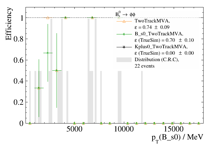
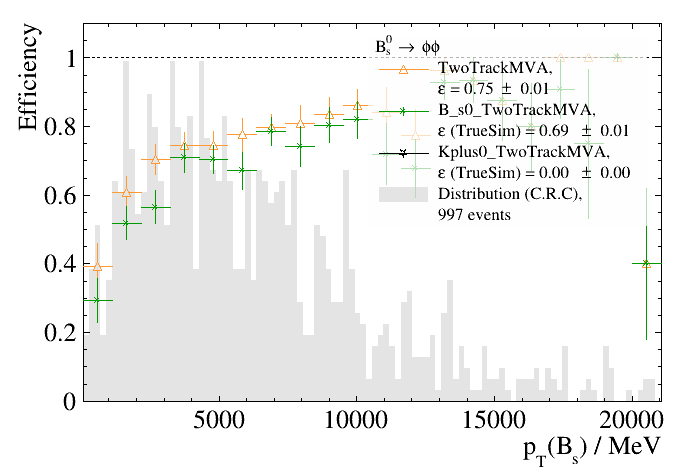
Although we could clearly do with more statistics - of the 100 events we ran over, just 25 passed the denominator requirement - we see efficiencies as a function of the parent’s \(p_{\textrm{T}}\) for the CanRecoChildren denominator (abbreviated to C.R.C). If we instead set evt_max: 5000 and use the xtitle key to make a pretty LaTeX label for the x-axis, the run will take quite a bit longer, but things look a lot better:

Note: If you prefer not to have the large legend and can remember which line is which, you can specify the no_legend: True in the analysis arguments.

Example: using the wizard to calculate HLT2 rates

The efficiencies of HLT1 serve as a simple introduction to the tool, but we expect that the main use case of this tool will be physics analysts writing HLT2 lines. This next example therefore shows how to use the tool to get the rate of a specific HLT2 line. We’ll this time follow the example decay of \(B_{s}^{0} \to J/\psi\phi\), which has an example HLT2 line written for the LHCb Starterkit. Here is the yaml config file that we’ll need:

# HltEfficiencyChecker "wizard" example for Hlt2 rates
ntuple_path: &NTUPLE hlt2_rate_ntuple.root
job:
    trigger_level: 2
    evt_max: 200
    testfiledb_key: expected_2024_min_bias_hlt1_filtered
    lines_from: Hlt2Conf.lines.topological_b
    hlt2_configuration: current_without_UT
    options:
        - $HLTEFFICIENCYCHECKERROOT/options/options_template.py.jinja  # first rendered with jinja2
analysis:
    script: $HLTEFFICIENCYCHECKERROOT/scripts/hlt_calculate_rates.py
    args:
        input: *NTUPLE
        input_rate: 1140 # See links in TestFileDB entry
        json: Hlt2_rates.json

The first thing you might notice is the absence of the annotated_decay_descriptor. We are interested in estimating the rate that a given line will fire on real data coming out of HLT1, which we simulate with HLT1-filtered minimum bias simulation. In minimum bias, all known, kinematically-accessible physics processes are possible, all of which can fire our line. The rate comes from counting all triggered events, all of which could potentially be a different process, which would all need a different decay descriptor! Given this, we can see that putting the MC truth information into a single tuple would be very difficult, and not very useful. Therefore, we don’t try to save it and thus don’t need a decay descriptor.

This time, instead of listing a script that configures the lines, we use the lines_from key, which is only supported for HLT2 and does the same job. A HLT2 reconstruction configuration has been chosen via the hlt2_configuration key, which is described more below. Finally, script now gives the path to the script that calculates rates, and we inform that script what the input rate of the sample is, which depends on if any filtering (e.g. by HLT1) was applied during the creation of the sample. The different input rates you can expect to put here is explained below). json is the name of a .json to which the rate will be saved.

There are a number of job options that we don’t require by default, but which are required to run over older samples or samples with different formats. These are:

• input_raw_format : a decimal version number telling the job how to read the input file. There is more guidance on raw formats here.

• use_old_calo_raw_banks: accepts True or False - the former asks the HLT2 calorimeter reconstruction to use an old format of the CALO raw banks. MC samples produced with the CondDB tag sim-20220614-vc-mu100 or later (see date in the tag) were produced with the new CALO raw banks. If you have such a sample, just omit the line use_old_calo_raw_banks: True entirely, and the reconstruction will know to use the new banks by default. If your file has old CALO raw banks and you do not provide use_old_calo_raw_banks: True, the calorimeter reconstruction will not find the banks - therefore do no CALO reco - but will not fail. It’s therefore important to get this right if you are reconstructing signals reliant on the calorimeters, for example electrons.

• muon_decoding_version has been updated over the years, and is (as of December 2023) at version 3 by default. Most older samples require version 2. If you provide the wrong version, the muon decoding will crash at runtime, so you will know to add this option.

• reco_from_file: True: in some very old samples in LDST format (corresponding to an input_raw_format of 4.3), the file contains reconstructed information based on a very-old Brunel reconstruction, which can be used instead of the state-of-the-art reconstruction in Moore. This is not generally recommended - this reconstruction is deprecated. In this case, you should not provide the hlt2_configuration key in addition.

Note

The configuration of the reconstruction is provided by the hlt2_configuration key, which currently supports the values current_without_UT and future_with_UT. The former is more representative of the start of 2024 data-taking conditions/expectations, whilst the latter should correspond to more nominal conditions when the UT is installed.

If the above code is put into a script with the path DaVinci/HltEfficiencyChecker/options/hlt2_rate_example.yaml, we can run as before:

DaVinci/run DaVinci/HltEfficiencyChecker/scripts/hlt_eff_checker.py DaVinci/HltEfficiencyChecker/options/hlt2_rate_example.yaml

we’ll see the printout:

--------------------------------------------------------------------------------------------------------------
INFO:   Starting /home/user/stack/DaVinci/HltEfficiencyChecker/scripts/hlt_calculate_rates.py...
--------------------------------------------------------------------------------------------------------------
INFO:   No lines specified. Defaulting to all...
HLT rates:
--------------------------------------------------------------------------------------------------------------
Line:   Hlt2Topo2BodyDecision       Incl: 11.4 +/- 8.0206 kHz, Excl: 11.4 +/- 8.0206 kHz
Line:   Hlt2Topo3BodyDecision       Incl:  5.7 +/- 5.6857 kHz, Excl:  0.0 +/- 0.0 kHz
Line:   Hlt2TopoMu2BodyDecision     Incl: 11.4 +/- 8.0206 kHz, Excl:  5.7 +/- 5.6857 kHz
Line:   Hlt2TopoMu3BodyDecision     Incl:  5.7 +/- 5.6857 kHz, Excl:  0.0 +/- 0.0 kHz
--------------------------------------------------------------------------------------------------------------
Hlt2 Total:                         Rate:   23 +/- 11.3 kHz
--------------------------------------------------------------------------------------------------------------
Finished printing HLT rates!

Note that both the inclusive rate (rate of that line firing agnostic to other lines) is returned as well as the exclusive rate (rate of firing on events that only this line fired for). There is also the total rate (rate that one or more lines fired on an event). Because the lines we’ve trigger on similar signals, the exclusive rates are sometimes smaller than the inclusive - this is typical for lines with overlapping selections. If we go into the temporary directory that has been auto-created (in this case it is called checker-20230427-141928) we’ll see:

[user@users-computer checker-20240314-151316]$ ls
Hlt2_rates.json  hlt2_rate_ntuple.root  lhcb-metainfo

How we define an efficiency

We saw above that HltEfficiencyChecker gave back two kinds of efficiency: one which had a particle prefix and a TrueSim suffix, (e.g. B_s0_Hlt1TwoTrackMVADecisionTrueSim) and one without (e.g. Hlt1TwoTrackMVADecision). The latter is defined as

\[\varepsilon = \frac{N_{\textrm{Triggered}}}{N_{\textrm{you might expect to trigger on}}} \, ,\]

whereas the former is

\[\varepsilon = \frac{N_{\textrm{Triggered & Matched}}}{N_{\textrm{you might expect to trigger on}}} \, .\]

Let’s first talk about the denominator that both of these efficiencies share. Firstly, it is subjective. One obvious choice is the total number of simulated events that you ran the trigger over. However, it is not guaranteed in these events that all the final state particles made tracks inside the detector’s fiducial acceptance, and you may not wish to count such events towards your efficiency. Furthermore, you may wish to see the effect of “offline” selection cuts on your trigger efficiency.

Both of these issues motivate the ability to make a set of selection cuts on MC truth information; to ask questions like “What is the efficiency of my shiny new line, given all the children fall inside the detector?”. Such a set of cuts is called a denominator requirement, because the denominator of the above equation is the total number of events that pass it. HltEfficiencyChecker has a pre-defined set of four such denominators:

• AllEvents: total number of events that the trigger ran over.

• CanRecoChildren: all final state children left charged, long tracks within \(2 < \eta < 5\).

• CanRecoChildrenParentCut: in addition to CanRecoChildren, the decay parent is also required to have a true decay time greater than 0.2 ps, and a minimum \(p_{\textrm{T}}\) of 2 GeV.

• CanRecoChildrenAndChildPt: in addition to CanRecoChildren, all final state children have \(p_{\textrm{T}} > 250\) MeV.

By default, efficiencies will be computed and plotted for the CanRecoChildren denominator. This can be changed using the denoms key. If none of these denominators suit your needs, you can add a new one - see Different denominators.

Now the numerator of both efficiencies. The first efficiency is a simple decision efficiency, because its numerator counts – from the subset of events that pass the denominator requirement – only the events where a positive trigger decision was made. The decision efficiency doesn’t care what fired the trigger, it would count an event where the trigger fired regardless of whether it was a signal particle that fired the trigger, or just some random noise or incorrect combination of tracks. This isn’t an ideal definition: our shiny new trigger line could be showing a high efficiency on signal MC, but there is a possibility that lots of those triggers didn’t correctly reconstruct the true signal particle. Therefore, HltEfficiencyChecker also gives you a triggered-on-true-simulated-signal (TrueSim) efficiency, which counts those events that fire the trigger and the trigger candidate “matches” to the simulated true signal particle in the event.

Matching to the true simulated signal

Please note that TrueSimEff matching will fail on neutral particles. Progress on this issue can be found in DaVinci#161, Note also that HLT1 TrueSim efficiencies are currently unavailable. Progress on this issue can be found in DaVinci#162.

“Matching” of the trigger candidate to the true MC signal particle is done by the algorithms in HltTrueSimEffAlg.cpp. In each event, it collects the LHCbIDs (which are unique identifiers for each hit that the particle left in the detector) from the true signal particle, and all the LHCbIDs from the signal candidate. It then compares these two sets of LHCbIDs on a track-by-track basis. For each track in the trigger candidate, if 70% or more of the track’s LHCbIDs match to the LHCbIDs in a track belonging to the true signal particle, then that track is matched. If every track in the trigger candidate matches to the true signal particle, then the trigger has triggered-on-signal in that event.

In our HLT1 efficiency example, we saw TrueSim efficiencies for the \(B_{s}^{0}\) and the \(K^{+}\) for each trigger line. Because the Hlt1TwoTrackMVA triggers on a two-track combination, it therefore built candidates for the two \(\phi\) particles in the decay. Conversely, the Hlt1TrackMVA triggers on a single track, so built candidates that could match to the four kaons. So we expect to see non-zero TrueSim efficiencies for the four kaons (two \(\phi\) s) in this in the TrackMVA (TwoTrackMVA) case. This is almost what we saw in that example, but the \(\phi\) TrueSim efficiencies were missing. This is because we didn’t include \(\phi\) in the true_signal_to_match_to argument, and we also didn’t ask for branches in the tree for the \(\phi\) when we gave our annotated decay descriptor. If we do true_signal_to_match_to: "B_s0,Kplus0,phi0,phi1" and add some extra branches to the annotated decay descriptor:

annotated_decay_descriptor:
    "[${B_s0}B_s0 => ${phi0}( phi(1020) => ${Kplus0}K+ ${Kminus0}K-) ${phi1}( phi(1020) => ${Kplus1}K+ ${Kminus1}K-) ]CC"

and re-run our HLT1 example, we’ll get:

------------------------------------------------------------------------------------
INFO:    Starting /home/user/stack/DaVinci/HltEfficiencyChecker/scripts/hlt_line_efficiencies.py...
------------------------------------------------------------------------------------
Integrated HLT efficiencies for the lines with denominator: CanRecoChildren
------------------------------------------------------------------------------------
Line:    B_s0_Hlt1TrackMVADecisionTrueSim        Efficiency:     0.391 +/- 0.102
Line:    B_s0_Hlt1TwoTrackMVADecisionTrueSim     Efficiency:     0.696 +/- 0.096
Line:    Hlt1TrackMVADecision                    Efficiency:     0.435 +/- 0.103
Line:    Hlt1TwoTrackMVADecision                 Efficiency:     0.739 +/- 0.092
Line:    Kplus0_Hlt1TrackMVADecisionTrueSim      Efficiency:     0.130 +/- 0.070
Line:    Kplus0_Hlt1TwoTrackMVADecisionTrueSim   Efficiency:     0.000 +/- 0.000
Line:    phi0_Hlt1TrackMVADecisionTrueSim        Efficiency:     0.217 +/- 0.086
Line:    phi0_Hlt1TwoTrackMVADecisionTrueSim     Efficiency:     0.261 +/- 0.092
Line:    phi1_Hlt1TrackMVADecisionTrueSim        Efficiency:     0.217 +/- 0.086
Line:    phi1_Hlt1TwoTrackMVADecisionTrueSim     Efficiency:     0.174 +/- 0.079
------------------------------------------------------------------------------------
Finished printing integrated HLT efficiencies for denominator: CanRecoChildren
------------------------------------------------------------------------------------

Great! But you may be wondering why there are non-zero TrueSim efficiencies for the \(B_{s}^{0}\), since neither of these lines are building a four-track candidate. This is a feature of our definition of TrueSim efficiency: we require a fraction of the trigger candidate LHCbIDs to match the true simulated signal. So if > 70% of the LHCbIDs in both tracks of two-track trigger candidate fully match any of the true signal’s tracks, it will be DecisionTrueSim == 1. This is why e.g. the TrackMVA gives positive TrueSim decisions on the final-state kaons, the intermediate \(\phi\) s, and the parent \(B_{s}^{0}\).

Note

The true_signal_to_match_to and the lines keys are your friend if you want to customize the output you get. If you don’t specify them, HltEfficiencyChecker will give you lots of efficiencies (all the combinations of all the lines you ran, all the true signal particles you can match to) and plots by default (the plots may be pretty busy as well!). The philosophy is that we’d rather give you too much information that you can switch off, as opposed to too little information with switches you have to find to add more. You can use these two arguments to help trim down the results to a more manageable/aesthetically-pleasing level.

How we define a rate

The rate of a trigger line is a much less subjective concept. It is simply the number of times per second that the line fires when it is running on real data. This is an important quantity to know because both levels of the HLT are constrained by their total output rate. We might like to loosen the cuts in our lines to be more efficient at selecting signal, but this will in turn increase the rate of that line. We estimate a line’s rate on real data by first calculating the efficiency of that line when run over minimum bias (min. bias), and then multiplying by the LHCb \(pp\) collision rate, which will be 30 MHz in Run 3. However, some minimum bias simulation, including what was used above in the HLT2 rate example, has been pre-filtered by an assumed HLT1 response. Like the real HLT1, this will throw away roughly 29-in-30 events, leaving only interesting events in the input file you’re about to process. With respect to non-HLT1-filtered MC, your HLT2 line will trigger more often on HLT1-filtered min. bias, enabling you to achieve a precise rate estimate running over fewer events and in less time. But since our HltEfficiencyChecker analysis scripts will see more triggers, we have to tell it what the input rate of the sample is (equivalently, the HLT1 output rate of the HLT1-filtering) to get the correct HLT2 output rate. This is achieved with the input_rate analysis key, which accepts a value in kHz. The default is therefore 30000. HLT1-filtered min. bias should have an input rate around 1000 kHz, but can differ between samples. For example, the expected_2024_min_bias_hlt1_filtered sample has a HLT1 output rate of 1.14 MHz, whilst the older upgrade_minbias_hlt1_filtered featured a looser HLT1 configuration and has an output rate of 1.65 MHz.

Beyond the wizard: writing and running your own options file

If you have some experience with writing options files for running Moore, and you already have some options file that you’ve written e.g. to test your new line, then you’ll be happy to learn that with a few small changes, you can use the same options file with HltEfficiencyChecker. Continuing with \(B_{s}^{0} \to J/\psi\phi\), you’ll first need to write a short script to configure your line as we saw above

from Moore import options
from Hlt2Conf.lines.topological_b import all_lines

def make_lines():
    return [builder() for builder in all_lines.values()]

options.lines_maker = make_lines

and an options file defining the input:

from Moore import options
from HltEfficiencyChecker.config import run_moore_with_tuples

# Imports for 2024-like no-UT reconstruction scenario aligned with hlt2_pp_thor_without_UT
from RecoConf.global_tools import (
    stateProvider_with_simplified_geom,
    trackMasterExtrapolator_with_simplified_geom,
)
from RecoConf.reconstruction_objects import reconstruction
from RecoConf.hlt2_global_reco import (
    reconstruction as hlt2_reconstruction,
    make_light_reco_pr_kf_without_UT,
)
from RecoConf.ttrack_selections_reco import make_ttrack_reco
from RecoConf.calorimeter_reconstruction import make_digits
from RecoConf.muonid import make_muon_hits

decay = "${Bs}[B_s0 => ( J/psi(1S) => ${mup}mu+ ${mum}mu- ) ( phi(1020) => ${Kp}K+ ${Km}K- )]CC"
options.input_files = [
    # HLT1-filtered
    # Bs -> J/psi Phi, 13144011
    # sim+std://MC/Upgrade/Beam7000GeV-Upgrade-MagDown-Nu7.6-25ns-Pythia8/Sim09c-Up02/Reco-Up01/Trig0x52000000/13144011/LDST
    "root://eoslhcb.cern.ch//eos/lhcb/grid/prod/lhcb/MC/Upgrade/LDST/00076706/0000/00076706_00000001_1.ldst",
    "root://eoslhcb.cern.ch//eos/lhcb/grid/prod/lhcb/MC/Upgrade/LDST/00076706/0000/00076706_00000002_1.ldst",
    "root://eoslhcb.cern.ch//eos/lhcb/grid/prod/lhcb/MC/Upgrade/LDST/00076706/0000/00076706_00000003_1.ldst",
    "root://eoslhcb.cern.ch//eos/lhcb/grid/prod/lhcb/MC/Upgrade/LDST/00076706/0000/00076706_00000004_1.ldst",
    "root://eoslhcb.cern.ch//eos/lhcb/grid/prod/lhcb/MC/Upgrade/LDST/00076706/0000/00076706_00000005_1.ldst",
    "root://eoslhcb.cern.ch//eos/lhcb/grid/prod/lhcb/MC/Upgrade/LDST/00076706/0000/00076706_00000006_1.ldst",
    "root://eoslhcb.cern.ch//eos/lhcb/grid/prod/lhcb/MC/Upgrade/LDST/00076706/0000/00076706_00000007_1.ldst",
    "root://eoslhcb.cern.ch//eos/lhcb/grid/prod/lhcb/MC/Upgrade/LDST/00076706/0000/00076706_00000064_1.ldst",
    "root://eoslhcb.cern.ch//eos/lhcb/grid/prod/lhcb/MC/Upgrade/LDST/00076706/0000/00076706_00000068_1.ldst",
]
options.input_type = "ROOT"
options.input_raw_format = 4.3
options.evt_max = 100

options.data_type = "Upgrade"
options.dddb_tag = "dddb-20171126"
options.conddb_tag = "sim-20171127-vc-md100"
options.ntuple_file = "hlt2_eff_ntuple.root"
options.scheduler_legacy_mode = False
options.simulation = True

make_digits.global_bind(calo_raw_bank=False)
make_muon_hits.global_bind(geometry_version=2)

public_tools = [
    trackMasterExtrapolator_with_simplified_geom(),
    stateProvider_with_simplified_geom(),
]
with reconstruction.bind(from_file=False), make_light_reco_pr_kf_without_UT.bind(
    skipRich=False, skipCalo=False, skipMuon=False
), make_ttrack_reco.bind(skipCalo=False), hlt2_reconstruction.bind(
    make_reconstruction=make_light_reco_pr_kf_without_UT
):
    run_moore_with_tuples(options, False, decay, public_tools=public_tools)

These two scripts could be put together, but we keep them separate for modularity.

If you’ve written an options file before, and you’ve followed the “wizard” examples, then hopefully you see that we’re providing all the same information, it is just specified in slightly different syntax. The most important difference is that, instead of calling run_moore() at the end of the script, we instead call run_moore_with_tuples(), which simply adds the tuple-creating tools into the control flow directly after Moore has run. The latter requires a flag that indicates whether HLT1 (True) or HLT2 (False) is running and the annotated decay descriptor, as was motivated earlier. To run the full HLT2 reconstruction, we wrap the run_moore_with_tuples call in with reconstruction.bind(from_file=False). Providing the reco_from_file key earlier amounts to putting from_file=True here. The hlt2_configuration key we provided earlier was current_without_UT, which maps to the make_light_reco_pr_kf_without_UT function and a series of binds. Alternatively, future_with_UT would map to the make_fastest_reconstruction reconstruction function. The lines:

make_digits.global_bind(calo_raw_bank=False)
make_muon_hits.global_bind(geometry_version=2)

correspond to the yaml keys use_old_calo_raw_banks and muon_decoding_version as detailed above - they are required here because the signal simulation being used is relatively old.

Assuming that the former of these scripts lives at DaVinci/HltEfficiencyChecker/options/hlt2_lines_example.py and the second at DaVinci/HltEfficiencyChecker/options/hlt2_eff_example.py, we can then pass both of these options files to gaudirun.py, in the same way you would to run Moore alone:

DaVinci/run gaudirun.py DaVinci/HltEfficiencyChecker/options/hlt2_lines_example.py DaVinci/HltEfficiencyChecker/options/hlt2_eff_example.py

which will produce the tuple eff_ntuple.root as before. Note that we haven’t used the “wizard” script hlt_eff_checker.py, so this tuple will not appear in an auto-generated temporary directory as before - it will appear in your current directory. You can then run the analysis script on the tuple when it is produced:

DaVinci/run DaVinci/HltEfficiencyChecker/scripts/hlt_line_efficiencies.py hlt2_eff_ntuple.root --reconstructible-children=Kp,Km,mup,mum --true-signal-to-match-to Bs --legend-header="B_{s} #rightarrow J/#psi #phi" --make-plots

Where we see for the first time the difference between the yaml keys and the command line arguments. This example should yield a plot that looks like this:

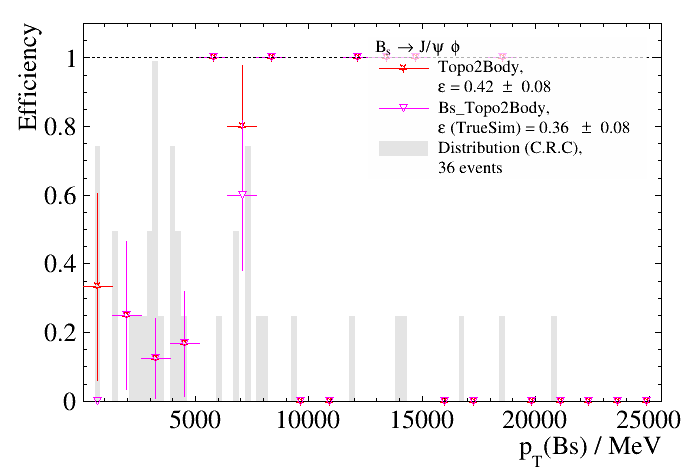
where the --true-signal-to-match-to argument was used to filter out the TrueSim efficiencies of the four final-state particles of this decay, since they will be zero for this line by our matching criteria.

The rate of this line can be calculated by first configuring a minimum bias run

from Moore import options
from HltEfficiencyChecker.config import run_moore_with_tuples

# Imports for 2024-like no-UT reconstruction scenario aligned with hlt2_pp_thor_without_UT
from RecoConf.global_tools import (
    stateProvider_with_simplified_geom,
    trackMasterExtrapolator_with_simplified_geom,
)
from RecoConf.reconstruction_objects import reconstruction
from RecoConf.hlt2_global_reco import (
    reconstruction as hlt2_reconstruction,
    make_light_reco_pr_kf_without_UT,
)
from RecoConf.ttrack_selections_reco import make_ttrack_reco

# Expected HLT1 output rate of this sample is ~1.14 MHz.
options.set_input_and_conds_from_testfiledb("expected_2024_min_bias_hlt1_filtered")
options.evt_max = 200
options.ntuple_file = "hlt2_rate_ntuple.root"
options.scheduler_legacy_mode = False
options.simulation = True

public_tools = [
    trackMasterExtrapolator_with_simplified_geom(),
    stateProvider_with_simplified_geom(),
]
with reconstruction.bind(from_file=False), make_light_reco_pr_kf_without_UT.bind(
    skipRich=False, skipCalo=False, skipMuon=False
), make_ttrack_reco.bind(skipCalo=False), hlt2_reconstruction.bind(
    make_reconstruction=make_light_reco_pr_kf_without_UT
):
    run_moore_with_tuples(options, False, public_tools=public_tools)

and then running these options (DaVinci/HltEfficiencyChecker/options/hlt2_rate_example.py) and then the rate-calculating script hlt_calculate_rates.py on rate_ntuple.root:

DaVinci/run gaudirun.py DaVinci/HltEfficiencyChecker/options/hlt2_lines_example.py DaVinci/HltEfficiencyChecker/options/hlt2_rate_example.py
DaVinci/run DaVinci/HltEfficiencyChecker/scripts/hlt_calculate_rates.py hlt2_rate_ntuple.root --input-rate 1140 --json Hlt2_rates.json

which gives the output:

--------------------------------------------------------------------------------------------------------------
INFO:    Starting /home/user/stack/DaVinci/HltEfficiencyChecker/scripts/hlt_calculate_rates.py...
--------------------------------------------------------------------------------------------------------------
INFO:    No lines specified. Defaulting to all...
HLT rates:
--------------------------------------------------------------------------------------------------------------
Line:    Hlt2Topo2BodyDecision       Incl: 11.4 +/- 8.0206 kHz, Excl: 11.4 +/- 8.0206 kHz
Line:    Hlt2Topo3BodyDecision       Incl:  5.7 +/- 5.6857 kHz, Excl:  0.0 +/- 0.0 kHz
Line:    Hlt2TopoMu2BodyDecision     Incl: 11.4 +/- 8.0206 kHz, Excl:  5.7 +/- 5.6857 kHz
Line:    Hlt2TopoMu3BodyDecision     Incl:  5.7 +/- 5.6857 kHz, Excl:  0.0 +/- 0.0 kHz
--------------------------------------------------------------------------------------------------------------
Hlt2 Total:                         Rate:    23 +/- 11.3 kHz
--------------------------------------------------------------------------------------------------------------
Finished printing HLT rates!

which is identical to what we calculated with the “wizard” earlier, reflecting that the two configurations are just two interfaces that run the same code under-the-hood.

Calculating overlaps between selections

From the ntuples produced through the wizard/options as above, the script hlt_overlap_tool.py can be used to determine the overlap between selections (e.g. trigger lines or groups of trigger lines). To answer this, we first need to consider how we quantify an overlap. This tool calculates the following quantities relating to the overlaps of selections:

Jaccard similarity index

The Jaccard similarity index between two selections, A and B, is defined as

J(A,B) = |A ∩ B| / |A ∪ B|,

where J(A,B) = 0 corresponds to mutually exclusive A and B, and J(A,B) = 1 corresponds to identical A and B. J(A,B) is typically used as it is symmetric in A and B; however, this is typically a very low value if the rates of A and B are significantly different.

Conditional probabilities

The conditional probablity between two selections, A and B, whilst not typically used alone, can provide further insight to J(A,B), particularly in cases where |A| >> |B| or |A| << |B|, and is defined as

P(A|B) = |A ∩ B| / |B|,

which is clearly not symmetric (unless A and B are identical). This can be useful in cases such as examining the overlap between inclusive and exclusive lines, where the exclusive line could be run as sprucing if a significant overlap is seen.

Exclusive intersection

The exclusive intersection of selections A, B, C, etc. is the total number of events passing a subset of lines AND not passing the remaining lines, i.e.

N(A,B,C,…) = |A ∩ B ∩ !C ∩ !…|,

where the subset {A,B} is studied here.

Inclusive intersection

The inclusive intersection of selections A, B, C, etc. is the total number of events passing a subset of lines, i.e.

N(A,B,C,…) = |A ∩ B ∩ C|,

where the subset {A,B,C} is studied here.

Running the tool

To run the tool the following are required:

• An ntuple containing decision information for lines of interest (e.g. produced as per Example: using the wizard to calculate HLT2 rates), processed at a given trigger level. This stage can be run using the wizard, just as when calculating rates.

Note

Any lines of interest must be included in tupling, either through hlt1_configuration/lines_from for HLT1/2 in the wizard or specifying a line maker.

The .yaml configuration of the wizard for overlap calculation is much the same as in the case of rate calculation. Looking at the example DaVinci/HltEfficiencyChecker/options/hlt1_overlap_example.yaml:

# HltEfficiencyChecker "wizard" example for Hlt1 overlap
ntuple_path: &NTUPLE hlt1_overlap_ntuple.root
job:
    trigger_level: 1
    evt_max: 100
    testfiledb_key: exp_24_minbias_Sim10c_magdown
    hlt1_configuration: hlt1_pp_forward_then_matching_no_ut
    options:
        - $HLTEFFICIENCYCHECKERROOT/options/options_template.py.jinja  # first rendered with jinja2
analysis:
    script: $HLTEFFICIENCYCHECKERROOT/scripts/hlt_overlap_tool.py
    args:
        input: *NTUPLE
        config: $HLTEFFICIENCYCHECKERROOT/options/hlt1_overlap_example.json

The main difference to DaVinci/HltEfficiencyChecker/options/hlt1_rate_example.yaml is in the specification of config within analysis: args. This file configures which combinations of selections the overlap metrics should be calculated over.

The tool can also be run on an existing ntuple, for example if hlt1_overlap_ntuple.root already exists, then the overlap tool can be run directly as:

DaVinci/run DaVinci/HltEfficiencyChecker/scripts/hlt_overlap_tool.py hlt1_overlap_ntuple.root DaVinci/HltEfficiencyChecker/options/hlt1_overlap_example.json

Overlap tool config files

The config file for hlt_overlap_tool.py is a .json file containing information to specify which overlaps should be computed, for example in DaVinci/HltEfficiencyChecker/options/hlt1_overlap_example.json:

{
    "path" : "hlt1_overlap_example/",
    "plot": true,
    "tables": true,
    "overlaps" : {
        "exampleLineLineOverlap" : ["Hlt1TrackMVA", "Hlt1TwoTrackMVA", "Hlt1TrackElectronMVA", "Hlt1TrackMuonMVA"],
        "exampleLineGroupOverlap" : ["Hlt1TrackMVA", "Hlt1MuonGroup"],
        "exampleGroupGroupOverlap" : ["Hlt1TrackMVAGroup", "Hlt1MuonGroup"],
        "exampleHlt1TrackMVAOverlaps" : {"intags" : ["Hlt1", "Track", "MVA"]}
    },
    "groups" : {
        "Hlt1TotalGroup" : {
            "intags" : ["Hlt1"]
        },
        "Hlt1TrackMVAGroup" : {
            "intags" : ["Hlt1","Track","MVA"]
        },
        "Hlt1MuonGroup" : {
            "intags" : ["Hlt1","Muon"]
        }
    }
}

Dissecting this config file field-by-field:

• path: the path at which to write overlap metrics.

• plot: whether to produce plots of the overlap metrics.

• tables: whether to produce human-readable tables of overlap metrics.

• tree: decay-tree in ntuple containing decision information.

• overlaps: Sets of selections (lines or groups of lines), which can be specified as a list of selections, or as a set of criteria in the syntax used for groups to identify lines.

• groups (compulsory if groups used in overlaps): groups to be used in the overlaps specified, using a set of criteria to construct a given group of lines (e.g. the lines of a given trigger). Each group may contain the following tags to identify lines.

  • intags: a list of strings, all of which must be present in a line for the line to be included, e.g. the line Hlt1TwoTrackMVA is included in Hlt1TrackMVAGroup as it contains all of "Hlt1", "Track", "MVA".

  • outtags: a list of strings, none of which must be present in a line for the line to be included, e.g. if the tag Two was added to the outtags of Hlt1TrackMVAGroup, the line Hlt1TwoTrackMVA would no longer be included.

Example: using the wizard to calculate HLT1 overlaps

Just as for rates, the wizard can be used to calculate overlaps between selections, for example HLT1 lines. The example DaVinci/HltEfficiencyChecker/options/hlt1_overlap_example.yaml can be run as:

DaVinci/run DaVinci/HltEfficiencyChecker/scripts/hlt_eff_checker.py DaVinci/HltEfficiencyChecker/options/hlt1_overlap_example.yaml

The result of which is (within the usual dated checker-YYYYMMDD-HHMMSS directory) a number of directories within hlt1_overlap_example/, one for each of the overlaps specified first. Looking at the sub-directory exampleHlt1TrackMVAOverlaps/, which examines any HLT1 line containing the keywords Track and MVA. The overlap metrics are written out to the following table:

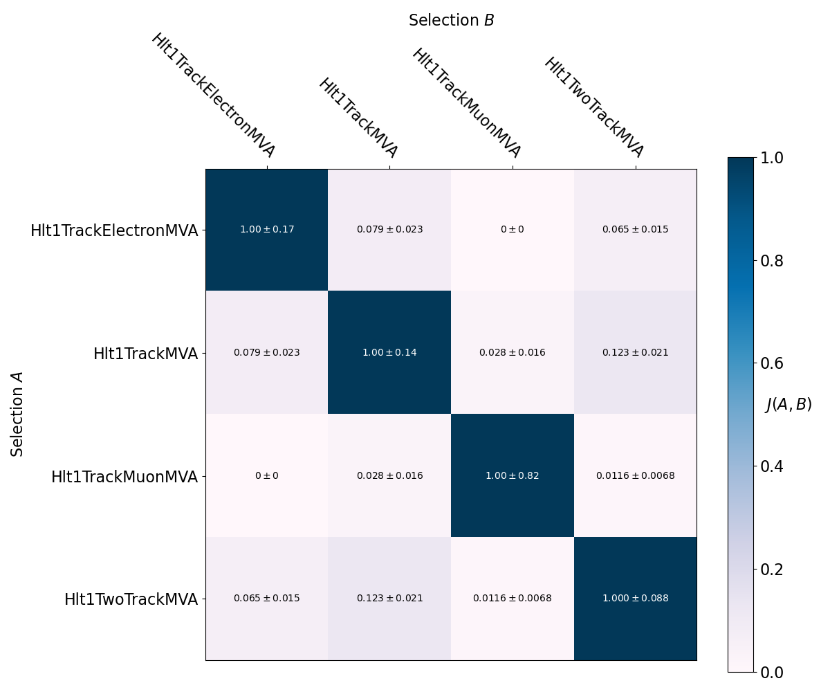
                        linesetA  countA  countA_err                      linesetB  countB  countB_err  countAnB  countAnB_err  countAuB  countAuB_err   probA|B  probA|B_err  jaccardAB  jaccardAB_err
0   Hlt1TrackElectronMVADecision      71    8.426150  Hlt1TrackElectronMVADecision      71    8.426150        71      8.426150        71      8.426150  1.000000     0.167836   1.000000       0.167836
1   Hlt1TrackElectronMVADecision      71    8.426150          Hlt1TrackMVADecision     107   10.344080        13      3.605551       165     12.845233  0.121495     0.035685   0.078788       0.022696
2   Hlt1TrackElectronMVADecision      71    8.426150      Hlt1TrackMuonMVADecision       3    1.732051         0      0.000000        74      8.602325  0.000000          NaN   0.000000            NaN
3   Hlt1TrackElectronMVADecision      71    8.426150       Hlt1TwoTrackMVADecision     258   16.062378        20      4.472136       309     17.578396  0.077519     0.017993   0.064725       0.014934
4           Hlt1TrackMVADecision     107   10.344080  Hlt1TrackElectronMVADecision      71    8.426150        13      3.605551       165     12.845233  0.183099     0.055236   0.078788       0.022696
5           Hlt1TrackMVADecision     107   10.344080          Hlt1TrackMVADecision     107   10.344080       107     10.344080       107     10.344080  1.000000     0.136717   1.000000       0.136717
6           Hlt1TrackMVADecision     107   10.344080      Hlt1TrackMuonMVADecision       3    1.732051         3      1.732051       107     10.344080  1.000000     0.816497   0.028037       0.016413
7           Hlt1TrackMVADecision     107   10.344080       Hlt1TwoTrackMVADecision     258   16.062378        40      6.324555       325     18.027756  0.155039     0.026346   0.123077       0.020623
8       Hlt1TrackMuonMVADecision       3    1.732051  Hlt1TrackElectronMVADecision      71    8.426150         0      0.000000        74      8.602325  0.000000          NaN   0.000000            NaN
9       Hlt1TrackMuonMVADecision       3    1.732051          Hlt1TrackMVADecision     107   10.344080         3      1.732051       107     10.344080  0.028037     0.016413   0.028037       0.016413
10      Hlt1TrackMuonMVADecision       3    1.732051      Hlt1TrackMuonMVADecision       3    1.732051         3      1.732051         3      1.732051  1.000000     0.816497   1.000000       0.816497
11      Hlt1TrackMuonMVADecision       3    1.732051       Hlt1TwoTrackMVADecision     258   16.062378         3      1.732051       258     16.062378  0.011628     0.006752   0.011628       0.006752
12       Hlt1TwoTrackMVADecision     258   16.062378  Hlt1TrackElectronMVADecision      71    8.426150        20      4.472136       309     17.578396  0.281690     0.071310   0.064725       0.014934
13       Hlt1TwoTrackMVADecision     258   16.062378          Hlt1TrackMVADecision     107   10.344080        40      6.324555       325     18.027756  0.373832     0.069281   0.123077       0.020623
14       Hlt1TwoTrackMVADecision     258   16.062378      Hlt1TrackMuonMVADecision       3    1.732051         3      1.732051       258     16.062378  1.000000     0.816497   0.011628       0.006752
15       Hlt1TwoTrackMVADecision     258   16.062378       Hlt1TwoTrackMVADecision     258   16.062378       258     16.062378       258     16.062378  1.000000     0.088045   1.000000       0.088045

Note

A larger sample of 10000 events have been used to produce clearer results here; DaVinci/HltEfficiencyChecker/options/hlt1_overlap_example.yaml is set up to use 100 events by default.

These overlap metrics are visualised in the following plots of J(A,B) and P(A|B):

The inclusive and exclusive intersections between each of the lines here are also calculated, for example in the following table of exclusive intersections:

    Hlt1TrackElectronMVADecision  Hlt1TrackMVADecision  Hlt1TrackMuonMVADecision  Hlt1TwoTrackMVADecision  count
0                           True                 False                     False                    False     44
1                          False                  True                     False                    False     60
2                          False                 False                      True                    False      0
3                          False                 False                     False                     True    204
4                           True                  True                     False                    False      7
5                           True                 False                      True                    False      0
6                           True                 False                     False                     True     14
7                          False                  True                      True                    False      0
8                          False                  True                     False                     True     31
9                          False                 False                      True                     True      0
10                          True                  True                      True                    False      0
11                          True                  True                     False                     True      6
12                          True                 False                      True                     True      0
13                         False                  True                      True                     True      3
14                          True                  True                      True                     True      0

Running a combined HLT1 and HLT2

When we run the real trigger on real data, the output of HLT1 becomes the input of HLT2. So, in development of a trigger line, it’s natural to ask questions like:

“What is the efficiency of my HLT2 line given Hlt1X line Z denominator?”,

and

“What is the rate of my HLT2 line given that events passed Hlt1Y line?”.

HltEfficiencyChecker can be configured to run (the Allen) HLT1 and then also HLT2, saving decisions from both levels of the trigger to your tuple. You can find example configuration files in the DaVinci/HltEfficiencyChecker/options directory: they all start with hlt1_and_hlt2. As you can imagine, the configuration files you end up writing are mostly an amalgamation of what we have already seen separately for HLT1 and HLT2. However – to help you answer questions like those posed above – there are some important new features in the analysis scripts that need some explanation.

Firstly, our efficiency-calculating script hlt_line_efficiencies.py has the argument --custom-denoms (or specify the custom_denoms key in the wizard). This accepts a comma-separated list of custom cut strings that will be applied in addition to the other denominators. For example, you could pass "Hlt1TrackMVADecision || Hlt1TwoTrackMVADecision", which would enable you to assess an Hlt2 efficiency with respect to these Hlt1 lines. To help you keep track of what custom cuts you’ve applied here, you can also pass each custom denominator a nickname by prepending a name and then a colon e.g "Hlt1TrackMVAs:Hlt1TrackMVADecision || Hlt1TwoTrackMVADecision". This is the example that is followed in DaVinci/HltEfficiencyChecker/options/hlt1_and_hlt2_eff_example.yaml. If you run that script, you should get an output that includes::

------------------------------------------------------------------------------------
INFO:    Starting /home/user/stack/DaVinci/HltEfficiencyChecker/scripts/hlt_line_efficiencies.py...
------------------------------------------------------------------------------------
Integrated HLT efficiencies for the lines with denominator: CanRecoChildren
------------------------------------------------------------------------------------
Line:    B_s0_Hlt2Topo2BodyDecisionTrueSim       Efficiency:     0.077 +/- 0.074
Line:    Hlt2Topo2BodyDecision                   Efficiency:     0.077 +/- 0.074
Line:    Kplus0_Hlt2Topo2BodyDecisionTrueSim     Efficiency:     0.000 +/- 0.000
------------------------------------------------------------------------------------
Finished printing integrated HLT efficiencies for denominator: CanRecoChildren
------------------------------------------------------------------------------------
Integrated HLT efficiencies for the lines with denominator: CanRecoChildrenAndHlt1trackmvas
------------------------------------------------------------------------------------
Line:    B_s0_Hlt2Topo2BodyDecisionTrueSim       Efficiency:     0.167 +/- 0.152
Line:    Hlt2Topo2BodyDecision                   Efficiency:     0.167 +/- 0.152
Line:    Kplus0_Hlt2Topo2BodyDecisionTrueSim     Efficiency:     0.000 +/- 0.000
------------------------------------------------------------------------------------
Finished printing integrated HLT efficiencies for denominator: CanRecoChildrenAndHlt1trackmvas
------------------------------------------------------------------------------------

where we see the expected increase in HLT2 efficiency if we require that events have first passed appropriate HLT1 lines.

Note

Notice in the quotation marks (”) given around --custom-denoms cut. Here this is explicitly required so that bash doesn’t confuse the logical OR (||) with a terminal pipe command; it ensures that everything between the quotation marks is treated as one string. As far as the author of this documentation is aware, it never hurts to add quotation marks to any of your args in this way, but usually we don’t need them. We do here.

To answer the second question, hlt_calculate_rates.py has the --filter-lines argument, which has a very similar effect to the --custom-denoms explained above. This one takes a comma-separated list of line names (no nicknames this time) which we calculate the rate with respect to (w.r.t.) i.e. at least one of these lines must pass in every considered event. This emulates the effect of e.g. HLT1 filtering out events before they reach your HLT2 lines. If you don’t care which HLT1 line let your events through, you can pass the special (case-insensitive) key word AnyHlt1Line: internally the script will just require that at least one of the HLT1 lines fired in each event it considers. This is illustrated in the example DaVinci/HltEfficiencyChecker/options/hlt1_and_hlt2_rate_example.yaml, which should have an output like:

--------------------------------------------------------------------------------------------------------------
INFO:    Starting /home/user/stack/DaVinci/HltEfficiencyChecker/scripts/hlt_calculate_rates.py...
--------------------------------------------------------------------------------------------------------------
HLT rates w.r.t. passing AnyHlt1Line:
--------------------------------------------------------------------------------------------------------------
Line:    Hlt2Topo2BodyDecision       Incl:  15.0 +/-  14.99 kHz,    Excl:   0.0 +/-   0.0 kHz
--------------------------------------------------------------------------------------------------------------
Hlt2 Total:                         Rate:    15 +/- 15.0 kHz
----------------------------------------------------------------------------------------------------

where the evt_max was turned up to 2000 events to get an appreciable rate.

Customizing your rate/efficiency results

Up until this point, we have looked at the basic features that are built-in to HltEfficiencyChecker. In this subsection, we take a look at some of the features that we hope will be useful to line developers. In addition to the features listed here, take a look at the two analysis scripts DaVinci/HltEfficiencyChecker/scripts/hlt_line_efficiencies.py and DaVinci/HltEfficiencyChecker/scripts/hlt_calculate_rates.py, in particular the arguments that they can accept in their respective get_parser() functions. If you’re calling these analysis scripts through the yaml wizard, you’ll need to translate them, which was described when we wrote our first yaml config. If you think an important feature is missing, feel free to get involved and add it in a merge request to DaVinci!

Different denominators

It was mentioned above that the “number of events that you might expect to trigger on” is a very subjective quantity, and thus the pre-defined denominators may not be enough. You can simply add a new one to the python dictionary in the get_denoms function in DaVinci/HltEfficiencyChecker/python/HltEfficiencyChecker/utils.py. For example, adding the line:

efficiency_denominators["ParentPtCutOnly"] = make_cut_string([parent_name + '_TRUEPT > 2000'])

to utils.py will define the new denominator. In the “wizard” case, use the denoms key in the set of analysis options to specify its use e.g.:

analysis:
    script: $HLTEFFICIENCYCHECKERROOT/scripts/hlt_line_efficiencies.py
    args:
        input: *NTUPLE
        reconstructible_children: muplus,muminus,Kplus,Kminus
        legend_header: "B^{0}_{s} #rightarrow J/#psi #phi"
        make_plots: true
        denoms: ParentPtCutOnly

or if calling hlt_line_efficiencies.py directly, use the --denoms argument.

Testing the inclusive rates and efficiencies of a group of lines

In the HLT2 rate examples, we saw that hlt_calculate_rates.py gives information on both the inclusive and exclusive rate of a line, as well as a total rate of the group of all the lines that were specified. You can also define further groups of lines and the script will give an inclusive rate of those groups, using the --rates-groups argument. For instance, two groups of lines could be specified as --rates-groups my_group1:line1_name,line2_name my_group2:line3_name,line4_name,line5_name. There is a similar feature in the efficiency script hlt_line_efficiencies.py: here you would pass the --effs-groups argument (effs_groups in the yaml wizard config file) followed by a similar argument e.g. --effs-groups my_group1:line1_name,line2_name my_group2:line3_name,line4_name. For every group you specify to hlt_line_efficiencies.py, you’ll see results from two groups: one that contains all the decision and TrueSim efficiencies corresponding to your specified lines, and a second one that just contains all the TrueSim efficiencies that correspond to the lines you specified (and with respect to the particles specified with --true-signal-to-match-to). The latter will be suffixed with TrueSim (e.g. my_group becomes my_groupTrueSim).

With these features it is hoped that line authors can get a feel for the overlap of lines; to see where 2 lines are perhaps doing the same job. In the future we hope to add some correlation matrices to the output of the analysis scripts, so that such this overlap can be easily visualized between every possible pair of lines.

Tweaking the parameters of your line

While you are developing your line, we expect that you’ll want to see the effect of changing the thresholds. Instructions on how you configure a line with modified thresholds are provided in the Modifying thresholds section of Writing an HLT2 line. In this way, if you configure several lines with slightly different thresholds and slightly different names, you will be able to extract rates and efficiencies of each of these new “lines” with the --lines argument of either analysis script. As of July 2020, configuring lines likes this in your options file isn’t possible with Allen, so any threshold tweaking must be done in Allen, but work is ongoing to provide this extra flexibility.

Footnotes

1

HltEfficiencyChecker once lived with the MooreAnalysis package, which was retired in December 2023. This is documented in MooreAnalysis#45.