

Compact Muon Solenoid
LHC, CERN
| CMS-B2G-15-006 ; CERN-EP-2017-102 | ||
| Search for top quark partners with charge 5/3 in proton-proton collisions at $ \sqrt{s} = $ 13 TeV | ||
| CMS Collaboration | ||
| 31 May 2017 | ||
| JHEP 08 (2017) 073 | ||
| Abstract: A search for the production of heavy partners of the top quark with charge 5/3 ($\mathrm{X}_{5/3}$) decaying into a top quark and a W boson is performed with a data sample corresponding to an integrated luminosity of 2.3 fb$^{-1}$, collected in proton-proton collisions at a center-of-mass energy of 13 TeV with the CMS detector at the CERN LHC. Final states with either a pair of same-sign leptons or a single lepton, along with jets, are considered. No significant excess is observed in the data above the expected standard model background contribution and an $\mathrm{X}_{5/3}$ quark with right-handed (left-handed) couplings is excluded at 95% confidence level for masses below 1020 (990) GeV. These are the first limits based on a combination of the same-sign dilepton and the single-lepton final states, as well as the most stringent limits on the $\mathrm{X}_{5/3}$ mass to date. | ||
| Links: e-print arXiv:1705.10967 [hep-ex] (PDF) ; CDS record ; inSPIRE record ; CADI line (restricted) ; | ||
| Figures | |
png pdf |
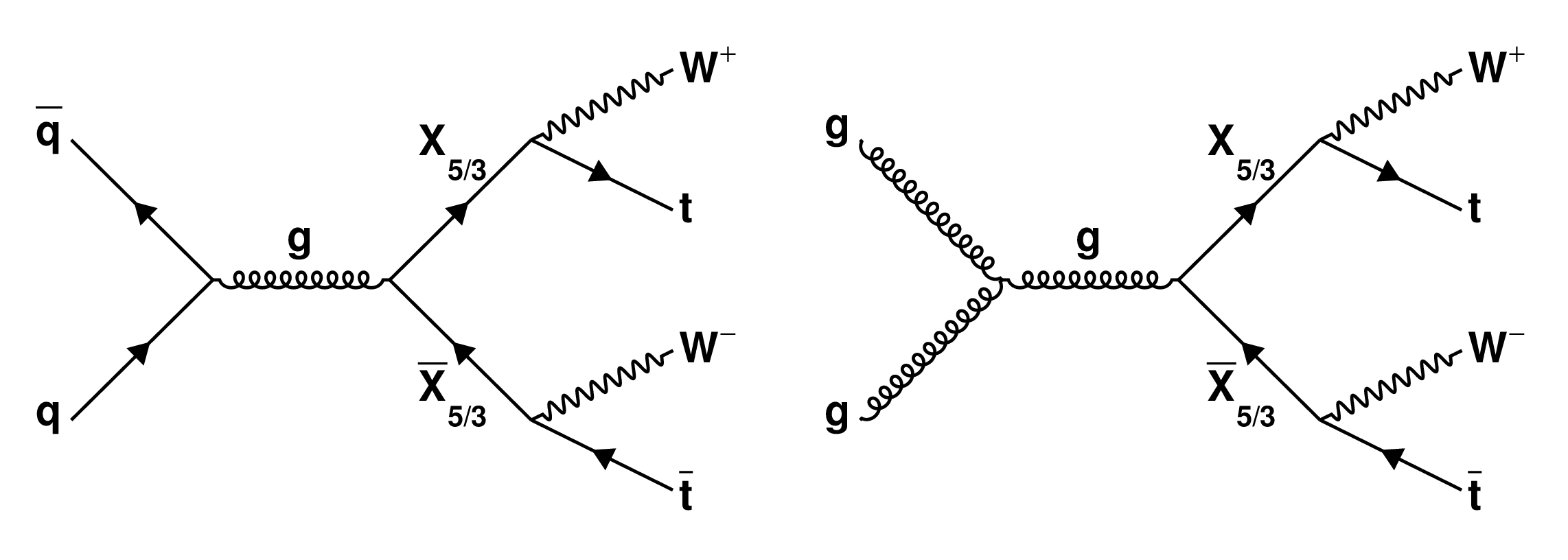
Figure 1:
Leading order Feynman diagrams for the production and decay of pairs of $ {\mathrm {X}_{5/3}} $ particles via QCD processes. |

png pdf |
Figure 1-a:
Leading order Feynman diagram for the production and decay of pairs of $ {\mathrm {X}_{5/3}} $ particles via a QCD gluon-gluon process. |

png pdf |
Figure 1-b:
Leading order Feynman diagrams for the production and decay of pairs of $ {\mathrm {X}_{5/3}} $ particles via QCD processes. |

png pdf |
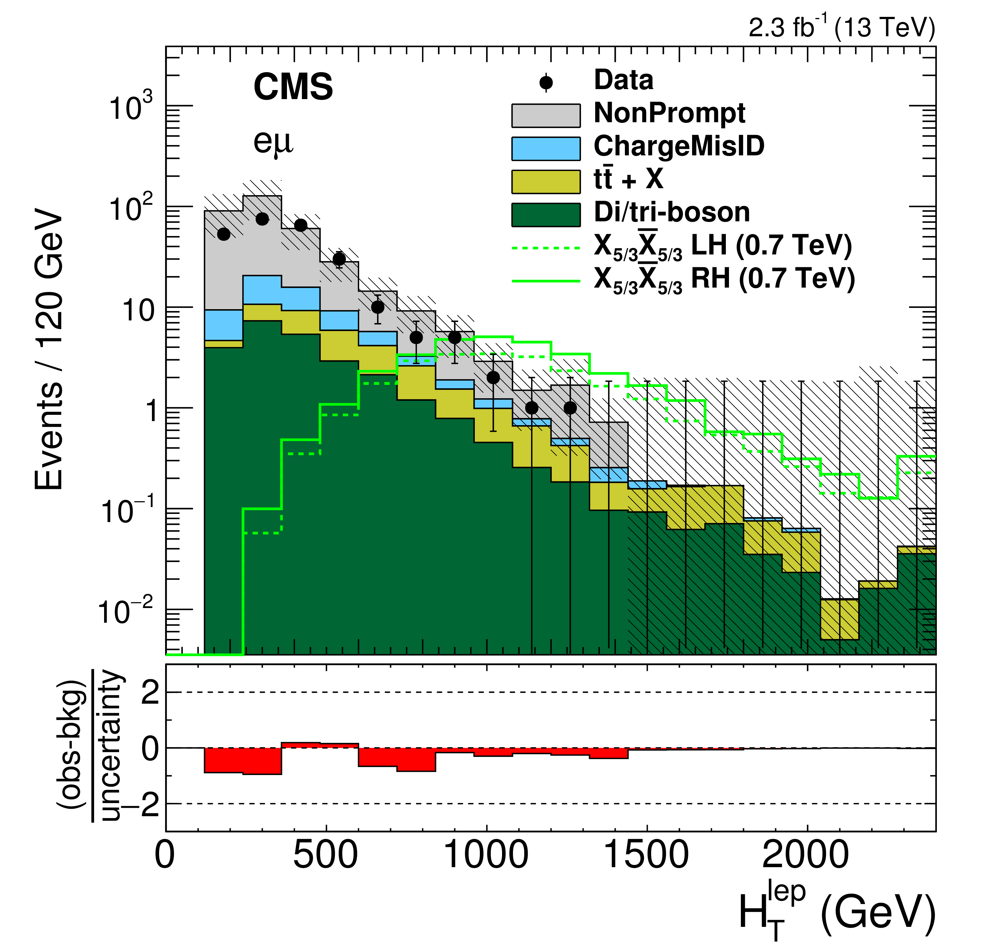
Figure 2:
The $ {H^{\text {lep}}_{\mathrm {T}}}$ distributions after the same-sign dilepton selection, Z quarkonia lepton invariant mass vetoes, and the requirement of at least two AK4 jets in the event. The hatched area shows the combined systematic and statistical uncertainty in the background prediction for each bin. The lower panel in all plots shows the difference between the observed and the predicted numbers of events divided by the total uncertainty. The total uncertainty is calculated as the sum in quadrature of the statistical uncertainty in the observed measurement and the uncertainty in the background, including both statistical and systematic components. Also shown are the distributions for a 700 GeV $ {\mathrm {X}_{5/3}} $ with right-handed (solid line) and left-handed (dashed line) couplings to W bosons. |

png pdf |
Figure 2-a:
$ {H^{\text {lep}}_{\mathrm {T}}}$ distribution (ee+e$\mu$+$\mu\mu$) after the same-sign dilepton selection, Z/quarkonia lepton invariant mass vetoes, and the requirement of at least two AK4 jets in the event. The hatched area shows the combined systematic and statistical uncertainty in the background prediction for each bin. The lower panel shows the difference between the observed and the predicted numbers of events divided by the total uncertainty. The total uncertainty is calculated as the sum in quadrature of the statistical uncertainty in the observed measurement and the uncertainty in the background, including both statistical and systematic components. Also shown are the distributions for a 700 GeV $ {\mathrm {X}_{5/3}} $ with right-handed (solid line) and left-handed (dashed line) couplings to W bosons. |

png pdf |
Figure 2-b:
$ {H^{\text {lep}}_{\mathrm {T}}}$ distribution (ee) after the same-sign dilepton selection, Z/quarkonia lepton invariant mass vetoes, and the requirement of at least two AK4 jets in the event. The hatched area shows the combined systematic and statistical uncertainty in the background prediction for each bin. The lower panel shows the difference between the observed and the predicted numbers of events divided by the total uncertainty. The total uncertainty is calculated as the sum in quadrature of the statistical uncertainty in the observed measurement and the uncertainty in the background, including both statistical and systematic components. Also shown are the distributions for a 700 GeV $ {\mathrm {X}_{5/3}} $ with right-handed (solid line) and left-handed (dashed line) couplings to W bosons. |
png pdf |
Figure 2-c:
$ {H^{\text {lep}}_{\mathrm {T}}}$ distribution (e$\mu$) after the same-sign dilepton selection, Z/quarkonia lepton invariant mass vetoes, and the requirement of at least two AK4 jets in the event. The hatched area shows the combined systematic and statistical uncertainty in the background prediction for each bin. The lower panel shows the difference between the observed and the predicted numbers of events divided by the total uncertainty. The total uncertainty is calculated as the sum in quadrature of the statistical uncertainty in the observed measurement and the uncertainty in the background, including both statistical and systematic components. Also shown are the distributions for a 700 GeV $ {\mathrm {X}_{5/3}} $ with right-handed (solid line) and left-handed (dashed line) couplings to W bosons. |

png pdf |
Figure 2-d:
$ {H^{\text {lep}}_{\mathrm {T}}}$ distribution ($\mu\mu$) after the same-sign dilepton selection, Z/quarkonia lepton invariant mass vetoes, and the requirement of at least two AK4 jets in the event. The hatched area shows the combined systematic and statistical uncertainty in the background prediction for each bin. The lower panel shows the difference between the observed and the predicted numbers of events divided by the total uncertainty. The total uncertainty is calculated as the sum in quadrature of the statistical uncertainty in the observed measurement and the uncertainty in the background, including both statistical and systematic components. Also shown are the distributions for a 700 GeV $ {\mathrm {X}_{5/3}} $ with right-handed (solid line) and left-handed (dashed line) couplings to W bosons. |

png pdf |
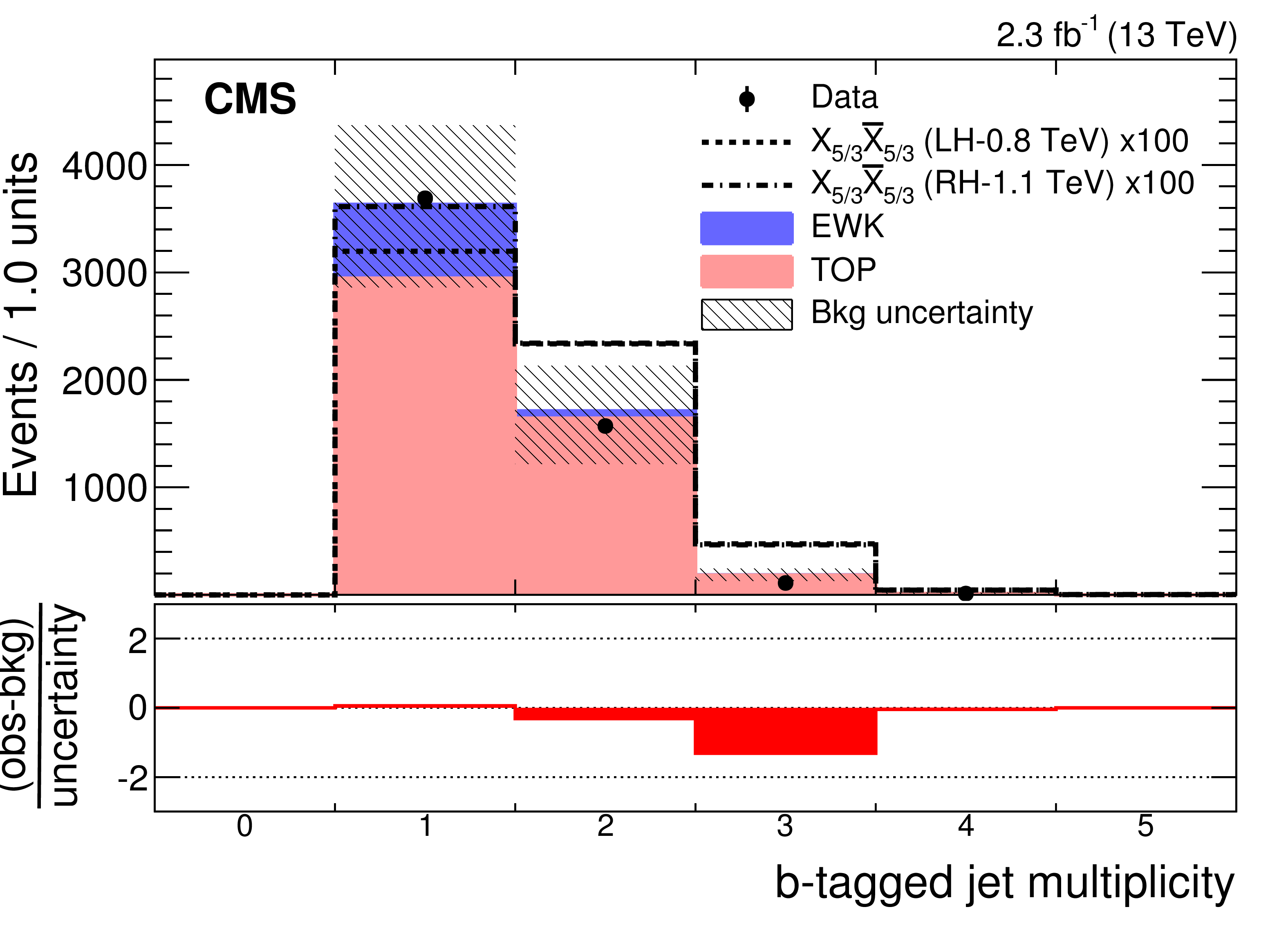
Figure 3:
Distributions of the number of AK4 jets (upper left), the numbers of b-tagged (upper right), W-tagged (lower left), and t-tagged jets (lower right) in data and simulation for combined electron and muon event samples, at the preselection level. The lower panel in all plots shows the difference between the observed and the predicted numbers of events divided by the total uncertainty. The total uncertainty is calculated as the sum in quadrature of the statistical uncertainty in the observed measurement and the uncertainty in the background, including both statistical and systematic components. Also shown are the distributions of representative signal events, which are scaled by a factor of 100. |

png pdf |
Figure 3-a:
Distribution of the number of AK4 jets in data and simulation for combined electron and muon event samples, at the preselection level. The lower panel shows the difference between the observed and the predicted numbers of events divided by the total uncertainty. The total uncertainty is calculated as the sum in quadrature of the statistical uncertainty in the observed measurement and the uncertainty in the background, including both statistical and systematic components. Also shown is the distribution of representative signal events, which are scaled by a factor of 100. |
png pdf |
Figure 3-b:
Distribution of the number of b-tagged jets in data and simulation for combined electron and muon event samples, at the preselection level. The lower panel shows the difference between the observed and the predicted numbers of events divided by the total uncertainty. The total uncertainty is calculated as the sum in quadrature of the statistical uncertainty in the observed measurement and the uncertainty in the background, including both statistical and systematic components. Also shown is the distribution of representative signal events, which are scaled by a factor of 100. |

png pdf |
Figure 3-c:
Distribution of the number of W-tagged jets in data and simulation for combined electron and muon event samples, at the preselection level. The lower panel shows the difference between the observed and the predicted numbers of events divided by the total uncertainty. The total uncertainty is calculated as the sum in quadrature of the statistical uncertainty in the observed measurement and the uncertainty in the background, including both statistical and systematic components. Also shown is the distribution of representative signal events, which are scaled by a factor of 100. |

png pdf |
Figure 3-d:
Distribution of the number of t-tagged jets in data and simulation for combined electron and muon event samples, at the preselection level. The lower panel shows the difference between the observed and the predicted numbers of events divided by the total uncertainty. The total uncertainty is calculated as the sum in quadrature of the statistical uncertainty in the observed measurement and the uncertainty in the background, including both statistical and systematic components. Also shown is the distribution of representative signal events, which are scaled by a factor of 100. |

png pdf |
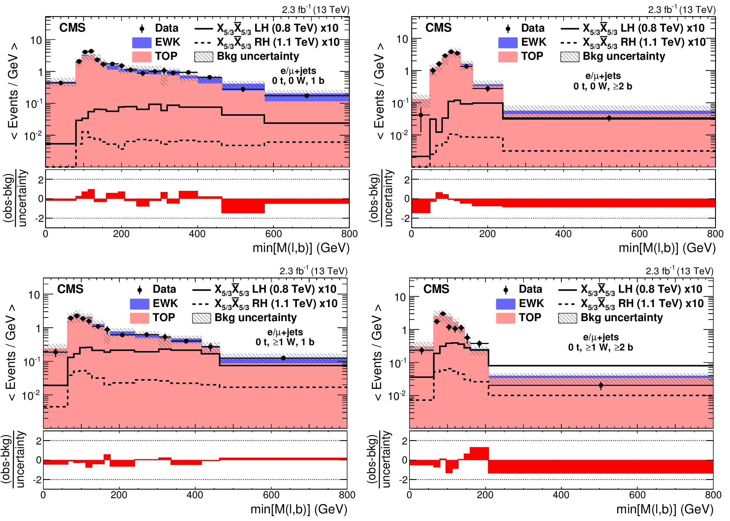
Figure 4:
Distributions of min [M($\ell, \mathrm{ b } $)] (left) and $\Delta R$($\ell $, $j_{2}$) (right) in data and simulation for selected events with at least four jets and lepton $ {p_{\mathrm {T}}} > $ 80 GeV. The lower panel in all plots shows the difference between the observed and the predicted numbers of events divided by the total uncertainty. The total uncertainty is calculated as the sum in quadrature of the statistical uncertainty in the observed measurement and the uncertainty in the background, including both statistical and systematic components. Also shown are the min [M($\ell $, $\mathrm{ b } $)] ($\Delta R$($\ell $, $j_{2}$)) distributions of representative signal events, which are scaled by a factor of 100 (50) so that the shape differences between signal and background are visible. |

png pdf |
Figure 4-a:
Distribution of min [M($\ell, \mathrm{ b } $)] in data and simulation for selected events with at least four jets and lepton $ {p_{\mathrm {T}}} > $ 80 GeV. The lower panel shows the difference between the observed and the predicted numbers of events divided by the total uncertainty. The total uncertainty is calculated as the sum in quadrature of the statistical uncertainty in the observed measurement and the uncertainty in the background, including both statistical and systematic components. Also shown is the min [M($\ell $, $\mathrm{ b } $)] distribution of representative signal events, which are scaled by a factor of 100 (50) so that the shape differences between signal and background are visible. |

png pdf |
Figure 4-b:
Distribution of $\Delta R$($\ell $, $j_{2}$) in data and simulation for selected events with at least four jets and lepton $ {p_{\mathrm {T}}} > $ 80 GeV. The lower panel shows the difference between the observed and the predicted numbers of events divided by the total uncertainty. The total uncertainty is calculated as the sum in quadrature of the statistical uncertainty in the observed measurement and the uncertainty in the background, including both statistical and systematic components. Also shown is the $\Delta R$($\ell $, $j_{2}$) distribution of representative signal events, which are scaled by a factor of 100 (50) so that the shape differences between signal and background are visible. |

png pdf |
Figure 5:
Distributions of min [M($\ell $, $\mathrm{ b } $)] in the ${\mathrm{ t } {}\mathrm{ \bar{t} } } $ control region, for 1 b-tagged jet (upper left) and $\ge $2 b-tagged jets (upper right) categories, and of min [M($\ell $, jet)] in the W+jets control region, for 0 W-tagged (lower left) and $\ge $1 W-tagged jet (lower right) categories for combined electron and muon event samples. The horizontal bars on the data points indicate the bin widths. The lower panel in all plots shows the difference between the observed and the predicted numbers of events divided by the total uncertainty. The total uncertainty is calculated as the sum in quadrature of the statistical uncertainty in the observed measurement and the uncertainty in the background, including both statistical and systematic components. A small QCD multijet contribution is displayed in the bottom left plot; in all other distributions, it is less than 0.5% and is not shown. |

png pdf |
Figure 5-a:
Distribution of min [M($\ell $, $\mathrm{ b } $)] in the ${\mathrm{ t } {}\mathrm{ \bar{t} } } $ control region, for the 1 b-tagged jet category, for combined electron and muon event samples. The horizontal bars on the data points indicate the bin widths. The lower panel shows the difference between the observed and the predicted numbers of events divided by the total uncertainty. The total uncertainty is calculated as the sum in quadrature of the statistical uncertainty in the observed measurement and the uncertainty in the background, including both statistical and systematic components. The QCD contribution is less than 0.5% and is not shown. |

png pdf |
Figure 5-b:
Distribution of min [M($\ell $, $\mathrm{ b } $)] in the ${\mathrm{ t } {}\mathrm{ \bar{t} } } $ control region, for the $\ge $2 b-tagged jets category, for combined electron and muon event samples. The horizontal bars on the data points indicate the bin widths. The lower panel shows the difference between the observed and the predicted numbers of events divided by the total uncertainty. The total uncertainty is calculated as the sum in quadrature of the statistical uncertainty in the observed measurement and the uncertainty in the background, including both statistical and systematic components. The QCD contribution is less than 0.5% and is not shown. |

png pdf |
Figure 5-c:
Distribution of min [M($\ell $, jet)] in the W+jets control region, for the 0 W-tagged category for combined electron and muon event samples. The horizontal bars on the data points indicate the bin widths. The lower panel shows the difference between the observed and the predicted numbers of events divided by the total uncertainty. The total uncertainty is calculated as the sum in quadrature of the statistical uncertainty in the observed measurement and the uncertainty in the background, including both statistical and systematic components. A small QCD multijet contribution is displayed. |

png pdf |
Figure 5-d:
Distribution of min [M($\ell $, jet)] in the W+jets control region, for the $\ge $1 W-tagged jet category for combined electron and muon event samples. The horizontal bars on the data points indicate the bin widths. The lower panel shows the difference between the observed and the predicted numbers of events divided by the total uncertainty. The total uncertainty is calculated as the sum in quadrature of the statistical uncertainty in the observed measurement and the uncertainty in the background, including both statistical and systematic components. The QCD contribution is less than 0.5% and is not shown. |
png pdf |
Figure 6:
Distributions of min [M($\ell $, $\mathrm{ b } $)] in (upper) 0 or (lower) $\ge $1 W-tagged jets and (left) 1 or (right) $\ge $2 b-tagged jets categories with 0 t-tagged jets for combined electron and muon samples, at the final selection level. The horizontal bars on the data points indicate the bin widths. The lower panel in all plots shows the difference between the observed and the predicted numbers of events divided by the total uncertainty. The total uncertainty is calculated as the sum in quadrature of the statistical uncertainty in the observed measurement and the uncertainty in the background, including both statistical and systematic components. Also shown are the distributions of representative signal events, which are scaled by a factor of 10. |

png pdf |
Figure 6-a:
Distributions of min [M($\ell $, $\mathrm{ b } $)] in the 0 W-tagged jet and 1 b-tagged jet category with 0 t-tagged jets for combined electron and muon samples, at the final selection level. The horizontal bars on the data points indicate the bin widths. The lower panel shows the difference between the observed and the predicted numbers of events divided by the total uncertainty. The total uncertainty is calculated as the sum in quadrature of the statistical uncertainty in the observed measurement and the uncertainty in the background, including both statistical and systematic components. Also shown are the distributions of representative signal events, which are scaled by a factor of 10. |

png pdf |
Figure 6-b:
Distributions of min [M($\ell $, $\mathrm{ b } $)] in the 0 W-tagged jet and $\ge $2 b-tagged jets category with 0 t-tagged jets for combined electron and muon samples, at the final selection level. The horizontal bars on the data points indicate the bin widths. The lower panel shows the difference between the observed and the predicted numbers of events divided by the total uncertainty. The total uncertainty is calculated as the sum in quadrature of the statistical uncertainty in the observed measurement and the uncertainty in the background, including both statistical and systematic components. Also shown are the distributions of representative signal events, which are scaled by a factor of 10. |

png pdf |
Figure 6-c:
Distributions of min [M($\ell $, $\mathrm{ b } $)] in the $\ge $1 W-tagged jets and 1 b-tagged jet category with 0 t-tagged jets for combined electron and muon samples, at the final selection level. The horizontal bars on the data points indicate the bin widths. The lower panel shows the difference between the observed and the predicted numbers of events divided by the total uncertainty. The total uncertainty is calculated as the sum in quadrature of the statistical uncertainty in the observed measurement and the uncertainty in the background, including both statistical and systematic components. Also shown are the distributions of representative signal events, which are scaled by a factor of 10. |

png pdf |
Figure 6-d:
Distributions of min [M($\ell $, $\mathrm{ b } $)] in the $\ge $1 W-tagged jets and $\ge $2 b-tagged jets category with 0 t-tagged jets for combined electron and muon samples, at the final selection level. The horizontal bars on the data points indicate the bin widths. The lower panel shows the difference between the observed and the predicted numbers of events divided by the total uncertainty. The total uncertainty is calculated as the sum in quadrature of the statistical uncertainty in the observed measurement and the uncertainty in the background, including both statistical and systematic components. Also shown are the distributions of representative signal events, which are scaled by a factor of 10. |

png pdf |
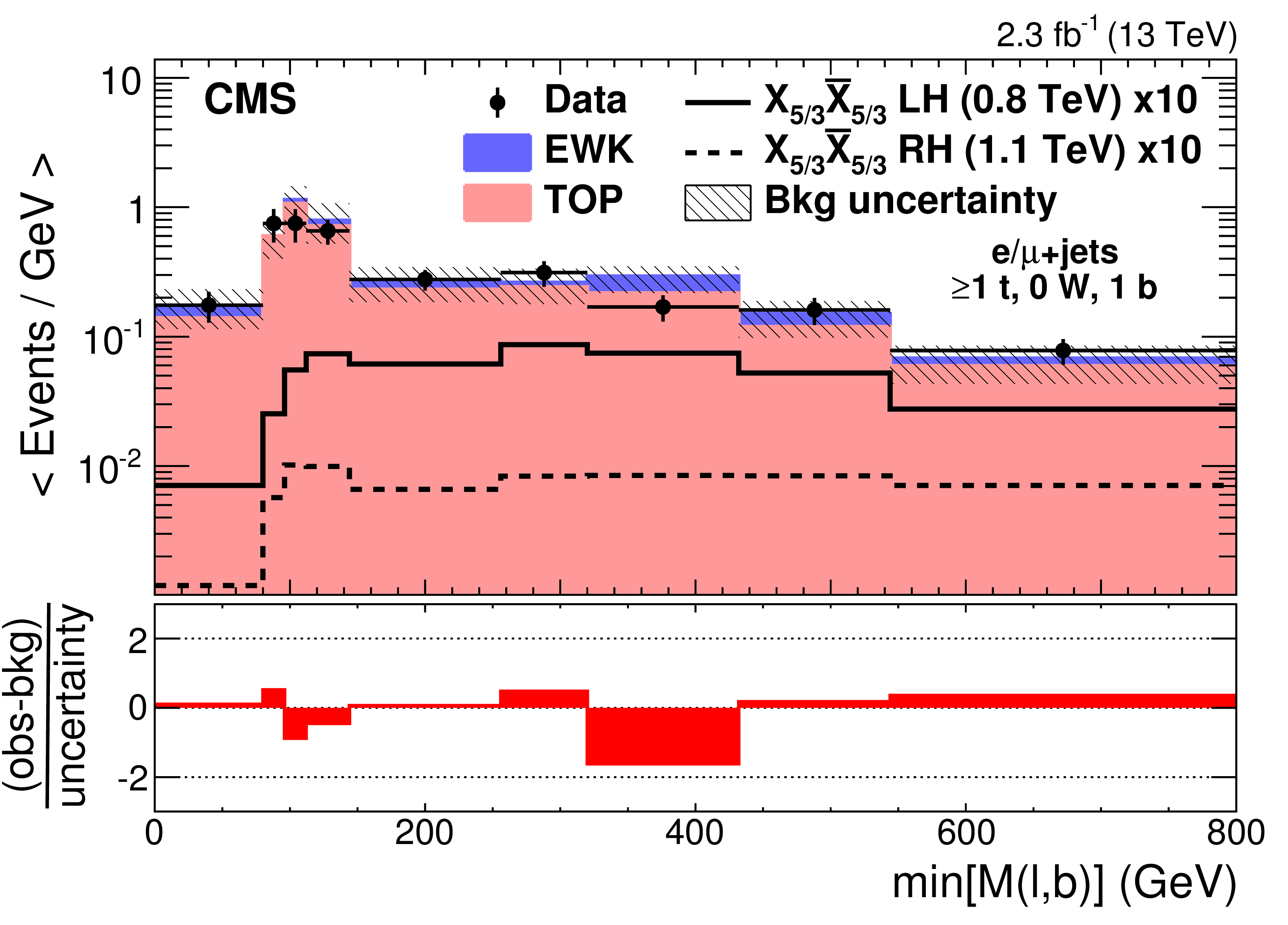
Figure 7:
Distributions of min [M($\ell $, $\mathrm{ b } $)] in 0 (upper) and $\ge $1 (lower) W-tagged jets and 1 (left) and $\ge $2 (right) b-tagged jets categories with $\ge $1 t-tagged jets for combined electron and muon samples, at the final selection level. The horizontal bars on the data points indicate the bin widths. The lower panel in all plots shows the difference between the observed and the predicted numbers of events divided by the total uncertainty. The total uncertainty is calculated as the sum in quadrature of the statistical uncertainty in the observed measurement and the uncertainty in the background, including both statistical and systematic components. Also shown are the distributions of representative signal events, which are scaled by a factor of 10. |
png pdf |
Figure 7-a:
Distributions of min [M($\ell $, $\mathrm{ b } $)] in the 0 W-tagged jet and 1 b-tagged jet category with $\ge $1 t-tagged jets for combined electron and muon samples, at the final selection level. The horizontal bars on the data points indicate the bin widths. The lower panel shows the difference between the observed and the predicted numbers of events divided by the total uncertainty. The total uncertainty is calculated as the sum in quadrature of the statistical uncertainty in the observed measurement and the uncertainty in the background, including both statistical and systematic components. Also shown are the distributions of representative signal events, which are scaled by a factor of 10. |

png pdf |
Figure 7-b:
Distributions of min [M($\ell $, $\mathrm{ b } $)] in the 0 W-tagged jet and $\ge $2 b-tagged jets category with $\ge $1 t-tagged jets for combined electron and muon samples, at the final selection level. The horizontal bars on the data points indicate the bin widths. The lower panel shows the difference between the observed and the predicted numbers of events divided by the total uncertainty. The total uncertainty is calculated as the sum in quadrature of the statistical uncertainty in the observed measurement and the uncertainty in the background, including both statistical and systematic components. Also shown are the distributions of representative signal events, which are scaled by a factor of 10. |

png pdf |
Figure 7-c:
Distributions of min [M($\ell $, $\mathrm{ b } $)] in the $\ge $1 W-tagged jet and 1 b-tagged jet category with $\ge $1 t-tagged jets for combined electron and muon samples, at the final selection level. The horizontal bars on the data points indicate the bin widths. The lower panel shows the difference between the observed and the predicted numbers of events divided by the total uncertainty. The total uncertainty is calculated as the sum in quadrature of the statistical uncertainty in the observed measurement and the uncertainty in the background, including both statistical and systematic components. Also shown are the distributions of representative signal events, which are scaled by a factor of 10. |

png pdf |
Figure 7-d:
Distributions of min [M($\ell $, $\mathrm{ b } $)] in the $\ge $1 W-tagged jet and $\ge $2 b-tagged jets category with $\ge $1 t-tagged jets for combined electron and muon samples, at the final selection level. The horizontal bars on the data points indicate the bin widths. The lower panel shows the difference between the observed and the predicted numbers of events divided by the total uncertainty. The total uncertainty is calculated as the sum in quadrature of the statistical uncertainty in the observed measurement and the uncertainty in the background, including both statistical and systematic components. Also shown are the distributions of representative signal events, which are scaled by a factor of 10. |

png pdf |
Figure 8:
The expected and observed upper limits at 95% CL for a left-handed (left) and right-handed (right) $ {\mathrm {X}_{5/3}} $ for the same-sign dilepton signature (upper) and the single-lepton signature (lower) after combining all channels in each signature. The theoretical prediction for the $ {\mathrm {X}_{5/3}} $ pair production cross section is shown as a band including its uncertainty. |

png pdf |
Figure 8-a:
The expected and observed upper limits at 95% CL for a left-handed $ {\mathrm {X}_{5/3}} $ for the same-sign dilepton signature after combining all channels in each signature. The theoretical prediction for the $ {\mathrm {X}_{5/3}} $ pair production cross section is shown as a band including its uncertainty. |

png pdf |
Figure 8-b:
The expected and observed upper limits at 95% CL for a right-handed $ {\mathrm {X}_{5/3}} $ for the same-sign dilepton signature after combining all channels in each signature. The theoretical prediction for the $ {\mathrm {X}_{5/3}} $ pair production cross section is shown as a band including its uncertainty. |

png pdf |
Figure 8-c:
The expected and observed upper limits at 95% CL for a left-handed $ {\mathrm {X}_{5/3}} $ for the single-lepton signature after combining all channels in each signature. The theoretical prediction for the $ {\mathrm {X}_{5/3}} $ pair production cross section is shown as a band including its uncertainty. |

png pdf |
Figure 8-d:
The expected and observed upper limits at 95% CL for a right-handed $ {\mathrm {X}_{5/3}} $ for the single-lepton signature after combining all channels in each signature. The theoretical prediction for the $ {\mathrm {X}_{5/3}} $ pair production cross section is shown as a band including its uncertainty. |

png pdf |
Figure 9:
The expected and observed upper limits at 95% CL after combining the same-sign dilepton and the single-lepton signatures for left-handed (left) and right-handed (right) $ {\mathrm {X}_{5/3}} $ scenarios. The theoretical prediction for the $ {\mathrm {X}_{5/3}} $ pair production cross section is shown as a band including its uncertainty. |

png pdf |
Figure 9-a:
The expected and observed upper limits at 95% CL after combining the same-sign dilepton and the single-lepton signatures for left-handed $ {\mathrm {X}_{5/3}} $ scenario. The theoretical prediction for the $ {\mathrm {X}_{5/3}} $ pair production cross section is shown as a band including its uncertainty. |

png pdf |
Figure 9-b:
The expected and observed upper limits at 95% CL after combining the same-sign dilepton and the single-lepton signatures for right-handed $ {\mathrm {X}_{5/3}} $ scenario. The theoretical prediction for the $ {\mathrm {X}_{5/3}} $ pair production cross section is shown as a band including its uncertainty. |
| Tables | |

png pdf |
Table 1:
Summary of background yields from SM processes with two same-sign prompt leptons (SSP MC), same-sign non-prompt leptons (NonPrompt), and opposite-sign prompt leptons (ChargeMisID), as well as observed data events after the full analysis selection for the same-sign dilepton channel, with an integrated luminosity of 2.3 fb$^{-1}$. Also shown are the numbers of expected events for a right-handed $ {\mathrm {X}_{5/3}} $ with a mass of 800 GeV. The uncertainties include both statistical and systematic components, as discussed in Section 7. |

png pdf |
Table 2:
Expected (observed) numbers of background (data) events passing the final selection requirements, in the eight tagging categories after combining electron and muon categories, for the single-lepton channel, with an integrated luminosity of 2.3 fb$^{-1}$. Also shown are the numbers of expected events for a LH $ {\mathrm {X}_{5/3}} $ with a mass of 800 GeV and an RH $ {\mathrm {X}_{5/3}} $ with a mass of 1.1 TeV. Uncertainties quoted in the table include both statistical as well as the systematic components listed in Table 5. The Poisson uncertainty upper bound (${<}$1.8) is used for the categories where the QCD multijet event yield is zero. |

png pdf |
Table 3:
Details of systematic uncertainties applied for lepton triggering, identification (''ID''), isolation (''ISO''), and integrated luminosity. |

png pdf |
Table 4:
Systematic uncertainties in the same-sign dilepton final state, associated with the simulated processes. The ''Normalization'' column refers to uncertainties from the cross section normalization and the choice of PDF. |

png pdf |
Table 5:
Summary of all systematic uncertainties considered in the single-lepton channel. Each uncertainty is included in both signal and all background processes unless noted otherwise. |
| Summary |
| A search has been performed for the production of heavy partners of the top quark with charge 5/3 decaying into a top quark and a W boson, using 2.3 fb$^{-1}$ of proton-proton collision data collected by the CMS experiment at 13 TeV. Events with two different signatures are analyzed: final states with either a pair of same-sign leptons or a single lepton, along with jets. No significant excess is observed in the data above the expected standard model background. Upper bounds at 95% confidence level are set on the production cross section of heavy top quark partners. The $\mathrm{X}_{5/3}$ masses with right-handed (left-handed) couplings below 1020 (990) GeV are excluded at 95% confidence level. These are the most stringent limits placed on the $\mathrm{X}_{5/3}$ mass and the first limits based on a combination of these two different final states. |
| References | ||||
| 1 | A. De Simone, O. Matsedonskyi, R. Rattazzi, and A. Wulzer | A first top partner hunter's guide | JHEP 04 (2013) 004 | 1211.5663 |
| 2 | J. Mrazek and A. Wulzer | A strong sector at the LHC: Top partners in same-sign dileptons | PRD 81 (2010) 075006 | 0909.3977 |
| 3 | G. Dissertori, E. Furlan, F. Moortgat, and P. Nef | Discovery potential of top-partners in a realistic composite Higgs model with early LHC data | JHEP 09 (2010) 019 | 1005.4414 |
| 4 | R. Contino and G. Servant | Discovering the top partners at the LHC using same-sign dilepton final states | JHEP 06 (2008) 026 | 0801.1679 |
| 5 | A. Azatov and J. Galloway | Light custodians and Higgs physics in composite models | PRD 85 (2012) 055013 | 1110.5646 |
| 6 | CMS Collaboration | Search for top-quark partners with charge 5/3 in the same-sign dilepton final state | PRL 112 (2014) 171801 | CMS-B2G-12-012 1312.2391 |
| 7 | ATLAS Collaboration | Analysis of events with $ b $-jets and a pair of leptons of the same charge in $ pp $ collisions at $ \sqrt{s} = $ 8 TeV with the ATLAS detector | JHEP 10 (2015) 150 | 1504.04605 |
| 8 | ATLAS Collaboration | Search for vector-like $ B $ quarks in events with one isolated lepton, missing transverse momentum and jets at $ \sqrt{s} = $ 8 TeV with the ATLAS detector | PRD 91 (2015) 112011 | 1503.05425 |
| 9 | CMS Collaboration | The CMS experiment at the CERN LHC | JINST 3 (2008) S08004 | CMS-00-001 |
| 10 | J. Alwall et al. | The automated computation of tree-level and next-to-leading order differential cross sections, and their matching to parton shower simulations | JHEP 07 (2014) 079 | 1405.0301 |
| 11 | P. Artoisenet, R. Frederix, O. Mattelaer, and R. Rietkerk | Automatic spin-entangled decays of heavy resonances in Monte Carlo simulations | JHEP 03 (2013) 015 | 1212.3460 |
| 12 | M. Czakon and A. Mitov | Top++: A program for the calculation of the top-pair cross-section at hadron colliders | CPC 185 (2014) 2930 | |
| 13 | M. Czakon, P. Fiedler, and A. Mitov | Total top-quark pair-production cross section at hadron colliders through $ \mathcal{O}({ {\alpha}}_{S}^{4}) $ | PRL 110 (2013) 252004 | |
| 14 | M. Czakon and A. Mitov | NNLO corrections to top pair production at hadron colliders: the quark-gluon reaction | JHEP 01 (2013) 080 | |
| 15 | M. Czakon and A. Mitov | NNLO corrections to top-pair production at hadron colliders: the all-fermionic scattering channels | JHEP 12 (2012) 054 | |
| 16 | P. Barnreuther, M. Czakon, and A. Mitov | Percent-level-precision physics at the Tevatron: Next-to-next-to-leading order QCD corrections to $ q \bar{q} \to t \bar{t} + X $ | PRL 109 (2012) 132001 | 1204.5201 |
| 17 | M. Cacciari et al. | Top-pair production at hadron colliders with next-to-next-to-leading logarithmic soft-gluon resummation | PLB 710 (2012) 612 | |
| 18 | J. Alwall et al. | Comparative study of various algorithms for the merging of parton showers and matrix elements in hadronic collisions | EPJC 53 (2008) 473 | 0706.2569 |
| 19 | R. Frederix and S. Frixione | Merging meets matching in MC@NLO | JHEP 12 (2012) 061 | 1209.6215 |
| 20 | P. Nason | A new method for combining NLO QCD with shower Monte Carlo algorithms | JHEP 11 (2004) 040 | hep-ph/0409146 |
| 21 | S. Frixione, P. Nason, and C. Oleari | Matching NLO QCD computations with parton shower simulations: the POWHEG method | JHEP 11 (2007) 070 | 0709.2092 |
| 22 | S. Alioli, P. Nason, C. Oleari, and E. Re | A general framework for implementing NLO calculations in shower Monte Carlo programs: the POWHEG BOX | JHEP 06 (2010) 043 | 1002.2581 |
| 23 | S. Alioli, S.-O. Moch, and P. Uwer | Hadronic top-quark pair-production with one jet and parton showering | JHEP 01 (2012) 137 | 1110.5251 |
| 24 | T. Sjostrand, S. Mrenna, and P. Z. Skands | A brief introduction to PYTHIA 8.1 | CPC 178 (2008) 852 | 0710.3820 |
| 25 | T. Sjostrand et al. | An introduction to PYTHIA 8.2 | CPC 191 (2015) 159 | 1410.3012 |
| 26 | NNPDF Collaboration | Parton distributions for the LHC Run II | JHEP 04 (2015) 040 | 1410.8849 |
| 27 | P. Skands, S. Carrazza, and J. Rojo | Tuning PYTHIA 8.1: the Monash 2013 tune | EPJC 74 (2014) 3024 | 1404.5630 |
| 28 | GEANT4 Collaboration | GEANT4---a simulation toolkit | NIMA 506 (2003) 250 | |
| 29 | J. Allison et al. | Geant4 developments and applications | IEEE Trans. Nucl. Sci. 53 (2006) 270 | |
| 30 | CMS Collaboration | Particle-flow reconstruction and global event description with the CMS detector | Submitted to JINST | CMS-PRF-14-001 1706.04965 |
| 31 | CMS Collaboration | Performance of electron reconstruction and selection with the CMS detector in proton-proton collisions at $ \sqrt{s} = $ 8 TeV | JINST 10 (2015) P06005 | CMS-EGM-13-001 1502.02701 |
| 32 | CMS Collaboration | Description and performance of track and primary-vertex reconstruction with the CMS tracker | JINST 9 (2014) P10009 | CMS-TRK-11-001 1405.6569 |
| 33 | W. Adam, R. Fruhwirth, A. Strandlie, and T. Todorov | Reconstruction of electrons with the Gaussian-sum filter in the CMS tracker at LHC | J. Phys G 31 (2005) N9 | physics/0306087 |
| 34 | M. Cacciari and G. P. Salam | Pileup subtraction using jet areas | PLB 659 (2008) 119 | 0707.1378 |
| 35 | CMS Collaboration | Measurement of the inclusive W and Z production cross sections in pp collisions at $ \sqrt{s} = $ 7 TeV | JHEP 10 (2011) 132 | CMS-EWK-10-005 1107.4789 |
| 36 | M. Cacciari, G. P. Salam, and G. Soyez | The anti-$ k_t $ jet clustering algorithm | JHEP 04 (2008) 063 | 0802.1189 |
| 37 | M. Cacciari, G. P. Salam, and G. Soyez | The catchment area of jets | JHEP 04 (2008) 005 | 0802.1188 |
| 38 | M. Cacciari, G. P. Salam, and G. Soyez | FastJet user manual | EPJC 72 (2012) 1896 | 1111.6097 |
| 39 | CMS Collaboration | Jet energy scale and resolution in the CMS experiment in $ \mathrm{ p }\mathrm{ p } collisions $ at 8 TeV | JINST 12 (2017) P02014 | CMS-JME-13-004 1607.03663 |
| 40 | CMS Collaboration | Search for new physics in same-sign dilepton events in proton-proton collisions at $ \sqrt{s} = $ 13 TeV | EPJC 76 (2016) 439 | CMS-SUS-15-008 1605.03171 |
| 41 | CMS Collaboration | Search for new physics with same-sign isolated dilepton events with jets and missing transverse energy at the LHC | JHEP 06 (2011) 077 | CMS-SUS-10-004 1104.3168 |
| 42 | CMS Collaboration | Identification of b quark jets at the CMS experiment in the LHC Run 2 | CMS-PAS-BTV-15-001 | CMS-PAS-BTV-15-001 |
| 43 | CMS Collaboration | Top tagging with new approaches | CMS-PAS-JME-15-002 | CMS-PAS-JME-15-002 |
| 44 | J. Thaler and K. Van Tilburg | Maximizing boosted top identification by minimizing N-subjettiness | JHEP 02 (2012) 093 | 1108.2701 |
| 45 | S. D. Ellis, C. K. Vermilion, and J. R. Walsh | Techniques for improved heavy particle searches with jet substructure | PRD 80 (2009) 051501 | 0903.5081 |
| 46 | A. J. Larkoski, S. Marzani, G. Soyez, and J. Thaler | Soft drop | JHEP 05 (2014) 146 | 1402.2657 |
| 47 | CMS Collaboration | CMS luminosity measurement for the 2015 data-taking period | CMS-PAS-LUM-15-001 | CMS-PAS-LUM-15-001 |
| 48 | J. Butterworth et al. | PDF4LHC recommendations for LHC Run II | JPG 43 (2016) 023001 | 1510.03865 |
| 49 | CMS Collaboration | Measurement of the differential cross section for top quark pair production in pp collisions at $ \sqrt{s} = $ 8 TeV | EPJC 75 (2015) 542 | CMS-TOP-12-028 1505.04480 |
| 50 | T. Muller, J. Ott, and J. Wagner-Kuhr | Theta---a framework for template-based modeling and inference | ||
|
|
Compact Muon Solenoid LHC, CERN |
|

|

|

|

|

|