

Compact Muon Solenoid
LHC, CERN
| CMS-JME-13-004 ; CERN-PH-EP-2015-305 | ||
| Jet energy scale and resolution in the CMS experiment in pp collisions at 8 TeV | ||
| CMS Collaboration | ||
| 13 July 2016 | ||
| JINST 12 (2017) P02014 | ||
| Abstract: Improved jet energy scale corrections, based on a data sample corresponding to an integrated luminosity of 19.7 fb$^{-1}$ collected by the CMS experiment in proton-proton collisions at a center-of-mass energy of 8 TeV, are presented. The corrections as a function of pseudorapidity $\eta$ and transverse momentum $p_{\mathrm{T}}$ are extracted from data and simulated events combining several channels and methods. They account successively for the effects of pileup, uniformity of the detector response, and residual data-simulation jet energy scale differences. Further corrections, depending on the jet flavor and distance parameter (jet size) $R$, are also presented. The jet energy resolution is measured in data and simulated events and is studied as a function of pileup, jet size, and jet flavor. Typical jet energy resolutions at the central rapidities are 15-20% at 30 GeV, about 10% at 100 GeV, and 5% at 1 TeV. The studies exploit events with dijet topology, as well as photon+jet, Z+jet and multijet events. Several new techniques are used to account for the various sources of jet energy scale corrections, and a full set of uncertainties, and their correlations, are provided.The final uncertainties on the jet energy scale are below 3% across the phase space considered by most analyses ($p_{\mathrm{T}}> $ 30 GeV and $| \eta| < $ 5.0). In the barrel region ($| \eta| < $ 1.3) an uncertainty below 1% for $p_{\mathrm{T}}> $ 30 GeV is reached, when excluding the jet flavor uncertainties, which are provided separately for different jet flavors. A new benchmark for jet energy scale determination at hadron colliders is achieved with 0.32% uncertainty for jets with $p_{\mathrm{T}}$ of the order of 165-330 GeV, and $| \eta| < $ 0.8. | ||
| Links: e-print arXiv:1607.03663 [hep-ex] (PDF) ; CDS record ; inSPIRE record ; CADI line (restricted) ; | ||
| Figures | |
png pdf |
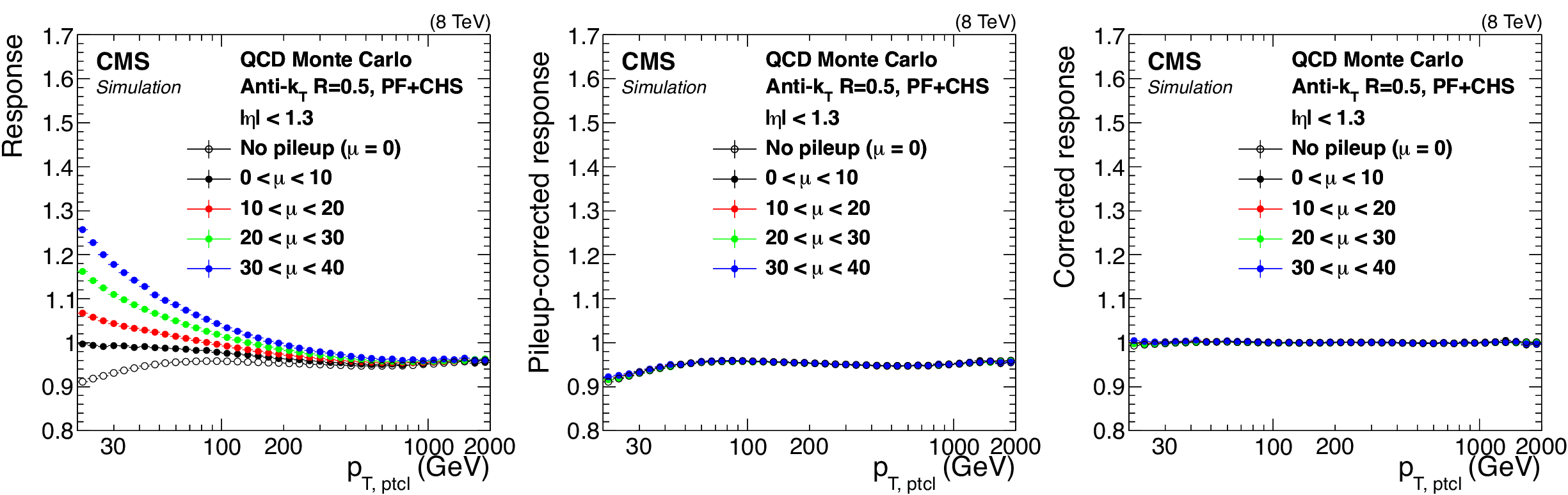
Figure 1:
Ratio of measured jet $ {p_{\mathrm {T}}} $ to particle-level jet $p_{\rm T,ptcl}$ in QCD MC simulation at various stages of JEC: before any corrections (a), after pileup offset corrections (b), after all JEC (c). Here $\mu $ is the average number of pileup interactions per bunch crossing. |
png pdf |
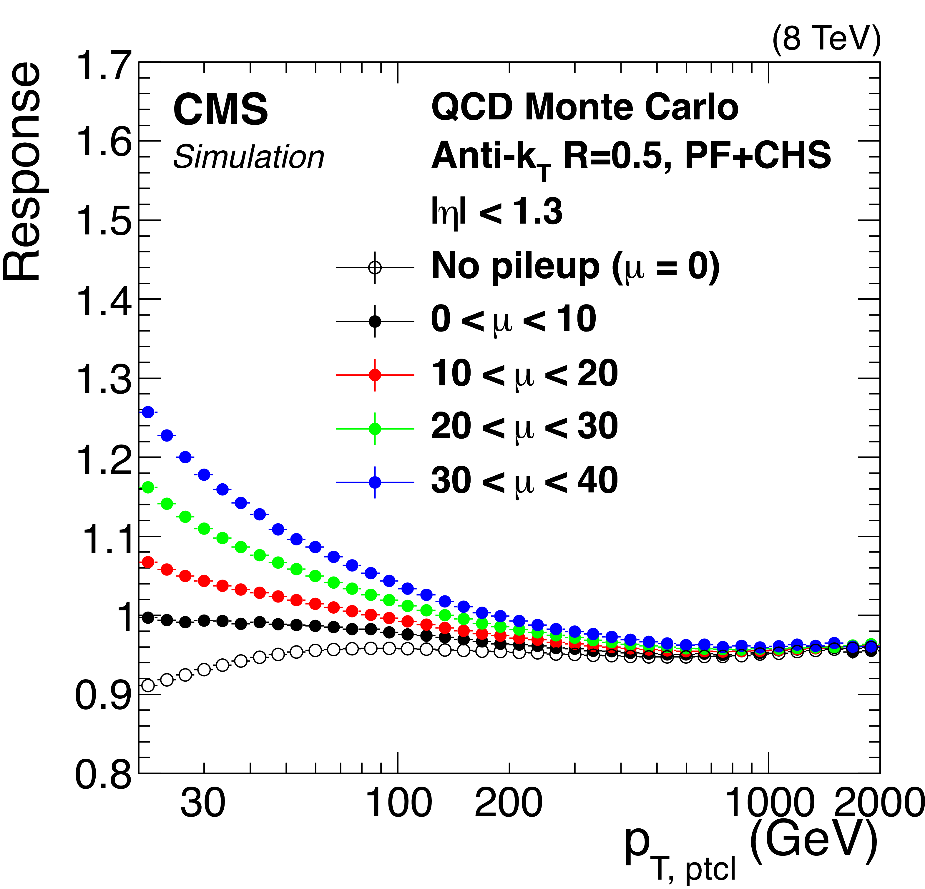
Figure 1-a:
Ratio of measured jet $ {p_{\mathrm {T}}} $ to particle-level jet $p_{\rm T,ptcl}$ in QCD MC simulation at various stages of JEC: before any corrections (a), after pileup offset corrections (b), after all JEC (c). Here $\mu $ is the average number of pileup interactions per bunch crossing. |

png pdf |
Figure 1-b:
Ratio of measured jet $ {p_{\mathrm {T}}} $ to particle-level jet $p_{\rm T,ptcl}$ in QCD MC simulation at various stages of JEC: before any corrections (a), after pileup offset corrections (b), after all JEC (c). Here $\mu $ is the average number of pileup interactions per bunch crossing. |
png pdf |
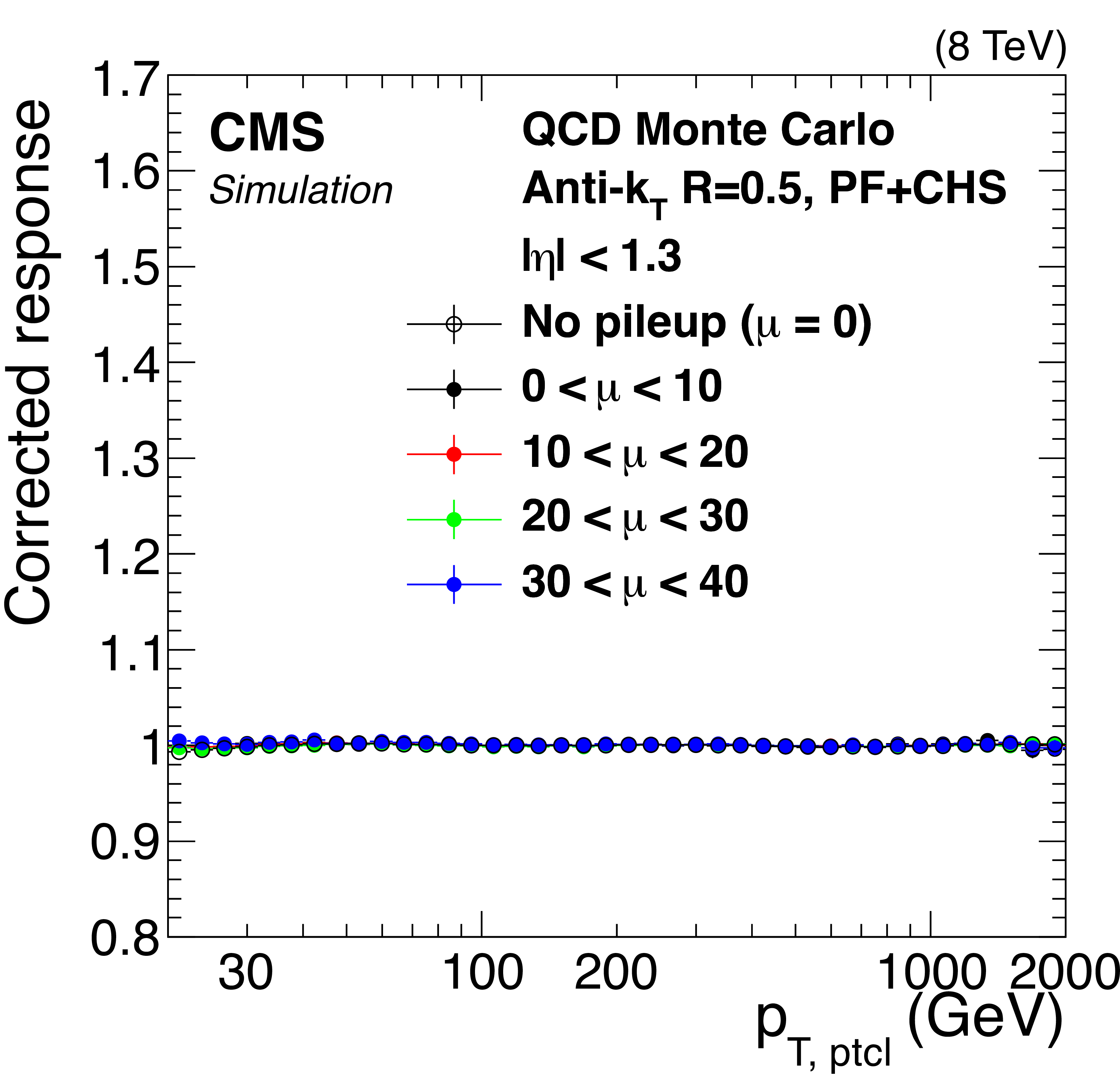
Figure 1-c:
Ratio of measured jet $ {p_{\mathrm {T}}} $ to particle-level jet $p_{\rm T,ptcl}$ in QCD MC simulation at various stages of JEC: before any corrections (a), after pileup offset corrections (b), after all JEC (c). Here $\mu $ is the average number of pileup interactions per bunch crossing. |
png pdf |
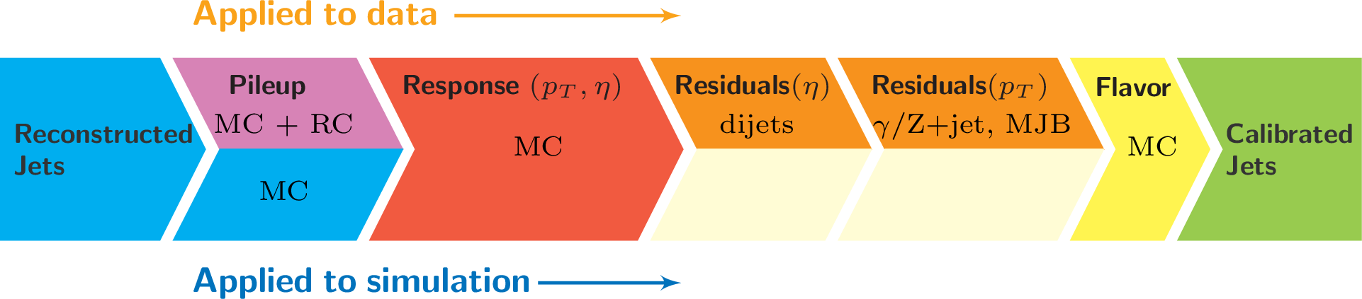
Figure 2:
Consecutive stages of JEC, for data and MC simulation. All corrections marked with MC are derived from simulation studies, RC stands for random cone, and MJB refers to the analysis of multijet events. |
png pdf |
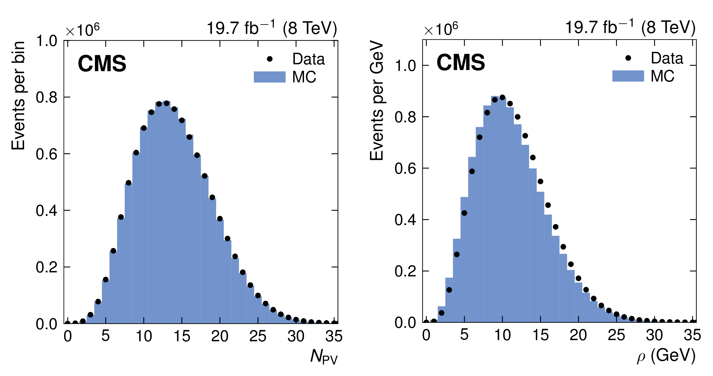
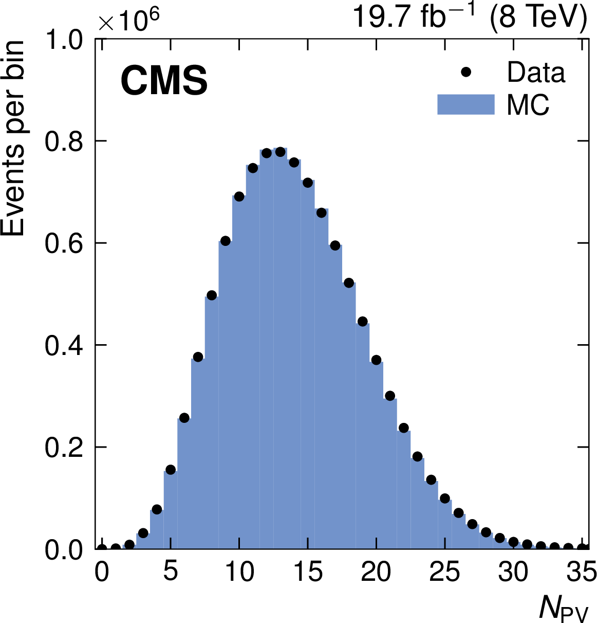
Figure 3:
Comparison of data (circles) and Pythia6.4 simulation (histograms) for the distributions of the number of reconstructed primary vertices $N_{\rm PV}$ (a), and of the offset energy density $\rho $ (b). |
png pdf |
Figure 3-a:
Comparison of data (circles) and Pythia6.4 simulation (histograms) for the distributions of the number of reconstructed primary vertices $N_{\rm PV}$ (a), and of the offset energy density $\rho $ (b). |

png pdf |
Figure 3-b:
Comparison of data (circles) and Pythia6.4 simulation (histograms) for the distributions of the number of reconstructed primary vertices $N_{\rm PV}$ (a), and of the offset energy density $\rho $ (b). |

png pdf |
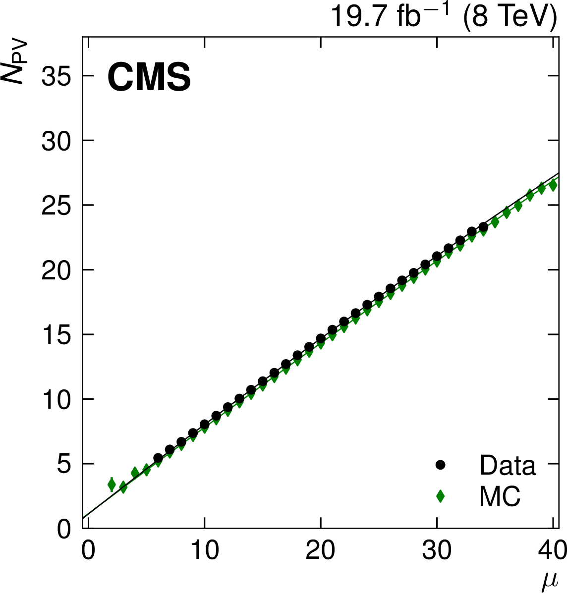
Figure 4:
Mean of the number of good primary vertices per event, $< N_{\rm PV}> $ (a), and mean diffuse offset energy density, $< \rho > $ (ribght), versus the average number of pileup interactions per bunch crossing, $\mu $, for data (circles) and Pythia6.4 simulation (diamonds). |
png pdf |
Figure 4-a:
Mean of the number of good primary vertices per event, $< N_{\rm PV}> $ (a), and mean diffuse offset energy density, $< \rho > $ (ribght), versus the average number of pileup interactions per bunch crossing, $\mu $, for data (circles) and Pythia6.4 simulation (diamonds). |

png pdf |
Figure 4-b:
Mean of the number of good primary vertices per event, $< N_{\rm PV}> $ (a), and mean diffuse offset energy density, $< \rho > $ (ribght), versus the average number of pileup interactions per bunch crossing, $\mu $, for data (circles) and Pythia6.4 simulation (diamonds). |
png pdf |
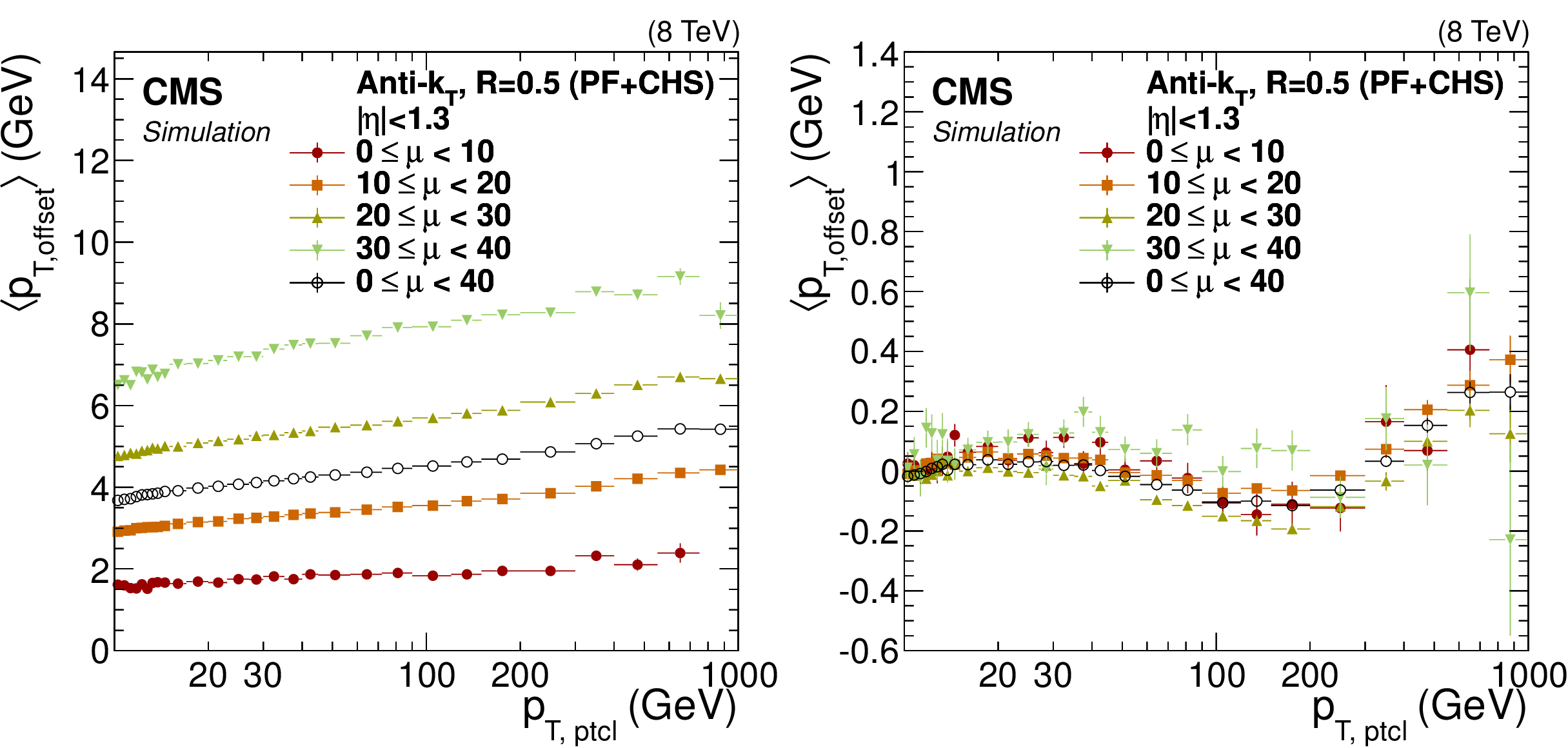
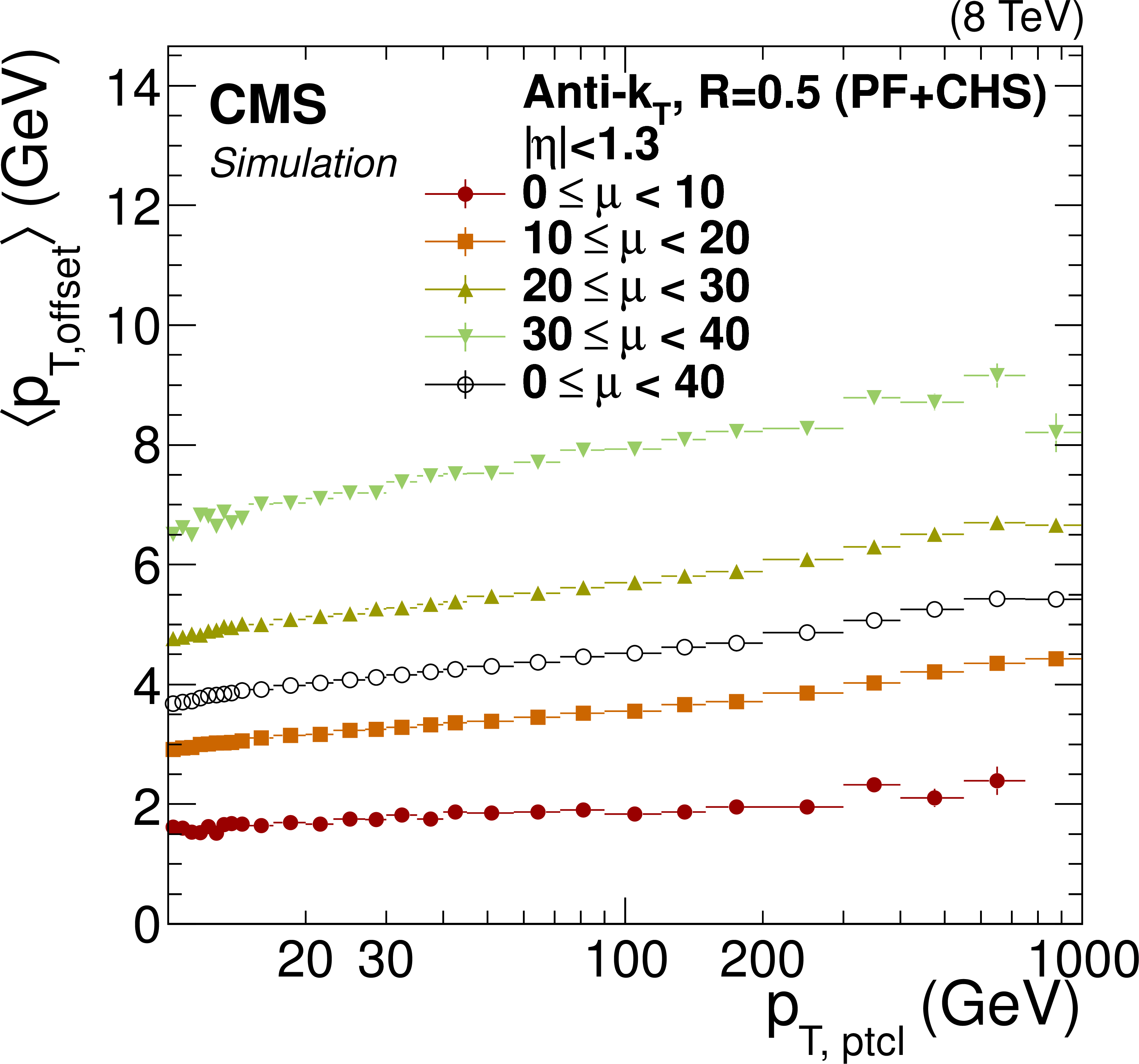
Figure 5:
Simulated particle-level offset $< p_{\rm T, offsetptcl}> $ defined in Eq.(3) (a), and residual offset after correcting for pileup with Eq.(2) (b) for $|\eta |< $ 1.3 , versus particle jet $ {p_{\mathrm {T}}} $, for different values of average number of pileup interactions per bunch crossing $< \mu > $. |
png pdf |
Figure 5-a:
Simulated particle-level offset $< p_{\rm T, offsetptcl}> $ defined in Eq.(3) (a), and residual offset after correcting for pileup with Eq.(2) (b) for $|\eta |< $ 1.3 , versus particle jet $ {p_{\mathrm {T}}} $, for different values of average number of pileup interactions per bunch crossing $< \mu > $. |

png pdf |
Figure 5-b:
Simulated particle-level offset $< p_{\rm T, offsetptcl}> $ defined in Eq.(3) (a), and residual offset after correcting for pileup with Eq.(2) (b) for $|\eta |< $ 1.3 , versus particle jet $ {p_{\mathrm {T}}} $, for different values of average number of pileup interactions per bunch crossing $< \mu > $. |
png pdf |
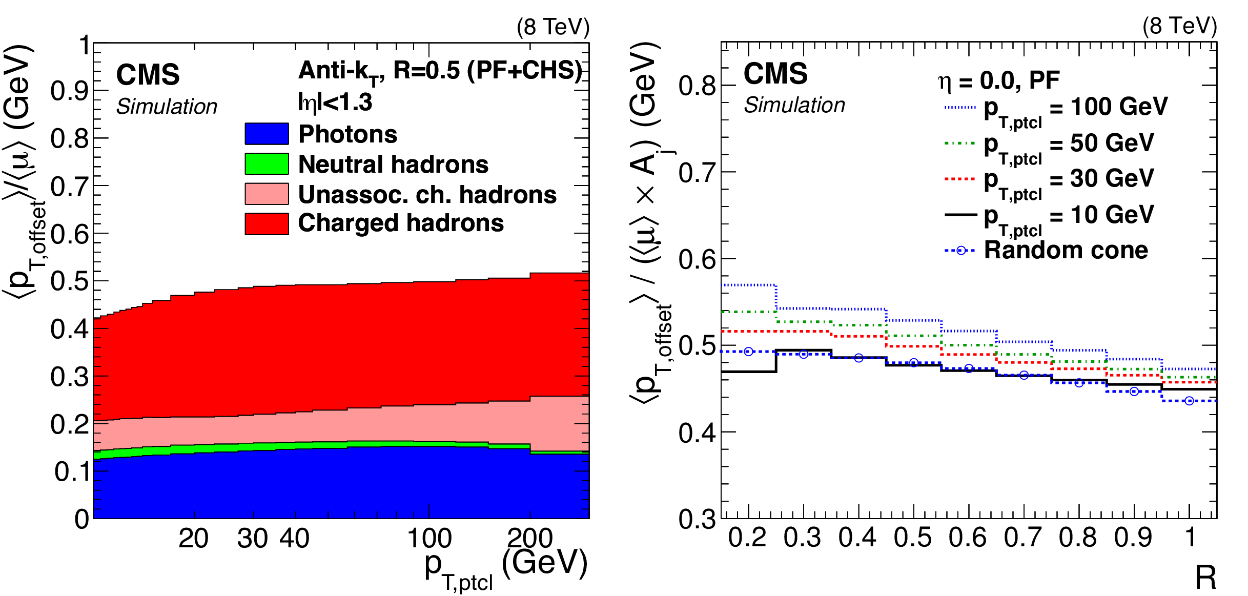
Figure 6:
Simulated particle-level offset versus $ {p_{\mathrm {T}}} $ separately for each type of PF candidate (a). Average $ {p_{\mathrm {T}}} $ offset density versus jet distance parameter $R$ for various $p_{{\rm T},\rm ptcl}$ compared to a random-cone offset density versus cone radius (b). The jet or cone area $A_j$ corresponds to $\pi R^2$. |

png pdf |
Figure 6-a:
Simulated particle-level offset versus $ {p_{\mathrm {T}}} $ separately for each type of PF candidate (a). Average $ {p_{\mathrm {T}}} $ offset density versus jet distance parameter $R$ for various $p_{{\rm T},\rm ptcl}$ compared to a random-cone offset density versus cone radius (b). The jet or cone area $A_j$ corresponds to $\pi R^2$. |

png pdf |
Figure 6-b:
Simulated particle-level offset versus $ {p_{\mathrm {T}}} $ separately for each type of PF candidate (a). Average $ {p_{\mathrm {T}}} $ offset density versus jet distance parameter $R$ for various $p_{{\rm T},\rm ptcl}$ compared to a random-cone offset density versus cone radius (b). The jet or cone area $A_j$ corresponds to $\pi R^2$. |
png pdf |
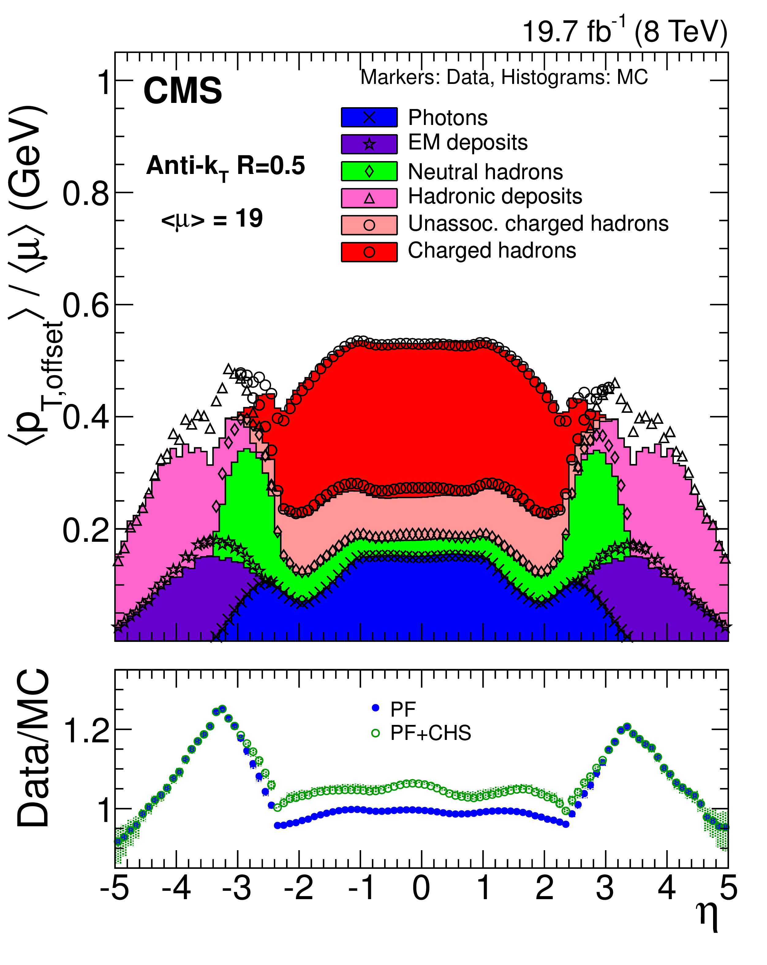
Figure 7:
Random-cone offset measured in data (markers) and MC simulation (histograms) normalized by the average number of pileup interactions $< \mu > $, separated by the type of PF candidate. The fraction labeled 'charged hadrons' is removed by CHS. The ratio of data over simulation, representing the scale factor applied for pileup offset in data, is also shown for PF and PF+CHS. |
png pdf |
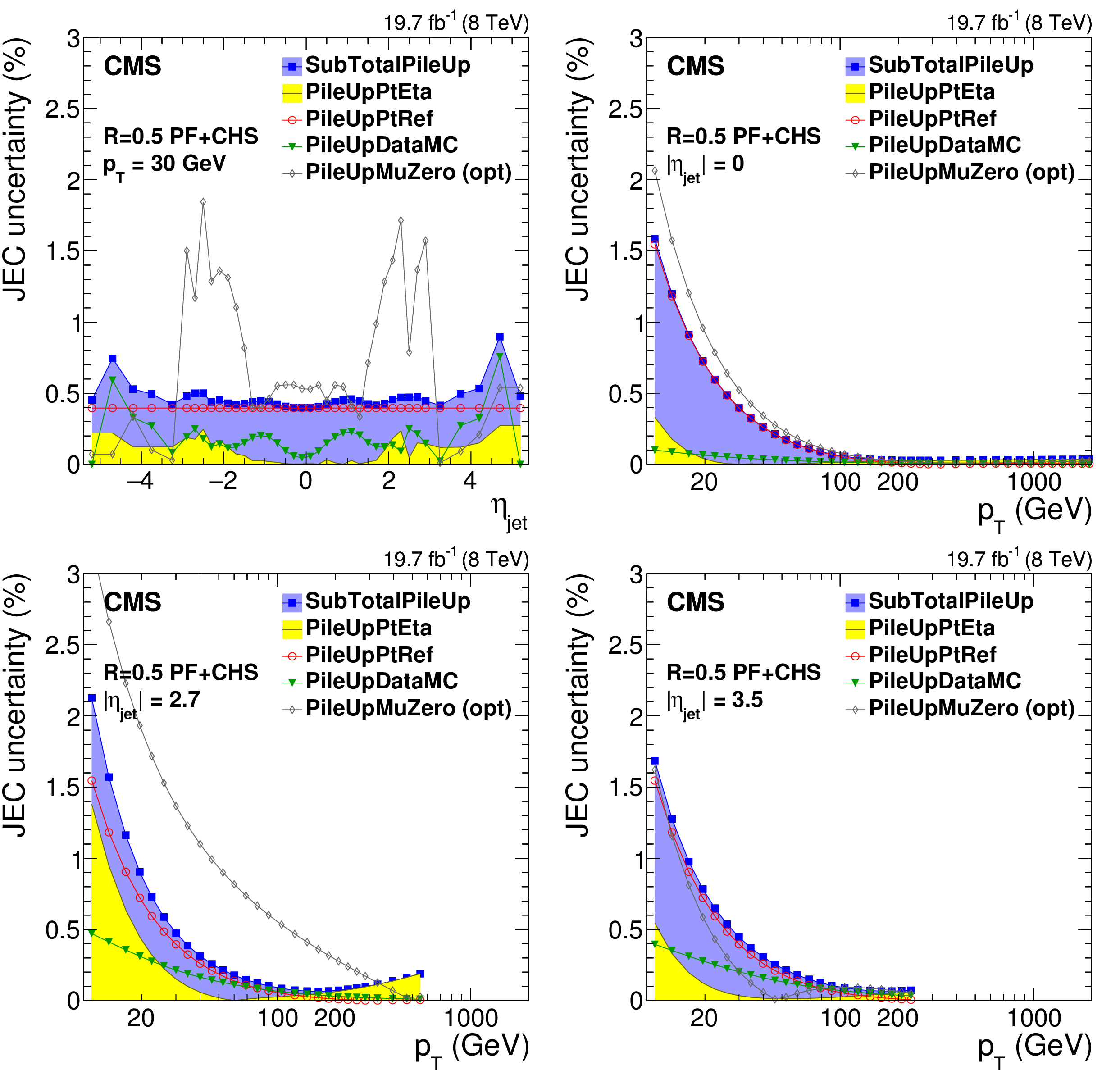
Figure 8:
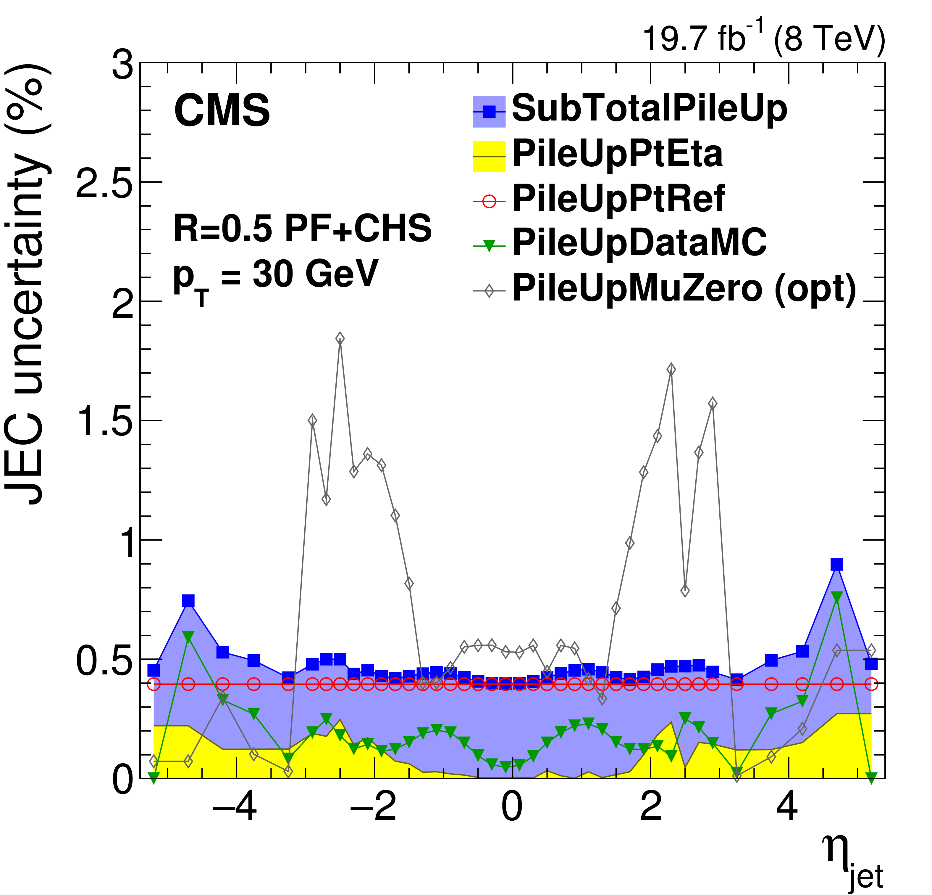
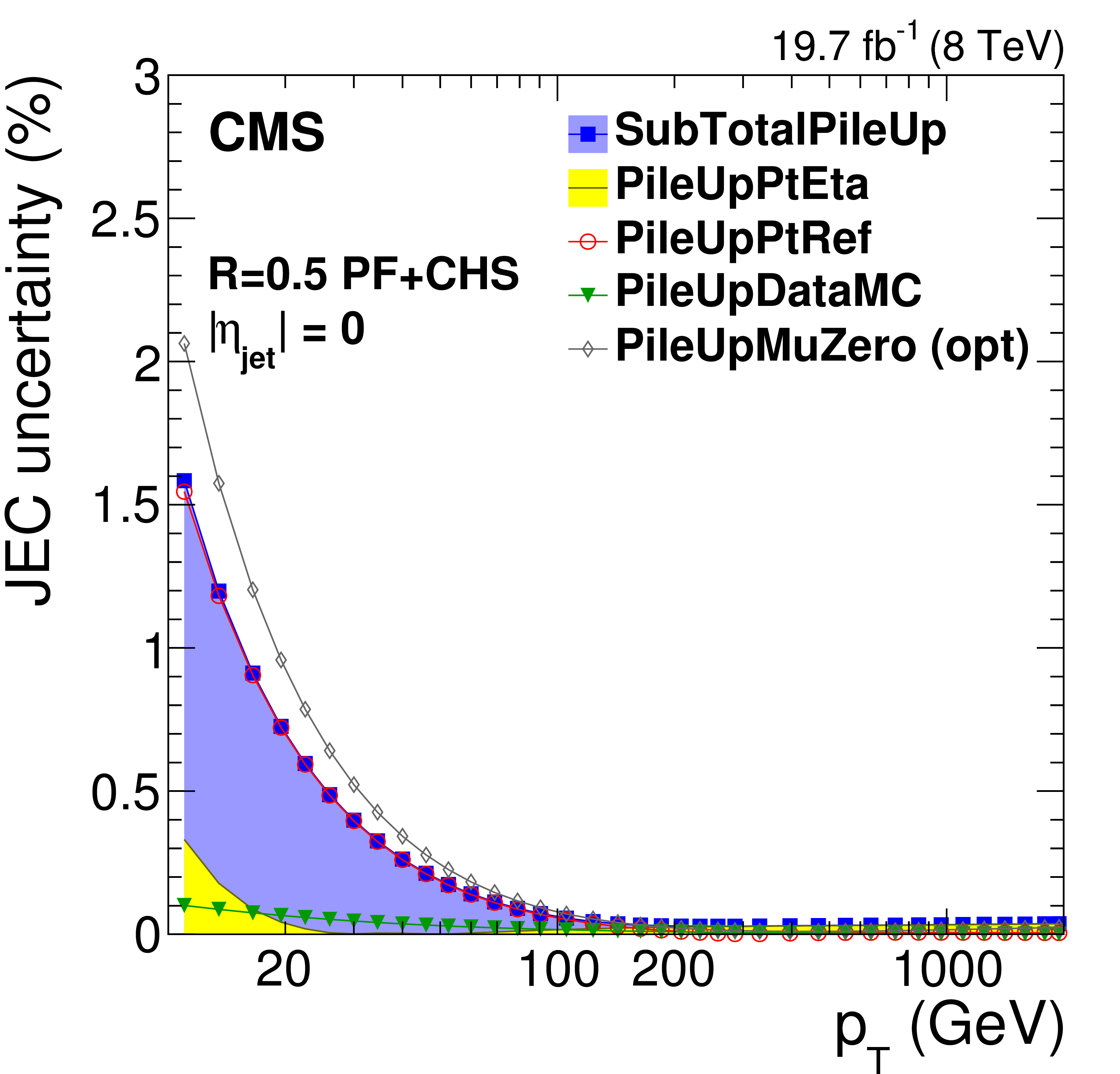
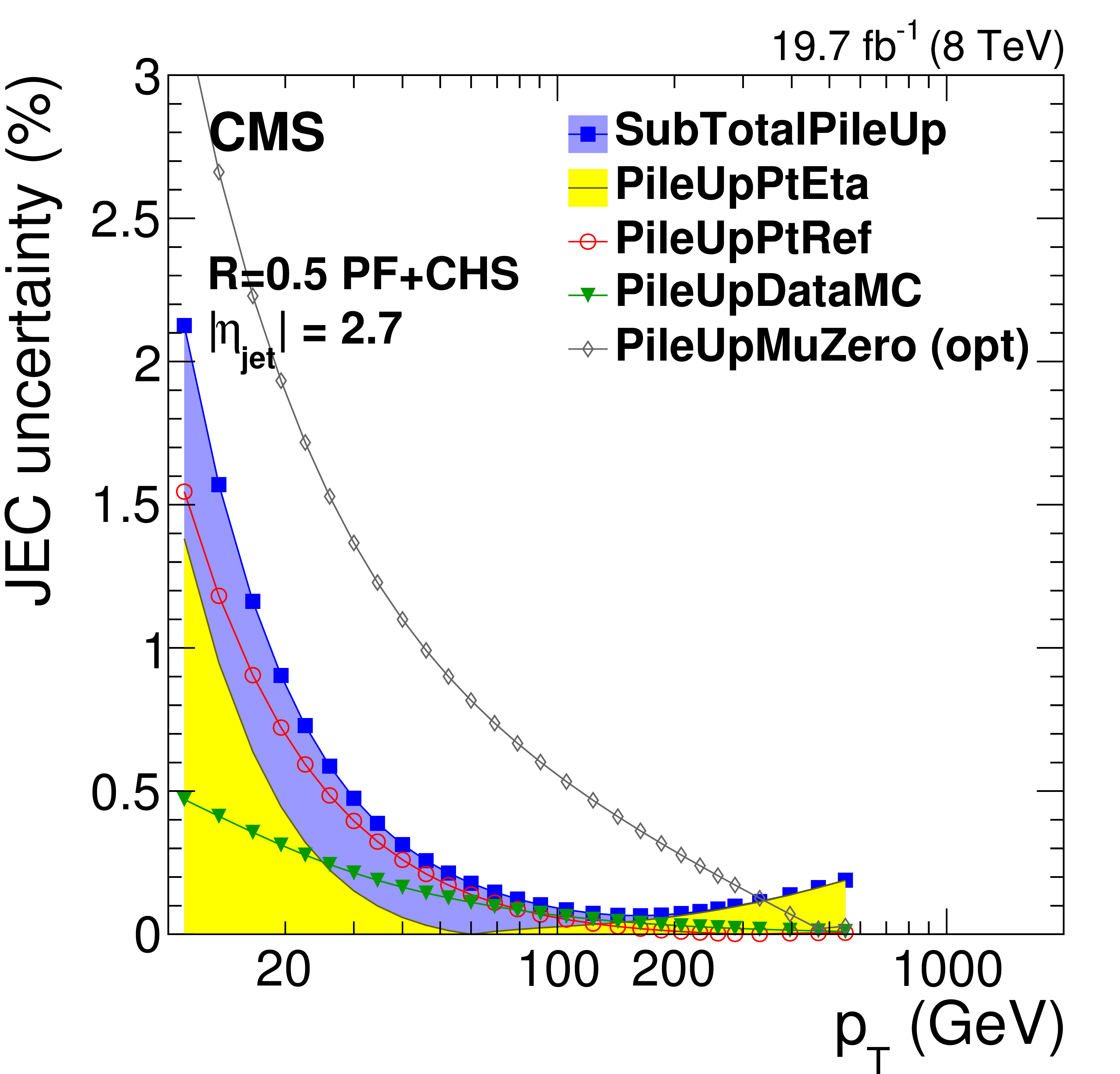
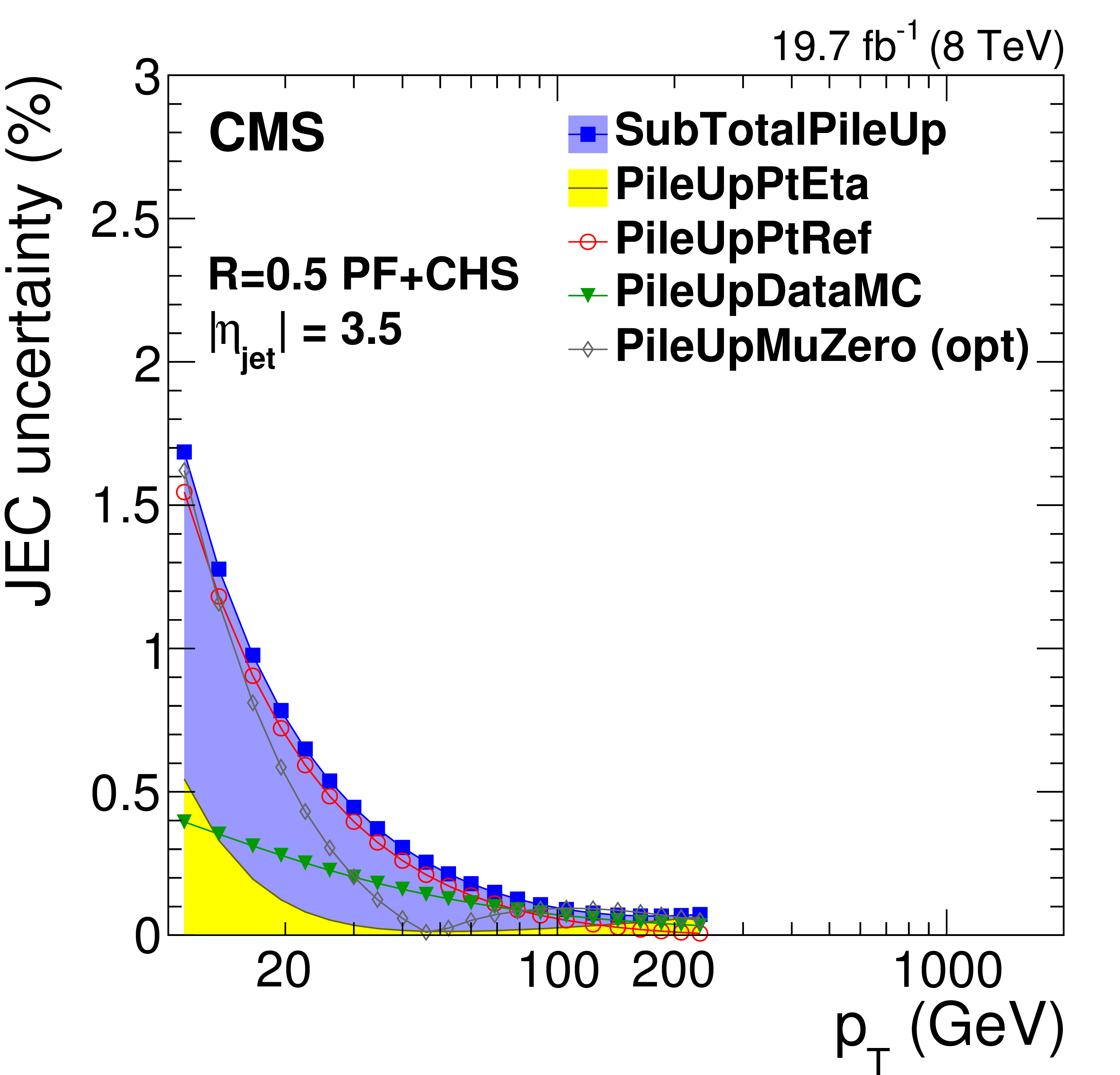
Pileup offset correction uncertainties for the average 2012 (8 TeV) conditions for PF jets with CHS and $R= $ 0.5 as a function of $\eta _{\rm jet}$ for fixed $ {p_{\mathrm {T}}} = $ 30 GeV (a) and as a function of jet $ {p_{\mathrm {T}}} $ (b, and c,d panels). The plots are limited to a jet energy $E= {p_{\mathrm {T}}} \cosh \eta = $ 4000 GeV so as to show only uncertainties for reasonable $ {p_{\mathrm {T}}} $ in the considered data-taking period. PileUpMuZero is an optional alternative uncertainty for zero-pileup ($< \mu > \approx$ 0) events, and it is therefore not included in the quadratic sum SubTotalPileUp. It accounts for the pileup uncertainty absorbed in the residual response corrections at $< \mu > \approx 20$, which is particularly prominent at 1.5 $ <|\eta |< $ 3. |
png pdf |
Figure 8-a:
Pileup offset correction uncertainties for the average 2012 (8 TeV) conditions for PF jets with CHS and $R= $ 0.5 as a function of $\eta _{\rm jet}$ for fixed $ {p_{\mathrm {T}}} = $ 30 GeV (a) and as a function of jet $ {p_{\mathrm {T}}} $ (b, and c,d panels). The plots are limited to a jet energy $E= {p_{\mathrm {T}}} \cosh \eta = $ 4000 GeV so as to show only uncertainties for reasonable $ {p_{\mathrm {T}}} $ in the considered data-taking period. PileUpMuZero is an optional alternative uncertainty for zero-pileup ($< \mu > \approx$ 0) events, and it is therefore not included in the quadratic sum SubTotalPileUp. It accounts for the pileup uncertainty absorbed in the residual response corrections at $< \mu > \approx 20$, which is particularly prominent at 1.5 $ <|\eta |< $ 3. |
png pdf |
Figure 8-b:
Pileup offset correction uncertainties for the average 2012 (8 TeV) conditions for PF jets with CHS and $R= $ 0.5 as a function of $\eta _{\rm jet}$ for fixed $ {p_{\mathrm {T}}} = $ 30 GeV (a) and as a function of jet $ {p_{\mathrm {T}}} $ (b, and c,d panels). The plots are limited to a jet energy $E= {p_{\mathrm {T}}} \cosh \eta = $ 4000 GeV so as to show only uncertainties for reasonable $ {p_{\mathrm {T}}} $ in the considered data-taking period. PileUpMuZero is an optional alternative uncertainty for zero-pileup ($< \mu > \approx$ 0) events, and it is therefore not included in the quadratic sum SubTotalPileUp. It accounts for the pileup uncertainty absorbed in the residual response corrections at $< \mu > \approx 20$, which is particularly prominent at 1.5 $ <|\eta |< $ 3. |
png pdf |
Figure 8-c:
Pileup offset correction uncertainties for the average 2012 (8 TeV) conditions for PF jets with CHS and $R= $ 0.5 as a function of $\eta _{\rm jet}$ for fixed $ {p_{\mathrm {T}}} = $ 30 GeV (a) and as a function of jet $ {p_{\mathrm {T}}} $ (b, and c,d panels). The plots are limited to a jet energy $E= {p_{\mathrm {T}}} \cosh \eta = $ 4000 GeV so as to show only uncertainties for reasonable $ {p_{\mathrm {T}}} $ in the considered data-taking period. PileUpMuZero is an optional alternative uncertainty for zero-pileup ($< \mu > \approx$ 0) events, and it is therefore not included in the quadratic sum SubTotalPileUp. It accounts for the pileup uncertainty absorbed in the residual response corrections at $< \mu > \approx 20$, which is particularly prominent at 1.5 $ <|\eta |< $ 3. |
png pdf |
Figure 8-d:
Pileup offset correction uncertainties for the average 2012 (8 TeV) conditions for PF jets with CHS and $R= $ 0.5 as a function of $\eta _{\rm jet}$ for fixed $ {p_{\mathrm {T}}} = $ 30 GeV (a) and as a function of jet $ {p_{\mathrm {T}}} $ (b, and c,d panels). The plots are limited to a jet energy $E= {p_{\mathrm {T}}} \cosh \eta = $ 4000 GeV so as to show only uncertainties for reasonable $ {p_{\mathrm {T}}} $ in the considered data-taking period. PileUpMuZero is an optional alternative uncertainty for zero-pileup ($< \mu > \approx$ 0) events, and it is therefore not included in the quadratic sum SubTotalPileUp. It accounts for the pileup uncertainty absorbed in the residual response corrections at $< \mu > \approx 20$, which is particularly prominent at 1.5 $ <|\eta |< $ 3. |
png pdf |
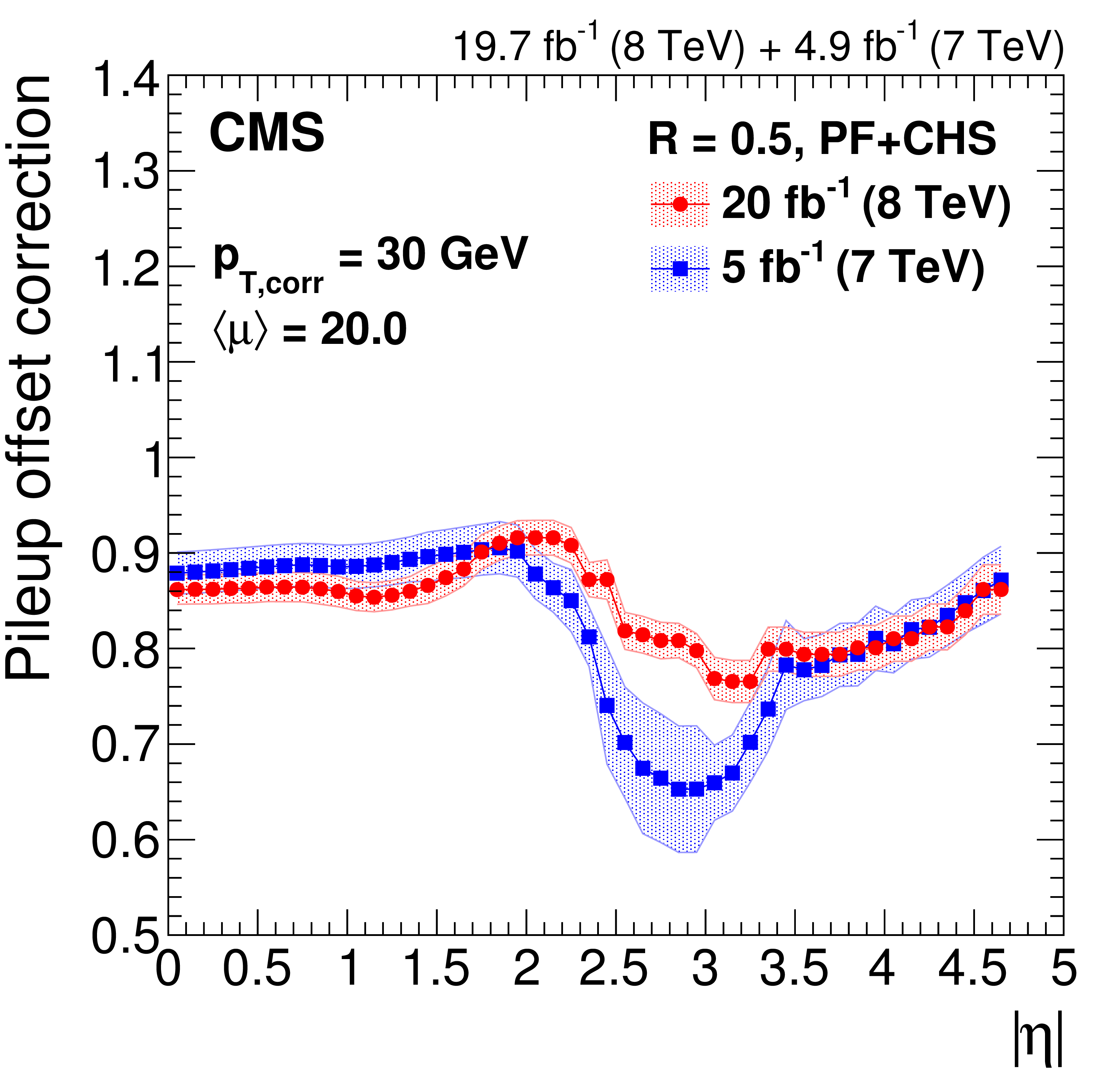
Figure 9:
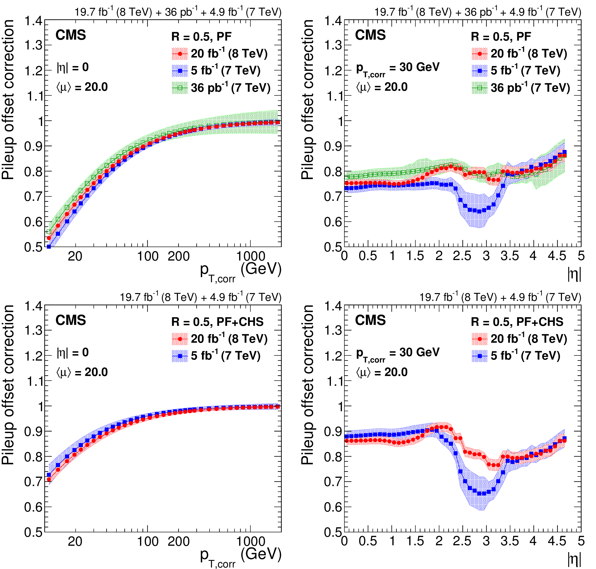
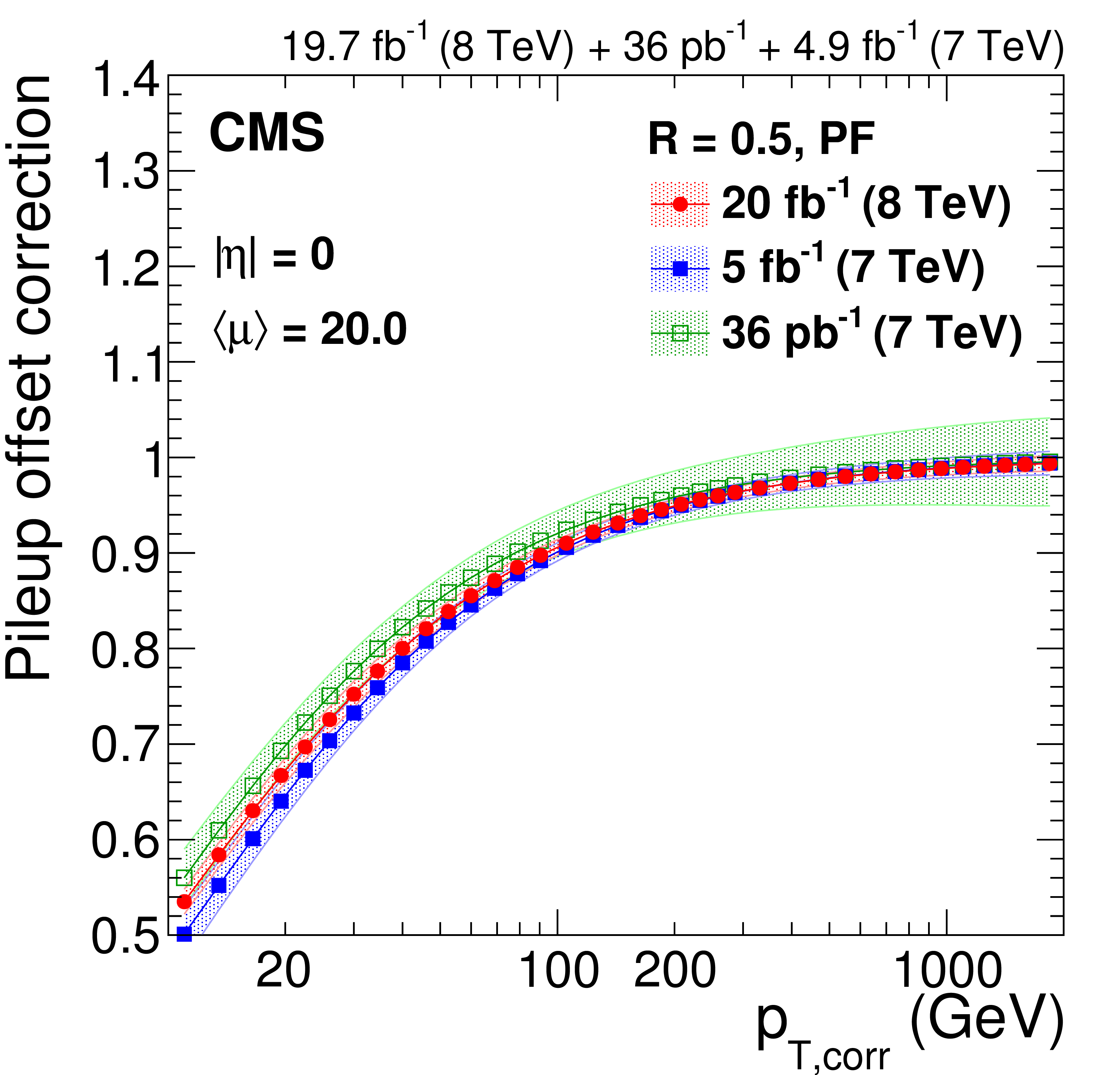
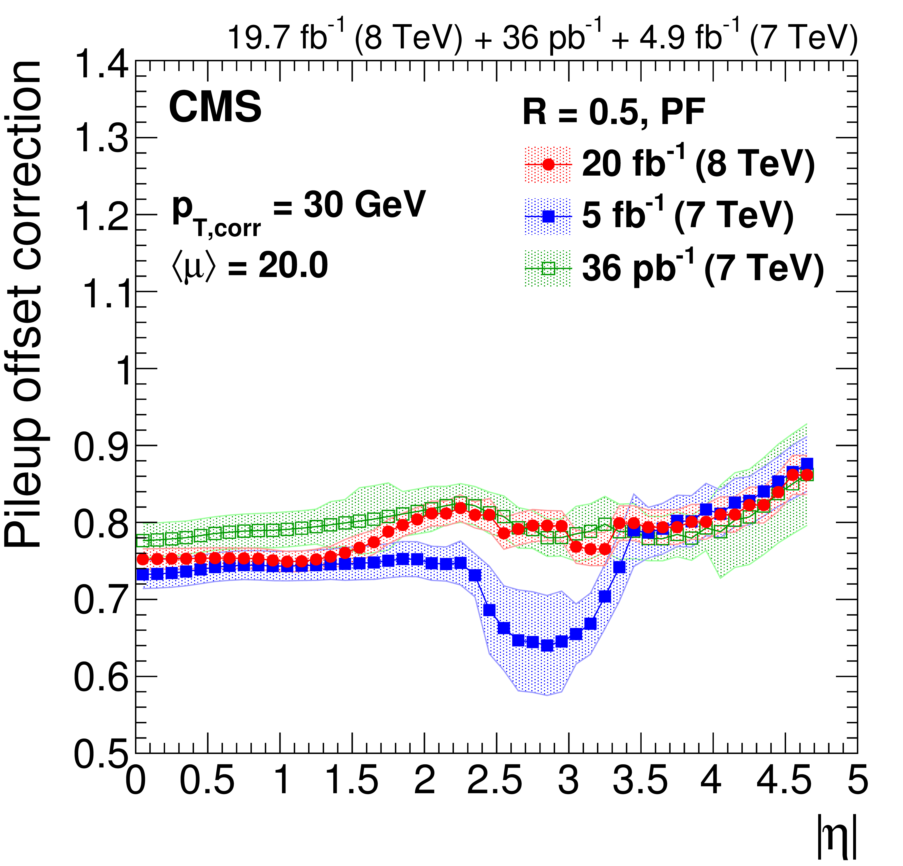
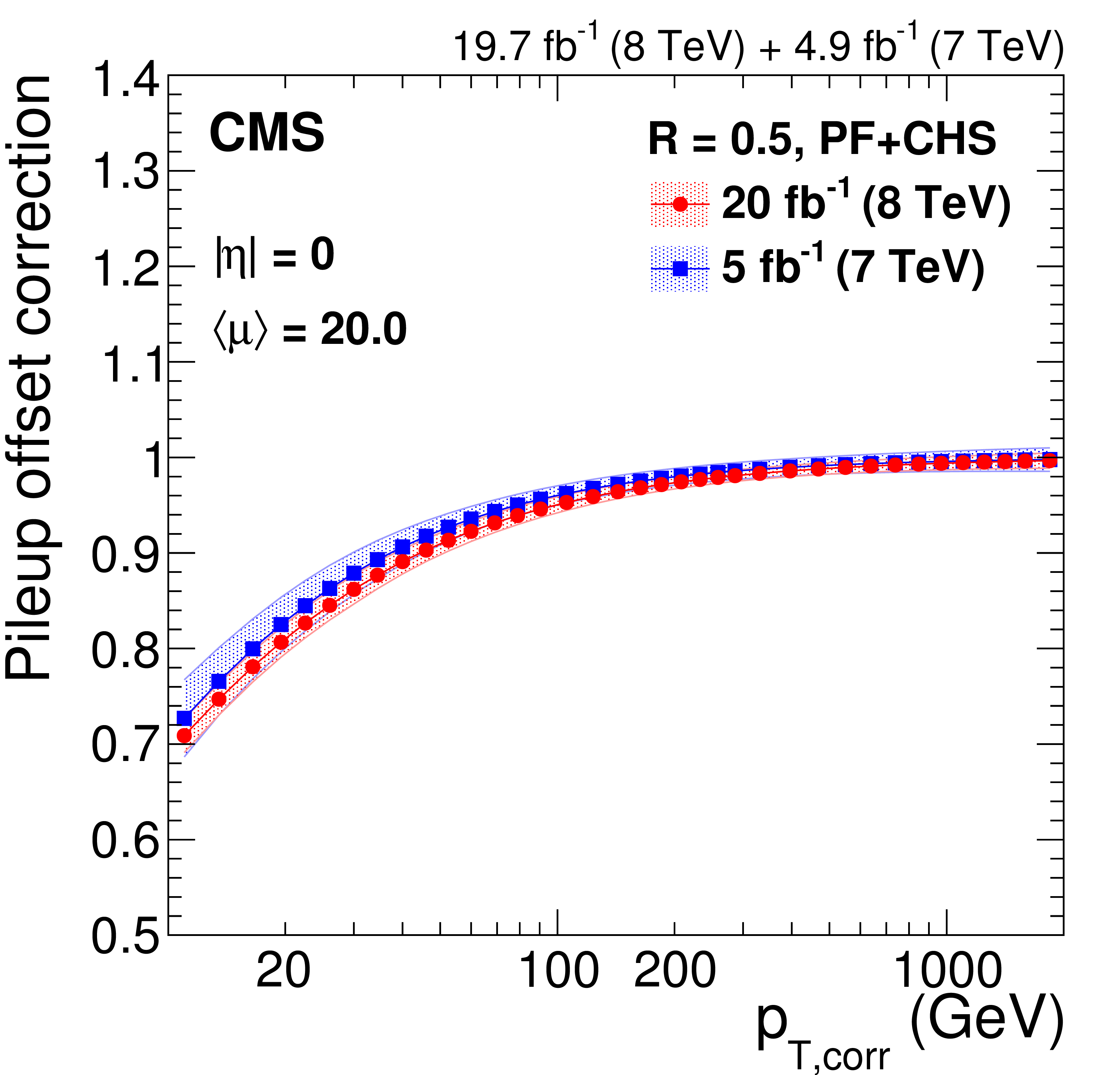
Pileup offset correction $C_{\rm hybrid}$ including data/MC scale factors, with systematic uncertainty band, for the average 2012 (8 TeV) conditions of $< \mu > = $ 20 for PF jets without CHS and $R= $ 0.5 at $|\eta |= $ 0 versus $p_{\rm T, corr}$ (a), and at $p_{{\rm T},\rm corr}= $ 30 GeV versus $|\eta |$ (b), compared to corrections for 2010 [13] and 2011 [45] data at 7 TeV after extrapolation to similar pileup conditions. The same results are also shown for PF jets with CHS and $R= $ 0.5 at $|\eta |= $ 0 versus $ {p_{\mathrm {T}}} $ (c), and at $p_{{\rm T},\rm corr}= $ 30 GeV versus $|\eta |$ (d), compared to corrections for 2011 data at 7 TeV [45]. |
png pdf |
Figure 9-a:
Pileup offset correction $C_{\rm hybrid}$ including data/MC scale factors, with systematic uncertainty band, for the average 2012 (8 TeV) conditions of $< \mu > = $ 20 for PF jets without CHS and $R= $ 0.5 at $|\eta |= $ 0 versus $p_{\rm T, corr}$ (a), and at $p_{{\rm T},\rm corr}= $ 30 GeV versus $|\eta |$ (b), compared to corrections for 2010 [13] and 2011 [45] data at 7 TeV after extrapolation to similar pileup conditions. The same results are also shown for PF jets with CHS and $R= $ 0.5 at $|\eta |= $ 0 versus $ {p_{\mathrm {T}}} $ (c), and at $p_{{\rm T},\rm corr}= $ 30 GeV versus $|\eta |$ (d), compared to corrections for 2011 data at 7 TeV [45]. |
png pdf |
Figure 9-b:
Pileup offset correction $C_{\rm hybrid}$ including data/MC scale factors, with systematic uncertainty band, for the average 2012 (8 TeV) conditions of $< \mu > = $ 20 for PF jets without CHS and $R= $ 0.5 at $|\eta |= $ 0 versus $p_{\rm T, corr}$ (a), and at $p_{{\rm T},\rm corr}= $ 30 GeV versus $|\eta |$ (b), compared to corrections for 2010 [13] and 2011 [45] data at 7 TeV after extrapolation to similar pileup conditions. The same results are also shown for PF jets with CHS and $R= $ 0.5 at $|\eta |= $ 0 versus $ {p_{\mathrm {T}}} $ (c), and at $p_{{\rm T},\rm corr}= $ 30 GeV versus $|\eta |$ (d), compared to corrections for 2011 data at 7 TeV [45]. |
png pdf |
Figure 9-c:
Pileup offset correction $C_{\rm hybrid}$ including data/MC scale factors, with systematic uncertainty band, for the average 2012 (8 TeV) conditions of $< \mu > = $ 20 for PF jets without CHS and $R= $ 0.5 at $|\eta |= $ 0 versus $p_{\rm T, corr}$ (a), and at $p_{{\rm T},\rm corr}= $ 30 GeV versus $|\eta |$ (b), compared to corrections for 2010 [13] and 2011 [45] data at 7 TeV after extrapolation to similar pileup conditions. The same results are also shown for PF jets with CHS and $R= $ 0.5 at $|\eta |= $ 0 versus $ {p_{\mathrm {T}}} $ (c), and at $p_{{\rm T},\rm corr}= $ 30 GeV versus $|\eta |$ (d), compared to corrections for 2011 data at 7 TeV [45]. |
png pdf |
Figure 9-d:
Pileup offset correction $C_{\rm hybrid}$ including data/MC scale factors, with systematic uncertainty band, for the average 2012 (8 TeV) conditions of $< \mu > = $ 20 for PF jets without CHS and $R= $ 0.5 at $|\eta |= $ 0 versus $p_{\rm T, corr}$ (a), and at $p_{{\rm T},\rm corr}= $ 30 GeV versus $|\eta |$ (b), compared to corrections for 2010 [13] and 2011 [45] data at 7 TeV after extrapolation to similar pileup conditions. The same results are also shown for PF jets with CHS and $R= $ 0.5 at $|\eta |= $ 0 versus $ {p_{\mathrm {T}}} $ (c), and at $p_{{\rm T},\rm corr}= $ 30 GeV versus $|\eta |$ (d), compared to corrections for 2011 data at 7 TeV [45]. |
png pdf |
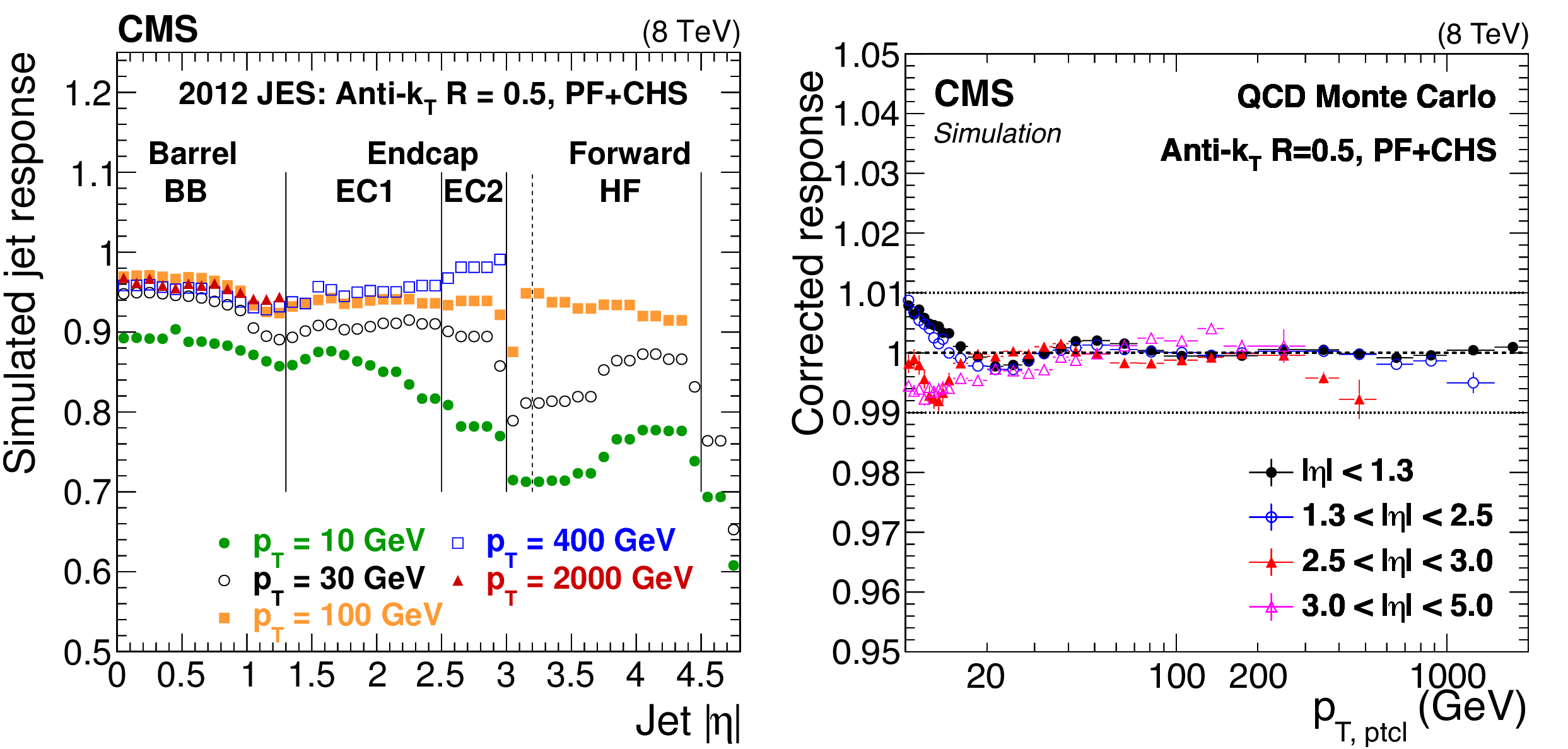
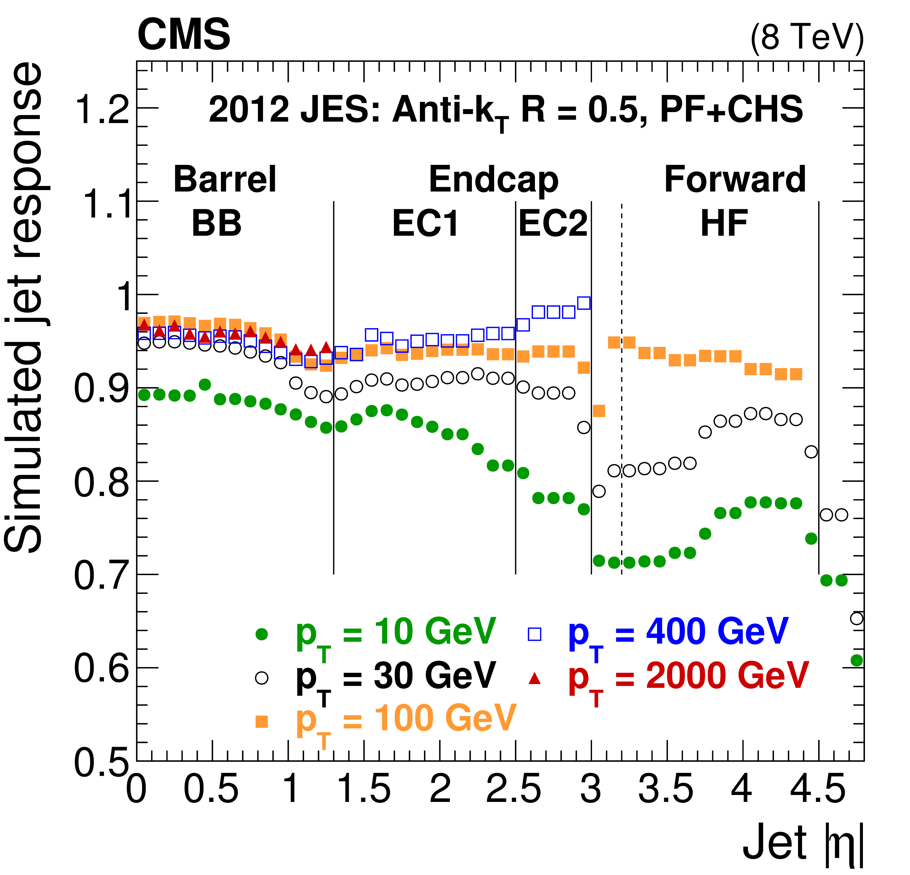
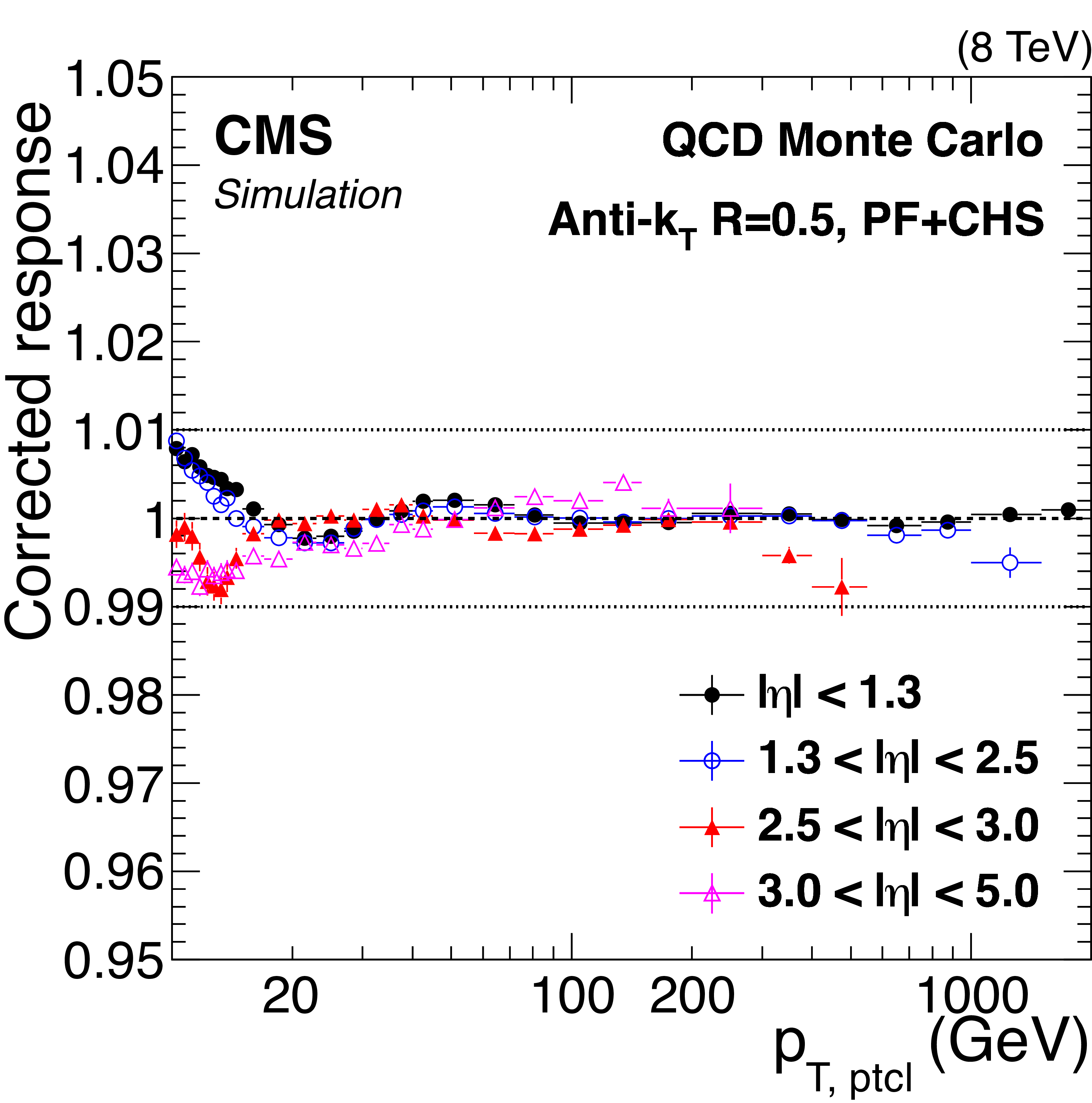
Figure 10:
Simulated jet response $R_{\rm ptcl}$ versus $|\eta |$ for $R= $ 0.5 (a). Simulated jet response $R_{\rm ptcl}$, after JEC have been applied, versus $p_{\rm T, ptcl}$ for $R= $ 0.5 in various $\eta $ regions (b). |
png pdf |
Figure 10-a:
Simulated jet response $R_{\rm ptcl}$ versus $|\eta |$ for $R= $ 0.5 (a). Simulated jet response $R_{\rm ptcl}$, after JEC have been applied, versus $p_{\rm T, ptcl}$ for $R= $ 0.5 in various $\eta $ regions (b). |
png pdf |
Figure 10-b:
Simulated jet response $R_{\rm ptcl}$ versus $|\eta |$ for $R= $ 0.5 (a). Simulated jet response $R_{\rm ptcl}$, after JEC have been applied, versus $p_{\rm T, ptcl}$ for $R= $ 0.5 in various $\eta $ regions (b). |
png pdf |
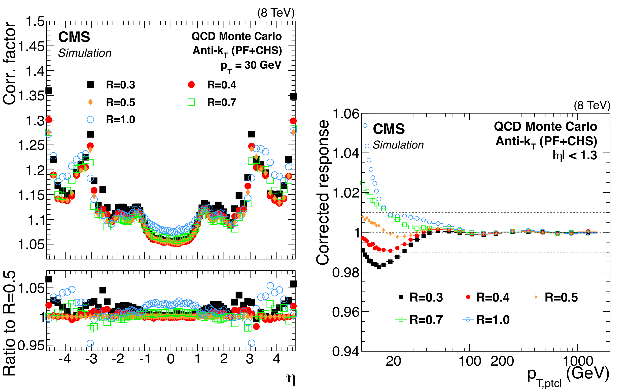
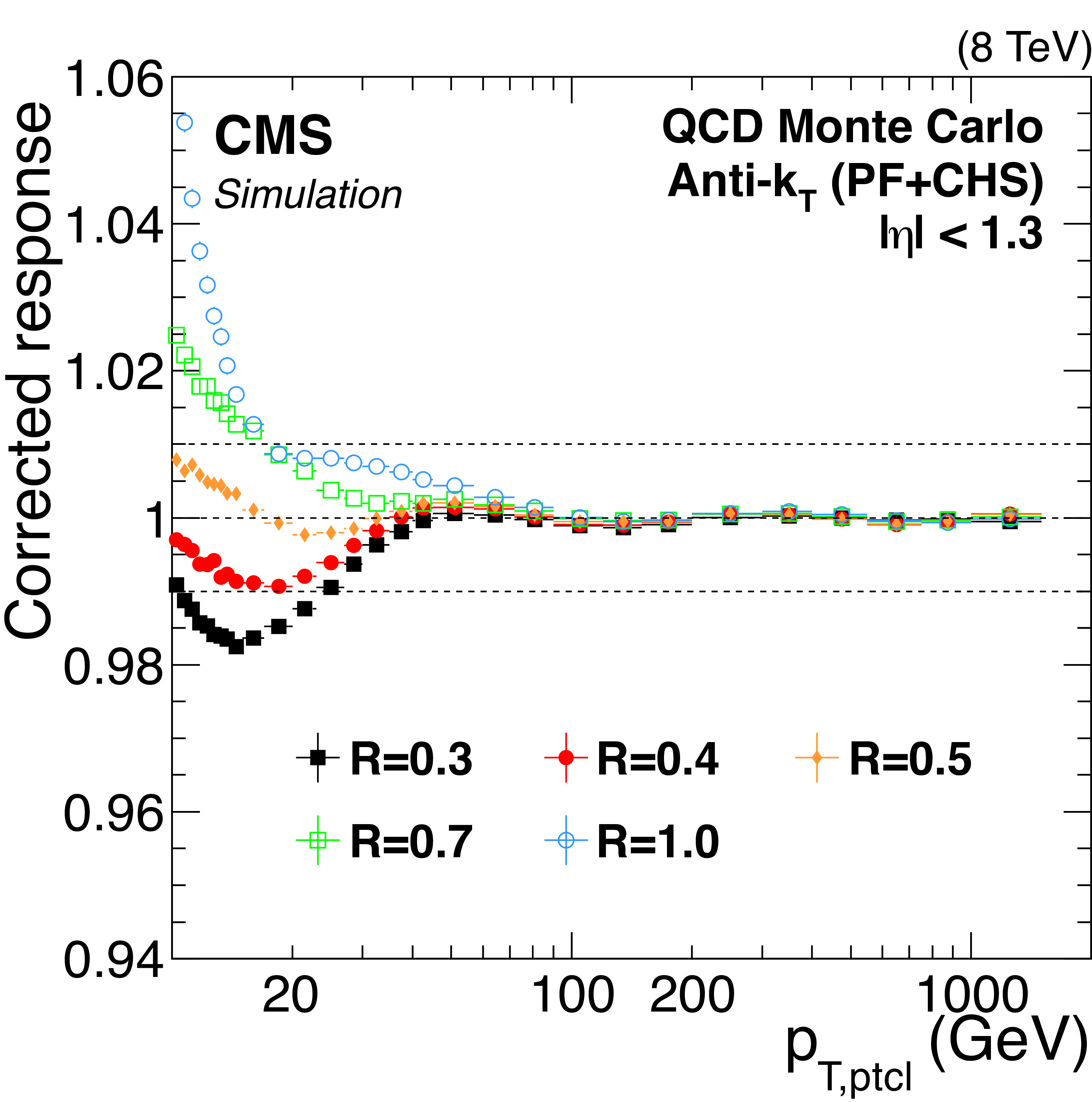
Figure 11:
Jet energy correction factors for a jet with $ {p_{\mathrm {T}}} = $ 30 GeV, as a function of $\eta $ and for various jet sizes $R$ (a). Simulated jet energy response $R_{\rm ptcl}$ after JEC for $|\eta |< $ 1.3 as a function of the jet $ {p_{\mathrm {T}}} $ for various jet sizes $R$ (b). |

png pdf |
Figure 11-a:
Jet energy correction factors for a jet with $ {p_{\mathrm {T}}} = $ 30 GeV, as a function of $\eta $ and for various jet sizes $R$ (a). Simulated jet energy response $R_{\rm ptcl}$ after JEC for $|\eta |< $ 1.3 as a function of the jet $ {p_{\mathrm {T}}} $ for various jet sizes $R$ (b). |
png pdf |
Figure 11-b:
Jet energy correction factors for a jet with $ {p_{\mathrm {T}}} = $ 30 GeV, as a function of $\eta $ and for various jet sizes $R$ (a). Simulated jet energy response $R_{\rm ptcl}$ after JEC for $|\eta |< $ 1.3 as a function of the jet $ {p_{\mathrm {T}}} $ for various jet sizes $R$ (b). |
png pdf |
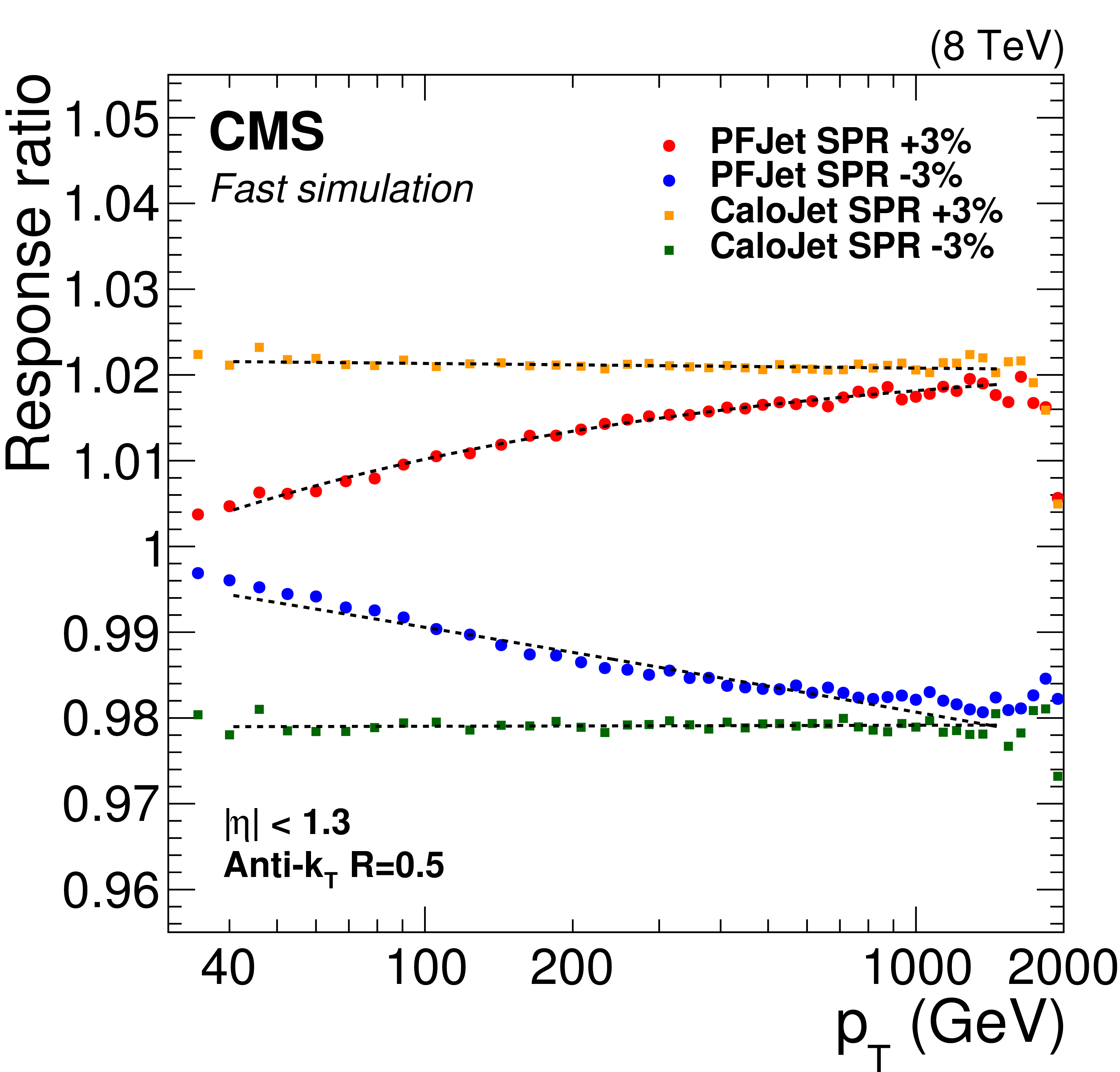
Figure 12:
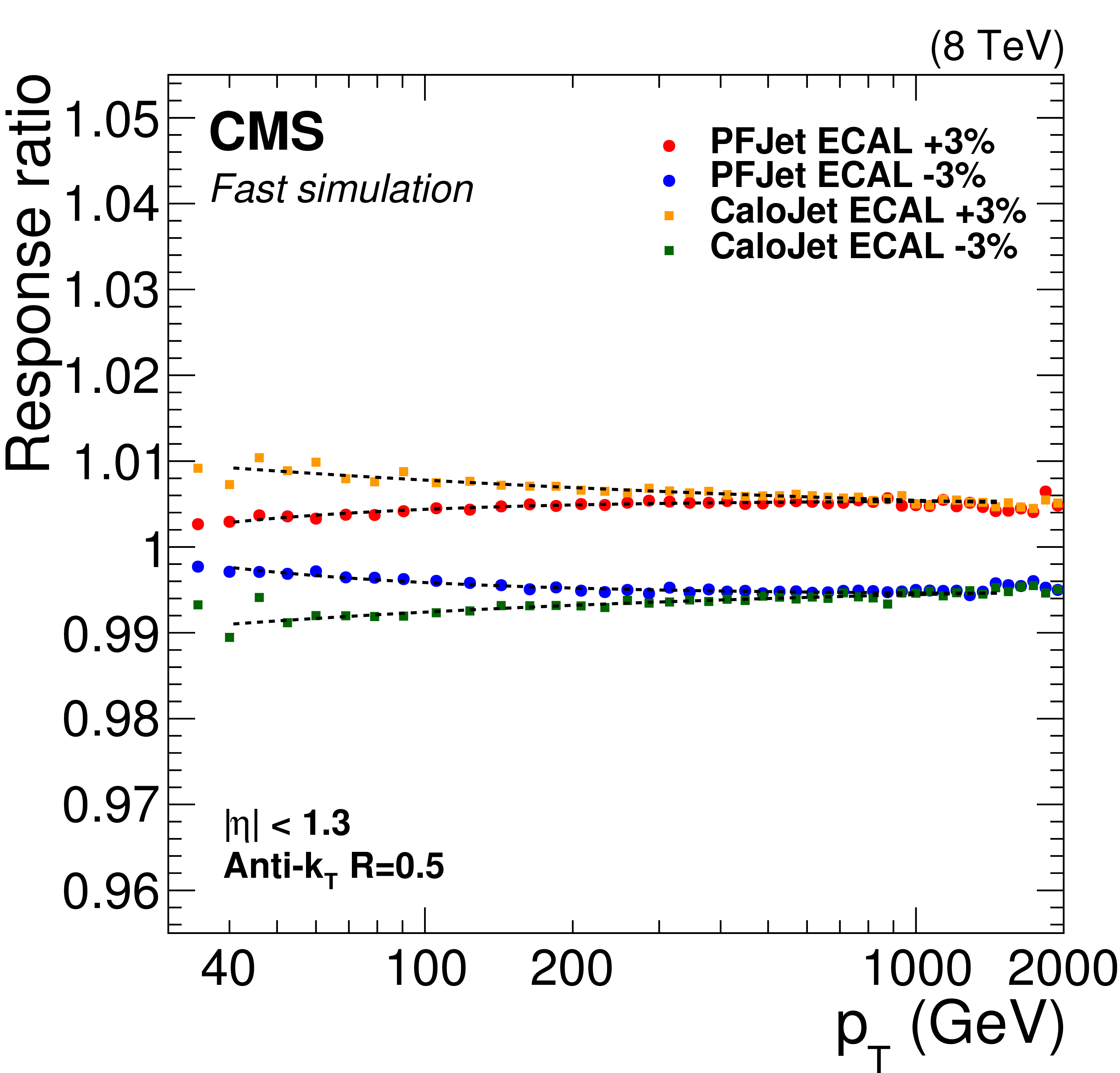
Changes in PF jet and calorimeter jet response resulting from $\pm$3% variations of single-pion response in parameterized fast simulation in HCAL+ECAL. |
png pdf |
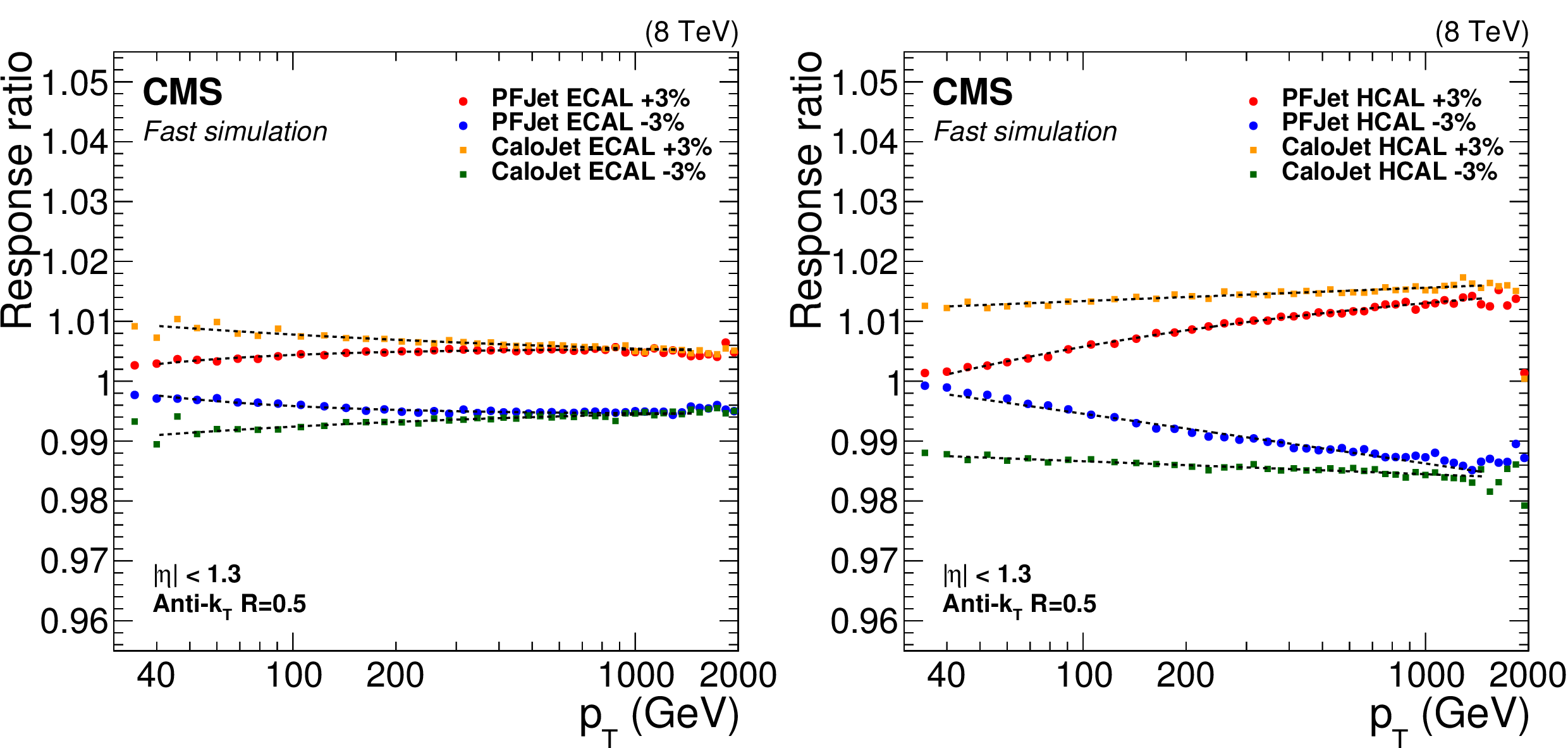
Figure 13:
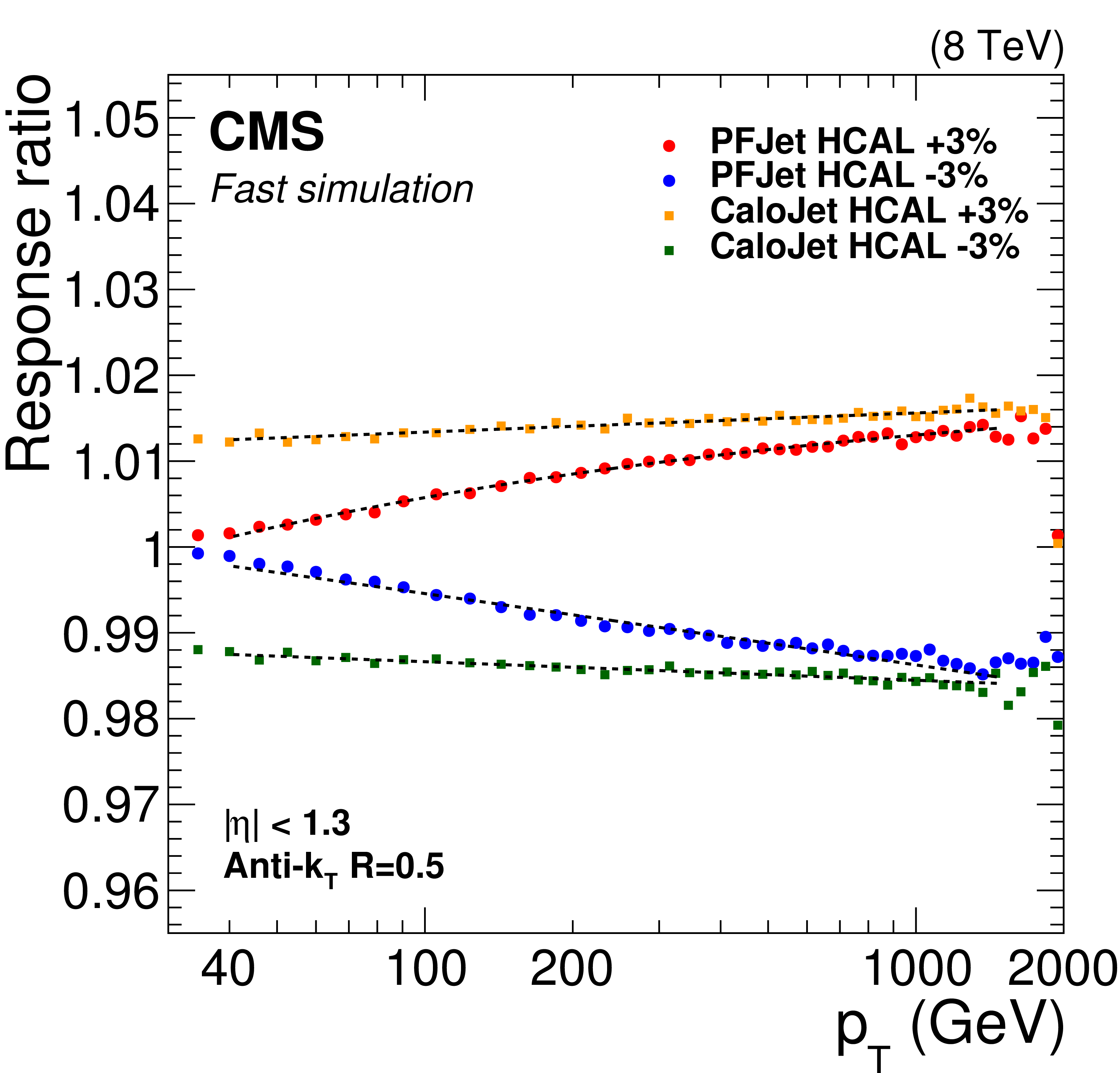
Changes in PF jet and calorimeter jet response resulting from $\pm$3% variations of single-pion response in parameterized fast simulation in ECAL (a), and HCAL (b). |
png pdf |
Figure 13-a:
Changes in PF jet and calorimeter jet response resulting from $\pm$3% variations of single-pion response in parameterized fast simulation in ECAL (a), and HCAL (b). |
png pdf |
Figure 13-b:
Changes in PF jet and calorimeter jet response resulting from $\pm$3% variations of single-pion response in parameterized fast simulation in ECAL (a), and HCAL (b). |
png pdf |
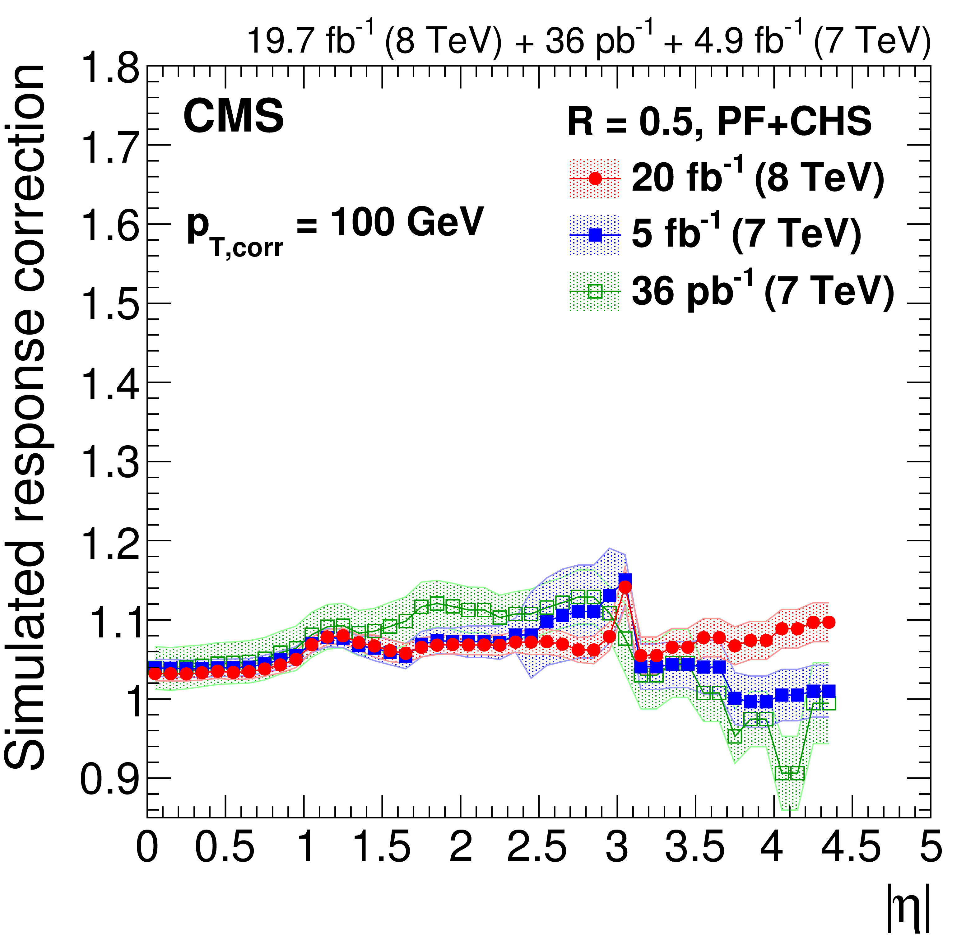
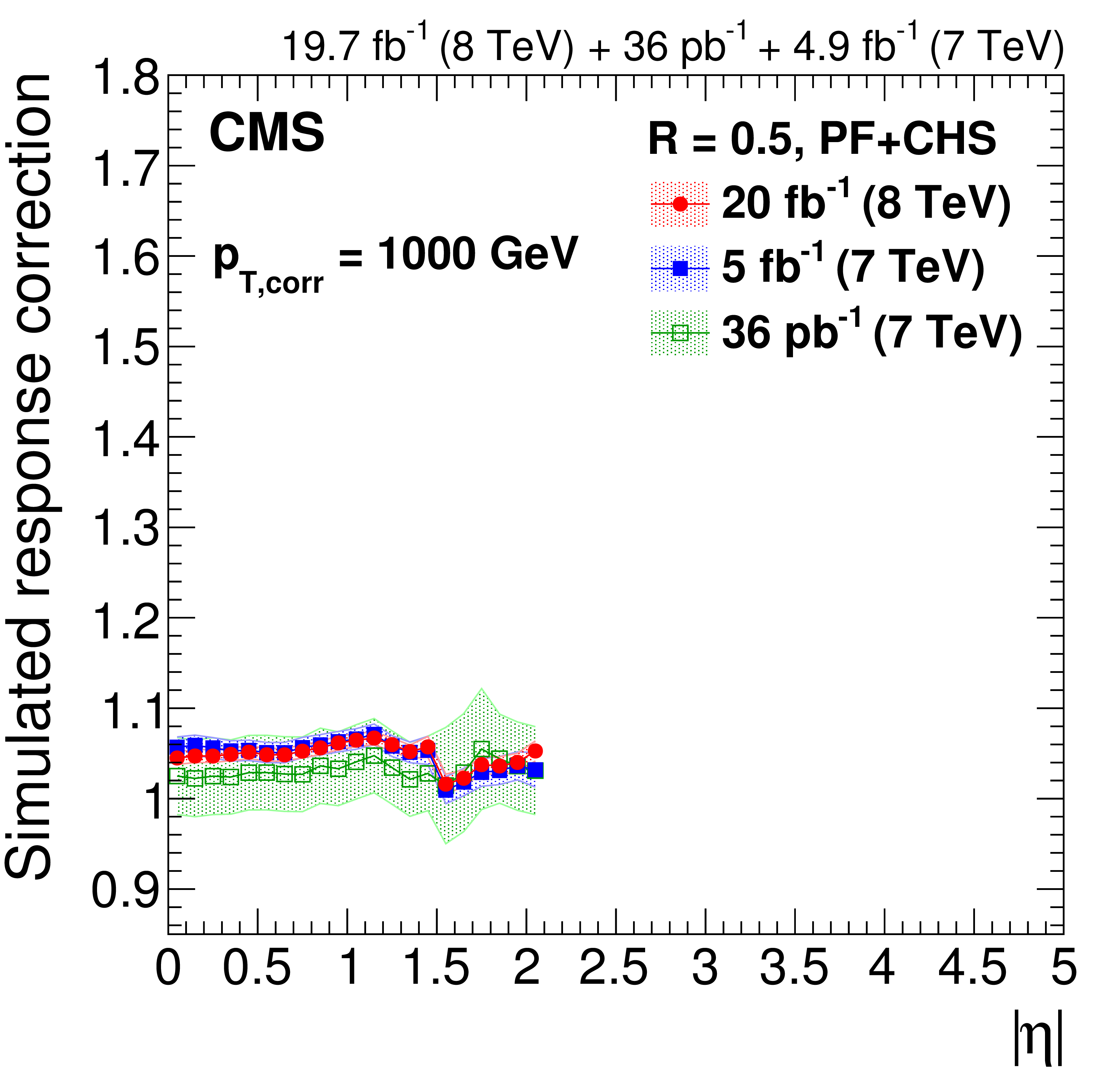
Figure 14:
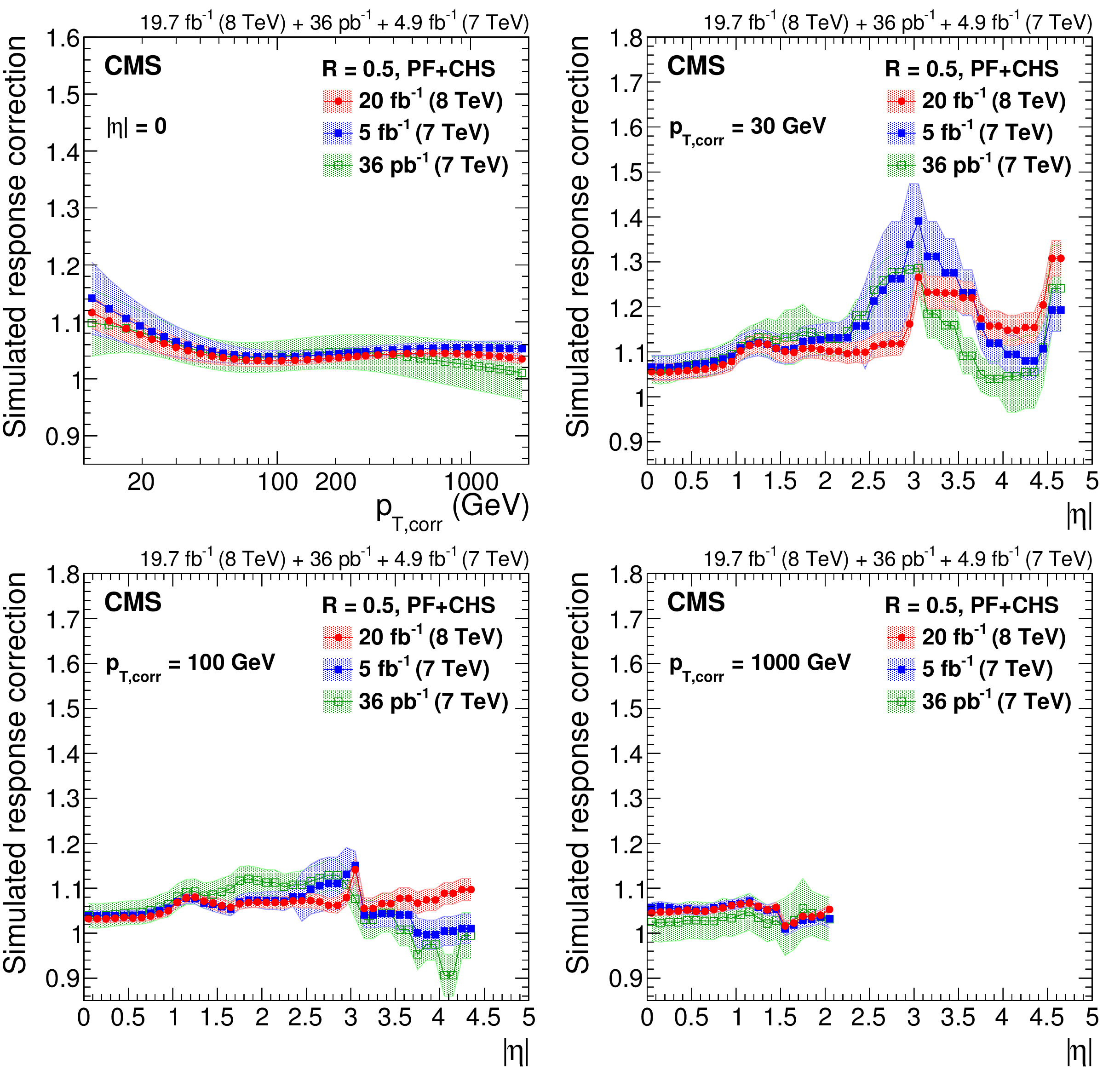
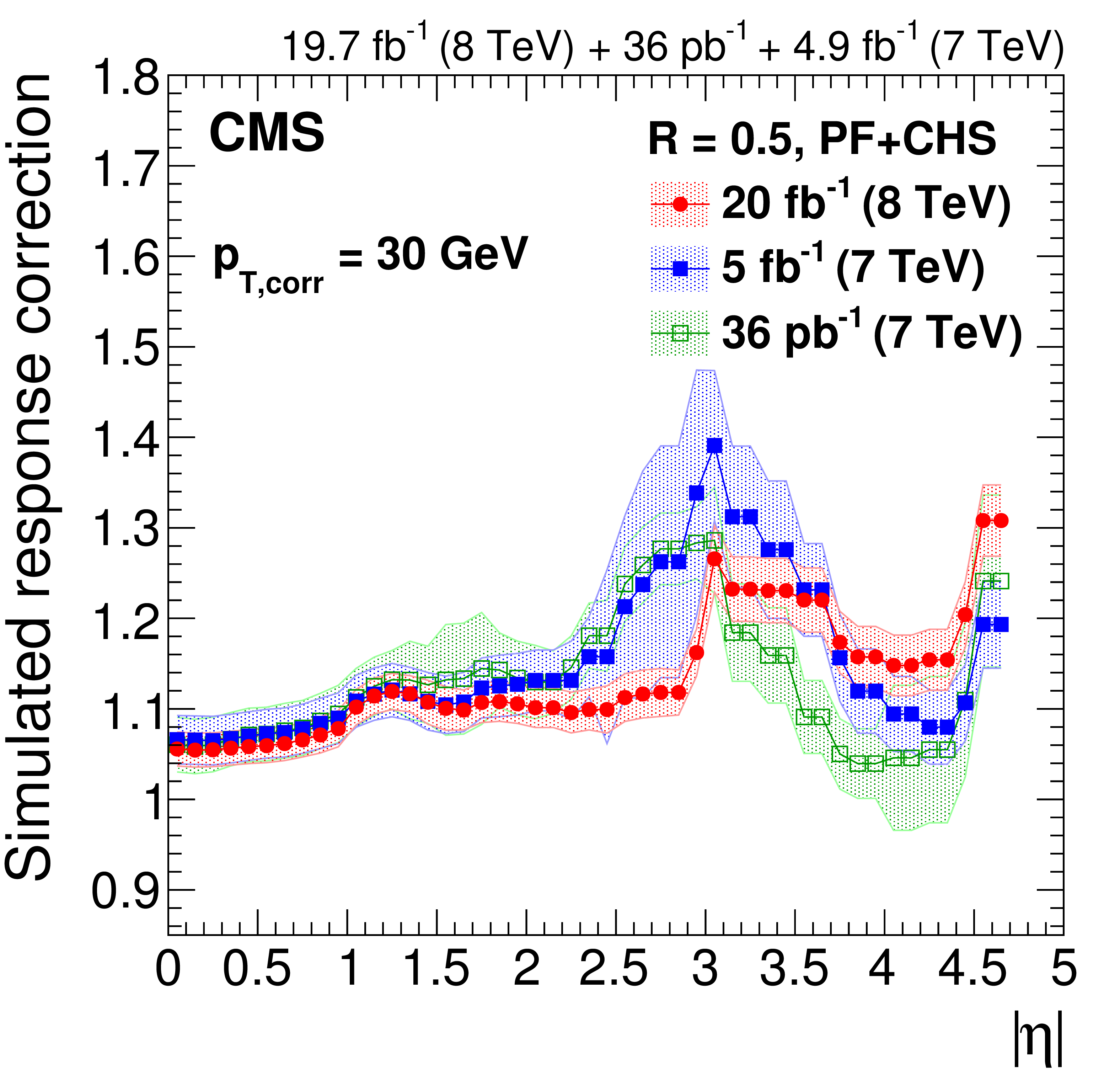
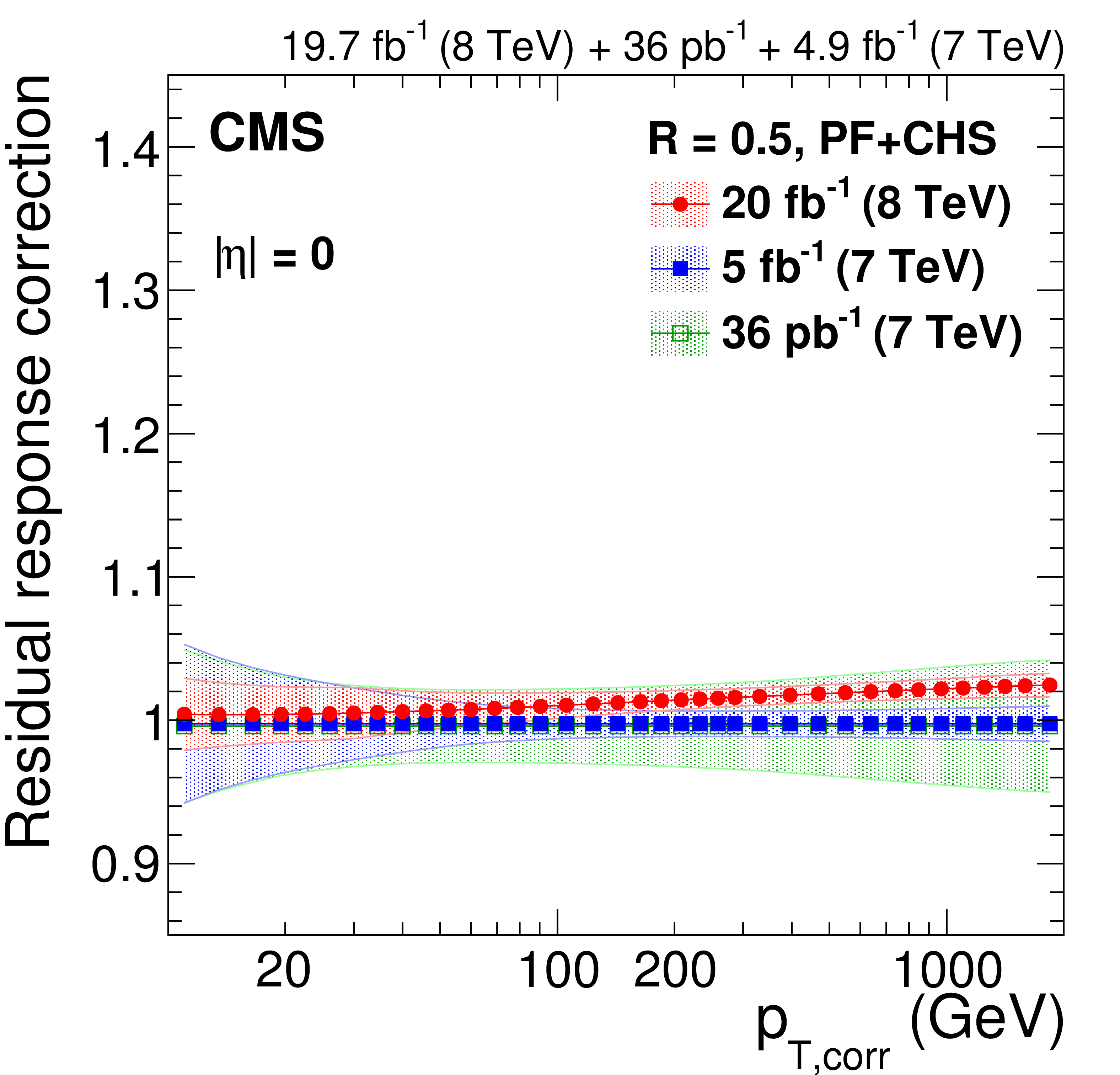
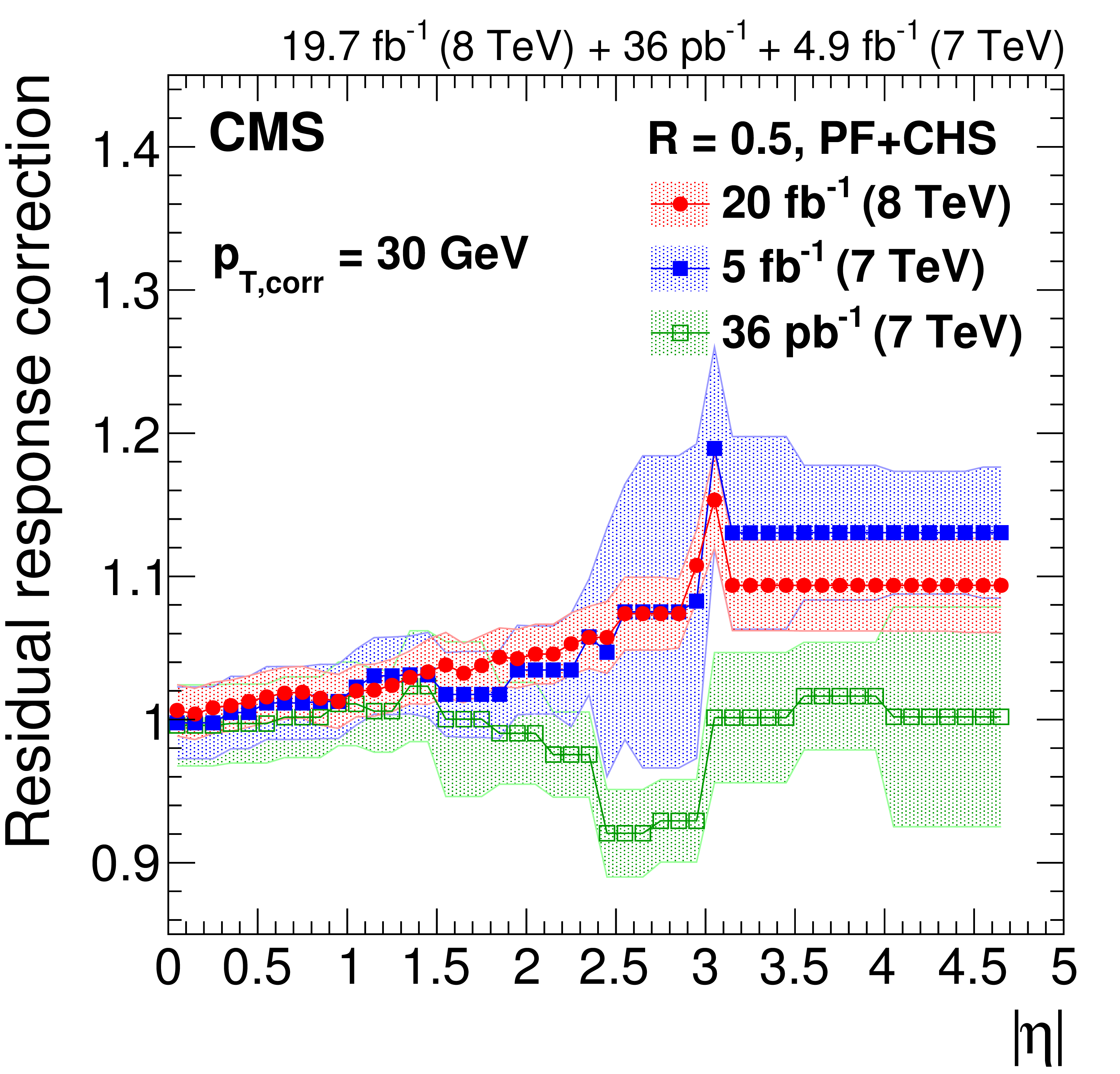
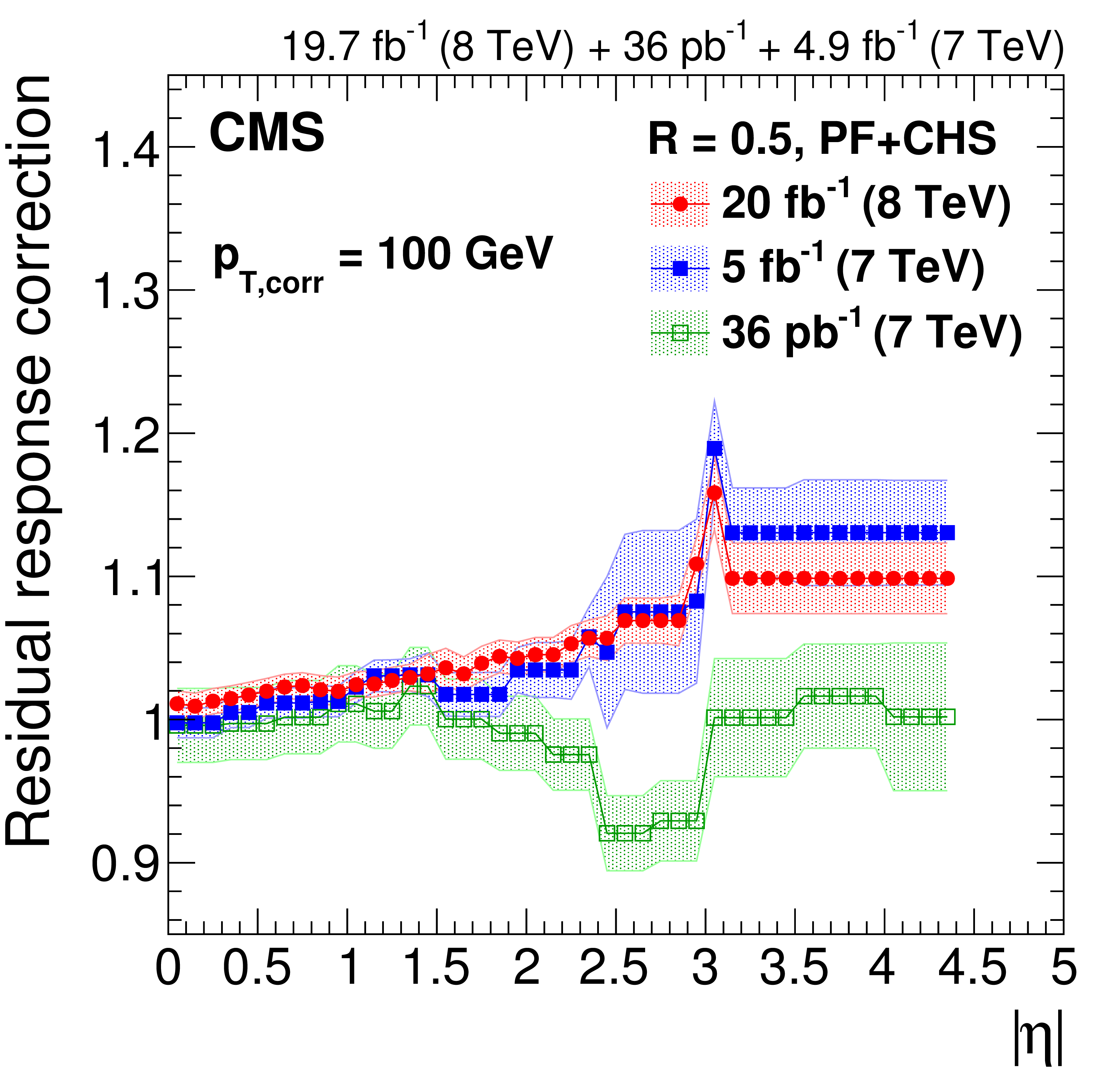
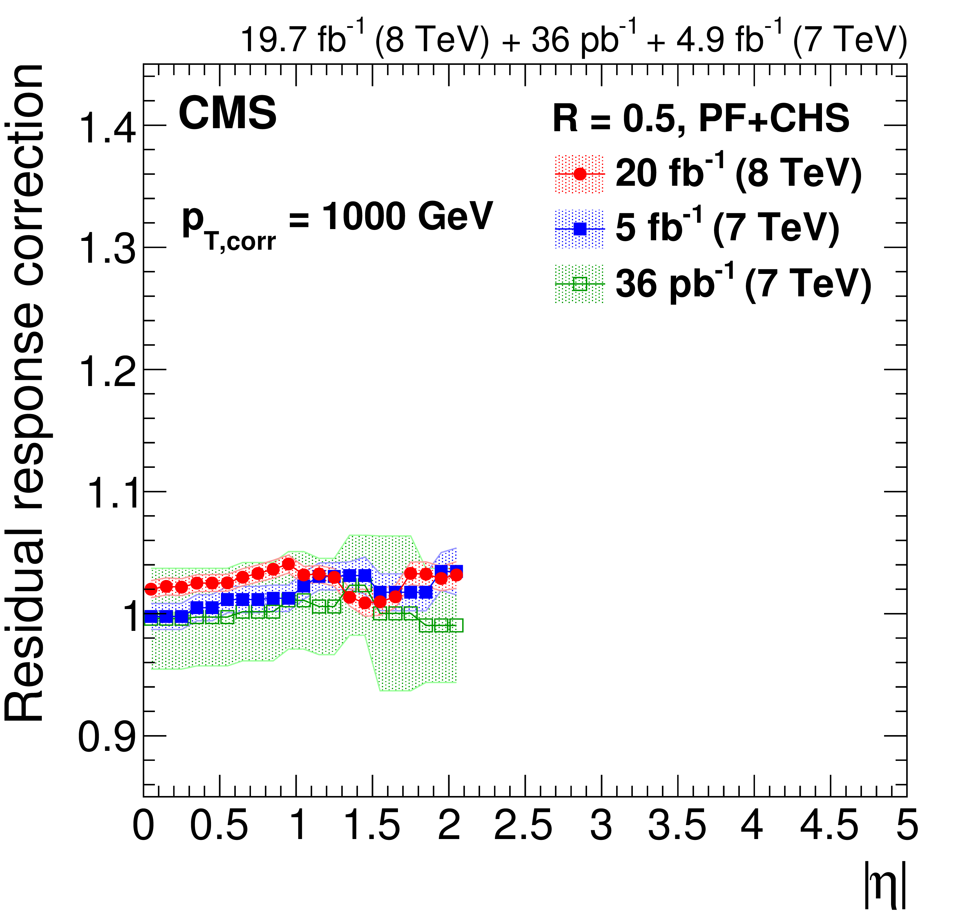
Response correction factors with their systematic uncertainty band from simulation for the 2012 data collected at 8 TeV for PF jets with CHS and $R= $ 0.5 , compared to corrections at 7 TeV corresponding to 36 pb$^{-1}$ of data taken in 2010 [13] and 5 fb$^{-1}$ taken in 2011 [45]. The comparison is shown at $|\eta |= $ 0 versus $p_{\rm T, corr}$ (a), and as a function of $|\eta |$ at $p_{\rm T, corr}= $ 30 GeV (b), $p_{\rm T, corr}= $ 100 GeV (c) and $p_{\rm T, corr}= $ 1000 GeV (d). The plots are limited to a jet energy $E= {p_{\mathrm {T}}} \cosh\eta = $ 3500 GeV so as to show only the correction factors for reasonable $ {p_{\mathrm {T}}} $ in the considered data-taking periods. |

png pdf |
Figure 14-a:
Response correction factors with their systematic uncertainty band from simulation for the 2012 data collected at 8 TeV for PF jets with CHS and $R= $ 0.5 , compared to corrections at 7 TeV corresponding to 36 pb$^{-1}$ of data taken in 2010 [13] and 5 fb$^{-1}$ taken in 2011 [45]. The comparison is shown at $|\eta |= $ 0 versus $p_{\rm T, corr}$ (a), and as a function of $|\eta |$ at $p_{\rm T, corr}= $ 30 GeV (b), $p_{\rm T, corr}= $ 100 GeV (c) and $p_{\rm T, corr}= $ 1000 GeV (d). The plots are limited to a jet energy $E= {p_{\mathrm {T}}} \cosh\eta = $ 3500 GeV so as to show only the correction factors for reasonable $ {p_{\mathrm {T}}} $ in the considered data-taking periods. |
png pdf |
Figure 14-b:
Response correction factors with their systematic uncertainty band from simulation for the 2012 data collected at 8 TeV for PF jets with CHS and $R= $ 0.5 , compared to corrections at 7 TeV corresponding to 36 pb$^{-1}$ of data taken in 2010 [13] and 5 fb$^{-1}$ taken in 2011 [45]. The comparison is shown at $|\eta |= $ 0 versus $p_{\rm T, corr}$ (a), and as a function of $|\eta |$ at $p_{\rm T, corr}= $ 30 GeV (b), $p_{\rm T, corr}= $ 100 GeV (c) and $p_{\rm T, corr}= $ 1000 GeV (d). The plots are limited to a jet energy $E= {p_{\mathrm {T}}} \cosh\eta = $ 3500 GeV so as to show only the correction factors for reasonable $ {p_{\mathrm {T}}} $ in the considered data-taking periods. |
png pdf |
Figure 14-c:
Response correction factors with their systematic uncertainty band from simulation for the 2012 data collected at 8 TeV for PF jets with CHS and $R= $ 0.5 , compared to corrections at 7 TeV corresponding to 36 pb$^{-1}$ of data taken in 2010 [13] and 5 fb$^{-1}$ taken in 2011 [45]. The comparison is shown at $|\eta |= $ 0 versus $p_{\rm T, corr}$ (a), and as a function of $|\eta |$ at $p_{\rm T, corr}= $ 30 GeV (b), $p_{\rm T, corr}= $ 100 GeV (c) and $p_{\rm T, corr}= $ 1000 GeV (d). The plots are limited to a jet energy $E= {p_{\mathrm {T}}} \cosh\eta = $ 3500 GeV so as to show only the correction factors for reasonable $ {p_{\mathrm {T}}} $ in the considered data-taking periods. |
png pdf |
Figure 14-d:
Response correction factors with their systematic uncertainty band from simulation for the 2012 data collected at 8 TeV for PF jets with CHS and $R= $ 0.5 , compared to corrections at 7 TeV corresponding to 36 pb$^{-1}$ of data taken in 2010 [13] and 5 fb$^{-1}$ taken in 2011 [45]. The comparison is shown at $|\eta |= $ 0 versus $p_{\rm T, corr}$ (a), and as a function of $|\eta |$ at $p_{\rm T, corr}= $ 30 GeV (b), $p_{\rm T, corr}= $ 100 GeV (c) and $p_{\rm T, corr}= $ 1000 GeV (d). The plots are limited to a jet energy $E= {p_{\mathrm {T}}} \cosh\eta = $ 3500 GeV so as to show only the correction factors for reasonable $ {p_{\mathrm {T}}} $ in the considered data-taking periods. |

png pdf |
Figure 15:
Relative energy scale correction for $ {p_{\mathrm {T}}} = $ 60 , 120, 240 and 480 GeV as a function of $|\eta |$. The residual corrections increase toward high rapidity and low $ {p_{\mathrm {T}}} $, where effects from nonlinear calorimeter response become more important. The curves are limited to a jet energy $E= {p_{\mathrm {T}}} \cosh \eta = $ 4000 GeV (corresponding to $\eta \approx 2.8$ for a jet with $ {p_{\mathrm {T}}} = $ 480 GeV) so as to show only the correction factors for reasonable $ {p_{\mathrm {T}}} $ in the considered data-taking period. The statistical uncertainty associated with a constant fit versus $ {p_{\mathrm {T}}} $ is shown for $ {p_{\mathrm {T}}} = $ 120 GeV (markers). |
png pdf |
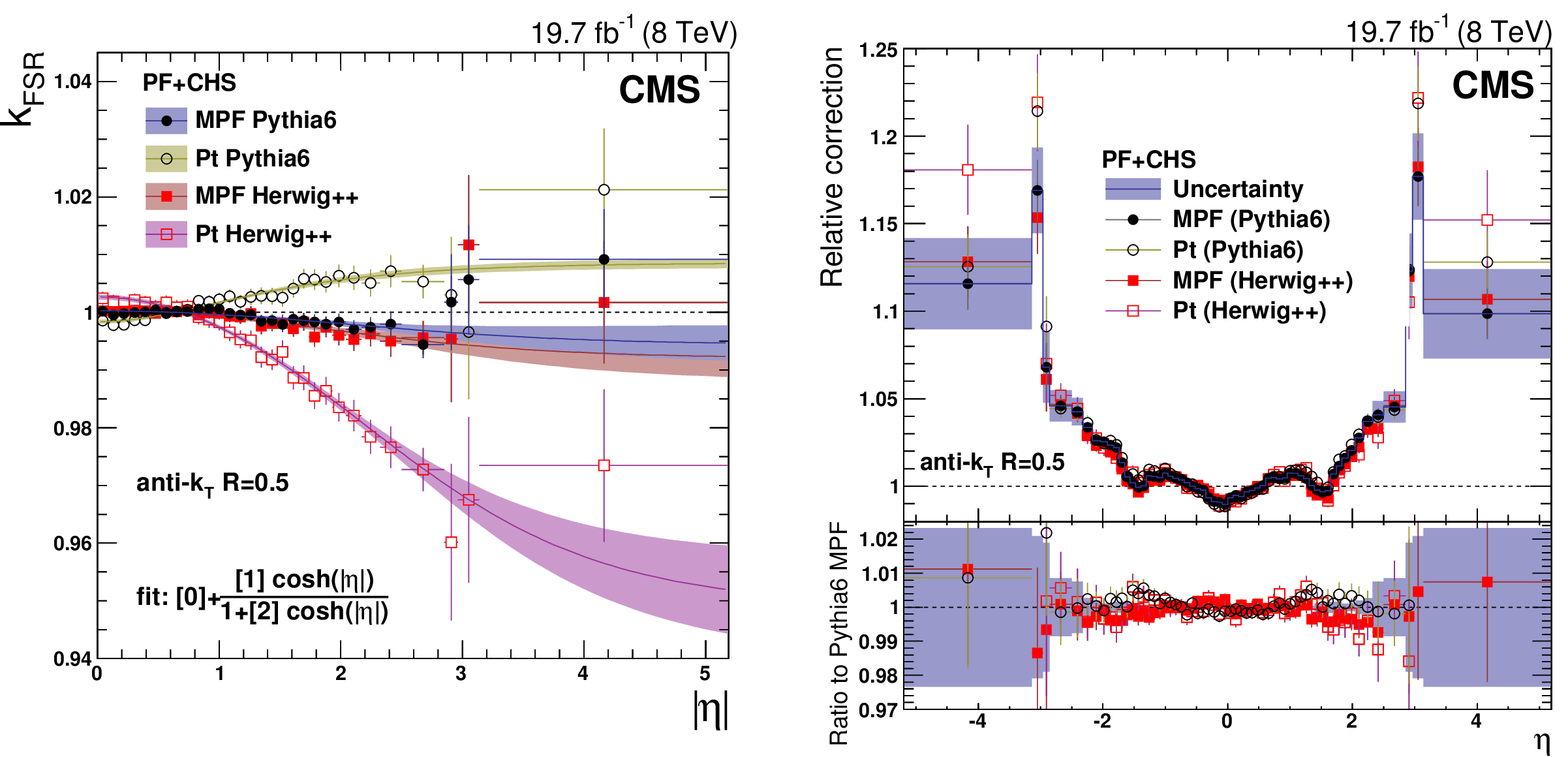
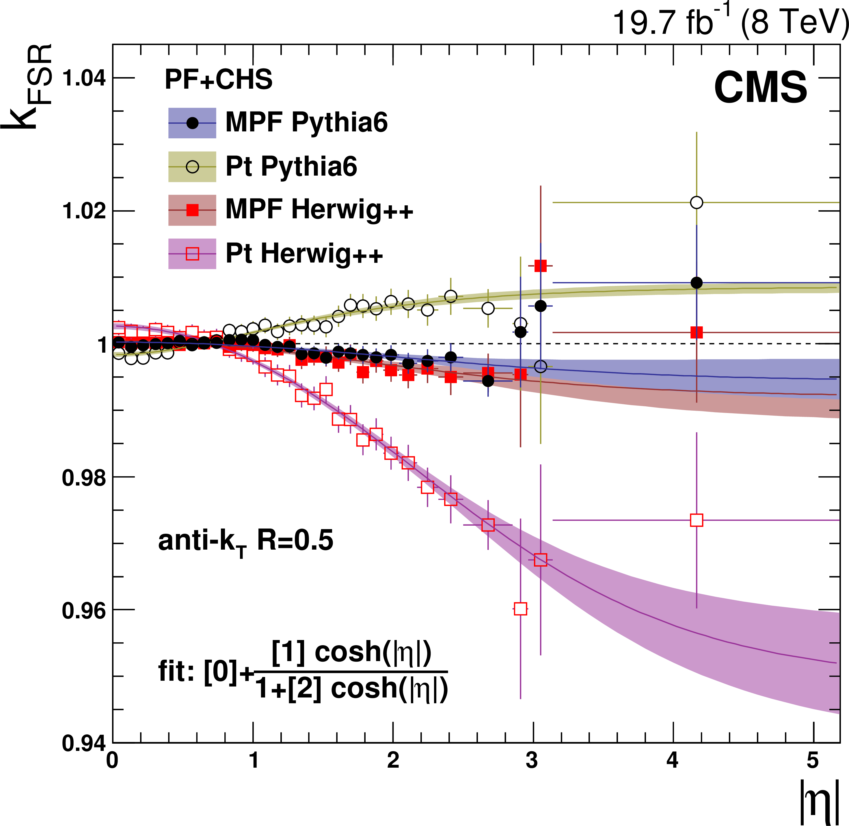
Figure 16:
The $k_{\rm FSR}(\alpha =0.2)$ correction factor (defined in Eq.(14)) plotted vs. $|\eta |$ (a). This ratio is used for ISR+FSR corrections that are applied to dijet events with $\alpha < $ 0.2 , for the MPF and $ {p_{\mathrm {T}}} $-balance methods, and for Pythia6.4 tune Z2* and Herwig++2.3 tune EE3C. The points are fitted with $f(\eta) = p_0 + {p_1 \cosh \eta}/{( 1 + p_2 \cosh \eta )}$ as in Ref. [13]. Relative $\eta $ corrections obtained with the MPF and balance methods and the Pythia6.4 tune Z2* and Herwig++2.3 tune EE3C MC generators (b). The results are shown after corrections for ISR+FSR, and compared to the central values, obtained with the MPF method and Pythia6.4 tune Z2* simulated events. |
png pdf |
Figure 16-a:
The $k_{\rm FSR}(\alpha =0.2)$ correction factor (defined in Eq.(14)) plotted vs. $|\eta |$ (a). This ratio is used for ISR+FSR corrections that are applied to dijet events with $\alpha < $ 0.2 , for the MPF and $ {p_{\mathrm {T}}} $-balance methods, and for Pythia6.4 tune Z2* and Herwig++2.3 tune EE3C. The points are fitted with $f(\eta) = p_0 + {p_1 \cosh \eta}/{( 1 + p_2 \cosh \eta )}$ as in Ref. [13]. Relative $\eta $ corrections obtained with the MPF and balance methods and the Pythia6.4 tune Z2* and Herwig++2.3 tune EE3C MC generators (b). The results are shown after corrections for ISR+FSR, and compared to the central values, obtained with the MPF method and Pythia6.4 tune Z2* simulated events. |
png pdf |
Figure 16-b:
The $k_{\rm FSR}(\alpha =0.2)$ correction factor (defined in Eq.(14)) plotted vs. $|\eta |$ (a). This ratio is used for ISR+FSR corrections that are applied to dijet events with $\alpha < $ 0.2 , for the MPF and $ {p_{\mathrm {T}}} $-balance methods, and for Pythia6.4 tune Z2* and Herwig++2.3 tune EE3C. The points are fitted with $f(\eta) = p_0 + {p_1 \cosh \eta}/{( 1 + p_2 \cosh \eta )}$ as in Ref. [13]. Relative $\eta $ corrections obtained with the MPF and balance methods and the Pythia6.4 tune Z2* and Herwig++2.3 tune EE3C MC generators (b). The results are shown after corrections for ISR+FSR, and compared to the central values, obtained with the MPF method and Pythia6.4 tune Z2* simulated events. |

png pdf |
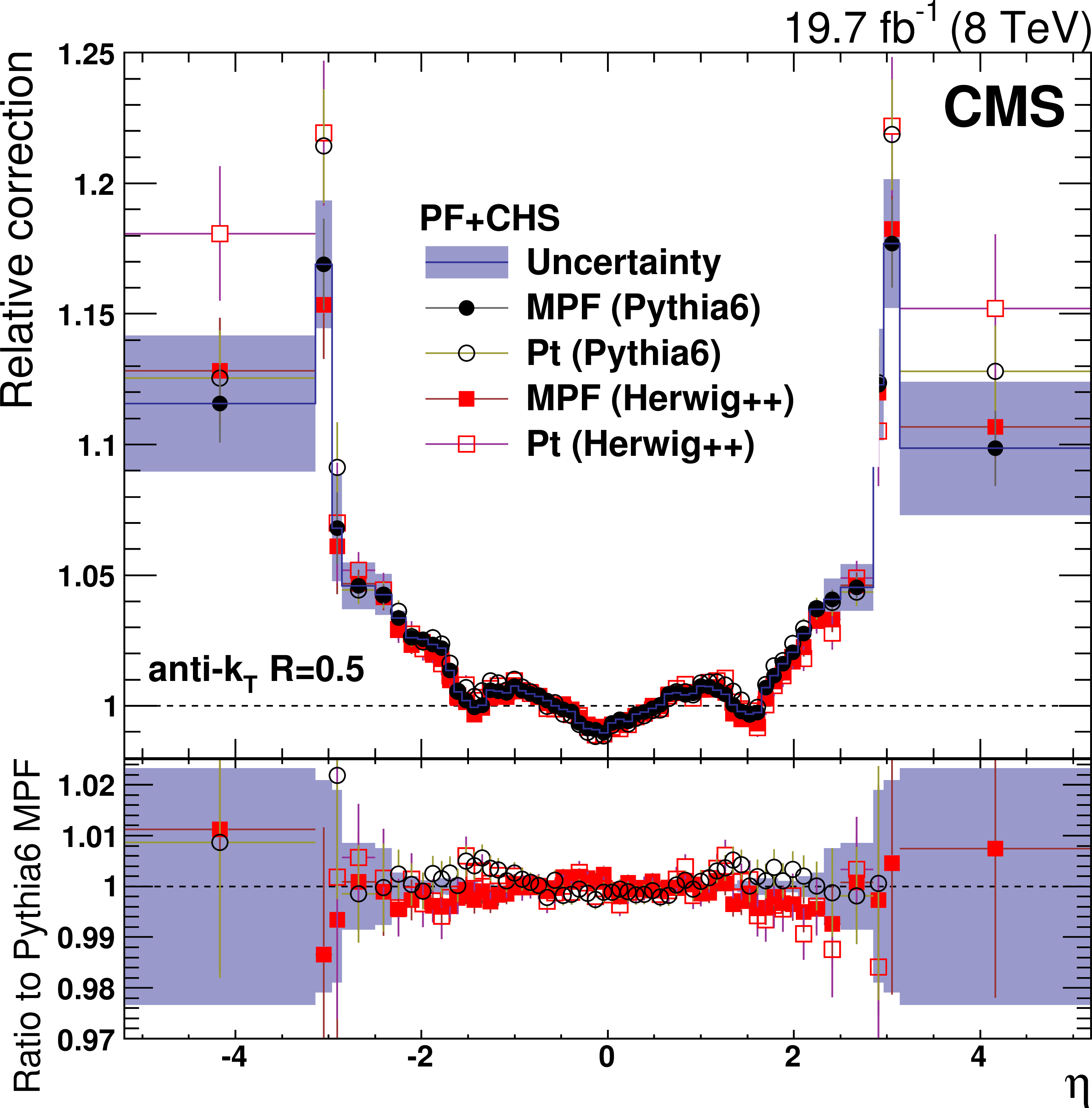
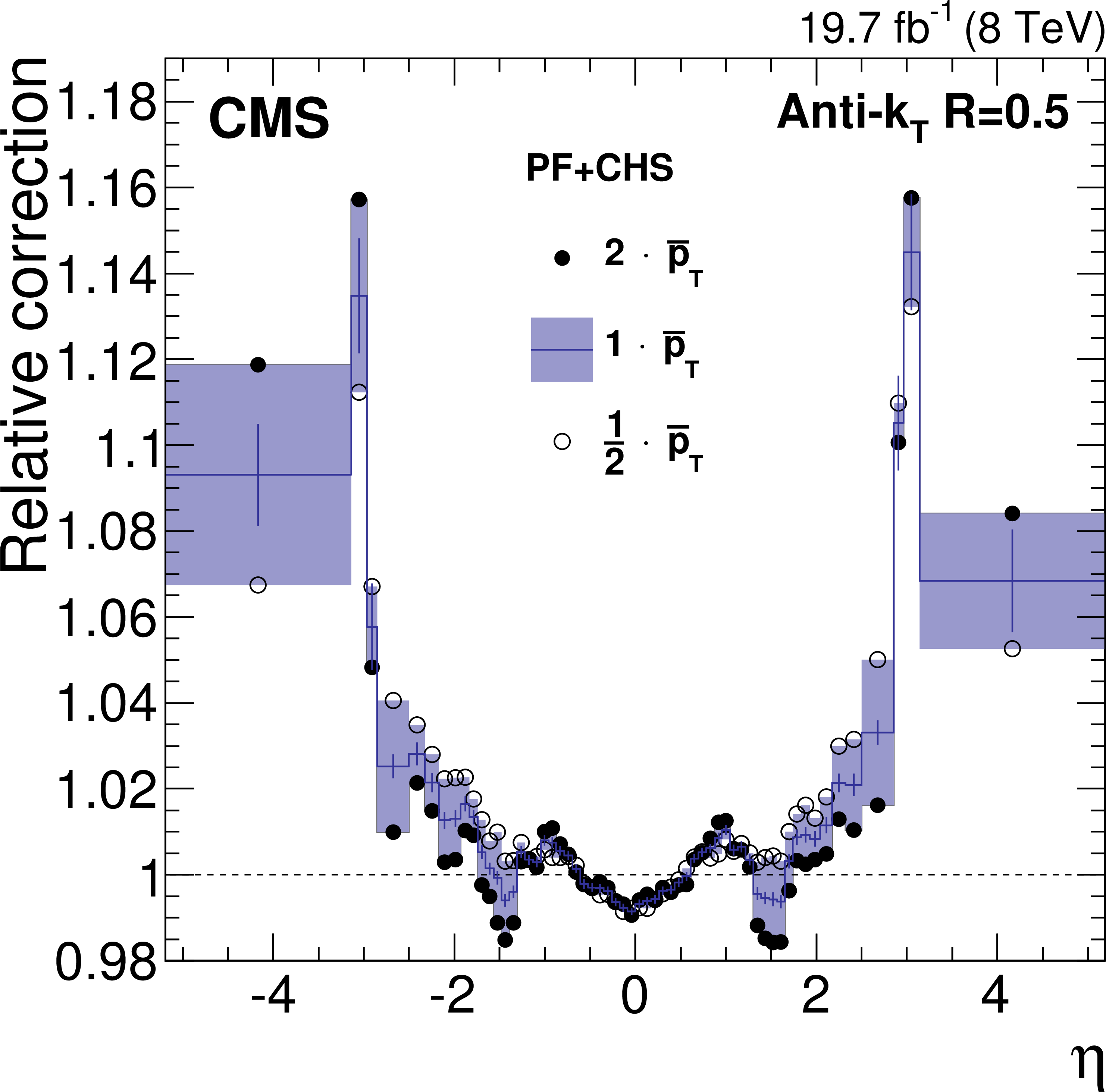
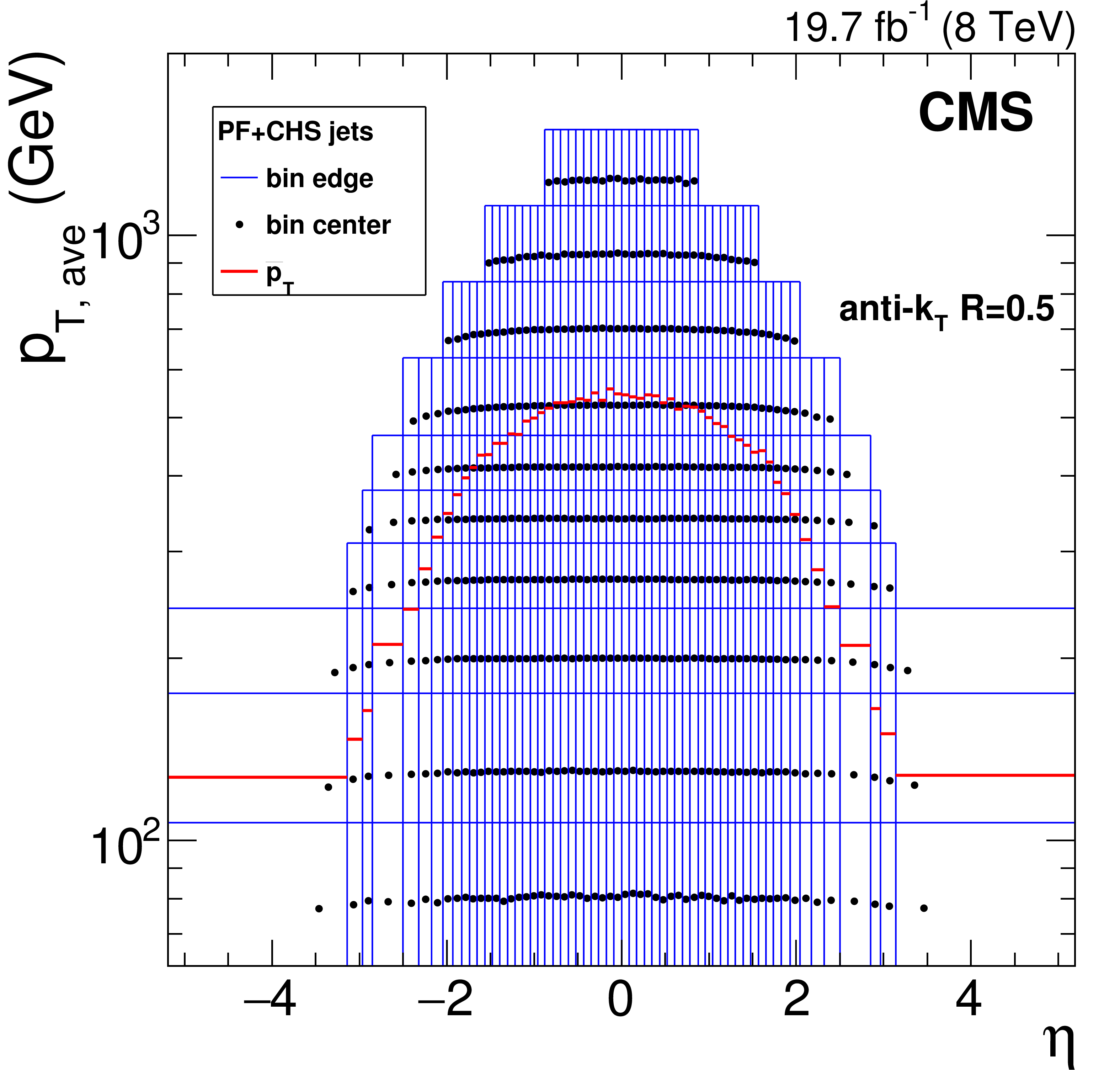
Figure 17:
Relative $\eta $ correction factor at the crossover $\bar{p}_{\rm T}$ (defined as the value of $ {p_{\mathrm {T}}} $ where the log-linear and constant fits versus $p_{\rm T, ave}$ agree) value, and at half and twice the $\bar{p}_{\rm T}$ values (a). The statistical uncertainty in the constant fit at each value of $\bar{p}_{\rm T}$ is also shown. Distribution of the $ {p_{\mathrm {T}}} $ and $\eta $ bins used in the dijet balance measurement, with a point at the average $ {p_{\mathrm {T}}} $ and $\eta $ for each bin (b). The horizontal red lines indicate the crossover $\bar{p}_{\rm T}$ value for each bin. |
png pdf |
Figure 17-a:
Relative $\eta $ correction factor at the crossover $\bar{p}_{\rm T}$ (defined as the value of $ {p_{\mathrm {T}}} $ where the log-linear and constant fits versus $p_{\rm T, ave}$ agree) value, and at half and twice the $\bar{p}_{\rm T}$ values (a). The statistical uncertainty in the constant fit at each value of $\bar{p}_{\rm T}$ is also shown. Distribution of the $ {p_{\mathrm {T}}} $ and $\eta $ bins used in the dijet balance measurement, with a point at the average $ {p_{\mathrm {T}}} $ and $\eta $ for each bin (b). The horizontal red lines indicate the crossover $\bar{p}_{\rm T}$ value for each bin. |
png pdf |
Figure 17-b:
Relative $\eta $ correction factor at the crossover $\bar{p}_{\rm T}$ (defined as the value of $ {p_{\mathrm {T}}} $ where the log-linear and constant fits versus $p_{\rm T, ave}$ agree) value, and at half and twice the $\bar{p}_{\rm T}$ values (a). The statistical uncertainty in the constant fit at each value of $\bar{p}_{\rm T}$ is also shown. Distribution of the $ {p_{\mathrm {T}}} $ and $\eta $ bins used in the dijet balance measurement, with a point at the average $ {p_{\mathrm {T}}} $ and $\eta $ for each bin (b). The horizontal red lines indicate the crossover $\bar{p}_{\rm T}$ value for each bin. |

png pdf |
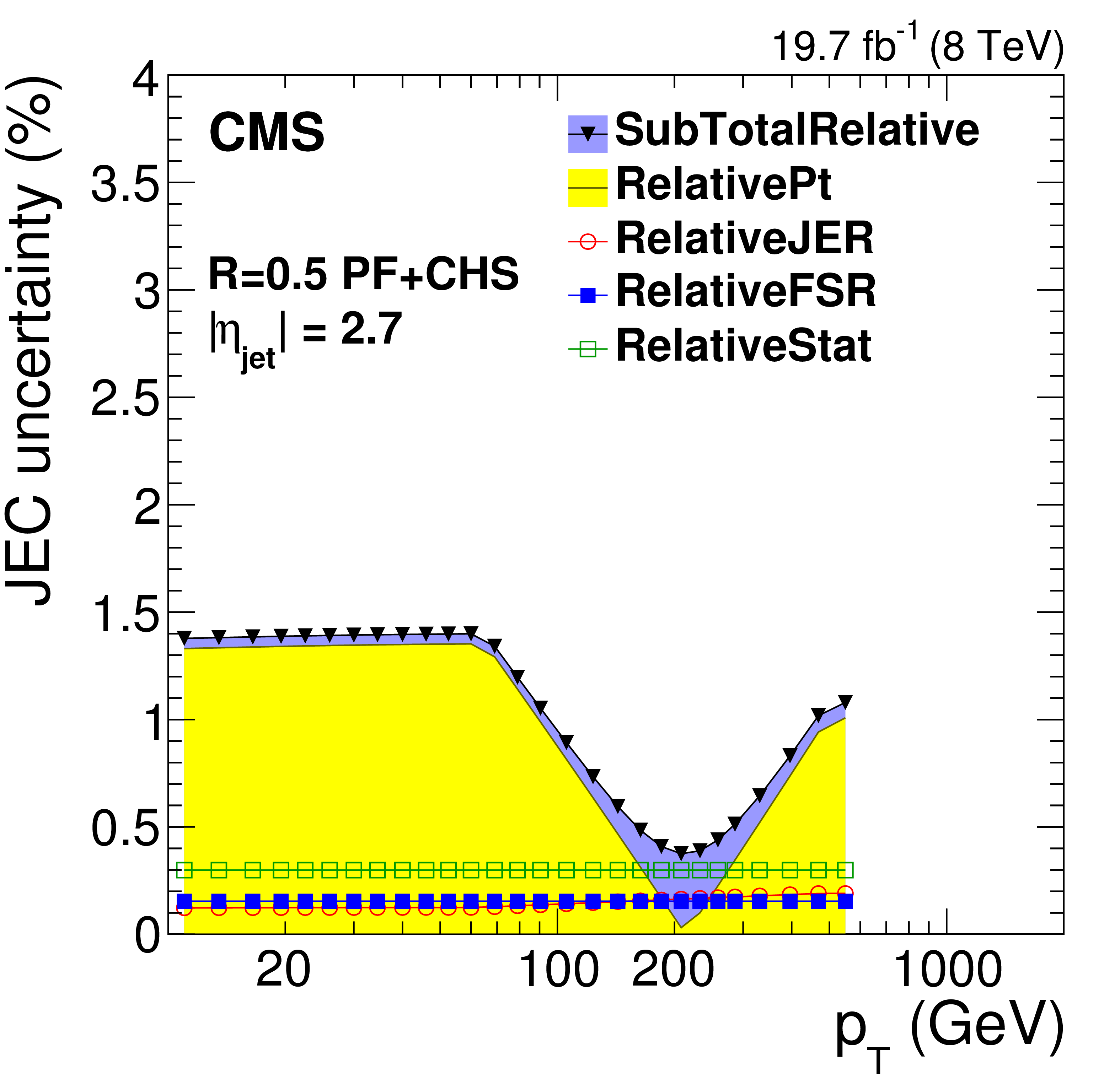
Figure 18:
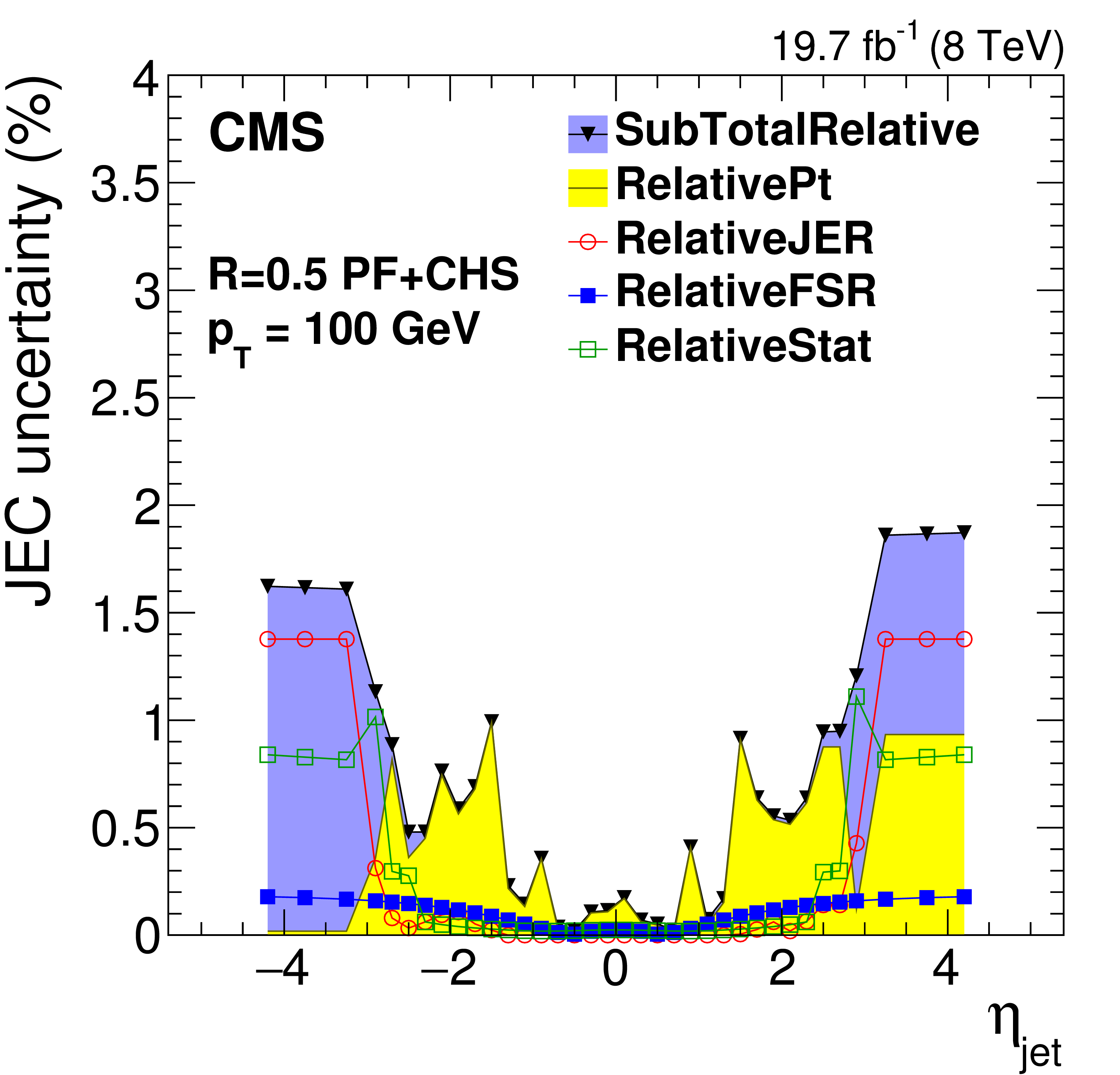
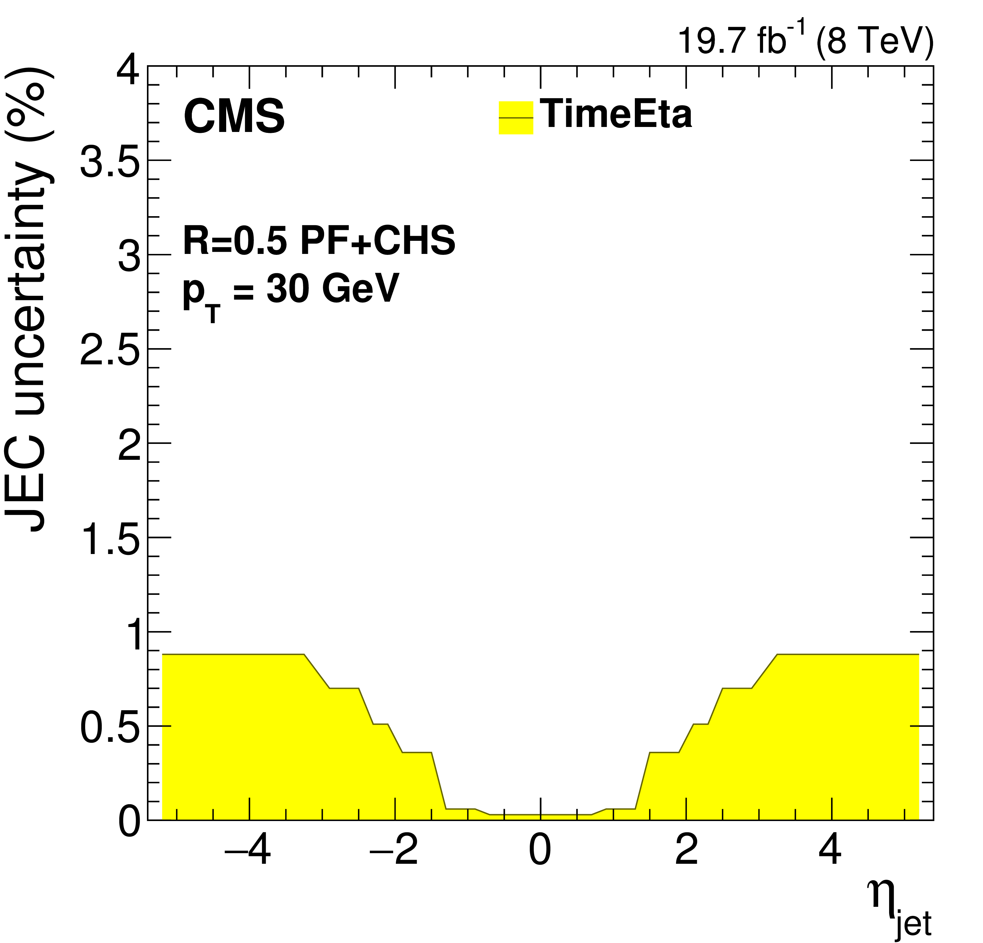
Systematic uncertainties for the relative $\eta $-dependent corrections as a function of jet $ {p_{\mathrm {T}}} $ (a) and as a function of jet $\eta $ for jets with $ {p_{\mathrm {T}}} = $ 30 GeV (b) and for jets with $ {p_{\mathrm {T}}} = $ 100 GeV (c). Time-dependent uncertainties as a function of jet $\eta $ for jets with $ {p_{\mathrm {T}}} = $ 30 GeV (d). The plots are limited to a jet energy $E= {p_{\mathrm {T}}} \cosh\eta = $ 4000 GeV so as to show only uncertainties for reasonable $ {p_{\mathrm {T}}} $ in the considered data-taking period. SubTotalRelative is the quadratic sum of RelativePt, RelativeJER, RelativeFSR and RelativeStat. |
png pdf |
Figure 18-a:
Systematic uncertainties for the relative $\eta $-dependent corrections as a function of jet $ {p_{\mathrm {T}}} $ (a) and as a function of jet $\eta $ for jets with $ {p_{\mathrm {T}}} = $ 30 GeV (b) and for jets with $ {p_{\mathrm {T}}} = $ 100 GeV (c). Time-dependent uncertainties as a function of jet $\eta $ for jets with $ {p_{\mathrm {T}}} = $ 30 GeV (d). The plots are limited to a jet energy $E= {p_{\mathrm {T}}} \cosh\eta = $ 4000 GeV so as to show only uncertainties for reasonable $ {p_{\mathrm {T}}} $ in the considered data-taking period. SubTotalRelative is the quadratic sum of RelativePt, RelativeJER, RelativeFSR and RelativeStat. |

png pdf |
Figure 18-b:
Systematic uncertainties for the relative $\eta $-dependent corrections as a function of jet $ {p_{\mathrm {T}}} $ (a) and as a function of jet $\eta $ for jets with $ {p_{\mathrm {T}}} = $ 30 GeV (b) and for jets with $ {p_{\mathrm {T}}} = $ 100 GeV (c). Time-dependent uncertainties as a function of jet $\eta $ for jets with $ {p_{\mathrm {T}}} = $ 30 GeV (d). The plots are limited to a jet energy $E= {p_{\mathrm {T}}} \cosh\eta = $ 4000 GeV so as to show only uncertainties for reasonable $ {p_{\mathrm {T}}} $ in the considered data-taking period. SubTotalRelative is the quadratic sum of RelativePt, RelativeJER, RelativeFSR and RelativeStat. |
png pdf |
Figure 18-c:
Systematic uncertainties for the relative $\eta $-dependent corrections as a function of jet $ {p_{\mathrm {T}}} $ (a) and as a function of jet $\eta $ for jets with $ {p_{\mathrm {T}}} = $ 30 GeV (b) and for jets with $ {p_{\mathrm {T}}} = $ 100 GeV (c). Time-dependent uncertainties as a function of jet $\eta $ for jets with $ {p_{\mathrm {T}}} = $ 30 GeV (d). The plots are limited to a jet energy $E= {p_{\mathrm {T}}} \cosh\eta = $ 4000 GeV so as to show only uncertainties for reasonable $ {p_{\mathrm {T}}} $ in the considered data-taking period. SubTotalRelative is the quadratic sum of RelativePt, RelativeJER, RelativeFSR and RelativeStat. |
png pdf |
Figure 18-d:
Systematic uncertainties for the relative $\eta $-dependent corrections as a function of jet $ {p_{\mathrm {T}}} $ (a) and as a function of jet $\eta $ for jets with $ {p_{\mathrm {T}}} = $ 30 GeV (b) and for jets with $ {p_{\mathrm {T}}} = $ 100 GeV (c). Time-dependent uncertainties as a function of jet $\eta $ for jets with $ {p_{\mathrm {T}}} = $ 30 GeV (d). The plots are limited to a jet energy $E= {p_{\mathrm {T}}} \cosh\eta = $ 4000 GeV so as to show only uncertainties for reasonable $ {p_{\mathrm {T}}} $ in the considered data-taking period. SubTotalRelative is the quadratic sum of RelativePt, RelativeJER, RelativeFSR and RelativeStat. |

png pdf |
Figure 19:
Jet response obtained with the $ {p_{\mathrm {T}}} $-balance and MPF methods in Z+jet events (points), for both data and simulation ({\sc Madgraph}4+Pythia6.4 tune Z2*), plotted as a function of $\alpha =p_{\rm T,2ndjet}/p_{\rm T,Z}$ (top). The response in data is scaled by a factor of 1.02, constant as a function of $ {p_{\mathrm {T}}} $. A fit to a first-order polynomial (dashed lines) is shown, together with the statistical uncertainty from the fit (shaded bands). Only events with $p_{\rm T, Z}> $ 30 GeV and $|\eta _{\rm jet}|< $ 1.3 are considered. The ratio of the jet response from the $ {p_{\mathrm {T}}} $-balance and MPF methods in data and simulation shown in the bottom panel. The simulated jet response $p_{\rm T,jet}/p_{\rm T,ptcl}$ is higher than unity because the jets are corrected with JEC from QCD dijet events with lower jet response than Z+jet events due to higher gluon fraction and larger underlying event. |
png pdf |
Figure 20:
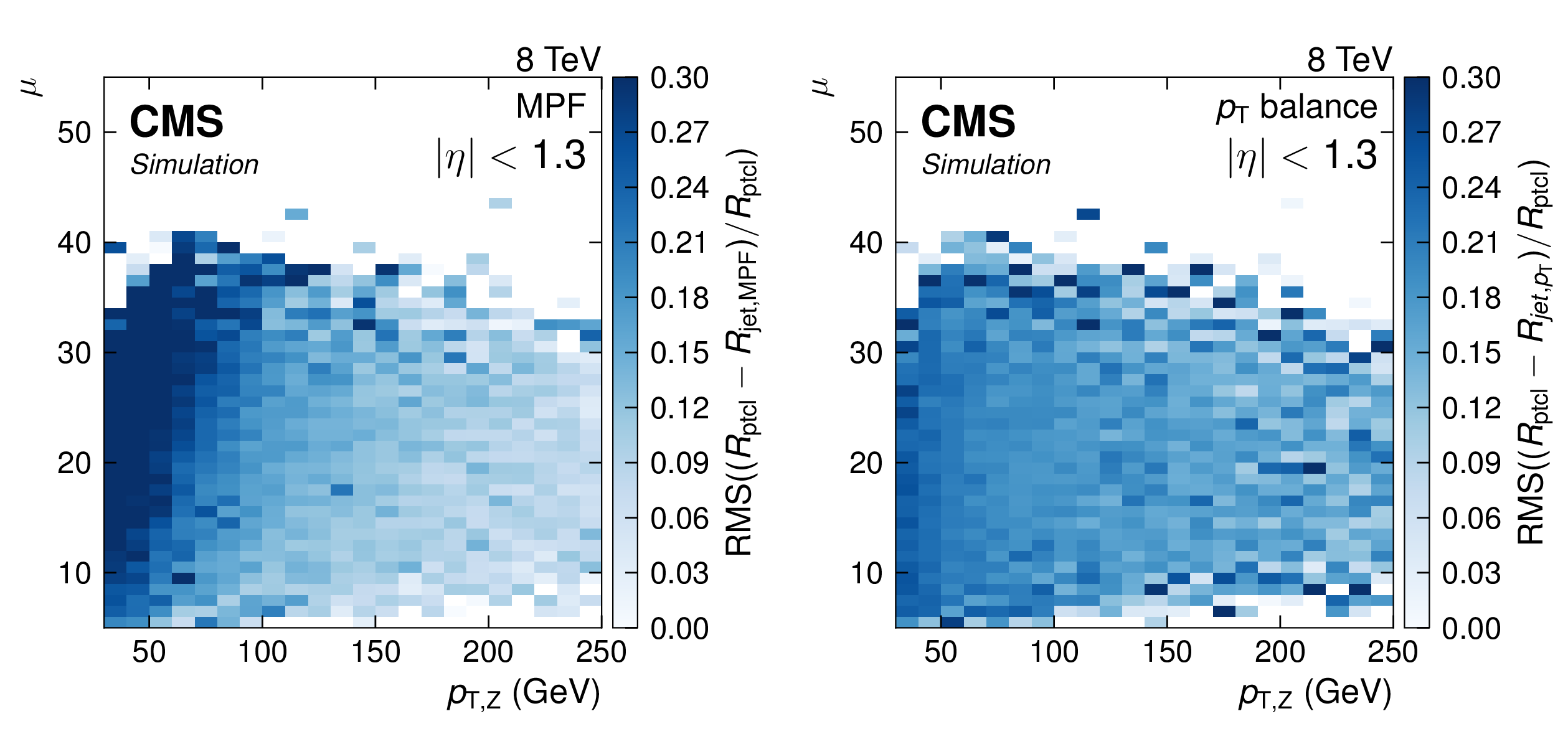
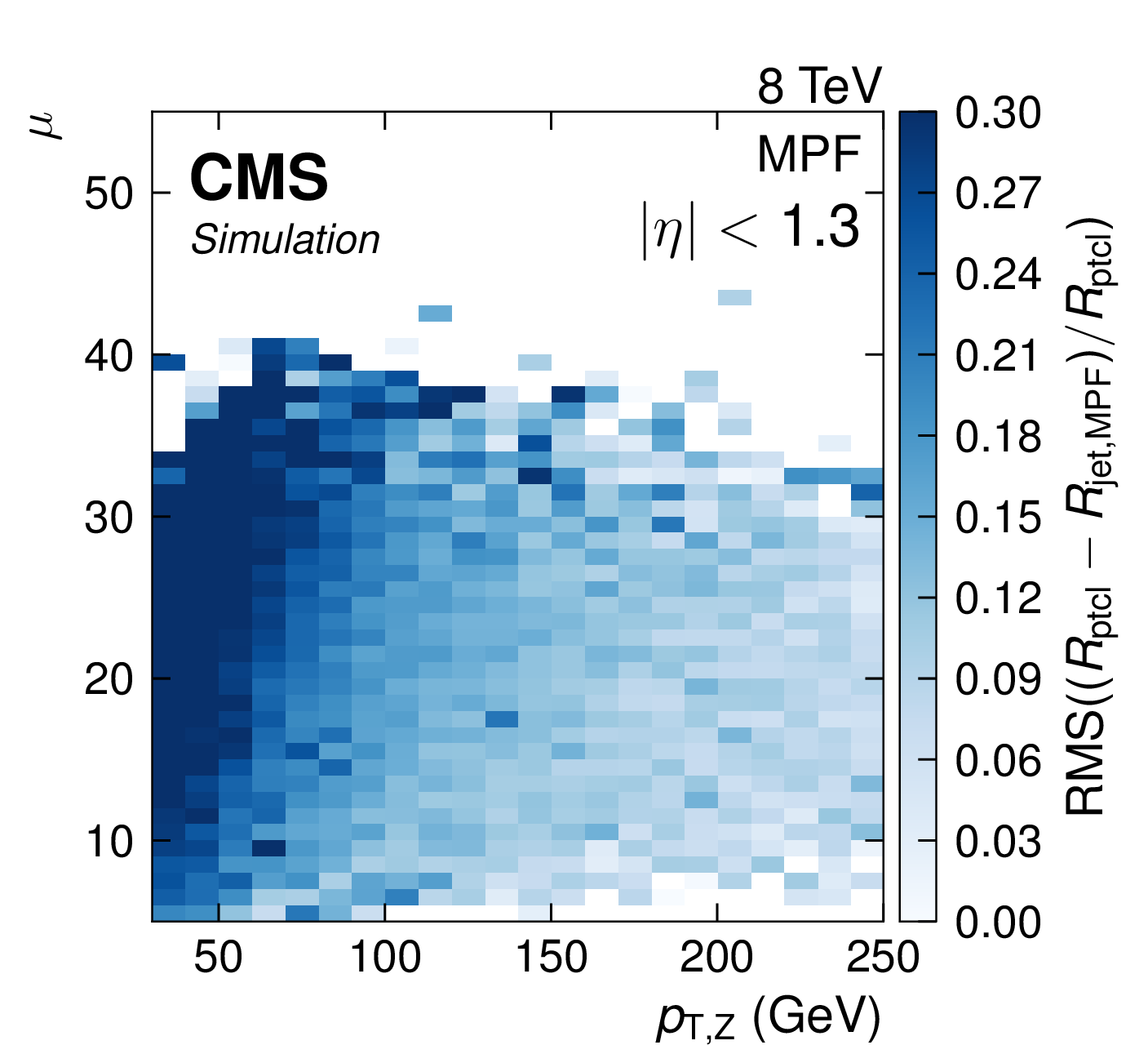
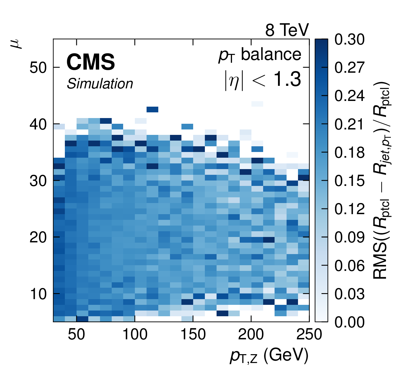
Relative resolution (blue scale) in the plane of mean number of pileup events ($\mu $) and Z boson transverse momentum ($p_{\rm T, Z}$) for the MPF balance (a) and $ {p_{\mathrm {T}}} $-balance methods (b). |
png pdf |
Figure 20-a:
Relative resolution (blue scale) in the plane of mean number of pileup events ($\mu $) and Z boson transverse momentum ($p_{\rm T, Z}$) for the MPF balance (a) and $ {p_{\mathrm {T}}} $-balance methods (b). |
png pdf |
Figure 20-b:
Relative resolution (blue scale) in the plane of mean number of pileup events ($\mu $) and Z boson transverse momentum ($p_{\rm T, Z}$) for the MPF balance (a) and $ {p_{\mathrm {T}}} $-balance methods (b). |
png pdf |
Figure 21:
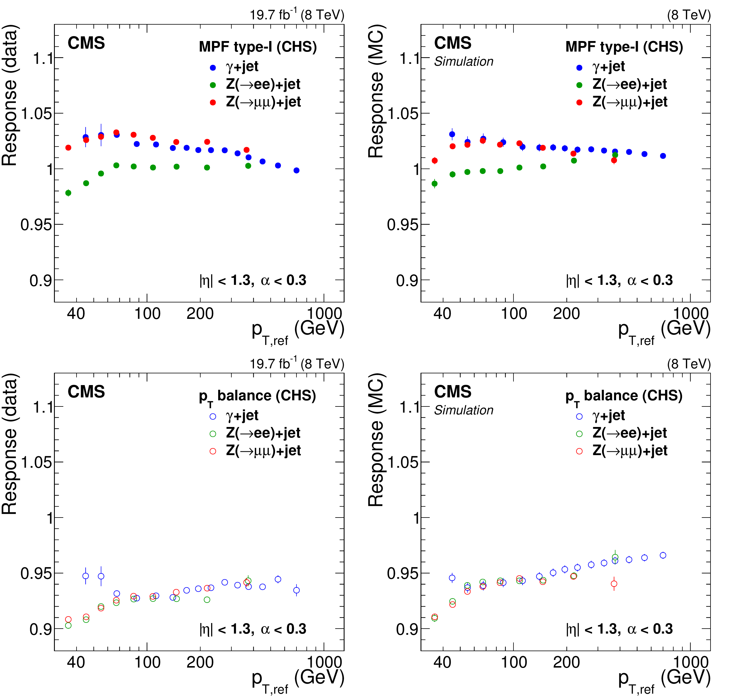
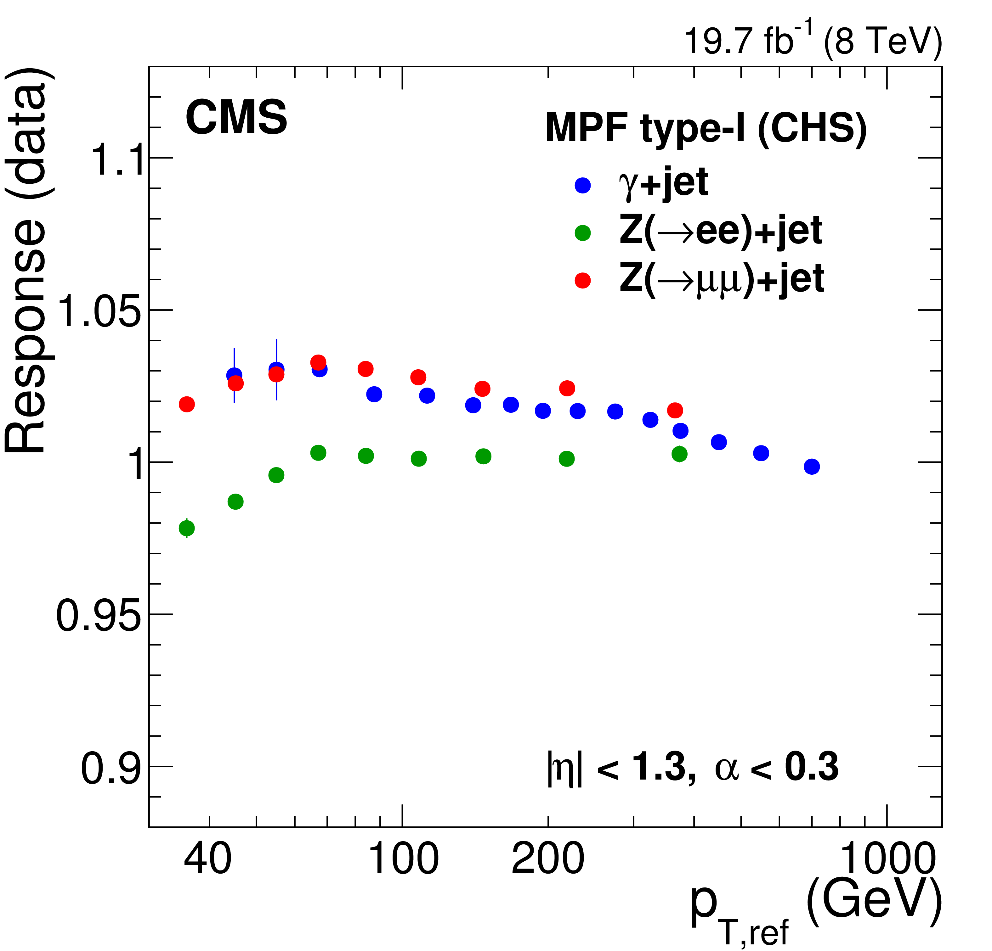
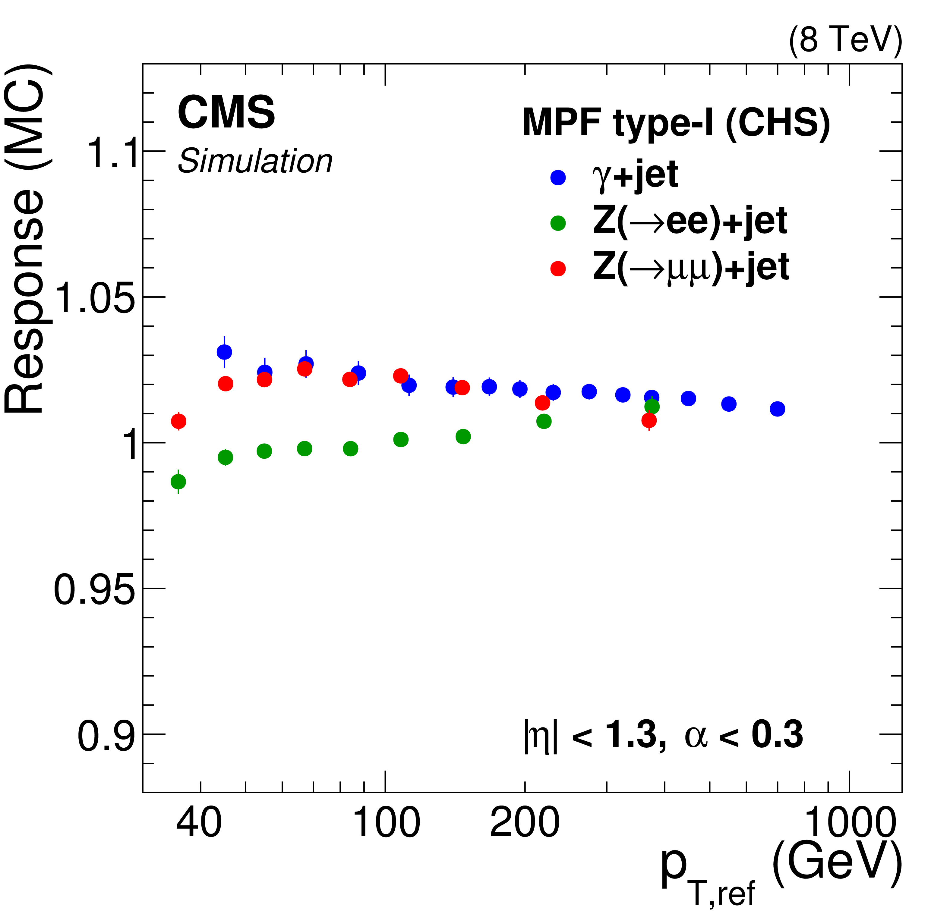
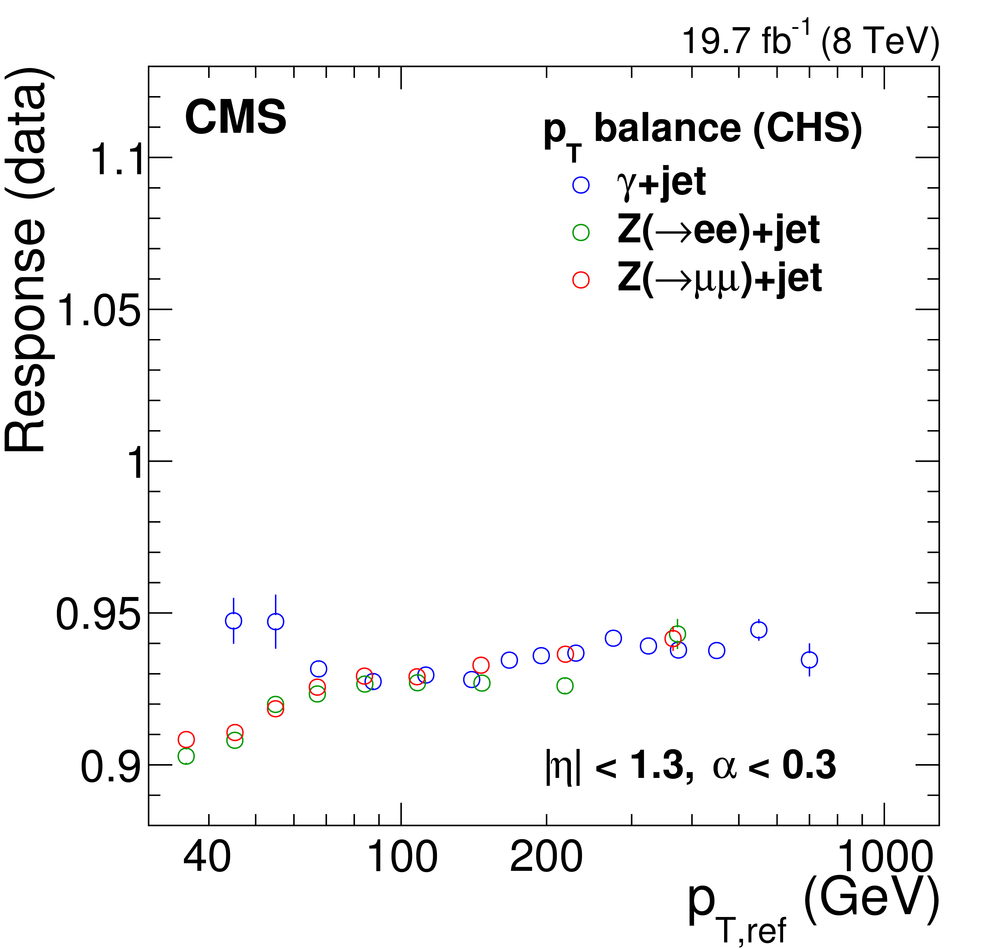
Comparison of jet response measurements from $ \mathrm{ Z } (\to \mu \mu)$+jet, $ \mathrm{ Z } (\to \mathrm{ e } \mathrm{ e })$+jet, and $\gamma $+jet samples as a function of Z boson or photon $ {p_{\mathrm {T}}} $. The jet response from the MPF method (a,b) and the $ {p_{\mathrm {T}}} $-balance method (c,d) is shown as a function of Z and $\gamma $ $ {p_{\mathrm {T}}} $ for data (a,c) and simulation (b,d). The $ \mathrm{ Z } (\to \mathrm{ e } \mathrm{ e })$+jet sample has not been corrected for the electron EM footprint in ${\vec{p}_{\mathrm {T}}^{\, \text {miss}}} $, explaining the low MPF response in both data and simulation. The footprint effect is absent for muons and corrected for photons. |
png pdf |
Figure 21-a:
Comparison of jet response measurements from $ \mathrm{ Z } (\to \mu \mu)$+jet, $ \mathrm{ Z } (\to \mathrm{ e } \mathrm{ e })$+jet, and $\gamma $+jet samples as a function of Z boson or photon $ {p_{\mathrm {T}}} $. The jet response from the MPF method (a,b) and the $ {p_{\mathrm {T}}} $-balance method (c,d) is shown as a function of Z and $\gamma $ $ {p_{\mathrm {T}}} $ for data (a,c) and simulation (b,d). The $ \mathrm{ Z } (\to \mathrm{ e } \mathrm{ e })$+jet sample has not been corrected for the electron EM footprint in ${\vec{p}_{\mathrm {T}}^{\, \text {miss}}} $, explaining the low MPF response in both data and simulation. The footprint effect is absent for muons and corrected for photons. |
png pdf |
Figure 21-b:
Comparison of jet response measurements from $ \mathrm{ Z } (\to \mu \mu)$+jet, $ \mathrm{ Z } (\to \mathrm{ e } \mathrm{ e })$+jet, and $\gamma $+jet samples as a function of Z boson or photon $ {p_{\mathrm {T}}} $. The jet response from the MPF method (a,b) and the $ {p_{\mathrm {T}}} $-balance method (c,d) is shown as a function of Z and $\gamma $ $ {p_{\mathrm {T}}} $ for data (a,c) and simulation (b,d). The $ \mathrm{ Z } (\to \mathrm{ e } \mathrm{ e })$+jet sample has not been corrected for the electron EM footprint in ${\vec{p}_{\mathrm {T}}^{\, \text {miss}}} $, explaining the low MPF response in both data and simulation. The footprint effect is absent for muons and corrected for photons. |
png pdf |
Figure 21-c:
Comparison of jet response measurements from $ \mathrm{ Z } (\to \mu \mu)$+jet, $ \mathrm{ Z } (\to \mathrm{ e } \mathrm{ e })$+jet, and $\gamma $+jet samples as a function of Z boson or photon $ {p_{\mathrm {T}}} $. The jet response from the MPF method (a,b) and the $ {p_{\mathrm {T}}} $-balance method (c,d) is shown as a function of Z and $\gamma $ $ {p_{\mathrm {T}}} $ for data (a,c) and simulation (b,d). The $ \mathrm{ Z } (\to \mathrm{ e } \mathrm{ e })$+jet sample has not been corrected for the electron EM footprint in ${\vec{p}_{\mathrm {T}}^{\, \text {miss}}} $, explaining the low MPF response in both data and simulation. The footprint effect is absent for muons and corrected for photons. |
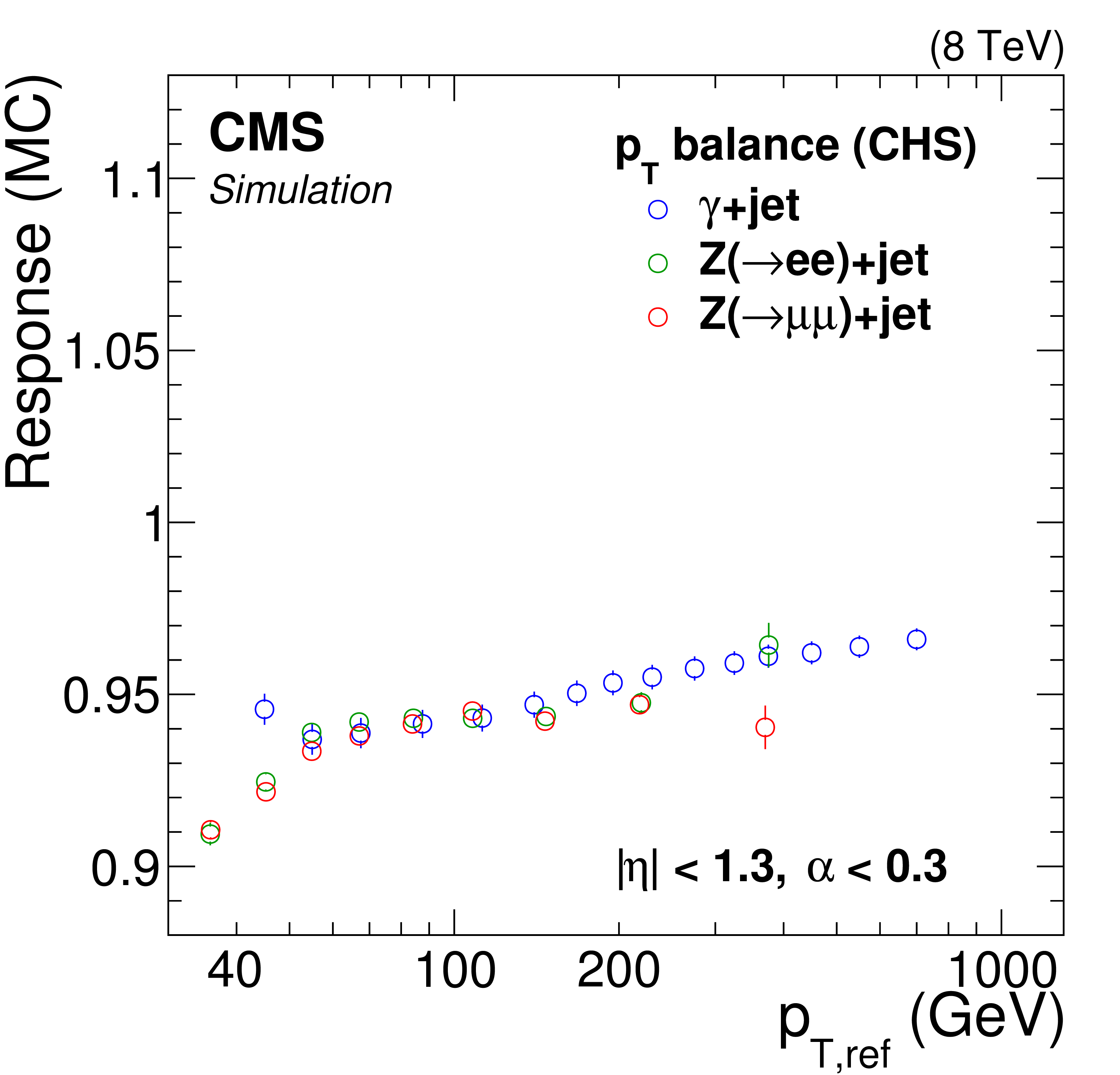
png pdf |
Figure 21-d:
Comparison of jet response measurements from $ \mathrm{ Z } (\to \mu \mu)$+jet, $ \mathrm{ Z } (\to \mathrm{ e } \mathrm{ e })$+jet, and $\gamma $+jet samples as a function of Z boson or photon $ {p_{\mathrm {T}}} $. The jet response from the MPF method (a,b) and the $ {p_{\mathrm {T}}} $-balance method (c,d) is shown as a function of Z and $\gamma $ $ {p_{\mathrm {T}}} $ for data (a,c) and simulation (b,d). The $ \mathrm{ Z } (\to \mathrm{ e } \mathrm{ e })$+jet sample has not been corrected for the electron EM footprint in ${\vec{p}_{\mathrm {T}}^{\, \text {miss}}} $, explaining the low MPF response in both data and simulation. The footprint effect is absent for muons and corrected for photons. |

png pdf |
Figure 22:
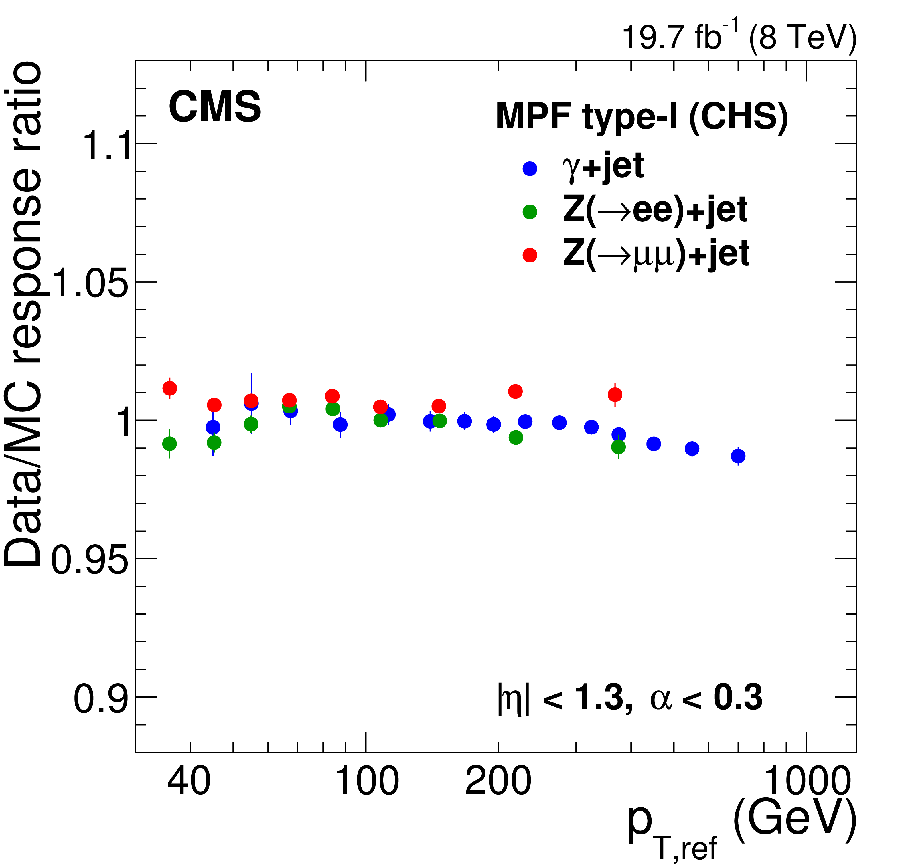
Ratio of the jet response measurement obtained from data and simulation with the MPF method (a) and $ {p_{\mathrm {T}}} $-balance method (b). Results are shown for the $ \mathrm{ Z } (\to \mu \mu)$+jet, $ \mathrm{ Z } (\to \mathrm{ e } \mathrm{ e })$+jet, and $\gamma $+jet samples. The $ \mathrm{ Z } (\to \mathrm{ e } \mathrm{ e })$+jet\ sample has not been corrected for the electron EM footprint in ${\vec{p}_{\mathrm {T}}^{\, \text {miss}}} $, but the effect cancels out in the ratio of data over simulation. |
png pdf |
Figure 22-a:
Ratio of the jet response measurement obtained from data and simulation with the MPF method (a) and $ {p_{\mathrm {T}}} $-balance method (b). Results are shown for the $ \mathrm{ Z } (\to \mu \mu)$+jet, $ \mathrm{ Z } (\to \mathrm{ e } \mathrm{ e })$+jet, and $\gamma $+jet samples. The $ \mathrm{ Z } (\to \mathrm{ e } \mathrm{ e })$+jet\ sample has not been corrected for the electron EM footprint in ${\vec{p}_{\mathrm {T}}^{\, \text {miss}}} $, but the effect cancels out in the ratio of data over simulation. |

png pdf |
Figure 22-b:
Ratio of the jet response measurement obtained from data and simulation with the MPF method (a) and $ {p_{\mathrm {T}}} $-balance method (b). Results are shown for the $ \mathrm{ Z } (\to \mu \mu)$+jet, $ \mathrm{ Z } (\to \mathrm{ e } \mathrm{ e })$+jet, and $\gamma $+jet samples. The $ \mathrm{ Z } (\to \mathrm{ e } \mathrm{ e })$+jet\ sample has not been corrected for the electron EM footprint in ${\vec{p}_{\mathrm {T}}^{\, \text {miss}}} $, but the effect cancels out in the ratio of data over simulation. |
png pdf |
Figure 23:
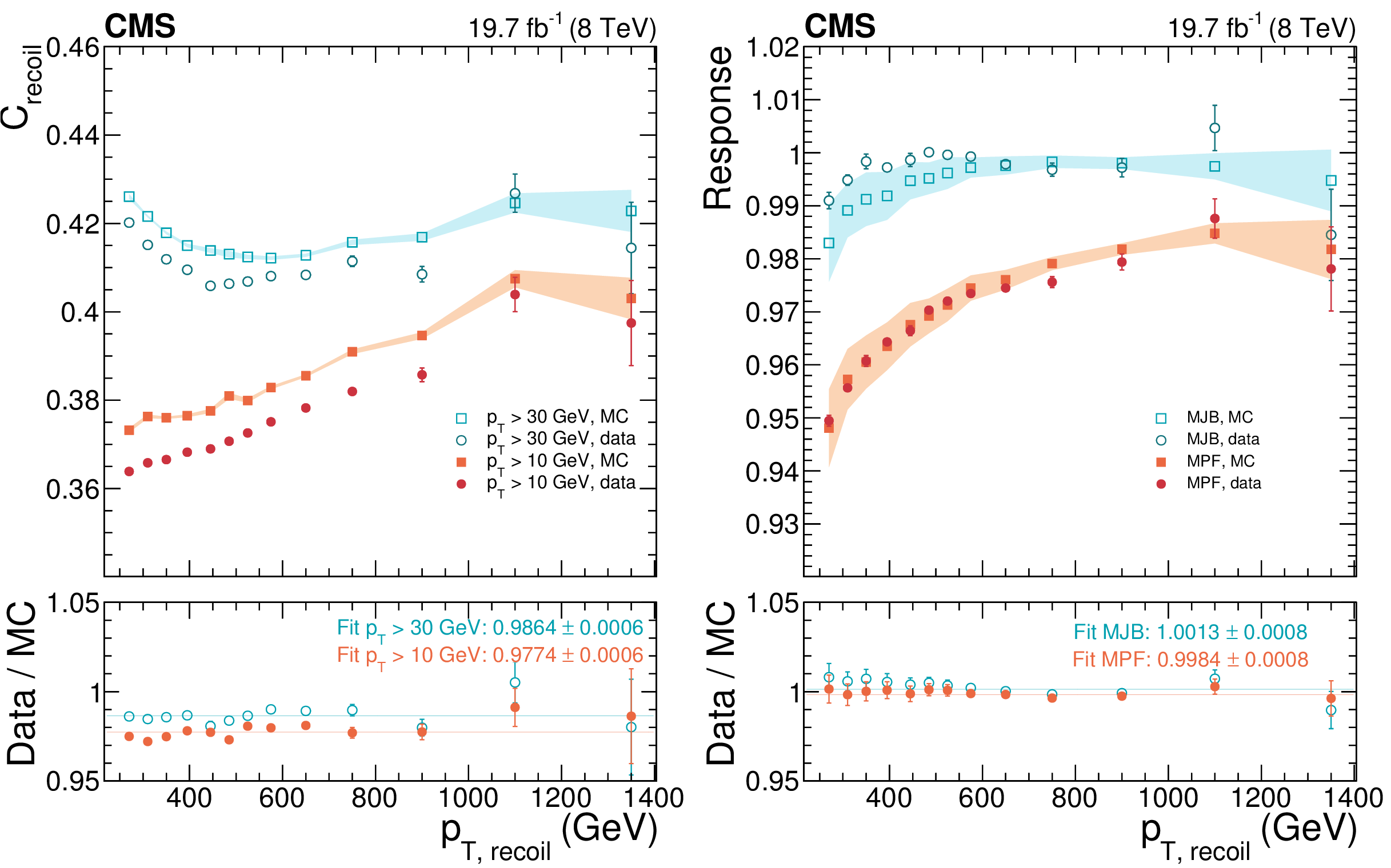
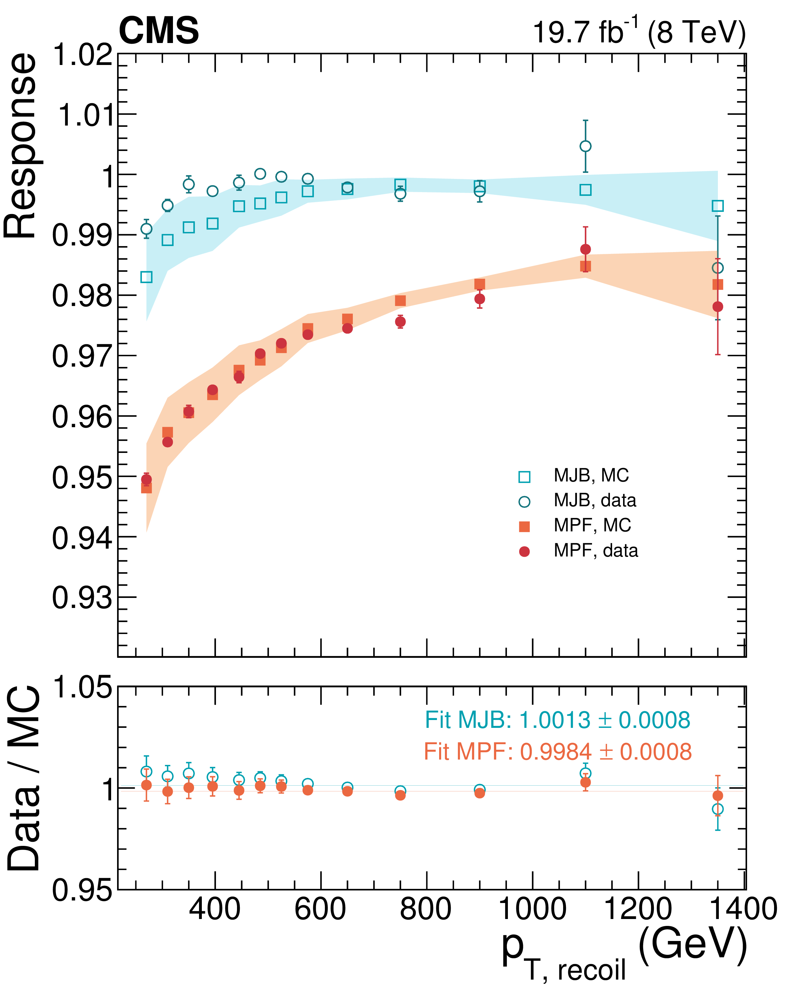
$C_{\rm recoil}$ ratio of the effective jet $ {p_{\mathrm {T}}} $ of jets in the recoil over the total recoil $ {p_{\mathrm {T}}} $, (Eq.(23)), calculated with recoil jets of $ {p_{\mathrm {T}}} > $ 30 GeV (for MJB) and $ {p_{\mathrm {T}}} > $ 10 GeV (for MPF) in data and MC simulation (a). Multijet balance response calculated with the MJB and MPF methods for data and MC simulation (b). The filled bands show the total (statistical and systematic) uncertainty on MC and the error bars the statistical uncertainty on data. |

png pdf |
Figure 23-a:
$C_{\rm recoil}$ ratio of the effective jet $ {p_{\mathrm {T}}} $ of jets in the recoil over the total recoil $ {p_{\mathrm {T}}} $, (Eq.(23)), calculated with recoil jets of $ {p_{\mathrm {T}}} > $ 30 GeV (for MJB) and $ {p_{\mathrm {T}}} > $ 10 GeV (for MPF) in data and MC simulation (a). Multijet balance response calculated with the MJB and MPF methods for data and MC simulation (b). The filled bands show the total (statistical and systematic) uncertainty on MC and the error bars the statistical uncertainty on data. |
png pdf |
Figure 23-b:
$C_{\rm recoil}$ ratio of the effective jet $ {p_{\mathrm {T}}} $ of jets in the recoil over the total recoil $ {p_{\mathrm {T}}} $, (Eq.(23)), calculated with recoil jets of $ {p_{\mathrm {T}}} > $ 30 GeV (for MJB) and $ {p_{\mathrm {T}}} > $ 10 GeV (for MPF) in data and MC simulation (a). Multijet balance response calculated with the MJB and MPF methods for data and MC simulation (b). The filled bands show the total (statistical and systematic) uncertainty on MC and the error bars the statistical uncertainty on data. |
png pdf |
Figure 24:
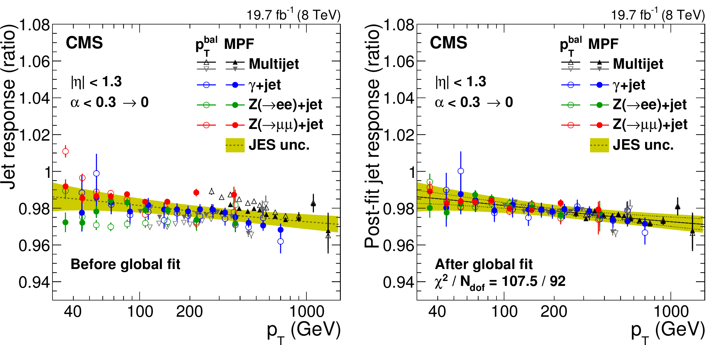
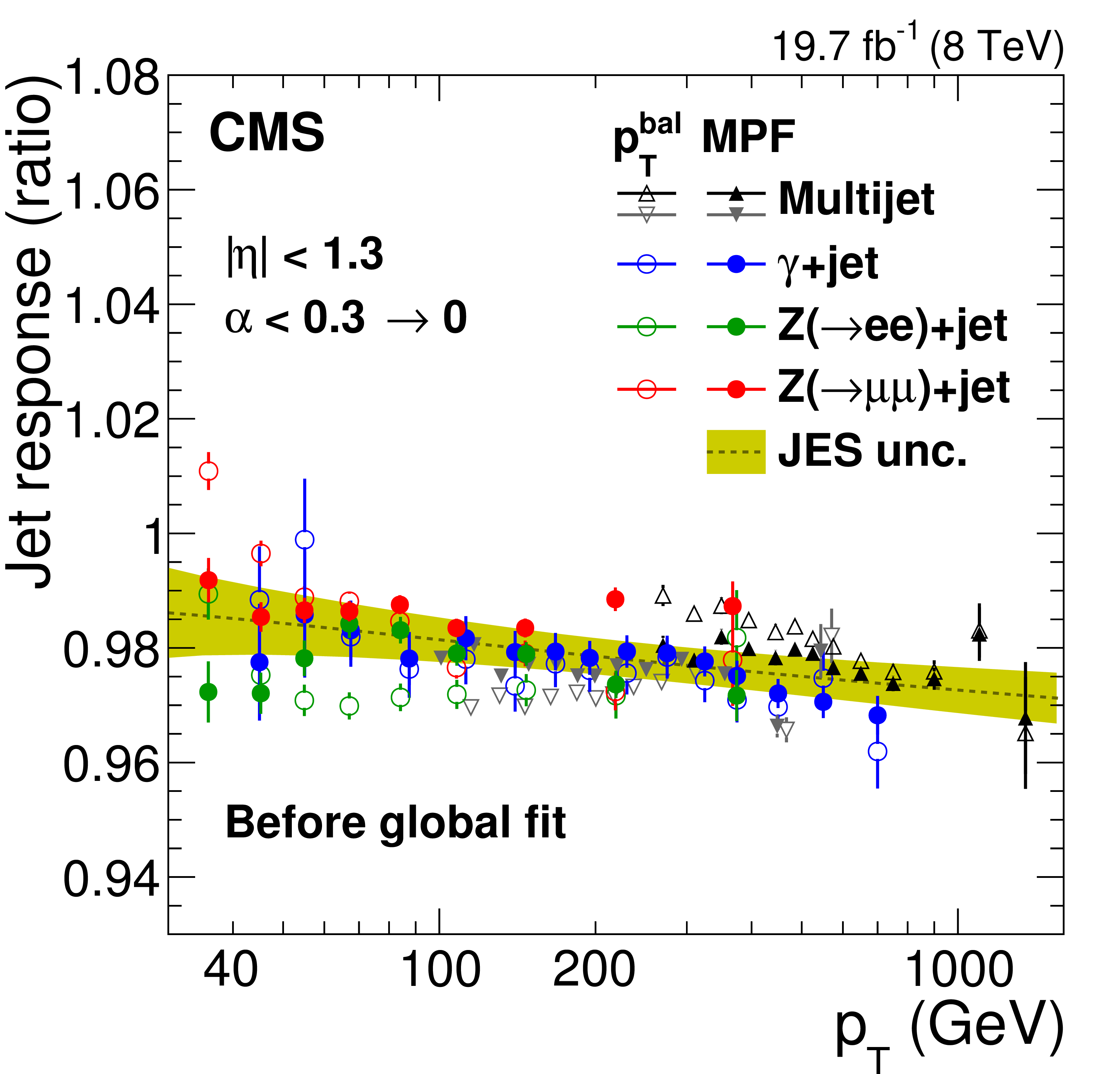
Comparison of the data-to-simulation ratio of the jet response measurements from $ \mathrm{ Z } (\to \mu \mu)$+jet, $ \mathrm{ Z } (\to \mathrm{ e } \mathrm{ e })$+jet, $\gamma $+jet, and multijet samples after applying the corrections for JES and ISR+FSR (a) and after applying, in addition, the nuisance parameter values found by the global fit (b). The uncertainty in the ratio, excluding jet-flavor and time-dependent effects, is shown by the shaded region. The solid line shows the global fit central value and the dotted curves the statistical uncertainty of the fit. As the multijet analysis connects the jet energy scale of jets in two different $ {p_{\mathrm {T}}} $ ranges (Eq.(24)), it can be used to constrain one given the other or vice versa: the two sets of points are relative to the two approaches. |
png pdf |
Figure 24-a:
Comparison of the data-to-simulation ratio of the jet response measurements from $ \mathrm{ Z } (\to \mu \mu)$+jet, $ \mathrm{ Z } (\to \mathrm{ e } \mathrm{ e })$+jet, $\gamma $+jet, and multijet samples after applying the corrections for JES and ISR+FSR (a) and after applying, in addition, the nuisance parameter values found by the global fit (b). The uncertainty in the ratio, excluding jet-flavor and time-dependent effects, is shown by the shaded region. The solid line shows the global fit central value and the dotted curves the statistical uncertainty of the fit. As the multijet analysis connects the jet energy scale of jets in two different $ {p_{\mathrm {T}}} $ ranges (Eq.(24)), it can be used to constrain one given the other or vice versa: the two sets of points are relative to the two approaches. |

png pdf |
Figure 24-b:
Comparison of the data-to-simulation ratio of the jet response measurements from $ \mathrm{ Z } (\to \mu \mu)$+jet, $ \mathrm{ Z } (\to \mathrm{ e } \mathrm{ e })$+jet, $\gamma $+jet, and multijet samples after applying the corrections for JES and ISR+FSR (a) and after applying, in addition, the nuisance parameter values found by the global fit (b). The uncertainty in the ratio, excluding jet-flavor and time-dependent effects, is shown by the shaded region. The solid line shows the global fit central value and the dotted curves the statistical uncertainty of the fit. As the multijet analysis connects the jet energy scale of jets in two different $ {p_{\mathrm {T}}} $ ranges (Eq.(24)), it can be used to constrain one given the other or vice versa: the two sets of points are relative to the two approaches. |
png pdf |
Figure 25:
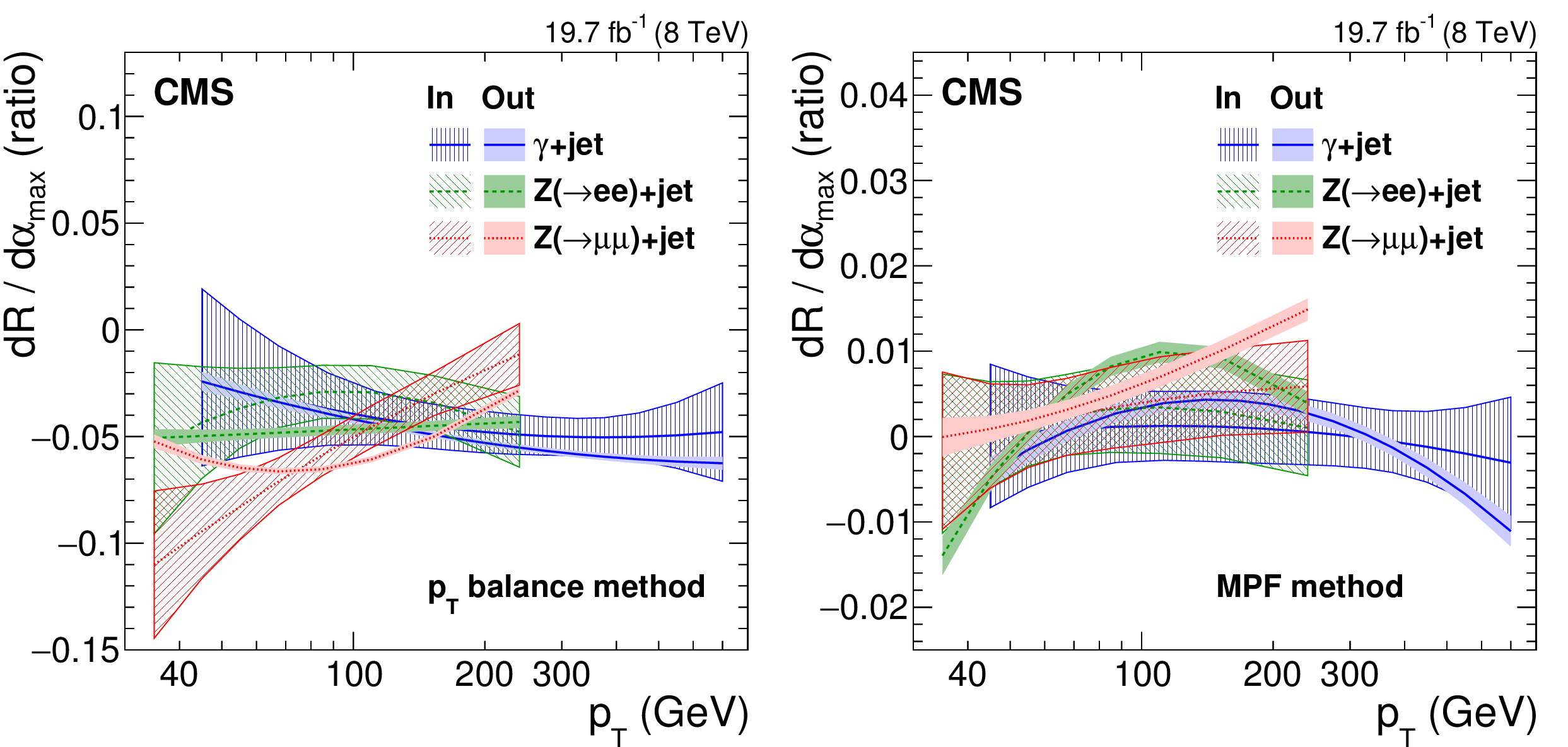
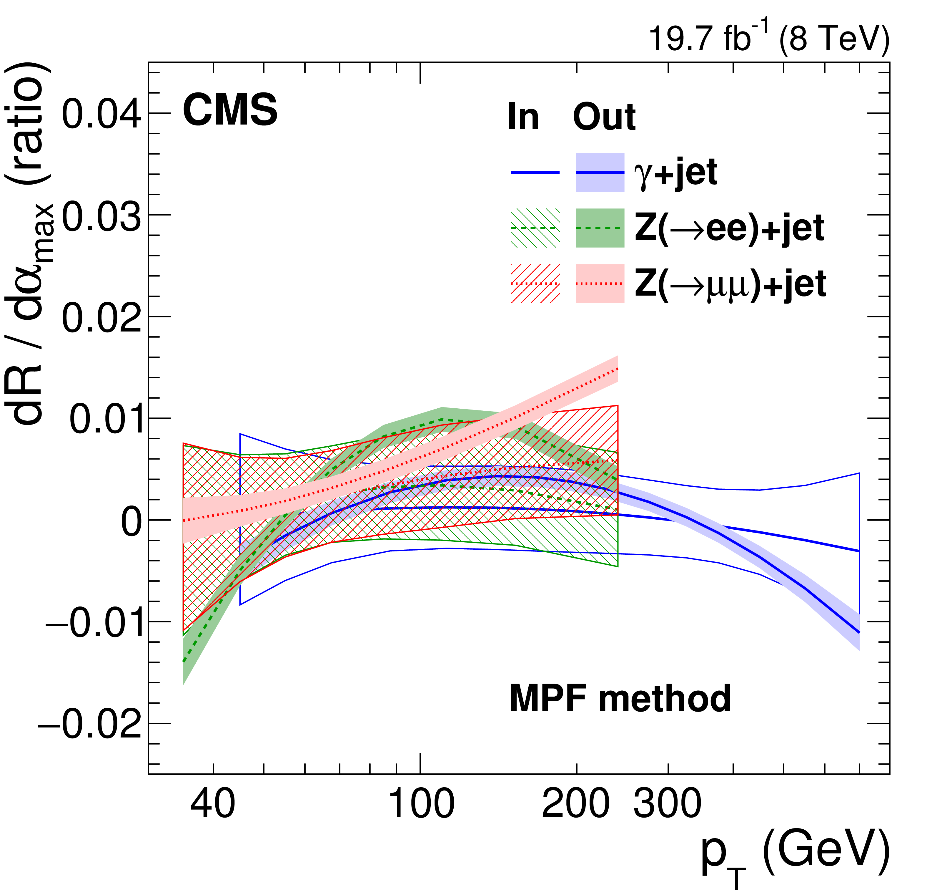
Central value of the data-to-simulation ratio of ${\rm d}R/{\rm d}\alpha _{\rm max}$, and its 68% probability region, as a function of jet $ {p_{\mathrm {T}}} $, for the $ {p_{\mathrm {T}}} $-balance (a) and MPF (b) methods. The ${\rm d}R/{\rm d}\alpha _{\rm max}$ is the derivative of the jet response evaluated in events with $\alpha <\alpha _{\rm max}$. The y-axis scale for the MPF method is zoomed by ${\times } 4$ compared to the $ {p_{\mathrm {T}}} $-balance method, demonstrating the much smaller initial ISR+FSR uncertainty for this method. The shadowed regions show the input distributions to the global fit, while the full color regions show the post-fit distributions. The uncertainties on ${\rm d}R/{\rm d}\alpha _{\rm max}$ before the global fit are labeled 'In', and the uncertainties constrained by the global fit are labeled 'Out'. |

png pdf |
Figure 25-a:
Central value of the data-to-simulation ratio of ${\rm d}R/{\rm d}\alpha _{\rm max}$, and its 68% probability region, as a function of jet $ {p_{\mathrm {T}}} $, for the $ {p_{\mathrm {T}}} $-balance (a) and MPF (b) methods. The ${\rm d}R/{\rm d}\alpha _{\rm max}$ is the derivative of the jet response evaluated in events with $\alpha <\alpha _{\rm max}$. The y-axis scale for the MPF method is zoomed by ${\times } 4$ compared to the $ {p_{\mathrm {T}}} $-balance method, demonstrating the much smaller initial ISR+FSR uncertainty for this method. The shadowed regions show the input distributions to the global fit, while the full color regions show the post-fit distributions. The uncertainties on ${\rm d}R/{\rm d}\alpha _{\rm max}$ before the global fit are labeled 'In', and the uncertainties constrained by the global fit are labeled 'Out'. |
png pdf |
Figure 25-b:
Central value of the data-to-simulation ratio of ${\rm d}R/{\rm d}\alpha _{\rm max}$, and its 68% probability region, as a function of jet $ {p_{\mathrm {T}}} $, for the $ {p_{\mathrm {T}}} $-balance (a) and MPF (b) methods. The ${\rm d}R/{\rm d}\alpha _{\rm max}$ is the derivative of the jet response evaluated in events with $\alpha <\alpha _{\rm max}$. The y-axis scale for the MPF method is zoomed by ${\times } 4$ compared to the $ {p_{\mathrm {T}}} $-balance method, demonstrating the much smaller initial ISR+FSR uncertainty for this method. The shadowed regions show the input distributions to the global fit, while the full color regions show the post-fit distributions. The uncertainties on ${\rm d}R/{\rm d}\alpha _{\rm max}$ before the global fit are labeled 'In', and the uncertainties constrained by the global fit are labeled 'Out'. |
png pdf |
Figure 26:
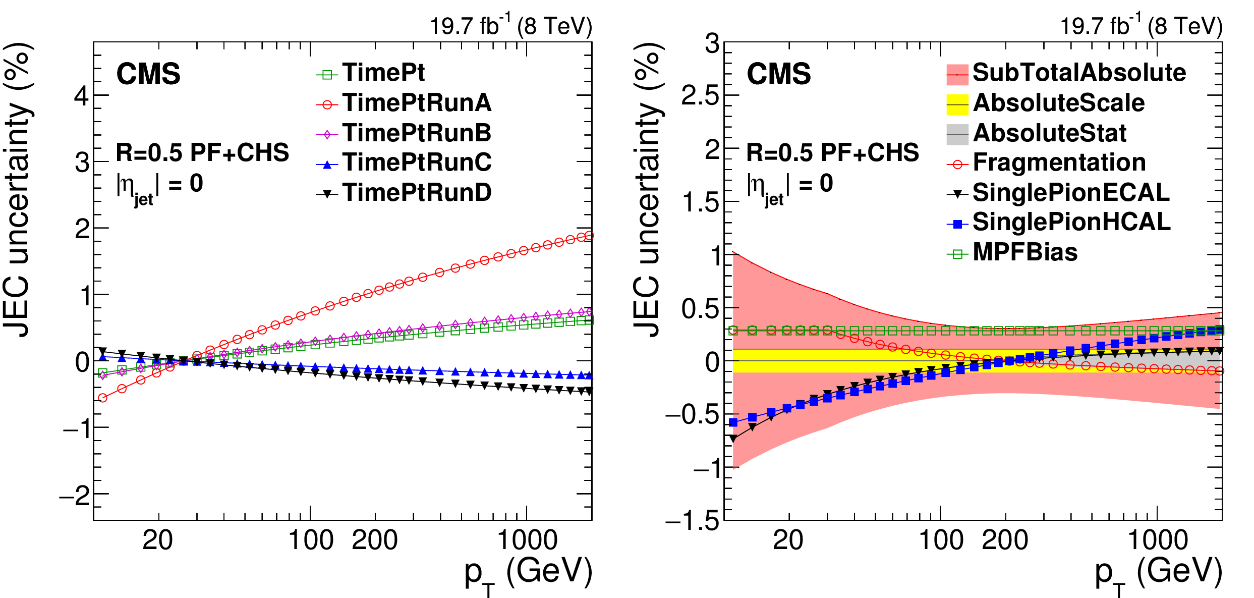
Absolute scale time-dependent uncertainty as a function of jet $ {p_{\mathrm {T}}} $ for various data-taking periods (a). Systematic uncertainties for the absolute jet scale as a function of $ {p_{\mathrm {T}}} $ (b). SubTotalAbsolute is the quadratic sum of AbsoluteScale, AbsoluteStat, Fragmentation, SinglePionECAL, SinglePionHCAL and MPFBias. |
png pdf |
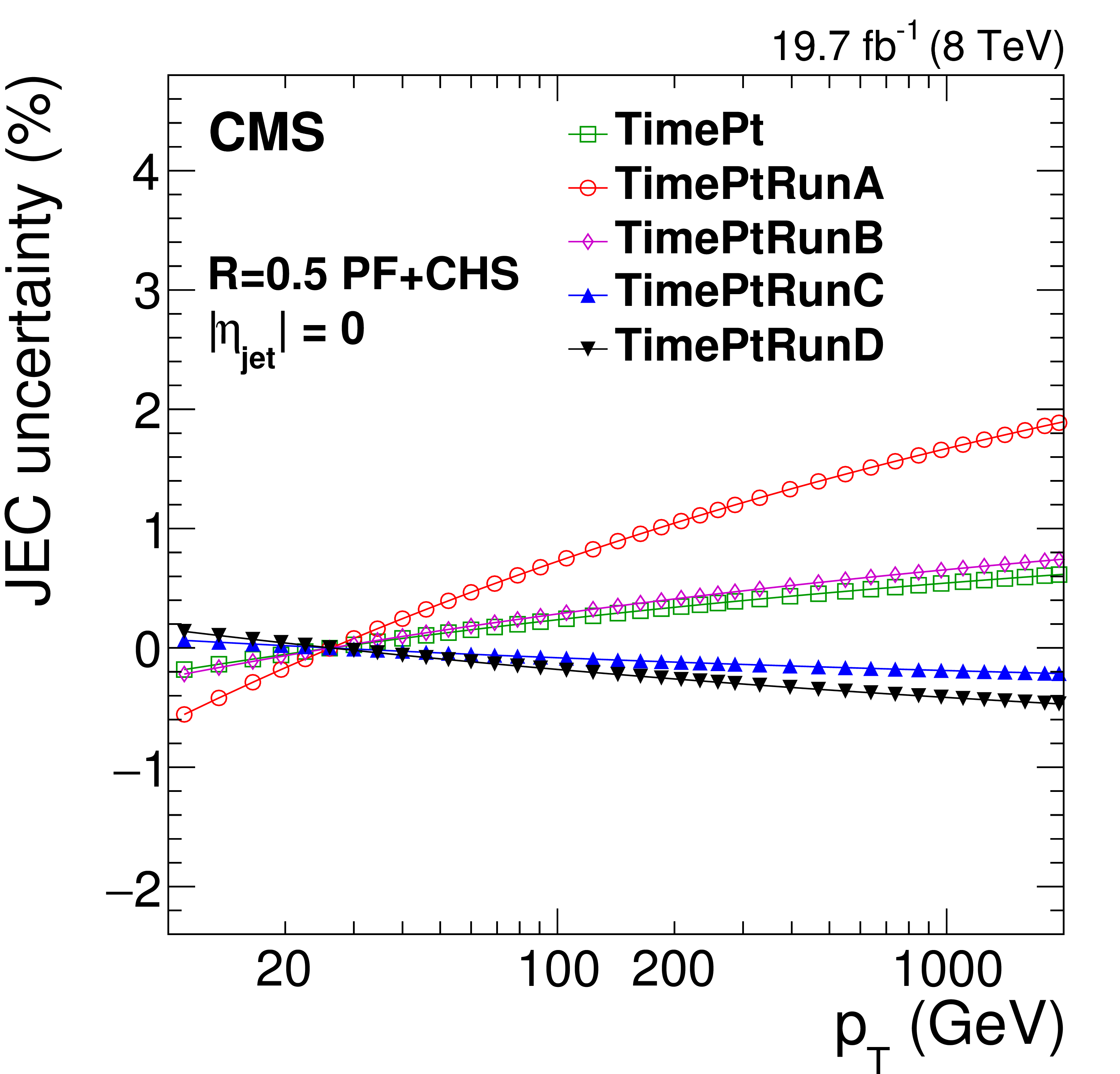
Figure 26-a:
Absolute scale time-dependent uncertainty as a function of jet $ {p_{\mathrm {T}}} $ for various data-taking periods (a). Systematic uncertainties for the absolute jet scale as a function of $ {p_{\mathrm {T}}} $ (b). SubTotalAbsolute is the quadratic sum of AbsoluteScale, AbsoluteStat, Fragmentation, SinglePionECAL, SinglePionHCAL and MPFBias. |
png pdf |
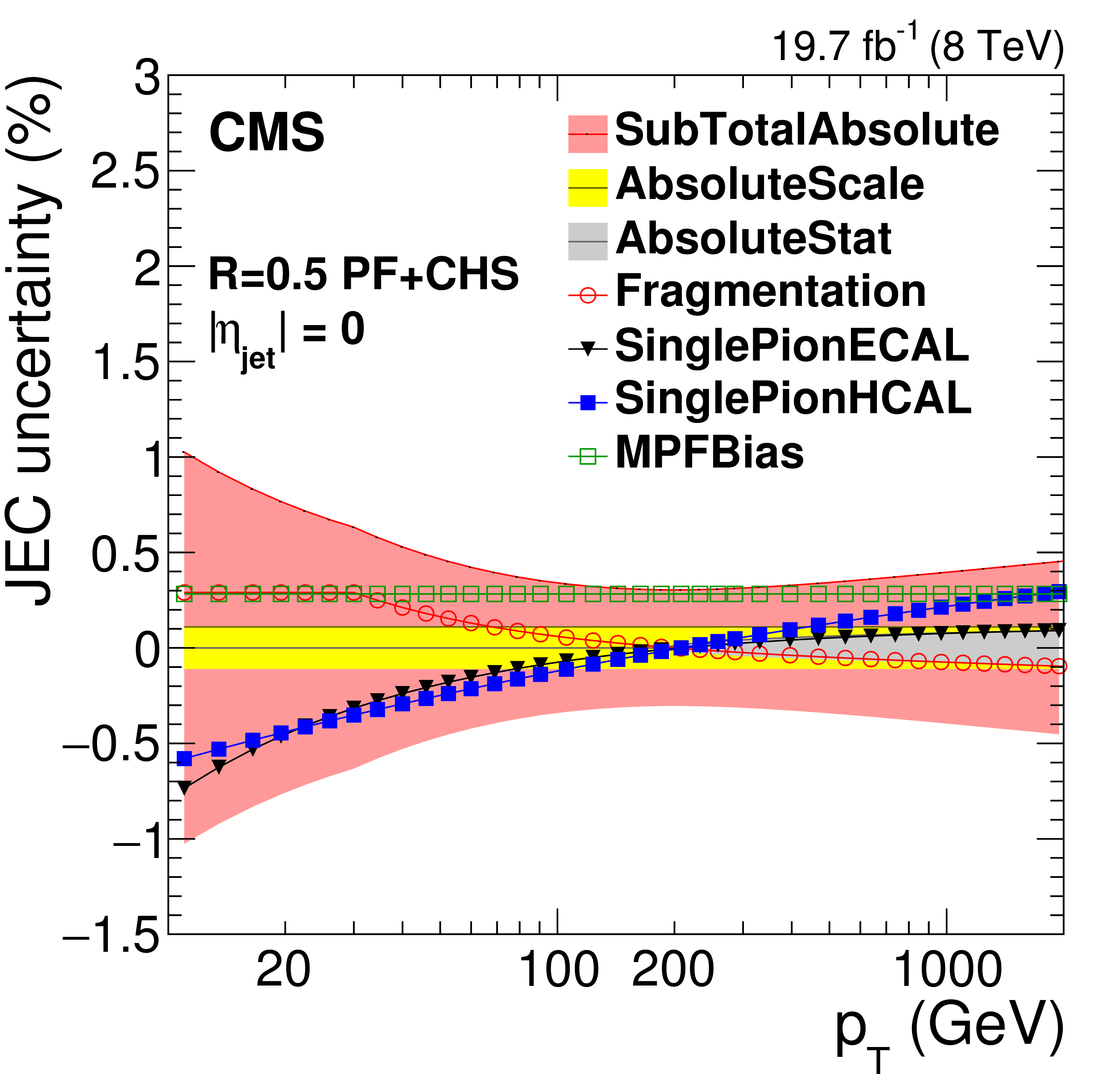
Figure 26-b:
Absolute scale time-dependent uncertainty as a function of jet $ {p_{\mathrm {T}}} $ for various data-taking periods (a). Systematic uncertainties for the absolute jet scale as a function of $ {p_{\mathrm {T}}} $ (b). SubTotalAbsolute is the quadratic sum of AbsoluteScale, AbsoluteStat, Fragmentation, SinglePionECAL, SinglePionHCAL and MPFBias. |

png pdf |
Figure 27:
Residual data/simulation response correction factors for the 2012 data collected at 8 TeV for PF jets with CHS and $R= $ 0.5 , compared to corrections at 7 TeV corresponding to 36 pb$^{-1}$ of data taken in 2010 [13] and 5 fb$^{-1}$ taken in 2011 [45]. The comparison is shown at $|\eta |= $ 0 versus $p_{{\rm T},\rm corr}$ (a), and as a function of $|\eta |$ for $p_{{\rm T},\rm corr}= $ 30 GeV (b), $p_{{\rm T},\rm corr}= $ 100 GeV (c), and $p_{{\rm T}, \rm corr}= $ 1000 GeV (d). The plots are limited to a jet energy $E= {p_{\mathrm {T}}} \cosh\eta = $ 3500 GeV so as to show only correction factors for reasonable $ {p_{\mathrm {T}}} $ in the considered data-taking period. |
png pdf |
Figure 27-a:
Residual data/simulation response correction factors for the 2012 data collected at 8 TeV for PF jets with CHS and $R= $ 0.5 , compared to corrections at 7 TeV corresponding to 36 pb$^{-1}$ of data taken in 2010 [13] and 5 fb$^{-1}$ taken in 2011 [45]. The comparison is shown at $|\eta |= $ 0 versus $p_{{\rm T},\rm corr}$ (a), and as a function of $|\eta |$ for $p_{{\rm T},\rm corr}= $ 30 GeV (b), $p_{{\rm T},\rm corr}= $ 100 GeV (c), and $p_{{\rm T}, \rm corr}= $ 1000 GeV (d). The plots are limited to a jet energy $E= {p_{\mathrm {T}}} \cosh\eta = $ 3500 GeV so as to show only correction factors for reasonable $ {p_{\mathrm {T}}} $ in the considered data-taking period. |
png pdf |
Figure 27-b:
Residual data/simulation response correction factors for the 2012 data collected at 8 TeV for PF jets with CHS and $R= $ 0.5 , compared to corrections at 7 TeV corresponding to 36 pb$^{-1}$ of data taken in 2010 [13] and 5 fb$^{-1}$ taken in 2011 [45]. The comparison is shown at $|\eta |= $ 0 versus $p_{{\rm T},\rm corr}$ (a), and as a function of $|\eta |$ for $p_{{\rm T},\rm corr}= $ 30 GeV (b), $p_{{\rm T},\rm corr}= $ 100 GeV (c), and $p_{{\rm T}, \rm corr}= $ 1000 GeV (d). The plots are limited to a jet energy $E= {p_{\mathrm {T}}} \cosh\eta = $ 3500 GeV so as to show only correction factors for reasonable $ {p_{\mathrm {T}}} $ in the considered data-taking period. |
png pdf |
Figure 27-c:
Residual data/simulation response correction factors for the 2012 data collected at 8 TeV for PF jets with CHS and $R= $ 0.5 , compared to corrections at 7 TeV corresponding to 36 pb$^{-1}$ of data taken in 2010 [13] and 5 fb$^{-1}$ taken in 2011 [45]. The comparison is shown at $|\eta |= $ 0 versus $p_{{\rm T},\rm corr}$ (a), and as a function of $|\eta |$ for $p_{{\rm T},\rm corr}= $ 30 GeV (b), $p_{{\rm T},\rm corr}= $ 100 GeV (c), and $p_{{\rm T}, \rm corr}= $ 1000 GeV (d). The plots are limited to a jet energy $E= {p_{\mathrm {T}}} \cosh\eta = $ 3500 GeV so as to show only correction factors for reasonable $ {p_{\mathrm {T}}} $ in the considered data-taking period. |
png pdf |
Figure 27-d:
Residual data/simulation response correction factors for the 2012 data collected at 8 TeV for PF jets with CHS and $R= $ 0.5 , compared to corrections at 7 TeV corresponding to 36 pb$^{-1}$ of data taken in 2010 [13] and 5 fb$^{-1}$ taken in 2011 [45]. The comparison is shown at $|\eta |= $ 0 versus $p_{{\rm T},\rm corr}$ (a), and as a function of $|\eta |$ for $p_{{\rm T},\rm corr}= $ 30 GeV (b), $p_{{\rm T},\rm corr}= $ 100 GeV (c), and $p_{{\rm T}, \rm corr}= $ 1000 GeV (d). The plots are limited to a jet energy $E= {p_{\mathrm {T}}} \cosh\eta = $ 3500 GeV so as to show only correction factors for reasonable $ {p_{\mathrm {T}}} $ in the considered data-taking period. |
png pdf |
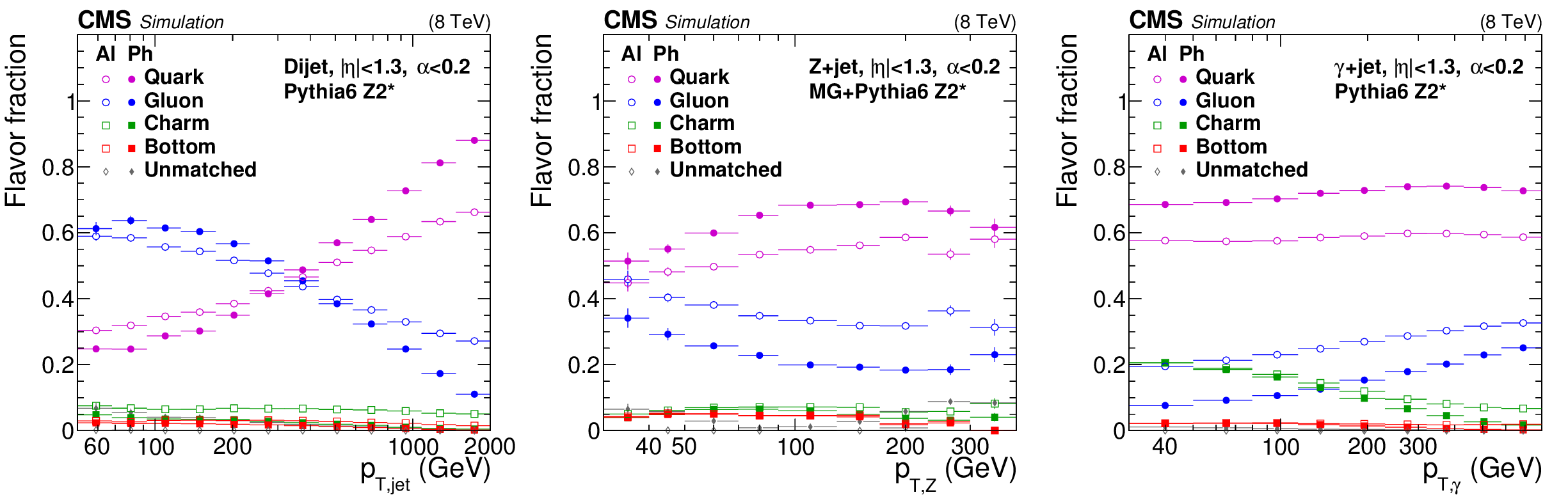
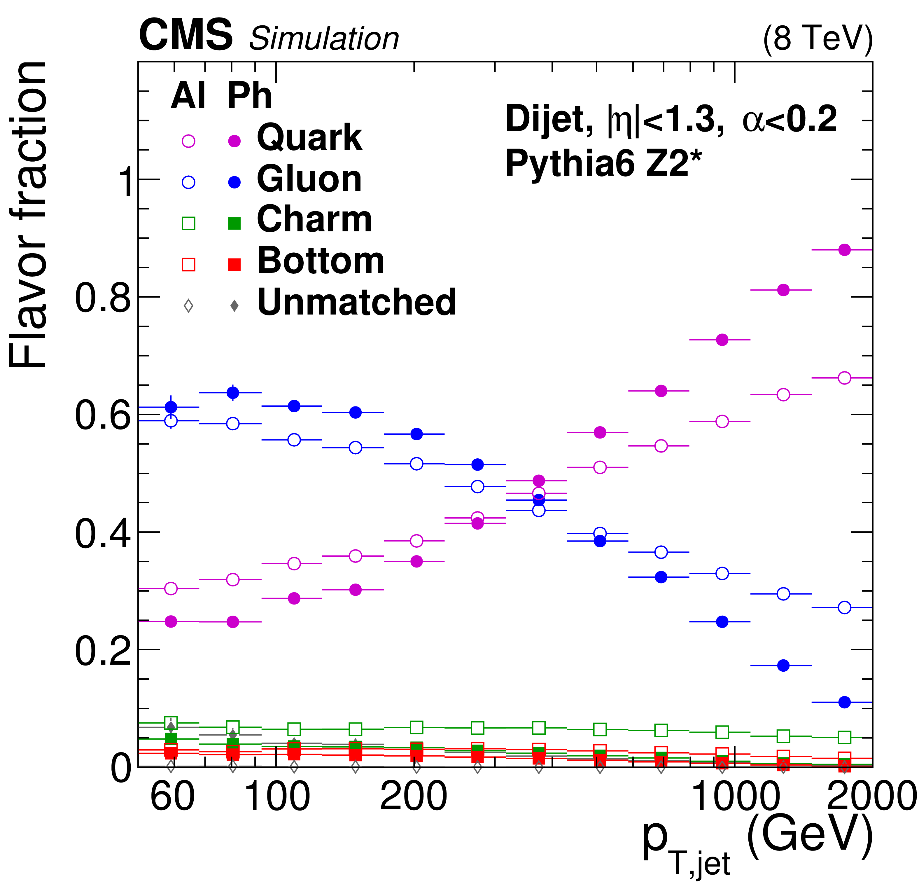
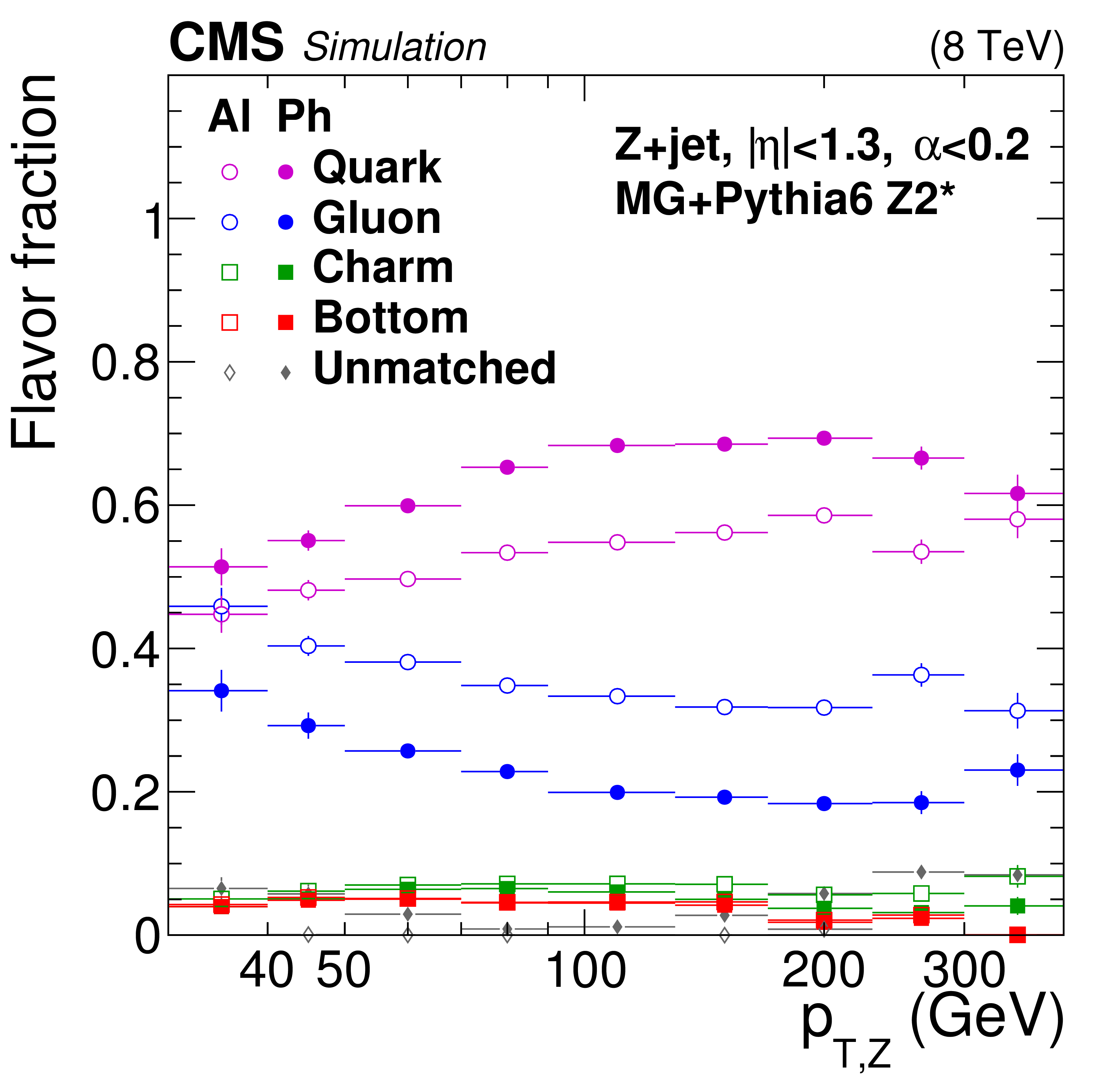
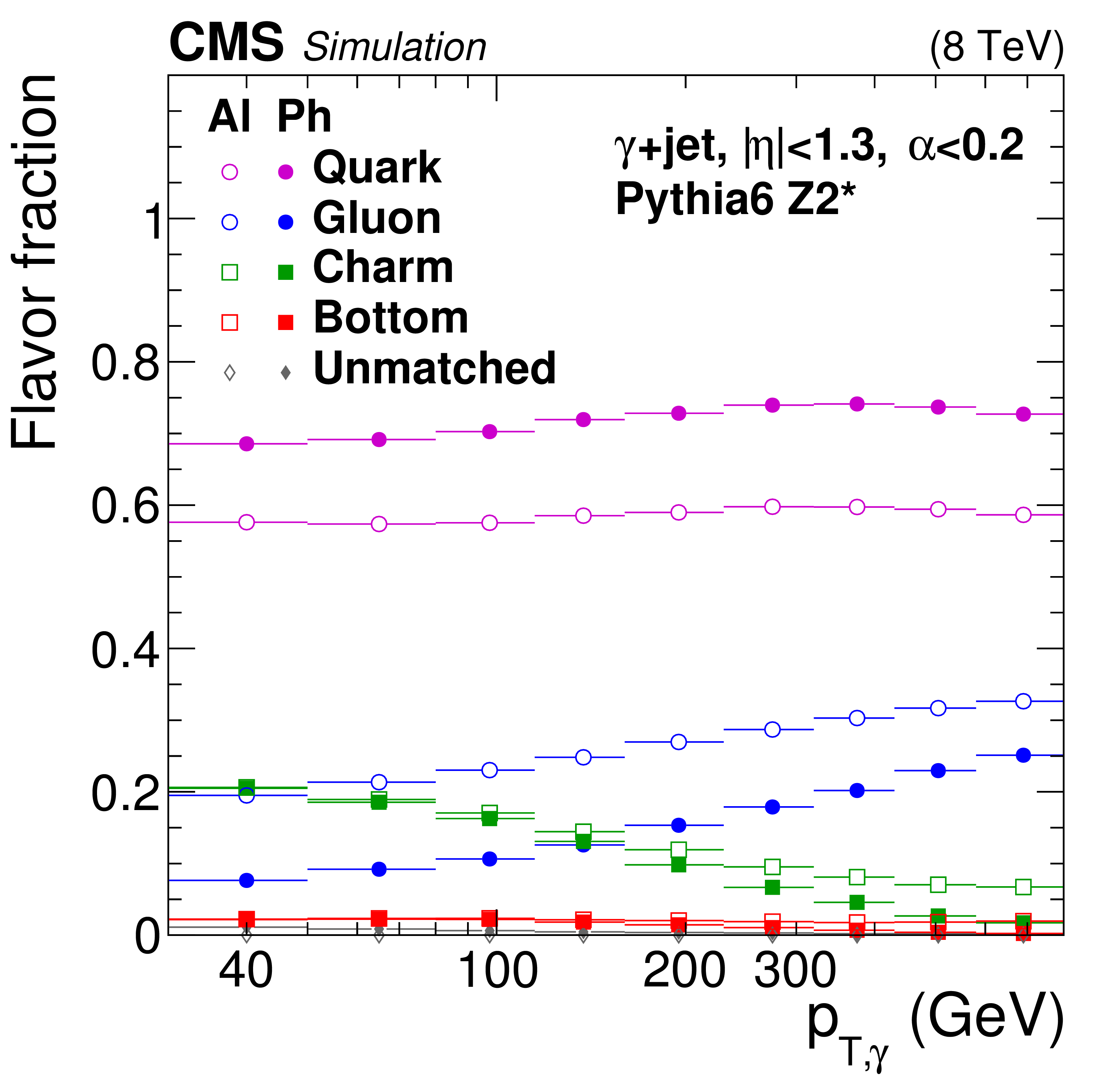
Figure 28:
Jet-flavor fractions in the physics (Ph) and algorithmic (Al) flavor definitions for QCD dijet (a), Z+jet (b), and $\gamma $+jet (c) samples. As explained in Section 6, the variable $\alpha =p_{\rm T, 3rdjet}/p_{\rm T, ave}$ for dijet events and $\alpha =p_{\rm T, 2ndjet}/p_{{\rm T}, \gamma /{\rm Z}}$ for Z+jet and $\gamma +$jet events. |
png pdf |
Figure 28-a:
Jet-flavor fractions in the physics (Ph) and algorithmic (Al) flavor definitions for QCD dijet (a), Z+jet (b), and $\gamma $+jet (c) samples. As explained in Section 6, the variable $\alpha =p_{\rm T, 3rdjet}/p_{\rm T, ave}$ for dijet events and $\alpha =p_{\rm T, 2ndjet}/p_{{\rm T}, \gamma /{\rm Z}}$ for Z+jet and $\gamma +$jet events. |
png pdf |
Figure 28-b:
Jet-flavor fractions in the physics (Ph) and algorithmic (Al) flavor definitions for QCD dijet (a), Z+jet (b), and $\gamma $+jet (c) samples. As explained in Section 6, the variable $\alpha =p_{\rm T, 3rdjet}/p_{\rm T, ave}$ for dijet events and $\alpha =p_{\rm T, 2ndjet}/p_{{\rm T}, \gamma /{\rm Z}}$ for Z+jet and $\gamma +$jet events. |
png pdf |
Figure 28-c:
Jet-flavor fractions in the physics (Ph) and algorithmic (Al) flavor definitions for QCD dijet (a), Z+jet (b), and $\gamma $+jet (c) samples. As explained in Section 6, the variable $\alpha =p_{\rm T, 3rdjet}/p_{\rm T, ave}$ for dijet events and $\alpha =p_{\rm T, 2ndjet}/p_{{\rm T}, \gamma /{\rm Z}}$ for Z+jet and $\gamma +$jet events. |
png pdf |
Figure 29:
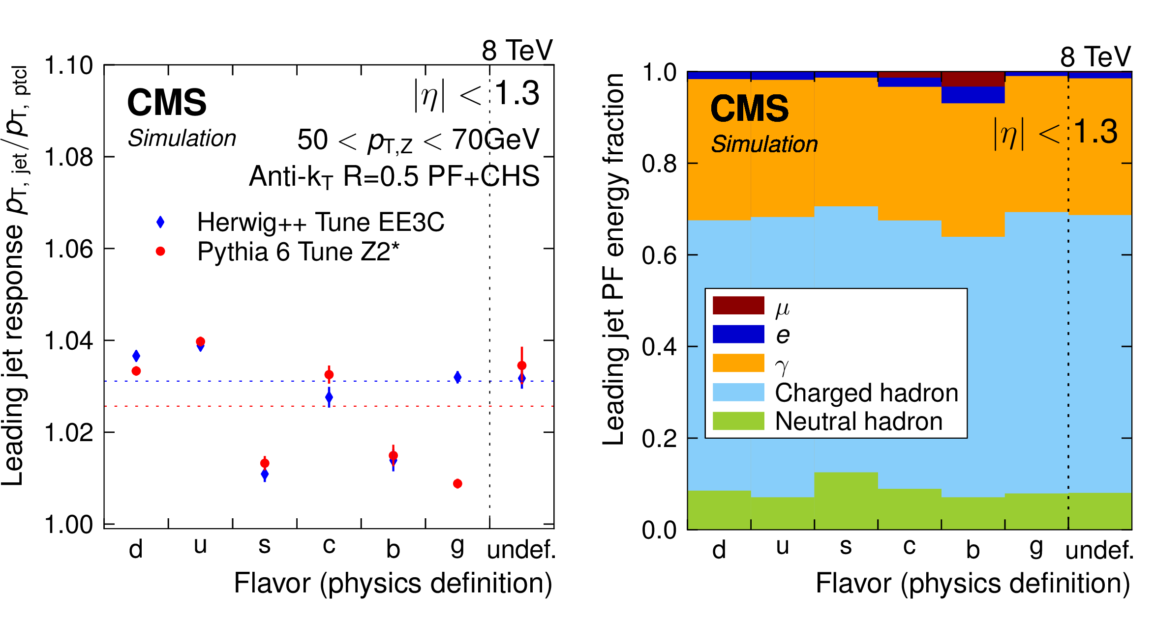
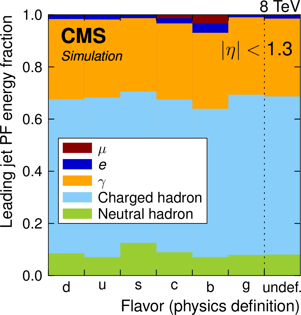
Comparison of jet response (a) and simulated composition (b) for different flavors of leading jets in Z+jet events with 50 $ < {p_{\mathrm {T}}} ^Z< $ 70 GeV, $|\eta _{\rm jet}|< $ 1.3 , and $\alpha = $ 0.3 (defined in Eq.(16)). The response values are compared for Pythia6.4 and Herwig++2.3, the composition is from Pythia6.4. |

png pdf |
Figure 29-a:
Comparison of jet response (a) and simulated composition (b) for different flavors of leading jets in Z+jet events with 50 $ < {p_{\mathrm {T}}} ^Z< $ 70 GeV, $|\eta _{\rm jet}|< $ 1.3 , and $\alpha = $ 0.3 (defined in Eq.(16)). The response values are compared for Pythia6.4 and Herwig++2.3, the composition is from Pythia6.4. |
png pdf |
Figure 29-b:
Comparison of jet response (a) and simulated composition (b) for different flavors of leading jets in Z+jet events with 50 $ < {p_{\mathrm {T}}} ^Z< $ 70 GeV, $|\eta _{\rm jet}|< $ 1.3 , and $\alpha = $ 0.3 (defined in Eq.(16)). The response values are compared for Pythia6.4 and Herwig++2.3, the composition is from Pythia6.4. |
png pdf |
Figure 30:
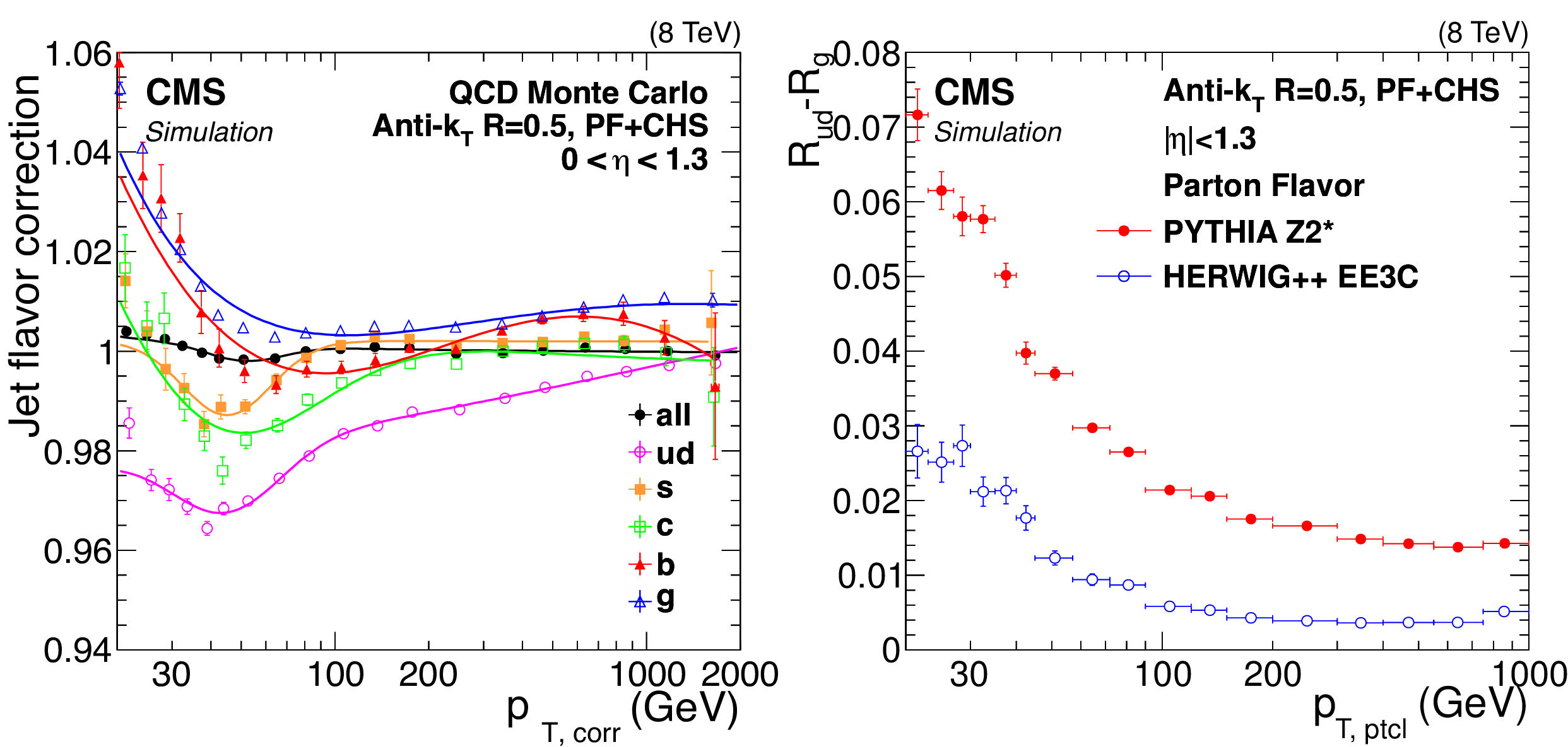
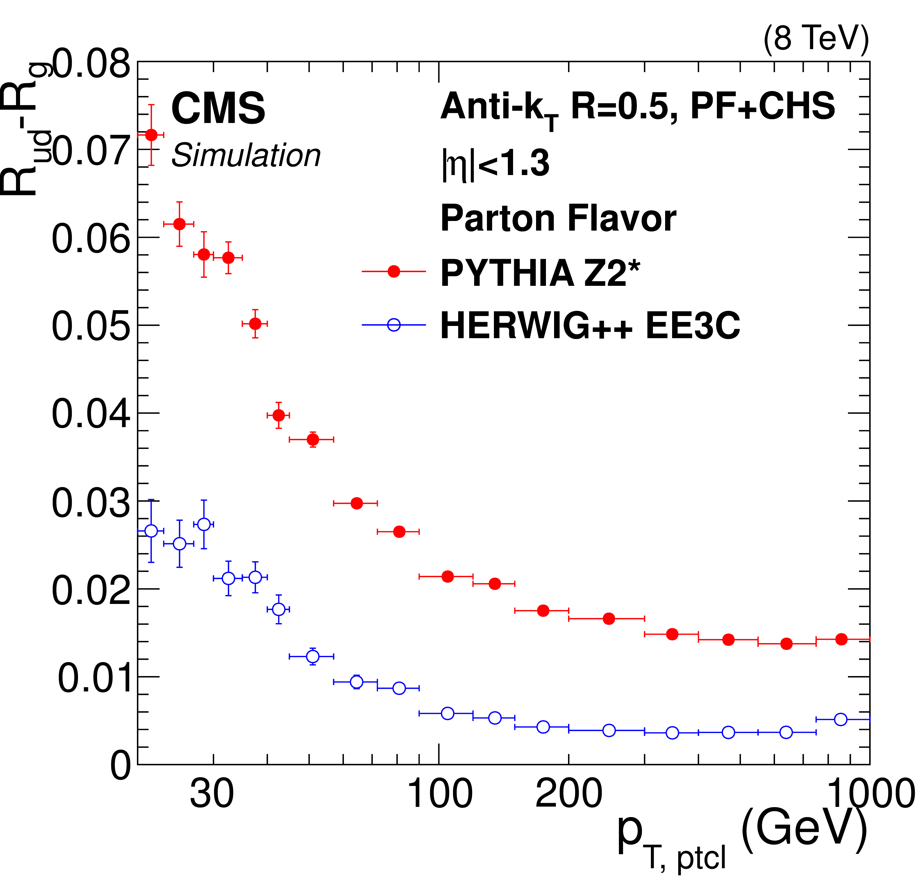
Residual jet-flavor correction factor as a function of jet $p_{\rm T,corr}$ from Pythia6.4 tune Z2*, derived on top of inclusive JEC and defined relative to the QCD flavor mixture (a). The neutrinos are excluded from particle jets, which brings c- and b-jet response in between that of light quarks and gluons. The lines show the parameterizations used for residual jet-flavor corrections. Difference in light-quark and gluon jet response as a function of jet $p_{\rm T,corr}$, as predicted by Pythia6.4 and Herwig++2.3 (b). |

png pdf |
Figure 30-a:
Residual jet-flavor correction factor as a function of jet $p_{\rm T,corr}$ from Pythia6.4 tune Z2*, derived on top of inclusive JEC and defined relative to the QCD flavor mixture (a). The neutrinos are excluded from particle jets, which brings c- and b-jet response in between that of light quarks and gluons. The lines show the parameterizations used for residual jet-flavor corrections. Difference in light-quark and gluon jet response as a function of jet $p_{\rm T,corr}$, as predicted by Pythia6.4 and Herwig++2.3 (b). |
png pdf |
Figure 30-b:
Residual jet-flavor correction factor as a function of jet $p_{\rm T,corr}$ from Pythia6.4 tune Z2*, derived on top of inclusive JEC and defined relative to the QCD flavor mixture (a). The neutrinos are excluded from particle jets, which brings c- and b-jet response in between that of light quarks and gluons. The lines show the parameterizations used for residual jet-flavor corrections. Difference in light-quark and gluon jet response as a function of jet $p_{\rm T,corr}$, as predicted by Pythia6.4 and Herwig++2.3 (b). |

png pdf |
Figure 31:
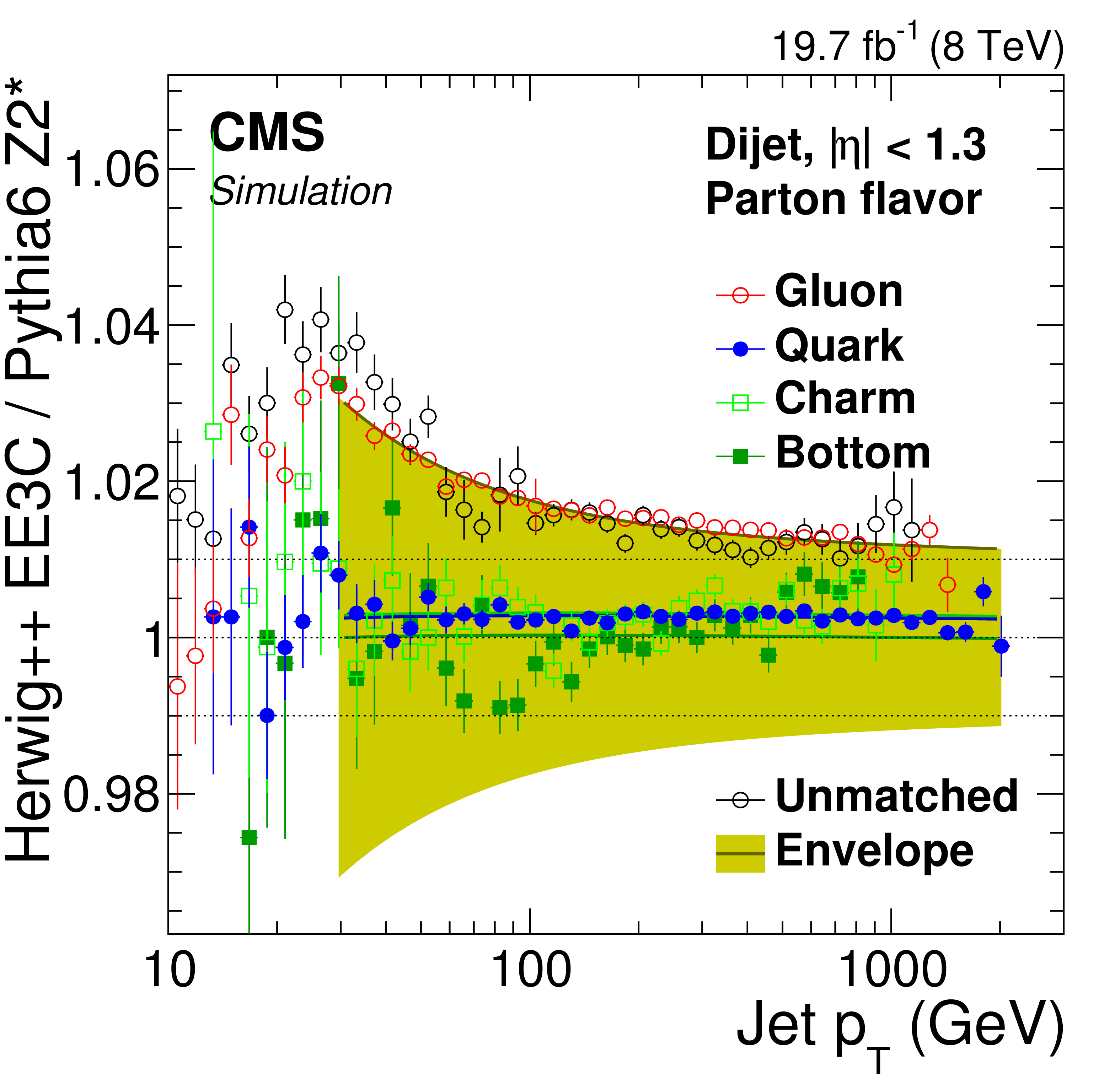
a: Ratio of jet responses in Pythia6.4 (tune Z2*) and Herwig++2.3 (tune EE3C) versus jet $ {p_{\mathrm {T}}} $, for pure jet flavors selected using the physics definition, where the shaded envelope highlights the largest differences observed for the gluon jets. b: Pythia6.4/Herwig++2.3 response differences as a function of jet $ {p_{\mathrm {T}}} $ for QCD dijet and Z/$\gamma $+jet flavor mixtures calculated from the parameterized flavor response differences and compared to the full simulation for dijet and Z+jet samples. The ``20% glue'' corresponds to the effective Z/$\gamma $+jet flavor mixture at $ {p_{\mathrm {T}}} = $ 200 GeV, which has 20% of gluons. |
png pdf |
Figure 31-a:
a: Ratio of jet responses in Pythia6.4 (tune Z2*) and Herwig++2.3 (tune EE3C) versus jet $ {p_{\mathrm {T}}} $, for pure jet flavors selected using the physics definition, where the shaded envelope highlights the largest differences observed for the gluon jets. b: Pythia6.4/Herwig++2.3 response differences as a function of jet $ {p_{\mathrm {T}}} $ for QCD dijet and Z/$\gamma $+jet flavor mixtures calculated from the parameterized flavor response differences and compared to the full simulation for dijet and Z+jet samples. The ``20% glue'' corresponds to the effective Z/$\gamma $+jet flavor mixture at $ {p_{\mathrm {T}}} = $ 200 GeV, which has 20% of gluons. |

png pdf |
Figure 31-b:
a: Ratio of jet responses in Pythia6.4 (tune Z2*) and Herwig++2.3 (tune EE3C) versus jet $ {p_{\mathrm {T}}} $, for pure jet flavors selected using the physics definition, where the shaded envelope highlights the largest differences observed for the gluon jets. b: Pythia6.4/Herwig++2.3 response differences as a function of jet $ {p_{\mathrm {T}}} $ for QCD dijet and Z/$\gamma $+jet flavor mixtures calculated from the parameterized flavor response differences and compared to the full simulation for dijet and Z+jet samples. The ``20% glue'' corresponds to the effective Z/$\gamma $+jet flavor mixture at $ {p_{\mathrm {T}}} = $ 200 GeV, which has 20% of gluons. |
png pdf |
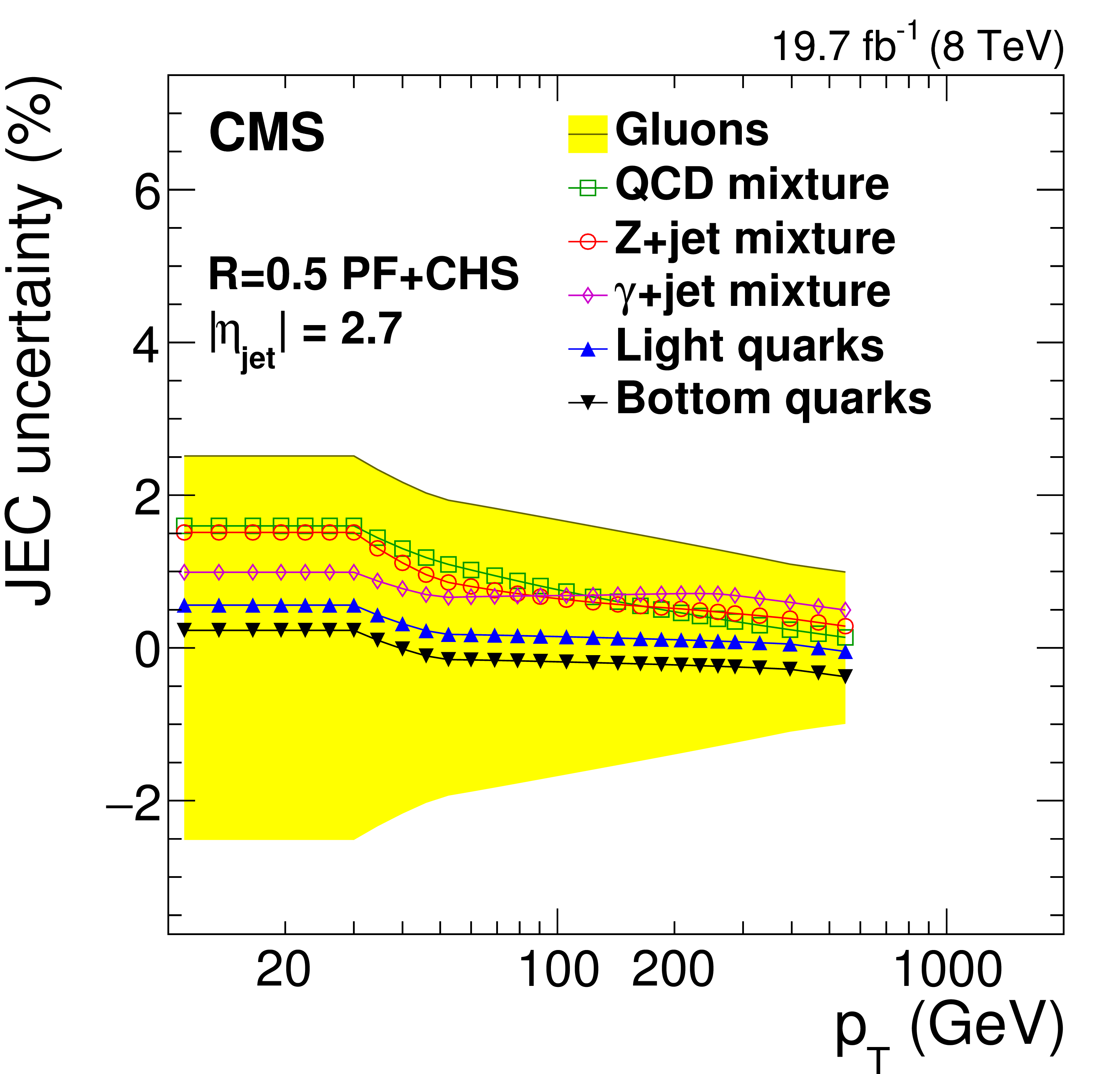
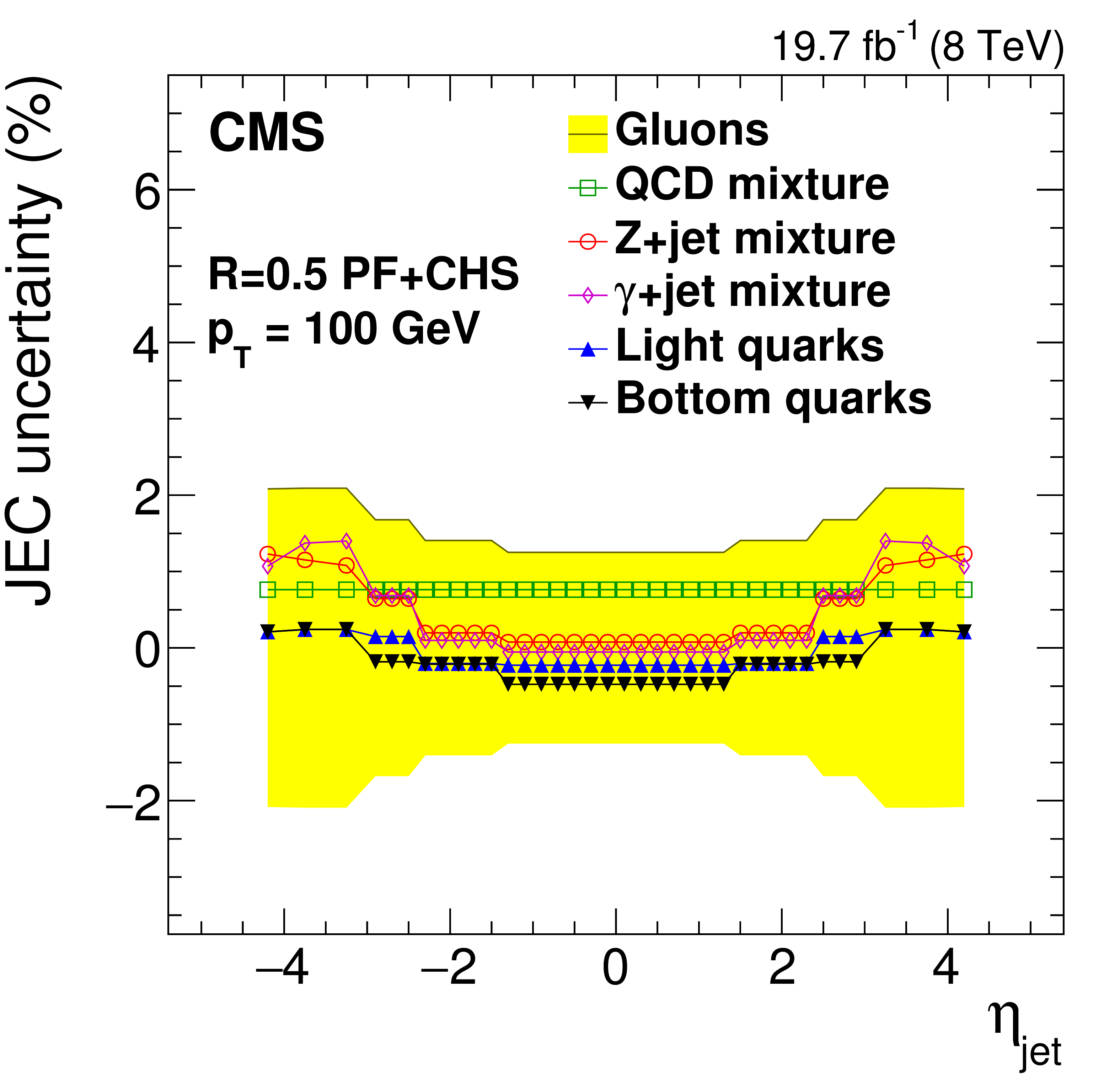
Figure 32:
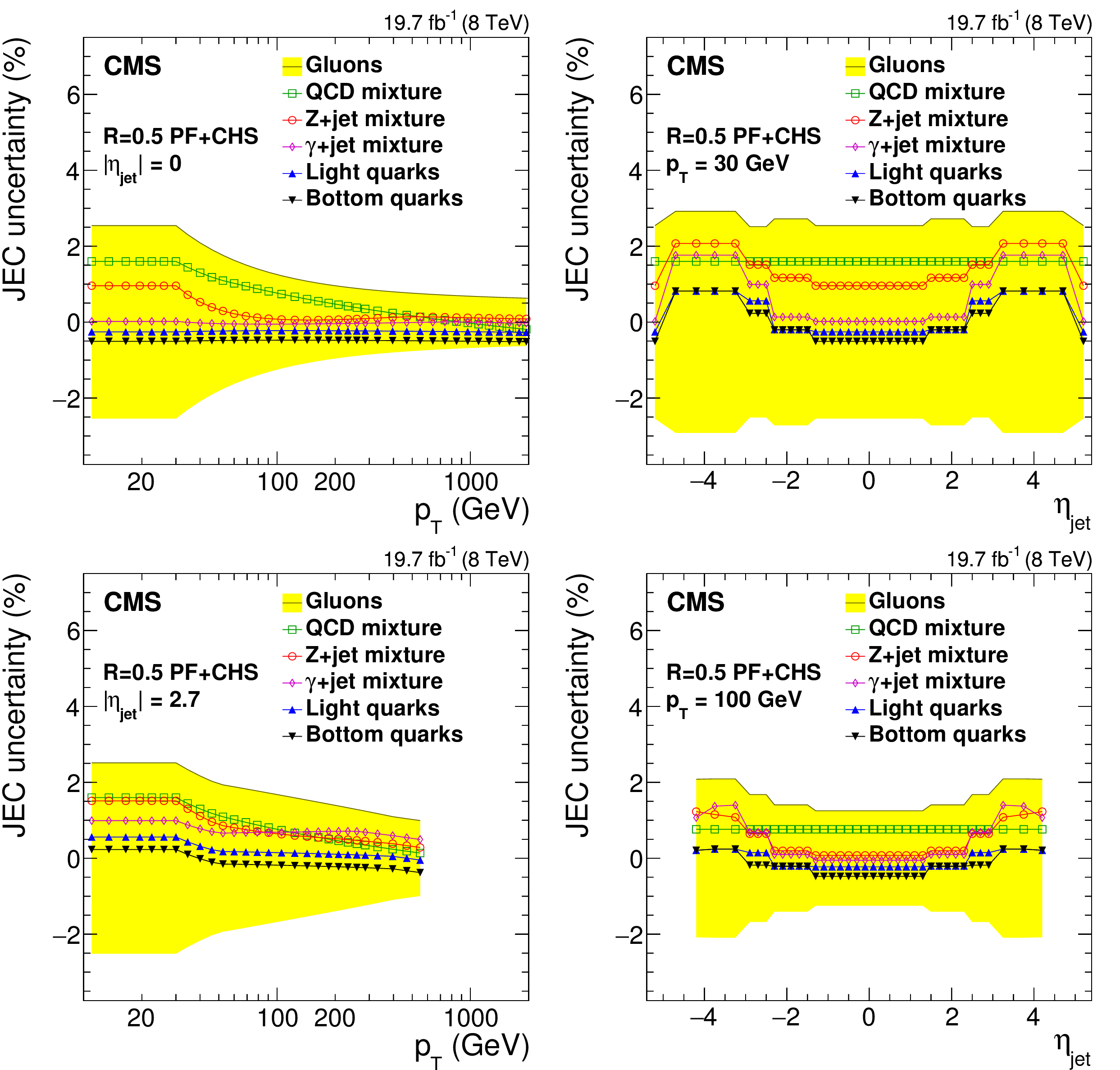
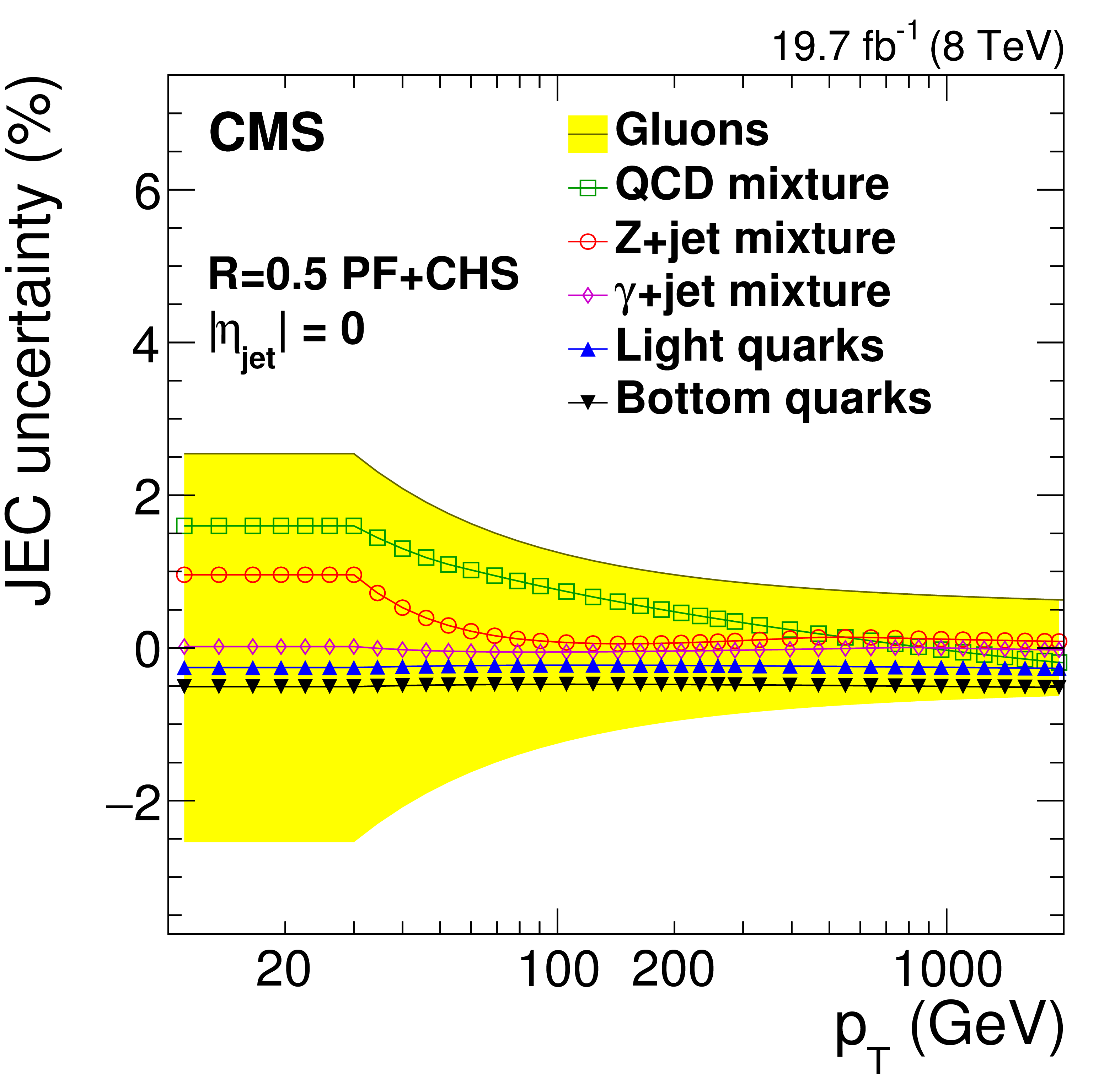
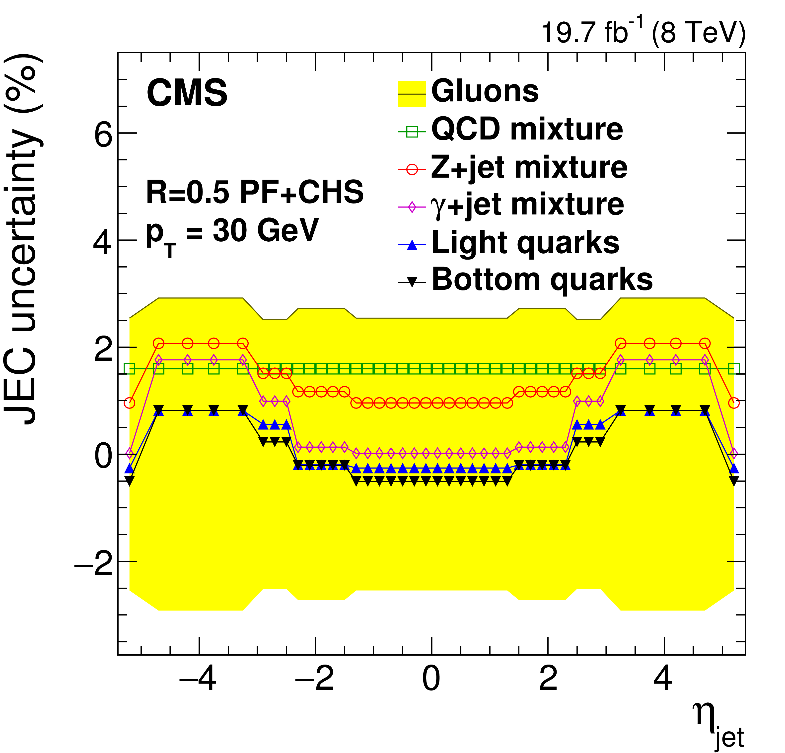
Systematic uncertainties in jet energy corrections for various flavor mixtures (QCD dijets, Z+jet and $\gamma $+jet) and pure flavors (gluons, light quarks and bottom quarks) as a function of jet $ {p_{\mathrm {T}}} $ (a,c, for fixed $|\eta _{\rm jet}|= $ 0 , a,b, and $|\eta _{\rm jet}|= $ 2.7 , c,d) and $\eta _{\rm jet}$ (b,d, for fixed $ {p_{\mathrm {T}}} = $ 30 GeV, a,b, and 100 GeV , c,d). The sign of the systematic source indicates the sign of the Pythia6.4 tune Z2* and Herwig++2.3 tune EE3C difference. The shaded band shows gluon flavor response uncertainty symmetrically around zero. |
png pdf |
Figure 32-a:
Systematic uncertainties in jet energy corrections for various flavor mixtures (QCD dijets, Z+jet and $\gamma $+jet) and pure flavors (gluons, light quarks and bottom quarks) as a function of jet $ {p_{\mathrm {T}}} $ (a,c, for fixed $|\eta _{\rm jet}|= $ 0 , a,b, and $|\eta _{\rm jet}|= $ 2.7 , c,d) and $\eta _{\rm jet}$ (b,d, for fixed $ {p_{\mathrm {T}}} = $ 30 GeV, a,b, and 100 GeV , c,d). The sign of the systematic source indicates the sign of the Pythia6.4 tune Z2* and Herwig++2.3 tune EE3C difference. The shaded band shows gluon flavor response uncertainty symmetrically around zero. |
png pdf |
Figure 32-b:
Systematic uncertainties in jet energy corrections for various flavor mixtures (QCD dijets, Z+jet and $\gamma $+jet) and pure flavors (gluons, light quarks and bottom quarks) as a function of jet $ {p_{\mathrm {T}}} $ (a,c, for fixed $|\eta _{\rm jet}|= $ 0 , a,b, and $|\eta _{\rm jet}|= $ 2.7 , c,d) and $\eta _{\rm jet}$ (b,d, for fixed $ {p_{\mathrm {T}}} = $ 30 GeV, a,b, and 100 GeV , c,d). The sign of the systematic source indicates the sign of the Pythia6.4 tune Z2* and Herwig++2.3 tune EE3C difference. The shaded band shows gluon flavor response uncertainty symmetrically around zero. |
png pdf |
Figure 32-c:
Systematic uncertainties in jet energy corrections for various flavor mixtures (QCD dijets, Z+jet and $\gamma $+jet) and pure flavors (gluons, light quarks and bottom quarks) as a function of jet $ {p_{\mathrm {T}}} $ (a,c, for fixed $|\eta _{\rm jet}|= $ 0 , a,b, and $|\eta _{\rm jet}|= $ 2.7 , c,d) and $\eta _{\rm jet}$ (b,d, for fixed $ {p_{\mathrm {T}}} = $ 30 GeV, a,b, and 100 GeV , c,d). The sign of the systematic source indicates the sign of the Pythia6.4 tune Z2* and Herwig++2.3 tune EE3C difference. The shaded band shows gluon flavor response uncertainty symmetrically around zero. |
png pdf |
Figure 32-d:
Systematic uncertainties in jet energy corrections for various flavor mixtures (QCD dijets, Z+jet and $\gamma $+jet) and pure flavors (gluons, light quarks and bottom quarks) as a function of jet $ {p_{\mathrm {T}}} $ (a,c, for fixed $|\eta _{\rm jet}|= $ 0 , a,b, and $|\eta _{\rm jet}|= $ 2.7 , c,d) and $\eta _{\rm jet}$ (b,d, for fixed $ {p_{\mathrm {T}}} = $ 30 GeV, a,b, and 100 GeV , c,d). The sign of the systematic source indicates the sign of the Pythia6.4 tune Z2* and Herwig++2.3 tune EE3C difference. The shaded band shows gluon flavor response uncertainty symmetrically around zero. |
png pdf |
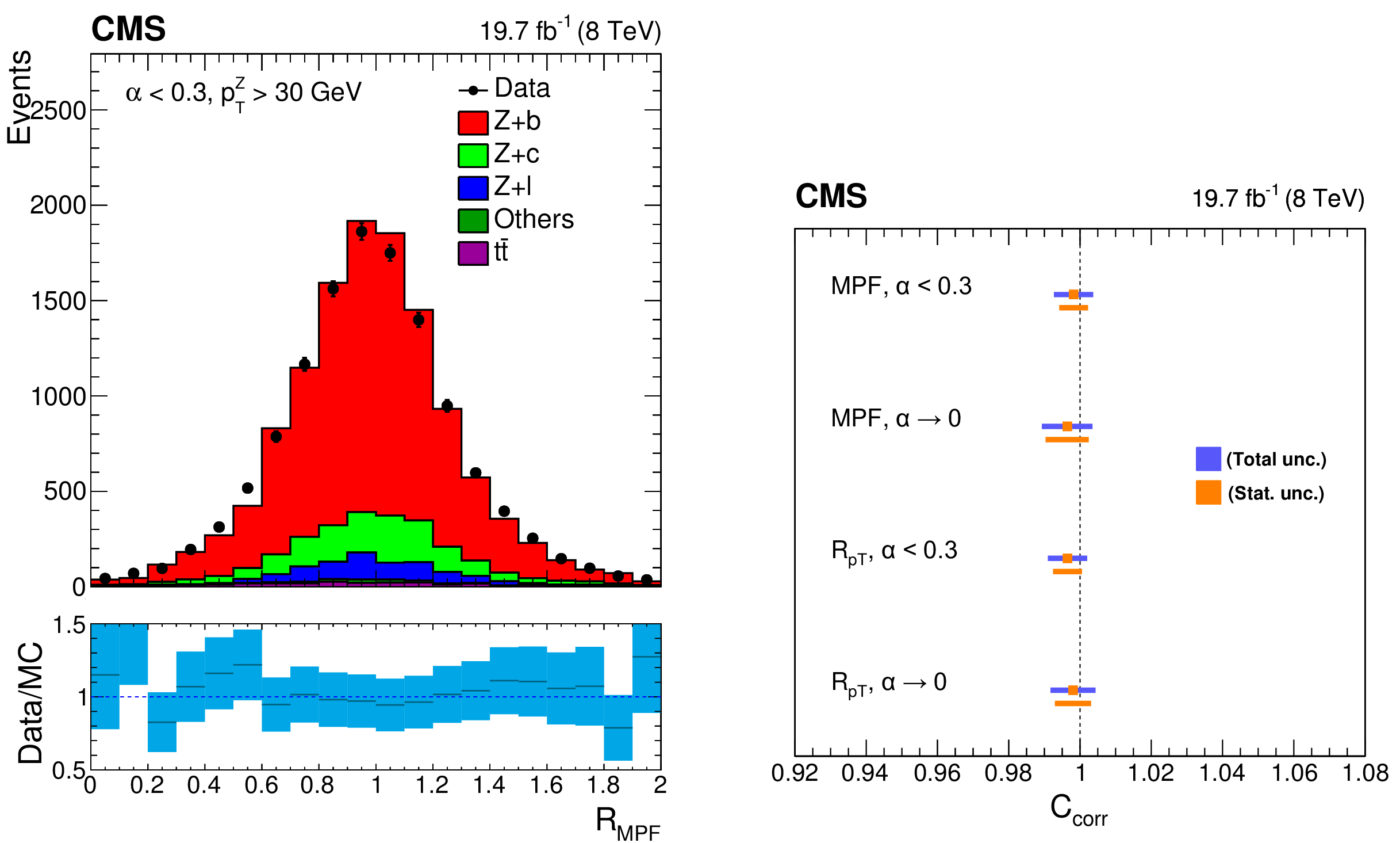
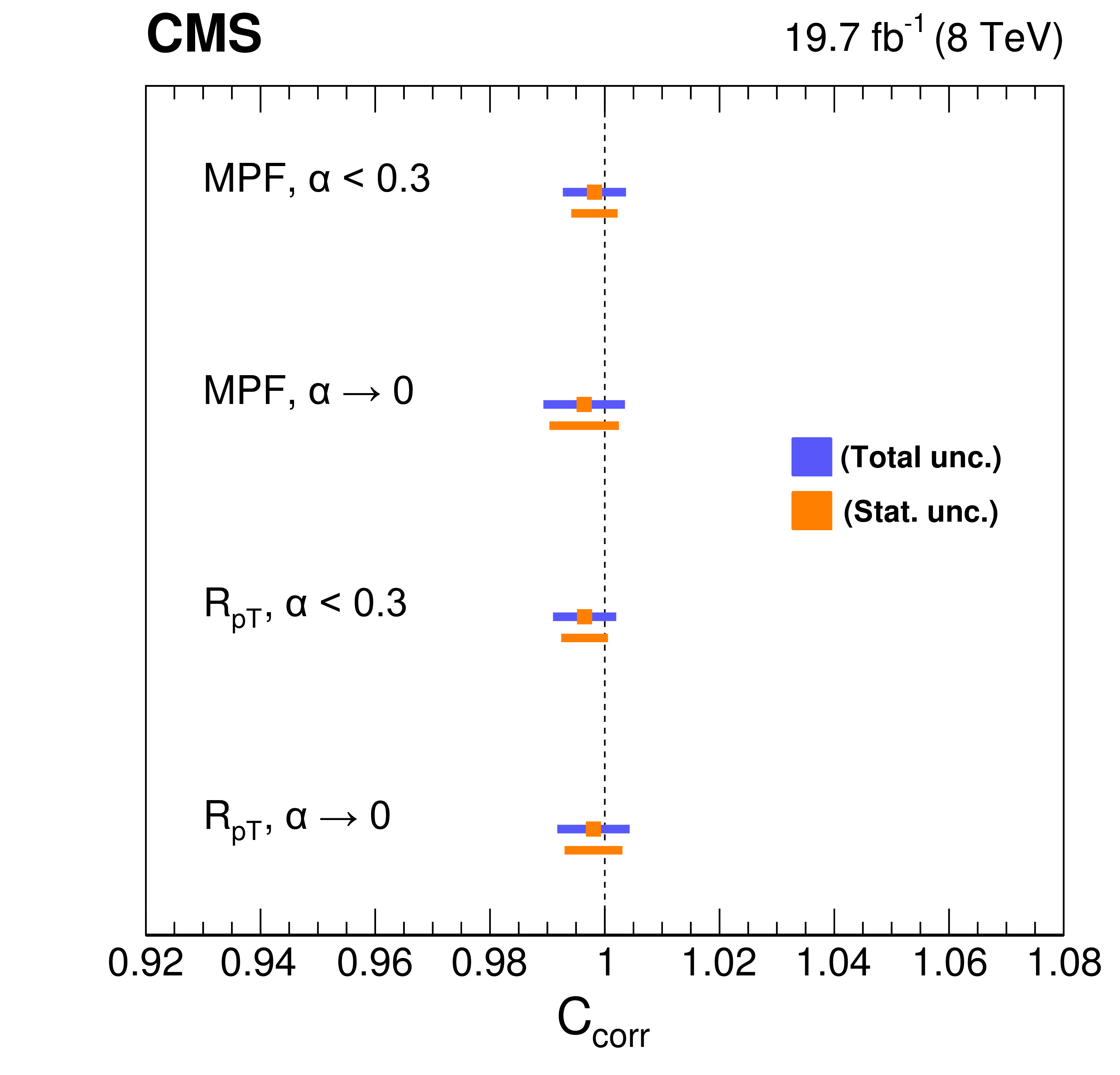
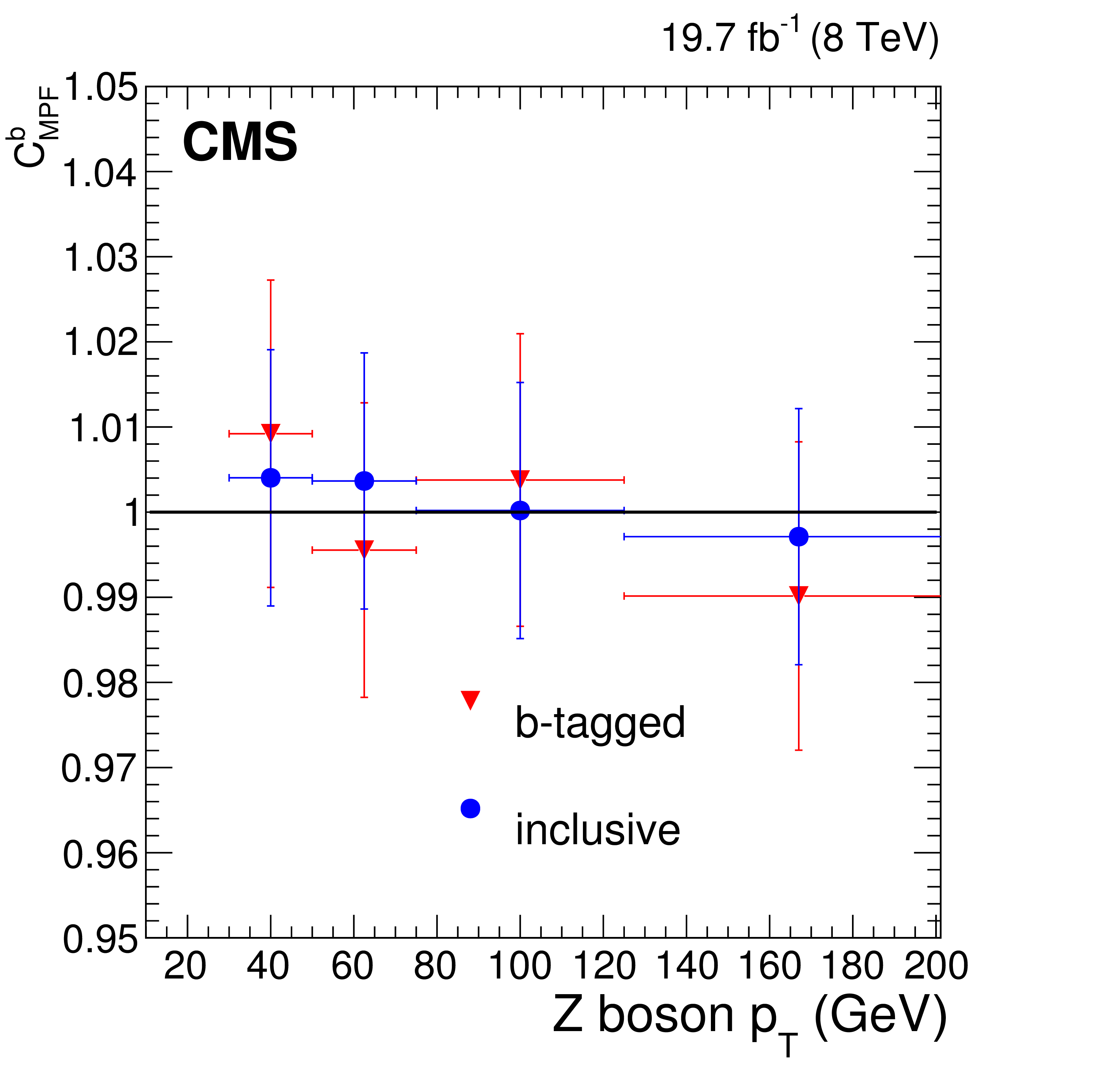
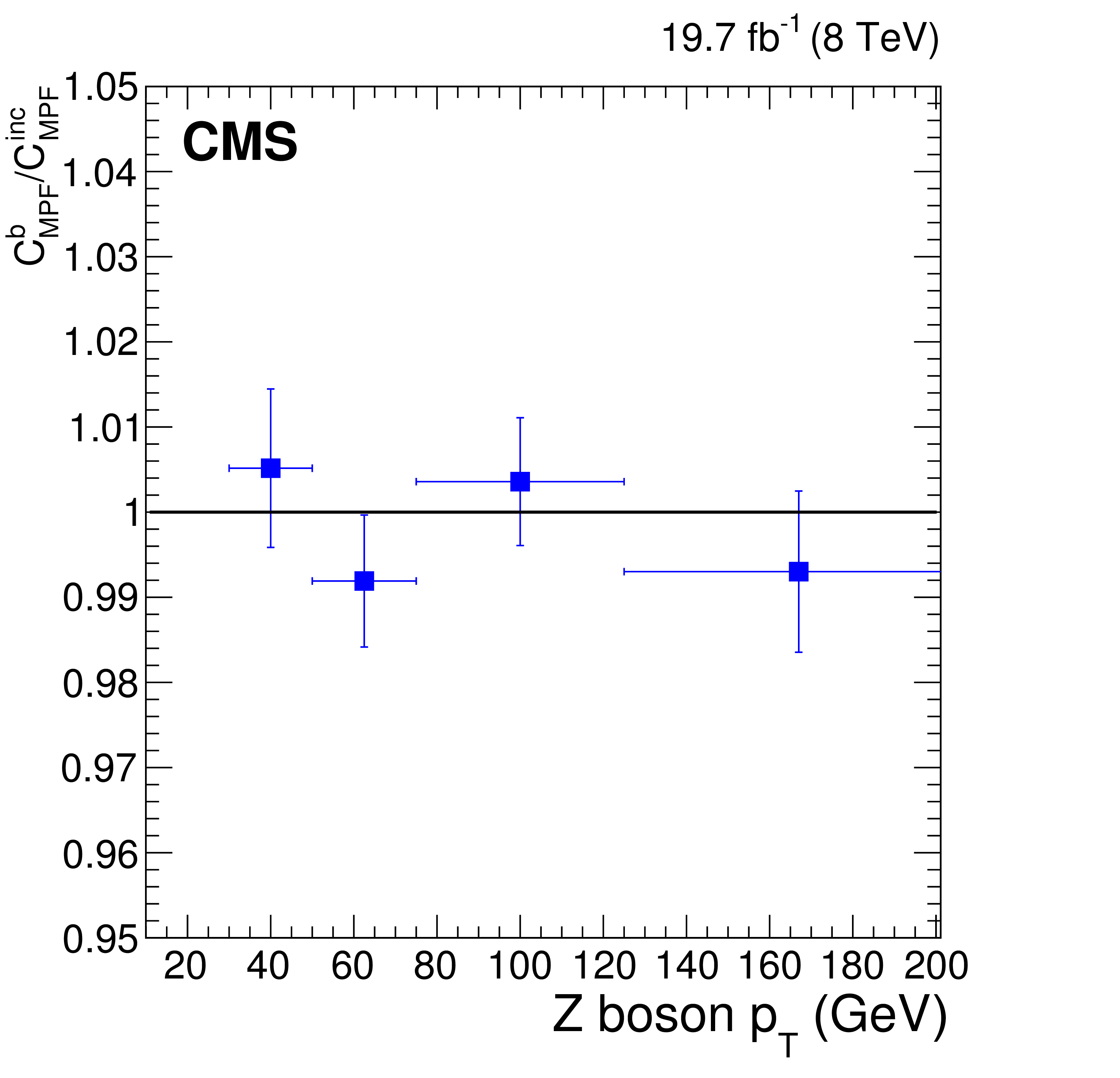
Figure 33:
Distribution of the Z+b-jet response using the MPF method with a fixed requirement $\alpha < $ 0.3 (a). Data-to-simulation ratio of the Z+b-jet response relative to the inclusive Z+jet sample with the MPF and the $ {p_{\mathrm {T}}} $-balance methods (b). |

png pdf |
Figure 33-a:
Distribution of the Z+b-jet response using the MPF method with a fixed requirement $\alpha < $ 0.3 (a). Data-to-simulation ratio of the Z+b-jet response relative to the inclusive Z+jet sample with the MPF and the $ {p_{\mathrm {T}}} $-balance methods (b). |
png pdf |
Figure 33-b:
Distribution of the Z+b-jet response using the MPF method with a fixed requirement $\alpha < $ 0.3 (a). Data-to-simulation ratio of the Z+b-jet response relative to the inclusive Z+jet sample with the MPF and the $ {p_{\mathrm {T}}} $-balance methods (b). |

png pdf |
Figure 34:
Residual correction factors (calculated as the ratio of the MC and data MPF response) as a function of Z boson $ {p_{\mathrm {T}}} $, for Z+b-jet and Z+jet events with $\alpha < $ 0.3 (a), and their ratio (b). |
png pdf |
Figure 34-a:
Residual correction factors (calculated as the ratio of the MC and data MPF response) as a function of Z boson $ {p_{\mathrm {T}}} $, for Z+b-jet and Z+jet events with $\alpha < $ 0.3 (a), and their ratio (b). |
png pdf |
Figure 34-b:
Residual correction factors (calculated as the ratio of the MC and data MPF response) as a function of Z boson $ {p_{\mathrm {T}}} $, for Z+b-jet and Z+jet events with $\alpha < $ 0.3 (a), and their ratio (b). |
png pdf |
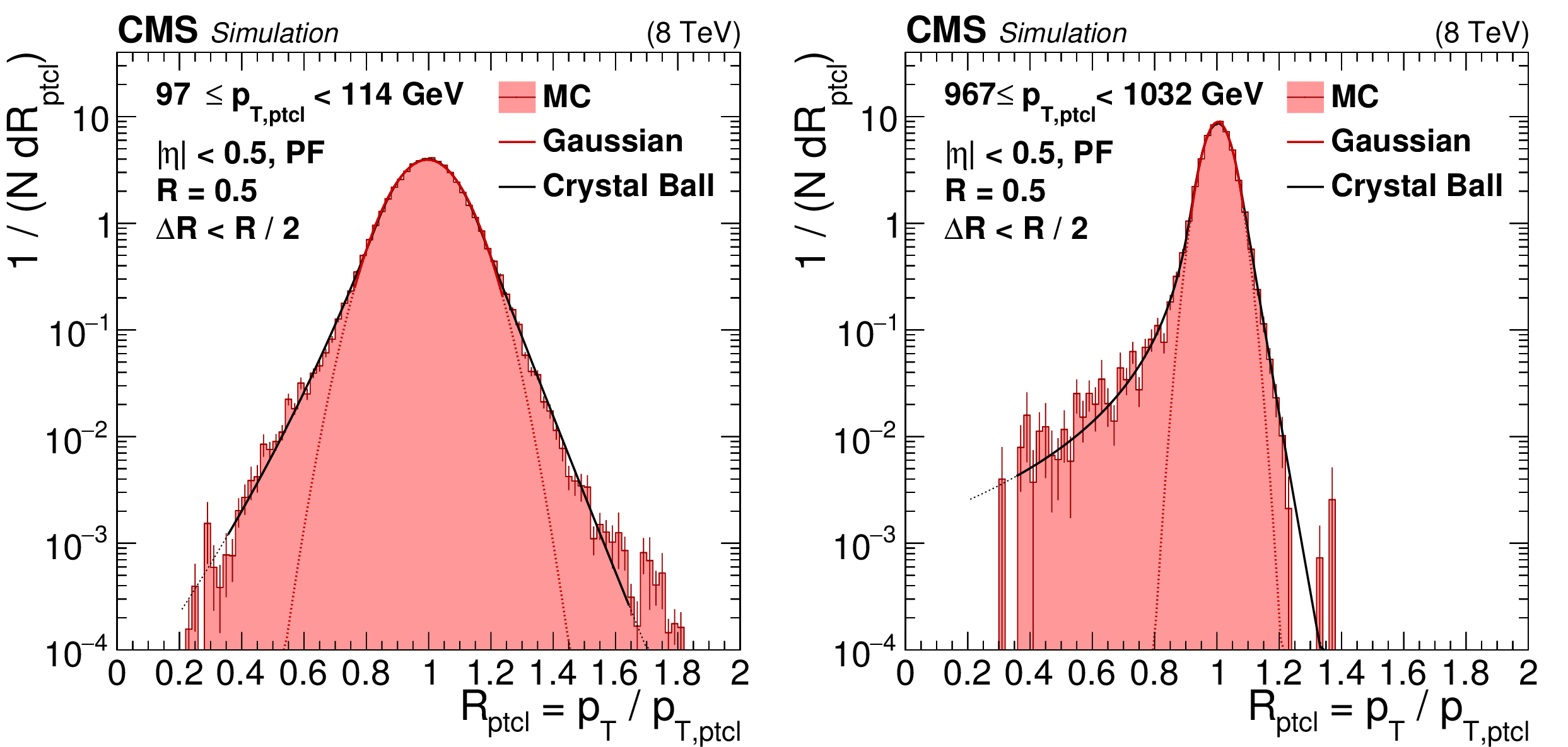
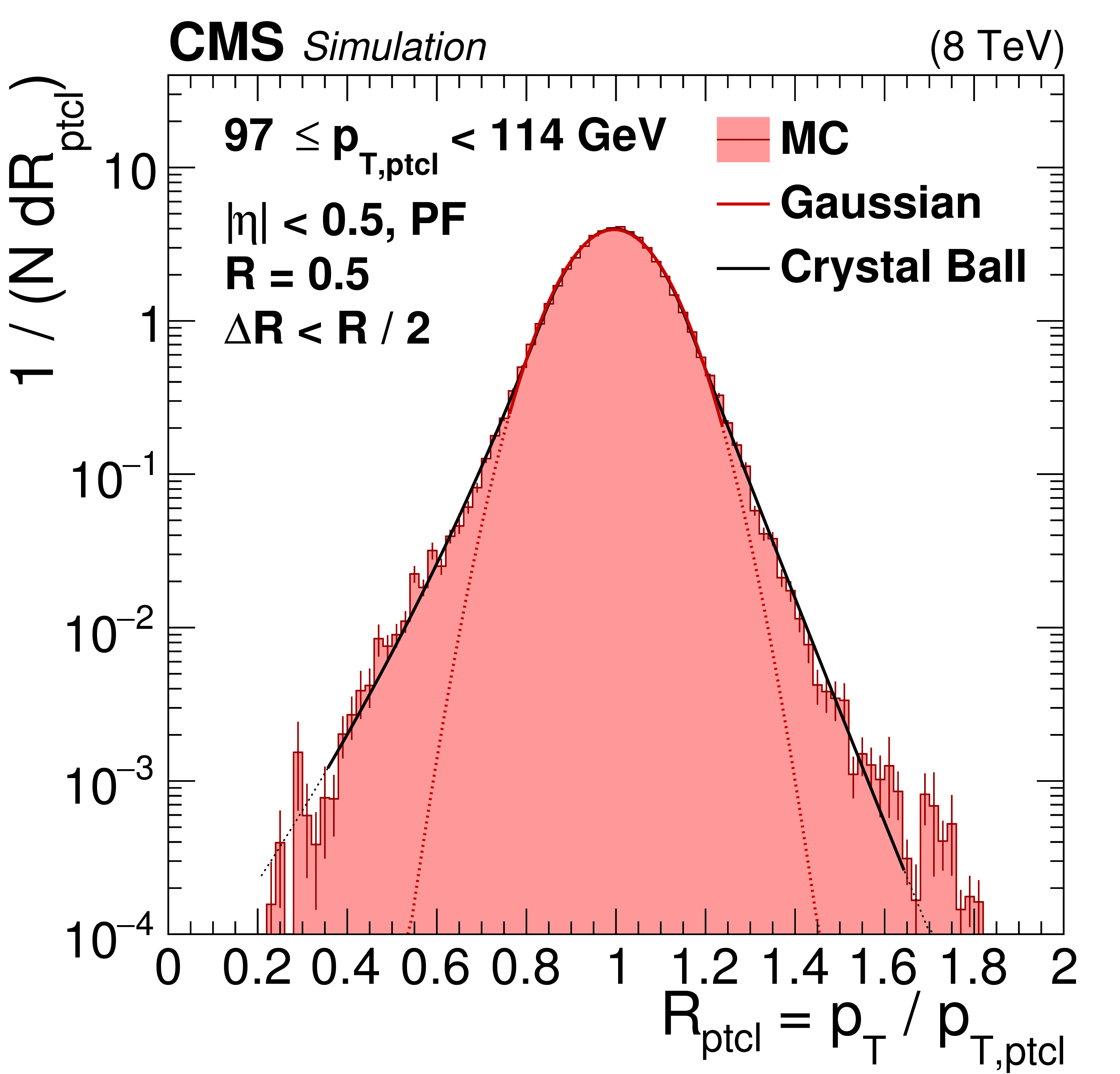
Figure 35:
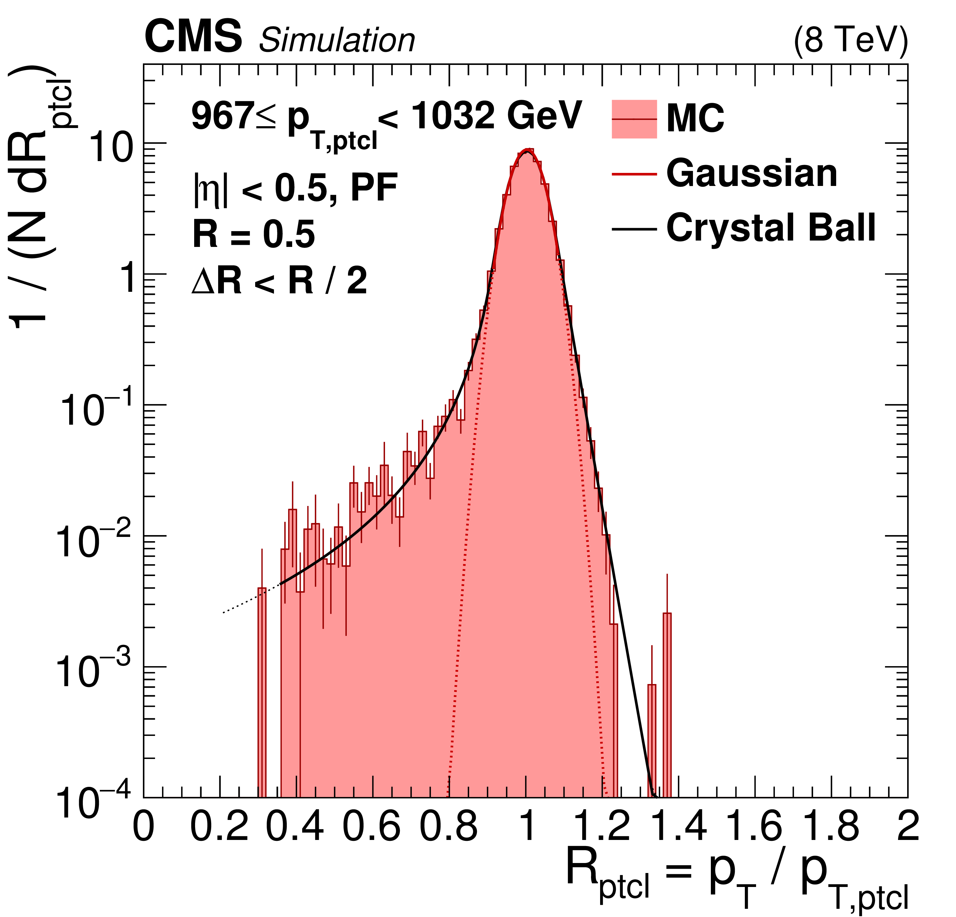
Jet $ {p_{\mathrm {T}}} $ resolution distributions in the barrel for two bins of jet $ {p_{\mathrm {T}}} $. $\Delta R$ indicates the distance parameter value used for matching reconstructed jets to the corresponding particle-level jets. The nongaussian tails due to inactive areas of the ECAL and HCAL punchthrough become more visible for narrow high-$ {p_{\mathrm {T}}} $ jets with small core resolution. The Gaussian core resolution is fit to within $\pm$2$ \sigma $ (solid line) and its extrapolation is indicated with a dotted line. The tails are well modeled by a double-sided Crystal Ball function. |
png pdf |
Figure 35-a:
Jet $ {p_{\mathrm {T}}} $ resolution distributions in the barrel for two bins of jet $ {p_{\mathrm {T}}} $. $\Delta R$ indicates the distance parameter value used for matching reconstructed jets to the corresponding particle-level jets. The nongaussian tails due to inactive areas of the ECAL and HCAL punchthrough become more visible for narrow high-$ {p_{\mathrm {T}}} $ jets with small core resolution. The Gaussian core resolution is fit to within $\pm$2$ \sigma $ (solid line) and its extrapolation is indicated with a dotted line. The tails are well modeled by a double-sided Crystal Ball function. |
png pdf |
Figure 35-b:
Jet $ {p_{\mathrm {T}}} $ resolution distributions in the barrel for two bins of jet $ {p_{\mathrm {T}}} $. $\Delta R$ indicates the distance parameter value used for matching reconstructed jets to the corresponding particle-level jets. The nongaussian tails due to inactive areas of the ECAL and HCAL punchthrough become more visible for narrow high-$ {p_{\mathrm {T}}} $ jets with small core resolution. The Gaussian core resolution is fit to within $\pm$2$ \sigma $ (solid line) and its extrapolation is indicated with a dotted line. The tails are well modeled by a double-sided Crystal Ball function. |
png pdf |
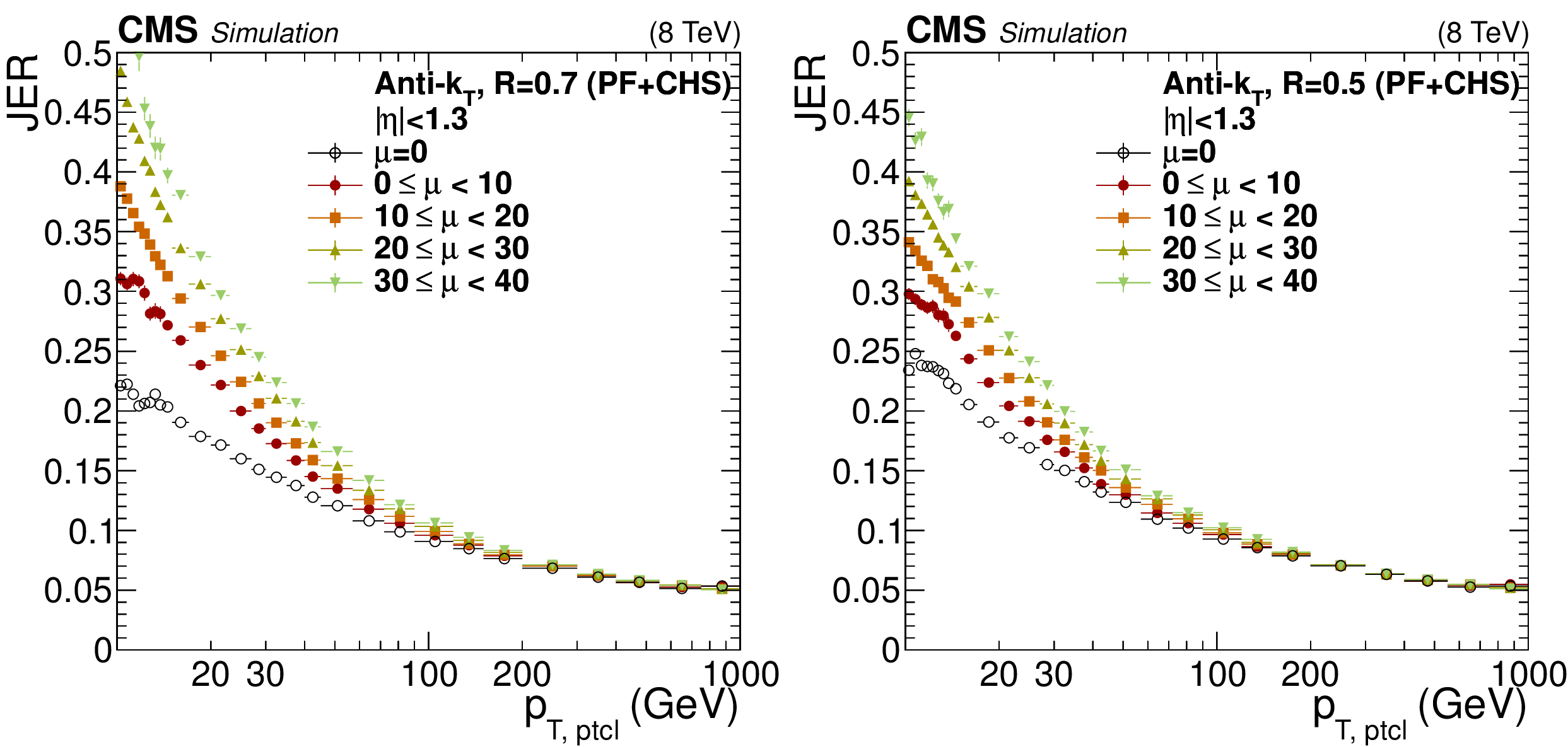
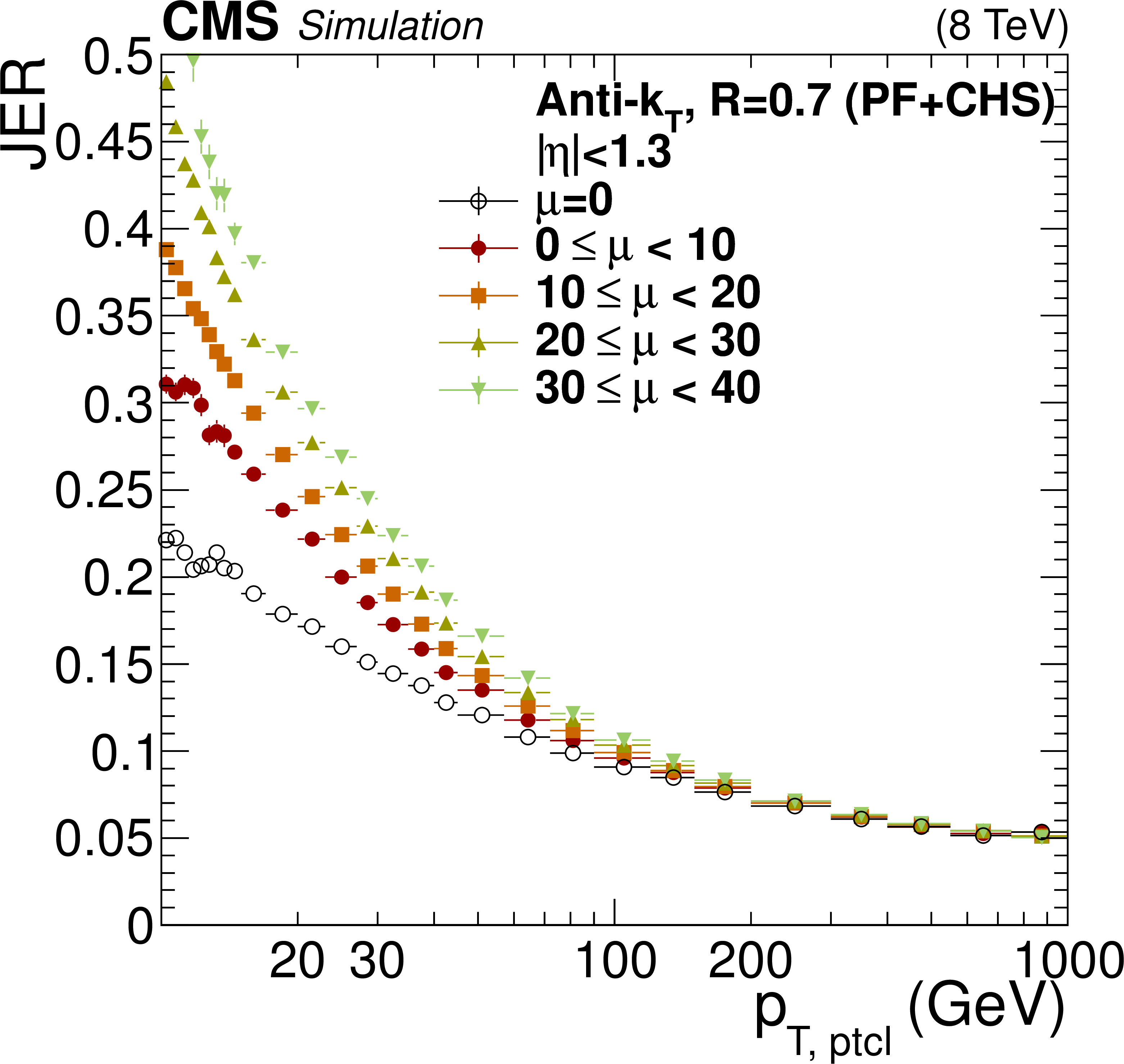
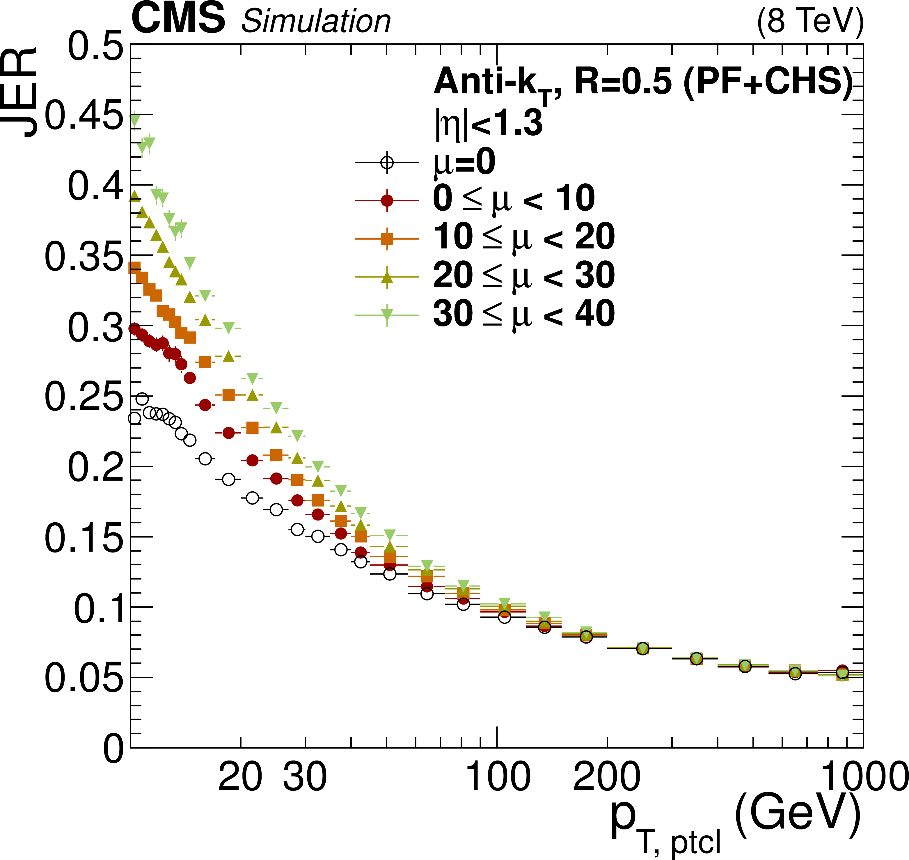
Figure 36:
JER versus $ {p_{\mathrm {T}}} $ in the barrel for varying levels of pileup $\mu $. The results are shown separately for PF+CHS jets with size $R= $ 0.7 (a), and for PF+CHS jets with size $R= $ 0.5 (b). |
png pdf |
Figure 36-a:
JER versus $ {p_{\mathrm {T}}} $ in the barrel for varying levels of pileup $\mu $. The results are shown separately for PF+CHS jets with size $R= $ 0.7 (a), and for PF+CHS jets with size $R= $ 0.5 (b). |
png pdf |
Figure 36-b:
JER versus $ {p_{\mathrm {T}}} $ in the barrel for varying levels of pileup $\mu $. The results are shown separately for PF+CHS jets with size $R= $ 0.7 (a), and for PF+CHS jets with size $R= $ 0.5 (b). |
png pdf |
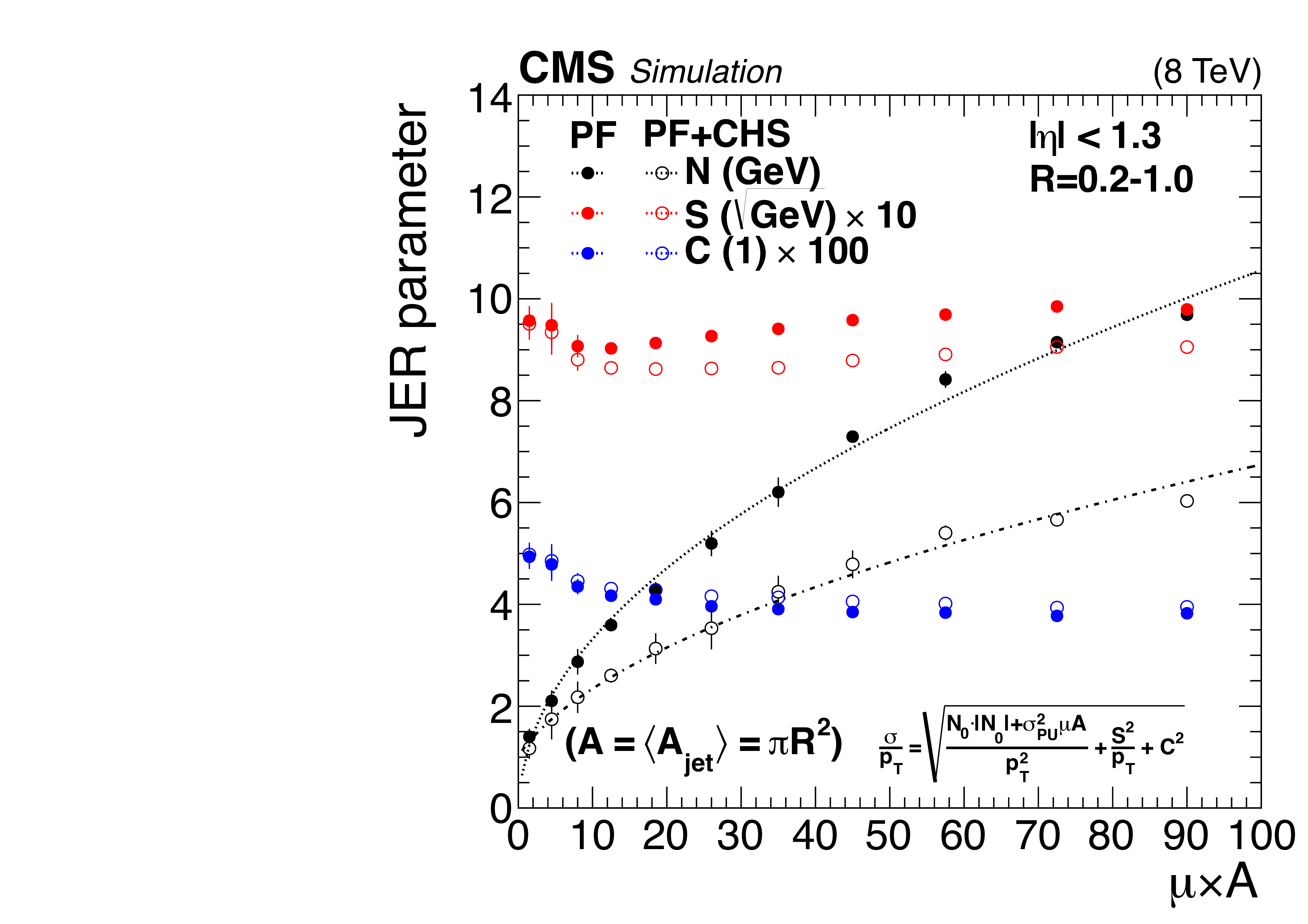
Figure 37:
JER parameters ($N$, $S$, $C$; see text) fitted in bins of $\mu $ for various values of the distance parameter $R$, as a function of their average value of pileup times jet area ($\mu A$). The results are compared between PF (solid symbols) and PF+CHS (open symbols). The dotted and dash-dotted curves represent the fit for PF and PF+CHS jets, respectively. |

png pdf |
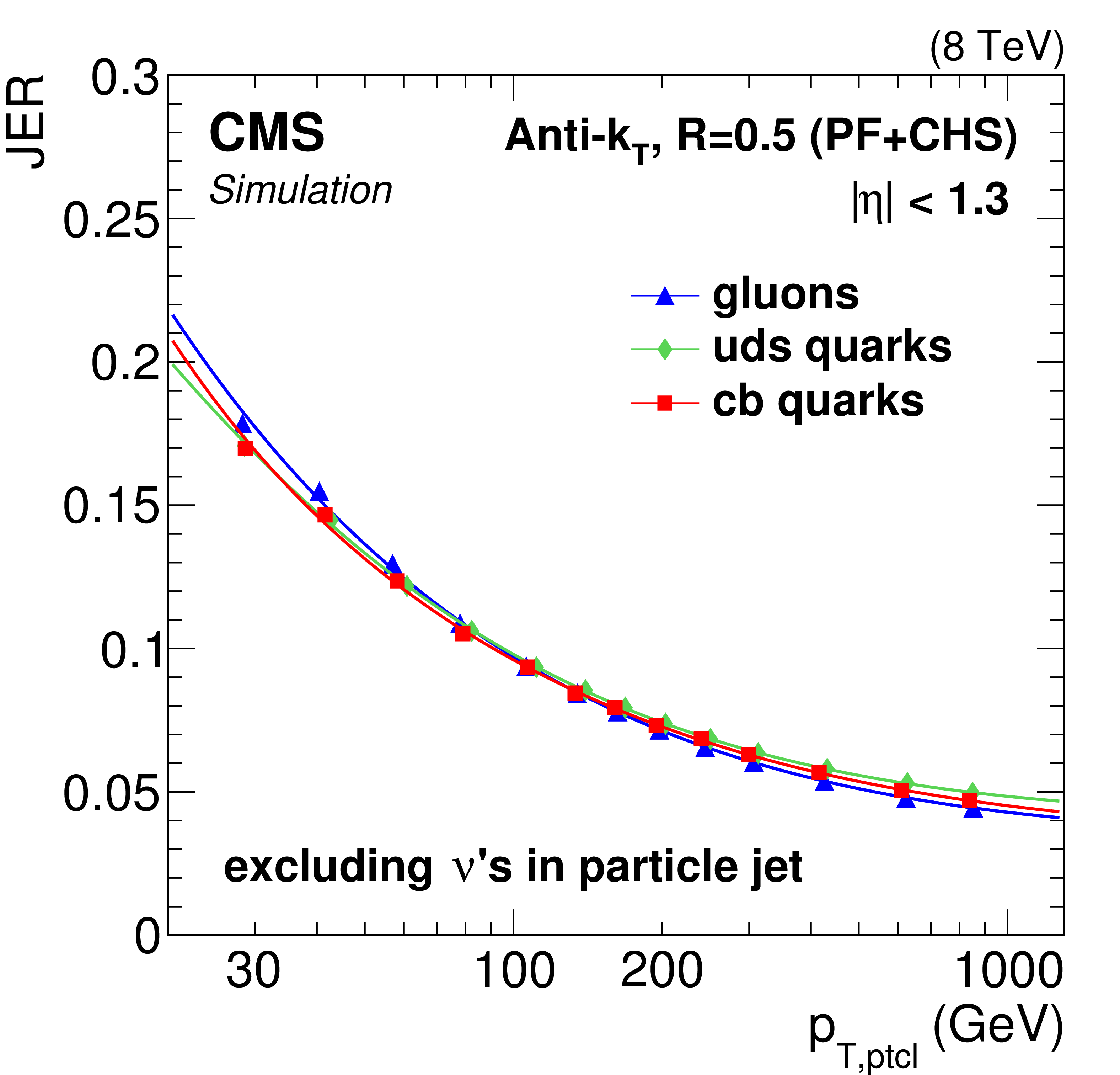
Figure 38:
True JER in simulation for different jet flavors in the $\gamma $+jet sample, for jets with $|\eta |< $ 0.5. The distributions are shown for particle-level jets with no neutrinos (a), and with neutrinos exceptionally included (b) to demonstrate the large fluctuations this induces for c and b jets. |
png pdf |
Figure 38-a:
True JER in simulation for different jet flavors in the $\gamma $+jet sample, for jets with $|\eta |< $ 0.5. The distributions are shown for particle-level jets with no neutrinos (a), and with neutrinos exceptionally included (b) to demonstrate the large fluctuations this induces for c and b jets. |

png pdf |
Figure 38-b:
True JER in simulation for different jet flavors in the $\gamma $+jet sample, for jets with $|\eta |< $ 0.5. The distributions are shown for particle-level jets with no neutrinos (a), and with neutrinos exceptionally included (b) to demonstrate the large fluctuations this induces for c and b jets. |
png pdf |
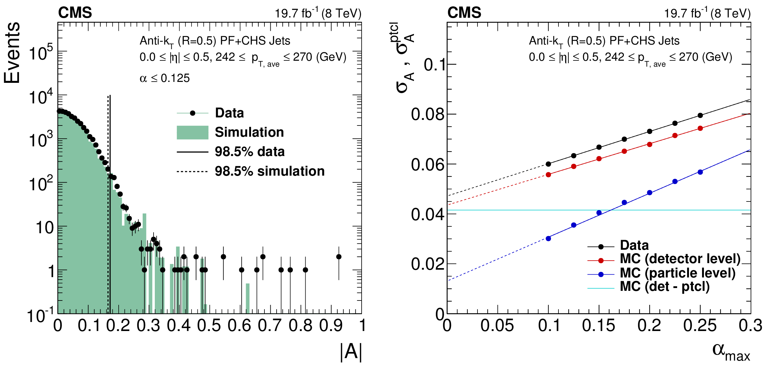
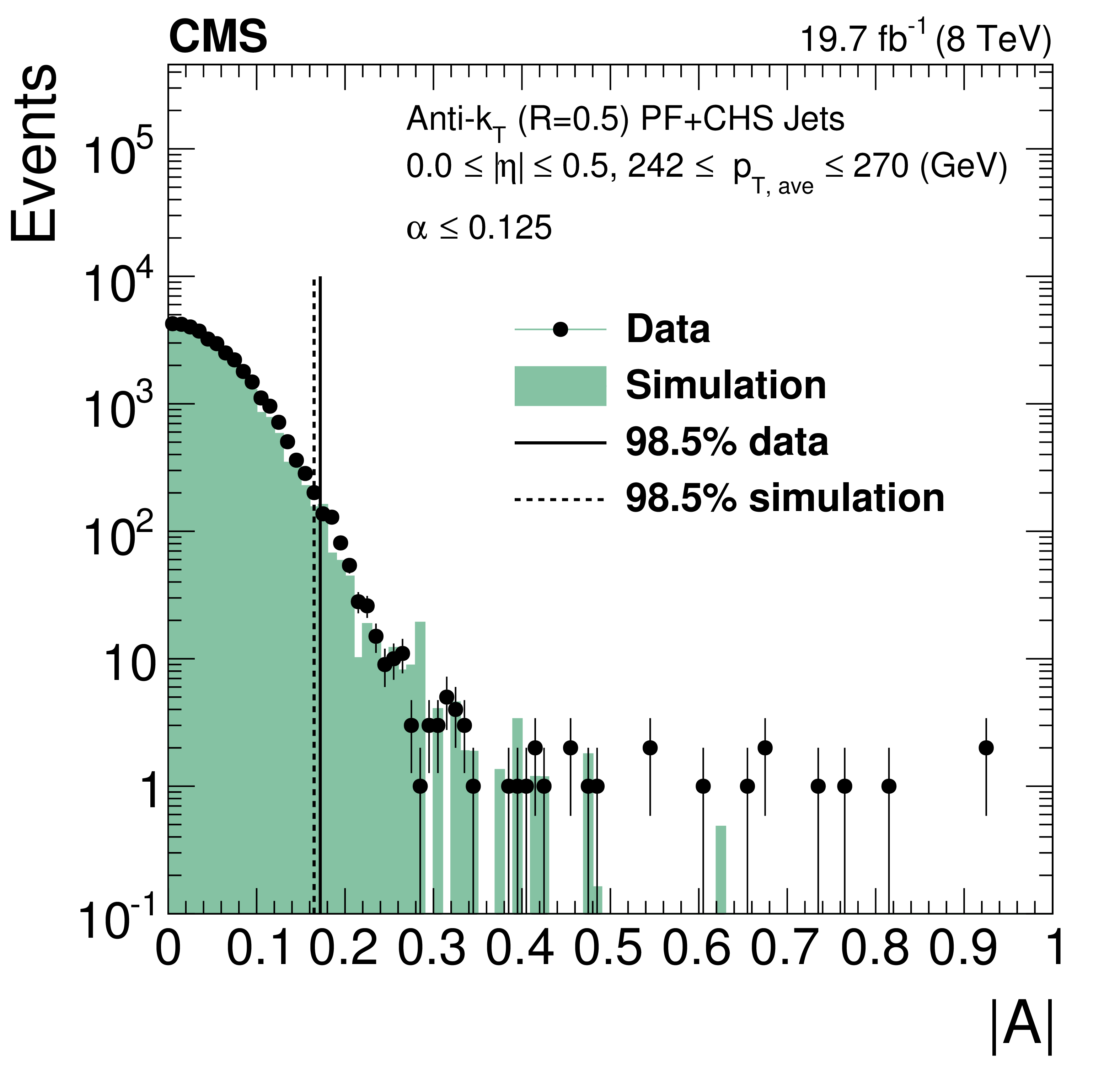
Figure 39:
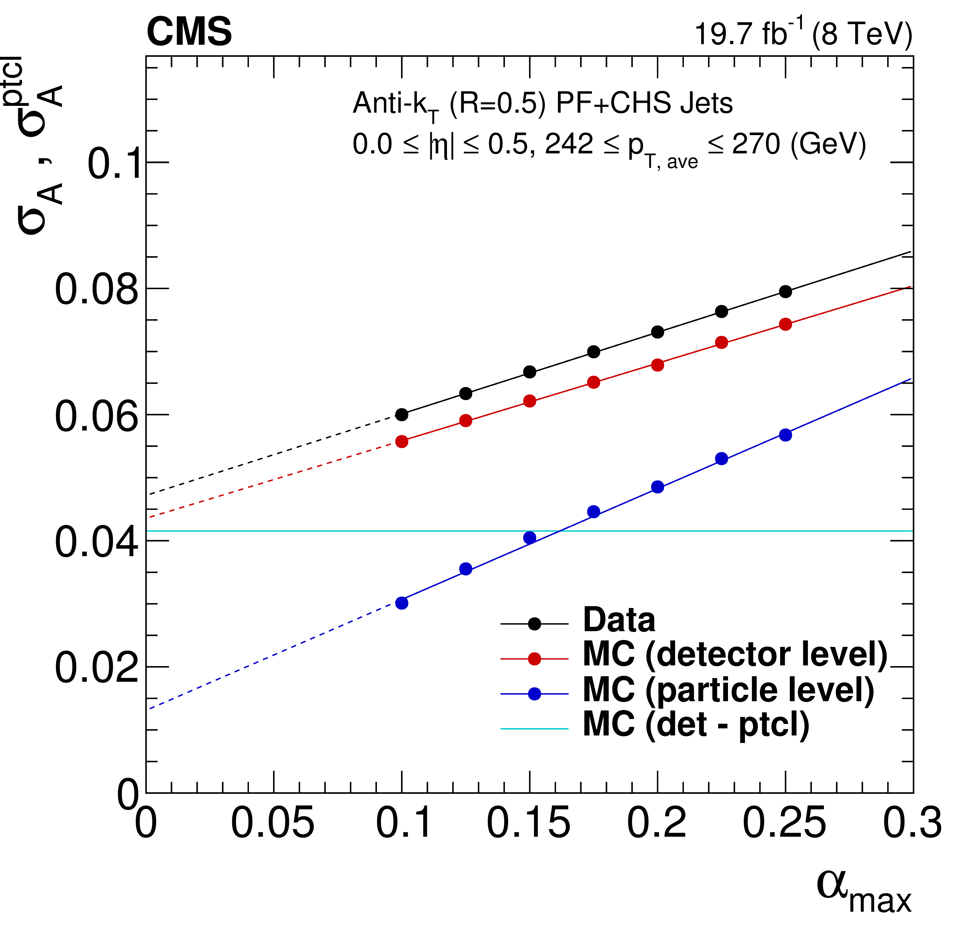
a: Asymmetry distribution, Eq.(39), for data and simulation for jets with $ {p_{\mathrm {T}}} \approx$ 250 GeV and $|\eta |< $ 0.5. b: Asymmetry measured for various thresholds $\alpha _{\rm max}$, extrapolated to zero additional jet activity, for jets with $ {p_{\mathrm {T}}} \approx$ 250 GeV and $|\eta |< $ 0.5 in data and MC simulation at the detector- and particle-level. The light horizontal line indicates the average particle-level resolution obtained as the difference in quadrature of MC simulation reconstructed asymmetry and particle-level imbalance, extrapolated to zero additional jet activity. |
png pdf |
Figure 39-a:
a: Asymmetry distribution, Eq.(39), for data and simulation for jets with $ {p_{\mathrm {T}}} \approx$ 250 GeV and $|\eta |< $ 0.5. b: Asymmetry measured for various thresholds $\alpha _{\rm max}$, extrapolated to zero additional jet activity, for jets with $ {p_{\mathrm {T}}} \approx$ 250 GeV and $|\eta |< $ 0.5 in data and MC simulation at the detector- and particle-level. The light horizontal line indicates the average particle-level resolution obtained as the difference in quadrature of MC simulation reconstructed asymmetry and particle-level imbalance, extrapolated to zero additional jet activity. |
png pdf |
Figure 39-b:
a: Asymmetry distribution, Eq.(39), for data and simulation for jets with $ {p_{\mathrm {T}}} \approx$ 250 GeV and $|\eta |< $ 0.5. b: Asymmetry measured for various thresholds $\alpha _{\rm max}$, extrapolated to zero additional jet activity, for jets with $ {p_{\mathrm {T}}} \approx$ 250 GeV and $|\eta |< $ 0.5 in data and MC simulation at the detector- and particle-level. The light horizontal line indicates the average particle-level resolution obtained as the difference in quadrature of MC simulation reconstructed asymmetry and particle-level imbalance, extrapolated to zero additional jet activity. |
png pdf |
Figure 40:
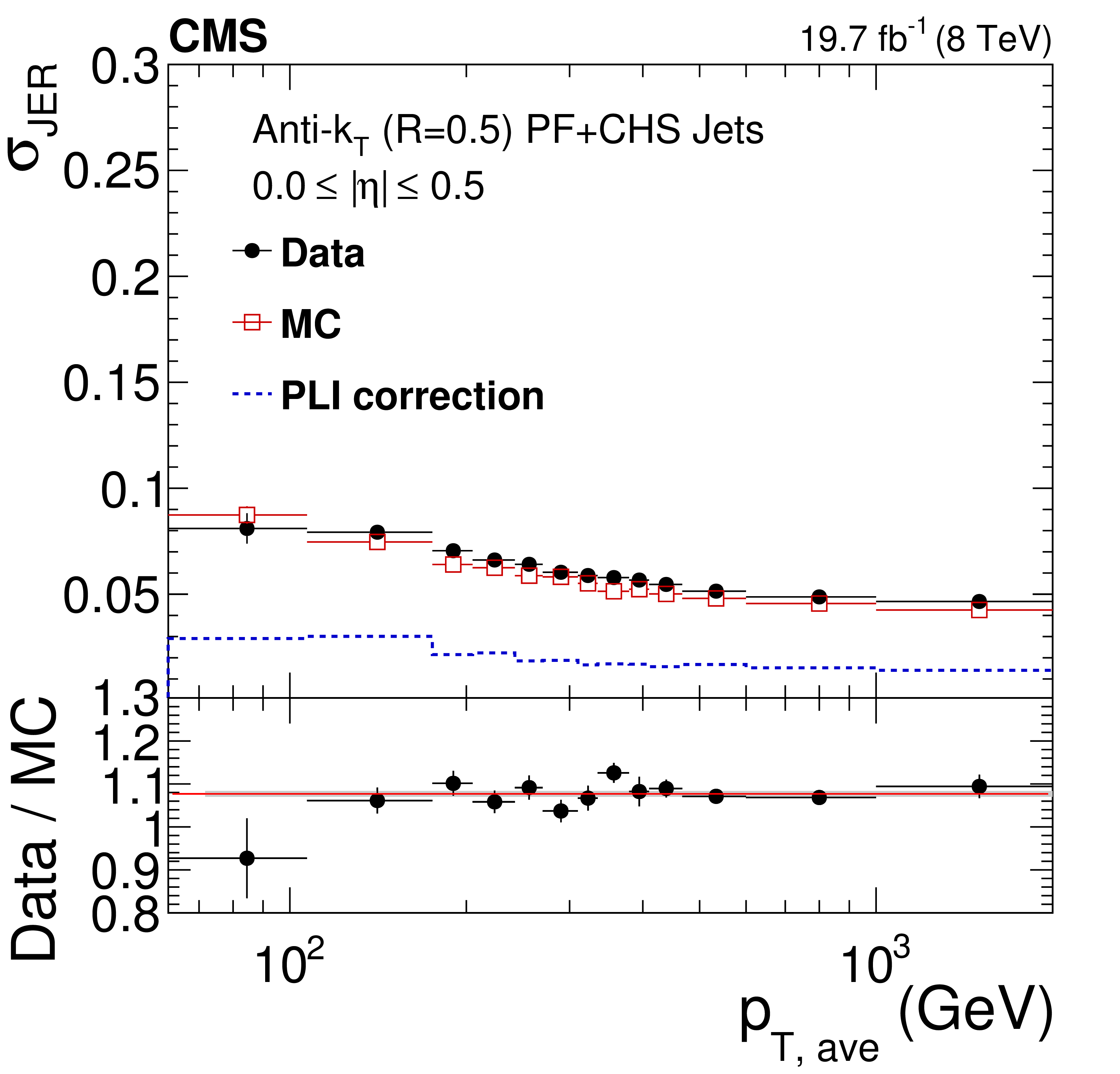
Extrapolated JER as a function of jet $ {p_{\mathrm {T}}} $ obtained with the asymmetry method on dijet events for data (solid circles), reconstructed MC simulation (open squares), and particle-level simulation with PLI (dashed line). The bottom plot shows the ratio of data over MC. |
png pdf |
Figure 41:
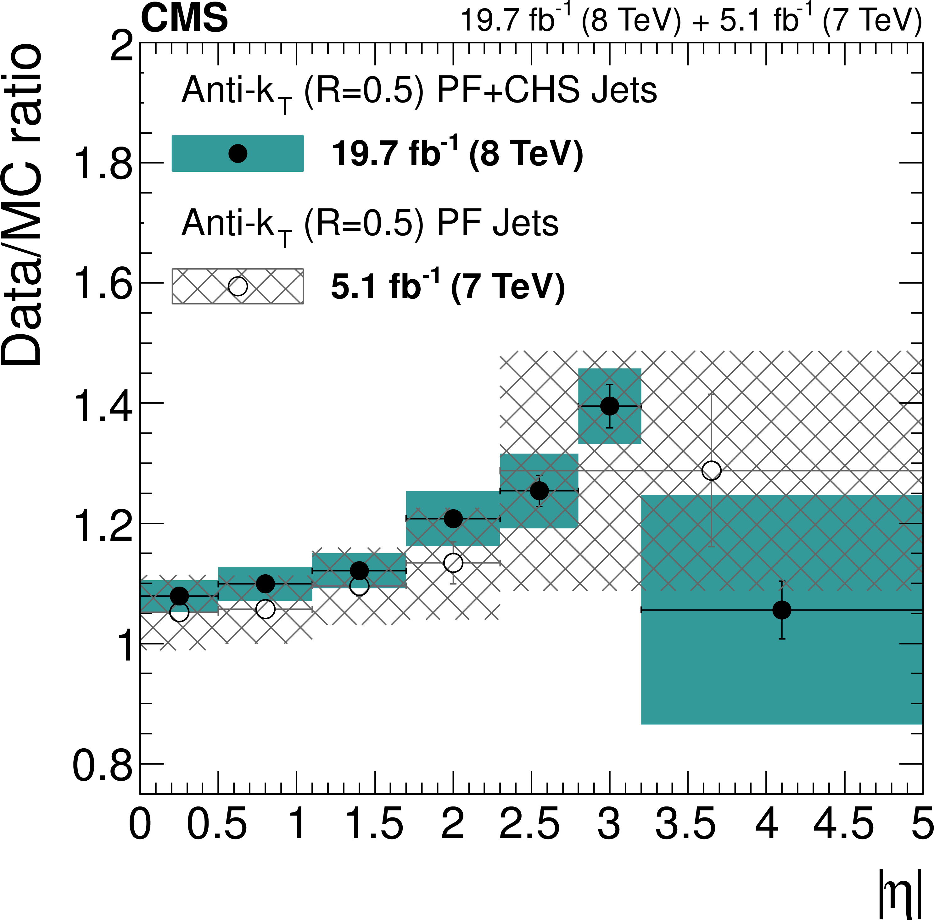
Jet energy resolution data/MC scale factor versus $|\eta |$ for dijet data collected at 8 TeV (closed circles, solid area) compared to results at 7 TeV (open circles, dashed area). |
png pdf |
Figure 42:
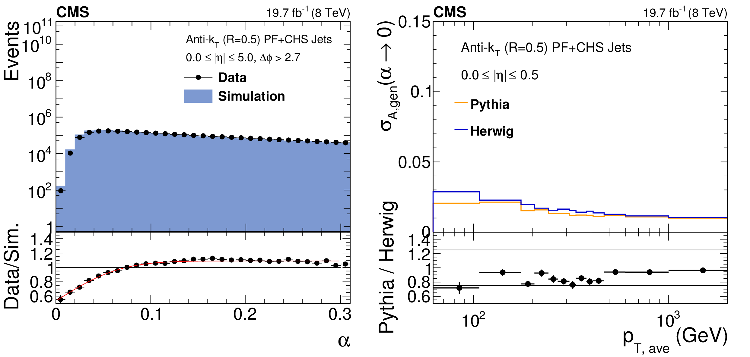
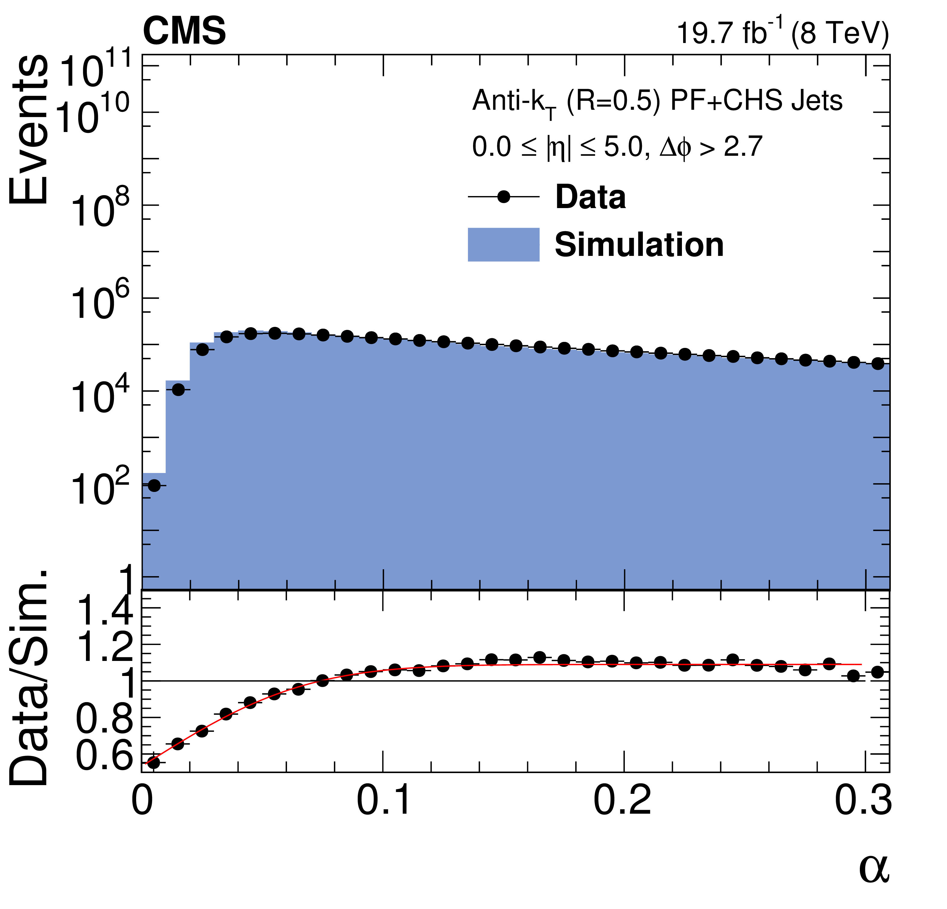
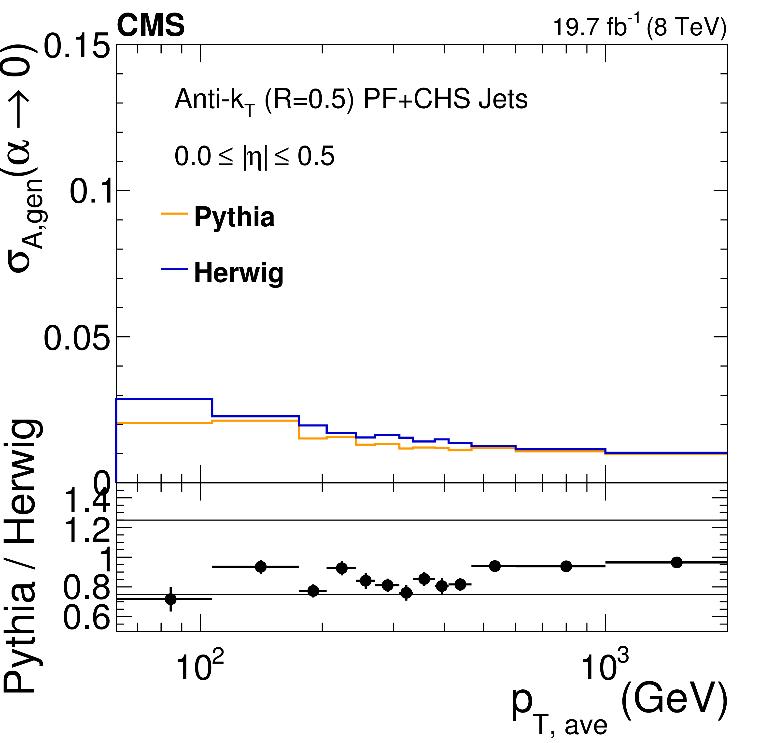
a: The $\alpha $ distribution in data (circles) and simulation (histogram), with the function used for simulation reweighting overlaid on the ratio of data over simulation in the bottom plot. b: Comparison of particle-level imbalances $\sigma _{A,\rm gen}(\alpha \rightarrow 0)$ in Pythia6.4 tune Z2* and Herwig++2.3 tune EE3C as a function of jet $p_{\rm T,ave}$. The bottom plot shows the ratio of Pythia over Herwig. |
png pdf |
Figure 42-a:
a: The $\alpha $ distribution in data (circles) and simulation (histogram), with the function used for simulation reweighting overlaid on the ratio of data over simulation in the bottom plot. b: Comparison of particle-level imbalances $\sigma _{A,\rm gen}(\alpha \rightarrow 0)$ in Pythia6.4 tune Z2* and Herwig++2.3 tune EE3C as a function of jet $p_{\rm T,ave}$. The bottom plot shows the ratio of Pythia over Herwig. |
png pdf |
Figure 42-b:
a: The $\alpha $ distribution in data (circles) and simulation (histogram), with the function used for simulation reweighting overlaid on the ratio of data over simulation in the bottom plot. b: Comparison of particle-level imbalances $\sigma _{A,\rm gen}(\alpha \rightarrow 0)$ in Pythia6.4 tune Z2* and Herwig++2.3 tune EE3C as a function of jet $p_{\rm T,ave}$. The bottom plot shows the ratio of Pythia over Herwig. |
png pdf |
Figure 43:
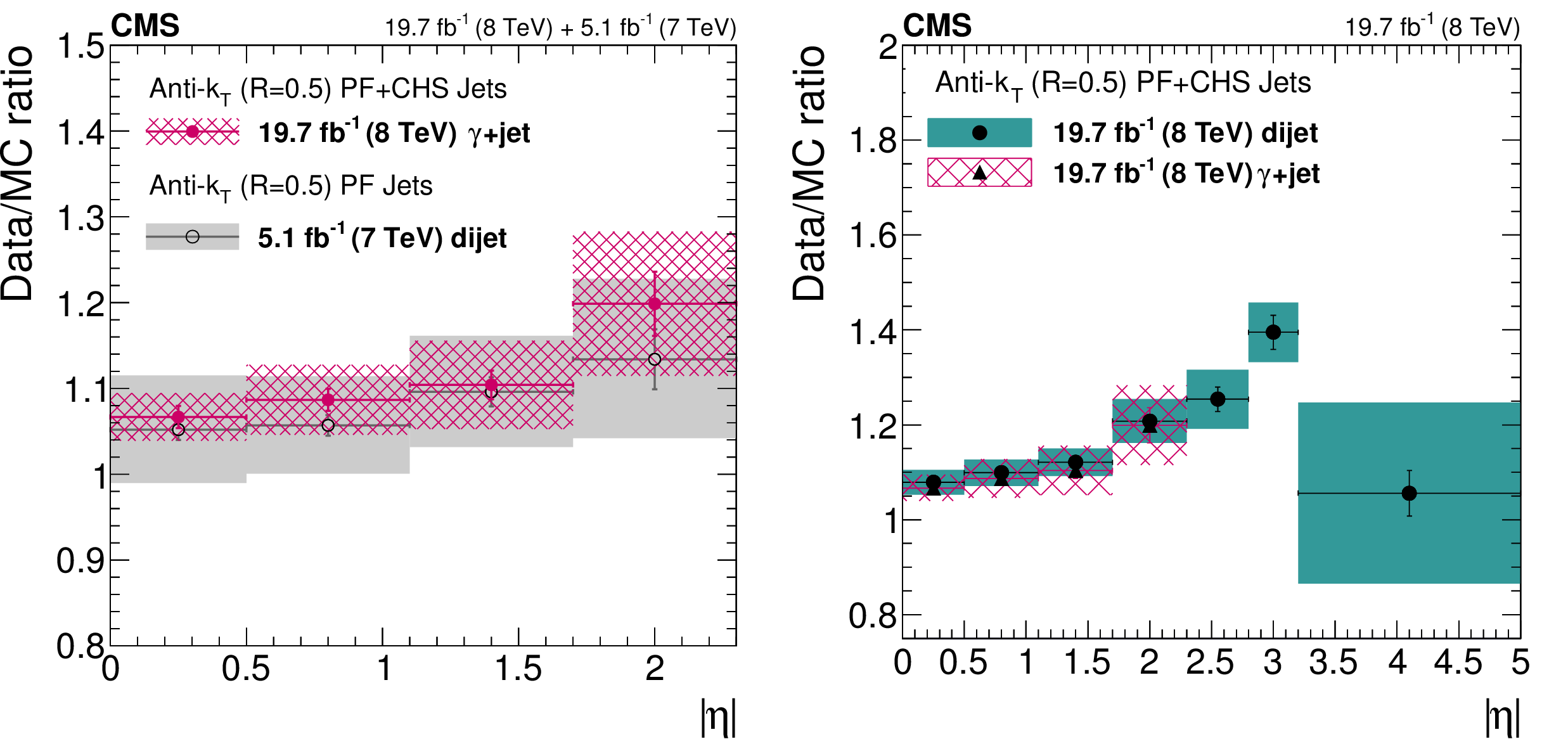
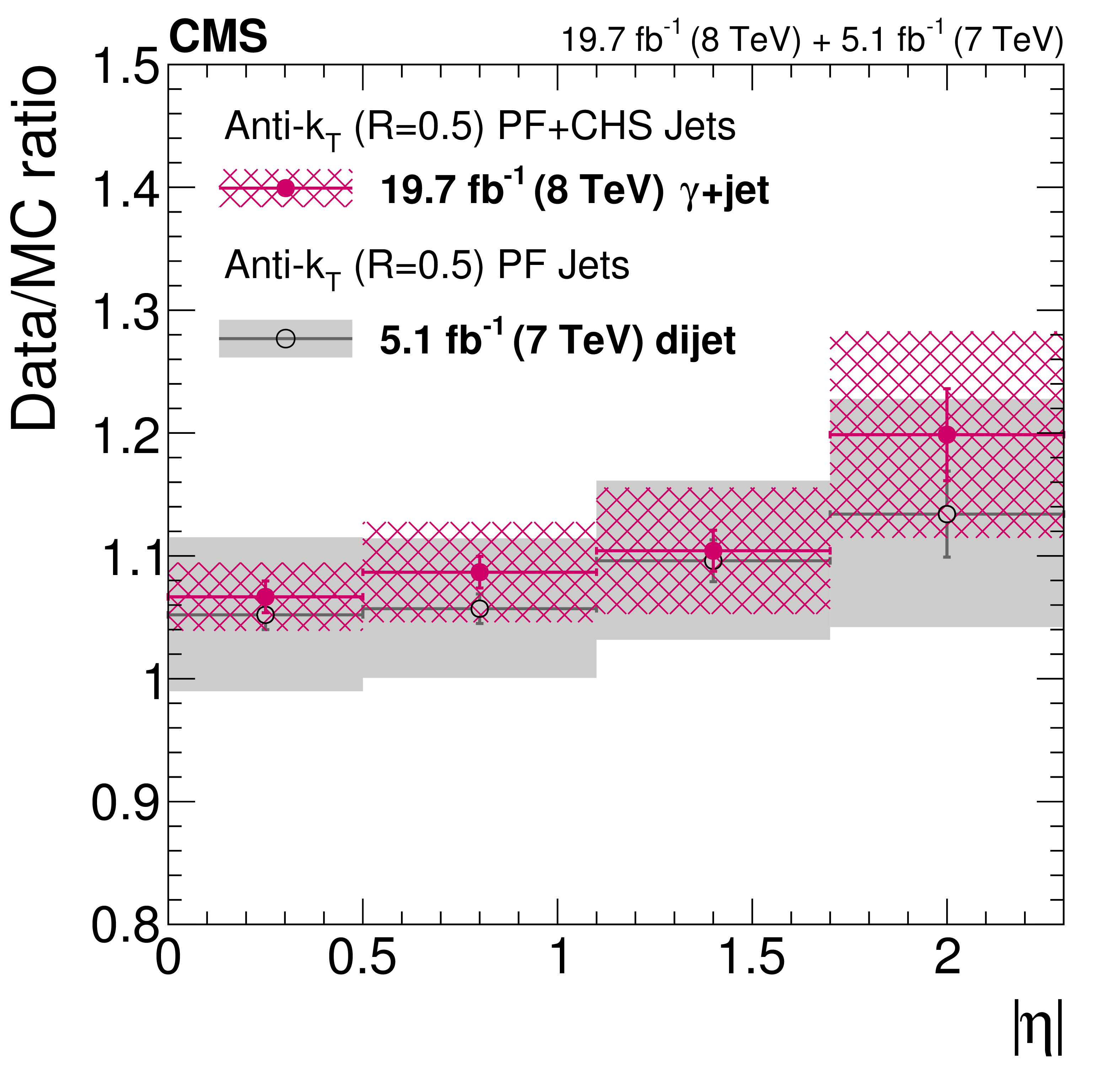
Data/MC scale factors for the jet $ {p_{\mathrm {T}}} $ resolution as a function of $|\eta |$, determined from 8-TeV $\gamma $+jet data (hatched boxes) compared to those obtained from dijet data (solid boxes) at 7 TeV (a) and at 8 TeV (b). |
png pdf |
Figure 43-a:
Data/MC scale factors for the jet $ {p_{\mathrm {T}}} $ resolution as a function of $|\eta |$, determined from 8-TeV $\gamma $+jet data (hatched boxes) compared to those obtained from dijet data (solid boxes) at 7 TeV (a) and at 8 TeV (b). |

png pdf |
Figure 43-b:
Data/MC scale factors for the jet $ {p_{\mathrm {T}}} $ resolution as a function of $|\eta |$, determined from 8-TeV $\gamma $+jet data (hatched boxes) compared to those obtained from dijet data (solid boxes) at 7 TeV (a) and at 8 TeV (b). |
png pdf |
Figure 44:
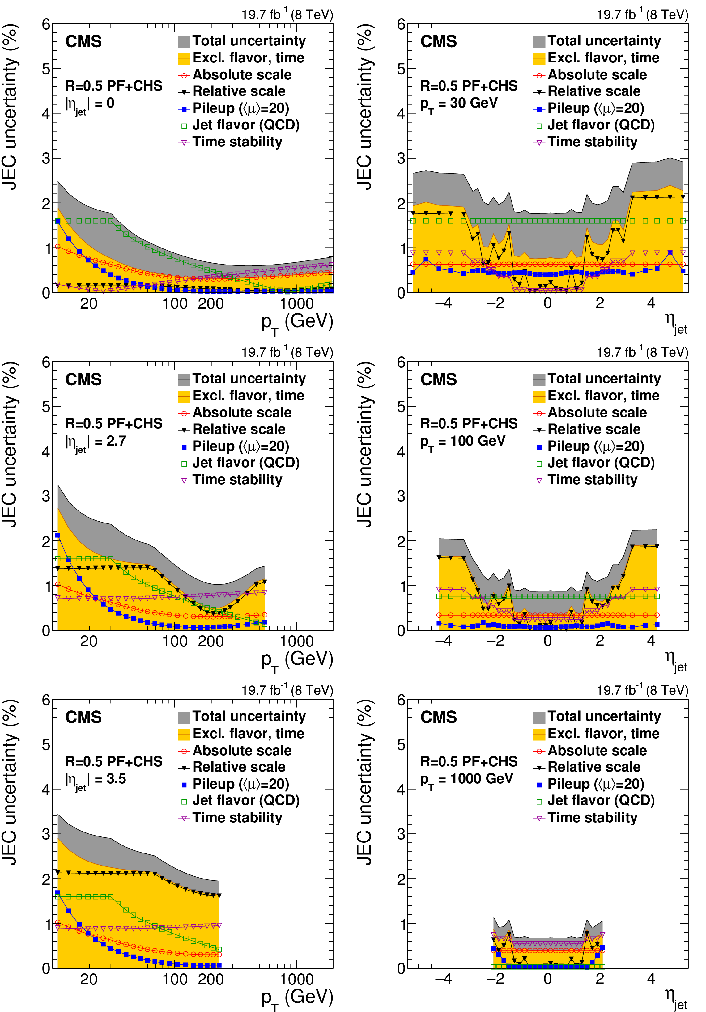
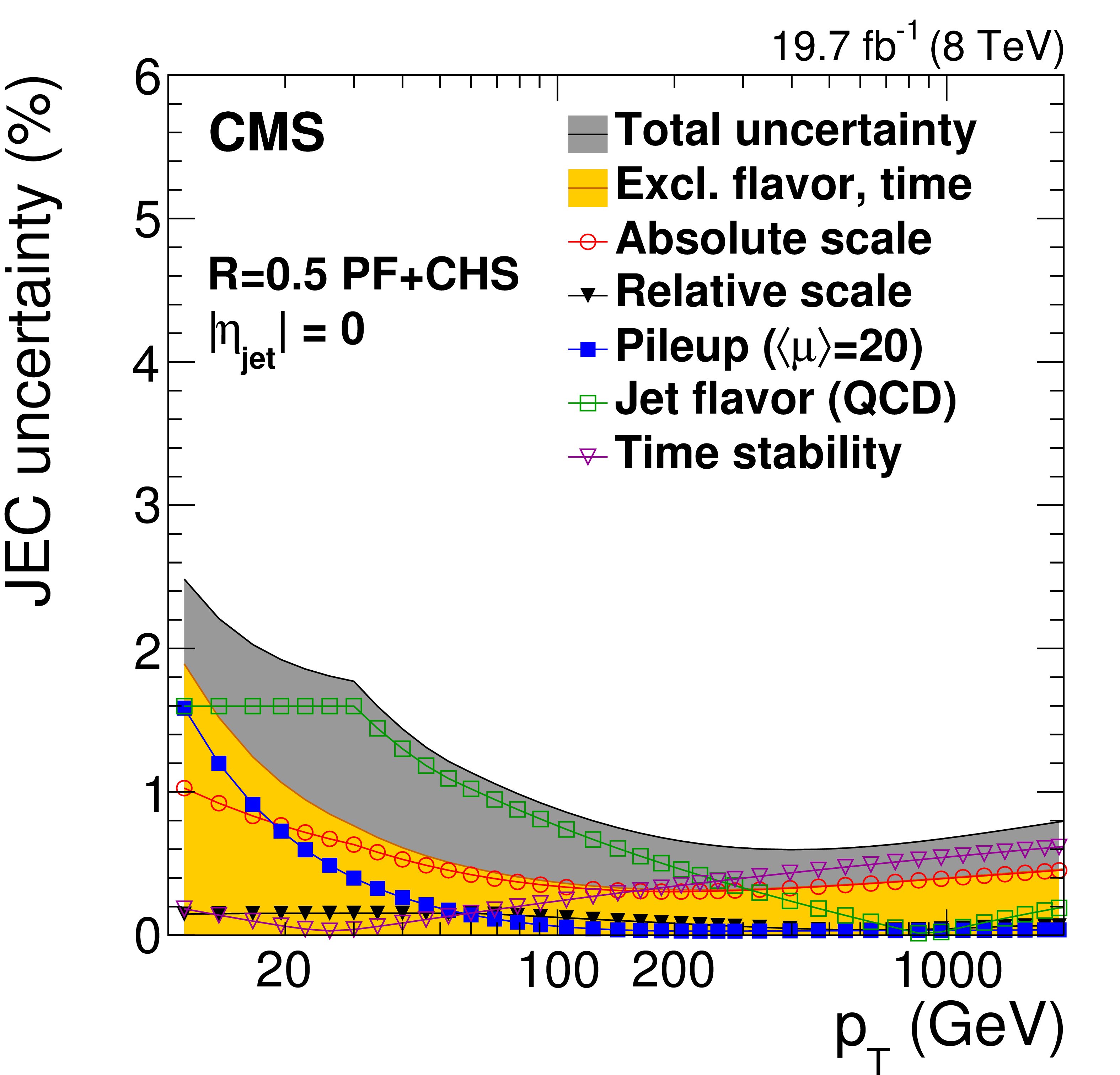
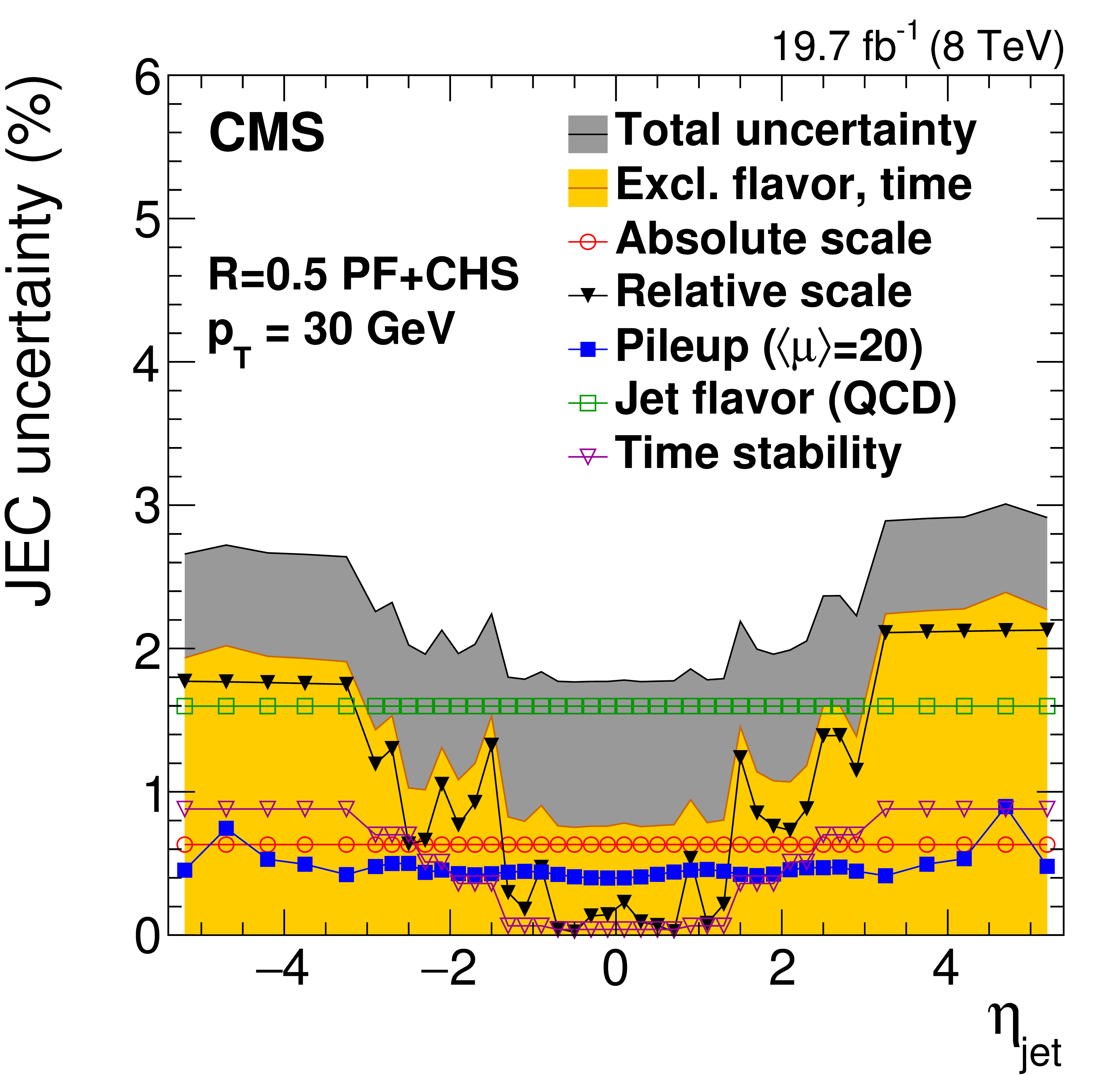
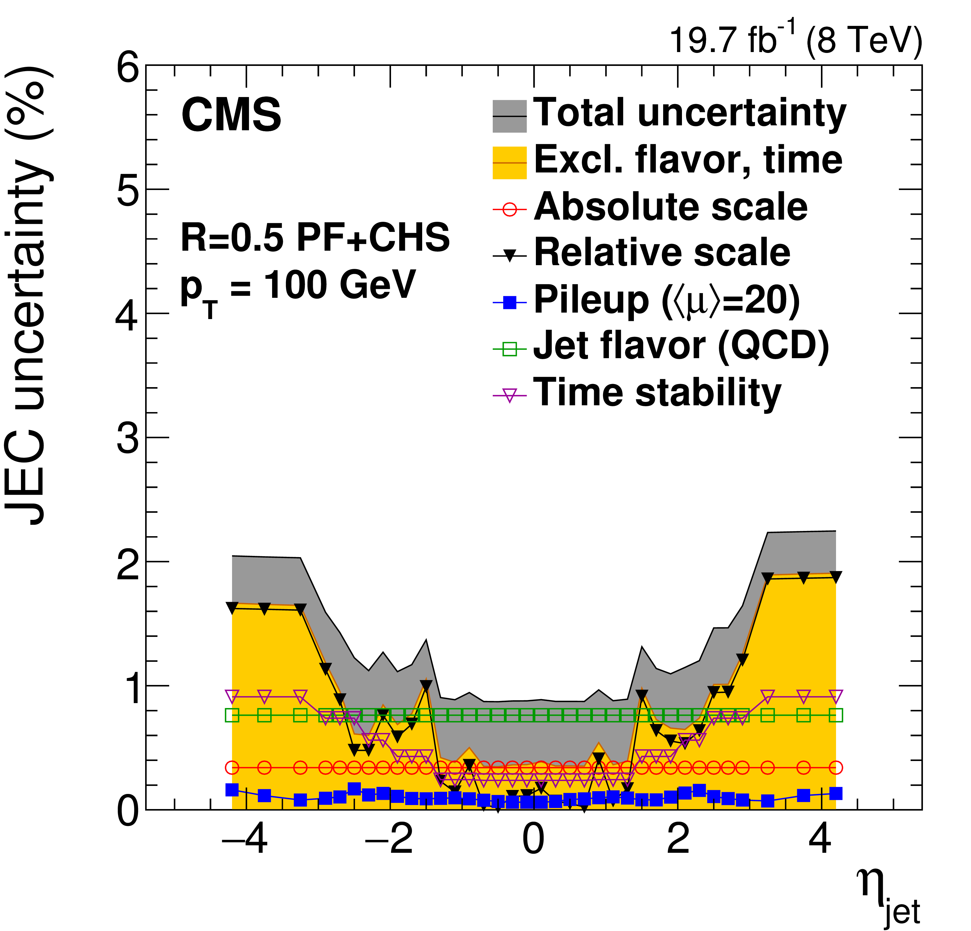
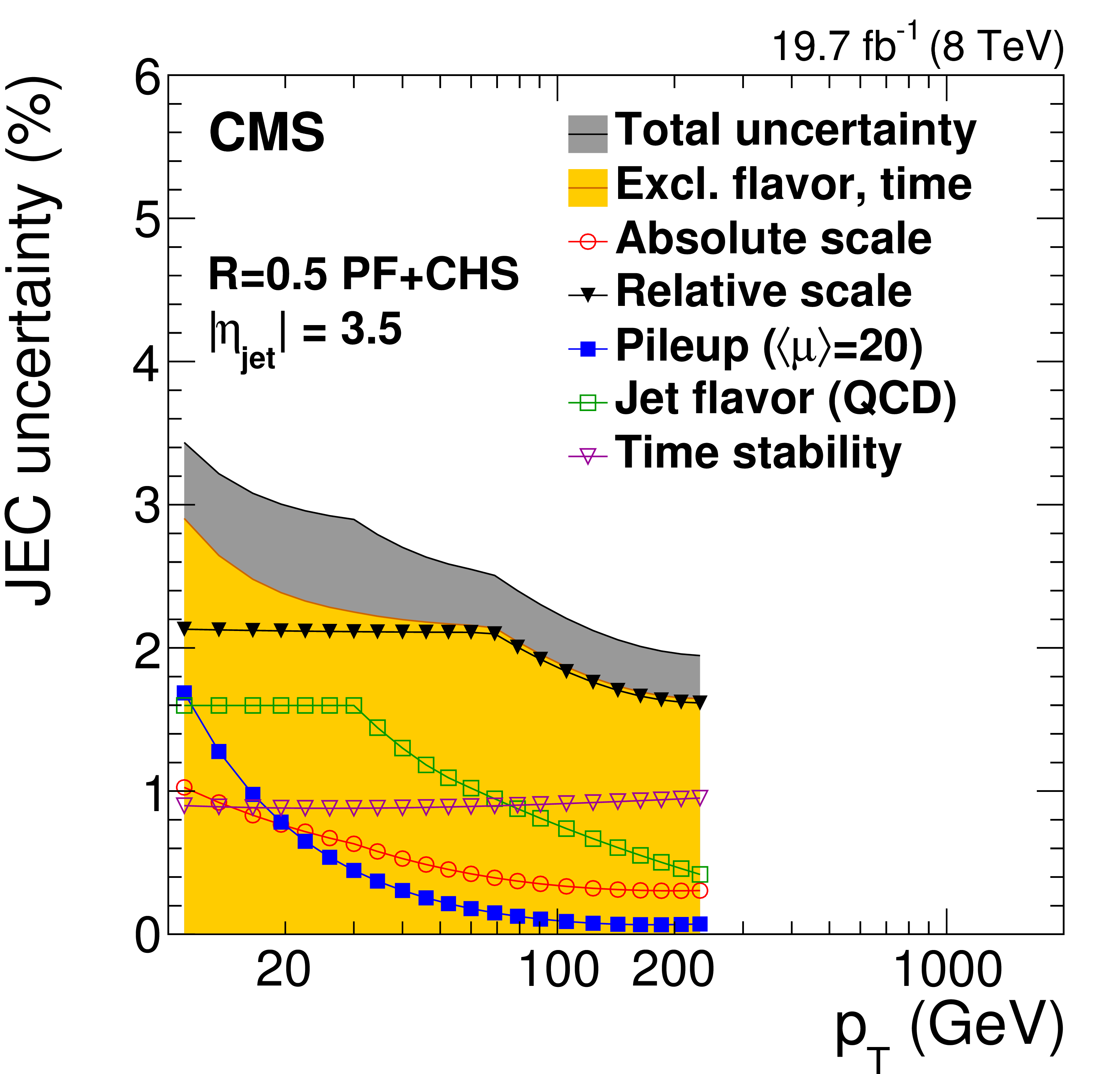
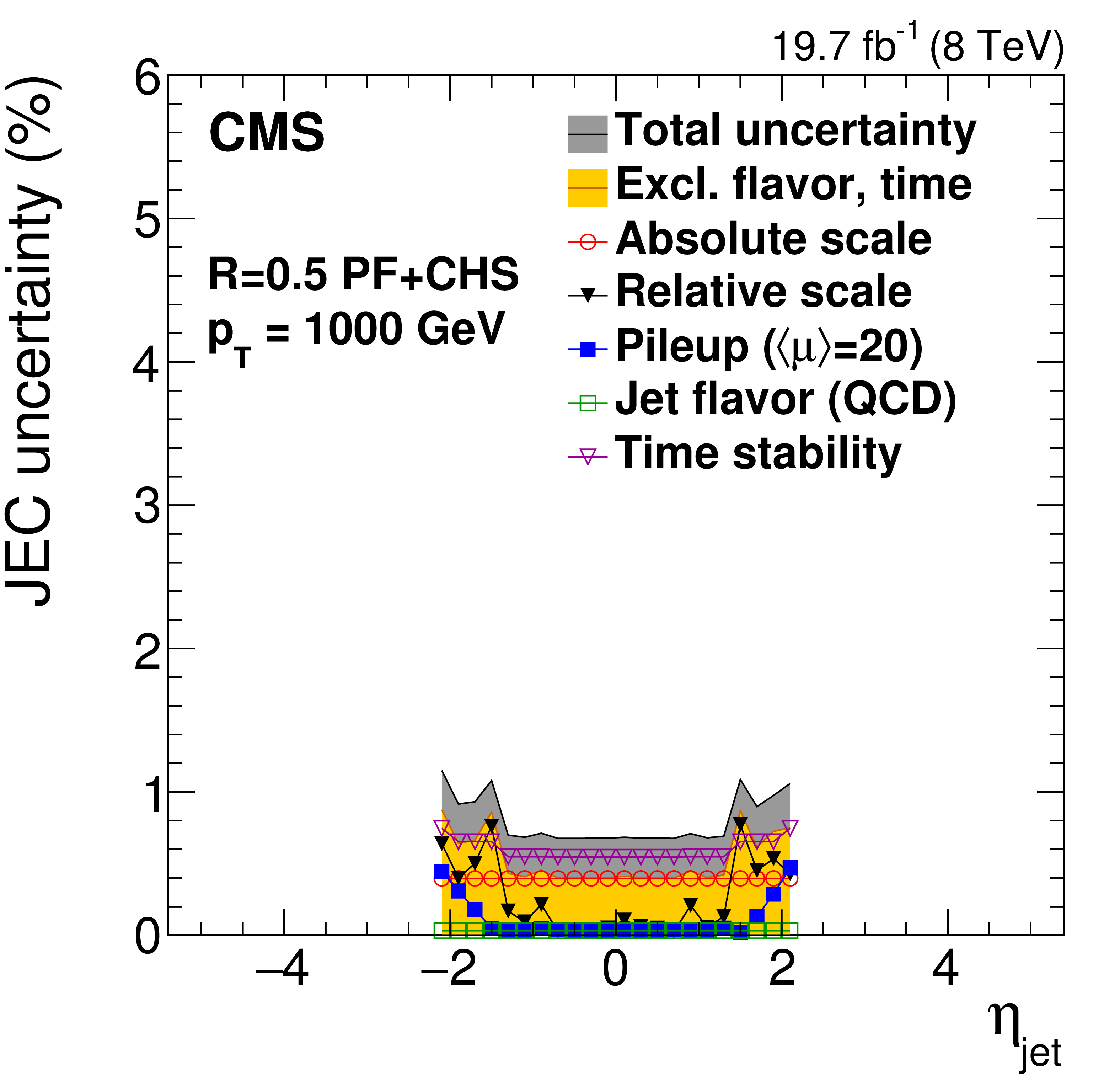
Summary of JES systematic uncertainties as a function of jet $ {p_{\mathrm {T}}} $ (for 3 different $|\eta _{\rm jet}|$ values, a,c,e) and of $\eta _{\rm jet}$ (for 3 different $ {p_{\mathrm {T}}} $ values, b,d,f). The markers show the single effect of different sources, the gray dark band the cumulative total uncertainty. The total uncertainty, when excluding the effects of time dependence and flavor, is also shown in yellow light. The plots are limited to a jet energy $E= {p_{\mathrm {T}}} \cosh\eta = $ 4000 GeV so as to show only the correction factors for reasonable $ {p_{\mathrm {T}}} $ in the considered data-taking period. |
png pdf |
Figure 44-a:
Summary of JES systematic uncertainties as a function of jet $ {p_{\mathrm {T}}} $ (for 3 different $|\eta _{\rm jet}|$ values, a,c,e) and of $\eta _{\rm jet}$ (for 3 different $ {p_{\mathrm {T}}} $ values, b,d,f). The markers show the single effect of different sources, the gray dark band the cumulative total uncertainty. The total uncertainty, when excluding the effects of time dependence and flavor, is also shown in yellow light. The plots are limited to a jet energy $E= {p_{\mathrm {T}}} \cosh\eta = $ 4000 GeV so as to show only the correction factors for reasonable $ {p_{\mathrm {T}}} $ in the considered data-taking period. |
png pdf |
Figure 44-b:
Summary of JES systematic uncertainties as a function of jet $ {p_{\mathrm {T}}} $ (for 3 different $|\eta _{\rm jet}|$ values, a,c,e) and of $\eta _{\rm jet}$ (for 3 different $ {p_{\mathrm {T}}} $ values, b,d,f). The markers show the single effect of different sources, the gray dark band the cumulative total uncertainty. The total uncertainty, when excluding the effects of time dependence and flavor, is also shown in yellow light. The plots are limited to a jet energy $E= {p_{\mathrm {T}}} \cosh\eta = $ 4000 GeV so as to show only the correction factors for reasonable $ {p_{\mathrm {T}}} $ in the considered data-taking period. |
png pdf |
Figure 44-c:
Summary of JES systematic uncertainties as a function of jet $ {p_{\mathrm {T}}} $ (for 3 different $|\eta _{\rm jet}|$ values, a,c,e) and of $\eta _{\rm jet}$ (for 3 different $ {p_{\mathrm {T}}} $ values, b,d,f). The markers show the single effect of different sources, the gray dark band the cumulative total uncertainty. The total uncertainty, when excluding the effects of time dependence and flavor, is also shown in yellow light. The plots are limited to a jet energy $E= {p_{\mathrm {T}}} \cosh\eta = $ 4000 GeV so as to show only the correction factors for reasonable $ {p_{\mathrm {T}}} $ in the considered data-taking period. |
png pdf |
Figure 44-d:
Summary of JES systematic uncertainties as a function of jet $ {p_{\mathrm {T}}} $ (for 3 different $|\eta _{\rm jet}|$ values, a,c,e) and of $\eta _{\rm jet}$ (for 3 different $ {p_{\mathrm {T}}} $ values, b,d,f). The markers show the single effect of different sources, the gray dark band the cumulative total uncertainty. The total uncertainty, when excluding the effects of time dependence and flavor, is also shown in yellow light. The plots are limited to a jet energy $E= {p_{\mathrm {T}}} \cosh\eta = $ 4000 GeV so as to show only the correction factors for reasonable $ {p_{\mathrm {T}}} $ in the considered data-taking period. |
png pdf |
Figure 44-e:
Summary of JES systematic uncertainties as a function of jet $ {p_{\mathrm {T}}} $ (for 3 different $|\eta _{\rm jet}|$ values, a,c,e) and of $\eta _{\rm jet}$ (for 3 different $ {p_{\mathrm {T}}} $ values, b,d,f). The markers show the single effect of different sources, the gray dark band the cumulative total uncertainty. The total uncertainty, when excluding the effects of time dependence and flavor, is also shown in yellow light. The plots are limited to a jet energy $E= {p_{\mathrm {T}}} \cosh\eta = $ 4000 GeV so as to show only the correction factors for reasonable $ {p_{\mathrm {T}}} $ in the considered data-taking period. |
png pdf |
Figure 44-f:
Summary of JES systematic uncertainties as a function of jet $ {p_{\mathrm {T}}} $ (for 3 different $|\eta _{\rm jet}|$ values, a,c,e) and of $\eta _{\rm jet}$ (for 3 different $ {p_{\mathrm {T}}} $ values, b,d,f). The markers show the single effect of different sources, the gray dark band the cumulative total uncertainty. The total uncertainty, when excluding the effects of time dependence and flavor, is also shown in yellow light. The plots are limited to a jet energy $E= {p_{\mathrm {T}}} \cosh\eta = $ 4000 GeV so as to show only the correction factors for reasonable $ {p_{\mathrm {T}}} $ in the considered data-taking period. |
png pdf |
Figure 45:
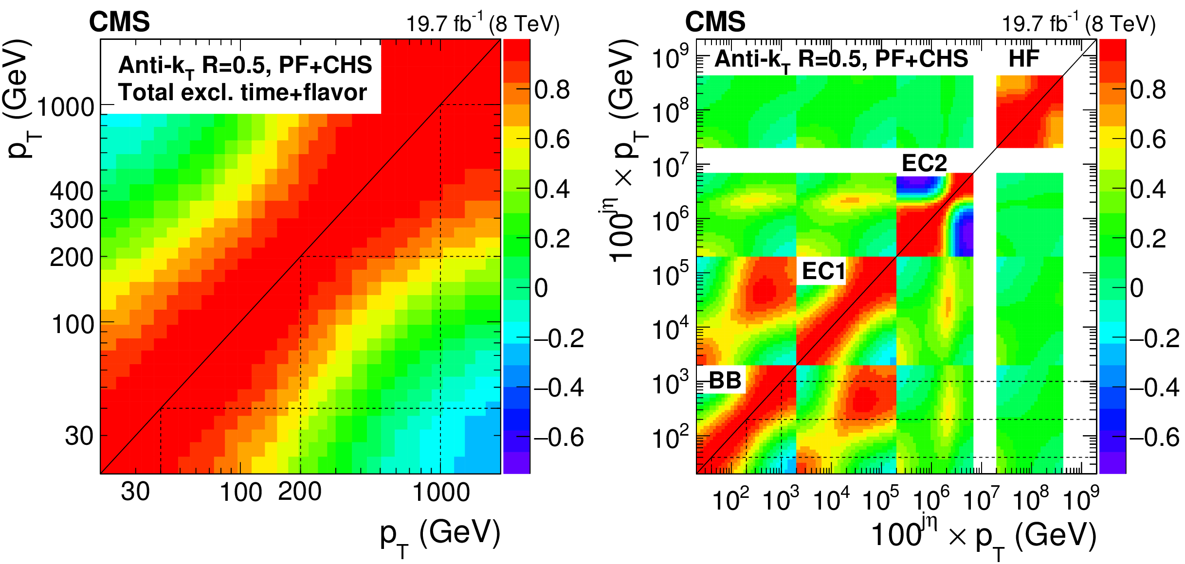
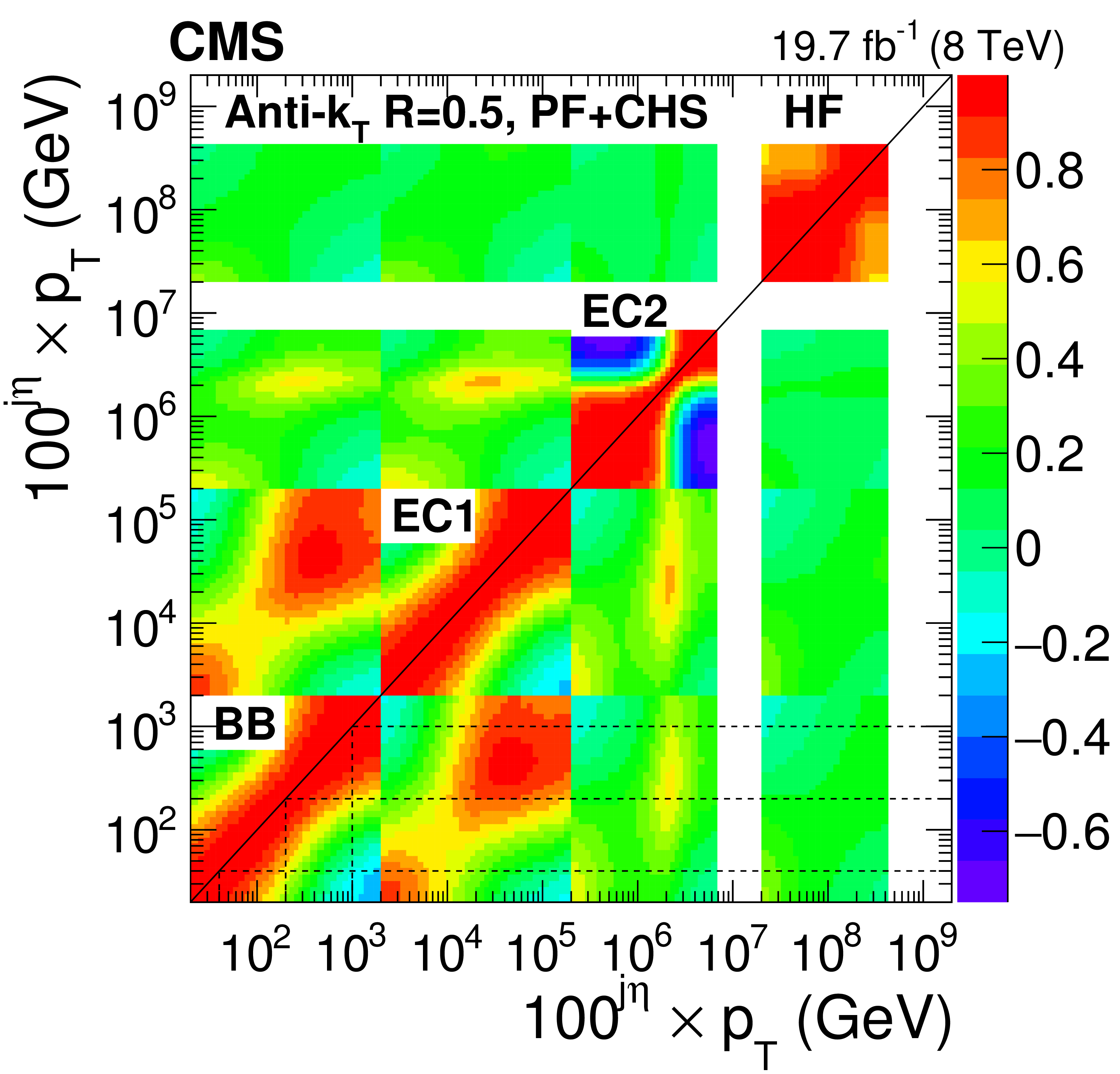
Correlation of total JES systematic uncertainties excluding time-dependent and flavor uncertainties (TotalNoTimeNoFlavor) for PF+CHS versus $ {p_{\mathrm {T}}} $ at $|\eta |< $ 1.3 (a). The color represents the degree of correlation (between $-1$ and $1$). Correlation of JES systematic uncertainties (TotalNoTimeNoFlavor) for PF+CHS versus $ {p_{\mathrm {T}}} $ (multiplied by $100^{{\rm j}\eta }$) and j$\eta $ bin (b). The integer j$\eta $ is introduced for illustration purposes, with j$\eta = $ 0 for the barrel region (BB), j$\eta = $ 1 for the endcap inside tracker coverage (EC1), j$\eta = $ 2 for the endcap outside tracker coverage (EC2), and j$\eta = $ 3 for the forward region (HF). |

png pdf |
Figure 45-a:
Correlation of total JES systematic uncertainties excluding time-dependent and flavor uncertainties (TotalNoTimeNoFlavor) for PF+CHS versus $ {p_{\mathrm {T}}} $ at $|\eta |< $ 1.3 (a). The color represents the degree of correlation (between $-1$ and $1$). Correlation of JES systematic uncertainties (TotalNoTimeNoFlavor) for PF+CHS versus $ {p_{\mathrm {T}}} $ (multiplied by $100^{{\rm j}\eta }$) and j$\eta $ bin (b). The integer j$\eta $ is introduced for illustration purposes, with j$\eta = $ 0 for the barrel region (BB), j$\eta = $ 1 for the endcap inside tracker coverage (EC1), j$\eta = $ 2 for the endcap outside tracker coverage (EC2), and j$\eta = $ 3 for the forward region (HF). |
png pdf |
Figure 45-b:
Correlation of total JES systematic uncertainties excluding time-dependent and flavor uncertainties (TotalNoTimeNoFlavor) for PF+CHS versus $ {p_{\mathrm {T}}} $ at $|\eta |< $ 1.3 (a). The color represents the degree of correlation (between $-1$ and $1$). Correlation of JES systematic uncertainties (TotalNoTimeNoFlavor) for PF+CHS versus $ {p_{\mathrm {T}}} $ (multiplied by $100^{{\rm j}\eta }$) and j$\eta $ bin (b). The integer j$\eta $ is introduced for illustration purposes, with j$\eta = $ 0 for the barrel region (BB), j$\eta = $ 1 for the endcap inside tracker coverage (EC1), j$\eta = $ 2 for the endcap outside tracker coverage (EC2), and j$\eta = $ 3 for the forward region (HF). |
png pdf |
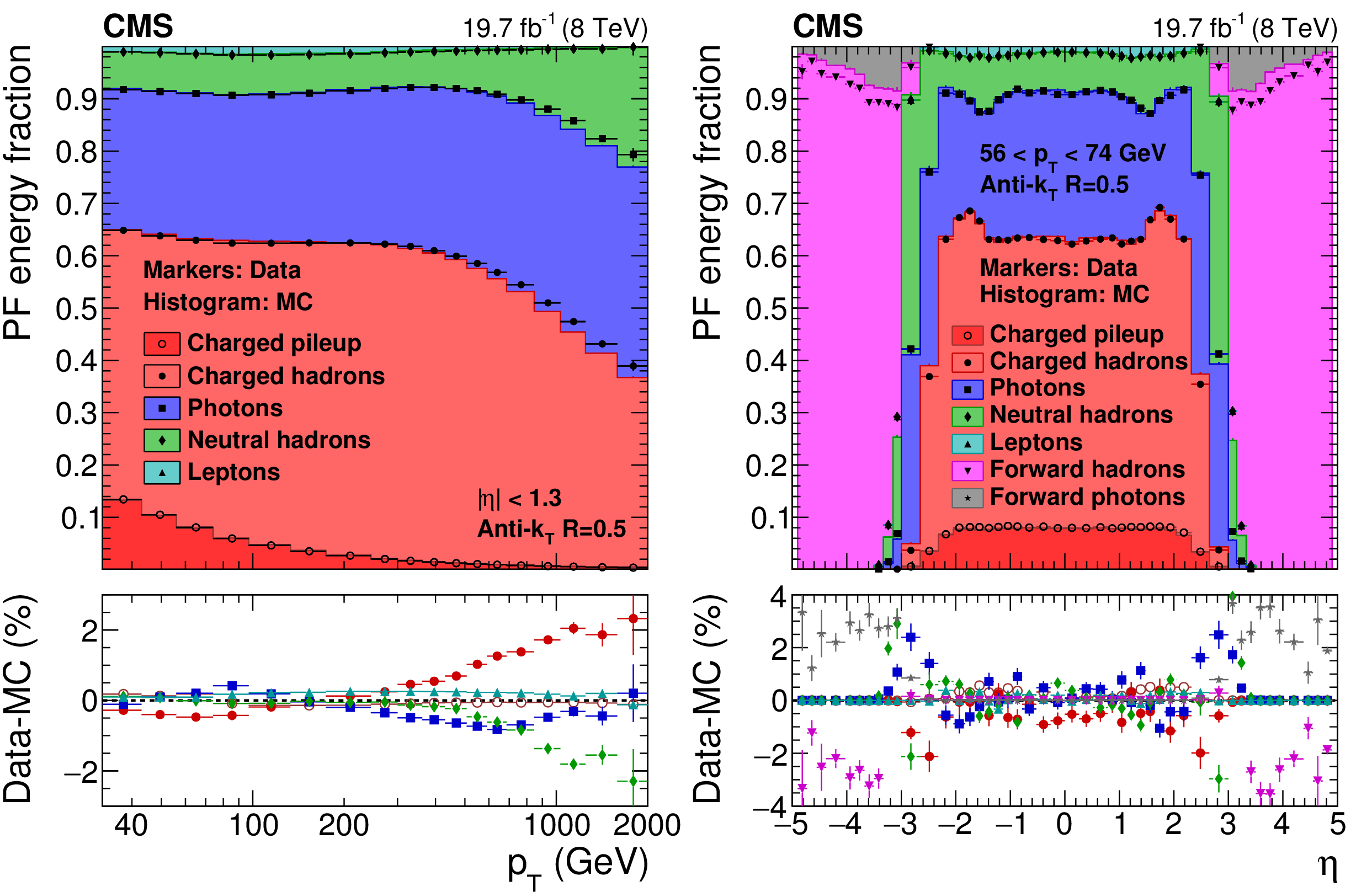
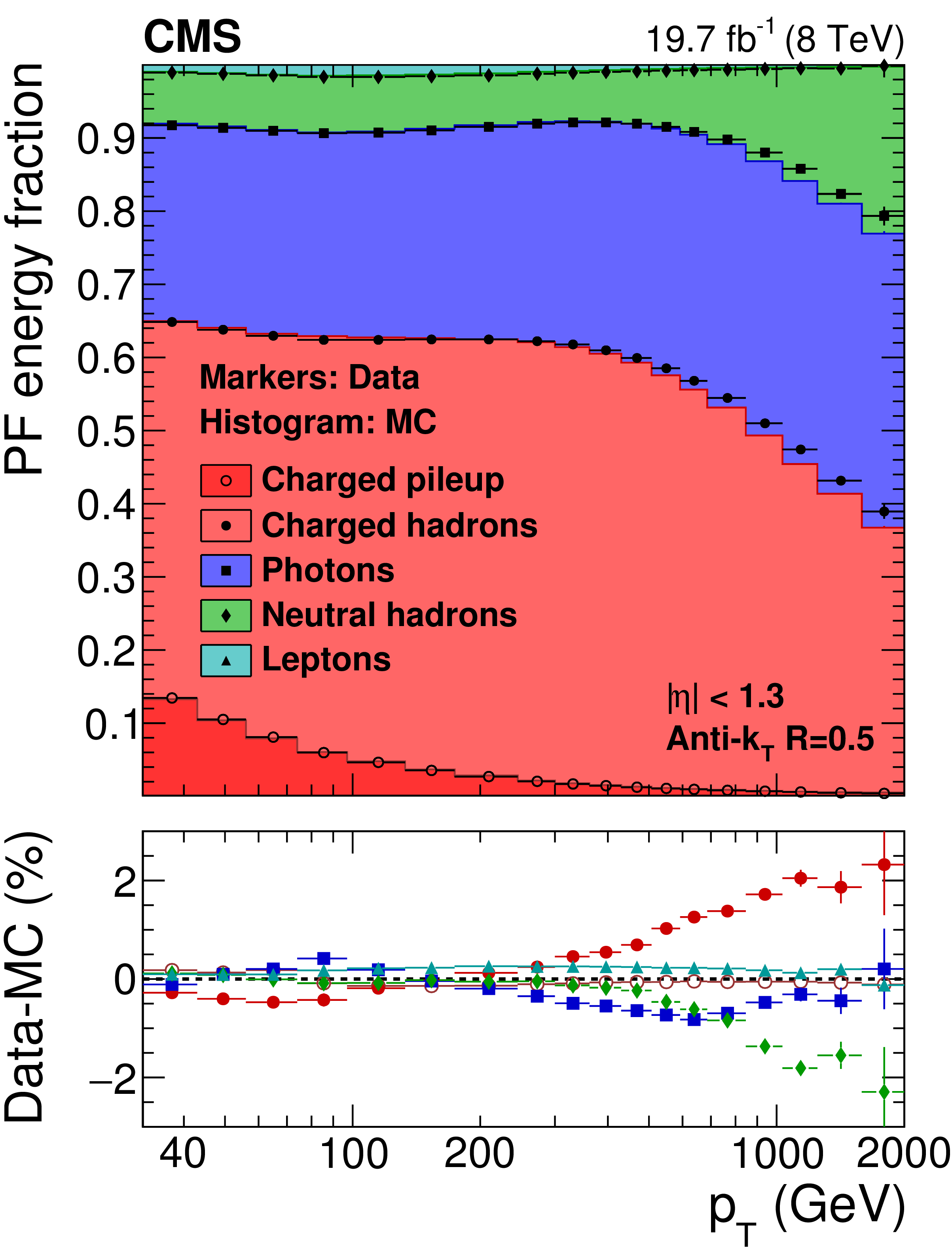
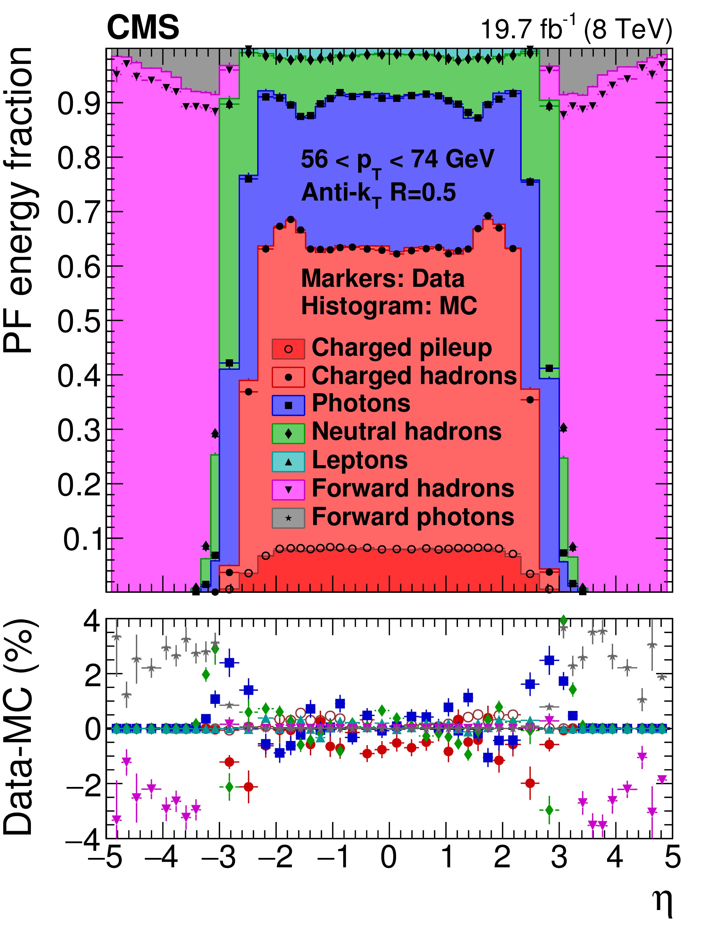
Figure 46:
PF jet composition in data and simulation versus $ {p_{\mathrm {T}}} $ at $|\eta |< $ 1.3 (a), and versus $\eta $ at 56 $ < {p_{\mathrm {T}}} < $ 74 GeV (b). |
png pdf |
Figure 46-a:
PF jet composition in data and simulation versus $ {p_{\mathrm {T}}} $ at $|\eta |< $ 1.3 (a), and versus $\eta $ at 56 $ < {p_{\mathrm {T}}} < $ 74 GeV (b). |
png pdf |
Figure 46-b:
PF jet composition in data and simulation versus $ {p_{\mathrm {T}}} $ at $|\eta |< $ 1.3 (a), and versus $\eta $ at 56 $ < {p_{\mathrm {T}}} < $ 74 GeV (b). |
png pdf |
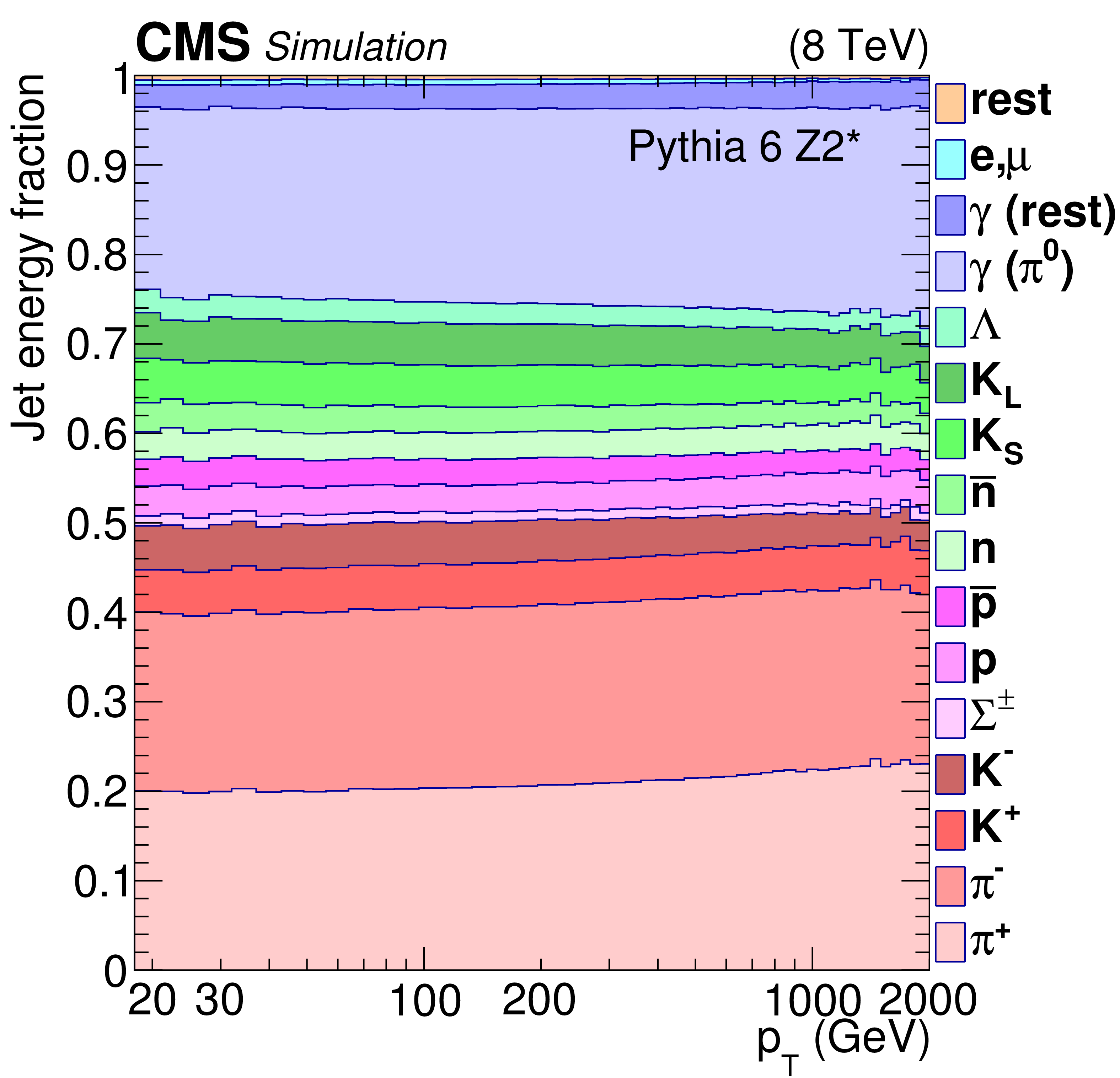
Figure 47:
Jet composition at particle level in the Pythia6.4 tune Z2* for QCD dijet sample, shown versus $ {p_{\mathrm {T}}} $ at $|\eta |< $ 1.3. The component labeled '$\gamma (\mathrm {rest})$' denotes all photons not coming from $\pi ^0$s, and the component labeled 'rest' refers to all particles not listed specifically. |
| Tables | |
png pdf |
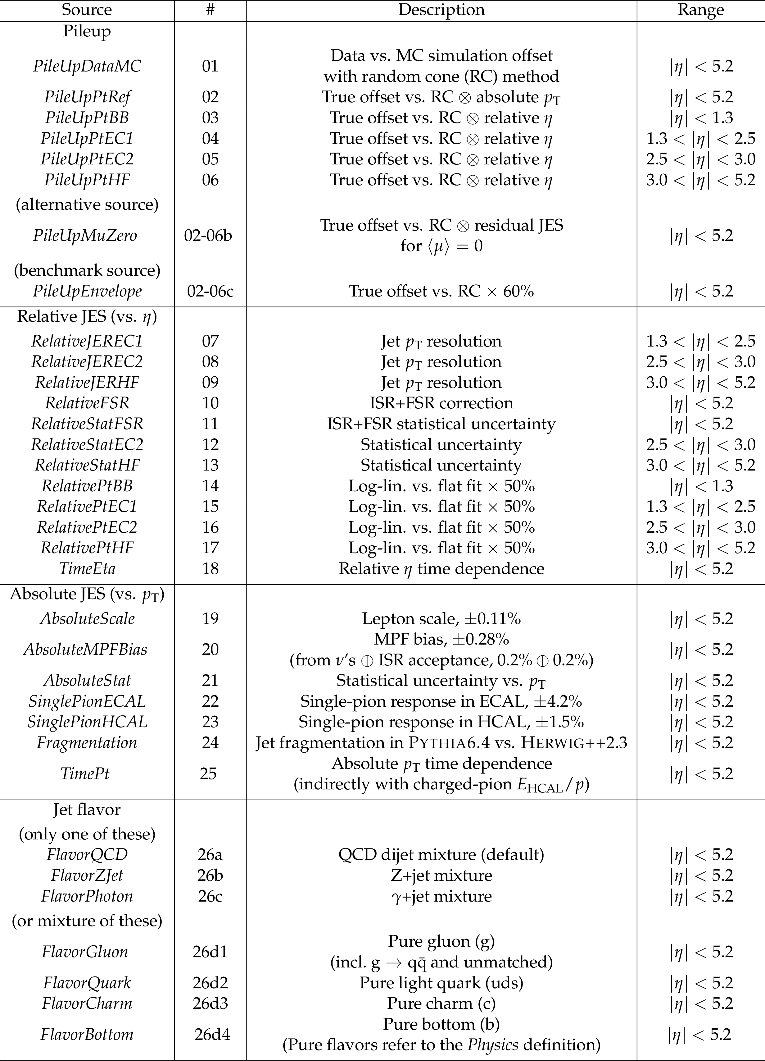
Table 1:
List of JES uncertainty sources, grouped by categories, with numbering, a short description, and range of validity in $|\eta |$. |
png pdf |
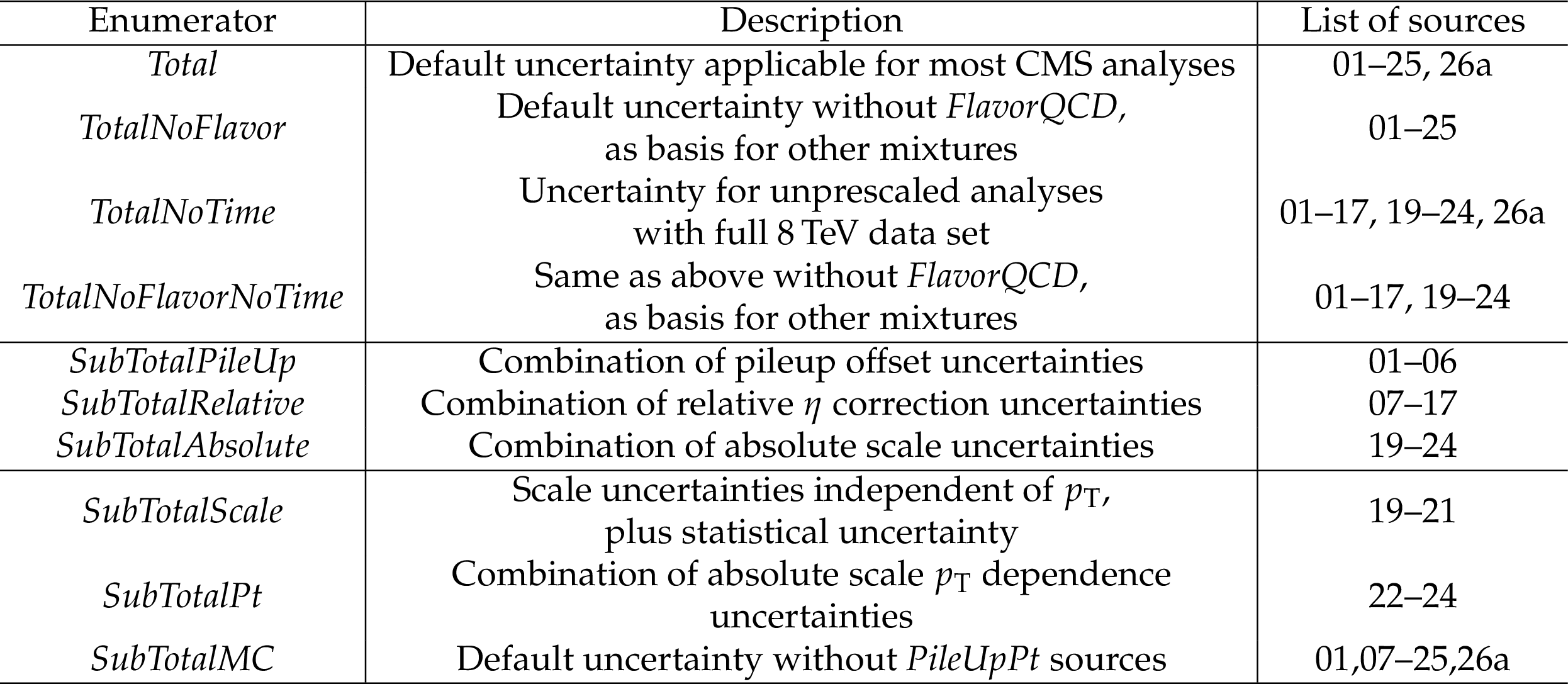
Table 2:
List of JES uncertainty source combinations with a short description and list of uncertainty components. The numbering of the sources ($3^{\rm rd}$ column) corresponds to that used in Table 1 (2$^{\rm nd}$ column). |
| Summary |
|
The understanding of jet energy scale and resolution achieved by the CMS experiment exploiting the pp data taken at 8 TeV, corresponding to an integrated luminosity of 19.7 fb$^{-1}$, has been documented. The CMS strategy involves the sequential correction of the jets for the pileup offset, simulated response, and residual $\eta$ and $p_{\mathrm{T}}$ dependencies in data with respect to simulation, with optional corrections depending on the jet flavor. The pileup offset corrections are determined from QCD dijet simulations processed with and without pileup overlay, with additional corrections for residual differences between data and detector simulation, extracted using the random-cone method in zero-bias events. The simulated jet response corrections are determined from a Monte Carlo event sample, as a function of jet $p_{\mathrm{T}}$ and $\eta$, for various jet algorithms and distance parameter sizes. The $\eta$-dependent corrections for residual differences between data and MC simulation are determined with dijet events, relative to a jet in the central region $|\eta|< $ 1.3. The $p_{\mathrm{T}}$-dependent corrections for residual differences within $|\eta|< $ 1.3 at 30 $ < p_{\mathrm{T}} < $ 800 GeV are measured combining photon+jet, $ \mathrm{Z} ( \to \mu \mu) $+jets, and $ \mathrm{Z} ( \to \mathrm{ee}) $+jets events. The $p_{\mathrm{T}}$ dependence at $p_{\mathrm{T}}> $ 800 GeV is directly constrained with multijet events. The optional jet-flavor corrections are derived from MC simulation and checked for b jets. The simulated jet $p_{\mathrm{T}}$ resolution is determined, as a function of jet $p_{\mathrm{T}}$ and $\eta$, for different levels of pileup. The dependence of the resolution on the jet flavor is also studied. The $\eta$-dependent corrections for residual differences between data and MC simulation in the jet resolution are determined with both dijet and $\gamma$+jet events. In all methods using MC simulation, the uncertainties arising from the modeling of jet radiation and hadronization are constrained from the study of the differences between Pythia6.4 and Herwig++ 2.3 generators. Detailed studies are performed to correct for biases in the data-based methods due to differences with respect to the MC simulation, in initial- and final-state radiation as well as in jet $p_{\mathrm{T}}$ resolution. The systematic uncertainties in the jet energy corrections, and their correlations, are provided as a function of $\eta$ and $p_{\mathrm{T}}$. The final uncertainties on the jet energy scale are below 3% across the phase space considered by most analyses ($p_{\mathrm{T}}> $ 30 GeV and $|\eta|< $ 5.0). In the barrel region we reach an uncertainty below 1% for $p_{\mathrm{T}}> $ 30 GeV, when excluding the jet-flavor uncertainties, provided separately for different jet-flavor mixtures. At its lowest, the core uncertainty (excluding optional time-dependent and flavor systematics) is 0.32% for jets with $p_{\mathrm{T}}$ between 165 and 330 GeV, and $|\eta|< $ 0.8. These results set a new benchmark for jet energy scale determination at hadron colliders. |
| References | ||||
| 1 | CMS Collaboration | Measurements of differential jet cross sections in proton-proton collisions at $ \sqrt{s} = $ 7 TeV with the CMS detector | PRD 87 (2013) 112002 | CMS-QCD-11-004 1212.6660 |
| 2 | CMS Collaboration | measurement of the inclusive jet cross section in pp collisions at $ \sqrt{s} = $ 7 TeV | PRL 107 (2011) 132001 | CMS-QCD-10-011 1106.0208 |
| 3 | CMS Collaboration | Measurement of the differential dijet production cross section in proton-proton collisions at $ \sqrt{s} = $ 7 TeV | PLB 700 (2011) 187 | CMS-QCD-10-025 1104.1693 |
| 4 | CMS Collaboration | Measurement of the ratio of inclusive jet cross sections using the anti-$ k_t $ algorithm with radius parameters $ R= $ 0.5 and 0.7 in pp collisions at $ \sqrt{s} = $ 7 TeV | PRD 90 (2014) 072006 | CMS-SMP-13-002 1406.0324 |
| 5 | CMS Collaboration | Distributions of topological observables in inclusive three- and four-jet events in pp collisions at $ \sqrt{s} = $ 7 TeV | EPJC 75 (2015) 302 | CMS-QCD-11-006 1502.04785 |
| 6 | CMS Collaboration | Measurement of the top-quark mass in all-jets $ \mathrm{ t \bar{t} } $ events in pp collisions at $ \sqrt{s} = $ 7 TeV | EPJC 74 (2014) 2758 | CMS-TOP-11-017 1307.4617 |
| 7 | CMS Collaboration | Determination of the top-quark pole mass and strong coupling constant from the $ \mathrm{ t \bar{t} } $ production cross section in pp collisions at $ \sqrt{s} = $ 7 TeV | PLB 728 (2014) 496 | CMS-TOP-12-022 1307.1907 |
| 8 | CMS Collaboration | Measurement of the top-quark mass in $ \mathrm{ t \bar{t} } $ events with lepton+jets final states in pp collisions at $ \sqrt{s} = $ 7 TeV | JHEP 12 (2012) 105 | CMS-TOP-11-015 1209.2319 |
| 9 | CMS Collaboration | Measurement of the top quark mass using proton-proton data at $ \sqrt{s}= $ 7 and 8 TeV | PRD 93 (2016) 072004 | CMS-TOP-14-022 1509.04044 |
| 10 | CMS Collaboration | Particle--flow event reconstruction in CMS and performance for jets, taus, and $ E_{\mathrm{T}}^{\text{miss}} $ | CMS-PAS-PFT-09-001 | |
| 11 | CMS Collaboration | Commissioning of the particle--flow event reconstruction with the first LHC collisions recorded in the CMS detector | CMS-PAS-PFT-10-001 | |
| 12 | M. Cacciari, G. P. Salam, and G. Soyez | The anti-$ k_t $ jet clustering algorithm | JHEP 04 (2008) 063 | 0802.1189 |
| 13 | CMS Collaboration | Determination of jet energy calibration and transverse momentum resolution in CMS | JINST 6 (2011) P11002 | CMS-JME-10-011 1107.4277 |
| 14 | ATLAS Collaboration | Jet energy measurement with the ATLAS detector in proton-proton collisions at $ \sqrt{s} = $ 7 TeV | EPJC 73 (2013) 2304 | 1112.6426 |
| 15 | CDF Collaboration | Determination of the jet energy scale at the Collider Detector at Fermilab | NIMA 566 (2006) 375 | hep-ex/0510047 |
| 16 | D0 Collaboration | Jet energy scale determination in the D0 experiment | NIMA 763 (2014) 442 | 1312.6873 |
| 17 | ATLAS Collaboration | Jet energy measurement and its systematic uncertainty in proton-proton collisions at $ \sqrt{s} = $ 7 TeV with the ATLAS detector | EPJC 75 (2015) 17 | 1406.0076 |
| 18 | GEANT4 Collaboration | GEANT4---a simulation toolkit | NIMA 506 (2003) 250 | |
| 19 | T. Sj ostrand, S. Mrenna, and P. Skands | PYTHIA 6.4 physics and manual | JHEP 05 (2006) 026 | hep-ph/0603175 |
| 20 | CMS Collaboration | Event generator tunes obtained from underlying event and multiparton scattering measurements | EPJC 76 (2016) 155 | CMS-GEN-14-001 1512.00815 |
| 21 | M. Bahr et al. | Herwig++ physics and manual | EPJC 58 (2008) 639 | 0803.0883 |
| 22 | S. Gieseke, C. Rohr, and A. Siodmok | Colour reconnections in Herwig++ | EPJC 72 (2012) 2225 | 1206.0041 |
| 23 | A. Giammanco | The Fast Simulation of the CMS Experiment | J. Phys. Conf. Ser. 513 (2014) 022012 | |
| 24 | CMS Collaboration | The CMS experiment at the CERN LHC | JINST 3 (2008) S08004 | CMS-00-001 |
| 25 | J. Alwall et al. | MadGraph 5: going beyond | JHEP 06 (2011) 128 | 1106.0522 |
| 26 | S. Frixione, P. Nason, and C. Oleari | Matching NLO QCD computations with Parton Shower simulations: the POWHEG method | JHEP 11 (2007) 070 | 0709.2092 |
| 27 | CMS Collaboration | Description and performance of track and primary-vertex reconstruction with the CMS tracker | JINST 9 (2014) P10009 | CMS-TRK-11-001 1405.6569 |
| 28 | CMS Collaboration | Jet performance in pp collisions at $ \sqrt{s}=$ 7 TeV | CMS-PAS-JME-10-003 | |
| 29 | CMS Collaboration | Performance of CMS muon reconstruction in pp collision events at $ \sqrt{s} = $ 7 TeV | JINST 7 (2012) P10002 | CMS-MUO-10-004 1206.4071 |
| 30 | CMS Collaboration | Performance of electron reconstruction and selection with the CMS detector in proton-proton collisions at $ \sqrt{s} = $ 8 TeV | JINST 10 (2015) P06005 | CMS-EGM-13-001 1502.02701 |
| 31 | CMS Collaboration | Identification of b-quark jets with the CMS experiment | JINST 8 (2013) P04013 | CMS-BTV-12-001 1211.4462 |
| 32 | CMS Collaboration | Performance of photon reconstruction and identification with the CMS detector in proton-proton collisions at $ \sqrt{s} = $ 8 TeV | JINST 10 (2015) P08010 | CMS-EGM-14-001 1502.02702 |
| 33 | M. Cacciari, G. P. Salam, and G. Soyez | FastJet user manual | EPJC 72 (2012) 1896 | 1111.6097 |
| 34 | M. Cacciari and G. P. Salam | Dispelling the $ N^{3} $ myth for the $ k_t $ jet-finder | PLB 641 (2006) 57 | hep-ph/0512210 |
| 35 | S. Catani, Y. L. Dokshitzer, and B. R. Webber | The $ k_{\perp} $-clustering algorithm for jets in deep inelastic scattering and hadron collisions | PLB 285 (1992) 291 | |
| 36 | S. Catani, Y. L. Dokshitzer, M. H. Seymour, and B. R. Webber | Longitudinally invariant $ k_{\perp} $-clustering algorithms for hadron-hadron collisions | NPB 406 (1993) 187 | |
| 37 | S. D. Ellis and D. E. Soper | Successive combination jet algorithm for hadron collisions | PRD 48 (1993) 3160 | |
| 38 | M. Cacciari and G. P. Salam | Pileup subtraction using jet areas | PLB 659 (2008) 119 | 0707.1378 |
| 39 | CMS Collaboration | Measurement of the inelastic proton-proton cross section at $ \sqrt{s} = $ 7 TeV | PLB 722 (2013) 5 | CMS-FWD-11-001 1210.6718 |
| 40 | CMS Collaboration | Cms luminosity based on pixel cluster counting --- summer 2013 update | CMS-PAS-LUM-13-001 | CMS-PAS-LUM-13-001 |
| 41 | CMS Collaboration | CMS technical design report, volume II: Physics performance | JPG 34 (2007) 995 | |
| 42 | CMS Collaboration | Transverse-momentum and pseudorapidity distributions of charged hadrons in pp collisions at $ \sqrt{s} = $ 7 TeV | PRL 105 (2010) 022002 | CMS-QCD-10-006 1005.3299 |
| 43 | D. Bertolini, P. Harris, M. Low, and N. Tran | Pileup per particle identification | JHEP 10 (2014) 59 | 1407.6013 |
| 44 | CMS Collaboration | Pileup jet identification | CMS-PAS-JME-13-005 | CMS-PAS-JME-13-005 |
| 45 | CMS Collaboration | Measurement of the underlying event activity in pp collisions at $ \sqrt{s} = $ 0.9 and 7 TeV with the novel jet-area/median approach | JHEP 08 (2012) 130 | CMS-QCD-10-021 1207.2392 |
| 46 | CMS Collaboration | Jet energy scale performance in 2011 | CDS | |
| 47 | CMS Collaboration | Single-particle response in the CMS calorimeters | CMS-PAS-JME-10-008 | |
| 48 | CMS Collaboration | Energy calibration and resolution of the CMS electromagnetic calorimeter in pp collisions at $ \sqrt{s} = $ 7 TeV | JINST 8 (2013) P09009 | CMS-EGM-11-001 1306.2016 |
| 49 | CMS Collaboration | Performance of quark/gluon discrimination in 8 TeV pp data | CMS-PAS-JME-13-002 | CMS-PAS-JME-13-002 |
| 50 | CMS Collaboration | Calculation of Residual Energy Correction for b Jets Using Z+b Events in 8 TeV pp Collisions | CMS-PAS-JME-13-001 | CMS-PAS-JME-13-001 |
| 51 | M. J. Oreglia | A study of the reactions $\psi' \to \gamma\gamma \psi$ | PhD thesis, Stanford University, 1980 SLAC Report SLAC-R-236, see Appendix D | |
| 52 | H. L. Lai et al. | Global QCD analysis and the CTEQ parton distributions | PRD 51 (1995) 4763 | hep-ph/9410404 |
| 53 | D. E. Groom | A simplistic view of hadron calorimetry | AIP Conf. Proc. 896 (2007) 137 | |
|
|
Compact Muon Solenoid LHC, CERN |
|

|

|

|

|

|