

Compact Muon Solenoid
LHC, CERN
| CMS-PRF-14-001 ; CERN-EP-2017-110 | ||
| Particle-flow reconstruction and global event description with the CMS detector | ||
| CMS Collaboration | ||
| 15 June 2017 | ||
| JINST 12 (2017) P10003 | ||
| Abstract: The CMS apparatus was identified, a few years before the start of the LHC operation at CERN, to feature properties well suited to particle-flow (PF) reconstruction: a highly-segmented tracker, a fine-grained electromagnetic calorimeter, a hermetic hadron calorimeter, a strong magnetic field, and an excellent muon spectrometer. A fully-fledged PF reconstruction algorithm tuned to the CMS detector was therefore developed and has been consistently used in physics analyses for the first time at a hadron collider. For each collision, the comprehensive list of final-state particles identified and reconstructed by the algorithm provides a global event description that leads to unprecedented CMS performance for jet and hadronic $\tau$ decay reconstruction, missing transverse momentum determination, and electron and muon identification. This approach also allows particles from pileup interactions to be identified and enables efficient pileup mitigation methods. The data collected by CMS at a centre-of-mass energy of 8 TeV show excellent agreement with the simulation and confirm the superior PF performance at least up to an average of 20 pileup interactions. | ||
| Links: e-print arXiv:1706.04965 [physics.ins-det] (PDF) ; CDS record ; inSPIRE record ; CADI line (restricted) ; | ||
| Figures | |
png pdf |
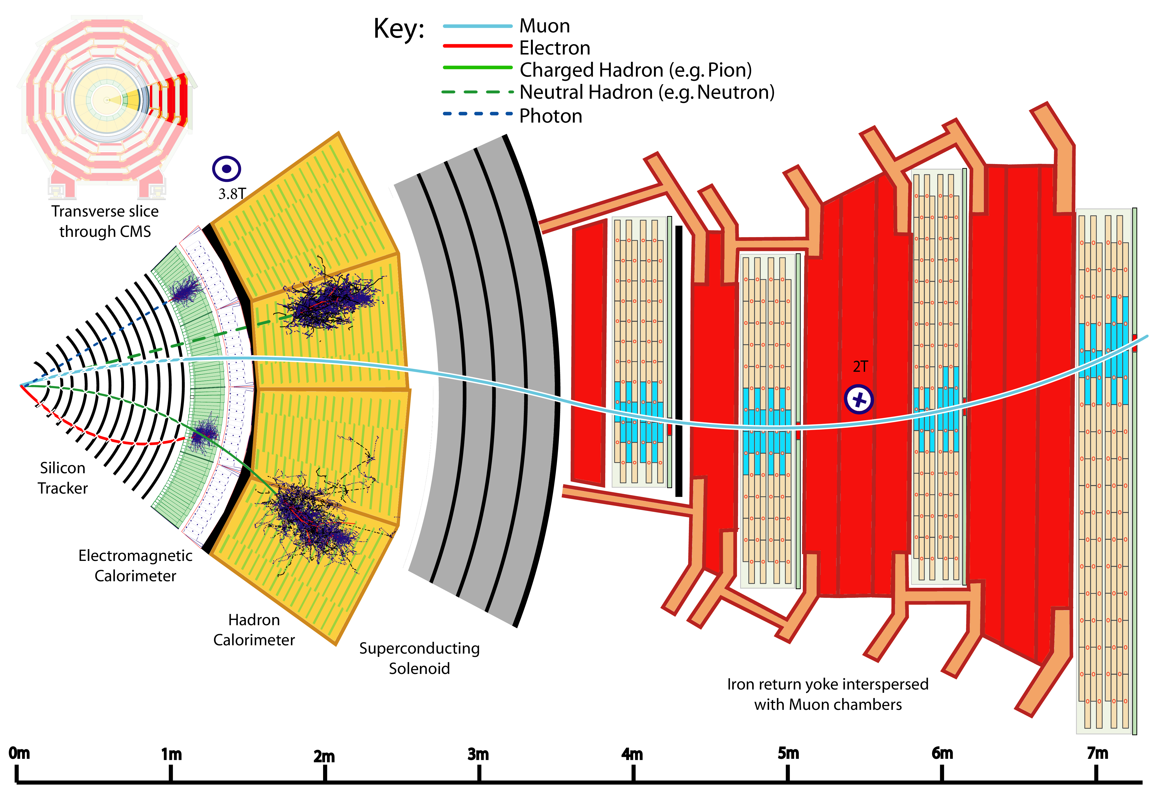
Figure 1:
A sketch of the specific particle interactions in a transverse slice of the CMS detector, from the beam interaction region to the muon detector. The muon and the charged pion are positively charged, and the electron is negatively charged. |

png pdf |
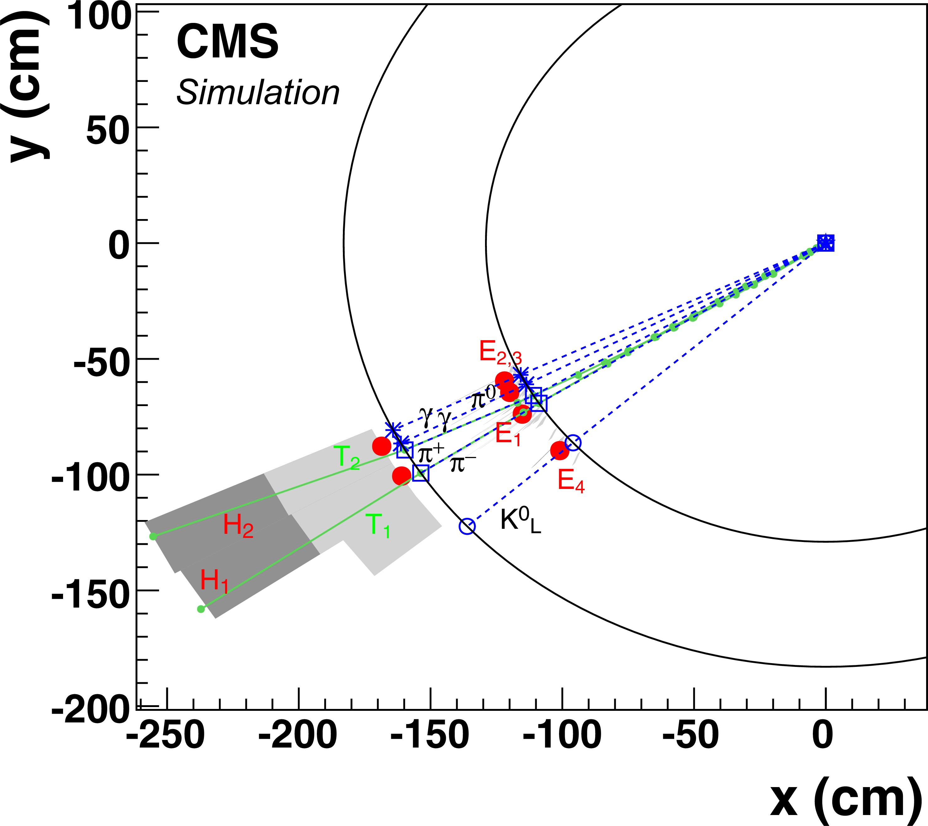
Figure 2:
Event display of an illustrative jet made of five particles only in the $(x,y)$ view (upper panel), and in the ($\eta,\varphi $) view on the ECAL surface (lower left) and the HCAL surface (lower right). In the top view, these two surfaces are represented as circles centred around the interaction point. The $\mathrm {K}^0_\mathrm {L}$, the $\pi ^-$, and the two photons from the $\pi ^0$ decay are detected as four well-separated ECAL clusters denoted $\mathrm {E}_{1,2,3,4}$. The $\pi ^+$ does not create a cluster in the ECAL. The two charged pions are reconstructed as charged-particle tracks $\mathrm {T}_{1,2}$, appearing as vertical solid lines in the ($\eta,\varphi $) views and circular arcs in the $(x,y)$ view. These tracks point towards two HCAL clusters $\mathrm {H}_{1,2}$. In the bottom views, the ECAL and HCAL cells are represented as squares, with an inner area proportional to the logarithm of the cell energy. Cells with an energy larger than those of the neighbouring cells are shown in dark grey. In all three views, the cluster positions are represented by dots, the simulated particles by dashed lines, and the positions of their impacts on the calorimeter surfaces by various open markers. |
png pdf |
Figure 2-a:
Event display of an illustrative jet made of five particles only in the $(x,y)$ view. The ECAL and HCAL surfaces are represented as circles centred around the interaction point. The $\mathrm {K}^0_\mathrm {L}$, the $\pi ^-$, and the two photons from the $\pi ^0$ decay are detected as four well-separated ECAL clusters denoted $\mathrm {E}_{1,2,3,4}$. The $\pi ^+$ does not create a cluster in the ECAL. The two charged pions are reconstructed as charged-particle tracks $\mathrm {T}_{1,2}$, appearing as vertical solid lines in the ($\eta,\varphi $) views and circular arcs in the $(x,y)$ view. These tracks point towards two HCAL clusters $\mathrm {H}_{1,2}$. |
png pdf |
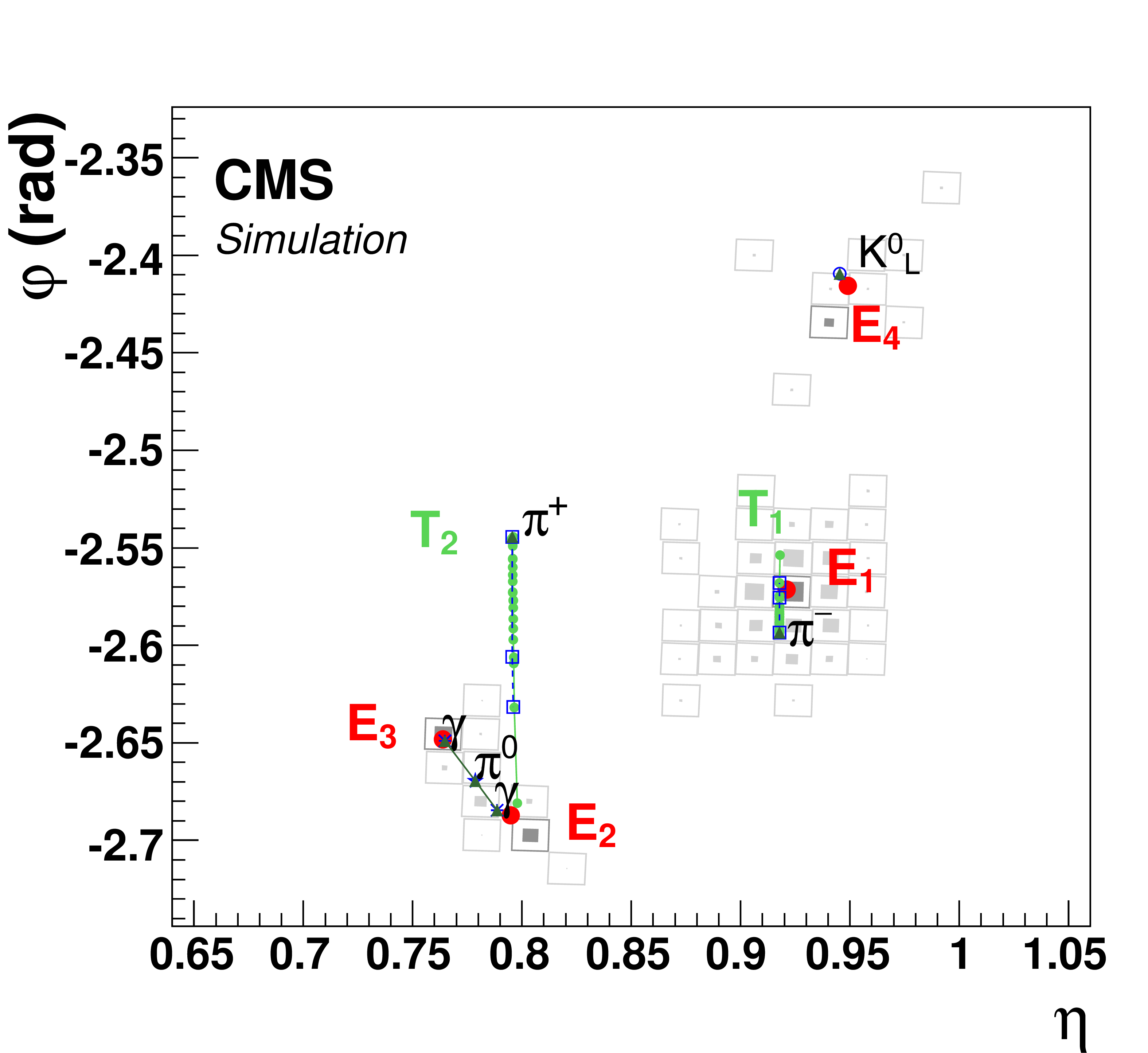
Figure 2-b:
Event display of an illustrative jet made of five particles only in the ($\eta,\varphi $) view on the ECAL surface. The $\mathrm {K}^0_\mathrm {L}$, the $\pi ^-$, and the two photons from the $\pi ^0$ decay are detected as four well-separated ECAL clusters denoted $\mathrm {E}_{1,2,3,4}$. The $\pi ^+$ does not create a cluster in the ECAL. The ECAL cells are represented as squares, with an inner area proportional to the logarithm of the cell energy. Cells with an energy larger than those of the neighbouring cells are shown in dark grey. In all three views, the cluster positions are represented by dots, the simulated particles by dashed lines, and the positions of their impacts on the calorimeter surfaces by various open markers. |

png pdf |
Figure 2-c:
Event display of an illustrative jet made of five particles only in the ($\eta,\varphi $) view on the HCAL surface. The two charged pions are reconstructed as charged-particle tracks $\mathrm {T}_{1,2}$, appearing as vertical solid lines in the ($\eta,\varphi $) views and circular arcs in the $(x,y)$ view. These tracks point towards two HCAL clusters $\mathrm {H}_{1,2}$. The HCAL cells are represented as squares, with an inner area proportional to the logarithm of the cell energy. Cells with an energy larger than those of the neighbouring cells are shown in dark grey. In all three views, the cluster positions are represented by dots, the simulated particles by dashed lines, and the positions of their impacts on the calorimeter surfaces by various open markers. |
png pdf |
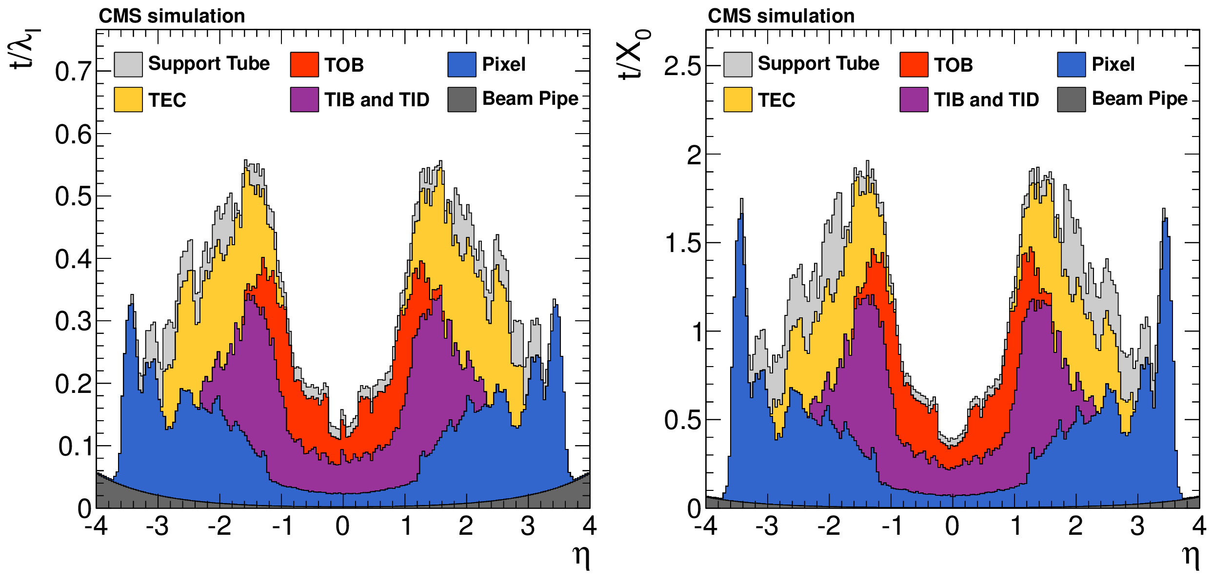
Figure 3:
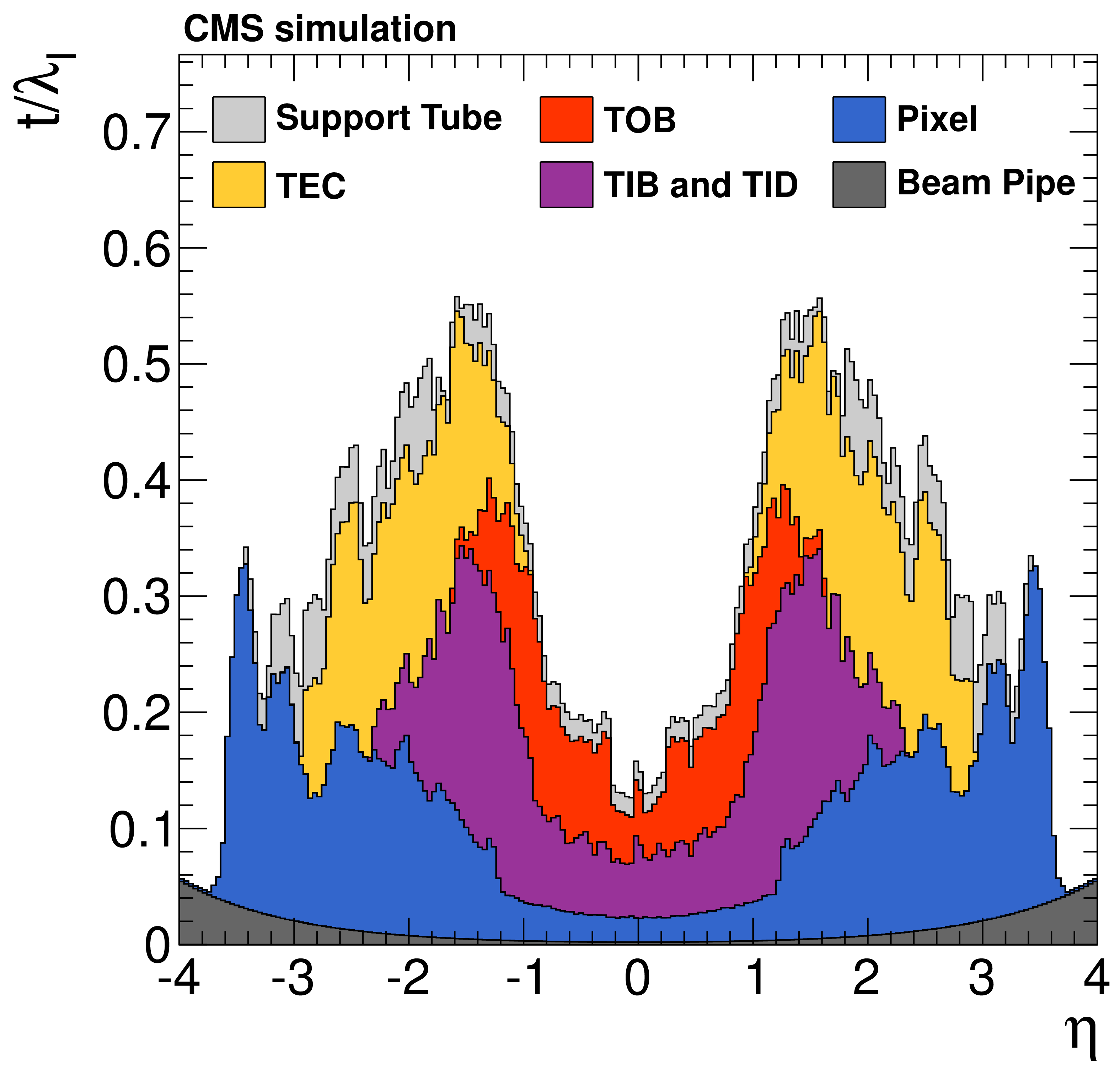
Total thickness $t$ of the inner tracker material expressed in units of interaction lengths $\lambda _l$ (left) and radiation lengths $X_0$ (right), as a function of the pseudorapidity $\eta $. The acronyms TIB, TID, TOB, and TEC stand for "tracker inner barrel'', "tracker inner disks'', "tracker outer barrel'', and "tracker endcaps'', respectively. The two figures are taken from Ref. [18]. |
png pdf |
Figure 3-a:
Total thickness $t$ of the inner tracker material expressed in units of interaction lengths $\lambda _l$, as a function of the pseudorapidity $\eta $. The acronyms TIB, TID, TOB, and TEC stand for "tracker inner barrel'', "tracker inner disks'', "tracker outer barrel'', and "tracker endcaps'', respectively. The figure is taken from Ref. [18]. |

png pdf |
Figure 3-b:
Total thickness $t$ of the inner tracker material expressed in units of radiation lengths $X_0$, as a function of the pseudorapidity $\eta $. The acronyms TIB, TID, TOB, and TEC stand for "tracker inner barrel'', "tracker inner disks'', "tracker outer barrel'', and "tracker endcaps'', respectively. The figure is taken from Ref. [18]. |
png pdf |
Figure 4:
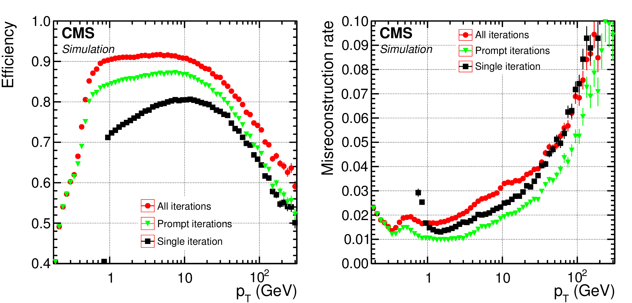
Efficiency (left) and misreconstruction rate (right) of the global combinatorial track finder (black squares); and of the iterative tracking method (green triangles: prompt iterations based on seeds with at least one hit in the pixel detector; red circles: all iterations, including those with displaced seeds), as a function of the track $ {p_{\mathrm {T}}} $, for charged hadrons in multijet events without pileup interactions. Only tracks with $ {| \eta | } < $ 2.5 are considered in the efficiency and misreconstruction rate determination. The efficiency is displayed for tracks originating from within 3.5 cm of the beam axis and $\pm$30 cm of the nominal centre of CMS along the beam axis. |
png pdf |
Figure 4-a:
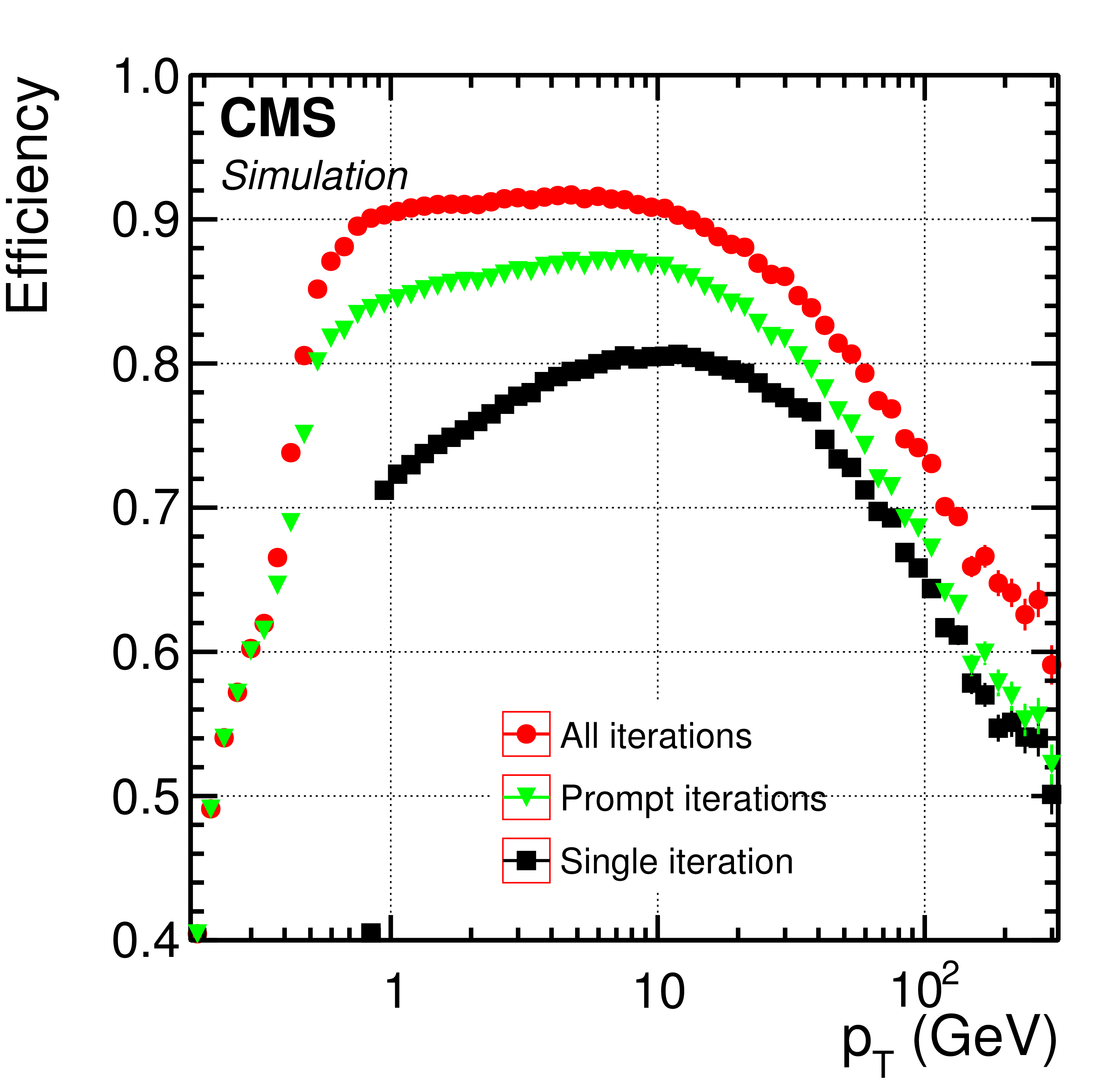
Efficiency of the global combinatorial track finder (black squares); and of the iterative tracking method (green triangles: prompt iterations based on seeds with at least one hit in the pixel detector; red circles: all iterations, including those with displaced seeds), as a function of the track $ {p_{\mathrm {T}}} $, for charged hadrons in multijet events without pileup interactions. Only tracks with $ {| \eta | } < $ 2.5 are considered. The efficiency is displayed for tracks originating from within 3.5 cm of the beam axis and $\pm$30 cm of the nominal centre of CMS along the beam axis. |
png pdf |
Figure 4-b:
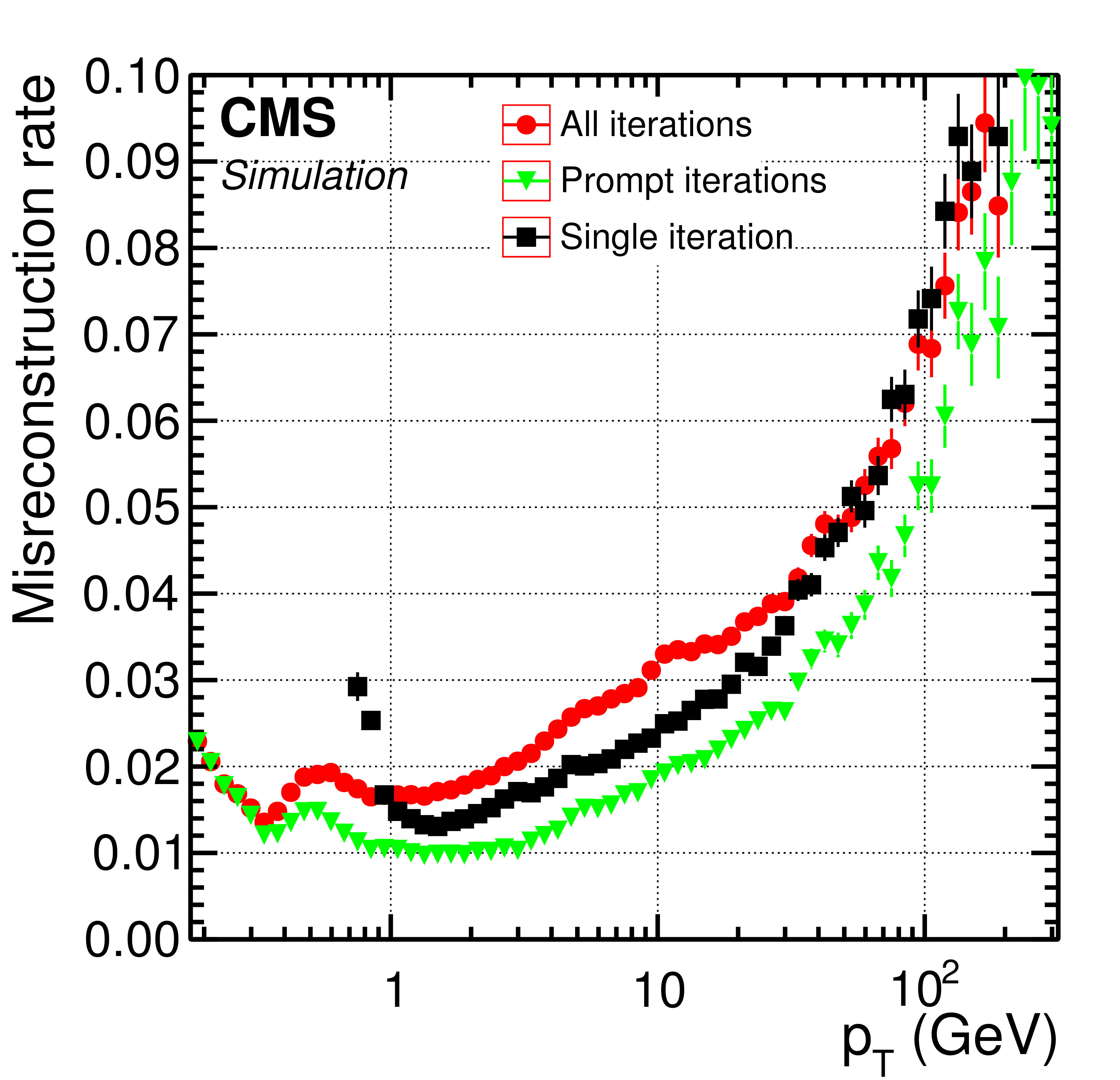
Misreconstruction rate of the global combinatorial track finder (black squares); and of the iterative tracking method (green triangles: prompt iterations based on seeds with at least one hit in the pixel detector; red circles: all iterations, including those with displaced seeds), as a function of the track $ {p_{\mathrm {T}}} $, for charged hadrons in multijet events without pileup interactions. Only tracks with $ {| \eta | } < $ 2.5 are considered. |
png pdf |
Figure 5:
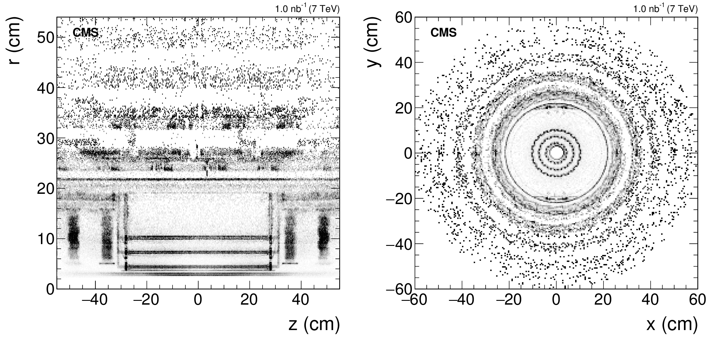
Maps of nuclear interaction vertices for data collected by CMS in 2011 at $\sqrt {s} = $ 7 TeV, corresponding to an integrated luminosity of 1 nb$^{-1}$, in the longitudinal (left) and transverse (right) cross sections of the inner part of the tracker, exhibiting its structure in concentric layers around the beam axis. The different shades of grey indicate the reconstructed nuclear interaction probability per event and per unit of surface, the darker the larger. |
png pdf |
Figure 5-a:
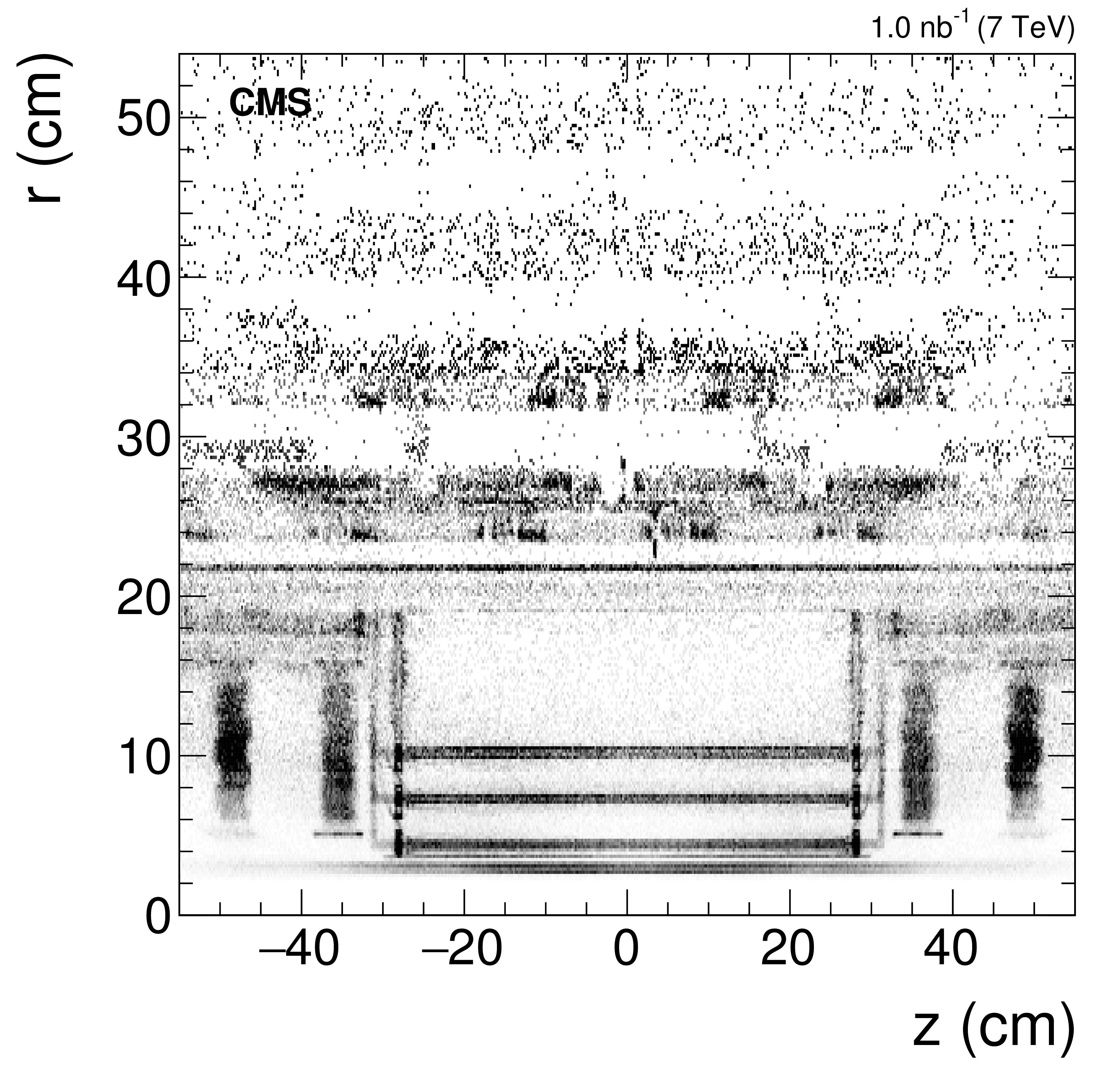
Map of nuclear interaction vertices for data collected by CMS in 2011 at $\sqrt {s} = $ 7 TeV, corresponding to an integrated luminosity of 1 nb$^{-1}$, in the longitudinal cross section of the inner part of the tracker. The different shades of grey indicate the reconstructed nuclear interaction probability per event and per unit of surface, the darker the larger. |
png pdf |
Figure 5-b:
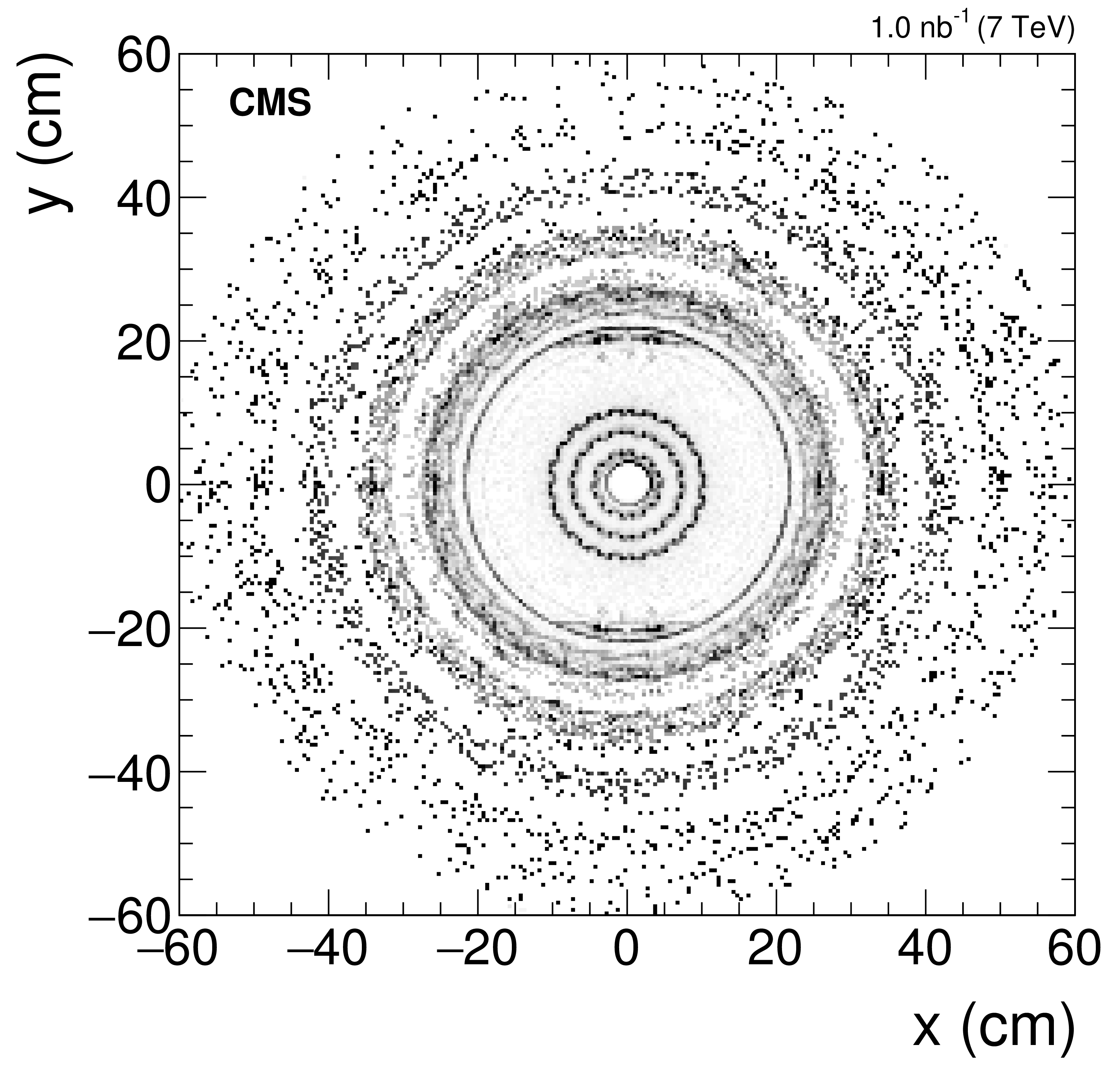
Map of nuclear interaction vertices for data collected by CMS in 2011 at $\sqrt {s} = $ 7 TeV, corresponding to an integrated luminosity of 1 nb$^{-1}$, in the transverse cross section of the inner part of the tracker, exhibiting its structure in concentric layers around the beam axis. The different shades of grey indicate the reconstructed nuclear interaction probability per event and per unit of surface, the darker the larger. |

png pdf |
Figure 6:
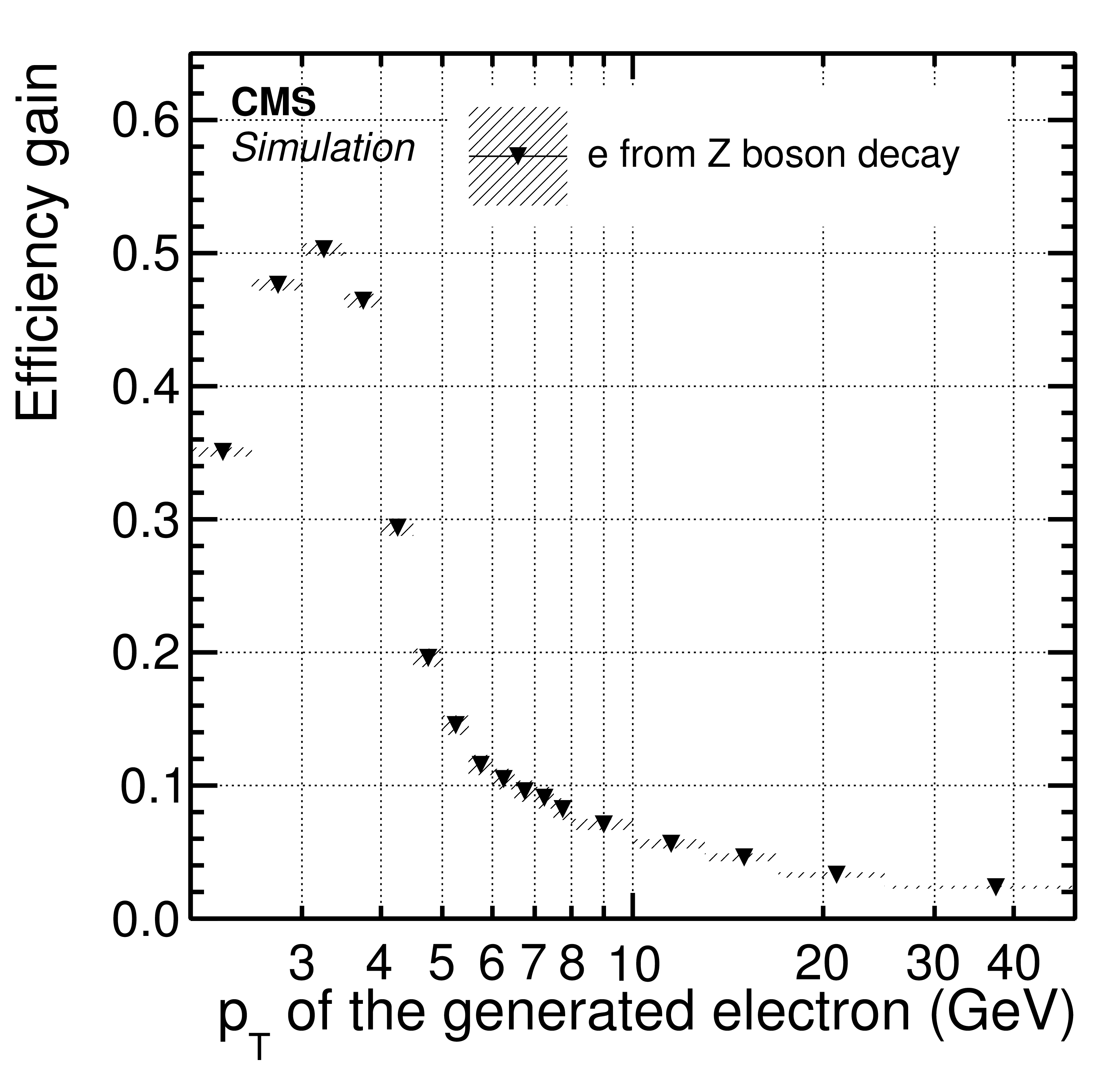
Left: Electron seeding efficiency for electrons (triangles) and pions (circles) as a function of $ {p_{\mathrm {T}}} $, from a simulated event sample enriched in b quark jets with $ {p_{\mathrm {T}}} $ between 80 and 170 GeV, and with at least one semileptonic b hadron decay. Both the efficiencies for ECAL-based seeding only (hollow symbols) and with the tracker-based seeding added (solid symbols) are displayed. Right: Absolute efficiency gain from the tracker-based seeding for electrons from Z boson decays as a function of $ {p_{\mathrm {T}}} $. |

png pdf |
Figure 6-a:
Electron seeding efficiency for electrons (triangles) and pions (circles) as a function of $ {p_{\mathrm {T}}} $, from a simulated event sample enriched in b quark jets with $ {p_{\mathrm {T}}} $ between 80 and 170 GeV, and with at least one semileptonic b hadron decay. Both the efficiencies for ECAL-based seeding only (hollow symbols) and with the tracker-based seeding added (solid symbols) are displayed. |
png pdf |
Figure 6-b:
Absolute efficiency gain from the tracker-based seeding for electrons from Z boson decays as a function of $ {p_{\mathrm {T}}} $. |
png pdf |
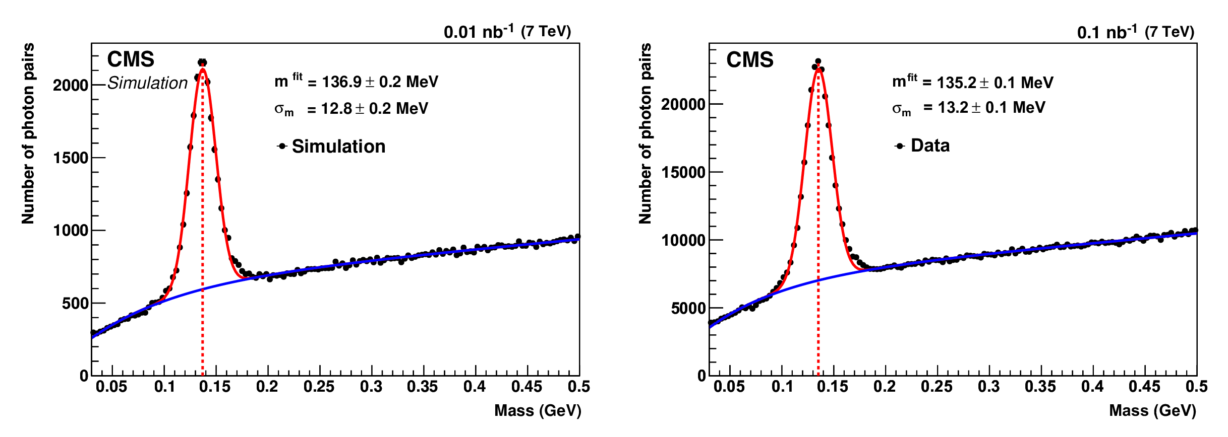
Figure 7:
Photon pair invariant mass distribution in the barrel ($ {| \eta | } <$ 1.0) for the simulation (left) and the data (right). The $\pi ^0$ signal is modelled by a Gaussian (red curve) and the background by an exponential function (blue curve). The Gaussian mean value (vertical dashed line) and its standard deviation are denoted $m^\text {fit}$ and $\sigma _\mathrm {m}$, respectively. |
png pdf |
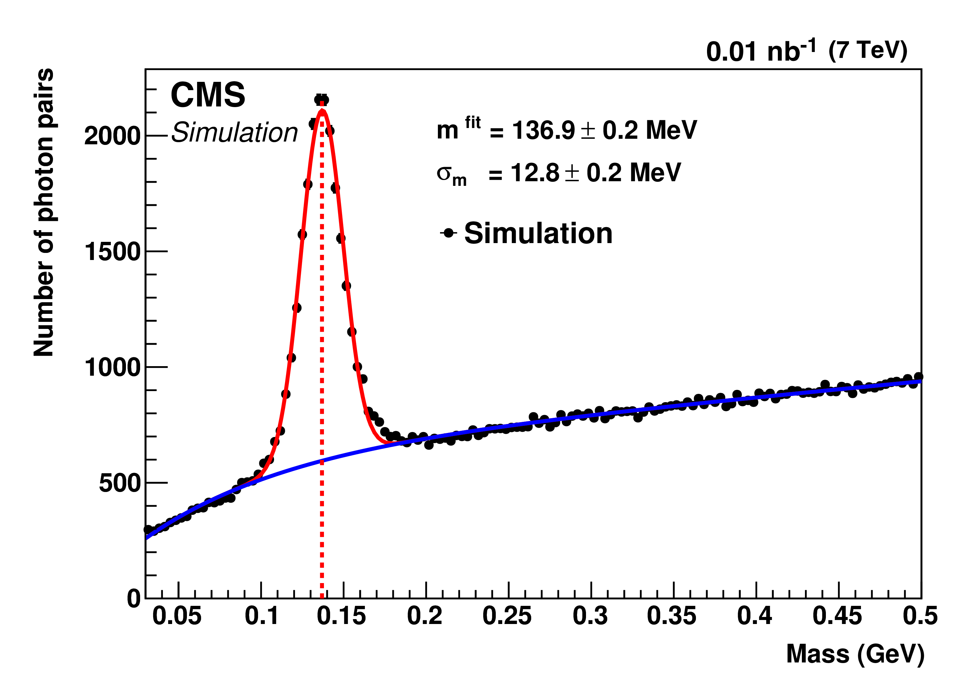
Figure 7-a:
Photon pair invariant mass distribution in the barrel ($ {| \eta | } <$ 1.0) for the simulation. The $\pi ^0$ signal is modelled by a Gaussian (red curve) and the background by an exponential function (blue curve). The Gaussian mean value (vertical dashed line) and its standard deviation are denoted $m^\text {fit}$ and $\sigma _\mathrm {m}$, respectively. |
png pdf |
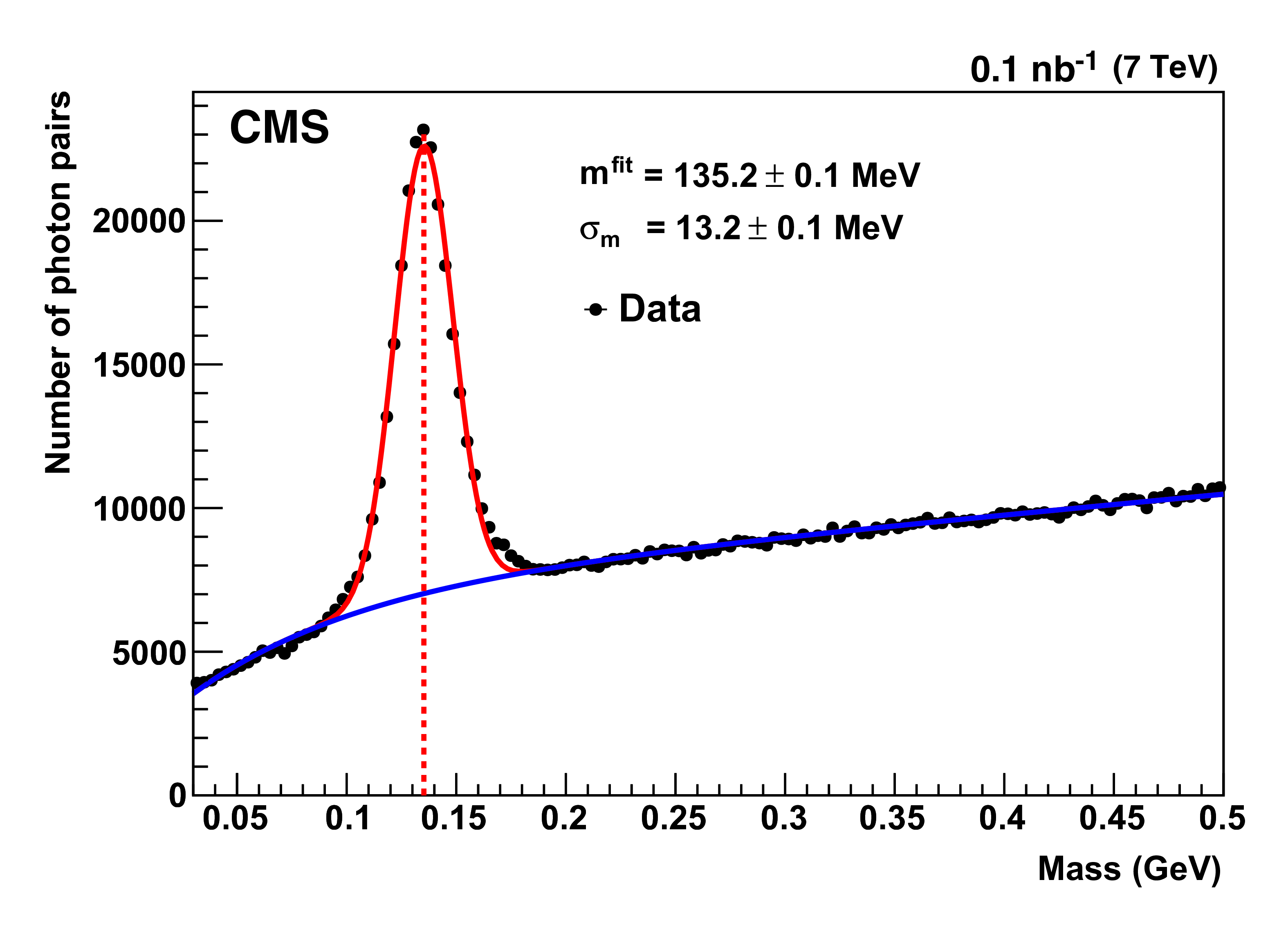
Figure 7-b:
Photon pair invariant mass distribution in the barrel ($ {| \eta | } <$ 1.0) for the data. The $\pi ^0$ signal is modelled by a Gaussian (red curve) and the background by an exponential function (blue curve). The Gaussian mean value (vertical dashed line) and its standard deviation are denoted $m^\text {fit}$ and $\sigma _\mathrm {m}$, respectively. |
png pdf |
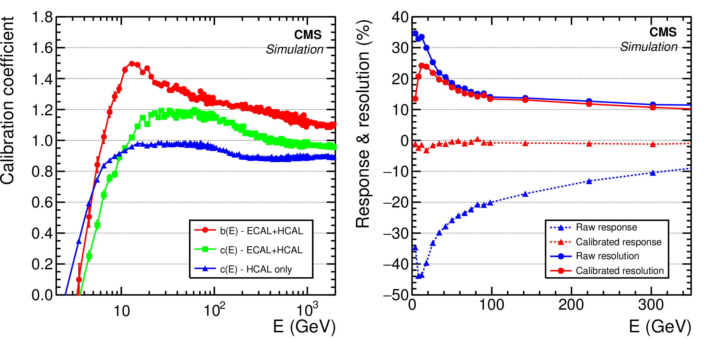
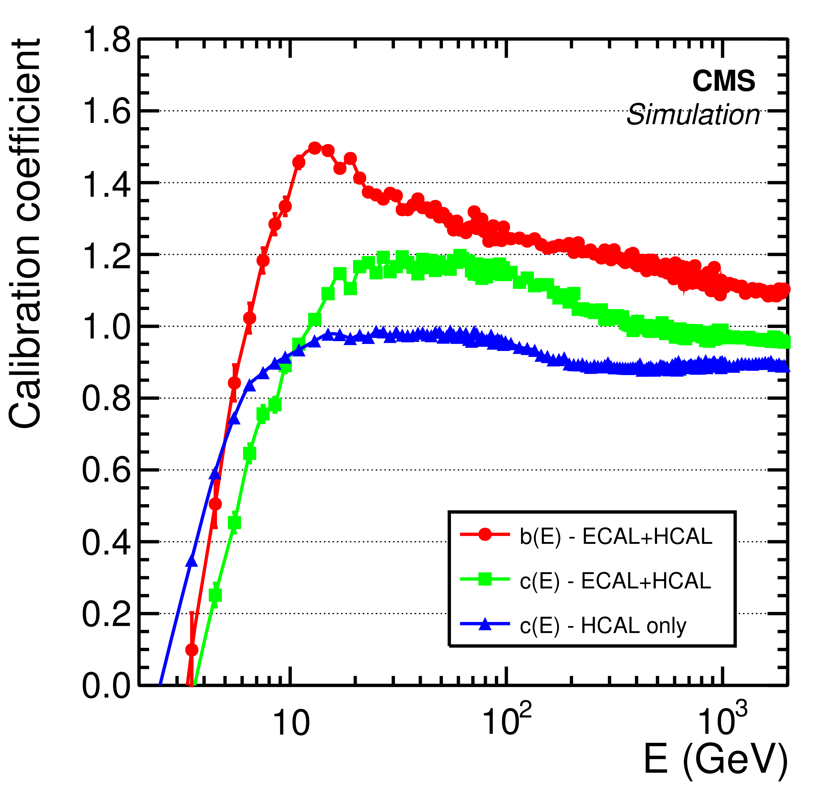
Figure 8:
Left: Calibration coefficients obtained from single hadrons in the barrel as a function of their true energy $E$, for hadrons depositing energy only in the HCAL (blue triangles), and for hadrons depositing energy in both the ECAL and HCAL, for the ECAL (red circles) and for the HCAL (green squares) clusters. Right: Relative raw (blue) and calibrated (red) energy response (dashed curves and triangles) and resolution (full curves and circles) for single hadrons in the barrel, as a function of their true energy $E$. Here the raw (calibrated) response and resolution are obtained by a Gaussian fit to the distribution of the relative difference between the raw (calibrated) calorimetric energy and the true hadron energy. |
png pdf |
Figure 8-a:
Calibration coefficients obtained from single hadrons in the barrel as a function of their true energy $E$, for hadrons depositing energy only in the HCAL (blue triangles), and for hadrons depositing energy in both the ECAL and HCAL, for the ECAL (red circles) and for the HCAL (green squares) clusters. |

png pdf |
Figure 8-b:
Relative raw (blue) and calibrated (red) energy response (dashed curves and triangles) and resolution (full curves and circles) for single hadrons in the barrel, as a function of their true energy $E$. Here the raw (calibrated) response and resolution are obtained by a Gaussian fit to the distribution of the relative difference between the raw (calibrated) calorimetric energy and the true hadron energy. |
png pdf |
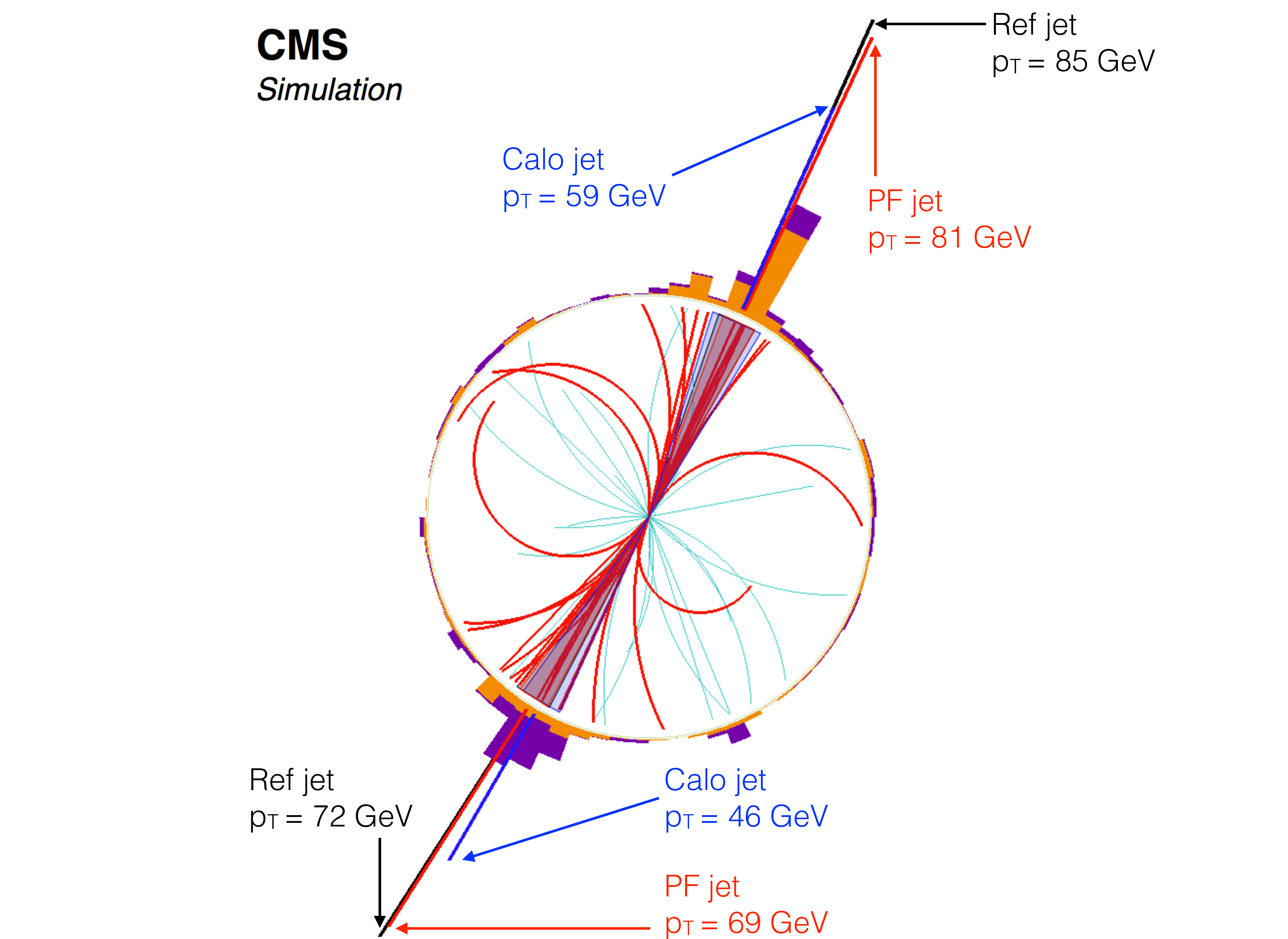
Figure 9:
Jet reconstruction in a simulated dijet event. The particles clustered in the two PF jets are displayed with a thicker line. For clarity, particles with $ {p_{\mathrm {T}}} < $ 1 GeV are not shown. The PF jet ${{\vec p}_{\mathrm {T}}}$, indicated as a radial line, is compared to the ${{\vec p}_{\mathrm {T}}}$ of the corresponding generated (Ref) and calorimeter (Calo) jets. In all cases, the four-momentum of the jet is obtained by summing the four-momenta of its constituents, and no jet energy correction is applied. |
png pdf |
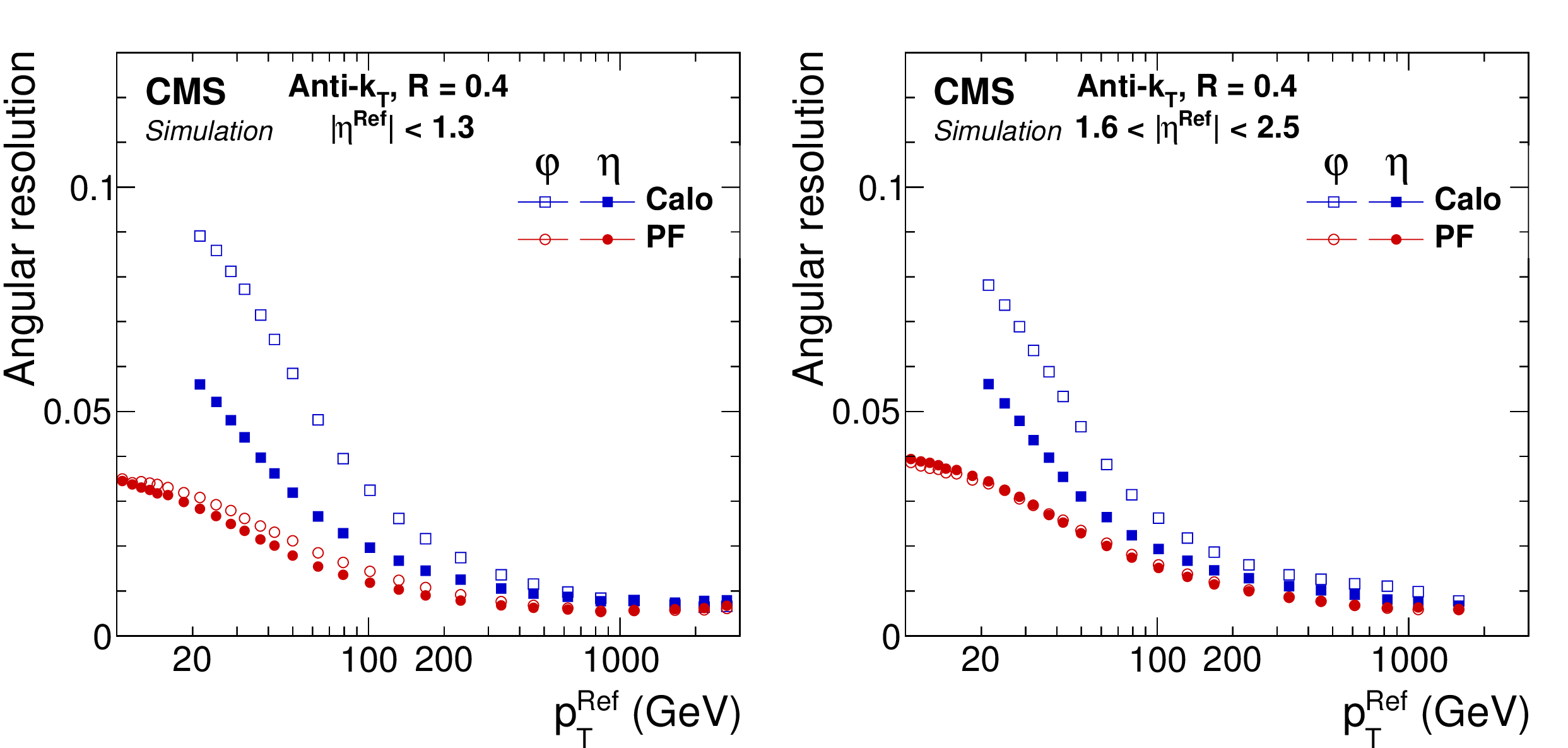
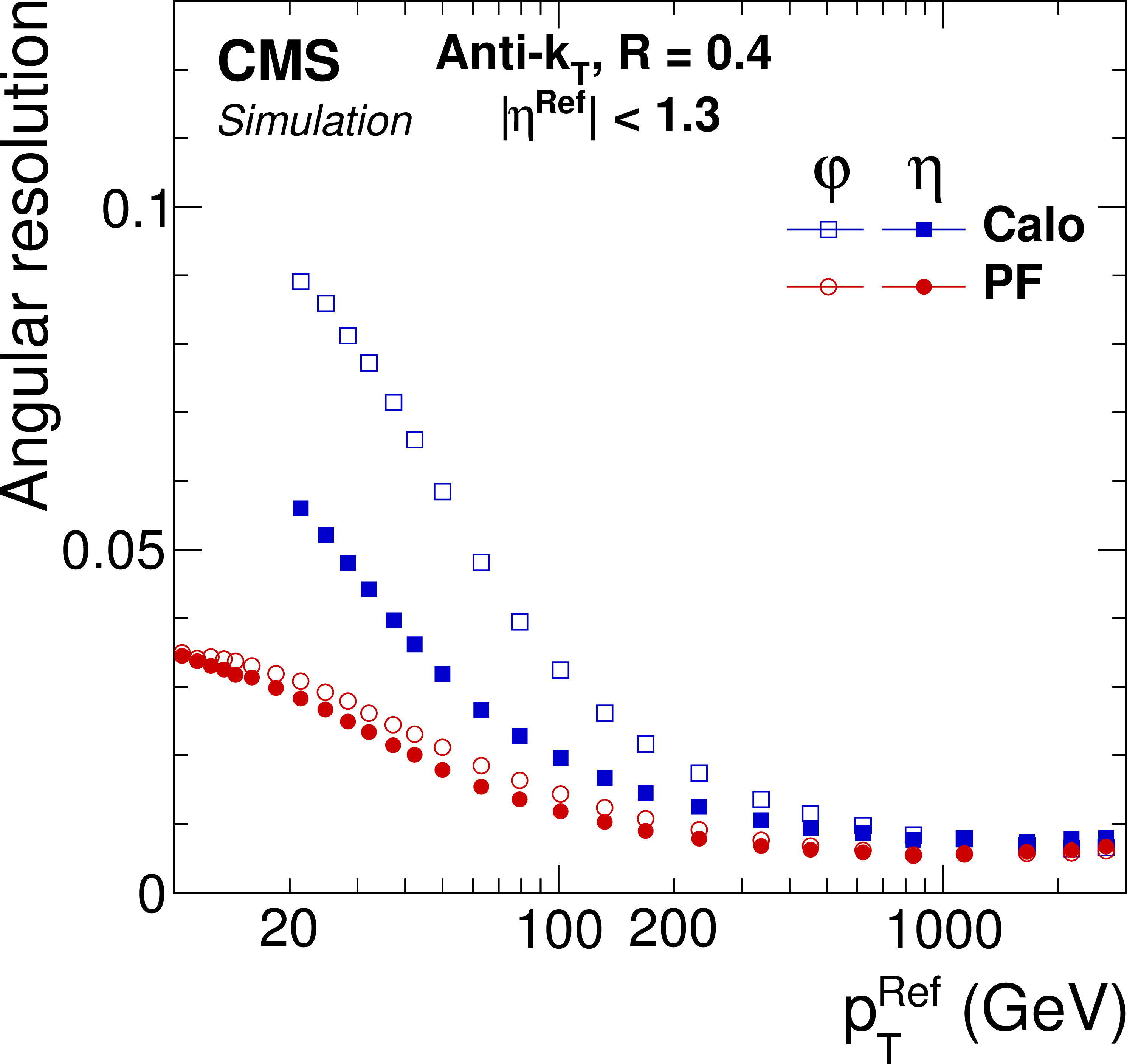
Figure 10:
Jet angular resolution in the barrel (left) and endcap (right) regions, as a function of the $ {p_{\mathrm {T}}} $ of the reference jet. The $\varphi $ resolution is expressed in radians. |
png pdf |
Figure 10-a:
Jet angular resolution in the barrel region, as a function of the $ {p_{\mathrm {T}}} $ of the reference jet. The $\varphi $ resolution is expressed in radians. |

png pdf |
Figure 10-b:
Jet angular resolution in the endcap region, as a function of the $ {p_{\mathrm {T}}} $ of the reference jet. The $\varphi $ resolution is expressed in radians. |
png pdf |
Figure 11:
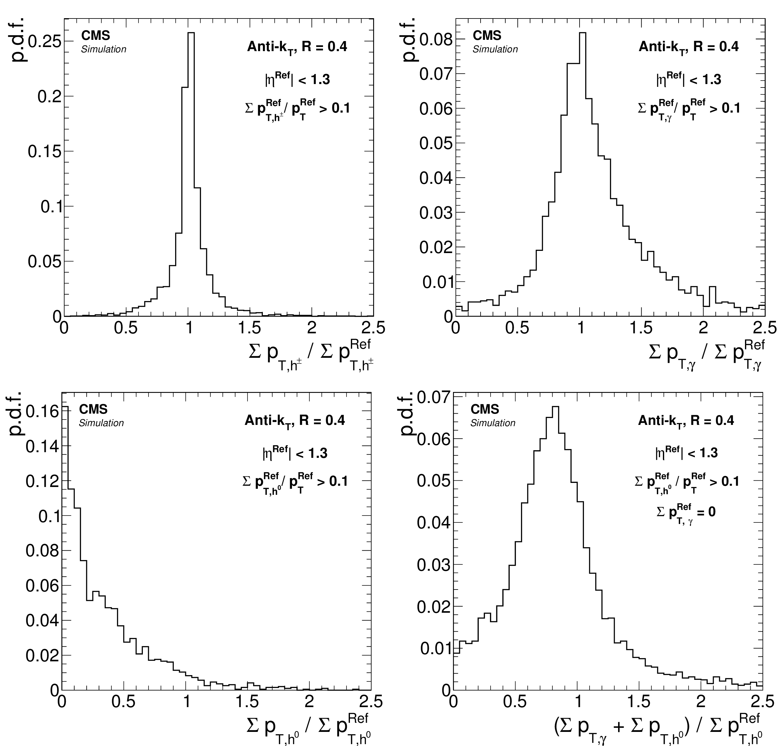
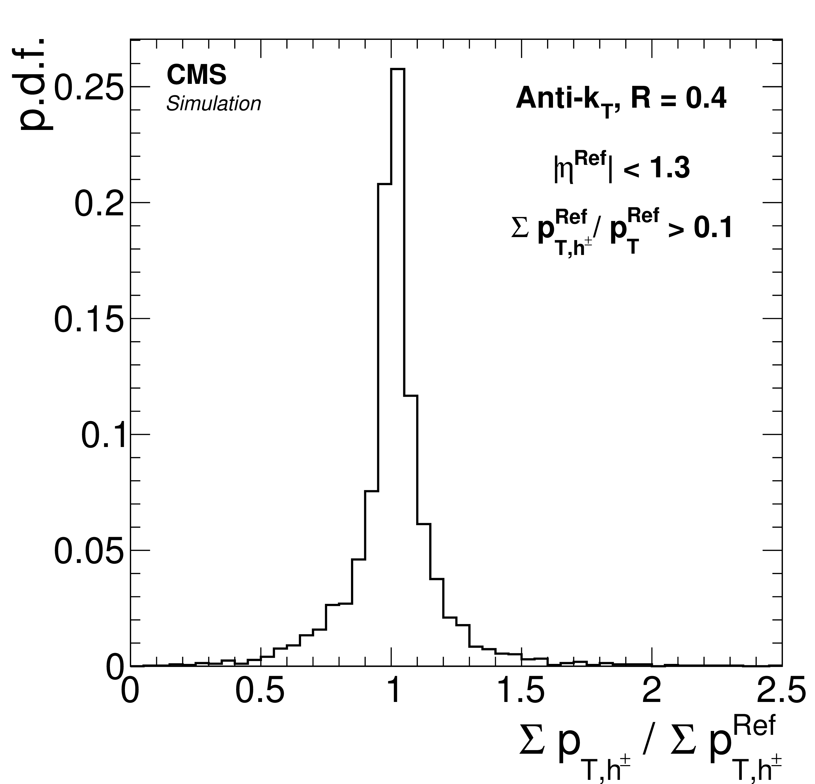
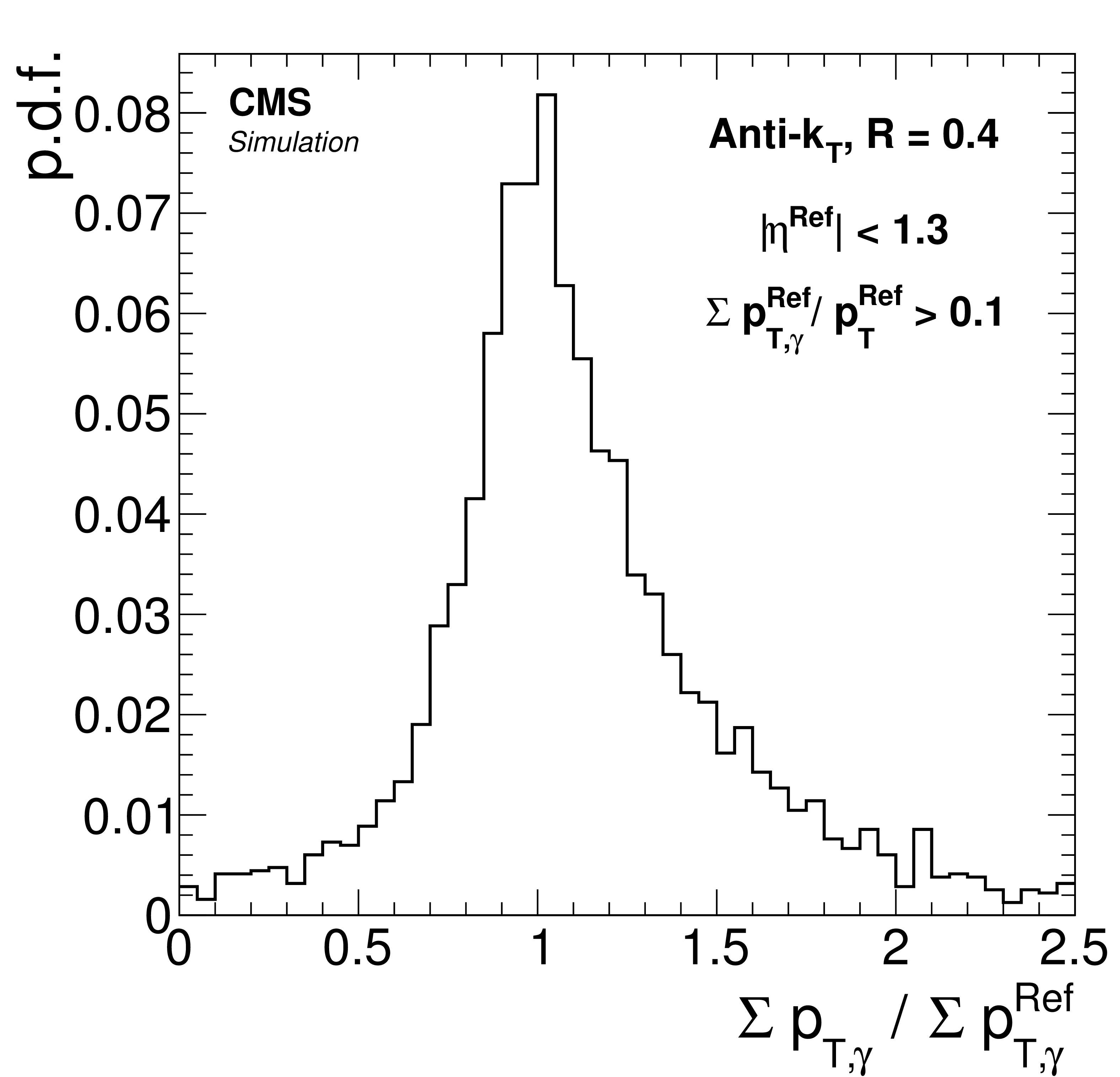
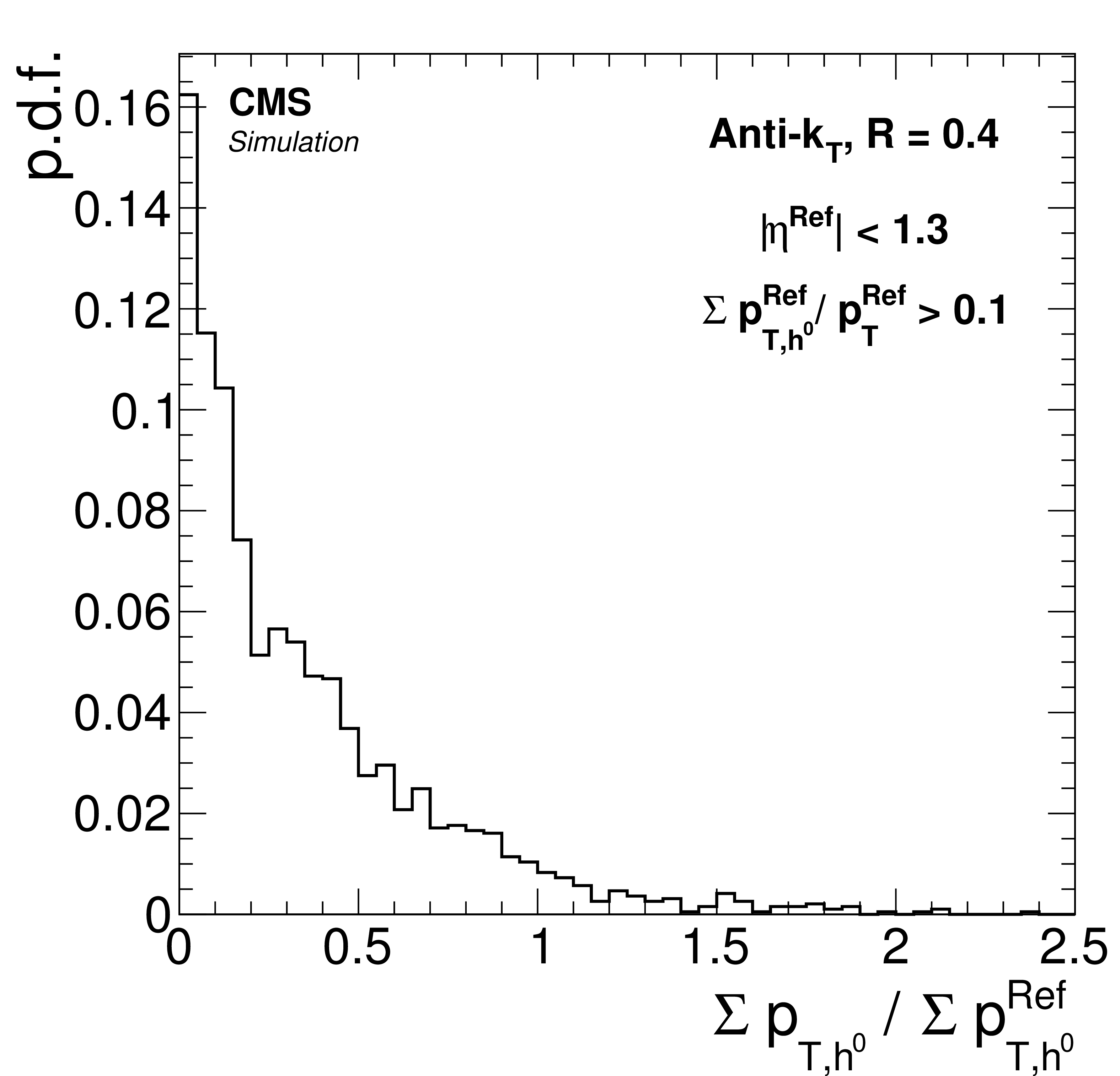
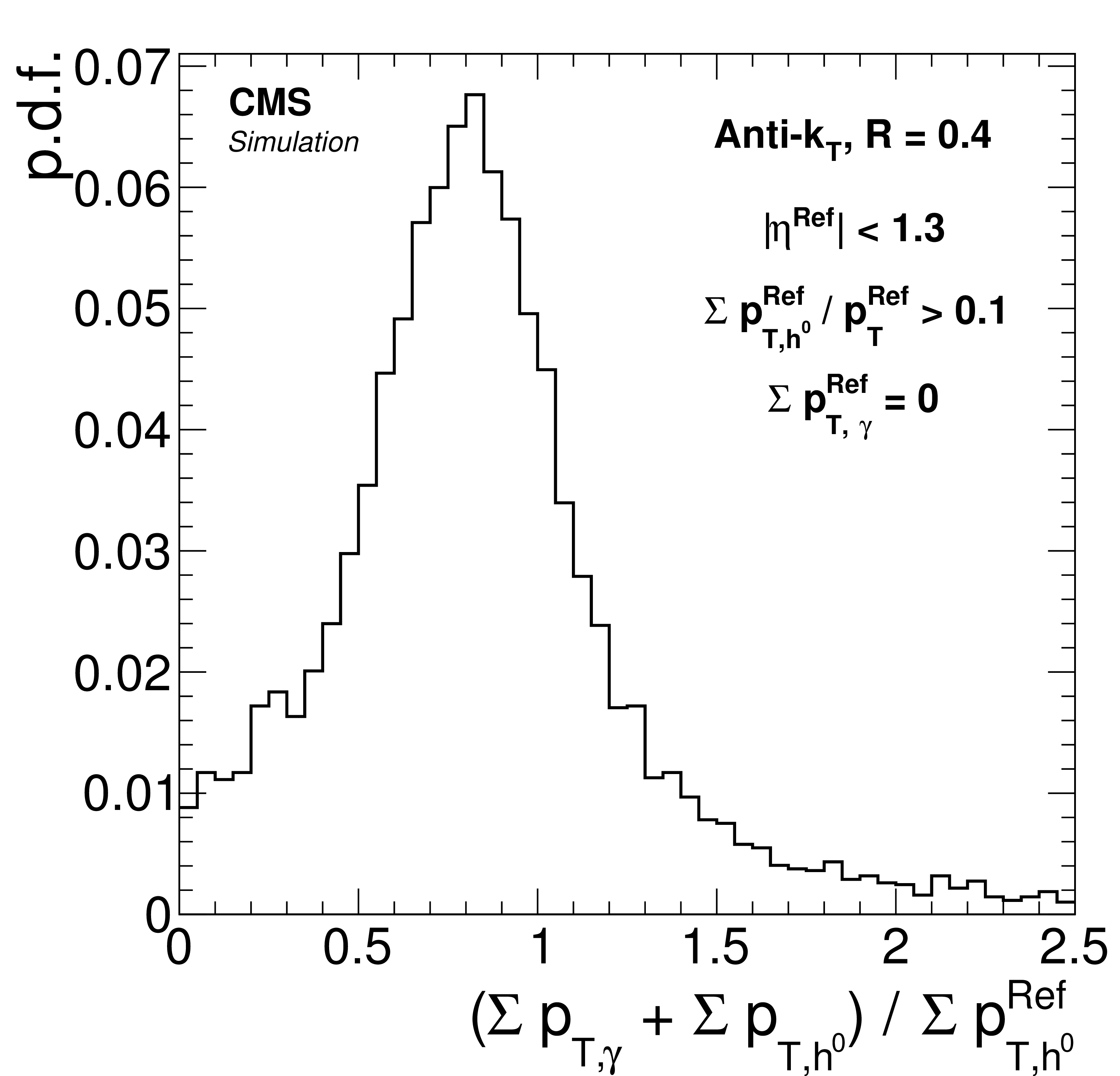
Distribution of the ratio between the reconstructed and reference transverse momenta, $\Sigma p_{\mathrm {T},i} / \Sigma p_{\mathrm {T},i}^\text {Ref}$, for charged hadrons (top left), photons (top right), neutral hadrons (bottom left), and for all neutral particles in Ref jets with no photon (bottom right). The Ref jet is required to have at least 10% of its $ {p_{\mathrm {T}}} $ carried by particles of type $i$, and to be located in the barrel. |
png pdf |
Figure 11-a:
Distribution of the ratio between the reconstructed and reference transverse momenta, $\Sigma p_{\mathrm {T},i} / \Sigma p_{\mathrm {T},i}^\text {Ref}$, for charged hadrons. The Ref jet is required to have at least 10% of its $ {p_{\mathrm {T}}} $ carried by particles of type $i$, and to be located in the barrel. |
png pdf |
Figure 11-b:
Distribution of the ratio between the reconstructed and reference transverse momenta, $\Sigma p_{\mathrm {T},i} / \Sigma p_{\mathrm {T},i}^\text {Ref}$, for photons. The Ref jet is required to have at least 10% of its $ {p_{\mathrm {T}}} $ carried by particles of type $i$, and to be located in the barrel. |
png pdf |
Figure 11-c:
Distribution of the ratio between the reconstructed and reference transverse momenta, $\Sigma p_{\mathrm {T},i} / \Sigma p_{\mathrm {T},i}^\text {Ref}$, for neutral hadrons. The Ref jet is required to have at least 10% of its $ {p_{\mathrm {T}}} $ carried by particles of type $i$, and to be located in the barrel. |
png pdf |
Figure 11-d:
Distribution of the ratio between the reconstructed and reference transverse momenta, $\Sigma p_{\mathrm {T},i} / \Sigma p_{\mathrm {T},i}^\text {Ref}$, for all neutral particles in Ref jets with no photon. The Ref jet is required to have at least 10% of its $ {p_{\mathrm {T}}} $ carried by particles of type $i$, and to be located in the barrel. |
png pdf |
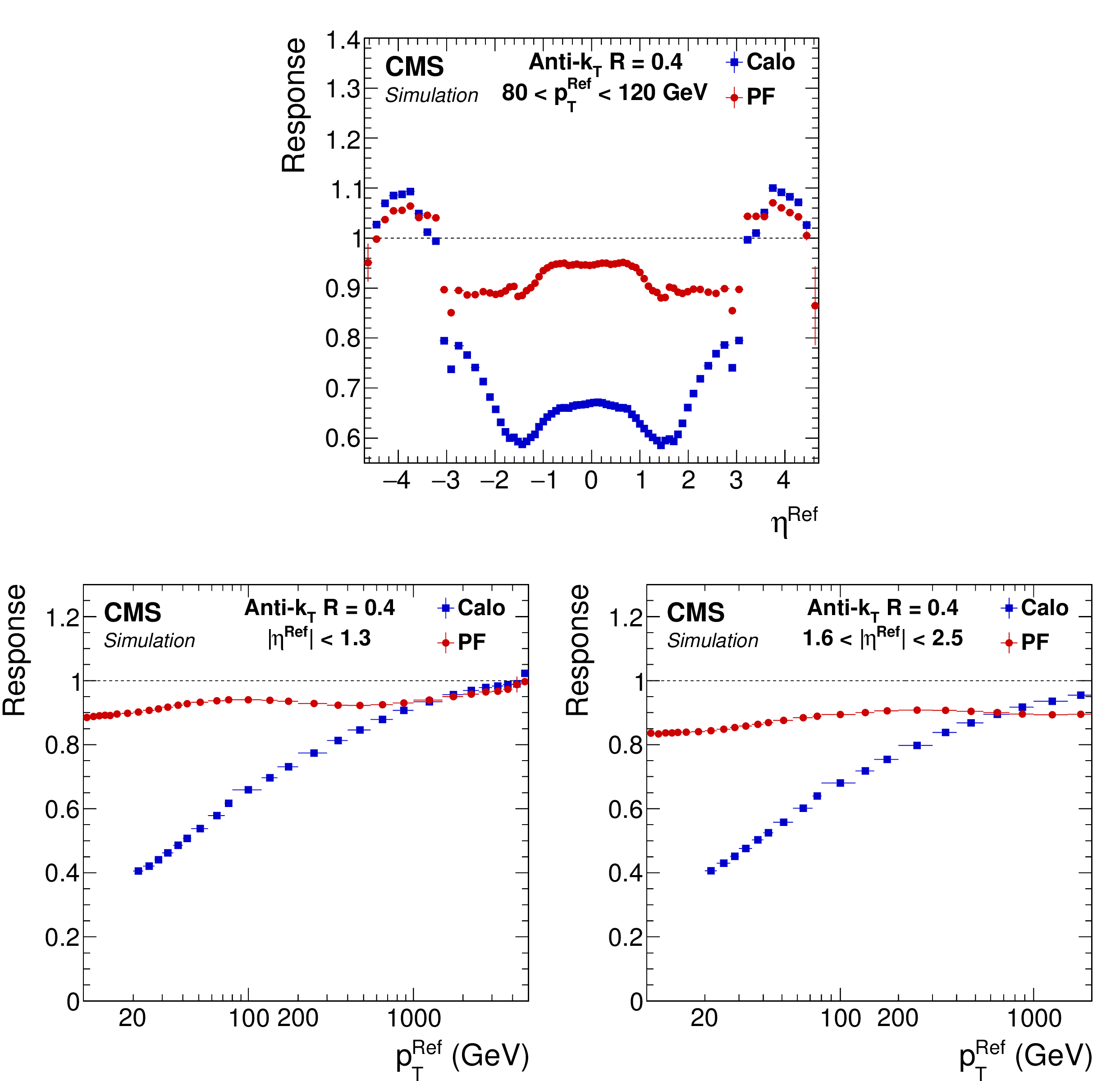
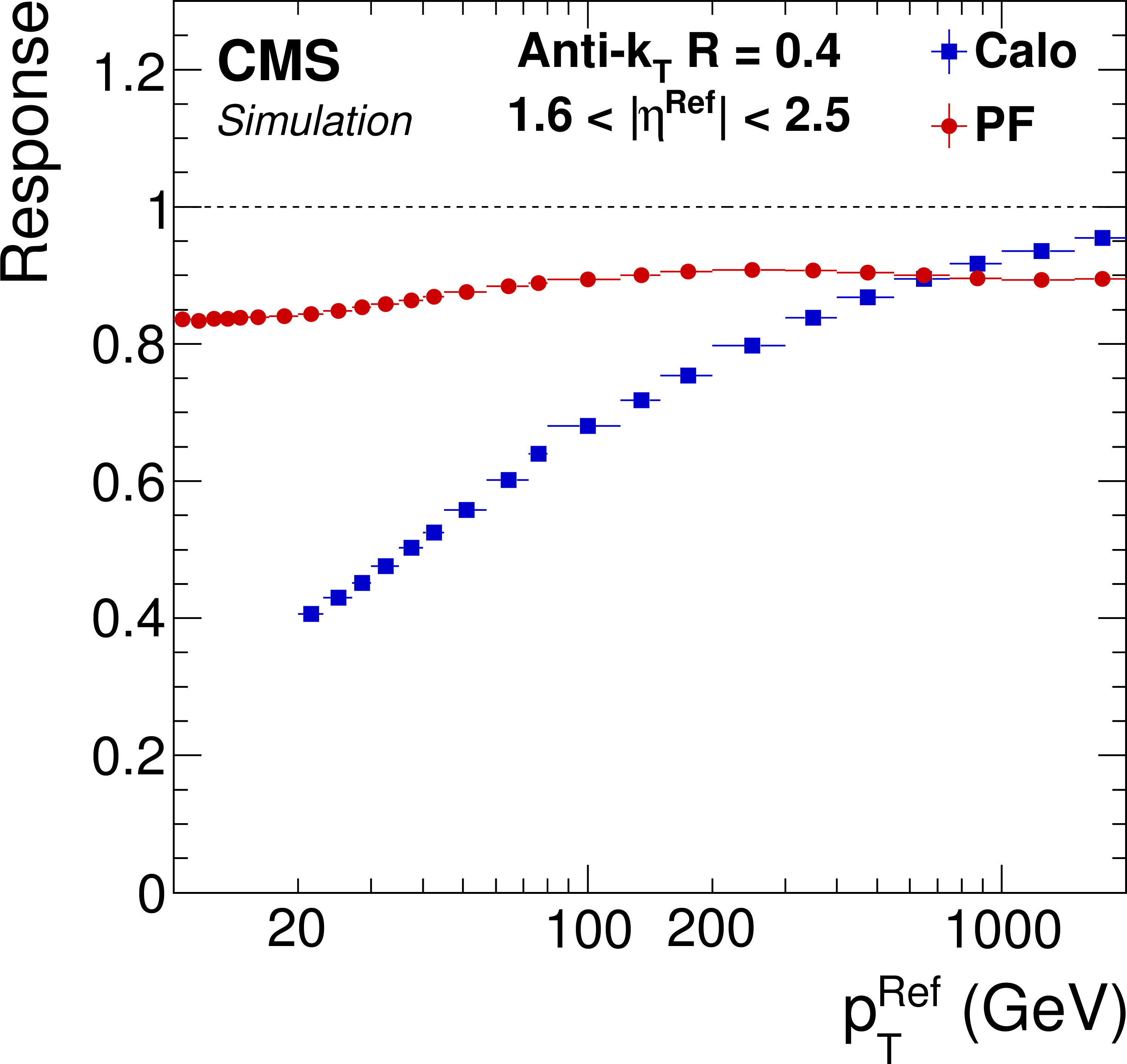
Figure 12:
Jet response as a function of $\eta ^\text {Ref}$ for the range 80 $ < {p_\mathrm {T}^\text {Ref}} < $ 120 GeV (top) and as a function of ${p_\mathrm {T}^\text {Ref}}$ in the barrel (left) and in the endcap (right) regions. |
png pdf |
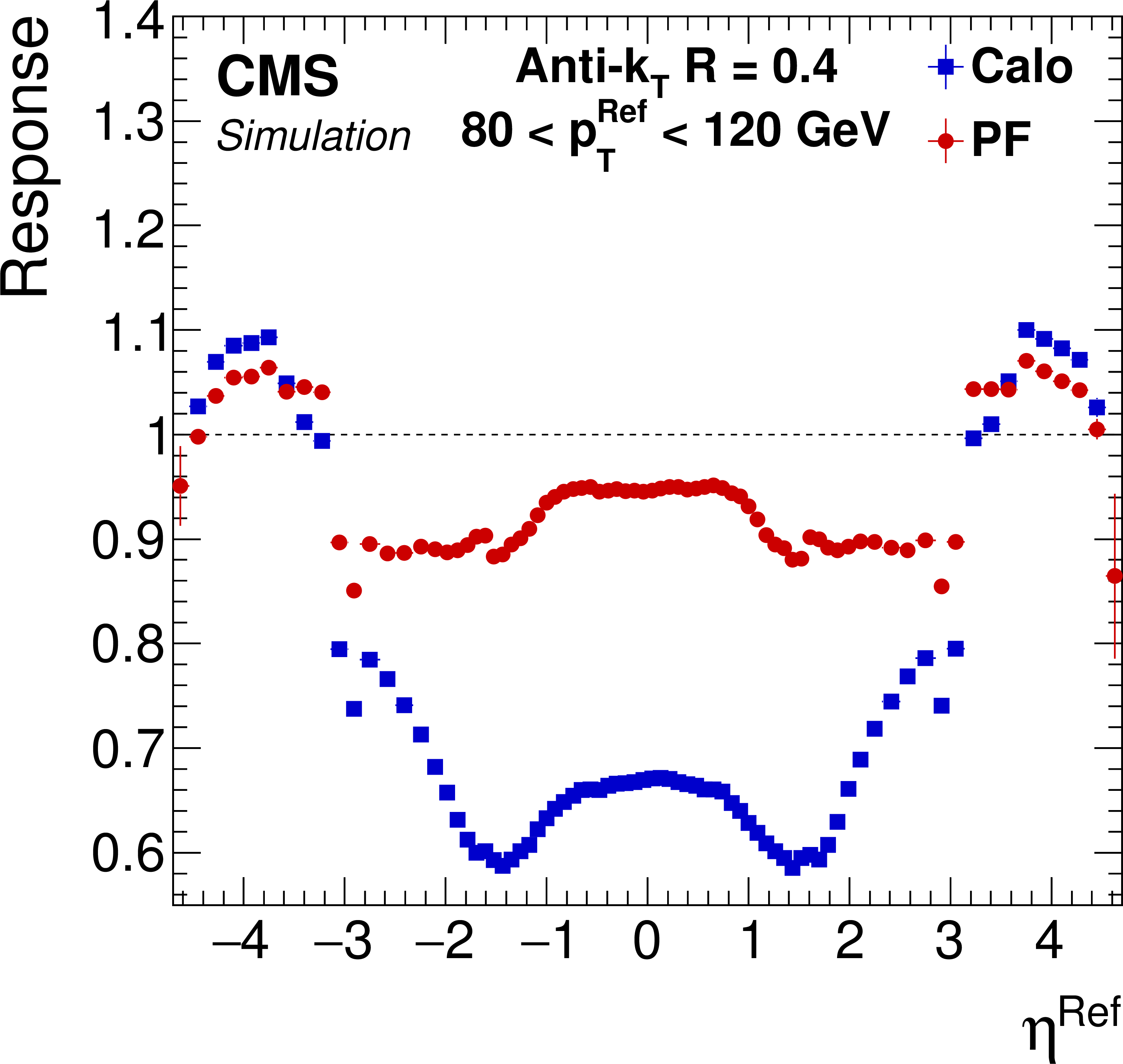
Figure 12-a:
Jet response as a function of $\eta ^\text {Ref}$ for the range 80 $ < {p_\mathrm {T}^\text {Ref}} < $ 120 GeV. |
png pdf |
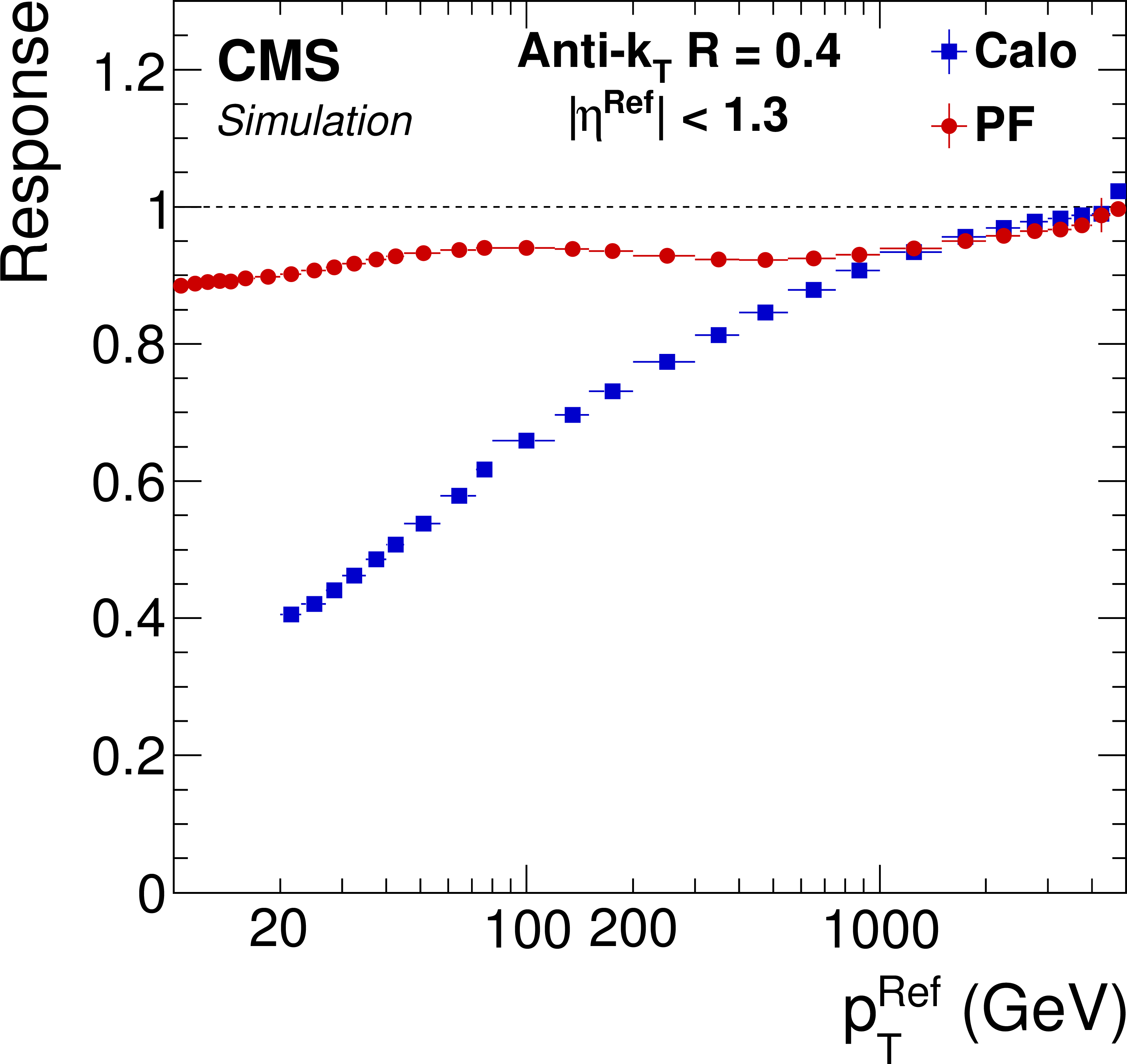
Figure 12-b:
Jet response as a function of ${p_\mathrm {T}^\text {Ref}}$ in the barrel region. |
png pdf |
Figure 12-c:
Jet response as a function of ${p_\mathrm {T}^\text {Ref}}$ in the endcap region. |
png pdf |
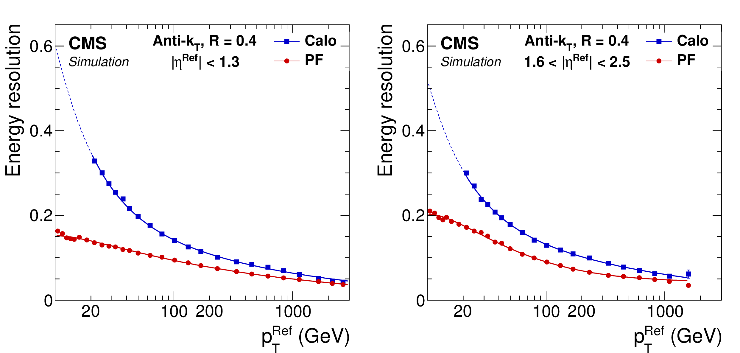
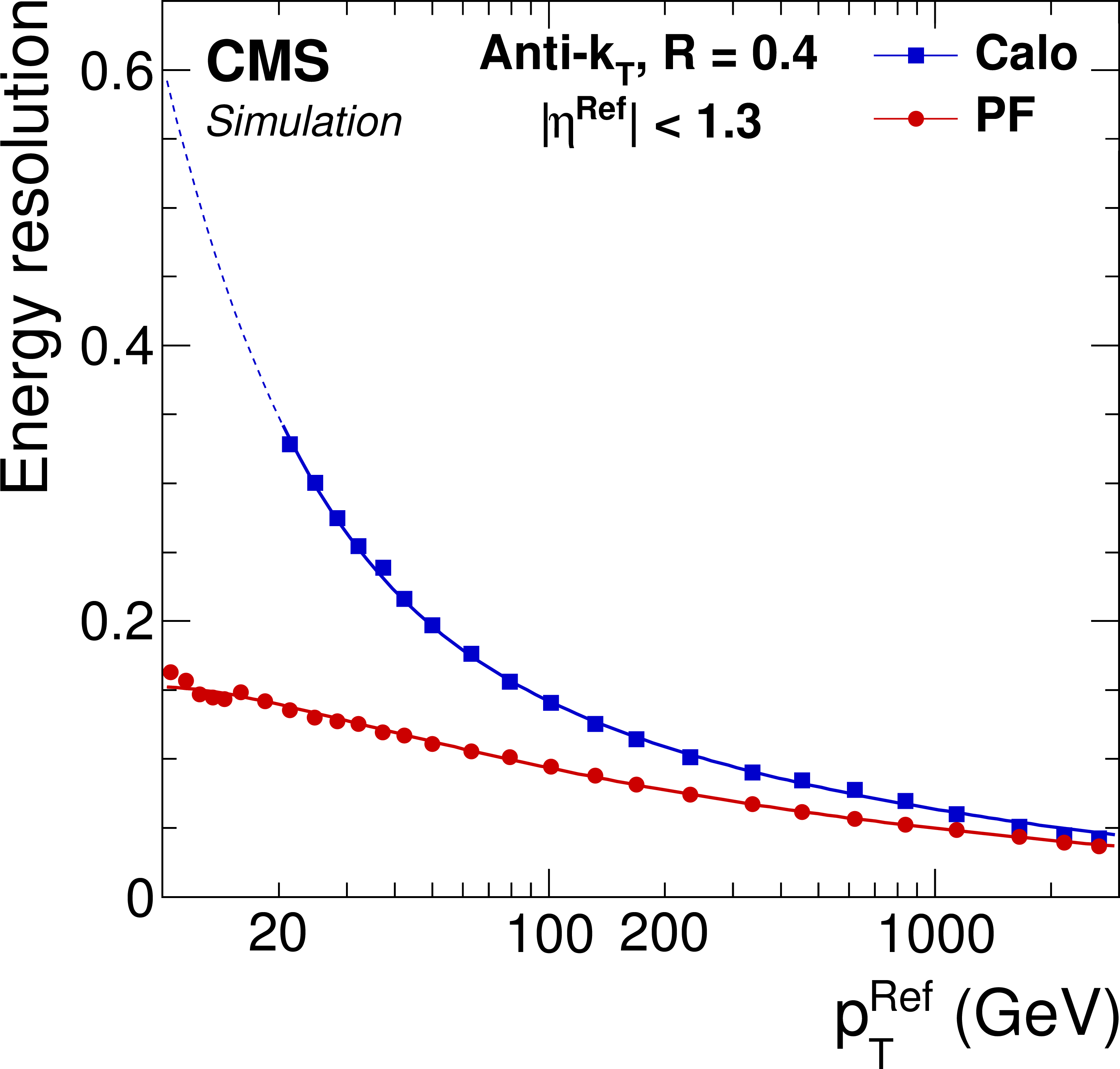
Figure 13:
Jet energy resolution as a function of ${p_\mathrm {T}^\text {Ref}}$ in the barrel (left) and in the endcap (right) regions. The lines, added to guide the eye, correspond to fitted functions with ad hoc parametrizations. |
png pdf |
Figure 13-a:
Jet energy resolution as a function of ${p_\mathrm {T}^\text {Ref}}$ in the barrel region. The lines, added to guide the eye, correspond to fitted functions with ad hoc parametrizations. |

png pdf |
Figure 13-b:
Jet energy resolution as a function of ${p_\mathrm {T}^\text {Ref}}$ in the endcap region. The lines, added to guide the eye, correspond to fitted functions with ad hoc parametrizations. |
png pdf |
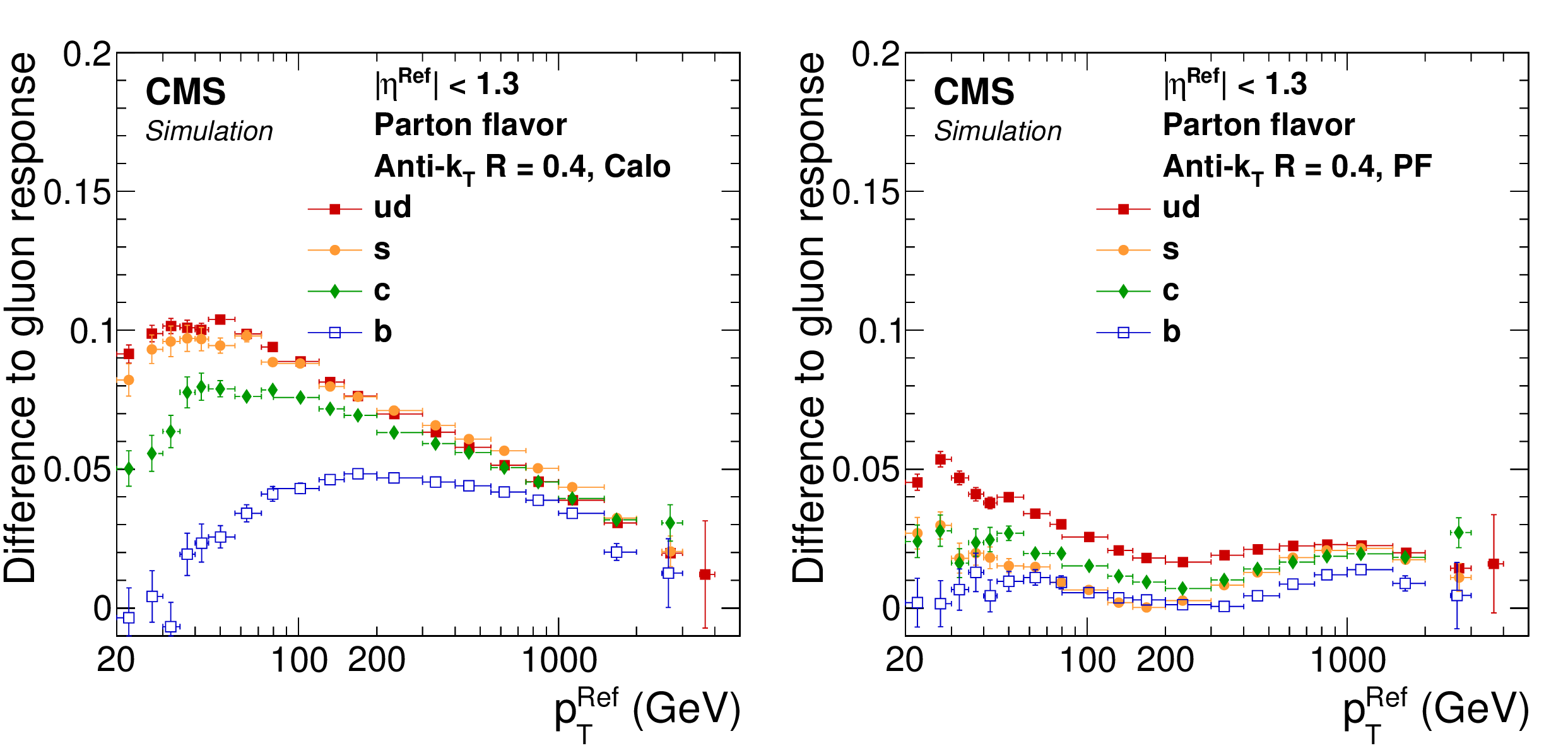
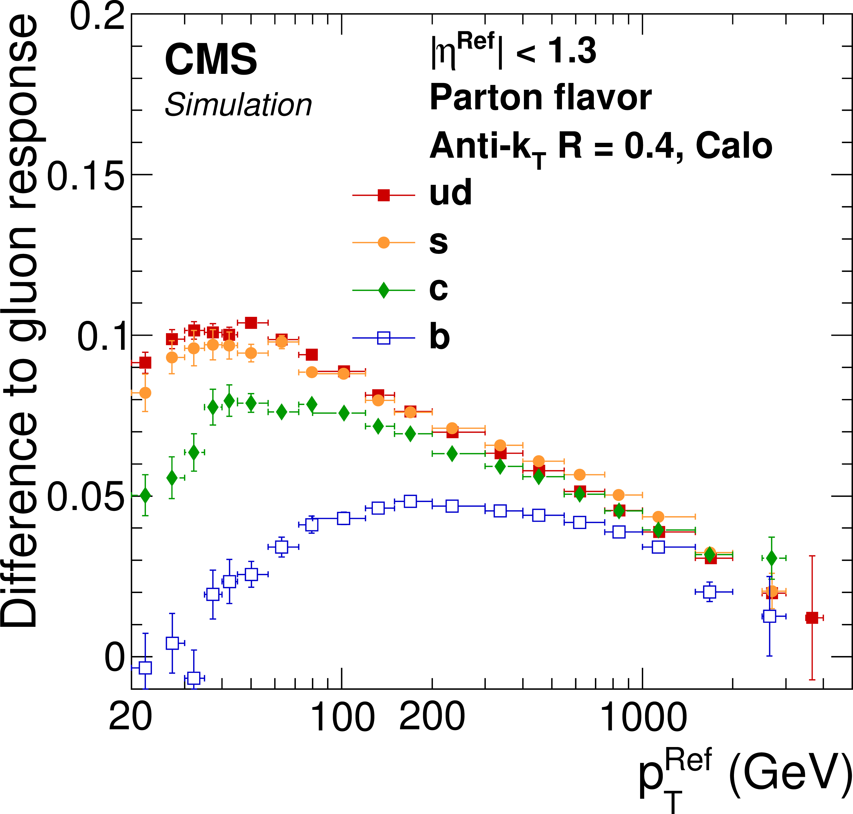
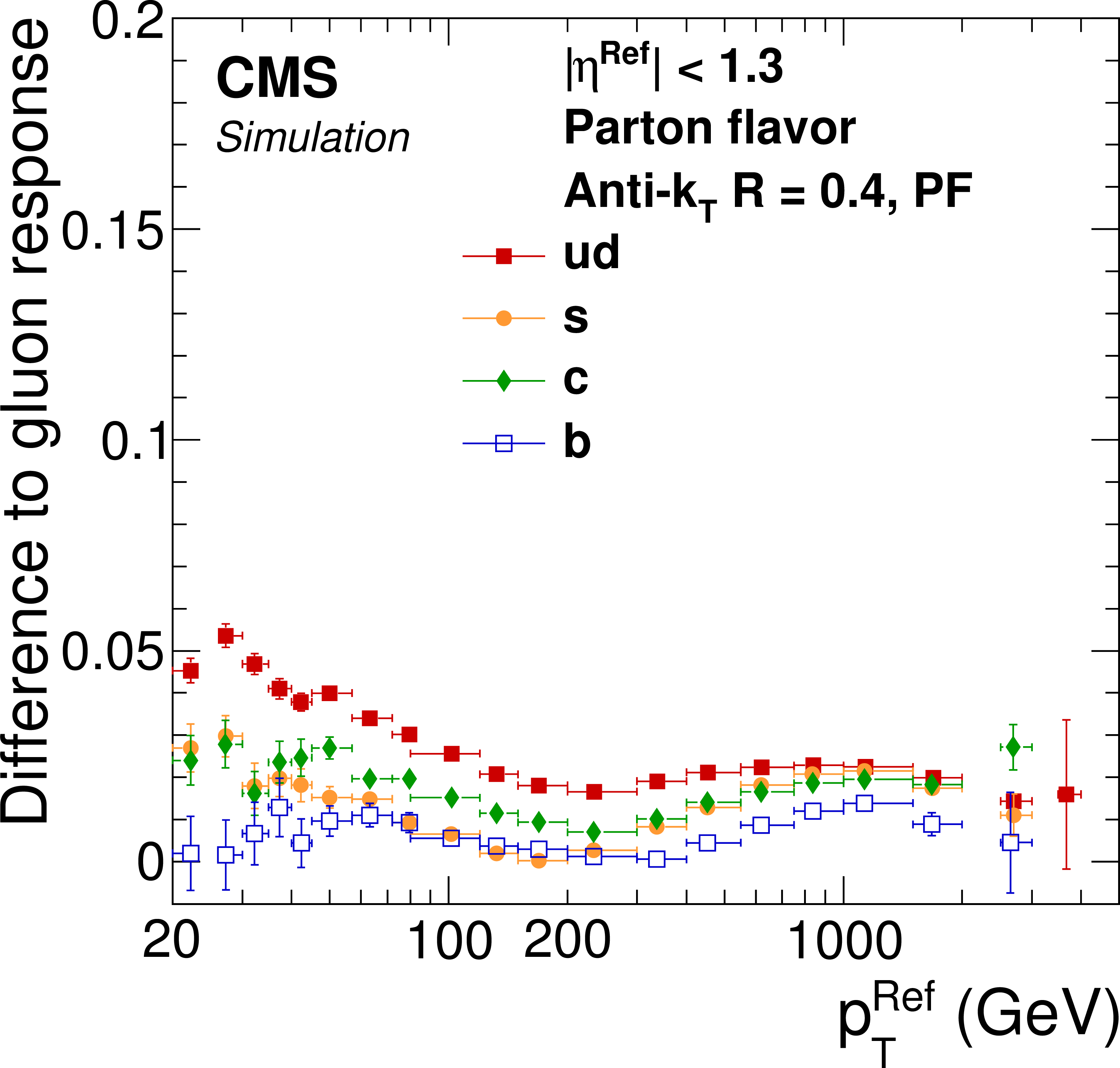
Figure 14:
Absolute difference in jet energy response between quark and gluon jets as a function of ${p_\mathrm {T}^\text {Ref}}$ for Calo jets (left) and PF jets (right). |
png pdf |
Figure 14-a:
Absolute difference in jet energy response between quark and gluon jets as a function of ${p_\mathrm {T}^\text {Ref}}$ for Calo jets. |
png pdf |
Figure 14-b:
Absolute difference in jet energy response between quark and gluon jets as a function of ${p_\mathrm {T}^\text {Ref}}$ for PF jets. |
png pdf |
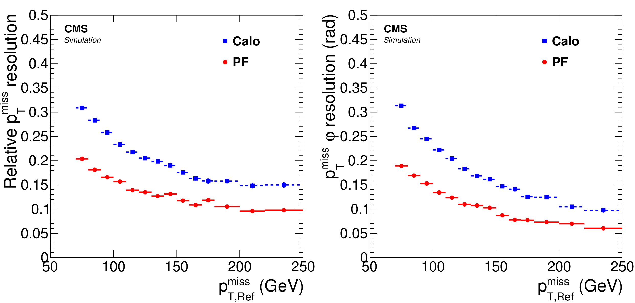
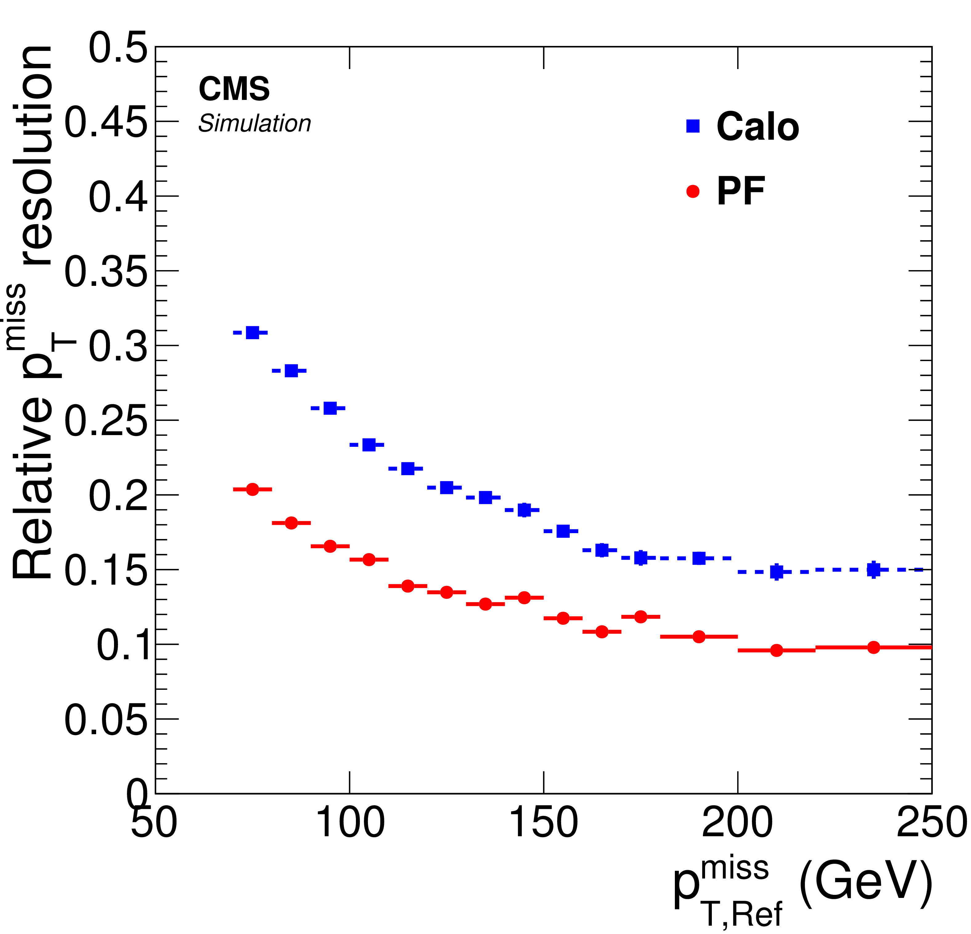
Figure 15:
Relative ${ {p_{\mathrm {T}}} ^\text {miss}}$ resolution and resolution on the ${{\vec p}_{\mathrm {T}}}^{\, \text{miss}} $ direction as a function of $ {p_\text {T,Ref}^\text {miss}} $ for a simulated $ {\mathrm{ t } {}\mathrm{ \bar{t} } } $ sample. |
png pdf |
Figure 15-a:
Relative ${ {p_{\mathrm {T}}} ^\text {miss}}$ resolution as a function of $ {p_\text {T,Ref}^\text {miss}} $ for a simulated $ {\mathrm{ t } {}\mathrm{ \bar{t} } } $ sample. |

png pdf |
Figure 15-b:
Resolution on the ${{\vec p}_{\mathrm {T}}}^{\, \text{miss}} $ direction as a function of $ {p_\text {T,Ref}^\text {miss}} $ for a simulated $ {\mathrm{ t } {}\mathrm{ \bar{t} } } $ sample. |
png pdf |
Figure 16:
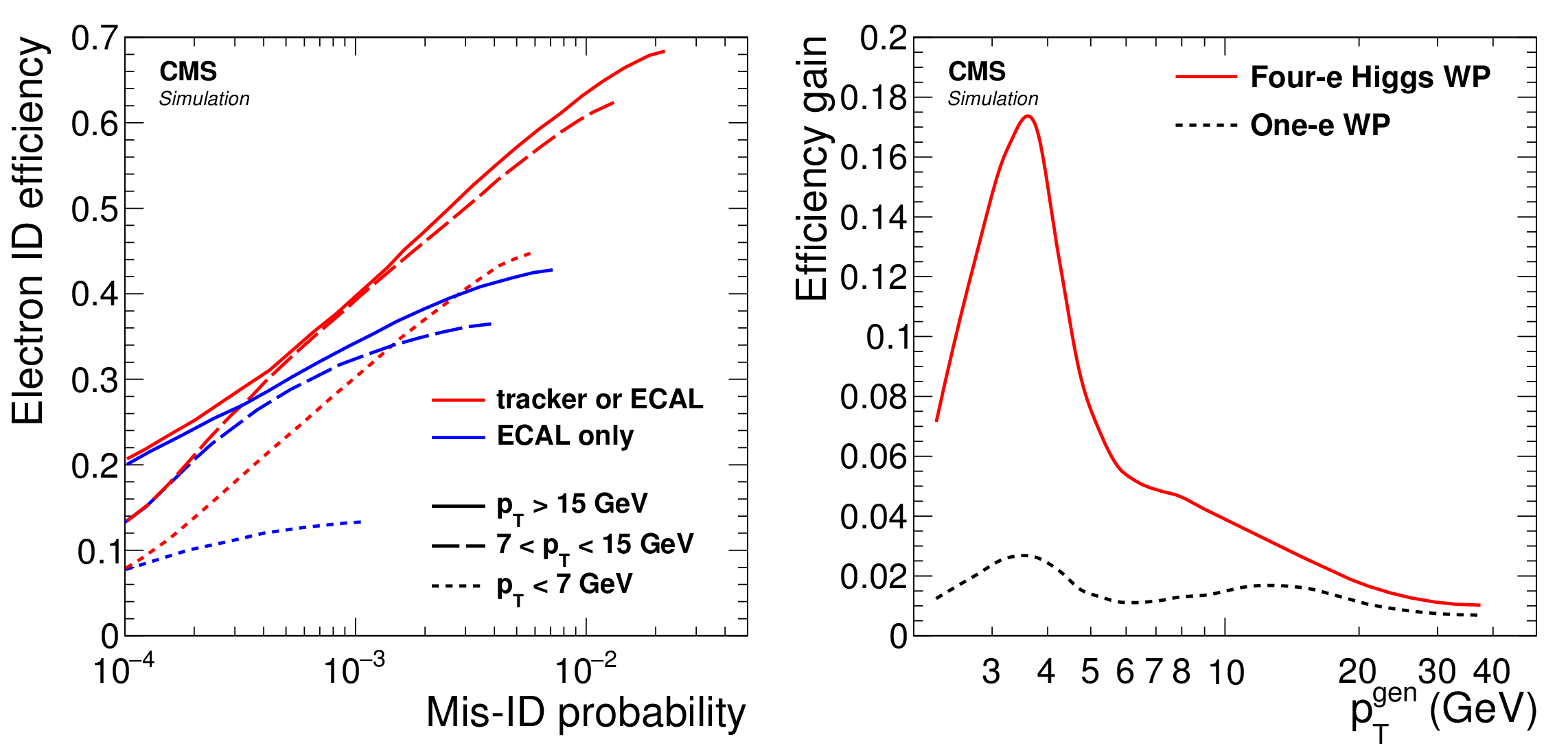
Left: Efficiency to reconstruct electrons from b hadron decays (signal) versus the probability to misidentify a hadron as an electron (background). The solid, long-dashed, and short-dashed lines refer to electrons and hadrons with $ {p_{\mathrm {T}}} $ larger than 15, within $ [7,15]$, and lower than $7 GeV $, respectively. The curves correspond to a threshold scan on the BDT classifier score for ECAL-based seeded electrons and for tracker- or ECAL-based seeded electrons. Right: Absolute gain in reconstruction and identification efficiency provided by the tracker-based seeding procedure for two working points (WP) corresponding to different values of the threshold on the BDT classifier score. The solid line corresponds to the value used in the $\mathrm{ H } \to {\mathrm{ Z } } {\mathrm{ Z } } \to 4 \mathrm{ e } $ analyses and the dashed line to the value typically used in analyses of single-electron final states. In all cases, the classifier score of the BDT trained for electrons selected without any trigger requirement is used. |

png pdf |
Figure 16-a:
Efficiency to reconstruct electrons from b hadron decays (signal) versus the probability to misidentify a hadron as an electron (background). The solid, long-dashed, and short-dashed lines refer to electrons and hadrons with $ {p_{\mathrm {T}}} $ larger than 15, within $ [7,15]$, and lower than $7 GeV $, respectively. The curves correspond to a threshold scan on the BDT classifier score for ECAL-based seeded electrons and for tracker- or ECAL-based seeded electrons. |

png pdf |
Figure 16-b:
Absolute gain in reconstruction and identification efficiency provided by the tracker-based seeding procedure for two working points (WP) corresponding to different values of the threshold on the BDT classifier score. The solid line corresponds to the value used in the $\mathrm{ H } \to {\mathrm{ Z } } {\mathrm{ Z } } \to 4 \mathrm{ e } $ analyses and the dashed line to the value typically used in analyses of single-electron final states. In all cases, the classifier score of the BDT trained for electrons selected without any trigger requirement is used. |
png pdf |
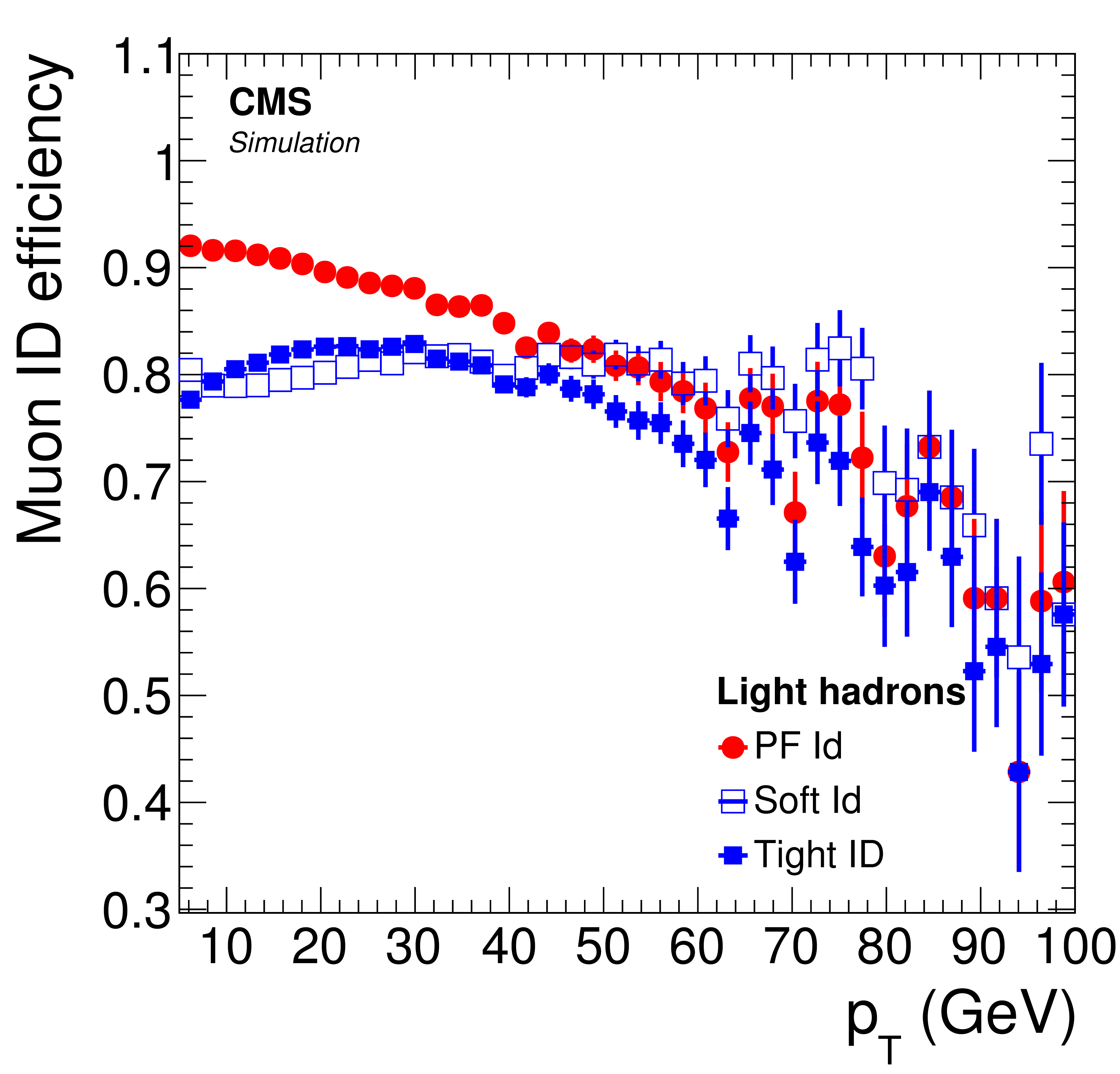
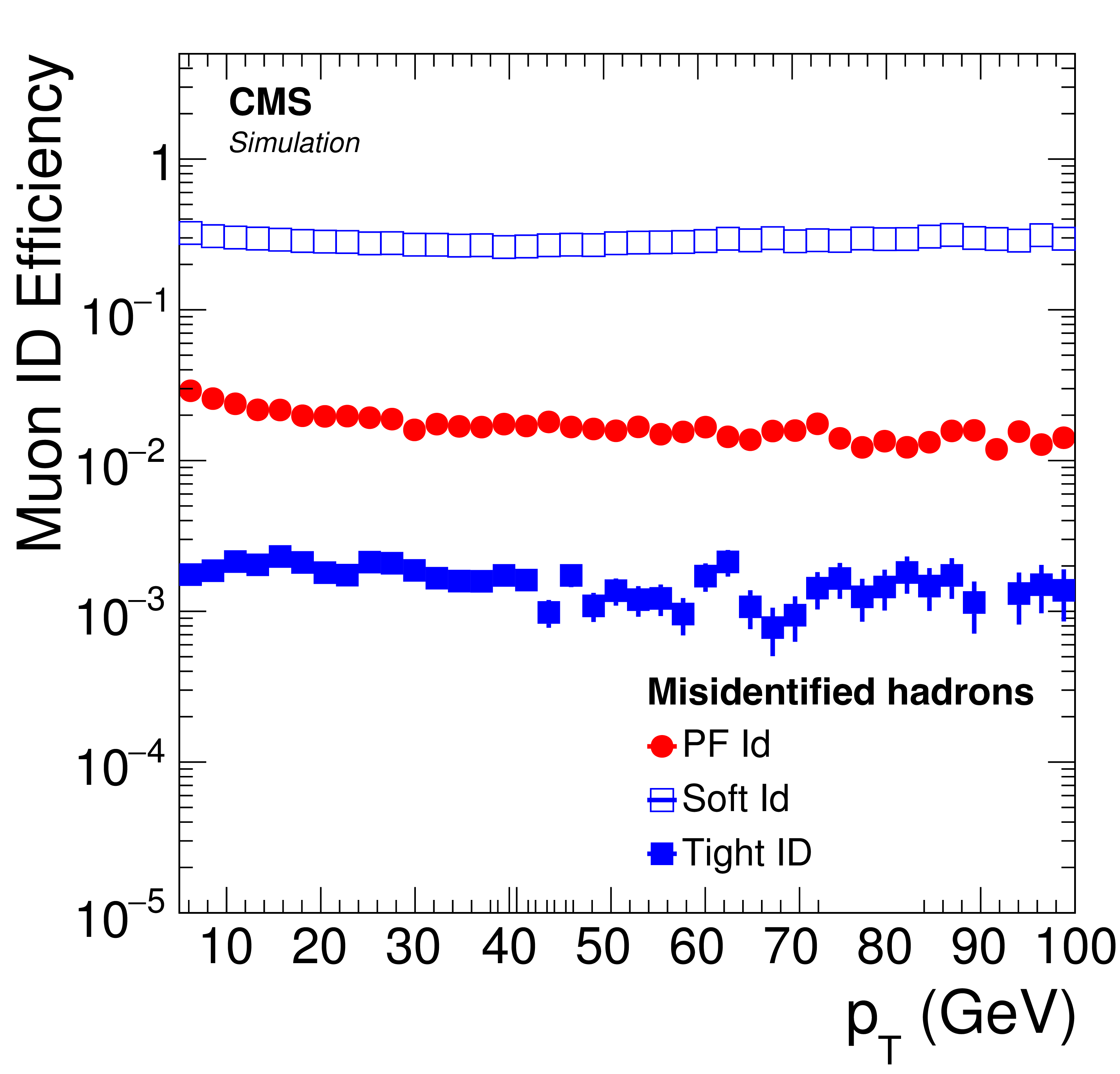
Figure 17:
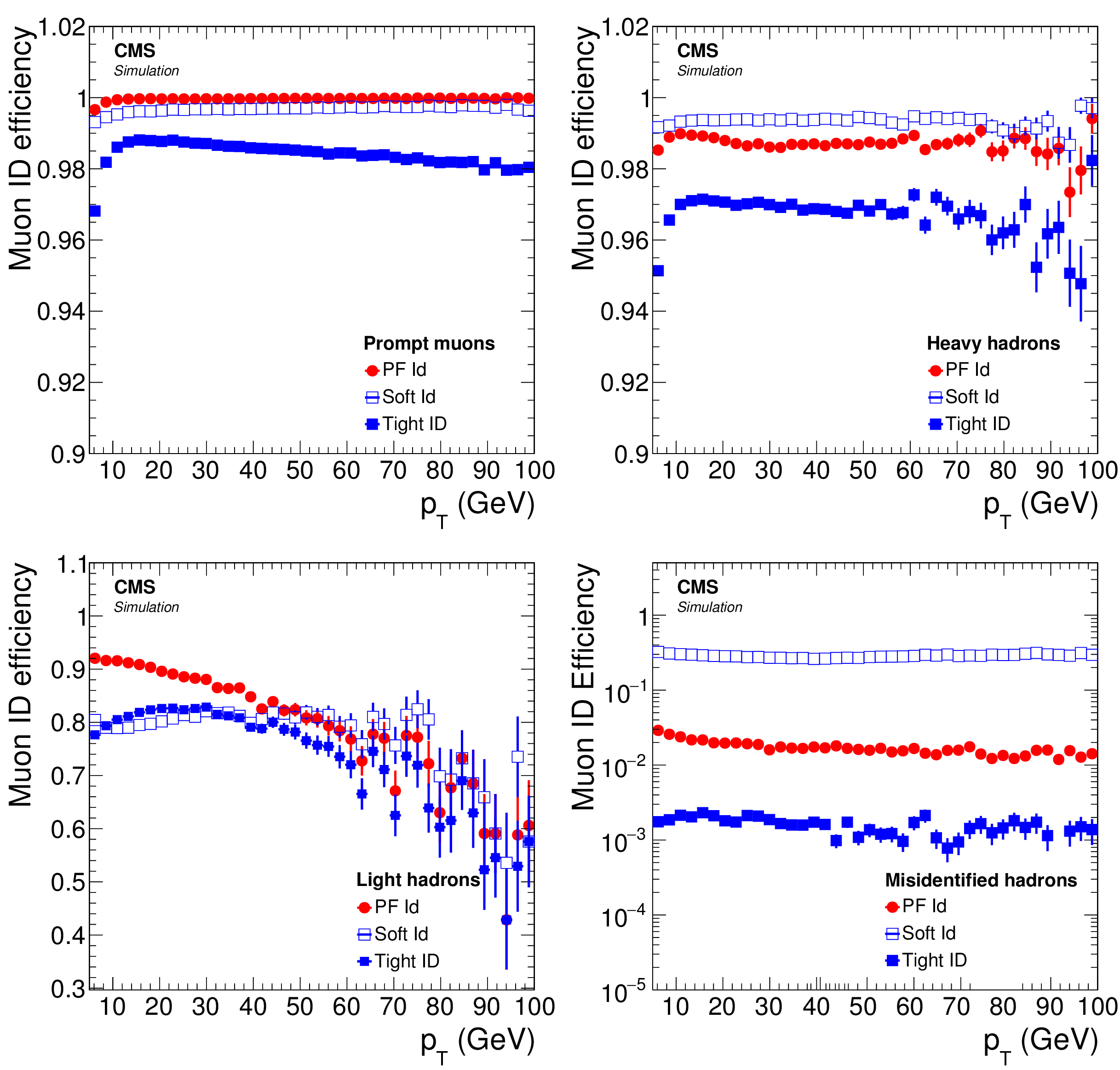
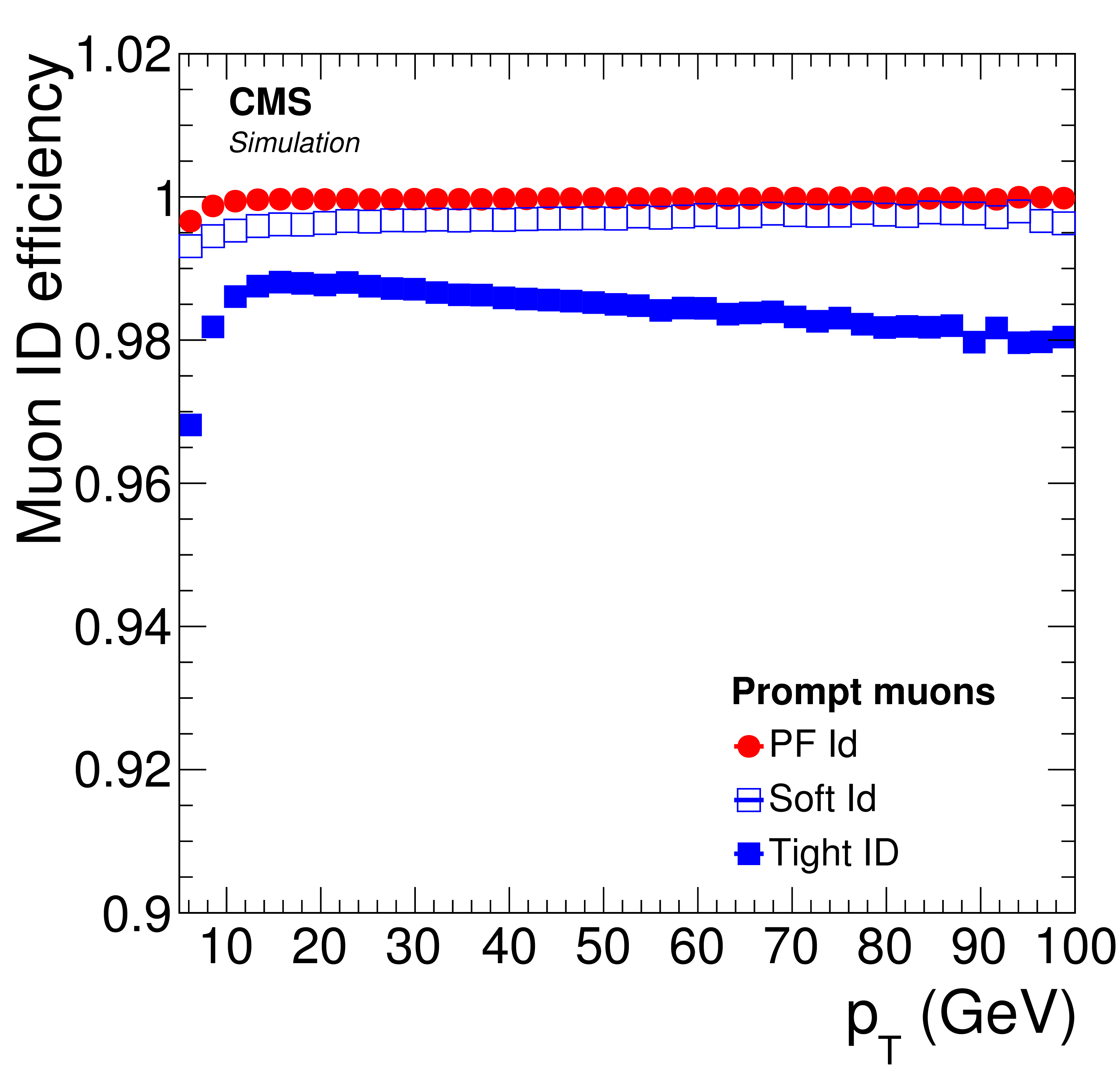
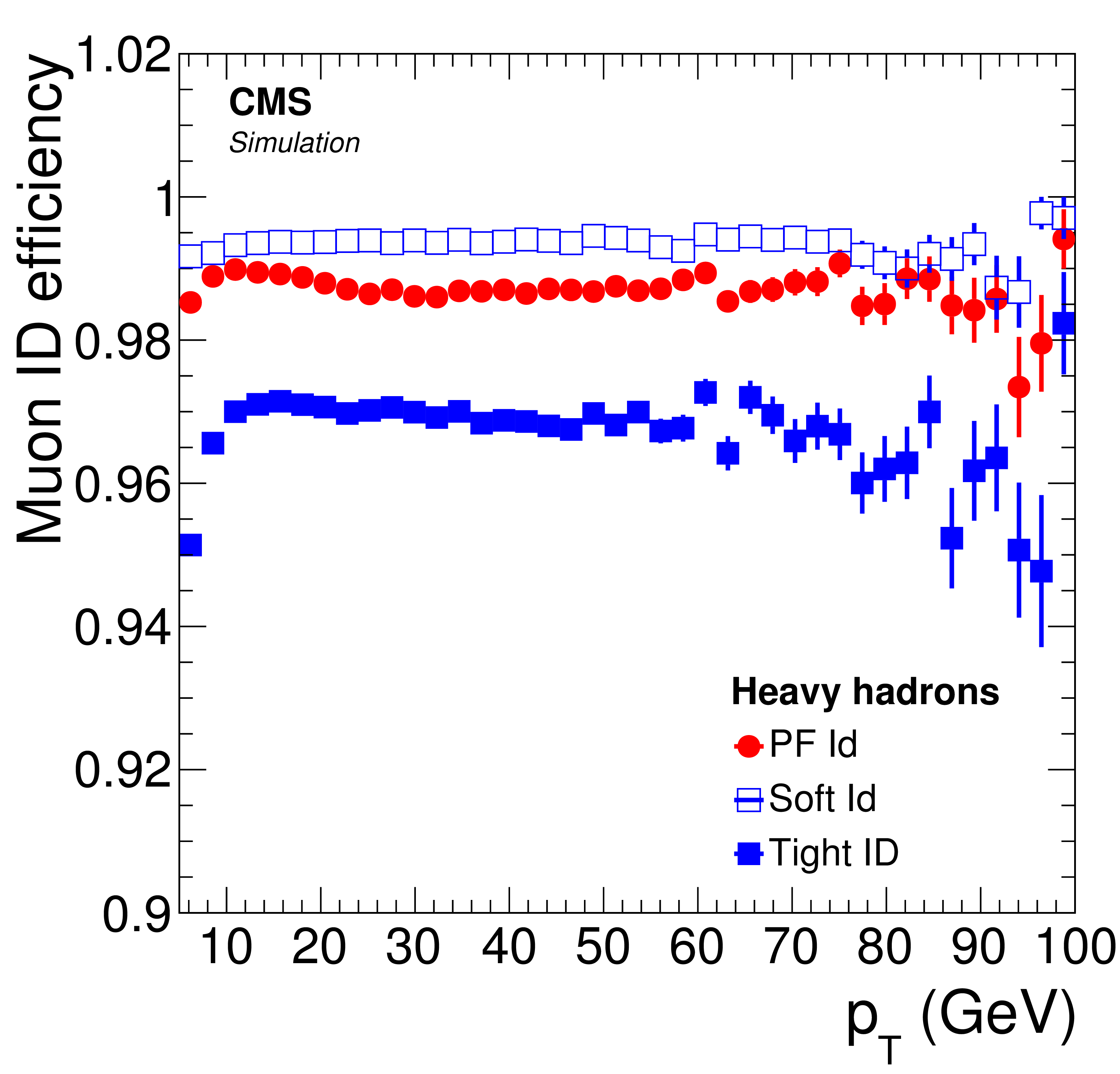
Efficiency for different algorithms (PF, soft, and tight) to identify a simulated muon track that has been reconstructed as a tracker muon, as a function of the $ {p_{\mathrm {T}}} $ of the reconstructed track. From top left to bottom right the efficiency of the three identification algorithms is shown for prompt muons, for muons from heavy-flavour decays, for muons from light-flavour decays, and for misidentified hadrons. |
png pdf |
Figure 17-a:
Efficiency for different algorithms (PF, soft, and tight) to identify a simulated muon track that has been reconstructed as a tracker muon, as a function of the $ {p_{\mathrm {T}}} $ of the reconstructed track. Here, the efficiency of the three identification algorithms is shown for prompt muons. |
png pdf |
Figure 17-b:
Efficiency for different algorithms (PF, soft, and tight) to identify a simulated muon track that has been reconstructed as a tracker muon, as a function of the $ {p_{\mathrm {T}}} $ of the reconstructed track. Here, the efficiency of the three identification algorithms is shown |
png pdf |
Figure 17-c:
Efficiency for different algorithms (PF, soft, and tight) to identify a simulated muon track that has been reconstructed as a tracker muon, as a function of the $ {p_{\mathrm {T}}} $ of the reconstructed track. Here, the efficiency of the three identification algorithms is shown for muons from light-flavour decays. |
png pdf |
Figure 17-d:
Efficiency for different algorithms (PF, soft, and tight) to identify a simulated muon track that has been reconstructed as a tracker muon, as a function of the $ {p_{\mathrm {T}}} $ of the reconstructed track. Here, the efficiency of the three identification algorithms is shown for misidentified hadrons. |
png pdf |
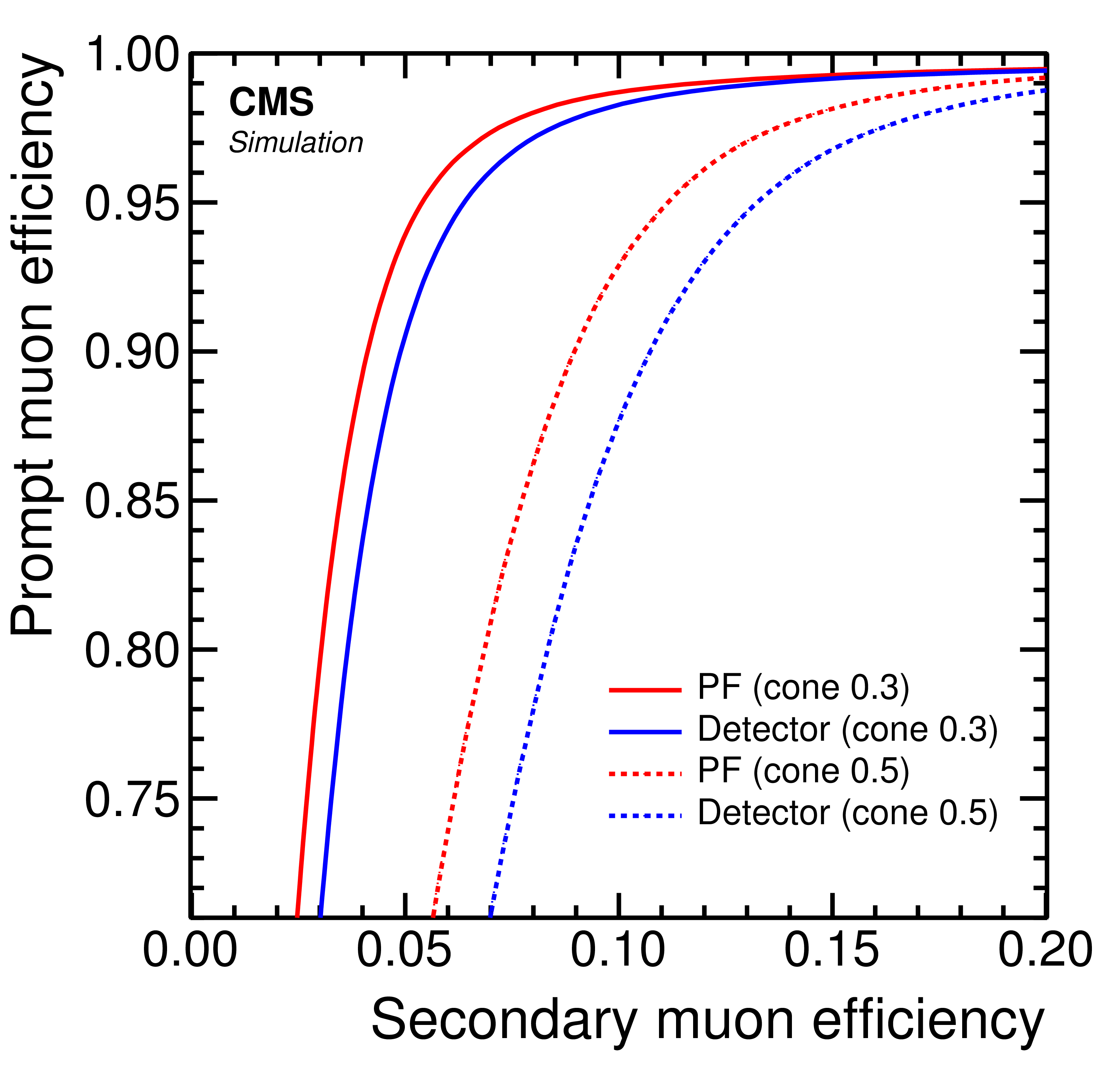
Figure 18:
Isolation efficiency for muons from $\mathrm{ W } $ boson decays versus isolation efficiency for muons from secondary decays, both obtained from simulated ${\mathrm{ t } {}\mathrm{ \bar{t} } } $ events, as a function of the threshold on the isolation for the detector- and particle-based methods. The efficiencies are shown for two choices of the maximum $\Delta R$ (isolation cone size): 0.3 and 0.5. |

png pdf |
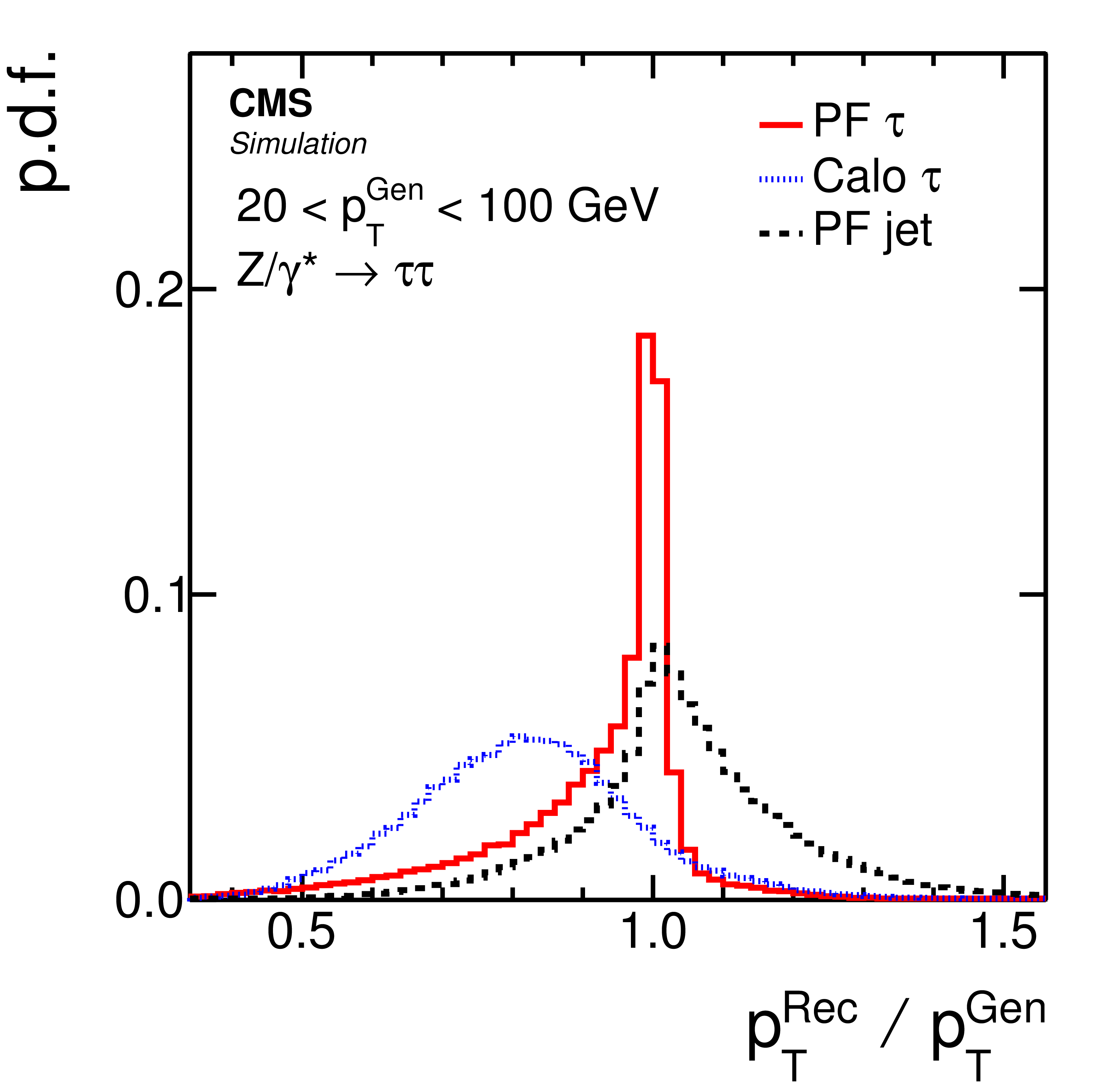
Figure 19:
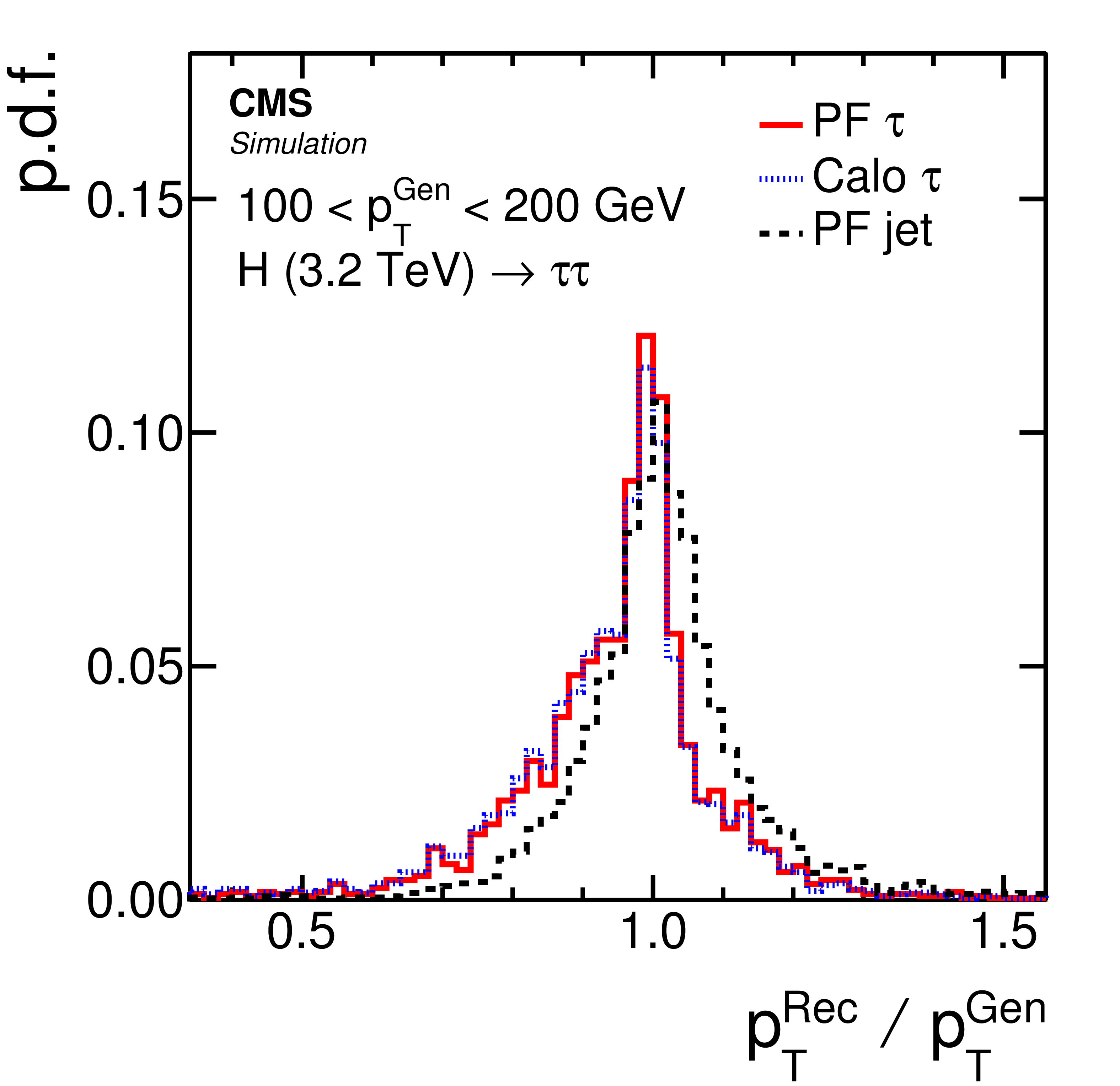
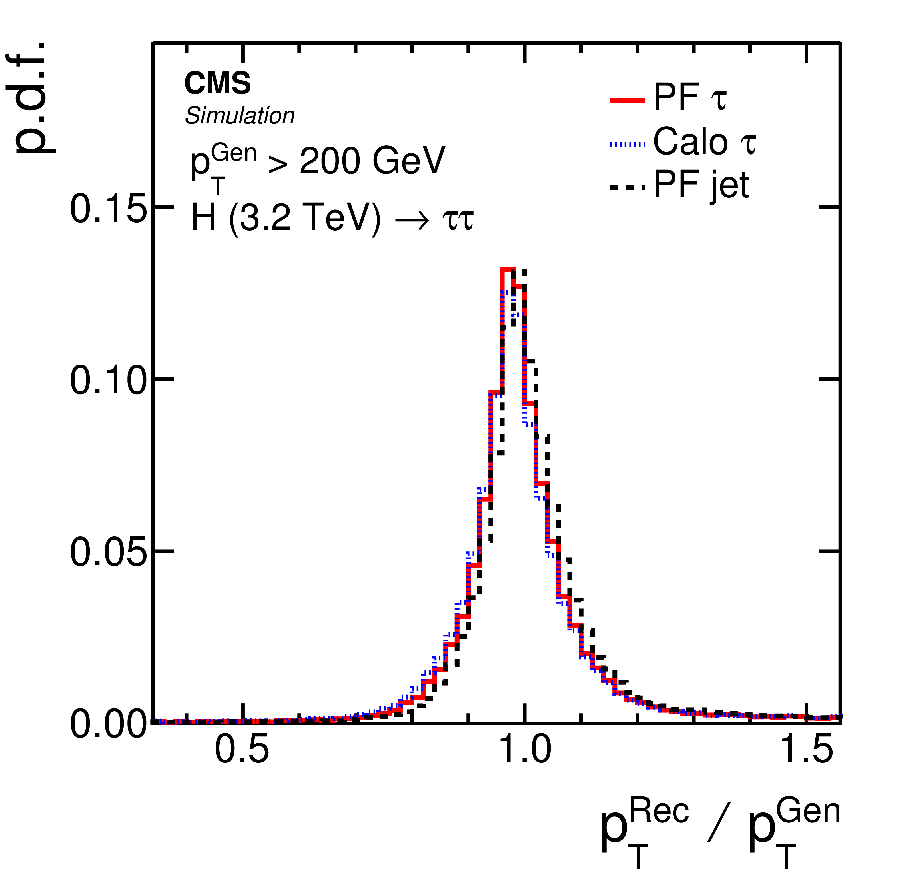
Ratio of reconstructed-to-generator level $ {p_{\mathrm {T}}} $ for genuine $ {\tau _\mathrm {h}} $ (left), and for quark and gluon jets that pass the $ {\tau _\mathrm {h}} $ identification criteria (right), for different intervals in generator level $ {p_{\mathrm {T}}} $. In the PF $\tau $ case, the $ {\tau _\mathrm {h}} $ candidates are reconstructed by the HPS algorithm and required to pass the loose isolation working point. In the Calo $\tau $ case, they are reconstructed solely with the calorimeters and required to pass the $ {\tau _\mathrm {h}} $ identification criteria. The generator level $ {p_{\mathrm {T}}} $ is taken to be either that of the $ {\tau _\mathrm {h}} $ or that of the jet. For comparison, the ratio is also shown for the closest PF jet in the $(\eta, \varphi )$ plane. |
png pdf |
Figure 19-a:
Ratio of reconstructed-to-generator level $ {p_{\mathrm {T}}} $ for genuine $ {\tau _\mathrm {h}} $ for 20 $ < {p_{\mathrm {T}}} < $ 100 GeV at generator level. In the PF $\tau $ case, the $ {\tau _\mathrm {h}} $ candidates are reconstructed by the HPS algorithm and required to pass the loose isolation working point. In the Calo $\tau $ case, they are reconstructed solely with the calorimeters and required to pass the $ {\tau _\mathrm {h}} $ identification criteria. The generator level $ {p_{\mathrm {T}}} $ is taken to be either that of the $ {\tau _\mathrm {h}} $ or that of the jet. For comparison, the ratio is also shown for the closest PF jet in the $(\eta, \varphi )$ plane. |

png pdf |
Figure 19-b:
Ratio of reconstructed-to-generator level $ {p_{\mathrm {T}}} $ for quark and gluon jets that pass the $ {\tau _\mathrm {h}} $ identification criteria for 20 $ < {p_{\mathrm {T}}} < $ 100 GeV at generator level. In the PF $\tau $ case, the $ {\tau _\mathrm {h}} $ candidates are reconstructed by the HPS algorithm and required to pass the loose isolation working point. In the Calo $\tau $ case, they are reconstructed solely with the calorimeters and required to pass the $ {\tau _\mathrm {h}} $ identification criteria. The generator level $ {p_{\mathrm {T}}} $ is taken to be either that of the $ {\tau _\mathrm {h}} $ or that of the jet. For comparison, the ratio is also shown for the closest PF jet in the $(\eta, \varphi )$ plane. |
png pdf |
Figure 19-c:
Ratio of reconstructed-to-generator level $ {p_{\mathrm {T}}} $ for genuine $ {\tau _\mathrm {h}} $ for 100 $ < {p_{\mathrm {T}}} < $ 200 GeV at generator level. In the PF $\tau $ case, the $ {\tau _\mathrm {h}} $ candidates are reconstructed by the HPS algorithm and required to pass the loose isolation working point. In the Calo $\tau $ case, they are reconstructed solely with the calorimeters and required to pass the $ {\tau _\mathrm {h}} $ identification criteria. The generator level $ {p_{\mathrm {T}}} $ is taken to be either that of the $ {\tau _\mathrm {h}} $ or that of the jet. For comparison, the ratio is also shown for the closest PF jet in the $(\eta, \varphi )$ plane. |

png pdf |
Figure 19-d:
Ratio of reconstructed-to-generator level $ {p_{\mathrm {T}}} $ for quark and gluon jets that pass the $ {\tau _\mathrm {h}} $ identification criteria for 100 $ < {p_{\mathrm {T}}} < $ 200 GeV at generator level. In the PF $\tau $ case, the $ {\tau _\mathrm {h}} $ candidates are reconstructed by the HPS algorithm and required to pass the loose isolation working point. In the Calo $\tau $ case, they are reconstructed solely with the calorimeters and required to pass the $ {\tau _\mathrm {h}} $ identification criteria. The generator level $ {p_{\mathrm {T}}} $ is taken to be either that of the $ {\tau _\mathrm {h}} $ or that of the jet. For comparison, the ratio is also shown for the closest PF jet in the $(\eta, \varphi )$ plane. |
png pdf |
Figure 19-e:
Ratio of reconstructed-to-generator level $ {p_{\mathrm {T}}} $ for genuine $ {\tau _\mathrm {h}} $ for $ {p_{\mathrm {T}}} > $ 200 GeV at generator level. In the PF $\tau $ case, the $ {\tau _\mathrm {h}} $ candidates are reconstructed by the HPS algorithm and required to pass the loose isolation working point. In the Calo $\tau $ case, they are reconstructed solely with the calorimeters and required to pass the $ {\tau _\mathrm {h}} $ identification criteria. The generator level $ {p_{\mathrm {T}}} $ is taken to be either that of the $ {\tau _\mathrm {h}} $ or that of the jet. For comparison, the ratio is also shown for the closest PF jet in the $(\eta, \varphi )$ plane. |

png pdf |
Figure 19-f:
Ratio of reconstructed-to-generator level $ {p_{\mathrm {T}}} $ for quark and gluon jets that pass the $ {\tau _\mathrm {h}} $ identification criteria for $ {p_{\mathrm {T}}} > $ 200 GeV at generator level. In the PF $\tau $ case, the $ {\tau _\mathrm {h}} $ candidates are reconstructed by the HPS algorithm and required to pass the loose isolation working point. In the Calo $\tau $ case, they are reconstructed solely with the calorimeters and required to pass the $ {\tau _\mathrm {h}} $ identification criteria. The generator level $ {p_{\mathrm {T}}} $ is taken to be either that of the $ {\tau _\mathrm {h}} $ or that of the jet. For comparison, the ratio is also shown for the closest PF jet in the $(\eta, \varphi )$ plane. |

png pdf |
Figure 20:
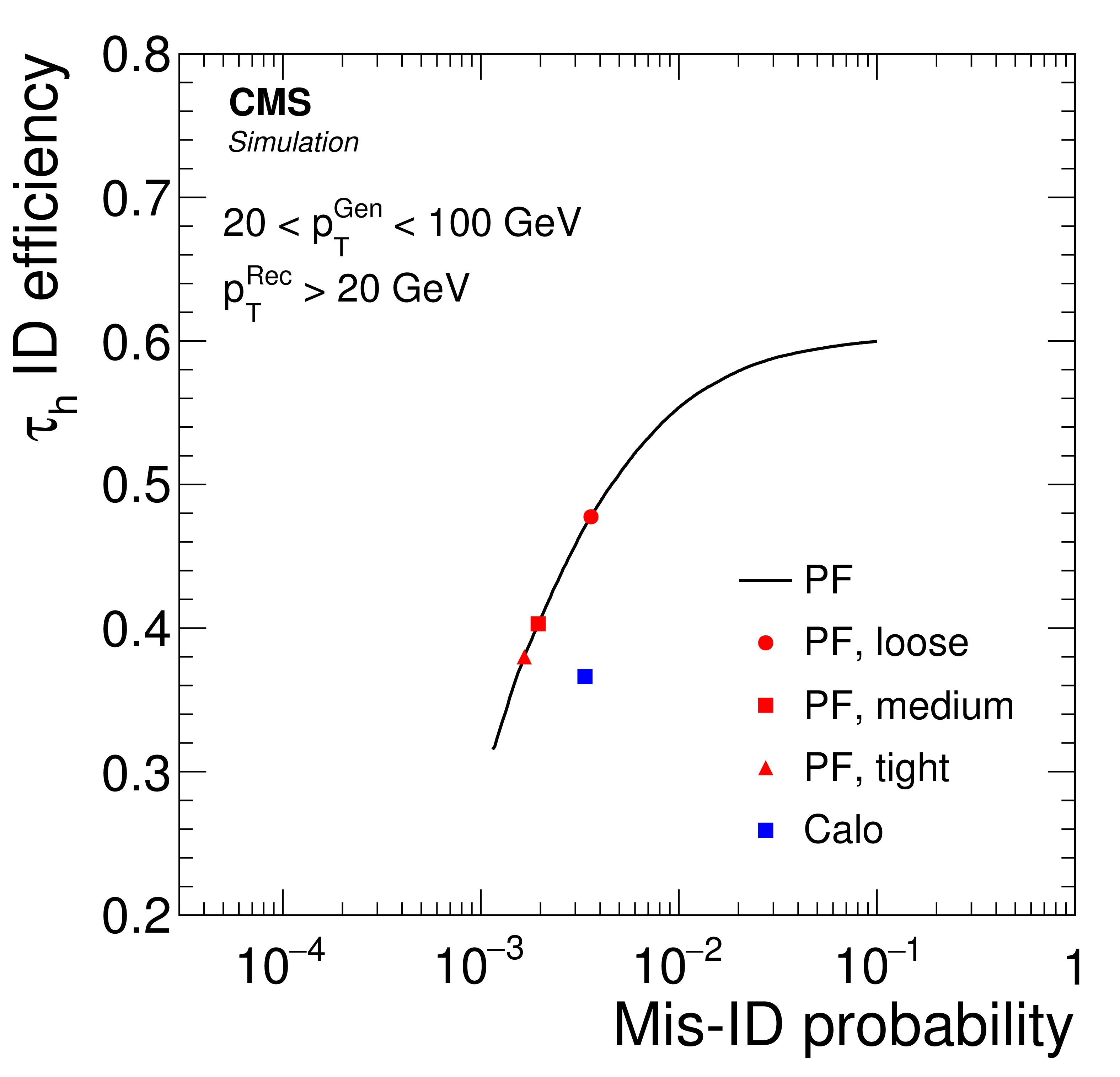
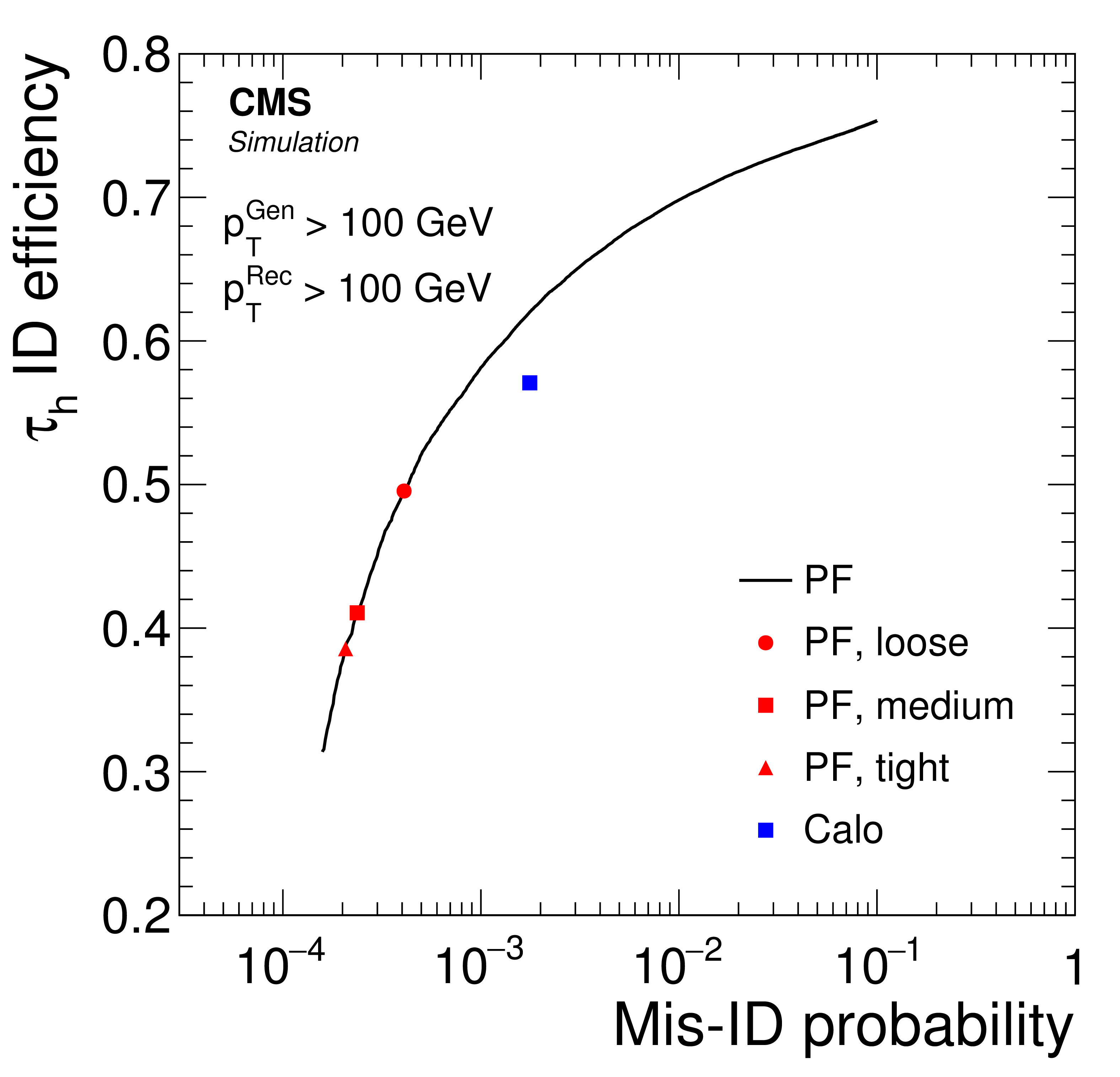
Efficiency of the $ {\tau _\mathrm {h}} $ identification versus misidentification probability for quark and gluon jets. The efficiency is measured for $ {\tau _\mathrm {h}} $ produced at low $ {p_{\mathrm {T}}} $ in simulated $\mathrm{ Z } / {\gamma ^{*}} \to \tau \tau $ events (left), and at high $ {p_{\mathrm {T}}} $ in the decay of a heavy particle $\mathrm{ H } $(3.2 TeV) $\to \tau \tau $ events (right). The misidentification probability is measured for quark and gluon jets in simulated multijet events. The line is obtained by varying the threshold on the absolute isolation for PF $ {\tau _\mathrm {h}} $ identified with the HPS algorithm. On this curve, the three points indicate the loose, medium and tight isolation working points. The performance of the calorimeter-based $ {\tau _\mathrm {h}} $ identification is depicted by a square away from the line. |
png pdf |
Figure 20-a:
Efficiency of the $ {\tau _\mathrm {h}} $ identification versus misidentification probability for quark and gluon jets. The efficiency is measured for $ {\tau _\mathrm {h}} $ produced at low $ {p_{\mathrm {T}}} $ in simulated $\mathrm{ Z } / {\gamma ^{*}} \to \tau \tau $ events. The misidentification probability is measured for quark and gluon jets in simulated multijet events. The line is obtained by varying the threshold on the absolute isolation for PF $ {\tau _\mathrm {h}} $ identified with the HPS algorithm. On this curve, the three points indicate the loose, medium and tight isolation working points. The performance of the calorimeter-based $ {\tau _\mathrm {h}} $ identification is depicted by a square away from the line. |
png pdf |
Figure 20-b:
Efficiency of the $ {\tau _\mathrm {h}} $ identification versus misidentification probability for quark and gluon jets. The efficiency is measured for $ {\tau _\mathrm {h}} $ produced at high $ {p_{\mathrm {T}}} $ in the decay of a heavy particle $\mathrm{ H } $(3.2 TeV) $\to \tau \tau $ events. The misidentification probability is measured for quark and gluon jets in simulated multijet events. The line is obtained by varying the threshold on the absolute isolation for PF $ {\tau _\mathrm {h}} $ identified with the HPS algorithm. On this curve, the three points indicate the loose, medium and tight isolation working points. The performance of the calorimeter-based $ {\tau _\mathrm {h}} $ identification is depicted by a square away from the line. |
png pdf |
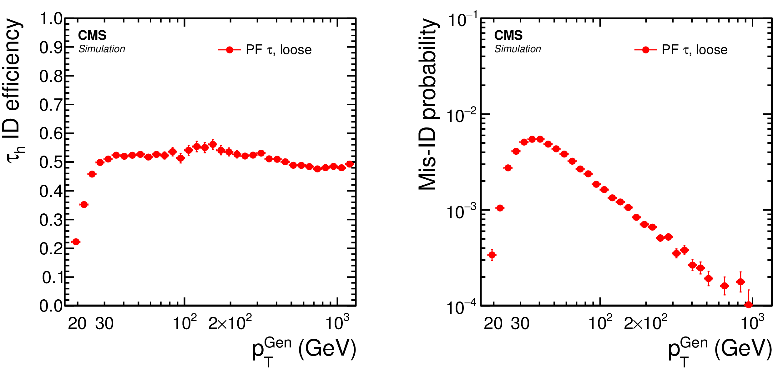
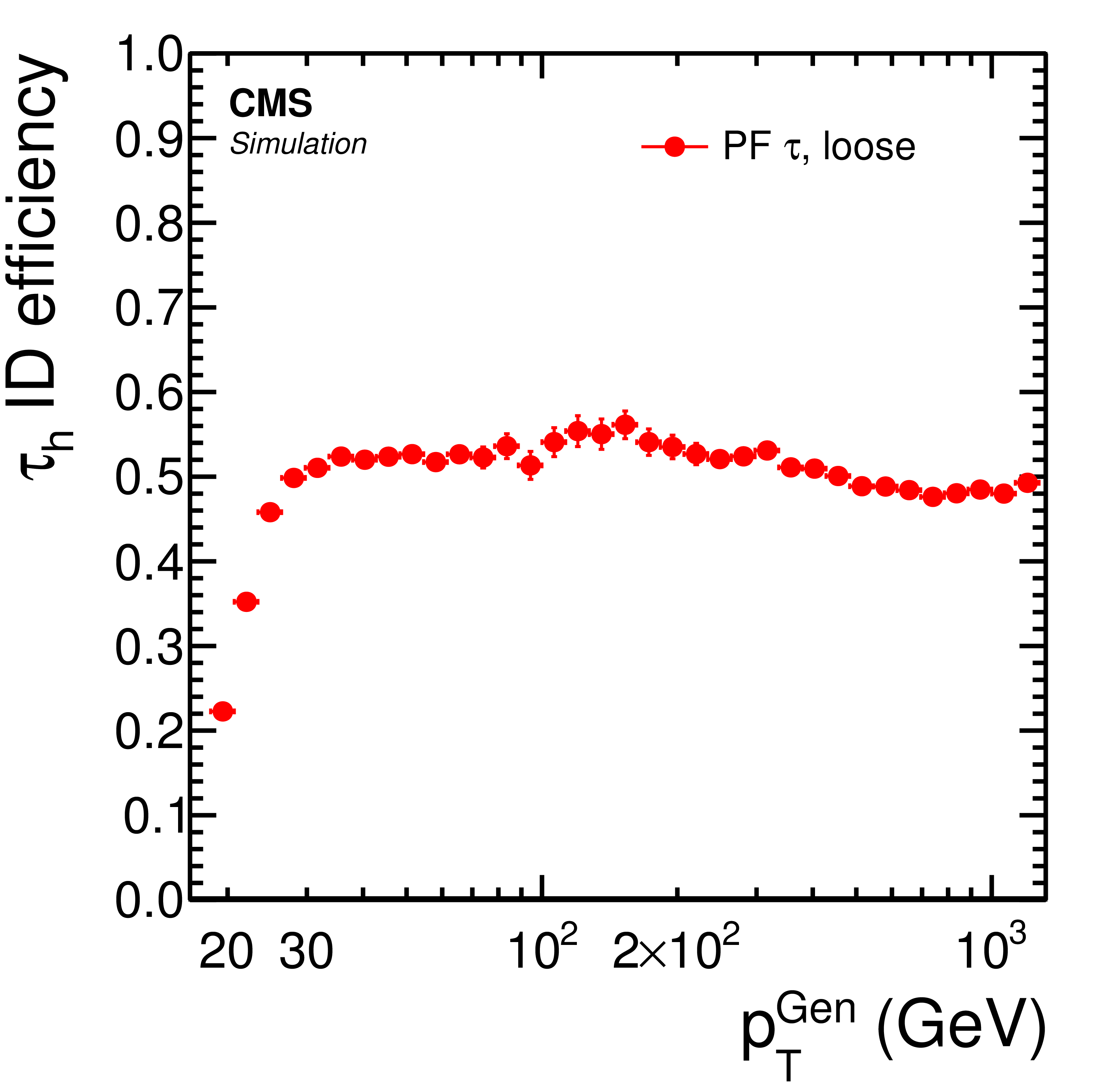
Figure 21:
Identification efficiency for genuine $ {\tau _\mathrm {h}} $ (left), and $ {\tau _\mathrm {h}} $ misidentification probability for quark and gluon jets (right). Low-$ {p_{\mathrm {T}}} $ $ {\tau _\mathrm {h}} $ are obtained from simulated $\mathrm{ Z } / {\gamma ^{*}} \to \tau \tau $ events and high-$ {p_{\mathrm {T}}} $ $ {\tau _\mathrm {h}} $ from simulated $\mathrm{ H } $(3.2 TeV)$ \to \tau \tau $ events. Quark and gluon jets are obtained from simulated QCD multijet events. The $ {\tau _\mathrm {h}} $ are required to be reconstructed by the HPS (PF) algorithm, to have $ {p_{\mathrm {T}}} > $ 20 GeV and $ {| \eta | } < $ 2.3, and to satisfy the loose $ {\tau _\mathrm {h}} $ identification criteria. |
png pdf |
Figure 21-a:
Identification efficiency for genuine $ {\tau _\mathrm {h}} $. Low-$ {p_{\mathrm {T}}} $ $ {\tau _\mathrm {h}} $ are obtained from simulated $\mathrm{ Z } / {\gamma ^{*}} \to \tau \tau $ events and high-$ {p_{\mathrm {T}}} $ $ {\tau _\mathrm {h}} $ from simulated $\mathrm{ H } $(3.2 TeV)$ \to \tau \tau $ events. Quark and gluon jets are obtained from simulated QCD multijet events. The $ {\tau _\mathrm {h}} $ are required to be reconstructed by the HPS (PF) algorithm, to have $ {p_{\mathrm {T}}} > $ 20 GeV and $ {| \eta | } < $ 2.3, and to satisfy the loose $ {\tau _\mathrm {h}} $ identification criteria. |

png pdf |
Figure 21-b:
$ {\tau _\mathrm {h}} $ misidentification probability for quark and gluon jets. Low-$ {p_{\mathrm {T}}} $ $ {\tau _\mathrm {h}} $ are obtained from simulated $\mathrm{ Z } / {\gamma ^{*}} \to \tau \tau $ events and high-$ {p_{\mathrm {T}}} $ $ {\tau _\mathrm {h}} $ from simulated $\mathrm{ H } $(3.2 TeV)$ \to \tau \tau $ events. Quark and gluon jets are obtained from simulated QCD multijet events. The $ {\tau _\mathrm {h}} $ are required to be reconstructed by the HPS (PF) algorithm, to have $ {p_{\mathrm {T}}} > $ 20 GeV and $ {| \eta | } < $ 2.3, and to satisfy the loose $ {\tau _\mathrm {h}} $ identification criteria. |
png pdf |
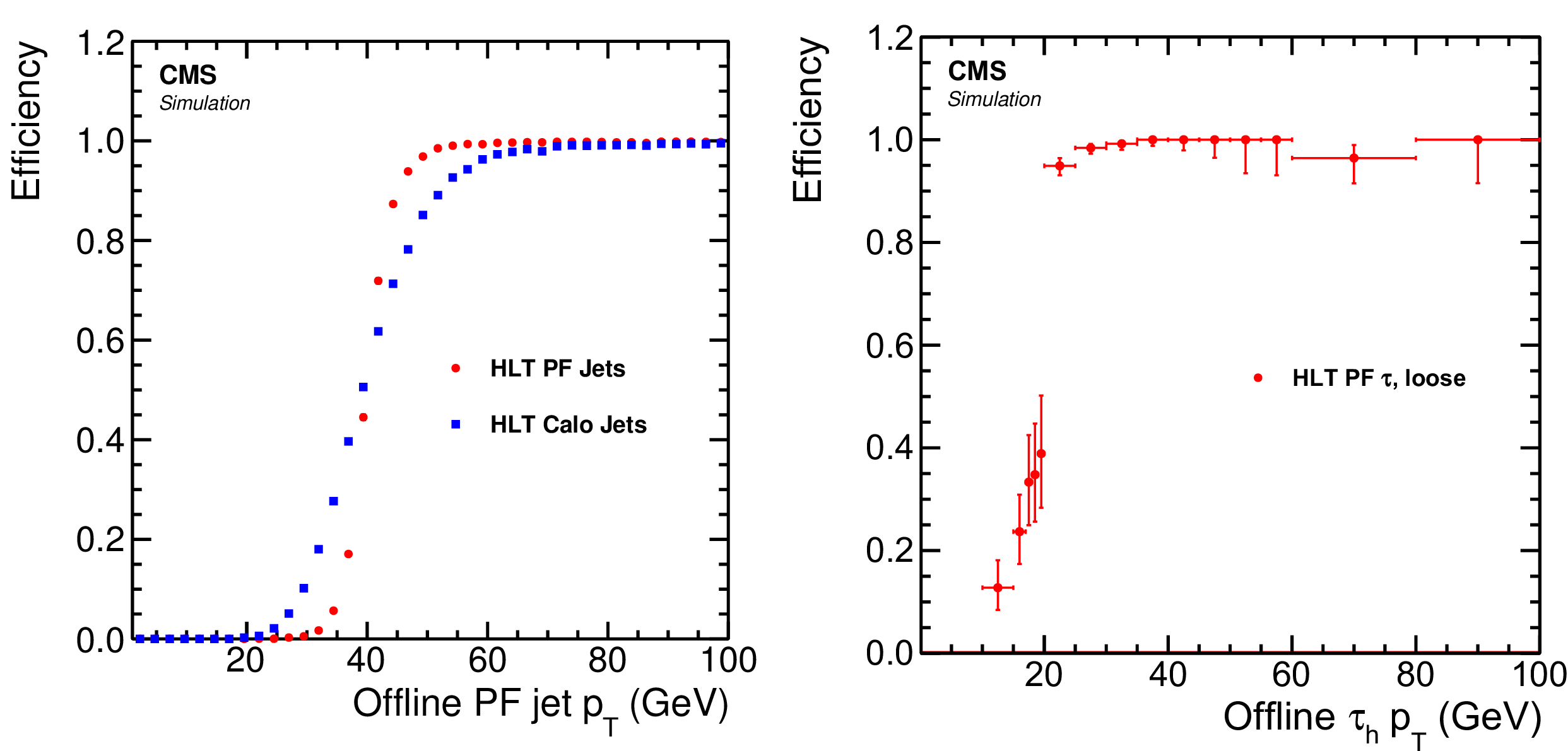
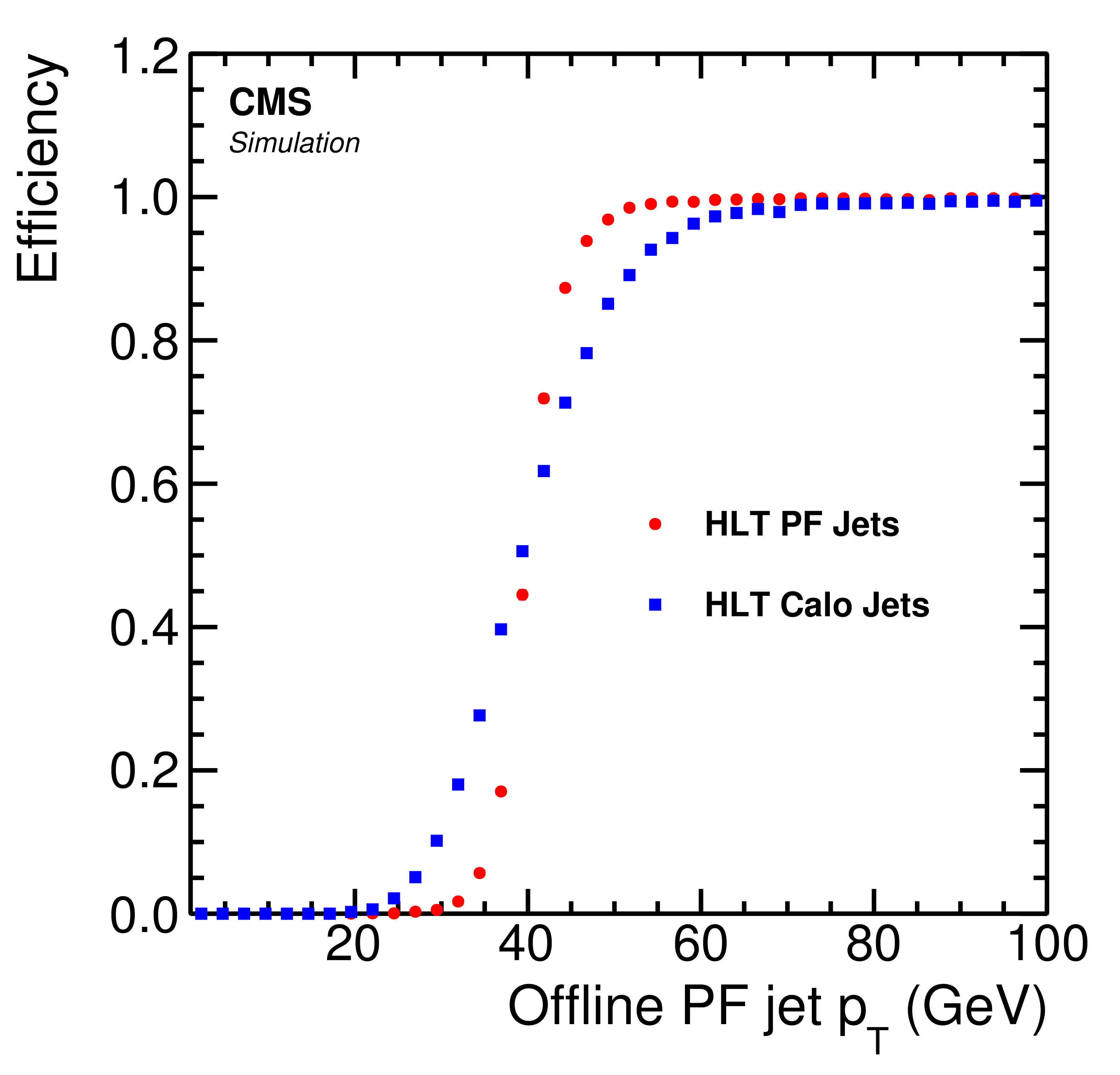
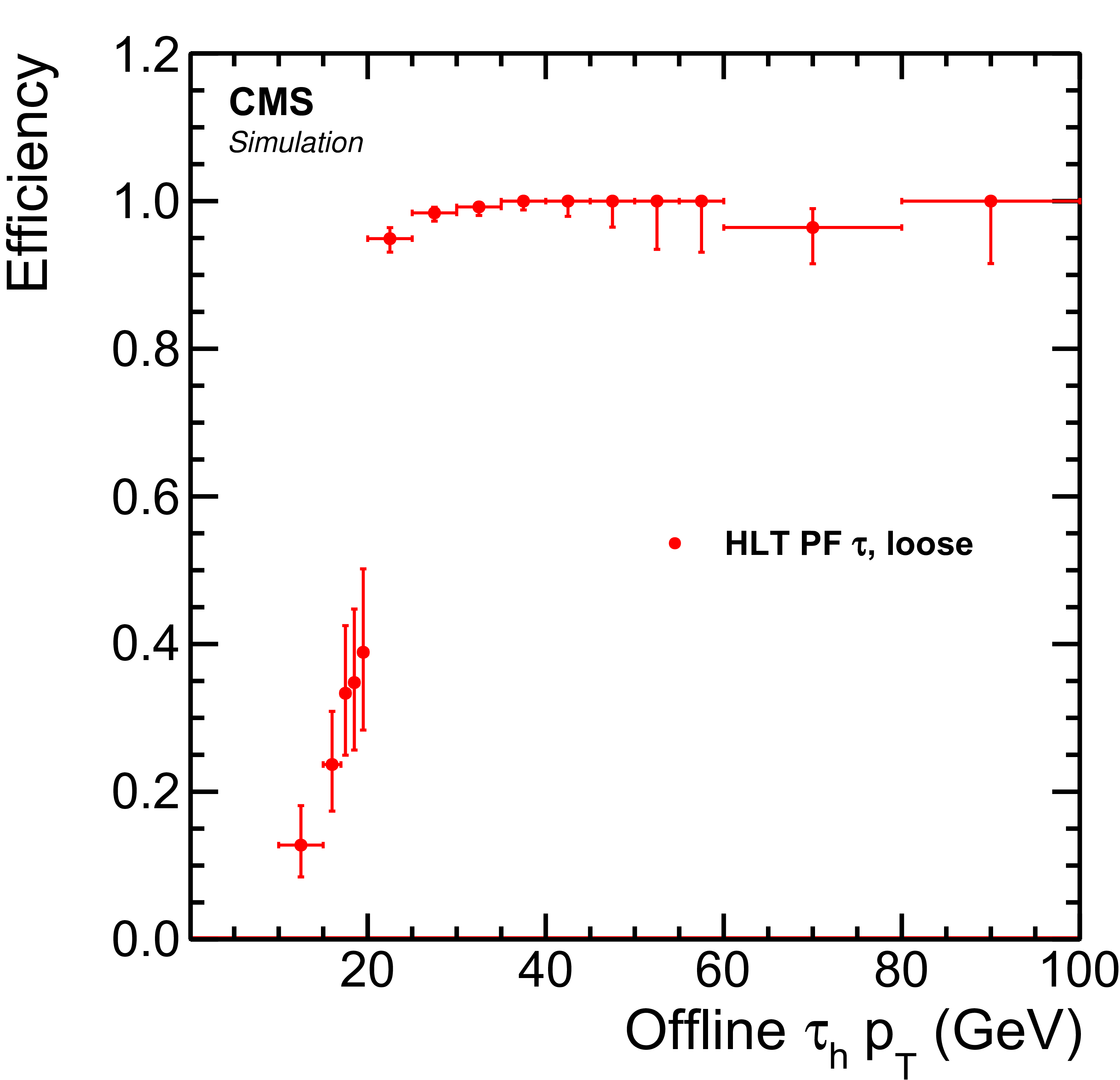
Figure 22:
Left: Probability to find at HLT a jet with $ {p_{\mathrm {T}}} >40 GeV $ matching the jet reconstructed offline, as a function of the offline jet $ {p_{\mathrm {T}}} $. At the threshold, the curve is steeper for HLT PF jets (circles) than for HLT calorimeter jets (squares). Right: Probability to find a $ {\tau _\mathrm {h}} $ with $ {p_{\mathrm {T}}} >20 GeV $ at HLT matching the $ {\tau _\mathrm {h}} $ reconstructed and identified offline with the loose isolation working point. |
png pdf |
Figure 22-a:
Probability to find at HLT a jet with $ {p_{\mathrm {T}}} >40 GeV $ matching the jet reconstructed offline, as a function of the offline jet $ {p_{\mathrm {T}}} $. At the threshold, the curve is steeper for HLT PF jets (circles) than for HLT calorimeter jets (squares). |
png pdf |
Figure 22-b:
Probability to find a $ {\tau _\mathrm {h}} $ with $ {p_{\mathrm {T}}} >20 GeV $ at HLT matching the $ {\tau _\mathrm {h}} $ reconstructed and identified offline with the loose isolation working point. |
png pdf |
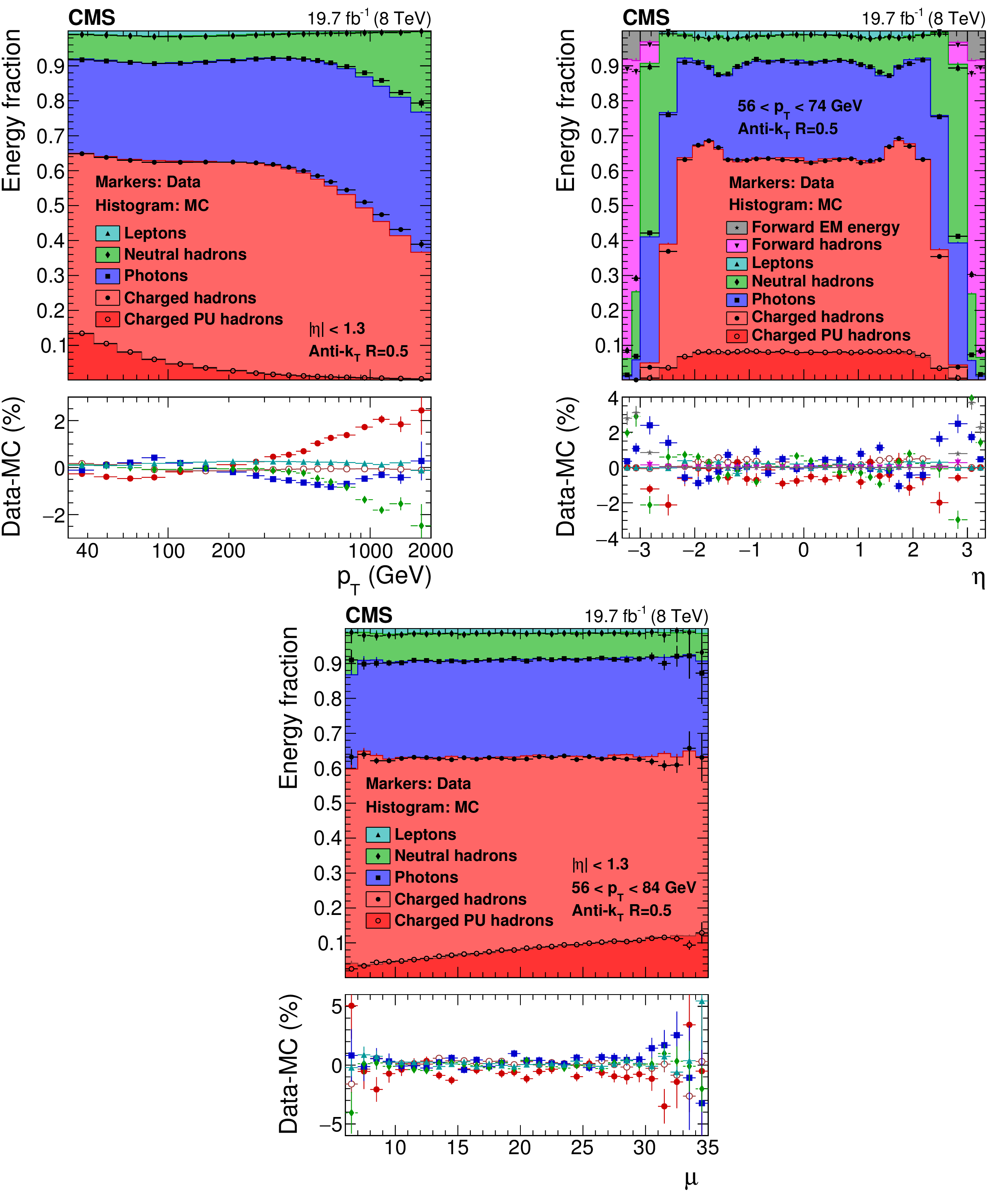
Figure 23:
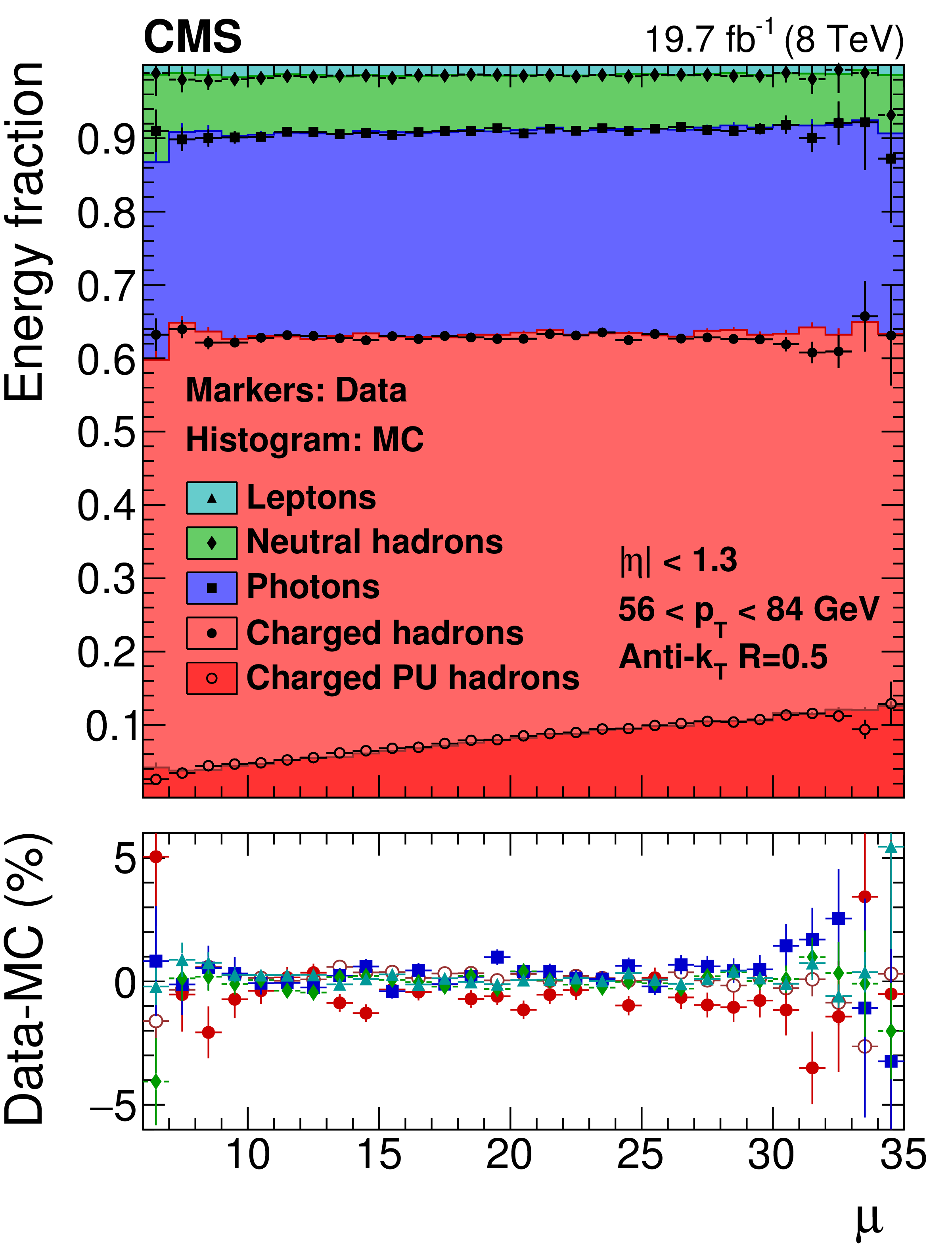
Jet energy composition in observed and simulated events as a function of $ {p_{\mathrm {T}}} $ (top left), $\eta $ (top right), and number of pileup interactions (bottom). The top panels show the measured and simulated energy fractions stacked, whereas the bottom panels show the difference between observed and simulated events. Charged hadrons associated with pileup vertices are denoted as charged PU hadrons. |
png pdf |
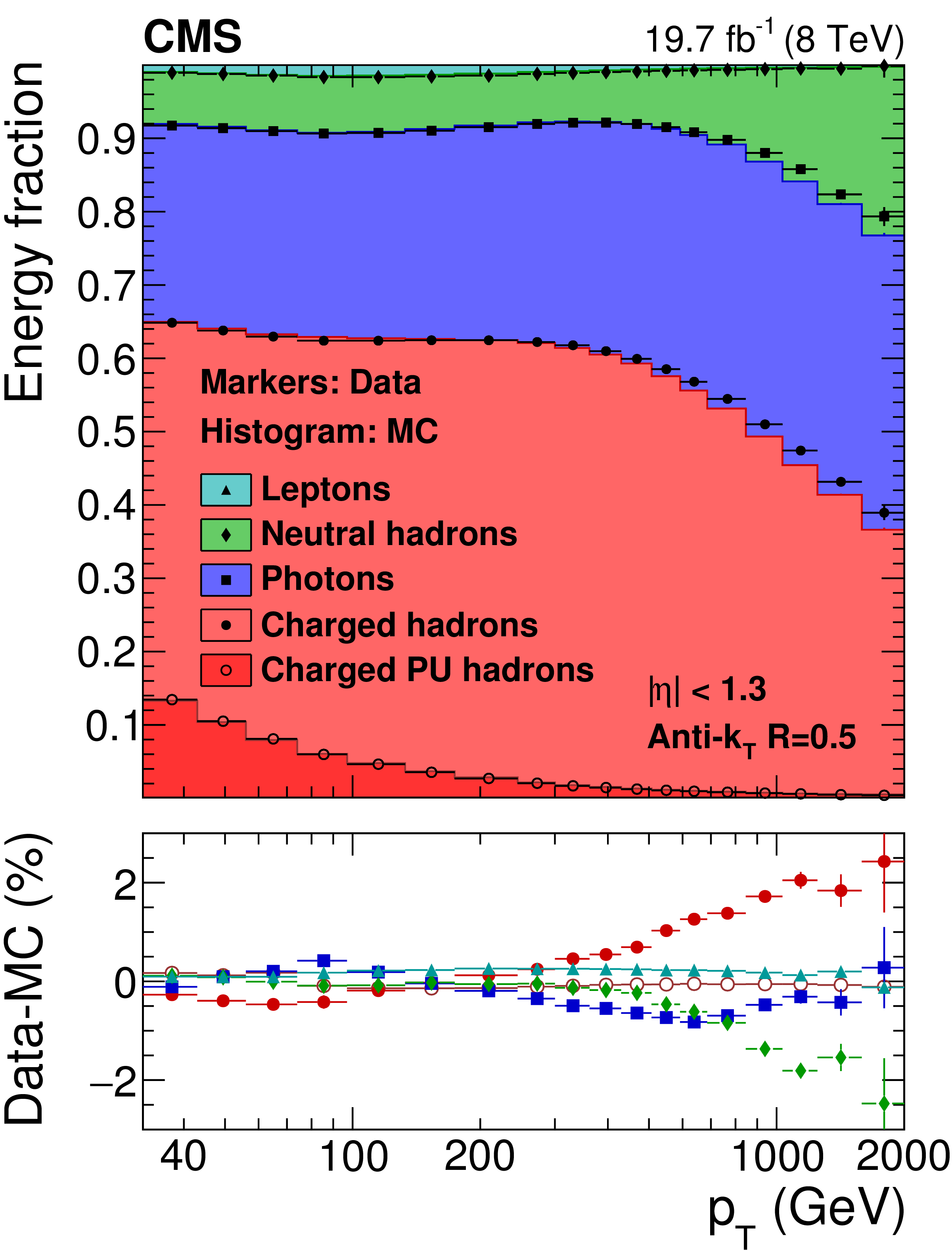
Figure 23-a:
Jet energy composition in observed and simulated events as a function of $ {p_{\mathrm {T}}} $. The top panels show the measured and simulated energy fractions stacked, whereas the bottom panels show the difference between observed and simulated events. Charged hadrons associated with pileup vertices are denoted as charged PU hadrons. |
png pdf |
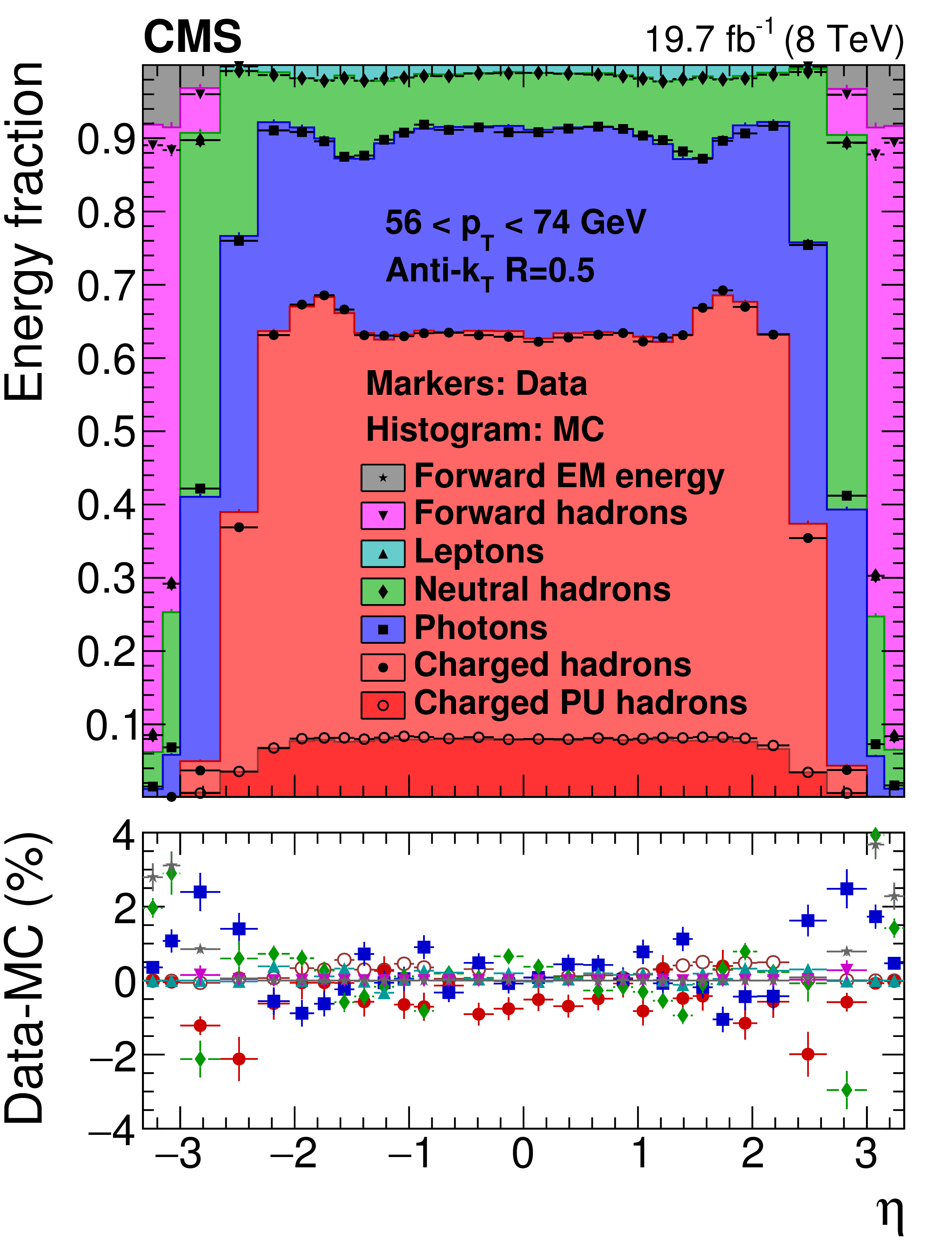
Figure 23-b:
Jet energy composition in observed and simulated events as a function of $\eta $. The top panels show the measured and simulated energy fractions stacked, whereas the bottom panels show the difference between observed and simulated events. Charged hadrons associated with pileup vertices are denoted as charged PU hadrons. |
png pdf |
Figure 23-c:
Jet energy composition in observed and simulated events as a function of the number of pileup interactions. The top panels show the measured and simulated energy fractions stacked, whereas the bottom panels show the difference between observed and simulated events. Charged hadrons associated with pileup vertices are denoted as charged PU hadrons. |
png pdf |
Figure 24:
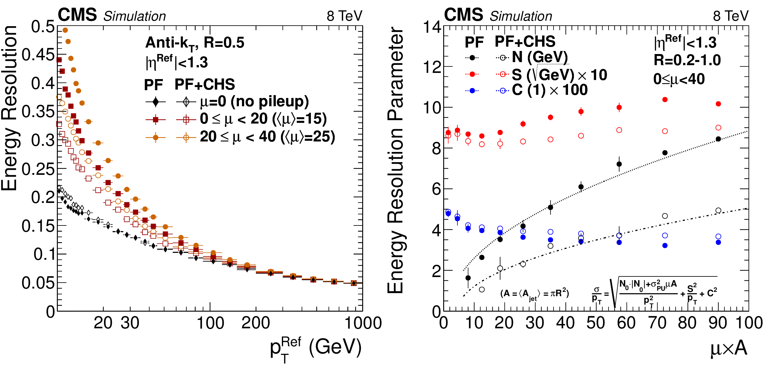
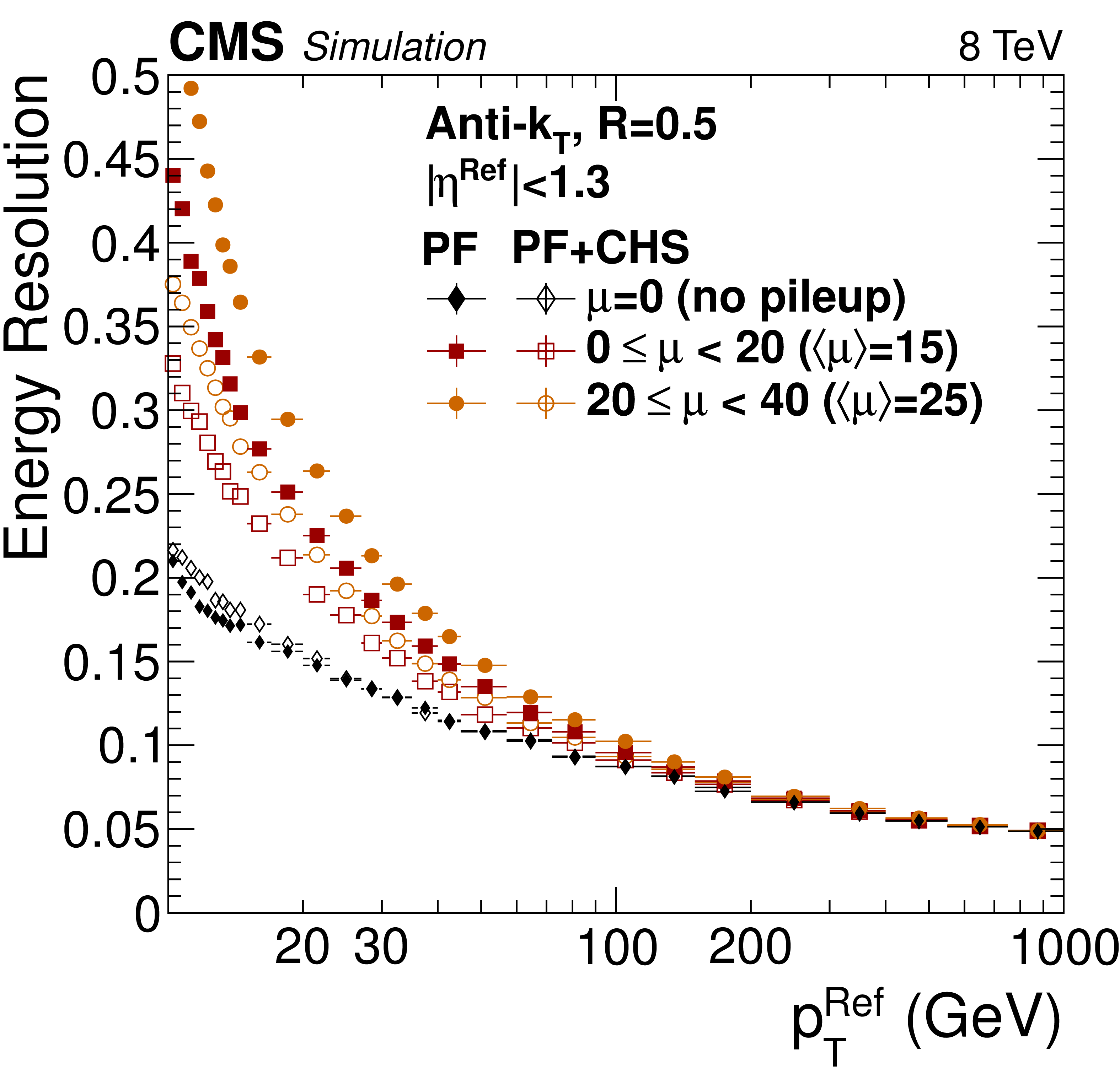
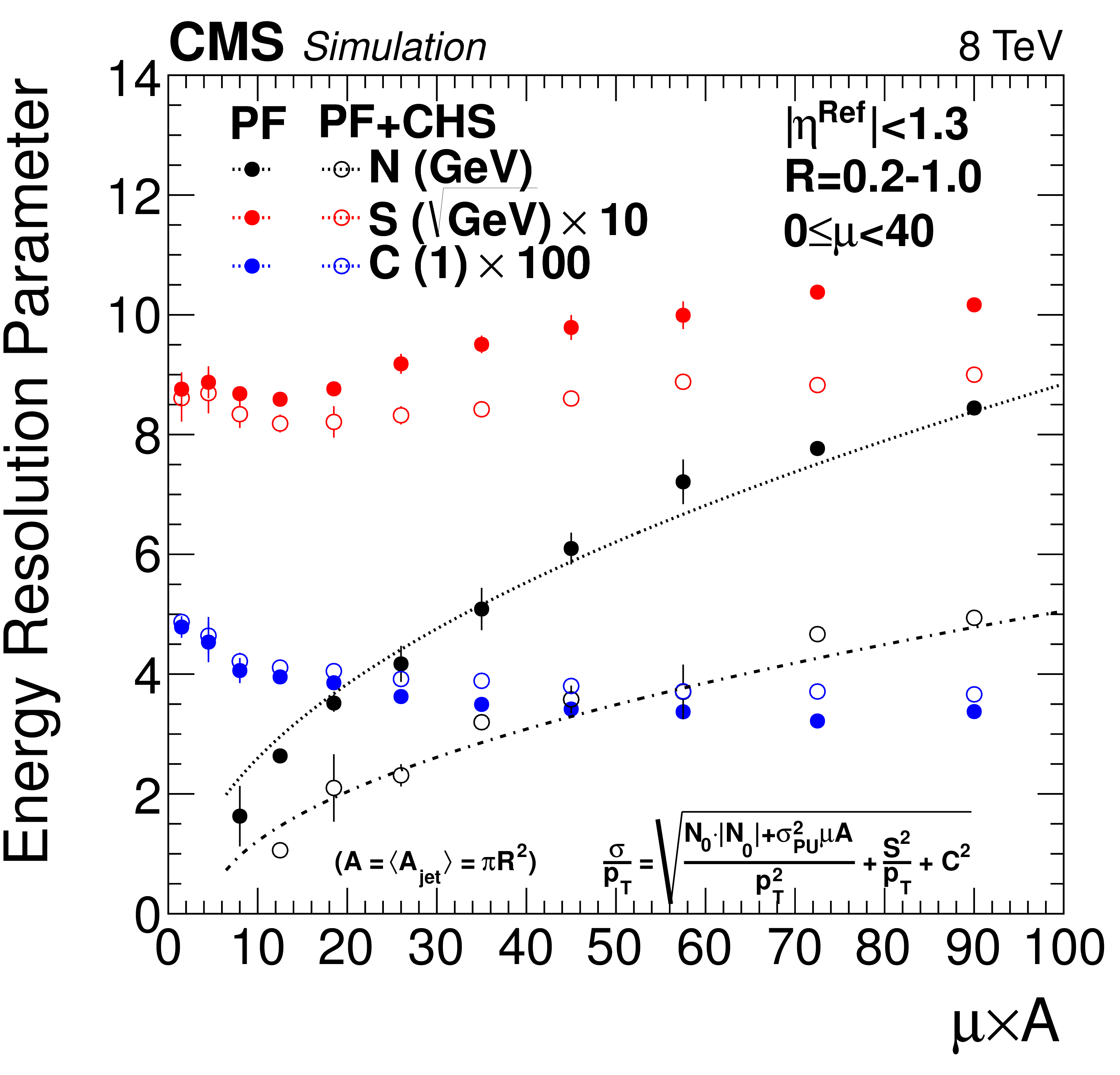
Jet $ {p_{\mathrm {T}}} $ resolution for PF+CHS jets (open markers) and PF jets (full markers) under three different pileup conditions (left), and jet energy resolution parameters (right). The jet $ {p_{\mathrm {T}}} $ resolution is shown as a function of $ {p_{\mathrm {T}}} ^\text {Ref}$. The jet energy resolution parameters are shown as a function of the number of pileup interactions $\mu $ times the jet area $A$ for PF jets and PF+CHS jets. The three resolution parameters are determined in bins of $\mu $ for various radius parameters $R$, and then averaged in bins of $\mu A$. |
png pdf |
Figure 24-a:
Jet $ {p_{\mathrm {T}}} $ resolution for PF+CHS jets (open markers) and PF jets (full markers) under three different pileup conditions. The jet $ {p_{\mathrm {T}}} $ resolution is shown as a function of $ {p_{\mathrm {T}}} ^\text {Ref}$. The jet energy resolution parameters are shown as a function of the number of pileup interactions $\mu $ times the jet area $A$ for PF jets and PF+CHS jets. The three resolution parameters are determined in bins of $\mu $ for various radius parameters $R$, and then averaged in bins of $\mu A$. |
png pdf |
Figure 24-b:
Jet $ {p_{\mathrm {T}}} $ resolution for PF+CHS jets (open markers) and PF jets (full markers) under three different jet energy resolution parameters. The jet $ {p_{\mathrm {T}}} $ resolution is shown as a function of $ {p_{\mathrm {T}}} ^\text {Ref}$. The jet energy resolution parameters are shown as a function of the number of pileup interactions $\mu $ times the jet area $A$ for PF jets and PF+CHS jets. The three resolution parameters are determined in bins of $\mu $ for various radius parameters $R$, and then averaged in bins of $\mu A$. |

png pdf |
Figure 25:
Ratio of PF jet multiplicity with and without application of CHS, for hard jets, pileup jets, and soft jets, as a function of the reconstructed jet pseudorapidity. The uncertainty bands include both statistical uncertainties and uncertainties in the jet energy corrections. |
png pdf |
Figure 26:
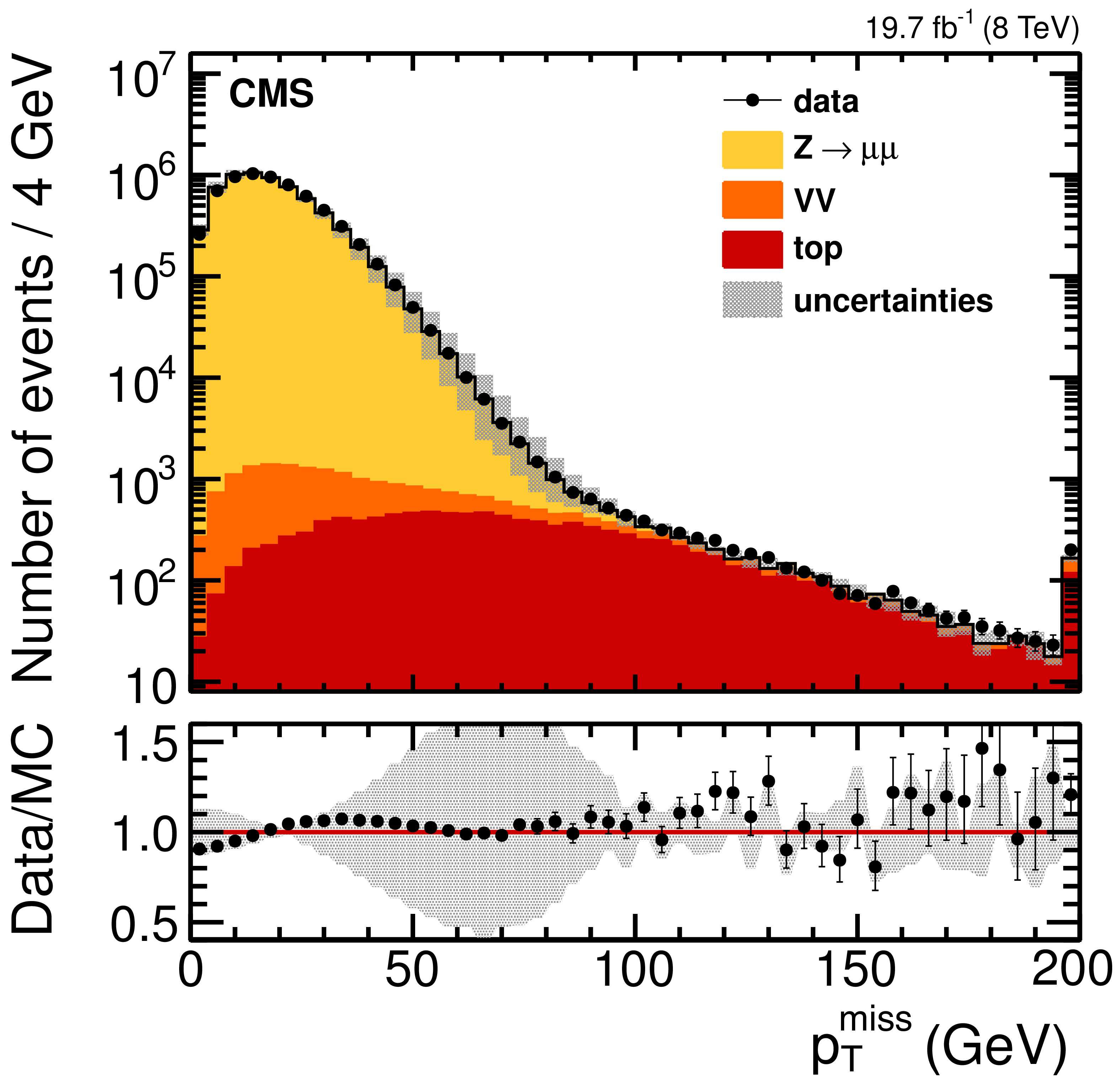
Spectrum of PF $ { {p_{\mathrm {T}}} ^\text {miss}} $ in a $\mathrm{ Z } \to \mu \mu $ data set [47]. The observed data are compared to simulated $\mathrm{ Z } \to \mu \mu $, diboson (VV), and ${\mathrm{ t } {}\mathrm{ \bar{t} } } $ plus single top quark events. The lower panel shows the ratio of data to simulation, with the uncertainty bars of the points including the statistical uncertainties of both observed and simulated events and the grey uncertainty band displaying the systematic uncertainty in the simulation. The last bin contains the overflow. |

png pdf |
Figure 27:
Comparison of the average response of the parallel recoil component, $- < u_{\text{parallel}} > q_\mathrm {T}$, for the PF ${{\vec p}_{\mathrm {T}}}^{\, \text{miss}} $, No-PU PF ${{\vec p}_{\mathrm {T}}}^{\, \text{miss}} $, and MVA PF ${{\vec p}_{\mathrm {T}}}^{\, \text{miss}} $ (denoted as MVA Unity PF ${E_{\mathrm {T}}}$) algorithms as a function of $q_\mathrm {T}$, as determined in $\mathrm{ Z } \to \mu \mu $ events. |

png pdf |
Figure 28:
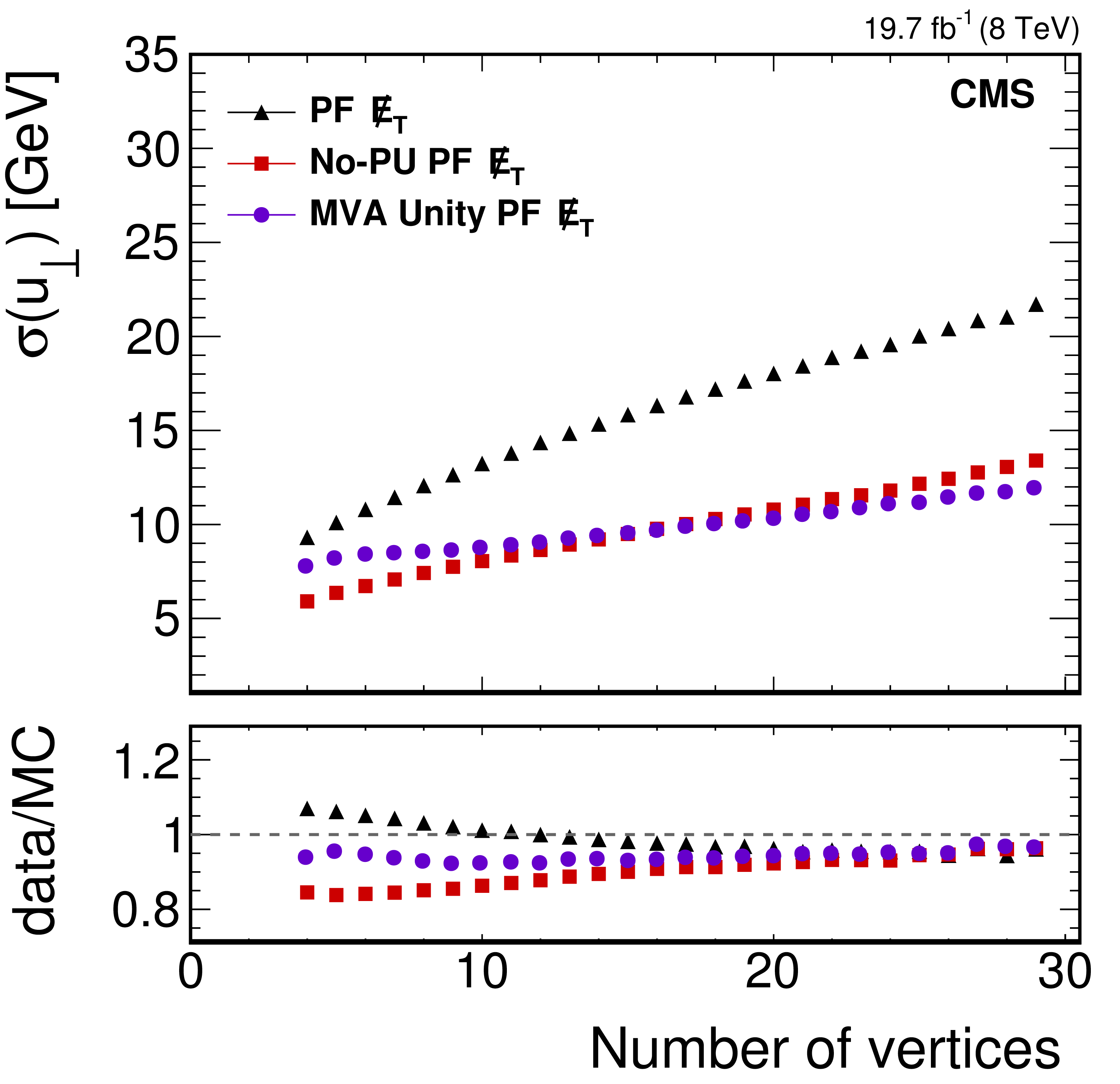
Comparison of the resolutions of the parallel (left) and perpendicular (right) recoil components for the PF ${{\vec p}_{\mathrm {T}}}^{\, \text{miss}} $, No-PU PF ${{\vec p}_{\mathrm {T}}}^{\, \text{miss}} $, and MVA PF ${{\vec p}_{\mathrm {T}}}^{\, \text{miss}} $ algorithms as a function of the number of reconstructed vertices in $\mathrm{ Z } \to \mu \mu $ events [47]. The upper frame of each figure shows the resolution in observed events; the lower frame shows the ratio of data to simulation. |

png pdf |
Figure 28-a:
Comparison of the resolutions of the parallel recoil components for the PF ${{\vec p}_{\mathrm {T}}}^{\, \text{miss}} $, No-PU PF ${{\vec p}_{\mathrm {T}}}^{\, \text{miss}} $, and MVA PF ${{\vec p}_{\mathrm {T}}}^{\, \text{miss}} $ algorithms as a function of the number of reconstructed vertices in $\mathrm{ Z } \to \mu \mu $ events [47]. The upper frame of the figure shows the resolution in observed events; the lower frame shows the ratio of data to simulation. |
png pdf |
Figure 28-b:
Comparison of the resolutions of the perpendicular recoil components for the PF ${{\vec p}_{\mathrm {T}}}^{\, \text{miss}} $, No-PU PF ${{\vec p}_{\mathrm {T}}}^{\, \text{miss}} $, and MVA PF ${{\vec p}_{\mathrm {T}}}^{\, \text{miss}} $ algorithms as a function of the number of reconstructed vertices in $\mathrm{ Z } \to \mu \mu $ events [47]. The upper frame of the figure shows the resolution in observed events; the lower frame shows the ratio of data to simulation. |
png pdf |
Figure 29:
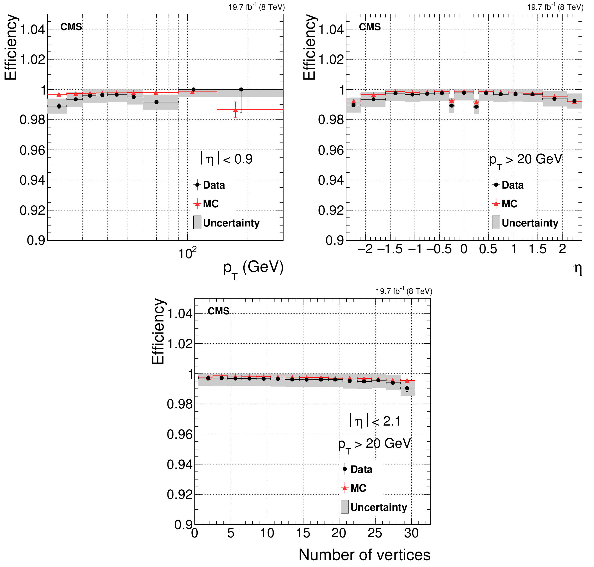
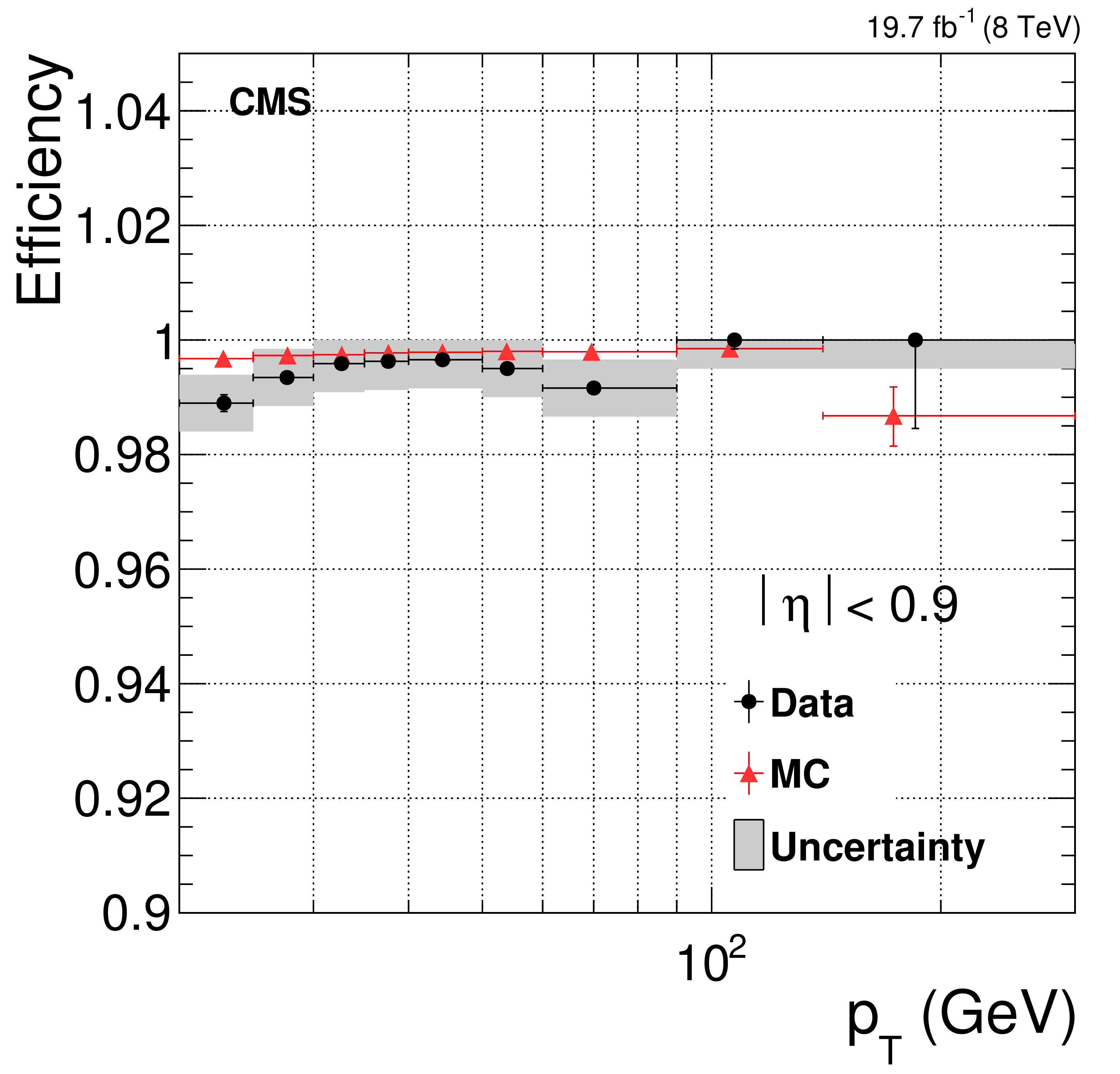
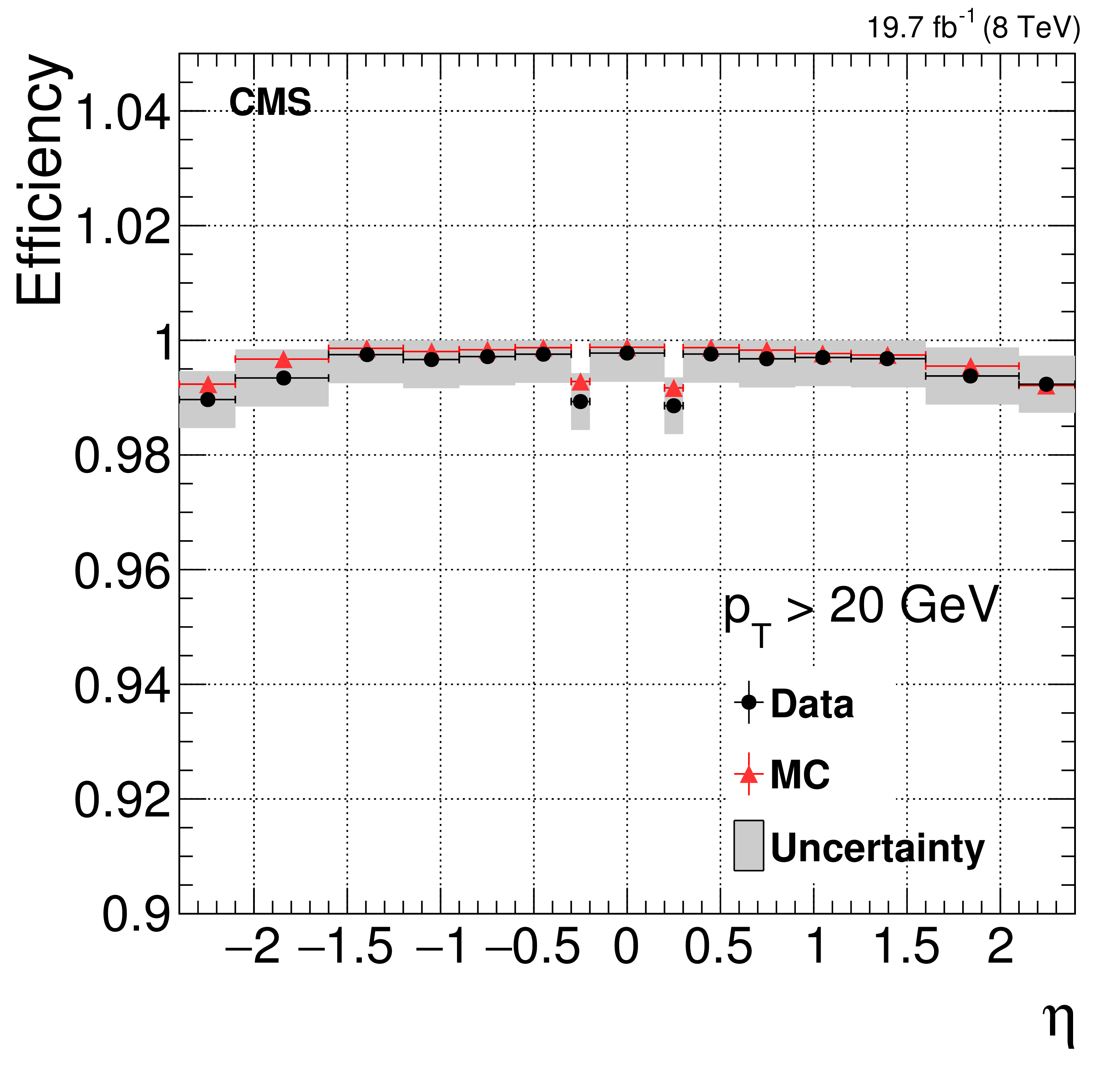
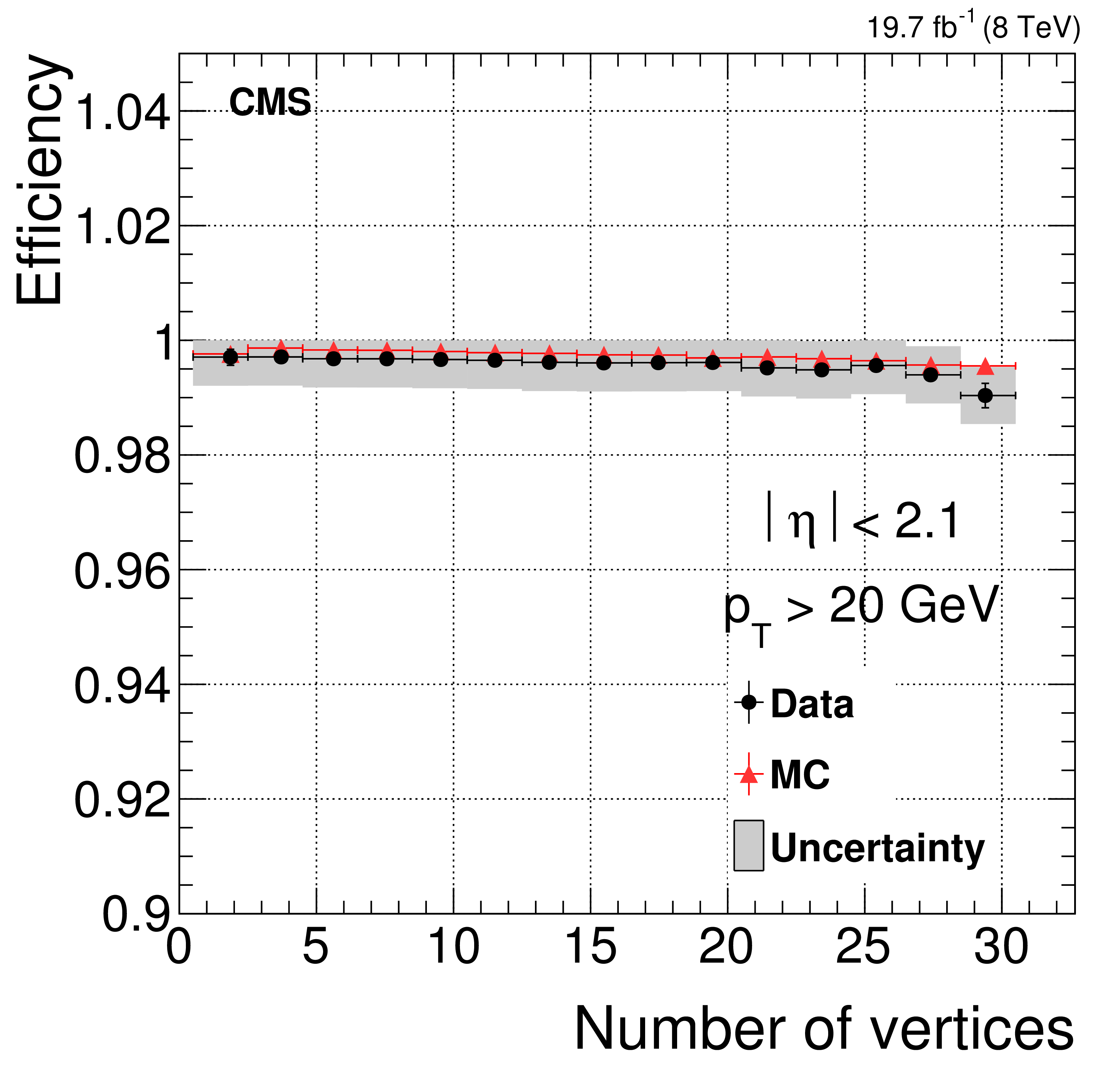
Efficiency of the PF muon identification for muons from ${\mathrm{ Z } } $boson decays as a function of $ {p_{\mathrm {T}}} $ (top left), $\eta $ (top right), and $N_\text {vtx}$ (bottom). |
png pdf |
Figure 29-a:
Efficiency of the PF muon identification for muons from ${\mathrm{ Z } } $boson decays as a function of $ {p_{\mathrm {T}}} $. |
png pdf |
Figure 29-b:
Efficiency of the PF muon identification for muons from ${\mathrm{ Z } } $boson decays as a function of $\eta $. |
png pdf |
Figure 29-c:
Efficiency of the PF muon identification for muons from ${\mathrm{ Z } } $boson decays as a function of $N_\text {vtx}$. |

png pdf |
Figure 30:
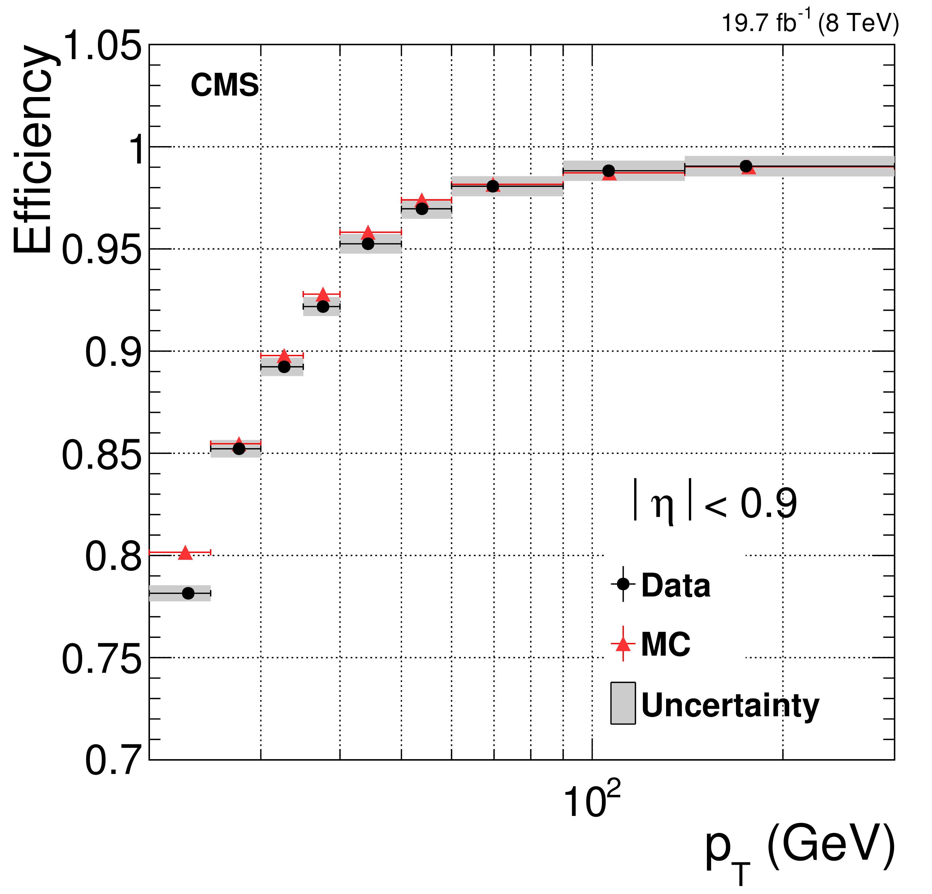
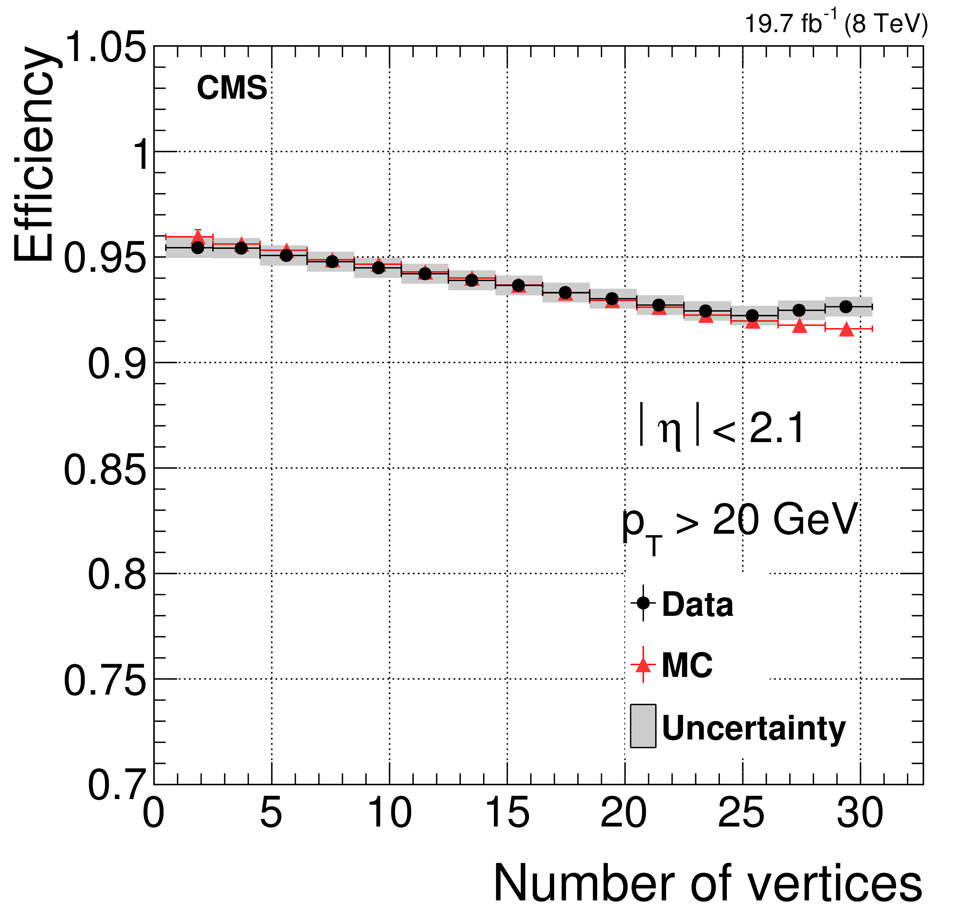
Isolation efficiency for muons from ${\mathrm{ Z } } $ boson decays as a function of $ {p_{\mathrm {T}}} $ (left) and $N_\text {vtx}$ (right). |
png pdf |
Figure 30-a:
Isolation efficiency for muons from ${\mathrm{ Z } } $ boson decays as a function of $ {p_{\mathrm {T}}} $. |
png pdf |
Figure 30-b:
Isolation efficiency for muons from ${\mathrm{ Z } } $ boson decays as a function of $N_\text {vtx}$. |
png pdf |
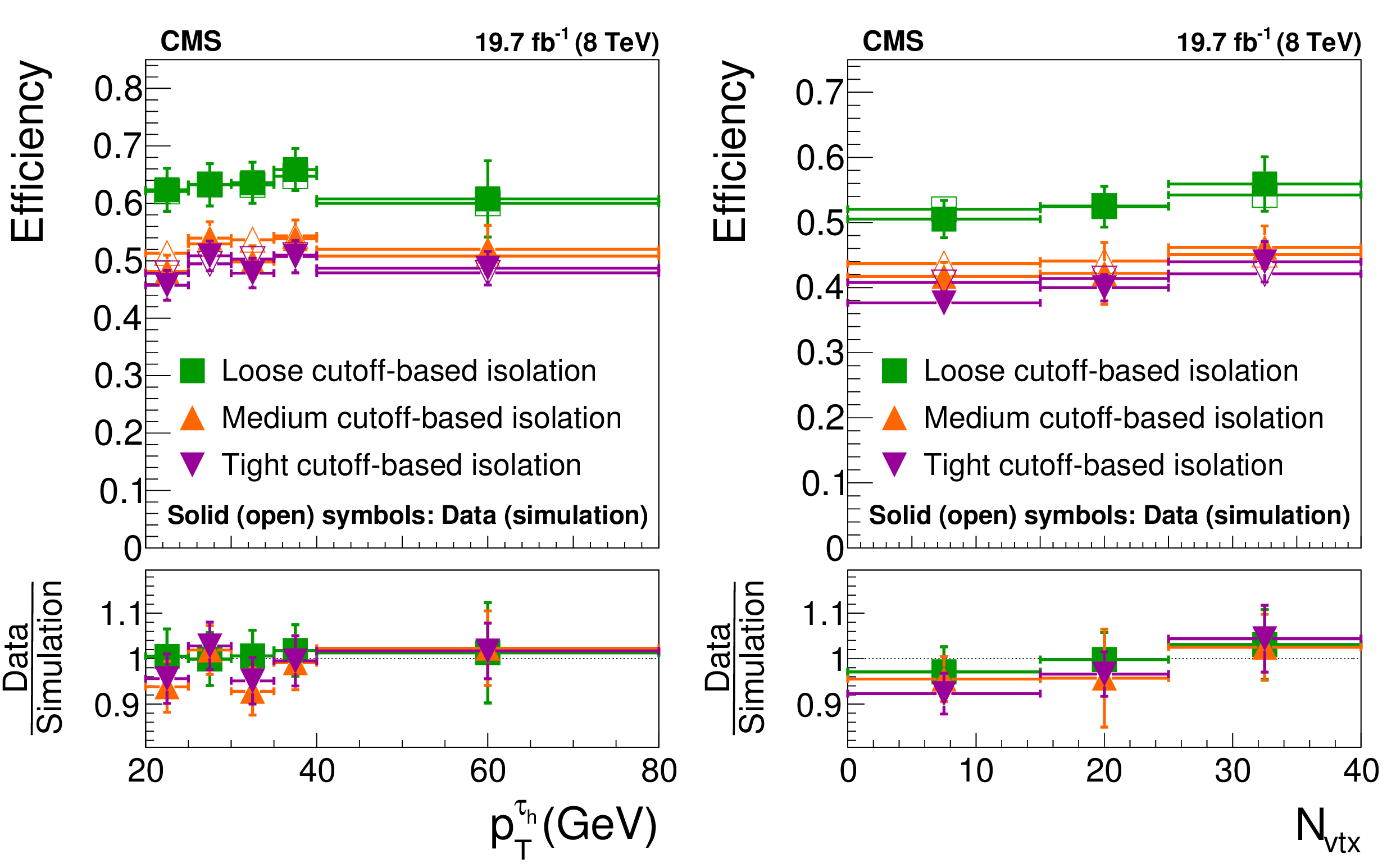
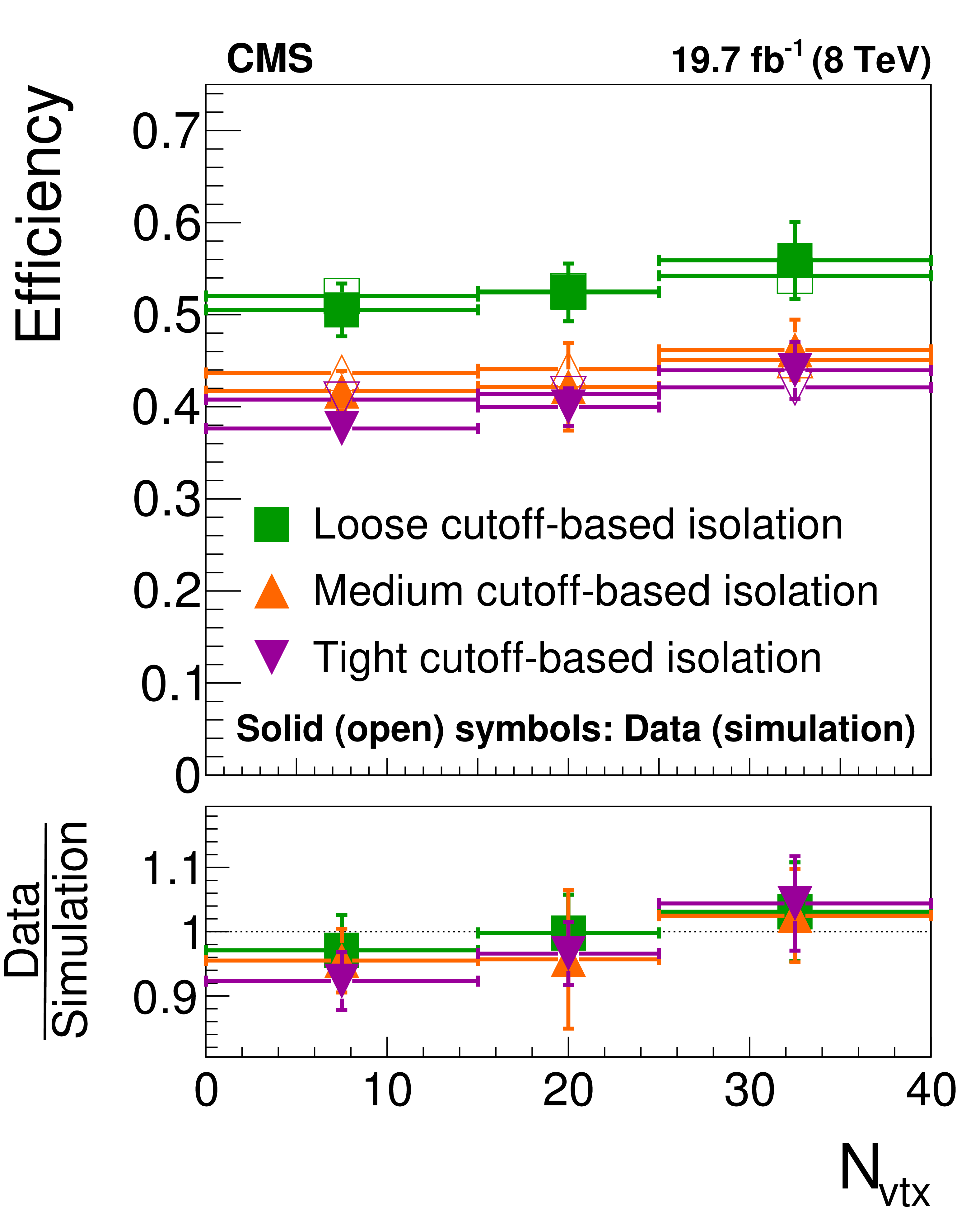
Figure 31:
Efficiency for hadronic $\tau $ decays to pass the loose, medium and tight working points of the HPS $ {\tau _\mathrm {h}} $ identification algorithm, as measured with the tag-and-probe technique in recorded and simulated $\mathrm{ Z } / {\gamma ^{*}} \to \tau \tau $ events [52]. The efficiency is presented as a function of $ {\tau _\mathrm {h}} $ $ {p_{\mathrm {T}}} $ (left), and as function of the reconstructed vertex multiplicity (right). |

png pdf |
Figure 31-a:
Efficiency for hadronic $\tau $ decays to pass the loose, medium and tight working points of the HPS $ {\tau _\mathrm {h}} $ identification algorithm, as measured with the tag-and-probe technique in recorded and simulated $\mathrm{ Z } / {\gamma ^{*}} \to \tau \tau $ events [52]. The efficiency is presented as a function of $ {\tau _\mathrm {h}} $ $ {p_{\mathrm {T}}} $. |
png pdf |
Figure 31-b:
Efficiency for hadronic $\tau $ decays to pass the loose, medium and tight working points of the HPS $ {\tau _\mathrm {h}} $ identification algorithm, as measured with the tag-and-probe technique in recorded and simulated $\mathrm{ Z } / {\gamma ^{*}} \to \tau \tau $ events [52]. The efficiency is presented as a function of the reconstructed vertex multiplicity. |

png pdf |
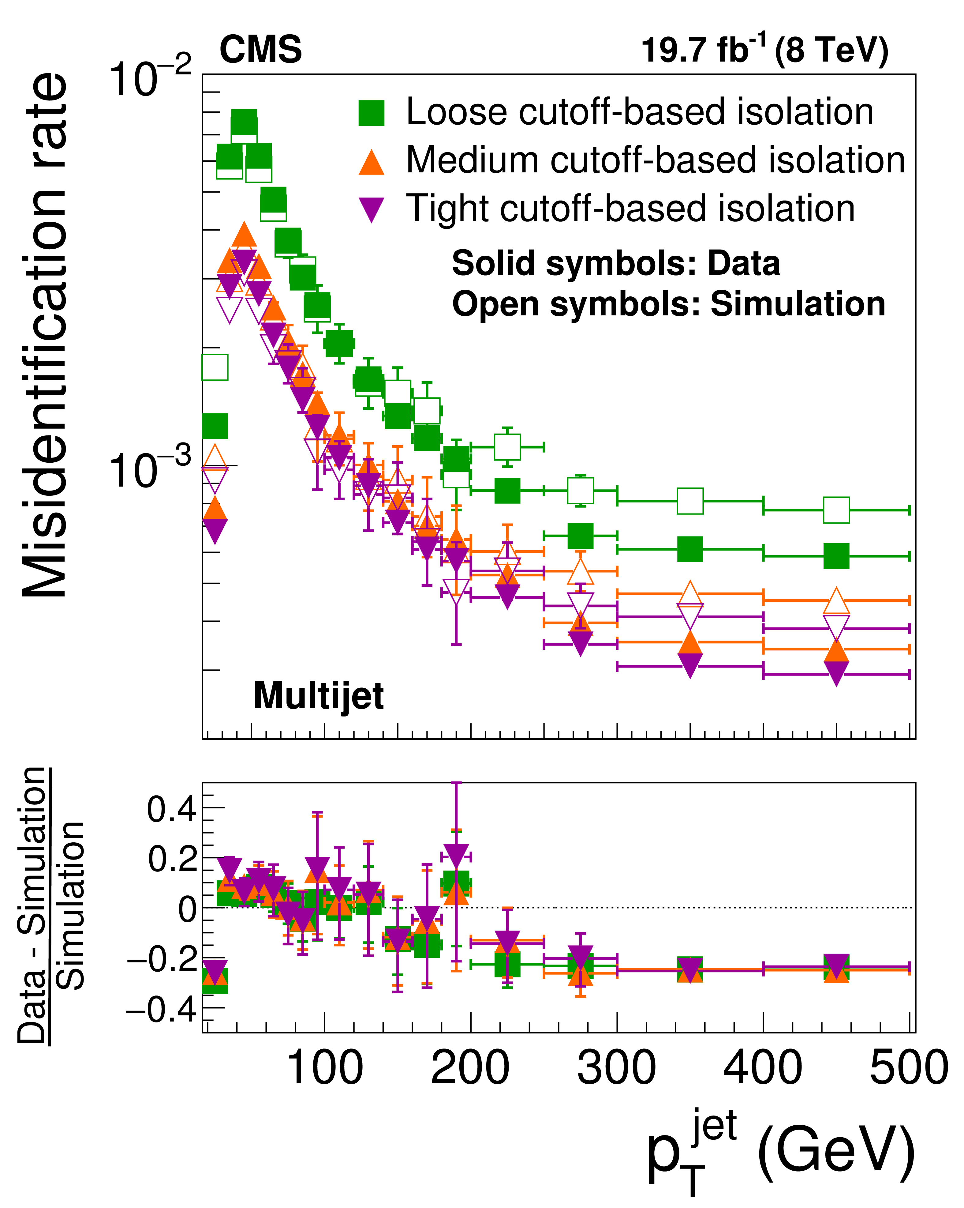
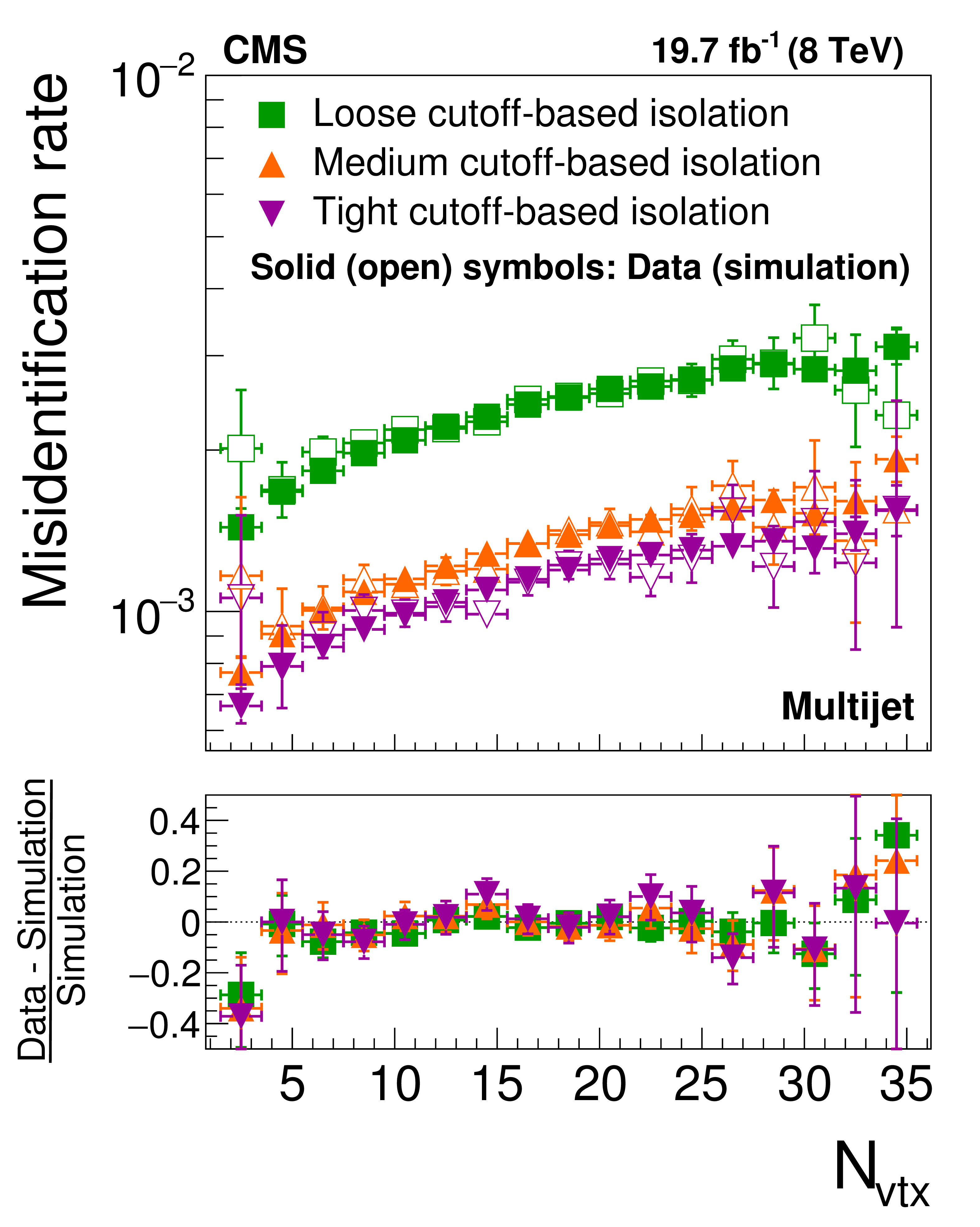
Figure 32:
Probability for quark and gluon jets to pass the $ {\tau _\mathrm {h}} $ reconstruction and $ {\tau _\mathrm {h}} $ isolation criteria as a function of jet $ {p_{\mathrm {T}}} $ (left) and number of reconstructed vertices (right) [52]. The misidentification rates measured in QCD multijet data are compared to the simulation. |
png pdf |
Figure 32-a:
Probability for quark and gluon jets to pass the $ {\tau _\mathrm {h}} $ reconstruction and $ {\tau _\mathrm {h}} $ isolation criteria as a function of jet $ {p_{\mathrm {T}}} $ [52]. The misidentification rates measured in QCD multijet data are compared to the simulation. |
png pdf |
Figure 32-b:
Probability for quark and gluon jets to pass the $ {\tau _\mathrm {h}} $ reconstruction and $ {\tau _\mathrm {h}} $ isolation criteria as a function of number of reconstructed vertices [52]. The misidentification rates measured in QCD multijet data are compared to the simulation. |
png pdf |
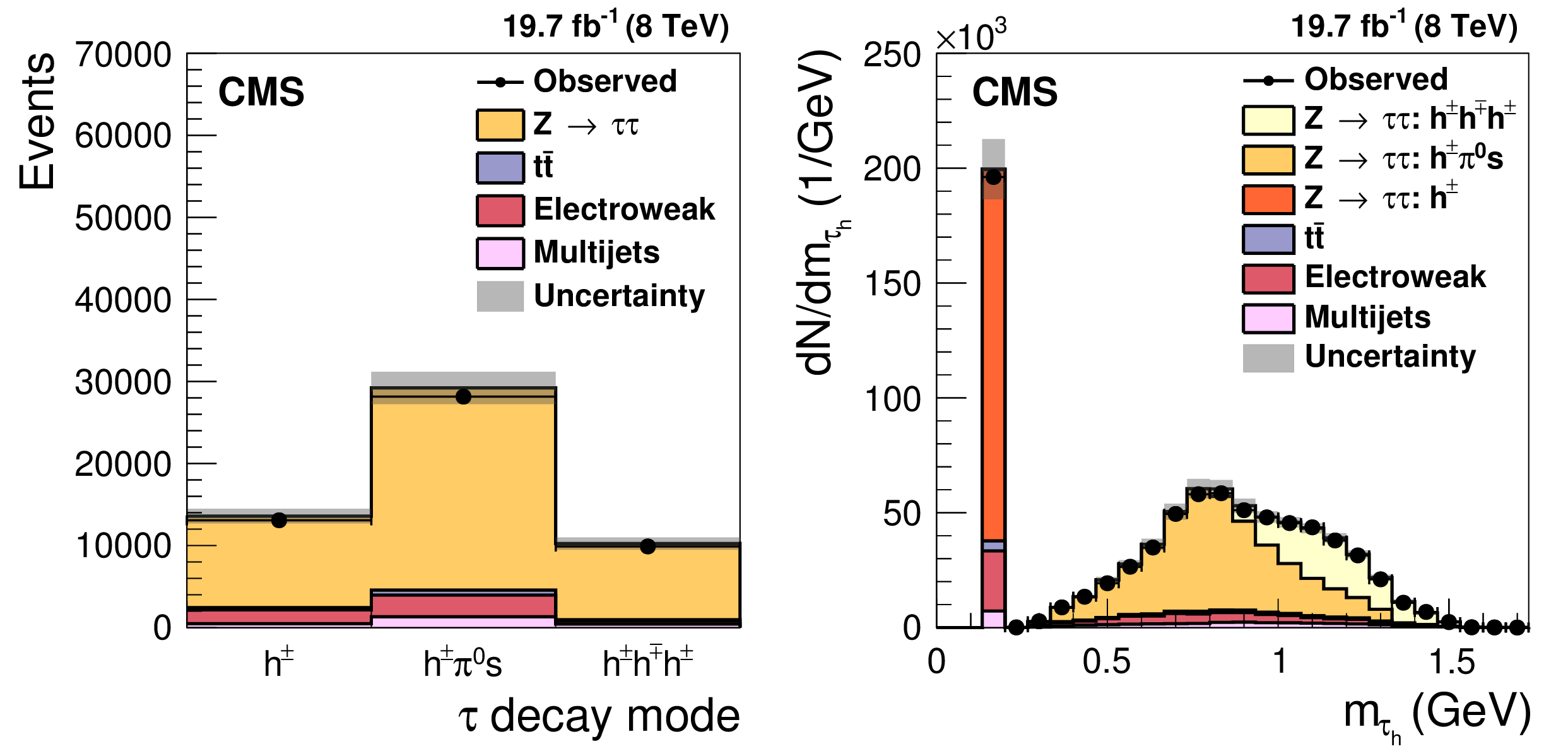
Figure 33:
Distribution of reconstructed $\tau $ decay mode (left) and of $ {\tau _\mathrm {h}} $ mass (right) in $\mathrm{ Z } / {\gamma ^{*}} \to \tau \tau $ events selected in data compared to the MC expectation. The $\mathrm{ Z } / {\gamma ^{*}} \to \tau \tau $ events are selected in the decay channel with a muon and a $ {\tau _\mathrm {h}} $. The $ {\tau _\mathrm {h}} $ is required to be reconstructed in one of the three allowed decay modes and to be isolated [52]. |

png pdf |
Figure 33-a:
Distribution of reconstructed $\tau $ decay mode in $\mathrm{ Z } / {\gamma ^{*}} \to \tau \tau $ events selected in data compared to the MC expectation. The $\mathrm{ Z } / {\gamma ^{*}} \to \tau \tau $ events are selected in the decay channel with a muon and a $ {\tau _\mathrm {h}} $. The $ {\tau _\mathrm {h}} $ is required to be reconstructed in one of the three allowed decay modes and to be isolated [52]. |

png pdf |
Figure 33-b:
Distribution of $ {\tau _\mathrm {h}} $ mass in $\mathrm{ Z } / {\gamma ^{*}} \to \tau \tau $ events selected in data compared to the MC expectation. The $\mathrm{ Z } / {\gamma ^{*}} \to \tau \tau $ events are selected in the decay channel with a muon and a $ {\tau _\mathrm {h}} $. The $ {\tau _\mathrm {h}} $ is required to be reconstructed in one of the three allowed decay modes and to be isolated [52]. |
| Tables | |
png pdf |
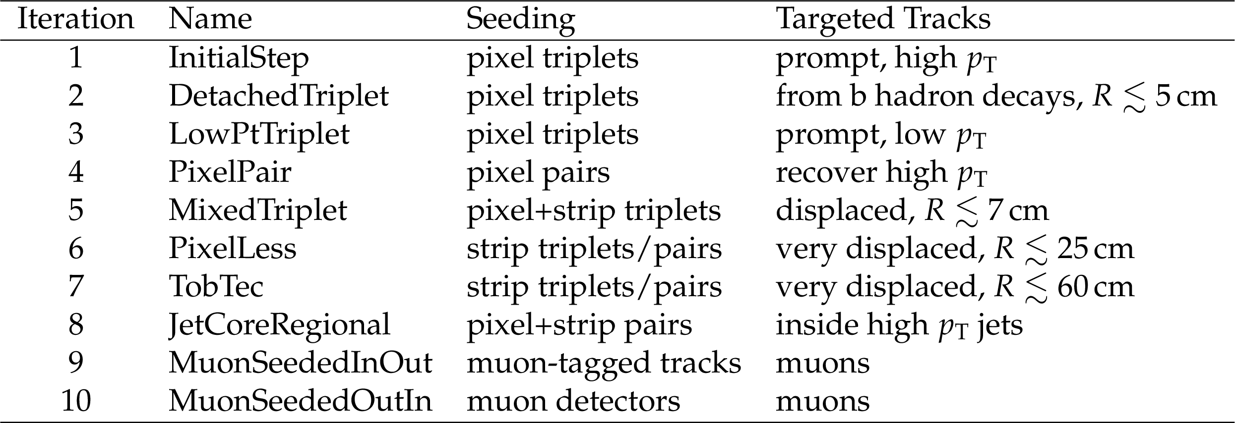
Table 1:
Seeding configuration and targeted tracks of the ten tracking iterations. In the last column, $R$ is the targeted distance between the track production position and the beam axis. |
png pdf |
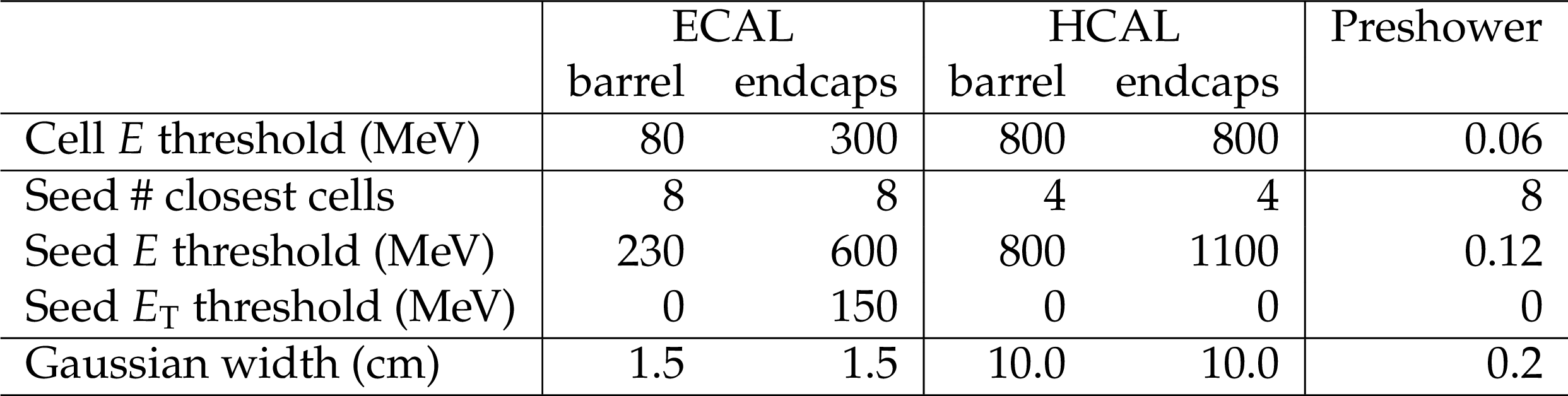
Table 2:
Clustering parameters for the ECAL, the HCAL, and the preshower. All values result from optimizations based on the simulation of single photons, $\pi ^{0}$, $\mathrm {K}^{0}_\mathrm {L}$, and jets. |

png pdf |
Table 3:
Branching fraction $\mathcal {B}$ of the main (negative) $\tau $ decay modes [50]. The generic symbol $ {\mathrm{h} ^-} $ represents a charged hadron, pion or kaon. In some cases, the decay products arise from an intermediate mesonic resonance. |

png pdf |
Table 4:
Correlation between the reconstructed and generated decay modes, for $ {\tau _\mathrm {h}} $ produced in simulated $\mathrm{ Z } / {\gamma ^{*}} \to \tau \tau $ events. Reconstructed $ {\tau _\mathrm {h}} $ candidates are required to be matched to a generated $ {\tau _\mathrm {h}} $, to be reconstructed with $ {p_{\mathrm {T}}} > 20$ GeV and $ {| \eta | } < 2.3$ under one of the HPS decay modes, and to satisfy the loose isolation working point. |
| Summary |
|
The CMS detector was designed 20 years ago to identify energetic and isolated leptons and photons and measure their momenta with high precision, to provide a calorimetric determination of jets and missing transverse momentum, and to efficiently tag b quark jets. The CMS detector turned out to feature properties well-suited for particle-flow (PF) reconstruction. For the first time in a hadron collider experiment, a PF algorithm aimed at identifying and reconstructing all final-state particles was implemented. The technical challenges posed by the complexity of proton-proton collisions and the amount of material in the tracker were overcome with the development of new, high-performance reconstruction algorithms in the different subdetectors, and of discriminating particle identification algorithms combining their information. The PF reconstruction computing time was kept under control both for offline data processing and for triggering the data acquisition, irrespective of the final state intricacy. The resulting global event description augmented the performance of all physics objects (efficiency, purity, response bias, energy and angular resolutions, etc.), thereby reducing the associated systematic biases and the need for a posteriori corrections. Knowledge of the detailed particle content of these physics objects enhanced the scope of many physics analyses. Excellent agreement was obtained between the simulation and the data recorded by CMS at a centre-of-mass energy of 8 TeV, thereby validating the use of PF reconstruction in real data-taking conditions. The PF approach also paved the way for particle-level pileup mitigation methods, the simplest of which have been presented in this paper for an average of 20 and up to 35 concurrent pileup interactions. Machine learning algorithms based on the detailed PF information were shown to preserve the improved physics object performance even in the presence of a large number of background particles produced in pileup interactions. The future CMS detector upgrades have been planned to provide optimal conditions for PF performance. In the first phase of the upgrade programme, a better and lighter pixel detector [64] will reduce the rate of misreconstructed charged-particle tracks, and the readout of multiple layers with low noise photodetectors in the hadron calorimeter [65] will improve the neutral-hadron identification, which currently limits the jet energy resolution. The second phase [66] will include a lighter and extended tracker (integrated into the level 1 trigger) and high-granularity endcap calorimeters, enhancing the PF capabilities for online and offline reconstruction. These detector evolutions, accompanied by the necessary PF software developments, should help to respond to the new challenges posed by the 200 pileup interactions foreseen at the LHC by the end of the next decade. |
| References | ||||
| 1 | CMS Collaboration | The CMS experiment at the CERN LHC | JINST 3 (2008) S08004 | CMS-00-001 |
| 2 | ALEPH Collaboration | Performance of the ALEPH detector at LEP | NIMA 360 (1995) 481 | |
| 3 | M. A. Thomson | Particle Flow Calorimetry and the PandoraPFA Algorithm | NIMA 611 (2009) 25 | 0907.3577 |
| 4 | M. Ruan and H. Videau | Arbor, a new approach of the Particle Flow Algorithm | in Proceedings, International Conference on Calorimetry for the High Energy Frontier (CHEF 2013) | 1403.4784 |
| 5 | M. Bicer et al. | First Look at the Physics Case of TLEP | JHEP 01 (2014) 164 | 1308.6176 |
| 6 | CEPC-SPPC Study Group | CEPC-SPPC Preliminary Conceptual Design Report: Physics and Detector | IHEP-CEPC-DR-2015-01, IHEP-TH-2015-01, IHEP-EP-2015-01 | |
| 7 | DELPHI Collaboration | Performance of the DELPHI detector | NIMA 378 (1996) 57 | |
| 8 | E. Sauvan | Petit periple aux confins du modele standard avec HERA | PhD thesis, CPPM-H-2009-3, Appendix A (2009) | |
| 9 | ZEUS Collaboration, M. Wing | Precise measurement of jet energies with the ZEUS detector | in Calorimetry in high energy physics. Proceedings, 9th International Conference, CALOR 2000, volume 21, p. 617 Annecy, France, October, 2001 [Frascati Phys. Ser. 21 (2001) 617] | hep-ex/0011046 |
| 10 | D0 Collaboration | Measurement of $ \sigma(p\bar{p} \to Z + X) $ Br($ Z \to \tau^+ \tau^- $) at $ \sqrt{s} = $ 1.96$ \,TeV $ | PLB 670 (2009) 292 | 0808.1306 |
| 11 | CDF Collaboration | Measurement of $ {\sigma}(p\overline{p} \mathcal{B}(Z {\rightarrow} {\tau} {\tau}) $ in $ p\overline{p} $ collisions at $ \sqrt{s}=$ 1.96 TeV | PRD 75 (2007) 092004 | |
| 12 | CMS Collaboration | Determination of jet energy calibration and transverse momentum resolution in CMS | JINST 6 (2011) P11002 | CMS-JME-10-011 1107.4277 |
| 13 | ATLAS Collaboration | Reconstruction of hadronic decay products of tau leptons with the ATLAS experiment | EPJC 76 (2016) 295 | 1512.05955 |
| 14 | A. Collaboration | Jet reconstruction and performance using particle flow with the ATLAS Detector | Submitted to EPJC | 1703.10485 |
| 15 | CMS Collaboration | Technical Design Report CMS | CERN-LHCC-97-10 | |
| 16 | CMS Collaboration | Technical Design Report CMS | CERN-LHCC-98-006 | |
| 17 | CMS Collaboration | Technical Design Report CMS | CERN-LHCC-2000-016 | |
| 18 | CMS Collaboration | Description and performance of track and primary-vertex reconstruction with the CMS tracker | JINST 9 (2014) P10009 | CMS-TRK-11-001 1405.6569 |
| 19 | CMS Collaboration | Technical Design Report CMS | CERN-LHCC-97-033 | |
| 20 | CMS Collaboration | Technical Design Report CMS | CERN-LHCC-2002-027 | |
| 21 | P. Adzic et al. | Energy resolution of the barrel of the CMS electromagnetic calorimeter | JINST 2 (2007) P04004 | |
| 22 | W. Bialas and D. A. Petyt | Mitigation of anomalous APD signals in the CMS ECAL | JINST 8 (2013) C03020 | |
| 23 | CMS Collaboration | Technical Design Report CMS | CERN-LHCC-97-31 | |
| 24 | CMS HCAL/ECAL Collaboration | The CMS Barrel Calorimeter Response to Particle Beams from 2 to 350 GeV/c | EPJC 60 (2009) 359 | |
| 25 | CMS Collaboration | Identification and filtering of uncharacteristic noise in the CMS hadron calorimeter | JINST 5 (2010) T03014 | CMS-CFT-09-019 0911.4881 |
| 26 | CMS Collaboration | Technical Design Report CMS | CERN-LHCC-97-32 | |
| 27 | CMS Collaboration | The performance of the CMS muon detector in proton-proton collisions at $ \sqrt{s} = $ 7 TeV at the LHC | JINST 8 (2013) P11002 | CMS-MUO-11-001 1306.6905 |
| 28 | CMS Collaboration | Technical Design Report CMS | CERN-LHCC-2006-001 | |
| 29 | CMS Collaboration | Track Reconstruction in the CMS tracker | CDS | |
| 30 | P. Azzurri | Track Reconstruction Performance in CMS | NPPS B 197 (2009) 275 | 0812.5036 |
| 31 | CMS Collaboration | Studies of Tracker Material in the CMS Detector | CDS | |
| 32 | CMS Collaboration | CMS tracking performance results from early LHC operation | EPJC 70 (2010) 1165 | CMS-TRK-10-001 1007.1988 |
| 33 | CMS Collaboration | Performance of electron reconstruction and selection with the CMS detector in proton-proton collisions at $ \sqrt{s} = $ 8 TeV | JINST 10 (2015) P06005 | CMS-EGM-13-001 1502.02701 |
| 34 | W. Adam, R. Fruhwirth, A. Strandlie, and T. Todorov | Reconstruction of electrons with the Gaussian-sum filter in the CMS tracker at the LHC | JPG 31 (2005) N9 | physics/0306087 |
| 35 | CMS Collaboration | Performance of CMS muon reconstruction in pp collision events at .$ \sqrt{s} = $ 7 TeV | JINST 7 (2012) P10002 | CMS-MUO-10-004 1206.4071 |
| 36 | CMS Collaboration | Energy calibration and resolution of the CMS electromagnetic calorimeter in pp collisions at $ \sqrt{s} = $ 7 TeV | JINST 8 (2013) P09009 | CMS-EGM-11-001 1306.2016 |
| 37 | J. Allison et al. | GEANT4 developments and applications | IEEE Trans. Nucl. Sci. 53 (2006) 270 | |
| 38 | J. L. Bentley | Multidimensional Binary Search Trees Used for Associative Searching | Commun. ACM 18 (1975) 509 | |
| 39 | CMS Collaboration | Performance of photon reconstruction and identification with the CMS detector in proton-proton collisions at $ \sqrt{s} = $ 8 TeV | JINST 10 (2015) P08010 | CMS-EGM-14-001 1502.02702 |
| 40 | S. Baffioni et al. | Electron reconstruction in CMS | EPJC 49 (2007) 1099 | |
| 41 | T. Sjostrand, S. Mrenna, and P. Skands | PYTHIA 6.4 physics and manual | JHEP 05 (2006) 026 | hep-ph/0603175 |
| 42 | T. Sjostrand et al. | An Introduction to PYTHIA 8.2 | CPC 191 (2015) 159 | 1410.3012 |
| 43 | M. Cacciari, G. P. Salam, and G. Soyez | The anti-$ k_t $ jet clustering algorithm | JHEP 04 (2008) 063 | 0802.1189 |
| 44 | M. Cacciari, G. P. Salam, and G. Soyez | FastJet user manual | EPJC 72 (2012) 1896 | 1111.6097 |
| 45 | CMS Collaboration | Jet energy scale and resolution in the CMS experiment in pp collisions at 8 TeV | JINST 12 (2017) P02014 | CMS-JME-13-004 1607.03663 |
| 46 | DELPHI Collaboration | Measurement of the gluon fragmentation function and a comparison of the scaling violation in gluon and quark jets | EPJC 13 (2000) 573 | |
| 47 | CMS Collaboration | Performance of the CMS missing transverse momentum reconstruction in pp data at $ \sqrt{s} = $ 8 TeV | JINST 10 (2015) P02006 | CMS-JME-13-003 1411.0511 |
| 48 | CMS Collaboration | Observation of a new boson with mass near 125 GeV in pp collisions at $ \sqrt{s} = $ 7 and 8 TeV | JHEP 06 (2013) 081 | CMS-HIG-12-036 1303.4571 |
| 49 | CMS Collaboration | Measurement of the properties of a Higgs boson in the four-lepton final state | PRD 89 (2014) 092007 | CMS-HIG-13-002 1312.5353 |
| 50 | Particle Data Group, C. Patrignani et al. | Review of Particle Physics | CPC 40 (2016), no. 10, 100001 | |
| 51 | CMS Collaboration | Performance of tau-lepton reconstruction and identification in CMS | JINST 7 (2012) P01001 | CMS-TAU-11-001 1109.6034 |
| 52 | CMS Collaboration | Reconstruction and identification of $\tau $ lepton decays to hadrons and $ \nu_{\tau} $ at CMS | JINST 11 (2016) P01019 | CMS-TAU-14-001 1510.07488 |
| 53 | CMS Collaboration | CMS technical design report, volume II: Physics performance | JPG 34 (2007) 995 | |
| 54 | CMS Collaboration | Reconstruction and identification performance of $ \tau $ lepton decays to hadrons and $ \nu_\tau $ in LHC Run-2 | ||
| 55 | CMS Collaboration | The CMS trigger system | JINST 12 (2017) P01020 | CMS-TRG-12-001 1609.02366 |
| 56 | CMS Collaboration | Measurement of the inelastic proton-proton cross section at $ \sqrt{s}=$ 7 TeV | PLB 722 (2013) 5 | CMS-FWD-11-001 1210.6718 |
| 57 | M. Cacciari and G. P. Salam | Pileup subtraction using jet areas | PLB 659 (2008) 119 | 0707.1378 |
| 58 | M. Cacciari, G. P. Salam, and G. Soyez | The Catchment Area of Jets | JHEP 04 (2008) 005 | 0802.1188 |
| 59 | D. Bertolini, P. Harris, M. Low, and N. Tran | Pileup Per Particle Identification | JHEP 10 (2014) 059 | 1407.6013 |
| 60 | CMS Collaboration | Study of Pileup Removal Algorithms for Jets | CMS-PAS-JME-14-001 | CMS-PAS-JME-14-001 |
| 61 | CMS Collaboration | Measurements of Inclusive $ W $ and $ Z $ Cross Sections in $ pp $ Collisions at $ \sqrt{s}=$ 7 TeV | JHEP 01 (2011) 080 | CMS-EWK-10-002 1012.2466 |
| 62 | CMS Collaboration | Pileup Jet Identification | CMS-PAS-JME-13-005 | CMS-PAS-JME-13-005 |
| 63 | CMS Collaboration | Event generator tunes obtained from underlying event and multiparton scattering measurements | EPJC 76 (2016) 155 | CMS-GEN-14-001 1512.00815 |
| 64 | CMS Collaboration | Technical Design Report CMS | CERN-LHCC-2012-016 | |
| 65 | CMS Collaboration | Technical Design Report CMS | CERN-LHCC-2012-015 | |
| 66 | CMS Collaboration | Technical Design Report CMS | CERN-LHCC-2015-019 | |
|
|
Compact Muon Solenoid LHC, CERN |
|

|

|

|

|

|