

Compact Muon Solenoid
LHC, CERN
| CMS-EXO-20-014 ; CERN-EP-2021-266 | ||
| Search for long-lived particles decaying into muon pairs in proton-proton collisions at $\sqrt{s} = $ 13 TeV collected with a dedicated high-rate data stream | ||
| CMS Collaboration | ||
| 27 December 2021 | ||
| JHEP 04 (2022) 062 | ||
| Abstract: A search for long-lived particles decaying into muon pairs is performed using proton-proton collisions at a center-of-mass energy of 13 TeV, collected by the CMS experiment at the LHC in 2017 and 2018, corresponding to an integrated luminosity of 101 fb$^{-1}$. The data sets used in this search were collected with a dedicated dimuon trigger stream with low transverse momentum thresholds, recorded at high rate by retaining a reduced amount of information, in order to explore otherwise inaccessible phase space at low dimuon mass and nonzero displacement from the primary interaction vertex. No significant excess of events beyond the standard model expectation is found. Upper limits on branching fractions at 95% confidence level are set on a wide range of mass and lifetime hypotheses in beyond the standard model frameworks with the Higgs boson decaying into a pair of long-lived dark photons, or with a long-lived scalar resonance arising from a decay of a b hadron. The limits are the most stringent to date for substantial regions of the parameter space. These results can be also used to constrain models of displaced dimuons that are not explicitly considered in this paper. | ||
| Links: e-print arXiv:2112.13769 [hep-ex] (PDF) ; CDS record ; inSPIRE record ; HepData record ; CADI line (restricted) ; | ||
| Figures | Summary | Additional Figures & Tables | References | CMS Publications |
|---|
| Figures | |
png pdf |
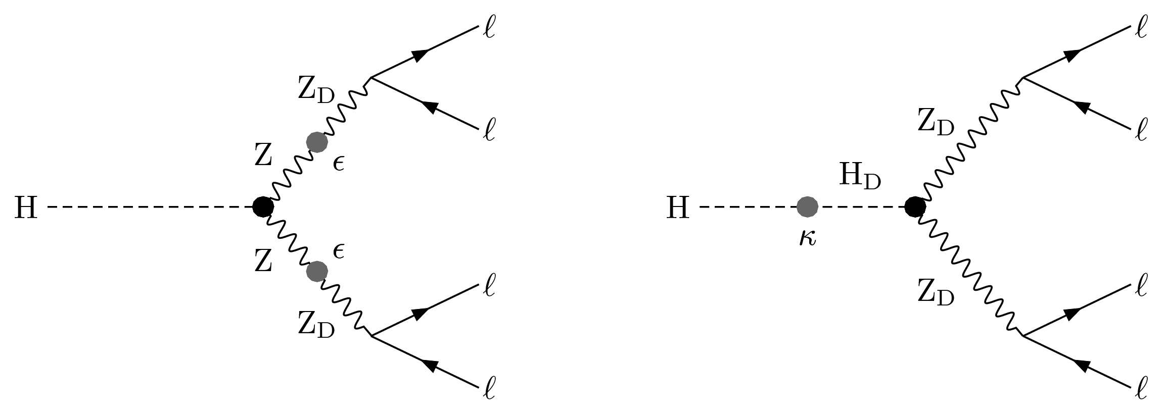
Figure 1:
Diagrams illustrating an SM-like Higgs boson (H) decay to four leptons ($\ell $) via two intermediate dark photons, Z$_{\mathrm {D}}$ [6]: (left) through the hypercharge portal; (right) through the Higgs portal, via a dark Higgs boson (H$_{\mathrm {D}}$). |
png pdf |
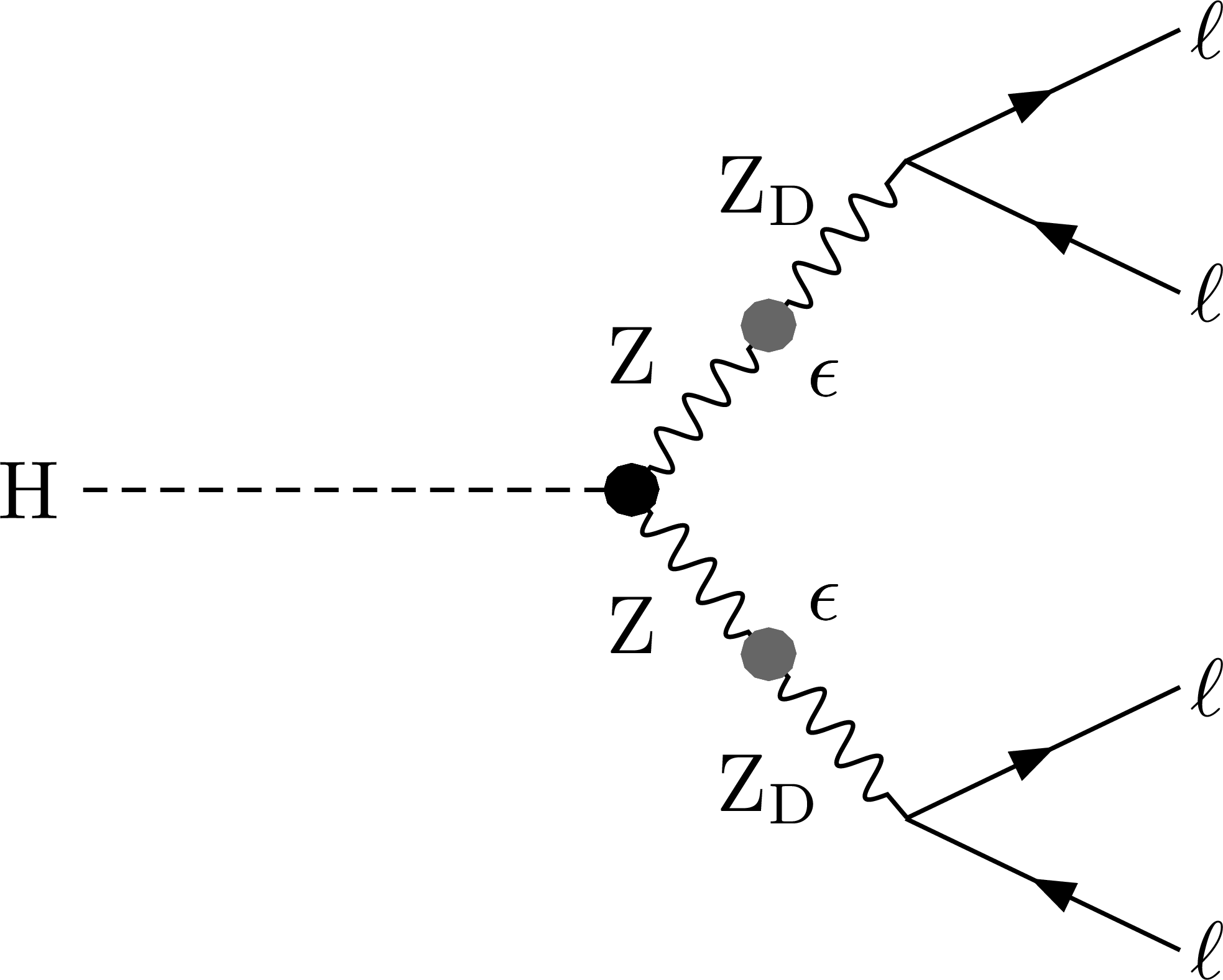
Figure 1-a:
Diagram illustrating an SM-like Higgs boson (H) decay to four leptons ($\ell $) via two intermediate dark photons, Z$_{\mathrm {D}}$ [6], through the hypercharge portal. |

png pdf |
Figure 1-b:
Diagram illustrating an SM-like Higgs boson (H) decay to four leptons ($\ell $) via two intermediate dark photons, Z$_{\mathrm {D}}$ [6], through the Higgs portal, via a dark Higgs boson (H$_{\mathrm {D}}$). |
png pdf |
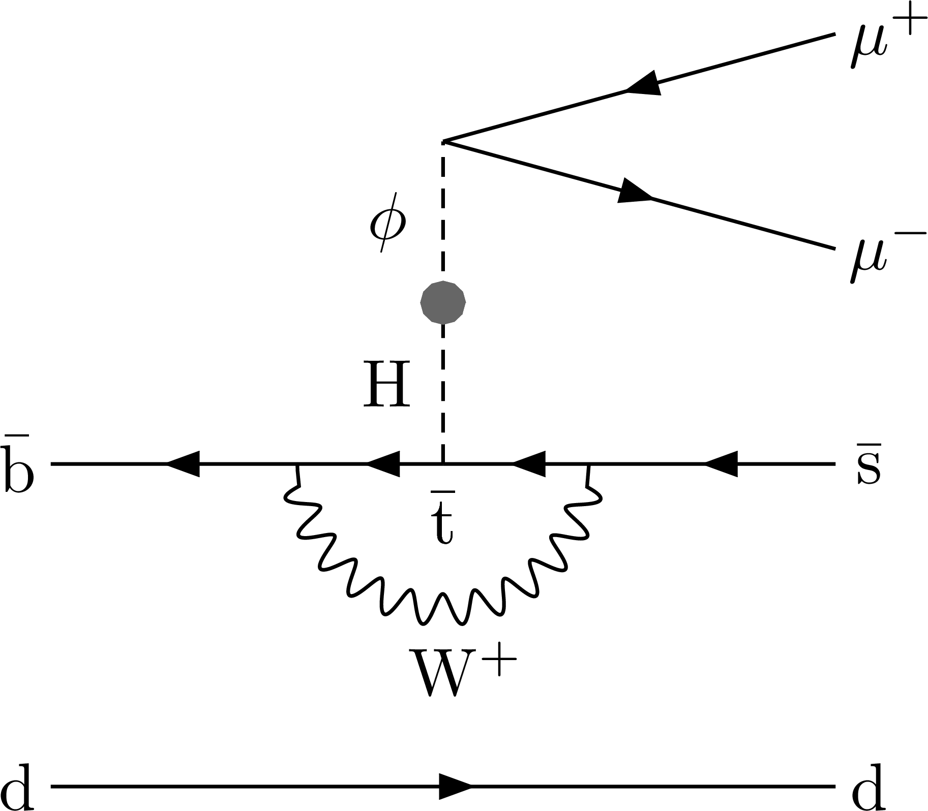
Figure 2:
Diagram illustrating the production of a scalar resonance $\phi $ in a b hadron decay, through mixing with an SM-like Higgs boson (H). |
png pdf |
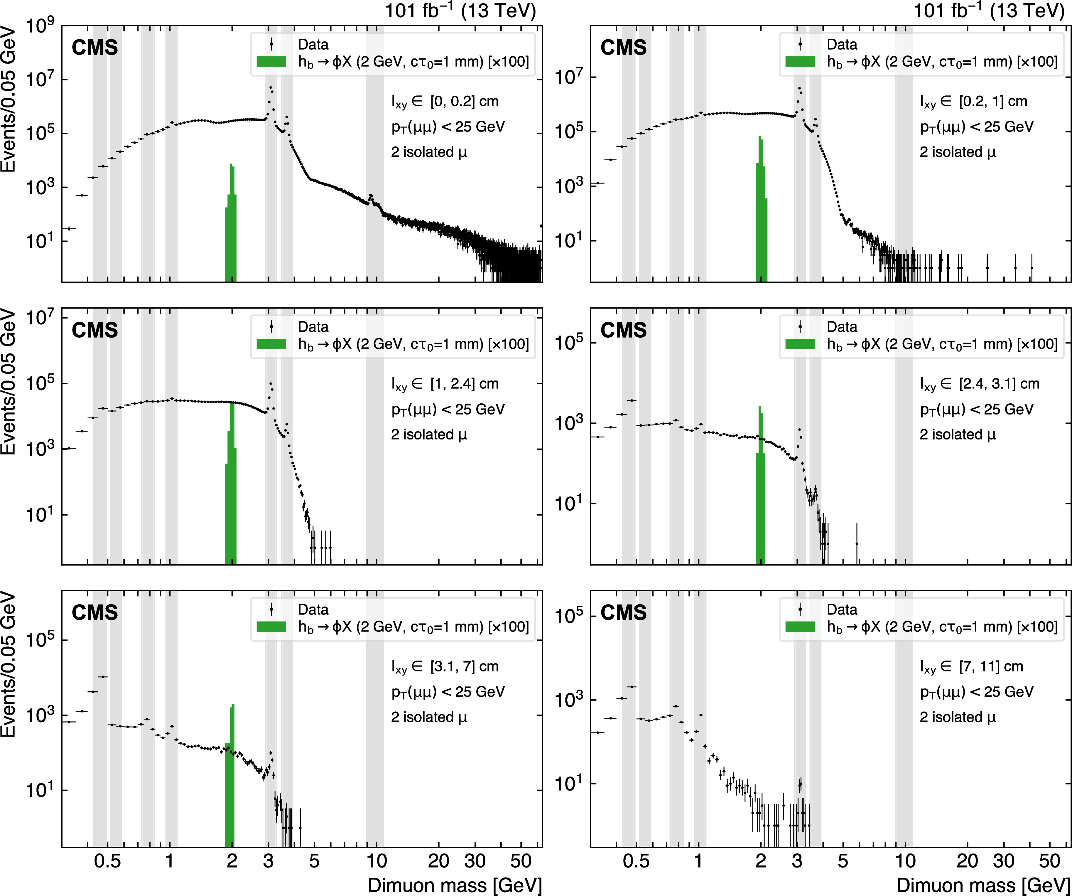
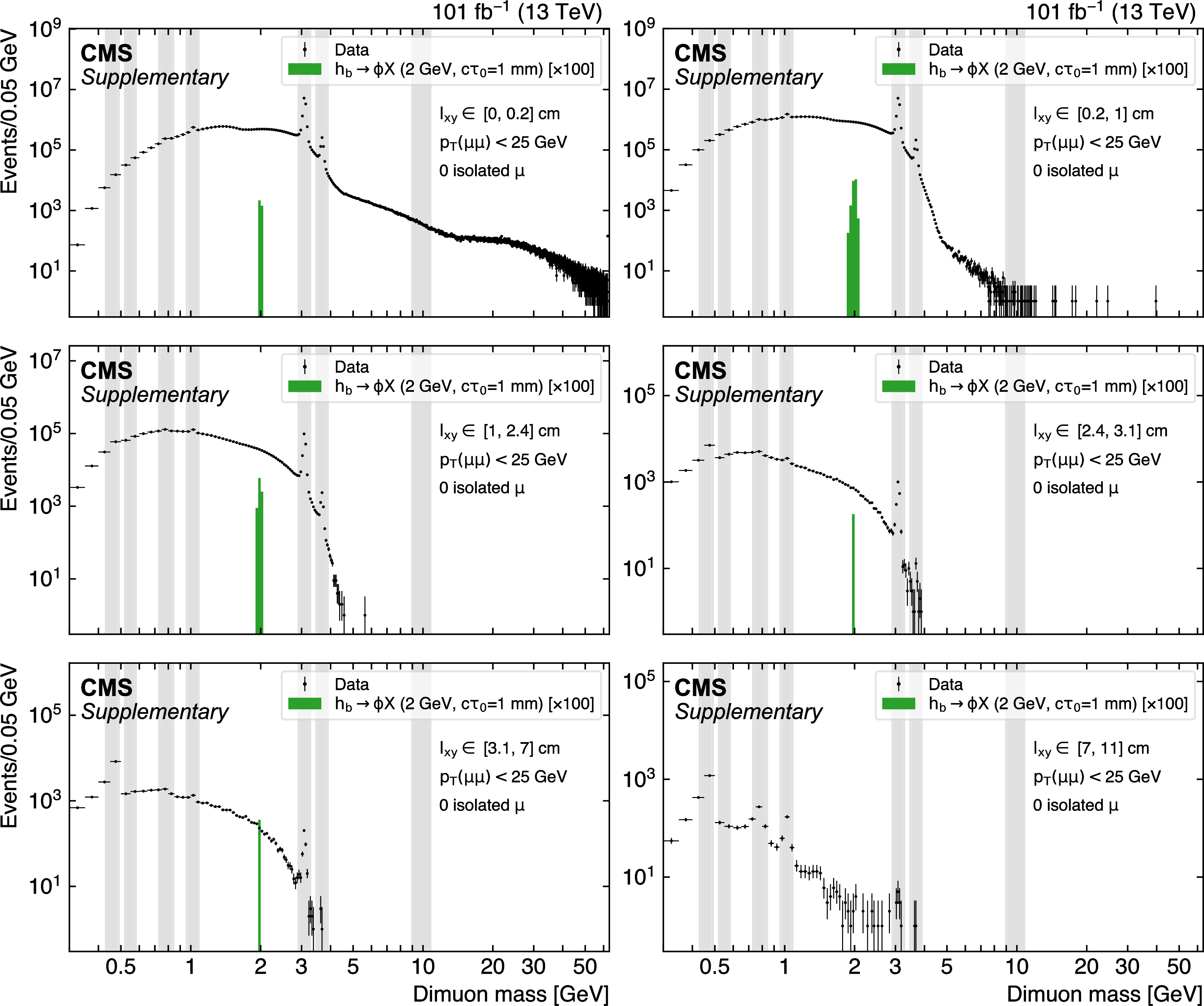
Figure 3:
The dimuon invariant mass distribution is shown in bins of ${l_\mathrm {xy}}$ as obtained from selected dimuon events in data where both muons are isolated with $ {{p_{\mathrm {T}}} ^{\mu \mu}} < $ 25 GeV: (upper left) 0.0 $\leq {l_\mathrm {xy}} < $ 0.2 cm ; (upper right) 0.2 $\leq {l_\mathrm {xy}} < $ 1.0 cm ; (middle left) 1.0 $\leq {l_\mathrm {xy}} < $ 2.4 cm ; (middle right) 2.4 $\leq {l_\mathrm {xy}} < $ 3.1 cm ; (lower left) 3.1 $ \leq {l_\mathrm {xy}} < $ 7.0 cm; (lower right) 7.0 $\leq {l_\mathrm {xy}} < $ 11.0 cm. The distribution expected for a representative $h_{\mathrm{b}}\to \phi X$ signal model with $m_{\phi} = $ 2 GeV and $c\tau _{0}^{\phi}=$ 1 mm is overlaid. The signal event yield corresponds to a value of the branching fraction product $\mathcal {B}(h_{\mathrm{b}}\to \phi X) \, \mathcal {B}(\phi \to \mu \mu) = $ 1.2$\times $10$^{-8}$, equal to the median expected exclusion limit at 95% CL set in this paper (see Section 7), and is multiplied by a factor of 100 for display purposes. The vertical gray bands indicate mass ranges containing known SM resonances, which are masked for the purpose of this search. |
png pdf |
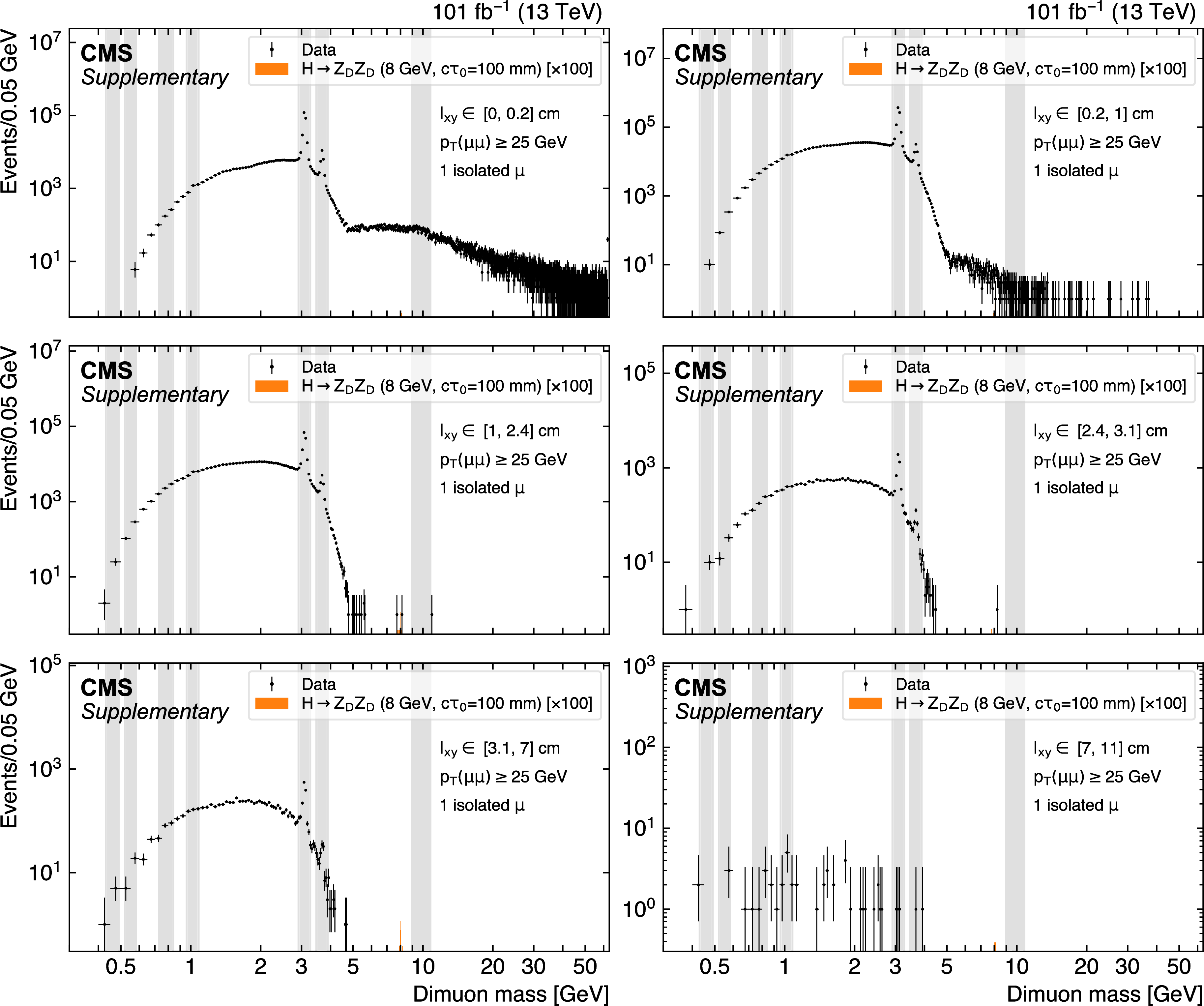
Figure 4:
The dimuon invariant mass distribution is shown in bins of ${l_\mathrm {xy}}$ as obtained from selected dimuon events in data where both muons are isolated with $ {{p_{\mathrm {T}}} ^{\mu \mu}} \geq $ 25 GeV: (upper left) 0.0 $\leq {l_\mathrm {xy}} < $ 0.2 cm ; (upper right) 0.2 $\leq {l_\mathrm {xy}} < $ 1.0 cm ; (middle left) 1.0 $\leq {l_\mathrm {xy}} < $ 2.4 cm ; (middle right) 2.4 $\leq {l_\mathrm {xy}} < $ 3.1 cm ; (lower left) 3.1 $ \leq {l_\mathrm {xy}} < $ 7.0 cm; (lower right) 7.0 $\leq {l_\mathrm {xy}} < $ 11.0 cm. The distribution expected for a representative $\mathrm{H} \to \mathrm{Z} _{\mathrm {D}}\mathrm{Z} _{\mathrm {D}}$ signal model with $m_{\mathrm{Z} _{\mathrm {D}}} = $ 8 GeV and $c\tau _{0}^{\mathrm{Z} _{\mathrm {D}}}=$ 100 mm, corresponding to $\epsilon =1.2 \times 10^{-7}$, is overlaid. The signal event yield corresponds to a value of the branching fraction product $\mathcal {B}(\mathrm{H} \to \mathrm{Z} _{\mathrm {D}}\mathrm{Z} _{\mathrm {D}}) \, \mathcal {B}(\mathrm{Z} _{\mathrm {D}}\to \mu \mu) = $ 1.2$\times $10$^{-5}$, equal to the median expected exclusion limit at 95% CL set in this paper (see Section 7), and is multiplied by a factor of 100 for display purposes. The vertical gray bands indicate mass ranges containing known SM resonances, which are masked for the purpose of this search. |
png pdf |
Figure 5:
The dimuon invariant mass distribution is shown in a mass window around 2 GeV, in one of the dimuon search bins (3.1 $ \leq {l_\mathrm {xy}} < $ 7.0 cm, $ {{p_{\mathrm {T}}} ^{\mu \mu}} < $ 25 GeV, with two isolated muons). The result of the background-only fit to the data is also shown (blue) together with the dimuon invariant mass distribution expected for a representative $h_{\mathrm{b}}\to \phi X$ signal model (green) with $m_{\phi} = $ 2 GeV and $c\tau _{0}^{\phi}=$ 1 mm . The signal event yield corresponds to a value of the branching fraction product $\mathcal {B}(h_{\mathrm{b}}\to \phi X) \, \mathcal {B}(\phi \to \mu \mu) = $ 1.2$\times $10$^{-8}$, equal to the median expected exclusion limit at 95% CL set in this paper (see Section 7), and is multiplied by a factor of 5 for display purposes. The lower panel shows the ratio of the data to the background prediction, with error bars corresponding to the statistical uncertainty in the data. |

png pdf |
Figure 6:
Exclusion limits at 95% CL on the branching fraction product $\mathcal {B}(h_{\mathrm{b}}\to \phi X) \, \mathcal {B}(\phi \to \mu \mu)$, as functions of the signal mass ($m_{\phi}$) for $c\tau _{0}^{\phi}=$ 1 mm (upper) and 100 mm (lower). The solid black (dashed red) line represents the observed (median expected) exclusion. The inner green (outer yellow) band indicates the region containing 68 (95)% of the distribution of limits expected under the background-only hypothesis. The vertical gray bands indicate mass ranges containing known SM resonances, which are masked for the purpose of this search. The limits are obtained using the combination of all dimuon event categories. |
png pdf |
Figure 6-a:
Exclusion limits at 95% CL on the branching fraction product $\mathcal {B}(h_{\mathrm{b}}\to \phi X) \, \mathcal {B}(\phi \to \mu \mu)$, as functions of the signal mass ($m_{\phi}$) for $c\tau _{0}^{\phi}=$ 1 mm. The solid black (dashed red) line represents the observed (median expected) exclusion. The inner green (outer yellow) band indicates the region containing 68 (95)% of the distribution of limits expected under the background-only hypothesis. The vertical gray bands indicate mass ranges containing known SM resonances, which are masked for the purpose of this search. The limits are obtained using the combination of all dimuon event categories. |
png pdf |
Figure 6-b:
Exclusion limits at 95% CL on the branching fraction product $\mathcal {B}(h_{\mathrm{b}}\to \phi X) \, \mathcal {B}(\phi \to \mu \mu)$, as functions of the signal mass ($m_{\phi}$) for $c\tau _{0}^{\phi}=$ 100 mm. The solid black (dashed red) line represents the observed (median expected) exclusion. The inner green (outer yellow) band indicates the region containing 68 (95)% of the distribution of limits expected under the background-only hypothesis. The vertical gray bands indicate mass ranges containing known SM resonances, which are masked for the purpose of this search. The limits are obtained using the combination of all dimuon event categories. |
png pdf |
Figure 7:
Exclusion limits at 95% CL on the branching fraction product $\mathcal {B}(\mathrm{H} \to \mathrm{Z} _{\mathrm {D}}\mathrm{Z} _{\mathrm {D}}) \, \mathcal {B}(\mathrm{Z} _{\mathrm {D}}\to \mu \mu)$, as functions of the signal mass ($m_{\mathrm{Z} _{\mathrm {D}}}$) for $c\tau _{0}^{\mathrm{Z} _{\mathrm {D}}}=$ 1 mm (upper) and 100 mm (lower). The solid black (dashed red) line represents the observed (median expected) exclusion. The inner green (outer yellow) band indicates the region containing 68 (95)% of the distribution of limits expected under the background-only hypothesis. The vertical gray bands indicate mass ranges containing known SM resonances, which are masked for the purpose of this search. The limits are obtained using the combination of all dimuon event categories. |

png pdf |
Figure 7-a:
Exclusion limits at 95% CL on the branching fraction product $\mathcal {B}(\mathrm{H} \to \mathrm{Z} _{\mathrm {D}}\mathrm{Z} _{\mathrm {D}}) \, \mathcal {B}(\mathrm{Z} _{\mathrm {D}}\to \mu \mu)$, as functions of the signal mass ($m_{\mathrm{Z} _{\mathrm {D}}}$) for $c\tau _{0}^{\mathrm{Z} _{\mathrm {D}}}=$ 1 mm. The solid black (dashed red) line represents the observed (median expected) exclusion. The inner green (outer yellow) band indicates the region containing 68 (95)% of the distribution of limits expected under the background-only hypothesis. The vertical gray bands indicate mass ranges containing known SM resonances, which are masked for the purpose of this search. The limits are obtained using the combination of all dimuon event categories. |
png pdf |
Figure 7-b:
Exclusion limits at 95% CL on the branching fraction product $\mathcal {B}(\mathrm{H} \to \mathrm{Z} _{\mathrm {D}}\mathrm{Z} _{\mathrm {D}}) \, \mathcal {B}(\mathrm{Z} _{\mathrm {D}}\to \mu \mu)$, as functions of the signal mass ($m_{\mathrm{Z} _{\mathrm {D}}}$) for $c\tau _{0}^{\mathrm{Z} _{\mathrm {D}}}=$ 100 mm. The solid black (dashed red) line represents the observed (median expected) exclusion. The inner green (outer yellow) band indicates the region containing 68 (95)% of the distribution of limits expected under the background-only hypothesis. The vertical gray bands indicate mass ranges containing known SM resonances, which are masked for the purpose of this search. The limits are obtained using the combination of all dimuon event categories. |

png pdf |
Figure 8:
Exclusion limits at 95% CL on the branching fraction $\mathcal {B}(\mathrm{H} \to \mathrm{Z} _{\mathrm {D}}\mathrm{Z} _{\mathrm {D}})$, as functions of the signal mass ($m_{\mathrm{Z} _{\mathrm {D}}}$) for $c\tau _{0}^{\mathrm{Z} _{\mathrm {D}}}=$ 1 mm (upper) and 100 mm (lower), for the $\mathrm{H} \to \mathrm{Z} _{\mathrm {D}}\mathrm{Z} _{\mathrm {D}}$ signal model, assuming values of $\mathcal {B}(\mathrm{Z} _{\mathrm {D}}\to \mu \mu)$ from the model of Ref. [6]. The solid black (dashed red) line represents the observed (median expected) exclusion. The inner green (outer yellow) band indicates the region containing 68 (95)% of the distribution of limits expected under the background-only hypothesis. The vertical gray bands indicate mass ranges containing known SM resonances, which are masked for the purpose of this search. The limits are obtained using the combination of all dimuon and four-muon event categories. |
png pdf |
Figure 8-a:
Exclusion limits at 95% CL on the branching fraction $\mathcal {B}(\mathrm{H} \to \mathrm{Z} _{\mathrm {D}}\mathrm{Z} _{\mathrm {D}})$, as functions of the signal mass ($m_{\mathrm{Z} _{\mathrm {D}}}$) for $c\tau _{0}^{\mathrm{Z} _{\mathrm {D}}}=$ 1 mm, for the $\mathrm{H} \to \mathrm{Z} _{\mathrm {D}}\mathrm{Z} _{\mathrm {D}}$ signal model, assuming values of $\mathcal {B}(\mathrm{Z} _{\mathrm {D}}\to \mu \mu)$ from the model of Ref. [6]. The solid black (dashed red) line represents the observed (median expected) exclusion. The inner green (outer yellow) band indicates the region containing 68 (95)% of the distribution of limits expected under the background-only hypothesis. The vertical gray bands indicate mass ranges containing known SM resonances, which are masked for the purpose of this search. The limits are obtained using the combination of all dimuon and four-muon event categories. |
png pdf |
Figure 8-b:
Exclusion limits at 95% CL on the branching fraction $\mathcal {B}(\mathrm{H} \to \mathrm{Z} _{\mathrm {D}}\mathrm{Z} _{\mathrm {D}})$, as functions of the signal mass ($m_{\mathrm{Z} _{\mathrm {D}}}$) for $c\tau _{0}^{\mathrm{Z} _{\mathrm {D}}}=$ 100 mm, for the $\mathrm{H} \to \mathrm{Z} _{\mathrm {D}}\mathrm{Z} _{\mathrm {D}}$ signal model, assuming values of $\mathcal {B}(\mathrm{Z} _{\mathrm {D}}\to \mu \mu)$ from the model of Ref. [6]. The solid black (dashed red) line represents the observed (median expected) exclusion. The inner green (outer yellow) band indicates the region containing 68 (95)% of the distribution of limits expected under the background-only hypothesis. The vertical gray bands indicate mass ranges containing known SM resonances, which are masked for the purpose of this search. The limits are obtained using the combination of all dimuon and four-muon event categories. |
png pdf |
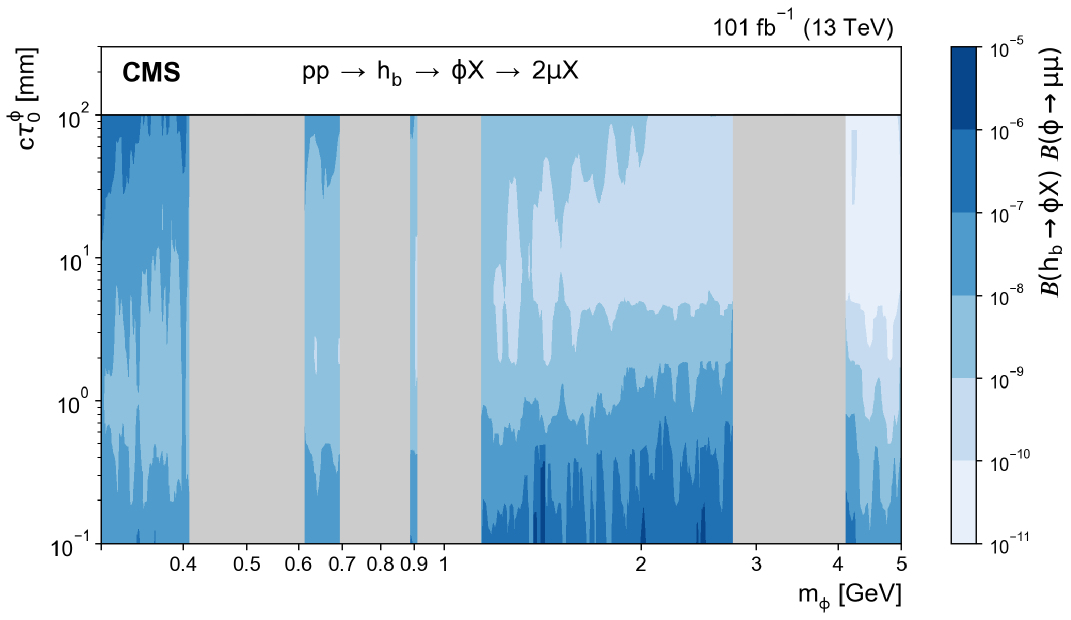
Figure 9:
Observed limits at 95% CL on the branching fraction product $\mathcal {B}(h_{\mathrm{b}}\to \phi X) \, \mathcal {B}(\phi \to \mu \mu)$ as contours in the parameter space containing the signal mass ($m_{\phi}$) and the signal lifetime $c\tau _{0}^{\phi}$. The vertical gray bands indicate mass ranges containing known SM resonances, which are masked for the purpose of this search. The limits are obtained using the combination of all dimuon event categories. |
png pdf |
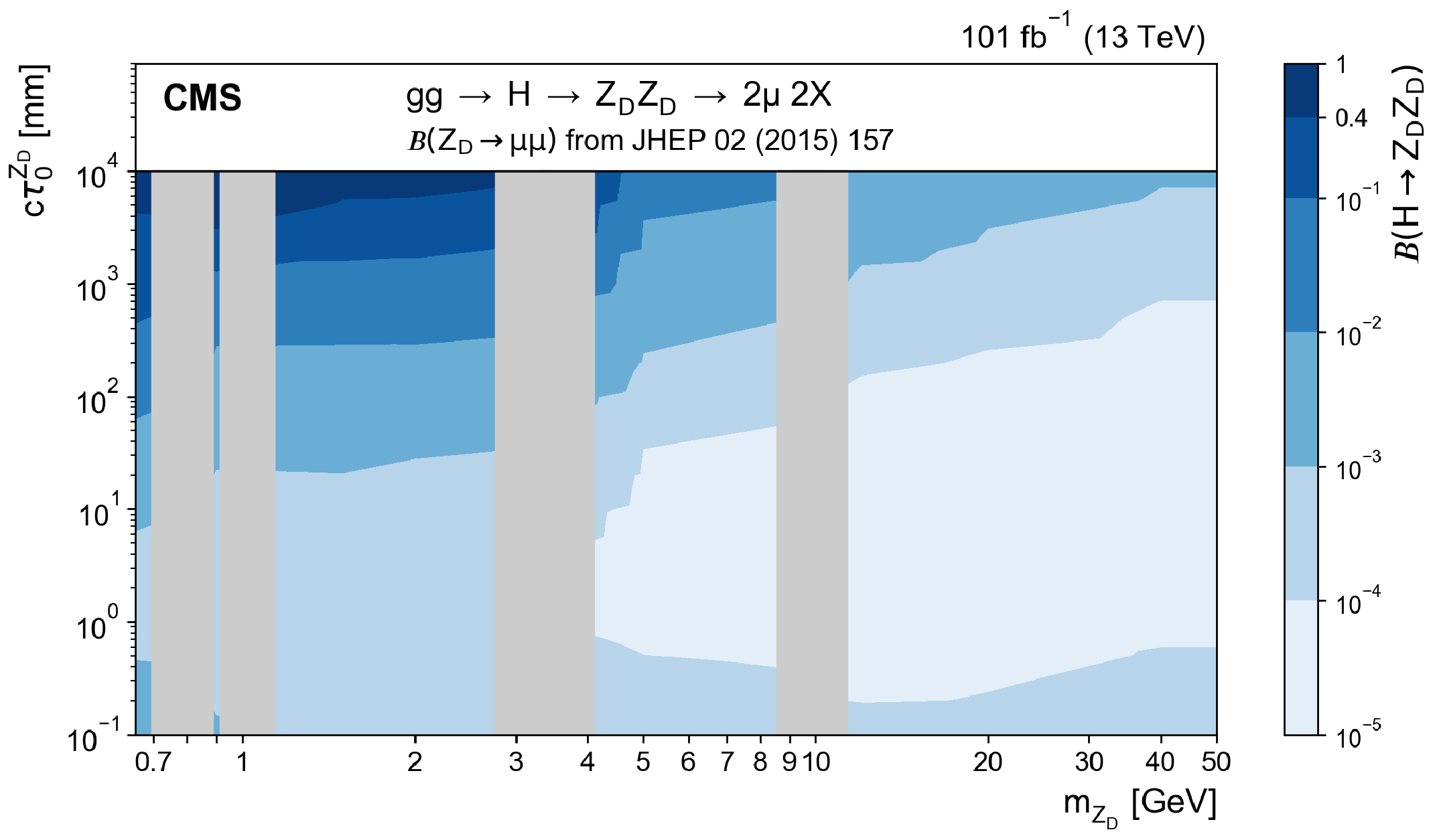
Figure 10:
Observed limits at 95% CL on the branching fraction $\mathcal {B}(\mathrm{H} \to \mathrm{Z} _{\mathrm {D}}\mathrm{Z} _{\mathrm {D}})$ as contours in the parameter space containing the signal mass ($m_{\mathrm{Z} _{\mathrm {D}}}$) and the signal lifetime $c\tau _{0}^{\mathrm{Z} _{\mathrm {D}}}$ for the $\mathrm{H} \to \mathrm{Z} _{\mathrm {D}}\mathrm{Z} _{\mathrm {D}}$ signal model assuming values of $\mathcal {B}(\mathrm{Z} _{\mathrm {D}}\to \mu \mu)$ from the model of Ref. [6]. The vertical gray bands indicate mass ranges containing known SM resonances, which are masked for the purpose of this search. The limits are obtained using the combination of all dimuon and four-muon event categories. |
png pdf |
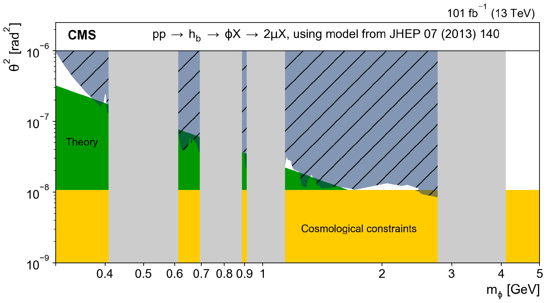
Figure 11:
Region excluded at 95% CL using this search (shown in hatched gray) for the inflaton model [15] in the parameter space containing the signal mass ($m_{\phi}$) and the square of the signal mixing angle ($\theta ^{2}$). The regions forbidden by theory and cosmological constraints are shown in green and yellow respectively. The vertical gray bands indicate mass ranges containing known SM resonances, which are masked for the purpose of this search. The limits are obtained using the combination of all dimuon event categories. |
png pdf |
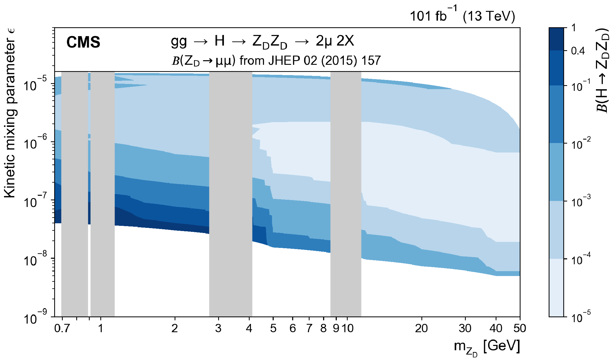
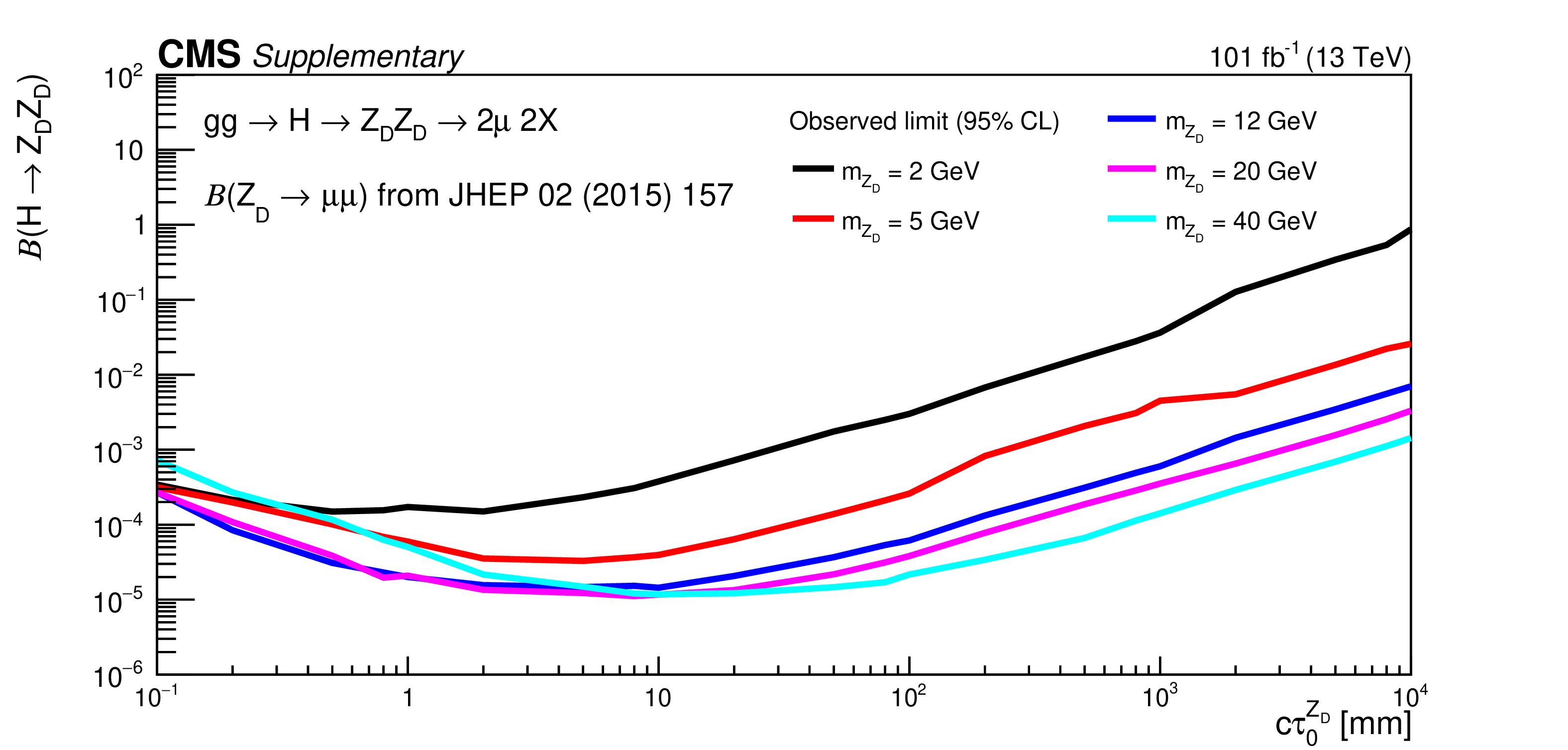
Figure 12:
Observed limits at 95% CL on the branching fraction $\mathcal {B}(\mathrm{H} \to \mathrm{Z} _{\mathrm {D}}\mathrm{Z} _{\mathrm {D}})$ as contours in the parameter space containing the signal mass ($m_{\mathrm{Z} _{\mathrm {D}}}$) and the signal kinetic mixing parameter $\epsilon $ for the $\mathrm{H} \to \mathrm{Z} _{\mathrm {D}}\mathrm{Z} _{\mathrm {D}}$ signal model assuming values of $\mathcal {B}(\mathrm{Z} _{\mathrm {D}}\to \mu \mu)$ from the model of Ref. [6]. The vertical gray bands indicate mass ranges containing known SM resonances, which are masked for the purpose of this search. The white regions at the top (bottom) correspond to values of $c\tau _0^{\mathrm{Z} _{\mathrm {D}}} < $ 0.1 mm ($ > $ 10$^{4}$ mm). The limits are obtained using the combination of all dimuon and four-muon event categories. |
| Summary |
| A search for displaced dimuon resonances has been performed using proton-proton collisions at a center-of-mass energy of 13 TeV, collected by the CMS experiment at the LHC in 2017 and 2018, corresponding to an integrated luminosity of 101 fb$^{-1}$. The data sets used in this search are collected using a dedicated dimuon trigger stream with low transverse momentum thresholds, recorded at high rate by retaining a reduced amount of information, in order to explore otherwise inaccessible phase space at low dimuon mass and nonzero displacement from the primary interaction vertex. No significant excess beyond the standard model expectation is found, and the data are used to set constraints on a wide range of mass and lifetime hypotheses for models of physics beyond the standard model where a Higgs boson decays to a pair of long-lived dark photons, or where a long-lived scalar resonance arises from the decay of a b hadron. These constraints are the most stringent to date for substantial regions of the parameter space. |
| Additional Figures | |

png pdf |
Additional Figure 1:
Distribution of ${{p_{\mathrm {T}}} ^{{\mu} {\mu}}}$ for data events and illustrative benchmark signal models, after applying the full event selection. |
png pdf |
Additional Figure 2:
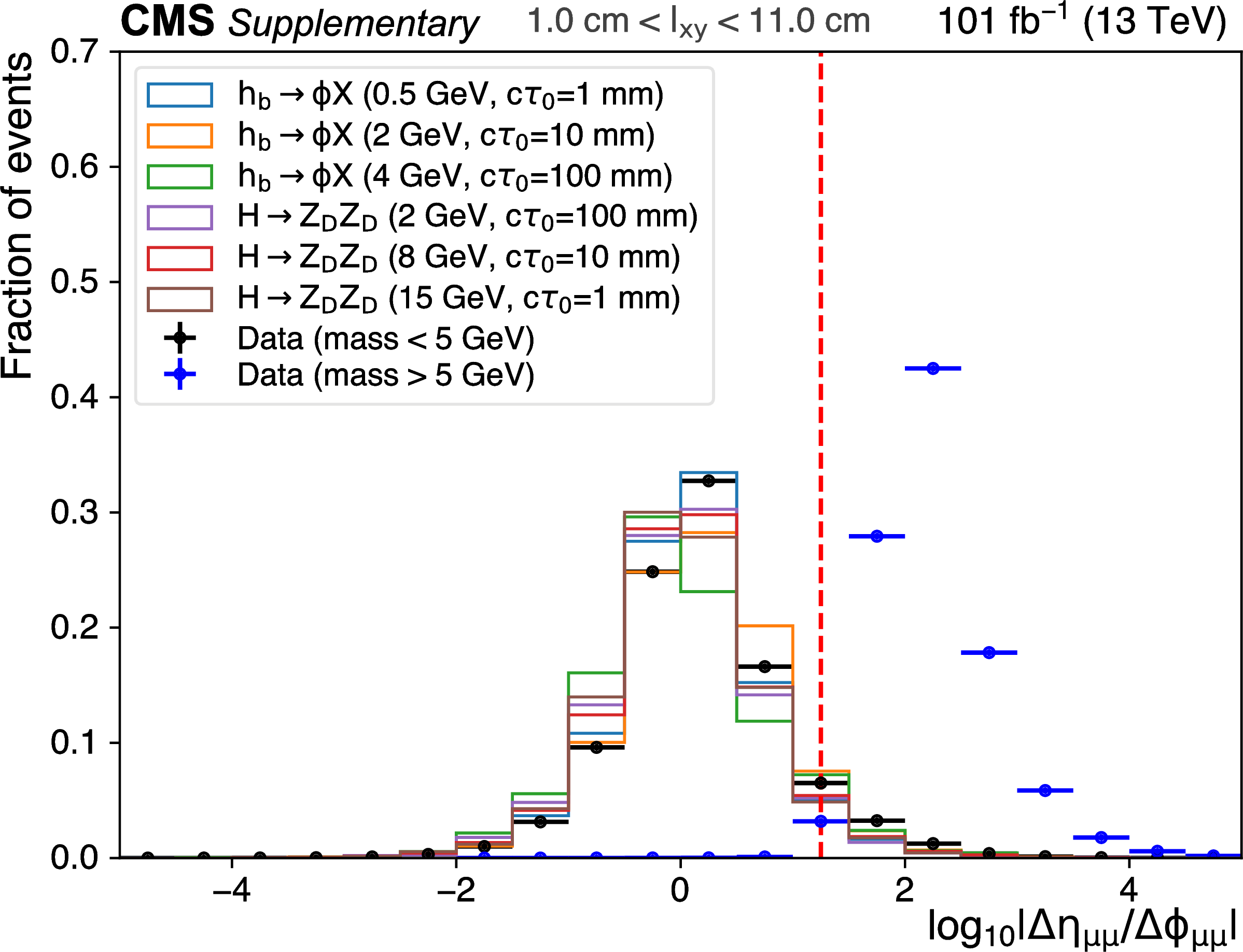
Distribution of ${\log_{10}(|\Delta \eta _{{\mu} {\mu}}|/|\Delta \phi _{{\mu} {\mu}}|)}$ in data events and illustrative benchmark signal models. The cut value is indicated by the red vertical dashed line. All selections except those involving muon isolation, ${d_\mathrm {xy}}$, and number of excess hits in the pixel tracker for each muon are applied. |

png pdf |
Additional Figure 3:
Distribution of ${{| {d_\mathrm {xy}} |}/({l_\mathrm {xy}} {m_{{\mu} {\mu}}} / {{p_{\mathrm {T}}} ^{{\mu} {\mu}}})}$ in data events and illustrative benchmark signal models. The cut value is indicated by the red vertical dashed line. All selections except those involving ${d_\mathrm {xy}}$ are applied. |
png pdf |
Additional Figure 4:
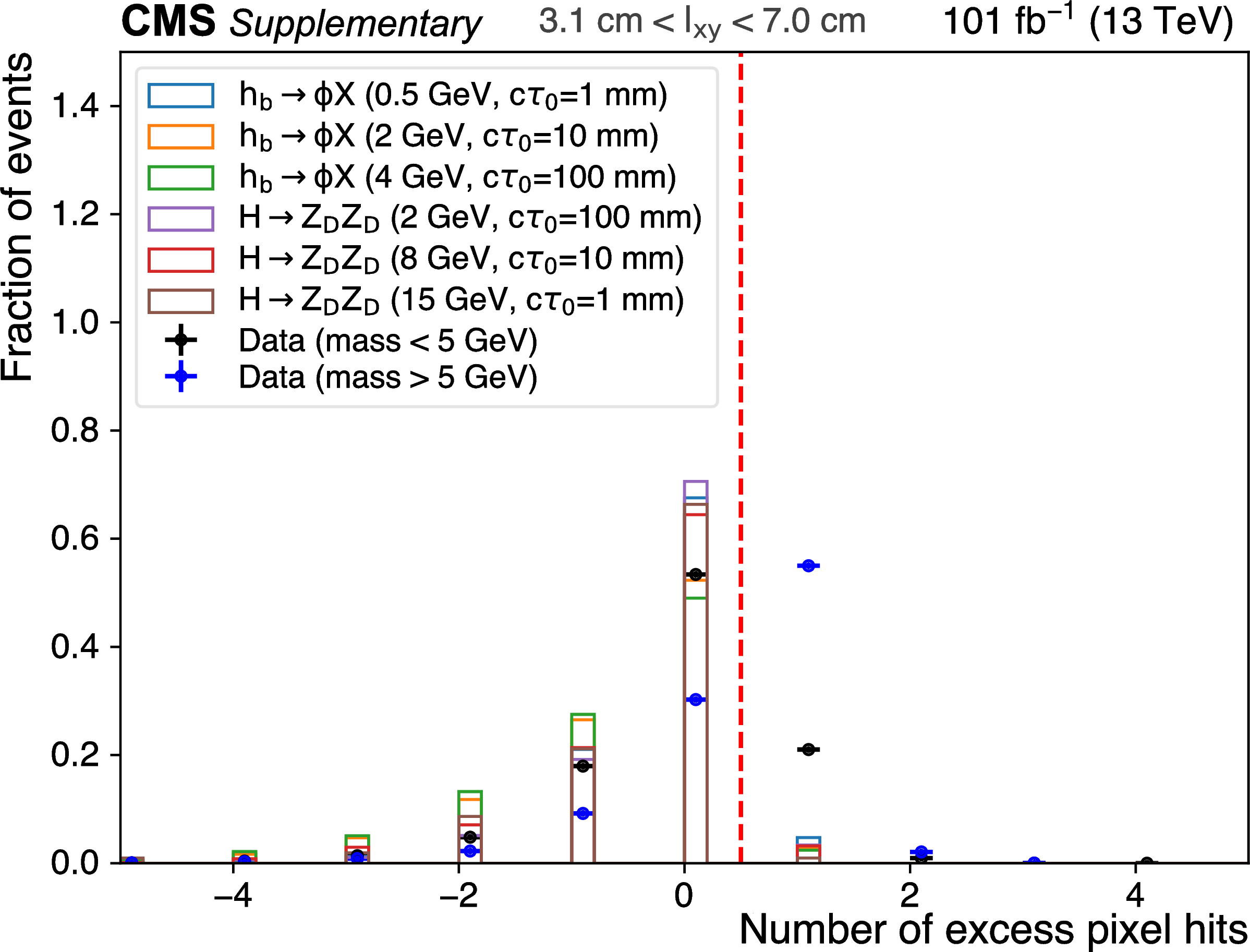
Distribution of the number of excess pixel hits (number of observed hits minus expected hits) in data and illustrative benchmark signal models for the trailing muon. The cut value is indicated by the red vertical dashed line. All selections except those involving muon isolation, ${d_\mathrm {xy}}$, and ${\log_{10}(|\Delta \eta _{{\mu} {\mu}}|/|\Delta \phi _{{\mu} {\mu}}|)}$ are applied. |
png pdf |
Additional Figure 5:
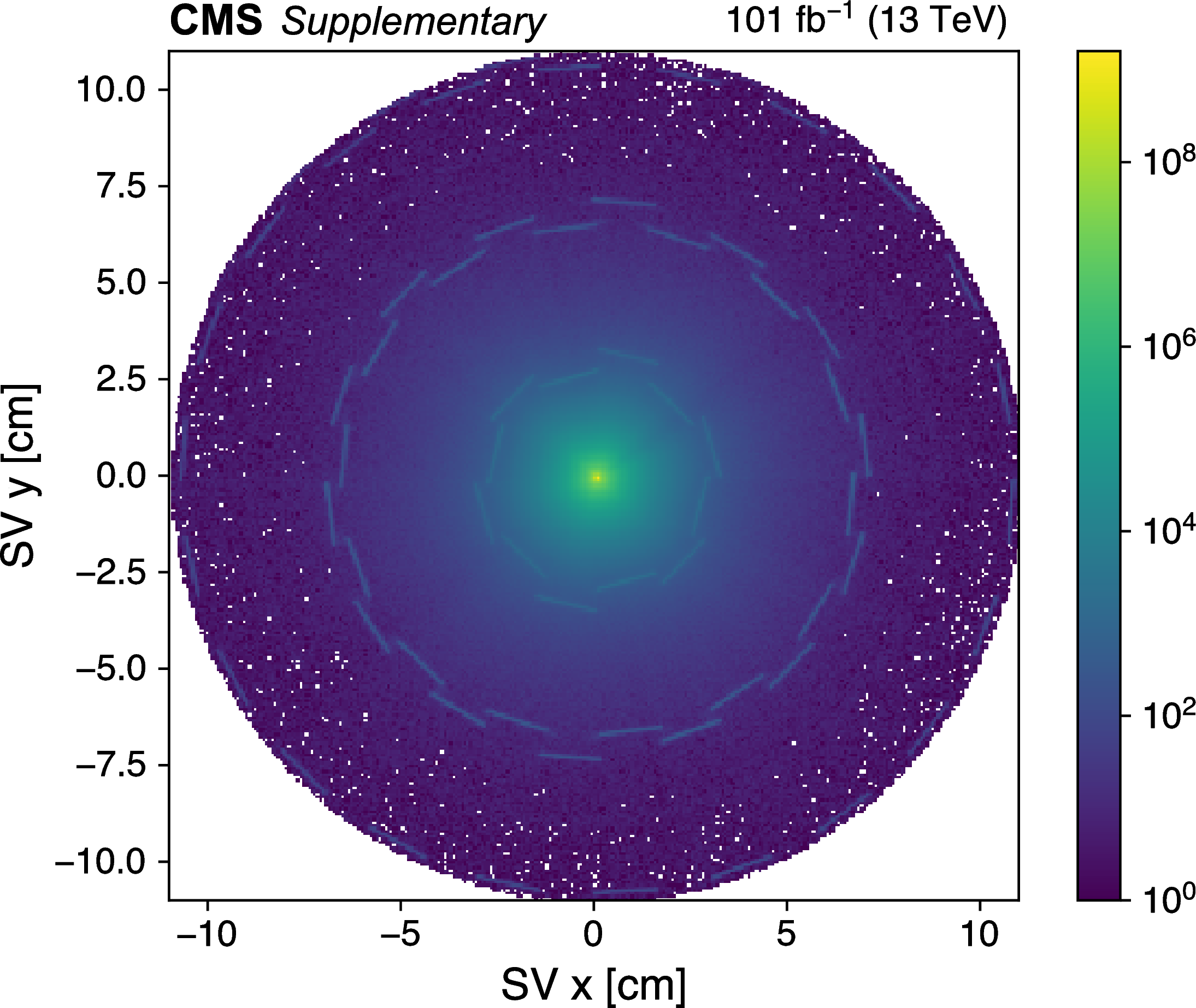
Distribution of DV position in the $x-y$ plane in data events passing trigger selections before a pixel tracker material veto is applied. |

png pdf |
Additional Figure 6:
Distribution of DV position in the $x-y$ plane in data events passing trigger selections after a pixel tracker material veto is applied. |
png pdf |
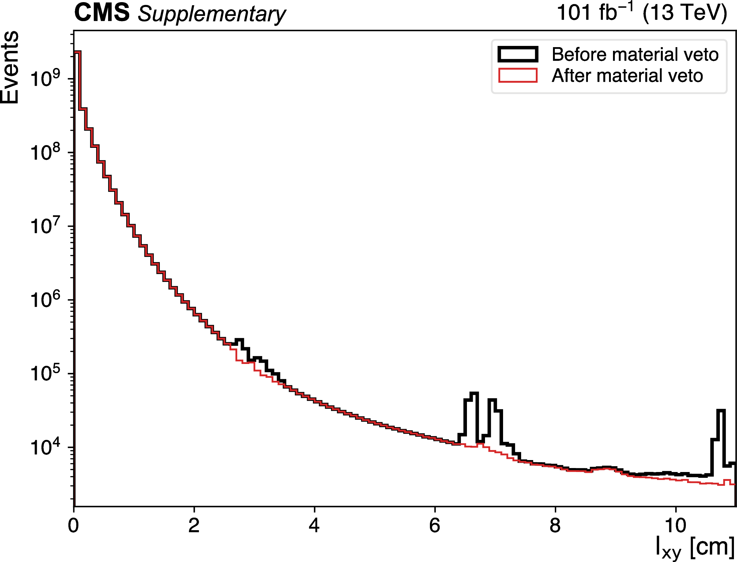
Additional Figure 7:
Distribution of ${l_\mathrm {xy}}$ for data events passing trigger selections before (black) and after (red) a pixel tracker material veto is applied. |
png pdf |
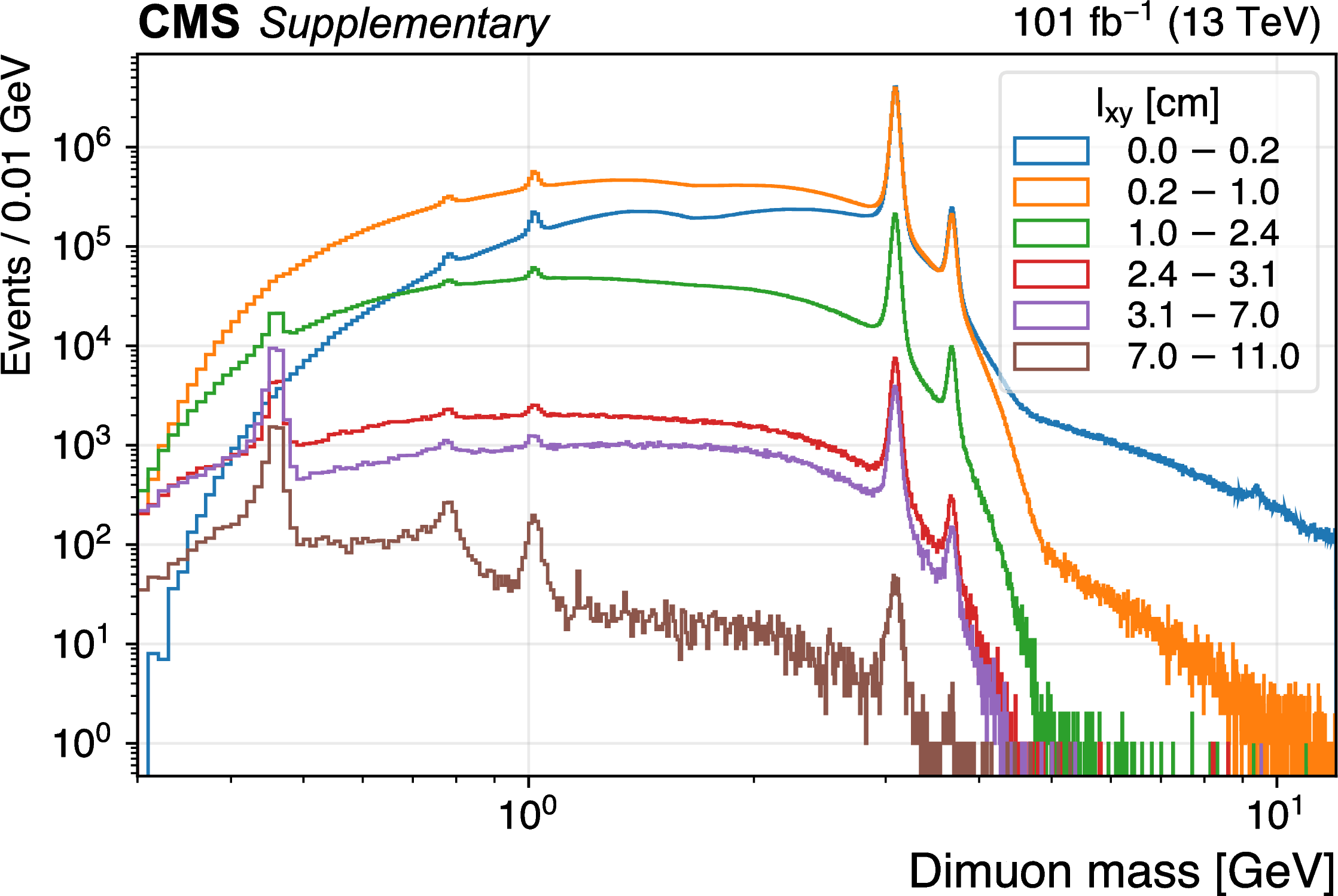
Additional Figure 8:
The dimuon invariant mass distribution is shown in bins of ${l_\mathrm {xy}}$ as obtained from all selected dimuon events. |
png pdf |
Additional Figure 9:
The dimuon invariant mass distribution is shown in bins of ${l_\mathrm {xy}}$ as obtained from selected dimuon events in data where none of the two muons are isolated with $ {{p_{\mathrm {T}}} ^{{\mu} {\mu}}} < $ 25 GeV: (upper left) 0.0 $ \leq {l_\mathrm {xy}} < $ 0.2 cm; (upper right) 0.2 $ \leq {l_\mathrm {xy}} < $ 1.0 cm; (middle left) 1.0 $ \leq {l_\mathrm {xy}} < $ 2.4 cm; (middle right) 2.4 $ \leq {l_\mathrm {xy}} < $ 3.1 cm; (lower left) 3.1 $ \leq {l_\mathrm {xy}} < $ 7.0 cm; (lower right) 7.0 $ \leq {l_\mathrm {xy}} < $ 11.0 cm. The distribution expected for representative signal models is overlaid. The vertical gray bands indicate mass ranges containing known SM resonances, which are masked for the purpose of this search. |

png pdf |
Additional Figure 10:
The dimuon invariant mass distribution is shown in bins of ${l_\mathrm {xy}}$ as obtained from selected dimuon events in data where none of the two muons are isolated with $ {{p_{\mathrm {T}}} ^{{\mu} {\mu}}} \geq $ 25 GeV: (upper left) 0.0 $ \leq {l_\mathrm {xy}} < $ 0.2 cm; (upper right) 0.2 $ \leq {l_\mathrm {xy}} < $ 1.0 cm; (middle left) 1.0 $ \leq {l_\mathrm {xy}} < $ 2.4 cm; (middle right) 2.4 $ \leq {l_\mathrm {xy}} < $ 3.1 cm; (lower left) 3.1 $ \leq {l_\mathrm {xy}} < $ 7.0 cm; (lower right) 7.0 $ \leq {l_\mathrm {xy}} < $ 11.0 cm. The distribution expected for representative signal models is overlaid. The vertical gray bands indicate mass ranges containing known SM resonances, which are masked for the purpose of this search. |
png pdf |
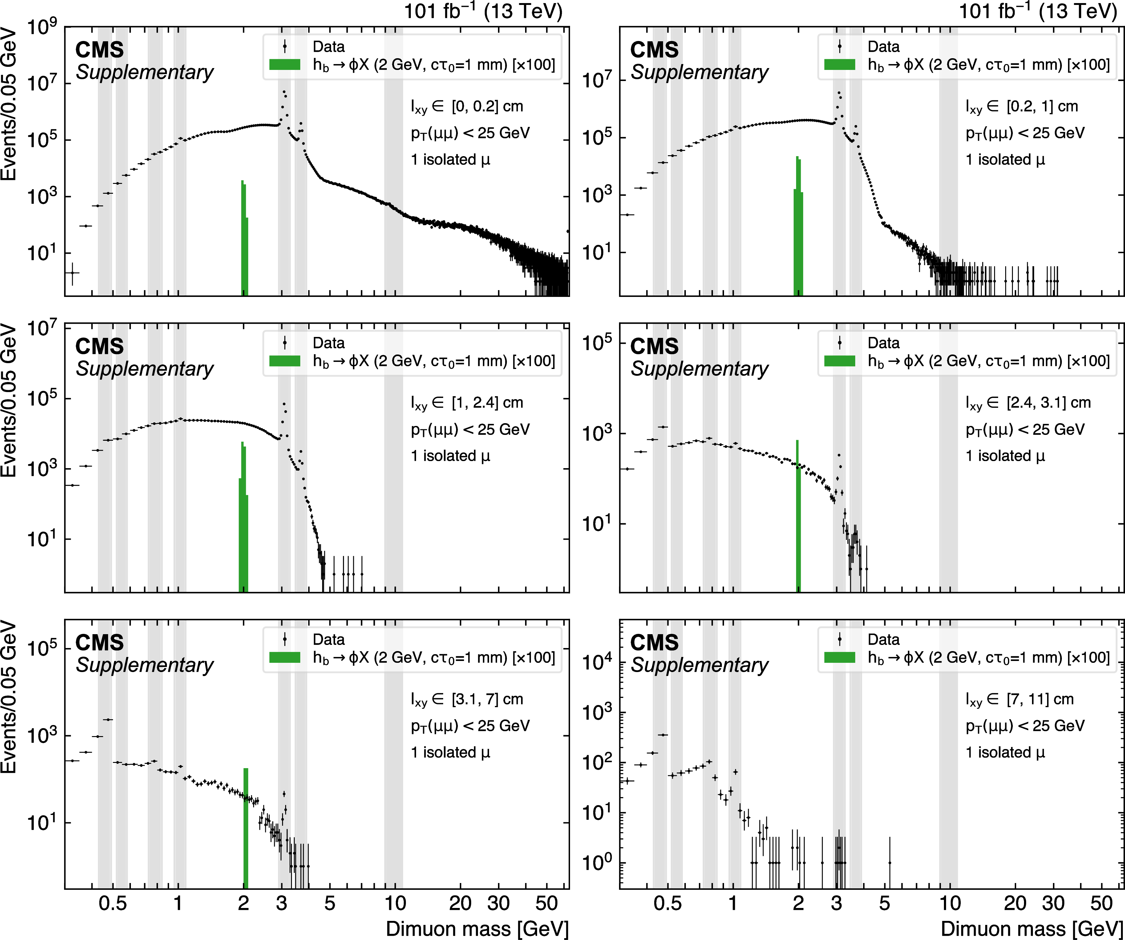
Additional Figure 11:
The dimuon invariant mass distribution is shown in bins of ${l_\mathrm {xy}}$ as obtained from selected dimuon events in data where only one muon is isolated with $ {{p_{\mathrm {T}}} ^{{\mu} {\mu}}} < $ 25 GeV: (upper left) 0.0 $ \leq {l_\mathrm {xy}} < $ 0.2 cm; (upper right) 0.2 $ \leq {l_\mathrm {xy}} < $ 1.0 cm; (middle left) 1.0 $ \leq {l_\mathrm {xy}} < $ 2.4 cm; (middle right) 2.4 $ \leq {l_\mathrm {xy}} < $ 3.1 cm; (lower left) 3.1 $ \leq {l_\mathrm {xy}} < $ 7.0 cm; (lower right) 7.0 $ \leq {l_\mathrm {xy}} < $ 11.0 cm. The distribution expected for representative signal models is overlaid. The vertical gray bands indicate mass ranges containing known SM resonances, which are masked for the purpose of this search. |
png pdf |
Additional Figure 12:
The dimuon invariant mass distribution is shown in bins of ${l_\mathrm {xy}}$ as obtained from selected dimuon events in data where only one muon is isolated with $ {{p_{\mathrm {T}}} ^{{\mu} {\mu}}} \geq $ 25 GeV: (upper left) 0.0 $ \leq {l_\mathrm {xy}} < $ 0.2 cm; (upper right) 0.2 $ \leq {l_\mathrm {xy}} < $ 1.0 cm; (middle left) 1.0 $ \leq {l_\mathrm {xy}} < $ 2.4 cm; (middle right) 2.4 $ \leq {l_\mathrm {xy}} < $ 3.1 cm; (lower left) 3.1 $ \leq {l_\mathrm {xy}} < $ 7.0 cm; (lower right) 7.0 $ \leq {l_\mathrm {xy}} < $ 11.0 cm. The distribution expected for representative signal models is overlaid. The vertical gray bands indicate mass ranges containing known SM resonances, which are masked for the purpose of this search. |

png pdf |
Additional Figure 13:
Observed exclusion limits at 95% CL on the branching fraction $\mathcal {B}(h_{{\mathrm {b}}}\to \phi X) \, \mathcal {B}(\phi \to {\mu} {\mu})$ as a function of $c\tau _{0}^{\phi}$ for various benchmark $m_{\phi}$ hypotheses, for the $h_{{\mathrm {b}}}\to \phi X$ signal model. The upper limits are obtained using the combination of all dimuon event categories. |
png pdf |
Additional Figure 14:
Observed exclusion limits at 95% CL on the branching fraction $\mathcal {B}({\mathrm {H}} \to {\mathrm {Z}} _{\mathrm {D}} {\mathrm {Z}} _{\mathrm {D}})$ as a function of $c\tau _{0}^{{\mathrm {Z}} _{\mathrm {D}}}$ for various benchmark $m_{{\mathrm {Z}} _{\mathrm {D}}}$ hypotheses, for the $ {\mathrm {H}} \to {\mathrm {Z}} _{\mathrm {D}} {\mathrm {Z}} _{\mathrm {D}}$ signal model. The upper limits are obtained using the combination of all dimuon event categories and the four-muon event category. |
png pdf |
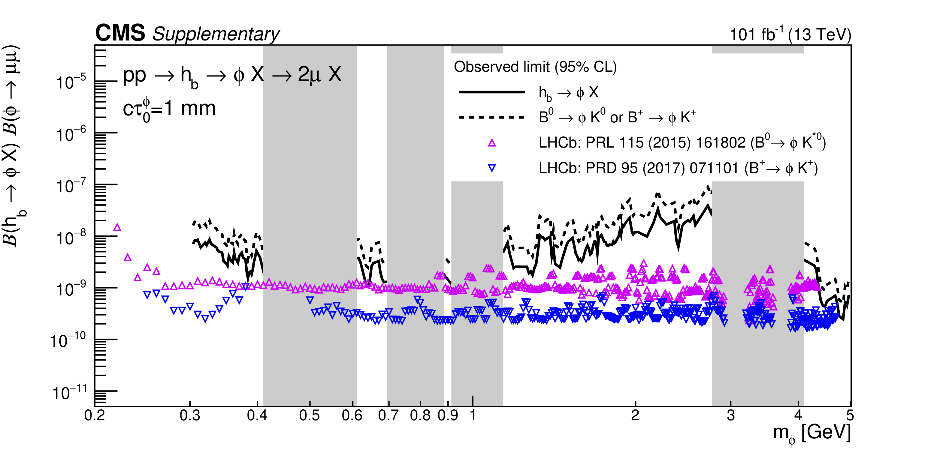
Additional Figure 15:
Observed exclusion limits at 95% CL on the branching fraction $\mathcal {B}(h_{{\mathrm {b}}}\to \phi X) \, \mathcal {B}(\phi \to {\mu} {\mu})$ as a function of $m_{\phi}$ for $c\tau _{0}^{\phi}=$ 1 mm, for the $h_{{\mathrm {b}}}\to \phi X$ signal model. The solid black line represents the observed exclusion when the inclusive $ {\mathrm {b}} $ hadron production process is considered. The dashed black line represents the observed exclusion after scaling the signal acceptance by the fraction of $ {\mathrm {B}} ^{\pm}$ or $ {\mathrm {B}} ^{0}$ hadrons at generator level. The exclusion limits are compared to recent LHCb results on the corresponding exclusive production and decay channels, represented by the triangular markers. The vertical gray bands indicate mass ranges containing known SM resonances, which are masked for the purpose of this search. The upper limits are obtained using the combination of all dimuon event categories. |
png pdf |
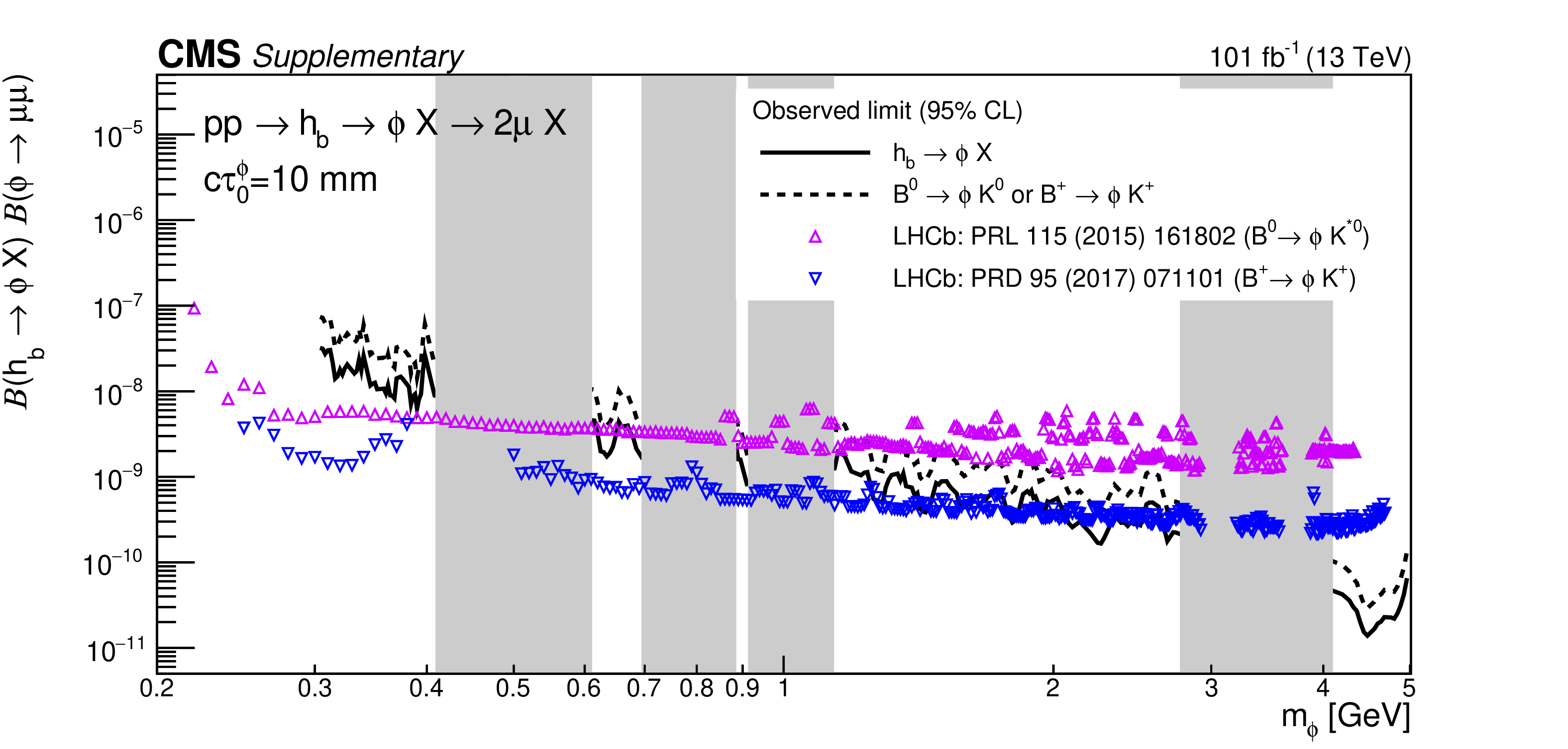
Additional Figure 16:
Observed exclusion limits at 95% CL on the branching fraction $\mathcal {B}(h_{{\mathrm {b}}}\to \phi X) \, \mathcal {B}(\phi \to {\mu} {\mu})$ as a function of $m_{\phi}$ for $c\tau _{0}^{\phi}=$ 10 mm, for the $h_{{\mathrm {b}}}\to \phi X$ signal model. The solid black line represents the observed exclusion when the inclusive $ {\mathrm {b}} $ hadron production process is considered. The dashed black line represents the observed exclusion after scaling the signal acceptance by the fraction of $ {\mathrm {B}} ^{\pm}$ or $ {\mathrm {B}} ^{0}$ hadrons at generator level. The exclusion limits are compared to recent LHCb results on the corresponding exclusive production and decay channels, represented by the triangular markers. The vertical gray bands indicate mass ranges containing known SM resonances, which are masked for the purpose of this search. The upper limits are obtained using the combination of all dimuon event categories. |
png pdf |
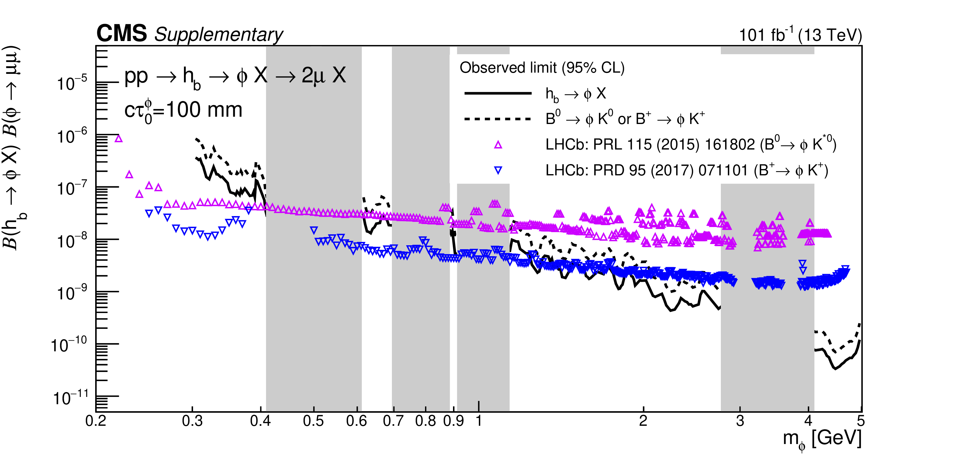
Additional Figure 17:
Observed exclusion limits at 95% CL on the branching fraction $\mathcal {B}(h_{{\mathrm {b}}}\to \phi X) \, \mathcal {B}(\phi \to {\mu} {\mu})$ as a function of $m_{\phi}$ for $c\tau _{0}^{\phi}=$ 100 mm, for the $h_{{\mathrm {b}}}\to \phi X$ signal model. The solid black line represents the observed exclusion when the inclusive $ {\mathrm {b}} $ hadron production process is considered. The dashed black line represents the observed exclusion after scaling the signal acceptance by the fraction of $ {\mathrm {B}} ^{\pm}$ or $ {\mathrm {B}} ^{0}$ hadrons at generator level. The exclusion limits are compared to recent LHCb results on the corresponding exclusive production and decay channels, represented by the triangular markers. The vertical gray bands indicate mass ranges containing known SM resonances, which are masked for the purpose of this search. The upper limits are obtained using the combination of all dimuon event categories. |

png pdf |
Additional Figure 18:
Observed exclusion limits at 95% CL on the branching fraction $\mathcal {B}(h_{{\mathrm {b}}}\to \phi X) \, \mathcal {B}(\phi \to {\mu} {\mu})$ as a function of $c\tau _{0}^{\phi}$ and $m_{\phi}$, for the $h_{{\mathrm {b}}}\to \phi X$ signal model. The vertical gray bands indicate mass ranges containing known SM resonances, which are masked for the purpose of this search. The upper limits are obtained using the combination of all dimuon event categories. |

png pdf |
Additional Figure 19:
Observed exclusion limits at 95% CL on the branching fraction $\mathcal {B}({\mathrm {H}} \to {\mathrm {Z}} _{\mathrm {D}} {\mathrm {Z}} _{\mathrm {D}})$ as a function of $c\tau _{0}^{{\mathrm {Z}} _{\mathrm {D}}}$ and $m_{{\mathrm {Z}} _{\mathrm {D}}}$, for the $ {\mathrm {H}} \to {\mathrm {Z}} _{\mathrm {D}} {\mathrm {Z}} _{\mathrm {D}}$ signal model. The vertical gray bands indicate mass ranges containing known SM resonances, which are masked for the purpose of this search. The upper limits are obtained using the combination of all dimuon event categories and the four-muon event category. |
png pdf |
Additional Figure 20:
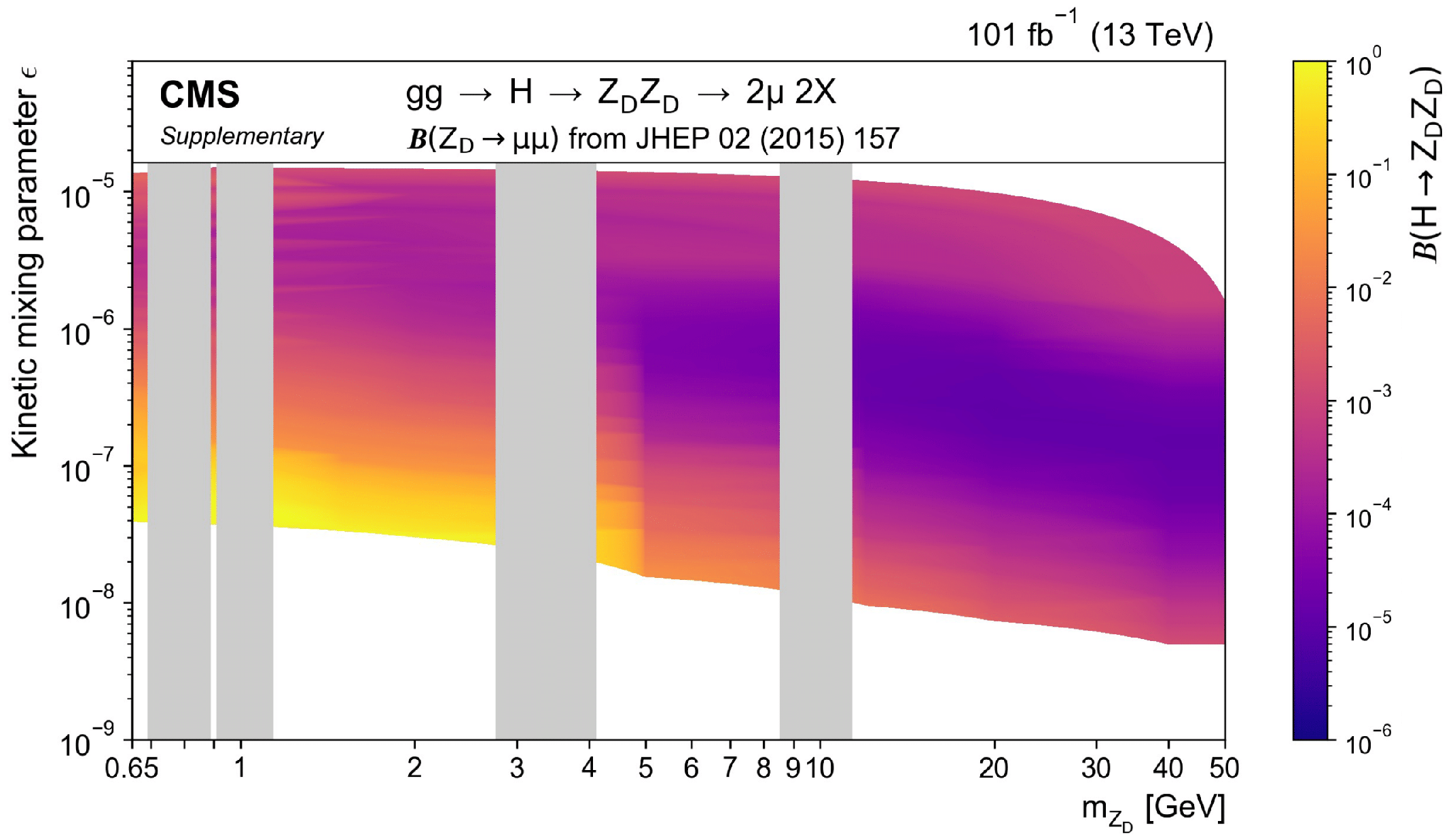
Observed exclusion limits at 95% CL on the branching fraction $\mathcal {B}({\mathrm {H}} \to {\mathrm {Z}} _{\mathrm {D}} {\mathrm {Z}} _{\mathrm {D}})$ as a function of the kinetic mixing parameter $\epsilon $ and $m_{{\mathrm {Z}} _{\mathrm {D}}}$, for the $ {\mathrm {H}} \to {\mathrm {Z}} _{\mathrm {D}} {\mathrm {Z}} _{\mathrm {D}}$ signal model. The vertical gray bands indicate mass ranges containing known SM resonances, which are masked for the purpose of this search. The upper limits are obtained using the combination of all dimuon event categories and the four-muon event category. |
png pdf |
Additional Figure 21:
Trigger efficiency as a function of generated ${l_\mathrm {xy}}$ and generated trailing muon ${p_{\mathrm {T}}}$, for the $h_{{\mathrm {b}}}\to \phi X$ signal model with $m_{\phi} < $ 3 GeV. The trigger efficiency is measured in simulated events with a pair of oppositely charged generated muons, each with generated $ p_{\mathrm {T}} >$ 3 GeV and generated $|\eta| <$ 2.4. |
png pdf |
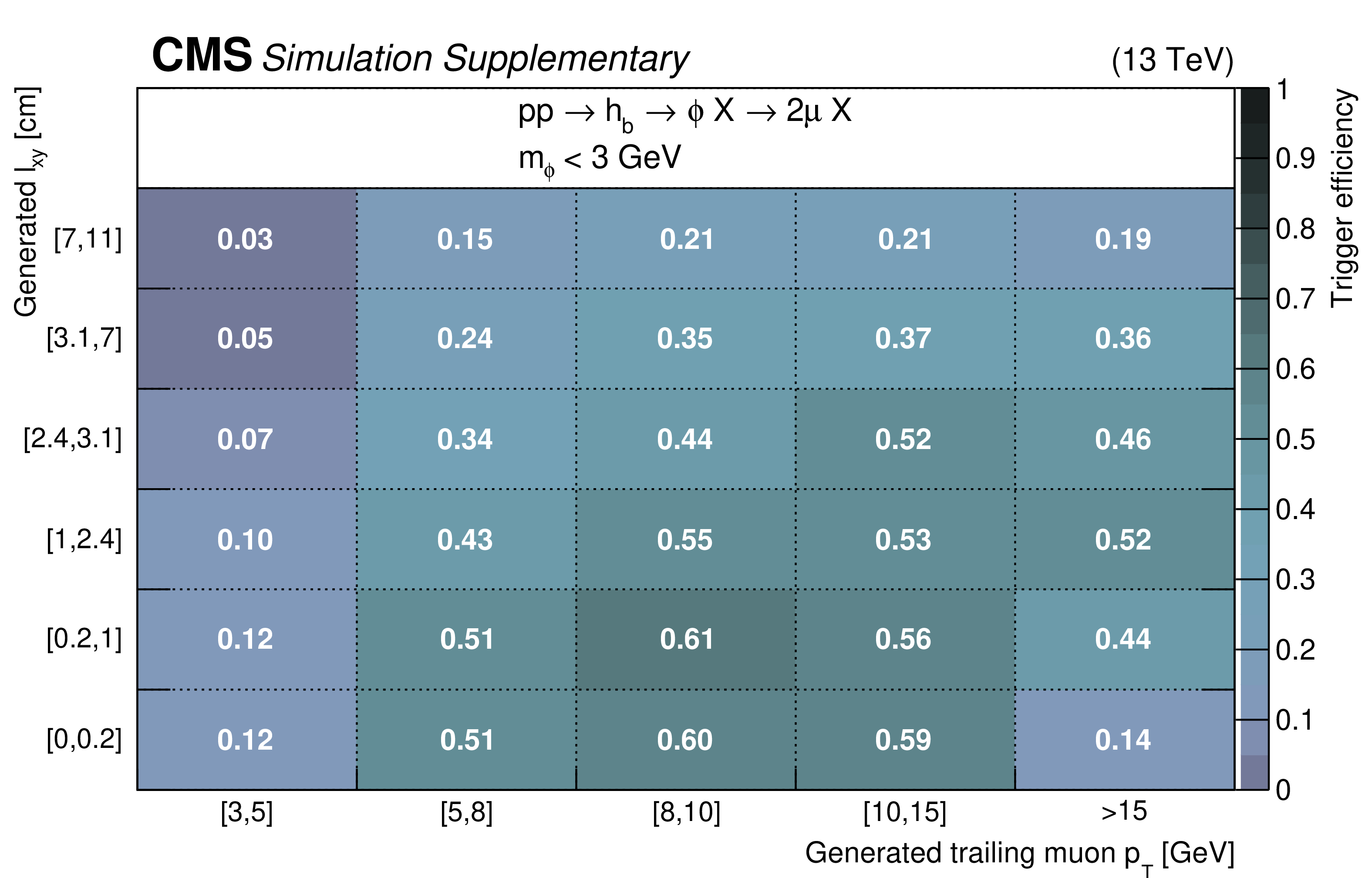
Additional Figure 22:
Trigger efficiency as a function of generated ${l_\mathrm {xy}}$ and generated trailing muon ${p_{\mathrm {T}}}$, for the $h_{{\mathrm {b}}}\to \phi X$ signal model with 3 $ < m_{\phi} < $ 5 GeV. The trigger efficiency is measured in simulated events with a pair of oppositely charged generated muons, each with generated $ p_{\mathrm {T}} >$ 3 GeV and generated $|\eta| <$ 2.4. |
png pdf |
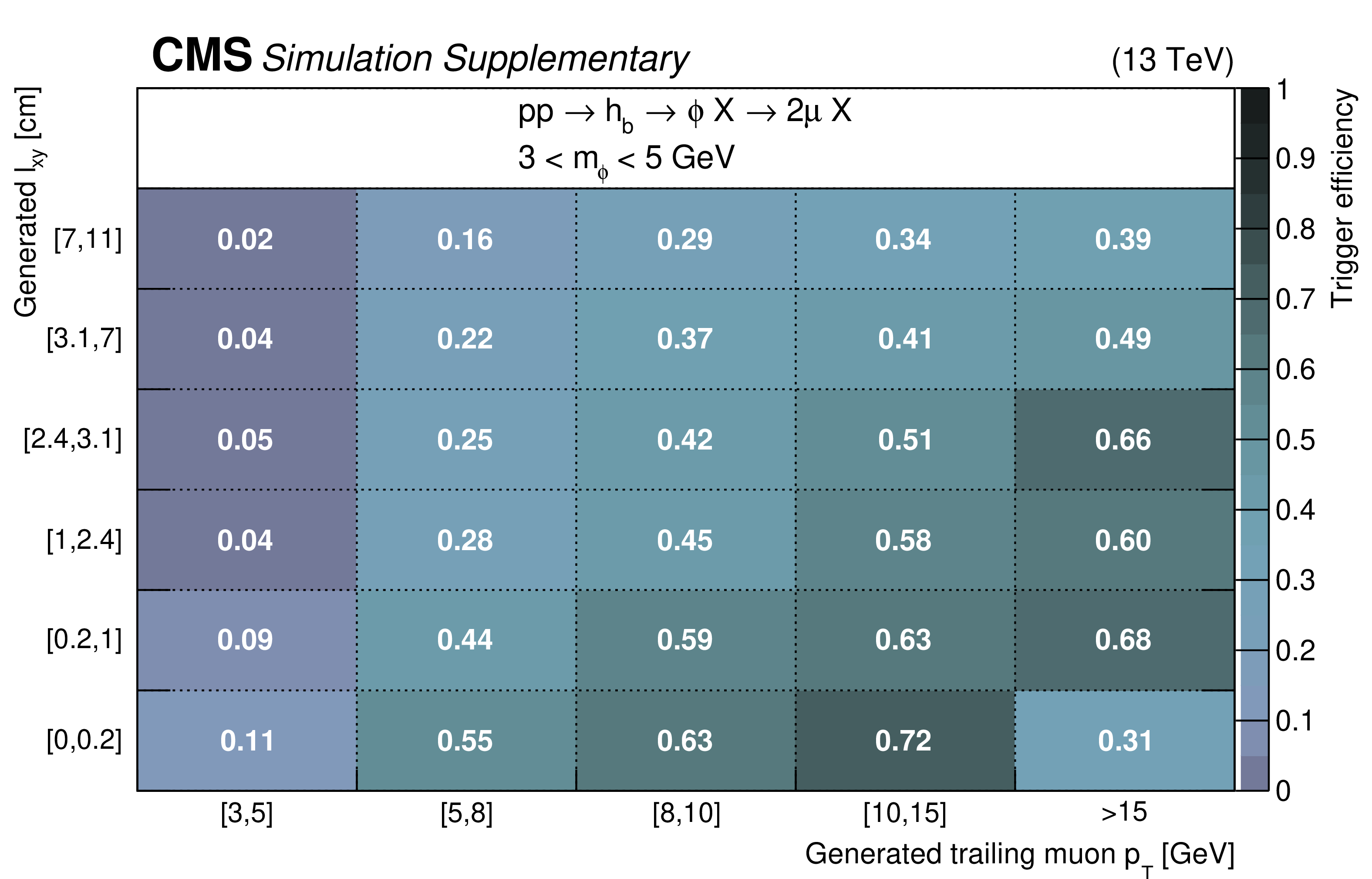
Additional Figure 23:
Trigger efficiency as a function of generated ${l_\mathrm {xy}}$ and generated trailing muon ${p_{\mathrm {T}}}$, for the $ {\mathrm {H}} \to {\mathrm {Z}} _{\mathrm {D}} {\mathrm {Z}} _{\mathrm {D}}$ signal model with $m_{{\mathrm {Z}} _{\mathrm {D}}} < $ 3 GeV. The trigger efficiency is measured in simulated events with a pair of oppositely charged generated muons, each with generated $ p_{\mathrm {T}} >$ 3 GeV and generated $|\eta| <$ 2.4. |

png pdf |
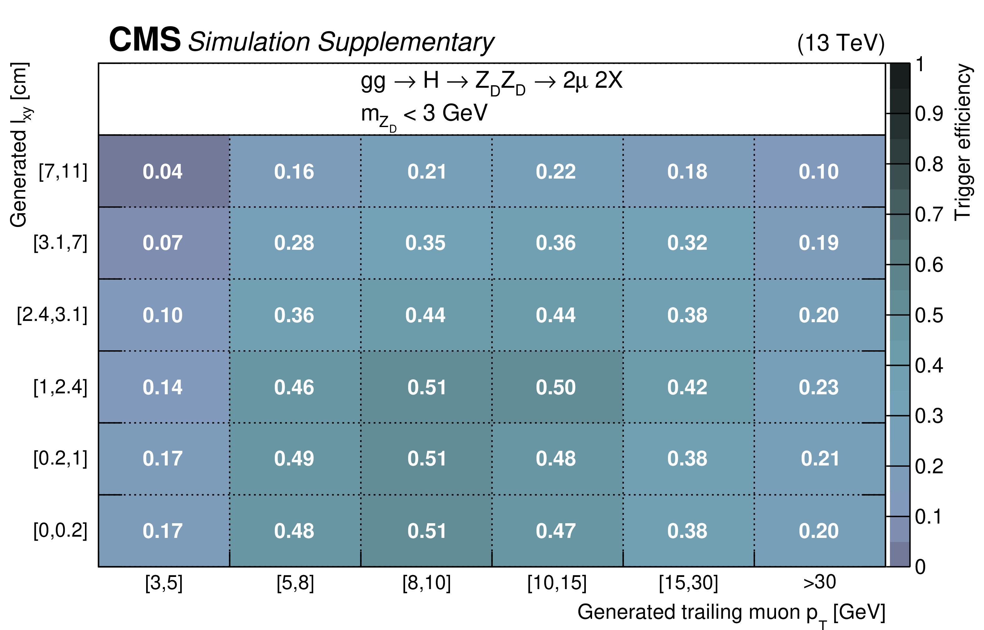
Additional Figure 24:
Trigger efficiency as a function of generated ${l_\mathrm {xy}}$ and generated trailing muon ${p_{\mathrm {T}}}$, for the $ {\mathrm {H}} \to {\mathrm {Z}} _{\mathrm {D}} {\mathrm {Z}} _{\mathrm {D}}$ signal model with 3 $ < m_{{\mathrm {Z}} _{\mathrm {D}}} < $ 5 GeV. The trigger efficiency is measured in simulated events with a pair of oppositely charged generated muons, each with generated $ p_{\mathrm {T}} >$ 3 GeV and generated $|\eta| <$ 2.4. |
png pdf |
Additional Figure 25:
Trigger efficiency as a function of generated ${l_\mathrm {xy}}$ and generated trailing muon ${p_{\mathrm {T}}}$, for the $ {\mathrm {H}} \to {\mathrm {Z}} _{\mathrm {D}} {\mathrm {Z}} _{\mathrm {D}}$ signal model with 5 $ < m_{{\mathrm {Z}} _{\mathrm {D}}} < $ 10 GeV. The trigger efficiency is measured in simulated events with a pair of oppositely charged generated muons, each with generated $ p_{\mathrm {T}} >$ 3 GeV and generated $|\eta| <$ 2.4. |
png pdf |
Additional Figure 26:
Trigger efficiency as a function of generated ${l_\mathrm {xy}}$ and generated trailing muon ${p_{\mathrm {T}}}$, for the $ {\mathrm {H}} \to {\mathrm {Z}} _{\mathrm {D}} {\mathrm {Z}} _{\mathrm {D}}$ signal model with 10 $ < m_{{\mathrm {Z}} _{\mathrm {D}}} < $ 20 GeV. The trigger efficiency is measured in simulated events with a pair of oppositely charged generated muons, each with generated $ p_{\mathrm {T}} >$ 3 GeV and generated $|\eta| <$ 2.4. |
png pdf |
Additional Figure 27:
Trigger efficiency as a function of generated ${l_\mathrm {xy}}$ and generated trailing muon ${p_{\mathrm {T}}}$, for the $ {\mathrm {H}} \to {\mathrm {Z}} _{\mathrm {D}} {\mathrm {Z}} _{\mathrm {D}}$ signal model with 20 $ < m_{{\mathrm {Z}} _{\mathrm {D}}} < $ 40 GeV. The trigger efficiency is measured in simulated events with a pair of oppositely charged generated muons, each with generated $ p_{\mathrm {T}} >$ 3 GeV and generated $|\eta| <$ 2.4. |

png pdf |
Additional Figure 28:
Trigger efficiency as a function of generated ${l_\mathrm {xy}}$ and generated trailing muon ${p_{\mathrm {T}}}$, for the $ {\mathrm {H}} \to {\mathrm {Z}} _{\mathrm {D}} {\mathrm {Z}} _{\mathrm {D}}$ signal model with $m_{{\mathrm {Z}} _{\mathrm {D}}} > $ 40 GeV. The trigger efficiency is measured in simulated events with a pair of oppositely charged generated muons, each with generated $ p_{\mathrm {T}} >$ 3 GeV and generated $|\eta| <$ 2.4. |
png pdf |
Additional Figure 29:
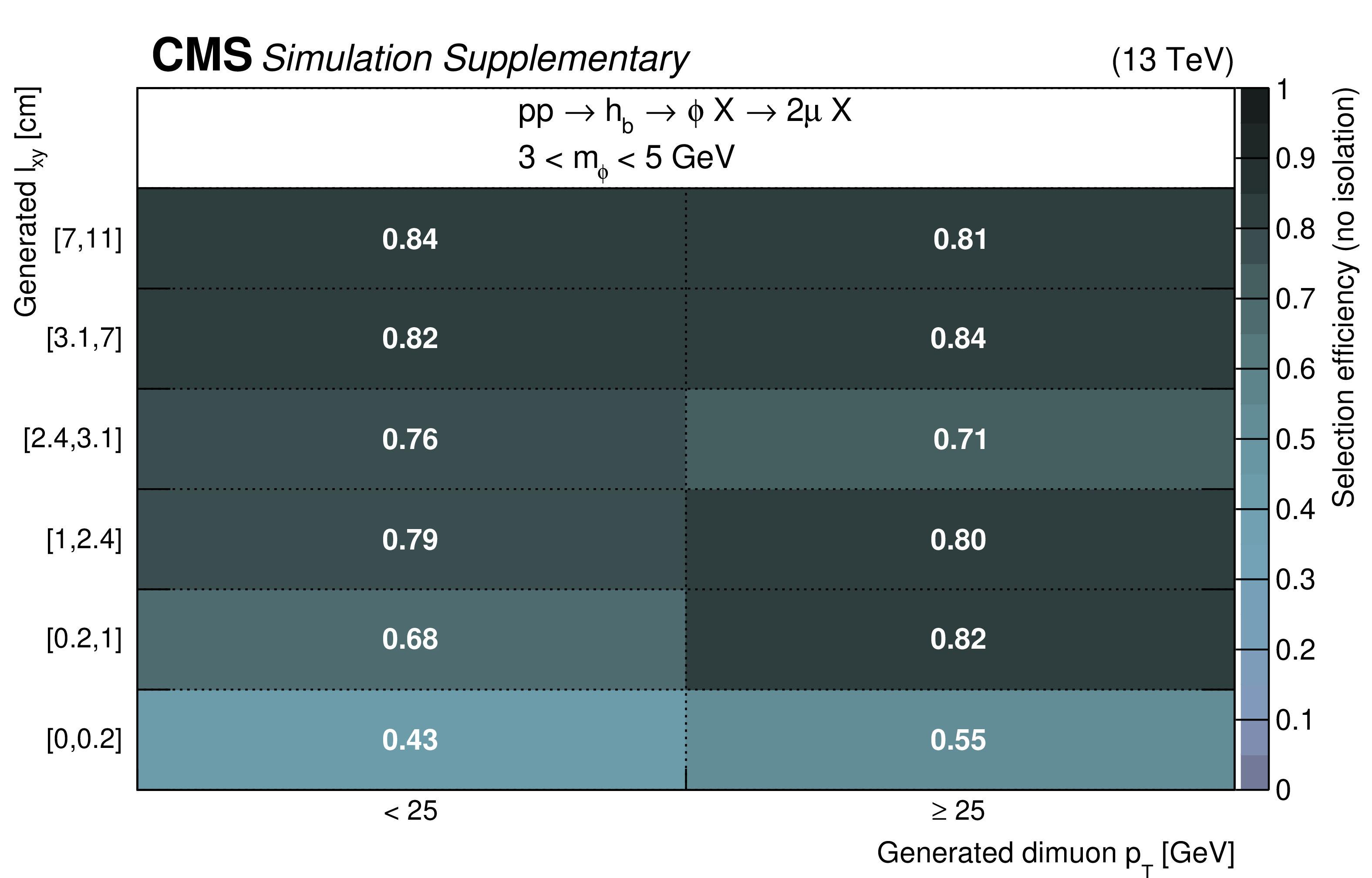
Efficiency of the selection applied after trigger, without requirements on the muon isolation, as a function of generated ${l_\mathrm {xy}}$ and generated ${{p_{\mathrm {T}}} ^{{\mu} {\mu}}}$, for the $h_{{\mathrm {b}}}\to \phi X$ signal model with $m_{\phi} < $ 3 GeV. |
png pdf |
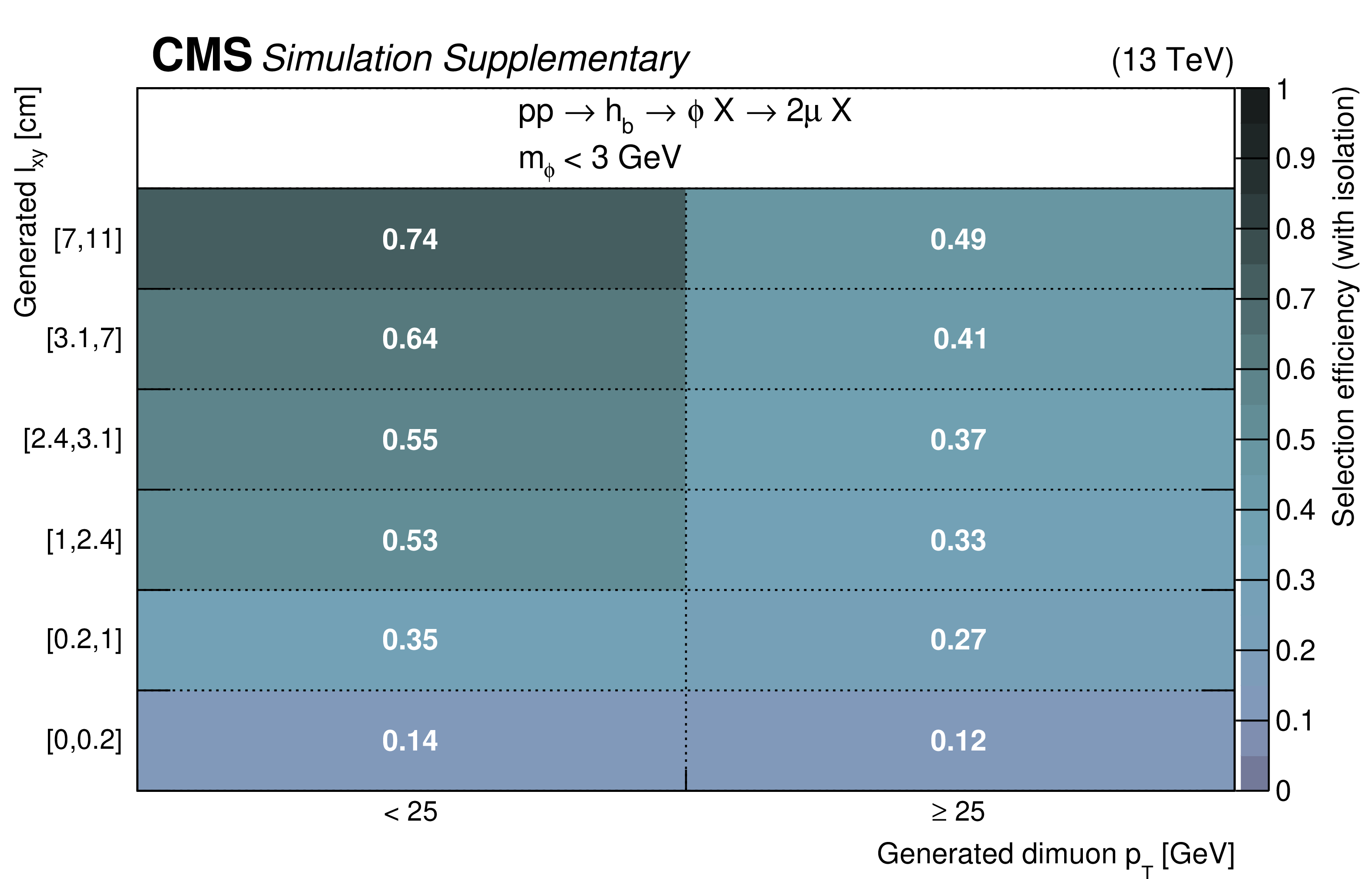
Additional Figure 30:
Efficiency of the selection applied after trigger, with requirements on the muon isolation, as a function of generated ${l_\mathrm {xy}}$ and generated ${{p_{\mathrm {T}}} ^{{\mu} {\mu}}}$, for the $h_{{\mathrm {b}}}\to \phi X$ signal model with $m_{\phi} < $ 3 GeV. |
png pdf |
Additional Figure 31:
Efficiency of the selection applied after trigger, without requirements on the muon isolation, as a function of generated ${l_\mathrm {xy}}$ and generated ${{p_{\mathrm {T}}} ^{{\mu} {\mu}}}$, for the $h_{{\mathrm {b}}}\to \phi X$ signal model with 3 $ < m_{\phi} < $ 5 GeV. |
png pdf |
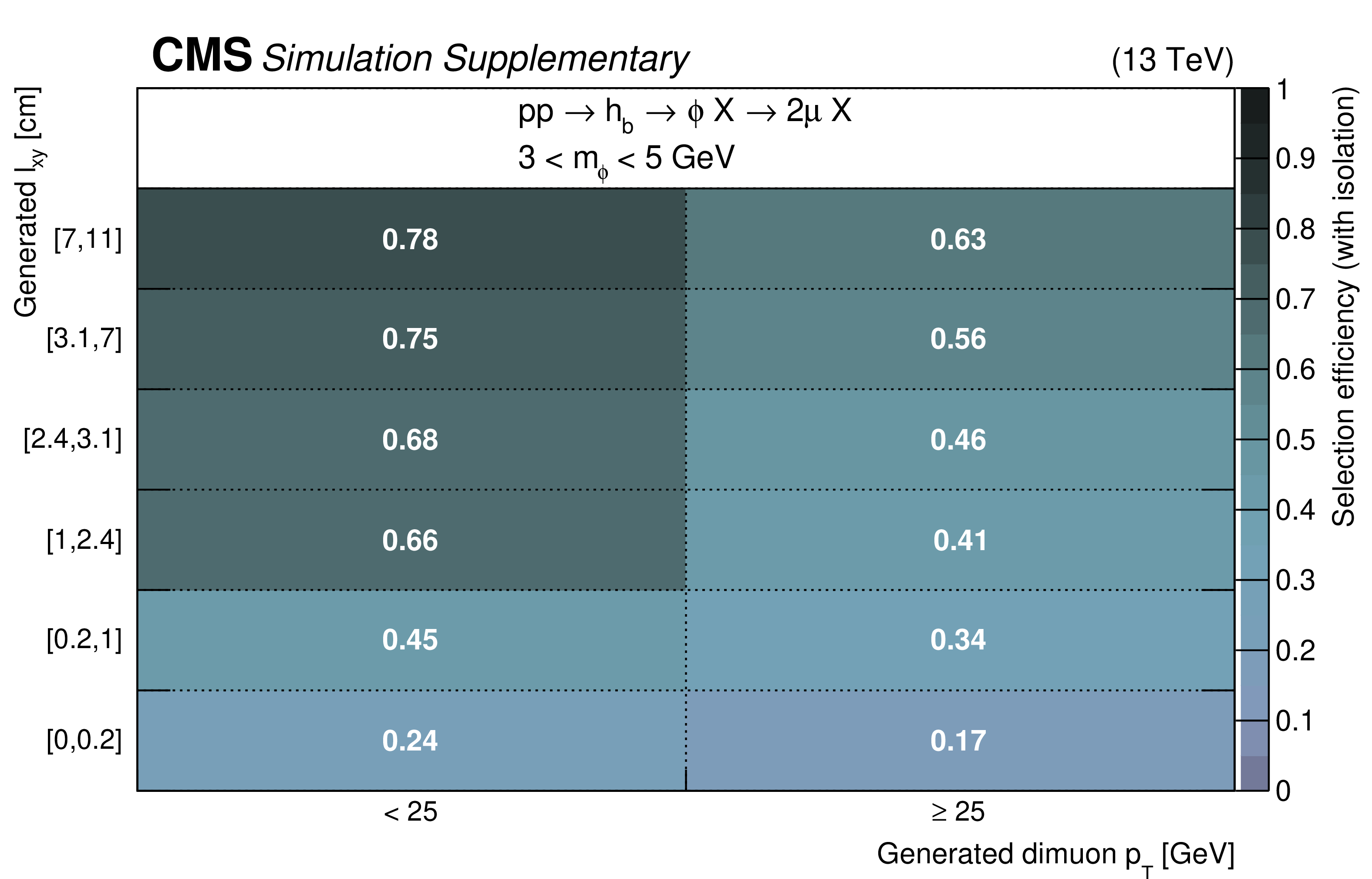
Additional Figure 32:
Efficiency of the selection applied after trigger, with requirements on the muon isolation, as a function of generated ${l_\mathrm {xy}}$ and generated ${{p_{\mathrm {T}}} ^{{\mu} {\mu}}}$, for the $h_{{\mathrm {b}}}\to \phi X$ signal model with 3 $ < m_{\phi} < $ 5 GeV. |
png pdf |
Additional Figure 33:
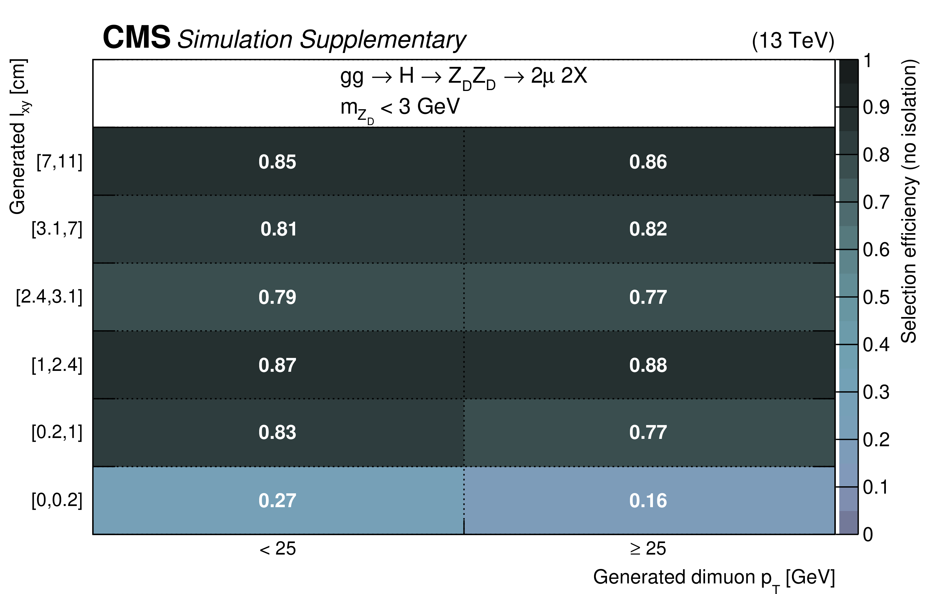
Efficiency of the selection applied after trigger, without requirements on the muon isolation, as a function of generated ${l_\mathrm {xy}}$ and generated ${{p_{\mathrm {T}}} ^{{\mu} {\mu}}}$, for the $ {\mathrm {H}} \to {\mathrm {Z}} _{\mathrm {D}} {\mathrm {Z}} _{\mathrm {D}}$ signal model with $m_{{\mathrm {Z}} _{\mathrm {D}}} < $ 3 GeV. |

png pdf |
Additional Figure 34:
Efficiency of the selection applied after trigger, with requirements on the muon isolation, as a function of generated ${l_\mathrm {xy}}$ and generated ${{p_{\mathrm {T}}} ^{{\mu} {\mu}}}$, for the $ {\mathrm {H}} \to {\mathrm {Z}} _{\mathrm {D}} {\mathrm {Z}} _{\mathrm {D}}$ signal model with $m_{{\mathrm {Z}} _{\mathrm {D}}} < $ 3 GeV. |
png pdf |
Additional Figure 35:
Efficiency of the selection applied after trigger, without requirements on the muon isolation, as a function of generated ${l_\mathrm {xy}}$ and generated ${{p_{\mathrm {T}}} ^{{\mu} {\mu}}}$, for the $ {\mathrm {H}} \to {\mathrm {Z}} _{\mathrm {D}} {\mathrm {Z}} _{\mathrm {D}}$ signal model with 3 $ < m_{{\mathrm {Z}} _{\mathrm {D}}} < $ 5 GeV. |

png pdf |
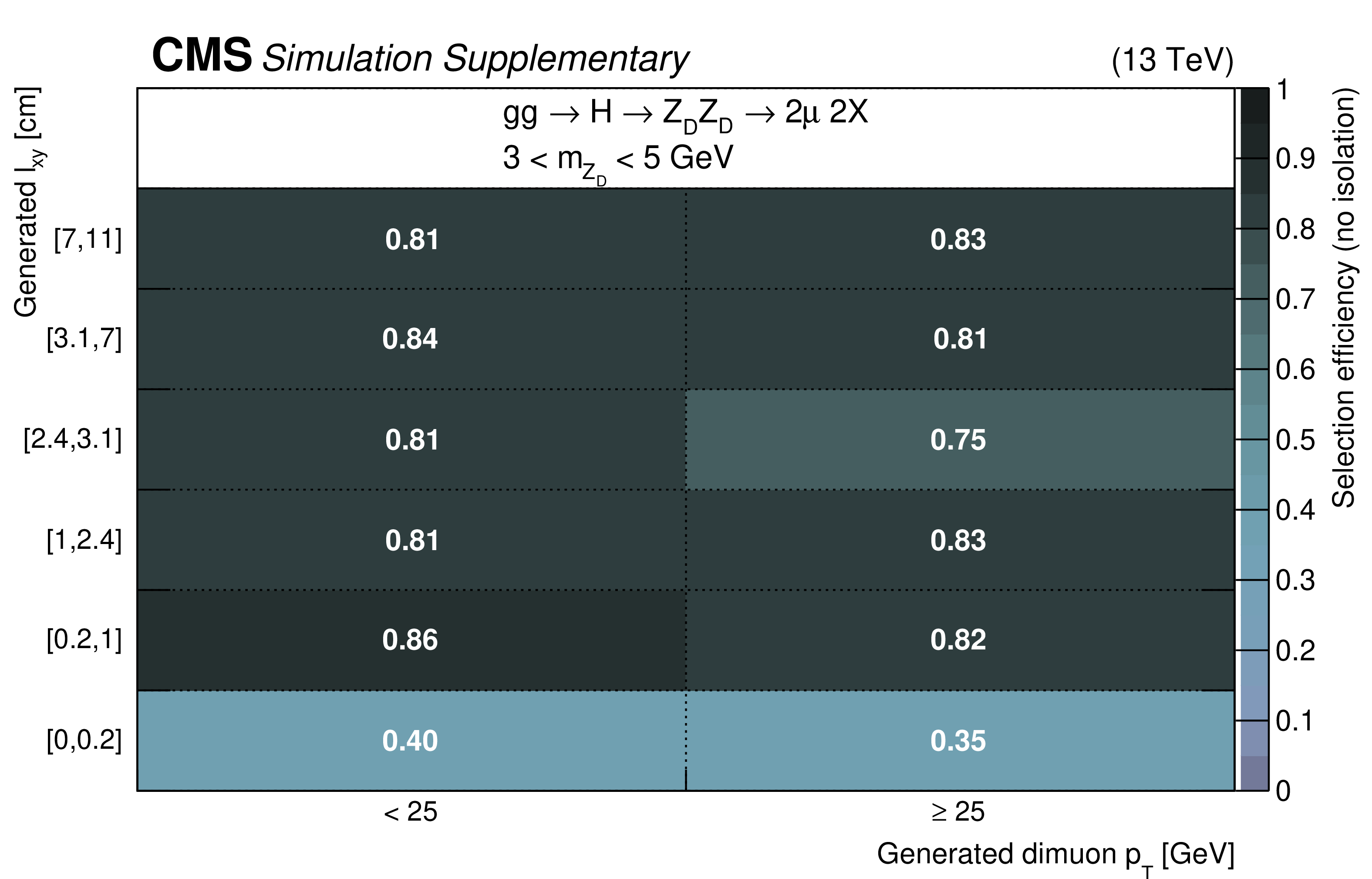
Additional Figure 36:
Efficiency of the selection applied after trigger, with requirements on the muon isolation, as a function of generated ${l_\mathrm {xy}}$ and generated ${{p_{\mathrm {T}}} ^{{\mu} {\mu}}}$, for the $ {\mathrm {H}} \to {\mathrm {Z}} _{\mathrm {D}} {\mathrm {Z}} _{\mathrm {D}}$ signal model with 3 $ < m_{{\mathrm {Z}} _{\mathrm {D}}} < $ 5 GeV. |
png pdf |
Additional Figure 37:
Efficiency of the selection applied after trigger, without requirements on the muon isolation, as a function of generated ${l_\mathrm {xy}}$ and generated ${{p_{\mathrm {T}}} ^{{\mu} {\mu}}}$, for the $ {\mathrm {H}} \to {\mathrm {Z}} _{\mathrm {D}} {\mathrm {Z}} _{\mathrm {D}}$ signal model with 5 $ < m_{{\mathrm {Z}} _{\mathrm {D}}} < $ 10 GeV. |
png pdf |
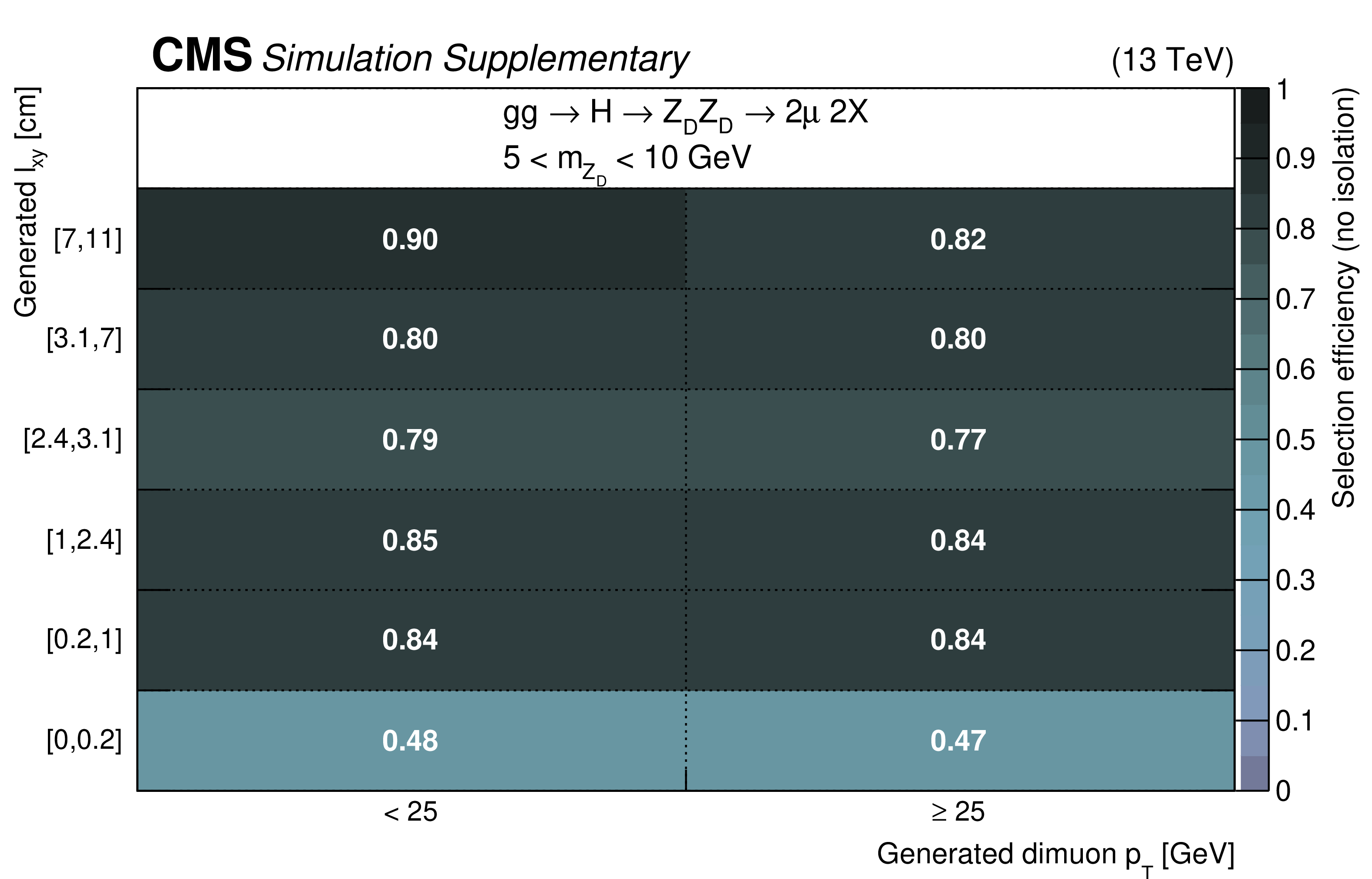
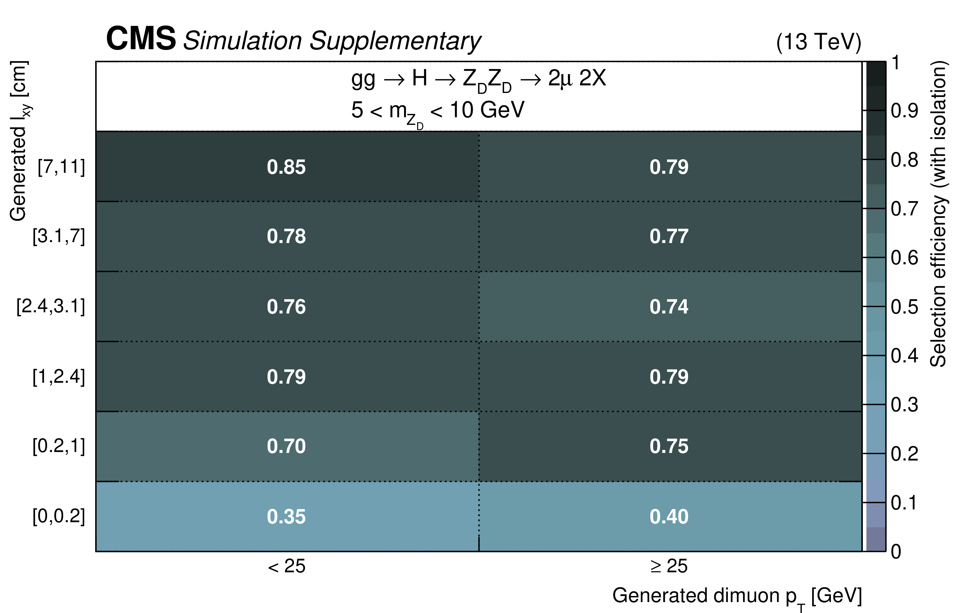
Additional Figure 38:
Efficiency of the selection applied after trigger, with requirements on the muon isolation, as a function of generated ${l_\mathrm {xy}}$ and generated ${{p_{\mathrm {T}}} ^{{\mu} {\mu}}}$, for the $ {\mathrm {H}} \to {\mathrm {Z}} _{\mathrm {D}} {\mathrm {Z}} _{\mathrm {D}}$ signal model with 5 $ < m_{{\mathrm {Z}} _{\mathrm {D}}} < $ 10 GeV. |
png pdf |
Additional Figure 39:
Efficiency of the selection applied after trigger, without requirements on the muon isolation, as a function of generated ${l_\mathrm {xy}}$ and generated ${{p_{\mathrm {T}}} ^{{\mu} {\mu}}}$, for the $ {\mathrm {H}} \to {\mathrm {Z}} _{\mathrm {D}} {\mathrm {Z}} _{\mathrm {D}}$ signal model with 10 $ < m_{{\mathrm {Z}} _{\mathrm {D}}} < $ 20 GeV. |
png pdf |
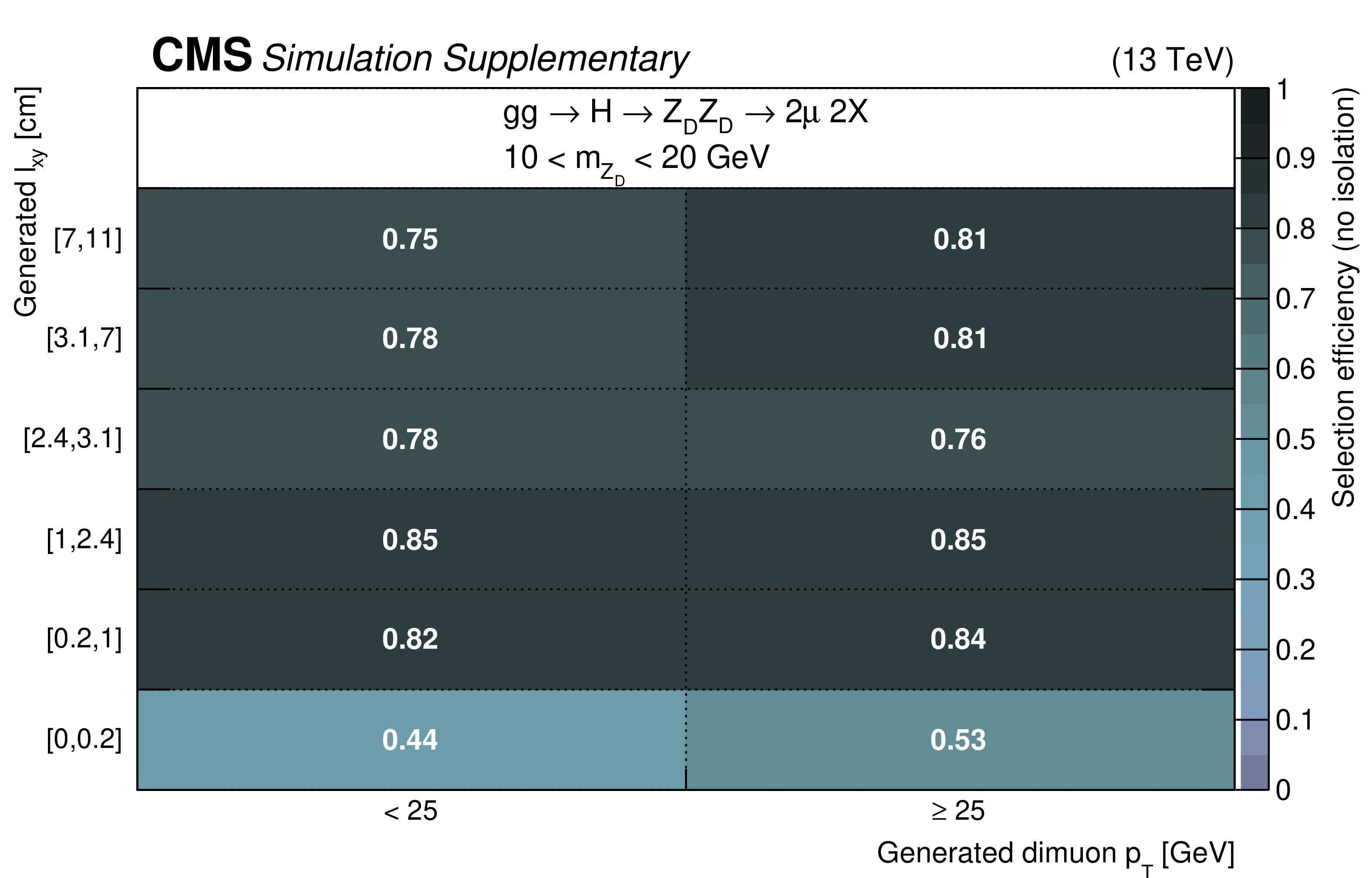
Additional Figure 40:
Efficiency of the selection applied after trigger, with requirements on the muon isolation, as a function of generated ${l_\mathrm {xy}}$ and generated ${{p_{\mathrm {T}}} ^{{\mu} {\mu}}}$, for the $ {\mathrm {H}} \to {\mathrm {Z}} _{\mathrm {D}} {\mathrm {Z}} _{\mathrm {D}}$ signal model with 10 $ < m_{{\mathrm {Z}} _{\mathrm {D}}} < $ 20 GeV. |

png pdf |
Additional Figure 41:
Efficiency of the selection applied after trigger, without requirements on the muon isolation, as a function of generated ${l_\mathrm {xy}}$ and generated ${{p_{\mathrm {T}}} ^{{\mu} {\mu}}}$, for the $ {\mathrm {H}} \to {\mathrm {Z}} _{\mathrm {D}} {\mathrm {Z}} _{\mathrm {D}}$ signal model with 20 $ < m_{{\mathrm {Z}} _{\mathrm {D}}} < $ 40 GeV. |
png pdf |
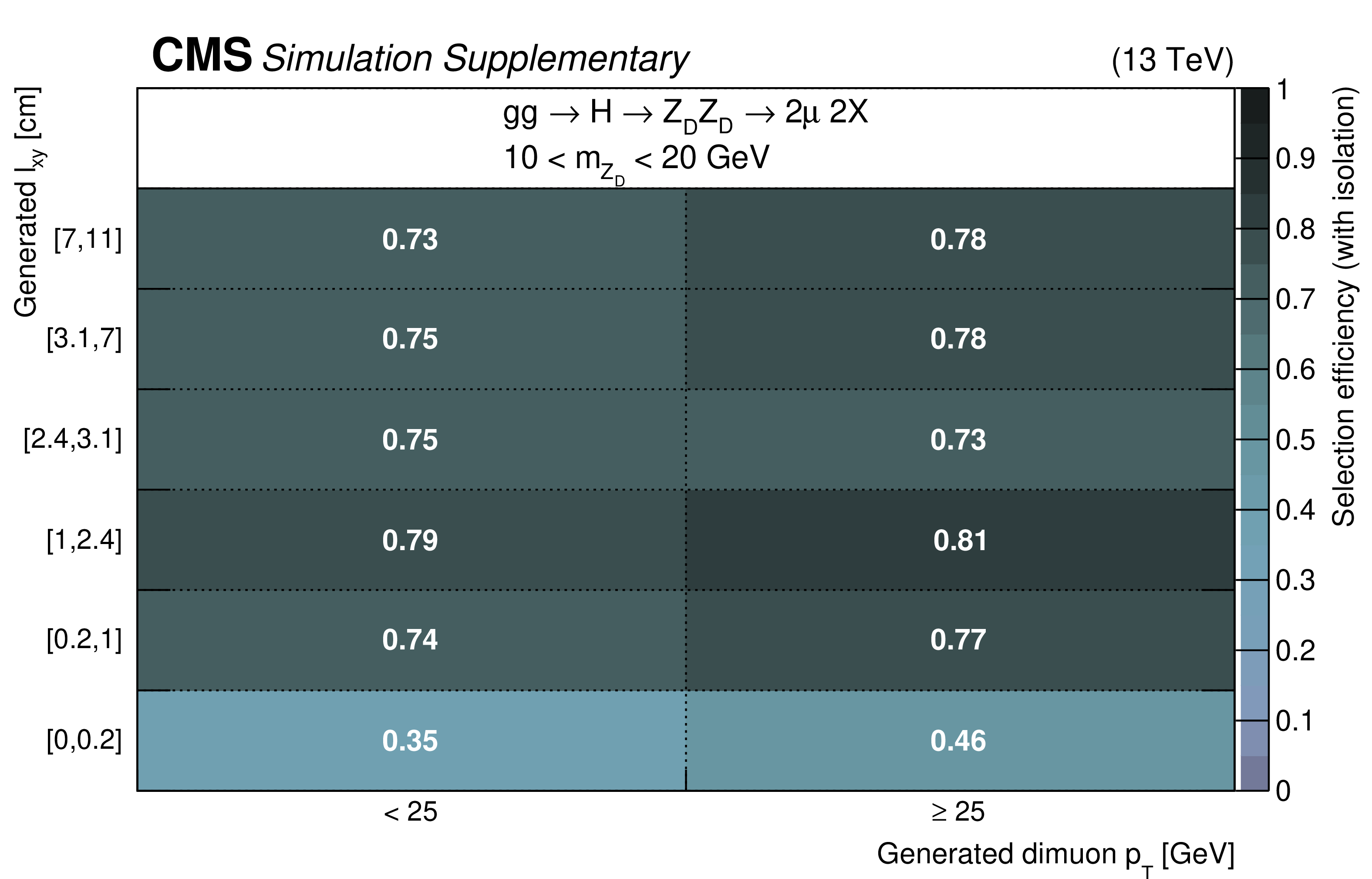
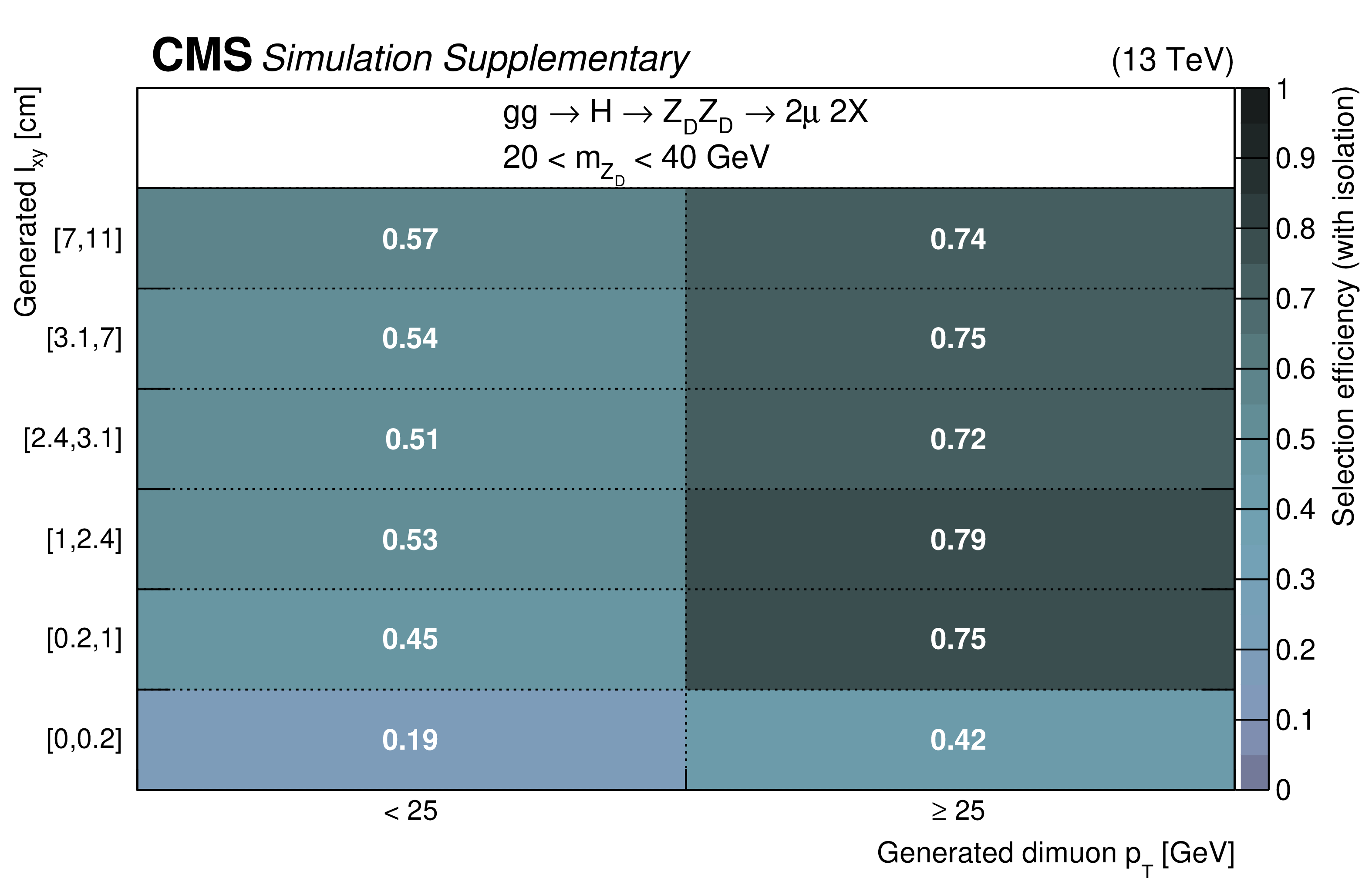
Additional Figure 42:
Efficiency of the selection applied after trigger, with requirements on the muon isolation, as a function of generated ${l_\mathrm {xy}}$ and generated ${{p_{\mathrm {T}}} ^{{\mu} {\mu}}}$, for the $ {\mathrm {H}} \to {\mathrm {Z}} _{\mathrm {D}} {\mathrm {Z}} _{\mathrm {D}}$ signal model with 20 $ < m_{{\mathrm {Z}} _{\mathrm {D}}} < $ 40 GeV. |
png pdf |
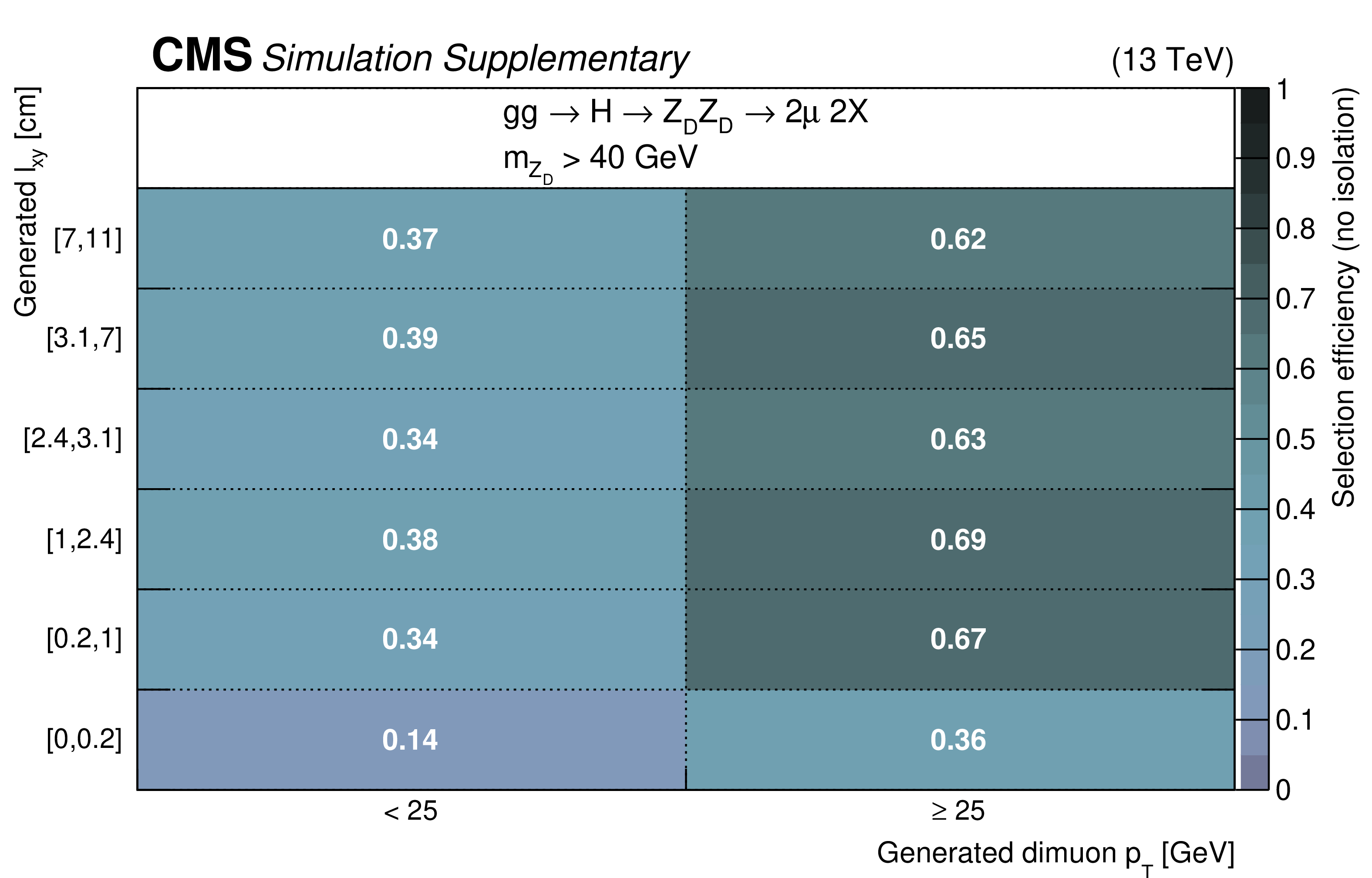
Additional Figure 43:
Efficiency of the selection applied after trigger, without requirements on the muon isolation, as a function of generated ${l_\mathrm {xy}}$ and generated ${{p_{\mathrm {T}}} ^{{\mu} {\mu}}}$, for the $ {\mathrm {H}} \to {\mathrm {Z}} _{\mathrm {D}} {\mathrm {Z}} _{\mathrm {D}}$ signal model with $m_{{\mathrm {Z}} _{\mathrm {D}}} > $ 40 GeV. |

png pdf |
Additional Figure 44:
Efficiency of the selection applied after trigger, with requirements on the muon isolation, as a function of generated ${l_\mathrm {xy}}$ and generated ${{p_{\mathrm {T}}} ^{{\mu} {\mu}}}$, for the $ {\mathrm {H}} \to {\mathrm {Z}} _{\mathrm {D}} {\mathrm {Z}} _{\mathrm {D}}$ signal model with $m_{{\mathrm {Z}} _{\mathrm {D}}} > $ 40 GeV. |
png pdf |
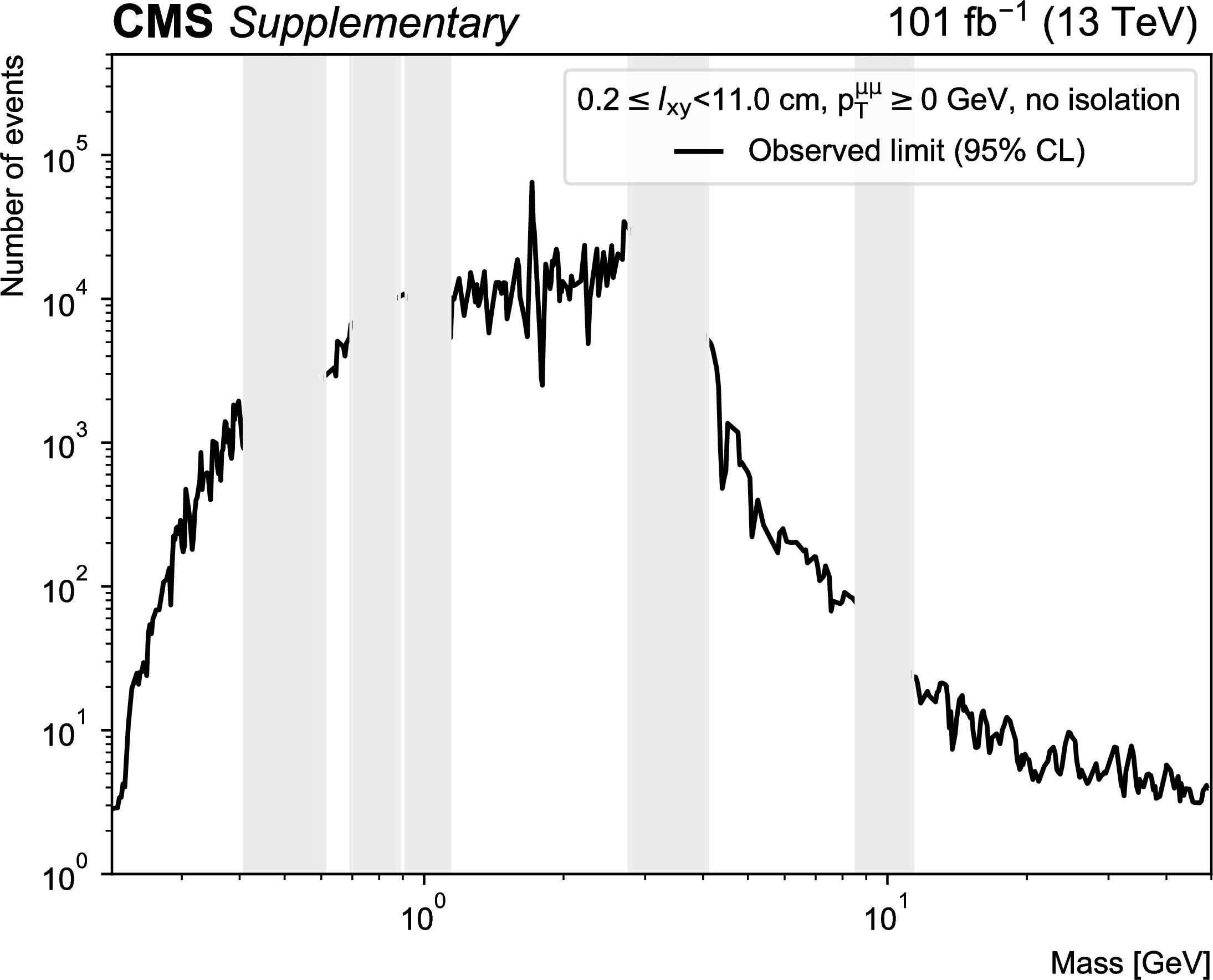
Additional Figure 45:
Observed upper limit at 95% CL on number of signal events in aggregate signal region with 0.2 $ \leq {l_\mathrm {xy}} < $ 11.0 cm, $ {{p_{\mathrm {T}}} ^{{\mu} {\mu}}} \geq $ 0 GeV and no requirement on muon isolation. The vertical gray bands indicate mass ranges containing known SM resonances, which are masked for the purpose of this search. |
png pdf |
Additional Figure 46:
Observed upper limit at 95% CL on number of signal events in aggregate signal region with 0.2 $ \leq {l_\mathrm {xy}} < $ 11.0 cm, $ {{p_{\mathrm {T}}} ^{{\mu} {\mu}}} \geq $ 0 GeV and two isolated muons. The vertical gray bands indicate mass ranges containing known SM resonances, which are masked for the purpose of this search. |
png pdf |
Additional Figure 47:
Observed upper limit at 95% CL on number of signal events in aggregate signal region with 0.2 $ \leq {l_\mathrm {xy}} < $ 11.0 cm, $ {{p_{\mathrm {T}}} ^{{\mu} {\mu}}} \geq $ 25 GeV and no requirement on muon isolation. The vertical gray bands indicate mass ranges containing known SM resonances, which are masked for the purpose of this search. |
png pdf |
Additional Figure 48:
Observed upper limit at 95% CL on number of signal events in aggregate signal region with 0.2 $ \leq {l_\mathrm {xy}} < $ 11.0 cm, $ {{p_{\mathrm {T}}} ^{{\mu} {\mu}}} \geq $ 25 GeV and two isolated muons. The vertical gray bands indicate mass ranges containing known SM resonances, which are masked for the purpose of this search. |

png pdf |
Additional Figure 49:
Observed upper limit at 95% CL on number of signal events in aggregate signal region with 1.0 $ \leq {l_\mathrm {xy}} < $ 11.0 cm, $ {{p_{\mathrm {T}}} ^{{\mu} {\mu}}} \geq $ 0 GeV and no requirement on muon isolation. The vertical gray bands indicate mass ranges containing known SM resonances, which are masked for the purpose of this search. |

png pdf |
Additional Figure 50:
Observed upper limit at 95% CL on number of signal events in aggregate signal region with 1.0 $ \leq {l_\mathrm {xy}} < $ 11.0 cm, $ {{p_{\mathrm {T}}} ^{{\mu} {\mu}}} \geq $ 0 GeV and two isolated muons. The vertical gray bands indicate mass ranges containing known SM resonances, which are masked for the purpose of this search. |

png pdf |
Additional Figure 51:
Observed upper limit at 95% CL on number of signal events in aggregate signal region with 1.0 $ \leq {l_\mathrm {xy}} < $ 11.0 cm, $ {{p_{\mathrm {T}}} ^{{\mu} {\mu}}} \geq $ 25 GeV and no requirement on muon isolation. The vertical gray bands indicate mass ranges containing known SM resonances, which are masked for the purpose of this search. |

png pdf |
Additional Figure 52:
Observed upper limit at 95% CL on number of signal events in aggregate signal region with 1.0 $ \leq {l_\mathrm {xy}} < $ 11.0 cm, $ {{p_{\mathrm {T}}} ^{{\mu} {\mu}}} \geq $ 25 GeV and two isolated muons. The vertical gray bands indicate mass ranges containing known SM resonances, which are masked for the purpose of this search. |
png pdf |
Additional Figure 53:
Observed upper limit at 95% CL on number of signal events in aggregate signal region with 2.4 $ \leq {l_\mathrm {xy}} < $ 11.0 cm, $ {{p_{\mathrm {T}}} ^{{\mu} {\mu}}} \geq $ 0 GeV and no requirement on muon isolation. The vertical gray bands indicate mass ranges containing known SM resonances, which are masked for the purpose of this search. |
png pdf |
Additional Figure 54:
Observed upper limit at 95% CL on number of signal events in aggregate signal region with 2.4 $ \leq {l_\mathrm {xy}} < $ 11.0 cm, $ {{p_{\mathrm {T}}} ^{{\mu} {\mu}}} \geq $ 0 GeV and two isolated muons. The vertical gray bands indicate mass ranges containing known SM resonances, which are masked for the purpose of this search. |
png pdf |
Additional Figure 55:
Observed upper limit at 95% CL on number of signal events in aggregate signal region with 2.4 $ \leq {l_\mathrm {xy}} < $ 11.0 cm, $ {{p_{\mathrm {T}}} ^{{\mu} {\mu}}} \geq $ 25 GeV and no requirement on muon isolation. The vertical gray bands indicate mass ranges containing known SM resonances, which are masked for the purpose of this search. |
png pdf |
Additional Figure 56:
Observed upper limit at 95% CL on number of signal events in aggregate signal region with 2.4 $ \leq {l_\mathrm {xy}} < $ 11.0 cm, $ {{p_{\mathrm {T}}} ^{{\mu} {\mu}}} \geq $ 25 GeV and two isolated muons. The vertical gray bands indicate mass ranges containing known SM resonances, which are masked for the purpose of this search. |

png pdf |
Additional Figure 57:
Observed upper limit at 95% CL on number of signal events in aggregate signal region with 3.1 $ \leq {l_\mathrm {xy}} < $ 11.0 cm, $ {{p_{\mathrm {T}}} ^{{\mu} {\mu}}} \geq $ 0 GeV and no requirement on muon isolation. The vertical gray bands indicate mass ranges containing known SM resonances, which are masked for the purpose of this search. |
png pdf |
Additional Figure 58:
Observed upper limit at 95% CL on number of signal events in aggregate signal region with 3.1 $ \leq {l_\mathrm {xy}} < $ 11.0 cm, $ {{p_{\mathrm {T}}} ^{{\mu} {\mu}}} \geq $ 0 GeV and two isolated muons. The vertical gray bands indicate mass ranges containing known SM resonances, which are masked for the purpose of this search. |
png pdf |
Additional Figure 59:
Observed upper limit at 95% CL on number of signal events in aggregate signal region with 3.1 $ \leq {l_\mathrm {xy}} < $ 11.0 cm, $ {{p_{\mathrm {T}}} ^{{\mu} {\mu}}} \geq $ 25 GeV and no requirement on muon isolation. The vertical gray bands indicate mass ranges containing known SM resonances, which are masked for the purpose of this search. |
png pdf |
Additional Figure 60:
Observed upper limit at 95% CL on number of signal events in aggregate signal region with 3.1 $ \leq {l_\mathrm {xy}} < $ 11.0 cm, $ {{p_{\mathrm {T}}} ^{{\mu} {\mu}}} \geq $ 25 GeV and two isolated muons. The vertical gray bands indicate mass ranges containing known SM resonances, which are masked for the purpose of this search. |
png pdf |
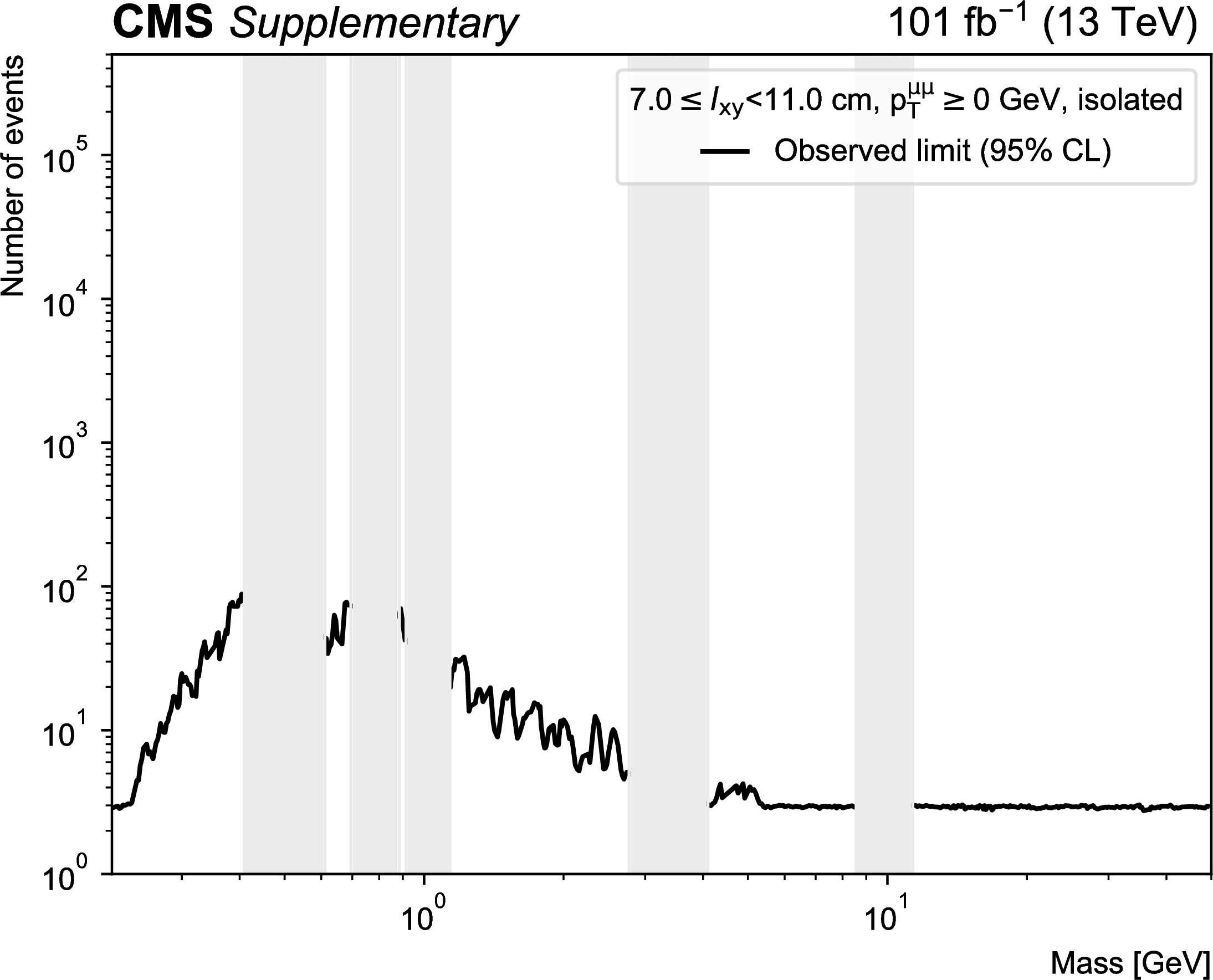
Additional Figure 61:
Observed upper limit at 95% CL on number of signal events in aggregate signal region with 7.0 $ \leq {l_\mathrm {xy}} < $ 11.0 cm, $ {{p_{\mathrm {T}}} ^{{\mu} {\mu}}} \geq $ 0 GeV and no requirement on muon isolation. The vertical gray bands indicate mass ranges containing known SM resonances, which are masked for the purpose of this search. |
png pdf |
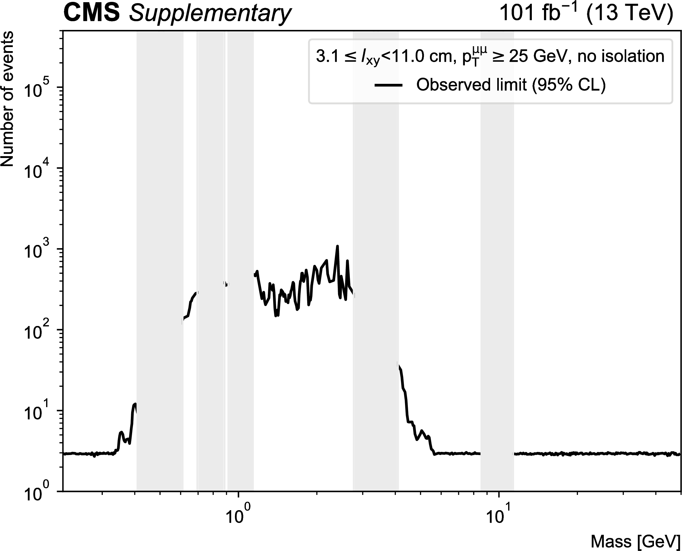
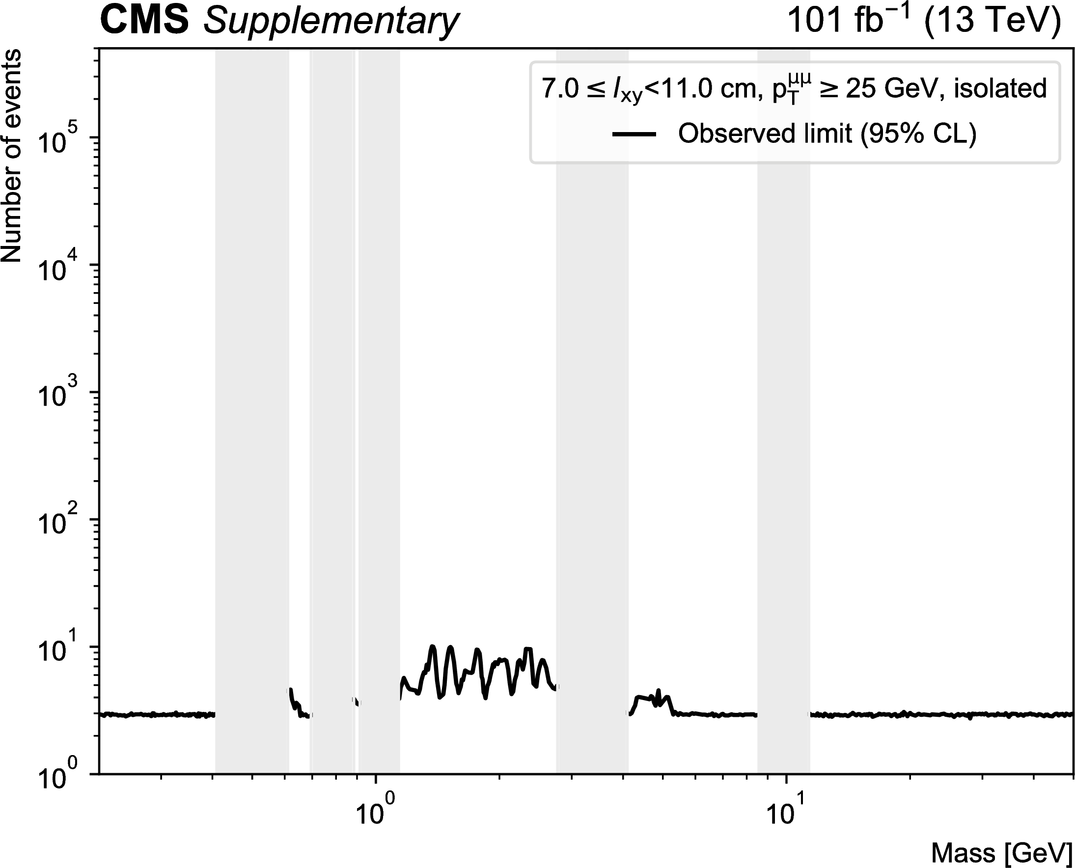
Additional Figure 62:
Observed upper limit at 95% CL on number of signal events in aggregate signal region with 7.0 $ \leq {l_\mathrm {xy}} < $ 11.0 cm, $ {{p_{\mathrm {T}}} ^{{\mu} {\mu}}} \geq $ 0 GeV and two isolated muons. The vertical gray bands indicate mass ranges containing known SM resonances, which are masked for the purpose of this search. |
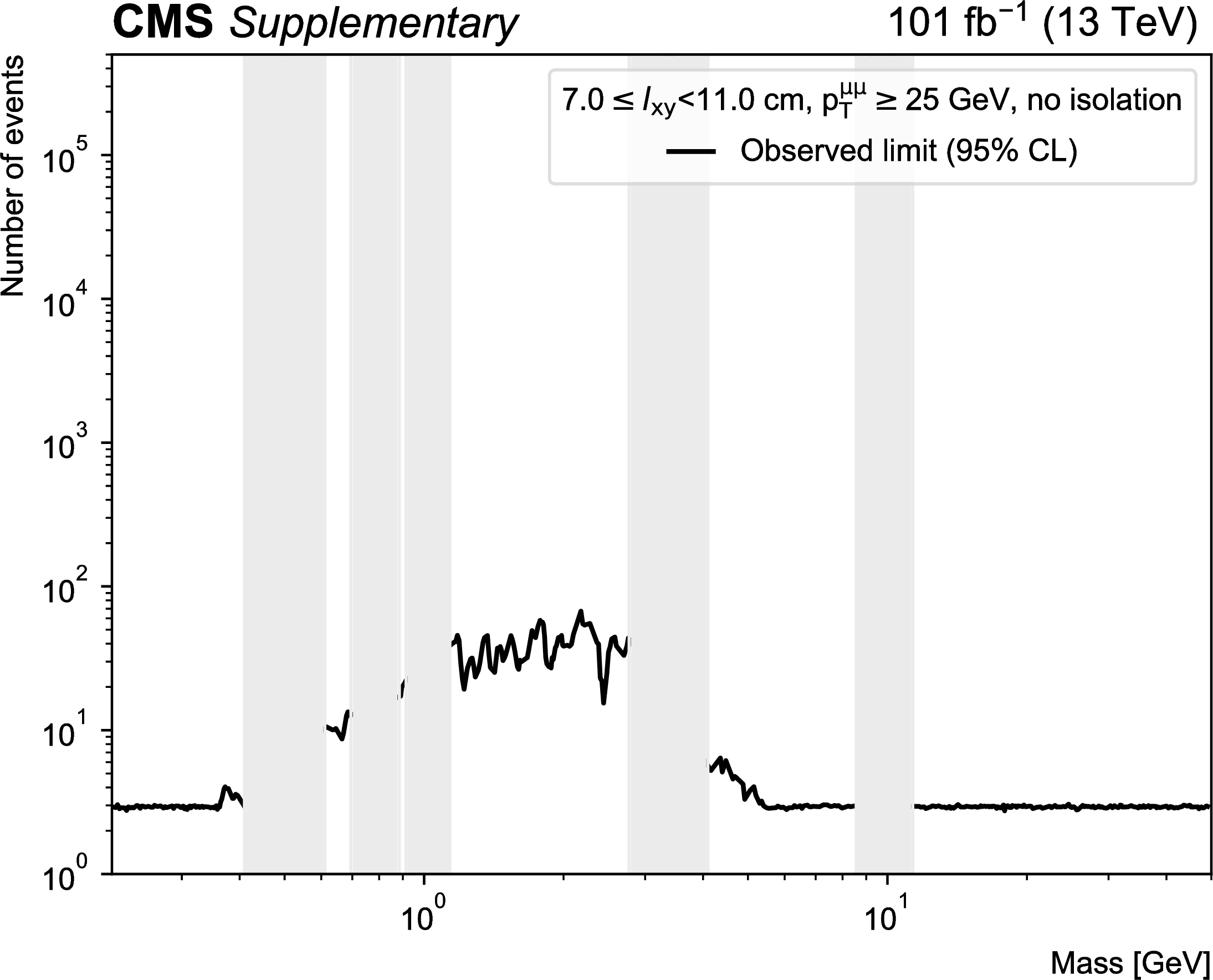
png pdf |
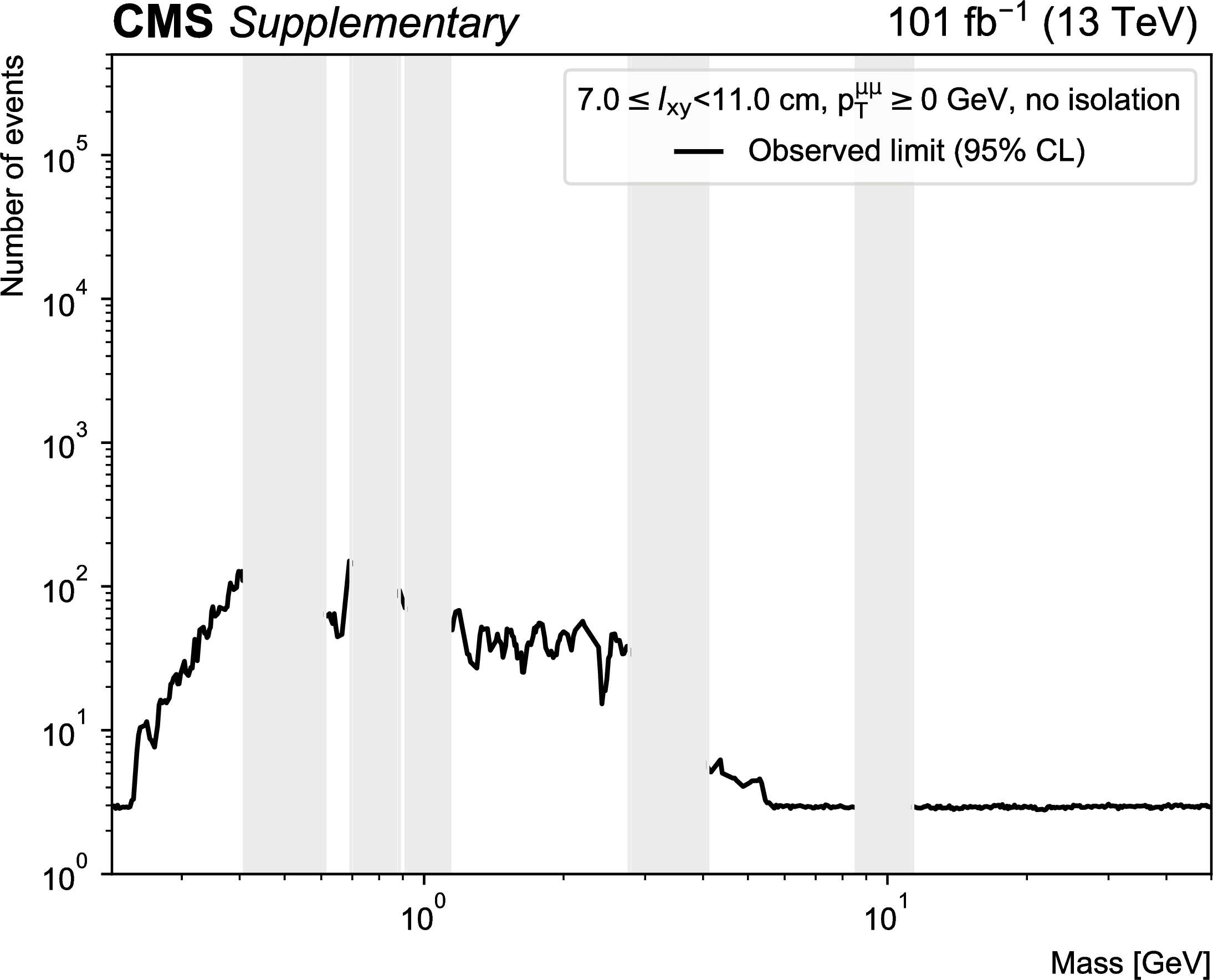
Additional Figure 63:
Observed upper limit at 95% CL on number of signal events in aggregate signal region with 7.0 $ \leq {l_\mathrm {xy}} < $ 11.0 cm, $ {{p_{\mathrm {T}}} ^{{\mu} {\mu}}} \geq $ 25 GeV and no requirement on muon isolation. The vertical gray bands indicate mass ranges containing known SM resonances, which are masked for the purpose of this search. |
png pdf |
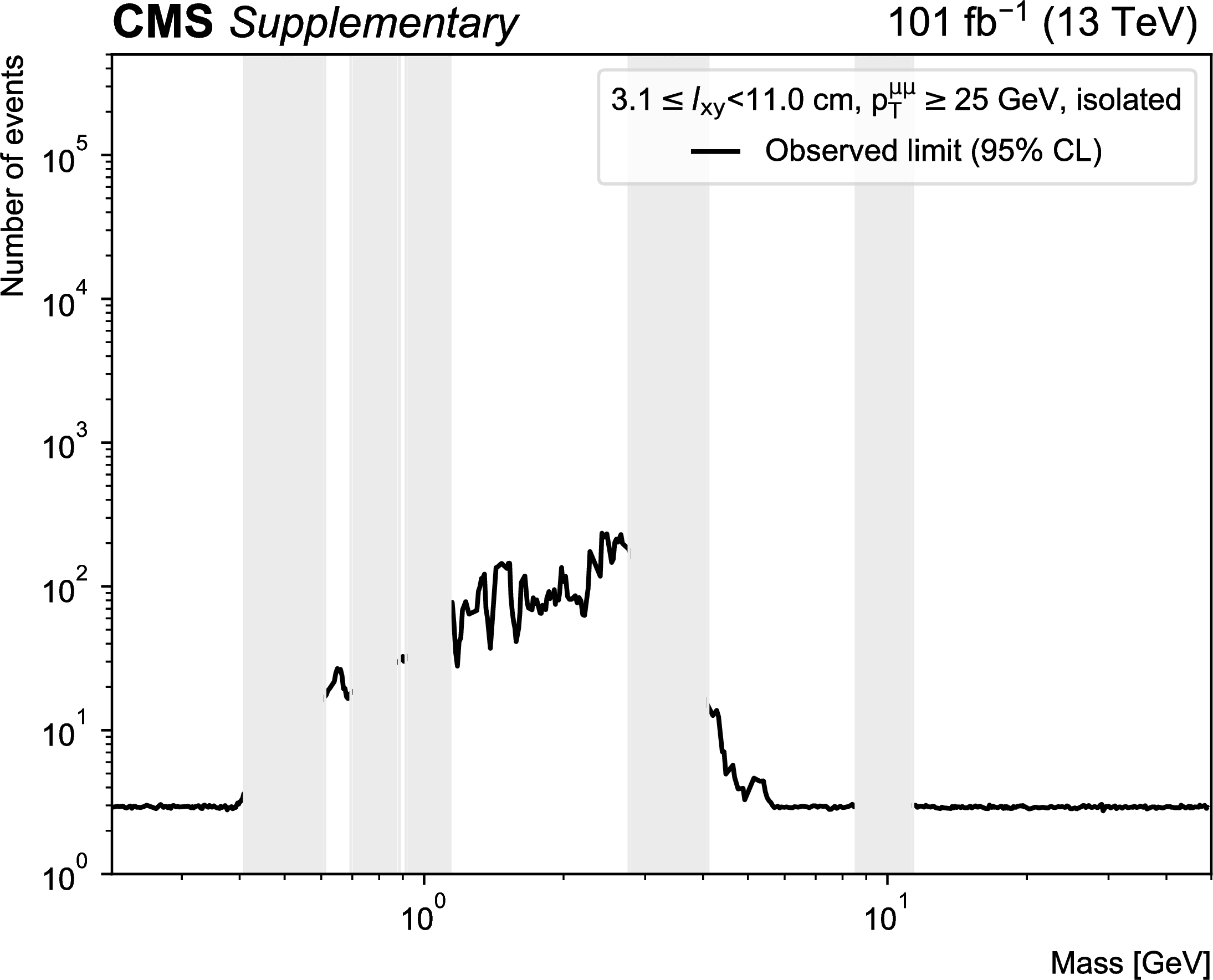
Additional Figure 64:
Observed upper limit at 95% CL on number of signal events in aggregate signal region with 7.0 $ \leq {l_\mathrm {xy}} < $ 11.0 cm, $ {{p_{\mathrm {T}}} ^{{\mu} {\mu}}} \geq $ 25 GeV and two isolated muons. The vertical gray bands indicate mass ranges containing known SM resonances, which are masked for the purpose of this search. |
| Additional Tables | |
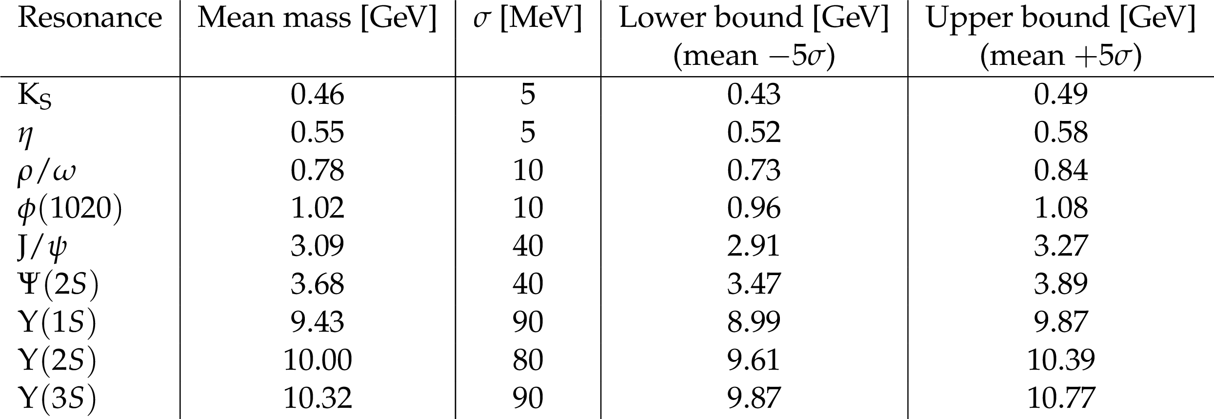
png pdf |
Additional Table 1:
List of known resonances and corresponding masked mass windows, equal to $ \pm $5$ \sigma $ around the mean mass, where mean and resolution ($\sigma $) are determined from a fit to data. |
png pdf |
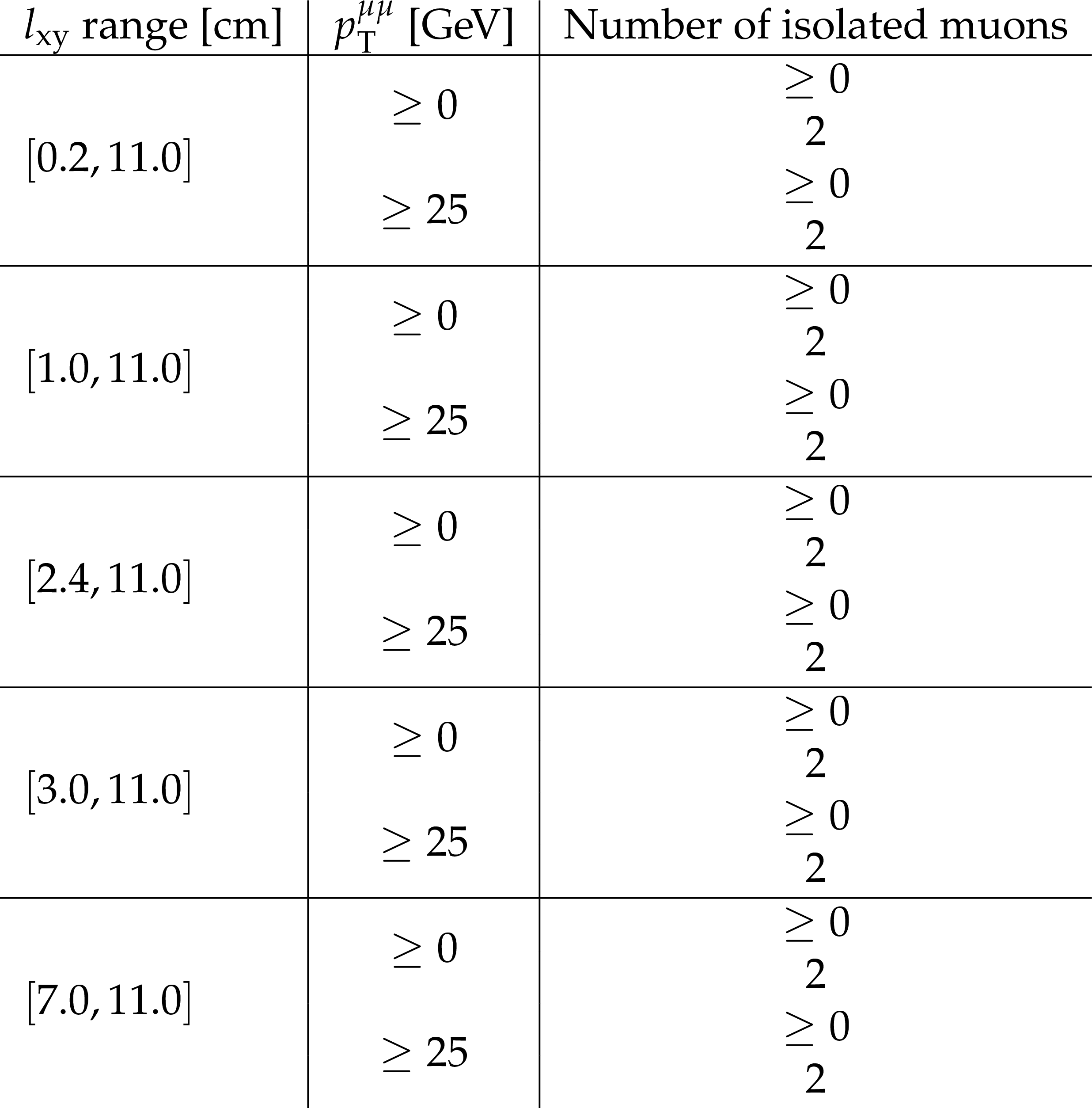
Additional Table 2:
List of aggregate signal regions for reinterpretation of the results. The aggregate signal regions are not mutually exclusive. |
| References | ||||
| 1 | G. Bertone and J. Silk | Particle Dark Matter: Observations, Models and Searches | Cambridge Univ. Press, Cambridge, 2010 | |
| 2 | J. L. Feng | Dark matter candidates from particle physics and methods of detection | Ann. Rev. Astron. Astrophys. 48 (2010) 495 | 1003.0904 |
| 3 | T. A. Porter, R. P. Johnson, and P. W. Graham | Dark matter searches with astroparticle data | Ann. Rev. Astron. Astrophys. 49 (2011) 155 | 1104.2836 |
| 4 | Planck Collaboration | Planck 2015 results. XIII. Cosmological parameters | Astron. Astrophys. 594 (2016) A13 | 1502.01589 |
| 5 | R. Essig et al. | Working group report: New light weakly coupled particles | in Community Summer Study 2013: Snowmass on the Mississippi 2013 | 1311.0029 |
| 6 | D. Curtin, R. Essig, S. Gori, and J. Shelton | Illuminating dark photons with high-energy colliders | JHEP 02 (2015) 157 | 1412.0018 |
| 7 | A. Konaka et al. | Search for neutral particles in electron beam dump experiment | PRL 57 (1986) 659 | |
| 8 | APEX Collaboration | Search for a new gauge boson in electron-nucleus fixed-target scattering by the APEX experiment | PRL 107 (2011) 191804 | 1108.2750 |
| 9 | BaBar Collaboration | Search for dimuon decays of a light scalar boson in radiative transitions $ \Upsilon\rightarrow\gamma A^{0} $ | PRL 103 (2009) 081803 | 0905.4539 |
| 10 | SINDRUM I Collaboration | Search for weakly interacting neutral bosons produced in $ \pi^{-}p $ interactions at rest and decaying into $ e^{+}e^{-} $ pairs. | PRL 68 (1992) 3845 | |
| 11 | LHCb Collaboration | Proposed inclusive dark photon search at LHCb | PRL 116 (2016) 251803 | 1603.08926 |
| 12 | LHCb Collaboration | Search for dark photons produced in 13 TeV pp collisions | PRL 120 (2018) 061801 | 1710.02867 |
| 13 | LHCb Collaboration | Search for $ A'\to\mu^+\mu^- $ decays | PRL 124 (2020) 041801 | 1910.06926 |
| 14 | CMS Collaboration | Search for a narrow resonance lighter than 200 GeV decaying to a pair of muons in proton-proton collisions at $ \sqrt{s}= $ 13 TeV | PRL 124 (2020) 131802 | CMS-EXO-19-018 1912.04776 |
| 15 | F. Bezrukov and D. Gorbunov | Light inflaton after LHC8 and WMAP9 results | JHEP 07 (2013) 140 | 1303.4395 |
| 16 | J. A. Evans, A. Gandrakota, S. Knapen, and H. Routray | Searching for exotic B meson decays with the CMS L1 track trigger | PRD 103 (2021) 015026 | 2008.06918 |
| 17 | CHARM Collaboration | Search for axion like particle production in 400 GeV proton-copper interactions | PLB 157 (1985) 458 | |
| 18 | LHCb Collaboration | Search for hidden-sector bosons in $ B^0 \!\to K^{*0}\mu^+\mu^- $ decays | PRL 115 (2015) 161802 | 1508.04094 |
| 19 | LHCb Collaboration | Search for long-lived scalar particles in $ B^+ \to K^+ \chi (\mu^+\mu^-) $ decays | PRD 95 (2017) 071101 | 1612.07818 |
| 20 | The Tracker Group of the CMS Collaboration | The CMS Phase-1 Pixel Detector Upgrade | JINST 16 (2021) P02027 | 2012.14304 |
| 21 | CMS Collaboration | The CMS experiment at the CERN LHC | JINST 3 (2008) S08004 | CMS-00-001 |
| 22 | CMS Collaboration | Performance of the CMS Level-1 trigger in proton-proton collisions at $ \sqrt{s} = $ 13 TeV | JINST 15 (2020) P10017 | CMS-TRG-17-001 2006.10165 |
| 23 | CMS Collaboration | The CMS trigger system | JINST 12 (2017) P01020 | CMS-TRG-12-001 1609.02366 |
| 24 | CMS Collaboration | Search for narrow resonances in dijet final states at $ \sqrt{s}= $ 8 TeV with the novel CMS technique of data scouting | PRL 117 (2016) 031802 | CMS-EXO-14-005 1604.08907 |
| 25 | M. Cacciari, G. P. Salam, and G. Soyez | The anti-$ {k_{\mathrm{T}}} $ jet clustering algorithm | JHEP 04 (2008) 063 | 0802.1189 |
| 26 | M. Cacciari, G. P. Salam, and G. Soyez | FastJet user manual | EPJC 72 (2012) 1896 | 1111.6097 |
| 27 | P. Nason | A new method for combining NLO QCD with shower Monte Carlo algorithms | JHEP 11 (2004) 040 | hep-ph/0409146 |
| 28 | S. Frixione, P. Nason, and C. Oleari | Matching NLO QCD computations with parton shower simulations: the POWHEG method | JHEP 11 (2007) 070 | 0709.2092 |
| 29 | S. Alioli, P. Nason, C. Oleari, and E. Re | NLO single-top production matched with shower in POWHEG: $ s $- and $ t $-channel contributions | JHEP 09 (2009) 111 | 0907.4076 |
| 30 | Y. Gao et al. | Spin determination of single-produced resonances at hadron colliders | PRD 81 (2010) 075022 | 1001.3396 |
| 31 | S. Bolognesi et al. | On the spin and parity of a single-produced resonance at the LHC | PRD 86 (2012) 095031 | 1208.4018 |
| 32 | I. Anderson et al. | Constraining anomalous HVV interactions at proton and lepton colliders | PRD 89 (2014) 035007 | 1309.4819 |
| 33 | A. V. Gritsan, R. Rontsch, M. Schulze, and M. Xiao | Constraining anomalous Higgs boson couplings to the heavy flavor fermions using matrix element techniques | PRD 94 (2016) 055023 | 1606.03107 |
| 34 | A. V. Gritsan et al. | New features in the JHU generator framework: constraining Higgs boson properties from on-shell and off-shell production | PRD 102 (2020) 056022 | 2002.09888 |
| 35 | T. Sjostrand et al. | An introduction to PYTHIA 8.2 | CPC 191 (2015) 159 | 1410.3012 |
| 36 | M. Cepeda et al. | Report from Working Group 2: Higgs physics at the HL-LHC and HE-LHC | CERN Yellow Rep. Monogr. 7 (2019) 221 | 1902.00134 |
| 37 | M. Cacciari, M. Greco, and P. Nason | The $ p_\mathrm{T} $ spectrum in heavy flavor hadroproduction | JHEP 05 (1998) 007 | hep-ph/9803400 |
| 38 | M. Cacciari, S. Frixione, and P. Nason | The $ p_\mathrm{T} $ spectrum in heavy flavor photoproduction | JHEP 03 (2001) 006 | hep-ph/0102134 |
| 39 | M. Cacciari et al. | Theoretical predictions for charm and bottom production at the LHC | JHEP 10 (2012) 137 | 1205.6344 |
| 40 | M. Cacciari, M. L. Mangano, and P. Nason | Gluon PDF constraints from the ratio of forward heavy-quark production at the LHC at $ \sqrt{s}= $ 7 and 13 TeV | EPJC 75 (2015) 610 | 1507.06197 |
| 41 | CMS Collaboration | Measurement of the differential inclusive $ \mathrm{B}^{+} $ hadron cross sections in pp collisions at $ \sqrt{s}= $ 13 TeV | PLB 771 (2017) 435 | |
| 42 | CMS Collaboration | Extraction and validation of a new set of CMS PYTHIA8 tunes from underlying-event measurements | EPJC 80 (2020) 4 | CMS-GEN-17-001 1903.12179 |
| 43 | NNPDF Collaboration | Parton distributions from high-precision collider data | EPJC 77 (2017) 663 | 1706.00428 |
| 44 | GEANT4 Collaboration | GEANT4--a simulation toolkit | NIMA 506 (2003) 250 | |
| 45 | M. J. Oreglia | A study of the reactions $\psi' \to \gamma\gamma \psi$ | PhD thesis, Stanford University, 1980 SLAC Report SLAC-R-236, see Appendix D | |
| 46 | J. Gaiser | Charmonium Spectroscopy From Radiative Decays of the $\mathrm{J}/\psi$ and $\psi'$ | PhD thesis, SLAC | |
| 47 | R. A. Fisher | On the interpretation of $ \chi^{2} $ from contingency tables, and the calculation of P | J. R. Stat. Soc 85 (1922) 87 | |
| 48 | P. D. Dauncey, M. Kenzie, N. Wardle, and G. J. Davies | Handling uncertainties in background shapes: the discrete profiling method | JINST 10 (2015) P04015 | 1408.6865 |
| 49 | A. L. Read | Presentation of search results: The $ {\mathrm{CL_s}} $ technique | JPG 28 (2002) 2693 | |
| 50 | T. Junk | Confidence level computation for combining searches with small statistics | NIMA 434 (1999) 435 | hep-ex/9902006 |
| 51 | G. Cowan, K. Cranmer, E. Gross, and O. Vitells | Asymptotic formulae for likelihood-based tests of new physics | EPJC 71 (2011) 1554 | 1007.1727 |
| 52 | ATLAS and CMS Collaborations | Procedure for the LHC Higgs boson search combination in summer 2011 | ATL-PHYS-PUB-2011-011, CMS NOTE-2011/005 | |
| 53 | CMS Collaboration | CMS luminosity measurement for the 2017 data-taking period at $ \sqrt{s} = $ 13 TeV | CMS-PAS-LUM-17-004 | |
| 54 | CMS Collaboration | CMS luminosity measurement for the 2018 data-taking period at $ \sqrt{s} = $ 13 TeV | CMS-PAS-LUM-18-002 | |
| 55 | CMS Collaboration | HEPData record for this analysis | link | |
|
|
Compact Muon Solenoid LHC, CERN |
|

|

|

|

|

|