

Compact Muon Solenoid
LHC, CERN
| CMS-TRG-17-001 ; CERN-EP-2020-065 | ||
| Performance of the CMS Level-1 trigger in proton-proton collisions at $\sqrt{s} = $ 13 TeV | ||
| CMS Collaboration | ||
| 18 June 2020 | ||
| JINST 15 (2020) P10017 | ||
| Abstract: At the start of Run 2 in 2015, the LHC delivered proton-proton collisions at a center-of-mass energy of 13 TeV. During Run 2 (years 2015-2018) the LHC eventually reached a luminosity of 2.1 $\times $ 10$^{34} $ cm$^{-2}$s$^{-1}$, almost three times that reached during Run 1 (2009-2013) and a factor of two larger than the LHC design value, leading to events with up to a mean of about 50 simultaneous inelastic proton-proton collisions per bunch crossing (pileup). The CMS Level-1 trigger was upgraded prior to 2016 to improve the selection of physics events in the challenging conditions posed by the second run of the LHC. This paper describes the performance of the CMS Level-1 trigger upgrade during the data taking period of 2016-2018. The upgraded trigger implements pattern recognition and boosted decision tree regression techniques for muon reconstruction, includes pileup subtraction for jets and energy sums, and incorporates pileup-dependent isolation requirements for electrons and tau leptons. In addition, the new trigger calculates high-level quantities such as the invariant mass of pairs of reconstructed particles. The upgrade reduces the trigger rate from background processes and improves the trigger efficiency for a wide variety of physics signals. | ||
| Links: e-print arXiv:2006.10165 [hep-ex] (PDF) ; CDS record ; inSPIRE record ; CADI line (restricted) ; | ||
| Figures | |

png pdf |
Figure 1:
Fractions of the 100 kHz rate allocation for single- and multi-object triggers and cross triggers in a typical CMS physics menu during Run 2. |
png pdf |
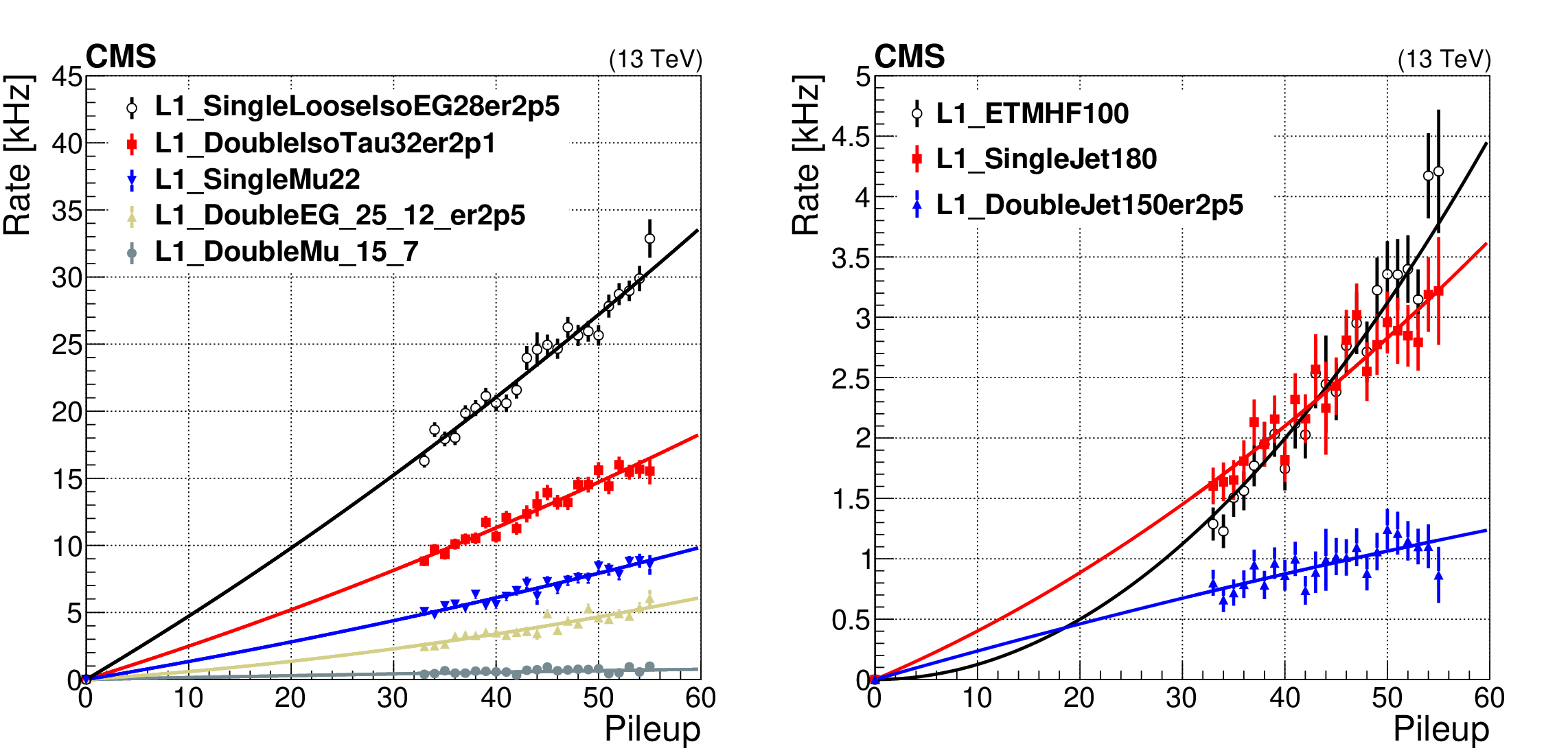
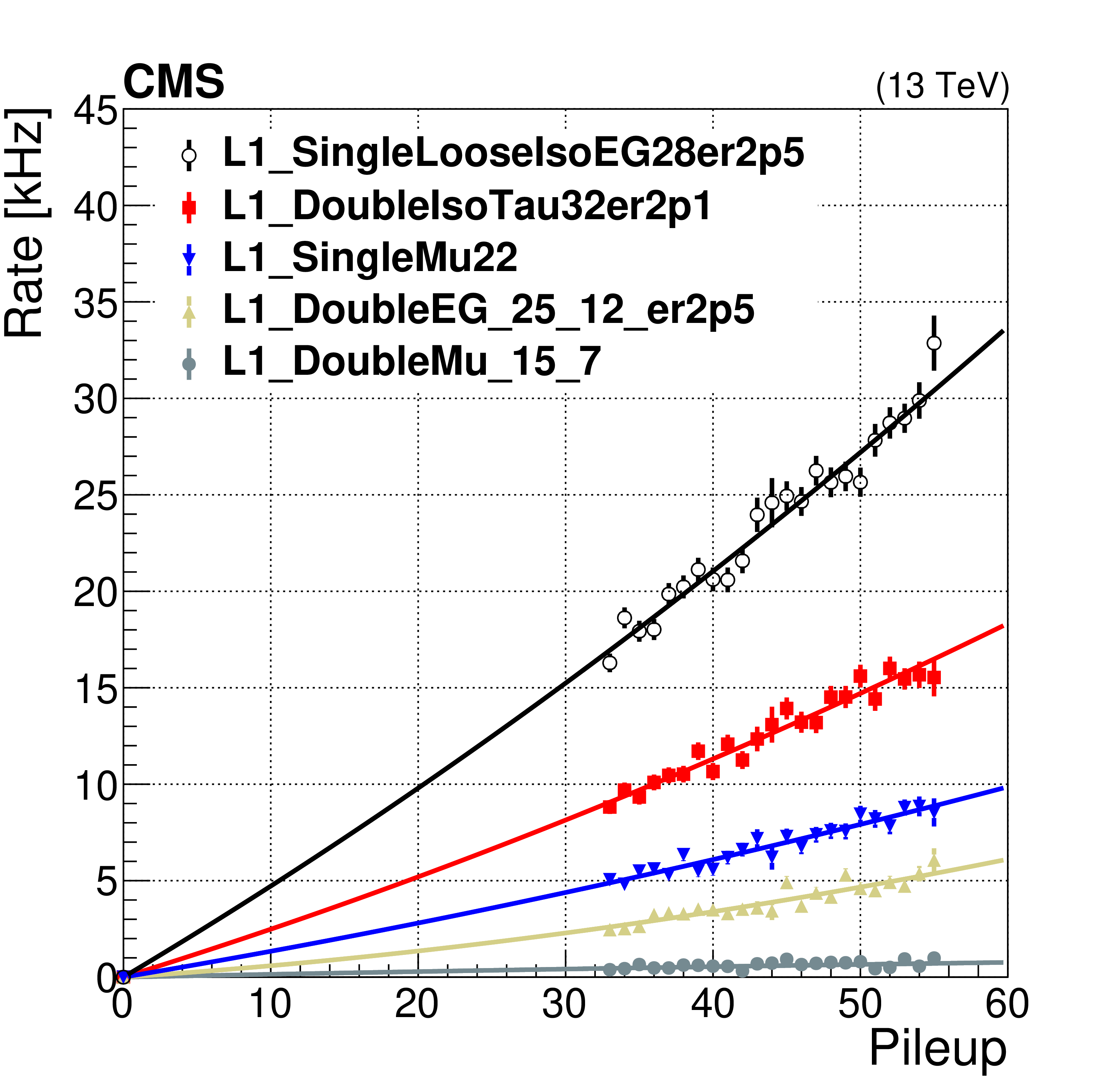
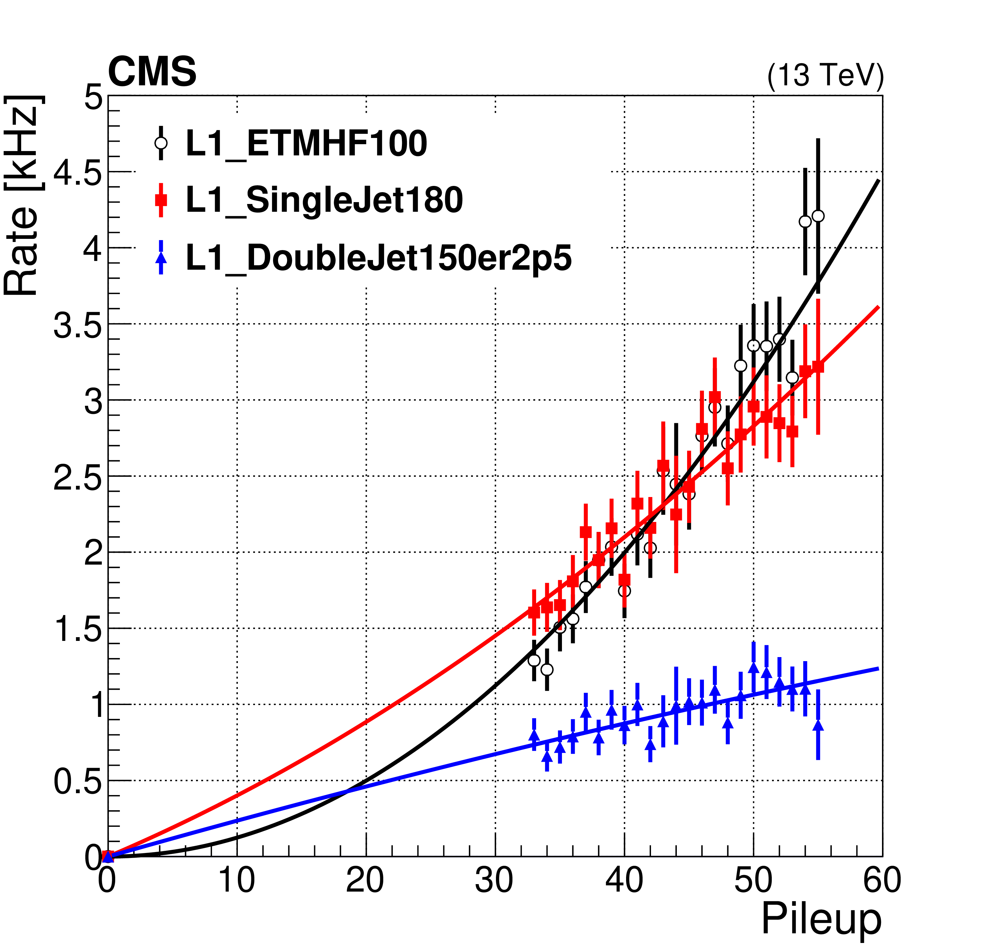
Figure 2:
Level-1 trigger rates as a function of pileup for some benchmark seeds targeting leptons (left) and hadrons (right). Rates are measured using data recorded during the 2018 LHC run. Definitions of the seed names are in Table 1. The curves represent fits to the data points that are quadratic and constrained to pass through the origin. |
png pdf |
Figure 2-a:
Level-1 trigger rates as a function of pileup for some benchmark seeds targeting leptons. Rates are measured using data recorded during the 2018 LHC run. Definitions of the seed names are in Table 1. The curves represent fits to the data points that are quadratic and constrained to pass through the origin. |
png pdf |
Figure 2-b:
Level-1 trigger rates as a function of pileup for some benchmark seeds targeting hadrons. Rates are measured using data recorded during the 2018 LHC run. Definitions of the seed names are in Table 1. The curves represent fits to the data points that are quadratic and constrained to pass through the origin. |
png pdf |
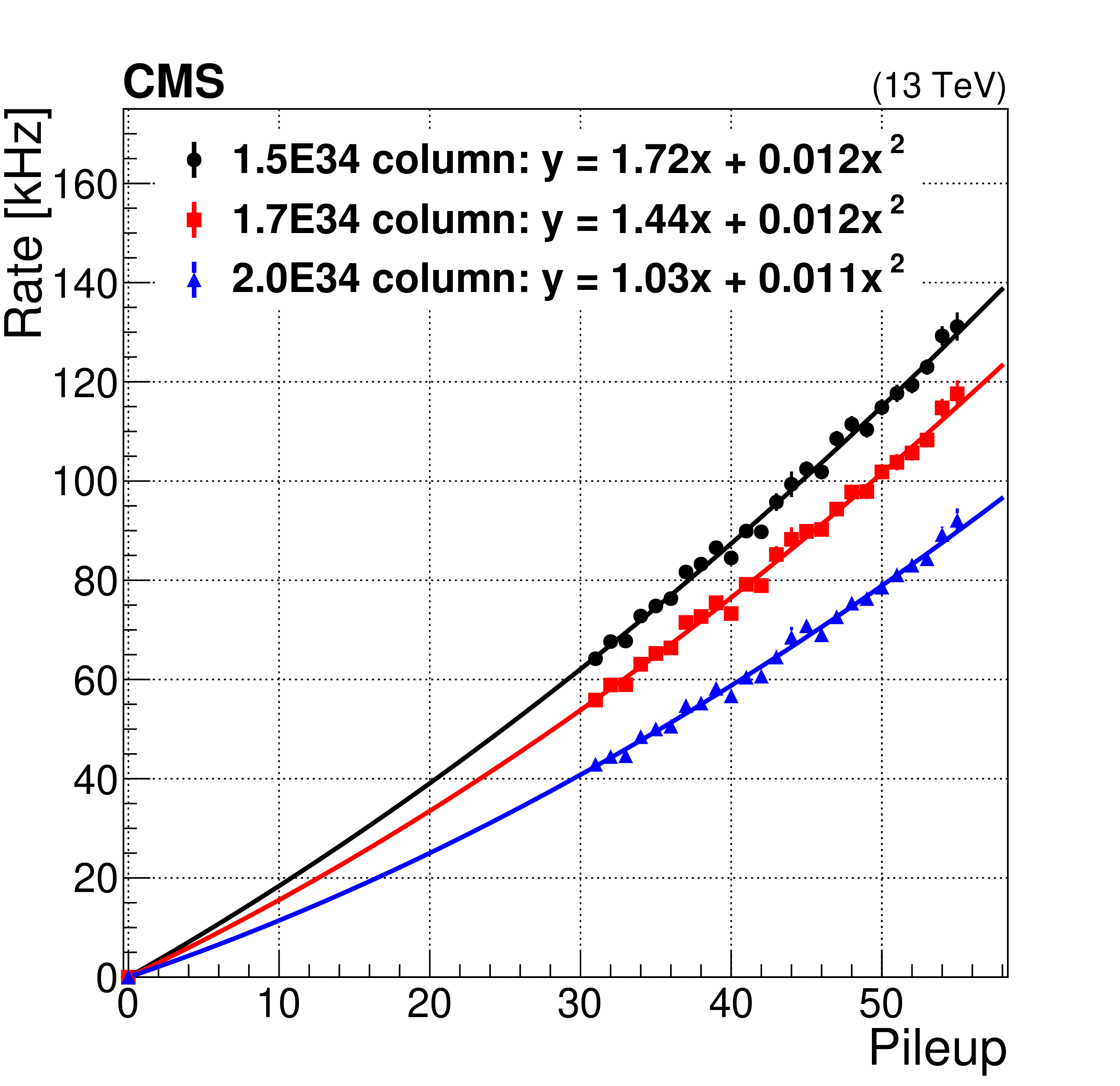
Figure 3:
Total Level-1 menu rates as a function of pileup for three sets of algorithms, or "prescale columns'', defined in the text. The rates were recorded during a LHC fill with 2544 proton bunches. The instantaneous luminosities of 2.0 $\times $ 1.7 $\times $, and 1.5 $\times $ 10$^{34}$ cm$^{-2}$s$^{-1} $ correspond to an average pileup of 55, 47, and 42 respectively. The curves represent fits to the data points that are quadratic and constrained to pass through the origin. |
png pdf |
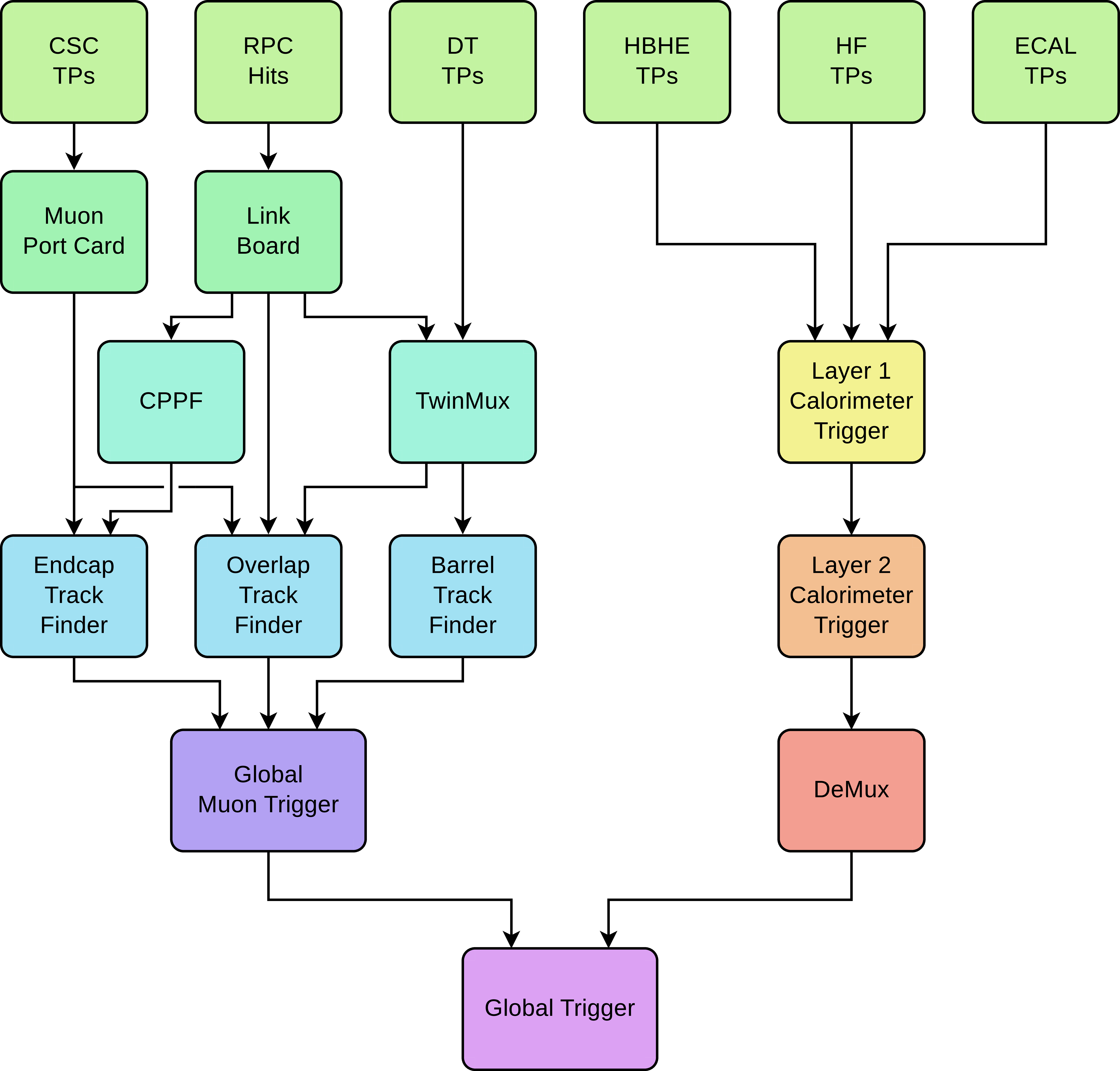
Figure 4:
Diagram of the upgraded CMS Level-1 trigger system during Run 2. |
png pdf |
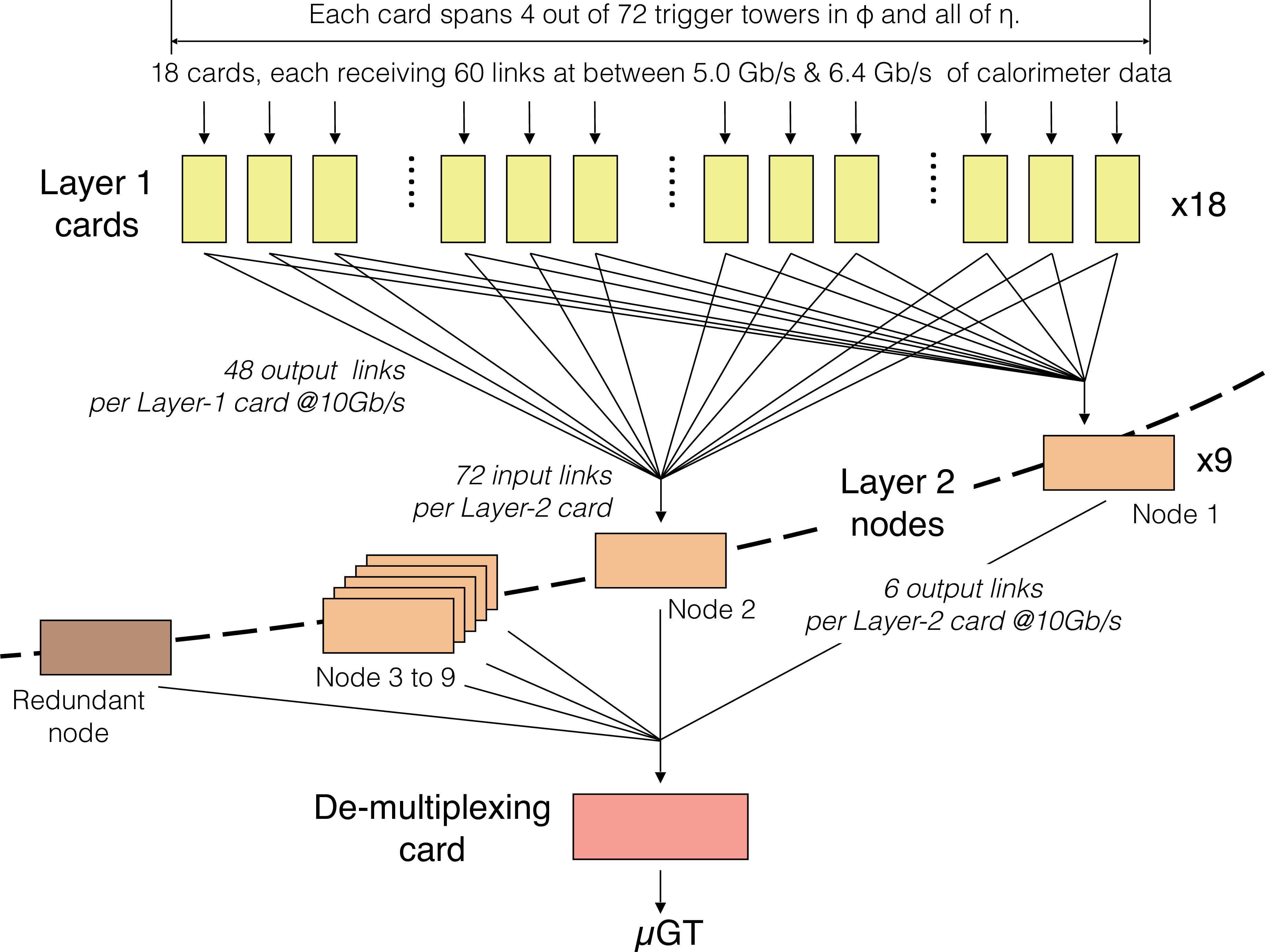
Figure 5:
The time-multiplexed trigger architecture of the upgraded CMS calorimeter trigger. |
png pdf |
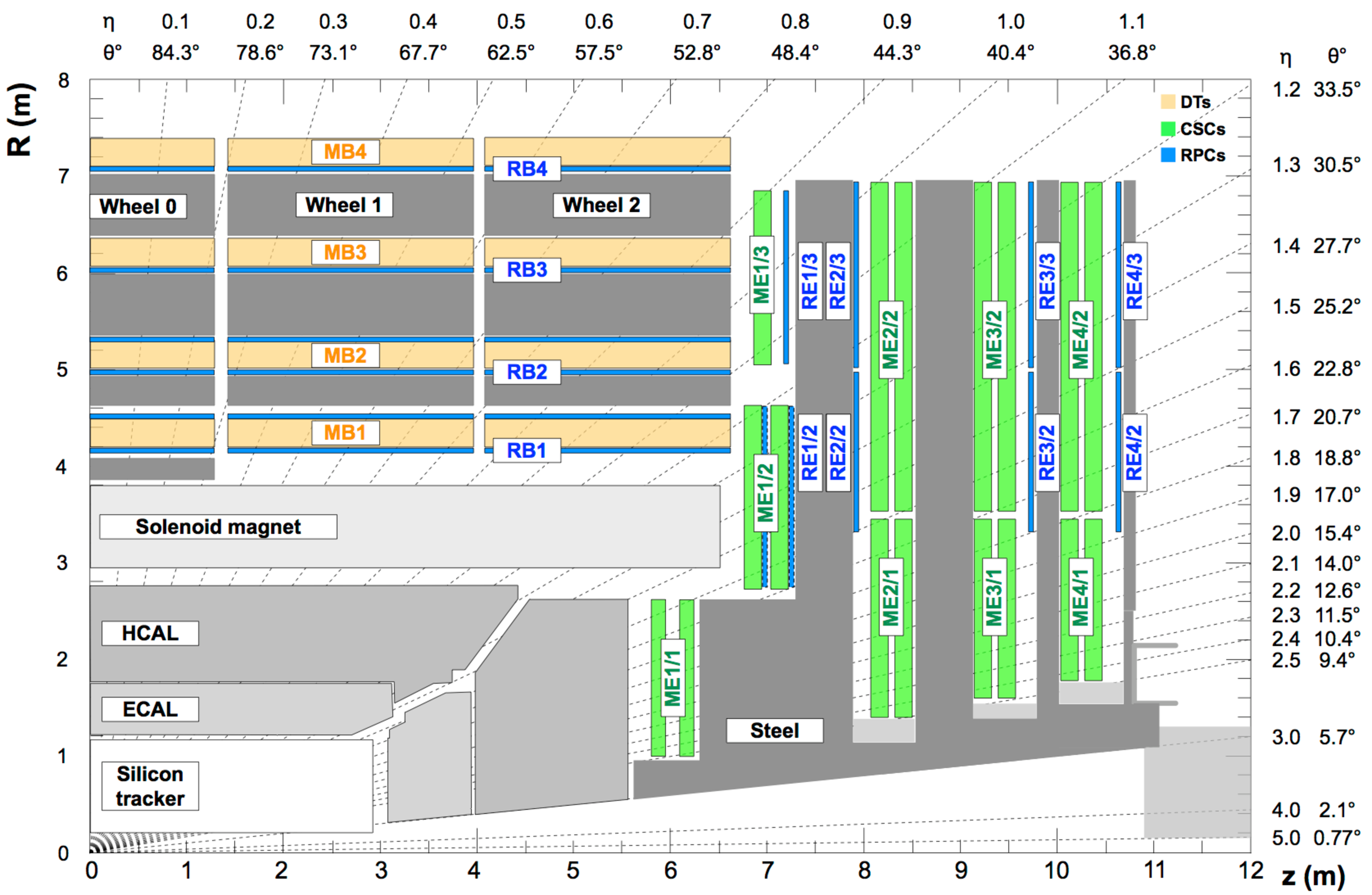
Figure 6:
An $R$-$z$ slice of a quadrant of the CMS detector [15]. The origin of the axes represents the interaction point. The proton beams travel along the $z$-axis and cross at the interaction point. The three CMS muon subdetectors are shown: four stations of DTs in yellow, labelled MB; four stations of CSCs in green, labelled ME; and four stations of RPCs in blue, labelled RB or RE. |
png pdf |
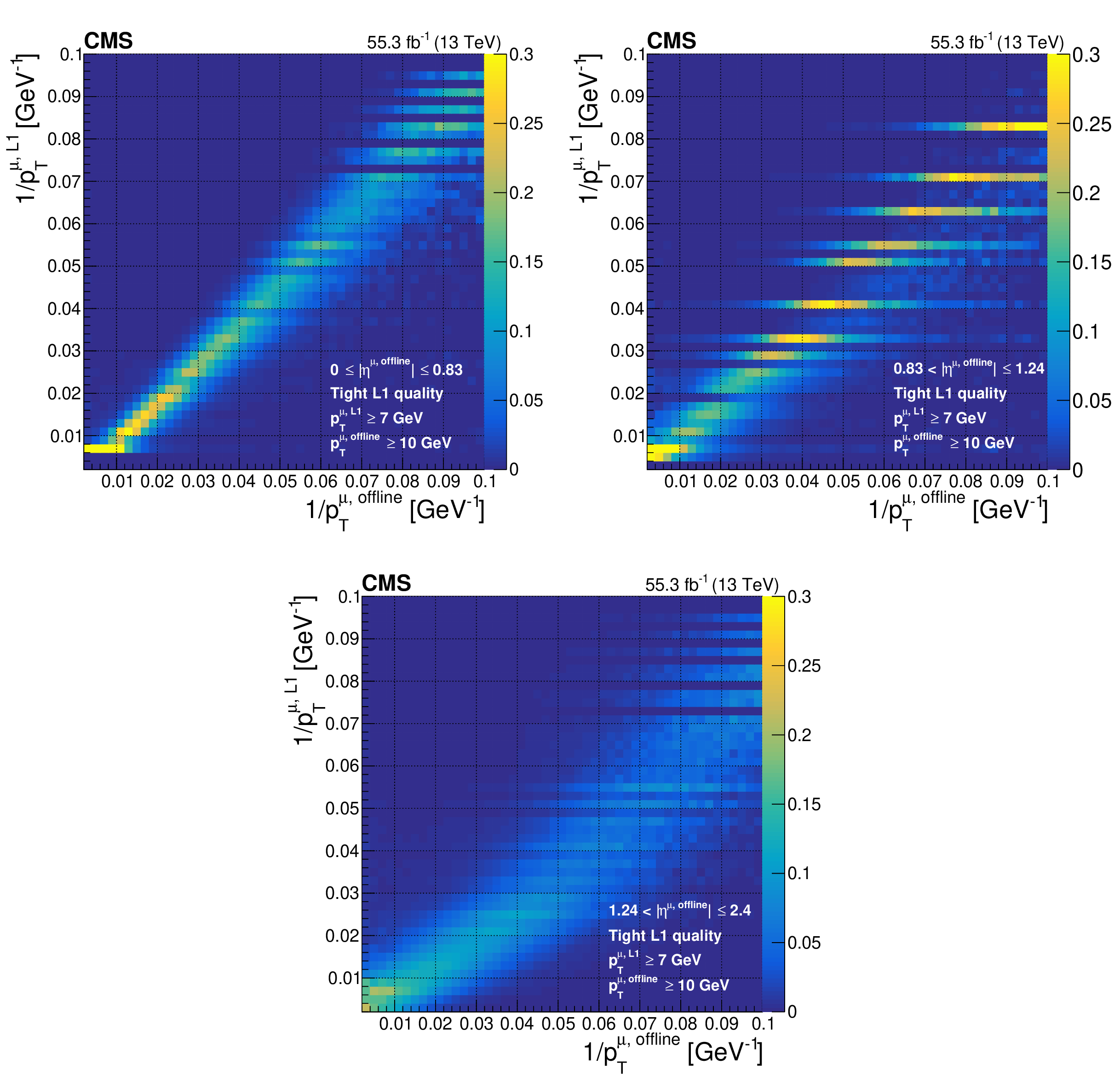
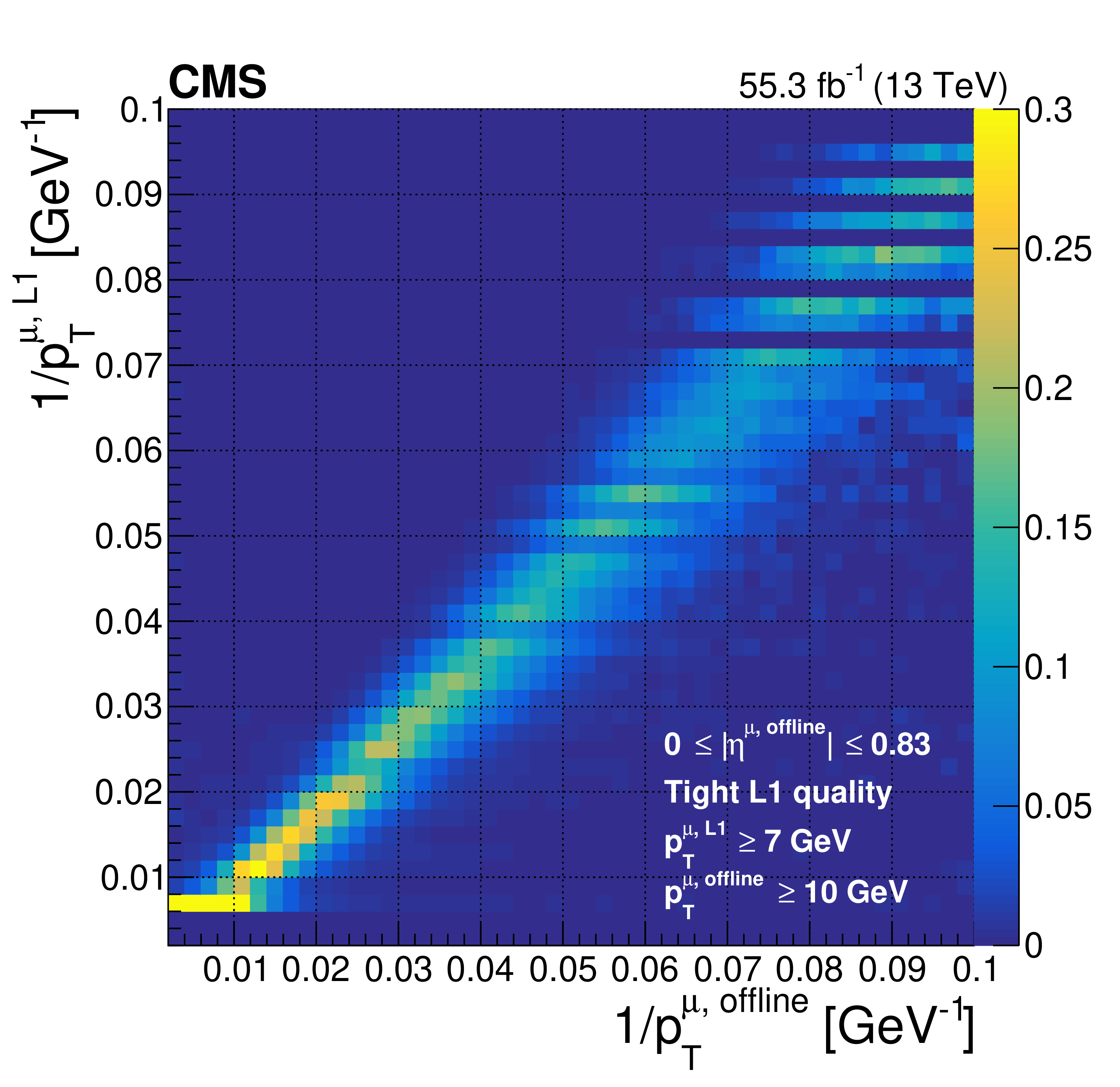
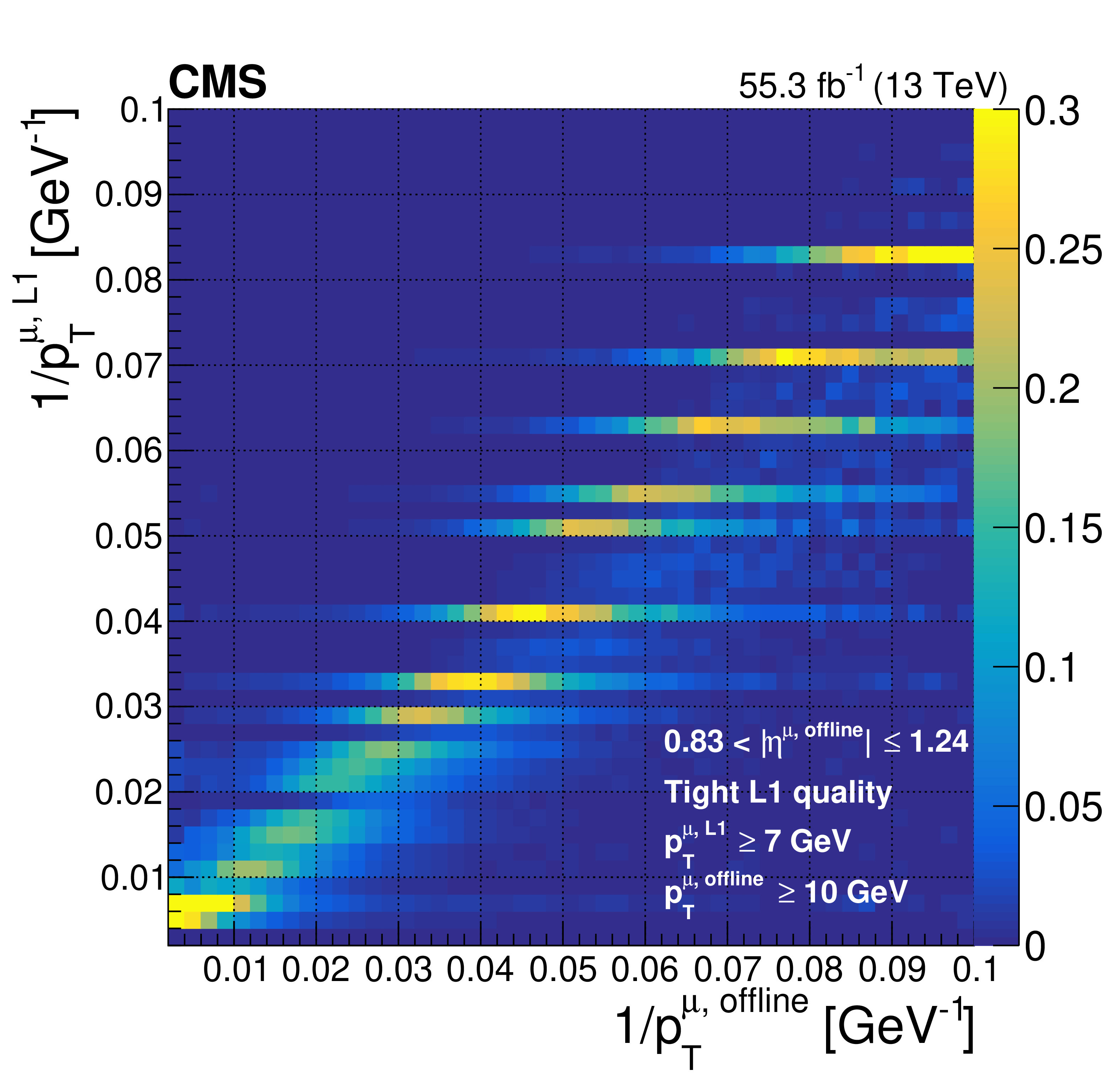
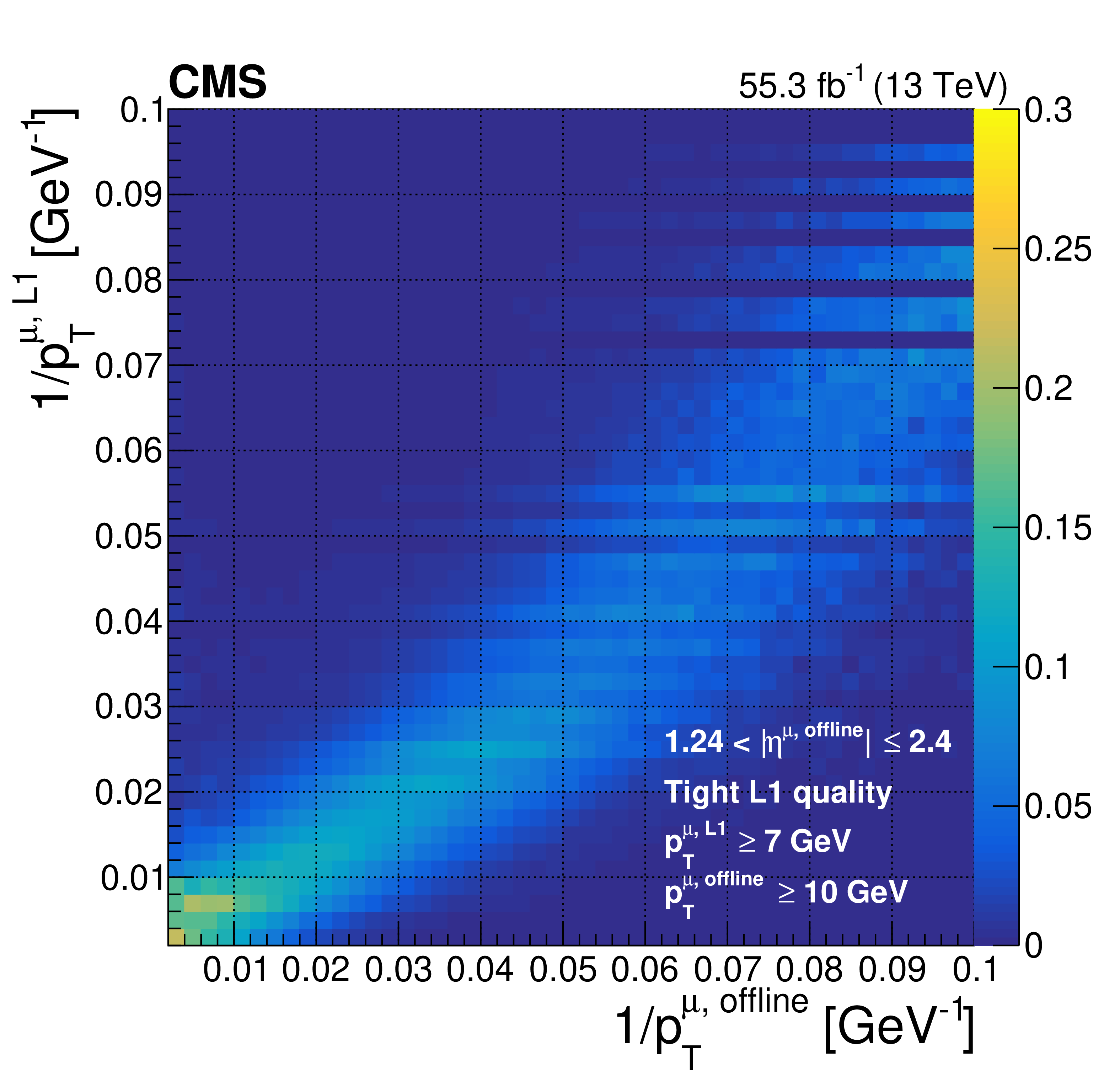
Figure 7:
Correlation between 1/$ {p_{\mathrm {T}}} $ of the muon (proportional to curvature) as assigned at Level-1 vs. offline for three $ {| \eta |}$ regions: barrel (top left), overlap (top right), and endcap (bottom). The measurements come from a data set enriched with events with a Z boson. Distinct bands in the overlap region come from more discrete ${p_{\mathrm {T}}}$ assignment with the OMTF patterns. |
png pdf |
Figure 7-a:
Correlation between 1/$ {p_{\mathrm {T}}} $ of the muon (proportional to curvature) as assigned at Level-1 vs. offline for the barrel region. The measurements come from a data set enriched with events with a Z boson. |
png pdf |
Figure 7-b:
Correlation between 1/$ {p_{\mathrm {T}}} $ of the muon (proportional to curvature) as assigned at Level-1 vs. offline for the barrel/endcap overlap region. The measurements come from a data set enriched with events with a Z boson. Distinct bands come from more discrete ${p_{\mathrm {T}}}$ assignment with the OMTF patterns. |
png pdf |
Figure 7-c:
Correlation between 1/$ {p_{\mathrm {T}}} $ of the muon (proportional to curvature) as assigned at Level-1 vs. offline for the overlap endcap region. The measurements come from a data set enriched with events with a Z boson. |

png pdf |
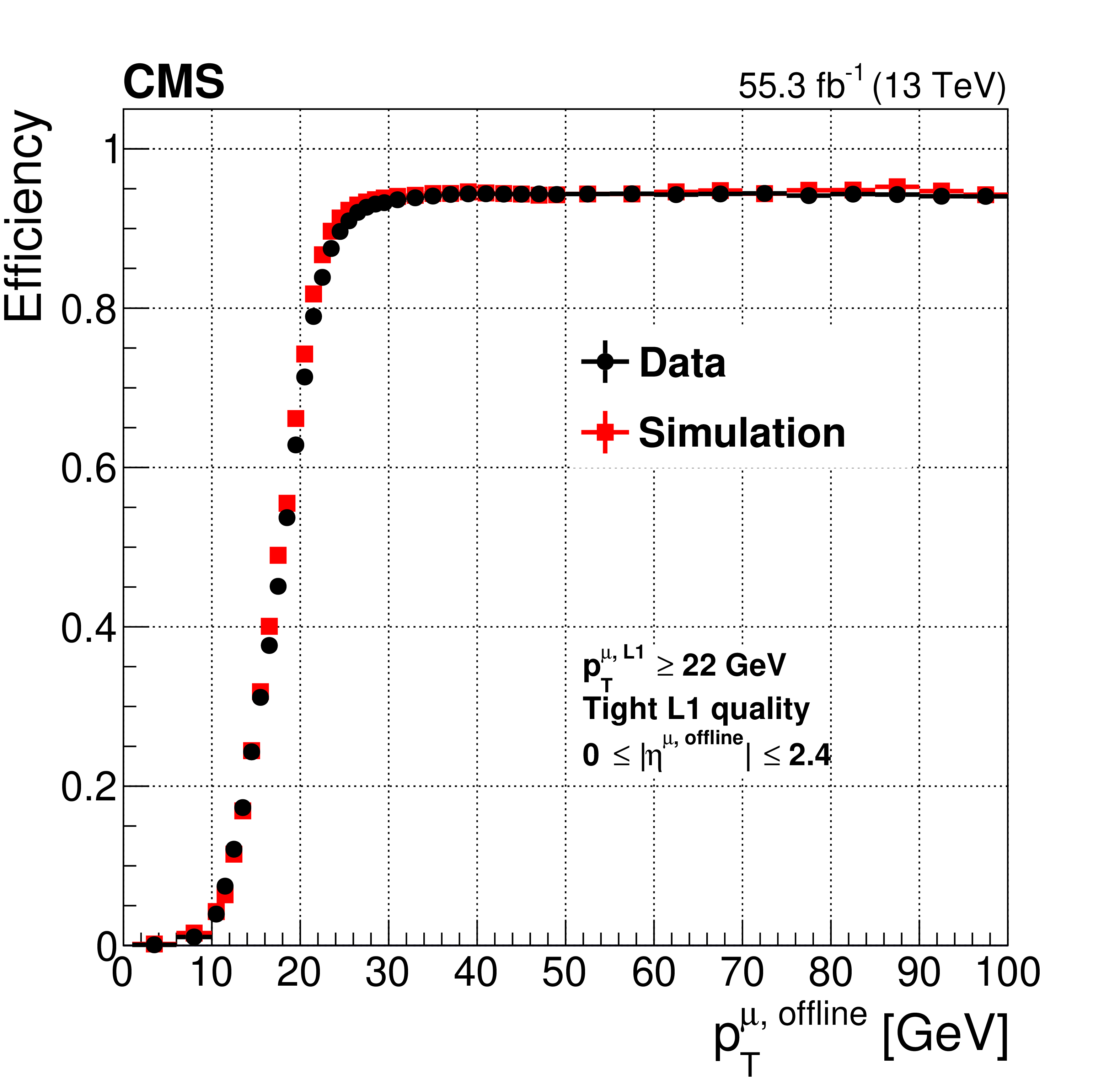
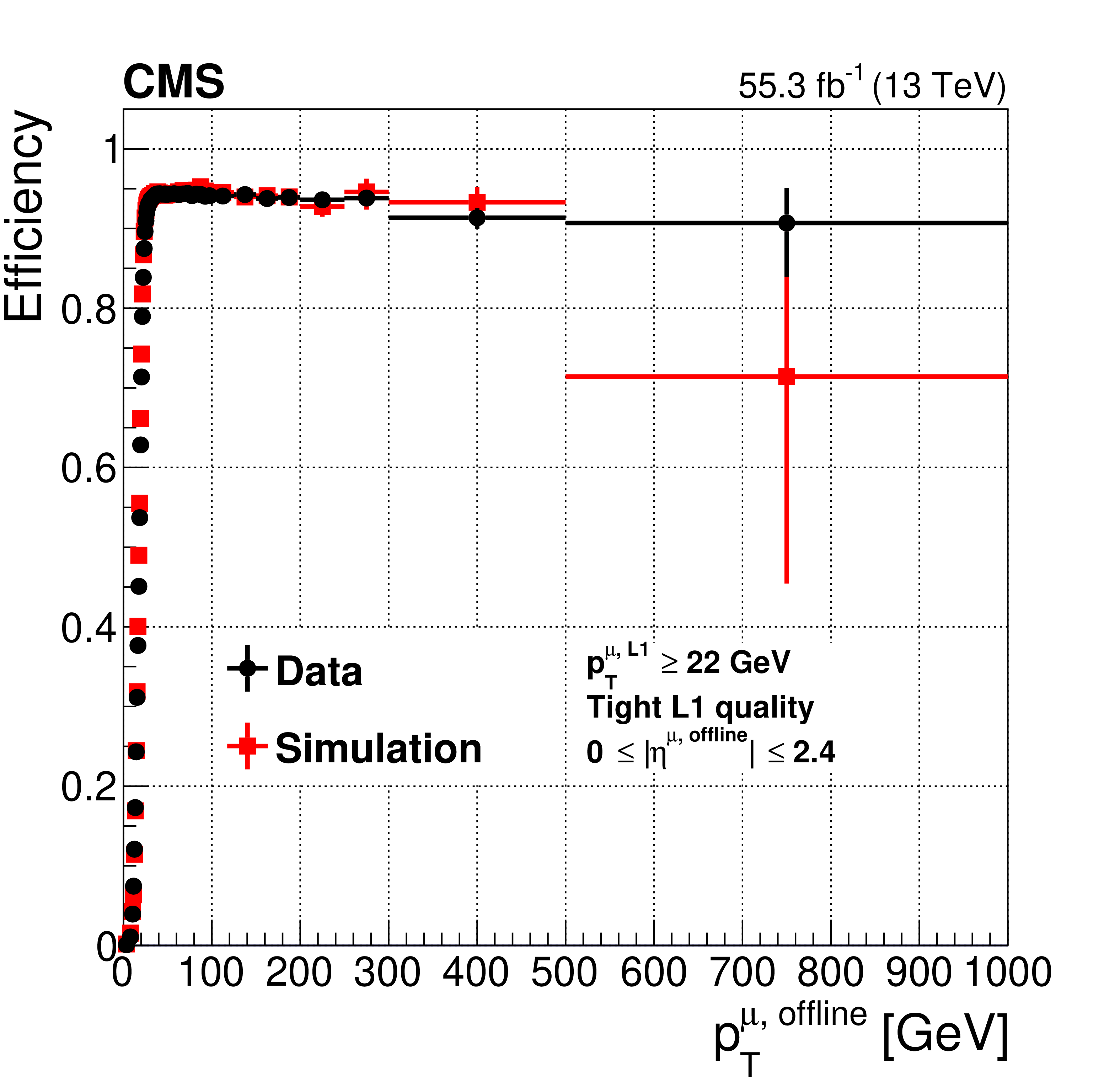
Figure 8:
Level-1 trigger efficiency, for data and simulation as a function of ${{p_{\mathrm {T}}} ^{\text {offline}}}$, for all reconstructed muons in the CMS acceptance $({| {\eta ^{\text {offline}}} |} < 2.4)$ for the most commonly used single-muon trigger during Run 2 $({{p_{\mathrm {T}}} ^{\text {L1}}} > 22 GeV)$, measured with the tag-and-probe method described in the text with the full 2018 data set. The left plot focuses on the steep increase part of the curve close to the trigger threshold. The right plot shows the full momentum range up to 1 TeV. The simulation reproduces the data within a few percent accuracy. The Level-1 trigger efficiency plateau is stable as a function of the muon transverse momentum, retaining an efficiency higher than 90% for muon $ {{p_{\mathrm {T}}} ^{\text {offline}}}\leq $ 1 TeV. |
png pdf |
Figure 8-a:
Level-1 trigger efficiency, for data and simulation as a function of ${{p_{\mathrm {T}}} ^{\text {offline}}}$, for all reconstructed muons in the CMS acceptance $({| {\eta ^{\text {offline}}} |} < 2.4)$ for the most commonly used single-muon trigger during Run 2 $({{p_{\mathrm {T}}} ^{\text {L1}}} > 22 GeV)$, measured with the tag-and-probe method described in the text with the full 2018 data set. The plot focuses on the steep increase part of the curve close to the trigger threshold. The simulation reproduces the data within a few percent accuracy. The Level-1 trigger efficiency plateau is stable as a function of the muon transverse momentum, retaining an efficiency higher than 90% for muon $ {{p_{\mathrm {T}}} ^{\text {offline}}}\leq $ 1 TeV. |
png pdf |
Figure 8-b:
Level-1 trigger efficiency, for data and simulation as a function of ${{p_{\mathrm {T}}} ^{\text {offline}}}$, for all reconstructed muons in the CMS acceptance $({| {\eta ^{\text {offline}}} |} < 2.4)$ for the most commonly used single-muon trigger during Run 2 $({{p_{\mathrm {T}}} ^{\text {L1}}} > 22 GeV)$, measured with the tag-and-probe method described in the text with the full 2018 data set. The plot shows the full momentum range up to 1 TeV. The simulation reproduces the data within a few percent accuracy. The Level-1 trigger efficiency plateau is stable as a function of the muon transverse momentum, retaining an efficiency higher than 90% for muon $ {{p_{\mathrm {T}}} ^{\text {offline}}}\leq $ 1 TeV. |
png pdf |
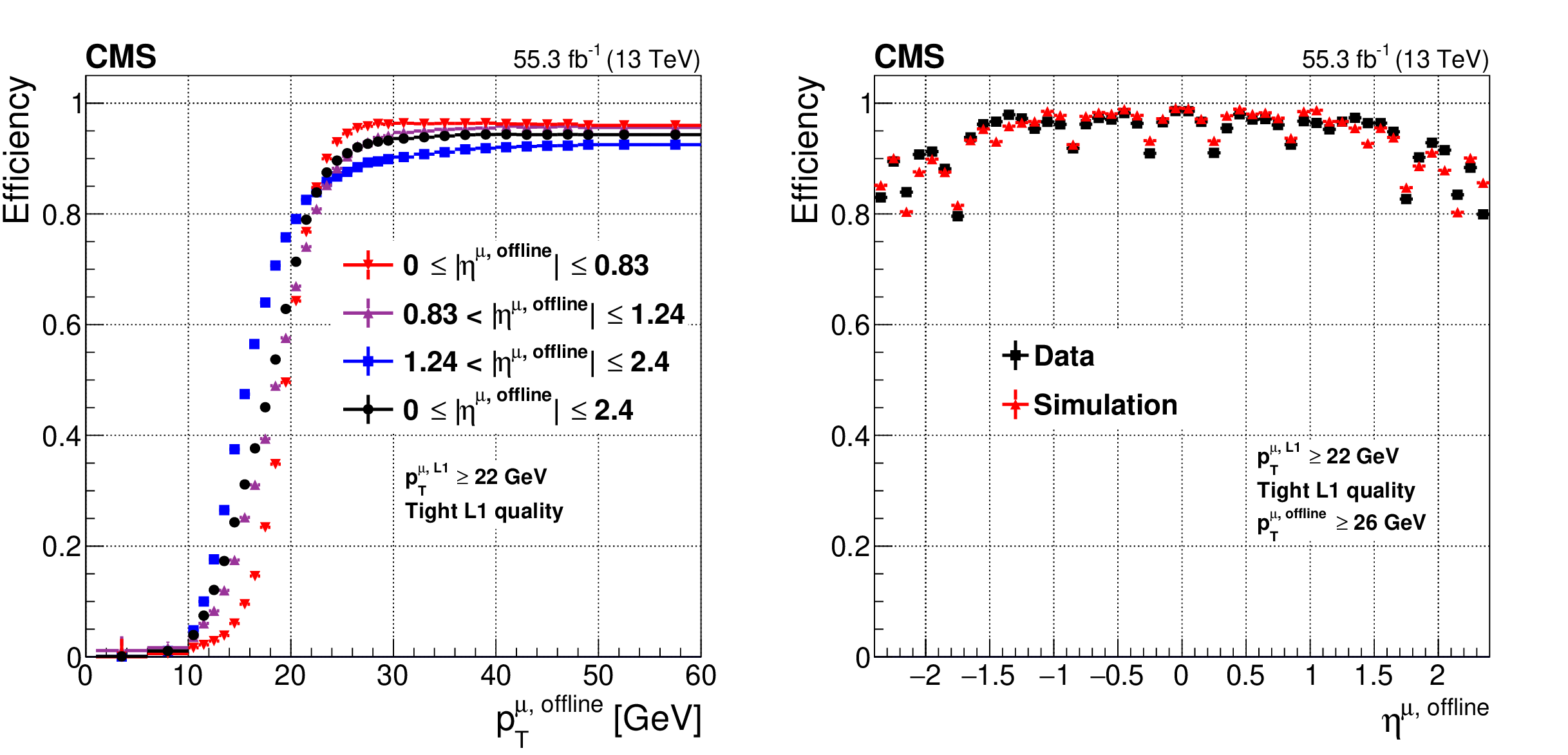
Figure 9:
The left plot shows the Level-1 muon trigger efficiency for data as a function of the offline reconstructed muon ${{p_{\mathrm {T}}} ^{\text {offline}}}$ for each $\eta $ region : barrel region in red, overlap region in purple, endcap region in blue, and the total in black. Turn-on curves for more central muons rise faster primarily because of improved momentum resolution from increased bending in the magnetic field of the yoke. The right plot shows the Level-1 muon efficiency for data and simulation as a function of the offline reconstructed muon $\eta $. The modulation of the efficiency in $\eta $ is because of the acceptance of the muon systems. The efficiency is measured with the tag-and-probe method described in the text with the full 2018 data set. |

png pdf |
Figure 9-a:
The plot shows the Level-1 muon trigger efficiency for data as a function of the offline reconstructed muon ${{p_{\mathrm {T}}} ^{\text {offline}}}$ for each $\eta $ region : barrel region in red, overlap region in purple, endcap region in blue, and the total in black. Turn-on curves for more central muons rise faster primarily because of improved momentum resolution from increased bending in the magnetic field of the yoke. |
png pdf |
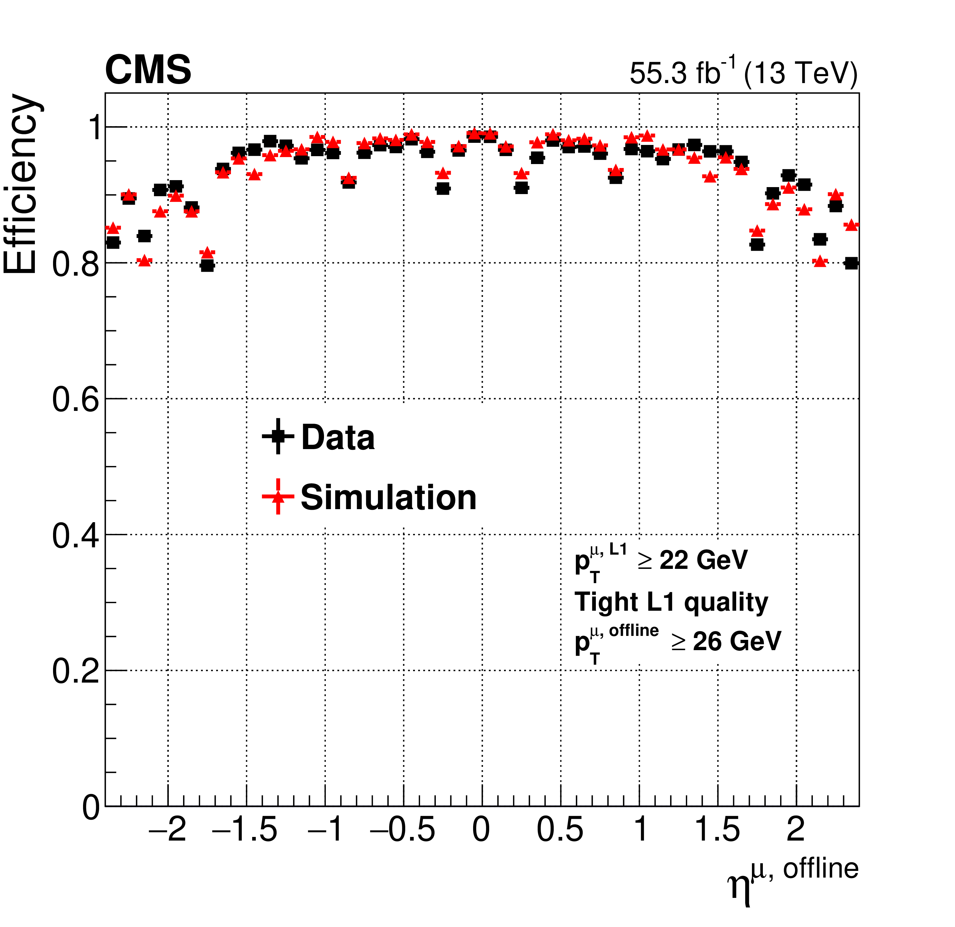
Figure 9-b:
The plot shows the Level-1 muon efficiency for data and simulation as a function of the offline reconstructed muon $\eta $. The modulation of the efficiency in $\eta $ is because of the acceptance of the muon systems. The efficiency is measured with the tag-and-probe method described in the text with the full 2018 data set. |
png pdf |
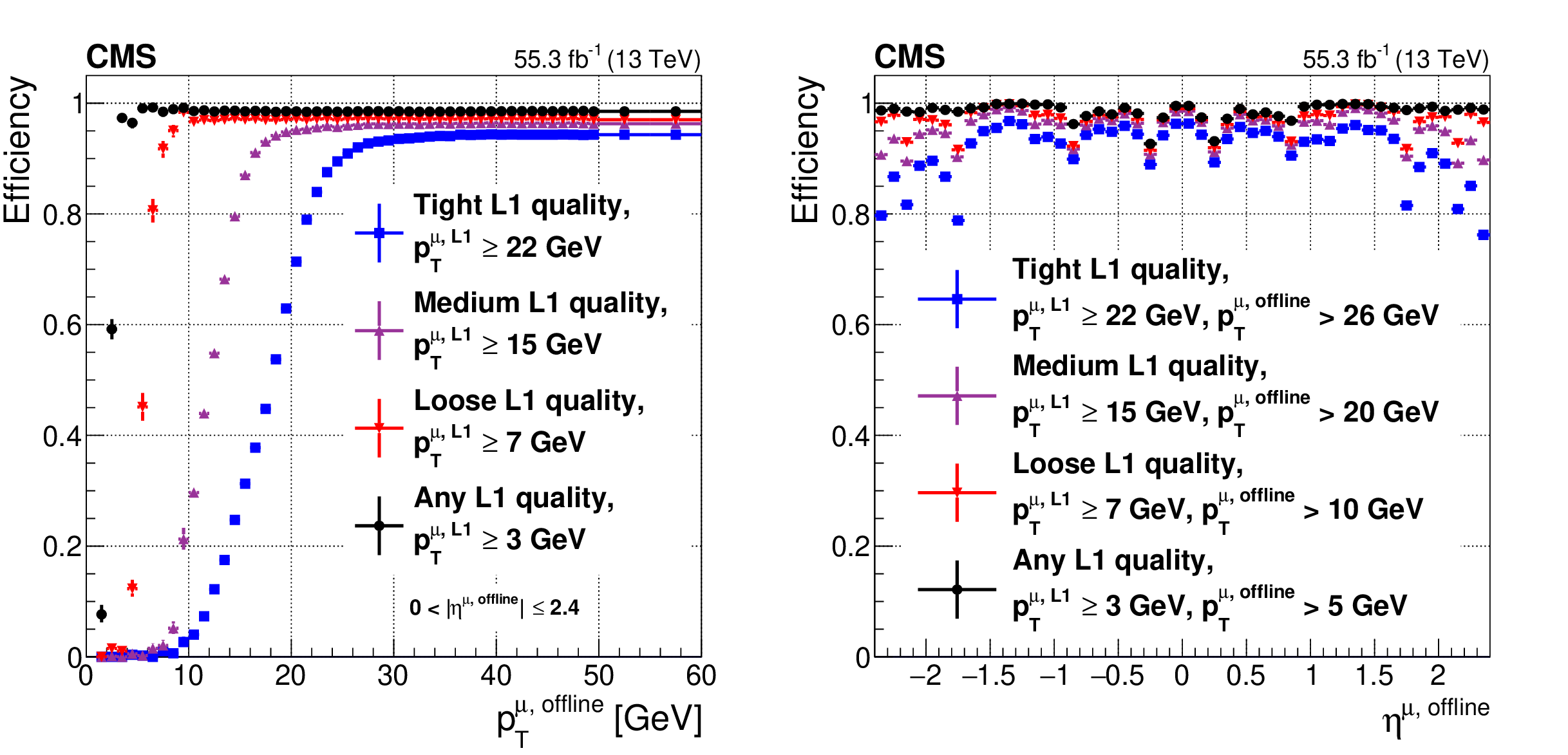
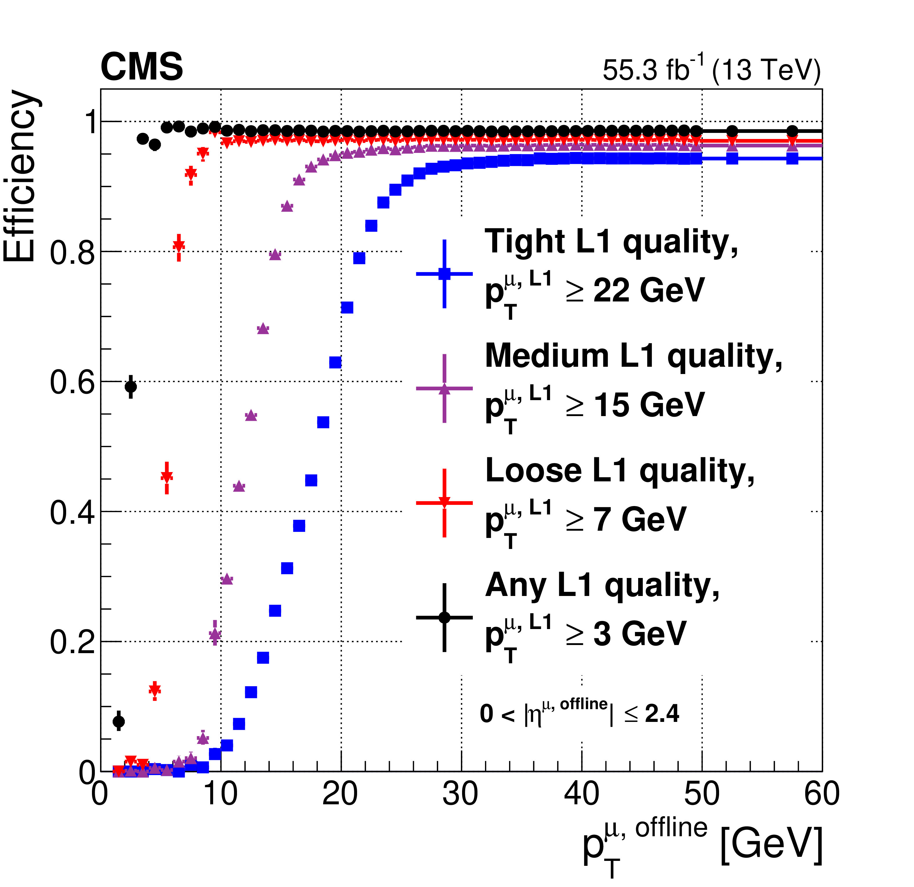
Figure 10:
Level-1 muon trigger efficiency for all possible Level-1 muon qualities as a function of ${{p_{\mathrm {T}}} ^{\text {offline}}}$ (left) and $ {\eta ^{\text {offline}}}$ (right), for all reconstructed muons in the CMS acceptance (${| {\eta ^{\text {offline}}} |} < $ 2.4), measured with the tag-and-probe method described in the text with the full 2018 data set. The ${{p_{\mathrm {T}}} ^{\text {L1}}}$ threshold choices differ based on quality to reproduce the most commonly used algorithm conditions during Run 2. The efficiency in the right plot is for muons with ${{p_{\mathrm {T}}} ^{\text {offline}}}$ in the plateau region, well above the ${{p_{\mathrm {T}}} ^{\text {L1}}}$ threshold. |
png pdf |
Figure 10-a:
Level-1 muon trigger efficiency for all possible Level-1 muon qualities as a function of ${{p_{\mathrm {T}}} ^{\text {offline}}}$, for all reconstructed muons in the CMS acceptance (${| {\eta ^{\text {offline}}} |} < $ 2.4), measured with the tag-and-probe method described in the text with the full 2018 data set. The ${{p_{\mathrm {T}}} ^{\text {L1}}}$ threshold choices differ based on quality to reproduce the most commonly used algorithm conditions during Run 2. |

png pdf |
Figure 10-b:
Level-1 muon trigger efficiency for all possible Level-1 muon qualities as a function of $ {\eta ^{\text {offline}}}$, |
png pdf |
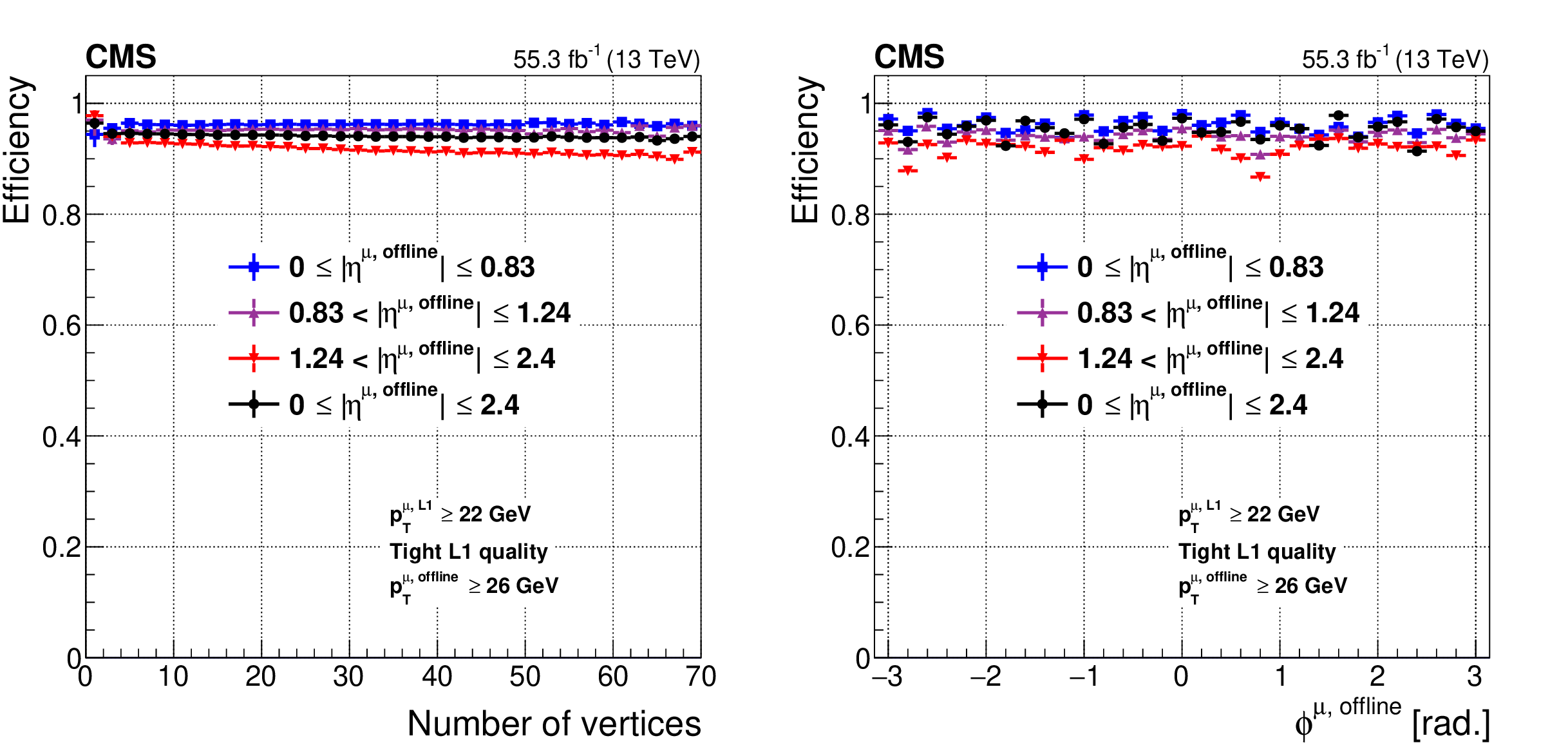
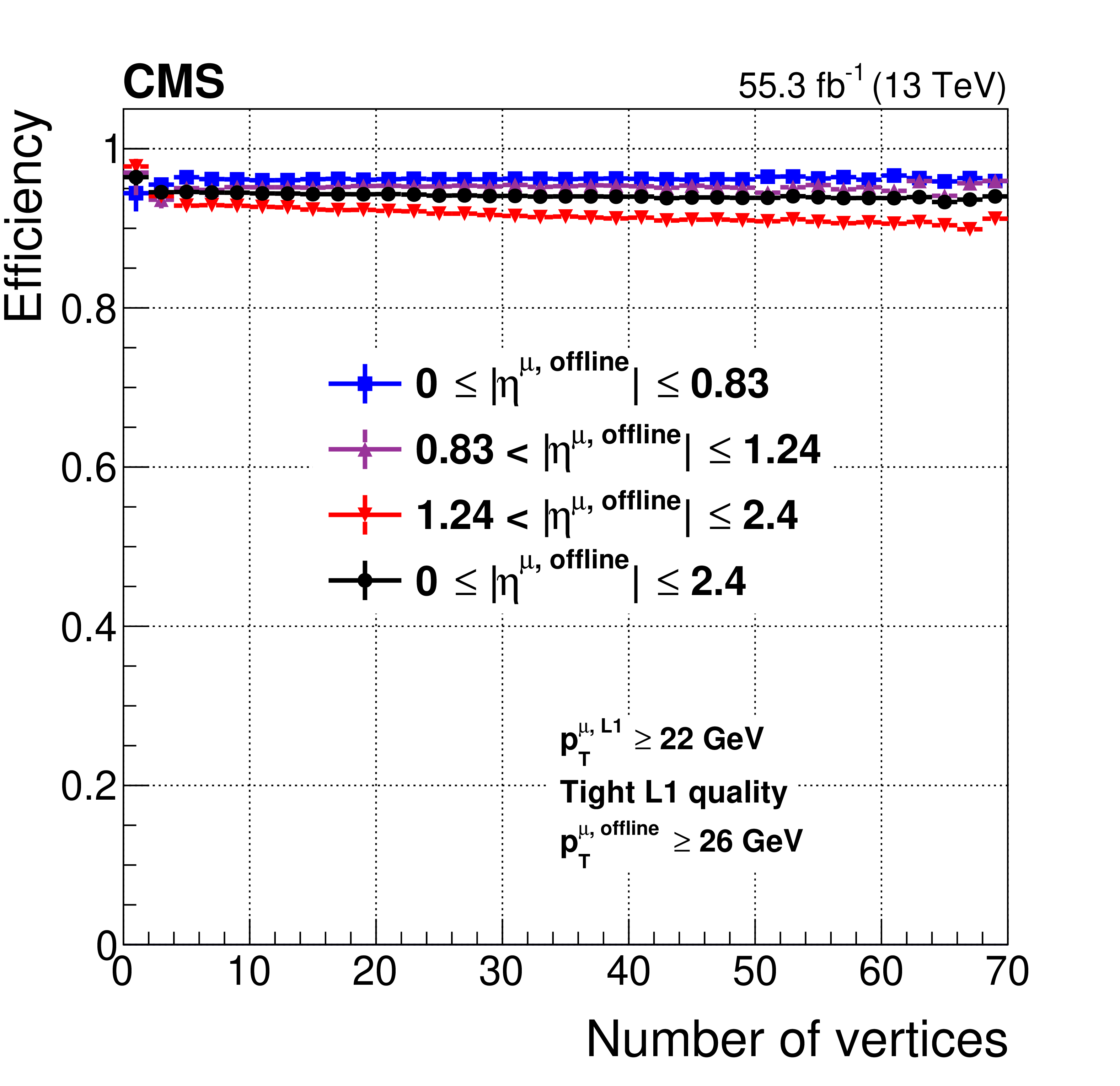
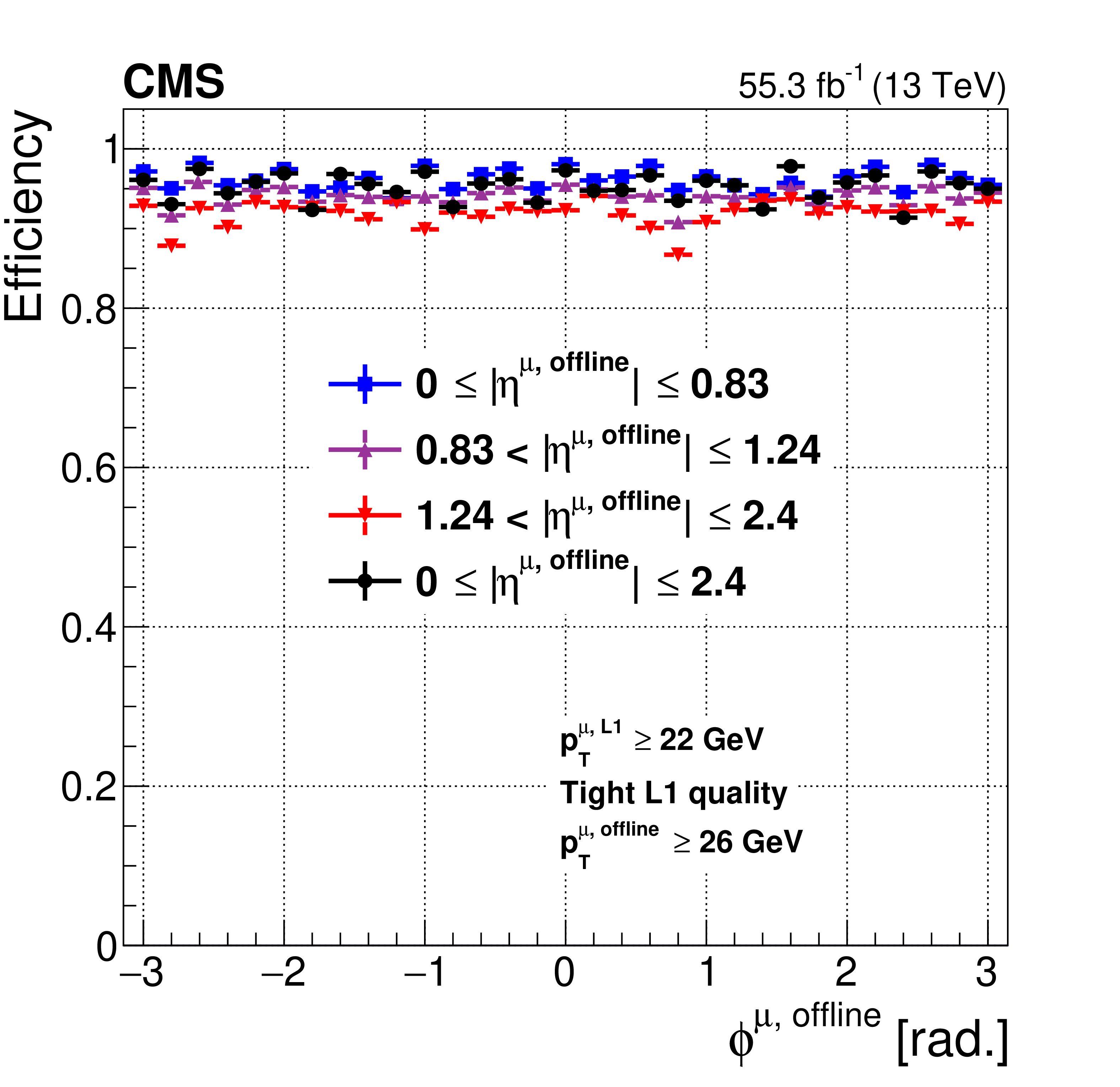
Figure 11:
Level-1 trigger efficiency of the muon track finders as a function of the number of offline reconstructed vertices (left) and muon $\phi $ (right), measured with the tag-and-probe method described in the text with the full 2018 data set. These measurements are shown for the most commonly used single-muon trigger threshold in 2018 (${{p_{\mathrm {T}}} ^{\text {L1}}} > $ 22 GeV). The efficiency has no dependence on the number of vertices for central muons, and a very mild dependence for endcap muons. The efficiency modulation in $\phi $ follows the geometrical acceptance of the muon detector: the efficiency is higher in the regions where the detector layers overlap. The efficiency drops at $\phi =-$2.8 and 0.8 are caused by detector inefficiencies. |
png pdf |
Figure 11-a:
Level-1 trigger efficiency of the muon track finders as a function of the number of offline reconstructed vertices, measured with the tag-and-probe method described in the text with the full 2018 data set. These measurements are shown for the most commonly used single-muon trigger threshold in 2018 (${{p_{\mathrm {T}}} ^{\text {L1}}} > $ 22 GeV). The efficiency has no dependence on the number of vertices for central muons, and a very mild dependence for endcap muons. |
png pdf |
Figure 11-b:
Level-1 trigger efficiency of the muon track finders as a function of the muon $\phi $, measured with the tag-and-probe method described in the text with the full 2018 data set. These measurements are shown for the most commonly used single-muon trigger threshold in 2018 (${{p_{\mathrm {T}}} ^{\text {L1}}} > $ 22 GeV). The efficiency modulation in $\phi $ follows the geometrical acceptance of the muon detector: the efficiency is higher in the regions where the detector layers overlap. The efficiency drops at $\phi =-$2.8 and 0.8 are caused by detector inefficiencies. |

png pdf |
Figure 12:
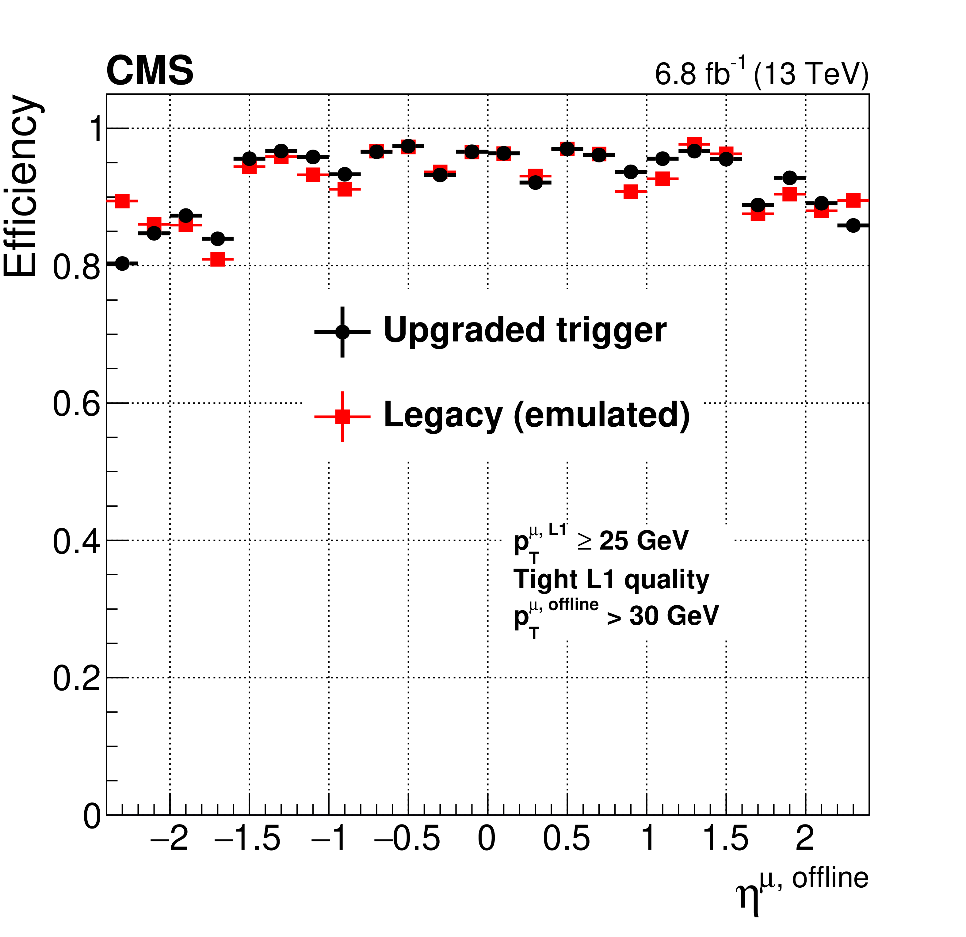
Efficiency of the re-emulated legacy Run 1 algorithms compared with the upgraded Run 2 algorithms, measured using a tag-and-probe technique described in the text, plotted as a function of the offline reconstructed muon ${p_{\mathrm {T}}}$ (left) and $\eta $ (right). The left figure shows a sharper turn-on efficiency for the upgraded system for muons with ${p_{\mathrm {T}}}$ between 5 and 25 GeV. |
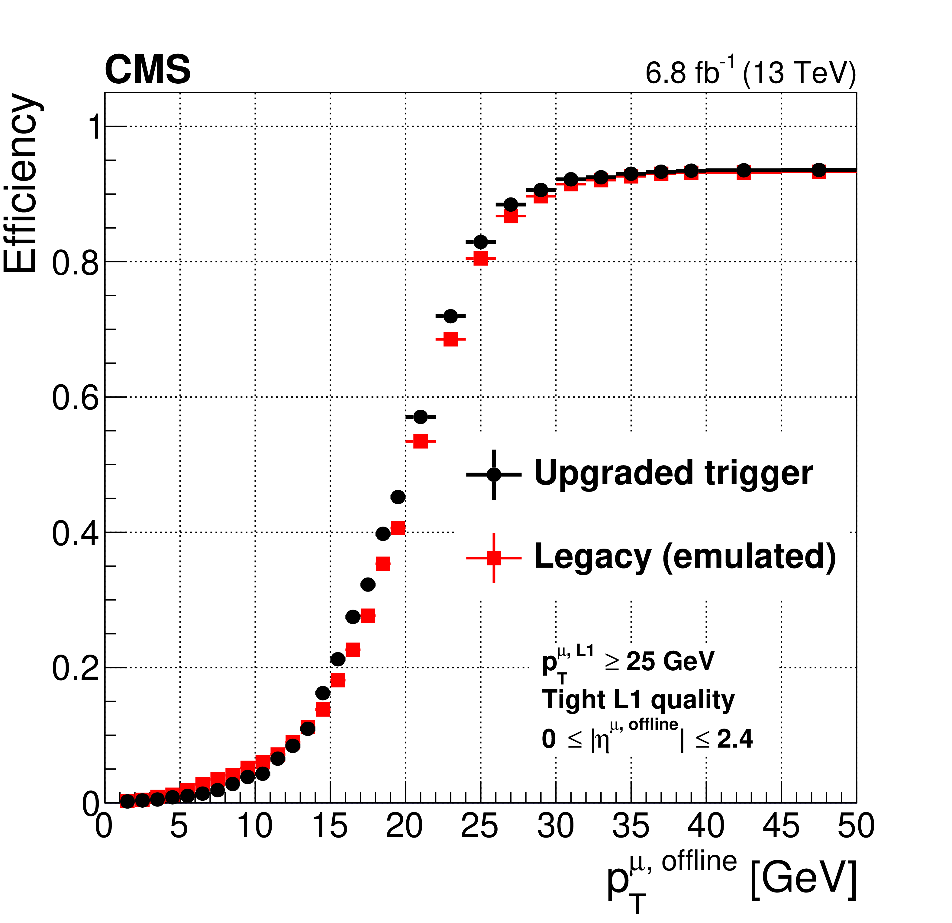
png pdf |
Figure 12-a:
Efficiency of the re-emulated legacy Run 1 algorithms compared with the upgraded Run 2 algorithms, measured using a tag-and-probe technique described in the text, plotted as a function of the offline reconstructed muon ${p_{\mathrm {T}}}$. The figure shows a sharper turn-on efficiency for the upgraded system for muons with ${p_{\mathrm {T}}}$ between 5 and 25 GeV. |
png pdf |
Figure 12-b:
Efficiency of the re-emulated legacy Run 1 algorithms compared with the upgraded Run 2 algorithms, measured using a tag-and-probe technique described in the text, plotted as a function of the offline reconstructed muon $\eta $. |
png pdf |
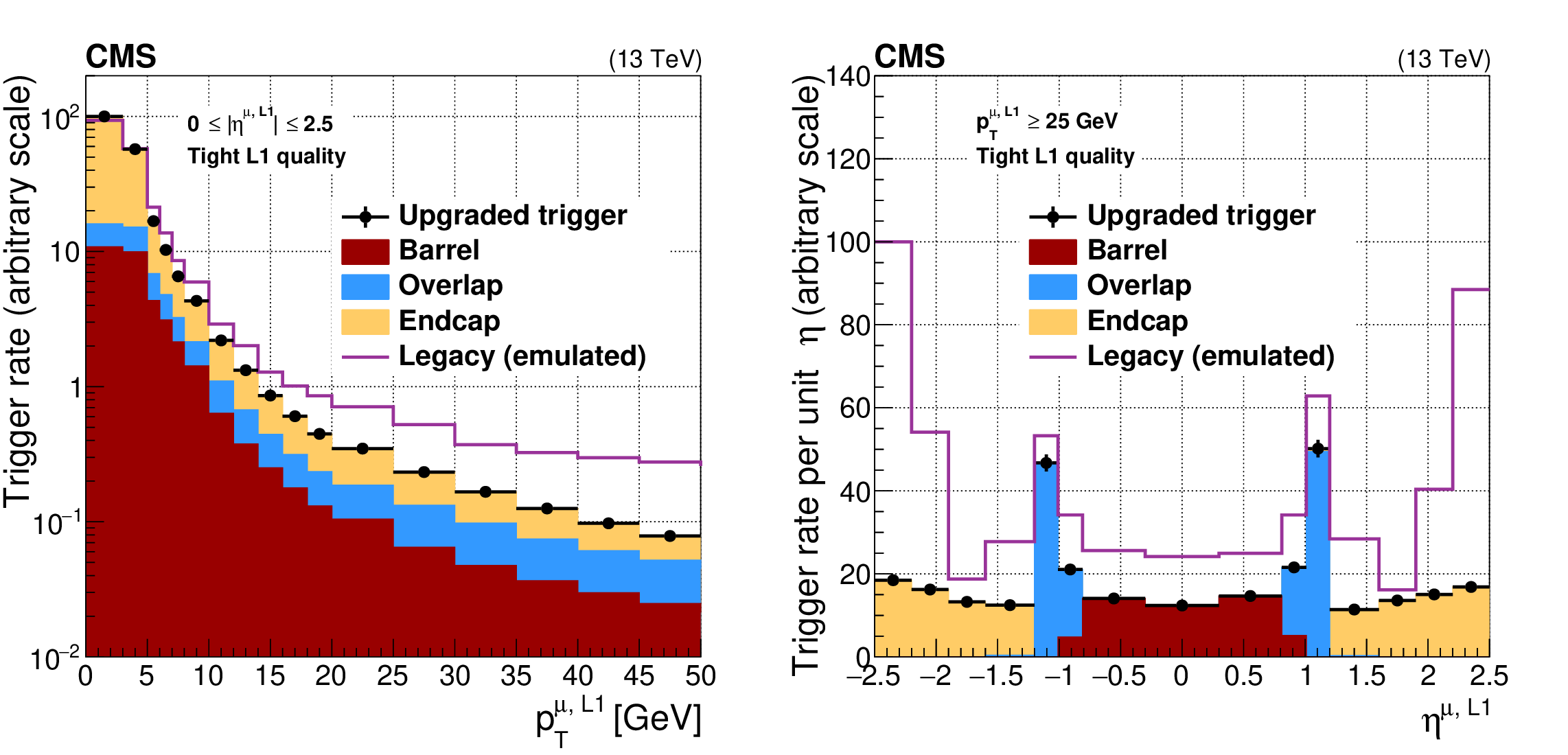
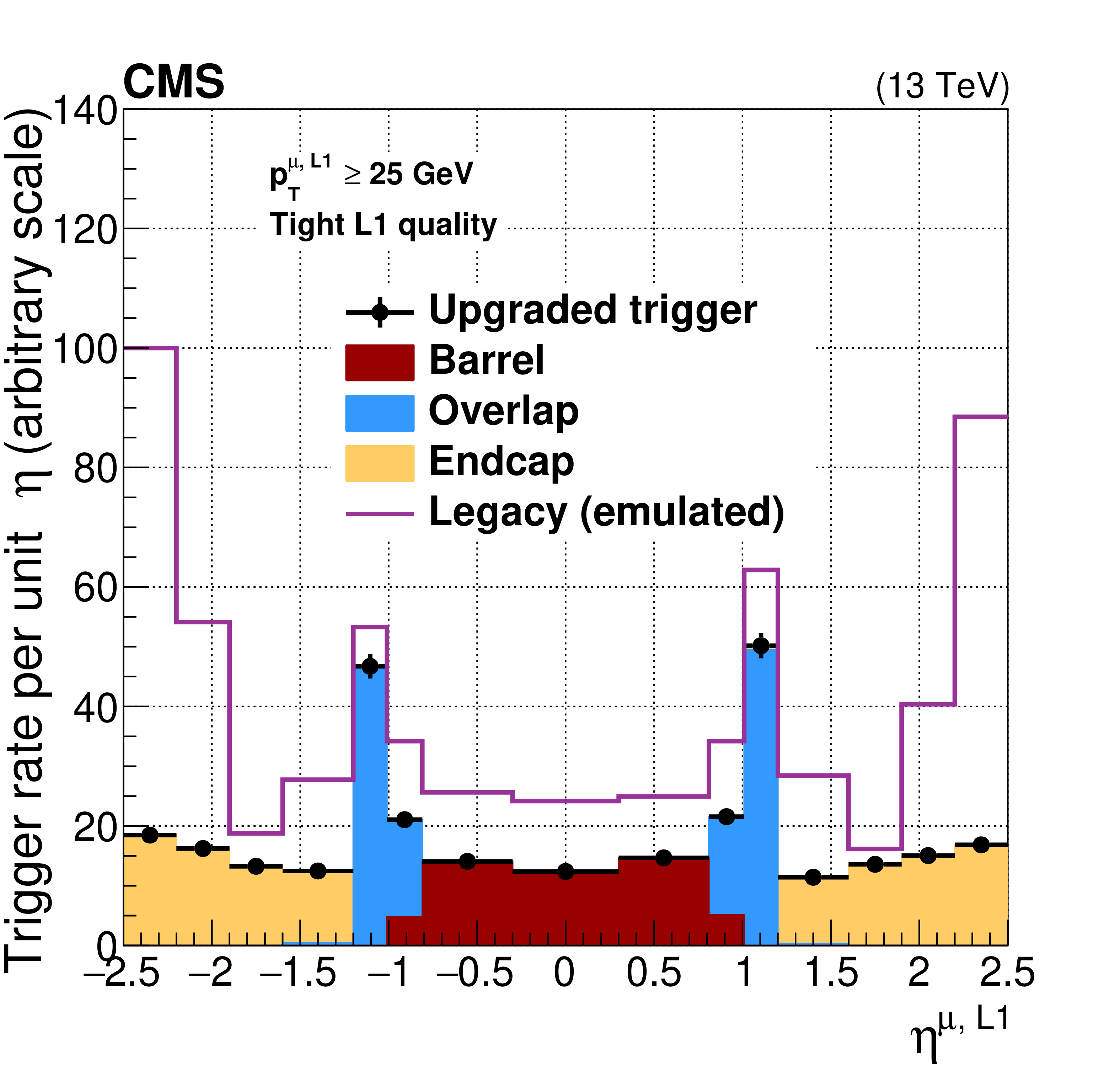
Figure 13:
Rates of the re-emulated legacy Run 1 algorithms compared to the upgraded Run 2 algorithms, as a function of the Level-1 muon trigger ${p_{\mathrm {T}}}$ threshold (left) and $\eta $ (right). The most common Level-1 single-muon trigger threshold used in 2017 was $p_{\mathrm {T}}^{\mu \text {, L1}} {\geq} $ 25 GeV. |

png pdf |
Figure 13-a:
Rates of the re-emulated legacy Run 1 algorithms compared to the upgraded Run 2 algorithms, as a function of the Level-1 muon trigger ${p_{\mathrm {T}}}$ threshold. The most common Level-1 single-muon trigger threshold used in 2017 was $p_{\mathrm {T}}^{\mu \text {, L1}} {\geq} $ 25 GeV. |
png pdf |
Figure 13-b:
Rates of the re-emulated legacy Run 1 algorithms compared to the upgraded Run 2 algorithms, as a function of the Level-1 muon $\eta $. |
png pdf |
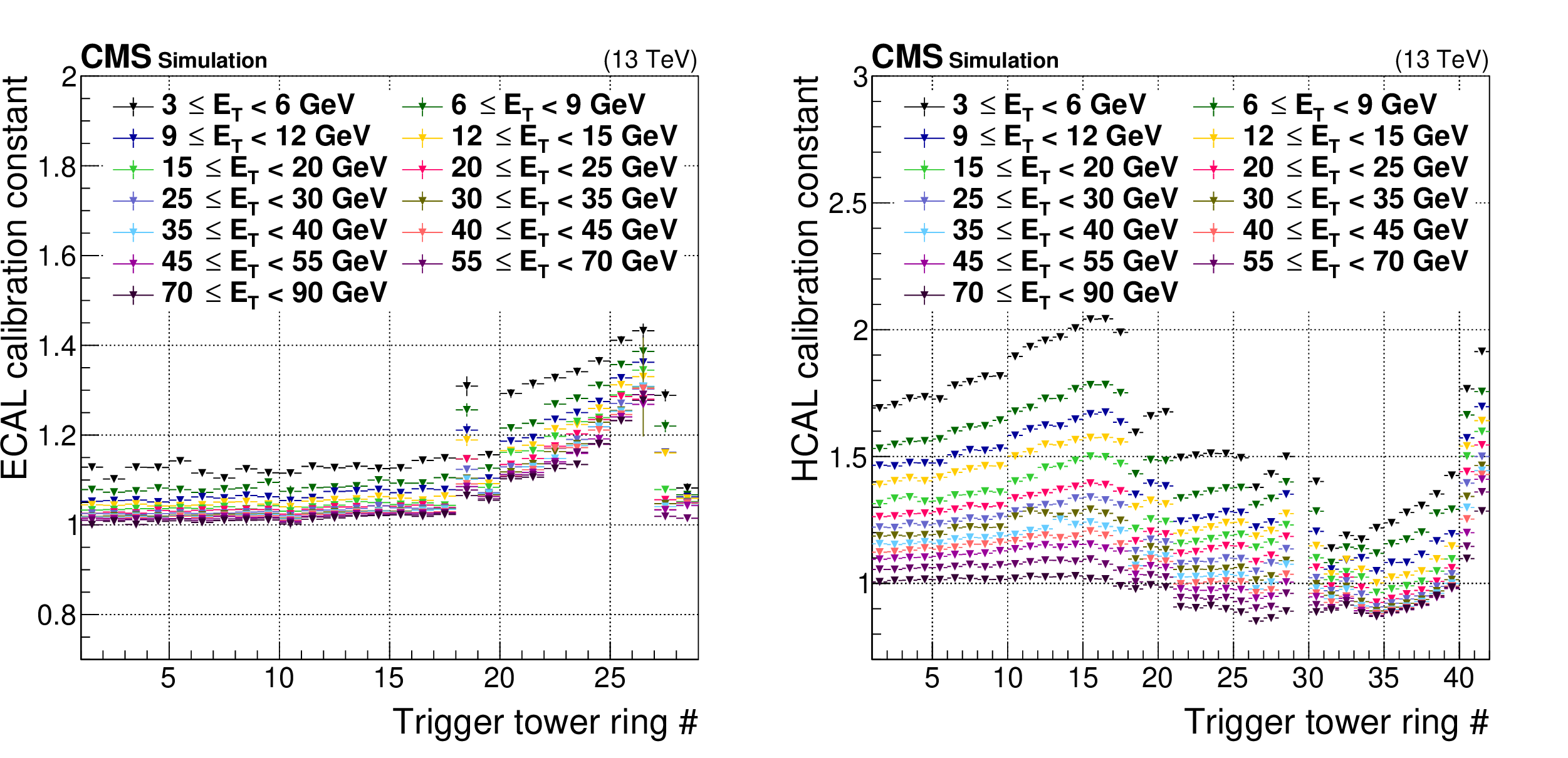
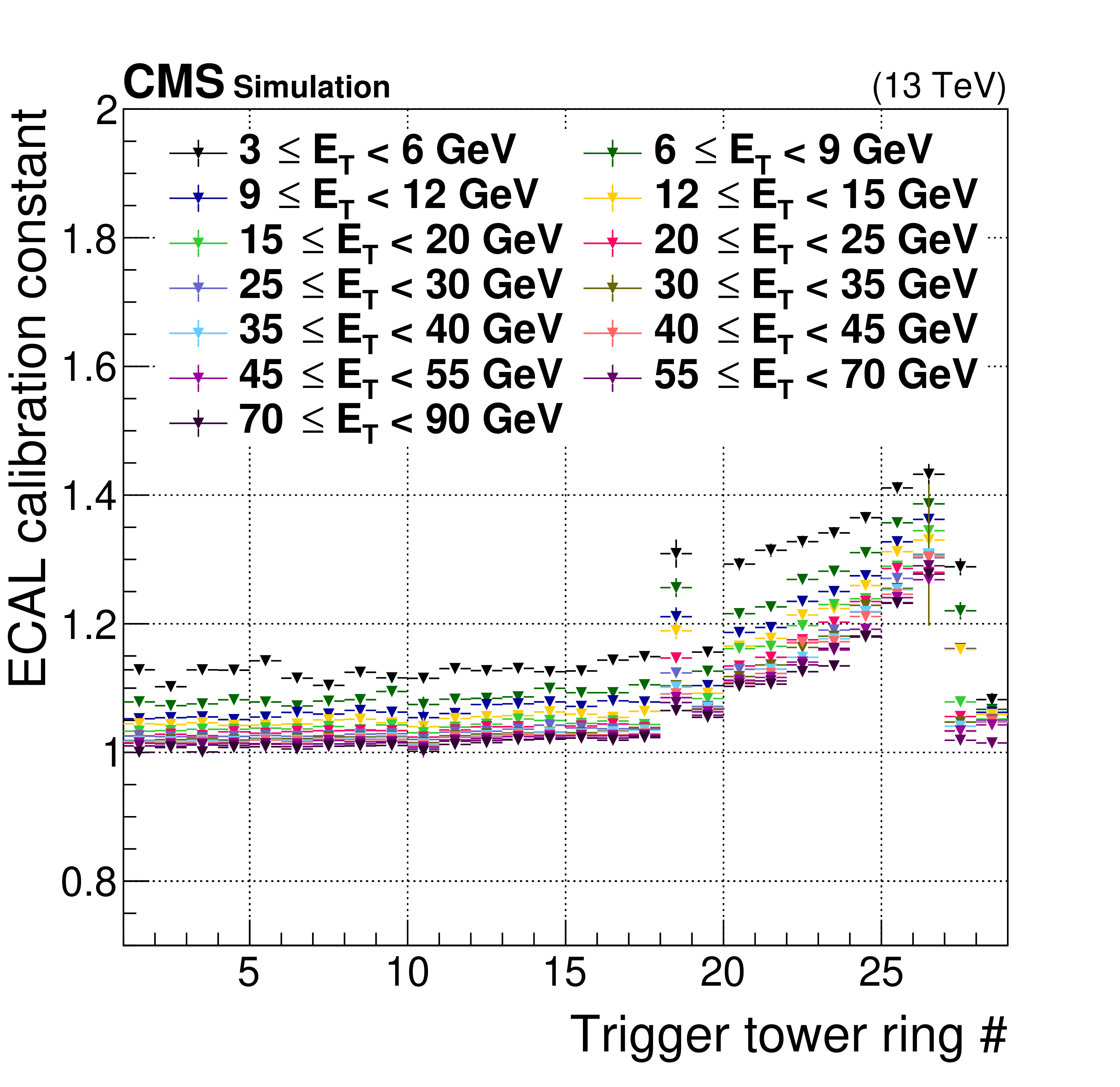
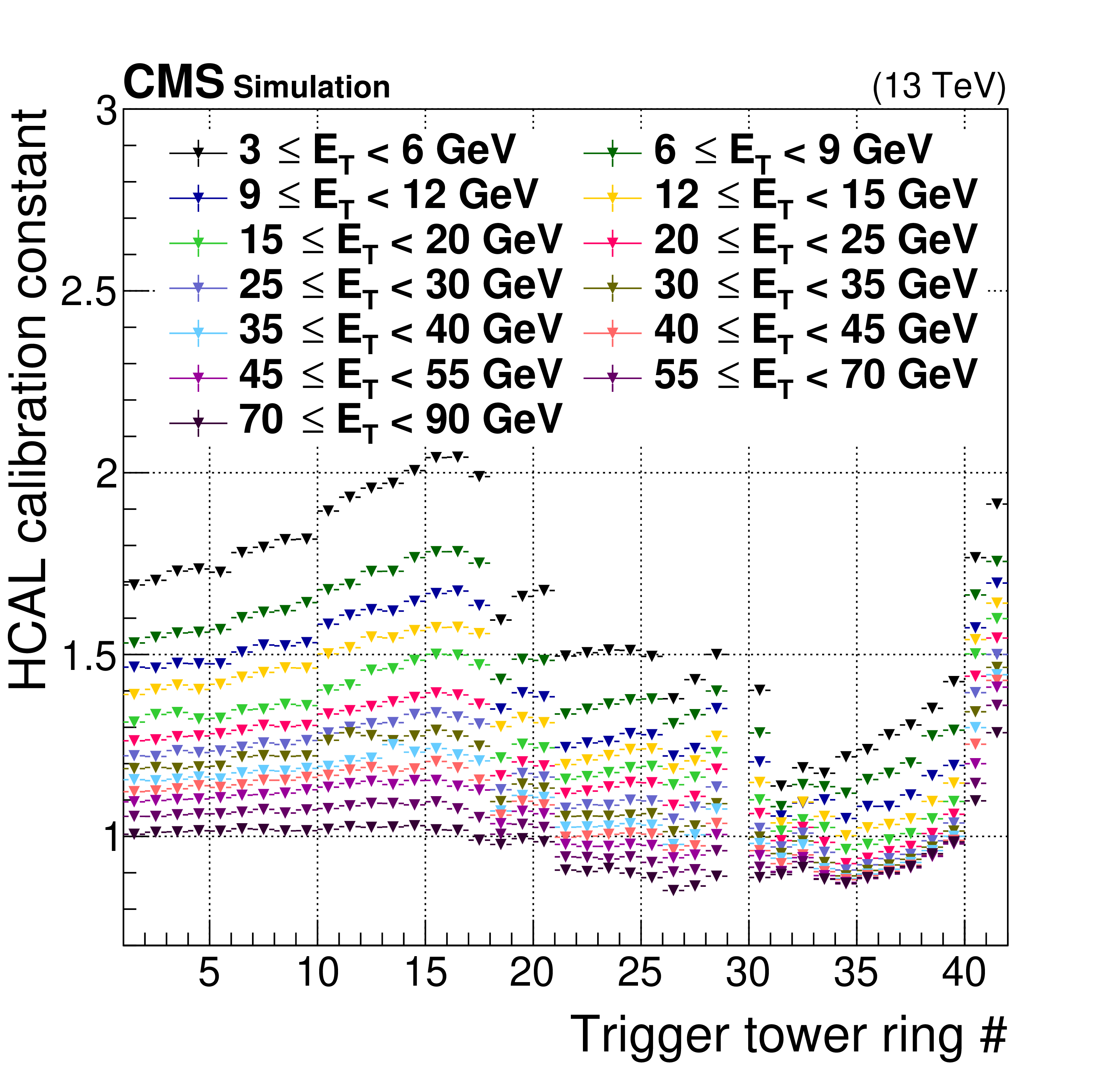
Figure 14:
Layer-1 energy scale factors for ECAL (left) and HCAL (right), shown for each constant-$ {| \eta |}$ ring of trigger towers. As specified in the legend, the color of each point corresponds to a range of uncalibrated trigger primitive transverse energy values received by the Layer-1 calorimeter trigger. Since the signals from trigger tower ring 29 are divided between rings 28 and 30, no scale factors are assigned to it. |
png pdf |
Figure 14-a:
Layer-1 energy scale factors for ECAL, shown for each constant-$ {| \eta |}$ ring of trigger towers. As specified in the legend, the color of each point corresponds to a range of uncalibrated trigger primitive transverse energy values received by the Layer-1 calorimeter trigger. |
png pdf |
Figure 14-b:
Layer-1 energy scale factors for HCAL, shown for each constant-$ {| \eta |}$ ring of trigger towers. As specified in the legend, the color of each point corresponds to a range of uncalibrated trigger primitive transverse energy values received by the Layer-1 calorimeter trigger. Since the signals from trigger tower ring 29 are divided between rings 28 and 30, no scale factors are assigned to it. |

png pdf |
Figure 15:
The Level-1 e/$ {\gamma}$ clustering algorithm and isolation definition. A candidate is formed by clustering neighboring towers (orange and yellow) if they can be linked to the seed tower (red). Each square represents a trigger tower. A candidate is considered isolated if the ${E_{\mathrm {T}}}$ in the isolation region (blue) is smaller than a given value. Details are given in the text. |
png pdf |
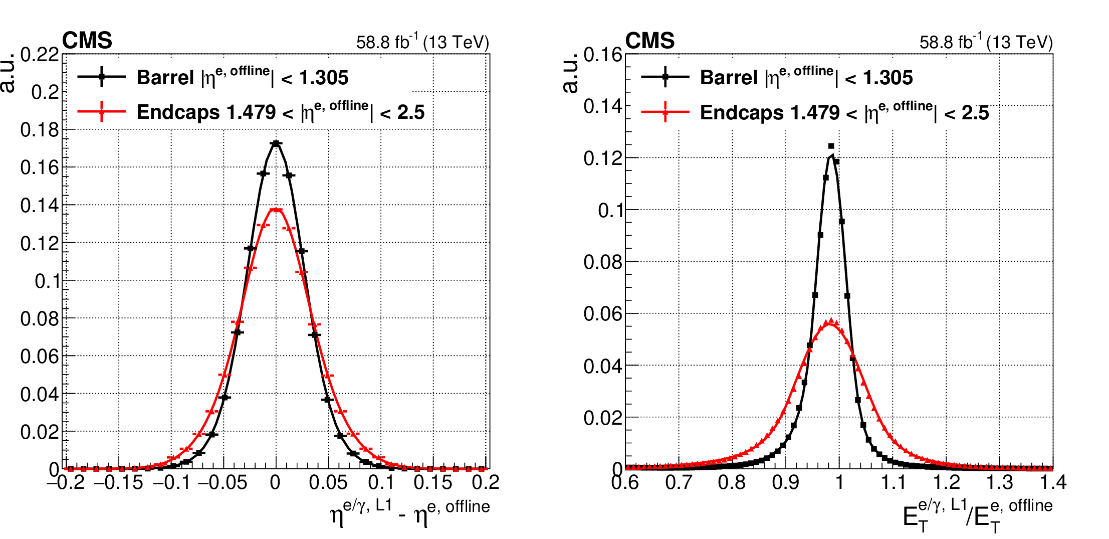
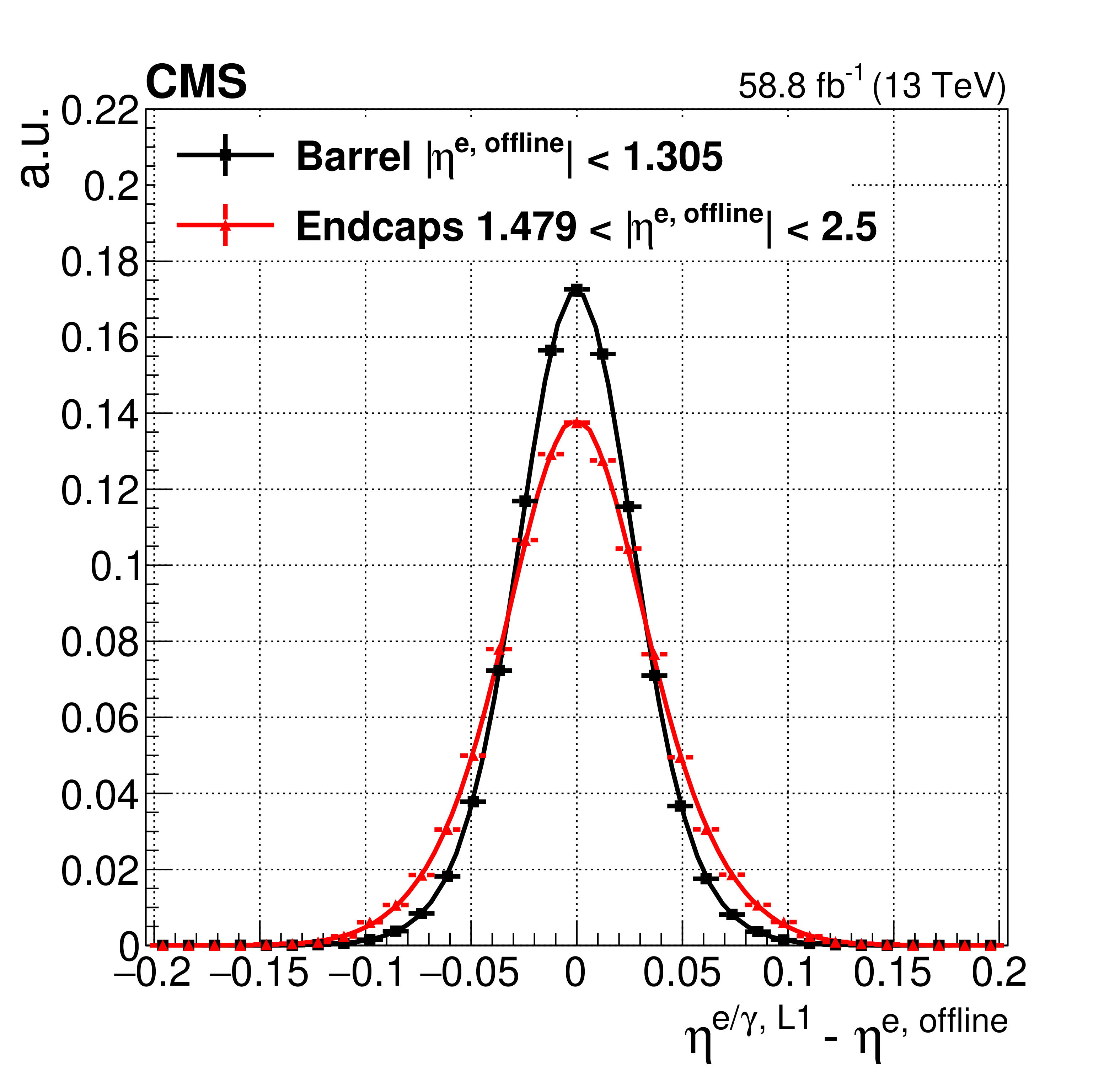
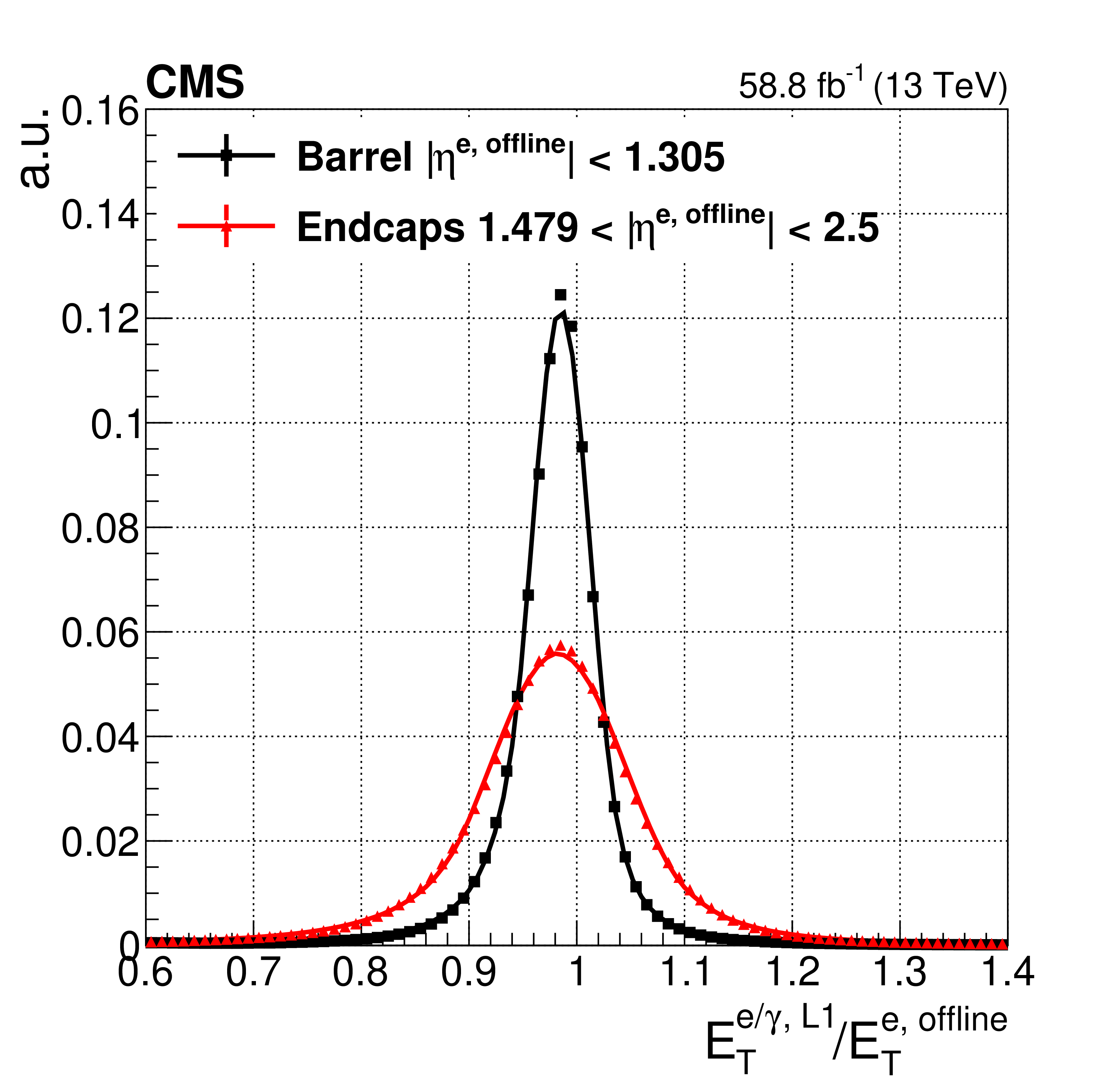
Figure 16:
The pseudorapidity position of Level-1 e/$ {\gamma}$ candidates with respect to the offline reconstructed electron position, separately for the barrel and endcap regions(left). The relative transverse energy of the Level-1 e/$ {\gamma}$ candidates with respect to the offline reconstructed electron transverse energy, also separately for the barrel and endcap regions (right). The functional form of the fits consists of a two-sided tail symmetric Crystal Ball function for the left plot and a combination of a Gaussian and an one-sided tail asymmetric Crystal Ball function for the right plot. |
png pdf |
Figure 16-a:
The pseudorapidity position of Level-1 e/$ {\gamma}$ candidates with respect to the offline reconstructed electron position, separately for the barrel and endcap regions. The functional form of the fits consists of a two-sided tail symmetric Crystal Ball function. |
png pdf |
Figure 16-b:
The relative transverse energy of the Level-1 e/$ {\gamma}$ candidates with respect to the offline reconstructed electron transverse energy, also separately for the barrel and endcap regions. The functional form of the fits consists of a combination of a Gaussian and an one-sided tail asymmetric Crystal Ball function. |
png pdf |
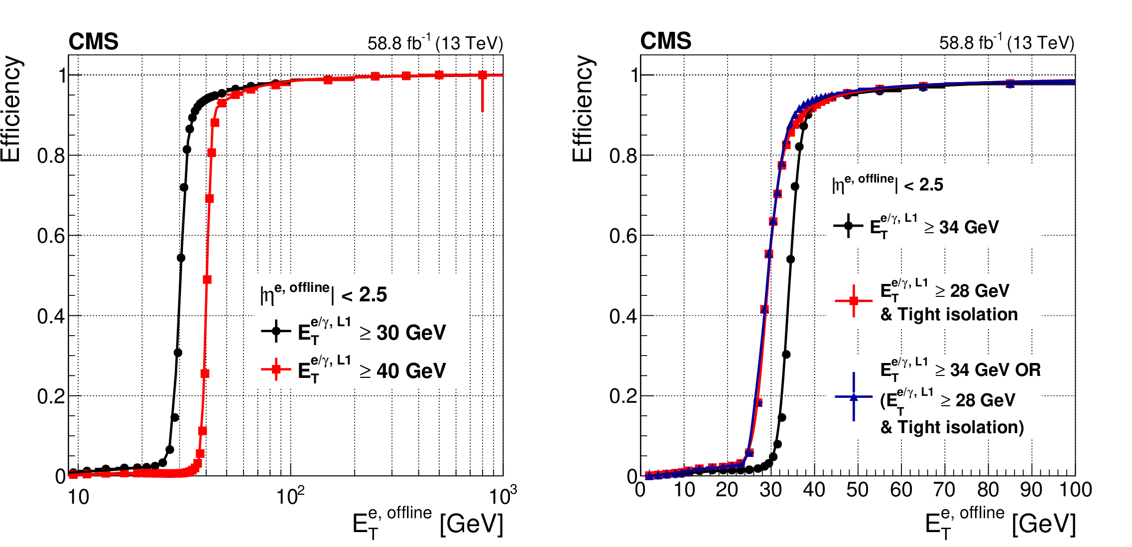
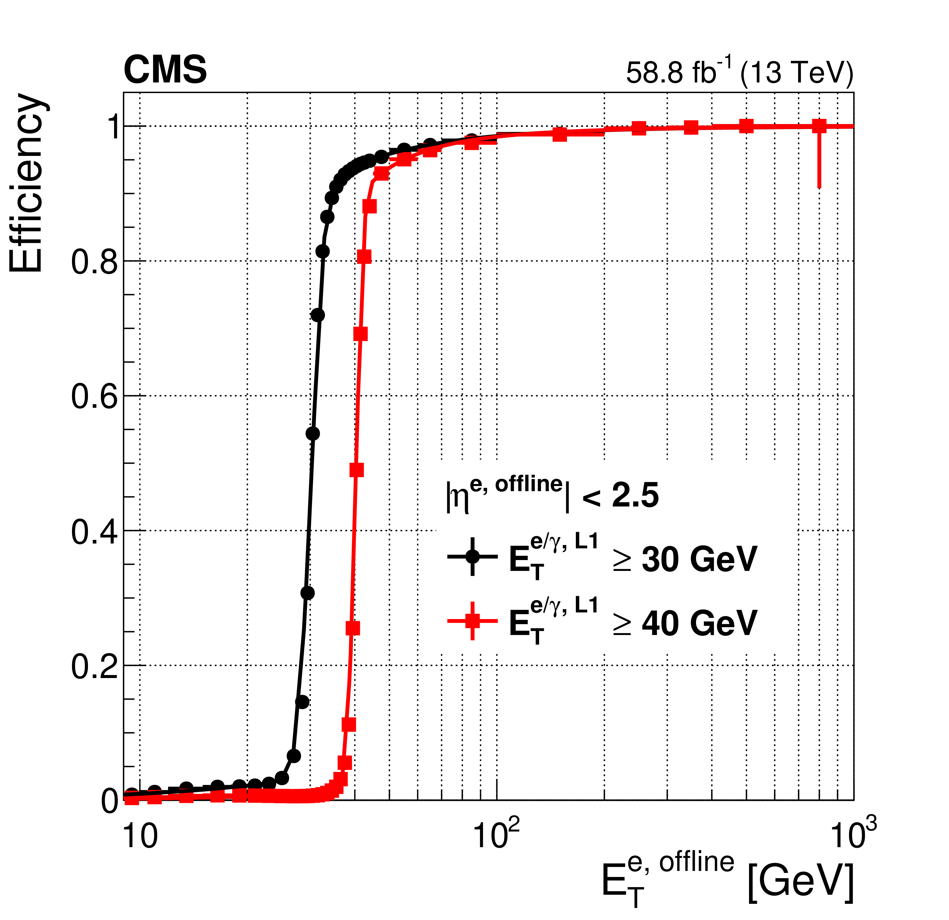
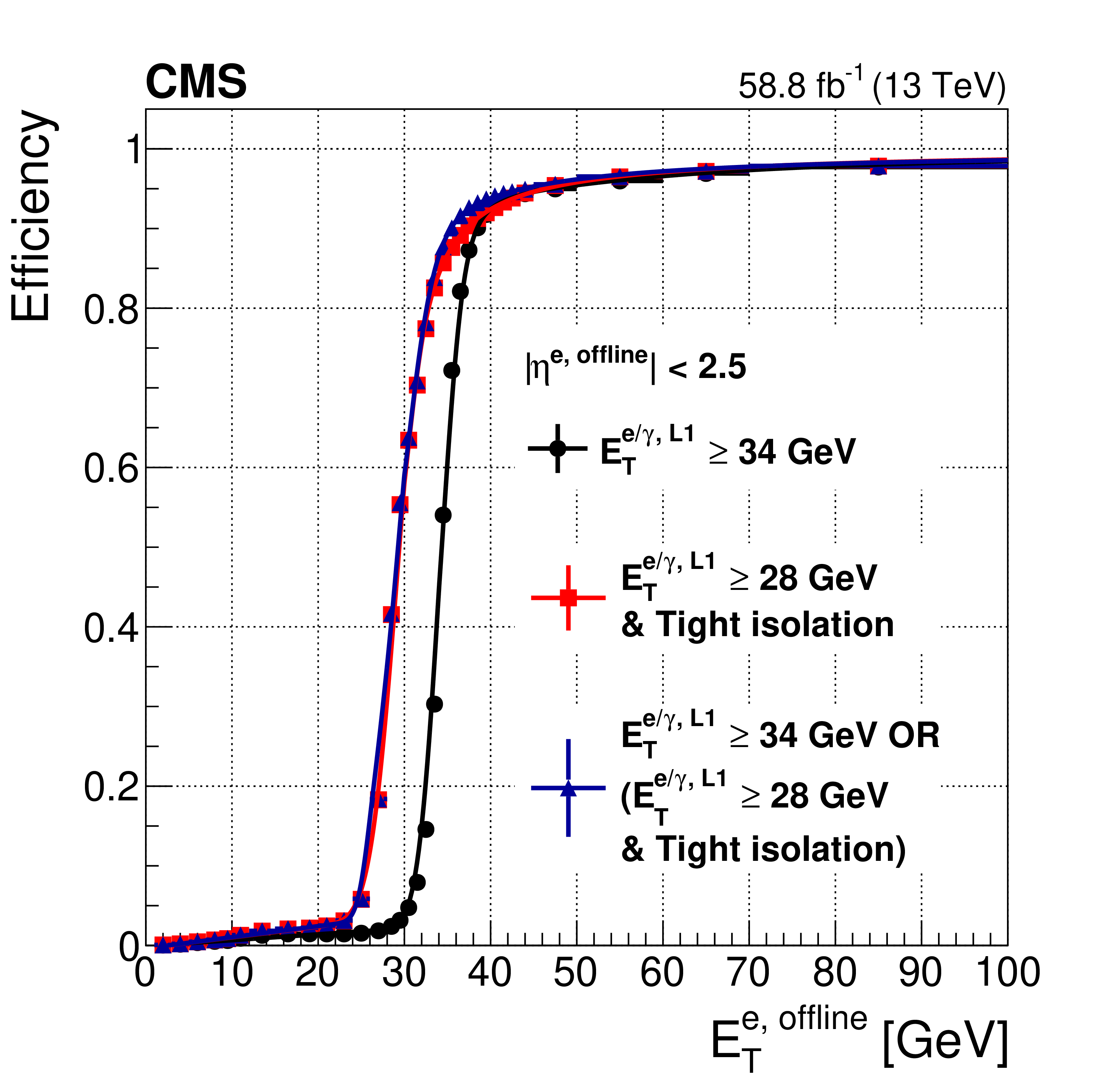
Figure 17:
The Level-1 e/$ {\gamma}$ trigger efficiency as a function of the offline reconstructed electron ${E_{\mathrm {T}}}$ for thresholds of 30 and 40 GeV (left). The Level-1 trigger efficiency as a function of the offline reconstructed electron ${E_{\mathrm {T}}}$ for two typical unprescaled algorithms used in 2018 (right): an ${E_{\mathrm {T}}}$ threshold of 34 GeV in black, and of 28 GeV with the tight set of isolation requirements in red (as discussed in the text). The efficiency curve for the logical OR of the two algorithms is shown in blue. The functional form of the fits consists of a cumulative Crystal Ball function convolved with a polynomial or exponential function in the low ${E_{\mathrm {T}}}$ region. |
png pdf |
Figure 17-a:
The Level-1 e/$ {\gamma}$ trigger efficiency as a function of the offline reconstructed electron ${E_{\mathrm {T}}}$ for thresholds of 30 and 40 GeV. The functional form of the fits consists of a cumulative Crystal Ball function convolved with a polynomial or exponential function in the low ${E_{\mathrm {T}}}$ region. |
png pdf |
Figure 17-b:
The Level-1 trigger efficiency as a function of the offline reconstructed electron ${E_{\mathrm {T}}}$ for two typical unprescaled algorithms used in 2018: an ${E_{\mathrm {T}}}$ threshold of 34 GeV in black, and of 28 GeV with the tight set of isolation requirements in red (as discussed in the text). The efficiency curve for the logical OR of the two algorithms is shown in blue. The functional form of the fits consists of a cumulative Crystal Ball function convolved with a polynomial or exponential function in the low ${E_{\mathrm {T}}}$ region. |
png pdf |
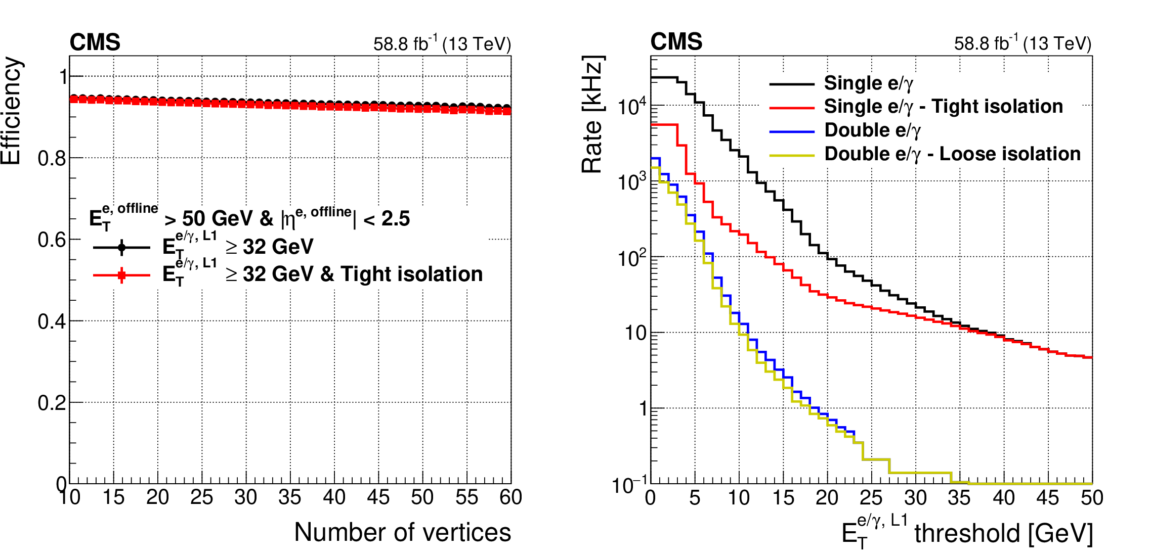
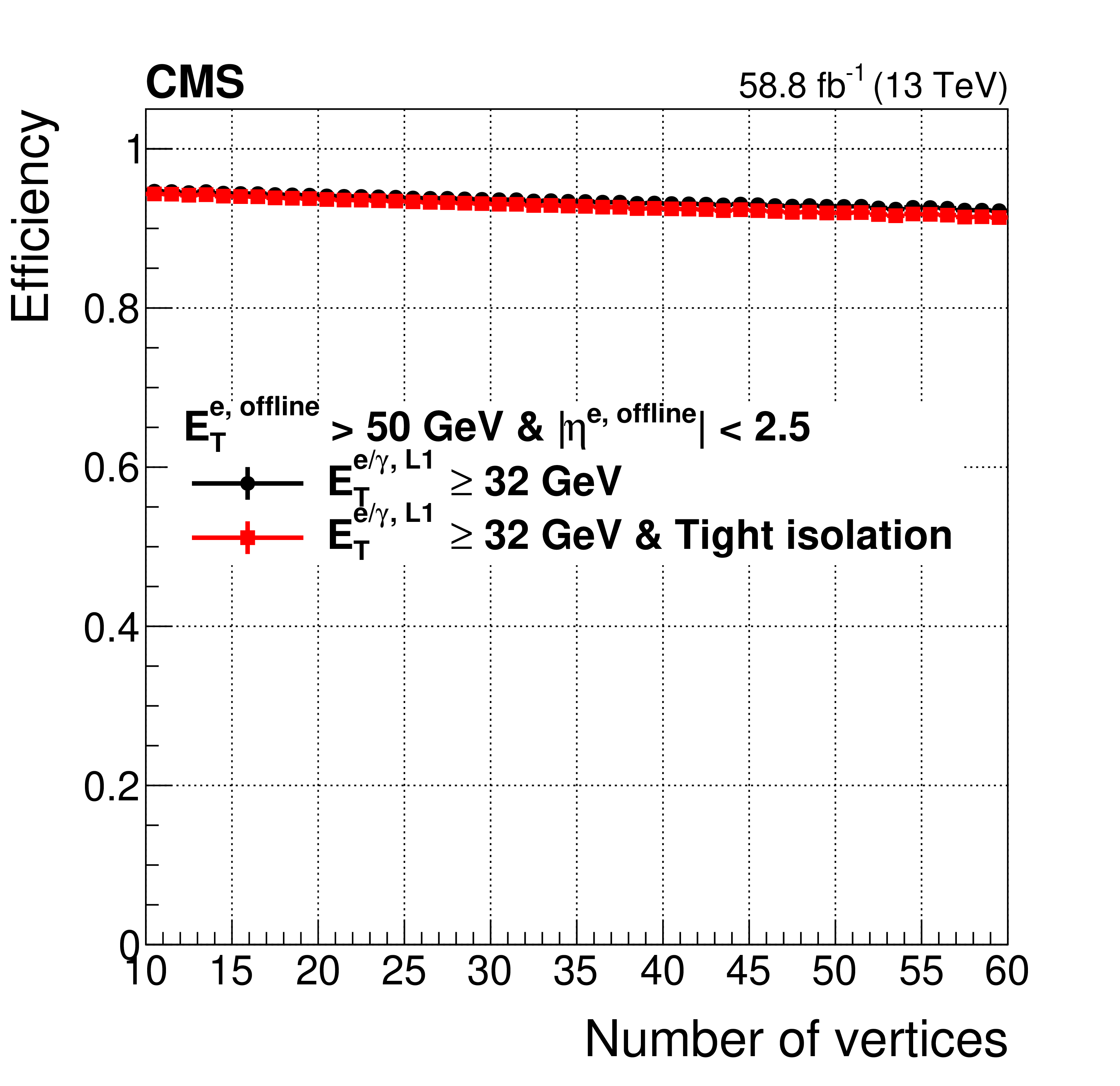
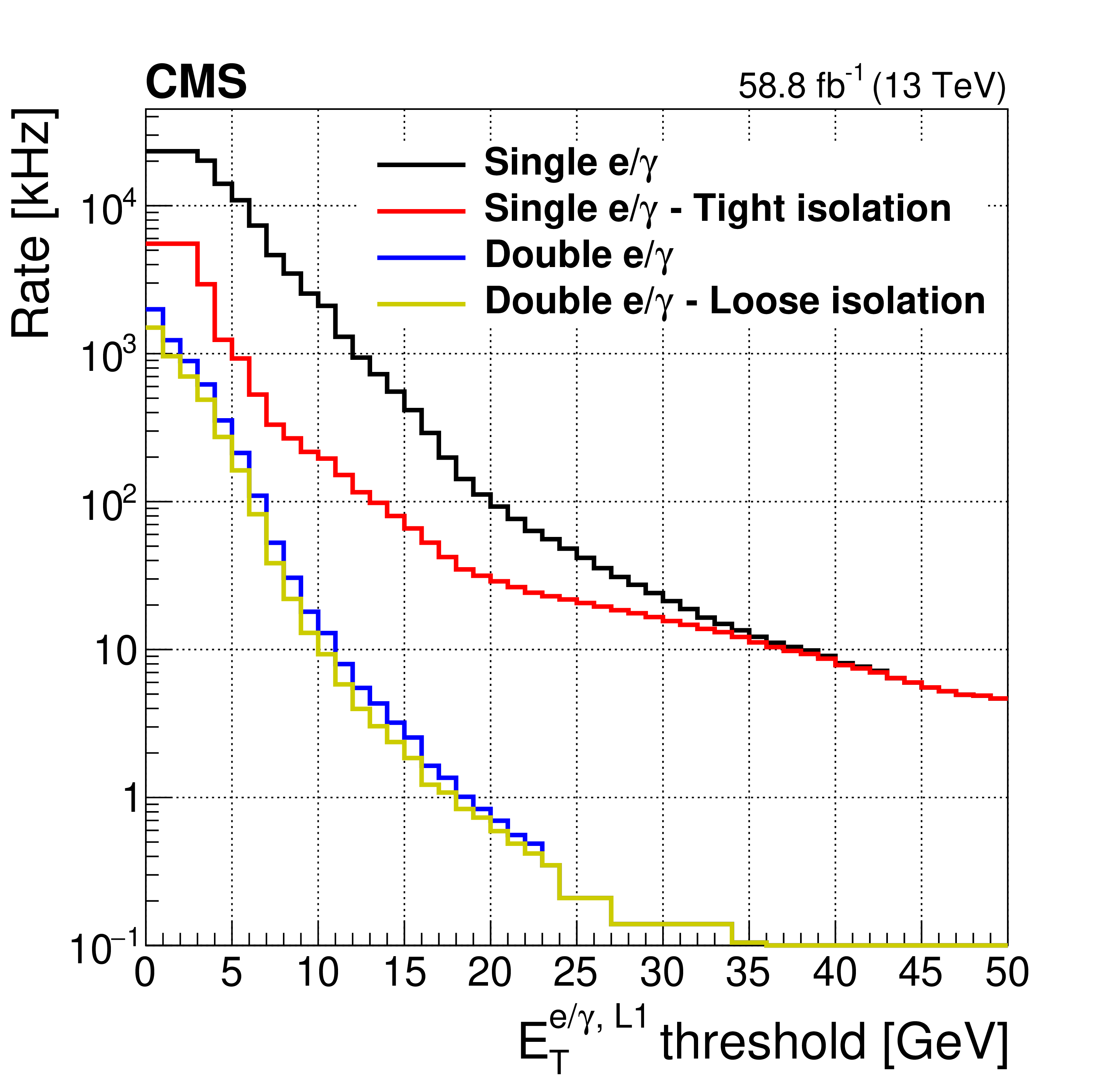
Figure 18:
The Level-1 e/$ {\gamma}$ isolated trigger efficiency (left) as a function of the offline reconstructed vertices and the Level-1 trigger rate (right) as a function of the ${E_{\mathrm {T}}}$ threshold applied on the candidate. |
png pdf |
Figure 18-a:
The Level-1 e/$ {\gamma}$ isolated trigger efficiency as a function of the offline reconstructed vertices. |
png pdf |
Figure 18-b:
The Level-1 trigger rate as a function of the ${E_{\mathrm {T}}}$ threshold applied on the candidate. |
png pdf |
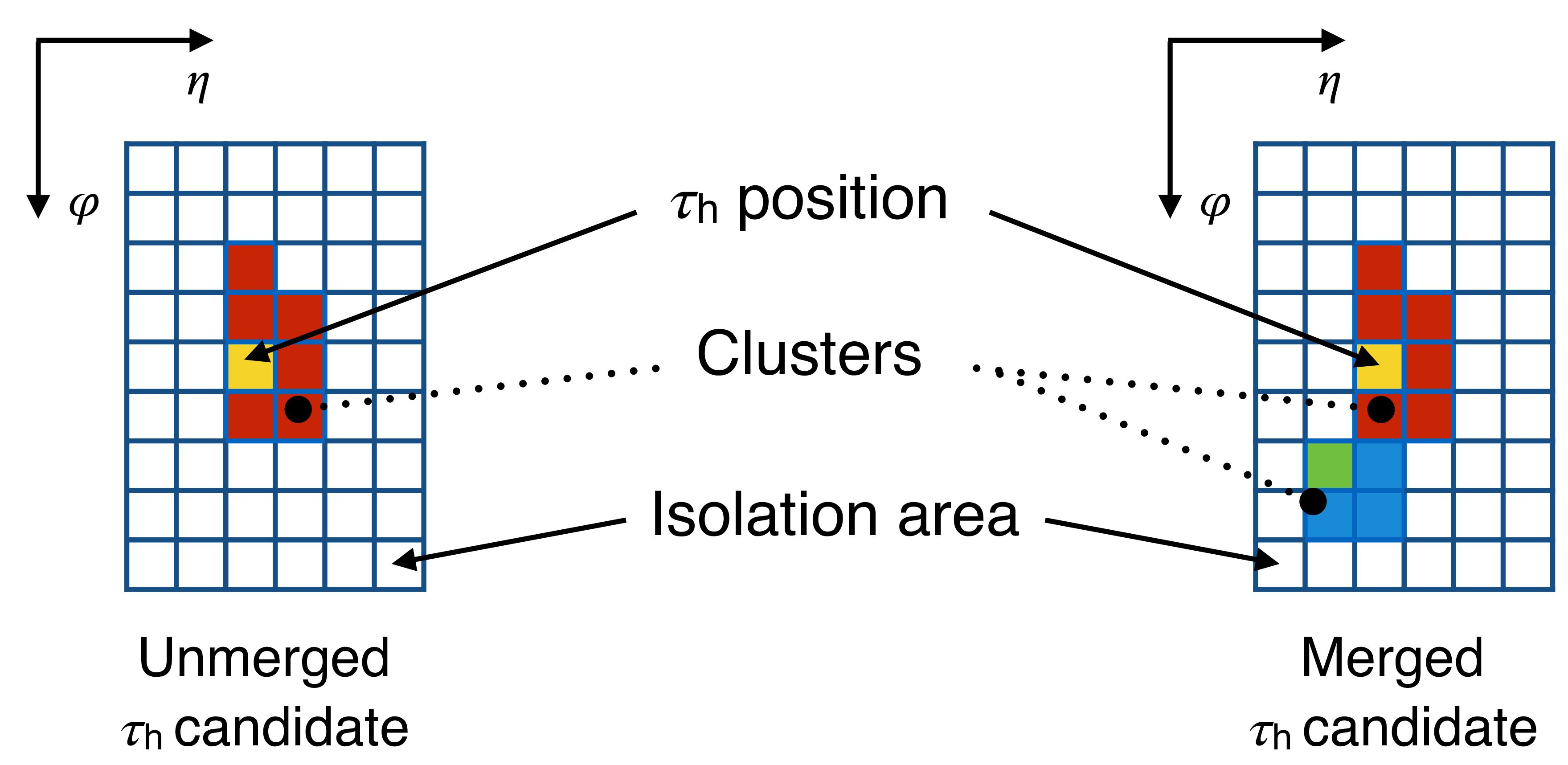
Figure 19:
The Level-1 $\tau $ clustering algorithm and isolation definition. The e/$ {\gamma}$ dynamic clustering is used to reconstruct single clusters around local maxima or seeds (yellow and green), which can then be merged into a single $\tau _\mathrm {h}$ candidate. Each square represents a trigger tower where the ECAL and HCAL energies are summed. A candidate is considered isolated if the ${E_{\mathrm {T}}}$ in the isolation region (white) is smaller than a chosen value. |

png pdf |
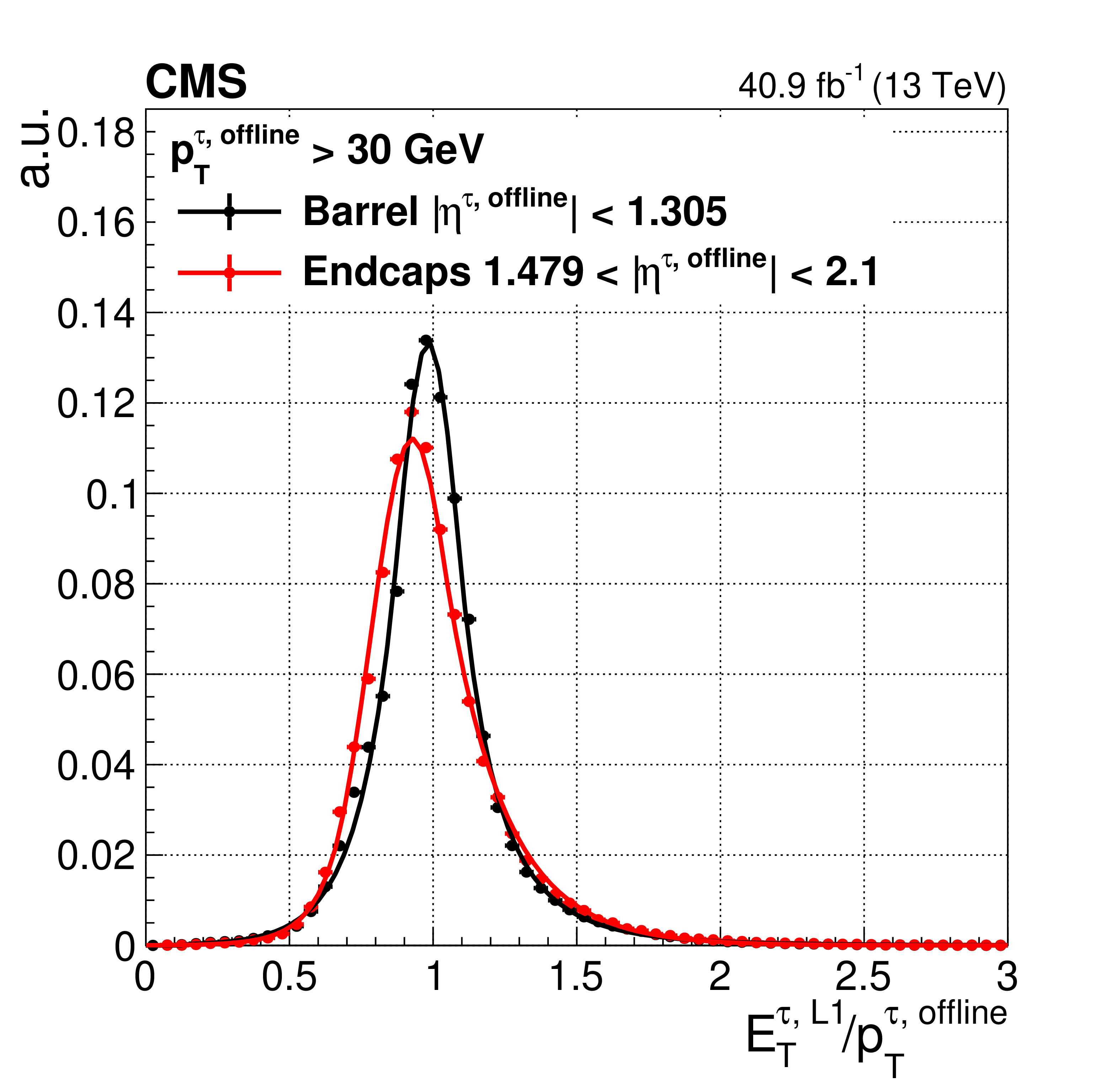
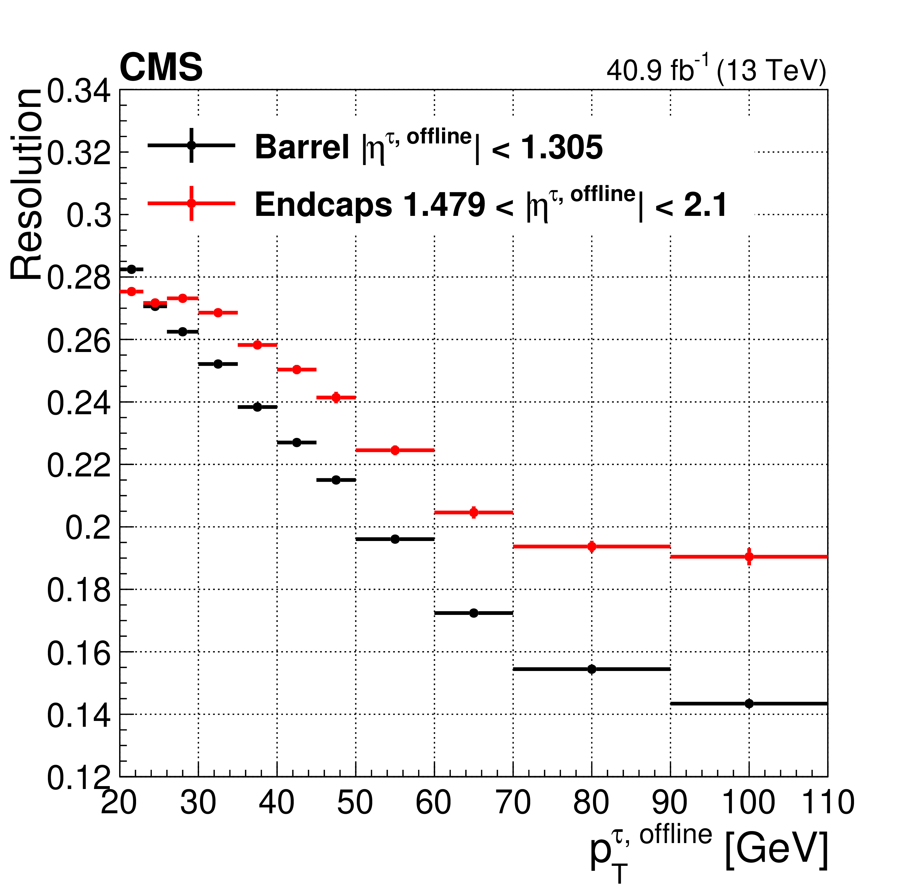
Figure 20:
The Level-1 $\tau $ trigger energy response with respect to the offline reconstructed $\tau $ lepton ${p_{\mathrm {T}}}$, as measured in 2017 data for the barrel and endcap regions (left). The fits consist in Crystal Ball functions. The resolution as a function of the offline $\tau $ lepton ${p_{\mathrm {T}}}$ (right), where the resolution is estimated by the root-mean-square of the $ {E_{\mathrm {T}}} ^{\tau,\text {L1}}/ {p_{\mathrm {T}}} ^{\tau, \text {offline}}$ distribution, divided by its mean, in bins of $ {p_{\mathrm {T}}} ^{\tau, \text {offline}}$. |
png pdf |
Figure 20-a:
The Level-1 $\tau $ trigger energy response with respect to the offline reconstructed $\tau $ lepton ${p_{\mathrm {T}}}$, as measured in 2017 data for the barrel and endcap regions. The fits consist in Crystal Ball functions. |
png pdf |
Figure 20-b:
The resolution as a function of the offline $\tau $ lepton ${p_{\mathrm {T}}}$, where the resolution is estimated by the root-mean-square of the $ {E_{\mathrm {T}}} ^{\tau,\text {L1}}/ {p_{\mathrm {T}}} ^{\tau, \text {offline}}$ distribution, divided by its mean, in bins of $ {p_{\mathrm {T}}} ^{\tau, \text {offline}}$. |
png pdf |
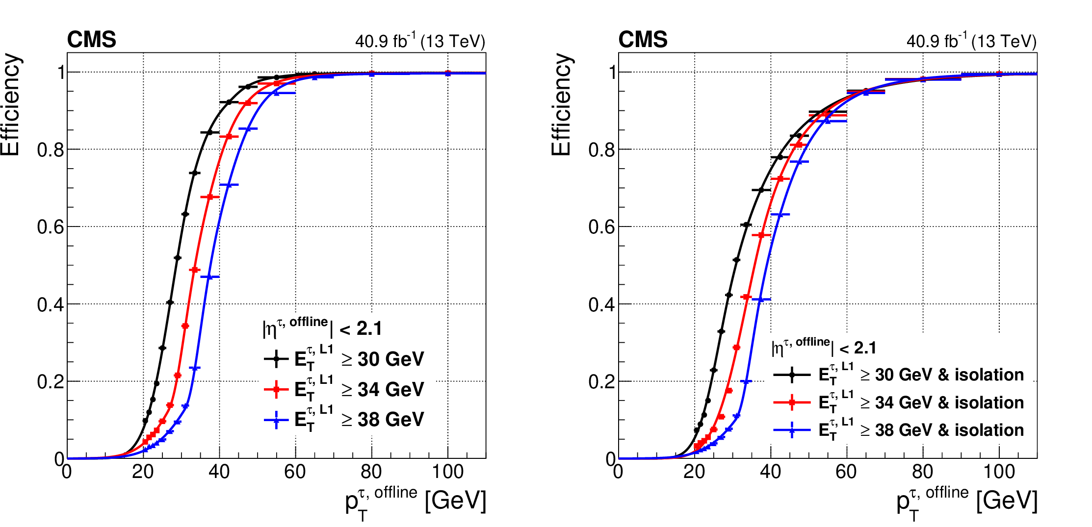
Figure 21:
The Level-1 $\tau $ trigger efficiency, as a function of the offline reconstructed $\tau $ lepton ${p_{\mathrm {T}}}$, for typical thresholds of 30, 34, and 38 GeV (left). The Level-1 isolated $\tau $ trigger efficiency, as a function of the offline reconstructed $\tau $ ${E_{\mathrm {T}}}$, for the same three thresholds (right). The functional form of the fits consists of a cumulative Crystal Ball function convolved with an arc-tangent. |
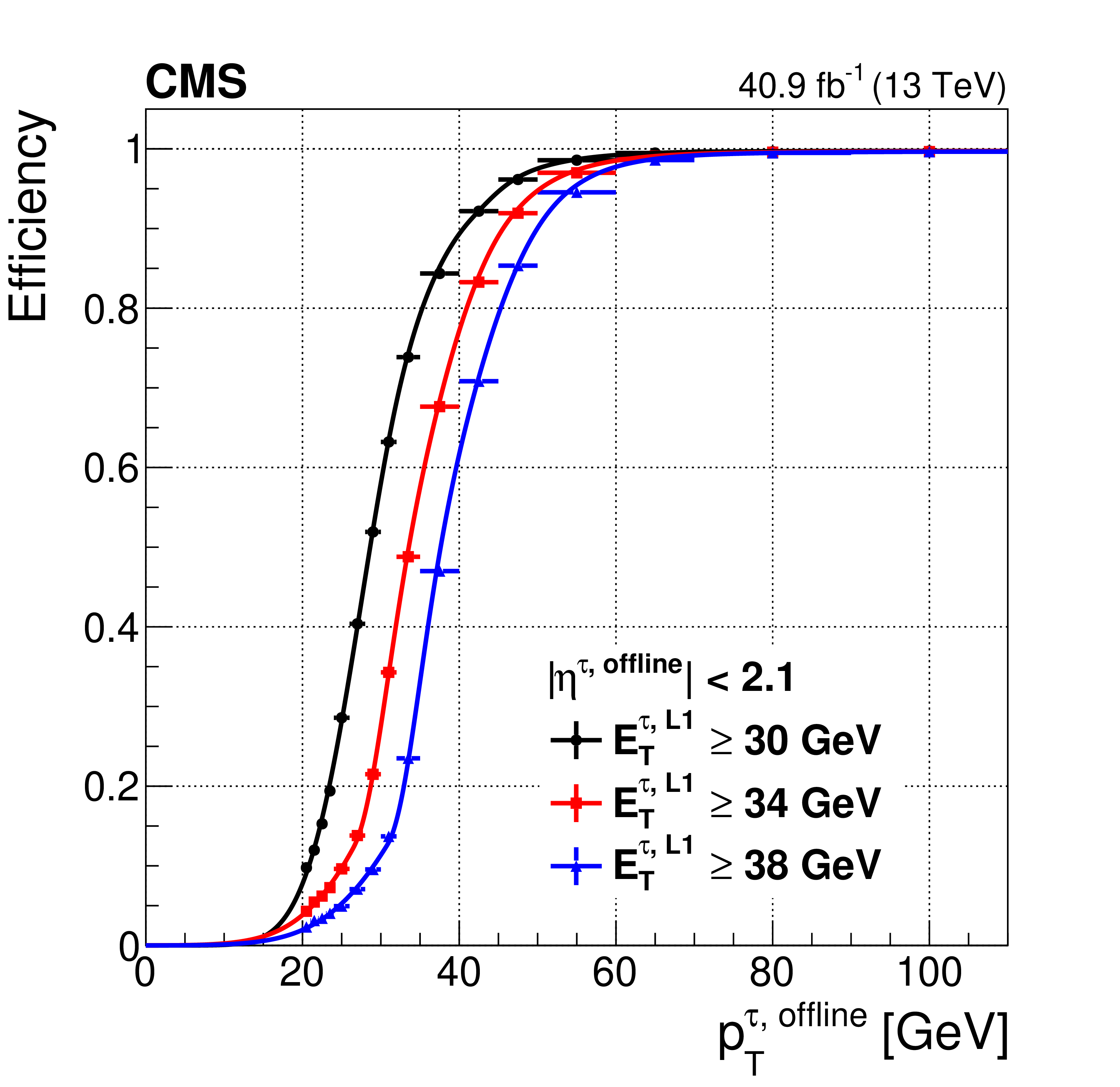
png pdf |
Figure 21-a:
The Level-1 $\tau $ trigger efficiency, as a function of the offline reconstructed $\tau $ lepton ${p_{\mathrm {T}}}$, for typical thresholds of 30, 34, and 38 GeV. The functional form of the fits consists of a cumulative Crystal Ball function convolved with an arc-tangent. |
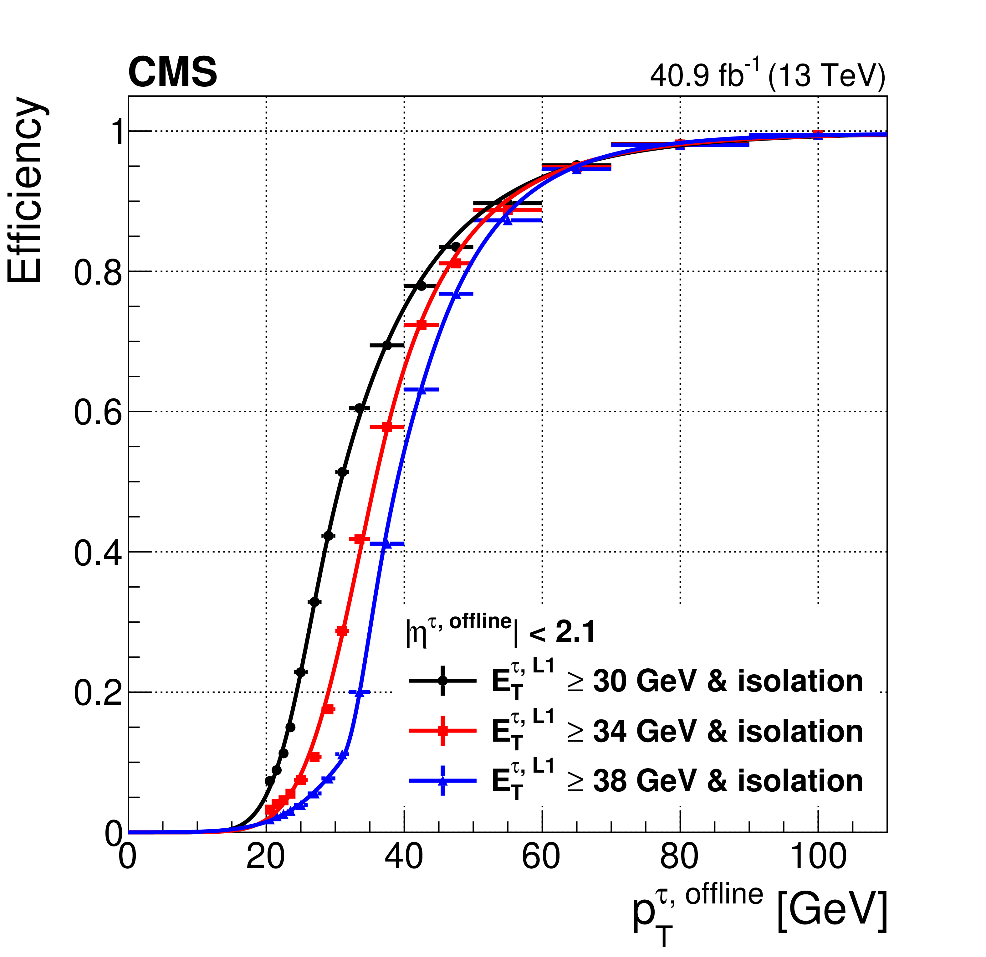
png pdf |
Figure 21-b:
The Level-1 isolated $\tau $ trigger efficiency, as a function of the offline reconstructed $\tau $ ${E_{\mathrm {T}}}$, for the same three thresholds. The functional form of the fits consists of a cumulative Crystal Ball function convolved with an arc-tangent. |
png pdf |
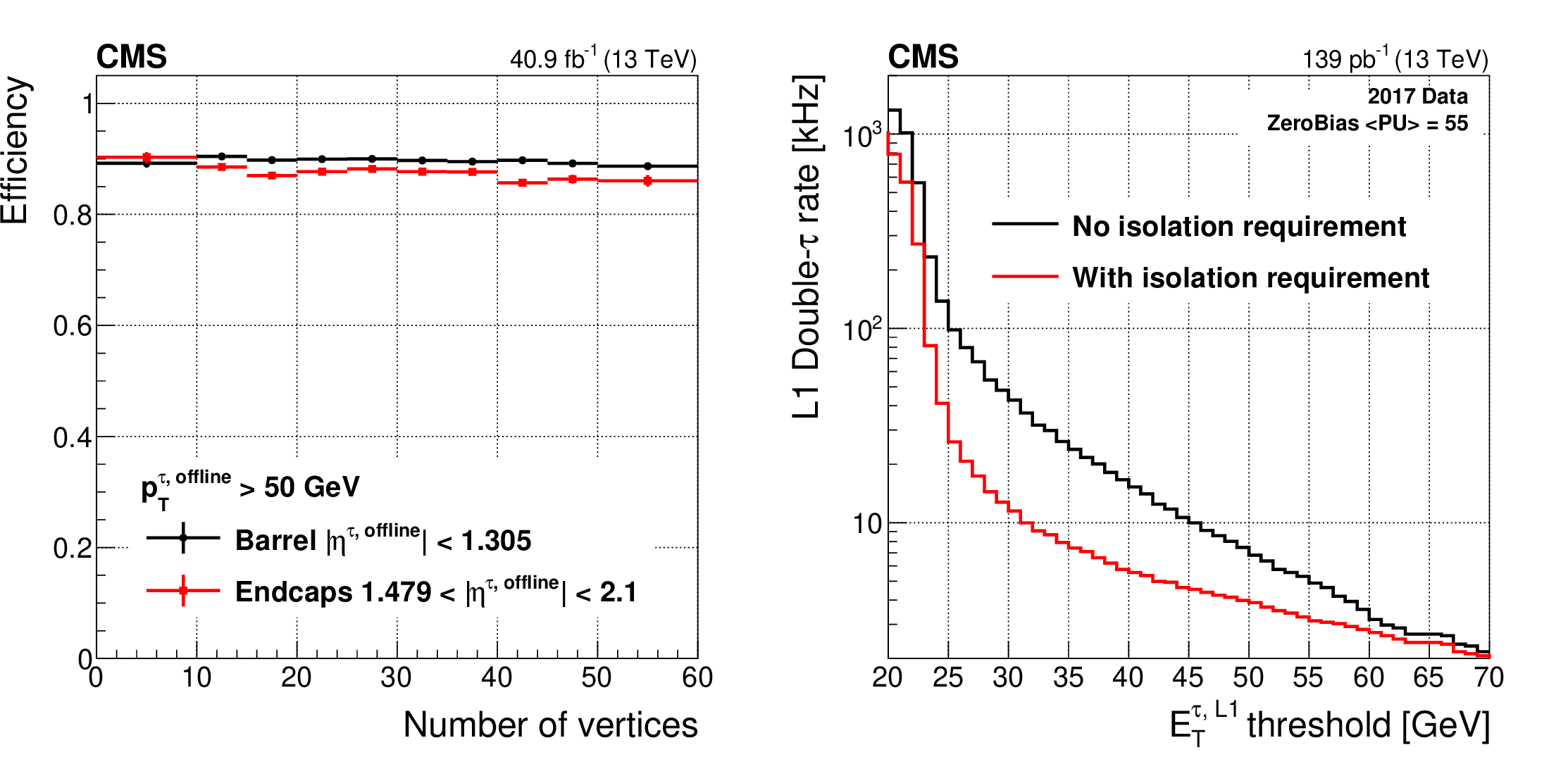
Figure 22:
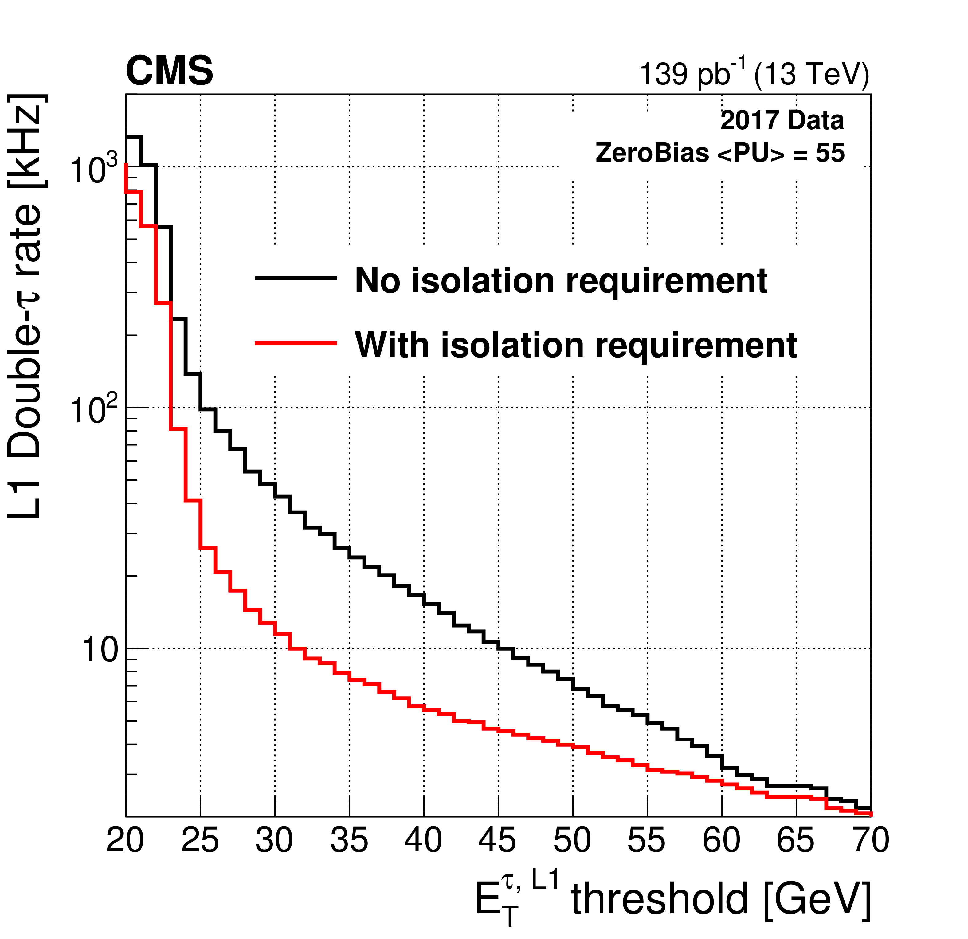
The integrated Level-1 selection efficiency for the isolated $\tau $ trigger with $ {E_{\mathrm {T}}} {\geq} $ 30 GeV, matched to an offline reconstructed and identified $\tau $ lepton with $ {p_{\mathrm {T}}} > $ 50 GeV, as a function of the number of offline reconstructed vertices (left). The Level-1 double-$\tau $ trigger rate, as a function of the ${E_{\mathrm {T}}}$ threshold, for $\tau $ candidates with and without an isolation requirement applied (right). The rate is measured requiring two $\tau $ candidates with ${E_{\mathrm {T}}}$ larger than the bin value, in a unbiased data set with an average pileup of 55. |
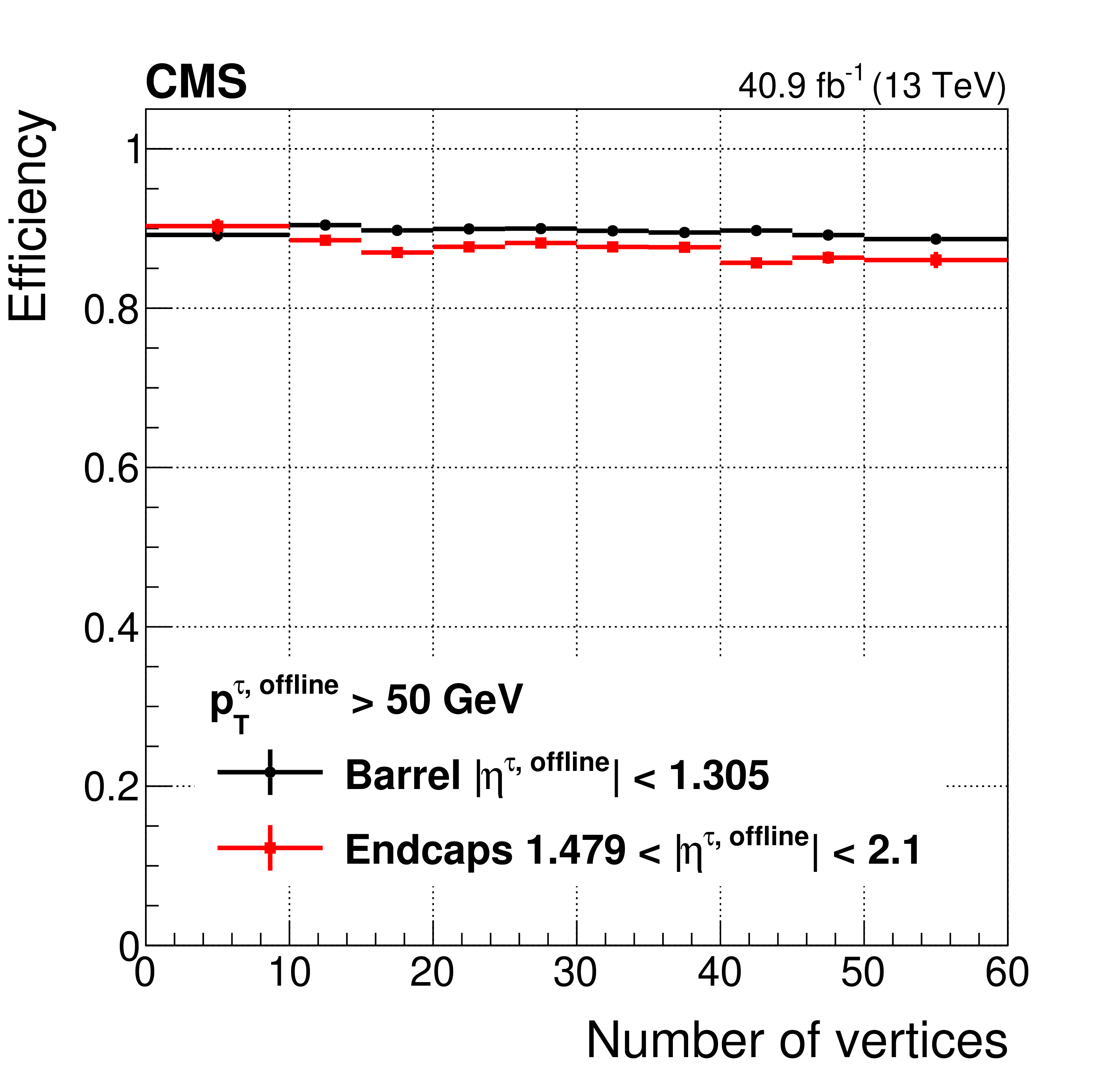
png pdf |
Figure 22-a:
The integrated Level-1 selection efficiency for the isolated $\tau $ trigger with $ {E_{\mathrm {T}}} {\geq} $ 30 GeV, matched to an offline reconstructed and identified $\tau $ lepton with $ {p_{\mathrm {T}}} > $ 50 GeV, as a function of the number of offline reconstructed vertices. |
png pdf |
Figure 22-b:
The Level-1 double-$\tau $ trigger rate, as a function of the ${E_{\mathrm {T}}}$ threshold, for $\tau $ candidates with and without an isolation requirement applied. The rate is measured requiring two $\tau $ candidates with ${E_{\mathrm {T}}}$ larger than the bin value, in a unbiased data set with an average pileup of 55. |

png pdf |
Figure 23:
The area used by the jet pileup subtraction algorithm to estimate the energy deposit from the local pileup, in blue, and the area used to measure the energy of the Level-1 jet, in orange. |
png pdf |
Figure 24:
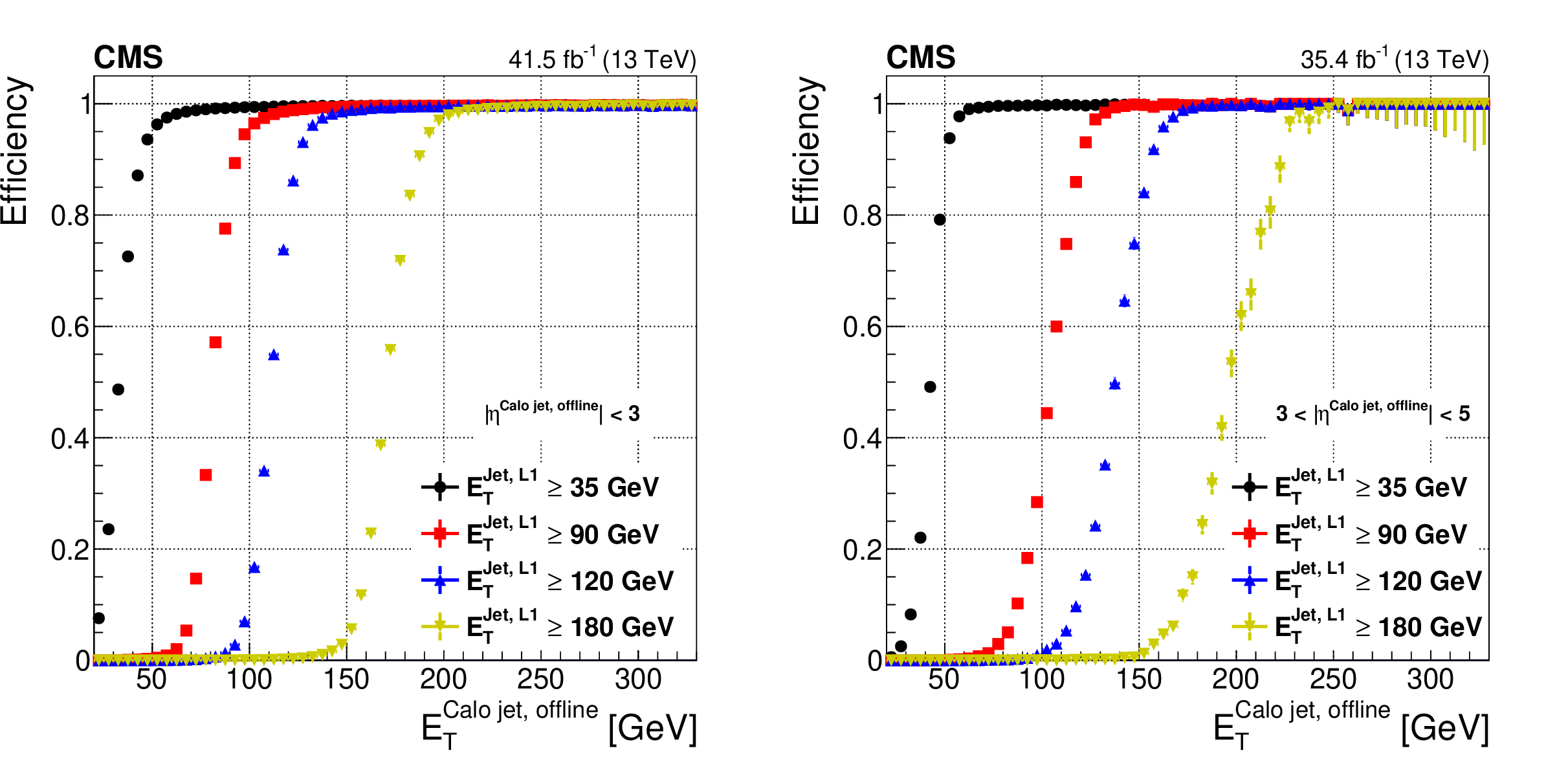
Efficiency curves for the Level-1 jet trigger for the barrel + endcap pseudorapidity range. |

png pdf |
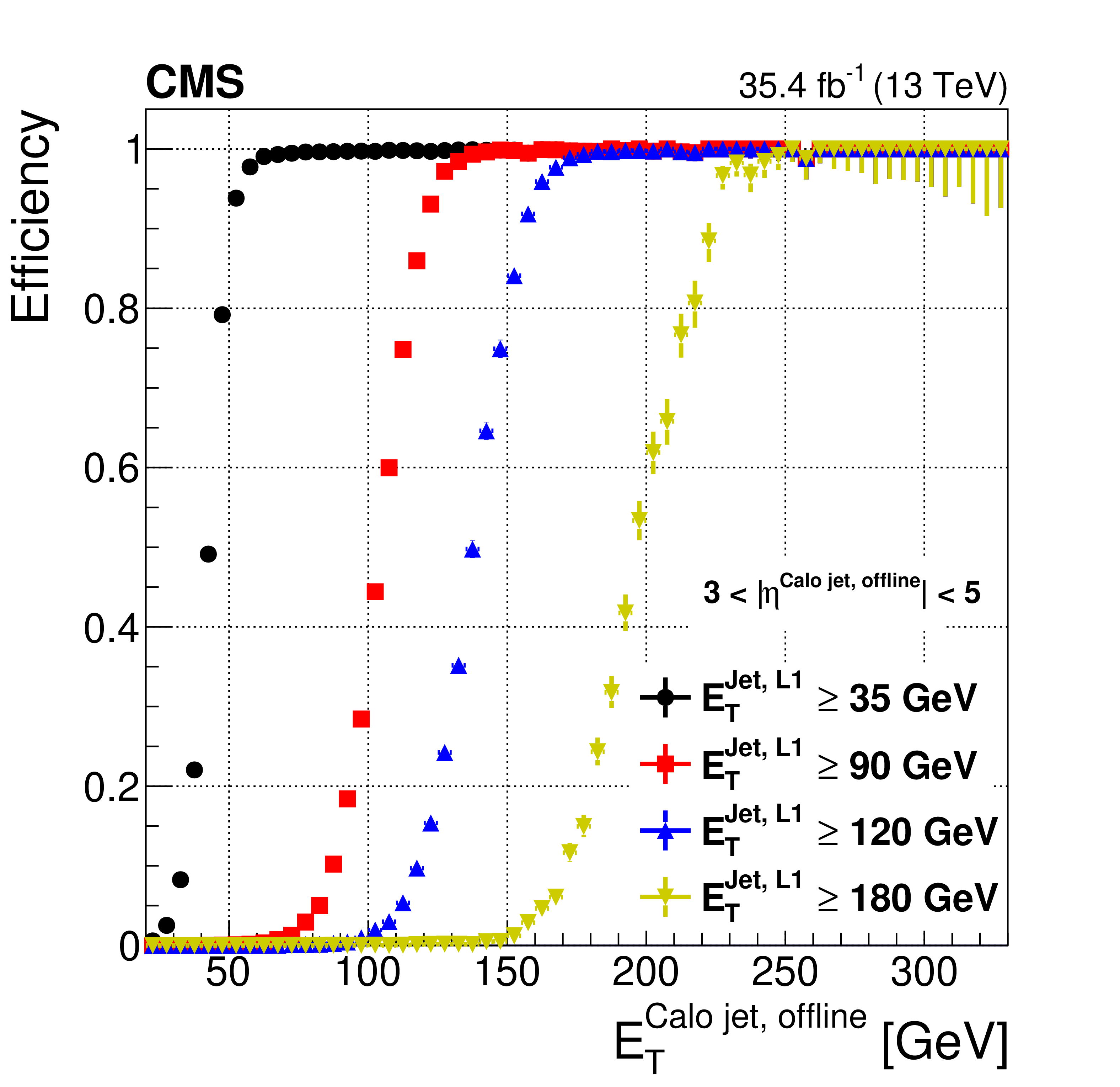
Figure 24-a:
Efficiency curves for the Level-1 jet trigger for the forward pseudorapidity ranges. |
png pdf |
Figure 24-b:
Efficiency curves for the Level-1 jet trigger for the barrel + endcap pseudorapidity range. |
png pdf |
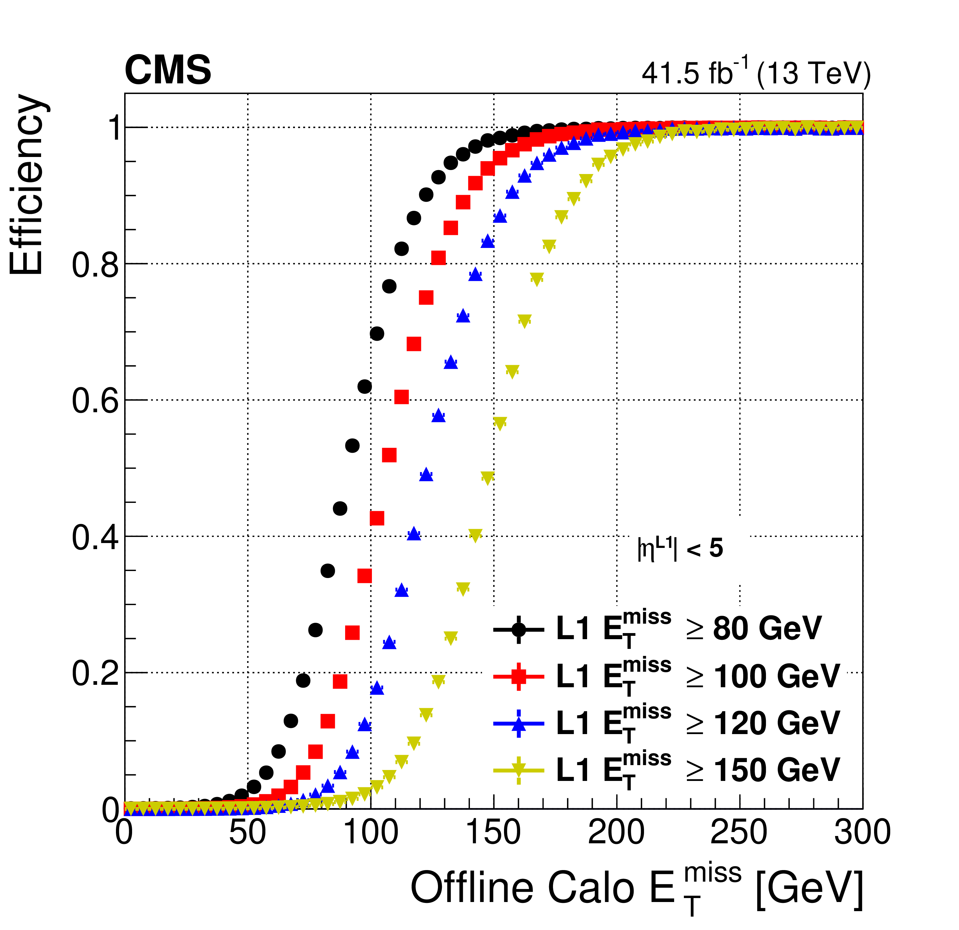
Figure 25:
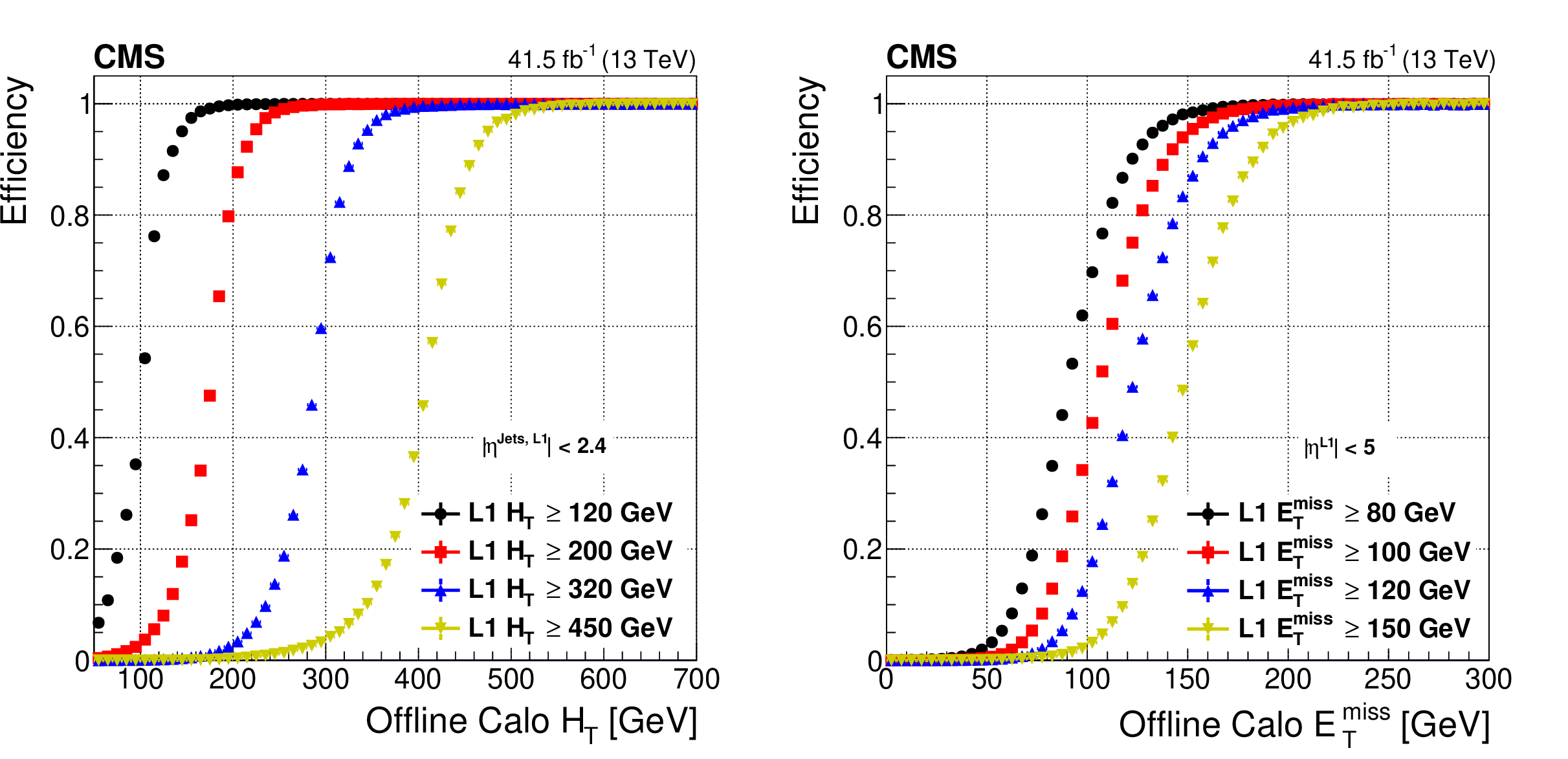
Efficiency curves for the scalar sum of jet energy with $ {E_{\mathrm {T}}} {\geq}$ 30 GeV (left) and missing transverse energy (right) for various thresholds. The thresholds are indicated as L1 ${H_{\mathrm {T}}} $ and L1 ${E_{\mathrm {T}}^{\text {miss}}} $ in the legends. |
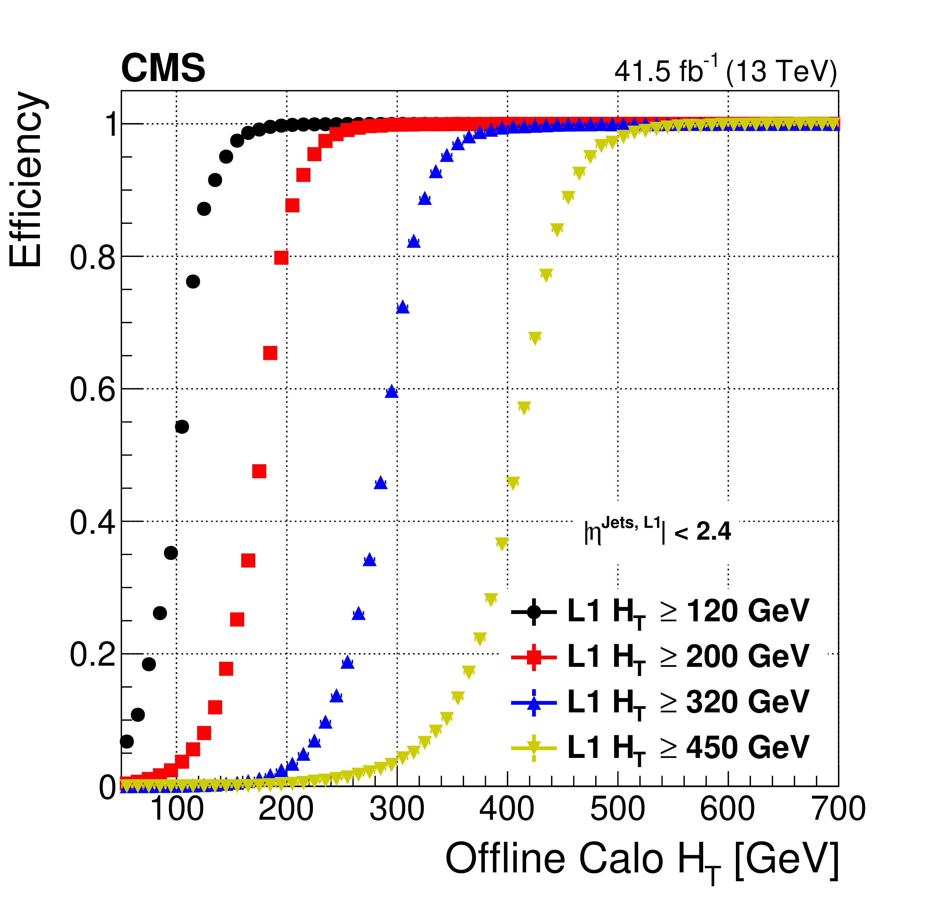
png pdf |
Figure 25-a:
Efficiency curves for the scalar sum of jet energy with $ {E_{\mathrm {T}}} {\geq}$ 30 GeV for various thresholds. The thresholds are indicated as L1 ${H_{\mathrm {T}}} $ in the legends. |
png pdf |
Figure 25-b:
Efficiency curves for the scalar sum of jet energy with missing transverse energy for various thresholds. The thresholds are indicated as L1 ${E_{\mathrm {T}}^{\text {miss}}} $ in the legends. |
png pdf |
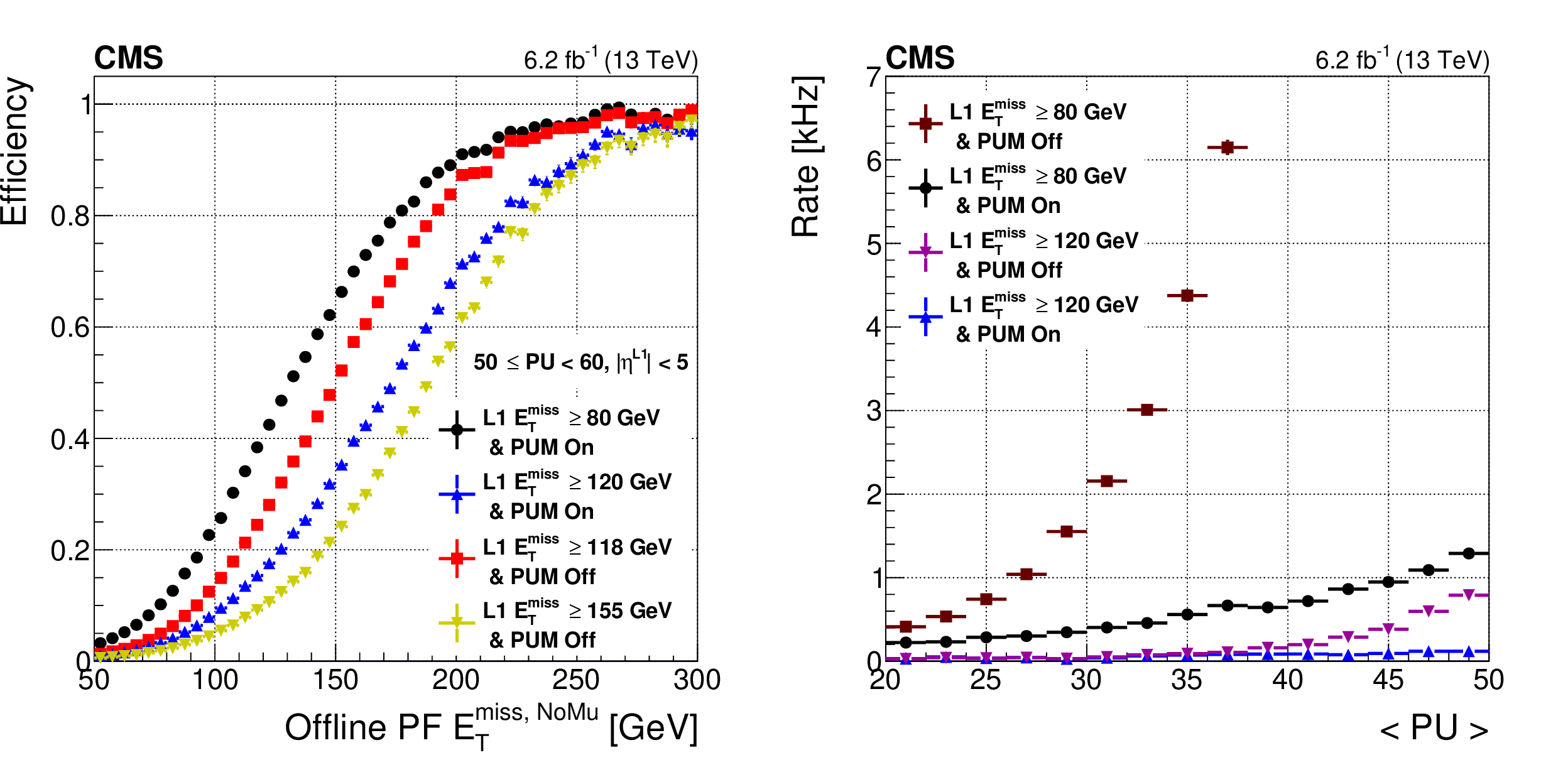
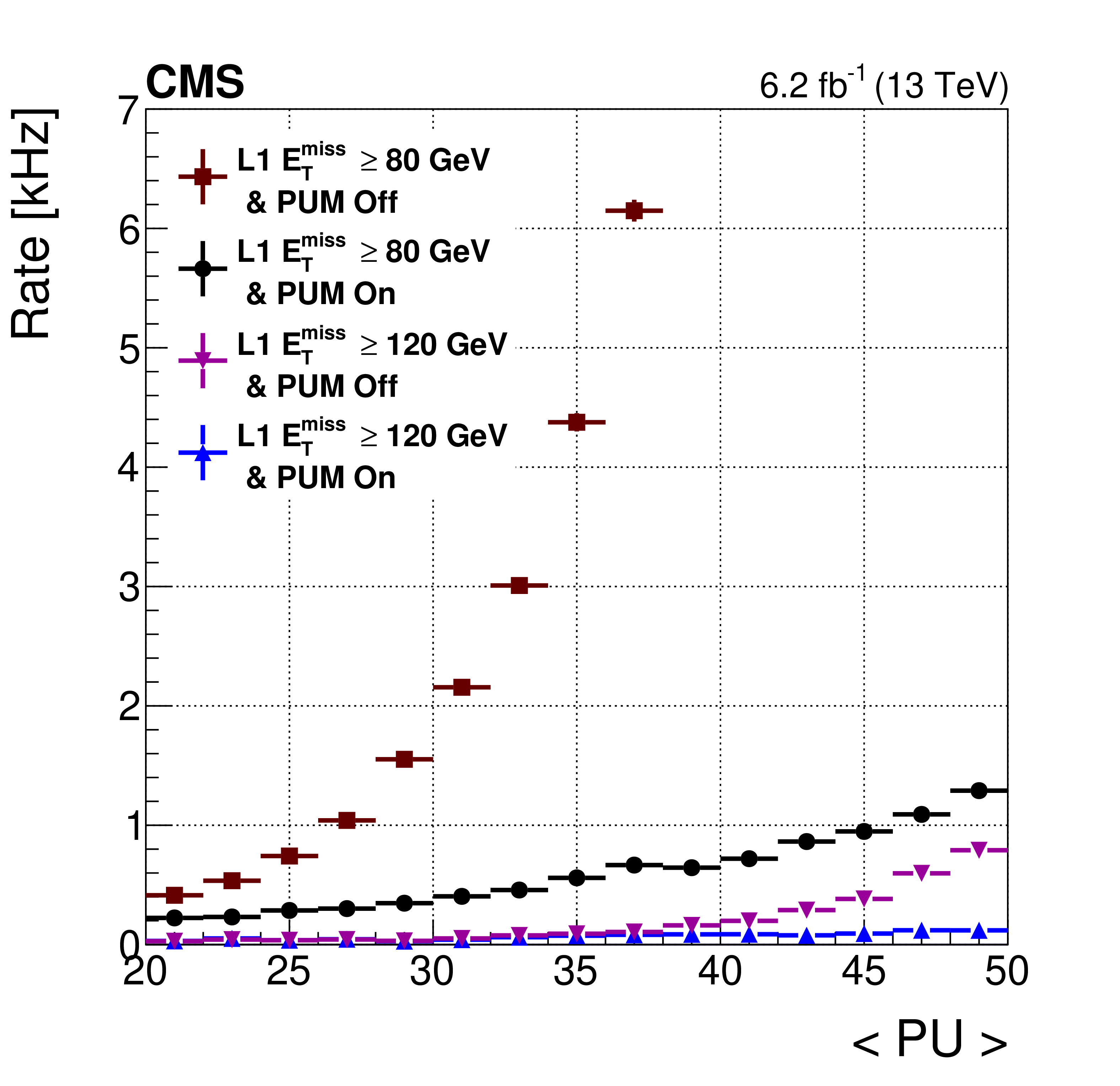
Figure 26:
Efficiency curves with and without pileup mitigation (PUM) applied are compared (left) for the thresholds that give the same rate. These are shown as a function of the offline reconstructed particle flow missing energy excluding muons (PF $ {E_{\mathrm {T}}^{\text {miss}}} {}^{\text {,NoMu}}$). Rate versus the average pileup per luminosity section (right) with and without pileup mitigation applied. |

png pdf |
Figure 26-a:
Efficiency curves with and without pileup mitigation (PUM) applied are compared for the thresholds that give the same rate. These are shown as a function of the offline reconstructed particle flow missing energy excluding muons (PF $ {E_{\mathrm {T}}^{\text {miss}}} {}^{\text {,NoMu}}$). |
png pdf |
Figure 26-b:
Rate versus the average pileup per luminosity section with and without pileup mitigation applied. |
png pdf |
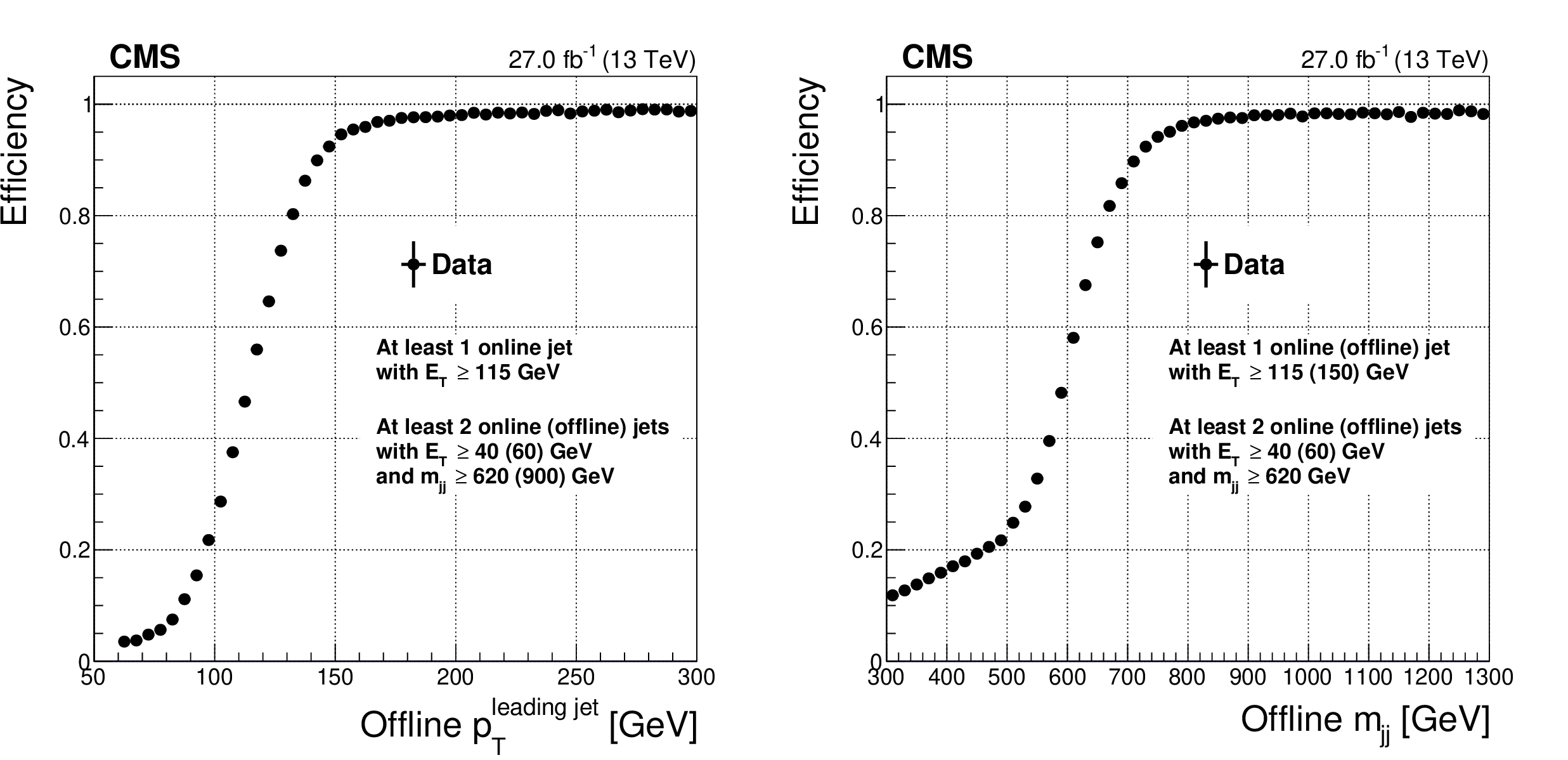
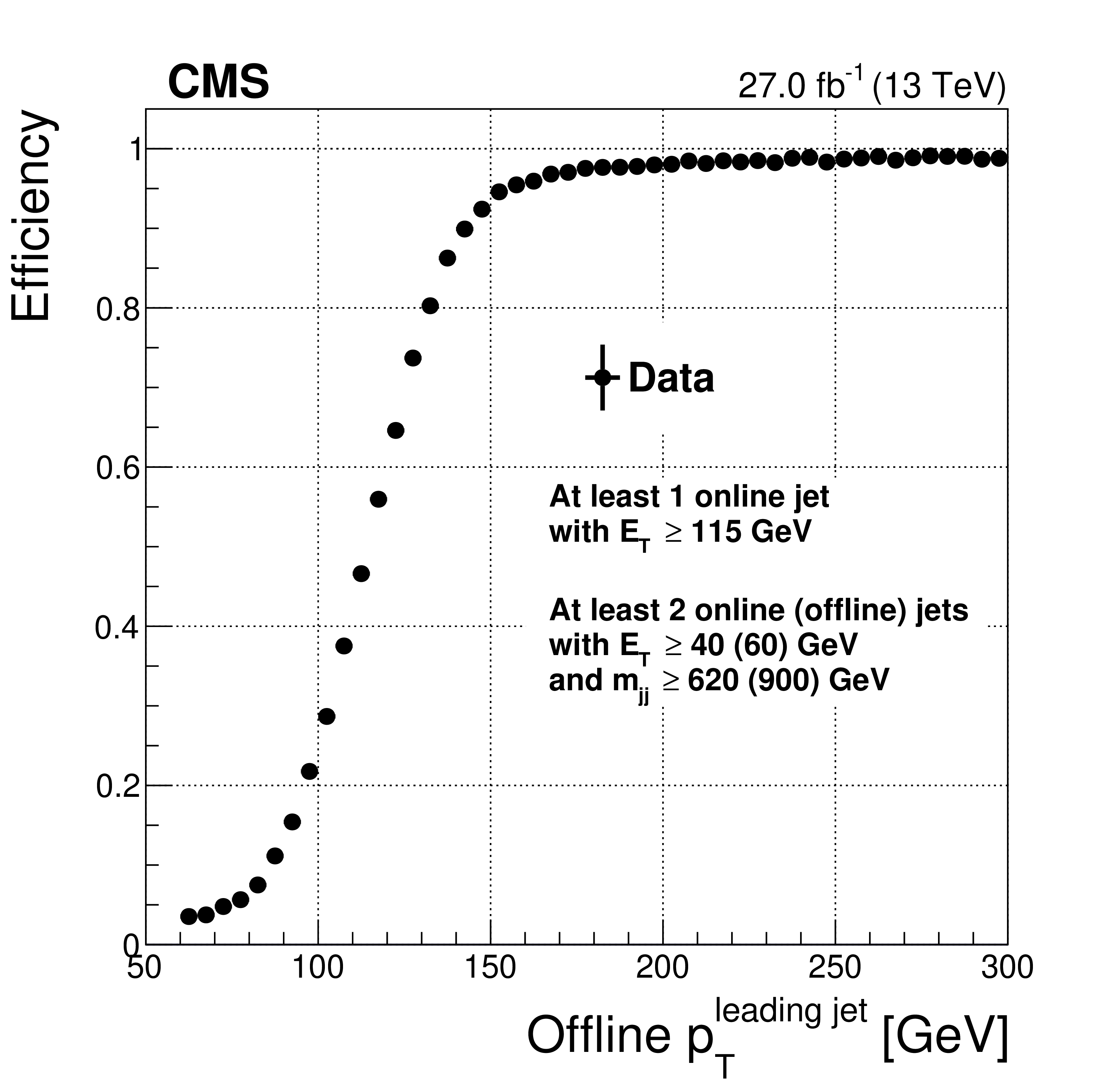
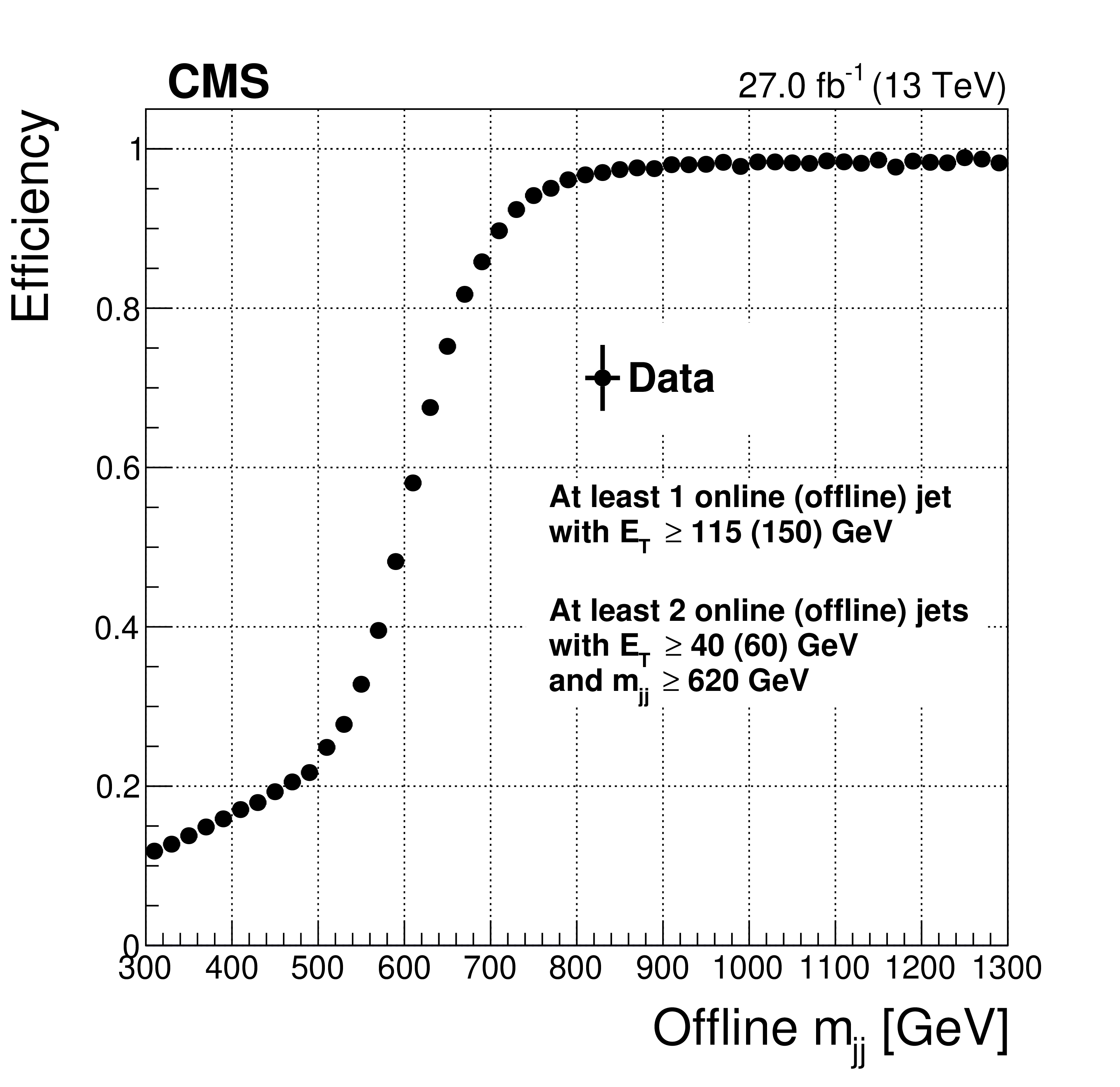
Figure 27:
Efficiency of the Level-1 VBF trigger as a function of the offline leading jet ${p_{\mathrm {T}}}$ (left) and $ {m_\mathrm {jj}}$ (right), estimated as the fraction of $\mathrm{H} \to \tau \tau $ analysis-like offline events passing the Level-1 VBF trigger selection (the Level-1 and offline requirements applied are detailed in the plots). The efficiency is evaluated using 2017 data. |
png pdf |
Figure 27-a:
Efficiency of the Level-1 VBF trigger as a function of the offline leading jet ${p_{\mathrm {T}}}$, estimated as the fraction of $\mathrm{H} \to \tau \tau $ analysis-like offline events passing the Level-1 VBF trigger selection (the Level-1 and offline requirements applied are detailed in the plots). The efficiency is evaluated using 2017 data. |
png pdf |
Figure 27-b:
Efficiency of the Level-1 VBF trigger as a function of the offline leading jet $ {m_\mathrm {jj}}$, estimated as the fraction of $\mathrm{H} \to \tau \tau $ analysis-like offline events passing the Level-1 VBF trigger selection (the Level-1 and offline requirements applied are detailed in the plots). The efficiency is evaluated using 2017 data. |
png pdf |
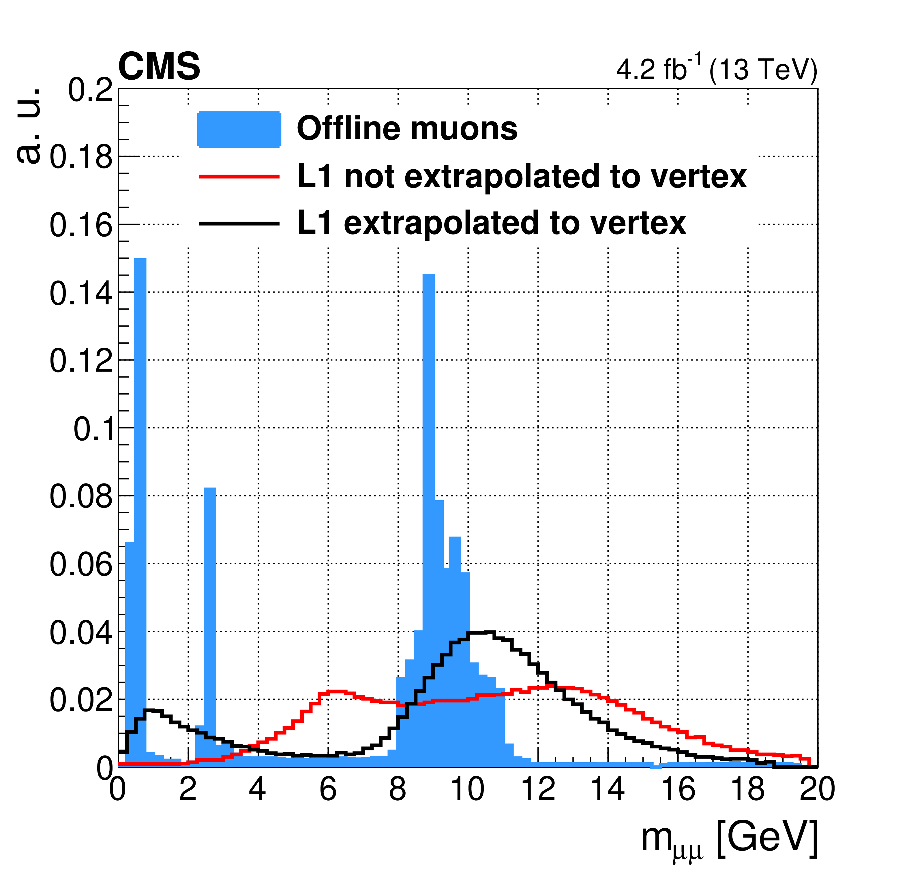
Figure 28:
The offline and Level-1 $ {m_{\mu \mu}}$ spectra of oppositely charged muons, with and without extrapolation of the Level-1 track parameters to the nominal vertex, using a data set of low-mass dimuons. The highest-mass resonance corresponds to the $\Upsilon $ mesons, and is clearly identifiable both offline and in Level-1, after extrapolation. The Level-1 $ {m_{\mu \mu}}$ spectrum is shifted higher compared with the offline spectrum because of ${p_{\mathrm {T}}}$ offsets designed to make the Level-1 muon trigger 90% efficient at any given ${p_{\mathrm {T}}}$ threshold. |
| Tables | |
png pdf |
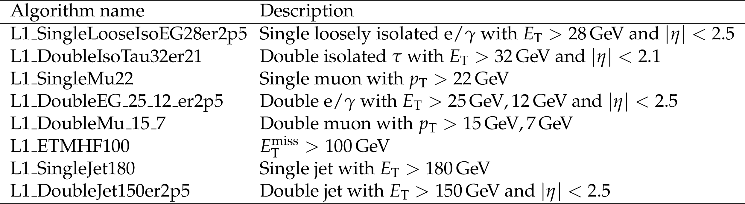
Table 1:
Detailed description of Level-1 trigger seed names used in Figure 2. |
png pdf |
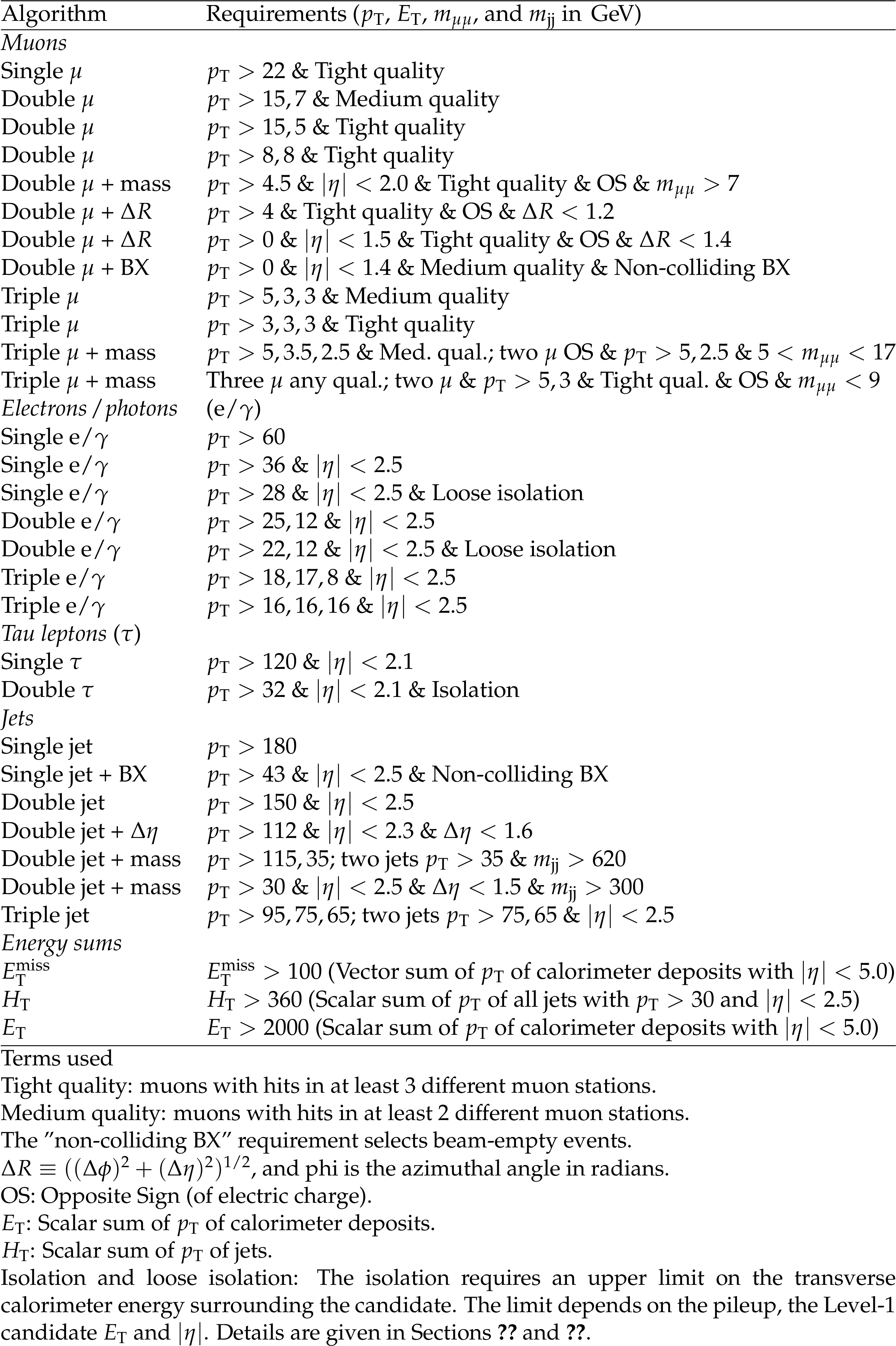
Table 2:
List of the most used unprescaled Level-1 trigger algorithms (seeds) during Run 2 and their requirements. |
png pdf |
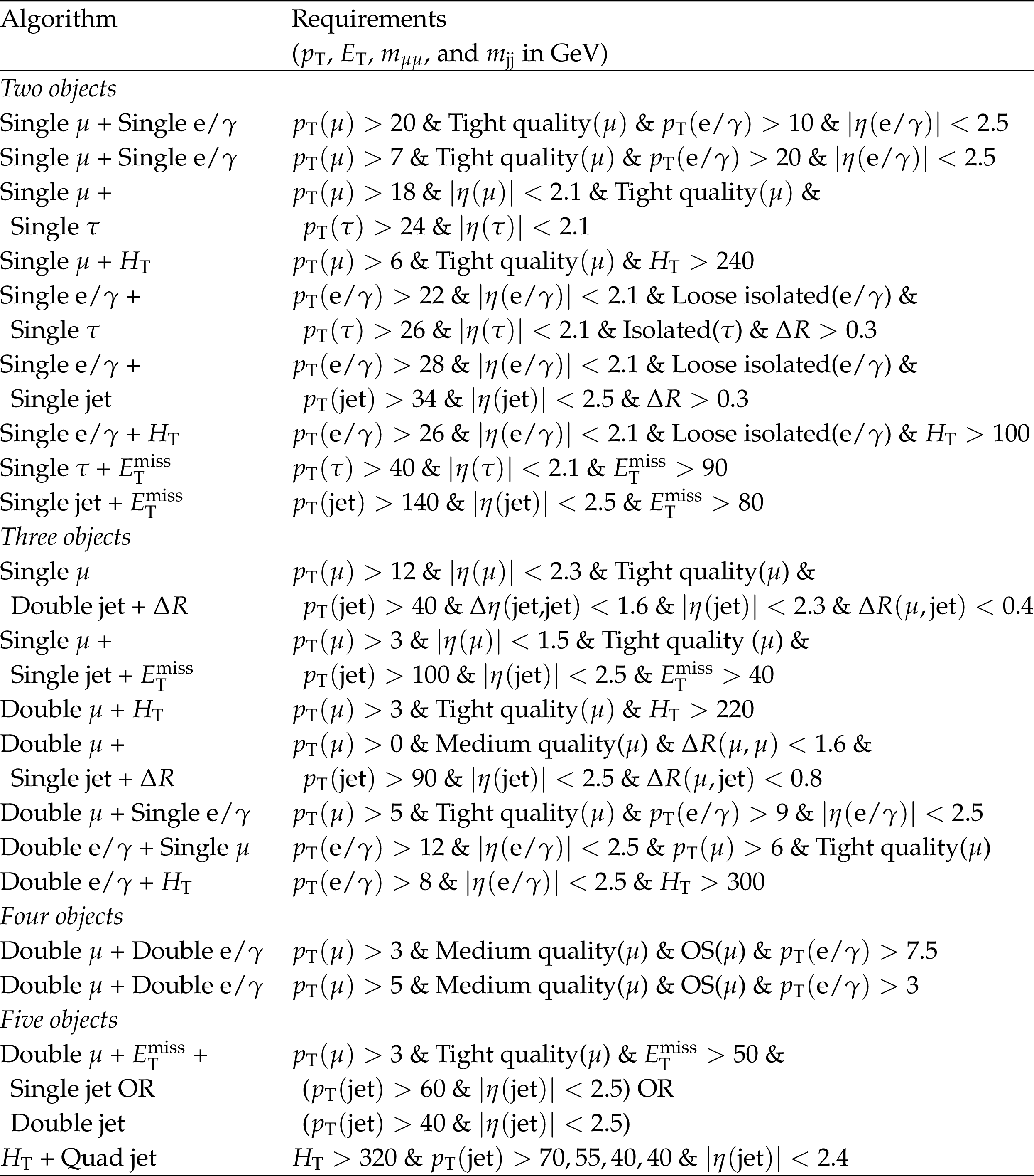
Table 3:
List of the most used cross object unprescaled Level-1 trigger algorithms (seeds) during Run 2 and their corresponding requirements. |
| Summary |
|
The CMS Level-1 trigger system was upgraded for Run 2 of the LHC. The system improved in performance and flexibility using high-bandwidth serial I/O links for data transfer and large, modern field-programmable gate arrays for reconfigurable algorithms. Maintenance improved with increased standardization through the use of the MicroTCA telecommunications standard and common hardware designs for its components. The new trigger hardware provides improved e/${\gamma}$ isolation performance, substantially more efficient $\tau$ lepton identification, improved muon transverse momentum resolution, and the ability to reconstruct jets with finer calorimeter granularity. New features, such as pileup subtraction and invariant mass calculations, expand the trigger design possibilities. These improvements help to control trigger rates and keep thresholds at lower levels than would be required with the previous system despite the significantly increased LHC energy, luminosity, and pileup in Run 2. The adoption of more powerful trigger processors led to the deployment of more advanced trigger algorithms, targeting specific analyses, resulting in significant improvements in physics capability compared to Run 1. The upgraded Level-1 trigger system operated during Run 2 with high efficiency for all physics objects, and adapted to the rapidly changing LHC running conditions. As a result, the trigger efficiency was stable and independent of the evolving LHC parameters. Special LHC running conditions and heavy-ion data taking were accommodated effectively as well, exploiting the full capability and flexibility of the trigger system. The upgraded system improved the energy and momentum resolution, and the identification efficiency and background rejection of the Level-1 physics objects. This significantly lowered the rate at a given threshold compared with the Run 1 system, thereby allowing similar trigger requirements to fit within the unchanged Level-1 rate limit. An analysis of Run 2 data shows that the trigger rate reduction and efficiency gain benefited the physics program of the CMS Collaboration under conditions of increased LHC energy, luminosity, and pileup. An example includes the $\mathrm{H}\to \tau \tau$ analysis [27], which shows a significant improvement in trigger efficiency; other Higgs boson decay channel analyses maintained a similar trigger efficiency despite the harsher beam conditions. Moreover, all analyses looking for large transverse missing energy ($E_{\mathrm{T}}^{\text{miss}}$), including searches for dark matter, supersymmetry [28], and invisible Higgs boson decay [25], were only possible in Run 2 because of the improved resolution of the Level-1 $E_{\mathrm{T}}^{\text{miss}}$ and the pileup mitigation algorithm. Searches for low-mass dimuon resonances exploited the invariant mass requirement for reducing the rate and lowering the muon momentum requirement [26]. |
| References | ||||
| 1 | CMS Collaboration | CMS. the TriDAS project: Technical design report, vol. 1: The trigger systems | CDS | |
| 2 | CMS Collaboration | The CMS trigger system | JINST 12 (2017) P01020 | CMS-TRG-12-001 1609.02366 |
| 3 | CMS Collaboration | CMS technical design report for the level-1 trigger upgrade | CDS | |
| 4 | CMS Collaboration | The CMS experiment at the CERN LHC | JINST 3 (2008) S08004 | CMS-00-001 |
| 5 | CMS Collaboration | Technical proposal for the upgrade of the CMS detector through 2020 | CDS | |
| 6 | G. Rumolo et al. | Electron cloud effects at the LHC and LHC injectors | in 8th International Particle Accelerator Conference (IPAC), p. 30 2017 | |
| 7 | CMS Collaboration | Van der Meer calibration of the CMS luminosity detectors in 2017 | CDS | |
| 8 | ATLAS Collaboration | Observation of a new particle in the search for the standard model Higgs boson with the ATLAS detector at the LHC | PLB 716 (2012) 1 | 1207.7214 |
| 9 | CMS Collaboration | Observation of a new boson at a mass of 125 GeV with the CMS experiment at the LHC | PLB 716 (2012) 30 | CMS-HIG-12-028 1207.7235 |
| 10 | CMS Collaboration | Observation of a new boson with mass near 125 GeV in pp collisions at $ \sqrt{s} = $ 7 and 8 TeV | JHEP 06 (2013) P081 | CMS-HIG-12-036 1303.4571 |
| 11 | ATLAS and CMS Collaborations | Combined measurement of the Higgs boson mass in pp collisions at $ \sqrt{s}= $ 7 and 8 TeV with the ATLAS and CMS experiments | PRL 114 (2015) 191803 | 1503.07589 |
| 12 | PCI Industrial Computer Manufacturers Group | MTCA.0 R1.0 micro telecommunications computing architecture | http://www.picmg.org | |
| 13 | R. Frazier et al. | A demonstration of a time multiplexed trigger for the CMS experiment | in Topical workshop on electronics for particle physics (TWEPP11), p. C01060 2012 | |
| 14 | E. Hazen et al. | The AMC13XG: a new generation clock/timing/DAQ module for CMS MicroTCA | in Topical workshop on electronics for particle physics (TWEPP13), p. C12036 2013 | |
| 15 | CMS Collaboration | Performance of the CMS muon detector and muon reconstruction with proton-proton collisions at $ \sqrt{s}= $ 13 TeV | JINST 13 (2018) P06015 | CMS-MUO-16-001 1804.04528 |
| 16 | A. Triossi et al. | The CMS barrel muon trigger upgrade | in Topical workshop on electronics for particle physics (TWEPP16), p. C01095 2017 | |
| 17 | C.-J. Wang, Z.-A. Liu, J.-Z. Zhao, and Z. Liu | Design of a high throughput electronics module for high energy physics experiments | CPC 40 (2016) 066102 | |
| 18 | J. Ero et al. | The CMS drift tube trigger track finder | JINST 3 (2008) P08006 | |
| 19 | D. Acosta at al. | Boosted decision trees in the level-1 muon endcap trigger at CMS | in XVIIIth International workshop on advanced computing and analysis techniques in physics research (ACAT 2017), p. 042042 2018 | |
| 20 | CMS Collaboration | Performance of CMS muon reconstruction in pp collision events at $ \sqrt{s}= $ 7 TeV | JINST 7 (2012) P10002 | CMS-MUO-10-004 1206.4071 |
| 21 | CMS Collaboration | Particle-flow reconstruction and global event description with the CMS detector | JINST 12 (2017) P10003 | CMS-PRF-14-001 1706.04965 |
| 22 | CMS Collaboration | Performance of the reconstruction and identification of high-momentum muons in proton-proton collisions at $ \sqrt{s} = $ 13 TeV | JINST 15 (2019) P02027 | CMS-MUO-17-001 1912.03516 |
| 23 | CMS Collaboration | Performance of reconstruction and identification of $ \tau $ leptons decaying to hadrons and $ \nu_\tau $ in pp collisions at $ \sqrt{s}= $ 13 TeV | JINST 13 (2018) P10005 | CMS-TAU-16-003 1809.02816 |
| 24 | M. Cacciari, G. P. Salam, and G. Soyez | The anti-$ {k_{\mathrm{T}}} $ jet clustering algorithm | JHEP 04 (2008) 063 | 0802.1189 |
| 25 | CMS Collaboration | Search for invisible decays of a Higgs boson produced through vector boson fusion in proton-proton collisions at $ \sqrt{s} = $ 13 TeV | PLB 793 (2019) 520 | CMS-HIG-17-023 1809.05937 |
| 26 | CMS Collaboration | Measurement of properties of B$ ^{0}_{\text{s}} \to\mu^+\mu^- $ decays and search for B$ ^{0}\to\mu^+\mu^- $ with the CMS experiment | JHEP 04 (2020) 188 | CMS-BPH-16-004 1910.12127 |
| 27 | CMS Collaboration | Observation of the Higgs boson decay to a pair of $ \tau $ leptons with the CMS detector | PLB 779 (2018) 283 | CMS-HIG-16-043 1708.00373 |
| 28 | CMS Collaboration | Search for natural and split supersymmetry in proton-proton collisions at $ \sqrt{s}= $ 13 TeV in final states with jets and missing transverse momentum | JHEP 05 (2018) 025 | CMS-SUS-16-038 1802.02110 |
|
|
Compact Muon Solenoid LHC, CERN |
|

|

|

|

|

|