

Compact Muon Solenoid
LHC, CERN
| CMS-HIG-14-035 ; CERN-PH-EP-2015-331 | ||
| Combined search for anomalous pseudoscalar HVV couplings in VH production and H $\rightarrow$ VV decay | ||
| CMS Collaboration | ||
| 13 February 2016 | ||
| Phys. Lett. B 759 (2016) 672 | ||
| Abstract: A search for anomalous pseudoscalar couplings of the Higgs boson H to electroweak vector bosons V (= W or Z) in a sample of proton-proton collision events corresponding to an integrated luminosity of 18.9 fb$^{-1}$ at a center-of-mass energy of 8 TeV is presented. Events consistent with the topology of associated VH production, where the Higgs boson decays to a pair of bottom quarks and the vector boson decays leptonically, are analyzed. The consistency of data with a potential pseudoscalar contribution to the HVV interaction, expressed by the effective pseudoscalar cross section fractions $f_{a_3}$, is assessed by means of profile likelihood scans. Results are given for the VH channels alone and for a combined analysis of the VH and previously published $ \mathrm{ H \rightarrow VV }$ channels. Assuming the standard model ratio of the coupling strengths of the Higgs boson to top and bottom quarks, $ f_{a_3}^{\mathrm{ZZ}}>0.0034$ is excluded at 95\% confidence level in the combination. | ||
| Links: e-print arXiv:1602.04305 [hep-ex] (PDF) ; CDS record ; inSPIRE record ; CADI line (restricted) ; | ||
| Figures & Tables | Summary | Additional Figures | References | CMS Publications |
|---|
| Figures | |

png pdf |
Figure 1-a:
Feynman diagrams representing gluon-initiated ZH production via a quark triangle (la) and box (b) loop. |

png pdf |
Figure 1-b:
Feynman diagrams representing gluon-initiated ZH production via a quark triangle (la) and box (b) loop. |

png pdf |
Figure 2-a:
The scalar (a), pseudoscalar (b), and total background (c) templates for the high-boost $ \mathrm{ W \to e \nu } $ channel. Bin content is normalized according to the bin area. |

png pdf |
Figure 2-b:
The scalar (a), pseudoscalar (b), and total background (c) templates for the high-boost $ \mathrm{ W \to e \nu } $ channel. Bin content is normalized according to the bin area. |

png pdf |
Figure 2-c:
The scalar (a), pseudoscalar (b), and total background (c) templates for the high-boost $ \mathrm{ W \to e \nu } $ channel. Bin content is normalized according to the bin area. |
png pdf |
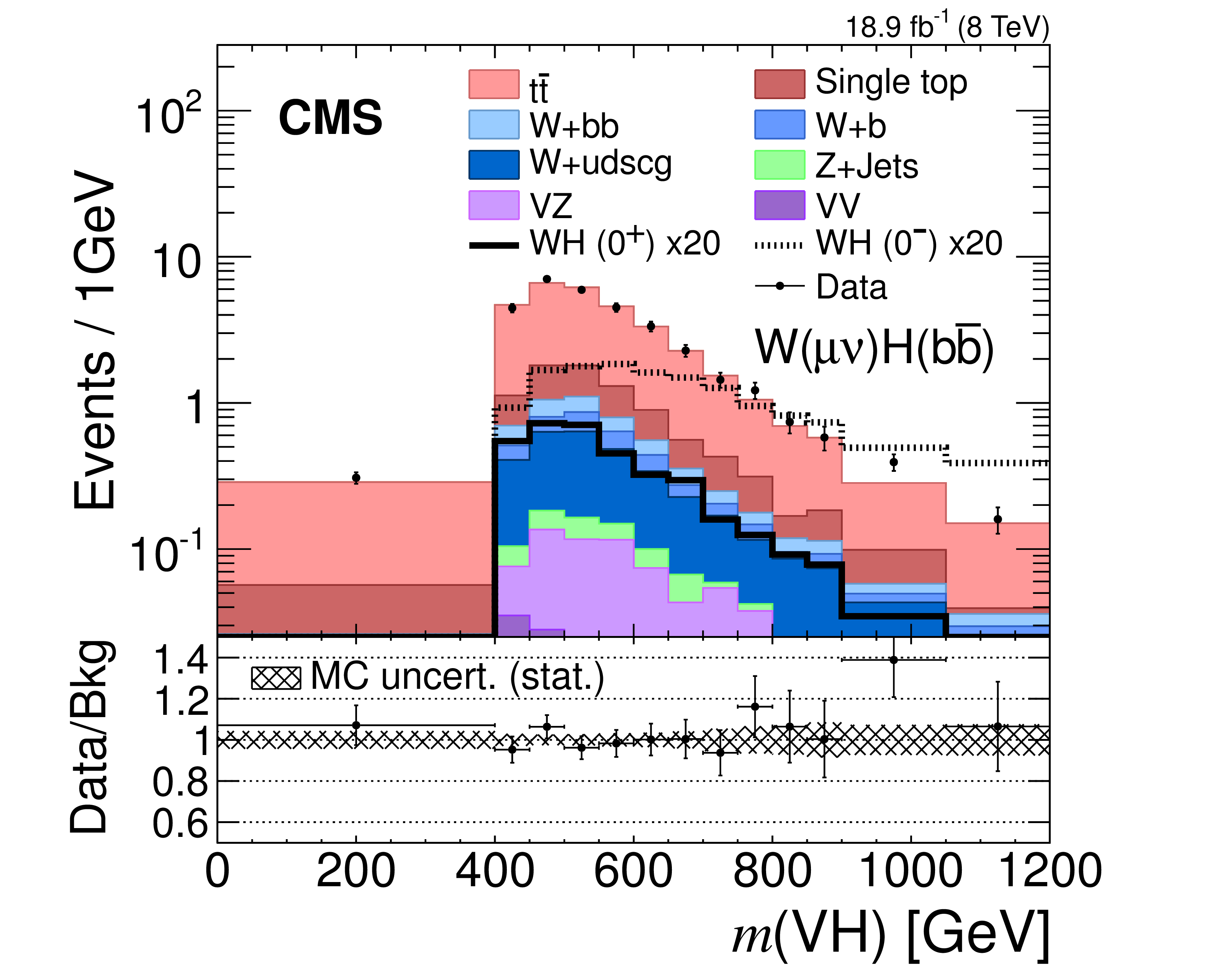
Figure 3-a:
The $ m(\mathrm{V} \mathrm{H} ) $ distributions for the high-boost region of the $ \mathrm{ W \to \mu \nu } $ (a) and $ \mathrm{ Z \to e e } $ (b) channels. The distribution observed in data is represented by points with error bars. SM backgrounds are represented by filled histograms. A pure scalar (pseudoscalar) Higgs boson signal is represented by the solid (dotted) histogram. The statistical uncertainty related to the finite size of the simulated background event samples is represented by the hatched region. Values of $ m(\mathrm{V} \mathrm{H} ) >$ 1200 GeV are included in the last bin. The bin content is normalized according to the bin width. The lower panel shows the ratio of the observed and expected background yields. |

png pdf |
Figure 3-b:
The $ m(\mathrm{V} \mathrm{H} ) $ distributions for the high-boost region of the $ \mathrm{ W \to \mu \nu } $ (a) and $ \mathrm{ Z \to e e } $ (b) channels. The distribution observed in data is represented by points with error bars. SM backgrounds are represented by filled histograms. A pure scalar (pseudoscalar) Higgs boson signal is represented by the solid (dotted) histogram. The statistical uncertainty related to the finite size of the simulated background event samples is represented by the hatched region. Values of $ m(\mathrm{V} \mathrm{H} ) >$ 1200 GeV are included in the last bin. The bin content is normalized according to the bin width. The lower panel shows the ratio of the observed and expected background yields. |
png pdf |
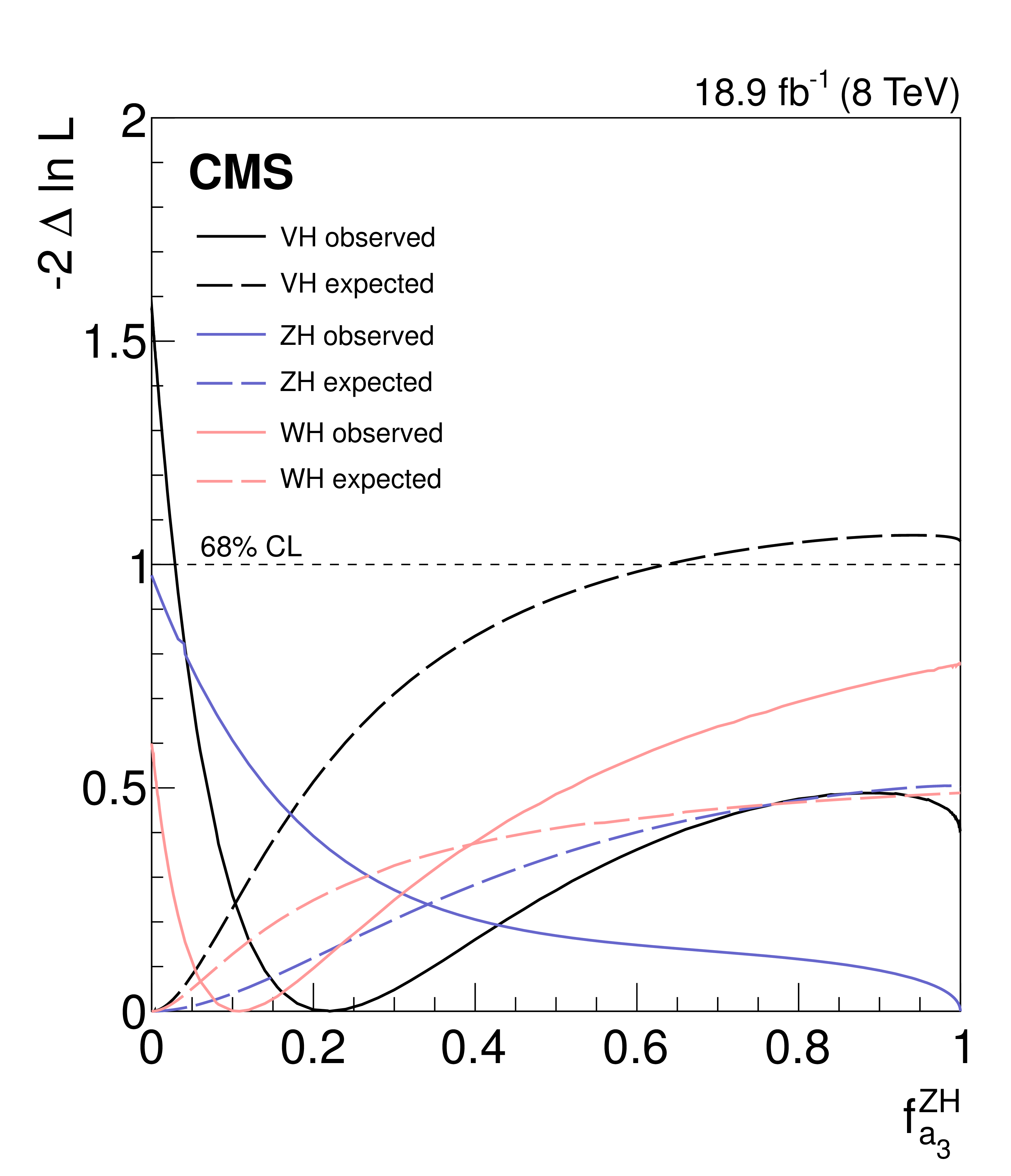
Figure 4:
Results of profile likelihood scans for the WH and ZH channels, as well as the combination (VH). The dotted (solid) lines show the expected (observed) -2$\Delta \mathrm {ln}\mathcal {L}$ value as a function of $ { {f_{a_3}} ^{\mathrm{ZH} }} $. A horizontal dashed line is shown, representing the 68% CL. |

png pdf |
Figure 5-a:
Results of profile likelihood scans for the VH and VV channels, plus their combination. The dotted (solid) lines show the expected (observed) -2$\Delta \mathrm {ln}\mathcal {L}$ value as a function of $ {f_{a_3}} $. The full range of $ {f_{a_3}} $ is shown on (a,c), with the low $ {f_{a_3}} $ region highlighted on (b,d). Horizontal dashed lines represent the 68%, 95%, and 99% CL. |

png pdf |
Figure 5-b:
Results of profile likelihood scans for the VH and VV channels, plus their combination. The dotted (solid) lines show the expected (observed) -2$\Delta \mathrm {ln}\mathcal {L}$ value as a function of $ {f_{a_3}} $. The full range of $ {f_{a_3}} $ is shown on (a,c), with the low $ {f_{a_3}} $ region highlighted on (b,d). Horizontal dashed lines represent the 68%, 95%, and 99% CL. |

png pdf |
Figure 5-c:
Results of profile likelihood scans for the VH and VV channels, plus their combination. The dotted (solid) lines show the expected (observed) -2$\Delta \mathrm {ln}\mathcal {L}$ value as a function of $ {f_{a_3}} $. The full range of $ {f_{a_3}} $ is shown on (a,c), with the low $ {f_{a_3}} $ region highlighted on (b,d). Horizontal dashed lines represent the 68%, 95%, and 99% CL. |

png pdf |
Figure 5-d:
Results of profile likelihood scans for the VH and VV channels, plus their combination. The dotted (solid) lines show the expected (observed) -2$\Delta \mathrm {ln}\mathcal {L}$ value as a function of $ {f_{a_3}} $. The full range of $ {f_{a_3}} $ is shown on (a,c), with the low $ {f_{a_3}} $ region highlighted on (b,d). Horizontal dashed lines represent the 68%, 95%, and 99% CL. |

png pdf |
Figure 6-a:
Results of profile likelihood scans for the VH and VV channels, as well as their combination. The dotted (solid) lines show the expected (observed) -2$\Delta \mathrm {ln}\mathcal {L}$ value as a function of $ {f_{a_3}} $. The full range of $ {f_{a_3}} $ is shown on (a,c), with the low $ {f_{a_3}} $ region highlighted on (b,d). The bottom plots contain the results of correlated-$\mu $ scans. Horizontal dashed lines represent the 68%, 95%, and 99% CL. In the legend, VH refers to the combination of the WH and ZH channels, and VV refers to the combination of the $ { {\mathrm{H \rightarrow W W }}} $ and $ { {\mathrm{H \rightarrow Z Z } }} $ channels. |

png pdf |
Figure 6-b:
Results of profile likelihood scans for the VH and VV channels, as well as their combination. The dotted (solid) lines show the expected (observed) -2$\Delta \mathrm {ln}\mathcal {L}$ value as a function of $ {f_{a_3}} $. The full range of $ {f_{a_3}} $ is shown on (a,c), with the low $ {f_{a_3}} $ region highlighted on (b,d). The bottom plots contain the results of correlated-$\mu $ scans. Horizontal dashed lines represent the 68%, 95%, and 99% CL. In the legend, VH refers to the combination of the WH and ZH channels, and VV refers to the combination of the $ { {\mathrm{H \rightarrow W W }}} $ and $ { {\mathrm{H \rightarrow Z Z } }} $ channels. |

png pdf |
Figure 6-c:
Results of profile likelihood scans for the VH and VV channels, as well as their combination. The dotted (solid) lines show the expected (observed) -2$\Delta \mathrm {ln}\mathcal {L}$ value as a function of $ {f_{a_3}} $. The full range of $ {f_{a_3}} $ is shown on (a,c), with the low $ {f_{a_3}} $ region highlighted on (b,d). The bottom plots contain the results of correlated-$\mu $ scans. Horizontal dashed lines represent the 68%, 95%, and 99% CL. In the legend, VH refers to the combination of the WH and ZH channels, and VV refers to the combination of the $ { {\mathrm{H \rightarrow W W }}} $ and $ { {\mathrm{H \rightarrow Z Z } }} $ channels. |

png pdf |
Figure 6-d:
Results of profile likelihood scans for the VH and VV channels, as well as their combination. The dotted (solid) lines show the expected (observed) -2$\Delta \mathrm {ln}\mathcal {L}$ value as a function of $ {f_{a_3}} $. The full range of $ {f_{a_3}} $ is shown on (a,c), with the low $ {f_{a_3}} $ region highlighted on (b,d). The bottom plots contain the results of correlated-$\mu $ scans. Horizontal dashed lines represent the 68%, 95%, and 99% CL. In the legend, VH refers to the combination of the WH and ZH channels, and VV refers to the combination of the $ { {\mathrm{H \rightarrow W W }}} $ and $ { {\mathrm{H \rightarrow Z Z } }} $ channels. |

png pdf |
Figure 7-a:
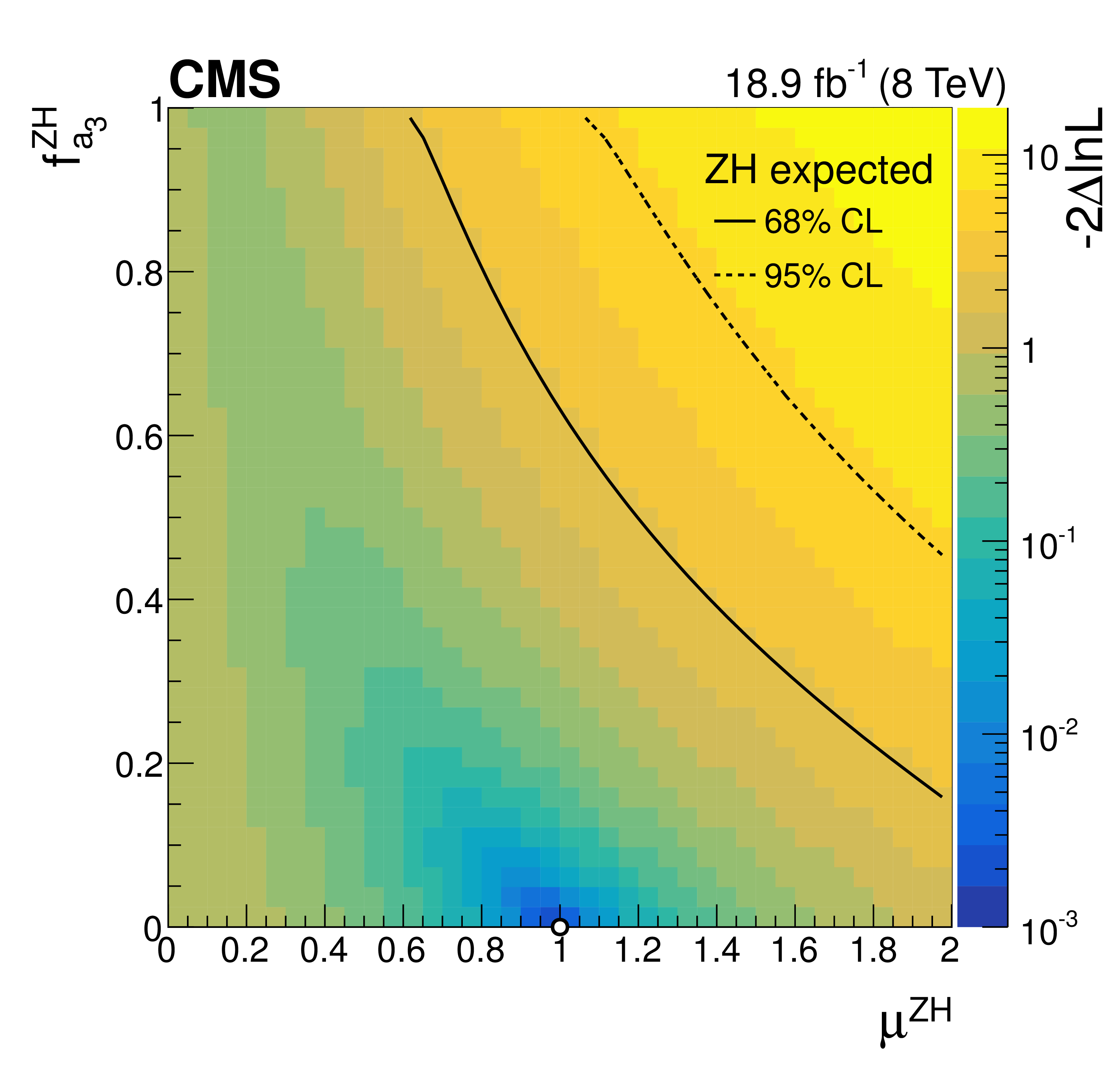
Expected (a) and observed (b) two-dimensional profile likelihood scans based on a combination of the WH and ZH channels in the ${ {f_{a_3}} ^{ \mathrm{ZH} }} $ versus $\mu ^{\mathrm{ZH} }$ plane. The colour coding represents $-2\Delta \mathrm {ln}\mathcal {L}$ calculated with respect to the global minimum. The scan minimum is indicated by a white dot. The 68% and 95% CL contours at $-2\Delta \mathrm {ln}\mathcal {L}=$ 2.30 and 5.99, respectively, are shown. The observed result includes upper and lower bounds while the expected result contains only upper bounds, as the expected result is consistent with $ { {f_{a_3}} ^{\mathrm{ZH} }} =$ 0 at 68% CL. |

png pdf |
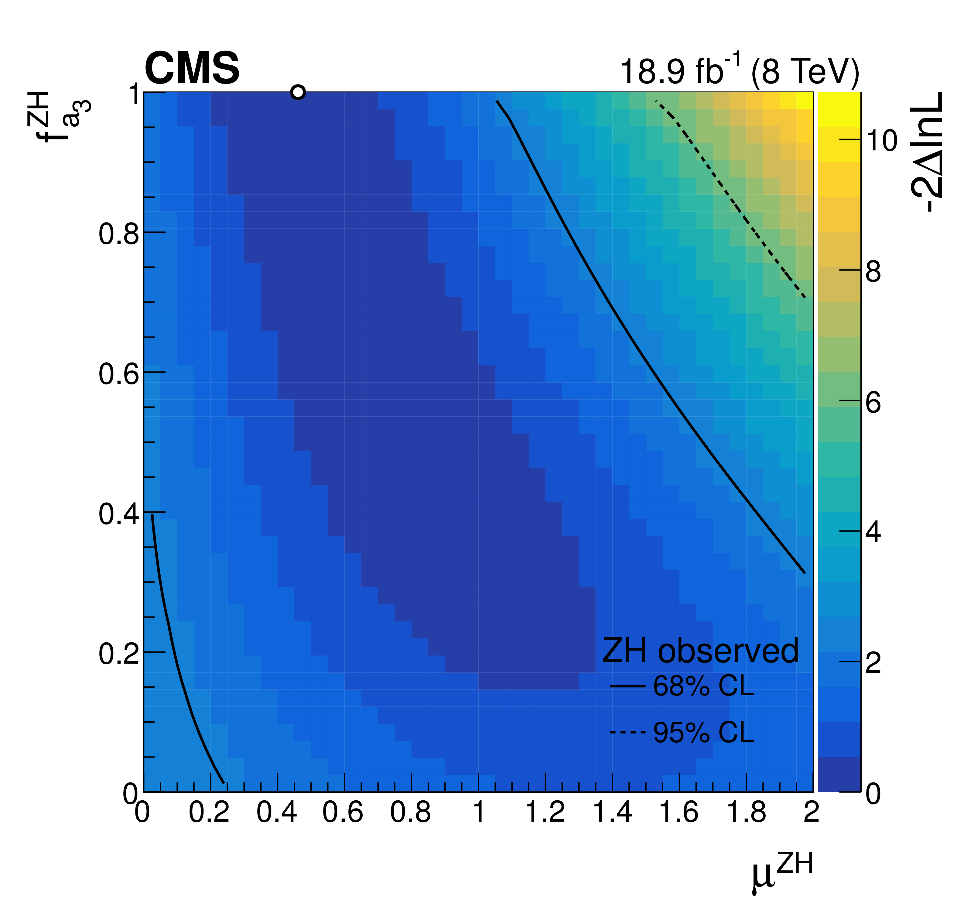
Figure 7-b:
Expected (a) and observed (b) two-dimensional profile likelihood scans based on a combination of the WH and ZH channels in the ${ {f_{a_3}} ^{ \mathrm{ZH} }} $ versus $\mu ^{\mathrm{ZH} }$ plane. The colour coding represents $-2\Delta \mathrm {ln}\mathcal {L}$ calculated with respect to the global minimum. The scan minimum is indicated by a white dot. The 68% and 95% CL contours at $-2\Delta \mathrm {ln}\mathcal {L}=$ 2.30 and 5.99, respectively, are shown. The observed result includes upper and lower bounds while the expected result contains only upper bounds, as the expected result is consistent with $ { {f_{a_3}} ^{\mathrm{ZH} }} =$ 0 at 68% CL. |

png pdf |
Figure 8-a:
Results of expected (a) and observed (b) $ { {f_{a_3}} ^{\mathrm{ZH} }} $ scans based on a combination of the WH and ZH channels, with various scales of new physics $\Lambda $. The coloured lines show the -2$\Delta \mathrm {ln}\mathcal {L}$ value as a function of ${ {f_{a_3}} ^{\mathrm{ZH} }} $. The horizontal dashed line represents the 68% CL. |

png pdf |
Figure 8-b:
Results of expected (a) and observed (b) $ { {f_{a_3}} ^{\mathrm{ZH} }} $ scans based on a combination of the WH and ZH channels, with various scales of new physics $\Lambda $. The coloured lines show the -2$\Delta \mathrm {ln}\mathcal {L}$ value as a function of ${ {f_{a_3}} ^{\mathrm{ZH} }} $. The horizontal dashed line represents the 68% CL. |
| Tables | |

png pdf |
Table 1:
$\sigma _1/\sigma _3$ cross section ratios calculated with JHUGen . |

png pdf |
Table 2:
Values of $\Omega ^{i,j}$ which relate the channels studied in this paper, as defined in Eq.7. |
png pdf |
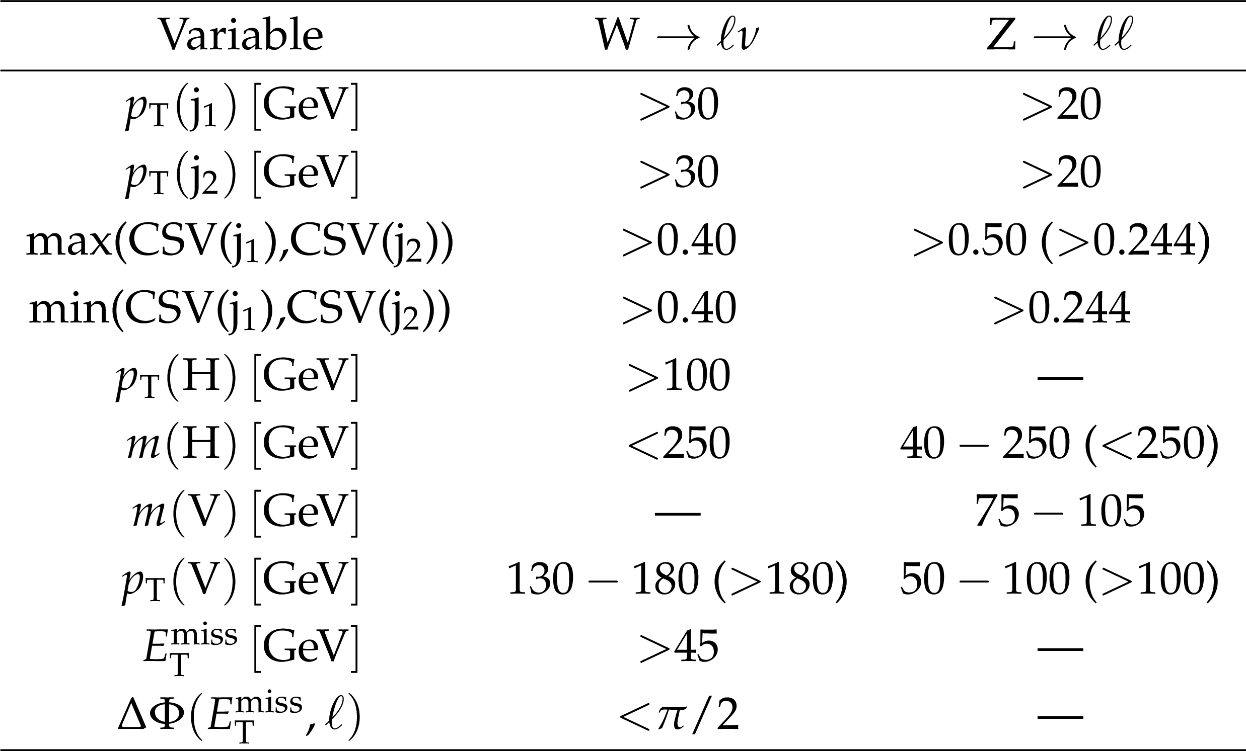
Table 3:
Summary of the event selection criteria. Numbers in parentheses refer to the high-boost region defined in the text. |

png pdf |
Table 4:
Summary of the sources of systematic uncertainty on the background and signal yields. The size of the uncertainties that only affect normalizations are given. Uncertainties that also affect the shapes are implemented with template morphing, a smooth vertical interpolation between the nominal shape and systematic shape variations. |

png pdf |
Table 5:
A summary of the locations of the minimum -2$\Delta \mathrm {ln}\mathcal {L}$ values in one-dimensional $ {f_{a_3}} $ profile likelihood scans. Parentheses contain 68% CL intervals, and brackets contain 95% CL intervals. The ranges are truncated at the physical boundaries 0 $< {f_{a_3}} <$ 1. The results of combinations which involve both VH and $ { \mathrm{H \rightarrow VV } } $ channels are given with and without assuming the SM ratio of the coupling strengths of the Higgs boson to top and bottom quarks. |
| Summary |
| A search has been performed for anomalous pseudoscalar HVV interactions in $ \sqrt{s} = $ 8 TeV pp data collected with the CMS detector. This is the first study of such interactions at the LHC in associated VH production. The VH channels alone do not currently have sufficient sensitivity to constrain the effective pseudoscalar cross section fractions $ f_{a_3} $ at 95% CL. In a combination of the VH and H $\rightarrow$ VV channels, when assuming the absence of additional anomalous Higgs boson couplings and treating the scalar $a_1^{\mathrm{HVV}}$ and pseudoscalar $a_3^{\mathrm{HVV}}$ couplings as constants, $ f_{a_3} ^{\mathrm{ZZ}}>$ 0.0034 is excluded at 95% CL. This exclusion represents a significant improvement with respect to previous results. |
| Additional Figures | |

png pdf |
Additional Figure 1:
Results of profile likelihood scans for the ZH and ZZ channels, plus their combination. The dotted (solid) lines show the expected (observed) $-2 \Delta \mathrm {ln}\mathcal {L}$ value as a function of $ { {f_{a_3}} ^{\mathrm{Z} \mathrm{H} }} $. Horizontal dashed lines represent the 68%, 95%, and 99% CL. These channels exclusively probe the HZZ coupling, and therefore the results do not include any assumption on the relationship between the HWW and HZZ couplings. |

png pdf |
Additional Figure 2:
Results of profile likelihood scans for the ZH and ZZ channels, plus their combination, highlighting the low -2$\Delta \mathrm {ln}\mathcal {L}$ region. The dotted (solid) lines show the expected (observed) $-2 \Delta \mathrm {ln}\mathcal {L}$ value as a function of $ { {f_{a_3}} ^{\mathrm{Z} \mathrm{H} }} $. A horizontal dashed line is shown, representing the 68% CL. These channels exclusively probe the HZZ coupling, and therefore the results do not include any assumption on the relationship between the HWW and HZZ couplings. |

png pdf |
Additional Figure 3:
Expected two-dimensional profile likelihood scan based on a combination of the WH and ZH channels in the $ { {f_{a_3}} ^{\mathrm{Z} \mathrm{H} }} $ versus $\mu ^{\mathrm {ZH}}$ plane. The colour coding represents $-2\Delta \mathrm {ln}\mathcal {L}$ calculated with respect to the global minimum. The scan minimum is indicated by a white dot. The 68% and 95% CL contours at $-2\Delta \mathrm {ln}\mathcal {L}=$ 2.30 and 5.99, respectively, are shown. |

png pdf |
Additional Figure 4:
Observed two-dimensional profile likelihood scan based on a combination of the WH and ZH channels in the $ { {f_{a_3}} ^{\mathrm{Z} \mathrm{H} }} $ versus $\mu ^{\mathrm {ZH}}$ plane. The colour coding represents $-2\Delta \mathrm {ln}\mathcal {L}$ calculated with respect to the global minimum. The scan minimum is indicated by a white dot. The 68% and 95% CL contours at $-2\Delta \mathrm {ln}\mathcal {L}=$ 2.30 and 5.99, respectively, are shown. |

png pdf |
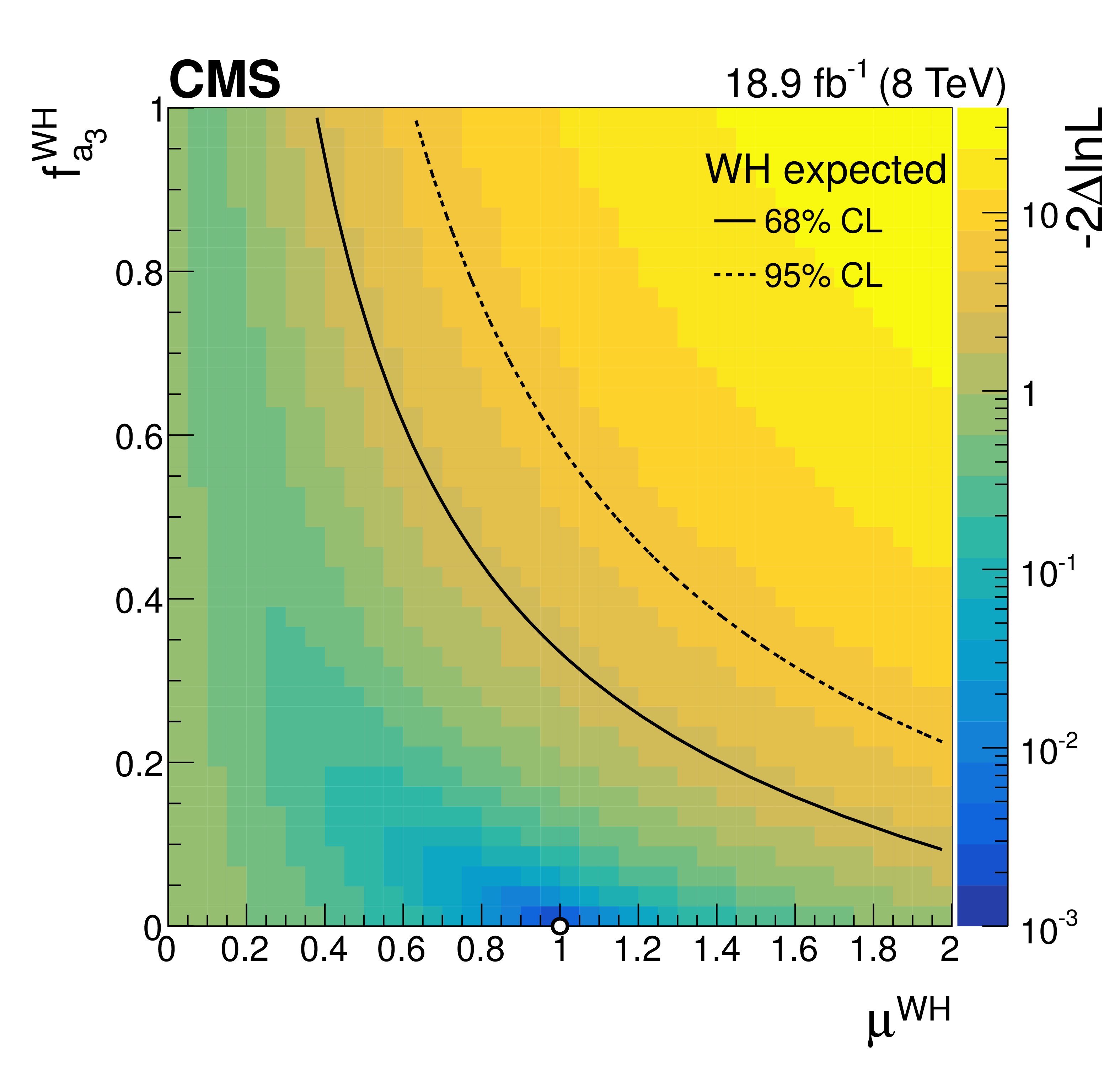
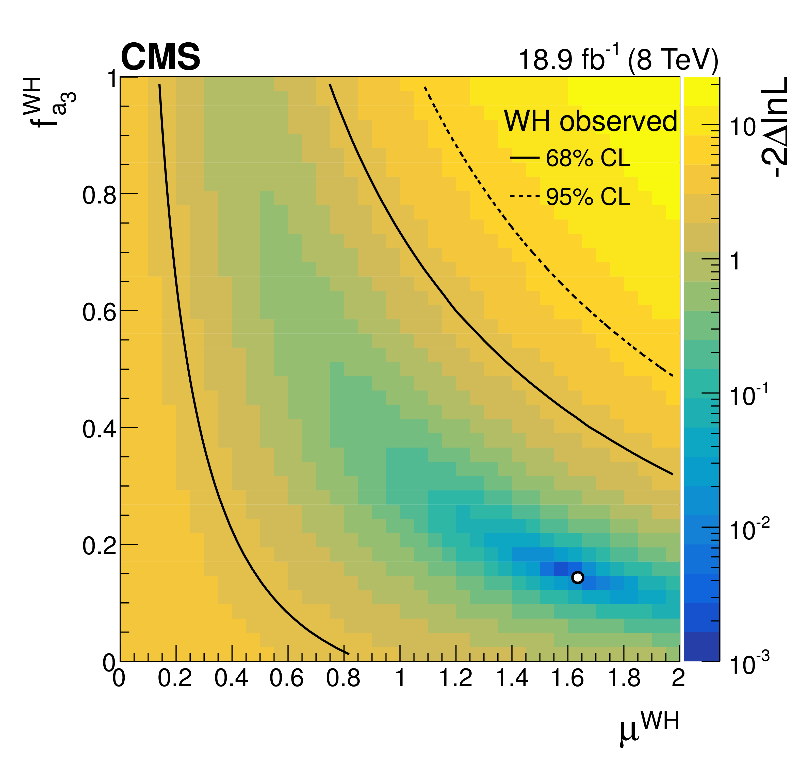
Additional Figure 5:
Expected two-dimensional profile likelihood scan based on the WH channel in the $ { {f_{a_3}} ^{\mathrm{W} \mathrm{H} }} $ versus $\mu ^{\mathrm {WH}}$ plane. The colour coding represents $-2\Delta \mathrm {ln}\mathcal {L}$ calculated with respect to the global minimum. The scan minimum is indicated by a white dot. The 68% and 95% CL contours at $-2\Delta \mathrm {ln}\mathcal {L}=$ 2.30 and 5.99, respectively, are shown. |

png pdf |
Additional Figure 6:
Observed two-dimensional profile likelihood scan based on the WH channel in the $ { {f_{a_3}} ^{\mathrm{W} \mathrm{H} }} $ versus $\mu ^{\mathrm {WH}}$ plane. The colour coding represents $-2\Delta \mathrm {ln}\mathcal {L}$ calculated with respect to the global minimum. The scan minimum is indicated by a white dot. The 68% and 95% CL contours at $-2\Delta \mathrm {ln}\mathcal {L}=$ 2.30 and 5.99, respectively, are shown. |
png pdf |
Additional Figure 7:
Expected two-dimensional profile likelihood scan based on the WH channel in the $ { {f_{a_3}} ^{\mathrm{W} \mathrm{H} }} $ versus $\mu ^{\mathrm {WH}}$ plane. The colour coding represents $-2\Delta \mathrm {ln}\mathcal {L}$ calculated with respect to the global minimum. The scan minimum is indicated by a white dot. The 68% and 95% CL contours at $-2\Delta \mathrm {ln}\mathcal {L}=2.30$ and $5.99$, respectively, are shown. |
png pdf |
Additional Figure 8:
Observed two-dimensional profile likelihood scan based on the WH channel in the $ { {f_{a_3}} ^{\mathrm{W} \mathrm{H} }} $ versus $\mu ^{\mathrm {WH}}$ plane. The colour coding represents $-2\Delta \mathrm {ln}\mathcal {L}$ calculated with respect to the global minimum. The scan minimum is indicated by a white dot. The 68% and 95% CL contours at $-2\Delta \mathrm {ln}\mathcal {L}=$ 2.30 and 5.99, respectively, are shown. |

png pdf |
Additional Figure 9:
Expected two-dimensional profile likelihood scan based on the ZH channel in the $ { {f_{a_3}} ^{\mathrm{Z} \mathrm{H} }} $ versus $\mu ^{\mathrm {ZH}}$ plane. The colour coding represents $-2\Delta \mathrm {ln}\mathcal {L}$ calculated with respect to the global minimum. The scan minimum is indicated by a white dot. The 68% and 95% CL contours at $-2\Delta \mathrm {ln}\mathcal {L}=$ 2.30 and 5.99, respectively, are shown. |
png pdf |
Additional Figure 10:
Observed two-dimensional profile likelihood scan based on the ZH channel in the $ { {f_{a_3}} ^{\mathrm{Z} \mathrm{H} }} $ versus $\mu ^{\mathrm {ZH}}$ plane. The colour coding represents $-2\Delta \mathrm {ln}\mathcal {L}$ calculated with respect to the global minimum. The scan minimum is indicated by a white dot. The 68% and 95% CL contours at $-2\Delta \mathrm {ln}\mathcal {L}=$ 2.30 and 5.99, respectively, are shown. |
png pdf |
Additional Figure 11:
Expected two-dimensional profile likelihood scan based on the ZH channel in the $ { {f_{a_3}} ^{\mathrm{Z} \mathrm{H} }} $ versus $\mu ^{\mathrm {ZH}}$ plane. The colour coding represents $-2\Delta \mathrm {ln}\mathcal {L}$ calculated with respect to the global minimum. The scan minimum is indicated by a white dot. The 68% and 95% CL contours at $-2\Delta \mathrm {ln}\mathcal {L}=$ 2.30 and 5.99, respectively, are shown. |

png pdf |
Additional Figure 12:
Observed two-dimensional profile likelihood scan based on the ZH channel in the $ { {f_{a_3}} ^{\mathrm{Z} \mathrm{H} }} $ versus $\mu ^{\mathrm {ZH}}$ plane. The colour coding represents $-2\Delta \mathrm {ln}\mathcal {L}$ calculated with respect to the global minimum. The scan minimum is indicated by a white dot. The 68% and 95% CL contours at $-2\Delta \mathrm {ln}\mathcal {L}=$ 2.30 and 5.99, respectively, are shown. |

png pdf |
Additional Figure 13:
Observed BDT discriminant vs $m$(VH) distribution in the high-boost region of the $ {\mathrm{W} \rightarrow \mathrm{e} \nu } $ channel. Bin content is normalized by the bin area. |

png pdf |
Additional Figure 14:
Unrolled BDT discriminant vs $m$(VH) distribution in the high-boost region of the $ {\mathrm{Z} \rightarrow \mu \mu } $ channel. 13 $m$(VH) distributions are shown in various bins of the BDT discriminant, demarcated by vertical pink dashed lines, with the BDT discriminant increasing from left to right. The distribution observed in data is represented by points with error bars. SM backgrounds are represented by filled histograms. A pure scalar (pseudoscalar) Higgs boson signal is represented by the solid (dotted) histogram. The statistical uncertainty related to the finite size of the simulated background event samples is represented by the hatched region. The bin content is normalized by the bin area. The lower panel shows the ratio of the observed and expected background yields. |

png pdf |
Additional Figure 15:
The BDT discriminant distribution for the high-boost region of the $ {\mathrm{Z} \rightarrow \mu \mu } $ channel. The distribution observed in data is represented by points with error bars. SM backgrounds are represented by filled histograms. A pure scalar (pseudoscalar) Higgs boson signal is represented by the solid (dotted) histogram. The statistical uncertainty related to the finite size of the simulated background event samples is represented by the hatched region. The bin content is normalized by the bin width. The lower panel shows the ratio of the observed and expected background yields. |

png pdf |
Additional Figure 16:
The BDT discriminant distribution for the high-boost region of the $ {\mathrm{W} \rightarrow \mathrm{e} \nu } $ channel. The distribution observed in data is represented by points with error bars. SM backgrounds are represented by filled histograms. A pure scalar (pseudoscalar) Higgs boson signal is represented by the solid (dotted) histogram. The statistical uncertainty related to the finite size of the simulated background event samples is represented by the hatched region. The bin content is normalized by the bin width. The lower panel shows the ratio of the observed and expected background yields. |

png pdf |
Additional Figure 17:
A summary of the locations of the minimum -2$\Delta \mathrm {ln}\mathcal {L}$ values in one-dimensional $ {f_{a_3}} \cos \left (\mathrm{H}i _{a_3}\right )$ profile likelihood scans allowing for $ \cos\left (\mathrm{H}i _{a_3}\right ) =$ -1, 1. Parentheses contain 68% CL intervals, and brackets contain 95% CL intervals. The ranges are truncated at the physical boundaries -1 $< {f_{a_3}} \cos \left (\mathrm{H}i _{a_3}\right )<$ 1. The results of combinations which involve both VH and $ { {\mathrm{H} \rightarrow \mathrm{VV} } } $ channels are given with and without assuming the SM ratio of the coupling strengths of the Higgs boson to top and bottom quarks. |
| References | ||||
| 1 | ATLAS Collaboration | Observation of a new particle in the search for the Standard Model Higgs boson with the ATLAS detector at the LHC | PLB 716 (2012) 1 | 1207.7214 |
| 2 | CMS Collaboration | Observation of a new boson at a mass of 125$ GeV $ with the CMS experiment at the LHC | PLB 716 (2012) 30 | CMS-HIG-12-028 1207.7235 |
| 3 | CMS Collaboration | Observation of a new boson with mass near 125$ GeV $ in $ \mathrm{ p } \mathrm{ p } $ collisions at $ \sqrt{s} = 7 $ and $ 8 TeV $ | JHEP 06 (2013) 081 | CMS-HIG-12-036 1303.4571 |
| 4 | S. L. Glashow | Partial-symmetries of weak interactions | Nucl. Phys. 22 (1961) 579 | |
| 5 | F. Englert and R. Brout | Broken symmetry and the mass of gauge vector mesons | PRL 13 (1964) 321 | |
| 6 | P. W. Higgs | Broken symmetries, massless particles and gauge fields | PL12 (1964) 132 | |
| 7 | P. W. Higgs | Broken symmetries and the masses of gauge bosons | PRL 13 (1964) 508 | |
| 8 | G. S. Guralnik, C. R. Hagen, and T. W. B. Kibble | Global conservation laws and massless particles | PRL 13 (1964) 585 | |
| 9 | S. Weinberg | A model of leptons | PRL 19 (1967) 1264 | |
| 10 | A. Salam | Weak and electromagnetic interactions | in Elementary particle physics: relativistic groups and analyticity, 1968 Proceedings of the eighth Nobel symposium | |
| 11 | CMS Collaboration | On the mass and spin-parity of the Higgs boson candidate via its decays to $ \mathrm{ Z } $ boson pairs | PRL 110 (2013) 081803 | CMS-HIG-12-041 1212.6639 |
| 12 | CMS Collaboration | Measurement of the properties of a Higgs boson in the four-lepton final state | PRD 89 (2014) 092007 | CMS-HIG-13-002 1312.5353 |
| 13 | CMS Collaboration | Measurement of Higgs boson production and properties in the $ \mathrm{ W } \mathrm{ W } $ decay channel with leptonic final states | JHEP 01 (2014) 096 | CMS-HIG-13-023 1312.1129 |
| 14 | CMS Collaboration | Observation of the diphoton decay of the Higgs boson and measurement of its properties | EPJC 74 (2014) 3076 | CMS-HIG-13-001 1407.0558 |
| 15 | CMS Collaboration | Constraints on the spin-parity and anomalous $ \mathrm{ H } V V $ couplings of the Higgs boson in proton collisions at 7 and 8$ TeV $ | PRD 92 (2015) 012004 | CMS-HIG-14-018 1411.3441 |
| 16 | ATLAS Collaboration | Evidence for the spin-0 nature of the Higgs boson using ATLAS data | PLB 726 (2013) 120 | 1307.1432 |
| 17 | CDF and D0 Collaborations | Tevatron constraints on models of the Higgs boson with exotic spin and parity using decays to bottom-antibottom quark pairs | PRL 114 (2015) 151802 | 1502.00967 |
| 18 | ATLAS Collaboration | Study of the spin and parity of the Higgs boson in diboson decays with the ATLAS detector | EPJC 75 (2015) 476 | 1506.05669 |
| 19 | I. Anderson et al. | Constraining anomalous $ \mathrm{ H } V V $ interactions at proton and lepton colliders | PRD 89 (2014) 035007 | 1309.4819 |
| 20 | J. Ellis, D. S. Hwang, V. Sanz, and T. You | A fast track towards the `Higgs' spin and parity | JHEP 11 (2012) 134 | 1208.6002 |
| 21 | R. M. Barnett, G. Senjanovi\'c, L. Wolfenstein, and D. Wyler | Implications of a light Higgs scalar | PLB 136 (1984) 191 | |
| 22 | CMS Collaboration | The CMS experiment at the CERN LHC | JINST 3 (2008) S08004 | CMS-00-001 |
| 23 | CMS Collaboration | Search for the standard model Higgs boson produced in association with a $ \mathrm{ W } $ or a $ \mathrm{ Z } $ boson and decaying to bottom quarks | PRD 89 (2014) 012003 | CMS-HIG-13-012 1310.3687 |
| 24 | ATLAS and CMS Collaborations | Procedure for the LHC Higgs boson search combination in summer 2011 | Technical Report ATL-PHYS-PUB-2011-011, CMS NOTE-2011/005, (2011) | |
| 25 | S. Bolognesi et al. | On the spin and parity of a single-produced resonance at the LHC | PRD 86 (2012) 095031 | 1208.4018 |
| 26 | Y. Gao et al. | Spin determination of single-produced resonances at hadron colliders | PRD 81 (2010) 075022 | 1001.3396 |
| 27 | T. Han and S. Willenbrock | QCD correction to the $ \mathrm{ p } \mathrm{ p } \rightarrow \mathrm{ W } \mathrm{ H } $ and $ \mathrm{ Z } \mathrm{ H } $ total cross-sections | PLB 273 (1991) 167 | |
| 28 | W. L. van Neerven and E. B. Zijlstra | The $ \mathcal{O}(\alpha_S^2) $ corrected Drell-Yan K-factor in the DIS and MS schemes | Nucl. Phys. B 382 (1992) 11 | |
| 29 | O. Brein, R. V. Harlander, M. Wiesemann, and T. Zirke | Top-quark mediated effects in hadronic Higgs-Strahlung | EPJC 72 (2012) 1 | 1111.0761 |
| 30 | LHC Higgs Cross Section Working Group | Handbook of LHC Higgs cross sections: 2. Differential distributions | CERN Report CERN-2012-002 | 1201.3084 |
| 31 | M. L. Ciccolini, S. Dittmaier, and M. Kramer | Electroweak radiative corrections to associated $ \mathrm{ W } \mathrm{ H } $ and $ \mathrm{ Z } \mathrm{ H } $ production at hadron colliders | PRD 68 (2003) 073003 | hep-ph/0306234 |
| 32 | C. Englert, M. McCullough, and M. Spannowsky | Gluon-initiated associated production boosts Higgs physics | PRD 89 (2014) 013013 | 1310.4828 |
| 33 | K. Arnold et al. | VBFNLO: A parton level Monte Carlo for processes with Electroweak bosons | CPC 180 (2009) 1661 | 0811.4559 |
| 34 | J. Alwall et al. | MadGraph 5: going beyond | JHEP 06 (2011) 128 | 1106.0522 |
| 35 | S. Frixione, P. Nason, and C. Oleari | Matching NLO QCD computations with parton shower simulations: the POWHEG method | JHEP 11 (2007) 070 | 0709.2092 |
| 36 | M. Bahr et al. | Herwig++ physics and manual | EPJC 58 (2008) 639 | 0803.0883 |
| 37 | T. Sjostrand, S. Mrenna, and P. Z. Skands | PYTHIA 6.4 physics and manual | JHEP 05 (2006) 026 | hep-ph/0603175 |
| 38 | GEANT4 Collaboration | GEANT4---a simulation toolkit | NIMA 506 (2003) 250 | |
| 39 | CMS Collaboration | Particle-flow event reconstruction in CMS and performance for jets, taus, and $ E_{\mathrm{T}}^{\text{miss}} $ | CDS | |
| 40 | CMS Collaboration | Commissioning of the particle-flow event reconstruction with the first LHC collisions recorded in the CMS detector | CDS | |
| 41 | CMS Collaboration | Performance of electron reconstruction and selection with the CMS detector in proton-proton collisions at $ \sqrt{s} = $ 8 TeV | JINST 10 (2015) P06005 | CMS-EGM-13-001 1502.02701 |
| 42 | CMS Collaboration | Performance of CMS muon reconstruction in pp collision events at $ \sqrt{s} = $ 7 TeV | JINST 7 (2012) P10002 | CMS-MUO-10-004 1206.4071 |
| 43 | M. Cacciari, G. P. Salam, and G. Soyez | The anti-$ k_t $ jet clustering algorithm | JHEP 04 (2008) 063 | 0802.1189 |
| 44 | M. Cacciari and G. P. Salam | Pileup subtraction using jet areas | PLB 659 (2008) 119 | 0707.1378 |
| 45 | CMS Collaboration | Identification of b-quark jets with the CMS experiment | JINST 8 (2013) P04013 | CMS-BTV-12-001 1211.4462 |
| 46 | G. Cowan, K. Cranmer, E. Gross, and O. Vitells | Asymptotic formulae for likelihood-based tests of new physics | EPJC 71 (2011) 1 | 1007.1727 |
|
|
Compact Muon Solenoid LHC, CERN |
|

|

|

|

|

|