

Compact Muon Solenoid
LHC, CERN
| CMS-SUS-14-003 ; CERN-EP-2016-097 | ||
| Searches for $R$-parity-violating supersymmetry in pp collisions at $\sqrt{s}= $ 8 TeV in final states with 0-4 leptons | ||
| CMS Collaboration | ||
| 26 June 2016 | ||
| Phys. Rev. D 94 (2016) 112009 | ||
| Abstract: Results are presented from searches for $R$-parity-violating supersymmetry in events produced in pp collisions at $\sqrt{s}= $ 8 TeV at the LHC. Final states with 0, 1, 2, or multiple leptons are considered independently. The analysis is performed on data collected by the CMS experiment corresponding to an integrated luminosity of 19.5 fb$^{-1}$. No excesses of events above the standard model expectations are observed, and 95% confidence level limits are set on supersymmetric particle masses and production cross sections. The results are interpreted in models featuring $R$-parity-violating decays of the lightest supersymmetric particle, which in the studied scenarios can be either the gluino, a bottom squark, or a neutralino. In a gluino pair production model with baryon number violation, gluinos with a mass less than 0.98 and 1.03 TeV are excluded, by analyses in a fully hadronic and one-lepton final state, respectively. An analysis in a dilepton final state is used to exclude bottom squarks with masses less than 307 GeV in a model considering bottom squark pair production. Multilepton final states are considered in the context of either strong or electroweak production of superpartners, and are used to set limits on the masses of the lightest supersymmetric particles. These limits range from 300 to 900 GeV in models with leptonic and up to approximately 700 GeV in models with semileptonic $R$-parity-violating couplings. | ||
| Links: e-print arXiv:1606.08076 [hep-ex] (PDF) ; CDS record ; inSPIRE record ; CADI line (restricted) ; | ||
| Figures | |
png pdf |
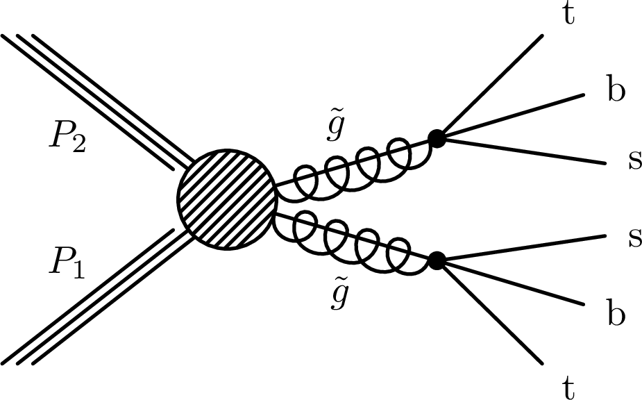
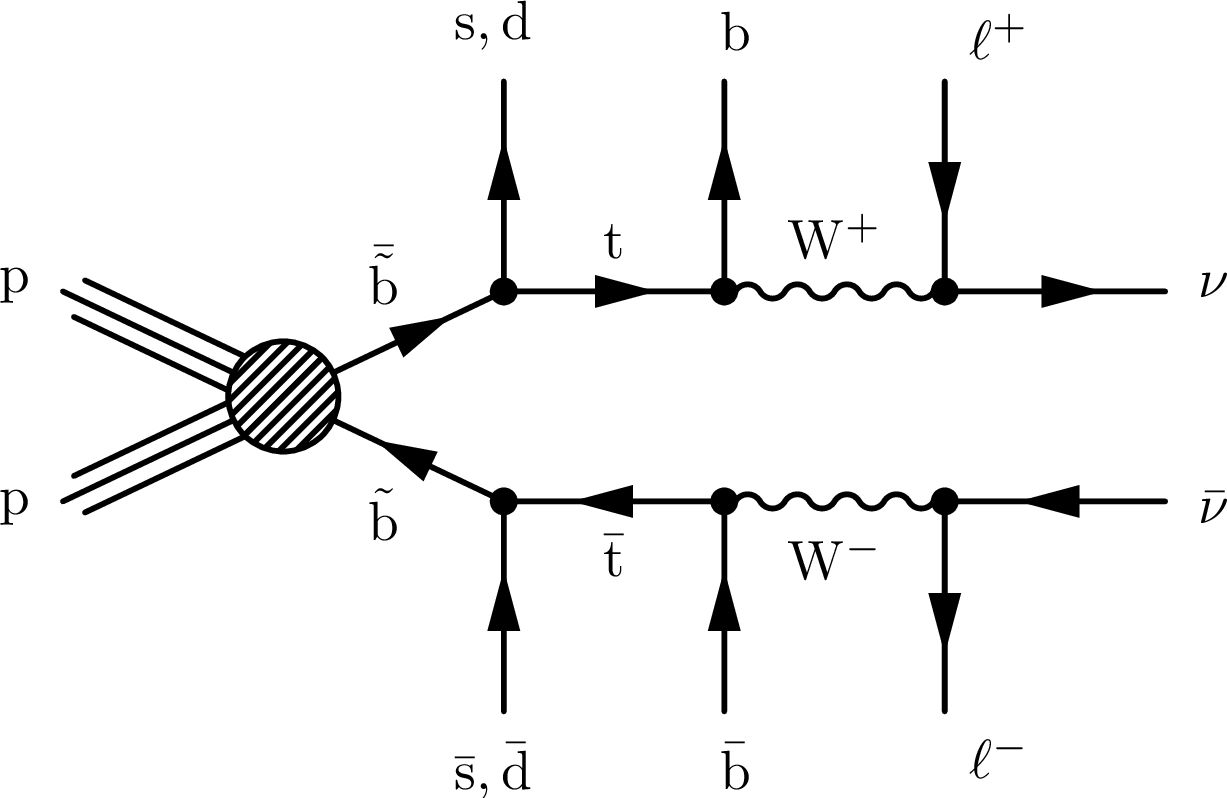
Figure 1:
Diagram for pair production of gluinos that decay to $\mathrm{ t } \mathrm{ b } \mathrm{ s } $. |
png pdf |
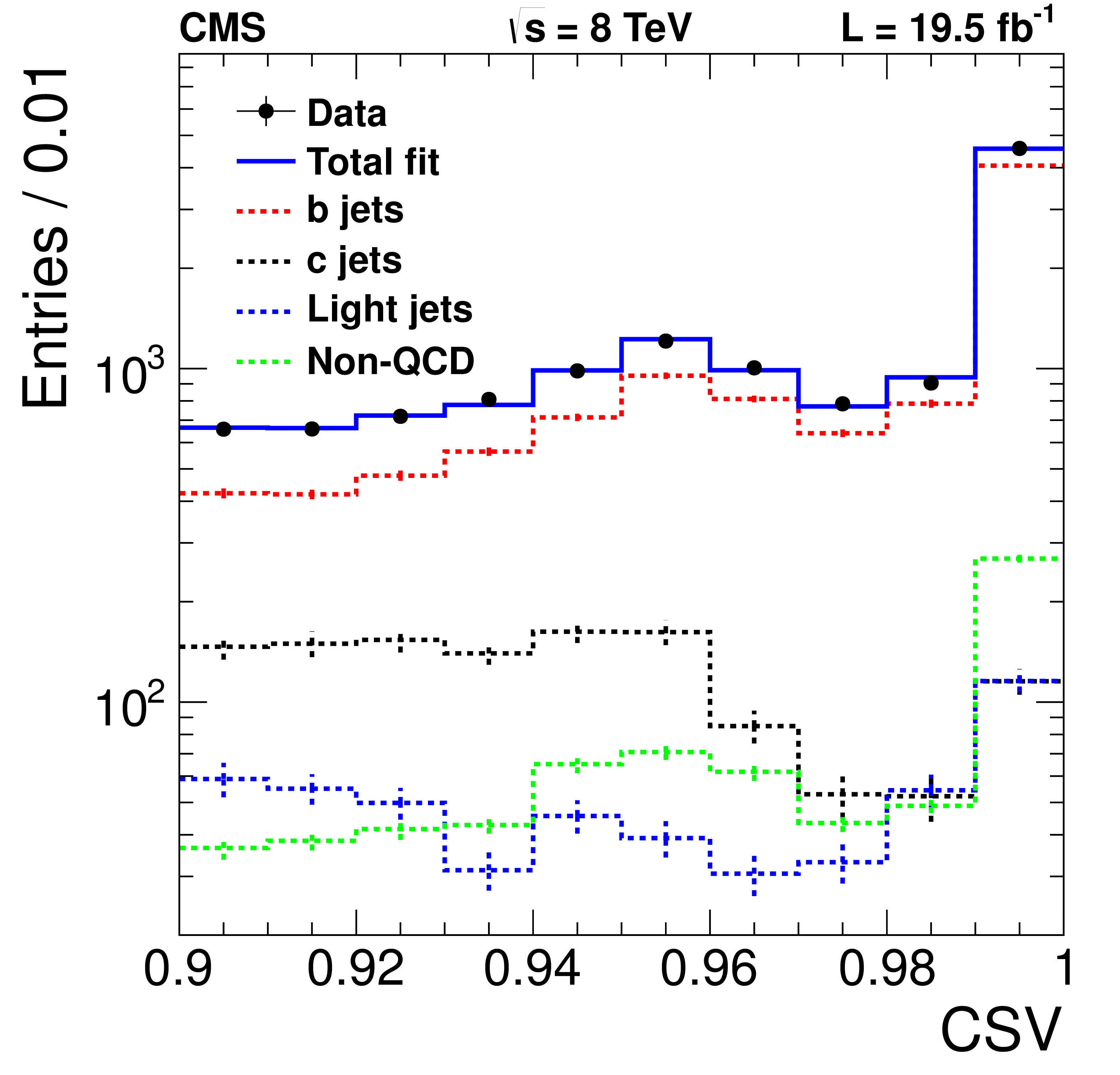
Figure 2:
The CSV distribution in data for $4\le {N_{\text {jet}}} \le$ 5, $ {H_{\mathrm {T}}} > $ 1.1 TeV, and $\mathrm {CSV}> $ 0.9 . The solid line is the result of a fit to the data with MC templates. Error bars reflect statistical uncertainties in the data (smaller than the marker) and MC samples. |
png pdf |
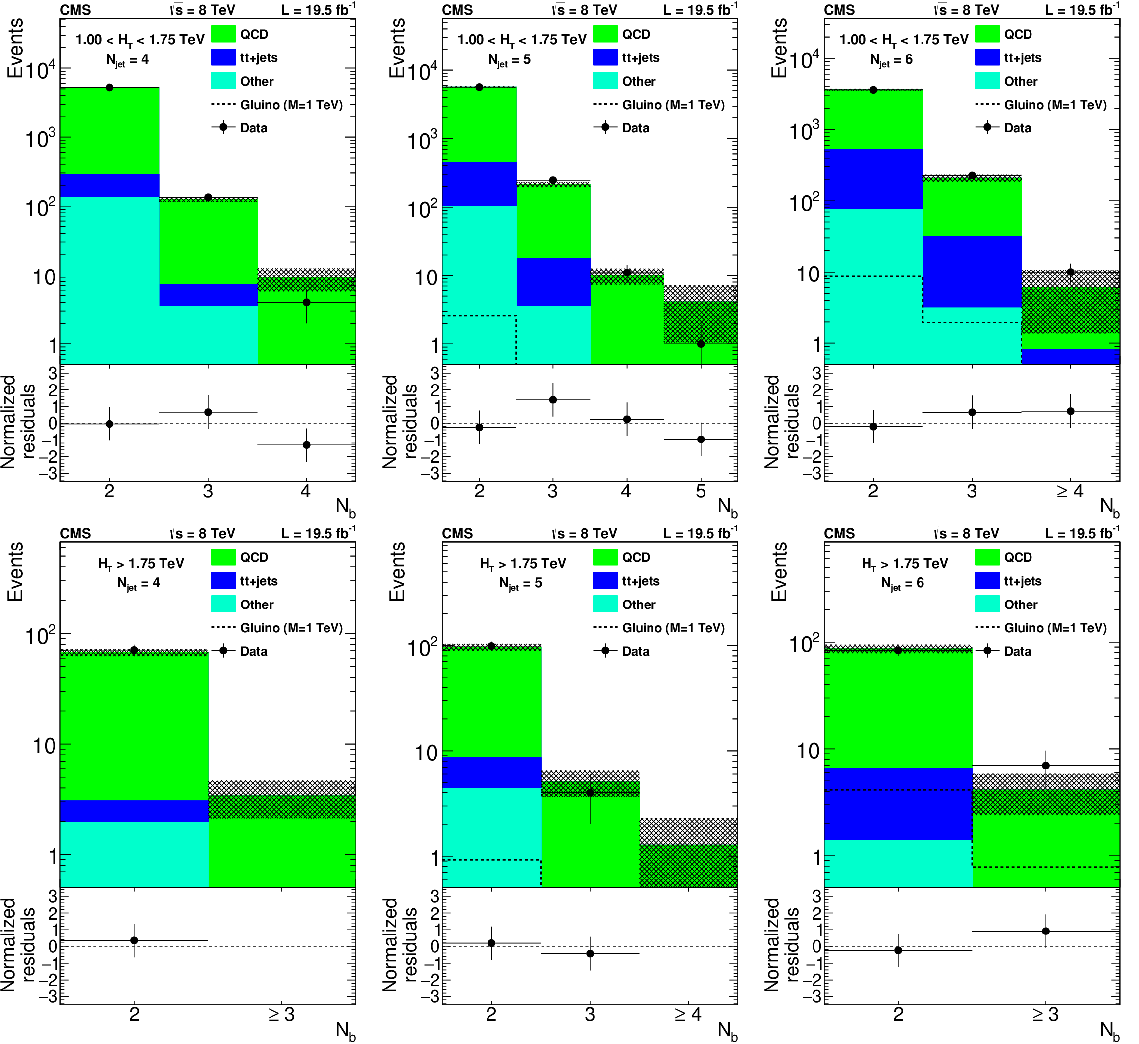
Figure 3:
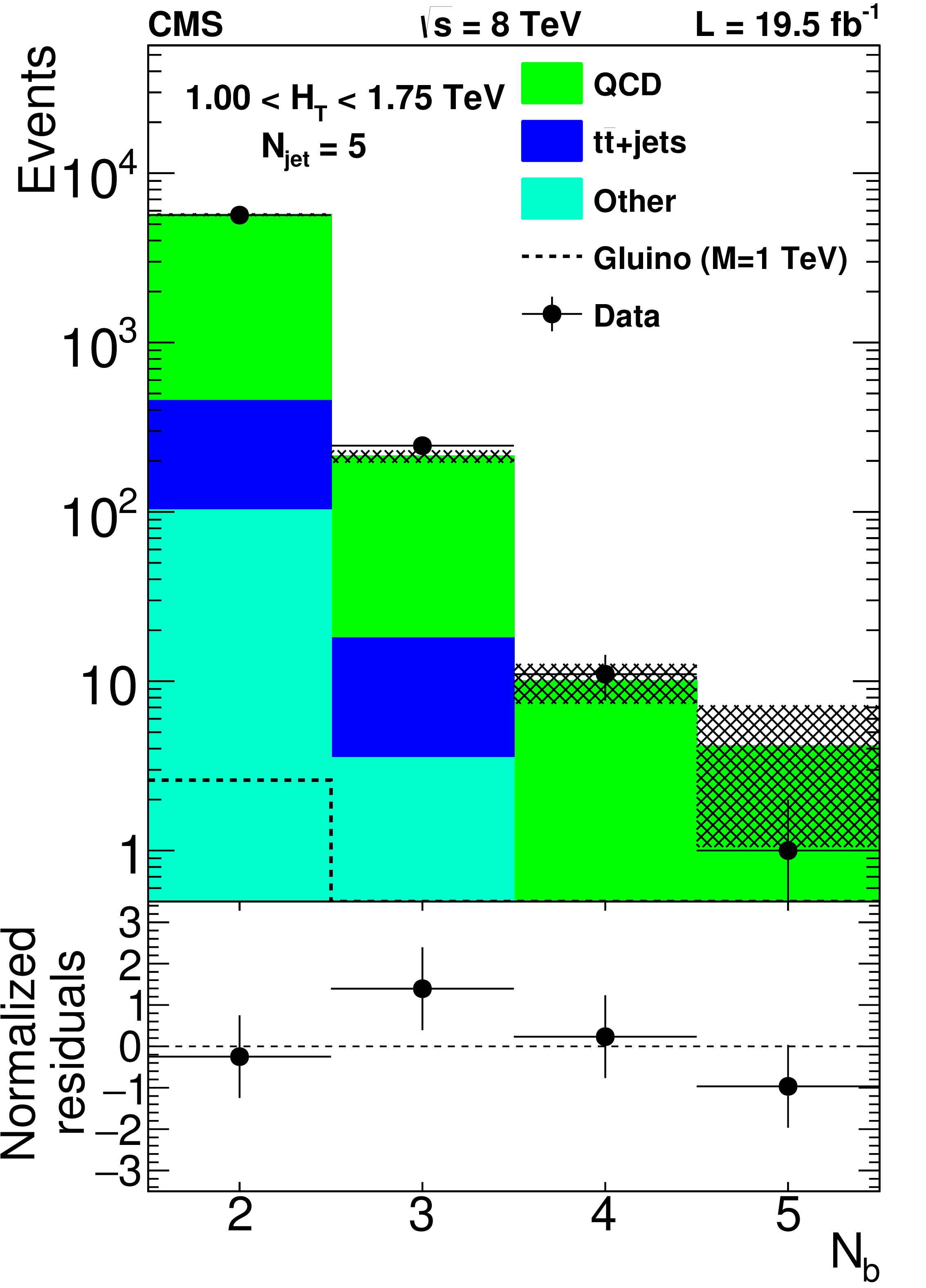
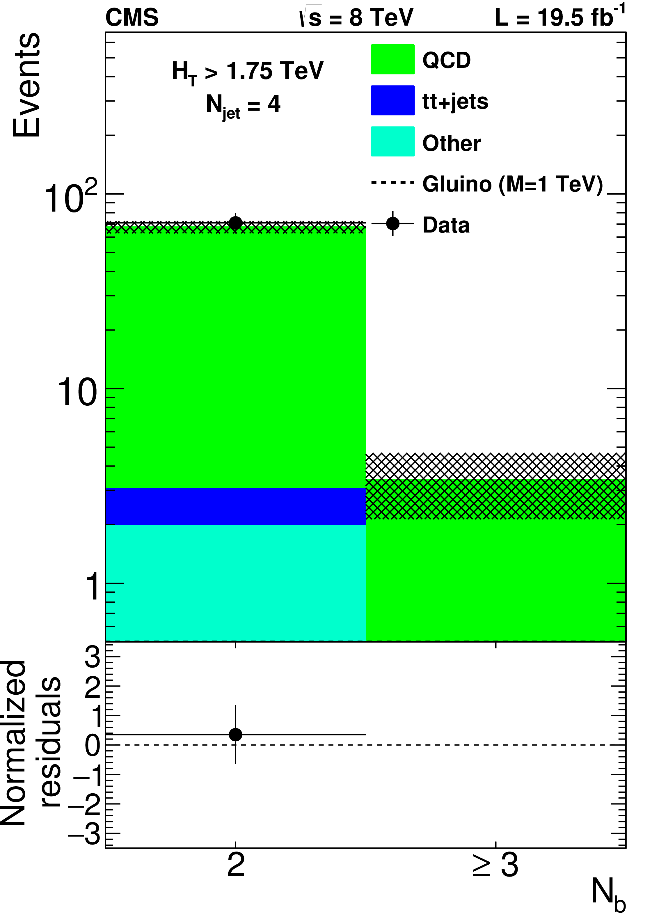
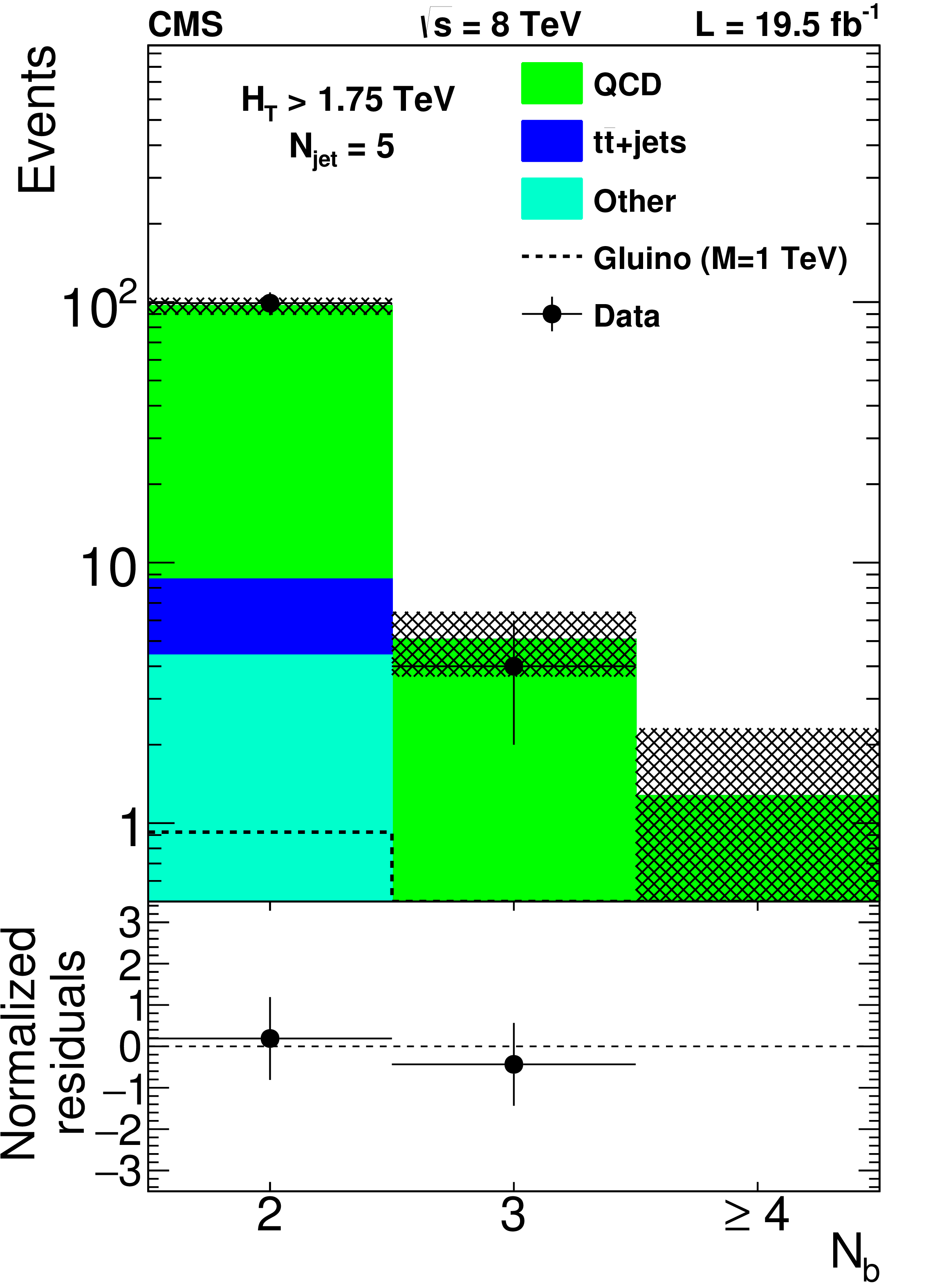
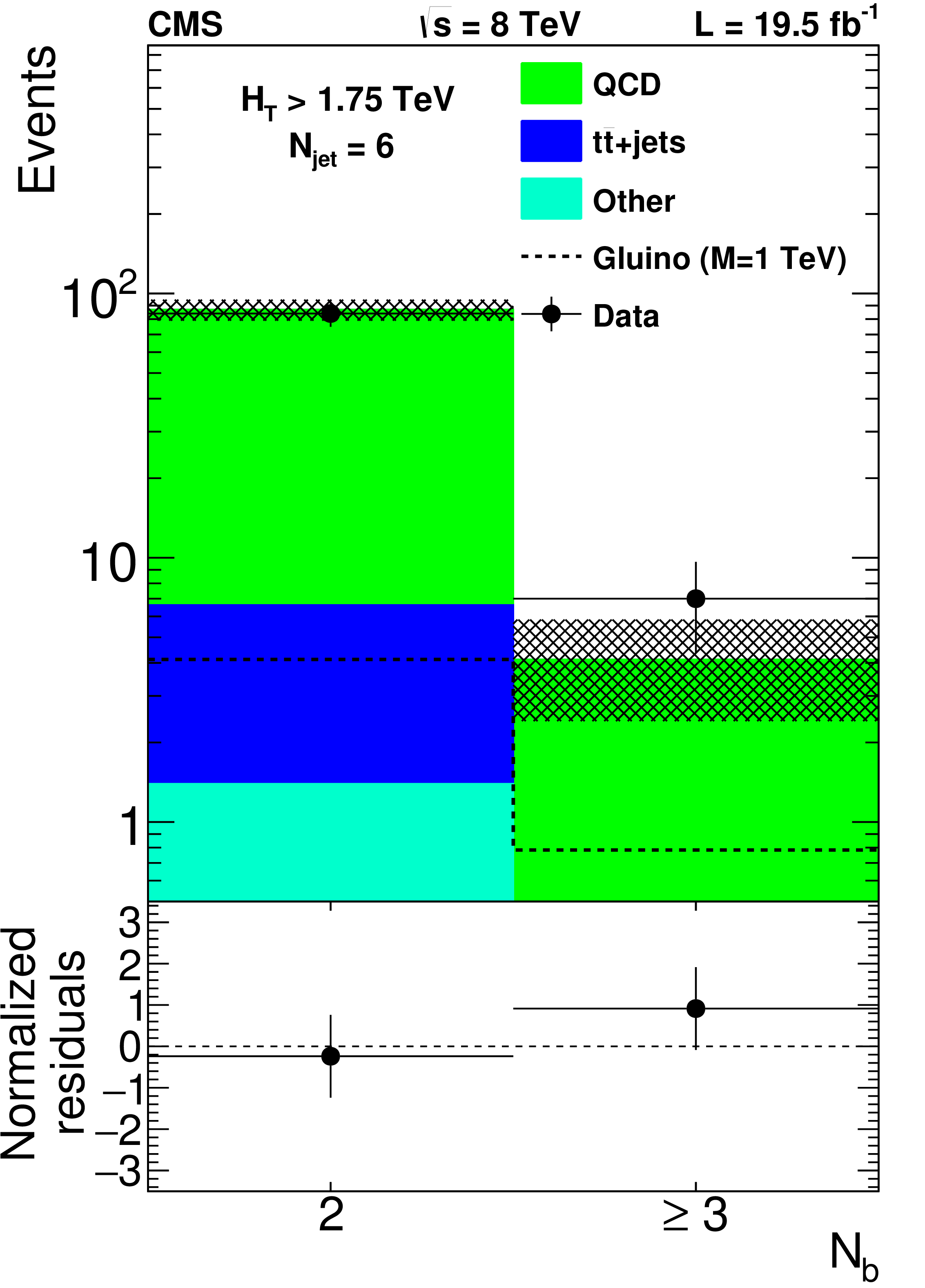
Distribution of $N_{\mathrm{ b } }$ for data(dots with error bars) and corrected predictions. The a,b,c (d,e,f) row shows data in which events are required to have 1.00 $ < {H_{\mathrm {T}}} < $ 1.75 TeV ($ {H_{\mathrm {T}}} > $ 1.75 TeV). The jet multiplicity requirements are $ {N_{\text {jet}}} = $ 4 (a,d), $ {N_{\text {jet}}} = $ 5 (b,e), and $ {N_{\text {jet}}} = $ 6 (c,f). The hatched bands shows the statistical uncertainty of the simulated data. The bottom panels of each plot show the difference between the data and corrected prediction divided by the sum in quadrature of the statistical uncertainties associated with each. |
png pdf |
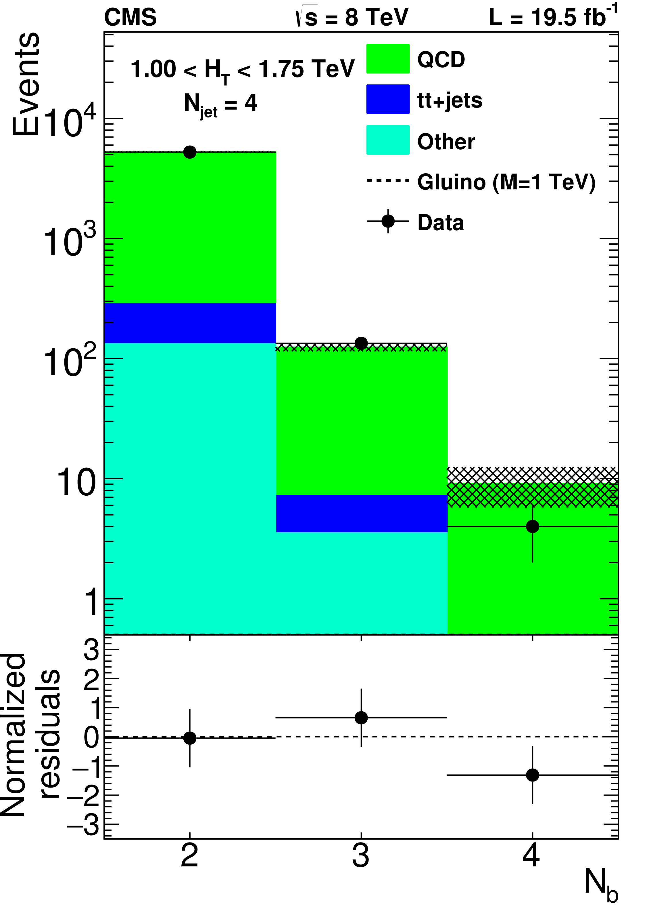
Figure 3-a:
Distribution of $N_{\mathrm{ b } }$ for data(dots with error bars) and corrected predictions. The a,b,c (d,e,f) row shows data in which events are required to have 1.00 $ < {H_{\mathrm {T}}} < $ 1.75 TeV ($ {H_{\mathrm {T}}} > $ 1.75 TeV). The jet multiplicity requirements are $ {N_{\text {jet}}} = $ 4 (a,d), $ {N_{\text {jet}}} = $ 5 (b,e), and $ {N_{\text {jet}}} = $ 6 (c,f). The hatched bands shows the statistical uncertainty of the simulated data. The bottom panels of each plot show the difference between the data and corrected prediction divided by the sum in quadrature of the statistical uncertainties associated with each. |
png pdf |
Figure 3-b:
Distribution of $N_{\mathrm{ b } }$ for data(dots with error bars) and corrected predictions. The a,b,c (d,e,f) row shows data in which events are required to have 1.00 $ < {H_{\mathrm {T}}} < $ 1.75 TeV ($ {H_{\mathrm {T}}} > $ 1.75 TeV). The jet multiplicity requirements are $ {N_{\text {jet}}} = $ 4 (a,d), $ {N_{\text {jet}}} = $ 5 (b,e), and $ {N_{\text {jet}}} = $ 6 (c,f). The hatched bands shows the statistical uncertainty of the simulated data. The bottom panels of each plot show the difference between the data and corrected prediction divided by the sum in quadrature of the statistical uncertainties associated with each. |

png pdf |
Figure 3-c:
Distribution of $N_{\mathrm{ b } }$ for data(dots with error bars) and corrected predictions. The a,b,c (d,e,f) row shows data in which events are required to have 1.00 $ < {H_{\mathrm {T}}} < $ 1.75 TeV ($ {H_{\mathrm {T}}} > $ 1.75 TeV). The jet multiplicity requirements are $ {N_{\text {jet}}} = $ 4 (a,d), $ {N_{\text {jet}}} = $ 5 (b,e), and $ {N_{\text {jet}}} = $ 6 (c,f). The hatched bands shows the statistical uncertainty of the simulated data. The bottom panels of each plot show the difference between the data and corrected prediction divided by the sum in quadrature of the statistical uncertainties associated with each. |
png pdf |
Figure 3-d:
Distribution of $N_{\mathrm{ b } }$ for data(dots with error bars) and corrected predictions. The a,b,c (d,e,f) row shows data in which events are required to have 1.00 $ < {H_{\mathrm {T}}} < $ 1.75 TeV ($ {H_{\mathrm {T}}} > $ 1.75 TeV). The jet multiplicity requirements are $ {N_{\text {jet}}} = $ 4 (a,d), $ {N_{\text {jet}}} = $ 5 (b,e), and $ {N_{\text {jet}}} = $ 6 (c,f). The hatched bands shows the statistical uncertainty of the simulated data. The bottom panels of each plot show the difference between the data and corrected prediction divided by the sum in quadrature of the statistical uncertainties associated with each. |
png pdf |
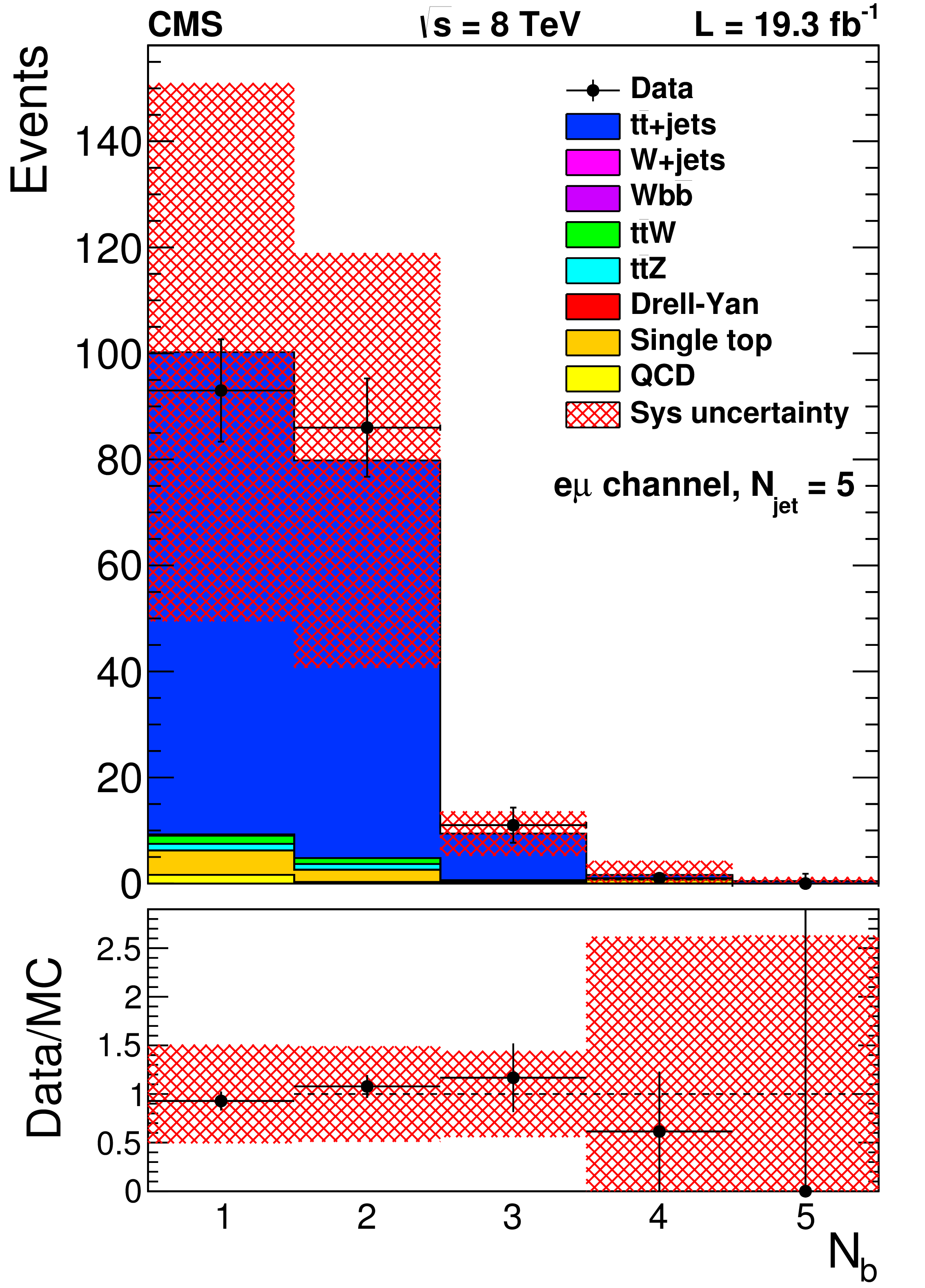
Figure 3-e:
Distribution of $N_{\mathrm{ b } }$ for data(dots with error bars) and corrected predictions. The a,b,c (d,e,f) row shows data in which events are required to have 1.00 $ < {H_{\mathrm {T}}} < $ 1.75 TeV ($ {H_{\mathrm {T}}} > $ 1.75 TeV). The jet multiplicity requirements are $ {N_{\text {jet}}} = $ 4 (a,d), $ {N_{\text {jet}}} = $ 5 (b,e), and $ {N_{\text {jet}}} = $ 6 (c,f). The hatched bands shows the statistical uncertainty of the simulated data. The bottom panels of each plot show the difference between the data and corrected prediction divided by the sum in quadrature of the statistical uncertainties associated with each. |
png pdf |
Figure 3-f:
Distribution of $N_{\mathrm{ b } }$ for data(dots with error bars) and corrected predictions. The a,b,c (d,e,f) row shows data in which events are required to have 1.00 $ < {H_{\mathrm {T}}} < $ 1.75 TeV ($ {H_{\mathrm {T}}} > $ 1.75 TeV). The jet multiplicity requirements are $ {N_{\text {jet}}} = $ 4 (a,d), $ {N_{\text {jet}}} = $ 5 (b,e), and $ {N_{\text {jet}}} = $ 6 (c,f). The hatched bands shows the statistical uncertainty of the simulated data. The bottom panels of each plot show the difference between the data and corrected prediction divided by the sum in quadrature of the statistical uncertainties associated with each. |
png pdf |
Figure 4:
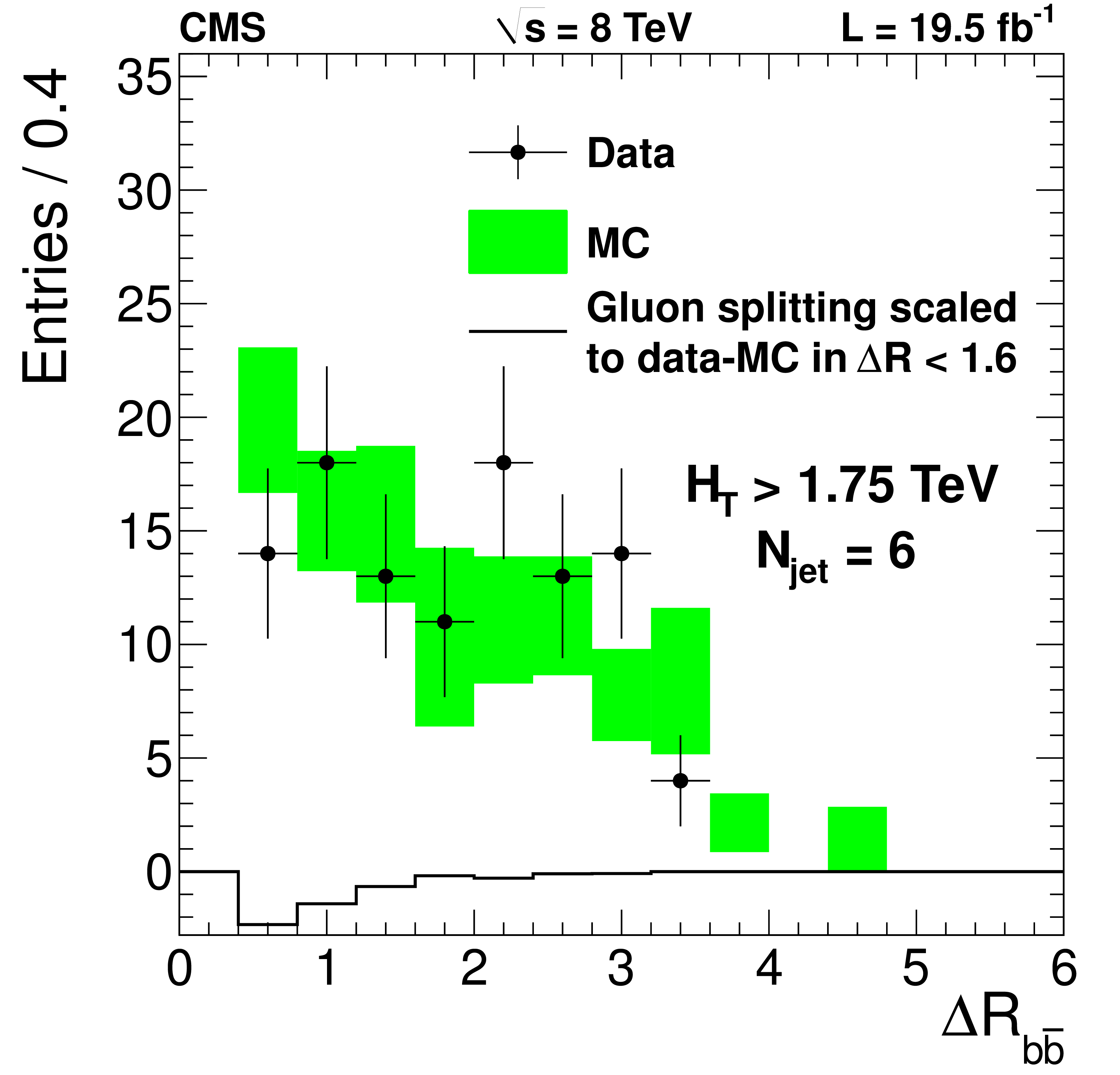
Distribution of the angular distance between any two b-tagged jets for data(dots with error bars), uncorrected MC prediction (band), and generator-matched gluon splitting events scaled by the data/simulation difference in $\Delta R_{ {\mathrm{ b \bar{b} } } }< $ 1.6 (histogram) for events with $ {H_{\mathrm {T}}} > $ 1.75 TeV and $ {N_{\text {jet}}} = $ 6 . The error bars and bands include the statistical uncertainty in the data and MC simulation, respectively. There are no entries with $\Delta R_{ {\mathrm{ b \bar{b} } } }< $ 0.4 as a consequence of the jet definition. |

png pdf |
Figure 5:
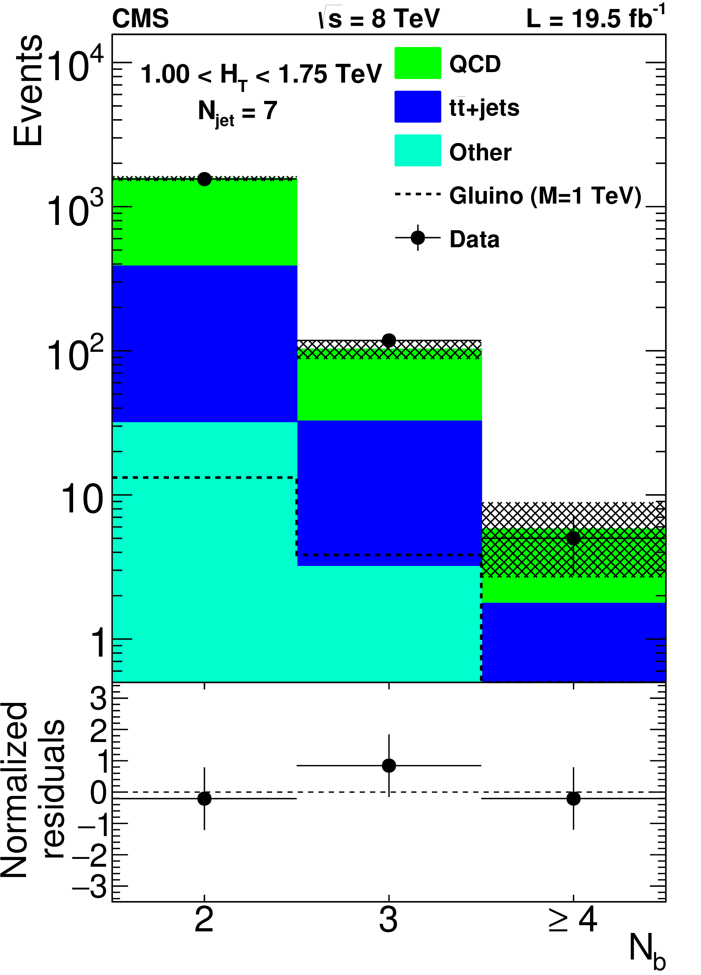
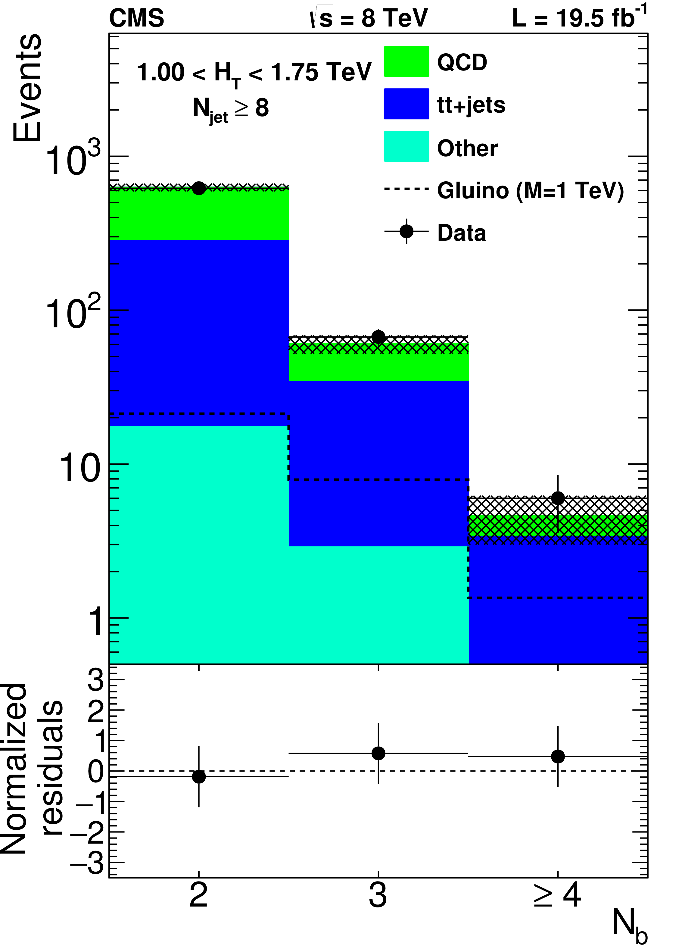
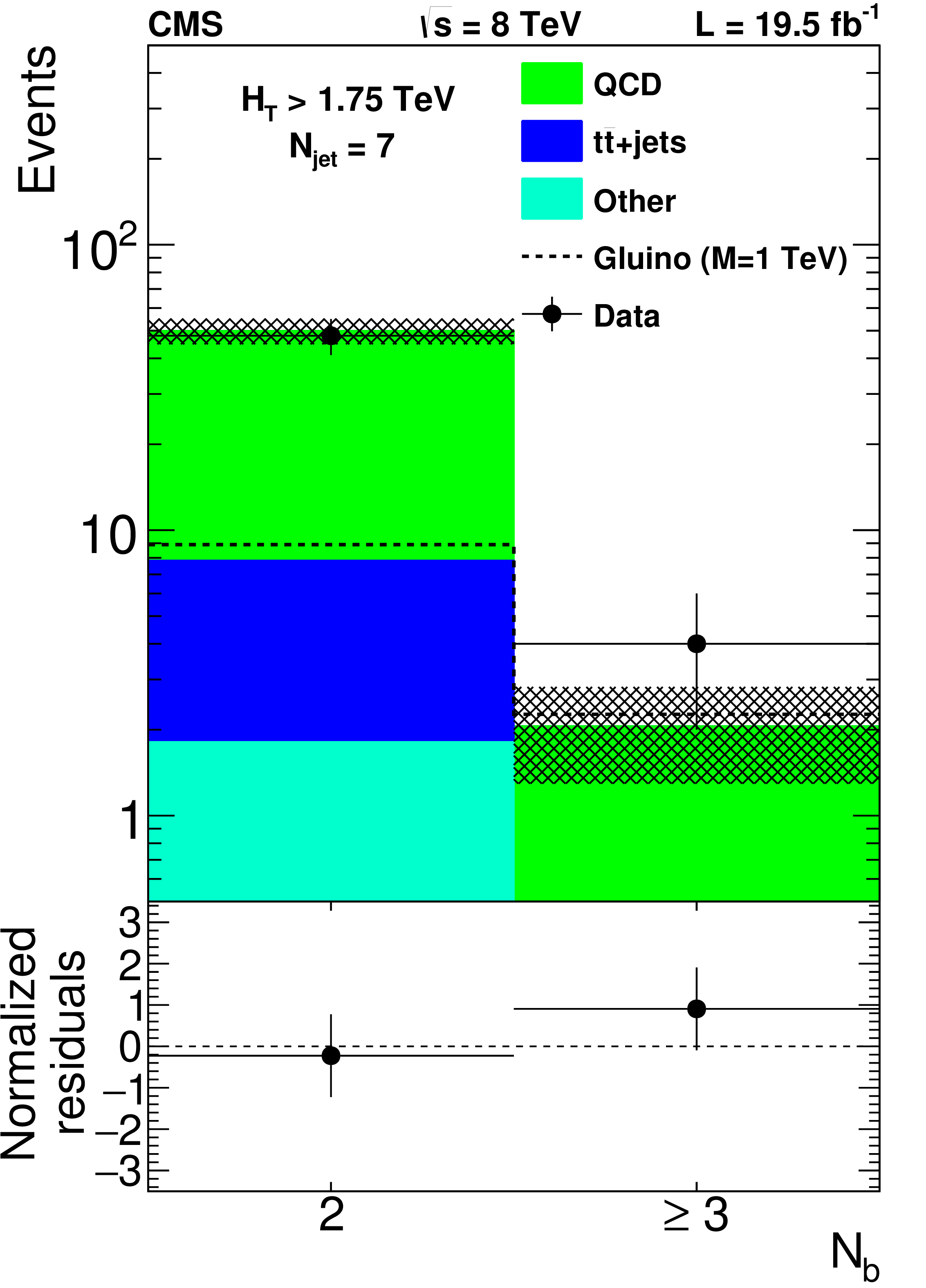
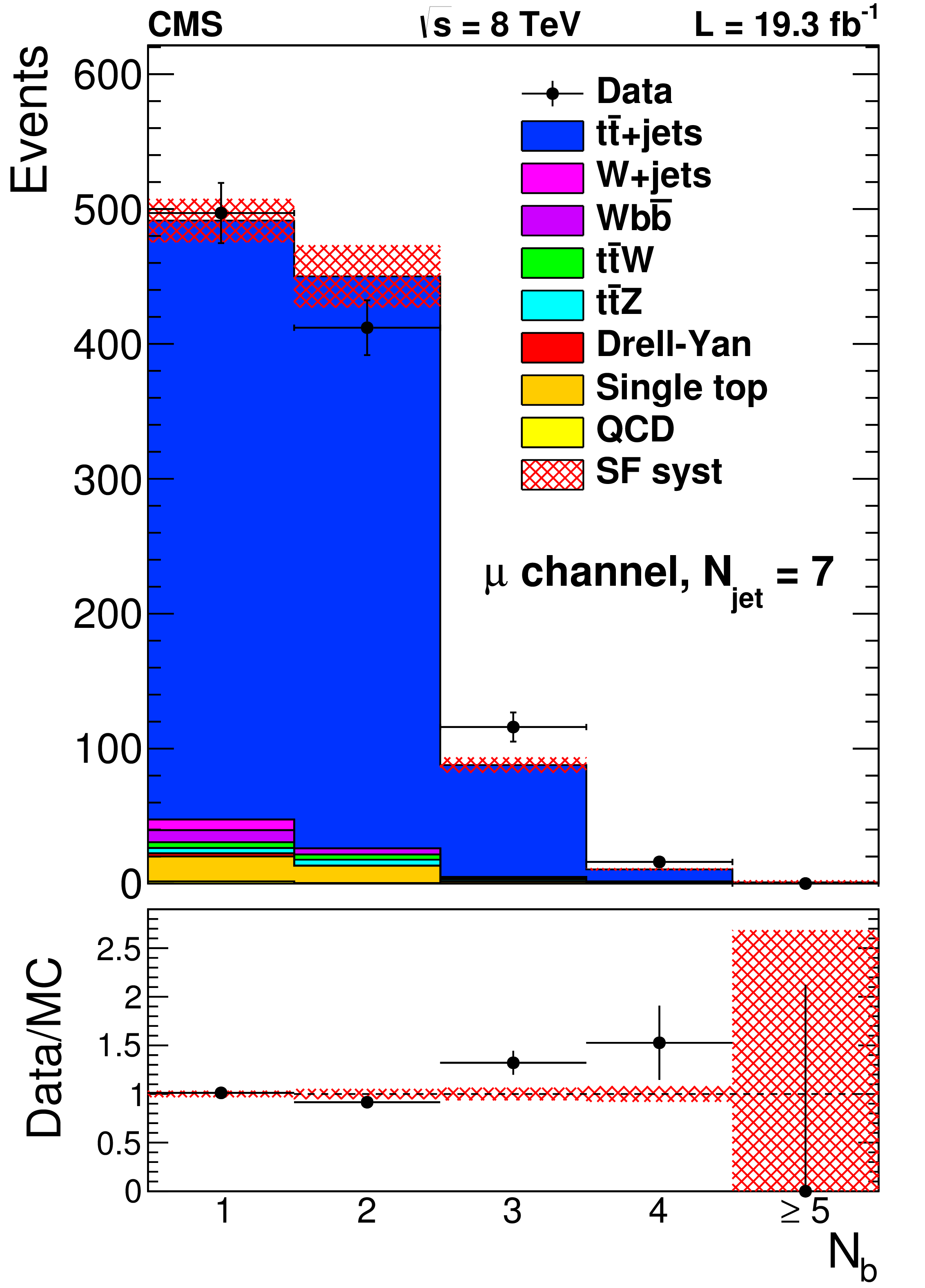
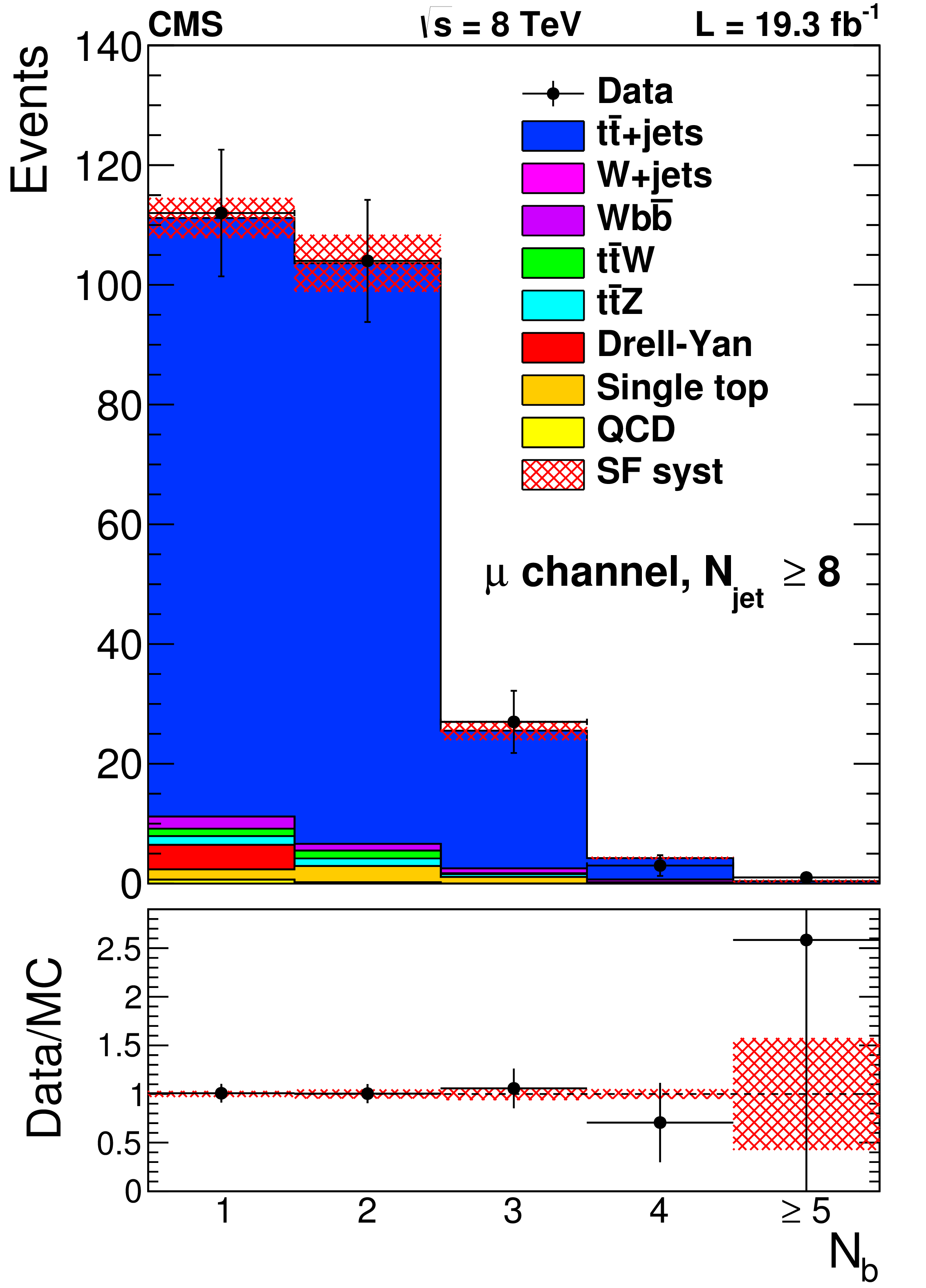
Data(dots with error bars) and the corrected prediction of the $N_{\mathrm{ b } }$ distribution in the high-$ {N_{\text {jet}}}$ signal region. The hatched band shows the MC statistical uncertainty. The a,b (c,d) row shows events with 1.00 $ < {H_{\mathrm {T}}} < $ 1.75 TeV ($ {H_{\mathrm {T}}} > $ 1.75 TeV ). The jet multiplicity requirements are $ {N_{\text {jet}}} = $ 7 (a,c) and $ {N_{\text {jet}}} \geq$ 8 (b,d). The bottom panels of each plot show the difference between the data and corrected prediction divided by the sum in quadrature of the statistical uncertainties associated with each. |
png pdf |
Figure 5-a:
Data(dots with error bars) and the corrected prediction of the $N_{\mathrm{ b } }$ distribution in the high-$ {N_{\text {jet}}}$ signal region. The hatched band shows the MC statistical uncertainty. The a,b (c,d) row shows events with 1.00 $ < {H_{\mathrm {T}}} < $ 1.75 TeV ($ {H_{\mathrm {T}}} > $ 1.75 TeV ). The jet multiplicity requirements are $ {N_{\text {jet}}} = $ 7 (a,c) and $ {N_{\text {jet}}} \geq$ 8 (b,d). The bottom panels of each plot show the difference between the data and corrected prediction divided by the sum in quadrature of the statistical uncertainties associated with each. |
png pdf |
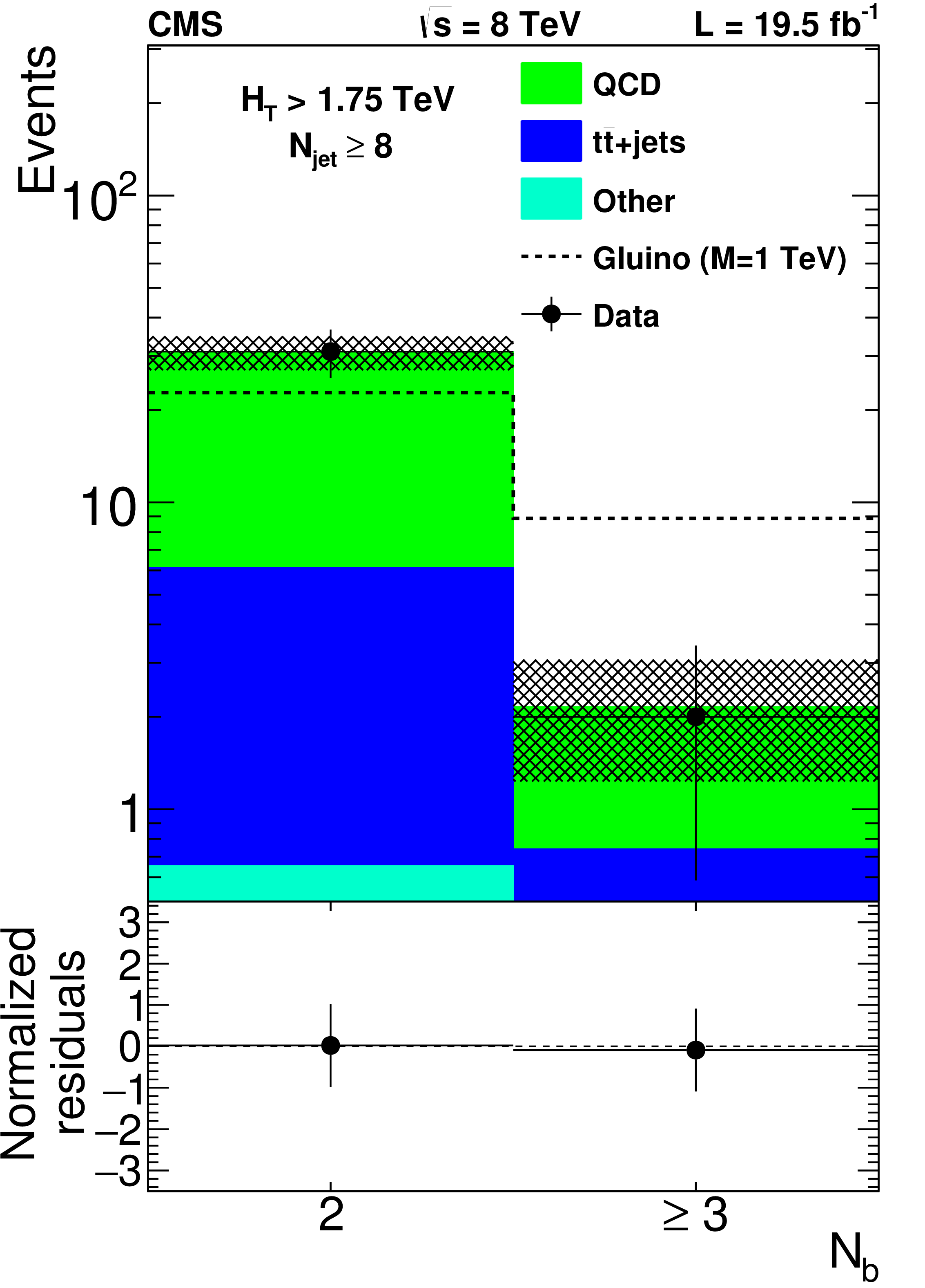
Figure 5-b:
Data(dots with error bars) and the corrected prediction of the $N_{\mathrm{ b } }$ distribution in the high-$ {N_{\text {jet}}}$ signal region. The hatched band shows the MC statistical uncertainty. The a,b (c,d) row shows events with 1.00 $ < {H_{\mathrm {T}}} < $ 1.75 TeV ($ {H_{\mathrm {T}}} > $ 1.75 TeV ). The jet multiplicity requirements are $ {N_{\text {jet}}} = $ 7 (a,c) and $ {N_{\text {jet}}} \geq$ 8 (b,d). The bottom panels of each plot show the difference between the data and corrected prediction divided by the sum in quadrature of the statistical uncertainties associated with each. |
png pdf |
Figure 5-c:
Data(dots with error bars) and the corrected prediction of the $N_{\mathrm{ b } }$ distribution in the high-$ {N_{\text {jet}}}$ signal region. The hatched band shows the MC statistical uncertainty. The a,b (c,d) row shows events with 1.00 $ < {H_{\mathrm {T}}} < $ 1.75 TeV ($ {H_{\mathrm {T}}} > $ 1.75 TeV ). The jet multiplicity requirements are $ {N_{\text {jet}}} = $ 7 (a,c) and $ {N_{\text {jet}}} \geq$ 8 (b,d). The bottom panels of each plot show the difference between the data and corrected prediction divided by the sum in quadrature of the statistical uncertainties associated with each. |
png pdf |
Figure 5-d:
Data(dots with error bars) and the corrected prediction of the $N_{\mathrm{ b } }$ distribution in the high-$ {N_{\text {jet}}}$ signal region. The hatched band shows the MC statistical uncertainty. The a,b (c,d) row shows events with 1.00 $ < {H_{\mathrm {T}}} < $ 1.75 TeV ($ {H_{\mathrm {T}}} > $ 1.75 TeV ). The jet multiplicity requirements are $ {N_{\text {jet}}} = $ 7 (a,c) and $ {N_{\text {jet}}} \geq$ 8 (b,d). The bottom panels of each plot show the difference between the data and corrected prediction divided by the sum in quadrature of the statistical uncertainties associated with each. |
png pdf |
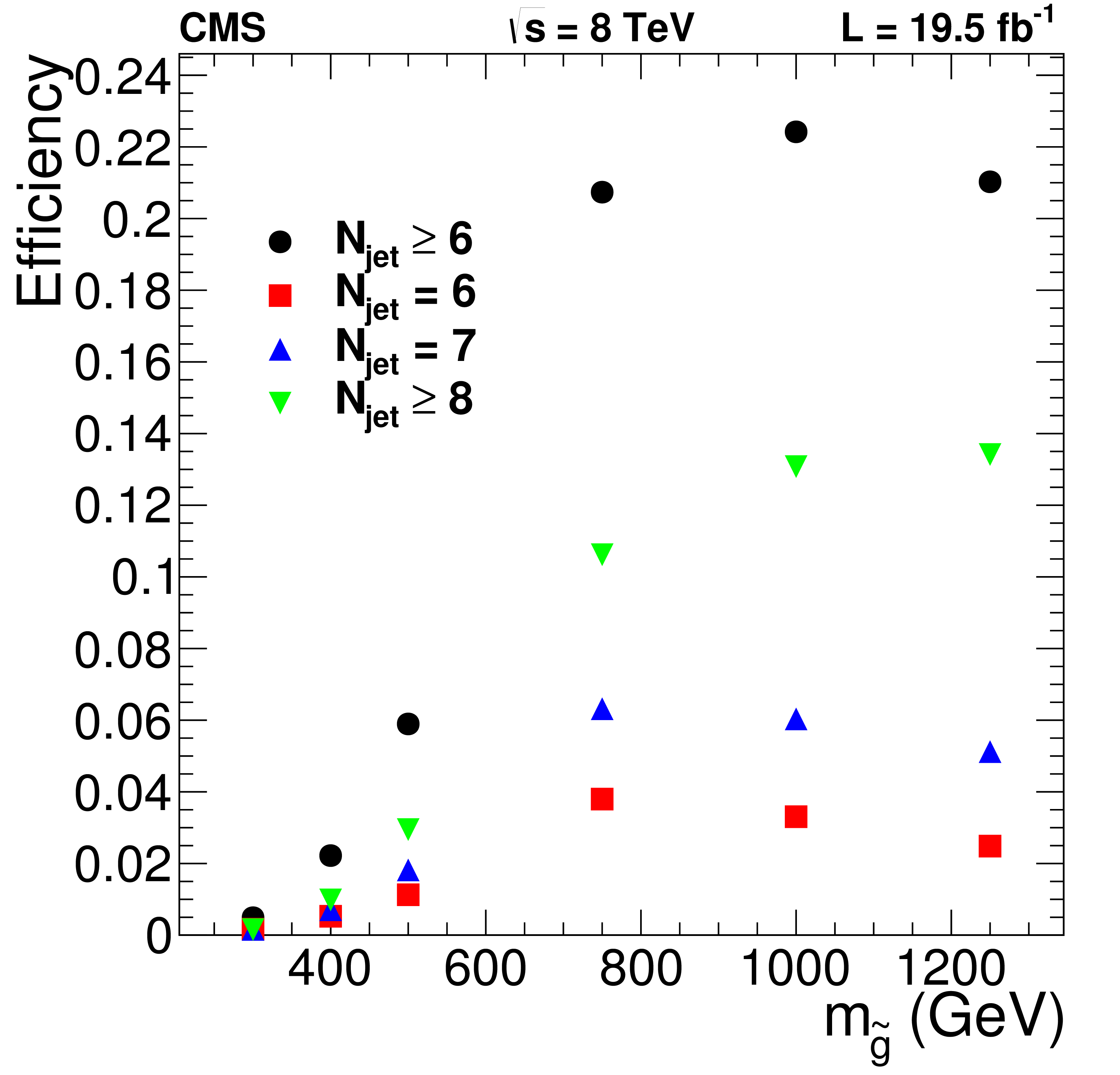
Figure 6:
Signal efficiencies as a function of $m_{\tilde{ \mathrm{ g } } }$ for $N_{\mathrm{ b } }\geq 2$, $ {H_{\mathrm {T}}} > $ 1 TeV , and $ {N_{\text {jet}}} \geq 6$, together with the breakdown among ${N_{\text {jet}}}$ bins. |
png pdf |
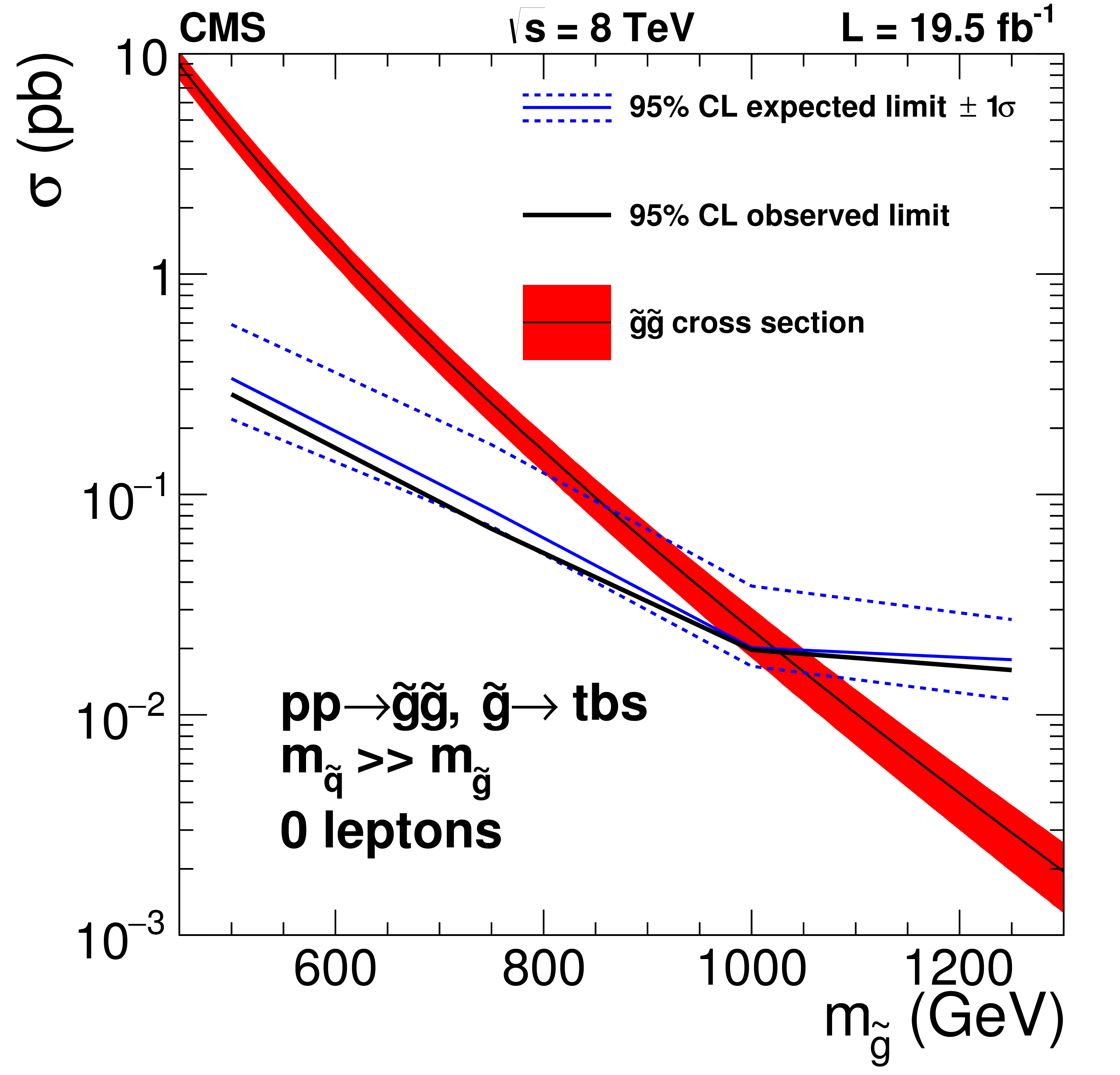
Figure 7:
The $95%$ CL limit on the gluino pair production cross section as a function of $m_{\tilde{ \mathrm{ g } } }$ in the analysis of all-hadronic final states. The signal considered is $\mathrm{ p } \mathrm{ p } \to \tilde{ \mathrm{ g } } \tilde{ \mathrm{ g } } $, followed by the decay $\tilde{ \mathrm{ g } } \to \mathrm{ t } \mathrm{ b } \mathrm{ s } $. The red band shows the theoretical cross section and its uncertainty. The blue dashed lines show the uncertainty on the expected limit. |
png pdf |
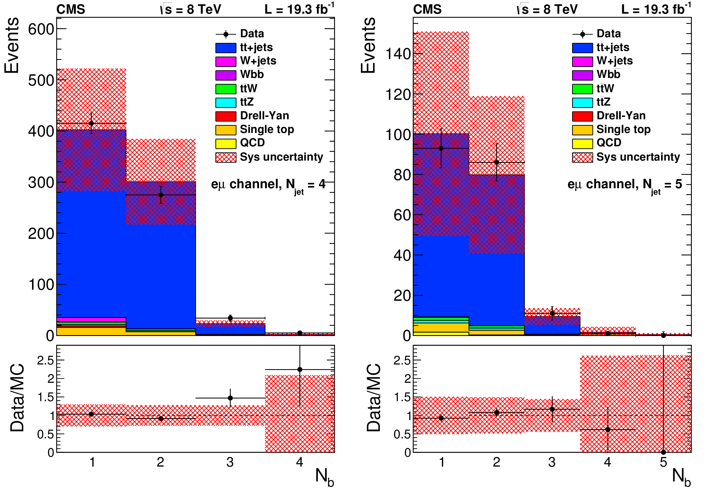
Figure 8:
Distribution of the number of b-tagged jets for events with one electron, one muon, and $ {N_{\text {jets}}} = $ 4 (a), or $ {N_{\text {jets}}} = $ 5 (b) in data, compared to the background prediction from simulation corrected for the b tagging response. The hatched region represents the total uncertainty on the background yield. |

png pdf |
Figure 8-a:
Distribution of the number of b-tagged jets for events with one electron, one muon, and $ {N_{\text {jets}}} = $ 4 (a), or $ {N_{\text {jets}}} = $ 5 (b) in data, compared to the background prediction from simulation corrected for the b tagging response. The hatched region represents the total uncertainty on the background yield. |
png pdf |
Figure 8-b:
Distribution of the number of b-tagged jets for events with one electron, one muon, and $ {N_{\text {jets}}} = $ 4 (a), or $ {N_{\text {jets}}} = $ 5 (b) in data, compared to the background prediction from simulation corrected for the b tagging response. The hatched region represents the total uncertainty on the background yield. |

png pdf |
Figure 9:
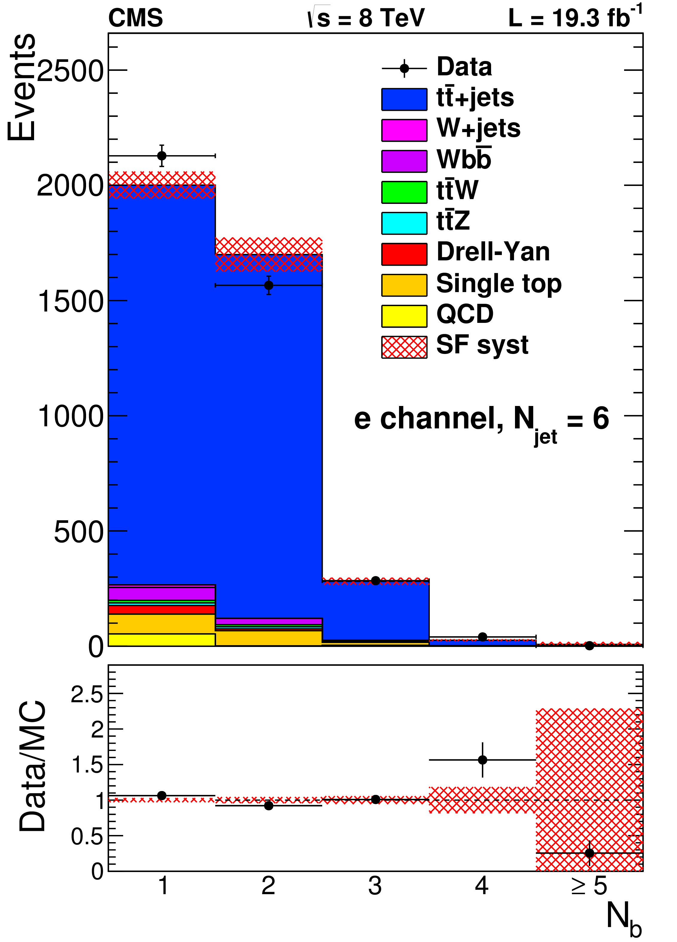
Distribution of the number of b-tagged jets for events with one electron (a,b,c) or muon (d,e,f) and 6 (a,d), 7 (b,e) or $\geq $8 (c,f) jets, compared to the background prediction from simulation corrected for the b tagging response in data. The hatched region represents the uncertainty originating from the uncertainty in the b tagging correction factors. Most other uncertainties affect only the normalization and will cancel in the fit. |
png pdf |
Figure 9-a:
Distribution of the number of b-tagged jets for events with one electron (a,b,c) or muon (d,e,f) and 6 (a,d), 7 (b,e) or $\geq $8 (c,f) jets, compared to the background prediction from simulation corrected for the b tagging response in data. The hatched region represents the uncertainty originating from the uncertainty in the b tagging correction factors. Most other uncertainties affect only the normalization and will cancel in the fit. |

png pdf |
Figure 9-b:
Distribution of the number of b-tagged jets for events with one electron (a,b,c) or muon (d,e,f) and 6 (a,d), 7 (b,e) or $\geq $8 (c,f) jets, compared to the background prediction from simulation corrected for the b tagging response in data. The hatched region represents the uncertainty originating from the uncertainty in the b tagging correction factors. Most other uncertainties affect only the normalization and will cancel in the fit. |
png pdf |
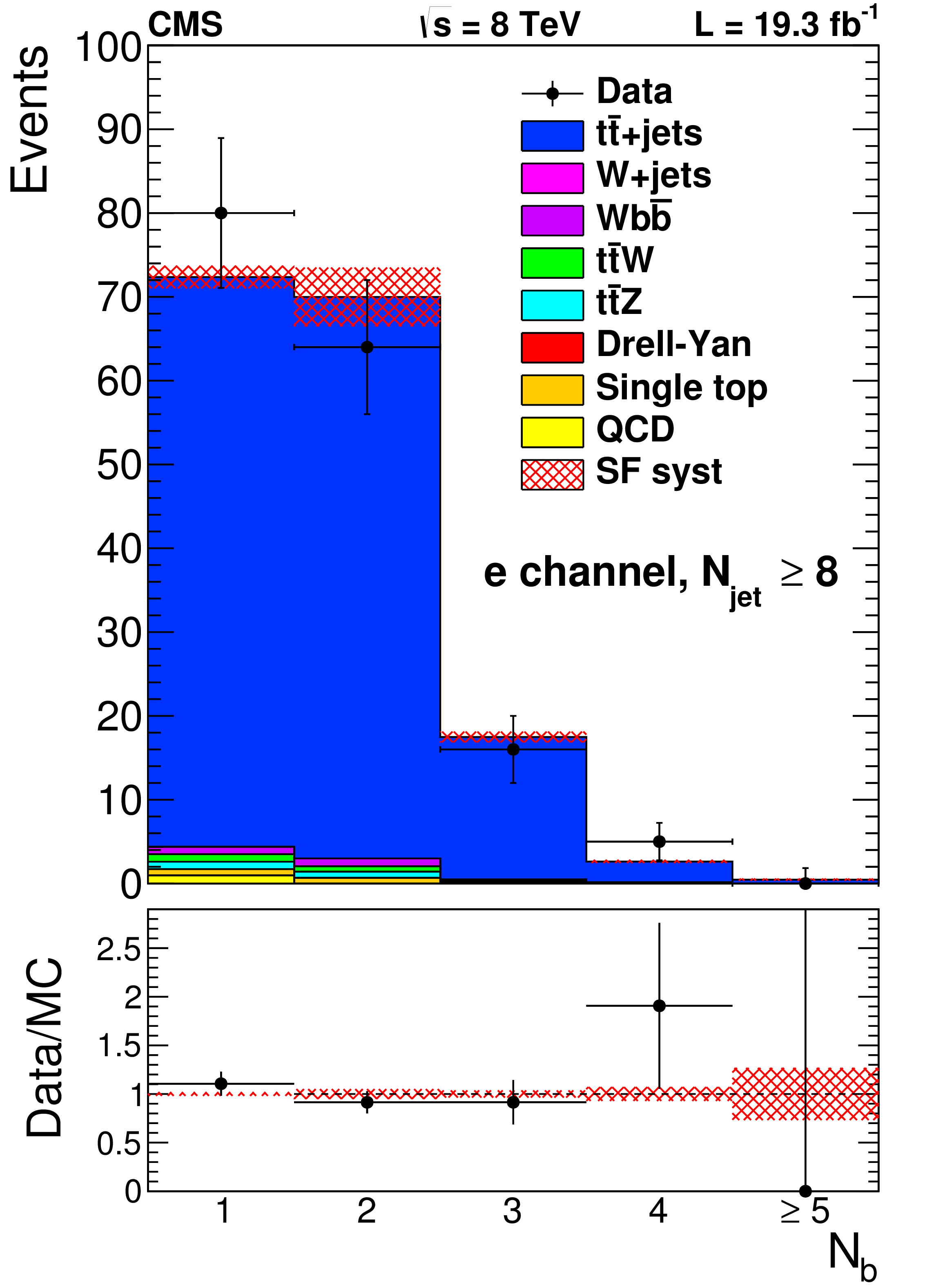
Figure 9-c:
Distribution of the number of b-tagged jets for events with one electron (a,b,c) or muon (d,e,f) and 6 (a,d), 7 (b,e) or $\geq $8 (c,f) jets, compared to the background prediction from simulation corrected for the b tagging response in data. The hatched region represents the uncertainty originating from the uncertainty in the b tagging correction factors. Most other uncertainties affect only the normalization and will cancel in the fit. |
png pdf |
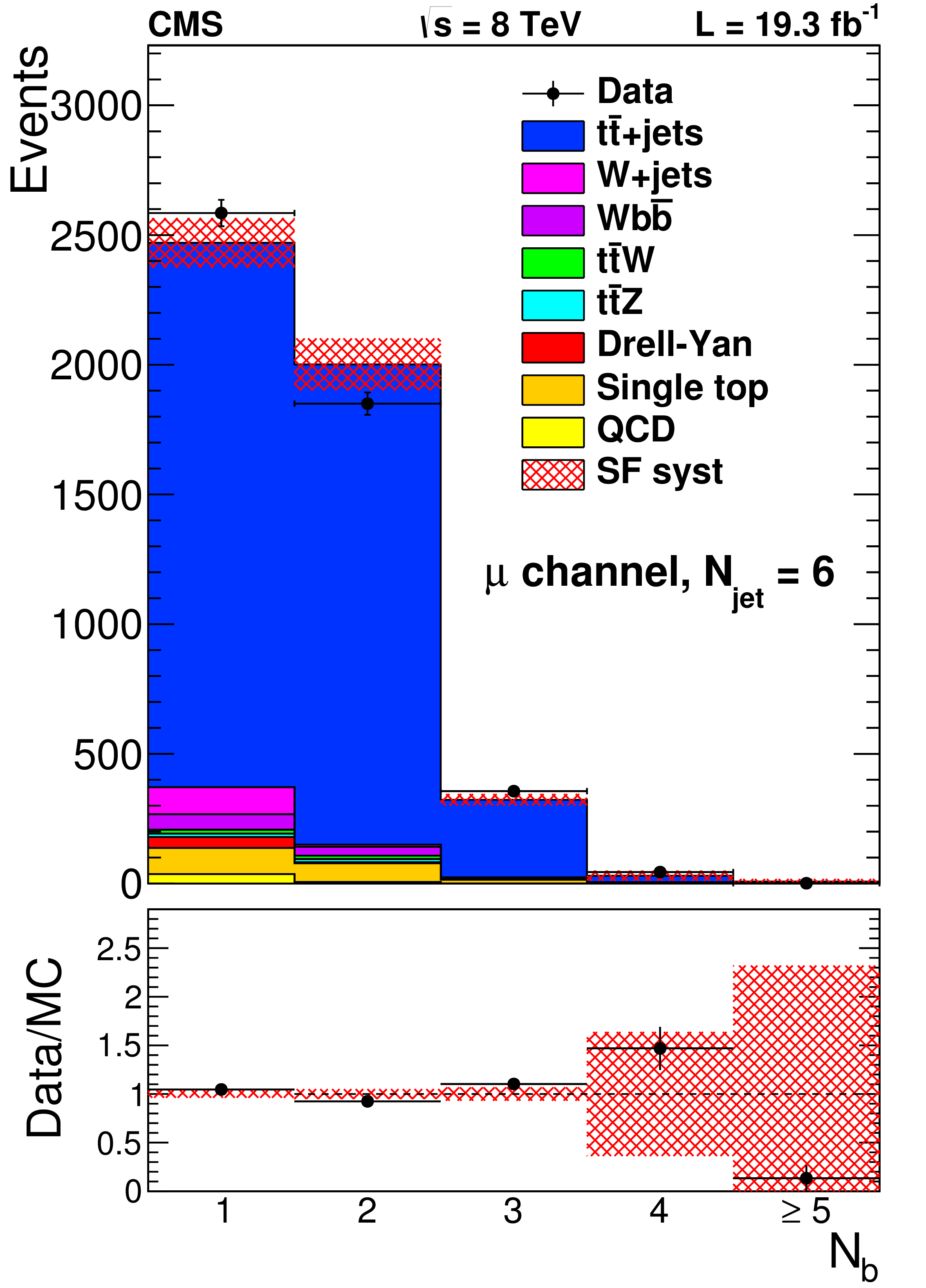
Figure 9-d:
Distribution of the number of b-tagged jets for events with one electron (a,b,c) or muon (d,e,f) and 6 (a,d), 7 (b,e) or $\geq $8 (c,f) jets, compared to the background prediction from simulation corrected for the b tagging response in data. The hatched region represents the uncertainty originating from the uncertainty in the b tagging correction factors. Most other uncertainties affect only the normalization and will cancel in the fit. |
png pdf |
Figure 9-e:
Distribution of the number of b-tagged jets for events with one electron (a,b,c) or muon (d,e,f) and 6 (a,d), 7 (b,e) or $\geq $8 (c,f) jets, compared to the background prediction from simulation corrected for the b tagging response in data. The hatched region represents the uncertainty originating from the uncertainty in the b tagging correction factors. Most other uncertainties affect only the normalization and will cancel in the fit. |
png pdf |
Figure 9-f:
Distribution of the number of b-tagged jets for events with one electron (a,b,c) or muon (d,e,f) and 6 (a,d), 7 (b,e) or $\geq $8 (c,f) jets, compared to the background prediction from simulation corrected for the b tagging response in data. The hatched region represents the uncertainty originating from the uncertainty in the b tagging correction factors. Most other uncertainties affect only the normalization and will cancel in the fit. |
png pdf |
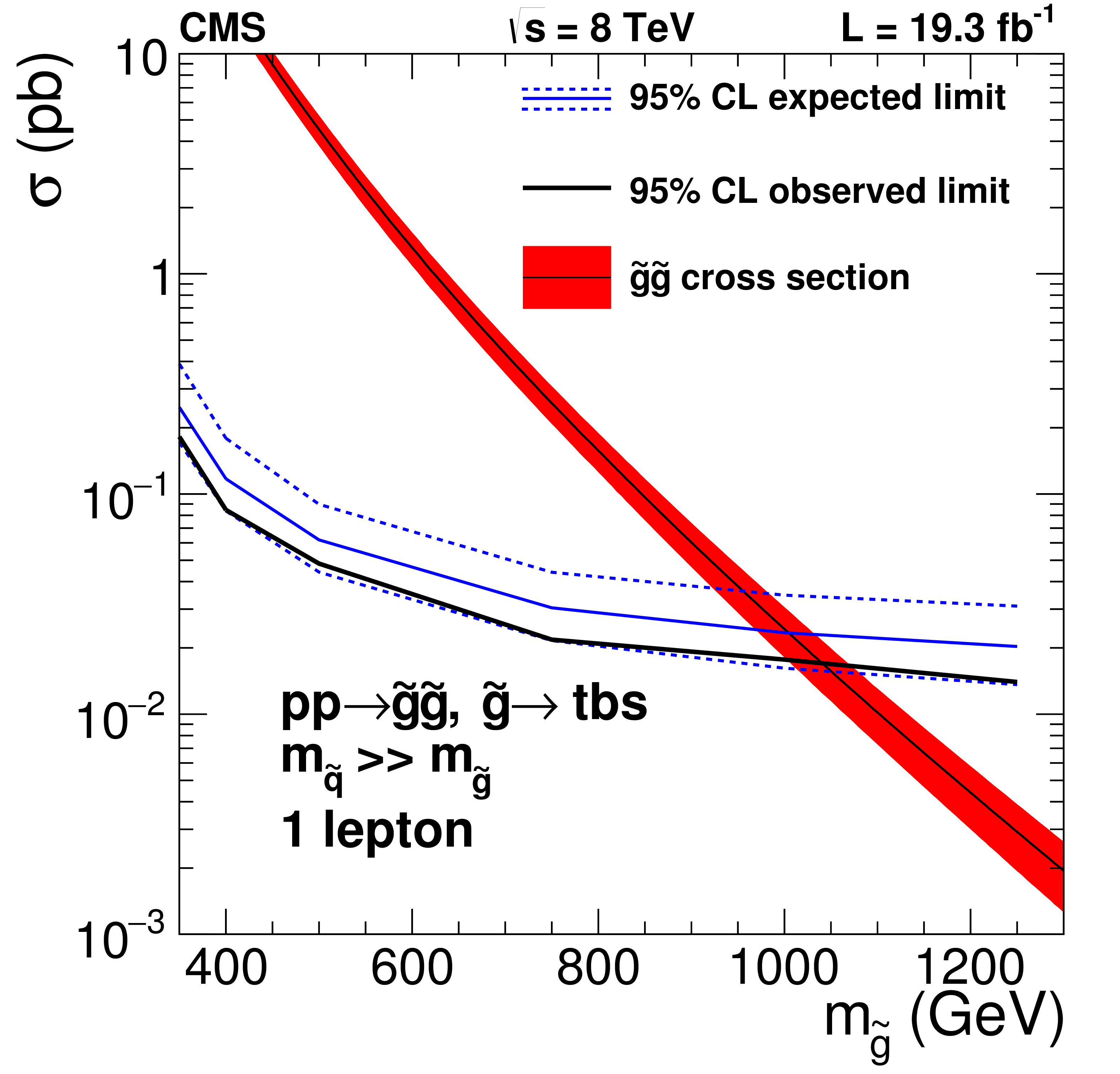
Figure 10:
The 95% CL limit on the gluino pair production cross section as a function of $m_{\tilde{ \mathrm{ g } } }$ in the one-lepton analysis. The signal considered is $\mathrm{ p } \mathrm{ p } \to \tilde{ \mathrm{ g } } \tilde{ \mathrm{ g } } $, followed by the decay $\tilde{ \mathrm{ g } } \to \mathrm{ t } \mathrm{ b } \mathrm{ s } $. The band shows the theoretical cross section and its uncertainty. The dashed lines show the uncertainty on the expected limit. |
png pdf |
Figure 11:
Diagram for pair production of bottom squarks and their RPV decay. |
png pdf |
Figure 12:
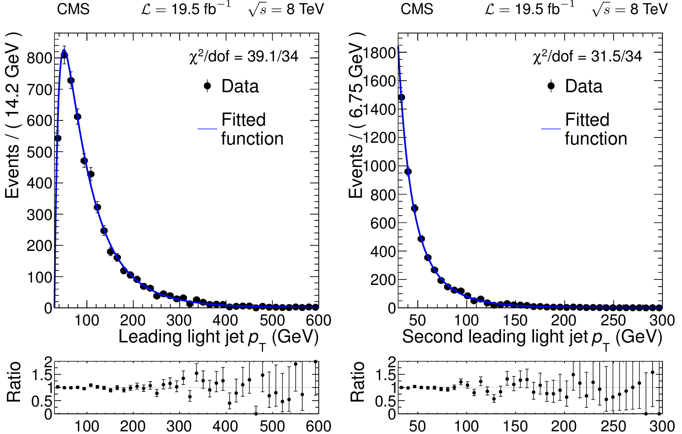
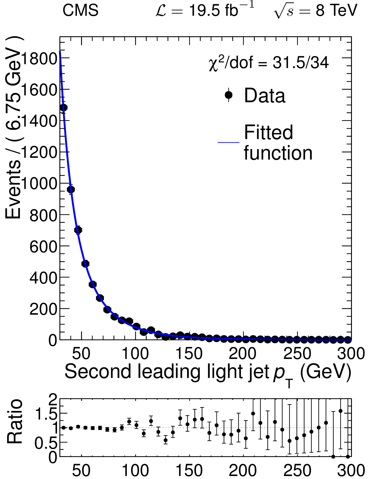
Background only likelihood fits for the light-parton jet $ {p_{\mathrm {T}}} $ distributions, with signal cross section set to zero, for the (a) leading and the (b) second-leading light-quark jet. The line represents the fitted function and the points represent the data. The ratio of the data to the fitted function is also shown. |

png pdf |
Figure 12-a:
Background only likelihood fits for the light-parton jet $ {p_{\mathrm {T}}} $ distributions, with signal cross section set to zero, for the (a) leading and the (b) second-leading light-quark jet. The line represents the fitted function and the points represent the data. The ratio of the data to the fitted function is also shown. |
png pdf |
Figure 12-b:
Background only likelihood fits for the light-parton jet $ {p_{\mathrm {T}}} $ distributions, with signal cross section set to zero, for the (a) leading and the (b) second-leading light-quark jet. The line represents the fitted function and the points represent the data. The ratio of the data to the fitted function is also shown. |
png pdf |
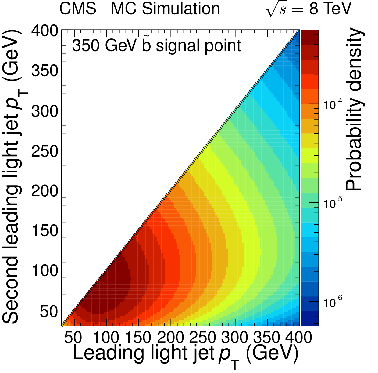
Figure 13:
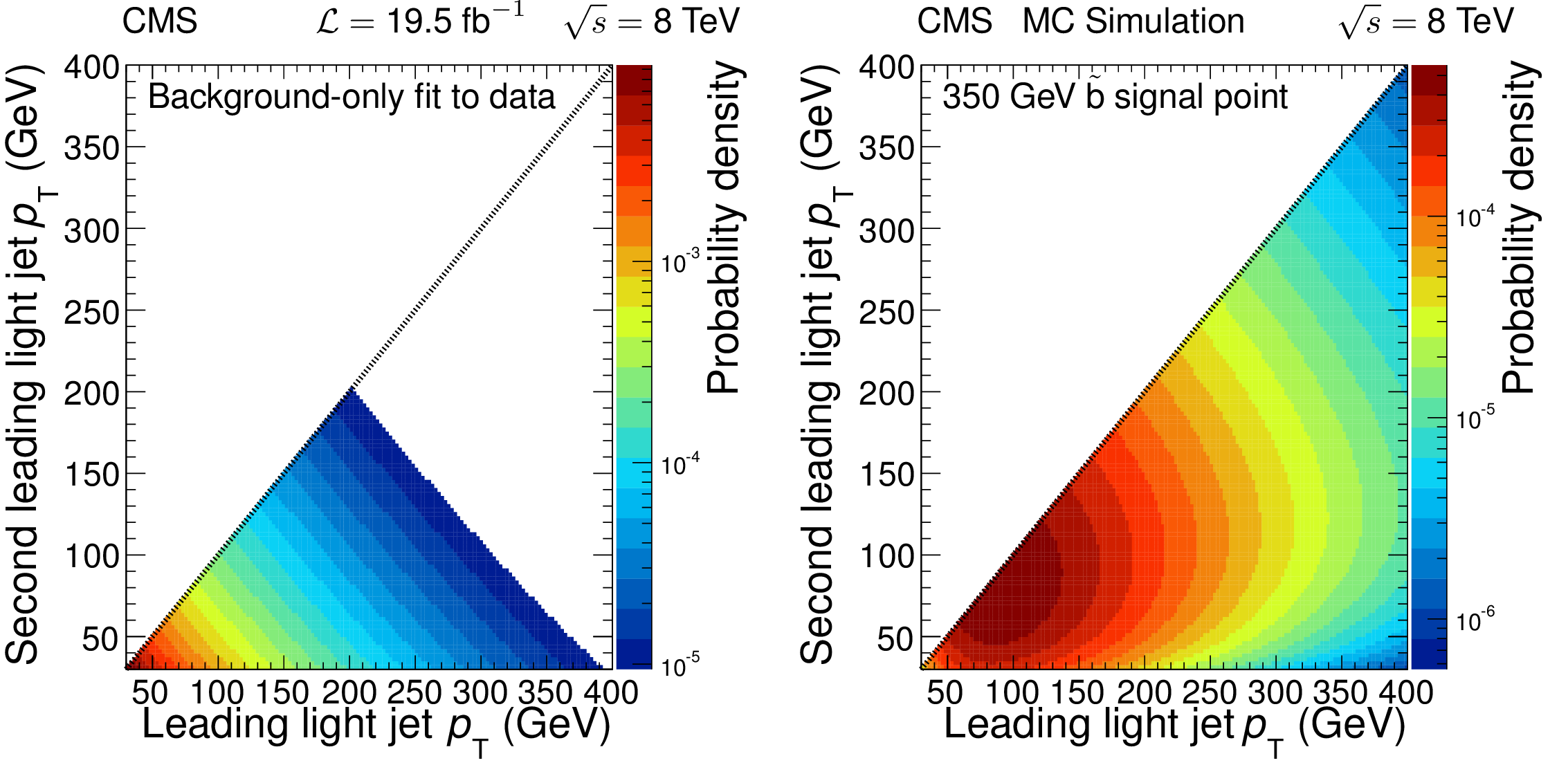
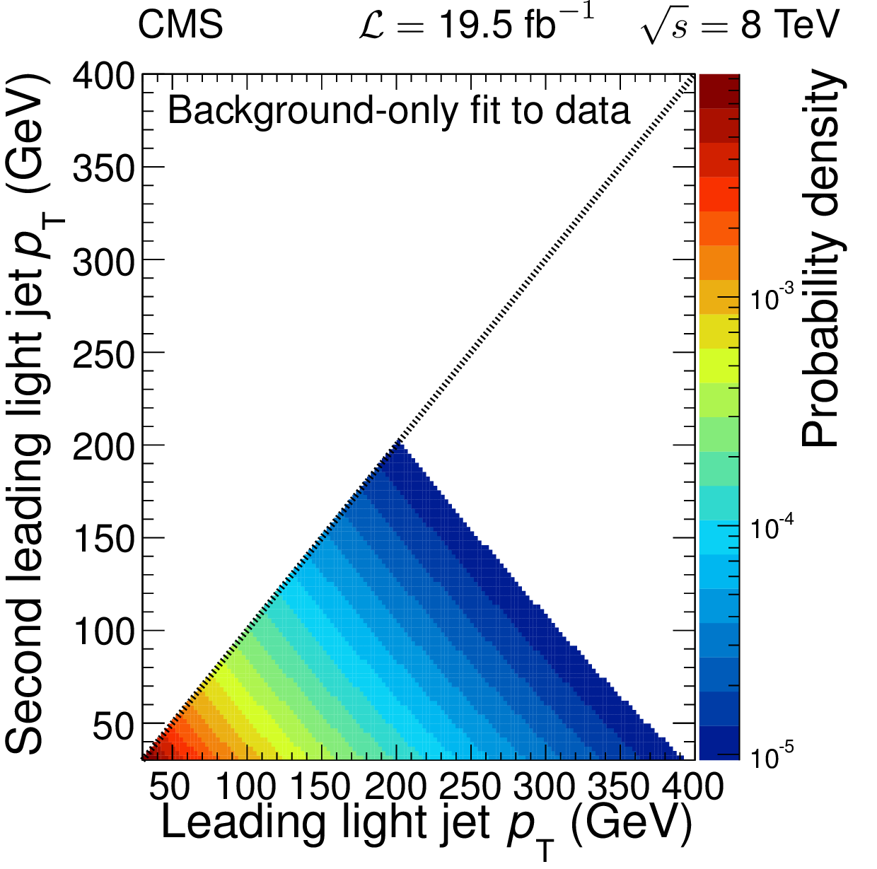
Two-dimensional light-parton jet ${p_{\mathrm {T}}}$ distributions for (a) the background-only hypothesis fit to data, and (b) the signal with $m_{\tilde{ mathrm{ b } } }= $ 350 GeV. The scales are logarithmic and a line has been drawn along the diagonal to illustrate the ordering of the jets by ${p_{\mathrm {T}}} $. |
png pdf |
Figure 13-a:
Two-dimensional light-parton jet ${p_{\mathrm {T}}}$ distributions for (a) the background-only hypothesis fit to data, and (b) the signal with $m_{\tilde{ mathrm{ b } } }= $ 350 GeV. The scales are logarithmic and a line has been drawn along the diagonal to illustrate the ordering of the jets by ${p_{\mathrm {T}}} $. |
png pdf |
Figure 13-b:
Two-dimensional light-parton jet ${p_{\mathrm {T}}}$ distributions for (a) the background-only hypothesis fit to data, and (b) the signal with $m_{\tilde{ mathrm{ b } } }= $ 350 GeV. The scales are logarithmic and a line has been drawn along the diagonal to illustrate the ordering of the jets by ${p_{\mathrm {T}}} $. |
png pdf |
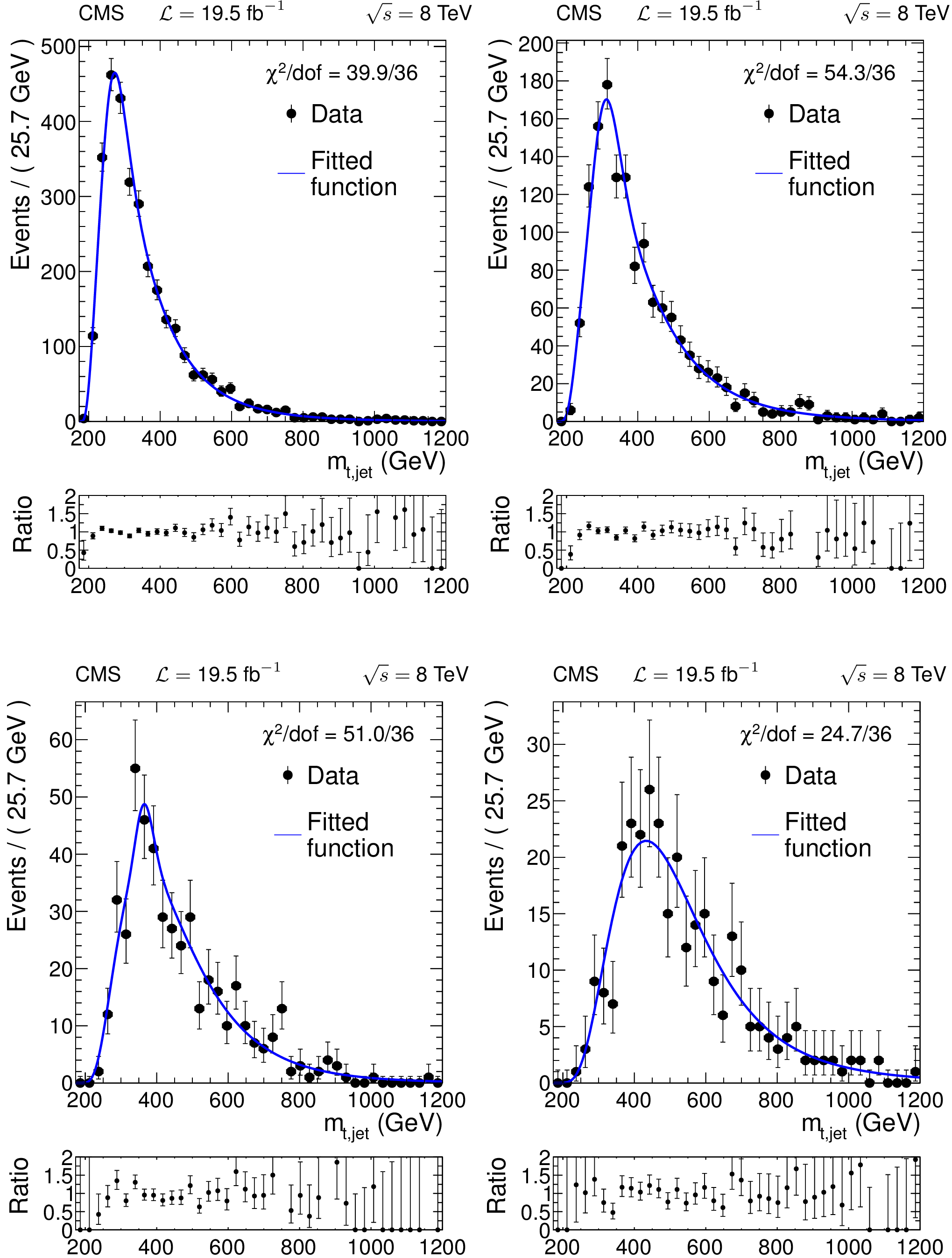
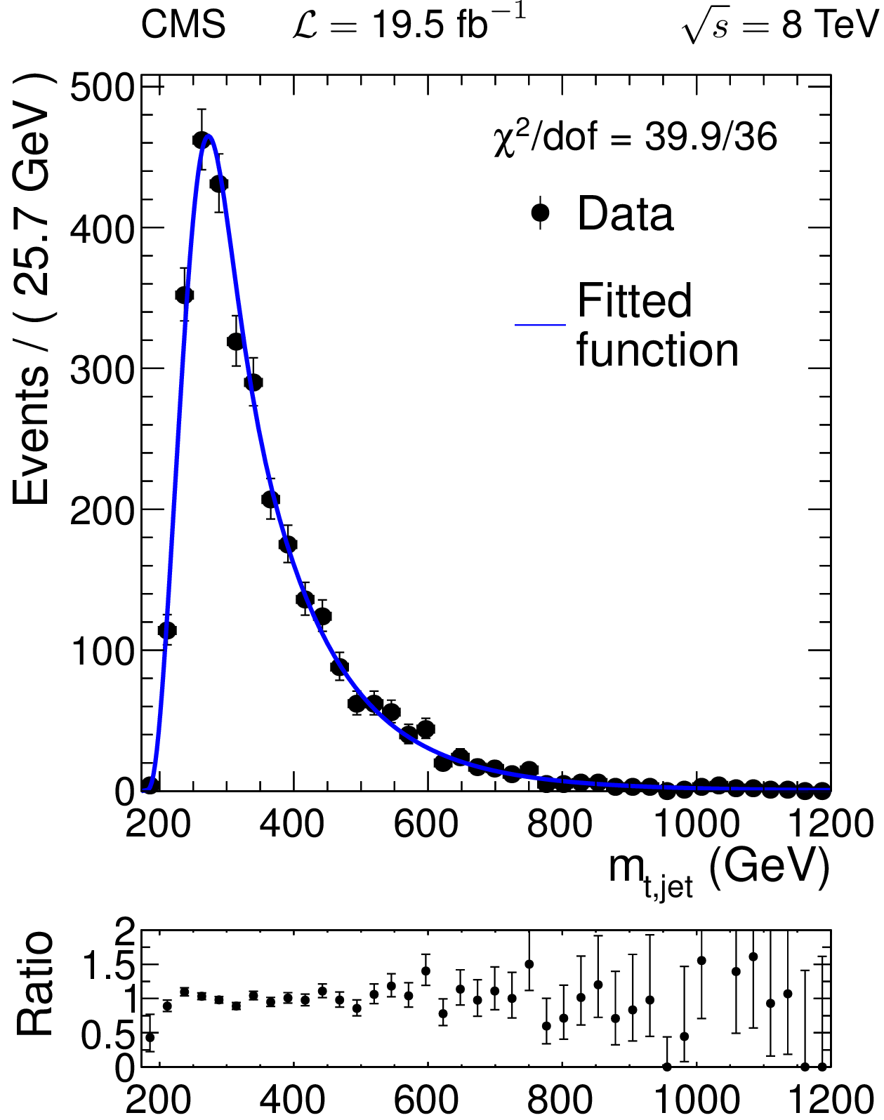
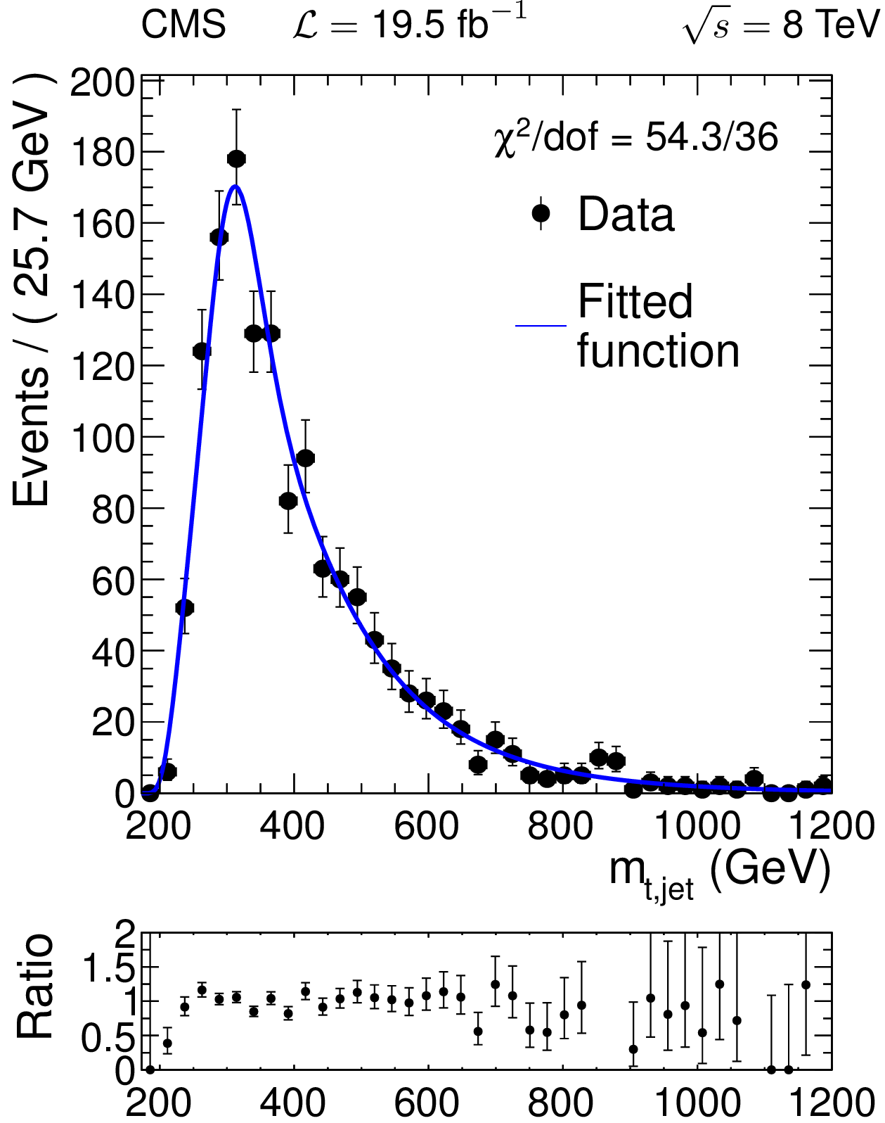
Figure 14:
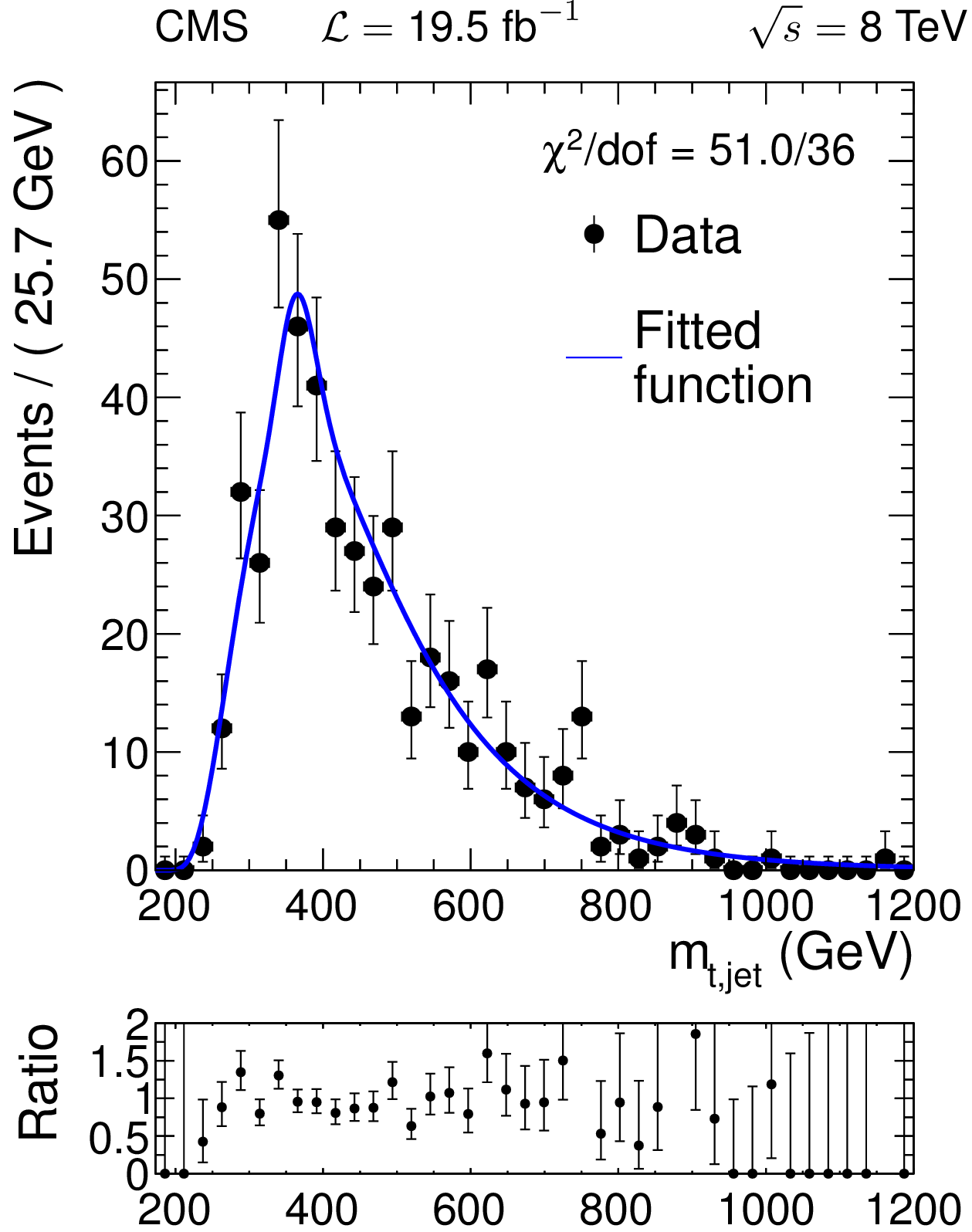
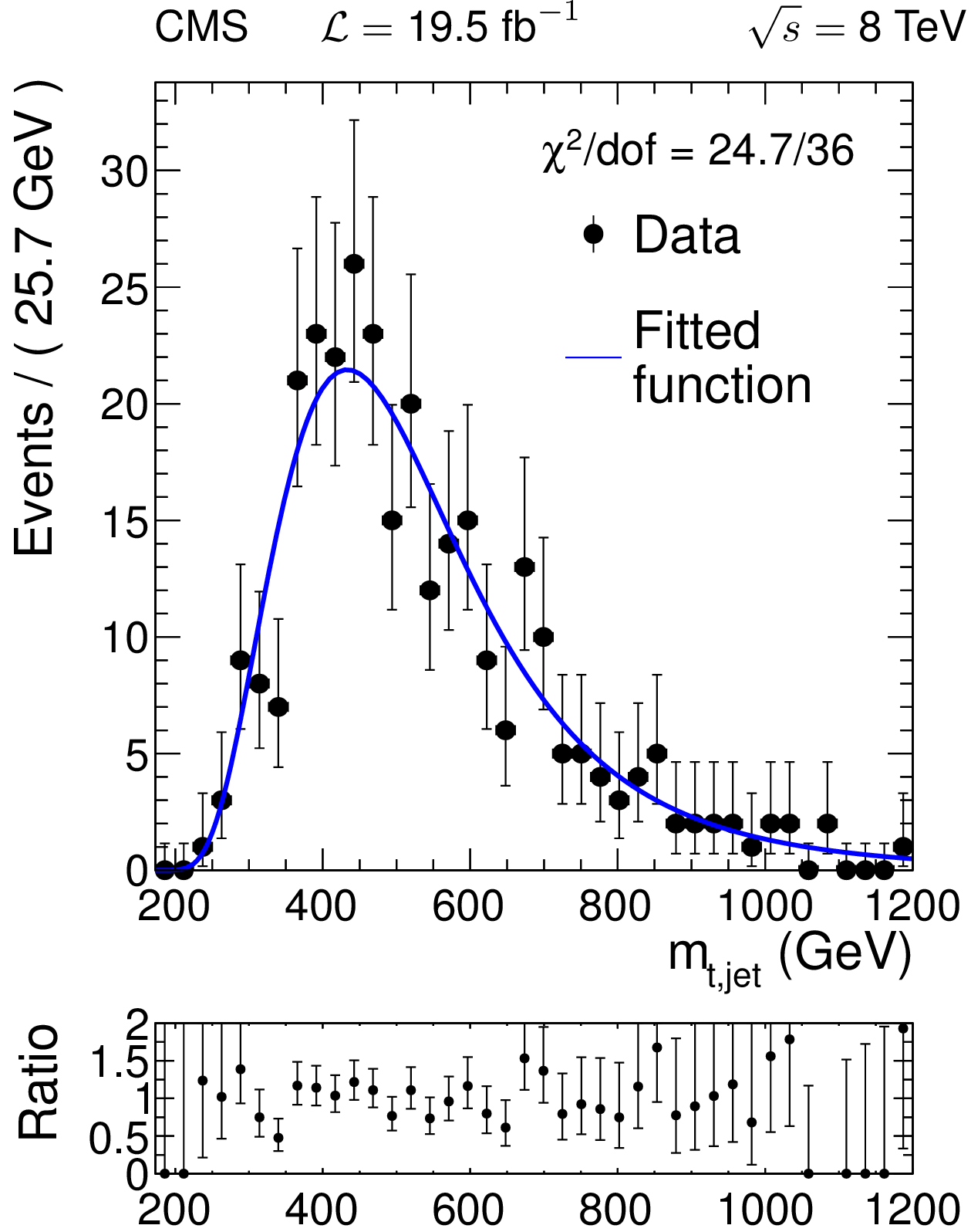
Reconstructed invariant mass distributions for data together with the result of the likelihood function maximization with signal cross section set to zero for the four light-parton jet regions defined in Table 5: CR (a), SR1 (b), SR2 (c) and SR3 (d). |
png pdf |
Figure 14-a:
Reconstructed invariant mass distributions for data together with the result of the likelihood function maximization with signal cross section set to zero for the four light-parton jet regions defined in Table 5: CR (a), SR1 (b), SR2 (c) and SR3 (d). |
png pdf |
Figure 14-b:
Reconstructed invariant mass distributions for data together with the result of the likelihood function maximization with signal cross section set to zero for the four light-parton jet regions defined in Table 5: CR (a), SR1 (b), SR2 (c) and SR3 (d). |
png pdf |
Figure 14-c:
Reconstructed invariant mass distributions for data together with the result of the likelihood function maximization with signal cross section set to zero for the four light-parton jet regions defined in Table 5: CR (a), SR1 (b), SR2 (c) and SR3 (d). |
png pdf |
Figure 14-d:
Reconstructed invariant mass distributions for data together with the result of the likelihood function maximization with signal cross section set to zero for the four light-parton jet regions defined in Table 5: CR (a), SR1 (b), SR2 (c) and SR3 (d). |

png pdf |
Figure 15:
Observed and expected 95% CL upper limits on the production cross section of $\tilde{ mathrm{ b } } $ pairs, where the $\tilde{ mathrm{ b } } $ decays to a top and down (strange) quark via the RPV coupling $\lambda ''_{331}$ ($\lambda ''_{332}$), as a function of $\tilde{ mathrm{ b } } $ mass derived using ${\mathrm {CL}_\mathrm {s}}$ intervals. The difference between observed and expected limits is correlated between neighboring signal points. The hatched region represents the theoretical uncertainty on the signal cross section. |

png pdf |
Figure 16:
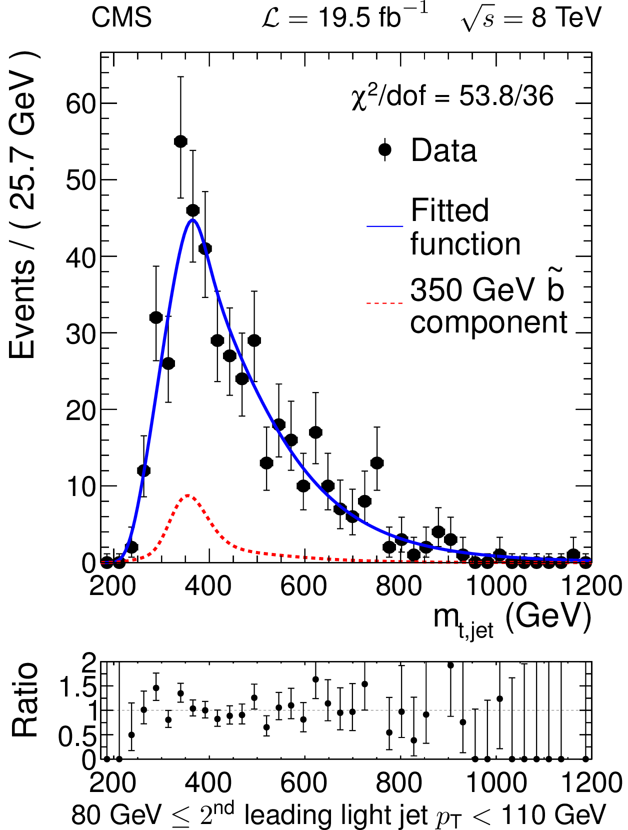
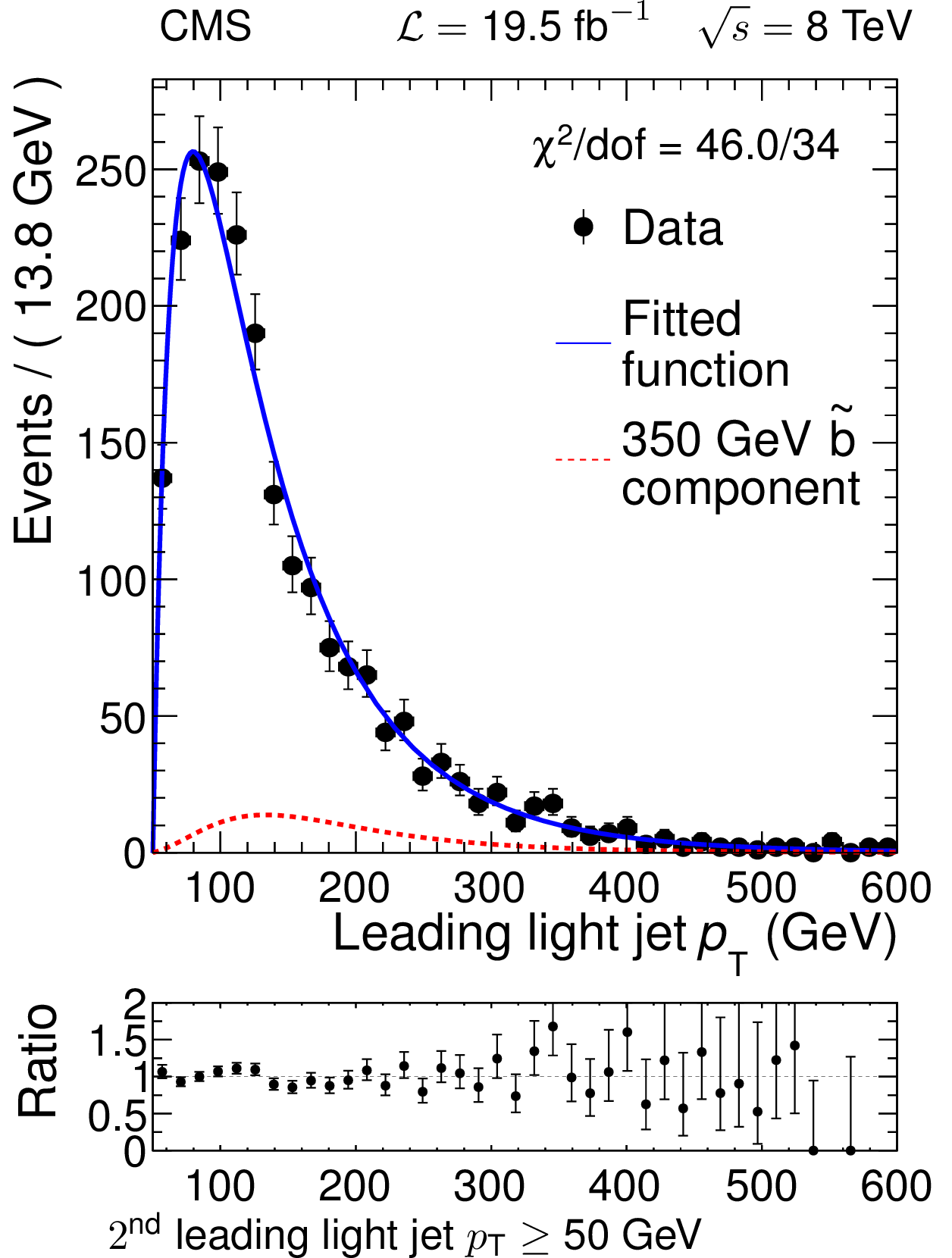
Results of likelihood maximization with the signal cross section set to the calculated 95% CL upper limit of the 350 GeV $\tilde{ mathrm{ b } } $ point. The solid line shows the fitted function, the dashed line shows the signal component, and the points show the data. The ratio of the data to the fitted function is also shown. From a to c, these are the invariant mass distribution in SR2, the invariant mass distribution in SR3, and the leading light jet $ {p_{\mathrm {T}}} $ distribution for events with $ {p_{\mathrm {T}}} ^{(2)}> $ 50 GeV. |
png pdf |
Figure 16-a:
Results of likelihood maximization with the signal cross section set to the calculated 95% CL upper limit of the 350 GeV $\tilde{ mathrm{ b } } $ point. The solid line shows the fitted function, the dashed line shows the signal component, and the points show the data. The ratio of the data to the fitted function is also shown. From a to c, these are the invariant mass distribution in SR2, the invariant mass distribution in SR3, and the leading light jet $ {p_{\mathrm {T}}} $ distribution for events with $ {p_{\mathrm {T}}} ^{(2)}> $ 50 GeV. |

png pdf |
Figure 16-b:
Results of likelihood maximization with the signal cross section set to the calculated 95% CL upper limit of the 350 GeV $\tilde{ mathrm{ b } } $ point. The solid line shows the fitted function, the dashed line shows the signal component, and the points show the data. The ratio of the data to the fitted function is also shown. From a to c, these are the invariant mass distribution in SR2, the invariant mass distribution in SR3, and the leading light jet $ {p_{\mathrm {T}}} $ distribution for events with $ {p_{\mathrm {T}}} ^{(2)}> $ 50 GeV. |
png pdf |
Figure 16-c:
Results of likelihood maximization with the signal cross section set to the calculated 95% CL upper limit of the 350 GeV $\tilde{ mathrm{ b } } $ point. The solid line shows the fitted function, the dashed line shows the signal component, and the points show the data. The ratio of the data to the fitted function is also shown. From a to c, these are the invariant mass distribution in SR2, the invariant mass distribution in SR3, and the leading light jet $ {p_{\mathrm {T}}} $ distribution for events with $ {p_{\mathrm {T}}} ^{(2)}> $ 50 GeV. |
png pdf |
Figure 17:
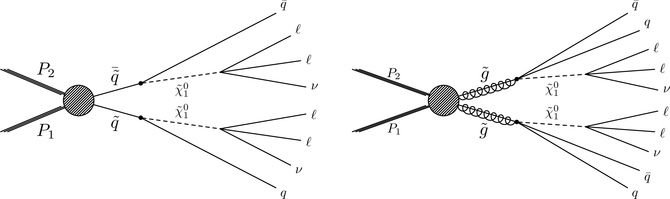
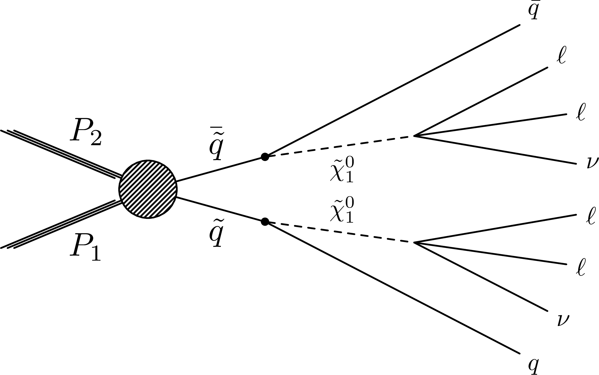
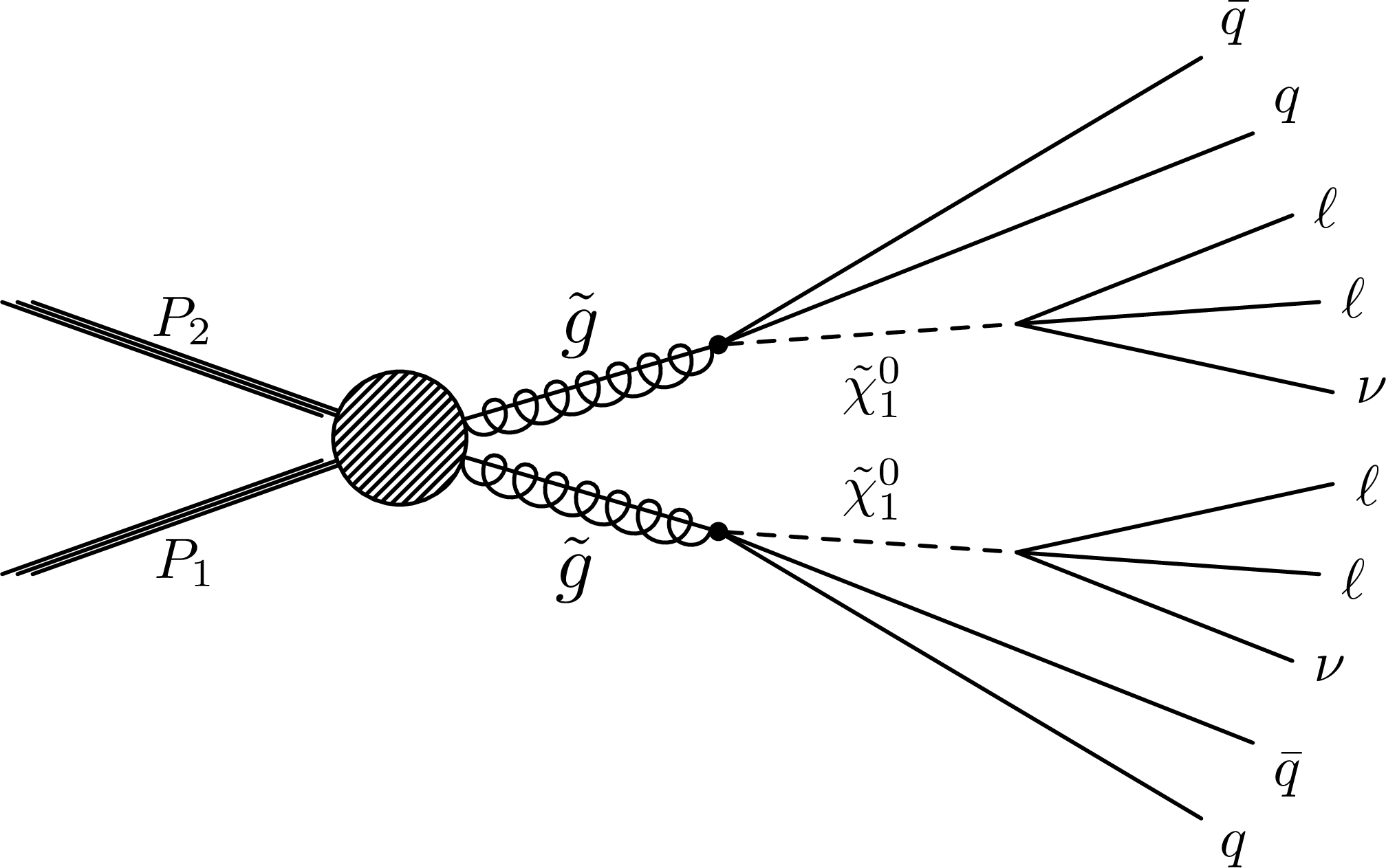
Diagrams of two simplified models with RPV [43]. a : A simplified model featuring squark pair production, with $\tilde{ \mathrm{ q } } \to \mathrm{ q } \tilde{\chi}^0_1 $, and $m(\tilde{ \mathrm{ g } } ) \gg m(\tilde{ \mathrm{ q } } )$. b : A simplified model featuring gluino pair production, with $\tilde{ \mathrm{ g } } \to \mathrm{ q } \mathrm{ \bar{q} } \tilde{\chi}^0_1 $, and $m(\tilde{ \mathrm{ q } } ) \gg m(\tilde{ \mathrm{ g } } )$. In both models the neutralinos decay to two charged leptons and a neutrino via an RPV term. |
png pdf |
Figure 17-a:
Diagrams of two simplified models with RPV [43]. a : A simplified model featuring squark pair production, with $\tilde{ \mathrm{ q } } \to \mathrm{ q } \tilde{\chi}^0_1 $, and $m(\tilde{ \mathrm{ g } } ) \gg m(\tilde{ \mathrm{ q } } )$. b : A simplified model featuring gluino pair production, with $\tilde{ \mathrm{ g } } \to \mathrm{ q } \mathrm{ \bar{q} } \tilde{\chi}^0_1 $, and $m(\tilde{ \mathrm{ q } } ) \gg m(\tilde{ \mathrm{ g } } )$. In both models the neutralinos decay to two charged leptons and a neutrino via an RPV term. |
png pdf |
Figure 17-b:
Diagrams of two simplified models with RPV [43]. a : A simplified model featuring squark pair production, with $\tilde{ \mathrm{ q } } \to \mathrm{ q } \tilde{\chi}^0_1 $, and $m(\tilde{ \mathrm{ g } } ) \gg m(\tilde{ \mathrm{ q } } )$. b : A simplified model featuring gluino pair production, with $\tilde{ \mathrm{ g } } \to \mathrm{ q } \mathrm{ \bar{q} } \tilde{\chi}^0_1 $, and $m(\tilde{ \mathrm{ q } } ) \gg m(\tilde{ \mathrm{ g } } )$. In both models the neutralinos decay to two charged leptons and a neutrino via an RPV term. |

png pdf |
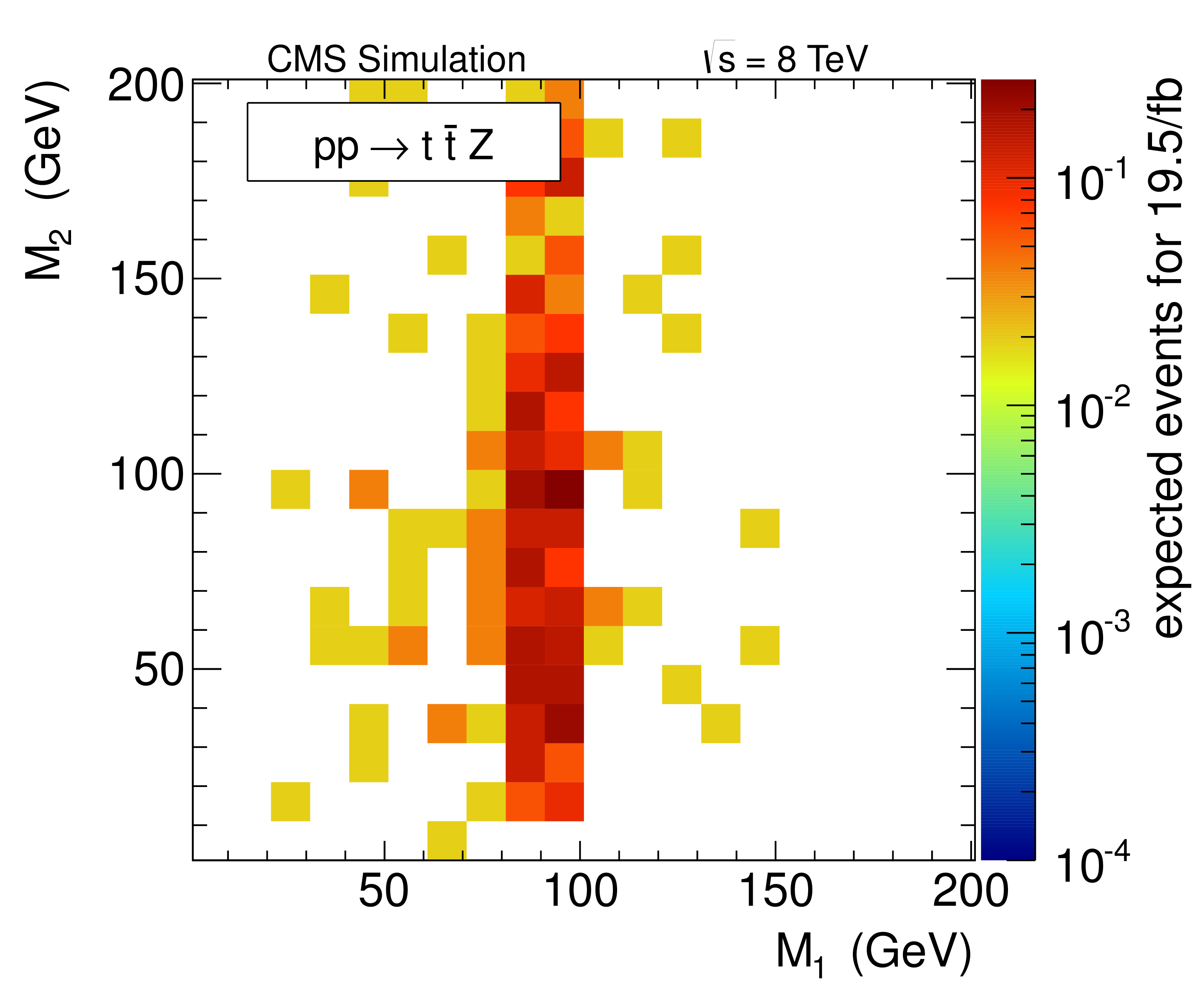
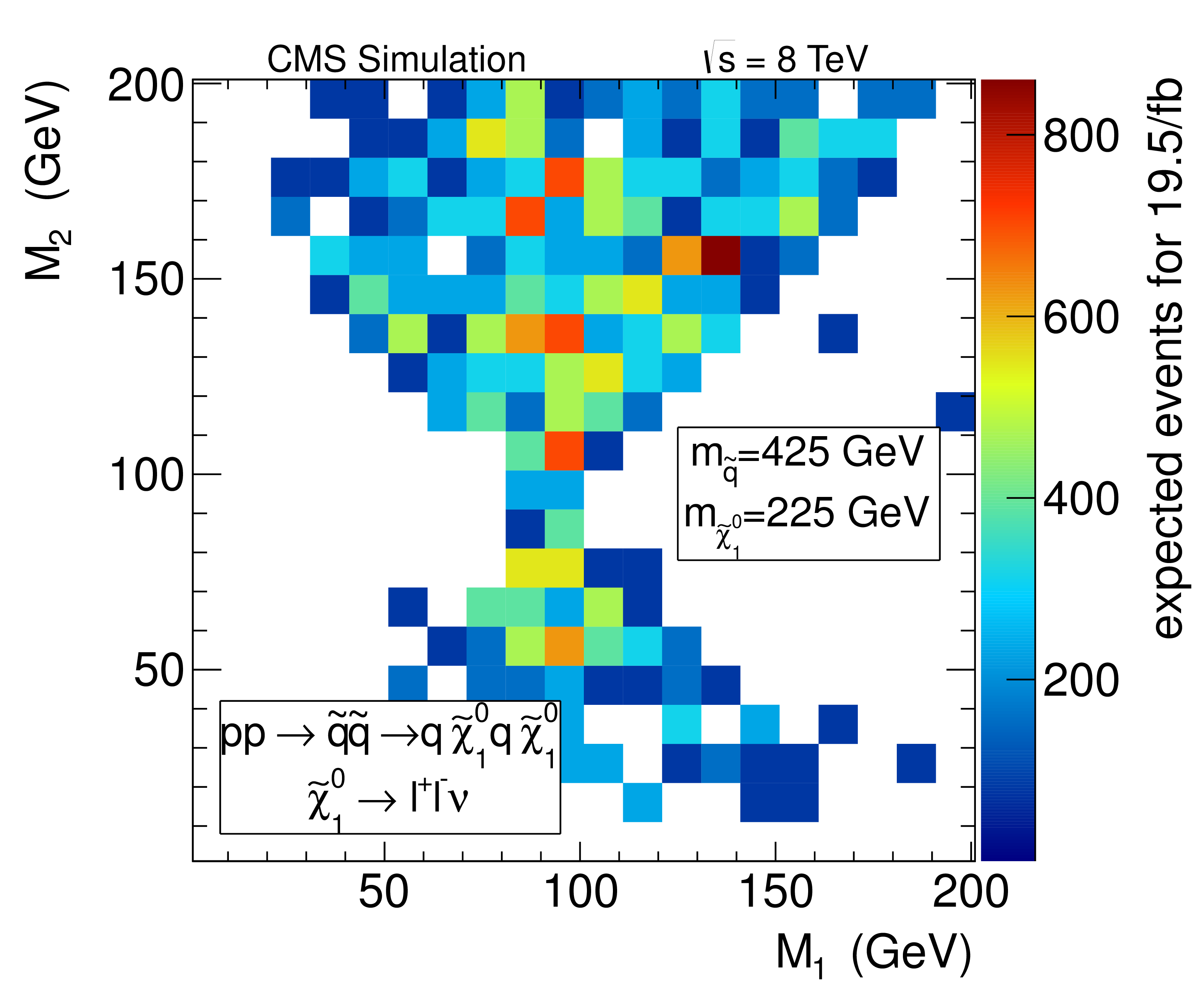
Figure 18:
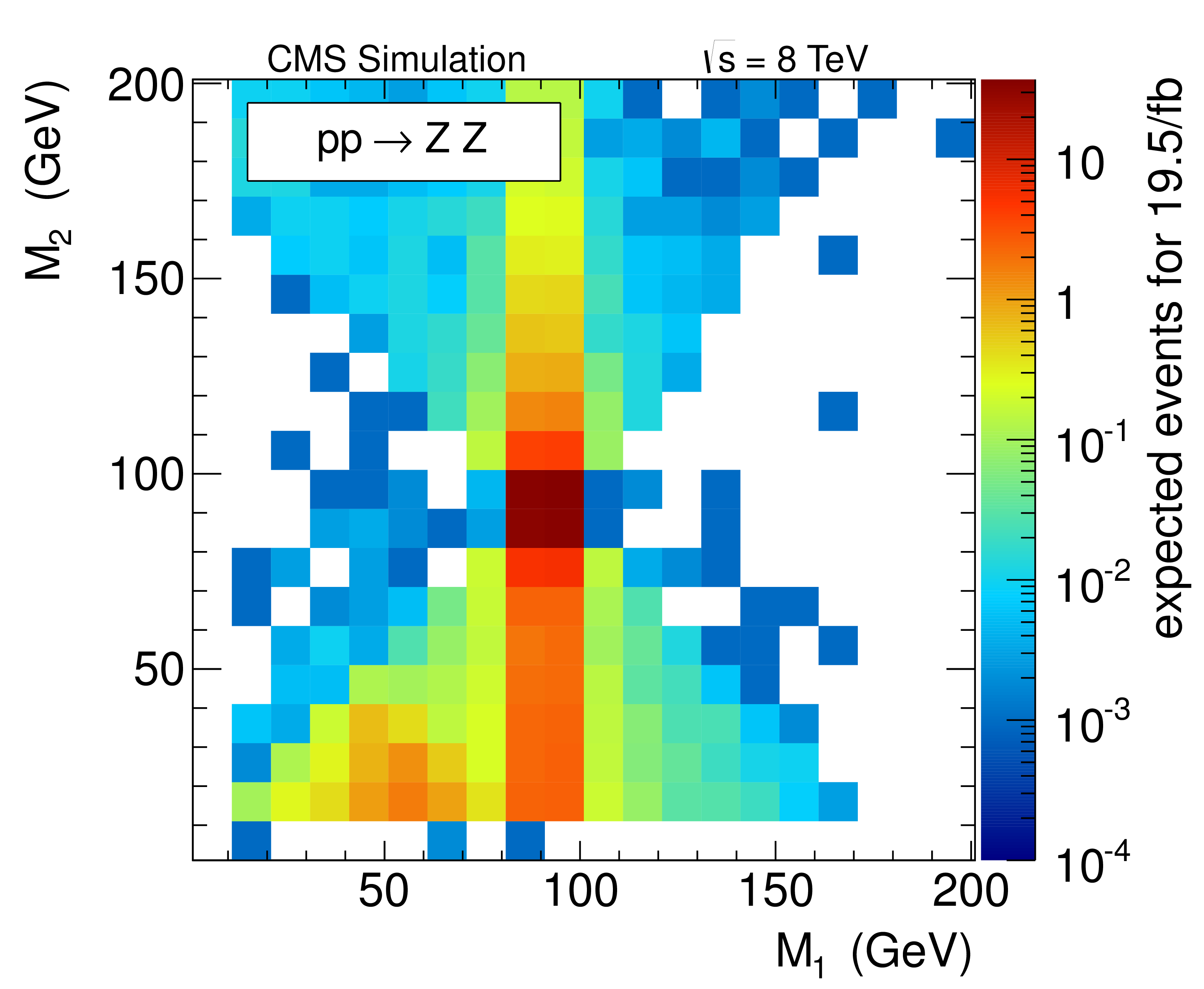
Expected shapes of the $(M_1,\, M_2)$ distribution for the ${\mathrm{ Z } } {\mathrm{ Z } } $ background (a), $ {\mathrm{ t \bar{t} } } {\mathrm{ Z } } $ background (b), $ {\mathrm{ t \bar{t} } } \mathrm{ W } \mathrm{ W } $ background (c), as well as for the model of Fig. 17 (a) with $m_{\tilde{ \mathrm{ q } } }= $ 425 GeV and $m_{\tilde{\chi}^0_1 }= $ 225 GeV (d). |
png pdf |
Figure 18-a:
Expected shapes of the $(M_1,\, M_2)$ distribution for the ${\mathrm{ Z } } {\mathrm{ Z } } $ background (a), $ {\mathrm{ t \bar{t} } } {\mathrm{ Z } } $ background (b), $ {\mathrm{ t \bar{t} } } \mathrm{ W } \mathrm{ W } $ background (c), as well as for the model of Fig. 17 (a) with $m_{\tilde{ \mathrm{ q } } }= $ 425 GeV and $m_{\tilde{\chi}^0_1 }= $ 225 GeV (d). |
png pdf |
Figure 18-b:
Expected shapes of the $(M_1,\, M_2)$ distribution for the ${\mathrm{ Z } } {\mathrm{ Z } } $ background (a), $ {\mathrm{ t \bar{t} } } {\mathrm{ Z } } $ background (b), $ {\mathrm{ t \bar{t} } } \mathrm{ W } \mathrm{ W } $ background (c), as well as for the model of Fig. 17 (a) with $m_{\tilde{ \mathrm{ q } } }= $ 425 GeV and $m_{\tilde{\chi}^0_1 }= $ 225 GeV (d). |

png pdf |
Figure 18-c:
Expected shapes of the $(M_1,\, M_2)$ distribution for the ${\mathrm{ Z } } {\mathrm{ Z } } $ background (a), $ {\mathrm{ t \bar{t} } } {\mathrm{ Z } } $ background (b), $ {\mathrm{ t \bar{t} } } \mathrm{ W } \mathrm{ W } $ background (c), as well as for the model of Fig. 17 (a) with $m_{\tilde{ \mathrm{ q } } }= $ 425 GeV and $m_{\tilde{\chi}^0_1 }= $ 225 GeV (d). |
png pdf |
Figure 18-d:
Expected shapes of the $(M_1,\, M_2)$ distribution for the ${\mathrm{ Z } } {\mathrm{ Z } } $ background (a), $ {\mathrm{ t \bar{t} } } {\mathrm{ Z } } $ background (b), $ {\mathrm{ t \bar{t} } } \mathrm{ W } \mathrm{ W } $ background (c), as well as for the model of Fig. 17 (a) with $m_{\tilde{ \mathrm{ q } } }= $ 425 GeV and $m_{\tilde{\chi}^0_1 }= $ 225 GeV (d). |
png pdf |
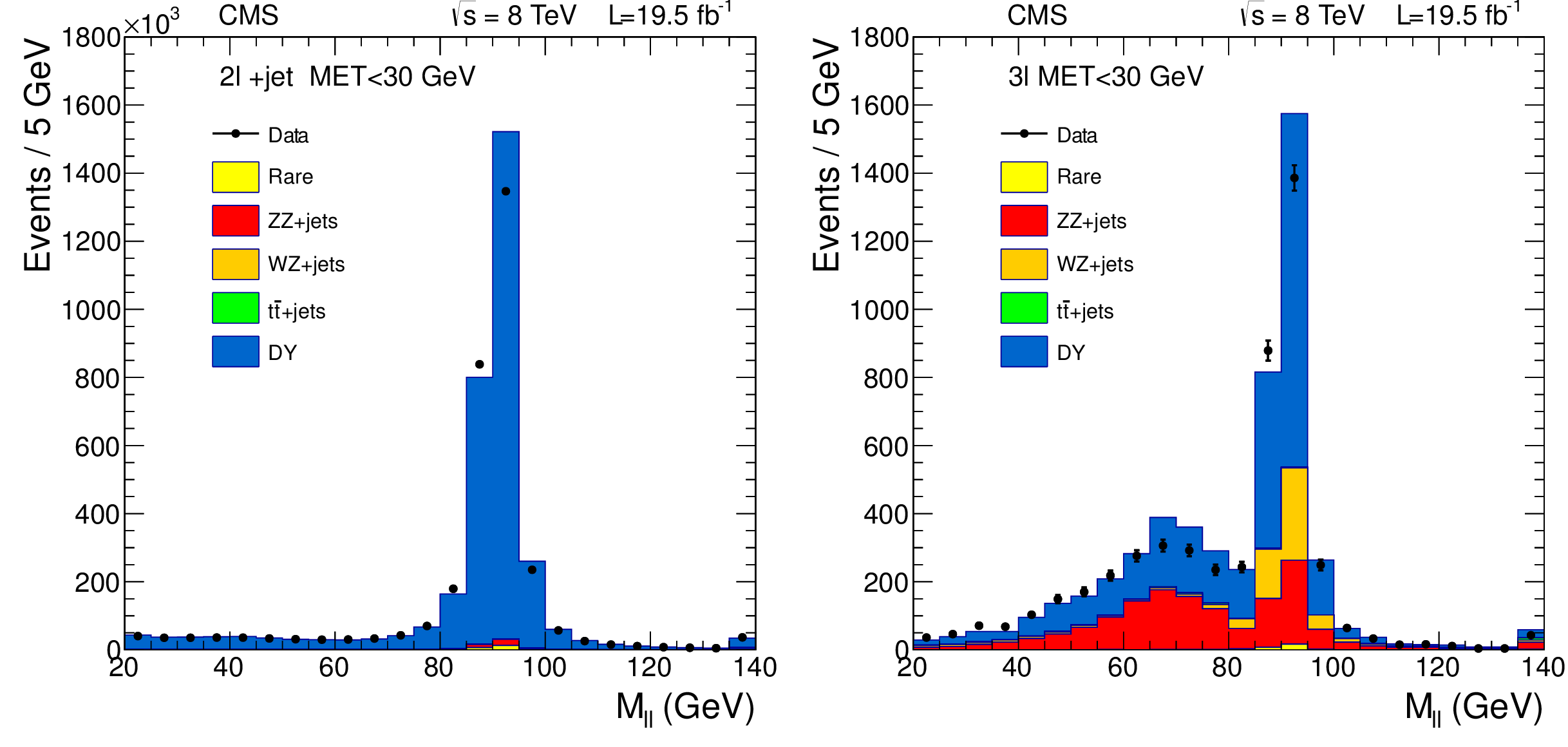
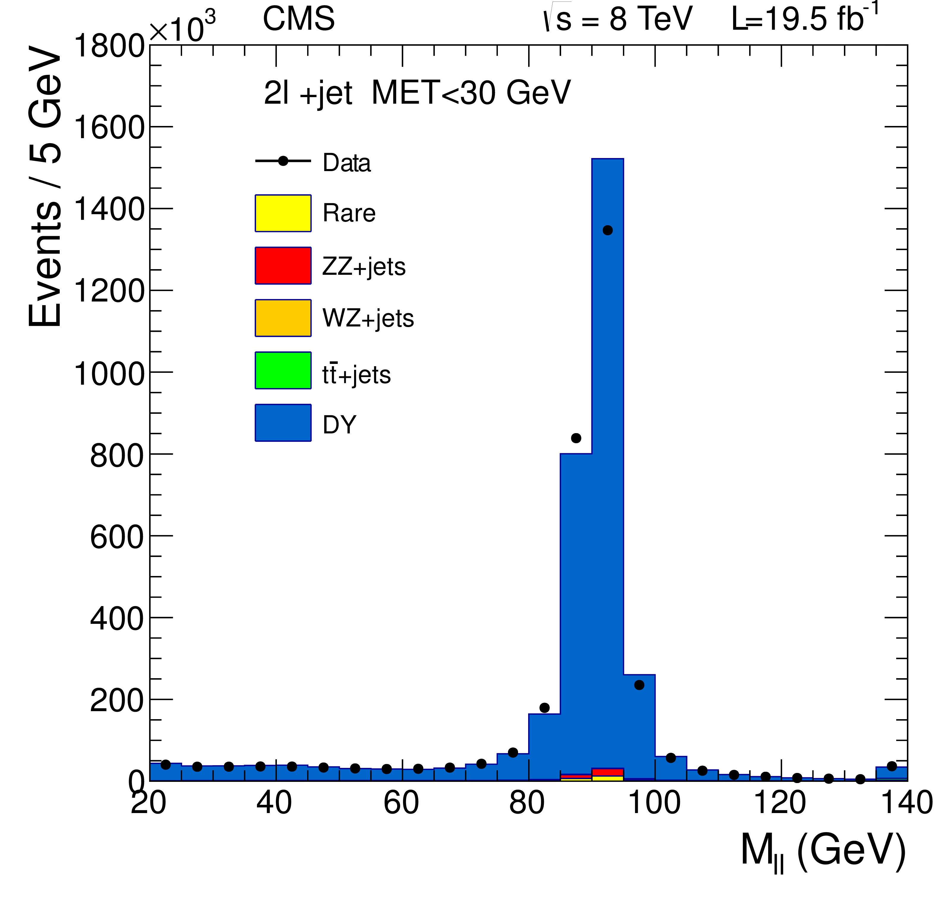
Figure 19:
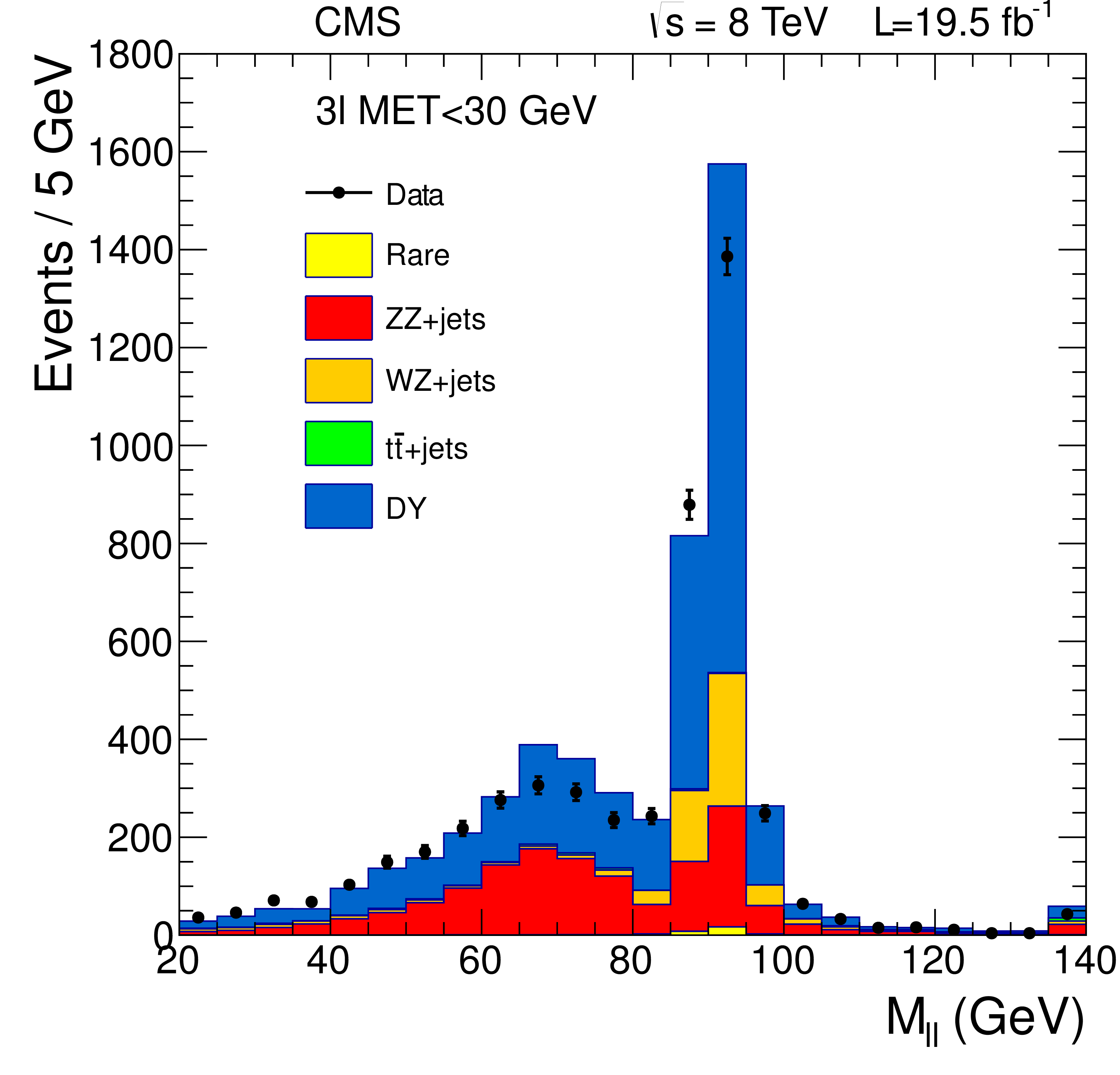
Invariant mass of OSSF lepton pairs in events with $ {E_{\mathrm {T}}^{\text {miss}}} < $ 30 GeV. Data are overlaid with contributions from different sources, predicted by simulation. a : Events with two isolated leptons and exactly one jet with $ {p_{\mathrm {T}}} > $ 30 GeV. b : invariant mass of the two OSSF isolated leptons closest to the Z boson mass in events with three isolated leptons. |
png pdf |
Figure 19-a:
Invariant mass of OSSF lepton pairs in events with $ {E_{\mathrm {T}}^{\text {miss}}} < $ 30 GeV. Data are overlaid with contributions from different sources, predicted by simulation. a : Events with two isolated leptons and exactly one jet with $ {p_{\mathrm {T}}} > $ 30 GeV. b : invariant mass of the two OSSF isolated leptons closest to the Z boson mass in events with three isolated leptons. |
png pdf |
Figure 19-b:
Invariant mass of OSSF lepton pairs in events with $ {E_{\mathrm {T}}^{\text {miss}}} < $ 30 GeV. Data are overlaid with contributions from different sources, predicted by simulation. a : Events with two isolated leptons and exactly one jet with $ {p_{\mathrm {T}}} > $ 30 GeV. b : invariant mass of the two OSSF isolated leptons closest to the Z boson mass in events with three isolated leptons. |
png pdf |
Figure 20:
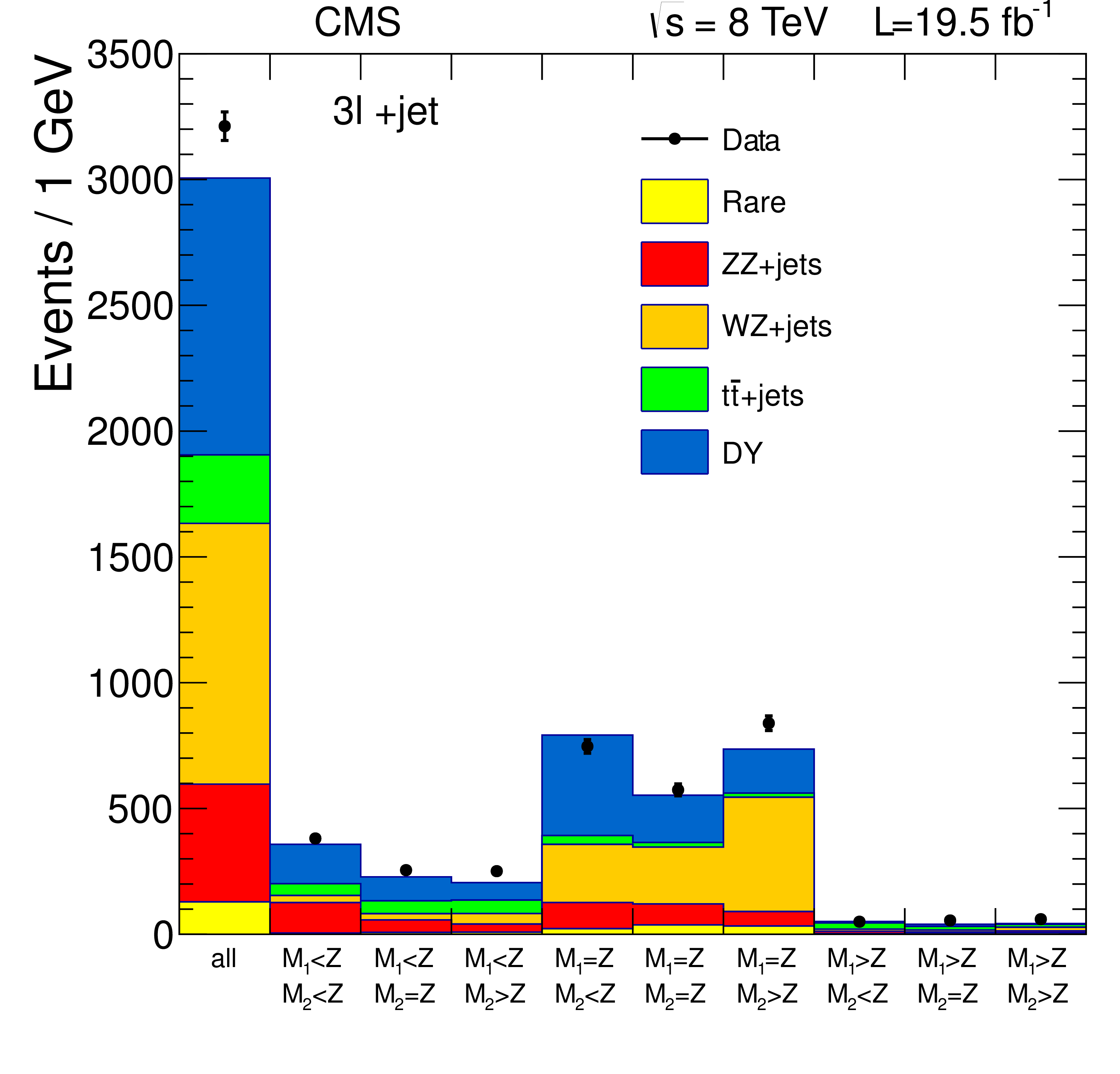
Number of events with three isolated leptons and one jet to different $(M_1,\, M_2)$ regions. Data are overlaid with predicted contributions from different sources. |
png pdf |
Figure 21:
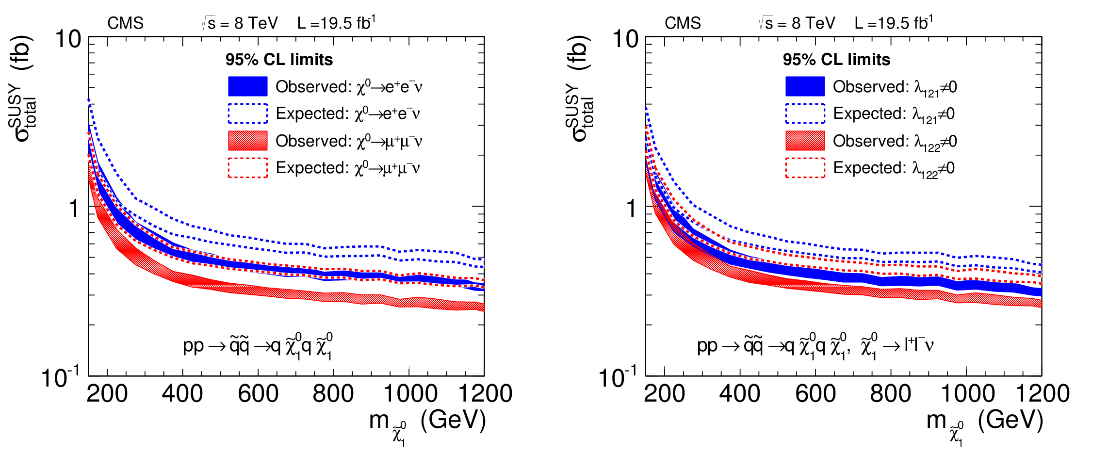
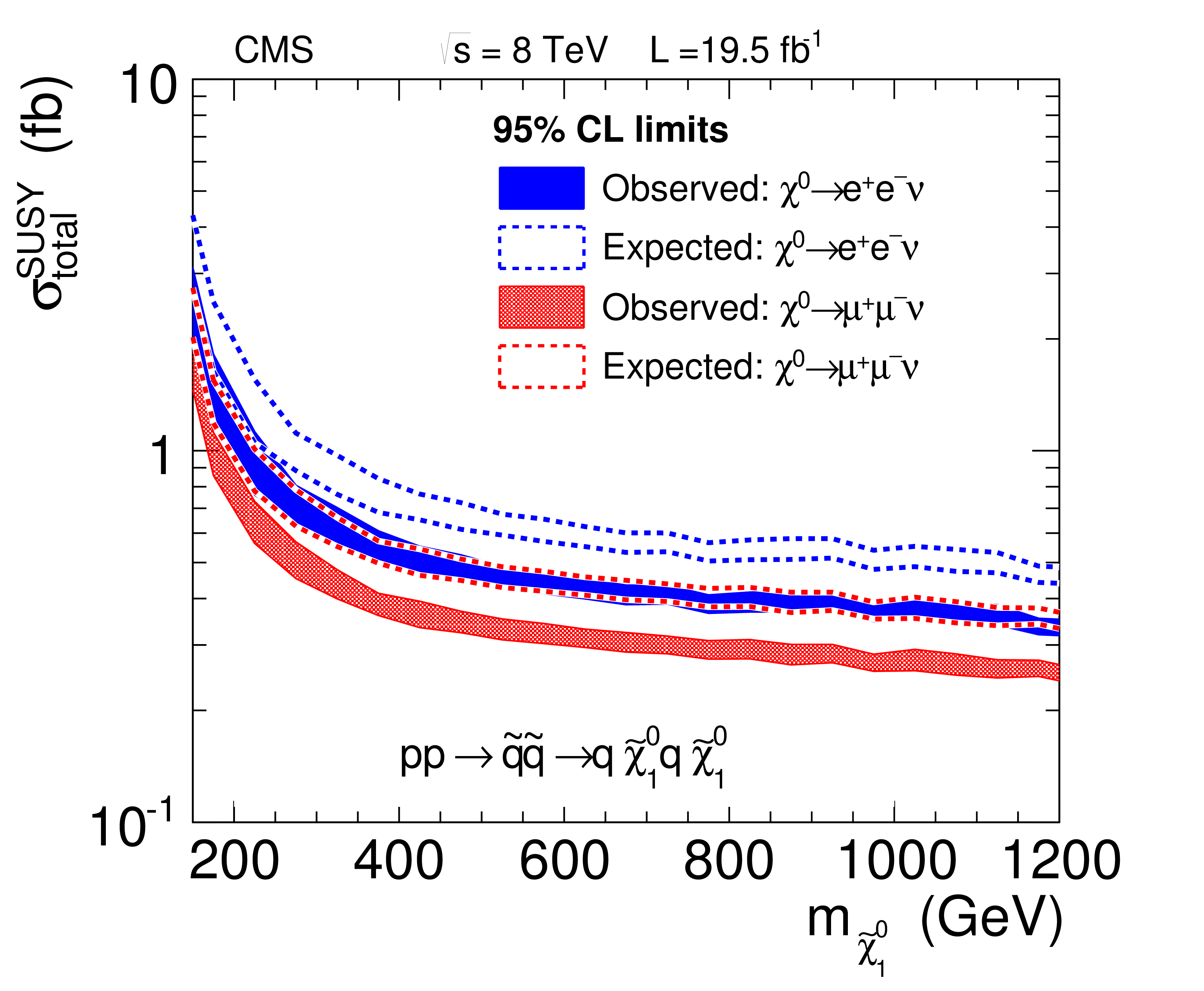
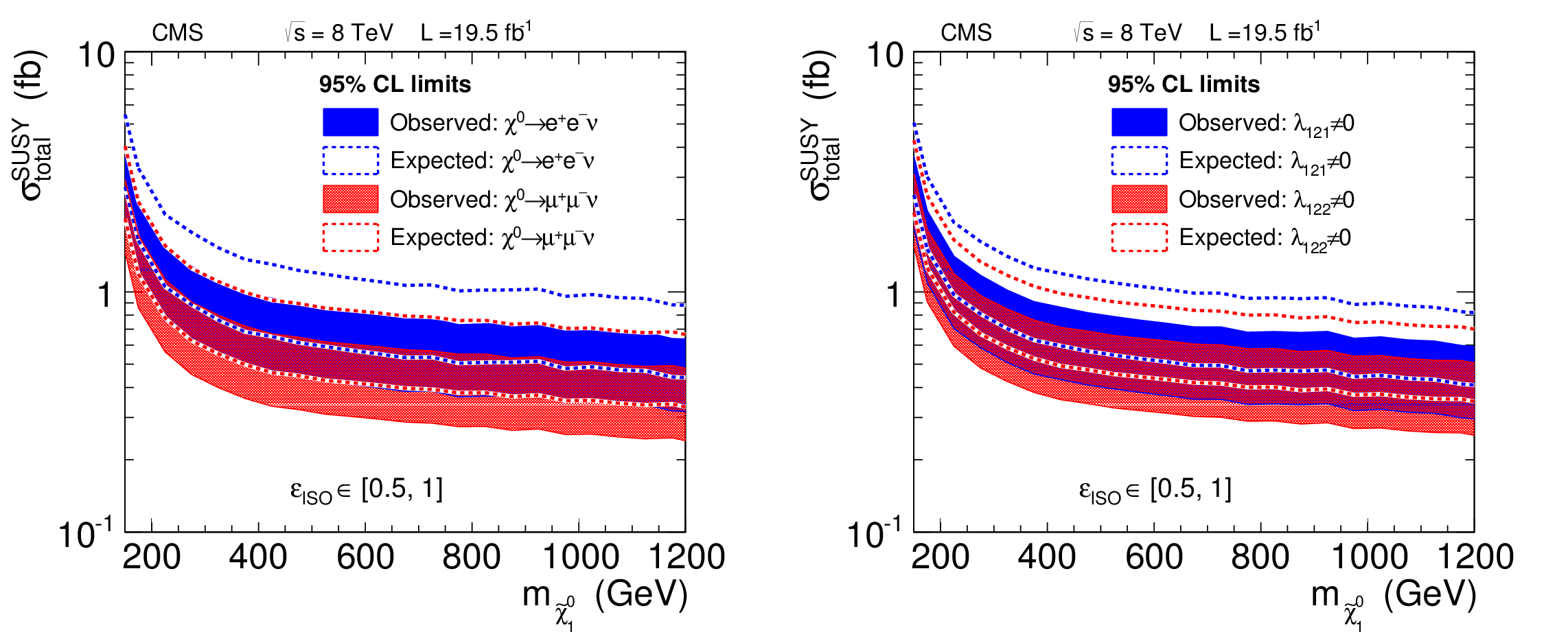
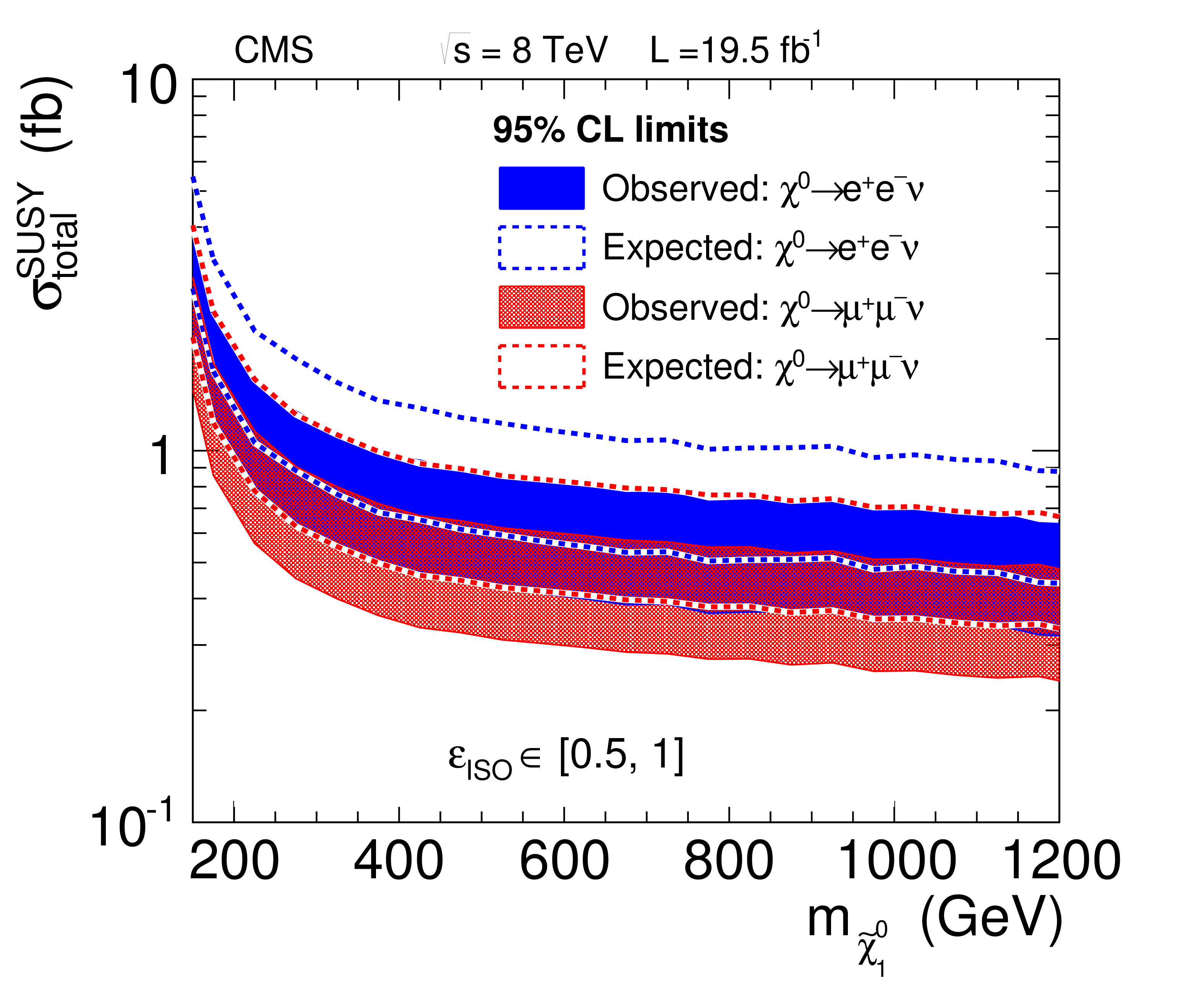
The 95% CL upper limit on the total cross section of the process sketched in Fig. 17 a , as a function of the mass of the RPV decaying neutralino. The band corresponds to the component of uncertainty from the lepton efficiency. Results are shown for neutralinos decaying exclusively to electrons or muons (a) and decaying with the appropriate lepton flavor mixture corresponding to $\lambda _{121} \not = $ 0 and $\lambda _{122} \not = $ 0 RPV scenarios (b). |
png pdf |
Figure 21-a:
The 95% CL upper limit on the total cross section of the process sketched in Fig. 17 a , as a function of the mass of the RPV decaying neutralino. The band corresponds to the component of uncertainty from the lepton efficiency. Results are shown for neutralinos decaying exclusively to electrons or muons (a) and decaying with the appropriate lepton flavor mixture corresponding to $\lambda _{121} \not = $ 0 and $\lambda _{122} \not = $ 0 RPV scenarios (b). |
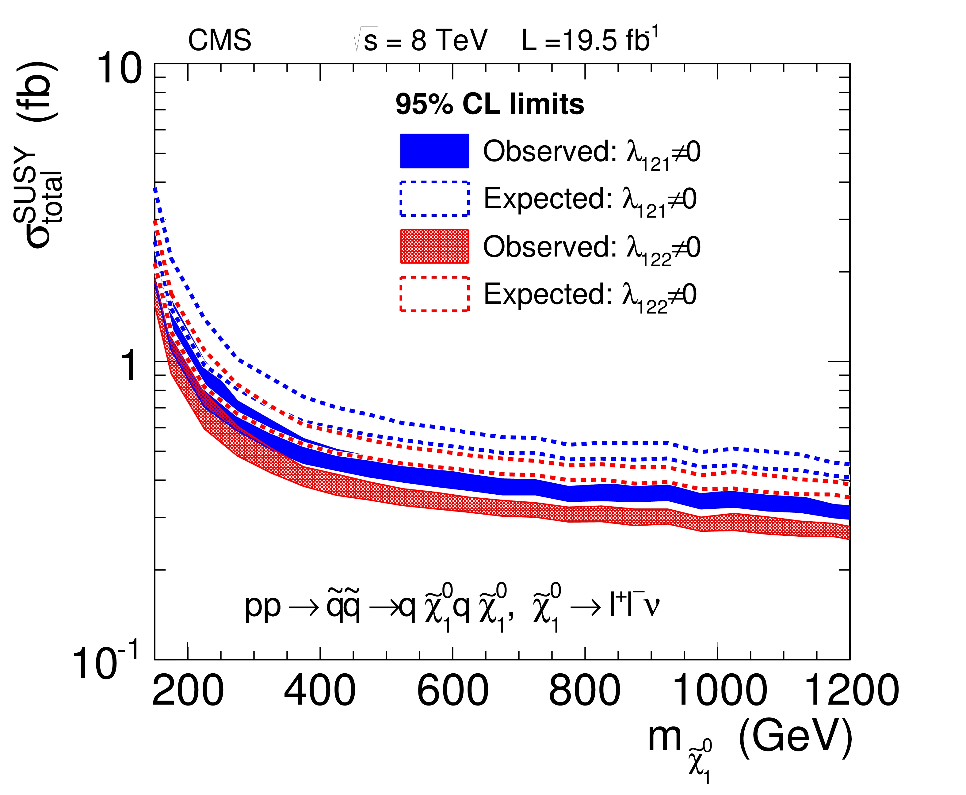
png pdf |
Figure 21-b:
The 95% CL upper limit on the total cross section of the process sketched in Fig. 17 a , as a function of the mass of the RPV decaying neutralino. The band corresponds to the component of uncertainty from the lepton efficiency. Results are shown for neutralinos decaying exclusively to electrons or muons (a) and decaying with the appropriate lepton flavor mixture corresponding to $\lambda _{121} \not = $ 0 and $\lambda _{122} \not = $ 0 RPV scenarios (b). |
png pdf |
Figure 22:
The 95% CL upper limit on total cross sections for generic SUSY models. The band corresponds to the efficiency uncertainty from the various pMSSM models. Results are shown for neutralinos decaying exclusively to electrons or muons (a) and decaying with the appropriate lepton flavor mixture corresponding to $\lambda _{121} \not = $ 0 and $\lambda _{122} \not = $ 0 RPV scenarios (b). |
png pdf |
Figure 22-a:
The 95% CL upper limit on total cross sections for generic SUSY models. The band corresponds to the efficiency uncertainty from the various pMSSM models. Results are shown for neutralinos decaying exclusively to electrons or muons (a) and decaying with the appropriate lepton flavor mixture corresponding to $\lambda _{121} \not = $ 0 and $\lambda _{122} \not = $ 0 RPV scenarios (b). |

png pdf |
Figure 22-b:
The 95% CL upper limit on total cross sections for generic SUSY models. The band corresponds to the efficiency uncertainty from the various pMSSM models. Results are shown for neutralinos decaying exclusively to electrons or muons (a) and decaying with the appropriate lepton flavor mixture corresponding to $\lambda _{121} \not = $ 0 and $\lambda _{122} \not = $ 0 RPV scenarios (b). |
png pdf |
Figure 23:
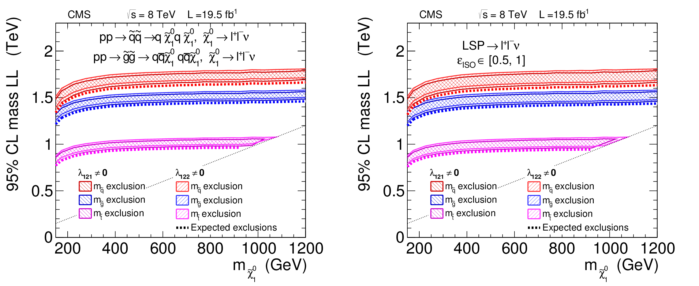
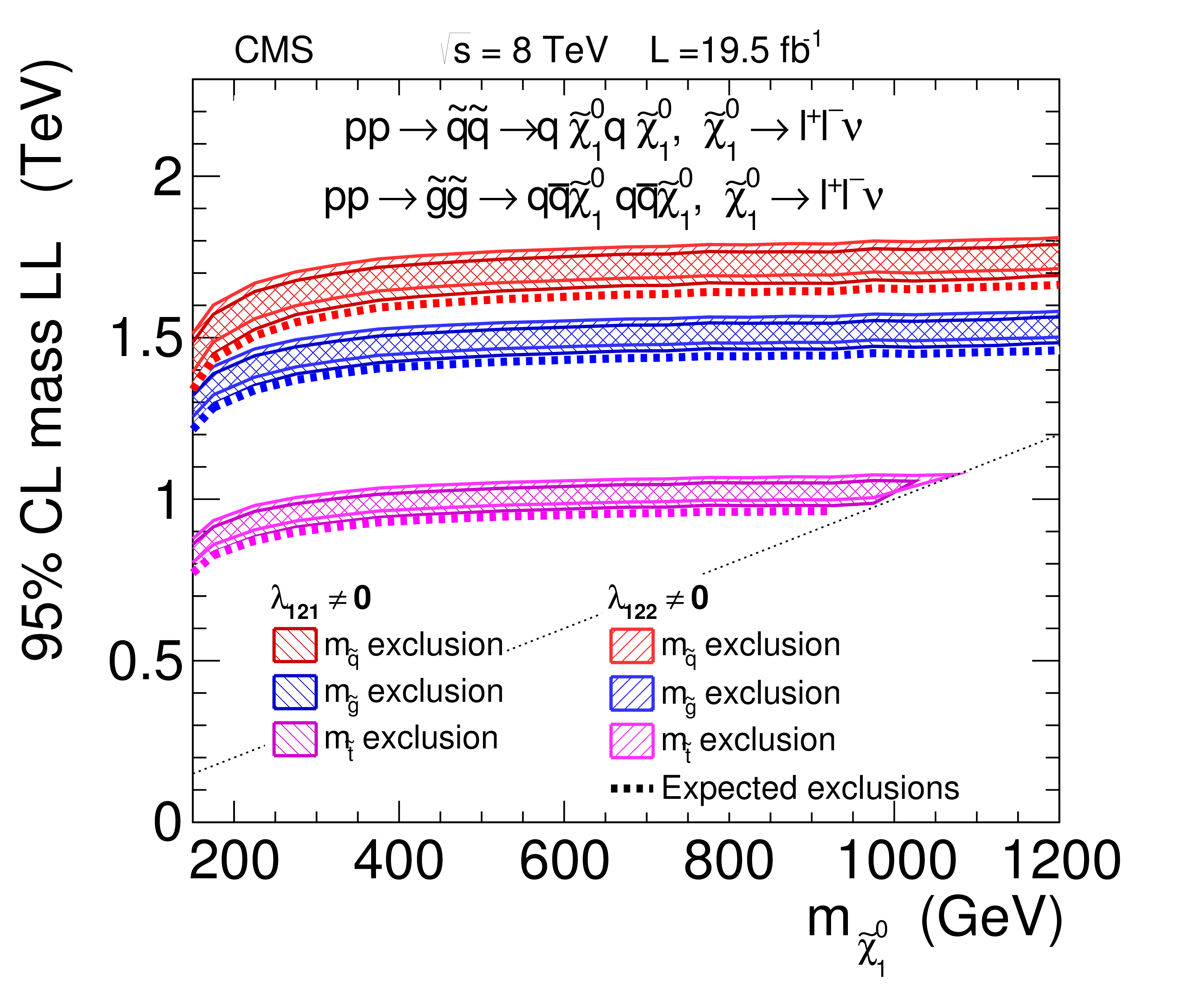
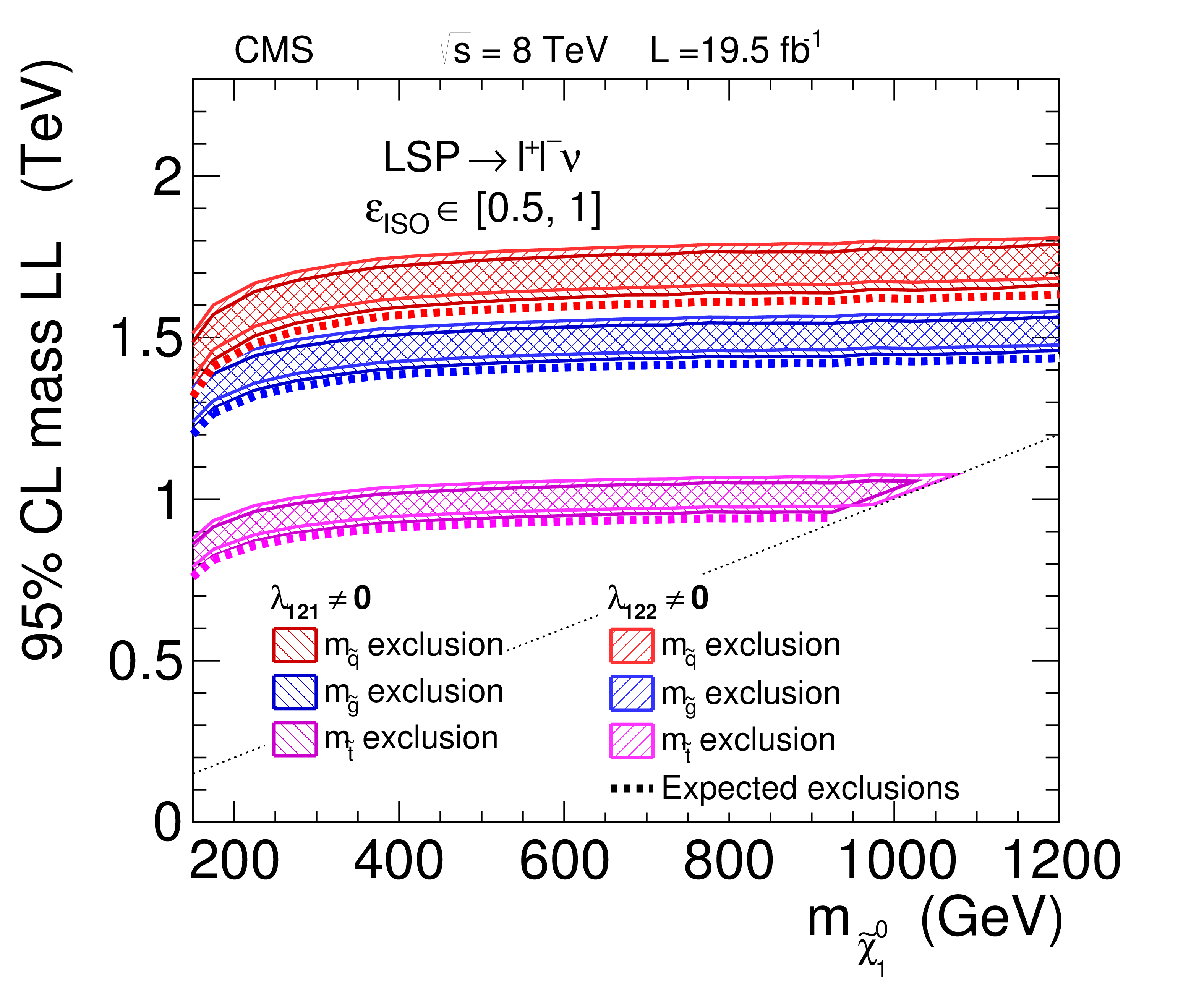
Lower limits on the masses of intermediate-state particles for various SUSY production mechanisms as a function of the neutralino mass when the neutralino is the LSP. The limits shown in the plot (a) on the gluino mass, top squark mass, and squark mass are for gluino pair production, top squark pair production, and first and second generation squark pair production, respectively. The first and second generation squark mass exclusion is obtained from the cross section limit of Fig. 21 (b), combined with the corresponding cross section for this model, displayed in Fig. 17(a). The other exclusions are obtained in a similar fashion. The limits shown in the plot (b) are obtained from the generic total RPV SUSY cross section limit from Fig. 22 (b). The bands include the uncertainty in SUSY production cross sections, along with the efficiency uncertainties. The models below the diagonal line were not investigated as the neutralino is no longer the LSP. |
png pdf |
Figure 23-a:
Lower limits on the masses of intermediate-state particles for various SUSY production mechanisms as a function of the neutralino mass when the neutralino is the LSP. The limits shown in the plot (a) on the gluino mass, top squark mass, and squark mass are for gluino pair production, top squark pair production, and first and second generation squark pair production, respectively. The first and second generation squark mass exclusion is obtained from the cross section limit of Fig. 21 (b), combined with the corresponding cross section for this model, displayed in Fig. 17(a). The other exclusions are obtained in a similar fashion. The limits shown in the plot (b) are obtained from the generic total RPV SUSY cross section limit from Fig. 22 (b). The bands include the uncertainty in SUSY production cross sections, along with the efficiency uncertainties. The models below the diagonal line were not investigated as the neutralino is no longer the LSP. |
png pdf |
Figure 23-b:
Lower limits on the masses of intermediate-state particles for various SUSY production mechanisms as a function of the neutralino mass when the neutralino is the LSP. The limits shown in the plot (a) on the gluino mass, top squark mass, and squark mass are for gluino pair production, top squark pair production, and first and second generation squark pair production, respectively. The first and second generation squark mass exclusion is obtained from the cross section limit of Fig. 21 (b), combined with the corresponding cross section for this model, displayed in Fig. 17(a). The other exclusions are obtained in a similar fashion. The limits shown in the plot (b) are obtained from the generic total RPV SUSY cross section limit from Fig. 22 (b). The bands include the uncertainty in SUSY production cross sections, along with the efficiency uncertainties. The models below the diagonal line were not investigated as the neutralino is no longer the LSP. |
png pdf |
Figure 24:
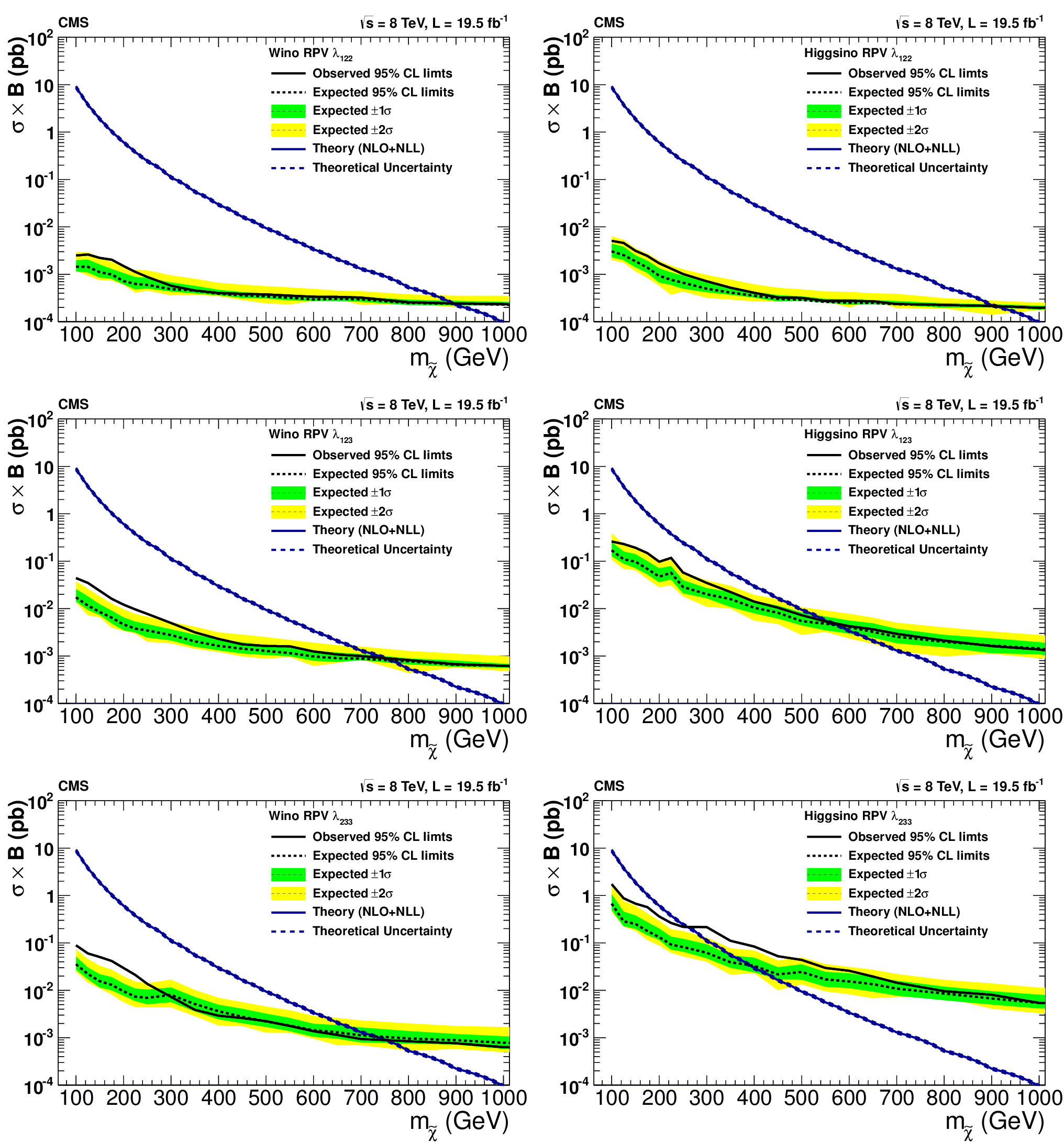
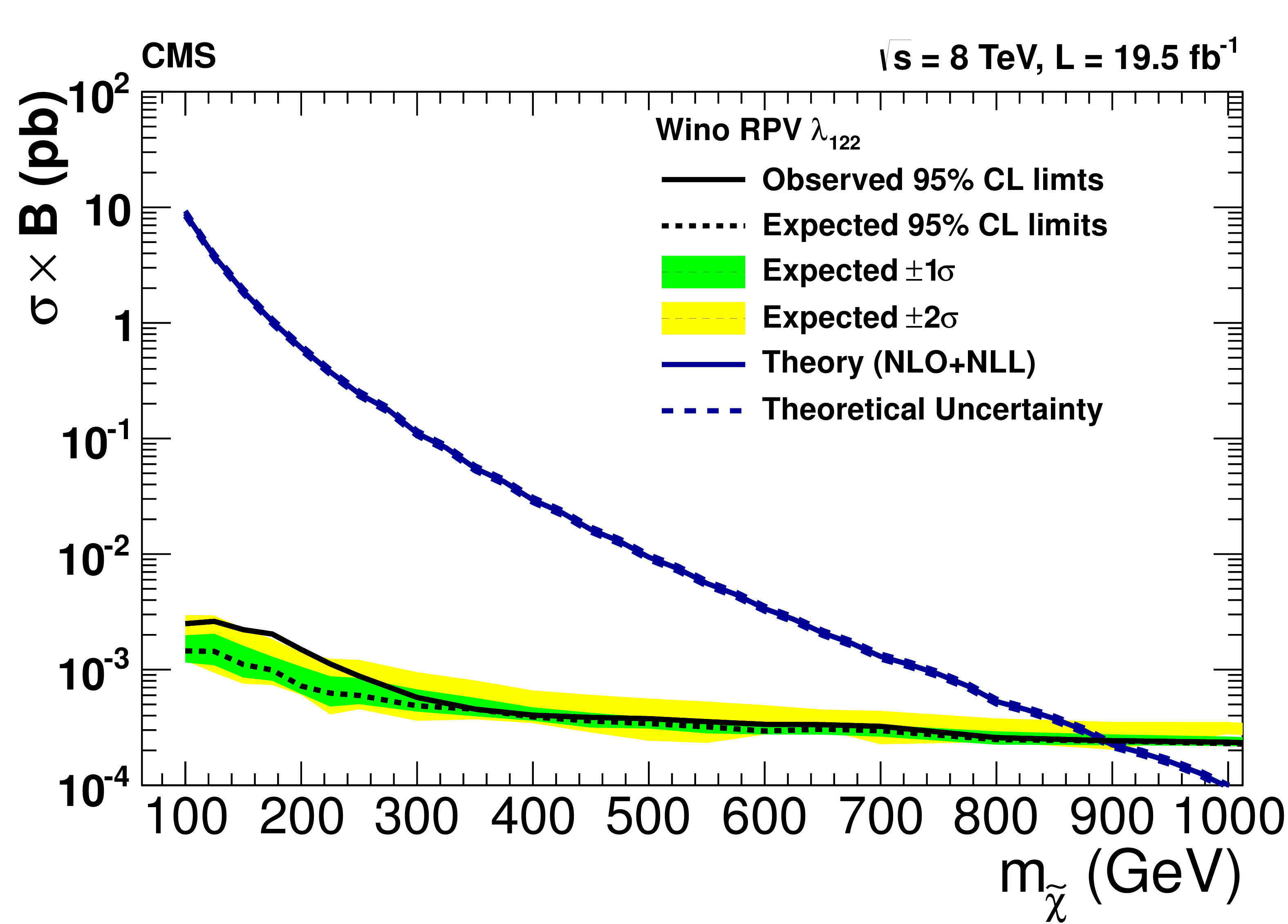
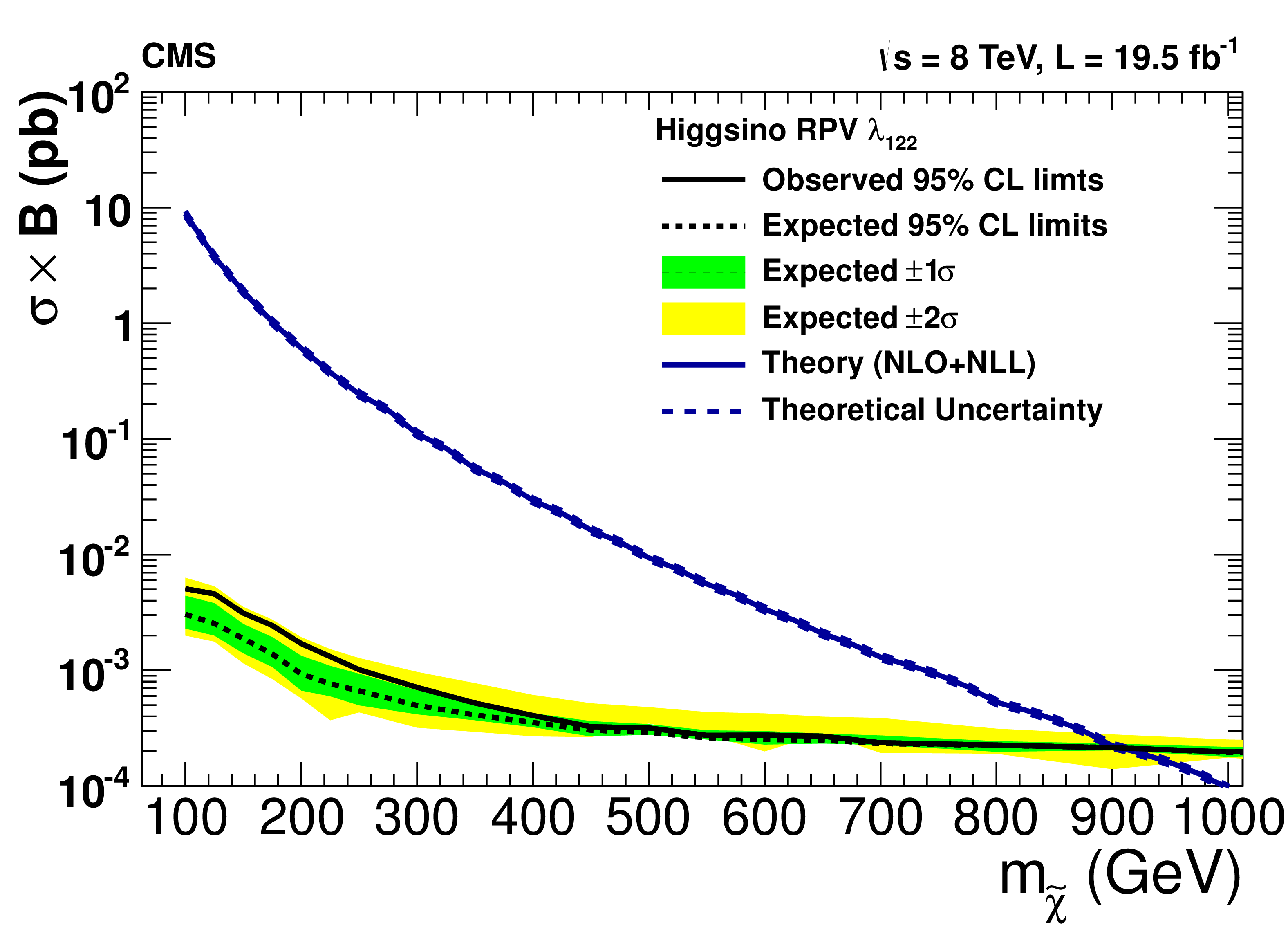
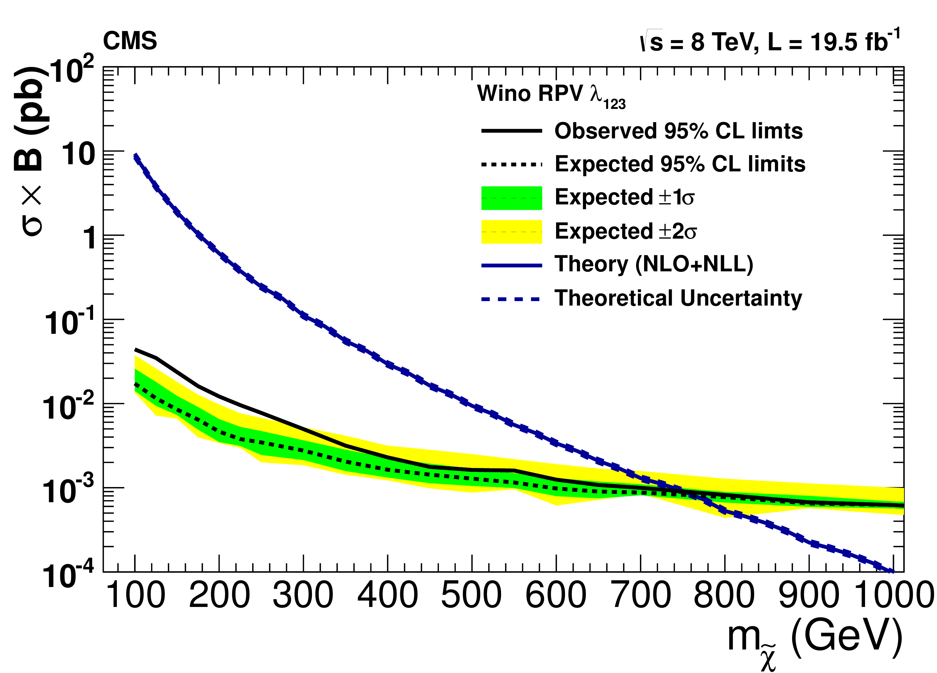
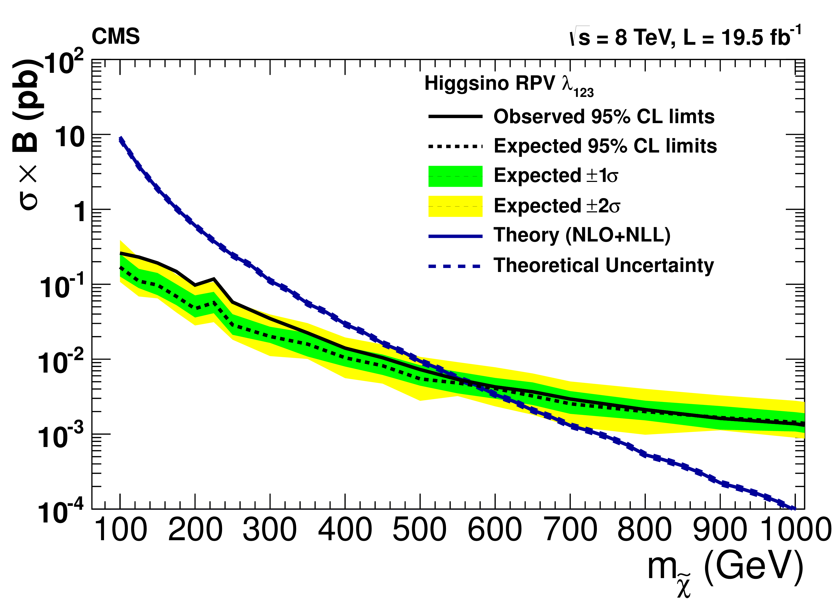
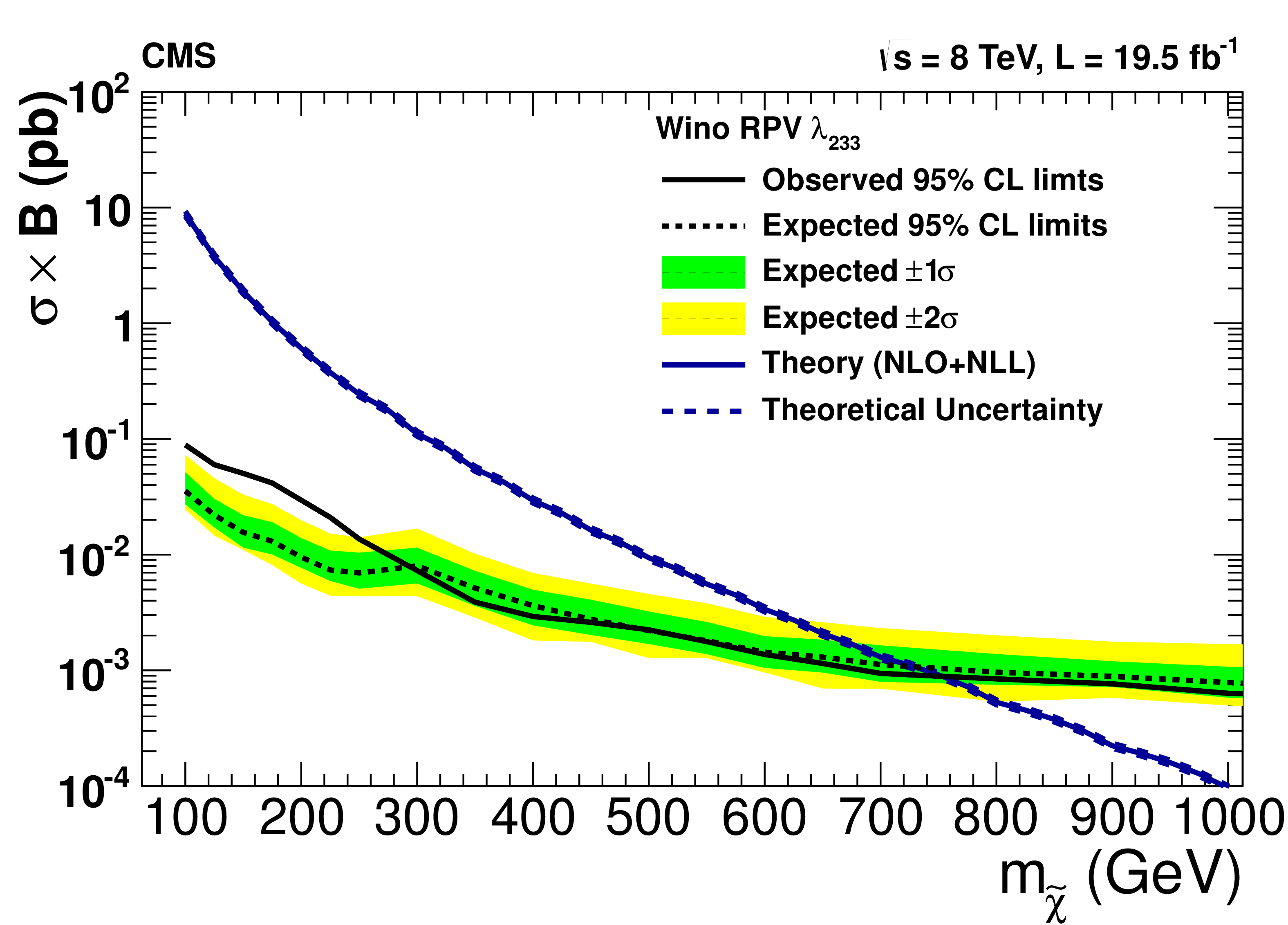
Upper 95% CL cross section times branching ratio limits as a function of the neutralino mass in models with wino production (a,c,e) and higgsino production (b,d,f), assuming non-zero $\lambda _{ijk}$ couplings: $\lambda _{122}$ (a,b), $\lambda _{123}$ (c,d), and $\lambda _{233}$ (e,f). The decays proceed promptly through slepton mediators. |
png pdf |
Figure 24-a:
Upper 95% CL cross section times branching ratio limits as a function of the neutralino mass in models with wino production (a,c,e) and higgsino production (b,d,f), assuming non-zero $\lambda _{ijk}$ couplings: $\lambda _{122}$ (a,b), $\lambda _{123}$ (c,d), and $\lambda _{233}$ (e,f). The decays proceed promptly through slepton mediators. |
png pdf |
Figure 24-b:
Upper 95% CL cross section times branching ratio limits as a function of the neutralino mass in models with wino production (a,c,e) and higgsino production (b,d,f), assuming non-zero $\lambda _{ijk}$ couplings: $\lambda _{122}$ (a,b), $\lambda _{123}$ (c,d), and $\lambda _{233}$ (e,f). The decays proceed promptly through slepton mediators. |
png pdf |
Figure 24-c:
Upper 95% CL cross section times branching ratio limits as a function of the neutralino mass in models with wino production (a,c,e) and higgsino production (b,d,f), assuming non-zero $\lambda _{ijk}$ couplings: $\lambda _{122}$ (a,b), $\lambda _{123}$ (c,d), and $\lambda _{233}$ (e,f). The decays proceed promptly through slepton mediators. |
png pdf |
Figure 24-d:
Upper 95% CL cross section times branching ratio limits as a function of the neutralino mass in models with wino production (a,c,e) and higgsino production (b,d,f), assuming non-zero $\lambda _{ijk}$ couplings: $\lambda _{122}$ (a,b), $\lambda _{123}$ (c,d), and $\lambda _{233}$ (e,f). The decays proceed promptly through slepton mediators. |
png pdf |
Figure 24-e:
Upper 95% CL cross section times branching ratio limits as a function of the neutralino mass in models with wino production (a,c,e) and higgsino production (b,d,f), assuming non-zero $\lambda _{ijk}$ couplings: $\lambda _{122}$ (a,b), $\lambda _{123}$ (c,d), and $\lambda _{233}$ (e,f). The decays proceed promptly through slepton mediators. |

png pdf |
Figure 24-f:
Upper 95% CL cross section times branching ratio limits as a function of the neutralino mass in models with wino production (a,c,e) and higgsino production (b,d,f), assuming non-zero $\lambda _{ijk}$ couplings: $\lambda _{122}$ (a,b), $\lambda _{123}$ (c,d), and $\lambda _{233}$ (e,f). The decays proceed promptly through slepton mediators. |
png pdf |
Figure 25:
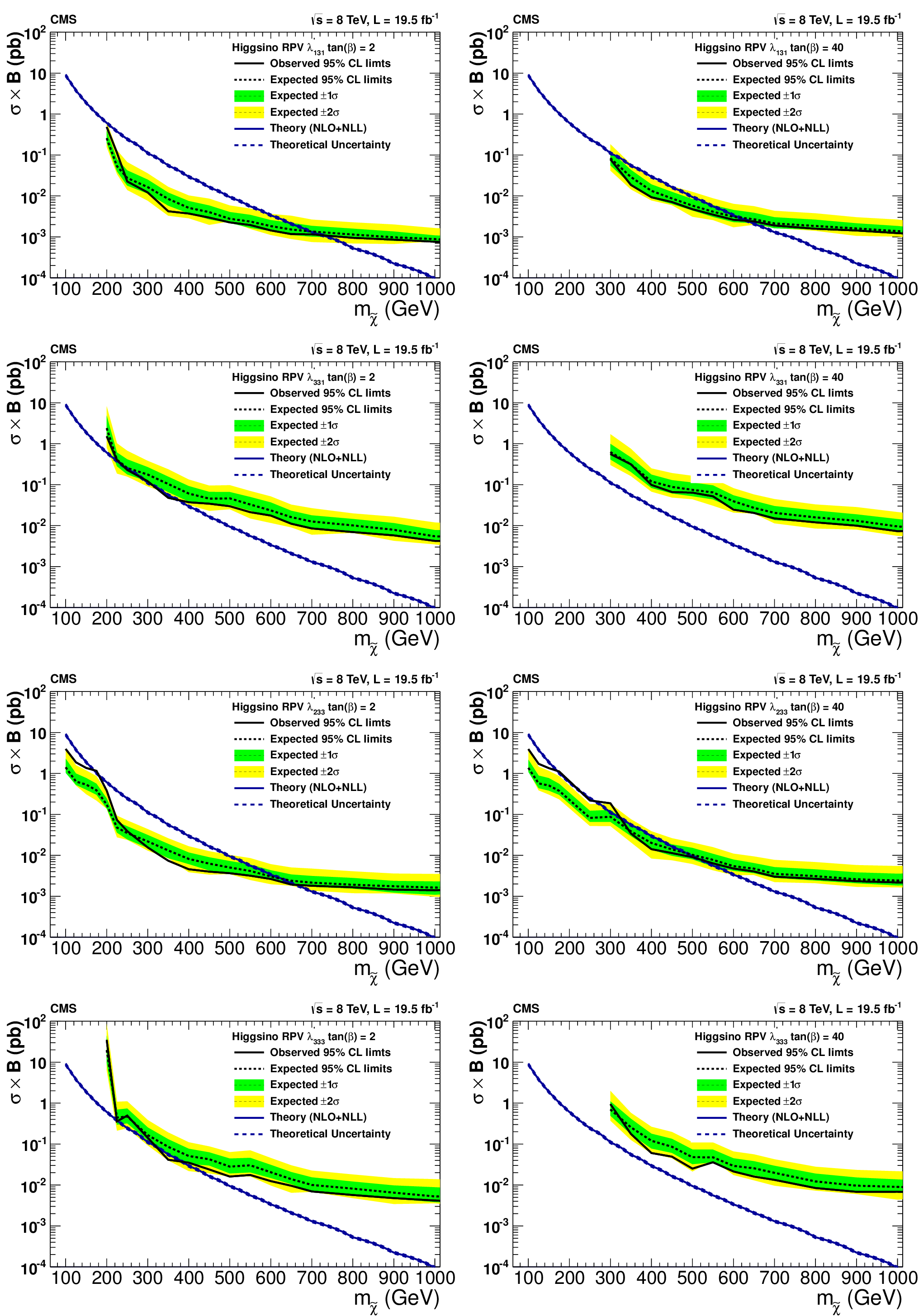
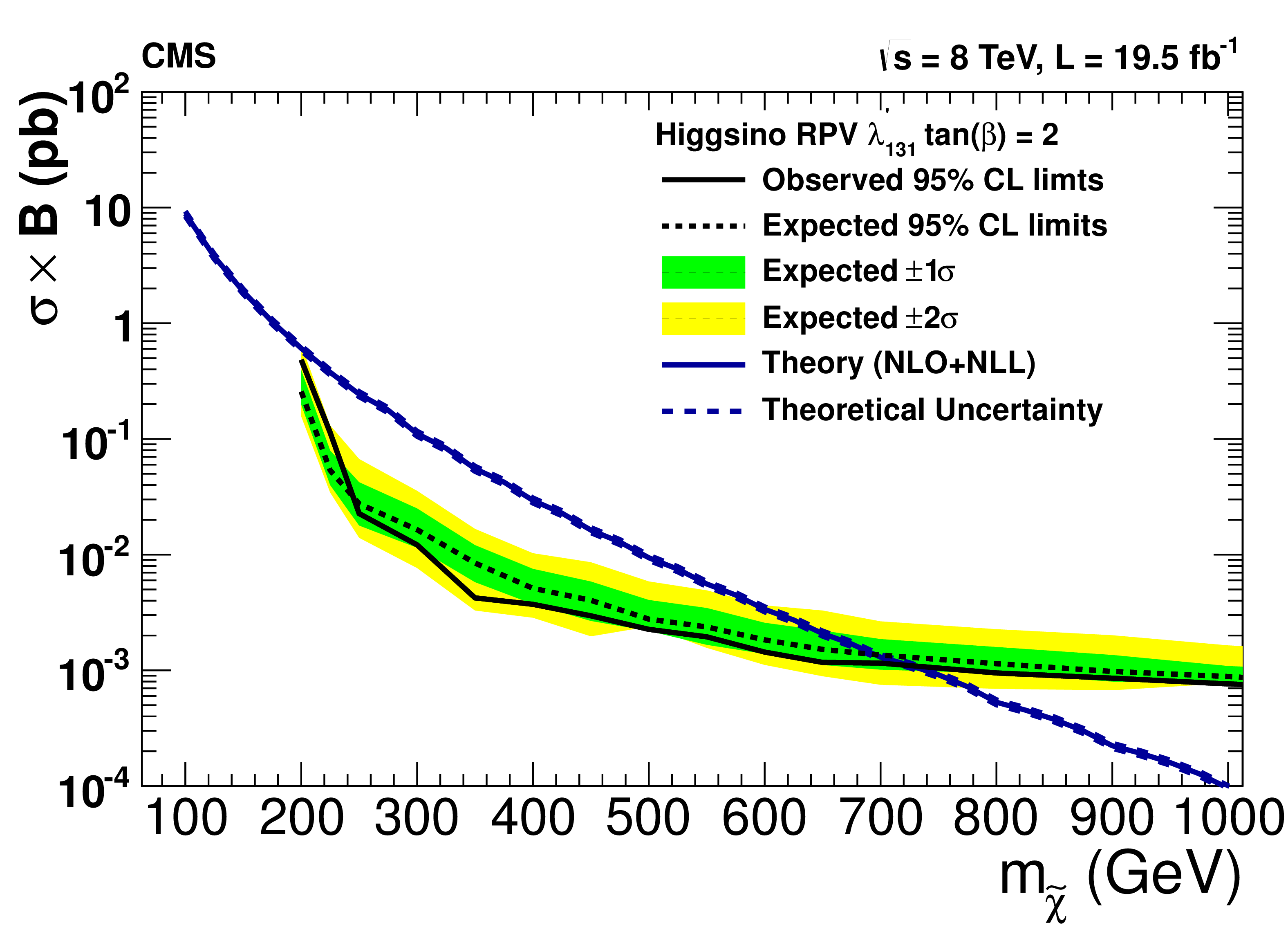
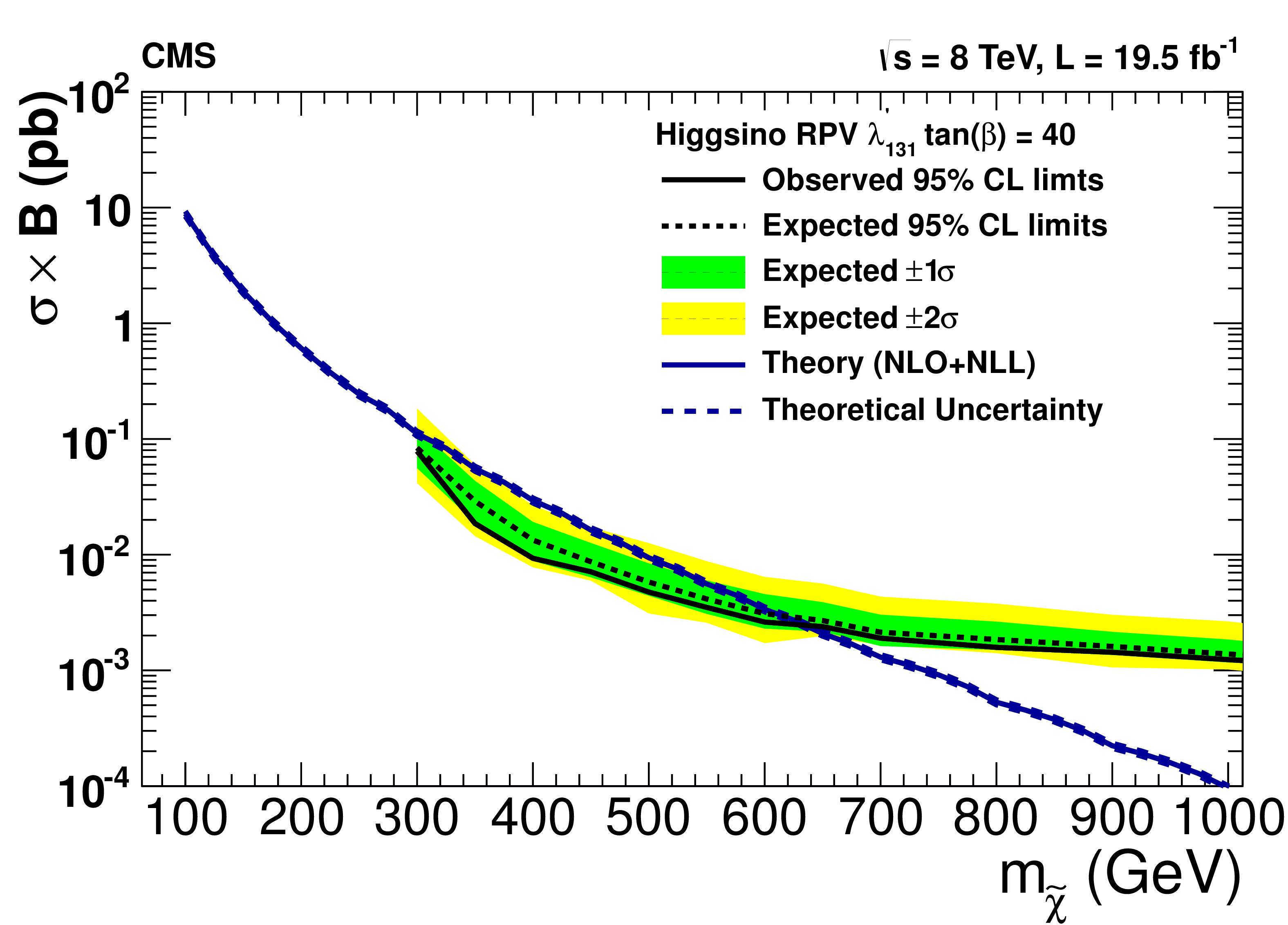
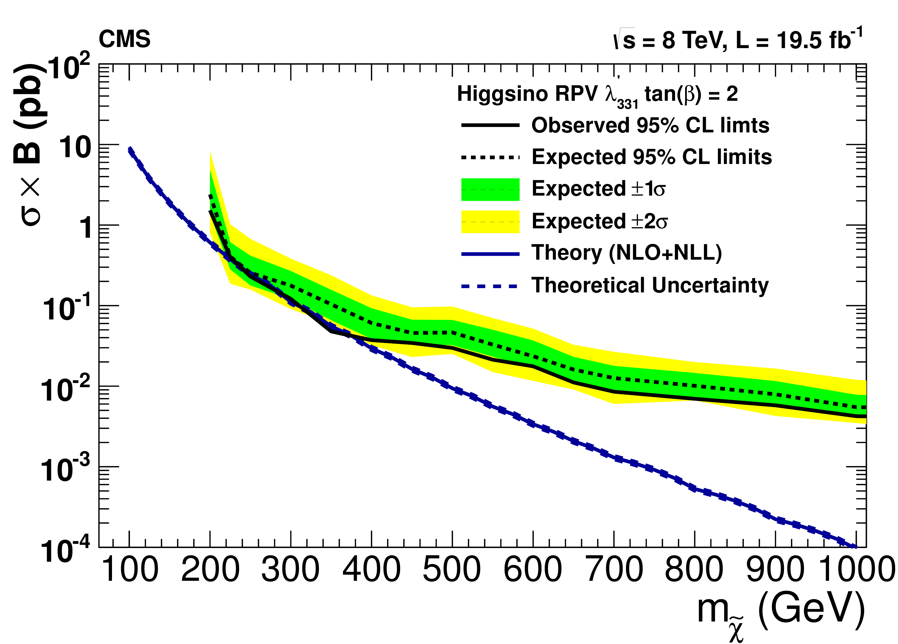
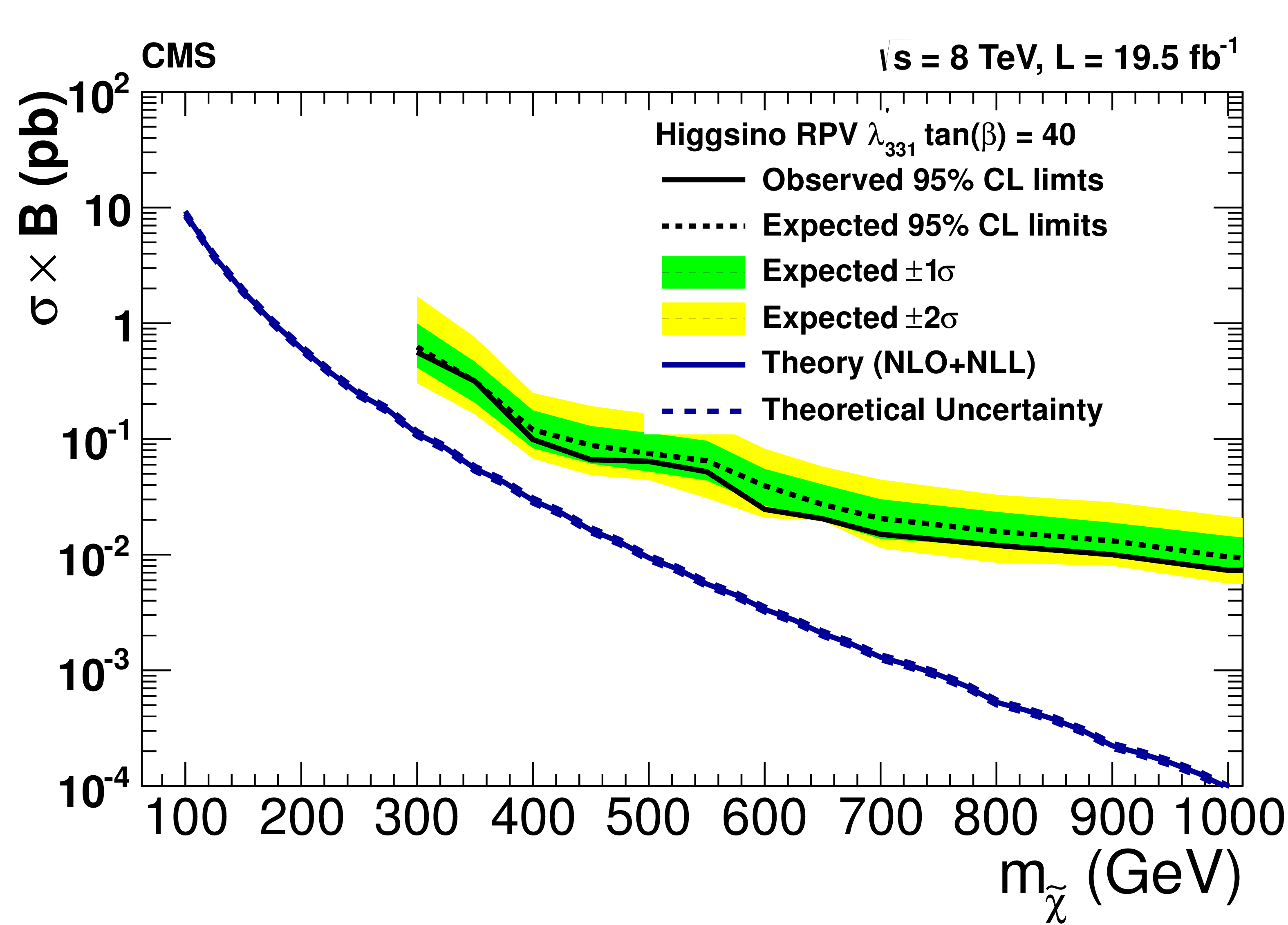
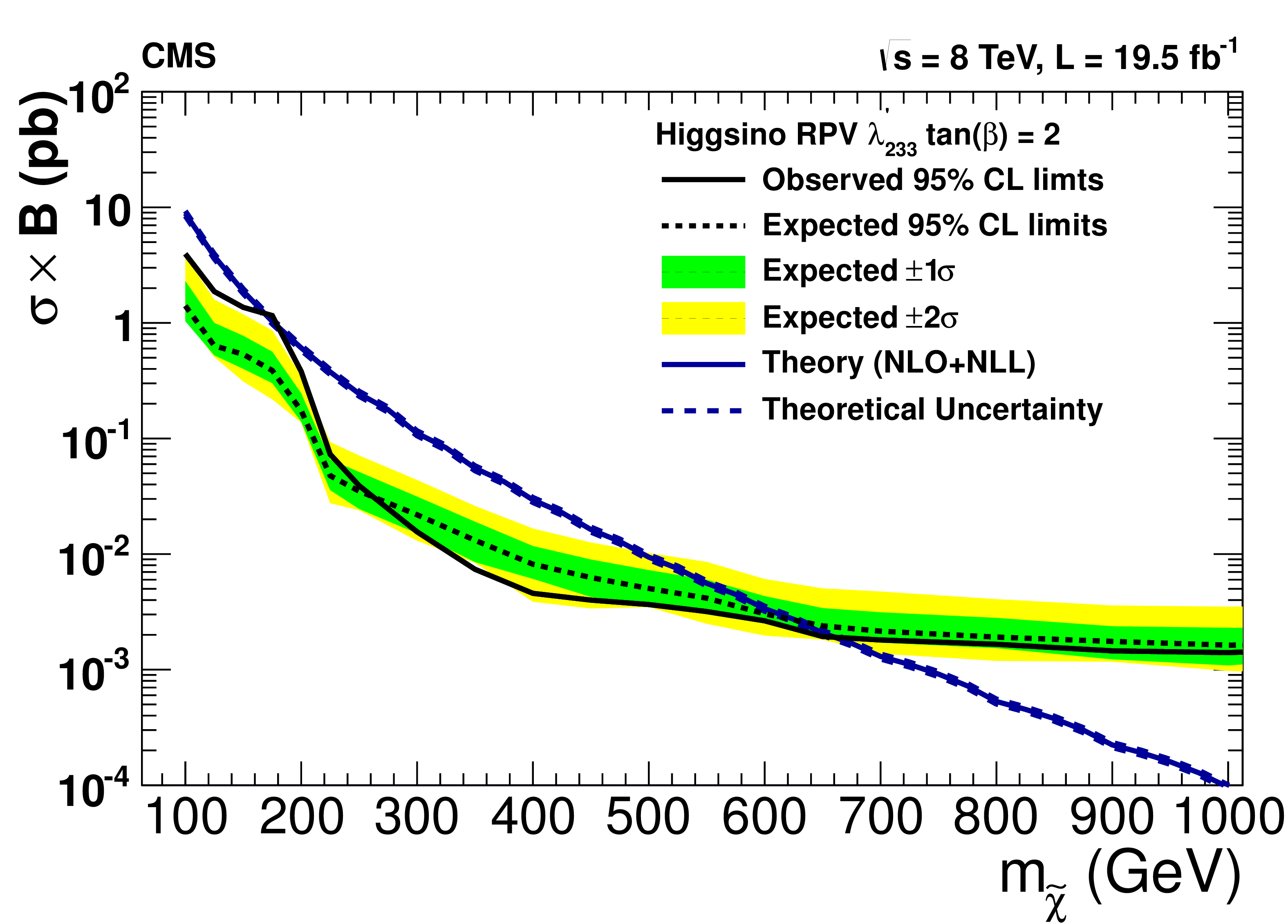
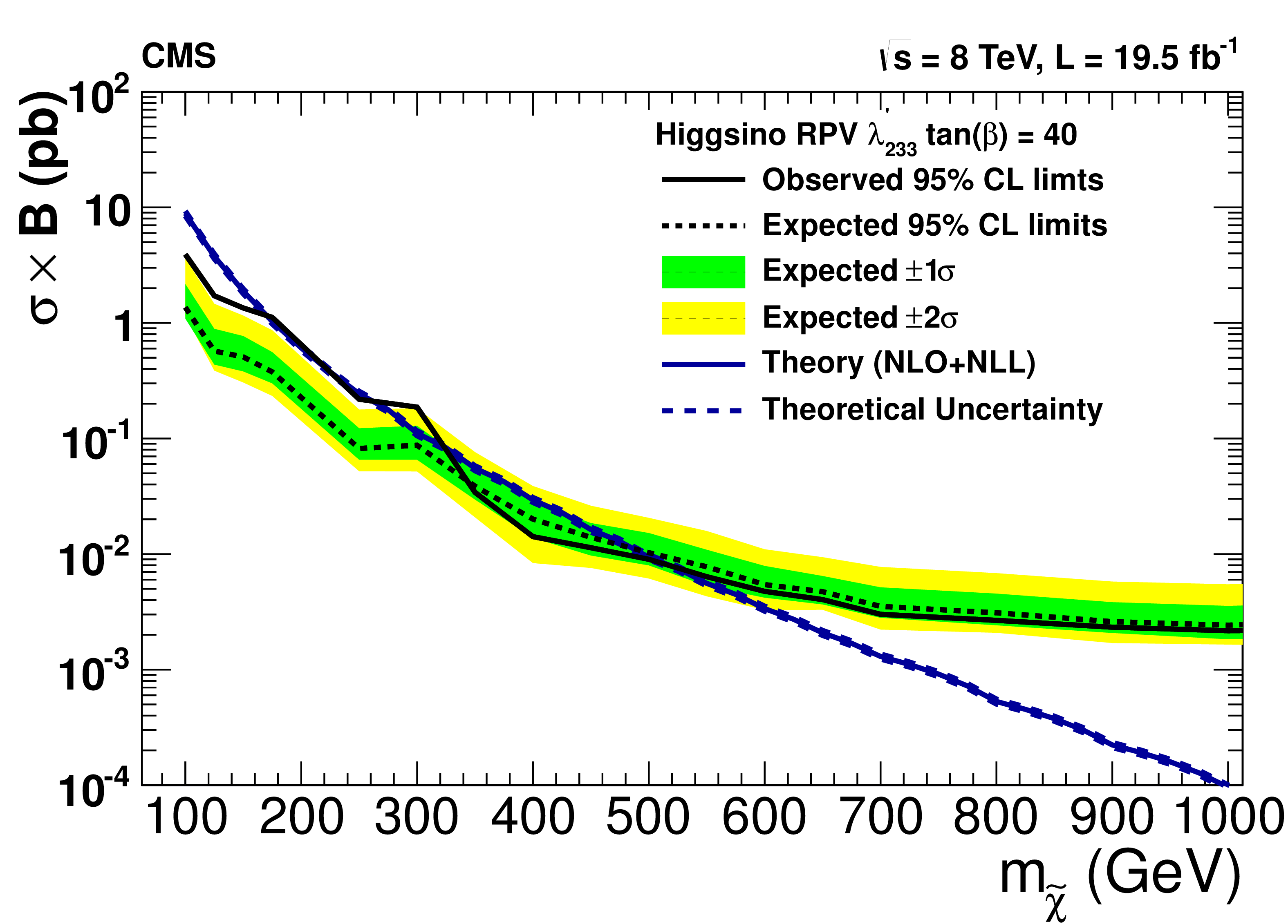
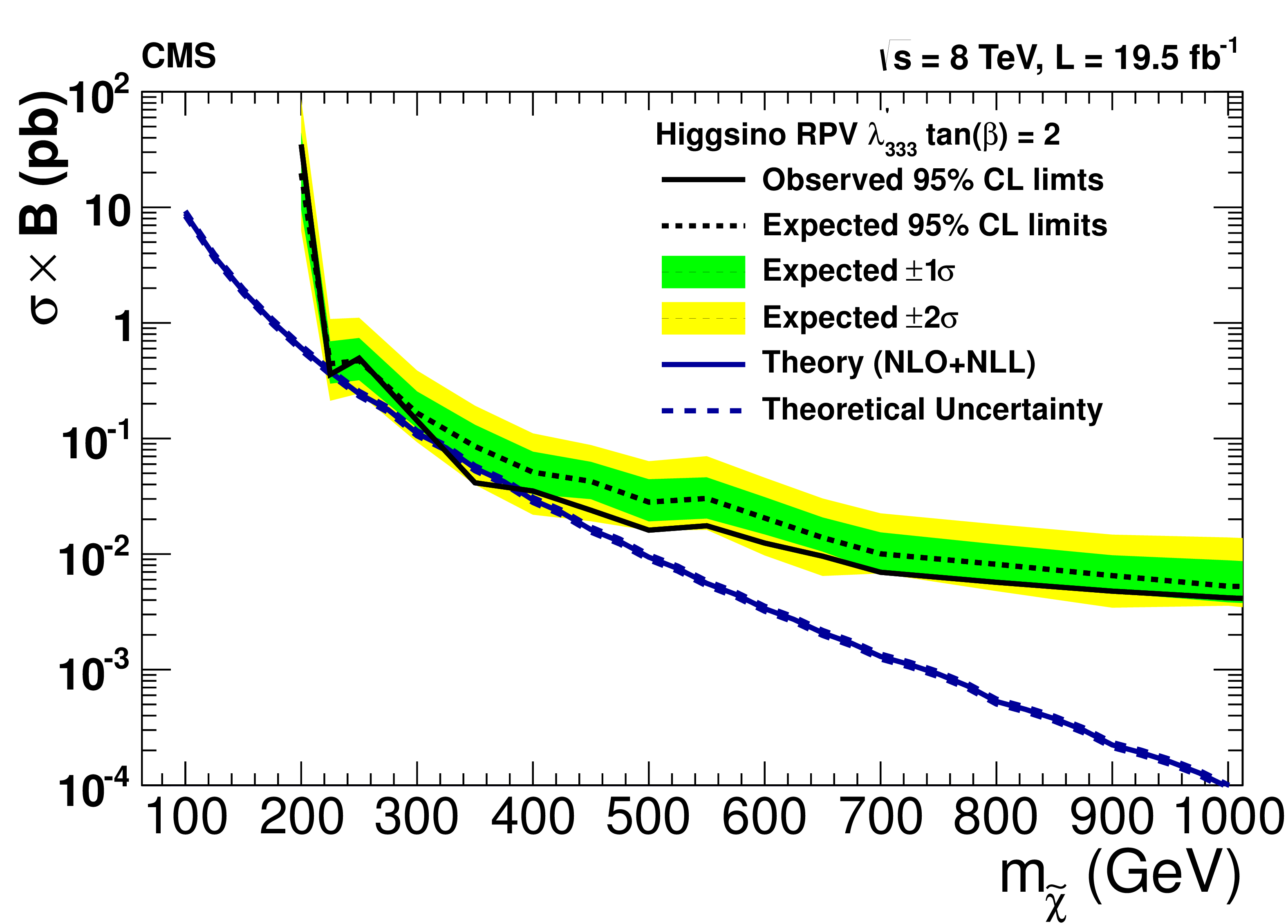
Upper 95% CL cross section times branching fraction limits as a function of the neutralino mass in models with higgsino production and non-zero $\lambda ^\prime _{ijk}$ couplings with (a,c,e,g) $\tan\beta = $ 2 and (b,d,f,h) $\tan\beta = $ 40 : $\lambda ^\prime _{131}$ (a,c), $\lambda ^\prime _{331}$ (b,d), $\lambda ^\prime _{233}$ (e,f), and $\lambda ^\prime _{333}$ (g,h). The decays proceed promptly through bottom and top squark mediators. The couplings of the higgsino to the mediator particles varies with $\tan\beta $, affecting the branching fraction to multileptons and the acceptance. |
png pdf |
Figure 25-a:
Upper 95% CL cross section times branching fraction limits as a function of the neutralino mass in models with higgsino production and non-zero $\lambda ^\prime _{ijk}$ couplings with (a,c,e,g) $\tan\beta = $ 2 and (b,d,f,h) $\tan\beta = $ 40 : $\lambda ^\prime _{131}$ (a,c), $\lambda ^\prime _{331}$ (b,d), $\lambda ^\prime _{233}$ (e,f), and $\lambda ^\prime _{333}$ (g,h). The decays proceed promptly through bottom and top squark mediators. The couplings of the higgsino to the mediator particles varies with $\tan\beta $, affecting the branching fraction to multileptons and the acceptance. |
png pdf |
Figure 25-b:
Upper 95% CL cross section times branching fraction limits as a function of the neutralino mass in models with higgsino production and non-zero $\lambda ^\prime _{ijk}$ couplings with (a,c,e,g) $\tan\beta = $ 2 and (b,d,f,h) $\tan\beta = $ 40 : $\lambda ^\prime _{131}$ (a,c), $\lambda ^\prime _{331}$ (b,d), $\lambda ^\prime _{233}$ (e,f), and $\lambda ^\prime _{333}$ (g,h). The decays proceed promptly through bottom and top squark mediators. The couplings of the higgsino to the mediator particles varies with $\tan\beta $, affecting the branching fraction to multileptons and the acceptance. |
png pdf |
Figure 25-c:
Upper 95% CL cross section times branching fraction limits as a function of the neutralino mass in models with higgsino production and non-zero $\lambda ^\prime _{ijk}$ couplings with (a,c,e,g) $\tan\beta = $ 2 and (b,d,f,h) $\tan\beta = $ 40 : $\lambda ^\prime _{131}$ (a,c), $\lambda ^\prime _{331}$ (b,d), $\lambda ^\prime _{233}$ (e,f), and $\lambda ^\prime _{333}$ (g,h). The decays proceed promptly through bottom and top squark mediators. The couplings of the higgsino to the mediator particles varies with $\tan\beta $, affecting the branching fraction to multileptons and the acceptance. |
png pdf |
Figure 25-d:
Upper 95% CL cross section times branching fraction limits as a function of the neutralino mass in models with higgsino production and non-zero $\lambda ^\prime _{ijk}$ couplings with (a,c,e,g) $\tan\beta = $ 2 and (b,d,f,h) $\tan\beta = $ 40 : $\lambda ^\prime _{131}$ (a,c), $\lambda ^\prime _{331}$ (b,d), $\lambda ^\prime _{233}$ (e,f), and $\lambda ^\prime _{333}$ (g,h). The decays proceed promptly through bottom and top squark mediators. The couplings of the higgsino to the mediator particles varies with $\tan\beta $, affecting the branching fraction to multileptons and the acceptance. |
png pdf |
Figure 25-e:
Upper 95% CL cross section times branching fraction limits as a function of the neutralino mass in models with higgsino production and non-zero $\lambda ^\prime _{ijk}$ couplings with (a,c,e,g) $\tan\beta = $ 2 and (b,d,f,h) $\tan\beta = $ 40 : $\lambda ^\prime _{131}$ (a,c), $\lambda ^\prime _{331}$ (b,d), $\lambda ^\prime _{233}$ (e,f), and $\lambda ^\prime _{333}$ (g,h). The decays proceed promptly through bottom and top squark mediators. The couplings of the higgsino to the mediator particles varies with $\tan\beta $, affecting the branching fraction to multileptons and the acceptance. |
png pdf |
Figure 25-f:
Upper 95% CL cross section times branching fraction limits as a function of the neutralino mass in models with higgsino production and non-zero $\lambda ^\prime _{ijk}$ couplings with (a,c,e,g) $\tan\beta = $ 2 and (b,d,f,h) $\tan\beta = $ 40 : $\lambda ^\prime _{131}$ (a,c), $\lambda ^\prime _{331}$ (b,d), $\lambda ^\prime _{233}$ (e,f), and $\lambda ^\prime _{333}$ (g,h). The decays proceed promptly through bottom and top squark mediators. The couplings of the higgsino to the mediator particles varies with $\tan\beta $, affecting the branching fraction to multileptons and the acceptance. |
png pdf |
Figure 25-g:
Upper 95% CL cross section times branching fraction limits as a function of the neutralino mass in models with higgsino production and non-zero $\lambda ^\prime _{ijk}$ couplings with (a,c,e,g) $\tan\beta = $ 2 and (b,d,f,h) $\tan\beta = $ 40 : $\lambda ^\prime _{131}$ (a,c), $\lambda ^\prime _{331}$ (b,d), $\lambda ^\prime _{233}$ (e,f), and $\lambda ^\prime _{333}$ (g,h). The decays proceed promptly through bottom and top squark mediators. The couplings of the higgsino to the mediator particles varies with $\tan\beta $, affecting the branching fraction to multileptons and the acceptance. |

png pdf |
Figure 25-h:
Upper 95% CL cross section times branching fraction limits as a function of the neutralino mass in models with higgsino production and non-zero $\lambda ^\prime _{ijk}$ couplings with (a,c,e,g) $\tan\beta = $ 2 and (b,d,f,h) $\tan\beta = $ 40 : $\lambda ^\prime _{131}$ (a,c), $\lambda ^\prime _{331}$ (b,d), $\lambda ^\prime _{233}$ (e,f), and $\lambda ^\prime _{333}$ (g,h). The decays proceed promptly through bottom and top squark mediators. The couplings of the higgsino to the mediator particles varies with $\tan\beta $, affecting the branching fraction to multileptons and the acceptance. |
| Tables | |

png pdf |
Table 1:
The b jet weights $w{ ^{ \mathrm{ b } \text{jet} } }_{i}$ derived from the fit of the $ {N_{\text {jet}}} = $ 4 -5 control region before and after reweighting the QCD MC sample. The last column shows the result of the validation by iteration of the fit. |
png pdf |
Table 2:
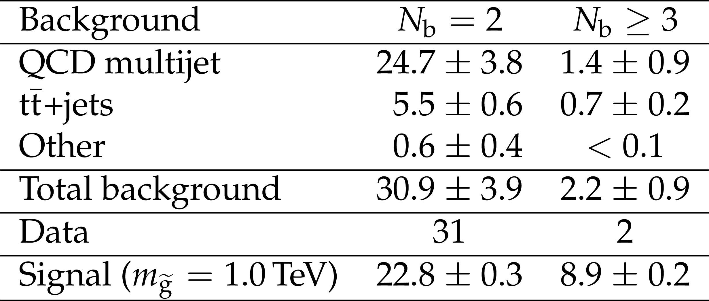
Summary of pre-fit expected background, expected signal for $m_{\tilde{ \mathrm{ g } } } = $ 1 TeV , and observed yields for $ {N_{\text {jet}}} \geq $ 8 and $ {H_{\mathrm {T}}} > $ 1.75 TeV . Uncertainties are statistical only. |
png pdf |
Table 3:
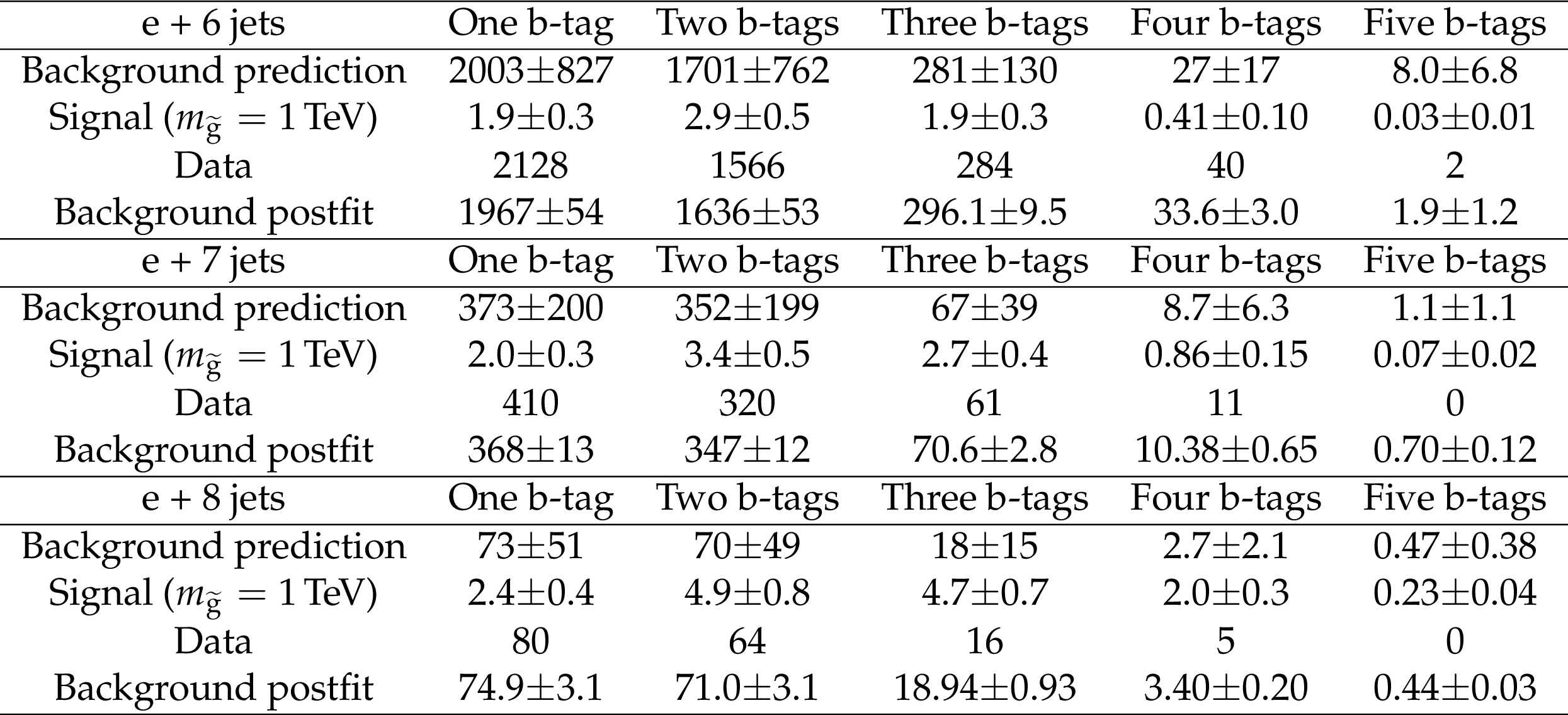
Summary of expected background, expected signal for $m_{\tilde{ \mathrm{ g } } }= $ 1 TeV , observed yields, and total background after the background-only fit for the electron samples considered in the analysis. The uncertainties given include all statistical and systematic uncertainties. |

png pdf |
Table 4:
Summary of the expected background, expected signal for $m_{\tilde{ \mathrm{ g } } }= $ 1 TeV , observed yields, and total background after the background-only fit for the muon samples. The uncertainties given include all statistical and systematic uncertainties. |

png pdf |
Table 5:
Definition of signal and control regions in the dilepton analysis. |
png pdf |
Table 6:
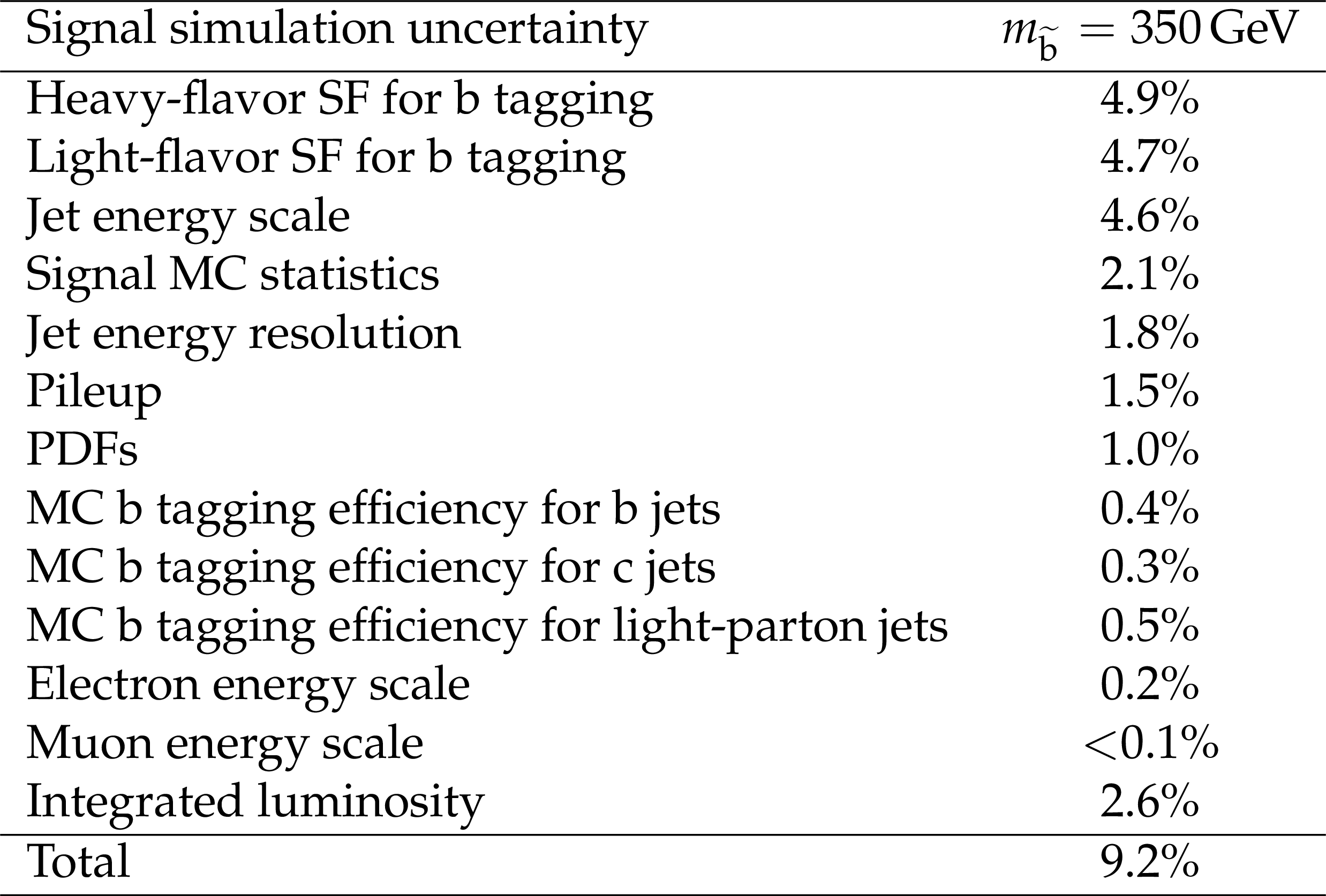
Relative systematic uncertainty in the signal selection efficiency broken down by source of signal systematic uncertainty for a characteristic mass point. |
png pdf |
Table 7:
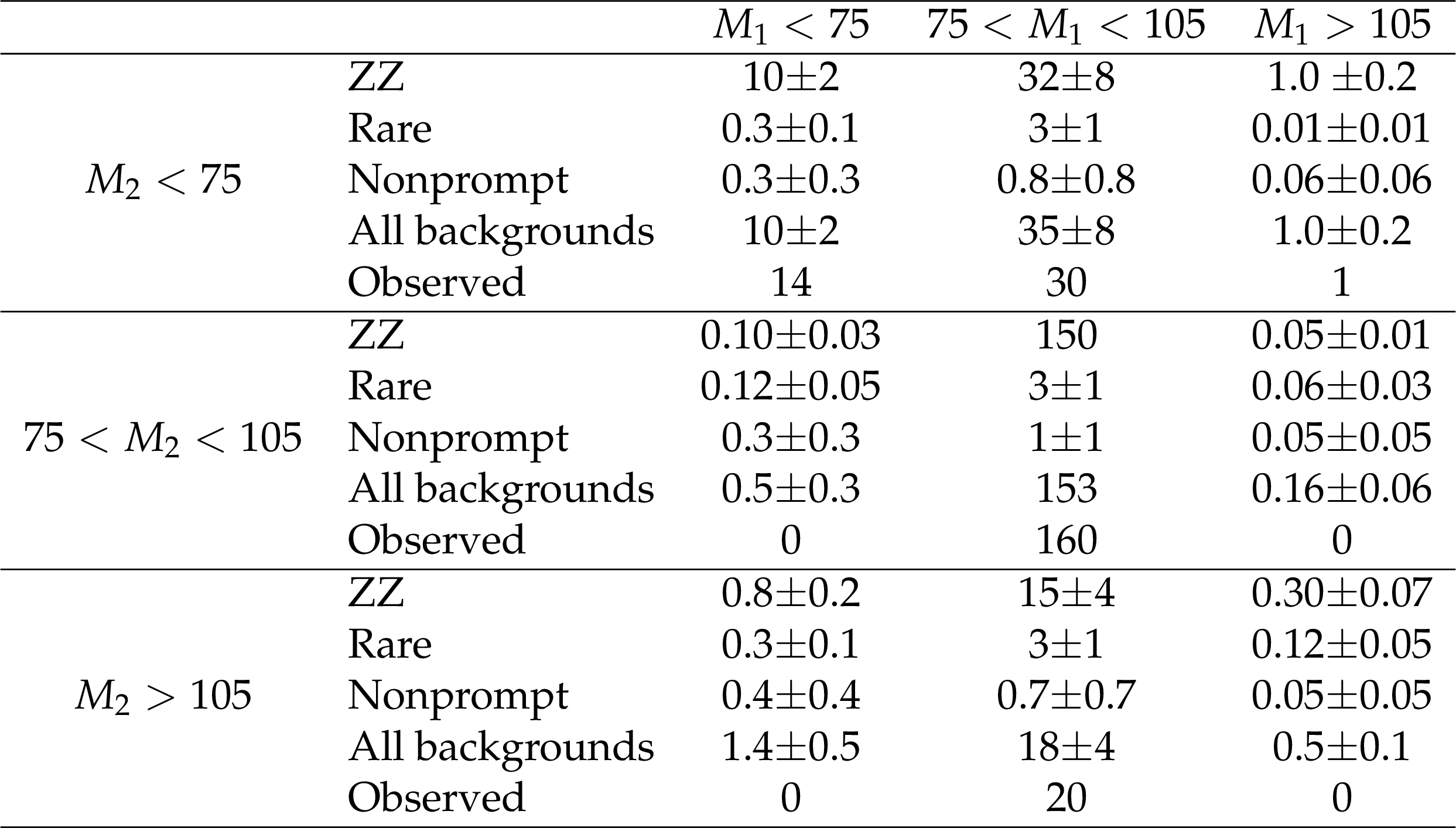
Expected background contributions from different SM sources and experimentally observed events in all analysis regions. The ZZ prediction in the region with both $M_1$ and $M_2$ falling in the ``at Z'' region is based on simulation normalized to the CMS ZZ production cross section measurement, and is therefore correlated with the observation in this analysis. The uncertainties take into account statistical and systematic contributions, combined quadratically. Mass ranges are given in GeV. |
png pdf |
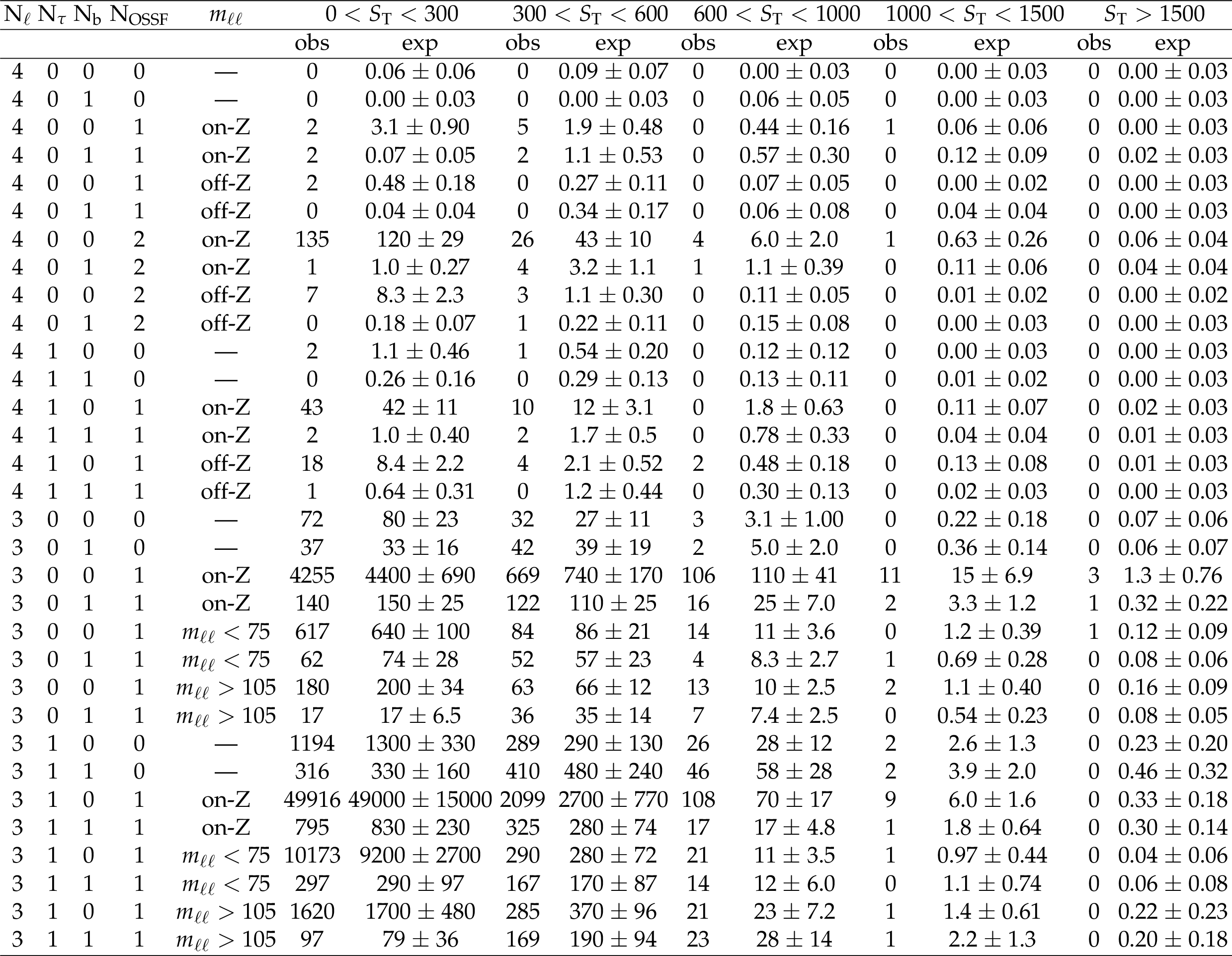
Table 8:
Expected and observed yields for three- and four-lepton events. The channels are split by the number of leptons ($\mathrm{N}_\ell $), the number of $ {\tau _\mathrm {h}} $ candidates ($\mathrm{N}_{\tau }$), whether the event contains b-tagged jets ($\mathrm{N}_{\mathrm{b} }$), the number of OSSF pairs ($\mathrm{N}_\text {OSSF}$), binning in the dilepton invariant mass ($m_{\ell \ell }$ of light leptons only), and the $ {S_\mathrm {T}} $. Events are considered on-Z if 75 $ < m_{\ell \ell } < $ 105 GeV. Expected yields are the sum of simulation and estimates of backgrounds from data in each channel. The channels are mutually exclusive. The uncertainties include statistical and systematic uncertainties. The $ {S_\mathrm {T}} $ and $m_{\ell \ell }$ values are given in GeV. Reproduced from Ref. [27]. |
| Summary |
|
This paper explores a variety of final states where $R$-parity-violating (RPV) supersymmetry could appear. Using data samples corresponding to 19.5 fb$^{-1}$ of proton-proton collision data collected with the CMS detector at $ \sqrt{s} = $ 8 TeV, no discrepancies from the expectations of the standard model are found. Limits on the masses of supersymmetric particles are set at 95% confidence level in several models that exhibit different RPV couplings and contain different lightest supersymmetric particles (LSP). The consequences of minimal flavor violation are explored in analyses that consider pair production of either gluinos or bottom squarks. The b-tagged and total jet multiplicity distributions are used to set limits on the mass of a gluino that decays to a top, a bottom, and a strange quark via the superpotential coupling $\lambda''_{332}$. Gluinos with masses less than 0.98 TeV are excluded. Using a search region characterized by one lepton and high multiplicity of jets and b-tagged jets, gluinos with masses less than 1.03 TeV are excluded in the same model. Another model assumes pair production of a bottom squark LSP that decays via $\lambda''_{332}$ or $\lambda''_{331}$. Using the reconstructed resonance mass distribution in the dilepton final state, bottom squark production is excluded for masses less than 307 GeV. Multilepton final states are sensitive to models with a variety of different leptonic or semileptonic RPV couplings. Limits on the mediator masses are established in a search in the four-lepton channel for strong production of neutralinos and their decay via the leptonic couplings $\lambda_{121}$ and $\lambda_{122}$. In a model of squark pair production with a neutralino LSP, lower limits on the squark mass are set at about 1.6 TeV. In models that feature electroweak production via leptonic couplings with wino- or higgsino-like LSPs, limits are set on the LSP mass that range from 300 to 900 GeV. In those with semileptonic couplings, there are a variety of scenarios. In the regions of highest sensitivity, lower limits on the higgsino masses reach approximately 700 GeV. |
| References | ||||
| 1 | H. P. Nilles | Supersymmetry, Supergravity and Particle Physics | PR 110 (1984) 1 | |
| 2 | H. E. Haber and G. L. Kane | The Search for Supersymmetry: Probing Physics Beyond the Standard Model | PR 117 (1985) 75 | |
| 3 | G. R. Farrar and P. Fayet | Phenomenology of the production, decay, and detection of new hadronic states associated with supersymmetry | PLB 76 (1978) 575 | |
| 4 | R. Barbier et al. | R-parity violating supersymmetry | PR 420 (2005) 1 | hep-ph/0406039 |
| 5 | Particle Data Group, J. Beringer et al. | Review of Particle Physics (RPP) | PRD 86 (2012) 010001 | |
| 6 | A. Y. Smirnov and F. Vissani | Upper bound on all products of R-parity violating couplings $ \lambda' $ and $ \lambda'' $ from proton decay | PLB 380 (1996) 317 | hep-ph/9601387 |
| 7 | E. Nikolidakis and C. Smith | Minimal flavor violation, seesaw mechanism, and R parity | PRD 77 (2008) 015021 | 0710.3129 |
| 8 | C. Cs\'aki, Y. Grossman, and B. Heidenreich | Minimal flavor violation supersymmetry: A natural theory for R-parity violation | PRD 85 (2012) 095009 | 1111.1239 |
| 9 | CDF Collaboration | First Search for Multijet Resonances in $ \sqrt{s} = 1.96 $~TeV $ p\bar{p} $ Collisions | PRL 107 (2011) 042001 | 1105.2815 |
| 10 | ATLAS Collaboration | Search for pair production of massive particles decaying into three quarks with the ATLAS detector in $ \sqrt{s}=7 $~TeV pp collisions at the LHC | JHEP 12 (2012) 086 | 1210.4813 |
| 11 | CMS Collaboration | Search for three-jet resonances in pp collisions at $ \sqrt{s}=7 $~TeV | PLB 718 (2012) 329 | CMS-EXO-11-060 1208.2931 |
| 12 | CMS Collaboration | Search for Three-Jet Resonances in $ pp $ Collisions at $ \sqrt{s}=7 $~TeV | PRL 107 (2011) 101801 | CMS-EXO-11-001 1107.3084 |
| 13 | CMS Collaboration | Searches for light- and heavy-flavour three-jet resonances in pp collisions at $ \sqrt{s} =$ 8 TeV | PLB 730 (2014) 193 | CMS-EXO-12-049 1311.1799 |
| 14 | ATLAS Collaboration | Search for massive supersymmetric particles decaying to many jets using the ATLAS detector in $ pp $ collisions at $ \sqrt{s} =$ 8 TeV | PRD 91 (2015) 112016 | 1502.05686 |
| 15 | ALEPH Collaboration | Search for supersymmetric particles with R-parity violating decays in $ e^{+} e^{-} $ collisions at $ \sqrt{s} $ up to 209 GeV | EPJC 31 (2003) 1 | hep-ex/0210014 |
| 16 | DELPHI Collaboration | Search for supersymmetric particles assuming R-parity nonconservation in e$ ^{+} $e$ ^{-} $ collisions at $ \sqrt{s} $ = 192 GeV to 208 GeV | EPJC 36 (2004) 1 | hep-ex/0406009 |
| 17 | L3 Collaboration | Search for R parity violating decays of supersymmetric particles in $ \textrm{e}^{+} \textrm{e}^{-} $ collisions at LEP | PLB 524 (2002) 65 | hep-ex/0110057 |
| 18 | D0 Collaboration | Search for Resonant Second Generation Slepton Production at the Fermilab Tevatron | PRL 97 (2006) 111801 | hep-ex/0605010 |
| 19 | D0 Collaboration | Search for R-parity violating supersymmetry via the $ LL \overline{E} $ couplings $ \lambda_{121} $, $ \lambda_{122} $ or $ \lambda_{133} $ in $ p \bar{p} $ collisions at $ \sqrt{s} $ = 1.96~TeV | PLB 638 (2006) 441 | hep-ex/0605005 |
| 20 | CDF Collaboration | Search for Anomalous Production of Multilepton Events in $ p \bar{p} $ Collisions at $ \sqrt{s} $ = 1.96 TeV | PRL 98 (2007) 131804 | 0706.4448 |
| 21 | H1 Collaboration | Search for Squarks in R-parity Violating Supersymmetry in ep Collisions at HERA | EPJC 71 (2011) 1572 | 1011.6359 |
| 22 | ZEUS Collaboration | Search for stop production in R-parity-violating supersymmetry at HERA | EPJC 50 (2007) 269 | hep-ex/0611018 |
| 23 | CMS Collaboration | Search for physics beyond the standard model using multilepton signatures in pp collisions at $ \sqrt{s} =$ 7 TeV | PLB 704 (2011) 411 | CMS-SUS-10-008 1106.0933 |
| 24 | CMS Collaboration | Search for anomalous production of multilepton events in pp collisions at $ \sqrt{s} $ = 7 TeV | JHEP 06 (2012) 169 | CMS-SUS-11-013 1204.5341 |
| 25 | ATLAS Collaboration | Search for R-parity-violating supersymmetry in events with four or more leptons in $ \sqrt{s} =$ 7 TeV $ pp $ collisions with the ATLAS detector | JHEP 12 (2012) 124 | 1210.4457 |
| 26 | ATLAS Collaboration | Search for a heavy narrow resonance decaying to $ e \mu $, $ e \tau $, or $ \mu \tau $ with the ATLAS detector in $ \sqrt{s} =$ 7 TeV $ pp $ collisions at the LHC | PLB 723 (2013) 15 | 1212.1272 |
| 27 | CMS Collaboration | Search for Top Squarks in $ R $-Parity-Violating Supersymmetry Using Three or More Leptons and b-Tagged Jets | PRL 111 (2013) 221801 | CMS-SUS-13-003 1306.6643 |
| 28 | ATLAS Collaboration | Search for supersymmetry in events with four or more leptons in $ \sqrt{s} =$ 8 TeV $ pp $ collisions with the ATLAS detector | PRD 90 (2014) 052001 | 1405.5086 |
| 29 | CMS Collaboration | The CMS experiment at the CERN LHC | JINST 3 (2008) S08004 | CMS-00-001 |
| 30 | CMS Collaboration | Study of tau reconstruction algorithms using $ \mathrm{ p }\mathrm{ p } $ collisions data collected at $ \sqrt{s} =$ 7 TeV | CDS | |
| 31 | CMS Collaboration | CMS Strategies for tau reconstruction and identification using particle-flow techniques | CDS | |
| 32 | CMS Collaboration | Commissioning of the Particle-Flow Reconstruction in Minimum-Bias and Jet Events from $ \mathrm{ p }\mathrm{ p } $ Collisions at 7 TeV | CDS | |
| 33 | F. Maltoni and T. Stelzer | MadEvent: automatic event generation with MadGraph | JHEP 02 (2003) 027 | hep-ph/0208156 |
| 34 | T. Sj\"ostrand, S. Mrenna, and P. Z. Skands | A brief introduction to PYTHIA 8.1 | CPC 178 (2008) 852 | 0710.3820 |
| 35 | GEANT4 Collaboration | GEANT4---a simulation toolkit | NIMA 506 (2003) 250 | |
| 36 | M. L. Mangano, M. Moretti, F. Piccinini, and M. Treccani | Matching matrix elements and shower evolution for top-quark production in hadronic collisions | JHEP 01 (2007) 013 | hep-ph/0611129 |
| 37 | J. A. Evans and Y. Kats | LHC coverage of RPV MSSM with light stops | JHEP 04 (2013) 028 | 1209.0764 |
| 38 | CMS Collaboration | The fast simulation of the CMS detector at LHC | J. Phys. Conf. Ser. 331 (2011) 032049 | |
| 39 | J. Pumplin et al. | New generation of parton distributions with uncertainties from global QCD analysis | JHEP 07 (2002) 012 | hep-ph/0201195 |
| 40 | CMS Collaboration | CMS Luminosity Based on Pixel Cluster Counting - Summer 2013 Update | CMS-PAS-LUM-13-001 | CMS-PAS-LUM-13-001 |
| 41 | N. Arkani-Hamed et al. | MARMOSET: The path from LHC data to the new standard model via on-shell effective theories | hep-ph/0703088 | |
| 42 | J. Alwall, P. Schuster, and N. Toro | Simplified models for a first characterization of new physics at the LHC | PRD 79 (2009) 075020 | 0810.3921 |
| 43 | LHC New Physics Working Group Collaboration | Simplified Models for LHC New Physics Searches | JPG 39 (2012) 105005 | 1105.2838 |
| 44 | S. Alekhin et al. | The PDF4LHC Working Group Interim Report | 1101.0536 | |
| 45 | M. Botje et al. | The PDF4LHC Working Group Interim Recommendations | 1101.0538 | |
| 46 | P. M. Nadolsky et al. | Implications of CTEQ global analysis for collider observables | PRD 78 (2008) 013004 | 0802.0007 |
| 47 | A. D. Martin, W. J. Stirling, R. S. Thorne, and G. Watt | Parton distributions for the LHC | EPJC 63 (2009) 189 | 0901.0002 |
| 48 | R. D. Ball et al. | A first unbiased global NLO determination of parton distributions and their uncertainties | Nucl. Phys. B 838 (2010) 136 | 1002.4407 |
| 49 | CMS Collaboration | Search for top-squark pair production in the single-lepton final state in pp collisions at $ \sqrt{s} $ = 8 TeV | EPJC 73 (2013) 2677 | CMS-SUS-13-011 1308.1586 |
| 50 | T. Junk | Confidence level computation for combining searches with small statistics | NIMA 434 (1999) 435 | hep-ex/9902006 |
| 51 | A. L. Read | Presentation of search results: the $ CL_s $ technique | JPG 28 (2002) 2693 | |
| 52 | ATLAS and CMS Collaborations | Procedure for the LHC Higgs boson search combination in Summer 2011 | CMS-NOTE-2011-005 | |
| 53 | W. Beenakker et al. | Production of Charginos, Neutralinos, and Sleptons at Hadron Colliders | PRL 83 (1999) 3780 | hep-ph/9906298 |
| 54 | A. Kulesza and L. Motyka | Threshold Resummation for Squark-Antisquark and Gluino-Pair Production at the LHC | PRL 102 (2009) 111802 | 0807.2405 |
| 55 | A. Kulesza and L. Motyka | Soft gluon resummation for the production of gluino-gluino and squark-antisquark pairs at the LHC | PRD 80 (2009) 095004 | 0905.4749 |
| 56 | W. Beenakker et al. | Soft-gluon resummation for squark and gluino hadroproduction | JHEP 12 (2009) 041 | 0909.4418 |
| 57 | W. Beenakker et al. | Squark and gluino hadroproduction | Int. J. Mod. Phys. A 26 (2011) 2637 | 1105.1110 |
| 58 | CMS Collaboration | Performance of electron reconstruction and selection with the CMS detector in proton-proton collisions at $ \sqrt{s} =$ 8 TeV | JINST 10 (2015) P06005 | CMS-EGM-13-001 1502.02701 |
| 59 | CMS Collaboration | Performance of CMS muon reconstruction in pp collision events at $ \sqrt{s} =$ 7 TeV | JINST 7 (2012) P10002 | CMS-MUO-10-004 1206.4071 |
| 60 | CMS Collaboration | Performance of $ \tau $-lepton reconstruction and identification in CMS | JINST 7 (2012) P01001 | CMS-TAU-11-001 1109.6034 |
| 61 | M. Cacciari, G. P. Salam, and G. Soyez | The anti-$ k_t $ jet clustering algorithm | JHEP 04 (2008) 063 | 0802.1189 |
| 62 | CMS Collaboration | Determination of jet energy calibration and transverse momentum resolution in CMS | JINST 6 (2011) P11002 | |
| 63 | CMS Collaboration | Identification of $\mathrm{b}$-quark jets with the CMS experiment | JINST 8 (2013) P04013 | CMS-BTV-12-001 1211.4462 |
| 64 | CMS Collaboration | Performance of b-tagging at $ \sqrt{s}=8 $~TeV in multijet, $\mathrm{ t \bar{t} }$ and boosted topology events | CMS-PAS-BTV-13-001 | CMS-PAS-BTV-13-001 |
| 65 | CMS Collaboration | Measurement of $ \mathrm{ t \overline{t} } $ production with additional jet activity, including b quark jets, in the dilepton decay channel using pp collisions at $ \sqrt{s} = $ 8 TeV | In proof, EPJC | CMS-TOP-12-041 1510.03072 |
| 66 | R. Barlow and C. Beeston | Fitting using finite Monte Carlo samples | CPC 77 (1993) 219 | |
| 67 | CMS Collaboration | Measurement of $ \mathrm{B}\overline{\mathrm{B}} $ angular correlations based on secondary vertex reconstruction at $ \sqrt{s} $ = 7 TeV | JHEP 03 (2011) 136 | |
| 68 | M. Czakon, P. Fiedler, and A. Mitov | Total Top-Quark Pair-Production Cross Section at Hadron Colliders Through $ \mathcal{O}(\alpha^4_S) $ | PRL 110 (2013) 252004 | 1303.6254 |
| 69 | CMS Collaboration | Measurement of the differential cross section for top quark pair production in pp collisions at $ \sqrt{s} =$ 8 TeV | EPJC 75 (2015) 542 | CMS-TOP-12-028 1505.04480 |
| 70 | L. Sonnenschein | Analytical solution of $ t\bar{t} $ dilepton equations | PRD 73 (2006) 054015, , Erratum: [\DOI10.1103/PhysRevD.78.079902] | hep-ph/0603011 |
| 71 | H.-C. Cheng et al. | Mass determination in SUSY-like events with missing energy | JHEP 12 (2007) 076 | 0707.0030 |
| 72 | CMS Collaboration | Measurement of the top-quark mass in $\mathrm{ t \bar{t} }$ events with dilepton final states in pp collisions at $ \sqrt{s} =$ 7 TeV | EPJC 72 (2012) 2202 | CMS-TOP-11-016 1209.2393 |
| 73 | CMS Collaboration | Measurement of the $ \mathrm{ t \bar{t} } $ production cross section in the e-$ \mu $ channel in proton-proton collisions at $ \sqrt{s} $ = 7 and 8 TeV | Submitted to JHEP | CMS-TOP-13-004 1603.02303 |
| 74 | G. J. Feldman and R. D. Cousins | Unified approach to the classical statistical analysis of small signals | PRD 57 (1998) 3873 | physics/9711021 |
| 75 | CMS Collaboration | Measurement of $ \mathrm{ W }^+\mathrm{ W }^- $ and ZZ production cross sections in pp collisions at $ \sqrt{s} $ = 8 TeV | PLB 721 (2013) 190 | CMS-SMP-12-024 1301.4698 |
| 76 | MSSM Working Group Collaboration | The minimal supersymmetric standard model: Group summary report | hep-ph/9901246 | |
| 77 | CMS Collaboration | Phenomenological MSSM interpretation of CMS searches in pp collisions at $ \sqrt{s} = 7 $ and 8 TeV | Submitted to JHEP | CMS-SUS-15-010 1606.03577 |
|
|
Compact Muon Solenoid LHC, CERN |
|

|

|

|

|

|