

Compact Muon Solenoid
LHC, CERN
| CMS-TOP-12-041 ; CERN-PH-EP-2015-240 | ||
| Measurement of $\mathrm{ t \bar{t} }$ production with additional jet activity, including b quark jets, in the dilepton decay channel using pp collisions at $ \sqrt{s} = $ 8 TeV | ||
| CMS Collaboration | ||
| 11 October 2015 | ||
| Eur. Phys. J. C 76 (2016) 379 | ||
| Abstract: Jet multiplicity distributions in top quark pair ($ \mathrm{ t \bar{t} } $) events are measured in pp collisions at a centre-of-mass energy of 8 TeV with the CMS detector at the LHC using a data set corresponding to an integrated luminosity of 19.7 fb$^{-1}$. The measurement is performed in the dilepton decay channels ($\mathrm{ e^+ e^- }$, $\mu^+ \mu^-$, and $\mathrm{ e^\pm } \mu^\mp$). The absolute and normalized differential cross sections for $ \mathrm{ t \bar{t} } $ production are measured as a function of the jet multiplicity in the event for different jet transverse momentum thresholds and the kinematic properties of the leading additional jets. The differential $ \mathrm{ t \bar{t} b} $ and $ \mathrm{ t \bar{t} b \bar{b} } $ cross sections are presented for the first time as a function of the kinematic properties of the leading additional b jets. Furthermore, the fraction of events without additional jets above a threshold is measured as a function of the transverse momenta of the leading additional jets and the scalar sum of the transverse momenta of all additional jets. The data are compared and found to be consistent with predictions from several perturbative quantum chromodynamics event generators and a next-to-leading order calculation. | ||
| Links: e-print arXiv:1510.03072 [hep-ex] (PDF) ; CDS record ; inSPIRE record ; HepData record ; CADI line (restricted) ; | ||
| Figures & Tables | Summary | Additional Figures | References | CMS Publications |
|---|
| Figures | |
png pdf |
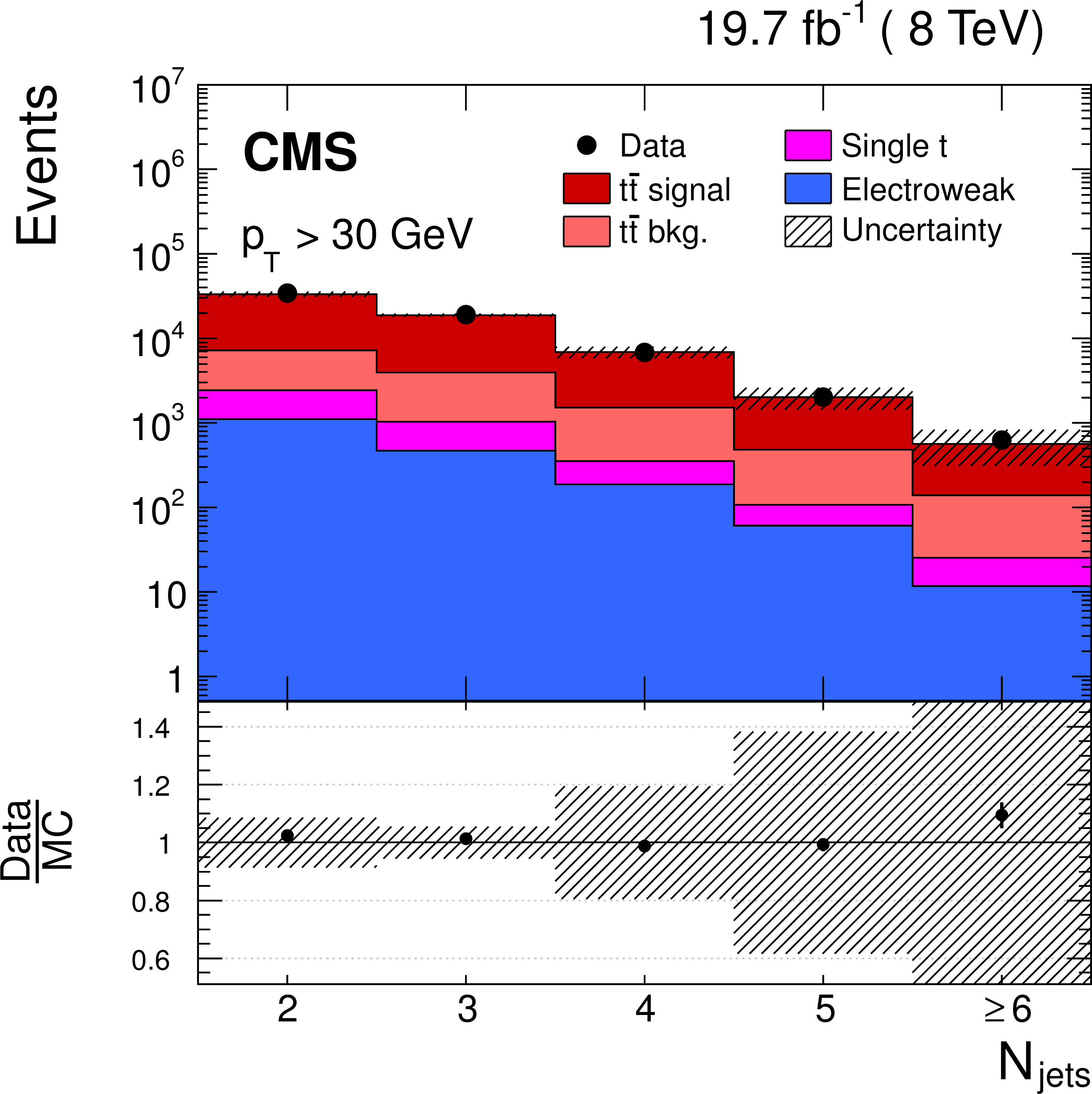
Figure 1-a:
Reconstructed jet multiplicity distribution after event selection in data (points) and from signal and background simulation (histograms) for all jets with ${p_{\mathrm {T}}}$ of at least 30 GeV (a), 60 GeV (b), and 100 GeV (c). The hatched regions correspond to the uncertainties affecting the shape of the distributions in the simulated signal ${\mathrm{ t } \mathrm{ \bar{t} } }$ events and backgrounds (cf. Section 6). The lower plots show the ratio of the data to the MC simulation prediction. Note that in all cases the event selection requires at least two jets with $ {p_{\mathrm {T}}} >$ 30 GeV. |

png pdf |
Figure 1-b:
Reconstructed jet multiplicity distribution after event selection in data (points) and from signal and background simulation (histograms) for all jets with ${p_{\mathrm {T}}}$ of at least 30 GeV (a), 60 GeV (b), and 100 GeV (c). The hatched regions correspond to the uncertainties affecting the shape of the distributions in the simulated signal ${\mathrm{ t } \mathrm{ \bar{t} } }$ events and backgrounds (cf. Section 6). The lower plots show the ratio of the data to the MC simulation prediction. Note that in all cases the event selection requires at least two jets with $ {p_{\mathrm {T}}} >$ 30 GeV. |
png pdf |
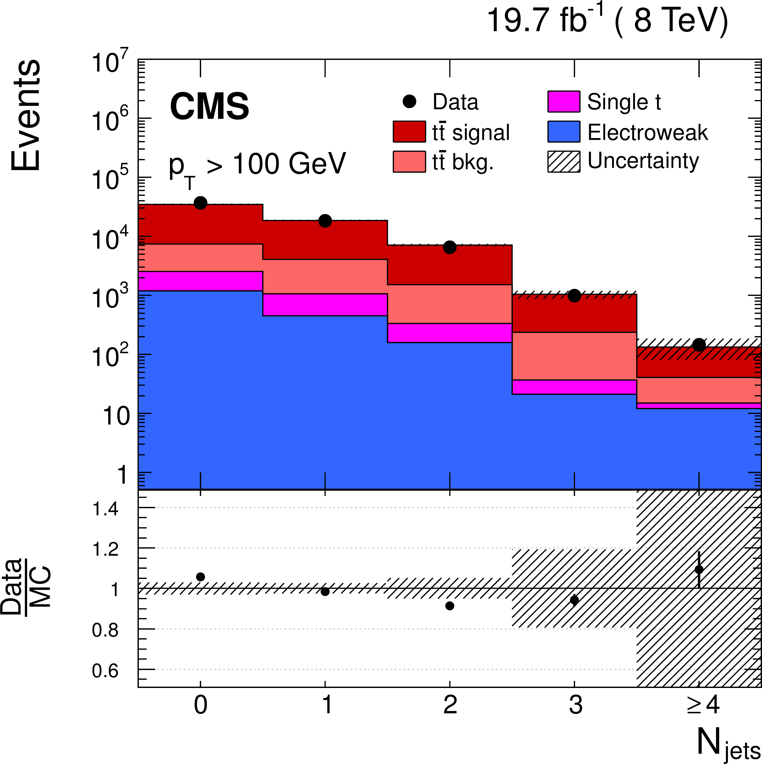
Figure 1-c:
Reconstructed jet multiplicity distribution after event selection in data (points) and from signal and background simulation (histograms) for all jets with ${p_{\mathrm {T}}}$ of at least 30 GeV (a), 60 GeV (b), and 100 GeV (c). The hatched regions correspond to the uncertainties affecting the shape of the distributions in the simulated signal ${\mathrm{ t } \mathrm{ \bar{t} } }$ events and backgrounds (cf. Section 6). The lower plots show the ratio of the data to the MC simulation prediction. Note that in all cases the event selection requires at least two jets with $ {p_{\mathrm {T}}} >$ 30 GeV. |

png pdf |
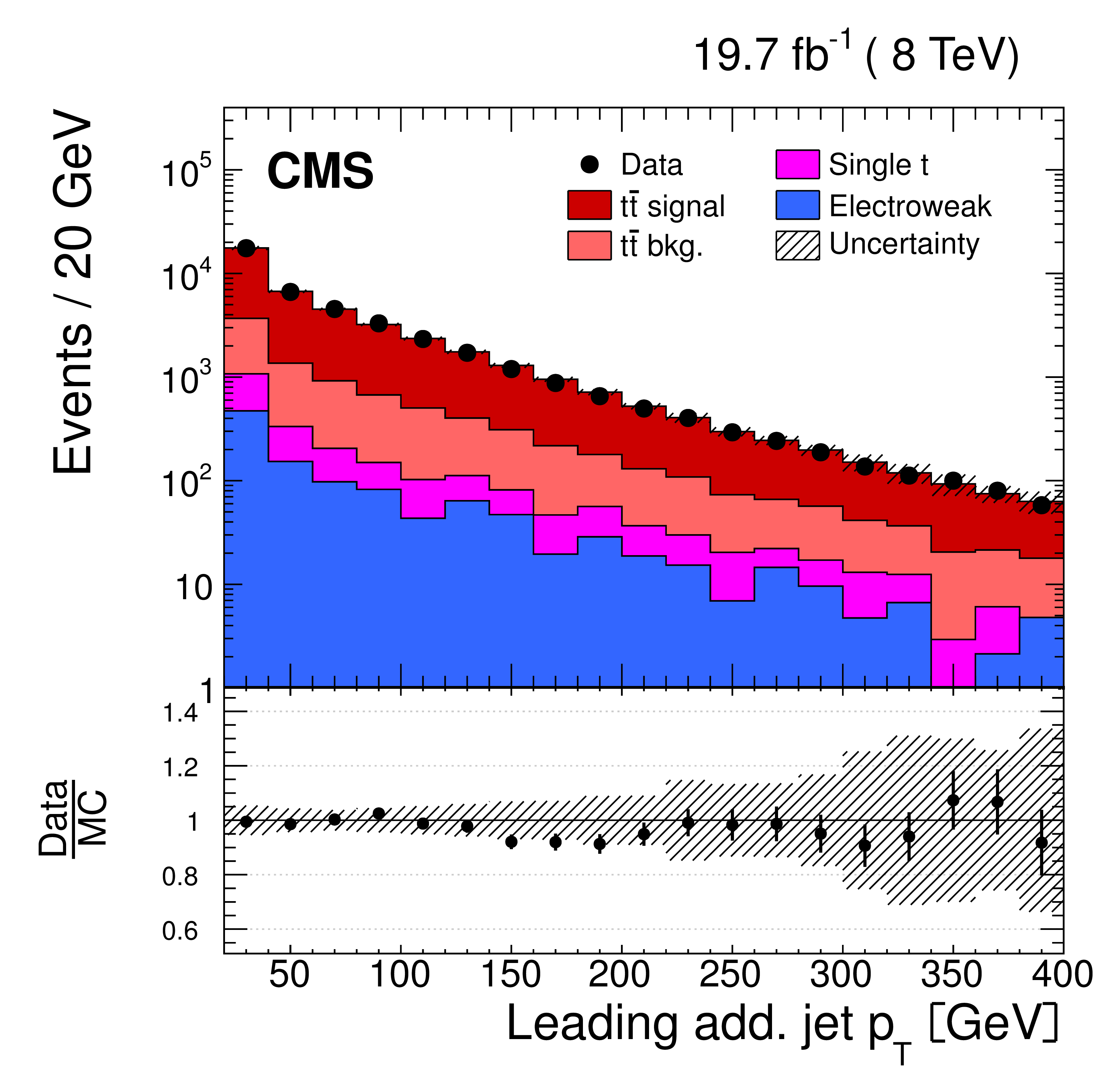
Figure 2-a:
Distribution of the $\eta $ (a,c) and ${p_{\mathrm {T}}}$ (b,d) of the leading (a,b) and subleading (c,d) additional reconstructed jets in data (points) and from signal and background simulation (histograms). The hatched regions correspond to the uncertainties affecting the shape of the simulated distributions in the signal ${\mathrm{ t } \mathrm{ \bar{t} } }$ events and backgrounds (cf. Section 6). The lower plots show the ratio of the data to the MC simulation prediction. |
png pdf |
Figure 2-b:
Distribution of the $\eta $ (a,c) and ${p_{\mathrm {T}}}$ (b,d) of the leading (a,b) and subleading (c,d) additional reconstructed jets in data (points) and from signal and background simulation (histograms). The hatched regions correspond to the uncertainties affecting the shape of the simulated distributions in the signal ${\mathrm{ t } \mathrm{ \bar{t} } }$ events and backgrounds (cf. Section 6). The lower plots show the ratio of the data to the MC simulation prediction. |

png pdf |
Figure 2-c:
Distribution of the $\eta $ (a,c) and ${p_{\mathrm {T}}}$ (b,d) of the leading (a,b) and subleading (c,d) additional reconstructed jets in data (points) and from signal and background simulation (histograms). The hatched regions correspond to the uncertainties affecting the shape of the simulated distributions in the signal ${\mathrm{ t } \mathrm{ \bar{t} } }$ events and backgrounds (cf. Section 6). The lower plots show the ratio of the data to the MC simulation prediction. |
png pdf |
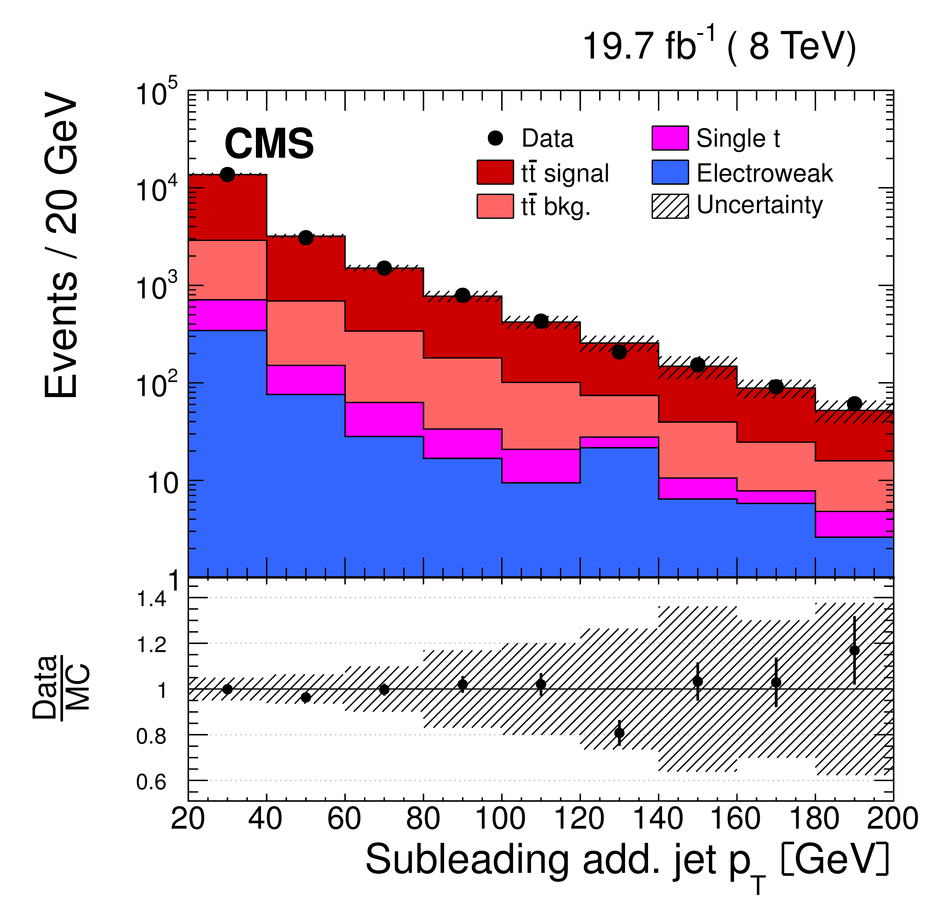
Figure 2-d:
Distribution of the $\eta $ (a,c) and ${p_{\mathrm {T}}}$ (b,d) of the leading (a,b) and subleading (c,d) additional reconstructed jets in data (points) and from signal and background simulation (histograms). The hatched regions correspond to the uncertainties affecting the shape of the simulated distributions in the signal ${\mathrm{ t } \mathrm{ \bar{t} } }$ events and backgrounds (cf. Section 6). The lower plots show the ratio of the data to the MC simulation prediction. |
png pdf |
Figure 3-a:
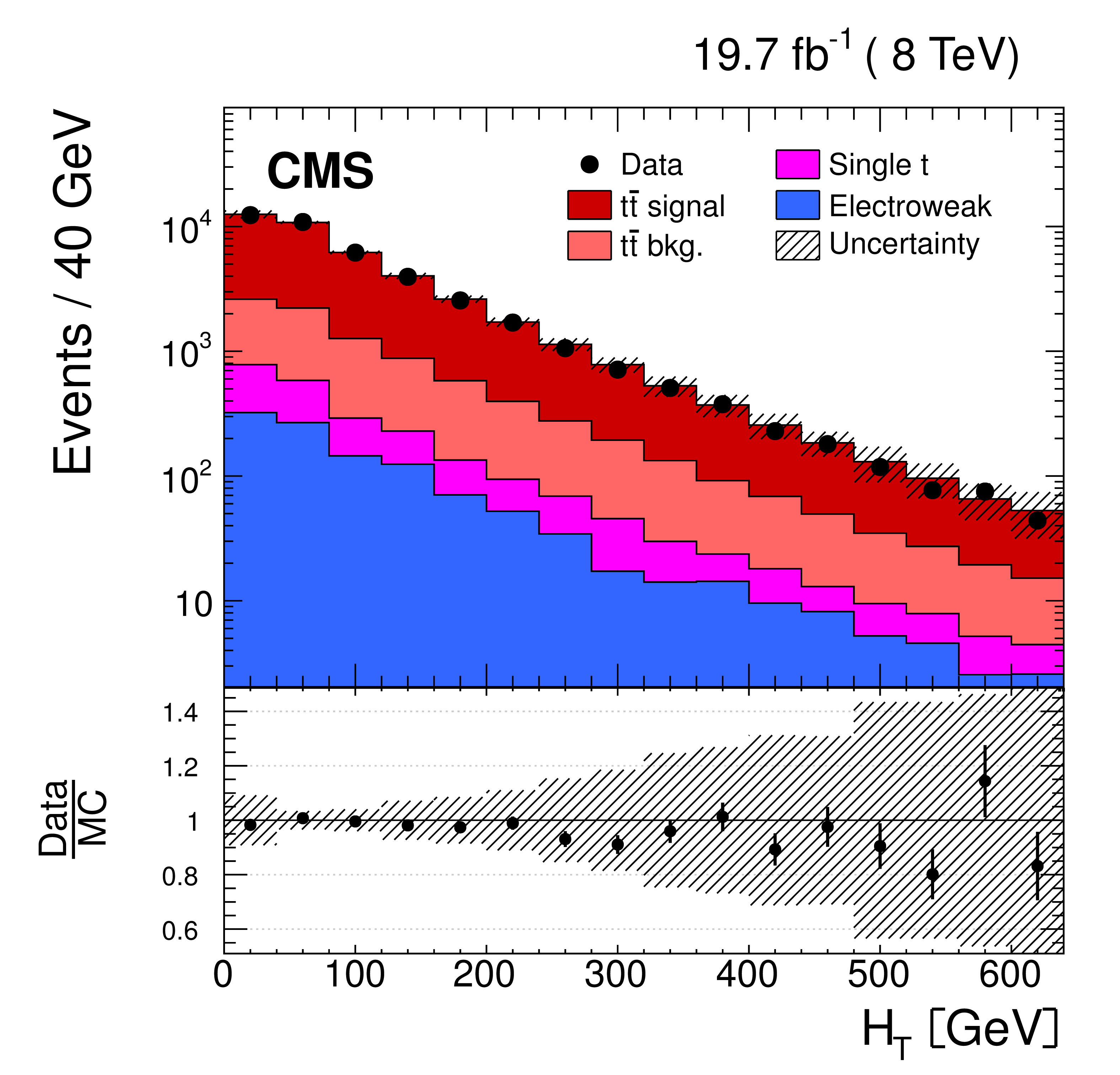
Distribution of the scalar sum of the ${p_{\mathrm {T}}}$ of all additional jets $ {H_{\mathrm {T}}} $ (a), the invariant mass of the leading and subleading additional jets ${m_{\mathrm {jj}}}$ (b), and their angular distance ${\Delta R_{\mathrm {jj}}}$ (c) in data (points) and from signal and background simulation (histograms). The hatched regions correspond to the uncertainties affecting the shape of the distributions in the simulated signal ${\mathrm{ t } \mathrm{ \bar{t} } }$ events and backgrounds (cf. Section 6). The lower plots show the ratio of the data to the MC simulation prediction. |

png pdf |
Figure 3-b:
Distribution of the scalar sum of the ${p_{\mathrm {T}}}$ of all additional jets $ {H_{\mathrm {T}}} $ (a), the invariant mass of the leading and subleading additional jets ${m_{\mathrm {jj}}}$ (b), and their angular distance ${\Delta R_{\mathrm {jj}}}$ (c) in data (points) and from signal and background simulation (histograms). The hatched regions correspond to the uncertainties affecting the shape of the distributions in the simulated signal ${\mathrm{ t } \mathrm{ \bar{t} } }$ events and backgrounds (cf. Section 6). The lower plots show the ratio of the data to the MC simulation prediction. |
png pdf |
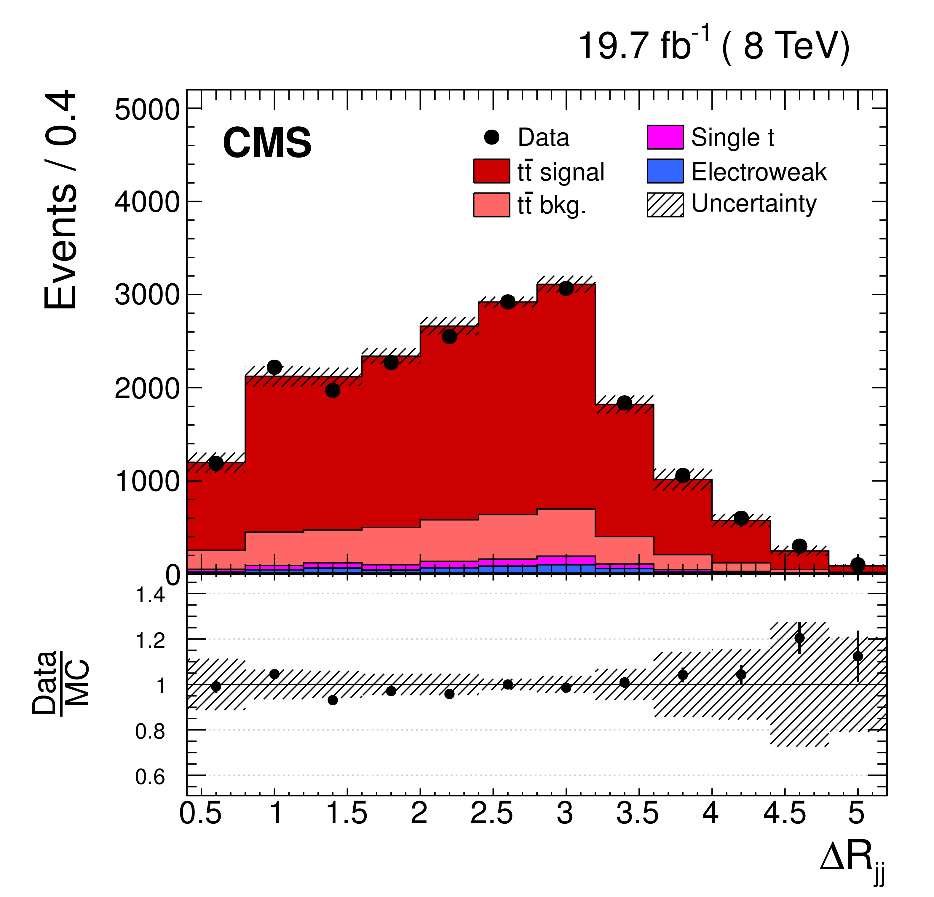
Figure 3-c:
Distribution of the scalar sum of the ${p_{\mathrm {T}}}$ of all additional jets $ {H_{\mathrm {T}}} $ (a), the invariant mass of the leading and subleading additional jets ${m_{\mathrm {jj}}}$ (b), and their angular distance ${\Delta R_{\mathrm {jj}}}$ (c) in data (points) and from signal and background simulation (histograms). The hatched regions correspond to the uncertainties affecting the shape of the distributions in the simulated signal ${\mathrm{ t } \mathrm{ \bar{t} } }$ events and backgrounds (cf. Section 6). The lower plots show the ratio of the data to the MC simulation prediction. |
png pdf |
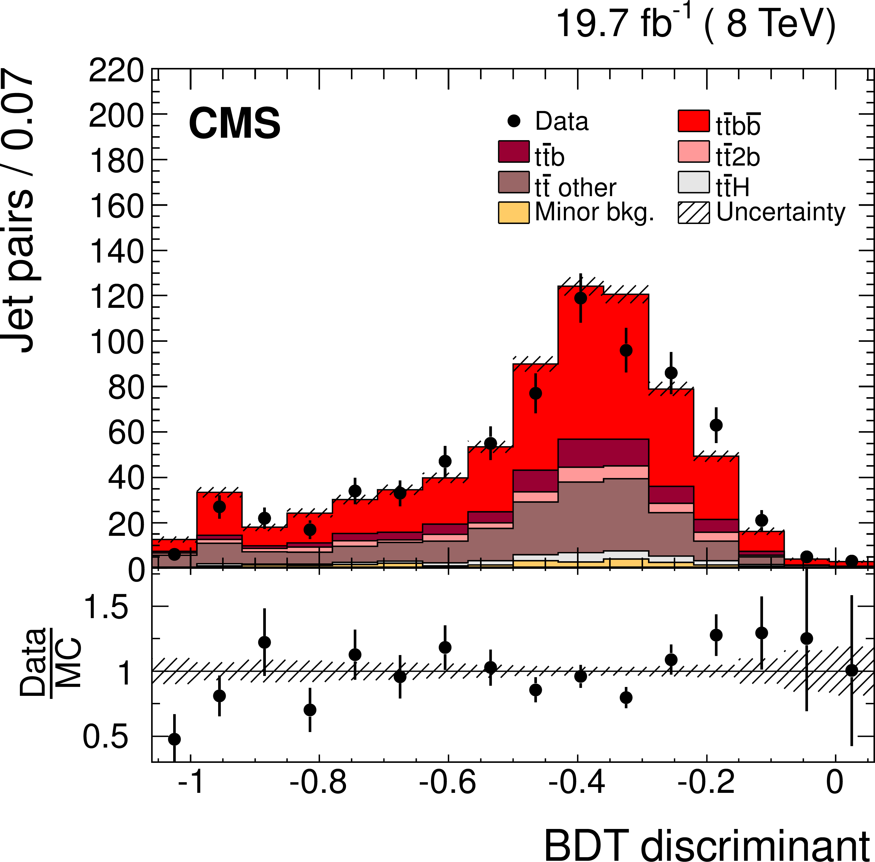
Figure 4-a:
The BDT discriminant of all dijet combinations in data (points) and from signal and background simulation (histograms) per event (left) and dijet combination with the highest discriminant per event (right) in events with at least four jets and exactly four b-tagged jets. The distributions include the correction obtained with the template fit to the b-tagged jet multiplicity (cf. Section {sec:ttbbreco}). The hatched area represents the statistical uncertainty in the simulated samples. ``Minor bkg." includes all non-${\mathrm{ t } \mathrm{ \bar{t} } }$ processes and ${\mathrm{ t } \mathrm{ \bar{t} } } $+$\mathrm{ Z } /\mathrm{ W } /\gamma $. The lower plots show the ratio of the data to the MC simulation prediction. |
png pdf |
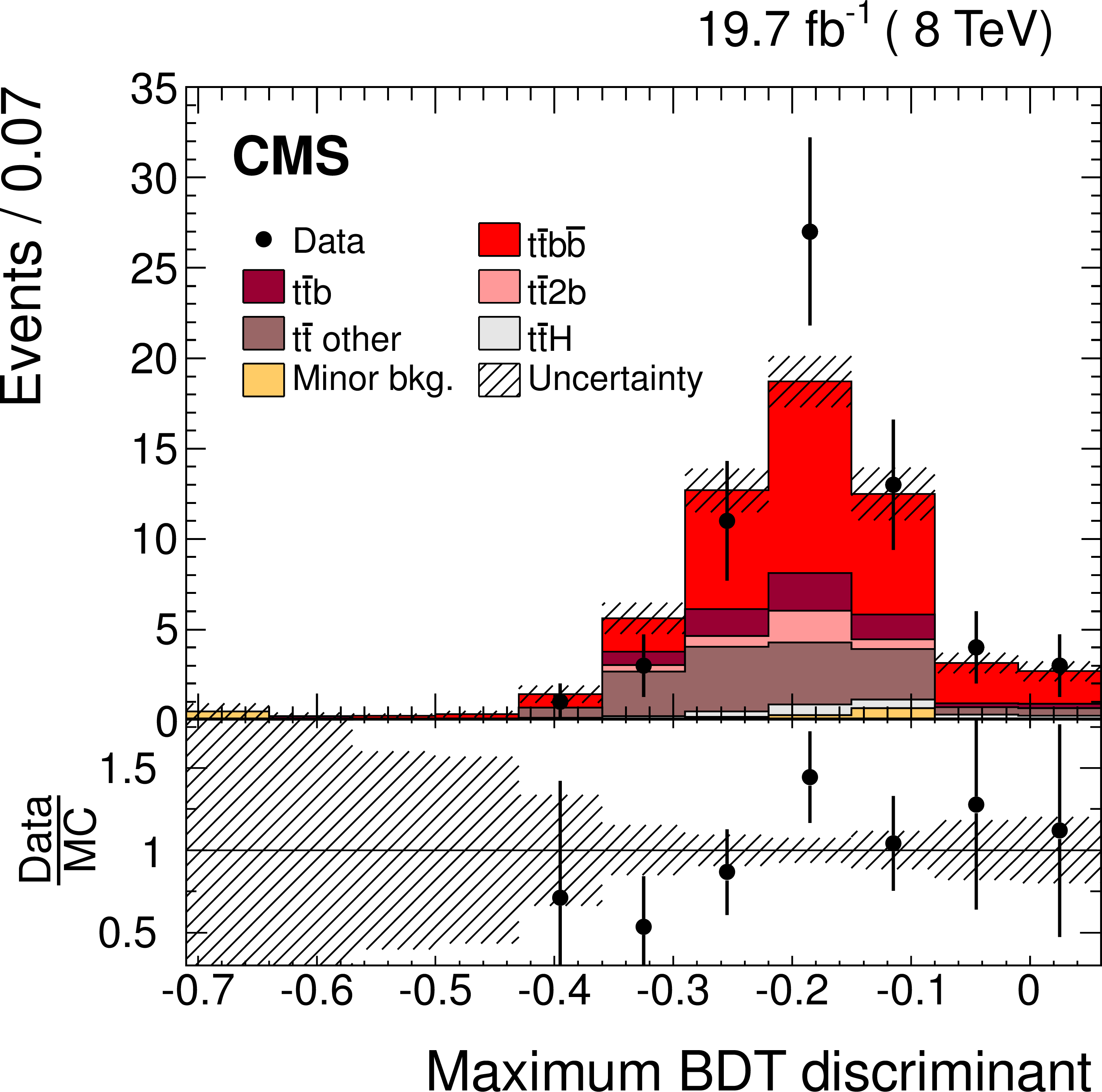
Figure 4-b:
The BDT discriminant of all dijet combinations in data (points) and from signal and background simulation (histograms) per event (left) and dijet combination with the highest discriminant per event (right) in events with at least four jets and exactly four b-tagged jets. The distributions include the correction obtained with the template fit to the b-tagged jet multiplicity (cf. Section {sec:ttbbreco}). The hatched area represents the statistical uncertainty in the simulated samples. ``Minor bkg." includes all non-${\mathrm{ t } \mathrm{ \bar{t} } }$ processes and ${\mathrm{ t } \mathrm{ \bar{t} } } $+$\mathrm{ Z } /\mathrm{ W } /\gamma $. The lower plots show the ratio of the data to the MC simulation prediction. |
png pdf |
Figure 5-a:
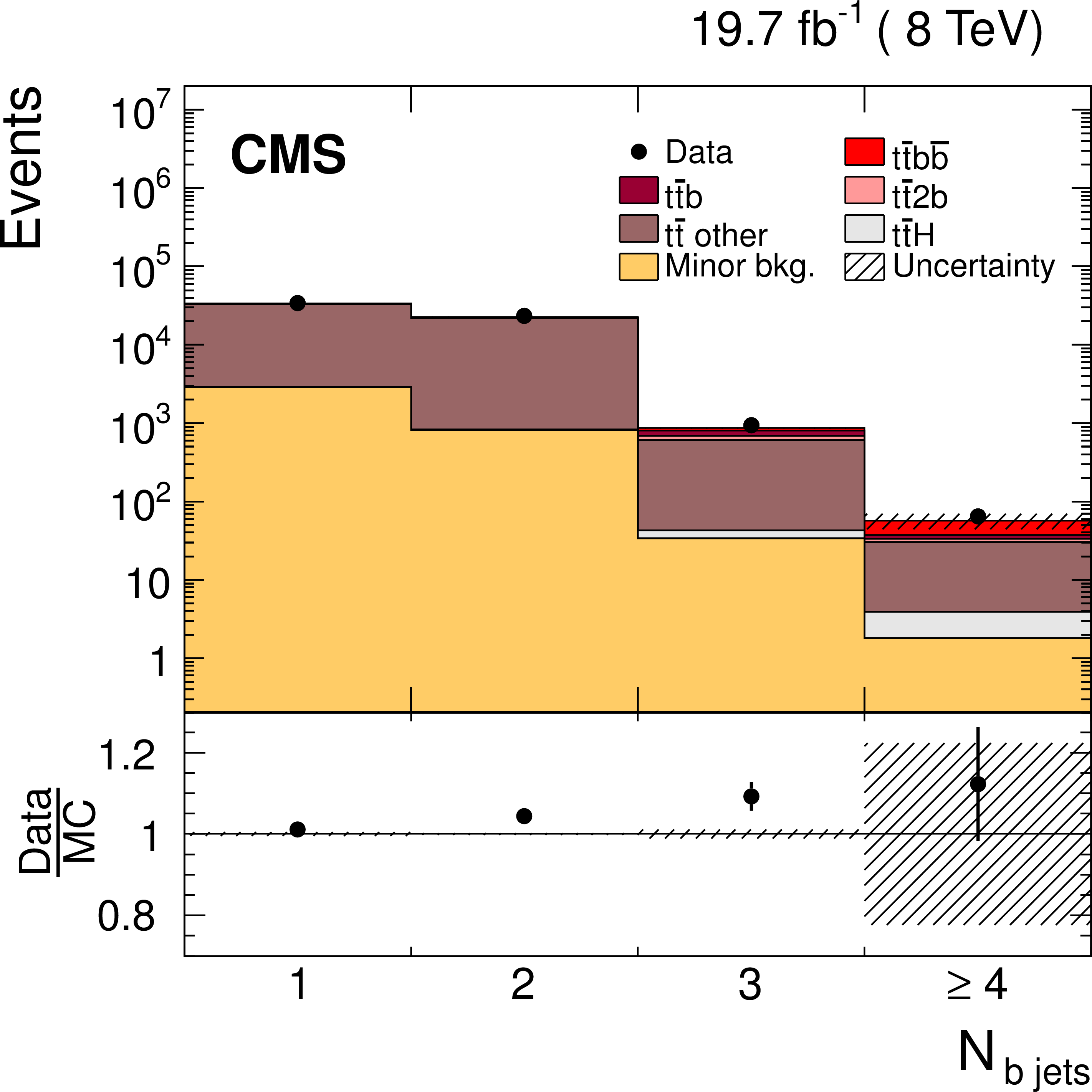
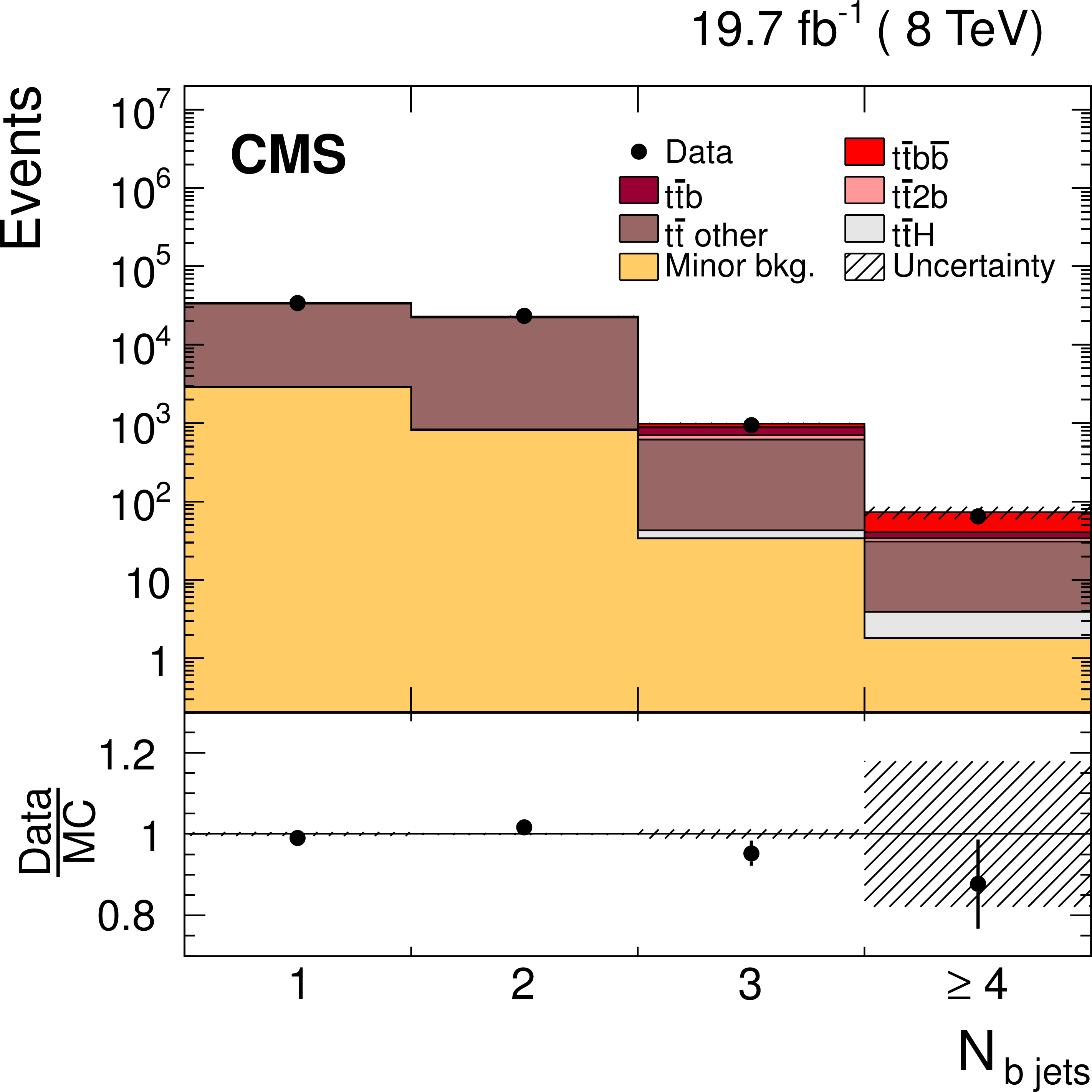
The pre-fit distribution of the b jet multiplicity in data (points) and from signal and background simulation (histograms) for events fulfilling the lepton selection criteria, having ${\ge } 2$ jets, ${\ge } 1$ b-tagged jet (left), and the post-fit distribution (right). The hatched area represents the statistical uncertainty in the simulated samples. ``Minor bkg." includes all non-${\mathrm{ t } \mathrm{ \bar{t} } }$ processes and ${\mathrm{ t } \mathrm{ \bar{t} } } $+$\mathrm{ Z } /\mathrm{ W } /\gamma $. The lower plots show the ratio of the data to the MC simulation prediction. |
png pdf |
Figure 5-b:
The pre-fit distribution of the b jet multiplicity in data (points) and from signal and background simulation (histograms) for events fulfilling the lepton selection criteria, having ${\ge } 2$ jets, ${\ge } 1$ b-tagged jet (left), and the post-fit distribution (right). The hatched area represents the statistical uncertainty in the simulated samples. ``Minor bkg." includes all non-${\mathrm{ t } \mathrm{ \bar{t} } }$ processes and ${\mathrm{ t } \mathrm{ \bar{t} } } $+$\mathrm{ Z } /\mathrm{ W } /\gamma $. The lower plots show the ratio of the data to the MC simulation prediction. |
png pdf |
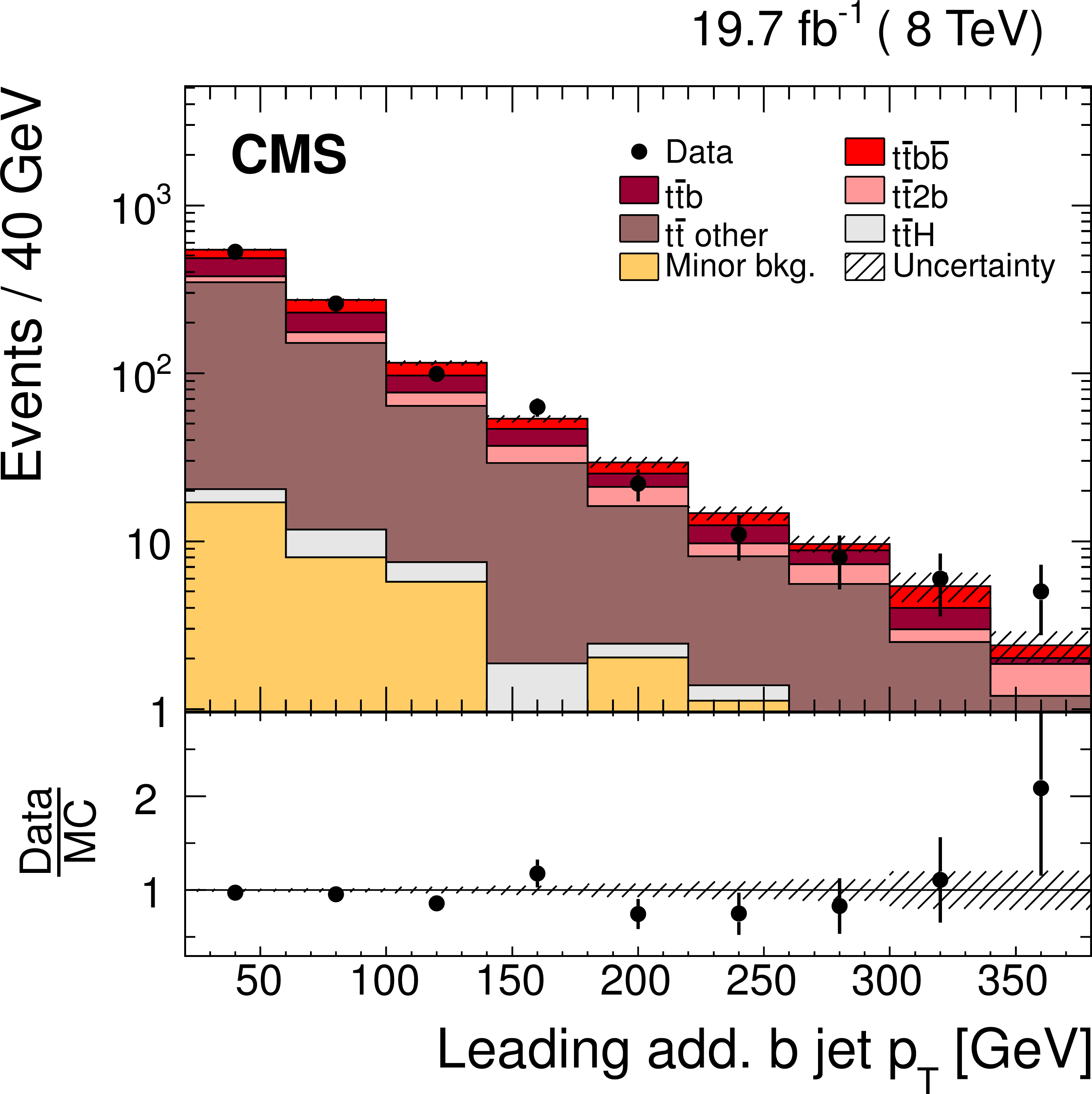
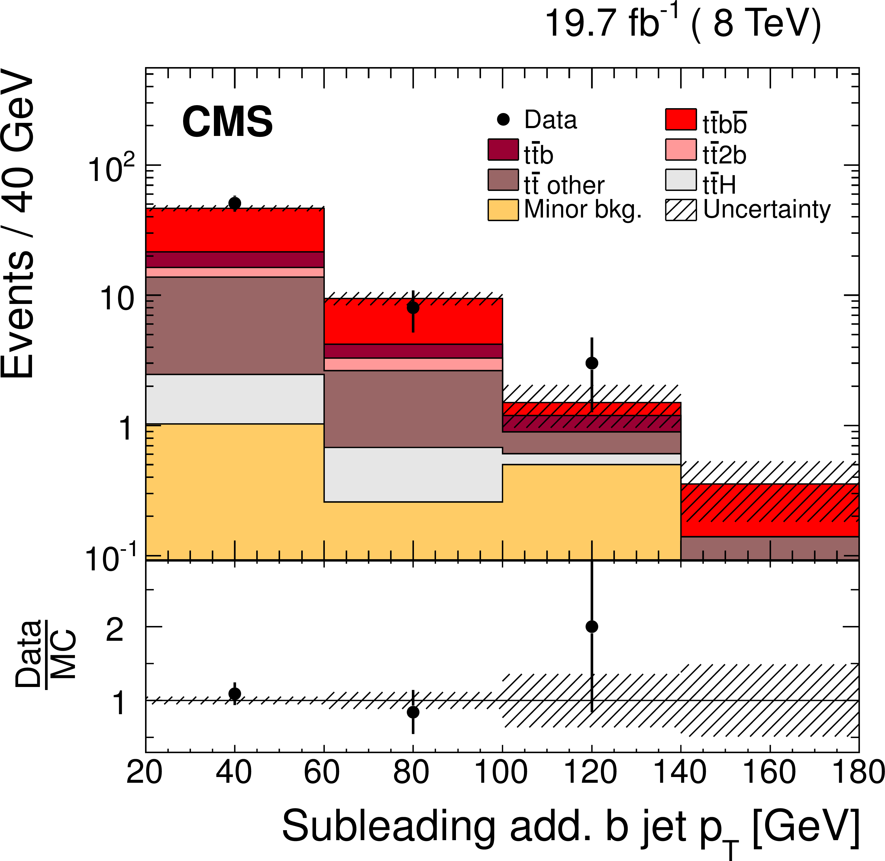
Figure 6-a:
Distributions of the leading additional b jet ${p_{\mathrm {T}}}$ (a) and ${|\eta |}$ (b), subleading additional b jet ${p_{\mathrm {T}}}$ (c) and ${|\eta |}$ (d), $\Delta R_{\mathrm{ b } \mathrm{ b } }$ (e), and ${m_{\mathrm{ b } \mathrm{ b } }} $(f) from data (points) and from signal and background simulation (histograms). The hatched area represents the statistical uncertainty in the simulated samples. ``Minor bkg." includes all non-${\mathrm{ t } \mathrm{ \bar{t} } }$ processes and ${\mathrm{ t } \mathrm{ \bar{t} } } $+$\mathrm{ Z } /\mathrm{ W } /\gamma $. The lower plots show the ratio of the data to the MC simulation prediction. |
png pdf |
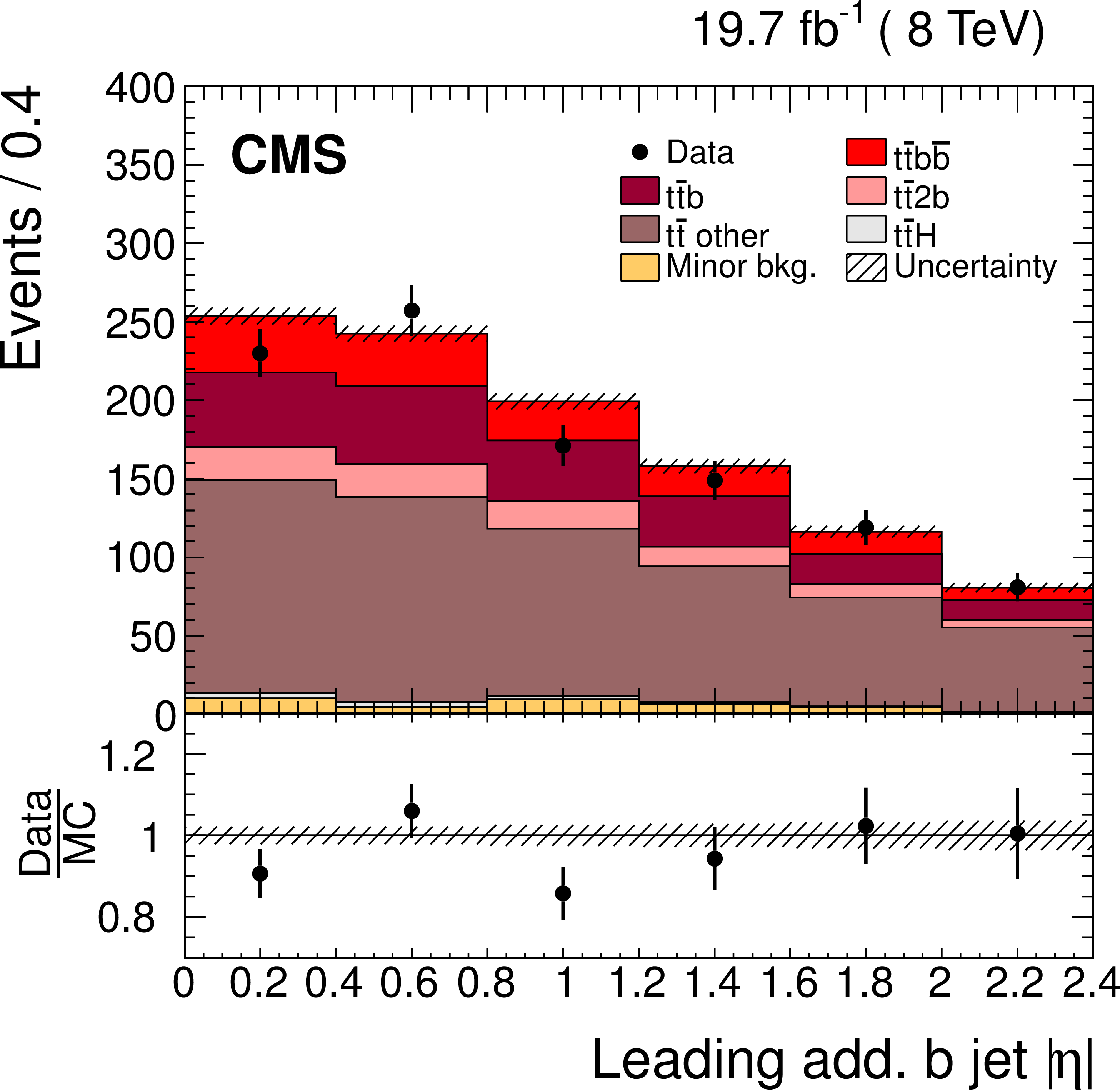
Figure 6-b:
Distributions of the leading additional b jet ${p_{\mathrm {T}}}$ (a) and ${|\eta |}$ (b), subleading additional b jet ${p_{\mathrm {T}}}$ (c) and ${|\eta |}$ (d), $\Delta R_{\mathrm{ b } \mathrm{ b } }$ (e), and ${m_{\mathrm{ b } \mathrm{ b } }} $(f) from data (points) and from signal and background simulation (histograms). The hatched area represents the statistical uncertainty in the simulated samples. ``Minor bkg." includes all non-${\mathrm{ t } \mathrm{ \bar{t} } }$ processes and ${\mathrm{ t } \mathrm{ \bar{t} } } $+$\mathrm{ Z } /\mathrm{ W } /\gamma $. The lower plots show the ratio of the data to the MC simulation prediction. |
png pdf |
Figure 6-c:
Distributions of the leading additional b jet ${p_{\mathrm {T}}}$ (a) and ${|\eta |}$ (b), subleading additional b jet ${p_{\mathrm {T}}}$ (c) and ${|\eta |}$ (d), $\Delta R_{\mathrm{ b } \mathrm{ b } }$ (e), and ${m_{\mathrm{ b } \mathrm{ b } }} $(f) from data (points) and from signal and background simulation (histograms). The hatched area represents the statistical uncertainty in the simulated samples. ``Minor bkg." includes all non-${\mathrm{ t } \mathrm{ \bar{t} } }$ processes and ${\mathrm{ t } \mathrm{ \bar{t} } } $+$\mathrm{ Z } /\mathrm{ W } /\gamma $. The lower plots show the ratio of the data to the MC simulation prediction. |

png pdf |
Figure 6-d:
Distributions of the leading additional b jet ${p_{\mathrm {T}}}$ (a) and ${|\eta |}$ (b), subleading additional b jet ${p_{\mathrm {T}}}$ (c) and ${|\eta |}$ (d), $\Delta R_{\mathrm{ b } \mathrm{ b } }$ (e), and ${m_{\mathrm{ b } \mathrm{ b } }} $(f) from data (points) and from signal and background simulation (histograms). The hatched area represents the statistical uncertainty in the simulated samples. ``Minor bkg." includes all non-${\mathrm{ t } \mathrm{ \bar{t} } }$ processes and ${\mathrm{ t } \mathrm{ \bar{t} } } $+$\mathrm{ Z } /\mathrm{ W } /\gamma $. The lower plots show the ratio of the data to the MC simulation prediction. |

png pdf |
Figure 6-e:
Distributions of the leading additional b jet ${p_{\mathrm {T}}}$ (a) and ${|\eta |}$ (b), subleading additional b jet ${p_{\mathrm {T}}}$ (c) and ${|\eta |}$ (d), $\Delta R_{\mathrm{ b } \mathrm{ b } }$ (e), and ${m_{\mathrm{ b } \mathrm{ b } }} $(f) from data (points) and from signal and background simulation (histograms). The hatched area represents the statistical uncertainty in the simulated samples. ``Minor bkg." includes all non-${\mathrm{ t } \mathrm{ \bar{t} } }$ processes and ${\mathrm{ t } \mathrm{ \bar{t} } } $+$\mathrm{ Z } /\mathrm{ W } /\gamma $. The lower plots show the ratio of the data to the MC simulation prediction. |
png pdf |
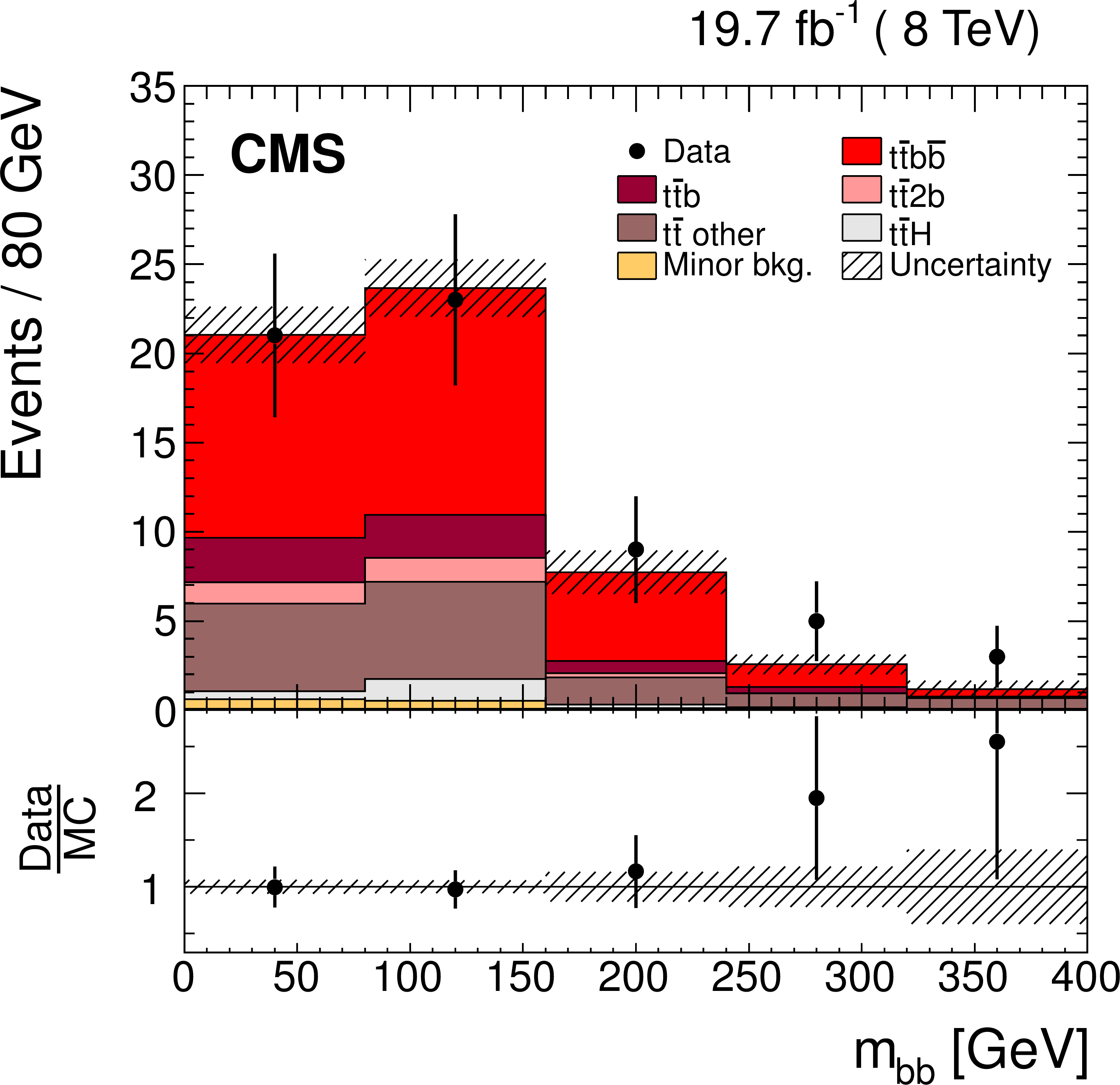
Figure 6-f:
Distributions of the leading additional b jet ${p_{\mathrm {T}}}$ (a) and ${|\eta |}$ (b), subleading additional b jet ${p_{\mathrm {T}}}$ (c) and ${|\eta |}$ (d), $\Delta R_{\mathrm{ b } \mathrm{ b } }$ (e), and ${m_{\mathrm{ b } \mathrm{ b } }} $(f) from data (points) and from signal and background simulation (histograms). The hatched area represents the statistical uncertainty in the simulated samples. ``Minor bkg." includes all non-${\mathrm{ t } \mathrm{ \bar{t} } }$ processes and ${\mathrm{ t } \mathrm{ \bar{t} } } $+$\mathrm{ Z } /\mathrm{ W } /\gamma $. The lower plots show the ratio of the data to the MC simulation prediction. |
png pdf |
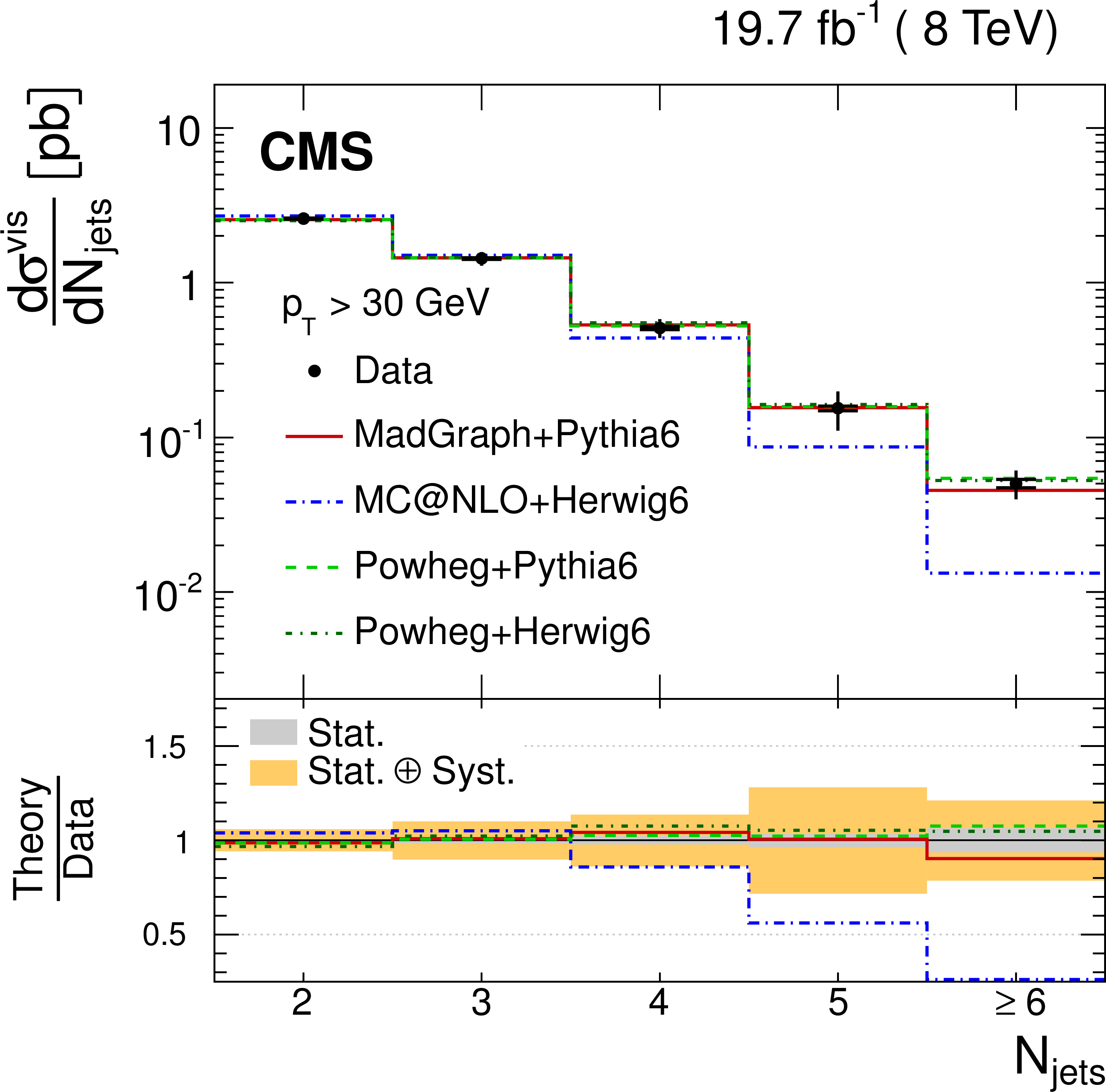
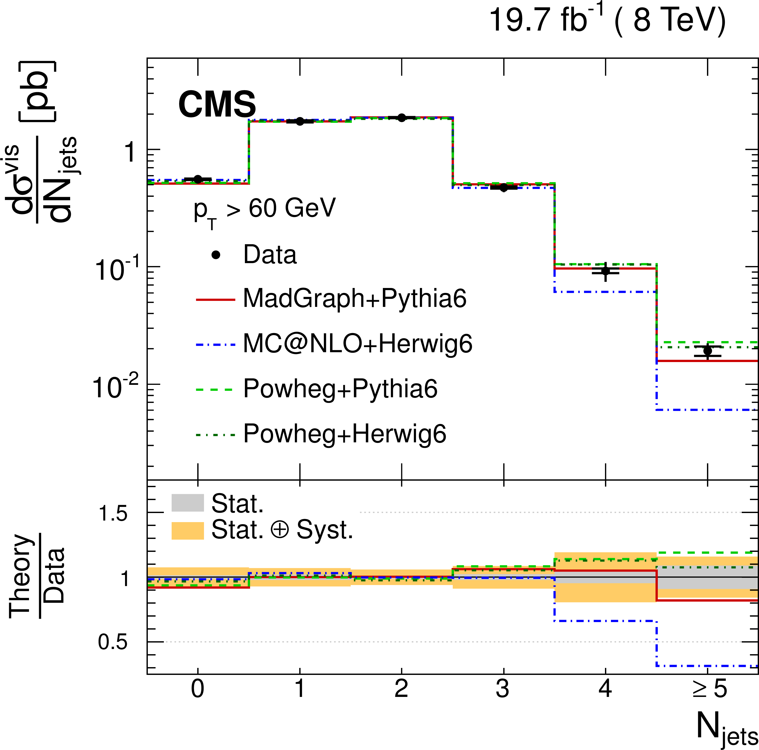
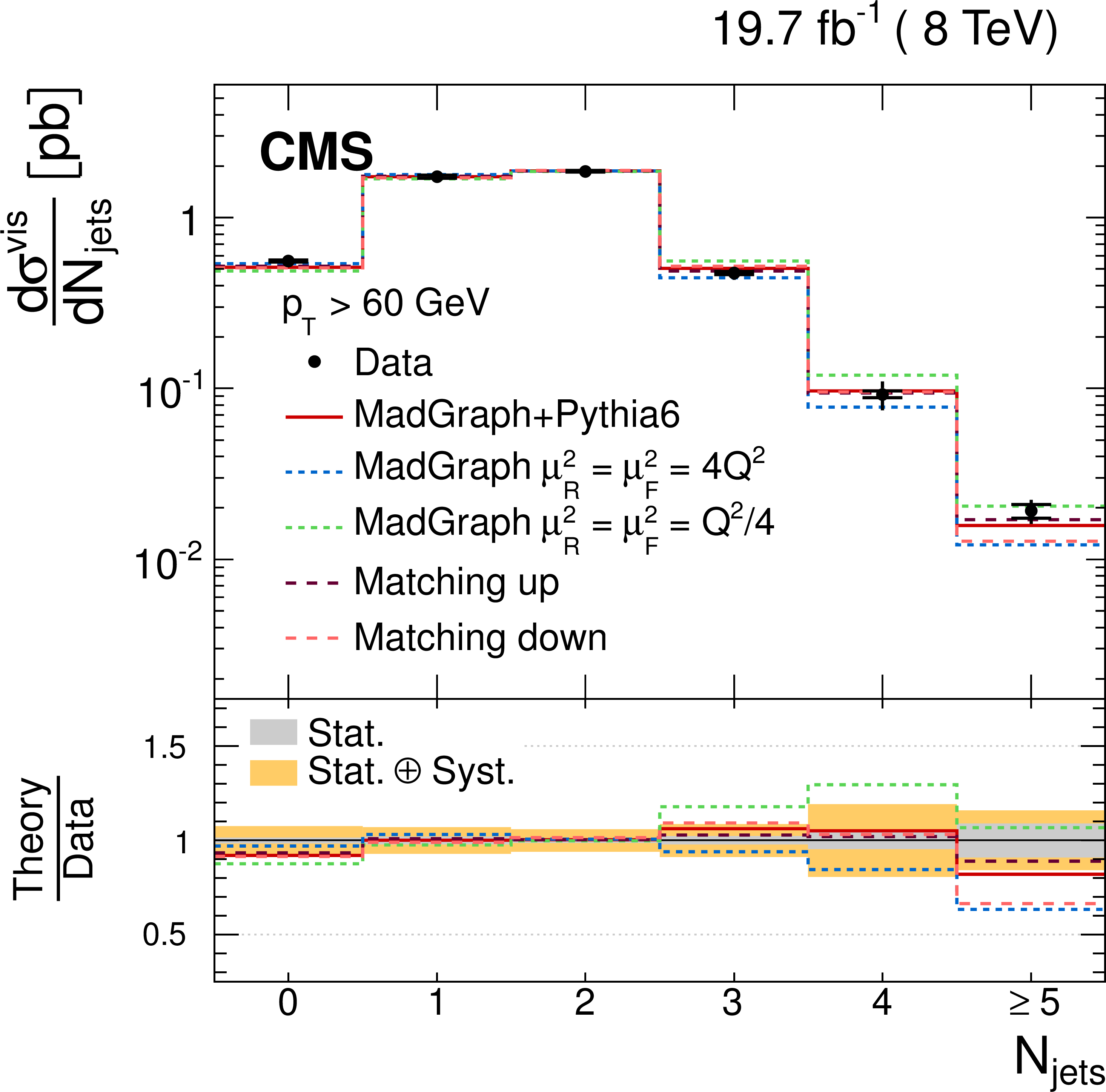
Figure 7-a:
Absolute differential ${\mathrm{ t } \mathrm{ \bar{t} } } $cross sections as a function of jet multiplicity for jets with $ {p_{\mathrm {T}}} >30 GeV $ (top row), 60 GeV (middle row), and 100 GeV (bottom row). In the figures on the left, the data are compared with predictions from MadGraph interfaced with PYTHIA 6, MC@NLO interfaced with HERWIG 6, and POWHEG with PYTHIA 6 and HERWIG 6. The figures on the right show the behaviour of the MadGraph generator with varied renormalization, factorization, and jet-parton matching scales. The inner (outer) vertical bars indicate the statistical (total) uncertainties. The lower part of each plot shows the ratio of the predictions to the data. |

png pdf |
Figure 7-b:
Absolute differential ${\mathrm{ t } \mathrm{ \bar{t} } } $cross sections as a function of jet multiplicity for jets with $ {p_{\mathrm {T}}} >30 GeV $ (top row), 60 GeV (middle row), and 100 GeV (bottom row). In the figures on the left, the data are compared with predictions from MadGraph interfaced with PYTHIA 6, MC@NLO interfaced with HERWIG 6, and POWHEG with PYTHIA 6 and HERWIG 6. The figures on the right show the behaviour of the MadGraph generator with varied renormalization, factorization, and jet-parton matching scales. The inner (outer) vertical bars indicate the statistical (total) uncertainties. The lower part of each plot shows the ratio of the predictions to the data. |
png pdf |
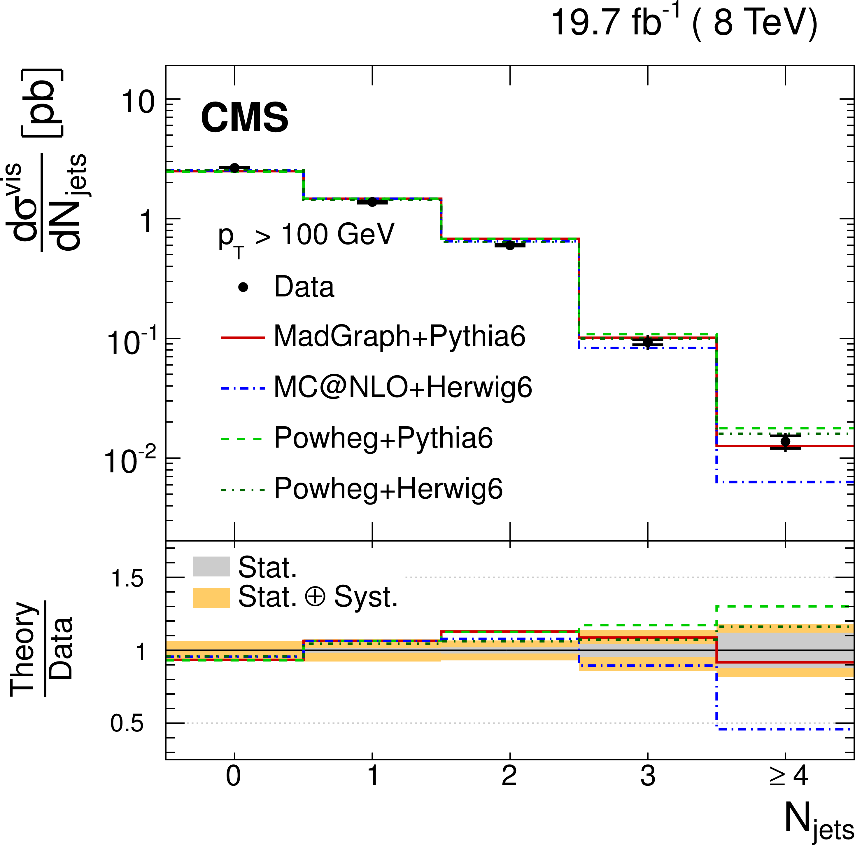
Figure 7-c:
Absolute differential ${\mathrm{ t } \mathrm{ \bar{t} } } $cross sections as a function of jet multiplicity for jets with $ {p_{\mathrm {T}}} >30 GeV $ (top row), 60 GeV (middle row), and 100 GeV (bottom row). In the figures on the left, the data are compared with predictions from MadGraph interfaced with PYTHIA 6, MC@NLO interfaced with HERWIG 6, and POWHEG with PYTHIA 6 and HERWIG 6. The figures on the right show the behaviour of the MadGraph generator with varied renormalization, factorization, and jet-parton matching scales. The inner (outer) vertical bars indicate the statistical (total) uncertainties. The lower part of each plot shows the ratio of the predictions to the data. |
png pdf |
Figure 7-d:
Absolute differential ${\mathrm{ t } \mathrm{ \bar{t} } } $cross sections as a function of jet multiplicity for jets with $ {p_{\mathrm {T}}} >30 GeV $ (top row), 60 GeV (middle row), and 100 GeV (bottom row). In the figures on the left, the data are compared with predictions from MadGraph interfaced with PYTHIA 6, MC@NLO interfaced with HERWIG 6, and POWHEG with PYTHIA 6 and HERWIG 6. The figures on the right show the behaviour of the MadGraph generator with varied renormalization, factorization, and jet-parton matching scales. The inner (outer) vertical bars indicate the statistical (total) uncertainties. The lower part of each plot shows the ratio of the predictions to the data. |
png pdf |
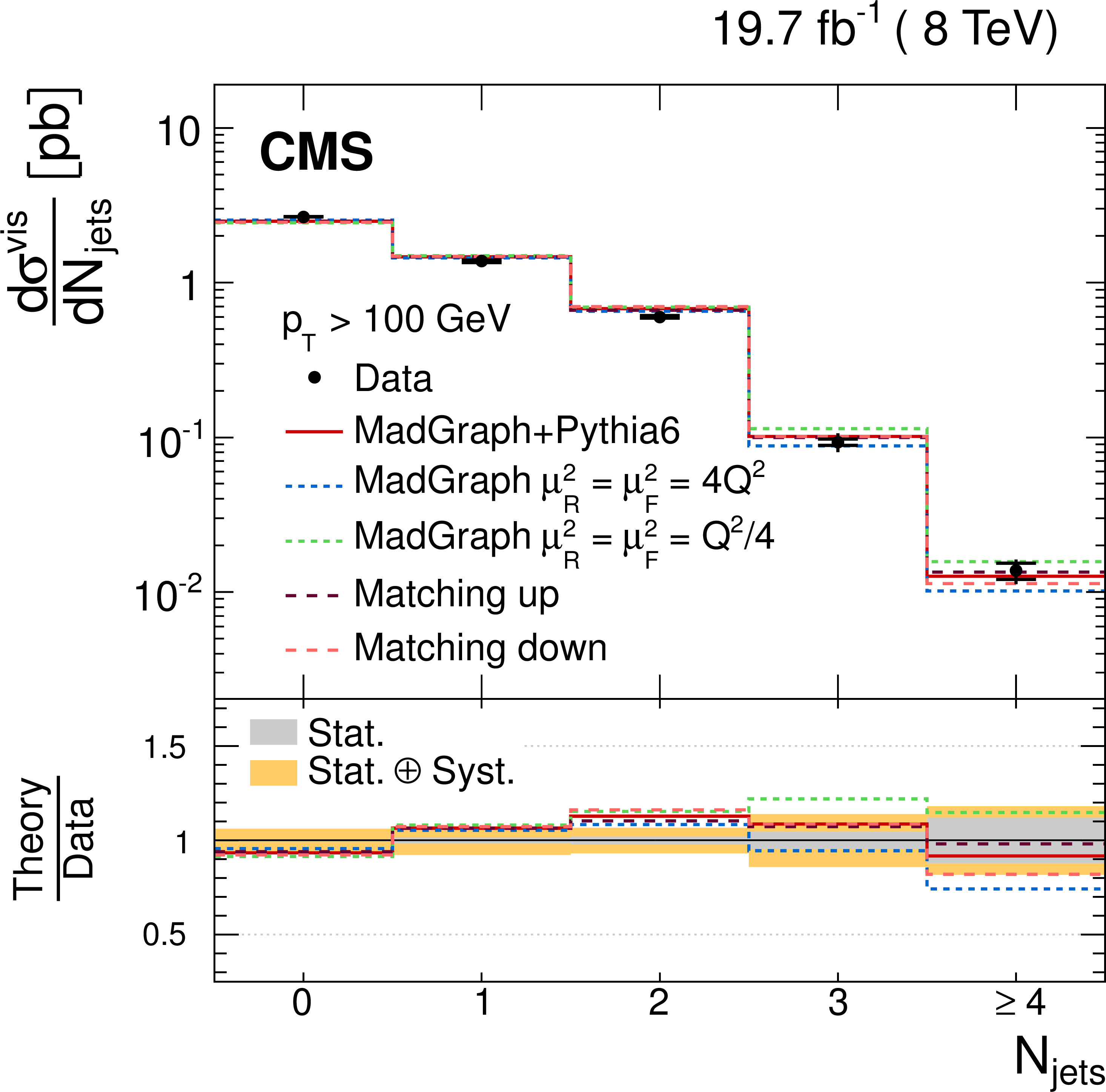
Figure 7-e:
Absolute differential ${\mathrm{ t } \mathrm{ \bar{t} } } $cross sections as a function of jet multiplicity for jets with $ {p_{\mathrm {T}}} >30 GeV $ (top row), 60 GeV (middle row), and 100 GeV (bottom row). In the figures on the left, the data are compared with predictions from MadGraph interfaced with PYTHIA 6, MC@NLO interfaced with HERWIG 6, and POWHEG with PYTHIA 6 and HERWIG 6. The figures on the right show the behaviour of the MadGraph generator with varied renormalization, factorization, and jet-parton matching scales. The inner (outer) vertical bars indicate the statistical (total) uncertainties. The lower part of each plot shows the ratio of the predictions to the data. |
png pdf |
Figure 7-f:
Absolute differential ${\mathrm{ t } \mathrm{ \bar{t} } } $cross sections as a function of jet multiplicity for jets with $ {p_{\mathrm {T}}} >30 GeV $ (top row), 60 GeV (middle row), and 100 GeV (bottom row). In the figures on the left, the data are compared with predictions from MadGraph interfaced with PYTHIA 6, MC@NLO interfaced with HERWIG 6, and POWHEG with PYTHIA 6 and HERWIG 6. The figures on the right show the behaviour of the MadGraph generator with varied renormalization, factorization, and jet-parton matching scales. The inner (outer) vertical bars indicate the statistical (total) uncertainties. The lower part of each plot shows the ratio of the predictions to the data. |
png pdf |
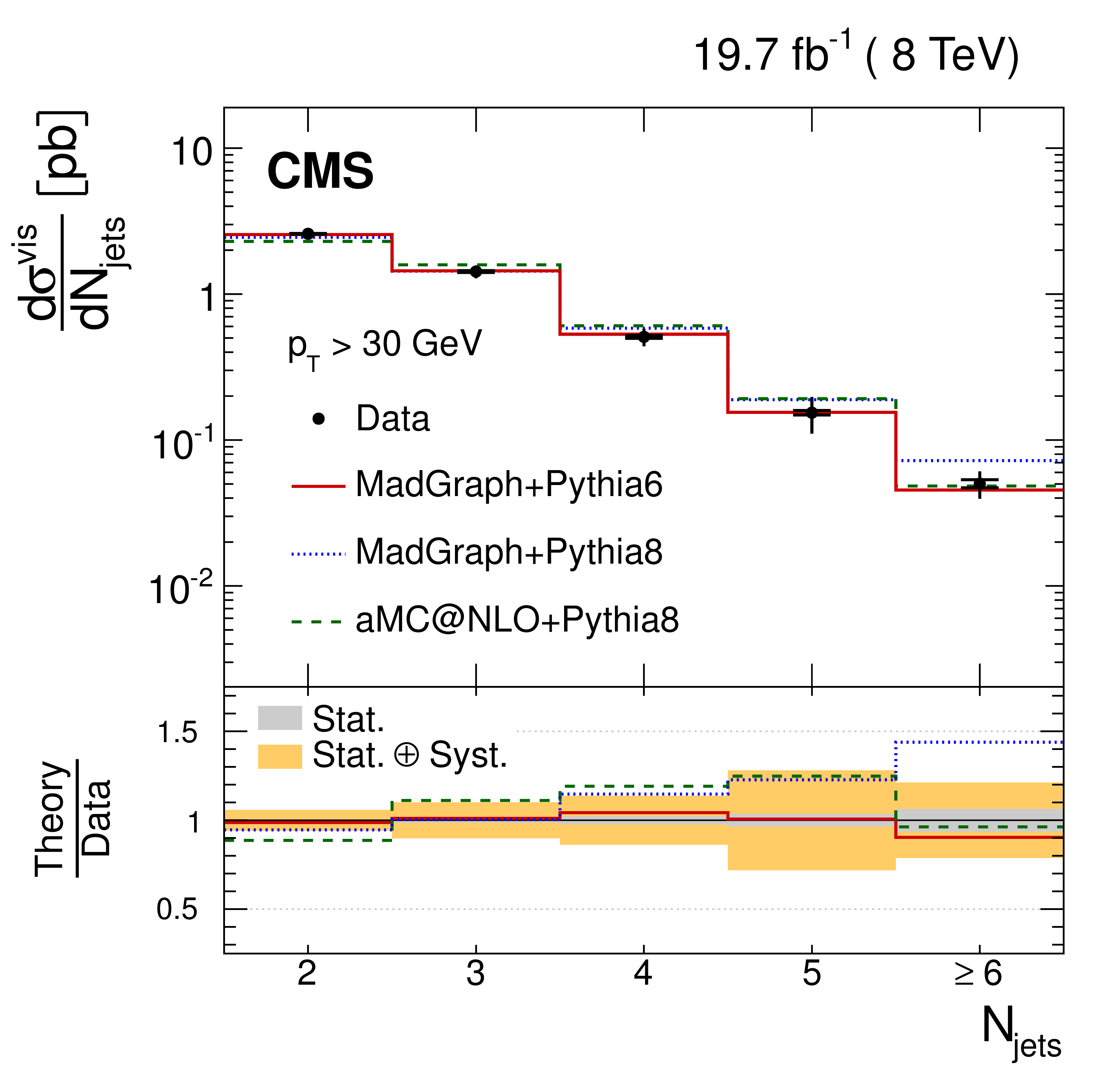
Figure 8-a:
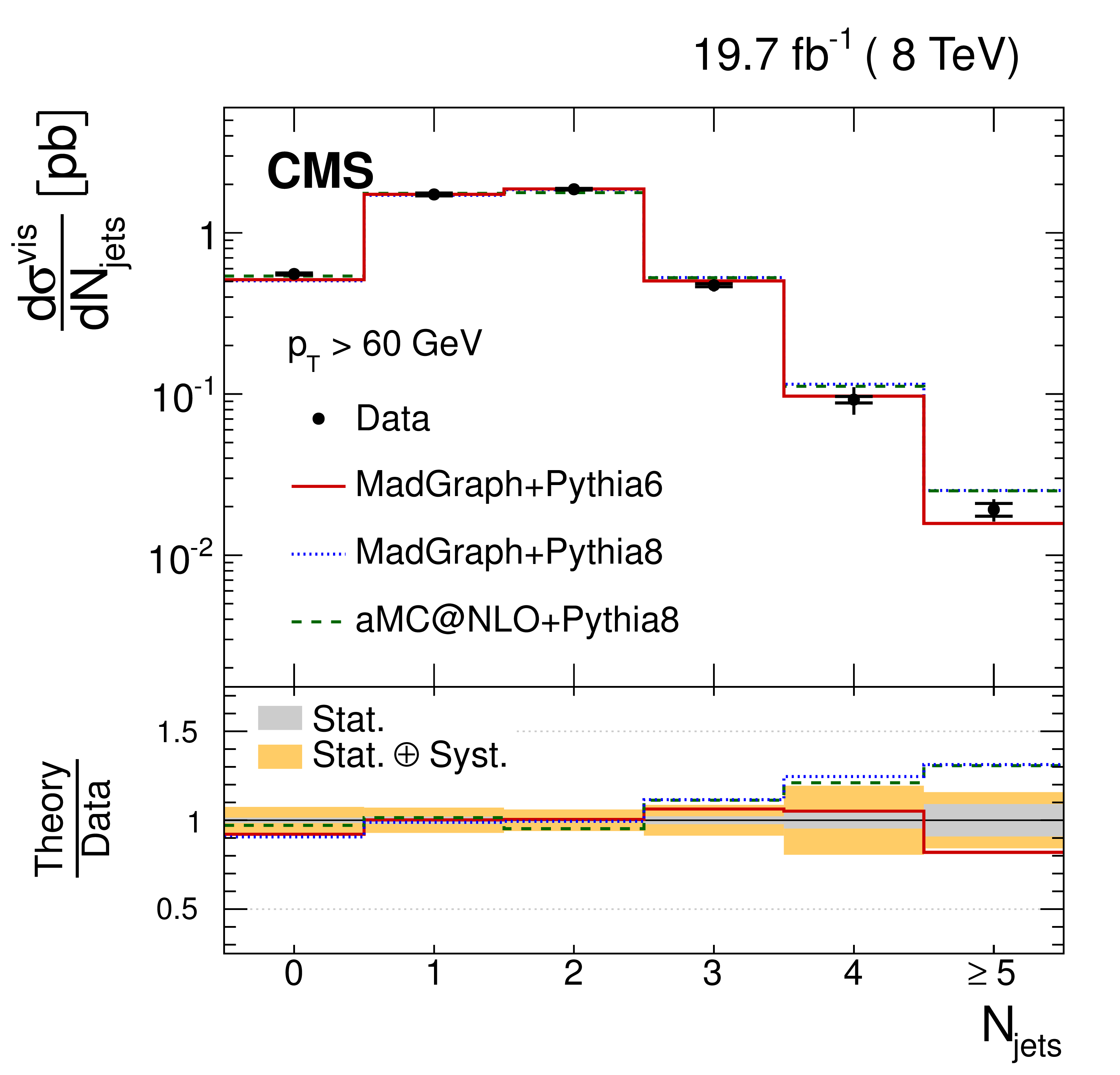
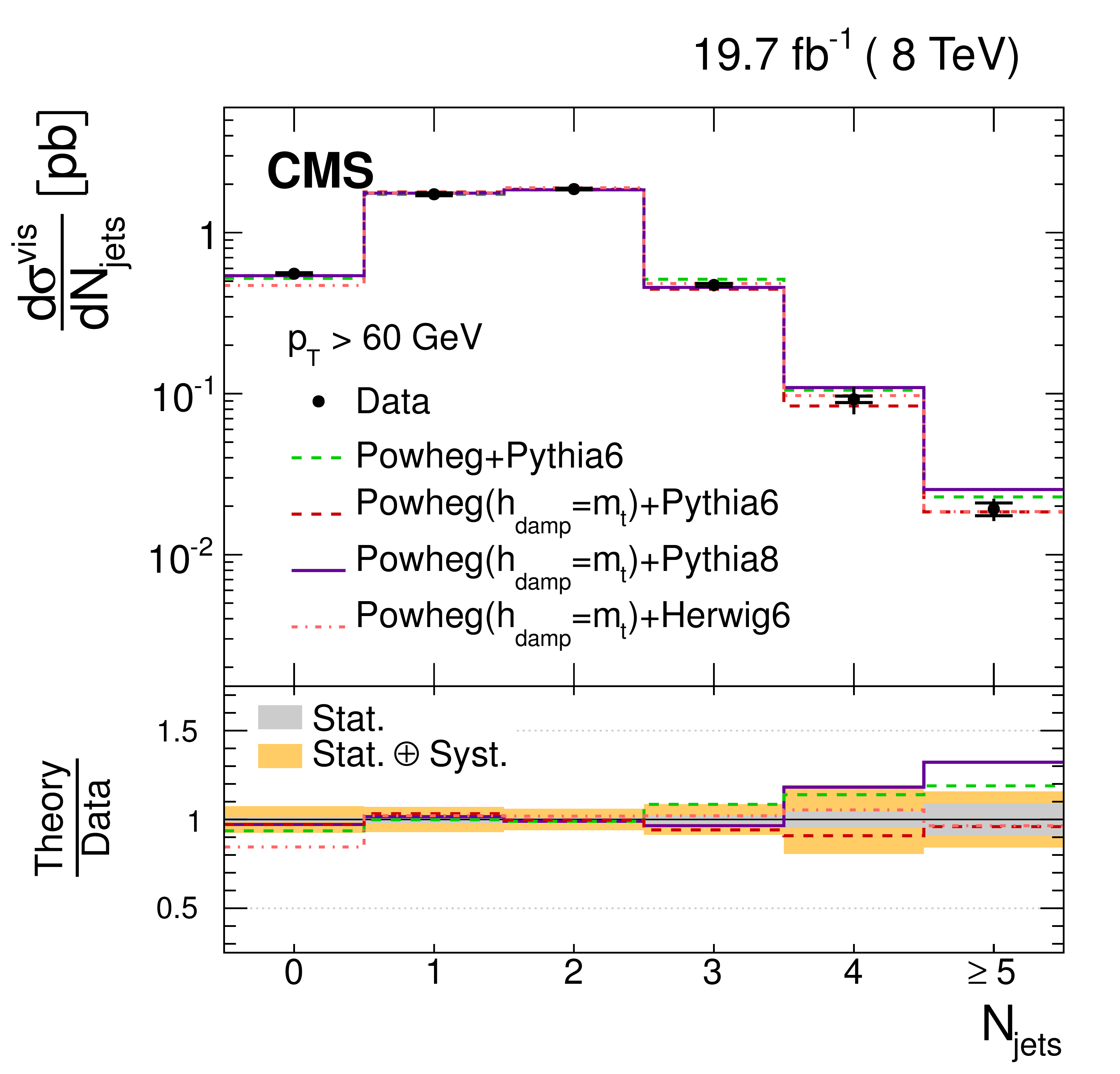
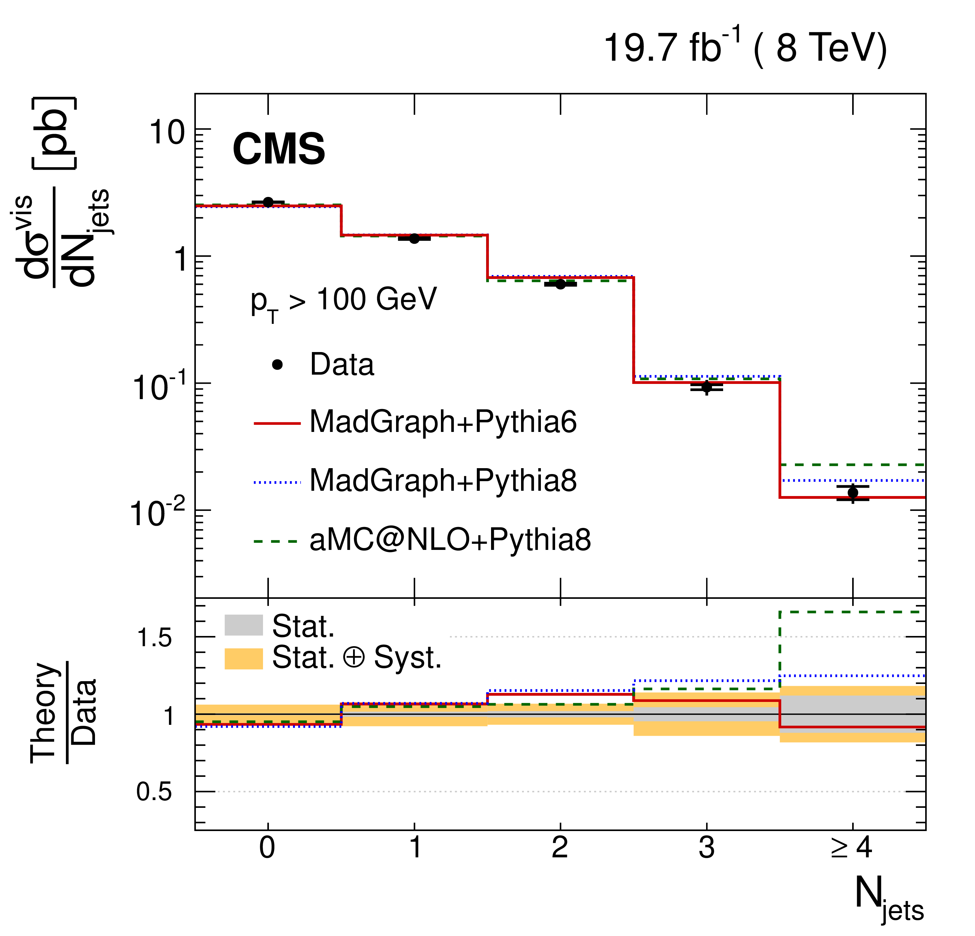
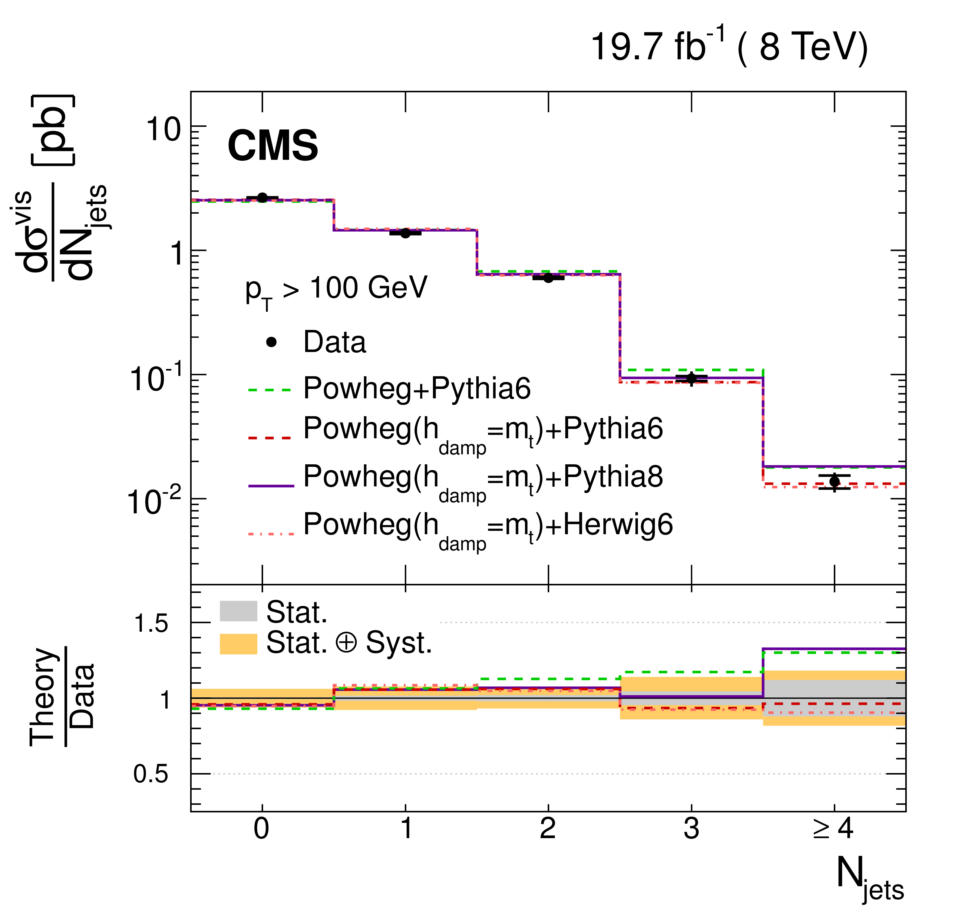
Absolute differential ${\mathrm{ t } \mathrm{ \bar{t} } } $cross sections as a function of jet multiplicity for jets with $ {p_{\mathrm {T}}} >30 GeV $ (top row), 60 GeV (middle row), and 100 GeV (bottom row). In the figures on the left, the data are compared with predictions from MadGraph interfaced with PYTHIA 6 and PYTHIA 8, and MG5\_aMC@NLO interfaced with PYTHIA 8. The figures on the right show the behaviour of the POWHEG generator without and with hdamp set to $m_{\mathrm{ t } }$, matched with different versions and tunes of PYTHIA and HERWIG 6. The inner (outer) vertical bars indicate the statistical (total) uncertainties. The lower part of each plot shows the ratio of the predictions to the data. |
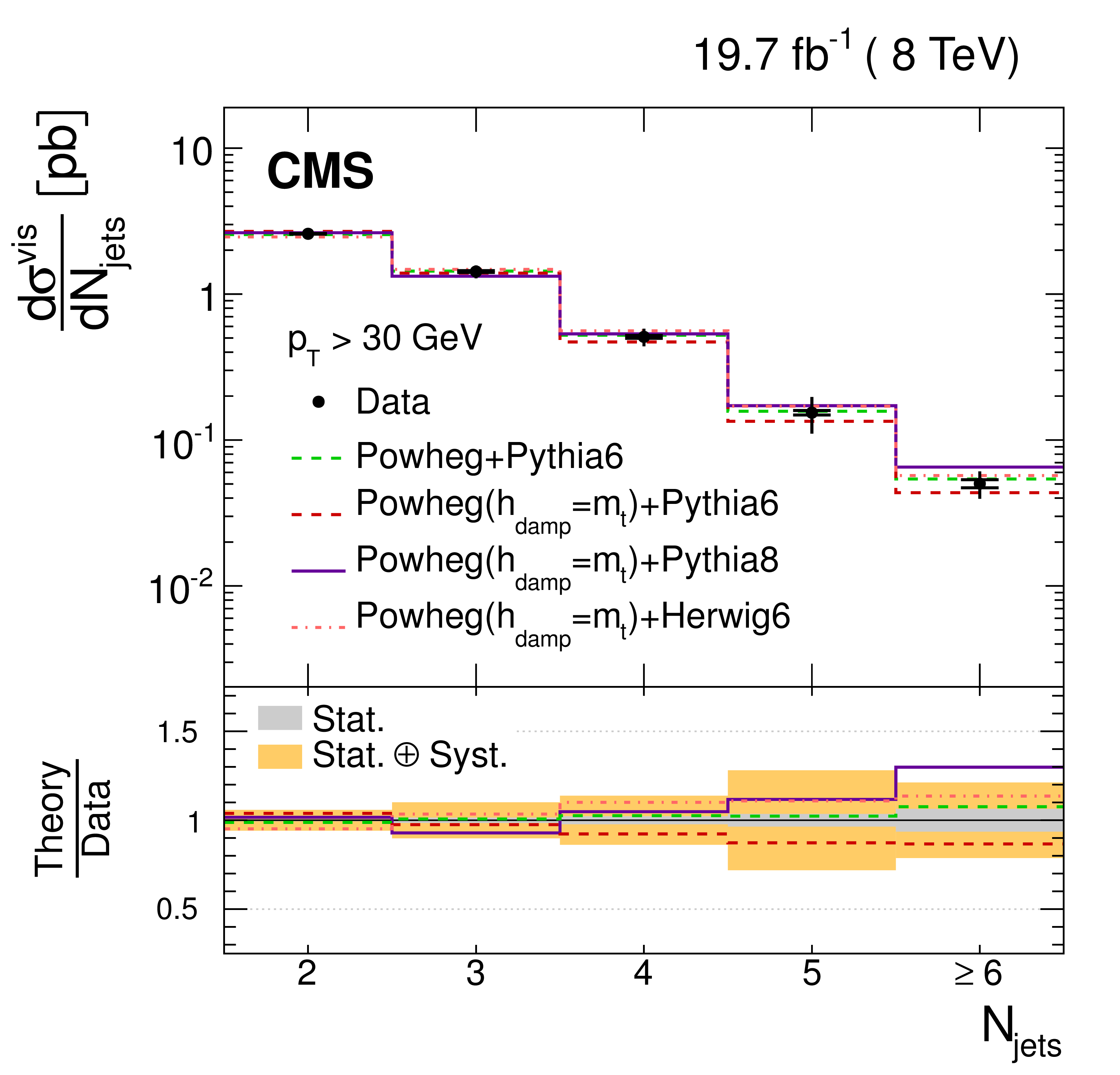
png pdf |
Figure 8-b:
Absolute differential ${\mathrm{ t } \mathrm{ \bar{t} } } $cross sections as a function of jet multiplicity for jets with $ {p_{\mathrm {T}}} >30 GeV $ (top row), 60 GeV (middle row), and 100 GeV (bottom row). In the figures on the left, the data are compared with predictions from MadGraph interfaced with PYTHIA 6 and PYTHIA 8, and MG5\_aMC@NLO interfaced with PYTHIA 8. The figures on the right show the behaviour of the POWHEG generator without and with hdamp set to $m_{\mathrm{ t } }$, matched with different versions and tunes of PYTHIA and HERWIG 6. The inner (outer) vertical bars indicate the statistical (total) uncertainties. The lower part of each plot shows the ratio of the predictions to the data. |
png pdf |
Figure 8-c:
Absolute differential ${\mathrm{ t } \mathrm{ \bar{t} } } $cross sections as a function of jet multiplicity for jets with $ {p_{\mathrm {T}}} >30 GeV $ (top row), 60 GeV (middle row), and 100 GeV (bottom row). In the figures on the left, the data are compared with predictions from MadGraph interfaced with PYTHIA 6 and PYTHIA 8, and MG5\_aMC@NLO interfaced with PYTHIA 8. The figures on the right show the behaviour of the POWHEG generator without and with hdamp set to $m_{\mathrm{ t } }$, matched with different versions and tunes of PYTHIA and HERWIG 6. The inner (outer) vertical bars indicate the statistical (total) uncertainties. The lower part of each plot shows the ratio of the predictions to the data. |
png pdf |
Figure 8-d:
Absolute differential ${\mathrm{ t } \mathrm{ \bar{t} } } $cross sections as a function of jet multiplicity for jets with $ {p_{\mathrm {T}}} >30 GeV $ (top row), 60 GeV (middle row), and 100 GeV (bottom row). In the figures on the left, the data are compared with predictions from MadGraph interfaced with PYTHIA 6 and PYTHIA 8, and MG5\_aMC@NLO interfaced with PYTHIA 8. The figures on the right show the behaviour of the POWHEG generator without and with hdamp set to $m_{\mathrm{ t } }$, matched with different versions and tunes of PYTHIA and HERWIG 6. The inner (outer) vertical bars indicate the statistical (total) uncertainties. The lower part of each plot shows the ratio of the predictions to the data. |
png pdf |
Figure 8-e:
Absolute differential ${\mathrm{ t } \mathrm{ \bar{t} } } $cross sections as a function of jet multiplicity for jets with $ {p_{\mathrm {T}}} >30 GeV $ (top row), 60 GeV (middle row), and 100 GeV (bottom row). In the figures on the left, the data are compared with predictions from MadGraph interfaced with PYTHIA 6 and PYTHIA 8, and MG5\_aMC@NLO interfaced with PYTHIA 8. The figures on the right show the behaviour of the POWHEG generator without and with hdamp set to $m_{\mathrm{ t } }$, matched with different versions and tunes of PYTHIA and HERWIG 6. The inner (outer) vertical bars indicate the statistical (total) uncertainties. The lower part of each plot shows the ratio of the predictions to the data. |
png pdf |
Figure 8-f:
Absolute differential ${\mathrm{ t } \mathrm{ \bar{t} } } $cross sections as a function of jet multiplicity for jets with $ {p_{\mathrm {T}}} >30 GeV $ (top row), 60 GeV (middle row), and 100 GeV (bottom row). In the figures on the left, the data are compared with predictions from MadGraph interfaced with PYTHIA 6 and PYTHIA 8, and MG5\_aMC@NLO interfaced with PYTHIA 8. The figures on the right show the behaviour of the POWHEG generator without and with hdamp set to $m_{\mathrm{ t } }$, matched with different versions and tunes of PYTHIA and HERWIG 6. The inner (outer) vertical bars indicate the statistical (total) uncertainties. The lower part of each plot shows the ratio of the predictions to the data. |
png pdf |
Figure 9-a:
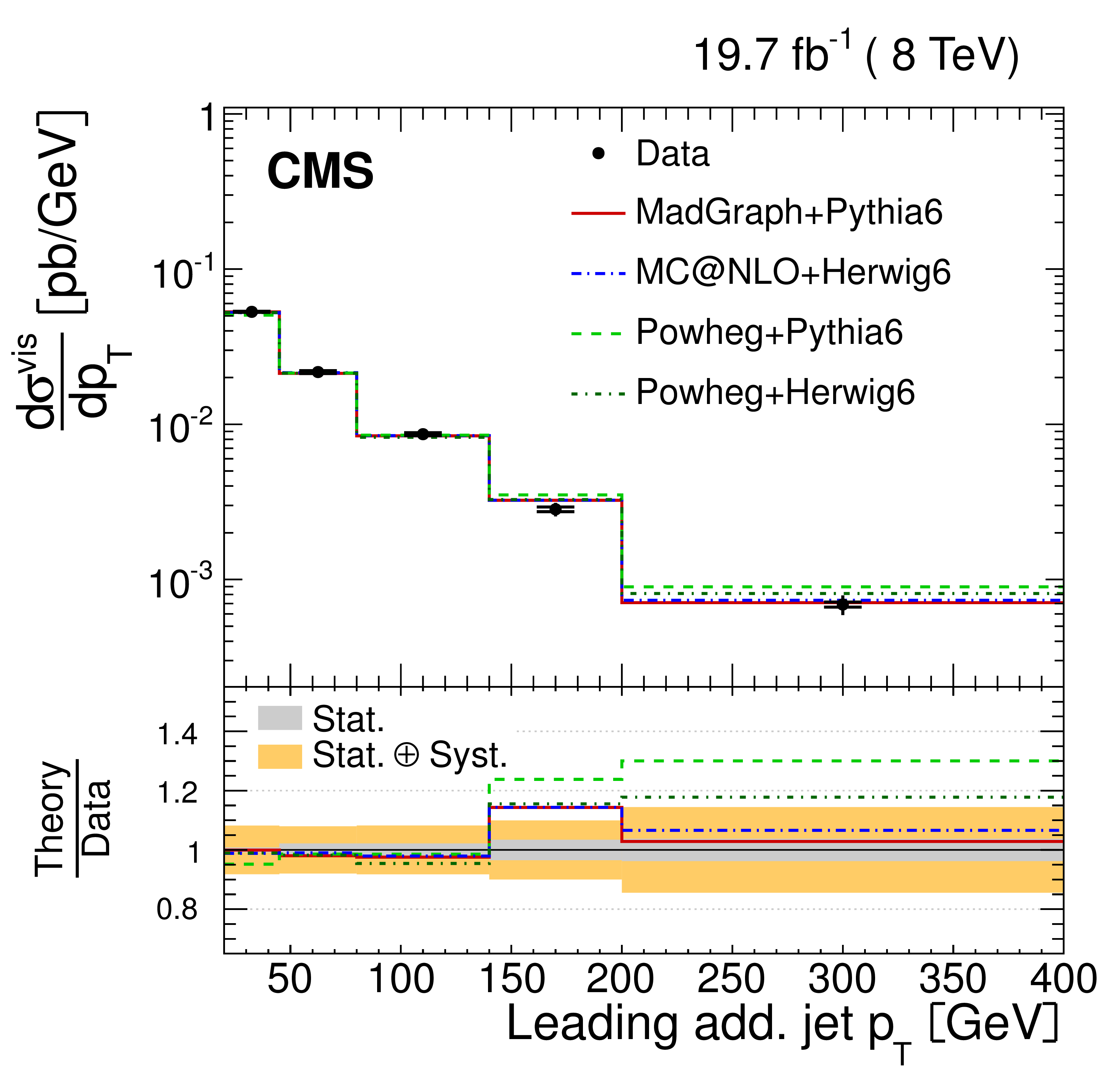
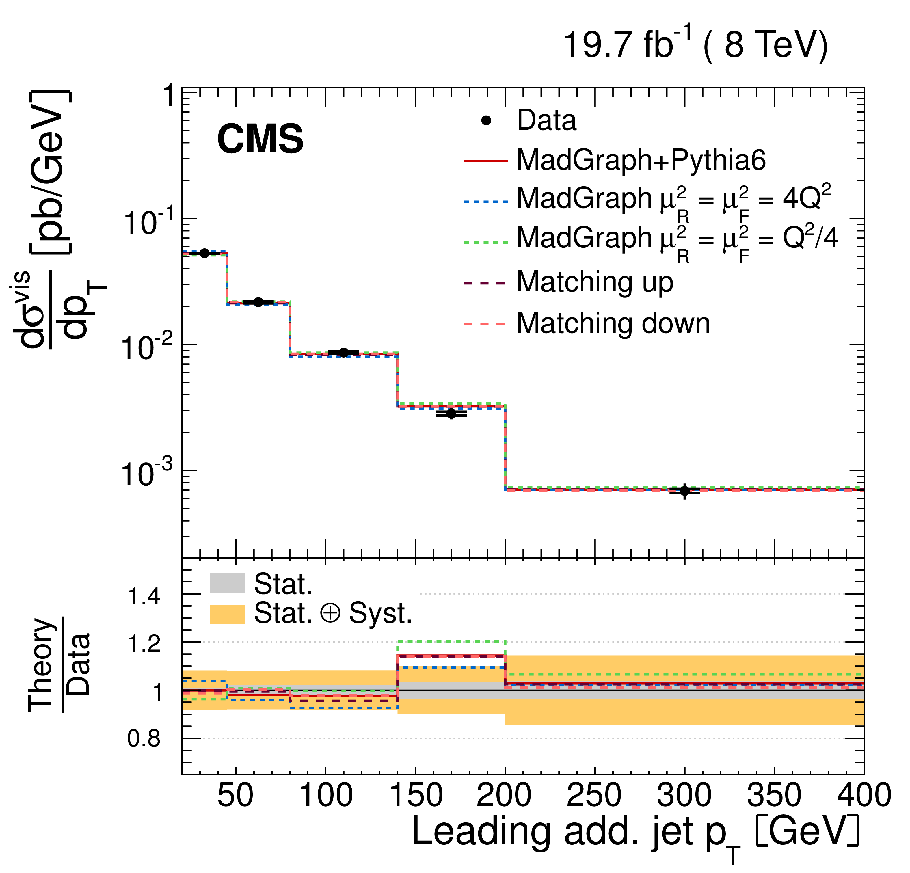
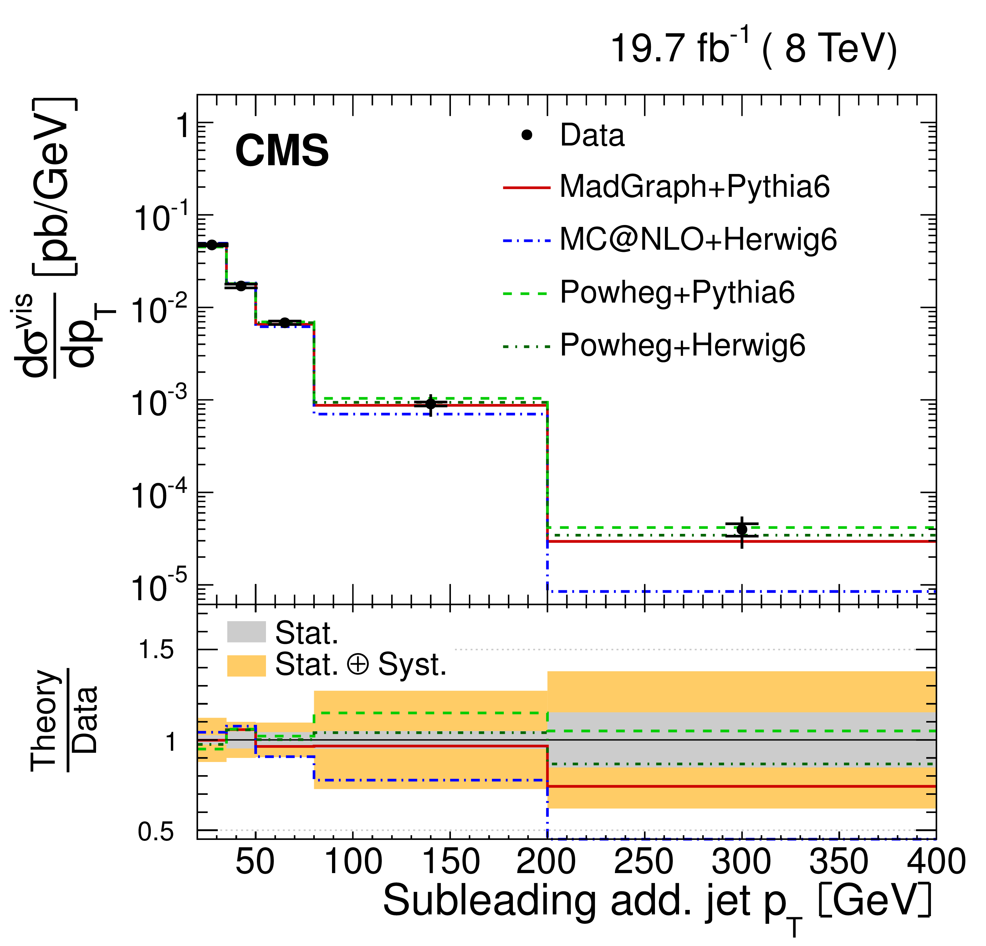
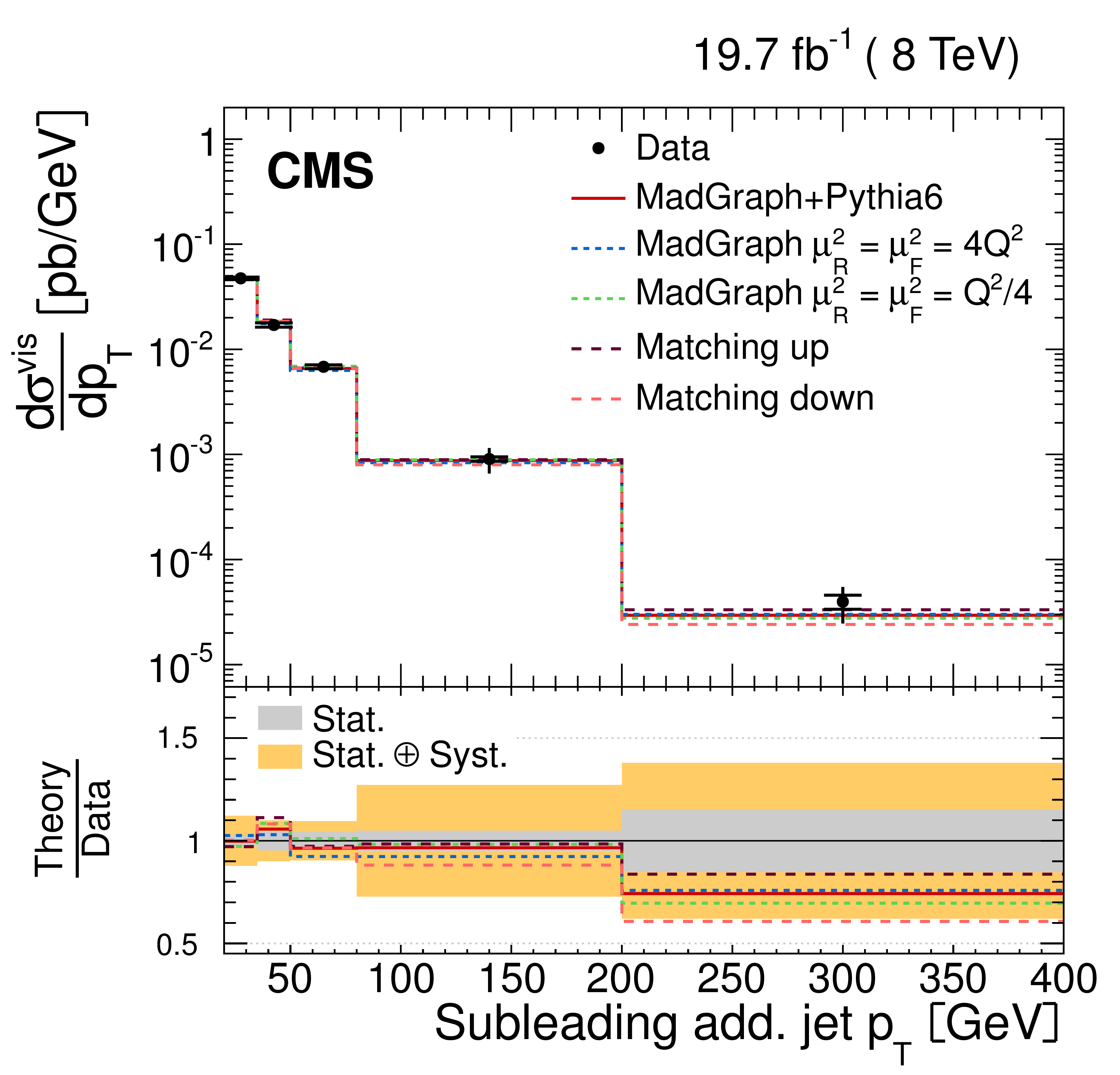
Absolute differential $ {\mathrm {t}\overline {\mathrm {t}}} $ cross section as a function of $ {p_{\mathrm {T}}} $ of the leading additional jet (a,b) and the subleading additional jet (e,f), and $H_{\rm T}$ (e,f) in the visible phase space of the $ {\mathrm {t}\overline {\mathrm {t}}} $ system and the additional jets. Data are compared to predictions from MADGRAPH+PYTHIA-6, POWHEG+PYTHIA-6, POWHEG+HERWIG-6, and MC@NLO+HERWIG-6 (a,c,e) and to MADGRAPH with varied renormalization, factorization, and jet-parton matching scales (b,d,f). The inner (outer) vertical bars indicate the statistical (total) uncertainties. The lower part of each plot shows the ratio of the predictions to the data. |
png pdf |
Figure 9-b:
Absolute differential $ {\mathrm {t}\overline {\mathrm {t}}} $ cross section as a function of $ {p_{\mathrm {T}}} $ of the leading additional jet (a,b) and the subleading additional jet (e,f), and $H_{\rm T}$ (e,f) in the visible phase space of the $ {\mathrm {t}\overline {\mathrm {t}}} $ system and the additional jets. Data are compared to predictions from MADGRAPH+PYTHIA-6, POWHEG+PYTHIA-6, POWHEG+HERWIG-6, and MC@NLO+HERWIG-6 (a,c,e) and to MADGRAPH with varied renormalization, factorization, and jet-parton matching scales (b,d,f). The inner (outer) vertical bars indicate the statistical (total) uncertainties. The lower part of each plot shows the ratio of the predictions to the data. |
png pdf |
Figure 9-c:
Absolute differential $ {\mathrm {t}\overline {\mathrm {t}}} $ cross section as a function of $ {p_{\mathrm {T}}} $ of the leading additional jet (a,b) and the subleading additional jet (e,f), and $H_{\rm T}$ (e,f) in the visible phase space of the $ {\mathrm {t}\overline {\mathrm {t}}} $ system and the additional jets. Data are compared to predictions from MADGRAPH+PYTHIA-6, POWHEG+PYTHIA-6, POWHEG+HERWIG-6, and MC@NLO+HERWIG-6 (a,c,e) and to MADGRAPH with varied renormalization, factorization, and jet-parton matching scales (b,d,f). The inner (outer) vertical bars indicate the statistical (total) uncertainties. The lower part of each plot shows the ratio of the predictions to the data. |
png pdf |
Figure 9-d:
Absolute differential $ {\mathrm {t}\overline {\mathrm {t}}} $ cross section as a function of $ {p_{\mathrm {T}}} $ of the leading additional jet (a,b) and the subleading additional jet (e,f), and $H_{\rm T}$ (e,f) in the visible phase space of the $ {\mathrm {t}\overline {\mathrm {t}}} $ system and the additional jets. Data are compared to predictions from MADGRAPH+PYTHIA-6, POWHEG+PYTHIA-6, POWHEG+HERWIG-6, and MC@NLO+HERWIG-6 (a,c,e) and to MADGRAPH with varied renormalization, factorization, and jet-parton matching scales (b,d,f). The inner (outer) vertical bars indicate the statistical (total) uncertainties. The lower part of each plot shows the ratio of the predictions to the data. |
png pdf |
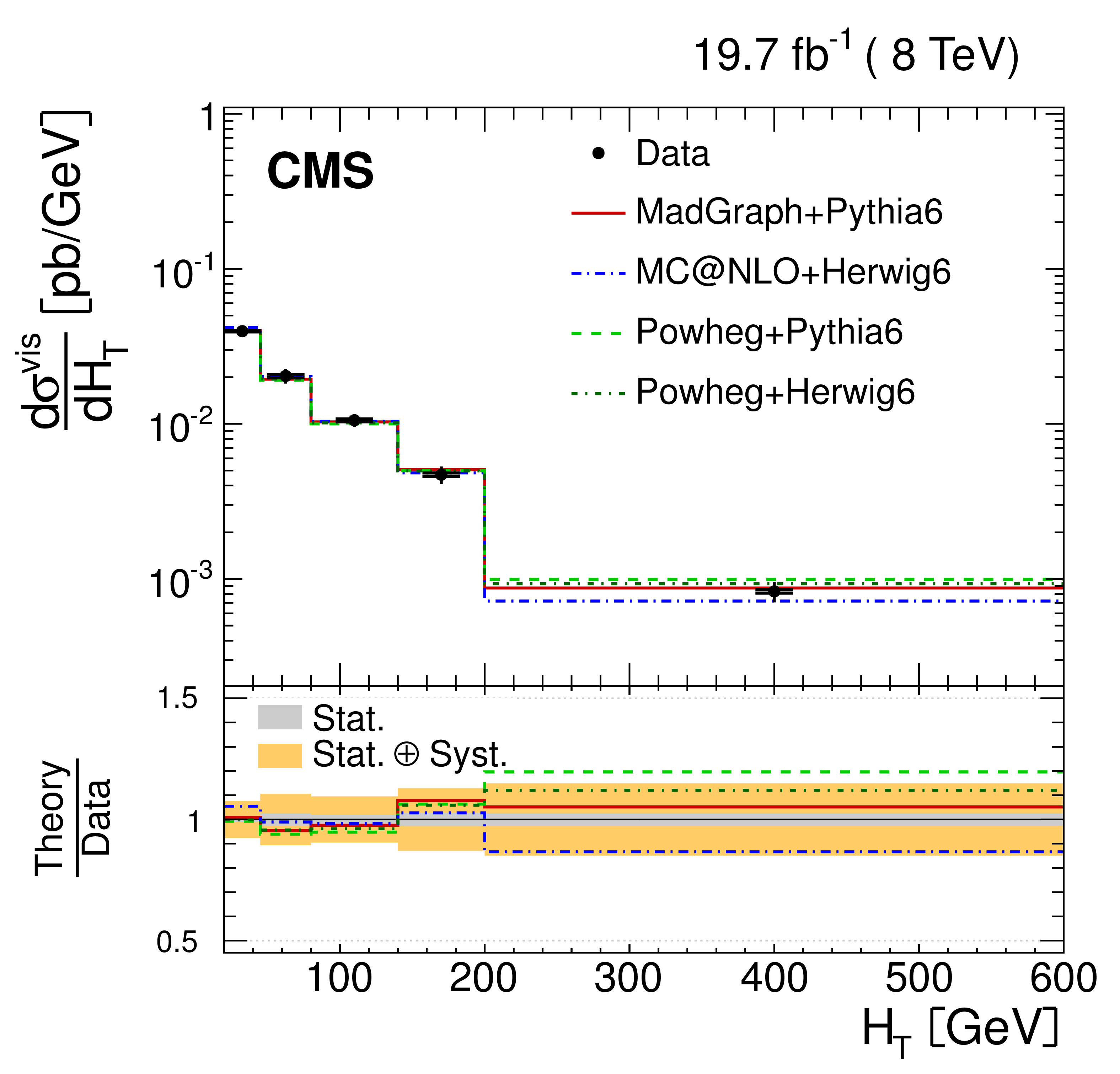
Figure 9-e:
Absolute differential $ {\mathrm {t}\overline {\mathrm {t}}} $ cross section as a function of $ {p_{\mathrm {T}}} $ of the leading additional jet (a,b) and the subleading additional jet (e,f), and $H_{\rm T}$ (e,f) in the visible phase space of the $ {\mathrm {t}\overline {\mathrm {t}}} $ system and the additional jets. Data are compared to predictions from MADGRAPH+PYTHIA-6, POWHEG+PYTHIA-6, POWHEG+HERWIG-6, and MC@NLO+HERWIG-6 (a,c,e) and to MADGRAPH with varied renormalization, factorization, and jet-parton matching scales (b,d,f). The inner (outer) vertical bars indicate the statistical (total) uncertainties. The lower part of each plot shows the ratio of the predictions to the data. |
png pdf |
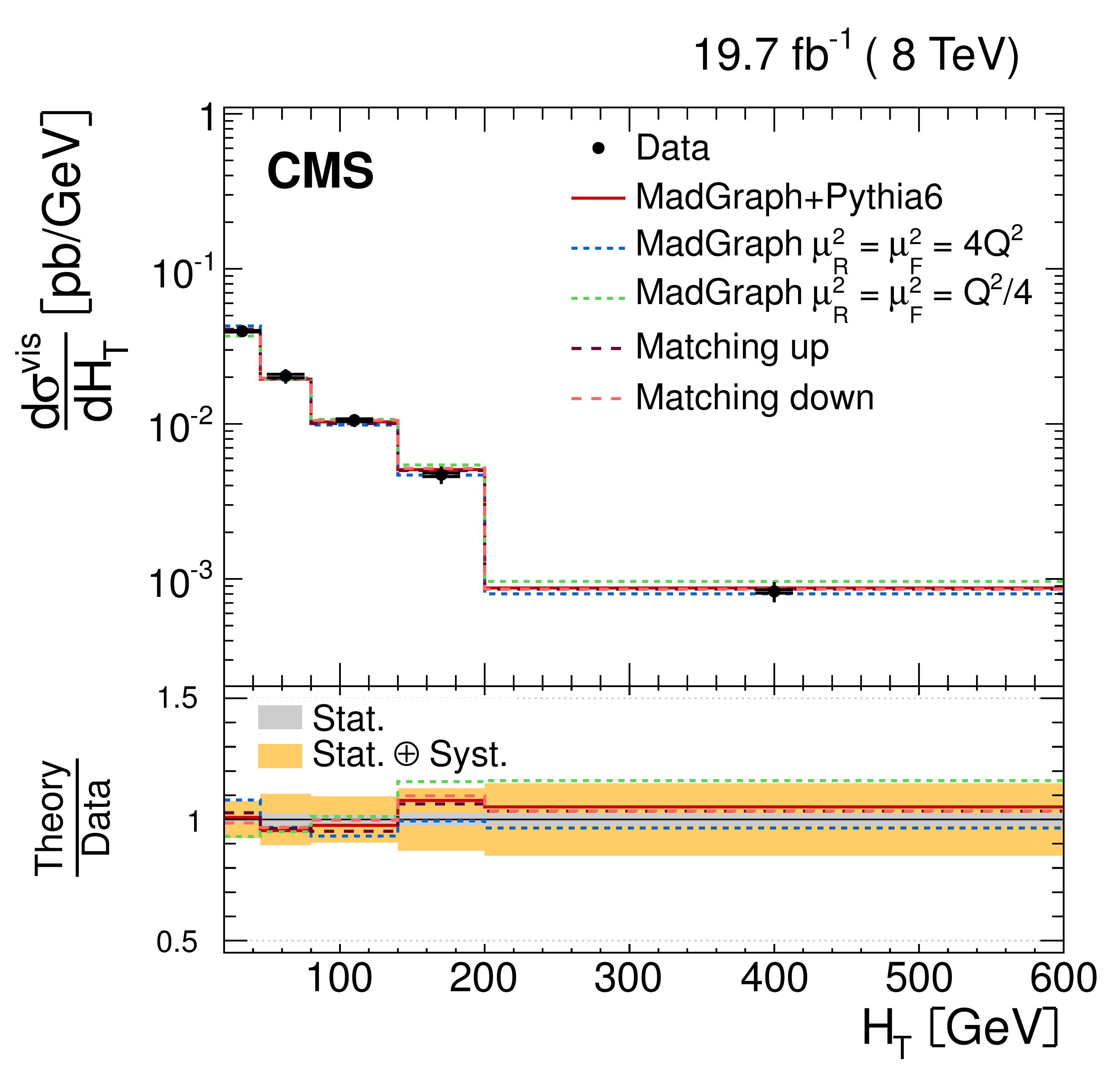
Figure 9-f:
Absolute differential $ {\mathrm {t}\overline {\mathrm {t}}} $ cross section as a function of $ {p_{\mathrm {T}}} $ of the leading additional jet (a,b) and the subleading additional jet (e,f), and $H_{\rm T}$ (e,f) in the visible phase space of the $ {\mathrm {t}\overline {\mathrm {t}}} $ system and the additional jets. Data are compared to predictions from MADGRAPH+PYTHIA-6, POWHEG+PYTHIA-6, POWHEG+HERWIG-6, and MC@NLO+HERWIG-6 (a,c,e) and to MADGRAPH with varied renormalization, factorization, and jet-parton matching scales (b,d,f). The inner (outer) vertical bars indicate the statistical (total) uncertainties. The lower part of each plot shows the ratio of the predictions to the data. |
png pdf |
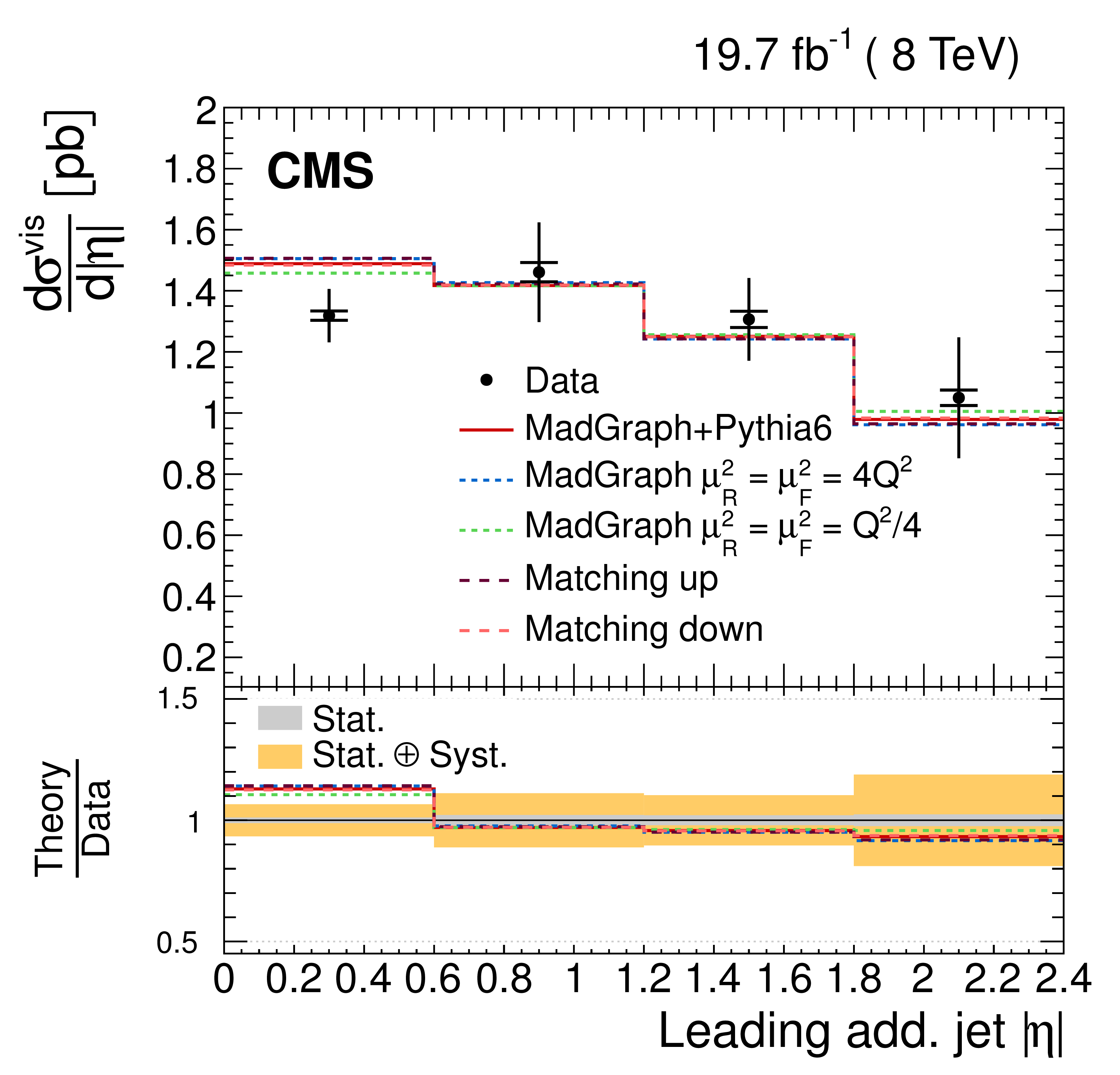
Figure 10-a:
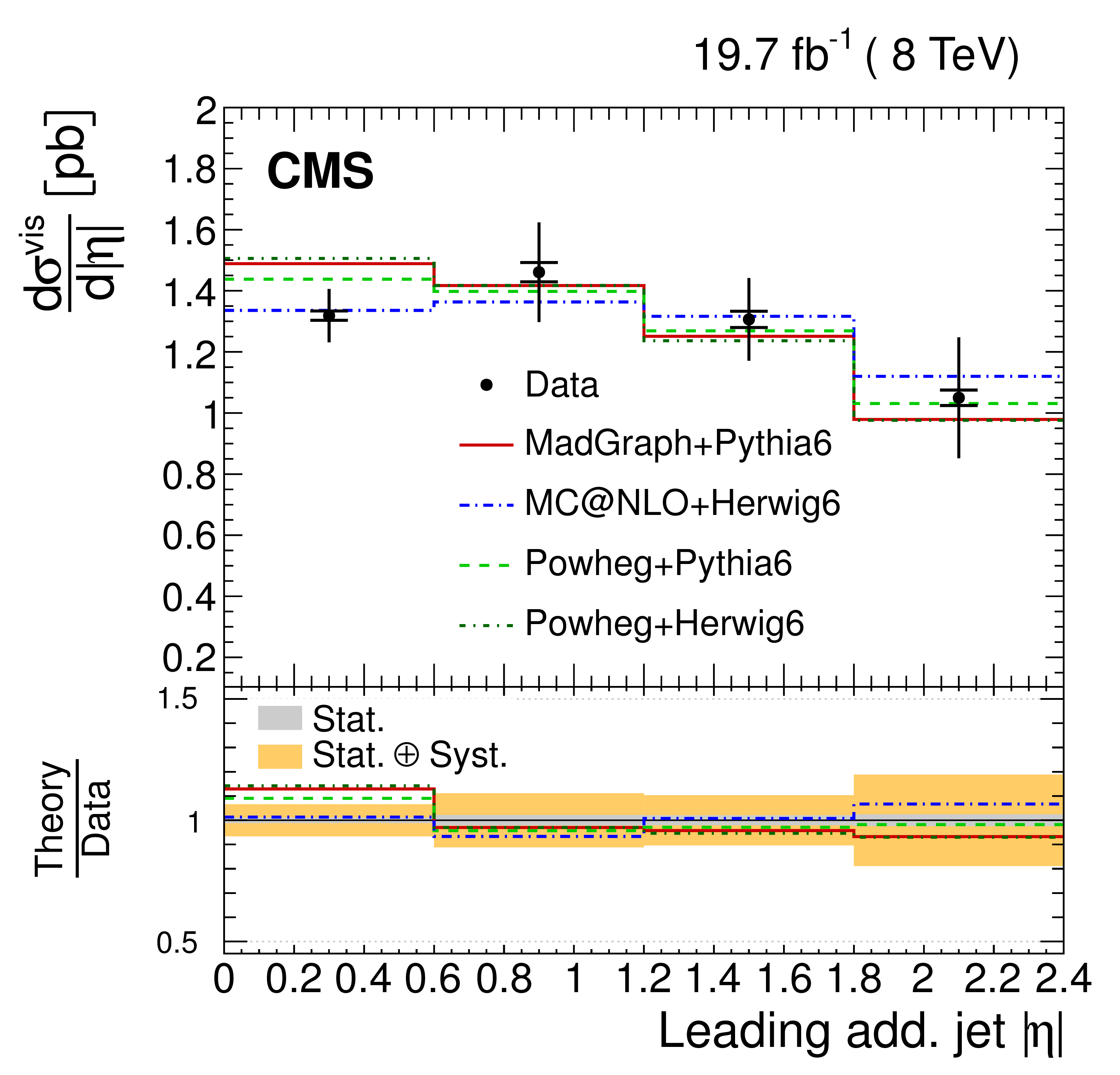
Absolute differential $ {\mathrm {t}\overline {\mathrm {t}}} $ cross section as a function of the $ {|\eta |} $ of the leading additional jet (a,b) and the subleading additional jet (c,d) in the visible phase space of the $ {\mathrm {t}\overline {\mathrm {t}}} $ system and the additional jets. Data are compared to predictions from MADGRAPH +PYTHIA-6, POWHEG +PYTHIA-6, POWHEG +HERWIG-6, and MC@NLO+HERWIG-6 (a,c) and to MADGRAPH with with varied renormalization, factorization, and jet-parton matching scales (b,d). The inner (outer) vertical bars indicate the statistical (total) uncertainties. The lower part of each plot shows the ratio of the predictions to the data. |
png pdf |
Figure 10-b:
Absolute differential $ {\mathrm {t}\overline {\mathrm {t}}} $ cross section as a function of the $ {|\eta |} $ of the leading additional jet (a,b) and the subleading additional jet (c,d) in the visible phase space of the $ {\mathrm {t}\overline {\mathrm {t}}} $ system and the additional jets. Data are compared to predictions from MADGRAPH +PYTHIA-6, POWHEG +PYTHIA-6, POWHEG +HERWIG-6, and MC@NLO+HERWIG-6 (a,c) and to MADGRAPH with with varied renormalization, factorization, and jet-parton matching scales (b,d). The inner (outer) vertical bars indicate the statistical (total) uncertainties. The lower part of each plot shows the ratio of the predictions to the data. |
png pdf |
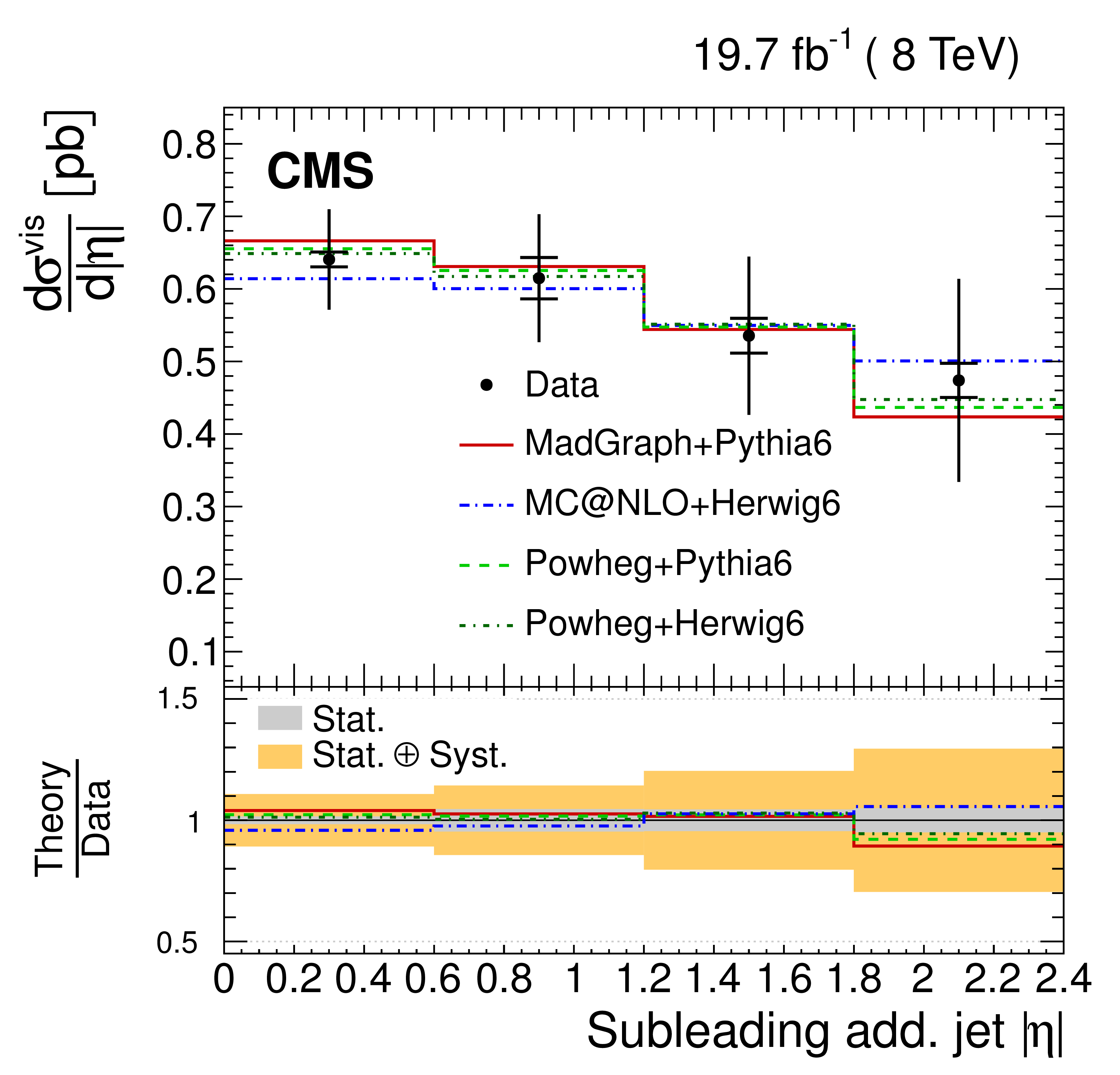
Figure 10-c:
Absolute differential $ {\mathrm {t}\overline {\mathrm {t}}} $ cross section as a function of the $ {|\eta |} $ of the leading additional jet (a,b) and the subleading additional jet (c,d) in the visible phase space of the $ {\mathrm {t}\overline {\mathrm {t}}} $ system and the additional jets. Data are compared to predictions from MADGRAPH +PYTHIA-6, POWHEG +PYTHIA-6, POWHEG +HERWIG-6, and MC@NLO+HERWIG-6 (a,c) and to MADGRAPH with with varied renormalization, factorization, and jet-parton matching scales (b,d). The inner (outer) vertical bars indicate the statistical (total) uncertainties. The lower part of each plot shows the ratio of the predictions to the data. |
png pdf |
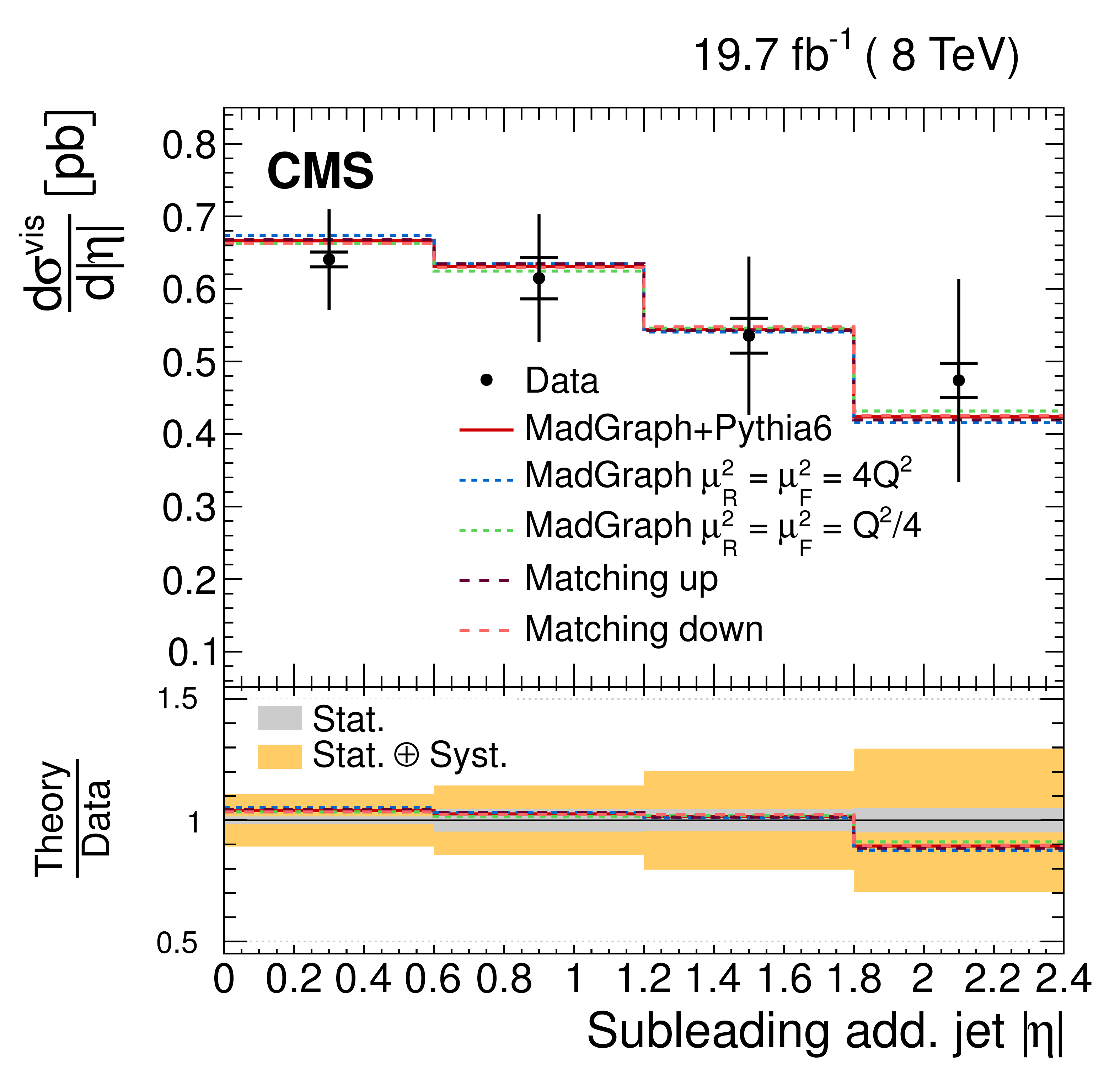
Figure 10-d:
Absolute differential $ {\mathrm {t}\overline {\mathrm {t}}} $ cross section as a function of the $ {|\eta |} $ of the leading additional jet (a,b) and the subleading additional jet (c,d) in the visible phase space of the $ {\mathrm {t}\overline {\mathrm {t}}} $ system and the additional jets. Data are compared to predictions from MADGRAPH +PYTHIA-6, POWHEG +PYTHIA-6, POWHEG +HERWIG-6, and MC@NLO+HERWIG-6 (a,c) and to MADGRAPH with with varied renormalization, factorization, and jet-parton matching scales (b,d). The inner (outer) vertical bars indicate the statistical (total) uncertainties. The lower part of each plot shows the ratio of the predictions to the data. |
png pdf |
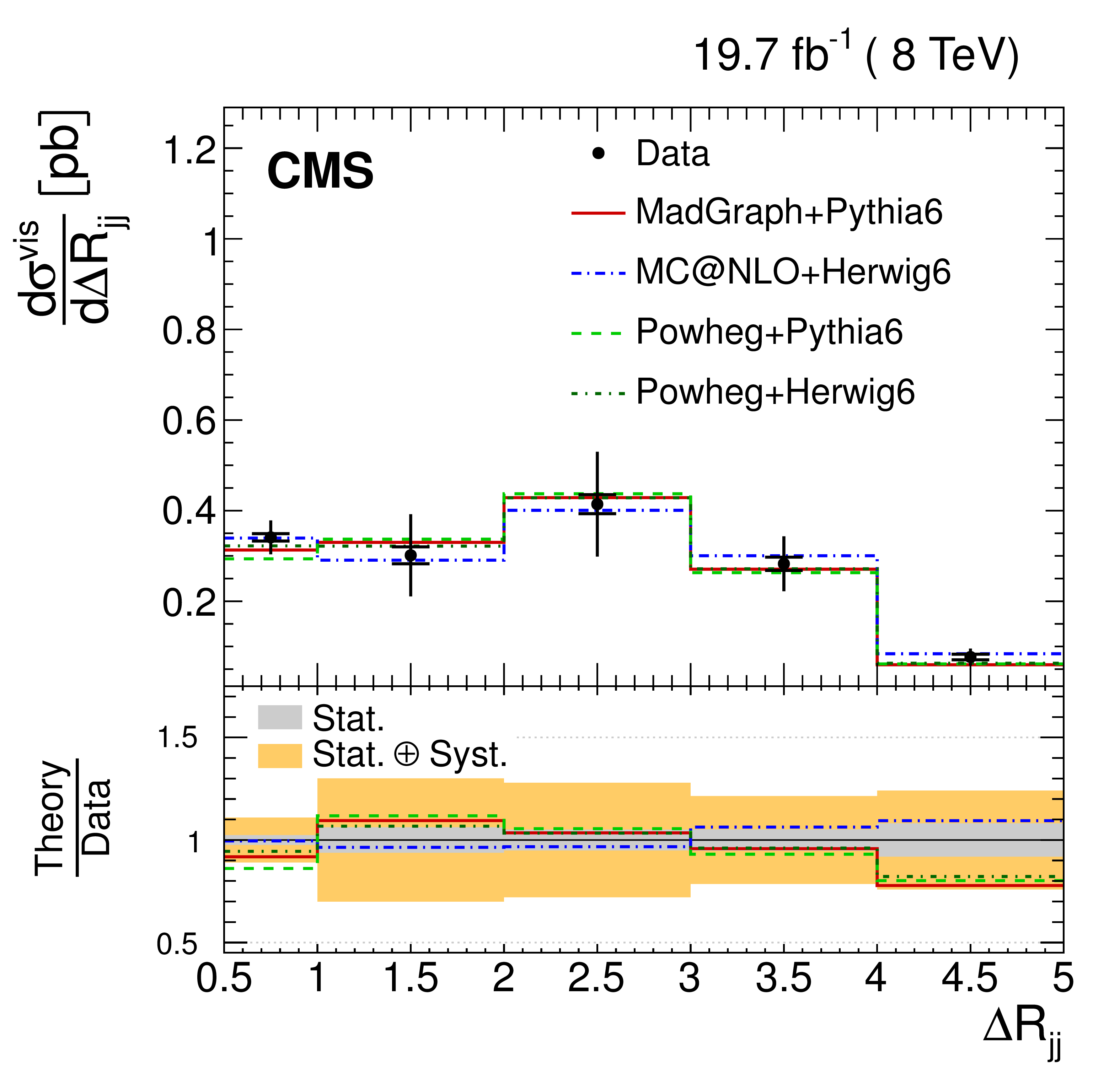
Figure 11-a:
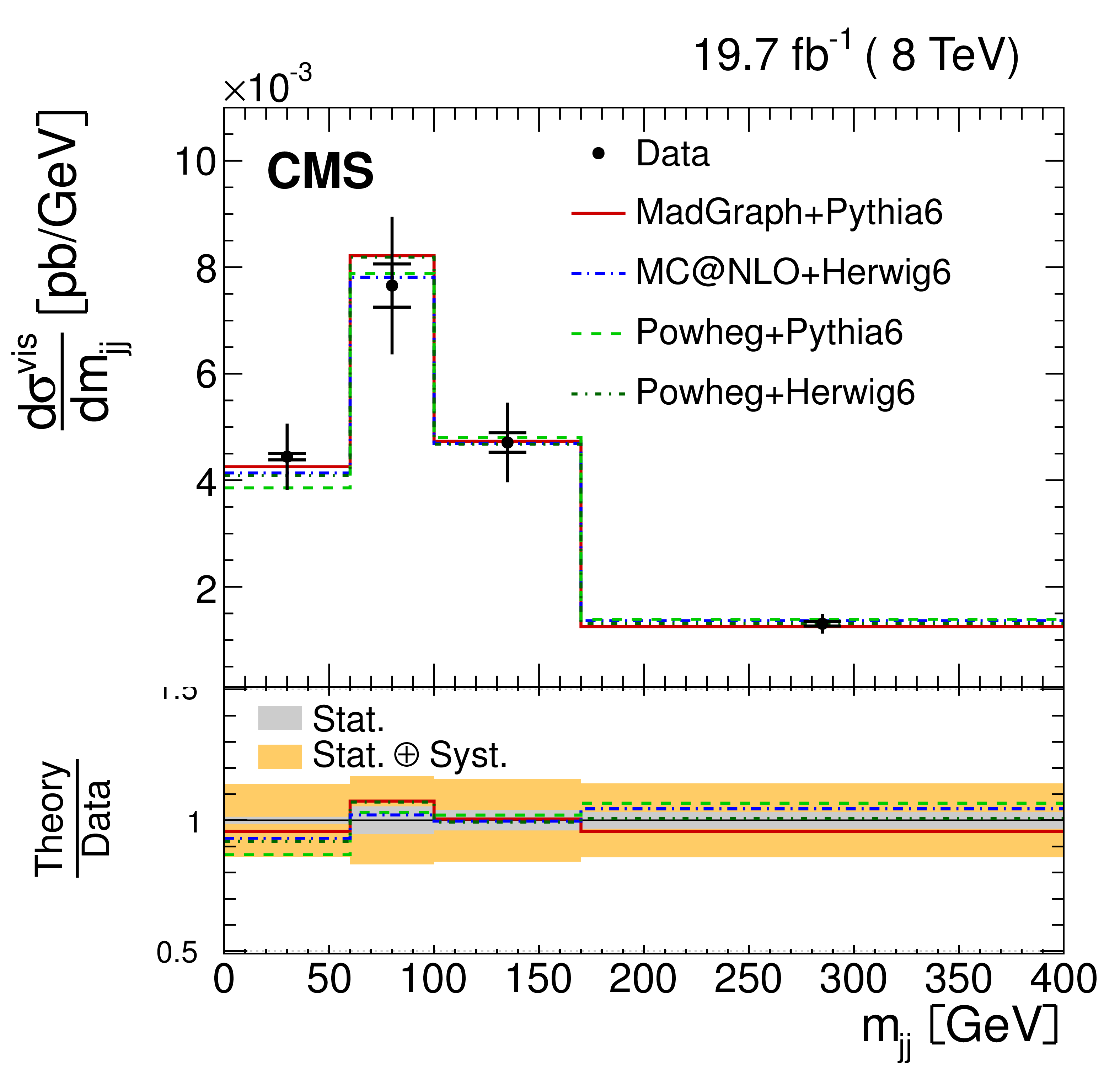
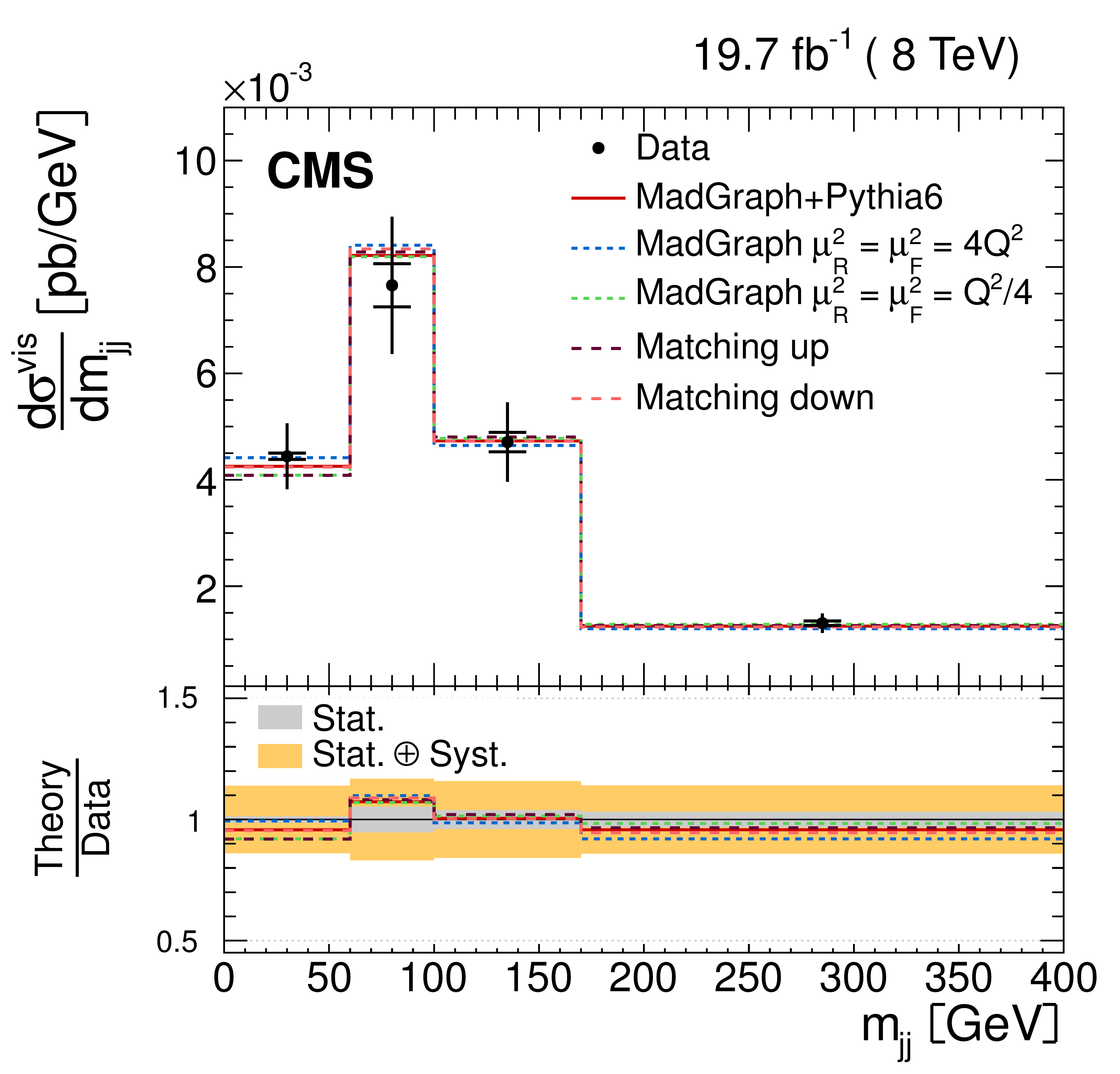
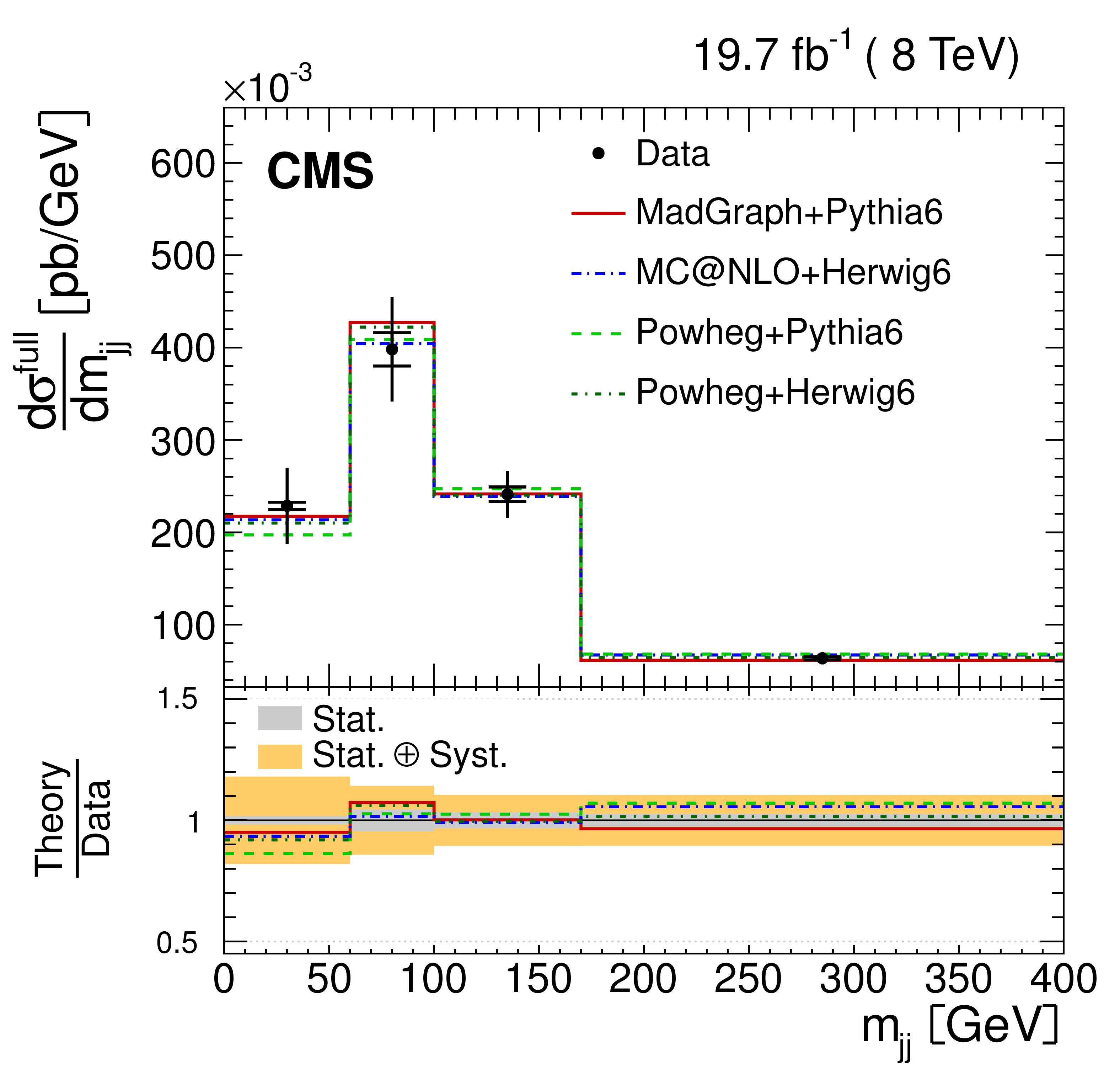
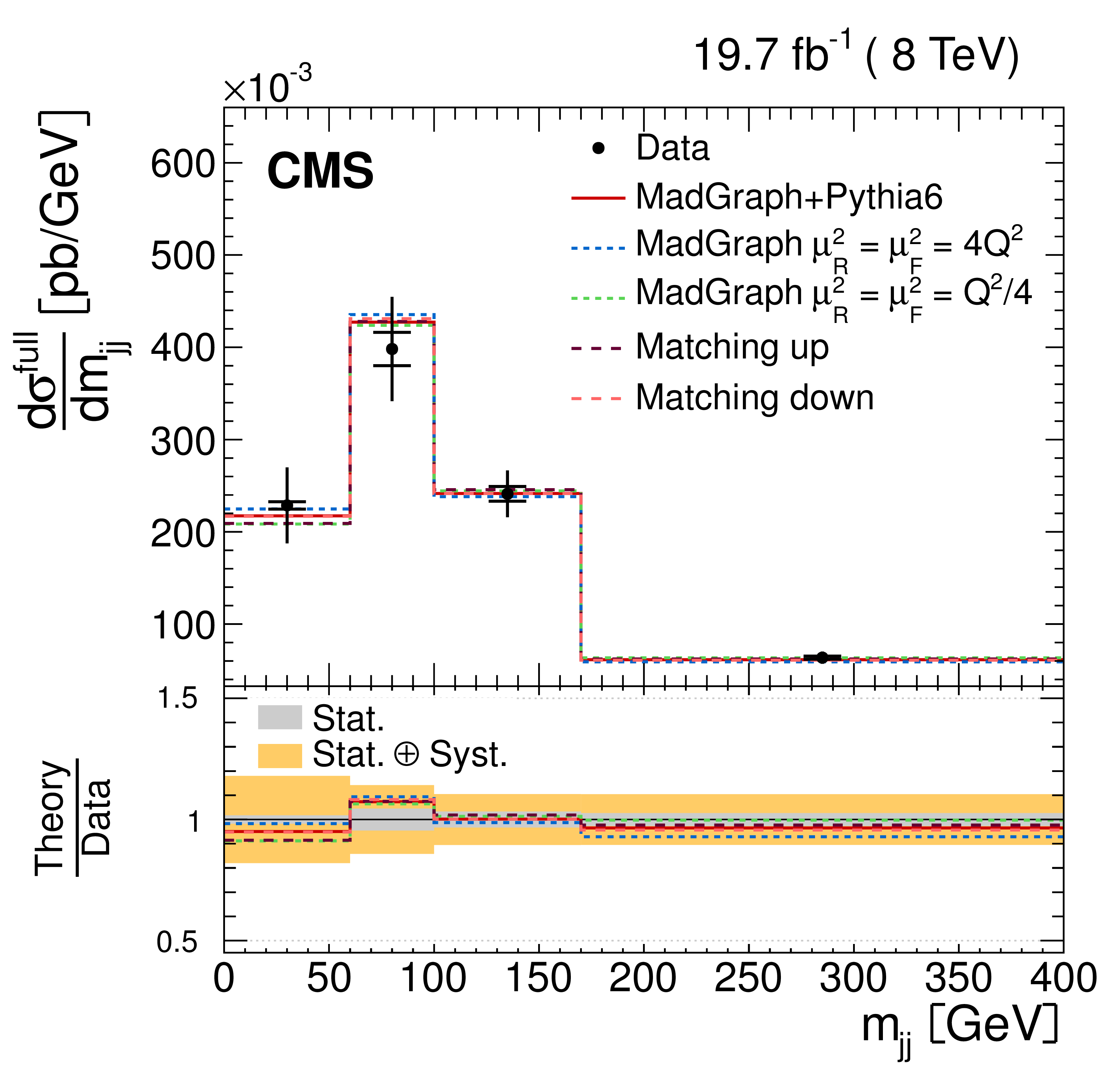
Absolute differential $ {\mathrm {t}\overline {\mathrm {t}}} $ cross section as a function of $ {\Delta R_{\rm {jj}}} $ between the leading and subleading additional jets (a,b) and their invariant mass, $ {m_{\rm {jj}}} $ (c,d). Data are compared to predictions from MADGRAPH +PYTHIA-6, POWHEG +PYTHIA-6, POWHEG +HERWIG-6, and MC@NLO+HERWIG-6 (a,c) and to MADGRAPH with varied renormalization, factorization, and jet-parton matching scales (b,d). The inner (outer) vertical bars indicate the statistical (total) uncertainties. The lower part of each plot shows the ratio of the predictions to the data. |
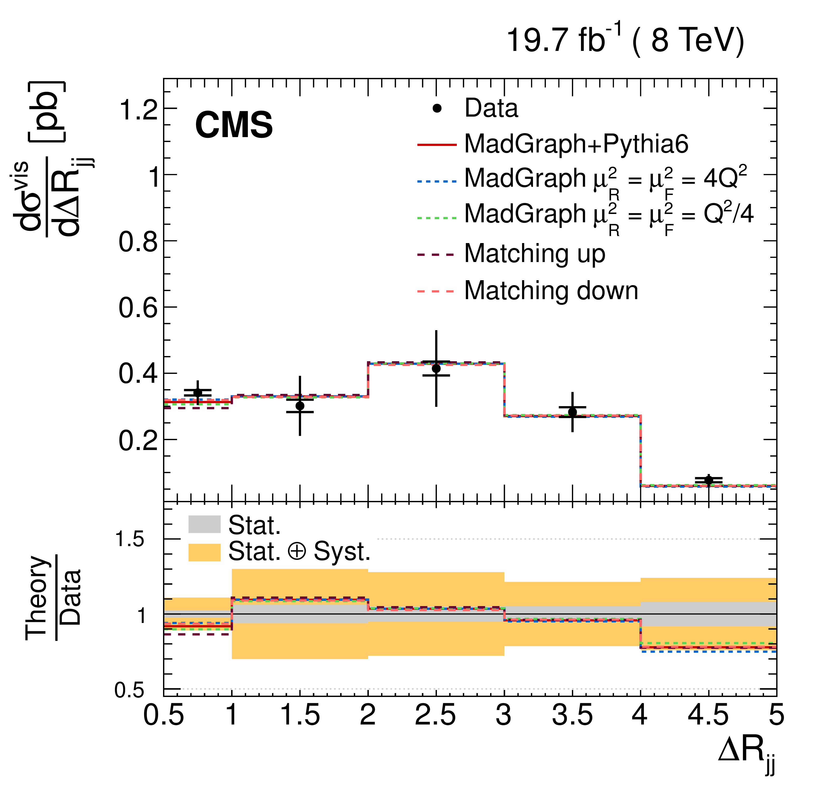
png pdf |
Figure 11-b:
Absolute differential $ {\mathrm {t}\overline {\mathrm {t}}} $ cross section as a function of $ {\Delta R_{\rm {jj}}} $ between the leading and subleading additional jets (a,b) and their invariant mass, $ {m_{\rm {jj}}} $ (c,d). Data are compared to predictions from MADGRAPH +PYTHIA-6, POWHEG +PYTHIA-6, POWHEG +HERWIG-6, and MC@NLO+HERWIG-6 (a,c) and to MADGRAPH with varied renormalization, factorization, and jet-parton matching scales (b,d). The inner (outer) vertical bars indicate the statistical (total) uncertainties. The lower part of each plot shows the ratio of the predictions to the data. |
png pdf |
Figure 11-c:
Absolute differential $ {\mathrm {t}\overline {\mathrm {t}}} $ cross section as a function of $ {\Delta R_{\rm {jj}}} $ between the leading and subleading additional jets (a,b) and their invariant mass, $ {m_{\rm {jj}}} $ (c,d). Data are compared to predictions from MADGRAPH +PYTHIA-6, POWHEG +PYTHIA-6, POWHEG +HERWIG-6, and MC@NLO+HERWIG-6 (a,c) and to MADGRAPH with varied renormalization, factorization, and jet-parton matching scales (b,d). The inner (outer) vertical bars indicate the statistical (total) uncertainties. The lower part of each plot shows the ratio of the predictions to the data. |
png pdf |
Figure 11-d:
Absolute differential $ {\mathrm {t}\overline {\mathrm {t}}} $ cross section as a function of $ {\Delta R_{\rm {jj}}} $ between the leading and subleading additional jets (a,b) and their invariant mass, $ {m_{\rm {jj}}} $ (c,d). Data are compared to predictions from MADGRAPH +PYTHIA-6, POWHEG +PYTHIA-6, POWHEG +HERWIG-6, and MC@NLO+HERWIG-6 (a,c) and to MADGRAPH with varied renormalization, factorization, and jet-parton matching scales (b,d). The inner (outer) vertical bars indicate the statistical (total) uncertainties. The lower part of each plot shows the ratio of the predictions to the data. |
png pdf |
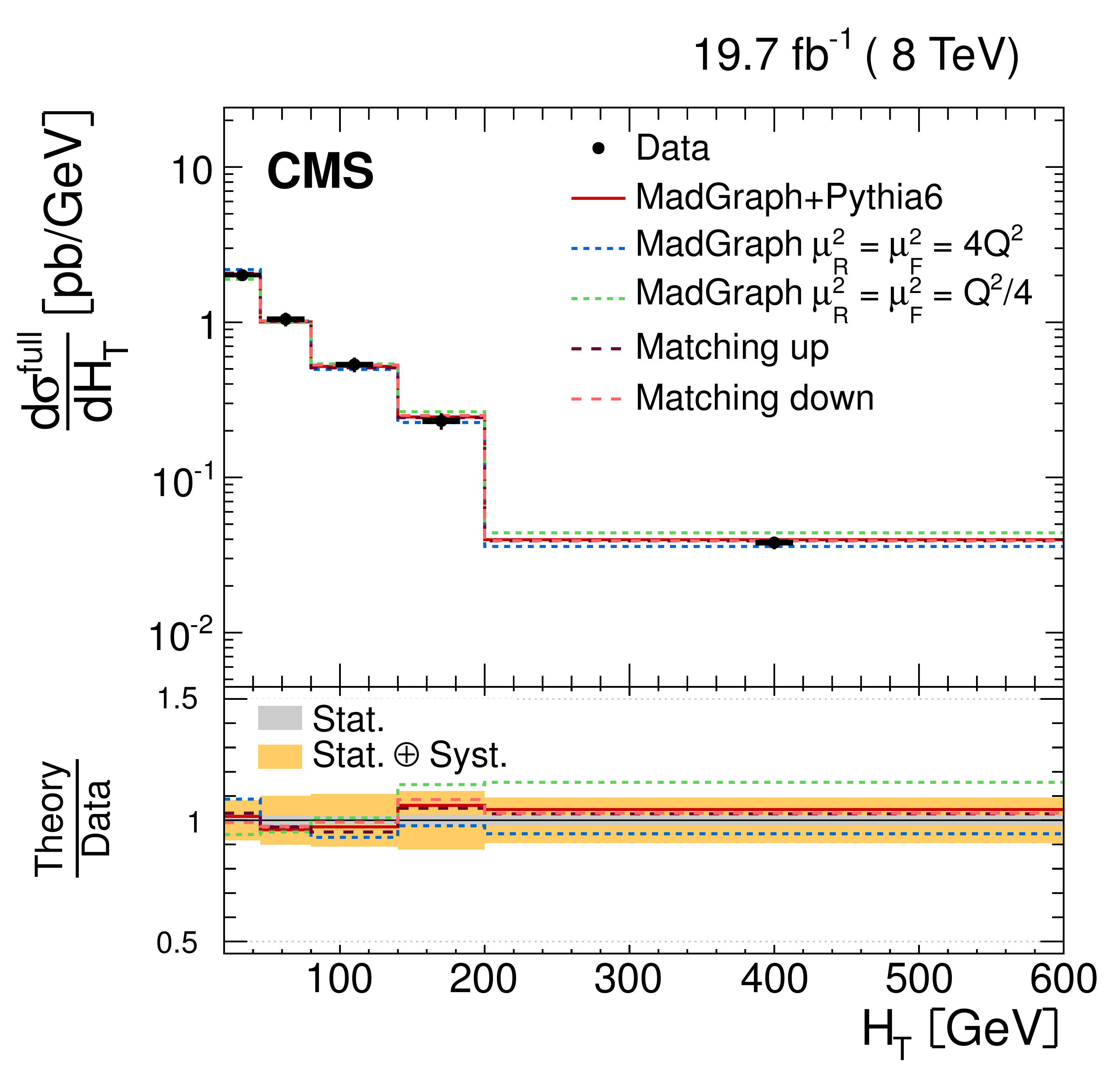
Figure 12-a:
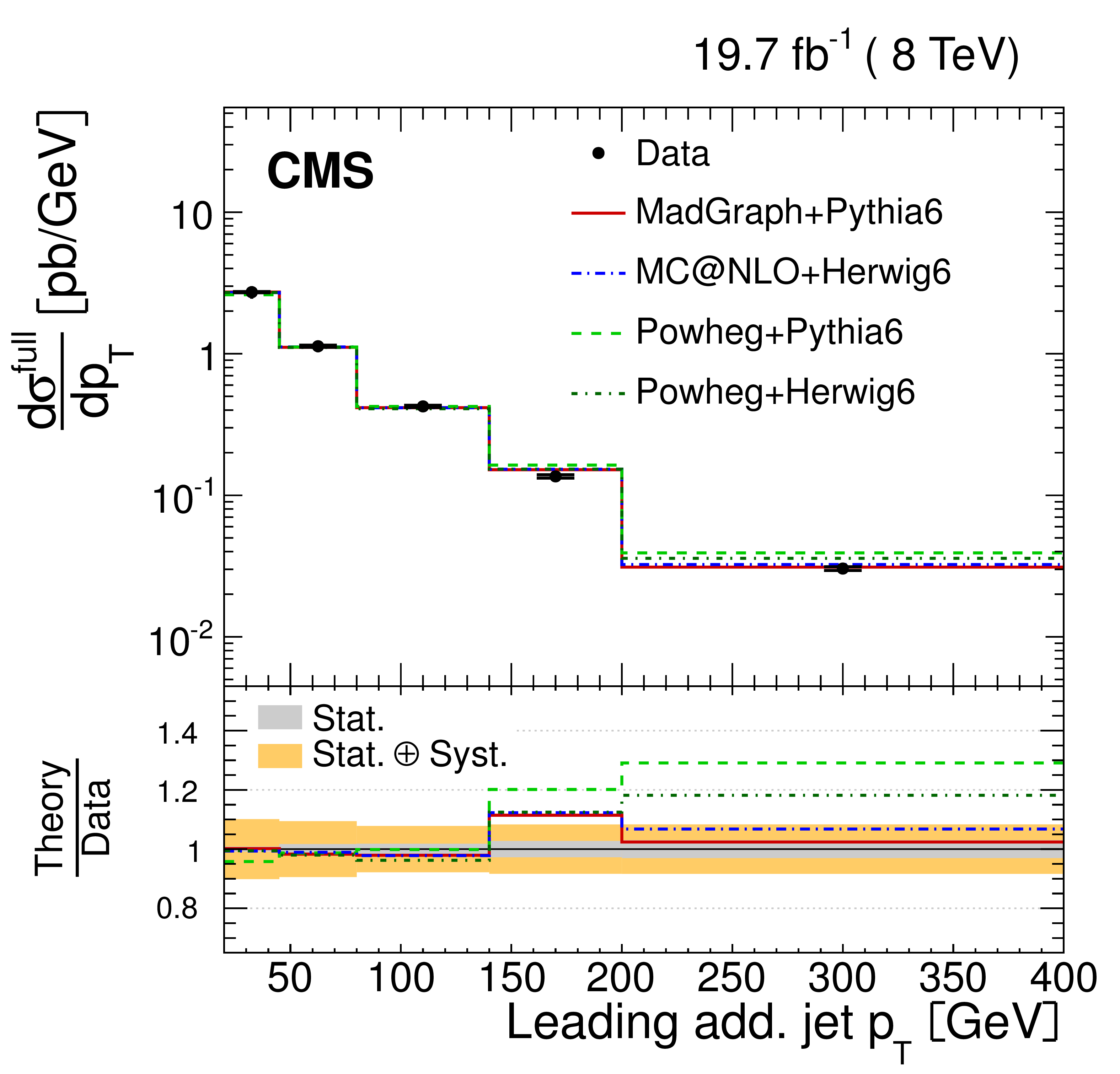
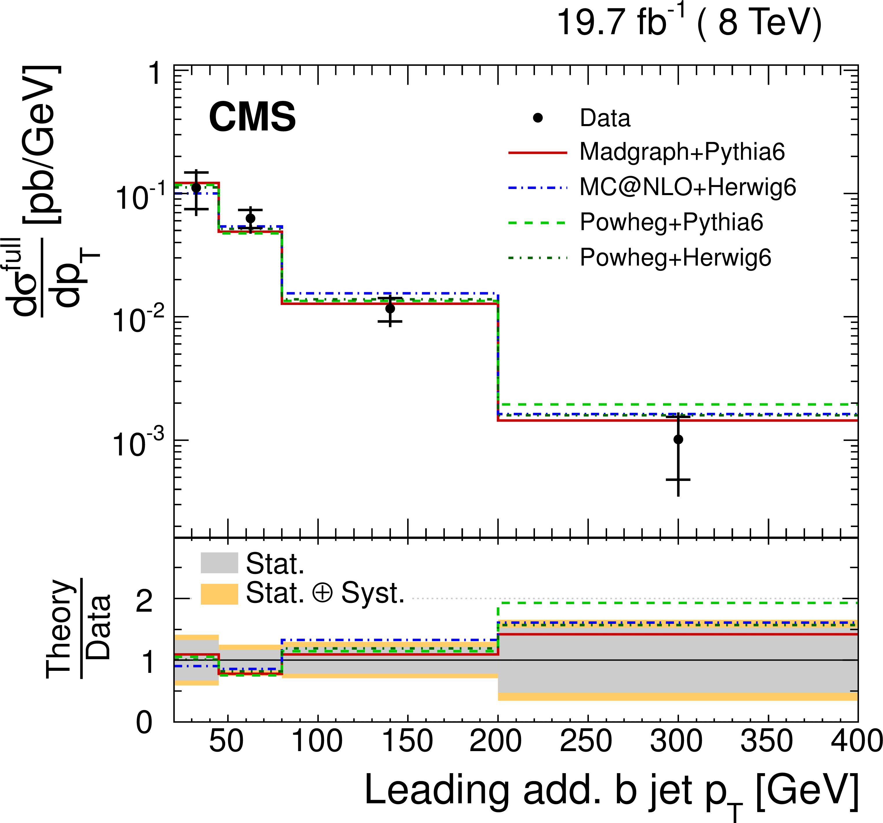
Absolute differential $ {\mathrm {t}\overline {\mathrm {t}}} $ cross section as a function of $ {p_{\mathrm {T}}} $ of the leading additional jet (a,b) and the subleading additional jet (c,d) and $H_{\rm T}$ (e,f) measured in the full phase space of the $ {\mathrm {t}\overline {\mathrm {t}}} $ system, corrected for acceptance and branching fractions. Data are compared to predictions from MADGRAPH +PYTHIA-6, POWHEG +PYTHIA-6, POWHEG +HERWIG-6, and MC@NLO+HERWIG-6 (a,c,e) and to MADGRAPH with varied renormalization, factorization, and jet-parton matching scales (b,d,f). The inner (outer) vertical bars indicate the statistical (total) uncertainties. The lower part of each plot shows the ratio of the predictions to the data. |
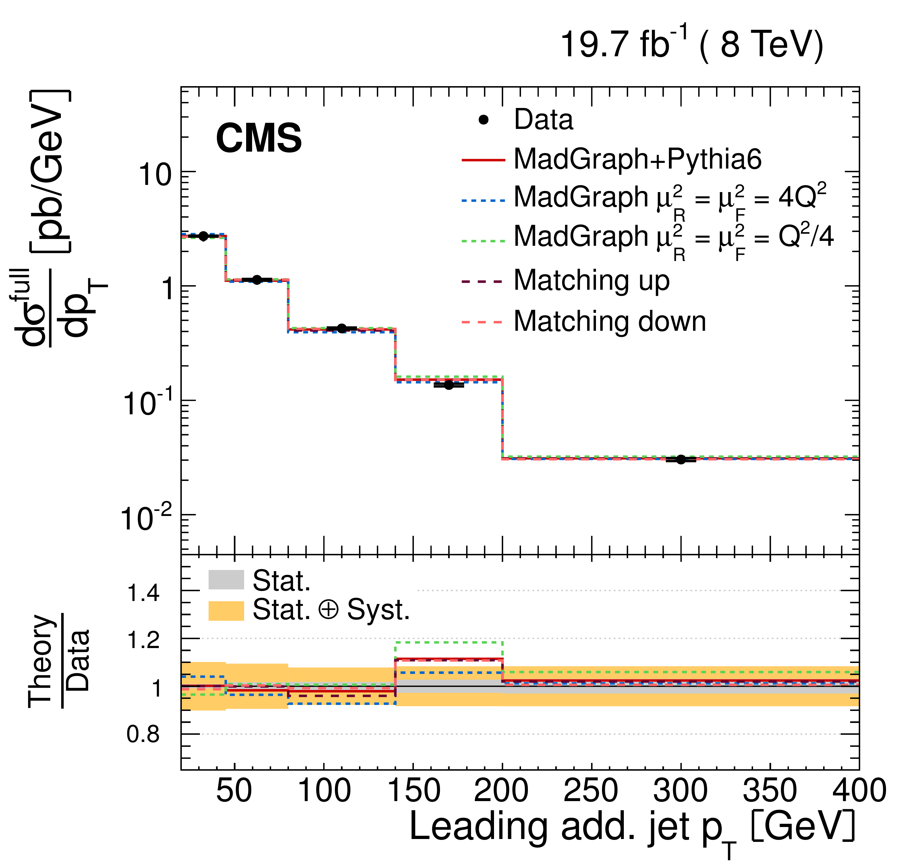
png pdf |
Figure 12-b:
Absolute differential $ {\mathrm {t}\overline {\mathrm {t}}} $ cross section as a function of $ {p_{\mathrm {T}}} $ of the leading additional jet (a,b) and the subleading additional jet (c,d) and $H_{\rm T}$ (e,f) measured in the full phase space of the $ {\mathrm {t}\overline {\mathrm {t}}} $ system, corrected for acceptance and branching fractions. Data are compared to predictions from MADGRAPH +PYTHIA-6, POWHEG +PYTHIA-6, POWHEG +HERWIG-6, and MC@NLO+HERWIG-6 (a,c,e) and to MADGRAPH with varied renormalization, factorization, and jet-parton matching scales (b,d,f). The inner (outer) vertical bars indicate the statistical (total) uncertainties. The lower part of each plot shows the ratio of the predictions to the data. |
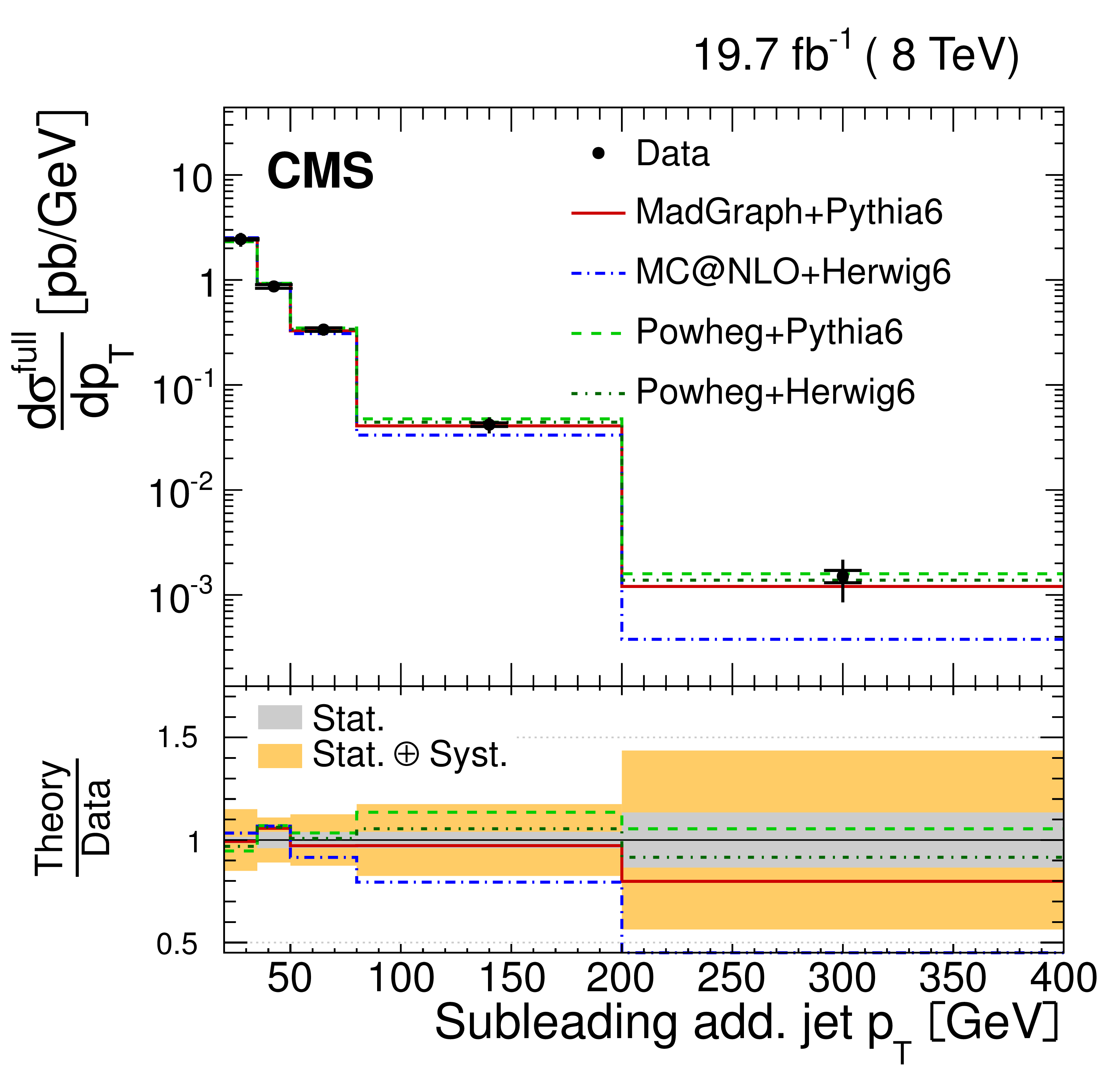
png pdf |
Figure 12-c:
Absolute differential $ {\mathrm {t}\overline {\mathrm {t}}} $ cross section as a function of $ {p_{\mathrm {T}}} $ of the leading additional jet (a,b) and the subleading additional jet (c,d) and $H_{\rm T}$ (e,f) measured in the full phase space of the $ {\mathrm {t}\overline {\mathrm {t}}} $ system, corrected for acceptance and branching fractions. Data are compared to predictions from MADGRAPH +PYTHIA-6, POWHEG +PYTHIA-6, POWHEG +HERWIG-6, and MC@NLO+HERWIG-6 (a,c,e) and to MADGRAPH with varied renormalization, factorization, and jet-parton matching scales (b,d,f). The inner (outer) vertical bars indicate the statistical (total) uncertainties. The lower part of each plot shows the ratio of the predictions to the data. |
png pdf |
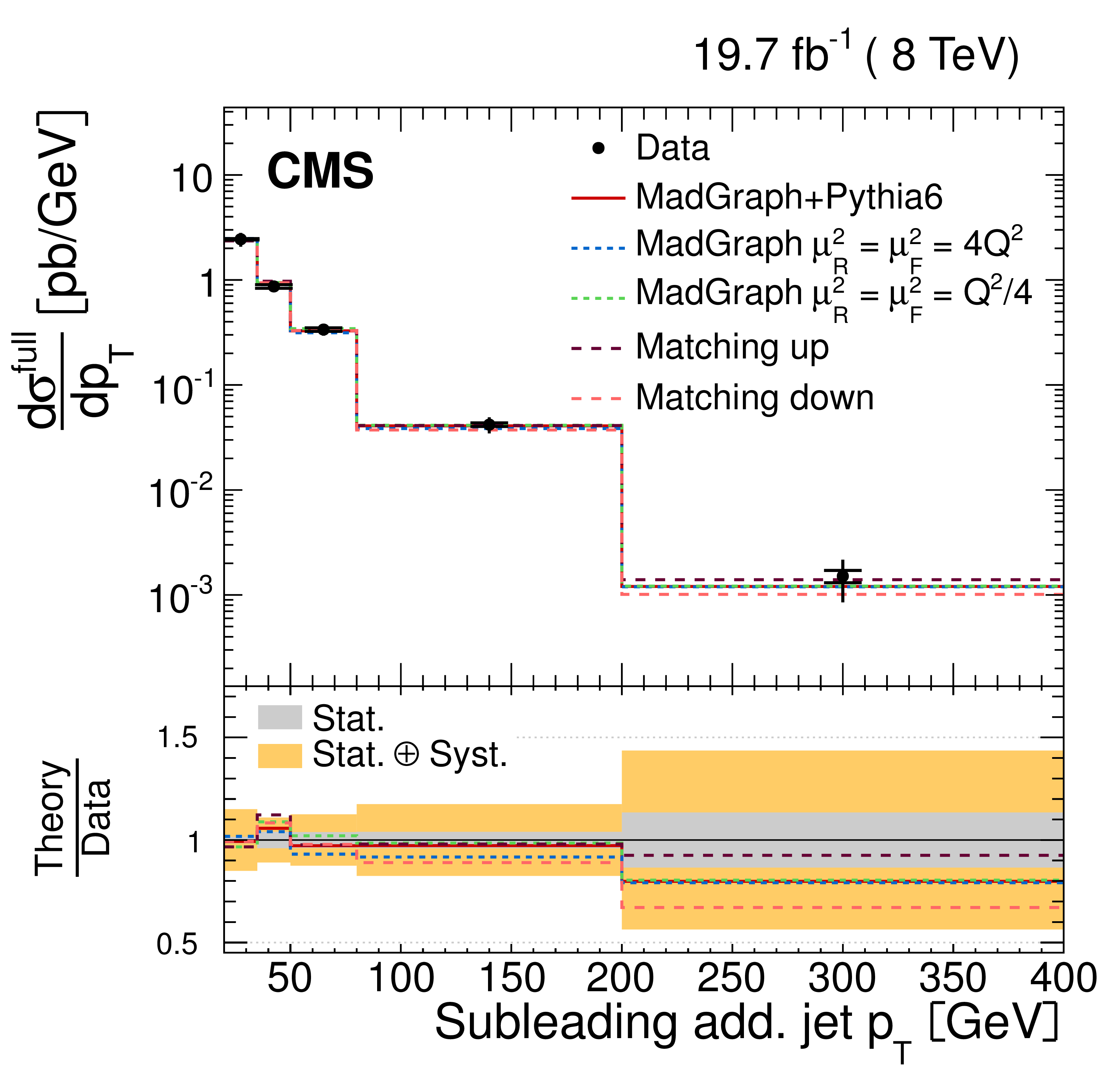
Figure 12-d:
Absolute differential $ {\mathrm {t}\overline {\mathrm {t}}} $ cross section as a function of $ {p_{\mathrm {T}}} $ of the leading additional jet (a,b) and the subleading additional jet (c,d) and $H_{\rm T}$ (e,f) measured in the full phase space of the $ {\mathrm {t}\overline {\mathrm {t}}} $ system, corrected for acceptance and branching fractions. Data are compared to predictions from MADGRAPH +PYTHIA-6, POWHEG +PYTHIA-6, POWHEG +HERWIG-6, and MC@NLO+HERWIG-6 (a,c,e) and to MADGRAPH with varied renormalization, factorization, and jet-parton matching scales (b,d,f). The inner (outer) vertical bars indicate the statistical (total) uncertainties. The lower part of each plot shows the ratio of the predictions to the data. |
png pdf |
Figure 12-e:
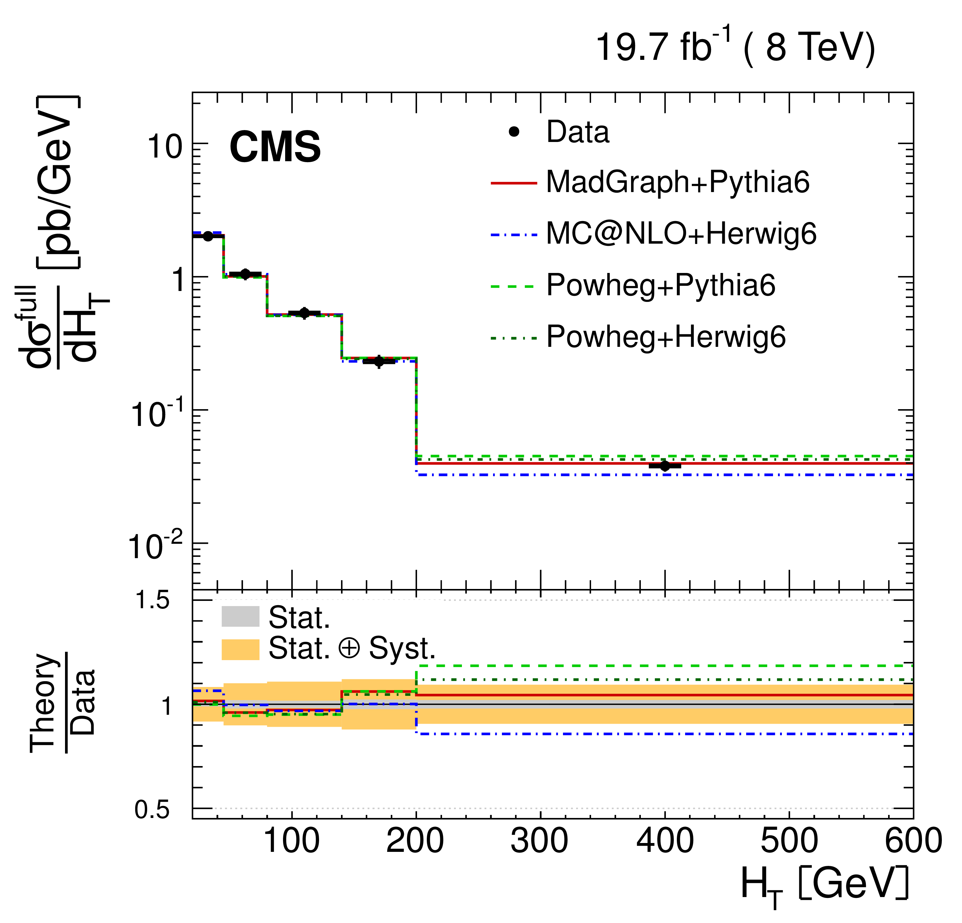
Absolute differential $ {\mathrm {t}\overline {\mathrm {t}}} $ cross section as a function of $ {p_{\mathrm {T}}} $ of the leading additional jet (a,b) and the subleading additional jet (c,d) and $H_{\rm T}$ (e,f) measured in the full phase space of the $ {\mathrm {t}\overline {\mathrm {t}}} $ system, corrected for acceptance and branching fractions. Data are compared to predictions from MADGRAPH +PYTHIA-6, POWHEG +PYTHIA-6, POWHEG +HERWIG-6, and MC@NLO+HERWIG-6 (a,c,e) and to MADGRAPH with varied renormalization, factorization, and jet-parton matching scales (b,d,f). The inner (outer) vertical bars indicate the statistical (total) uncertainties. The lower part of each plot shows the ratio of the predictions to the data. |
png pdf |
Figure 12-f:
Absolute differential $ {\mathrm {t}\overline {\mathrm {t}}} $ cross section as a function of $ {p_{\mathrm {T}}} $ of the leading additional jet (a,b) and the subleading additional jet (c,d) and $H_{\rm T}$ (e,f) measured in the full phase space of the $ {\mathrm {t}\overline {\mathrm {t}}} $ system, corrected for acceptance and branching fractions. Data are compared to predictions from MADGRAPH +PYTHIA-6, POWHEG +PYTHIA-6, POWHEG +HERWIG-6, and MC@NLO+HERWIG-6 (a,c,e) and to MADGRAPH with varied renormalization, factorization, and jet-parton matching scales (b,d,f). The inner (outer) vertical bars indicate the statistical (total) uncertainties. The lower part of each plot shows the ratio of the predictions to the data. |
png pdf |
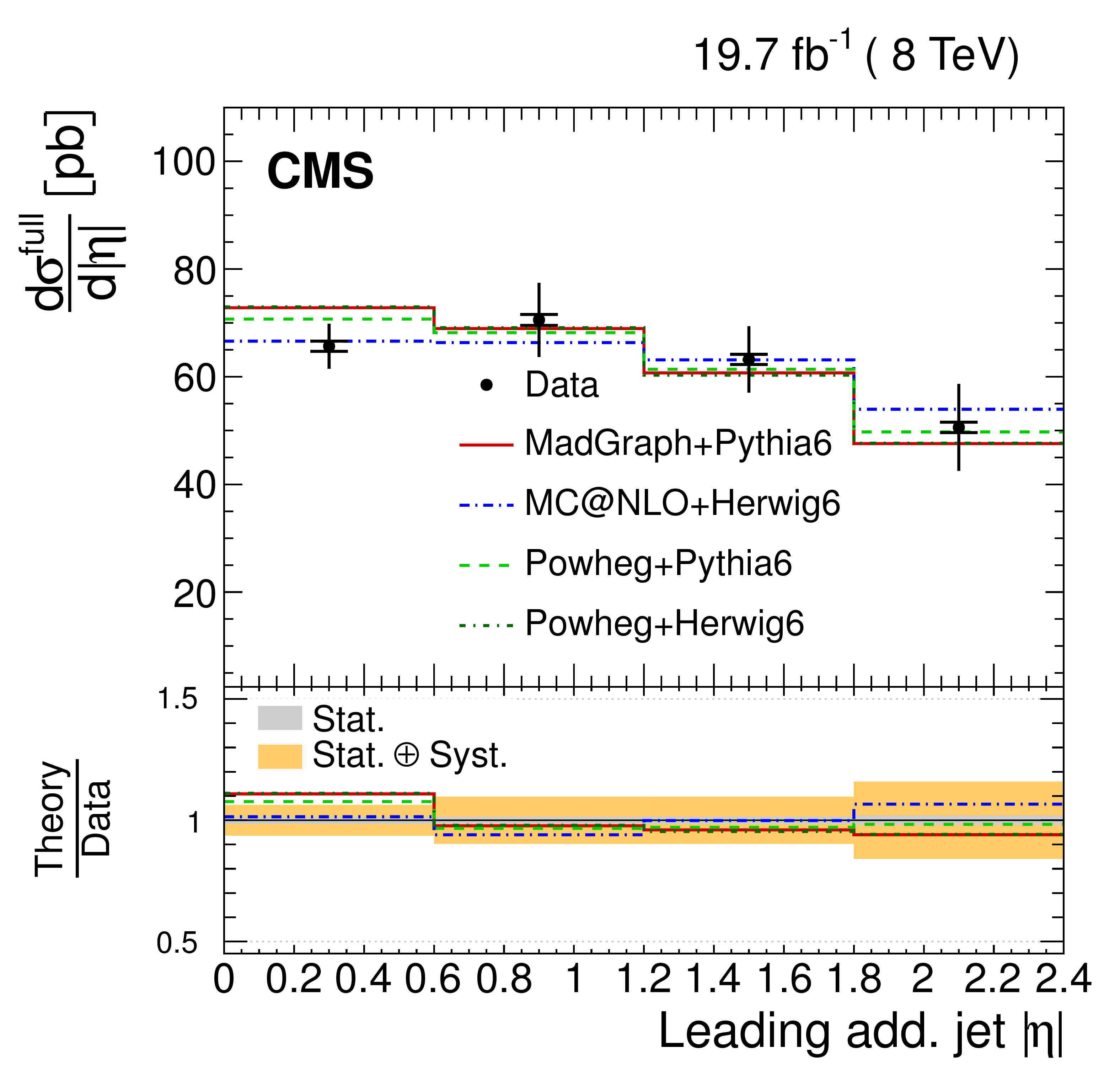
Figure 13-a:
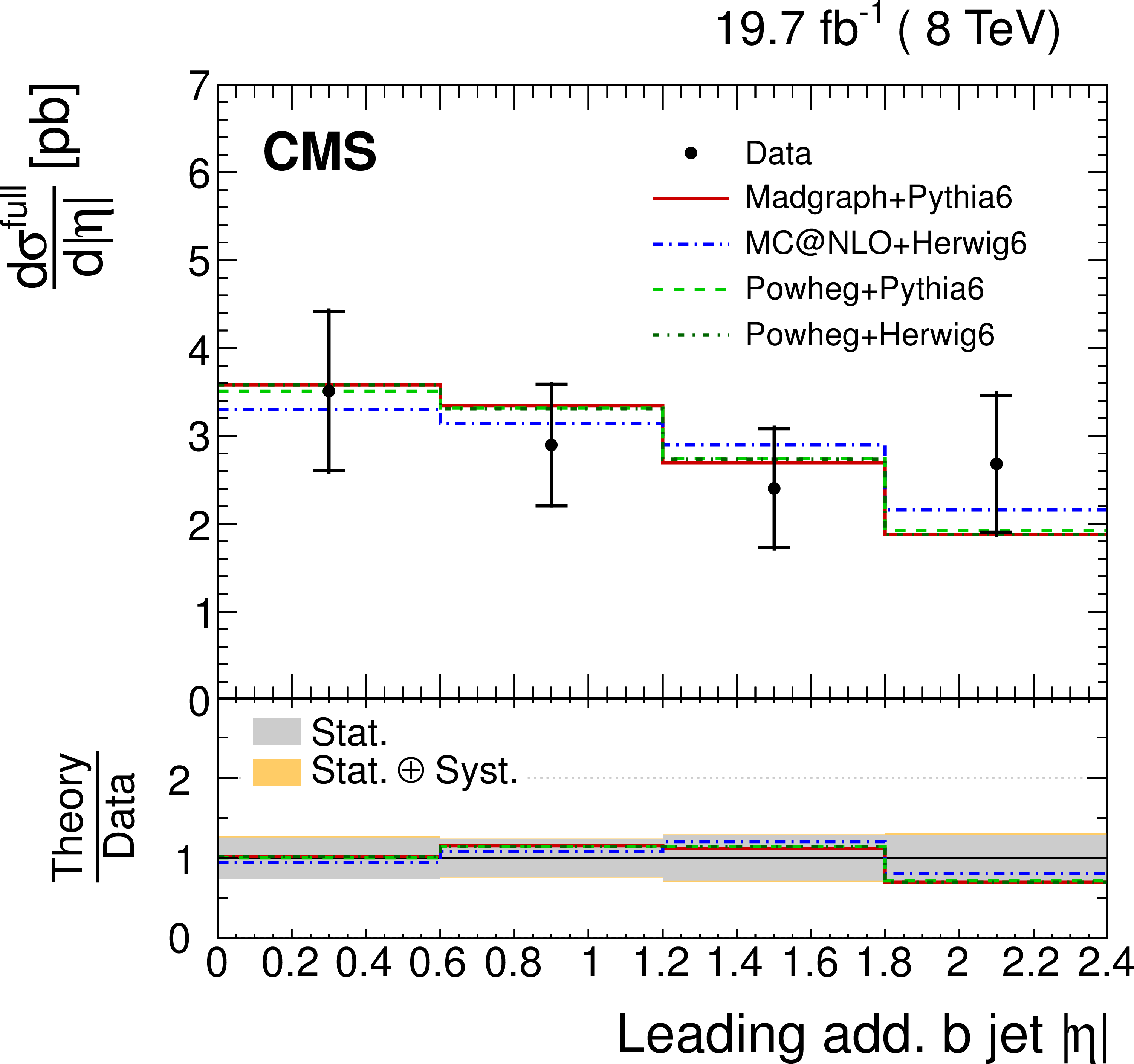
Absolute differential $ {\mathrm {t}\overline {\mathrm {t}}} $ cross section as a function of the $ {|\eta |} $ of the leading additional jet (a,b) and the subleading additional jet (c,d) measured in the full phase space of the $ {\mathrm {t}\overline {\mathrm {t}}} $ system, corrected for acceptance and branching fractions. Data are compared to predictions from MADGRAPH +PYTHIA-6, POWHEG +PYTHIA-6, POWHEG +HERWIG-6, and MC@NLO+HERWIG-6 (a,c) and to MADGRAPH with varied renormalization, factorization, and jet-parton matching scales (b,d). The inner (outer) vertical bars indicate the statistical (total) uncertainties. The lower part of each plot shows the ratio of the predictions to the data. |

png pdf |
Figure 13-b:
Absolute differential $ {\mathrm {t}\overline {\mathrm {t}}} $ cross section as a function of the $ {|\eta |} $ of the leading additional jet (a,b) and the subleading additional jet (c,d) measured in the full phase space of the $ {\mathrm {t}\overline {\mathrm {t}}} $ system, corrected for acceptance and branching fractions. Data are compared to predictions from MADGRAPH +PYTHIA-6, POWHEG +PYTHIA-6, POWHEG +HERWIG-6, and MC@NLO+HERWIG-6 (a,c) and to MADGRAPH with varied renormalization, factorization, and jet-parton matching scales (b,d). The inner (outer) vertical bars indicate the statistical (total) uncertainties. The lower part of each plot shows the ratio of the predictions to the data. |

png pdf |
Figure 13-c:
Absolute differential $ {\mathrm {t}\overline {\mathrm {t}}} $ cross section as a function of the $ {|\eta |} $ of the leading additional jet (a,b) and the subleading additional jet (c,d) measured in the full phase space of the $ {\mathrm {t}\overline {\mathrm {t}}} $ system, corrected for acceptance and branching fractions. Data are compared to predictions from MADGRAPH +PYTHIA-6, POWHEG +PYTHIA-6, POWHEG +HERWIG-6, and MC@NLO+HERWIG-6 (a,c) and to MADGRAPH with varied renormalization, factorization, and jet-parton matching scales (b,d). The inner (outer) vertical bars indicate the statistical (total) uncertainties. The lower part of each plot shows the ratio of the predictions to the data. |

png pdf |
Figure 13-d:
Absolute differential $ {\mathrm {t}\overline {\mathrm {t}}} $ cross section as a function of the $ {|\eta |} $ of the leading additional jet (a,b) and the subleading additional jet (c,d) measured in the full phase space of the $ {\mathrm {t}\overline {\mathrm {t}}} $ system, corrected for acceptance and branching fractions. Data are compared to predictions from MADGRAPH +PYTHIA-6, POWHEG +PYTHIA-6, POWHEG +HERWIG-6, and MC@NLO+HERWIG-6 (a,c) and to MADGRAPH with varied renormalization, factorization, and jet-parton matching scales (b,d). The inner (outer) vertical bars indicate the statistical (total) uncertainties. The lower part of each plot shows the ratio of the predictions to the data. |
png pdf |
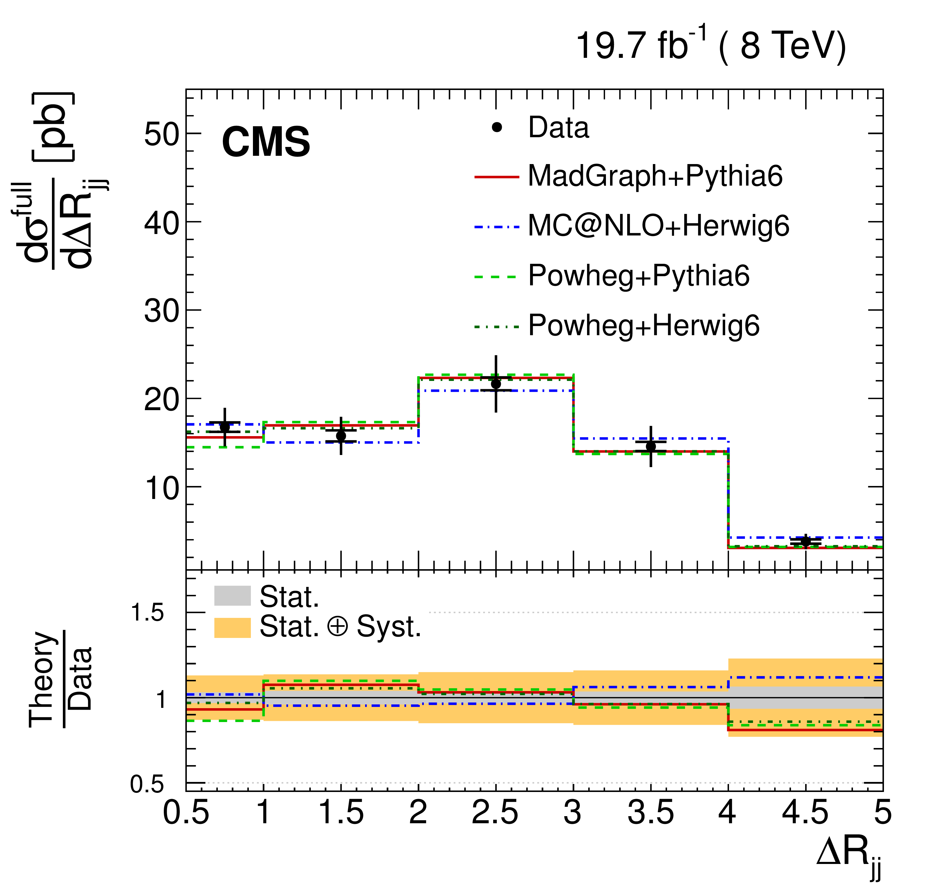
Figure 14-a:
Absolute differential $ {\mathrm {t}\overline {\mathrm {t}}} $ cross section as a function of $ {\Delta R_{\rm {jj}}} $ between the leading and subleading additional jets (a,b) and their invariant mass, $ {m_{\rm {jj}}} $ (c,d) measured in the full phase space of the $ {\mathrm {t}\overline {\mathrm {t}}} $ system, corrected for acceptance and branching fractions. Data are compared to predictions from MADGRAPH +PYTHIA-6, POWHEG +PYTHIA-6, POWHEG +HERWIG-6, and MC@NLO+HERWIG-6 (a,c) and to MADGRAPH with varied renormalization, factorization, and jet-parton matching scales (b,d). The inner (outer) vertical bars indicate the statistical (total) uncertainties. The lower part of each plot shows the ratio of the predictions to the data. |
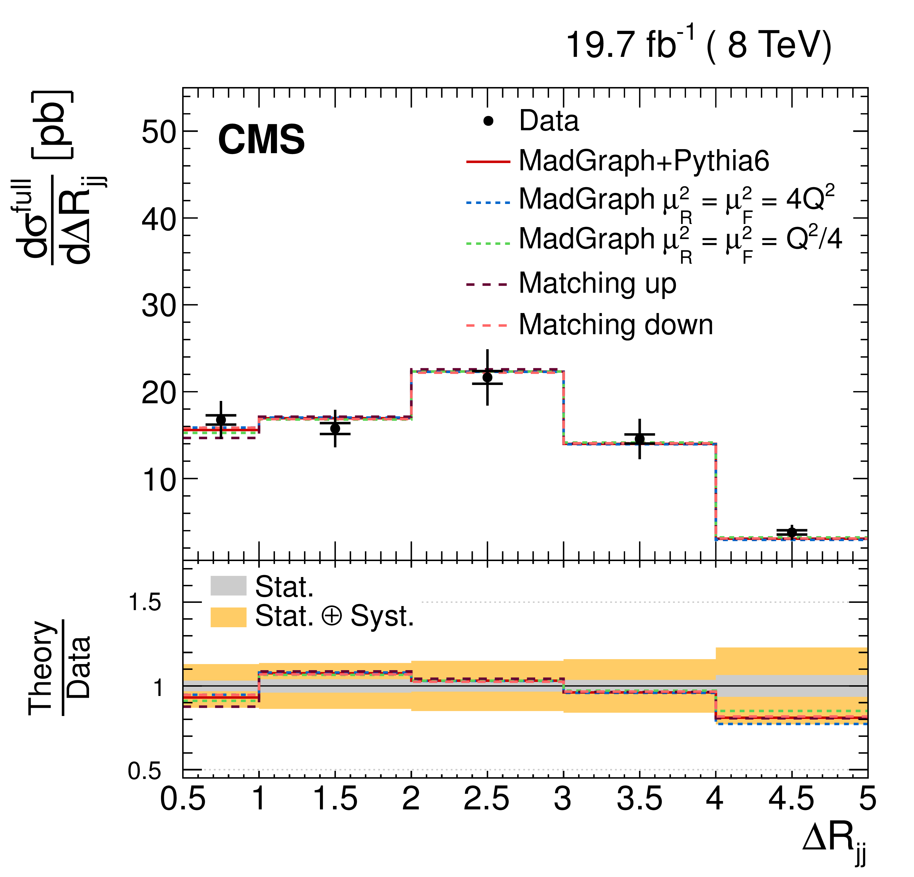
png pdf |
Figure 14-b:
Absolute differential $ {\mathrm {t}\overline {\mathrm {t}}} $ cross section as a function of $ {\Delta R_{\rm {jj}}} $ between the leading and subleading additional jets (a,b) and their invariant mass, $ {m_{\rm {jj}}} $ (c,d) measured in the full phase space of the $ {\mathrm {t}\overline {\mathrm {t}}} $ system, corrected for acceptance and branching fractions. Data are compared to predictions from MADGRAPH +PYTHIA-6, POWHEG +PYTHIA-6, POWHEG +HERWIG-6, and MC@NLO+HERWIG-6 (a,c) and to MADGRAPH with varied renormalization, factorization, and jet-parton matching scales (b,d). The inner (outer) vertical bars indicate the statistical (total) uncertainties. The lower part of each plot shows the ratio of the predictions to the data. |
png pdf |
Figure 14-c:
Absolute differential $ {\mathrm {t}\overline {\mathrm {t}}} $ cross section as a function of $ {\Delta R_{\rm {jj}}} $ between the leading and subleading additional jets (a,b) and their invariant mass, $ {m_{\rm {jj}}} $ (c,d) measured in the full phase space of the $ {\mathrm {t}\overline {\mathrm {t}}} $ system, corrected for acceptance and branching fractions. Data are compared to predictions from MADGRAPH +PYTHIA-6, POWHEG +PYTHIA-6, POWHEG +HERWIG-6, and MC@NLO+HERWIG-6 (a,c) and to MADGRAPH with varied renormalization, factorization, and jet-parton matching scales (b,d). The inner (outer) vertical bars indicate the statistical (total) uncertainties. The lower part of each plot shows the ratio of the predictions to the data. |
png pdf |
Figure 14-d:
Absolute differential $ {\mathrm {t}\overline {\mathrm {t}}} $ cross section as a function of $ {\Delta R_{\rm {jj}}} $ between the leading and subleading additional jets (a,b) and their invariant mass, $ {m_{\rm {jj}}} $ (c,d) measured in the full phase space of the $ {\mathrm {t}\overline {\mathrm {t}}} $ system, corrected for acceptance and branching fractions. Data are compared to predictions from MADGRAPH +PYTHIA-6, POWHEG +PYTHIA-6, POWHEG +HERWIG-6, and MC@NLO+HERWIG-6 (a,c) and to MADGRAPH with varied renormalization, factorization, and jet-parton matching scales (b,d). The inner (outer) vertical bars indicate the statistical (total) uncertainties. The lower part of each plot shows the ratio of the predictions to the data. |
png pdf |
Figure 15-a:
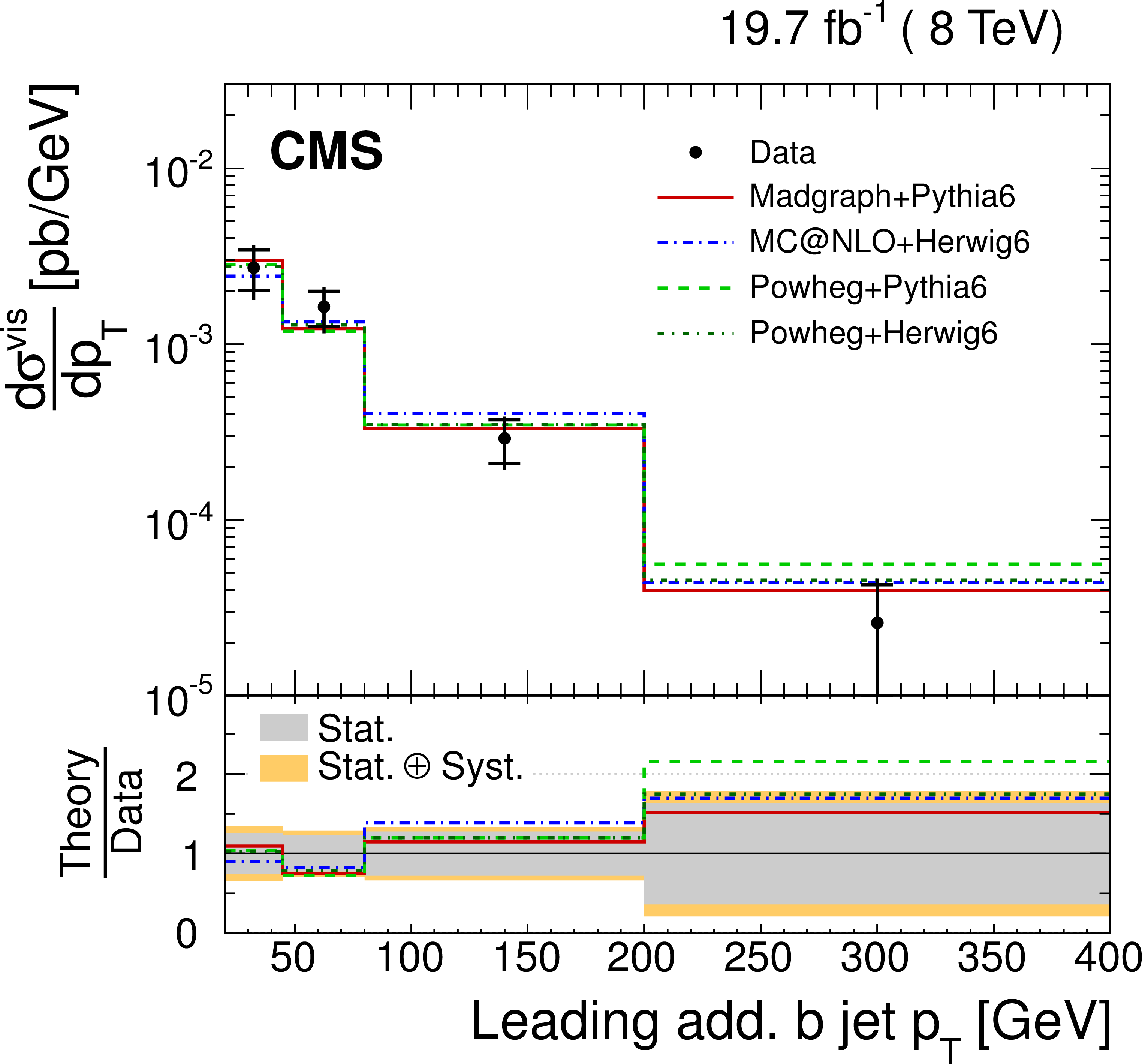
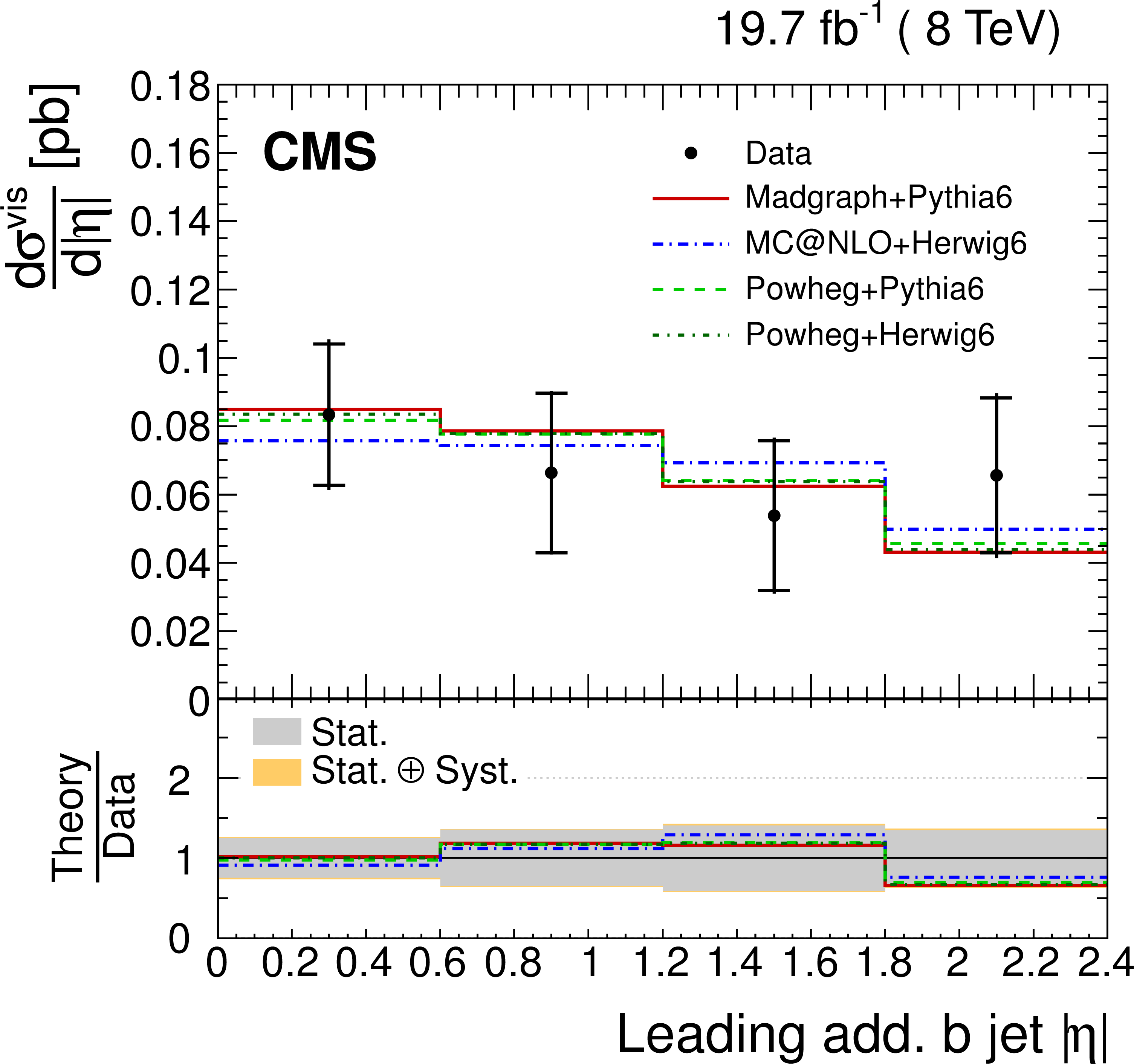
Absolute differential $ {\mathrm {t}\overline {\mathrm {t}}} $ cross section measured in the visible phase space of the $ {\mathrm {t}\overline {\mathrm {t}}} $ system and the additional b jets, as a function of the leading additional b jet $ {p_{\mathrm {T}}} $ (a) and $ {|\eta |} $ (b), subleading additional b jet $ {p_{\mathrm {T}}} $ (c) and $ {|\eta |} $ (d), the angular separation $\Delta R_{ {\mathrm {b}} {\mathrm {b}} }$ between the two leading additional b jets (e), and the invariant mass $ {m_{ {\mathrm {b}} {\mathrm {b}} }} $ of the two b jets. Data are compared with predictions from MADGRAPH interfaced with PYTHIA-6, MC@NLO interfaced with HERWIG-6, and POWHEG with PYTHIA-6 and HERWIG-6, normalized to the measured inclusive cross section. The inner (outer) vertical bars indicate the statistical (total) uncertainties. The lower part of each plot shows the ratio of the predictions to the data. |
png pdf |
Figure 15-b:
Absolute differential $ {\mathrm {t}\overline {\mathrm {t}}} $ cross section measured in the visible phase space of the $ {\mathrm {t}\overline {\mathrm {t}}} $ system and the additional b jets, as a function of the leading additional b jet $ {p_{\mathrm {T}}} $ (a) and $ {|\eta |} $ (b), subleading additional b jet $ {p_{\mathrm {T}}} $ (c) and $ {|\eta |} $ (d), the angular separation $\Delta R_{ {\mathrm {b}} {\mathrm {b}} }$ between the two leading additional b jets (e), and the invariant mass $ {m_{ {\mathrm {b}} {\mathrm {b}} }} $ of the two b jets. Data are compared with predictions from MADGRAPH interfaced with PYTHIA-6, MC@NLO interfaced with HERWIG-6, and POWHEG with PYTHIA-6 and HERWIG-6, normalized to the measured inclusive cross section. The inner (outer) vertical bars indicate the statistical (total) uncertainties. The lower part of each plot shows the ratio of the predictions to the data. |
png pdf |
Figure 15-c:
Absolute differential $ {\mathrm {t}\overline {\mathrm {t}}} $ cross section measured in the visible phase space of the $ {\mathrm {t}\overline {\mathrm {t}}} $ system and the additional b jets, as a function of the leading additional b jet $ {p_{\mathrm {T}}} $ (a) and $ {|\eta |} $ (b), subleading additional b jet $ {p_{\mathrm {T}}} $ (c) and $ {|\eta |} $ (d), the angular separation $\Delta R_{ {\mathrm {b}} {\mathrm {b}} }$ between the two leading additional b jets (e), and the invariant mass $ {m_{ {\mathrm {b}} {\mathrm {b}} }} $ of the two b jets. Data are compared with predictions from MADGRAPH interfaced with PYTHIA-6, MC@NLO interfaced with HERWIG-6, and POWHEG with PYTHIA-6 and HERWIG-6, normalized to the measured inclusive cross section. The inner (outer) vertical bars indicate the statistical (total) uncertainties. The lower part of each plot shows the ratio of the predictions to the data. |
png pdf |
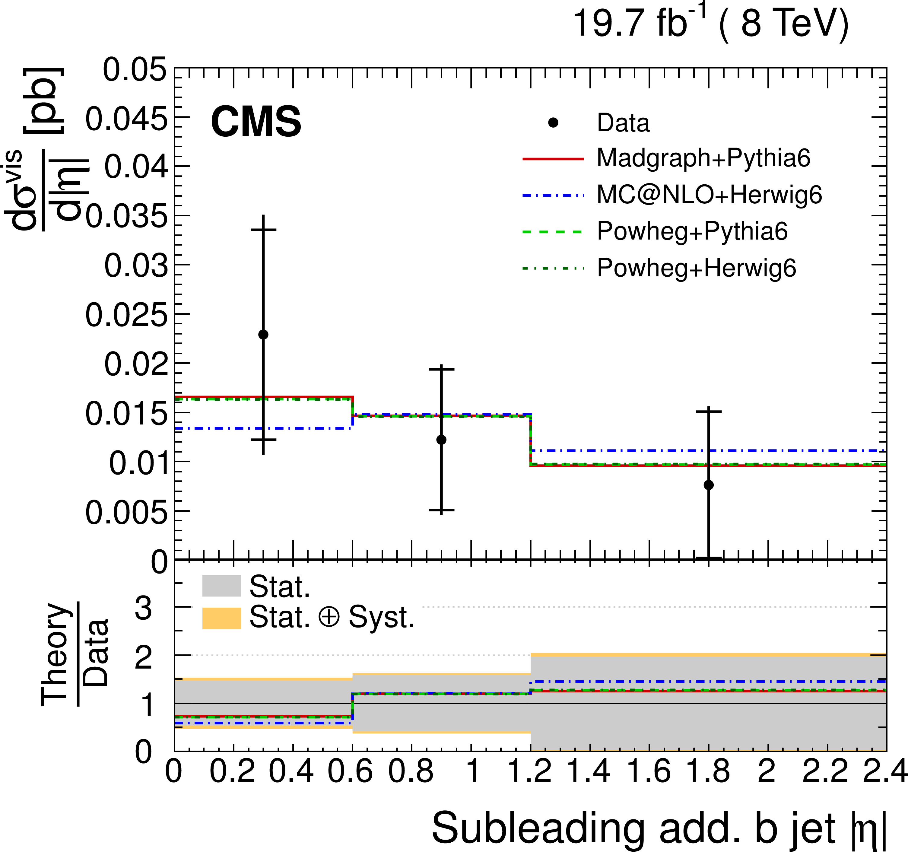
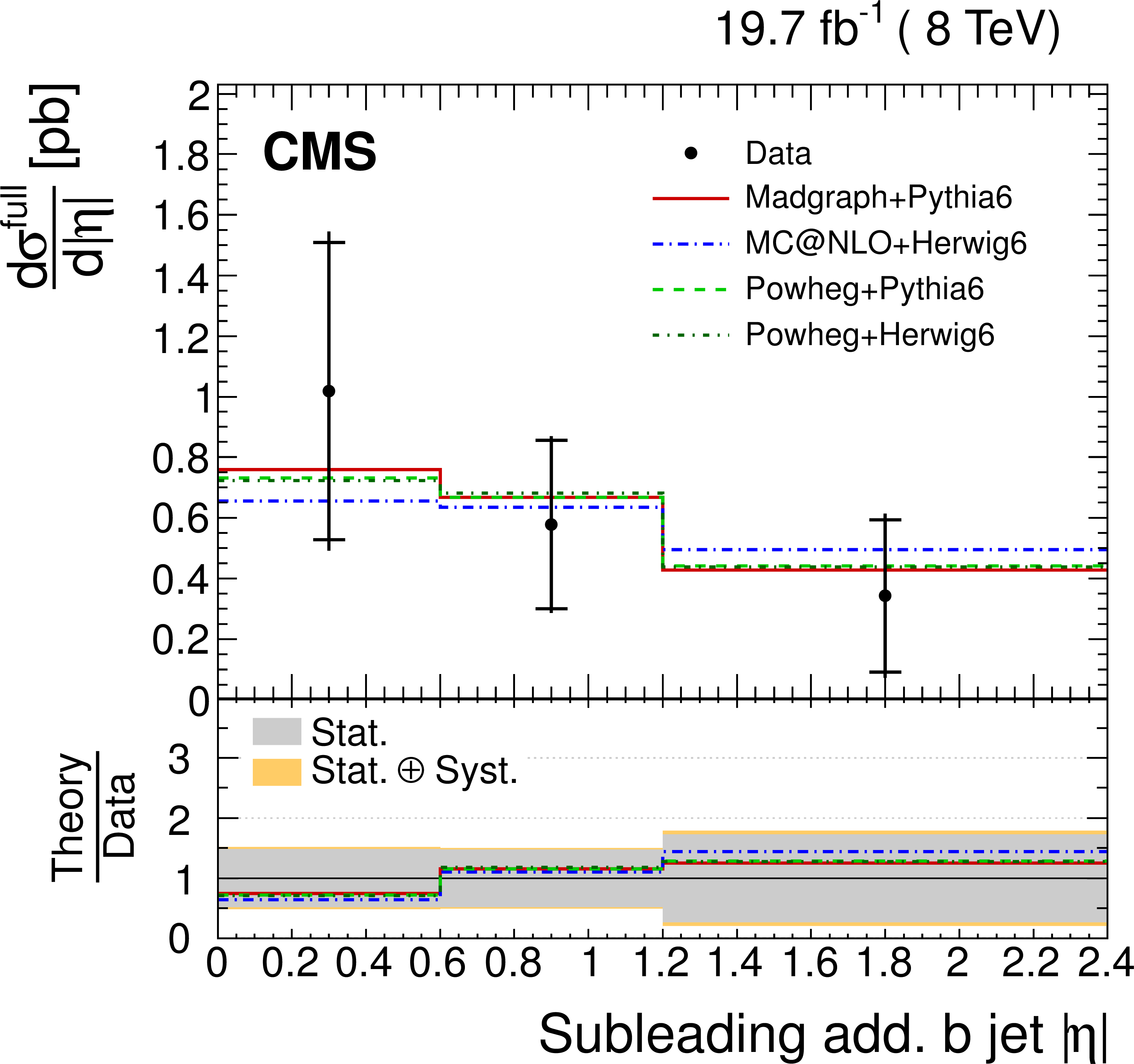
Figure 15-d:
Absolute differential $ {\mathrm {t}\overline {\mathrm {t}}} $ cross section measured in the visible phase space of the $ {\mathrm {t}\overline {\mathrm {t}}} $ system and the additional b jets, as a function of the leading additional b jet $ {p_{\mathrm {T}}} $ (a) and $ {|\eta |} $ (b), subleading additional b jet $ {p_{\mathrm {T}}} $ (c) and $ {|\eta |} $ (d), the angular separation $\Delta R_{ {\mathrm {b}} {\mathrm {b}} }$ between the two leading additional b jets (e), and the invariant mass $ {m_{ {\mathrm {b}} {\mathrm {b}} }} $ of the two b jets. Data are compared with predictions from MADGRAPH interfaced with PYTHIA-6, MC@NLO interfaced with HERWIG-6, and POWHEG with PYTHIA-6 and HERWIG-6, normalized to the measured inclusive cross section. The inner (outer) vertical bars indicate the statistical (total) uncertainties. The lower part of each plot shows the ratio of the predictions to the data. |
png pdf |
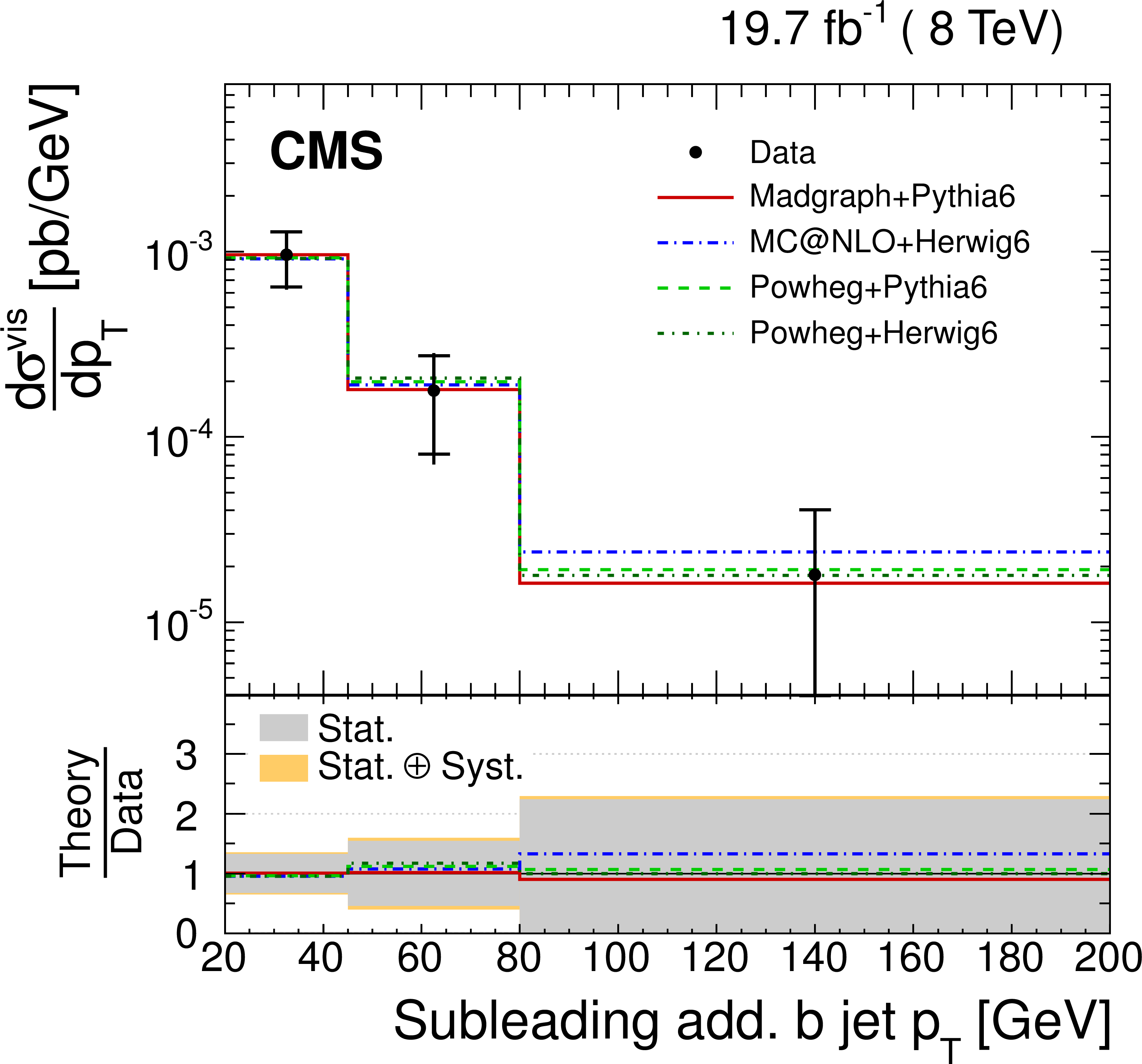
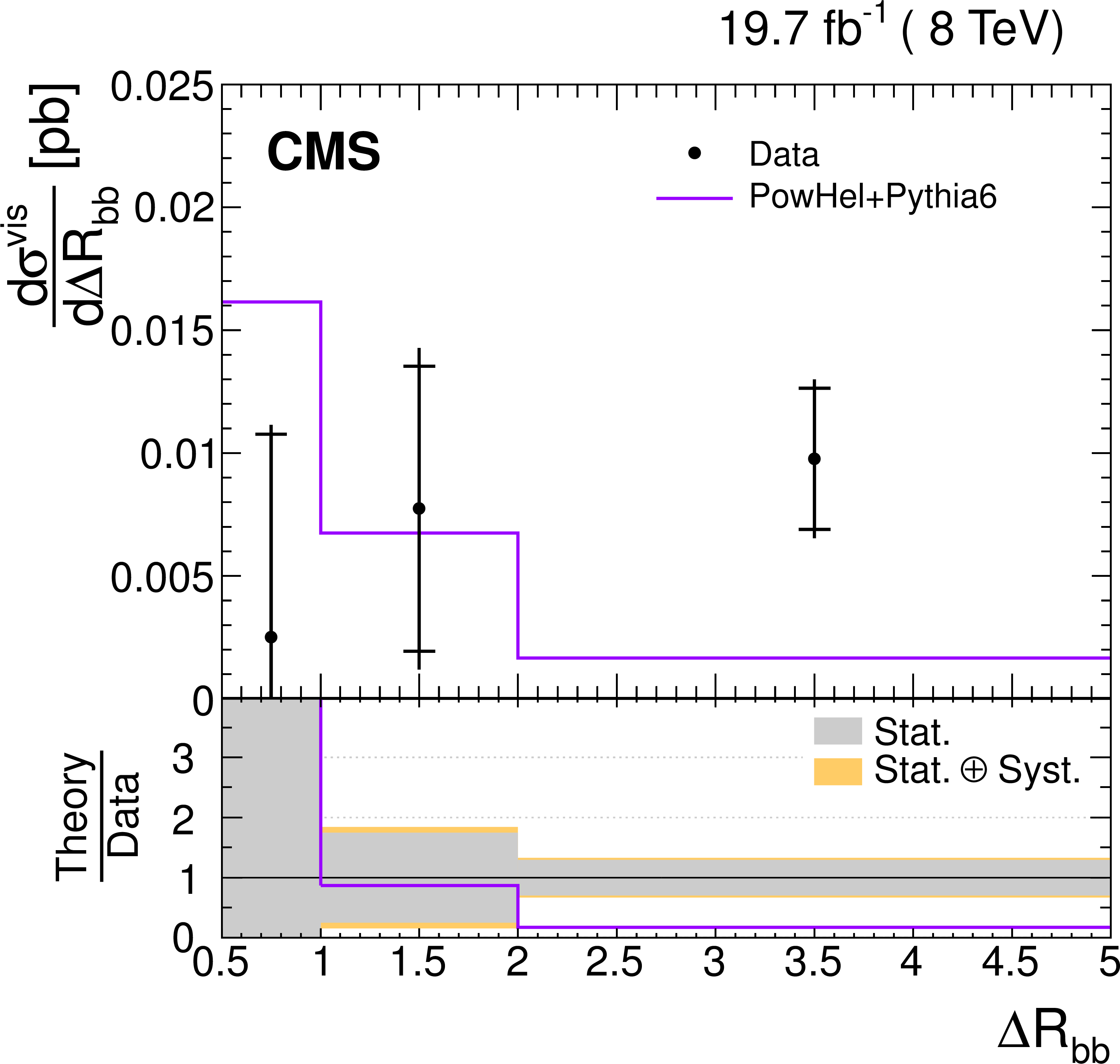
Figure 15-e:
Absolute differential $ {\mathrm {t}\overline {\mathrm {t}}} $ cross section measured in the visible phase space of the $ {\mathrm {t}\overline {\mathrm {t}}} $ system and the additional b jets, as a function of the leading additional b jet $ {p_{\mathrm {T}}} $ (a) and $ {|\eta |} $ (b), subleading additional b jet $ {p_{\mathrm {T}}} $ (c) and $ {|\eta |} $ (d), the angular separation $\Delta R_{ {\mathrm {b}} {\mathrm {b}} }$ between the two leading additional b jets (e), and the invariant mass $ {m_{ {\mathrm {b}} {\mathrm {b}} }} $ of the two b jets. Data are compared with predictions from MADGRAPH interfaced with PYTHIA-6, MC@NLO interfaced with HERWIG-6, and POWHEG with PYTHIA-6 and HERWIG-6, normalized to the measured inclusive cross section. The inner (outer) vertical bars indicate the statistical (total) uncertainties. The lower part of each plot shows the ratio of the predictions to the data. |

png pdf |
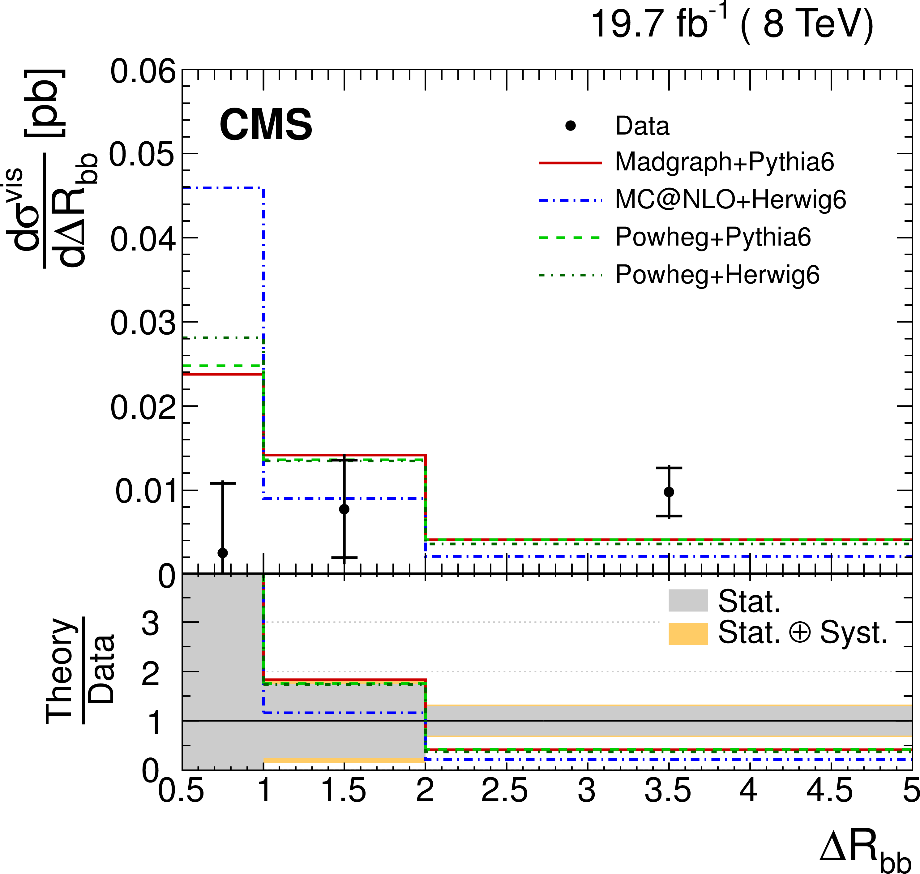
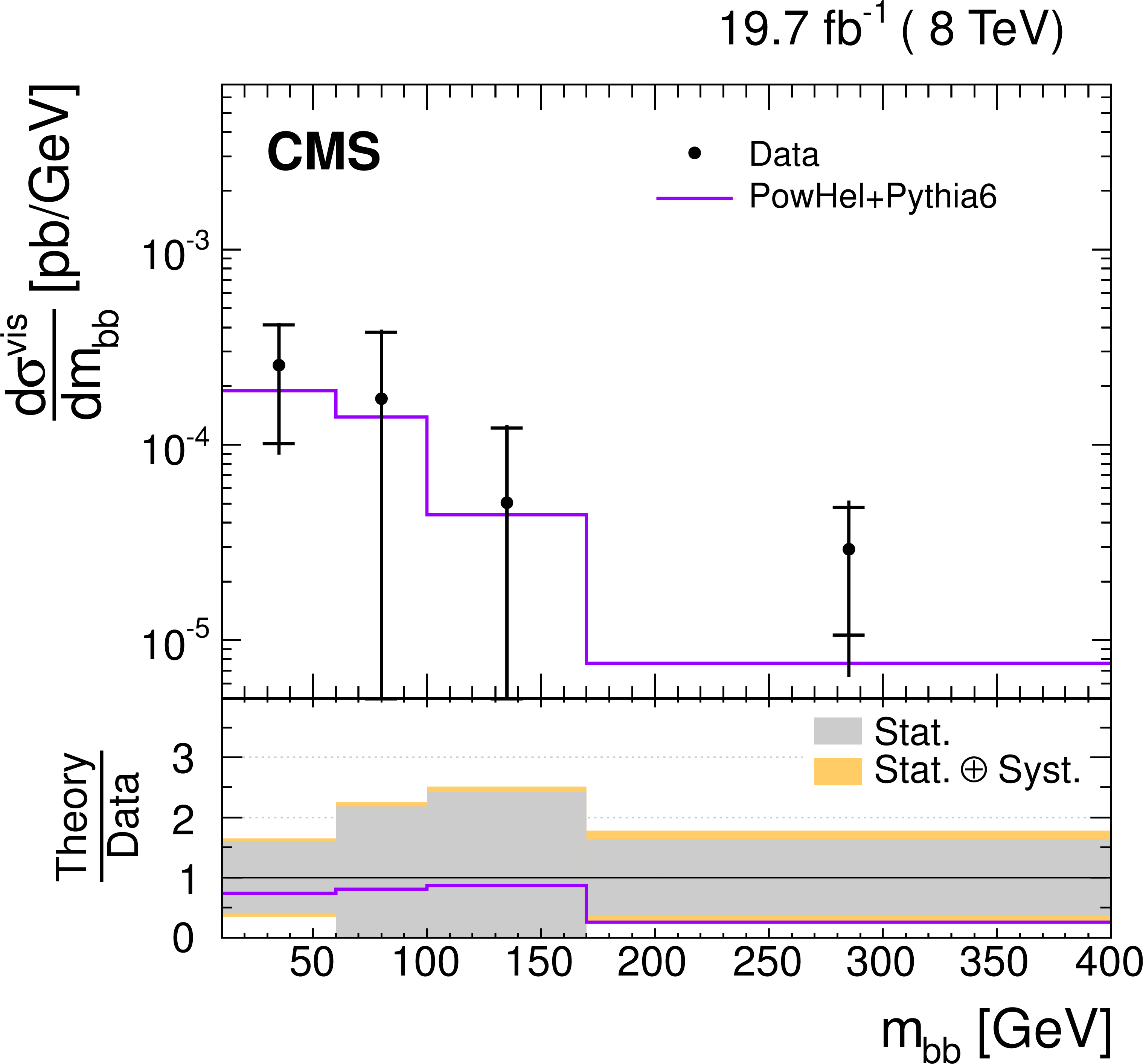
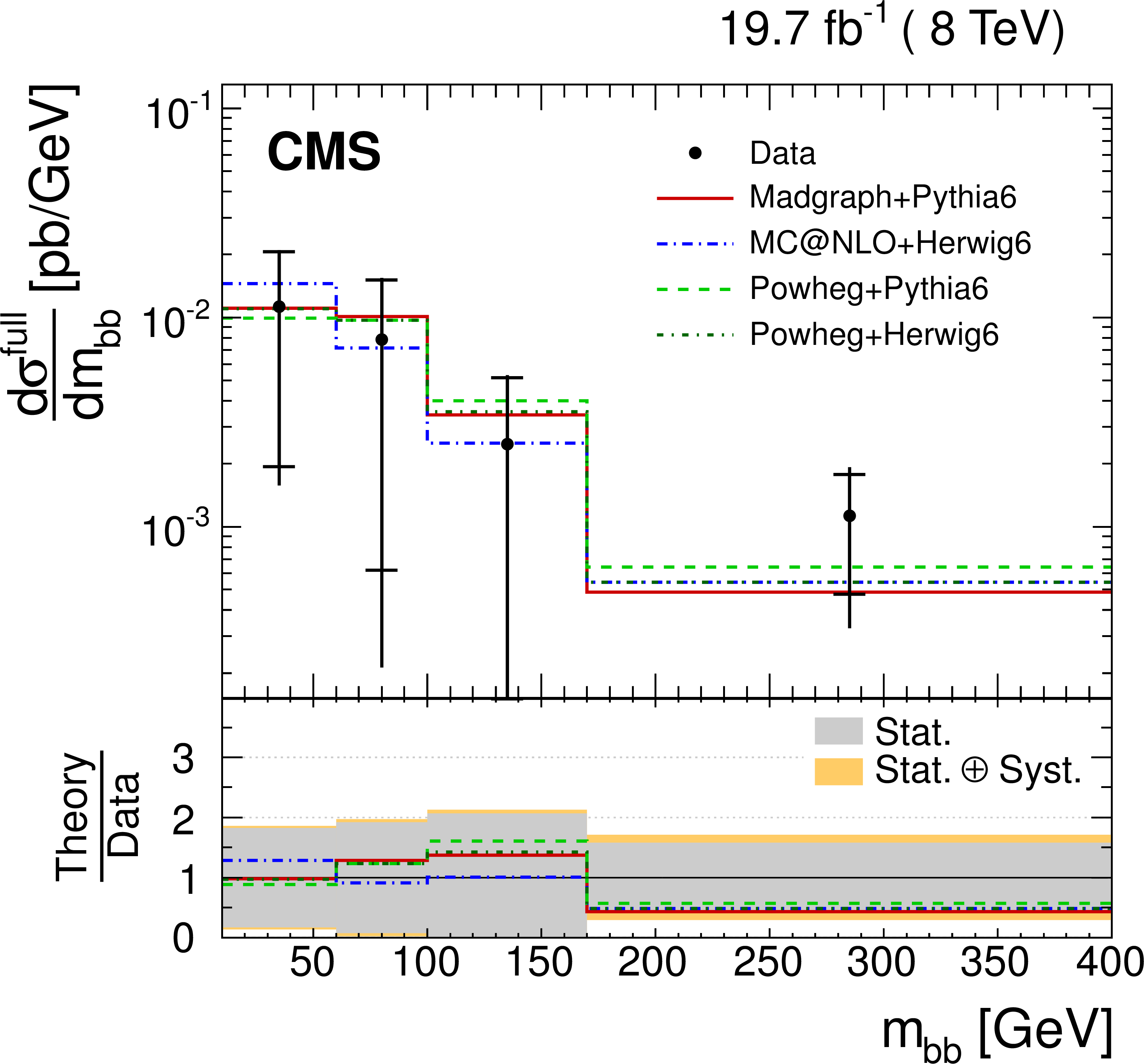
Figure 15-f:
Absolute differential $ {\mathrm {t}\overline {\mathrm {t}}} $ cross section measured in the visible phase space of the $ {\mathrm {t}\overline {\mathrm {t}}} $ system and the additional b jets, as a function of the leading additional b jet $ {p_{\mathrm {T}}} $ (a) and $ {|\eta |} $ (b), subleading additional b jet $ {p_{\mathrm {T}}} $ (c) and $ {|\eta |} $ (d), the angular separation $\Delta R_{ {\mathrm {b}} {\mathrm {b}} }$ between the two leading additional b jets (e), and the invariant mass $ {m_{ {\mathrm {b}} {\mathrm {b}} }} $ of the two b jets. Data are compared with predictions from MADGRAPH interfaced with PYTHIA-6, MC@NLO interfaced with HERWIG-6, and POWHEG with PYTHIA-6 and HERWIG-6, normalized to the measured inclusive cross section. The inner (outer) vertical bars indicate the statistical (total) uncertainties. The lower part of each plot shows the ratio of the predictions to the data. |

png pdf |
Figure 16-a:
Absolute differential $ {\mathrm {t}\overline {\mathrm {t}}} $ cross section measured in the visible phase space of the $ {\mathrm {t}\overline {\mathrm {t}}} $ system and the additional b jets, as a function of the second additional b jet $ {p_{\mathrm {T}}} $ (a) and $ {|\eta |} $ (b), the angular separation $\Delta R_{ {\mathrm {b}} {\mathrm {b}} }$ between the two leading additional b jets (c), and the invariant mass $ {m_{ {\mathrm {b}} {\mathrm {b}} }} $ of the two b jets (d). Data are compared with predictions from PowHel+PYTHIA-6. The inner (outer) vertical bars indicate the statistical (total) uncertainties. The lower part of each plot shows the ratio of the calculation to data. |
png pdf |
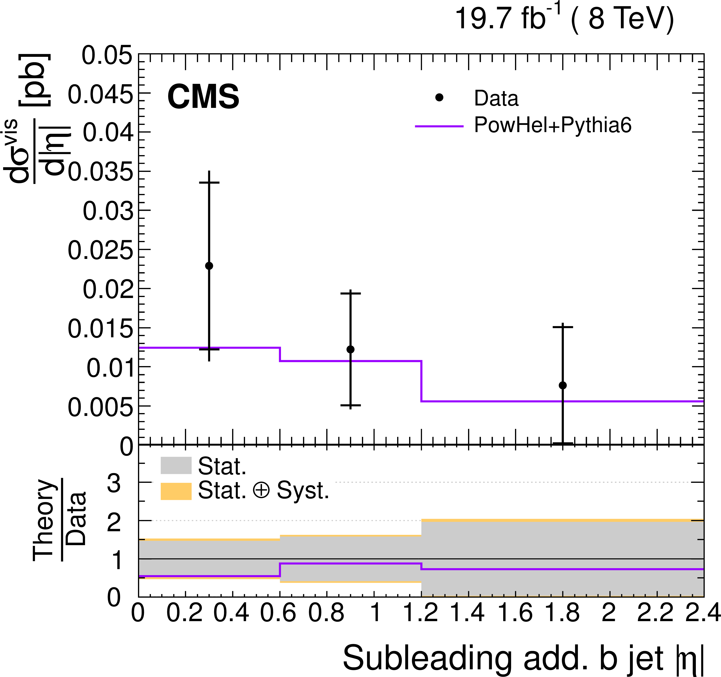
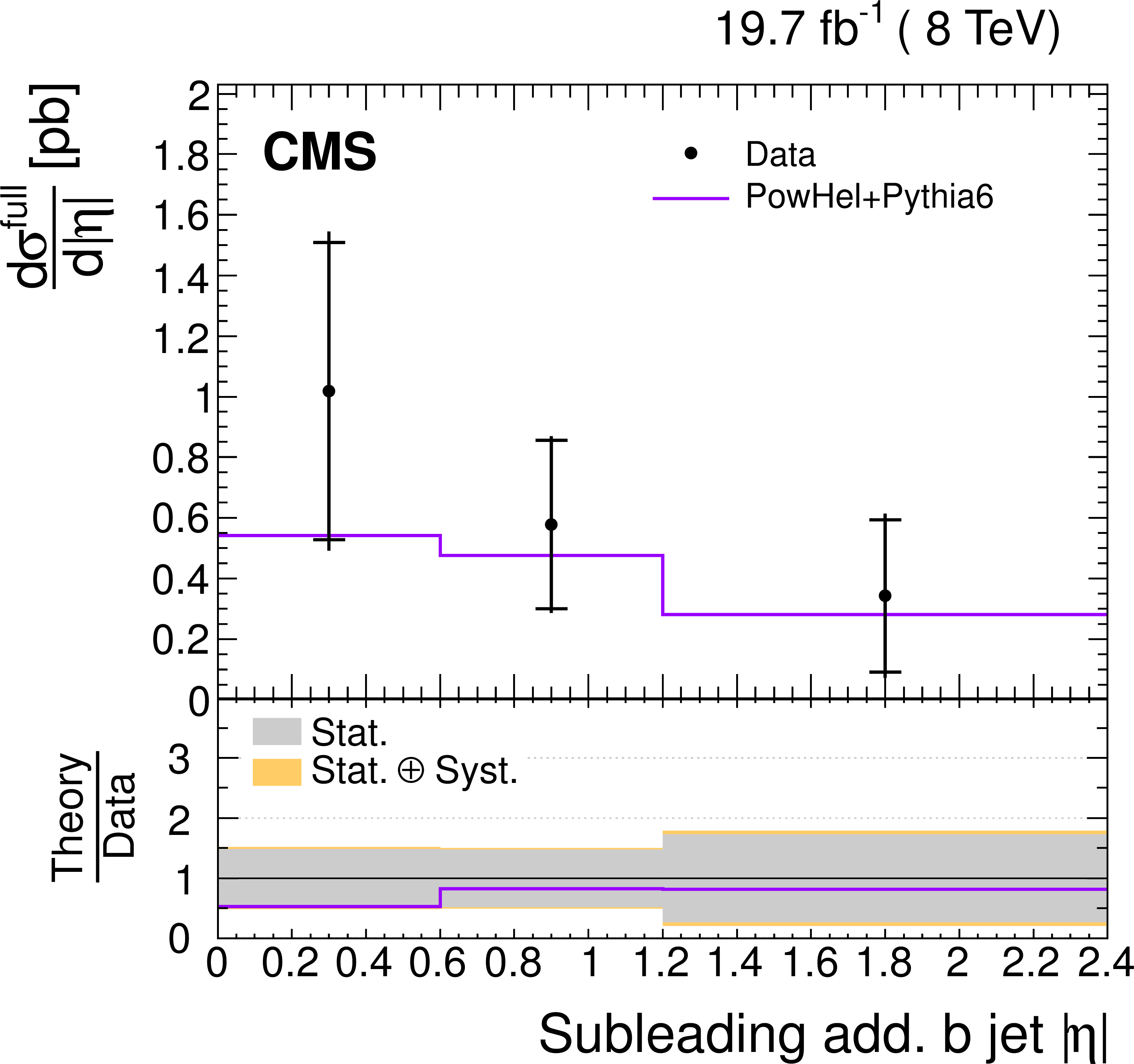
Figure 16-b:
Absolute differential $ {\mathrm {t}\overline {\mathrm {t}}} $ cross section measured in the visible phase space of the $ {\mathrm {t}\overline {\mathrm {t}}} $ system and the additional b jets, as a function of the second additional b jet $ {p_{\mathrm {T}}} $ (a) and $ {|\eta |} $ (b), the angular separation $\Delta R_{ {\mathrm {b}} {\mathrm {b}} }$ between the two leading additional b jets (c), and the invariant mass $ {m_{ {\mathrm {b}} {\mathrm {b}} }} $ of the two b jets (d). Data are compared with predictions from PowHel+PYTHIA-6. The inner (outer) vertical bars indicate the statistical (total) uncertainties. The lower part of each plot shows the ratio of the calculation to data. |
png pdf |
Figure 16-c:
Absolute differential $ {\mathrm {t}\overline {\mathrm {t}}} $ cross section measured in the visible phase space of the $ {\mathrm {t}\overline {\mathrm {t}}} $ system and the additional b jets, as a function of the second additional b jet $ {p_{\mathrm {T}}} $ (a) and $ {|\eta |} $ (b), the angular separation $\Delta R_{ {\mathrm {b}} {\mathrm {b}} }$ between the two leading additional b jets (c), and the invariant mass $ {m_{ {\mathrm {b}} {\mathrm {b}} }} $ of the two b jets (d). Data are compared with predictions from PowHel+PYTHIA-6. The inner (outer) vertical bars indicate the statistical (total) uncertainties. The lower part of each plot shows the ratio of the calculation to data. |
png pdf |
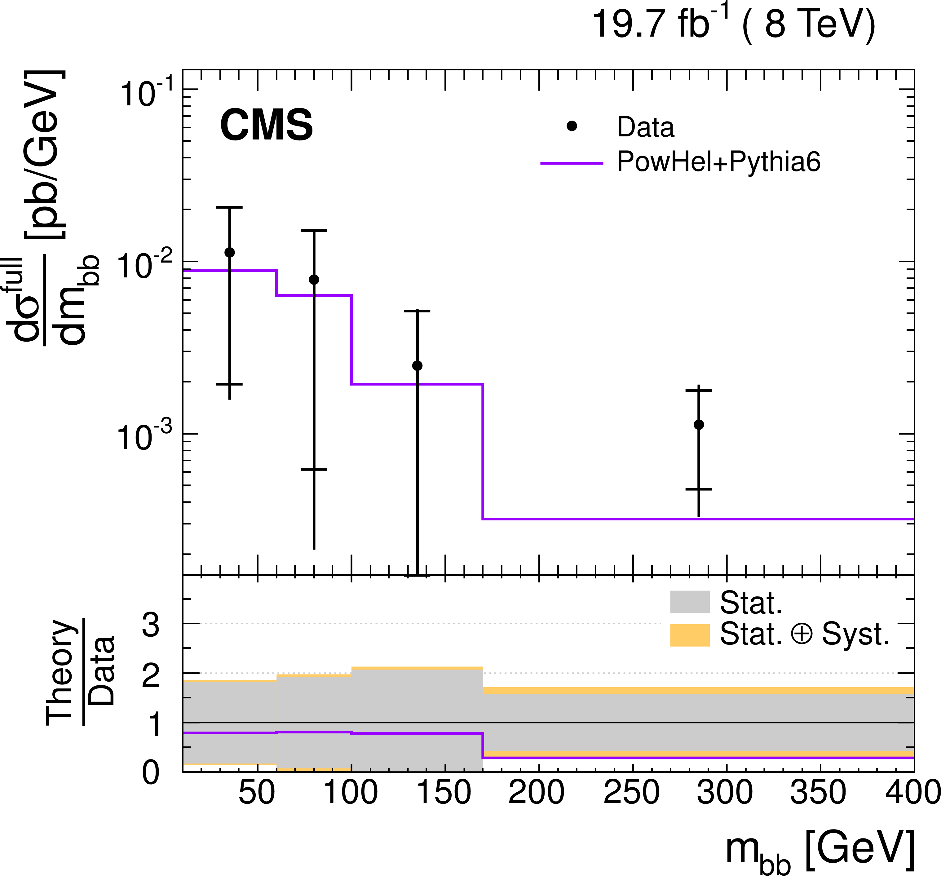
Figure 16-d:
Absolute differential $ {\mathrm {t}\overline {\mathrm {t}}} $ cross section measured in the visible phase space of the $ {\mathrm {t}\overline {\mathrm {t}}} $ system and the additional b jets, as a function of the second additional b jet $ {p_{\mathrm {T}}} $ (a) and $ {|\eta |} $ (b), the angular separation $\Delta R_{ {\mathrm {b}} {\mathrm {b}} }$ between the two leading additional b jets (c), and the invariant mass $ {m_{ {\mathrm {b}} {\mathrm {b}} }} $ of the two b jets (d). Data are compared with predictions from PowHel+PYTHIA-6. The inner (outer) vertical bars indicate the statistical (total) uncertainties. The lower part of each plot shows the ratio of the calculation to data. |
png pdf |
Figure 17-a:
Absolute differential $ {\mathrm {t}\overline {\mathrm {t}}} $ cross section measured in the full phase space of the $ {\mathrm {t}\overline {\mathrm {t}}} $ system, corrected for acceptance and branching fractions, and the visible phase space of the additional b jets, as a function of the leading additional b jet $ {p_{\mathrm {T}}} $ (a) and $ {|\eta |} $ (b), subleading additional b jet $ {p_{\mathrm {T}}} $ (c) and $ {|\eta |} $ (d), the angular separation $\Delta R_{ {\mathrm {b}} {\mathrm {b}} }$ between the leading and subleading additional b jets (e), and the invariant mass $ {m_{ {\mathrm {b}} {\mathrm {b}} }} $ of the two b jets (f). Data are compared with predictions from MADGRAPH interfaced with PYTHIA-6, MC@NLO interfaced with HERWIG-6, and POWHEG intefarced with both PYTHIA-6 and HERWIG-6, normalized to the measured inclusive cross section. The inner (outer) vertical bars indicate the statistical (total) uncertainties. The lower part of each plot shows the ratio of the predictions to the data. |
png pdf |
Figure 17-b:
Absolute differential $ {\mathrm {t}\overline {\mathrm {t}}} $ cross section measured in the full phase space of the $ {\mathrm {t}\overline {\mathrm {t}}} $ system, corrected for acceptance and branching fractions, and the visible phase space of the additional b jets, as a function of the leading additional b jet $ {p_{\mathrm {T}}} $ (a) and $ {|\eta |} $ (b), subleading additional b jet $ {p_{\mathrm {T}}} $ (c) and $ {|\eta |} $ (d), the angular separation $\Delta R_{ {\mathrm {b}} {\mathrm {b}} }$ between the leading and subleading additional b jets (e), and the invariant mass $ {m_{ {\mathrm {b}} {\mathrm {b}} }} $ of the two b jets (f). Data are compared with predictions from MADGRAPH interfaced with PYTHIA-6, MC@NLO interfaced with HERWIG-6, and POWHEG intefarced with both PYTHIA-6 and HERWIG-6, normalized to the measured inclusive cross section. The inner (outer) vertical bars indicate the statistical (total) uncertainties. The lower part of each plot shows the ratio of the predictions to the data. |

png pdf |
Figure 17-c:
Absolute differential $ {\mathrm {t}\overline {\mathrm {t}}} $ cross section measured in the full phase space of the $ {\mathrm {t}\overline {\mathrm {t}}} $ system, corrected for acceptance and branching fractions, and the visible phase space of the additional b jets, as a function of the leading additional b jet $ {p_{\mathrm {T}}} $ (a) and $ {|\eta |} $ (b), subleading additional b jet $ {p_{\mathrm {T}}} $ (c) and $ {|\eta |} $ (d), the angular separation $\Delta R_{ {\mathrm {b}} {\mathrm {b}} }$ between the leading and subleading additional b jets (e), and the invariant mass $ {m_{ {\mathrm {b}} {\mathrm {b}} }} $ of the two b jets (f). Data are compared with predictions from MADGRAPH interfaced with PYTHIA-6, MC@NLO interfaced with HERWIG-6, and POWHEG intefarced with both PYTHIA-6 and HERWIG-6, normalized to the measured inclusive cross section. The inner (outer) vertical bars indicate the statistical (total) uncertainties. The lower part of each plot shows the ratio of the predictions to the data. |
png pdf |
Figure 17-d:
Absolute differential $ {\mathrm {t}\overline {\mathrm {t}}} $ cross section measured in the full phase space of the $ {\mathrm {t}\overline {\mathrm {t}}} $ system, corrected for acceptance and branching fractions, and the visible phase space of the additional b jets, as a function of the leading additional b jet $ {p_{\mathrm {T}}} $ (a) and $ {|\eta |} $ (b), subleading additional b jet $ {p_{\mathrm {T}}} $ (c) and $ {|\eta |} $ (d), the angular separation $\Delta R_{ {\mathrm {b}} {\mathrm {b}} }$ between the leading and subleading additional b jets (e), and the invariant mass $ {m_{ {\mathrm {b}} {\mathrm {b}} }} $ of the two b jets (f). Data are compared with predictions from MADGRAPH interfaced with PYTHIA-6, MC@NLO interfaced with HERWIG-6, and POWHEG intefarced with both PYTHIA-6 and HERWIG-6, normalized to the measured inclusive cross section. The inner (outer) vertical bars indicate the statistical (total) uncertainties. The lower part of each plot shows the ratio of the predictions to the data. |

png pdf |
Figure 17-e:
Absolute differential $ {\mathrm {t}\overline {\mathrm {t}}} $ cross section measured in the full phase space of the $ {\mathrm {t}\overline {\mathrm {t}}} $ system, corrected for acceptance and branching fractions, and the visible phase space of the additional b jets, as a function of the leading additional b jet $ {p_{\mathrm {T}}} $ (a) and $ {|\eta |} $ (b), subleading additional b jet $ {p_{\mathrm {T}}} $ (c) and $ {|\eta |} $ (d), the angular separation $\Delta R_{ {\mathrm {b}} {\mathrm {b}} }$ between the leading and subleading additional b jets (e), and the invariant mass $ {m_{ {\mathrm {b}} {\mathrm {b}} }} $ of the two b jets (f). Data are compared with predictions from MADGRAPH interfaced with PYTHIA-6, MC@NLO interfaced with HERWIG-6, and POWHEG intefarced with both PYTHIA-6 and HERWIG-6, normalized to the measured inclusive cross section. The inner (outer) vertical bars indicate the statistical (total) uncertainties. The lower part of each plot shows the ratio of the predictions to the data. |
png pdf |
Figure 17-f:
Absolute differential $ {\mathrm {t}\overline {\mathrm {t}}} $ cross section measured in the full phase space of the $ {\mathrm {t}\overline {\mathrm {t}}} $ system, corrected for acceptance and branching fractions, and the visible phase space of the additional b jets, as a function of the leading additional b jet $ {p_{\mathrm {T}}} $ (a) and $ {|\eta |} $ (b), subleading additional b jet $ {p_{\mathrm {T}}} $ (c) and $ {|\eta |} $ (d), the angular separation $\Delta R_{ {\mathrm {b}} {\mathrm {b}} }$ between the leading and subleading additional b jets (e), and the invariant mass $ {m_{ {\mathrm {b}} {\mathrm {b}} }} $ of the two b jets (f). Data are compared with predictions from MADGRAPH interfaced with PYTHIA-6, MC@NLO interfaced with HERWIG-6, and POWHEG intefarced with both PYTHIA-6 and HERWIG-6, normalized to the measured inclusive cross section. The inner (outer) vertical bars indicate the statistical (total) uncertainties. The lower part of each plot shows the ratio of the predictions to the data. |

png pdf |
Figure 18-a:
Absolute differential $ {\mathrm {t}\overline {\mathrm {t}}} $ cross section measured in the full phase space of the $ {\mathrm {t}\overline {\mathrm {t}}} $ system, corrected for acceptance and branching fractions, and the additional b jets, as a function of the second additional b jet $ {p_{\mathrm {T}}} $ (a) and $ {|\eta |} $ (b), the angular separation $\Delta R_{ {\mathrm {b}} {\mathrm {b}} }$ between the leading and subleading additional b jets (c), and the invariant mass $ {m_{ {\mathrm {b}} {\mathrm {b}} }} $ of the two b jets (d). Data are compared with predictions from PowHel+PYTHIA-6. The inner (outer) vertical bars indicate the statistical (total) uncertainties. The lower part of each plot shows the ratio of the calculation to data. |
png pdf |
Figure 18-b:
Absolute differential $ {\mathrm {t}\overline {\mathrm {t}}} $ cross section measured in the full phase space of the $ {\mathrm {t}\overline {\mathrm {t}}} $ system, corrected for acceptance and branching fractions, and the additional b jets, as a function of the second additional b jet $ {p_{\mathrm {T}}} $ (a) and $ {|\eta |} $ (b), the angular separation $\Delta R_{ {\mathrm {b}} {\mathrm {b}} }$ between the leading and subleading additional b jets (c), and the invariant mass $ {m_{ {\mathrm {b}} {\mathrm {b}} }} $ of the two b jets (d). Data are compared with predictions from PowHel+PYTHIA-6. The inner (outer) vertical bars indicate the statistical (total) uncertainties. The lower part of each plot shows the ratio of the calculation to data. |

png pdf |
Figure 18-c:
Absolute differential $ {\mathrm {t}\overline {\mathrm {t}}} $ cross section measured in the full phase space of the $ {\mathrm {t}\overline {\mathrm {t}}} $ system, corrected for acceptance and branching fractions, and the additional b jets, as a function of the second additional b jet $ {p_{\mathrm {T}}} $ (a) and $ {|\eta |} $ (b), the angular separation $\Delta R_{ {\mathrm {b}} {\mathrm {b}} }$ between the leading and subleading additional b jets (c), and the invariant mass $ {m_{ {\mathrm {b}} {\mathrm {b}} }} $ of the two b jets (d). Data are compared with predictions from PowHel+PYTHIA-6. The inner (outer) vertical bars indicate the statistical (total) uncertainties. The lower part of each plot shows the ratio of the calculation to data. |
png pdf |
Figure 18-d:
Absolute differential $ {\mathrm {t}\overline {\mathrm {t}}} $ cross section measured in the full phase space of the $ {\mathrm {t}\overline {\mathrm {t}}} $ system, corrected for acceptance and branching fractions, and the additional b jets, as a function of the second additional b jet $ {p_{\mathrm {T}}} $ (a) and $ {|\eta |} $ (b), the angular separation $\Delta R_{ {\mathrm {b}} {\mathrm {b}} }$ between the leading and subleading additional b jets (c), and the invariant mass $ {m_{ {\mathrm {b}} {\mathrm {b}} }} $ of the two b jets (d). Data are compared with predictions from PowHel+PYTHIA-6. The inner (outer) vertical bars indicate the statistical (total) uncertainties. The lower part of each plot shows the ratio of the calculation to data. |

png pdf |
Figure 19-a:
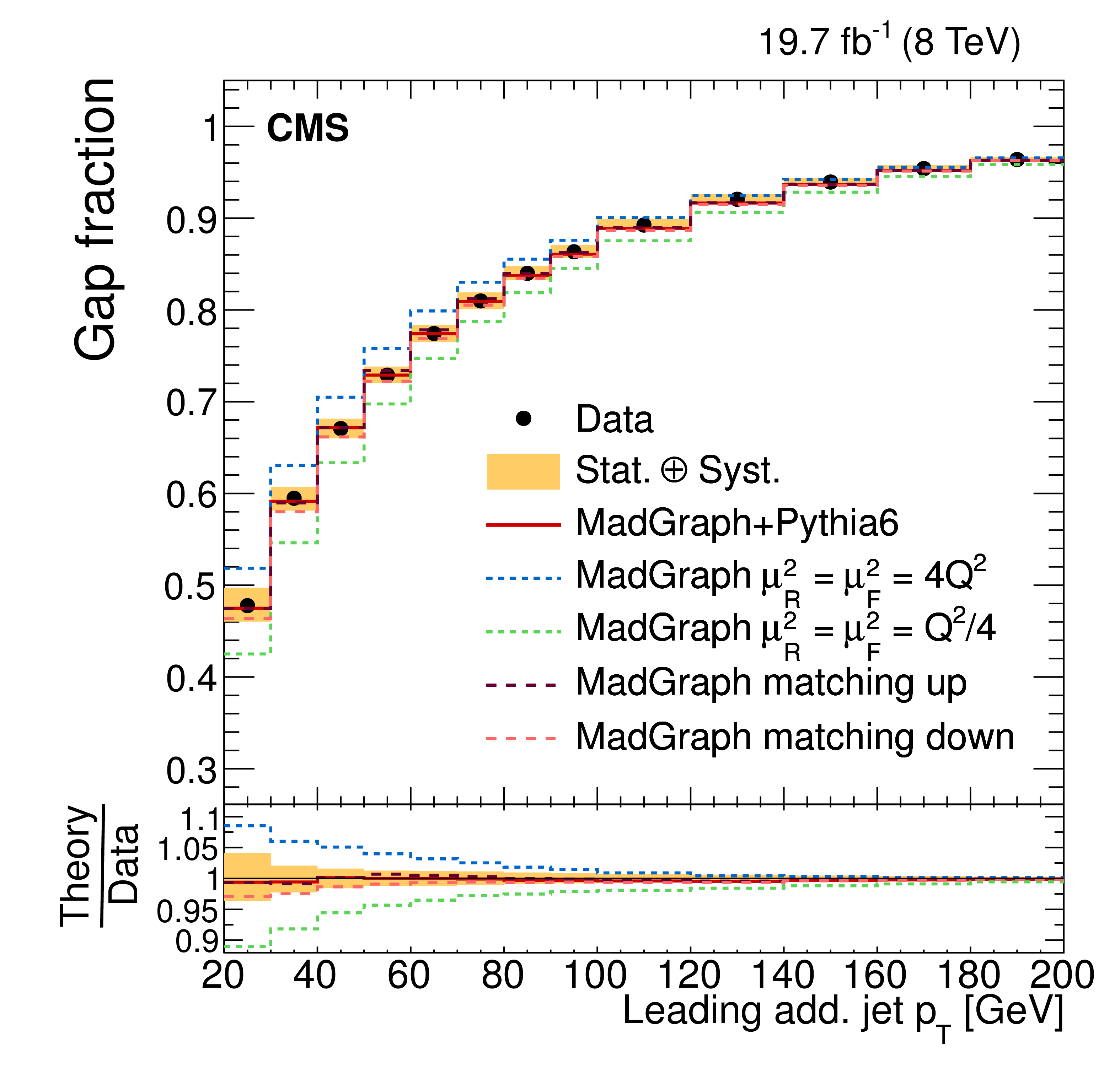
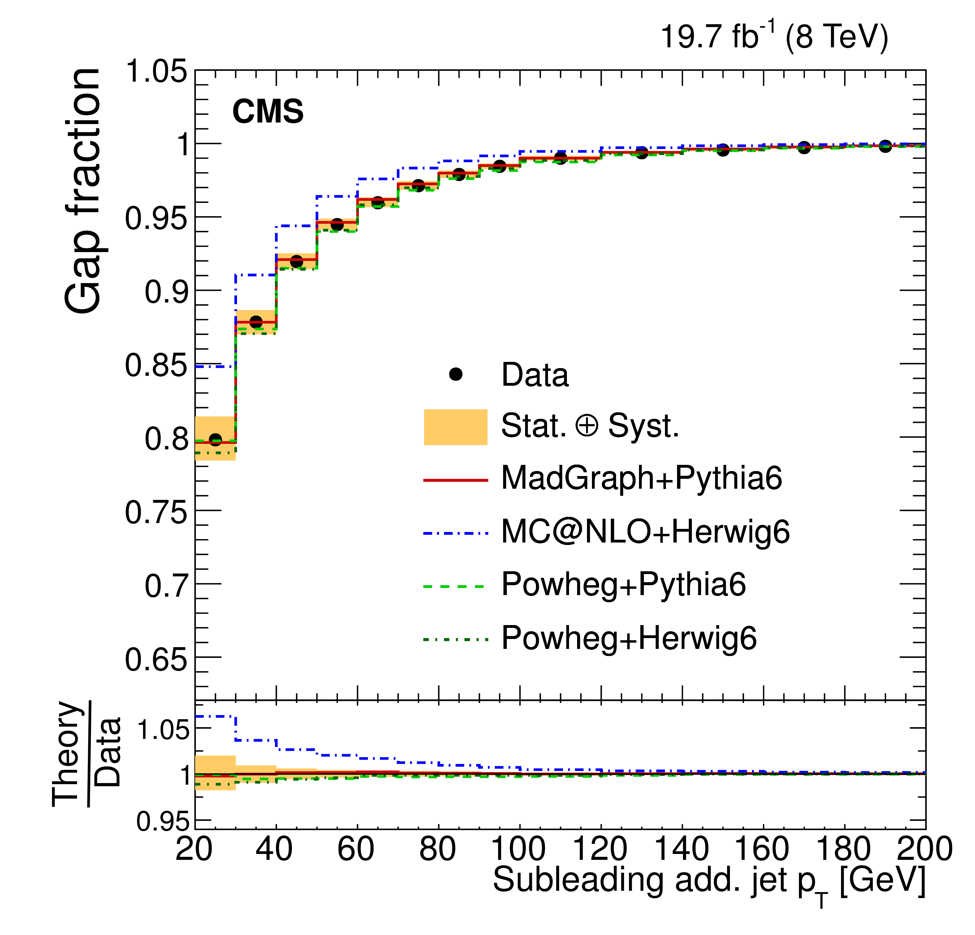
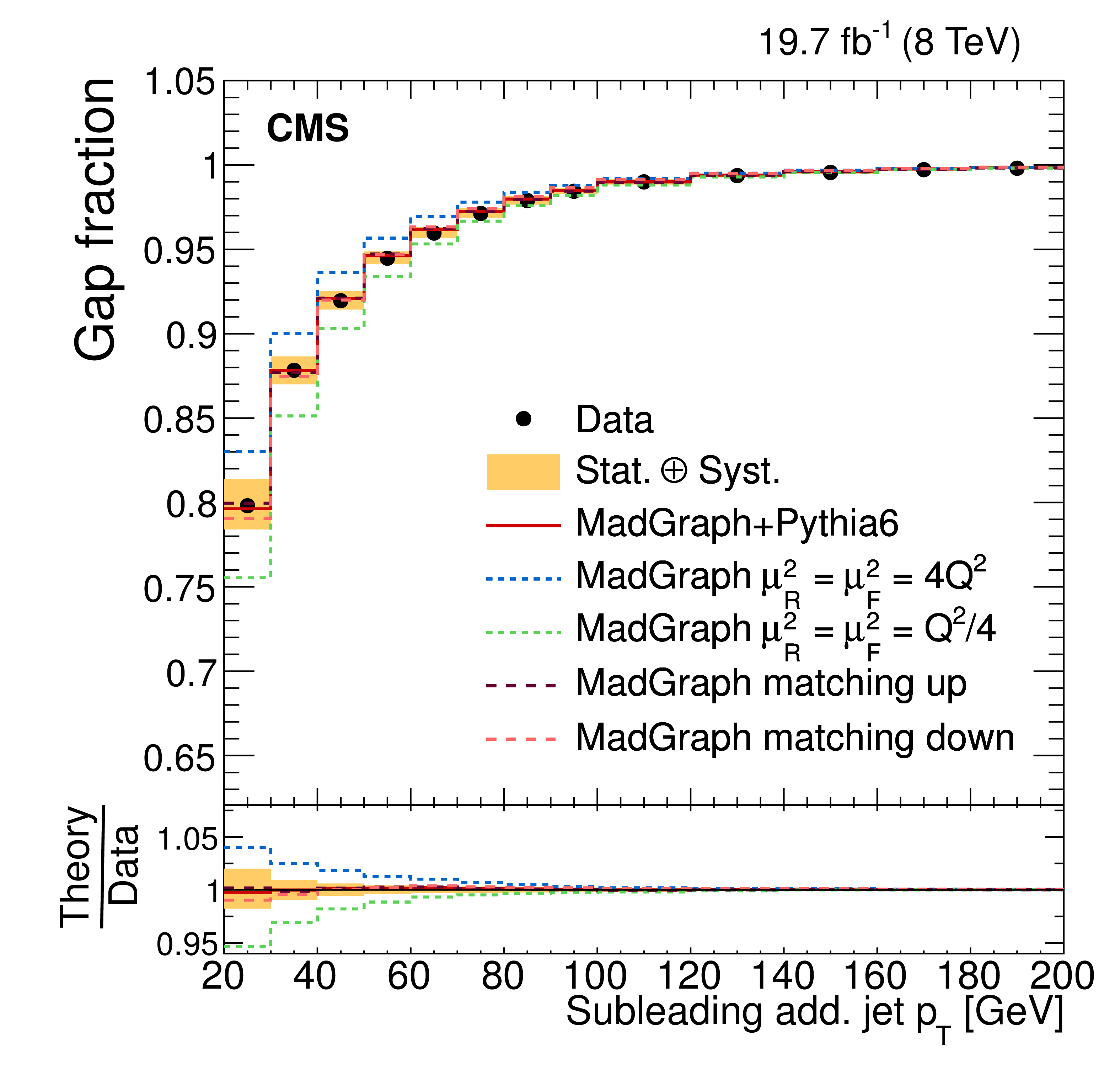
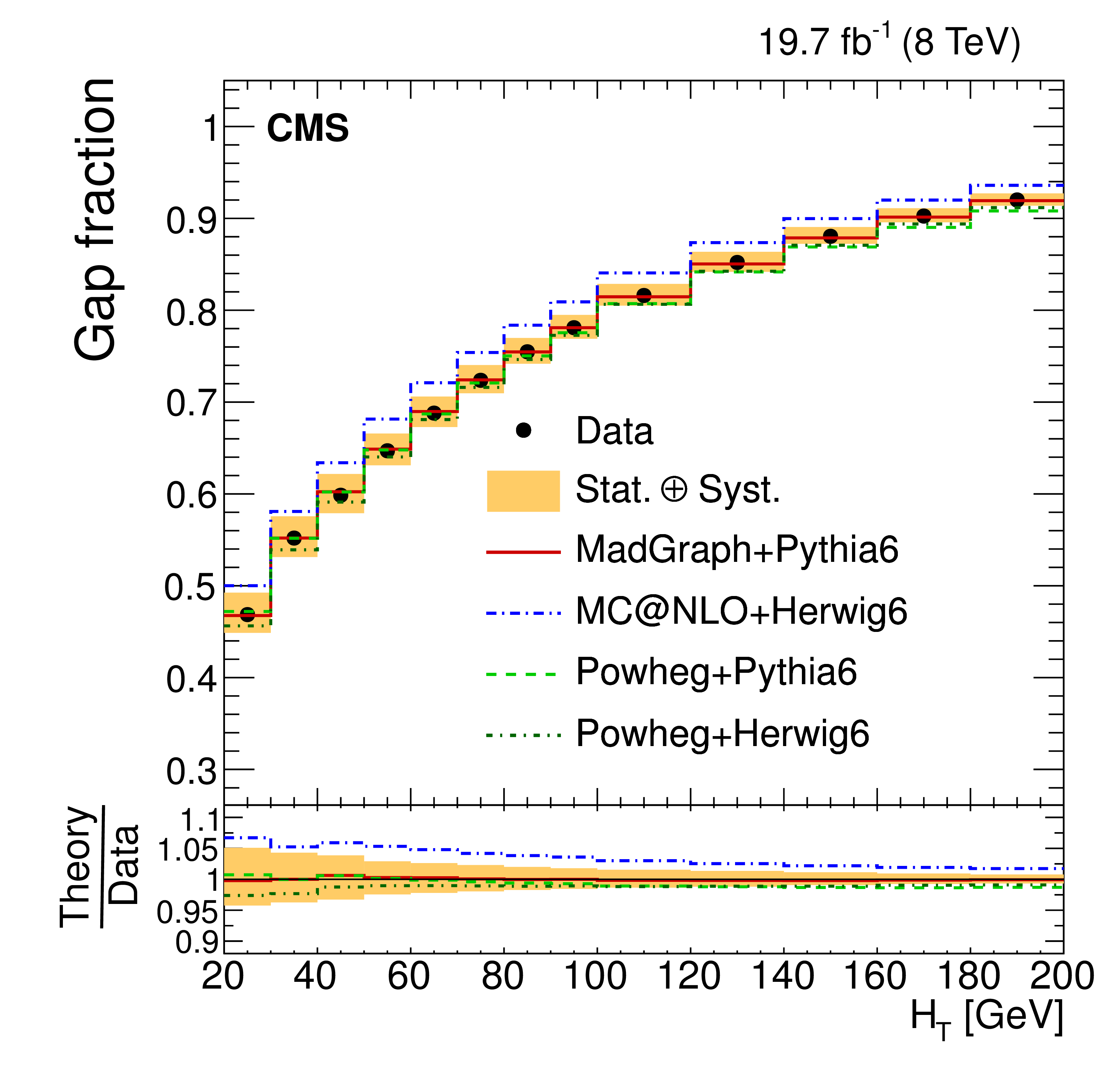
Measured gap fraction as a function of the leading additional jet $ {p_{\mathrm {T}}} $ (a,b), subleading additional jet $ {p_{\mathrm {T}}} $ (c,d), and of $H_{\rm T}$ (e,f). Data are compared to predictions from MADGRAPH , POWHEG interfaced with PYTHIA andHERWIG , and MC@NLO interfaced withHERWIG (a,c,e), and to MADGRAPH with varied renormalization, factorization, and jet-parton matching scales (b,d,f). For each bin the threshold is defined at the value where the data point is placed. The vertical bars on the data points indicate the statistical uncertainty. The shaded band corresponds to the statistical and the total systematic uncertainty added in quadrature. The lower part of each plot shows the ratio of the predictions to the data. |
png pdf |
Figure 19-b:
Measured gap fraction as a function of the leading additional jet $ {p_{\mathrm {T}}} $ (a,b), subleading additional jet $ {p_{\mathrm {T}}} $ (c,d), and of $H_{\rm T}$ (e,f). Data are compared to predictions from MADGRAPH , POWHEG interfaced with PYTHIA andHERWIG , and MC@NLO interfaced withHERWIG (a,c,e), and to MADGRAPH with varied renormalization, factorization, and jet-parton matching scales (b,d,f). For each bin the threshold is defined at the value where the data point is placed. The vertical bars on the data points indicate the statistical uncertainty. The shaded band corresponds to the statistical and the total systematic uncertainty added in quadrature. The lower part of each plot shows the ratio of the predictions to the data. |
png pdf |
Figure 19-c:
Measured gap fraction as a function of the leading additional jet $ {p_{\mathrm {T}}} $ (a,b), subleading additional jet $ {p_{\mathrm {T}}} $ (c,d), and of $H_{\rm T}$ (e,f). Data are compared to predictions from MADGRAPH , POWHEG interfaced with PYTHIA andHERWIG , and MC@NLO interfaced withHERWIG (a,c,e), and to MADGRAPH with varied renormalization, factorization, and jet-parton matching scales (b,d,f). For each bin the threshold is defined at the value where the data point is placed. The vertical bars on the data points indicate the statistical uncertainty. The shaded band corresponds to the statistical and the total systematic uncertainty added in quadrature. The lower part of each plot shows the ratio of the predictions to the data. |
png pdf |
Figure 19-d:
Measured gap fraction as a function of the leading additional jet $ {p_{\mathrm {T}}} $ (a,b), subleading additional jet $ {p_{\mathrm {T}}} $ (c,d), and of $H_{\rm T}$ (e,f). Data are compared to predictions from MADGRAPH , POWHEG interfaced with PYTHIA andHERWIG , and MC@NLO interfaced withHERWIG (a,c,e), and to MADGRAPH with varied renormalization, factorization, and jet-parton matching scales (b,d,f). For each bin the threshold is defined at the value where the data point is placed. The vertical bars on the data points indicate the statistical uncertainty. The shaded band corresponds to the statistical and the total systematic uncertainty added in quadrature. The lower part of each plot shows the ratio of the predictions to the data. |
png pdf |
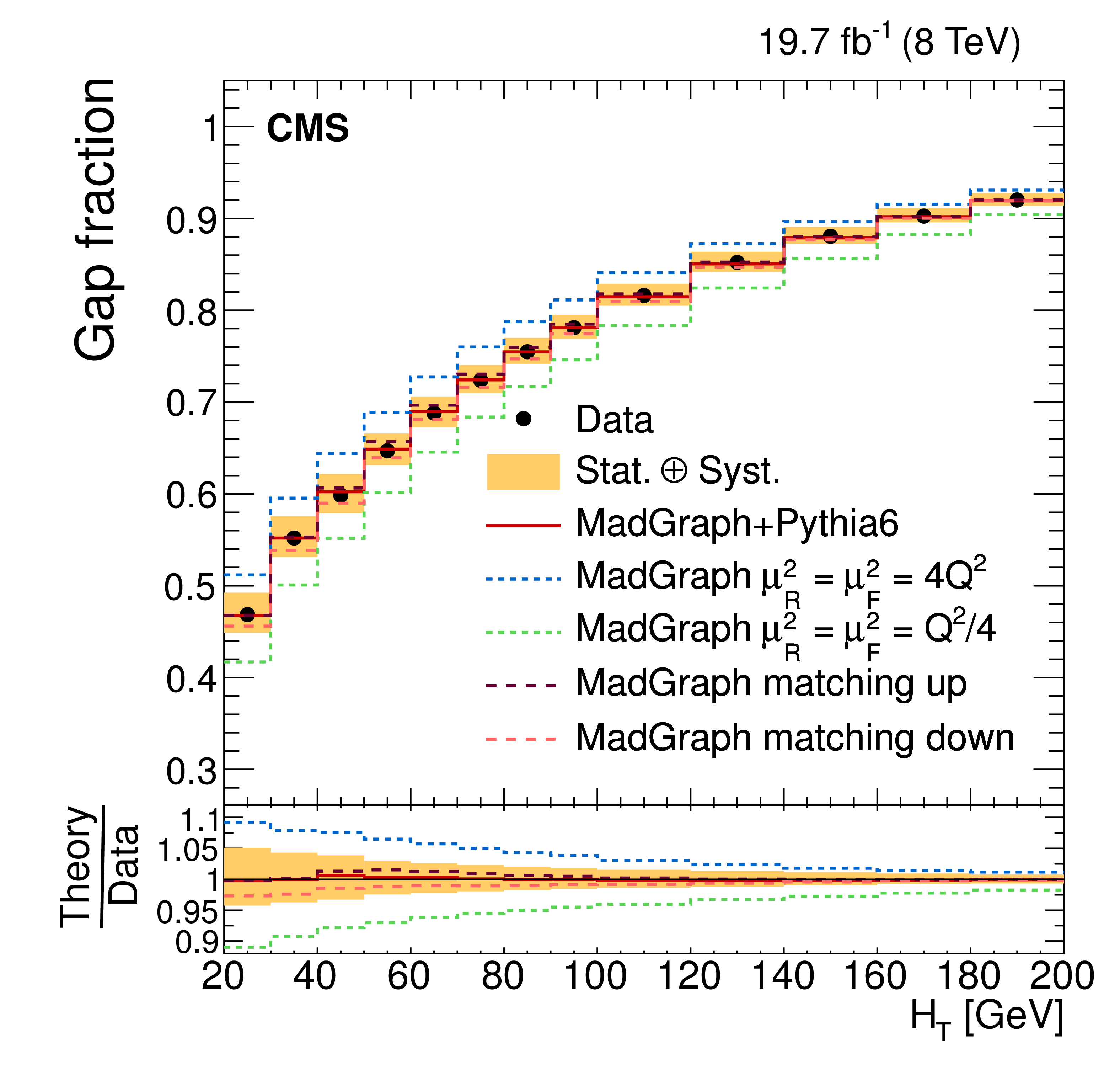
Figure 19-e:
Measured gap fraction as a function of the leading additional jet $ {p_{\mathrm {T}}} $ (a,b), subleading additional jet $ {p_{\mathrm {T}}} $ (c,d), and of $H_{\rm T}$ (e,f). Data are compared to predictions from MADGRAPH , POWHEG interfaced with PYTHIA andHERWIG , and MC@NLO interfaced withHERWIG (a,c,e), and to MADGRAPH with varied renormalization, factorization, and jet-parton matching scales (b,d,f). For each bin the threshold is defined at the value where the data point is placed. The vertical bars on the data points indicate the statistical uncertainty. The shaded band corresponds to the statistical and the total systematic uncertainty added in quadrature. The lower part of each plot shows the ratio of the predictions to the data. |
png pdf |
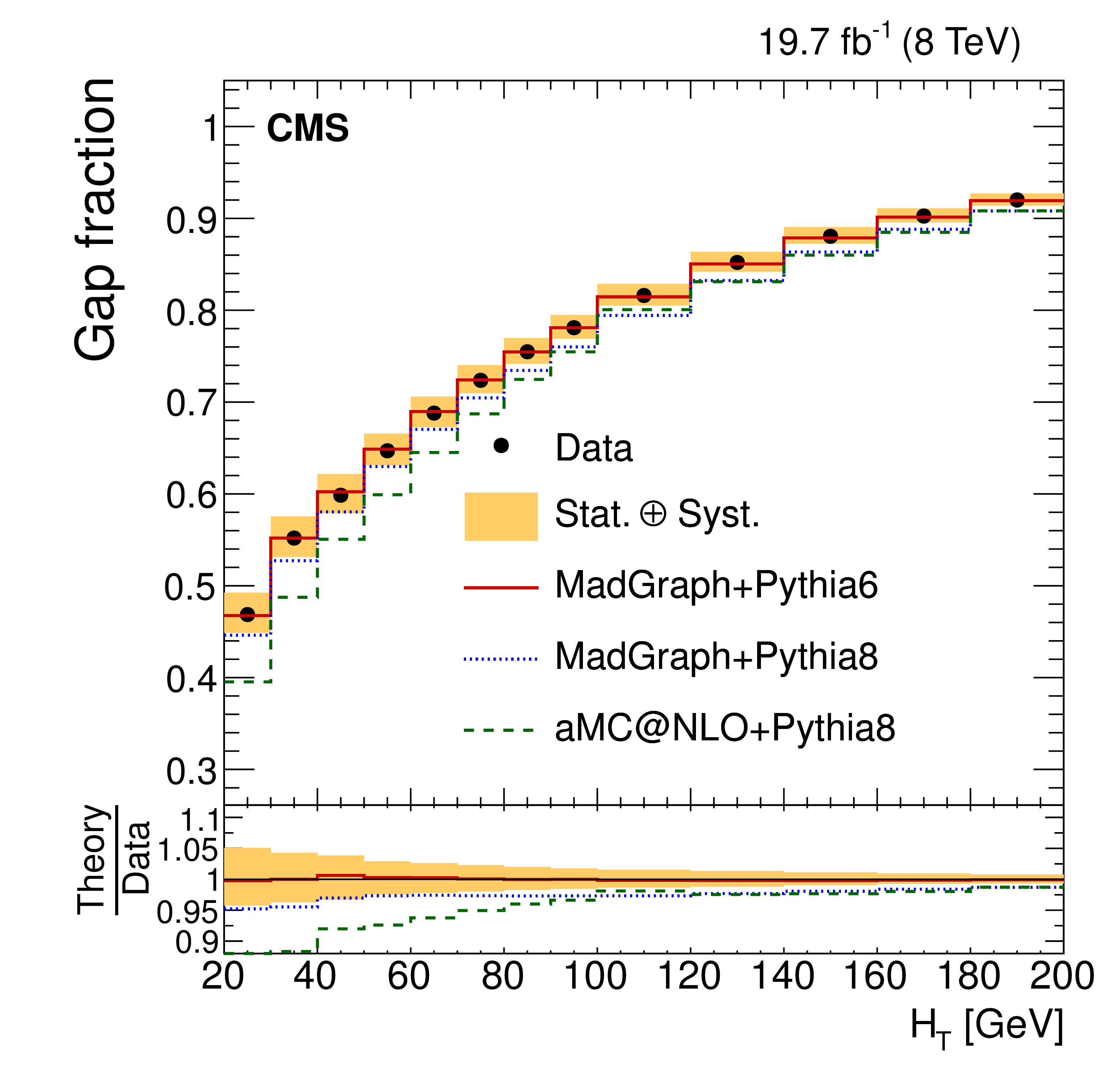
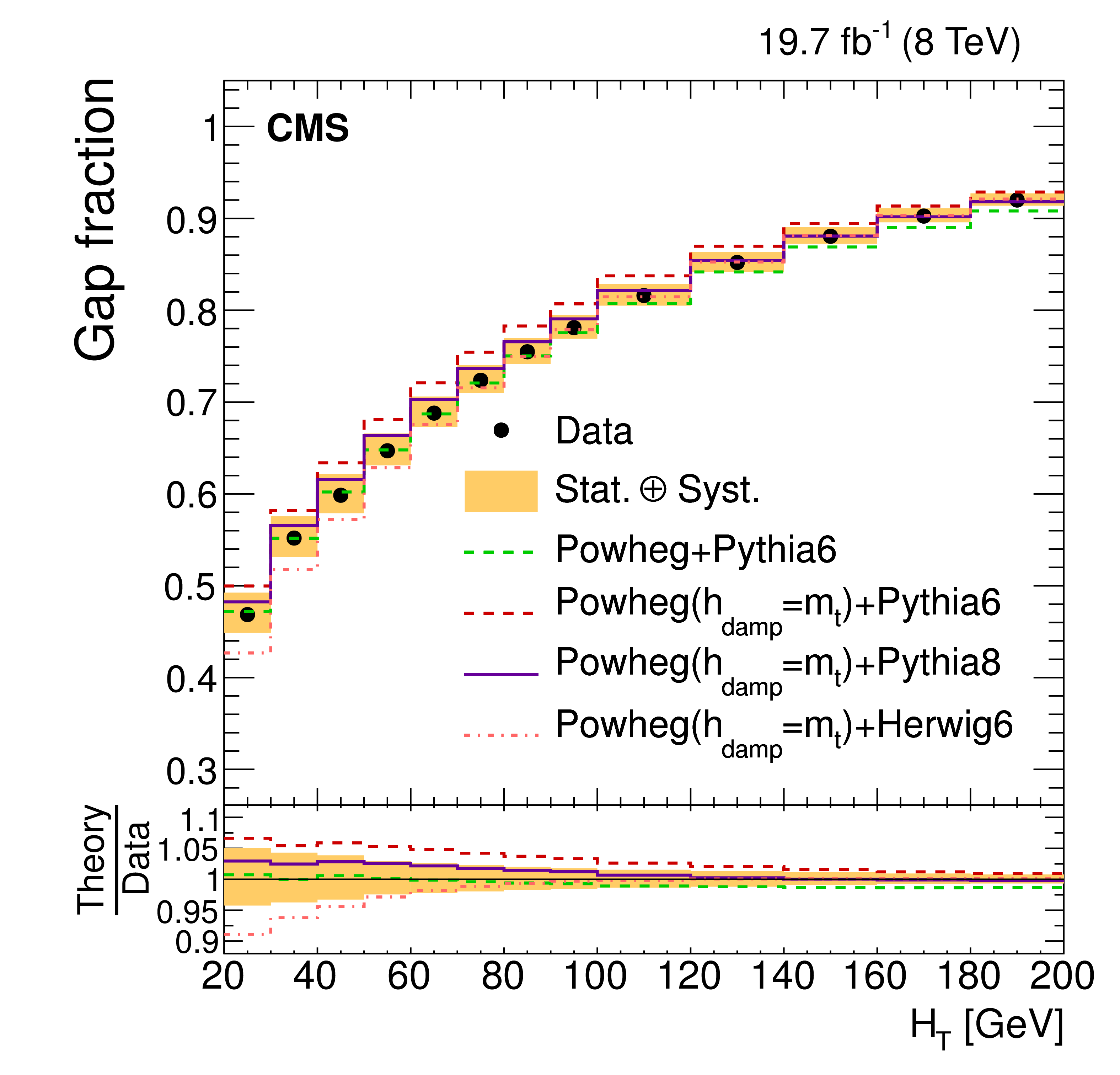
Figure 19-f:
Measured gap fraction as a function of the leading additional jet $ {p_{\mathrm {T}}} $ (a,b), subleading additional jet $ {p_{\mathrm {T}}} $ (c,d), and of $H_{\rm T}$ (e,f). Data are compared to predictions from MADGRAPH , POWHEG interfaced with PYTHIA andHERWIG , and MC@NLO interfaced withHERWIG (a,c,e), and to MADGRAPH with varied renormalization, factorization, and jet-parton matching scales (b,d,f). For each bin the threshold is defined at the value where the data point is placed. The vertical bars on the data points indicate the statistical uncertainty. The shaded band corresponds to the statistical and the total systematic uncertainty added in quadrature. The lower part of each plot shows the ratio of the predictions to the data. |

png pdf |
Figure 20-a:
Measured gap fraction as a function of the leading additional jet $ {p_{\mathrm {T}}} $ (a,b), subleading additional jet $ {p_{\mathrm {T}}} $ (c,d), and of $H_{\rm T}$ (e,f). Data are compared to predictions from MADGRAPH , interfaced with PYTHIA-6 and PYTHIA-8, and MG5-aMC@NLO interfaced with HERWIG-6 (a,c,e), and to POWHEG interfaced with different versions of PYTHIA andHERWIG (b,d,f). For each bin the threshold is defined at the value where the data point is placed. The vertical bars on the data points indicate the statistical uncertainty. The shaded band corresponds to the statistical and the total systematic uncertainty added in quadrature. The lower part of each plot shows the ratio of the predictions to the data. |
png pdf |
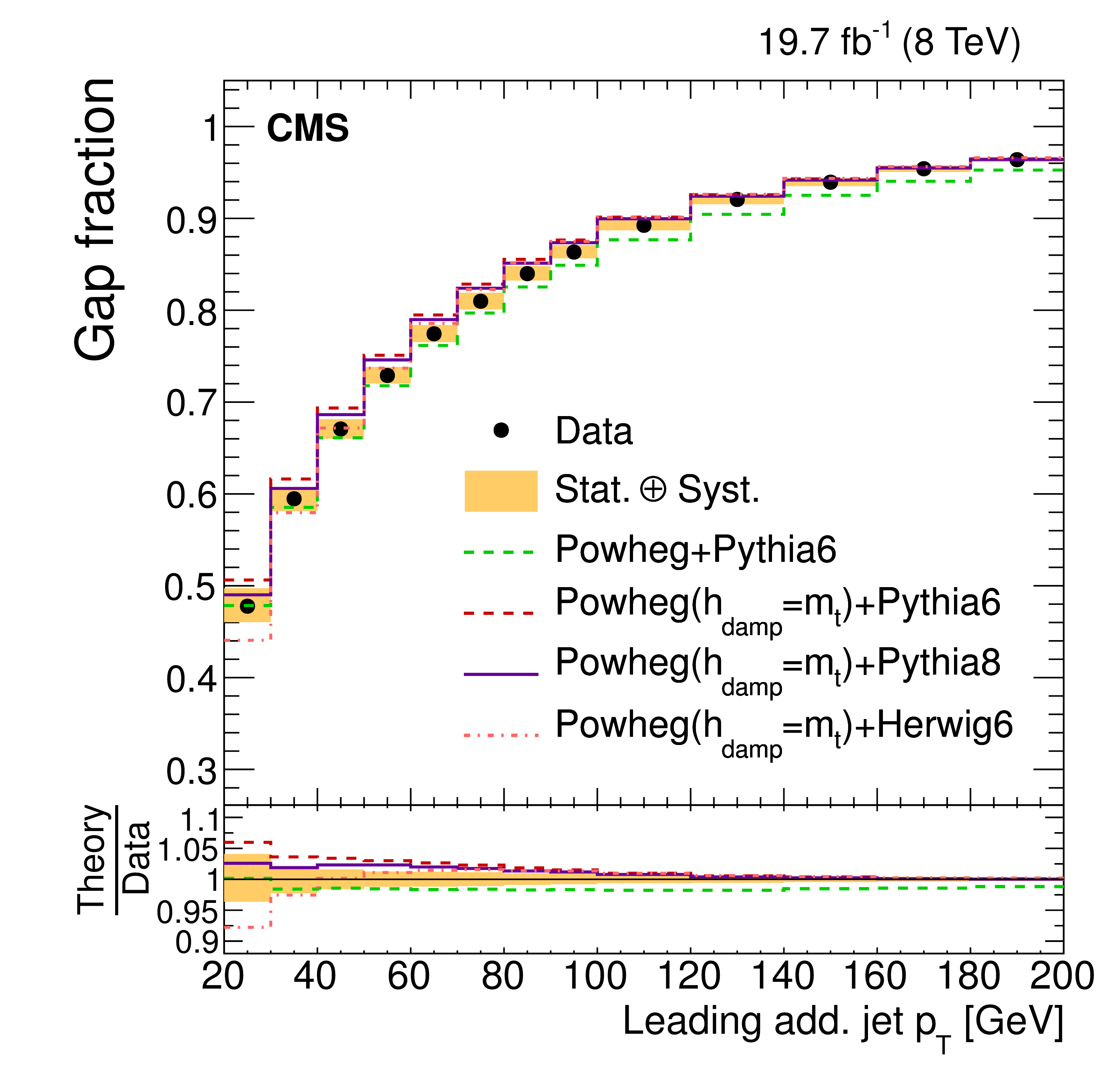
Figure 20-b:
Measured gap fraction as a function of the leading additional jet $ {p_{\mathrm {T}}} $ (a,b), subleading additional jet $ {p_{\mathrm {T}}} $ (c,d), and of $H_{\rm T}$ (e,f). Data are compared to predictions from MADGRAPH , interfaced with PYTHIA-6 and PYTHIA-8, and MG5-aMC@NLO interfaced with HERWIG-6 (a,c,e), and to POWHEG interfaced with different versions of PYTHIA andHERWIG (b,d,f). For each bin the threshold is defined at the value where the data point is placed. The vertical bars on the data points indicate the statistical uncertainty. The shaded band corresponds to the statistical and the total systematic uncertainty added in quadrature. The lower part of each plot shows the ratio of the predictions to the data. |
png pdf |
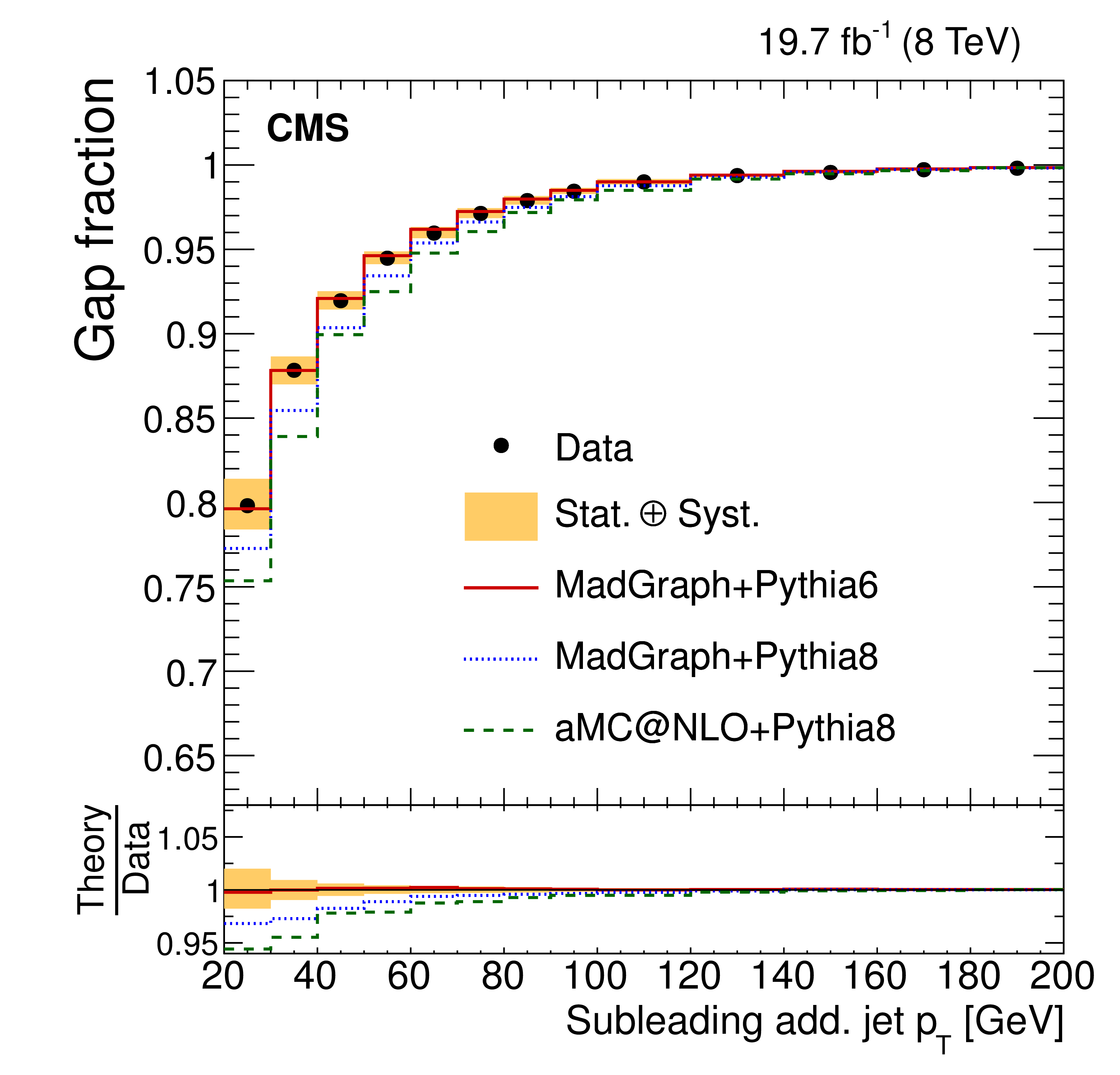
Figure 20-c:
Measured gap fraction as a function of the leading additional jet $ {p_{\mathrm {T}}} $ (a,b), subleading additional jet $ {p_{\mathrm {T}}} $ (c,d), and of $H_{\rm T}$ (e,f). Data are compared to predictions from MADGRAPH , interfaced with PYTHIA-6 and PYTHIA-8, and MG5-aMC@NLO interfaced with HERWIG-6 (a,c,e), and to POWHEG interfaced with different versions of PYTHIA andHERWIG (b,d,f). For each bin the threshold is defined at the value where the data point is placed. The vertical bars on the data points indicate the statistical uncertainty. The shaded band corresponds to the statistical and the total systematic uncertainty added in quadrature. The lower part of each plot shows the ratio of the predictions to the data. |
png pdf |
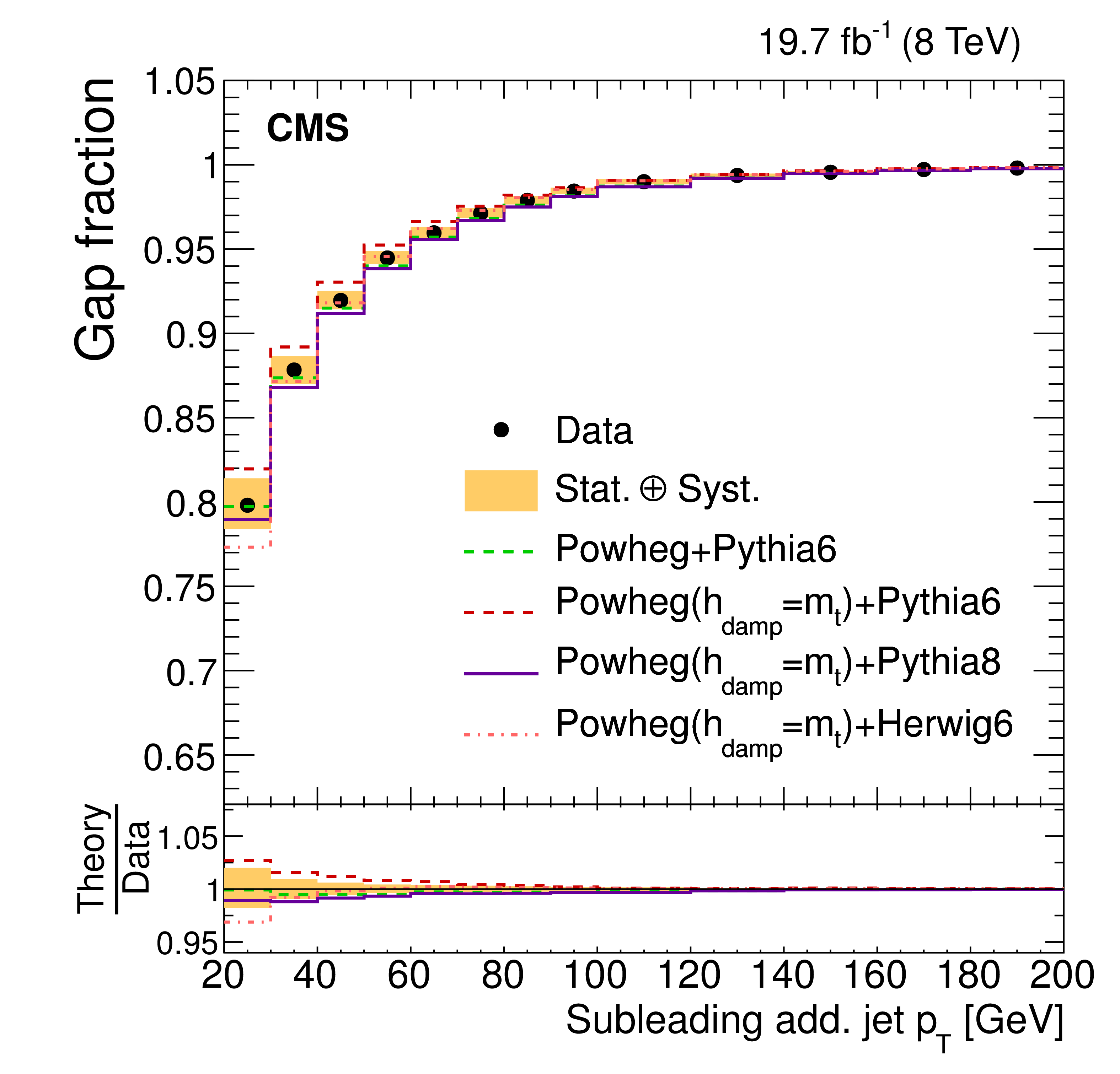
Figure 20-d:
Measured gap fraction as a function of the leading additional jet $ {p_{\mathrm {T}}} $ (a,b), subleading additional jet $ {p_{\mathrm {T}}} $ (c,d), and of $H_{\rm T}$ (e,f). Data are compared to predictions from MADGRAPH , interfaced with PYTHIA-6 and PYTHIA-8, and MG5-aMC@NLO interfaced with HERWIG-6 (a,c,e), and to POWHEG interfaced with different versions of PYTHIA andHERWIG (b,d,f). For each bin the threshold is defined at the value where the data point is placed. The vertical bars on the data points indicate the statistical uncertainty. The shaded band corresponds to the statistical and the total systematic uncertainty added in quadrature. The lower part of each plot shows the ratio of the predictions to the data. |
png pdf |
Figure 20-e:
Measured gap fraction as a function of the leading additional jet $ {p_{\mathrm {T}}} $ (a,b), subleading additional jet $ {p_{\mathrm {T}}} $ (c,d), and of $H_{\rm T}$ (e,f). Data are compared to predictions from MADGRAPH , interfaced with PYTHIA-6 and PYTHIA-8, and MG5-aMC@NLO interfaced with HERWIG-6 (a,c,e), and to POWHEG interfaced with different versions of PYTHIA andHERWIG (b,d,f). For each bin the threshold is defined at the value where the data point is placed. The vertical bars on the data points indicate the statistical uncertainty. The shaded band corresponds to the statistical and the total systematic uncertainty added in quadrature. The lower part of each plot shows the ratio of the predictions to the data. |
png pdf |
Figure 20-f:
Measured gap fraction as a function of the leading additional jet $ {p_{\mathrm {T}}} $ (a,b), subleading additional jet $ {p_{\mathrm {T}}} $ (c,d), and of $H_{\rm T}$ (e,f). Data are compared to predictions from MADGRAPH , interfaced with PYTHIA-6 and PYTHIA-8, and MG5-aMC@NLO interfaced with HERWIG-6 (a,c,e), and to POWHEG interfaced with different versions of PYTHIA andHERWIG (b,d,f). For each bin the threshold is defined at the value where the data point is placed. The vertical bars on the data points indicate the statistical uncertainty. The shaded band corresponds to the statistical and the total systematic uncertainty added in quadrature. The lower part of each plot shows the ratio of the predictions to the data. |
png pdf |
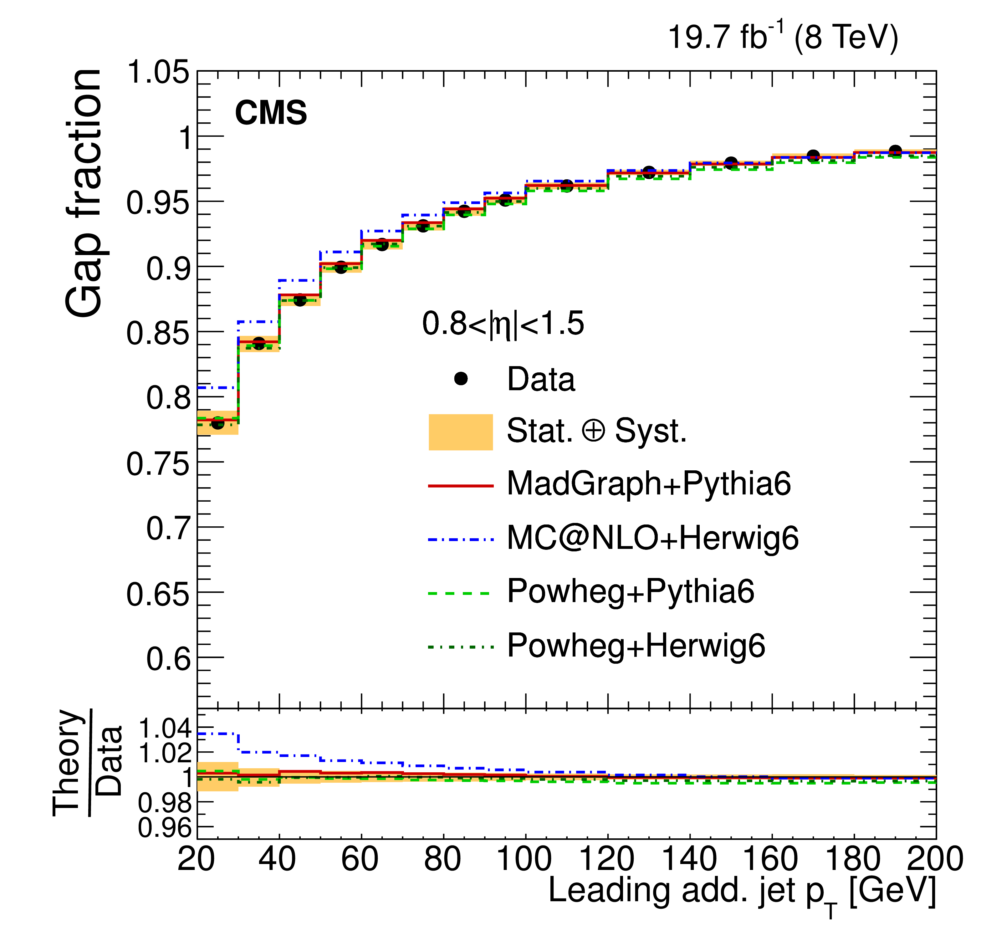
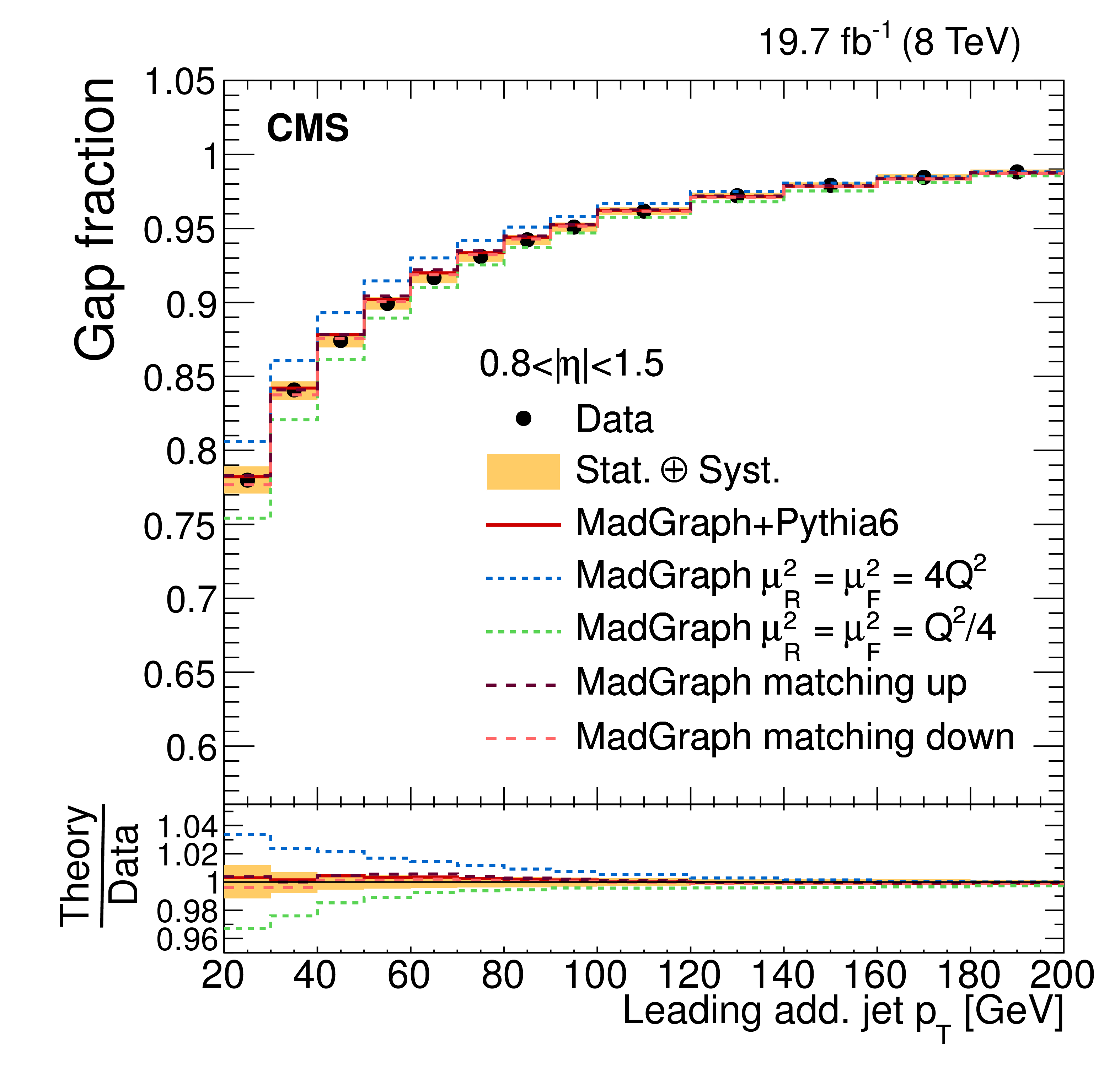
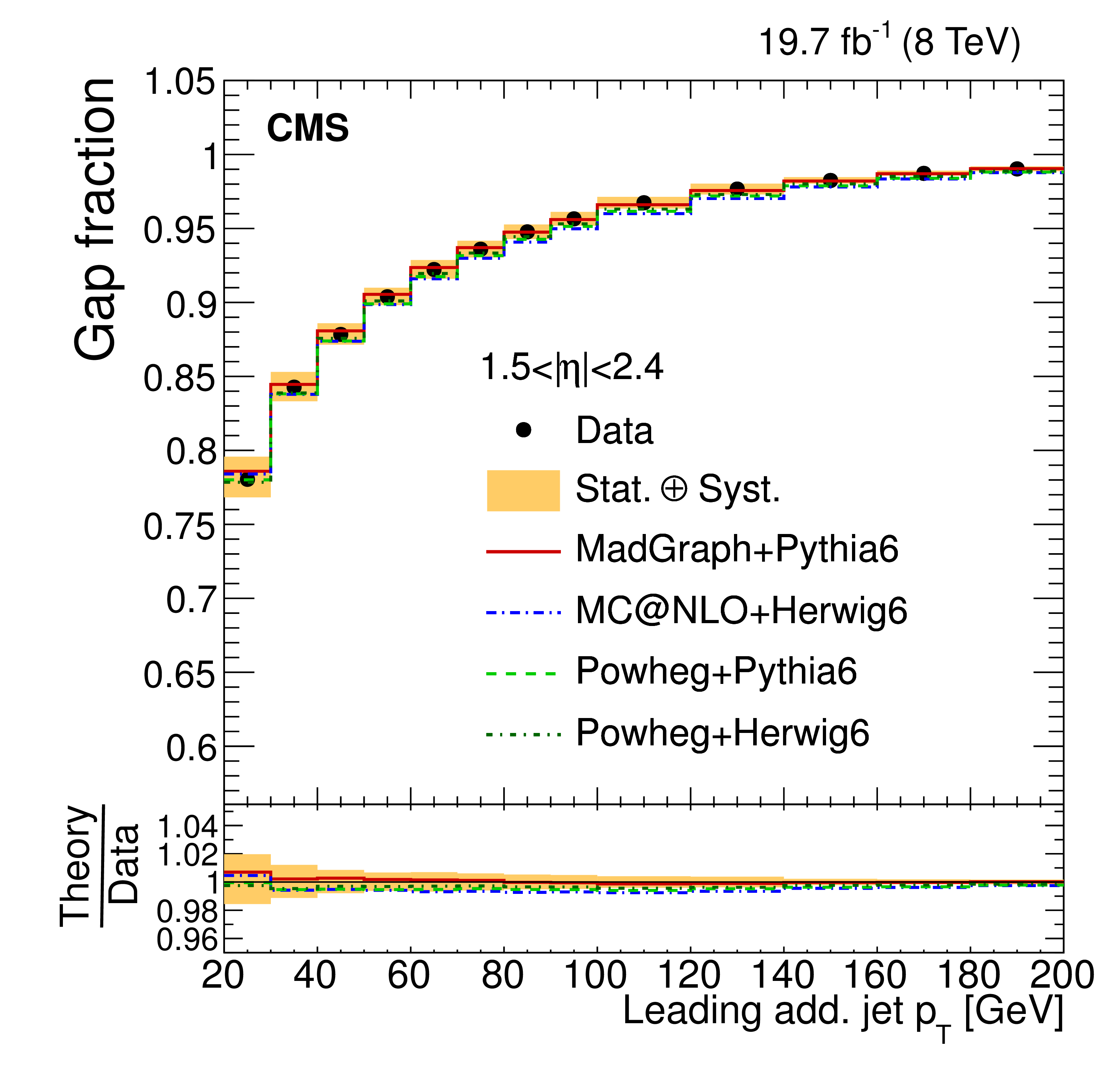
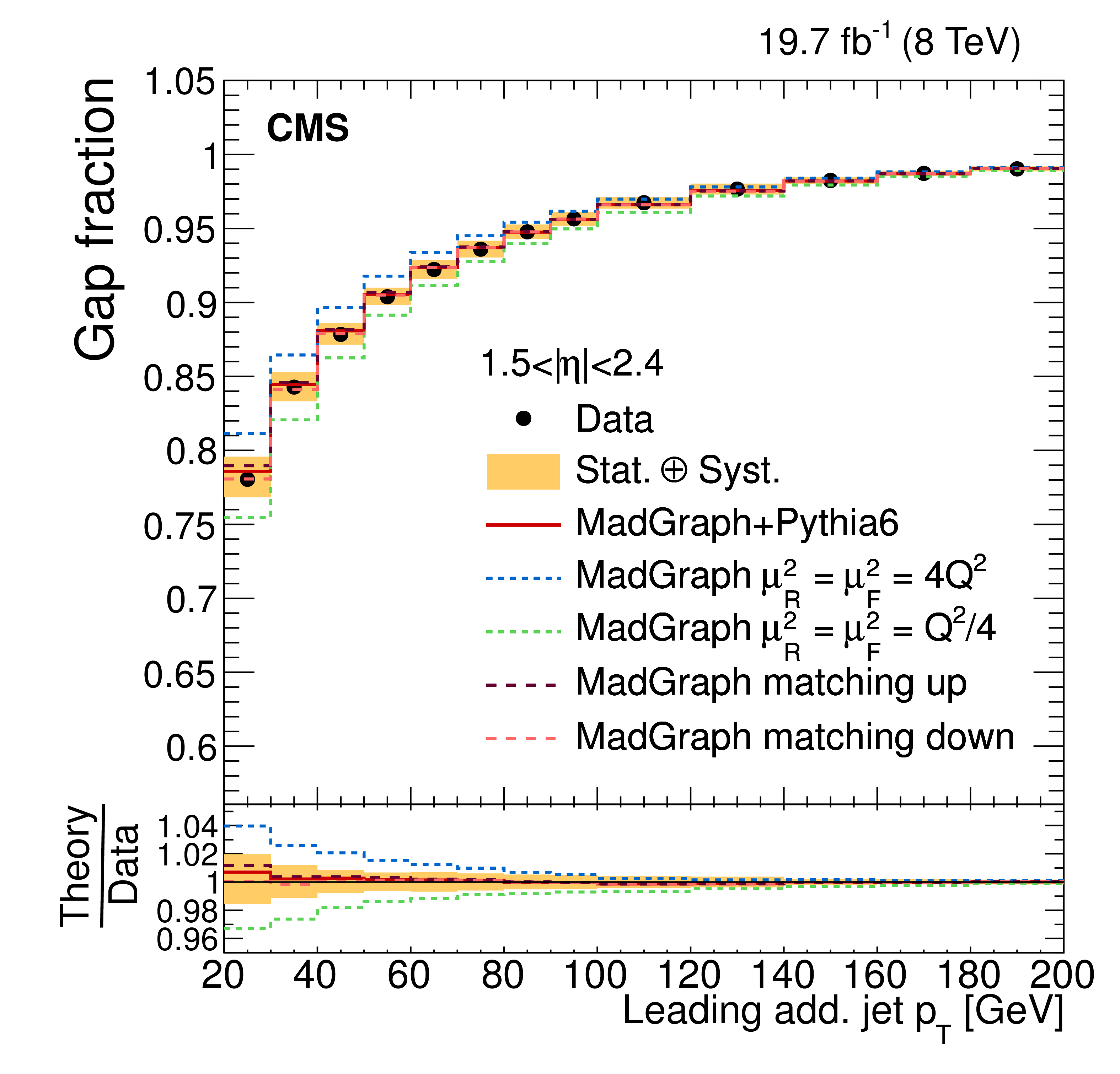
Figure 21-a:
Measured gap fraction as a function of the leading additional jet ${p_{\mathrm {T}}}$ in different $\eta $ regions. Data are compared to predictions from MadGraph , POWHEG interfaced with PYTHIA 6 and HERWIG 6, and MC@NLO interfaced with HERWIG 6 (left) and to MadGraph with varied renormalization, factorization, and jet-parton matching scales (right). For each bin the threshold is defined at the value where the data point is placed. The vertical bars on the data points indicate the statistical uncertainty. The shaded band corresponds to the statistical uncertainty and the total systematic uncertainty added in quadrature. The lower part of each plot shows the ratio of the predictions to the data. |
png pdf |
Figure 21-b:
Measured gap fraction as a function of the leading additional jet ${p_{\mathrm {T}}}$ in different $\eta $ regions. Data are compared to predictions from MadGraph , POWHEG interfaced with PYTHIA 6 and HERWIG 6, and MC@NLO interfaced with HERWIG 6 (left) and to MadGraph with varied renormalization, factorization, and jet-parton matching scales (right). For each bin the threshold is defined at the value where the data point is placed. The vertical bars on the data points indicate the statistical uncertainty. The shaded band corresponds to the statistical uncertainty and the total systematic uncertainty added in quadrature. The lower part of each plot shows the ratio of the predictions to the data. |
png pdf |
Figure 21-c:
Measured gap fraction as a function of the leading additional jet ${p_{\mathrm {T}}}$ in different $\eta $ regions. Data are compared to predictions from MadGraph , POWHEG interfaced with PYTHIA 6 and HERWIG 6, and MC@NLO interfaced with HERWIG 6 (left) and to MadGraph with varied renormalization, factorization, and jet-parton matching scales (right). For each bin the threshold is defined at the value where the data point is placed. The vertical bars on the data points indicate the statistical uncertainty. The shaded band corresponds to the statistical uncertainty and the total systematic uncertainty added in quadrature. The lower part of each plot shows the ratio of the predictions to the data. |
png pdf |
Figure 21-d:
Measured gap fraction as a function of the leading additional jet ${p_{\mathrm {T}}}$ in different $\eta $ regions. Data are compared to predictions from MadGraph , POWHEG interfaced with PYTHIA 6 and HERWIG 6, and MC@NLO interfaced with HERWIG 6 (left) and to MadGraph with varied renormalization, factorization, and jet-parton matching scales (right). For each bin the threshold is defined at the value where the data point is placed. The vertical bars on the data points indicate the statistical uncertainty. The shaded band corresponds to the statistical uncertainty and the total systematic uncertainty added in quadrature. The lower part of each plot shows the ratio of the predictions to the data. |
png pdf |
Figure 21-e:
Measured gap fraction as a function of the leading additional jet ${p_{\mathrm {T}}}$ in different $\eta $ regions. Data are compared to predictions from MadGraph , POWHEG interfaced with PYTHIA 6 and HERWIG 6, and MC@NLO interfaced with HERWIG 6 (left) and to MadGraph with varied renormalization, factorization, and jet-parton matching scales (right). For each bin the threshold is defined at the value where the data point is placed. The vertical bars on the data points indicate the statistical uncertainty. The shaded band corresponds to the statistical uncertainty and the total systematic uncertainty added in quadrature. The lower part of each plot shows the ratio of the predictions to the data. |
png pdf |
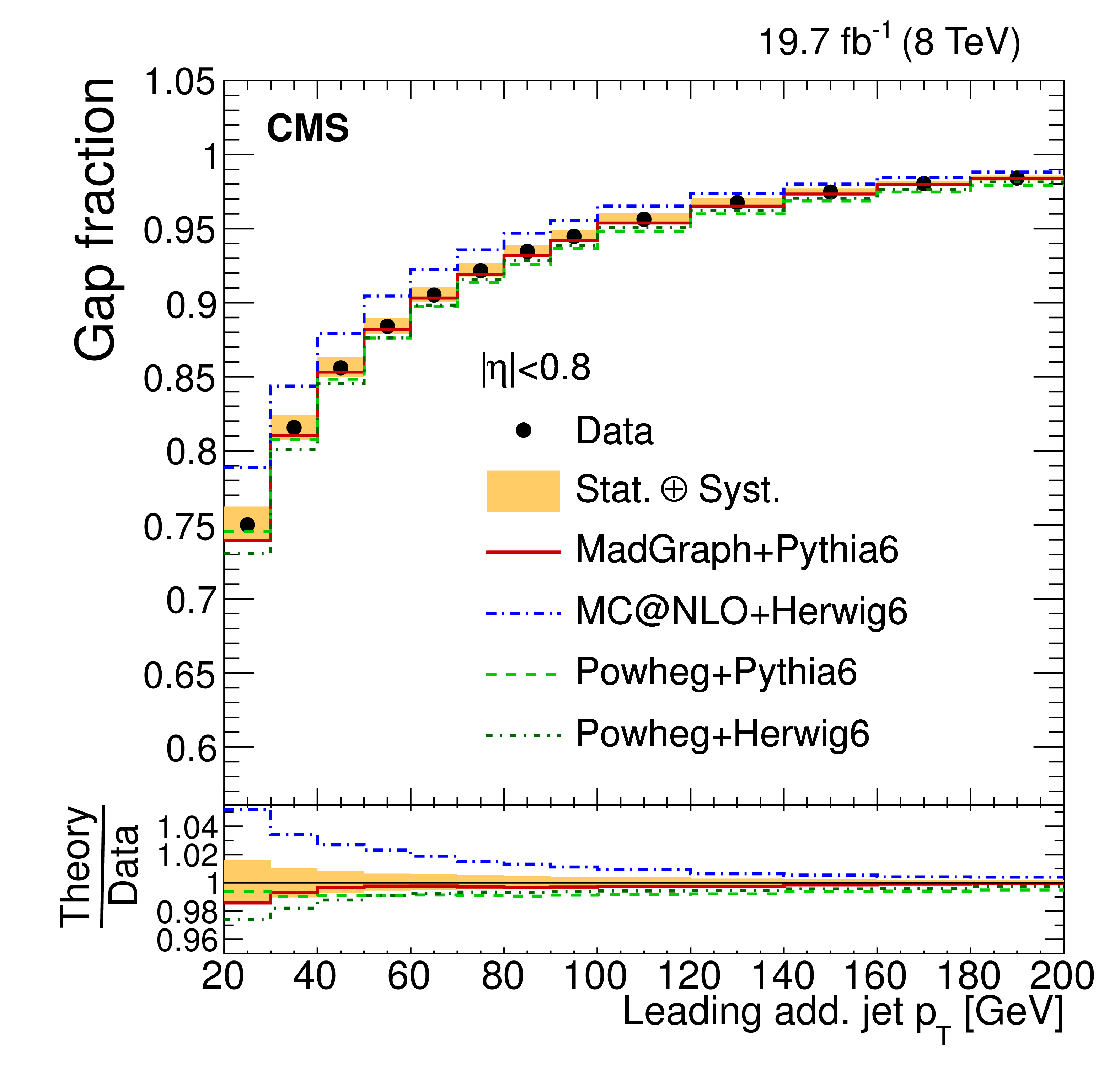
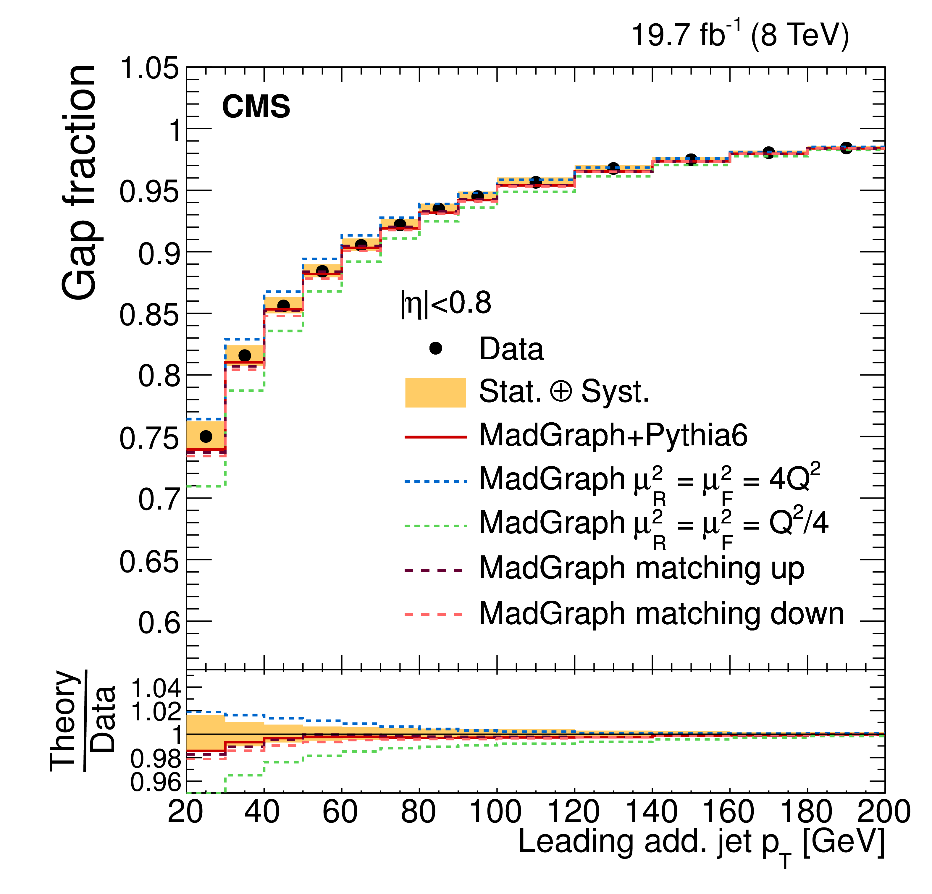
Figure 21-f:
Measured gap fraction as a function of the leading additional jet ${p_{\mathrm {T}}}$ in different $\eta $ regions. Data are compared to predictions from MadGraph , POWHEG interfaced with PYTHIA 6 and HERWIG 6, and MC@NLO interfaced with HERWIG 6 (left) and to MadGraph with varied renormalization, factorization, and jet-parton matching scales (right). For each bin the threshold is defined at the value where the data point is placed. The vertical bars on the data points indicate the statistical uncertainty. The shaded band corresponds to the statistical uncertainty and the total systematic uncertainty added in quadrature. The lower part of each plot shows the ratio of the predictions to the data. |
png pdf |
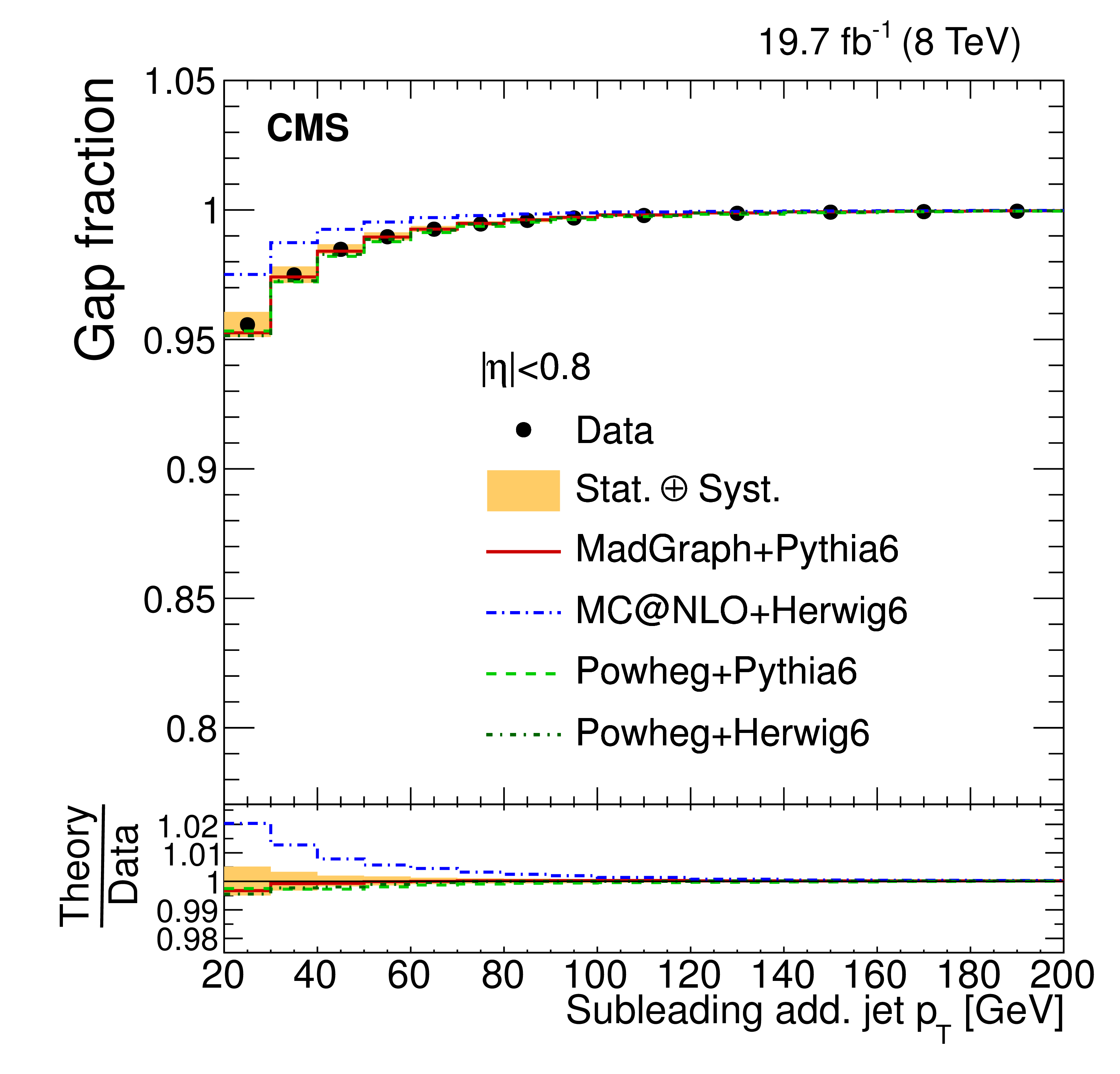
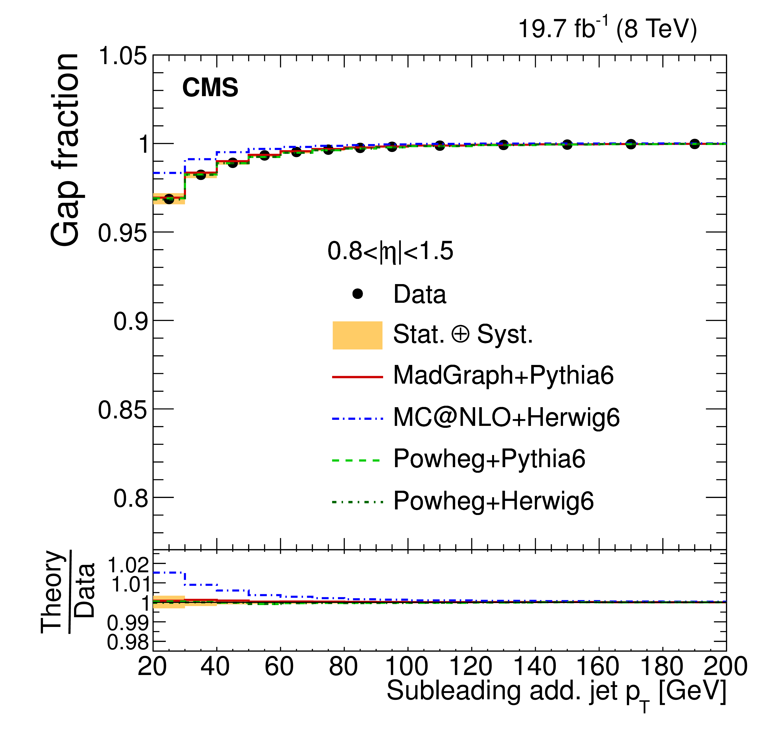
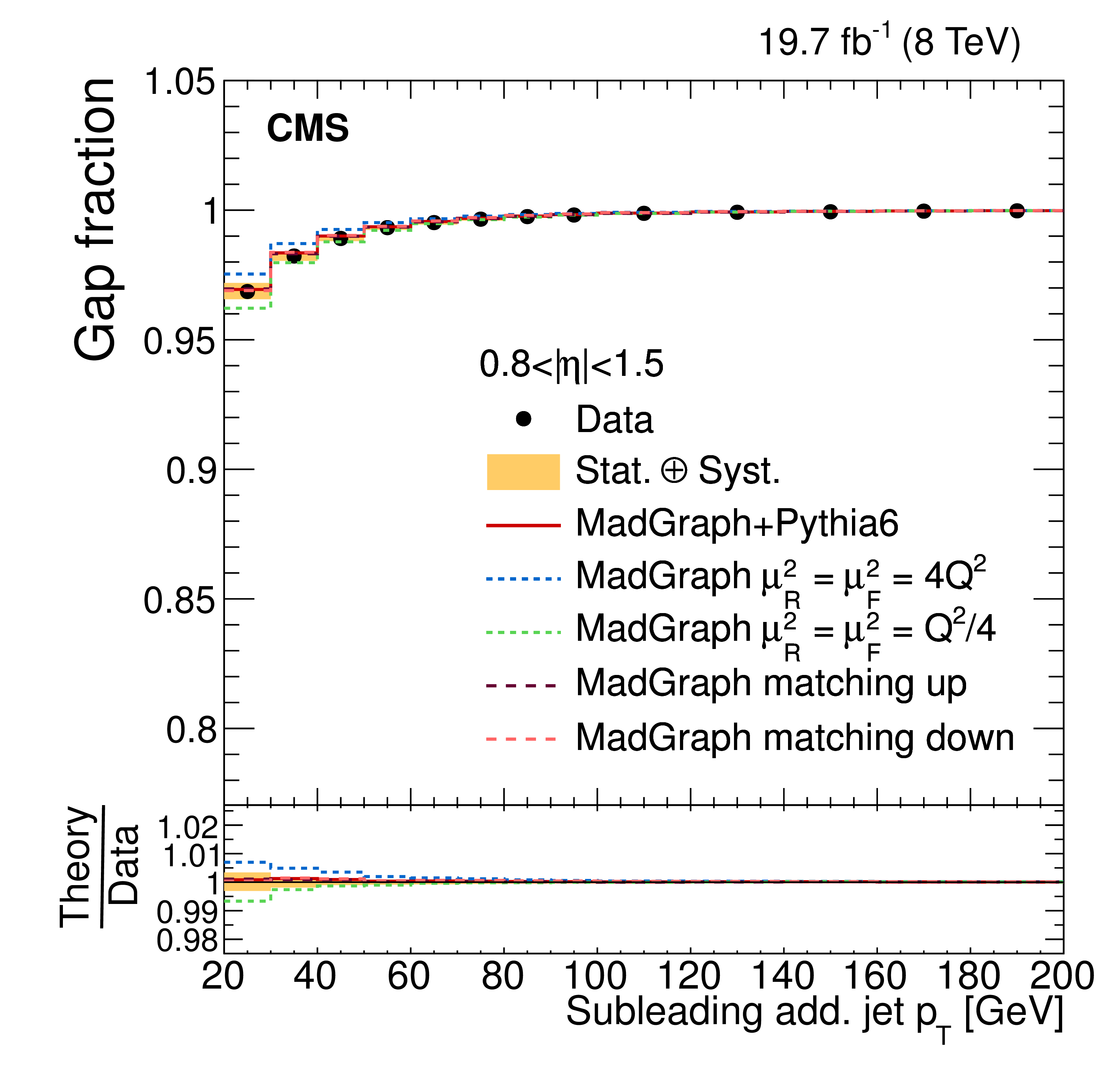
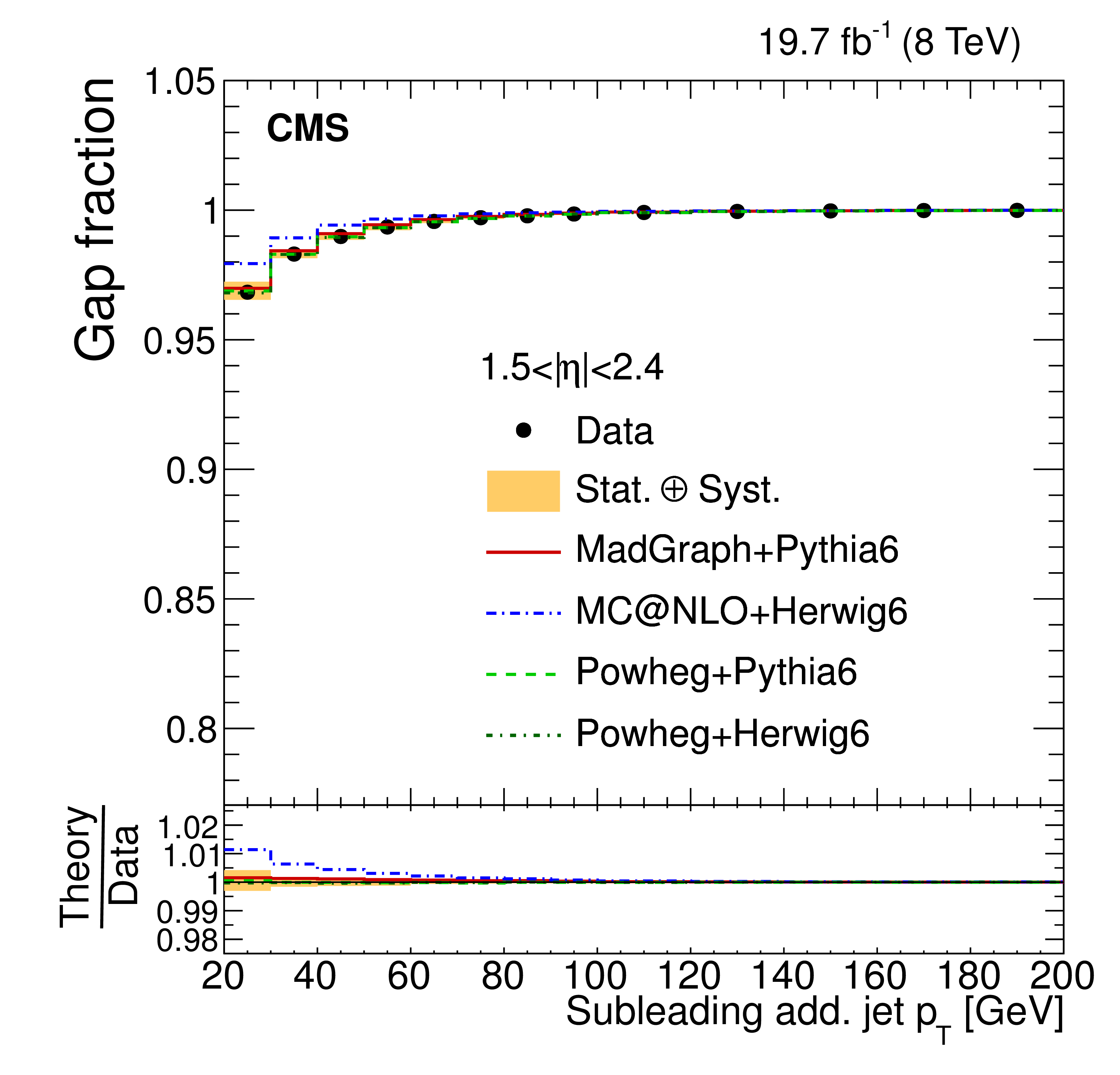
Figure 22-a:
Measured gap fraction as a function of the subleading additional jet $ {p_{\mathrm {T}}} $ in different $ {|\eta |} $ regions. Data are compared to predictions from MADGRAPH , POWHEG interfaced with PYTHIA-6 and HERWIG-6, and MC@NLO interfaced with HERWIG-6 (a,c,e) and to MADGRAPH with varied with varied renormalization, factorization, and jet-parton matching scales (b,d,f). For each bin the threshold is defined at the value where the data point is placed. The vertical bars on the data points indicate the statistical uncertainty. The shaded band corresponds to the statistical uncertainty and the total systematic uncertainty added in quadrature. The lower part of each plot shows the ratio of the predictions to the data. |

png pdf |
Figure 22-b:
Measured gap fraction as a function of the subleading additional jet $ {p_{\mathrm {T}}} $ in different $ {|\eta |} $ regions. Data are compared to predictions from MADGRAPH , POWHEG interfaced with PYTHIA-6 and HERWIG-6, and MC@NLO interfaced with HERWIG-6 (a,c,e) and to MADGRAPH with varied with varied renormalization, factorization, and jet-parton matching scales (b,d,f). For each bin the threshold is defined at the value where the data point is placed. The vertical bars on the data points indicate the statistical uncertainty. The shaded band corresponds to the statistical uncertainty and the total systematic uncertainty added in quadrature. The lower part of each plot shows the ratio of the predictions to the data. |
png pdf |
Figure 22-c:
Measured gap fraction as a function of the subleading additional jet $ {p_{\mathrm {T}}} $ in different $ {|\eta |} $ regions. Data are compared to predictions from MADGRAPH , POWHEG interfaced with PYTHIA-6 and HERWIG-6, and MC@NLO interfaced with HERWIG-6 (a,c,e) and to MADGRAPH with varied with varied renormalization, factorization, and jet-parton matching scales (b,d,f). For each bin the threshold is defined at the value where the data point is placed. The vertical bars on the data points indicate the statistical uncertainty. The shaded band corresponds to the statistical uncertainty and the total systematic uncertainty added in quadrature. The lower part of each plot shows the ratio of the predictions to the data. |
png pdf |
Figure 22-d:
Measured gap fraction as a function of the subleading additional jet $ {p_{\mathrm {T}}} $ in different $ {|\eta |} $ regions. Data are compared to predictions from MADGRAPH , POWHEG interfaced with PYTHIA-6 and HERWIG-6, and MC@NLO interfaced with HERWIG-6 (a,c,e) and to MADGRAPH with varied with varied renormalization, factorization, and jet-parton matching scales (b,d,f). For each bin the threshold is defined at the value where the data point is placed. The vertical bars on the data points indicate the statistical uncertainty. The shaded band corresponds to the statistical uncertainty and the total systematic uncertainty added in quadrature. The lower part of each plot shows the ratio of the predictions to the data. |
png pdf |
Figure 22-e:
Measured gap fraction as a function of the subleading additional jet $ {p_{\mathrm {T}}} $ in different $ {|\eta |} $ regions. Data are compared to predictions from MADGRAPH , POWHEG interfaced with PYTHIA-6 and HERWIG-6, and MC@NLO interfaced with HERWIG-6 (a,c,e) and to MADGRAPH with varied with varied renormalization, factorization, and jet-parton matching scales (b,d,f). For each bin the threshold is defined at the value where the data point is placed. The vertical bars on the data points indicate the statistical uncertainty. The shaded band corresponds to the statistical uncertainty and the total systematic uncertainty added in quadrature. The lower part of each plot shows the ratio of the predictions to the data. |
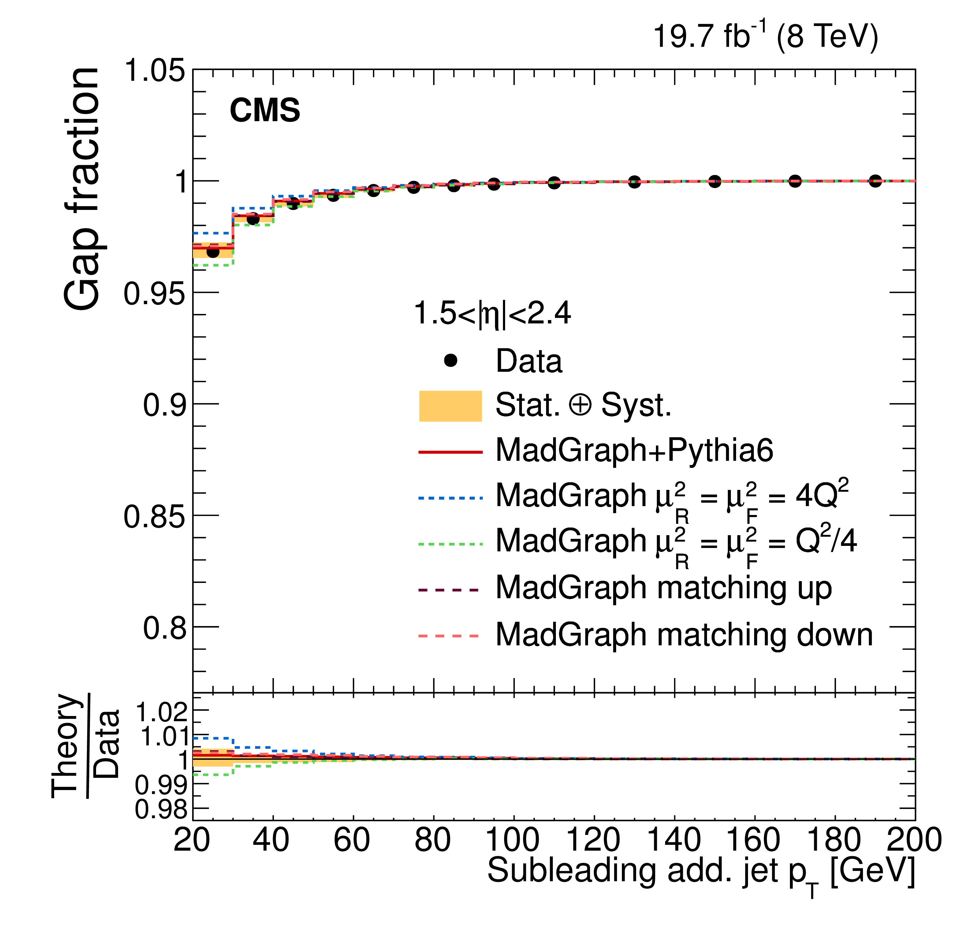
png pdf |
Figure 22-f:
Measured gap fraction as a function of the subleading additional jet $ {p_{\mathrm {T}}} $ in different $ {|\eta |} $ regions. Data are compared to predictions from MADGRAPH , POWHEG interfaced with PYTHIA-6 and HERWIG-6, and MC@NLO interfaced with HERWIG-6 (a,c,e) and to MADGRAPH with varied with varied renormalization, factorization, and jet-parton matching scales (b,d,f). For each bin the threshold is defined at the value where the data point is placed. The vertical bars on the data points indicate the statistical uncertainty. The shaded band corresponds to the statistical uncertainty and the total systematic uncertainty added in quadrature. The lower part of each plot shows the ratio of the predictions to the data. |

png pdf |
Figure 23-a:
Measured gap fraction as a function of $H_{\rm T}$ in different $\eta $ regions. Results in data are compared to the nominal MADGRAPH signal sample, POWHEG and MC@NLO (a,c,e) and to the samples with varied renormalization, factorization, and jet-parton matching scales (b,d,f). For each bin the threshold is defined at the value where the data point is placed. The vertical bars on the data points indicate the statistical uncertainty. The shaded band corresponds to the statistical uncertainty and the total systematic uncertainty added in quadrature. |
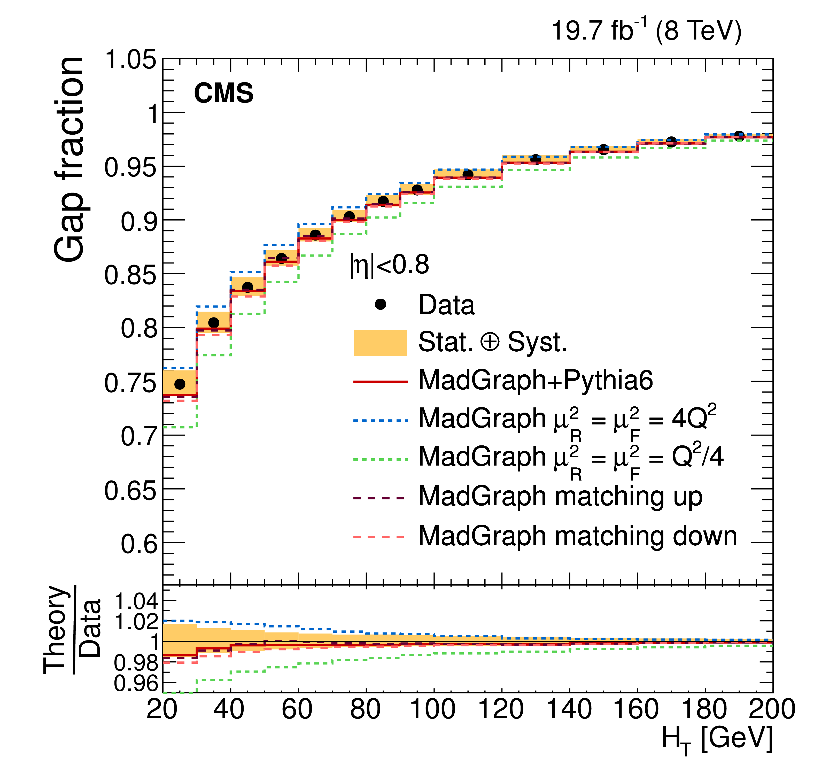
png pdf |
Figure 23-b:
Measured gap fraction as a function of $H_{\rm T}$ in different $\eta $ regions. Results in data are compared to the nominal MADGRAPH signal sample, POWHEG and MC@NLO (a,c,e) and to the samples with varied renormalization, factorization, and jet-parton matching scales (b,d,f). For each bin the threshold is defined at the value where the data point is placed. The vertical bars on the data points indicate the statistical uncertainty. The shaded band corresponds to the statistical uncertainty and the total systematic uncertainty added in quadrature. |
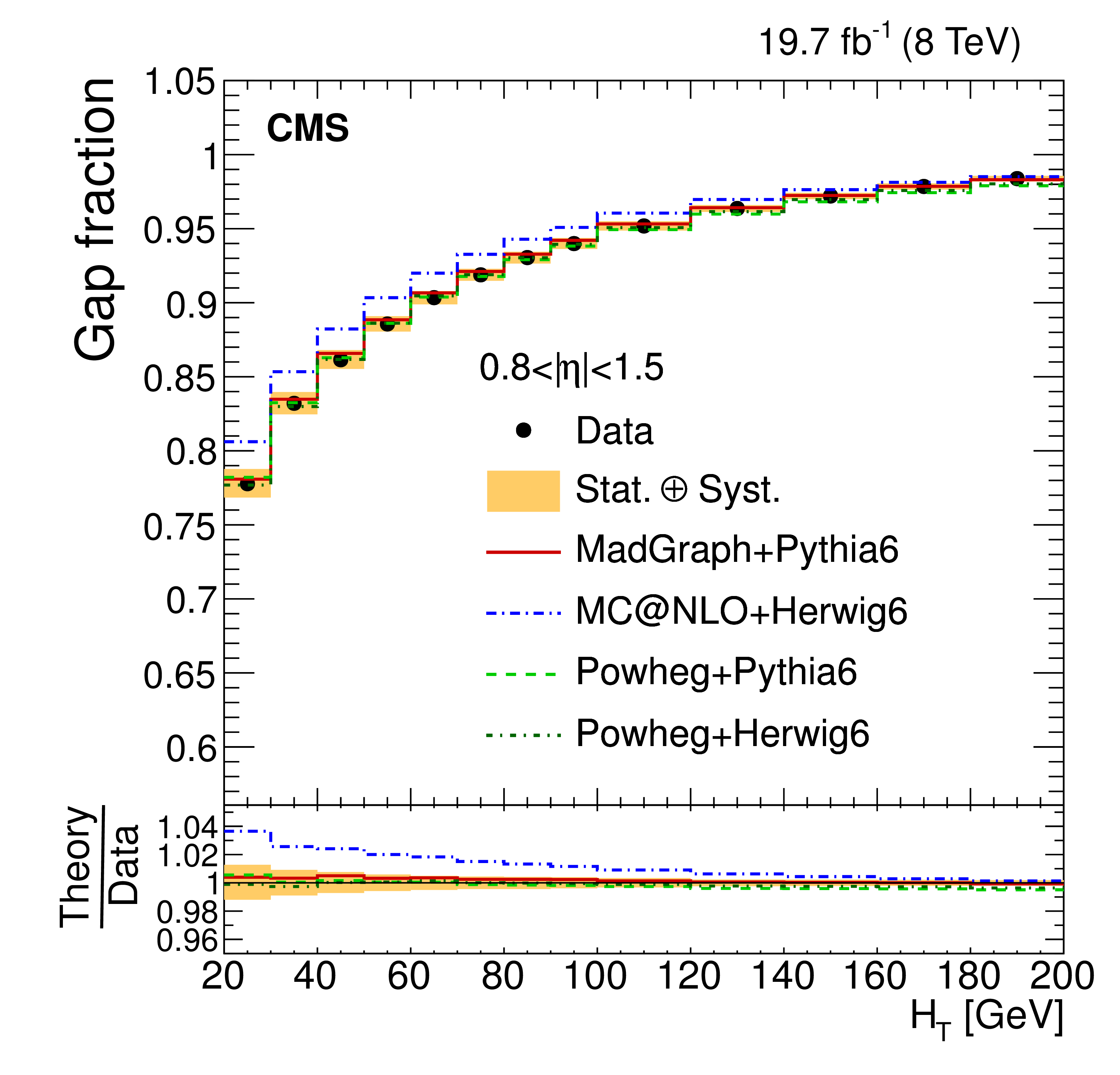
png pdf |
Figure 23-c:
Measured gap fraction as a function of $H_{\rm T}$ in different $\eta $ regions. Results in data are compared to the nominal MADGRAPH signal sample, POWHEG and MC@NLO (a,c,e) and to the samples with varied renormalization, factorization, and jet-parton matching scales (b,d,f). For each bin the threshold is defined at the value where the data point is placed. The vertical bars on the data points indicate the statistical uncertainty. The shaded band corresponds to the statistical uncertainty and the total systematic uncertainty added in quadrature. |
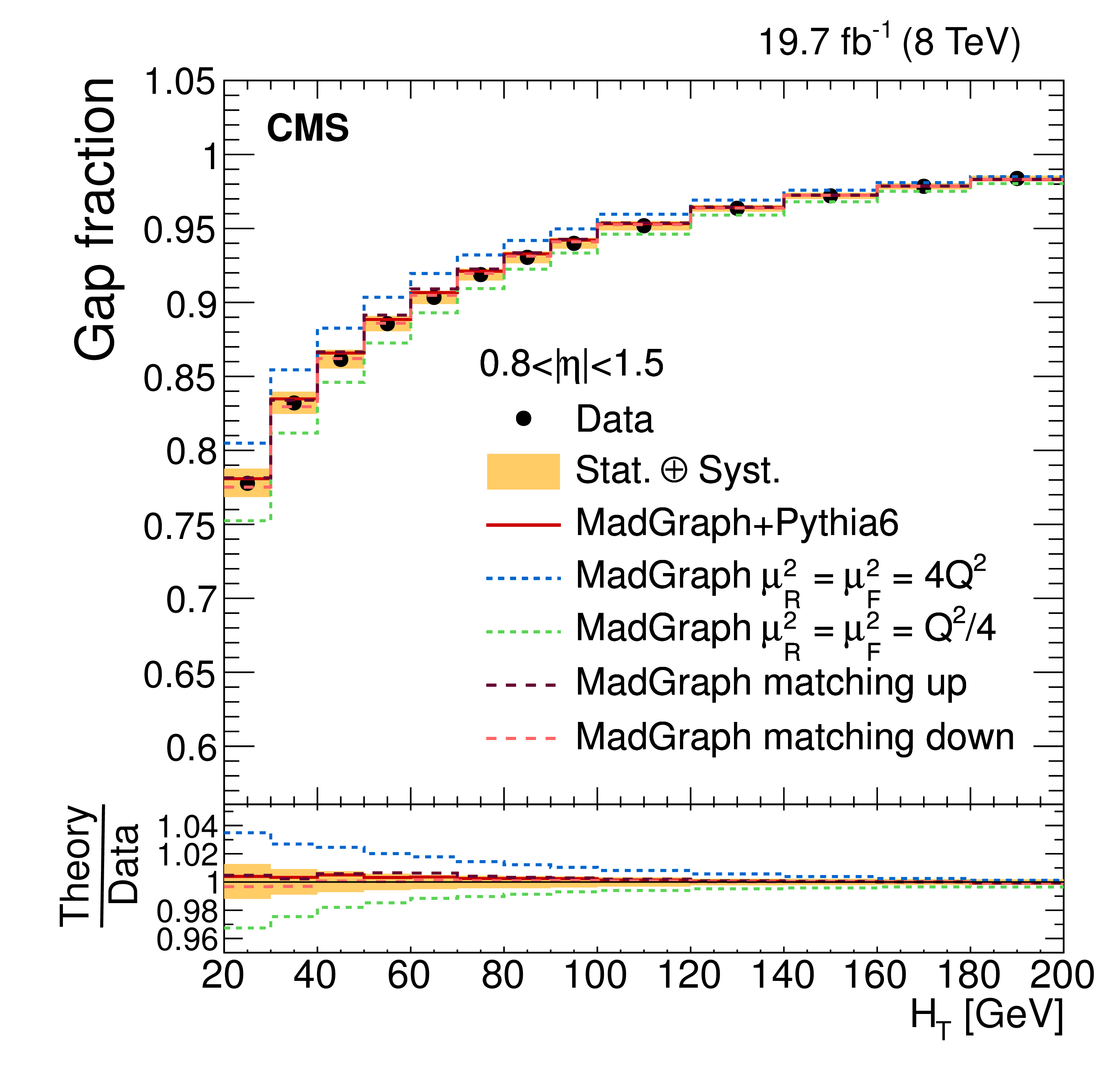
png pdf |
Figure 23-d:
Measured gap fraction as a function of $H_{\rm T}$ in different $\eta $ regions. Results in data are compared to the nominal MADGRAPH signal sample, POWHEG and MC@NLO (a,c,e) and to the samples with varied renormalization, factorization, and jet-parton matching scales (b,d,f). For each bin the threshold is defined at the value where the data point is placed. The vertical bars on the data points indicate the statistical uncertainty. The shaded band corresponds to the statistical uncertainty and the total systematic uncertainty added in quadrature. |
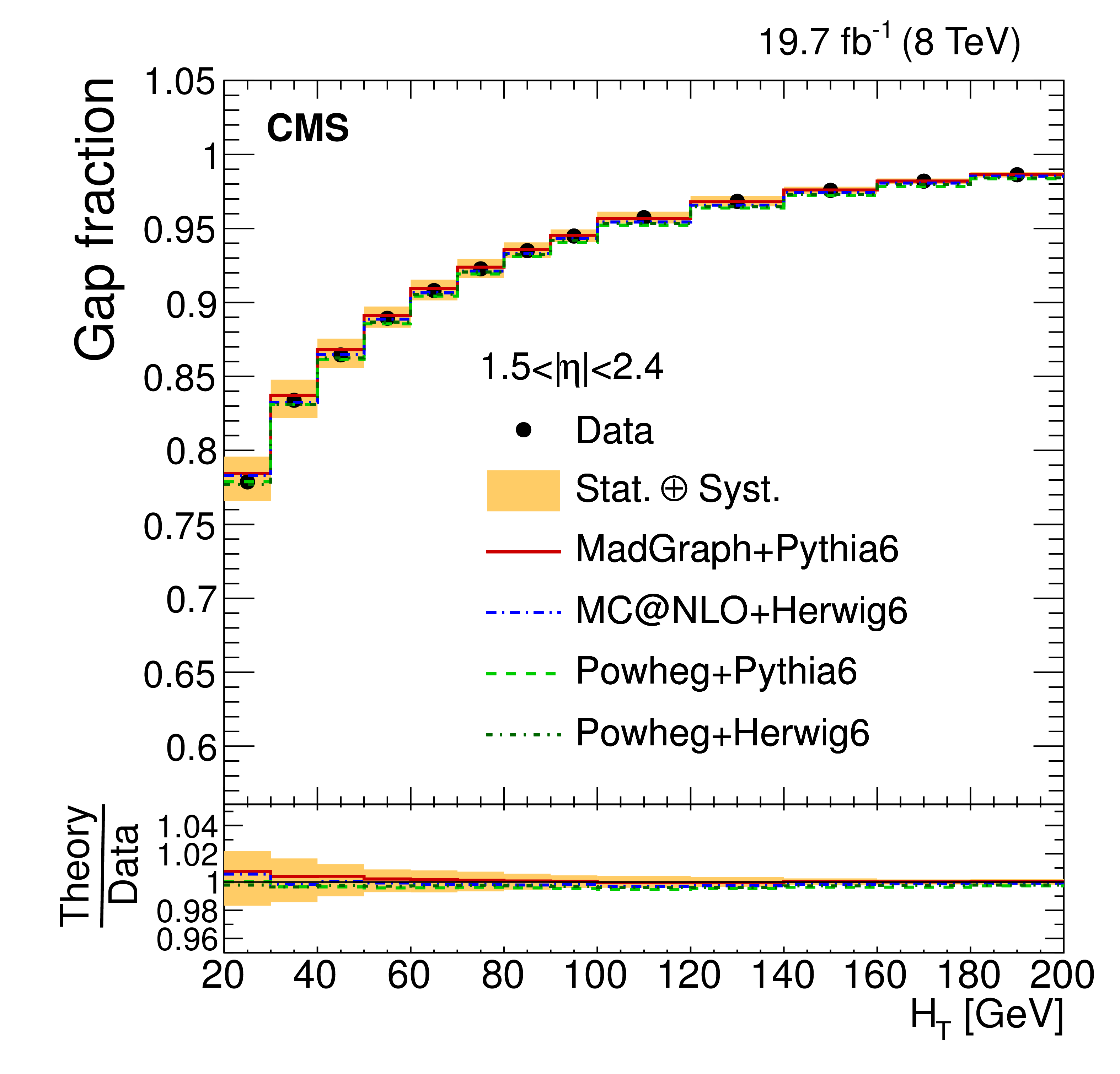
png pdf |
Figure 23-e:
Measured gap fraction as a function of $H_{\rm T}$ in different $\eta $ regions. Results in data are compared to the nominal MADGRAPH signal sample, POWHEG and MC@NLO (a,c,e) and to the samples with varied renormalization, factorization, and jet-parton matching scales (b,d,f). For each bin the threshold is defined at the value where the data point is placed. The vertical bars on the data points indicate the statistical uncertainty. The shaded band corresponds to the statistical uncertainty and the total systematic uncertainty added in quadrature. |
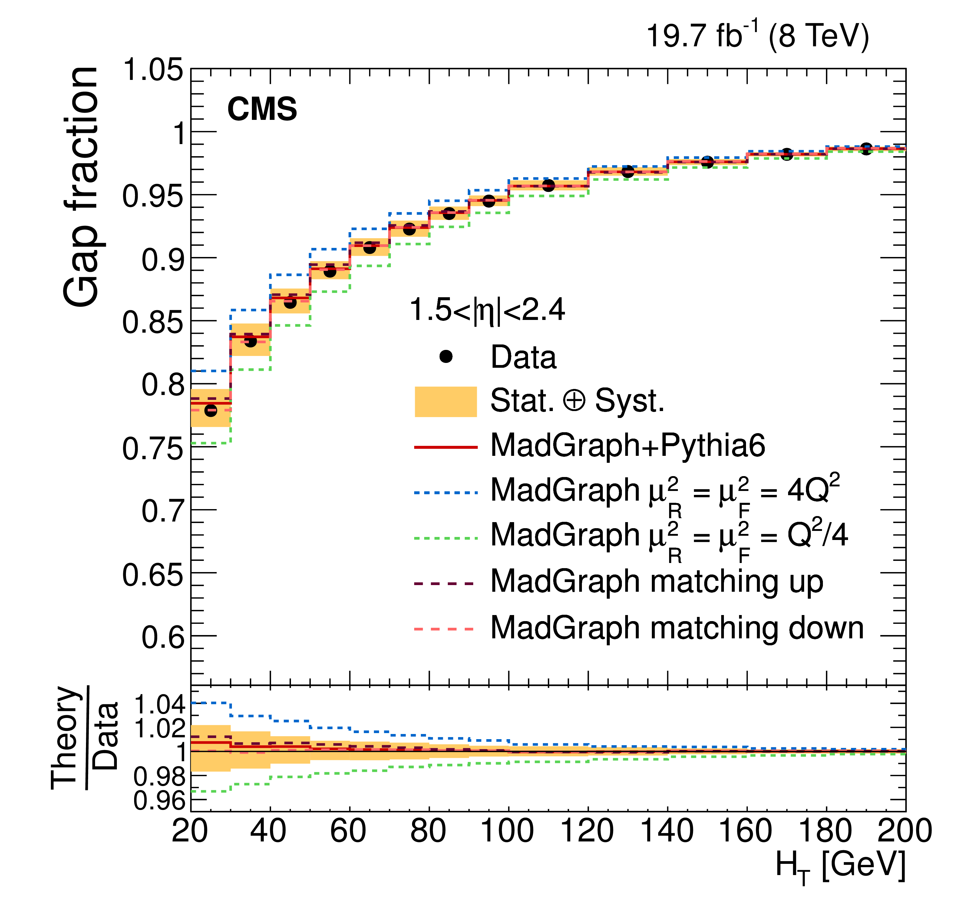
png pdf |
Figure 23-f:
Measured gap fraction as a function of $H_{\rm T}$ in different $\eta $ regions. Results in data are compared to the nominal MADGRAPH signal sample, POWHEG and MC@NLO (a,c,e) and to the samples with varied renormalization, factorization, and jet-parton matching scales (b,d,f). For each bin the threshold is defined at the value where the data point is placed. The vertical bars on the data points indicate the statistical uncertainty. The shaded band corresponds to the statistical uncertainty and the total systematic uncertainty added in quadrature. |

png pdf |
Figure 24-a:
The migration matrices relating the reconstructed level and the particle level in the visible phase space of the ${\mathrm{ t } \mathrm{ \bar{t} } } $ decay products and the additional jets for the ${p_{\mathrm {T}}}$ (a,c) and ${|\eta |}$ (b,d) of the leading (top row) and subleading (middle row) additional jets in the event, ${m_{\mathrm {jj}}}$ (c) and ${\Delta R_{\mathrm {jj}}}$ (d). The matrices are obtained from simulated ${\mathrm{ t } \mathrm{ \bar{t} } } $ events using MadGraph +PYTHIA 6. |
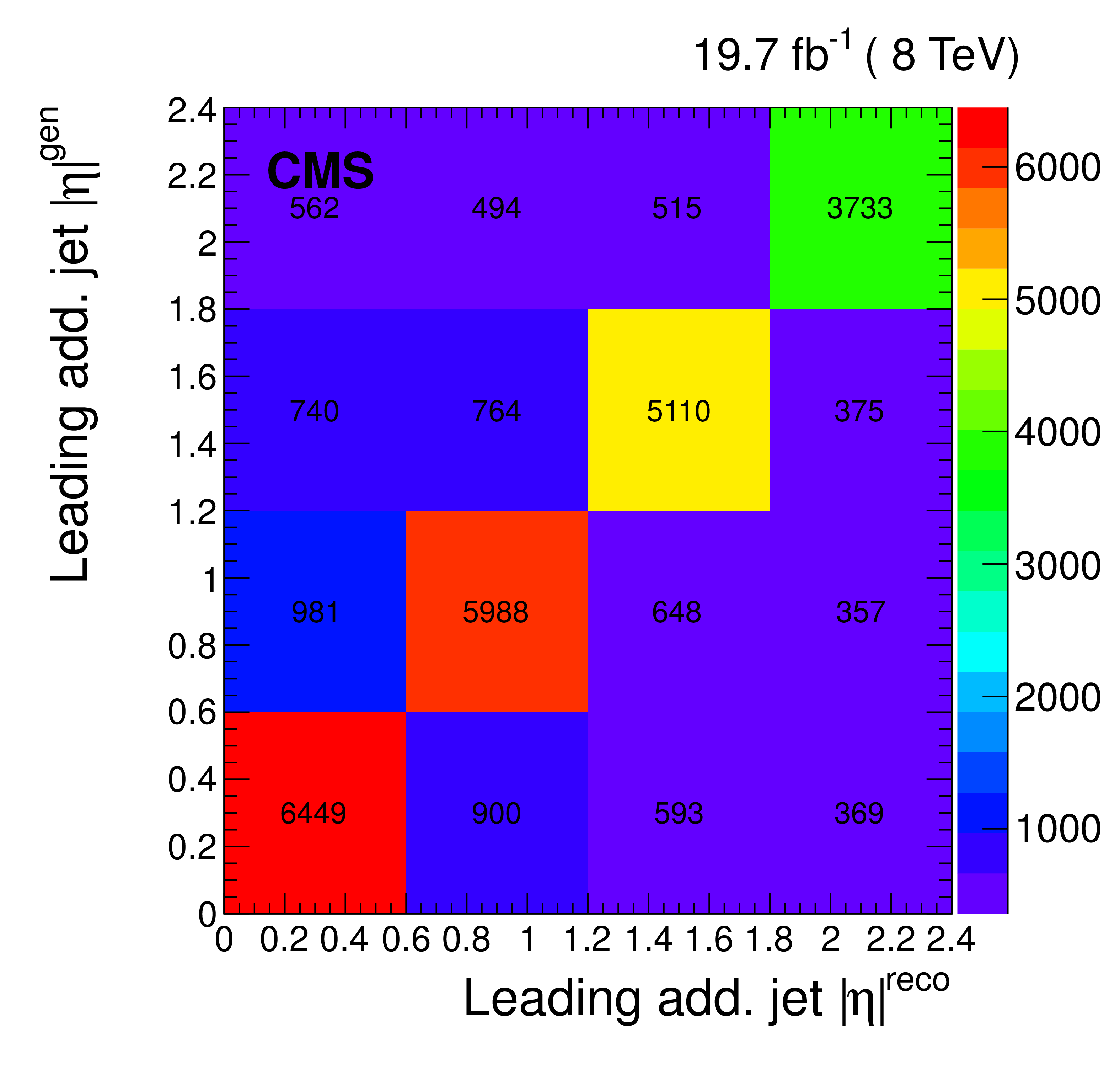
png pdf |
Figure 24-b:
The migration matrices relating the reconstructed level and the particle level in the visible phase space of the ${\mathrm{ t } \mathrm{ \bar{t} } } $ decay products and the additional jets for the ${p_{\mathrm {T}}}$ (a,c) and ${|\eta |}$ (b,d) of the leading (top row) and subleading (middle row) additional jets in the event, ${m_{\mathrm {jj}}}$ (c) and ${\Delta R_{\mathrm {jj}}}$ (d). The matrices are obtained from simulated ${\mathrm{ t } \mathrm{ \bar{t} } } $ events using MadGraph +PYTHIA 6. |

png pdf |
Figure 24-c:
The migration matrices relating the reconstructed level and the particle level in the visible phase space of the ${\mathrm{ t } \mathrm{ \bar{t} } } $ decay products and the additional jets for the ${p_{\mathrm {T}}}$ (a,c) and ${|\eta |}$ (b,d) of the leading (top row) and subleading (middle row) additional jets in the event, ${m_{\mathrm {jj}}}$ (c) and ${\Delta R_{\mathrm {jj}}}$ (d). The matrices are obtained from simulated ${\mathrm{ t } \mathrm{ \bar{t} } } $ events using MadGraph +PYTHIA 6. |

png pdf |
Figure 24-d:
The migration matrices relating the reconstructed level and the particle level in the visible phase space of the ${\mathrm{ t } \mathrm{ \bar{t} } } $ decay products and the additional jets for the ${p_{\mathrm {T}}}$ (a,c) and ${|\eta |}$ (b,d) of the leading (top row) and subleading (middle row) additional jets in the event, ${m_{\mathrm {jj}}}$ (c) and ${\Delta R_{\mathrm {jj}}}$ (d). The matrices are obtained from simulated ${\mathrm{ t } \mathrm{ \bar{t} } } $ events using MadGraph +PYTHIA 6. |
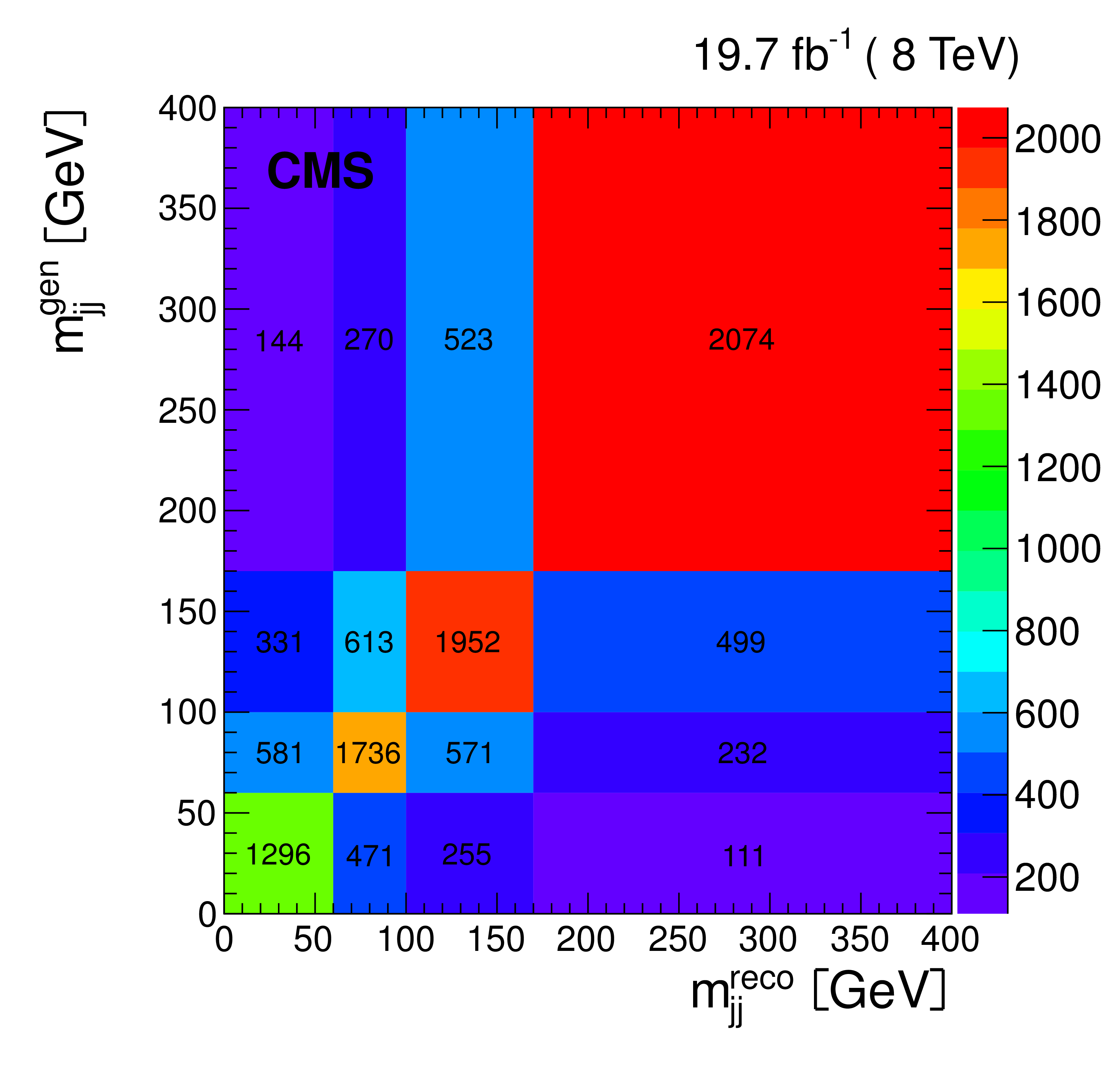
png pdf |
Figure 24-e:
The migration matrices relating the reconstructed level and the particle level in the visible phase space of the ${\mathrm{ t } \mathrm{ \bar{t} } } $ decay products and the additional jets for the ${p_{\mathrm {T}}}$ (a,c) and ${|\eta |}$ (b,d) of the leading (top row) and subleading (middle row) additional jets in the event, ${m_{\mathrm {jj}}}$ (c) and ${\Delta R_{\mathrm {jj}}}$ (d). The matrices are obtained from simulated ${\mathrm{ t } \mathrm{ \bar{t} } } $ events using MadGraph +PYTHIA 6. |
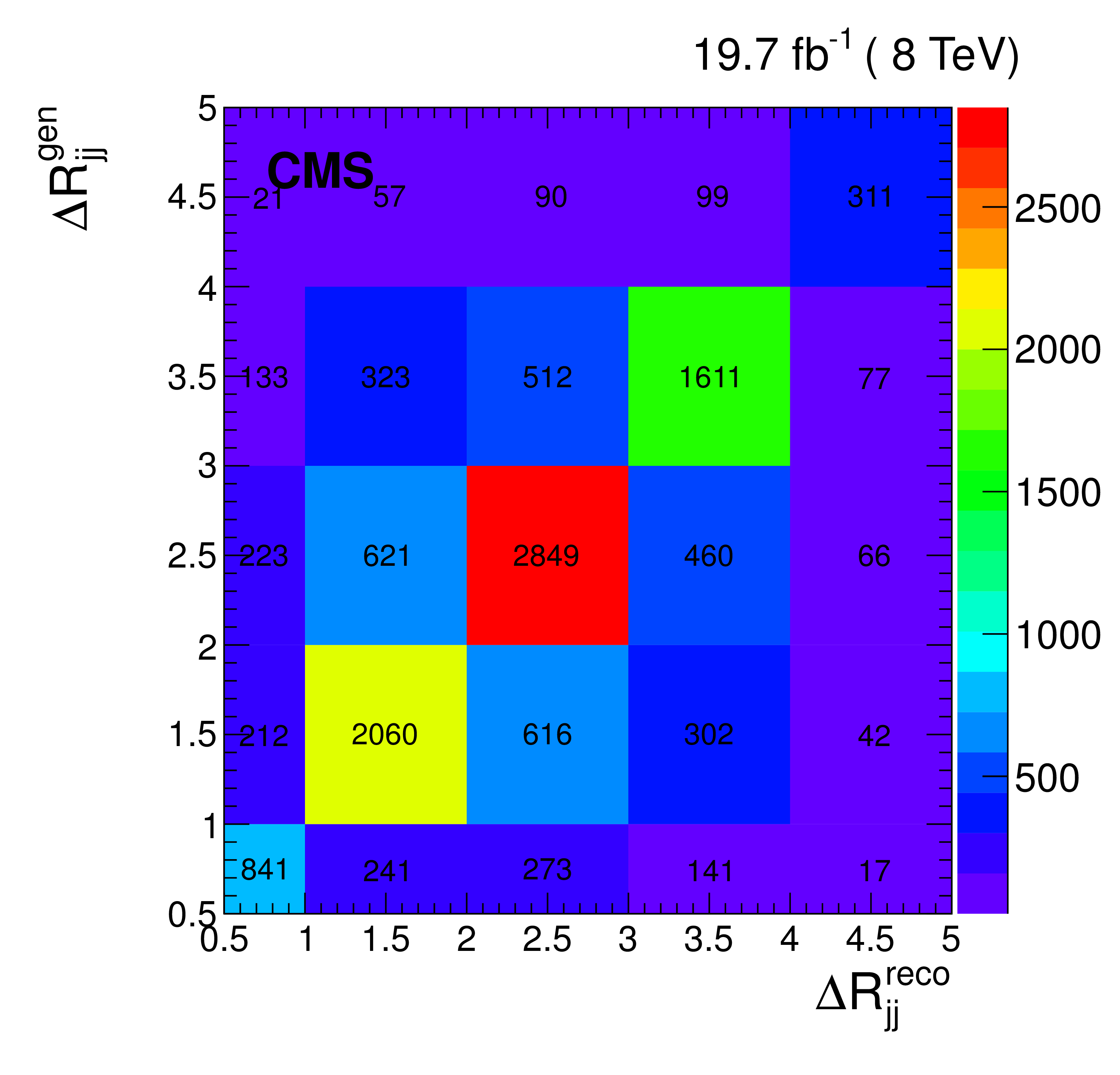
png pdf |
Figure 24-f:
The migration matrices relating the reconstructed level and the particle level in the visible phase space of the ${\mathrm{ t } \mathrm{ \bar{t} } } $ decay products and the additional jets for the ${p_{\mathrm {T}}}$ (a,c) and ${|\eta |}$ (b,d) of the leading (top row) and subleading (middle row) additional jets in the event, ${m_{\mathrm {jj}}}$ (c) and ${\Delta R_{\mathrm {jj}}}$ (d). The matrices are obtained from simulated ${\mathrm{ t } \mathrm{ \bar{t} } } $ events using MadGraph +PYTHIA 6. |

png pdf |
Figure 25-a:
The migration matrices relating the reconstructed level and the particle level in the visible phase space of the ${\mathrm{ t } \mathrm{ \bar{t} } } $ decay products and the additional jets for the ${p_{\mathrm {T}}}$ (a,c,e) and ${|\eta |}$ (b,d,f) of the leading (a,b) and subleading (c,d) additional b jets in the event, $ {m_{\mathrm{ b } \mathrm{ b } }} $ (e), and $ {\Delta R}_{{\mathrm{ b } \mathrm{ b } }}$ (f). The matrices are obtained from simulated ${\mathrm{ t } \mathrm{ \bar{t} } } $ events using MadGraph +PYTHIA 6. |
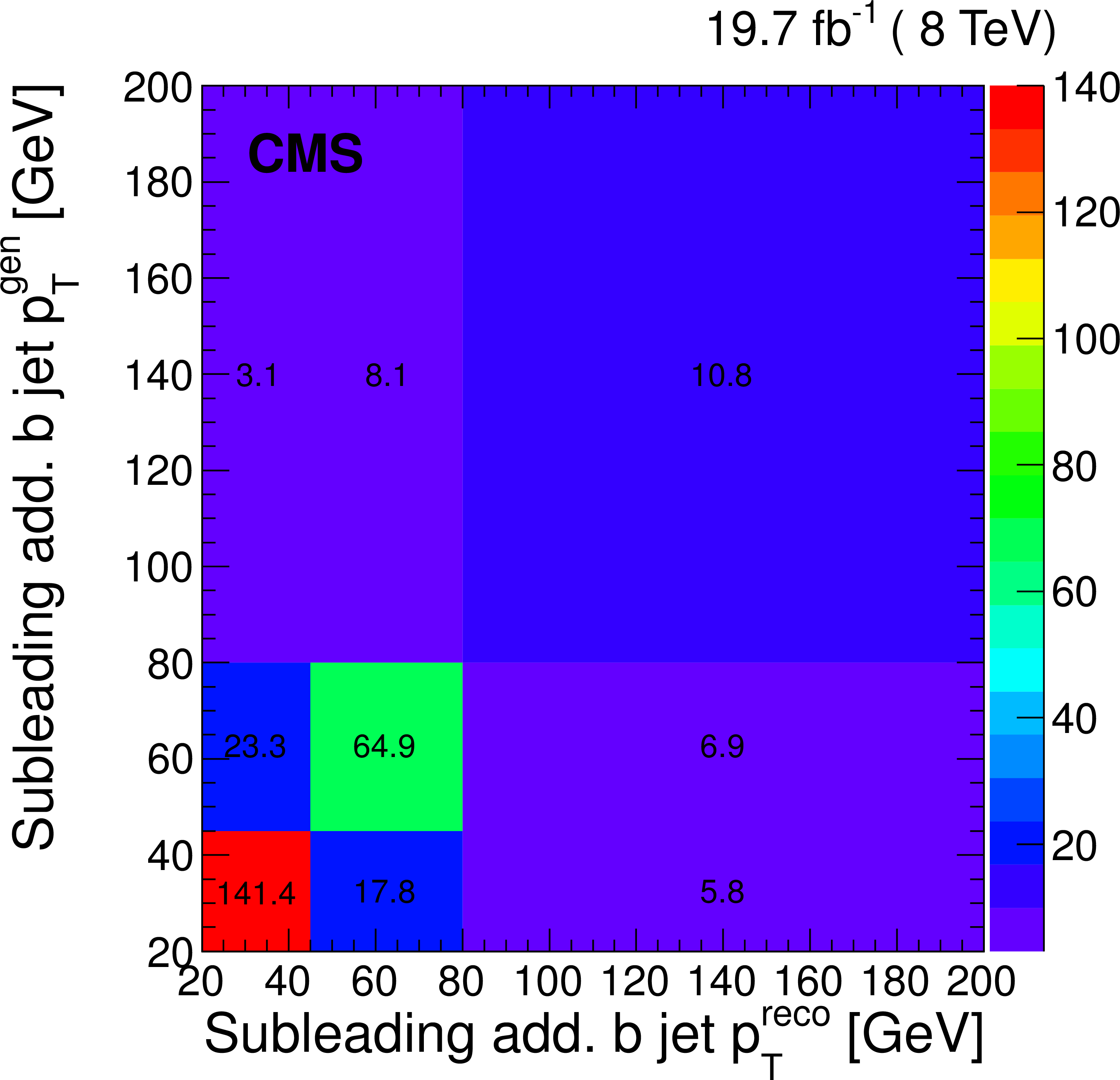
png pdf |
Figure 25-b:
The migration matrices relating the reconstructed level and the particle level in the visible phase space of the ${\mathrm{ t } \mathrm{ \bar{t} } } $ decay products and the additional jets for the ${p_{\mathrm {T}}}$ (a,c,e) and ${|\eta |}$ (b,d,f) of the leading (a,b) and subleading (c,d) additional b jets in the event, $ {m_{\mathrm{ b } \mathrm{ b } }} $ (e), and $ {\Delta R}_{{\mathrm{ b } \mathrm{ b } }}$ (f). The matrices are obtained from simulated ${\mathrm{ t } \mathrm{ \bar{t} } } $ events using MadGraph +PYTHIA 6. |
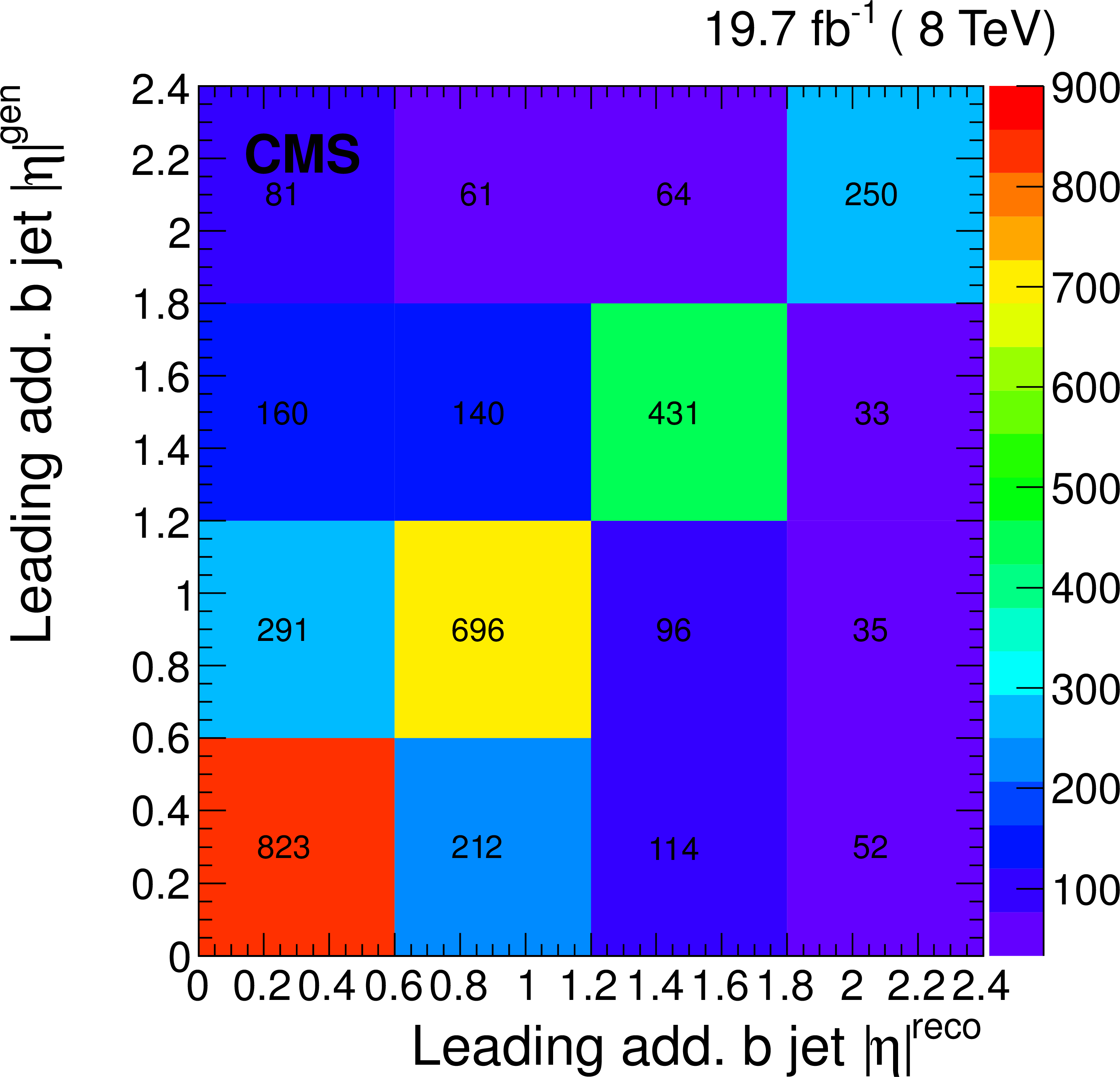
png pdf |
Figure 25-c:
The migration matrices relating the reconstructed level and the particle level in the visible phase space of the ${\mathrm{ t } \mathrm{ \bar{t} } } $ decay products and the additional jets for the ${p_{\mathrm {T}}}$ (a,c,e) and ${|\eta |}$ (b,d,f) of the leading (a,b) and subleading (c,d) additional b jets in the event, $ {m_{\mathrm{ b } \mathrm{ b } }} $ (e), and $ {\Delta R}_{{\mathrm{ b } \mathrm{ b } }}$ (f). The matrices are obtained from simulated ${\mathrm{ t } \mathrm{ \bar{t} } } $ events using MadGraph +PYTHIA 6. |
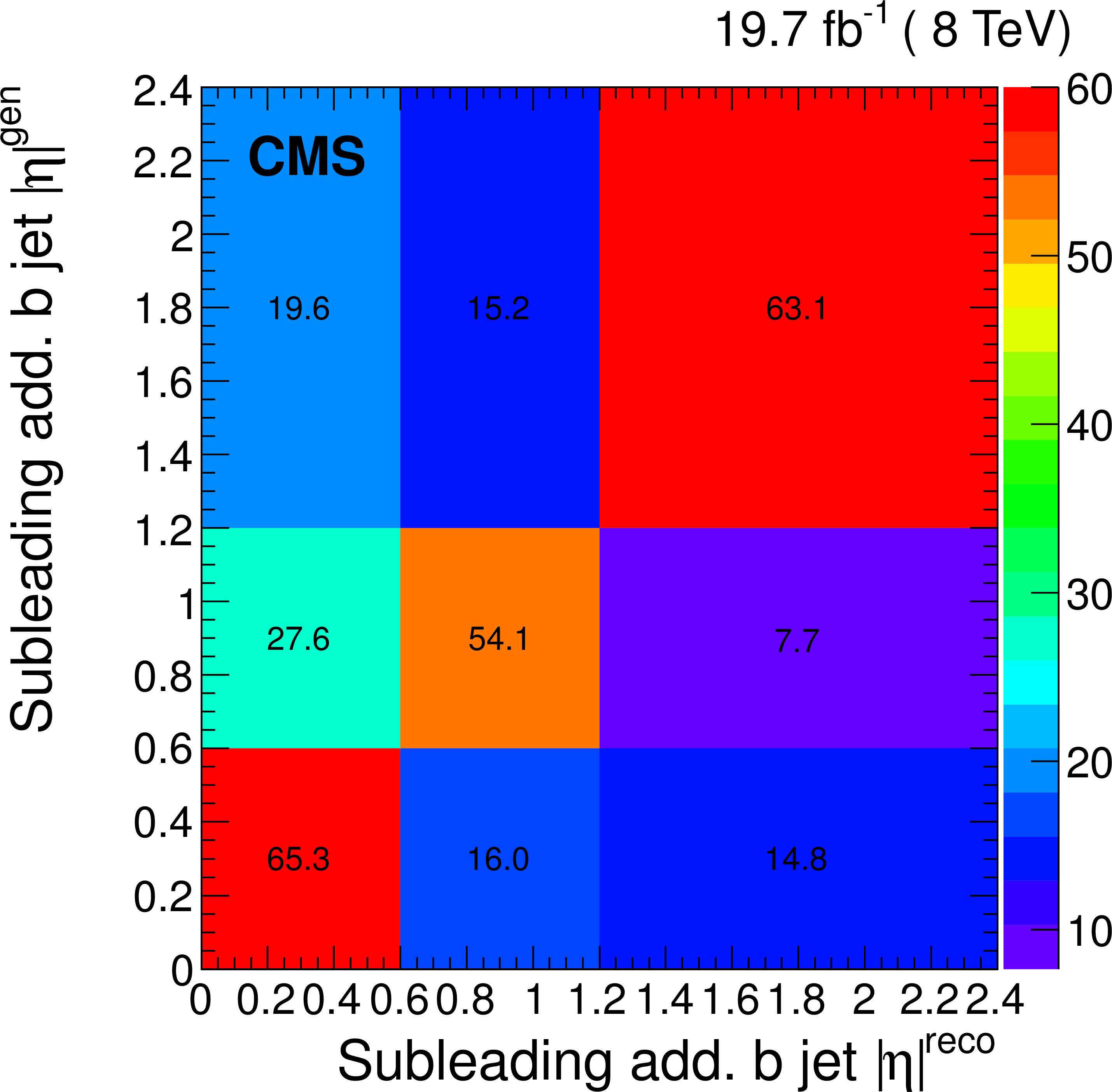
png pdf |
Figure 25-d:
The migration matrices relating the reconstructed level and the particle level in the visible phase space of the ${\mathrm{ t } \mathrm{ \bar{t} } } $ decay products and the additional jets for the ${p_{\mathrm {T}}}$ (a,c,e) and ${|\eta |}$ (b,d,f) of the leading (a,b) and subleading (c,d) additional b jets in the event, $ {m_{\mathrm{ b } \mathrm{ b } }} $ (e), and $ {\Delta R}_{{\mathrm{ b } \mathrm{ b } }}$ (f). The matrices are obtained from simulated ${\mathrm{ t } \mathrm{ \bar{t} } } $ events using MadGraph +PYTHIA 6. |
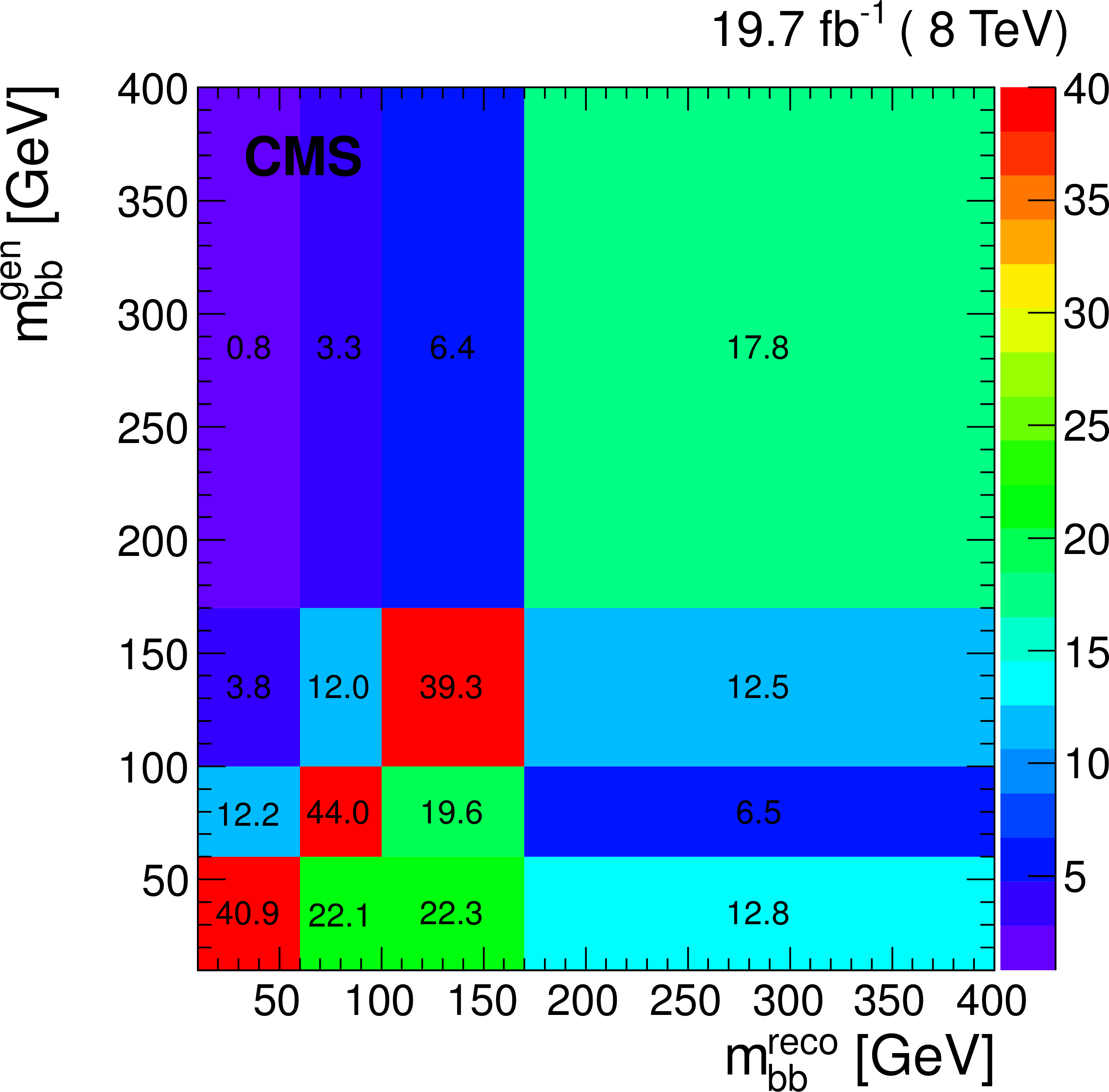
png pdf |
Figure 25-e:
The migration matrices relating the reconstructed level and the particle level in the visible phase space of the ${\mathrm{ t } \mathrm{ \bar{t} } } $ decay products and the additional jets for the ${p_{\mathrm {T}}}$ (a,c,e) and ${|\eta |}$ (b,d,f) of the leading (a,b) and subleading (c,d) additional b jets in the event, $ {m_{\mathrm{ b } \mathrm{ b } }} $ (e), and $ {\Delta R}_{{\mathrm{ b } \mathrm{ b } }}$ (f). The matrices are obtained from simulated ${\mathrm{ t } \mathrm{ \bar{t} } } $ events using MadGraph +PYTHIA 6. |
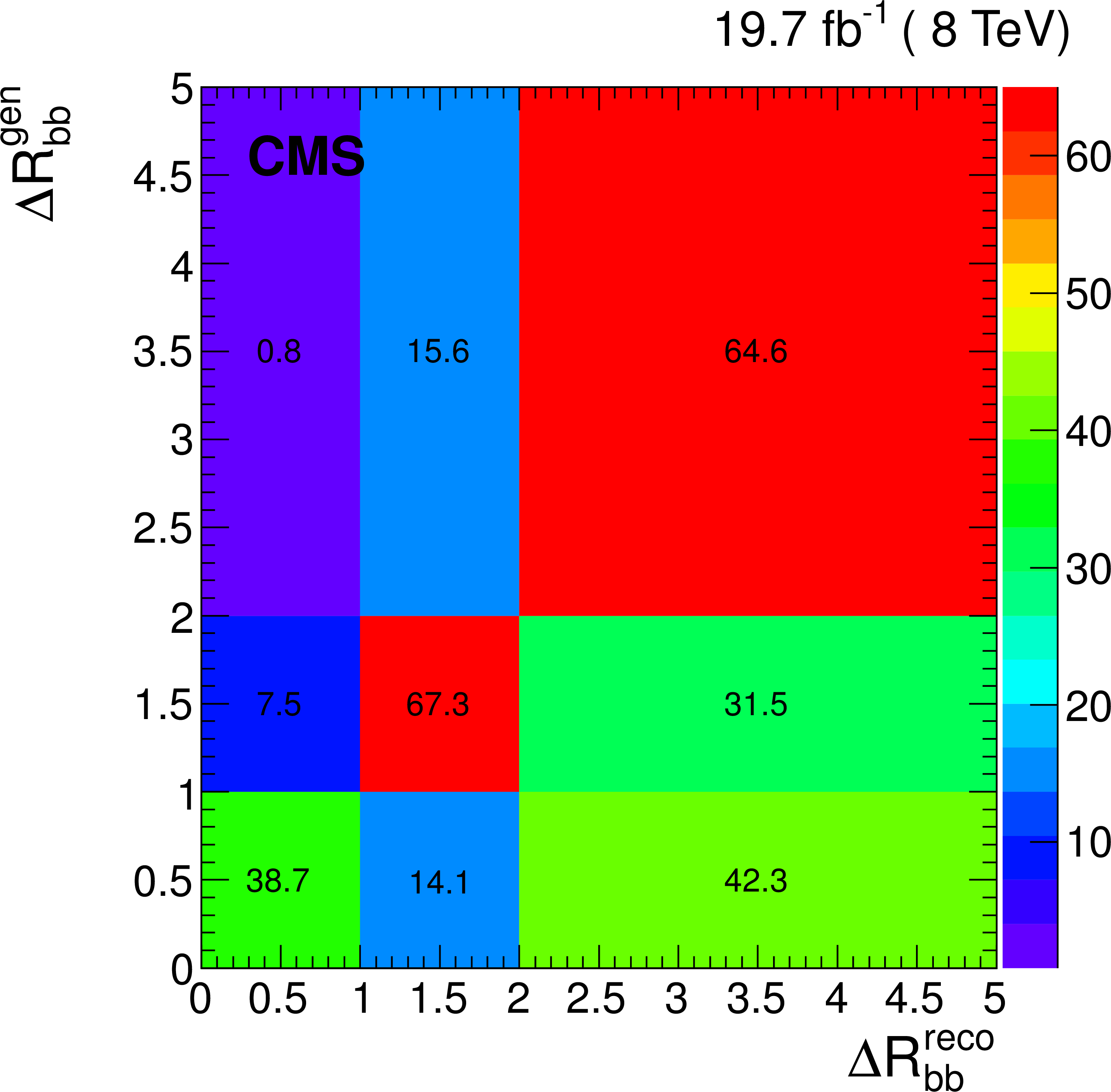
png pdf |
Figure 25-f:
The migration matrices relating the reconstructed level and the particle level in the visible phase space of the ${\mathrm{ t } \mathrm{ \bar{t} } } $ decay products and the additional jets for the ${p_{\mathrm {T}}}$ (a,c,e) and ${|\eta |}$ (b,d,f) of the leading (a,b) and subleading (c,d) additional b jets in the event, $ {m_{\mathrm{ b } \mathrm{ b } }} $ (e), and $ {\Delta R}_{{\mathrm{ b } \mathrm{ b } }}$ (f). The matrices are obtained from simulated ${\mathrm{ t } \mathrm{ \bar{t} } } $ events using MadGraph +PYTHIA 6. |
| Tables | |
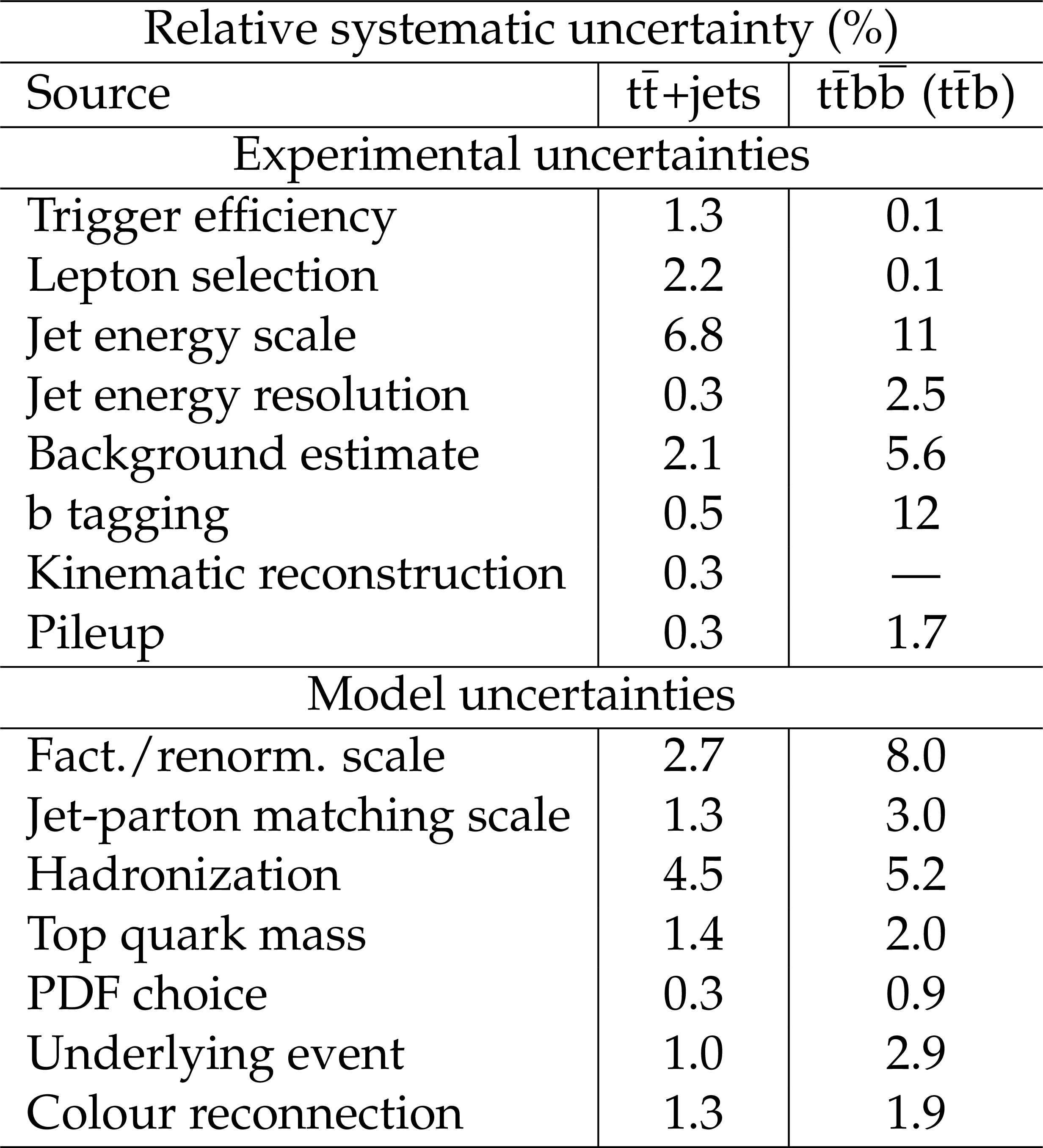
png pdf |
Table 1:
Summary of the typical systematic uncertainties in the measurements of the ${\mathrm{ t } \mathrm{ \bar{t} } } $+jets and ${\mathrm{ t \bar{t} } \mathrm{ b \bar{b} } }$ ($ {\mathrm{ t \bar{t} } \mathrm{ b } } $) absolute differential cross sections and their sources. The median of the distribution of uncertainties over all bins of each measured differential cross section is quoted. |
| Summary |
|
Measurements of the absolute and normalized differential top quark pair production cross sections have been presented using pp collisions at a centre-of-mass energy of 8 TeV, corresponding to an integrated luminosity of 19.7 fb$^{-1}$, in the dilepton decay channel as a function of the number of jets in the event, for three different jet $p_{\mathrm{T}}$ thresholds, and as a function of the kinematic variables of the leading and subleading additional jets. The results have been compared to the predictions from MadGraph interfaced with PYTHIA6, POWHEG interfaced with both PYTHIA6 and HERWIG6, MC interfaced with HERWIG6, and MadGraph samples with varied renormalization, factorization, and jet-parton matching scales. In general, all these generators are found to give a reasonable description of the data. The MadGraph and POWHEG generators interfaced with PYTHIA6 describe the data well for all measured jet multiplicities; while MC interfaced with HERWIG6 generates lower multiplicities than observed for the lower-$p_{\mathrm{T}}$ thresholds. The prediction from MadGraph with varied renormalization and factorization scales does not provide an improved description of the data compared to the nominal simulation. These results are also compared to the predictions from POWHEG with the hdamp parameter set to the top quark mass interfaced with PYTHIA6, PYTHIA8, and HERWIG6, which provide a reasonable description of the data within the uncertainties, and the predictions from MadGraph and MG5-aMC@NLO interfaced with PYTHIA8, which generate higher jet multiplicities for all the $p_{\mathrm{T}}$ thresholds. The measured kinematic variables of the leading and subleading additional jets are consistent with the various predictions. The simulations also describe well the data distributions of the leading additional jet $p_{\mathrm{T}}$ and $H_{\mathrm{T}}$, although they tend to predict higher $p_{\mathrm{T}}$ values and more central values in $\eta$. MadGraph with varied parameters yields similar predictions, except for varying the renormalization and factorization scales, which tends to give higher $H_{\mathrm{T}}$ values. The MC generator predicts lower yields than observed for the subleading additional jet $p_{\mathrm{T}}$. The uncertainties in the measured $\mathrm{ t }\mathrm{ \bar{t} } \mathrm{ b }\mathrm{ \bar{ b} }$ ($\mathrm{ t }\mathrm{ \bar{t} }\mathrm{ b }$) absolute and normalized differential cross sections as a function of the b jet kinematic variables are dominated by the statistical uncertainties. In general, the predictions describe well the shape of the measured cross sections as a function of the variables studied, except for $\Delta R_{\mathrm{ b }\mathrm{ b }}$, where they favour smaller values than the measurement. The predictions underestimate the total $\mathrm{ t }\mathrm{ \bar{t} }\mathrm{ b } \mathrm{ \bar{b} }$ cross section by approximately a factor of 2, in agreement with previous measurements [11]. The calculation by PowHel [19] describes well the shape of the distributions, while the predicted absolute cross section is about 30% lower, but compatible with the measurements within the uncertainties. The gap fraction has been measured as a function of the $p_{\mathrm{T}}$ of the leading and subleading additional jets and $H_{\mathrm{T}}$ of the additional jets in different $\eta$ ranges. For a given threshold value, the gap fraction as a function of $H_{\mathrm{T}}$ is lower than the gap fraction as a function of the $p_{\mathrm{T}}$ of the leading additional jet, showing that the measurement is probing multiple quark and gluon emission. Within the uncertainties, all predictions describe the gap fraction well as a function of the momentum of the first additional jet, while MC interfaced with HERWIG fails to describe the gap fraction as a function of the subleading additional jet $p_{\mathrm{T}}$ and $H_{\mathrm{T}}$. In general, MadGraph with decreased renormalization and factorization scales more poorly describes the observed gap fraction, while varying the jet-parton matching threshold provides a similar description of the data. The MadGraph and MG5\_aMC@NLO generators interfaced with PYTHIA8 predict lower values than measured. The POWHEG simulation with HDAMP $= m_{\mathrm{ t }}$ interfaced with PYTHIA8 is consistent with the data, while the simulation interfaced with HERWIG6 and PYTHIA6 tends to worsen the comparison with the measurement. In general, the different measurements presented are in agreement with the SM predictions as formulated by the various event generators, within their uncertainties. The correct description of $\mathrm{ t \bar{t} }$+jets production is important since it constitutes a major background in searches for new particles in several supersymmetric models and in ${\mathrm{ t }\mathrm{ \bar{t} }\mathrm{ H }}$ processes, where the Higgs boson decays into $\mathrm{ b \bar{b} }$. The $\mathrm{ t }\mathrm{ \bar{t} }\mathrm{ b } \mathrm{ \bar{b} }$ ($\mathrm{ t }\mathrm{ \bar{t} }\mathrm{ b }$) differential cross sections, measured here for the first time, also provide important information about the main irreducible background in the search for ${\mathrm{ t }\mathrm{ \bar{t} }\mathrm{ H }\,(\mathrm{ b }\mathrm{ \bar{b} })} $. |
| Additional Figures | |
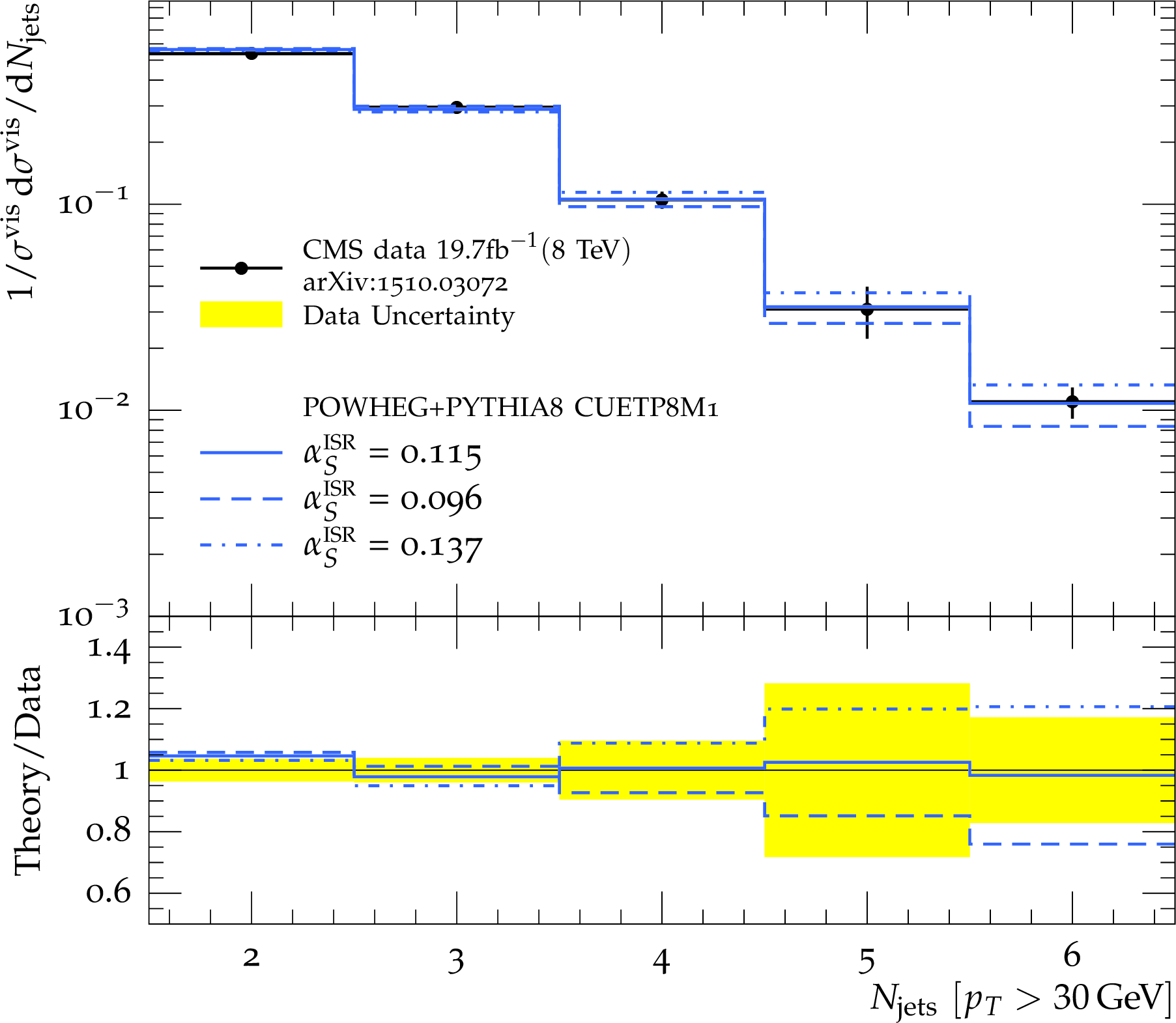
png pdf |
Additional Figure 1:
Results of $\alpha _s^{ISR}$ tuning. Jet multiplicity distribution, $N_{\text{jets}}$ (with $p_T^{jet}>$ 30 GeV), after tuning $\alpha _s^{ISR}$ with the $N_{\text{jets}}> $ 3 bins (where jets predominantly originate from the parton shower) is used as input to Professor [A. Buckley et al., Eur. Phys. J. C65 (2010) 331]. The unfolded CMS data are shown with total error bars. In each plot, the calculated distribution assuming the tuned $\alpha _s^{ISR}$ is shown with a solid line. The calculated distributions with the lower bound (dashed line) and the upper bound (dot-dashed line) of the tuned $\alpha _s^{ISR}$ are also displayed. Beneath each plot is shown the ratio of theory predictions to data. The yellow bands indicate the total data uncertainty. |
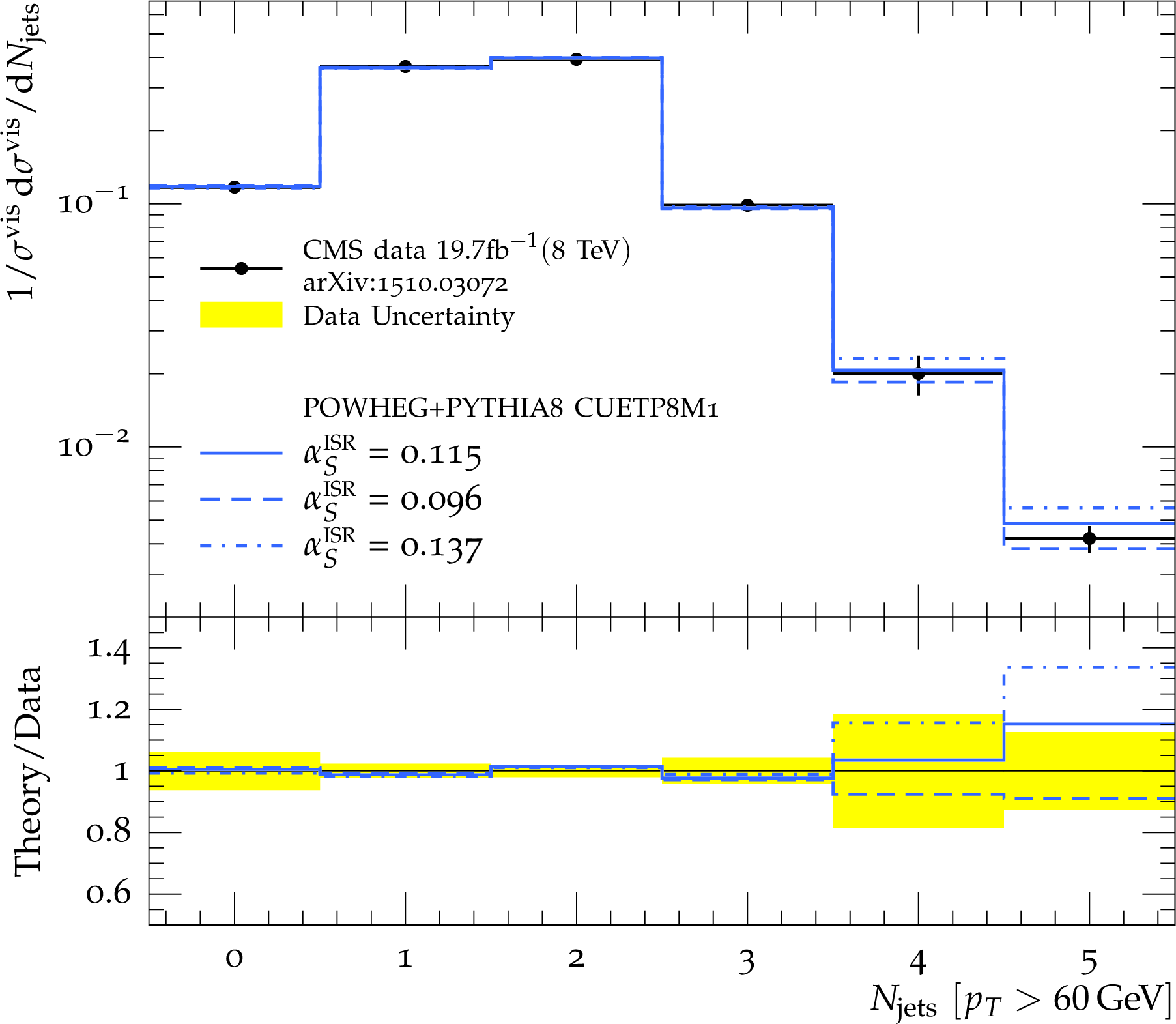
png pdf |
Additional Figure 2:
Results of $\alpha _s^{ISR}$ tuning. Jet multiplicity distribution, $N_{\text{jets}}$ (with $p_T^{jet}>$ 30 GeV), after tuning $\alpha _s^{ISR}$ with the $N_{\text{jets}}> $ 3 bins (where jets predominantly originate from the parton shower) is used as input to Professor [A. Buckley et al., Eur. Phys. J. C65 (2010) 331]. The unfolded CMS data are shown with total error bars. In each plot, the calculated distribution assuming the tuned $\alpha _s^{ISR}$ is shown with a solid line. The calculated distributions with the lower bound (dashed line) and the upper bound (dot-dashed line) of the tuned $\alpha _s^{ISR}$ are also displayed. Beneath each plot is shown the ratio of theory predictions to data. The yellow bands indicate the total data uncertainty. |

png pdf |
Additional Figure 3:
Results of $\alpha _s^{ISR}$ tuning. Jet multiplicity distribution, $N_{\text{jets}}$ (with $p_T^{jet}>$ 30 GeV), after tuning $\alpha _s^{ISR}$ with the $N_{\text{jets}}> $ 3 bins (where jets predominantly originate from the parton shower) is used as input to Professor [A. Buckley et al., Eur. Phys. J. C65 (2010) 331]. The unfolded CMS data are shown with total error bars. In each plot, the calculated distribution assuming the tuned $\alpha _s^{ISR}$ is shown with a solid line. The calculated distributions with the lower bound (dashed line) and the upper bound (dot-dashed line) of the tuned $\alpha _s^{ISR}$ are also displayed. Beneath each plot is shown the ratio of theory predictions to data. The yellow bands indicate the total data uncertainty. |
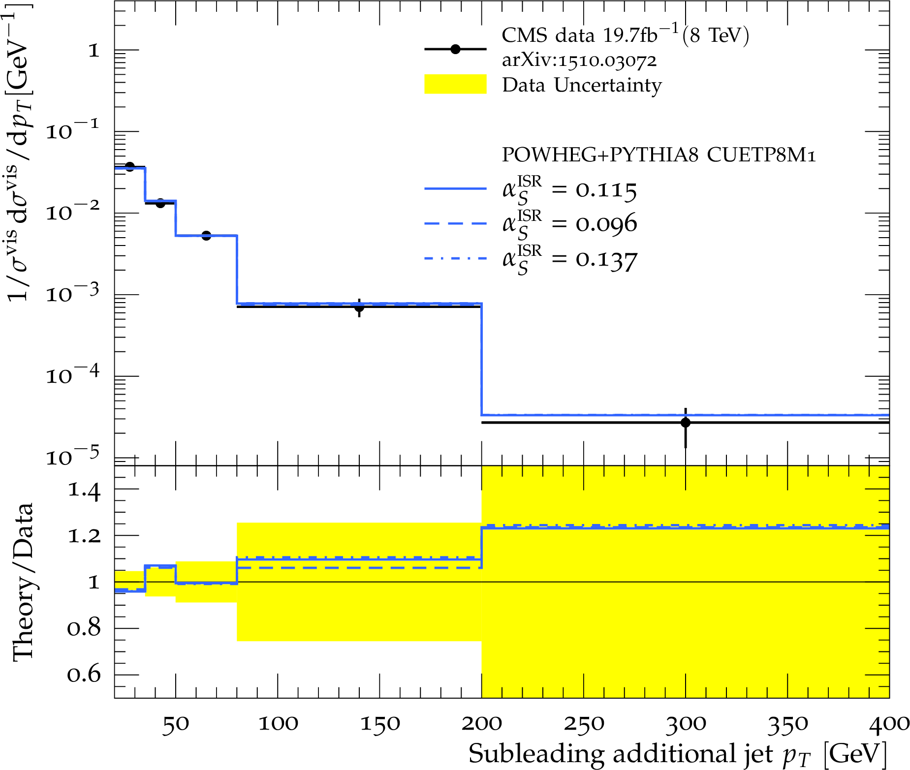
png pdf |
Additional Figure 4:
Results of $\alpha _s^{ISR}$ tuning. Jet multiplicity distribution, $N_{\text{jets}}$ (with $p_T^{jet}>$ 30 GeV), after tuning $\alpha _s^{ISR}$ with the $N_{\text{jets}}> $ 3 bins (where jets predominantly originate from the parton shower) is used as input to Professor [A. Buckley et al., Eur. Phys. J. C65 (2010) 331]. The unfolded CMS data are shown with total error bars. In each plot, the calculated distribution assuming the tuned $\alpha _s^{ISR}$ is shown with a solid line. The calculated distributions with the lower bound (dashed line) and the upper bound (dot-dashed line) of the tuned $\alpha _s^{ISR}$ are also displayed. Beneath each plot is shown the ratio of theory predictions to data. The yellow bands indicate the total data uncertainty. |
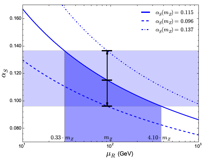
png pdf |
Additional Figure 5:
$\alpha _s$ as a function of the renormalization scale, $\mu _R$. The uncertainty on the tuned $\alpha _s$ value (0.115) corresponds to variations of $\mu _R$ by factors of 0.33 for the upper bound and 4.1 for the lower bound. |
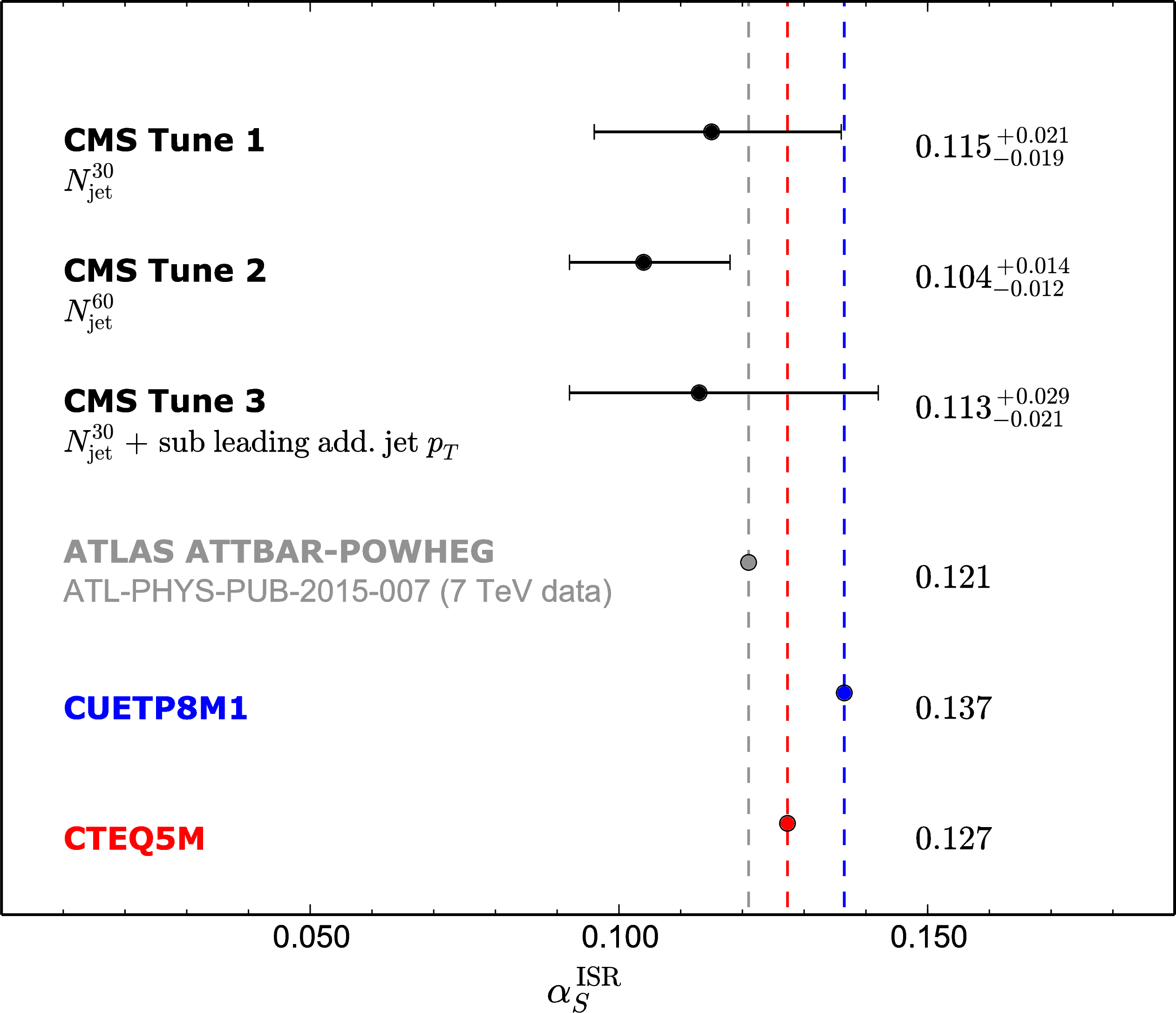
png pdf |
Additional Figure 6:
Summary of tune results and their uncertainties. Two alternative tunes are presented in addition to the previously described one. The input distribution(s) for each tune is indicated below the label of each tune. The $\alpha _s^{ISR}$ values in the ATLAS ATTBAR-POWHEG tune for PYTHIA8, the CMS CUETP8M1 tune for PYTHIA8 (CMS default in Run II), and the CMS Z2* PYTHIA6 tune (CMS default in Run I), using the CTEQ5M PDF set, are also displayed. |
| References | ||||
| 1 | CMS Collaboration | Measurement of the $ \mathrm{ t \bar{t} } $ production cross section in the dilepton channel in pp collisions at $ \sqrt{s} = $ 8 TeV | JHEP 02 (2014) 024, , [Erratum: \DOI10.1007/JHEP02(2014)102] | CMS-TOP-12-007 1312.7582 |
| 2 | ATLAS Collaboration | Measurement of the $ t\bar{t} $ production cross-section using $ e \mu $ events with $ b $-tagged jets in $ pp $ collisions at $ \sqrt{s}=7 $ and $ 8 TeV $ with the ATLAS detector | EPJC 74 (2014) 3109 | 1406.5375 |
| 3 | CMS Collaboration | Measurement of differential top-quark pair production cross sections in $ \mathrm{pp} $ collisions at $ \texorpdfstring $$ \sqrt{s} = $ 7 TeVsqrt(s) = 7 TeV | EPJC 73 (2013) 2339 | CMS-TOP-11-013 1211.2220 |
| 4 | ATLAS Collaboration | Measurements of top quark pair relative differential cross-sections with ATLAS in $ pp $ collisions at $ \sqrt{s} = $ 7 TeV | EPJC 73 (2013) 2261 | 1207.5644 |
| 5 | CMS Collaboration | Measurement of jet multiplicity distributions in $ \mathrm{ t \bar{t} } $ production in $ \mathrm{pp} $ collisions at $ \sqrt{s} = $ 7 TeV | EPJC 74 (2014) 3014 | CMS-TOP-12-018 1404.3171 |
| 6 | ATLAS Collaboration | Measurements of normalized differential cross-sections for $ t\bar{t} $ production in $ pp $ collisions at $ \sqrt{s} = $ 7 TeV using the ATLAS detector | PRD 90 (2014) 072004 | 1407.0371 |
| 7 | ATLAS Collaboration | Measurements of the production cross-section as a function of jet multiplicity and jet transverse momentum in 7 TeV proton-proton collisions with the ATLAS detector | JHEP 01 (2015) 020 | 1407.0891 |
| 8 | CMS Collaboration | Measurement of the differential cross section for top quark pair production cross section in $ \mathrm{pp} $ collisions at $ \sqrt{s} $ = 8 TeV | EPJC 75 (2015) 542 | CMS-TOP-12-028 1505.04480 |
| 9 | ATLAS Collaboration | Measurement of the top pair production cross section in 8 TeV proton-proton collisions using kinematic information in the lepton+jets final state with ATLAS | PRD 91 (2015) 112013 | 1504.04251 |
| 10 | CMS Collaboration | The CMS experiment at the CERN LHC | JINST 3 (2008) S08004 | CMS-00-001 |
| 11 | CMS Collaboration | Measurement of the cross section ratio $ \sigma_{\mathrm{t\bar{t}b\bar{b}}}/\sigma_{\mathrm{t\bar{t}jj}} $ in $ \mathrm{pp} $ collisions at $ \sqrt{s} = $ 8 TeV | PLB 746 (2015) 132 | CMS-TOP-13-010 1411.5621 |
| 12 | ATLAS Collaboration | Measurement of $ t\bar{t} $ production with a veto on additional central jet activity in $ pp $ collisions at $ \sqrt{s} = $ 7 TeV using the ATLAS detector | EPJC 72 (2012) 2043 | 1203.5015 |
| 13 | J. Alwall et al. | MadGraph v5: going beyond | JHEP 06 (2011) 128 | 1106.0522 |
| 14 | S. Frixione and B. R. Webber | Matching NLO QCD computations and parton shower simulations | JHEP 06 (2002) 029 | hep-ph/0204244 |
| 15 | S. Frixione, P. Nason, and C. Oleari | Matching NLO QCD computations with Parton Shower simulations: the POWHEG method | JHEP 11 (2007) 070 | 0709.2092 |
| 16 | J. Alwall et al. | The automated computation of tree-level and next-to-leading order differential cross sections, and their matching to parton shower simulations | JHEP 07 (2014) 079 | 1405.0301 |
| 17 | T. Sj\"ostrand, S. Mrenna, and P. Z. Skands | PYTHIA 6.4 physics and manual | JHEP 05 (2006) 026 | hep-ph/0603175 |
| 18 | G. Corcella et al. | HERWIG 6: An event generator for hadron emission reactions with interfering gluons (including supersymmetric processes) | JHEP 01 (2001) 010 | hep-ph/0011363 |
| 19 | M. V. Garzelli, A. Kardos, and Z. Tr\'ocs\'anyi | Hadroproduction of $ t\bar{t}b\bar{b} $ final states at LHC: predictions at NLO accuracy matched with parton shower | JHEP 03 (2015) 083 | 1408.0266 |
| 20 | GEANT4 Collaboration | GEANT4--A simulation toolkit | NIMA 506 (2003) 250 | |
| 21 | P. Artoisenet, R. Frederix, O. Mattelaer, and R. Rietkerk | Automatic spin-entangled decays of heavy resonances in Monte Carlo simulations | JHEP 03 (2013) 015 | 1212.3460 |
| 22 | J. Pumplin et al. | New generation of parton distributions with uncertainties from global QCD analysis | JHEP 07 (2002) 012 | hep-ph/0201195 |
| 23 | M. L. Mangano, M. Moretti, F. Piccinini, and M. Treccani | Matching matrix elements and shower evolution for top-quark production in hadronic collisions | JHEP 01 (2007) 013 | hep-ph/0611129 |
| 24 | R. Field | Early LHC Underlying Event Data - Findings and Surprises | in Hadron collider physics. Proceedings, 22nd Conference, HCP 2010, Toronto, Canada, August 23-27, 2010 2010 | 1010.3558 |
| 25 | H.-L. Lai et al. | New parton distributions for collider physics | PRD 82 (2010) 074024 | 1007.2241 |
| 26 | ATLAS Collaboration | ATLAS tunes of PYTHIA 6 and PYTHIA 8 for MC11 | Technical Report ATL-PHYS-PUB-2011-009 | |
| 27 | R. Astalos et al. | Proceedings of the sixth international workshop on multiple partonic interactions at the Large Hadron Collider | 1506.05829 | |
| 28 | R. Frederix and S. Frixione | Merging meets matching in MC@NLO | JHEP 12 (2012) 061 | 1209.6215 |
| 29 | NNPDF Collaboration | Parton distributions for the LHC Run II | JHEP 04 (2015) 040 | 1410.8849 |
| 30 | G. Bevilacqua et al. | HELAC-NLO | CPC 184 (2013) 986 | 1110.1499 |
| 31 | S. Alioli, P. Nason, C. Oleari, and E. Re | A general framework for implementing NLO calculations in shower Monte Carlo programs: the POWHEG BOX | JHEP 06 (2010) 043 | 1002.2581 |
| 32 | P. Nason | A new method for combining NLO QCD with shower Monte Carlo algorithms | JHEP 11 (2004) 040 | hep-ph/0409146 |
| 33 | P. Z. Skands | Tuning Monte Carlo generators: The Perugia tunes | PRD 82 (2010) 074018 | 1005.3457 |
| 34 | K. Melnikov and F. Petriello | The $ W $ boson production cross section at the LHC through $ O(\alpha^2_s) $ | PRL 96 (2006) 231803 | hep-ph/0603182 |
| 35 | K. Melnikov and F. Petriello | Electroweak gauge boson production at hadron colliders through $ O(\alpha^2_s) $ | PRD 74 (2006) 114017 | hep-ph/0609070 |
| 36 | N. Kidonakis | Two-loop soft anomalous dimensions for single top quark associated production with W$ ^- $ or H$ ^- $ | PRD 82 (2010) 054018 | hep-ph/1005.4451 |
| 37 | J. M. Campbell, R. K. Ellis, and C. Williams | Vector boson pair production at the LHC | JHEP 07 (2011) 018 | 1105.0020 |
| 38 | M. V. Garzelli, A. Kardos, C. Papadopoulos, and Z. Tr\'ocs\'anyi | $ t \bar{t} W^{\pm} $ + $ t \bar{t} Z $ hadroproduction at NLO accuracy in QCD with parton shower and hadronization effects | JHEP 11 (2012) 056 | 1208.2665 |
| 39 | S. Heinemeyer et al. | Handbook of LHC Higgs cross sections: 3. Higgs properties | CERN Report CERN-2013-004 | 1307.1347 |
| 40 | W. Kilian, T. Ohl, and J. Reuter | WHIZARD: Simulating multi-particle processes at LHC and ILC | EPJC 71 (2011) 1742 | hep-ph/9905386 |
| 41 | K. Melnikov, M. Schulze, and A. Scharf | QCD corrections to top quark pair production in association with a photon at hadron colliders | PRD 83 (2011) 074013 | 1102.1967 |
| 42 | M. Czakon and A. Mitov | Top++: A program for the calculation of the top-pair cross-section at hadron colliders | CPC 185 (2014) 2930 | 1112.5675 |
| 43 | M. Botje et al. | The PDF4LHC Working Group interim recommendations | 1101.0538 | |
| 44 | S. Alekhin et al. | The PDF4LHC Working Group interim report | 1101.0536 | |
| 45 | A. D. Martin, W. J. Stirling, R. S. Thorne, and G. Watt | Uncertainties on $ \alpha_s $ in global PDF analyses and implications for predicted hadronic cross sections | EPJC 64 (2009) 653 | 0905.3531 |
| 46 | J. Gao et al. | CT10 next-to-next-to-leading order global analysis of QCD | PRD 89 (2014) 033009 | 1302.6246 |
| 47 | NNPDF Collaboration | Parton distributions with LHC data | Nucl. Phys. B 867 (2013) 244 | 1207.1303 |
| 48 | CMS Collaboration | Commissioning of the particle-flow event reconstruction with the first LHC collisions recorded in the CMS detector | CDS | |
| 49 | CMS Collaboration | Particle-flow event reconstruction in CMS and performance for jets, taus, and MET | CDS | |
| 50 | CMS Collaboration | Description and performance of track and primary-vertex reconstruction with the CMS tracker | JINST 9 (2014) P10009 | CMS-TRK-11-001 1405.6569 |
| 51 | M. Cacciari, G. P. Salam, and G. Soyez | The catchment area of jets | JHEP 04 (2008) 005 | 0802.1188 |
| 52 | CMS Collaboration | Performance of CMS muon reconstruction in $ \mathrm{pp} $ collision events at $ \sqrt{s}=7 $ TeV | JINST 7 (2012) P10002 | CMS-MUO-10-004 1206.4071 |
| 53 | CMS Collaboration | Performance of electron reconstruction and selection with the CMS detector in proton-proton collisions at $ \sqrt{s} = $ 8 TeV | JINST 10 (2015) P06005 | CMS-EGM-13-001 1502.02701 |
| 54 | M. Cacciari, G. P. Salam, and G. Soyez | The anti-$ k_t $ jet clustering algorithm | JHEP 04 (2008) 063 | 0802.1189 |
| 55 | M. Cacciari, G. P. Salam, and G. Soyez | FastJet user manual | EPJC 72 (2012) 1896 | 1111.6097 |
| 56 | CMS Collaboration | Determination of jet energy calibration and transverse momentum resolution in CMS | JINST 6 (2011) P11002 | CMS-JME-10-011 1107.4277 |
| 57 | CMS Collaboration | Identification of b-quark jets with the CMS experiment | JINST 8 (2013) P04013 | CMS-BTV-12-001 1211.4462 |
| 58 | CMS Collaboration | Missing transverse energy performance of the CMS detector | JINST 6 (2011) P09001 | CMS-JME-10-009 1106.5048 |
| 59 | CMS Collaboration | Performance of the CMS missing transverse momentum reconstruction in pp data at $ \sqrt{s} $ = 8 TeV | JINST 10 (2015) P02006 | CMS-JME-13-003 1411.0511 |
| 60 | CMS Collaboration | Search for the associated production of the Higgs boson with a top-quark pair | JHEP 09 (2014) 087, , [Erratum: \DOI10.1007/JHEP10(2014)106] | CMS-HIG-13-029 1408.1682 |
| 61 | D0 Collaboration | Measurement of the top quark mass using dilepton events | PRL 80 (1998) 2063 | hep-ex/9706014 |
| 62 | Particle Data Group, K. A. Olive et al. | Review of Particle Physics | CPC 38 (2014) 090001 | |
| 63 | CMS Collaboration | Measurement of the $ \mathrm{ t \bar{t} } $ production cross section and the top quark mass in the dilepton channel in pp collisions at $ \sqrt{s} = $ 7 TeV | JHEP 07 (2011) 049 | hep-ph/1105.5661 |
| 64 | H. Voss, A. H\"ocker, J. Stelzer, and F. Tegenfeldt | TMVA, the toolkit for multivariate data analysis with ROOT | in XIth International Workshop on Advanced Computing and Analysis Techniques in Physics Research (ACAT), p. 40 2007 | physics/0703039 |
| 65 | CMS Collaboration | Measurement of the cross section and angular correlations for associated production of a Z boson with b hadrons in $ \mathrm{pp} $ collisions at $ \sqrt{s} = $ 7 TeV | JHEP 12 (2013) 039 | CMS-EWK-11-015 1310.1349 |
| 66 | CMS Collaboration | Measurement of the $ \mathrm{ t \bar{t} } $ production cross section in the dilepton channel in pp collisions at $ \sqrt{s} = $ 7 TeV | JHEP 11 (2012) 067 | CMS-TOP-11-005 1208.2671 |
| 67 | CMS Collaboration | CMS luminosity based on pixel cluster counting - Summer 2013 update | CMS-PAS-LUM-13-001 | CMS-PAS-LUM-13-001 |
| 68 | A. Hoecker and V. Kartvelishvili | SVD approach to data unfolding | NIMA 372 (1996) 469 | hep-ph/9509307 |
| 69 | V. Blobel | An unfolding method for high-energy physics experiments | hep-ex/0208022 | |
| 70 | F. James | World Scientific | ||
| 71 | G. Bevilacqua and M. Worek | On the ratio of $ t\overline{t} b\overline{b} $ and $ t\overline{t} jj $ cross sections at the CERN Large Hadron Collider | JHEP 07 (2014) 135 | 1403.2046 |
|
|
Compact Muon Solenoid LHC, CERN |
|

|

|

|

|

|