

Compact Muon Solenoid
LHC, CERN
| CMS-SUS-16-034 ; CERN-EP-2017-170 | ||
| Search for new phenomena in final states with two opposite-charge, same-flavor leptons, jets, and missing transverse momentum in pp collisions at $\sqrt{s} = $ 13 TeV | ||
| CMS Collaboration | ||
| 26 September 2017 | ||
| JHEP 03 (2018) 076 | ||
| Abstract: Search results are presented for physics beyond the standard model in final states with two opposite-charge, same-flavor leptons, jets, and missing transverse momentum. The data sample corresponds to an integrated luminosity of 35.9 fb$^{-1}$ of proton-proton collisions at $\sqrt{s} = $ 13 TeV collected with the CMS detector at the LHC in 2016. The analysis uses the invariant mass of the lepton pair, searching for a kinematic edge or a resonant-like excess compatible with the Z boson mass. The search for a kinematic edge targets production of particles sensitive to the strong force, while the resonance search targets both strongly and electroweakly produced new physics. The observed yields are consistent with the expectations from the standard model, and the results are interpreted in the context of simplified models of supersymmetry. In a gauge mediated supersymmetry breaking (GMSB) model of gluino pair production with decay chains including Z bosons, gluino masses up to 1500-1770 GeV are excluded at the 95% confidence level depending on the lightest neutralino mass. In a model of electroweak chargino-neutralino production, chargino masses as high as 610 GeV are excluded when the lightest neutralino is massless. In GMSB models of electroweak neutralino-neutralino production, neutralino masses up to 500-650 GeV are excluded depending on the decay mode assumed. Finally, in a model with bottom squark pair production and decay chains resulting in a kinematic edge in the dilepton invariant mass distribution, bottom squark masses up to 980-1200 GeV are excluded depending on the mass of the next-to-lightest neutralino. | ||
| Links: e-print arXiv:1709.08908 [hep-ex] (PDF) ; CDS record ; inSPIRE record ; CADI line (restricted) ; | ||
| Figures & Tables | Summary | Additional Figures & Tables | References | CMS Publications |
|---|
| Additional information on efficiencies needed for reinterpretation of these results are available here. Additional technical material for CMS speakers can be found here. |
| Figures | |
png pdf |
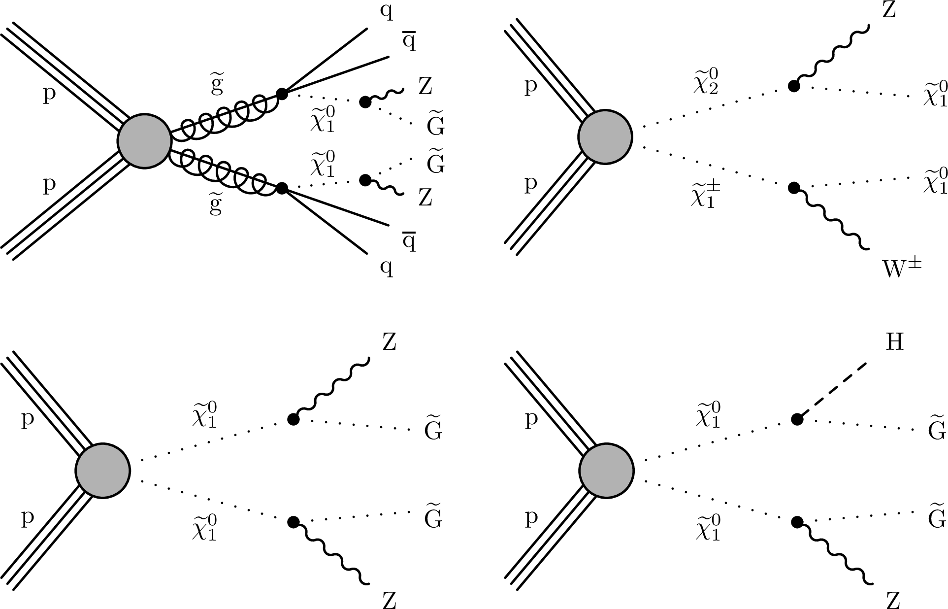
Figure 1:
Diagrams for models with decays containing at least one dilepton pair stemming from an on-shell Z boson decay studied in this analysis. The model targeted by the strong-production search is shown in the upper left. The three other diagrams correspond to EW production of chargino-neutralino or neutralino-neutralino pairs. All the diagrams containing a gravitino ($ \tilde{\mathrm{G}} $) represent gauge-mediated SUSY breaking (GMSB) models. |

png pdf |
Figure 1-a:
Diagram corresponding to the strong-production search: gauge-mediated SUSY breaking (GMSB) model. At least one dilepton pair stems from an on-shell Z boson decay. |

png pdf |
Figure 1-b:
Diagram corresponding to the EW production of a chargino-neutralino pair search. One dilepton pair stems from the on-shell Z boson decay. |
png pdf |
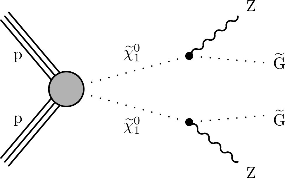
Figure 1-c:
Diagram corresponding to the EW production of a neutralino-neutralino pair search: gauge-mediated SUSY breaking (GMSB) model. At least one dilepton pair stems from an on-shell Z boson decay. |
png pdf |
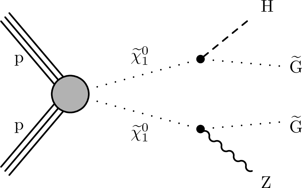
Figure 1-d:
Diagram corresponding to the EW production of a neutralino-neutralino pair search: gauge-mediated SUSY breaking (GMSB) model. One dilepton pair stems from the on-shell Z boson decay. |
png pdf |
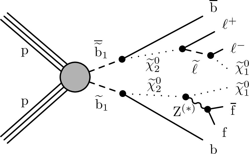
Figure 2:
Diagram showing a possible decay chain in the slepton edge model. Bottom squarks are pair produced with subsequent decays that frequently contain dilepton pairs. This model features a characteristic edge in the $ {m_{\ell \ell}} $ spectrum given approximately by the mass difference between the $ \tilde{\chi}^0_2 $ and $ \tilde{\chi}^0_1 $ particles. |
png pdf |
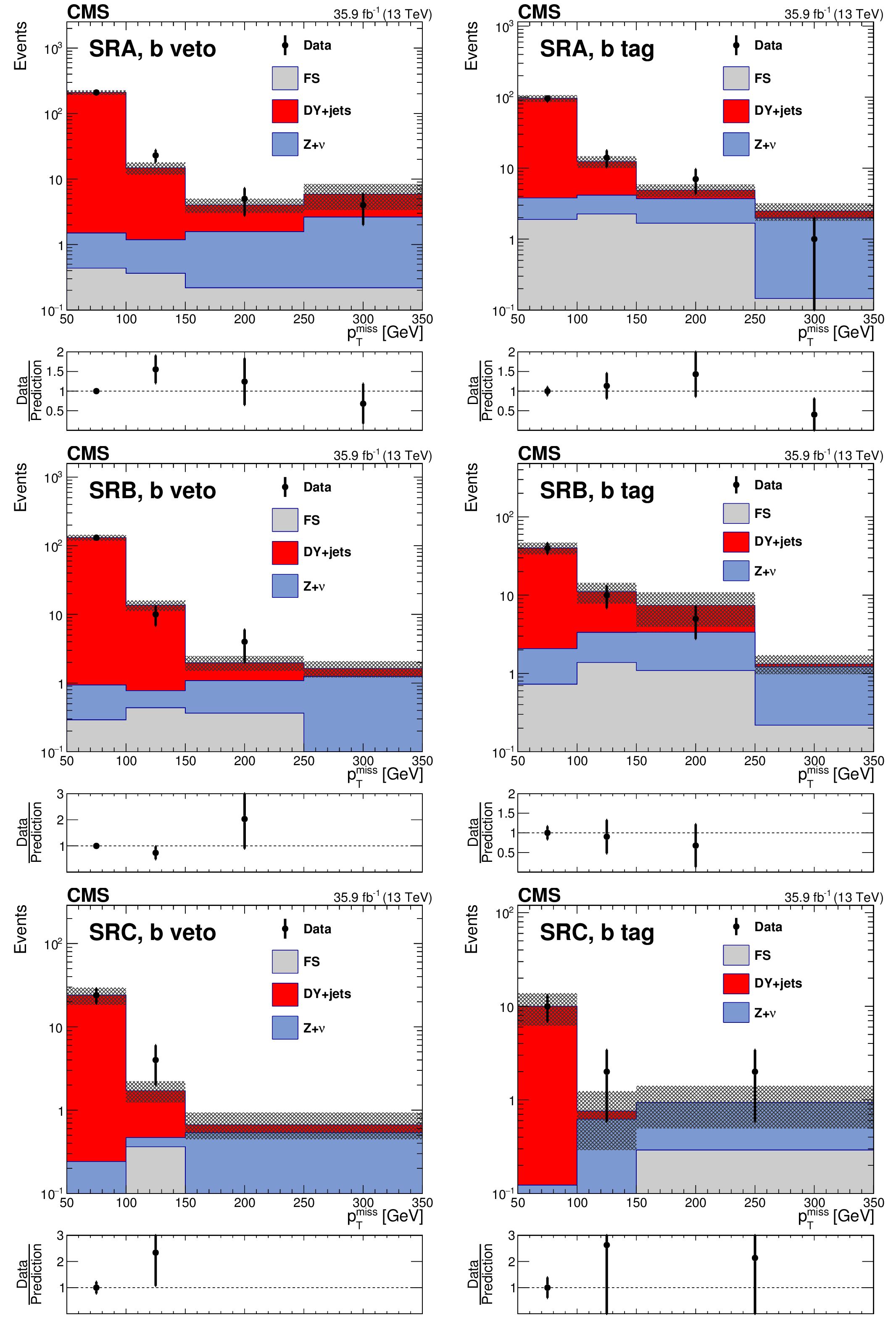
Figure 3:
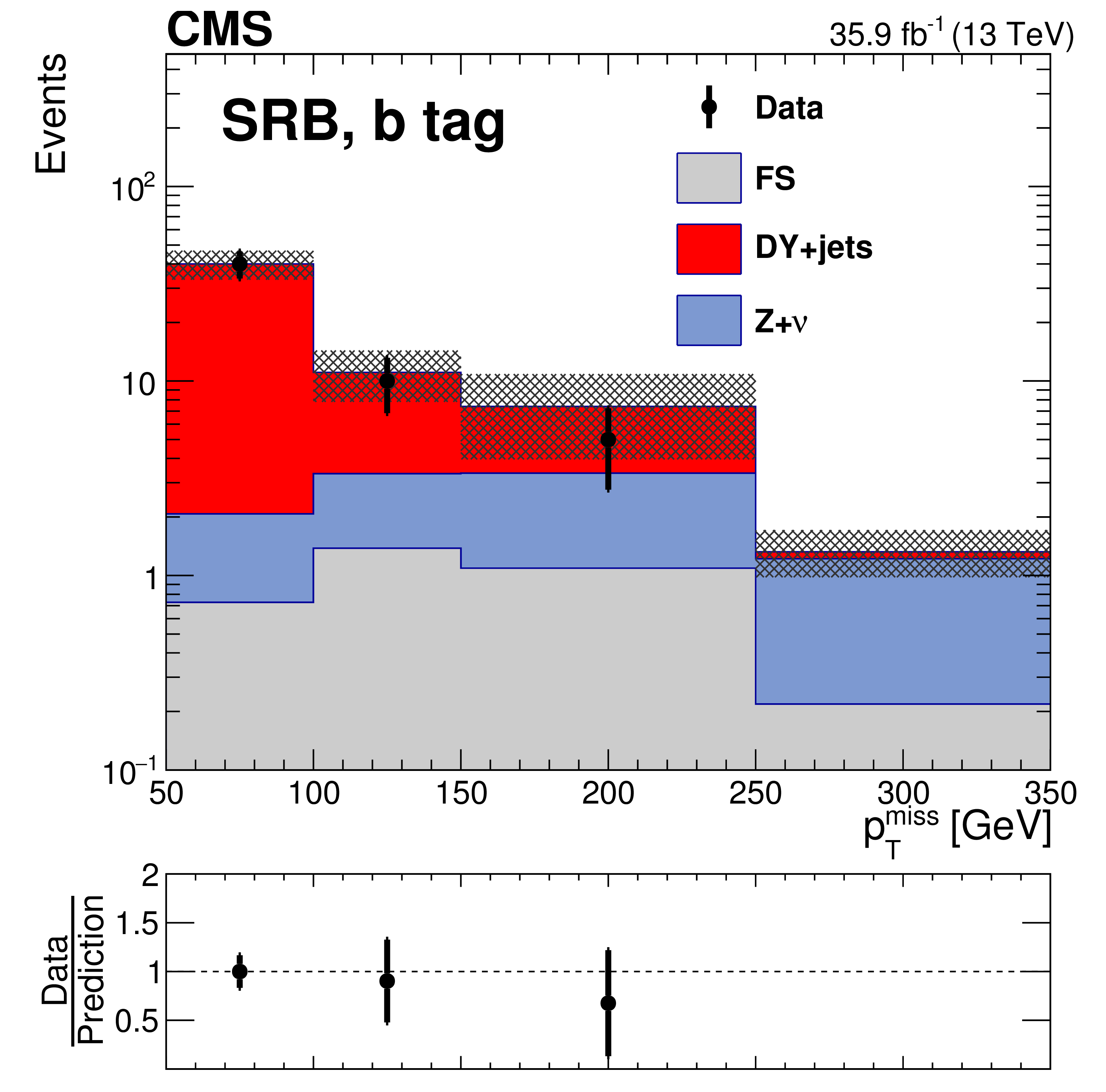
The $ {{p_{\mathrm {T}}} ^\text {miss}} $ distribution is shown for data compared to the background prediction in the on-Z strong-production SRs with no b-tagged jets (left) and at least 1 b-tagged jet (right). The rows show SRA (upper), SRB (middle), and SRC (lower). The lower panel of each plot shows the ratio of observed data to the predicted value in each bin. The hashed band in the upper panels shows the total uncertainty in the background prediction, including statistical and systematic components. The $ {{p_{\mathrm {T}}} ^\text {miss}} $ template prediction for each SR is normalized to the first bin of each distribution, and therefore the prediction agrees with the data by construction. |
png pdf |
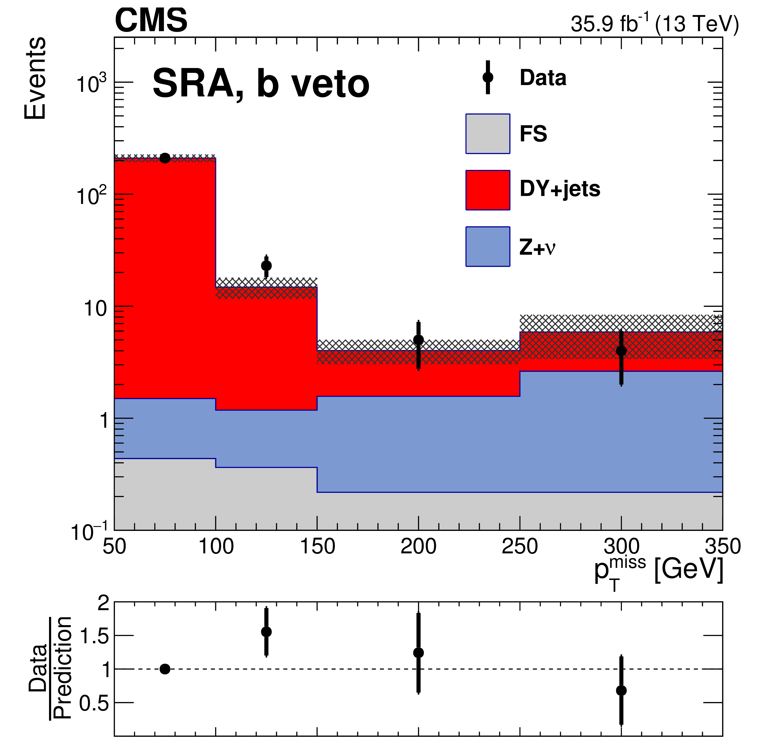
Figure 3-a:
The $ {{p_{\mathrm {T}}} ^\text {miss}} $ distribution is shown for data compared to the background prediction in the on-Z strong-production SRA signal region, with no b-tagged jet. The lower panel shows the ratio of observed data to the predicted value in each bin. The hashed band in the upper panel shows the total uncertainty in the background prediction, including statistical and systematic components. The $ {{p_{\mathrm {T}}} ^\text {miss}} $ template prediction is normalized to the first bin of the distribution, and therefore the prediction agrees with the data by construction. |
png pdf |
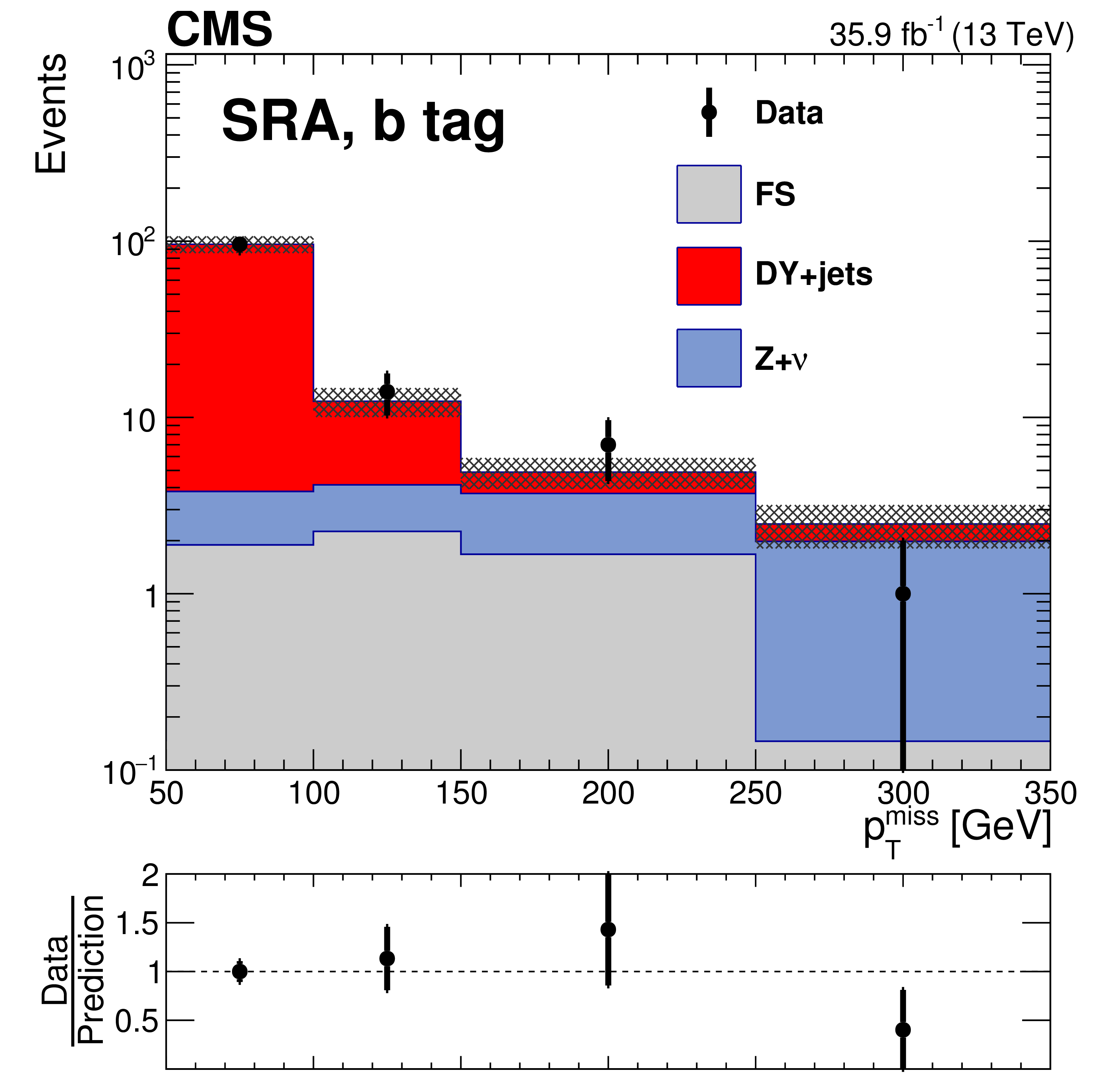
Figure 3-b:
The $ {{p_{\mathrm {T}}} ^\text {miss}} $ distribution is shown for data compared to the background prediction in the on-Z strong-production SRA signal region, with at least 1 b-tagged jet. The lower panel shows the ratio of observed data to the predicted value in each bin. The hashed band in the upper panel shows the total uncertainty in the background prediction, including statistical and systematic components. The $ {{p_{\mathrm {T}}} ^\text {miss}} $ template prediction is normalized to the first bin of the distribution, and therefore the prediction agrees with the data by construction. |
png pdf |
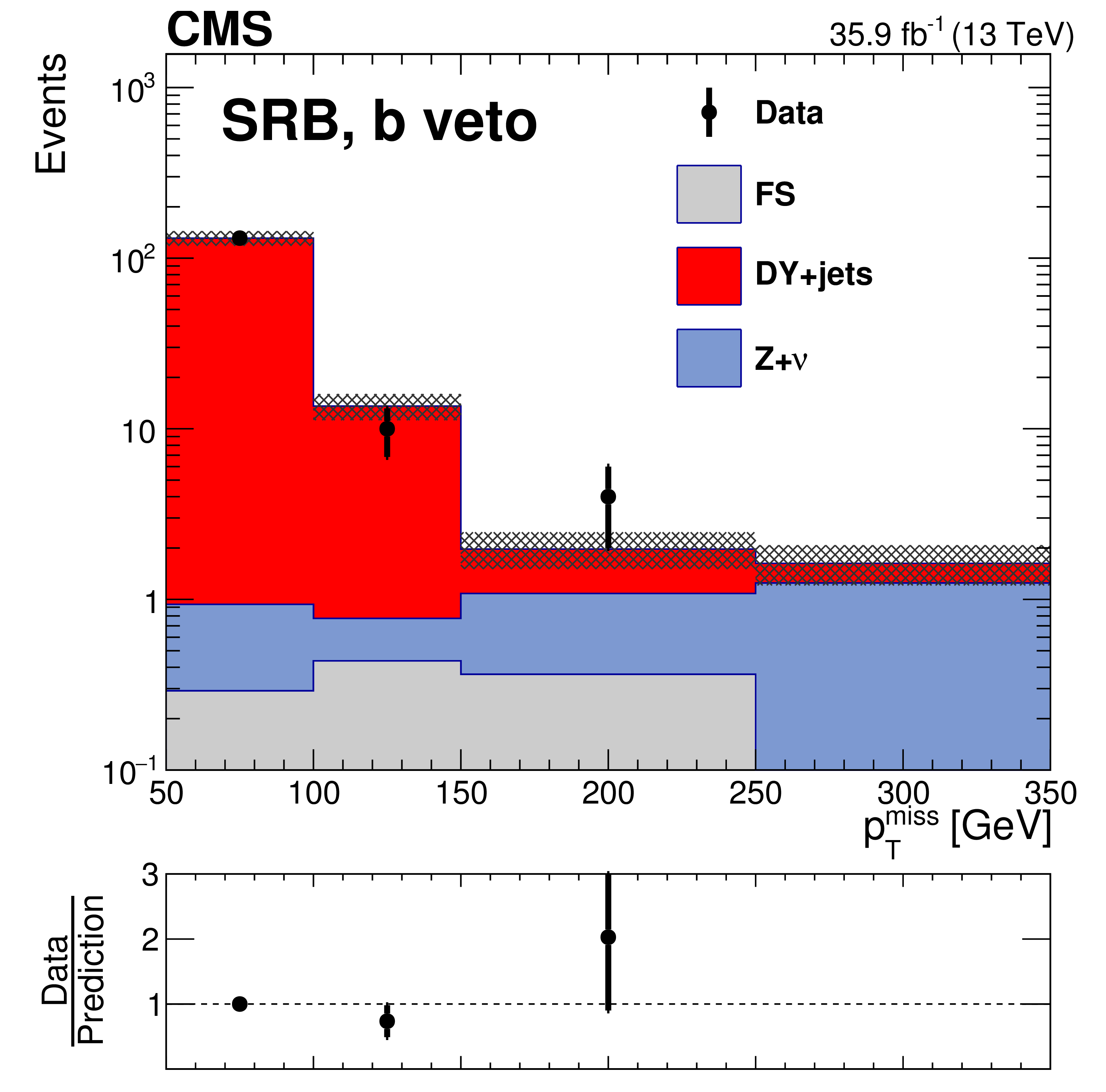
Figure 3-c:
The $ {{p_{\mathrm {T}}} ^\text {miss}} $ distribution is shown for data compared to the background prediction in the on-Z strong-production SRB signal region, with no b-tagged jet. The lower panel shows the ratio of observed data to the predicted value in each bin. The hashed band in the upper panel shows the total uncertainty in the background prediction, including statistical and systematic components. The $ {{p_{\mathrm {T}}} ^\text {miss}} $ template prediction is normalized to the first bin of the distribution, and therefore the prediction agrees with the data by construction. |
png pdf |
Figure 3-d:
The $ {{p_{\mathrm {T}}} ^\text {miss}} $ distribution is shown for data compared to the background prediction in the on-Z strong-production SRB signal region, with at least 1 b-tagged jet. The lower panel shows the ratio of observed data to the predicted value in each bin. The hashed band in the upper panel shows the total uncertainty in the background prediction, including statistical and systematic components. The $ {{p_{\mathrm {T}}} ^\text {miss}} $ template prediction is normalized to the first bin of the distribution, and therefore the prediction agrees with the data by construction. |
png pdf |
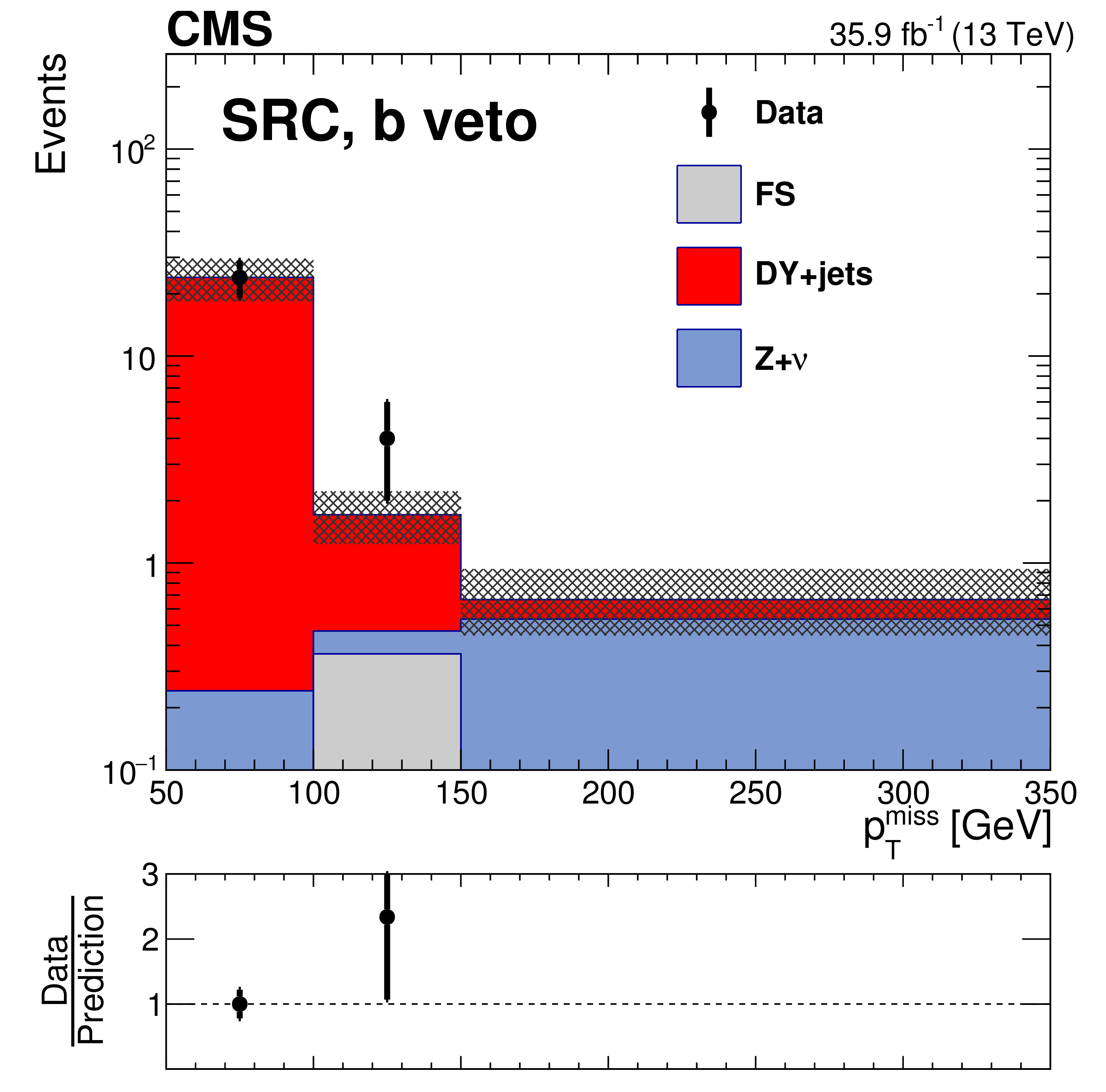
Figure 3-e:
The $ {{p_{\mathrm {T}}} ^\text {miss}} $ distribution is shown for data compared to the background prediction in the on-Z strong-production SRC signal region, with no b-tagged jet. The lower panel shows the ratio of observed data to the predicted value in each bin. The hashed band in the upper panel shows the total uncertainty in the background prediction, including statistical and systematic components. The $ {{p_{\mathrm {T}}} ^\text {miss}} $ template prediction is normalized to the first bin of the distribution, and therefore the prediction agrees with the data by construction. |
png pdf |
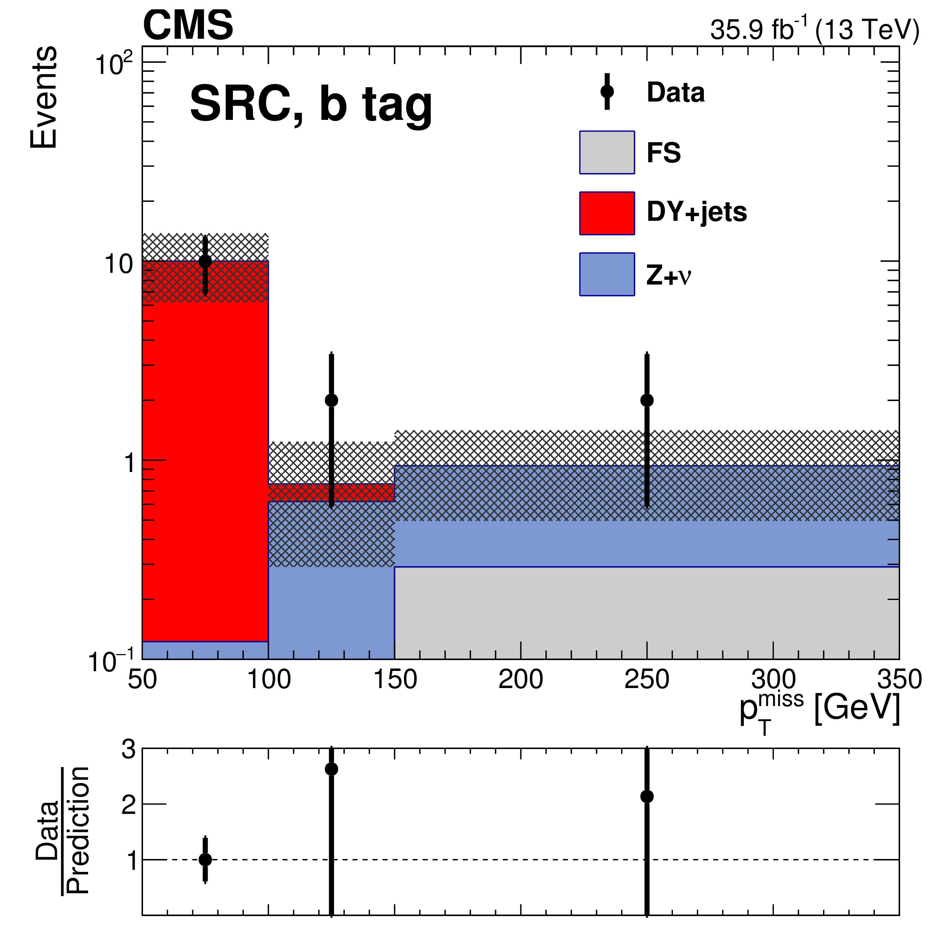
Figure 3-f:
The $ {{p_{\mathrm {T}}} ^\text {miss}} $ distribution is shown for data compared to the background prediction in the on-Z strong-production SRC signal region, with at least 1 b-tagged jet. The lower panel shows the ratio of observed data to the predicted value in each bin. The hashed band in the upper panel shows the total uncertainty in the background prediction, including statistical and systematic components. The $ {{p_{\mathrm {T}}} ^\text {miss}} $ template prediction is normalized to the first bin of the distribution, and therefore the prediction agrees with the data by construction. |
png pdf |
Figure 4:
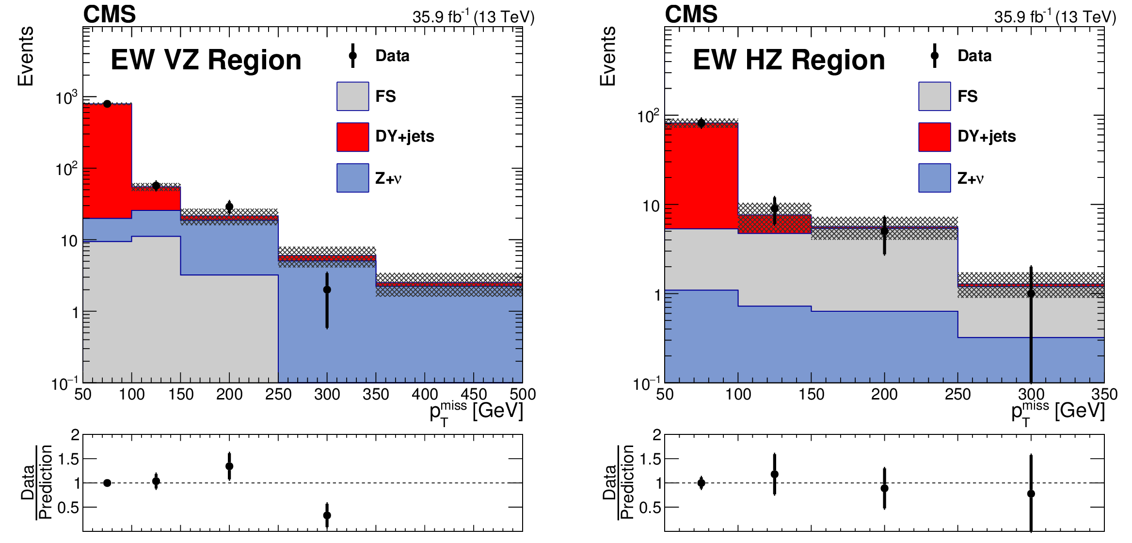
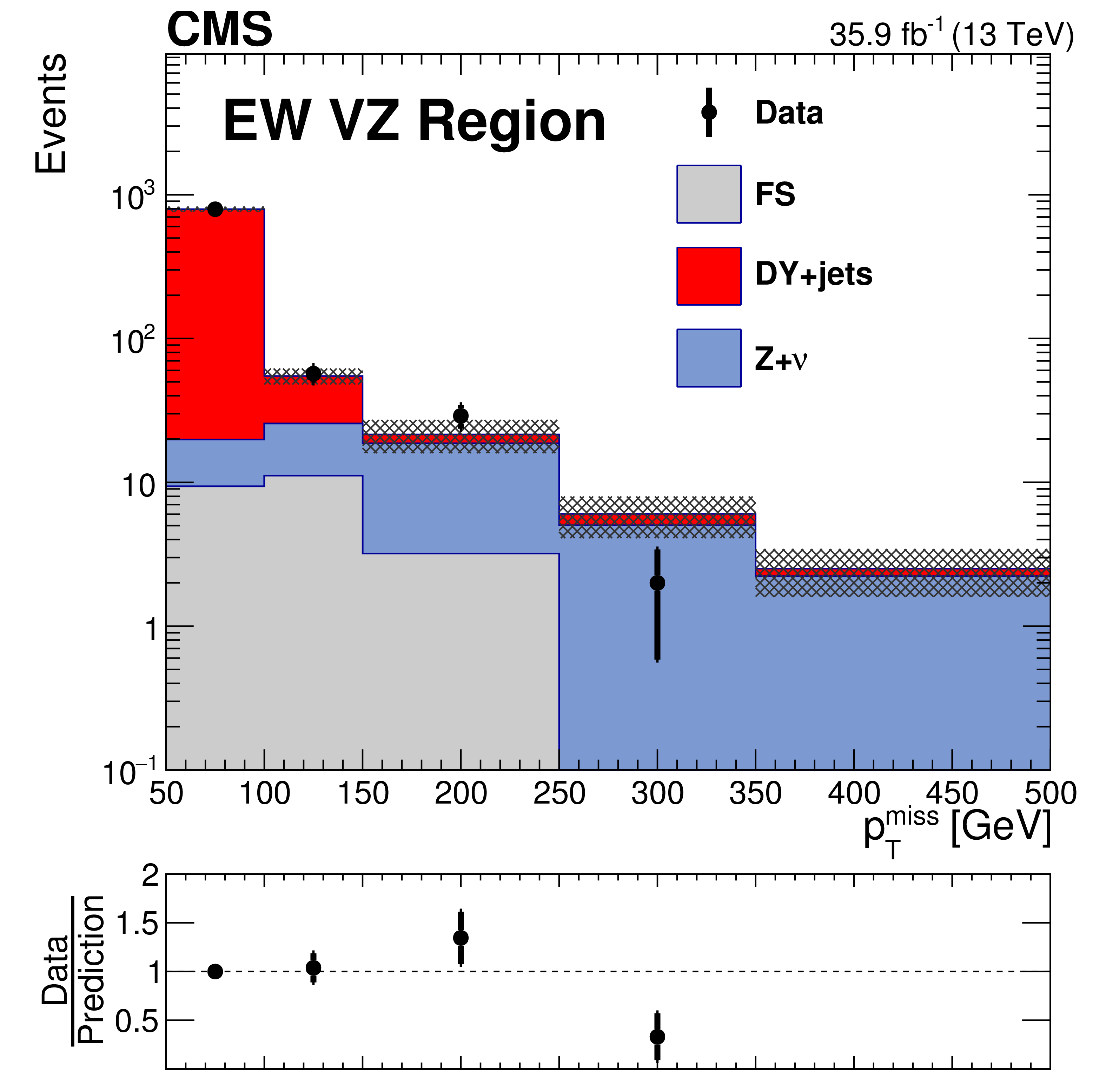
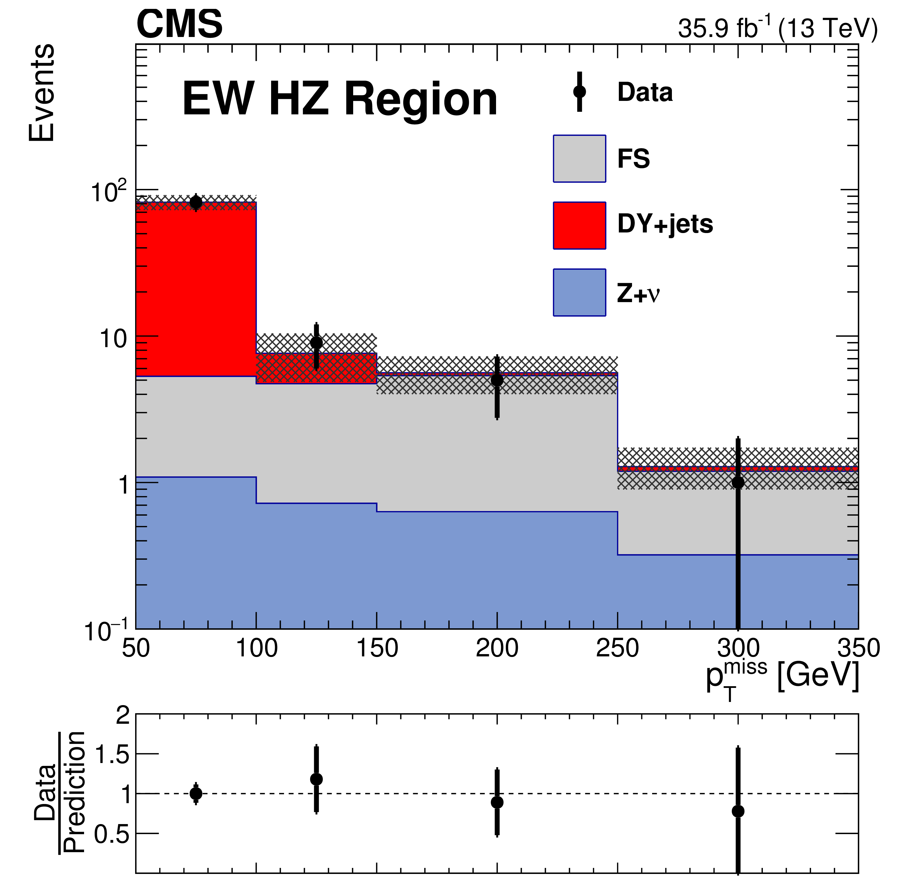
The $ {{p_{\mathrm {T}}} ^\text {miss}} $ distribution is shown for data compared to the background prediction in the on-Z $ {{\mathrm {V}}\mathrm{Z}} $ (left) and $\mathrm{H} \mathrm{Z} $ (right) electroweak-production SRs. The lower panel of each figure shows the ratio of observed data to the predicted value in each bin. The hashed band in the upper panels shows the total uncertainty in the background prediction, including statistical and systematic sources. The ${{p_{\mathrm {T}}} ^\text {miss}}$ template prediction for each SR is normalized to the first bin of each distribution, and therefore the prediction agrees with the data by construction. |
png pdf |
Figure 4-a:
The $ {{p_{\mathrm {T}}} ^\text {miss}} $ distribution is shown for data compared to the background prediction in the on-Z $ {{\mathrm {V}}\mathrm{Z}} $ electroweak-production SRs. The lower panel shows the ratio of observed data to the predicted value in each bin. The hashed band in the upper panel shows the total uncertainty in the background prediction, including statistical and systematic sources. The ${{p_{\mathrm {T}}} ^\text {miss}}$ template prediction for each SR is normalized to the first bin of each distribution, and therefore the prediction agrees with the data by construction. |
png pdf |
Figure 4-b:
The $ {{p_{\mathrm {T}}} ^\text {miss}} $ distribution is shown for data compared to the background prediction in the $\mathrm{H} \mathrm{Z} $ electroweak-production SRs. The lower panel shows the ratio of observed data to the predicted value in each bin. The hashed band in the upper panel shows the total uncertainty in the background prediction, including statistical and systematic sources. The ${{p_{\mathrm {T}}} ^\text {miss}}$ template prediction for each SR is normalized to the first bin of each distribution, and therefore the prediction agrees with the data by construction. |
png pdf |
Figure 5:
Results of the counting experiment of the edge search. For each SR, the number of observed events, shown as black data points, is compared to the total background estimate. The hashed band shows the total uncertainty in the background prediction, including statistical and systematic sources. |
png pdf |
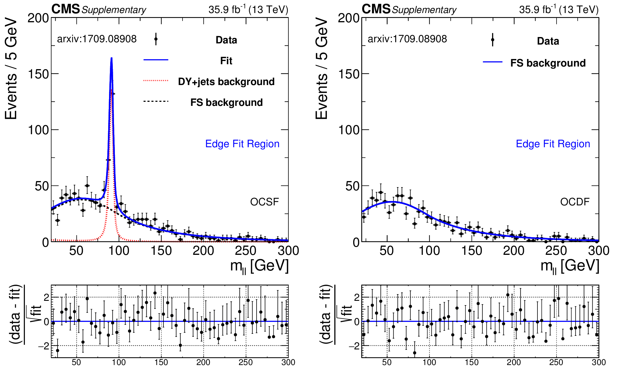
Figure 6:
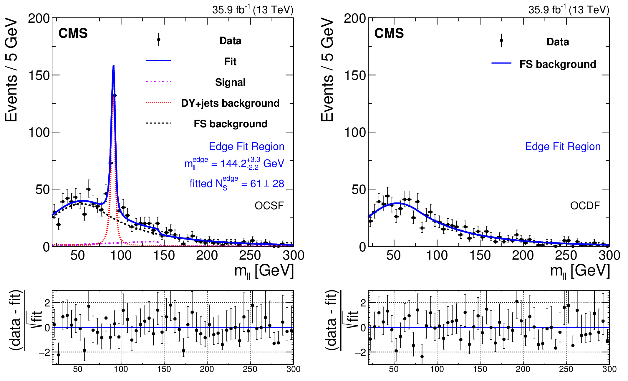
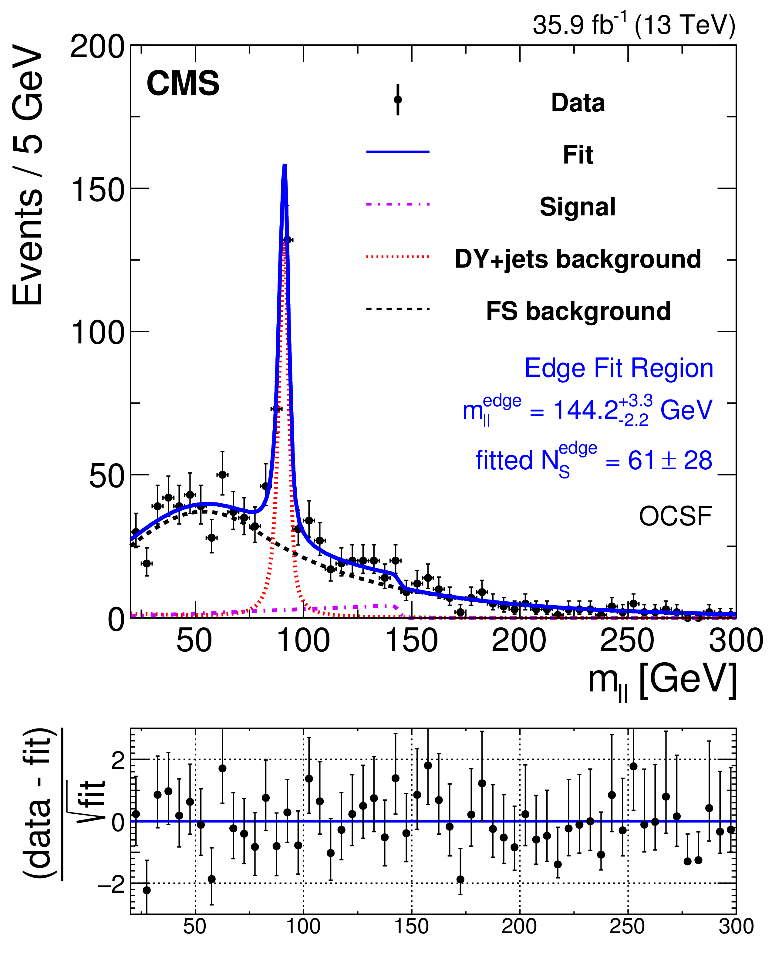
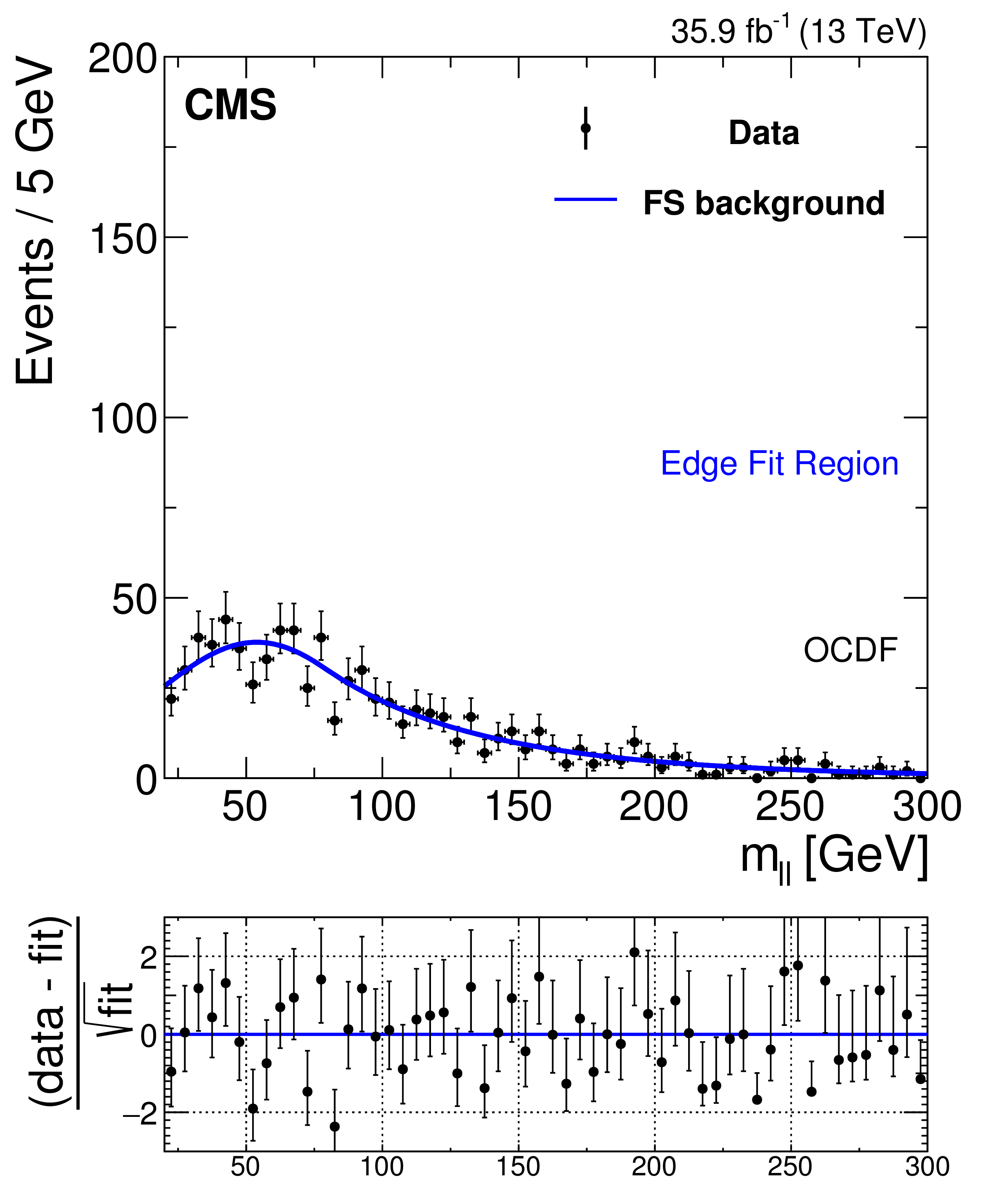
Fit of the dilepton mass distributions to the signal-plus-background hypothesis in the "Edge fit'' SR from Table 1, projected on the same-flavor (left) and different-flavor (right) event samples. The fit shape is shown as a solid blue line. The individual fit components are indicated by dashed and dotted lines. The FS background is shown with a black dashed line. The $ {\text {DY}{+}\text {jets}} $ background is displayed with a red dotted line. The extracted signal component is displayed with a purple dash-dotted line. The lower panel in each plot shows the difference between the observation and the fit, divided by the square root of the number of fitted events. |
png pdf |
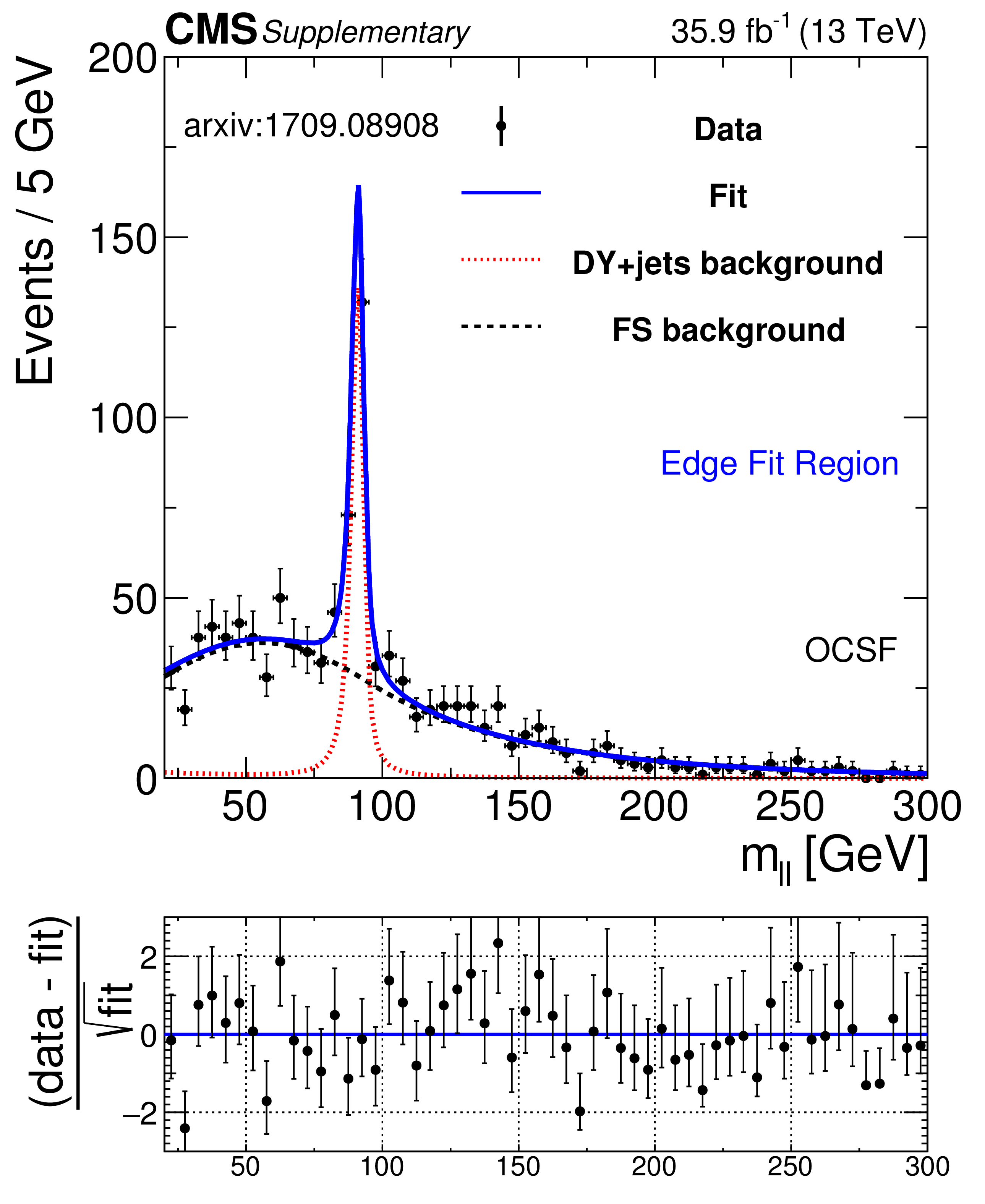
Figure 6-a:
Fit of the dilepton mass distribution to the signal-plus-background hypothesis in the "Edge fit'' SR from Table 1, projected on the same-flavor event sample. The fit shape is shown as a solid blue line. The individual fit components are indicated by dashed and dotted lines. The FS background is shown with a black dashed line. The $ {\text {DY}{+}\text {jets}} $ background is displayed with a red dotted line. The extracted signal component is displayed with a purple dash-dotted line. The lower panel in each plot shows the difference between the observation and the fit, divided by the square root of the number of fitted events. |
png pdf |
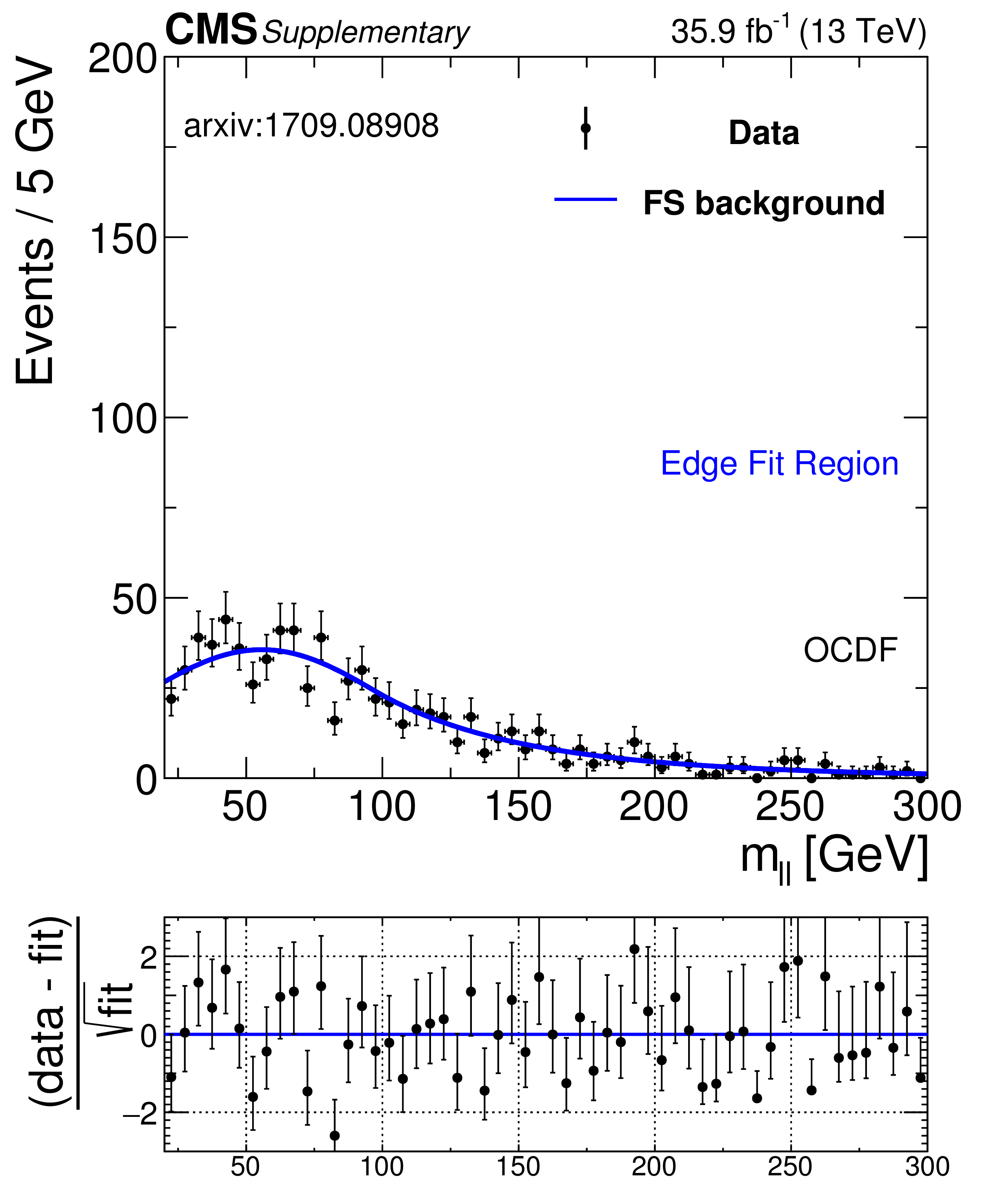
Figure 6-b:
Fit of the dilepton mass distribution to the signal-plus-background hypothesis in the "Edge fit'' SR from Table 1, projected on the different-flavor event sample. The fit shape is shown as a solid blue line. The individual fit components are indicated by dashed and dotted lines. The FS background is shown with a black dashed line. The $ {\text {DY}{+}\text {jets}} $ background is displayed with a red dotted line. The extracted signal component is displayed with a purple dash-dotted line. The lower panel in each plot shows the difference between the observation and the fit, divided by the square root of the number of fitted events. |

png pdf root |
Figure 7:
Cross section upper limit and exclusion contours at 95% CL for the gluino GMSB model as a function of the $ {\mathrm{\widetilde{g}}} $ and $ \tilde{\chi}^0_1 $ masses, obtained from the results of the strong production on-Z search. The region to the left of the thick red dotted (black solid) line is excluded by the expected (observed) limit. The thin red dotted curves indicate the regions containing 68 and 95% of the distribution of limits expected under the background-only hypothesis. The thin solid black curves show the change in the observed limit due to variation of the signal cross sections within their theoretical uncertainties. |
png pdf root |
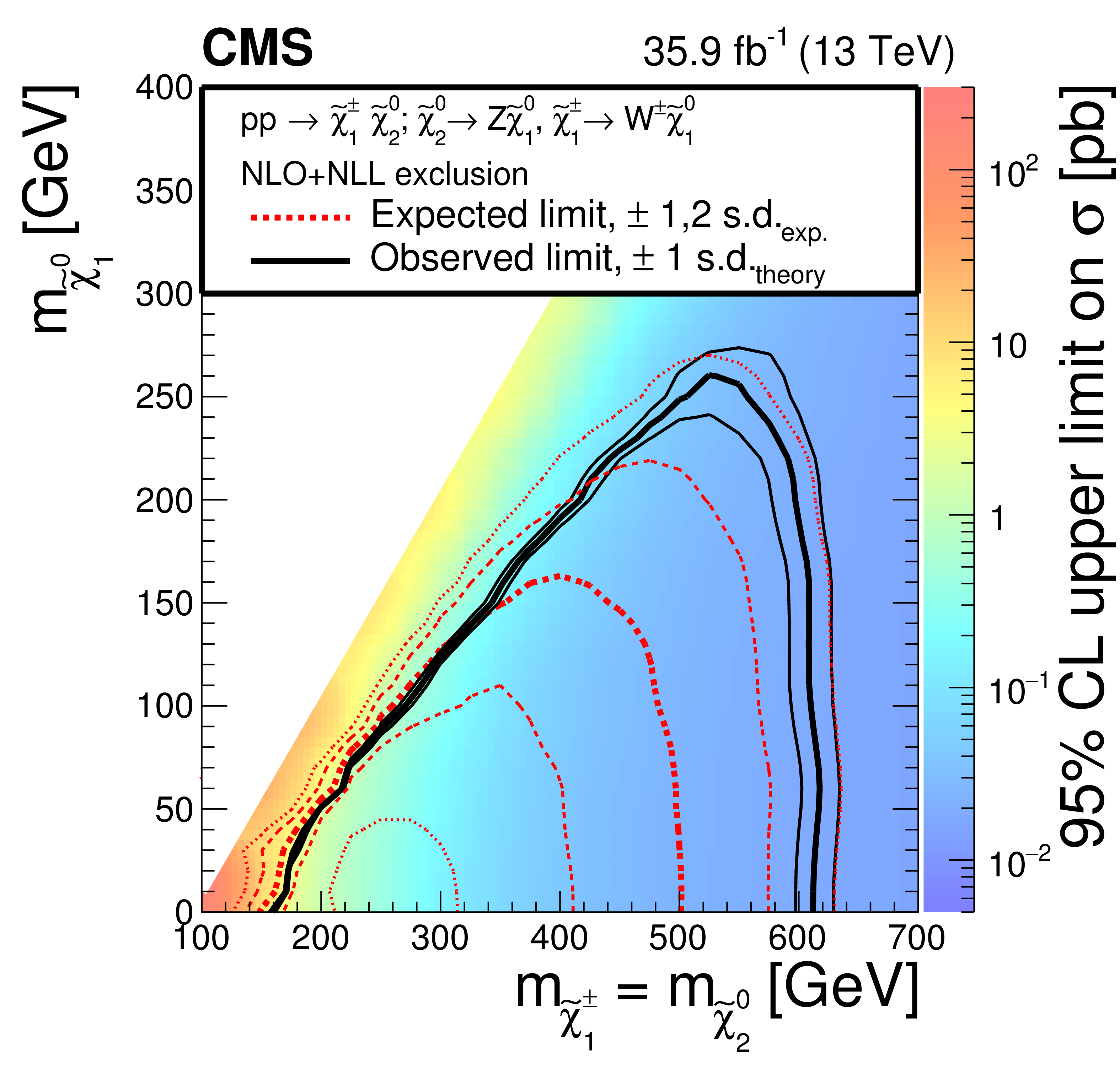
Figure 8:
Cross section upper limit and exclusion contours at 95% CL for the EW $\mathrm{W} \mathrm{Z} $ model as a function of the $\tilde{\chi}^{\pm}_1$ (equal to $ \tilde{\chi}^0_2 $) and $ \tilde{\chi}^0_1 $ masses, obtained using the on-Z search for EW production results. The region under the thick red dotted (black solid) line is excluded by the expected (observed) limit. The thin red dotted curves indicate the regions containing 68 and 95% of the distribution of limits expected under the background-only hypothesis. The thin solid black curves show the change in the observed limit due to variation of the signal cross sections within their theoretical uncertainties. |
png pdf |
Figure 9:
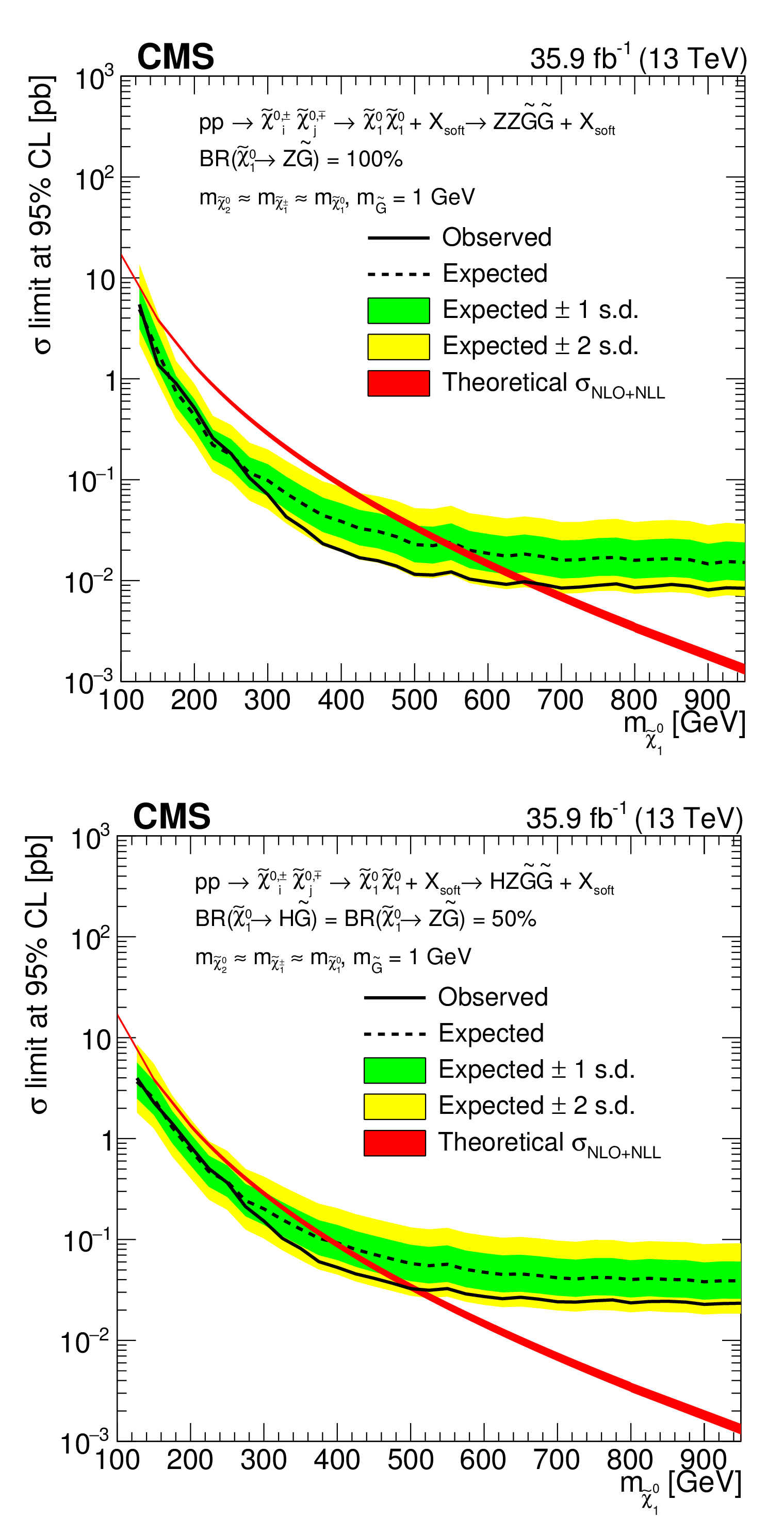
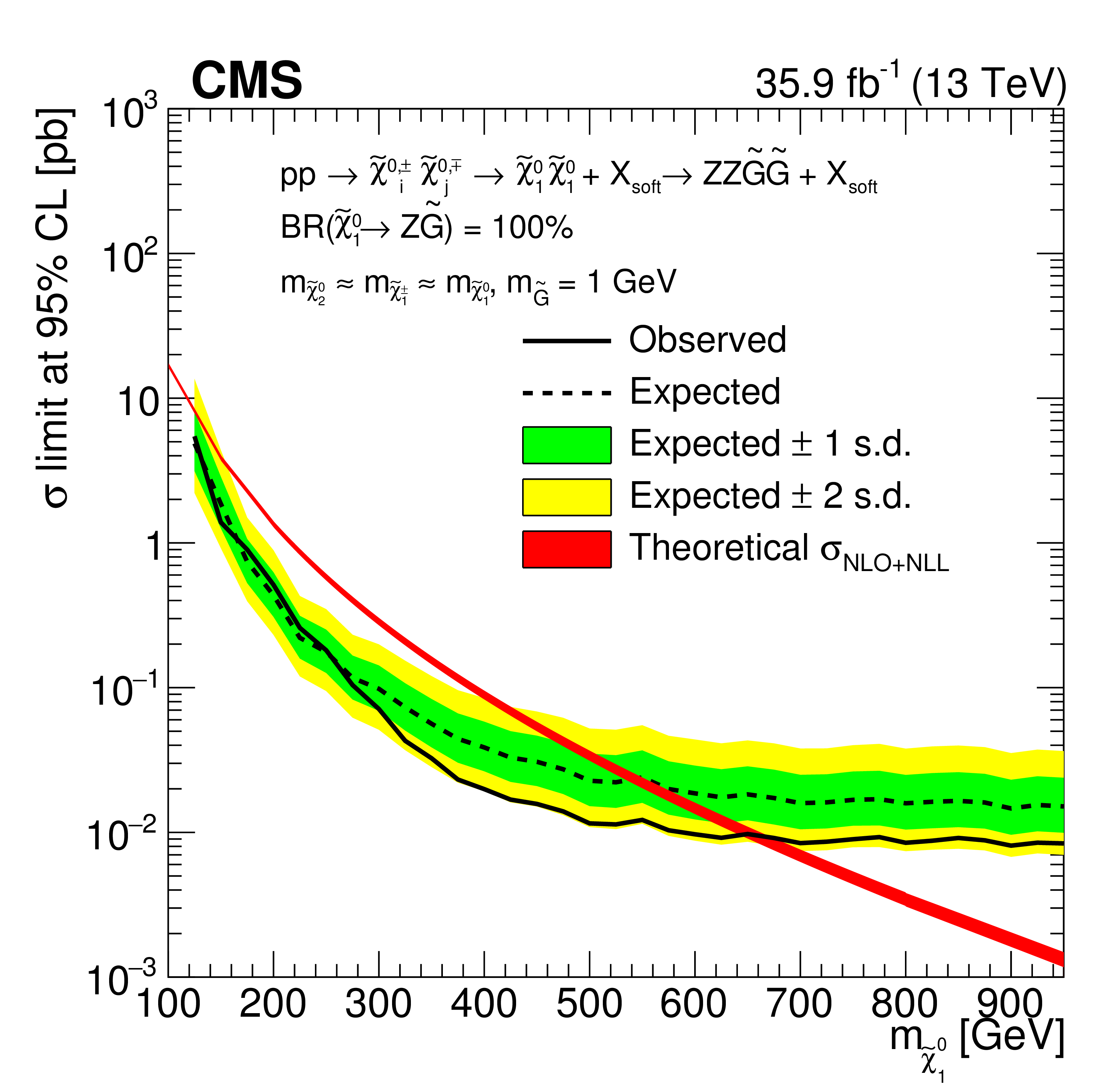
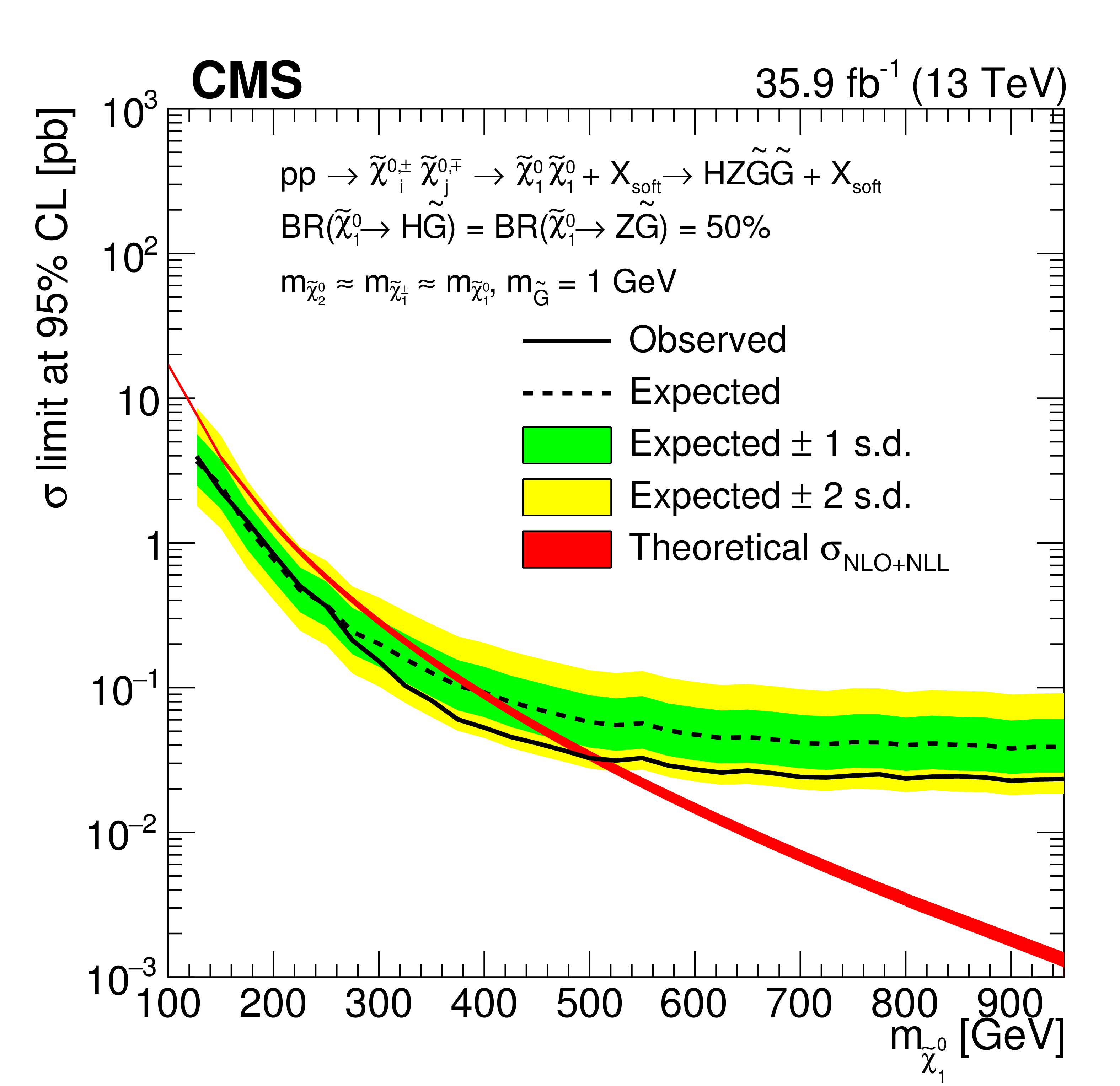
Cross section upper limit and exclusion lines at 95% CL, as a function of the $ \tilde{\chi}^0_1 $ mass, for the search for EW production in the ZZ topology (upper) and with a 50% branching fraction to each of the Z and Higgs bosons (lower). The red band shows the theoretical cross section, with the thickness of band representing the theoretical uncertainty in the signal cross section. Regions where the black dotted line reaches below the theoretical cross section are expected to be excluded. The green (yellow) band indicates the region containing 68 (95)% of the distribution of limits expected under the background-only hypothesis. The observed upper limit on the cross section is shown with a solid black line. |
png pdf root |
Figure 9-a:
Cross section upper limit and exclusion lines at 95% CL, as a function of the $ \tilde{\chi}^0_1 $ mass, for the search for EW production in the ZZ topology. The red band shows the theoretical cross section, with the thickness of band representing the theoretical uncertainty in the signal cross section. Regions where the black dotted line reaches below the theoretical cross section are expected to be excluded. The green (yellow) band indicates the region containing 68 (95)% of the distribution of limits expected under the background-only hypothesis. The observed upper limit on the cross section is shown with a solid black line. |
png pdf root |
Figure 9-b:
Cross section upper limit and exclusion lines at 95% CL, as a function of the $ \tilde{\chi}^0_1 $ mass, for the search for EW production in with a 50% branching fraction to each of the Z and Higgs bosons. The red band shows the theoretical cross section, with the thickness of band representing the theoretical uncertainty in the signal cross section. Regions where the black dotted line reaches below the theoretical cross section are expected to be excluded. The green (yellow) band indicates the region containing 68 (95)% of the distribution of limits expected under the background-only hypothesis. The observed upper limit on the cross section is shown with a solid black line. |
png pdf root |
Figure 10:
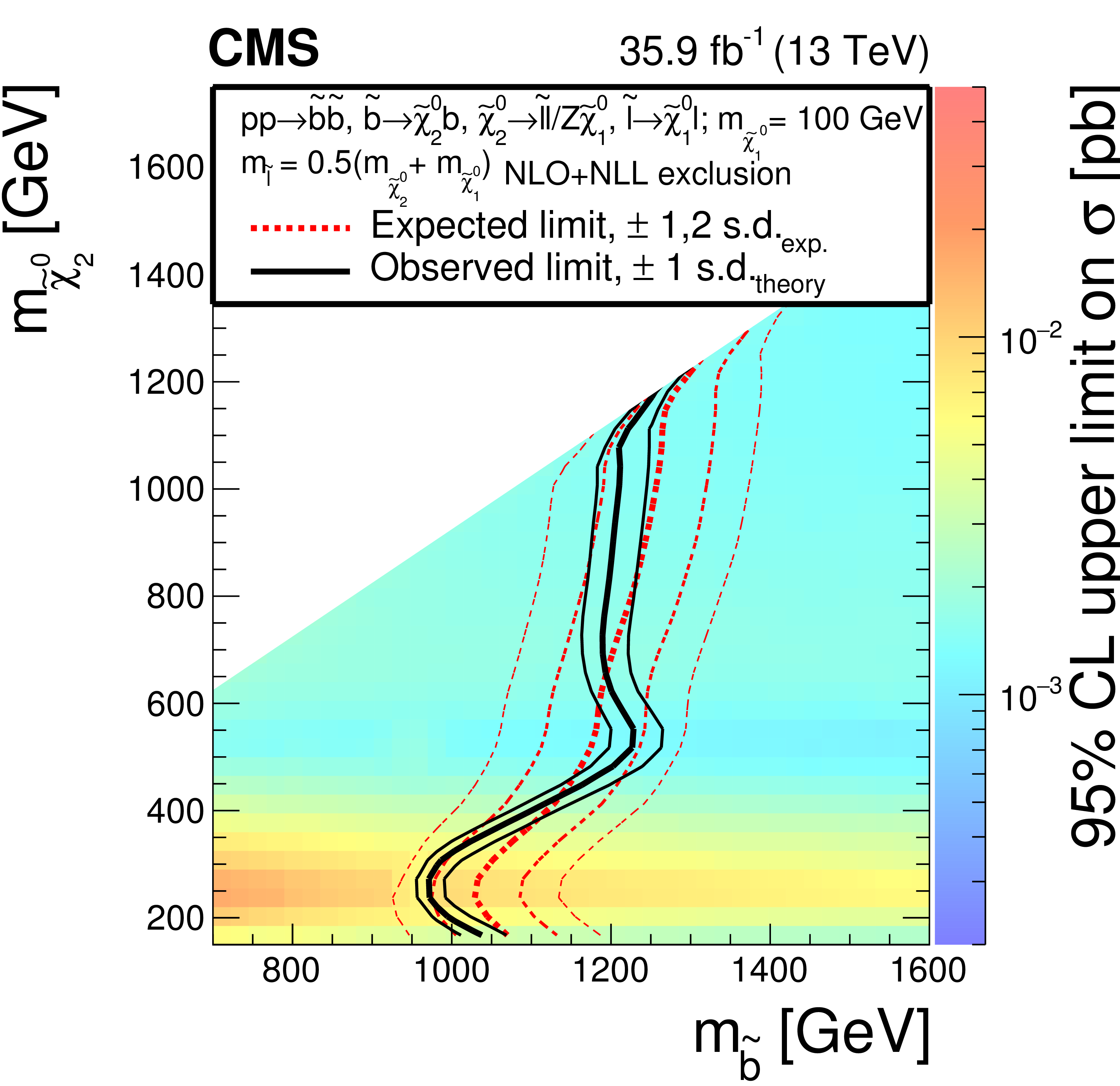
Cross section upper limit and exclusion contours at 95% CL for the slepton edge model as a function of the $\tilde{\mathrm{b}}$ and $ \tilde{\chi}^0_2 $ masses, obtained from the results of the edge search. The region to the left of the thick red dotted (black solid) line is excluded by the expected (observed) limit. The thin red dotted curves indicate the regions containing 68 and 95% of the distribution of limits expected under the background-only hypothesis. The thin solid black curves show the change in the observed limit due to variation of the signal cross sections within their theoretical uncertainties. |
png pdf root |
Figure 11:
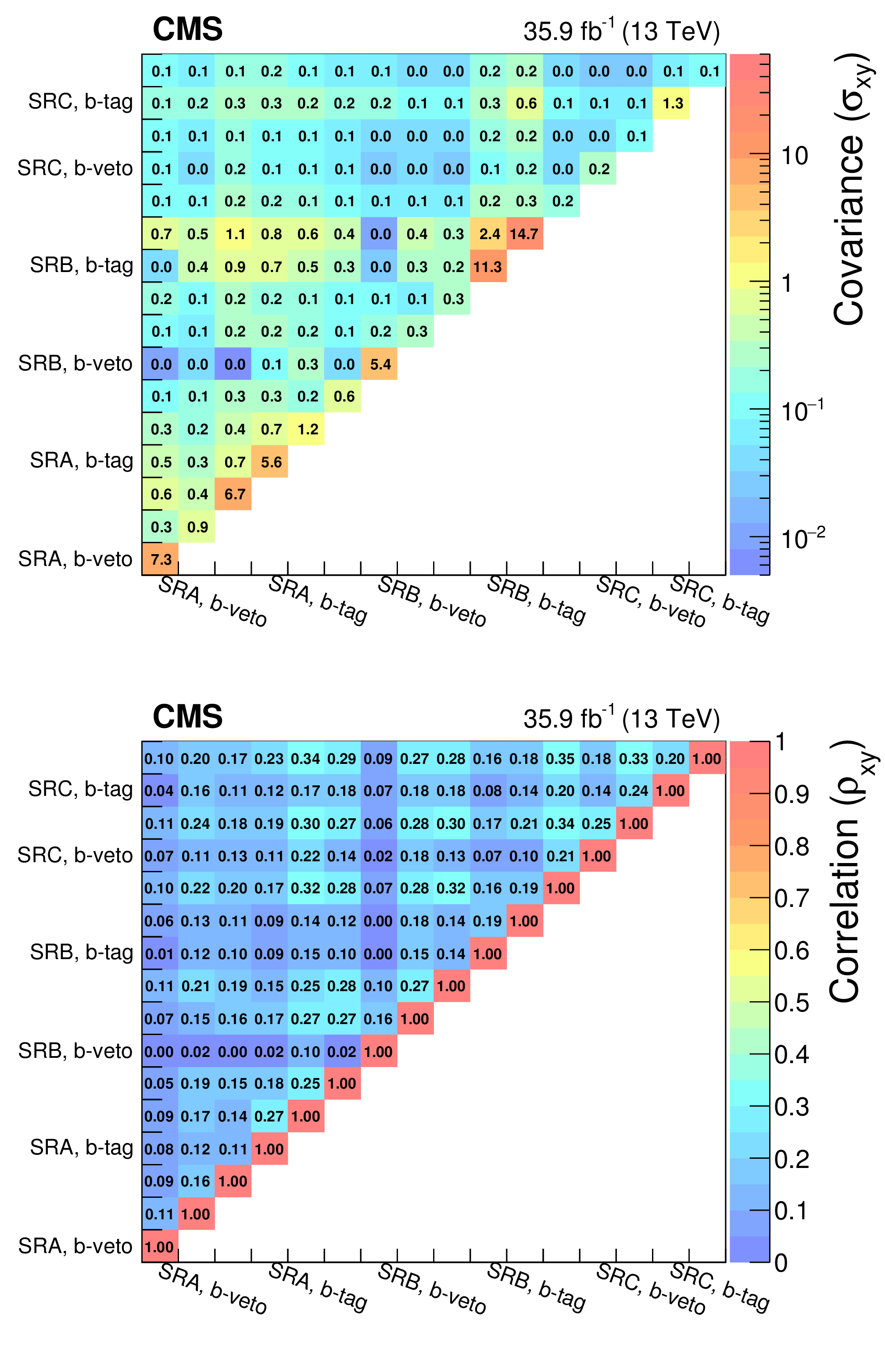
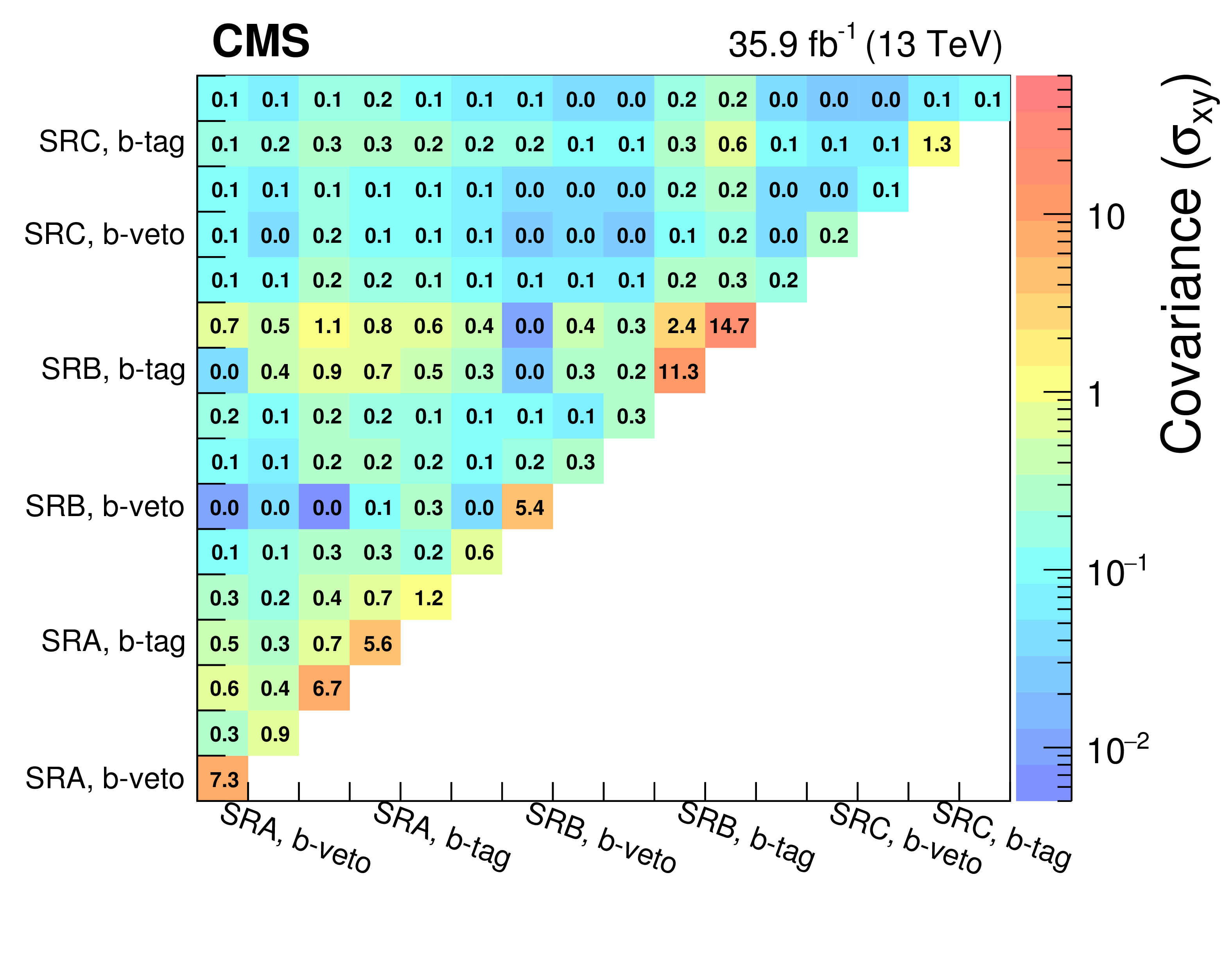
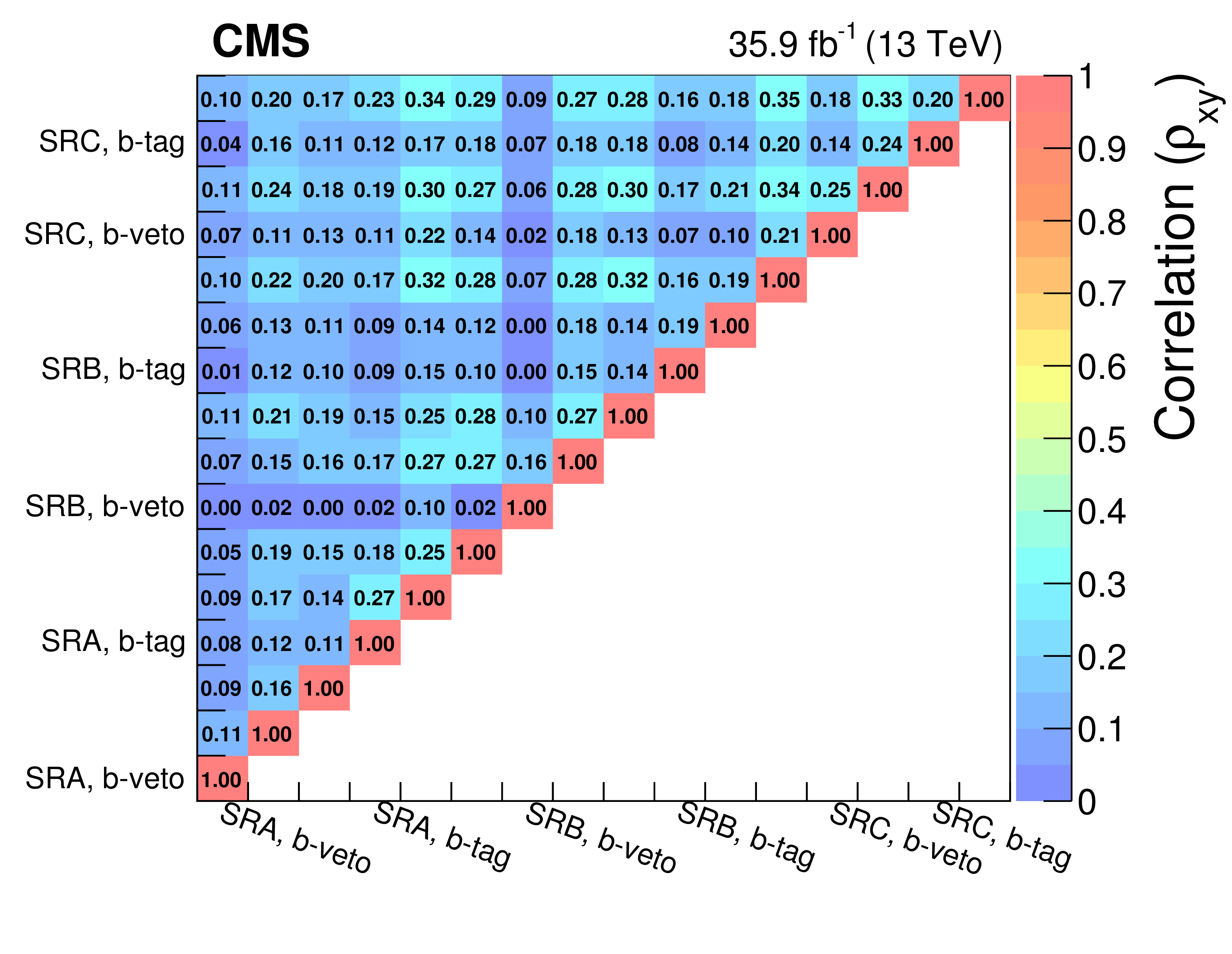
The covariance (upper) and correlation (lower) matrices for the background predictions in the on-Z strong-production SRs. Within each SR, the individual ${{p_{\mathrm {T}}} ^\text {miss}}$ bins are shown in increasing order starting from 100 GeV. The matrices are symmetric, but only the entries along and above the diagonal are shown for simplicity. |
png pdf root |
Figure 11-a:
The covariance matrix for the background predictions in the on-Z strong-production SRs. Within each SR, the individual ${{p_{\mathrm {T}}} ^\text {miss}}$ bins are shown in increasing order starting from 100 GeV. The matrix is symmetric, but only the entries along and above the diagonal are shown for simplicity. |
png pdf root |
Figure 11-b:
The correlation matrix for the background predictions in the on-Z strong-production SRs. Within each SR, the individual ${{p_{\mathrm {T}}} ^\text {miss}}$ bins are shown in increasing order starting from 100 GeV. The matrix is symmetric, but only the entries along and above the diagonal are shown for simplicity. |
png pdf root |
Figure 12:
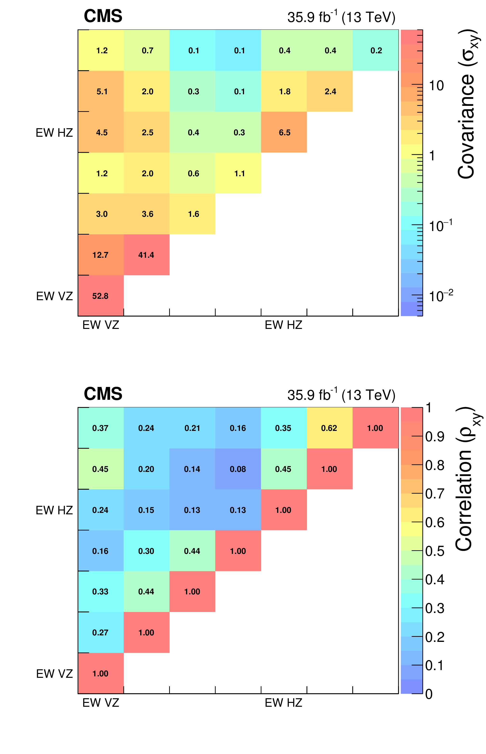
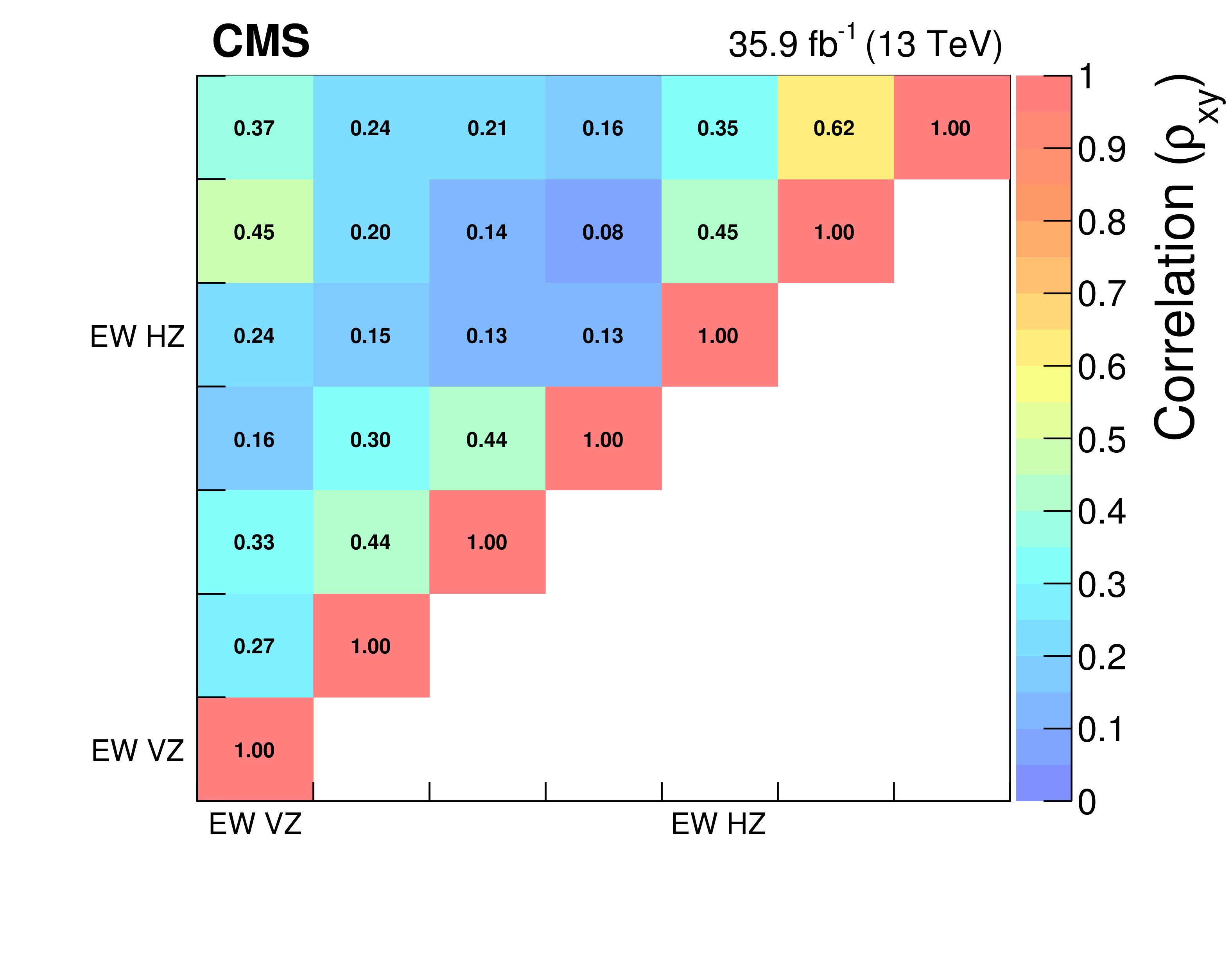
The covariance (upper) and correlation (lower) matrices for the background predictions in the on-Z EW-production SRs. Within each SR, the individual ${{p_{\mathrm {T}}} ^\text {miss}}$ bins are shown in increasing order starting from 100 GeV. The matrices are symmetric, but only the entries along and above the diagonal are shown for simplicity. |

png pdf root |
Figure 12-a:
The covariance matrix for the background predictions in the on-Z EW-production SRs. Within each SR, the individual ${{p_{\mathrm {T}}} ^\text {miss}}$ bins are shown in increasing order starting from 100 GeV. The matrix is symmetric, but only the entries along and above the diagonal are shown for simplicity. |
png pdf root |
Figure 12-b:
The correlation matrix for the background predictions in the on-Z EW-production SRs. Within each SR, the individual ${{p_{\mathrm {T}}} ^\text {miss}}$ bins are shown in increasing order starting from 100 GeV. The matrix is symmetric, but only the entries along and above the diagonal are shown for simplicity. |
png pdf root |
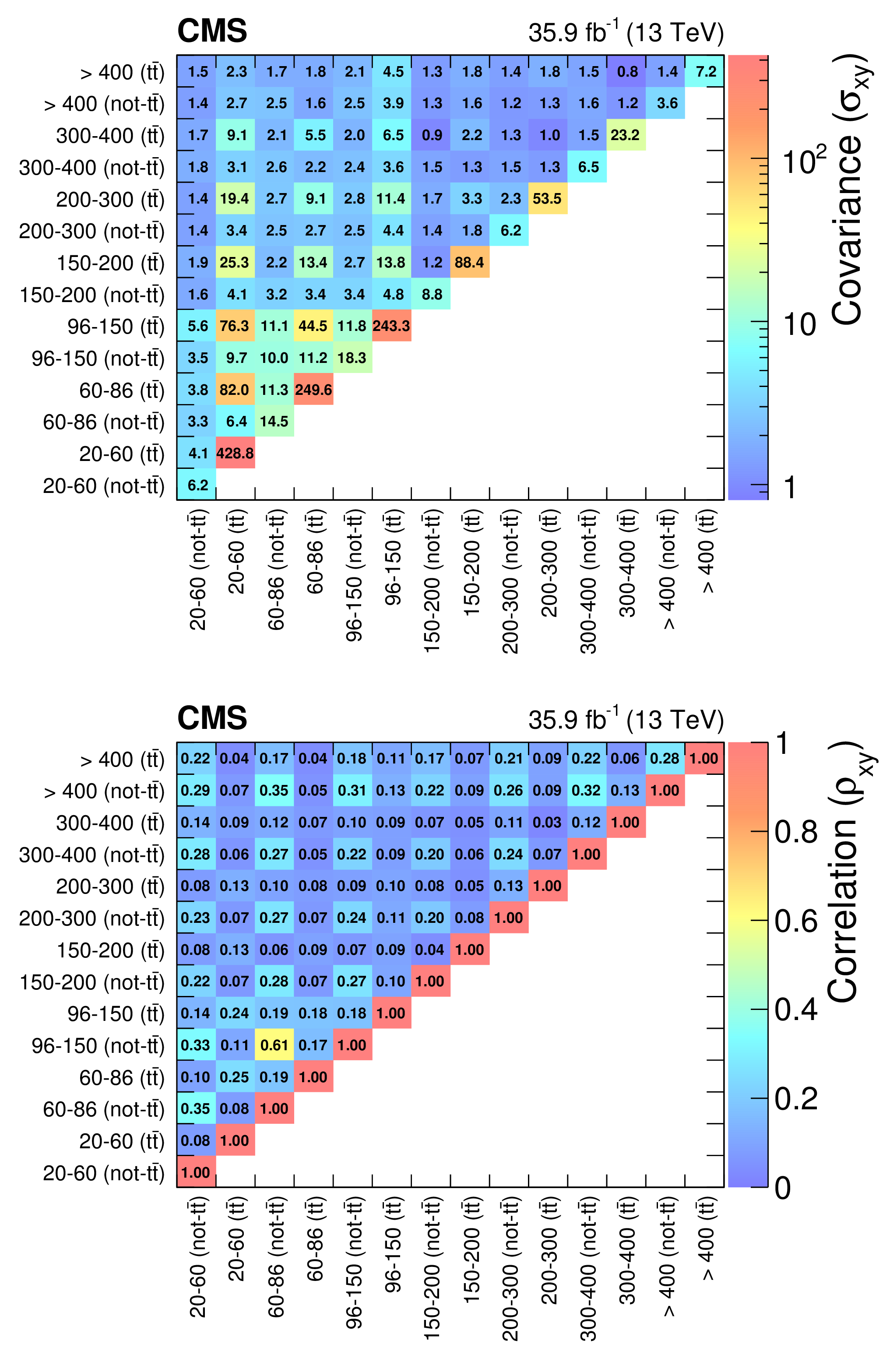
Figure 13:
The covariance (upper) and correlation (lower) matrices for the background predictions in the edge strong-production SRs. The matrices are symmetric, but only the entries along and above the diagonal are shown for simplicity. |

png pdf root |
Figure 13-a:
The covariance matrix for the background predictions in the edge strong-production SRs. The matrix is symmetric, but only the entries along and above the diagonal are shown for simplicity. |
png pdf root |
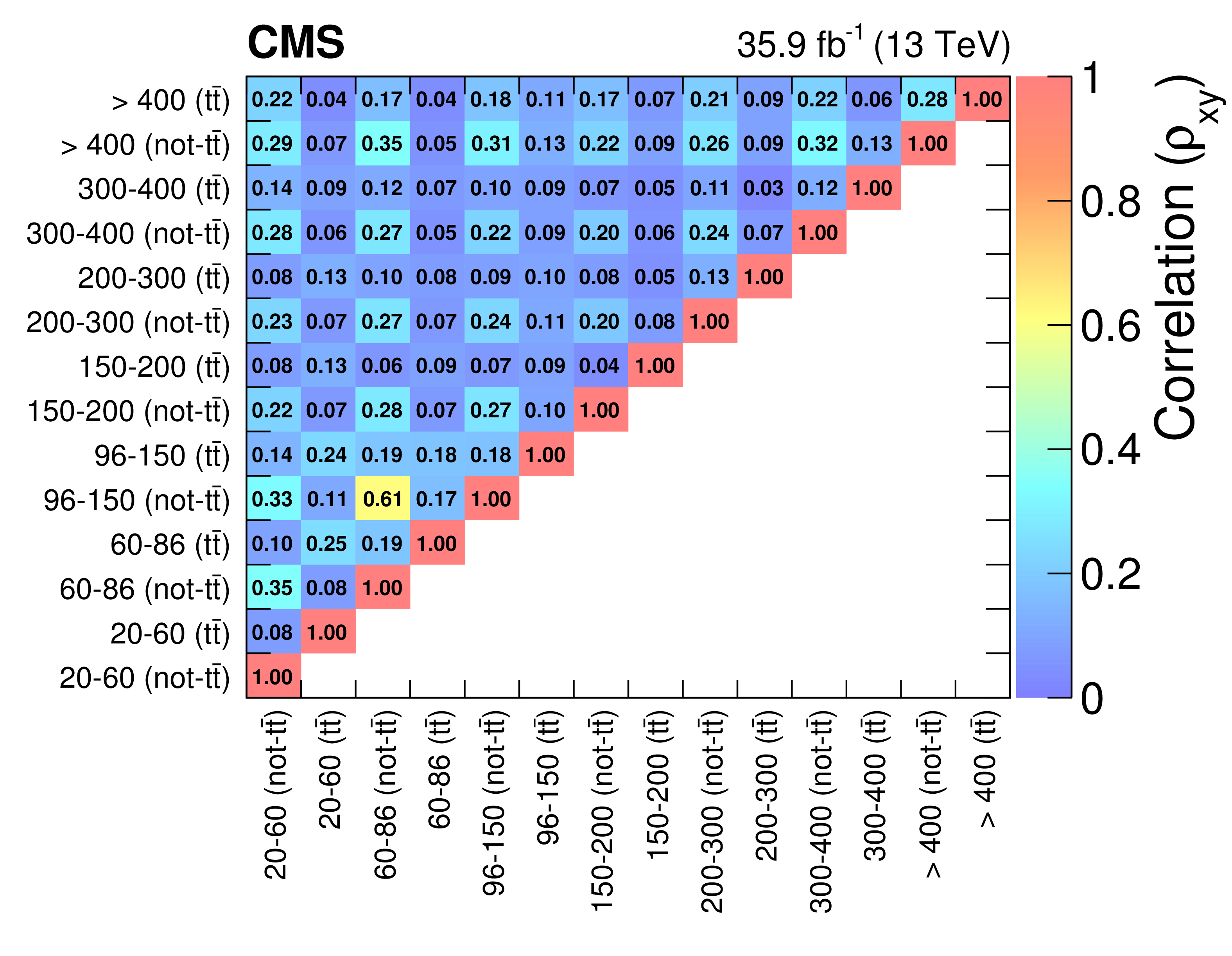
Figure 13-b:
The correlation matrix for the background predictions in the edge strong-production SRs. The matrix is symmetric, but only the entries along and above the diagonal are shown for simplicity. |
| Tables | |
png pdf |
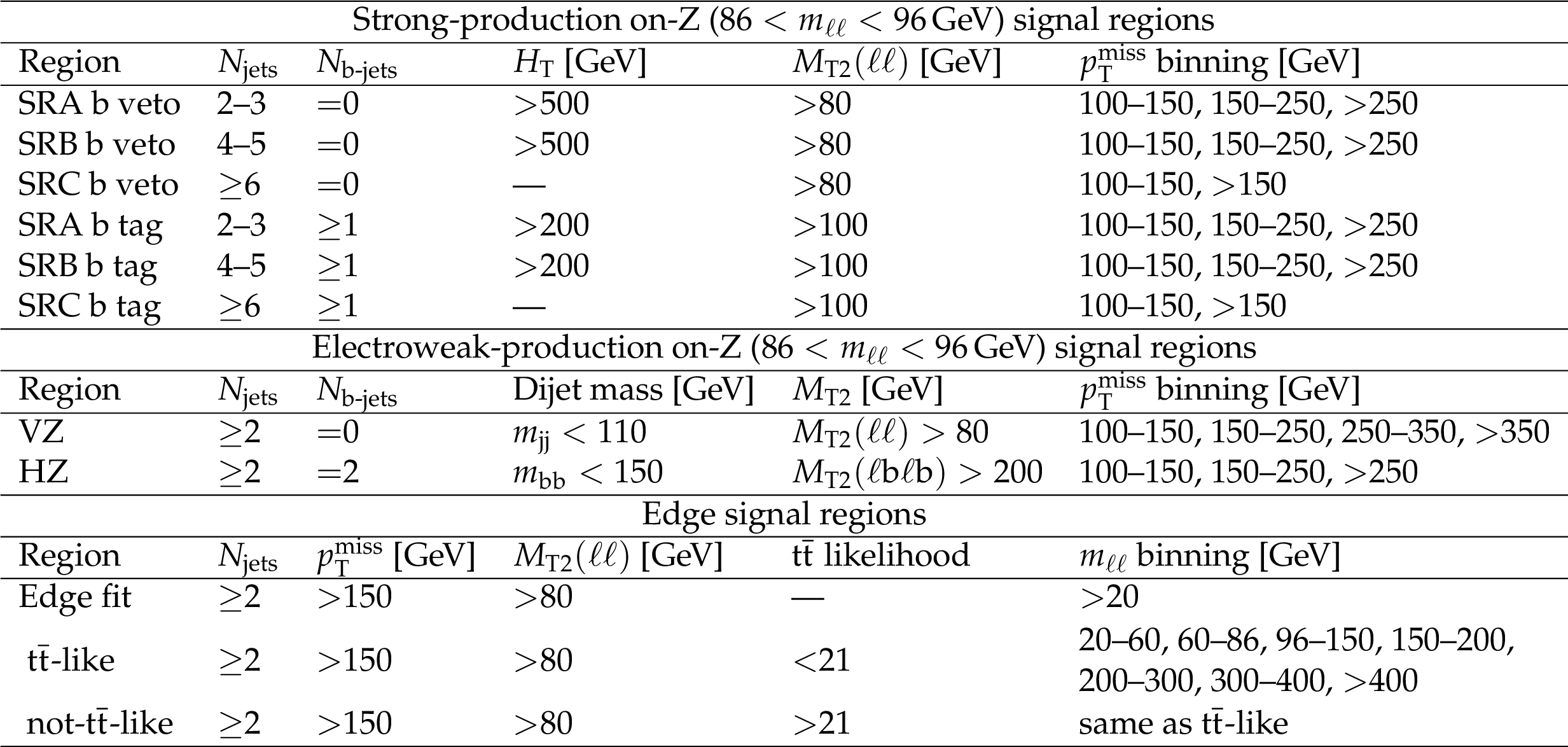
Table 1:
Summary of all SR selections. |

png pdf |
Table 2:
Predicted and observed event yields are shown for the on-Z strong-production SRs, for each ${{p_{\mathrm {T}}} ^\text {miss}} $ bin defined in Table 1. The uncertainties shown include both statistical and systematic components. |
png pdf |
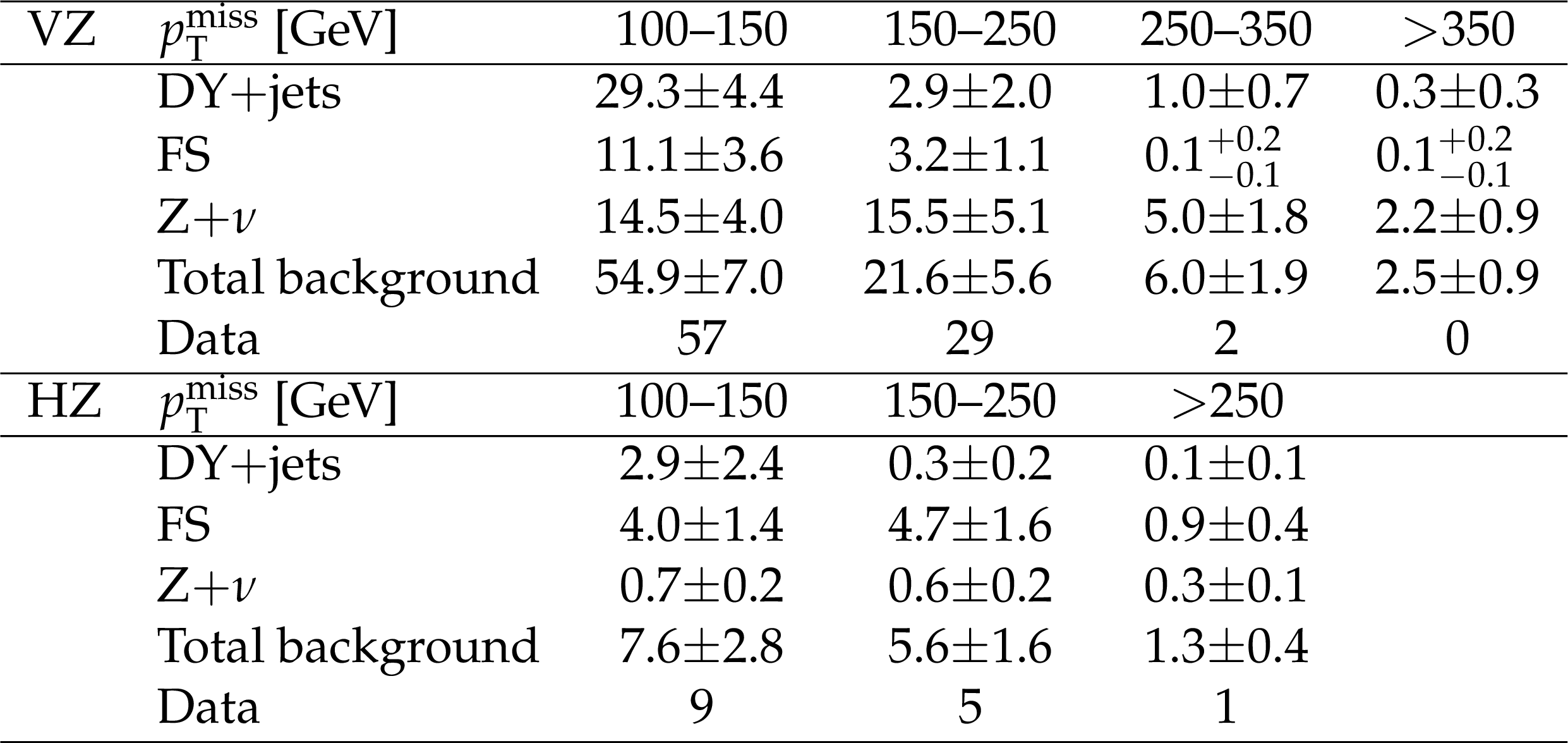
Table 3:
Predicted and observed event yields are shown for the EW on-Z SRs, for each ${{p_{\mathrm {T}}} ^\text {miss}} $ bin defined in Table 1. The uncertainties shown include both statistical and systematic sources. |
png pdf |
Table 4:
Predicted and observed yields in each bin of the edge search counting experiment. The uncertainties shown include both statistical and systematic sources. |
png pdf |
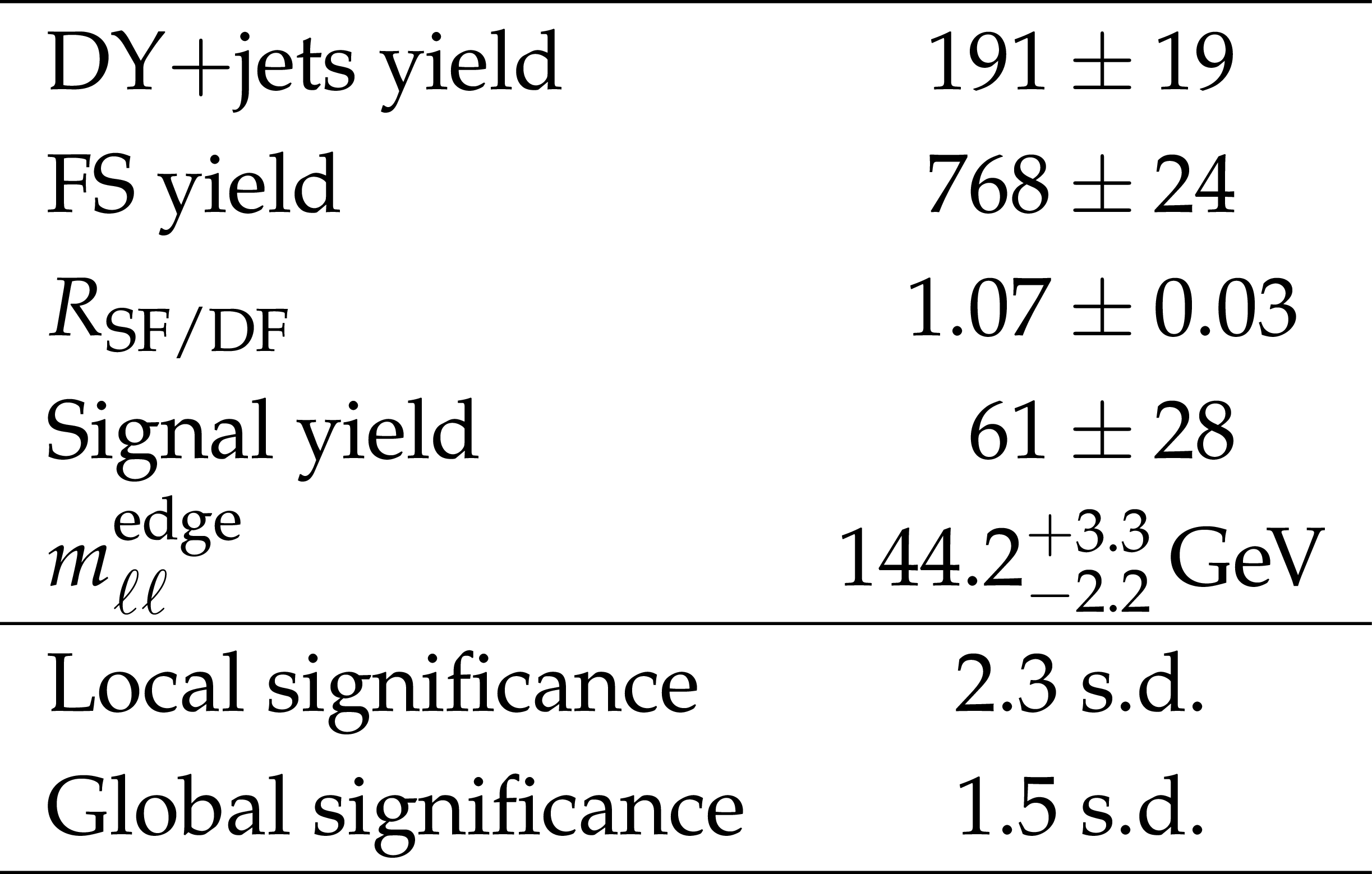
Table 5:
Results of the unbinned maximum likelihood fit for event yields in the edge fit SR of Table 1, including the $ {\text {DY}{+}\text {jets}} $ and FS background components, along with the fitted signal contribution and edge position. The fitted value for $ {R_{\text {SF/DF}}} $ and the local and global signal significances in terms of standard deviations are also given. The uncertainties account for both statistical and systematic components. |

png pdf |
Table 6:
Systematic uncertainties taken into account for the signal yields and their typical values. |
| Summary |
|
A search for phenomena beyond the standard model (SM) in events with opposite-charge, same-flavor leptons, jets, and missing transverse momentum has been presented. The data used corresponds to a sample of pp collisions collected with the CMS detector in 2016 at a center-of-mass energy of 13 TeV, corresponding to an integrated luminosity of 35.9 fb$^{-1}$. Searches are performed for signals with a dilepton invariant mass ($ {m_{\ell\ell}} $) compatible with the Z boson or producing a kinematic edge in the distribution of $ {m_{\ell\ell}} $. By comparing the observation to estimates for SM backgrounds obtained from data control samples, no statistically significant evidence for a signal has been observed. The search for strongly produced new physics containing an on-shell Z boson is interpreted in a model of gauge-mediated supersymmetry breaking (GMSB), where the Z bosons are produced in decay chains initiated through gluino pair production. Gluino masses below 1500-1770 GeV have been excluded, depending on the neutralino mass, extending the exclusion limits derived from the previous CMS publication by almost 500 GeV. The search for electroweak production with an on-shell Z boson has been interpreted in multiple simplified models. For chargino-neutralino production, where the neutralino decays to a Z boson and the lightest supersymmetric particle (LSP) and the chargino decays to a W boson and the LSP, we probe chargino masses in the range 160-610 GeV. In a GMSB model of neutralino-neutralino production decaying to ZZ and LSPs, we probe neutralino masses up to around 650 GeV. Assuming GMSB production where the neutralino has a branching fraction of 50% to the Z boson and 50% to the Higgs boson, we probe neutralino masses up to around 500 GeV. Compared to published CMS results using 8 TeV data, these extend the exclusion limits by around 200-300 GeV depending on the model. The search for a kinematic edge in the $ {m_{\ell\ell}} $ distribution is interpreted in a simplified model based on bottom squark pair production. Decay chains containing the two lightest neutralinos and a slepton are assumed, leading to edge-like signatures in the distribution of $ {m_{\ell\ell}} $. Bottom squark masses below 980-1200 GeV have been excluded, depending on the mass of the second neutralino. These extend the previous CMS exclusion limits in the same model by 400-600 GeV. |
| Additional Figures | |
png pdf |
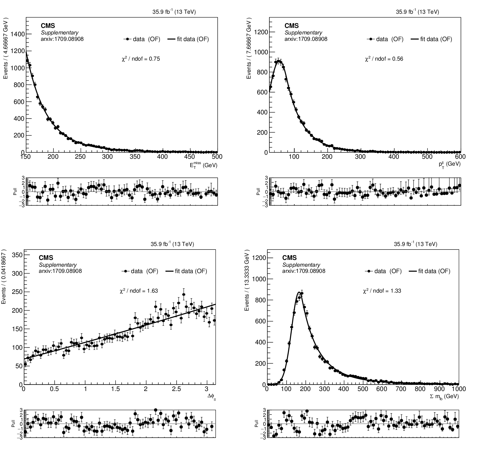
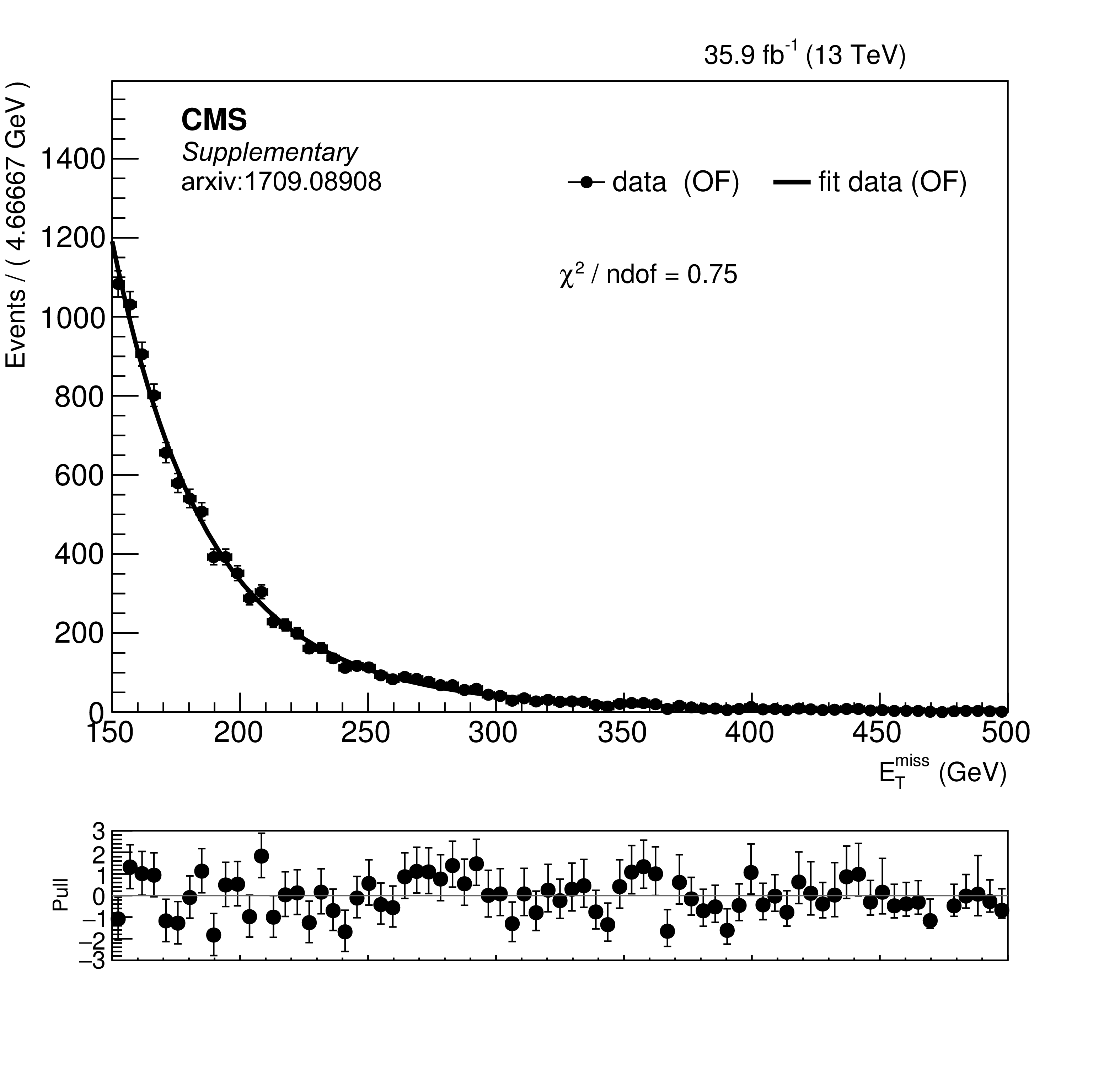
Additional Figure 1:
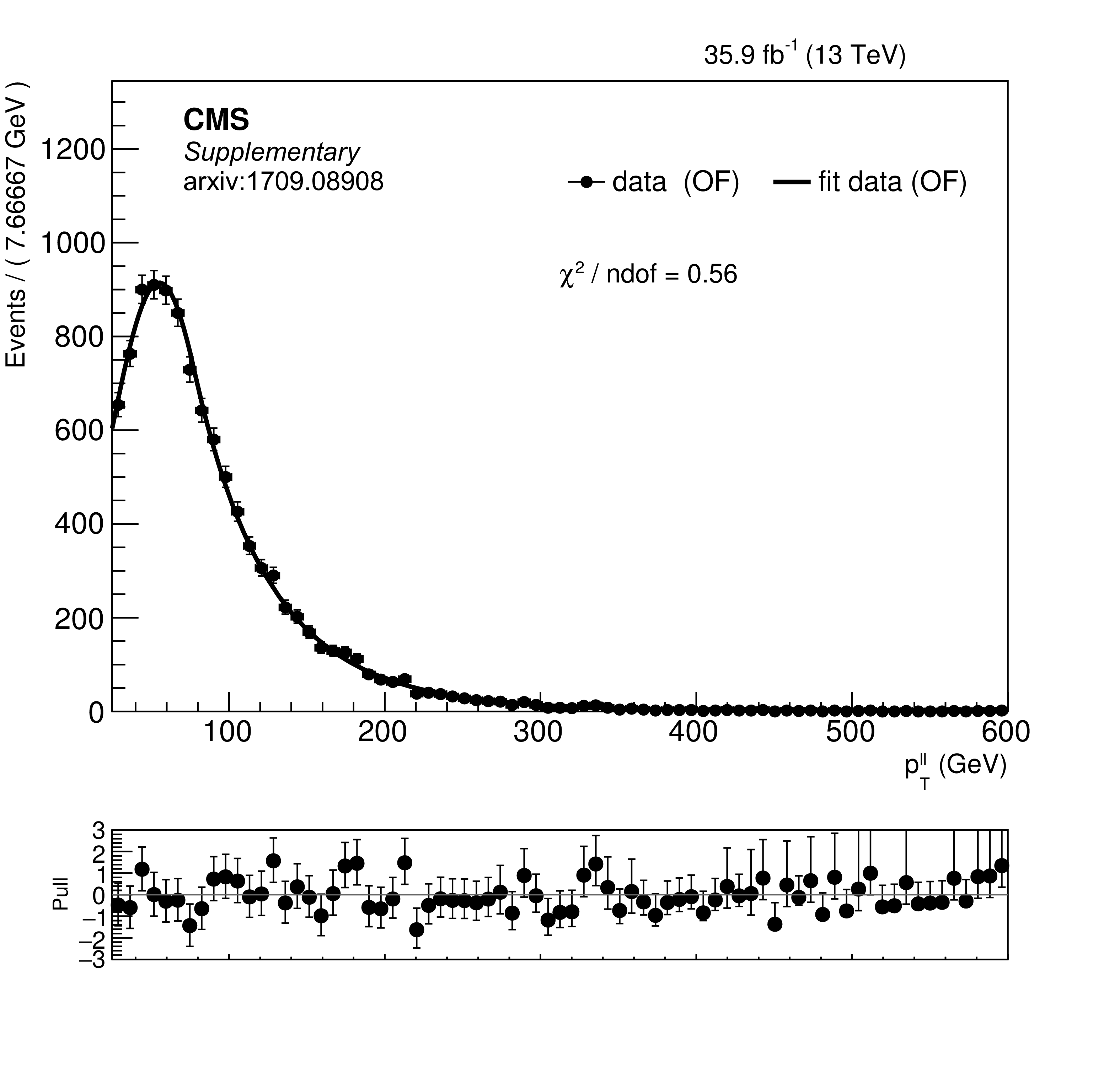
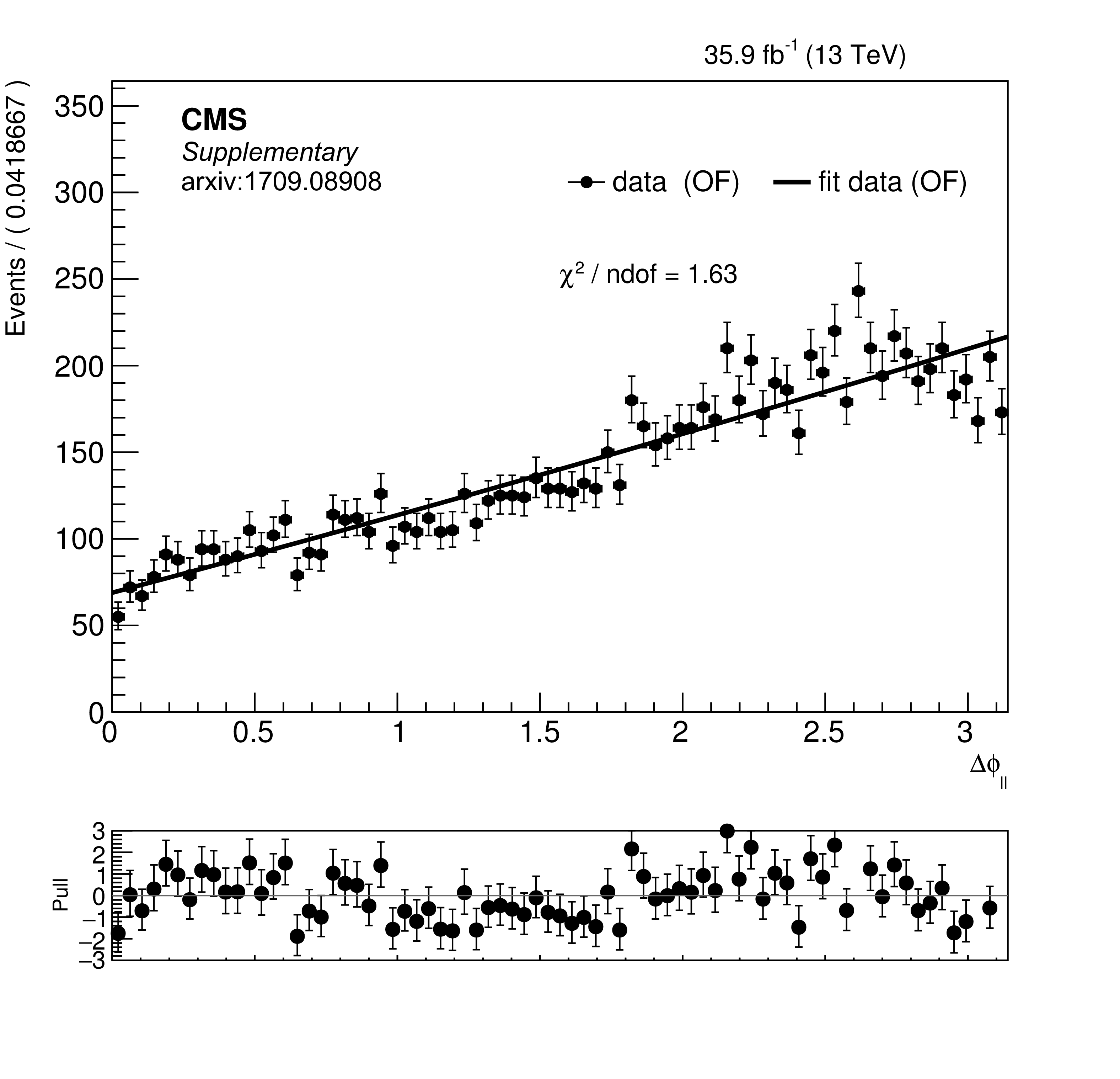
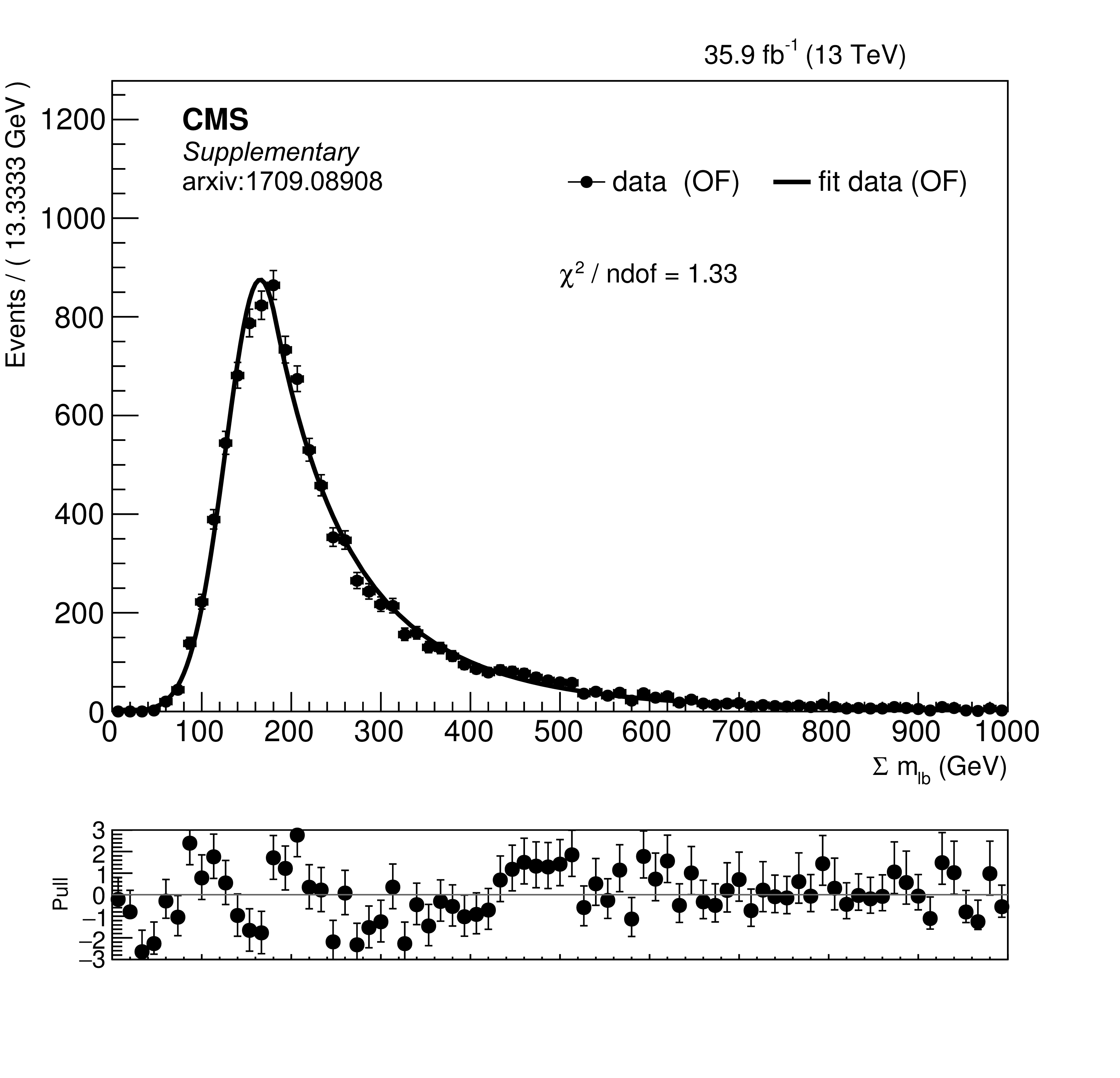
PDFs for the four input variables to the likelihood discriminant: ${E_{\mathrm {T}}^{\text {miss}}}$ (a), di-lepton $ {p_{\mathrm {T}}} $ (b), $|\Delta \phi |$ between the leptons (c), and $\Sigma m_{\ell \text {b}}$ (d) for data in the OF region. |
png pdf |
Additional Figure 1-a:
PDF for an input variable to the likelihood discriminant: ${E_{\mathrm {T}}^{\text {miss}}}$. |
png pdf |
Additional Figure 1-b:
PDF for an input variable to the likelihood discriminant: di-lepton $ {p_{\mathrm {T}}} $. |
png pdf |
Additional Figure 1-c:
PDF for an input variable to the likelihood discriminant: $|\Delta \phi |$ between the leptons. |
png pdf |
Additional Figure 1-d:
PDF for an input variable to the likelihood discriminant: $\Sigma m_{\ell \text {b}}$ (d) for data in the OF region. |

png pdf |
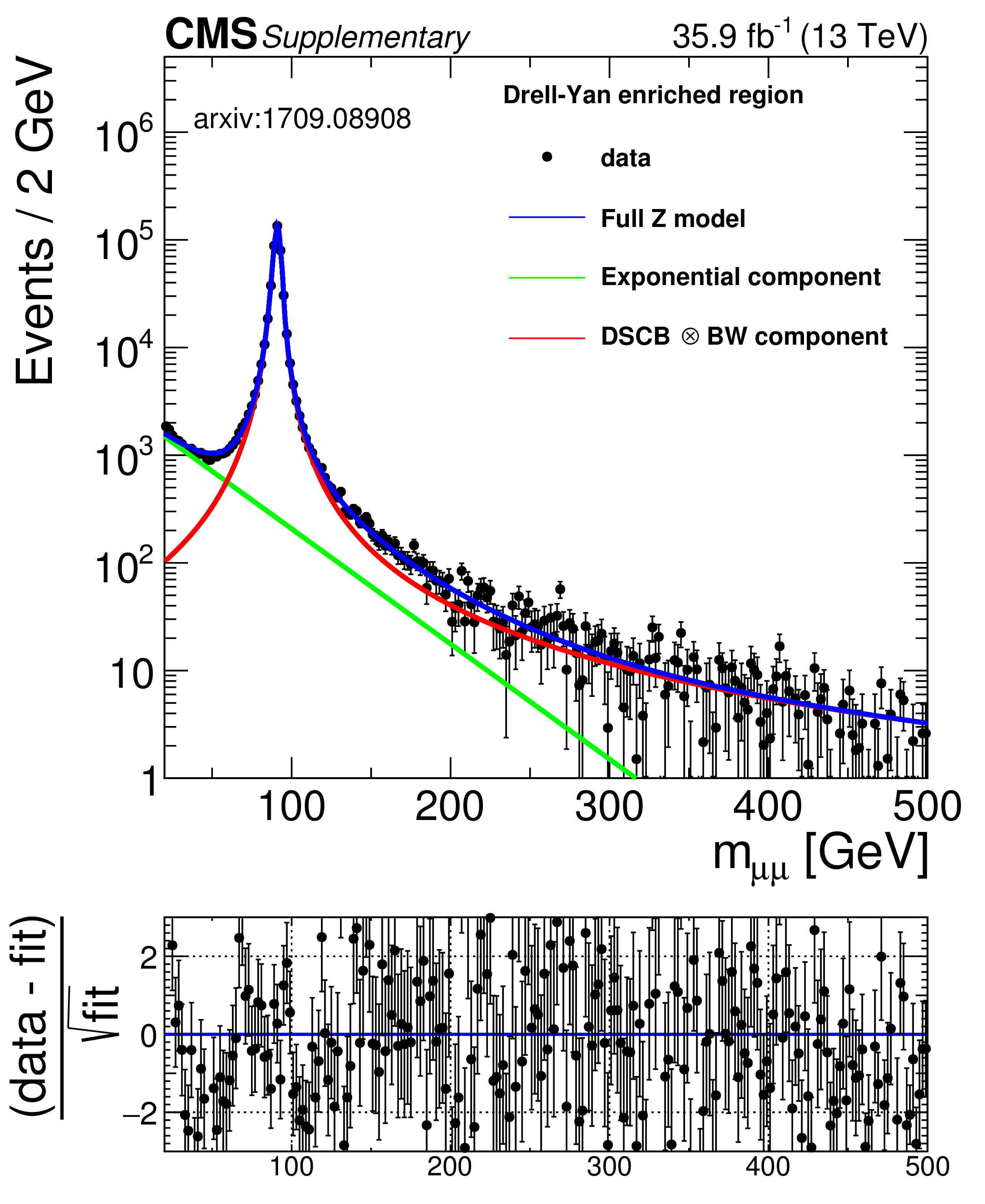
Additional Figure 2:
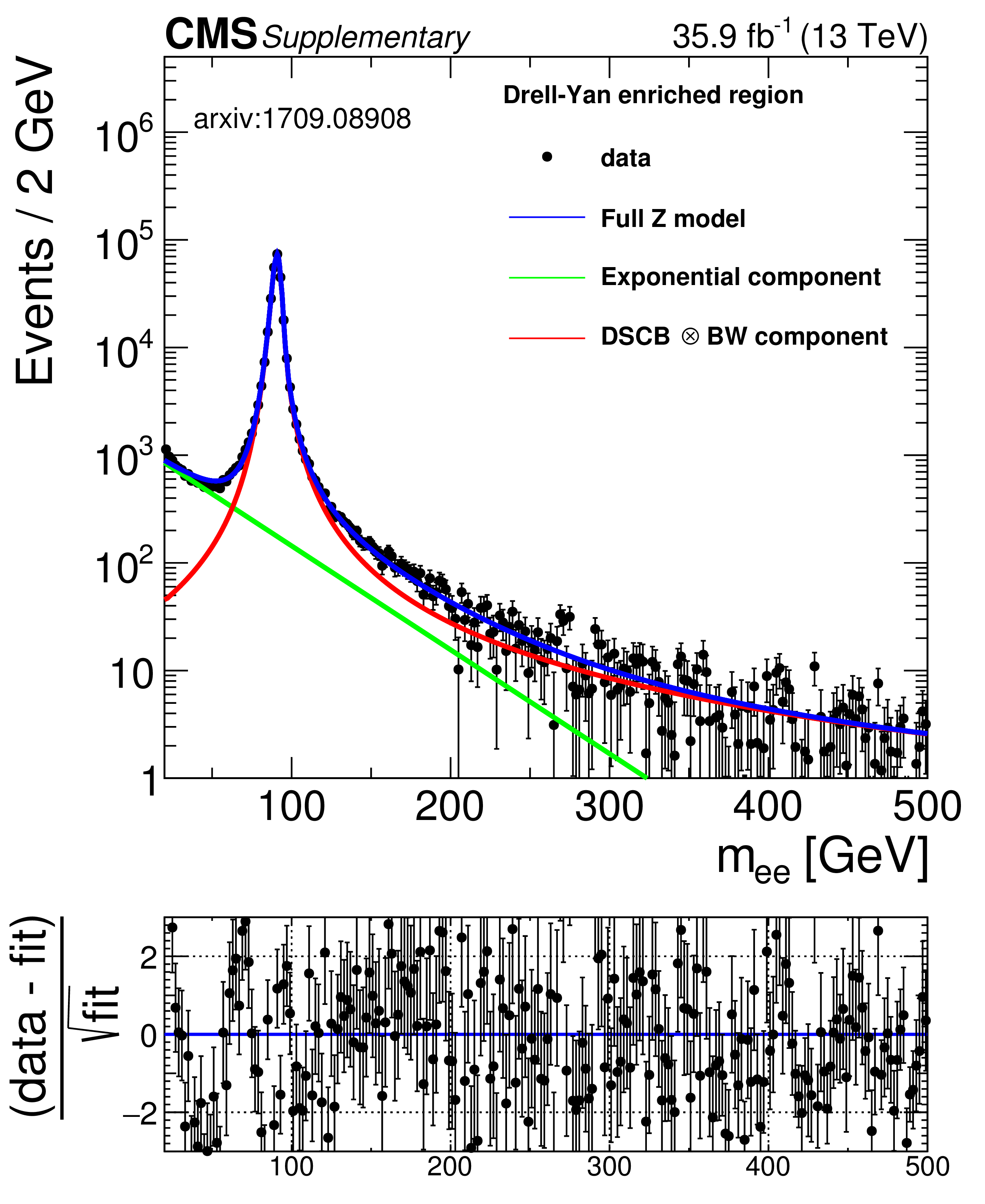
Fitted shape for backgrounds containing a Z boson for dielectron events (a) and dimuon events (b). The fitted shape consists of an exponential (green) and a Breit-wigner convolved with a double-sided Crystal-Ball (red), whose sum (blue) describes the backgrounds containing a Z boson. |
png pdf |
Additional Figure 2-a:
Fitted shape for backgrounds containing a Z boson for dielectron events. The fitted shape consists of an exponential (green) and a Breit-wigner convolved with a double-sided Crystal-Ball (red), whose sum (blue) describes the backgrounds containing a Z boson. |
png pdf |
Additional Figure 2-b:
Fitted shape for backgrounds containing a Z boson for dimuon events. The fitted shape consists of an exponential (green) and a Breit-wigner convolved with a double-sided Crystal-Ball (red), whose sum (blue) describes the backgrounds containing a Z boson. |
png pdf |
Additional Figure 3:
Result of fit in signal region for same-flavor (a) and different-flavor (b) events for data evaluating the null hypothesis. |
png pdf |
Additional Figure 3-a:
Result of fit in signal region for same-flavor events for data evaluating the null hypothesis. |
png pdf |
Additional Figure 3-b:
Result of fit in signal region for different-flavor events for data evaluating the null hypothesis. |
png pdf |
Additional Figure 4:
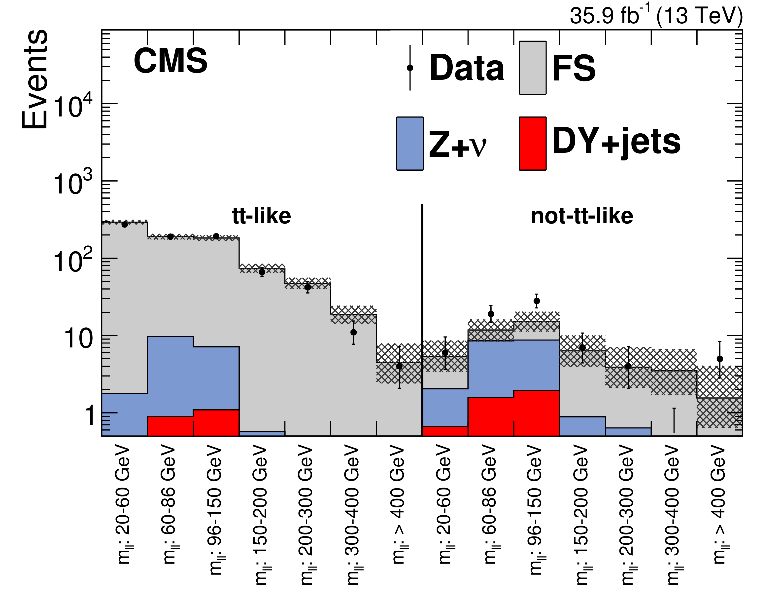
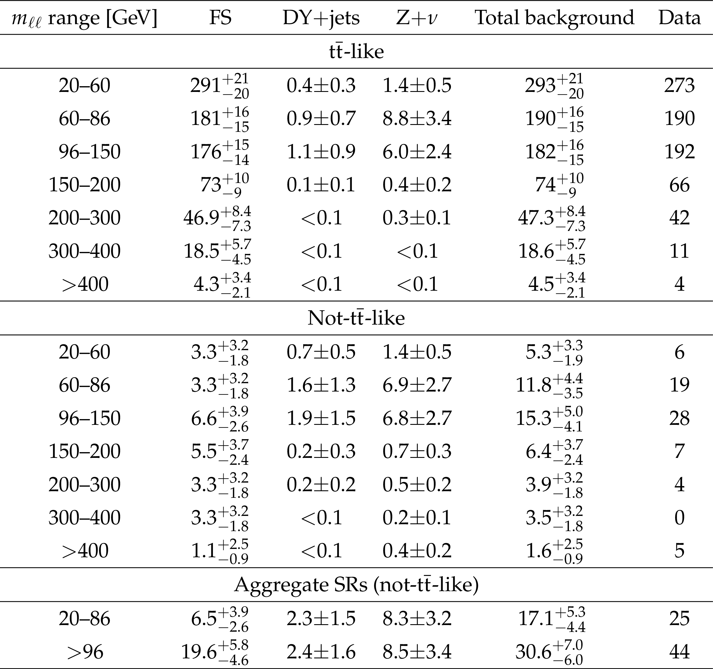
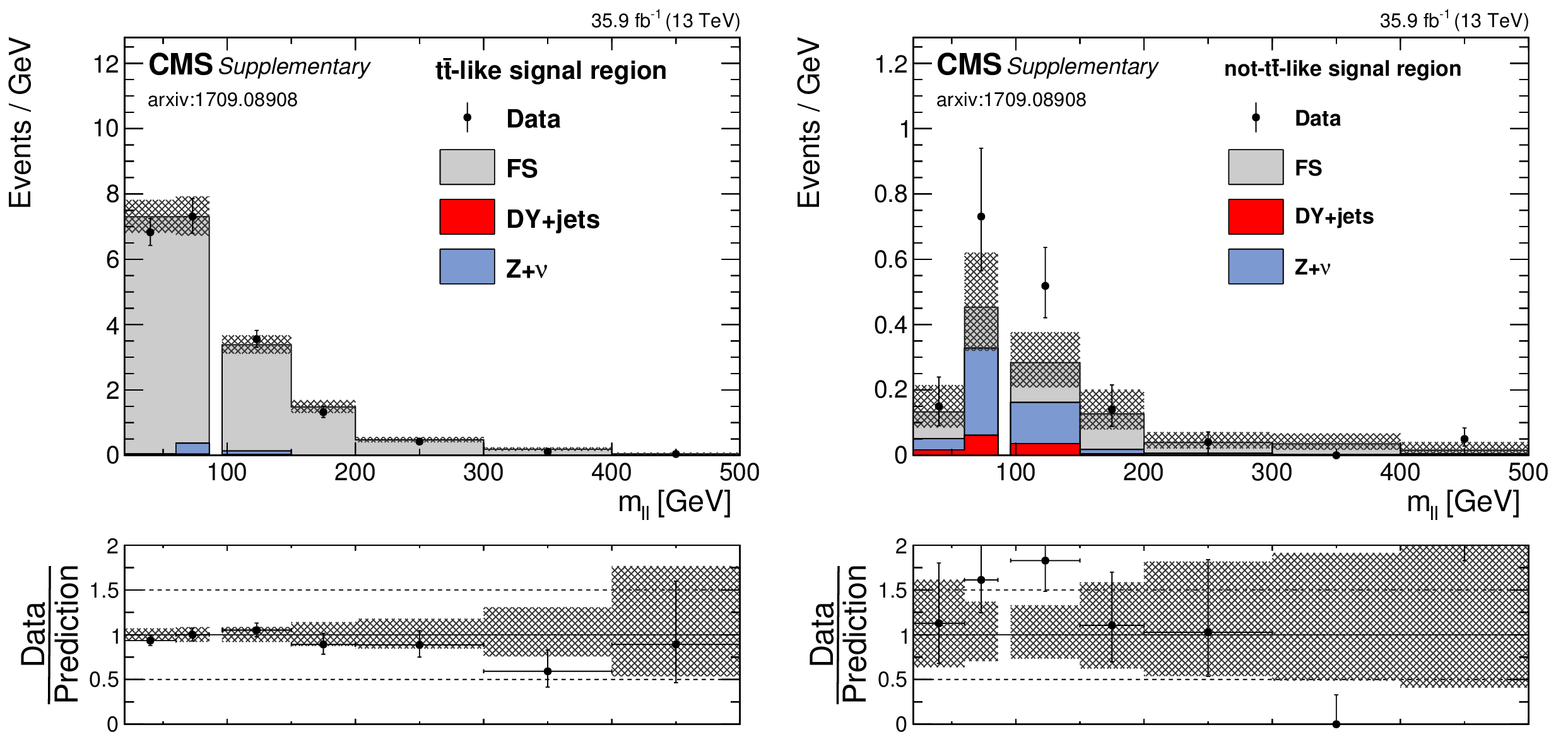
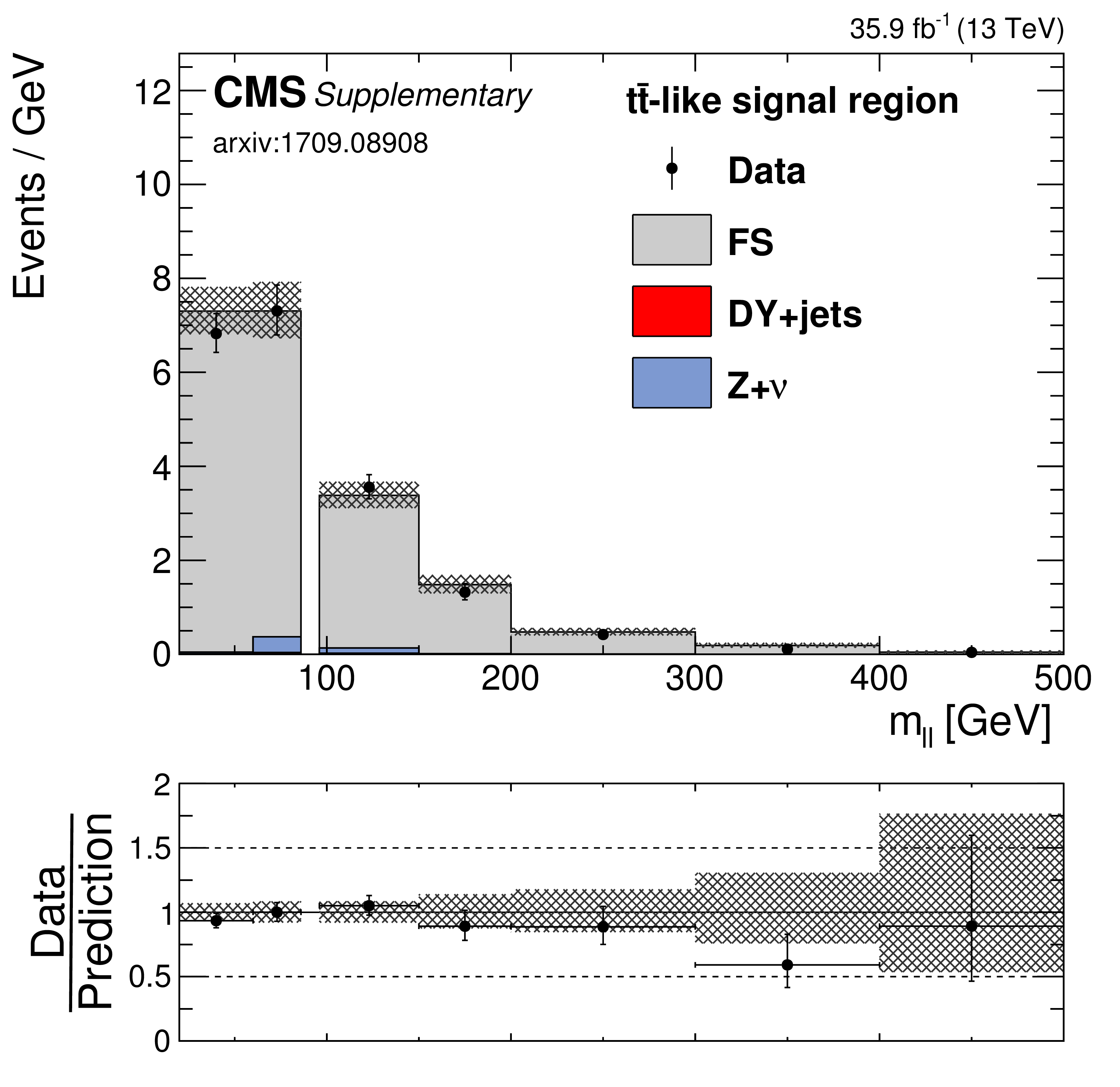
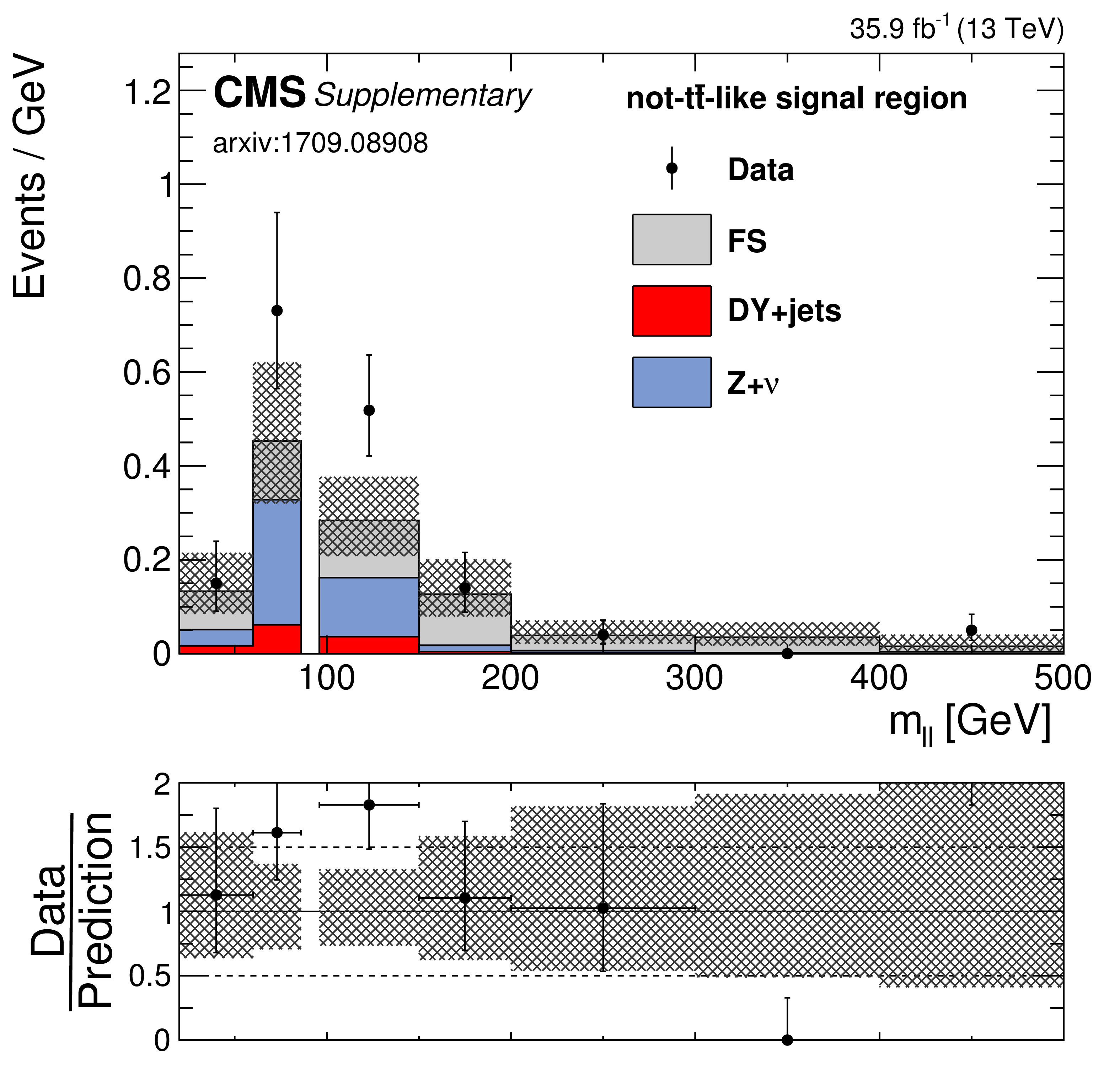
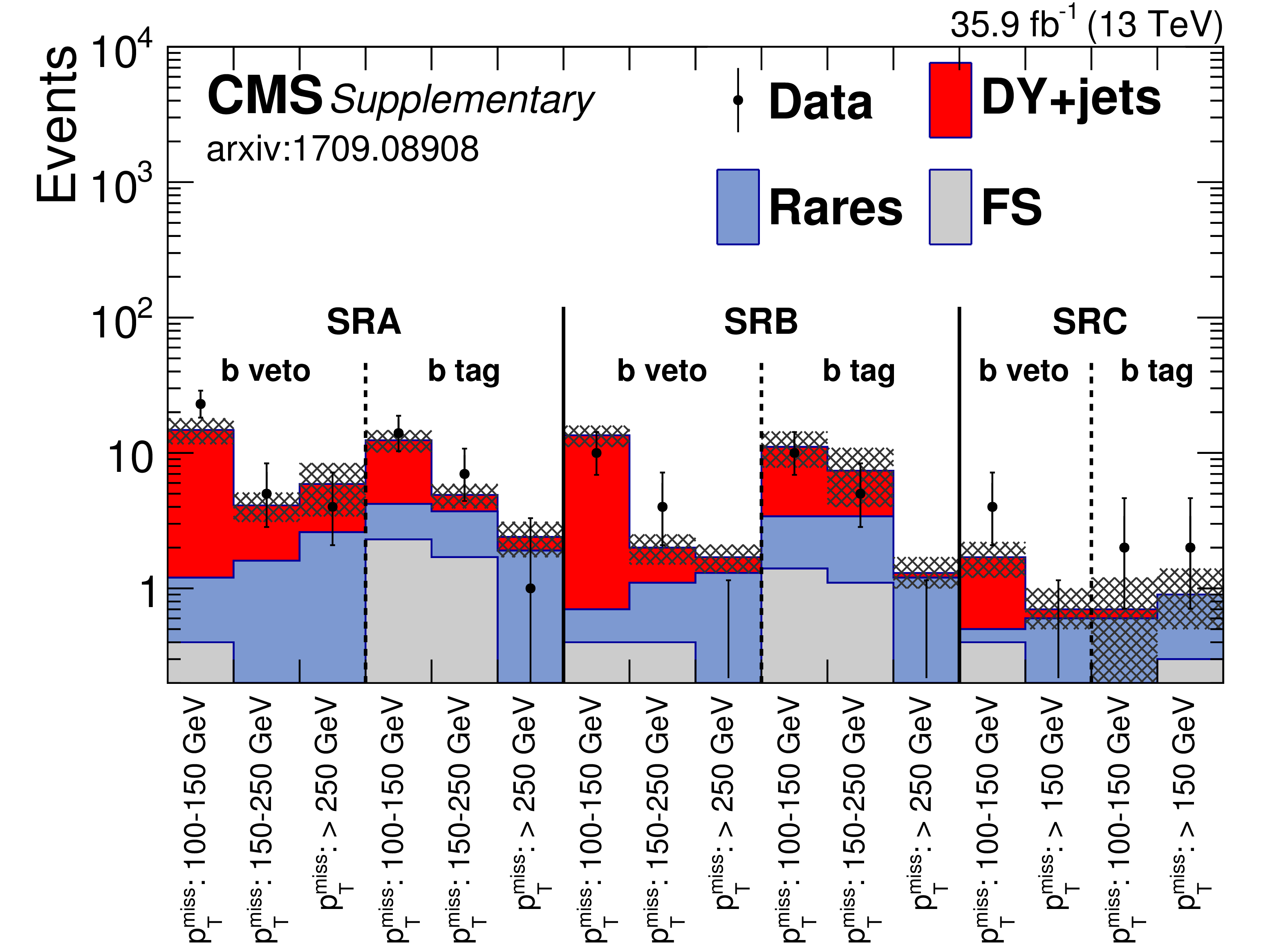
$ {m_{\ell \ell}} $ distribution in the $ {\mathrm{t} {}\mathrm{\bar{t}}} $ like (a) and non $ {\mathrm{t} {}\mathrm{\bar{t}}} $ like (b) edge signal regions.The number of observed events, shown as black data points, is compared to the total background estimate, shown as a blue line with a blue uncertainty band. The non flavor symmetric background component from instrumental $E_{\text {T}}^{\text {miss}}$ is indicated as a green area while the non flavor symmetric background with neutrinos is shown as a violet area. |
png pdf |
Additional Figure 4-a:
$ {m_{\ell \ell}} $ distribution in the $ {\mathrm{t} {}\mathrm{\bar{t}}} $ like edge signal regions.The number of observed events, shown as black data points, is compared to the total background estimate, shown as a blue line with a blue uncertainty band. The non flavor symmetric background component from instrumental $E_{\text {T}}^{\text {miss}}$ is indicated as a green area while the non flavor symmetric background with neutrinos is shown as a violet area. |
png pdf |
Additional Figure 4-b:
$ {m_{\ell \ell}} $ distribution in the non $ {\mathrm{t} {}\mathrm{\bar{t}}} $ like edge signal regions.The number of observed events, shown as black data points, is compared to the total background estimate, shown as a blue line with a blue uncertainty band. The non flavor symmetric background component from instrumental $E_{\text {T}}^{\text {miss}}$ is indicated as a green area while the non flavor symmetric background with neutrinos is shown as a violet area. |

png pdf |
Additional Figure 5:
Two-dimensional distribution of the observed significances in the slepton-edge signal model. |
png pdf |
Additional Figure 6:
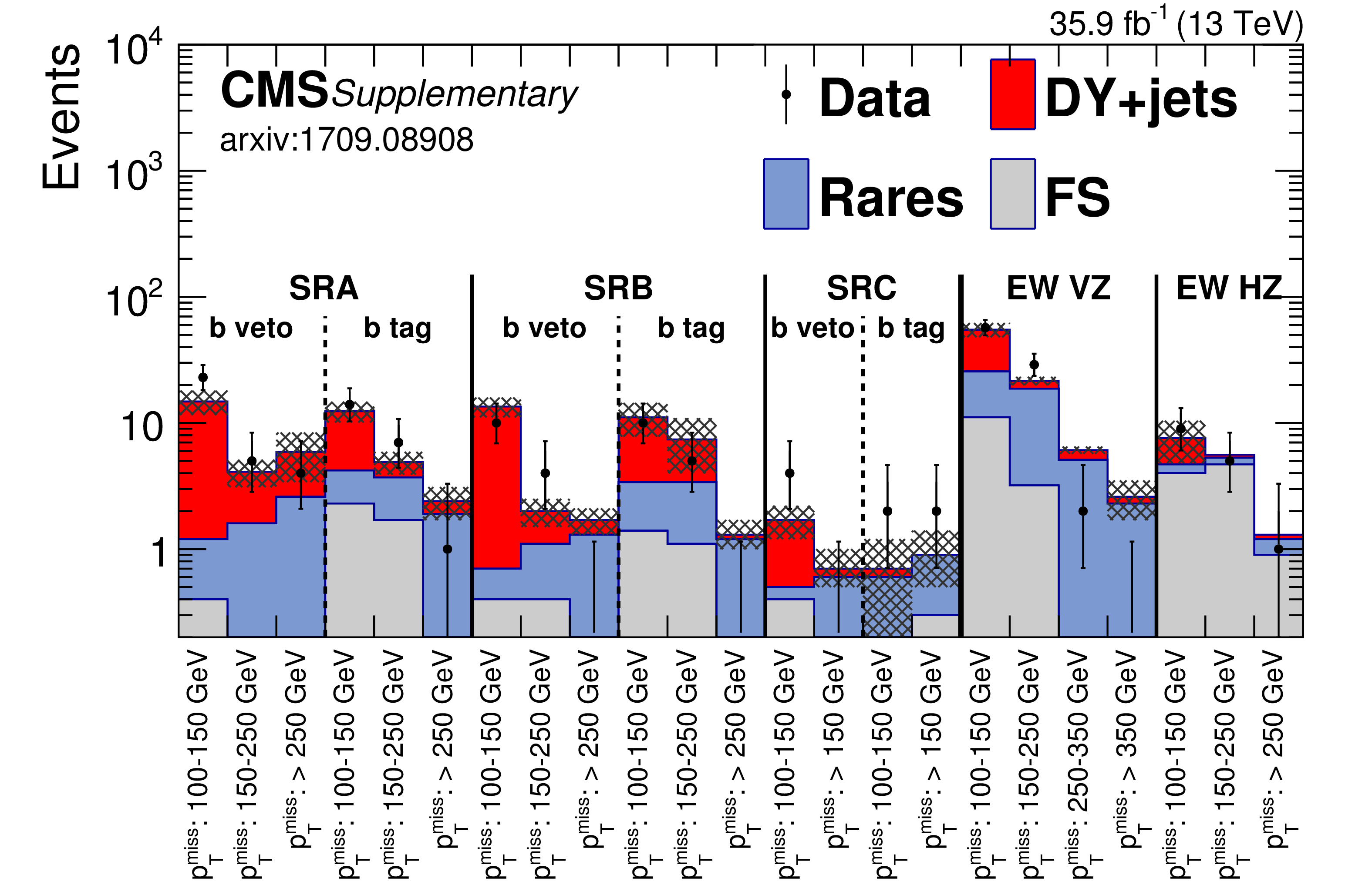
Summary of results in all the on-Z signal regions. The three blocks on the left correspond to the on-Z signal regions targeting the gluino GMSB signal model, while the two blocks on the right correspond to the on-Z signal regions looking for electroweakly produced new physics. |
png pdf |
Additional Figure 7:
Summary of results in the on-Z signal regions targeting the gluino GMSB model. |
| Additional Tables | |
png pdf |
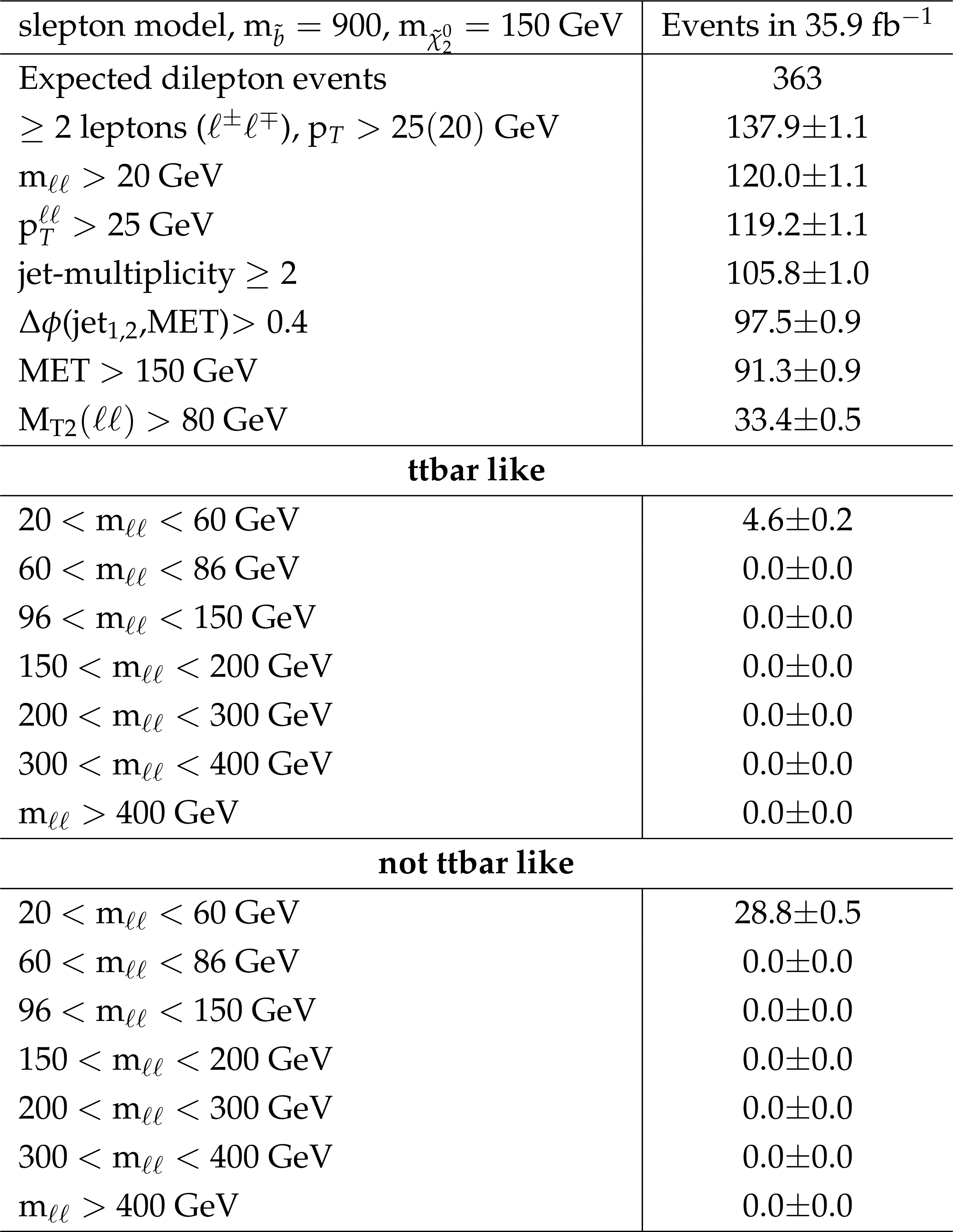
Additional Table 1:
Cut flow table for the edge signal model for a mass point at $m_{\tilde{b}}=$ 900 GeV and $m_{\tilde{\chi}_{2}^{0}}=$ 150 GeV. Expected dilepton events refers to luminosity$\times $cross section$\times $branching ratio. |
png pdf |
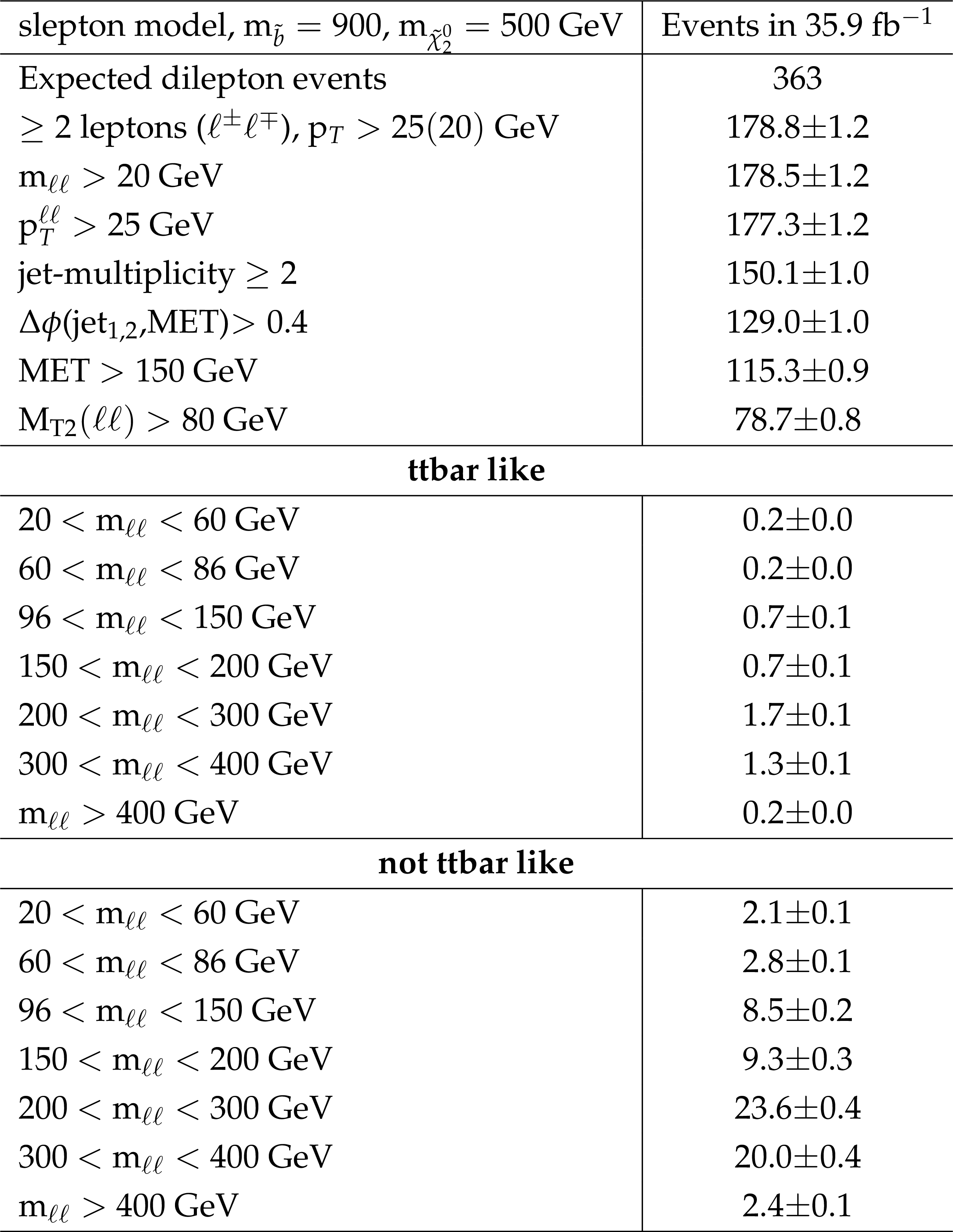
Additional Table 2:
Cut flow table for the edge signal model for a mass point at $m_{\tilde{b}}=$ 900 GeV and $m_{\tilde{\chi}_{2}^{0}}=$ 500 GeV. Expected dilepton events refers to luminosity$\times $cross section$\times $branching ratio. |
png pdf |
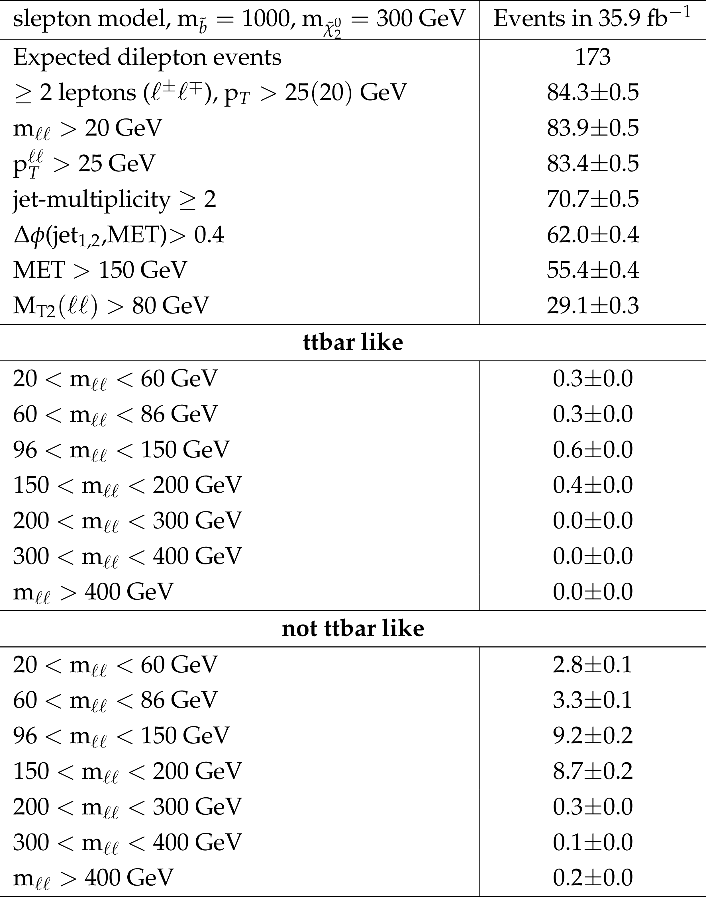
Additional Table 3:
Cut flow table for the edge signal model for a mass point at $m_{\tilde{b}}=$ 1000 GeV and $m_{\tilde{\chi}_{2}^{0}}=$ 300 GeV. Expected dilepton events refers to luminosity$\times $cross section$\times $branching ratio. |

png pdf |
Additional Table 4:
Cut flow table for the edge signal model for a mass point at $m_{\tilde{b}}=$ 1200 GeV and $m_{\tilde{\chi}_{2}^{0}}=$ 200 GeV. Expected dilepton events refers to luminosity$\times $cross section$\times $branching ratio. |
png pdf |
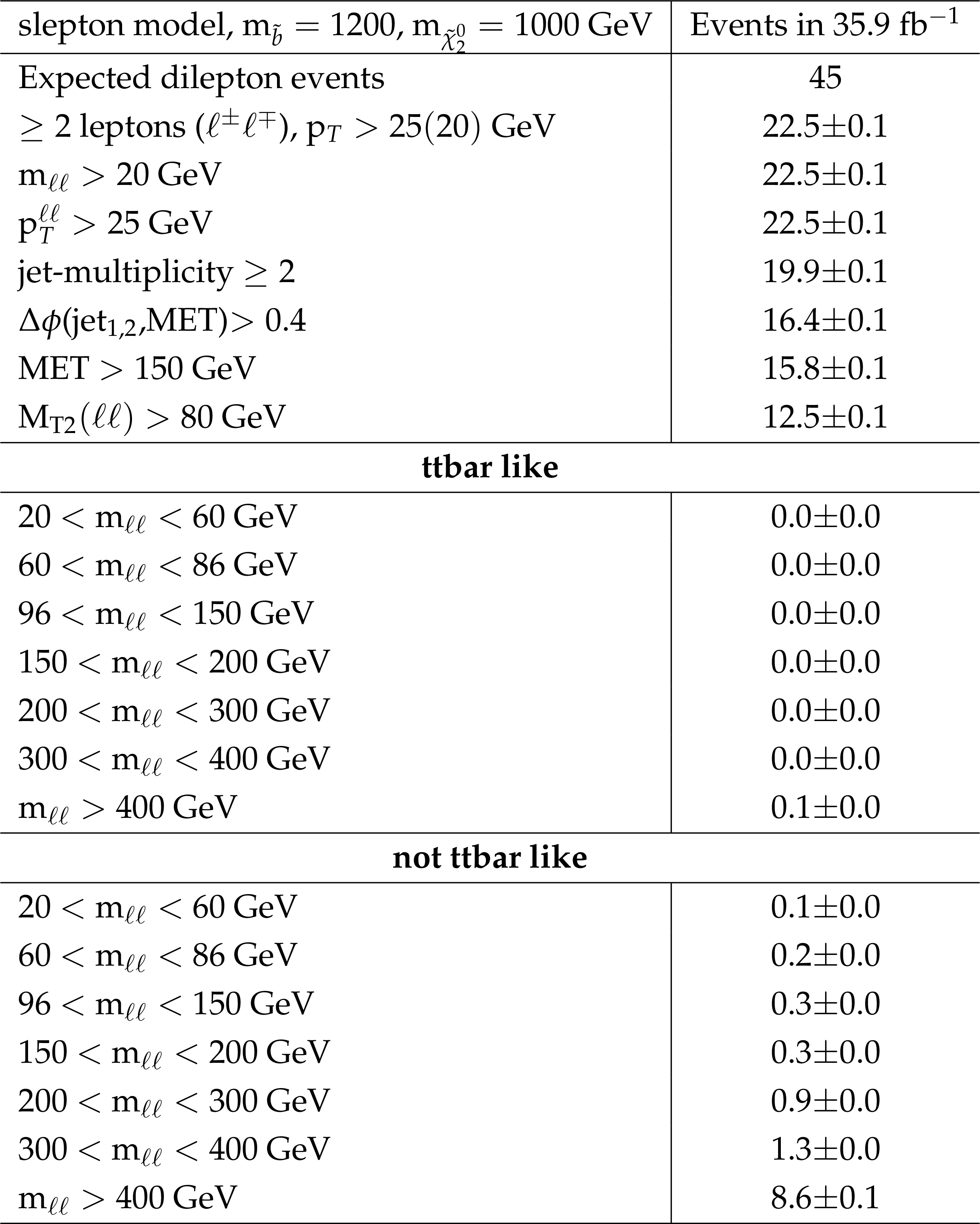
Additional Table 5:
Cut flow table for the edge signal model for a mass point at $m_{\tilde{b}}=$ 1200 GeV and $m_{\tilde{\chi}_{2}^{0}}=$ 1000 GeV. Expected dilepton events refers to luminosity$\times $cross section$\times $branching ratio. |
png pdf |
Additional Table 6:
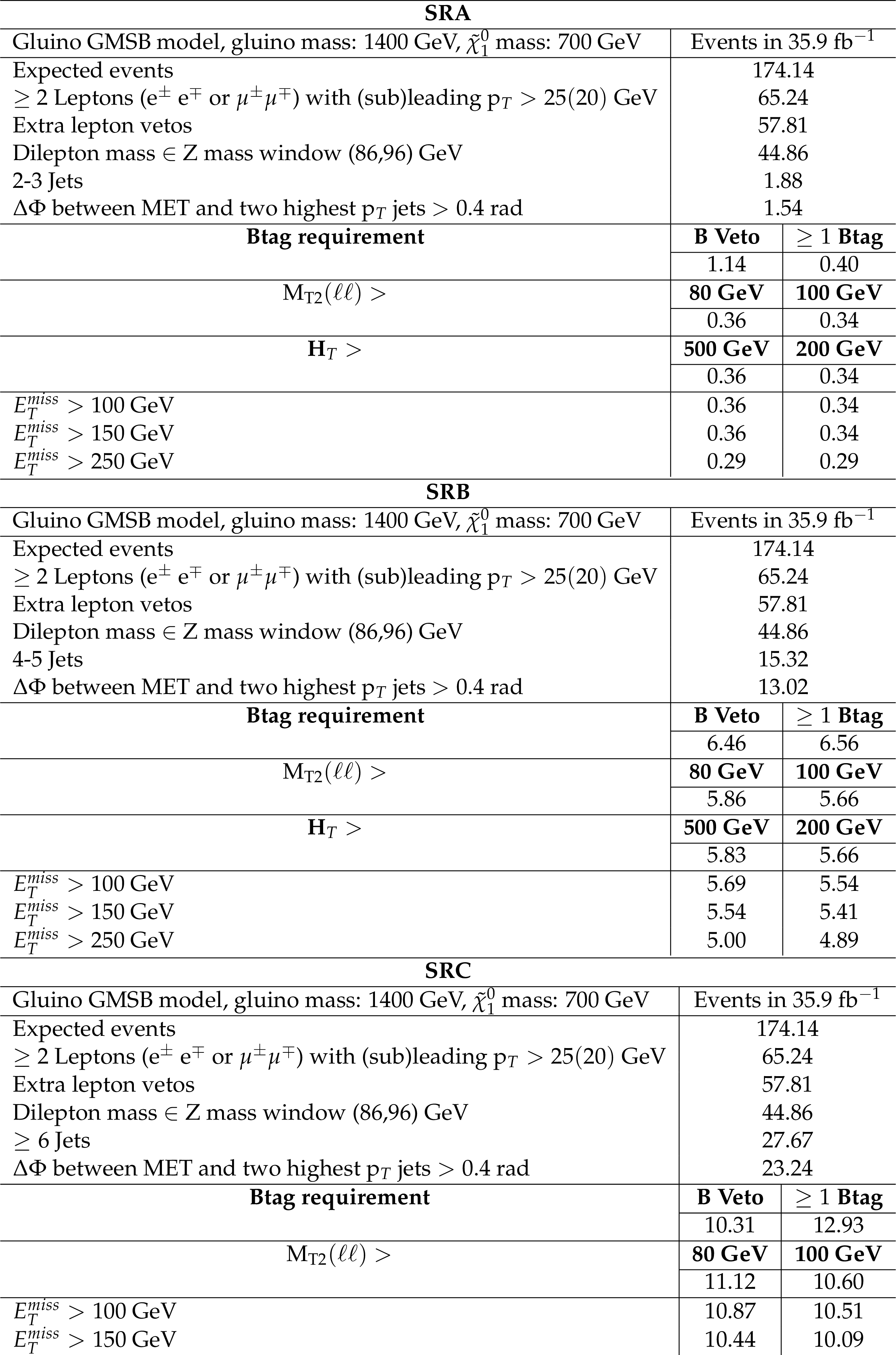
Cut flow table for the strong on-Z signal region selections for the gluino GMSB signal model with the mass of the gluino and the $\tilde{\chi}_{1}^{0}$ equal to 1400 and 700 GeV, respectively. The theoretical cross section for this signal is 25.3 fb and at least one Z boson was required to decay leptonically, for a branching fraction of 0.192. |
png pdf |
Additional Table 7:
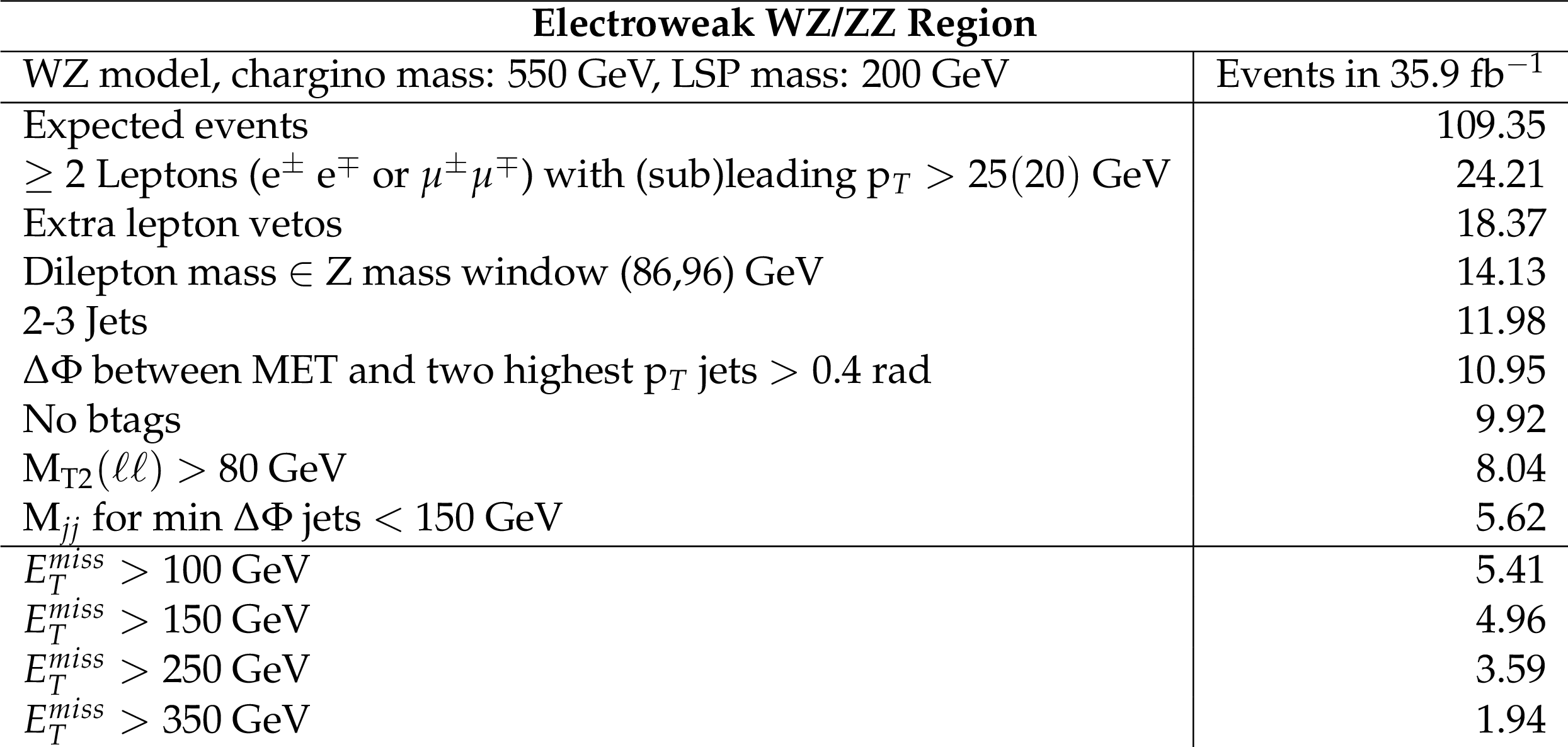
Cut flow table for the electroweak on-Z signal region selections for the WZ signal model with the mass of the chargino and the LSP equal to 550 and 200 GeV, respectively. The theoretical cross section for this signal is 30.2 fb and the Z boson was required to decay leptonically, for a branching fraction of 0.10. |
png pdf |
Additional Table 8:
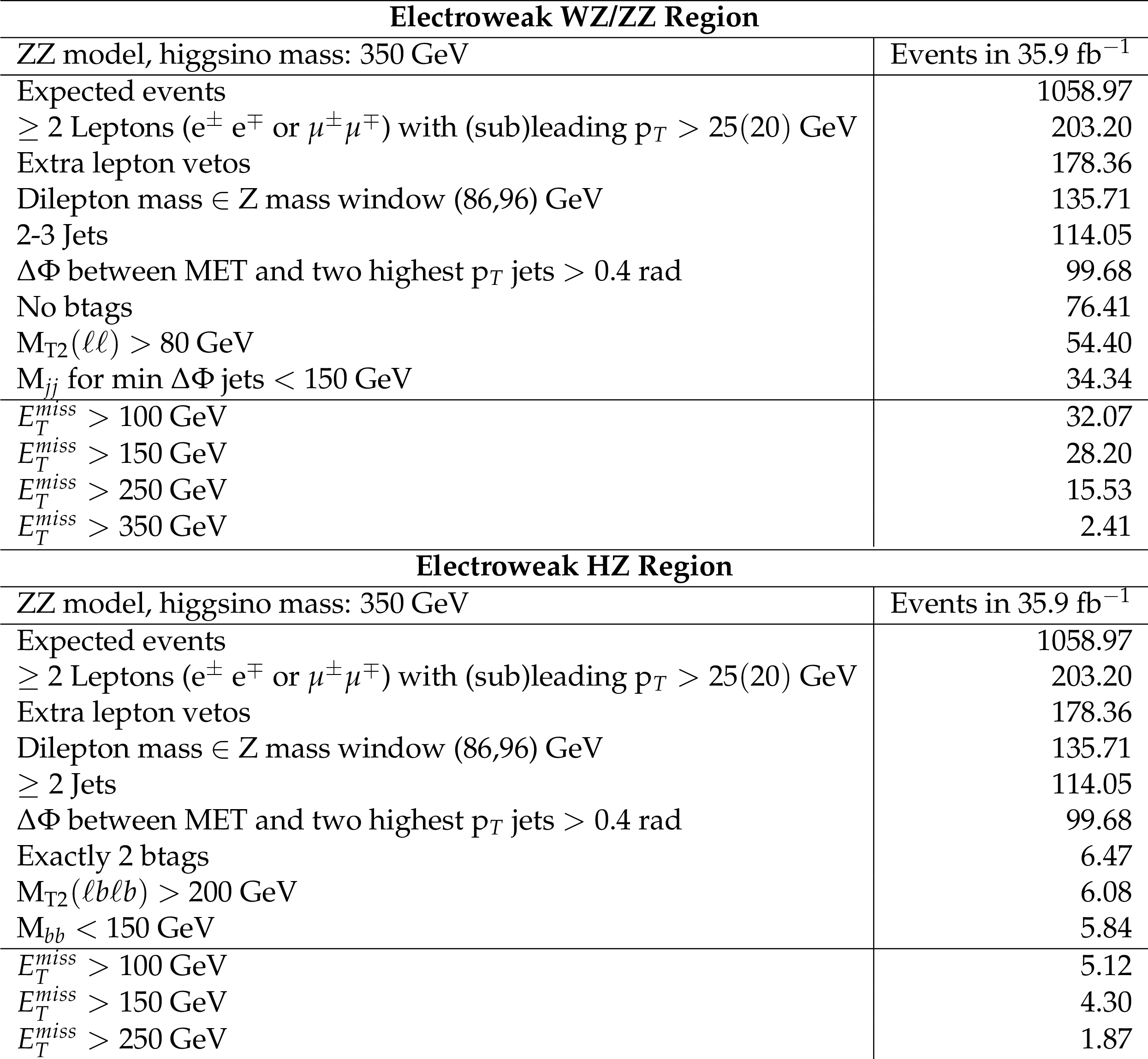
Cut flow table for the electroweak on-Z signal region selections for the ZZ signal model with the mass of the higginos equal to 350 GeV. The theoretical cross section for this signal is 154 fb (assuming scenario 1 from the text) and at least one Z boson was required to decay leptonically, for a branching fraction of 0.192. |
png pdf |
Additional Table 9:
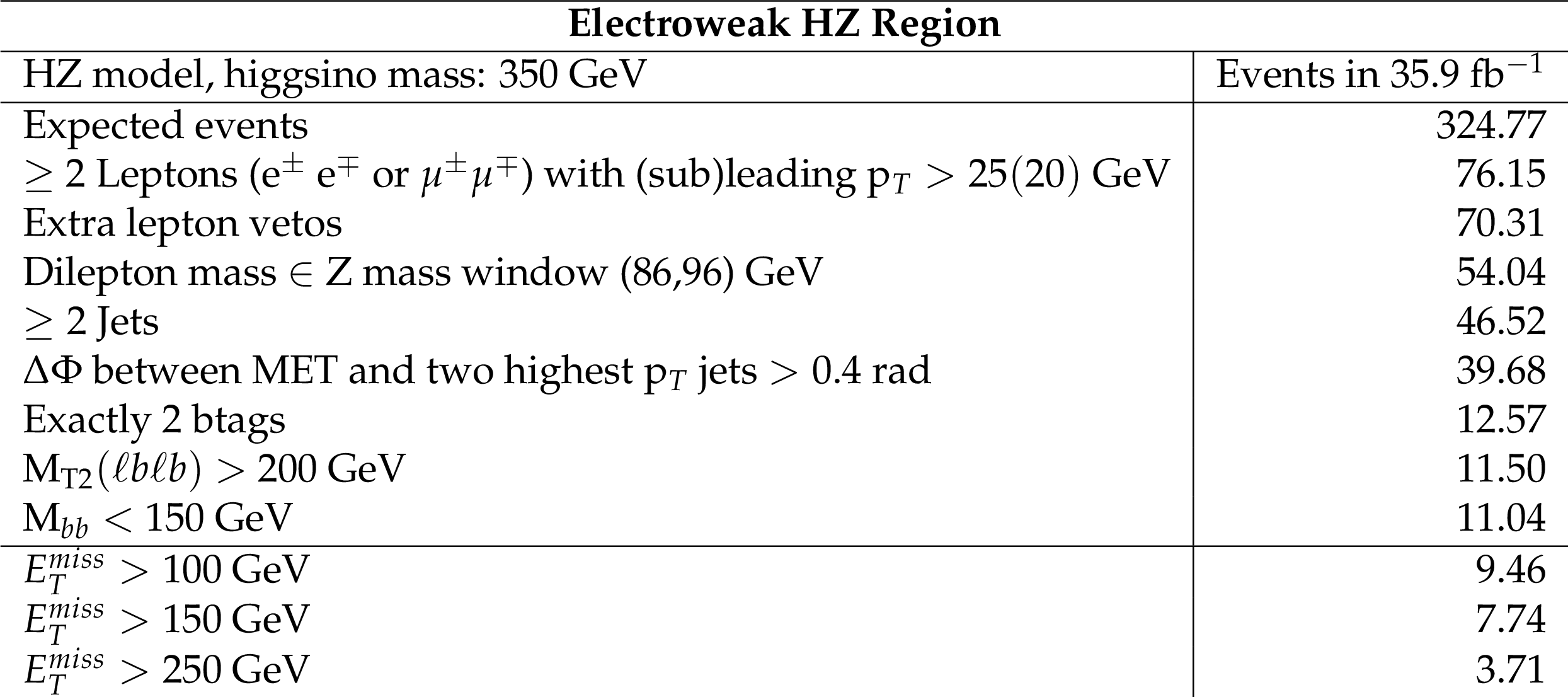
Cut flow table for the electroweak on-Z signal region selections for the HZ signal model with the mass of the higginos equal to 350 GeV. Only HZ events are considered here and a 100% branching fraction of the sparticles to the HZ final state is assumed in these numbers. The theoretical cross section for this signal is 154 fb (assuming scenario 1 from the text). The Z boson was required to decay leptonically and the Higgs boson to decay to ${\mathrm{b} \mathrm{\bar{b}}}$, for a branching fraction of 0.059. |
|
Code for calculating the $ M_{\mathrm{T2}} $ variable can be found here.
A macro for calculating the nll variable and the RooWorkSpace with the fitted pdfs used for the calculation is available here. |
| References | ||||
| 1 | P. Ramond | Dual theory for free fermions | PRD 3 (1971) 2415 | |
| 2 | Yu. A. Gol'fand and E. P. Likhtman | Extension of the algebra of Poincare group generators and violation of P invariance | JEPTL 13 (1971)323 | |
| 3 | A. Neveu and J. H. Schwarz | Factorizable dual model of pions | NPB 31 (1971) 86 | |
| 4 | D. V. Volkov and V. P. Akulov | Possible universal neutrino interaction | JEPTL 16 (1972)438 | |
| 5 | J. Wess and B. Zumino | A Lagrangian model invariant under supergauge transformations | PLB 49 (1974) 52 | |
| 6 | J. Wess and B. Zumino | Supergauge transformations in four dimensions | NPB 70 (1974) 39 | |
| 7 | P. Fayet | Supergauge invariant extension of the Higgs mechanism and a model for the electron and its neutrino | NPB 90 (1975) 104 | |
| 8 | H. P. Nilles | Supersymmetry, supergravity and particle physics | Phys. Rep. 110 (1984) 1 | |
| 9 | G. R. Farrar and P. Fayet | Phenomenology of the production, decay, and detection of new hadronic states associated with supersymmetry | PLB 76 (1978) 575 | |
| 10 | A. J. Buras, J. R. Ellis, M. K. Gaillard, and D. V. Nanopoulos | Aspects of the grand unification of strong, weak and electromagnetic interactions | NPB 135 (1978) 66 | |
| 11 | H. E. Haber and G. L. Kane | The search for supersymmetry: Probing physics beyond the standard model | PR 117 (1985) 75 | |
| 12 | I. Hinchliffe et al. | Precision SUSY measurements at CERN LHC | PRD 55 (1997) 5520 | hep-ph/9610544 |
| 13 | CMS Collaboration | Search for physics beyond the Standard Model in events with two leptons, jets, and missing transverse momentum in pp collisions at $ \sqrt{s} = $ 8 TeV | JHEP 04 (2015) 124 | CMS-SUS-14-014 1502.06031 |
| 14 | CMS Collaboration | Search for new physics in final states with two opposite-sign, same-flavor leptons, jets, and missing transverse momentum in pp collisions at $ \sqrt{s} = $ 13 TeV | JHEP 12 (2016) 013 | CMS-SUS-15-011 1607.00915 |
| 15 | CMS Collaboration | Search for new physics in events with opposite-sign leptons, jets, and missing transverse energy in pp collisions at $ \sqrt{s} = $ 7 TeV | PLB 718 (2013) 815 | CMS-SUS-11-011 1206.3949 |
| 16 | CMS Collaboration | Search for physics beyond the Standard Model in opposite-sign dilepton events in pp collisions at $ \sqrt{s} = $ 7 TeV | JHEP 06 (2011) 26 | CMS-SUS-10-007 1103.1348 |
| 17 | CMS Collaboration | Searches for electroweak production of charginos, neutralinos, and sleptons decaying to leptons and W, Z, and Higgs bosons in pp collisions at 8 TeV | EPJC 74 (2014) 3036 | CMS-SUS-13-006 1405.7570 |
| 18 | CMS Collaboration | Searches for electroweak neutralino and chargino production in channels with Higgs, Z, and W bosons in pp collisions at 8 TeV | PRD 90 (2014) 092007 | CMS-SUS-14-002 1409.3168 |
| 19 | ATLAS Collaboration | Search for supersymmetry in events containing a same-flavour opposite-sign dilepton pair, jets, and large missing transverse momentum in $ \sqrt{s} = $ 8 TeV pp collisions with the ATLAS detector | EPJC 75 (2015) 318 | 1503.03290 |
| 20 | ATLAS Collaboration | Search for the electroweak production of supersymmetric particles in $ \sqrt{s} = $ 8 TeV pp collisions with the ATLAS detector | PRD 93 (2016) 052002 | 1509.07152 |
| 21 | ATLAS Collaboration | Search for new phenomena in events containing a same-flavour opposite-sign dilepton pair, jets, and large missing transverse momentum in $ \sqrt{s} = $ 13 TeV pp collisions with the ATLAS detector | EPJC 77 (2017) 144 | 1611.05791 |
| 22 | N. Arkani-Hamed et al. | MARMOSET: The path from LHC data to the new Standard Model via on-shell effective theories | hep-ph/0703088 | |
| 23 | J. Alwall, P. Schuster, and N. Toro | Simplified models for a first characterization of new physics at the LHC | PRD 79 (2009) 075020 | 0810.3921 |
| 24 | J. Alwall, M.-P. Le, M. Lisanti, and J. G. Wacker | Model-independent jets plus missing energy searches | PRD 79 (2009) 015005 | 0809.3264 |
| 25 | D. Alves et al. | Simplified models for LHC new physics searches | JPG 39 (2012) 105005 | 1105.2838 |
| 26 | CMS Collaboration | Interpretation of searches for supersymmetry with simplified models | PRD 88 (2013) 052017 | CMS-SUS-11-016 1301.2175 |
| 27 | K. T. Matchev and S. D. Thomas | Higgs and Z boson signatures of supersymmetry | PRD 62 (2000) 077702 | hep-ph/9908482 |
| 28 | P. Meade, M. Reece, and D. Shih | Prompt decays of general neutralino NLSPs at the Tevatron | JHEP 05 (2010) 105 | 0911.4130 |
| 29 | J. T. Ruderman and D. Shih | General neutralino NLSPs at the early LHC | JHEP 08 (2012) 159 | 1103.6083 |
| 30 | P. Z. Skands et al. | SUSY Les Houches accord: interfacing SUSY spectrum calculators, decay packages, and event generators | JHEP 07 (2004) 036 | hep-ph/0311123 |
| 31 | CMS Collaboration | The CMS experiment at the CERN LHC | JINST 3 (2008) S08004 | CMS-00-001 |
| 32 | CMS Collaboration | Particle-flow reconstruction and global event description with the CMS detector | Accepted for publication by JINST | CMS-PRF-14-001 1706.04965 |
| 33 | M. Cacciari, G. P. Salam, and G. Soyez | The anti-$ k_t $ jet clustering algorithm | JHEP 04 (2008) 063 | 0802.1189 |
| 34 | M. Cacciari, G. P. Salam, and G. Soyez | FastJet user manual | EPJC 72 (2012) 1896 | 1111.6097 |
| 35 | CMS Collaboration | Performance of electron reconstruction and selection with the CMS detector in proton-proton collisions at $ \sqrt{s} = $ 8 TeV | JINST 10 (2015) P06005 | CMS-EGM-13-001 1502.02701 |
| 36 | K. Rehermann and B. Tweedie | Efficient identification of boosted semileptonic top quarks at the LHC | JHEP 03 (2011) 059 | 1007.2221 |
| 37 | CMS Collaboration | Performance of photon reconstruction and identification with the CMS detector in proton-proton collisions at $ \sqrt{s} = $ 8 TeV | JINST 10 (2015) P08010 | CMS-EGM-14-001 1502.02702 |
| 38 | M. Cacciari and G. P. Salam | Dispelling the N$ ^3 $ myth for the $ k_t $ jet-finder | PLB 641 (2006) 57 | hep-ph/0512210 |
| 39 | CMS Collaboration | Determination of jet energy calibration and transverse momentum resolution in CMS | JINST 6 (2011) P11002 | CMS-JME-10-011 1107.4277 |
| 40 | M. Cacciari and G. P. Salam | Pileup subtraction using jet areas | PLB 659 (2008) 119 | 0707.1378 |
| 41 | CMS Collaboration | Identification of b-quark jets with the CMS experiment | JINST 8 (2013) P04013 | CMS-BTV-12-001 1211.4462 |
| 42 | CMS Collaboration | Identification of b quark jets at the CMS Experiment in the LHC Run 2 | CMS-PAS-BTV-15-001 | CMS-PAS-BTV-15-001 |
| 43 | J. Alwall et al. | The automated computation of tree-level and next-to-leading order differential cross sections, and their matching to parton shower simulations | JHEP 07 (2014) 079 | 1405.0301 |
| 44 | S. Alioli, P. Nason, C. Oleari, and E. Re | NLO single-top production matched with shower in POWHEG: $ s $- and $ t $-channel contributions | JHEP 09 (2009) 111 | 0907.4076 |
| 45 | E. Re | Single-top Wt-channel production matched with parton showers using the POWHEG method | EPJC 71 (2011) 1547 | 1009.2450 |
| 46 | R. Gavin, Y. Li, F. Petriello, and S. Quackenbush | FEWZ 2.0: A code for hadronic Z production at next-to-next-to-leading order | CPC 182 (2011) 2388 | 1011.3540 |
| 47 | R. Gavin, Y. Li, F. Petriello, and S. Quackenbush | W physics at the LHC with FEWZ 2.1 | CPC 184 (2013) 208 | 1201.5896 |
| 48 | M. Czakon and A. Mitov | Top++: a program for the calculation of the top-pair cross-section at hadron colliders | CPC 185 (2014) 2930 | 1112.5675 |
| 49 | C. Borschensky et al. | Squark and gluino production cross sections in pp collisions at $ \sqrt{s} = $ 13, 14, 33 and 100 TeV | EPJC 74 (2014) 3174 | 1407.5066 |
| 50 | B. Fuks, M. Klasen, D. R. Lamprea, and M. Rothering | Gaugino production in proton-proton collisions at a center-of-mass energy of 8 TeV | JHEP 10 (2012) 081 | 1207.2159 |
| 51 | B. Fuks, M. Klasen, D. R. Lamprea, and M. Rothering | Precision predictions for electroweak superpartner production at hadron colliders with Resummino | EPJC 73 (2013) 2480 | 1304.0790 |
| 52 | J. Alwall et al. | Comparative study of various algorithms for the merging of parton showers and matrix elements in hadronic collisions | EPJC 53 (2008) 473 | 0706.2569 |
| 53 | S. Frixione, P. Nason, and C. Oleari | Matching NLO QCD computations with parton shower simulations: the POWHEG method | JHEP 11 (2007) 070 | 0709.2092 |
| 54 | T. Sjostrand, S. Mrenna, and P. Z. Skands | A brief introduction to PYTHIA 8.1 | CPC 178 (2008) 852 | 0710.3820 |
| 55 | NNPDF Collaboration | Parton distributions for the LHC Run II | JHEP 04 (2015) 040 | 1410.8849 |
| 56 | GEANT4 Collaboration | GEANT4 --- a simulation toolkit | NIMA 506 (2003) 250 | |
| 57 | S. Abdullin et al. | The fast simulation of the CMS detector at LHC | J. Phys. Conf. Ser. 331 (2011) 032049 | |
| 58 | C. G. Lester and D. J. Summers | Measuring masses of semiinvisibly decaying particles pair produced at hadron colliders | PLB 463 (1999) 99 | hep-ph/9906349 |
| 59 | A. Barr, C. Lester, and P. Stephens | A variable for measuring masses at hadron colliders when missing energy is expected; $ M_{T2} $: the truth behind the glamour | JPG 29 (2003) 2343 | hep-ph/0304226 |
| 60 | M. J. Oreglia | A study of the reactions $\psi' \to \gamma\gamma \psi$ | PhD thesis, Stanford University, 1980 SLAC Report SLAC-R-236, see Appendix D | |
| 61 | Particle Data Group, C. Patrignani et al. | Review of Particle Physics | CPC 40 (2016), no. 10, 100001 | |
| 62 | E. Gross and O. Vitells | Trial factors or the look elsewhere effect in high energy physics | EPJC 70 (2010) 525 | 1005.1891 |
| 63 | T. Junk | Confidence level computation for combining searches with small statistics | NIMA 434 (1999) 435 | hep-ex/9902006 |
| 64 | A. L. Read | Presentation of search results: the $ \rm CL_s $ technique | JPG 28 (2002) 2693 | |
| 65 | ATLAS and CMS Collaborations | Procedure for the LHC Higgs boson search combination in summer 2011 | CMS-NOTE-2011-005 | |
| 66 | G. Cowan, K. Cranmer, E. Gross, and O. Vitells | Asymptotic formulae for likelihood-based tests of new physics | EPJC 71 (2011) 1554 | 1007.1727 |
| 67 | CMS Collaboration | CMS Luminosity Measurements for the 2016 Data Taking Period | CMS-PAS-LUM-17-001 | CMS-PAS-LUM-17-001 |
| 68 | CMS Collaboration | Simplified likelihood for the re-interpretation of public CMS results | CDS | |
|
|
Compact Muon Solenoid LHC, CERN |
|

|

|

|

|

|