

Compact Muon Solenoid
LHC, CERN
| CMS-PAS-HIG-16-029 | ||
| Search for resonant Higgs boson pair production in the $\mathrm{b\overline{b}}\tau^+\tau^-$ final state using 2016 data | ||
| CMS Collaboration | ||
| August 2016 | ||
| Abstract: A search for resonant Higgs boson pair production in proton-proton collisions in the $\mathrm{b\overline{b}}\tau^+\tau^-$ final state is presented. The existence of a new heavy scalar boson H, which decays into a pair of the known h boson, is assumed. The search for ${\mathrm{pp} \to \mathrm{H} \to \mathrm{hh} \to \mathrm{b\overline{b}}\tau^+\tau^-}$ is performed using three $\tau\tau$ final states, $e\tau_{h}$, $\mu\tau_{h}$, and $\tau_{h}\tau_{h}$, where $\tau_{h}$ indicates a $\tau$ lepton decay involving hadrons. The analysis uses proton-proton collision data collected with the CMS detector at the LHC in 2016 at a centre-of-mass energy of 13 TeV and corresponding to an integrated luminosity of 12.9 fb$^{-1}$. | ||
| Links: CDS record (PDF) ; inSPIRE record ; CADI line (restricted) ; | ||
| Figures & Tables | Summary | Additional Figures | References | CMS Publications |
|---|
| Figures | |
png pdf |
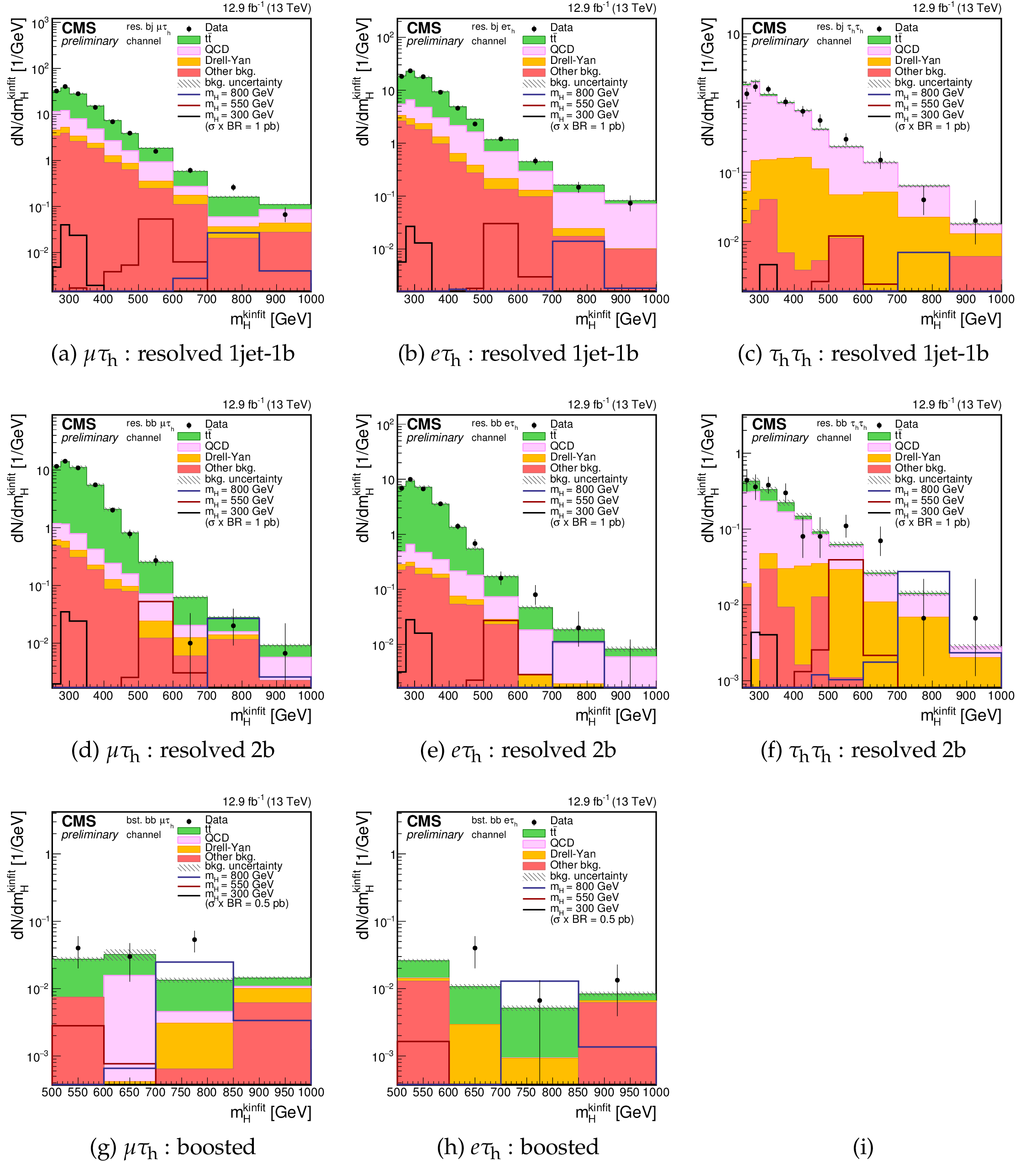
Figure 1:
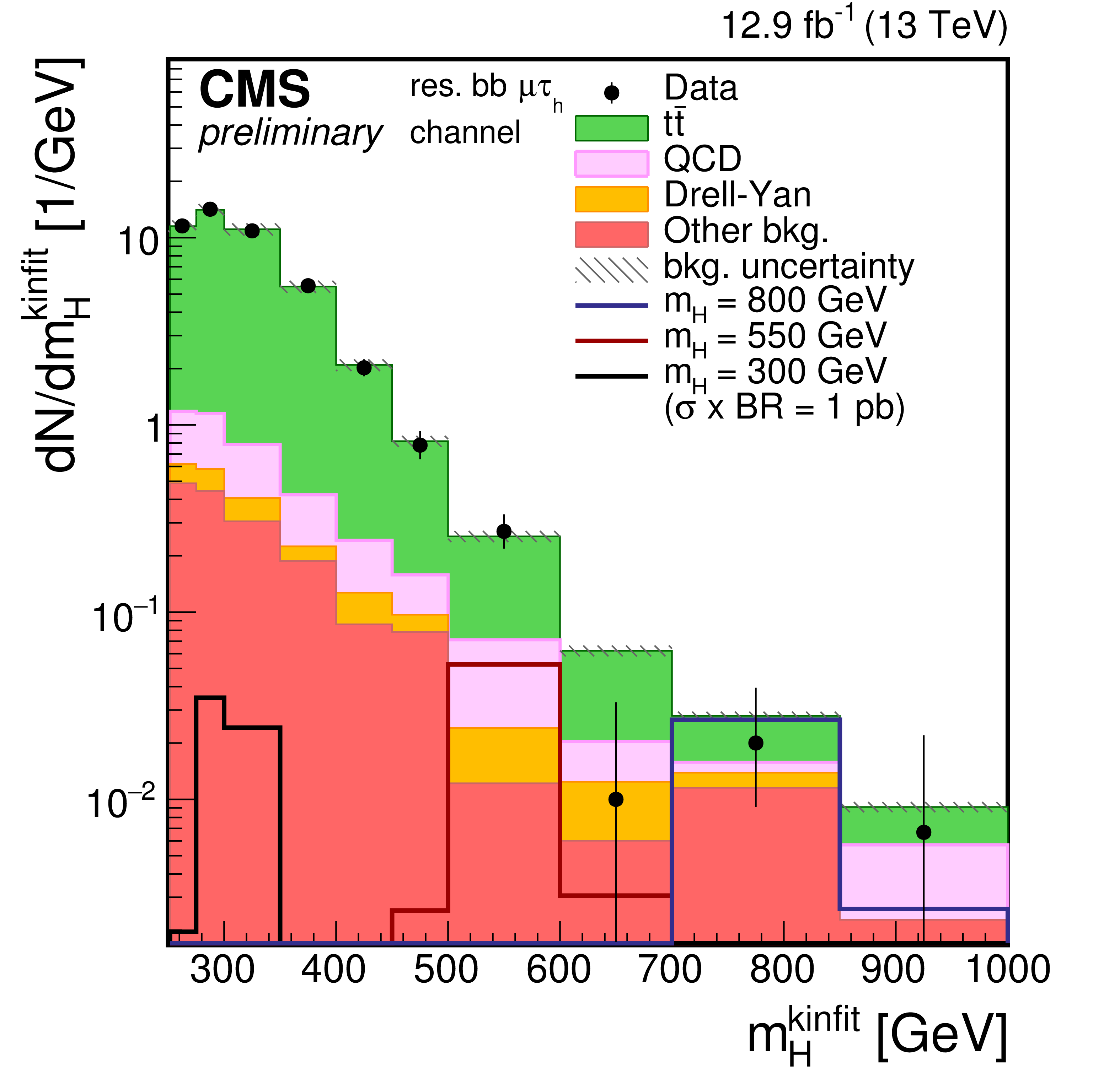
Distributions of the four-body mass reconstructed with the kinematic fit after applying the event selections. The plots are shown for (a)-(d)-(g) $\mu \tau _{\rm h}$, (b)-(e)-(h) $e\tau _{\rm h}$, and (c)-(f) $\tau _{\rm h}\tau _{\rm h}$ final states and for the three categories: resolved 1jet-1b (first row), resolved 2b (second row), and boosted (third row). In the boosted $\tau _{\rm h}\tau _{\rm h}$ category a counting experiment is performed and the plot is not shown. Points with error bars represent the data and shaded histograms represent the backgrounds. The black, red, and blue unshaded histograms are the signal expectations for $m_{\rm H}= $ 300 GeV, $m_{\rm H}= $ 550 GeV, and $m_{\rm H}= $ 800 GeV. The signal expectations are plotted for a value of $\sigma ({\rm pp} \to {\rm H} ) \times {\rm BR} ({\rm H} \to {\rm hh} )$ of 1pb in the resolved categories and 0.5 pb in the boosted categories. Event yields in each bin are divided by the bin width. Expected background contributions are shown for the values of nuisance parameters (systematic uncertainties) obtained after fitting the background-only hypothesis to the data. Signal and background histograms are not stacked. |
png pdf |
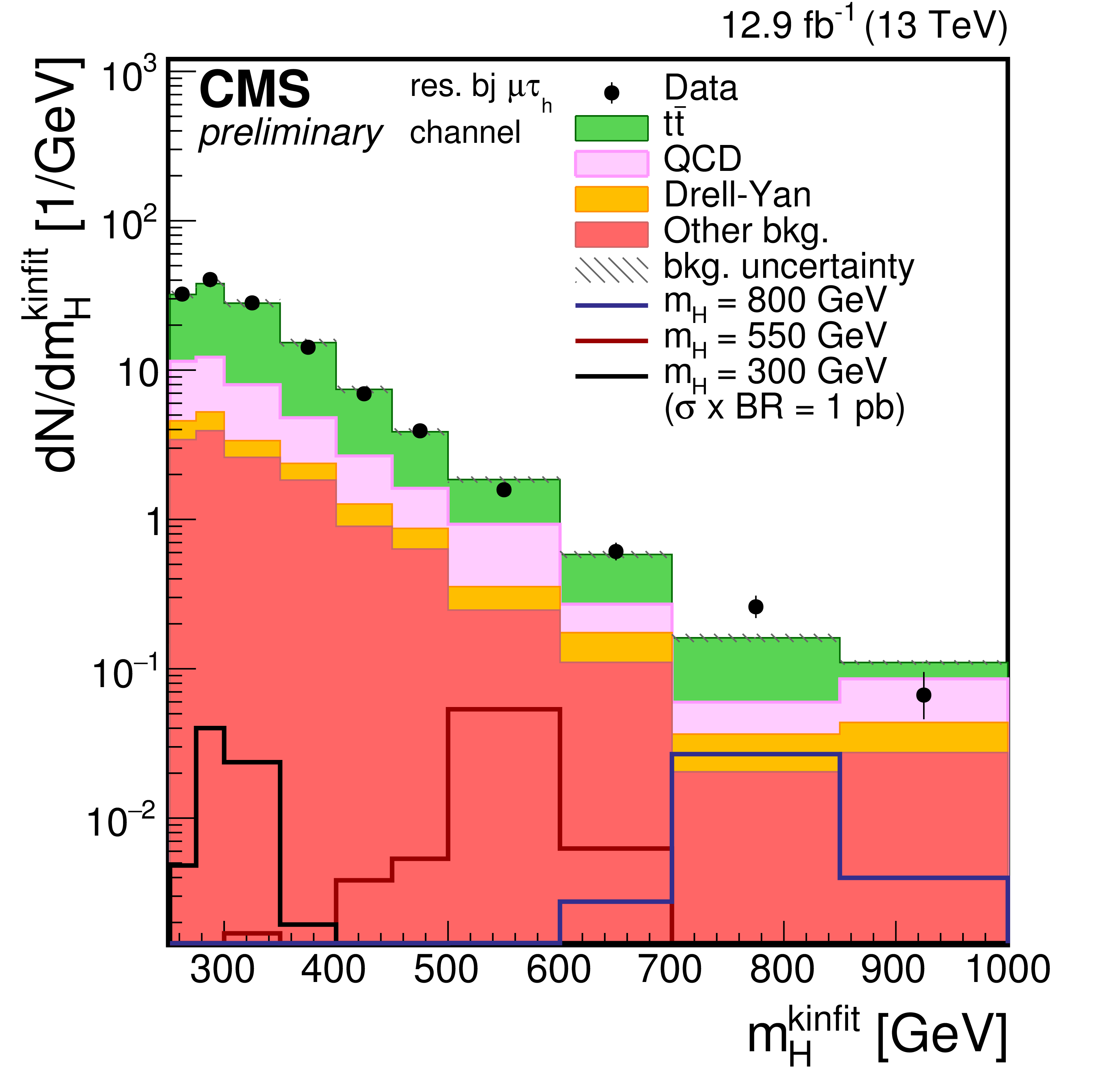
Figure 1-a:
Distributions of the four-body mass reconstructed with the kinematic fit after applying the event selections. The plot is shown for the $ \mu \tau _{\rm h} $ and for the resolved 1jet-1b category. Points with error bars represent the data and shaded histograms represent the backgrounds. The black, red, and blue unshaded histograms are the signal expectations for $m_{\rm H}= $ 300 GeV, $m_{\rm H}= $ 550 GeV, and $m_{\rm H}= $ 800 GeV. The signal expectations are plotted for a value of $\sigma ({\rm pp} \to {\rm H} ) \times {\rm BR} ({\rm H} \to {\rm hh} )$ of 1pb in the resolved categories and 0.5 pb in the boosted categories. Event yields in each bin are divided by the bin width. Expected background contributions are shown for the values of nuisance parameters (systematic uncertainties) obtained after fitting the background-only hypothesis to the data. Signal and background histograms are not stacked. |
png pdf |
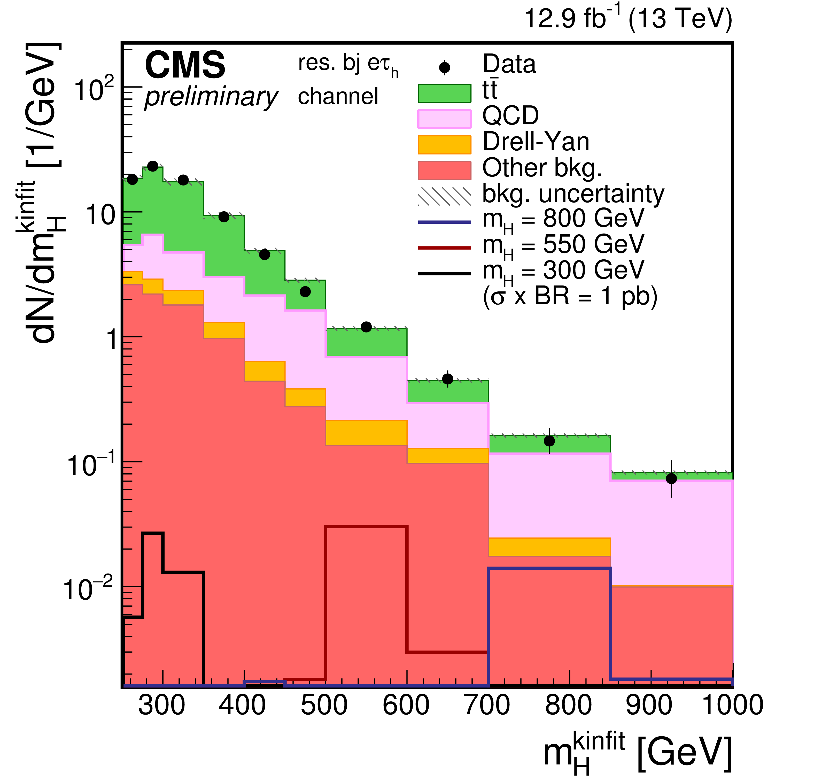
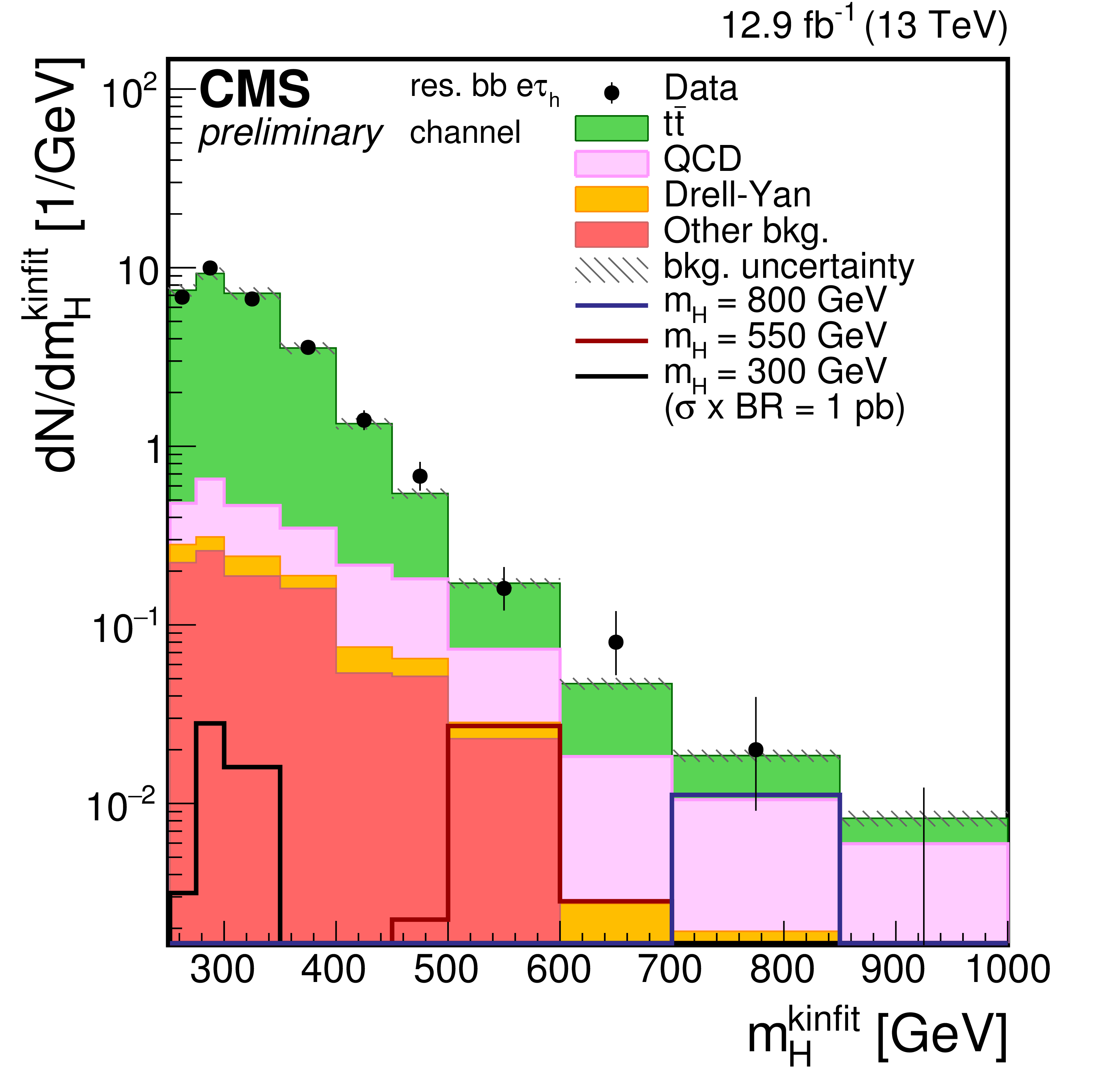
Figure 1-b:
Distributions of the four-body mass reconstructed with the kinematic fit after applying the event selections. The plot is shown for the $e\tau _{\rm h}$ final state and for the resolved 1jet-1b category. Points with error bars represent the data and shaded histograms represent the backgrounds. The black, red, and blue unshaded histograms are the signal expectations for $m_{\rm H}= $ 300 GeV, $m_{\rm H}= $ 550 GeV, and $m_{\rm H}= $ 800 GeV. The signal expectations are plotted for a value of $\sigma ({\rm pp} \to {\rm H} ) \times {\rm BR} ({\rm H} \to {\rm hh} )$ of 1pb in the resolved categories and 0.5 pb in the boosted categories. Event yields in each bin are divided by the bin width. Expected background contributions are shown for the values of nuisance parameters (systematic uncertainties) obtained after fitting the background-only hypothesis to the data. Signal and background histograms are not stacked. |
png pdf |
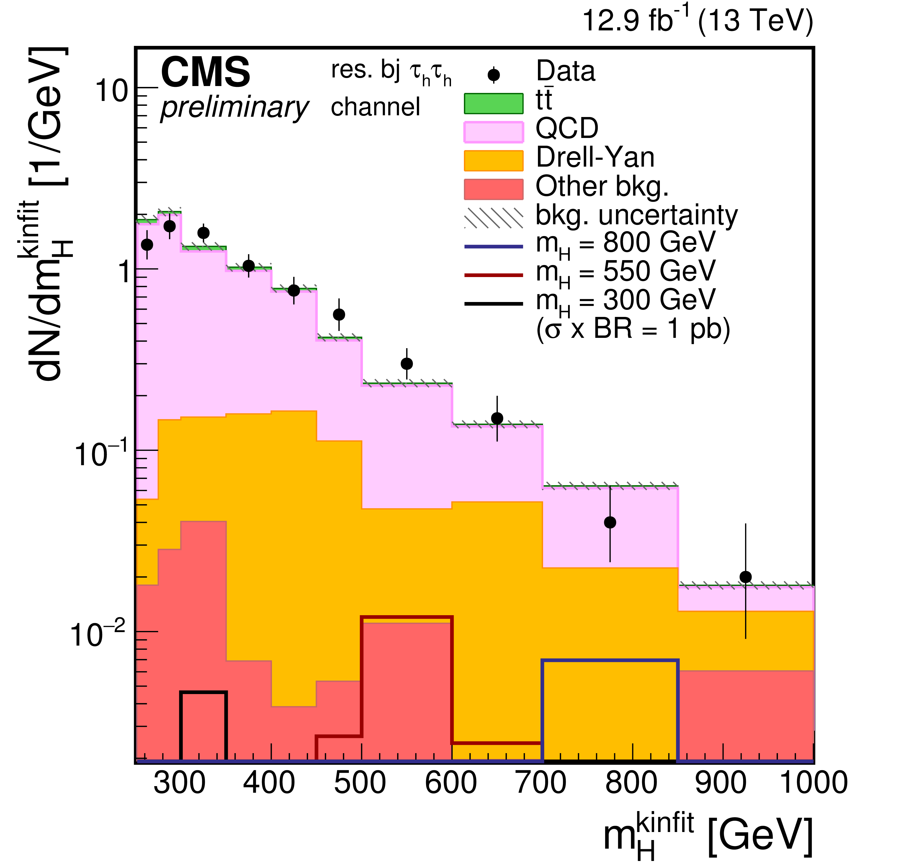
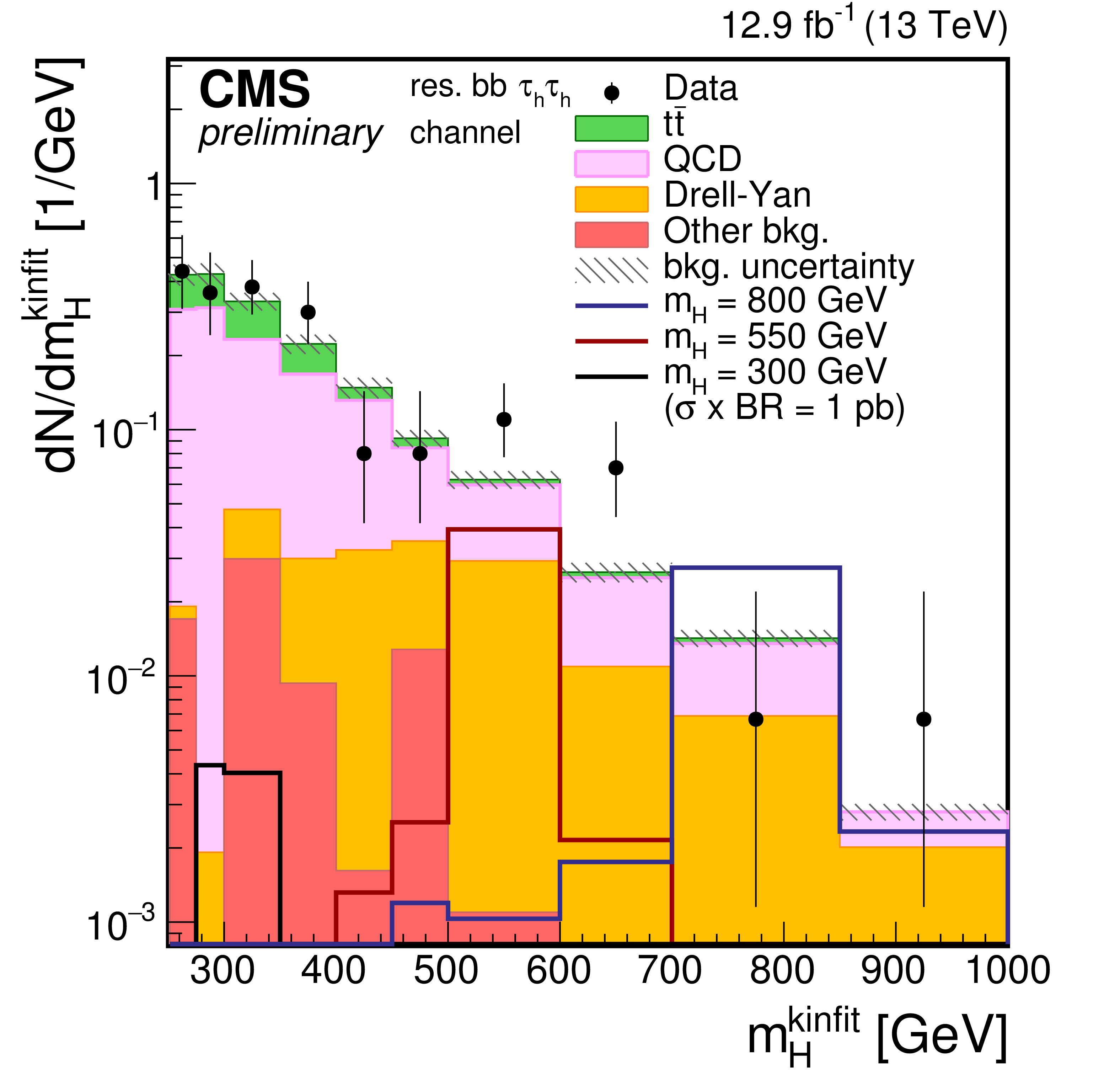
Figure 1-c:
Distributions of the four-body mass reconstructed with the kinematic fit after applying the event selections. The plot is shown for the $\tau _{\rm h}\tau _{\rm h}$ final state and for the resolved 1jet-1b category. Points with error bars represent the data and shaded histograms represent the backgrounds. The black, red, and blue unshaded histograms are the signal expectations for $m_{\rm H}= $ 300 GeV, $m_{\rm H}= $ 550 GeV, and $m_{\rm H}= $ 800 GeV. The signal expectations are plotted for a value of $\sigma ({\rm pp} \to {\rm H} ) \times {\rm BR} ({\rm H} \to {\rm hh} )$ of 1pb in the resolved categories and 0.5 pb in the boosted categories. Event yields in each bin are divided by the bin width. Expected background contributions are shown for the values of nuisance parameters (systematic uncertainties) obtained after fitting the background-only hypothesis to the data. Signal and background histograms are not stacked. |
png pdf |
Figure 1-d:
Distributions of the four-body mass reconstructed with the kinematic fit after applying the event selections. The plot is shown for the $\mu \tau _{\rm h}$ and for the resolved 2b category. Points with error bars represent the data and shaded histograms represent the backgrounds. The black, red, and blue unshaded histograms are the signal expectations for $m_{\rm H}= $ 300 GeV, $m_{\rm H}= $ 550 GeV, and $m_{\rm H}= $ 800 GeV. The signal expectations are plotted for a value of $\sigma ({\rm pp} \to {\rm H} ) \times {\rm BR} ({\rm H} \to {\rm hh} )$ of 1pb in the resolved categories and 0.5 pb in the boosted categories. Event yields in each bin are divided by the bin width. Expected background contributions are shown for the values of nuisance parameters (systematic uncertainties) obtained after fitting the background-only hypothesis to the data. Signal and background histograms are not stacked. |
png pdf |
Figure 1-e:
Distributions of the four-body mass reconstructed with the kinematic fit after applying the event selections. The plot is shown for the $e\tau _{\rm h}$ final state and for the resolved 2b category. Points with error bars represent the data and shaded histograms represent the backgrounds. The black, red, and blue unshaded histograms are the signal expectations for $m_{\rm H}= $ 300 GeV, $m_{\rm H}= $ 550 GeV, and $m_{\rm H}= $ 800 GeV. The signal expectations are plotted for a value of $\sigma ({\rm pp} \to {\rm H} ) \times {\rm BR} ({\rm H} \to {\rm hh} )$ of 1pb in the resolved categories and 0.5 pb in the boosted categories. Event yields in each bin are divided by the bin width. Expected background contributions are shown for the values of nuisance parameters (systematic uncertainties) obtained after fitting the background-only hypothesis to the data. Signal and background histograms are not stacked. |
png pdf |
Figure 1-f:
Distributions of the four-body mass reconstructed with the kinematic fit after applying the event selections. The plot is shown for the $\tau _{\rm h}\tau _{\rm h}$ final state and for the resolved 2b category. Points with error bars represent the data and shaded histograms represent the backgrounds. The black, red, and blue unshaded histograms are the signal expectations for $m_{\rm H}= $ 300 GeV, $m_{\rm H}= $ 550 GeV, and $m_{\rm H}= $ 800 GeV. The signal expectations are plotted for a value of $\sigma ({\rm pp} \to {\rm H} ) \times {\rm BR} ({\rm H} \to {\rm hh} )$ of 1pb in the resolved categories and 0.5 pb in the boosted categories. Event yields in each bin are divided by the bin width. Expected background contributions are shown for the values of nuisance parameters (systematic uncertainties) obtained after fitting the background-only hypothesis to the data. Signal and background histograms are not stacked. |
png pdf |
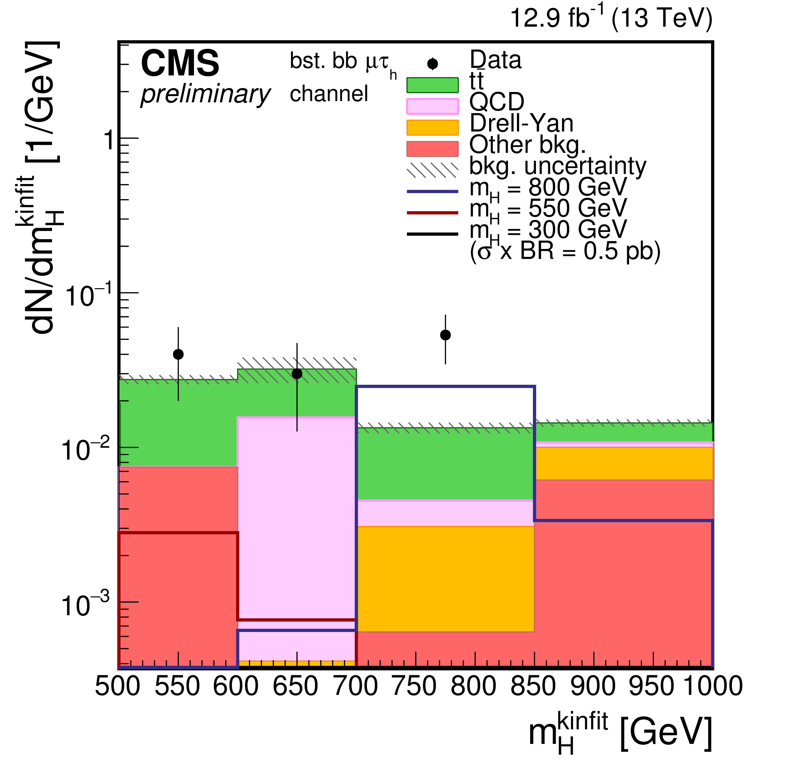
Figure 1-g:
Distributions of the four-body mass reconstructed with the kinematic fit after applying the event selections. The plot is shown for the $\mu \tau _{\rm h}$ final state and for the boosted category. Points with error bars represent the data and shaded histograms represent the backgrounds. The black, red, and blue unshaded histograms are the signal expectations for $m_{\rm H}= $ 300 GeV, $m_{\rm H}= $ 550 GeV, and $m_{\rm H}= $ 800 GeV. The signal expectations are plotted for a value of $\sigma ({\rm pp} \to {\rm H} ) \times {\rm BR} ({\rm H} \to {\rm hh} )$ of 1pb in the resolved categories and 0.5 pb in the boosted categories. Event yields in each bin are divided by the bin width. Expected background contributions are shown for the values of nuisance parameters (systematic uncertainties) obtained after fitting the background-only hypothesis to the data. Signal and background histograms are not stacked. |
png pdf |
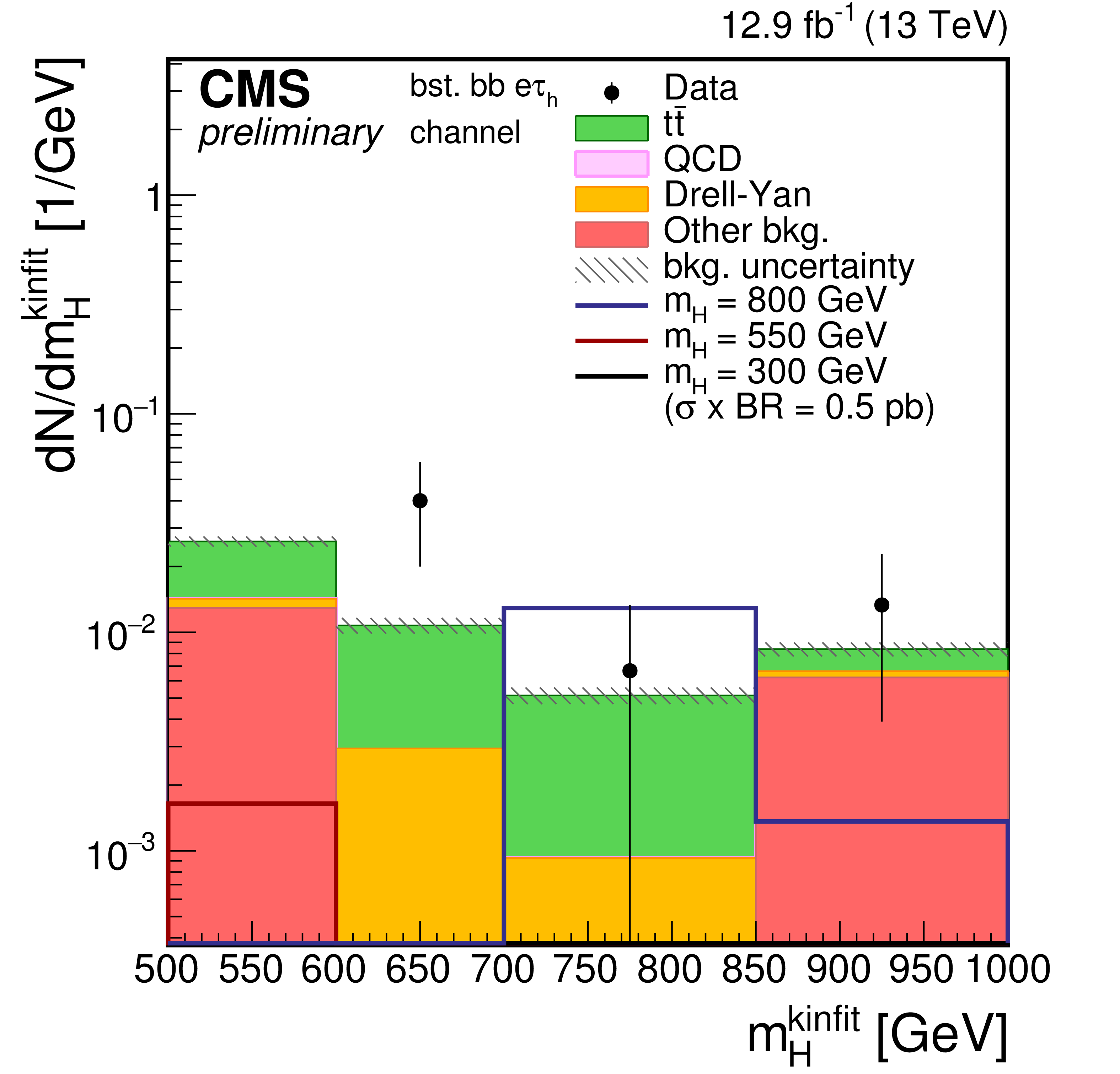
Figure 1-h:
Distributions of the four-body mass reconstructed with the kinematic fit after applying the event selections. The plot is shown for the $e \tau _{\rm h}$ and for the boosted category. Points with error bars represent the data and shaded histograms represent the backgrounds. The black, red, and blue unshaded histograms are the signal expectations for $m_{\rm H}= $ 300 GeV, $m_{\rm H}= $ 550 GeV, and $m_{\rm H}= $ 800 GeV. The signal expectations are plotted for a value of $\sigma ({\rm pp} \to {\rm H} ) \times {\rm BR} ({\rm H} \to {\rm hh} )$ of 1pb in the resolved categories and 0.5 pb in the boosted categories. Event yields in each bin are divided by the bin width. Expected background contributions are shown for the values of nuisance parameters (systematic uncertainties) obtained after fitting the background-only hypothesis to the data. Signal and background histograms are not stacked. |
png pdf |
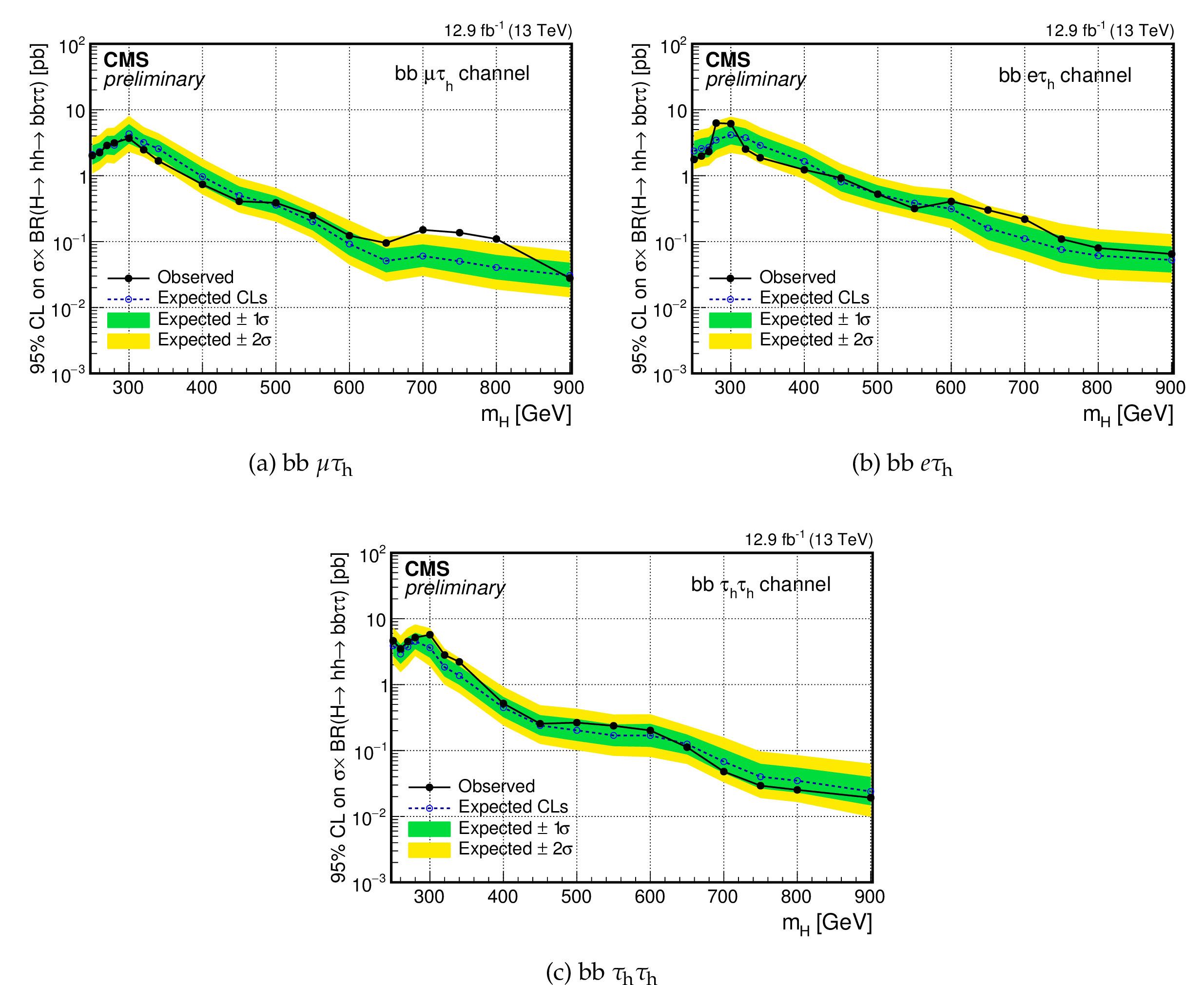
Figure 2:
Observed and expected 95% CL upper limits on ${\sigma ({\rm pp} \to {\rm H} ) \times {\rm BR} ({\rm H} \to {\rm hh} \to {\rm bb} \tau \tau )}$ as a function of the mass of the resonance $m_{\rm H}$ and combining the resolved and boosted categories. (a) bb $\mu \tau _{\rm h}$ (b) bb $e\tau _{\rm h}$ (c) bb $\tau _{\rm h}\tau _{\rm h}$. |
png pdf |
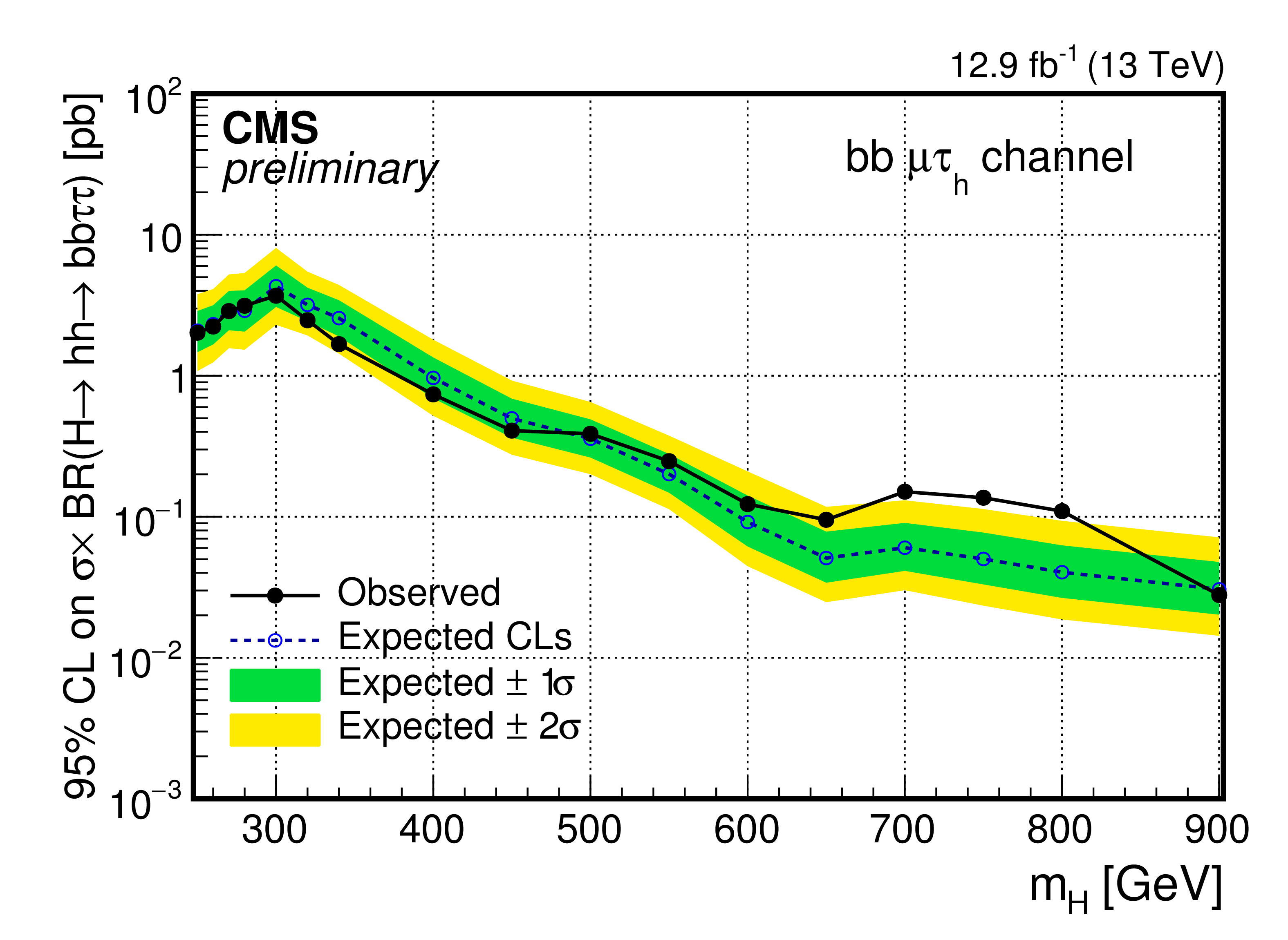
Figure 2-a:
Observed and expected 95% CL upper limits on ${\sigma ({\rm pp} \to {\rm H} ) \times {\rm BR} ({\rm H} \to {\rm hh} \to {\rm bb} \tau \tau )}$ as a function of the mass of the resonance $m_{\rm H}$ and combining the resolved and boosted categories: bb $\mu \tau _{\rm h}$ channel. |
png pdf |
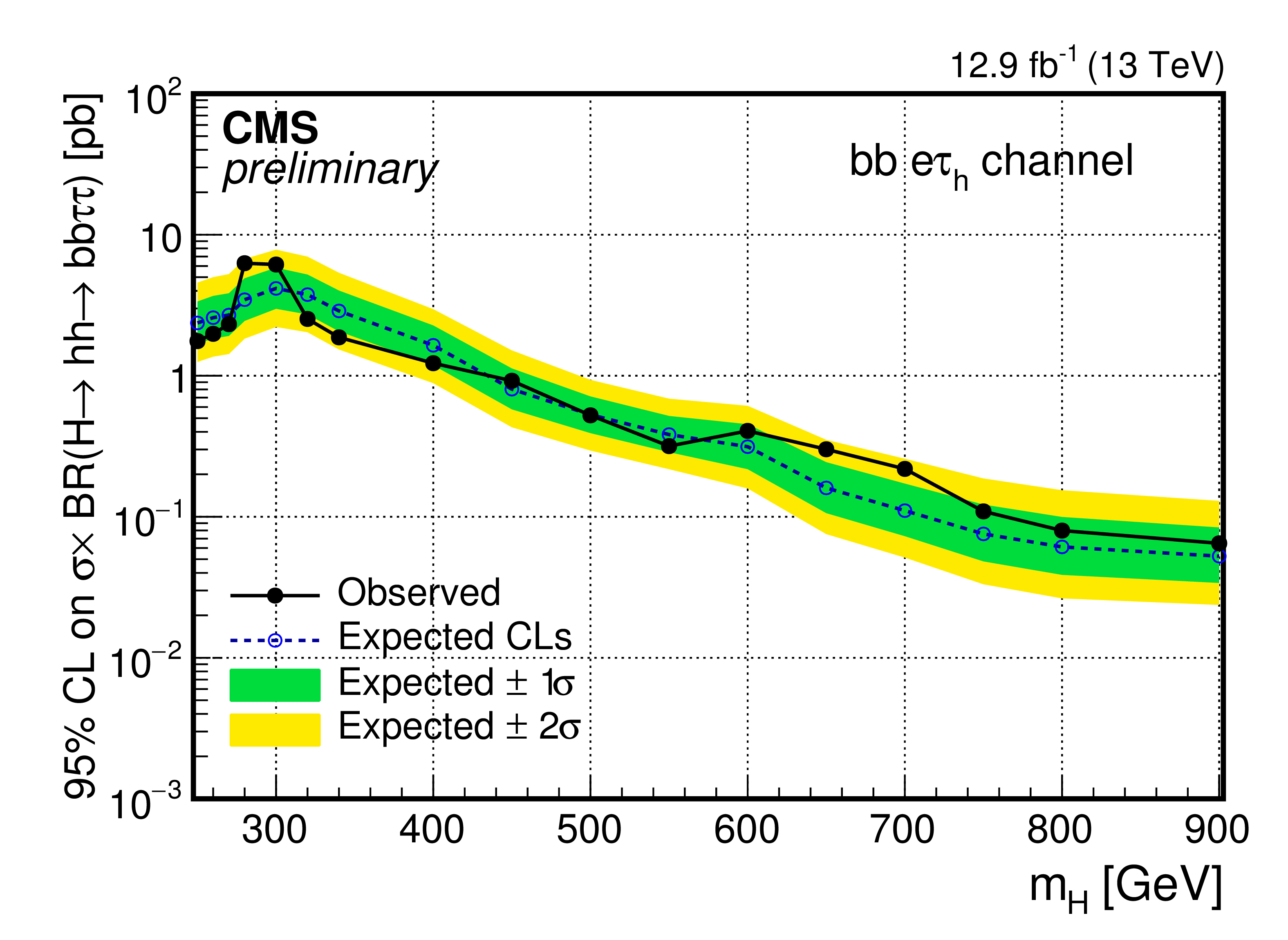
Figure 2-b:
Observed and expected 95% CL upper limits on ${\sigma ({\rm pp} \to {\rm H} ) \times {\rm BR} ({\rm H} \to {\rm hh} \to {\rm bb} \tau \tau )}$ as a function of the mass of the resonance $m_{\rm H}$ and combining the resolved and boosted categories: bb $e\tau _{\rm h}$ channel. |
png pdf |
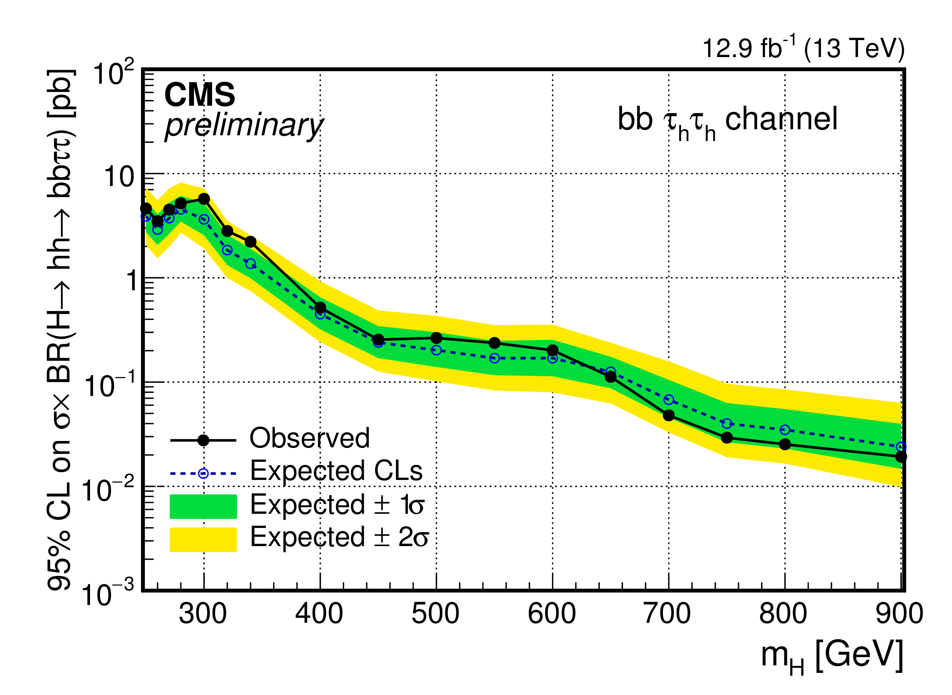
Figure 2-c:
Observed and expected 95% CL upper limits on ${\sigma ({\rm pp} \to {\rm H} ) \times {\rm BR} ({\rm H} \to {\rm hh} \to {\rm bb} \tau \tau )}$ as a function of the mass of the resonance $m_{\rm H}$ and combining the resolved and boosted categories: $\tau _{\rm h}\tau _{\rm h}$ channel. |
png pdf |
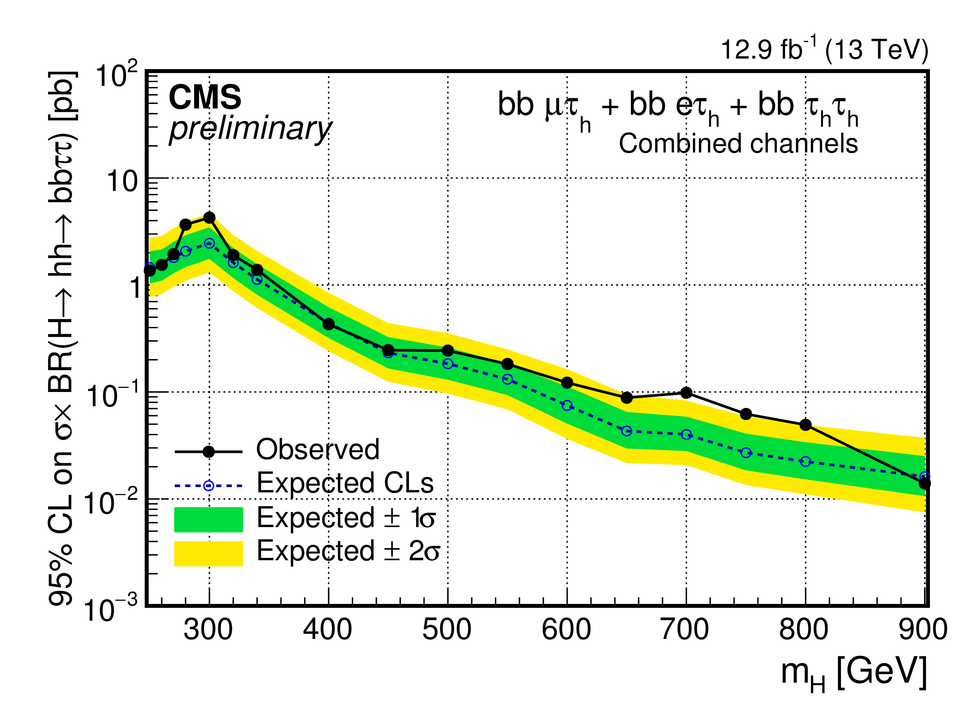
Figure 3:
Observed and expected 95% CL upper limits on ${\sigma ({\rm pp} \to {\rm H} ) \times {\rm BR} ({\rm H} \to {\rm hh} \to {\rm bb} \tau \tau )}$ from the combination of the three channels as a function of the mass of the resonance $m_{\rm H}$. |
| Tables | |
png pdf |
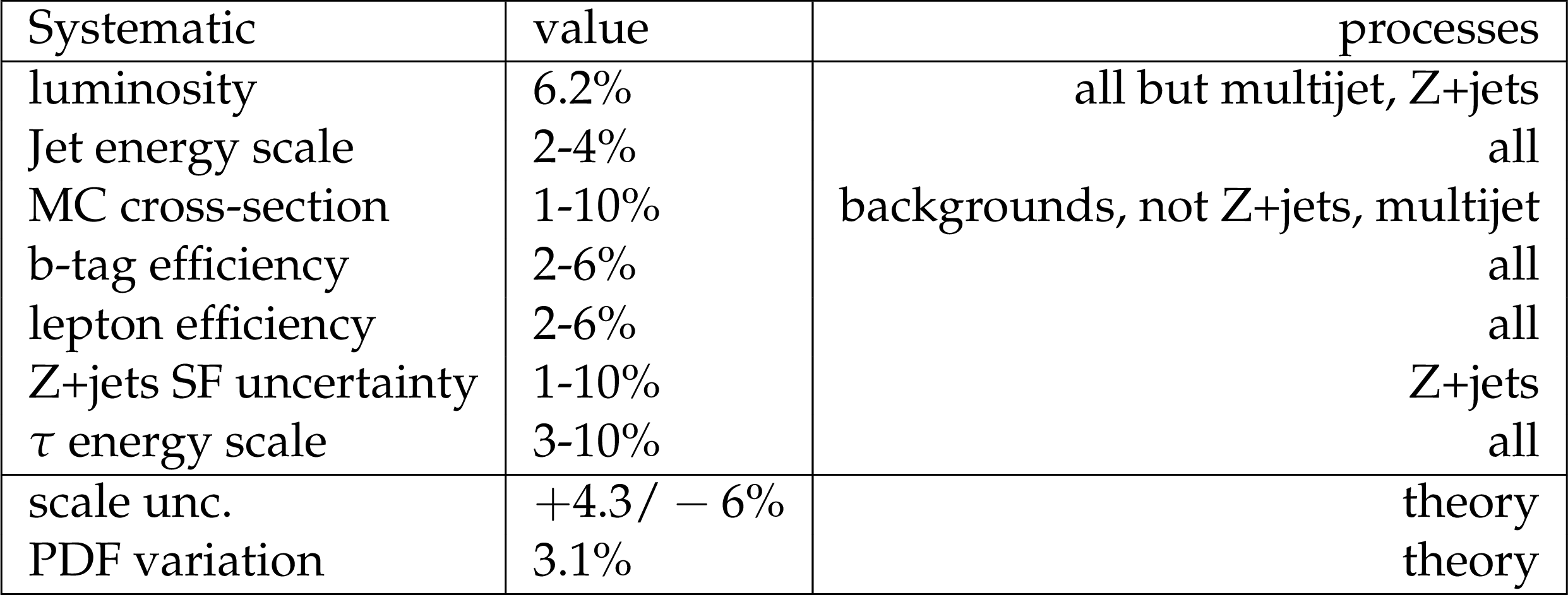
Table 1:
Lists of the systematic uncertainties affecting the normalization of the different processes. |
png pdf |
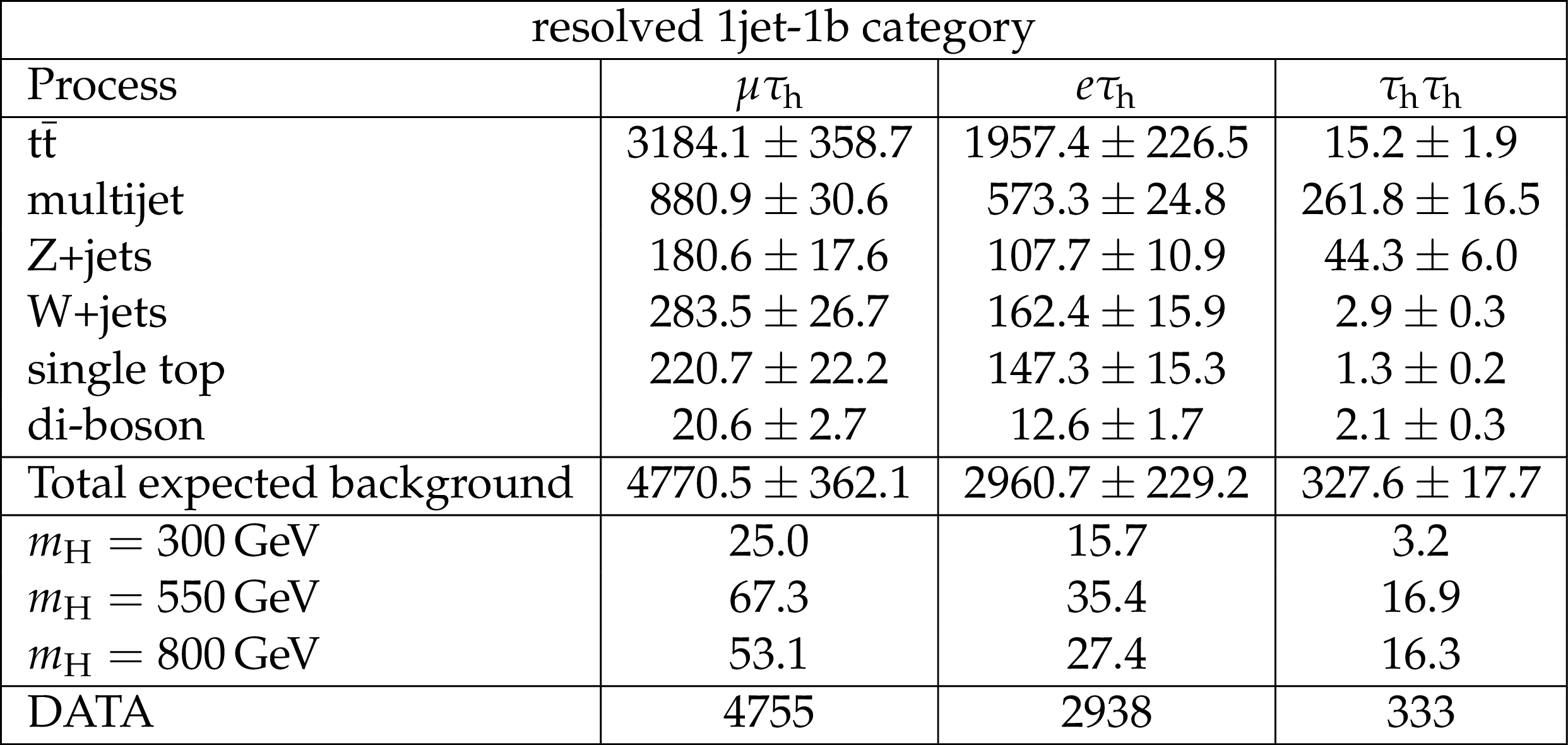
Table 2:
Observed and expected event yields in different final states for the resolved 1jet-1b category. Quoted uncertainties represent the combination of statistical plus systematic uncertainties. The signal expected yields are for $\sigma ({\rm pp} \rightarrow {\rm H}) \times {\rm BR} ({\rm H} \rightarrow {\rm hh} \rightarrow {\rm bb}\tau \tau ) = $ 10 pb. |
png pdf |
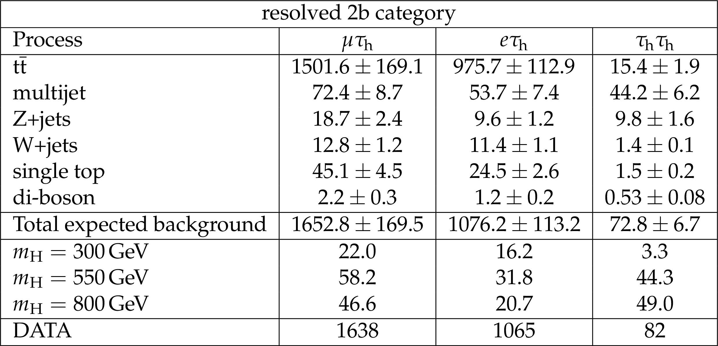
Table 3:
Observed and expected event yields in different final states for the resolved 2b category. Quoted uncertainties represent the combination of statistical plus systematic uncertainties. The signal expected yields are for $\sigma ({\rm pp} \rightarrow {\rm H}) \times {\rm BR} ({\rm H} \rightarrow {\rm hh} \rightarrow {\rm bb}\tau \tau ) = $ 10 pb. |
png pdf |
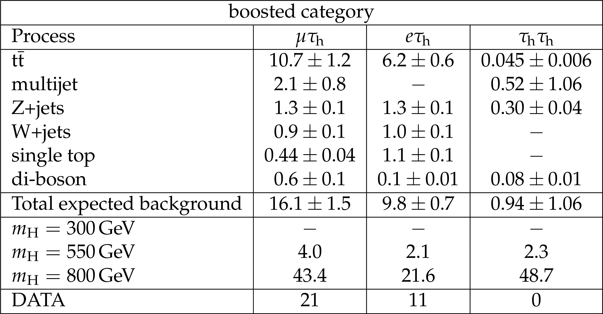
Table 4:
Observed and expected event yields in different final states for the boosted category. Quoted uncertainties represent the combination of statistical plus systematic uncertainties. The signal expected yields are for $\sigma ({\rm pp} \rightarrow {\rm H}) \times {\rm BR} ({\rm H} \rightarrow {\rm hh} \rightarrow {\rm bb}\tau \tau ) = $ 10 pb. |

png pdf |
Table 5:
Observed and expected 95% CL upper limits on $\sigma ({\rm pp} \to {\rm H} ) \times {\rm BR} ({\rm H} \to {\rm hh} \to {\rm bb} \tau \tau )$ for the combination of the three b-jet categories for the $\mu \tau _{\rm h}$, $e\tau _{\rm h}$, and $\tau _{\rm h}\tau _{\rm h}$ final states and their combination. |
| Summary |
| A search for resonant Higgs boson pair production in the bb$\tau\tau$ final state with the data collected by the CMS experiment in 2016 at $\sqrt{s} =$ 13 TeV, and corresponding to an integrated luminosity of 12.9 fb$^{-1}$, is presented. The search is performed using the three most sensitive decay channels of the $\tau$ lepton pair, $e\tau_{\rm h}, \mu\tau_{\rm h}, \tau_{\rm h}\tau_{\rm h}$, where $\tau_{\rm h}$ indicates a tau decay involving hadrons. No excess over the SM background prediction is observed and model independent upper limits on the values of the cross section times branching ratio are derived for different signal mass hypotheses between 250 and 900 GeV. These are currently the best limits on Higgs boson pair production in the high mass range considered for this analysis and substantially improve the sensitivity with respect to the previous analysis. |
| Additional Figures | |
png pdf |
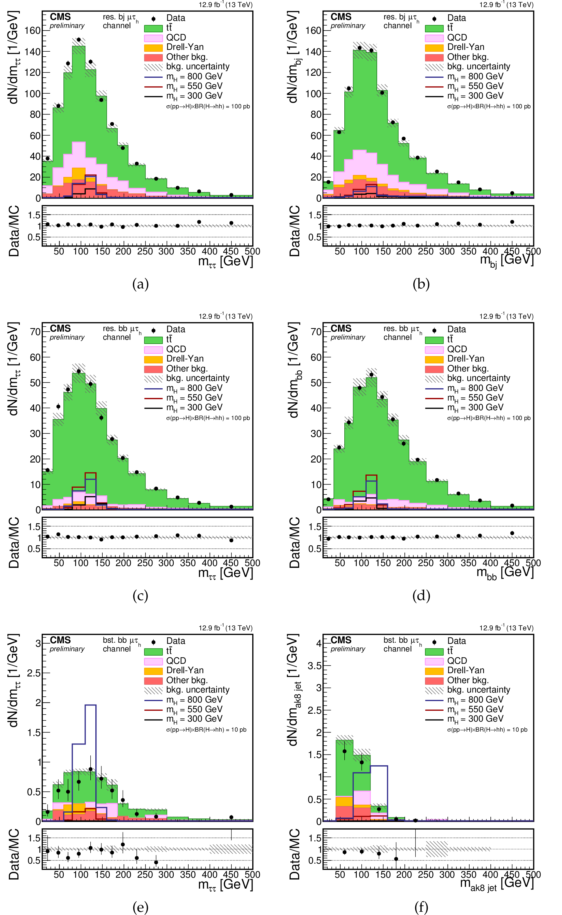
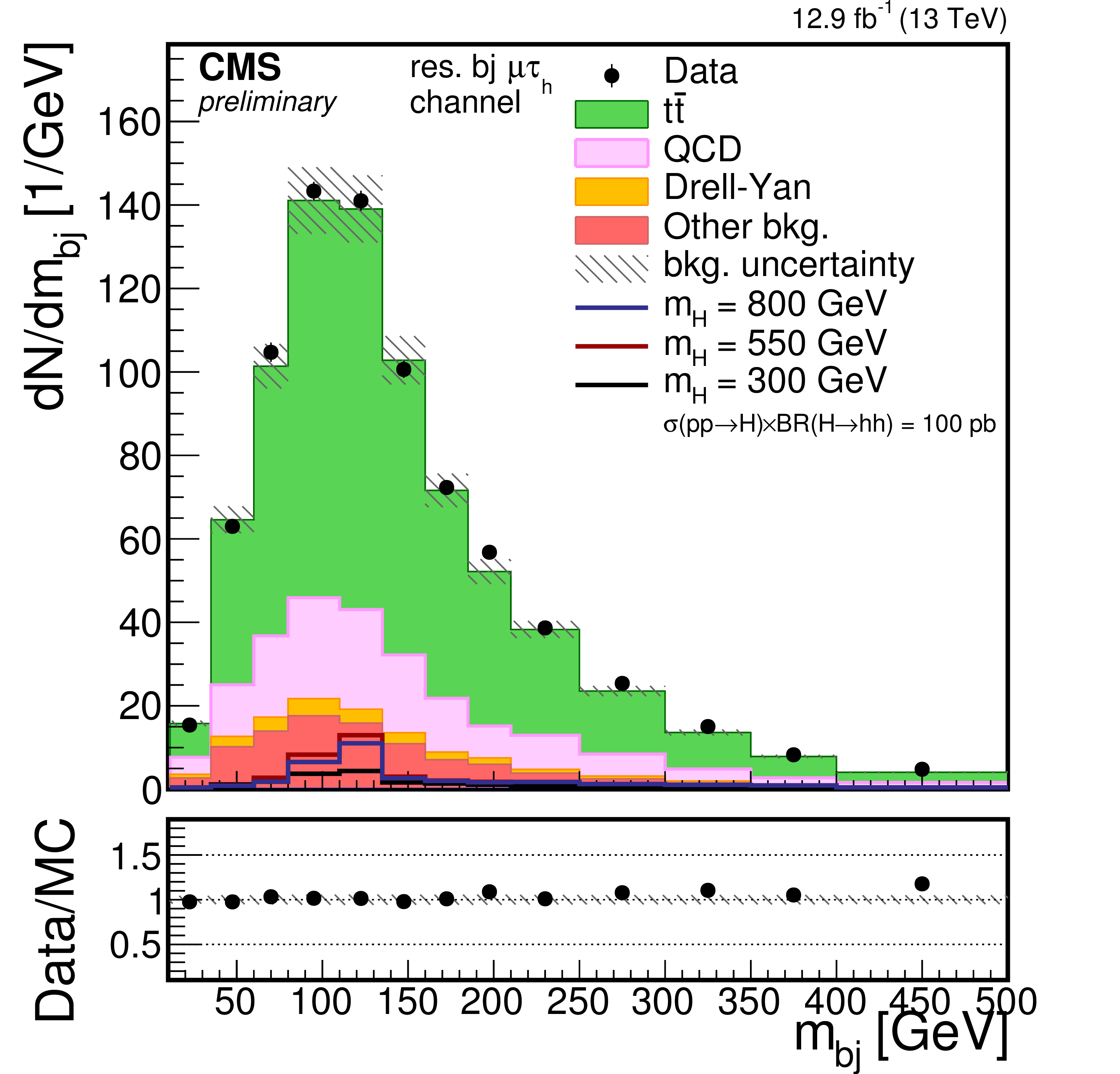
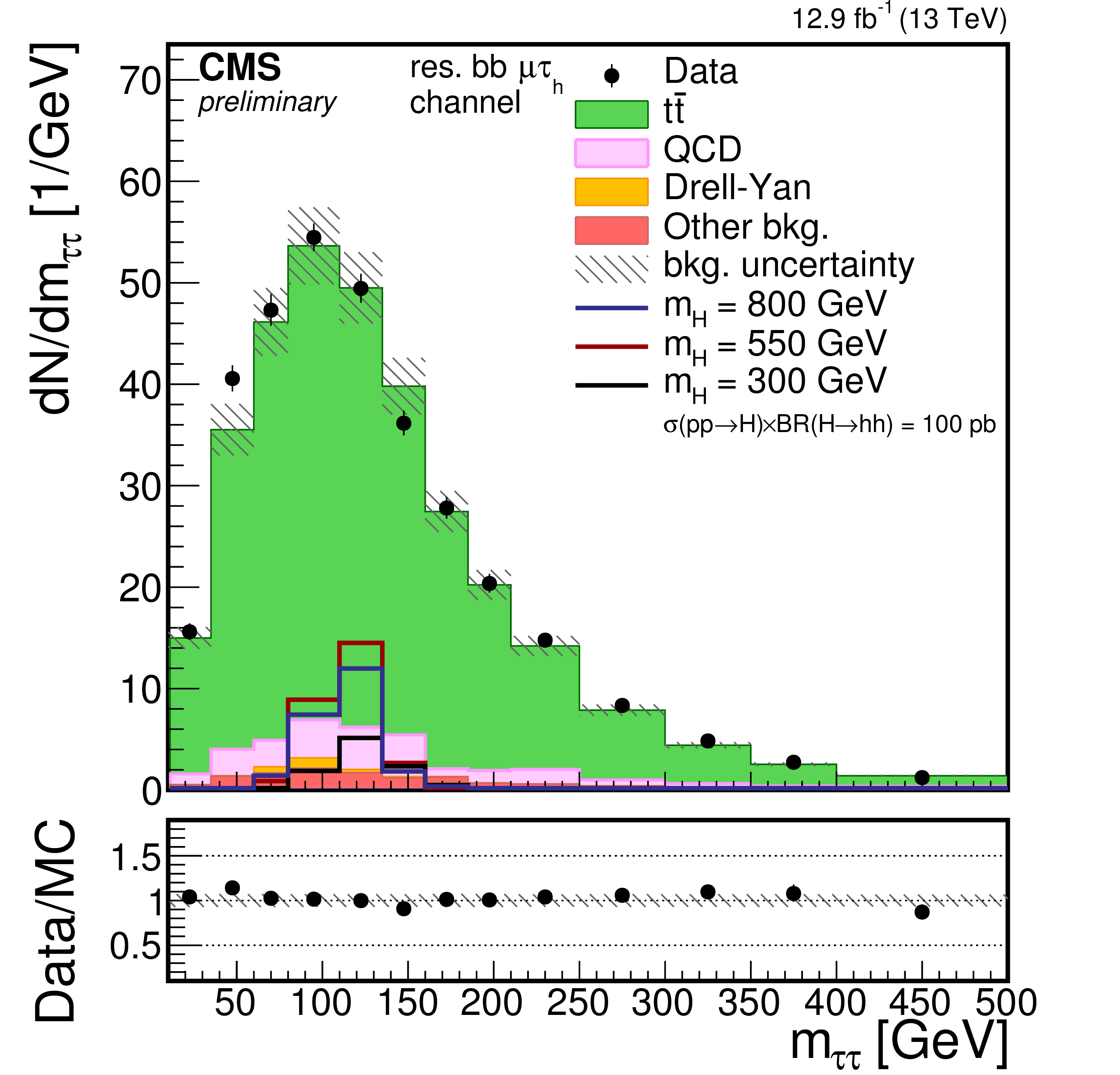
Additional Figure 1:
(a)-(c)-(e) distributions of the invariant mass of the $\tau \tau $ pair reconstructed using the SVfit algorithm, (b)-(d) distributions of the invariant mass of the bb pair, and (f) distribution of the invariant mass of the ak8 jet. $\tau \tau $ and bb candidates selections are applied but no selection on the invariant mass is requested. (a)-(b) resolved 1b-1jet $\mu \tau _{\rm h}$ category, (c)-(d) resolved 2b $\mu \tau _{\rm h}$ category, and (e)-(f) boosted $\mu \tau _{\rm h}$ category. Points with error bars represent the data and shaded histograms represent the backgrounds. The blue, black, and red lines denote respectively the signal hypothesis of 800, 550, and 300 GeV, and are scaled to a production cross section of the hh pair of 10 pb. Expected background contributions are shown for the values of nuisance parameters (systematic uncertainties) obtained after fitting the background-only hypothesis to the data. Signal and background histograms are not stacked. The bottom panel shows the ratio of the observed data to the simulation prediction. |
png pdf |
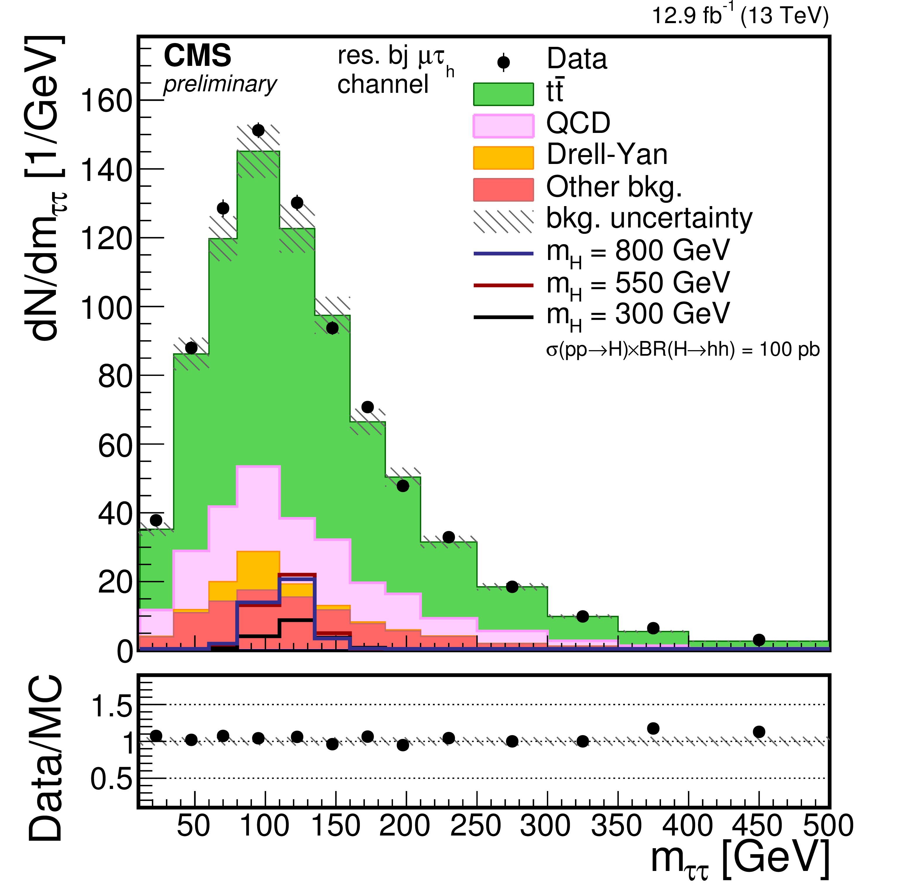
Additional Figure 1-a:
Distribution of the invariant mass of the $\tau \tau $ pair reconstructed using the SVfit algorithm for the resolved 1b-1jet $\mu \tau _{\rm h}$ category. Points with error bars represent the data and shaded histograms represent the backgrounds. $\tau \tau $ and bb candidates selections are applied but no selection on the invariant mass is requested. The blue, black, and red lines denote respectively the signal hypothesis of 800, 550, and 300 GeV, and are scaled to a production cross section of the hh pair of 10 pb. Expected background contributions are shown for the values of nuisance parameters (systematic uncertainties) obtained after fitting the background-only hypothesis to the data. Signal and background histograms are not stacked. The bottom panel shows the ratio of the observed data to the simulation prediction. |
png pdf |
Additional Figure 1-b:
Distribution of the invariant mass of the bb pair for the resolved 1b-1jet $\mu \tau _{\rm h}$ category. Points with error bars represent the data and shaded histograms represent the backgrounds. $\tau \tau $ and bb candidates selections are applied but no selection on the invariant mass is requested. The blue, black, and red lines denote respectively the signal hypothesis of 800, 550, and 300 GeV, and are scaled to a production cross section of the hh pair of 10 pb. Expected background contributions are shown for the values of nuisance parameters (systematic uncertainties) obtained after fitting the background-only hypothesis to the data. Signal and background histograms are not stacked. The bottom panel shows the ratio of the observed data to the simulation prediction. |
png pdf |
Additional Figure 1-c:
Distribution of the invariant mass of the $\tau \tau $ pair reconstructed using the SVfit algorithm for the resolved 2b $\mu \tau _{\rm h}$ category. Points with error bars represent the data and shaded histograms represent the backgrounds. $\tau \tau $ and bb candidates selections are applied but no selection on the invariant mass is requested. The blue, black, and red lines denote respectively the signal hypothesis of 800, 550, and 300 GeV, and are scaled to a production cross section of the hh pair of 10 pb. Expected background contributions are shown for the values of nuisance parameters (systematic uncertainties) obtained after fitting the background-only hypothesis to the data. Signal and background histograms are not stacked. The bottom panel shows the ratio of the observed data to the simulation prediction. |

png pdf |
Additional Figure 1-d:
Distribution of the invariant mass of the bb pair for the resolved 2b $\mu \tau _{\rm h}$ category. Points with error bars represent the data and shaded histograms represent the backgrounds. $\tau \tau $ and bb candidates selections are applied but no selection on the invariant mass is requested. The blue, black, and red lines denote respectively the signal hypothesis of 800, 550, and 300 GeV, and are scaled to a production cross section of the hh pair of 10 pb. Expected background contributions are shown for the values of nuisance parameters (systematic uncertainties) obtained after fitting the background-only hypothesis to the data. Signal and background histograms are not stacked. The bottom panel shows the ratio of the observed data to the simulation prediction. |
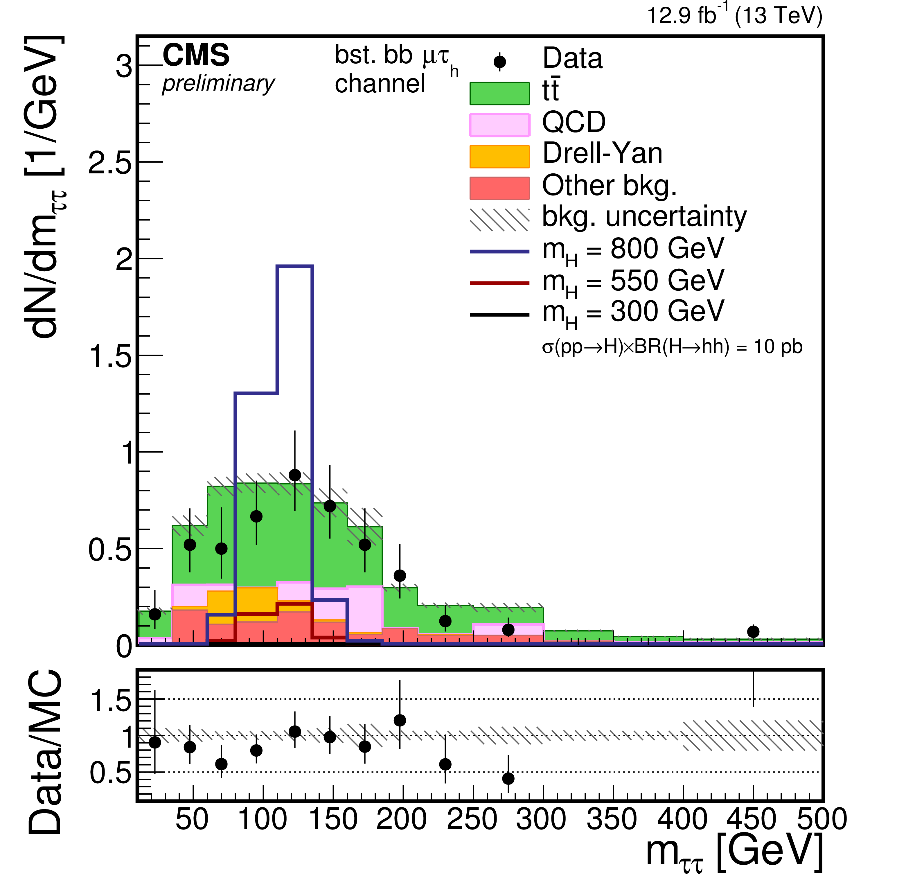
png pdf |
Additional Figure 1-e:
Distribution of the invariant mass of the $\tau \tau $ pair reconstructed using the SVfit algorithm for the boosted $\mu \tau _{\rm h}$ category. Points with error bars represent the data and shaded histograms represent the backgrounds. $\tau \tau $ and bb candidates selections are applied but no selection on the invariant mass is requested. The blue, black, and red lines denote respectively the signal hypothesis of 800, 550, and 300 GeV, and are scaled to a production cross section of the hh pair of 10 pb. Expected background contributions are shown for the values of nuisance parameters (systematic uncertainties) obtained after fitting the background-only hypothesis to the data. Signal and background histograms are not stacked. The bottom panel shows the ratio of the observed data to the simulation prediction. |
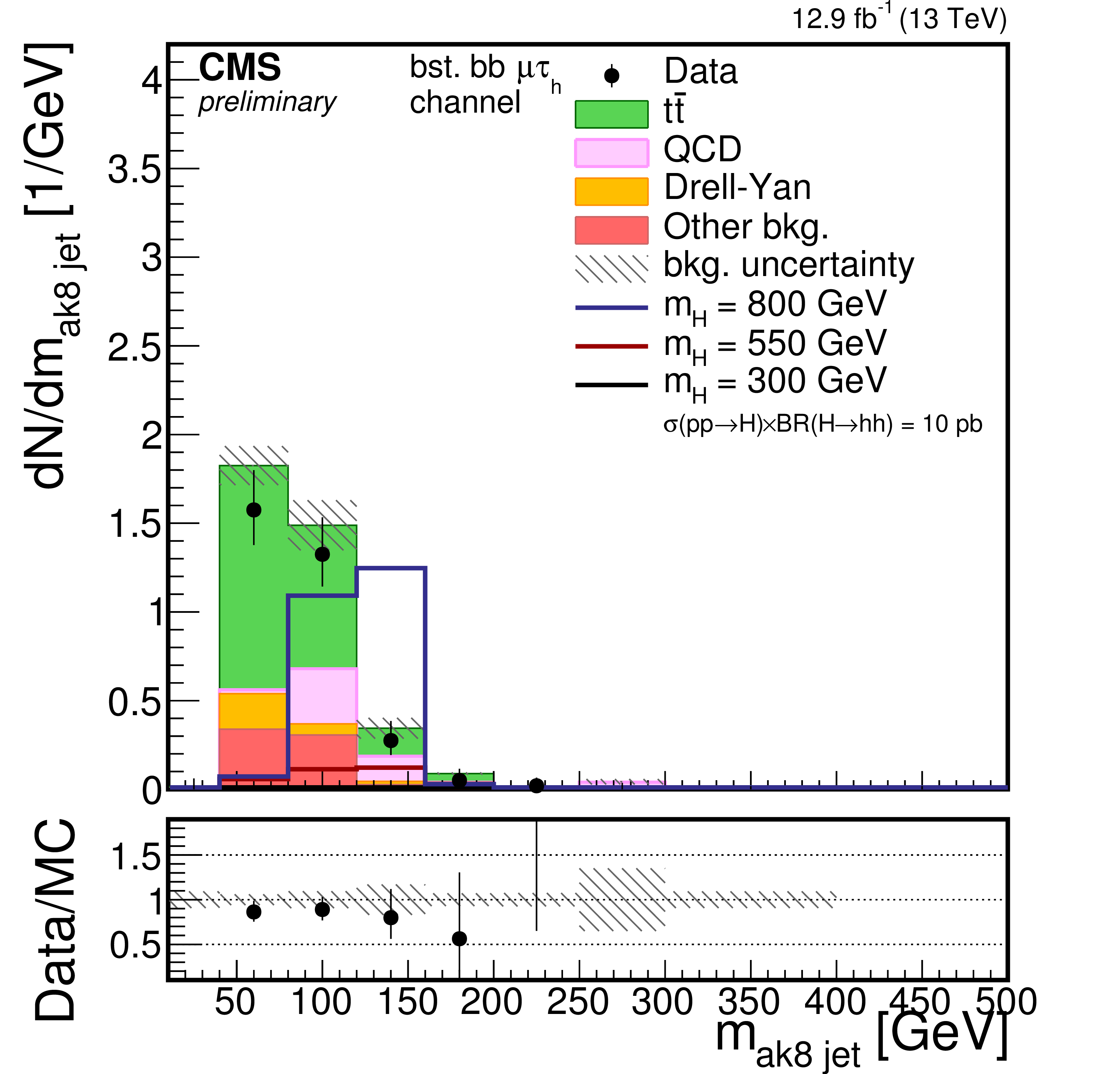
png pdf |
Additional Figure 1-f:
Distribution of the invariant mass of the ak8 jet for the boosted $\mu \tau _{\rm h}$ category. Points with error bars represent the data and shaded histograms represent the backgrounds. $\tau \tau $ and bb candidates selections are applied but no selection on the invariant mass is requested. The blue, black, and red lines denote respectively the signal hypothesis of 800, 550, and 300 GeV, and are scaled to a production cross section of the hh pair of 10 pb. Expected background contributions are shown for the values of nuisance parameters (systematic uncertainties) obtained after fitting the background-only hypothesis to the data. Signal and background histograms are not stacked. The bottom panel shows the ratio of the observed data to the simulation prediction. |
png pdf |
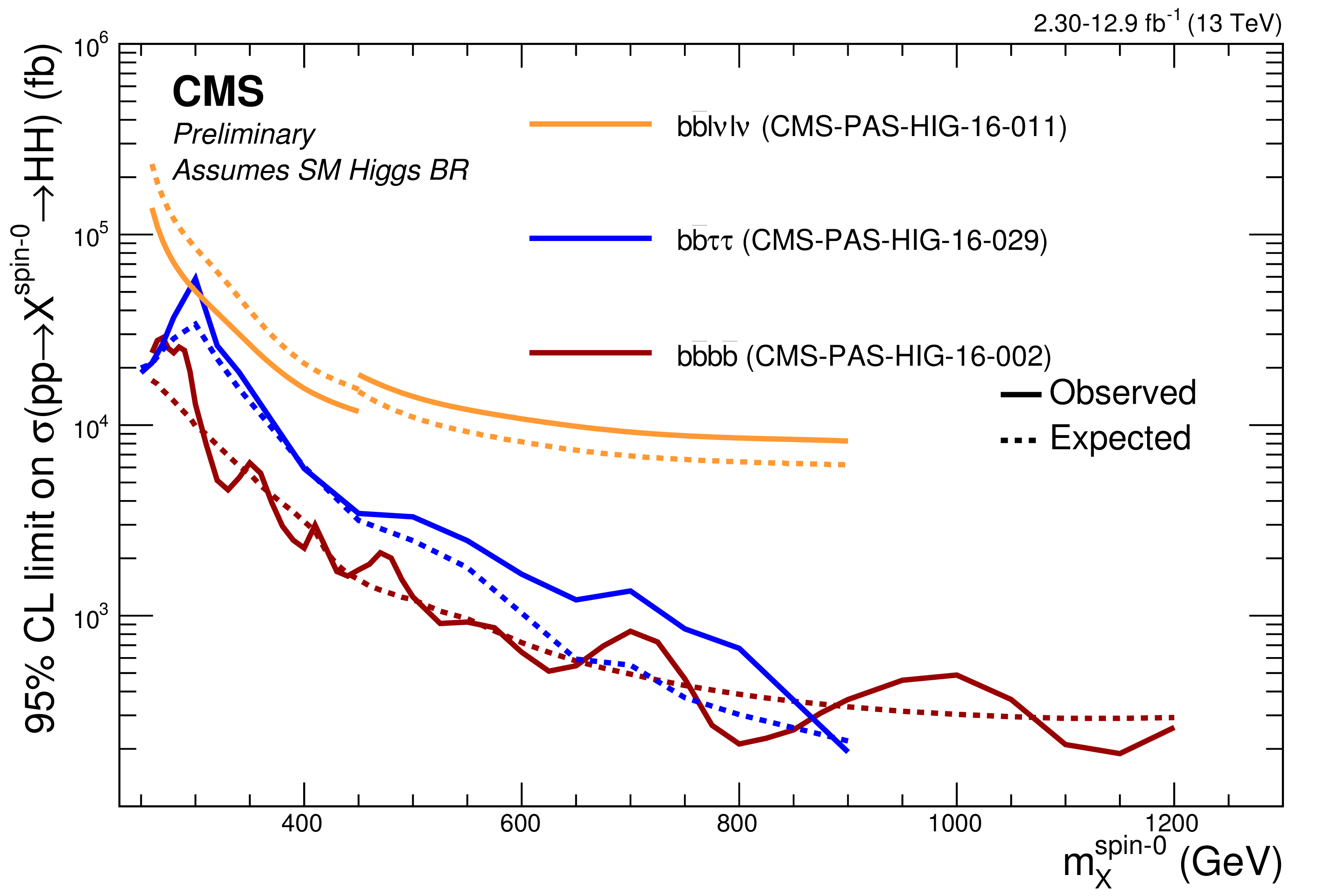
Additional Figure 2:
Comparison of the observed (solid lines) and expected (dashed lines) 95% CL upper limits on $\sigma ({\rm gg\rightarrow {\rm hh}})$ from the analyses currently performed by the CMS collaboration using the data collected ad $ \sqrt{s} = $ 13 TeV. Orange: ${\rm hh} \rightarrow {\rm bb}{\rm l}\nu _{\rm l} {\rm l}\nu _{\rm l}$ (CMS-PAS-HIG-16-011). Red: ${{\rm hh} \rightarrow {\rm bbbb}}$ (CMS-PAS-HIG-16-002). Blue: ${\rm hh} \rightarrow {\rm bb}\tau \tau $ (this analyis). |
| References | ||||
| 1 | ATLAS Collaboration | Observation of a new particle in the search for the Standard Model Higgs boson with the ATLAS detector at the LHC | Physics Letters B 716 (2012), no. 1, 1 -- 29 | |
| 2 | CMS Collaboration | Observation of a new boson at a mass of 125 GeV with the CMS experiment at the LHC | Physics Letters B 716 (2012), no. 1, 30 -- 61 | |
| 3 | ATLAS, CMS Collaboration | Combined Measurement of the Higgs Boson Mass in $ pp $ Collisions at $ \sqrt{s}=7 $ and 8 TeV with the ATLAS and CMS Experiments | PRL 114 (2015) 191803 | 1503.07589 |
| 4 | ATLAS and CMS Collaborations | Measurements of the Higgs boson production and decay rates and constraints on its couplings from a combined ATLAS and CMS analysis of the LHC pp collision data at $ \sqrt{s} $ = 7 and 8 TeV | CMS-PAS-HIG-15-002 | CMS-PAS-HIG-15-002 |
| 5 | T. Binoth and J. J. van der Bij | Influence of strongly coupled, hidden scalars on Higgs signals | Z. Phys. C75 (1997) 17--25 | hep-ph/9608245 |
| 6 | R. Schabinger and J. D. Wells | A Minimal spontaneously broken hidden sector and its impact on Higgs boson physics at the large hadron collider | PRD72 (2005) 093007 | hep-ph/0509209 |
| 7 | B. Patt and F. Wilczek | Higgs-field portal into hidden sectors | hep-ph/0605188 | |
| 8 | S. Y. Choi, C. Englert, and P. M. Zerwas | Multiple Higgs-Portal and Gauge-Kinetic Mixings | EPJC73 (2013) 2643 | 1308.5784 |
| 9 | ATLAS Collaboration | Constraints on New Phenomena via Higgs Coupling Measurements with the ATLAS Detector | ATLAS-CONF-2014-010 | |
| 10 | T. Robens and T. Stefaniak | Status of the Higgs Singlet Extension of the Standard Model after LHC Run 1 | EPJC75 (2015) 104 | 1501.02234 |
| 11 | P. Fayet | Supergauge Invariant Extension of the Higgs Mechanism and a Model for the electron and Its Neutrino | Nucl. Phys. B90 (1975) 104--124 | |
| 12 | P. Fayet | Spontaneously Broken Supersymmetric Theories of Weak, Electromagnetic and Strong Interactions | PLB69 (1977) 489 | |
| 13 | A. Djouadi et al. | Fully covering the MSSM Higgs sector at the LHC | JHEP 06 (2015) 168 | 1502.05653 |
| 14 | ATLAS Collaboration | Searches for Higgs boson pair production in the $ hh\to bb\tau\tau, \gamma\gamma WW^*, \gamma\gamma bb, bbbb $ channels with the ATLAS detector | PRD92 (2015) 092004 | 1509.04670 |
| 15 | CMS Collaboration | Searches for a heavy scalar boson H decaying to a pair of 125 GeV Higgs bosons hh or for a heavy pseudoscalar boson A decaying to Zh, in the final states with $ h \to \tau \tau $ | PLB755 (2016) 217--244 | CMS-HIG-14-034 1510.01181 |
| 16 | CMS Collaboration | Search for resonant Higgs boson pair production in the $ \mathrm{b\overline{b}}\tau^+\tau^- $ final state | CMS-PAS-HIG-16-013 | CMS-PAS-HIG-16-013 |
| 17 | CMS Collaboration | The CMS experiment at the CERN LHC | JINST 3 (2008) S08004 | CMS-00-001 |
| 18 | J. Alwall et al. | The automated computation of tree-level and next-to-leading order differential cross sections, and their matching to parton shower simulations | JHEP 07 (2014) 079 | 1405.0301 |
| 19 | S. Alioli, P. Nason, C. Oleari, and E. Re | NLO single-top production matched with shower in POWHEG: s- and t-channel contributions | JHEP 09 (2009) 111, , [Erratum: JHEP02,011(2010)] | 0907.4076 |
| 20 | J. M. Campbell, R. K. Ellis, P. Nason, and E. Re | Top-pair production and decay at NLO matched with parton showers | JHEP 04 (2015) 114 | 1412.1828 |
| 21 | T. Sjostrand, S. Mrenna, and P. Z. Skands | A Brief Introduction to PYTHIA 8.1 | CPC 178 (2008) 852--867 | 0710.3820 |
| 22 | CMS Collaboration | Particle--flow event reconstruction in CMS and performance for jets, taus, and $ E_{\mathrm{T}}^{\text{miss}} $ | CDS | |
| 23 | CMS Collaboration | Commissioning of the particle-flow event reconstruction with the first LHC collisions recorded in the CMS detector | CDS | |
| 24 | K. Rose | Deterministic annealing for clustering, compression, classification, regression and related optimisation problems | in Proceedings of the IEEE, volume 86, p. 86 1998 | |
| 25 | W. Waltenberger, R. Fr\"uhwirth, and P. Vanlaer | Adaptive vertex fitting | JPG 34 (2007) N343 | |
| 26 | CMS Collaboration | Performance of electron reconstruction and selection with the CMS detector in proton-proton collisions at $ \sqrt{s} $ = 8 TeV | JINST 10 (2015), no. 06, P06005 | CMS-EGM-13-001 1502.02701 |
| 27 | A. Hocker et al. | TMVA - Toolkit for Multivariate Data Analysis | PoS ACAT (2007) 040 | physics/0703039 |
| 28 | CMS Collaboration | Performance of CMS muon reconstruction in $ pp $ collision events at $ \sqrt{s}=7 $ TeV | JINST 7 (2012) P10002 | CMS-MUO-10-004 1206.4071 |
| 29 | M. Cacciari, G. P. Salam, and G. Soyez | The anti-$ k_t $ jet clustering algorithm | JHEP 04 (2008) 063 | 0802.1189 |
| 30 | M. Cacciari, G. P. Salam, and G. Soyez | FastJet user manual | EPJC 72 (2012) 1896 | 1111.6097 |
| 31 | A. J. Larkoski, S. Marzani, G. Soyez, and J. Thaler | Soft Drop | JHEP 05 (2014) 146 | 1402.2657 |
| 32 | CMS Collaboration | Algorithms for b Jet identification in CMS | CDS | |
| 33 | CMS Collaboration | Performance of tau-lepton reconstruction and identification in CMS | JINST 7 (2012) P01001 | CMS-TAU-11-001 1109.6034 |
| 34 | CMS Collaboration | Reconstruction and identification of $ \tau $ lepton decays to hadrons and $ \nu_\tau $ at CMS | CMS-TAU-14-001 1510.07488 |
|
| 35 | CMS Collaboration | Performance of reconstruction and identification of tau leptons in their decays to hadrons and tau neutrino in LHC Run-2 | CMS-PAS-TAU-16-002 | CMS-PAS-TAU-16-002 |
| 36 | L. Bianchini, J. Conway, E. K. Friis, and C. Veelken | Reconstruction of the Higgs mass in H to tautau Events by Dynamical Likelihood techniques | Journal of Physics: Conference Series 513 (2014), no. 2, 022035 | |
| 37 | CMS Collaboration | Measurement of the inclusive and differential tt production cross sections in lepton + jets final states at 13 TeV | CMS-PAS-TOP-15-005 | CMS-PAS-TOP-15-005 |
| 38 | M. Czakon and A. Mitov | Top++: A Program for the Calculation of the Top-Pair Cross-Section at Hadron Colliders | CPC 185 (2014) 2930 | 1112.5675 |
| 39 | G. Cowan, K. Cranmer, E. Gross, and O. Vitells | Asymptotic formulae for likelihood-based tests of new physics | EPJC71 (2011) 1554, , [Erratum: Eur. Phys. J.C73,2501(2013)] | 1007.1727 |
|
|
Compact Muon Solenoid LHC, CERN |
|

|

|

|

|

|