

Compact Muon Solenoid
LHC, CERN
| CMS-PAS-HIG-19-005 | ||
| Combined Higgs boson production and decay measurements with up to 137 fb$^{-1}$ of proton-proton collision data at $\sqrt{s}=$ 13 TeV | ||
| CMS Collaboration | ||
| January 2020 | ||
| Abstract: Combined measurements of the production and decay rates of the Higgs boson, its couplings to vector bosons and fermions, and interpretations in the effective field theory framework are presented. The analysis uses the LHC proton-proton collision data set recorded with the CMS detector at $\sqrt{s}=$ 13 TeV in 2016, 2017, and 2018, corresponding to an integrated luminosity of up to 137 fb$^{-1}$, depending on the decay channel. All results are found to be compatible with the standard model expectation within the current uncertainties. | ||
| Links: CDS record (PDF) ; inSPIRE record ; CADI line (restricted) ; | ||
| Figures & Tables | Summary | Additional Figures | References | CMS Publications |
|---|
| Figures | |
png pdf |
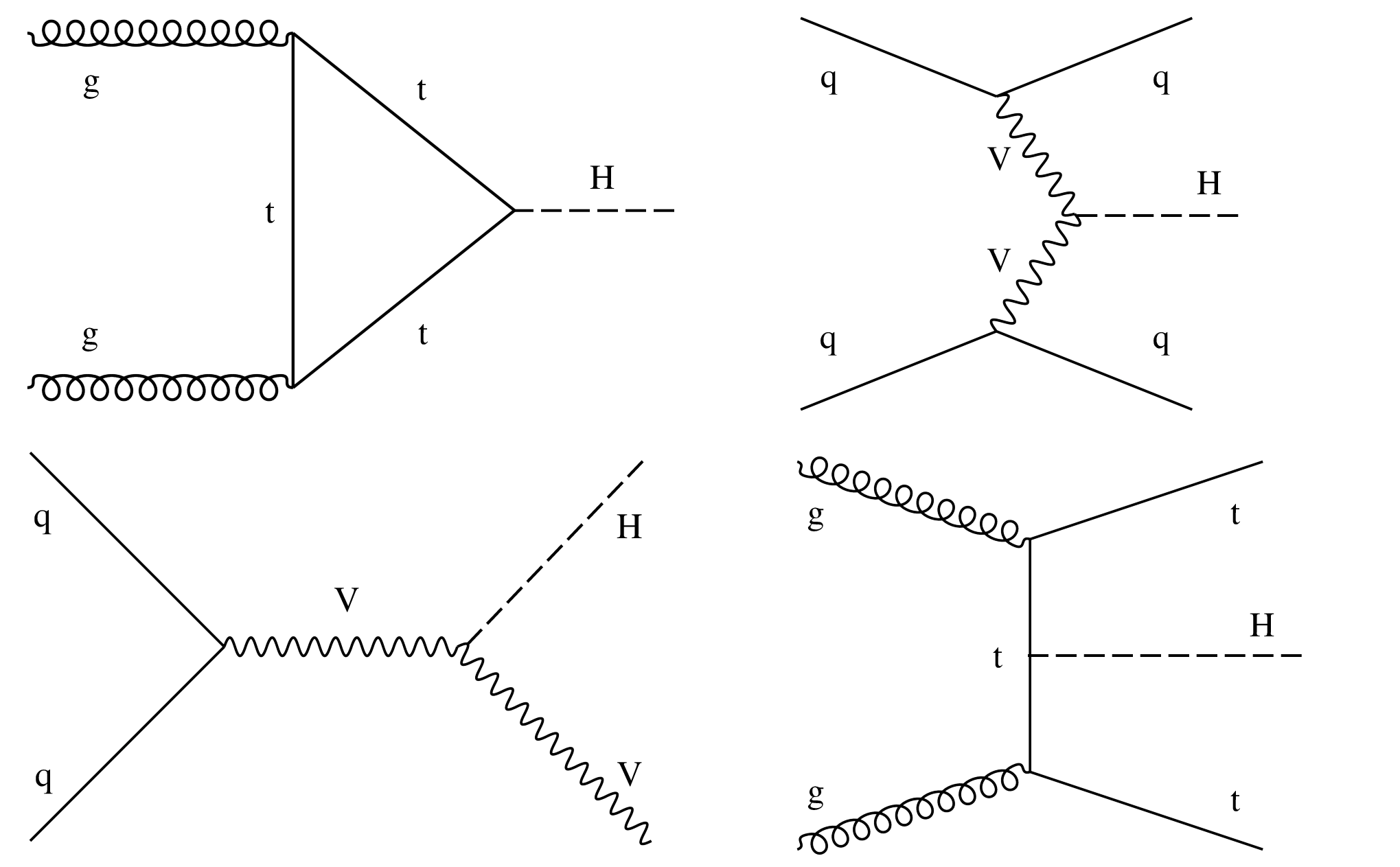
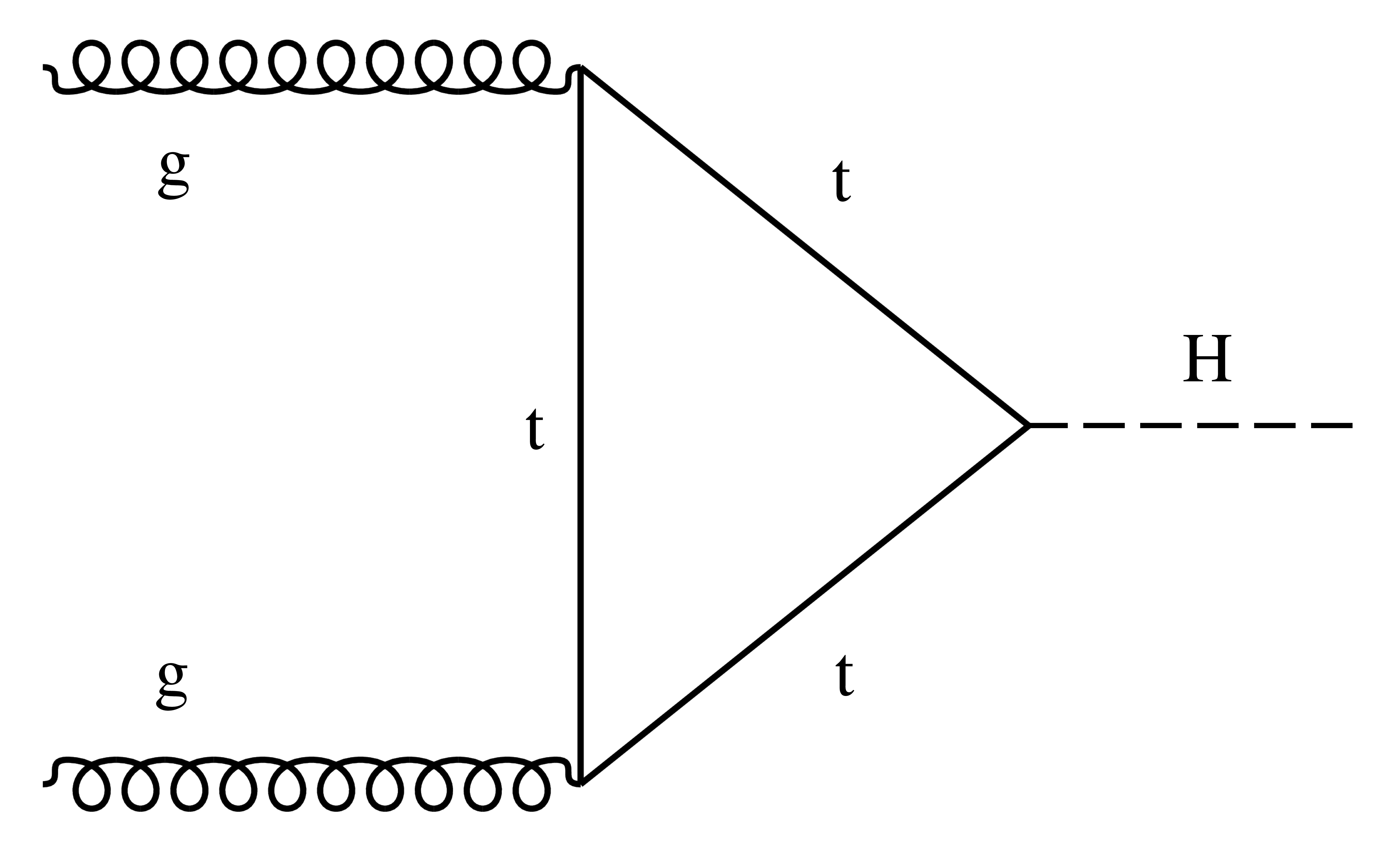
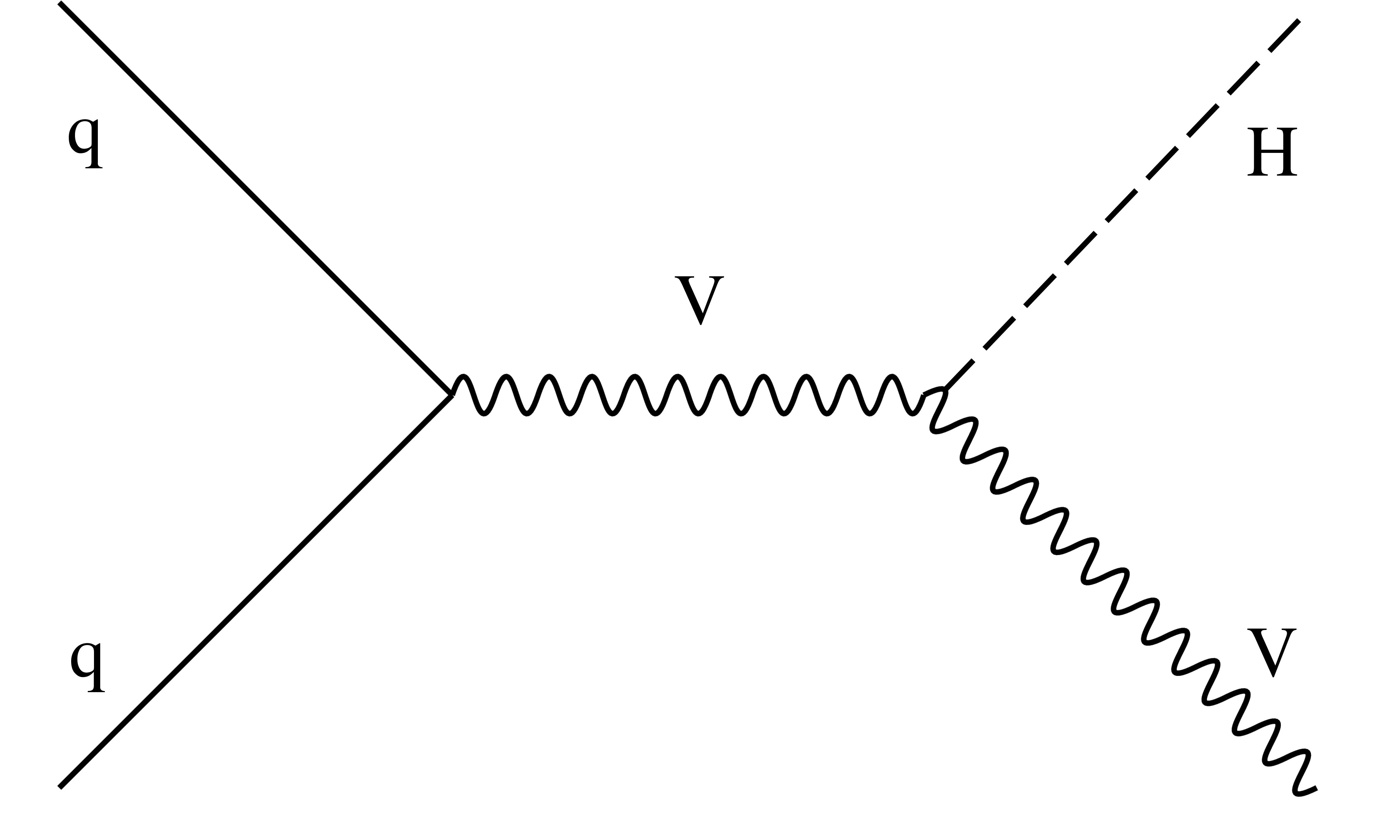
Figure 1:
Examples of leading-order Feynman diagrams for the ${\mathrm{g} \mathrm{g} \mathrm{H}}$ (upper left), ${\mathrm {VBF}}$ (upper right), ${\mathrm {V}\mathrm{H}}$ (lower left), and ${\mathrm{t} \mathrm{t} \mathrm{H}}$ (lower right) production modes. |
png pdf |
Figure 1-a:
Example of leading-order Feynman diagram for the ${\mathrm{g} \mathrm{g} \mathrm{H}}$ production mode. |

png pdf |
Figure 1-b:
Example of leading-order Feynman diagram for the ${\mathrm {VBF}}$ production mode. |
png pdf |
Figure 1-c:
Example of leading-order Feynman diagram for the ${\mathrm {V}\mathrm{H}}$ production mode. |

png pdf |
Figure 1-d:
Example of leading-order Feynman diagram for the ${\mathrm{t} \mathrm{t} \mathrm{H}}$ production mode. |
png pdf |
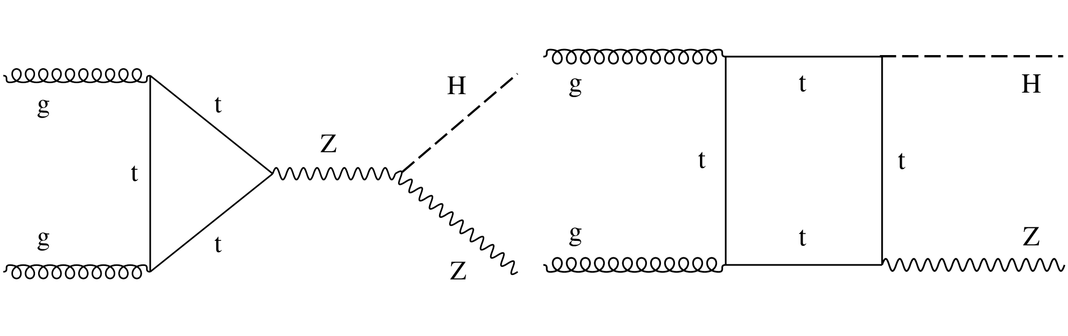
Figure 2:
Examples of leading-order Feynman diagrams for the $\text {gg}\to {\mathrm{Z} \mathrm{H}} $ production mode. |

png pdf |
Figure 2-a:
Example of leading-order Feynman diagram for the $\text {gg}\to {\mathrm{Z} \mathrm{H}} $ production mode. |

png pdf |
Figure 2-b:
Example of leading-order Feynman diagram for the $\text {gg}\to {\mathrm{Z} \mathrm{H}} $ production mode. |
png pdf |
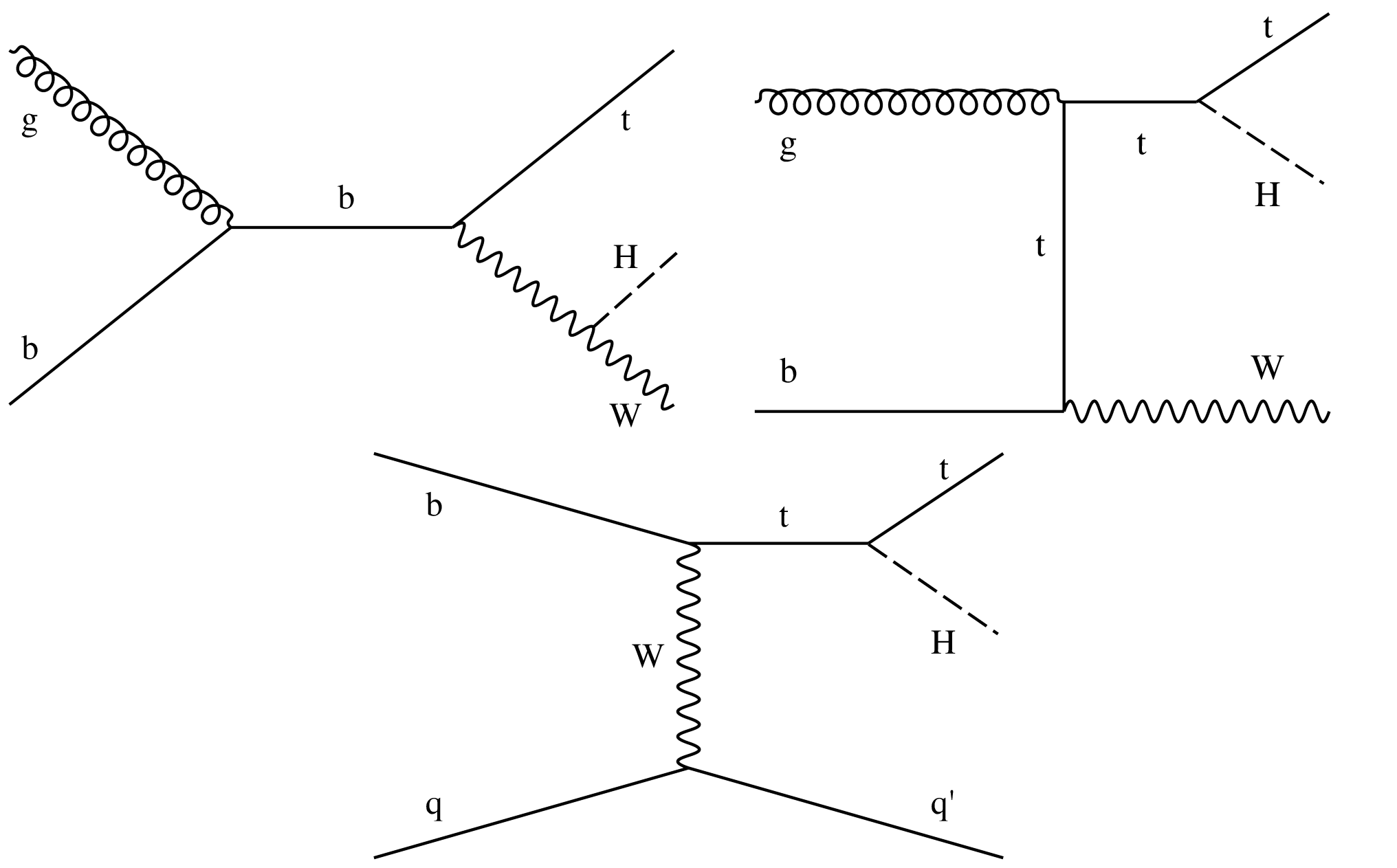
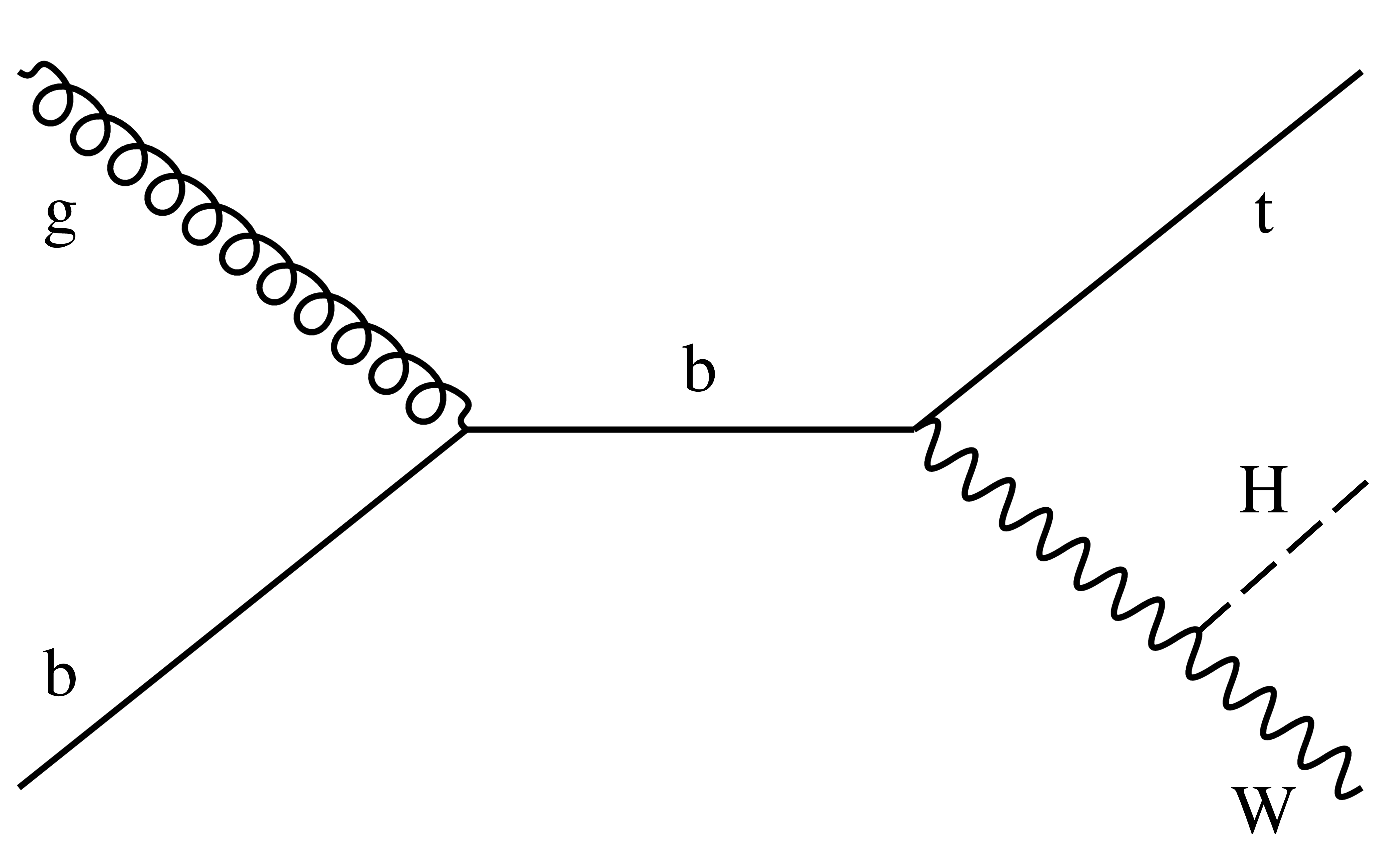
Figure 3:
Examples of leading-order Feynman diagrams for ${\mathrm{t} \mathrm{H}}$ production via the ${\mathrm{t} \mathrm{H} \mathrm{W}}$ (upper left and right) and ${\mathrm{t} \mathrm{H} \mathrm{q}}$ (lower) modes. |
png pdf |
Figure 3-a:
Example of leading-order Feynman diagram for ${\mathrm{t} \mathrm{H}}$ production via the ${\mathrm{t} \mathrm{H} \mathrm{W}}$ mode. |

png pdf |
Figure 3-b:
Example of leading-order Feynman diagram for ${\mathrm{t} \mathrm{H}}$ production via the ${\mathrm{t} \mathrm{H} \mathrm{W}}$ mode. |

png pdf |
Figure 3-c:
Example of leading-order Feynman diagram for ${\mathrm{t} \mathrm{H}}$ production via the ${\mathrm{t} \mathrm{H} \mathrm{q}}$ mode. |

png pdf |
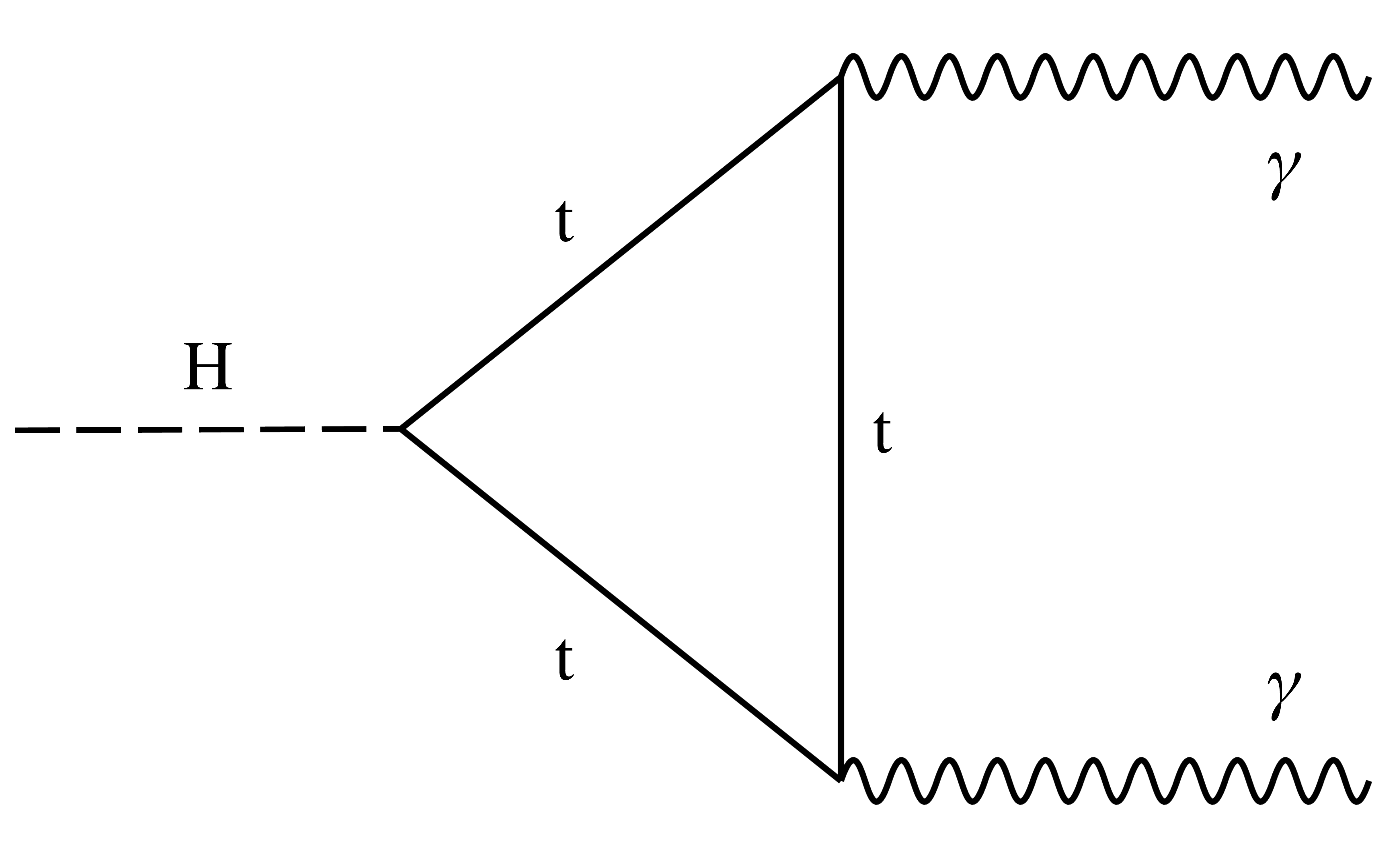
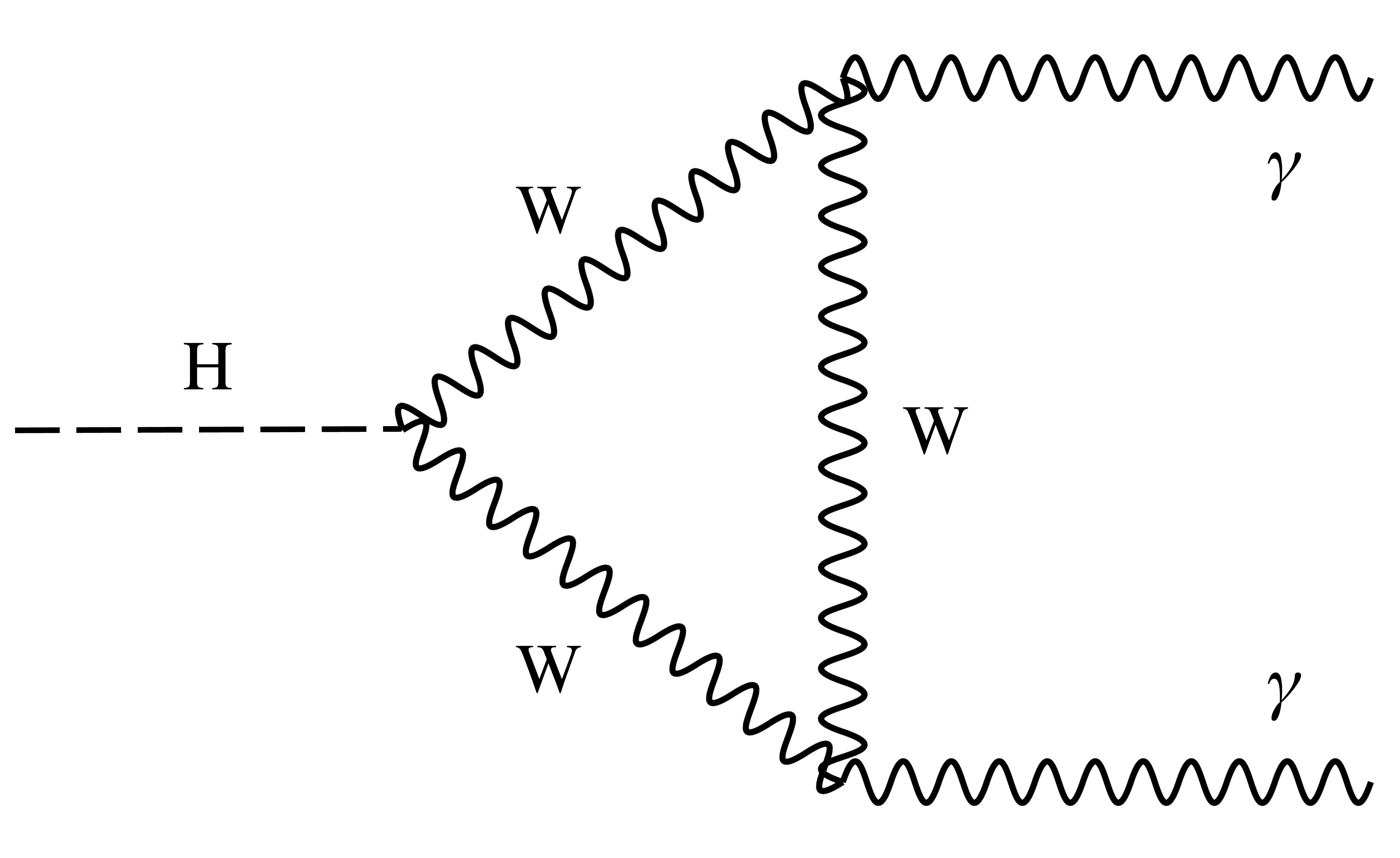
Figure 4:
Examples of leading-order Feynman diagrams for Higgs boson decays in the $\mathrm{H\to b\bar{b}}$, $\mathrm{H\to \tau\tau}$, and $\mathrm{H\to \mu\mu}$ (upper left); $\mathrm{H\to ZZ}$ and $\mathrm{H\to WW}$ (upper right); and $\mathrm{H\to \gamma\gamma}$ (lower) channels. |

png pdf |
Figure 4-a:
Example of leading-order Feynman diagram for Higgs boson decay in the $\mathrm{H\to b\bar{b}}$, $\mathrm{H\to \tau\tau}$ and $\mathrm{H\to \mu\mu}$ channels. |

png pdf |
Figure 4-b:
Example of leading-order Feynman diagram for Higgs boson decay in the $\mathrm{H\to ZZ}$ and $\mathrm{H\to WW}$ channels. |
png pdf |
Figure 4-c:
Example of leading-order Feynman diagram for Higgs boson decay in the $\mathrm{H\to \gamma\gamma}$ channel. |
png pdf |
Figure 4-d:
Example of leading-order Feynman diagram for Higgs boson decay in the $\mathrm{H\to \gamma\gamma}$ channel. |

png pdf |
Figure 5:
Signal strength modifiers for the production, $\mu _i$, and for the decay, $\mu ^f$, modes on the left and the right panel, respectively. The thick (thin) black lines report the $1\sigma $ ($2\sigma $) confidence intervals. The thick blue and red lines report the statistical and systematic components of the $1\sigma $ confidence intervals. The assumptions used in this fit are described in the text. |

png pdf |
Figure 5-a:
Signal strength modifiers for the production, $\mu _i$. The thick (thin) black lines report the $1\sigma $ ($2\sigma $) confidence intervals. The thick blue and red lines report the statistical and systematic components of the $1\sigma $ confidence intervals. The assumptions used in this fit are described in the text. |

png pdf |
Figure 5-b:
Signal strength modifiers for the decay, $\mu ^f$. The thick (thin) black lines report the $1\sigma $ ($2\sigma $) confidence intervals. The thick blue and red lines report the statistical and systematic components of the $1\sigma $ confidence intervals. The assumptions used in this fit are described in the text. |
png pdf |
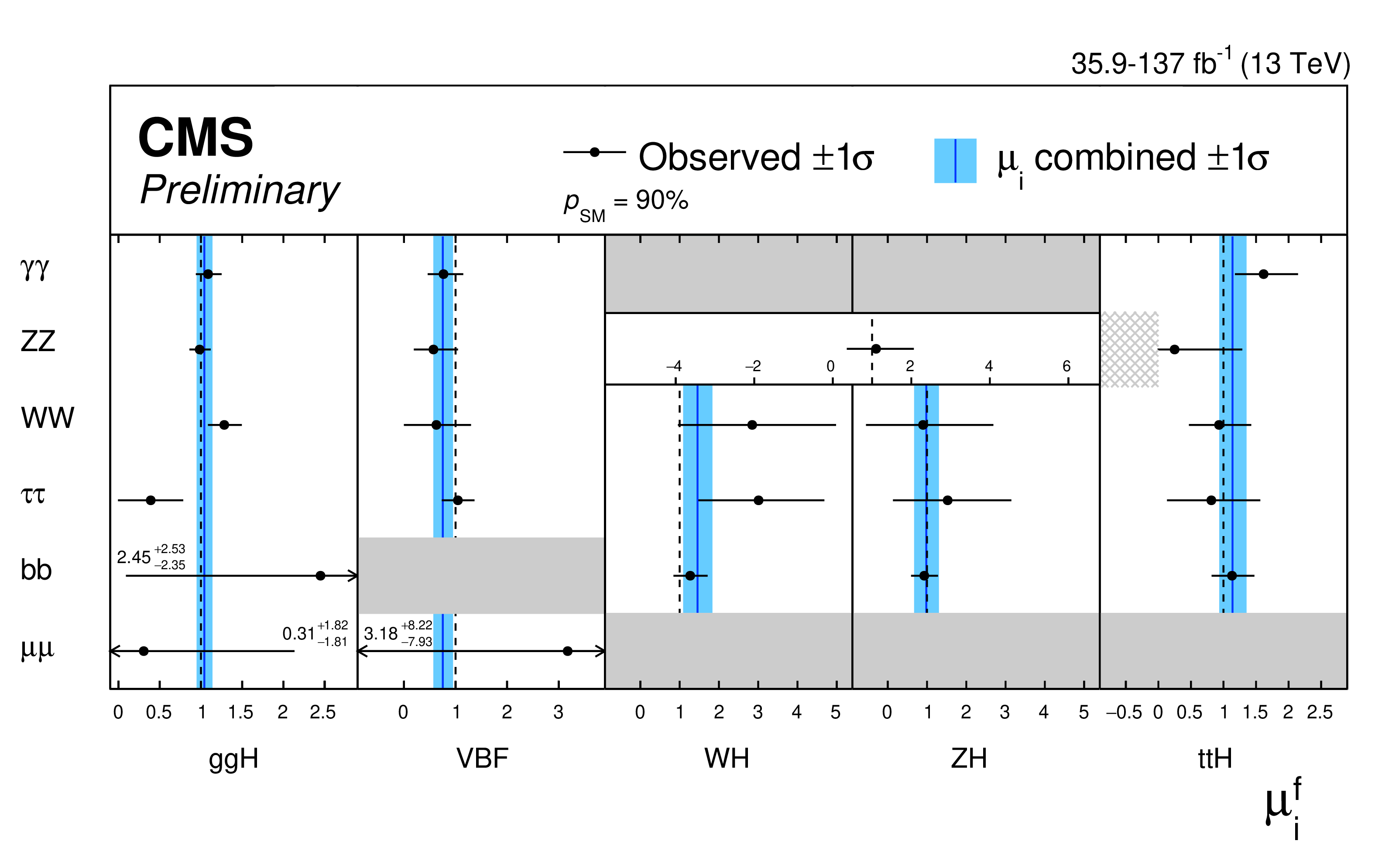
Figure 6:
Signal strength modifiers for the production times decay mode, $\mu _i^f$. The black points and horizontal error bars show the best-fit values and $1\sigma $ confidence intervals, respectively. The arrows indicate cases where the confidence intervals exceed the scale of the horizontal axis. The gray filled boxes indicate signal strength modifiers which are not included in the model, while the gray hatched box indicates the region for which the sum of signal and background becomes negative in the fit for $\mu _{{\mathrm{t} \mathrm{t} \mathrm{H}}}^{{\mathrm{Z} \mathrm{Z}}}$. In the $ {\mathrm{H} \to {\mathrm{Z} \mathrm{Z}}} $ decay mode, a common modifier is fit to the $ {\mathrm{W} \mathrm{H}} $ and $ {\mathrm{Z} \mathrm{H}} $ production modes. The measured value and $1\sigma $ confidence interval for each production cross section modifier, $\mu _{i}$, from the combination across decay channels, is indicated by the blue vertical line, and the blue bands, respectively. The indicated p-value is given for the production times decay mode signal strength modifiers. The assumptions used in this fit are described in the text. |

png pdf |
Figure 7:
Summary of the couplings modifiers $\vec{\kappa}$. The thick (thin) black lines report the $1\sigma $ ($2\sigma $) confidence intervals. |

png pdf |
Figure 8:
Profile likelihood scans as a function of $ {\kappa _{\lambda}} $ for the observed data (black solid line). The expected result assuming a SM Higgs boson (red dashed line), derived from an Asimov data set with $ {\kappa _{\lambda}} =1$ is also shown. |

png pdf |
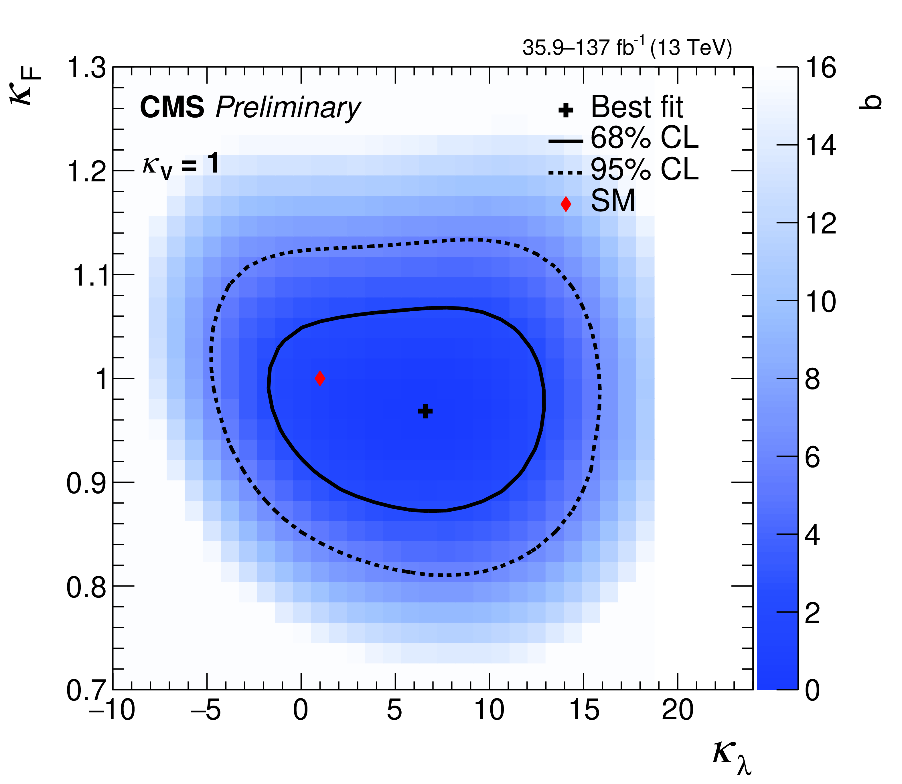
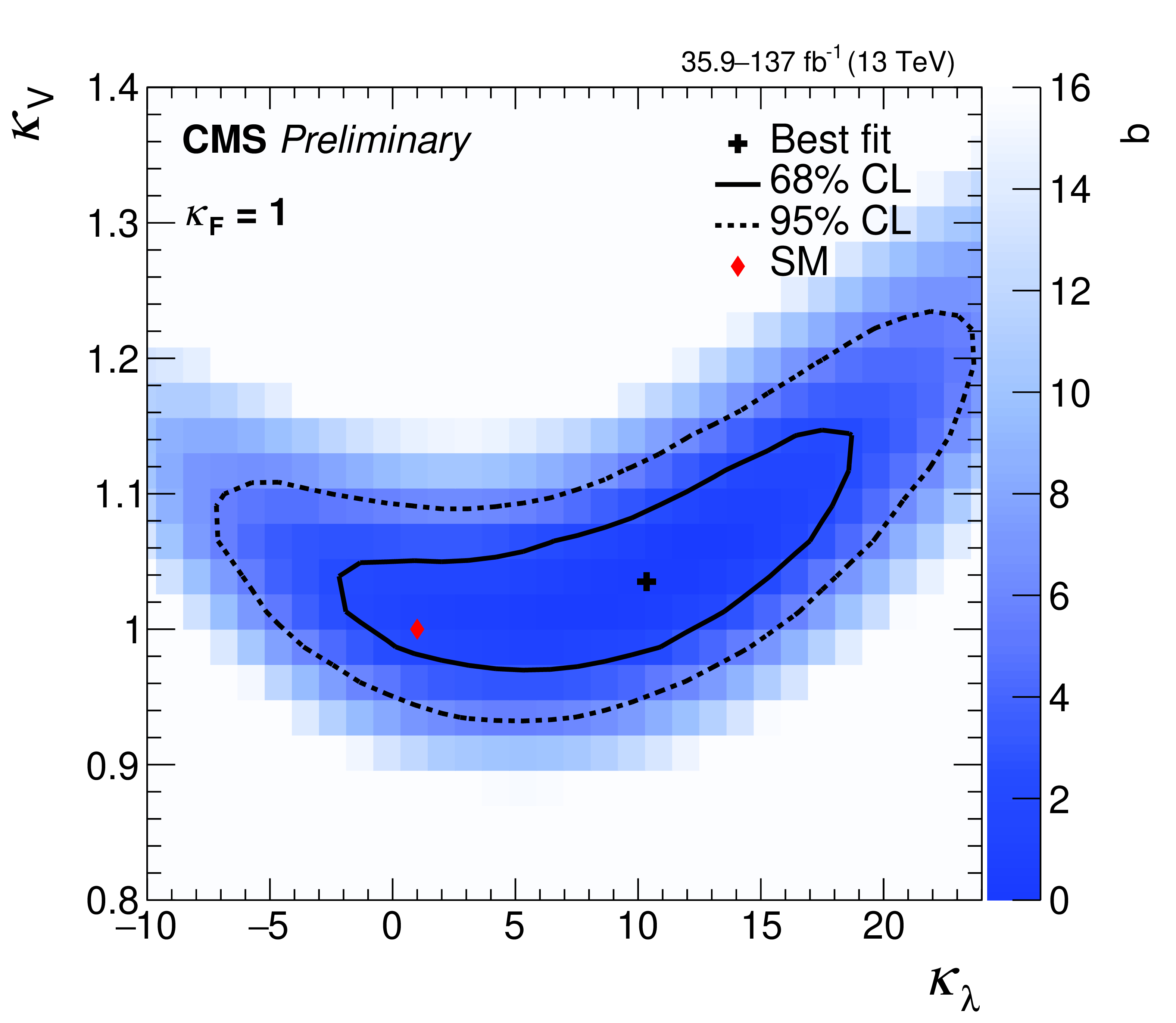
Figure 9:
Profile likelihood scans as a function of $ {\kappa _{\lambda}} $ and $ {\kappa _{\mathrm {F}}} $ (left), and $ {\kappa _{\lambda}} $ and $ {\kappa _{\mathrm {V}}} $ (right). The blue color scale shows the value of $q$ at each point in the scan, while the black marker, and solid and dashed lines show the best-fit point, and the 68% and 95% CL contours, respectively. The red marker corresponds to the SM prediction. |
png pdf |
Figure 9-a:
Profile likelihood scans as a function of $ {\kappa _{\lambda}} $ and $ {\kappa _{\mathrm {F}}} $. The blue color scale shows the value of $q$ at each point in the scan, while the black marker, and solid and dashed lines show the best-fit point, and the 68% and 95% CL contours, respectively. The red marker corresponds to the SM prediction. |
png pdf |
Figure 9-b:
Profile likelihood scans as a function of $ {\kappa _{\lambda}} $ and $ {\kappa _{\mathrm {V}}} $. The blue color scale shows the value of $q$ at each point in the scan, while the black marker, and solid and dashed lines show the best-fit point, and the 68% and 95% CL contours, respectively. The red marker corresponds to the SM prediction. |
png pdf |
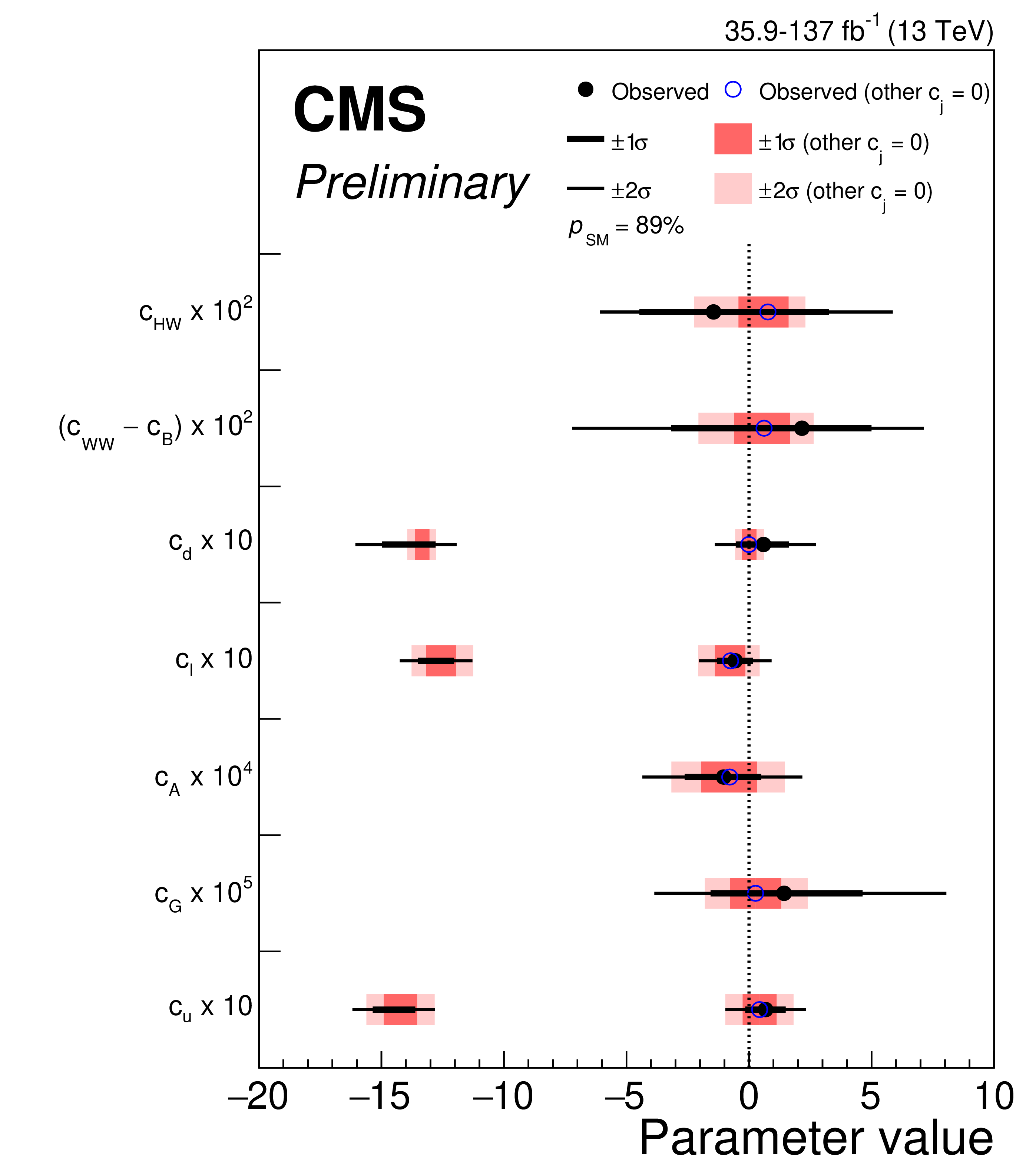
Figure 10:
Summary plot for the HEL parameter scans. The best fit values when profiling (fixing) the other parameters are shown by the solid black (hollow blue) points. The $\pm 1\sigma $ and $\pm 2\sigma $ confidence intervals are represented by the thick and thin black lines respectively for the profiled scenario, and the green and yellow bands respectively for the fixed scenario. The assumptions used in this fit are described in the text. |

png pdf |
Figure 11:
Profiled likelihood scans for (clockwise from top left) $c_G$, $c_A$, $c_{HW}$, and $c_{WW}-c_B$. The solid black lines correspond to the fit in which all parameters are allowed to vary simultaneously and the dashed blue lines to the fits where only one parameter is varied at a time. The assumptions used in this fit are described in the text. |

png pdf |
Figure 11-a:
Profiled likelihood scans for $c_G$. The solid black lines correspond to the fit in which all parameters are allowed to vary simultaneously and the dashed blue lines to the fits where only one parameter is varied at a time. The assumptions used in this fit are described in the text. |

png pdf |
Figure 11-b:
Profiled likelihood scans for $c_A$. The solid black lines correspond to the fit in which all parameters are allowed to vary simultaneously and the dashed blue lines to the fits where only one parameter is varied at a time. The assumptions used in this fit are described in the text. |

png pdf |
Figure 11-c:
Profiled likelihood scans for $c_{WW}-c_B$. The solid black lines correspond to the fit in which all parameters are allowed to vary simultaneously and the dashed blue lines to the fits where only one parameter is varied at a time. The assumptions used in this fit are described in the text. |

png pdf |
Figure 11-d:
Profiled likelihood scans for $c_{HW}$. The solid black lines correspond to the fit in which all parameters are allowed to vary simultaneously and the dashed blue lines to the fits where only one parameter is varied at a time. The assumptions used in this fit are described in the text. |

png pdf |
Figure 12:
Profiled likelihood scans for (clockwise from top left) $c_u$, $c_d$, $c_{\ell}$. The solid black lines correspond to the fit in which all parameters are allowed to vary simultaneously and the dashed blue lines to the fits where only one parameter is varied at a time. The assumptions used in this fit are described in the text. |

png pdf |
Figure 12-a:
Profiled likelihood scans for $c_u$. The solid black lines correspond to the fit in which all parameters are allowed to vary simultaneously and the dashed blue lines to the fits where only one parameter is varied at a time. The assumptions used in this fit are described in the text. |

png pdf |
Figure 12-b:
Profiled likelihood scans for $c_d$. The solid black lines correspond to the fit in which all parameters are allowed to vary simultaneously and the dashed blue lines to the fits where only one parameter is varied at a time. The assumptions used in this fit are described in the text. |

png pdf |
Figure 12-c:
Profiled likelihood scans for $c_{\ell}$. The solid black lines correspond to the fit in which all parameters are allowed to vary simultaneously and the dashed blue lines to the fits where only one parameter is varied at a time. The assumptions used in this fit are described in the text. |

png pdf |
Figure 13:
Observed correlations in the HEL parameters. The size of the correlation is given by the colour scale with positive (negative) correlation represented by blue (yellow). The assumptions used in this fit are described in the text. |
| Tables | |

png pdf |
Table 2:
Best-fit values and $ \pm 1 \sigma $ uncertainties for the production mode signal strength parametrization. The expected uncertainties for $\mu _{i} = 1$ are given in brackets. |

png pdf |
Table 3:
Best-fit values and $ \pm 1 \sigma $ uncertainties for the decay channel signal strength parametrization. The expected uncertainties for $\mu ^{f} = 1$ are given in brackets. |

png pdf |
Table 4:
Best-fit values and $ \pm 1 \sigma $ uncertainties for the production times decay signal strength parametrization. The expected uncertainties for $\mu _{i}^{f}=1$ are given in brackets. |
png pdf |
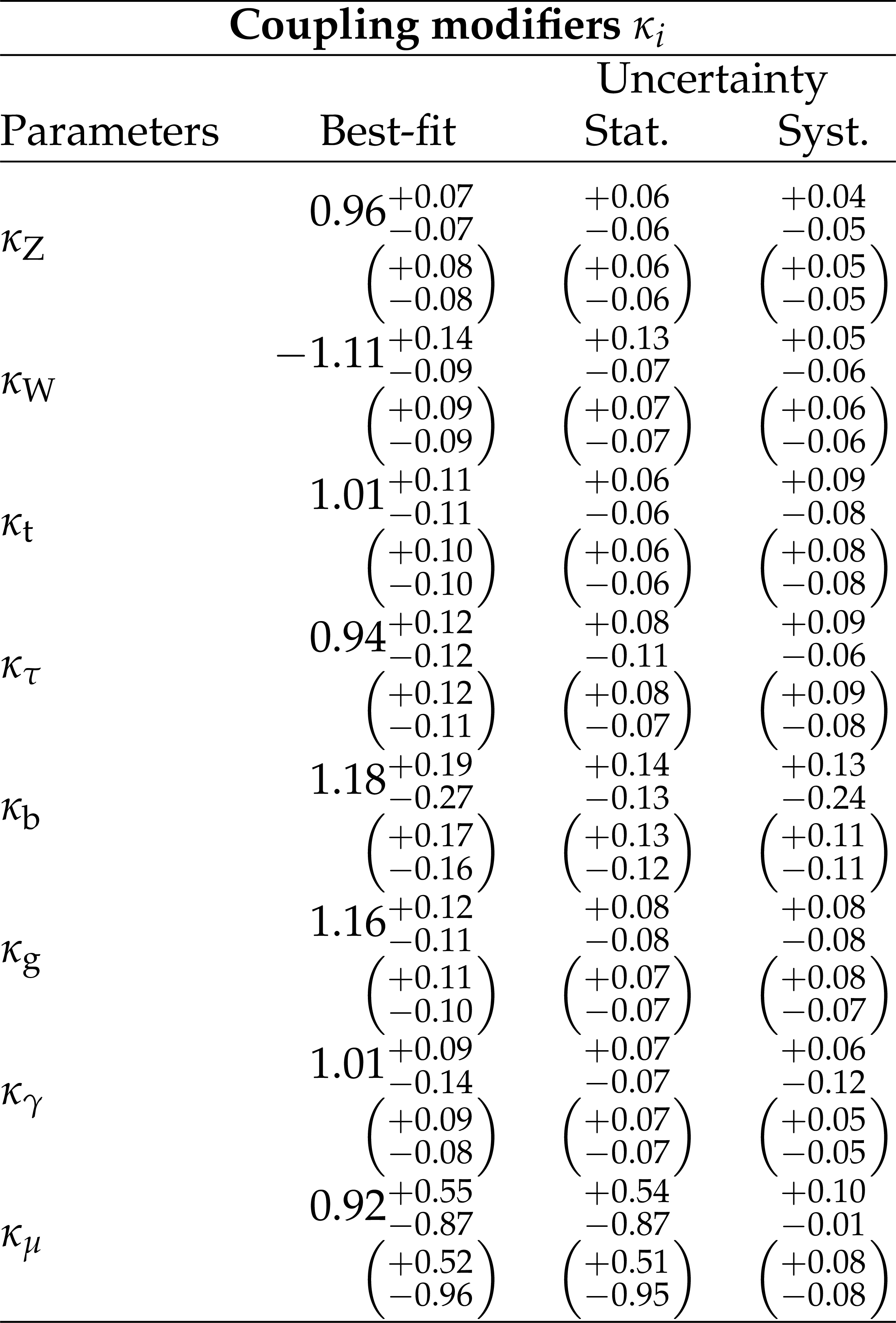
Table 5:
Best-fit values and $ \pm 1 \sigma $ uncertainties for the parameters of the coupling modifier model. The expected uncertainties for $\kappa _{i}=1$ are given in brackets. |

png pdf |
Table 6:
$K_{\mathrm {BSM}}$ values for parametrization of Higgs boson production modifiers $\mu _{i}$, in the Higgs boson self-coupling modifier model. |

png pdf |
Table 7:
$C^{f}$ values for parametrization of Higgs boson branching ratio modifiers $\mu ^{f}$, in the Higgs boson self-coupling modifier model. |
png pdf |
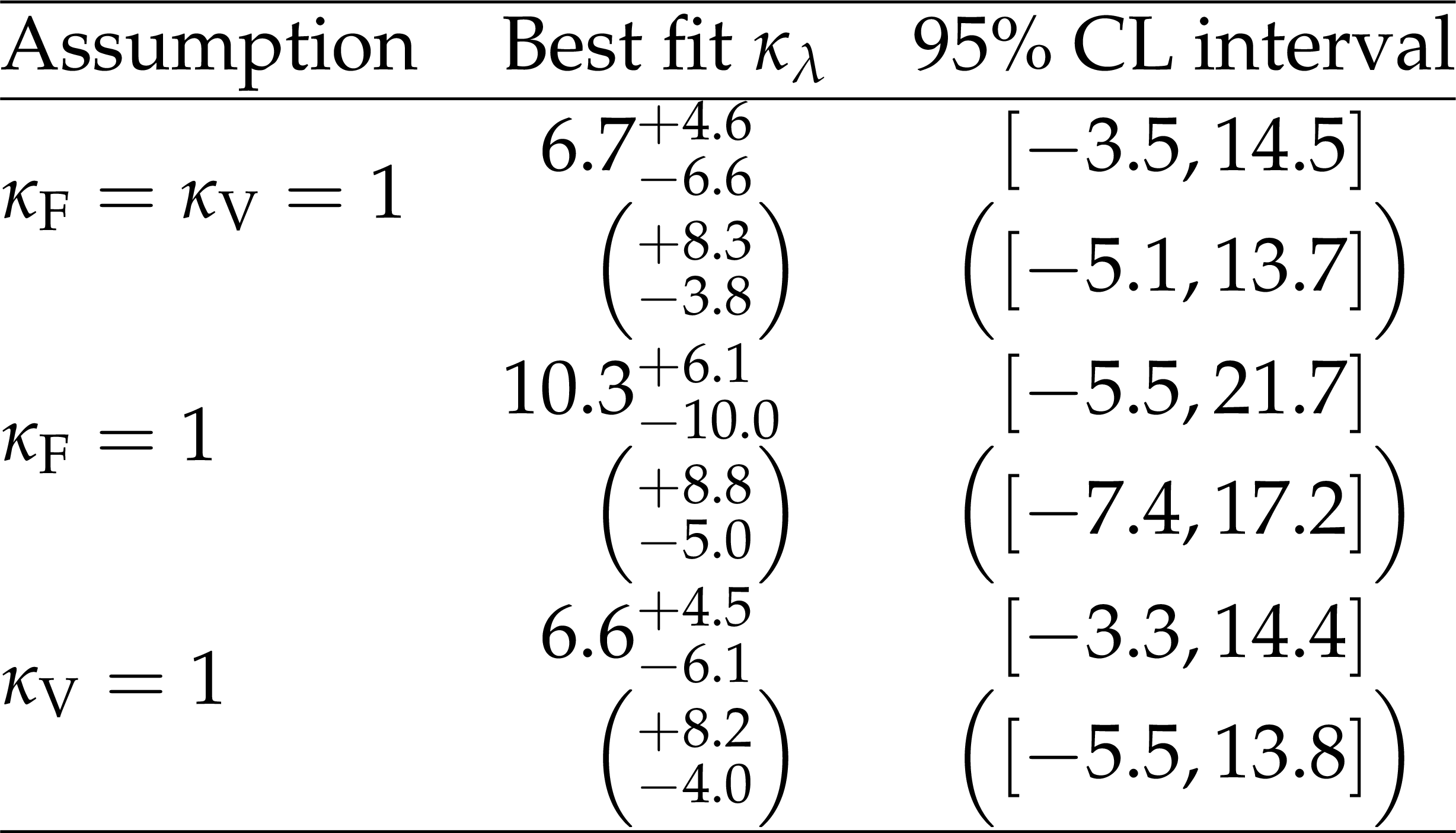
Table 8:
Best fit values, $\pm 1\sigma $ uncertainties and $95%$ CL intervals for $ {\kappa _{\lambda}} $ under different assumptions for the vector boson and fermion Higgs boson couplings. The expected uncertainties and intervals for $\kappa _{\lambda}=1$, evaluated on an Asimov data set, are given in brackets. |

png pdf |
Table 9:
Best fit values and $\pm 1\sigma $ uncertainties for the fitted HEL parameters. The expected uncertainties for $c_{j}=0$, evaluated on an Asimov data set are given in brackets. The definition of the HEL parameters in terms of the EFT Wilson coefficients, $f_j/\Lambda ^2$, are also provided. The $\pm 1\sigma $ uncertainties for $c_u$, $c_d$ and $c_\ell $ are related to the minima around zero. |

png pdf |
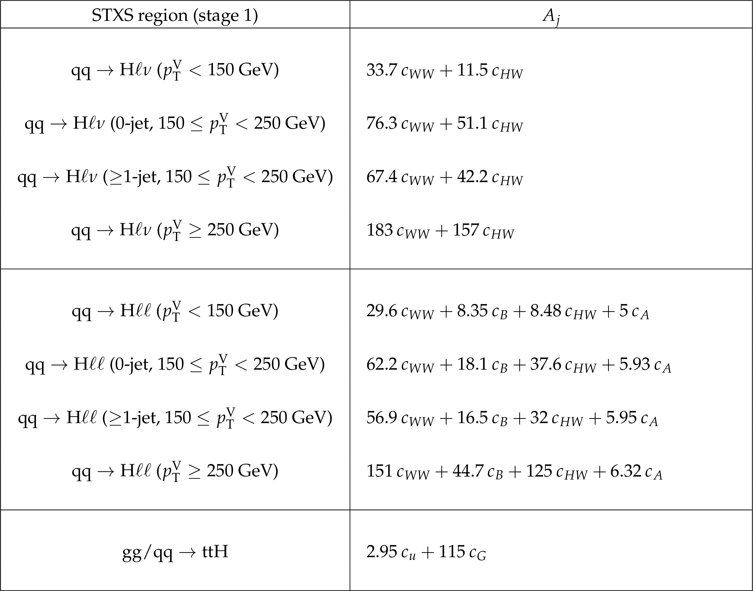
Table 10:
$A_j$ coefficients for the STXS stage 0 bins. |
png pdf |
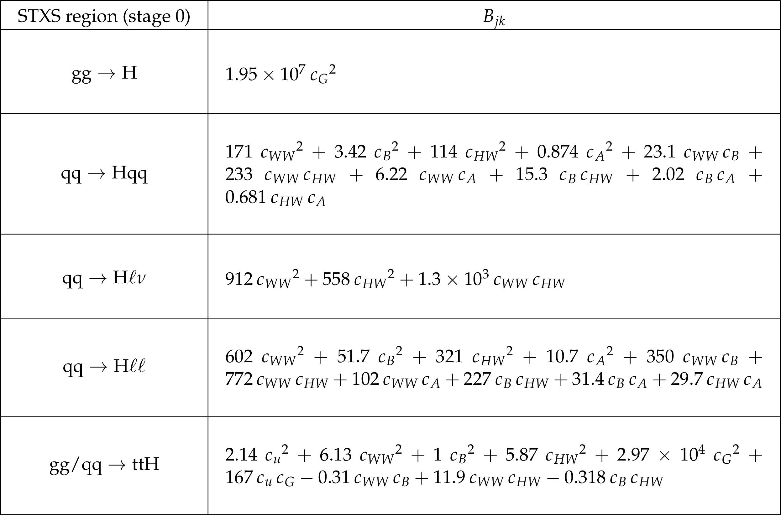
Table 11:
$B_{jk}$ coefficients for the STXS stage 0 bins. |

png pdf |
Table 12:
$A_j$ coefficients for the ${\mathrm{g} \mathrm{g} \mathrm{H}}$ and ${\mathrm {VBF}}$ STXS stage 1.0 bins. |
png pdf |
Table 13:
$A_j$ coefficients for the ${\mathrm{W} \mathrm{H}}$, ${\mathrm{Z} \mathrm{H}}$ and ${\mathrm{t} \mathrm{t} \mathrm{H}}$ STXS stage 1.0 bins. |

png pdf |
Table 14:
$B_{jk}$ coefficients for the ${\mathrm{g} \mathrm{g} \mathrm{H}}$ STXS stage 1.0 bins. |
png pdf |
Table 15:
$B_{jk}$ coefficients for the ${\mathrm {VBF}}$ STXS stage 1.0 bins. |

png pdf |
Table 16:
$B_{jk}$ coefficients for the ${\mathrm{W} \mathrm{H}}$, ${\mathrm{Z} \mathrm{H}}$ and ${\mathrm{t} \mathrm{t} \mathrm{H}}$ STXS stage 1.0 bins. |
png pdf |
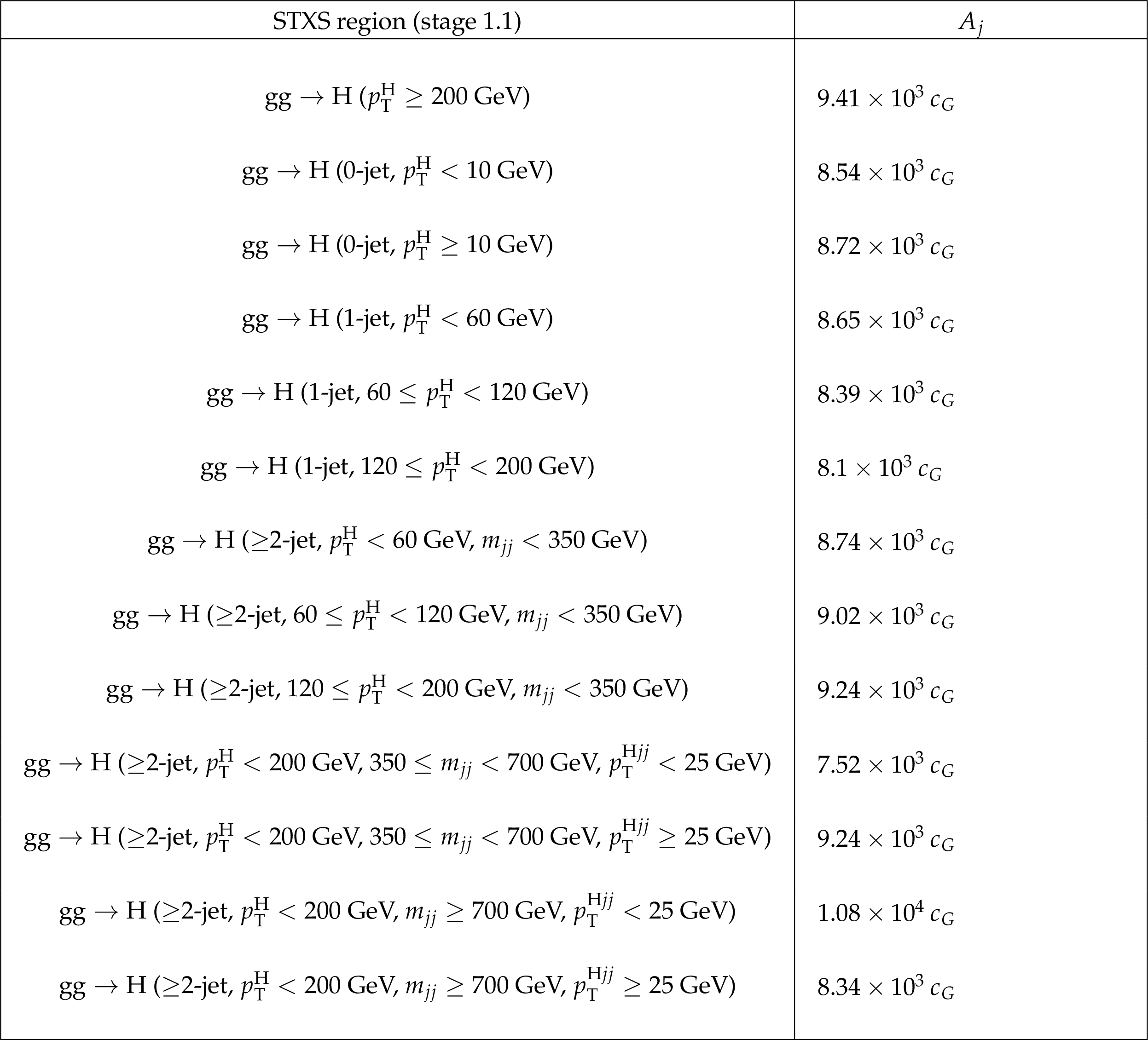
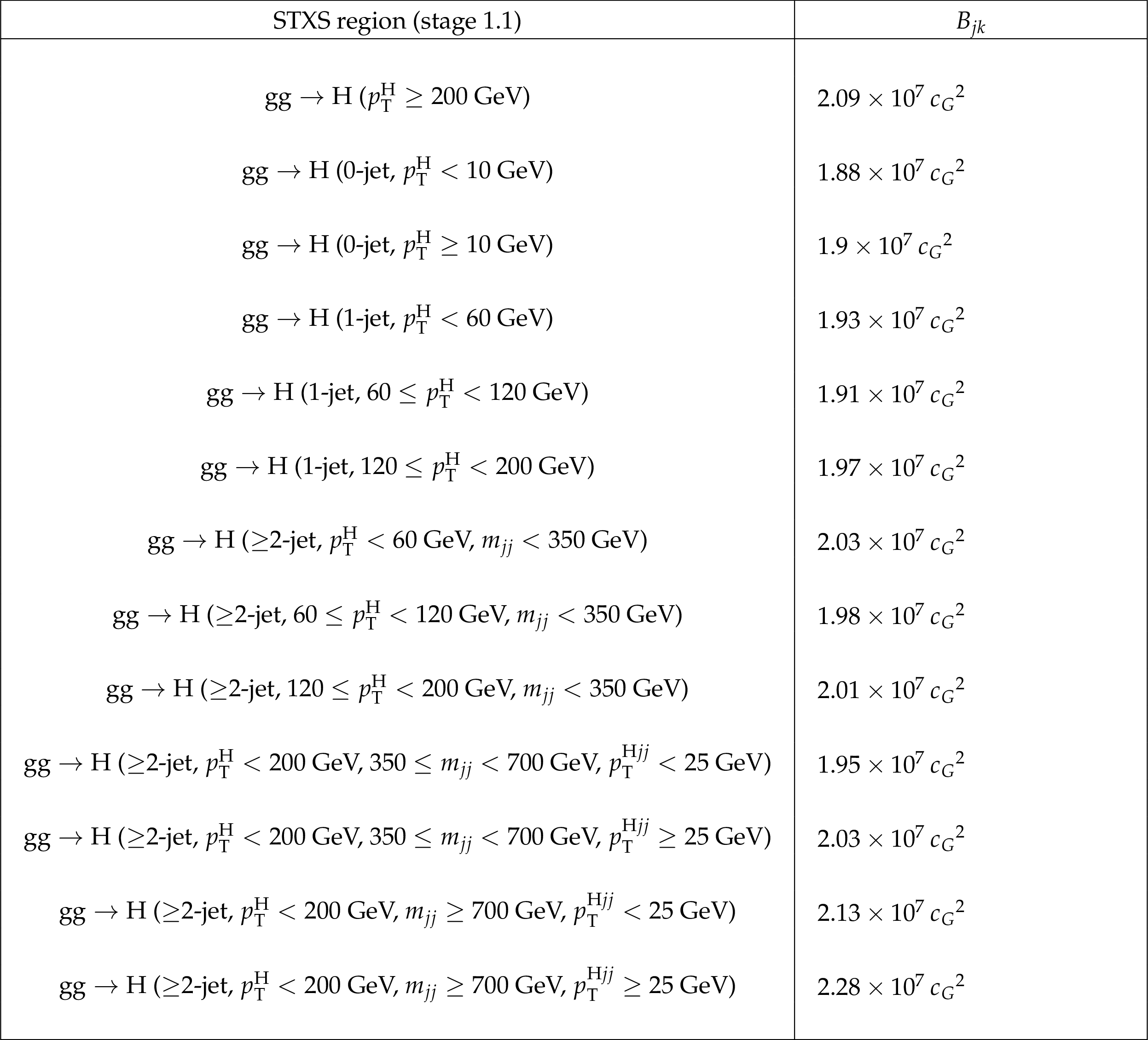
Table 17:
$A_j$ coefficients for the ${\mathrm{g} \mathrm{g} \mathrm{H}}$ STXS stage 1.1 bins. |

png pdf |
Table 18:
$A_j$ coefficients for the ${\mathrm {VBF}}$ STXS stage 1.1 bins. |
png pdf |
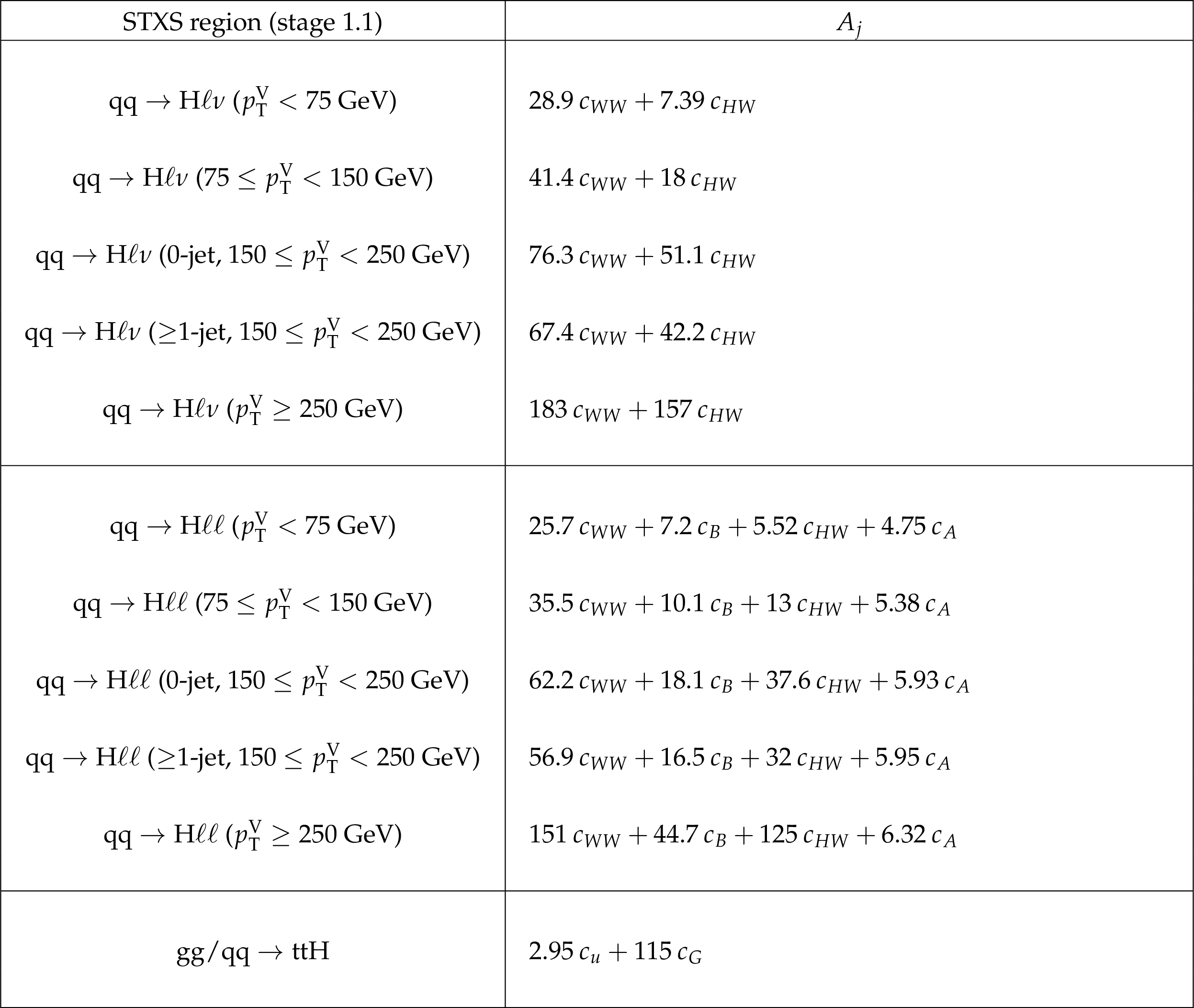
Table 19:
$A_j$ coefficients for the ${\mathrm{W} \mathrm{H}}$, ${\mathrm{Z} \mathrm{H}}$ and ${\mathrm{t} \mathrm{t} \mathrm{H}}$ STXS stage 1.1 bins. |
png pdf |
Table 20:
$B_{jk}$ coefficients for the ${\mathrm{g} \mathrm{g} \mathrm{H}}$ STXS stage 1.1 bins. |

png pdf |
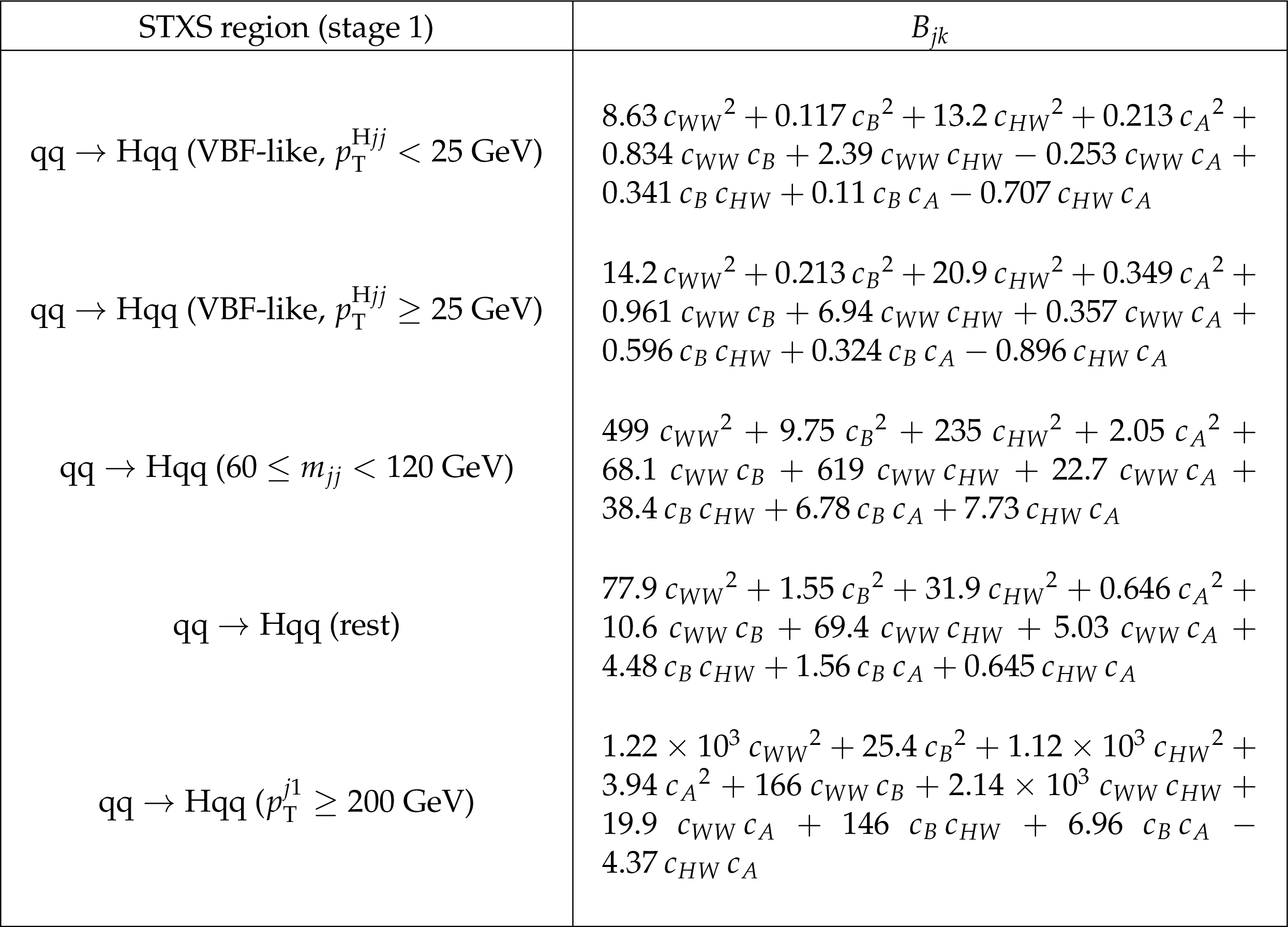
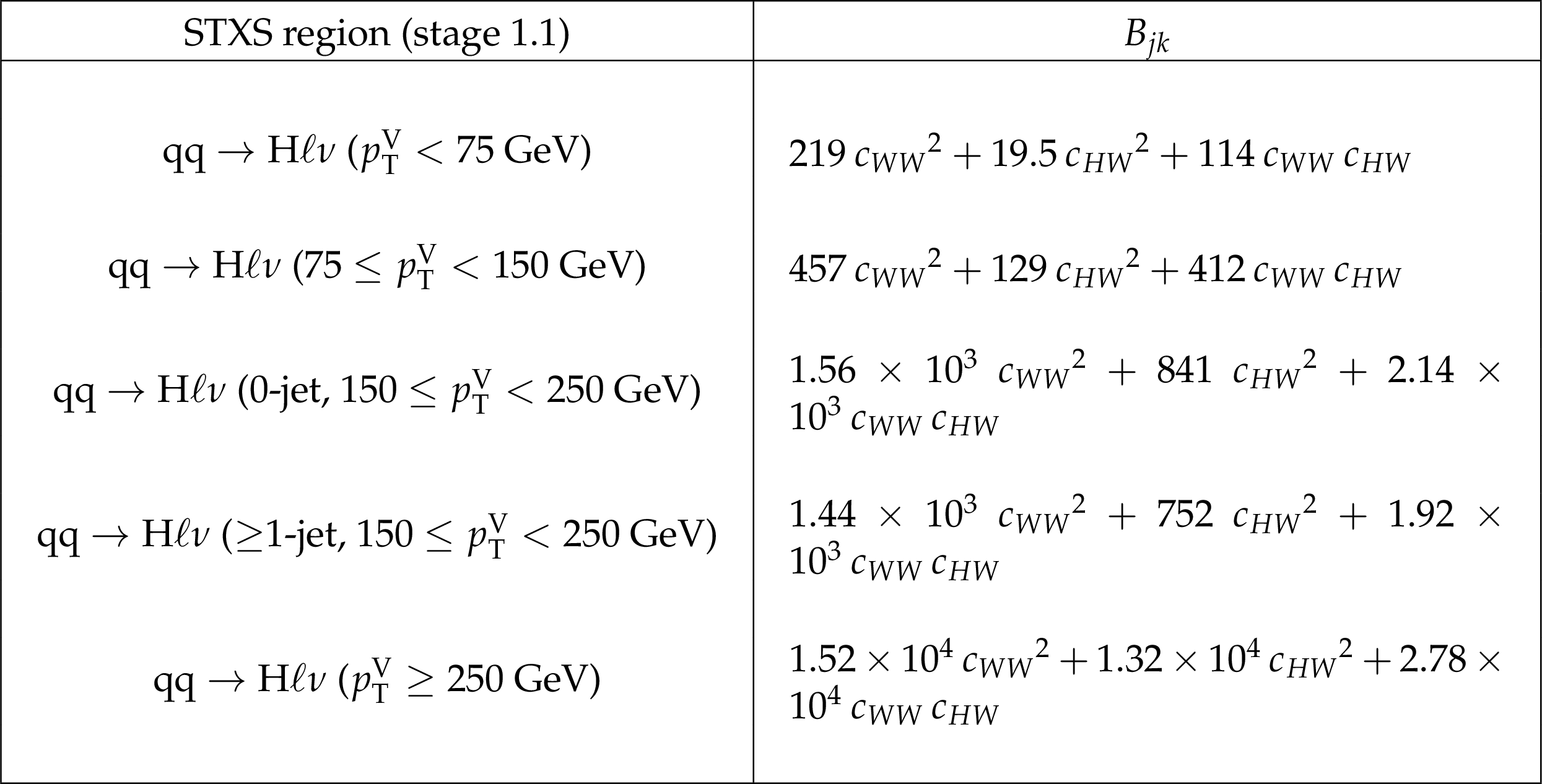
Table 21:
$B_{jk}$ coefficients for the ${\mathrm {VBF}}$ STXS stage 1.1 bins. |

png pdf |
Table 22:
$B_{jk}$ coefficients for the ${\mathrm {VBF}}$ STXS stage 1.1 bins. |
png pdf |
Table 23:
$B_{jk}$ coefficients for the ${\mathrm{W} \mathrm{H}}$ STXS stage 1.1 bins. |

png pdf |
Table 24:
$B_{jk}$ coefficients for the ${\mathrm{Z} \mathrm{H}}$ and ${\mathrm{t} \mathrm{t} \mathrm{H}}$ STXS stage 1.1 bins. |
| Summary |
|
This note has presented a set of combined measurements of Higgs boson production and decay rates; coupling modifiers to the standard model (SM) particles; and interpretations in terms of the Higgs boson self coupling and parameters in the effective field theory. Analyses targeting the gluon fusion, vector boson fusion, $\mathrm{W}$-, $\mathrm{Z}$- and $\mathrm{t\bar{t}}$-associated production modes are included in the combination. These analyses target Higgs boson decays to $\gg$, ${\mathrm{Z}\mathrm{Z}} $, ${\mathrm{W}\mathrm{W}} $, ${\tau\tau} $, ${\mathrm{b}\mathrm{b}} $, and $ {\mu\mu} $ pairs, using 13 TeV proton-proton collision data collected between 2016-2018 with integrated luminosities of between 35.9-137 fb$^{-1}$ depending on the analysis. The combined Higgs boson signal strength is measured to be 1.02$^{+0.07}_{-0.06}$, and signal strengths measured per production and decay mode are also found to be in agreement with the SM prediction. In addition, an interpretation is provided in which these production and decay rates are parameterised by the Higgs boson self-coupling modifier $\kappa_{\lambda}$. The measured value is compatible with the SM expectation, and a 95% confidence level interval of $[-3.5, 14.5]$ is determined under the assumption that the Higgs boson couplings to fermions and vector bosons take their SM values. An effective field theory interpretation is also presented, in which constraints on the parameters of the Higgs Effective Lagrangian model are determined. For many of the parameters these results represent the strongest constraints to date. |
| Additional Figures | |

png pdf |
Additional Figure 1:
Signal strength modifiers $\mu _i$ for the production modes. The thick (thin) black lines report the 1$\sigma $ (2$\sigma $) confidence intervals. The thick blue and red lines report the statistical and systematic components of the 1$\sigma $ confidence intervals. The probability of compatibility between the measurement and the SM prediction ($p_\text {SM}$) is reported. The assumptions used in this fit are described in the text. |

png pdf |
Additional Figure 2:
Signal strength modifiers $\mu ^f$ for the decay modes. The thick (thin) black lines report the 1$\sigma $ (2$\sigma $) confidence intervals. The thick blue and red lines report the statistical and systematic components of the 1$\sigma $ confidence intervals. The probability of compatibility between the measurement and the SM prediction ($p_\text {SM}$) is reported. The assumptions used in this fit are described in the text. |
png pdf |
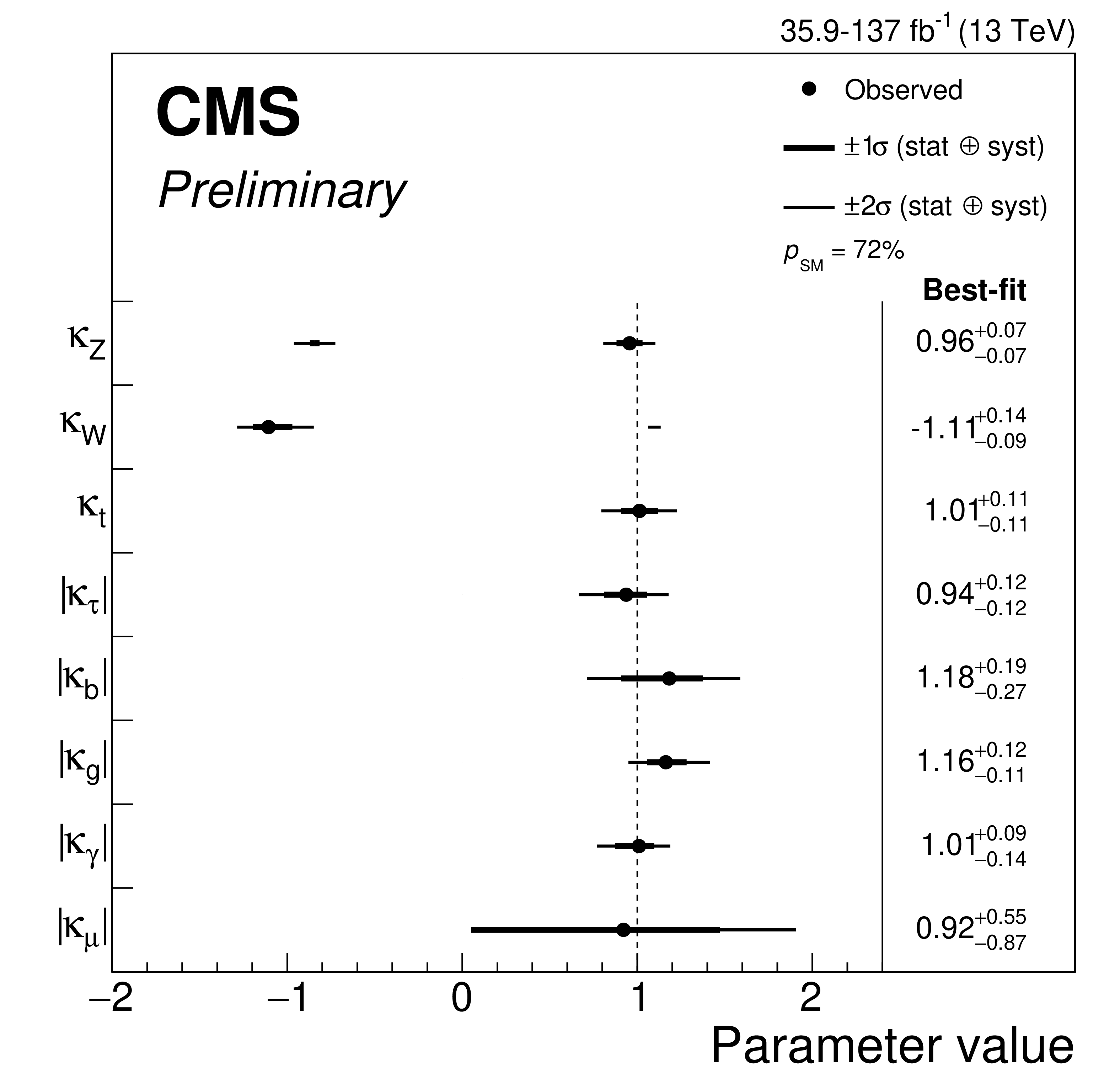
Additional Figure 3:
Summary of the couplings modifiers $\vec{\kappa}$. The thick (thin) black lines report the 1$\sigma $ (2$\sigma $) confidence intervals. The probability of compatibility between the measurement and the SM prediction ($p_\text {SM}$) is reported. The assumptions used in this fit are described in the text. |
png pdf |
Additional Figure 4:
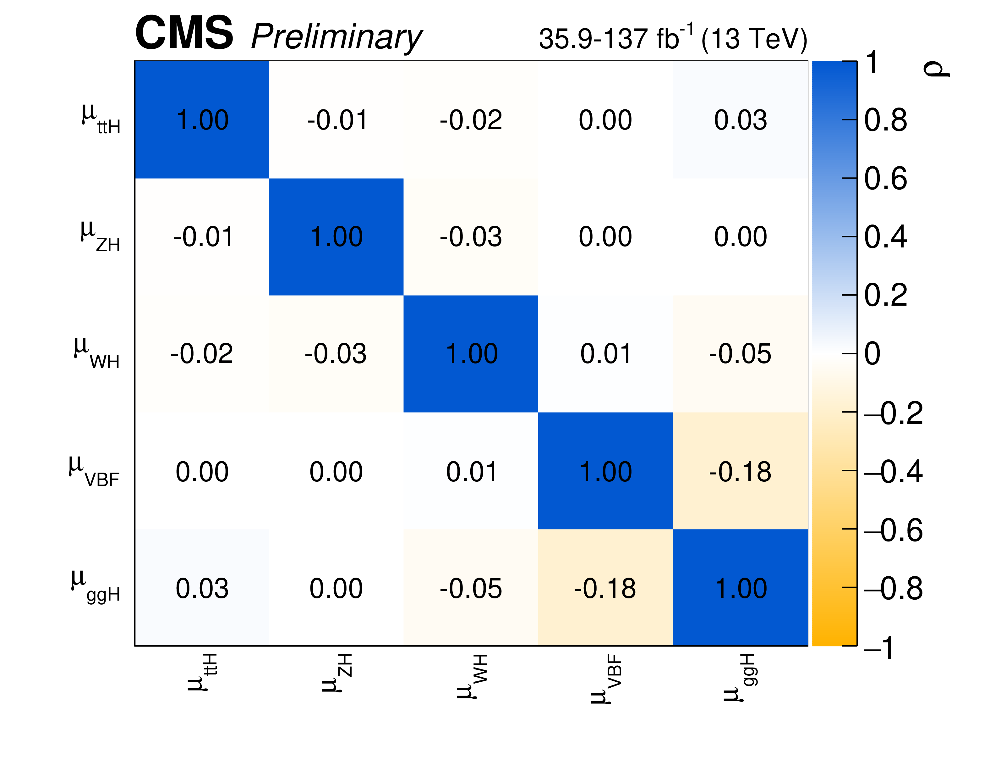
Observed correlations between the production mode signal strength modifiers. The size of the correlation is given by the colour scale with positive (negative) correlation represented by blue (yellow). The assumptions used in this fit are described in the text. |
png pdf |
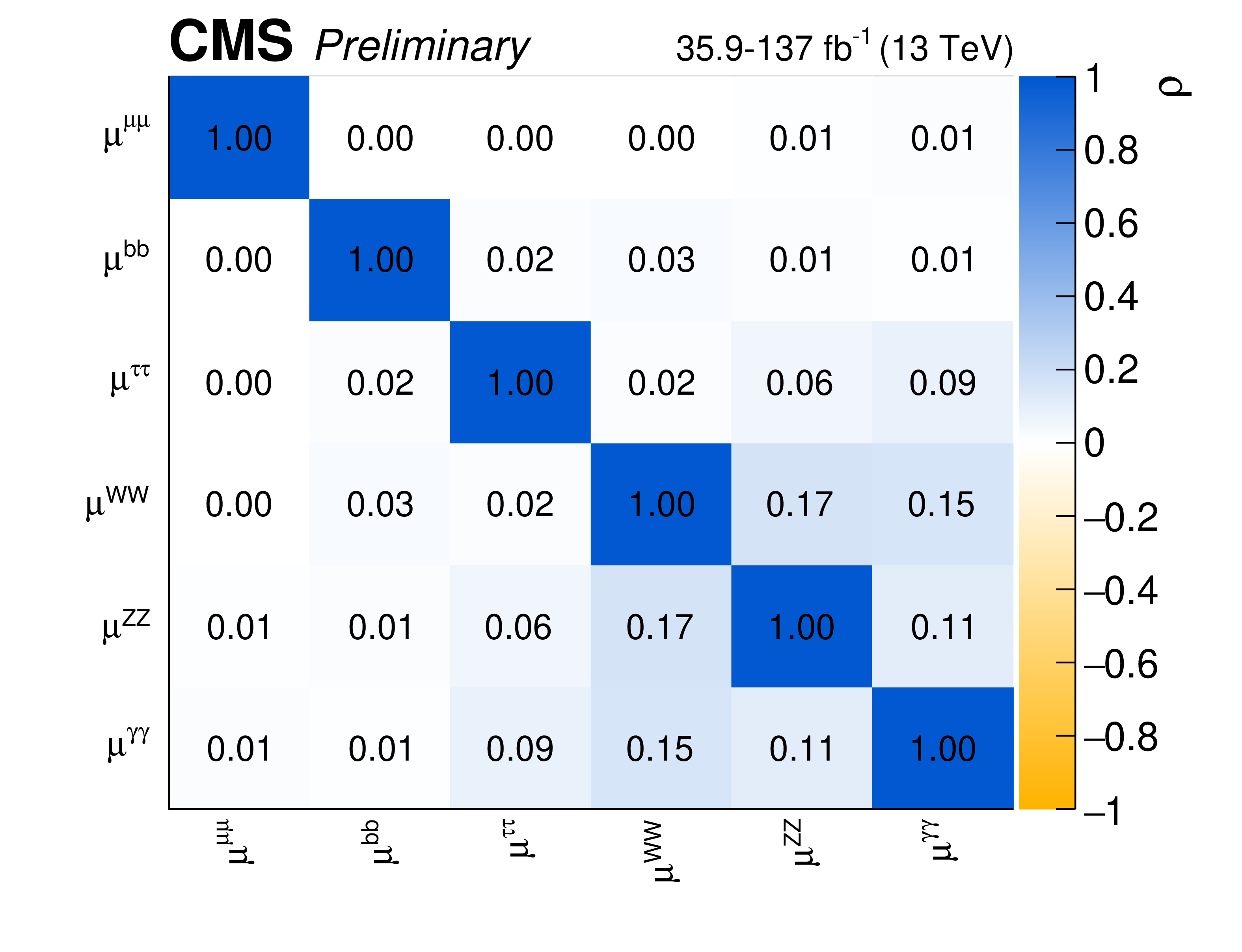
Additional Figure 5:
Observed correlations between the decay mode signal strength modifiers. The size of the correlation is given by the colour scale with positive (negative) correlation represented by blue (yellow). The assumptions used in this fit are described in the text. |
png pdf |
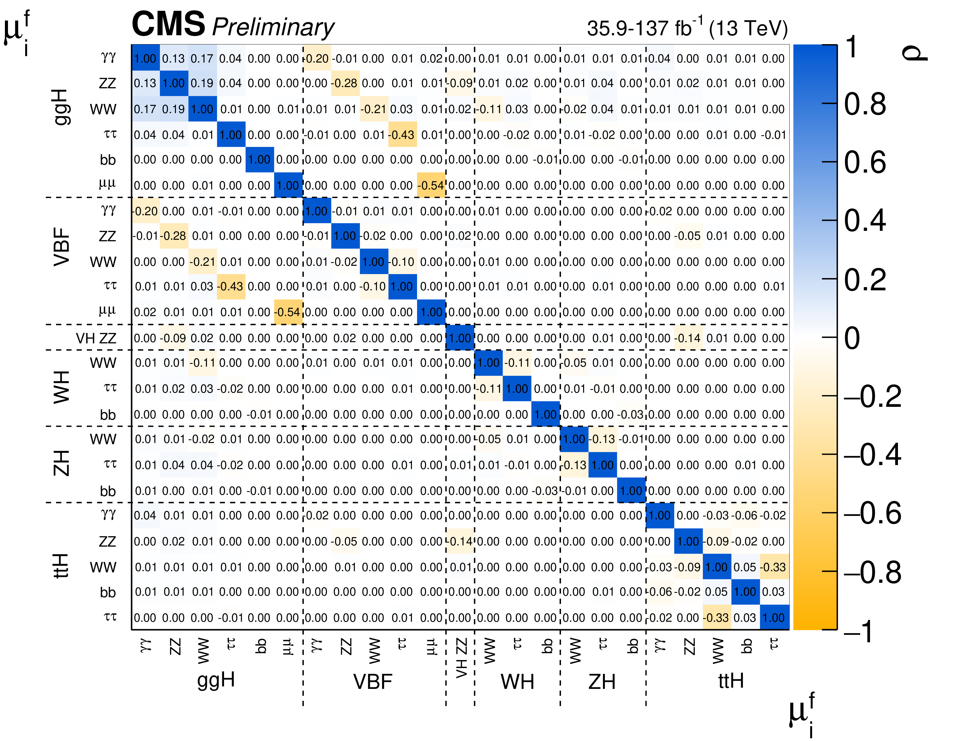
Additional Figure 6:
Observed correlations between the production times decay mode signal strength modifiers. The size of the correlation is given by the colour scale with positive (negative) correlation represented by blue (yellow). The assumptions used in this fit are described in the text. |
| References | ||||
| 1 | S. L. Glashow | Partial-symmetries of weak interactions | NP 22 (1961) 579 | |
| 2 | S. Weinberg | A model of leptons | PRL 19 (1967) 1264 | |
| 3 | A. Salam | Weak and electromagnetic interactions | in Elementary particle physics: relativistic groups and analyticity, N. Svartholm, ed., p. 367 Almqvist \& Wiskell, 1968Proceedings of the 8$^\text{th}$ Nobel symposium | |
| 4 | G. 't Hooft and M. J. G. Veltman | Regularization and renormalization of gauge fields | NPB 44 (1972) 189 | |
| 5 | F. Englert and R. Brout | Broken symmetry and the mass of gauge vector mesons | PRL 13 (1964) 321 | |
| 6 | P. W. Higgs | Broken symmetries, massless particles and gauge fields | PL12 (1964) 132 | |
| 7 | P. W. Higgs | Broken symmetries and the masses of gauge bosons | PRL 13 (1964) 508 | |
| 8 | G. S. Guralnik, C. R. Hagen, and T. W. B. Kibble | Global conservation laws and massless particles | PRL 13 (1964) 585 | |
| 9 | P. W. Higgs | Spontaneous symmetry breakdown without massless bosons | PR145 (1966) 1156 | |
| 10 | T. W. B. Kibble | Symmetry breaking in non-Abelian gauge theories | PR155 (1967) 1554 | |
| 11 | Y. Nambu and G. Jona-Lasinio | Dynamical model of elementary particles based on an analogy with superconductivity. I | PR122 (1961) 345 | |
| 12 | K. G. Wilson | Renormalization group and strong interactions | PRD 3 (1971) 1818 | |
| 13 | E. Gildener | Gauge-symmetry hierarchies | PRD 14 (1976) 1667 | |
| 14 | S. Weinberg | Gauge hierarchies | PLB 82 (1979) 387 | |
| 15 | G. 't Hooft | Naturalness, chiral symmetry, and spontaneous chiral symmetry breaking | NATO Sci. Ser. B 59 (1980) 135 | |
| 16 | L. Susskind | Dynamics of spontaneous symmetry breaking in the Weinberg-Salam theory | PRD 20 (1979) 2619 | |
| 17 | ATLAS Collaboration | Observation of a new particle in the search for the standard model higgs boson with the ATLAS detector at the LHC | PLB 716 (2012) 1 | 1207.7214 |
| 18 | CMS Collaboration | Observation of a new boson at a mass of 125 GeV with the CMS experiment at the LHC | PLB 716 (2012) 30 | CMS-HIG-12-028 1207.7235 |
| 19 | CMS Collaboration | Observation of a new boson with mass near 125 GeV in pp collisions at $ \sqrt{s} = $ 7 and 8 TeV | JHEP 06 (2013) 81 | CMS-HIG-12-036 1303.4571 |
| 20 | LHC Higgs Cross Section Working Group | Handbook of LHC Higgs cross sections: 4. deciphering the nature of the Higgs sector | CERN (2016) | 1610.07922 |
| 21 | C. Anastasiou et al. | Higgs boson gluon-fusion production in QCD at three loops | PRL 114 (2015) 212001 | 1503.06056 |
| 22 | C. Anastasiou et al. | High precision determination of the gluon fusion Higgs boson cross-section at the LHC | JHEP 05 (2016) 58 | 1602.00695 |
| 23 | M. Ciccolini, A. Denner, and S. Dittmaier | Strong and electroweak corrections to the production of a Higgs boson+2 jets via weak interactions at the Large Hadron Collider | PRL 99 (2007) 161803 | 0707.0381 |
| 24 | M. Ciccolini, A. Denner, and S. Dittmaier | Electroweak and QCD corrections to Higgs production via vector-boson fusion at the LHC | PRD 77 (2008) 013002 | 0710.4749 |
| 25 | P. Bolzoni, F. Maltoni, S.-O. Moch, and M. Zaro | Higgs production via vector-boson fusion at NNLO in QCD | PRL 105 (2010) 011801 | 1003.4451 |
| 26 | P. Bolzoni, F. Maltoni, S.-O. Moch, and M. Zaro | Vector boson fusion at next-to-next-to-leading order in QCD: Standard model Higgs boson and beyond | PRD 85 (2012) 035002 | 1109.3717 |
| 27 | O. Brein, A. Djouadi, and R. Harlander | NNLO QCD corrections to the Higgs-strahlung processes at hadron colliders | PLB 579 (2004) 149 | hep-ph/0307206 |
| 28 | M. L. Ciccolini, S. Dittmaier, and M. Kramer | Electroweak radiative corrections to associated $ WH $ and $ ZH $ production at hadron colliders | PRD 68 (2003) 073003 | hep-ph/0306234 |
| 29 | W. Beenakker et al. | Higgs radiation off top quarks at the Tevatron and the LHC | PRL 87 (2001) 201805 | hep-ph/0107081 |
| 30 | W. Beenakker et al. | NLO QCD corrections to $ \mathrm{t\bar{t}} $ H production in hadron collisions. | NPB 653 (2003) 151 | hep-ph/0211352 |
| 31 | S. Dawson, L. H. Orr, L. Reina, and D. Wackeroth | Associated top quark Higgs boson production at the LHC | PRD 67 (2003) 071503 | hep-ph/0211438 |
| 32 | S. Dawson et al. | Associated Higgs production with top quarks at the Large Hadron Collider: NLO QCD corrections | PRD 68 (2003) 034022 | hep-ph/0305087 |
| 33 | Z. Yu et al. | QCD NLO and EW NLO corrections to $ t\bar{t}H $ production with top quark decays at hadron collider | PLB 738 (2014) 1 | 1407.1110 |
| 34 | S. S. Frixione et al. | Weak corrections to Higgs hadroproduction in association with a top-quark pair | JHEP 09 (2014) 65 | 1407.0823 |
| 35 | F. Demartin, F. Maltoni, K. Mawatari, and M. Zaro | Higgs production in association with a single top quark at the LHC | EPJC 75 (2015) 267 | 1504.0611 |
| 36 | F. Demartin et al. | tWH associated production at the LHC | EPJC 77 (2017) 34 | 1607.05862 |
| 37 | A. Denner et al. | Standard model Higgs-boson branching ratios with uncertainties | EPJC 71 (2011) 1753 | 1107.5909 |
| 38 | A. Djouadi, J. Kalinowski, and M. Spira | HDECAY: A Program for Higgs boson decays in the standard model and its supersymmetric extension | CPC 108 (1998) 56 | hep-ph/9704448 |
| 39 | A. Djouadi, J. Kalinowski, M. Muhlleitner, and M. Spira | An update of the program HDECAY | in The Les Houches 2009 workshop on TeV colliders: The tools and Monte Carlo working group summary report 2010 | 1003.1643 |
| 40 | A. Bredenstein, A. Denner, S. Dittmaier, and M. M. Weber | Precise predictions for the Higgs-boson decay H $ \rightarrow $ WW/ZZ $ \rightarrow $ 4 leptons | PRD 74 (2006) 013004 | hep-ph/0604011 |
| 41 | A. Bredenstein, A. Denner, S. Dittmaier, and M. M. Weber | Radiative corrections to the semileptonic and hadronic Higgs-boson decays H $ \rightarrow $WW/ZZ$ \rightarrow $ 4 fermions | JHEP 02 (2007) 80 | hep-ph/0611234 |
| 42 | S. Boselli et al. | Higgs boson decay into four leptons at NLOPS electroweak accuracy | JHEP 06 (2015) 23 | 1503.07394 |
| 43 | S. Actis, G. Passarino, C. Sturm, and S. Uccirati | NNLO computational techniques: the cases $ H \to \gamma \gamma $ and $ H \to g g $ | NPB 811 (2009) 182 | 0809.3667 |
| 44 | ATLAS Collaboration | Measurements of the Higgs boson production and decay rates and coupling strengths using $ pp $ collision data at $ \sqrt{s} = $ 7 and 8 TeV in the ATLAS experiment | EPJC 76 (2016) 6 | 1507.04548 |
| 45 | CMS Collaboration | Precise determination of the mass of the Higgs boson and tests of compatibility of its couplings with the standard model predictions using proton collisions at 7 and 8 TeV | EPJC 75 (2015) 212 | CMS-HIG-14-009 1412.8662 |
| 46 | CMS Collaboration | Combined measurements of Higgs boson couplings in proton--proton collisions at $ \sqrt{s}=$ 13 TeV | EPJC 79 (2019), no. 5, 421 | CMS-HIG-17-031 1809.10733 |
| 47 | ATLAS Collaboration | Combined measurements of Higgs boson production and decay using up to 80 fb$ ^{-1} $ of proton-proton collision data at $ \sqrt{s}= $ 13 TeV collected with the ATLAS experiment | PRD 101 (2020), no. 1, 012002 | 1909.02845 |
| 48 | ATLAS and CMS Collaborations | Measurements of the Higgs boson production and decay rates and constraints on its couplings from a combined ATLAS and CMS analysis of the LHC $ pp $ collision data at $ \sqrt{s} = $ 7 and 8 TeV | JHEP 08 (2016) 45 | 1606.02266 |
| 49 | ATLAS and CMS Collaborations | Combined Measurement of the Higgs Boson Mass in $ pp $ Collisions at $ \sqrt{s}= $ 7 and 8 TeV with the ATLAS and CMS Experiments | PRL 114 (2015) 191803 | 1503.07589 |
| 50 | CMS Collaboration | The CMS experiment at the CERN LHC | JINST 3 (2008) S08004 | CMS-00-001 |
| 51 | CMS Collaboration | The CMS trigger system | JINST 12 (2017), no. 01, P01020 | CMS-TRG-12-001 1609.02366 |
| 52 | M. Delmastro et al. | Simplified Template Cross Sections - Stage 1.1 | (Apr, 2019). 14 pages, 3 figures | |
| 53 | CMS Collaboration | Measurements of Higgs boson production via gluon fusion and vector boson fusion in the diphoton decay channel at $ \sqrt{s} = $ 13 TeV | CMS-PAS-HIG-18-029 | CMS-PAS-HIG-18-029 |
| 54 | CMS Collaboration | Measurements of Higgs boson properties in the diphoton decay channel in proton-proton collisions at $ \sqrt{s} = $ 13 TeV | JHEP 11 (2018) 185 | CMS-HIG-16-040 1804.02716 |
| 55 | CMS Collaboration | Measurement of the associated production of a Higgs boson and a pair of top-antitop quarks with the Higgs boson decaying to two photons in proton-proton collisions at $ \sqrt{s}= $ 13 TeV | CMS-PAS-HIG-18-018 | CMS-PAS-HIG-18-018 |
| 56 | CMS Collaboration | Measurements of properties of the Higgs boson in the four-lepton final state in proton-proton collisions at $ \sqrt{s}= $ 13 TeV | CMS-PAS-HIG-19-001 | CMS-PAS-HIG-19-001 |
| 57 | CMS Collaboration | Measurements of properties of the Higgs boson decaying to a W boson pair in pp collisions at $ \sqrt{s}= $ 13 TeV | PLB 791 (2019) 96 | CMS-HIG-16-042 1806.05246 |
| 58 | CMS Collaboration | Measurement of Higgs boson production and decay to the $ \tau\tau $ final state | CMS-PAS-HIG-18-032 | CMS-PAS-HIG-18-032 |
| 59 | CMS Collaboration | Search for the associated production of the Higgs boson and a vector boson in proton-proton collisions at $ \sqrt{s}= $ 13 TeV via Higgs boson decays to $ \tau $ leptons | JHEP 06 (2019) 093 | CMS-HIG-18-007 1809.03590 |
| 60 | CMS Collaboration | Evidence for the Higgs boson decay to a bottom quark-antiquark pair | PLB 780 (2018) 501 | CMS-HIG-16-044 1709.07497 |
| 61 | CMS Collaboration | Observation of Higgs boson decay to bottom quarks | PRL 121 (2018), no. 12, 121801 | CMS-HIG-18-016 1808.08242 |
| 62 | CMS Collaboration | Measurement of $ \mathrm{t\overline{t}H} $ production in the $ \mathrm{H\rightarrow b\overline{b}} $ decay channel in $ 41.5 \mathrm{fb}^{-1} $ of proton-proton collision data at $ \sqrt{s}=$ 13 TeV | CMS-PAS-HIG-18-030 | CMS-PAS-HIG-18-030 |
| 63 | CMS Collaboration | Inclusive search for a highly boosted Higgs boson decaying to a bottom quark-antiquark pair | PRL 120 (2018) 071802 | CMS-HIG-17-010 1709.05543 |
| 64 | CMS Collaboration | Evidence for associated production of a Higgs boson with a top quark pair in final states with electrons, muons, and hadronically decaying $ \tau $ leptons at $ \sqrt{s} = $ 13 TeV | JHEP 08 (2018) 066 | CMS-HIG-17-018 1803.05485 |
| 65 | CMS Collaboration | Measurement of the associated production of a Higgs boson with a top quark pair in final states with electrons, muons and hadronically decaying $ \tau $ leptons in data recorded in 2017 at $ \sqrt{s} = $ 13 TeV | CMS-PAS-HIG-18-019 | CMS-PAS-HIG-18-019 |
| 66 | CMS Collaboration | Search for the Higgs boson decaying to two muons in proton-proton collisions at $ \sqrt{s} = $ 13 TeV | PRL 122 (2019), no. 2, 021801 | CMS-HIG-17-019 1807.06325 |
| 67 | R. Barlow and C. Beeston | Fitting using finite Monte Carlo samples | CPC 77 (1993) 219 | |
| 68 | The ATLAS Collaboration, The CMS Collaboration, The LHC Higgs Combination Group | Procedure for the LHC Higgs boson search combination in Summer 2011 | ||
| 69 | CMS Collaboration | Combined results of searches for the standard model Higgs boson in pp collisions at $ \sqrt{s} = $ 7 TeV | PLB 710 (2012) 26 | CMS-HIG-11-032 1202.1488 |
| 70 | W. Verkerke and D. P. Kirkby | The RooFit toolkit for data modeling | in 13$^\textth$ International Conference for Computing in High Energy and Nuclear Physics (CHEP03) 2003 CHEP-2003-MOLT007 | physics/0306116 |
| 71 | L. Moneta et al. | The RooStats project | in 13th International Workshop on Advanced Computing and Analysis Techniques in Physics Research (ACAT2010) SISSA, 2010 PoS(ACAT2010)057 | 1009.1003 |
| 72 | G. Cowan, K. Cranmer, E. Gross, and O. Vitells | Asymptotic formulae for likelihood-based tests of new physics | EPJC 71 (2011) 1554 | 1007.1727 |
| 73 | CMS Collaboration | CMS Luminosity Measurements for the 2016 Data Taking Period | CMS-PAS-LUM-17-001 | CMS-PAS-LUM-17-001 |
| 74 | CMS Collaboration | CMS luminosity measurement for the 2017 data-taking period at $ \sqrt{s} = $ 13 TeV | CMS-PAS-LUM-17-004 | CMS-PAS-LUM-17-004 |
| 75 | CMS Collaboration | CMS luminosity measurement for the 2018 data-taking period at $ \sqrt{s} = $ 13 TeV | CMS-PAS-LUM-18-002 | CMS-PAS-LUM-18-002 |
| 76 | LHC Higgs Cross Section Working Group | Handbook of LHC Higgs Cross Sections: 3. Higgs Properties | 1307.1347 | |
| 77 | CMS Collaboration | Search for associated production of a Higgs boson and a single top quark in proton-proton collisions at $ \sqrt{s} = $ TeV | PRD 99 (2019), no. 9, 092005 | CMS-HIG-18-009 1811.09696 |
| 78 | G. Degrassi, P. P. Giardino, F. Maltoni, and D. Pagani | Probing the Higgs self coupling via single Higgs production at the LHC | JHEP 12 (2016) 080 | 1607.04251 |
| 79 | F. Maltoni, D. Pagani, A. Shivaji, and X. Zhao | Trilinear Higgs coupling determination via single-Higgs differential measurements at the LHC | EPJC 77 (2017), no. 12, 887 | 1709.08649 |
| 80 | I. Brivio and M. Trott | The Standard Model as an Effective Field Theory | PR 793 (2019) 1 | 1706.08945 |
| 81 | Particle Data Group, C. Patrignani et al. | Review of particle physics | CPC 40 (2016) 100001 | |
| 82 | J. Aebischer et al. | WCxf: an exchange format for Wilson coefficients beyond the Standard Model | CPC 232 (2018) 71 | 1712.05298 |
| 83 | I. Brivio, Y. Jiang, and M. Trott | The SMEFTsim package, theory and tools | JHEP 12 (2017) 070 | 1709.06492 |
| 84 | R. Contino et al. | Effective Lagrangian for a light Higgs-like scalar | JHEP 07 (2013) 035 | 1303.3876 |
| 85 | A. Alloul, B. Fuks, and V. Sanz | Phenomenology of the Higgs Effective Lagrangian via FEYNRULES | JHEP 04 (2014) 110 | 1310.5150 |
| 86 | C. Hays, V. Sanz Gonzalez, and G. Zemaityte | Constraining EFT parameters using simplified template cross sections | (May, 2019) | |
| 87 | J. Alwall et al. | The automated computation of tree-level and next-to-leading order differential cross sections, and their matching to parton shower simulations | JHEP 07 (2014) 079 | 1405.0301 |
| 88 | T. Sjostrand et al. | An Introduction to PYTHIA 8.2 | CPC 191 (2015) 159 | 1410.3012 |
| 89 | S. Boselli et al. | Higgs decay into four charged leptons in the presence of dimension-six operators | JHEP 01 (2018) 096 | 1703.06667 |
| 90 | CMS Collaboration | Constraints on the spin-parity and anomalous HVV couplings of the Higgs boson in proton collisions at 7 and 8 TeV | PRD 92 (2015), no. 1, 012004 | CMS-HIG-14-018 1411.3441 |
| 91 | J. Ellis, V. Sanz, and T. You | The Effective Standard Model after LHC Run I | JHEP 03 (2015) 157 | 1410.7703 |
| 92 | ATLAS Collaboration | Constraints on an effective Lagrangian from the combined $ H\to ZZ^*\to 4\ell $ and $ H\to\gamma\gamma $ channels using 36.1 fb$ ^{-1} $ of $ \sqrt{s}= $ 13 TeV pp collision data collected with the ATLAS detector | (Nov, 2017) | |
|
|
Compact Muon Solenoid LHC, CERN |
|

|

|

|

|

|