

Compact Muon Solenoid
LHC, CERN
| CMS-PAS-HIG-19-017 | ||
| Measurement of Higgs boson production in association with a W or Z boson in the H $\rightarrow$ WW decay channel | ||
| CMS Collaboration | ||
| March 2021 | ||
| Abstract: The cross section for Higgs boson production in association with leptonically decaying vector bosons in pp collisions at $\sqrt{s} = $ 13 TeV is measured using events where the Higgs boson decays into a pair of W bosons. Events in which at least one W boson decays leptonically are considered in this analysis. The measurements are based on a data sample collected with the CMS detector at the LHC at a center-of-mass energy of 13 TeV, corresponding to an integrated luminosity of 137 fb$^{-1}$. In addition to an inclusive measurement, the production cross sections are measured with respect to the vector boson transverse momentum, according to a simplified template cross sections framework. | ||
| Links: CDS record (PDF) ; inSPIRE record ; CADI line (restricted) ; | ||
| Figures | |

png pdf |
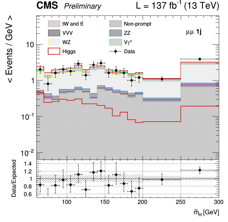
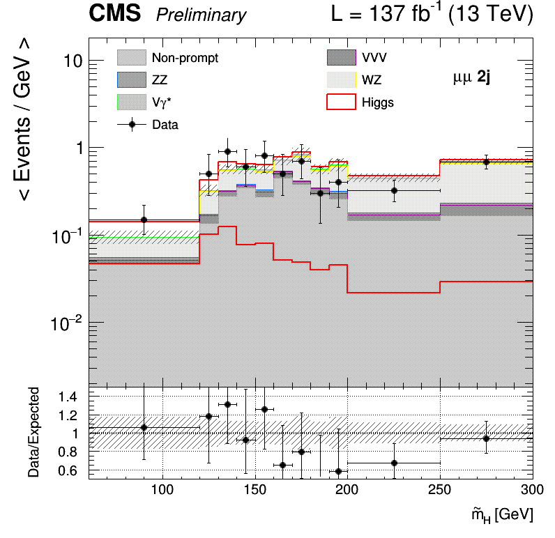
Figure 1:
The $\tilde{m}_{\mathrm{H}}$ distributions in the e$\mu $ 1j (upper left), e$\mu $ 2j (upper right), $\mu \mu $ 1j (lower left), and $\mu \mu $ 2j (lower right) signal regions after the fit to data. The bin contents are normalized by bin width for ease of presentation. The signal is shown as the topmost contribution to the stacked plot, as well as overlaid for shape comparison. |

png |
Figure 1-a:
The $\tilde{m}_{\mathrm{H}}$ distributions in the e$\mu $ 1j (upper left), e$\mu $ 2j (upper right), $\mu \mu $ 1j (lower left), and $\mu \mu $ 2j (lower right) signal regions after the fit to data. The bin contents are normalized by bin width for ease of presentation. The signal is shown as the topmost contribution to the stacked plot, as well as overlaid for shape comparison. |

png |
Figure 1-b:
The $\tilde{m}_{\mathrm{H}}$ distributions in the e$\mu $ 1j (upper left), e$\mu $ 2j (upper right), $\mu \mu $ 1j (lower left), and $\mu \mu $ 2j (lower right) signal regions after the fit to data. The bin contents are normalized by bin width for ease of presentation. The signal is shown as the topmost contribution to the stacked plot, as well as overlaid for shape comparison. |
png |
Figure 1-c:
The $\tilde{m}_{\mathrm{H}}$ distributions in the e$\mu $ 1j (upper left), e$\mu $ 2j (upper right), $\mu \mu $ 1j (lower left), and $\mu \mu $ 2j (lower right) signal regions after the fit to data. The bin contents are normalized by bin width for ease of presentation. The signal is shown as the topmost contribution to the stacked plot, as well as overlaid for shape comparison. |
png |
Figure 1-d:
The $\tilde{m}_{\mathrm{H}}$ distributions in the e$\mu $ 1j (upper left), e$\mu $ 2j (upper right), $\mu \mu $ 1j (lower left), and $\mu \mu $ 2j (lower right) signal regions after the fit to data. The bin contents are normalized by bin width for ease of presentation. The signal is shown as the topmost contribution to the stacked plot, as well as overlaid for shape comparison. |
png pdf |
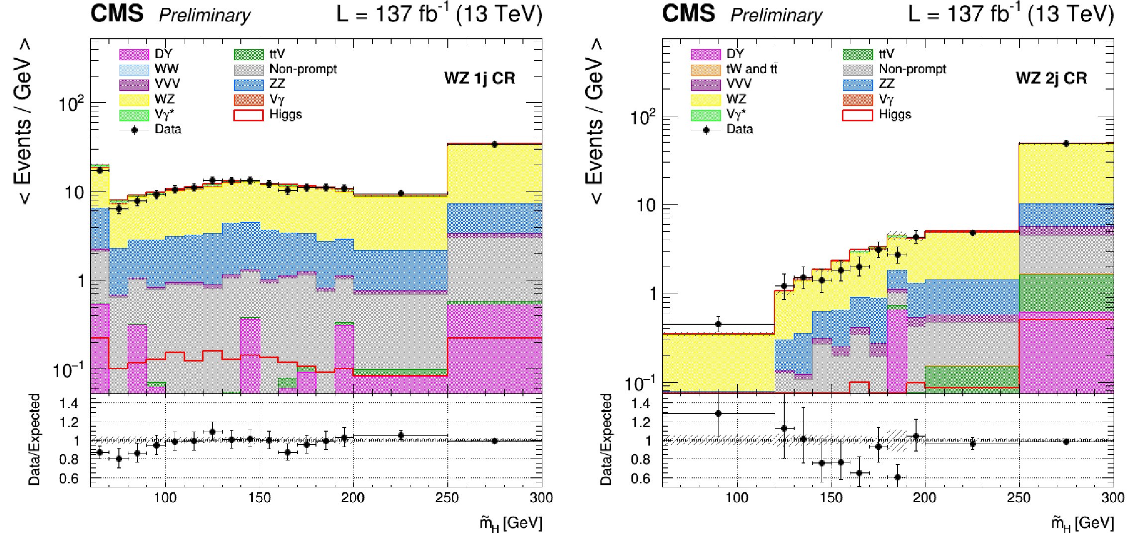
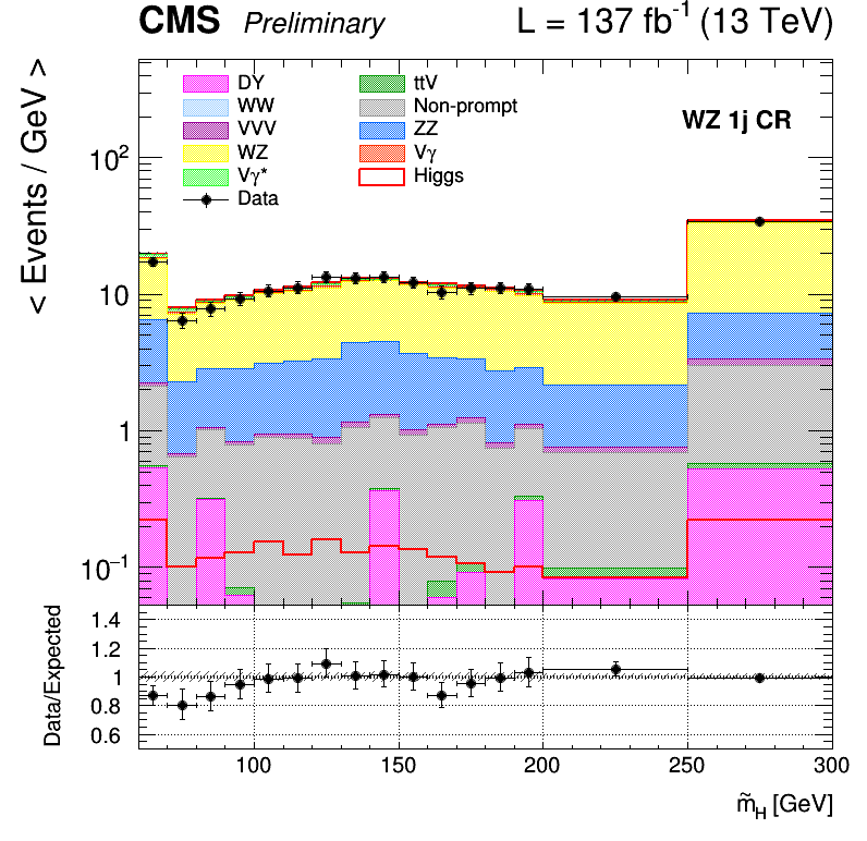
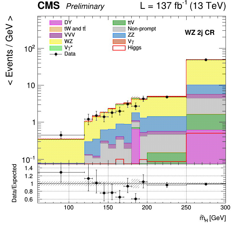
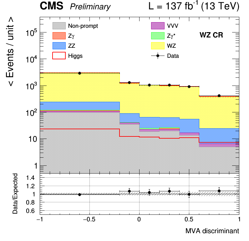
Figure 2:
The $\tilde{m}_{\mathrm{H}}$ distributions in the 1j (left) and 2j (right) WZ CRs after the fit to data. The bin contents are normalized by bin width for ease of presentation. The signal is shown as the topmost contribution to the stacked plot, as well as overlaid for shape comparison. |
png |
Figure 2-a:
The $\tilde{m}_{\mathrm{H}}$ distributions in the 1j (left) and 2j (right) WZ CRs after the fit to data. The bin contents are normalized by bin width for ease of presentation. The signal is shown as the topmost contribution to the stacked plot, as well as overlaid for shape comparison. |
png |
Figure 2-b:
The $\tilde{m}_{\mathrm{H}}$ distributions in the 1j (left) and 2j (right) WZ CRs after the fit to data. The bin contents are normalized by bin width for ease of presentation. The signal is shown as the topmost contribution to the stacked plot, as well as overlaid for shape comparison. |
png pdf |
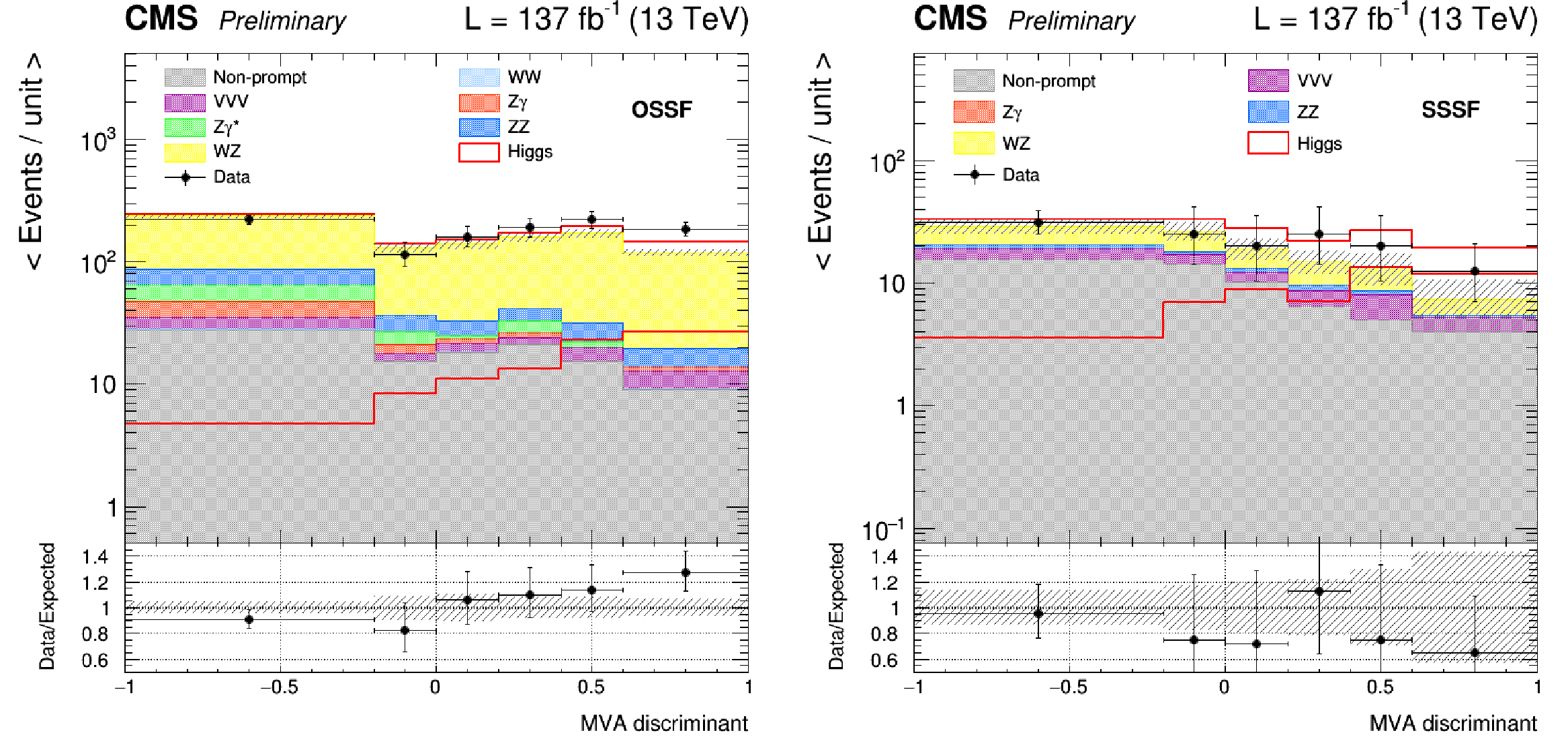
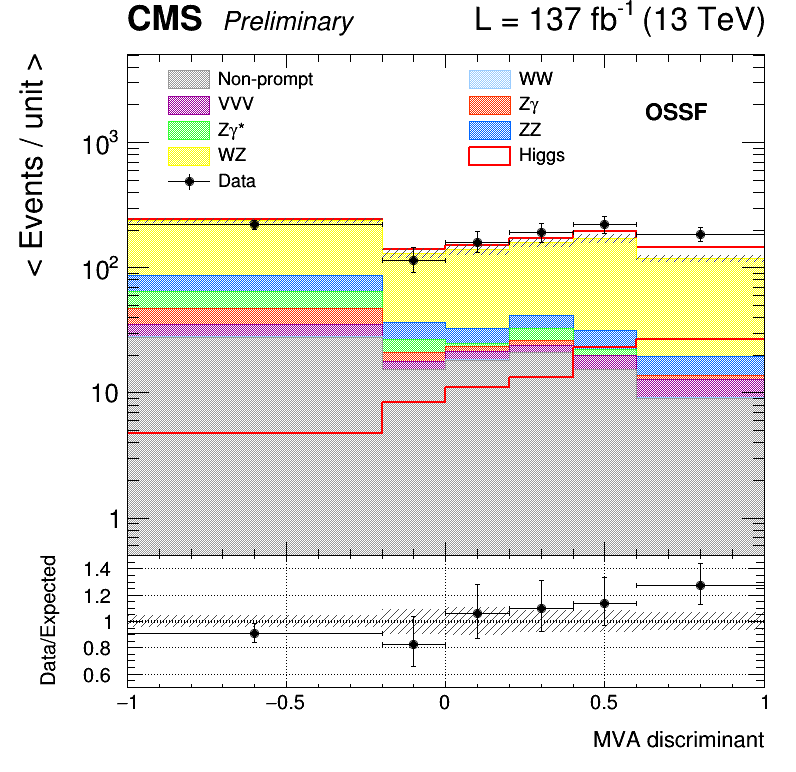
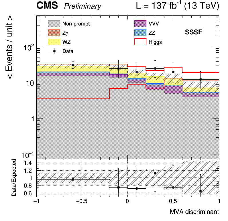
Figure 3:
BDT distributions in the OSSF (left) and SSSF (right) SRs after the fit to data. The bin contents are normalized by bin width for ease of presentation. The signal is shown as the topmost contribution to the stacked plot, as well as overlaid for shape comparison. |
png |
Figure 3-a:
BDT distributions in the OSSF (left) and SSSF (right) SRs after the fit to data. The bin contents are normalized by bin width for ease of presentation. The signal is shown as the topmost contribution to the stacked plot, as well as overlaid for shape comparison. |
png |
Figure 3-b:
BDT distributions in the OSSF (left) and SSSF (right) SRs after the fit to data. The bin contents are normalized by bin width for ease of presentation. The signal is shown as the topmost contribution to the stacked plot, as well as overlaid for shape comparison. |
png pdf |
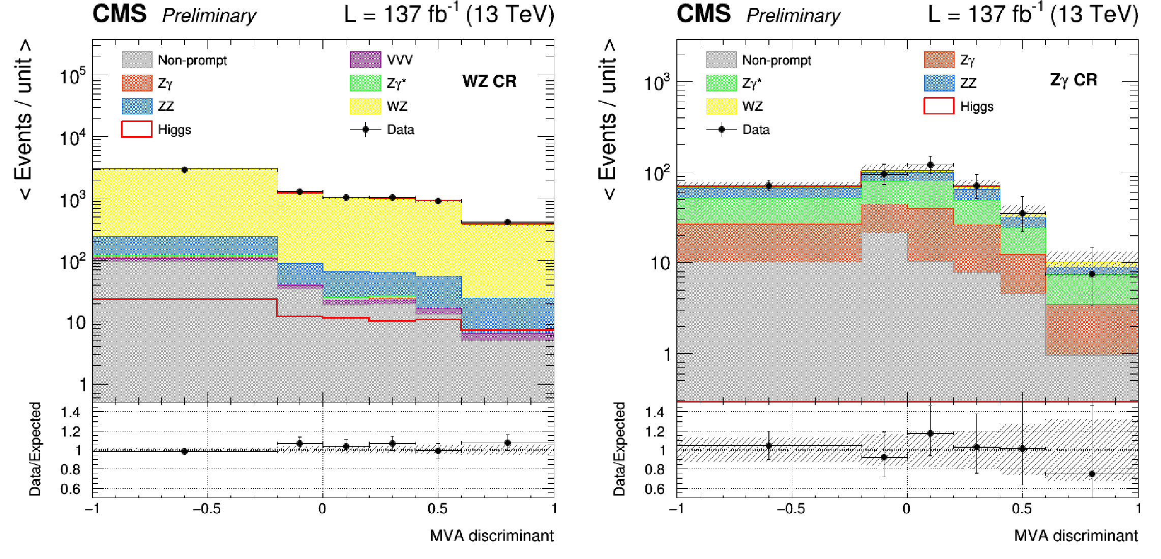
Figure 4:
BDT distributions in the WZ (left) and Z$\gamma $ (right) CRs after the fit to data. The bin contents are normalized by bin width for ease of presentation. The signal is shown as the topmost contribution to the stacked plot, as well as overlaid for shape comparison. |
png |
Figure 4-a:
BDT distributions in the WZ (left) and Z$\gamma $ (right) CRs after the fit to data. The bin contents are normalized by bin width for ease of presentation. The signal is shown as the topmost contribution to the stacked plot, as well as overlaid for shape comparison. |

png |
Figure 4-b:
BDT distributions in the WZ (left) and Z$\gamma $ (right) CRs after the fit to data. The bin contents are normalized by bin width for ease of presentation. The signal is shown as the topmost contribution to the stacked plot, as well as overlaid for shape comparison. |

png pdf |
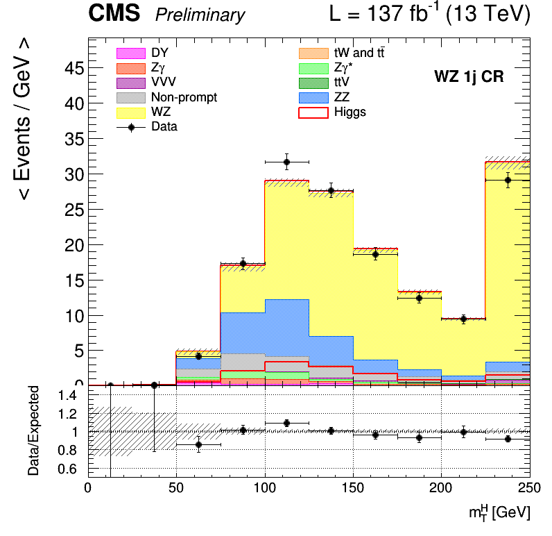
Figure 5:
$m_{\mathrm{T}}^{\mathrm{H}}$ distribution in the 1j (left) and 2j (right) SRs after the fit to data. The bin contents are normalized to bin width for ease of presentation. The signal is shown as the topmost contribution to the stacked plot, as well as overlaid for shape comparison. The overlaid signal is scaled x10 for visibility. |

png |
Figure 5-a:
$m_{\mathrm{T}}^{\mathrm{H}}$ distribution in the 1j (left) and 2j (right) SRs after the fit to data. The bin contents are normalized to bin width for ease of presentation. The signal is shown as the topmost contribution to the stacked plot, as well as overlaid for shape comparison. The overlaid signal is scaled x10 for visibility. |

png |
Figure 5-b:
$m_{\mathrm{T}}^{\mathrm{H}}$ distribution in the 1j (left) and 2j (right) SRs after the fit to data. The bin contents are normalized to bin width for ease of presentation. The signal is shown as the topmost contribution to the stacked plot, as well as overlaid for shape comparison. The overlaid signal is scaled x10 for visibility. |

png pdf |
Figure 6:
$m_{\mathrm{T}}^{\mathrm{H}}$ distributions in the 1j (left) and 2j (right) WZ CRs after the fit to data. The bin contents are normalized by bin width for ease of presentation. The signal is shown as the topmost contribution to the stacked plot, as well as overlaid for shape comparison. The overlaid signal is scaled x10 for visibility. |
png |
Figure 6-a:
$m_{\mathrm{T}}^{\mathrm{H}}$ distributions in the 1j (left) and 2j (right) WZ CRs after the fit to data. The bin contents are normalized by bin width for ease of presentation. The signal is shown as the topmost contribution to the stacked plot, as well as overlaid for shape comparison. The overlaid signal is scaled x10 for visibility. |

png |
Figure 6-b:
$m_{\mathrm{T}}^{\mathrm{H}}$ distributions in the 1j (left) and 2j (right) WZ CRs after the fit to data. The bin contents are normalized by bin width for ease of presentation. The signal is shown as the topmost contribution to the stacked plot, as well as overlaid for shape comparison. The overlaid signal is scaled x10 for visibility. |

png pdf |
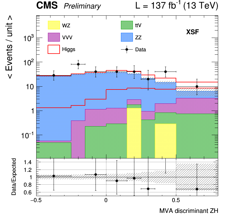
Figure 7:
BDT discriminant distributions in the XDF (left) and XSF (right) SRs after the fit to data. The bin contents are normalized by bin width for ease of presentation. The signal is shown as the topmost contribution to the stacked plot, as well as overlaid for shape comparison. |

png |
Figure 7-a:
BDT discriminant distributions in the XDF (left) and XSF (right) SRs after the fit to data. The bin contents are normalized by bin width for ease of presentation. The signal is shown as the topmost contribution to the stacked plot, as well as overlaid for shape comparison. |
png |
Figure 7-b:
BDT discriminant distributions in the XDF (left) and XSF (right) SRs after the fit to data. The bin contents are normalized by bin width for ease of presentation. The signal is shown as the topmost contribution to the stacked plot, as well as overlaid for shape comparison. |

png pdf |
Figure 8:
BDT discriminant distribution in the ZZ CR after the fit to data. The bin contents are normalized by bin width for ease of presentation. The signal is shown as the topmost contribution to the stacked plot, as well as overlaid for shape comparison. |

png pdf |
Figure 9:
Signal composition in each channel. Signal yields show the expected (a priori) values; while the overall rate of Higgs boson production is scaled in the fit, the signal composition is fixed to its SM value. |

png pdf |
Figure 10:
Expected and observed likelihood profiles as a function of the signal strength. Dashed curves include only statistical uncertainties. 68% and 95% likelihood intervals may be constructed observing where the likelihood profile passes 1.0 and 3.84, respectively. |

png pdf |
Figure 11:
Comparison of the combined and individual signal strengths. |

png pdf |
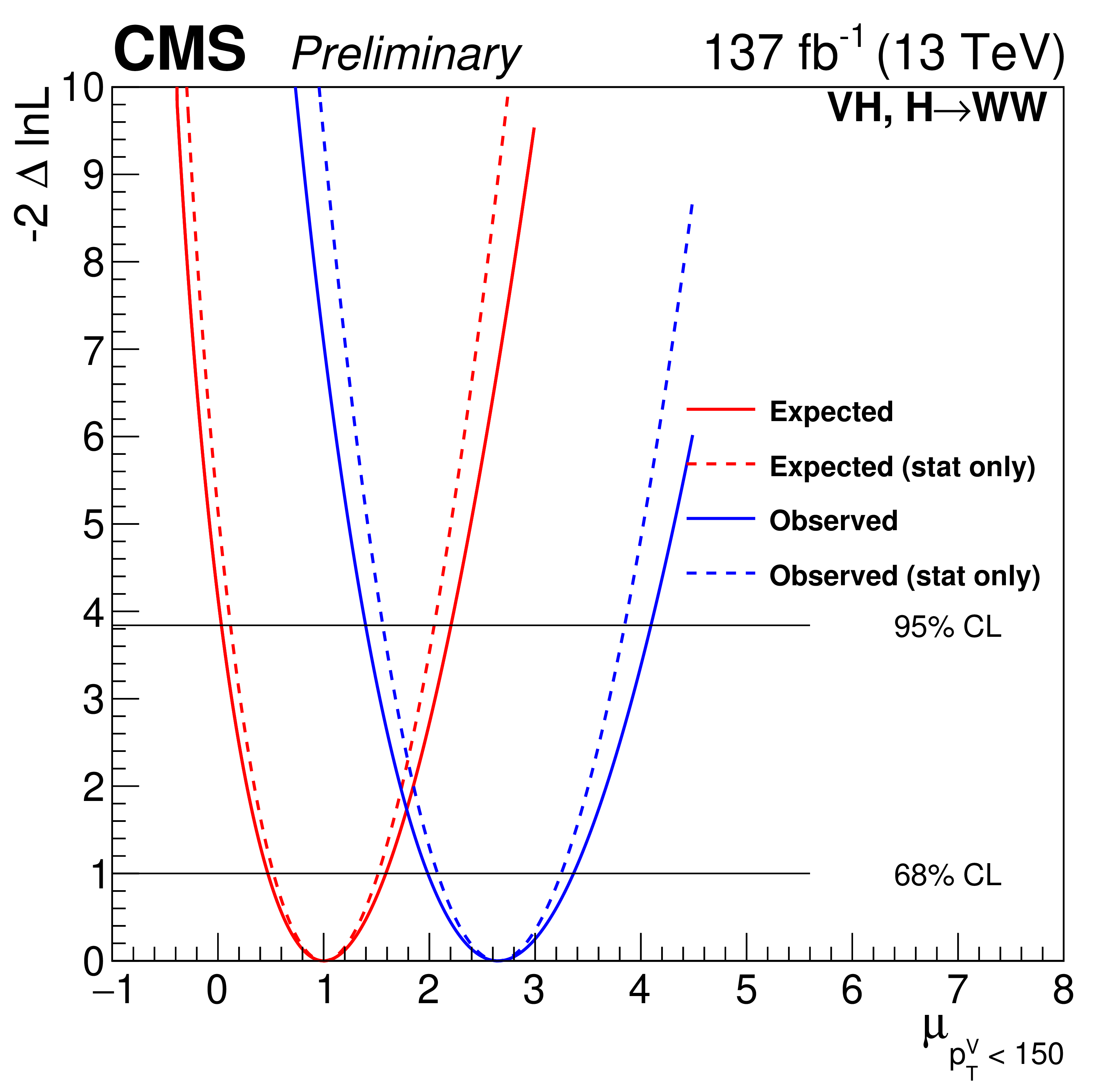
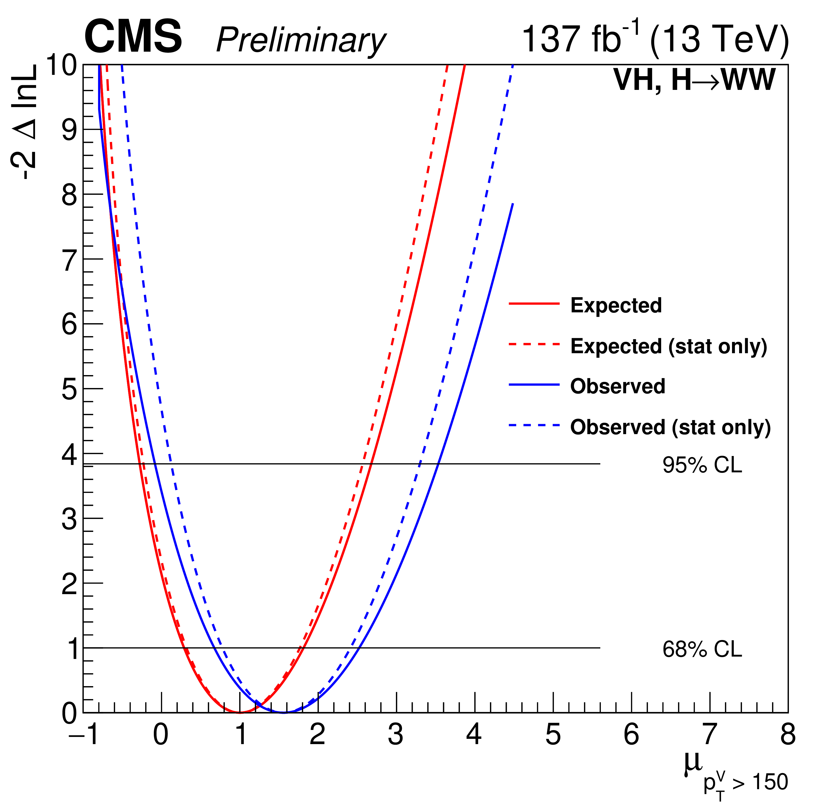
Figure 12:
Expected and observed likelihood profiles as a function of the signal strength, for the ${{p_{\mathrm {T}}} ^{\mathrm{V}}} < $ 150 GeV (upper figure) and ${{p_{\mathrm {T}}} ^{\mathrm{V}}} > $ 150 GeV (lower figure) STXS bins. Dashed curves include only statistical uncertainties. 68% and 95% likelihood intervals shown for reference. |
png pdf |
Figure 12-a:
Expected and observed likelihood profiles as a function of the signal strength, for the ${{p_{\mathrm {T}}} ^{\mathrm{V}}} < $ 150 GeV (upper figure) and ${{p_{\mathrm {T}}} ^{\mathrm{V}}} > $ 150 GeV (lower figure) STXS bins. Dashed curves include only statistical uncertainties. 68% and 95% likelihood intervals shown for reference. |
png pdf |
Figure 12-b:
Expected and observed likelihood profiles as a function of the signal strength, for the ${{p_{\mathrm {T}}} ^{\mathrm{V}}} < $ 150 GeV (upper figure) and ${{p_{\mathrm {T}}} ^{\mathrm{V}}} > $ 150 GeV (lower figure) STXS bins. Dashed curves include only statistical uncertainties. 68% and 95% likelihood intervals shown for reference. |

png pdf |
Figure 13:
Comparison between the combined signal strength, determined by applying a single signal strength to both ${{p_{\mathrm {T}}} ^{\mathrm{V}}}$ bins and all VH production modes in the STXS fit, and the signal strengths for each ${{p_{\mathrm {T}}} ^{\mathrm{V}}}$ bin and production mode (WH, ZH, and VH inclusive). |
| Tables | |
png pdf |
Table 1:
Basic selection to ensure channel orthogonality. |

png pdf |
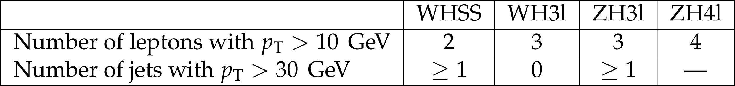
Table 2:
Event selection and categorization in the WHSS channel |
png pdf |
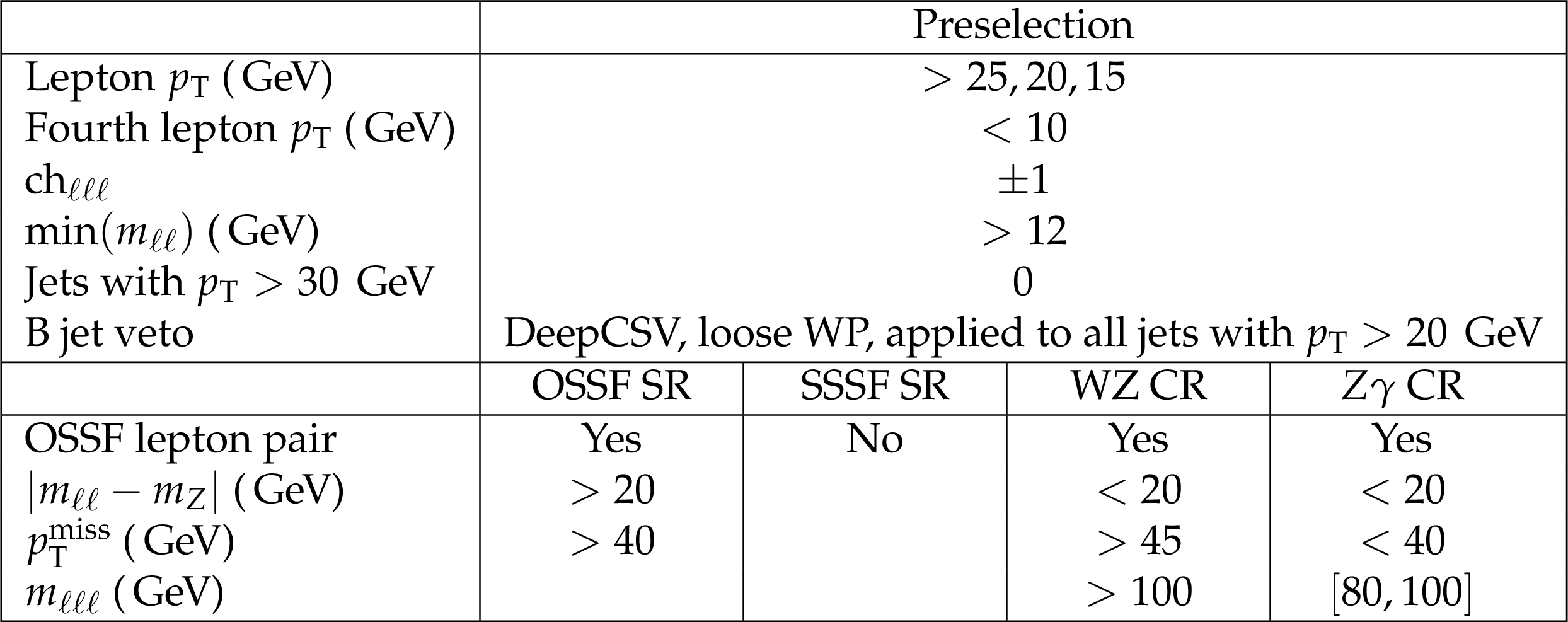
Table 3:
Event selection and categorization in the WH3l channel. |

png pdf |
Table 4:
Event selection and categorization in the ZH3l channel. |

png pdf |
Table 5:
Event selection and categorization in the ZH4l channel. |

png pdf |
Table 6:
Signal and background yields compared to number of observed events in all channels after the full event selection. Yields are given in the format posterior (a priori) ($\pm $ posterior uncertainty), where the posterior values come from a combined fit to data. To produce the per-channel yields, separate signal strengths are used in each channel, while the yields for the combined phase space use a single signal strength in all channels. Correlations between uncertainties are accounted for in the total uncertainty shown. |

png pdf |
Table 7:
Impacts of sources of systematic uncertainty on signal strength. |

png pdf |
Table 8:
The posterior signal strengths and significances for the signal strengths extracted from the WHSS, WH3l, ZH3l, and ZH4l categories, as well as the combined signal strength. The per-channel significances correspond to the probability of observing a signal at least as large under the background-only hypothesis where the signal strength in that channel is set to 0. |
| Summary |
| The cross sections for Higgs boson production in association with a leptonically decaying vector boson have been measured in events where the Higgs decays to a pair of W bosons. The measurements have been performed with pp collision data sets recorded by the CMS detector at a center-of-mass energy of 13 TeV in 2016, 2017, and 2018, corresponding to a total integrated luminosity of 137 fb${-1}$ total. In addition to the inclusive measurement, the cross section for VH production was measured with respect to the transverse momentum of the associated vector boson, following the simplified template cross sections framework. The cross sections are extracted through a simultaneous template fit to kinematic distributions of the signal candidate events finely categorized to maximize the sensitivity to Higgs boson production. The observed significance of the inclusive VH production cross section is 4.7$\sigma$, while the observed significance of the VH production cross section for $p_{\mathrm{T}}^{\text{V}} < $ 150 ($>$ 150) is 4.7$\sigma$ (1.8$\sigma$). |
| References | ||||
| 1 | ATLAS Collaboration | Observation of a new particle in the search for the Standard Model Higgs boson with the ATLAS detector at the LHC | PLB 716 (2012) 1 | 1207.7214 |
| 2 | CMS Collaboration | Observation of a new boson at a mass of 125 GeV with the CMS experiment at the LHC | PLB 716 (2012) 30 | CMS-HIG-12-028 1207.7235 |
| 3 | CMS Collaboration | Observation of a New Boson with Mass Near 125 GeV in $ pp $ Collisions at $ \sqrt{s} = $ 7 and 8 TeV | JHEP 06 (2013) 081 | CMS-HIG-12-036 1303.4571 |
| 4 | LHC Higgs Cross Section Working Group | Handbook of LHC Higgs cross sections: 4. deciphering the nature of the Higgs sector | CERN (2016) | 1610.07922 |
| 5 | G. Aad et al. | Measurements of the Higgs boson production and decay rates and constraints on its couplings from a combined ATLAS and CMS analysis of the LHC pp collision data at $ \sqrt{s} = $ 7 and 8 TeV | Journal of High Energy Physics 2016 (2016) 45 | |
| 6 | M. Delmastro et al. | Simplified Template Cross Sections - Stage 1.1 | arXiv:1906.02754, CERN, Geneva, Apr | |
| 7 | J. Ellis, V. Sanz, and T. You | Complete higgs sector constraints on dimension-6 operators | Journal of High Energy Physics 2014 (2014) 36 | 1404.3667 |
| 8 | G. Branco et al. | Theory and phenomenology of two-higgs-doublet models | Physics Reports 516 (2012) 1--102 | 1106.0034 |
| 9 | Particle Data Group, P. A. Zyla et al. | Review of particle physics | Prog. Theor. Exp. Phys. 2020 (2020) 083C01 | |
| 10 | CMS Collaboration | Particle-flow reconstruction and global event description with the cms detector | JINST 12 (2017) P10003 | CMS-PRF-14-001 1706.04965 |
| 11 | CMS Collaboration | Performance of electron reconstruction and selection with the CMS detector in proton-proton collisions at $ \sqrt{s} = $ 8 TeV | JINST 10 (2015) P06005 | CMS-EGM-13-001 1502.02701 |
| 12 | CMS Collaboration | Performance of the CMS muon detector and muon reconstruction with proton-proton collisions at $ \sqrt{s}= $ 13 TeV | JINST 13 (2018) P06015 | CMS-MUO-16-001 1804.04528 |
| 13 | M. Cacciari, G. P. Salam, and G. Soyez | The anti-$ {k_{\mathrm{T}}} $ jet clustering algorithm | JHEP 04 (2008) 063 | 0802.1189 |
| 14 | M. Cacciari, G. P. Salam, and G. Soyez | FastJet user manual | EPJC 72 (2012) 1896 | 1111.6097 |
| 15 | CMS Collaboration | Jet energy scale and resolution in the CMS experiment in pp collisions at 8 TeV | JINST 12 (2017) P02014 | CMS-JME-13-004 1607.03663 |
| 16 | CMS Collaboration | Identification of heavy-flavour jets with the CMS detector in pp collisions at 13 TeV | JINST 13 (2018), no. 05, P05011 | CMS-BTV-16-002 1712.07158 |
| 17 | CMS Collaboration | Performance of missing transverse momentum reconstruction in proton-proton collisions at $ \sqrt{s} = $ 13 TeV using the CMS detector | JINST 14 (2019) P07004 | CMS-JME-17-001 1903.06078 |
| 18 | CMS Collaboration | Pileup mitigation at CMS in 13 TeV data | CMS-PAS-JME-18-001 | CMS-PAS-JME-18-001 |
| 19 | CMS Collaboration | The CMS trigger system | JINST 12 (2017) P01020 | CMS-TRG-12-001 1609.02366 |
| 20 | CMS Collaboration | The CMS experiment at the CERN LHC | JINST 3 (2008) S08004 | CMS-00-001 |
| 21 | CMS Collaboration | CMS luminosity measurements for the 2016 data-taking period | CMS-PAS-LUM-17-001 | CMS-PAS-LUM-17-001 |
| 22 | CMS Collaboration | CMS luminosity measurement for the 2017 data-taking period at $ \sqrt{s} = $ 13 TeV | CMS-PAS-LUM-17-004 | CMS-PAS-LUM-17-004 |
| 23 | CMS Collaboration | CMS luminosity measurement for the 2018 data-taking period at $ \sqrt{s} = $ 13 TeV | CMS-PAS-LUM-18-002 | CMS-PAS-LUM-18-002 |
| 24 | T. Sjostrand et al. | An Introduction to PYTHIA 8.2 | CPC 191 (2015) 159 | 1410.3012 |
| 25 | NNPDF Collaboration | Parton distributions for the LHC Run II | JHEP 04 (2015) 040 | 1410.8849 |
| 26 | CMS Collaboration | Event generator tunes obtained from underlying event and multiparton scattering measurements | EPJC 76 (2016) 155 | CMS-GEN-14-001 1512.00815 |
| 27 | NNPDF Collaboration | Parton distributions from high-precision collider data | EPJC 77 (2017) 663 | 1706.00428 |
| 28 | CMS Collaboration | Extraction and validation of a new set of CMS PYTHIA8 tunes from underlying-event measurements | EPJC 80 (2020) 4 | CMS-GEN-17-001 1903.12179 |
| 29 | P. Nason | A New method for combining NLO QCD with shower Monte Carlo algorithms | JHEP 11 (2004) 040 | hep-ph/0409146 |
| 30 | S. Frixione, P. Nason, and C. Oleari | Matching NLO QCD computations with Parton Shower simulations: the POWHEG method | JHEP 11 (2007) 070 | 0709.2092 |
| 31 | S. Alioli, P. Nason, C. Oleari, and E. Re | A general framework for implementing NLO calculations in shower Monte Carlo programs: the POWHEG BOX | JHEP 06 (2010) 043 | 1002.2581 |
| 32 | S. Bolognesi et al. | On the spin and parity of a single-produced resonance at the LHC | PRD 86 (2012) 095031 | 1208.4018 |
| 33 | J. Alwall et al. | The automated computation of tree-level and next-to-leading order differential cross sections, and their matching to parton shower simulations | JHEP 07 (2014) 079 | 1405.0301 |
| 34 | J. M. Campbell and R. K. Ellis | An Update on vector boson pair production at hadron colliders | PRD 60 (1999) 113006 | hep-ph/9905386 |
| 35 | J. M. Campbell, R. K. Ellis, and C. Williams | Vector boson pair production at the LHC | JHEP 07 (2011) 018 | 1105.0020 |
| 36 | J. M. Campbell, R. K. Ellis, and W. T. Giele | A Multi-Threaded Version of MCFM | EPJC 75 (2015) 246 | 1503.06182 |
| 37 | J. Alwall et al. | Comparative study of various algorithms for the merging of parton showers and matrix elements in hadronic collisions | EPJC 53 (2008) 473 | 0706.2569 |
| 38 | R. Frederix and S. Frixione | Merging meets matching in MC@NLO | JHEP 12 (2012) 061 | 1209.6215 |
| 39 | GEANT4 Collaboration | GEANT4--a simulation toolkit | NIMA 506 (2003) 250 | |
| 40 | CMS Collaboration | Measurements of properties of the Higgs boson decaying to a W boson pair in pp collisions at $ \sqrt{s}= $ 13 TeV | PLB 791 (2019) 96 | CMS-HIG-16-042 1806.05246 |
| 41 | The ATLAS Collaboration, The CMS Collaboration, The LHC Higgs Combination Group | Procedure for the LHC Higgs boson search combination in Summer 2011 | CMS-NOTE-2011-005 | |
| 42 | J. S. Conway | Incorporating nuisance parameters in likelihoods for multisource spectra | 1103.0354 | |
| 43 | CMS Collaboration | Measurement of Higgs boson production and properties in the WW decay channel with leptonic final states | JHEP 01 (2014) 096 | CMS-HIG-13-023 1312.1129 |
| 44 | D. Bertolini, P. Harris, M. Low, and N. Tran | Pileup Per Particle Identification | JHEP 10 (2014) 059 | 1407.6013 |
| 45 | CMS Collaboration | Performance of b tagging algorithms in proton-proton collisions at 13 TeV with Phase 1 CMS detector | CDS | |
| 46 | A. Hocker et al. | TMVA - toolkit for multivariate data analysis | PoS ACAT (2007) 040 | physics/0703039 |
| 47 | CMS Collaboration | Measurements of inclusive $ \mathrm{W} $ and $ \mathrm{Z} $ cross sections in $ {\mathrm{p}}{\mathrm{p}} $ collisions at $ \sqrt{s} = $ 7 TeV | JHEP 01 (2011) 080 | CMS-EWK-10-002 1012.2466 |
| 48 | CMS Collaboration | Measurement of the inelastic proton-proton cross section at $ \sqrt{s}= $ 13 TeV | JHEP 07 (2018) 161 | CMS-FSQ-15-005 1802.02613 |
|
|
Compact Muon Solenoid LHC, CERN |
|

|

|

|

|

|