

Compact Muon Solenoid
LHC, CERN
| CMS-PAS-LUM-17-002 | ||
| CMS luminosity measurement using 2016 proton-nucleus collisions at ${\sqrt {\smash [b]{s_{_{\mathrm {NN}}}}}} = $ 8.16 TeV | ||
| CMS Collaboration | ||
| July 2018 | ||
| Abstract: The calibration of the integrated luminosity delivered to the CMS experiment during the 2016 lead-proton (Pbp) and proton-lead (pPb) periods at ${\sqrt {\smash [b]{s_{_{\mathrm {NN}}}}}} = $ 8.16 TeV is presented. Three different subdetectors are used: the forward hadronic calorimeter, the pixel luminosity telescope, and the silicon tracker. Visible cross sections are obtained using the van der Meer procedure for integrating the luminometer rate as a function of beam separation. After taking into account the effects due to horizontal-vertical beam correlations, bunch-to-bunch and scan-to-scan variations, spurious charges, adjustments of the length scale measurements provided by LHC magnet currents, and beam-beam effects, an overall uncertainty of 3.2 (3.7)% is assessed for the Pbp (pPb) period. The total uncertainty is obtained from the combination of the visible cross sections in the two periods and is found to be 3.5%. Time stability of these calibrations is considered and included in the final systematic uncertainty. | ||
| Links: CDS record (PDF) ; inSPIRE record ; CADI line (restricted) ; | ||
| Figures | |
png pdf |
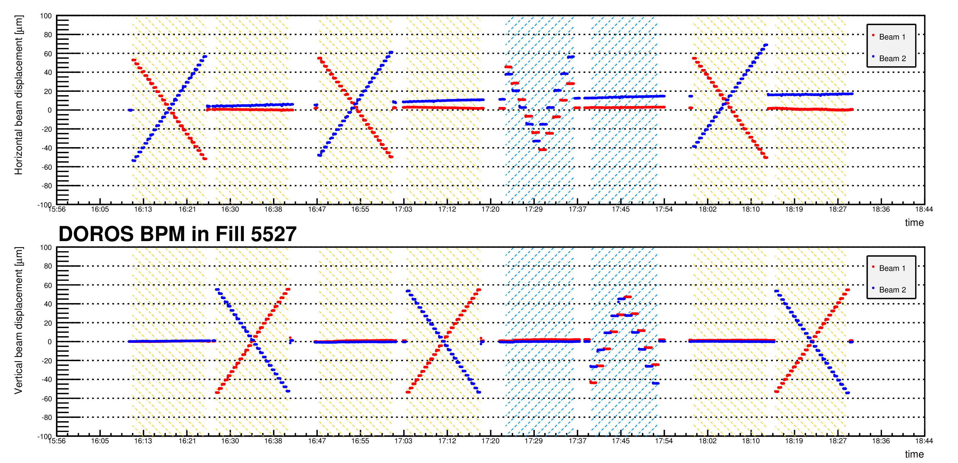
Figure 2Te:
Horizontal (bottom) and vertical (bottom) beam displacements, measured with the DOROS BPM, during the vdM scan campaign 5563 (pPb). |

png pdf |
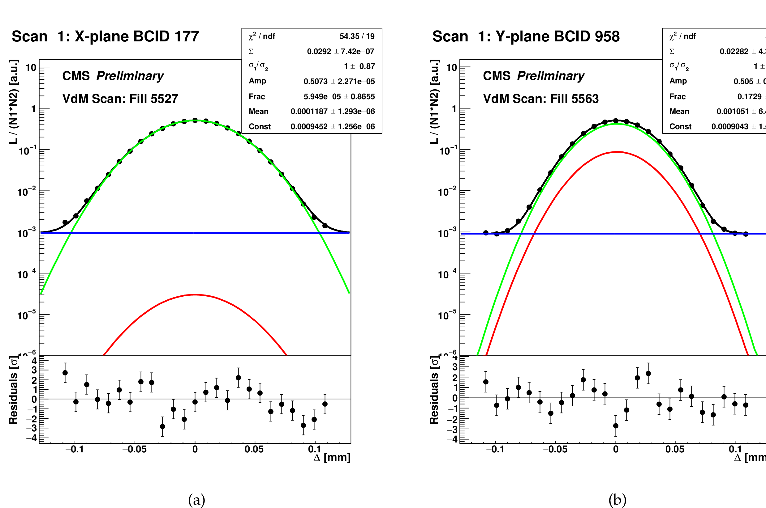
Figure 3:
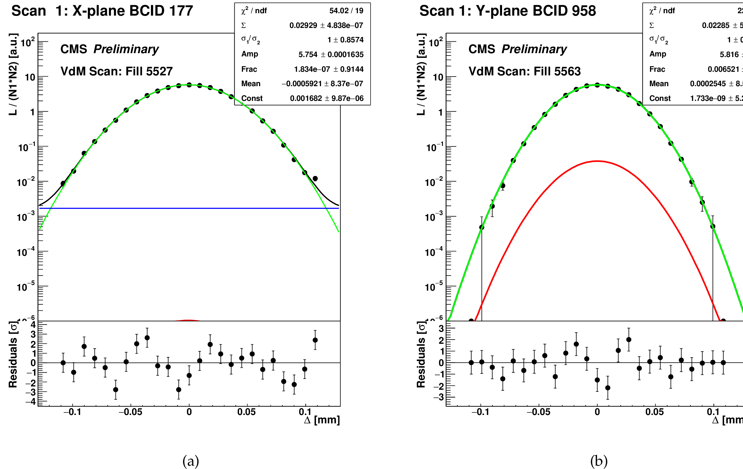
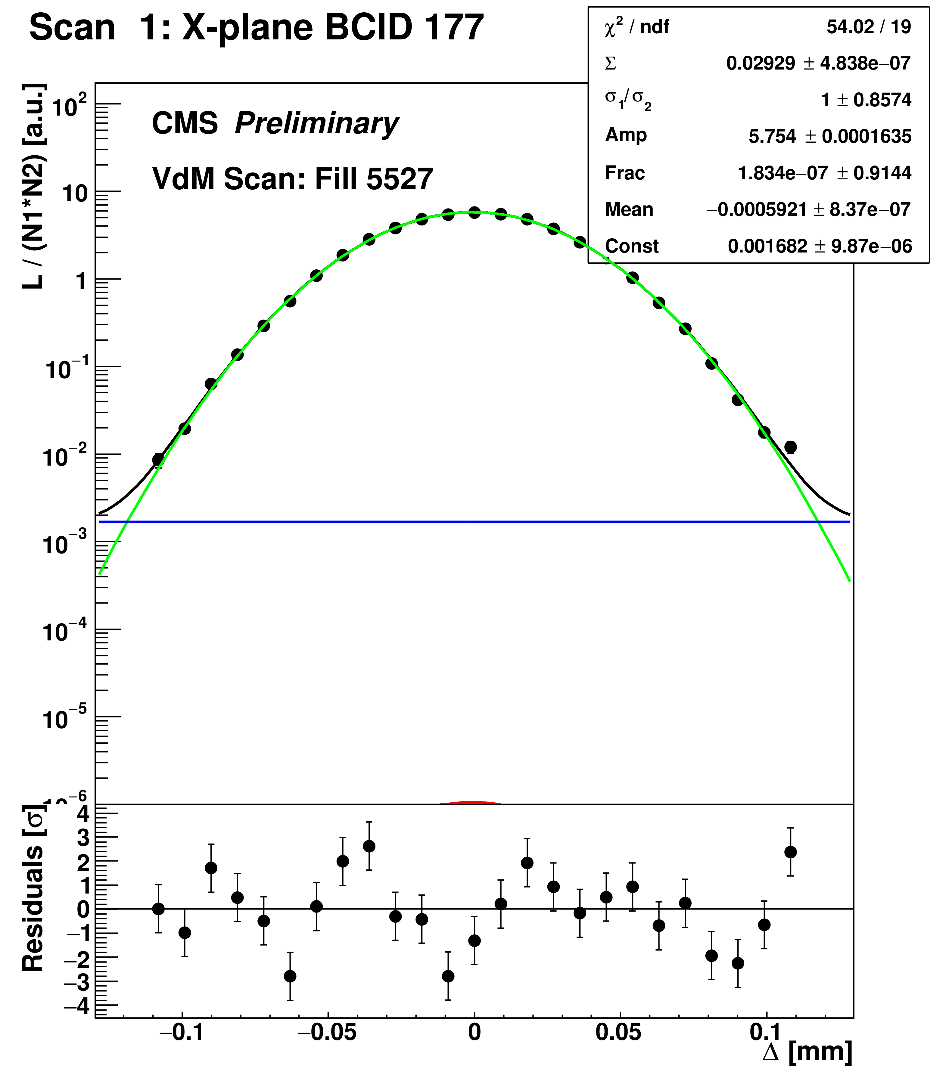
Examples of the fitted scan curves, i.e., normalized rates recorded by PLT as a function of the beam separation ($\Delta $) in the Pbp (a) and pPb (b) periods, respectively. The applied fit model is represented as the green and red, blue, and black curves corresponding to the two Gaussian components, the constant term, and their sum, respectively. The values and the statistical uncertainties of the fitted parameters are shown in the legend, along with the reduced $\chi ^2$. The bottom panels include the residuals, i.e., the difference between the measured and fitted values divided by the statistical uncertainty. |

png pdf |
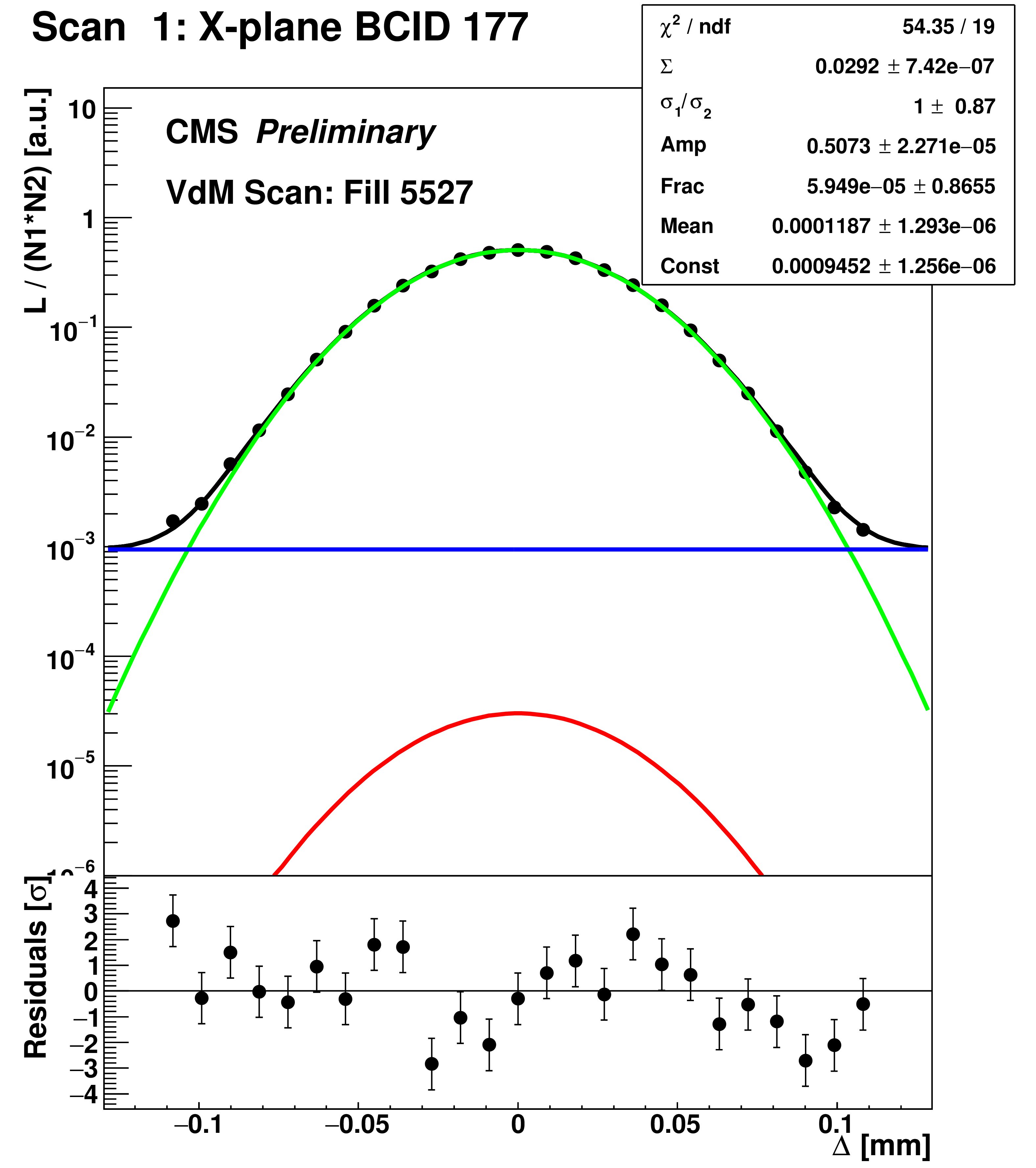
Figure 3-a:
Examples of the fitted scan curves, i.e., normalized rates recorded by PLT as a function of the beam separation ($\Delta $) in the Pbp (a) and pPb (b) periods, respectively. The applied fit model is represented as the green and red, blue, and black curves corresponding to the two Gaussian components, the constant term, and their sum, respectively. The values and the statistical uncertainties of the fitted parameters are shown in the legend, along with the reduced $\chi ^2$. The bottom panels include the residuals, i.e., the difference between the measured and fitted values divided by the statistical uncertainty. |

png pdf |
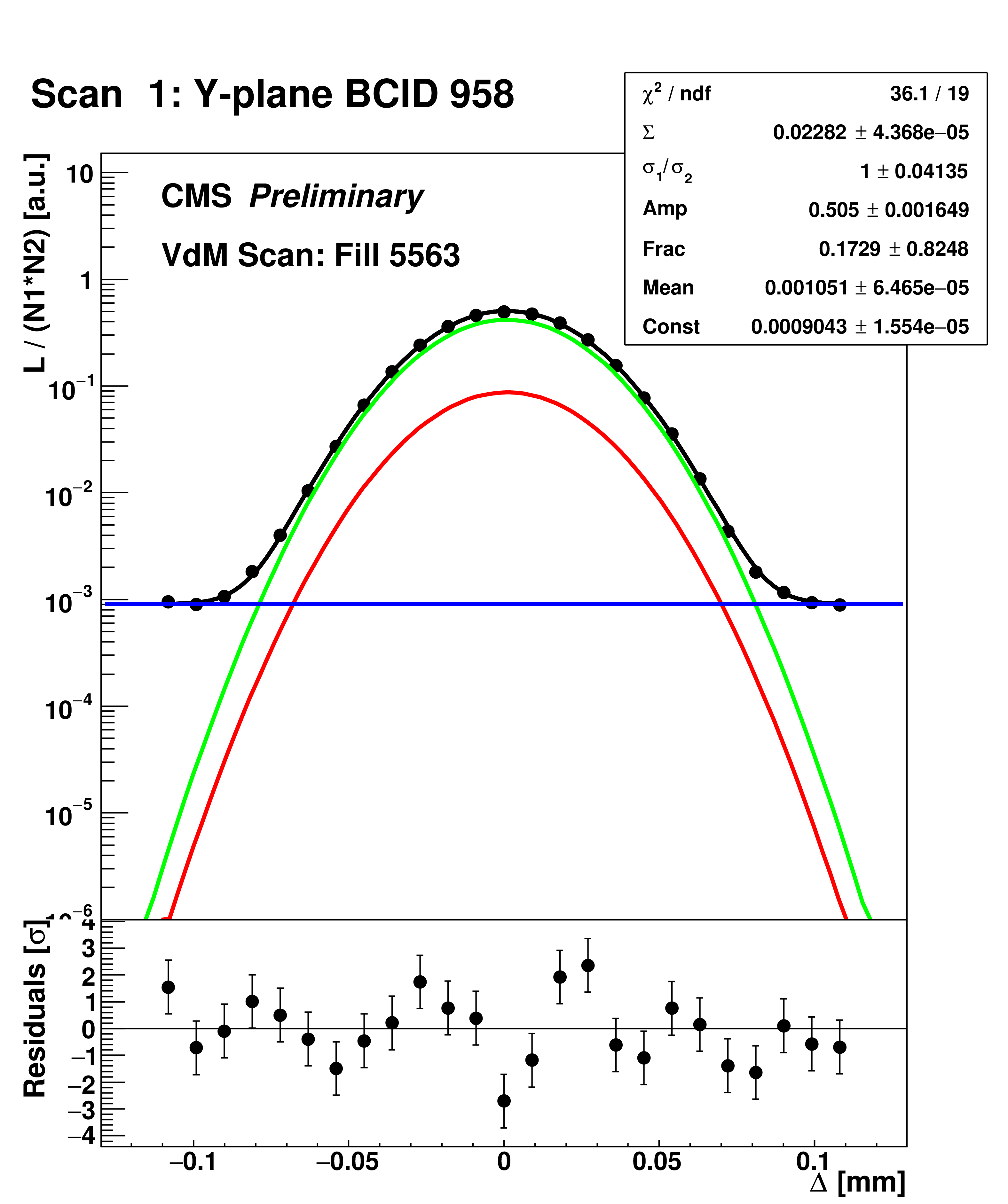
Figure 3-b:
Examples of the fitted scan curves, i.e., normalized rates recorded by PLT as a function of the beam separation ($\Delta $) in the Pbp (a) and pPb (b) periods, respectively. The applied fit model is represented as the green and red, blue, and black curves corresponding to the two Gaussian components, the constant term, and their sum, respectively. The values and the statistical uncertainties of the fitted parameters are shown in the legend, along with the reduced $\chi ^2$. The bottom panels include the residuals, i.e., the difference between the measured and fitted values divided by the statistical uncertainty. |
png pdf |
Figure 4:
Examples of the fitted scan curves, i.e., normalized rates recorded by HF as a function of the beam separation ($\Delta $) in the Pbp (a) and pPb (b) periods, respectively. The conventions of Fig. 3 are adopted. |
png pdf |
Figure 4-a:
Examples of the fitted scan curves, i.e., normalized rates recorded by HF as a function of the beam separation ($\Delta $) in the Pbp (a) and pPb (b) periods, respectively. The conventions of Fig. 3 are adopted. |
png pdf |
Figure 4-b:
Examples of the fitted scan curves, i.e., normalized rates recorded by HF as a function of the beam separation ($\Delta $) in the Pbp (a) and pPb (b) periods, respectively. The conventions of Fig. 3 are adopted. |
png pdf |
Figure 5:
Examples of the fitted scan curves, i.e., normalized rates recorded based on the vertex counting method as a function of the beam separation ($\Delta $) in the Pbp (a) and pPb (b) periods, respectively. The conventions of Fig. 3 are adopted. |
png pdf |
Figure 5-a:
Examples of the fitted scan curves, i.e., normalized rates recorded based on the vertex counting method as a function of the beam separation ($\Delta $) in the Pbp (a) and pPb (b) periods, respectively. The conventions of Fig. 3 are adopted. |

png pdf |
Figure 5-b:
Examples of the fitted scan curves, i.e., normalized rates recorded based on the vertex counting method as a function of the beam separation ($\Delta $) in the Pbp (a) and pPb (b) periods, respectively. The conventions of Fig. 3 are adopted. |

png pdf |
Figure 6:
The fitted $\Sigma _{x/y}$ (a,b) from the vertex counting method as a function of BCID (a,c) and scan pair (b,d) separately for the Pbp (top) and pPb (bottom) periods. The sequential naming convention adheres to the horizontal and vertical scan sequence as illustrated in Fig. 1 and Fig. 2, respectively. |

png pdf |
Figure 6-a:
The fitted $\Sigma _{x/y}$ (a,b) from the vertex counting method as a function of BCID (a,c) and scan pair (b,d) separately for the Pbp (top) and pPb (bottom) periods. The sequential naming convention adheres to the horizontal and vertical scan sequence as illustrated in Fig. 1 and Fig. 2, respectively. |

png pdf |
Figure 6-b:
The fitted $\Sigma _{x/y}$ (a,b) from the vertex counting method as a function of BCID (a,c) and scan pair (b,d) separately for the Pbp (top) and pPb (bottom) periods. The sequential naming convention adheres to the horizontal and vertical scan sequence as illustrated in Fig. 1 and Fig. 2, respectively. |

png pdf |
Figure 6-c:
The fitted $\Sigma _{x/y}$ (a,b) from the vertex counting method as a function of BCID (a,c) and scan pair (b,d) separately for the Pbp (top) and pPb (bottom) periods. The sequential naming convention adheres to the horizontal and vertical scan sequence as illustrated in Fig. 1 and Fig. 2, respectively. |

png pdf |
Figure 6-d:
The fitted $\Sigma _{x/y}$ (a,b) from the vertex counting method as a function of BCID (a,c) and scan pair (b,d) separately for the Pbp (top) and pPb (bottom) periods. The sequential naming convention adheres to the horizontal and vertical scan sequence as illustrated in Fig. 1 and Fig. 2, respectively. |

png pdf |
Figure 7:
The measured $ {\sigma _{\mathrm {vis}}} $ as extracted from PLT per BCID (a, c) and scan pair (b, d) during the Pbp (a, b) and pPb (c, d) periods. The weighted averages are found to be 248.84 $\pm$ 0.05 (stat) and 237.84 $\pm$ 0.04 (stat) ${ \mu }$b, respectively. |
png pdf |
Figure 7-a:
The measured $ {\sigma _{\mathrm {vis}}} $ as extracted from PLT per BCID (a, c) and scan pair (b, d) during the Pbp (a, b) and pPb (c, d) periods. The weighted averages are found to be 248.84 $\pm$ 0.05 (stat) and 237.84 $\pm$ 0.04 (stat) ${ \mu }$b, respectively. |

png pdf |
Figure 7-b:
The measured $ {\sigma _{\mathrm {vis}}} $ as extracted from PLT per BCID (a, c) and scan pair (b, d) during the Pbp (a, b) and pPb (c, d) periods. The weighted averages are found to be 248.84 $\pm$ 0.05 (stat) and 237.84 $\pm$ 0.04 (stat) ${ \mu }$b, respectively. |

png pdf |
Figure 7-c:
The measured $ {\sigma _{\mathrm {vis}}} $ as extracted from PLT per BCID (a, c) and scan pair (b, d) during the Pbp (a, b) and pPb (c, d) periods. The weighted averages are found to be 248.84 $\pm$ 0.05 (stat) and 237.84 $\pm$ 0.04 (stat) ${ \mu }$b, respectively. |

png pdf |
Figure 7-d:
The measured $ {\sigma _{\mathrm {vis}}} $ as extracted from PLT per BCID (a, c) and scan pair (b, d) during the Pbp (a, b) and pPb (c, d) periods. The weighted averages are found to be 248.84 $\pm$ 0.05 (stat) and 237.84 $\pm$ 0.04 (stat) ${ \mu }$b, respectively. |

png pdf |
Figure 8:
The measured $ {\sigma _{\mathrm {vis}}} $ as extracted from HF per BCID (a, c) and scan pair (b, d) during the Pbp (a, b) and pPb (c, d) periods. The weighted averages are found to be 2087.51 $\pm$ 0.15 (stat) and 2099.51 $\pm$ 0.11 (stat) ${ \mu }$b, respectively. |

png pdf |
Figure 8-a:
The measured $ {\sigma _{\mathrm {vis}}} $ as extracted from HF per BCID (a, c) and scan pair (b, d) during the Pbp (a, b) and pPb (c, d) periods. The weighted averages are found to be 2087.51 $\pm$ 0.15 (stat) and 2099.51 $\pm$ 0.11 (stat) ${ \mu }$b, respectively. |

png pdf |
Figure 8-b:
The measured $ {\sigma _{\mathrm {vis}}} $ as extracted from HF per BCID (a, c) and scan pair (b, d) during the Pbp (a, b) and pPb (c, d) periods. The weighted averages are found to be 2087.51 $\pm$ 0.15 (stat) and 2099.51 $\pm$ 0.11 (stat) ${ \mu }$b, respectively. |

png pdf |
Figure 8-c:
The measured $ {\sigma _{\mathrm {vis}}} $ as extracted from HF per BCID (a, c) and scan pair (b, d) during the Pbp (a, b) and pPb (c, d) periods. The weighted averages are found to be 2087.51 $\pm$ 0.15 (stat) and 2099.51 $\pm$ 0.11 (stat) ${ \mu }$b, respectively. |

png pdf |
Figure 8-d:
The measured $ {\sigma _{\mathrm {vis}}} $ as extracted from HF per BCID (a, c) and scan pair (b, d) during the Pbp (a, b) and pPb (c, d) periods. The weighted averages are found to be 2087.51 $\pm$ 0.15 (stat) and 2099.51 $\pm$ 0.11 (stat) ${ \mu }$b, respectively. |

png pdf |
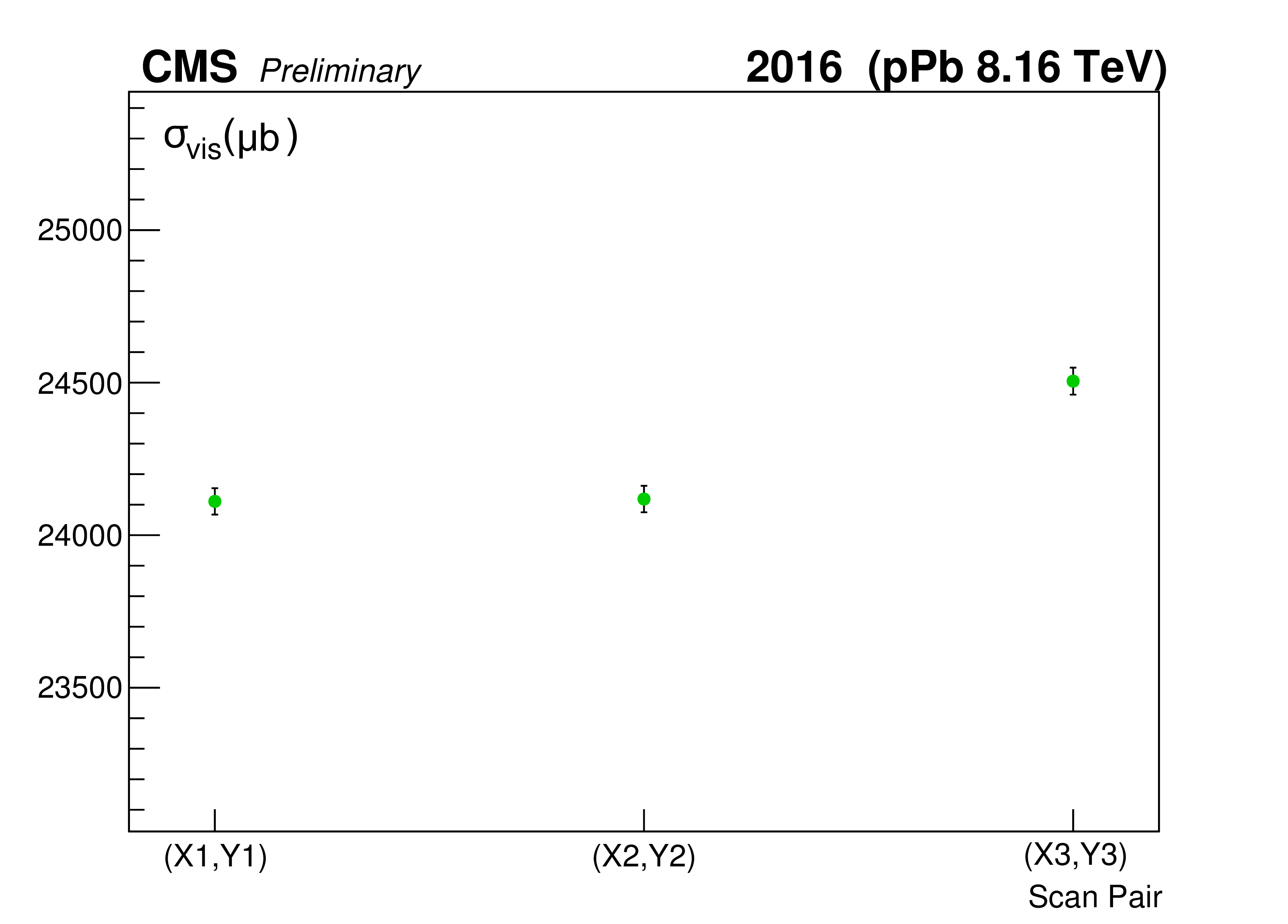
Figure 9:
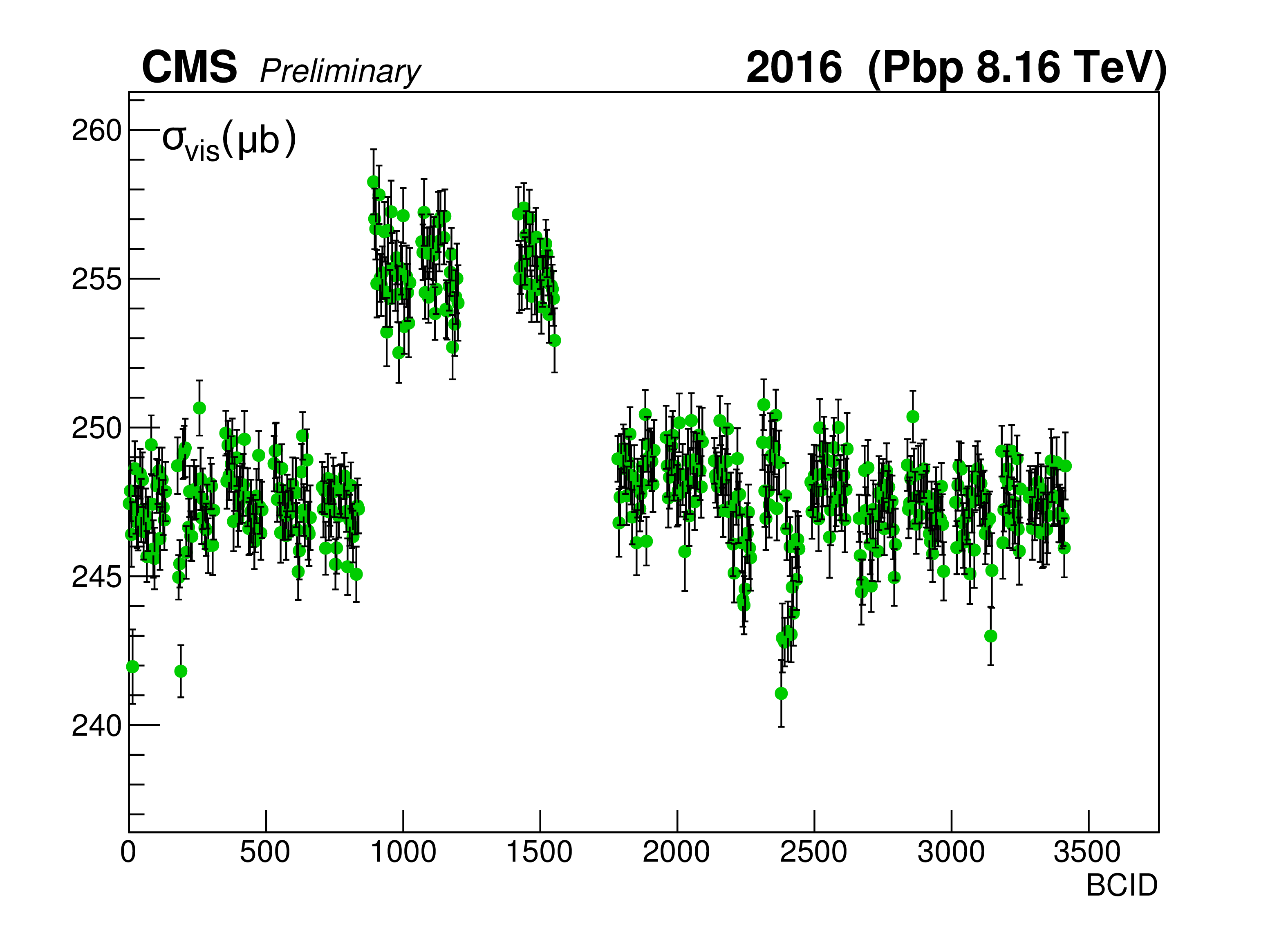
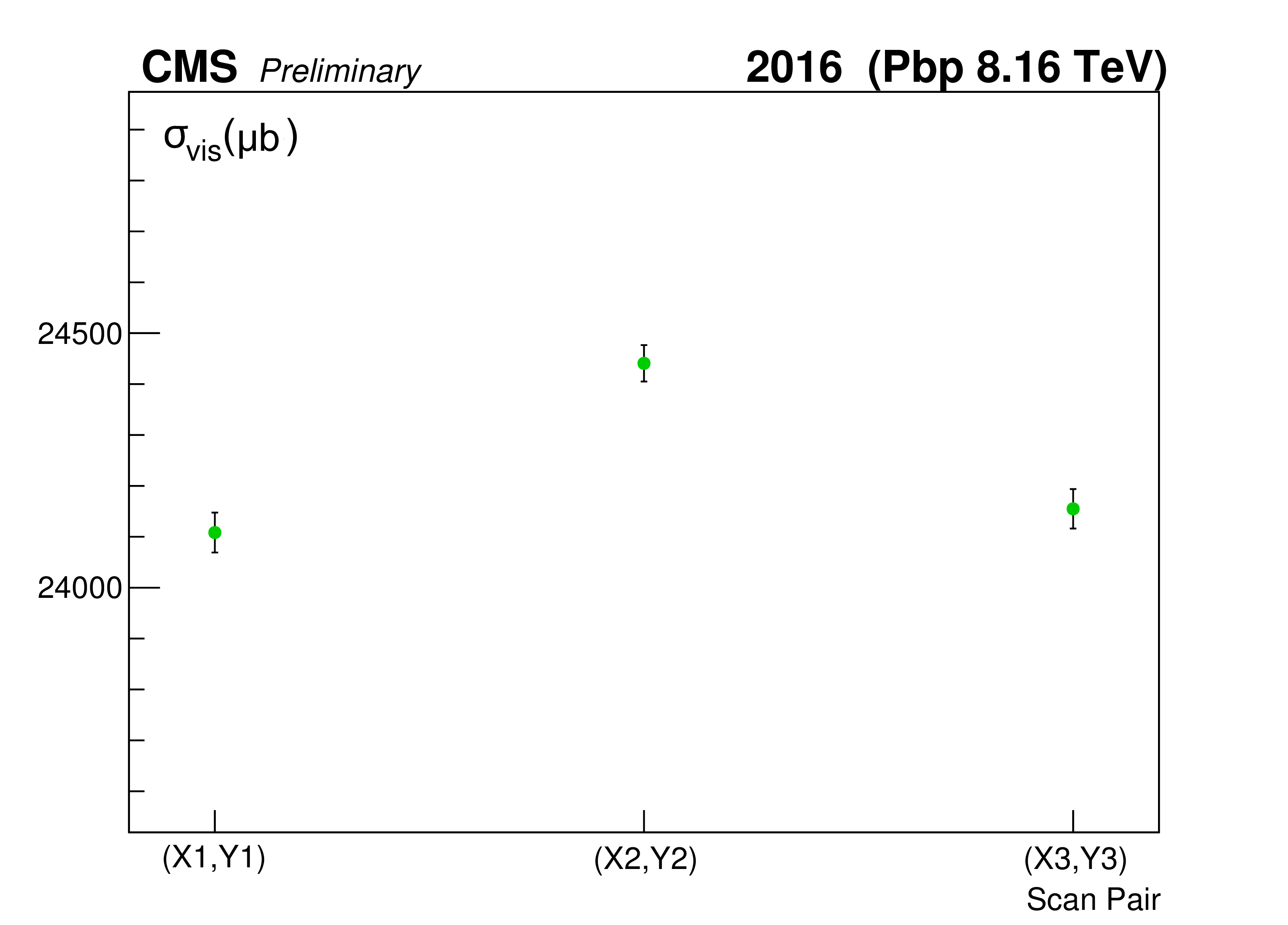
The measured $ {\sigma _{\mathrm {vis}}} $ as extracted from the vertex counting method per BCID (a, c) and scan pair (b, d) during the Pbp (a, b) and pPb (c, d) periods. The weighted averages are found to be 24246.74 $\pm$ 21.85 (stat) and 24241.16 $\pm$ 25.20 (stat) ${ \mu }$b, respectively. |

png pdf |
Figure 9-a:
The measured $ {\sigma _{\mathrm {vis}}} $ as extracted from the vertex counting method per BCID (a, c) and scan pair (b, d) during the Pbp (a, b) and pPb (c, d) periods. The weighted averages are found to be 24246.74 $\pm$ 21.85 (stat) and 24241.16 $\pm$ 25.20 (stat) ${ \mu }$b, respectively. |
png pdf |
Figure 9-b:
The measured $ {\sigma _{\mathrm {vis}}} $ as extracted from the vertex counting method per BCID (a, c) and scan pair (b, d) during the Pbp (a, b) and pPb (c, d) periods. The weighted averages are found to be 24246.74 $\pm$ 21.85 (stat) and 24241.16 $\pm$ 25.20 (stat) ${ \mu }$b, respectively. |

png pdf |
Figure 9-c:
The measured $ {\sigma _{\mathrm {vis}}} $ as extracted from the vertex counting method per BCID (a, c) and scan pair (b, d) during the Pbp (a, b) and pPb (c, d) periods. The weighted averages are found to be 24246.74 $\pm$ 21.85 (stat) and 24241.16 $\pm$ 25.20 (stat) ${ \mu }$b, respectively. |
png pdf |
Figure 9-d:
The measured $ {\sigma _{\mathrm {vis}}} $ as extracted from the vertex counting method per BCID (a, c) and scan pair (b, d) during the Pbp (a, b) and pPb (c, d) periods. The weighted averages are found to be 24246.74 $\pm$ 21.85 (stat) and 24241.16 $\pm$ 25.20 (stat) ${ \mu }$b, respectively. |

png pdf |
Figure 10:
Pull distributions using the Gaussian fit model of Eq. (9). The pull is defined as the difference between the number of measured vertices and the number of vertices predicted by the fit, divided by the statistical uncertainty of the measurement. These plots show the results from the scan constraining beam 1 in $y$. Left: two-dimensional pull distribution as a function of $x$ and $y$ position. Right: one-dimensional projections, in slices of constant radius (top) and azimuthal angle (bottom). |

png pdf |
Figure 10-a:
Pull distributions using the Gaussian fit model of Eq. (9). The pull is defined as the difference between the number of measured vertices and the number of vertices predicted by the fit, divided by the statistical uncertainty of the measurement. These plots show the results from the scan constraining beam 1 in $y$. Left: two-dimensional pull distribution as a function of $x$ and $y$ position. Right: one-dimensional projections, in slices of constant radius (top) and azimuthal angle (bottom). |

png pdf |
Figure 10-b:
Pull distributions using the Gaussian fit model of Eq. (9). The pull is defined as the difference between the number of measured vertices and the number of vertices predicted by the fit, divided by the statistical uncertainty of the measurement. These plots show the results from the scan constraining beam 1 in $y$. Left: two-dimensional pull distribution as a function of $x$ and $y$ position. Right: one-dimensional projections, in slices of constant radius (top) and azimuthal angle (bottom). |

png pdf |
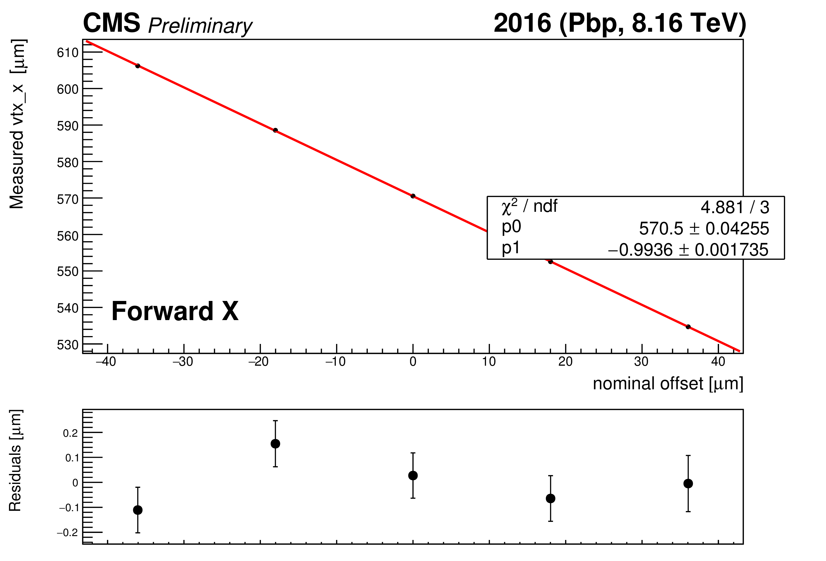
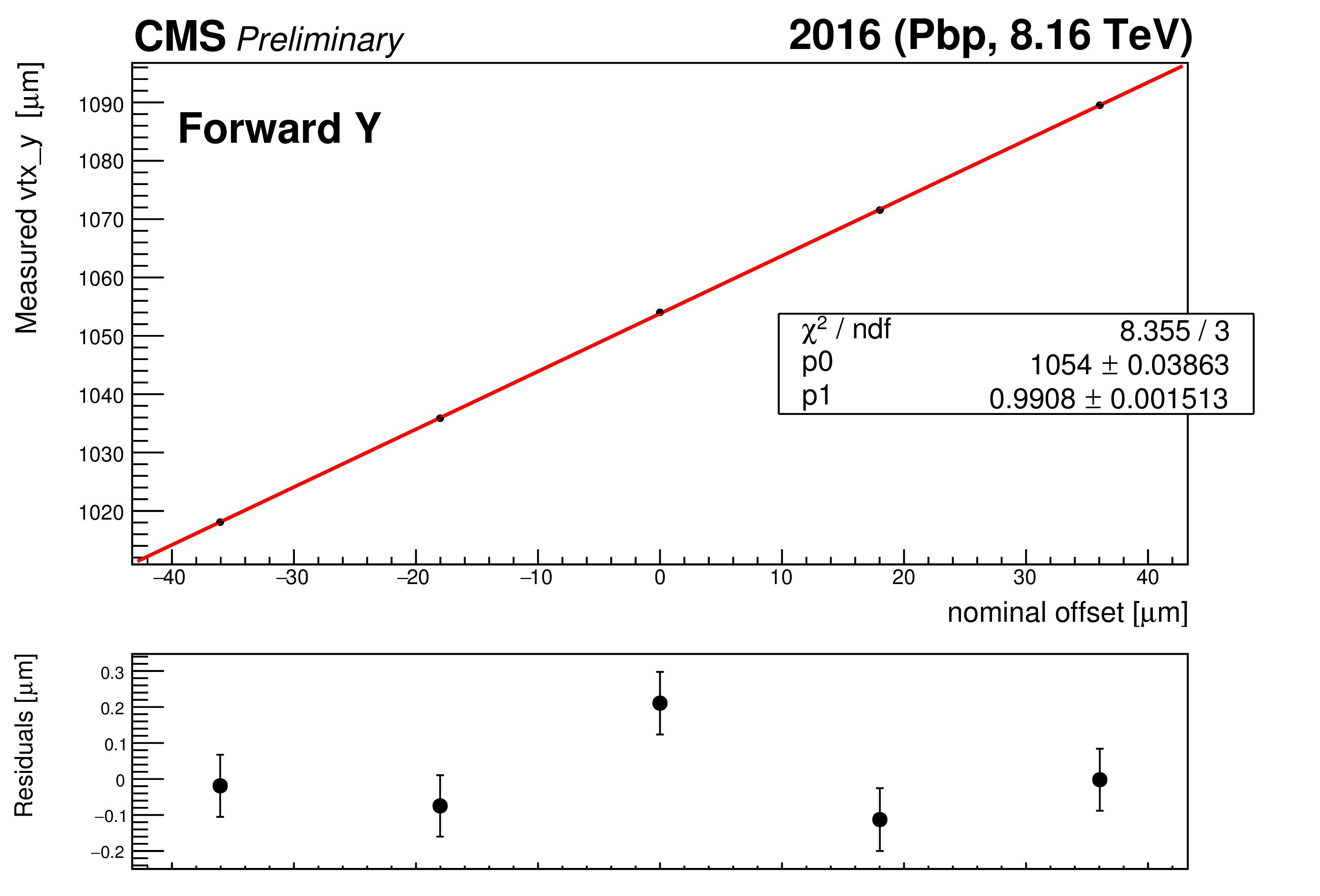
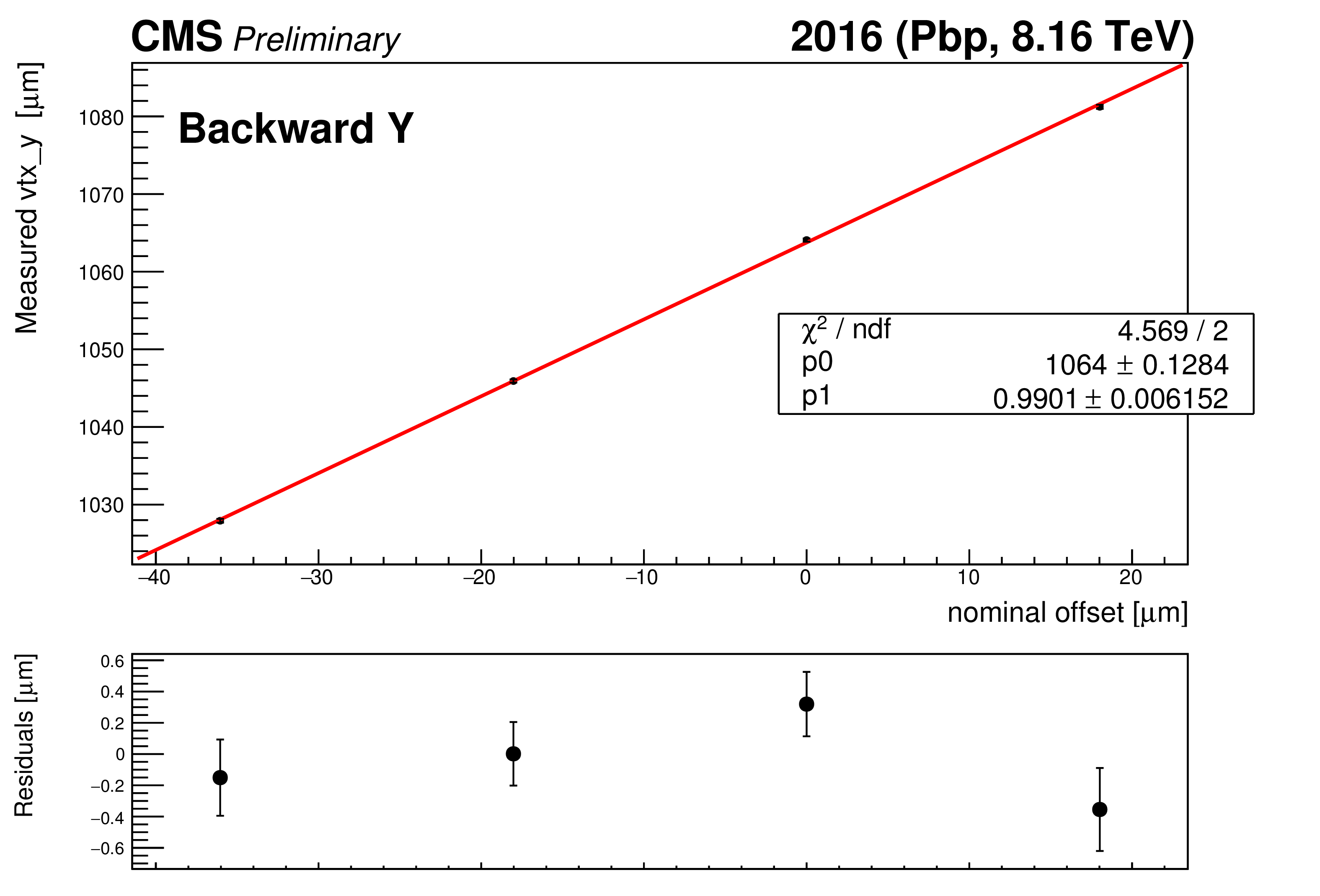
Figure 11:
Examples of the measured beam-spot positions as a function of the beam centroid offsets are shown for forward (a,c) and backward (b,d) LSC scans in both horizontal (a,b) and vertical (c,d) directions. A problem in the DAQ acquisition system prevented the reconstructed vertices from being registered for one equidistant configuration in the backward Y LSC. |
png pdf |
Figure 11-a:
Examples of the measured beam-spot positions as a function of the beam centroid offsets are shown for forward (a,c) and backward (b,d) LSC scans in both horizontal (a,b) and vertical (c,d) directions. A problem in the DAQ acquisition system prevented the reconstructed vertices from being registered for one equidistant configuration in the backward Y LSC. |

png pdf |
Figure 11-b:
Examples of the measured beam-spot positions as a function of the beam centroid offsets are shown for forward (a,c) and backward (b,d) LSC scans in both horizontal (a,b) and vertical (c,d) directions. A problem in the DAQ acquisition system prevented the reconstructed vertices from being registered for one equidistant configuration in the backward Y LSC. |
png pdf |
Figure 11-c:
Examples of the measured beam-spot positions as a function of the beam centroid offsets are shown for forward (a,c) and backward (b,d) LSC scans in both horizontal (a,b) and vertical (c,d) directions. A problem in the DAQ acquisition system prevented the reconstructed vertices from being registered for one equidistant configuration in the backward Y LSC. |
png pdf |
Figure 11-d:
Examples of the measured beam-spot positions as a function of the beam centroid offsets are shown for forward (a,c) and backward (b,d) LSC scans in both horizontal (a,b) and vertical (c,d) directions. A problem in the DAQ acquisition system prevented the reconstructed vertices from being registered for one equidistant configuration in the backward Y LSC. |

png pdf |
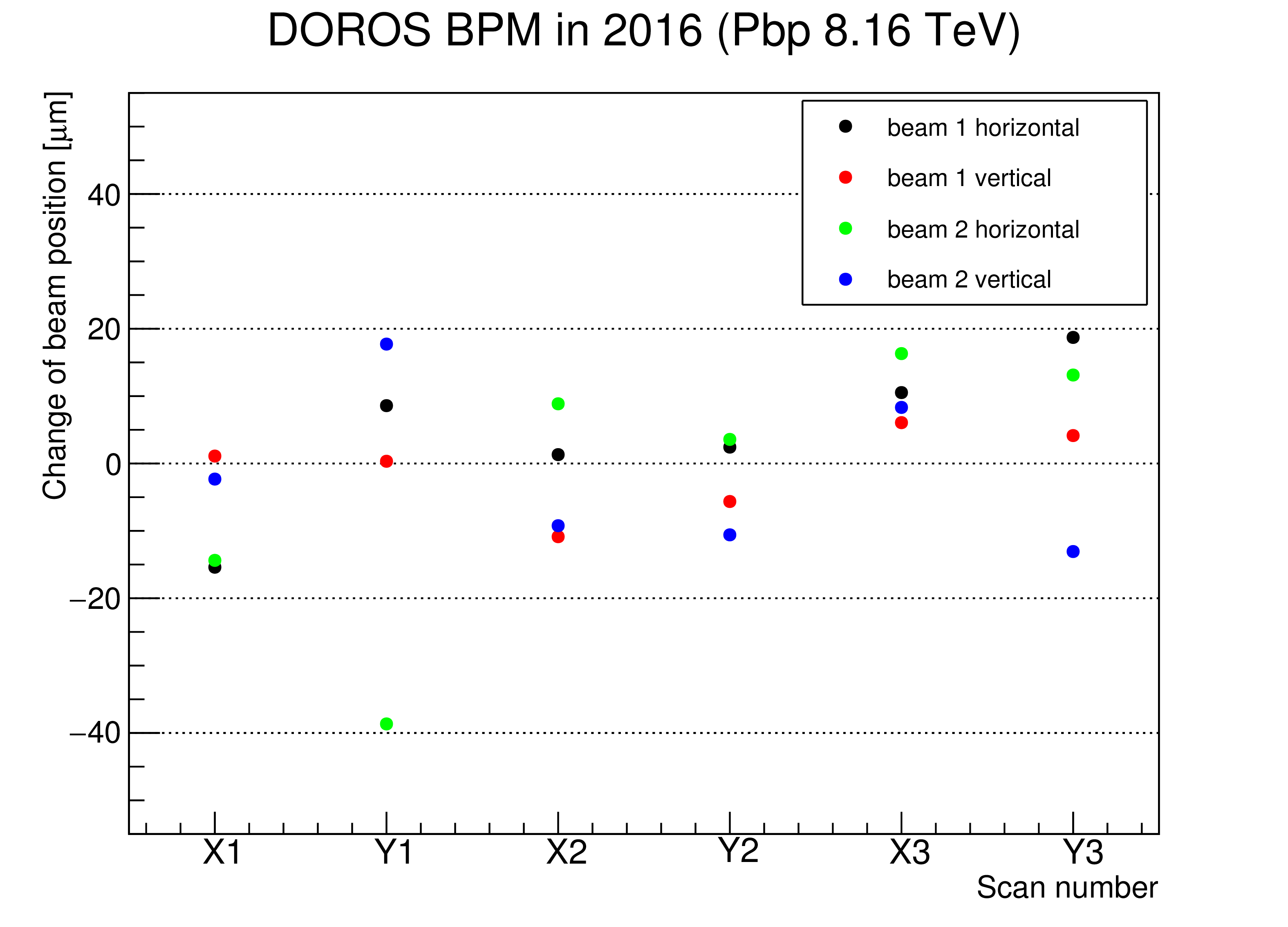
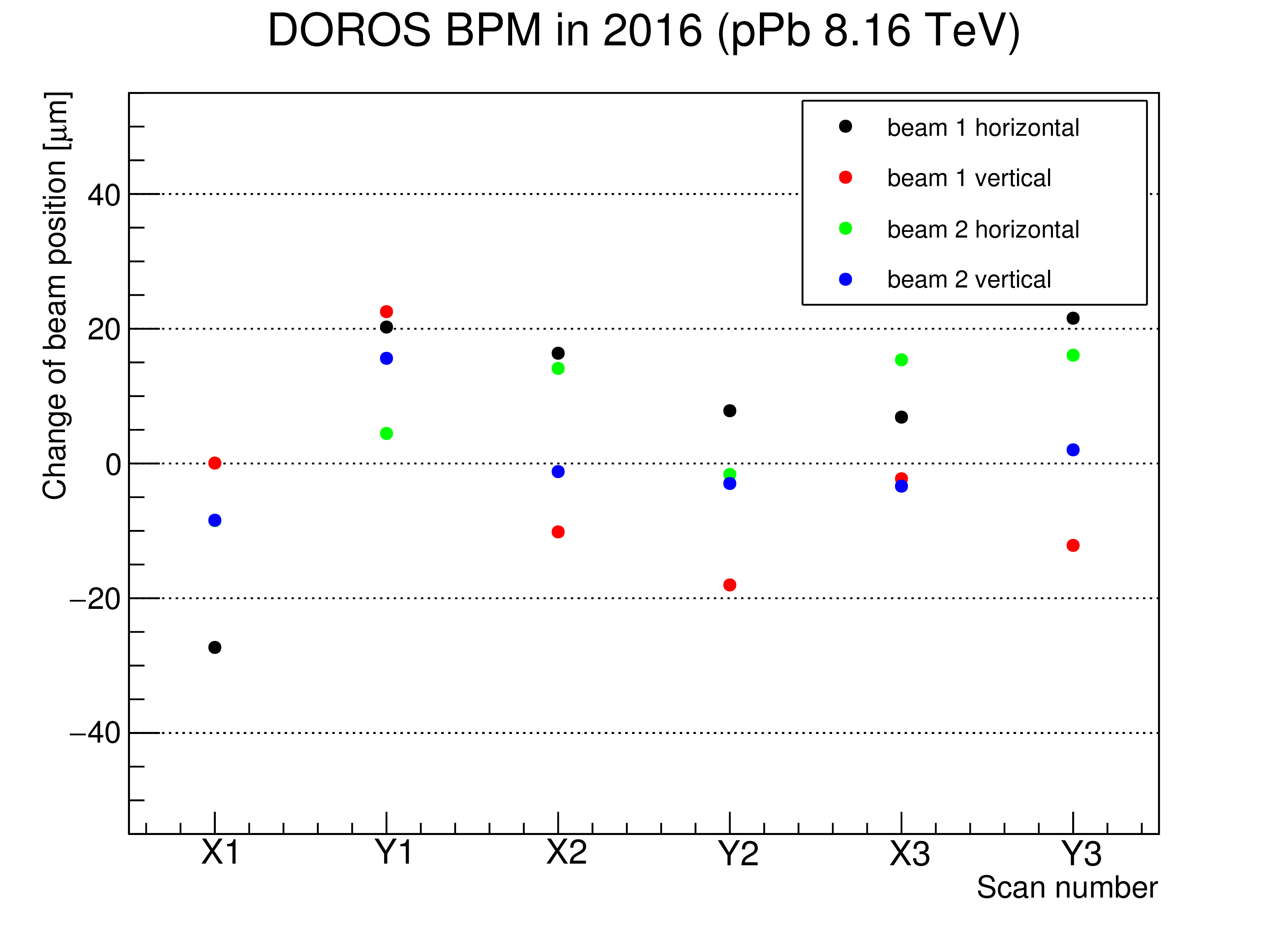
Figure 12:
Difference of the two vertical and horizontal beam positions before and after each scan as measured by the DOROS BPM in ${ \mu }$m is shown. |
png pdf |
Figure 12-a:
Difference of the two vertical and horizontal beam positions before and after each scan as measured by the DOROS BPM in ${ \mu }$m is shown. |
png pdf |
Figure 12-b:
Difference of the two vertical and horizontal beam positions before and after each scan as measured by the DOROS BPM in ${ \mu }$m is shown. |
png pdf |
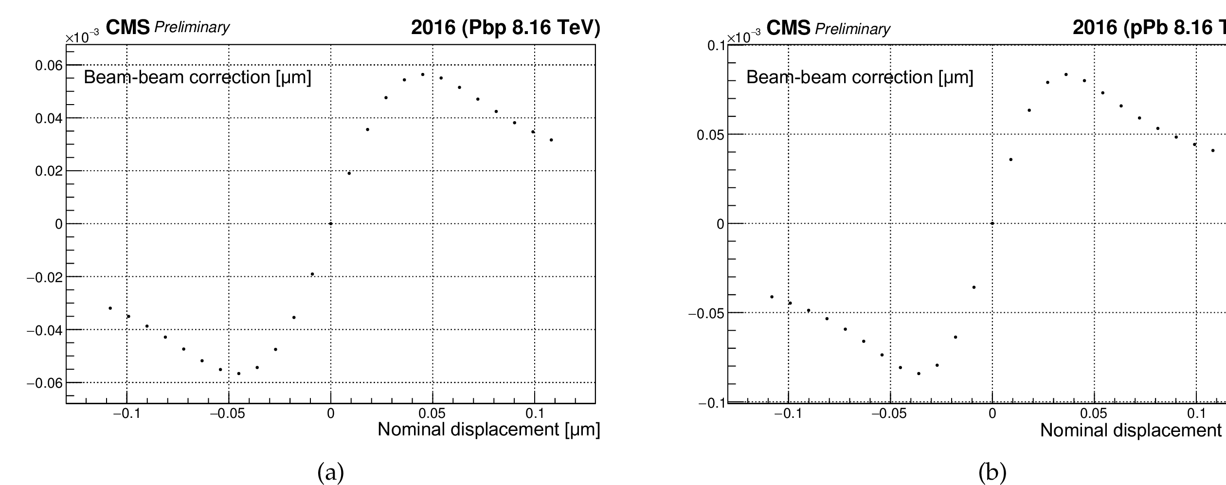
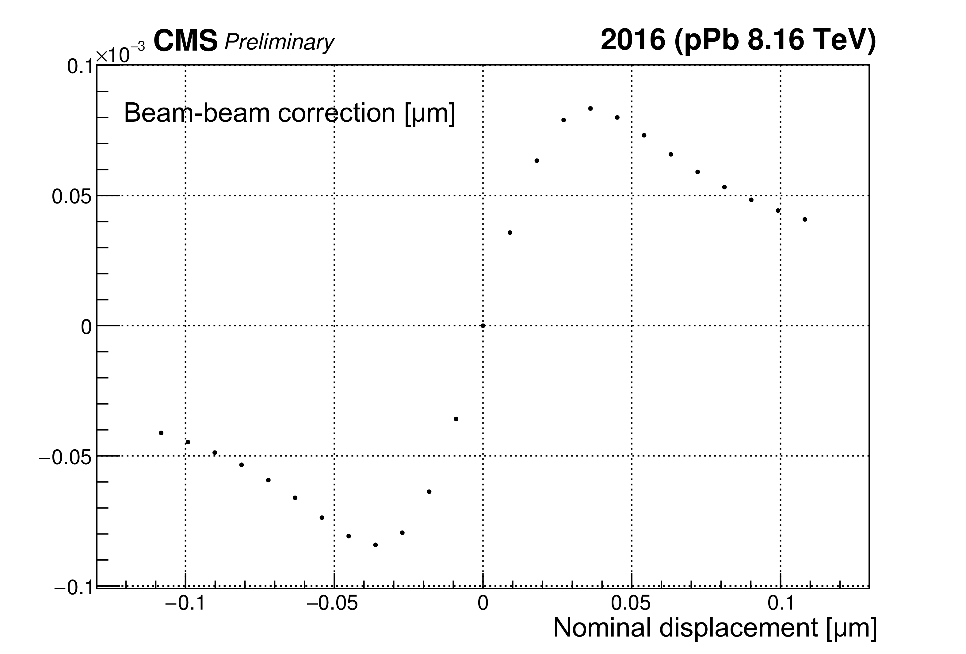
Figure 13:
Shown are two examples of beam-beam deflection estimates as a function of beam-beam separation in Pbp (a) and pPb (b) configuration. The difference in the magnitude of the beam-beam deflections stems from the beam current products, though its impact on the corrected $ {\sigma _{\mathrm {vis}}} $ is non-visible. |
png pdf |
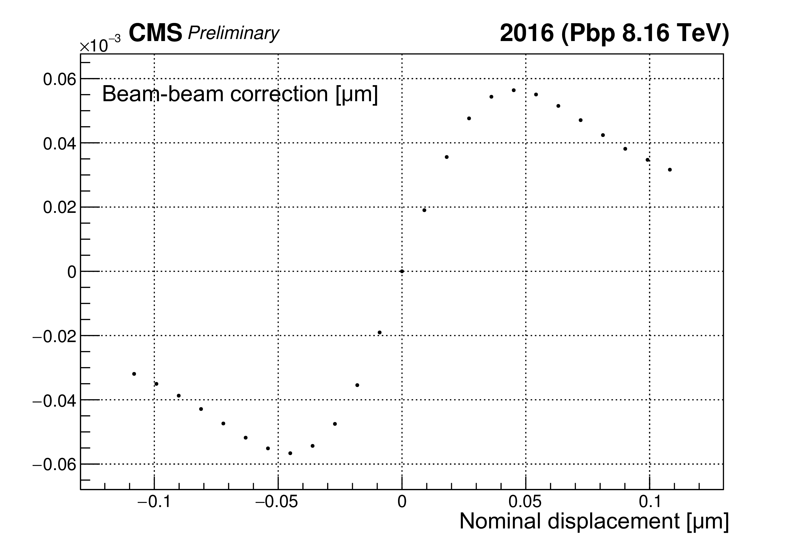
Figure 13-a:
Shown are two examples of beam-beam deflection estimates as a function of beam-beam separation in Pbp (a) and pPb (b) configuration. The difference in the magnitude of the beam-beam deflections stems from the beam current products, though its impact on the corrected $ {\sigma _{\mathrm {vis}}} $ is non-visible. |
png pdf |
Figure 13-b:
Shown are two examples of beam-beam deflection estimates as a function of beam-beam separation in Pbp (a) and pPb (b) configuration. The difference in the magnitude of the beam-beam deflections stems from the beam current products, though its impact on the corrected $ {\sigma _{\mathrm {vis}}} $ is non-visible. |

png pdf |
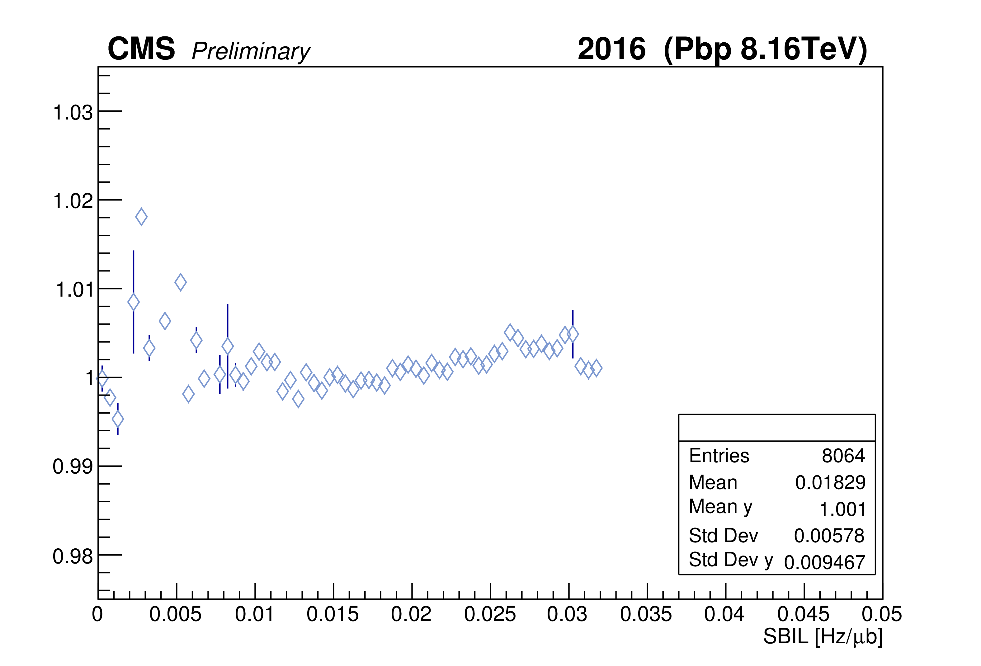
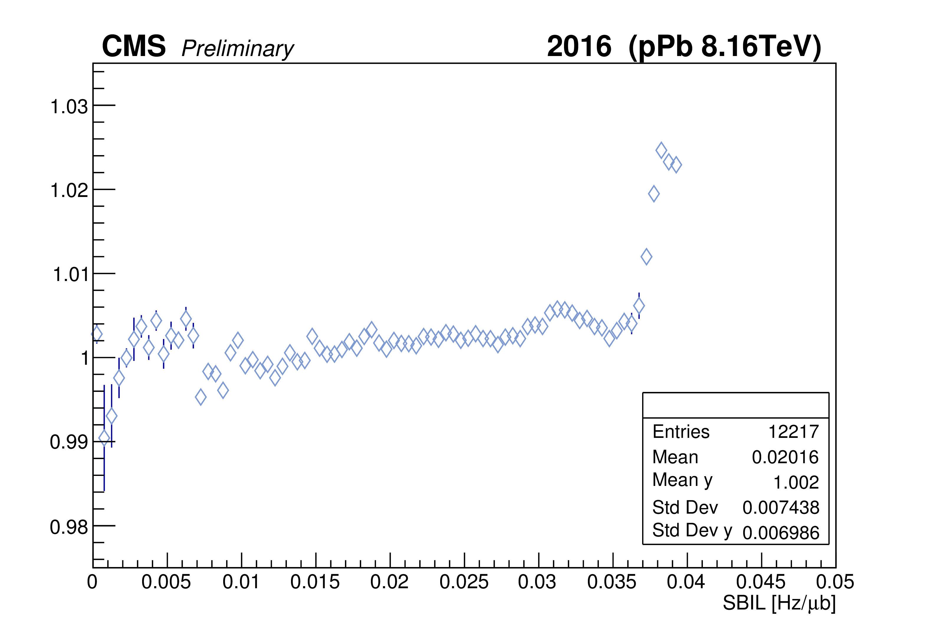
Figure 14:
Comparison of the PLT over HF luminosity ratio against the single bunch instantaneous luminosity, the latter estimated based on PLT for the Pbp (a) and pPb (b) periods. The last part of the Pbp period, corresponding to LHC fill 5538 with active leveling in IP5 and contributing negligibly to the total luminosity, has been excluded, while the rising trend for SBIL higher than about 0.035 Hz/${ \mu }$b includes less than 2% of the integrated luminosity. |
png pdf |
Figure 14-a:
Comparison of the PLT over HF luminosity ratio against the single bunch instantaneous luminosity, the latter estimated based on PLT for the Pbp (a) and pPb (b) periods. The last part of the Pbp period, corresponding to LHC fill 5538 with active leveling in IP5 and contributing negligibly to the total luminosity, has been excluded, while the rising trend for SBIL higher than about 0.035 Hz/${ \mu }$b includes less than 2% of the integrated luminosity. |
png pdf |
Figure 14-b:
Comparison of the PLT over HF luminosity ratio against the single bunch instantaneous luminosity, the latter estimated based on PLT for the Pbp (a) and pPb (b) periods. The last part of the Pbp period, corresponding to LHC fill 5538 with active leveling in IP5 and contributing negligibly to the total luminosity, has been excluded, while the rising trend for SBIL higher than about 0.035 Hz/${ \mu }$b includes less than 2% of the integrated luminosity. |
png pdf |
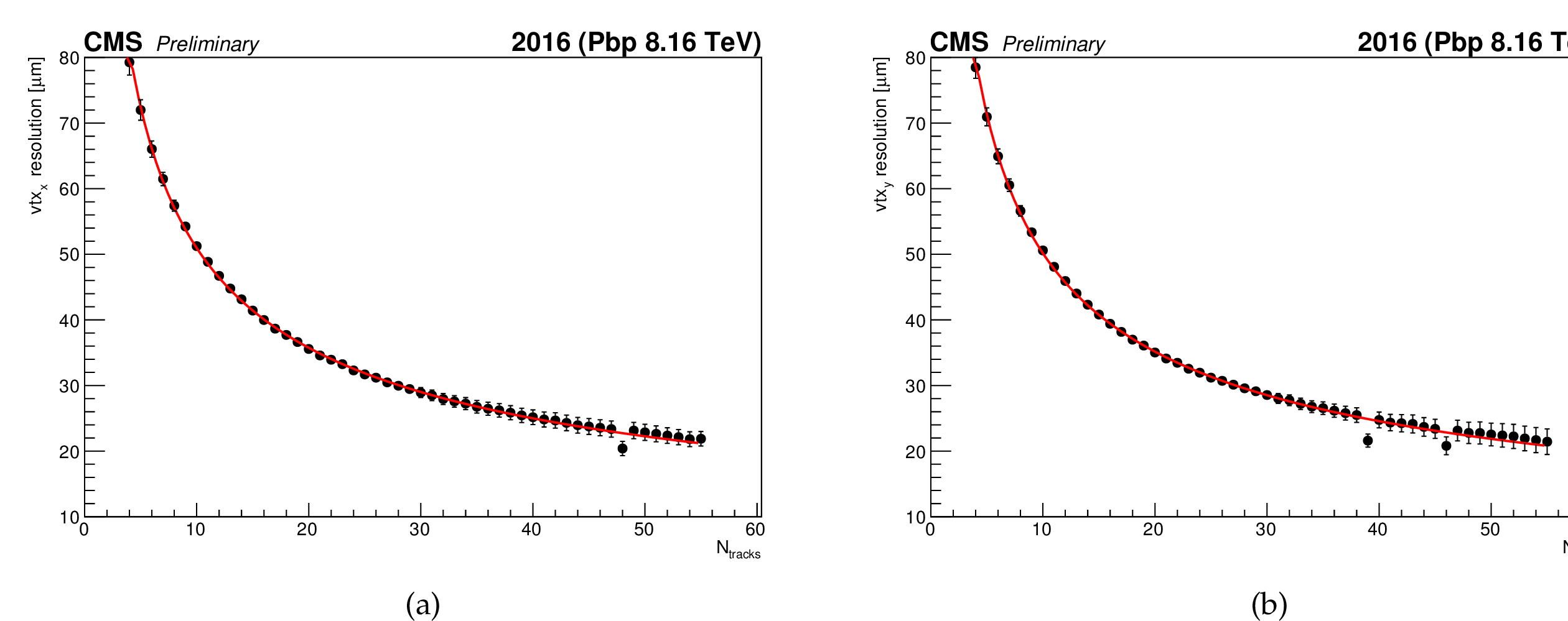
Figure 15:
Primary vertex transverse resolution in the horizontal (a) and vertical (b) direction in zero-bias events. The reconstructed tracks associated to primary vertices are selected with the high-purity [15] requirement, while vertices within a radial (longitudinal) distance of 24 (2) cm are retained. The curve shows the results of the resolution fitted using a three-parameter function of the form $A/\mathrm {N_{tracks}}^B+C$. |

png pdf |
Figure 15-a:
Primary vertex transverse resolution in the horizontal (a) and vertical (b) direction in zero-bias events. The reconstructed tracks associated to primary vertices are selected with the high-purity [15] requirement, while vertices within a radial (longitudinal) distance of 24 (2) cm are retained. The curve shows the results of the resolution fitted using a three-parameter function of the form $A/\mathrm {N_{tracks}}^B+C$. |

png pdf |
Figure 15-b:
Primary vertex transverse resolution in the horizontal (a) and vertical (b) direction in zero-bias events. The reconstructed tracks associated to primary vertices are selected with the high-purity [15] requirement, while vertices within a radial (longitudinal) distance of 24 (2) cm are retained. The curve shows the results of the resolution fitted using a three-parameter function of the form $A/\mathrm {N_{tracks}}^B+C$. |

png pdf |
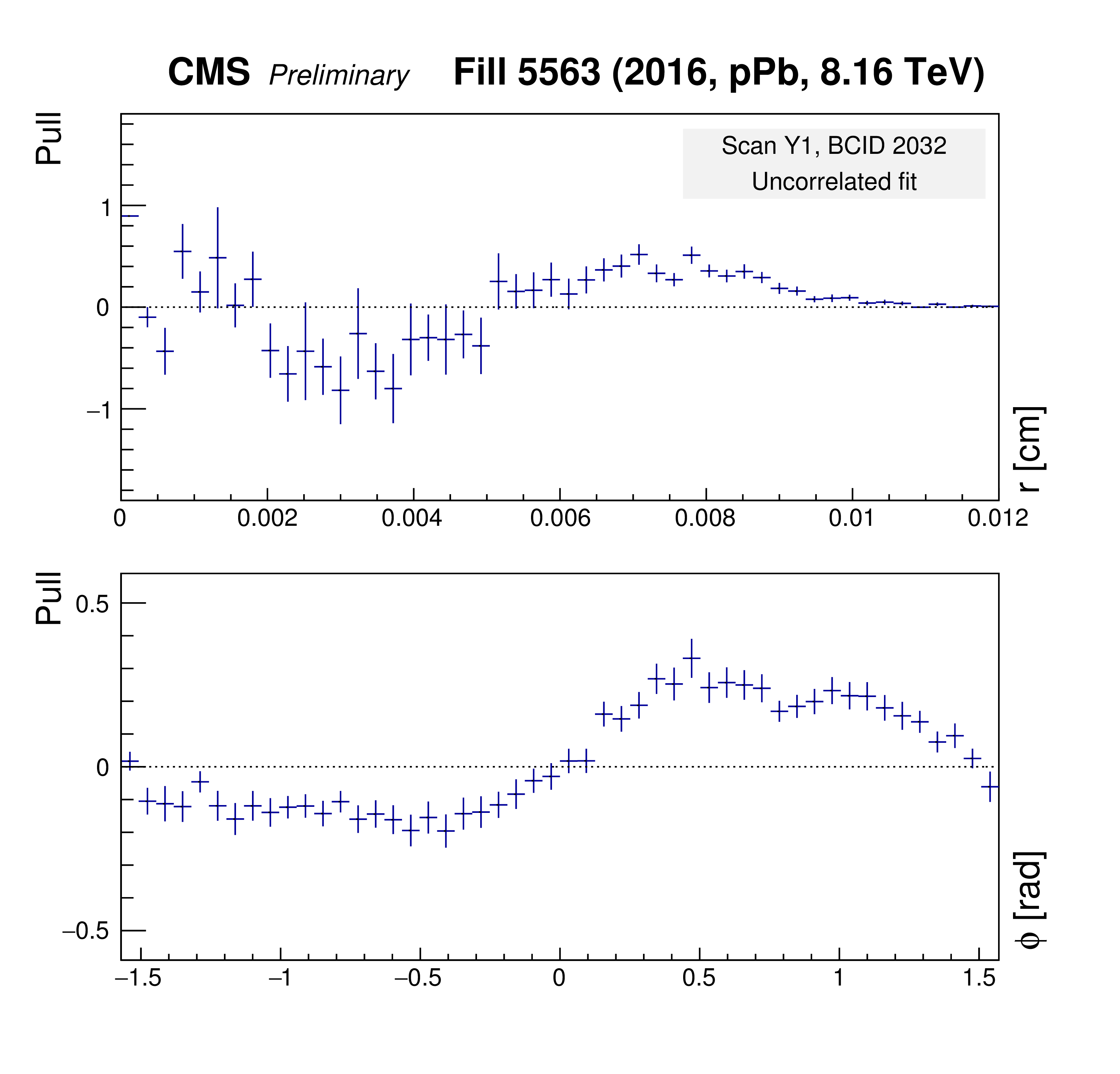
Figure 16:
Pull distributions using the Gaussian fit model of Eq. (9) but fixing the correlation parameter $r$ to zero. The pull is defined as the difference between the number of measured vertices and the number of vertices predicted by the fit, divided by the statistical uncertainty of the measurement. These plots show the results from the scan constraining beam 1 in $y$. Left: two-dimensional pull distribution as a function of $x$ and $y$ position. Right: one-dimensional projections, in slices of constant radius (top) and azimuthal angle (bottom). |

png pdf |
Figure 16-a:
Pull distributions using the Gaussian fit model of Eq. (9) but fixing the correlation parameter $r$ to zero. The pull is defined as the difference between the number of measured vertices and the number of vertices predicted by the fit, divided by the statistical uncertainty of the measurement. These plots show the results from the scan constraining beam 1 in $y$. Left: two-dimensional pull distribution as a function of $x$ and $y$ position. Right: one-dimensional projections, in slices of constant radius (top) and azimuthal angle (bottom). |
png pdf |
Figure 16-b:
Pull distributions using the Gaussian fit model of Eq. (9) but fixing the correlation parameter $r$ to zero. The pull is defined as the difference between the number of measured vertices and the number of vertices predicted by the fit, divided by the statistical uncertainty of the measurement. These plots show the results from the scan constraining beam 1 in $y$. Left: two-dimensional pull distribution as a function of $x$ and $y$ position. Right: one-dimensional projections, in slices of constant radius (top) and azimuthal angle (bottom). |

png pdf |
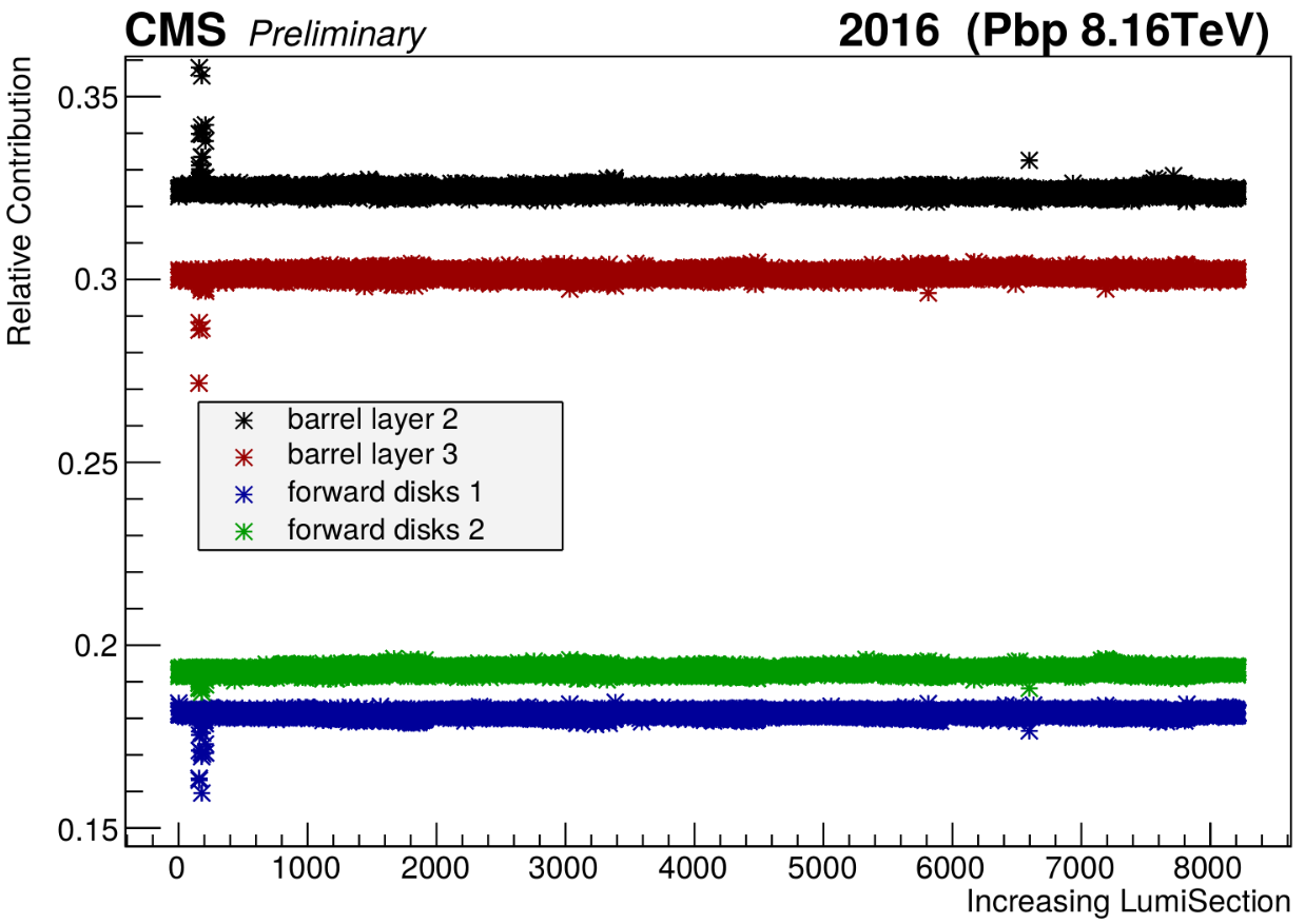
Figure 17:
An intrinsic cross check reveals excellent stability and independence to various data-taking conditions of the different pixel layers relative to the total response for the Pbp (a) and pPb (b) periods. The last part of the Pbp period, corresponding to LHC fill 5538 with active leveling in IP5 and contributing negligibly to the total luminosity, has been excluded. |
png |
Figure 17-a:
An intrinsic cross check reveals excellent stability and independence to various data-taking conditions of the different pixel layers relative to the total response for the Pbp (a) and pPb (b) periods. The last part of the Pbp period, corresponding to LHC fill 5538 with active leveling in IP5 and contributing negligibly to the total luminosity, has been excluded. |

png |
Figure 17-b:
An intrinsic cross check reveals excellent stability and independence to various data-taking conditions of the different pixel layers relative to the total response for the Pbp (a) and pPb (b) periods. The last part of the Pbp period, corresponding to LHC fill 5538 with active leveling in IP5 and contributing negligibly to the total luminosity, has been excluded. |
| Tables | |

png pdf |
Table 1:
Summary of the LHC beam parameters at the start of fill 5527 (5563). |

png pdf |
Table 2:
Bunch-to-bunch consistency in the Pbp and pPb periods. Differences are obtained from the RMS of the distribution of the cross sections measured for all colliding bunch pairs, after subtracting in quadrature the bunch-averaged statistical uncertainty. |

png pdf |
Table 3:
Results of the length-scale calibration for the two horizontal and vertical LSC scans. |

png pdf |
Table 4:
Difference of the beam positions before and after each scan as measured by the DOROS BPM and the absolute value of the orbit drift in the Pbp period. |

png pdf |
Table 5:
Difference of the beam positions before and after each scan as measured by the DOROS BPM and the absolute value of the orbit drift in the pPb period. |

png pdf |
Table 6:
Summary of the systematic uncertainties entering the CMS luminosity measurement for ${\sqrt {\smash [b]{s_{_{\mathrm {NN}}}}}} = $ 8.16 TeV Pbp (pPb) collisions. When applicable, the percentage correction is shown. |
| Summary |
|
Table 6 summarizes the derived corrections along with their associated systematic uncertainties. The various sources of systematic uncertainties are grouped into i) "normalization'' uncertainties; that is, luminosity scale calibration from the vdM scan procedure, and ii) "integration'' uncertainties; that is, uncertainties associated to the extrapolation of ${\sigma_{\mathrm{vis}}}$ to luminometer rate measurements under usual data-taking conditions. An uncertainty of 0.5% associated to the deadtime estimate from the CMS DAQ system is additionally included affecting the recorded integrated luminosity. The dominating uncertainty contributing to the luminosity scale calibration is associated to the non-factorizability of the colliding beam bunch densities. The uncertainties in the integration and normalization are treated as uncorrelated and are summed in quadrature resulting in 3.2 (3.7)% for the Pbp (pPb) period (see Table 6). The weighted averages of ${\sigma_{\mathrm{vis}}}$ for all BCIDs measured over the considered scans in the Pbp relative to the pPb period, corrected for effects impacting the accuracy of the absolute and relative bunch populations (Section 5.3) and for beam-beam interactions (Section 5.5), is found to be in excellent agreement for the symmetric luminometers. A combined result is then determined by computing a weighted average from the ${\sigma_{\mathrm{vis}}}$ calibrations in the two periods. To avoid underestimating the uncertainty in the combined result, it is assumed that most of the systematic uncertainties are fully correlated except for the uncertainties related to bunch-to-bunch variation, scan-to-scan variation, and cross-detector stability. In summary, the total uncertainty in the CMS luminosity measurement in November-December 2016 is estimated to be 3.5% for data recorded with proton-nucleus collisions at $ {\sqrt {\smash [b]{s_{_{\mathrm {NN}}}}}} = $ 8.16 TeV. |
| References | ||||
| 1 | CMS Collaboration | The CMS experiment at the CERN LHC | JINST 3 (2008) S08004 | CMS-00-001 |
| 2 | M. Hempel | PhD thesis, DESY, 2017 DESY-THESIS-2017-030 | ||
| 3 | CMS Collaboration | The CMS trigger system | JINST 12 (2017) P01020 | CMS-TRG-12-001 1609.02366 |
| 4 | S. van der Meer | Calibration of the effective beam height in the ISR | CERN-ISR-PO-68-31 | |
| 5 | ALICE Collaboration | Measurement of visible cross sections in proton-lead collisions at $ \sqrt{s_{\rm NN}} = $ 5.02 TeV in van der Meer scans with the ALICE detector | JINST 9 (2014) P11003 | 1405.1849 |
| 6 | ATLAS Collaboration | Improved luminosity determination in pp collisions at $ \sqrt{s} = $ 7 TeV using the ATLAS detector at the LHC | EPJC 73 (2013) 2518 | 1302.4393 |
| 7 | LHCb Collaboration | Precision luminosity measurements at LHCb | JINST 9 (2014) P12005 | 1410.0149 |
| 8 | CMS Collaboration | CMS luminosity based on pixel cluster counting - Summer 2013 update | CMS-PAS-LUM-13-001 | CMS-PAS-LUM-13-001 |
| 9 | CMS Collaboration | CMS luminosity measurement for the 2015 data taking period | CMS-PAS-LUM-15-001 | CMS-PAS-LUM-15-001 |
| 10 | CMS Collaboration | CMS luminosity calibration for the pp reference run at $ \sqrt{s} = $ 5.02 TeV | CMS-PAS-LUM-16-001 | CMS-PAS-LUM-16-001 |
| 11 | CMS Collaboration | CMS luminosity measurements for the 2016 data taking period | CMS-PAS-LUM-17-001 | CMS-PAS-LUM-17-001 |
| 12 | CMS Collaboration | CMS luminosity measurement for the 2017 data taking period at $ \sqrt{s} = $ 13 TeV | CMS-PAS-LUM-17-004 | CMS-PAS-LUM-17-004 |
| 13 | A. Kornmayer | The CMS pixel luminosity telescope | in Proceedings of the 13th Pisa Meeting on Advanced Detectors: Frontier Detectors for Frontier Physics, volume 824, p. 304 2016 | |
| 14 | P. Lujan | Performance of the pixel luminosity telescope for luminosity measurement at CMS during Run 2 | in Proceedings of the European Physical Society Conference on High Energy Physics, (EPS-HEP 2017), volume 314, p. 504 2017 | |
| 15 | CMS Collaboration | Description and performance of track and primary-vertex reconstruction with the CMS tracker | JINST 9 (2014) P10009 | CMS-TRK-11-001 1405.6569 |
| 16 | C. Barschel et al. | Results of the LHC DCCT calibration studies | CERN-ATS-Note-2012-026 PERF | |
| 17 | D. Belohrad et al. | The LHC Fast BCT system: A comparison of design parameters with initial performance | CERN-BE-2010-010 | |
| 18 | G. Papotti, T. Bohl, F. Follin, and U. Wehrle | Longitudinal beam measurements at the LHC: The LHC Beam Quality Monitor | in Proceedings of the 2nd International Particle Accelerator Conference, (IPAC 2011), volume C110904, p. 1852 2011 | |
| 19 | M. Gasior, J. Olexa, and R. Steinhagen | BPM electronics based on compensated diode detectors – Results from development systems | in Proceedings of the 2012 Beam Instrumentation Workshop, (BIW2012), volume C1204151, p. 44 2012 | |
| 20 | M. Zanetti | Beams scan based absolute normalization of the CMS luminosity measurement. CMS 2010 luminosity determination | in Proceedings of the LHC Lumi Days: LHC Workshop on LHC Luminosity Calibration, p. 69 2011 | |
| 21 | G. Anders et al. | Study of the relative LHC bunch populations for luminosity calibration | CERN-ATS-Note-2012-028 | |
| 22 | M. Klute, C. A. Medlock, and J. Salfeld-Nebgen | Beam imaging and luminosity calibration | JINST 12 (2017) P03018 | 1603.03566 |
| 23 | CMS Collaboration | CMS luminosity based on pixel cluster sounting - Summer 2012 update | CMS-PAS-LUM-12-001 | |
| 24 | A. Alici et al. | Study of the LHC ghost charge and satellite bunches for luminosity calibration | CERN-ATS-Note-2012-029 PERF | |
| 25 | A. Jeff et al. | Longitudinal density monitor for the LHC | PRST Accel. Beams 15 (2012) 032803 | |
| 26 | C. Barschel | PhD thesis, RWTH Aachen University, 2014 CERN-THESIS-2013-301 | ||
| 27 | W. Kozanecki, T. Pieloni, and J. Wenninger | Observation of Beam-beam Deflections with LHC Orbit Data | CERN-ACC-NOTE-2013-0006 | |
|
|
Compact Muon Solenoid LHC, CERN |
|

|

|

|

|

|