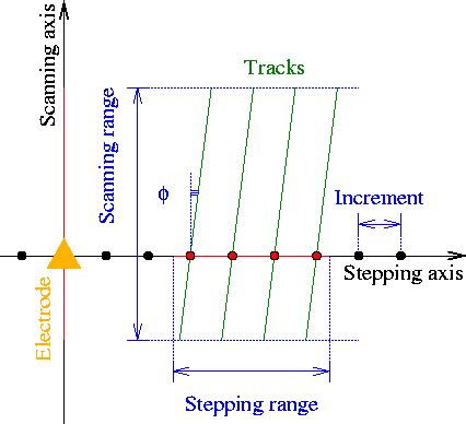
In all 3 cases, one of the 2 axes of the plane, the one that we call here "stepping axis" serves as coordinate in the calibration curve. The tracks cross a line through the centre of the electrode being studied and parallel to the stepping axis at multiples of a user-defined INCREMENT.
The axis which should serve as stepping axis is identified with the STEP keyword. You can set the RANGE of coordinates along the stepping axis for which tracks should be generated.
The other axis in the plane is called "scanning axis". The tracks can be at an ANGLE to this axis, but will usually be parallel to it.
The axis which should serve as stepping axis is identified with the SCAN keyword. Like for the stepping axis, You can limit the RANGE of coordinates along the stepping axis.

|
In the rest of the descriptions, these electrons are referred to as the 'selected electrons'.
If a value is negative, then the electrons will be counted from the back, the last electron corresponds to a value of 0. For the 4 last electrons, you can also type LAST, ONE-BUT-LAST, TWO-BUT-LAST and THREE-BUT-LAST.
[Default: initially, only the 25th electron is selected. The set of selected is remembered as default for the next call.]
[Default: initially 0.5, the median of the distribution. The value set is kept as default for the next call.]
You have, for these histograms, the choice between:
If you specify an explicit time window, then this time window is also used for the all-electrons arrival time histogram. Otherwise, these histograms are booked with the full time range of the track.
Setting a time window is most useful in conjunction with the KEEP-HISTOGRAMS option when you wish to study the histograms in more detail by other programs.
[Default: by default the time range of the selected electron histogram is computed from the first 100 entries of this histogram, whereas the range of the all-electron histogram is set to the time range for the track under study.]
Additional information on:
Tracks are usually perpendicular to the stepping axis and at regularly spaced distances from the centre of the electrode. The distance between 2 successive tracks, measured along the stepping axis, can be set with INCREMENT. The part of the stepping axis for which tracks are to be generated can be set with RANGE.
The stepping axis must be either the x-, the y- or the z-axis and must be distinct from the scanning axis.
[By default: X]
Additional information on:
Tracks are usually parallel to the scanning axis, or at a small ANGLE to it.
The scanning axis must be either the x-, the y- or the z-axis and must be distinct from the stepping axis.
[By default: Y]
Additional information on:
If you wish to compute arrival time distributions in a parallel plane, then specify OFFSET followed by the 3rd coordinate of the plane.
The parameter lines is the total amount of drift-lines that are calculated this way: 75\ % in the first step and 25\ % in the second.
[Default: the LINES parameter from the drift section.]
[Default: initially half of MXLIST, usually 100-500 bins. The value that you set is kept as default for the next call.]
A common application of this option seems to be the Gaussian fit of the arrival time histograms. This can be done using the FIT_GAUSSIAN procedure, or by a user program after writing the histograms out with the WRITE_HISTOGRAM procedure.
You have to declare the Global variables before the loop if
[Default: histograms are not kept. The setting is kept across calls of ARRIVAL.]
| Global | Description | Type |
|---|---|---|
[X|Y|Z]_<electrode> |
Distance from electrode | Matrix |
MEAN_<electrode> |
mean time all electrons | Matrix |
MEDIAN_<electrode> |
median time all electrons | Matrix |
RMS_<electrode> |
RMS time all electrons | Matrix |
MEAN<electron>_<electrode> |
mean time selected electron | Matrix |
MEDIAN<electron_<electrode> |
median time selected electron | Matrix |
RMS<electron>_<electrode> |
RMS time selected electron | Matrix |
E_<electron> |
sequence # selected electron | Number |
The string "<electrode>" in the global variable name is set to 1 for the first selected electrode, 2 for the next etc.
The string "<electron>" is an index that runs from 1 to the number of selected electrons. E_<electron> shows which electron a given index corresponds to. This can be zero or a negative number: 0 means the last electron, -1 the one but last etc.
You have to declare the Global variables before the loop if
[This option is not on by default, but its setting is remembered from one call to the next.]
It seems therefore tempting to select a large value for this parameter. When saving the distributions (KEEP-HISTOGRAMS) and then using them in a fit, this may indeed be a good approach. However, when extracting information from the MC process with means and RMS, the accuracy tends to degrade for large values of loop, mainly because of single entries with are far from the mean.
When specifying SINGLE-CLUSTER, only one cluster is generated per track, as a result the default value will be low and you are advised to choose a larger value in this case.
[Default: initially 1000. Each ARRIVAL statement has as default the value set in the previous invocation.]
For the lower orders, you may also specify the keywords LINEAR, QUADRATIC or PARABOLIC and CUBIC.
Although values between 1 and 10 are accepted, orders larger than 2 are not recommended since they tend to lead to oscillation.
[Default: 2, parabolic interpolation. The setting will be remembered from one call to the next.]
[Dataset output is only done on request.]
Additional information on:
The PLOT-SELECTED-ELECTRONS and PLOT-ALL-ELECTRONS options tend to lead to very bulky output, but these plots can be instructive.
Additional information on:
[The setting is remembered from one call to the next.]
Additional information on:
Formatted on 21/01/18 at 16:55.