

Compact Muon Solenoid
LHC, CERN
| CMS-BPH-17-005 ; CERN-EP-2020-070 | ||
| Observation of the $\mathrm{B_{s}^{0} \to \mathrm{X}(3872)\phi}$ decay | ||
| CMS Collaboration | ||
| 10 May 2020 | ||
| Phys. Rev. Lett. 125 (2020) 152001 | ||
| Abstract: Using a data sample of proton-proton collisions at $\sqrt{s} = $ 13 TeV, corresponding to an integrated luminosity of 140 fb$^{-1}$ collected by the CMS experiment in 2016-2018, the $\mathrm{B_{s}^{0} \to \mathrm{X}(3872)\phi}$ decay is observed. Decays into $\mathrm{J/\psi}\pi^{+}\pi^{-}$ and $\mathrm{K^{+}K^{-}}$ are used to reconstruct, respectively, the $\mathrm{X(3872)}$ and $\phi$. The ratio of the product of branching fractions $\mathcal{B}(\mathrm{B_{s}^{0} \to \mathrm{X}(3872)\phi})\,\mathcal{B}(\mathrm{\mathrm{X}(3872)} \to \mathrm{J/\psi}\pi^{+}\pi^{-} )$ to the product $\mathcal{B}(\mathrm{B_{s}^{0} \to \psi(2S)\phi})\,\mathcal{B}(\mathrm{\psi(2S)} \to \mathrm{J/\psi}\pi^{+}\pi^{-} )$ is measured to be (2.21 $\pm$ 0.29 (stat) $\pm$ 0.17 (syst))%. The ratio $\mathcal{B}(\mathrm{B_{s}^{0} \to \mathrm{X}(3872)\phi})/\mathcal{B}(\mathrm{B^{0} \to \mathrm{X}(3872) K^{0}})$ is found to be consistent with one, while the ratio $\mathcal{B}(\mathrm{B_{s}^{0} \to \mathrm{X}(3872)\phi})/\mathcal{B}(\mathrm{B^{+} \to \mathrm{X}(3872) K^{+}})$ is two times smaller. This suggests a difference in the production dynamics of the $\mathrm{X(3872)}$ in $\mathrm{B^{0}}$ and $\mathrm{B_{s}^{0}}$ meson decays compared to $\mathrm{B^{+}}$. The reported observation may shed new light on the nature of the $\mathrm{X(3872)}$ particle. | ||
| Links: e-print arXiv:2005.04764 [hep-ex] (PDF) ; CDS record ; inSPIRE record ; HepData record ; CADI line (restricted) ; | ||
| Figures & Tables | Summary | Additional Figures | References | CMS Publications |
|---|
| Figures | |
png pdf |
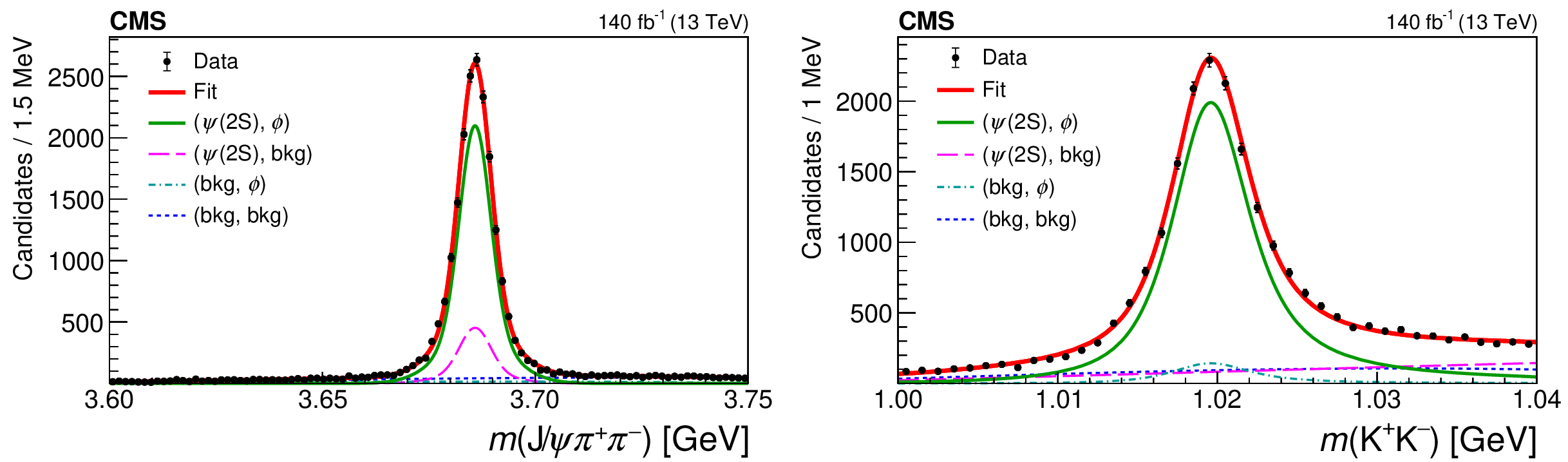
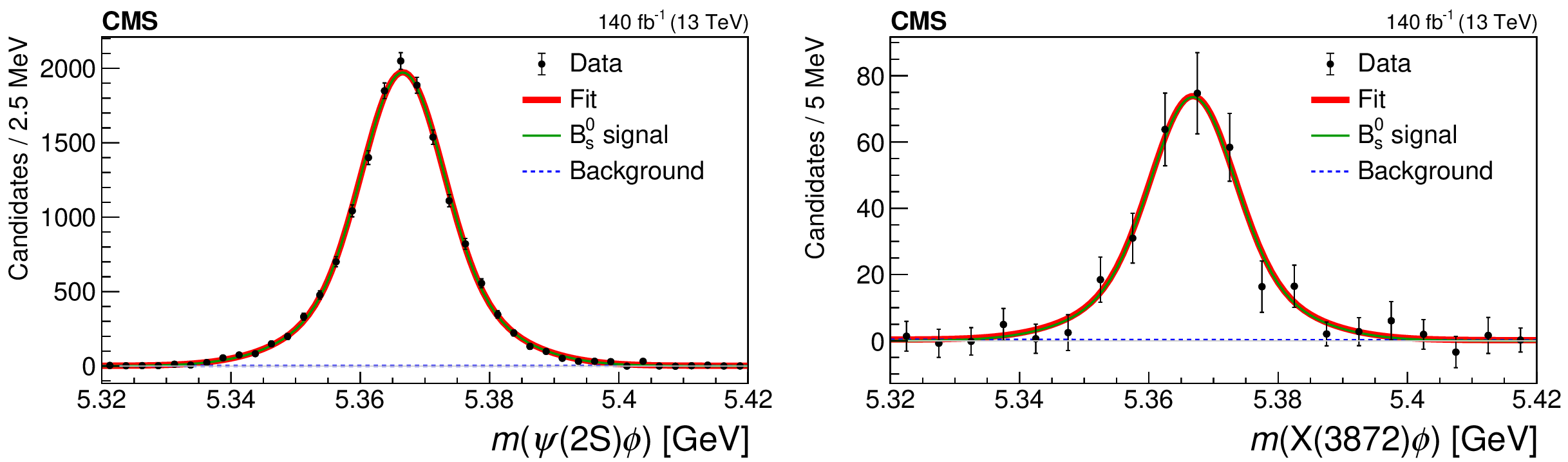
Figure 1:
The observed $\mathrm{J/\psi}\pi^{+}\pi^{-}$ (left) and ${\mathrm{K^{+}} \mathrm{K^{-}}}$ (right) invariant mass distributions for the ${\mathrm{B_{s}^{0}} \to \psi(\text{2S})\phi}$ candidates are shown by the points, with the vertical bars representing the statistical uncertainties. The projections of the 2D fit and its various components are shown by the lines. |
png pdf |
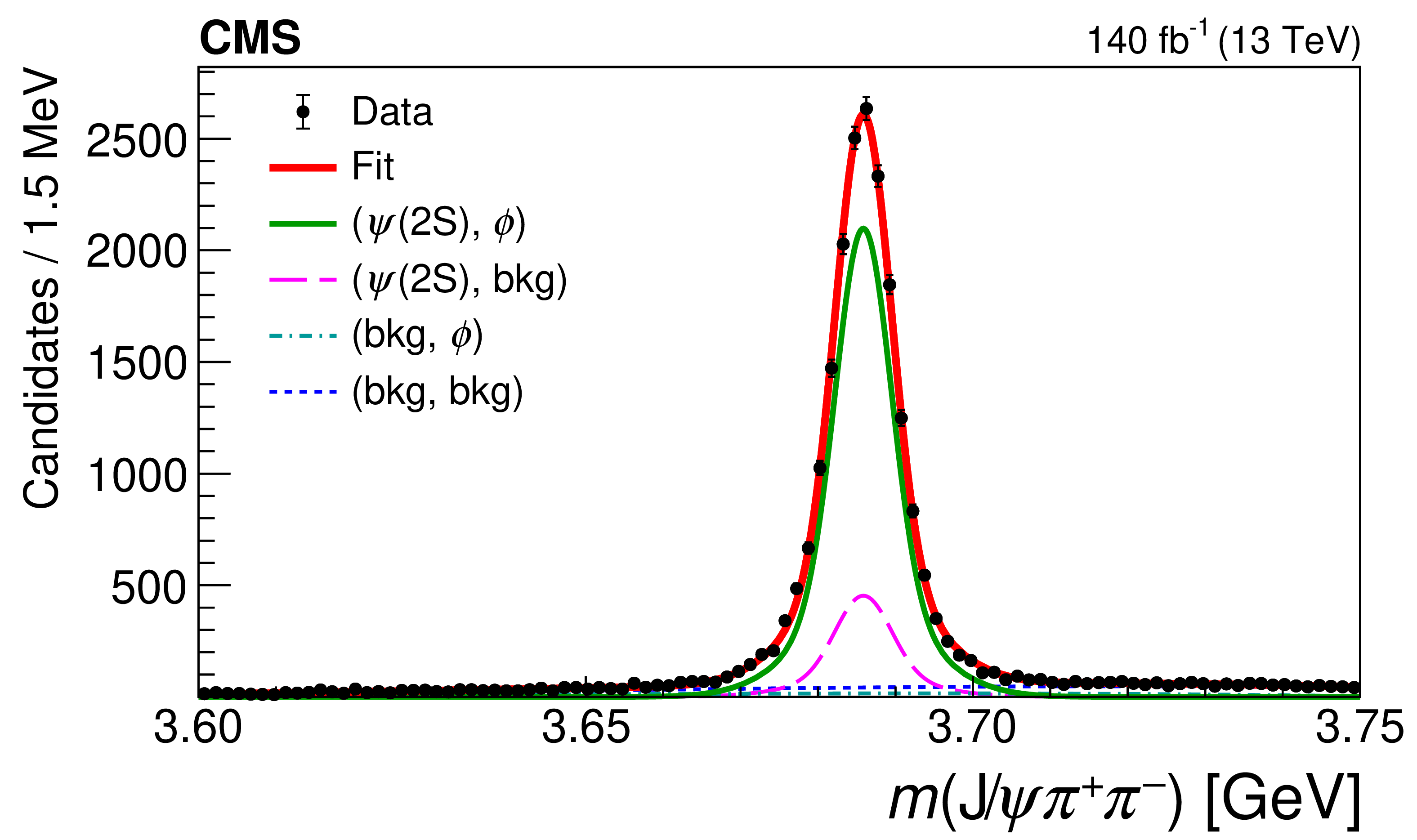
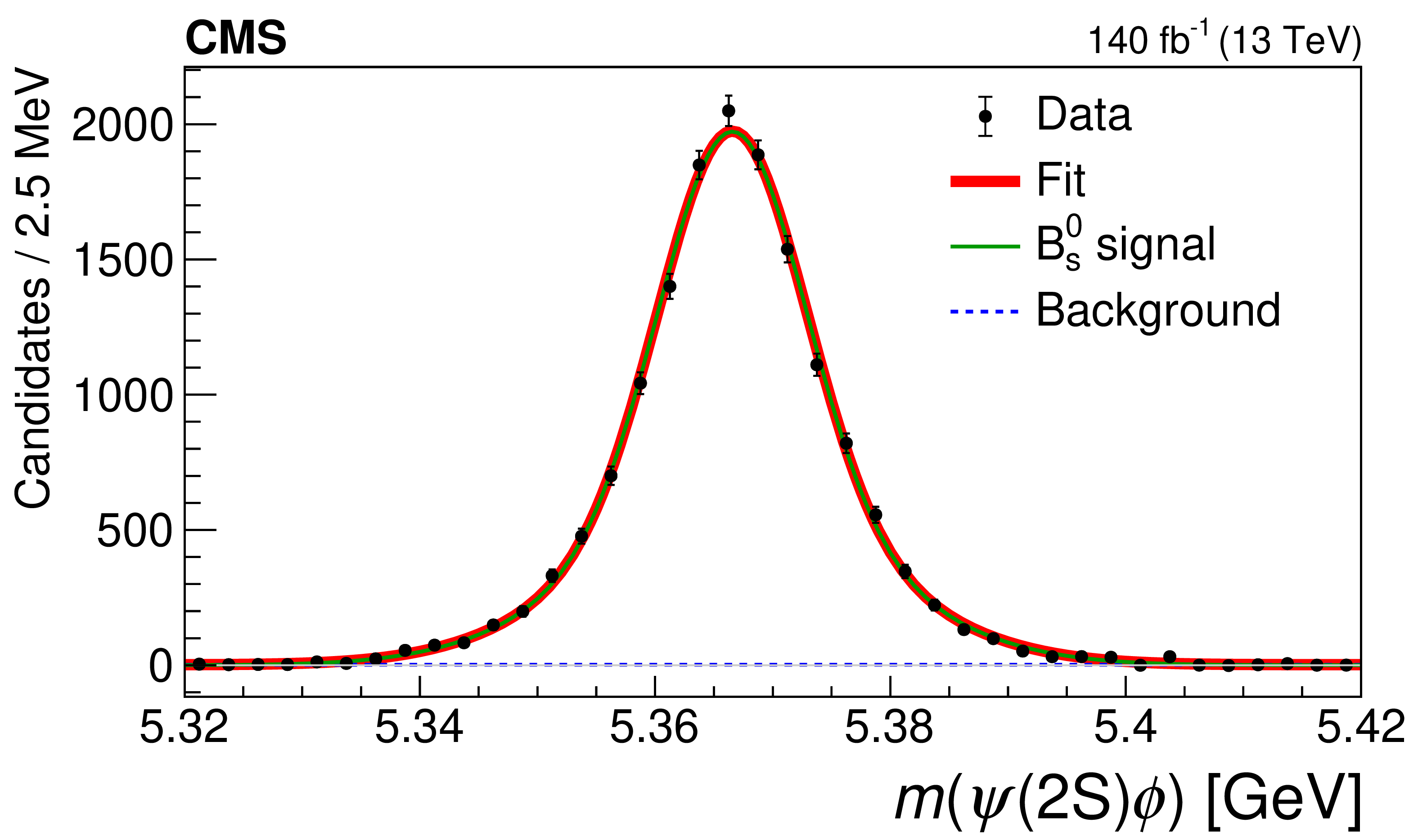
Figure 1-a:
The observed $\mathrm{J/\psi}\pi^{+}\pi^{-}$ invariant mass distribution for the ${\mathrm{B_{s}^{0}} \to \psi(\text{2S})\phi}$ candidates is shown by the points, with the vertical bars representing the statistical uncertainties. The projections of the 2D fit and its various components are shown by the lines. |
png pdf |
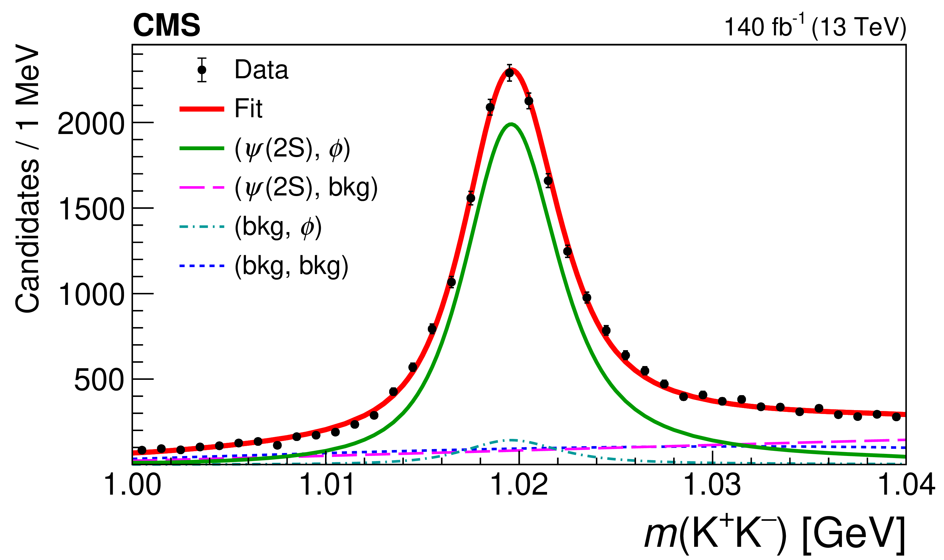
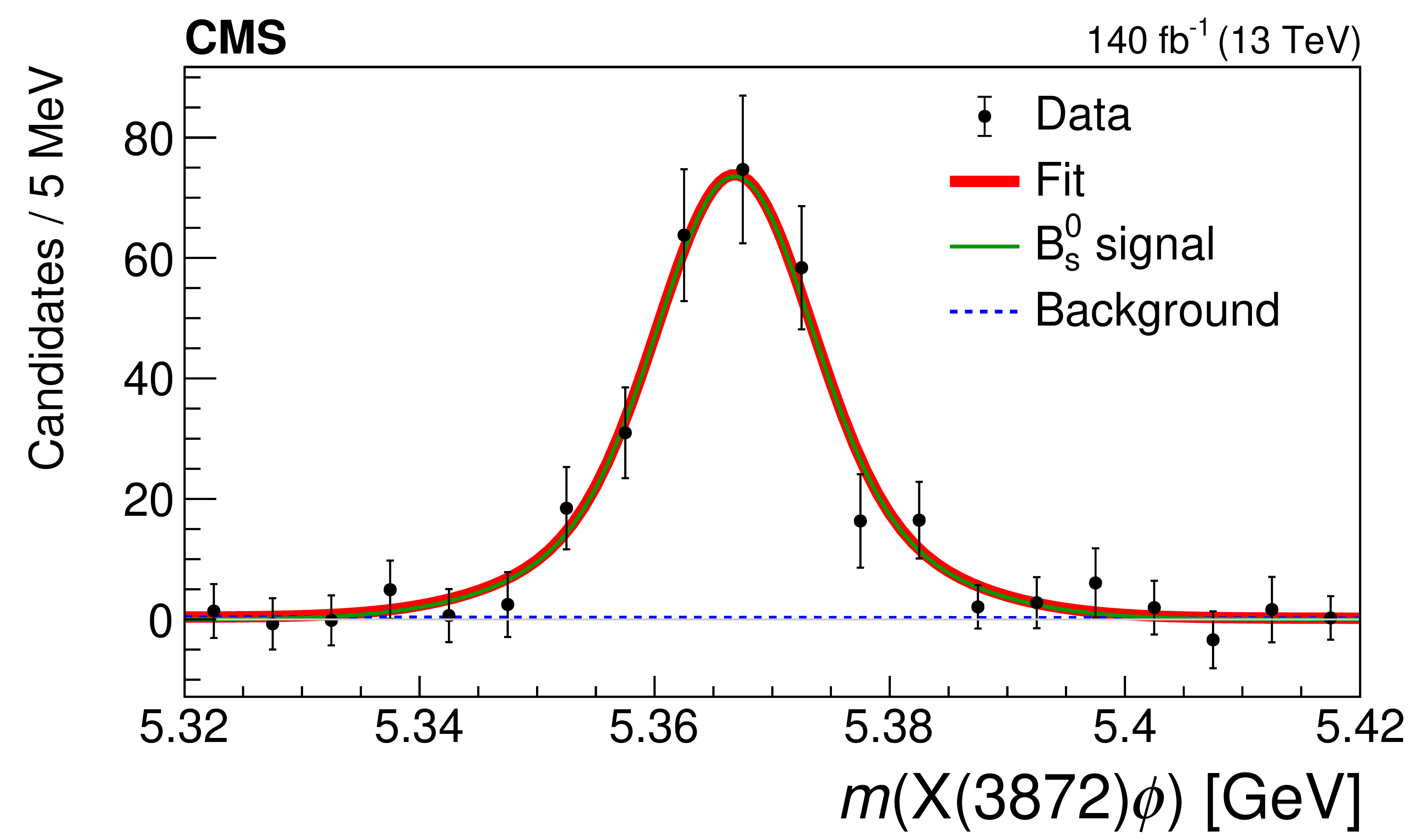
Figure 1-b:
The observed ${\mathrm{K^{+}} \mathrm{K^{-}}}$ invariant mass distribution for the ${\mathrm{B_{s}^{0}} \to \psi(\text{2S})\phi}$ candidates is shown by the points, with the vertical bars representing the statistical uncertainties. The projections of the 2D fit and its various components are shown by the lines. |

png pdf |
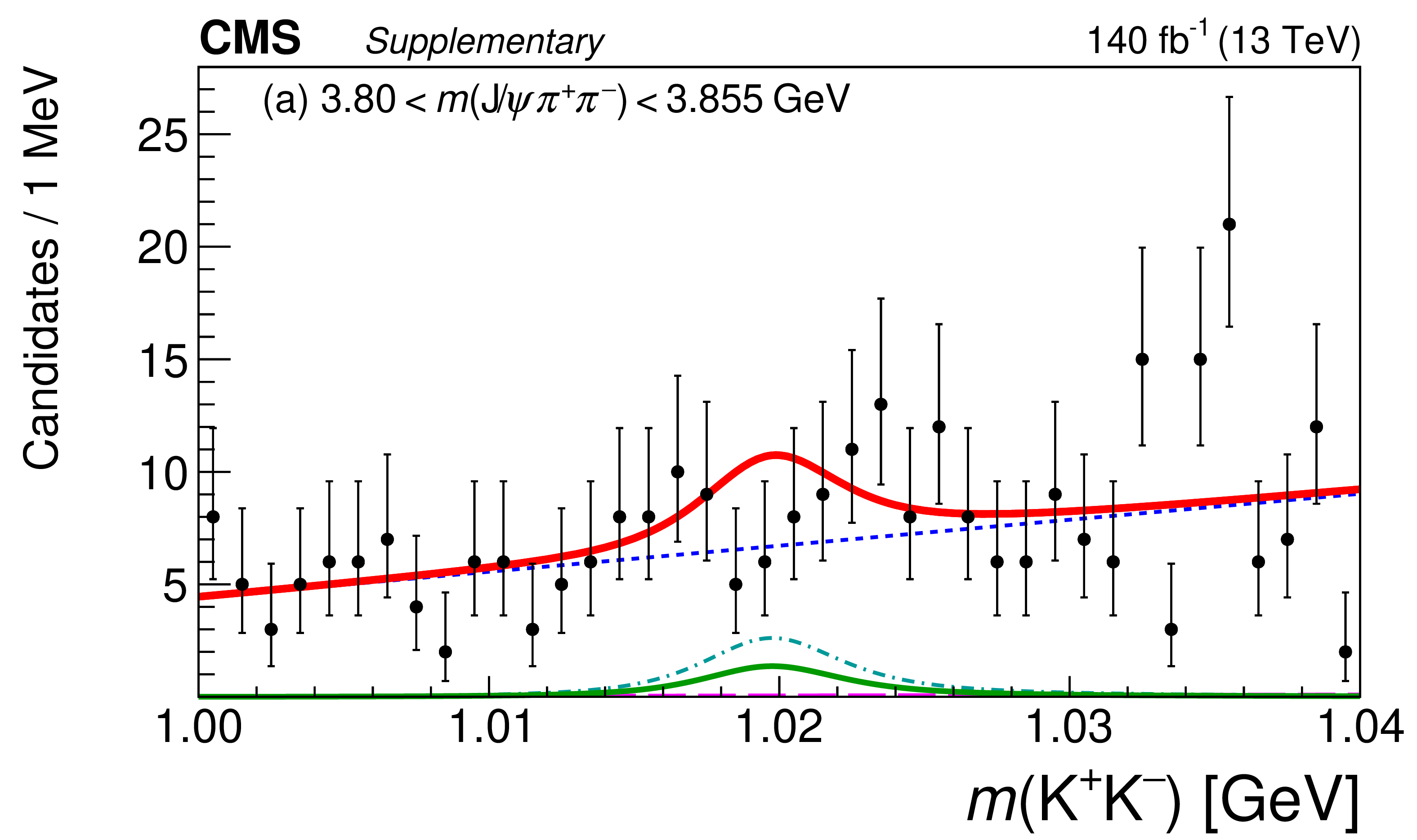
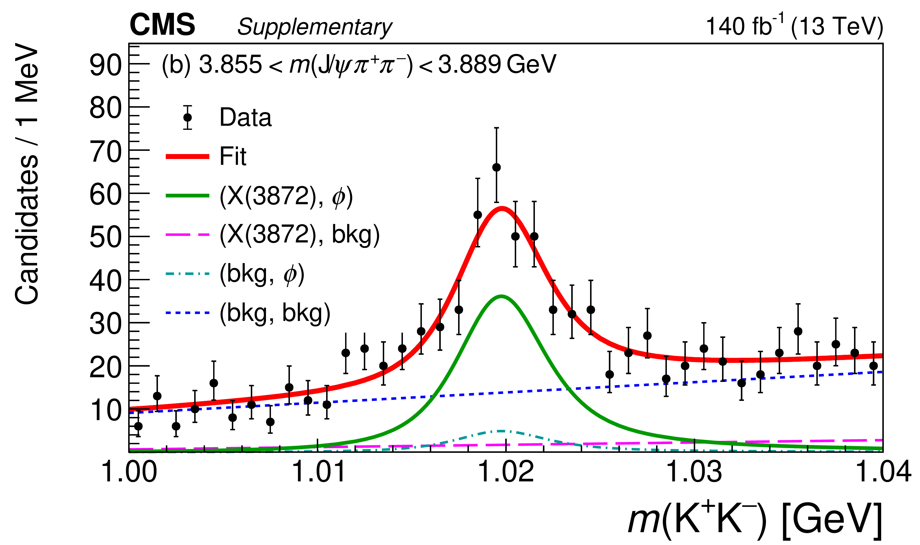
Figure 2:
The observed $\mathrm{J/\psi}\pi^{+}\pi^{-}$ (left) and ${\mathrm{K^{+}} \mathrm{K^{-}}}$ (right) invariant mass distributions for the ${\mathrm{B_{s}^{0}} \to \mathrm{X(3872)} \phi}$ candidates are shown by the points, with the vertical bars representing the statistical uncertainties. The projections of the 2D fit and its various components are shown by the lines. |
png pdf |
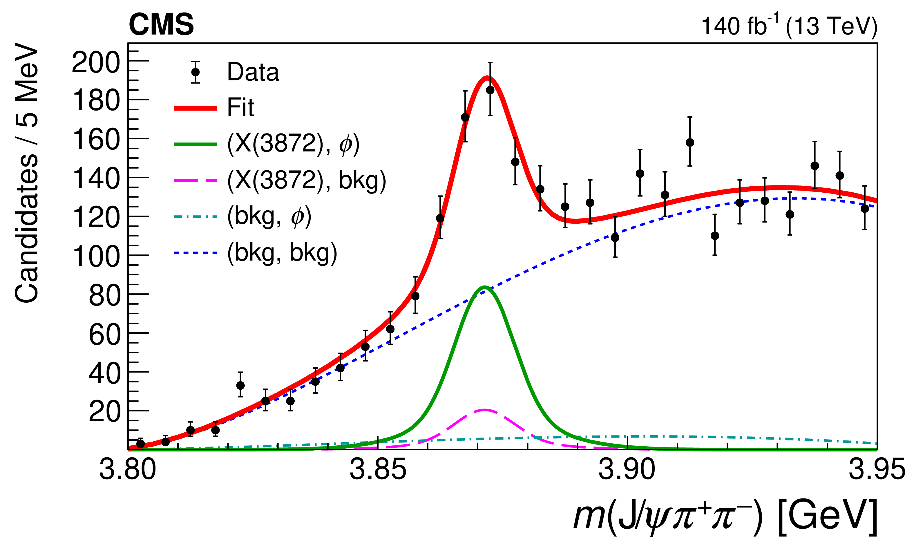
Figure 2-a:
The observed $\mathrm{J/\psi}\pi^{+}\pi^{-}$ invariant mass distribution for the ${\mathrm{B_{s}^{0}} \to \mathrm{X(3872)} \phi}$ candidates is shown by the points, with the vertical bars representing the statistical uncertainties. The projections of the 2D fit and its various components are shown by the lines. |

png pdf |
Figure 2-b:
The observed ${\mathrm{K^{+}} \mathrm{K^{-}}}$ invariant mass distribution for the ${\mathrm{B_{s}^{0}} \to \mathrm{X(3872)} \phi}$ candidates is shown by the points, with the vertical bars representing the statistical uncertainties. The projections of the 2D fit and its various components are shown by the lines. |
png pdf |
Figure 3:
Background-subtracted $\psi(\text{2S})\phi $ (left) and $\mathrm{X(3872)} \phi $ (right) invariant mass distributions obtained by ${{}_{s}\mathcal {P}\mathrm {lot}}$ weighting. The result of each fit and its components are shown by the lines. |
png pdf |
Figure 3-a:
Background-subtracted $\psi(\text{2S})\phi $ invariant mass distribution obtained by ${{}_{s}\mathcal {P}\mathrm {lot}}$ weighting. The result of each fit and its components are shown by the lines. |
png pdf |
Figure 3-b:
Background-subtracted $\mathrm{X(3872)} \phi $ invariant mass distribution obtained by ${{}_{s}\mathcal {P}\mathrm {lot}}$ weighting. The result of each fit and its components are shown by the lines. |
| Tables | |
png pdf |
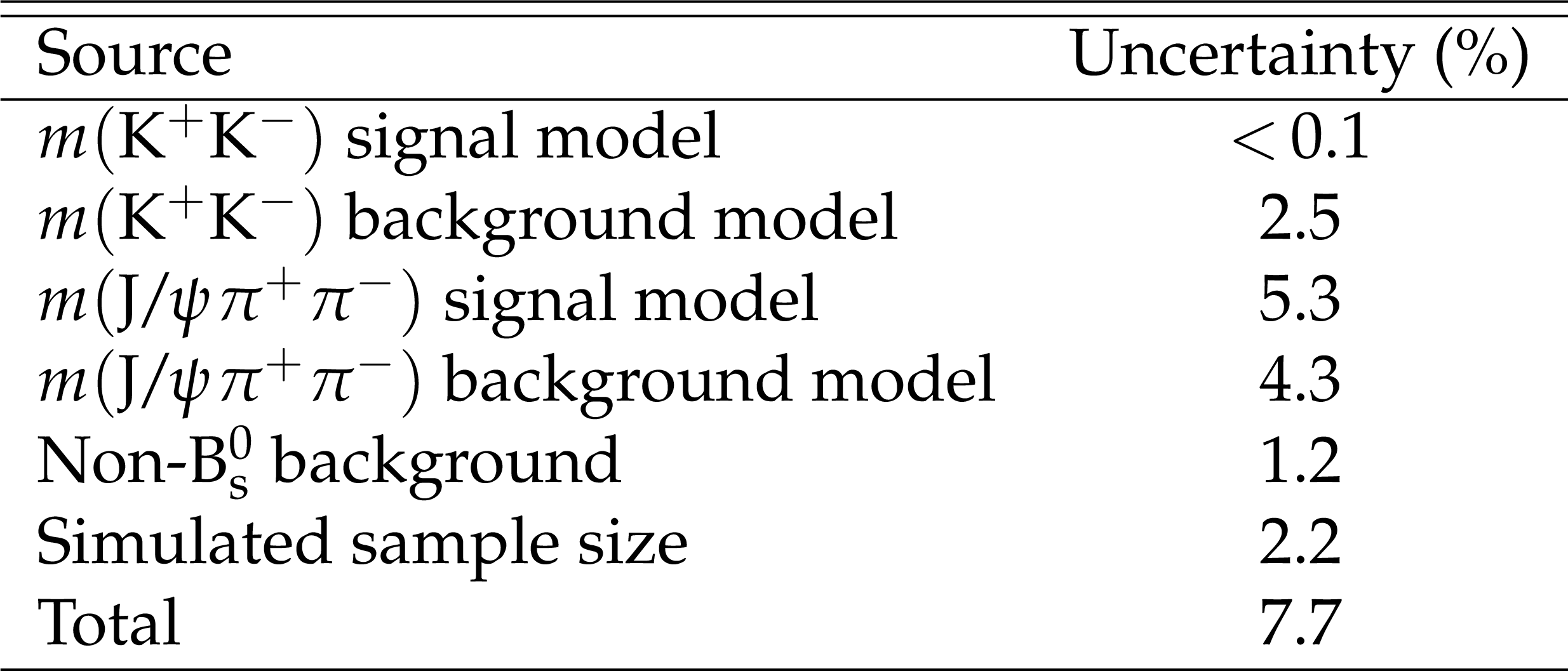
Table 1:
Relative systematic uncertainties in the ratio $R$. |
| Summary |
| In summary, using a data sample corresponding to an integrated luminosity of 140 fb$^{-1}$ of proton-proton collisions collected by the CMS experiment at $\sqrt{s}= $ 13 TeV in 2016--2018, the $\mathrm{B_{s}^{0} \to X(3872)\phi}$ decay is observed for the first time. The comparison with similar decays of $\mathrm{B^{0}}$ and $\mathrm{B^{+}}$ mesons indicates that the $\mathrm{X(3872)}$ formation in B meson decays is different from $\psi(\text{2S})$ formation, suggesting that $\mathrm{X(3872)}$ is not a pure charmonium state and supporting similar conclusions derived from other experimental measurements [2, 5, 8–12]. This observation may shed new light on the nature of the $\mathrm{X(3872)}$ particle. |
| Additional Figures | |

png pdf |
Additional Figure 1:
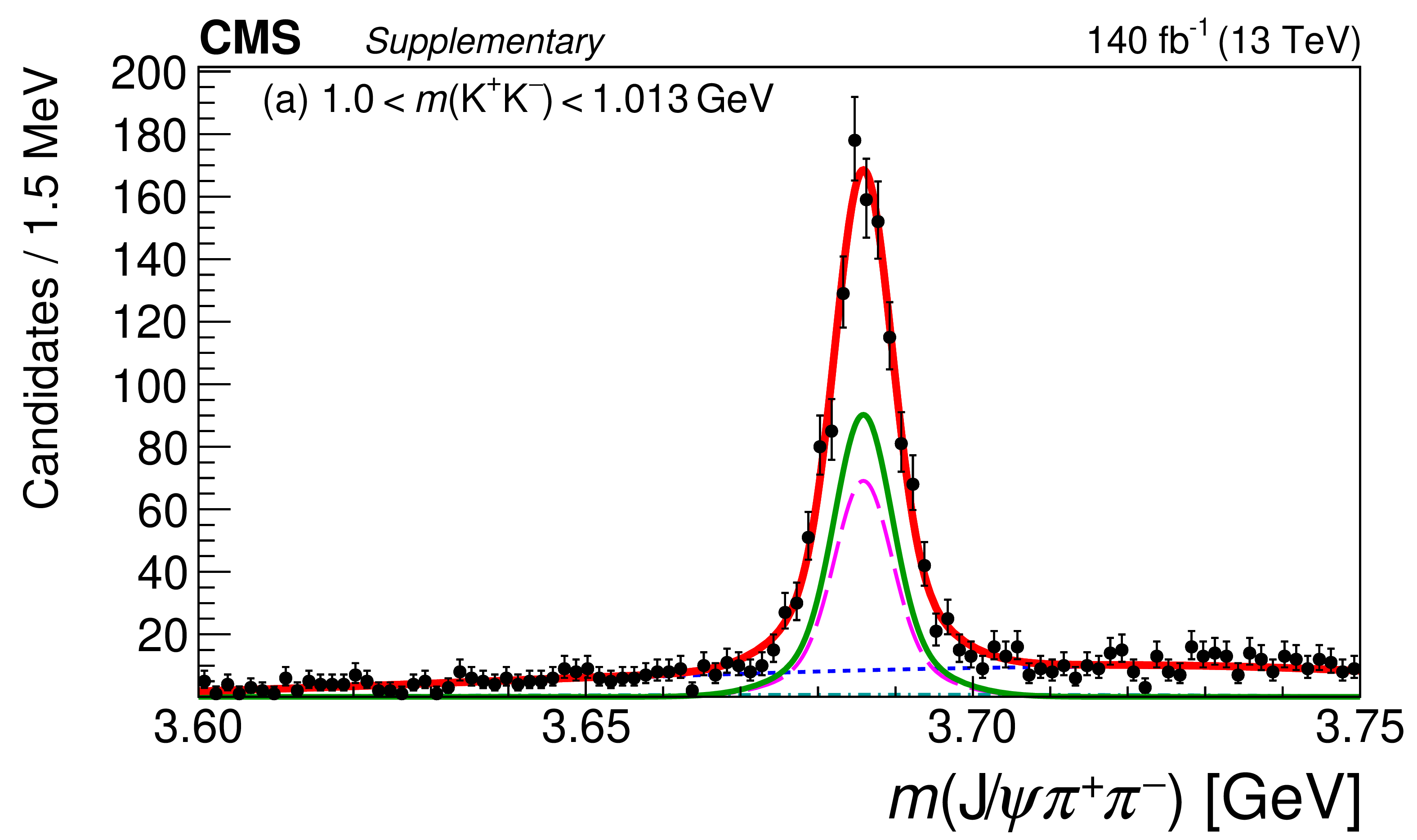
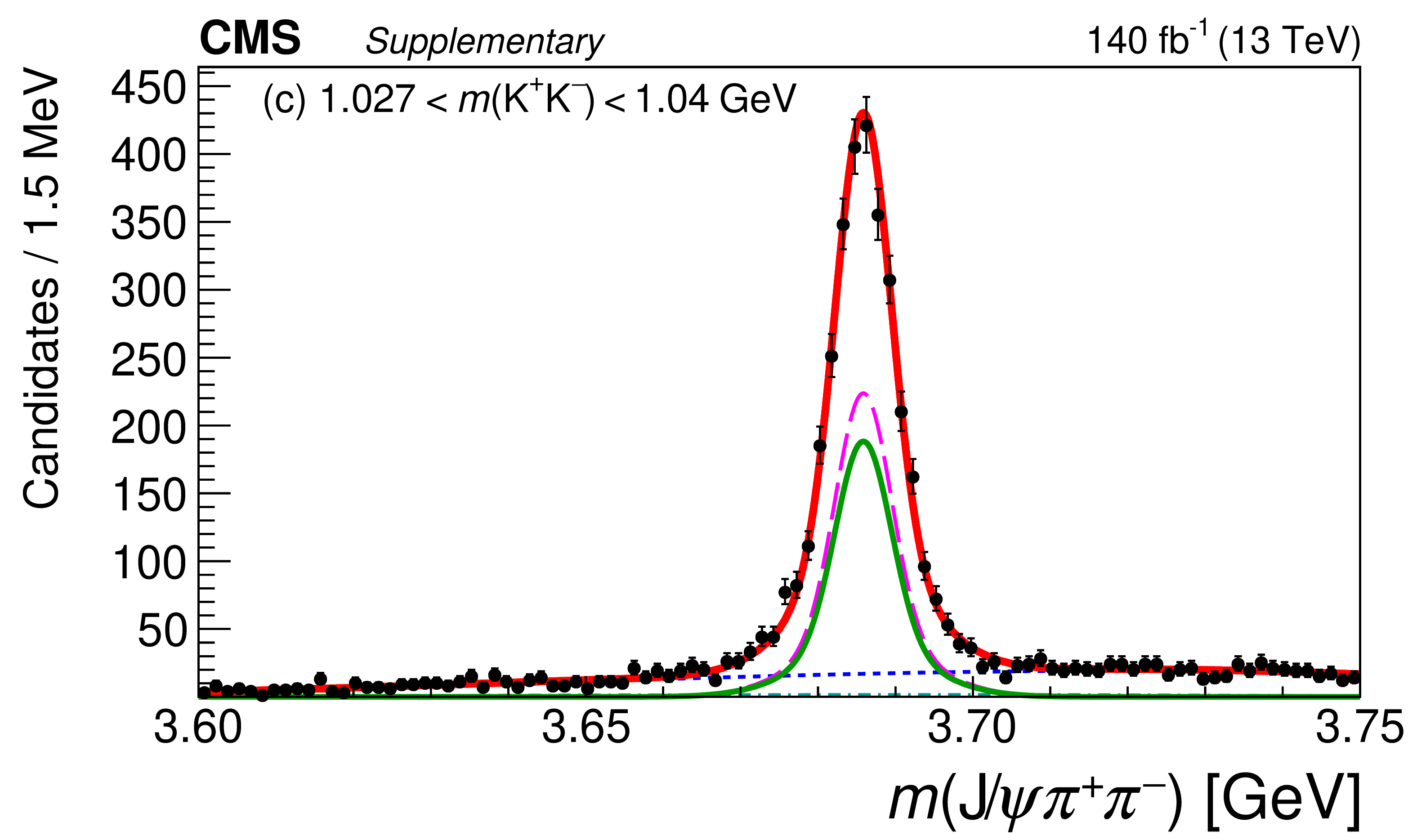
The observed $ {\mathrm {J}/\psi} \, {\pi ^{+}} {\pi ^{-}} $ invariant mass distribution for the selected $ {\mathrm {B}^0_\mathrm {s}} \to {\psi \mathrm {(2S)}}\, \phi$ candidates in three ranges of $m({\mathrm {K^{+}}} {\mathrm {K^{-}}})$: (a) left $\phi$ sideband, (b) $\phi$ signal region, (c) right $\phi$ sideband. The projections of the two dimensional fit and its various components are shown by the lines explained in the legend in (b). |
png pdf |
Additional Figure 1-a:
The observed $ {\mathrm {J}/\psi} \, {\pi ^{+}} {\pi ^{-}} $ invariant mass distribution for the selected $ {\mathrm {B}^0_\mathrm {s}} \to {\psi \mathrm {(2S)}}\, \phi$ candidates in three ranges of $m({\mathrm {K^{+}}} {\mathrm {K^{-}}})$: left $\phi$ sideband. |

png pdf |
Additional Figure 1-b:
The observed $ {\mathrm {J}/\psi} \, {\pi ^{+}} {\pi ^{-}} $ invariant mass distribution for the selected $ {\mathrm {B}^0_\mathrm {s}} \to {\psi \mathrm {(2S)}}\, \phi$ candidates in three ranges of $m({\mathrm {K^{+}}} {\mathrm {K^{-}}})$: $\phi$ signal region. The projection of the two dimensional fit and its various components are shown by the lines explained in the legend. |
png pdf |
Additional Figure 1-c:
The observed $ {\mathrm {J}/\psi} \, {\pi ^{+}} {\pi ^{-}} $ invariant mass distribution for the selected $ {\mathrm {B}^0_\mathrm {s}} \to {\psi \mathrm {(2S)}}\, \phi$ candidates in three ranges of $m({\mathrm {K^{+}}} {\mathrm {K^{-}}})$: right $\phi$ sideband. |

png pdf |
Additional Figure 2:
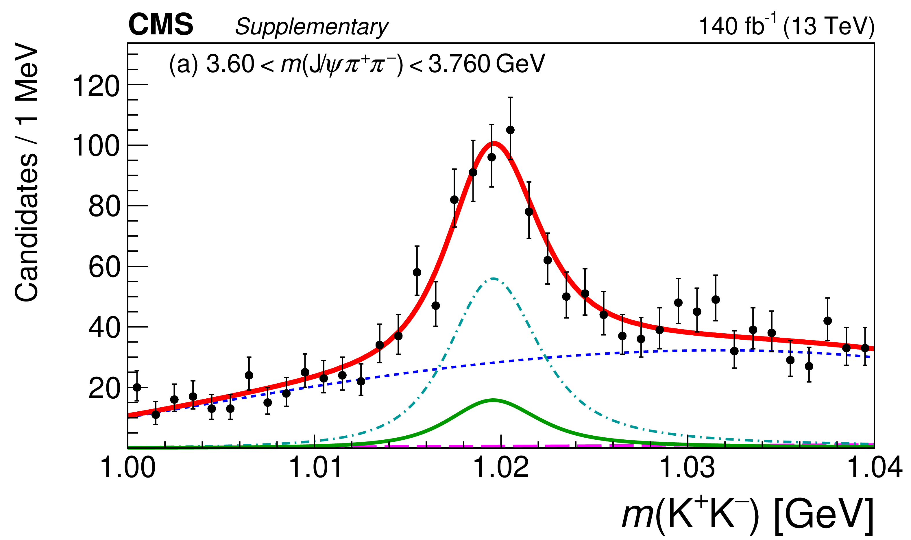
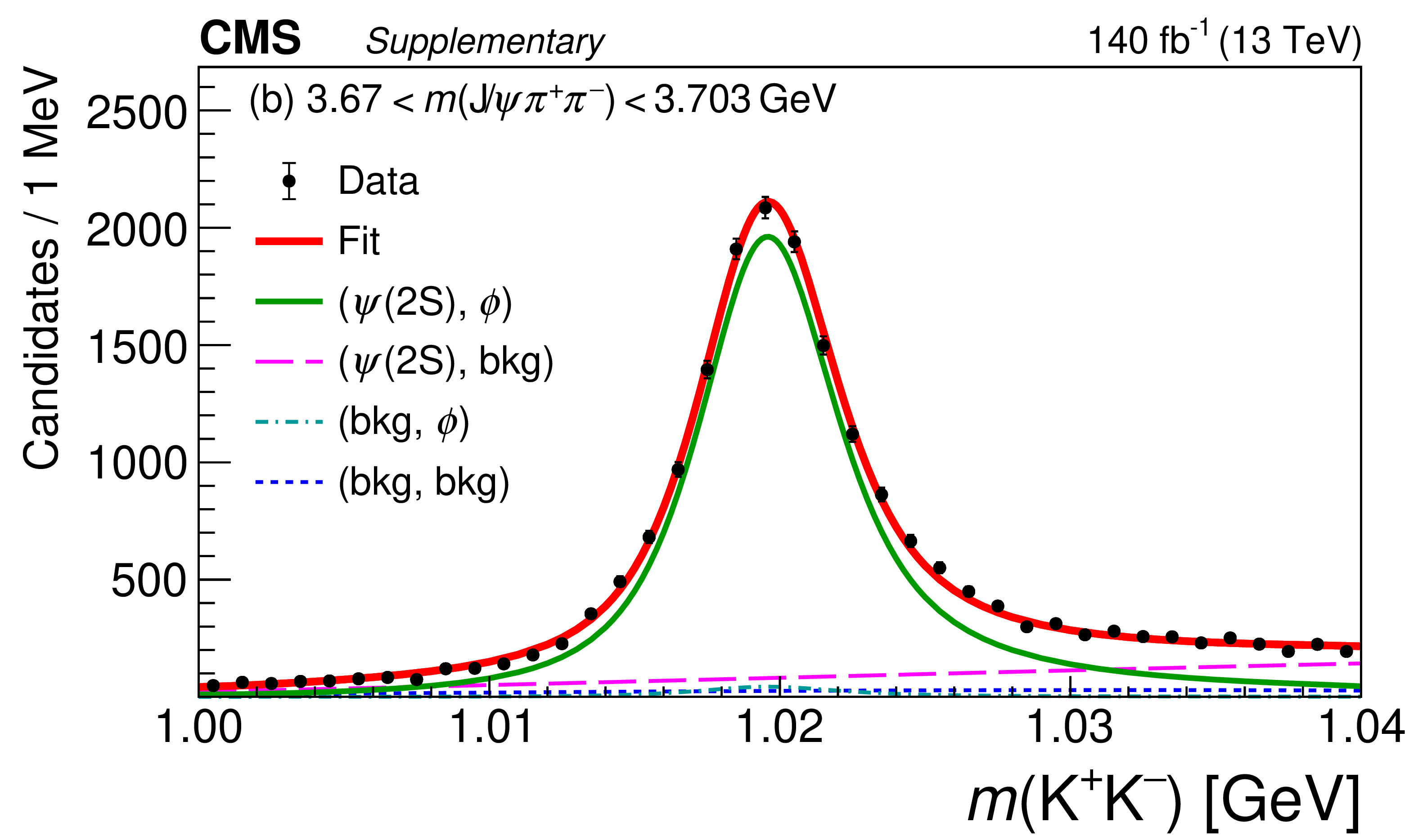
The observed $ {\mathrm {K^{+}}} {\mathrm {K^{-}}}$ invariant mass distribution for the selected $ {\mathrm {B}^0_\mathrm {s}} \to {\psi \mathrm {(2S)}}\, \phi$ candidates in three ranges of $m({\mathrm {J}/\psi} \, {\pi ^{+}} {\pi ^{-}})$: (a) left ${\psi \mathrm {(2S)}}$ sideband, (b) ${\psi \mathrm {(2S)}}$ signal region, (c) right ${\psi \mathrm {(2S)}}$ sideband. The projections of the two dimensional fit and its various components are shown by the lines explained in the legend in (b). |
png pdf |
Additional Figure 2-a:
The observed $ {\mathrm {K^{+}}} {\mathrm {K^{-}}}$ invariant mass distribution for the selected $ {\mathrm {B}^0_\mathrm {s}} \to {\psi \mathrm {(2S)}}\, \phi$ candidates in three ranges of $m({\mathrm {J}/\psi} \, {\pi ^{+}} {\pi ^{-}})$: left ${\psi \mathrm {(2S)}}$ sideband. |
png pdf |
Additional Figure 2-b:
The observed $ {\mathrm {K^{+}}} {\mathrm {K^{-}}}$ invariant mass distribution for the selected $ {\mathrm {B}^0_\mathrm {s}} \to {\psi \mathrm {(2S)}}\, \phi$ candidates in three ranges of $m({\mathrm {J}/\psi} \, {\pi ^{+}} {\pi ^{-}})$: ${\psi \mathrm {(2S)}}$ signal region. The projection of the two dimensional fit and its various components are shown by the lines explained in the legend. |

png pdf |
Additional Figure 2-c:
The observed $ {\mathrm {K^{+}}} {\mathrm {K^{-}}}$ invariant mass distribution for the selected $ {\mathrm {B}^0_\mathrm {s}} \to {\psi \mathrm {(2S)}}\, \phi$ candidates in three ranges of $m({\mathrm {J}/\psi} \, {\pi ^{+}} {\pi ^{-}})$: right ${\psi \mathrm {(2S)}}$ sideband. |
png pdf |
Additional Figure 3:
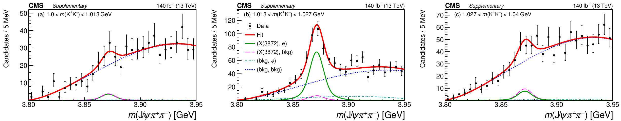
The observed $ {\mathrm {J}/\psi} \, {\pi ^{+}} {\pi ^{-}} $ invariant mass distribution for the selected $ {\mathrm {B}^0_\mathrm {s}} \to \mathrm {X}(3872)\, \phi$ candidates in three ranges of $m({\mathrm {K^{+}}} {\mathrm {K^{-}}})$: (a) left $\phi$ sideband, (b) $\phi$ signal region, (c) right $\phi$ sideband. The projections of the two dimensional fit and its various components are shown by the lines explained in the legend in (b). |

png pdf |
Additional Figure 3-a:
The observed $ {\mathrm {J}/\psi} \, {\pi ^{+}} {\pi ^{-}} $ invariant mass distribution for the selected $ {\mathrm {B}^0_\mathrm {s}} \to \mathrm {X}(3872)\, \phi$ candidates in three ranges of $m({\mathrm {K^{+}}} {\mathrm {K^{-}}})$: left $\phi$ sideband. |
png pdf |
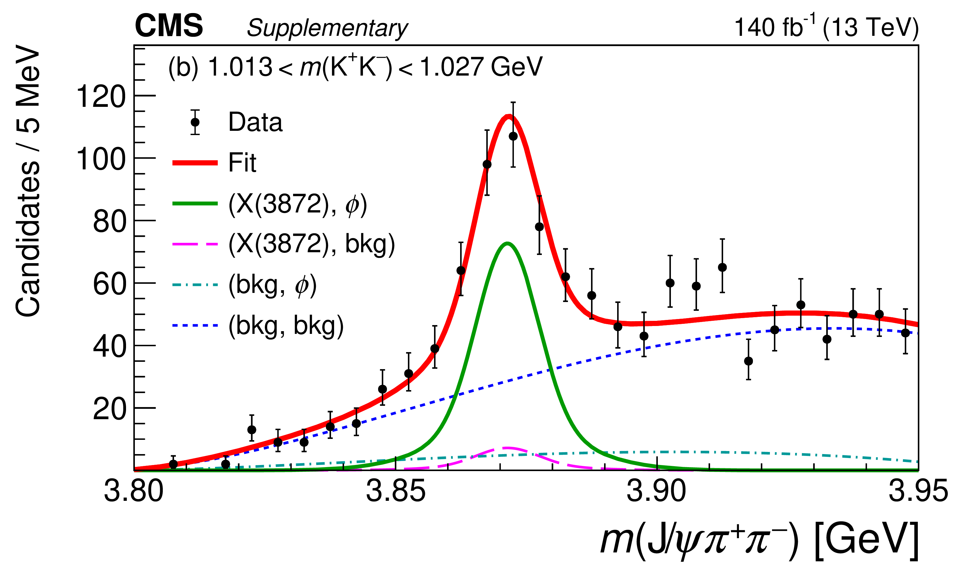
Additional Figure 3-b:
The observed $ {\mathrm {J}/\psi} \, {\pi ^{+}} {\pi ^{-}} $ invariant mass distribution for the selected $ {\mathrm {B}^0_\mathrm {s}} \to \mathrm {X}(3872)\, \phi$ candidates in three ranges of $m({\mathrm {K^{+}}} {\mathrm {K^{-}}})$: $\phi$ signal region. right $\phi$ sideband. The projection of the two dimensional fit and its various components are shown by the lines explained in the legend. |
png pdf |
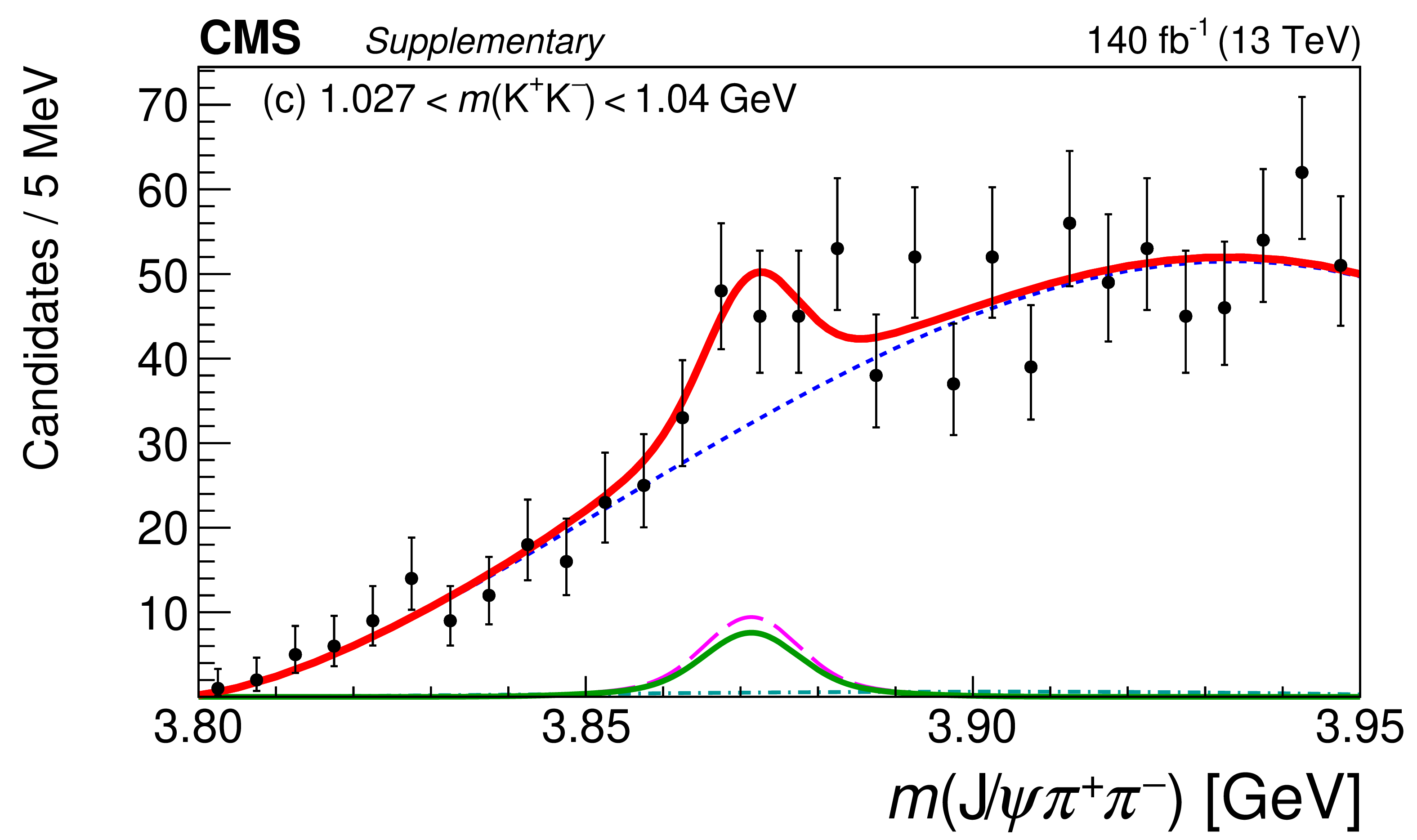
Additional Figure 3-c:
The observed $ {\mathrm {J}/\psi} \, {\pi ^{+}} {\pi ^{-}} $ invariant mass distribution for the selected $ {\mathrm {B}^0_\mathrm {s}} \to \mathrm {X}(3872)\, \phi$ candidates in three ranges of $m({\mathrm {K^{+}}} {\mathrm {K^{-}}})$: right $\phi$ sideband. |
png pdf |
Additional Figure 4:
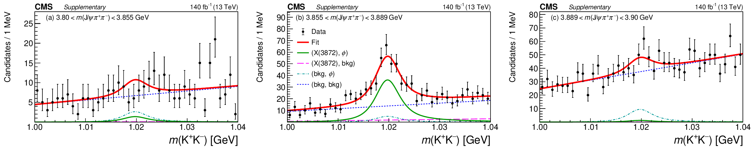
The observed $ {\mathrm {K^{+}}} {\mathrm {K^{-}}}$ invariant mass distribution for the selected $ {\mathrm {B}^0_\mathrm {s}} \to \mathrm {X}(3872)\, \phi$ candidates in three ranges of $m({\mathrm {J}/\psi} \, {\pi ^{+}} {\pi ^{-}})$: (a) left $\mathrm {X}$ sideband, (b) $\mathrm {X}$ signal region, (c) right $\mathrm {X}$ sideband. The projections of the two dimensional fit and its various components are shown by the lines explained in the legend in (b). |
png pdf |
Additional Figure 4-a:
The observed $ {\mathrm {K^{+}}} {\mathrm {K^{-}}}$ invariant mass distribution for the selected $ {\mathrm {B}^0_\mathrm {s}} \to \mathrm {X}(3872)\, \phi$ candidates in three ranges of $m({\mathrm {J}/\psi} \, {\pi ^{+}} {\pi ^{-}})$: left $\mathrm {X}$ sideband. |
png pdf |
Additional Figure 4-b:
The observed $ {\mathrm {K^{+}}} {\mathrm {K^{-}}}$ invariant mass distribution for the selected $ {\mathrm {B}^0_\mathrm {s}} \to \mathrm {X}(3872)\, \phi$ candidates in three ranges of $m({\mathrm {J}/\psi} \, {\pi ^{+}} {\pi ^{-}})$: $\mathrm {X}$ signal region. The projection of the two dimensional fit and its various components are shown by the lines explained in the legend. |

png pdf |
Additional Figure 4-c:
The observed $ {\mathrm {K^{+}}} {\mathrm {K^{-}}}$ invariant mass distribution for the selected $ {\mathrm {B}^0_\mathrm {s}} \to \mathrm {X}(3872)\, \phi$ candidates in three ranges of $m({\mathrm {J}/\psi} \, {\pi ^{+}} {\pi ^{-}})$: right $\mathrm {X}$ sideband. |
png pdf |
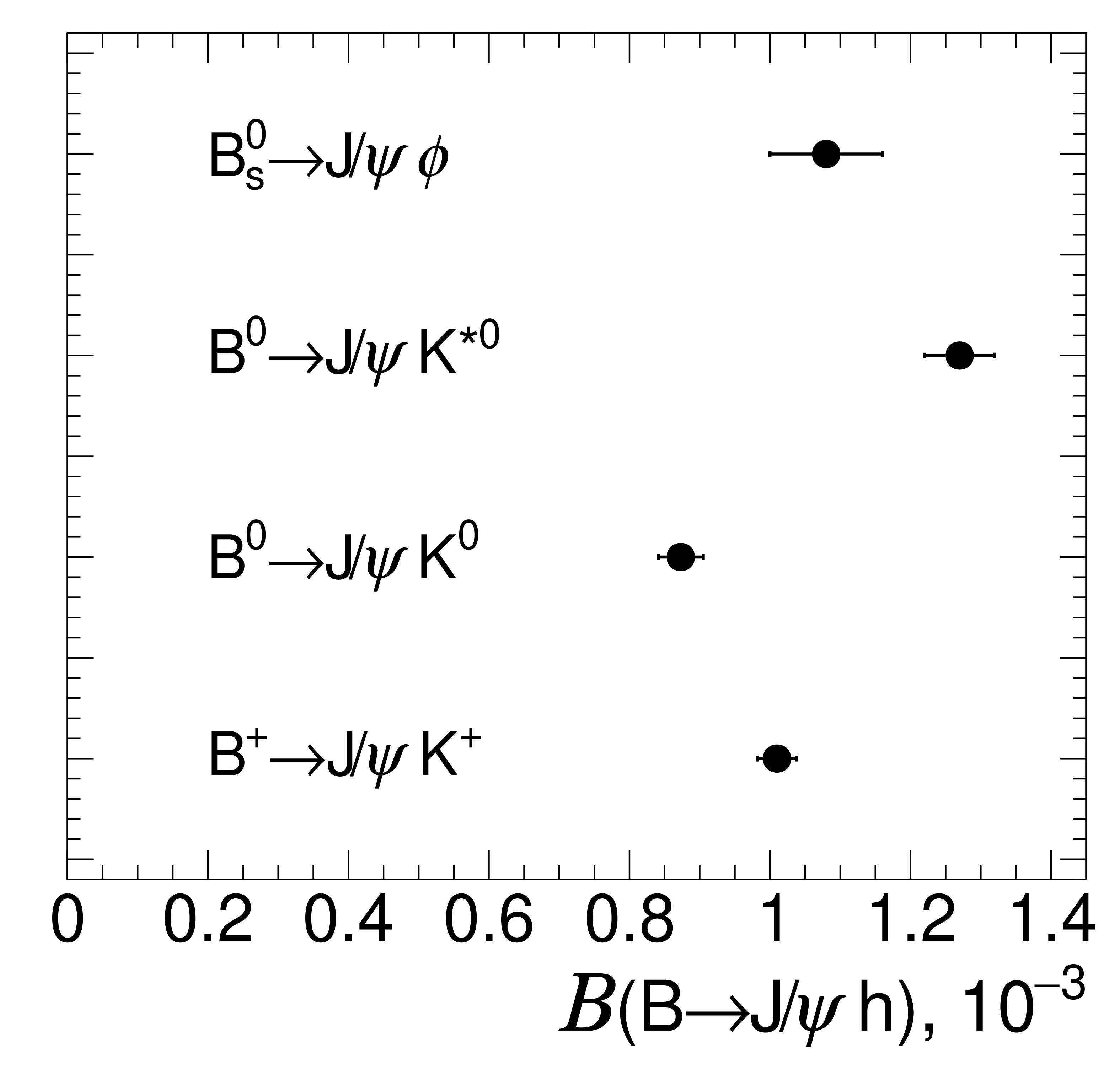
Additional Figure 5:
Comparison of the branching fractions $\mathcal {B}({{\mathrm {B}}}\to {\mathrm {J}/\psi}\, \mathrm {h})$ for ${{\mathrm {B}^{+}}}$, ${{\mathrm {B}^0}}$, and ${\mathrm {B}^0_\mathrm {s}}$ decays. The values are taken from Ref. [4]. |
png pdf |
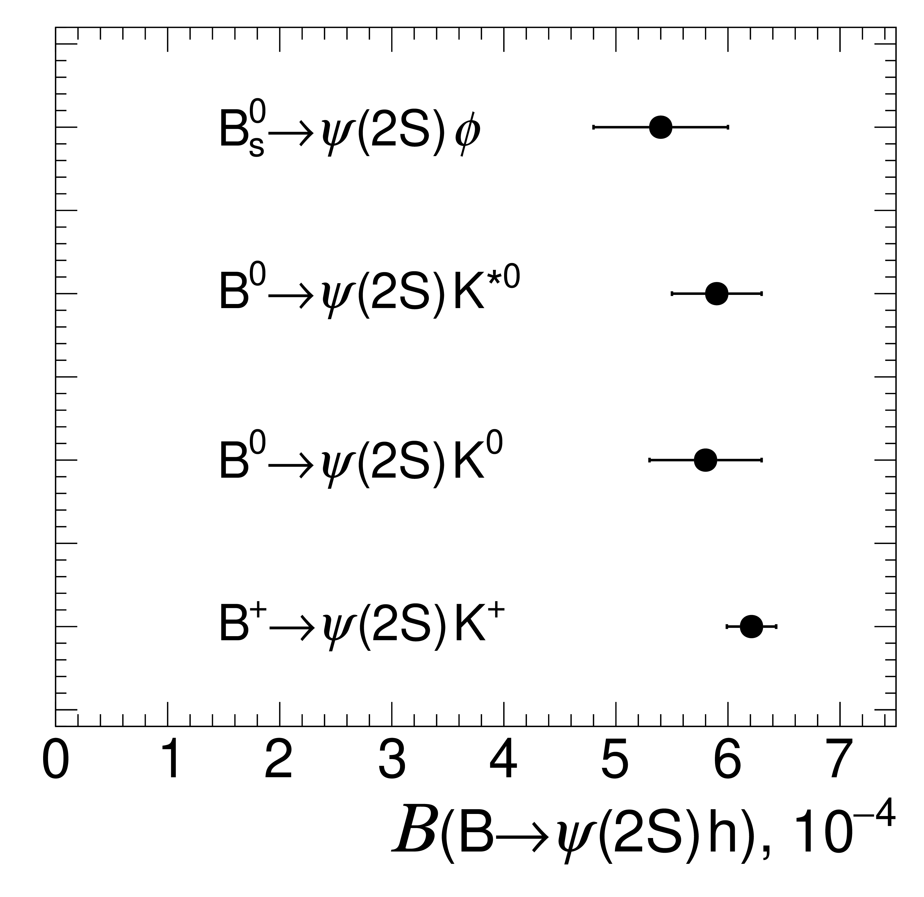
Additional Figure 6:
Comparison of the branching fractions $\mathcal {B}({{\mathrm {B}}}\to {\psi \mathrm {(2S)}}\, \mathrm {h})$ for ${{\mathrm {B}^{+}}}$, ${{\mathrm {B}^0}}$, and ${\mathrm {B}^0_\mathrm {s}}$ decays. The values are taken from Ref. [4]. |
png pdf |
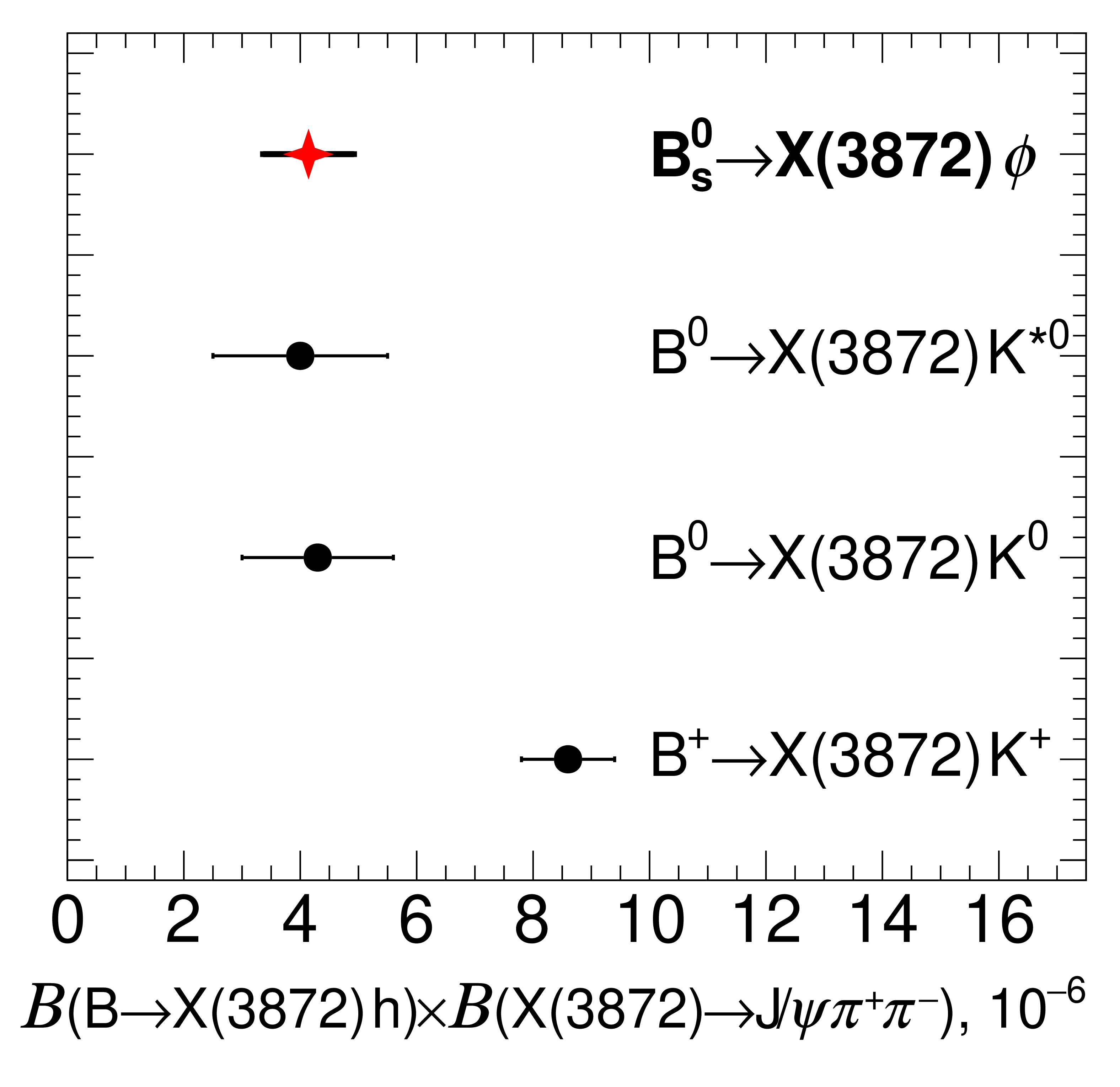
Additional Figure 7:
Comparison of the branching fraction products $\mathcal {B}({{\mathrm {B}}}\to \mathrm {X}(3872)\, \mathrm {h})\times \mathcal {B}(\mathrm {X}(3872)\to {\mathrm {J}/\psi} \, {\pi ^{+}} {\pi ^{-}})$ for ${{\mathrm {B}^{+}}}$, ${{\mathrm {B}^0}}$ [4], and ${\mathrm {B}^0_\mathrm {s}}$ decays, where the last result by CMS is highlighted in red. |
| References | ||||
| 1 | M. B. Voloshin | Charmonium | Prog. Part. NP 61 (2008) 455 | 0711.4556 |
| 2 | N. Brambilla et al. | Heavy quarkonium: Progress, puzzles, and opportunities | EPJC 71 (2011) 1534 | 1010.5827 |
| 3 | Belle Collaboration | Observation of a narrow charmoniumlike state in exclusive $ \mathrm{B^{\pm}}\to\mathrm{K^{\pm}}\pi^{+}\pi^{-}\mathrm{J/\psi} $ decays | PRL 91 (2003) 262001 | hep-ex/0309032 |
| 4 | Particle Data Group, M. Tanabashi et al. | Review of particle physics | PRD 98 (2018) 030001 | |
| 5 | Belle Collaboration | Bounds on the width, mass difference and other properties of $ \mathrm{X(3872)} \to \pi^+ \pi^- \mathrm{J/\psi} $ decays | PRD 84 (2011) 052004 | 1107.0163 |
| 6 | N. Brambilla et al. | The XYZ states: experimental and theoretical status and perspectives | 1907.07583 | |
| 7 | CDF Collaboration | The $ \mathrm{X(3872)} $ at CDF II | Int. J. Mod. Phys. A 20 (2005) 3765 | hep-ex/0409052 |
| 8 | CMS Collaboration | Measurement of the $ \mathrm{X(3872)} $ production cross section via decays to $ \mathrm{J/\psi \pi^{+}\pi^{-}} $ in pp collisions at $ \sqrt{s} = $ 7 TeV | JHEP 04 (2013) 154 | CMS-BPH-11-011 1302.3968 |
| 9 | ATLAS Collaboration | Measurements of $ \psi(\text{2S}) $ and $ \mathrm{X(3872)}\to \mathrm{J/\psi \pi^{+}\pi^{-}} $ production in pp collisions at $ \sqrt{s} = $ 8 TeV with the ATLAS detector | JHEP 01 (2017) 117 | 1610.09303 |
| 10 | CDF Collaboration | Analysis of the quantum numbers $ J^{PC} $ of the $ \mathrm{X(3872)} $ | PRL 98 (2007) 132002 | hep-ex/0612053 |
| 11 | LHCb Collaboration | Determination of the $ \mathrm{X(3872)} $ meson quantum numbers | PRL 110 (2013) 222001 | 1302.6269 |
| 12 | LHCb Collaboration | Quantum numbers of the $ \mathrm{X(3872)} $ state and orbital angular momentum in its $ \rho^0 \mathrm{J/\psi} $ decay | PRD 92 (2015) 011102 | 1504.06339 |
| 13 | CDF Collaboration | Measurement of the dipion mass spectrum in $ \mathrm{X(3872)}\to \mathrm{J/\psi \pi^{+}\pi^{-}} $ decays | PRL 96 (2006) 102002 | hep-ex/0512074 |
| 14 | CMS Collaboration | The CMS experiment at the CERN LHC | JINST 3 (2008) S08004 | CMS-00-001 |
| 15 | CMS Collaboration | The CMS trigger system | JINST 12 (2017) P01020 | CMS-TRG-12-001 1609.02366 |
| 16 | T. Sjostrand et al. | An introduction to PYTHIA 8.2 | CPC 191 (2015) 159 | 1410.3012 |
| 17 | D. J. Lange | The EvtGen particle decay simulation package | NIMA 462 (2001) 152 | |
| 18 | E. Barberio, B. van Eijk, and Z. Was | PHOTOS --- a universal Monte Carlo for QED radiative corrections in decays | CPC 66 (1991) 115 | |
| 19 | E. Barberio and Z. Was | PHOTOS -- a universal Monte Carlo for QED radiative corrections: version 2.0 | CPC 79 (1994) 291 | |
| 20 | GEANT4 Collaboration | GEANT4--A simulation toolkit | NIMA 506 (2003) 250 | |
| 21 | CMS Collaboration | Performance of CMS muon reconstruction in pp collision events at $ \sqrt{s} = $ 7 TeV | JINST 7 (2012) P10002 | CMS-MUO-10-004 1206.4071 |
| 22 | CMS Collaboration | Description and performance of track and primary-vertex reconstruction with the CMS tracker | JINST 9 (2014) P10009 | CMS-TRK-11-001 1405.6569 |
| 23 | CMS Collaboration | Search for the X(5568) state decaying into $ \mathrm{B}^{0}_{\mathrm{s}}\pi^{\pm} $ in proton-proton collisions at $ \sqrt{s} = $ 8 TeV | PRL 120 (2018) 202005 | CMS-BPH-16-002 1712.06144 |
| 24 | CMS Collaboration | Studies of $ {\mathrm {B}}^{*}_{\mathrm {s}2}(5840)^0 $ and $ {\mathrm {B}}_{{\mathrm {s}}1}(5830)^0 $ mesons including the observation of the $ {\mathrm {B}}^{*}_{\mathrm {s}2}(5840)^0 \rightarrow {\mathrm {B}} ^0 \mathrm {K} ^0_{\mathrm {S}} $ decay in proton-proton collisions at $ \sqrt{s}= $ 8 TeV | EPJC 78 (2018) 939 | CMS-BPH-16-003 1809.03578 |
| 25 | CMS Collaboration | Study of the $ {\mathrm{B}}^{+}\to \mathrm{J}/\psi \overline{\Lambda}\mathrm{p} $ decay in proton-proton collisions at $ \sqrt{s} = $ 8 TeV | JHEP 12 (2019) 100 | CMS-BPH-18-005 1907.05461 |
| 26 | CMS Collaboration | Observation of the $ \Lambda_\mathrm{b}^0 \to\mathrm{J/\psi} \Lambda \phi $ decay in proton-proton collisions at $ \sqrt{s}= $ 13 TeV | PLB 802 (2020) 135203 | CMS-BPH-19-002 1911.03789 |
| 27 | CMS Collaboration | Observation of two excited B$ ^+_\mathrm{c} $ states and measurement of the B$ ^+_\mathrm{c} $(2S) mass in pp collisions at $ \sqrt{s} = $ 13 TeV | PRL 122 (2019) 132001 | CMS-BPH-18-007 1902.00571 |
| 28 | CMS Collaboration | Study of excited $ \Lambda_\mathrm{b}^0 $ states decaying to $ \Lambda_\mathrm{b}^0\pi^+\pi^- $ in proton-proton collisions at $ \sqrt{s} = $ 13 TeV | PLB 803 (2020) 135345 | CMS-BPH-19-003 2001.06533 |
| 29 | G. Punzi | Sensitivity of searches for new signals and its optimization | in Statistical problems in particle physics, astrophysics and cosmology. PHYSTAT 2003, Stanford | physics/0308063 |
| 30 | G. Cowan, K. Cranmer, E. Gross, and O. Vitells | Asymptotic formulae for likelihood-based tests of new physics | EPJC 71 (2011) 1554 | 1007.1727 |
| 31 | S. S. Wilks | The large-sample distribution of the likelihood ratio for testing composite hypotheses | Annals Math. Statist. 9 (1938) 60 | |
| 32 | M. Pivk and F. R. Le Diberder | $ {{}_{s}\mathcal {P}\mathrm {lot}} $: a statistical tool to unfold data distributions | NIMA 555 (2005) 356 | physics/0402083 |
| 33 | S. Jackman | Bayesian analysis for the social sciences | John Wiley \& Sons, New Jersey, USA | |
|
|
Compact Muon Solenoid LHC, CERN |
|

|

|

|

|

|