

Compact Muon Solenoid
LHC, CERN
| CMS-SMP-21-004 ; CERN-EP-2023-279 | ||
| Nonresonant central exclusive production of charged-hadron pairs in proton-proton collisions at $ \sqrt{s} = $ 13 TeV | ||
| CMS and TOTEM Collaborations | ||
| 25 January 2024 | ||
| Accepted for publication in Phys. Rev. D | ||
| Abstract: The central exclusive production of charged-hadron pairs in pp collisions at a centre-of-mass energy of 13 TeV is examined, based on data collected in a special high-$ \beta^* $ run of the LHC. The nonresonant continuum processes are studied with the invariant mass of the centrally produced two-pion system in the resonance-free region, $ m_{\pi^{+}\pi^{-}} < $ 0.7 GeV or $ m_{\pi^{+}\pi^{-}} > $ 1.8 GeV. Differential cross sections as functions of the azimuthal angle between the surviving protons, squared exchanged four-momenta, and $ m_{\pi^{+}\pi^{-}} $ are measured in a wide region of scattered proton transverse momenta, between 0.2 and 0.8 GeV, and for pion rapidities $ |y| < $ 2. A rich structure of interactions related to double-pomeron exchange is observed. A parabolic minimum in the distribution of the two-proton azimuthal angle is observed for the first time. It can be interpreted as an effect of additional pomeron exchanges between the protons from the interference between the bare and the rescattered amplitudes. After model tuning, various physical quantities are determined that are related to the pomeron cross section, proton-pomeron and meson-pomeron form factors, pomeron trajectory and intercept, and coefficients of diffractive eigenstates of the proton. | ||
| Links: e-print arXiv:2401.14494 [hep-ex] (PDF) ; CDS record ; inSPIRE record ; HepData record ; Physics Briefing ; CADI line (restricted) ; | ||
| Figures | |
png pdf |
Figure 1:
Born-level Feynman diagrams for central exclusive production of hadron pairs via double-pomeron exchange, depicting resonant (left) and nonresonant continuum (centre: $ t $-channel, right: $ u $-channel) contributions. |

png pdf |
Figure 2:
Feynman diagram for the nonresonant continuum of central exclusive production of hadron pairs via double-pomeron exchange, including the rescattering correction. |
png pdf |
Figure 3:
Left: Fraction of elastic-like events left after the veto trigger as functions of momentum components in the $ y $ direction in Arms 1 and 2, shown here for the two diagonal trigger configurations: bottom pots in Arm 2 with top pots in Arm 1 (upper left), and top pots in Arm 2 with bottom pots in Arm 1 (lower left). Centre and right: Joint distribution of detected proton momenta $ (p_{1,y},p_{2,y}) $ in Arms 1 and 2 for all four trigger configurations (centre: TB and BT, right: TT and BB). Limits of single-proton acceptance are indicated with long dashed lines. |
png pdf |
Figure 4:
Calculated detection efficiencies for the pair of scattered protons as functions of their transverse momenta $ (p_\text{1,T}, p_\text{2,T}) $ in some selected bins of the pp azimuthal angle $ \phi $ (indicated on the right side of each row). The first four columns show the efficiencies for each trigger configuration, the four rows show four different angular ranges, and the rightmost column displays the coverage of the measurement with colour codes (white: not covered; green: covered by at least one configuration; red: covered by all configurations). Lines corresponding to 0.2 GeV are drawn in the rightmost plots. |
png pdf |
Figure 4-a:
Calculated detection efficiencies for the pair of scattered protons as functions of their transverse momenta $ (p_\text{1,T}, p_\text{2,T}) $ in the bin of the pp azimuthal angle 0 $ < \phi < $ 10$^o$. The first four plots show the efficiencies for each trigger configuration, and the rightmost plot displays the coverage of the measurement with colour codes (white: not covered; green: covered by at least one configuration; red: covered by all configurations). Lines corresponding to 0.2 GeV are drawn in the rightmost plot. |
png pdf |
Figure 4-b:
Calculated detection efficiencies for the pair of scattered protons as functions of their transverse momenta $ (p_\text{1,T}, p_\text{2,T}) $ in the bin of the pp azimuthal angle 45 $ < \phi < $ 50$^o$. The first four plots show the efficiencies for each trigger configuration, and the rightmost plot displays the coverage of the measurement with colour codes (white: not covered; green: covered by at least one configuration; red: covered by all configurations). Lines corresponding to 0.2 GeV are drawn in the rightmost plot. |
png pdf |
Figure 4-c:
Calculated detection efficiencies for the pair of scattered protons as functions of their transverse momenta $ (p_\text{1,T}, p_\text{2,T}) $ in the bin of the pp azimuthal angle 80 $ < \phi < $ 90$^o$. The first four plots show the efficiencies for each trigger configuration, and the rightmost plot displays the coverage of the measurement with colour codes (white: not covered; green: covered by at least one configuration; red: covered by all configurations). Lines corresponding to 0.2 GeV are drawn in the rightmost plot. |
png pdf |
Figure 4-d:
Calculated detection efficiencies for the pair of scattered protons as functions of their transverse momenta $ (p_\text{1,T}, p_\text{2,T}) $ in the bin of the pp azimuthal angle 120 $ < \phi < $ 130$^o$. The first four plots show the efficiencies for each trigger configuration, and the rightmost plot displays the coverage of the measurement with colour codes (white: not covered; green: covered by at least one configuration; red: covered by all configurations). Lines corresponding to 0.2 GeV are drawn in the rightmost plot. |
png pdf |
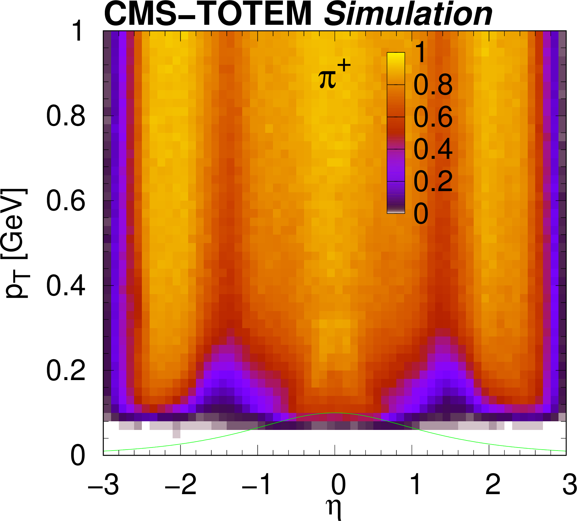
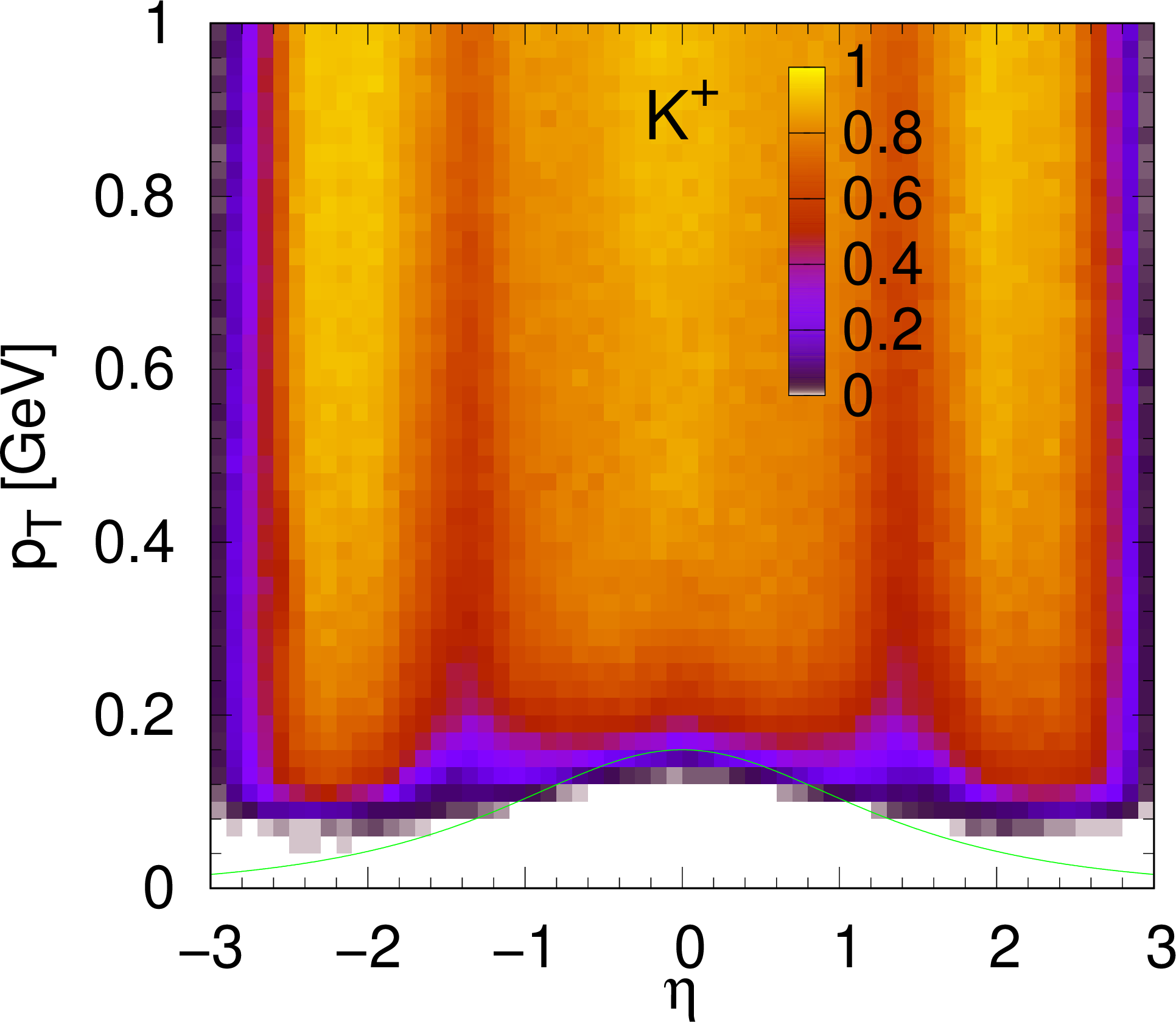
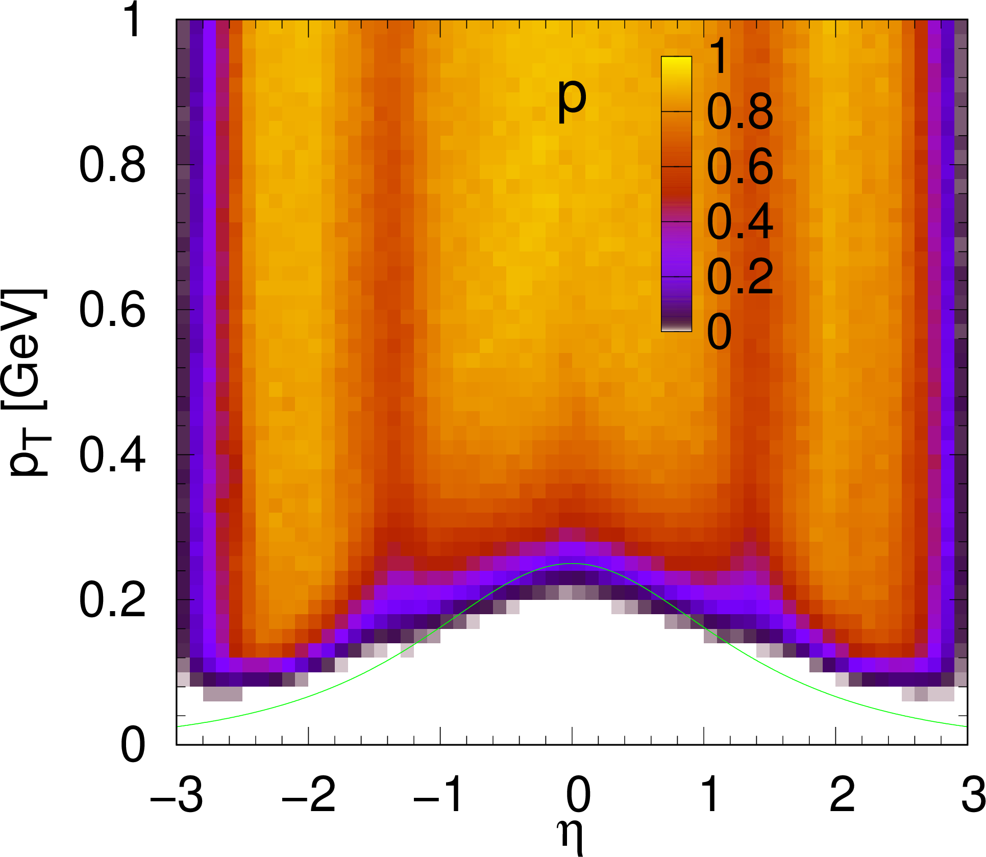
Figure 5:
The combined reconstruction and HLT efficiency (reconstructed and passing the HLT selection) for positively charged pions, kaons, and protons as functions of $ (\eta,p_{\mathrm{T}}) $. Curves indicate constant total momentum ($ p = $ 0.1 GeV for pions, 0.16 GeV for kaons, 0.25 GeV for protons). Plots for negatively charged particles are similar. |
png pdf |
Figure 5-a:
The combined reconstruction and HLT efficiency (reconstructed and passing the HLT selection) for positively charged pions as functions of $ (\eta,p_{\mathrm{T}}) $. Curves indicate constant total momentum ($ p = $ 0.1 0.16 0.25 GeV). Plots for negatively charged pions are similar. |
png pdf |
Figure 5-b:
The combined reconstruction and HLT efficiency (reconstructed and passing the HLT selection) for positively charged kaons as functions of $ (\eta,p_{\mathrm{T}}) $. Curves indicate constant total momentum ($ p = $ 0.1 0.16 0.25 GeV). Plots for negatively charged kaons are similar. |
png pdf |
Figure 5-c:
The combined reconstruction and HLT efficiency (reconstructed and passing the HLT selection) for positively charged protons as functions of $ (\eta,p_{\mathrm{T}}) $. Curves indicate constant total momentum ($ p = $ 0.1 0.16 0.25 GeV). Plots for negatively charged protons are similar. |
png pdf |
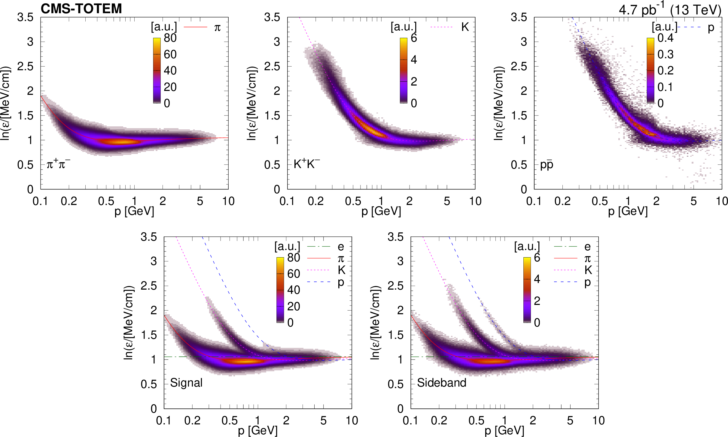
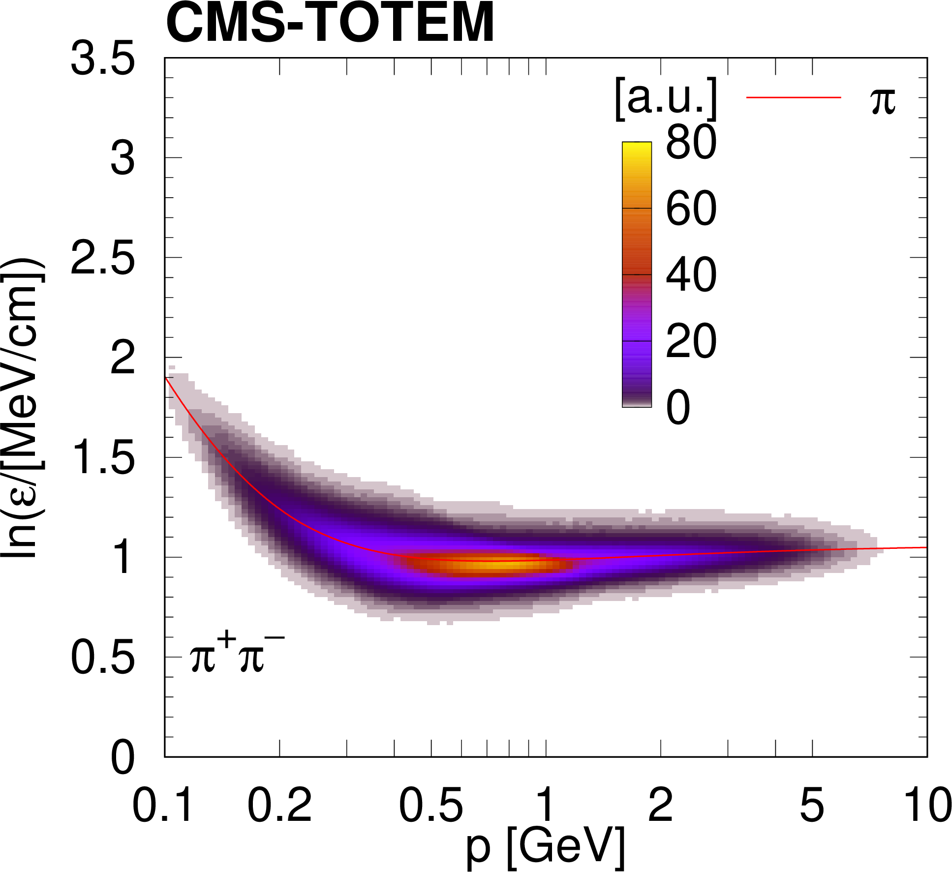
Figure 6:
Distribution of $ \ln\varepsilon $ as a function of total momentum, for reconstructed charged particles in selected two-track events (identified $ \pi^{+}\pi^{-} $, $ \mathrm{K^+}\mathrm{K^-} $, $ \mathrm{p}\overline{\mathrm{p}} $, signal, and sideband; Section 5). The variable $ \varepsilon $ is the most probable energy loss rate at a reference path length $ l_0 = $ 450 m. The colour scale is shown in arbitrary units and is linear. The curves show the expected $ \ln\varepsilon $ for electrons, pions, kaons, and protons (Eq. (34.12) in Ref. [1]). |
png pdf |
Figure 6-a:
Distribution of $ \ln\varepsilon $ as a function of total momentum, for reconstructed charged particles in selected two-track events (identified $ \pi^{+}\pi^{-} $; Section 5). The variable $ \varepsilon $ is the most probable energy loss rate at a reference path length $ l_0 = $ 450 m. The colour scale is shown in arbitrary units and is linear. The curve shows the expected $ \ln\varepsilon $ for pions (Eq. (34.12) in Ref. [1]). |
png pdf |
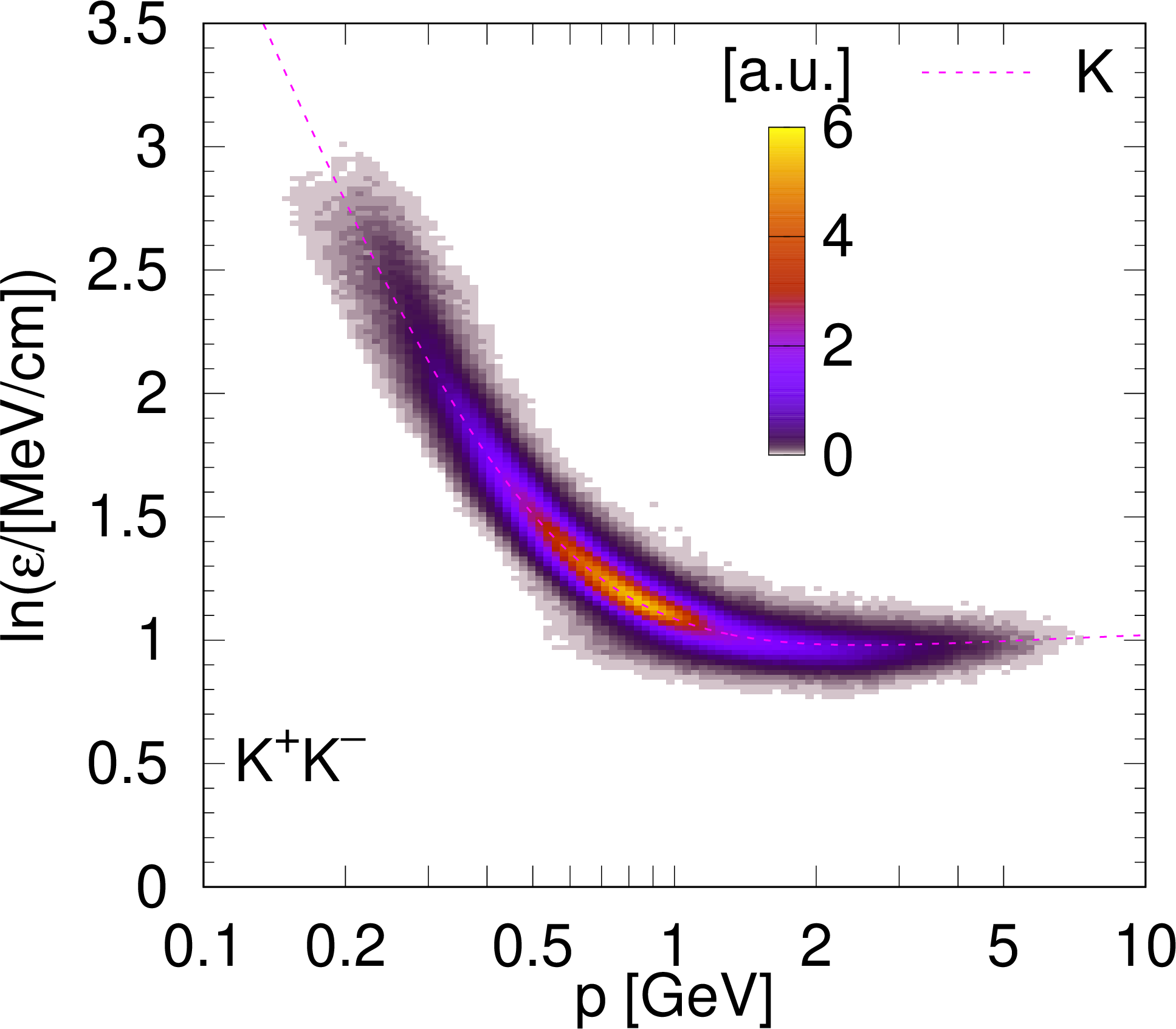
Figure 6-b:
Distribution of $ \ln\varepsilon $ as a function of total momentum, for reconstructed charged particles in selected two-track events (identified $ \mathrm{K^+}\mathrm{K^-} $; Section 5). The variable $ \varepsilon $ is the most probable energy loss rate at a reference path length $ l_0 = $ 450 m. The colour scale is shown in arbitrary units and is linear. The curve shows the expected $ \ln\varepsilon $ for kaons (Eq. (34.12) in Ref. [1]). |
png pdf |
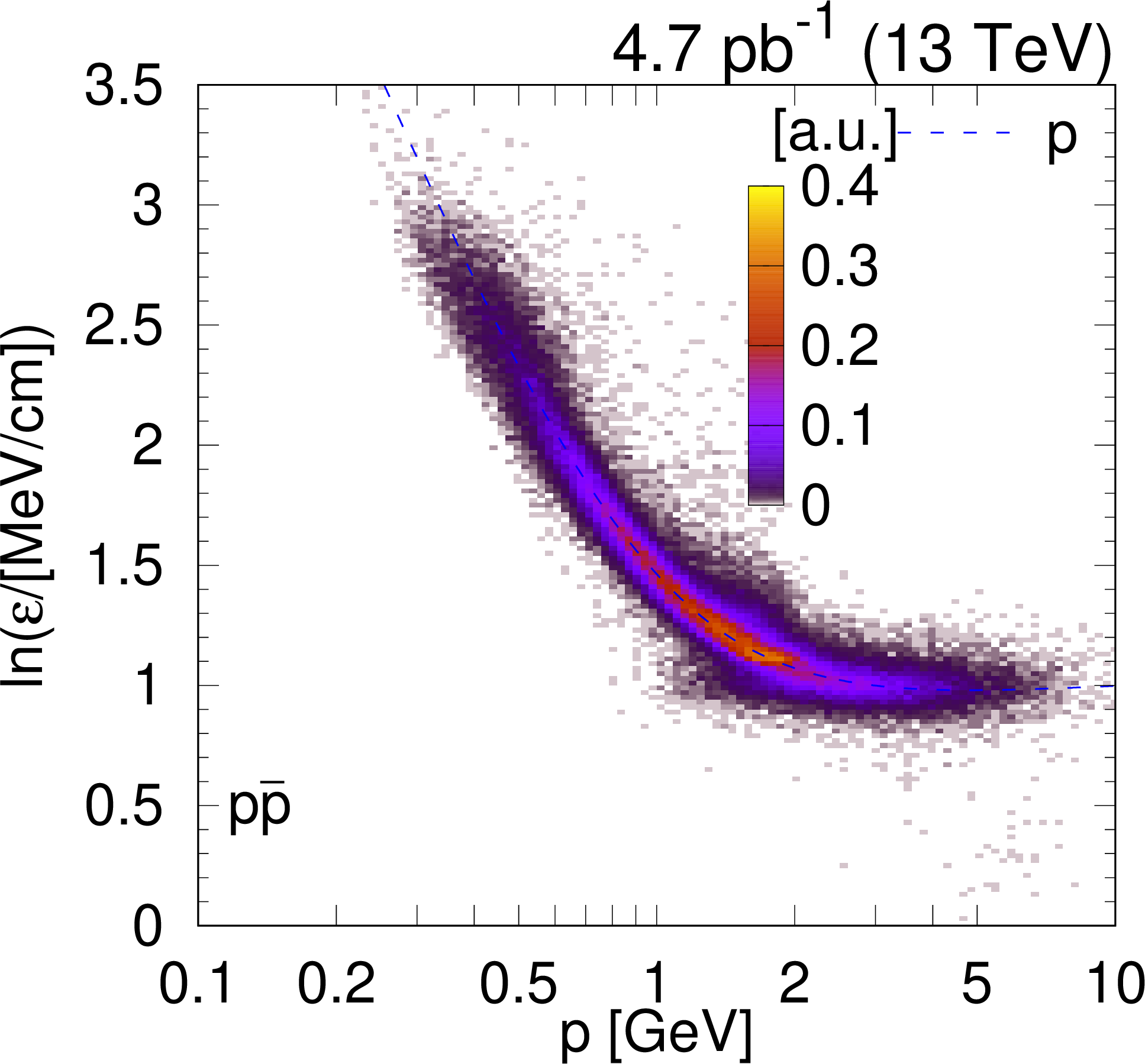
Figure 6-c:
Distribution of $ \ln\varepsilon $ as a function of total momentum, for reconstructed charged particles in selected two-track events (identified $ \mathrm{p}\overline{\mathrm{p}} $; Section 5). The variable $ \varepsilon $ is the most probable energy loss rate at a reference path length $ l_0 = $ 450 m. The colour scale is shown in arbitrary units and is linear. The curve shows the expected $ \ln\varepsilon $ for protons (Eq. (34.12) in Ref. [1]). |

png pdf |
Figure 6-d:
Distribution of $ \ln\varepsilon $ as a function of total momentum, for reconstructed charged particles in selected two-track events (signal; Section 5). The variable $ \varepsilon $ is the most probable energy loss rate at a reference path length $ l_0 = $ 450 m. The colour scale is shown in arbitrary units and is linear. The curves show the expected $ \ln\varepsilon $ for electrons, pions, kaons, and protons (Eq. (34.12) in Ref. [1]). |
png pdf |
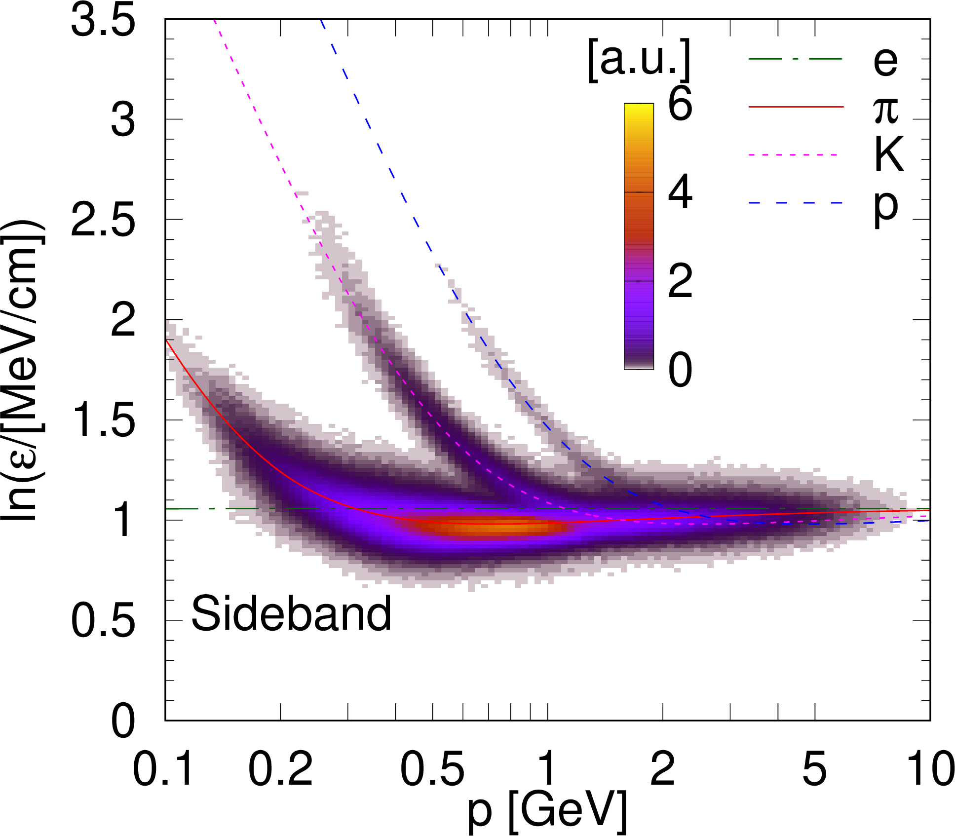
Figure 6-e:
Distribution of $ \ln\varepsilon $ as a function of total momentum, for reconstructed charged particles in selected two-track events (sideband; Section 5). The variable $ \varepsilon $ is the most probable energy loss rate at a reference path length $ l_0 = $ 450 m. The colour scale is shown in arbitrary units and is linear. The curves show the expected $ \ln\varepsilon $ for electrons, pions, kaons, and protons (Eq. (34.12) in Ref. [1]). |

png pdf |
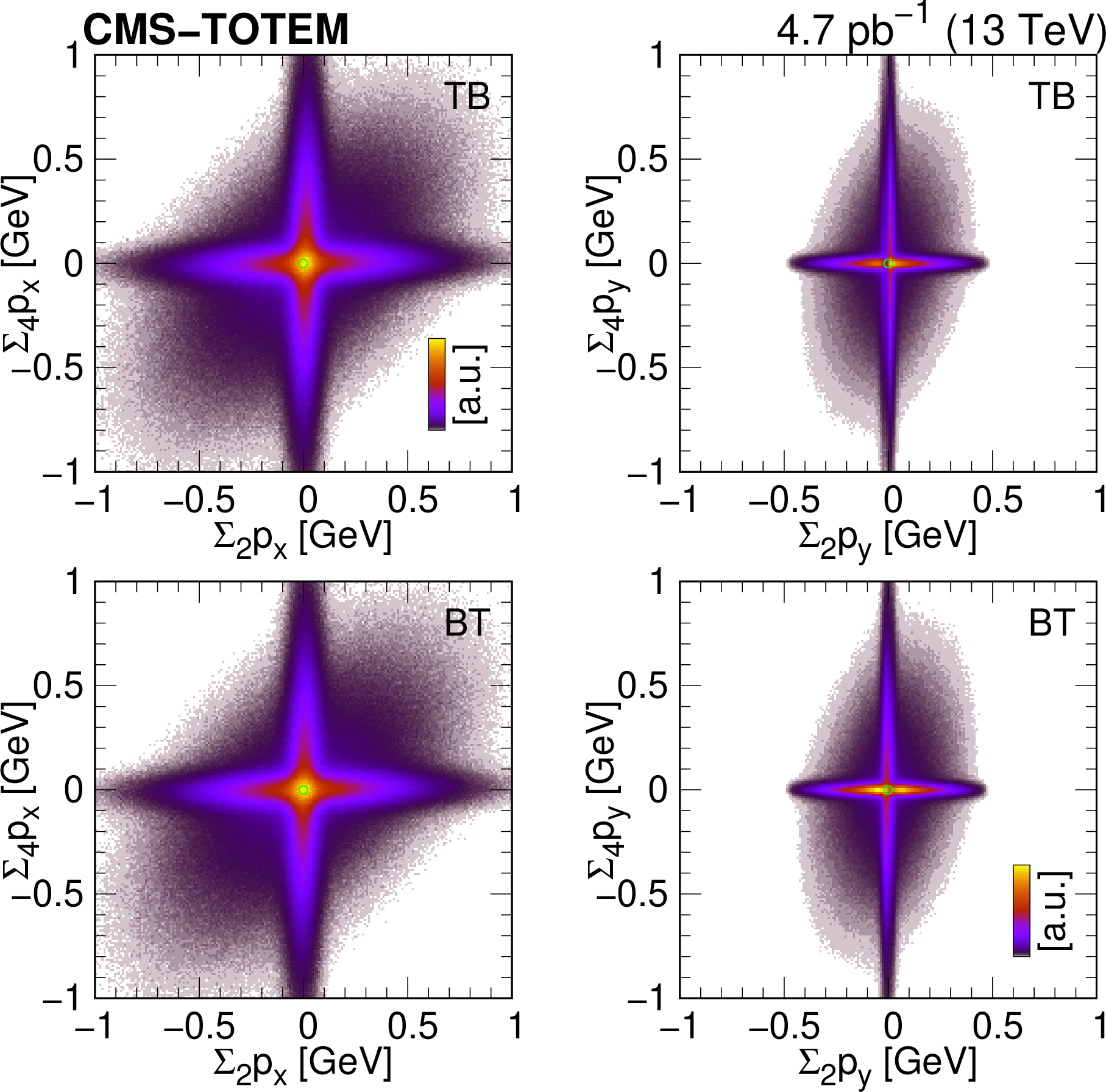
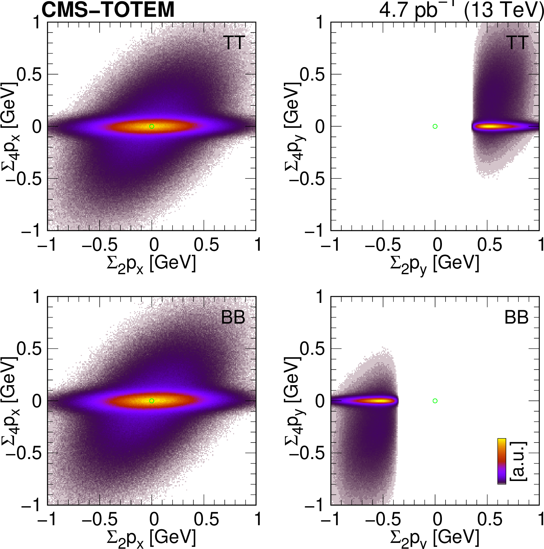
Figure 7:
Distribution of the sum of the scattered proton and central hadron momenta and the sum of the scattered proton momenta ($ \sum_4 p_x $ vs. $ \sum_2 p_x $, $ \sum_4 p_y $ vs. $ \sum_2 p_y $) shown for the diagonal trigger configurations (TB and BT, left) and the parallel ones (TT and BB, right) in the case of 2-track events. |
png pdf |
Figure 7-a:
Distribution of the sum of the scattered proton and central hadron momenta and the sum of the scattered proton momenta ($ \sum_4 p_x $ vs. $ \sum_2 p_x $, $ \sum_4 p_y $ vs. $ \sum_2 p_y $) shown for the diagonal trigger configurations (TB and BT) in the case of 2-track events. |
png pdf |
Figure 7-b:
Distribution of the sum of the scattered proton and central hadron momenta and the sum of the scattered proton momenta ($ \sum_4 p_x $ vs. $ \sum_2 p_x $, $ \sum_4 p_y $ vs. $ \sum_2 p_y $) shown for the parallel trigger configurations (TT and BB) in the case of 2-track events. |
png pdf |
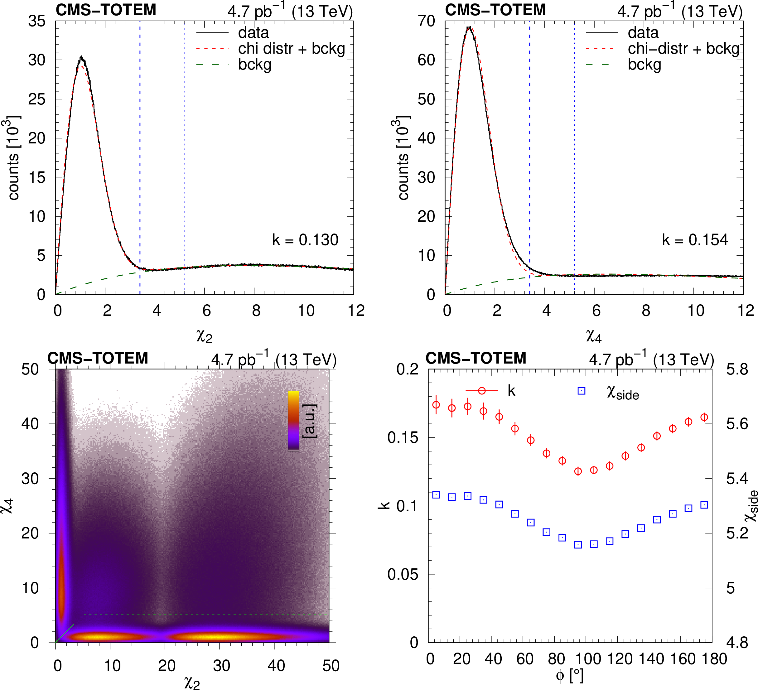
Figure 8:
Distributions of the classification variables $ \chi_2 $ (upper left) and $ \chi_4 $ (upper right). Fits using a two-component model are indicated. The distributions are integrated over the angle between the scattered protons $ \phi $. Selection lines at $ \chi_\text{sign} = $ 3.4 (green solid) and $ \chi_\text{side} \approx $ 5.2 (green dotted) are also plotted. Lower left: Joint distributions of classification variables $ \chi_2 $ and $ \chi_4 $. Central exclusive signal events are at the bottom whereas elastic events are at the left margin. Lower right: Coefficient $ k $ and the position of the upper cutoff $ \chi_\text{side} $ for $ \chi_4 $ to describe the background component as a function of the angle between the scattered protons $ \phi $, in the plane transverse to the beam direction. |

png pdf |
Figure 8-a:
Distribution of the classification variables $ \chi_2 $. A fit using a two-component model is indicated. The distribution is integrated over the angle between the scattered protons $ \phi $. Selection lines at $ \chi_\text{sign} = $ 3.4 (green solid) and $ \chi_\text{side} \approx $ 5.2 (green dotted) are also plotted. |

png pdf |
Figure 8-b:
Distribution of the classification variables $ \chi_4 $. A fit using a two-component model is indicated. The distribution is integrated over the angle between the scattered protons $ \phi $. Selection lines at $ \chi_\text{sign} = $ 3.4 (green solid) and $ \chi_\text{side} \approx $ 5.2 (green dotted) are also plotted. |

png pdf |
Figure 8-c:
Joint distributions of classification variables $ \chi_2 $ and $ \chi_4 $. Central exclusive signal events are at the bottom whereas elastic events are at the left margin. |
png pdf |
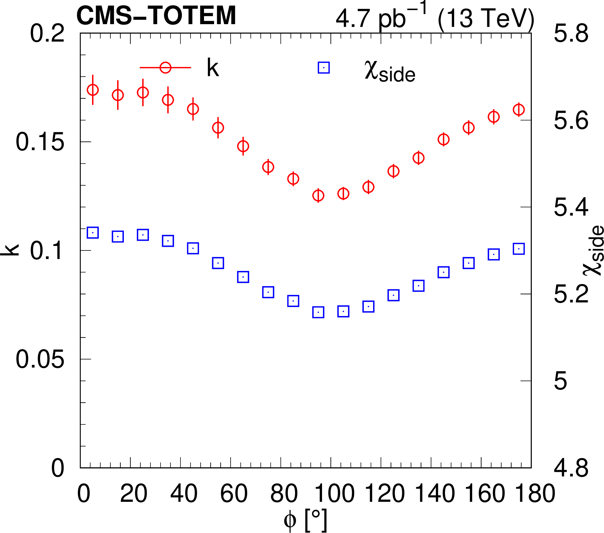
Figure 8-d:
Coefficient $ k $ and the position of the upper cutoff $ \chi_\text{side} $ for $ \chi_4 $ to describe the background component as a function of the angle between the scattered protons $ \phi $, in the plane transverse to the beam direction. |
png pdf |
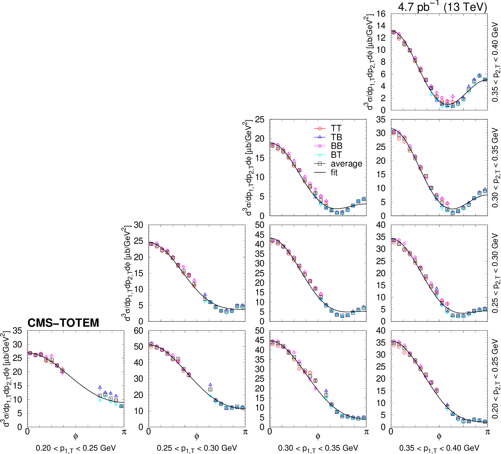
Figure 9:
Distributions of $ \mathrm{d}^3\sigma/\mathrm{d} p_\text{1,T} \mathrm{d} p_\text{2,T} \mathrm{d}\phi $ as functions of $ \phi $ in the $ \pi^{+}\pi^{-} $ nonresonant region (0.35 $ < m_{\pi^{+}\pi^{-}} < $ 0.65 GeV) in several $ (p_\text{1,T},p_\text{2,T}) $ bins in the range 0.20 $ < p_\text{1,T} < $ 0.40 GeV and 0.20 $ < p_\text{2,T} < $ 0.40 GeV, in units of $ \mu\mathrm{b}/$GeV$^2$. Values based on data from each RP trigger configuration (TB, BT, TT, and TT) are shown separately with coloured symbols, whereas the weighted average is indicated with black symbols. Results of individual fits with the form $ [A(R - \cos\phi)]^2 + c^2 $ (Eq. 8) are plotted with the curves. The error bars indicate the statistical uncertainties. |
png pdf |
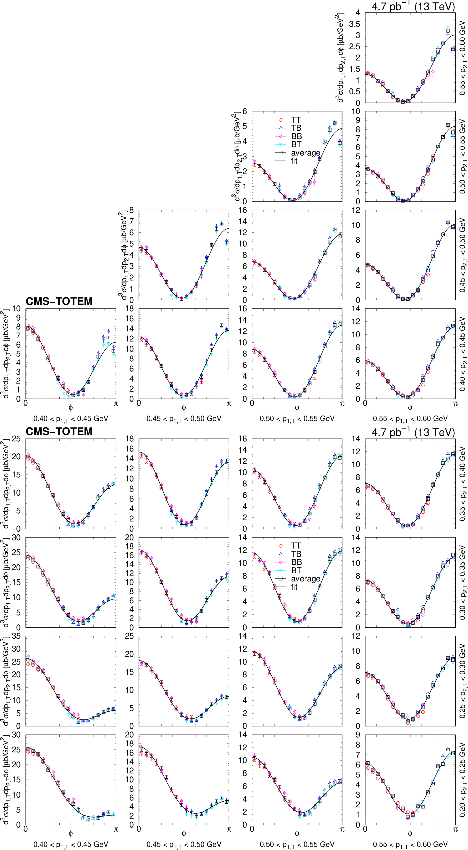
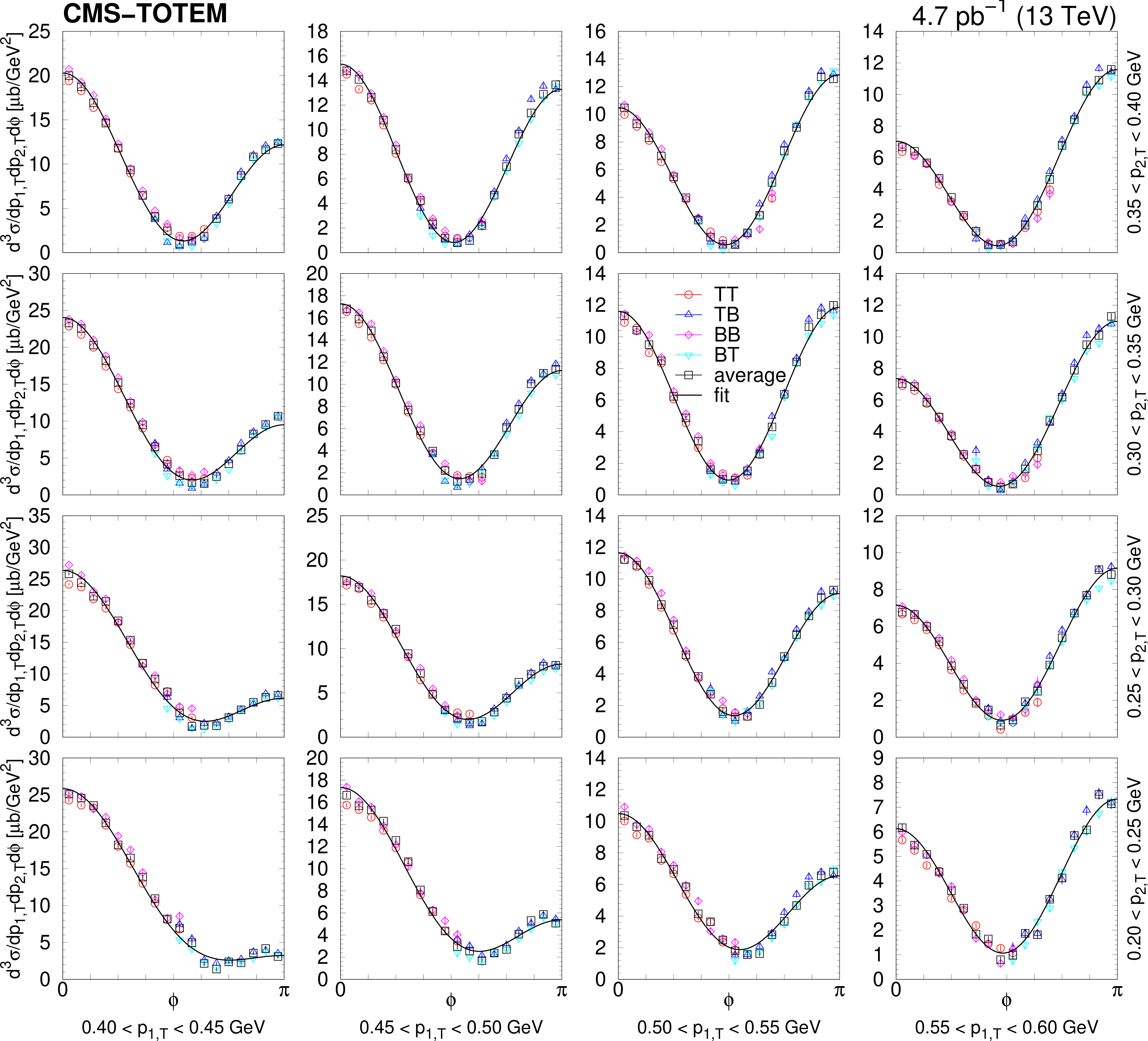
Figure 10:
Distributions of $ \mathrm{d}^3\sigma/\mathrm{d} p_\text{1,T} \mathrm{d} p_\text{2,T} \mathrm{d}\phi $ as functions of $ \phi $ in the $ \pi^{+}\pi^{-} $ nonresonant region (0.35 $ < m_{\pi^{+}\pi^{-}} < $ 0.65 GeV) in several $ (p_\text{1,T},p_\text{2,T}) $ bins in the range 0.40 $ < p_\text{1,T} < $ 0.60 GeV and 0.20 $ < p_\text{2,T} < $ 0.60 GeV, in units of $ \mu\mathrm{b}/$GeV$^2$. Values based on data from each RP trigger configuration (TB, BT, TT, and TT) are shown separately with coloured symbols, whereas the weighted average is indicated with black symbols. Results of individual fits with the form $ [A(R - \cos\phi)]^2 + c^2 $ (Eq. 8) are plotted with the curves. The error bars indicate the statistical uncertainties. |

png pdf |
Figure 10-a:
Distributions of $ \mathrm{d}^3\sigma/\mathrm{d} p_\text{1,T} \mathrm{d} p_\text{2,T} \mathrm{d}\phi $ as functions of $ \phi $ in the $ \pi^{+}\pi^{-} $ nonresonant region (0.35 $ < m_{\pi^{+}\pi^{-}} < $ 0.65 GeV) in several $ (p_\text{1,T},p_\text{2,T}) $ bins in the range 0.40 $ < p_\text{1,T} < $ 0.60 GeV and 0.20 $ < p_\text{2,T} < $ 0.60 GeV, in units of $ \mu\mathrm{b}/$GeV$^2$. Values based on data from each RP trigger configuration (TB, BT, TT, and TT) are shown separately with coloured symbols, whereas the weighted average is indicated with black symbols. Results of individual fits with the form $ [A(R - \cos\phi)]^2 + c^2 $ (Eq. 8) are plotted with the curves. The error bars indicate the statistical uncertainties. |
png pdf |
Figure 10-b:
Distributions of $ \mathrm{d}^3\sigma/\mathrm{d} p_\text{1,T} \mathrm{d} p_\text{2,T} \mathrm{d}\phi $ as functions of $ \phi $ in the $ \pi^{+}\pi^{-} $ nonresonant region (0.35 $ < m_{\pi^{+}\pi^{-}} < $ 0.65 GeV) in several $ (p_\text{1,T},p_\text{2,T}) $ bins in the range 0.40 $ < p_\text{1,T} < $ 0.60 GeV and 0.20 $ < p_\text{2,T} < $ 0.60 GeV, in units of $ \mu\mathrm{b}/$GeV$^2$. Values based on data from each RP trigger configuration (TB, BT, TT, and TT) are shown separately with coloured symbols, whereas the weighted average is indicated with black symbols. Results of individual fits with the form $ [A(R - \cos\phi)]^2 + c^2 $ (Eq. 8) are plotted with the curves. The error bars indicate the statistical uncertainties. |
png pdf |
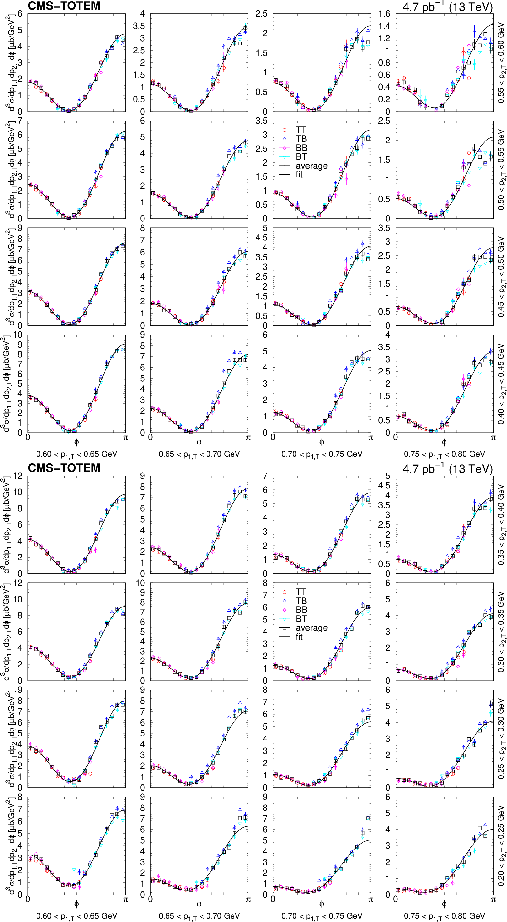
Figure 11:
Distributions of $ \mathrm{d}^3\sigma/\mathrm{d} p_\text{1,T} \mathrm{d} p_\text{2,T} \mathrm{d}\phi $ as functions of $ \phi $ in the $ \pi^{+}\pi^{-} $ nonresonant region (0.35 $ < m_{\pi^{+}\pi^{-}} < $ 0.65 GeV) in several $ (p_\text{1,T},p_\text{2,T}) $ bins in the range 0.60 $ < p_\text{1,T} < $ 0.80 GeV and 0.20 $ < p_\text{2,T} < $ 0.60 GeV, in units of $ \mu\mathrm{b}/$GeV$^2$. Values based on data from each RP trigger configuration (TB, BT, TT, and TT) are shown separately with coloured symbols, whereas the weighted average is indicated with black symbols. Results of individual fits with the form $ [A(R - \cos\phi)]^2 + c^2 $ (Eq. 8) are plotted with the curves. The error bars indicate the statistical uncertainties. |

png pdf |
Figure 11-a:
Distributions of $ \mathrm{d}^3\sigma/\mathrm{d} p_\text{1,T} \mathrm{d} p_\text{2,T} \mathrm{d}\phi $ as functions of $ \phi $ in the $ \pi^{+}\pi^{-} $ nonresonant region (0.35 $ < m_{\pi^{+}\pi^{-}} < $ 0.65 GeV) in several $ (p_\text{1,T},p_\text{2,T}) $ bins in the range 0.60 $ < p_\text{1,T} < $ 0.80 GeV and 0.20 $ < p_\text{2,T} < $ 0.60 GeV, in units of $ \mu\mathrm{b}/$GeV$^2$. Values based on data from each RP trigger configuration (TB, BT, TT, and TT) are shown separately with coloured symbols, whereas the weighted average is indicated with black symbols. Results of individual fits with the form $ [A(R - \cos\phi)]^2 + c^2 $ (Eq. 8) are plotted with the curves. The error bars indicate the statistical uncertainties. |

png pdf |
Figure 11-b:
Distributions of $ \mathrm{d}^3\sigma/\mathrm{d} p_\text{1,T} \mathrm{d} p_\text{2,T} \mathrm{d}\phi $ as functions of $ \phi $ in the $ \pi^{+}\pi^{-} $ nonresonant region (0.35 $ < m_{\pi^{+}\pi^{-}} < $ 0.65 GeV) in several $ (p_\text{1,T},p_\text{2,T}) $ bins in the range 0.60 $ < p_\text{1,T} < $ 0.80 GeV and 0.20 $ < p_\text{2,T} < $ 0.60 GeV, in units of $ \mu\mathrm{b}/$GeV$^2$. Values based on data from each RP trigger configuration (TB, BT, TT, and TT) are shown separately with coloured symbols, whereas the weighted average is indicated with black symbols. Results of individual fits with the form $ [A(R - \cos\phi)]^2 + c^2 $ (Eq. 8) are plotted with the curves. The error bars indicate the statistical uncertainties. |
png pdf |
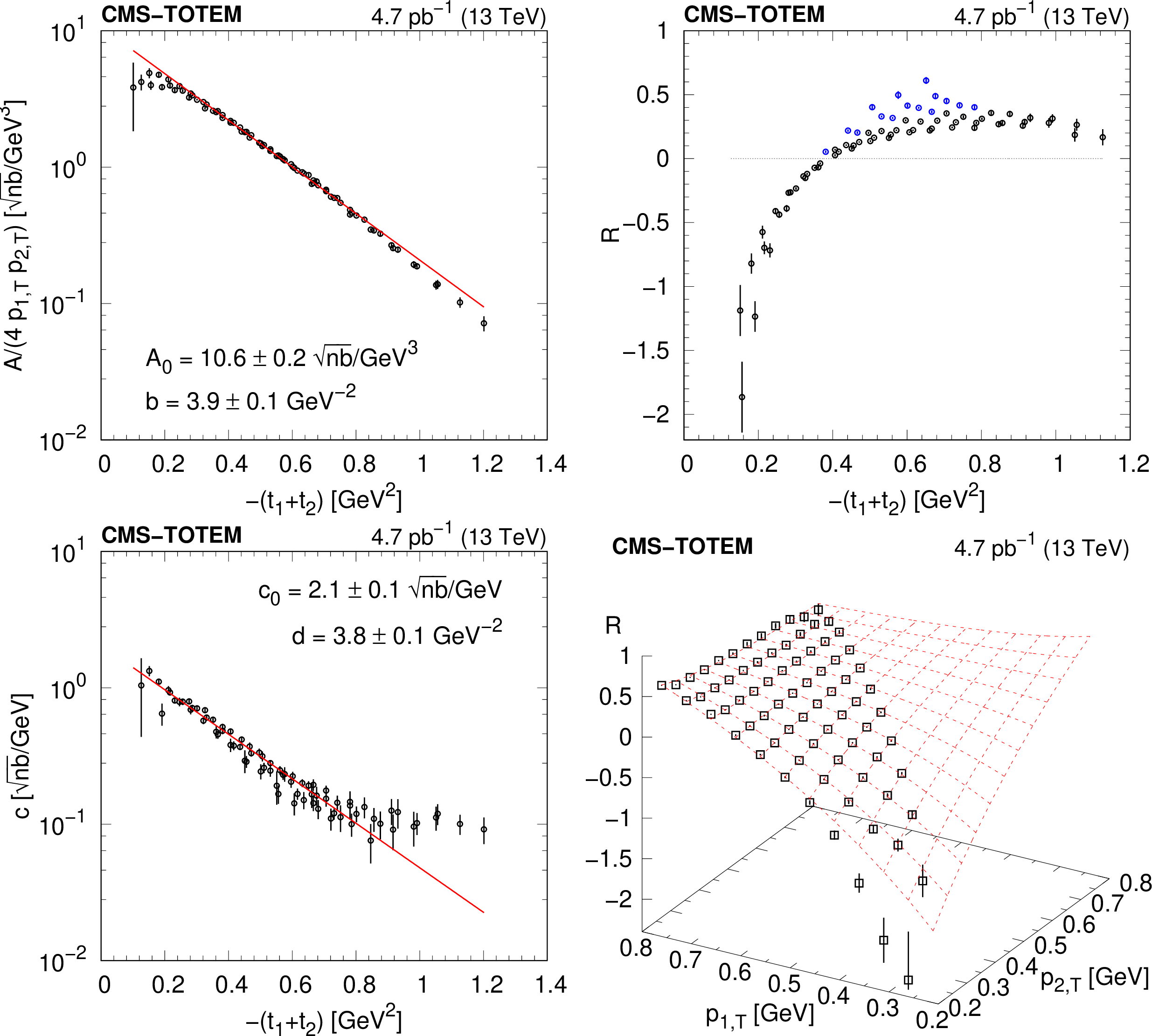
Figure 12:
Dependence of the parameters $ A $, $ R $, and $ c $ (Eq. 8) on $ (t_1,t_2) $. The fits correspond to the functional forms displayed in Eqs. 9. In the upper right plot, points with significantly different proton transverse momenta ($ |p_\text{1,T} - p_\text{2,T}| > $ 0.35 GeV) are coloured blue. The lower right plot shows the dependence of $ R $ on the two scattered proton transverse momenta. |

png pdf |
Figure 12-a:
Dependence of the parameter $ A $ (Eq. 8) on $ (t_1,t_2) $. The fit corresponds to the functional forms displayed in Eqs. 9. |
png pdf |
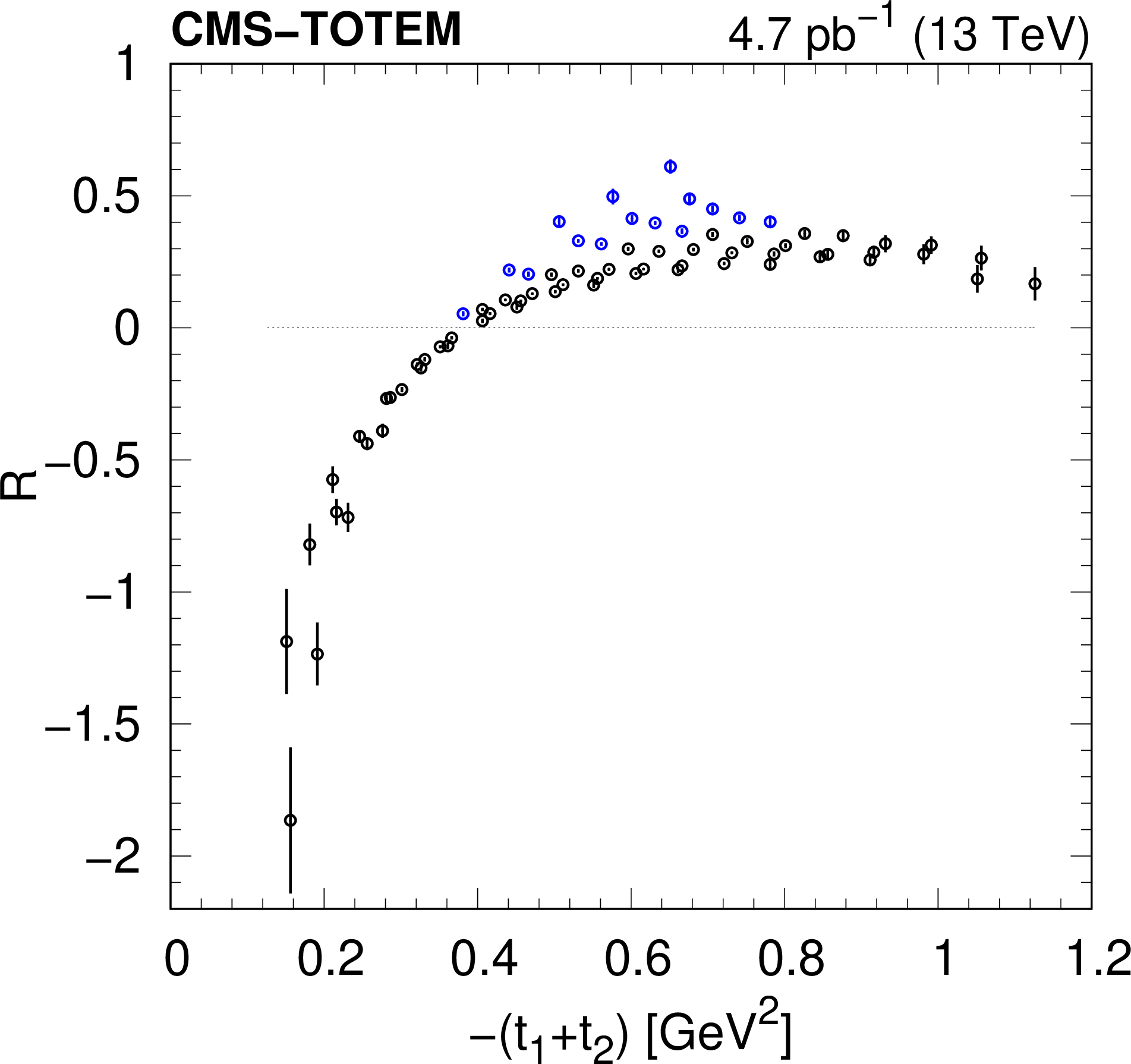
Figure 12-b:
Dependence of the parameter $ R $ (Eq. 8) on $ (t_1,t_2) $. The fit corresponds to the functional forms displayed in Eqs. 9. Points with significantly different proton transverse momenta ($ |p_\text{1,T} - p_\text{2,T}| > $ 0.35 GeV) are coloured blue. |

png pdf |
Figure 12-c:
Dependence of the parameter $ c $ (Eq. 8) on $ (t_1,t_2) $. The fit corresponds to the functional forms displayed in Eqs. 9. |
png pdf |
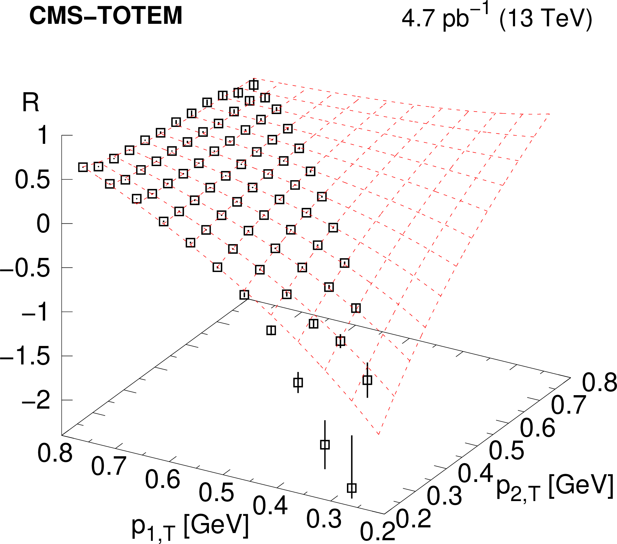
Figure 12-d:
The plot shows the dependence of $ R $ on the two scattered proton transverse momenta. |

png pdf |
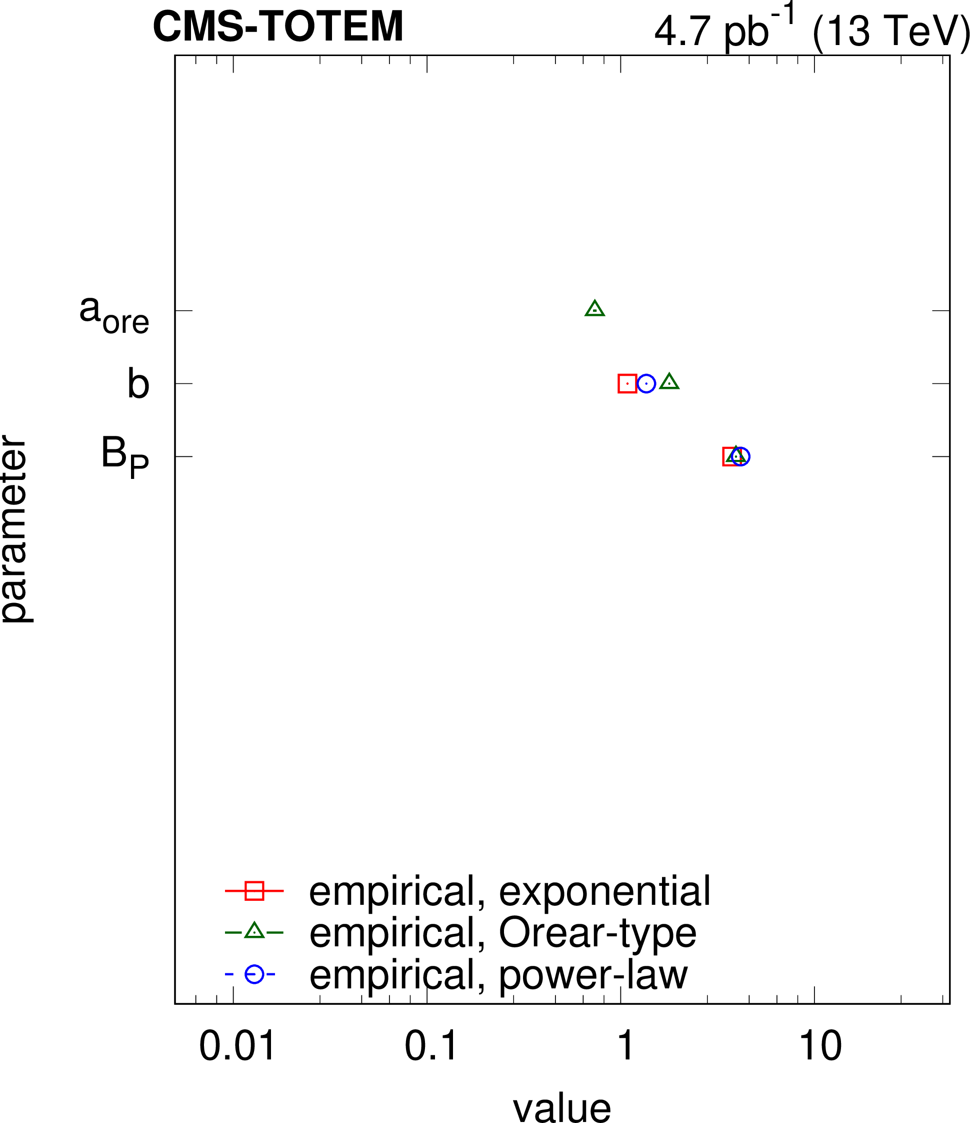
Figure 13:
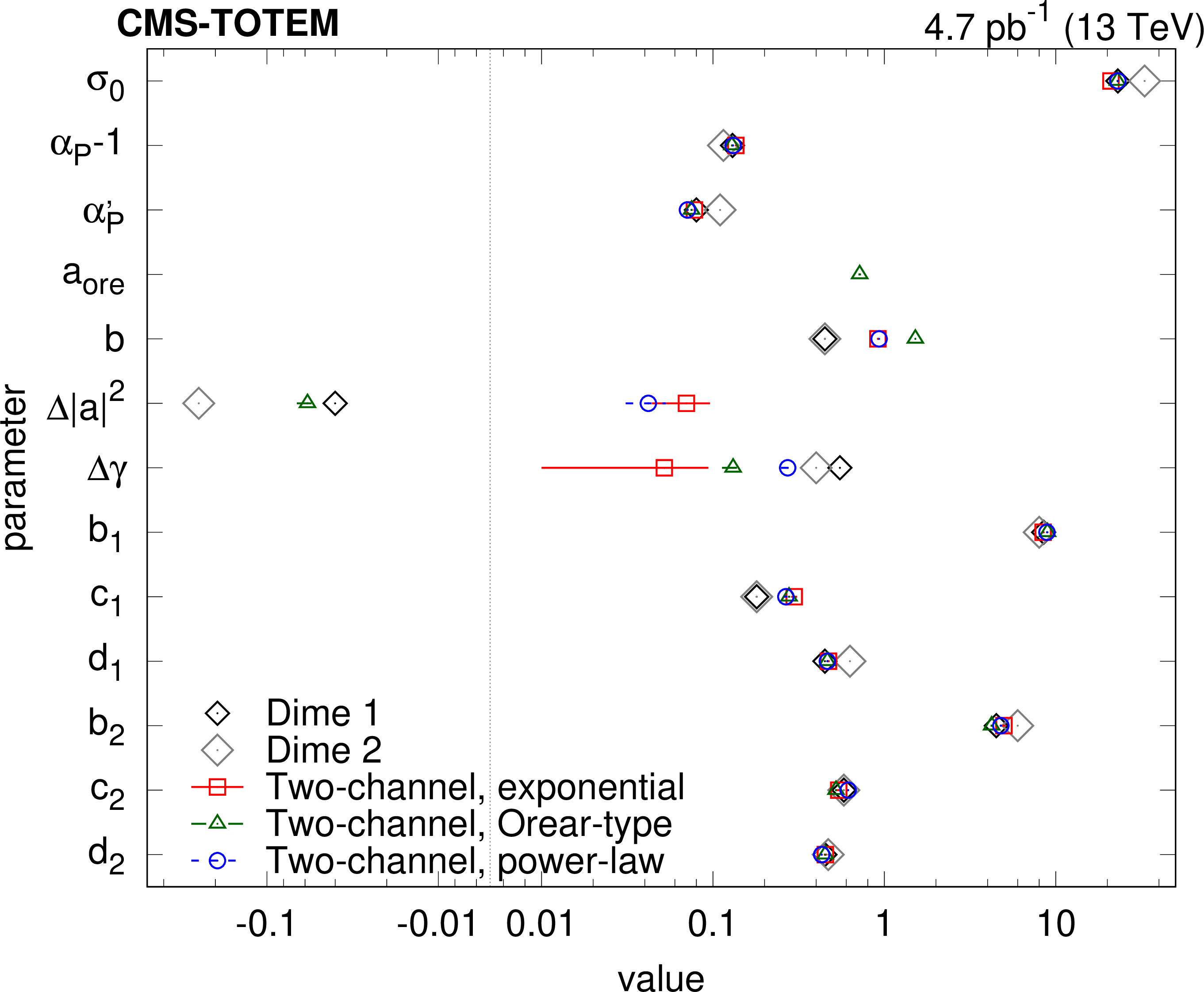
Values of best parameters for the empirical (upper left), one-channel (upper right), and two-channel (lower) models with several choices of the proton-pomeron form factor (exponential, Orear-type, power-law). In the case of the two-channel model, parameter values of models describing the elastic differential pp cross section from Ref. [26] are also indicated (DIME 1 and 2). |
png pdf |
Figure 13-a:
Values of best parameters for the empirical model with several choices of the proton-pomeron form factor (exponential, Orear-type, power-law). |

png pdf |
Figure 13-b:
Values of best parameters for the one-channel model with several choices of the proton-pomeron form factor (exponential, Orear-type, power-law). |
png pdf |
Figure 13-c:
Values of best parameters for the two-channel model with several choices of the proton-pomeron form factor (exponential, Orear-type, power-law). Parameter values of models describing the elastic differential pp cross section from Ref. [26] are also indicated (DIME 1 and 2). |
png pdf |
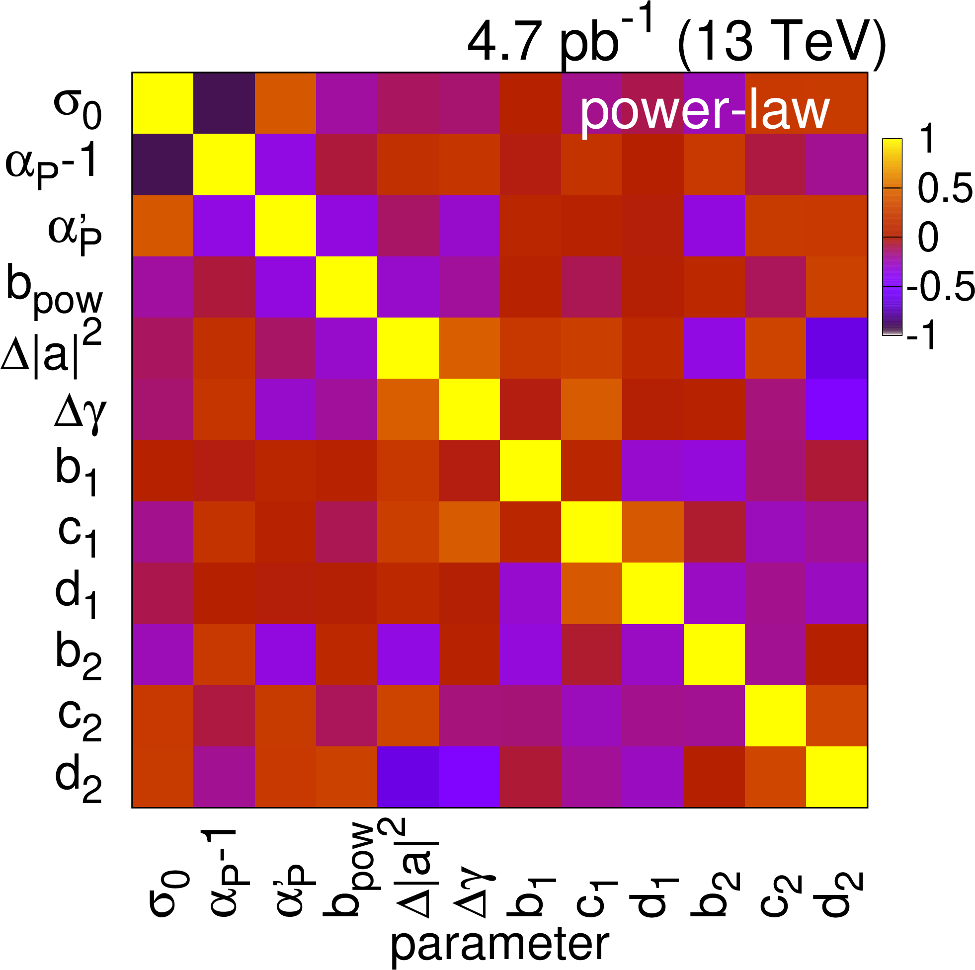
Figure 14:
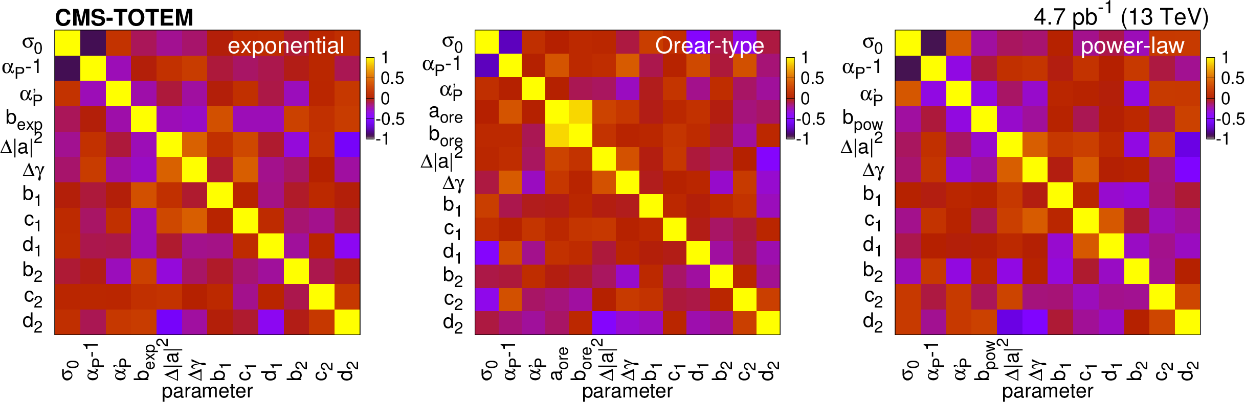
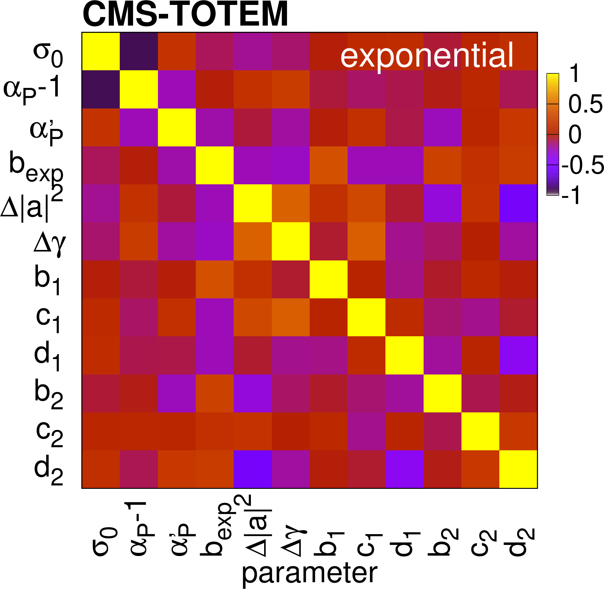
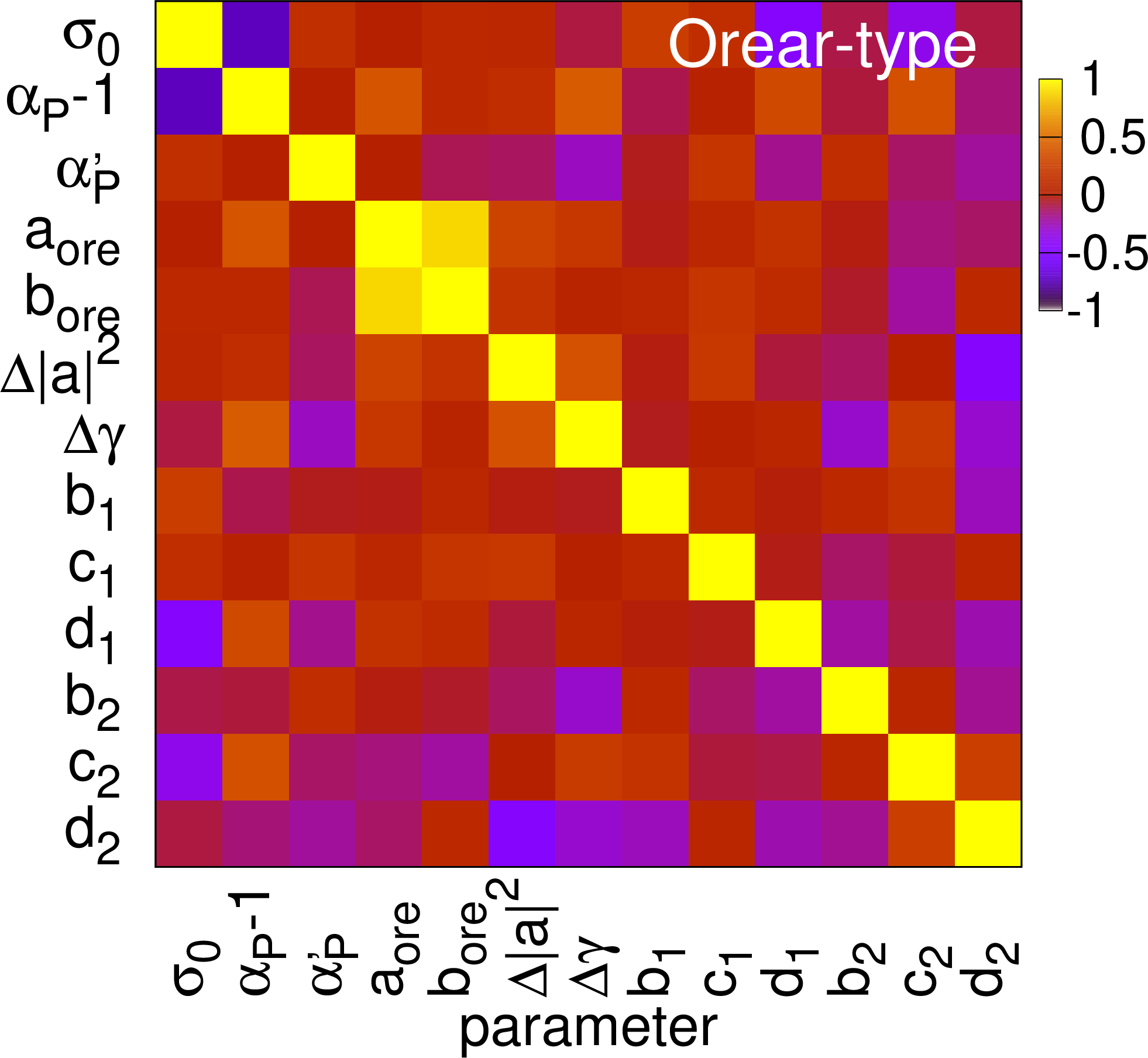
Correlation coefficients among values of best parameters for the two-channel model, in the case of the exponential (left), Orear-type (centre), and power-law (right) parametrisations of the proton-pomeron form factor. |
png pdf |
Figure 14-a:
Correlation coefficients among values of best parameters for the two-channel model, in the case of the exponential parametrisation of the proton-pomeron form factor. |
png pdf |
Figure 14-b:
Correlation coefficients among values of best parameters for the two-channel model, in the case of the Orear-type parametrisation of the proton-pomeron form factor. |
png pdf |
Figure 14-c:
Correlation coefficients among values of best parameters for the two-channel model, in the case of the power-law parametrisation of the proton-pomeron form factor. |
png pdf |
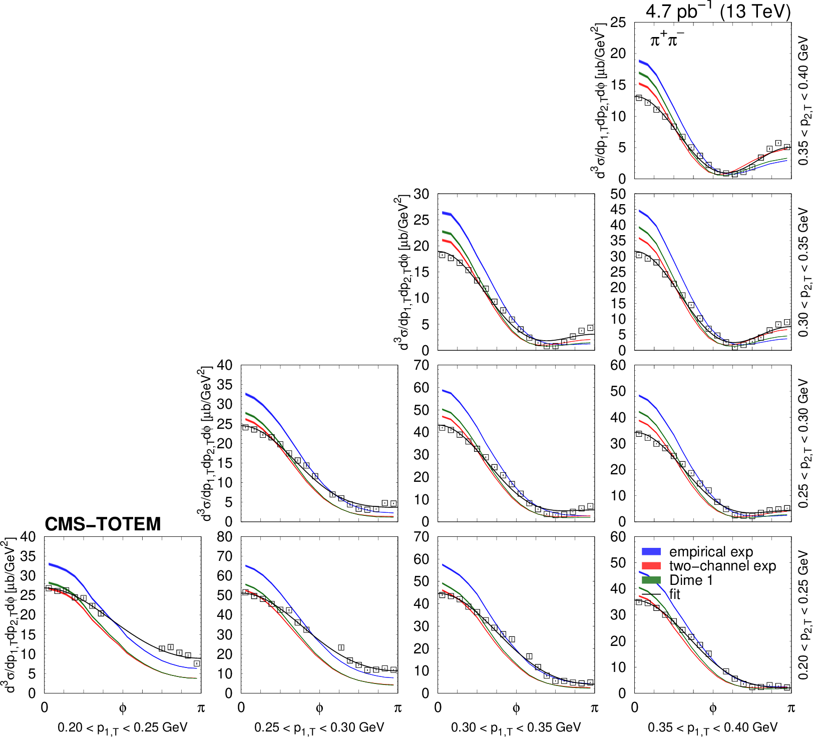
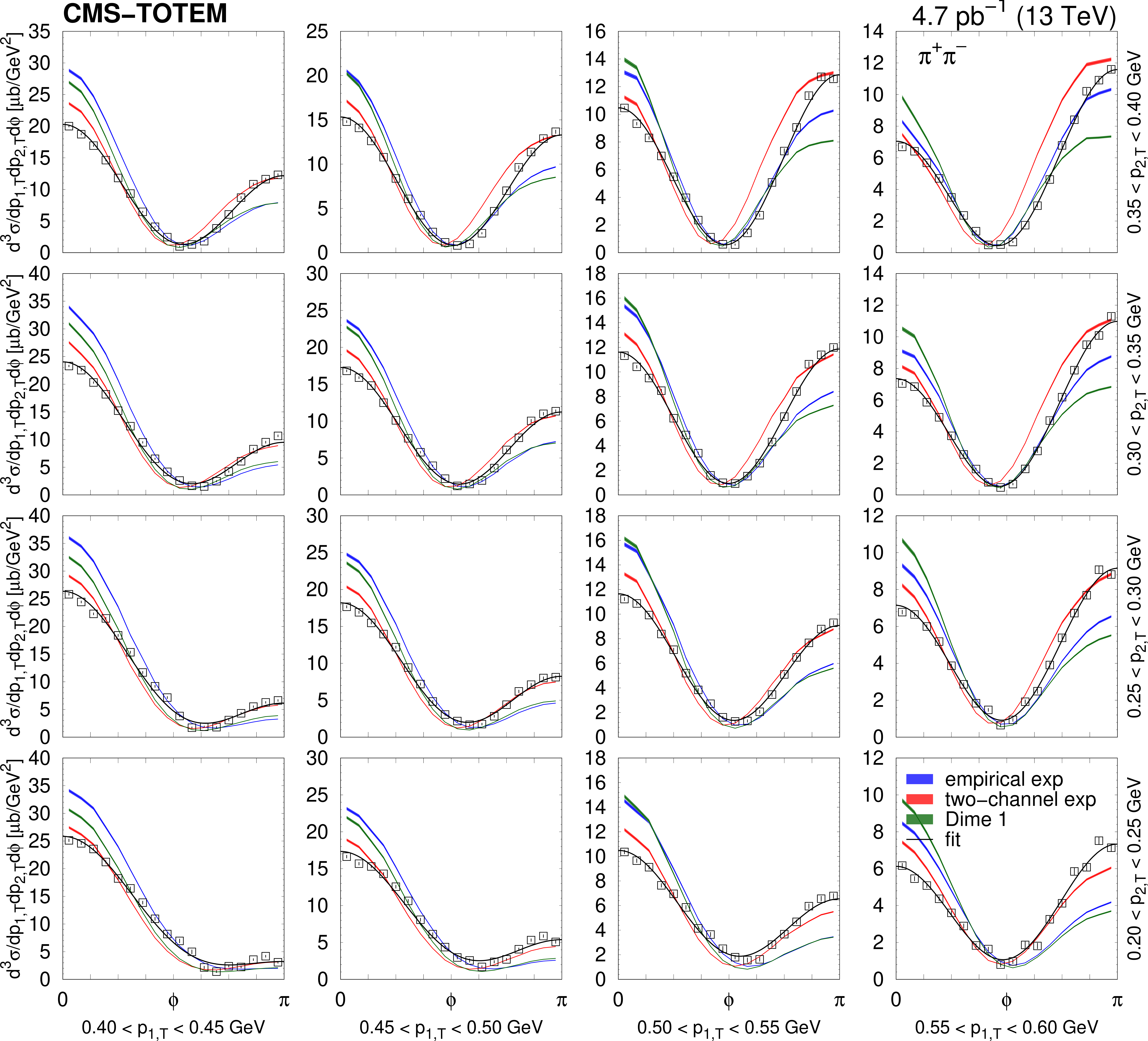
Figure 15:
Distribution of $ \mathrm{d}^3\sigma/\mathrm{d} p_\text{1,T} \mathrm{d} p_\text{2,T} \mathrm{d}\phi $ as a function of $ \phi $ in several $ (p_\text{1,T},p_\text{2,T}) $ bins in the range 0.20 $ < p_\text{1,T} < $ 0.40 GeV and 0.20 $ < p_\text{2,T} < $ 0.60 GeV, in units of $ \mu\mathrm{b}/$GeV$^2$, for the mass range 0.35 $ < m_{\pi^{+}\pi^{-}} < $ 0.65 GeV. Measured values (black symbols) are shown together with the predictions of the empirical and the two-channel models (coloured curves) using the tuned parameters for the exponential proton-pomeron form factors (see text for details). Curves corresponding to DIME (model 1) are also plotted. Results of individual fits with the form $ [A(R - \cos\phi)]^2 + c^2 $ (Eq. 8) are plotted with the curves. The error bars indicate the statistical uncertainties. |
png pdf |
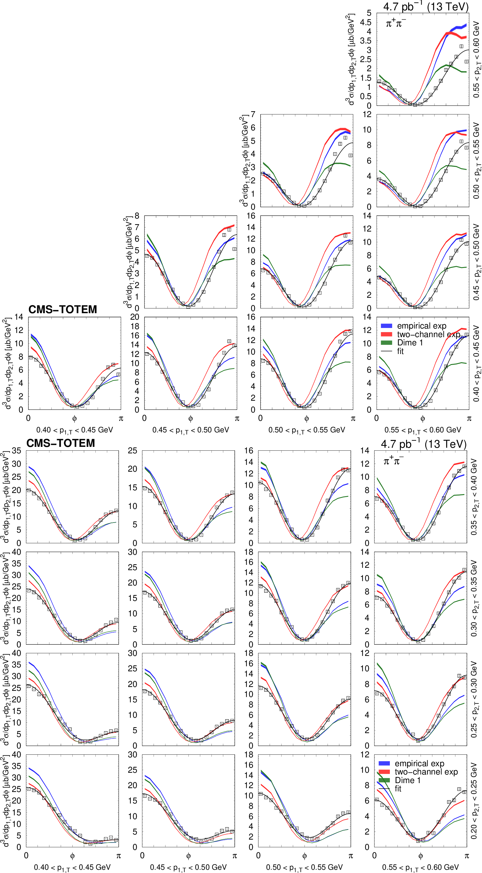
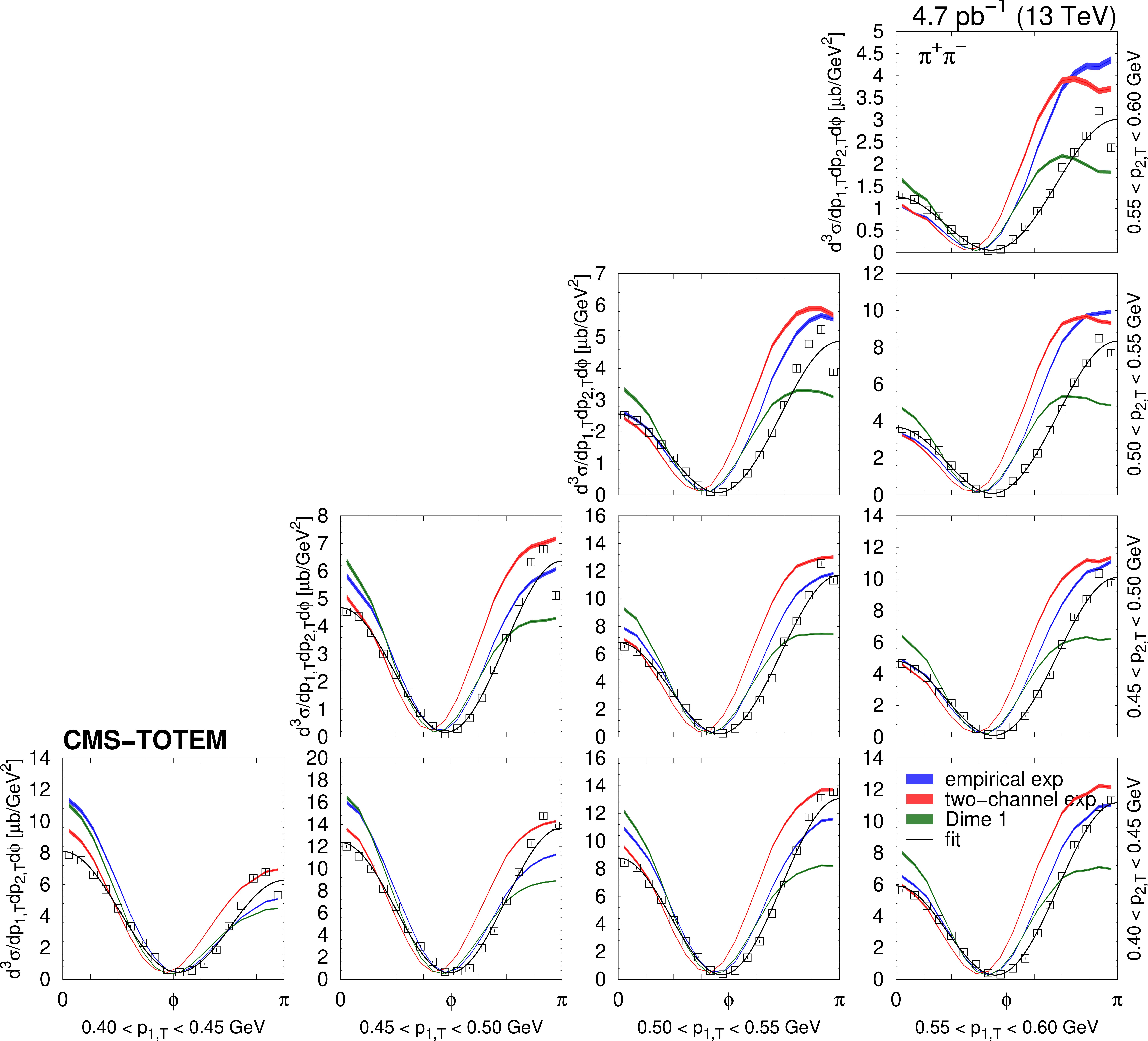
Figure 16:
Distribution of $ \mathrm{d}^3\sigma/\mathrm{d} p_\text{1,T} \mathrm{d} p_\text{2,T} \mathrm{d}\phi $ as a function of $ \phi $ in several $ (p_\text{1,T},p_\text{2,T}) $ bins in the range 0.40 $ < p_\text{1,T} < $ 0.60 GeV and 0.20 $ < p_\text{2,T} < $ 0.60 GeV, in units of $ \mu\mathrm{b}/$GeV$^2$, for the mass range 0.35 $ < m_{\pi^{+}\pi^{-}} < $ 0.65 GeV. Measured values (black symbols) are shown together with the predictions of the empirical and the two-channel models (coloured curves) using the tuned parameters for the exponential proton-pomeron form factors (see text for details). Curves corresponding to DIME (model 1) are also plotted. Results of individual fits with the form $ [A(R - \cos\phi)]^2 + c^2 $ (Eq. 8) are plotted with the curves. The error bars indicate the statistical uncertainties. |
png pdf |
Figure 16-a:
Distribution of $ \mathrm{d}^3\sigma/\mathrm{d} p_\text{1,T} \mathrm{d} p_\text{2,T} \mathrm{d}\phi $ as a function of $ \phi $ in several $ (p_\text{1,T},p_\text{2,T}) $ bins in the range 0.40 $ < p_\text{1,T} < $ 0.60 GeV and 0.20 $ < p_\text{2,T} < $ 0.60 GeV, in units of $ \mu\mathrm{b}/$GeV$^2$, for the mass range 0.35 $ < m_{\pi^{+}\pi^{-}} < $ 0.65 GeV. Measured values (black symbols) are shown together with the predictions of the empirical and the two-channel models (coloured curves) using the tuned parameters for the exponential proton-pomeron form factors (see text for details). Curves corresponding to DIME (model 1) are also plotted. Results of individual fits with the form $ [A(R - \cos\phi)]^2 + c^2 $ (Eq. 8) are plotted with the curves. The error bars indicate the statistical uncertainties. |
png pdf |
Figure 16-b:
Distribution of $ \mathrm{d}^3\sigma/\mathrm{d} p_\text{1,T} \mathrm{d} p_\text{2,T} \mathrm{d}\phi $ as a function of $ \phi $ in several $ (p_\text{1,T},p_\text{2,T}) $ bins in the range 0.40 $ < p_\text{1,T} < $ 0.60 GeV and 0.20 $ < p_\text{2,T} < $ 0.60 GeV, in units of $ \mu\mathrm{b}/$GeV$^2$, for the mass range 0.35 $ < m_{\pi^{+}\pi^{-}} < $ 0.65 GeV. Measured values (black symbols) are shown together with the predictions of the empirical and the two-channel models (coloured curves) using the tuned parameters for the exponential proton-pomeron form factors (see text for details). Curves corresponding to DIME (model 1) are also plotted. Results of individual fits with the form $ [A(R - \cos\phi)]^2 + c^2 $ (Eq. 8) are plotted with the curves. The error bars indicate the statistical uncertainties. |

png pdf |
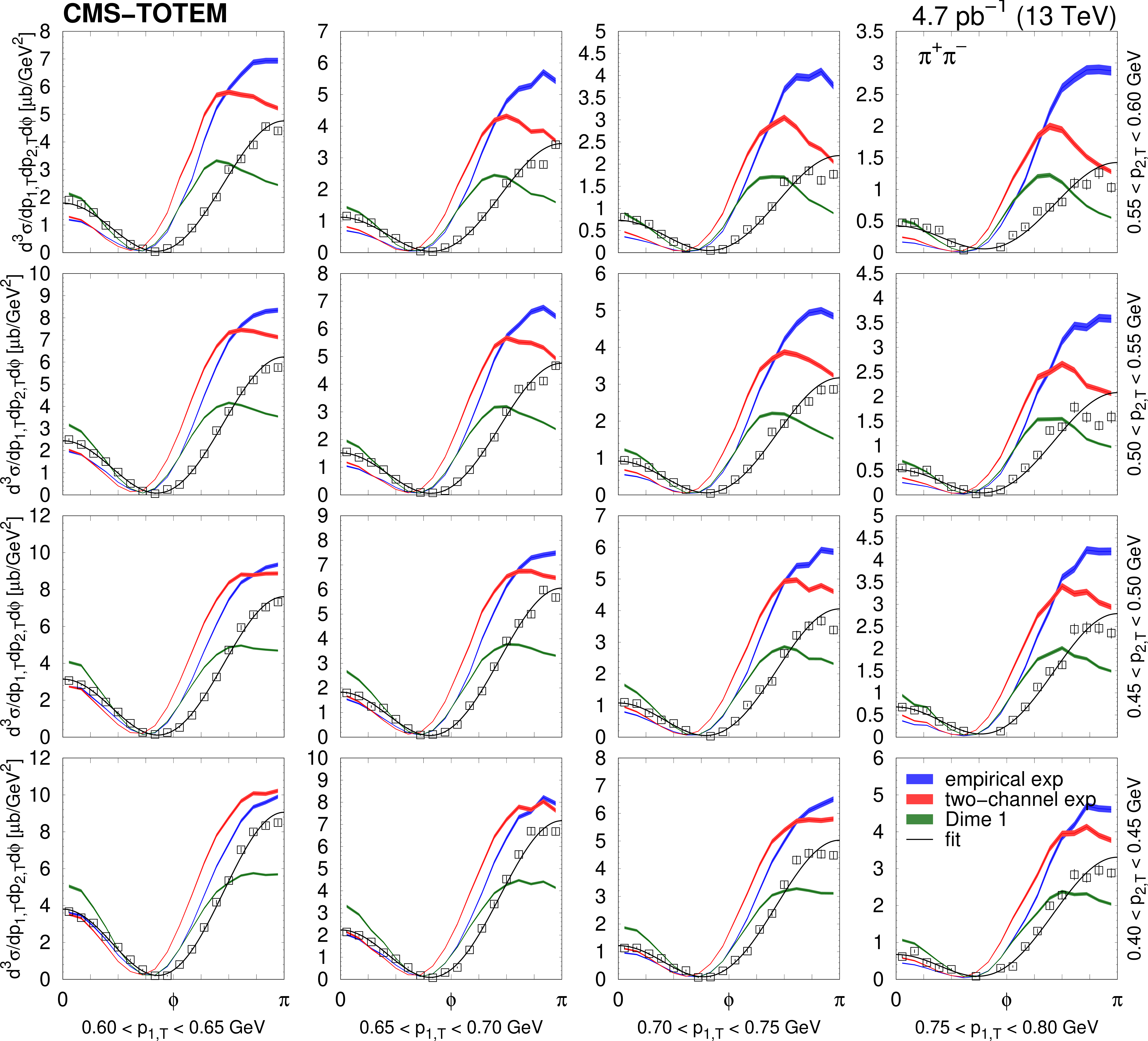
Figure 17:
Distribution of $ \mathrm{d}^3\sigma/\mathrm{d} p_\text{1,T} \mathrm{d} p_\text{2,T} \mathrm{d}\phi $ as a function of $ \phi $ in several $ (p_\text{1,T},p_\text{2,T}) $ bins in the range 0.60 $ < p_\text{1,T} < $ 0.80 GeV and 0.20 $ < p_\text{2,T} < $ 0.60 GeV, in units of $ \mu\mathrm{b}/$GeV$^2$, for the mass range 0.35 $ < m_{\pi^{+}\pi^{-}} < $ 0.65 GeV. Measured values (black symbols) are shown together with the predictions of the empirical and the two-channel models (coloured curves) using the tuned parameters for the exponential proton-pomeron form factors (see text for details). Curves corresponding to DIME (model 1) are also plotted. Results of individual fits with the form $ [A(R - \cos\phi)]^2 + c^2 $ (Eq. 8) are plotted with the curves. The error bars indicate the statistical uncertainties. |
png pdf |
Figure 17-a:
Distribution of $ \mathrm{d}^3\sigma/\mathrm{d} p_\text{1,T} \mathrm{d} p_\text{2,T} \mathrm{d}\phi $ as a function of $ \phi $ in several $ (p_\text{1,T},p_\text{2,T}) $ bins in the range 0.60 $ < p_\text{1,T} < $ 0.80 GeV and 0.20 $ < p_\text{2,T} < $ 0.60 GeV, in units of $ \mu\mathrm{b}/$GeV$^2$, for the mass range 0.35 $ < m_{\pi^{+}\pi^{-}} < $ 0.65 GeV. Measured values (black symbols) are shown together with the predictions of the empirical and the two-channel models (coloured curves) using the tuned parameters for the exponential proton-pomeron form factors (see text for details). Curves corresponding to DIME (model 1) are also plotted. Results of individual fits with the form $ [A(R - \cos\phi)]^2 + c^2 $ (Eq. 8) are plotted with the curves. The error bars indicate the statistical uncertainties. |

png pdf |
Figure 17-b:
Distribution of $ \mathrm{d}^3\sigma/\mathrm{d} p_\text{1,T} \mathrm{d} p_\text{2,T} \mathrm{d}\phi $ as a function of $ \phi $ in several $ (p_\text{1,T},p_\text{2,T}) $ bins in the range 0.60 $ < p_\text{1,T} < $ 0.80 GeV and 0.20 $ < p_\text{2,T} < $ 0.60 GeV, in units of $ \mu\mathrm{b}/$GeV$^2$, for the mass range 0.35 $ < m_{\pi^{+}\pi^{-}} < $ 0.65 GeV. Measured values (black symbols) are shown together with the predictions of the empirical and the two-channel models (coloured curves) using the tuned parameters for the exponential proton-pomeron form factors (see text for details). Curves corresponding to DIME (model 1) are also plotted. Results of individual fits with the form $ [A(R - \cos\phi)]^2 + c^2 $ (Eq. 8) are plotted with the curves. The error bars indicate the statistical uncertainties. |
png pdf |
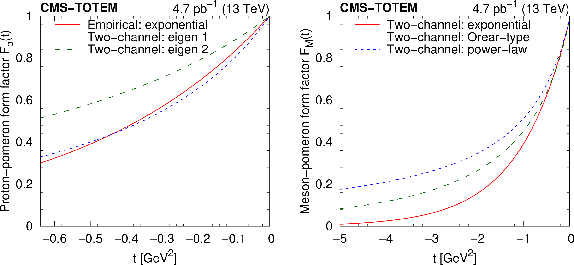
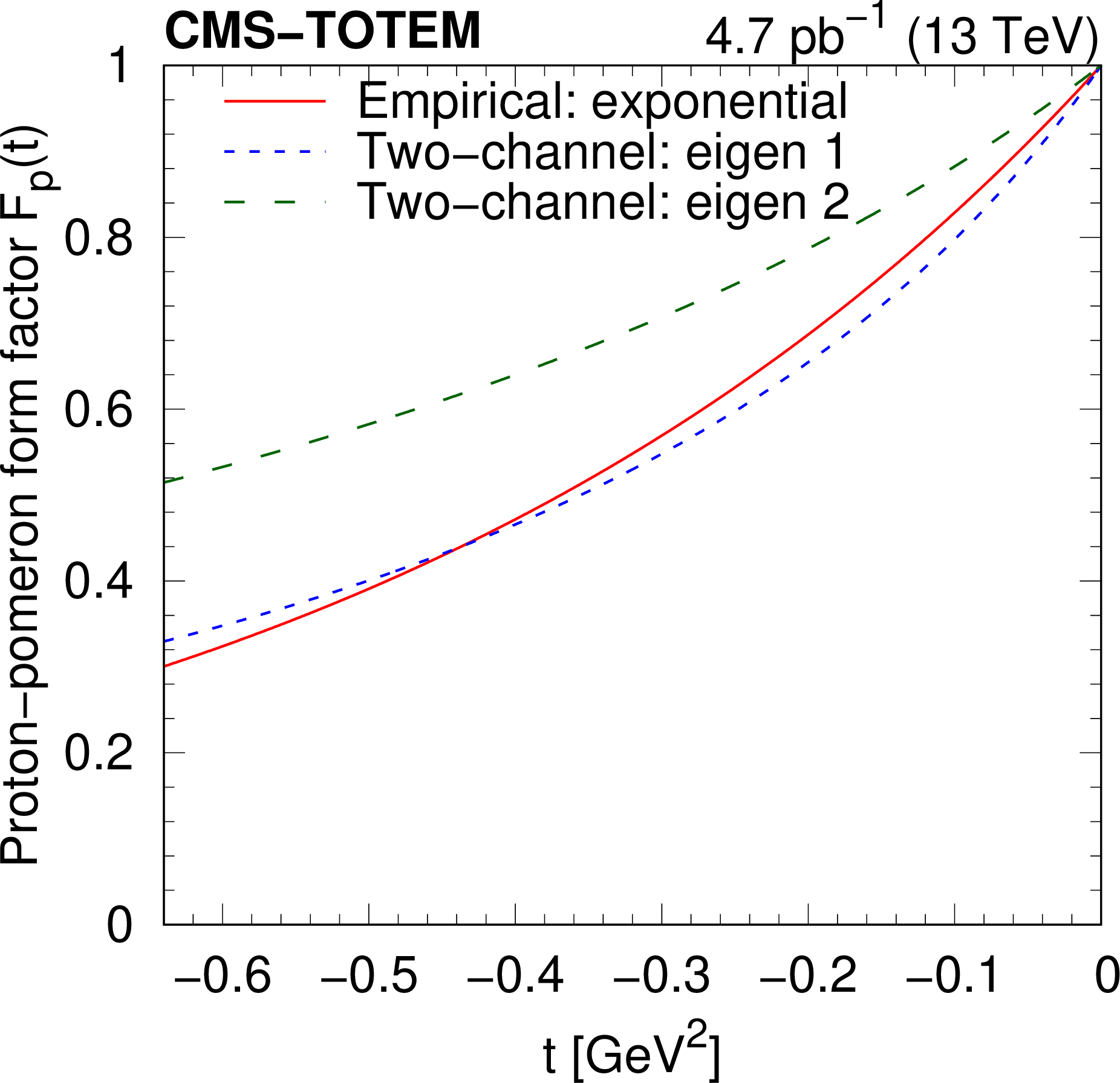
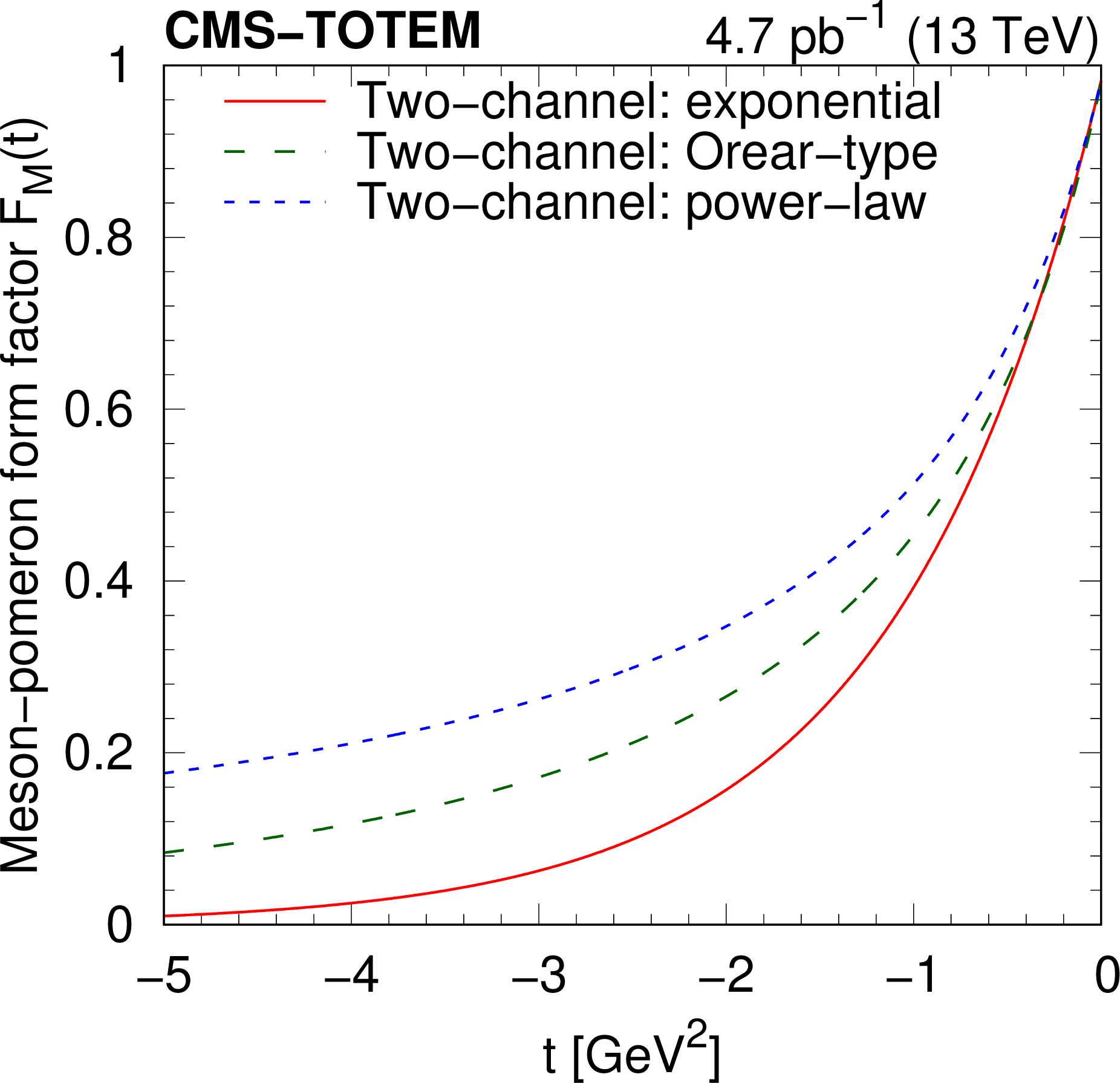
Figure 18:
Results of model tuning. Left: The plain exponential proton-pomeron form factor compared with those of the two diffractive proton eigenstates. Right: Various options of the meson-pomeron form factor, shown for the exponential, Orear-type, and power-law parametrisations. |
png pdf |
Figure 18-a:
Results of model tuning. The plain exponential proton-pomeron form factor compared with those of the two diffractive proton eigenstates. |
png pdf |
Figure 18-b:
Results of model tuning. Various options of the meson-pomeron form factor, shown for the exponential, Orear-type, and power-law parametrisations. |
png pdf |
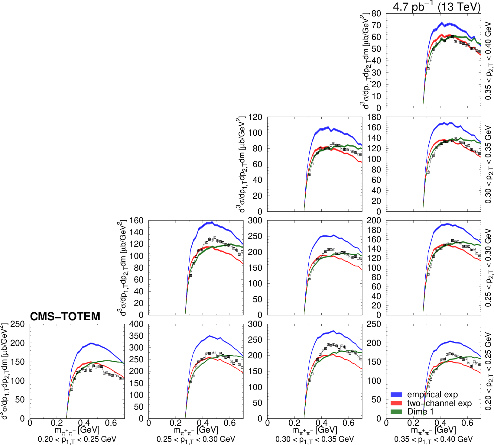
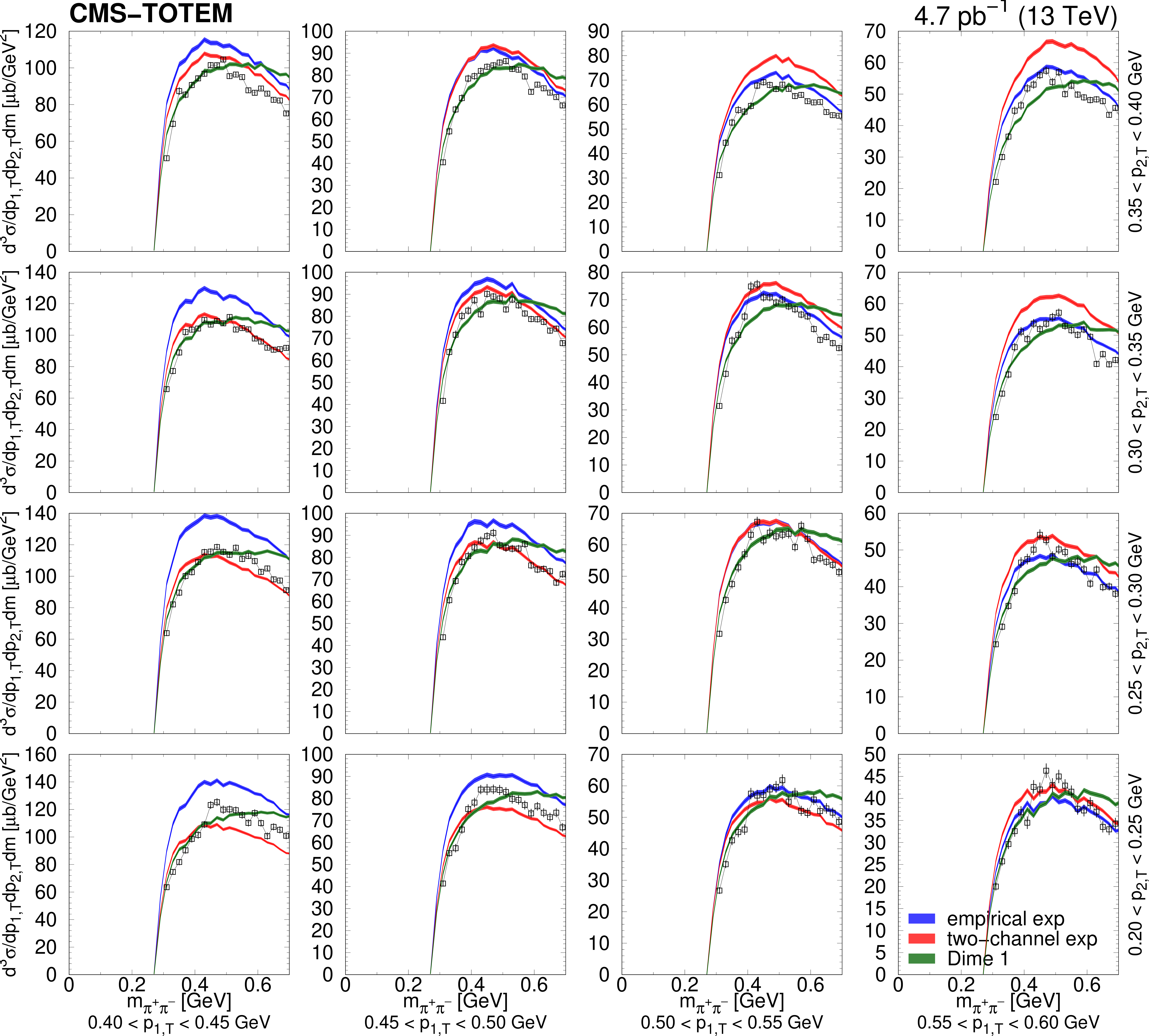
Figure 19:
Distribution of $ \mathrm{d}^3\sigma/\mathrm{d} p_\text{1,T} \mathrm{d} p_\text{2,T} \mathrm{d} m $ as a function of $ m $ for $ \pi^{+}\pi^{-} $ pairs in several $ (p_\text{1,T},p_\text{2,T}) $ bins, in units of $ \mu\mathrm{b}/\text{Ge\hspace{-.08em}V}^3 $, for the mass range 0.35 $ < m_{\pi^{+}\pi^{-}} < $ 0.65 GeV. Measured values (black symbols) are shown together with the predictions of the empirical and the two-channel models (coloured curves) using the tuned parameters for the exponential proton-pomeron form factors (see text for details). Curves corresponding to DIME (model 1) are also plotted. The error bars indicate the statistical uncertainties. Lines connecting the data points are drawn to guide the eye. |
png pdf |
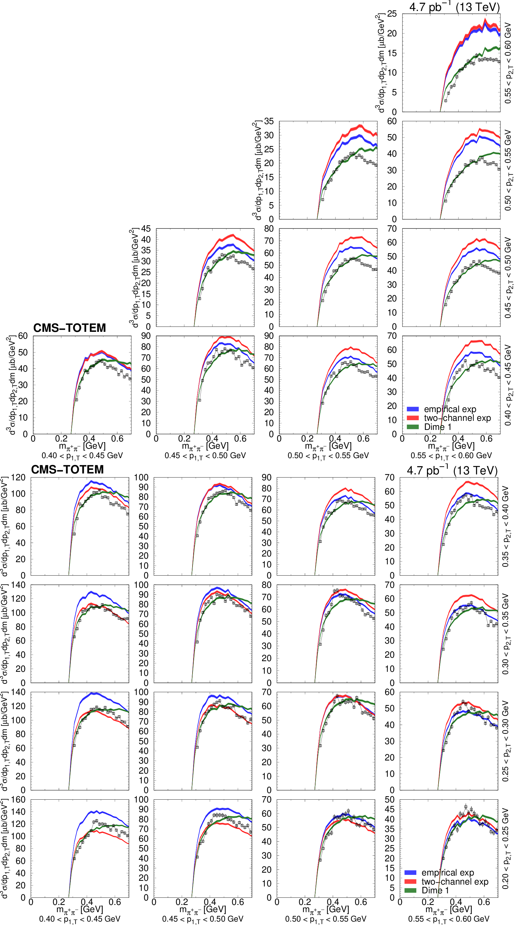
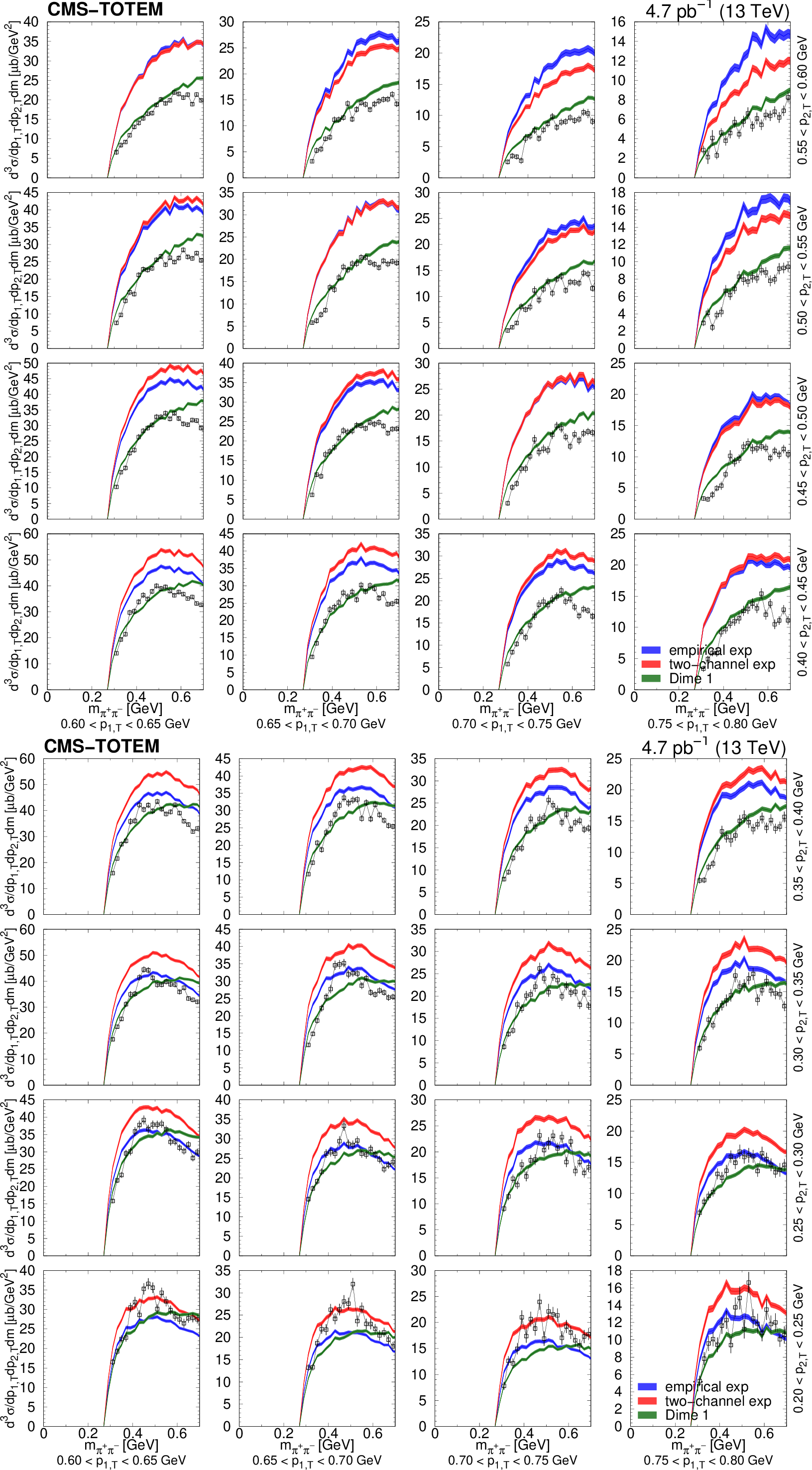
Figure 20:
Distribution of $ \mathrm{d}^3\sigma/\mathrm{d} p_\text{1,T} \mathrm{d} p_\text{2,T} \mathrm{d} m $ as a function of $ m $ for $ \pi^{+}\pi^{-} $ pairs in several $ (p_\text{1,T},p_\text{2,T}) $ bins, in units of $ \mu\mathrm{b}/\text{Ge\hspace{-.08em}V}^3 $, for the mass range 0.35 $ < m_{\pi^{+}\pi^{-}} < $ 0.65 GeV. Measured values (black symbols) are shown together with the predictions of the empirical and the two-channel models (coloured curves) using the tuned parameters for the exponential proton-pomeron form factors (see text for details). Curves corresponding to DIME (model 1) are also plotted. The error bars indicate the statistical uncertainties. Lines connecting the data points are drawn to guide the eye. |
png pdf |
Figure 20-a:
Distribution of $ \mathrm{d}^3\sigma/\mathrm{d} p_\text{1,T} \mathrm{d} p_\text{2,T} \mathrm{d} m $ as a function of $ m $ for $ \pi^{+}\pi^{-} $ pairs in several $ (p_\text{1,T},p_\text{2,T}) $ bins, in units of $ \mu\mathrm{b}/\text{Ge\hspace{-.08em}V}^3 $, for the mass range 0.35 $ < m_{\pi^{+}\pi^{-}} < $ 0.65 GeV. Measured values (black symbols) are shown together with the predictions of the empirical and the two-channel models (coloured curves) using the tuned parameters for the exponential proton-pomeron form factors (see text for details). Curves corresponding to DIME (model 1) are also plotted. The error bars indicate the statistical uncertainties. Lines connecting the data points are drawn to guide the eye. |
png pdf |
Figure 20-b:
Distribution of $ \mathrm{d}^3\sigma/\mathrm{d} p_\text{1,T} \mathrm{d} p_\text{2,T} \mathrm{d} m $ as a function of $ m $ for $ \pi^{+}\pi^{-} $ pairs in several $ (p_\text{1,T},p_\text{2,T}) $ bins, in units of $ \mu\mathrm{b}/\text{Ge\hspace{-.08em}V}^3 $, for the mass range 0.35 $ < m_{\pi^{+}\pi^{-}} < $ 0.65 GeV. Measured values (black symbols) are shown together with the predictions of the empirical and the two-channel models (coloured curves) using the tuned parameters for the exponential proton-pomeron form factors (see text for details). Curves corresponding to DIME (model 1) are also plotted. The error bars indicate the statistical uncertainties. Lines connecting the data points are drawn to guide the eye. |
png pdf |
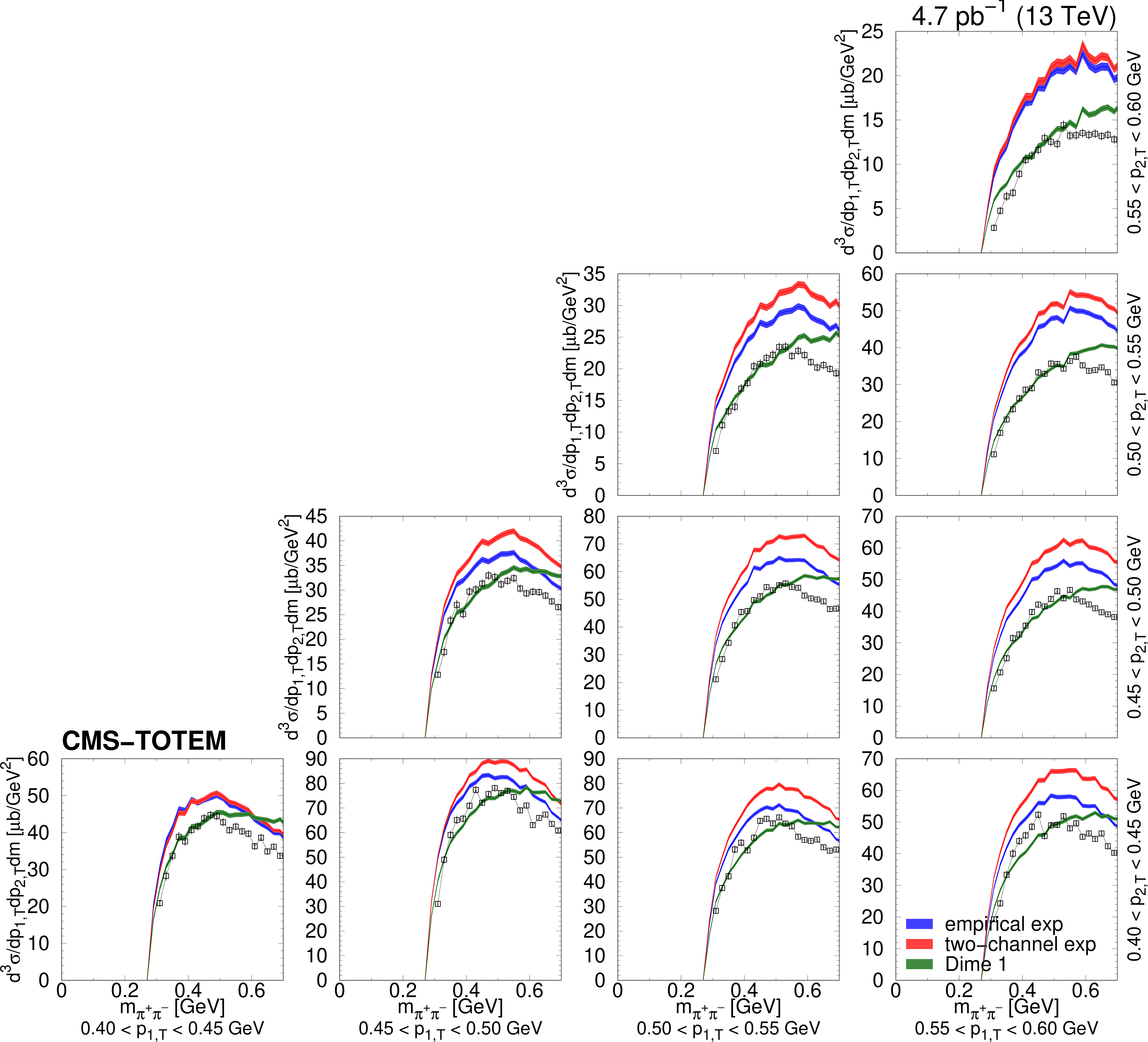
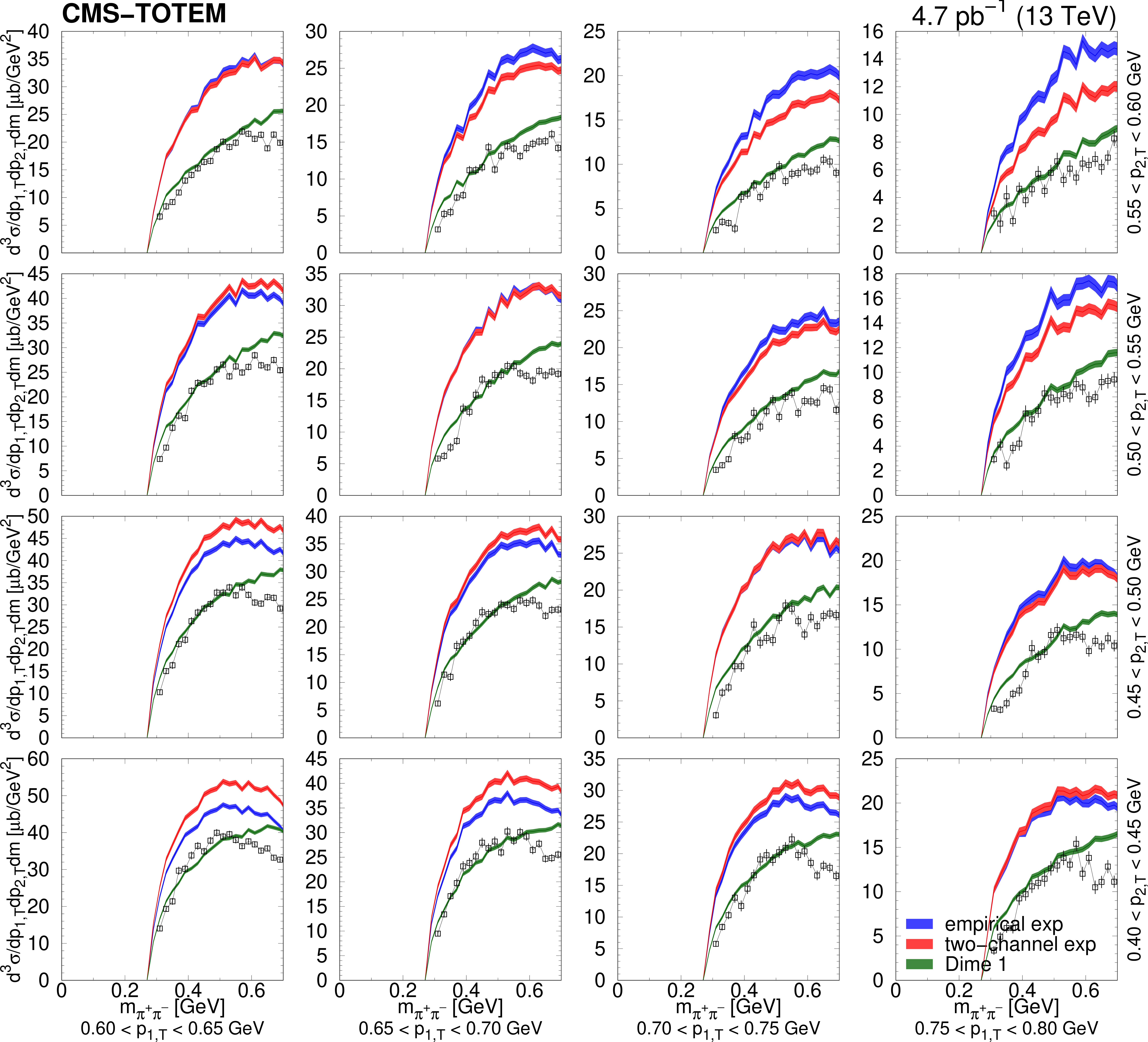
Figure 21:
Distribution of $ \mathrm{d}^3\sigma/\mathrm{d} p_\text{1,T} \mathrm{d} p_\text{2,T} \mathrm{d} m $ as a function of $ m $ for $ \pi^{+}\pi^{-} $ pairs in several $ (p_\text{1,T},p_\text{2,T}) $ bins, in units of $ \mu\mathrm{b}/\text{Ge\hspace{-.08em}V}^3 $, for the mass range 0.35 $ < m_{\pi^{+}\pi^{-}} < $ 0.65 GeV. Measured values (black symbols) are shown together with the predictions of the empirical and the two-channel models (coloured curves) using the tuned parameters for the exponential proton-pomeron form factors (see text for details). Curves corresponding to DIME (model 1) are also plotted. The error bars indicate the statistical uncertainties. Lines connecting the data points are drawn to guide the eye. |
png pdf |
Figure 21-a:
Distribution of $ \mathrm{d}^3\sigma/\mathrm{d} p_\text{1,T} \mathrm{d} p_\text{2,T} \mathrm{d} m $ as a function of $ m $ for $ \pi^{+}\pi^{-} $ pairs in several $ (p_\text{1,T},p_\text{2,T}) $ bins, in units of $ \mu\mathrm{b}/\text{Ge\hspace{-.08em}V}^3 $, for the mass range 0.35 $ < m_{\pi^{+}\pi^{-}} < $ 0.65 GeV. Measured values (black symbols) are shown together with the predictions of the empirical and the two-channel models (coloured curves) using the tuned parameters for the exponential proton-pomeron form factors (see text for details). Curves corresponding to DIME (model 1) are also plotted. The error bars indicate the statistical uncertainties. Lines connecting the data points are drawn to guide the eye. |

png pdf |
Figure 21-b:
Distribution of $ \mathrm{d}^3\sigma/\mathrm{d} p_\text{1,T} \mathrm{d} p_\text{2,T} \mathrm{d} m $ as a function of $ m $ for $ \pi^{+}\pi^{-} $ pairs in several $ (p_\text{1,T},p_\text{2,T}) $ bins, in units of $ \mu\mathrm{b}/\text{Ge\hspace{-.08em}V}^3 $, for the mass range 0.35 $ < m_{\pi^{+}\pi^{-}} < $ 0.65 GeV. Measured values (black symbols) are shown together with the predictions of the empirical and the two-channel models (coloured curves) using the tuned parameters for the exponential proton-pomeron form factors (see text for details). Curves corresponding to DIME (model 1) are also plotted. The error bars indicate the statistical uncertainties. Lines connecting the data points are drawn to guide the eye. |

png pdf |
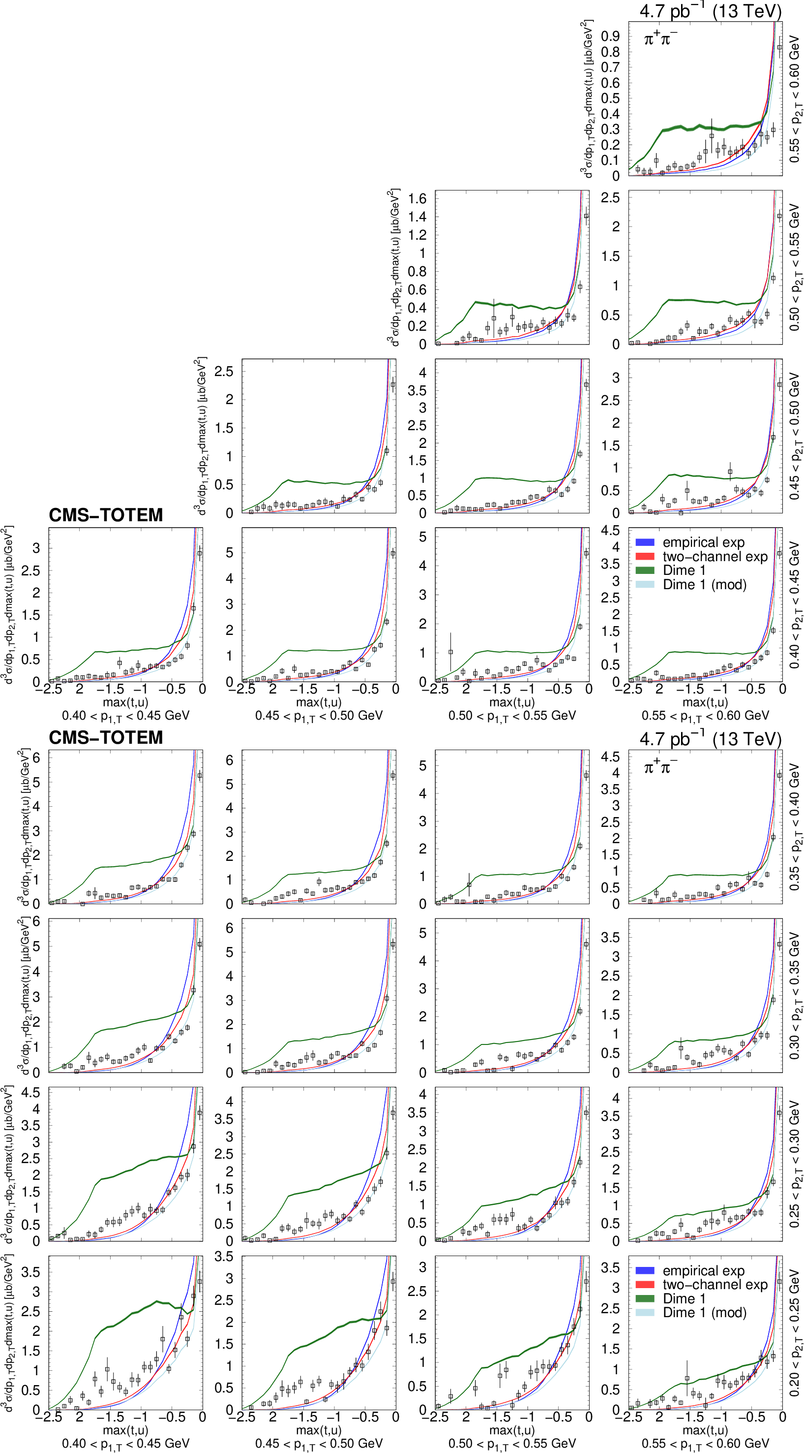
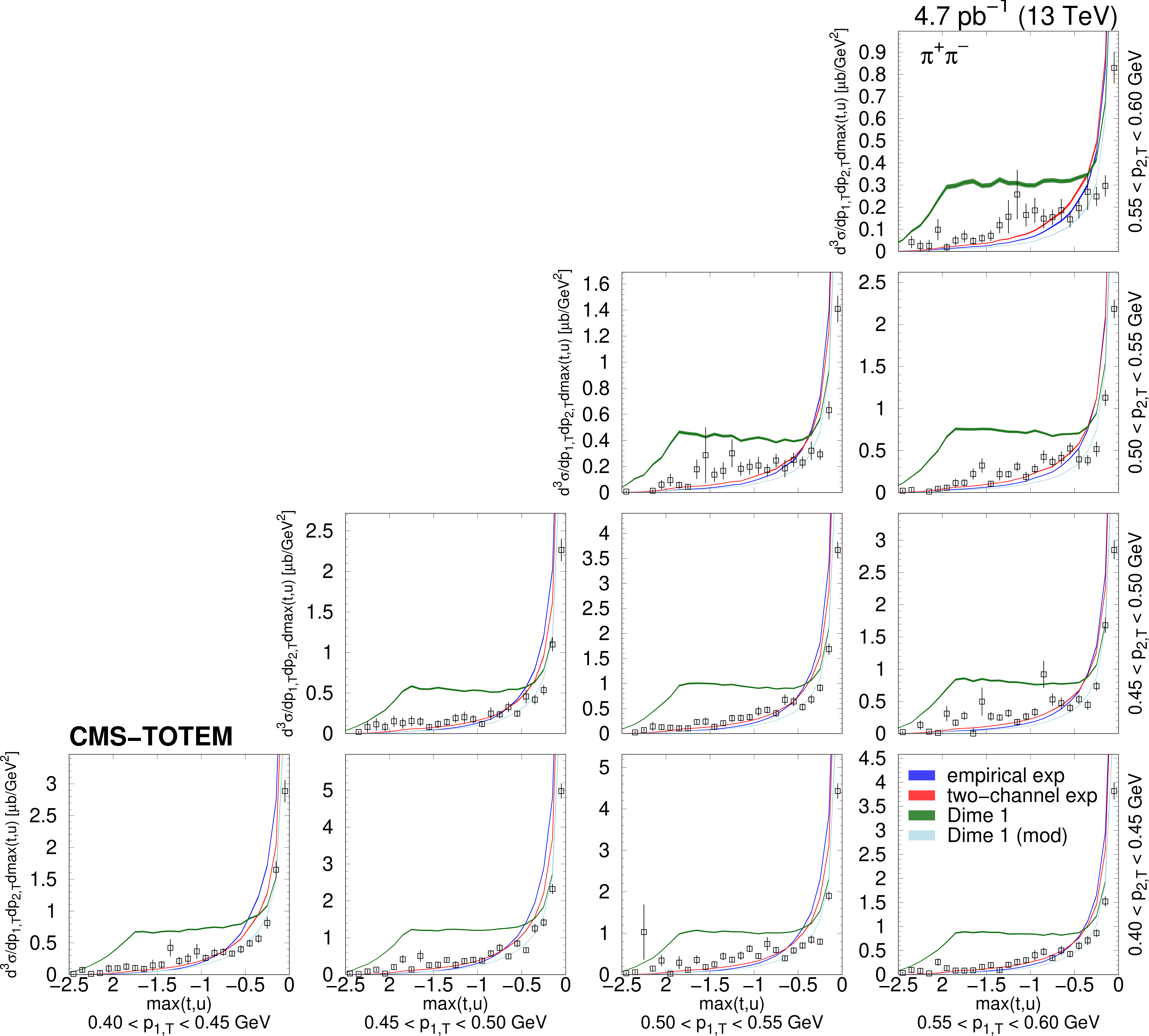
Figure 22:
Distribution of the squared momentum transfer of the virtual pion in several $ (p_\text{1,T},p_\text{2,T}) $ bins, in units of $ \mu\mathrm{b}/\text{Ge\hspace{-.08em}V}^3 $, for the mass range 1.8 $ < m_{\pi^{+}\pi^{-}} < $ 2.2 GeV. Measured values (black symbols) are shown together with the predictions of the empirical and the two-channel models (coloured curves) using the tuned parameters for the exponential proton-pomeron form factors (see text for details). Curves corresponding to DIME (model 1, ``Dime 1'') and its modification (labelled ``Dime 1 (mod)'') with $ b_\text{exp} = 0.9\,\text{Ge\hspace{-.08em}V}^{-2} $ are also plotted. The error bars indicate the statistical uncertainties. |
png pdf |
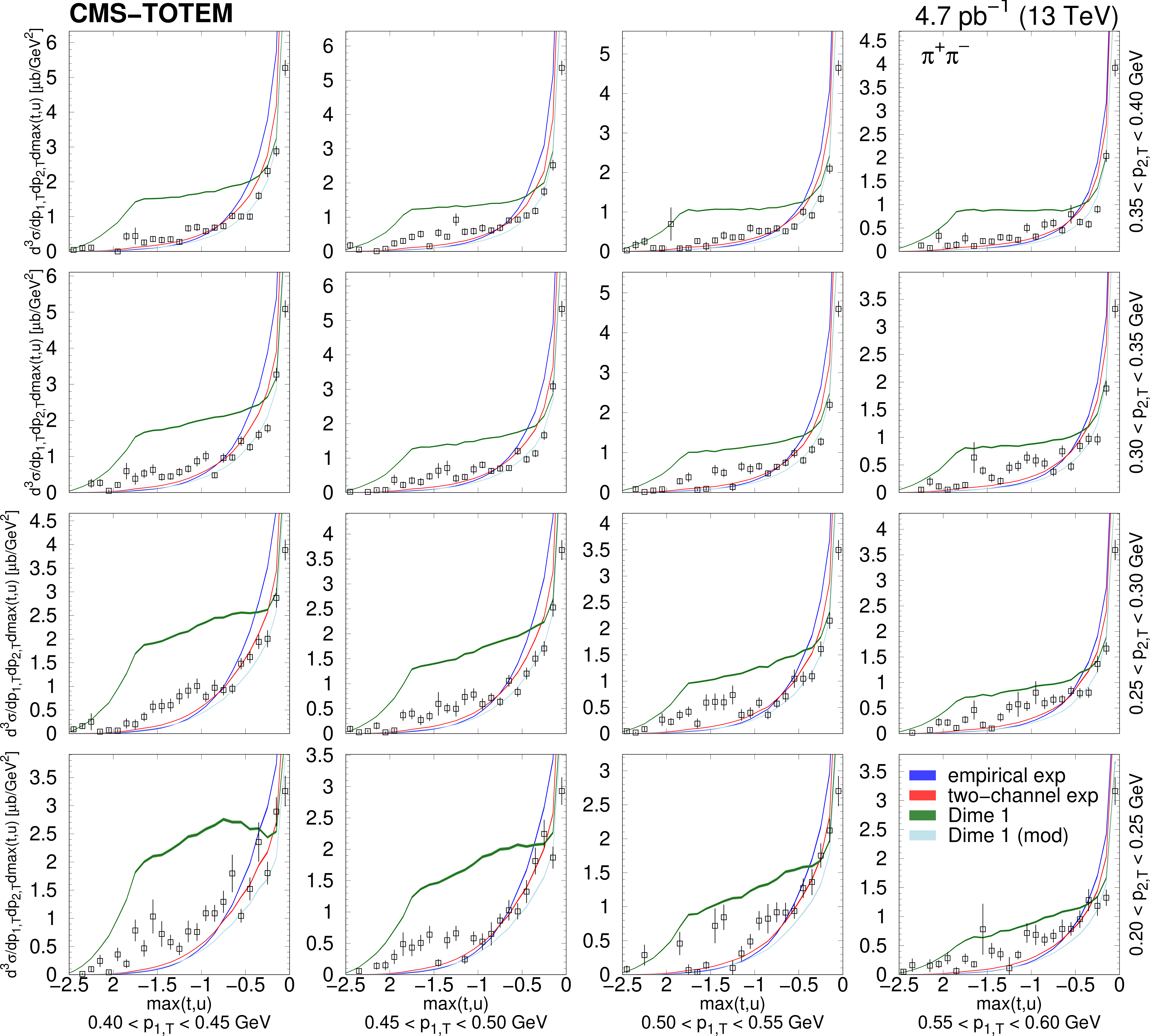
Figure 23:
Distribution of the squared momentum transfer of the virtual pion in several $ (p_\text{1,T},p_\text{2,T}) $ bins, in units of $ \mu\mathrm{b}/\text{Ge\hspace{-.08em}V}^3 $, for the mass range 1.8 $ < m_{\pi^{+}\pi^{-}} < $ 2.2 GeV. Measured values (black symbols) are shown together with the predictions of the empirical and the two-channel models (coloured curves) using the tuned parameters for the exponential proton-pomeron form factors (see text for details). Curves corresponding to DIME (model 1, ``Dime 1'') and its modification (labelled ``Dime 1 (mod)'') with $ b_\text{exp} = 0.9\,\text{Ge\hspace{-.08em}V}^{-2} $ are also plotted. The error bars indicate the statistical uncertainties. |
png pdf |
Figure 23-a:
Distribution of the squared momentum transfer of the virtual pion in several $ (p_\text{1,T},p_\text{2,T}) $ bins, in units of $ \mu\mathrm{b}/\text{Ge\hspace{-.08em}V}^3 $, for the mass range 1.8 $ < m_{\pi^{+}\pi^{-}} < $ 2.2 GeV. Measured values (black symbols) are shown together with the predictions of the empirical and the two-channel models (coloured curves) using the tuned parameters for the exponential proton-pomeron form factors (see text for details). Curves corresponding to DIME (model 1, ``Dime 1'') and its modification (labelled ``Dime 1 (mod)'') with $ b_\text{exp} = 0.9\,\text{Ge\hspace{-.08em}V}^{-2} $ are also plotted. The error bars indicate the statistical uncertainties. |
png pdf |
Figure 23-b:
Distribution of the squared momentum transfer of the virtual pion in several $ (p_\text{1,T},p_\text{2,T}) $ bins, in units of $ \mu\mathrm{b}/\text{Ge\hspace{-.08em}V}^3 $, for the mass range 1.8 $ < m_{\pi^{+}\pi^{-}} < $ 2.2 GeV. Measured values (black symbols) are shown together with the predictions of the empirical and the two-channel models (coloured curves) using the tuned parameters for the exponential proton-pomeron form factors (see text for details). Curves corresponding to DIME (model 1, ``Dime 1'') and its modification (labelled ``Dime 1 (mod)'') with $ b_\text{exp} = 0.9\,\text{Ge\hspace{-.08em}V}^{-2} $ are also plotted. The error bars indicate the statistical uncertainties. |
| Tables | |
png pdf |
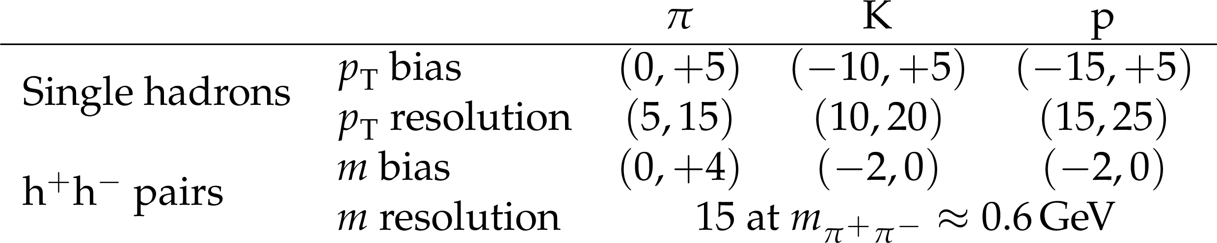
Table 1:
Ranges (in parentheses) for bias and resolution of the reconstructed transverse momentum and the two-hadron invariant mass, shown for pions, kaons, and protons, in MeV units. |
png pdf |
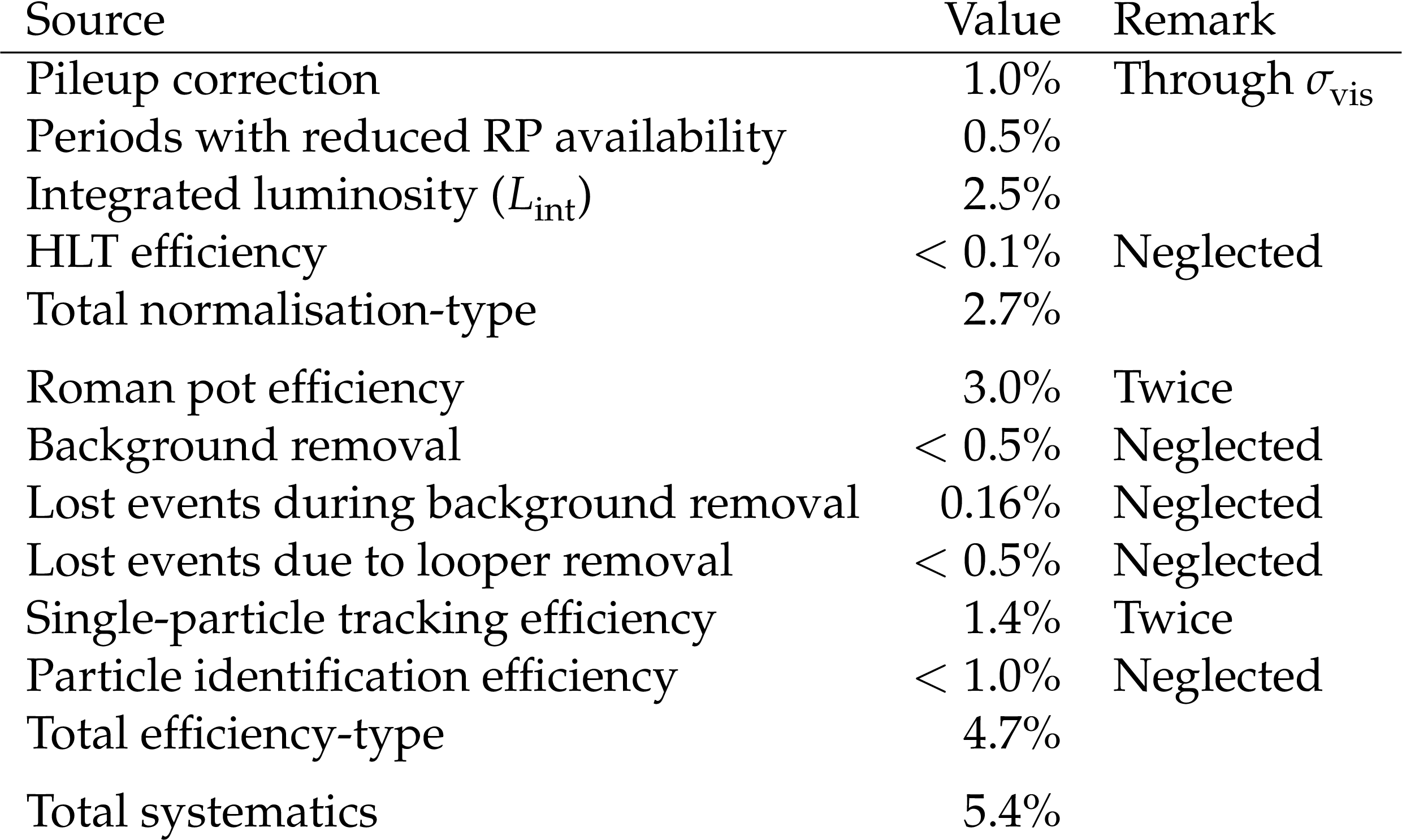
Table 2:
Systematic uncertainties of the differential cross sections. |
png pdf |
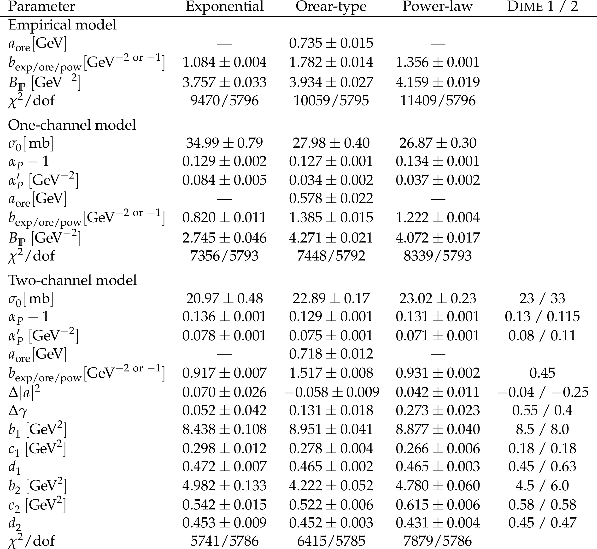
Table 3:
Values and statistical uncertainties of the parameters tuned using the PROFESSOR\ tool, given for the empirical, one-channel, and two-channel models along with the DIME\ soft models 1 and 2 with the exponential, power-law, and the Orear-type parametrisations of the proton-pomeron form factor. Goodness-of-fit ($ \chi^2/\mathrm{dof} $) values are also listed. |
| Summary |
| We examined the central exclusive production of charged hadron pairs in proton-proton collisions at a centre-of-mass energy of 13 TeV. Events are selected by requiring both scattered protons to be detected in the TOTEM Roman pots and exactly two oppositely charged identified pions in the CMS silicon tracker. The process is studied in the resonance-free region, for invariant masses of the centrally produced two-pion system $ m_{\pi^{+}\pi^{-}} < $ 0.7 GeV or $ m_{\pi^{+}\pi^{-}} > $ 1.8 GeV. Differential cross sections are measured as a function of the azimuthal angle between the surviving protons in a wide region of scattered proton transverse momenta, between 0.2 and 0.8 GeV, and for pion rapidities $ |y| < $ 2. A rich structure of nonperturbative interactions related to double-pomeron exchange emerges and is measured with good precision. The parabolic minimum in the distribution of the two-proton azimuthal angle is observed for the first time. It can be understood as an effect of additional pomeron exchanges between the incoming protons, resulting from the interference of the bare and the rescattered amplitudes. With model tuning, various physical quantities related to the pomeron cross section, proton-pomeron, and meson-pomeron form factors, pomeron trajectory and intercept, as well as coefficients of diffractive eigenstates of the proton are determined. |
| References | ||||
| 1 | Particle Data Group , R. L. Workman et al. | Review of particle physics | PTEP 2022 (2022) 083C01 | |
| 2 | V. B. Berestetsky and I. Y. Pomeranchuk | On the asymptotic behaviour of cross sections at high energies | NP 22 (1961) 629 | |
| 3 | S. Donnachie, H. G. Dosch, O. Nachtmann, and P. Landshoff | Pomeron physics and QCD | volume~19. Cambridge University Press, . ISBN~978-0-511-06050-2, 978-0-521-78039-1, 978-0-521-67570-3, 2004 | |
| 4 | D. Amati, A. Stanghellini, and S. Fubini | Theory of high-energy scattering and multiple production | Nuovo Cim. 26 (1962) 896 | |
| 5 | H. B. Meyer and M. J. Teper | Glueball Regge trajectories and the pomeron: A lattice study | PLB 605 (2005) 344 | hep-ph/0409183 |
| 6 | D0 and TOTEM Collaborations | Odderon exchange from elastic scattering differences between pp and $ \mathrm{p\bar{p}} $ data at 1.96 TeV and from pp forward scattering measurements | PRL 127 (2021) 062003 | 2012.03981 |
| 7 | M. G. Albrow, T. D. Coughlin, and J. R. Forshaw | Central exclusive particle production at high energy hadron colliders | Prog. Part. Nucl. Phys. 65 (2010) 149 | 1006.1289 |
| 8 | W. Ochs | The status of glueballs | JPG 40 (2013) 043001 | 1301.5183 |
| 9 | WA76 Collaboration | Study of the centrally produced $ \pi\pi $ and $ \mathrm{K\overline{K}} $ systems at 85 and 300 GeV/c | Z. Phys. C 51 (1991) 351 | |
| 10 | WA91 Collaboration | A further study of the centrally produced $ \pi^{+}\pi^{-} $ and $ \pi^{+}\pi^{-}\pi^{+}\pi^{-} $ channels in pp interactions at 300 and 450 GeV/c | PLB 353 (1995) 5894 | |
| 11 | F. E. Close and G. A. Schuler | Evidence that the pomeron transforms as a non-conserved vector current | PLB 464 (1999) 279 | hep-ph/9905305 |
| 12 | WA102 Collaboration | Experimental evidence for a vector-like behavior of Pomeron exchange | PLB 467 (1999) 165 | hep-ex/9909013 |
| 13 | F. E. Close, A. Kirk, and G. Schuler | Dynamics of glueball and $ \mathrm{q\overline{q}} $ production in the central region of pp collisions | PLB 477 (2000) 13 | hep-ph/0001158 |
| 14 | A. Kirk | Resonance production in central pp collisions at the CERN Omega spectrometer | PLB 489 (2000) 29 | hep-ph/0008053 |
| 15 | CDF Collaboration | Measurement of central exclusive $ \pi^+ \pi^- $ production in $ \mathrm{p\bar{p}} $ collisions at $ \sqrt{s} = $ 0.9 and 1.96 TeV at CDF | PRD 91 (2015) 091101 | 1502.01391 |
| 16 | STAR Collaboration | Measurement of the central exclusive production of charged particle pairs in proton-proton collisions at $ \sqrt{s} = $ 200 GeV with the STAR detector at RHIC | JHEP 07 (2020) 178 | 2004.11078 |
| 17 | ATLAS Collaboration | Measurement of exclusive pion pair production in proton-proton collisions at $ \sqrt{s}={7}\,\text {TeV} $ with the ATLAS detector | EPJC 83 (2023) 627 | 2212.00664 |
| 18 | CMS Collaboration | Study of central exclusive $ \pi^+\pi^- $ production in proton-proton collisions at $ \sqrt{s} = $ 5.02 and 13 TeV | EPJC 80 (2020) 718 | CMS-FSQ-16-006 2003.02811 |
| 19 | P. Lebiedowicz and A. Szczurek | Exclusive $ pp \to pp \pi^{+}\pi^{-} $ reaction: from the threshold to LHC | PRD 81 (2010) 036003 | 0912.0190 |
| 20 | P. Lebiedowicz and A. Szczurek | Revised model of absorption corrections for the $ p p \to p p \pi^{+} \pi^{-} $ process | PRD 92 (2015) 054001 | 1504.07560 |
| 21 | P. Lebiedowicz, O. Nachtmann, and A. Szczurek | Central exclusive diffractive production of $ \pi^{+}\pi^{-} $ continuum, scalar and tensor resonances in pp and $ \mathrm{p \bar{p}} $ scattering within tensor Pomeron approach | PRD 93 (2016) 054015 | 1601.04537 |
| 22 | P. Lebiedowicz, O. Nachtmann, and A. Szczurek | Towards a complete study of central exclusive production of $ K^{+}K^{-} $ pairs in proton-proton collisions within the tensor Pomeron approach | PRD 98 (2018) 014001 | 1804.04706 |
| 23 | P. Lebiedowicz, O. Nachtmann, and A. Szczurek | Central exclusive diffractive production of $ \mathrm{p \bar{p}} $ pairs in proton-proton collisions at high energies | PRD 97 (2018) 094027 | 1801.03902 |
| 24 | M. G. Ryskin, A. D. Martin, and V. A. Khoze | Proton opacity in the light of LHC diffractive data | EPJC 72 (2012) 1937 | 1201.6298 |
| 25 | L. A. Harland-Lang, V. A. Khoze, M. G. Ryskin, and W. J. Stirling | The phenomenology of central exclusive production at hadron colliders | EPJC 72 (2012) 2110 | 1204.4803 |
| 26 | V. A. Khoze, A. D. Martin, and M. G. Ryskin | Diffraction at the LHC | EPJC 73 (2013) 2503 | 1306.2149 |
| 27 | L. A. Harland-Lang, V. A. Khoze, and M. G. Ryskin | Modelling exclusive meson pair production at hadron colliders | EPJC 74 (2014) 2848 | 1312.4553 |
| 28 | A. Grau, S. Pacetti, G. Pancheri, and Y. N. Srivastava | Checks of asymptotia in pp elastic scattering at LHC | PLB 714 (2012) 70 | 1206.1076 |
| 29 | D. A. Fagundes et al. | Elastic pp scattering from the optical point to past the dip: An empirical parametrization from ISR to the LHC | PRD 88 (2013) 094019 | 1306.0452 |
| 30 | L. Lukaszuk and B. Nicolescu | A possible interpretation of pp rising total cross sections | Lett. Nuovo Cim. 8 (1973) 405 | |
| 31 | A. Donnachie and P. V. Landshoff | Total cross sections | PLB 296 (1992) 227 | hep-ph/9209205 |
| 32 | J. R. Cudell et al. | Hadronic scattering amplitudes: medium-energy constraints on asymptotic behavior | PRD 65 (2002) 074024 | hep-ph/0107219 |
| 33 | J. Orear | Transverse momentum distribution of protons in p-p elastic scattering | PRL 12 (1964) 112 | |
| 34 | CMS Collaboration | Track impact parameter resolution for the full pseudorapidity coverage in the 2017 dataset with the CMS Phase-1 Pixel detector | CMS Detector Performance Note CMS-DP-2020-049, 2020 CDS |
|
| 35 | CMS Collaboration | The CMS experiment at the CERN LHC | JINST 3 (2008) S08004 | |
| 36 | TOTEM Collaboration | The TOTEM experiment at the CERN Large Hadron Collider | JINST 3 (2008) S08007 | |
| 37 | TOTEM Collaboration | Performance of the TOTEM detectors at the LHC | Int. J. Mod. Phys. A 28 (2013) 1330046 | 1310.2908 |
| 38 | GEANT4 Collaboration | GEANT 4 -- a simulation toolkit | NIM A 506 (2003) 250 | |
| 39 | K. Gottfried and J. D. Jackson | On the connection between production mechanism and decay of resonances at high-energies | Nuovo Cim. 33 (1964) 309 | |
| 40 | H. Wiedemann | Particle accelerator physics: basic principles and linear beam dynamics | Springer Berlin Heidelberg, . ISBN~978366039, 2013 | |
| 41 | CMS Collaboration | The CMS trigger system | JINST 12 (2017) P01020 | CMS-TRG-12-001 1609.02366 |
| 42 | ATLAS Collaboration | Measurement of the inelastic proton-proton cross section at $ \sqrt{s} = $ 13 TeV with the ATLAS detector at the LHC | PRL 117 (2016) 182002 | 1606.02625 |
| 43 | CMS Collaboration | Measurement of the inelastic proton-proton cross section at $ \sqrt{s}= $ 13 TeV | JHEP 07 (2018) 161 | CMS-FSQ-15-005 1802.02613 |
| 44 | LHCb Collaboration | Measurement of the inelastic pp cross-section at a centre-of-mass energy of 13 TeV | JHEP 06 (2018) 100 | 1803.10974 |
| 45 | TOTEM Collaboration | First measurement of elastic, inelastic and total cross-section at $ \sqrt{s}= $ 13 TeV by TOTEM and overview of cross-section data at LHC energies | EPJC 79 (2019) 103 | 1712.06153 |
| 46 | CMS and TOTEM Collaborations | Proton reconstruction using the TOTEM Roman pot detectors during the high-$ \beta^* $ data taking period | paper in preparation | |
| 47 | CMS Collaboration | Description and performance of track and primary-vertex reconstruction with the CMS tracker | JINST 9 (2014) P10009 | CMS-TRK-11-001 1405.6569 |
| 48 | CMS Collaboration | Measurement of charged pion, kaon, and proton production in proton-proton collisions at $ \sqrt{s}= $ 13 TeV | PRD 96 (2017) 112003 | CMS-FSQ-16-004 1706.10194 |
| 49 | R. M. Sternheimer, M. J. Berger, and S. M. Seltzer | Density effect for the ionization loss of charged particles in various substances | Atom. Data Nucl. Data Tabl. 30 (1984) 261 | |
| 50 | P. C. Mahalanobis | On the generalized distance in statistics | in Proceedings of the National Institute of Sciences of India, volume~2, 1936 | |
| 51 | CMSnoop | none | \hrefHEPData record for this analysis, 2023 link |
|
| 52 | CMS Collaboration | CMS luminosity measurement for the 2018 data-taking period at $ \sqrt{s} = $ 13 TeV | CMS Physics Analysis Summary, 2018 CMS-PAS-LUM-18-002 |
CMS-PAS-LUM-18-002 |
| 53 | CMS Collaboration | Measurements of inclusive W and Z cross sections in pp collisions at $ \sqrt{s}= $ 7 TeV | JHEP 01 (2011) 080 | CMS-EWK-10-002 1012.2466 |
| 54 | CMS Collaboration | Measurement of tracking efficiency | CMS Physics Analysis Summary, 2010 CMS-PAS-TRK-10-002 |
|
| 55 | L. A. Harland-Lang, V. A. Khoze, and M. G. Ryskin | Exclusive physics at the LHC with SuperChic 2 | EPJC 76 (2016) 9 | 1508.02718 |
| 56 | R. A. Kycia, J. Chwastowski, R. Staszewski, and J. Turnau | GenEx: A simple generator structure for exclusive processes in high energy collisions | Commun. Comput. Phys. 24 (2018) 860 | 1411.6035 |
| 57 | M. Mieskolainen | GRANIITTI: A Monte Carlo event generator for high energy diffraction | 1910.06300 | |
| 58 | TOTEM Collaboration | First determination of the $ {\rho } $ parameter at $ {\sqrt{s} = 13} $ TeV: probing the existence of a colourless C-odd three-gluon compound state | EPJC 79 (2019) 785 | 1812.04732 |
| 59 | TOTEM Collaboration | Elastic differential cross section measurement at $ \sqrt{s}= $ 13 TeV by TOTEM | EPJC 79 (2019) 861 | 1812.08283 |
| 60 | V. A. Khoze, A. D. Martin, and M. G. Ryskin | t dependence of the slope of the high energy elastic pp cross section | JPG 42 (2015) 025003 | 1410.0508 |
| 61 | A. Buckley et al. | Systematic event generator tuning for the LHC | EPJC 65 (2010) 331 | 0907.2973 |
|
|
Compact Muon Solenoid LHC, CERN |
|

|

|

|

|

|