

Compact Muon Solenoid
LHC, CERN
| CMS-SUS-16-036 ; CERN-EP-2017-084 | ||
| Search for new phenomena with the $ \mathrm{ M_{\mathrm T2} } $ variable in the all-hadronic final state produced in proton-proton collisions at $\sqrt{s} = $ 13 TeV | ||
| CMS Collaboration | ||
| 12 May 2017 | ||
| Eur. Phys. J C 77 (2017) 710 | ||
| Abstract: A search for new phenomena is performed using events with jets and significant transverse momentum imbalance, as inferred through the $M_{\mathrm{{T2}}}$ variable. The results are based on a sample of proton-proton collisions collected in 2016 at a center-of-mass energy of 13 TeV with the CMS detector and corresponding to an integrated luminosity of 35.9 fb$^{-1}$. No excess event yield is observed above the predicted standard model background, and the results are interpreted as limits on the masses of predicted particles in a variety of simplified models of $R$-parity conserving supersymmetry. Depending on the details of the model, 95% confidence level lower limits on the gluino (light-flavor squark) masses are placed up to 2025 (1550) GeV. Mass limits as high as 1070 (1175) GeV are set on the masses of top (bottom) squarks. Information is provided to enable re-interpretation of these results, including model-independent limits on the number of non-standard model events for a set of simplified, inclusive search regions. | ||
| Links: e-print arXiv:1705.04650 [hep-ex] (PDF) ; CDS record ; inSPIRE record ; CADI line (restricted) ; | ||
| Figures & Tables | Summary | Additional Figures & Tables | References | CMS Publications |
|---|
|
Additional information on efficiencies needed for reinterpretation of these results are available here. Additional technical material for CMS speakers can be found here. |
| Figures | |

png pdf |
Figure 1:
Distributions of the $ {M_{\mathrm {T2}}} $ variable in data and simulation for the single-lepton control region selection, after normalizing the simulation to data in the control region bins of $ {H_{\mathrm {T}}} $, $ {N_{\mathrm {j}}} $, and $ {N_{\mathrm{ b } }} $ for events with no b-tagged jets (left), and events with at least one b-tagged jet (right). The hatched bands on the top panels show the MC statistical uncertainty, while the solid gray bands in the ratio plots show the systematic uncertainty in the $ {M_{\mathrm {T2}}} $ shape. |

png pdf |
Figure 1-a:
Distributions of the $ {M_{\mathrm {T2}}} $ variable in data and simulation for the single-lepton control region selection, after normalizing the simulation to data in the control region bins of $ {H_{\mathrm {T}}} $, $ {N_{\mathrm {j}}} $, and $ {N_{\mathrm{ b } }} $ for events with no b-tagged jets. The hatched bands on the top panels show the MC statistical uncertainty, while the solid gray bands in the ratio plots show the systematic uncertainty in the $ {M_{\mathrm {T2}}} $ shape. |

png pdf |
Figure 1-b:
Distributions of the $ {M_{\mathrm {T2}}} $ variable in data and simulation for the single-lepton control region selection, after normalizing the simulation to data in the control region bins of $ {H_{\mathrm {T}}} $, $ {N_{\mathrm {j}}} $, and $ {N_{\mathrm{ b } }} $ for events with at least one b-tagged jet. The hatched bands on the top panels show the MC statistical uncertainty, while the solid gray bands in the ratio plots show the systematic uncertainty in the $ {M_{\mathrm {T2}}} $ shape. |
png pdf |
Figure 2:
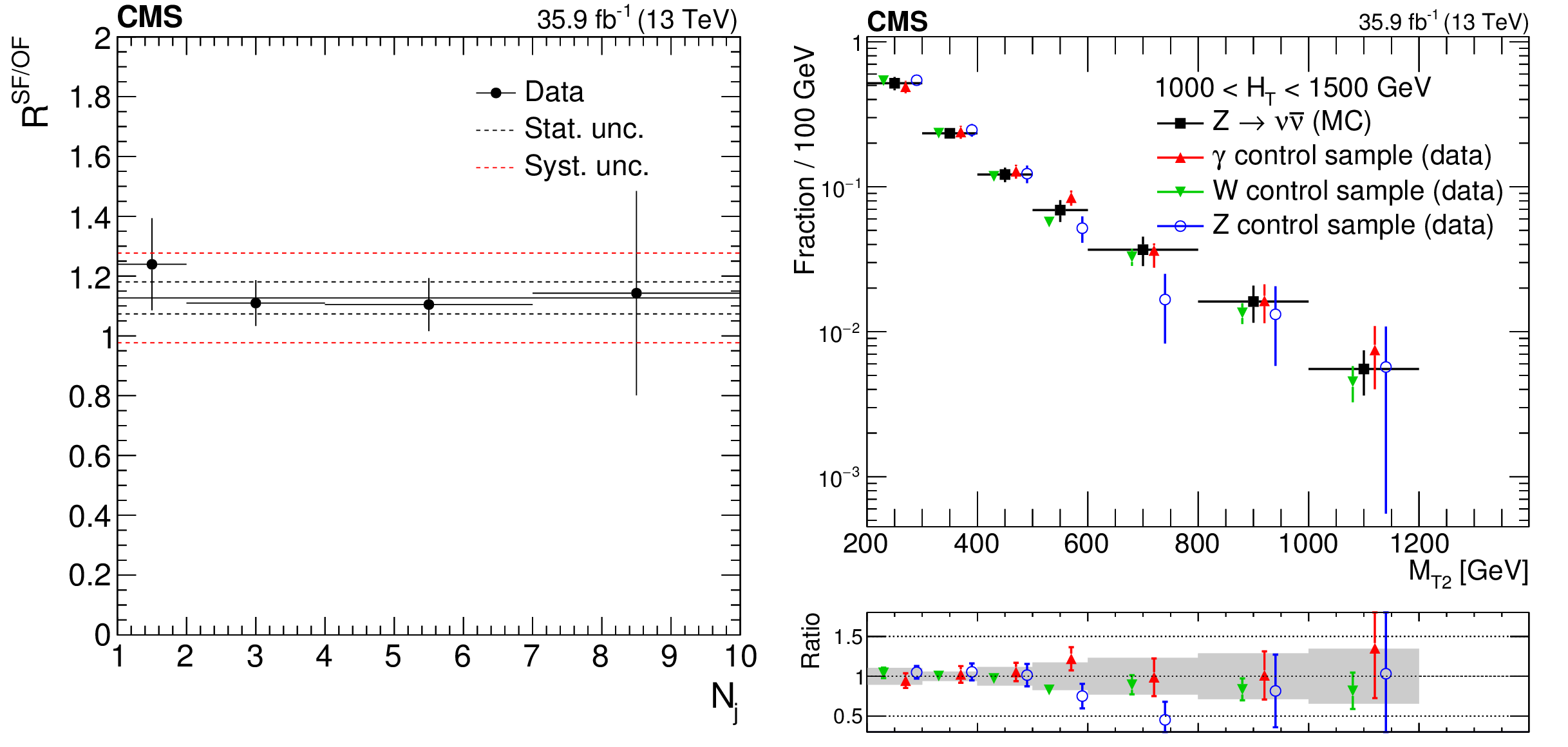
(Left) Ratio $R^{\mathrm {SF}/\mathrm {OF}}$ in data as a function of $ {N_{\mathrm {j}}} $. The solid black line enclosed by the red dashed lines corresponds to a value of 1.13 $\pm$ 0.15 that is observed to be stable with respect to event kinematics, while the two dashed black lines denote the statistical uncertainty in the $R^{\mathrm {SF}/\mathrm {OF}}$ value. (Right) The shape of the $ {M_{\mathrm {T2}}} $ distribution in ${\mathrm{ Z } \to \nu \bar{\nu} }$ simulation compared to shapes from $\gamma $, W, and Z data control samples in a region with 1000 $ < {H_{\mathrm {T}}} < $ 1500 GeV and $ {N_{\mathrm {j}}} \ge $ 2, inclusive in $ {N_{\mathrm{ b } }} $. The solid gray band on the ratio plot shows the systematic uncertainty in the $ {M_{\mathrm {T2}}} $ shape. |
png pdf |
Figure 2-a:
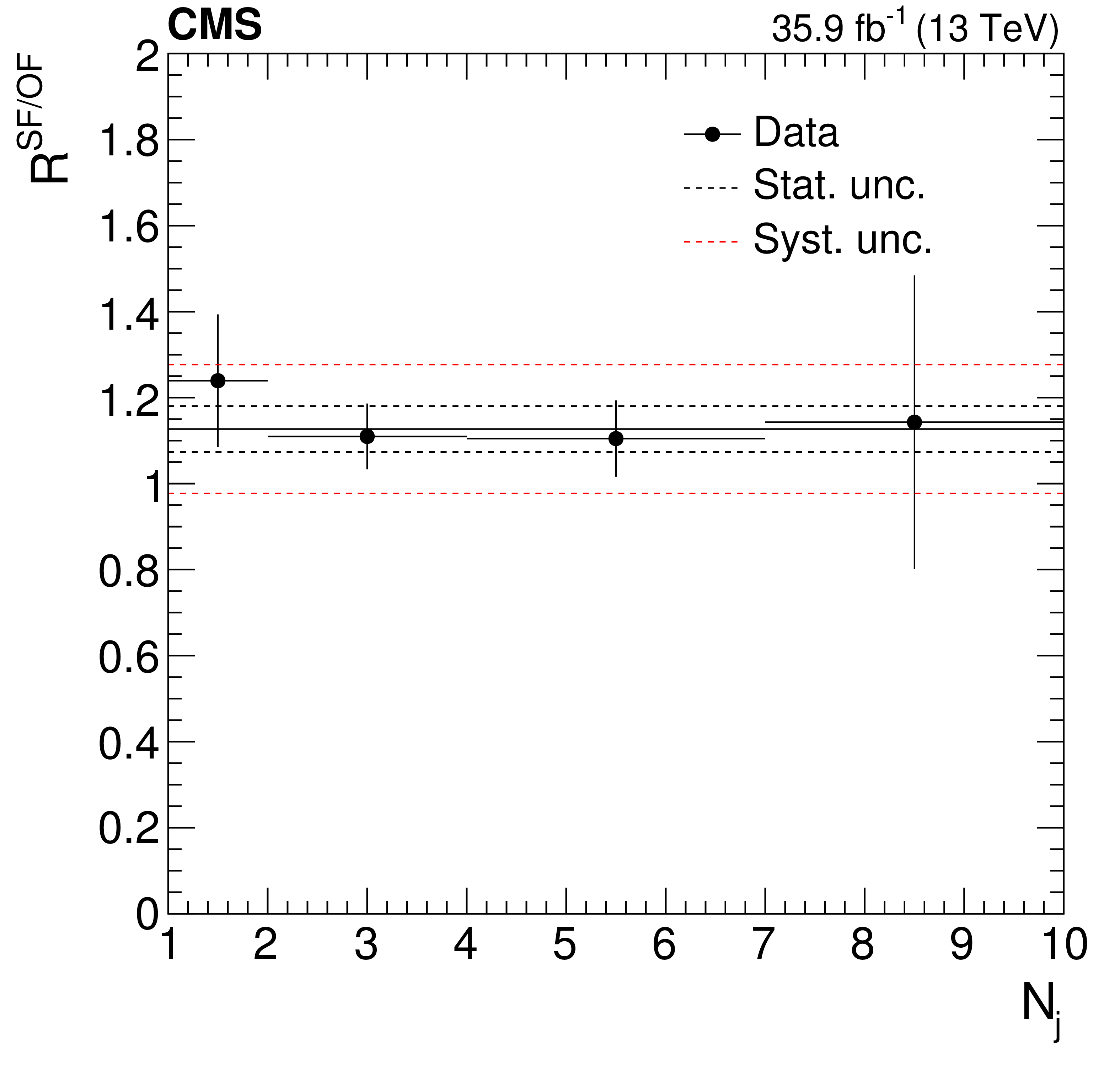
Ratio $R^{\mathrm {SF}/\mathrm {OF}}$ in data as a function of $ {N_{\mathrm {j}}} $. The solid black line enclosed by the red dashed lines corresponds to a value of 1.13 $\pm$ 0.15 that is observed to be stable with respect to event kinematics, while the two dashed black lines denote the statistical uncertainty in the $R^{\mathrm {SF}/\mathrm {OF}}$ value. |
png pdf |
Figure 2-b:
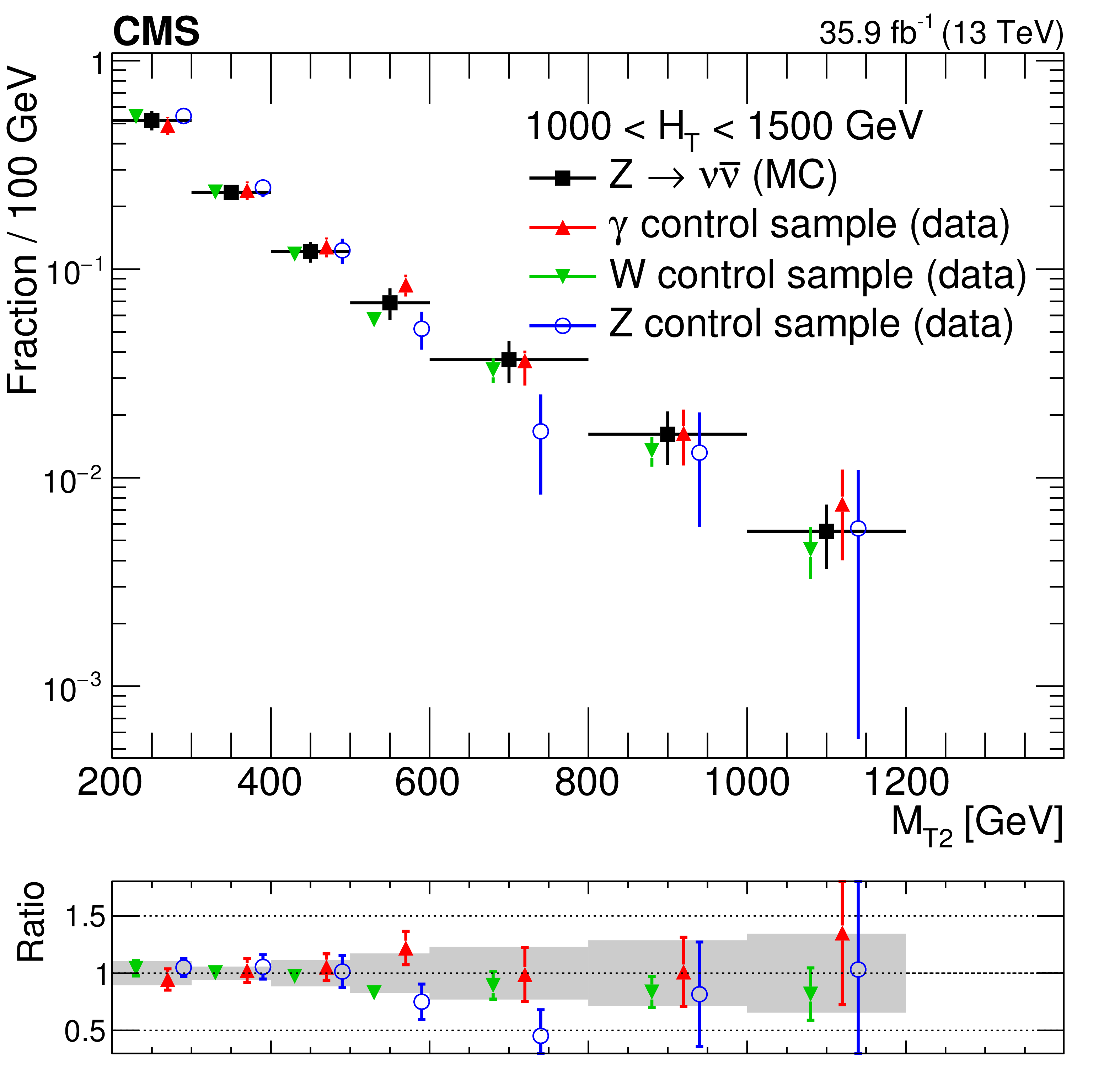
The shape of the $ {M_{\mathrm {T2}}} $ distribution in ${\mathrm{ Z } \to \nu \bar{\nu} }$ simulation compared to shapes from $\gamma $, W, and Z data control samples in a region with 1000 $ < {H_{\mathrm {T}}} < $ 1500 GeV and $ {N_{\mathrm {j}}} \ge $ 2, inclusive in $ {N_{\mathrm{ b } }} $. The solid gray band on the ratio plot shows the systematic uncertainty in the $ {M_{\mathrm {T2}}} $ shape. |
png pdf |
Figure 3:
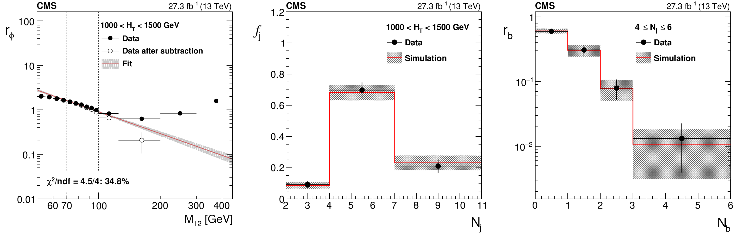
The ratio $r_{\phi }$ as a function of $ {M_{\mathrm {T2}}} $ for 1000 $ < {H_{\mathrm {T}}} < $ 1500 GeV (left). The superimposed fit is performed to the open circle data points. The black points represent the data before subtracting non-QCD contributions using simulation. Data point uncertainties are statistical only. The red line and the grey band around it show the result of the fit to a power-law function performed in the window 70 $ < {M_{\mathrm {T2}}} < $ 100 GeV and the associated fit uncertainty. Values of $f_\mathrm {j}$, the fraction of events in bin $ {N_{\mathrm {j}}} $, (middle) and $r_{\mathrm{ b } }$, the fraction of events in bin $ {N_{\mathrm {j}}} $ that fall in bin $ {N_{\mathrm{ b } }} $, (right) are measured in data after requiring $ {\Delta \phi _{\text {min}}} < $ 0.3 and 100 $ < {M_{\mathrm {T2}}} < $ 200 GeV. The hatched bands represent both statistical and systematic uncertainties. |

png pdf |
Figure 3-a:
The ratio $r_{\phi }$ as a function of $ {M_{\mathrm {T2}}} $ for 1000 $ < {H_{\mathrm {T}}} < $ 1500 GeV. The superimposed fit is performed to the open circle data points. The black points represent the data before subtracting non-QCD contributions using simulation. Data point uncertainties are statistical only. The red line and the grey band around it show the result of the fit to a power-law function performed in the window 70 $ < {M_{\mathrm {T2}}} < $ 100 GeV and the associated fit uncertainty. |

png pdf |
Figure 3-b:
Values of $f_\mathrm {j}$, the fraction of events in bin $ {N_{\mathrm {j}}} $, are measured in data after requiring $ {\Delta \phi _{\text {min}}} < $ 0.3 and 100 $ < {M_{\mathrm {T2}}} < $ 200 GeV. The hatched band represents both statistical and systematic uncertainties. |

png pdf |
Figure 3-c:
Values of $r_{\mathrm{ b } }$, the fraction of events in bin $ {N_{\mathrm {j}}} $ that fall in bin $ {N_{\mathrm{ b } }} $, are measured in data after requiring $ {\Delta \phi _{\text {min}}} < $ 0.3 and 100 $ < {M_{\mathrm {T2}}} < $ 200 GeV. The hatched band represents both statistical and systematic uncertainties. |
png pdf |
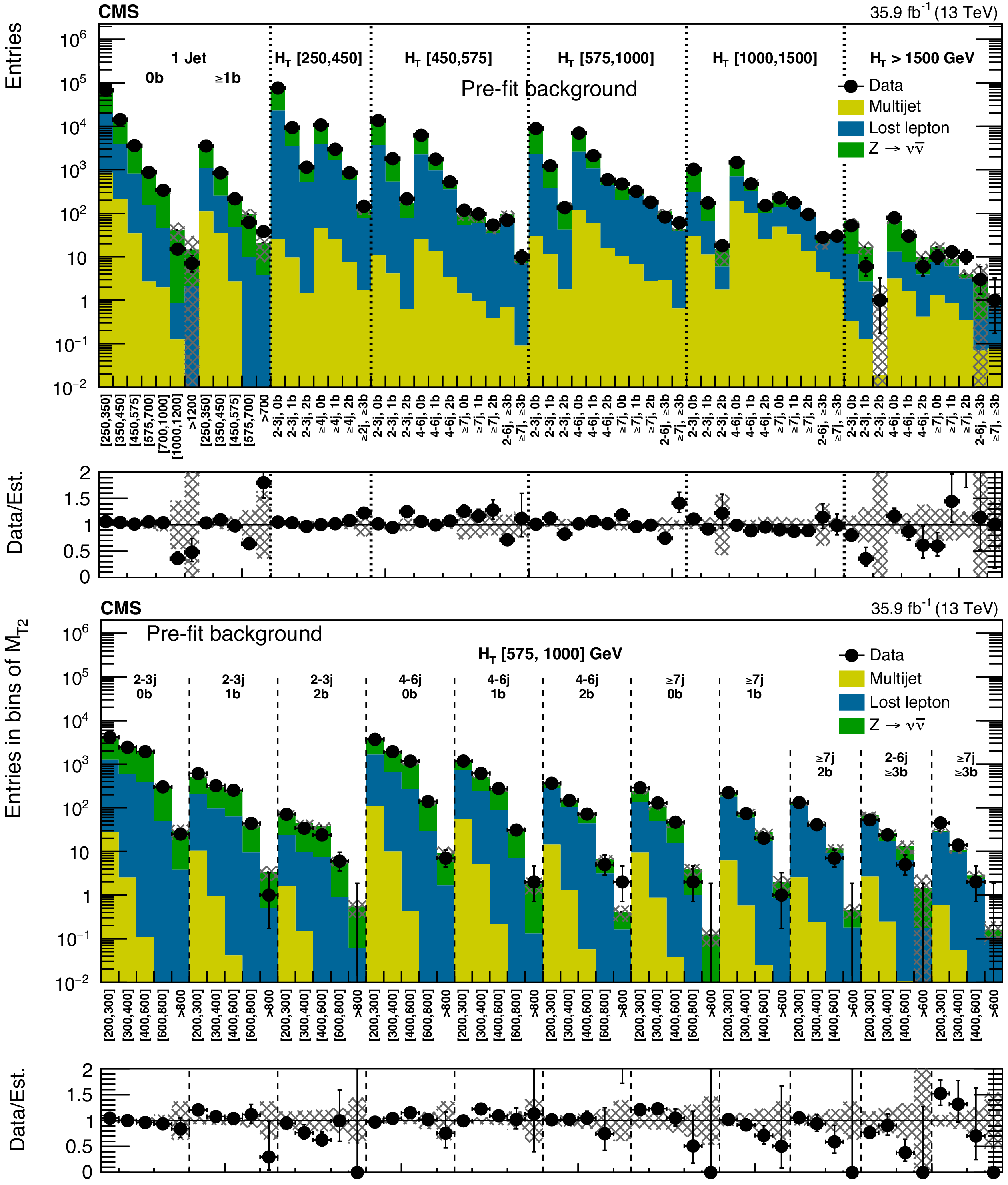
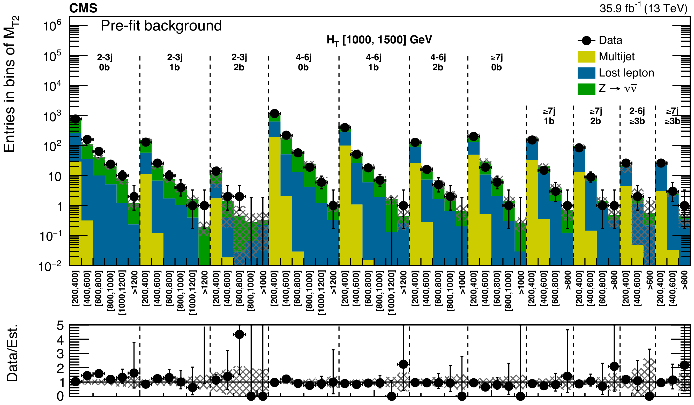
Figure 4:
(Upper) Comparison of estimated (pre-fit) background and observed data events in each topological region. Hatched bands represent the full uncertainty in the background estimate. The results shown for $ {N_{\mathrm {j}}} = $ 1 correspond to the monojet search regions binned in jet $ {p_{\mathrm {T}}} $, whereas for the multijet signal regions, the notations j, b indicate $ {N_{\mathrm {j}}} $, $ {N_{\mathrm{ b } }} $ labeling. (Lower) Same for individual $ {M_{\mathrm {T2}}} $ signal bins in the medium $ {H_{\mathrm {T}}} $ region. On the $x$-axis, the $ {M_{\mathrm {T2}}} $ binning is shown in units of GeV. |

png pdf |
Figure 4-a:
Comparison of estimated (pre-fit) background and observed data events in each topological region. Hatched bands represent the full uncertainty in the background estimate. The results shown for $ {N_{\mathrm {j}}} = $ 1 correspond to the monojet search regions binned in jet $ {p_{\mathrm {T}}} $, whereas for the multijet signal regions, the notations j, b indicate $ {N_{\mathrm {j}}} $, $ {N_{\mathrm{ b } }} $ labeling. |

png pdf |
Figure 4-b:
Comparison of estimated (pre-fit) background and observed data events Same for individual $ {M_{\mathrm {T2}}} $ signal bins in the medium $ {H_{\mathrm {T}}} $ region. On the $x$-axis, the $ {M_{\mathrm {T2}}} $ binning is shown in units of GeV. |
png pdf |
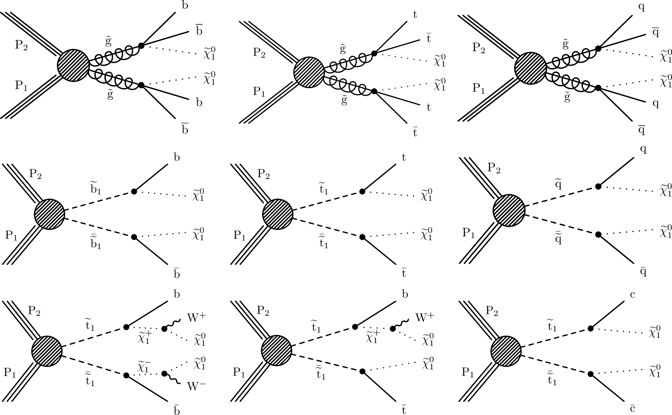
Figure 5:
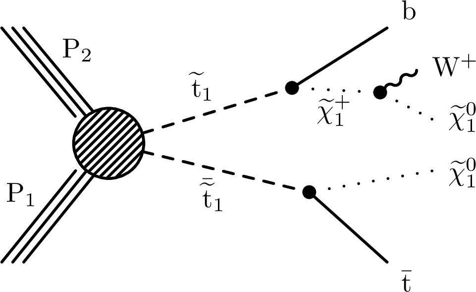
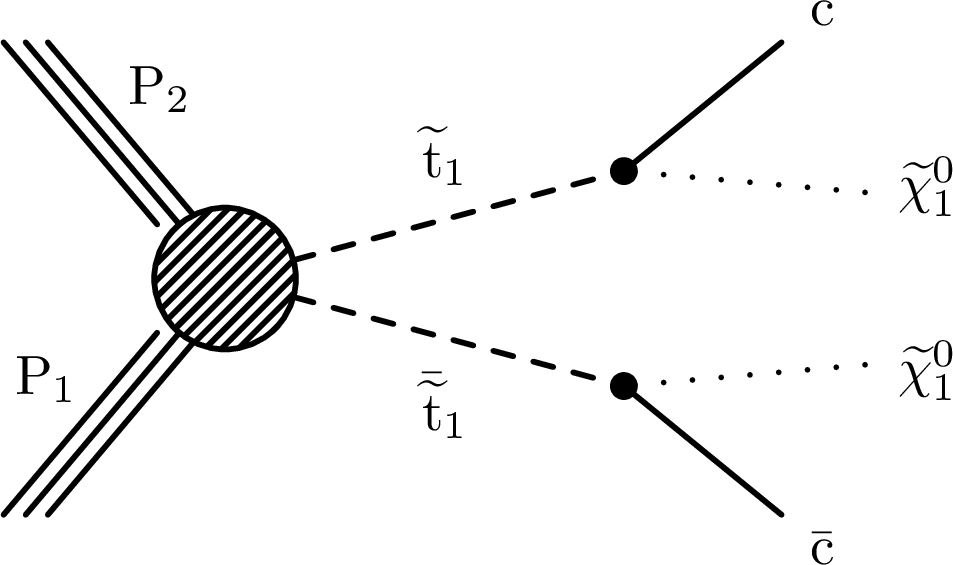
(Upper) Diagrams for the three scenarios of gluino-mediated bottom squark, top squark and light flavor squark production considered. (Middle) Diagrams for the direct production of bottom, top and light-flavor squark pairs. (Lower) Diagrams for three alternate scenarios of direct top squark production with different decay modes. For mixed decay scenarios, we assume a 50% branching fraction for each decay mode. |

png pdf |
Figure 5-a:
Diagram for the scenario of gluino-mediated bottom squark production considered. |
png pdf |
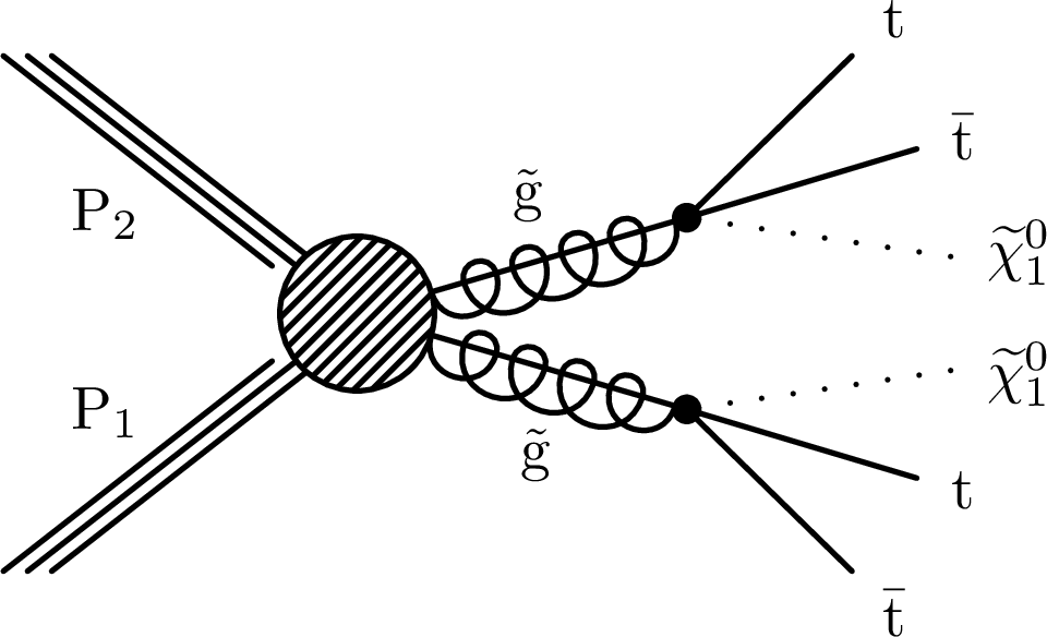
Figure 5-b:
Diagram for the scenario of gluino-mediated top squark production considered. |

png pdf |
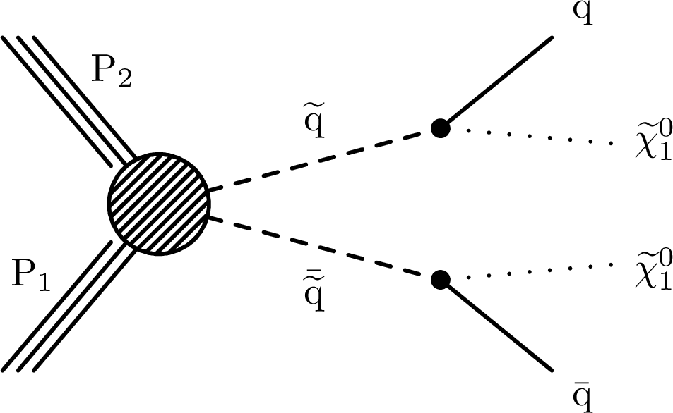
Figure 5-c:
Diagram for the scenario of gluino-mediated light flavor squark production considered. |

png pdf |
Figure 5-d:
Diagram for the direct production of bottom squark pairs. |

png pdf |
Figure 5-e:
Diagram for the direct production of top squark pairs. |
png pdf |
Figure 5-f:
Diagram for the direct production of light-flavor squark pairs. |

png pdf |
Figure 5-g:
Diagram for an alternate scenario of direct top squark production with different decay modes. |
png pdf |
Figure 5-h:
Diagram for an alternate scenario of direct top squark production with different decay modes. |
png pdf |
Figure 5-i:
Diagram for an alternate scenario of direct top squark production with different decay modes. |

png pdf |
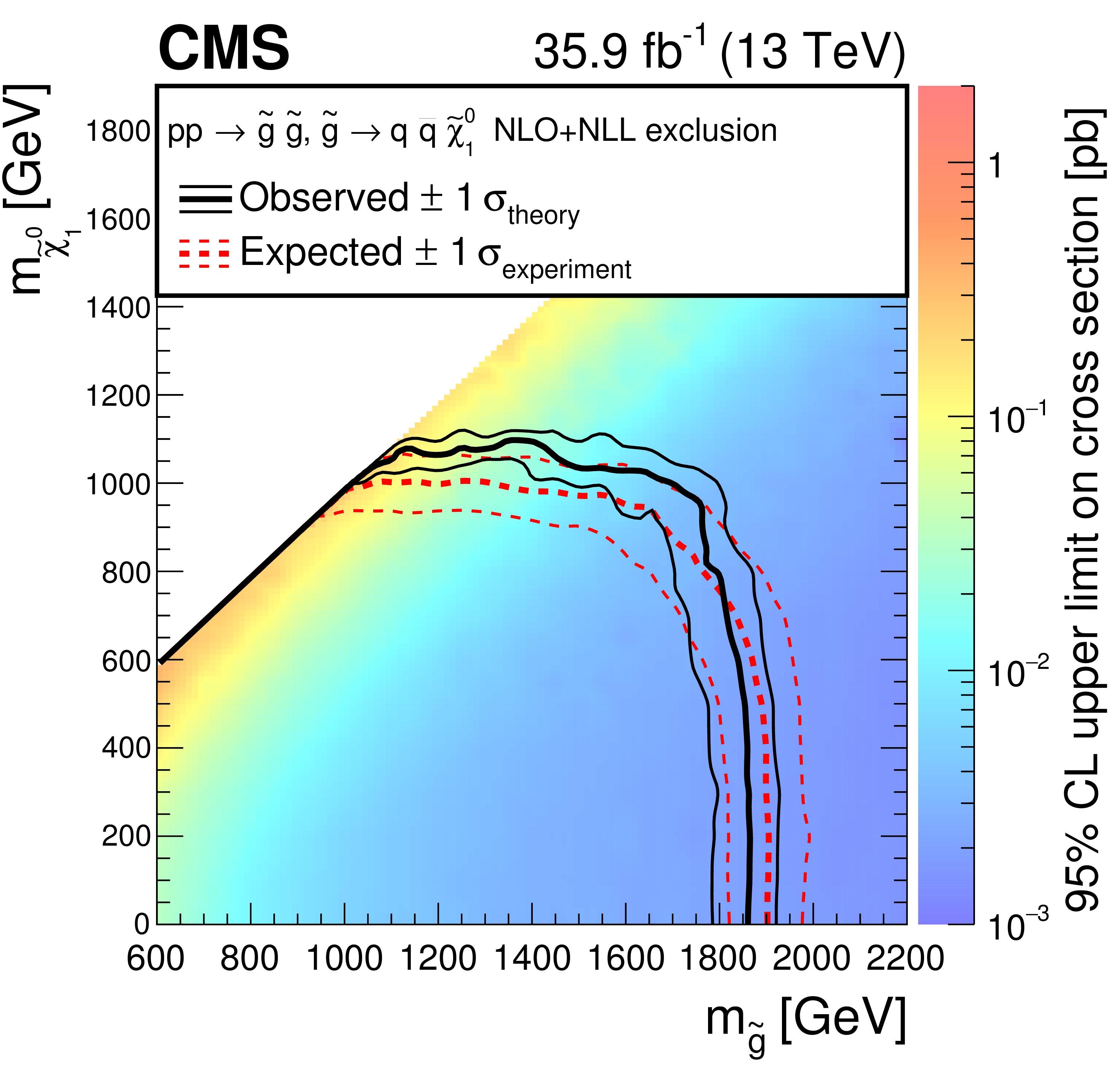
Figure 6:
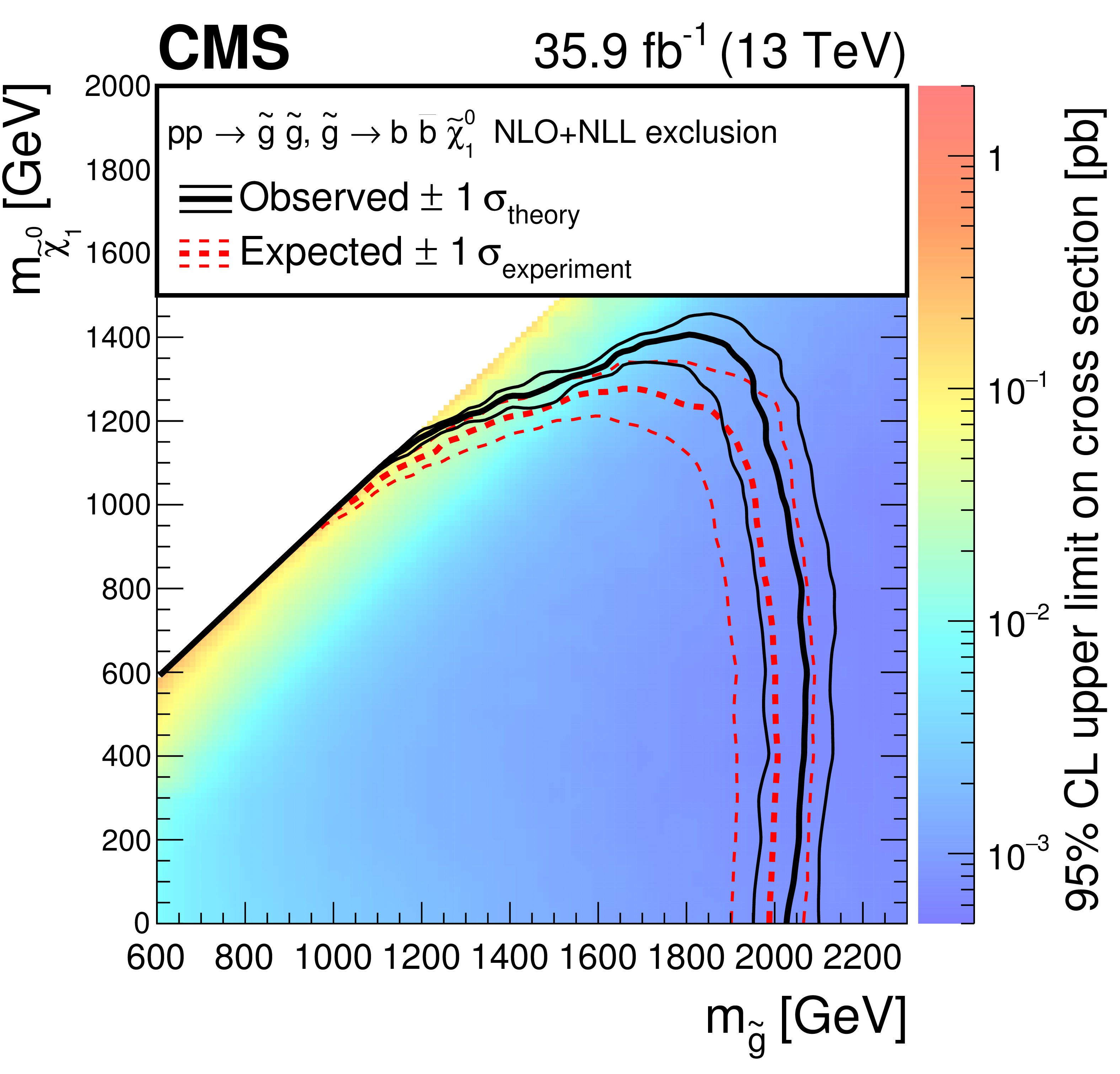
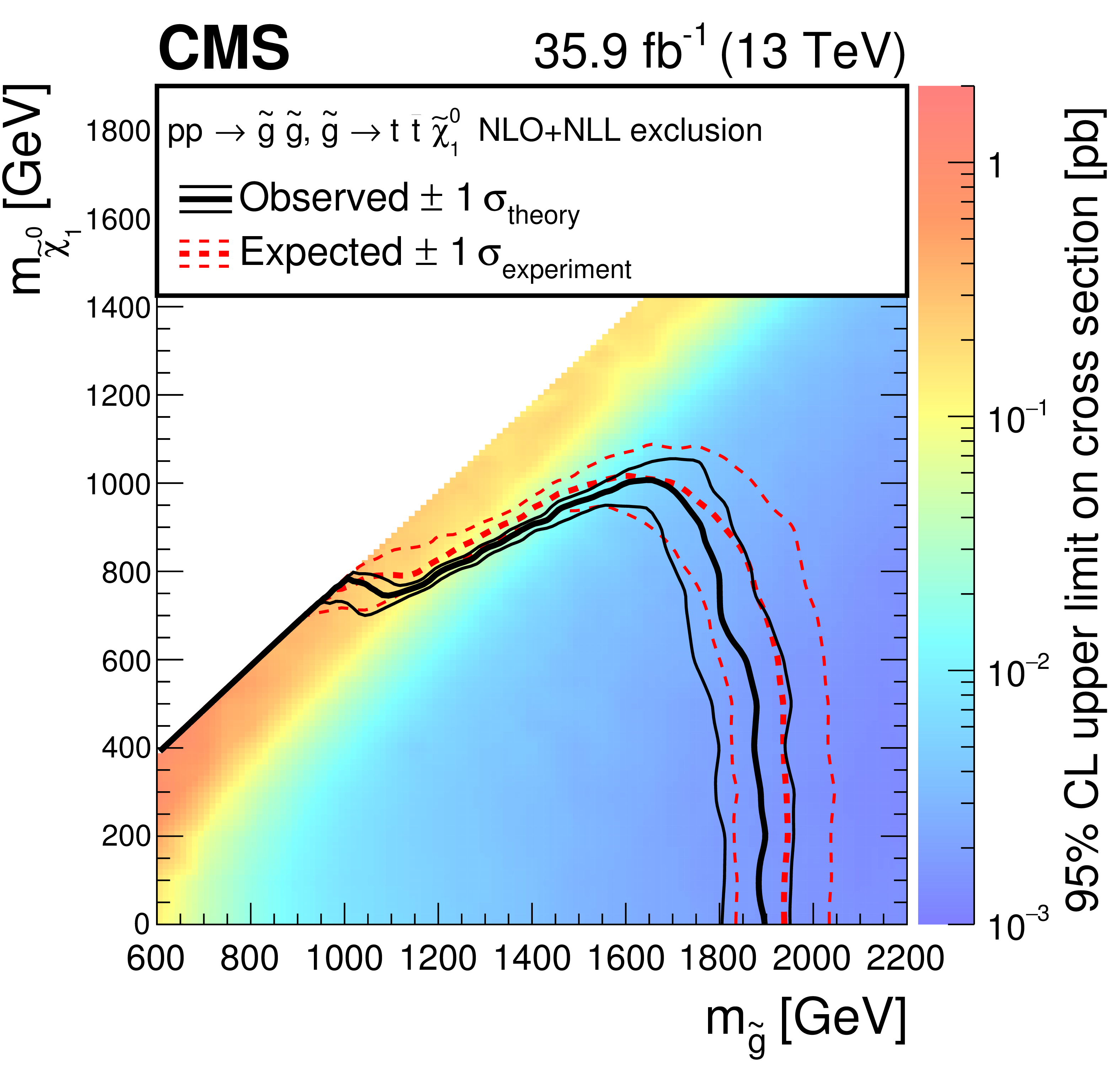
Exclusion limits at 95% CL for gluino-mediated bottom squark production (above left), gluino-mediated top squark production (above right), and gluino-mediated light-flavor (u, d, s, c) squark production (below). The area enclosed by the thick black curve represents the observed exclusion region, while the dashed red lines indicate the expected limits and their $\pm $1 standard deviation ranges. The thin black lines show the effect of the theoretical uncertainties on the signal cross section. |
png pdf root |
Figure 6-a:
Exclusion limits at 95% CL for gluino-mediated bottom squark production. The area enclosed by the thick black curve represents the observed exclusion region, while the dashed red lines indicate the expected limits and their $\pm $1 standard deviation ranges. The thin black lines show the effect of the theoretical uncertainties on the signal cross section. |
png pdf root |
Figure 6-b:
Exclusion limits at 95% CL for gluino-mediated top squark production. The area enclosed by the thick black curve represents the observed exclusion region, while the dashed red lines indicate the expected limits and their $\pm $1 standard deviation ranges. The thin black lines show the effect of the theoretical uncertainties on the signal cross section. |
png pdf root |
Figure 6-c:
Exclusion limits at 95% CL for gluino-mediated light-flavor (u, d, s, c) squark production. The area enclosed by the thick black curve represents the observed exclusion region, while the dashed red lines indicate the expected limits and their $\pm $1 standard deviation ranges. The thin black lines show the effect of the theoretical uncertainties on the signal cross section. |
png pdf |
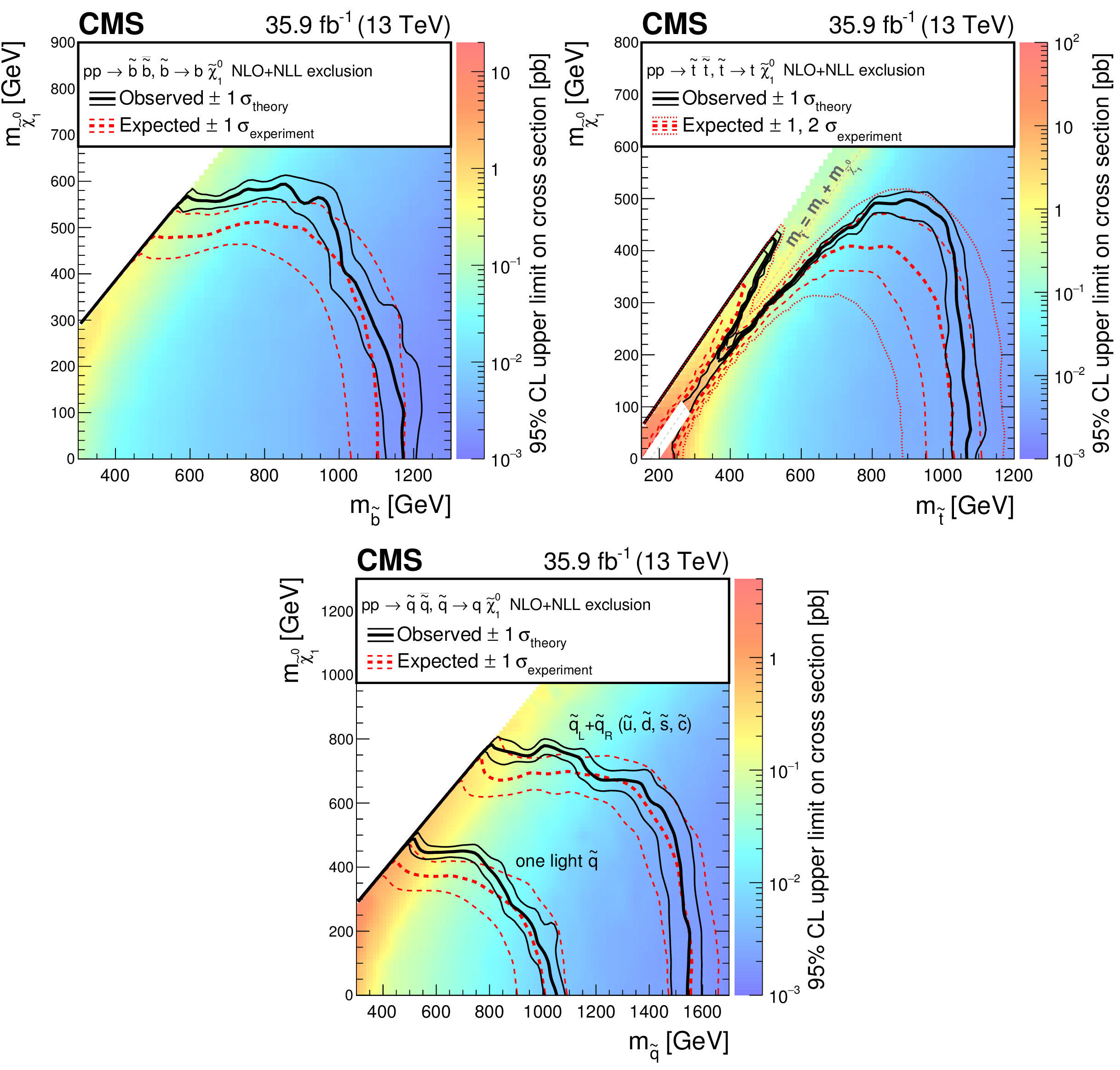
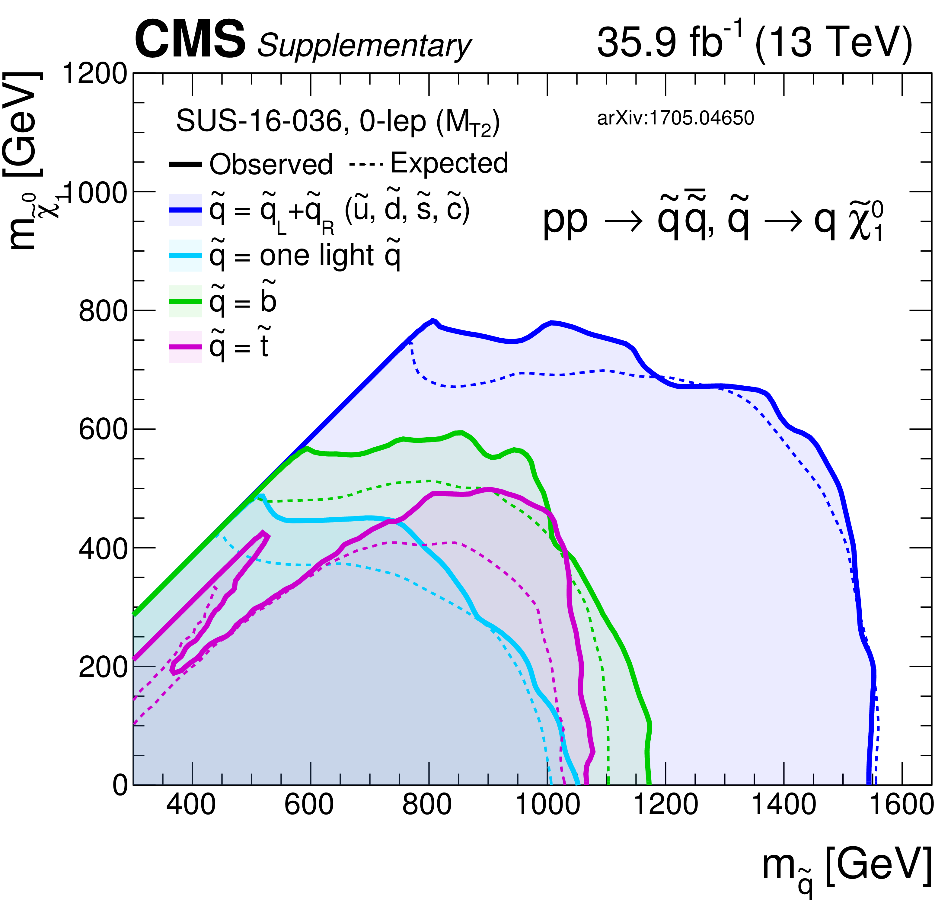
Figure 7:
Exclusion limit at 95% CL for bottom squark pair production (above left), top squark pair production (above right), and light-flavor squark pair production (below). The area enclosed by the thick black curve represents the observed exclusion region, while the dashed red lines indicate the expected limits and their $\pm $1 standard deviation ranges. For the top squark pair production plot, the $\pm $2 standard deviation ranges are also shown. The thin black lines show the effect of the theoretical uncertainties on the signal cross section. The white diagonal band in the upper right plot corresponds to the region $ {| m_{\tilde{ \mathrm{ t } } }-m_{\mathrm{ t } }-m_{\tilde{\chi}^0_1 } | }< $ 25 GeV and small $m_{\tilde{\chi}^0_1 }$. Here the efficiency of the selection is a strong function of $m_{\tilde{ \mathrm{ t } } }-m_{\tilde{\chi}^0_1 }$, and as a result the precise determination of the cross section upper limit is uncertain because of the finite granularity of the available MC samples in this region of the ($m_{\tilde{ \mathrm{ t } } }, m_{\tilde{\chi}^0_1 }$) plane. |

png pdf root |
Figure 7-a:
Exclusion limit at 95% CL for bottom squark pair production. The area enclosed by the thick black curve represents the observed exclusion region, while the dashed red lines indicate the expected limits and their $\pm $1 standard deviation ranges. |
png pdf root |
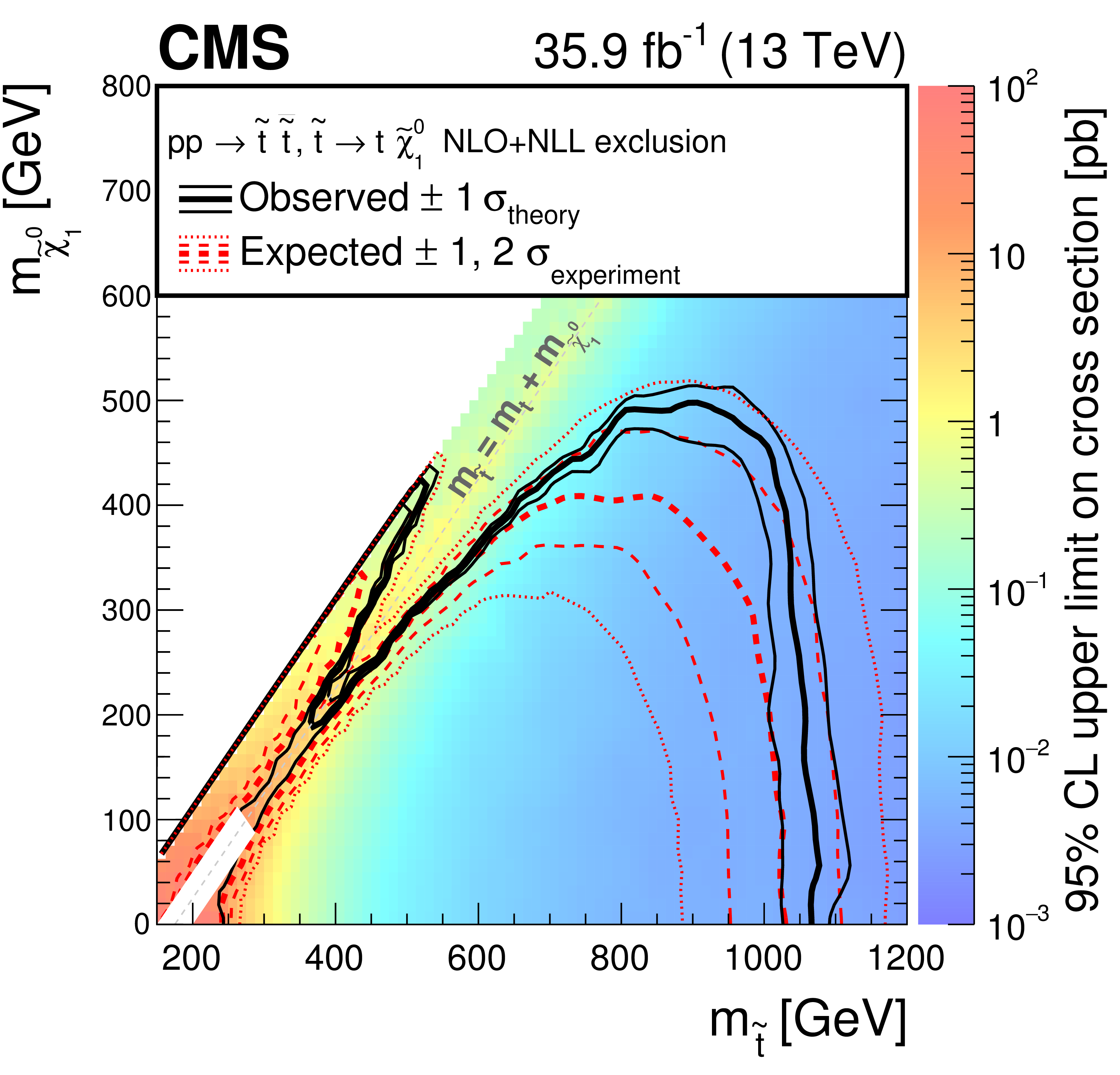
Figure 7-b:
Exclusion limit at 95% CL for top squark pair production. The area enclosed by the thick black curve represents the observed exclusion region, while the dashed red lines indicate the expected limits and their $\pm $1 standard deviation ranges. The $\pm $2 standard deviation ranges are also shown. The thin black lines show the effect of the theoretical uncertainties on the signal cross section. The white diagonal band corresponds to the region $ {| m_{\tilde{ \mathrm{ t } } }-m_{\mathrm{ t } }-m_{\tilde{\chi}^0_1 } | }< $ 25 GeV and small $m_{\tilde{\chi}^0_1 }$. Here the efficiency of the selection is a strong function of $m_{\tilde{ \mathrm{ t } } }-m_{\tilde{\chi}^0_1 }$, and as a result the precise determination of the cross section upper limit is uncertain because of the finite granularity of the available MC samples in this region of the ($m_{\tilde{ \mathrm{ t } } }, m_{\tilde{\chi}^0_1 }$) plane. |
png pdf root |
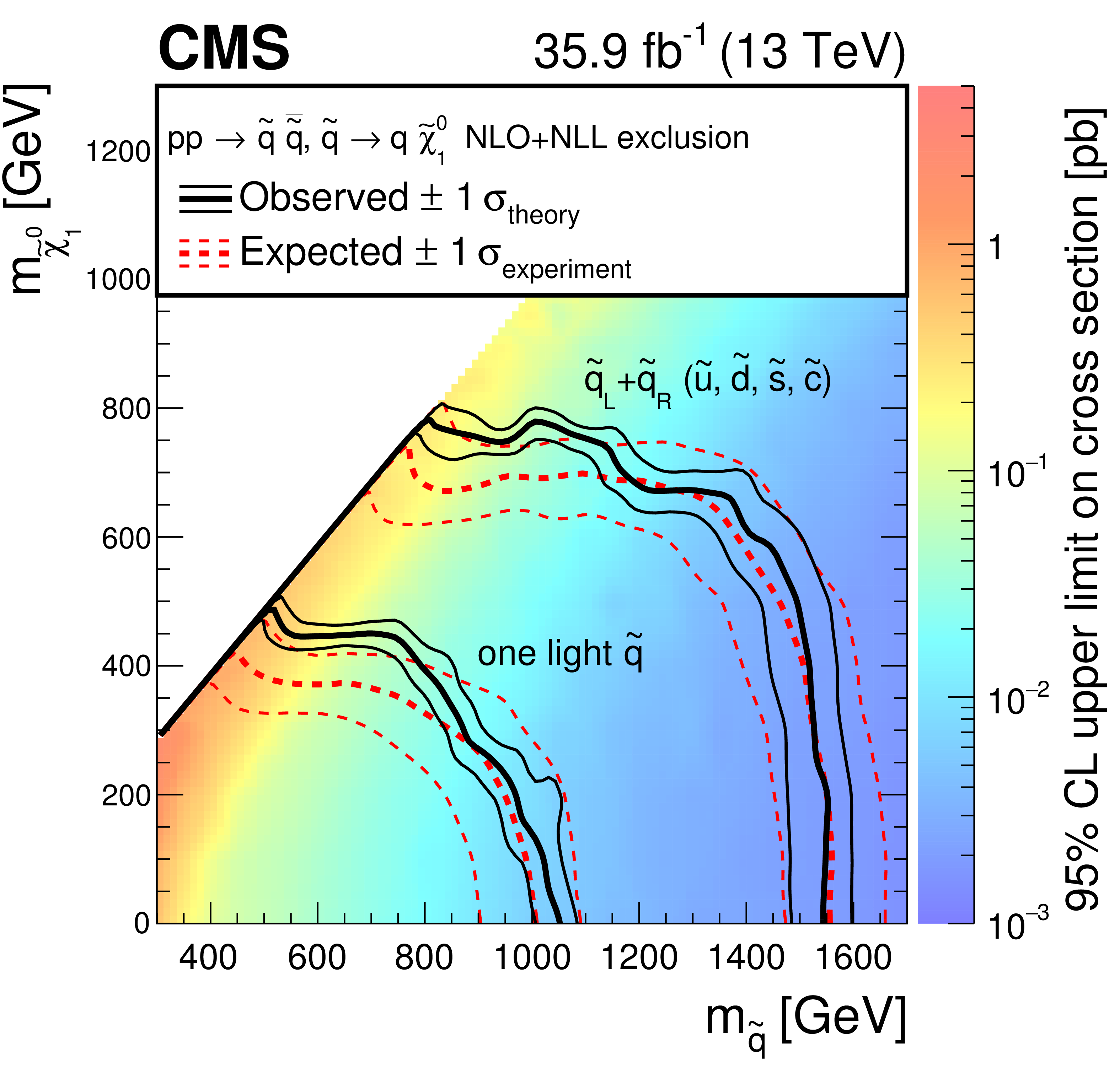
Figure 7-c:
Exclusion limit at 95% CL for light-flavor squark pair production. The area enclosed by the thick black curve represents the observed exclusion region, while the dashed red lines indicate the expected limits and their $\pm $1 standard deviation ranges. |
png pdf |
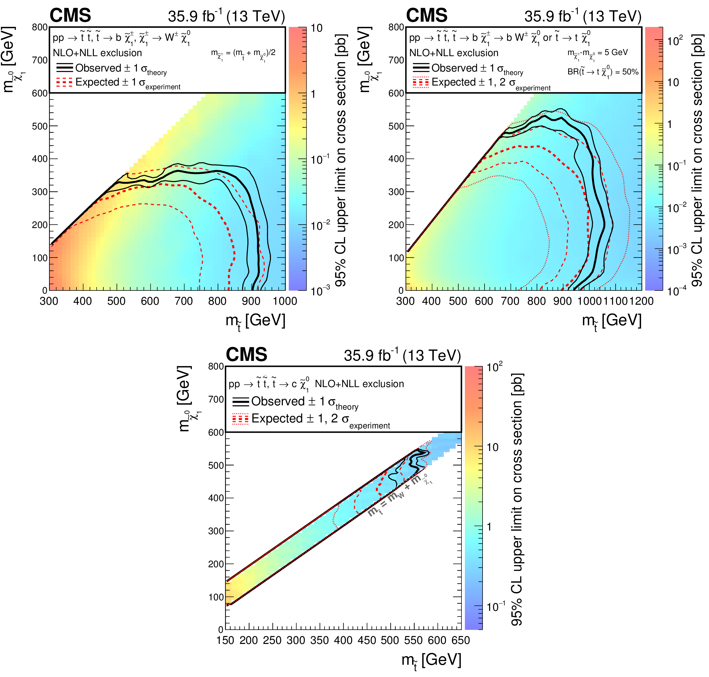
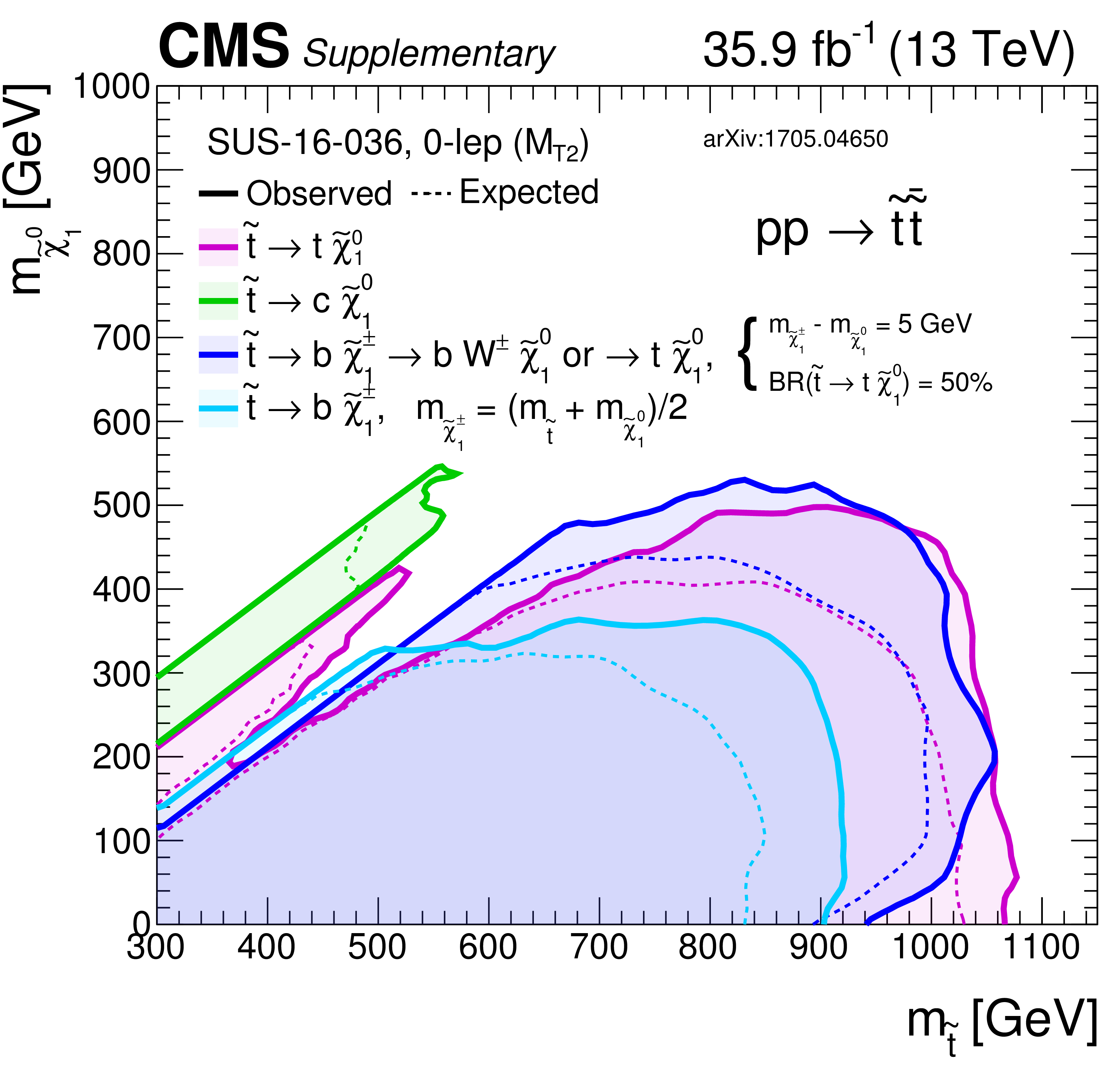
Figure 8:
Exclusion limit at 95% CL for top squark pair production for different decay modes of the top squark. For the scenario where $\mathrm{ p } \mathrm{ p } \to \tilde{ \mathrm{ t } } \tilde{ \mathrm{t} } \to \mathrm{ b \bar{b} } \tilde{\chi}^{\pm}_1 {\tilde{\chi}^\mp _{1}} $, $\tilde{\chi}^{\pm}_1 \to \mathrm{ W } ^{\pm } \tilde{\chi}^0_1 $ (above left), the mass of the chargino is chosen to be half way in between the masses of the top squark and the neutralino. A mixed decay scenario (above right), $\mathrm{ p } \mathrm{ p } \to \tilde{ \mathrm{ t } } \tilde{ \mathrm{t} } $ with equal branching fractions for the top squark decays $\tilde{ \mathrm{ t } } \to \mathrm{ t } \tilde{\chi}^0_1 $ and $\tilde{ \mathrm{ t } } \to \mathrm{ b } \tilde{\chi}^{\pm}_1 $, $\tilde{\chi}^{\pm}_1 \to \mathrm{ W } ^{*+}\tilde{\chi}^0_1 $, is also considered, with the chargino mass chosen such that $\Delta m\left (\tilde{\chi}^{\pm}_1,\tilde{\chi}^0_1 \right) = $ 5 GeV. Finally, we also consider a compressed scenario (below) where $\mathrm{ p } \mathrm{ p } \to \tilde{ \mathrm{ t } } \tilde{ \mathrm{t} } \to \mathrm{c} \tilde{ \mathrm{c} } \tilde{\chi}^0_1 \tilde{\chi}^0_1 $. The area enclosed by the thick black curve represents the observed exclusion region, while the dashed red lines indicate the expected limits and their $\pm $1 standard deviation ranges. The thin black lines show the effect of the theoretical uncertainties on the signal cross section. |

png pdf root |
Figure 8-a:
Exclusion limit at 95% CL for top squark pair production for a scenario where $\mathrm{ p } \mathrm{ p } \to \tilde{ \mathrm{ t } } \tilde{ \mathrm{t} } \to \mathrm{ b \bar{b} } \tilde{\chi}^{\pm}_1 {\tilde{\chi}^\mp _{1}} $, $\tilde{\chi}^{\pm}_1 \to \mathrm{ W } ^{\pm } \tilde{\chi}^0_1 $, and where the mass of the chargino is chosen to be half way in between the masses of the top squark and the neutralino. The area enclosed by the thick black curve represents the observed exclusion region, while the dashed red lines indicate the expected limits and their $\pm $1 standard deviation ranges. The thin black lines show the effect of the theoretical uncertainties on the signal cross section. |

png pdf root |
Figure 8-b:
Exclusion limit at 95% CL for top squark pair production for a mixed decay scenario, $\mathrm{ p } \mathrm{ p } \to \tilde{ \mathrm{ t } } \tilde{ \mathrm{t} } $ with equal branching fractions for the top squark decays $\tilde{ \mathrm{ t } } \to \mathrm{ t } \tilde{\chi}^0_1 $ and $\tilde{ \mathrm{ t } } \to \mathrm{ b } \tilde{\chi}^{\pm}_1 $, $\tilde{\chi}^{\pm}_1 \to \mathrm{ W } ^{*+}\tilde{\chi}^0_1 $, with the chargino mass chosen such that $\Delta m\left (\tilde{\chi}^{\pm}_1,\tilde{\chi}^0_1 \right) = $ 5 GeV. The area enclosed by the thick black curve represents the observed exclusion region, while the dashed red lines indicate the expected limits and their $\pm $1 standard deviation ranges. The thin black lines show the effect of the theoretical uncertainties on the signal cross section. |
png pdf root |
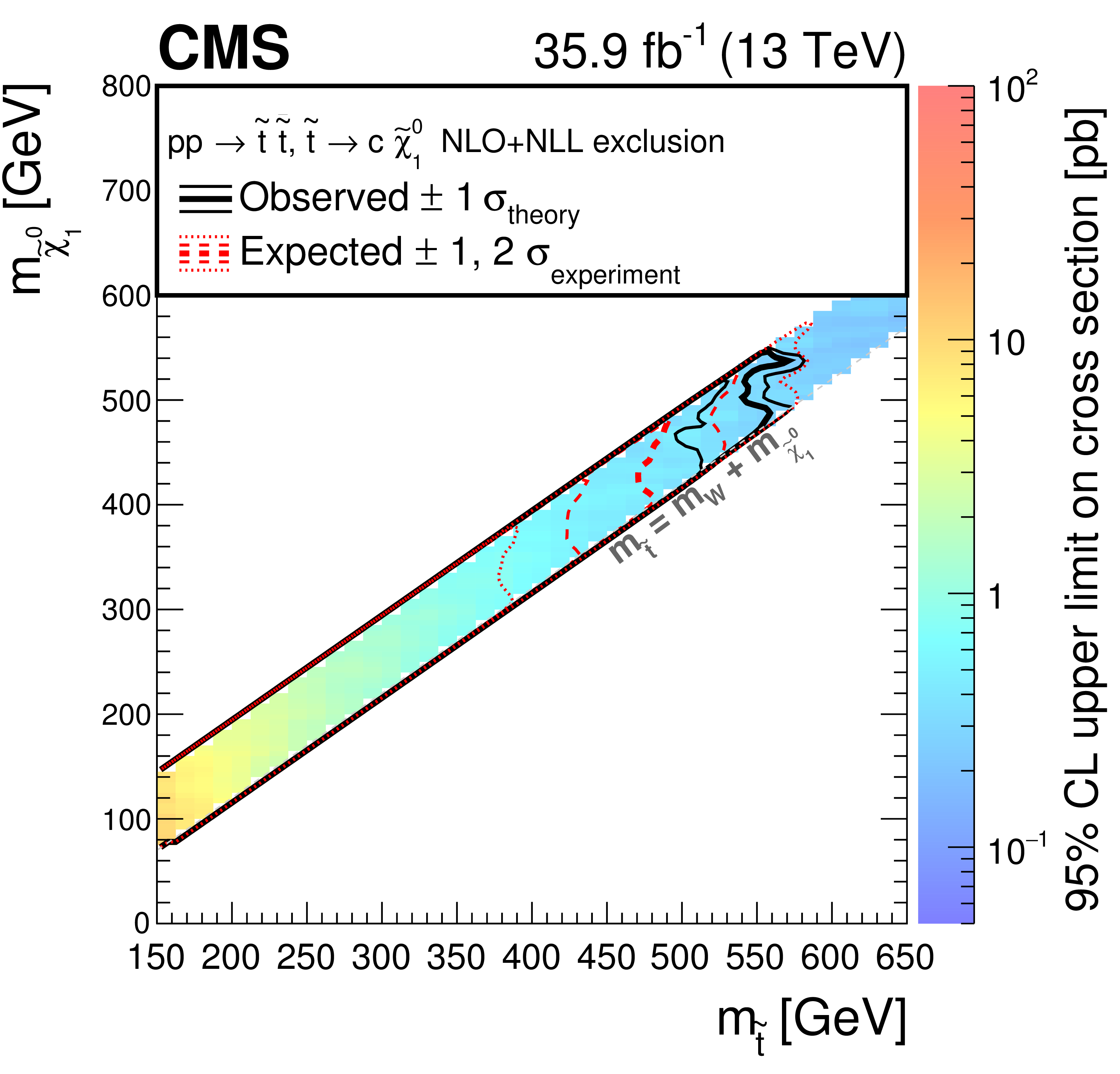
Figure 8-c:
Exclusion limit at 95% CL for top squark pair production for a compressed scenario where $\mathrm{ p } \mathrm{ p } \to \tilde{ \mathrm{ t } } \tilde{ \mathrm{t} } \to \mathrm{c} \tilde{ \mathrm{c} } \tilde{\chi}^0_1 \tilde{\chi}^0_1 $. The area enclosed by the thick black curve represents the observed exclusion region, while the dashed red lines indicate the expected limits and their $\pm $1 standard deviation ranges. The thin black lines show the effect of the theoretical uncertainties on the signal cross section. |

png pdf |
Figure 9:
(Upper) Comparison of the estimated background and observed data events in each signal bin in the monojet region. On the $x$-axis, the ${ {p_{\mathrm {T}}} ^{\text {jet1}}}$ binning is shown in units of GeV. Hatched bands represent the full uncertainty in the background estimate. (Lower) Same for the very low $ {H_{\mathrm {T}}} $ region. On the $x$-axis, the $ {M_{\mathrm {T2}}} $ binning is shown in units of GeV. |

png pdf |
Figure 9-a:
Comparison of the estimated background and observed data events in each signal bin in the monojet region. On the $x$-axis, the ${ {p_{\mathrm {T}}} ^{\text {jet1}}}$ binning is shown in units of GeV. Hatched bands represent the full uncertainty in the background estimate. |

png pdf |
Figure 9-b:
Comparison of the estimated background and observed data events in each signal bin in the very low $ {H_{\mathrm {T}}} $ region. On the $x$-axis, the $ {M_{\mathrm {T2}}} $ binning is shown in units of GeV. Hatched bands represent the full uncertainty in the background estimate. |

png pdf |
Figure 10:
(Upper) Comparison of the estimated background and observed data events in each signal bin in the low-$ {H_{\mathrm {T}}} $ region. Hatched bands represent the full uncertainty in the background estimate. Same for the high- (middle) and extreme- (lower) $ {H_{\mathrm {T}}} $ regions. On the $x$-axis, the $ {M_{\mathrm {T2}}} $ binning is shown in units of GeV. For the extreme-$ {H_{\mathrm {T}}} $ region, the last bin is left empty for visualization purposes. |

png pdf |
Figure 10-a:
Comparison of the estimated background and observed data events in the low-$ {H_{\mathrm {T}}} $ region. On the $x$-axis, the $ {M_{\mathrm {T2}}} $ binning is shown in units of GeV. Hatched bands represent the full uncertainty in the background estimate. |
png pdf |
Figure 10-b:
Comparison of the estimated background and observed data events in the high-$ {H_{\mathrm {T}}} $ region. On the $x$-axis, the $ {M_{\mathrm {T2}}} $ binning is shown in units of GeV. Hatched bands represent the full uncertainty in the background estimate. |

png pdf |
Figure 10-c:
Comparison of the estimated background and observed data events in the extreme-$ {H_{\mathrm {T}}} $ region. On the $x$-axis, the $ {M_{\mathrm {T2}}} $ binning is shown in units of GeV. The last bin is left empty for visualization purposes. Hatched bands represent the full uncertainty in the background estimate. |

png pdf |
Figure 11:
Comparison of post-fit background prediction and observed data events in each topological region. Hatched bands represent the post-fit uncertainty in the background prediction. For the monojet, on the $x$-axis the $ { {p_{\mathrm {T}}} ^{\text {jet1}}} $ binning is shown in units of GeV, whereas for the multijet signal regions, the notations j, b indicate $ {N_{\mathrm {j}}} $, $ {N_{\mathrm{ b } }} $ labeling. |

png pdf |
Figure 12:
(Upper) Comparison of the post-fit background prediction and observed data events in each signal bin in the monojet region. On the $x$-axis, the $ { {p_{\mathrm {T}}} ^{\text {jet1}}} $ binning is shown in units of GeV. (Middle) and (lower): Same for the very low and low-$ {H_{\mathrm {T}}} $ region. On the $x$-axis, the $ {M_{\mathrm {T2}}} $ binning is shown in units of GeV. The hatched bands represent the post-fit uncertainty in the background prediction. |

png pdf |
Figure 12-a:
Comparison of the post-fit background prediction and observed data events in each signal bin in the monojet region. On the $x$-axis, the $ { {p_{\mathrm {T}}} ^{\text {jet1}}} $ binning is shown in units of GeV. The hatched bands represent the post-fit uncertainty in the background prediction. |

png pdf |
Figure 12-b:
Comparison of the post-fit background prediction and observed data events in the very low-$ {H_{\mathrm {T}}} $ region. On the $x$-axis, the $ {M_{\mathrm {T2}}} $ binning is shown in units of GeV. The hatched bands represent the post-fit uncertainty in the background prediction. |
png pdf |
Figure 12-c:
Comparison of the post-fit background prediction and observed data events in the low-$ {H_{\mathrm {T}}} $ region. On the $x$-axis, the $ {M_{\mathrm {T2}}} $ binning is shown in units of GeV. The hatched bands represent the post-fit uncertainty in the background prediction. |
png pdf |
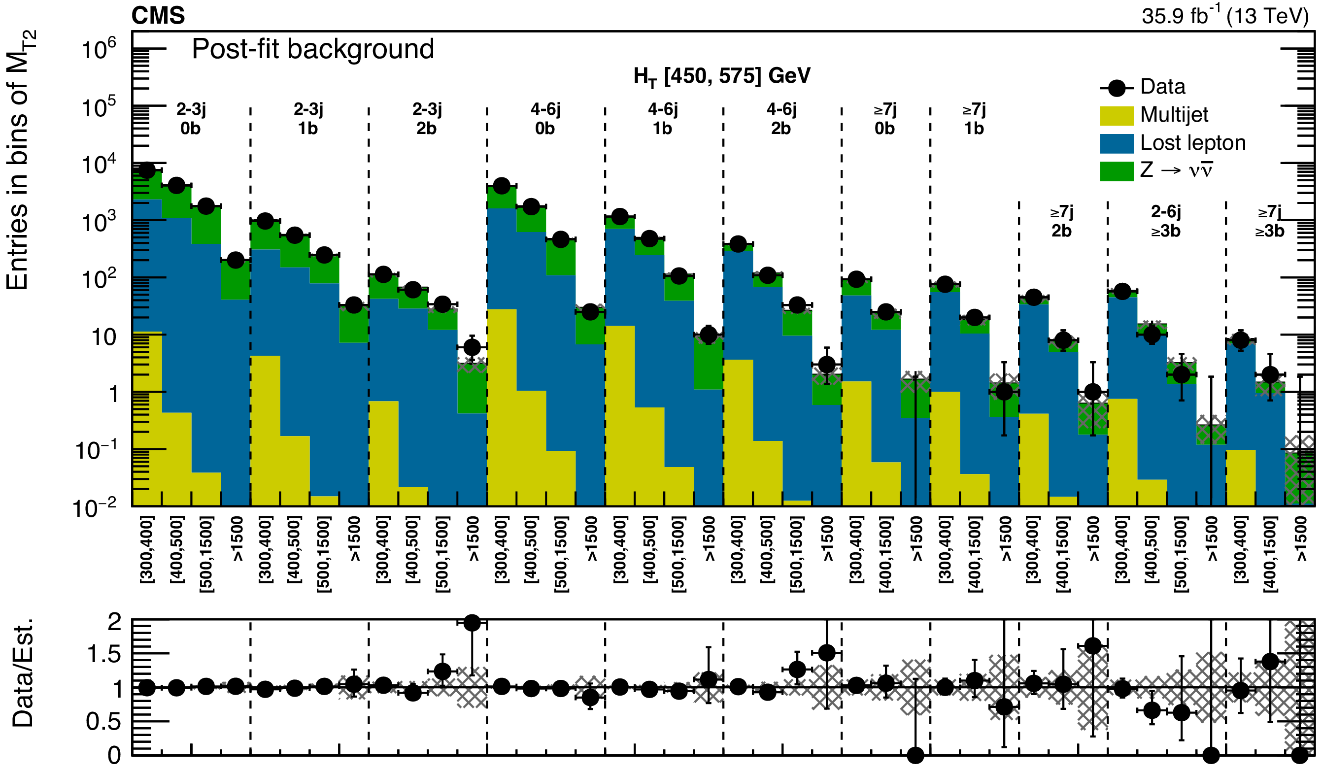
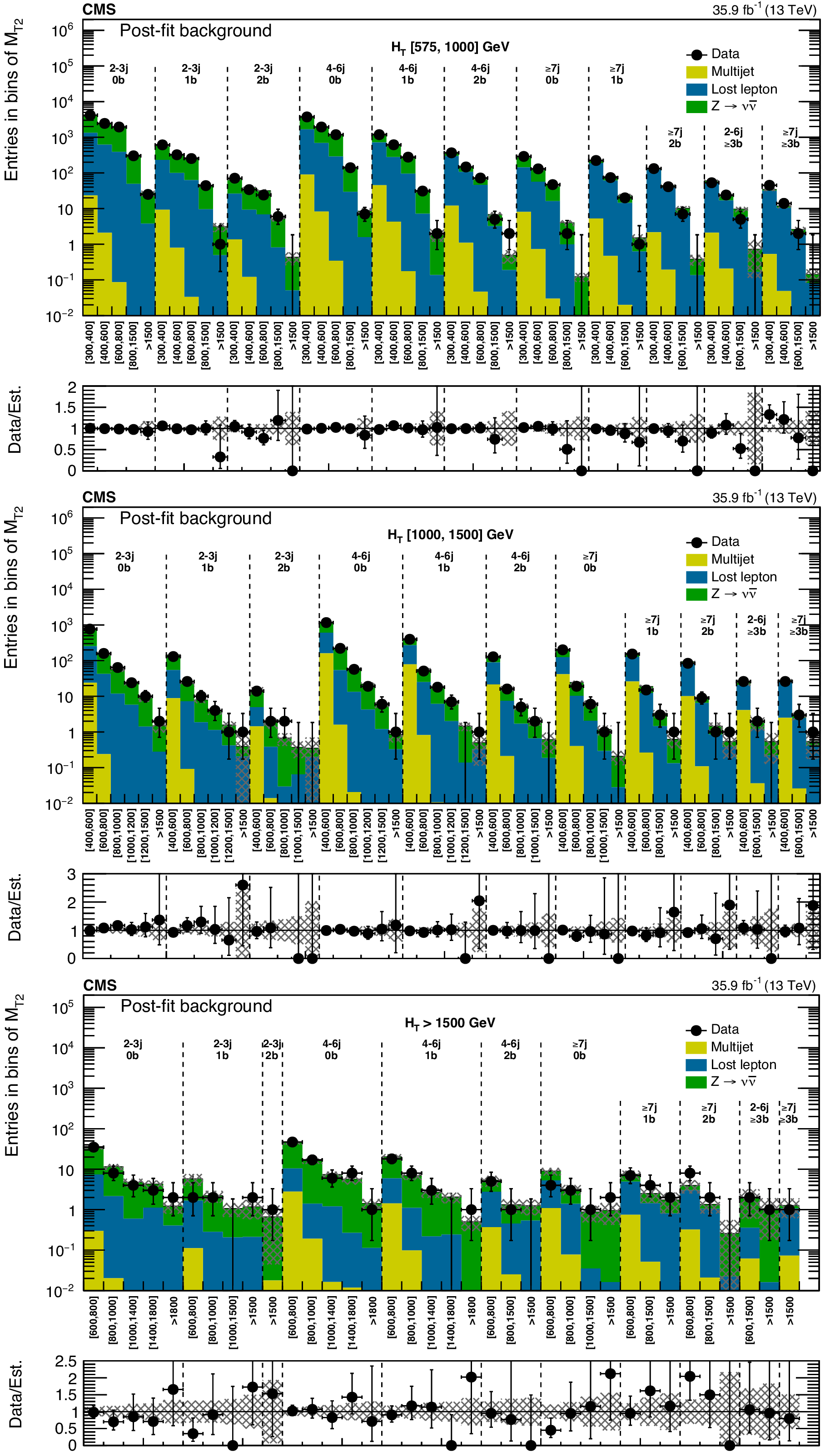
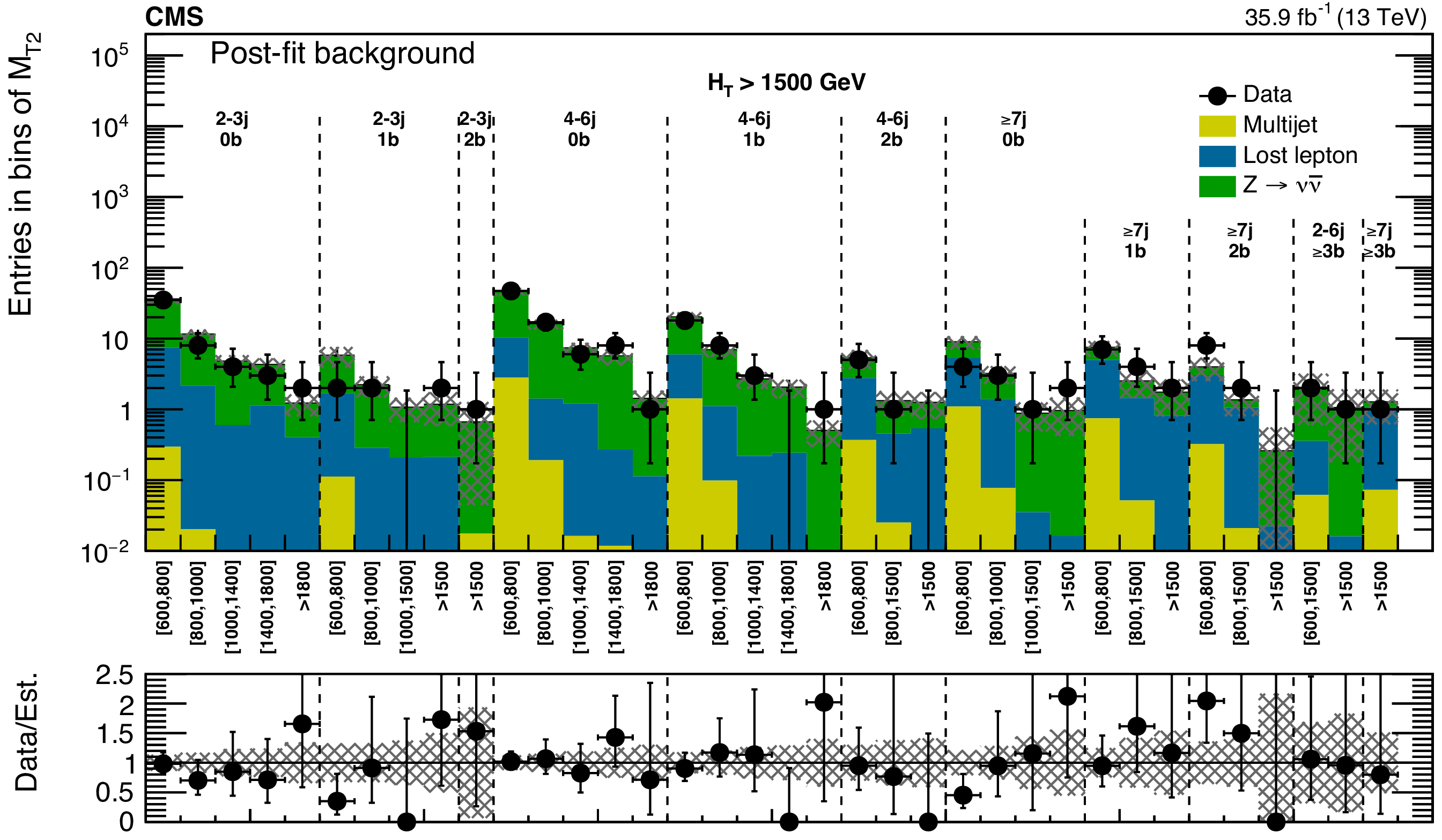
Figure 13:
(Upper) Comparison of the post-fit background prediction and observed data events in each signal bin in the medium-$ {H_{\mathrm {T}}} $ region. Same for the high- (middle) and extreme- (lower) $ {H_{\mathrm {T}}} $ regions. On the $x$-axis, the $ {M_{\mathrm {T2}}} $ binning is shown in units of GeV. The hatched bands represent the post-fit uncertainty in the background prediction. For the extreme-$ {H_{\mathrm {T}}} $ region, the last bin is left empty for visualization purposes. |

png pdf |
Figure 13-a:
Comparison of the post-fit background prediction and observed data events in each signal bin in the medium-$ {H_{\mathrm {T}}} $ region. On the $x$-axis, the $ {M_{\mathrm {T2}}} $ binning is shown in units of GeV. The hatched bands represent the post-fit uncertainty in the background prediction. |

png pdf |
Figure 13-b:
Comparison of the post-fit background prediction and observed data events in each signal bin in the high-$ {H_{\mathrm {T}}} $ region. On the $x$-axis, the $ {M_{\mathrm {T2}}} $ binning is shown in units of GeV. The hatched bands represent the post-fit uncertainty in the background prediction. |
png pdf |
Figure 13-c:
Comparison of the post-fit background prediction and observed data events in each signal bin in the extreme-$ {H_{\mathrm {T}}} $ region. On the $x$-axis, the $ {M_{\mathrm {T2}}} $ binning is shown in units of GeV. The hatched bands represent the post-fit uncertainty in the background prediction. The last bin is left empty for visualization purposes. |

png pdf |
Figure 14:
(Upper) The post-fit background prediction and observed data events in the analysis binning, for all topological regions with the expected yield for the signal model of gluino mediated bottom-squark production ($m_{\tilde{ \mathrm{g} } }= $ 1000 GeV, $m_{\tilde{\chi}^0_1 }= $ 800 GeV) stacked on top of the expected background. For the monojet regions, the $ { {p_{\mathrm {T}}} ^{\text {jet1}}} $ binning is in units of GeV. (Lower) Same for the extreme-$ {H_{\mathrm {T}}} $ region for the same signal with ($m_{\tilde{ \mathrm{g} } }= $ 1900 GeV, $m_{\tilde{\chi}^0_1 }= $ 100 GeV). On the $x$-axis, the $ {M_{\mathrm {T2}}} $ binning is shown in units of GeV. The hatched bands represent the post-fit uncertainty in the background prediction. For the extreme-$ {H_{\mathrm {T}}} $ region, the last bin is left empty for visualization purposes. |

png pdf |
Figure 14-a:
The post-fit background prediction and observed data events in the analysis binning, for all topological regions with the expected yield for the signal model of gluino mediated bottom-squark production ($m_{\tilde{ \mathrm{g} } }= $ 1000 GeV, $m_{\tilde{\chi}^0_1 }= $ 800 GeV) stacked on top of the expected background. For the monojet regions, the $ { {p_{\mathrm {T}}} ^{\text {jet1}}} $ binning is in units of GeV. |

png pdf |
Figure 14-b:
The post-fit background prediction and observed data events in the analysis binning, for the extreme-$ {H_{\mathrm {T}}} $ region for the signal with ($m_{\tilde{ \mathrm{g} } }= $ 1900 GeV, $m_{\tilde{\chi}^0_1 }= $ 100 GeV) stacked on top of the expected background. On the $x$-axis, the $ {M_{\mathrm {T2}}} $ binning is shown in units of GeV. The hatched bands represent the post-fit uncertainty in the background prediction. The last bin is left empty for visualization purposes. |
| Tables | |
png pdf |
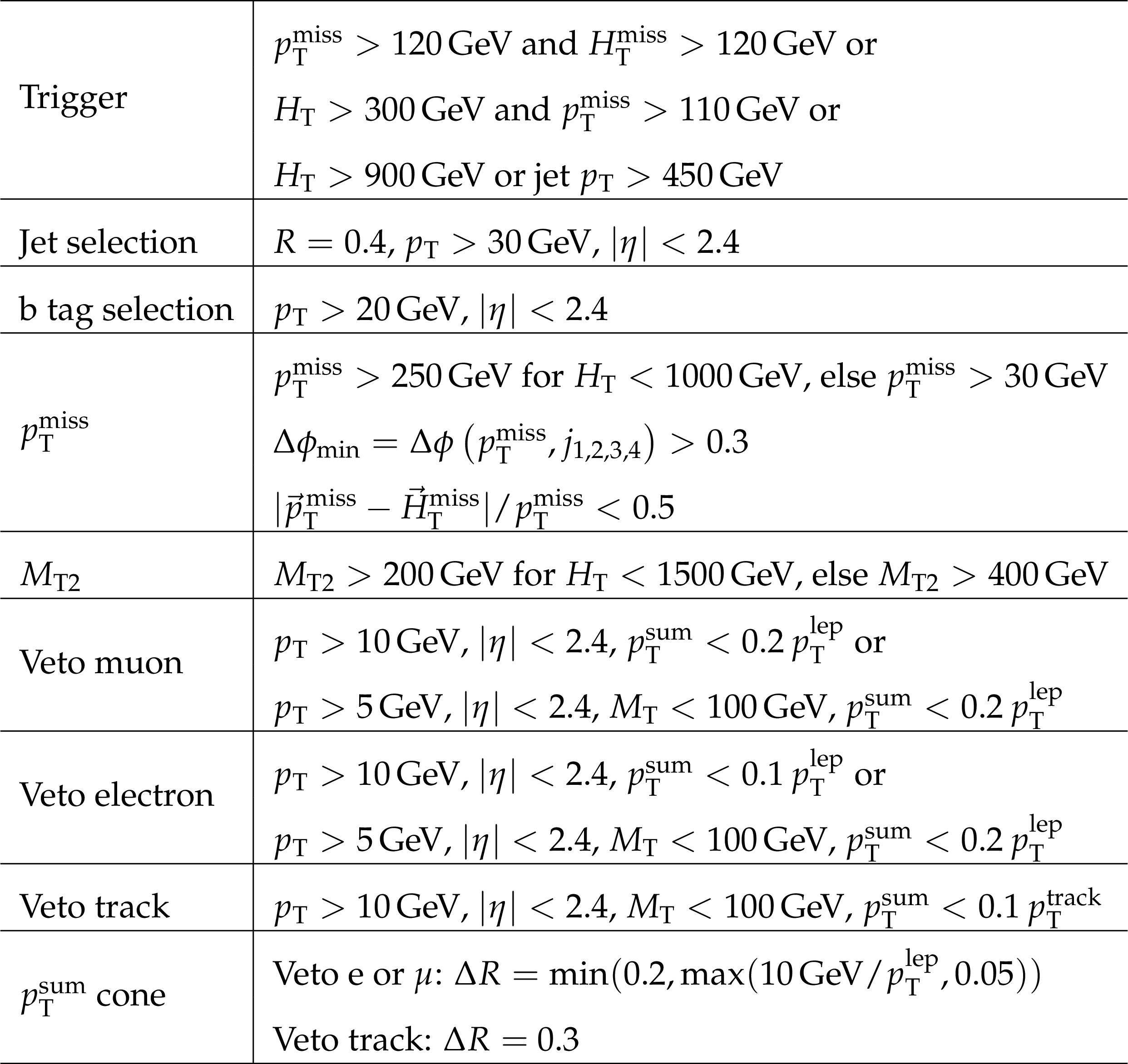
Table 1:
Summary of reconstruction objects and event preselection. Here $R$ is the distance parameter of the anti-$ {k_{\mathrm {T}}} $ algorithm. For veto leptons and tracks, the transverse mass $ {M_{\mathrm {T}}} $ is determined using the veto object and the ${\vec{p}_{\mathrm {T}}^{\text {miss}}} $, while $ {p_{\mathrm {T}}} ^{\text {sum}}$ denotes the sum of the transverse momenta of all the PF candidates in a cone around the lepton or track. The size of the cone, in units of $\Delta R \equiv \sqrt {{(\Delta \phi)^2 + (\Delta \eta)^2}}$ is given in the table. Further details of the lepton selection are described in Ref. [6]. The $i$th highest-$ {p_{\mathrm {T}}} $ jet is denoted as j$_i$. |
png pdf |
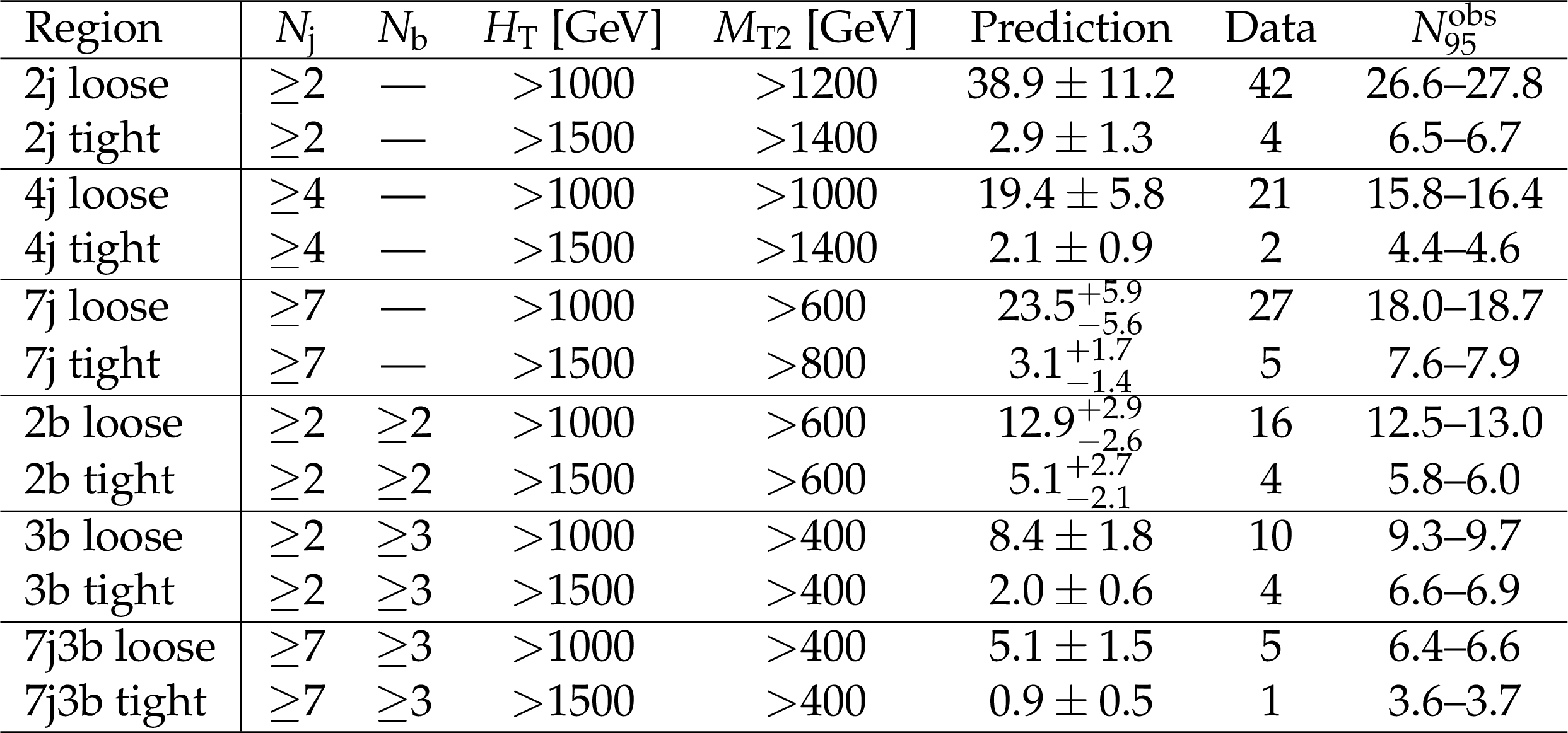
Table 2:
Definitions of super signal regions, along with predictions, observed data, and the observed 95% CL upper limits on the number of signal events contributing to each region ($N_{95}^{\text {obs}}$). The limits are shown as a range corresponding to an assumed uncertainty in the signal acceptance of 0-15%. A dash in the selections means that no requirement is applied. |
png pdf |
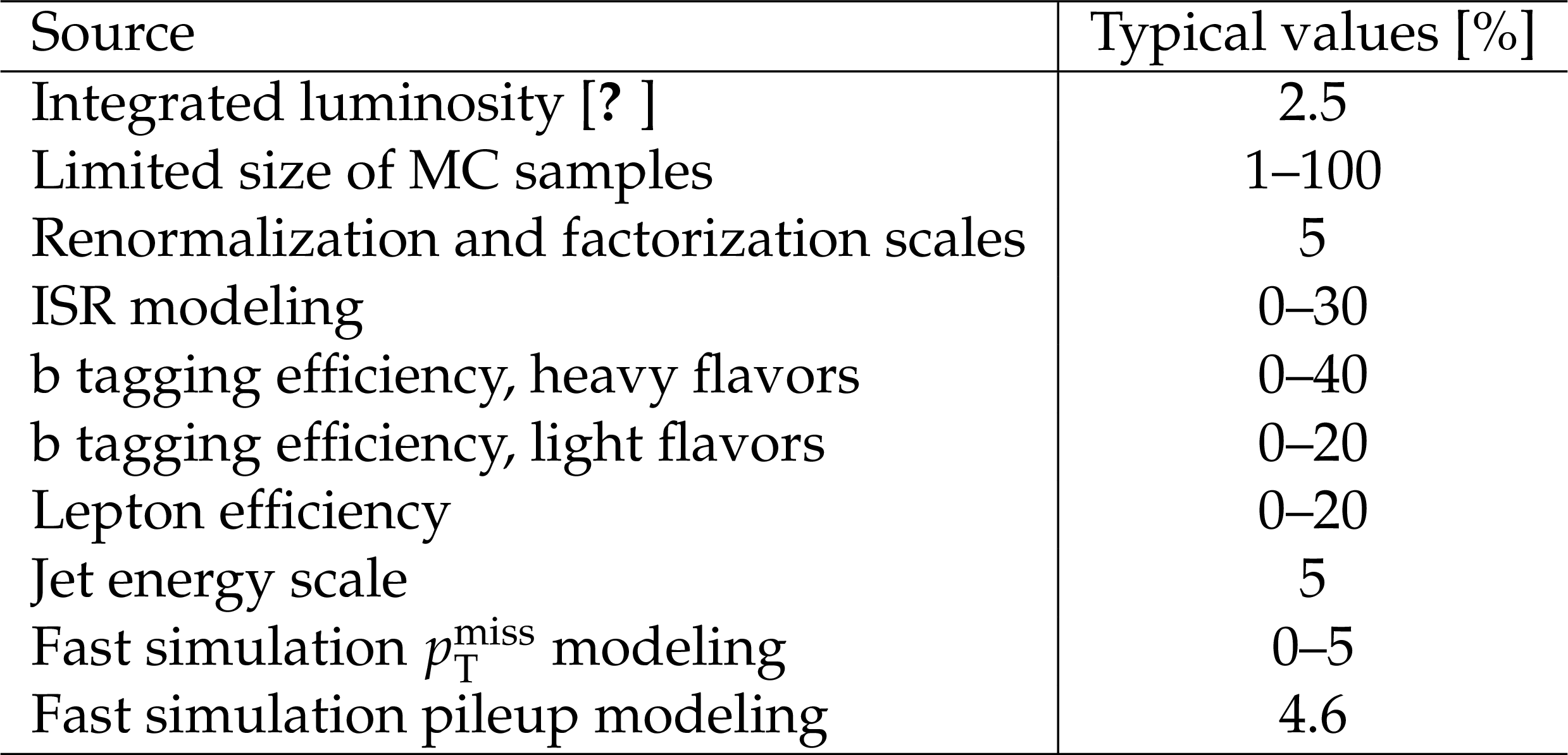
Table 3:
Typical values of the systematic uncertainties as evaluated for the simplified signal model of gluino-mediated bottom squark production, $\mathrm{ p } \mathrm{ p } \to \tilde{ \mathrm{g} } \tilde{ \mathrm{g} }, \tilde{ \mathrm{g} } \to {\mathrm{ b \bar{b} } } \tilde{\chi}^0_1 $. Uncertainties evaluated on other signal models are consistent with these ranges of values. The high statistical uncertainty in the simulated signal sample corresponds to a small number of signal bins with low acceptance, which are typically not among the most sensitive signal bins to that model point. |
png pdf |
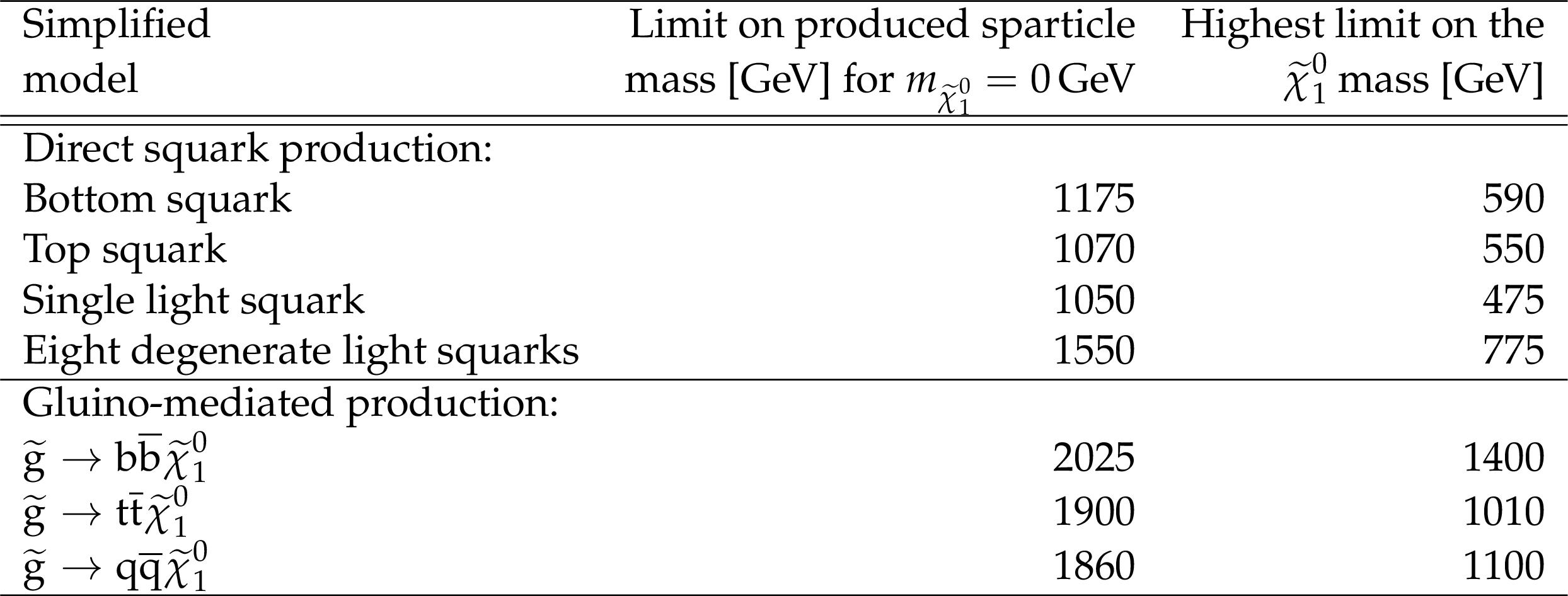
Table 4:
Summary of 95% CL observed exclusion limits on the masses of SUSY particles (sparticles) in different simplified model scenarios. The limit on the mass of the produced sparticle is quoted for a massless $\tilde{\chi}^0_1 $, while for the mass of the $\tilde{\chi}^0_1$ we quote the highest limit that is obtained. |
png pdf |
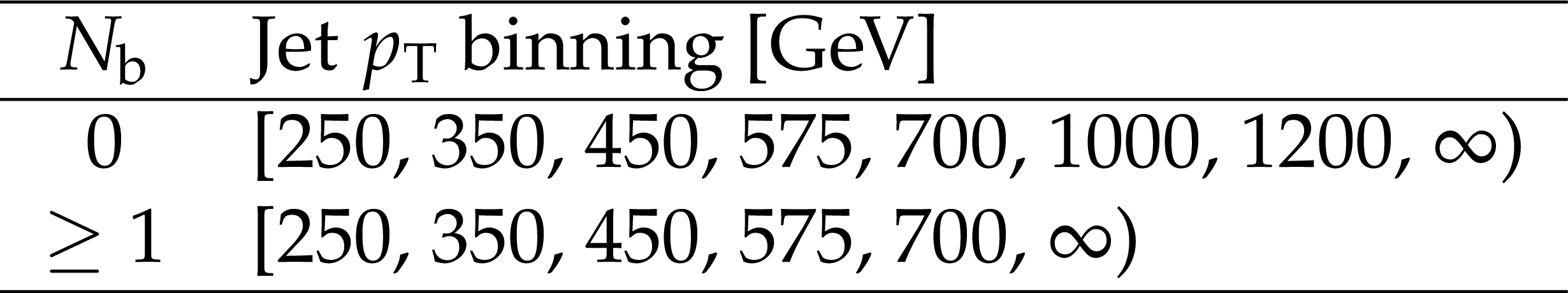
Table 5:
Summary of signal regions for the monojet selection. |
png pdf |
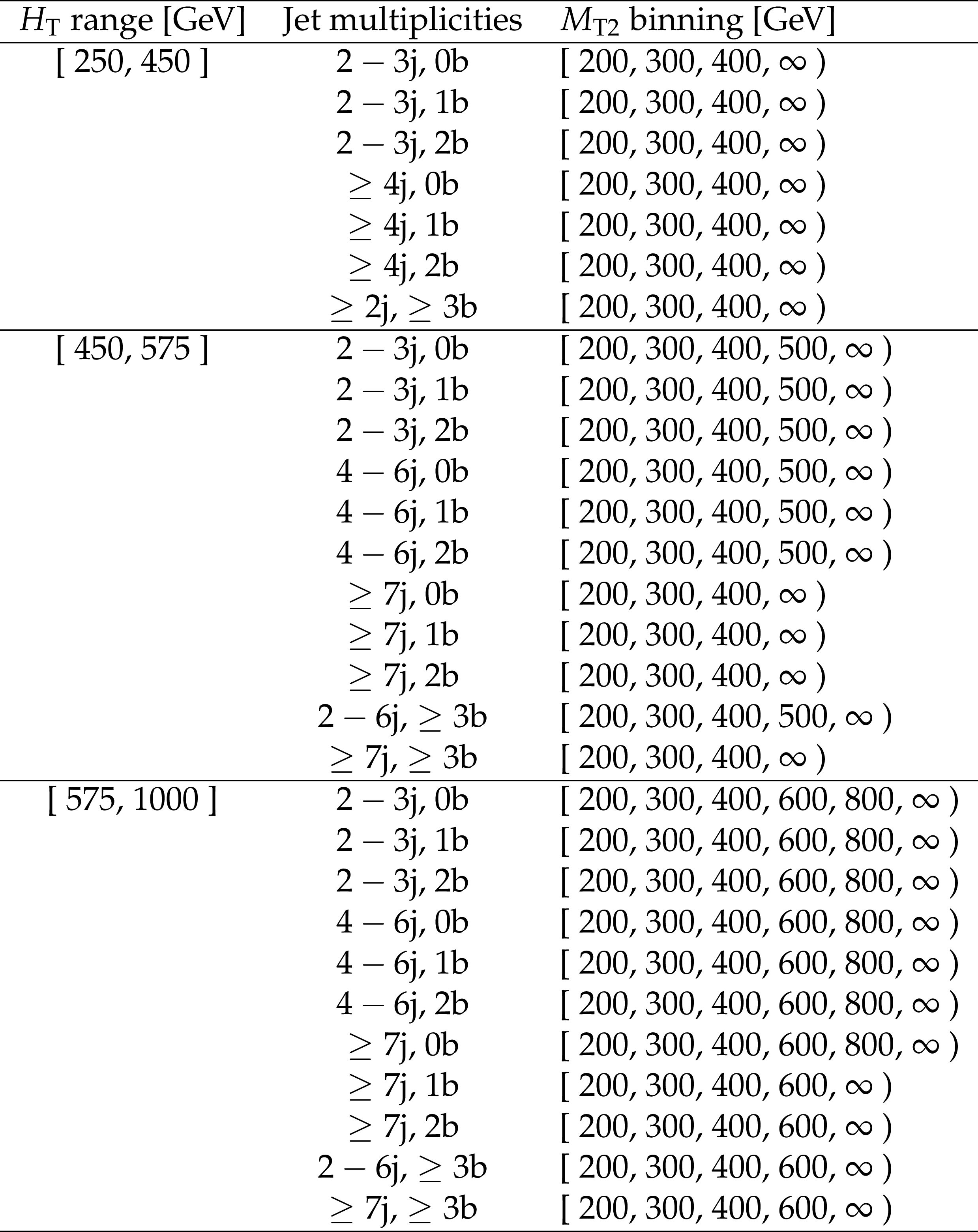
Table 6:
The $ {M_{\mathrm {T2}}} $ binning in each topological region of the multi-jet search regions, for the very low, low and medium $ {H_{\mathrm {T}}} $ regions. |

png pdf |
Table 7:
The $ {M_{\mathrm {T2}}} $ binning in each topological region of the multijet search regions, for the high- and extreme-$ {H_{\mathrm {T}}} $ regions. |
| Summary |
| This paper presents the results of a search for new phenomena using events with jets and large ${M_{\mathrm{T2}}} $. Results are based on a 35.9 fb$ {^{-1}} $ data sample of proton-proton collisions at $\sqrt{s} =$ 13 TeV collected in 2016 with the CMS detector. No significant deviations from the standard model expectations are observed. The results are interpreted as limits on the production of new, massive colored particles in simplified models of supersymmetry. This search probes gluino masses up to 2025 GeV and ${\tilde{\chi}^{0}_{1}} $ masses up to 1400 GeV. Constraints are also obtained on the pair production of light-flavor, bottom, and top squarks, probing masses up to 1550, 1175, and 1070 GeV, respectively, and ${\tilde{\chi}^{0}_{1}}$ masses up to 775, 590, and 550 GeV in each scenario. |
| Additional Figures | |
png pdf root |
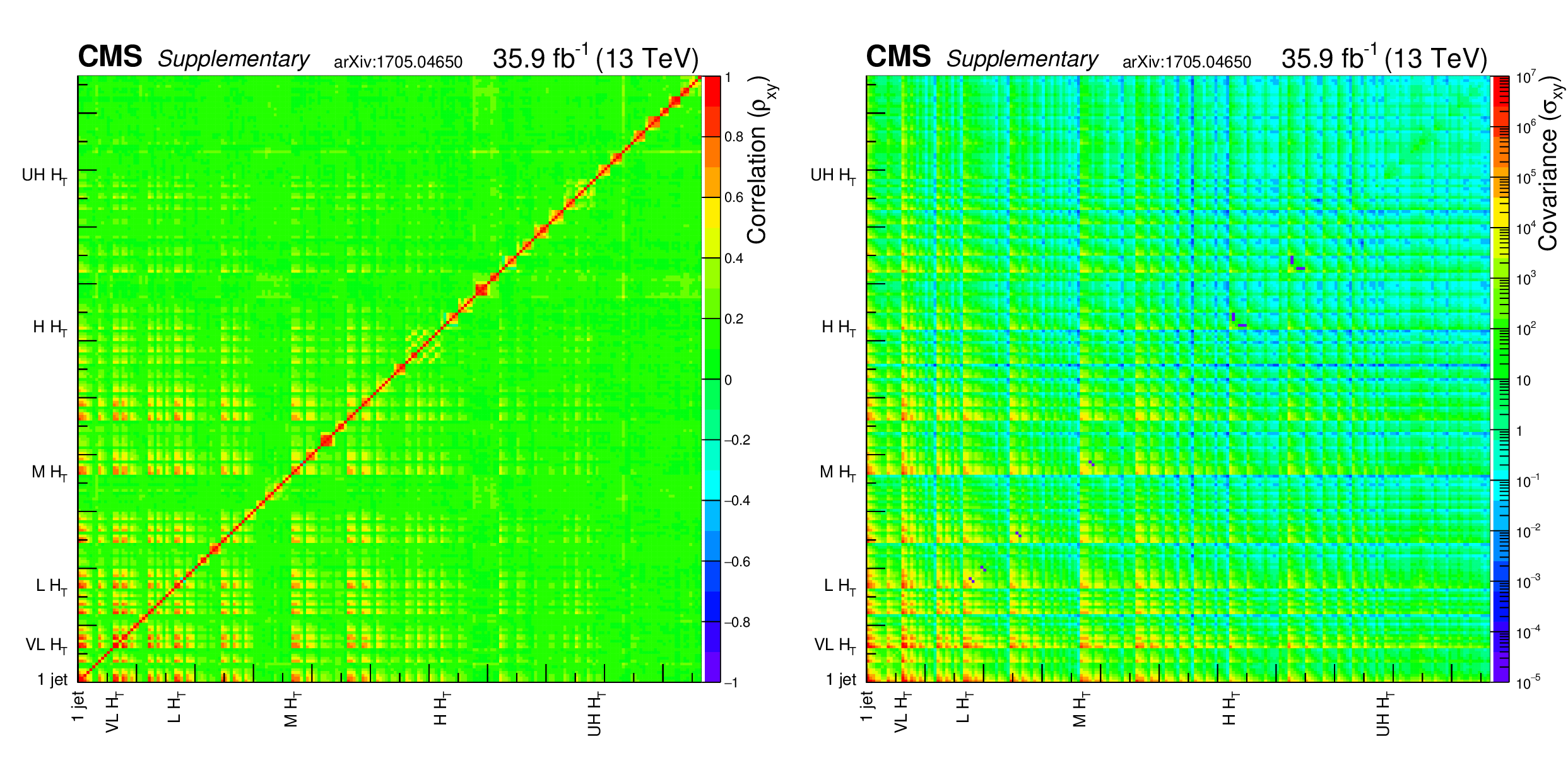
Additional Figure 1:
Full correlation (left) and covariance (right) matrices. |

png pdf root |
Additional Figure 1-a:
Full correlation matrix. |
png pdf root |
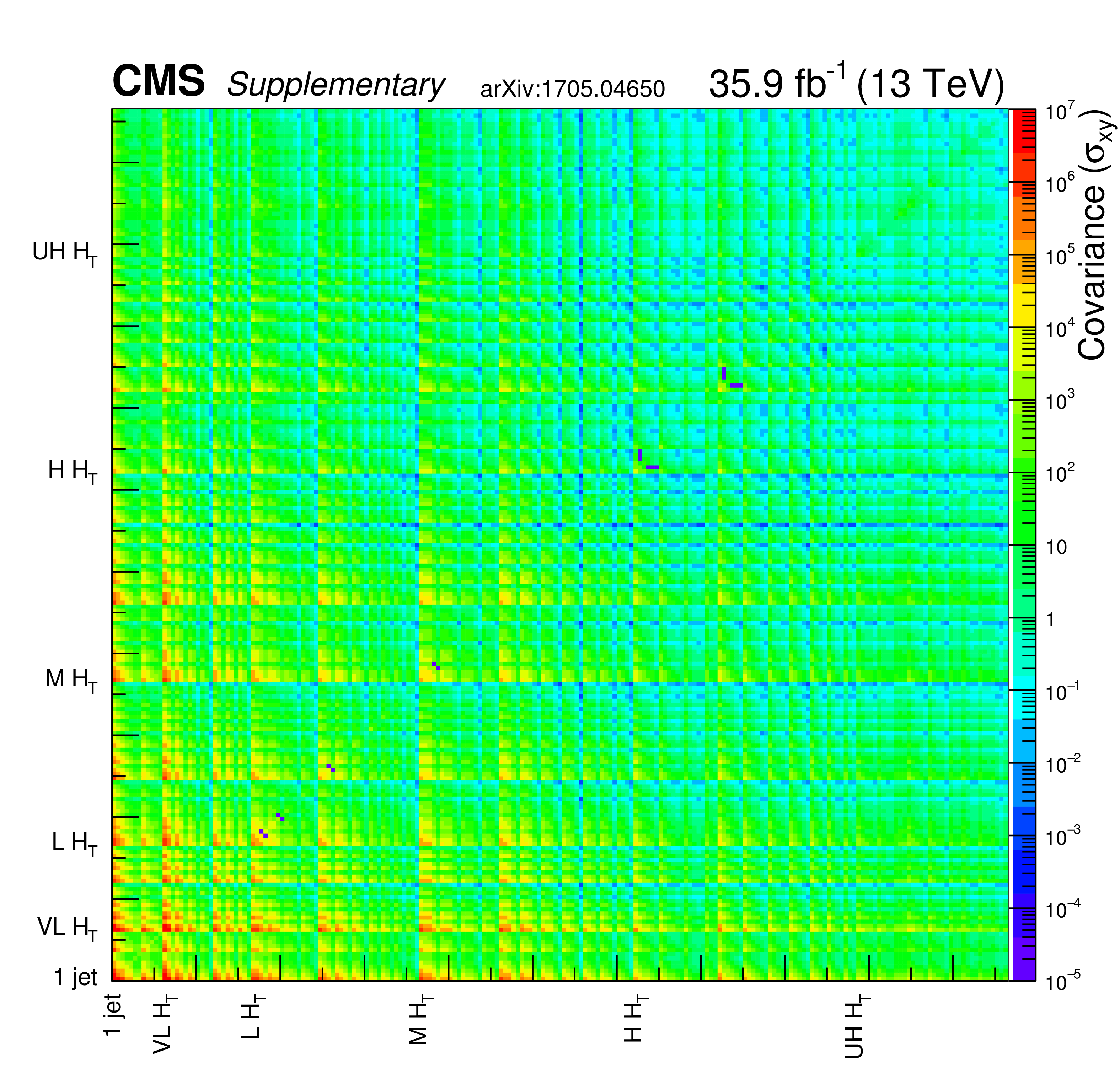
Additional Figure 1-b:
Full covariance matrix. |
png pdf root |
Additional Figure 2:
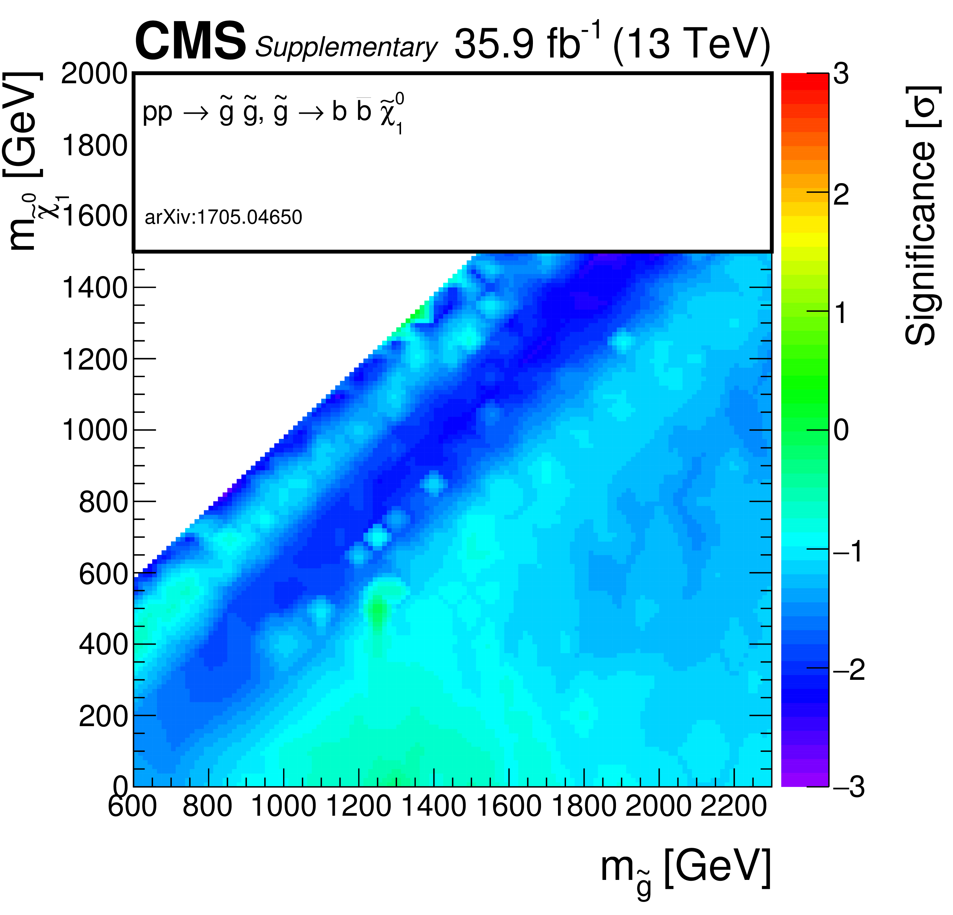
Observed significance for gluino-mediated bottom squark production model. A linear interpolation is performed across the plane, to account for the limited granularity of the simulated samples. Due to the non-linear nature of the significance, small fluctuations for single signal points may result into a visible effect on the plane. |
png pdf root |
Additional Figure 3:
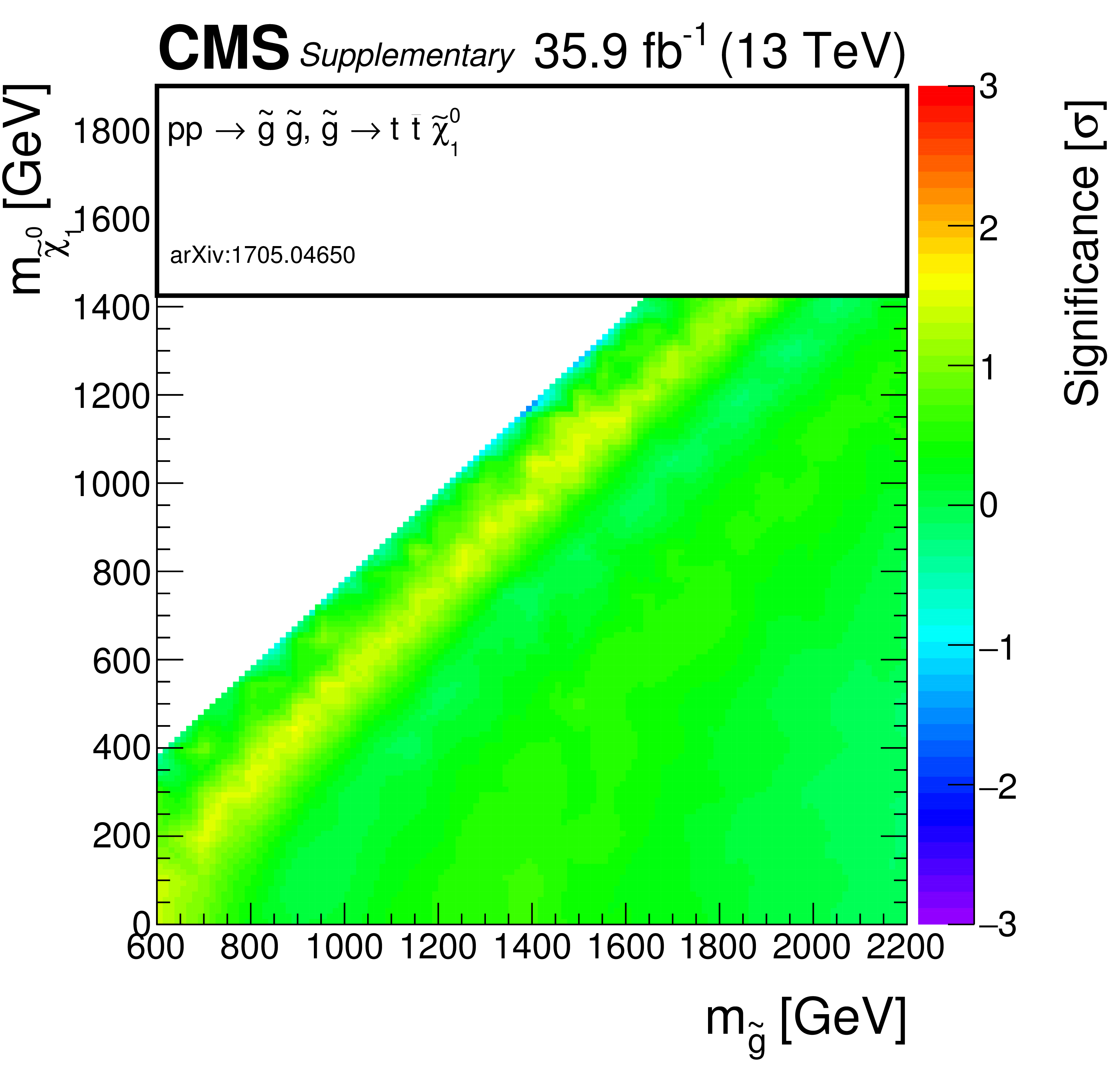
Observed significance for gluino-mediated top squark production model. A linear interpolation is performed across the plane, to account for the limited granularity of the simulated samples. Due to the non-linear nature of the significance, small fluctuations for single signal points may result into a visible effect on the plane. |
png pdf root |
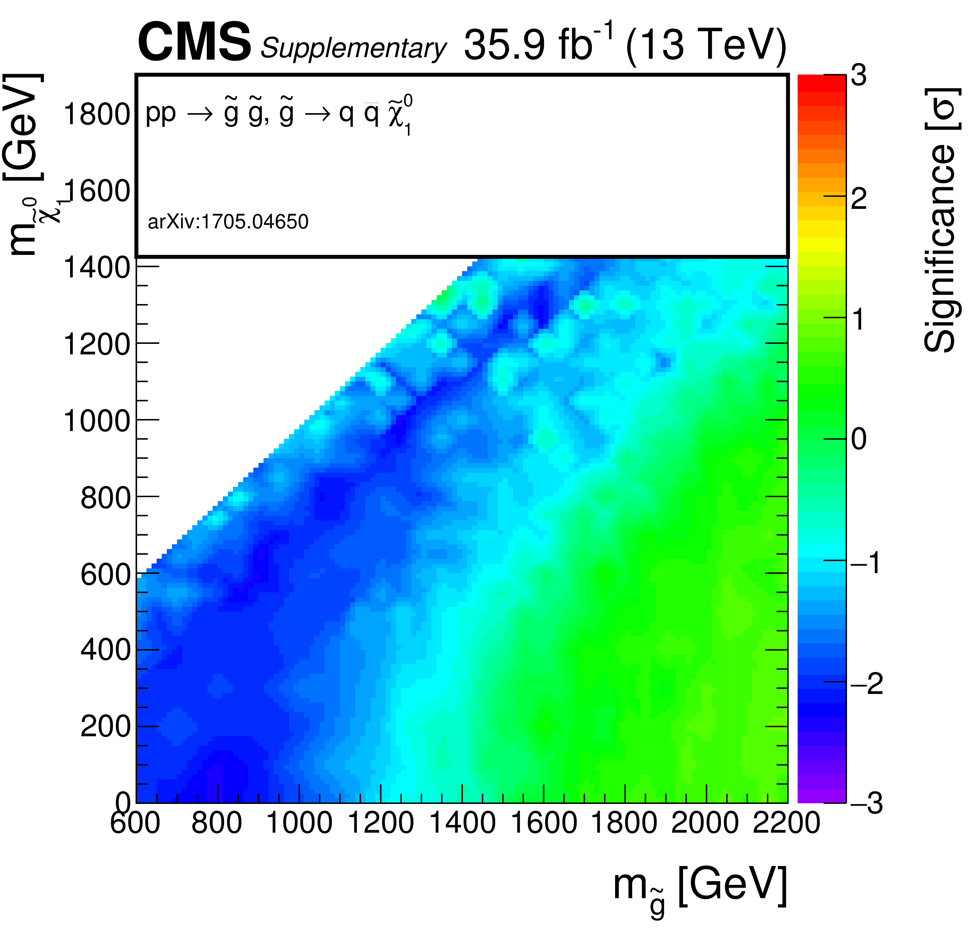
Additional Figure 4:
Observed significance for gluino-mediated light squark production model. A linear interpolation is performed across the plane, to account for the limited granularity of the simulated samples. Due to the non-linear nature of the significance, small fluctuations for single signal points may result into a visible effect on the plane. |
png pdf root |
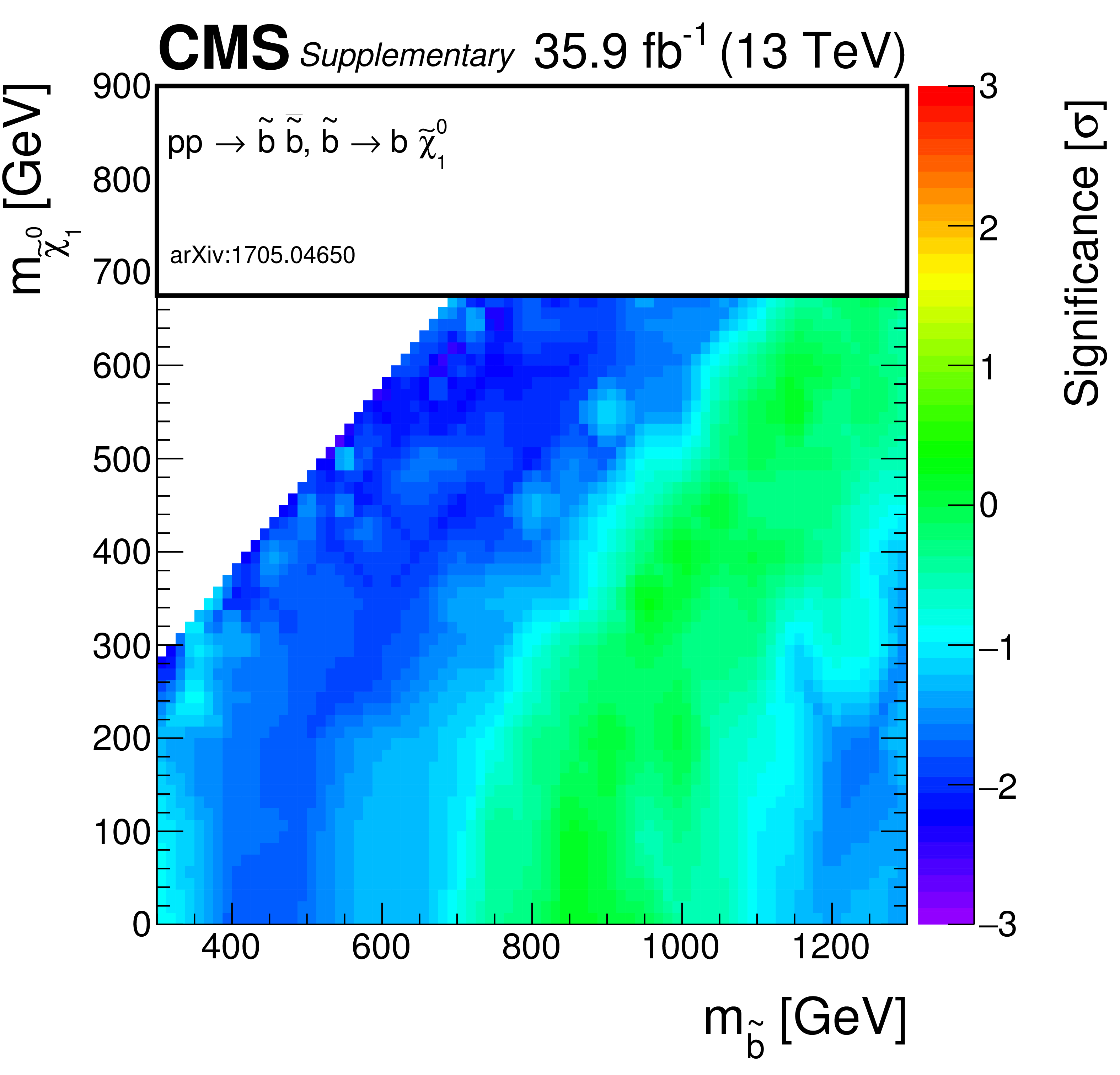
Additional Figure 5:
Observed significance for direct bottom squark production model. A linear interpolation is performed across the plane, to account for the limited granularity of the simulated samples. Due to the non-linear nature of the significance, small fluctuations for single signal points may result into a visible effect on the plane. |
png pdf root |
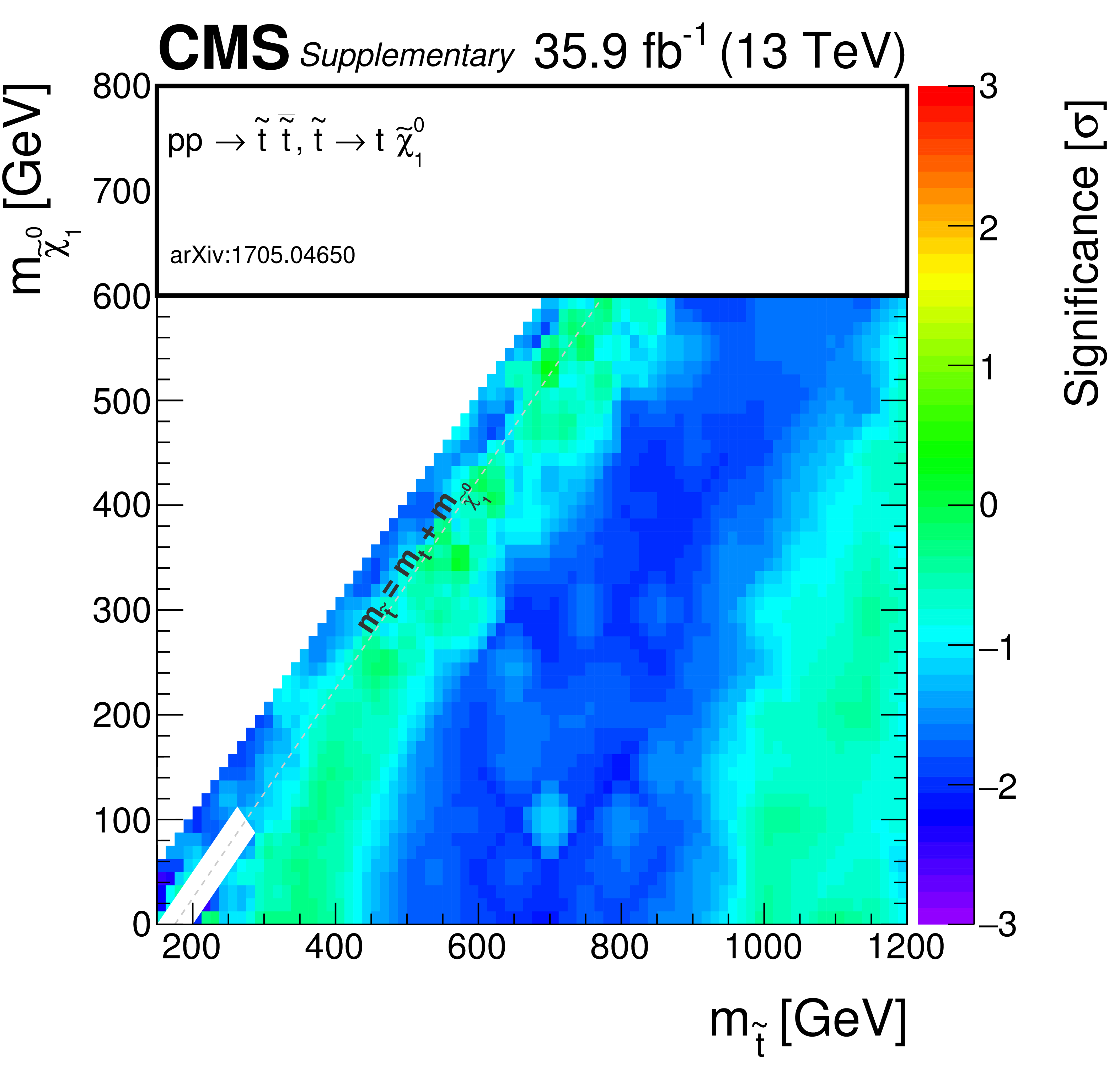
Additional Figure 6:
Observed significance for direct top squark production model. A linear interpolation is performed across the plane, to account for the limited granularity of the simulated samples. Due to the non-linear nature of the significance, small fluctuations for single signal points may result into a visible effect on the plane. |

png pdf root |
Additional Figure 7:
Observed significance for direct light squark production model. A linear interpolation is performed across the plane, to account for the limited granularity of the simulated samples. Due to the non-linear nature of the significance, small fluctuations for single signal points may result into a visible effect on the plane. |

png pdf root |
Additional Figure 8:
Observed significance for direct top squark pair production model, for the scenario where $\mathrm{ p } \mathrm{ p } \to \tilde{ \mathrm{ t } }_1 \tilde{ \mathrm{ t } }_1^* \to \mathrm{ b \bar{b} } \tilde{\chi}^{\pm}_1 \tilde{\chi}^{\pm}_1 $, $\tilde{\chi}^{\pm}_1 \to \mathrm{ W } \tilde{\chi}^0_1 $, with the mass of the chargino chosen to be half way in between the masses of the top squark and the neutralino. A linear interpolation is performed across the plane, to account for the limited granularity of the simulated samples. Due to the non-linear nature of the significance, small fluctuations for single signal points may result into a visible effect on the plane. |

png pdf root |
Additional Figure 9:
Observed significance for direct top squark pair production model, for the scenario where $\mathrm{ p } \mathrm{ p } \to \tilde{ \mathrm{ t } }_1 \tilde{ \mathrm{ t } }_1^*\to \mathrm{ t } \mathrm{ b } \tilde{\chi}^{\pm}_1 \tilde{\chi}^0_1 $, $\tilde{\chi}^{\pm}_1 \to \mathrm{ W } ^{*}\tilde{\chi}^0_1 $, with the chargino mass chosen such that $\Delta m\left (\tilde{\chi}^{\pm}_1,\tilde{\chi}^0_1 \right) = $ 5 GeV. A linear interpolation is performed across the plane, to account for the limited granularity of the simulated samples. Due to the non-linear nature of the significance, small fluctuations for single signal points may result into a visible effect on the plane. |

png pdf root |
Additional Figure 10:
Observed significance for direct top squark pair production model, for a compressed scenario where $\mathrm{ p } \mathrm{ p } \to \tilde{ \mathrm{ t } }_1 \tilde{ \mathrm{ t } }_1^*\to \mathrm{c} \mathrm{ \bar{c} } \tilde{\chi}^0_1 \tilde{\chi}^0_1 $. A linear interpolation is performed across the plane, to account for the limited granularity of the simulated samples. Due to the non-linear nature of the significance, small fluctuations for single signal points may result into a visible effect on the plane. |
png pdf |
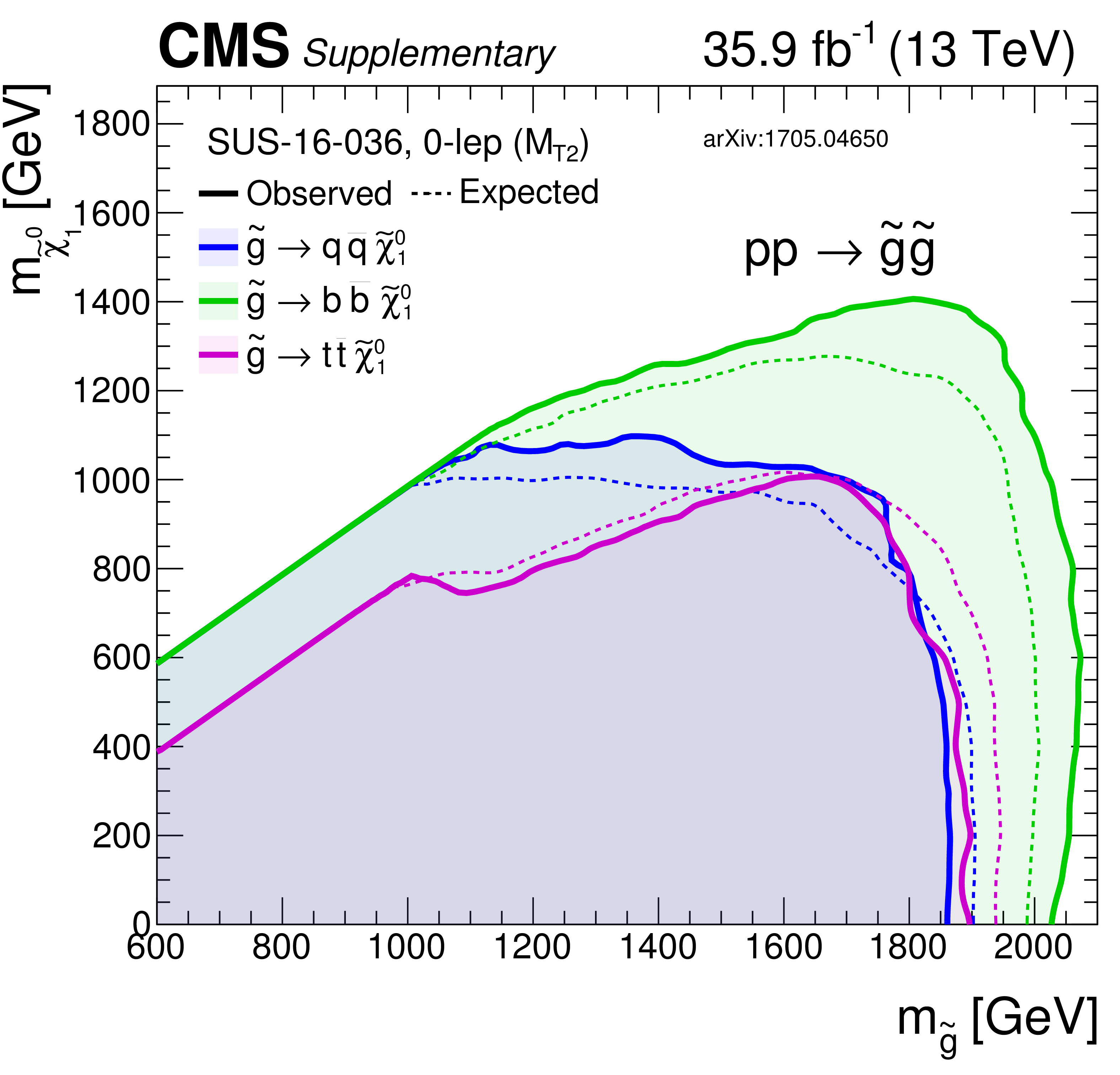
Additional Figure 11:
Summary of exclusion limits for gluino production models. |
png pdf |
Additional Figure 12:
Summary of exclusion limits for direct squark production models. |
png pdf |
Additional Figure 13:
Summary of exclusion limits for direct stop production models. |
| Additional Tables | |
png pdf |
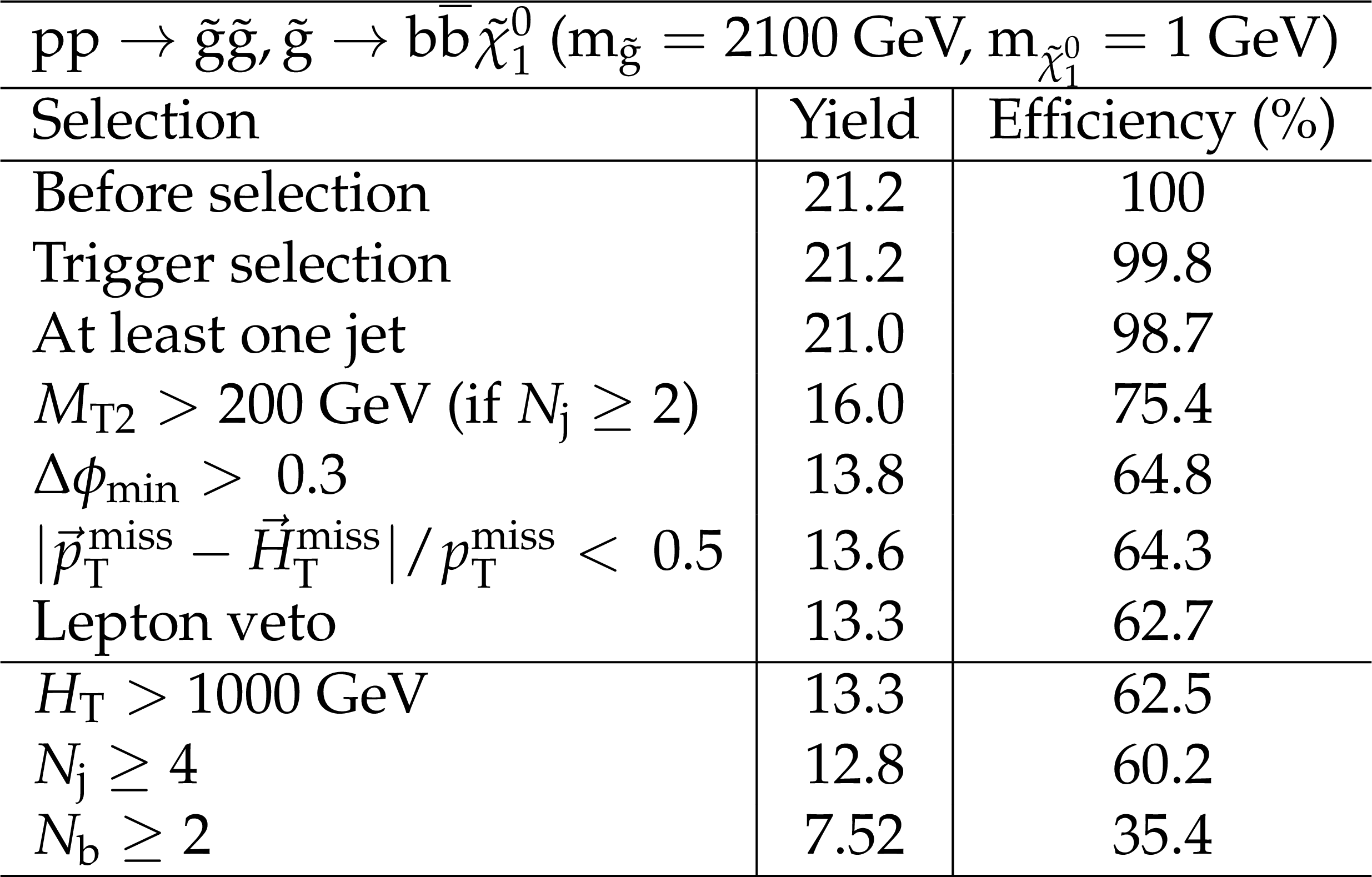
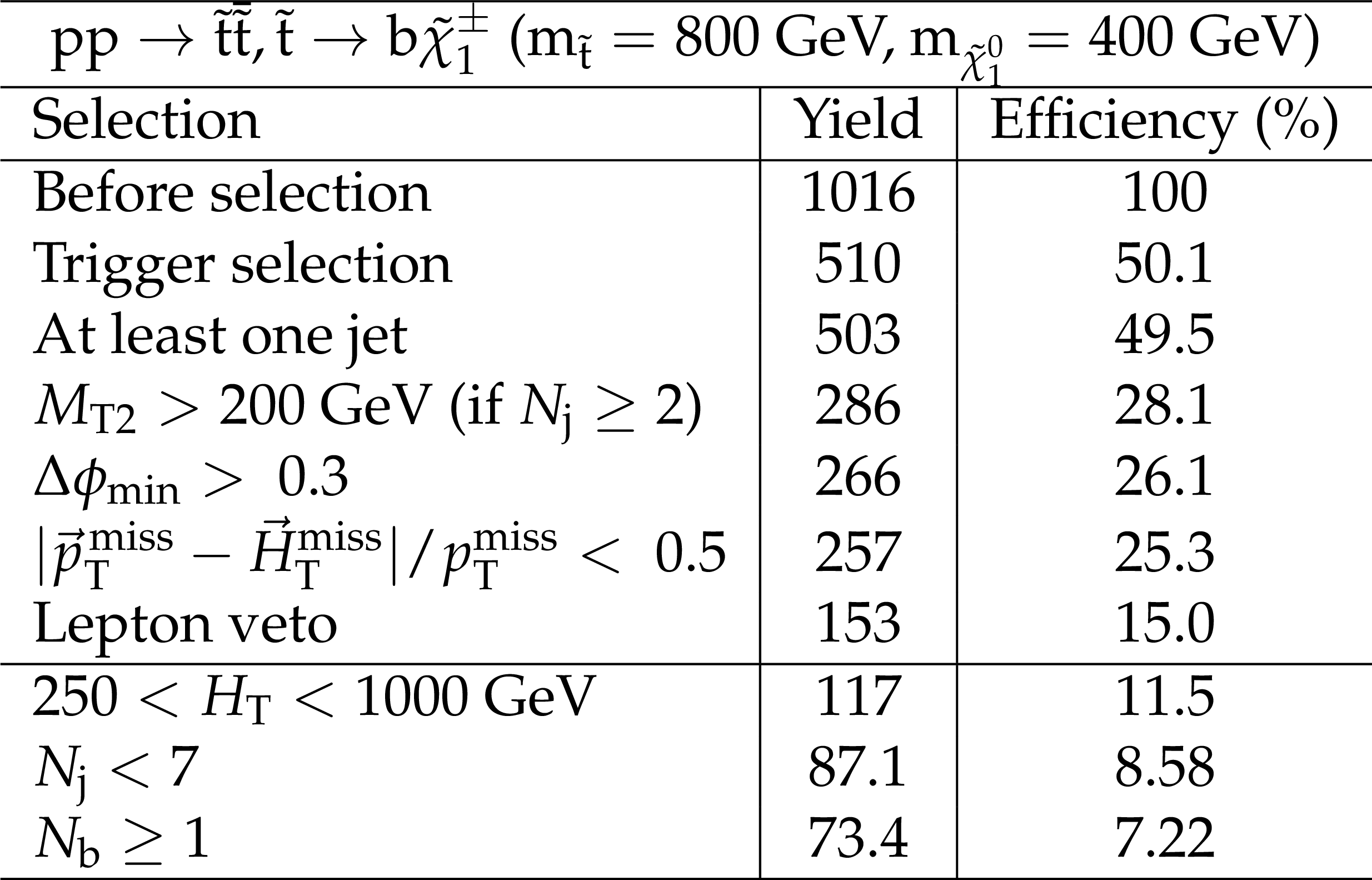
Additional Table 1:
Cut flow table for basline selection and several sample additional kinematic selections for a signal model of gluino-mediated bottom squark production with the mass of the gluino and the LSP equal to 2100 and 1GeV, respectively. Theory cross section for this signal is 0.59 fb. |

png pdf |
Additional Table 2:
Cut flow table for basline selection and several sample additional kinematic selections for a signal model of gluino-mediated bottom squark production with the mass of the gluino and the LSP equal to 1800 and 1300GeV, respectively. Theory cross section for this signal is 2.76 fb. |
png pdf |
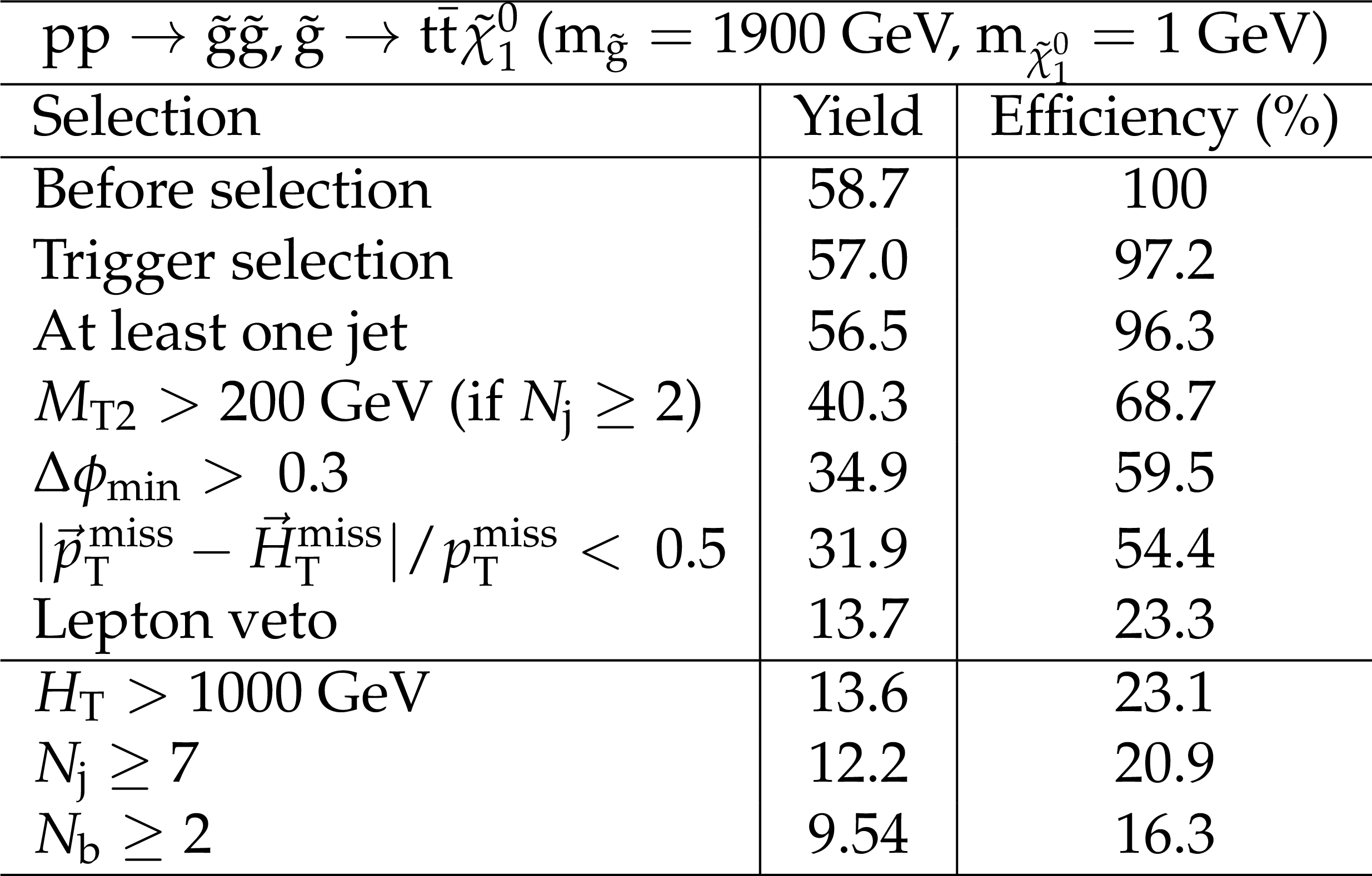
Additional Table 3:
Cut flow table for basline selection and several sample additional kinematic selections for a signal model of gluino-mediated top squark production with the mass of the gluino and the LSP equal to 1900 and 1GeV, respectively. Theory cross section for this signal is 1.64 fb. |
png pdf |
Additional Table 4:
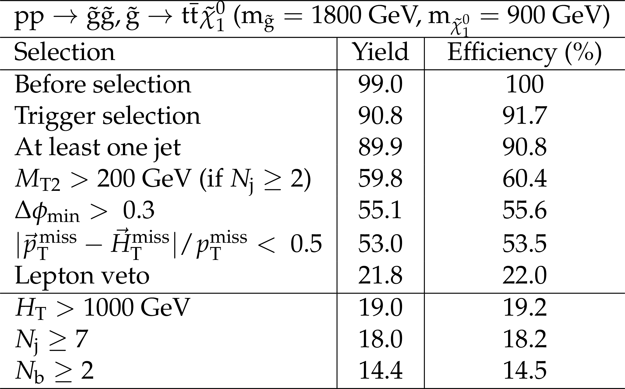
Cut flow table for basline selection and several sample additional kinematic selections for a signal model of gluino-mediated top squark production with the mass of the gluino and the LSP equal to 1800 and 900GeV, respectively. Theory cross section for this signal is 2.76 fb. |

png pdf |
Additional Table 5:
Cut flow table for basline selection and several sample additional kinematic selections for a signal model of gluino-mediated light squark production with the mass of the gluino and the LSP equal to 1900 and 1GeV, respectively. Theory cross section for this signal is 1.64 fb. |
png pdf |
Additional Table 6:
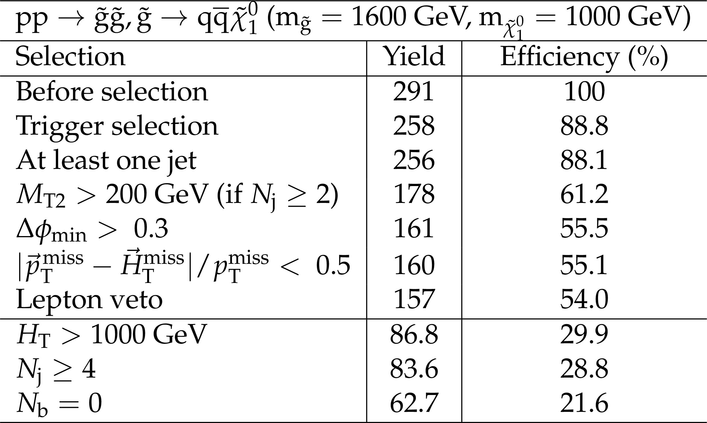
Cut flow table for basline selection and several sample additional kinematic selections for a signal model of gluino-mediated light squark production with the mass of the gluino and the LSP equal to 1600 and 1000GeV, respectively. Theory cross section for this signal is 8.10 fb. |
png pdf |
Additional Table 7:
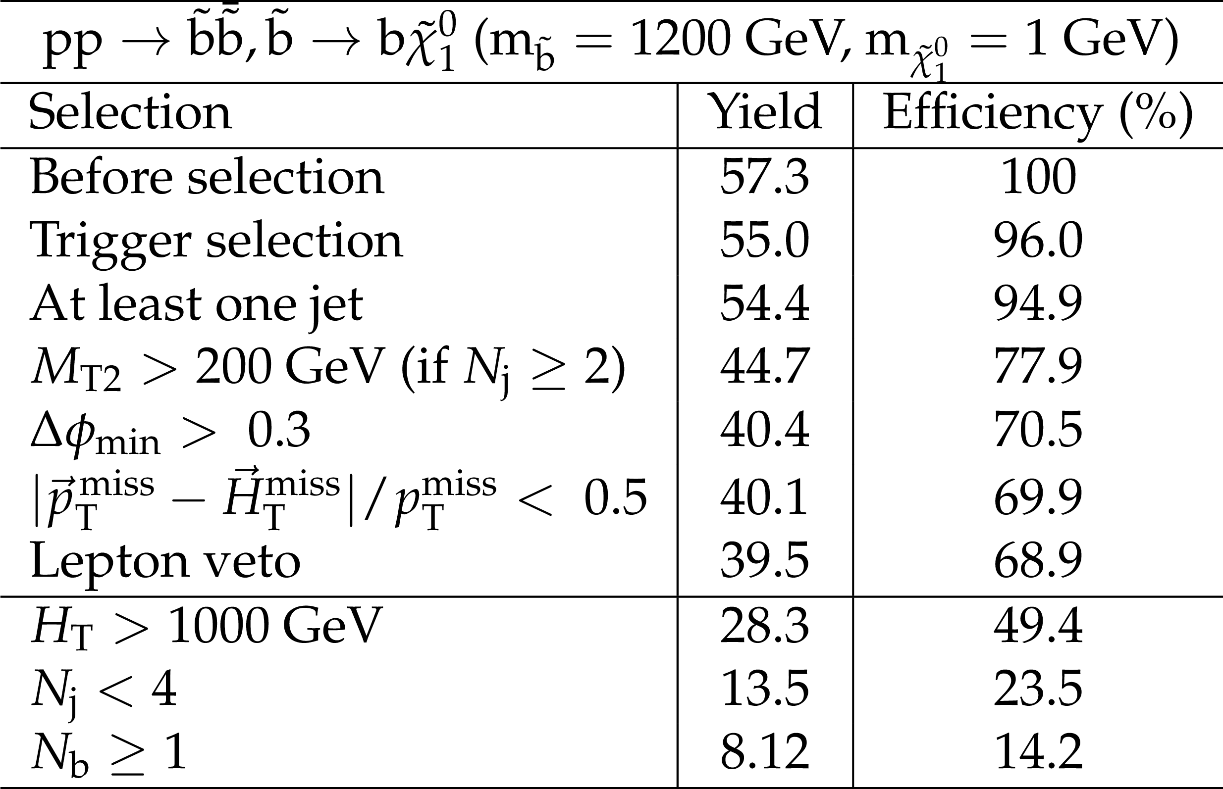
Cut flow table for basline selection and several sample additional kinematic selections for a signal model of direct bottom squark production with the mass of the squark and the LSP equal to 1200 and 1GeV, respectively. Theory cross section for this signal is 1.60 fb. |
png pdf |
Additional Table 8:
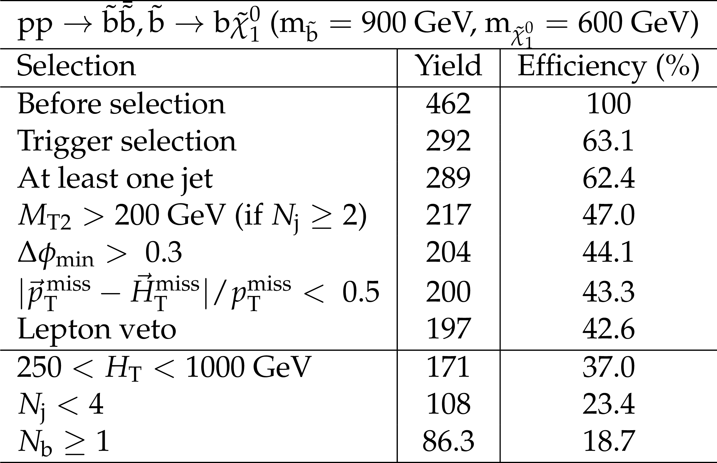
Cut flow table for basline selection and several sample additional kinematic selections for a signal model of direct bottom squark production with the mass of the squark and the LSP equal to 900 and 600GeV, respectively. Theory cross section for this signal is 12.9 fb. |

png pdf |
Additional Table 9:
Cut flow table for basline selection and several sample additional kinematic selections for a signal model of direct top squark production with the mass of the squark and the LSP equal to 1100 and 1GeV, respectively. Theory cross section for this signal is 3.07 fb. |
png pdf |
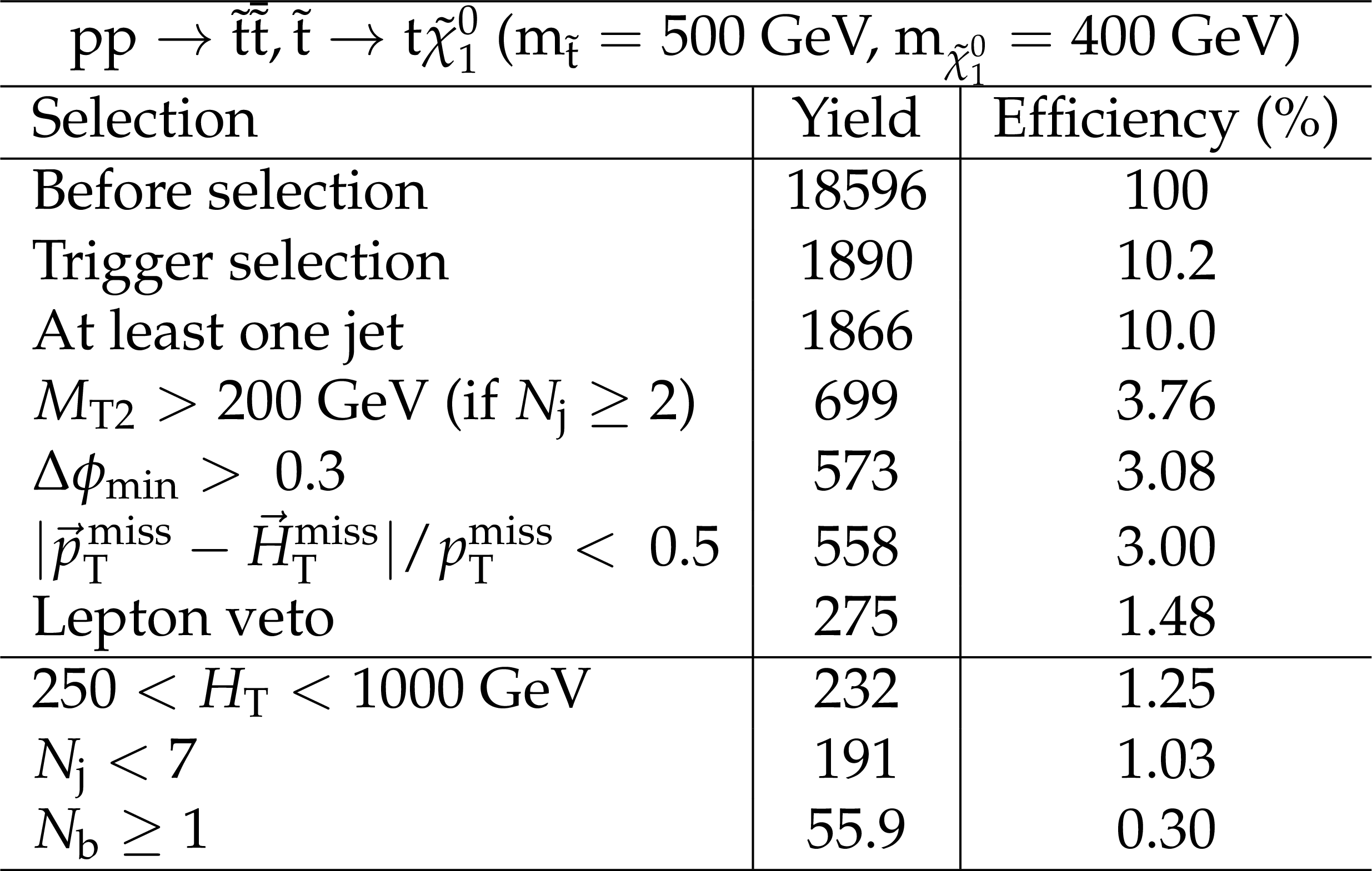
Additional Table 10:
Cut flow table for basline selection and several sample additional kinematic selections for a signal model of direct top squark production with the mass of the squark and the LSP equal to 500 and 400GeV, respectively. Theory cross section for this signal is 518 fb. |

png pdf |
Additional Table 11:
Cut flow table for basline selection and several sample additional kinematic selections for a signal model of direct light squark production with the mass of the squark and the LSP equal to 1500 and 1GeV, respectively. Theory cross section for this signal is 2.09 fb. |
png pdf |
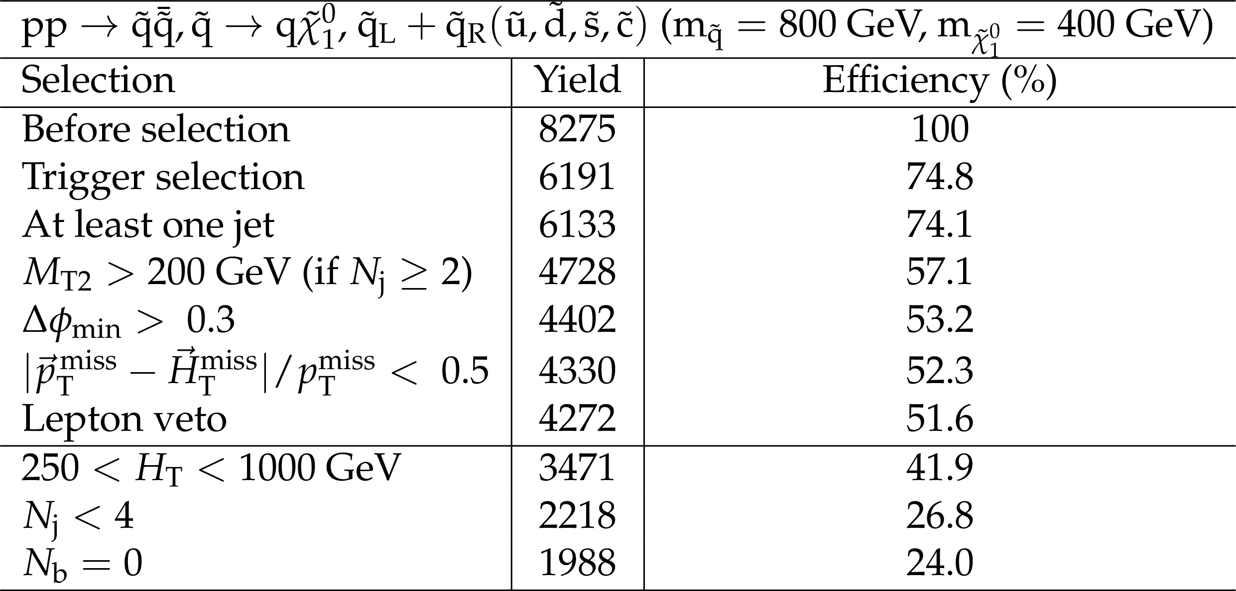
Additional Table 12:
Cut flow table for basline selection and several sample additional kinematic selections for a signal model of direct light squark production with the mass of the squark and the LSP equal to 800 and 400GeV, respectively. Theory cross section for this signal is 231 fb. |
png pdf |
Additional Table 13:
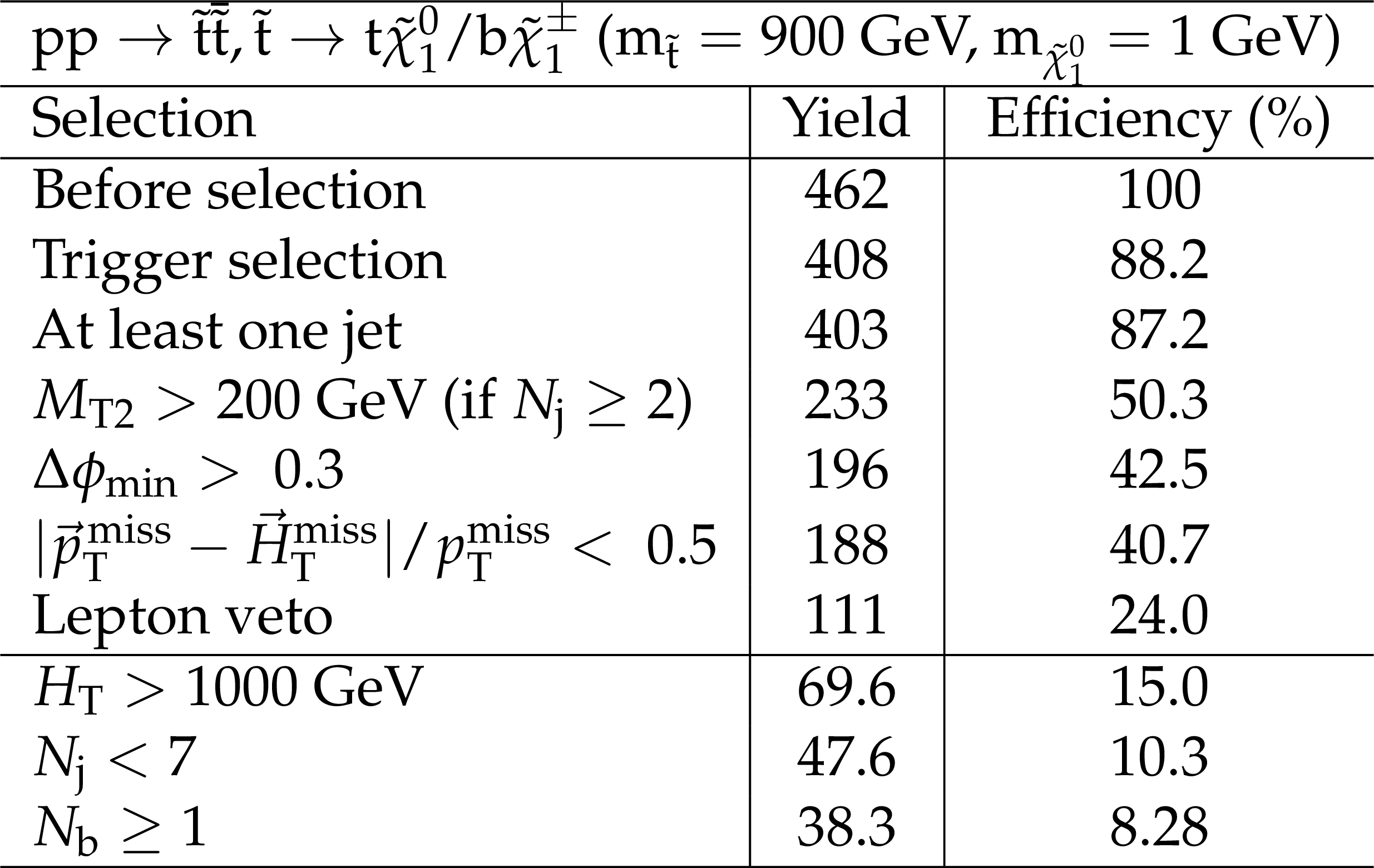
Cut flow table for basline selection and several sample additional kinematic selections for a signal model of direct top squark production, where one top squark decays via a bottom quark while the other decays via a top quark, with the mass of the squark and the LSP equal to 900 and 1GeV, respectively. Theory cross section for this signal is 12.9 fb. |

png pdf |
Additional Table 14:
Cut flow table for basline selection and several sample additional kinematic selections for a signal model of direct top squark production, where one top squark decays via a bottom quark while the other decays via a top quark, with the mass of the squark and the LSP equal to 800 and 400GeV, respectively. Theory cross section for this signal is 28.3 fb. |
png pdf |
Additional Table 15:
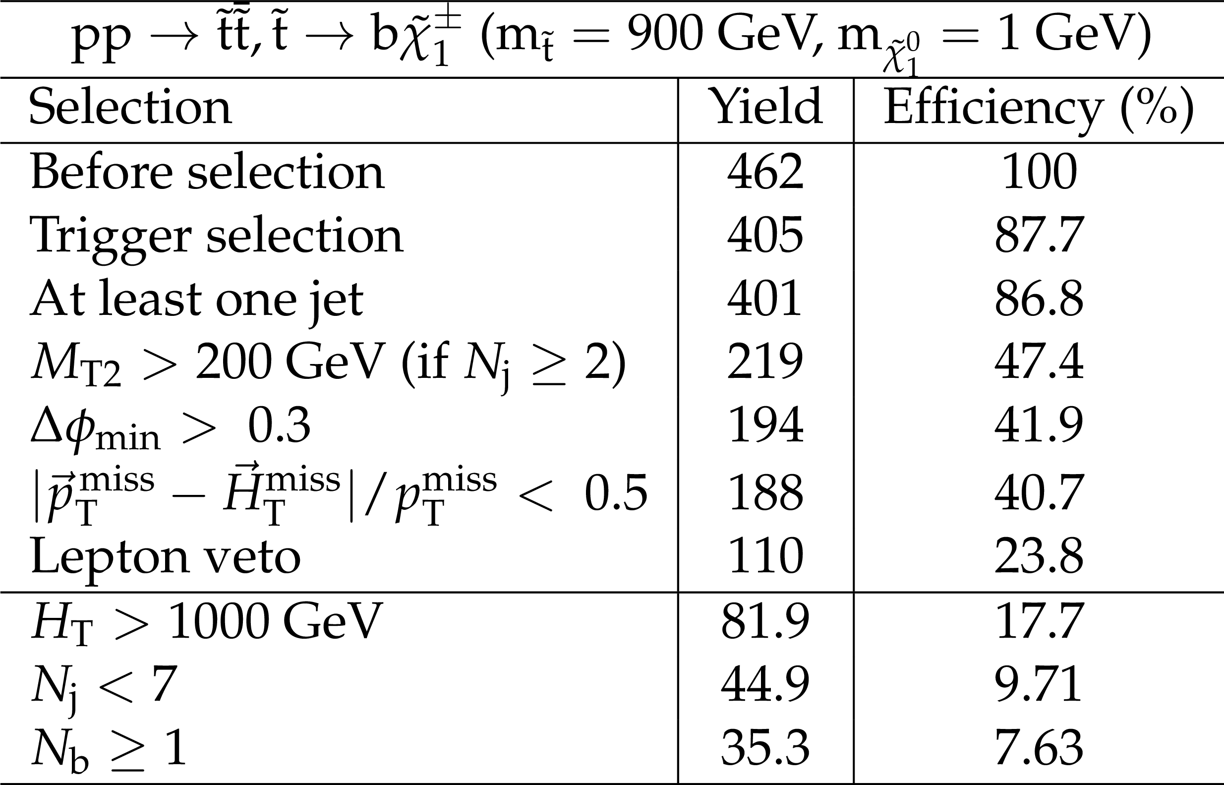
Cut flow table for basline selection and several sample additional kinematic selections for a signal model of direct top squark production, where the top squark decays via a bottom quark, with the mass of the squark and the LSP equal to 900 and 1GeV, respectively. Theory cross section for this signal is 12.9 fb. |
png pdf |
Additional Table 16:
Cut flow table for basline selection and several sample additional kinematic selections for a signal model of direct top squark production, where the top squark decays via a bottom quark, with the mass of the squark and the LSP equal to 800 and 400GeV, respectively. Theory cross section for this signal is 28.3 fb. |

png pdf |
Additional Table 17:
Cut flow table for basline selection and several sample additional kinematic selections for a signal model of direct top squark production, where the top squark decays via a charm quark, with the mass of the squark and the LSP equal to 450 and 370GeV, respectively. Theory cross section for this signal is 948 fb. |

png pdf |
Additional Table 18:
Cut flow table for basline selection and several sample additional kinematic selections for a signal model of direct top squark production, where the top squark decays via a charm quark, with the mass of the squark and the LSP equal to 450 and 440GeV, respectively. Theory cross section for this signal is 948 fb. |

png pdf |
Additional Table 19:
Background estimate and observation in bins of jet $p_{\mathrm {T}}$ for the monojet regions. The yields correspond to an integrated luminosity of 35.9 fb$^{-1}$. |

png pdf |
Additional Table 20:
Background estimate and observation in bins of $M_{\mathrm {T2}}$ for 250 $ < H_{\mathrm {T}} < $ 450 GeV. The yields correspond to an integrated luminosity of 35.9 fb$^{-1}$. |
png pdf |
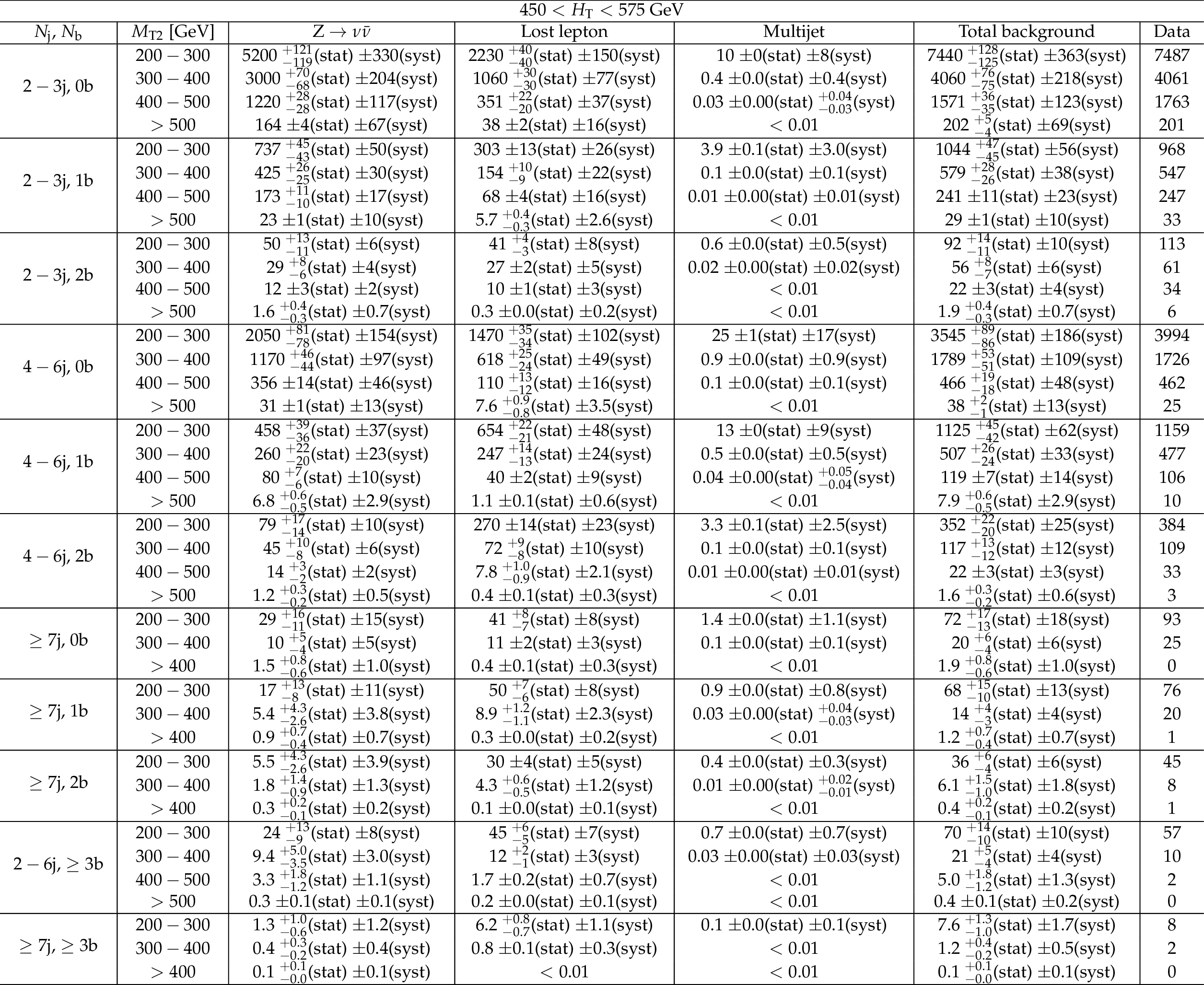
Additional Table 21:
Background estimate and observation in bins of $M_{\mathrm {T2}}$ for 450 $ < H_{\mathrm {T}} < $ 575 GeV. The yields correspond to an integrated luminosity of 35.9 fb$^{-1}$. |
png pdf |
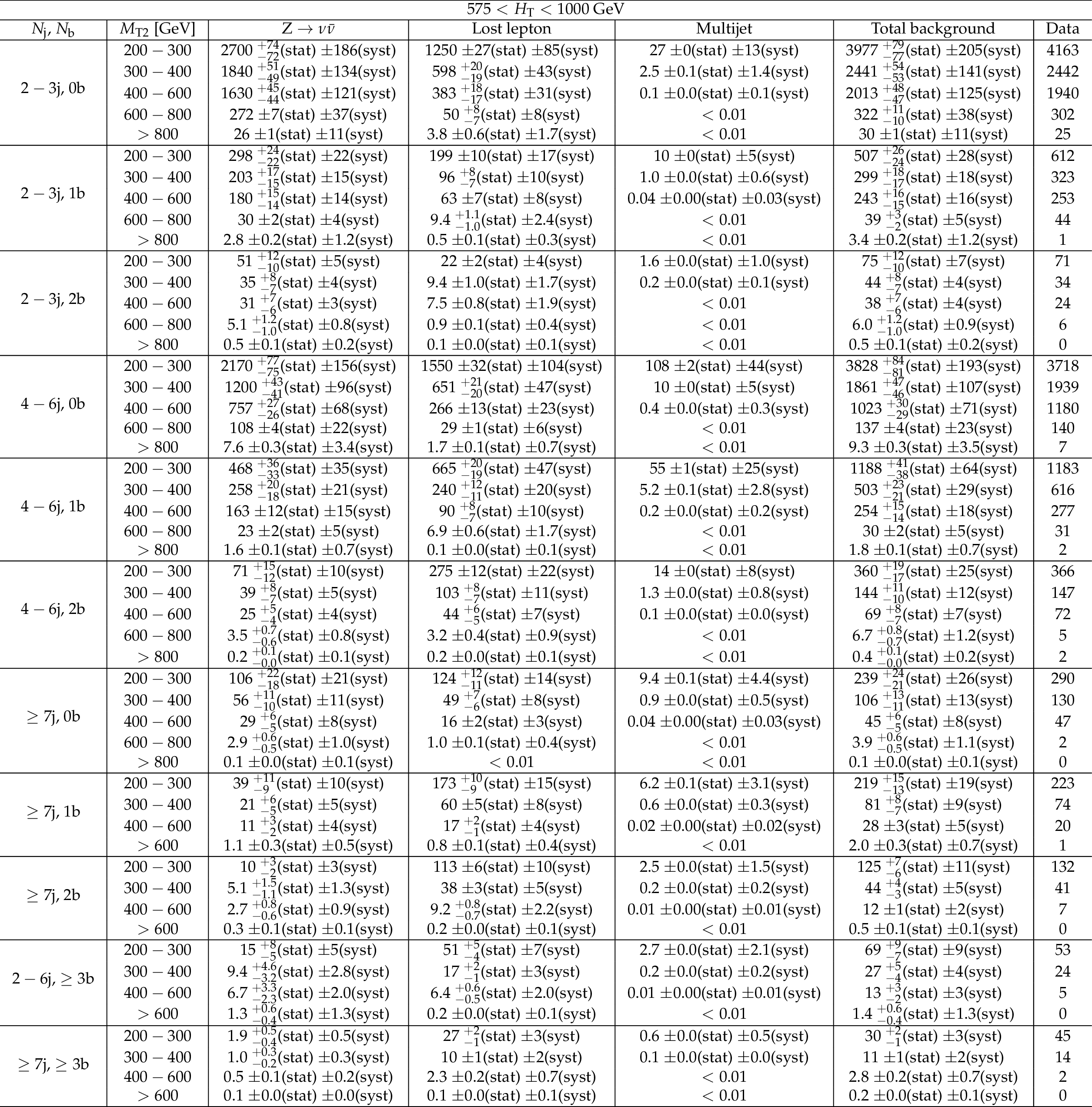
Additional Table 22:
Background estimate and observation in bins of $M_{\mathrm {T2}}$ for 575 $ < H_{\mathrm {T}} < $ 1000 GeV. The yields correspond to an integrated luminosity of 35.9 fb$^{-1}$. |
png pdf |
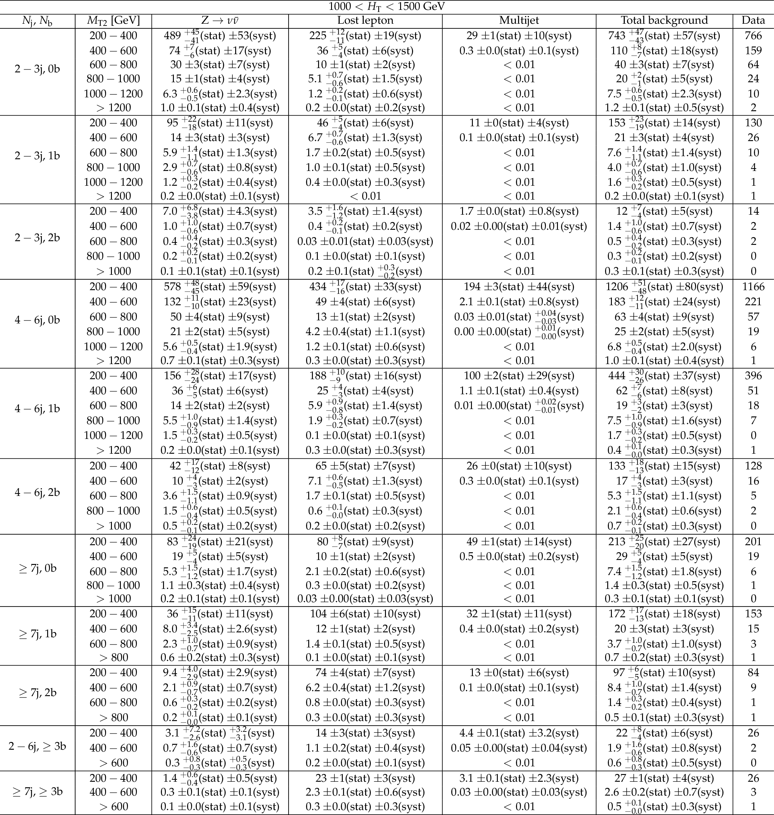
Additional Table 23:
Background estimate and observation in bins of $M_{\mathrm {T2}}$ for 1000 $ < H_{\mathrm {T}} < $ 1500 GeV. The yields correspond to an integrated luminosity of 35.9 fb$^{-1}$. |
png pdf |
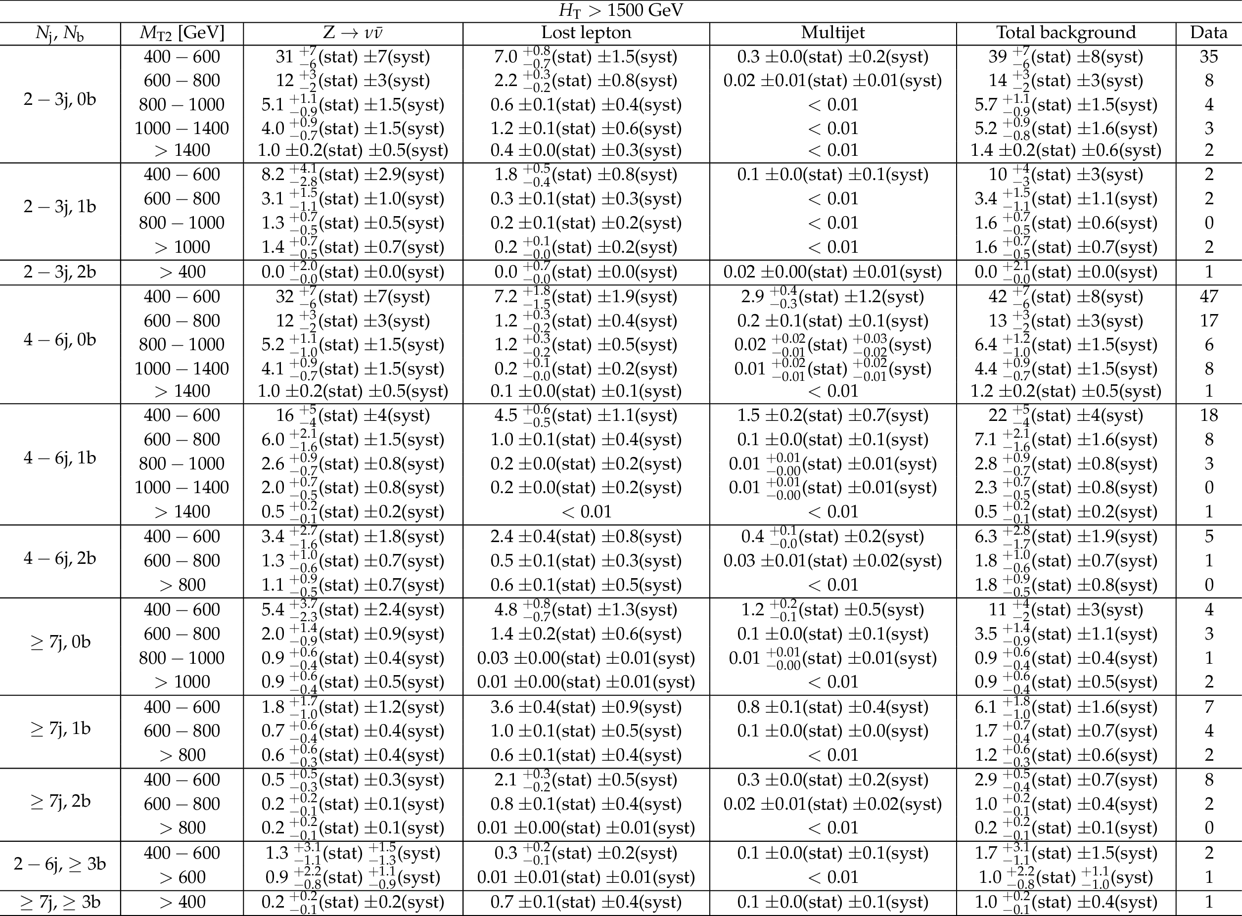
Additional Table 24:
Background estimate and observation in bins of $M_{\mathrm {T2}}$ for $H_{\mathrm {T}} > $ 1500 GeV. The yields correspond to an integrated luminosity of 35.9 fb$^{-1}$. |
|
Additional code to compute hemispheres and $M_{\mathrm{T2}}$ and an example of usage is available here.
The code available here also include python scripts to facilitate the access to the full covariance (correlation) matrix. One script allows to retrive the bin number on the covariance matrix axes for a given kinematic selection: with HT, jet pT, and/or MT2 expressed in GeV will return the bin number corresponding to the kinematic selection, together with the corresponding background predictions and observation. A second script allows to retrieve the kinematic selection corresponding to one bin number on the covariance matrix axes: will return the kinematic selection corresponding to the input bin number, together with the corresponding background predictions and observation. |
| References | ||||
| 1 | ATLAS Collaboration | Search for new phenomena in final states with large jet multiplicities and missing transverse momentum with ATLAS using $ \sqrt{s} = $ 13 TeV proton-proton collisions | PLB 757 (2016) 334 | 1602.06194 |
| 2 | ATLAS Collaboration | Search for new phenomena in final states with an energetic jet and large missing transverse momentum in pp collisions at $ \sqrt{s}= $ 13 TeV using the ATLAS detector | PRD 94 (2016) 032005 | 1604.07773 |
| 3 | ATLAS Collaboration | Search for squarks and gluinos in final states with jets and missing transverse momentum at $ \sqrt{s} = $ 13 TeV with the ATLAS detector | EPJC 76 (2016) 392 | 1605.03814 |
| 4 | ATLAS Collaboration | Search for pair production of gluinos decaying via stop and sbottom in events with $ b $-jets and large missing transverse momentum in $ pp $ collisions at $ \sqrt{s} = $ 13 TeV with the ATLAS detector | PRD 94 (2016) 032003 | 1605.09318 |
| 5 | ATLAS Collaboration | Search for bottom squark pair production in proton-proton collisions at $ \sqrt{s} = $ 13 TeV with the ATLAS detector | EPJC 76 (2016) 547 | 1606.08772 |
| 6 | CMS Collaboration | Search for new physics with the M$ _{T2} $ variable in all-jets final states produced in pp collisions at $ \sqrt{s} = $ 13 TeV | JHEP 10 (2016) 006 | CMS-SUS-15-003 1603.04053 |
| 7 | CMS Collaboration | Search for supersymmetry in the multijet and missing transverse momentum final state in pp collisions at 13 TeV | PLB 758 (2016) 152 | CMS-SUS-15-002 1602.06581 |
| 8 | CMS Collaboration | Inclusive search for supersymmetry using razor variables in $ pp $ collisions at $ \sqrt{s} = $ 13 TeV | PRD 95 (2017) 012003 | CMS-SUS-15-004 1609.07658 |
| 9 | CMS Collaboration | A search for new phenomena in pp collisions at $ \sqrt{s} = $ 13 TeV in final states with missing transverse momentum and at least one jet using the $ {\alpha_{\mathrm{T}}} $ variable | Submitted to: EPJC | CMS-SUS-15-005 1611.00338 |
| 10 | C. G. Lester and D. J. Summers | Measuring masses of semiinvisibly decaying particles pair produced at hadron colliders | PLB 463 (1999) 99 | hep-ph/9906349 |
| 11 | P. Ramond | Dual theory for free fermions | PRD 3 (1971) 2415 | |
| 12 | Y. A. Golfand and E. P. Likhtman | Extension of the algebra of Poincare group generators and violation of P invariance | JEPTL 13 (1971)323 | |
| 13 | A. Neveu and J. H. Schwarz | Factorizable dual model of pions | Nucl. Phys. B 31 (1971) 86 | |
| 14 | D. V. Volkov and V. P. Akulov | Possible universal neutrino interaction | JEPTL 16 (1972)438 | |
| 15 | J. Wess and B. Zumino | A lagrangian model invariant under supergauge transformations | PLB 49 (1974) 52 | |
| 16 | J. Wess and B. Zumino | Supergauge transformations in four dimensions | Nucl. Phys. B 70 (1974) 39 | |
| 17 | P. Fayet | Supergauge invariant extension of the Higgs mechanism and a model for the electron and its neutrino | Nucl. Phys. B 90 (1975) 104 | |
| 18 | H. P. Nilles | Supersymmetry, supergravity and particle physics | Phys. Rep. 110 (1984) 1 | |
| 19 | CMS Collaboration | The CMS experiment at the CERN LHC | JINST 3 (2008) S08004 | CMS-00-001 |
| 20 | CMS Collaboration | The CMS trigger system | JINST 12 (2017), no. 01, P01020 | CMS-TRG-12-001 1609.02366 |
| 21 | CMS Collaboration | Particle-Flow Event Reconstruction in CMS and Performance for Jets, Taus, and MET | ||
| 22 | CMS Collaboration | Commissioning of the Particle-flow Event Reconstruction with the first LHC collisions recorded in the CMS detector | CDS | |
| 23 | M. Cacciari, G. P. Salam, and G. Soyez | The anti-$ k_t $ jet clustering algorithm | JHEP 04 (2008) 063 | 0802.1189 |
| 24 | M. Cacciari, G. P. Salam, and G. Soyez | FastJet user manual | EPJC 72 (2012) 1896 | 1111.6097 |
| 25 | M. Cacciari and G. P. Salam | Pileup subtraction using jet areas | PLB 659 (2008) 119 | 0707.1378 |
| 26 | CMS Collaboration | Identification of b quark jets at the CMS Experiment in the LHC Run 2 | CMS-PAS-BTV-15-001 | CMS-PAS-BTV-15-001 |
| 27 | CMS Collaboration | Missing transverse energy performance of the CMS detector | JINST 6 (2011) P09001 | CMS-JME-10-009 1106.5048 |
| 28 | CMS Collaboration | Performance of missing energy reconstruction in 13 TeV pp collision data using the CMS detector | CMS-PAS-JME-16-004 | CMS-PAS-JME-16-004 |
| 29 | T. Sjostrand | The Lund Monte Carlo for e$ ^{+} $e$ ^{-} $ jet physics | CPC 28 (1983) 229 | |
| 30 | T. Sjostrand, S. Mrenna, and P. Skands | PYTHIA 6.4 physics and manual | JHEP 05 (2006) 026 | hep-ph/0603175 |
| 31 | J. Alwall et al. | MadGraph 5: going beyond | JHEP 06 (2011) 128 | 1106.0522 |
| 32 | T. Sjostrand, S. Mrenna, and P. Skands | A brief introduction to PYTHIA 8.1 | Comp. Phys. Comm. 178 (2008) 852 | 0710.3820 |
| 33 | S. Abdullin et al. | The fast simulation of the CMS detector at LHC | J. Phys. Conf. Ser. 331 (2011) 032049 | |
| 34 | R. Gavin, Y. Li, F. Petriello, and S. Quackenbush | FEWZ 2.0: A code for hadronic Z production at next-to-next-to-leading order | CPC 182 (2011) 2388 | 1011.3540 |
| 35 | R. Gavin, Y. Li, F. Petriello, and S. Quackenbush | W physics at the LHC with FEWZ 2.1 | CPC 184 (2013) 208 | 1201.5896 |
| 36 | M. Czakon and A. Mitov | Top++: A program for the calculation of the top-pair cross-section at hadron colliders | CPC 185 (2014) 2930 | 1112.5675 |
| 37 | J. Alwall et al. | The automated computation of tree-level and next-to-leading order differential cross sections, and their matching to parton shower simulations | JHEP 07 (2014) 079 | 1405.0301 |
| 38 | S. Alioli, P. Nason, C. Oleari, and E. Re | NLO single-top production matched with shower in POWHEG: $ s $- and $ t $-channel contributions | JHEP 09 (2009) 111 | 0907.4076 |
| 39 | E. Re | Single-top $ Wt $-channel production matched with parton showers using the POWHEG method | EPJC 71 (2011) 1547 | 1009.2450 |
| 40 | C. Borschensky et al. | Squark and gluino production cross sections in pp collisions at $ \sqrt{s} = $ 13, 14, 33 and 100 TeV | EPJC 74 (2014) 3174 | 1407.5066 |
| 41 | A. L. Read | Presentation of search results: The $ CL_{s} $ technique | JPG 28 (2002) 2693 | |
| 42 | T. Junk | Confidence level computation for combining searches with small statistics | NIMA 434 (1999) 435 | hep-ex/9902006 |
| 43 | G. Cowan, K. Cranmer, E. Gross, and O. Vitells | Asymptotic formulae for likelihood-based tests of new physics | EPJC 71 (2011) 1554 | 1007.1727 |
| 44 | ATLAS and CMS Collaboration | Procedure for the LHC Higgs boson search combination in summer 2011 | CMS-NOTE-2011-005 | |
| 45 | W. Beenakker, R. Hopker, M. Spira, and P. M. Zerwas | Squark and gluino production at hadron colliders | Nucl. Phys. B 492 (1997) 51 | hep-ph/9610490 |
| 46 | A. Kulesza and L. Motyka | Threshold resummation for squark-antisquark and gluino-pair production at the LHC | PRL 102 (2009) 111802 | 0807.2405 |
| 47 | A. Kulesza and L. Motyka | Soft gluon resummation for the production of gluino-gluino and squark-antisquark pairs at the LHC | PRD 80 (2009) 095004 | 0905.4749 |
| 48 | W. Beenakker et al. | Soft-gluon resummation for squark and gluino hadroproduction | JHEP 12 (2009) 041 | 0909.4418 |
| 49 | W. Beenakker et al. | Squark and gluino hadroproduction | Int. J. Mod. Phys. A 26 (2011) 2637 | 1105.1110 |
| 50 | CMS Collaboration | CMS Luminosity Measurements for the 2016 Data Taking Period | CMS-PAS-LUM-17-001 | CMS-PAS-LUM-17-001 |
|
|
Compact Muon Solenoid LHC, CERN |
|

|

|

|

|

|