

Compact Muon Solenoid
LHC, CERN
| CMS-SUS-15-005 ; CERN-EP-2016-246 | ||
| A search for new phenomena in pp collisions at $ \sqrt{s} = $ 13 TeV in final states with missing transverse momentum and at least one jet using the ${\alpha_{\mathrm{T}}} $ variable | ||
| CMS Collaboration | ||
| 1 November 2016 | ||
| Eur. Phys. J. C 77 (2017) 294 | ||
| Abstract: A search for new phenomena is performed in final states containing one or more jets and an imbalance in transverse momentum in pp collisions at a centre-of-mass energy of 13 TeV. The analysed data sample, recorded with the CMS detector at the CERN LHC, corresponds to an integrated luminosity of 2.3 fb$^{-1}$. Several kinematic variables are employed to suppress the dominant background, multijet production, as well as to discriminate between other standard model and new physics processes. The search provides sensitivity to a broad range of new-physics models that yield a stable weakly interacting massive particle. The number of observed candidate events is found to agree with the expected contributions from standard model processes, and the result is interpreted in the mass parameter space of fourteen simplified supersymmetric models that assume the pair production of gluinos or squarks and a range of decay modes. For models that assume gluino pair production, masses up to 1575 and 975 GeV are excluded for gluinos and neutralinos, respectively. For models involving the pair production of top squarks and compressed mass spectra, top squark masses up to 400 GeV are excluded. | ||
| Links: e-print arXiv:1611.00338 [hep-ex] (PDF) ; CDS record ; inSPIRE record ; HepData record ; CADI line (restricted) ; | ||
| Figures & Tables | Summary | Additional Figures & Tables & Material | References | CMS Publications |
|---|
| Figures | |

png pdf |
Figure 1:
The (left) ${\alpha _{\mathrm {T}}}$ and (right) ${\Delta \phi ^{*}_\text {min}}$ distributions observed in data for events that satisfy the selection criteria defined in the text. The statistical uncertainties for the multijet and SM expectations are represented by the hatched areas (visible only for statistically limited bins). The final bin of each distribution contains the overflow events. |

png pdf |
Figure 1-a:
The ${\alpha _{\mathrm {T}}}$ distribution observed in data for events that satisfy the selection criteria defined in the text. The statistical uncertainties for the multijet and SM expectations are represented by the hatched areas (visible only for statistically limited bins). The final bin of the distribution contains the overflow events. |

png pdf |
Figure 1-b:
The ${\Delta \phi ^{*}_\text {min}}$ distribution observed in data for events that satisfy the selection criteria defined in the text. The statistical uncertainties for the multijet and SM expectations are represented by the hatched areas (visible only for statistically limited bins). The final bin of the distribution contains the overflow events. |

png pdf |
Figure 2:
Validation of the ratio $\mathcal {R}^\mathrm {QCD}$ determined from simulation in bins of ${n_{\text {jet}}}$ and ${H_{\mathrm {T}}}$ [GeV] by comparing with an equivalent ratio $\mathcal {R}^\text {data}$ constructed from data in a multijet-enriched sideband to the signal region. A value of unity is expected for the double ratio $\mathcal {R}^\text {data} / \mathcal {R}^\mathrm {QCD}$, and the grey shaded band represents the assumed systematic uncertainty of 100% in $\mathcal {R}^\mathrm {QCD}$. |

png pdf |
Figure 3:
(Upper panel) Event yields observed in data (solid circles) and pre-fit SM expectations with their associated uncertainties (black histogram with shaded band), integrated over ${H_{\mathrm {T}}^{\text {miss}}}$, as a function of ${n_{\text {b}}}$ and ${H_{\mathrm {T}}}$ for the monojet category ($ {n_{\text {jet}}} = 1$) in the signal region. For illustration only, the expectations for a benchmark model (T2tt-degen with $m_{ \tilde{ \mathrm{ t } } } = $ 300 GeV and $m_{\tilde{\chi}^0_1 } =$ 290 GeV) are superimposed on the SM-only expectations. (Lower panel) The significance of deviations (pulls) observed in data with respect to the pre-fit (open circles) and post-fit (closed circles) SM expectations, expressed in terms of the total uncertainty in the SM expectations. The pulls cannot be considered independently due to inter-bin correlations. |

png pdf |
Figure 4:
(Upper panel) Event yields observed in data (solid circles) and pre-fit SM expectations with their associated uncertainties (black histogram with shaded band), integrated over ${H_{\mathrm {T}}^{\text {miss}}}$, as a function of ${n_{\text {jet}}}$, ${n_{\text {b}}}$, and ${H_{\mathrm {T}}}$ for the asymmetric ${n_{\text {jet}}}$ categories in the signal region. For illustration only, the expectations for two benchmark models (T2bb with $m_{ \tilde{ \mathrm{ b } } } = $ 400 GeV and $m_{\tilde{\chi}^0_1 } =$ 325 GeV, T1tttt with $m_{ \tilde{\mathrm{g}} } = $ 800 GeV and $m_{\tilde{\chi}^0_1 } = $ 400 GeV) are superimposed on the SM-only expectations. (Lower panel) The significance of deviations (pulls) observed in data with respect to the pre-fit (open circles) and post-fit (closed circles) SM expectations, expressed in terms of the total uncertainty in the SM expectations. The pulls cannot be considered independently due to inter-bin correlations. |

png pdf |
Figure 5:
(Upper panel) Event yields observed in data (solid circles) and pre-fit SM expectations with their associated uncertainties (black histogram with shaded band), integrated over ${H_{\mathrm {T}}^{\text {miss}}}$, as a function of ${n_{\text {jet}}}$, ${n_{\text {b}}}$, and ${H_{\mathrm {T}}}$ for the symmetric ${n_{\text {jet}}}$ categories in the signal region. For illustration only, the expectations for two benchmark models (T1tttt with $m_{ \tilde{\mathrm{g}} } = $ 1200 GeV and $m_{\tilde{\chi}^0_1 } = $ 100 GeV, T1qqqq with $m_{ \tilde{\mathrm{g}} } = $ 900 GeV and $m_{\tilde{\chi}^0_1 } = $ 700 GeV) are superimposed on the SM-only expectations. (Lower panel) The significance of deviations (pulls) observed in data with respect to the pre-fit (open circles) and post-fit (closed circles) SM expectations, expressed in terms of the total uncertainty in the SM expectations. The pulls cannot be considered independently due to inter-bin correlations. |

png pdf |
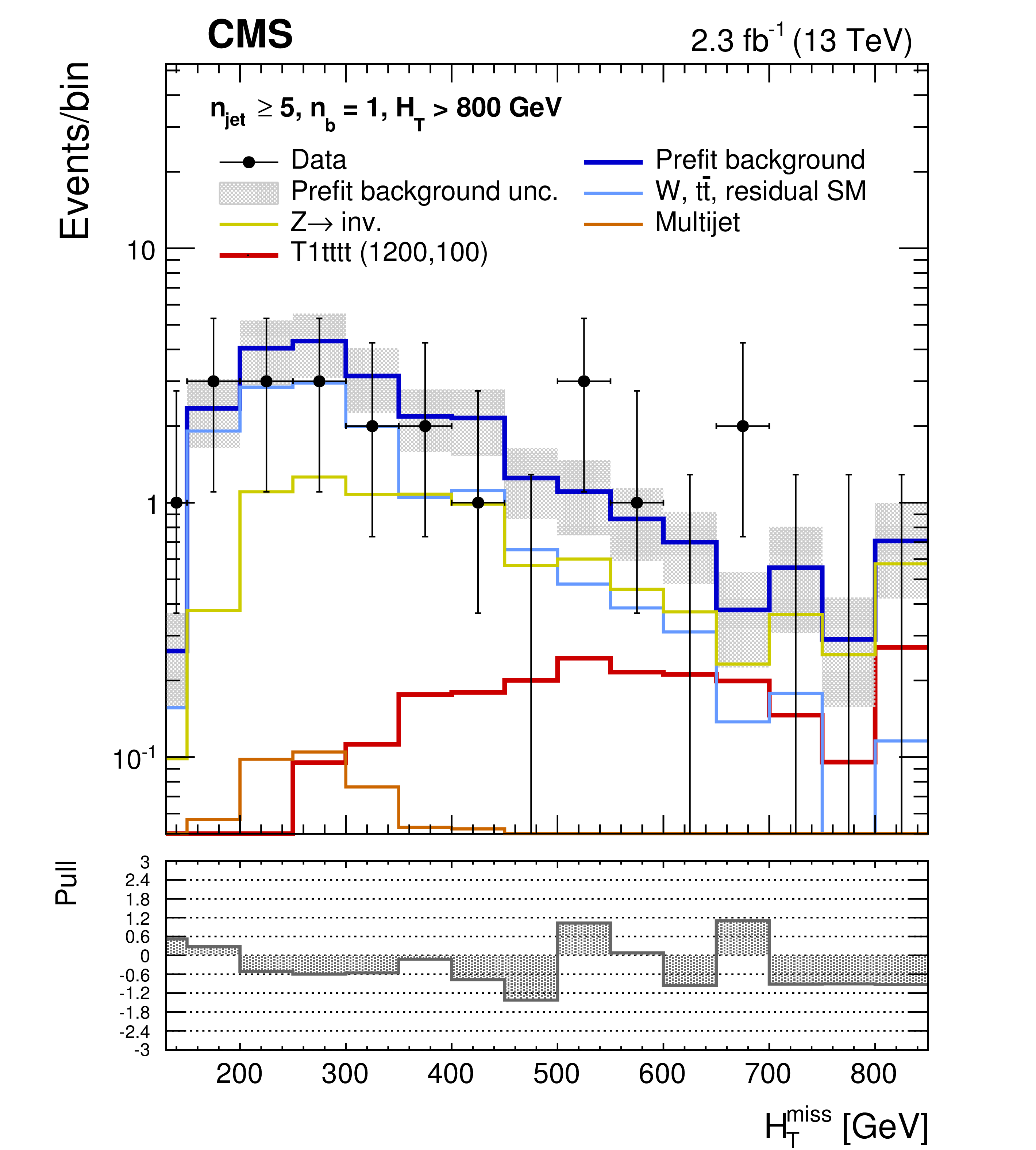
Figure 6:
Event yields observed in data (solid circles) and pre-fit SM expectations with their associated uncertainties (blue histogram with shaded band) as a function of ${H_{\mathrm {T}}^{\text {miss}}}$ for events in the signal region that satisfy $ {n_{\text {jet}}} \geq $ 5, $ {H_{\mathrm {T}}} > $ 800 GeV, and (left) $ {n_{\text {b}}} = $ 0 or (right) $ {n_{\text {b}}} = $ 1. For illustration only, the expectations for one of two benchmark models (T1qqqq and T1tttt, both with $m_{ \tilde{\mathrm{g}} } = $ 1200 GeV and $m_{\tilde{\chi}^0_1 } = $ 100 GeV) are superimposed on the SM-only expectations. The lower panels indicate the significance of deviations (pulls) observed in data with respect to both the pre-fit SM expectations, expressed in terms of the total uncertainty in the SM expectations. The pulls cannot be considered independently due to inter-bin correlations. |

png pdf |
Figure 6-a:
Event yields observed in data (solid circles) and pre-fit SM expectations with their associated uncertainties (blue histogram with shaded band) as a function of ${H_{\mathrm {T}}^{\text {miss}}}$ for events in the signal region that satisfy $ {n_{\text {jet}}} \geq $ 5, $ {H_{\mathrm {T}}} > $ 800 GeV, and $ {n_{\text {b}}} = $ 0. For illustration only, the expectations for one of two benchmark models (T1qqqq with $m_{ \tilde{\mathrm{g}} } = $ 1200 GeV and $m_{\tilde{\chi}^0_1 } = $ 100 GeV) are superimposed on the SM-only expectations. The lower panel indicates the significance of deviations (pulls) observed in data with respect to both the pre-fit SM expectations, expressed in terms of the total uncertainty in the SM expectations. The pulls cannot be considered independently due to inter-bin correlations. |
png pdf |
Figure 6-b:
Event yields observed in data (solid circles) and pre-fit SM expectations with their associated uncertainties (blue histogram with shaded band) as a function of ${H_{\mathrm {T}}^{\text {miss}}}$ for events in the signal region that satisfy $ {n_{\text {jet}}} \geq $ 5, $ {H_{\mathrm {T}}} > $ 800 GeV, and $ {n_{\text {b}}} = $ 1. For illustration only, the expectations for one of two benchmark models (T1tttt with $m_{ \tilde{\mathrm{g}} } = $ 1200 GeV and $m_{\tilde{\chi}^0_1 } = $ 100 GeV) are superimposed on the SM-only expectations. The lower panel indicates the significance of deviations (pulls) observed in data with respect to both the pre-fit SM expectations, expressed in terms of the total uncertainty in the SM expectations. The pulls cannot be considered independently due to inter-bin correlations. |

png pdf |
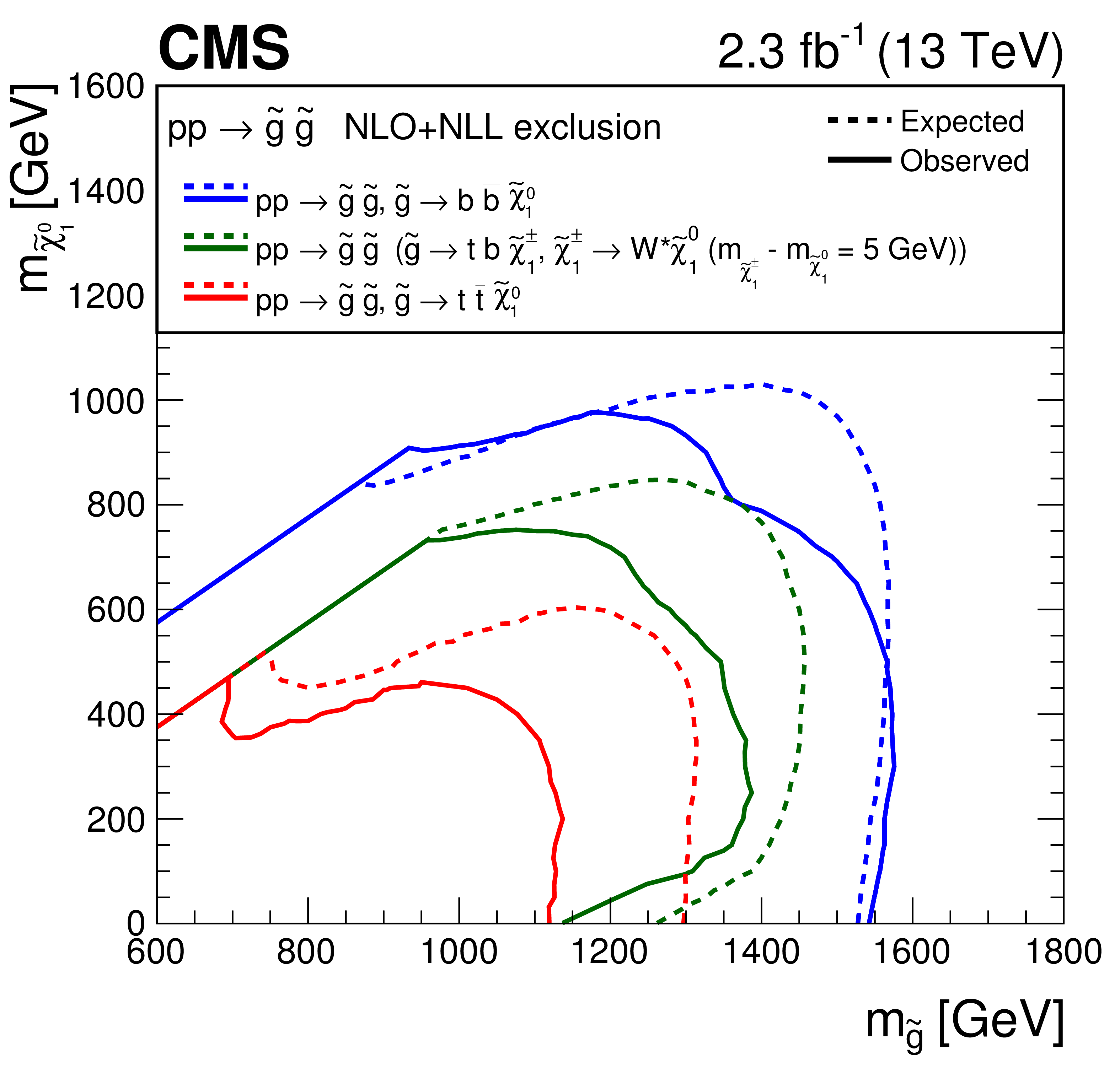
Figure 7:
Observed and expected mass exclusions at 95% CL (indicated, respectively, by solid and dashed contours) for various classes of simplified models. (Left) Gluino-mediated or direct pair production of light-flavour squarks. The two scenarios involve, respectively, the decay $\tilde{\mathrm{g}} \to \mathrm{ \bar{q} } \mathrm{ q } \tilde{\chi}^0_1 $ (T1qqqq) and $\tilde{\mathrm{q}} \to \mathrm{ q } \tilde{\chi}^0_1 $, and the latter involves two assumptions on the mass degeneracy of the squarks (T2qq-8fold and T2qq-1fold). (Right) Three scenarios involving the gluino-mediated pair production of off-shell third-generation squarks: $\tilde{\mathrm{g}} \to \mathrm{ \bar{b} } \mathrm{ b } \tilde{\chi}^0_1 $ (T1bbbb), $\tilde{\mathrm{g}} \to \mathrm{ \bar{t} } \tilde{ \mathrm{ t } } ^* \to \mathrm{ \bar{t} } \mathrm{ t } \tilde{\chi}^0_1 $ (T1tttt), and $\tilde{\mathrm{g}} \to \mathrm{ \bar{t} } \mathrm{ b } \tilde{ \chi }^{\pm} _1\to \mathrm{ \bar{t} } \mathrm{ b } \mathrm{ W } ^*\tilde{\chi}^0_1 $ (T1ttbb). |

png pdf |
Figure 7-a:
Observed and expected mass exclusions at 95% CL (indicated, respectively, by solid and dashed contours) for various classes of simplified models: Gluino-mediated or direct pair production of light-flavour squarks. The two scenarios involve, respectively, the decay $\tilde{\mathrm{g}} \to \mathrm{ \bar{q} } \mathrm{ q } \tilde{\chi}^0_1 $ (T1qqqq) and $\tilde{\mathrm{q}} \to \mathrm{ q } \tilde{\chi}^0_1 $, and the latter involves two assumptions on the mass degeneracy of the squarks (T2qq-8fold and T2qq-1fold). |
png pdf |
Figure 7-b:
Observed and expected mass exclusions at 95% CL (indicated, respectively, by solid and dashed contours) for various classes of simplified models: Three scenarios involving the gluino-mediated pair production of off-shell third-generation squarks: $\tilde{\mathrm{g}} \to \mathrm{ \bar{b} } \mathrm{ b } \tilde{\chi}^0_1 $ (T1bbbb), $\tilde{\mathrm{g}} \to \mathrm{ \bar{t} } \tilde{ \mathrm{ t } } ^* \to \mathrm{ \bar{t} } \mathrm{ t } \tilde{\chi}^0_1 $ (T1tttt), and $\tilde{\mathrm{g}} \to \mathrm{ \bar{t} } \mathrm{ b } \tilde{ \chi }^{\pm} _1\to \mathrm{ \bar{t} } \mathrm{ b } \mathrm{ W } ^*\tilde{\chi}^0_1 $ (T1ttbb). |

png pdf |
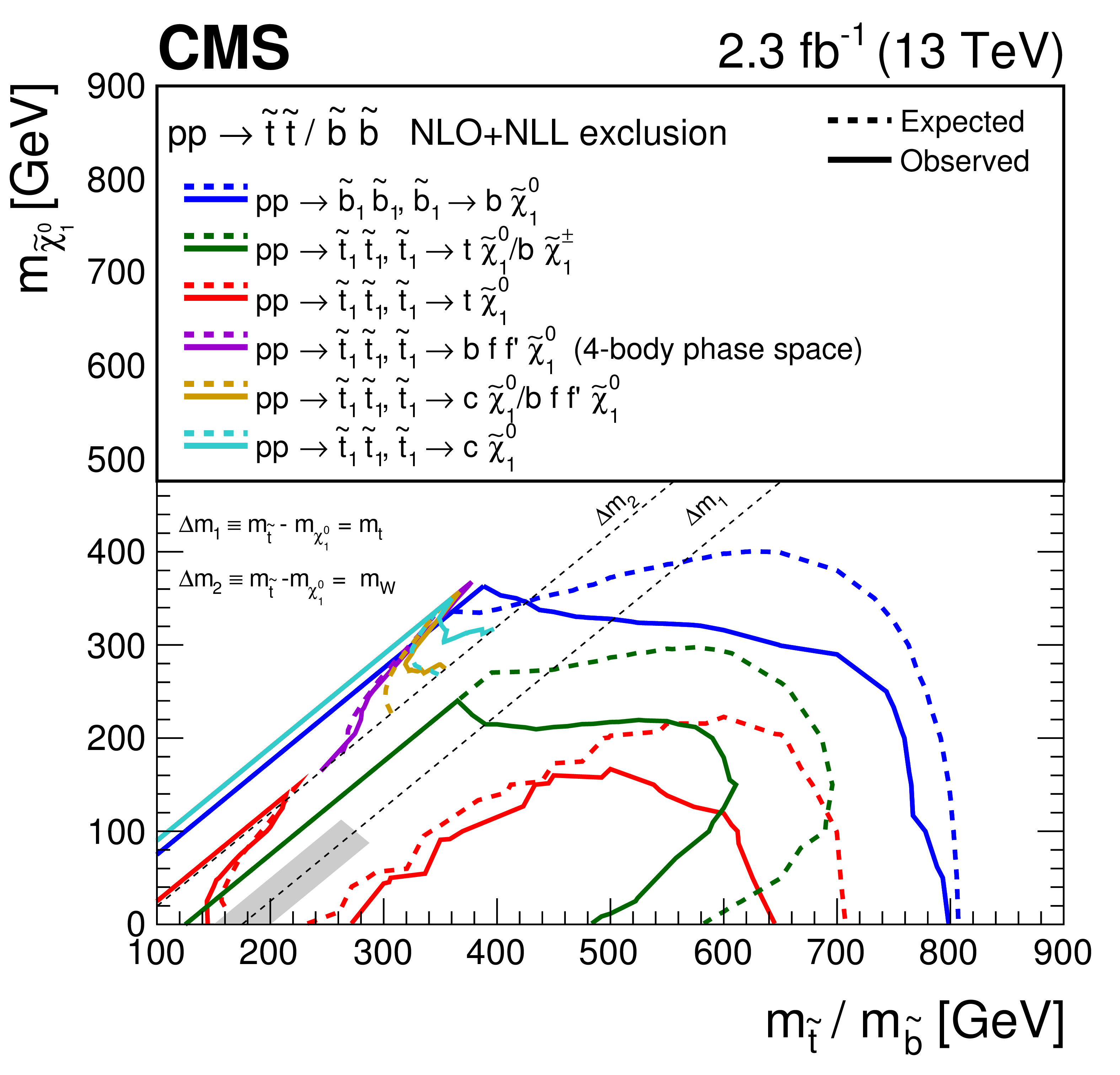
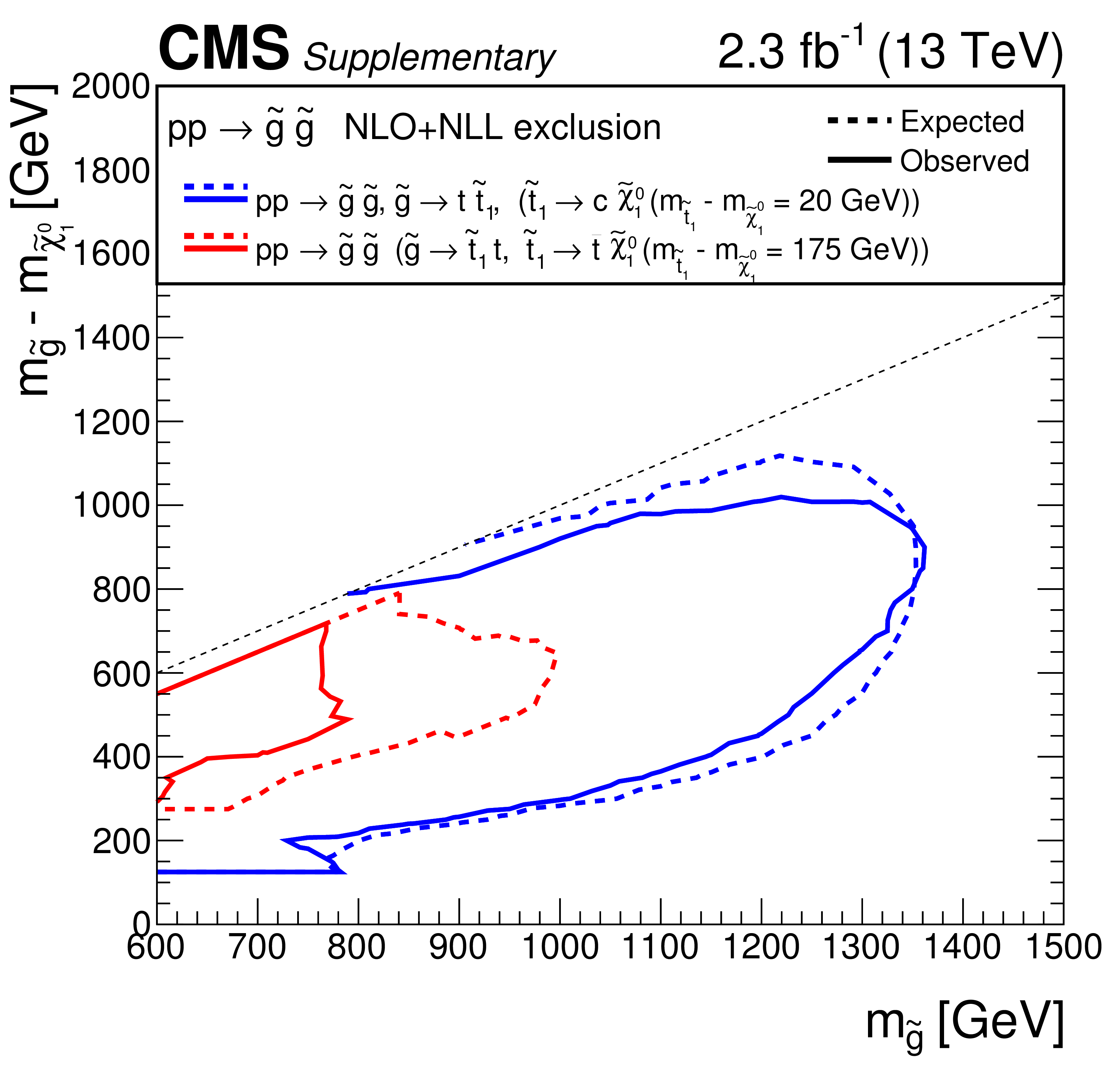
Figure 8:
Observed and expected mass exclusions at 95% CL (indicated, respectively, by solid and dashed contours) for a number of simplified models. (Left) Two scenarios involving the gluino-mediated pair production of on-shell top squarks: $\tilde{\mathrm{g}} \to \mathrm{ \bar{t} } \tilde{ \mathrm{ t } } \to \mathrm{ \bar{t} } \mathrm{ t } \tilde{\chi}^0_1 $ with $m_{ \tilde{ \mathrm{ t } } } - m_{\tilde{\chi}^0_1 } = $ 175 GeV (T5tttt-DM175) and $\tilde{\mathrm{g}} \to \mathrm{ \bar{t} } \tilde{ \mathrm{ t } } \to \mathrm{ \bar{t} } \mathrm{c} \tilde{\chi}^0_1 $ with $m_{ \tilde{ \mathrm{ t } } } - m_{\tilde{\chi}^0_1 } = $ 20 GeV (T5ttcc). Also shown, for comparison, is T1tttt. (Right) Six scenarios involving the direct pair production of third-generation squarks. The first scenario involves the pair production of bottom squarks, $\tilde{ \mathrm{ b } } \to \mathrm{ b } \tilde{\chi}^0_1 $ (T2bb). Two scenarios involve the decay of top squark pairs as follows: $\tilde{ \mathrm{ t } } \to \mathrm{ t } \tilde{\chi}^0_1 $ or $\tilde{ \mathrm{ t } } \to \mathrm{ b } \tilde{ \chi }^{\pm} _1\to \mathrm{ b } \mathrm{ W } ^*\tilde{\chi}^0_1 $ with $m_{\tilde{ \chi }^{\pm} _1} - m_{\tilde{\chi}^0_1 } = $ 5 GeV and branching fractions $50/50%$ (T2tb), or $\tilde{ \mathrm{ t } } \to \mathrm{ t } \tilde{\chi}^0_1 $ (T2tt). The final three scenarios consider top squark decays under the assumption 10 $ < m_{ \tilde{ \mathrm{ t } } } - m_{\tilde{\chi}^0_1 } < $ 80 GeV: $\tilde{ \mathrm{ t } } \to \mathrm{c} \tilde{\chi}^0_1 $ (T2cc), $\tilde{ \mathrm{ t } } \to \mathrm{ b } \mathrm{ W } ^*\tilde{\chi}^0_1 $ (T2tt-degen), and $\tilde{ \mathrm{ t } } \to \mathrm{c} \tilde{\chi}^0_1 $ or $\tilde{ \mathrm{ t } } \to \mathrm{ b } \mathrm{ W } ^*\tilde{\chi}^0_1 $ with branching fractions 50/50% (T2tt-mixed). The grey shaded region denotes T2tt models that are not considered for interpretation. |

png pdf |
Figure 8-a:
Observed and expected mass exclusions at 95% CL (indicated, respectively, by solid and dashed contours) for a number of simplified models: Two scenarios involving the gluino-mediated pair production of on-shell top squarks: $\tilde{\mathrm{g}} \to \mathrm{ \bar{t} } \tilde{ \mathrm{ t } } \to \mathrm{ \bar{t} } \mathrm{ t } \tilde{\chi}^0_1 $ with $m_{ \tilde{ \mathrm{ t } } } - m_{\tilde{\chi}^0_1 } = $ 175 GeV (T5tttt-DM175) and $\tilde{\mathrm{g}} \to \mathrm{ \bar{t} } \tilde{ \mathrm{ t } } \to \mathrm{ \bar{t} } \mathrm{c} \tilde{\chi}^0_1 $ with $m_{ \tilde{ \mathrm{ t } } } - m_{\tilde{\chi}^0_1 } = $ 20 GeV (T5ttcc). Also shown, for comparison, is T1tttt. |
png pdf |
Figure 8-b:
Observed and expected mass exclusions at 95% CL (indicated, respectively, by solid and dashed contours) for a number of simplified models: Six scenarios involving the direct pair production of third-generation squarks. The first scenario involves the pair production of bottom squarks, $\tilde{ \mathrm{ b } } \to \mathrm{ b } \tilde{\chi}^0_1 $ (T2bb). Two scenarios involve the decay of top squark pairs as follows: $\tilde{ \mathrm{ t } } \to \mathrm{ t } \tilde{\chi}^0_1 $ or $\tilde{ \mathrm{ t } } \to \mathrm{ b } \tilde{ \chi }^{\pm} _1\to \mathrm{ b } \mathrm{ W } ^*\tilde{\chi}^0_1 $ with $m_{\tilde{ \chi }^{\pm} _1} - m_{\tilde{\chi}^0_1 } = $ 5 GeV and branching fractions $50/50%$ (T2tb), or $\tilde{ \mathrm{ t } } \to \mathrm{ t } \tilde{\chi}^0_1 $ (T2tt). The final three scenarios consider top squark decays under the assumption 10 $ < m_{ \tilde{ \mathrm{ t } } } - m_{\tilde{\chi}^0_1 } < $ 80 GeV: $\tilde{ \mathrm{ t } } \to \mathrm{c} \tilde{\chi}^0_1 $ (T2cc), $\tilde{ \mathrm{ t } } \to \mathrm{ b } \mathrm{ W } ^*\tilde{\chi}^0_1 $ (T2tt-degen), and $\tilde{ \mathrm{ t } } \to \mathrm{c} \tilde{\chi}^0_1 $ or $\tilde{ \mathrm{ t } } \to \mathrm{ b } \mathrm{ W } ^*\tilde{\chi}^0_1 $ with branching fractions 50/50% (T2tt-mixed). The grey shaded region denotes T2tt models that are not considered for interpretation. |
| Tables | |

png pdf |
Table 1:
Summary of the event selection criteria and categorisation used to define the signal and control regions. |

png pdf |
Table 2:
Summary of the lower bounds of the first and final bins in ${H_{\mathrm {T}}}$ [GeV] (the latter in parentheses) as a function of ${n_{\text {jet}}}$ and ${n_{\text {b}}} $. |

png pdf |
Table 3:
Systematic uncertainties (in percent) in the transfer ($ {\mathcal {T}} $) factors used in the method to estimate the SM backgrounds with genuine ${\vec{p}}_{\mathrm {T}}^{\text {miss}}$ in the signal region. The quoted ranges provide representative values of the observed variations as a function of ${n_{\text {jet}}}$ and ${H_{\mathrm {T}}} $. |

png pdf |
Table 4:
A summary of the simplified SUSY models used to interpret the results of this search. All on-shell SUSY particles in the decay are stated. |

png pdf |
Table 5:
A summary of benchmark simplified models, the most sensitive ${n_{\text {jet}}}$ categories, and representative values for the corresponding experimental acceptance times efficiency ($\mathcal {A} \varepsilon $), the dominant systematic uncertainties, the theoretical production cross section ($\sigma _\text {theory}$), and the expected and observed upper limits on the production cross section, expressed in terms of the signal strength parameter ($\mu $). |

png pdf |
Table 6:
Summary of the mass limits obtained for the fourteen classes of simplified models. The limits indicate the strongest observed and expected (in parentheses) mass exclusions in $\tilde{\mathrm{g}} $, $\tilde{\mathrm{q}} $, $\tilde{ \mathrm{ b } } $, $\tilde{ \mathrm{ t } } $, and $\tilde{\chi}^0_1 $. The quoted values have uncertainties of $\pm $25 and $\pm $10 GeV for models involving the pair production of, respectively, gluinos and squarks. |
| Summary |
| An inclusive search for new-physics phenomena is reported, based on data from pp collisions at $ \sqrt{s} = $ 13 TeV. The data are recorded with the CMS detector and correspond to an integrated luminosity of 2.3$\pm$0.1 fb$^{-1}$. The final states analysed contain one or more jets with large transverse momenta and a significant imbalance of transverse momentum, as expected from the production of massive coloured SUSY particles, each decaying to SM particles and the lightest stable, weakly-interacting, SUSY particle. The sums of the standard model backgrounds are estimated from a simultaneous binned likelihood fit to the observed yields for samples of events categorised according to the number of reconstructed jets, the number of jets identified as originating from b quarks, and the scalar and the magnitude of the vector sums of the transverse momenta of jets. In addition to the signal region, $\mu$+jets, $\mu\mu$+jets, and $\gamma$+jets control regions are included in the likelihood fit. The observed yields are found to be in agreement with the expected contributions from standard model processes. The search result is interpreted in the mass parameter space of fourteen simplified SUSY models, which cover scenarios that involve the gluino-mediated or direct production of light- or heavy-flavour squarks, intermediate SUSY particle states, as well as natural and nearly mass-degenerate spectra. The increase in the centre-of-mass energy of the LHC, from 8 to 13 TeV, provides a significant gain in sensitivity to heavy particle states such as gluinos. In the case of pair-produced gluinos, each decaying via an off-shell b squark to the b quark and the LSP, models with masses up to $\sim$1.6 and $\sim$1.0 TeV are excluded for, respectively, the gluino and LSP. These limits improve on those obtained at $ \sqrt{s} = $ 8 TeV by, respectively, $\sim$250 and $\sim$300 GeV. In the case of direct pair production, models with masses up to $\sim$800 and $\sim$350 GeV are excluded for, respectively, the b squark and LSP. These mass limits are sensitive to the assumptions on the squark flavour and the presence of intermediate states such as charginos. Finally, a comprehensive study of nearly mass-degenerate models involving top squark pair production is performed. The two decay modes of the top squark are the loop-induced two-body decay to the neutralino and one c quark, and the four-body decay to the neutralino, one b quark, and an off-shell W boson. A third scenario is considered in which the two modes are simultaneously open, each with a branching fraction of 50%. Masses of the top squark and LSP up to, respectively, 400 and 360 GeV are excluded, depending on the decay modes considered. In conclusion, the analysis provides sensitivity across a large region of the natural SUSY parameter space, as characterised by interpretations with several simplified models. In particular, these studies improve on existing limits for nearly mass-degenerate models involving the production of pairs of top squarks. |
| Additional Figures | |

png pdf |
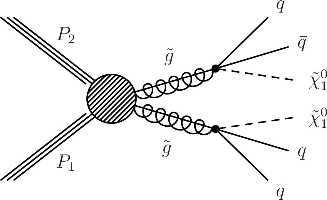
Additional Figure 1:
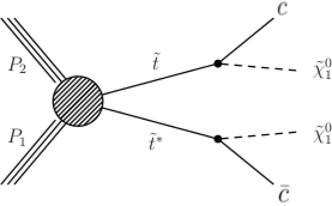
Simplified model diagrams that represent unique production and decay modes of supersymmetric particles. The figures correspond to the following models: T1qqqq (a), T2qq (b), T1bbbb (c), T1tttt (d), T1ttbb (e), T5tttt_DM175 (f), T5ttcc (g), T2bb (h), T2tb (i), T2tt (j), T2cc (k), T2tt_degen (l), and T2bW (m). Three-body decays of gluinos are assumed to proceed through off-shell squarks. The diagrams labelled T1qqqq and T2qq depict, respectively, the gluino-mediated and direct production of light-flavour squarks. The diagrams labelled T1bbbb, T1tttt, and T1ttbb depict models involving the gluino-mediated production of off-shell third-generation squarks. The diagrams labelled T5tttt_DM175 and T5ttcc depict "natural'' models comprising gluino-mediated production of on-shell top squarks. Finally, the remaining six diagrams depict the direct production of third-generation squarks, decaying via a range of channels. |
png pdf |
Additional Figure 1-a:
Diagram that represents the T1qqqq simplified model. The diagram depicts the gluino-mediated production of light-flavour squarks. Three-body decays of gluinos are assumed to proceed through off-shell squarks. |

png pdf |
Additional Figure 1-b:
Diagram that represents the T2qq simplified model. The diagram depicts the direct production of light-flavour squarks. |

png pdf |
Additional Figure 1-c:
Diagram that represents the T1bbbb simplified model. The diagram depicts a model involving the gluino-mediated production of off-shell third-generation squarks. Three-body decays of gluinos are assumed to proceed through off-shell squarks. |

png pdf |
Additional Figure 1-d:
Diagram that represents the T1tttt simplified model. The diagram depicts a model involving the gluino-mediated production of off-shell third-generation squarks. Three-body decays of gluinos are assumed to proceed through off-shell squarks. |

png pdf |
Additional Figure 1-e:
Diagram that represents the T1ttbb simplified model. The diagram depicts a model involving the gluino-mediated production of off-shell third-generation squarks. Three-body decays of gluinos are assumed to proceed through off-shell squarks. |

png pdf |
Additional Figure 1-f:
Diagram that represents the T5tttt_DM175 simplified model. The diagram depicts a "natural" model comprising gluino-mediated production of on-shell top squarks. |

png pdf |
Additional Figure 1-g:
Diagram that represents the T5ttcc simplified model. The diagram depicts a "natural" model comprising gluino-mediated production of on-shell top squarks. |

png pdf |
Additional Figure 1-h:
Diagram that represents the T2bb simplified model. The diagram is one that depicts the direct production of bottom squarks. |

png pdf |
Additional Figure 1-i:
Diagram that represents the T2tb simplified model. The diagram is one that depicts the direct production of top squarks and a unique decay mode. |

png pdf |
Additional Figure 1-j:
Diagram that represents the T2tt simplified model. The diagram is one that depicts the direct production of top squarks and a unique decay mode. |
png pdf |
Additional Figure 1-k:
Diagram that represents the T2cc simplified model. The diagram is one that depicts the direct production of top squarks and a unique decay mode. |

png pdf |
Additional Figure 1-l:
Diagram that represents the T2tt_degen simplified model. The diagram is one that depicts the direct production of top squarks and a unique decay mode. |

png pdf |
Additional Figure 1-m:
Diagram that represents the T2bW simplified model. The diagram is one that depicts the direct production of top squarks and a unique decay mode. |

png pdf |
Additional Figure 2:
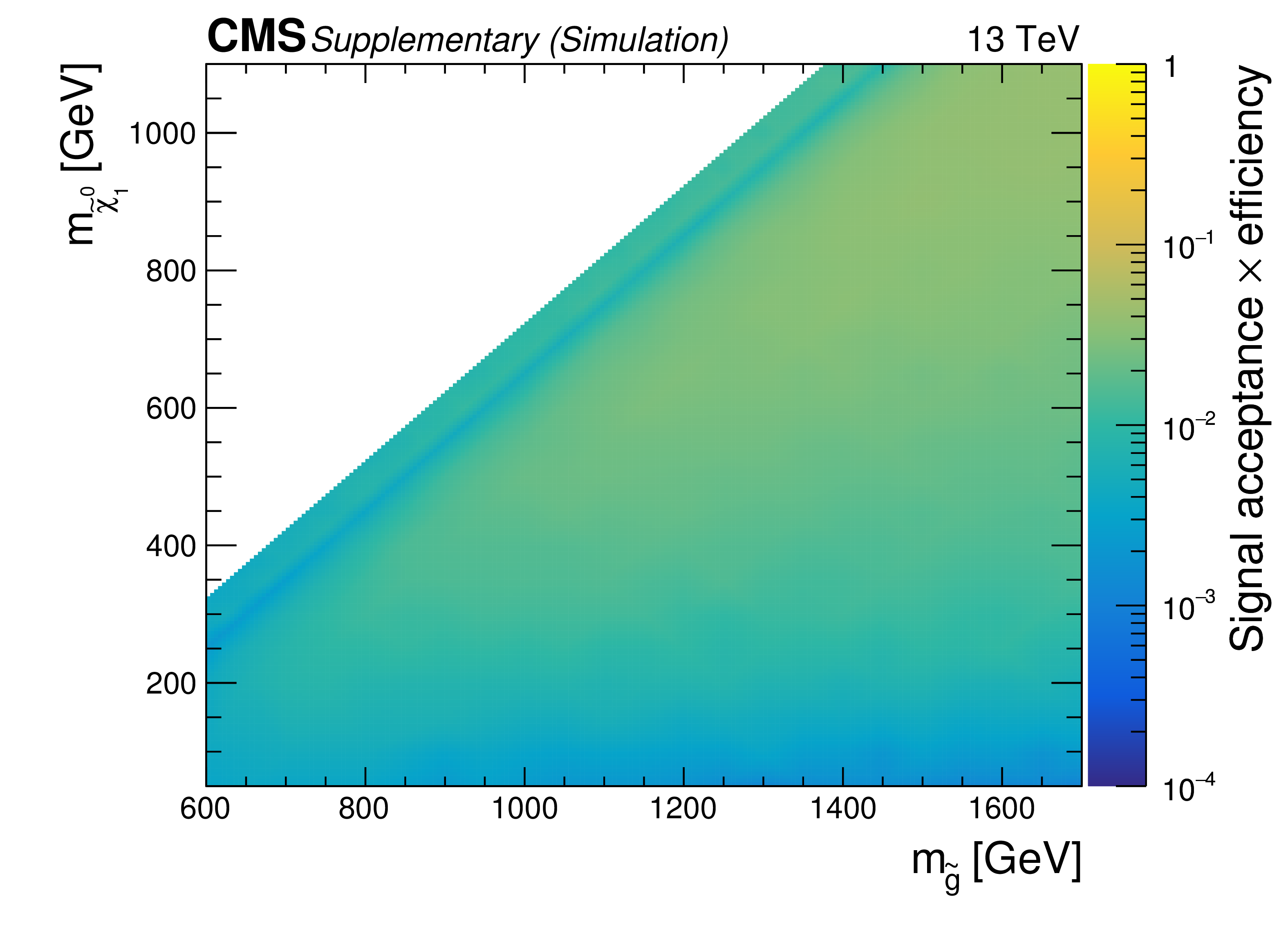
Left: (coloured histogram) upper limit on the cross section in the $(m_{ \tilde{ \mathrm{g} } }, m_{\tilde{\chi}^0_1 })$ plane for the T1qqqq model. The black (red) solid line is the observed (expected) exclusion. The red dashed lines are the $\pm$1$\sigma $ expected exclusion due to experimental uncertainties. The $\pm$1$\sigma $ observed exclusion due to theoretical uncertainties on the signal cross section are shown as thin black lines. Right: signal efficiency for the search regions included in the limit calculation as a function $(m_{ \tilde{ \mathrm{g} } }, m_{\tilde{\chi}^0_1 })$ plane for the T1qqqq model. |

png pdf root |
Additional Figure 2-a:
Upper limit on the cross section in the $(m_{ \tilde{ \mathrm{g} } }, m_{\tilde{\chi}^0_1 })$ plane for the T1qqqq model. The black (red) solid line is the observed (expected) exclusion. The red dashed lines are the $\pm$1$\sigma $ expected exclusion due to experimental uncertainties. The $\pm$1$\sigma $ observed exclusion due to theoretical uncertainties on the signal cross section are shown as thin black lines. |

png pdf root |
Additional Figure 2-b:
Signal efficiency for the search regions included in the limit calculation as a function $(m_{ \tilde{ \mathrm{g} } }, m_{\tilde{\chi}^0_1 })$ plane for the T1qqqq model. |

png pdf |
Additional Figure 3:
Left: (coloured histogram) upper limit on the cross section in the $(m_{ \tilde{ \mathrm{Q} } }, m_{\tilde{\chi}^0_1 })$ plane for the T2qq model. The black (red) solid line is the observed (expected) exclusion. The red dashed lines are the $\pm$1$\sigma $ expected exclusion due to experimental uncertainties. The $\pm$1$\sigma $ observed exclusion due to theoretical uncertainties on the signal cross section are shown as thin black lines. Right: signal efficiency for the search regions included in the limit calculation as a function $(m_{ \tilde{ \mathrm{Q} } }, m_{\tilde{\chi}^0_1 })$ plane for the T2qq model. |

png pdf root |
Additional Figure 3-a:
Upper limit on the cross section in the $(m_{ \tilde{ \mathrm{Q} } }, m_{\tilde{\chi}^0_1 })$ plane for the T2qq model. The black (red) solid line is the observed (expected) exclusion. The red dashed lines are the $\pm$1$\sigma $ expected exclusion due to experimental uncertainties. The $\pm$1$\sigma $ observed exclusion due to theoretical uncertainties on the signal cross section are shown as thin black lines. |

png pdf root |
Additional Figure 3-b:
Signal efficiency for the search regions included in the limit calculation as a function $(m_{ \tilde{ \mathrm{Q} } }, m_{\tilde{\chi}^0_1 })$ plane for the T2qq model. |

png pdf |
Additional Figure 4:
Left: (coloured histogram) upper limit on the cross section in the $(m_{ \tilde{ \mathrm{g} } }, m_{\tilde{\chi}^0_1 })$ plane for the T1bbbb model. The black (red) solid line is the observed (expected) exclusion. The red dashed lines are the $\pm$1$\sigma $ expected exclusion due to experimental uncertainties. The $\pm$1$\sigma $ observed exclusion due to theoretical uncertainties on the signal cross section are shown as thin black lines. Right: signal efficiency for the search regions included in the limit calculation as a function $(m_{ \tilde{ \mathrm{g} } }, m_{\tilde{\chi}^0_1 })$ plane for the T1bbbb model. |

png pdf root |
Additional Figure 4-a:
Upper limit on the cross section in the $(m_{ \tilde{ \mathrm{g} } }, m_{\tilde{\chi}^0_1 })$ plane for the T1bbbb model. The black (red) solid line is the observed (expected) exclusion. The red dashed lines are the $\pm$1$\sigma $ expected exclusion due to experimental uncertainties. The $\pm$1$\sigma $ observed exclusion due to theoretical uncertainties on the signal cross section are shown as thin black lines. |

png pdf root |
Additional Figure 4-b:
Signal efficiency for the search regions included in the limit calculation as a function $(m_{ \tilde{ \mathrm{g} } }, m_{\tilde{\chi}^0_1 })$ plane for the T1bbbb model. |

png pdf |
Additional Figure 5:
Left: (coloured histogram) upper limit on the cross section in the $(m_{ \tilde{ \mathrm{g} } }, m_{\tilde{\chi}^0_1 })$ plane for the T1tttt model. The black (red) solid line is the observed (expected) exclusion. The red dashed lines are the $\pm$1$\sigma $ expected exclusion due to experimental uncertainties. The $\pm$1$\sigma $ observed exclusion due to theoretical uncertainties on the signal cross section are shown as thin black lines. Right: signal efficiency for the search regions included in the limit calculation as a function $(m_{ \tilde{ \mathrm{g} } }, m_{\tilde{\chi}^0_1 })$ plane for the T1tttt model. |

png pdf root |
Additional Figure 5-a:
Upper limit on the cross section in the $(m_{ \tilde{ \mathrm{g} } }, m_{\tilde{\chi}^0_1 })$ plane for the T1tttt model. The black (red) solid line is the observed (expected) exclusion. The red dashed lines are the $\pm$1$\sigma $ expected exclusion due to experimental uncertainties. The $\pm$1$\sigma $ observed exclusion due to theoretical uncertainties on the signal cross section are shown as thin black lines. |
png pdf root |
Additional Figure 5-b:
Signal efficiency for the search regions included in the limit calculation as a function $(m_{ \tilde{ \mathrm{g} } }, m_{\tilde{\chi}^0_1 })$ plane for the T1tttt model. |
png pdf |
Additional Figure 6:
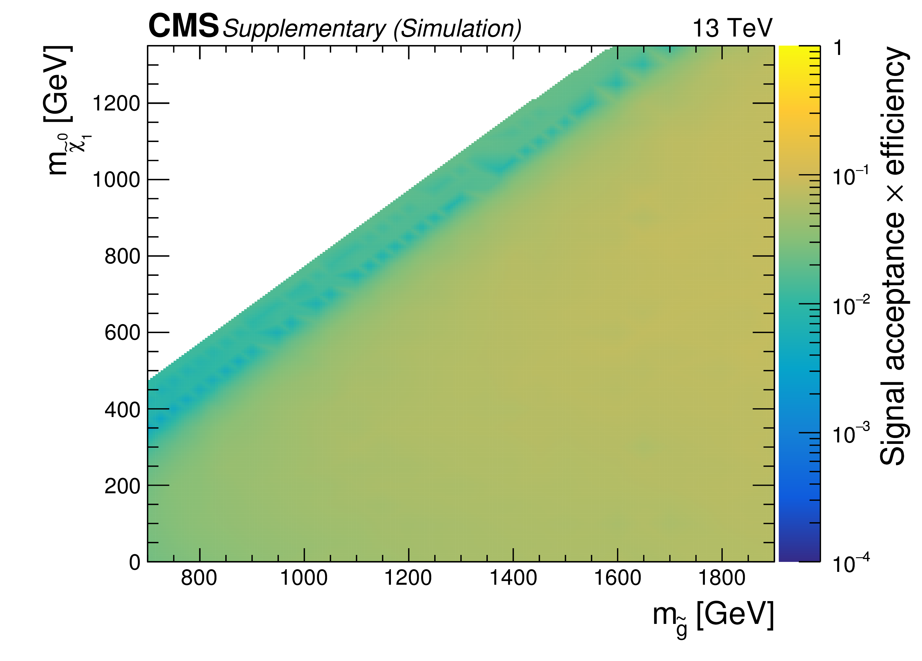
Left: (coloured histogram) upper limit on the cross section in the $(m_{ \tilde{ \mathrm{g} } }, m_{\tilde{\chi}^0_1 })$ plane for the T1ttbb model. The black (red) solid line is the observed (expected) exclusion. The red dashed lines are the $\pm$1$\sigma $ expected exclusion due to experimental uncertainties. The $\pm$1$\sigma $ observed exclusion due to theoretical uncertainties on the signal cross section are shown as thin black lines. Right: signal efficiency for the search regions included in the limit calculation as a function $(m_{ \tilde{ \mathrm{g} } }, m_{\tilde{\chi}^0_1 })$ plane for the T1ttbb model. |
png pdf root |
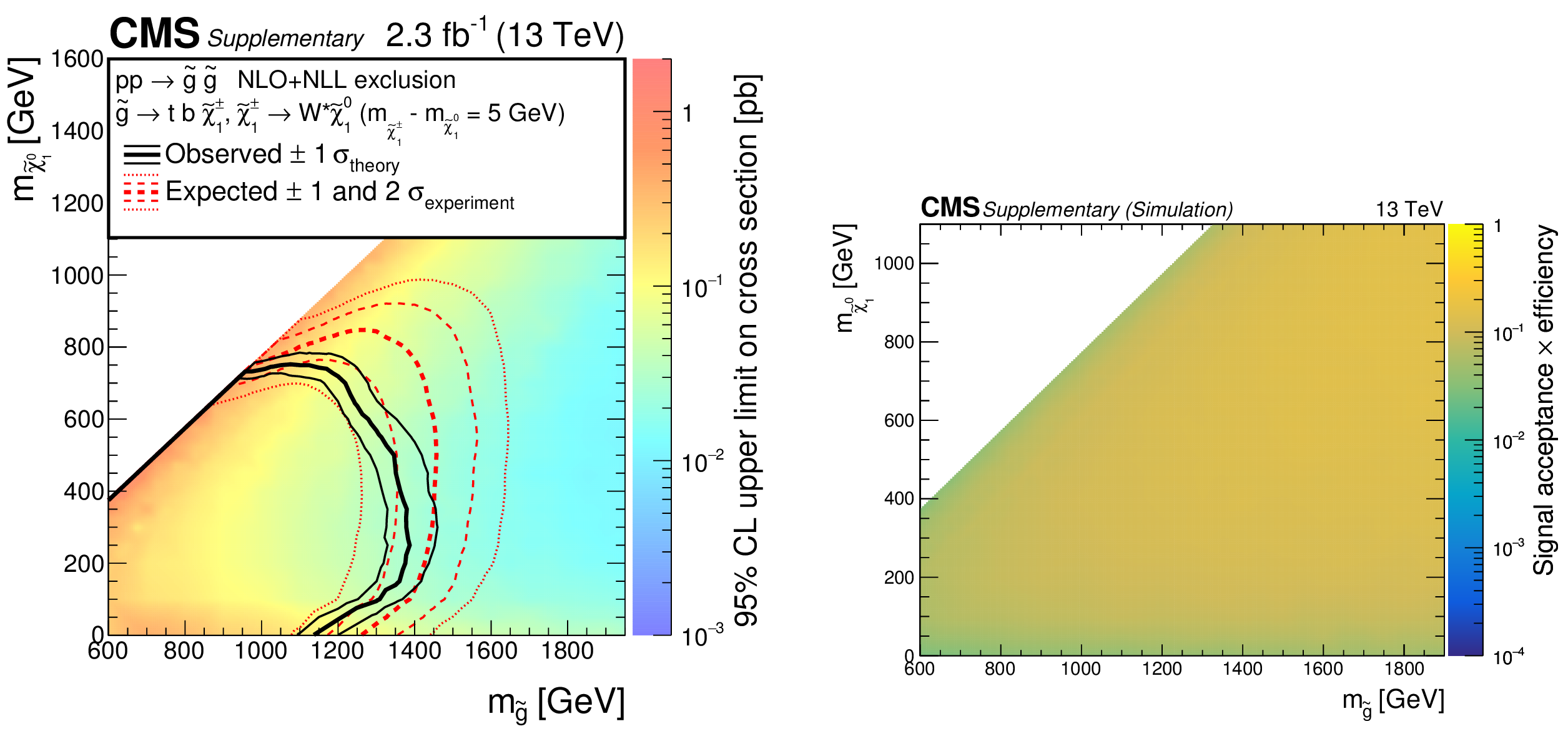
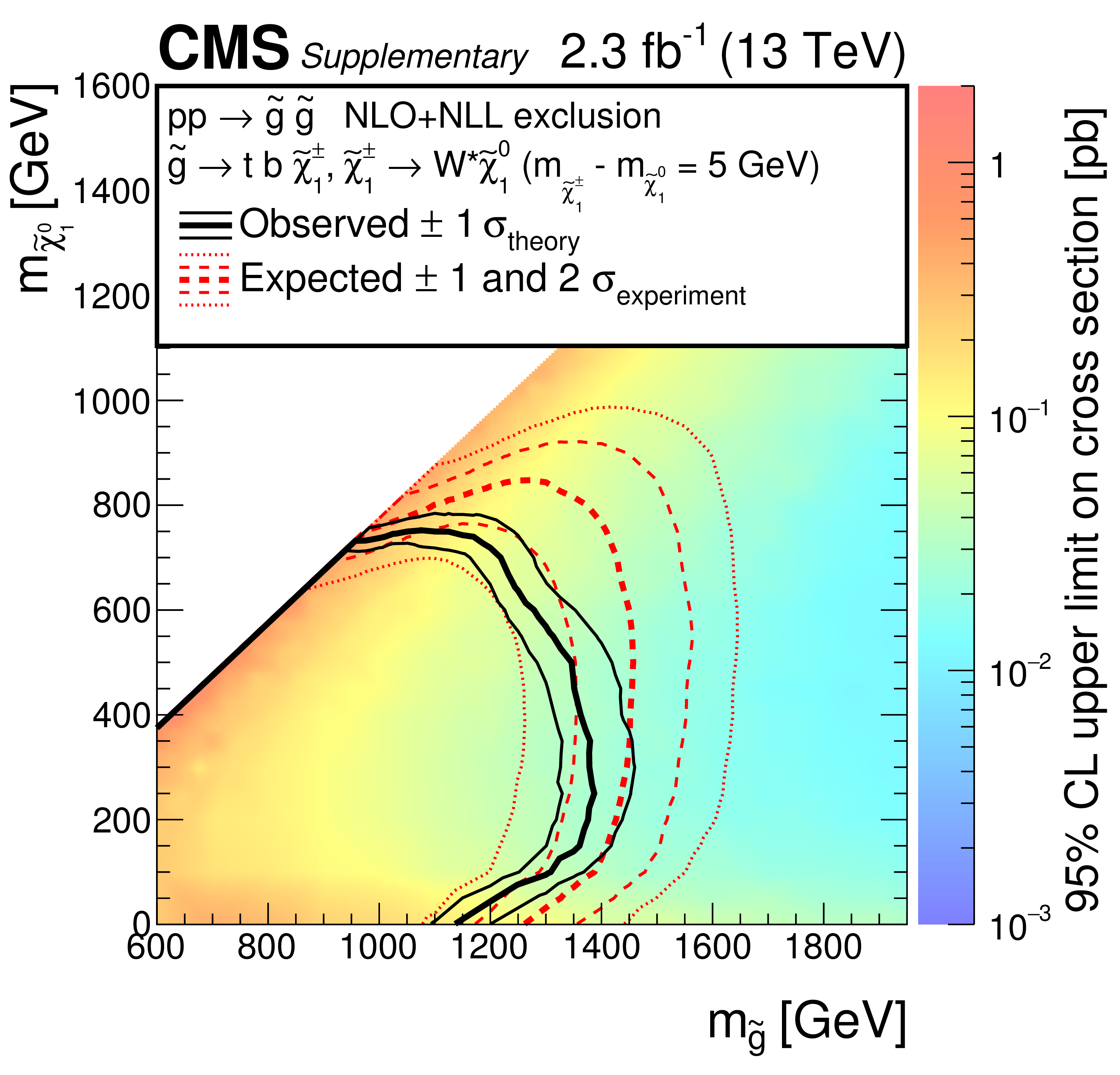
Additional Figure 6-a:
Upper limit on the cross section in the $(m_{ \tilde{ \mathrm{g} } }, m_{\tilde{\chi}^0_1 })$ plane for the T1ttbb model. The black (red) solid line is the observed (expected) exclusion. The red dashed lines are the $\pm$1$\sigma $ expected exclusion due to experimental uncertainties. The $\pm$1$\sigma $ observed exclusion due to theoretical uncertainties on the signal cross section are shown as thin black lines. |

png pdf root |
Additional Figure 6-b:
Signal efficiency for the search regions included in the limit calculation as a function $(m_{ \tilde{ \mathrm{g} } }, m_{\tilde{\chi}^0_1 })$ plane for the T1ttbb model. |

png pdf |
Additional Figure 7:
Left: (coloured histogram) upper limit on the cross section in the $(m_{ \tilde{ \mathrm{g} } }, m_{\tilde{\chi}^0_1 })$ plane for the T5tttt_DM175 model. The black (red) solid line is the observed (expected) exclusion. The red dashed lines are the $\pm$1$\sigma $ expected exclusion due to experimental uncertainties. The $\pm$1$\sigma $ observed exclusion due to theoretical uncertainties on the signal cross section are shown as thin black lines. Right: signal efficiency for the search regions included in the limit calculation as a function $(m_{ \tilde{ \mathrm{g} } }, m_{\tilde{\chi}^0_1 })$ plane for the T5tttt_DM175 model. |

png pdf root |
Additional Figure 7-a:
Upper limit on the cross section in the $(m_{ \tilde{ \mathrm{g} } }, m_{\tilde{\chi}^0_1 })$ plane for the T5tttt_DM175 model. The black (red) solid line is the observed (expected) exclusion. The red dashed lines are the $\pm$1$\sigma $ expected exclusion due to experimental uncertainties. The $\pm$1$\sigma $ observed exclusion due to theoretical uncertainties on the signal cross section are shown as thin black lines. |
png pdf root |
Additional Figure 7-b:
Signal efficiency for the search regions included in the limit calculation as a function $(m_{ \tilde{ \mathrm{g} } }, m_{\tilde{\chi}^0_1 })$ plane for the T5tttt_DM175 model. |

png pdf |
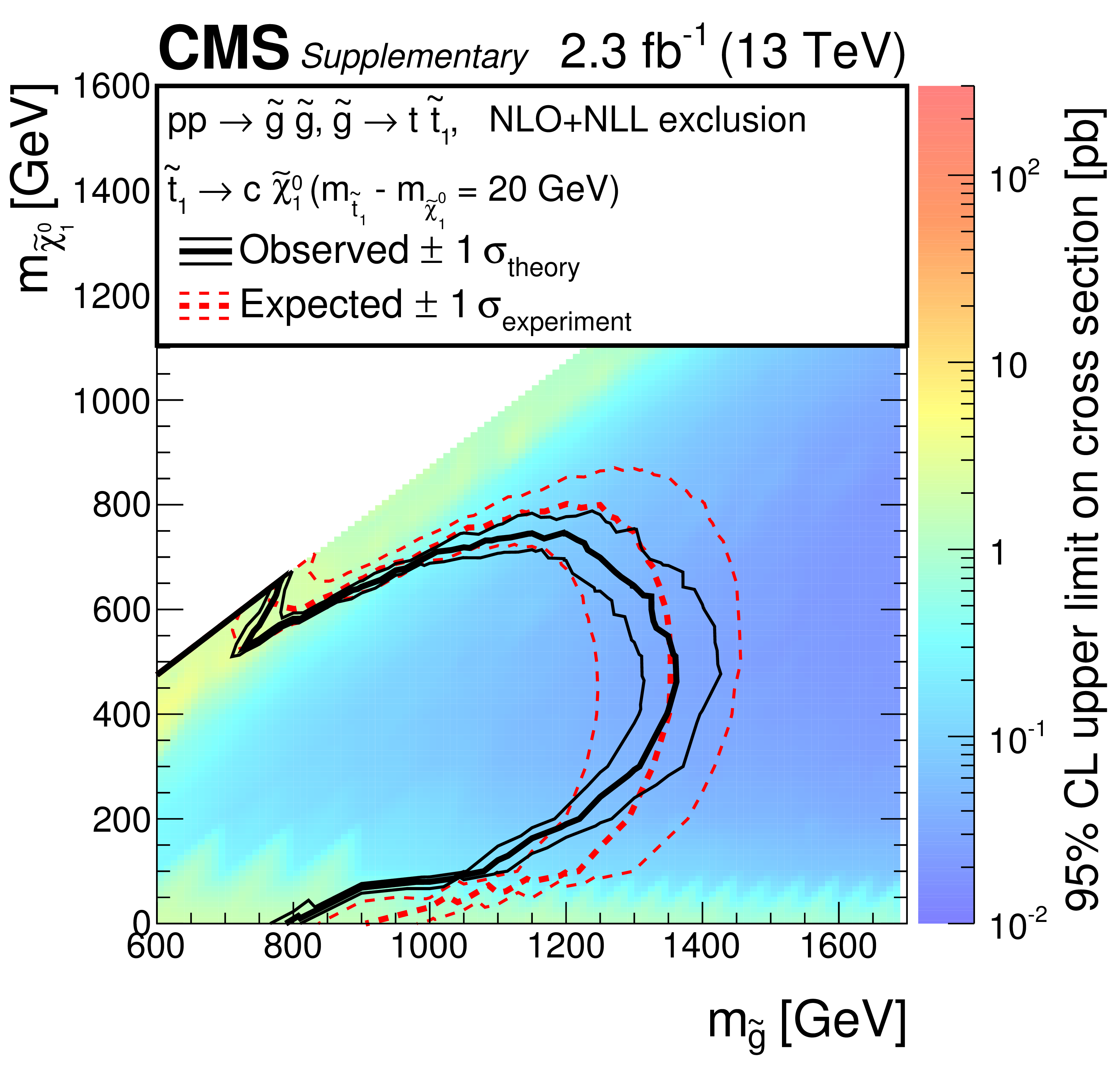
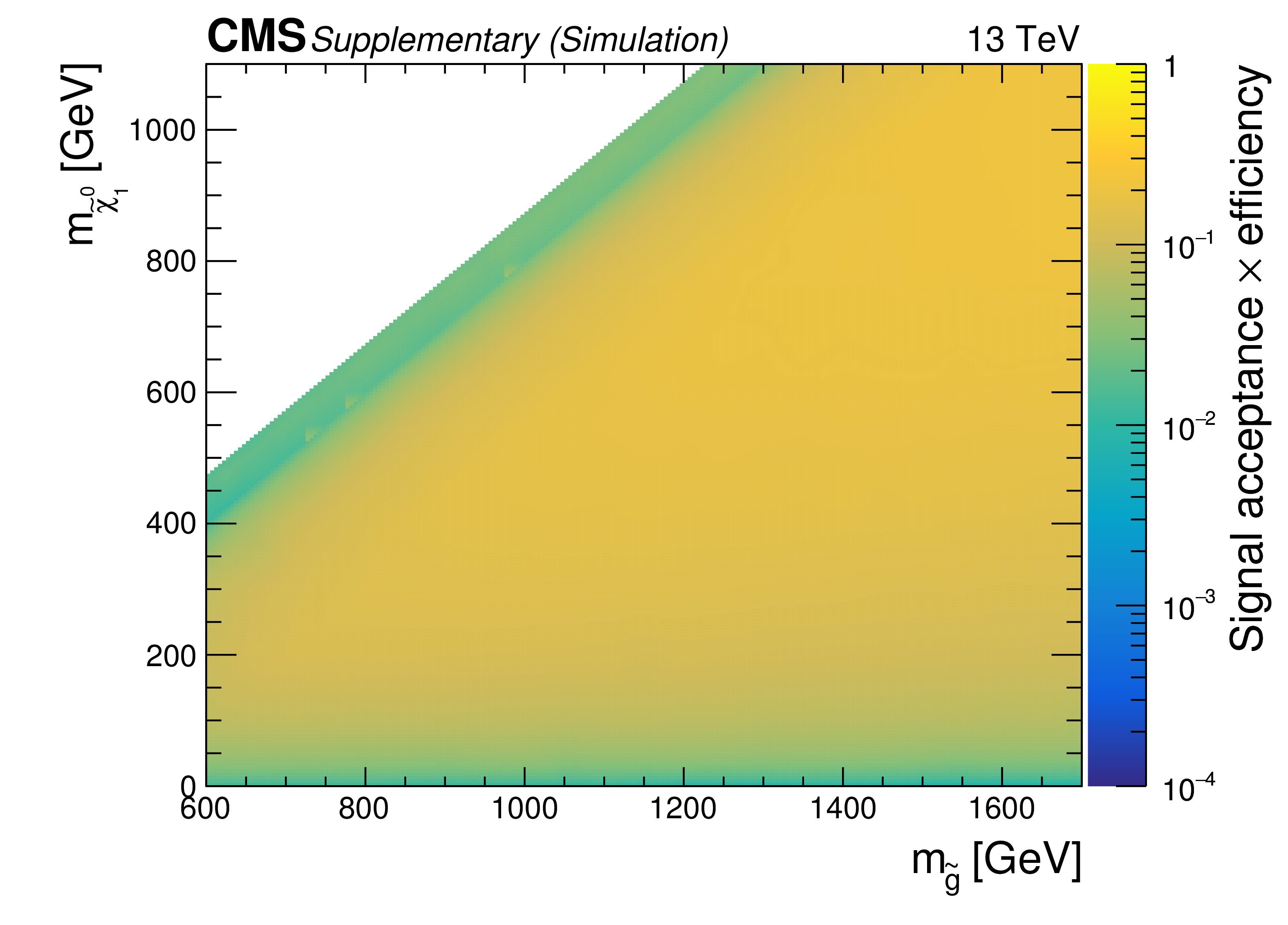
Additional Figure 8:
Left: (coloured histogram) upper limit on the cross section in the $(m_{ \tilde{ \mathrm{g} } }, m_{\tilde{\chi}^0_1 })$ plane for the T5ttcc model. The black (red) solid line is the observed (expected) exclusion. The red dashed lines are the $\pm$1$\sigma $ expected exclusion due to experimental uncertainties. The $\pm$1$\sigma $ observed exclusion due to theoretical uncertainties on the signal cross section are shown as thin black lines. Right: signal efficiency for the search regions included in the limit calculation as a function $(m_{ \tilde{ \mathrm{g} } }, m_{\tilde{\chi}^0_1 })$ plane for the T5ttcc model. |
png pdf root |
Additional Figure 8-a:
Upper limit on the cross section in the $(m_{ \tilde{ \mathrm{g} } }, m_{\tilde{\chi}^0_1 })$ plane for the T5ttcc model. The black (red) solid line is the observed (expected) exclusion. The red dashed lines are the $\pm$1$\sigma $ expected exclusion due to experimental uncertainties. The $\pm$1$\sigma $ observed exclusion due to theoretical uncertainties on the signal cross section are shown as thin black lines. |
png pdf root |
Additional Figure 8-b:
Signal efficiency for the search regions included in the limit calculation as a function $(m_{ \tilde{ \mathrm{g} } }, m_{\tilde{\chi}^0_1 })$ plane for the T5ttcc model. |

png pdf |
Additional Figure 9:
Left: (coloured histogram) upper limit on the cross section in the $(m_{ \tilde{ \mathrm{ b } } }, m_{\tilde{\chi}^0_1 })$ plane for the T2bb model. The black (red) solid line is the observed (expected) exclusion. The red dashed lines are the $\pm$1$\sigma $ expected exclusion due to experimental uncertainties. The $\pm$1$\sigma $ observed exclusion due to theoretical uncertainties on the signal cross section are shown as thin black lines. Right: signal efficiency for the search regions included in the limit calculation as a function $(m_{ \tilde{ \mathrm{ b } } }, m_{\tilde{\chi}^0_1 })$ plane for the T2bb model. |

png pdf root |
Additional Figure 9-a:
Upper limit on the cross section in the $(m_{ \tilde{ \mathrm{ b } } }, m_{\tilde{\chi}^0_1 })$ plane for the T2bb model. The black (red) solid line is the observed (expected) exclusion. The red dashed lines are the $\pm$1$\sigma $ expected exclusion due to experimental uncertainties. The $\pm$1$\sigma $ observed exclusion due to theoretical uncertainties on the signal cross section are shown as thin black lines. |

png pdf root |
Additional Figure 9-b:
Signal efficiency for the search regions included in the limit calculation as a function $(m_{ \tilde{ \mathrm{ b } } }, m_{\tilde{\chi}^0_1 })$ plane for the T2bb model. |

png pdf |
Additional Figure 10:
Left: (coloured histogram) upper limit on the cross section in the $(m_{ \tilde{ \mathrm{ t } } }, m_{\tilde{\chi}^0_1 })$ plane for the T2tb model. The black (red) solid line is the observed (expected) exclusion. The red dashed lines are the $\pm$1$\sigma $ expected exclusion due to experimental uncertainties. The $\pm$1$\sigma $ observed exclusion due to theoretical uncertainties on the signal cross section are shown as thin black lines. Right: signal efficiency for the search regions included in the limit calculation as a function $(m_{ \tilde{ \mathrm{ t } } }, m_{\tilde{\chi}^0_1 })$ plane for the T2tb model. |

png pdf root |
Additional Figure 10-a:
Upper limit on the cross section in the $(m_{ \tilde{ \mathrm{ t } } }, m_{\tilde{\chi}^0_1 })$ plane for the T2tb model. The black (red) solid line is the observed (expected) exclusion. The red dashed lines are the $\pm$1$\sigma $ expected exclusion due to experimental uncertainties. The $\pm$1$\sigma $ observed exclusion due to theoretical uncertainties on the signal cross section are shown as thin black lines. |

png pdf root |
Additional Figure 10-b:
Signal efficiency for the search regions included in the limit calculation as a function $(m_{ \tilde{ \mathrm{ t } } }, m_{\tilde{\chi}^0_1 })$ plane for the T2tb model. |

png pdf |
Additional Figure 11:
Left: (coloured histogram) upper limit on the cross section in the $(m_{ \tilde{ \mathrm{ t } } }, m_{\tilde{\chi}^0_1 })$ plane for the T2tt model. The black (red) solid line is the observed (expected) exclusion. The red dashed lines are the $\pm$1$\sigma $ expected exclusion due to experimental uncertainties. The $\pm$1$\sigma $ observed exclusion due to theoretical uncertainties on the signal cross section are shown as thin black lines. Right: signal efficiency for the search regions included in the limit calculation as a function $(m_{ \tilde{ \mathrm{ t } } }, m_{\tilde{\chi}^0_1 })$ plane for the T2tt model. |

png pdf root |
Additional Figure 11-a:
Upper limit on the cross section in the $(m_{ \tilde{ \mathrm{ t } } }, m_{\tilde{\chi}^0_1 })$ plane for the T2tt model. The black (red) solid line is the observed (expected) exclusion. The red dashed lines are the $\pm$1$\sigma $ expected exclusion due to experimental uncertainties. The $\pm$1$\sigma $ observed exclusion due to theoretical uncertainties on the signal cross section are shown as thin black lines. |
png pdf root |
Additional Figure 11-b:
signal efficiency for the search regions included in the limit calculation as a function $(m_{ \tilde{ \mathrm{ t } } }, m_{\tilde{\chi}^0_1 })$ plane for the T2tt model. |

png pdf |
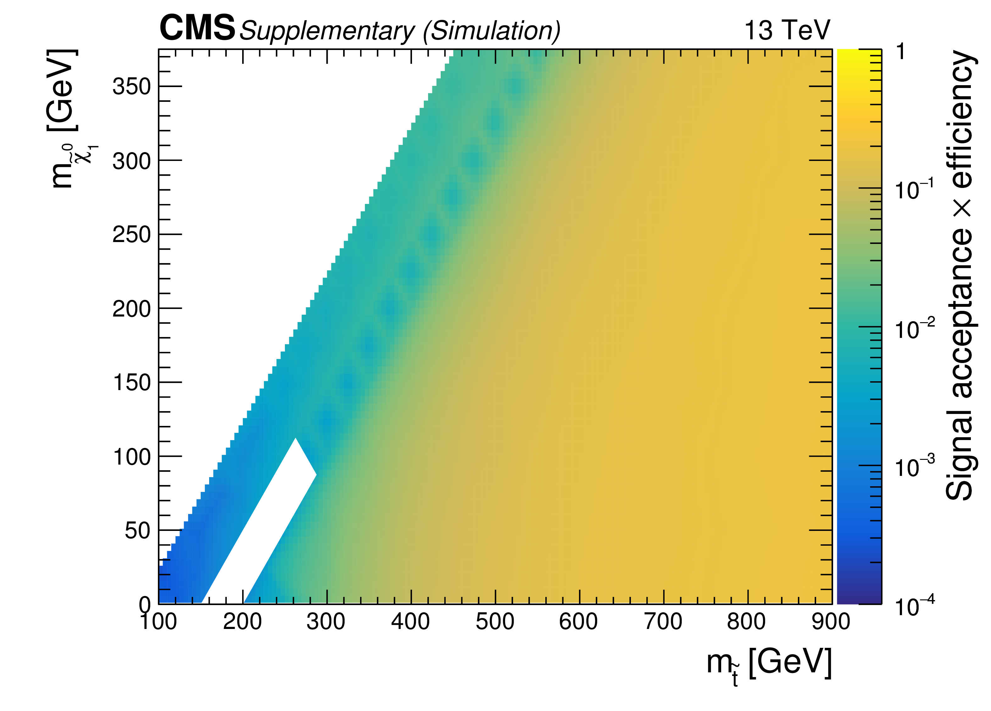
Additional Figure 12:
Left: (coloured histogram) upper limit on the cross section in the $(m_{ \tilde{ \mathrm{ t } } }, m_{\tilde{\chi}^0_1 })$ plane for the T2cc model. The black (red) solid line is the observed (expected) exclusion. The red dashed lines are the $\pm$1$\sigma $ expected exclusion due to experimental uncertainties. The $\pm$1$\sigma $ observed exclusion due to theoretical uncertainties on the signal cross section are shown as thin black lines. Right: signal efficiency for the search regions included in the limit calculation as a function $(m_{ \tilde{ \mathrm{ t } } }, m_{\tilde{\chi}^0_1 })$ plane for the T2cc model. |

png pdf root |
Additional Figure 12-a:
Upper limit on the cross section in the $(m_{ \tilde{ \mathrm{ t } } }, m_{\tilde{\chi}^0_1 })$ plane for the T2cc model. The black (red) solid line is the observed (expected) exclusion. The red dashed lines are the $\pm$1$\sigma $ expected exclusion due to experimental uncertainties. The $\pm$1$\sigma $ observed exclusion due to theoretical uncertainties on the signal cross section are shown as thin black lines. |
png pdf root |
Additional Figure 12-b:
Signal efficiency for the search regions included in the limit calculation as a function $(m_{ \tilde{ \mathrm{ t } } }, m_{\tilde{\chi}^0_1 })$ plane for the T2cc model. |

png pdf |
Additional Figure 13:
Left: (coloured histogram) upper limit on the cross section in the $(m_{ \tilde{ \mathrm{ t } } }, m_{\tilde{\chi}^0_1 })$ plane for the T2tt_degen model. The black (red) solid line is the observed (expected) exclusion. The red dashed lines are the $\pm$1$\sigma $ expected exclusion due to experimental uncertainties. The $\pm$1$\sigma $ observed exclusion due to theoretical uncertainties on the signal cross section are shown as thin black lines. Right: signal efficiency for the search regions included in the limit calculation as a function $(m_{ \tilde{ \mathrm{ t } } }, m_{\tilde{\chi}^0_1 })$ plane for the T2tt_degen model. |

png pdf root |
Additional Figure 13-a:
Upper limit on the cross section in the $(m_{ \tilde{ \mathrm{ t } } }, m_{\tilde{\chi}^0_1 })$ plane for the T2tt_degen model. The black (red) solid line is the observed (expected) exclusion. The red dashed lines are the $\pm$1$\sigma $ expected exclusion due to experimental uncertainties. The $\pm$1$\sigma $ observed exclusion due to theoretical uncertainties on the signal cross section are shown as thin black lines. |

png pdf root |
Additional Figure 13-b:
Signal efficiency for the search regions included in the limit calculation as a function $(m_{ \tilde{ \mathrm{ t } } }, m_{\tilde{\chi}^0_1 })$ plane for the T2tt_degen model. |

png pdf |
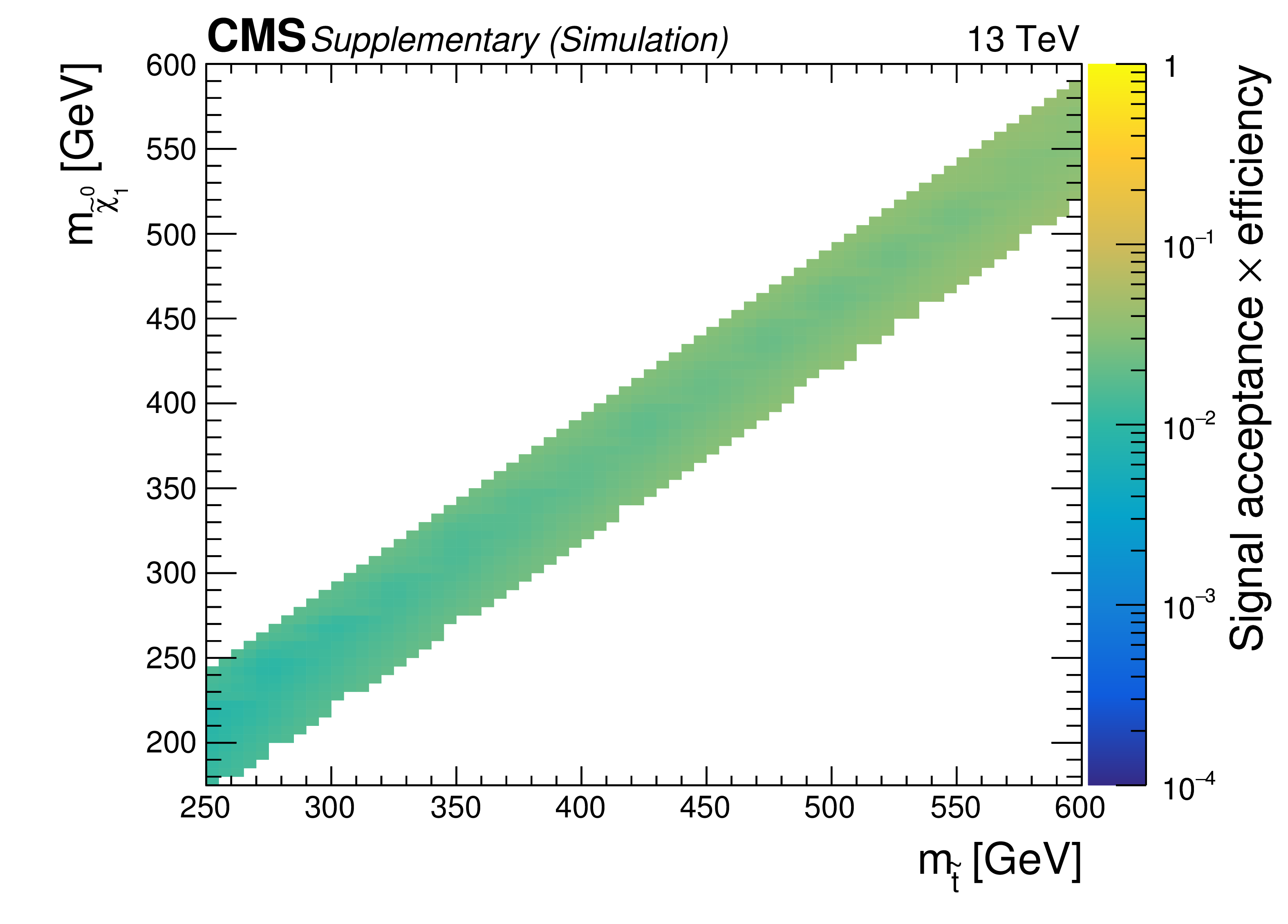
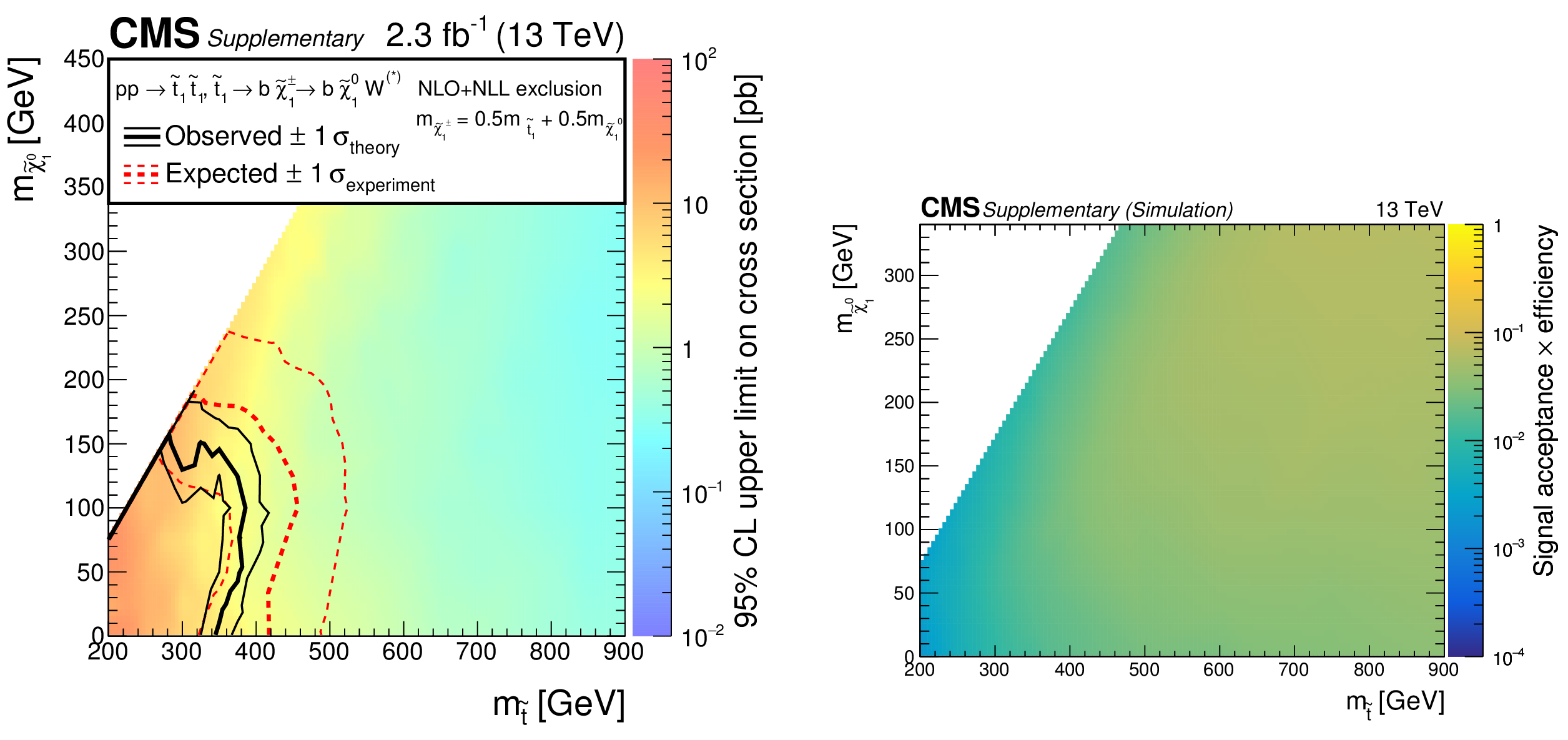
Additional Figure 14:
Left: (coloured histogram) upper limit on the cross section in the $(m_{ \tilde{ \mathrm{ t } } }, m_{\tilde{\chi}^0_1 })$ plane for the T2_mixed model. The black (red) solid line is the observed (expected) exclusion. The red dashed lines are the $\pm$1$\sigma $ expected exclusion due to experimental uncertainties. The $\pm$1$\sigma $ observed exclusion due to theoretical uncertainties on the signal cross section are shown as thin black lines. Right: signal efficiency for the search regions included in the limit calculation as a function $(m_{ \tilde{ \mathrm{ t } } }, m_{\tilde{\chi}^0_1 })$ plane for the T2_mixed model. |

png pdf root |
Additional Figure 14-a:
Upper limit on the cross section in the $(m_{ \tilde{ \mathrm{ t } } }, m_{\tilde{\chi}^0_1 })$ plane for the T2_mixed model. The black (red) solid line is the observed (expected) exclusion. The red dashed lines are the $\pm$1$\sigma $ expected exclusion due to experimental uncertainties. The $\pm$1$\sigma $ observed exclusion due to theoretical uncertainties on the signal cross section are shown as thin black lines. |

png pdf root |
Additional Figure 14-b:
Signal efficiency for the search regions included in the limit calculation as a function $(m_{ \tilde{ \mathrm{ t } } }, m_{\tilde{\chi}^0_1 })$ plane for the T2_mixed model. |
png pdf |
Additional Figure 15:
Left: (coloured histogram) upper limit on the cross section in the $(m_{ \tilde{ \mathrm{ t } } }, m_{\tilde{\chi}^0_1 })$ plane for the T2bW model. The black (red) solid line is the observed (expected) exclusion. The red dashed lines are the $\pm$1$\sigma $ expected exclusion due to experimental uncertainties. The $\pm$1$\sigma $ observed exclusion due to theoretical uncertainties on the signal cross section are shown as thin black lines. Right: signal efficiency for the search regions included in the limit calculation as a function $(m_{ \tilde{ \mathrm{ t } } }, m_{\tilde{\chi}^0_1 })$ plane for the T2bW model. |

png pdf root |
Additional Figure 15-a:
Upper limit on the cross section in the $(m_{ \tilde{ \mathrm{ t } } }, m_{\tilde{\chi}^0_1 })$ plane for the T2bW model. The black (red) solid line is the observed (expected) exclusion. The red dashed lines are the $\pm$1$\sigma $ expected exclusion due to experimental uncertainties. The $\pm$1$\sigma $ observed exclusion due to theoretical uncertainties on the signal cross section are shown as thin black lines. |

png pdf root |
Additional Figure 15-b:
Signal efficiency for the search regions included in the limit calculation as a function $(m_{ \tilde{ \mathrm{ t } } }, m_{\tilde{\chi}^0_1 })$ plane for the T2bW model. |

png pdf |
Additional Figure 16:
Summary for the observed (solid lines) and expected (dashed lines) exclusions in the $(m_{\mathrm {SUSY}}, m_{\mathrm {SUSY}} - m_{\tilde{\chi}^0_1 })$ plane for the models considered in the analysis. Exclusion contours are grouped into four summary figures: "direct and gluino-mediated production of off-shell (decoupled) light-flavour squarks'' (top left), "gluino-mediated production of off-shell (decoupled) third-generation squarks'' (top right), "gluino-mediated production of on-shell top squarks'' i.e. "natural'' models (bottom left), and "direct production of third-generation squarks'' (bottom right). |

png pdf |
Additional Figure 16-a:
Summary for the observed (solid lines) and expected (dashed lines) exclusions in the $(m_{\mathrm {SUSY}}, m_{\mathrm {SUSY}} - m_{\tilde{\chi}^0_1 })$ plane for the models considered in the analysis: "direct and gluino-mediated production of off-shell (decoupled) light-flavour squarks''. |

png pdf |
Additional Figure 16-b:
Summary for the observed (solid lines) and expected (dashed lines) exclusions in the $(m_{\mathrm {SUSY}}, m_{\mathrm {SUSY}} - m_{\tilde{\chi}^0_1 })$ plane for the models considered in the analysis: "gluino-mediated production of off-shell (decoupled) third-generation squarks''. |
png pdf |
Additional Figure 16-c:
Summary for the observed (solid lines) and expected (dashed lines) exclusions in the $(m_{\mathrm {SUSY}}, m_{\mathrm {SUSY}} - m_{\tilde{\chi}^0_1 })$ plane for the models considered in the analysis: "gluino-mediated production of on-shell top squarks'' i.e. "natural'' models. |

png pdf |
Additional Figure 16-d:
Summary for the observed (solid lines) and expected (dashed lines) exclusions in the $(m_{\mathrm {SUSY}}, m_{\mathrm {SUSY}} - m_{\tilde{\chi}^0_1 })$ plane for the models considered in the analysis: "direct production of third-generation squarks''. |

png pdf |
Additional Figure 17:
Summary for the observed (solid lines) and expected (dashed lines) exclusions in the $(m_{\mathrm {SUSY}}, m_{\mathrm {SUSY}} - m_{\tilde{\chi}^0_1 })$ plane for the models involving the direct production of third-generation squarks. |

png pdf |
Additional Figure 18:
(Upper panel) Event yields observed in data (solid circles) and SM expectations with their associated uncertainties (blue histogram with grey shaded band) determined from a simultaneous fit to data in the control regions only (CR-only fit). Event yields and expectations are shown as a function of $ {H_{\text {T}}^{\text {miss}}} $ for events in the "monojet-like'' topology that are required to satisfy 1 $ \leq {n_{\text {jet}}} \leq $ 2 or $ {n_{\text {jet}}^{\text {asym}}} = $ 2, $ {H_{\mathrm {T}}} > $ 200 GeV, and (left ) $ {n_{\text {b}}} = $ 0 or (right ) $ {n_{\text {b}}} \geq $ 1. (Lower panel) The significance of deviations (pulls) observed in data with respect to both the SM expectations from the CR-only fit, expressed in terms of the total uncertainty in the SM expectations. The pulls cannot be considered independently due to inter-bin correlations. |

png pdf |
Additional Figure 18-a:
(Upper panel) Event yields observed in data (solid circles) and SM expectations with their associated uncertainties (blue histogram with grey shaded band) determined from a simultaneous fit to data in the control regions only (CR-only fit). Event yields and expectations are shown as a function of $ {H_{\text {T}}^{\text {miss}}} $ for events in the "monojet-like'' topology that are required to satisfy 1 $ \leq {n_{\text {jet}}} \leq $ 2 or $ {n_{\text {jet}}^{\text {asym}}} = $ 2, $ {H_{\mathrm {T}}} > $ 200 GeV, and $ {n_{\text {b}}} = $ 0. (Lower panel) The significance of deviations (pulls) observed in data with respect to both the SM expectations from the CR-only fit, expressed in terms of the total uncertainty in the SM expectations. The pulls cannot be considered independently due to inter-bin correlations. |
png pdf |
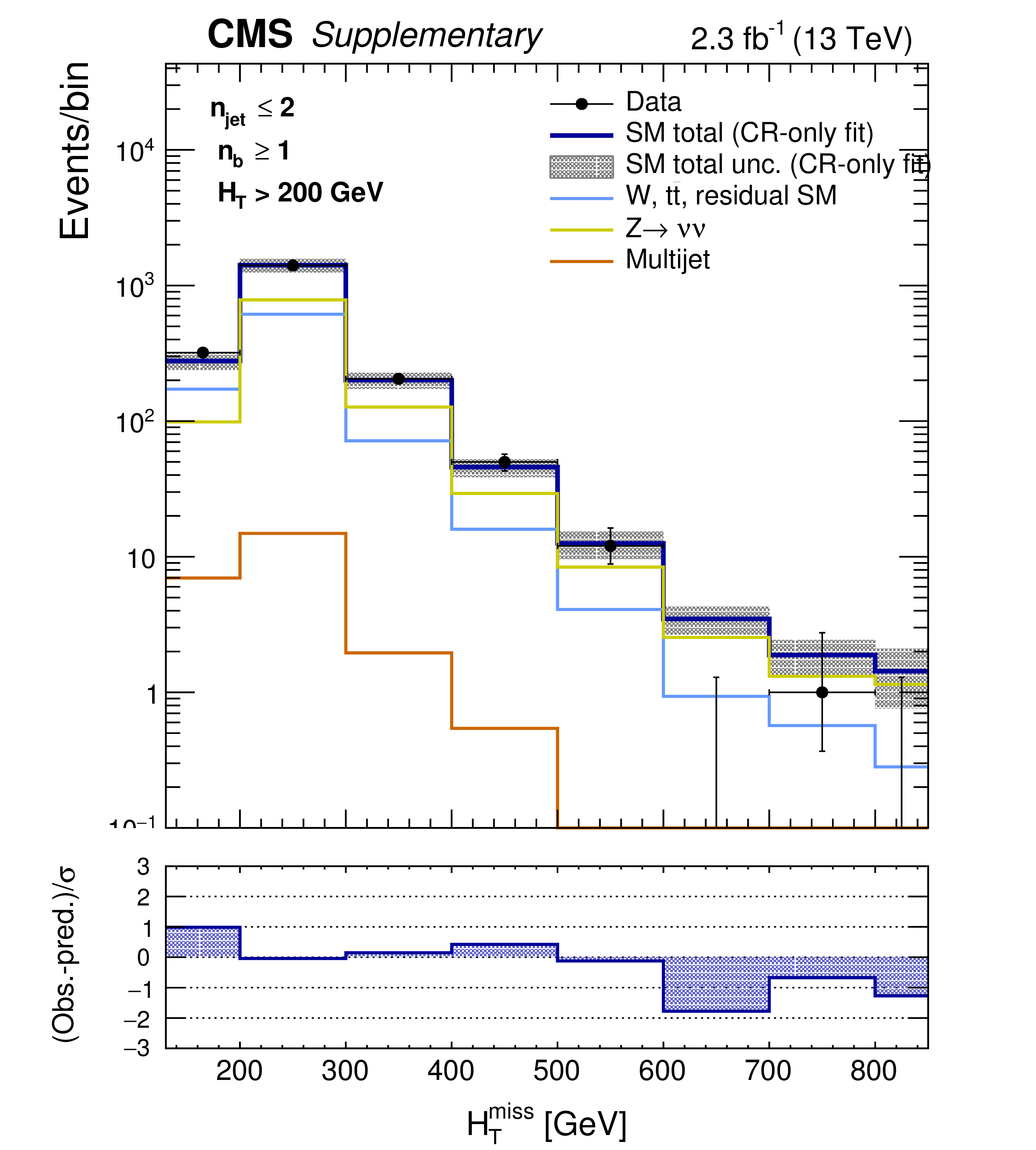
Additional Figure 18-b:
(Upper panel) Event yields observed in data (solid circles) and SM expectations with their associated uncertainties (blue histogram with grey shaded band) determined from a simultaneous fit to data in the control regions only (CR-only fit). Event yields and expectations are shown as a function of $ {H_{\text {T}}^{\text {miss}}} $ for events in the "monojet-like'' topology that are required to satisfy 1 $ \leq {n_{\text {jet}}} \leq $ 2 or $ {n_{\text {jet}}^{\text {asym}}} = $ 2, $ {H_{\mathrm {T}}} > $ 200 GeV, and $ {n_{\text {b}}} \geq $ 1. (Lower panel) The significance of deviations (pulls) observed in data with respect to both the SM expectations from the CR-only fit, expressed in terms of the total uncertainty in the SM expectations. The pulls cannot be considered independently due to inter-bin correlations. |

png pdf |
Additional Figure 19:
(Upper panel) Event yields observed in data (solid circles) and SM expectations with their associated uncertainties (blue histogram with grey shaded band) determined from a simultaneous fit to data in the control regions only (CR-only fit). Event yields and expectations are shown as a function of $ {H_{\text {T}}^{\text {miss}}} $ for events in the "asymmetric'' topology that are required to satisfy $ {n_{\text {jet}}^{\text {asym}}} \geq $ 3, $ {H_{\mathrm {T}}} > $ 200 GeV, and (left ) 0 $ \leq {n_{\text {b}}} \leq $ 1 or (right ) $ {n_{\text {b}}} \geq $ 2. (Lower panel) The significance of deviations (pulls) observed in data with respect to both the SM expectations from the CR-only fit, expressed in terms of the total uncertainty in the SM expectations. The pulls cannot be considered independently due to inter-bin correlations. |

png pdf |
Additional Figure 19-a:
(Upper panel) Event yields observed in data (solid circles) and SM expectations with their associated uncertainties (blue histogram with grey shaded band) determined from a simultaneous fit to data in the control regions only (CR-only fit). Event yields and expectations are shown as a function of $ {H_{\text {T}}^{\text {miss}}} $ for events in the "asymmetric'' topology that are required to satisfy $ {n_{\text {jet}}^{\text {asym}}} \geq $ 3, $ {H_{\mathrm {T}}} > $ 200 GeV, and 0 $ \leq {n_{\text {b}}} \leq $ 1. (Lower panel) The significance of deviations (pulls) observed in data with respect to both the SM expectations from the CR-only fit, expressed in terms of the total uncertainty in the SM expectations. The pulls cannot be considered independently due to inter-bin correlations. |

png pdf |
Additional Figure 19-b:
(Upper panel) Event yields observed in data (solid circles) and SM expectations with their associated uncertainties (blue histogram with grey shaded band) determined from a simultaneous fit to data in the control regions only (CR-only fit). Event yields and expectations are shown as a function of $ {H_{\text {T}}^{\text {miss}}} $ for events in the "asymmetric'' topology that are required to satisfy $ {n_{\text {jet}}^{\text {asym}}} \geq $ 3, $ {H_{\mathrm {T}}} > $ 200 GeV, and$ {n_{\text {b}}} \geq $ 2. (Lower panel) The significance of deviations (pulls) observed in data with respect to both the SM expectations from the CR-only fit, expressed in terms of the total uncertainty in the SM expectations. The pulls cannot be considered independently due to inter-bin correlations. |

png pdf |
Additional Figure 20:
(Upper panel) Event yields observed in data (solid circles) and SM expectations with their associated uncertainties (blue histogram with grey shaded band) determined from a simultaneous fit to data in the control regions only (CR-only fit). Event yields and expectations are shown as a function of $ {H_{\text {T}}^{\text {miss}}} $ for events in the "low $ {n_{\text {jet}}} $ '' topology that are required to satisfy 3 $ \leq {n_{\text {jet}}} \leq $ 4, $ {H_{\mathrm {T}}} > $ 200 GeV, and (left ) 0 $ \leq {n_{\text {b}}} \leq $ 1 or (right ) $ {n_{\text {b}}} \geq $ 2. (Lower panel) The significance of deviations (pulls) observed in data with respect to both the SM expectations from the CR-only fit, expressed in terms of the total uncertainty in the SM expectations. The pulls cannot be considered independently due to inter-bin correlations. |

png pdf |
Additional Figure 20-a:
(Upper panel) Event yields observed in data (solid circles) and SM expectations with their associated uncertainties (blue histogram with grey shaded band) determined from a simultaneous fit to data in the control regions only (CR-only fit). Event yields and expectations are shown as a function of $ {H_{\text {T}}^{\text {miss}}} $ for events in the "low $ {n_{\text {jet}}} $ '' topology that are required to satisfy 3 $ \leq {n_{\text {jet}}} \leq $ 4, $ {H_{\mathrm {T}}} > $ 200 GeV, and 0 $ \leq {n_{\text {b}}} \leq $ 1. (Lower panel) The significance of deviations (pulls) observed in data with respect to both the SM expectations from the CR-only fit, expressed in terms of the total uncertainty in the SM expectations. The pulls cannot be considered independently due to inter-bin correlations. |

png pdf |
Additional Figure 20-b:
(Upper panel) Event yields observed in data (solid circles) and SM expectations with their associated uncertainties (blue histogram with grey shaded band) determined from a simultaneous fit to data in the control regions only (CR-only fit). Event yields and expectations are shown as a function of $ {H_{\text {T}}^{\text {miss}}} $ for events in the "low $ {n_{\text {jet}}} $ '' topology that are required to satisfy 3 $ \leq {n_{\text {jet}}} \leq $ 4, $ {H_{\mathrm {T}}} > $ 200 GeV, and $ {n_{\text {b}}} \geq $ 2. (Lower panel) The significance of deviations (pulls) observed in data with respect to both the SM expectations from the CR-only fit, expressed in terms of the total uncertainty in the SM expectations. The pulls cannot be considered independently due to inter-bin correlations. |

png pdf |
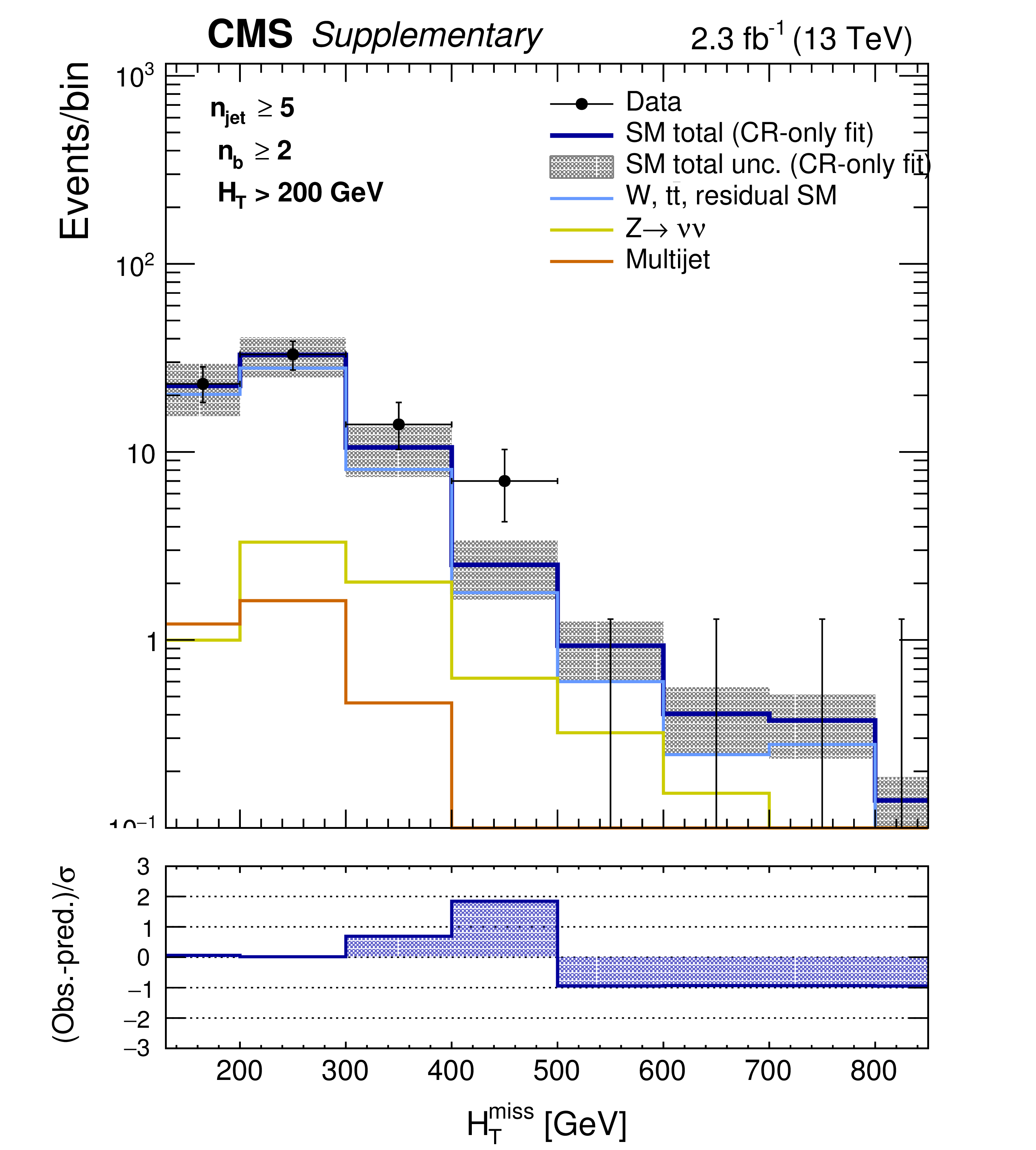
Additional Figure 21:
(Upper panel) Event yields observed in data (solid circles) and SM expectations with their associated uncertainties (blue histogram with grey shaded band) determined from a simultaneous fit to data in the control regions only (CR-only fit). Event yields and expectations are shown as a function of $ {H_{\text {T}}^{\text {miss}}} $ for events in the "high $ {n_{\text {jet}}} $ '' topology that are required to satisfy $ {n_{\text {jet}}} \geq $ 5, $ {H_{\mathrm {T}}} > $ 200 GeV, and (left ) 0 $ \leq {n_{\text {b}}} \leq $ 1 or (right ) $ {n_{\text {b}}} \geq $ 2. (Lower panel) The significance of deviations (pulls) observed in data with respect to both the SM expectations from the CR-only fit, expressed in terms of the total uncertainty in the SM expectations. The pulls cannot be considered independently due to inter-bin correlations. |

png pdf |
Additional Figure 21-a:
(Upper panel) Event yields observed in data (solid circles) and SM expectations with their associated uncertainties (blue histogram with grey shaded band) determined from a simultaneous fit to data in the control regions only (CR-only fit). Event yields and expectations are shown as a function of $ {H_{\text {T}}^{\text {miss}}} $ for events in the "high $ {n_{\text {jet}}} $ '' topology that are required to satisfy $ {n_{\text {jet}}} \geq $ 5, $ {H_{\mathrm {T}}} > $ 200 GeV, and 0 $ \leq {n_{\text {b}}} \leq $ 1. (Lower panel) The significance of deviations (pulls) observed in data with respect to both the SM expectations from the CR-only fit, expressed in terms of the total uncertainty in the SM expectations. The pulls cannot be considered independently due to inter-bin correlations. |
png pdf |
Additional Figure 21-b:
(Upper panel) Event yields observed in data (solid circles) and SM expectations with their associated uncertainties (blue histogram with grey shaded band) determined from a simultaneous fit to data in the control regions only (CR-only fit). Event yields and expectations are shown as a function of $ {H_{\text {T}}^{\text {miss}}} $ for events in the "high $ {n_{\text {jet}}} $ '' topology that are required to satisfy $ {n_{\text {jet}}} \geq $ 5, $ {H_{\mathrm {T}}} > $ 200 GeV, and $ {n_{\text {b}}} \geq $ 2. (Lower panel) The significance of deviations (pulls) observed in data with respect to both the SM expectations from the CR-only fit, expressed in terms of the total uncertainty in the SM expectations. The pulls cannot be considered independently due to inter-bin correlations. |

png pdf |
Additional Figure 22:
Covariance matrix for the SM background estimates obtained using the simplified binning scheme, determined from a simultaneous fit to data in the control regions only (CR-only fit). The uncertainties in the background estimates are correlated in such a way that the covariance is typically positive. Small positive values, as well as the few negative values, are not shown. |

png pdf |
Additional Figure 23:
Correlation matrix for the SM background estimates obtained using the simplified binning scheme, determined from a simultaneous fit to data in the control regions only (CR-only fit). |
| Additional Tables | |

png pdf |
Additional Table 1:
Observed data counts and "post-fit'' background expectations based on the result of a combined fit to the signal region and multiple control regions under the SM-only hypothesis for the "monojet'' event category. The rows labelled SM "pre-fit'' show the background expectations when excluding the signal region from the fit. The uncertainties include statistical as well as systematic contributions. |

png pdf |
Additional Table 2:
Observed data counts and "post-fit'' background expectations based on the result of a combined fit to the signal region and multiple control regions under the SM-only hypothesis for the "asymmetric'' event categories. The rows labelled SM "pre-fit'' show the background expectations when excluding the signal region from the fit. The uncertainties include statistical as well as systematic contributions. |

png pdf |
Additional Table 3:
Observed data counts and "post-fit'' background expectations based on the result of a combined fit to the signal region and multiple control regions under the SM-only hypothesis for the "symmetric'' event categories. The rows labelled SM "pre-fit'' show the background expectations when excluding the signal region from the fit. The uncertainties include statistical as well as systematic contributions. |

png pdf |
Additional Table 4:
Summary of a simplified binning scheme comprising $ {H_{\text {T}}^{\text {miss}}} $ shapes for eight representative event topologies, defined in terms of requirements on $ {n_{\text {jet}}} $ (both symmetric and asymmetric categories) and $ {n_{\text {b}}} $. For each topology, event yields are integrated over the full $ {H_{\mathrm {T}}} $ range, $ {H_{\mathrm {T}}} > $ 200 GeV, and are categorised according to eight bins in $ {H_{\text {T}}^{\text {miss}}} $ : 130 $ < {H_{\text {T}}^{\text {miss}}} < $ 200 GeV, six bins 100 GeV wide in the region 200 $ < {H_{\text {T}}^{\text {miss}}} < $ 800 GeV, and an open final bin, $ {H_{\text {T}}^{\text {miss}}} > $ 800 GeV. This categorisation scheme leads to 64 bins that are exclusive, contiguous, and provide complete coverage of the signal region. The corresponding SM background estimates for these 64 bins are obtained using the nominal likelihood model. The $ {H_{\text {T}}^{\text {miss}}} $ template for each topology is determined from simulation and the normalisation for each template is given by an aggregate of estimates from several ( $ {n_{\text {jet}}} $, $ {n_{\text {b}}} $, $ {H_{\mathrm {T}}} $ ) bins, defined according to the nominal binning scheme. |

png pdf |
Additional Table 5:
Observed data yields and "CR-only fit'' SM background expectations using the simplified binning scheme, as a function of topology and $ {H_{\text {T}}^{\text {miss}}} $. The SM backgrounds are determined from a simultaneous fit to data in the control regions. The data yields in the signal region are masked and excluded from the fit. The uncertainties include statistical as well as systematic contributions. |

png pdf |
Additional Table 6:
Expected ($\mu _{\text {exp}}$) and observed ($\mu _{\text {obs}}$) upper limits on the production cross section, expressed in terms of the signal strength parameter, obtained using both the nominal and simplified binning schema. Comparable values are obtained from the two schema for these benchmark SUSY models because the signal events typically populate bins at high values of $ {H_{\mathrm {T}}} $ and $ {H_{\text {T}}^{\text {miss}}} $ and so are at or near the limit of the search sensitivity. Larger differences in $\mu $ can be observed for models that populate the core of these distributions. |

png pdf |
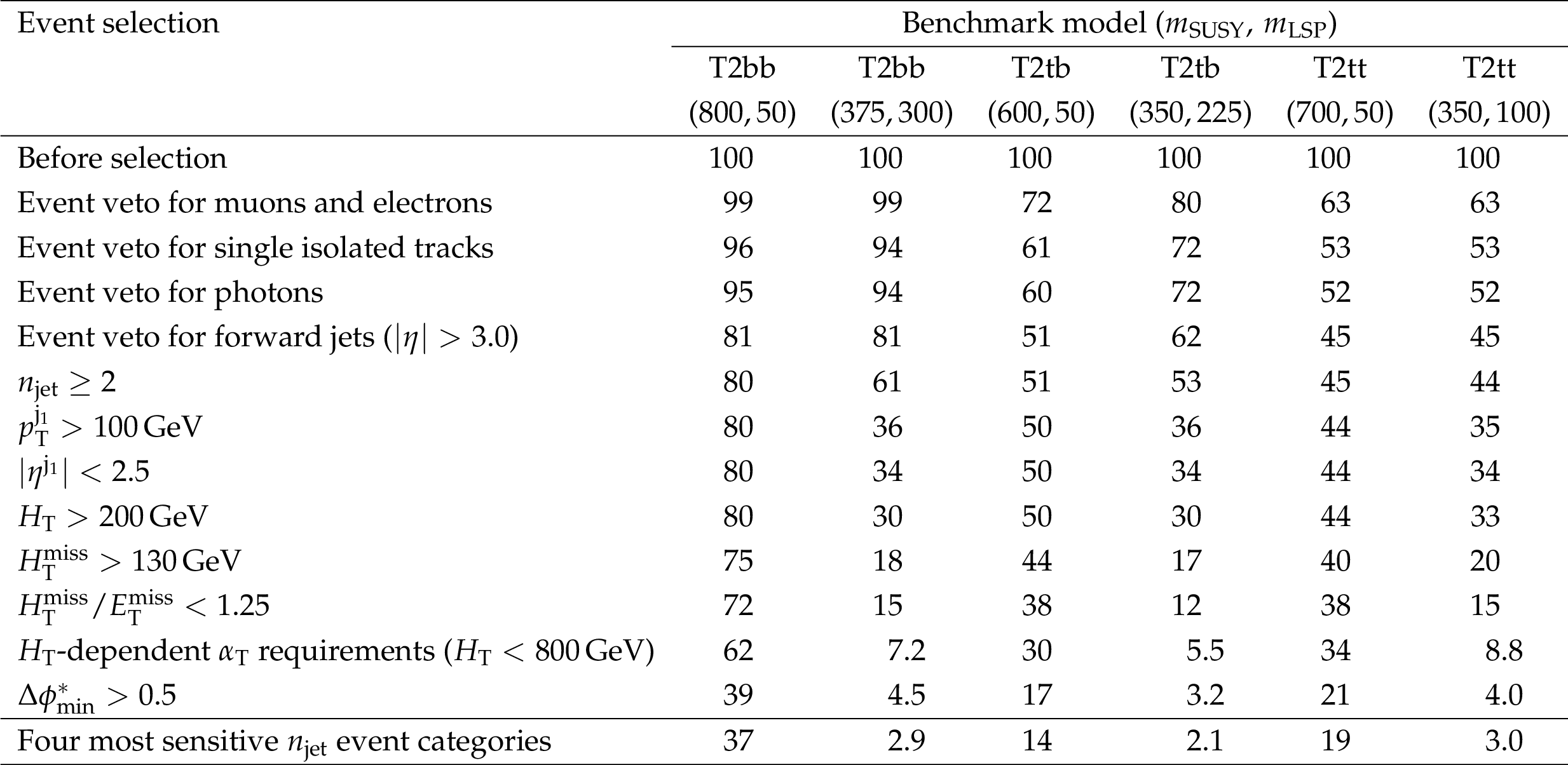
Additional Table 7:
A summary of the cumulative signal acceptance times efficiency, $ \mathcal {A} \varepsilon $, for various benchmark models with both compressed and uncompressed mass spectra, following the application of the event selection criteria used to define the signal region. Values for $ \mathcal {A} \varepsilon $ are also shown following the application of additional requirements that define the four most sensitive $ n_{\mathrm {jet}} $ event categories, as defined in Table 5 of the paper. Scale factor corrections to simulated signal events that account for the mismodelling of theoretical and experimental parameters are not applied, and so the values for $ \mathcal {A} \varepsilon $ differ with respect to those in Table 5 by up to 15%. |

png pdf |
Additional Table 8:
A summary of the cumulative signal acceptance times efficiency, $\mathcal {A} \varepsilon $ [%], for various benchmark models with both compressed and uncompressed mass spectra, following the application of the event selection criteria used to define the signal region. Values for $\mathcal {A} \varepsilon $ are also shown following the application of additional requirements that define the four most sensitive $n_{\mathrm {jet}}$ event categories, as defined in Table 5 of the paper. Scale factor corrections to simulated signal events that account for the mismodelling of theoretical and experimental parameters are not applied, and so the values for $\mathcal {A} \varepsilon $ differ with respect to those in Table 5 by up to 15%. |

png pdf |
Additional Table 9:
A summary of the cumulative signal acceptance times efficiency, $\mathcal {A} \varepsilon $ [%], for various benchmark models with both compressed and uncompressed mass spectra, following the application of the event selection criteria used to define the signal region. Values for $\mathcal {A} \varepsilon $ are also shown following the application of additional requirements that define the four most sensitive $n_{\mathrm {jet}}$ event categories, as defined in Table 5 of the paper. Scale factor corrections to simulated signal events that account for the mismodelling of theoretical and experimental parameters are not applied, and so the values for $\mathcal {A} \varepsilon $ differ with respect to those in Table 5 by up to 15%. |
png pdf |
Additional Table 10:
A summary of the cumulative signal acceptance times efficiency, $\mathcal {A} \varepsilon $ [%], for various benchmark models with both compressed and uncompressed mass spectra, following the application of the event selection criteria used to define the signal region. Values for $\mathcal {A} \varepsilon $ are also shown following the application of additional requirements that define the four most sensitive $n_{\mathrm {jet}}$ event categories, as defined in Table 5 of the paper. Scale factor corrections to simulated signal events that account for the mismodelling of theoretical and experimental parameters are not applied, and so the values for $\mathcal {A} \varepsilon $ differ with respect to those in Table 5 by up to 15%. |

png pdf |
Additional Table 11:
A summary of the cumulative signal acceptance times efficiency, $\mathcal {A} \varepsilon $ [%], for various benchmark models with both compressed and uncompressed mass spectra, following the application of the event selection criteria used to define the signal region. Values for $\mathcal {A} \varepsilon $ are also shown following the application of additional requirements that define the four most sensitive $n_{\mathrm {jet}}$ event categories, as defined in Table 5 of the paper. Scale factor corrections to simulated signal events that account for the mismodelling of theoretical and experimental parameters are not applied, and so the values for $\mathcal {A} \varepsilon $ differ with respect to those in Table 5 by up to 15%. |
| Additional Material |
|
The nominal result of the analysis is available in a digital format
(.csv) at the following links: pre-fit result, post-fit
result. Further, to aid reintepretation, the (CR-only) result obtained using a simplified binning scheme ("super signal regions") is available in .csv and .root digital formats. The latter file also contains the covariance matrix that specifies the level of inter-bin correlations in the SM background estimates. Supporting figures and tables can be found above in this page. Implementations of the αT and the Δφ*min variables can be found here and here, respectively. Instructions on how to use the aforementioned material can be found here. |
| References | ||||
| 1 | Y. A. Gol'fand and E. P. Likhtman | Extension of the Algebra of Poincare Group Generators and Violation of P Invariance | JEPTL 13 (1971) 323 | |
| 2 | J. Wess and B. Zumino | Supergauge transformations in four dimensions | Nucl. Phys. B 70 (1974) 39 | |
| 3 | R. Barbieri, S. Ferrara, and C. A. Savoy | Gauge models with spontaneously broken local supersymmetry | PLB 119 (1982) 343 | |
| 4 | H. P. Nilles | Supersymmetry, supergravity and particle physics | PR 110 (1984) 1 | |
| 5 | S. Dawson, E. Eichten, and C. Quigg | Search for supersymmetric particles in hadron--hadron collisions | PRD 31 (1985) 1581 | |
| 6 | H. E. Haber and G. L. Kane | The search for supersymmetry: Probing physics beyond the standard model | PR 117 (1987) 75 | |
| 7 | G. R. Farrar and P. Fayet | Phenomenology of the production, decay, and detection of new hadronic states associated with supersymmetry | PLB 76 (1978) 575 | |
| 8 | G. Jungman, M. Kamionkowski, and K. Griest | Supersymmetric dark matter | PR 267 (1996) 195 | hep-ph/9506380 |
| 9 | Particle Data Group, K. A. Olive et al. | Review of Particle Physics | CPC 38 (2014) 090001 | |
| 10 | S. Dimopoulos, S. Raby, and F. Wilczek | Supersymmetry and the scale of unification | PRD 24 (1981) 1681 | |
| 11 | L. E. Ibanez and G. G. Ross | Low-energy predictions in supersymmetric grand unified theories | PLB 105 (1981) 439 | |
| 12 | W. J. Marciano and G. Senjanovic | Predictions of supersymmetric grand unified theories | PRD 25 (1982) 3092 | |
| 13 | ATLAS Collaboration | Observation of a new particle in the search for the Standard Model Higgs boson with the ATLAS detector at the LHC | PLB 716 (2012) 1 | 1207.7214 |
| 14 | CMS Collaboration | Observation of a new boson at a mass of 125 GeV with the CMS experiment at the LHC | PLB 716 (2012) 30 | |
| 15 | CMS Collaboration | Observation of a new boson with mass near 125 GeV in pp collisions at $ \sqrt{s} = $ 7 and 8 TeV | JHEP 06 (2013) 081 | CMS-HIG-12-036 1303.4571 |
| 16 | E. Witten | Dynamical breaking of supersymmetry | Nucl. Phys. B 188 (1981) 513 | |
| 17 | S. Dimopoulos and H. Georgi | Softly broken supersymmetry and SU(5) | Nucl. Phys. B 193 (1981) 150 | |
| 18 | R. Barbieri and D. Pappadopulo | S-particles at their naturalness limits | JHEP 10 (2009) 061 | 0906.4546 |
| 19 | A. Delgado et al. | The light stop window | EPJC 73 (2013) 2370 | 1212.6847 |
| 20 | C. Boehm, A. Djouadi, and Y. Mambrini | Decays of the lightest top squark | PRD 61 (2000) 095006 | hep-ph/9907428 |
| 21 | M. Carena, A. Freitas, and C. E. M. Wagner | Light stop searches at the LHC in events with one hard photon or jet and missing energy | JHEP 10 (2008) 109 | 0808.2298 |
| 22 | R. Grober, M. M. Muhlleitner, E. Popenda, and A. Wlotzka | Light stop decays: implications for LHC searches | EPJC 75 (2015) 420 | 1408.4662 |
| 23 | R. Grober, M. Muhlleitner, E. Popenda, and A. Wlotzka | Light stop decays into $ \text{Wb}\tilde{\chi}^0_1 $ near the kinematic threshold | PLB 747 (2015) 144 | 1502.05935 |
| 24 | C. Boehm, A. Djouadi, and M. Drees | Light scalar top quarks and supersymmetric dark matter | PRD 62 (2000) 035012 | hep-ph/9911496 |
| 25 | C. Balazs, M. S. Carena, and C. E. M. Wagner | Dark matter, light stops and electroweak baryogenesis | PRD 70 (2004) 015007 | hep-ph/0403224 |
| 26 | S. P. Martin | Compressed supersymmetry and natural neutralino dark matter from top squark-mediated annihilation to top quarks | PRD 75 (2007) 115005 | hep-ph/0703097 |
| 27 | S. P. Martin | Top squark-mediated annihilation scenario and direct detection of dark matter in compressed supersymmetry | PRD 76 (2007) 095005 | 0707.2812 |
| 28 | CMS Collaboration | Search for Supersymmetry in pp Collisions at 7 TeV in Events with Jets and Missing Transverse Energy | PLB 698 (2011) 196 | CMS-SUS-10-003 1101.1628 |
| 29 | CMS Collaboration | Search for Supersymmetry at the LHC in Events with Jets and Missing Transverse Energy | PRL 107 (2011) 221804 | |
| 30 | CMS Collaboration | Search for supersymmetry in final states with missing transverse energy and 0, 1, 2, or $ {\ge}3 $ b-quark jets in 7 TeV pp collisions using the variable $ \alpha_\mathrm{T} $ | JHEP 01 (2013) 077 | |
| 31 | CMS Collaboration | Search for supersymmetry in hadronic final states with missing transverse energy using the variables $\alpha_{\mathrm{T}}$ and b-quark multiplicity in pp collisions at $ \sqrt{s} = $ 8 TeV | EPJC 73 (2013) 2568 | CMS-SUS-12-028 1303.2985 |
| 32 | CMS Collaboration | Search for top squark pair production in compressed-mass-spectrum scenarios in proton-proton collisions at $ \sqrt{s} = $ 8 TeV using the $ \alpha_\mathrm{T} $ variable | Submitted to PLB | CMS-SUS-14-006 1605.08993 |
| 33 | C. Borschensky et al. | Squark and gluino production cross sections in $ pp $ collisions at $ \sqrt{s} = $ 13, 14, 33 and 100 TeV | EPJC 74 (2014) 3174 | 1407.5066 |
| 34 | ATLAS Collaboration | Summary of the searches for squarks and gluinos using $ \sqrt{s} = $ 8 TeV pp collisions with the ATLAS experiment at the LHC | JHEP 10 (2015) 054 | 1507.05525 |
| 35 | ATLAS Collaboration | ATLAS Run 1 searches for direct pair production of third-generation squarks at the Large Hadron Collider | EPJC 75 (2015) 510 | 1506.08616 |
| 36 | CMS Collaboration | Searches for supersymmetry based on events with b jets and four W bosons in pp collisions at 8 TeV | PLB 745 (2015) 5 | CMS-SUS-14-010 1412.4109 |
| 37 | CMS Collaboration | Searches for supersymmetry using the $ M_\mathrm{T2} $ variable in hadronic events produced in pp collisions at 8 TeV | JHEP 05 (2015) 078 | |
| 38 | CMS Collaboration | Search for direct pair production of supersymmetric top quarks decaying to all-hadronic final states in pp collisions at $ \sqrt{s} = $ 8 TeV | EPJC 76 (2016) 460 | CMS-SUS-13-023 1603.00765 |
| 39 | CMS Collaboration | Search for gluino mediated bottom- and top-squark production in multijet final states in pp collisions at 8 TeV | PLB 725 (2013) 243 | CMS-SUS-12-024 1305.2390 |
| 40 | CMS Collaboration | Search for new physics in the multijet and missing transverse momentum final state in proton-proton collisions at $ \sqrt{s} = $ 8 TeV | JHEP 06 (2014) 055 | CMS-SUS-13-012 1402.4770 |
| 41 | CMS Collaboration | Search for supersymmetry using razor variables in events with $ b $-tagged jets in $ pp $ collisions at $ \sqrt{s} = $ 8 TeV | PRD 91 (2015) 052018 | CMS-SUS-13-004 1502.00300 |
| 42 | CMS Collaboration | Searches for third-generation squark production in fully hadronic final states in proton-proton collisions at $ \sqrt{s} = $ 8 TeV | JHEP 06 (2015) 116 | CMS-SUS-14-001 1503.08037 |
| 43 | CMS Collaboration | Search for supersymmetry in pp collisions at $ \sqrt{s} = $ 8 TeV in final states with boosted W bosons and b jets using razor variables | PRD 93 (2016) 092009 | CMS-SUS-14-007 1602.02917 |
| 44 | ATLAS Collaboration | Search for new phenomena in final states with large jet multiplicities and missing transverse momentum with ATLAS using $ \sqrt{s} = $ 13 TeV proton--proton collisions | PLB 757 (2016) 334 | 1602.06194 |
| 45 | ATLAS Collaboration | Search for new phenomena in final states with an energetic jet and large missing transverse momentum in pp collisions at $ \sqrt{s} = $ 13 TeV using the ATLAS detector | Submitted to \it PRD | 1604.07773 |
| 46 | ATLAS Collaboration | Search for squarks and gluinos in final states with jets and missing transverse momentum at $ \sqrt{s} = $ 13 TeV with the ATLAS detector | EPJC 76 (2016) 392 | 1605.03814 |
| 47 | ATLAS Collaboration | Search for pair production of gluinos decaying via stop and sbottom in events with $ b $-jets and large missing transverse momentum in pp collisions at $ \sqrt{s} = $ 13 TeV with the ATLAS detector | PRD 94 (2016) 032003 | 1605.09318 |
| 48 | ATLAS Collaboration | Search for bottom squark pair production in proton--proton collisions at $ \sqrt{s} = $ 13 TeV with the ATLAS detector | Submitted to EPJC | 1606.08772 |
| 49 | CMS Collaboration | Search for supersymmetry in the multijet and missing transverse momentum final state in pp collisions at 13 TeV | PLB 758 (2016) 152 | CMS-SUS-15-002 1602.06581 |
| 50 | CMS Collaboration | Search for new physics with the M$ _{T2} $ variable in all-jets final states produced in pp collisions at $ \sqrt{s} = $ 13 TeV | JHEP 10 (2016) 006 | |
| 51 | P. J. Fox, R. Harnik, R. Primulando, and C.-T. Yu | Taking a razor to dark matter parameter space at the LHC | PRD 86 (2012) 015010 | 1203.1662 |
| 52 | O. Buchmueller, S. A. Malik, C. McCabe, and B. Penning | Constraining Dark Matter Interactions with Pseudoscalar and Scalar Mediators using Collider Searches for Multijets plus Missing Transverse Energy | PRL 115 (2015) 181802 | 1505.07826 |
| 53 | L. Randall and D. Tucker-Smith | Dijet Searches for Supersymmetry at the Large Hadron Collider | PRL 101 (2008) 221803 | 0806.1049 |
| 54 | CMS Collaboration | The CMS experiment at the CERN LHC | JINST 3 (2008) S08004 | CMS-00-001 |
| 55 | J. Alwall et al. | The automated computation of tree-level and next-to-leading order differential cross sections, and their matching to parton shower simulations | JHEP 07 (2014) 079 | 1405.0301 |
| 56 | S. Alioli, P. Nason, C. Oleari, and E. Re | A general framework for implementing NLO calculations in shower Monte Carlo programs: the POWHEG BOX | JHEP 06 (2010) 043 | 1002.2581 |
| 57 | E. Re | Single-top Wt-channel production matched with parton showers using the POWHEG method | EPJC 71 (2011) 1547 | 1009.2450 |
| 58 | R. Gavin, Y. Li, F. Petriello, and S. Quackenbush | W Physics at the LHC with FEWZ 2.1 | CPC 184 (2013) 208 | 1201.5896 |
| 59 | R. Gavin, Y. Li, F. Petriello, and S. Quackenbush | FEWZ 2.0: A code for hadronic Z production at next-to-next-to-leading order | CPC 182 (2011) 2388 | 1011.3540 |
| 60 | T. Melia, P. Nason, R. Rontsch, and G. Zanderighi | W$ ^+ $W$ ^- $, WZ and ZZ production in the POWHEG BOX | JHEP 11 (2011) 078 | 1107.5051 |
| 61 | M. Czakon and A. Mitov | Top++: A program for the calculation of the top-pair cross-section at hadron colliders | CPC 185 (2014) 2930 | 1112.5675 |
| 62 | S. Alioli, P. Nason, C. Oleari, and E. Re | NLO single-top production matched with shower in POWHEG: $ s $- and $ t $-channel contributions | JHEP 09 (2009) 111 | 0907.4076 |
| 63 | GEANT4 Collaboration | GEANT4---a simulation toolkit | NIMA 506 (2003) 250 | |
| 64 | T. Sjostrand et al. | An Introduction to PYTHIA 8.2 | CPC 191 (2015) 159 | 1410.3012 |
| 65 | W. Beenakker, R. Hopker, M. Spira, and P. M. Zerwas | Squark and gluino production at hadron colliders | Nucl. Phys. B 492 (1997) 51 | hep-ph/9610490 |
| 66 | A. Kulesza and L. Motyka | Threshold Resummation for Squark-Antisquark and Gluino-Pair Production at the LHC | PRL 102 (2009) 111802 | 0807.2405 |
| 67 | A. Kulesza and L. Motyka | Soft gluon resummation for the production of gluino-gluino and squark-antisquark pairs at the LHC | PRD 80 (2009) 095004 | 0905.4749 |
| 68 | W. Beenakker et al. | Soft-gluon resummation for squark and gluino hadroproduction | JHEP 09 (2009) 041 | 0909.4418 |
| 69 | W. Beenakker et al. | Squark and gluino hadroproduction | Int. J. Mod. Phys. A 26 (2011) 2637 | 1105.1110 |
| 70 | P. M. Nadolsky et al. | Implications of CTEQ global analysis for collider observables | PRD 78 (2008) 013004 | 0802.0007 |
| 71 | A. D. Martin, W. J. Stirling, R. S. Thorne, and G. Watt | Parton distributions for the LHC | EPJC 63 (2009) 189 | 0901.0002 |
| 72 | CMS Collaboration | The fast simulation of the CMS detector at LHC | J. Phys. Conf. Ser. 331 (2011) 032049 | |
| 73 | NNPDF Collaboration | Parton distributions for the LHC Run II | JHEP 04 (2015) 040 | 1410.8849 |
| 74 | CMS Collaboration | Event generator tunes obtained from underlying event and multiparton scattering measurements | EPJC 76 (2016) 155 | CMS-GEN-14-001 1512.00815 |
| 75 | CMS Collaboration | Particle-flow event reconstruction in CMS and performance for jets, taus, and $ E_{\mathrm{T}}^{\text{miss}} $ | CDS | |
| 76 | CMS Collaboration | Commissioning of the particle-flow event with the first LHC collisions recorded in the CMS detector | CDS | |
| 77 | CMS Collaboration | Performance of photon reconstruction and identification with the CMS detector in proton-proton collisions at $ \sqrt{s} = $ 8 TeV | JINST 10 (2015) P08010 | CMS-EGM-14-001 1502.02702 |
| 78 | CMS Collaboration | Performance of electron reconstruction and selection with the CMS detector in proton-proton collisions at $ \sqrt{s} = $ 8 TeV | JINST 10 (2015) P06005 | CMS-EGM-13-001 1502.02701 |
| 79 | CMS Collaboration | Performance of CMS muon reconstruction in pp collision events at $ \sqrt{s} = $ 7 TeV | JINST 7 (2012) P10002 | CMS-MUO-10-004 1206.4071 |
| 80 | M. Cacciari, G. P. Salam, and G. Soyez | The anti-$ k_t $ jet clustering algorithm | JHEP 04 (2008) 063 | 0802.1189 |
| 81 | M. Cacciari and G. P. Salam | Pileup subtraction using jet areas | PLB 659 (2008) 119 | 0707.1378 |
| 82 | CMS Collaboration | Determination of jet energy calibration and transverse momentum resolution in CMS | JINST 6 (2011) P11002 | CMS-JME-10-011 1107.4277 |
| 83 | CMS Collaboration | Identification of b-quark jets with the CMS experiment | JINST 8 (2013) P04013 | |
| 84 | CMS Collaboration | Identification of b quark jets at the CMS Experiment in the LHC Run 2 | CMS-PAS-BTV-15-001 | CMS-PAS-BTV-15-001 |
| 85 | CMS Collaboration | Missing transverse energy performance of the CMS detector | JINST 6 (2011) P09001 | CMS-JME-10-009 1106.5048 |
| 86 | CMS Collaboration | Identification and filtering of uncharacteristic noise in the CMS hadron calorimeter | JINST 5 (2010) T03014 | CMS-CFT-09-019 0911.4881 |
| 87 | Z. Bern et al. | Driving Missing Data at Next-to-Leading Order | PRD 84 (2011) 114002 | 1106.1423 |
| 88 | ATLAS Collaboration | Measurement of the Inelastic Proton-Proton Cross Section at $ \sqrt{s} = $ 13 TeV with the ATLAS Detector at the LHC | Submitted to PRL | 1606.02625 |
| 89 | CMS Collaboration | Measurement of the differential cross section for top quark pair production in pp collisions at $ \sqrt{s} = $ 8 TeV | EPJC 75 (2015) 542 | CMS-TOP-12-028 1505.04480 |
| 90 | J. S. Conway | Incorporating Nuisance Parameters in Likelihoods for Multisource Spectra | in PHYSTAT 2011 Workshop on Statistical Issues Related to Discovery Claims in Search Experiments and Unfolding | |
| 91 | J. K. Lindsey | Parametric Statistical Inference | Oxford University Press, 1996 ISBN 0-19-852359-9 | |
| 92 | J. Alwall, P. Schuster, and N. Toro | Simplified models for a first characterization of new physics at the LHC | PRD 79 (2009) 075020 | 0810.3921 |
| 93 | J. Alwall, M.-P. Le, M. Lisanti, and J. G. Wacker | Model-independent jets plus missing energy searches | PRD 79 (2009) 015005 | 0809.3264 |
| 94 | D. Alves et al. | Simplified models for LHC new physics searches | JPG 39 (2012) 105005 | 1105.2838 |
| 95 | G. Cowan, K. Cranmer, E. Gross, and O. Vitells | Asymptotic formulae for likelihood-based tests of new physics | EPJC 71 (2011) 1554 | 1007.1727 |
| 96 | ATLAS and CMS Collaborations, and LHC Higgs Combination Group | Procedure for the LHC Higgs boson search combination in Summer 2011 | CMS-NOTE-2011-005 | |
| 97 | T. Junk | Confidence level computation for combining searches with small statistics | Nucl. Instr. Meth. A 434 (1999) 435 | hep-ex/9902006 |
| 98 | A. L. Read | Presentation of search results: the $ CL_s $ technique | JPG 28 (2002) 2693 | |
| 99 | CMS Collaboration | CMS Luminosity Measurement for the 2015 Data Taking Period | CMS-PAS-LUM-15-001 | CMS-PAS-LUM-15-001 |
| 100 | CMS Collaboration | Search for top-squark pair production in the single-lepton final state in pp collisions at $ \sqrt{s}=8 $ TeV | EPJC 73 (2013) 2677 | |
|
|
Compact Muon Solenoid LHC, CERN |
|

|

|

|

|

|