

Compact Muon Solenoid
LHC, CERN
| CMS-TOP-15-008 ; CERN-EP-2017-050 | ||
| Measurement of the top quark mass in the dileptonic $\mathrm{ t \bar{t} }$ decay channel using the mass observables $M_{\mathrm{ b }\ell}$, $M_{\mathrm{T}2}$, and $M_{\mathrm{ b }\ell\nu}$ in pp collisions at $\sqrt{s} = $ 8 TeV | ||
| CMS Collaboration | ||
| 20 April 2017 | ||
| Phys. Rev. D 96 (2017) 032002 | ||
| Abstract: A measurement of the top quark mass ($M_{\mathrm{ t }}$) in the dileptonic $\mathrm{ t \bar{t} }$ decay channel is performed using data from proton-proton collisions at a center-of-mass energy of 8 TeV. The data was recorded by the CMS experiment at the LHC and corresponding to an integrated luminosity of 19.7 $\pm$ 0.5 fb$^{-1}$. Events are selected with two oppositely charged leptons ($\ell=$ e, $\mu$) and two jets identified as originating from b quarks. The analysis is based on three kinematic observables whose distributions are sensitive to the value of $M_{\mathrm{ t }}$. An invariant mass observable, $M_{\mathrm{ b }\ell}$, and a 'stransverse mass' observable, $M_{\mathrm{T}2}$, are employed in a simultaneous fit to determine the value of $M_{\mathrm{ t }}$ and an overall jet energy scale factor (JSF). A complementary approach is used to construct an invariant mass observable, $M_{\mathrm{ b }\ell\nu}$, that is combined with $M_{\mathrm{T}2}$ to measure $M_{\mathrm{ t }}$. The shapes of the observables, along with their evolutions in $M_{\mathrm{ t }}$ and JSF, are modeled by a nonparametric Gaussian process regression technique. The sensitivity of the observables to the value of $M_{\mathrm{ t }}$ is investigated using a Fisher information density method. The top quark mass is measured to be 172.22 $\pm$ 0.18 (stat) $^{+0.89}_{-0.93}$ (syst) GeV. | ||
| Links: e-print arXiv:1704.06142 [hep-ex] (PDF) ; CDS record ; inSPIRE record ; CADI line (restricted) ; | ||
| Figures | |
png pdf |
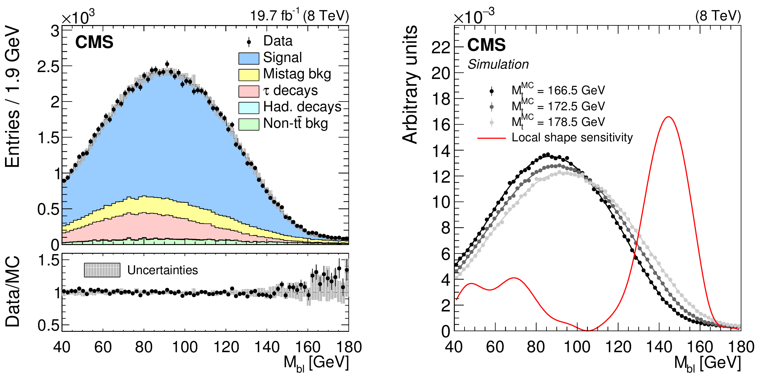
Figure 1:
(Left) the ${M_{\mathrm{ b } \ell }}$ distribution in data and simulation with $ {M_{\mathrm{ t } }^{\text {MC}}}= $ 172.5 GeV, normalized to the number of events in the 8 TeV data set corresponding to an integrated luminosity of 19.7 $\pm$ 0.5 fb$^{-1}$. The lower panel shows the ratio between the data and simulation. Statistical and systematic uncertainties on the distribution in simulation are represented by the shaded area. A description of the systematic uncertainties is given in Section 7. (Right) the ${M_{\mathrm{ b } \ell }}$ distribution shapes in simulation, normalized to unit area, corresponding to three values of $ {M_{\mathrm{ t } }^{\text {MC}}}$ are shown together with the 'local shape sensitivity' function, described in Appendix {sec:sensitivity}. The ${M_{\mathrm{ b } \ell }}$ distributions include two or three values of ${M_{\mathrm{ b } \ell }}$ for each event. The distribution shapes are modeled with a GP regression technique, described in Section 5. |
png pdf |
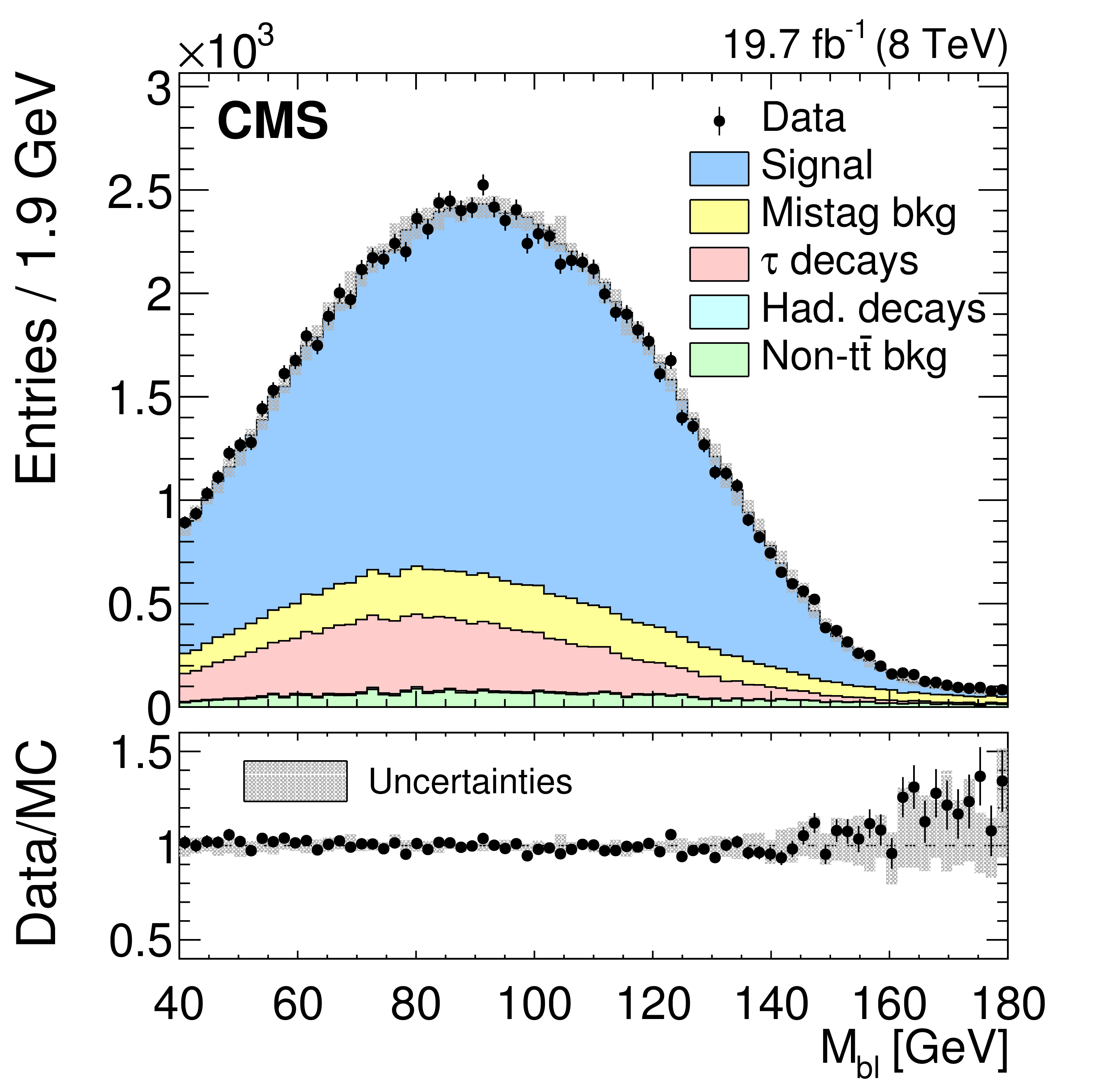
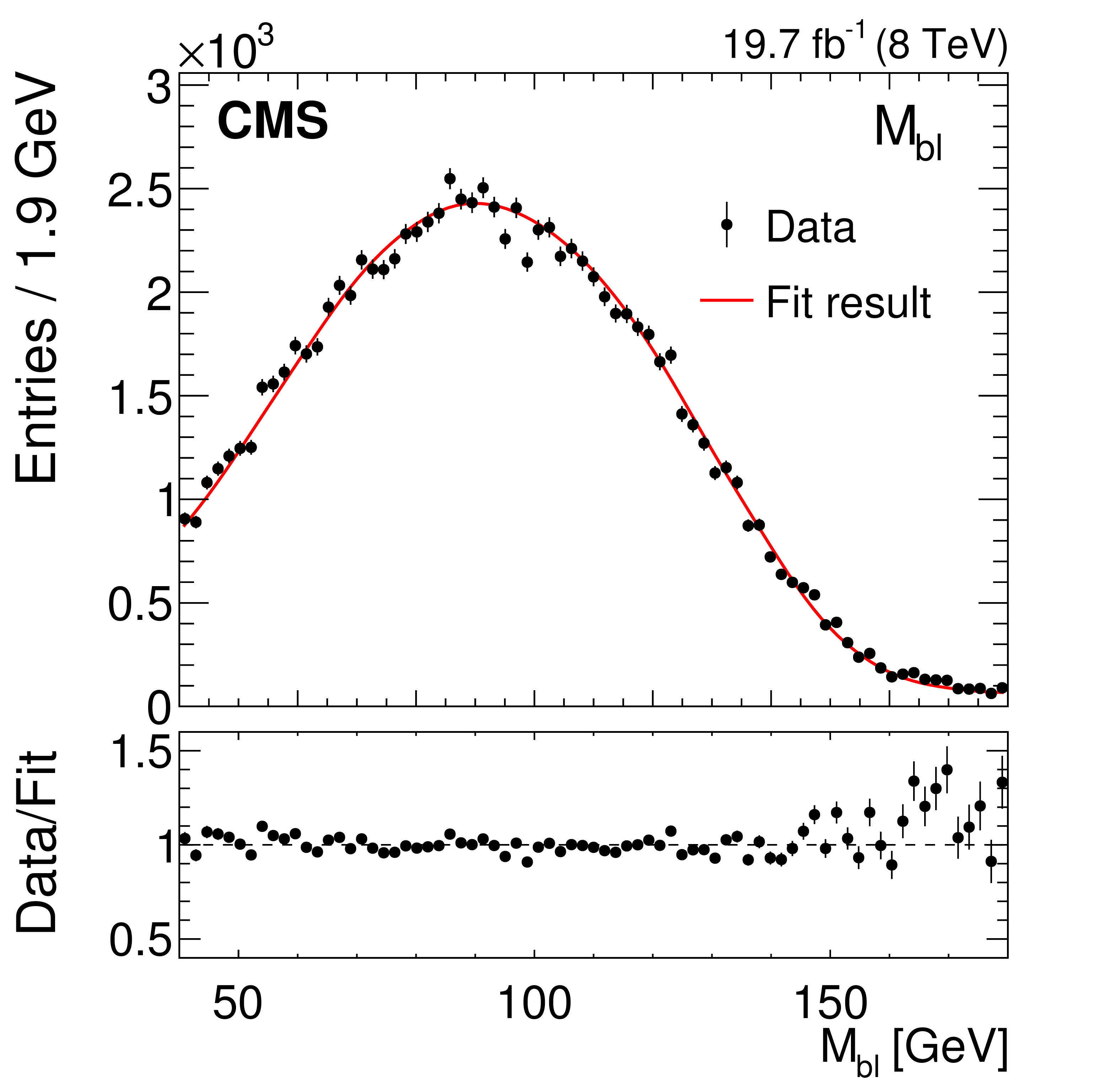
Figure 1-a:
The ${M_{\mathrm{ b } \ell }}$ distribution in data and simulation with $ {M_{\mathrm{ t } }^{\text {MC}}}= $ 172.5 GeV, normalized to the number of events in the 8 TeV data set corresponding to an integrated luminosity of 19.7 $\pm$ 0.5 fb$^{-1}$. The lower panel shows the ratio between the data and simulation. Statistical and systematic uncertainties on the distribution in simulation are represented by the shaded area. A description of the systematic uncertainties is given in Section 7. |

png pdf |
Figure 1-b:
The ${M_{\mathrm{ b } \ell }}$ distribution shapes in simulation, normalized to unit area, corresponding to three values of $ {M_{\mathrm{ t } }^{\text {MC}}}$ are shown together with the 'local shape sensitivity' function, described in Appendix {sec:sensitivity}. The ${M_{\mathrm{ b } \ell }}$ distributions include two or three values of ${M_{\mathrm{ b } \ell }}$ for each event. The distribution shapes are modeled with a GP regression technique, described in Section 5. |

png pdf |
Figure 2:
The ${M_{\mathrm {T}2}}$ subsystems in the dileptonic ${\mathrm{ t } {}\mathrm{ \bar{t} } } $ event topology. |
png pdf |
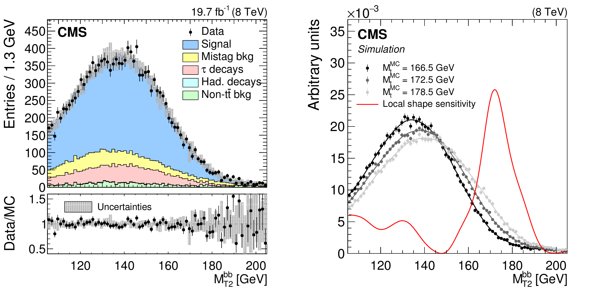
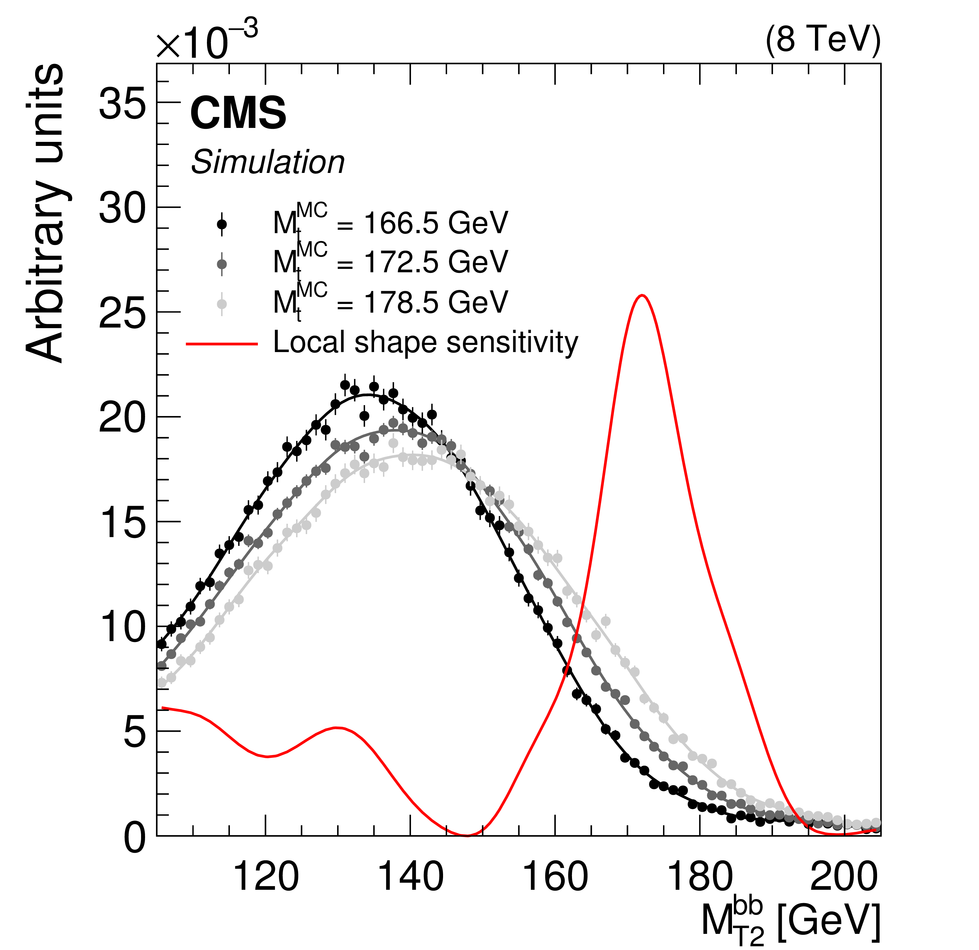
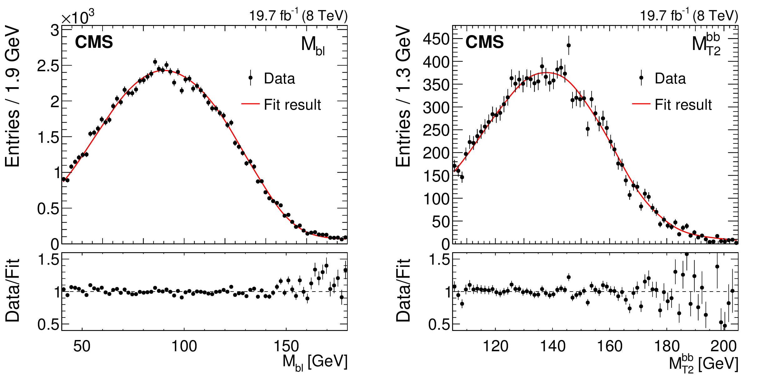
Figure 3:
Following the conventions of Fig. 1, shown are the (left) $ {M_{\mathrm {T}2}^{\mathrm{ b } \mathrm{ b } }}$ distribution in data and simulation with $ {M_{\mathrm{ t } }^{\text {MC}}}= $ 172.5 GeV, and (right) $ {M_{\mathrm {T}2}^{\mathrm{ b } \mathrm{ b } }}$ distribution shapes in simulation corresponding to three values of ${M_{\mathrm{ t } }^{\text {MC}}}$, along with the 'local shape sensitivity' function. The $ {M_{\mathrm {T}2}^{\mathrm{ b } \mathrm{ b } }}$ distributions include one value of $ {M_{\mathrm {T}2}^{\mathrm{ b } \mathrm{ b } }}$ for each event if it satisfies the kinematic requirement outlined in Section 4.2. |
png pdf |
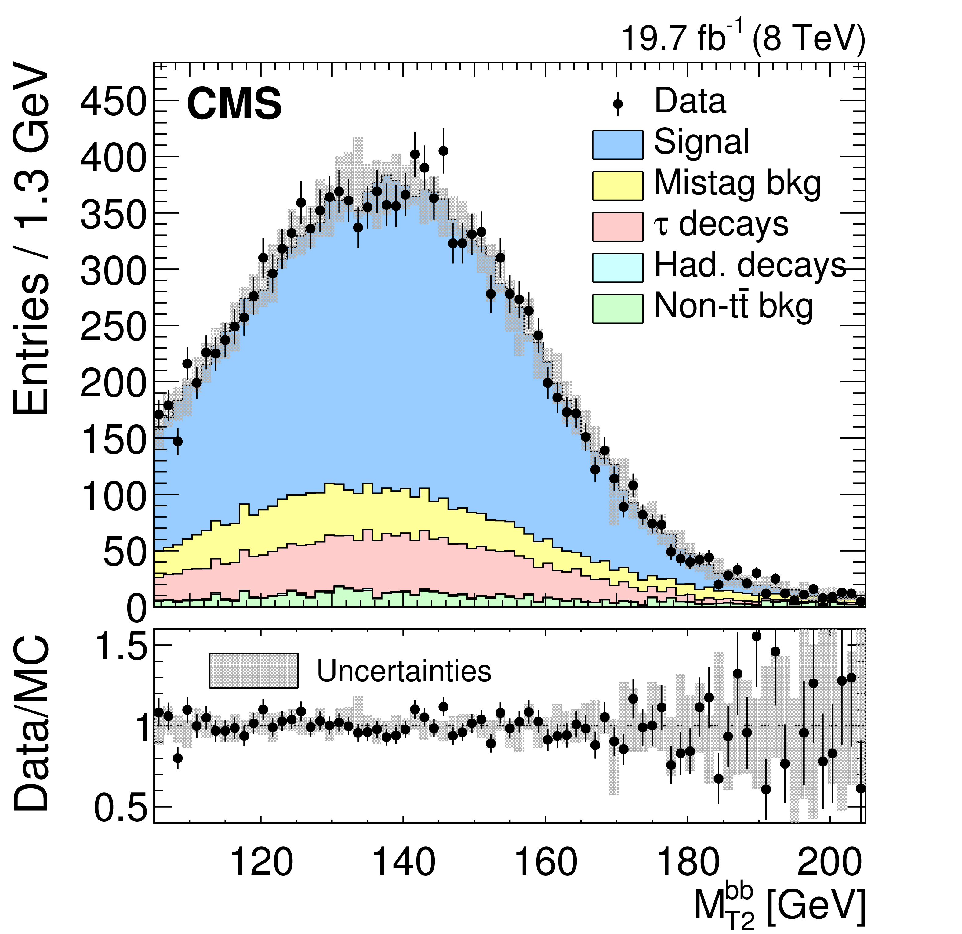
Figure 3-a:
Following the conventions of Fig. 1, shown is the $ {M_{\mathrm {T}2}^{\mathrm{ b } \mathrm{ b } }}$ distribution in data and simulation with $ {M_{\mathrm{ t } }^{\text {MC}}}= $ 172.5 GeV. The $ {M_{\mathrm {T}2}^{\mathrm{ b } \mathrm{ b } }}$ distribution includes one value of $ {M_{\mathrm {T}2}^{\mathrm{ b } \mathrm{ b } }}$ for each event if it satisfies the kinematic requirement outlined in Section 4.2. |
png pdf |
Figure 3-b:
Following the conventions of Fig. 1, shown is the $ {M_{\mathrm {T}2}^{\mathrm{ b } \mathrm{ b } }}$ distribution shapes in simulation corresponding to three values of ${M_{\mathrm{ t } }^{\text {MC}}}$, along with the 'local shape sensitivity' function. The $ {M_{\mathrm {T}2}^{\mathrm{ b } \mathrm{ b } }}$ distribution includes one value of $ {M_{\mathrm {T}2}^{\mathrm{ b } \mathrm{ b } }}$ for each event if it satisfies the kinematic requirement outlined in Section 4.2. |
png pdf |
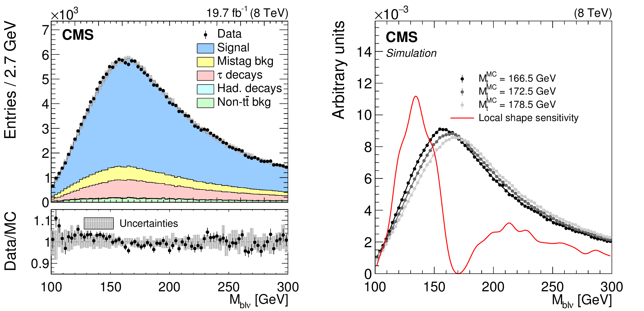
Figure 4:
Following the conventions of Fig. 1, shown are the (left) MAOS ${M_{\mathrm{ b } \ell \nu }}$ distribution in data and simulation with $ {M_{\mathrm{ t } }^{\text {MC}}}=$ 172.5 GeV, and (right) the MAOS ${M_{\mathrm{ b } \ell \nu }}$ distribution shapes in simulation corresponding to three values of $ {M_{\mathrm{ t } }^{\text {MC}}} $, along with the 'local shape sensitivity' function. The MAOS ${M_{\mathrm{ b } \ell \nu }}$ distributions include up to eight values of ${M_{\mathrm{ b } \ell \nu }}$ for each event. |

png pdf |
Figure 4-a:
Following the conventions of Fig. 1, shown is the MAOS ${M_{\mathrm{ b } \ell \nu }}$ distribution in data and simulation with $ {M_{\mathrm{ t } }^{\text {MC}}}=$ 172.5 GeV. The MAOS ${M_{\mathrm{ b } \ell \nu }}$ distribution includes up to eight values of ${M_{\mathrm{ b } \ell \nu }}$ for each event. |

png pdf |
Figure 4-b:
Following the conventions of Fig. 1, shown is the MAOS ${M_{\mathrm{ b } \ell \nu }}$ distribution shapes in simulation corresponding to three values of $ {M_{\mathrm{ t } }^{\text {MC}}} $, along with the 'local shape sensitivity' function. The MAOS ${M_{\mathrm{ b } \ell \nu }}$ distribution includes up to eight values of ${M_{\mathrm{ b } \ell \nu }}$ for each event. |
png pdf |
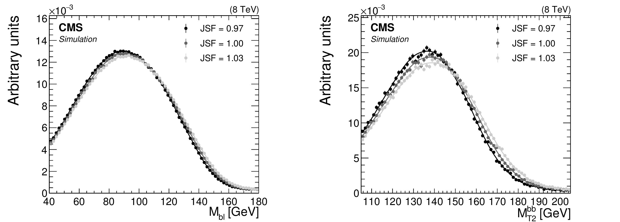
Figure 5:
The (left) ${M_{\mathrm{ b } \ell }}$ and (right) $ {M_{\mathrm {T}2}^{\mathrm{ b } \mathrm{ b } }}$ distributions in simulation with $ {M_{\mathrm{ t } }}= $ 172.5 GeV for several values of JSF. Two or three values are included in the ${M_{\mathrm{ b } \ell }}$ distribution for each event, and one value is included in the $ {M_{\mathrm {T}2}^{\mathrm{ b } \mathrm{ b } }}$ distribution if it satisfies the kinematic requirement outlined in Section 4.2. The distributions are normalized to unit area. The three curves corresponding to each of the ${M_{\mathrm{ b } \ell }}$ and $ {M_{\mathrm {T}2}^{\mathrm{ b } \mathrm{ b } }}$ distributions are obtained using a GP regression technique described in Section 5. |

png pdf |
Figure 5-a:
The ${M_{\mathrm{ b } \ell }}$ distribution in simulation with $ {M_{\mathrm{ t } }}= $ 172.5 GeV for several values of JSF. Two or three values are included in the ${M_{\mathrm{ b } \ell }}$ distribution for each event. The distributions are normalized to unit area. The three curves corresponding to each of the ${M_{\mathrm{ b } \ell }}$ distributions are obtained using a GP regression technique described in Section 5. |
png pdf |
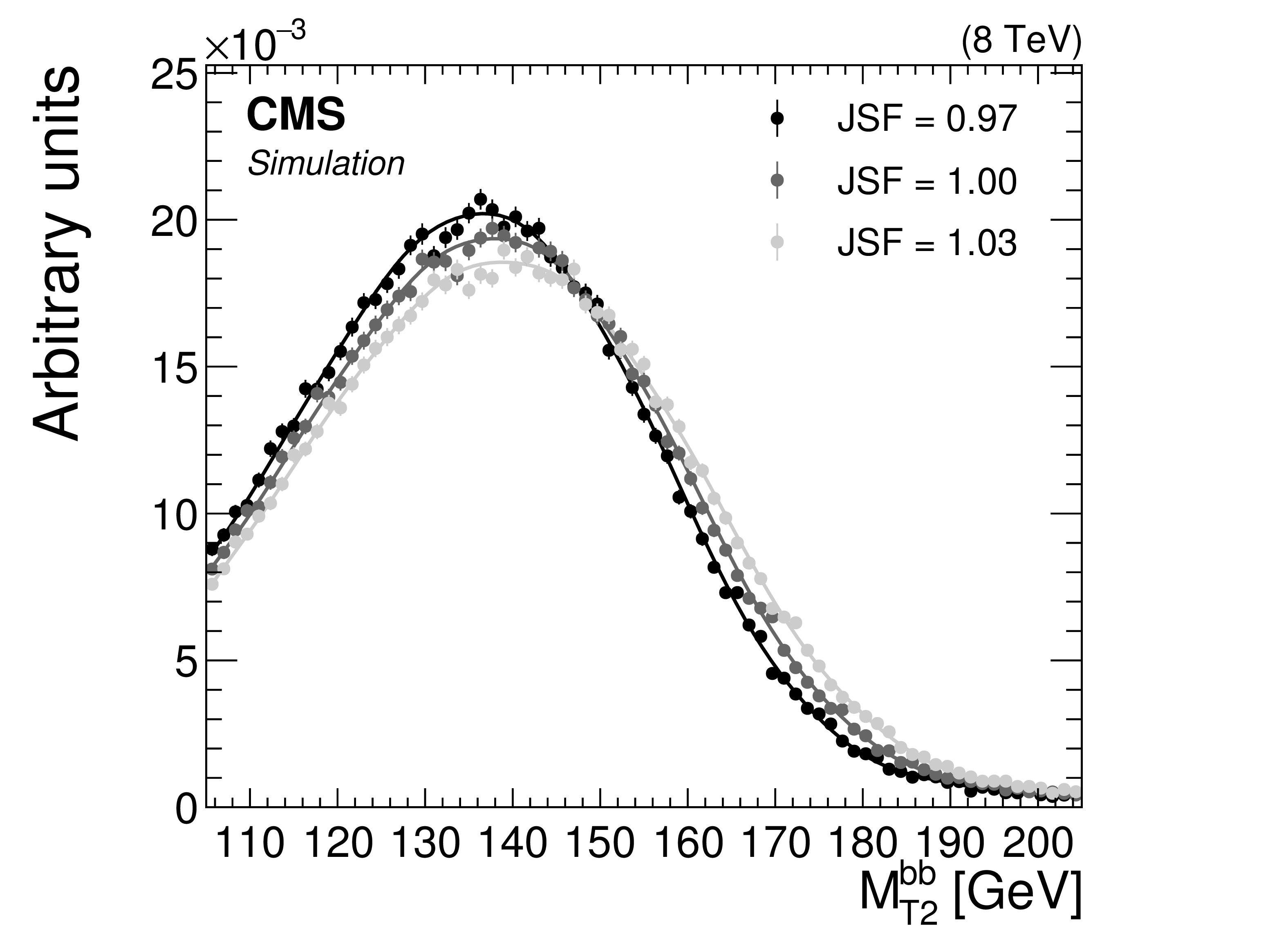
Figure 5-b:
The $ {M_{\mathrm {T}2}^{\mathrm{ b } \mathrm{ b } }}$ distribution in simulation with $ {M_{\mathrm{ t } }}= $ 172.5 GeV for several values of JSF. One value is included in the $ {M_{\mathrm {T}2}^{\mathrm{ b } \mathrm{ b } }}$ distribution if it satisfies the kinematic requirement outlined in Section 4.2. The distributions are normalized to unit area. The three curves corresponding to each of the $ {M_{\mathrm {T}2}^{\mathrm{ b } \mathrm{ b } }}$ distributions are obtained using a GP regression technique described in Section 5. |
png pdf |
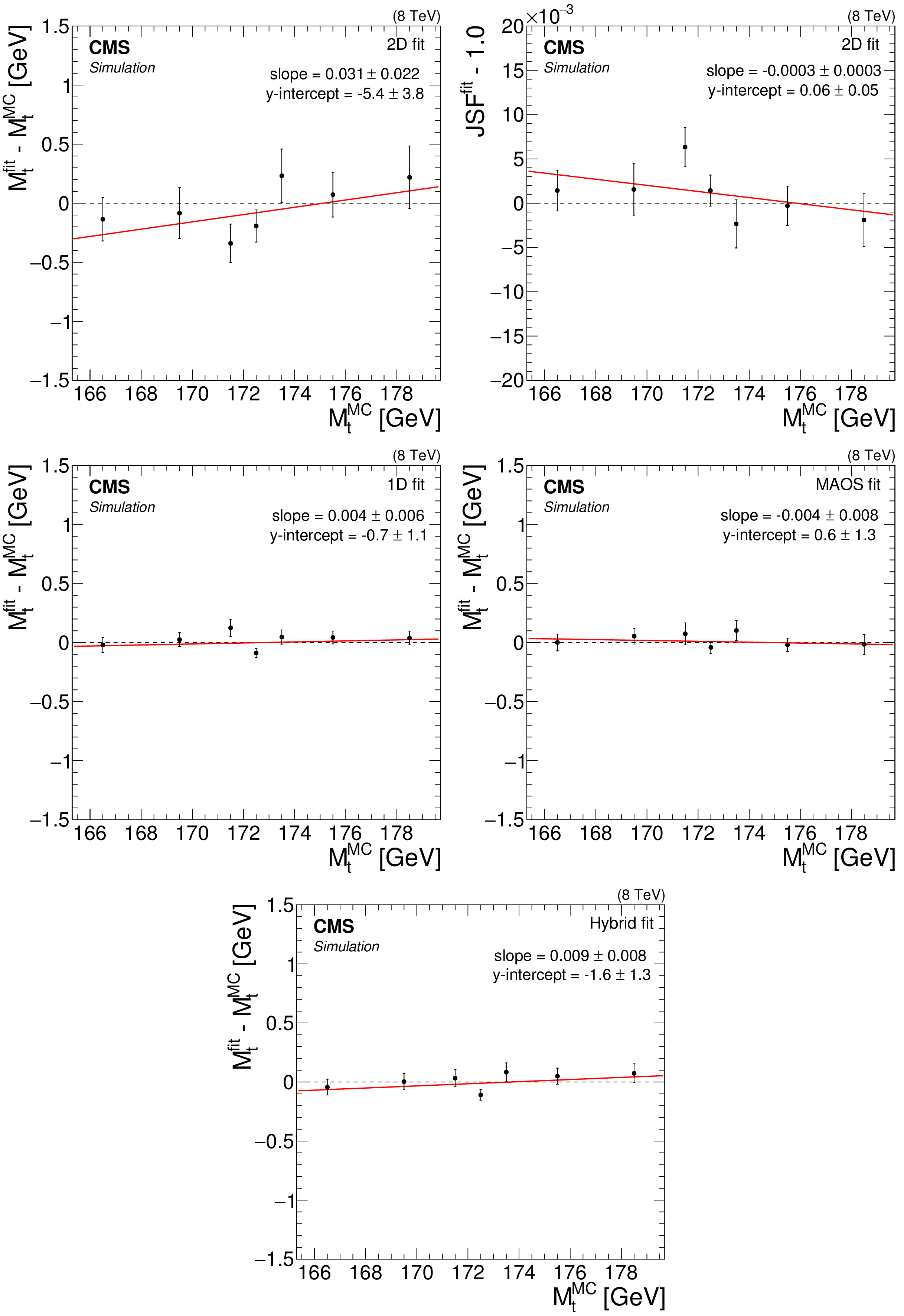
Figure 6:
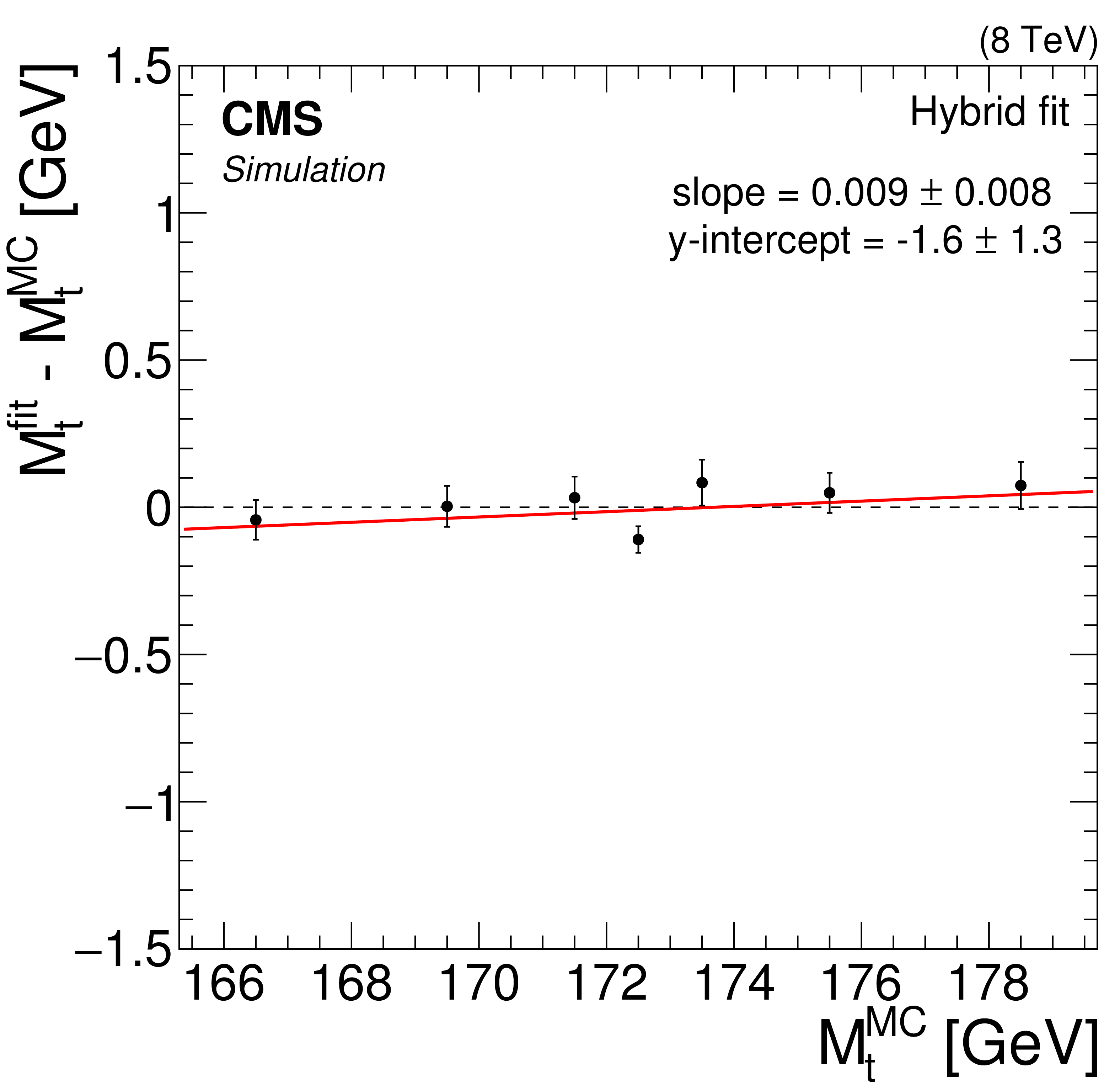
Likelihood fit results as a function of $ {M_{\mathrm{ t } }^{\text {MC}}}$ corresponding to the (top) 2D, (center left) 1D, (center right) MAOS, and (bottom) hybrid fits. For each value of $ {M_{\mathrm{ t } }^{\text {MC}}} $, the fit is conducted using 50 pseudo-experimentsin MC simulation. The mean parameter values, $ {M_{\mathrm{ t } }}^{\rm fit}$ and $ {\mathrm {JSF}}^{\rm fit}$, are represented by the points, with statistical uncertainties indicated by the error bars. A best-fit line of the form $y=ax + b$ is shown for each fit configuration. |

png pdf |
Figure 6-a:
Likelihood fit results as a function of $ {M_{\mathrm{ t } }^{\text {MC}}}$ corresponding to the 2D fit. For each value of $ {M_{\mathrm{ t } }^{\text {MC}}} $, the fit is conducted using 50 pseudo-experimentsin MC simulation. The mean parameter values $ {M_{\mathrm{ t } }}^{\rm fit}$ is represented by the points, with statistical uncertainties indicated by the error bars. A best-fit line of the form $y=ax + b$ is shown for each fit configuration. |
png pdf |
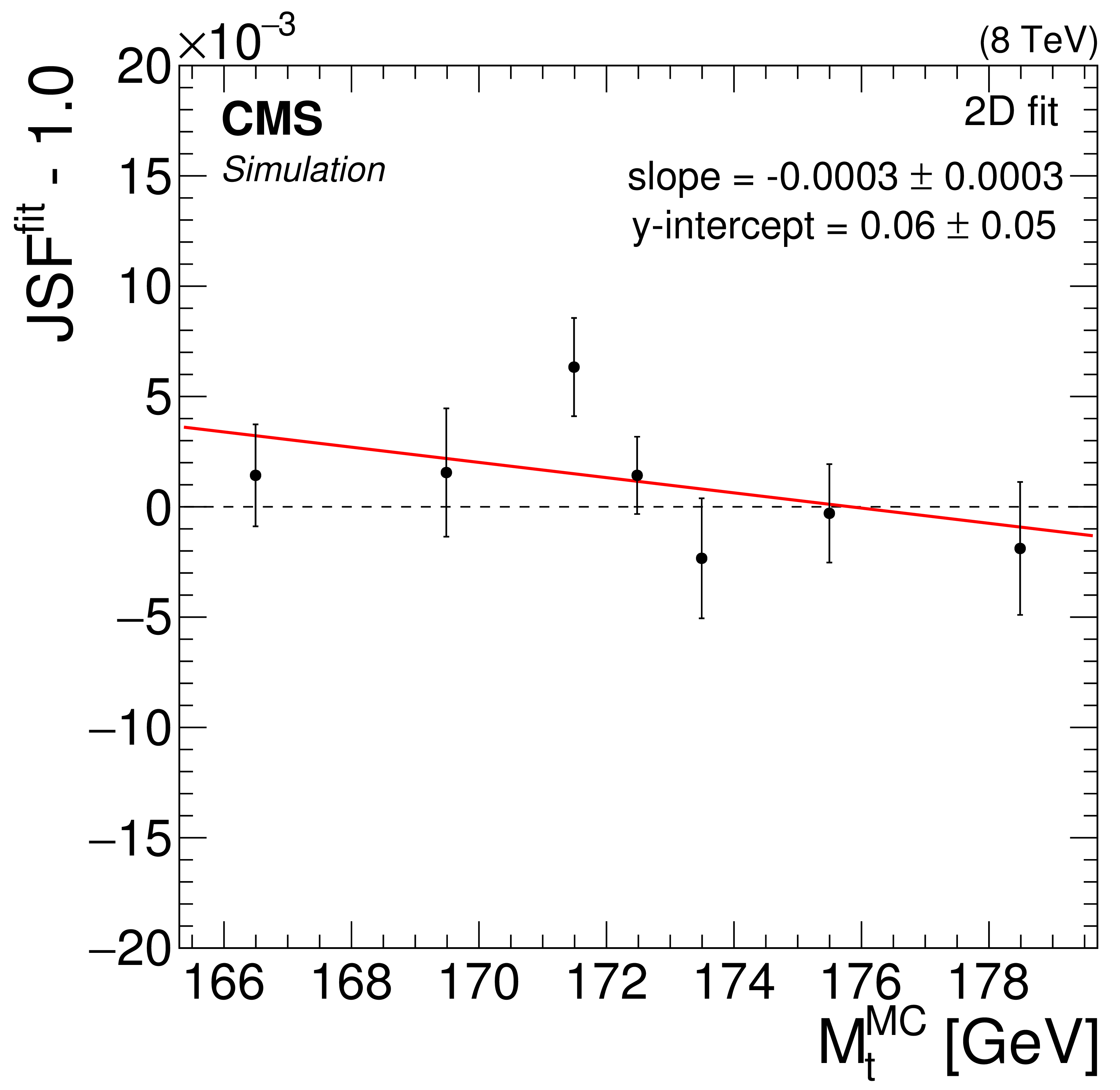
Figure 6-b:
Likelihood fit results as a function of $ {M_{\mathrm{ t } }^{\text {MC}}}$ corresponding to the 2D fit. For each value of $ {M_{\mathrm{ t } }^{\text {MC}}} $, the fit is conducted using 50 pseudo-experimentsin MC simulation. The mean parameter values $ {\mathrm {JSF}}^{\rm fit}$ is represented by the points, with statistical uncertainties indicated by the error bars. A best-fit line of the form $y=ax + b$ is shown for each fit configuration. |
png pdf |
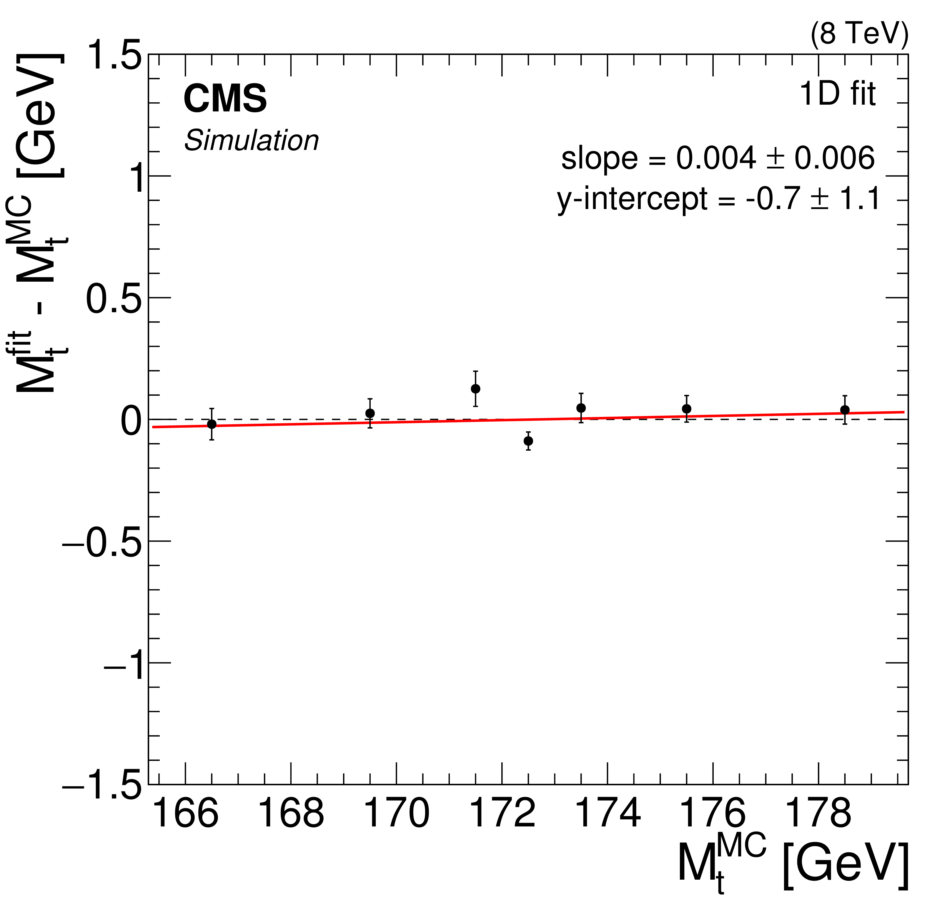
Figure 6-c:
Likelihood fit results as a function of $ {M_{\mathrm{ t } }^{\text {MC}}}$ corresponding to the 1D fit. For each value of $ {M_{\mathrm{ t } }^{\text {MC}}} $, the fit is conducted using 50 pseudo-experimentsin MC simulation. The mean parameter values $ {M_{\mathrm{ t } }}^{\rm fit}$ is represented by the points, with statistical uncertainties indicated by the error bars. A best-fit line of the form $y=ax + b$ is shown for each fit configuration. |
png pdf |
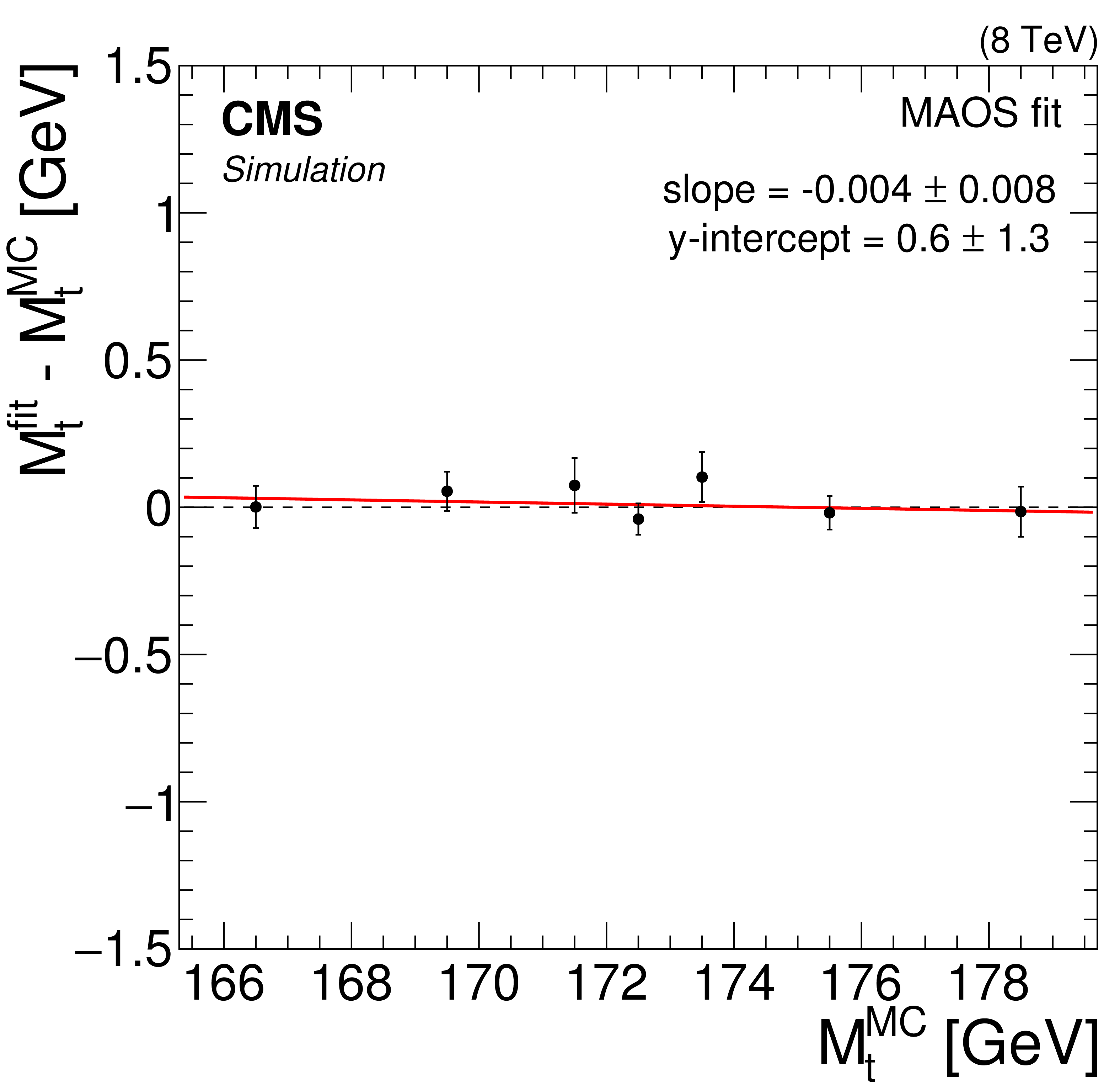
Figure 6-d:
Likelihood fit results as a function of $ {M_{\mathrm{ t } }^{\text {MC}}}$ corresponding to the MAOS fit. For each value of $ {M_{\mathrm{ t } }^{\text {MC}}} $, the fit is conducted using 50 pseudo-experimentsin MC simulation. The mean parameter values $ {M_{\mathrm{ t } }}^{\rm fit}$ is represented by the points, with statistical uncertainties indicated by the error bars. A best-fit line of the form $y=ax + b$ is shown for each fit configuration. |
png pdf |
Figure 6-e:
Likelihood fit results as a function of $ {M_{\mathrm{ t } }^{\text {MC}}}$ corresponding to the hybrid fit. For each value of $ {M_{\mathrm{ t } }^{\text {MC}}} $, the fit is conducted using 50 pseudo-experimentsin MC simulation. The mean parameter values $ {M_{\mathrm{ t } }}^{\rm fit}$ is represented by the points, with statistical uncertainties indicated by the error bars. A best-fit line of the form $y=ax + b$ is shown for each fit configuration. |

png pdf |
Figure 7:
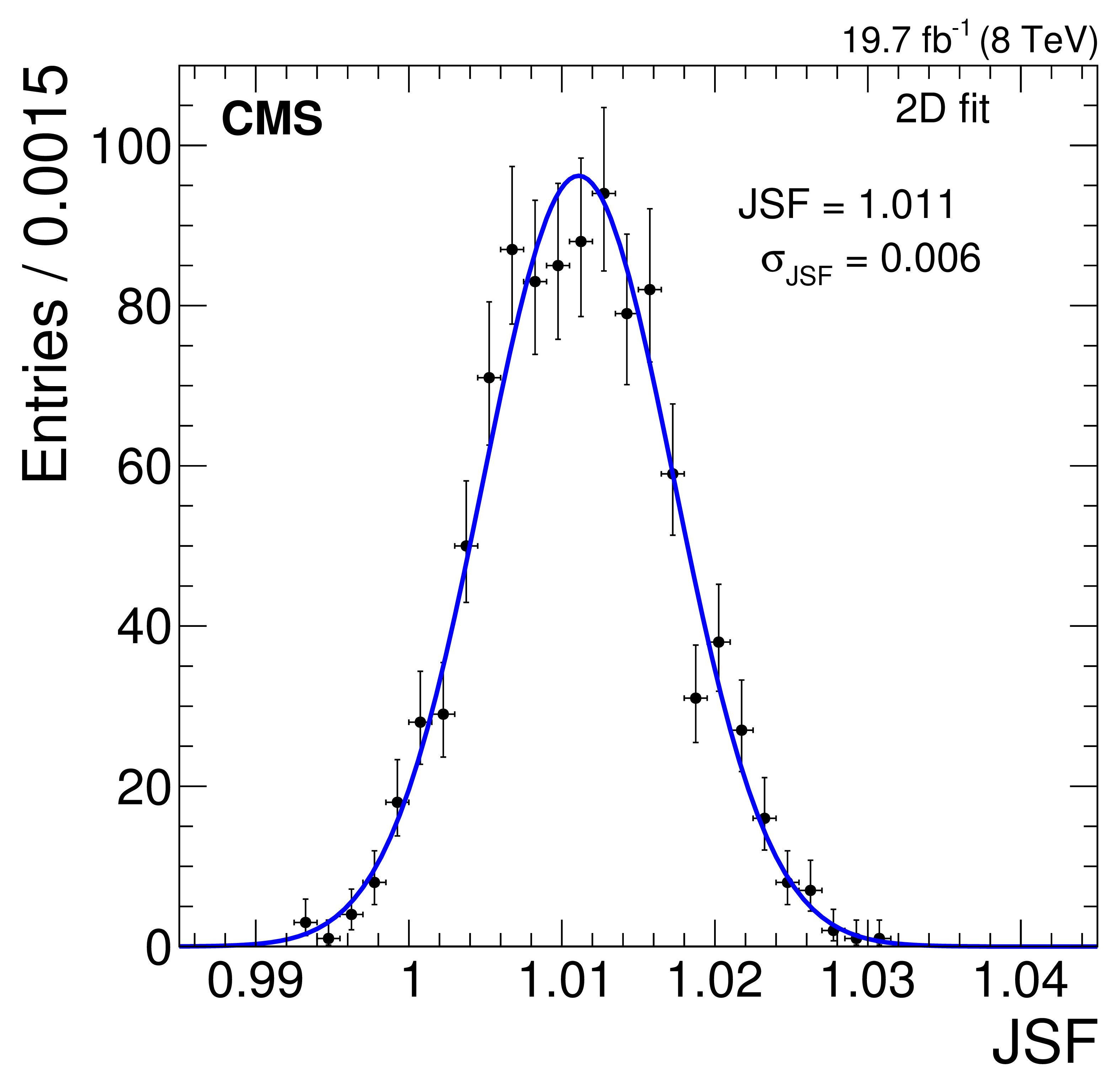
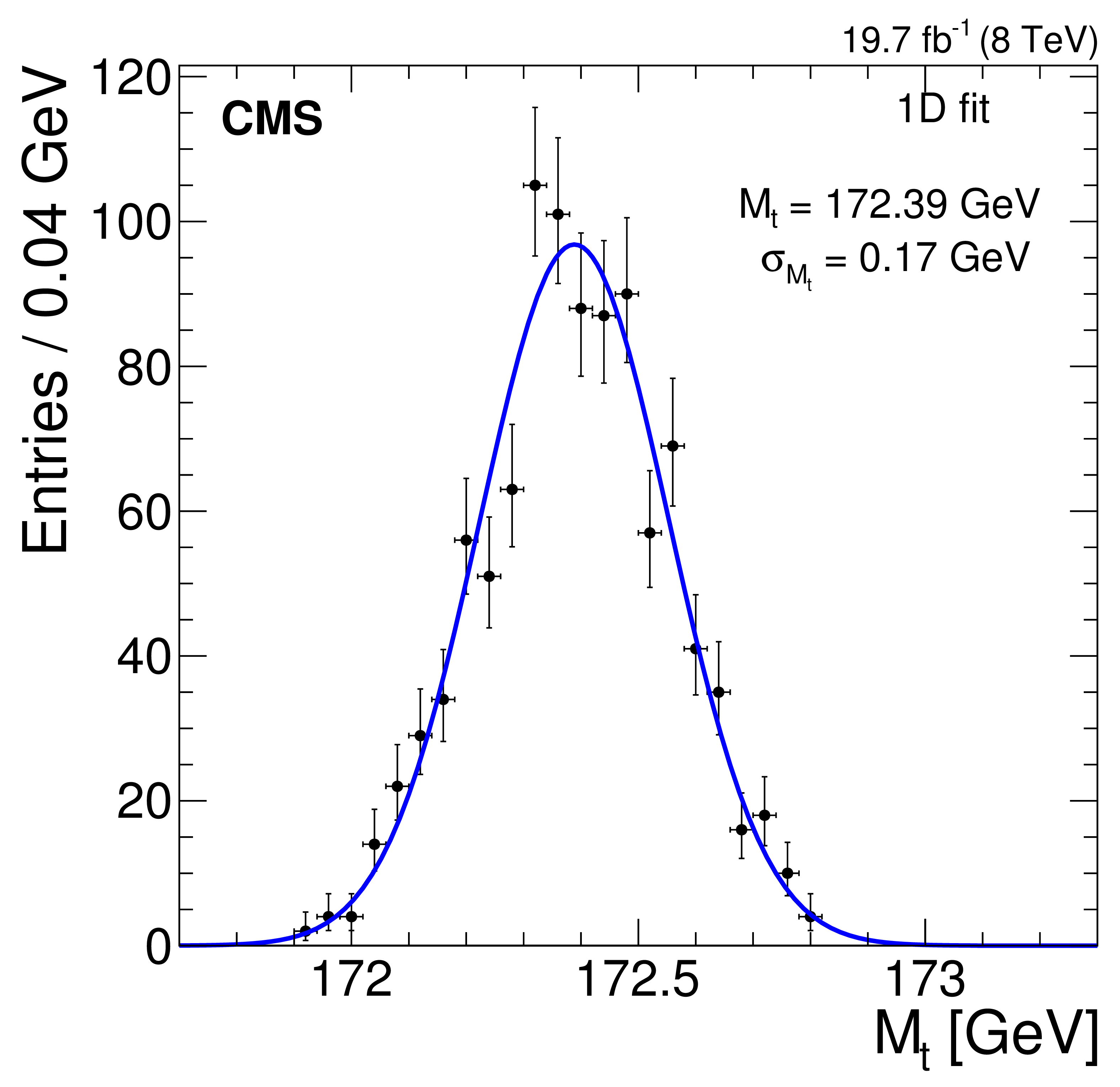
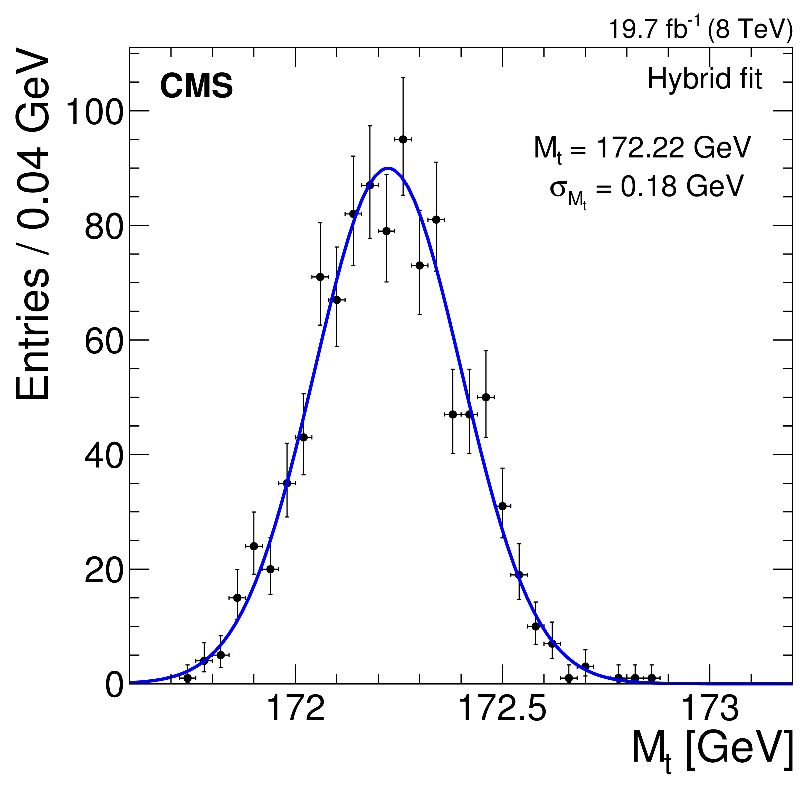
Likelihood fit results using 1000 bootstrap pseudo-experiments for the (top) 2D fit, (center left) 1D fit, (center right) MAOS fit. (Bottom) hybrid fit results given by the linear combination in Eq. (9) of the 1D and 2D fits. The error bars represent the statistical uncertainty corresponding to the number of pseudo-experiments in each bin. |

png pdf |
Figure 7-a:
Likelihood fit results using 1000 bootstrap pseudo-experiments for the 2D fit, for ${M_{\mathrm{ t } }}$. The error bars represent the statistical uncertainty corresponding to the number of pseudo-experiments in each bin. |
png pdf |
Figure 7-b:
Likelihood fit results using 1000 bootstrap pseudo-experiments for the 2D fit, for JSF. The error bars represent the statistical uncertainty corresponding to the number of pseudo-experiments in each bin. |
png pdf |
Figure 7-c:
Likelihood fit results using 1000 bootstrap pseudo-experiments for the 1D fit. The error bars represent the statistical uncertainty corresponding to the number of pseudo-experiments in each bin. |

png pdf |
Figure 7-d:
Likelihood fit results using 1000 bootstrap pseudo-experiments for the MAOS fit. The error bars represent the statistical uncertainty corresponding to the number of pseudo-experiments in each bin. |
png pdf |
Figure 7-e:
Likelihood fit results using 1000 bootstrap pseudo-experiments for the hybrid fit results given by the linear combination in Eq. (9) of the 1D and 2D fits. The error bars represent the statistical uncertainty corresponding to the number of pseudo-experiments in each bin. |
png pdf |
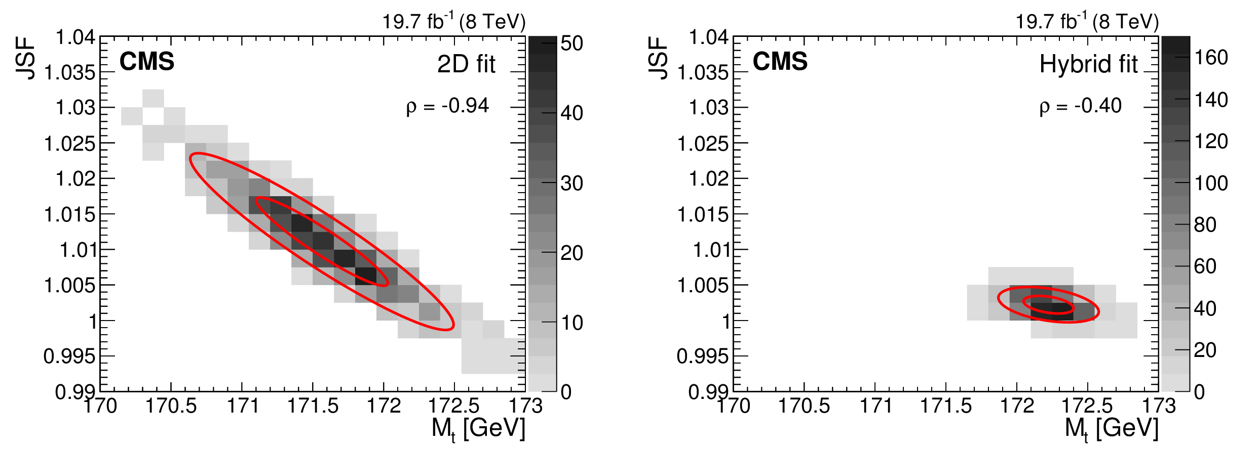
Figure 8:
Likelihood fit results corresponding to the 2D fit (left) and hybrid fit (right), obtained using 1000 pseudo-experiments constructed with the bootstrapping technique. The shaded histogram represents the number of pseudo-experiments in each bin of ${M_{\mathrm{ t } }}$ and JSF. Two-dimensional contours corresponding to $-2\Delta \log(\mathcal {L})=$ 1 (4) are shown, allowing the construction of one (two) $\sigma $ statistical intervals in ${M_{\mathrm{ t } }}$ and JSF. The hybrid fit results are given by a linear combination of the 1D and 2D fit results using Eq. (9). |
png pdf |
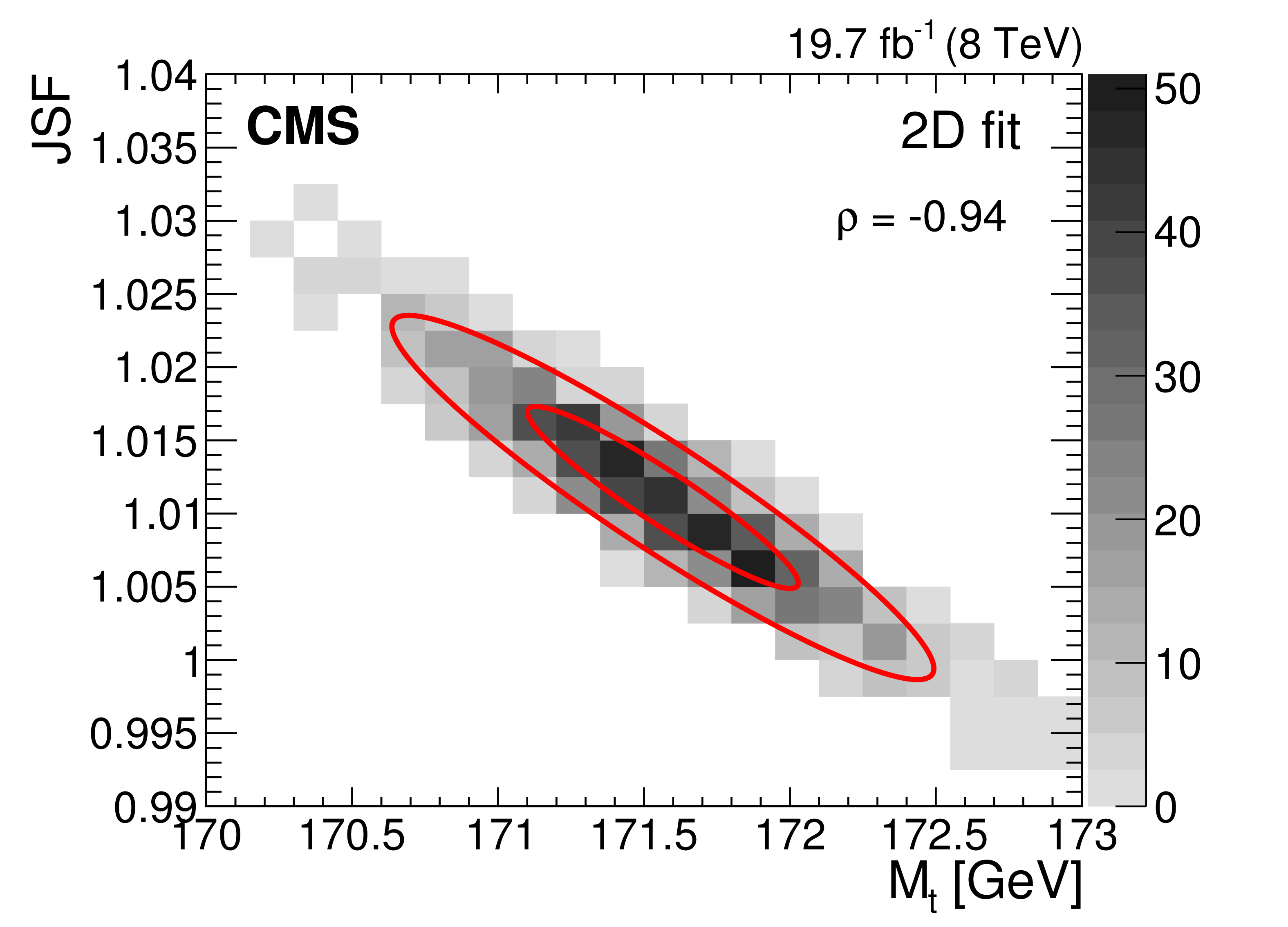
Figure 8-a:
Likelihood fit results corresponding to the 2D fit, obtained using 1000 pseudo-experiments constructed with the bootstrapping technique. The shaded histogram represents the number of pseudo-experiments in each bin of ${M_{\mathrm{ t } }}$ and JSF. Two-dimensional contours corresponding to $-2\Delta \log(\mathcal {L})=$ 1 (4) are shown, allowing the construction of one (two) $\sigma $ statistical intervals in ${M_{\mathrm{ t } }}$ and JSF. The hybrid fit results are given by a linear combination of the 1D and 2D fit results using Eq. (9). |

png pdf |
Figure 8-b:
Likelihood fit results corresponding to the hybrid fit, obtained using 1000 pseudo-experiments constructed with the bootstrapping technique. The shaded histogram represents the number of pseudo-experiments in each bin of ${M_{\mathrm{ t } }}$ and JSF. Two-dimensional contours corresponding to $-2\Delta \log(\mathcal {L})=$ 1 (4) are shown, allowing the construction of one (two) $\sigma $ statistical intervals in ${M_{\mathrm{ t } }}$ and JSF. The hybrid fit results are given by a linear combination of the 1D and 2D fit results using Eq. (9). |
png pdf |
Figure 9:
Maximum-likelihood fit result in a typical pseudo-experiment of the 2D likelihood fit in data. The best fit parameter values for this pseudo-experimentare $ {M_{\mathrm{ t } }}= $ 171.99 GeV and JSF = 1.007. When the JSF parameter is constrained to be unity in the 1D likelihood fit, the best fit value of ${M_{\mathrm{ t } }}$ is 172.48 GeV. The lower panel shows the ratio between the distribution in data and the best fit distribution in simulation. |
png pdf |
Figure 9-a:
Maximum-likelihood fit result in a typical pseudo-experiment of the 2D likelihood fit in data. The best fit parameter values for this pseudo-experimentare $ {M_{\mathrm{ t } }}= $ 171.99 GeV and JSF = 1.007. When the JSF parameter is constrained to be unity in the 1D likelihood fit, the best fit value of ${M_{\mathrm{ t } }}$ is 172.48 GeV. The lower panel shows the ratio between the distribution in data and the best fit distribution in simulation. |

png pdf |
Figure 9-b:
Maximum-likelihood fit result in a typical pseudo-experiment of the 2D likelihood fit in data. The best fit parameter values for this pseudo-experimentare $ {M_{\mathrm{ t } }}= $ 171.99 GeV and JSF = 1.007. When the JSF parameter is constrained to be unity in the 1D likelihood fit, the best fit value of ${M_{\mathrm{ t } }}$ is 172.48 GeV. The lower panel shows the ratio between the distribution in data and the best fit distribution in simulation. |
png pdf |
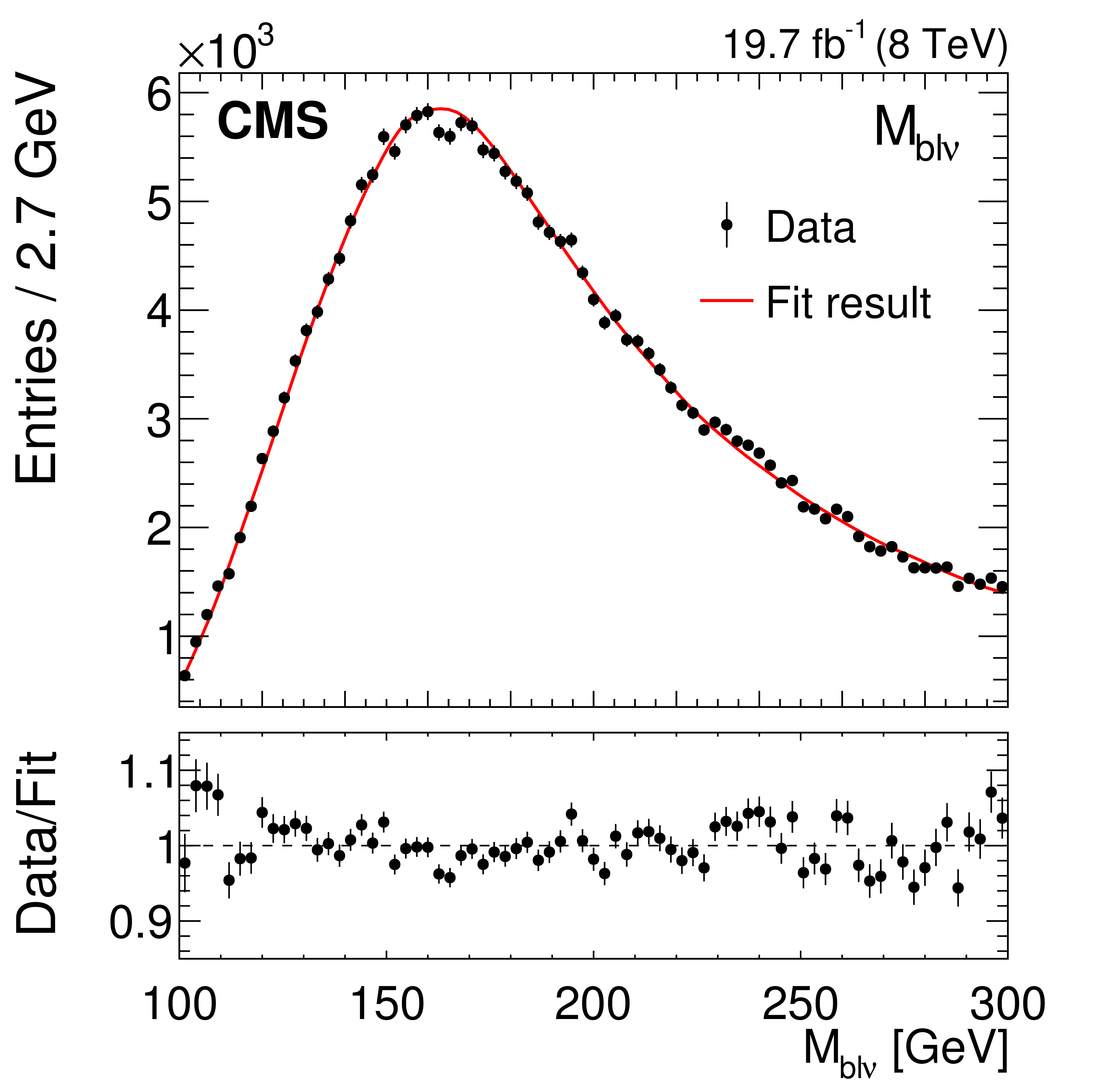
Figure 10:
The MAOS ${M_{\mathrm{ b } \ell \nu }}$ distribution corresponding to the maximum-likelihood fit result in a typical pseudo-experimentof the MAOS likelihood fit in data. The best fit value of ${M_{\mathrm{ t } }}$ for this pseudo-experimentis 171.54 GeV. The lower panel shows the ratio between the distribution in data and the best fit distribution in simulation. |
png pdf |
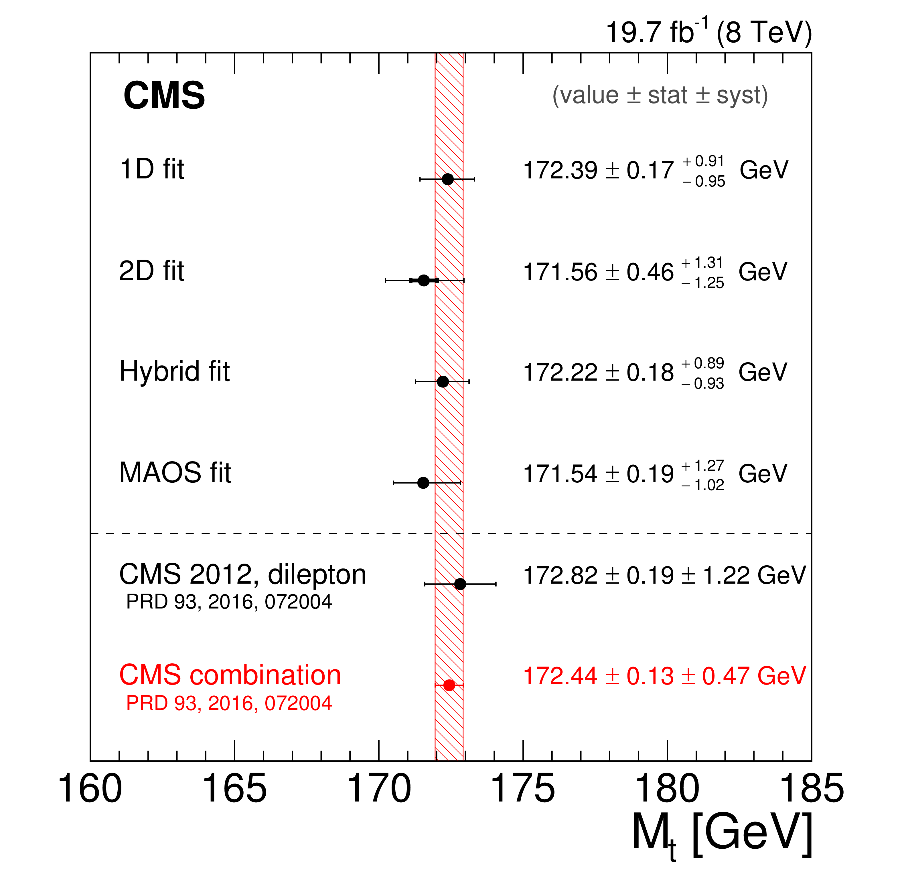
Figure 11:
Summary of the 1D, 2D, hybrid, and MAOS likelihood fit results using the 2012 data set at $ \sqrt{s} = $ 8 TeV, corresponding to an integrated luminosity of 19.7 $\pm$ 0.5 fb$^{-1}$. A recent dileptonic channel measurement using the 2012 data set and the most recent combination of ${M_{\mathrm{ t } }}$ measurements by CMS [6] are shown for reference. |
png pdf |
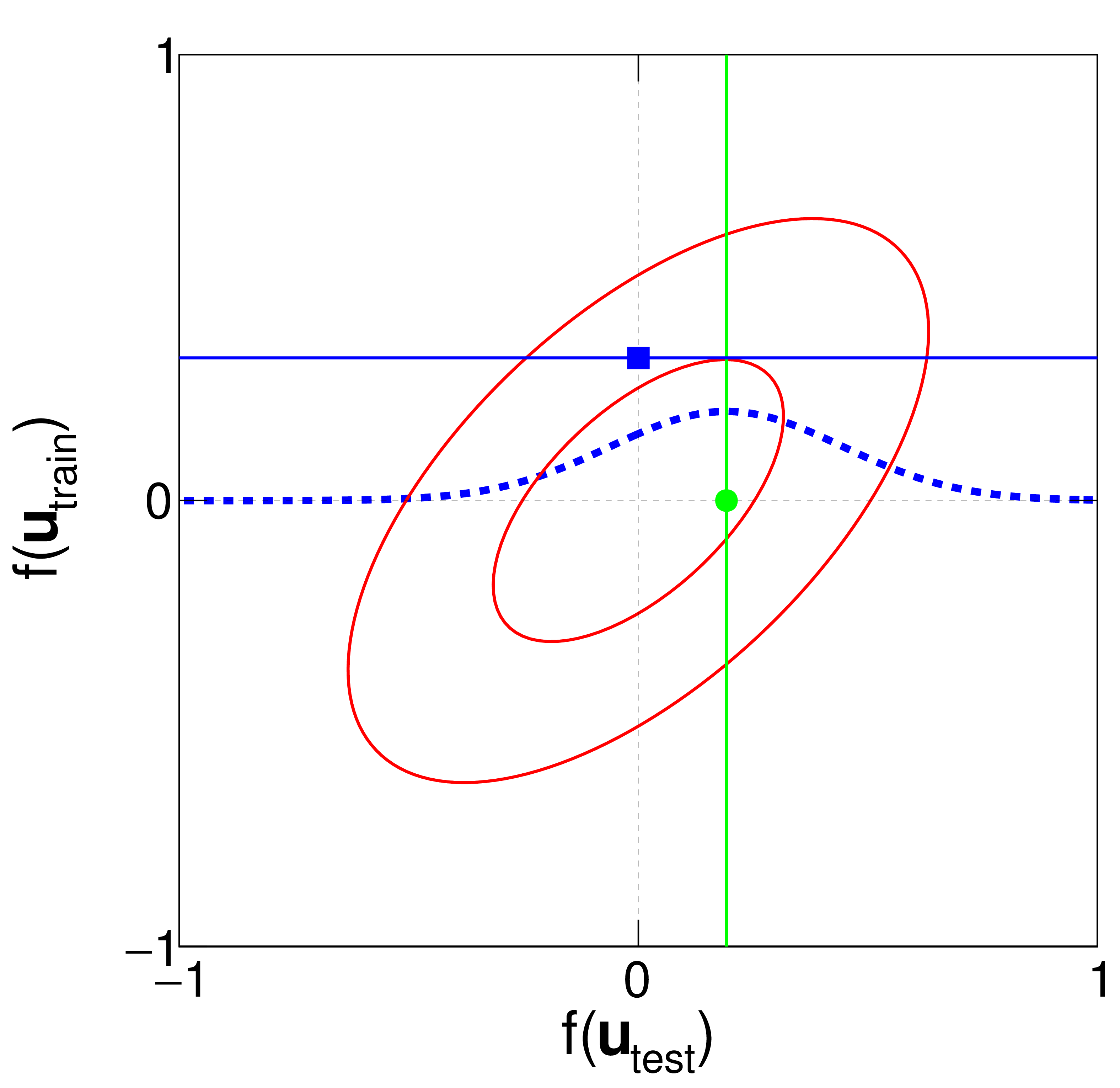
Figure 12:
Demonstration of the GP conditioning process, given in Eqs.(16) and (17), for one training point and one test point. The covariance between the value of the shape at the training and test point is represented by the ellipse. The known value of the shape at the training point (square point) determines the mean value of the shape at the test point (round point and vertical line). The distribution of possible values of the shape at the test point is represented by the dashed curve. |
| Tables | |
png pdf |
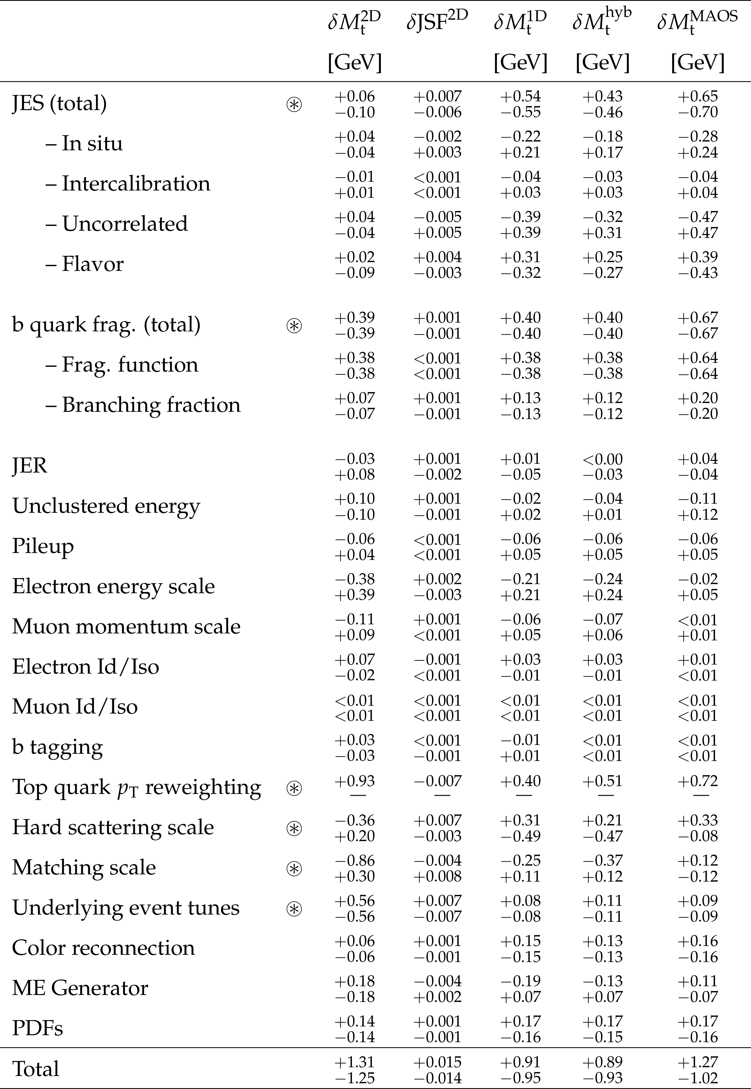
Table 1:
Systematic uncertainties for the 2D, 1D, hybrid, and MAOS likelihood fits. The breakdown of JES and b quark fragmentation uncertainties into separate components is shown, where the components are added in quadrature to obtain the total. The 'up' and 'down' variations are given separately, with the sign of each variation indicating the direction of the corresponding shift in ${M_{\mathrm{ t } }}$ or JSF. The circled star character highlights the uncertainty sources that are large in at least one of the likelihood fits. |
| Summary |
| A measurement of the top quark mass ($M_{\mathrm{ t }}$) in the dileptonic $\mathrm{ t \bar{t} }$ decay channel is performed using proton-proton collisions at $ \sqrt{s} = $ 8 TeV, corresponding to an integrated luminosity of 19.7 $\pm$ 0.5 fb$^{-1}$. The measurement is based on the mass observables $M_{\mathrm{ b }\ell}$, $M_{\mathrm{T}2}^{\mathrm{ b }\mathrm{ b }}$, and $M_{\mathrm{ b }\ell\nu}$, which allow for mass reconstruction in decay topologies that are kinematically underconstrained. The sensitivity of these observables to the value of $M_{\mathrm{ t }}$ is investigated using a Fisher information density technique. The observables are employed in three versions of an unbinned likelihood fit, where a Gaussian process technique is used to model the corresponding distribution shapes and their evolution in $M_{\mathrm{ t }}$ and an overall jet energy scale factor (JSF). The Gaussian process shapes are nonparametric, and allow for a likelihood fitting framework that gives unbiased results. The 2D fit provides the first simultaneous measurement of $M_{\mathrm{ t }}$ and JSF in the dileptonic channel. It is robust against uncertainties due to the determination of jet energy scale, including the flavor-dependent uncertainty component arising from differences in the response between b jets, light-quark jets, and gluon jets. The fit yields $M_{\mathrm{ t }} =$ 171.56 $\pm$ 0.46 (stat) $^{+1.31}_{-1.25}$ (syst) GeV and JSF = 1.011 $\pm$ 0.006 (stat) $^{+0.015}_{-0.014}$ (syst). The most precise measurement of $M_{\mathrm{ t }}$ is given by a linear combination of this result with a fit in which the JSF is constrained to be unity, yielding a value of 172.22 $\pm$ 0.18 (stat) $^{+0.89}_{-0.93}$ (syst) GeV. |
| References | ||||
| 1 | Gfitter Group | The global electroweak fit at NNLO and prospects for the LHC and ILC | EPJC 74 (2014) 3046 | 1407.3792 |
| 2 | G. Degrassi et al. | Higgs mass and vacuum stability in the Standard Model at NNLO | JHEP 08 (2012) 098 | 1205.6497 |
| 3 | A. H. Hoang and I. W. Stewart | Top Mass Measurements from Jets and the Tevatron Top-Quark Mass | NPPS 185 (2008) 220 | 0808.0222 |
| 4 | ATLAS, CDF, CMS, and D0 Collaborations | First combination of Tevatron and LHC measurements of the top-quark mass | 1403.4427 | |
| 5 | ATLAS Collaboration | Measurement of the top quark mass in the $ \mathrm{ t \bar{t} } \to $ dilepton channel from $ \sqrt{s}= $ 8 TeV ATLAS data | PLB 761 (2016) 350 | 1606.02179 |
| 6 | CMS Collaboration | Measurement of the top quark mass using proton-proton data at $ \sqrt{s}= $ 7 and 8 TeV | PRD 93 (2016) 072004 | CMS-TOP-14-022 1509.04044 |
| 7 | A. J. Barr and C. G. Lester | A review of the mass measurement techniques proposed for the Large Hadron Collider | JPG 37 (2010) 123001 | 1004.2732 |
| 8 | C. G. Lester and D. J. Summers | Measuring masses of semi-invisibly decaying particle pairs produced at hadron colliders | PLB 463 (1999) 99 | hep-ph/9906349 |
| 9 | H.-C. Cheng and Z. Han | Minimal kinematic constraints and $ m_{\mathrm{t \bar{t}}} $ | JHEP 12 (2008) 063 | 0810.5178 |
| 10 | W. S. Cho, K. Choi, Y. G. Kim, and C. B. Park | $ m_{\mathrm{t \bar{t}}} $-assisted on-shell reconstruction of missing momenta and its application to spin measurement at the LHC | PRD 79 (2009) 031701 | 0810.4853 |
| 11 | CMS Collaboration | Measurement of masses in the $ \mathrm{ t \bar{t} } $ system by kinematic endpoints in pp collisions at $ \sqrt{s} = $ 7 TeV | EPJC 73 (2013) 2494 | CMS-TOP-11-027 1304.5783 |
| 12 | C. E. Rasmussen and C. K. I. Williams | Gaussian Processes for Machine Learning | MIT Press, 2006 ISBN 026218253X | |
| 13 | C. Bishop | Pattern recognition and machine learning | Springer-Verlag, New York, 1 edition, 2006 ISBN 9780387310732 | |
| 14 | CMS Collaboration | The CMS trigger system | JINST 12 (2017) P01020 | CMS-TRG-12-001 1609.02366 |
| 15 | CMS Collaboration | The CMS experiment at the CERN LHC | JINST 3 (2008) S08004 | CMS-00-001 |
| 16 | CMS Collaboration | CMS Luminosity Based on Pixel Cluster Counting - Summer 2013 Update | CMS-PAS-LUM-13-001 | CMS-PAS-LUM-13-001 |
| 17 | CMS Collaboration | Particle-Flow Event Reconstruction in CMS and Performance for Jets, Taus, and $ p_{\mathrm{T}}^{\text{miss}} $ | CDS | |
| 18 | CMS Collaboration | Commissioning of the Particle-flow Event Reconstruction with the first LHC collisions recorded in the CMS detector | CDS | |
| 19 | CMS Collaboration | Performance of electron reconstruction and selection with the CMS detector in proton-proton collisions at $ \sqrt{s} = $ 8 TeV | JINST 10 (2015) P06005 | CMS-EGM-13-001 1502.02701 |
| 20 | CMS Collaboration | Performance of CMS muon reconstruction in pp collision events at $ \sqrt{s} = $ 7 TeV | JINST 7 (2012) P10002 | CMS-MUO-10-004 1206.4071 |
| 21 | Particle Data Group, C. Patrignani et al. | Review of particle physics | CPC 40 (2016) 100001 | |
| 22 | M. Cacciari, G. P. Salam, and G. Soyez | The anti-$ k_{\mathrm{t}} $ jet clustering algorithm | JHEP 04 (2008) 063 | 0802.1189 |
| 23 | M. Cacciari, G. P. Salam, and G. Soyez | FastJet user manual | EPJC 72 (2012) 1896 | 1111.6097 |
| 24 | CMS Collaboration | Jet energy scale and resolution in the CMS experiment in pp collisions at 8 TeV | JINST 12 (2017) P02014 | CMS-JME-13-004 1607.03663 |
| 25 | CMS Collaboration | Identification of b-quark jets with the CMS experiment | JINST 8 (2013) P04013 | CMS-BTV-12-001 1211.4462 |
| 26 | CMS Collaboration | Performance of the CMS missing transverse momentum reconstruction in pp data at $ \sqrt{s} = $ 8 TeV | JINST 10 (2015) P02006 | CMS-JME-13-003 1411.0511 |
| 27 | J. Alwall et al. | The automated computation of tree-level and next-to-leading order differential cross sections, and their matching to parton shower simulations | JHEP 07 (2014) 079 | 1405.0301 |
| 28 | P. Artoisenet, R. Frederix, O. Mattelaer, and R. Rietkerk | Automatic spin-entangled decays of heavy resonances in Monte Carlo simulations | JHEP 03 (2013) 015 | 1212.3460 |
| 29 | T. Sjostrand, S. Mrenna, and P. Skands | PYTHIA 6.4 physics and manual | JHEP 05 (2006) 026 | hep-ph/0603175 |
| 30 | S. Jadach, Z. Was, R. Decker, and J. H. Kuhn | The tau decay library TAUOLA: Version 2.4 | CPC 76 (1993) 361 | |
| 31 | W.-K. Tung | New Generation of Parton Distributions with Uncertainties from Global QCD Analysis | Acta Phys. Polon. B 33 (2002) 2933 | hep-ph/0206114 |
| 32 | S. Alioli, P. Nason, C. Oleari, and E. Re | NLO single-top production matched with shower in POWHEG: $ s $- and $ t $-channel contributions | JHEP 09 (2009) 111, , [Erratum: \DOI10.1007/JHEP02(2010)011] | 0907.4076 |
| 33 | E. Re | Single-top $ Wt $-channel production matched with parton showers using the POWHEG method | EPJC 71 (2011) 1547 | 1009.2450 |
| 34 | S. Frixione, P. Nason, and C. Oleari | Matching NLO QCD computations with Parton Shower simulations: the POWHEG method | JHEP 11 (2007) 070 | 0709.2092 |
| 35 | S. Alioli, P. Nason, C. Oleari, and E. Re | A general framework for implementing NLO calculations in shower Monte Carlo programs: the POWHEG BOX | JHEP 06 (2010) 043 | 1002.2581 |
| 36 | GEANT4 Collaboration | GEANT4---a simulation toolkit | NIMA 506 (2003) | |
| 37 | N. Kidonakis | Next-to-next-to-leading soft-gluon corrections for the top quark cross section and transverse momentum distribution | PRD 82 (2010) 114030 | 1009.4935 |
| 38 | N. Kidonakis | Differential and total cross sections for top pair and single top production | in Proceedings, 20th International Workshop on Deep-Inelastic Scattering and Related Subjects (DIS 2012), p. 831 2012 | 1205.3453 |
| 39 | K. Melnikov and F. Petriello | Electroweak gauge boson production at hadron colliders through $ O(\alpha_s^2) $ | PRD 74 (2006) 114017 | hep-ph/0609070 |
| 40 | J. M. Campbell and R. K. Ellis | MCFM for the Tevatron and the LHC | NPPS 205-206 (2010) 10 | 1007.3492 |
| 41 | M. Czakon, P. Fiedler, and A. Mitov | Total Top-Quark Pair-Production Cross Section at Hadron Colliders Through $ O(\alpha^4_s) $ | PRL 110 (2013) 252004 | 1303.6254 |
| 42 | M. Burns, K. Kong, K. T. Matchev, and M. Park | Using subsystem $ m_{\mathrm{t \bar{t}}} $ for complete mass determinations in decay chains with missing energy at hadron colliders | JHEP 03 (2009) 143 | 0810.5576 |
| 43 | B. Efron and R. Tibshirani | An Introduction to the Bootstrap | Monographs on Statistics and Applied Probability. Chapman \& Hall | |
| 44 | CMS and ATLAS Collaborations | Jet energy scale uncertainty correlations between ATLAS and CMS at 8 TeV | ||
| 45 | M. Bahr et al. | Herwig++ physics and manual | EPJC 58 (2008) 639 | 0803.0883 |
| 46 | ALEPH Collaboration | Study of the fragmentation of b quarks into B mesons at the Z peak | PLB 512 (2001) 30 | hep-ex/0106051 |
| 47 | DELPHI Collaboration | A study of the b-quark fragmentation function with the DELPHI detector at LEP I and an averaged distribution obtained at the Z Pole | EPJC 71 (2011) 1557 | 1102.4748 |
| 48 | CMS Collaboration | Measurement of the differential cross section for top quark pair production in pp collisions at $ \sqrt{s} = $ 8 TeV | EPJC 75 (2015) 542 | CMS-TOP-12-028 1505.04480 |
| 49 | P. Z. Skands | Tuning Monte Carlo Generators: the Perugia Tunes | PRD 82 (2010) 074018 | 1005.3457 |
| 50 | H.-L. Lai et al. | New parton distributions for collider physics | PRD 82 (2010) 074024 | 1007.2241 |
| 51 | H. Cramer | Mathematical Methods of Statistics | Princeton University Press, 1999 ISBN 9780691005478 | |
| 52 | A. DasGupta | Asymptotic Theory of Statistics and Probability | Springer, 2008 ISBN 9780387759708 | |
|
|
Compact Muon Solenoid LHC, CERN |
|

|

|

|

|

|