

Compact Muon Solenoid
LHC, CERN
| CMS-TOP-17-005 ; CERN-EP-2017-286 | ||
| Measurement of the cross section for top quark pair production in association with a W or Z boson in proton-proton collisions at $\sqrt {s} = $ 13 TeV | ||
| CMS Collaboration | ||
| 7 November 2017 | ||
| JHEP 08 (2018) 011 | ||
| Abstract: A measurement is performed of the cross section of top quark pair production in association with a W or Z boson using proton-proton collisions at a center-of-mass energy of 13 TeV at the LHC. The data sample corresponds to an integrated luminosity of 35.9 fb$^{-1}$, collected by the CMS experiment in 2016. The measurement is performed in the same-sign dilepton, three- and four-lepton final states. The production cross sections are measured to be $\sigma({\mathrm{t\bar{t}}\mathrm{W}} )= $ 0.77$^{+0.12}_{-0.11}$ (stat) $^{+0.13}_{-0.12}$ (syst) pb and $\sigma({\mathrm{t\bar{t}}\mathrm{Z}} )= $ 0.99$^{+0.09}_{-0.08}$ (stat) $^{+0.12}_{-0.10}$ (syst) pb. The expected (observed) signal significance for the ${\mathrm{t\bar{t}}\mathrm{W}} $ production in same-sign dilepton channel is found to be 4.5\,(5.3) standard deviations, while for the ${\mathrm{t\bar{t}}\mathrm{Z}} $ production in three- and four-lepton channels both the expected and the observed significances are found to be in excess of 5 standard deviations. The results are in agreement with the standard model predictions and are used to constrain the Wilson coefficients for eight dimension-six operators describing new interactions that would modify ${\mathrm{t\bar{t}}\mathrm{W}} $ and ${\mathrm{t\bar{t}}\mathrm{Z}} $ production. | ||
| Links: e-print arXiv:1711.02547 [hep-ex] (PDF) ; CDS record ; inSPIRE record ; CADI line (restricted) ; | ||
| Figures & Tables | Summary | Additional Figures | References | CMS Publications |
|---|
| Figures | |
png pdf |
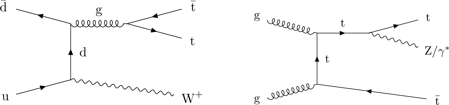
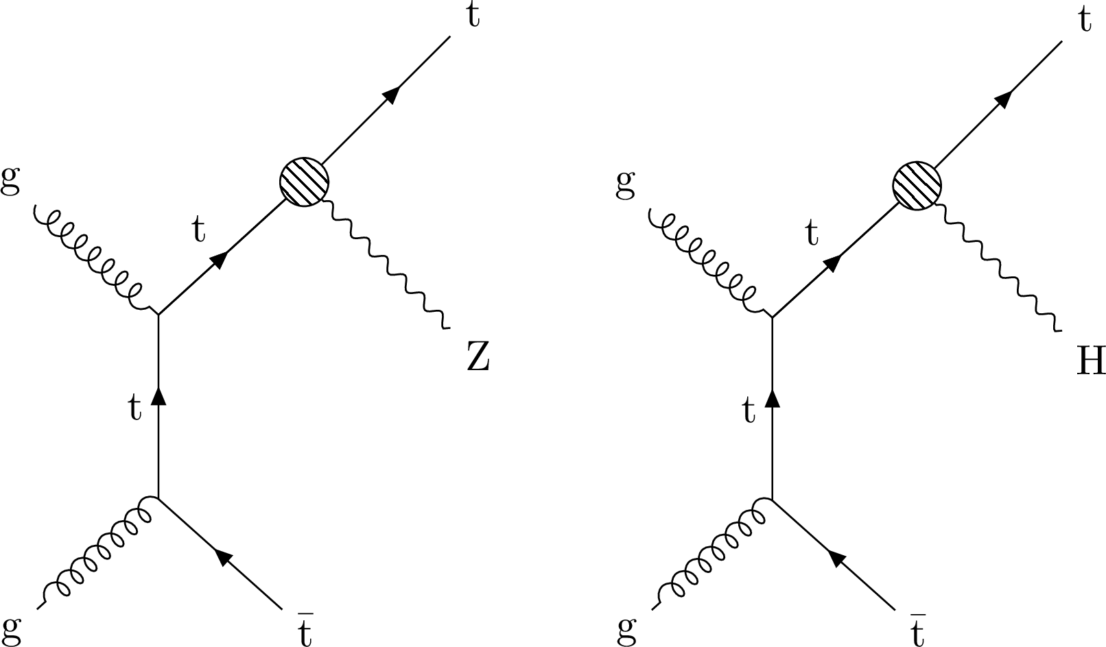
Figure 1:
Representative leading-order Feynman diagrams for $ {{\mathrm{t} {}\mathrm{\bar{t}}} \mathrm{W}} $ and $ {{\mathrm{t} {}\mathrm{\bar{t}}} \mathrm{Z}} $ production at the LHC. |
png pdf |
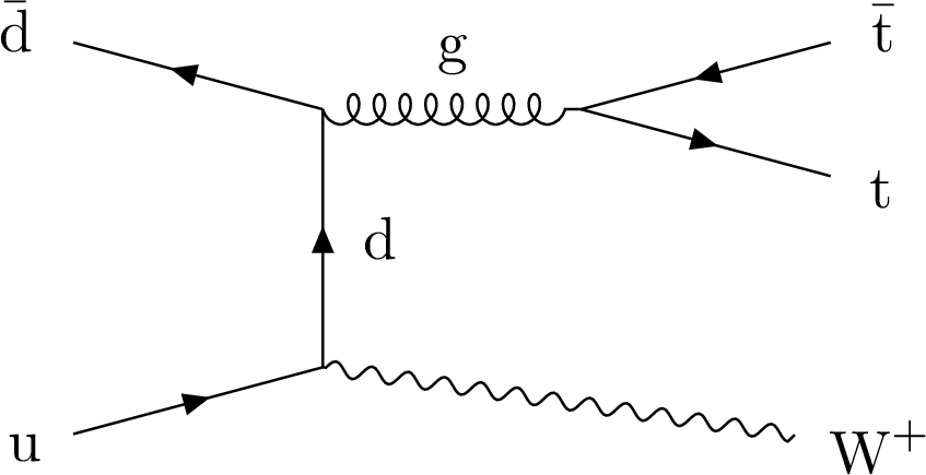
Figure 1-a:
Representative leading-order Feynman diagram for $ {{\mathrm{t} {}\mathrm{\bar{t}}} \mathrm{W}} $ and production at the LHC. |
png pdf |
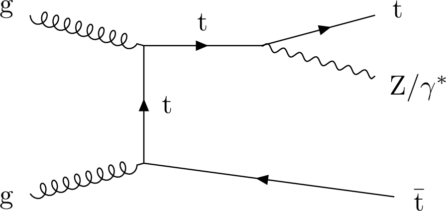
Figure 1-b:
Representative leading-order Feynman diagram for $ {{\mathrm{t} {}\mathrm{\bar{t}}} \mathrm{Z}} $ production at the LHC. |
png pdf |
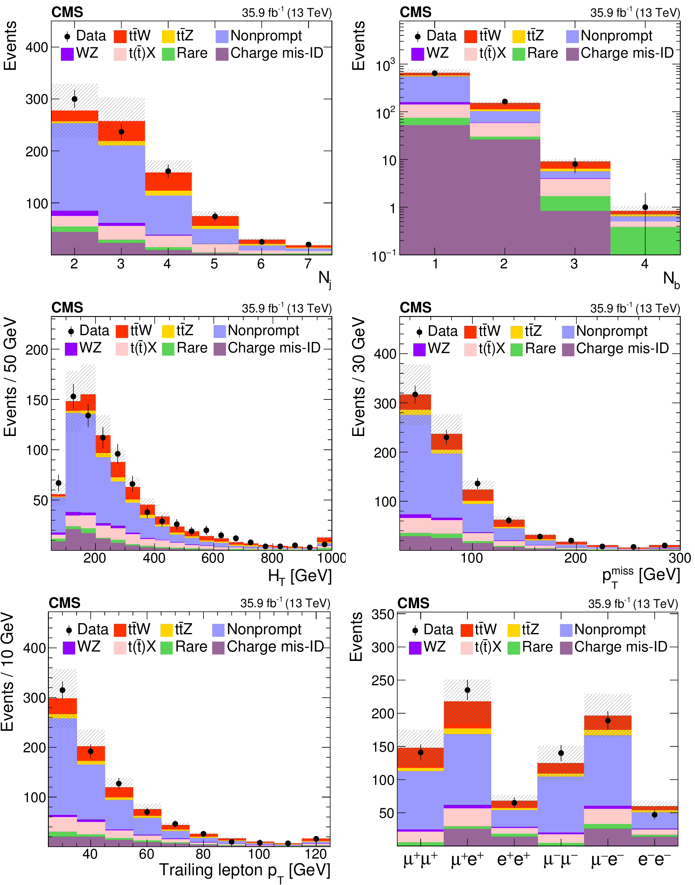
Figure 2:
Distributions of different variables in data from the SS dilepton analysis, compared to the MC generated expectations. From left to right: jet and b jet multiplicity (upper), $ {H_{\mathrm {T}}} $ and $ {{p_{\mathrm {T}}} ^\text {miss}} $ (center), trailing lepton $ {p_{\mathrm {T}}} $ and event yields in each lepton-flavor combination (lower). The expected contributions from the different background processes are stacked, as well as the expected contribution from the signal. The shaded band represents the total uncertainty in the prediction of the background and the signal processes. See Section 5 for the definition of each background category. |
png pdf |
Figure 2-a:
Jet multiplicity distribution in data from the SS dilepton analysis, compared to the MC generated expectations. The expected contributions from the different background processes are stacked, as well as the expected contribution from the signal. The shaded band represents the total uncertainty in the prediction of the background and the signal processes. See Section 5 for the definition of each background category. |
png pdf |
Figure 2-b:
b-jet multiplicity distribution in data from the SS dilepton analysis, compared to the MC generated expectations. The expected contributions from the different background processes are stacked, as well as the expected contribution from the signal. The shaded band represents the total uncertainty in the prediction of the background and the signal processes. See Section 5 for the definition of each background category. |
png pdf |
Figure 2-c:
$ {H_{\mathrm {T}}} $ distribution in data from the SS dilepton analysis, compared to the MC generated expectations. The expected contributions from the different background processes are stacked, as well as the expected contribution from the signal. The shaded band represents the total uncertainty in the prediction of the background and the signal processes. See Section 5 for the definition of each background category. |

png pdf |
Figure 2-d:
$ {{p_{\mathrm {T}}} ^\text {miss}} $ distribution in data from the SS dilepton analysis, compared to the MC generated expectations. The expected contributions from the different background processes are stacked, as well as the expected contribution from the signal. The shaded band represents the total uncertainty in the prediction of the background and the signal processes. See Section 5 for the definition of each background category. |

png pdf |
Figure 2-e:
Trailing lepton $ {p_{\mathrm {T}}} $ distribution in data from the SS dilepton analysis, compared to the MC generated expectations.The expected contributions from the different background processes are stacked, as well as the expected contribution from the signal. The shaded band represents the total uncertainty in the prediction of the background and the signal processes. See Section 5 for the definition of each background category. |
png pdf |
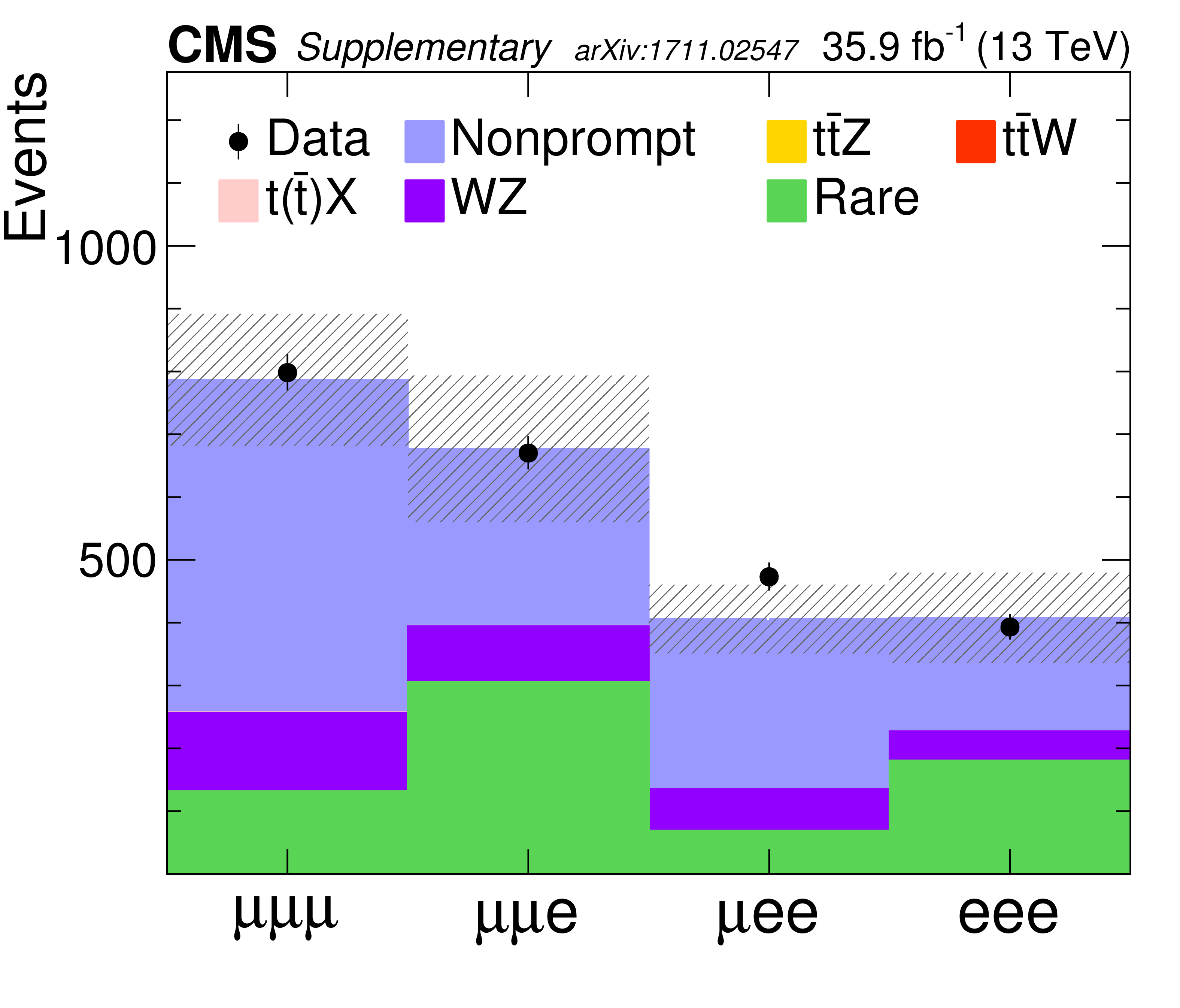
Figure 2-f:
Event yields in each lepton-flavor combination in data from the SS dilepton analysis, compared to the MC generated expectations. The expected contributions from the different background processes are stacked, as well as the expected contribution from the signal. The shaded band represents the total uncertainty in the prediction of the background and the signal processes. See Section 5 for the definition of each background category. |
png pdf |
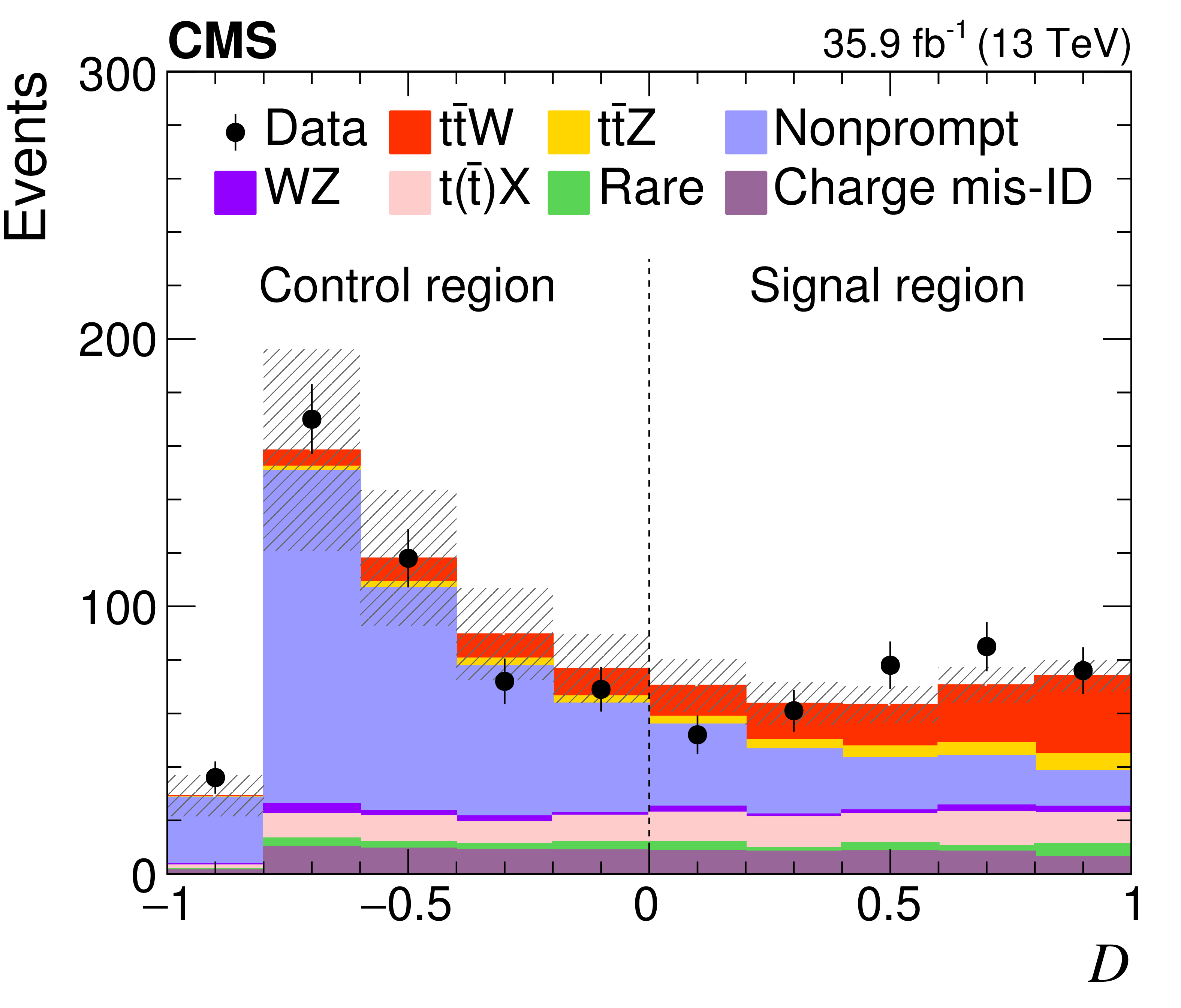
Figure 3:
Distribution of the boosted decision tree classifier ${\textit {D}}$ for background and signal processes in the SS dilepton analysis. The expected contribution from the different background processes, and the signal as well as the observed data are shown. The shaded band represents the total uncertainty in the prediction of the background and the signal processes. See Section 5 for the definition of each background category. |

png pdf |
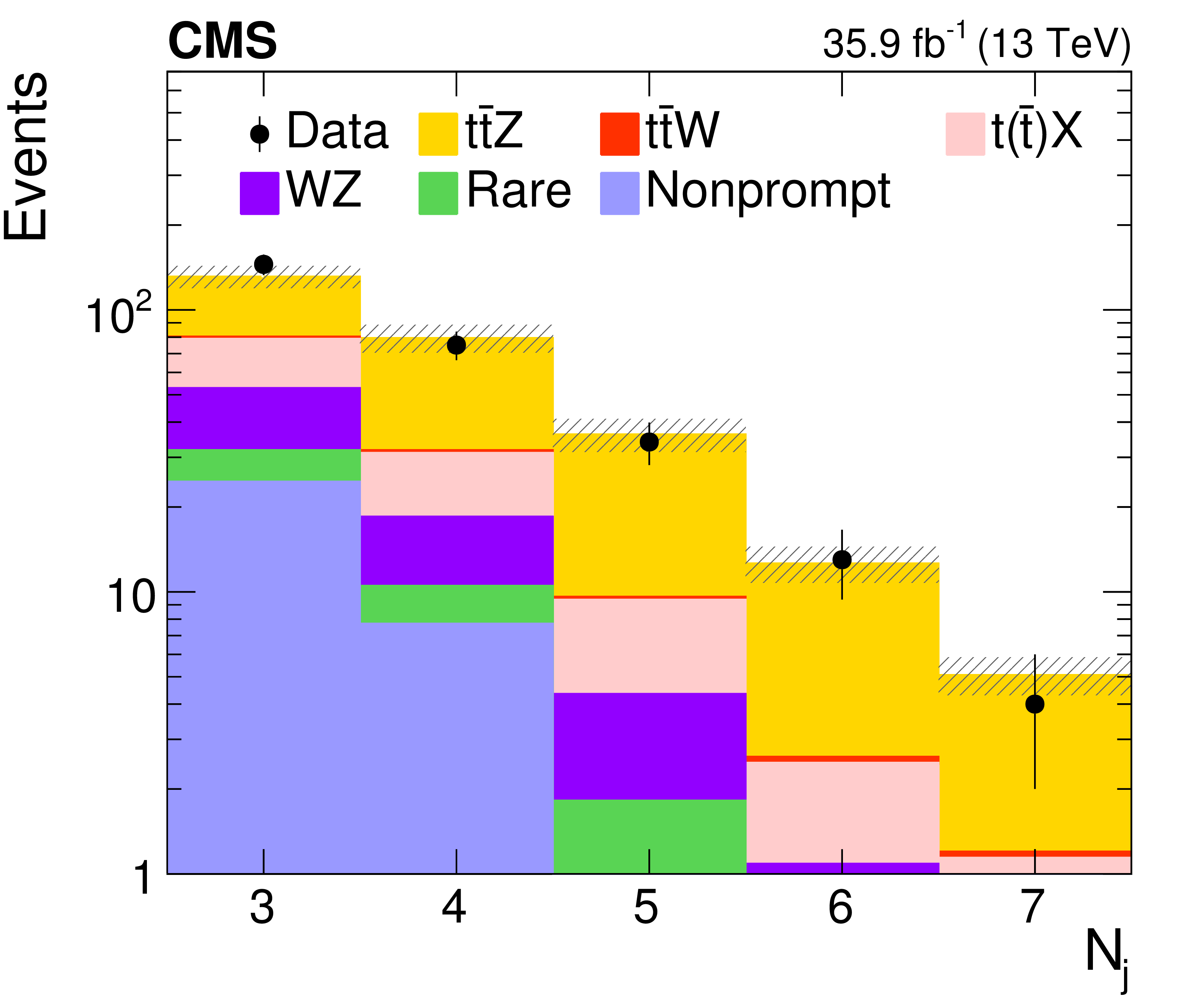
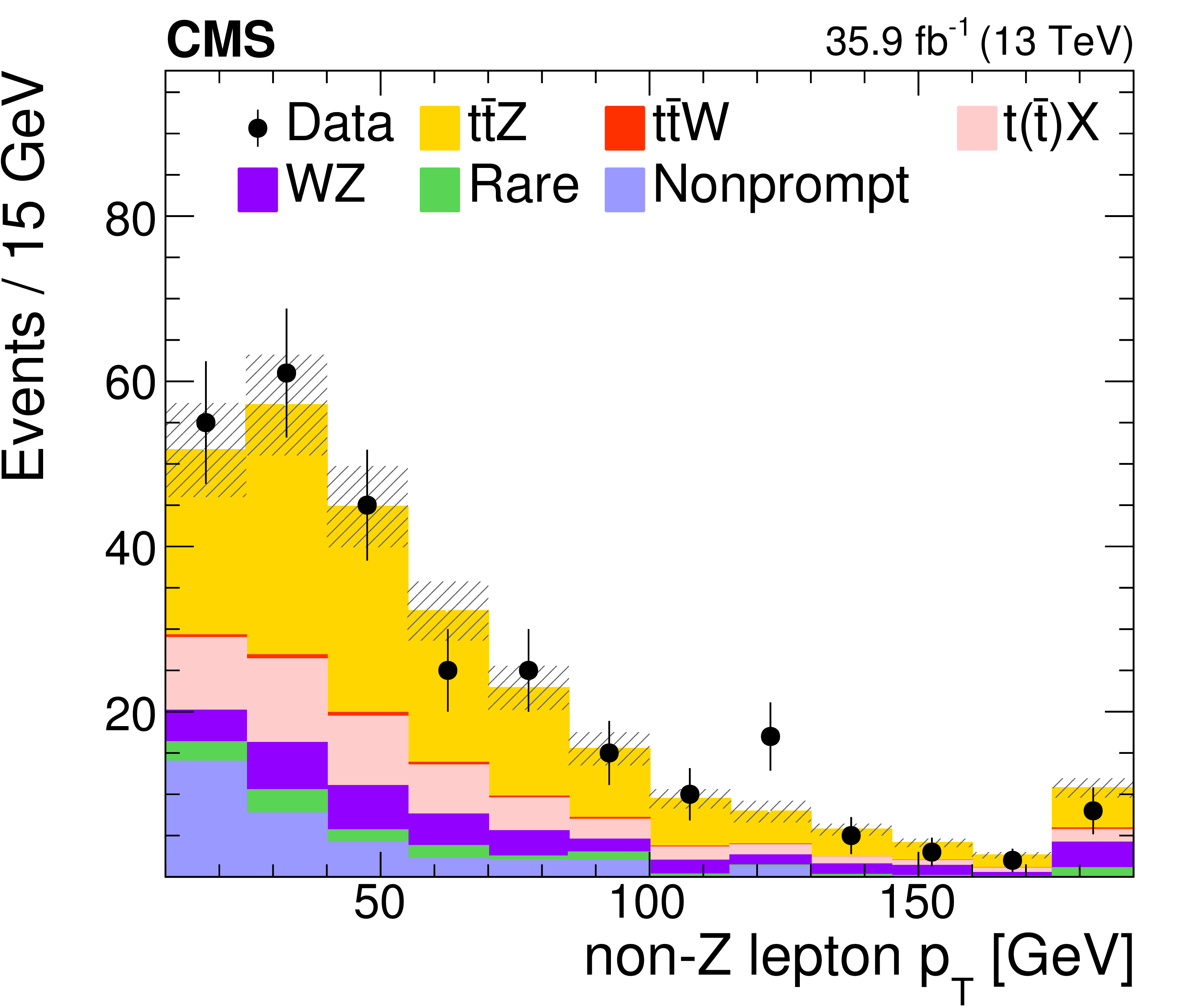
Figure 4:
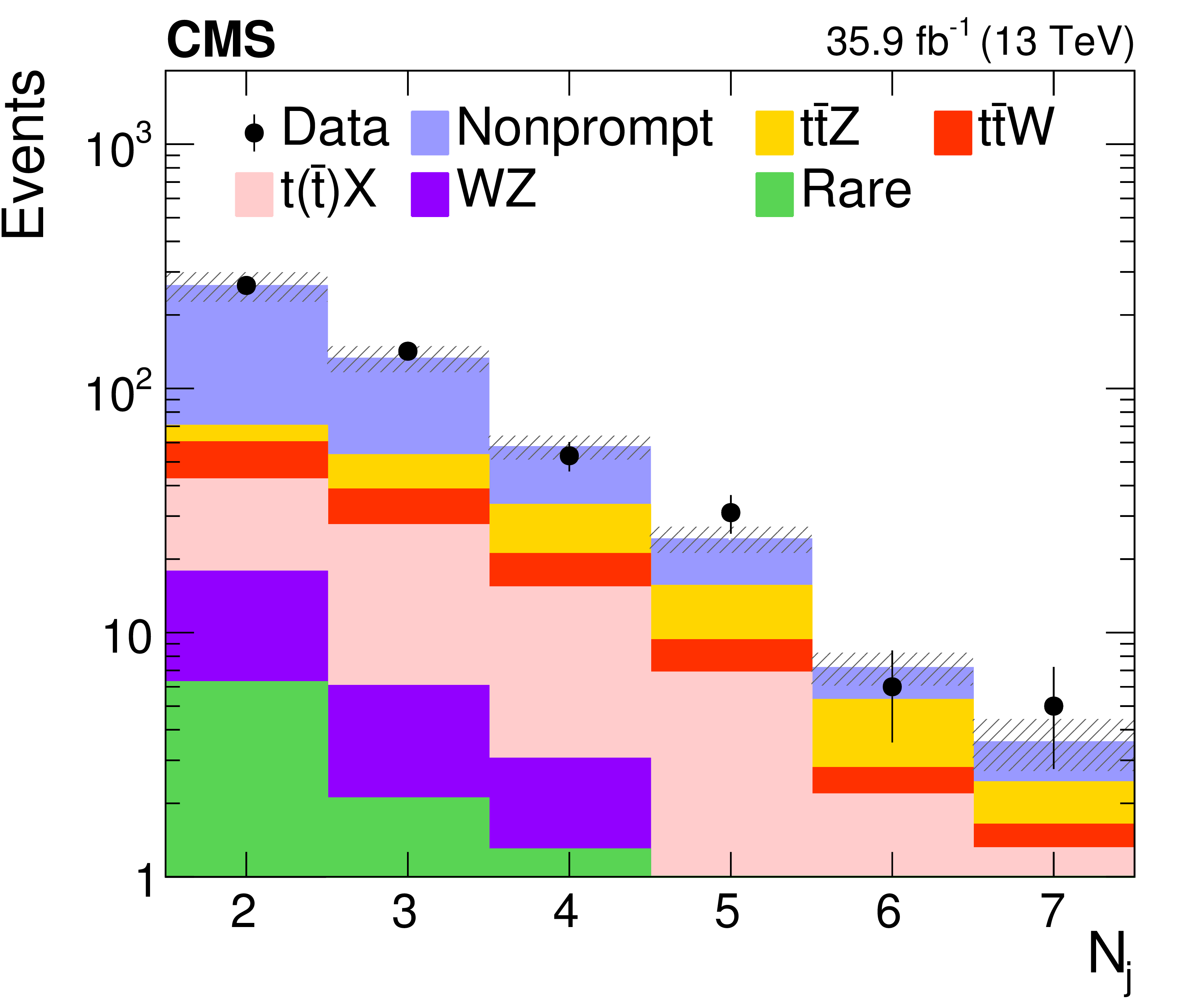
Distributions of the predicted and observed yields versus ${N_\text {j}}$ (left) and $ {p_{\mathrm {T}}} $ of the trailing lepton (right) in control regions enriched with nonprompt lepton background in the SS dilepton channel. The shaded band represents the total uncertainty in the prediction of the background and the signal processes. See Section 5 for the definition of each background category. |

png pdf |
Figure 4-a:
Distribution of the predicted and observed yields versus ${N_\text {j}}$ in control regions enriched with nonprompt lepton background in the SS dilepton channel. The shaded band represents the total uncertainty in the prediction of the background and the signal processes. See Section 5 for the definition of each background category. |

png pdf |
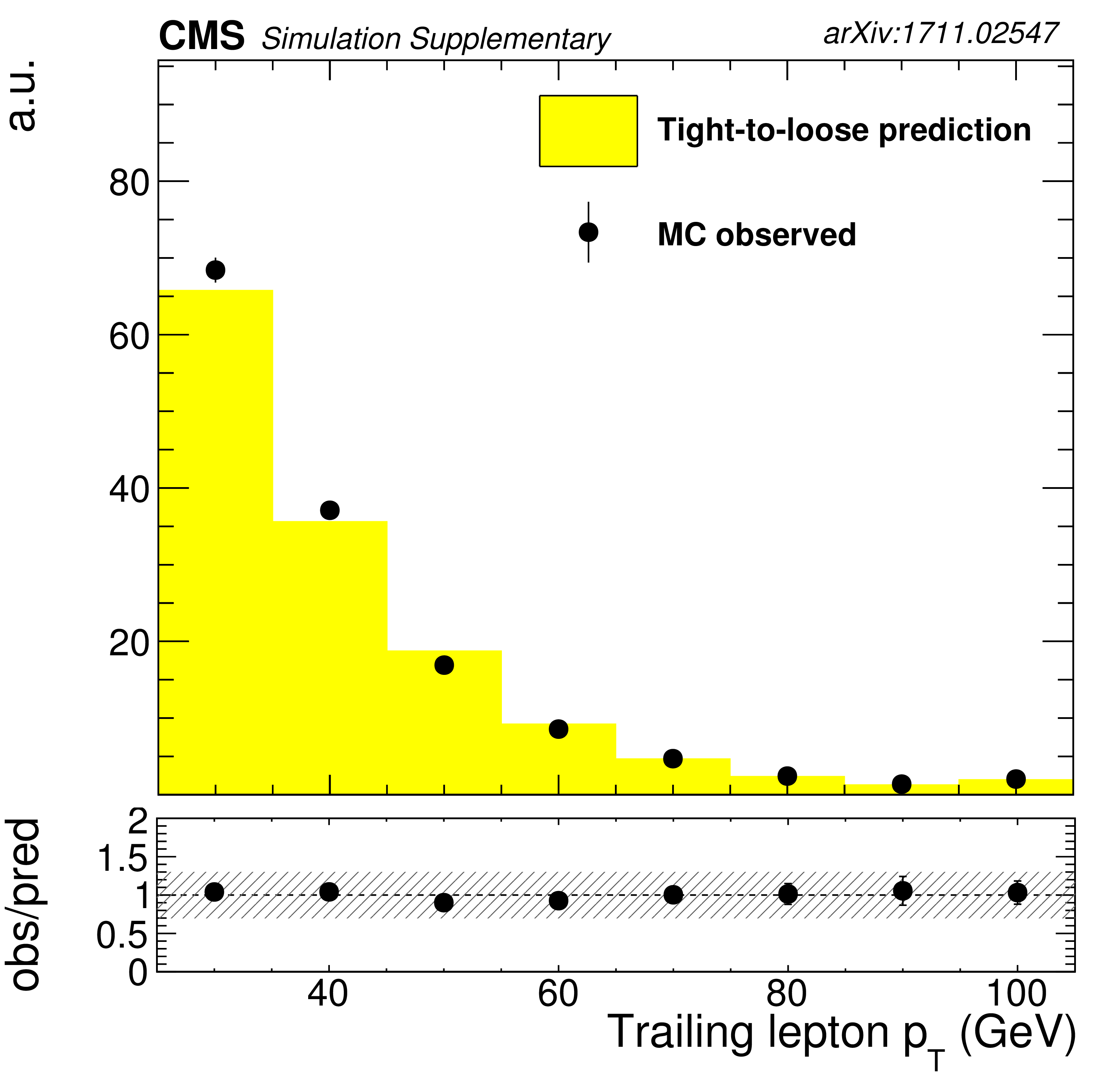
Figure 4-b:
Distribution of the predicted and observed yields versus $ {p_{\mathrm {T}}} $ of the trailing lepton in control regions enriched with nonprompt lepton background in the SS dilepton channel. The shaded band represents the total uncertainty in the prediction of the background and the signal processes. See Section 5 for the definition of each background category. |

png pdf |
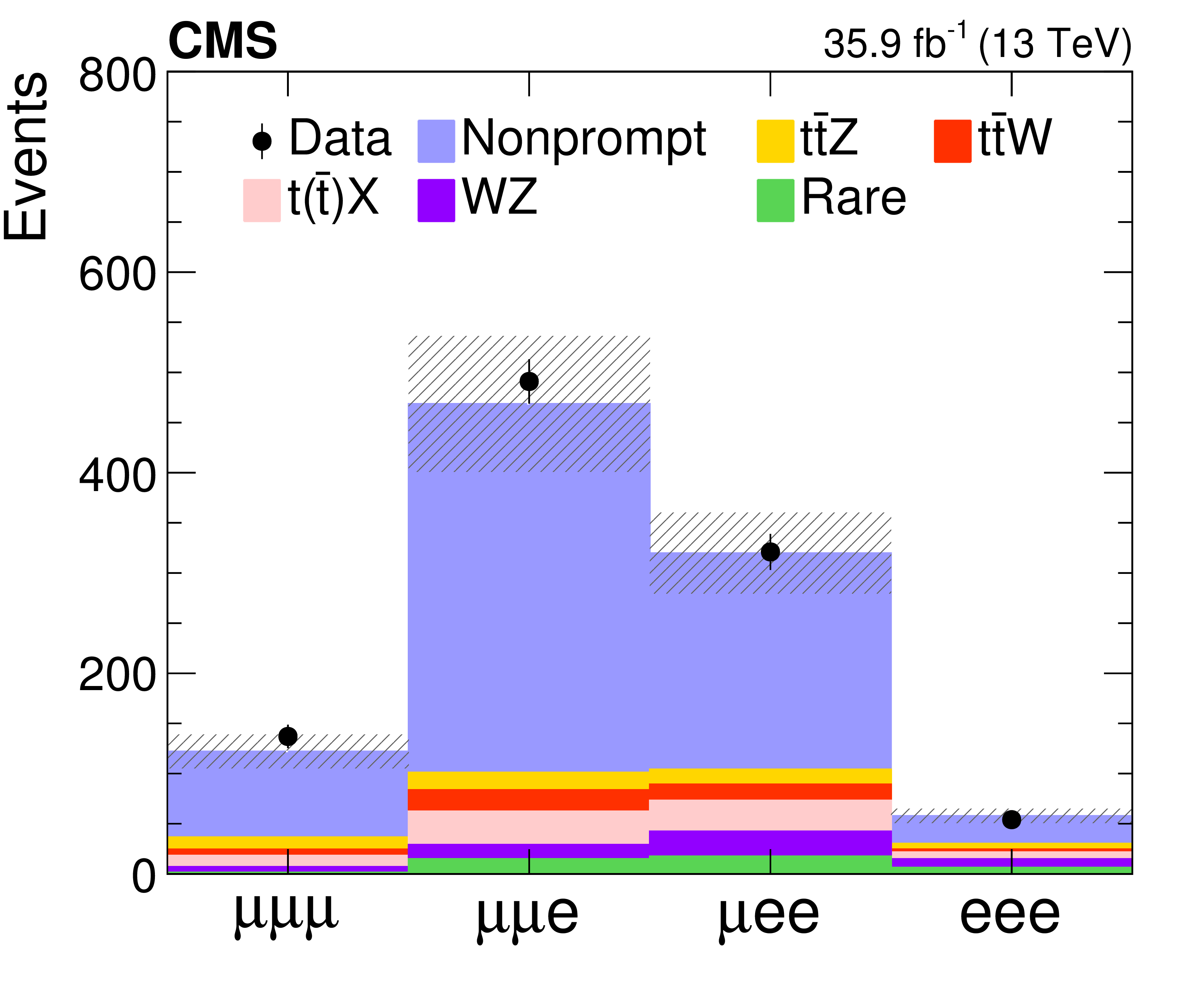
Figure 5:
Distributions of the predicted and observed yields versus different three-lepton channels, $ {{p_{\mathrm {T}}} ^\text {miss}} $ (upper panels), and jet and b jet multiplicity (lower panels) in control regions enriched with nonprompt lepton background. The shaded band represents the total uncertainty in the prediction of the background and the signal processes. See Section 5 for the definition of each background category. |
png pdf |
Figure 5-a:
Predicted and observed yields in the different three-lepton channels, in control regions enriched with nonprompt lepton background. The shaded band represents the total uncertainty in the prediction of the background and the signal processes. See Section 5 for the definition of each background category. |

png pdf |
Figure 5-b:
Distribution of the predicted and observed yields versus $ {{p_{\mathrm {T}}} ^\text {miss}} $, in control regions enriched with nonprompt lepton background. The shaded band represents the total uncertainty in the prediction of the background and the signal processes. See Section 5 for the definition of each background category. |
png pdf |
Figure 5-c:
Distributions of the predicted and observed yields versus jet multiplicity, in control regions enriched with nonprompt lepton background. The shaded band represents the total uncertainty in the prediction of the background and the signal processes. See Section 5 for the definition of each background category. |

png pdf |
Figure 5-d:
Distributions of the predicted and observed yields versus b jet multiplicity, in control regions enriched with nonprompt lepton background. The shaded band represents the total uncertainty in the prediction of the background and the signal processes. See Section 5 for the definition of each background category. |

png pdf |
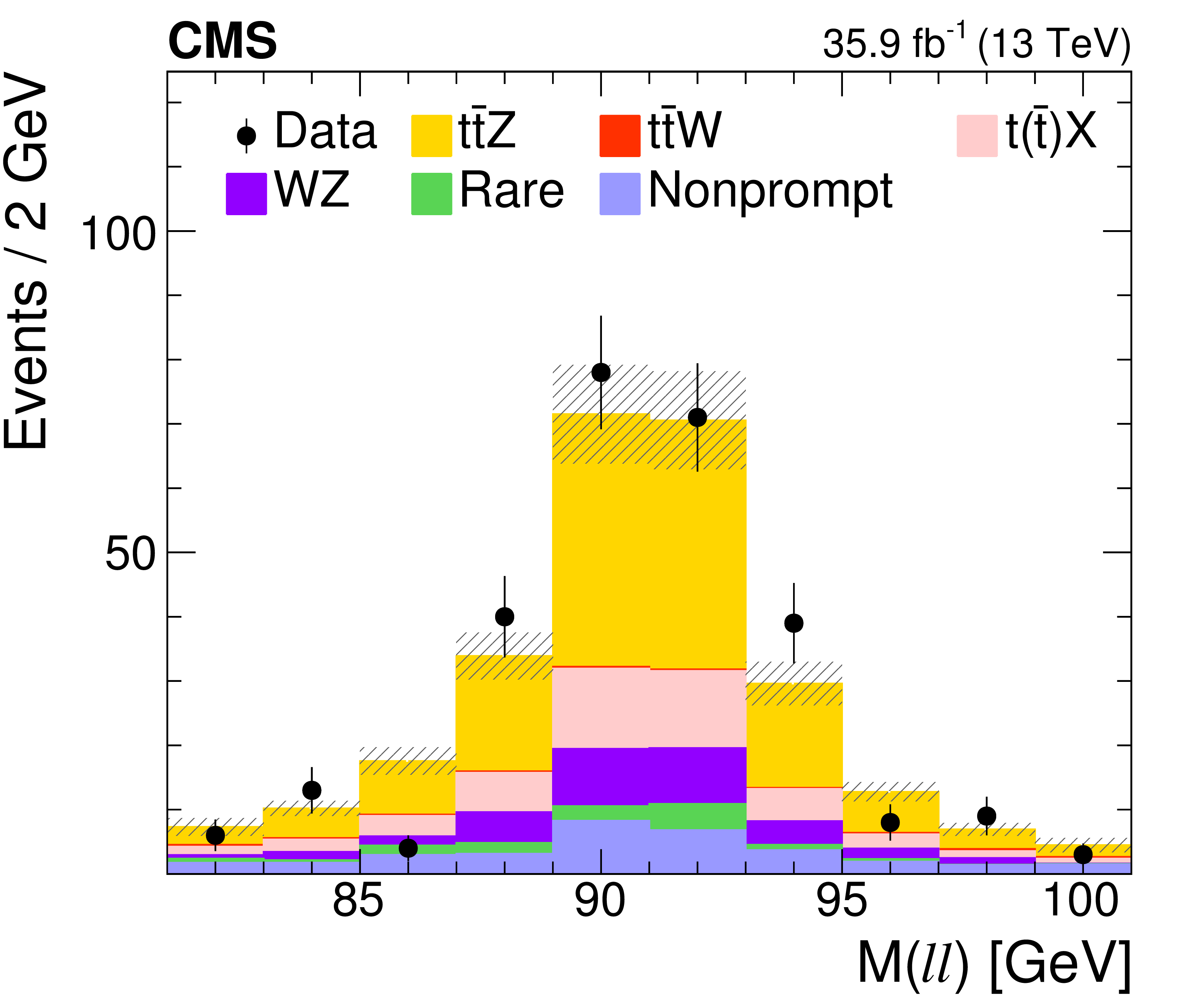
Figure 6:
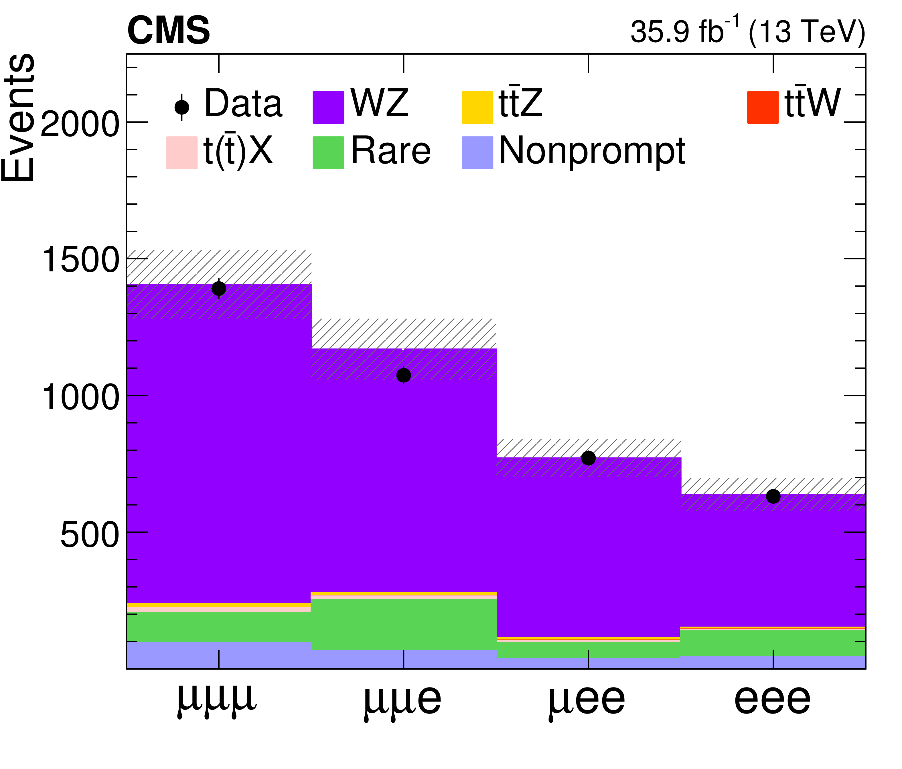
Distributions of the predicted and observed yields versus ${M_\text {T}}$ (upper left), lepton flavor (upper right), jet multiplicity (lower left), and the reconstructed invariant mass of the Z boson candidates (lower right) in the WZ-enriched control region. The requirements on ${M_\text {T}}$ and ${N_\text {j}}$ are removed for the distributions of these variables. The shaded band represents the total uncertainty in the prediction of the background and the signal processes. |

png pdf |
Figure 6-a:
Distribution of the predicted and observed yields versus ${M_\text {T}}$, in the WZ-enriched control region. The requirement on ${M_\text {T}}$ is removed. The shaded band represents the total uncertainty in the prediction of the background and the signal processes. |
png pdf |
Figure 6-b:
Distribution of the predicted and observed yields versus lepton flavor, in the WZ-enriched control region. The shaded band represents the total uncertainty in the prediction of the background and the signal processes. |

png pdf |
Figure 6-c:
Distribution of the predicted and observed yields versus jet multiplicity ${N_\text {j}}$, in the WZ-enriched control region. The requirement on ${N_\text {j}}$ is removed. The shaded band represents the total uncertainty in the prediction of the background and the signal processes. |

png pdf |
Figure 6-d:
Distribution of the predicted and observed yields versus the reconstructed invariant mass of the Z boson candidates, in the WZ-enriched control region. The shaded band represents the total uncertainty in the prediction of the background and the signal processes. |
png pdf |
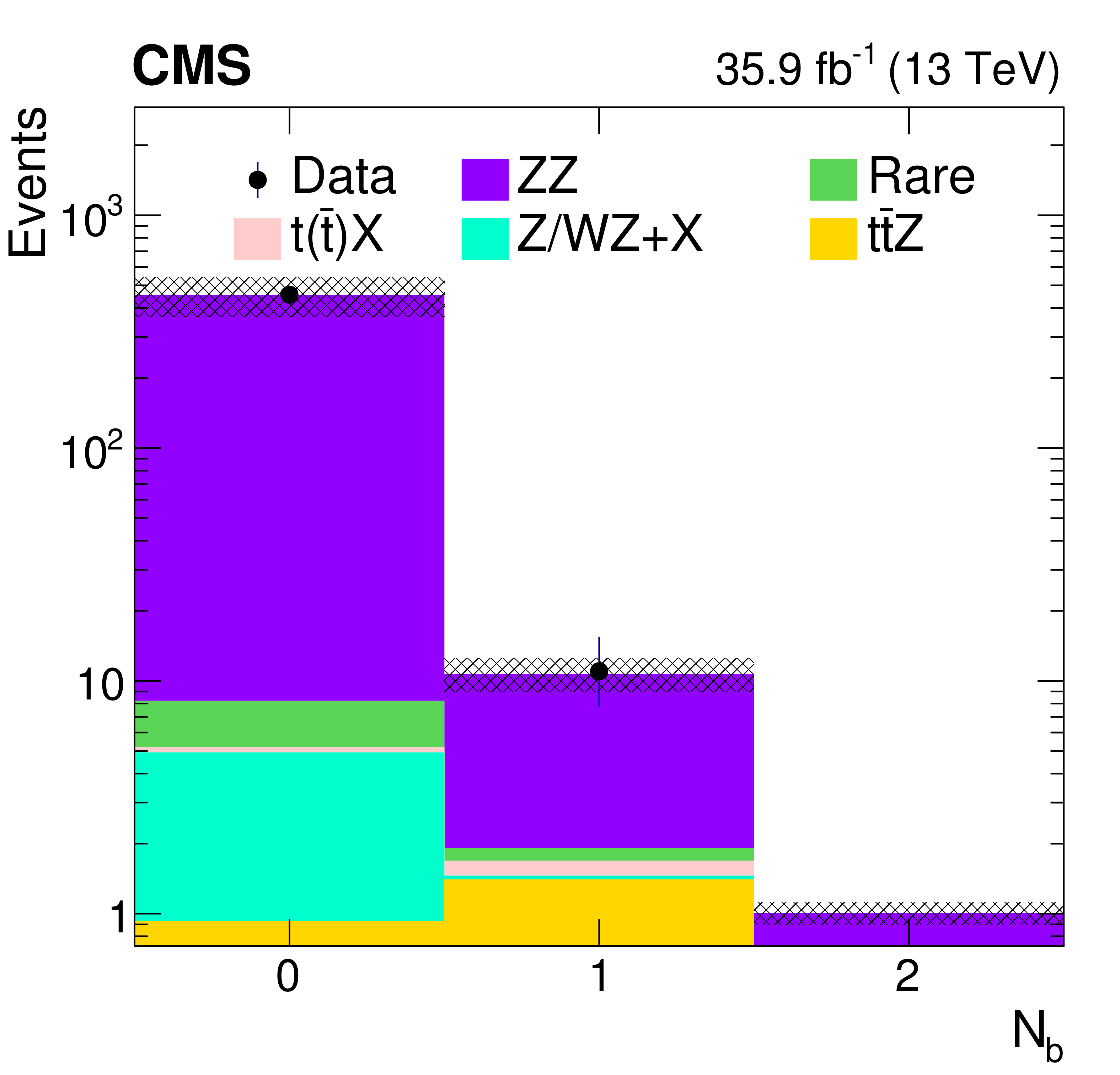
Figure 7:
Comparison of data with MC predictions for the mass of the Z boson candidate (upper left), event yields (upper right), jet multiplicity (lower left) and b jet multiplicity (lower right) in a ZZ-dominated background control region. The shaded band represents the total uncertainty in the prediction of the background and the signal processes. |
png pdf |
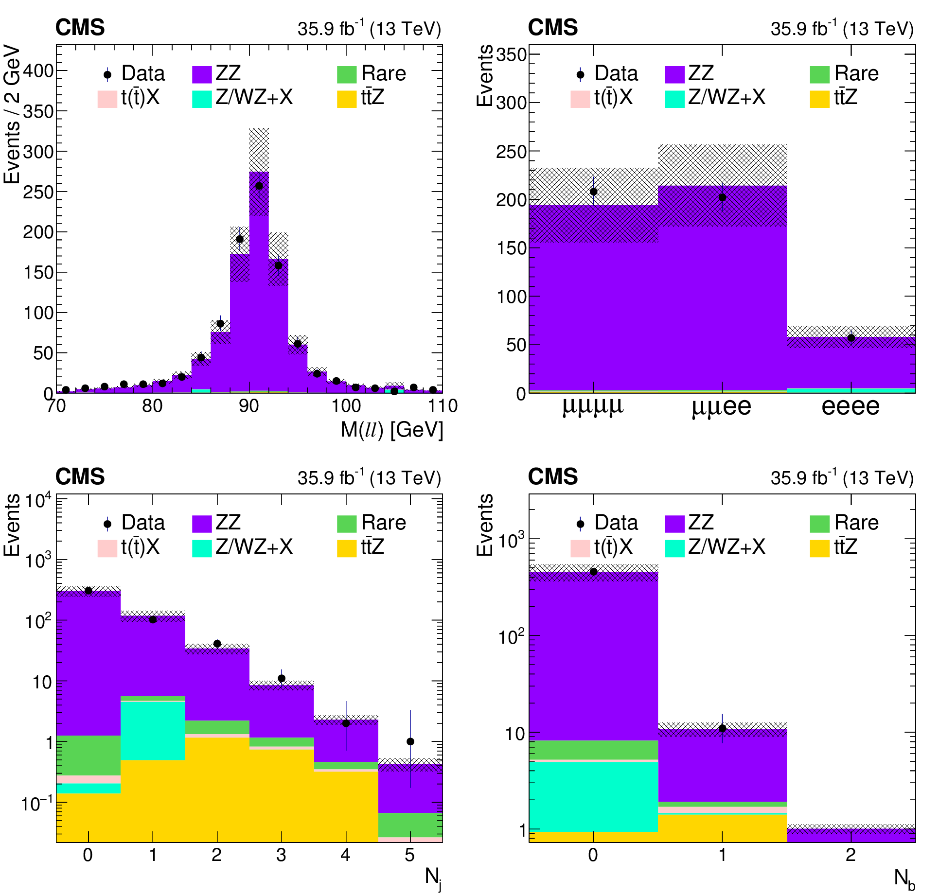
Figure 7-a:
Comparison of data with MC predictions for the mass of the Z boson candidate, in a ZZ-dominated background control region. The shaded band represents the total uncertainty in the prediction of the background and the signal processes. |
png pdf |
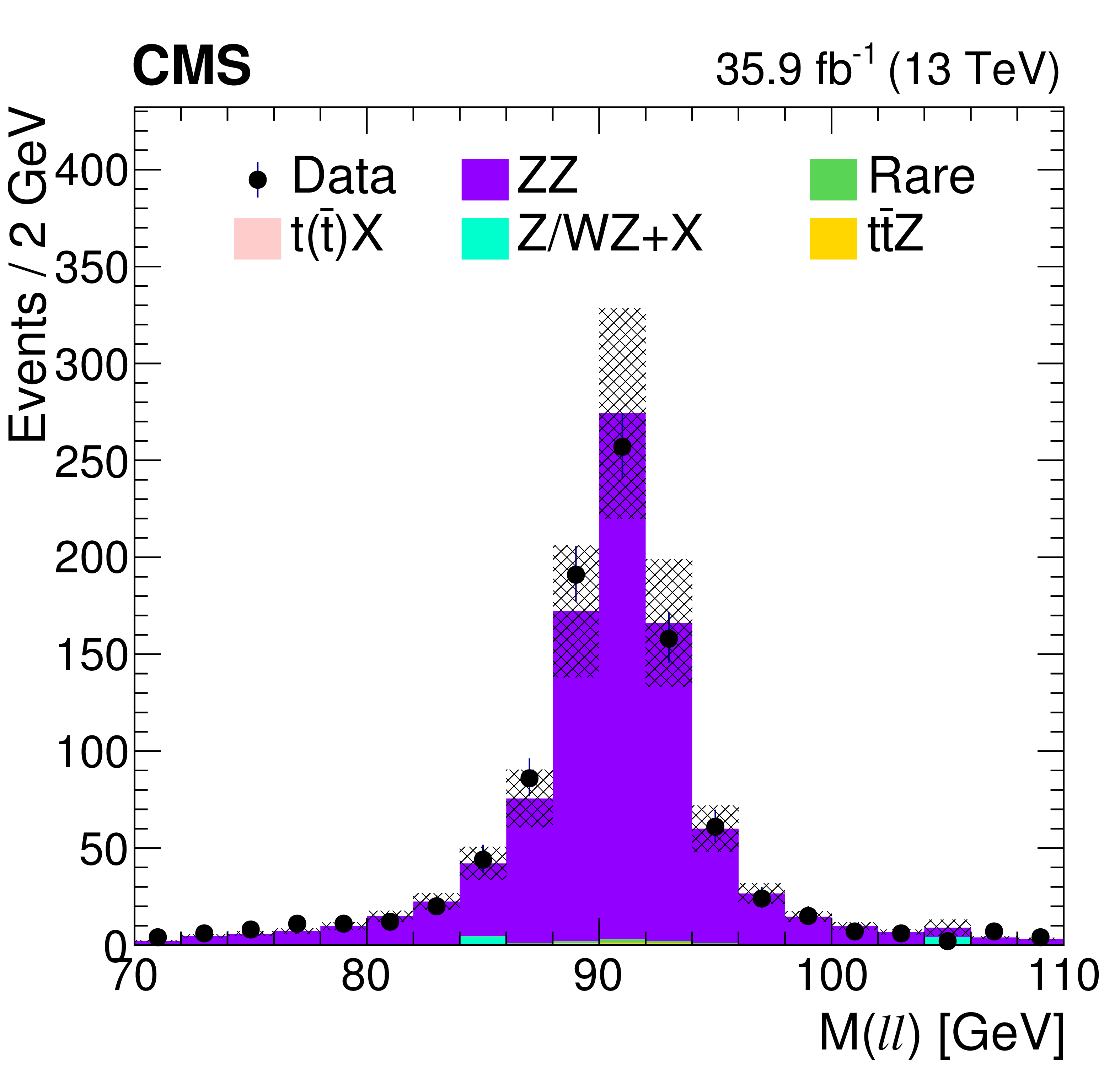
Figure 7-b:
Comparison of data with MC predictions for event yields, in a ZZ-dominated background control region. The shaded band represents the total uncertainty in the prediction of the background and the signal processes. |

png pdf |
Figure 7-c:
Comparison of data with MC predictions for the jet multiplicity, in a ZZ-dominated background control region. The shaded band represents the total uncertainty in the prediction of the background and the signal processes. |
png pdf |
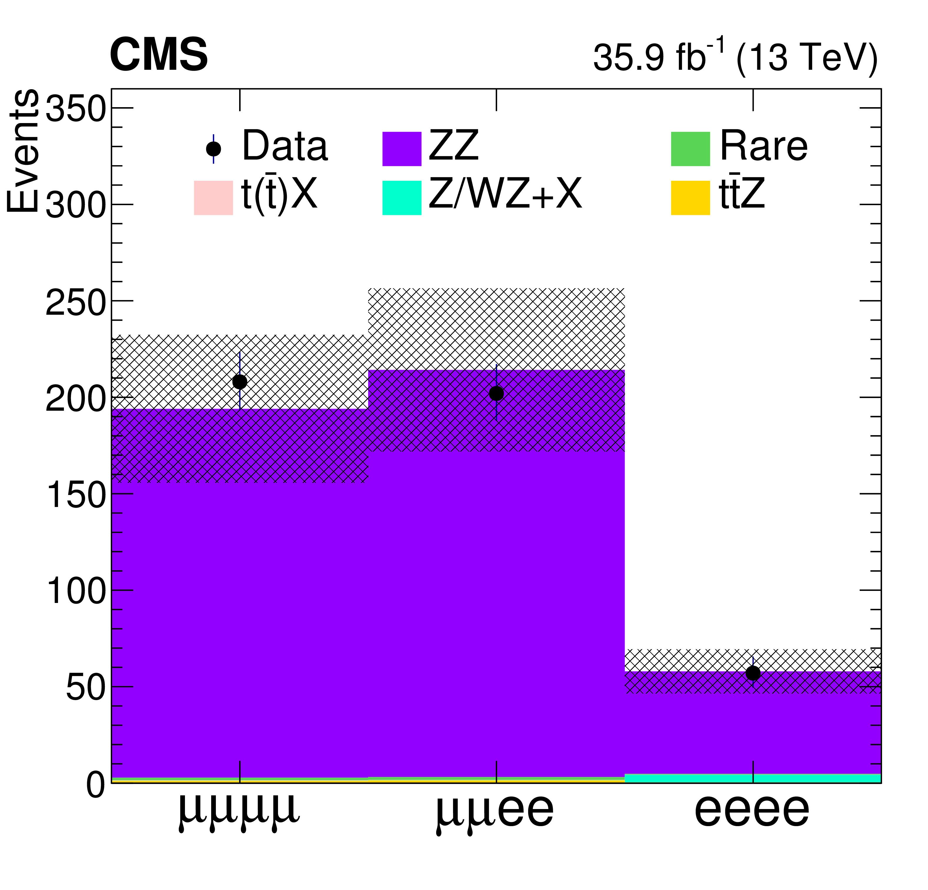
Figure 7-d:
Comparison of data with MC predictions for the b jet multiplicity, in a ZZ-dominated background control region. The shaded band represents the total uncertainty in the prediction of the background and the signal processes. |
png pdf |
Figure 8:
Predicted and observed yields in each analysis bin in the SS dilepton analysis. The hatched band shows the total uncertainty associated with the signal and background predictions, as obtained from the fit. |
png pdf |
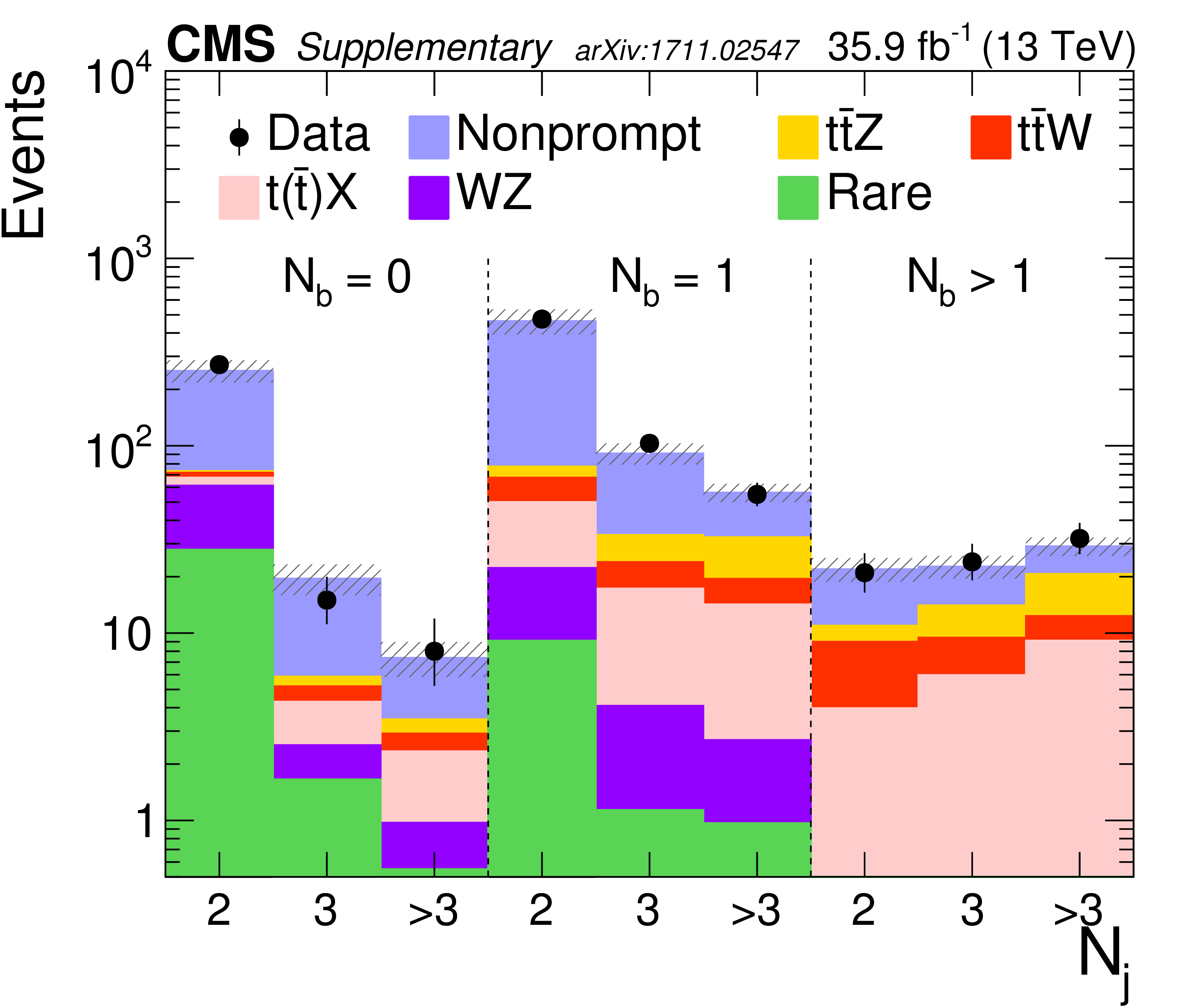
Figure 9:
Predicted and observed yields in $ {N_\text {j}} = $ 2, 3, and $ >$ 3 categories in the three-lepton analysis (left), and in $ {N_\text {b}} = $ 0, 1 categories in the four-lepton analysis (right). The hatched band shows the total uncertainty associated with the signal and background predictions, as obtained from the fit. |
png pdf |
Figure 9-a:
Predicted and observed yields in $ {N_\text {j}} = $ 2, 3, and $ >$ 3 categories in the three-lepton analysis. The hatched band shows the total uncertainty associated with the signal and background predictions, as obtained from the fit. |
png pdf |
Figure 9-b:
Predicted and observed yields in in $ {N_\text {b}} = $ 0, 1 categories in the four-lepton analysis. The hatched band shows the total uncertainty associated with the signal and background predictions, as obtained from the fit. |
png pdf |
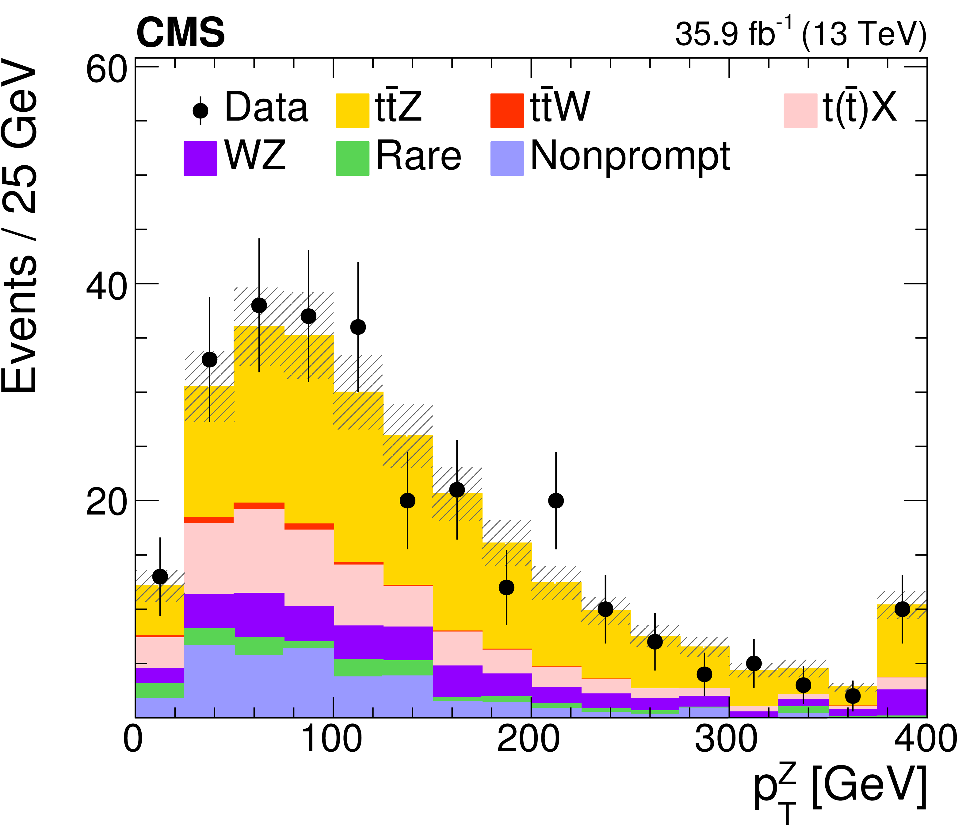
Figure 10:
The distributions of the observed and predicted signal and background yields versus the flavor and the charge combination of leptons (upper left), $ {{p_{\mathrm {T}}} ^\text {miss}} $ (upper right), jet multiplicity (lower left), and the $ {p_{\mathrm {T}}} $ of the leading lepton (lower right) in the SS dilepton channel with at least three jets and two b jets. The last bin in each distribution includes the overflow events, and the hatched area represents the combined statistical and systematic uncertainties in the prediction. |
png pdf |
Figure 10-a:
The distributions of the observed and predicted signal and background yields versus the flavor and the charge combination of leptons, in the SS dilepton channel with at least three jets and two b jets. The last bin includes the overflow events, and the hatched area represents the combined statistical and systematic uncertainties in the prediction. |

png pdf |
Figure 10-b:
The distributions of the observed and predicted signal and background yields versus $ {{p_{\mathrm {T}}} ^\text {miss}} $, in the SS dilepton channel with at least three jets and two b jets. The last bin includes the overflow events, and the hatched area represents the combined statistical and systematic uncertainties in the prediction. |

png pdf |
Figure 10-c:
The distributions of the observed and predicted signal and background yields versus jet multiplicity, in the SS dilepton channel with at least three jets and two b jets. The last bin includes the overflow events, and the hatched area represents the combined statistical and systematic uncertainties in the prediction. |
png pdf |
Figure 10-d:
The distributions of the observed and predicted signal and background yields versus the $ {p_{\mathrm {T}}} $ of the leading lepton, in the SS dilepton channel with at least three jets and two b jets. The last bin includes the overflow events, and the hatched area represents the combined statistical and systematic uncertainties in the prediction. |
png pdf |
Figure 11:
The distributions of the observed and predicted signal and background yields in the three-lepton channel for events containing at least one b jet and three jets. From left to right: the lepton flavor and jet multiplicity (upper), $ {p_{\mathrm {T}}} $ of the leading jet and the lepton not used to form Z (central), and invariant mass of the OSSF lepton pair and $ {p_{\mathrm {T}}} $ of the reconstructed Z boson (lower). The last bin in each distribution includes the overflow events, and the hatched area represents the combined statistical and systematic uncertainties in the prediction. |

png pdf |
Figure 11-a:
Distribution of the observed and predicted signal and background yields in the lepton flavor in the three-lepton channel for events containing at least one b jet and three jets. The last bin includes the overflow events, and the hatched area represents the combined statistical and systematic uncertainties in the prediction. |
png pdf |
Figure 11-b:
Distribution of the observed and predicted signal and background yields in the jet multiplicity, in the three-lepton channel for events containing at least one b jet and three jets. The last bin includes the overflow events, and the hatched area represents the combined statistical and systematic uncertainties in the prediction. |

png pdf |
Figure 11-c:
Distribution of the observed and predicted signal and background yields in the $ {p_{\mathrm {T}}} $ of the leading jet, in the three-lepton channel for events containing at least one b jet and three jets. The last bin includes the overflow events, and the hatched area represents the combined statistical and systematic uncertainties in the prediction. |
png pdf |
Figure 11-d:
Distribution of the observed and predicted signal and background yields in the $ {p_{\mathrm {T}}} $ of the lepton not used to form Z, in the three-lepton channel for events containing at least one b jet and three jets. The last bin includes the overflow events, and the hatched area represents the combined statistical and systematic uncertainties in the prediction. |
png pdf |
Figure 11-e:
Distribution of the observed and predicted signal and background yields in the invariant mass of the OSSF lepton pair, in the three-lepton channel for events containing at least one b jet and three jets. The last bin includes the overflow events, and the hatched area represents the combined statistical and systematic uncertainties in the prediction. |
png pdf |
Figure 11-f:
Distribution of the observed and predicted signal and background yields in the $ {p_{\mathrm {T}}} $ of the reconstructed Z boson, in the three-lepton channel for events containing at least one b jet and three jets. The last bin includes the overflow events, and the hatched area represents the combined statistical and systematic uncertainties in the prediction. |

png pdf |
Figure 12:
Result of the simultaneous fit for ${{\mathrm{t} {}\mathrm{\bar{t}}} \mathrm{W}}$ and ${{\mathrm{t} {}\mathrm{\bar{t}}} \mathrm{Z}}$ cross sections (denoted as star), along with its 68 and 95% CL contours are shown on the left panel. The right panel presents the individual measured cross sections along with the 68 and 95% CL intervals and the theory prediction [1] with their respective uncertainties for ${{\mathrm{t} {}\mathrm{\bar{t}}} \mathrm{W}}$ and ${{\mathrm{t} {}\mathrm{\bar{t}}} \mathrm{Z}}$. |
png pdf |
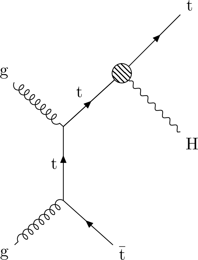
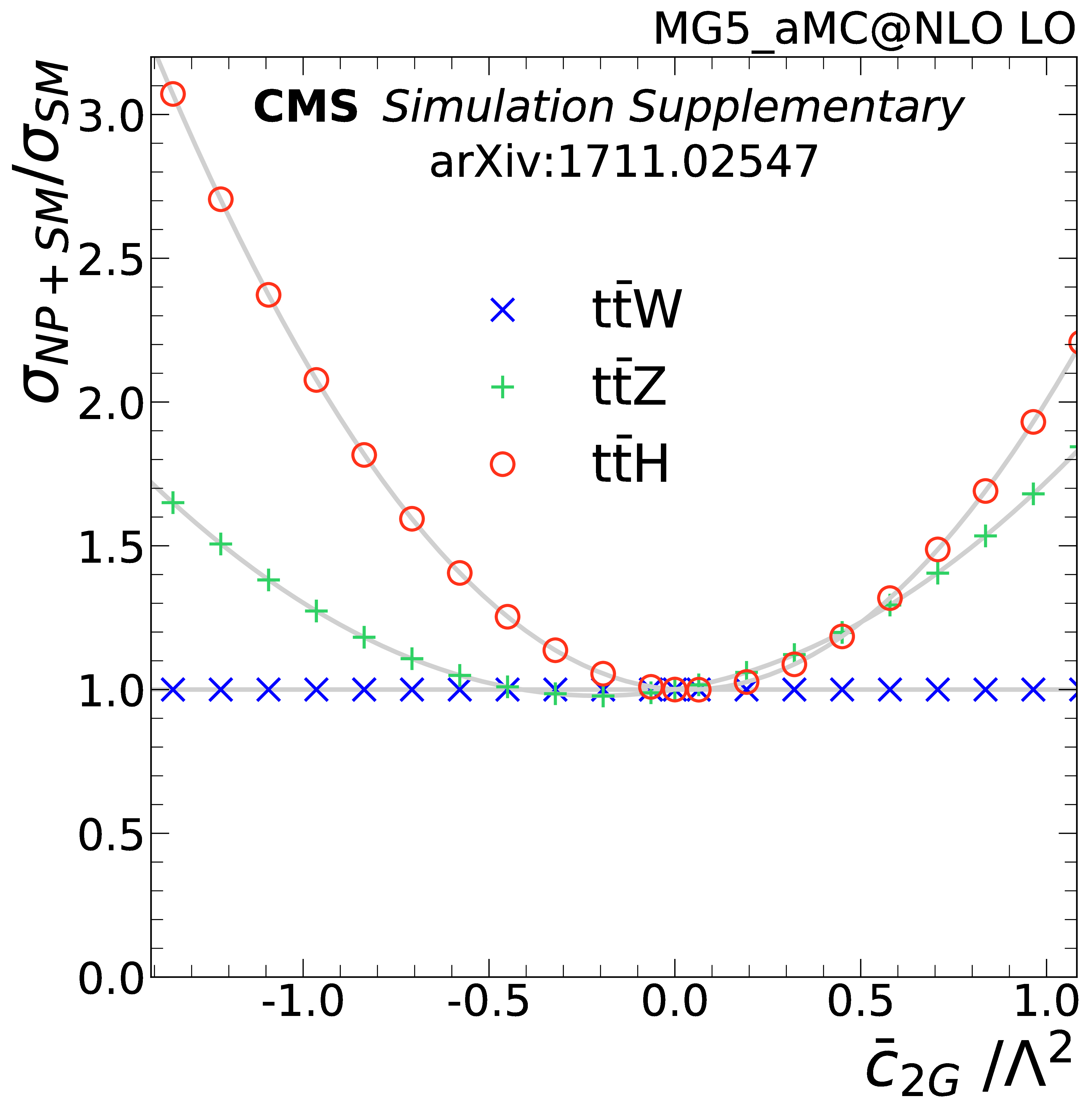
Figure 13:
Feynman diagrams representing the largest LO contribution for the process with the most significant NP effects are shown for ${\mathcal {O}_{\text {uB}}}$, ${\mathcal {O}_{\text {uW}}}$, and ${\mathcal {O}_{\text {Hu}}}$ (left), and ${\mathcal {O}_{\mathrm{H}}}$, ${\mathcal {O}_{\tilde{\text {3G}}}}$, ${\mathcal {O}_{\text {3G}}}$, ${\mathcal {O}_{\text {2G}}}$, and ${\mathcal {O}_{\text {uG}}}$ (right). |

png pdf |
Figure 13-a:
Feynman diagrams representing the largest LO contribution for the process with the most significant NP effects are shown for ${\mathcal {O}_{\text {uB}}}$, ${\mathcal {O}_{\text {uW}}}$, and ${\mathcal {O}_{\text {Hu}}}$ (left), and ${\mathcal {O}_{\mathrm{H}}}$, ${\mathcal {O}_{\tilde{\text {3G}}}}$, ${\mathcal {O}_{\text {3G}}}$, ${\mathcal {O}_{\text {2G}}}$, and ${\mathcal {O}_{\text {uG}}}$ (right). |
png pdf |
Figure 13-b:
Feynman diagrams representing the largest LO contribution for the process with the most significant NP effects are shown for ${\mathcal {O}_{\text {uB}}}$, ${\mathcal {O}_{\text {uW}}}$, and ${\mathcal {O}_{\text {Hu}}}$ (left), and ${\mathcal {O}_{\mathrm{H}}}$, ${\mathcal {O}_{\tilde{\text {3G}}}}$, ${\mathcal {O}_{\text {3G}}}$, ${\mathcal {O}_{\text {2G}}}$, and ${\mathcal {O}_{\text {uG}}}$ (right). |
png pdf |
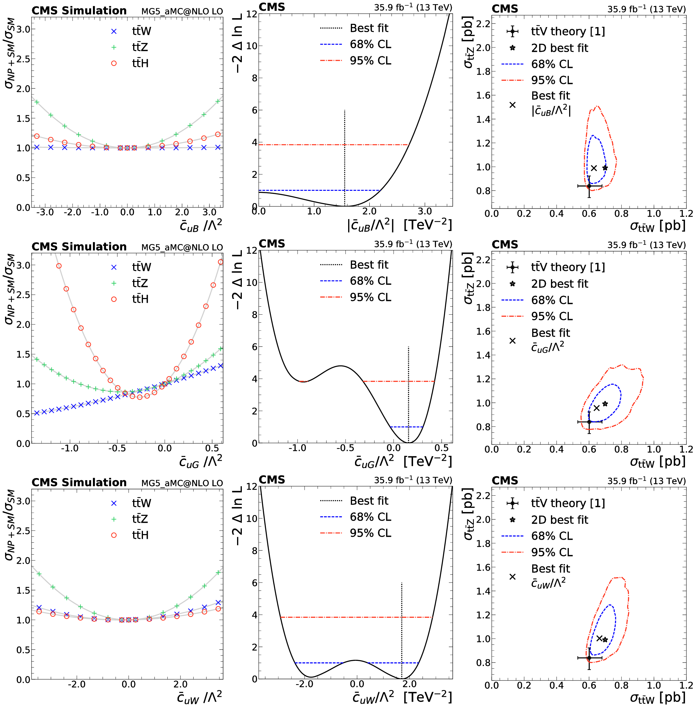
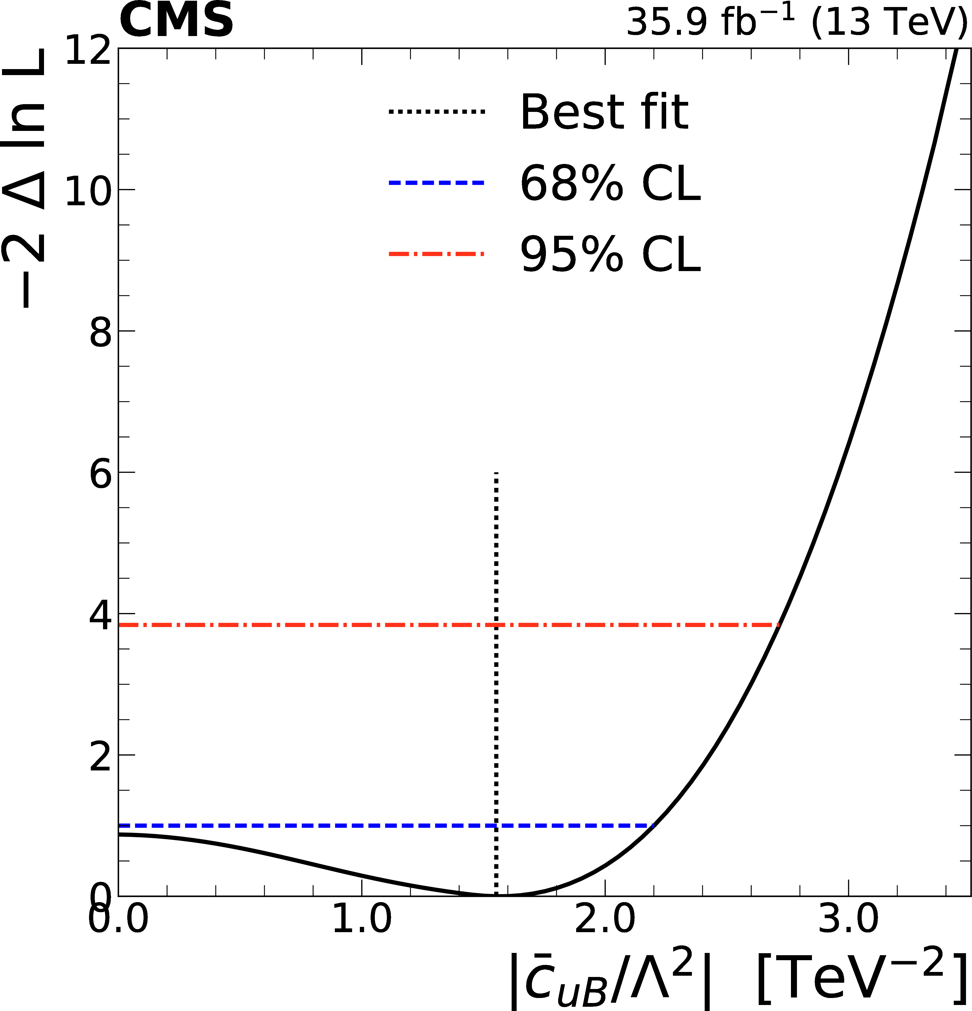
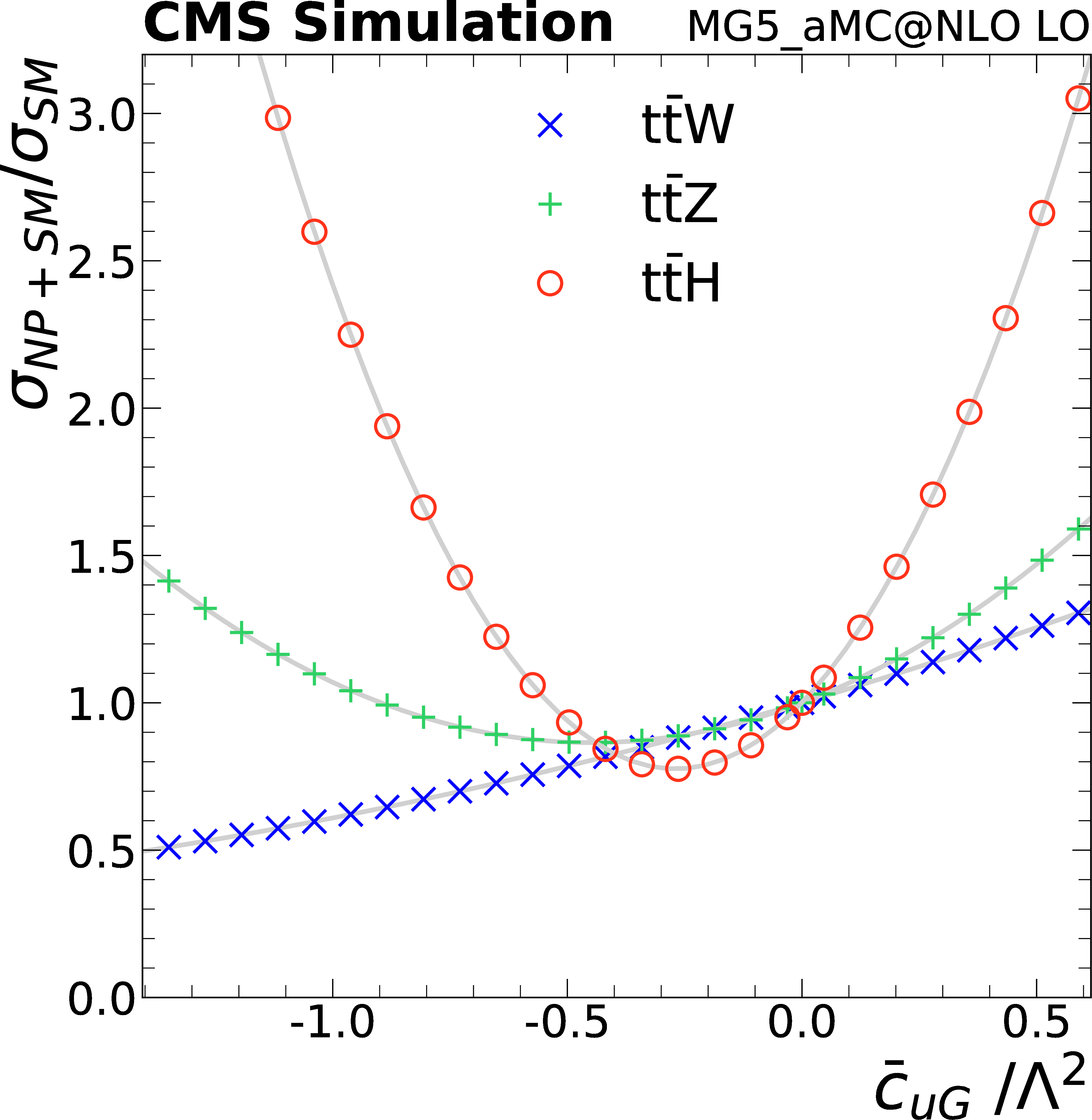
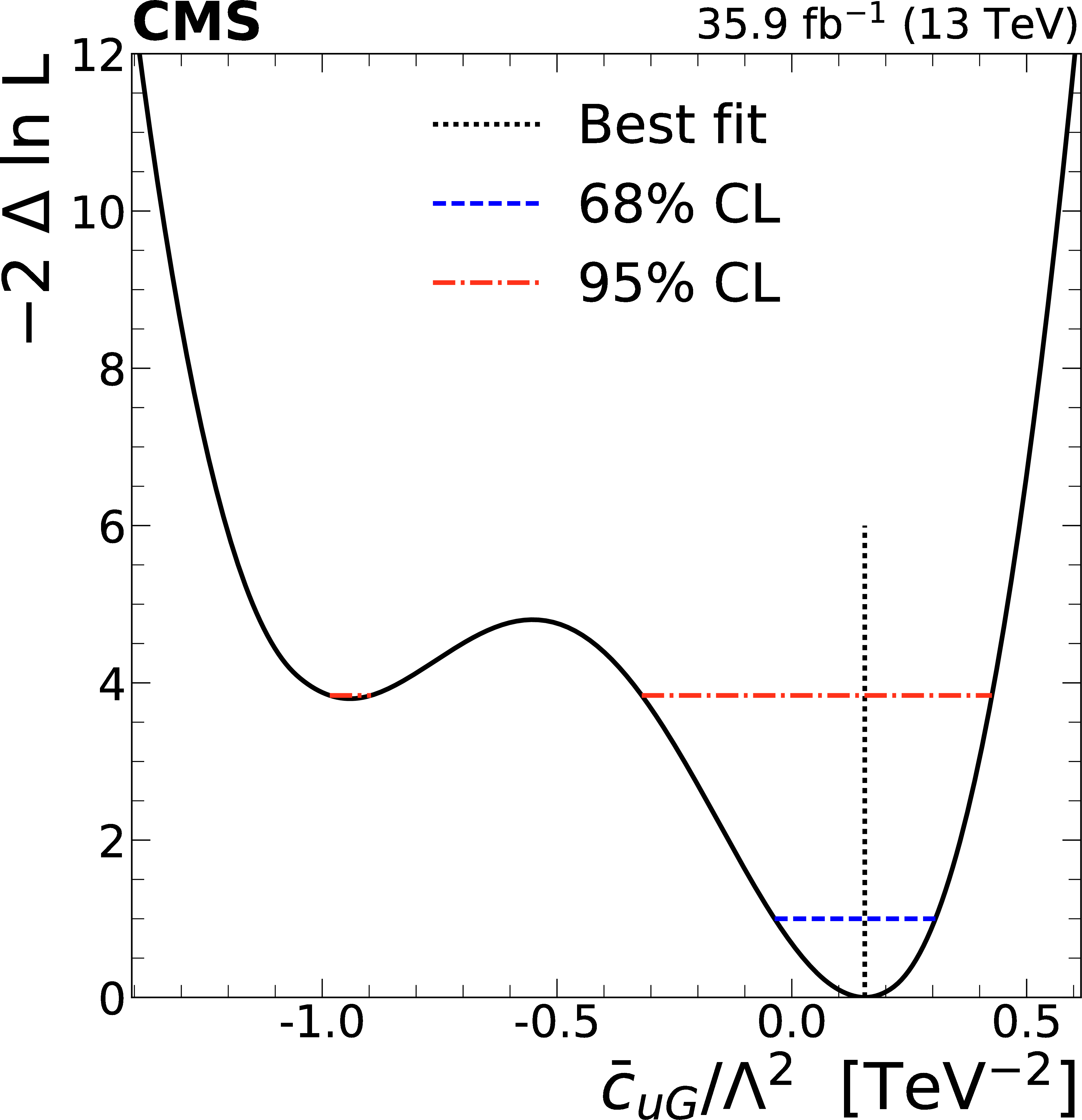
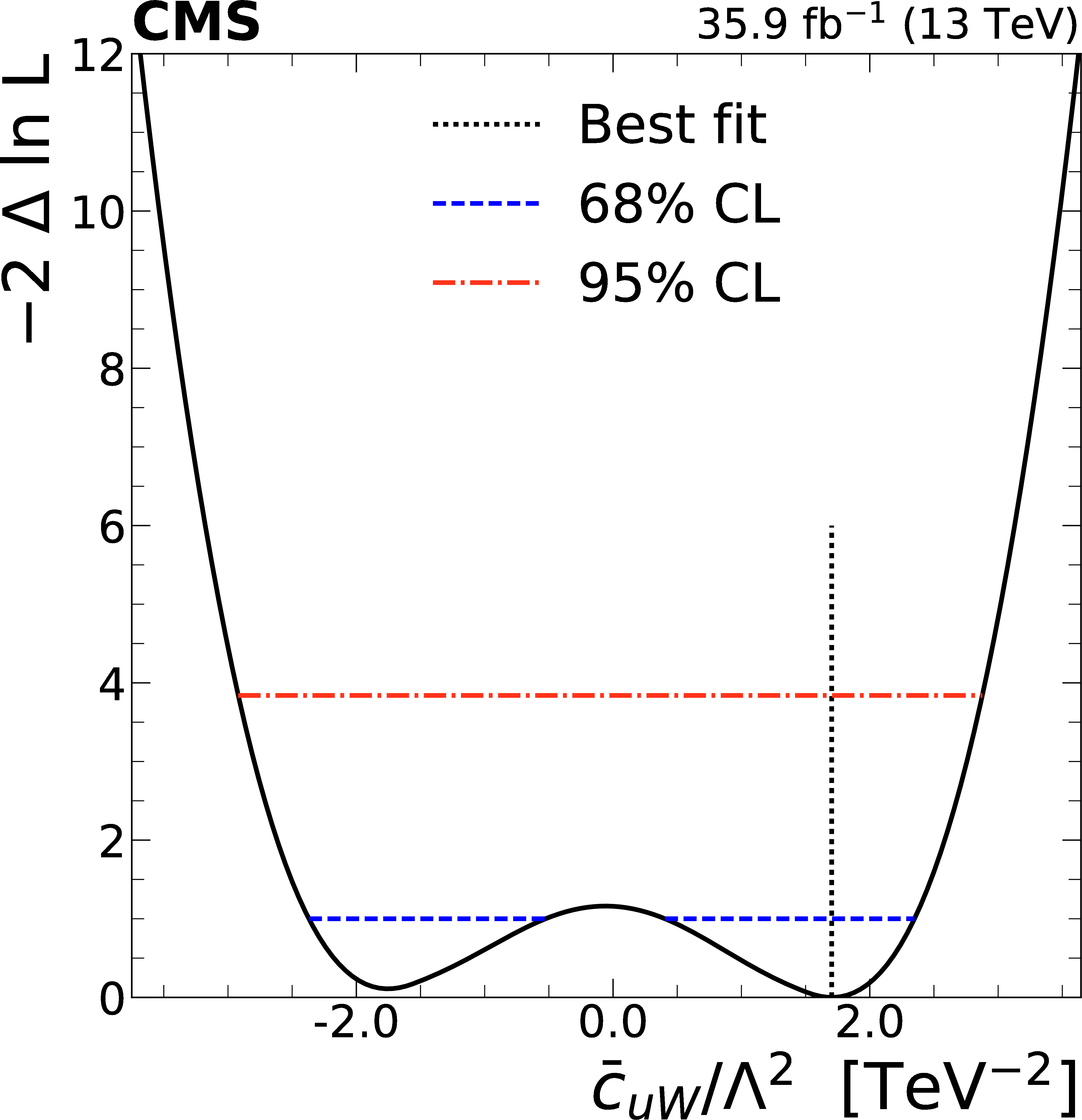
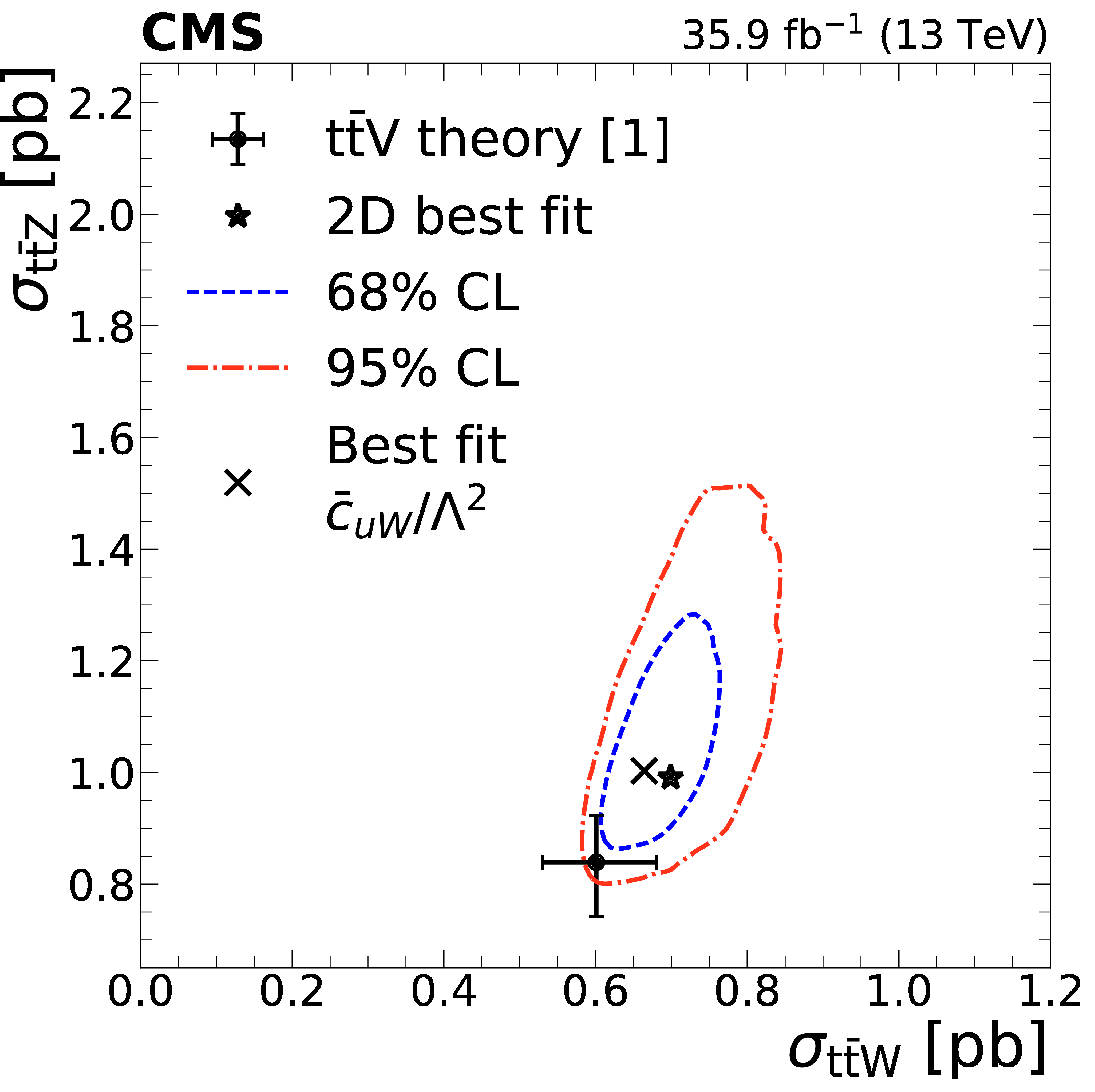
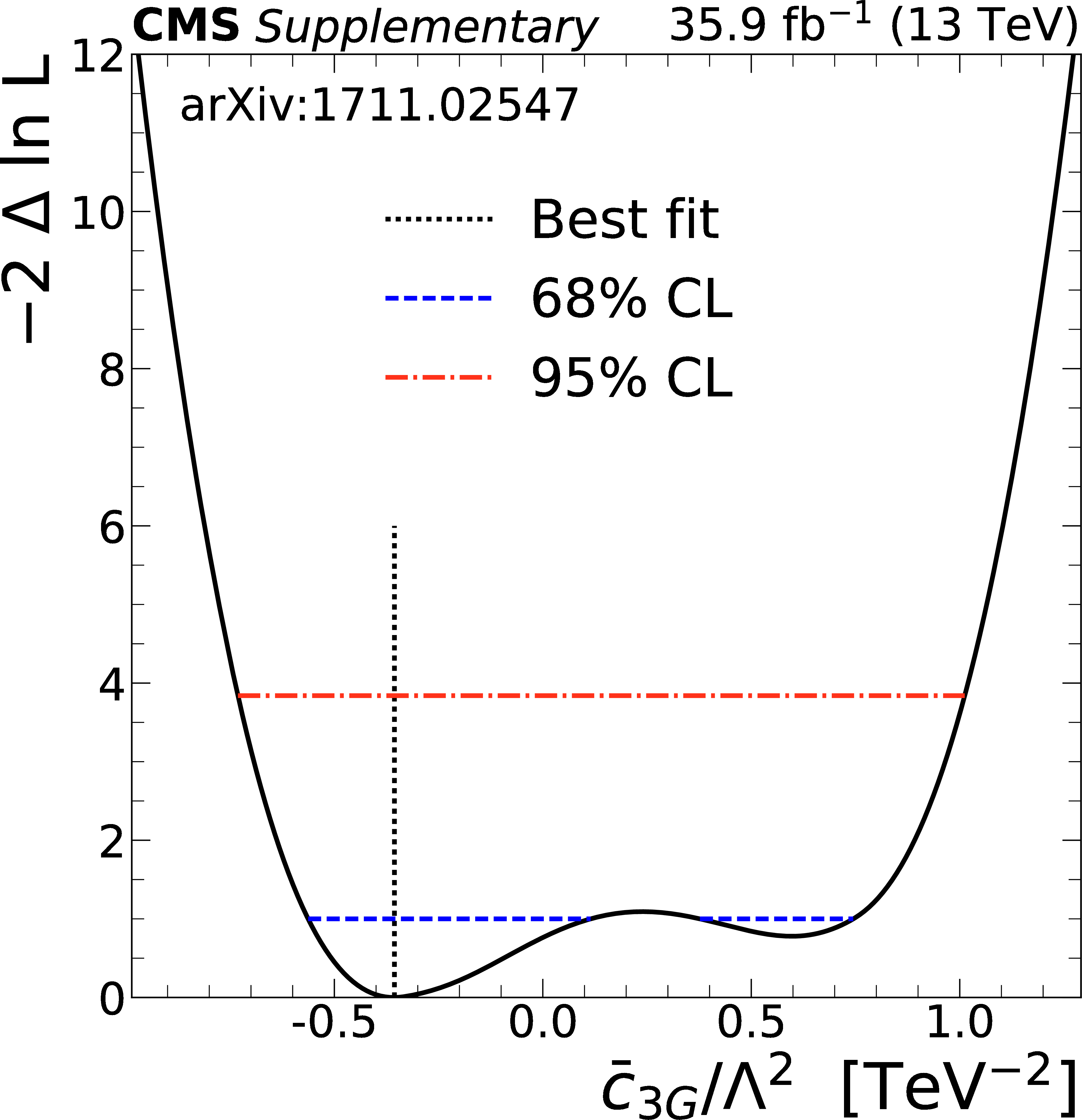
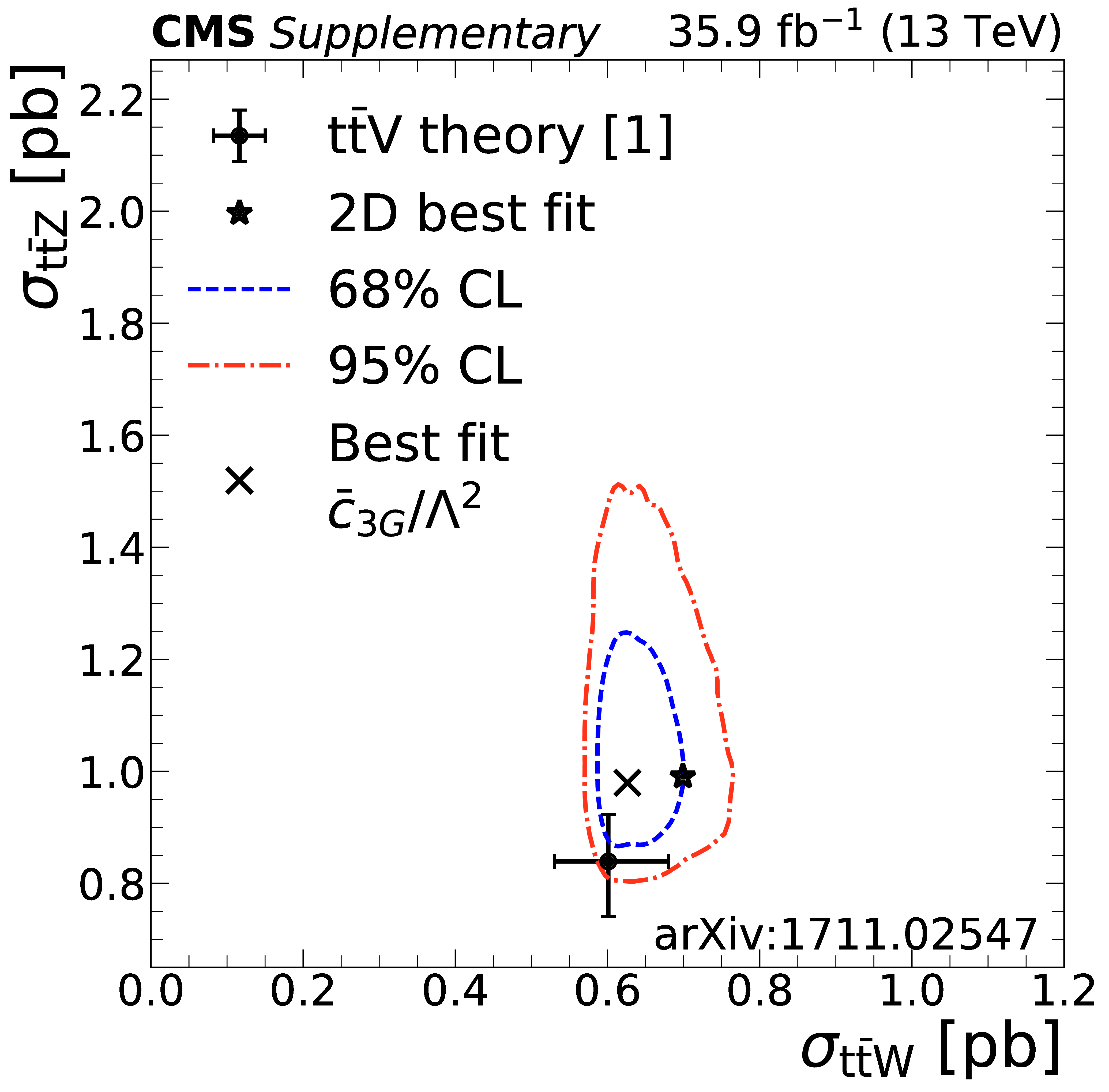
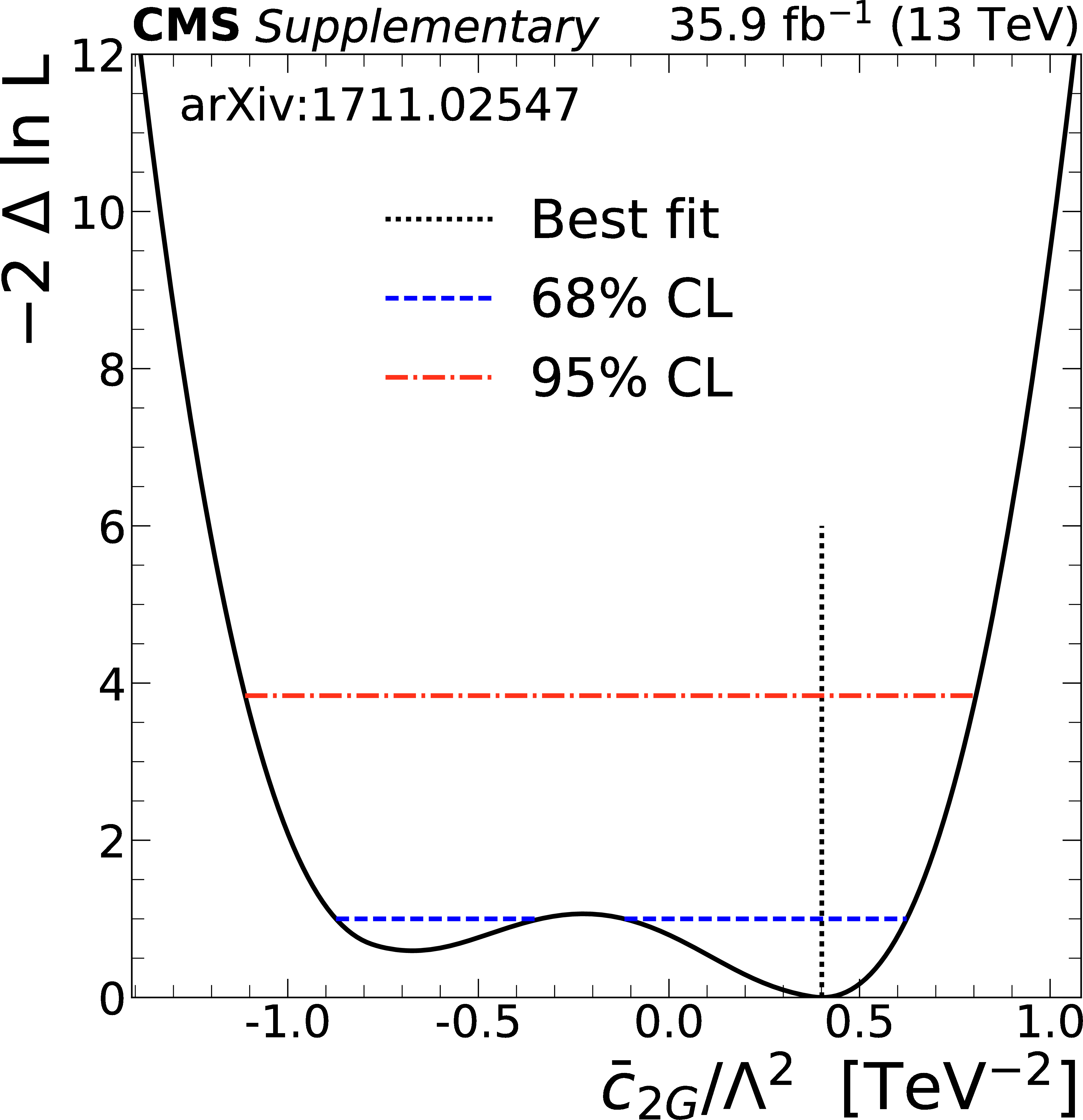
Figure 14:
Left: signal strength as a function of selected Wilson coefficients for $ {{\mathrm{t} {}\mathrm{\bar{t}}} \mathrm{W}} $ (crosses), $ {{\mathrm{t} {}\mathrm{\bar{t}}} \mathrm{Z}} $ (pluses), and $ {{\mathrm{t} {}\mathrm{\bar{t}}} \mathrm{H}} $ (circles). Center: the 1D test statistic $q(c_i)$ scan as a function of $c_i$, profiling all other nuisance parameters. The global best fit value is indicated by a dotted line. Dashed and dash-dotted lines indicate 68% and 95% CL intervals, respectively. Right: The $ {{\mathrm{t} {}\mathrm{\bar{t}}} \mathrm{Z}} $ and $ {{\mathrm{t} {}\mathrm{\bar{t}}} \mathrm{W}} $ cross section corresponding to the global best fit $c_i$ value is shown as a cross, along with the corresponding 68% (dashed) and 95% (dash-dotted) contours. The two-dimensional best fit to the $ {{\mathrm{t} {}\mathrm{\bar{t}}} \mathrm{W}} $ and $ {{\mathrm{t} {}\mathrm{\bar{t}}} \mathrm{Z}} $ cross sections is given by the star. The theory predictions [1] for ${{\mathrm{t} {}\mathrm{\bar{t}}} \mathrm{W}}$ and ${{\mathrm{t} {}\mathrm{\bar{t}}} \mathrm{Z}}$ are shown as a dot with bars representing their respective uncertainties. |

png pdf |
Figure 14-a:
Left: signal strength as a function of selected Wilson coefficients for $ {{\mathrm{t} {}\mathrm{\bar{t}}} \mathrm{W}} $ (crosses), $ {{\mathrm{t} {}\mathrm{\bar{t}}} \mathrm{Z}} $ (pluses), and $ {{\mathrm{t} {}\mathrm{\bar{t}}} \mathrm{H}} $ (circles). Center: the 1D test statistic $q(c_i)$ scan as a function of $c_i$, profiling all other nuisance parameters. The global best fit value is indicated by a dotted line. Dashed and dash-dotted lines indicate 68% and 95% CL intervals, respectively. Right: The $ {{\mathrm{t} {}\mathrm{\bar{t}}} \mathrm{Z}} $ and $ {{\mathrm{t} {}\mathrm{\bar{t}}} \mathrm{W}} $ cross section corresponding to the global best fit $c_i$ value is shown as a cross, along with the corresponding 68% (dashed) and 95% (dash-dotted) contours. The two-dimensional best fit to the $ {{\mathrm{t} {}\mathrm{\bar{t}}} \mathrm{W}} $ and $ {{\mathrm{t} {}\mathrm{\bar{t}}} \mathrm{Z}} $ cross sections is given by the star. The theory predictions [1] for ${{\mathrm{t} {}\mathrm{\bar{t}}} \mathrm{W}}$ and ${{\mathrm{t} {}\mathrm{\bar{t}}} \mathrm{Z}}$ are shown as a dot with bars representing their respective uncertainties. |
png pdf |
Figure 14-b:
Left: signal strength as a function of selected Wilson coefficients for $ {{\mathrm{t} {}\mathrm{\bar{t}}} \mathrm{W}} $ (crosses), $ {{\mathrm{t} {}\mathrm{\bar{t}}} \mathrm{Z}} $ (pluses), and $ {{\mathrm{t} {}\mathrm{\bar{t}}} \mathrm{H}} $ (circles). Center: the 1D test statistic $q(c_i)$ scan as a function of $c_i$, profiling all other nuisance parameters. The global best fit value is indicated by a dotted line. Dashed and dash-dotted lines indicate 68% and 95% CL intervals, respectively. Right: The $ {{\mathrm{t} {}\mathrm{\bar{t}}} \mathrm{Z}} $ and $ {{\mathrm{t} {}\mathrm{\bar{t}}} \mathrm{W}} $ cross section corresponding to the global best fit $c_i$ value is shown as a cross, along with the corresponding 68% (dashed) and 95% (dash-dotted) contours. The two-dimensional best fit to the $ {{\mathrm{t} {}\mathrm{\bar{t}}} \mathrm{W}} $ and $ {{\mathrm{t} {}\mathrm{\bar{t}}} \mathrm{Z}} $ cross sections is given by the star. The theory predictions [1] for ${{\mathrm{t} {}\mathrm{\bar{t}}} \mathrm{W}}$ and ${{\mathrm{t} {}\mathrm{\bar{t}}} \mathrm{Z}}$ are shown as a dot with bars representing their respective uncertainties. |

png pdf |
Figure 14-c:
Left: signal strength as a function of selected Wilson coefficients for $ {{\mathrm{t} {}\mathrm{\bar{t}}} \mathrm{W}} $ (crosses), $ {{\mathrm{t} {}\mathrm{\bar{t}}} \mathrm{Z}} $ (pluses), and $ {{\mathrm{t} {}\mathrm{\bar{t}}} \mathrm{H}} $ (circles). Center: the 1D test statistic $q(c_i)$ scan as a function of $c_i$, profiling all other nuisance parameters. The global best fit value is indicated by a dotted line. Dashed and dash-dotted lines indicate 68% and 95% CL intervals, respectively. Right: The $ {{\mathrm{t} {}\mathrm{\bar{t}}} \mathrm{Z}} $ and $ {{\mathrm{t} {}\mathrm{\bar{t}}} \mathrm{W}} $ cross section corresponding to the global best fit $c_i$ value is shown as a cross, along with the corresponding 68% (dashed) and 95% (dash-dotted) contours. The two-dimensional best fit to the $ {{\mathrm{t} {}\mathrm{\bar{t}}} \mathrm{W}} $ and $ {{\mathrm{t} {}\mathrm{\bar{t}}} \mathrm{Z}} $ cross sections is given by the star. The theory predictions [1] for ${{\mathrm{t} {}\mathrm{\bar{t}}} \mathrm{W}}$ and ${{\mathrm{t} {}\mathrm{\bar{t}}} \mathrm{Z}}$ are shown as a dot with bars representing their respective uncertainties. |
png pdf |
Figure 14-d:
Left: signal strength as a function of selected Wilson coefficients for $ {{\mathrm{t} {}\mathrm{\bar{t}}} \mathrm{W}} $ (crosses), $ {{\mathrm{t} {}\mathrm{\bar{t}}} \mathrm{Z}} $ (pluses), and $ {{\mathrm{t} {}\mathrm{\bar{t}}} \mathrm{H}} $ (circles). Center: the 1D test statistic $q(c_i)$ scan as a function of $c_i$, profiling all other nuisance parameters. The global best fit value is indicated by a dotted line. Dashed and dash-dotted lines indicate 68% and 95% CL intervals, respectively. Right: The $ {{\mathrm{t} {}\mathrm{\bar{t}}} \mathrm{Z}} $ and $ {{\mathrm{t} {}\mathrm{\bar{t}}} \mathrm{W}} $ cross section corresponding to the global best fit $c_i$ value is shown as a cross, along with the corresponding 68% (dashed) and 95% (dash-dotted) contours. The two-dimensional best fit to the $ {{\mathrm{t} {}\mathrm{\bar{t}}} \mathrm{W}} $ and $ {{\mathrm{t} {}\mathrm{\bar{t}}} \mathrm{Z}} $ cross sections is given by the star. The theory predictions [1] for ${{\mathrm{t} {}\mathrm{\bar{t}}} \mathrm{W}}$ and ${{\mathrm{t} {}\mathrm{\bar{t}}} \mathrm{Z}}$ are shown as a dot with bars representing their respective uncertainties. |
png pdf |
Figure 14-e:
Left: signal strength as a function of selected Wilson coefficients for $ {{\mathrm{t} {}\mathrm{\bar{t}}} \mathrm{W}} $ (crosses), $ {{\mathrm{t} {}\mathrm{\bar{t}}} \mathrm{Z}} $ (pluses), and $ {{\mathrm{t} {}\mathrm{\bar{t}}} \mathrm{H}} $ (circles). Center: the 1D test statistic $q(c_i)$ scan as a function of $c_i$, profiling all other nuisance parameters. The global best fit value is indicated by a dotted line. Dashed and dash-dotted lines indicate 68% and 95% CL intervals, respectively. Right: The $ {{\mathrm{t} {}\mathrm{\bar{t}}} \mathrm{Z}} $ and $ {{\mathrm{t} {}\mathrm{\bar{t}}} \mathrm{W}} $ cross section corresponding to the global best fit $c_i$ value is shown as a cross, along with the corresponding 68% (dashed) and 95% (dash-dotted) contours. The two-dimensional best fit to the $ {{\mathrm{t} {}\mathrm{\bar{t}}} \mathrm{W}} $ and $ {{\mathrm{t} {}\mathrm{\bar{t}}} \mathrm{Z}} $ cross sections is given by the star. The theory predictions [1] for ${{\mathrm{t} {}\mathrm{\bar{t}}} \mathrm{W}}$ and ${{\mathrm{t} {}\mathrm{\bar{t}}} \mathrm{Z}}$ are shown as a dot with bars representing their respective uncertainties. |

png pdf |
Figure 14-f:
Left: signal strength as a function of selected Wilson coefficients for $ {{\mathrm{t} {}\mathrm{\bar{t}}} \mathrm{W}} $ (crosses), $ {{\mathrm{t} {}\mathrm{\bar{t}}} \mathrm{Z}} $ (pluses), and $ {{\mathrm{t} {}\mathrm{\bar{t}}} \mathrm{H}} $ (circles). Center: the 1D test statistic $q(c_i)$ scan as a function of $c_i$, profiling all other nuisance parameters. The global best fit value is indicated by a dotted line. Dashed and dash-dotted lines indicate 68% and 95% CL intervals, respectively. Right: The $ {{\mathrm{t} {}\mathrm{\bar{t}}} \mathrm{Z}} $ and $ {{\mathrm{t} {}\mathrm{\bar{t}}} \mathrm{W}} $ cross section corresponding to the global best fit $c_i$ value is shown as a cross, along with the corresponding 68% (dashed) and 95% (dash-dotted) contours. The two-dimensional best fit to the $ {{\mathrm{t} {}\mathrm{\bar{t}}} \mathrm{W}} $ and $ {{\mathrm{t} {}\mathrm{\bar{t}}} \mathrm{Z}} $ cross sections is given by the star. The theory predictions [1] for ${{\mathrm{t} {}\mathrm{\bar{t}}} \mathrm{W}}$ and ${{\mathrm{t} {}\mathrm{\bar{t}}} \mathrm{Z}}$ are shown as a dot with bars representing their respective uncertainties. |

png pdf |
Figure 14-g:
Left: signal strength as a function of selected Wilson coefficients for $ {{\mathrm{t} {}\mathrm{\bar{t}}} \mathrm{W}} $ (crosses), $ {{\mathrm{t} {}\mathrm{\bar{t}}} \mathrm{Z}} $ (pluses), and $ {{\mathrm{t} {}\mathrm{\bar{t}}} \mathrm{H}} $ (circles). Center: the 1D test statistic $q(c_i)$ scan as a function of $c_i$, profiling all other nuisance parameters. The global best fit value is indicated by a dotted line. Dashed and dash-dotted lines indicate 68% and 95% CL intervals, respectively. Right: The $ {{\mathrm{t} {}\mathrm{\bar{t}}} \mathrm{Z}} $ and $ {{\mathrm{t} {}\mathrm{\bar{t}}} \mathrm{W}} $ cross section corresponding to the global best fit $c_i$ value is shown as a cross, along with the corresponding 68% (dashed) and 95% (dash-dotted) contours. The two-dimensional best fit to the $ {{\mathrm{t} {}\mathrm{\bar{t}}} \mathrm{W}} $ and $ {{\mathrm{t} {}\mathrm{\bar{t}}} \mathrm{Z}} $ cross sections is given by the star. The theory predictions [1] for ${{\mathrm{t} {}\mathrm{\bar{t}}} \mathrm{W}}$ and ${{\mathrm{t} {}\mathrm{\bar{t}}} \mathrm{Z}}$ are shown as a dot with bars representing their respective uncertainties. |
png pdf |
Figure 14-h:
Left: signal strength as a function of selected Wilson coefficients for $ {{\mathrm{t} {}\mathrm{\bar{t}}} \mathrm{W}} $ (crosses), $ {{\mathrm{t} {}\mathrm{\bar{t}}} \mathrm{Z}} $ (pluses), and $ {{\mathrm{t} {}\mathrm{\bar{t}}} \mathrm{H}} $ (circles). Center: the 1D test statistic $q(c_i)$ scan as a function of $c_i$, profiling all other nuisance parameters. The global best fit value is indicated by a dotted line. Dashed and dash-dotted lines indicate 68% and 95% CL intervals, respectively. Right: The $ {{\mathrm{t} {}\mathrm{\bar{t}}} \mathrm{Z}} $ and $ {{\mathrm{t} {}\mathrm{\bar{t}}} \mathrm{W}} $ cross section corresponding to the global best fit $c_i$ value is shown as a cross, along with the corresponding 68% (dashed) and 95% (dash-dotted) contours. The two-dimensional best fit to the $ {{\mathrm{t} {}\mathrm{\bar{t}}} \mathrm{W}} $ and $ {{\mathrm{t} {}\mathrm{\bar{t}}} \mathrm{Z}} $ cross sections is given by the star. The theory predictions [1] for ${{\mathrm{t} {}\mathrm{\bar{t}}} \mathrm{W}}$ and ${{\mathrm{t} {}\mathrm{\bar{t}}} \mathrm{Z}}$ are shown as a dot with bars representing their respective uncertainties. |
png pdf |
Figure 14-i:
Left: signal strength as a function of selected Wilson coefficients for $ {{\mathrm{t} {}\mathrm{\bar{t}}} \mathrm{W}} $ (crosses), $ {{\mathrm{t} {}\mathrm{\bar{t}}} \mathrm{Z}} $ (pluses), and $ {{\mathrm{t} {}\mathrm{\bar{t}}} \mathrm{H}} $ (circles). Center: the 1D test statistic $q(c_i)$ scan as a function of $c_i$, profiling all other nuisance parameters. The global best fit value is indicated by a dotted line. Dashed and dash-dotted lines indicate 68% and 95% CL intervals, respectively. Right: The $ {{\mathrm{t} {}\mathrm{\bar{t}}} \mathrm{Z}} $ and $ {{\mathrm{t} {}\mathrm{\bar{t}}} \mathrm{W}} $ cross section corresponding to the global best fit $c_i$ value is shown as a cross, along with the corresponding 68% (dashed) and 95% (dash-dotted) contours. The two-dimensional best fit to the $ {{\mathrm{t} {}\mathrm{\bar{t}}} \mathrm{W}} $ and $ {{\mathrm{t} {}\mathrm{\bar{t}}} \mathrm{Z}} $ cross sections is given by the star. The theory predictions [1] for ${{\mathrm{t} {}\mathrm{\bar{t}}} \mathrm{W}}$ and ${{\mathrm{t} {}\mathrm{\bar{t}}} \mathrm{Z}}$ are shown as a dot with bars representing their respective uncertainties. |
| Tables | |
png pdf |
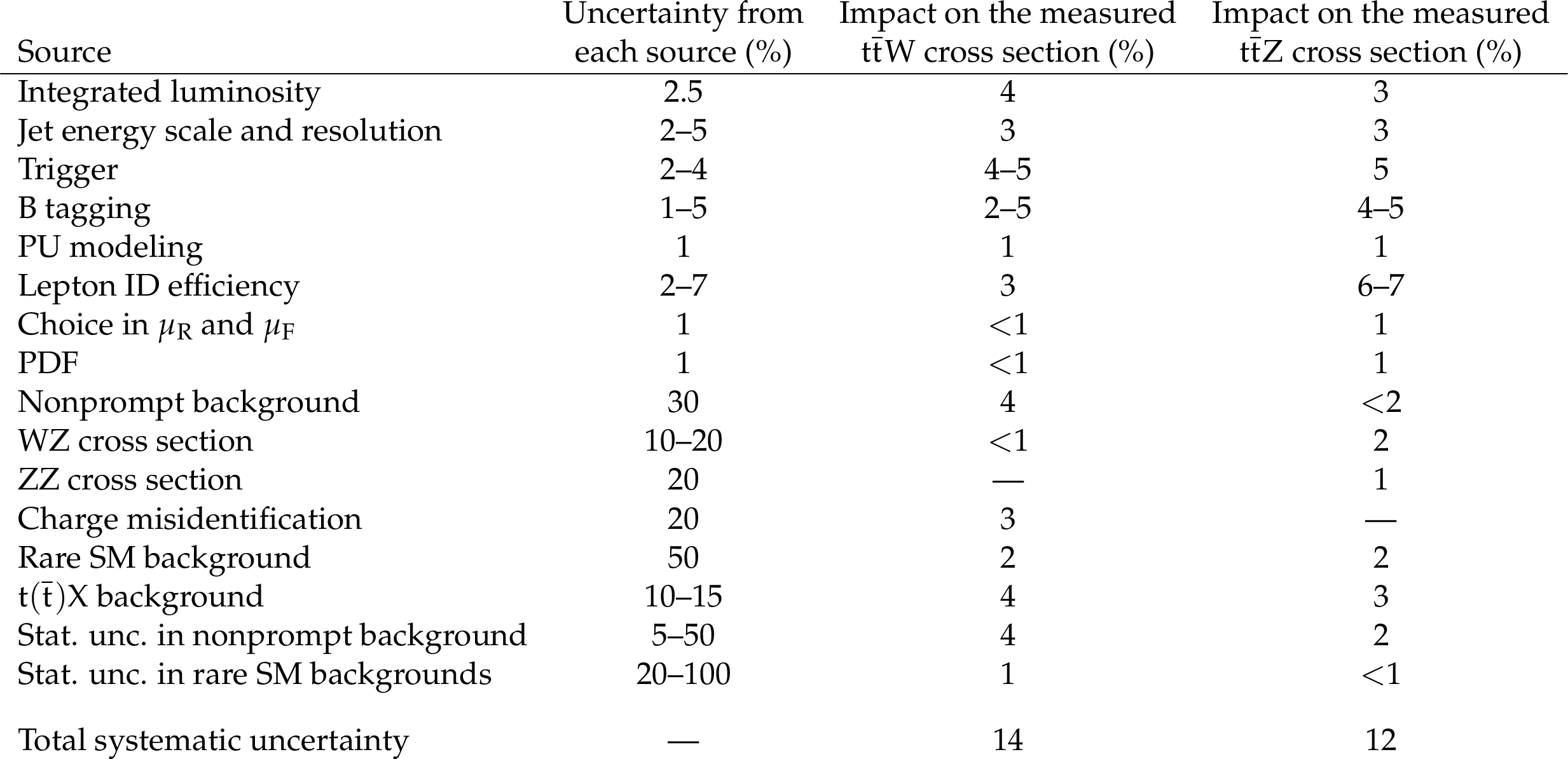
Table 1:
Summary of the sources of uncertainties, their magnitudes, and their effects in the final measurement. The first column indicates the source of the uncertainties, while the second column shows the corresponding input uncertainty on each background source and the signal. The third and fourth columns show the resulting uncertainties in the respective ${{\mathrm{t} {}\mathrm{\bar{t}}} \mathrm{W}}$ and ${{\mathrm{t} {}\mathrm{\bar{t}}} \mathrm{Z}} $ cross sections. |
png pdf |
Table 2:
Predicted and observed yields in the SS dilepton channel for the $ {\textit {D}} < $ 0 region, i.e. the nonprompt lepton control region. The total uncertainty obtained from the fit is also shown. |
png pdf |
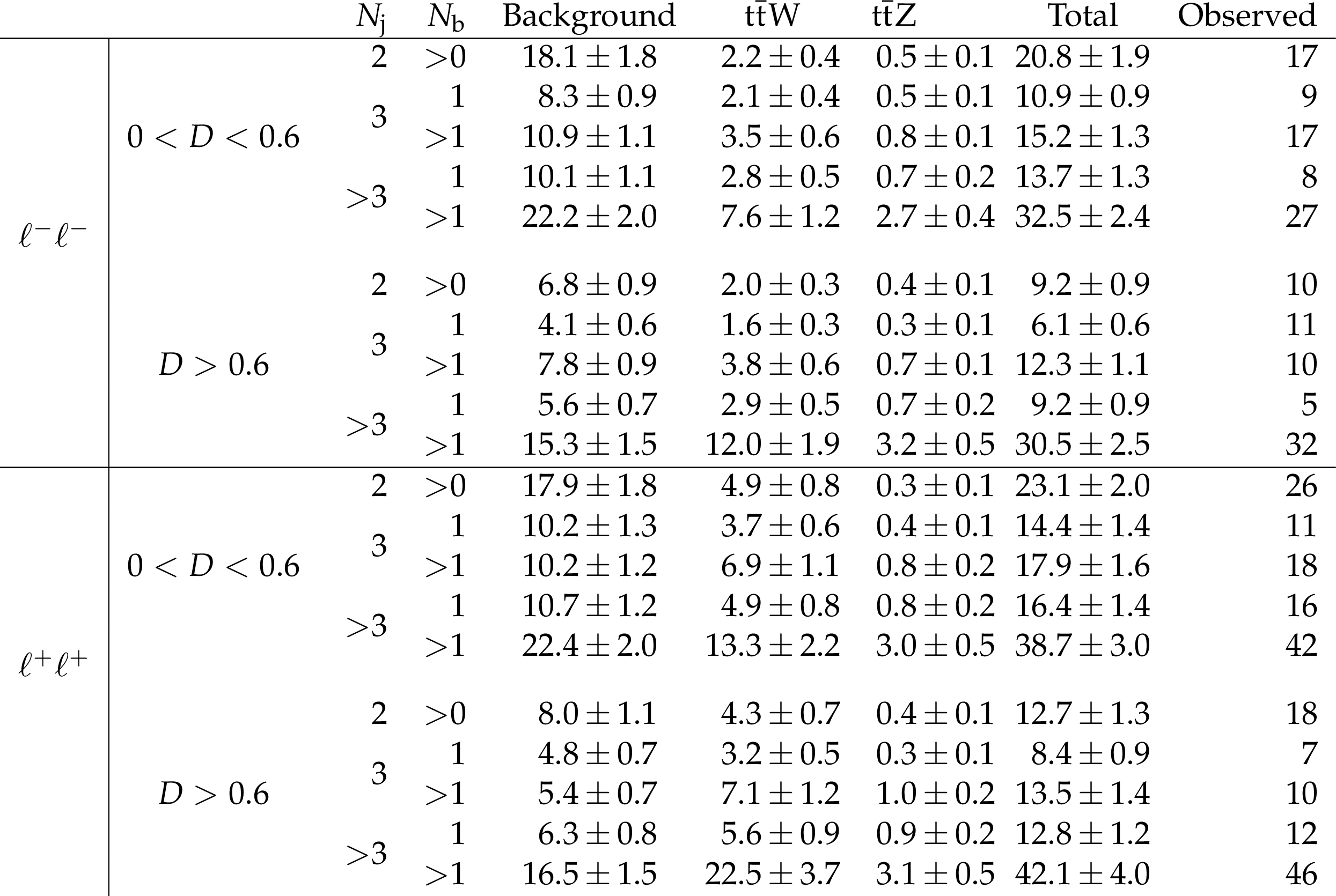
Table 3:
Predicted and observed yields in the SS dilepton final state. The total uncertainty obtained from the fit is also shown. |
png pdf |
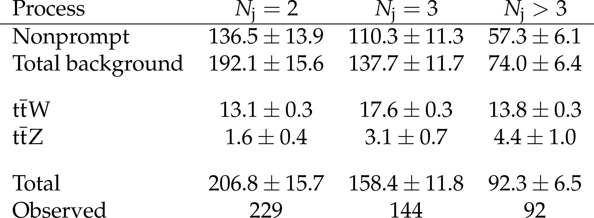
Table 4:
Predicted and observed yields in the three-lepton final state. The total uncertainty obtained from the fit is also shown. |

png pdf |
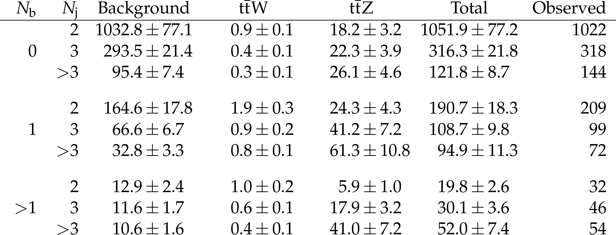
Table 5:
Predicted and observed yields in the four-lepton final state. The total uncertainty obtained from the fit is also shown. |
png pdf |
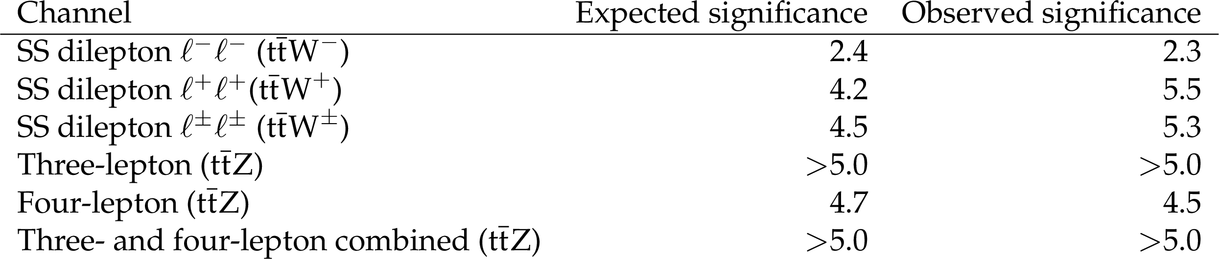
Table 6:
Summary of expected and observed significances (in standard deviations) for ${{\mathrm{t} {}\mathrm{\bar{t}}} \mathrm{W}} $ in the SS dilepton channel. |

png pdf |
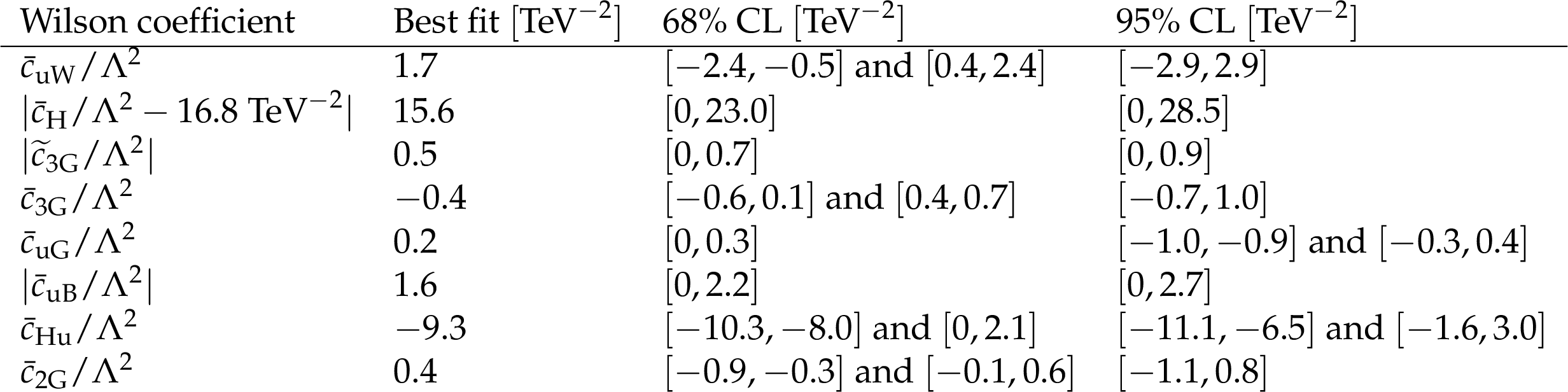
Table 7:
Expected 68% and 95% CL intervals for selected Wilson coefficients. |
png pdf |
Table 8:
Observed best fit values for selected Wilson coefficients determined from this $ {{\mathrm{t} {}\mathrm{\bar{t}}} \mathrm{W}} $ and $ {{\mathrm{t} {}\mathrm{\bar{t}}} \mathrm{Z}} $ measurement, along with corresponding 68% and 95% CL intervals. In some cases the profile likelihood shows another local minimum that cannot be excluded; the number reported here is the global minimum. |
| Summary |
| A measurement of top quark pair production in association with a W or a Z boson using proton-proton collisions at 13 TeV is presented. The analysis is performed in the same-sign dilepton final state for ${\mathrm{t\bar{t}}\mathrm{W}} $, and the three- and four-lepton final states for ${\mathrm{t\bar{t}}\mathrm{Z}} $, and these three final states are used to extract the cross sections for ${\mathrm{t\bar{t}}\mathrm{W}} $ and ${\mathrm{t\bar{t}}\mathrm{Z}} $ production. For both processes the observed signal significance exceeds 5 standard deviations. The measured cross sections are $\sigma({\mathrm{t\bar{t}}\mathrm{W}} )= $ 0.77$^{+0.12}_{-0.11}$ (stat) $^{+0.13}_{-0.12}$ (syst) pb and $\sigma({\mathrm{t\bar{t}}\mathrm{Z}} )=$ 0.99$^{+0.09}_{-0.08}$ (stat) $^{+0.12}_{-0.10}$ (syst) pb, in agreement with the standard model predictions. These results have been used to set constraints on the Wilson coefficients of dimension-six operators. Eight operators have been identified which are of particular interest because they change the expected cross sections of ${\mathrm{t\bar{t}}\mathrm{Z}} $, ${\mathrm{t\bar{t}}\mathrm{W}} $, or ${\mathrm{t\bar{t}}\mathrm{H}} $ without significantly impacting expected background yields. Both ${\mathrm{t\bar{t}}\mathrm{Z}} $ and ${\mathrm{t\bar{t}}\mathrm{H}} $ are affected by ${\mathcal{O}_{\text{3G}}} $, ${\mathcal{O}_{\widetilde{\text{3G}}}} $, ${\mathcal{O}_{\text{2G}}} $, and ${\mathcal{O}_{\text{uB}}} $. Only ${\mathrm{t\bar{t}}\mathrm{Z}} $ is affected by ${\mathcal{O}_{\mathrm{H}}} u$, while ${\mathcal{O}_{\mathrm{H}}} $ affects only ${\mathrm{t\bar{t}}\mathrm{H}} $. All three processes ${\mathrm{t\bar{t}}\mathrm{Z}} $, ${\mathrm{t\bar{t}}\mathrm{W}} $, and ${\mathrm{t\bar{t}}\mathrm{H}} $ are affected by ${\mathcal{O}_{\text{uG}}} $ and ${\mathcal{O}_{\text{uW}}} $. In cases where new physics beyond the standard model modifies the expected ${\mathrm{t\bar{t}}\mathrm{Z}} $ cross section, the sensitivity is mainly determined by ${\mathrm{t\bar{t}}\mathrm{Z}} $ and the fit is able to match the observed excess in data. No operators were identified which provide an independent handle on ${\mathrm{t\bar{t}}\mathrm{W}} $. The constraints presented, obtained by considering one operator at a time, are a useful first step toward more global approaches. |
| Additional Figures | |

png pdf |
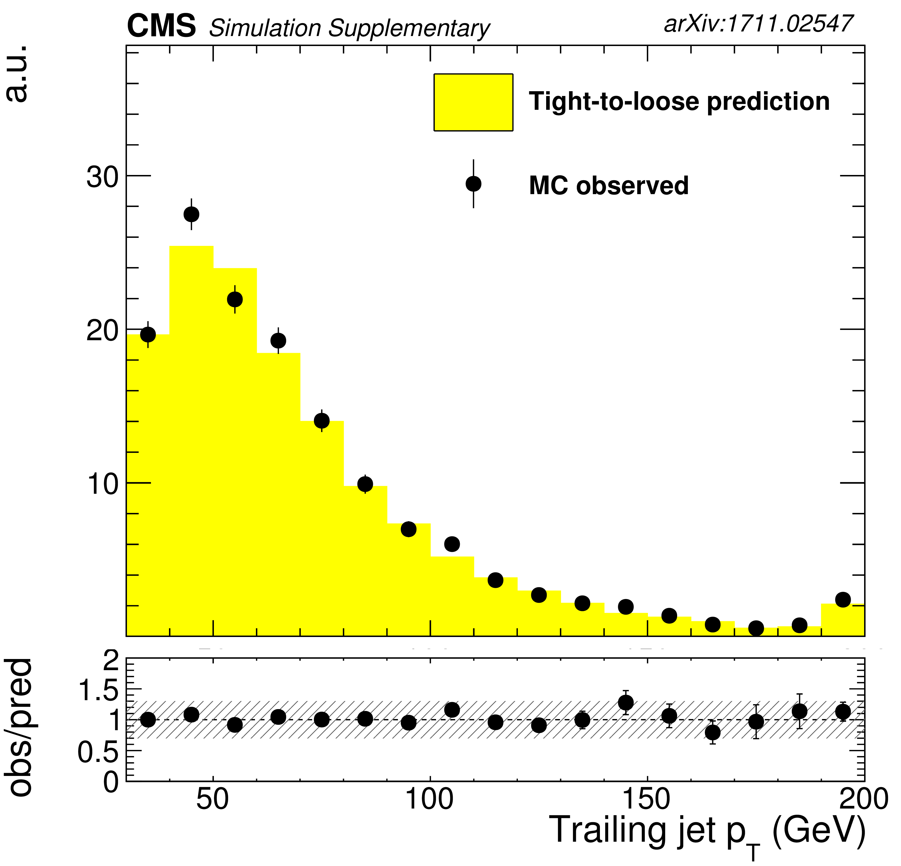
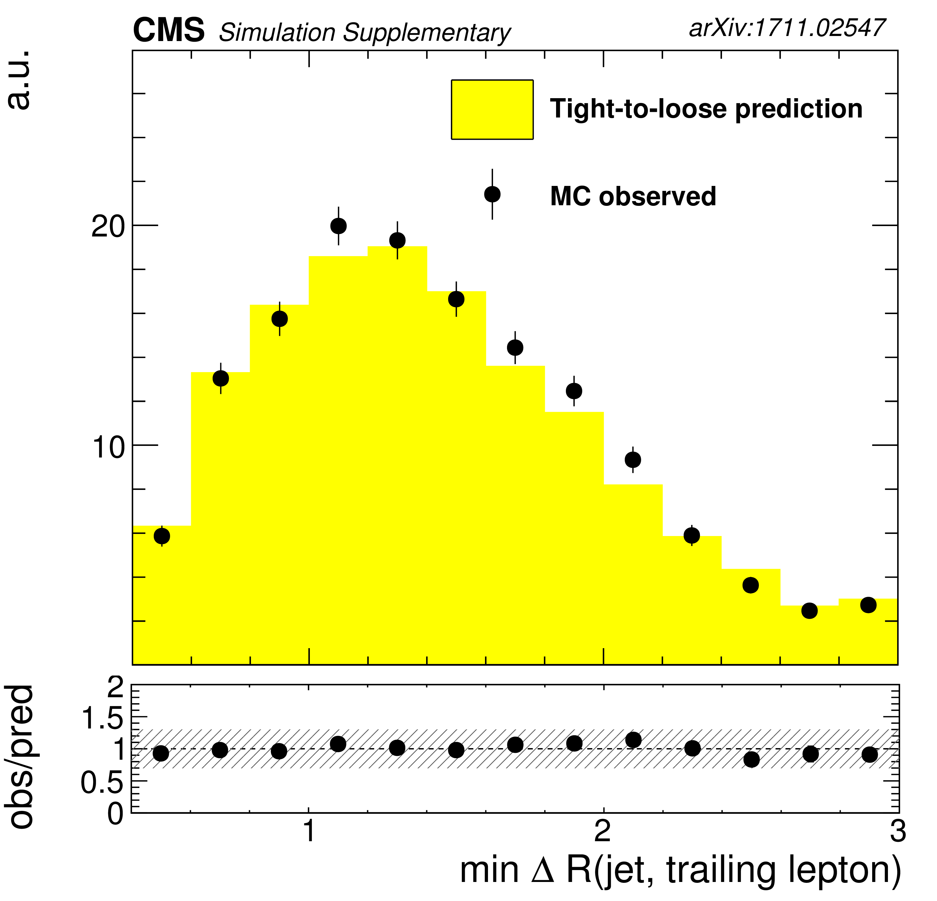
Additional Figure 1:
Fake background estimation closure with fake rate measured in QCD measurement region. Shown are the distributions of the jet multiplicity ${N_\text {jets}}$, transverse momentum of trailing jet, minimum $\Delta {\mathrm{R}} $ between trailing lepton and jet, transverse momentum of leading and trailing lepton and MVA score for events with same-sign dilepton pair as obtained from a $ {{\mathrm {t}\overline {\mathrm {t}}}} $ MadGraph sample. |

png pdf |
Additional Figure 1-a:
Fake background estimation closure with fake rate measured in QCD measurement region. Shown is the distribution of the jet multiplicity ${N_\text {jets}}$, as obtained from a $ {{\mathrm {t}\overline {\mathrm {t}}}} $ MadGraph sample. |
png pdf |
Additional Figure 1-b:
Fake background estimation closure with fake rate measured in QCD measurement region. Shown is the distribution of the transverse momentum of trailing jet, as obtained from a $ {{\mathrm {t}\overline {\mathrm {t}}}} $ MadGraph sample. |
png pdf |
Additional Figure 1-c:
Fake background estimation closure with fake rate measured in QCD measurement region. Shown is the distribution of the minimum $\Delta {\mathrm{R}} $ between trailing lepton and jet, as obtained from a $ {{\mathrm {t}\overline {\mathrm {t}}}} $ MadGraph sample. |

png pdf |
Additional Figure 1-d:
Fake background estimation closure with fake rate measured in QCD measurement region. Shown is the distribution of the transverse momentum of leading lepton, as obtained from a $ {{\mathrm {t}\overline {\mathrm {t}}}} $ MadGraph sample. |
png pdf |
Additional Figure 1-e:
Fake background estimation closure with fake rate measured in QCD measurement region. Shown is the distribution of the transverse momentum of trailing lepton, as obtained from a $ {{\mathrm {t}\overline {\mathrm {t}}}} $ MadGraph sample. |

png pdf |
Additional Figure 1-f:
Fake background estimation closure with fake rate measured in QCD measurement region. Shown is the distribution of the MVA score for events with same-sign dilepton pair, as obtained from a $ {{\mathrm {t}\overline {\mathrm {t}}}} $ MadGraph sample. |

png pdf |
Additional Figure 2:
Fake background estimation closure with fake rate measured in QCD measurement region. Shown are the distribution of the jet multiplicity ${N_\text {jets}}$ and event yields in each flavour composition for events with three leptons as obtained from a $ {{\mathrm {t}\overline {\mathrm {t}}}} $ MadGraph sample. |

png pdf |
Additional Figure 2-a:
Fake background estimation closure with fake rate measured in QCD measurement region. Shown is the distribution of the jet multiplicity ${N_\text {jets}}$, as obtained from a $ {{\mathrm {t}\overline {\mathrm {t}}}} $ MadGraph sample. |

png pdf |
Additional Figure 2-b:
Fake background estimation closure with fake rate measured in QCD measurement region. Shown is the distribution of the event yields in each flavour composition for events with three leptons, as obtained from a $ {{\mathrm {t}\overline {\mathrm {t}}}} $ MadGraph sample. |
png pdf |
Additional Figure 3:
Nonprompt control region plots in trilepton channel: distributions of the total yields in each ${N_\text {jets}}$ and $ {N_\text {b jets}} $ category. |

png pdf |
Additional Figure 4:
Nonprompt control region dominated by events from DY process. This control region is defined by an SFOC pair with an invariant close to Z boson and requirements on low (b)-jet multiplcity and missing transverse momentum. Shown are the distributions of the total yields in each flavour category, transverse momentum of trailing lepton and invariant mass of SFOC pair. |
png pdf |
Additional Figure 4-a:
Nonprompt control region dominated by events from DY process. This control region is defined by an SFOC pair with an invariant close to Z boson and requirements on low (b)-jet multiplcity and missing transverse momentum. Shown is the distribution of the total yields in each flavour category. |

png pdf |
Additional Figure 4-b:
Nonprompt control region dominated by events from DY process. This control region is defined by an SFOC pair with an invariant close to Z boson and requirements on low (b)-jet multiplcity and missing transverse momentum. Shown is the distribution of the transverse momentum of trailing lepton. |

png pdf |
Additional Figure 4-c:
Nonprompt control region dominated by events from DY process. This control region is defined by an SFOC pair with an invariant close to Z boson and requirements on low (b)-jet multiplcity and missing transverse momentum. Shown is the distribution of the invariant mass of SFOC pair. |
png pdf |
Additional Figure 5:
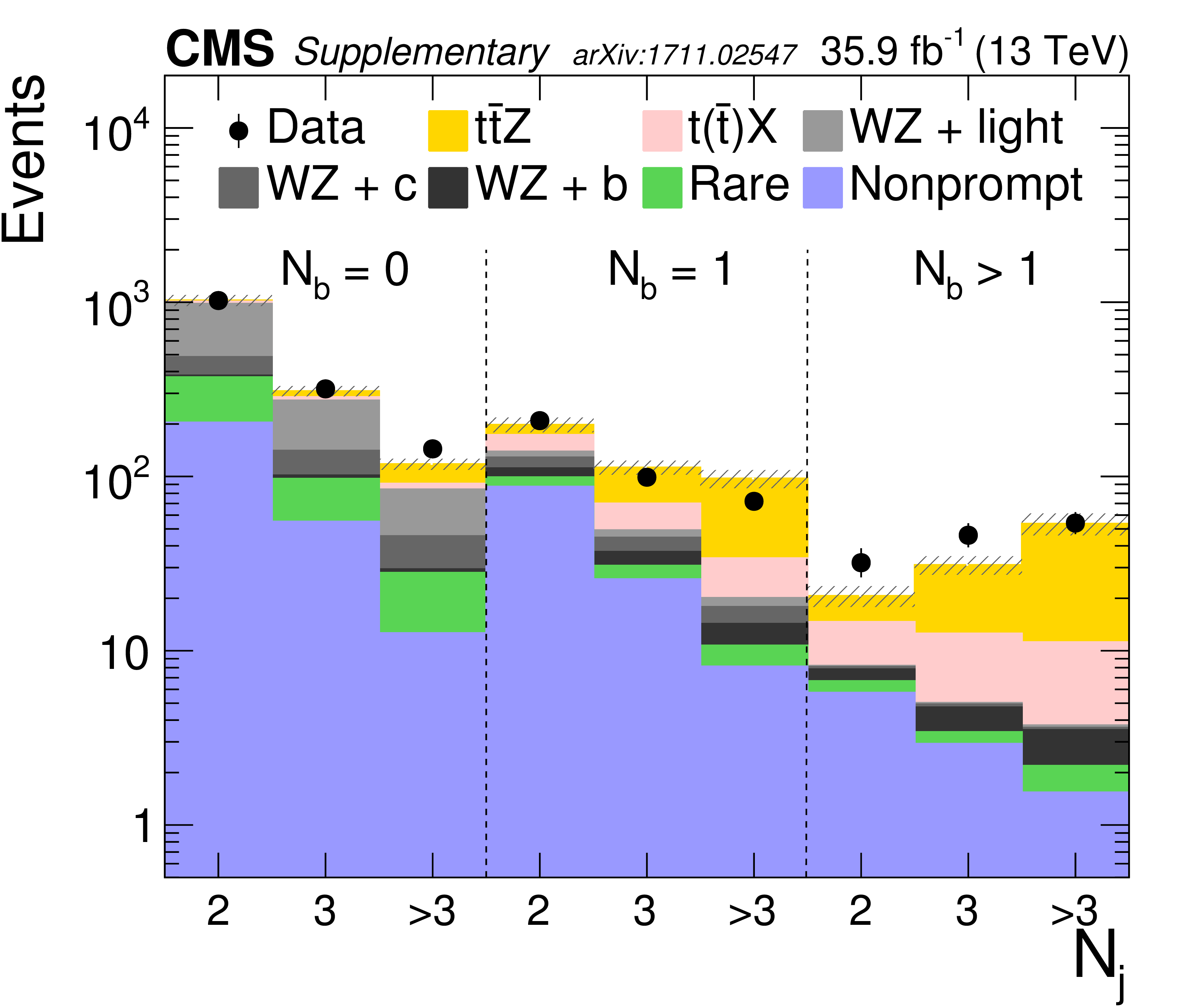
Post-fit predicted and observed yields in $ {N_\text {jets}} = $ 2, 3 and $\geq $4 categories in the three-lepton analyses. The yield from WZ background is split into three categories: events with at least 1 jet stemming from b-quark hadronization, at least 1 jet from c-quark hadronization and all jets are the yields of light quark hadronization. The hatched band shows the total uncertainty associated to signal and background predictions. |
png pdf |
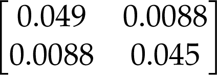
Additional Figure 6:
The covariance matrix obtained from the simultaneous fit for ${{{\mathrm {t}\overline {\mathrm {t}}}} {\mathrm {W}}}$ and ${{{\mathrm {t}\overline {\mathrm {t}}}} {\mathrm {Z}}}$ cross sections in same-sign dilepton, tri-lepton and four-lepton final states. The diagonal elements represent uncertainties for individual ${{{\mathrm {t}\overline {\mathrm {t}}}} {\mathrm {W}}}$ and ${{{\mathrm {t}\overline {\mathrm {t}}}} {\mathrm {Z}}}$ cross sections, while off-diagonal elements reflect the correlation between the two measurements. The units of the shown numbers are pb$^{2}$. |

png pdf |
Additional Figure 7:
Left: signal strength as a function of selected Wilson coefficients for $ { {{\mathrm {t}\overline {\mathrm {t}}}} {\mathrm {W}}} $ (blue crosses), $ {{{\mathrm {t}\overline {\mathrm {t}}}} {\mathrm {Z}}} $ (green pluses), and $ {{{\mathrm {t}\overline {\mathrm {t}}}} \mathrm{H}} $ (red circles). Center: the 1D test statistic $q(c_i)$ scan as a function of $c_i$, profiling all other nuisance parameters. The global best fit value is indicated by a black dotted line. Blue dotted and red dash-dotted lines indicate 68% and 95% CL intervals, respectively. Right: the $ {{{\mathrm {t}\overline {\mathrm {t}}}} {\mathrm {Z}}} $ and $ {{{\mathrm {t}\overline {\mathrm {t}}}} {\mathrm {W}}} $ cross section corresponding to the global best fit $c_i$ value is shown as a cross, along with the corresponding 68% (blue) and 95% (red) contours. The two-dimensional best fit to the $ {{{\mathrm {t}\overline {\mathrm {t}}}} {\mathrm {W}}} $ and $ {{{\mathrm {t}\overline {\mathrm {t}}}} {\mathrm {Z}}} $ cross sections is given by the star. |

png pdf |
Additional Figure 7-a:
Signal strength as a function of the $\bar{c}_{\text{H}}$ Wilson coefficient for $ { {{\mathrm {t}\overline {\mathrm {t}}}} {\mathrm {W}}} $ (blue crosses), $ {{{\mathrm {t}\overline {\mathrm {t}}}} {\mathrm {Z}}} $ (green pluses), and $ {{{\mathrm {t}\overline {\mathrm {t}}}} \mathrm{H}} $ (red circles). |
png pdf |
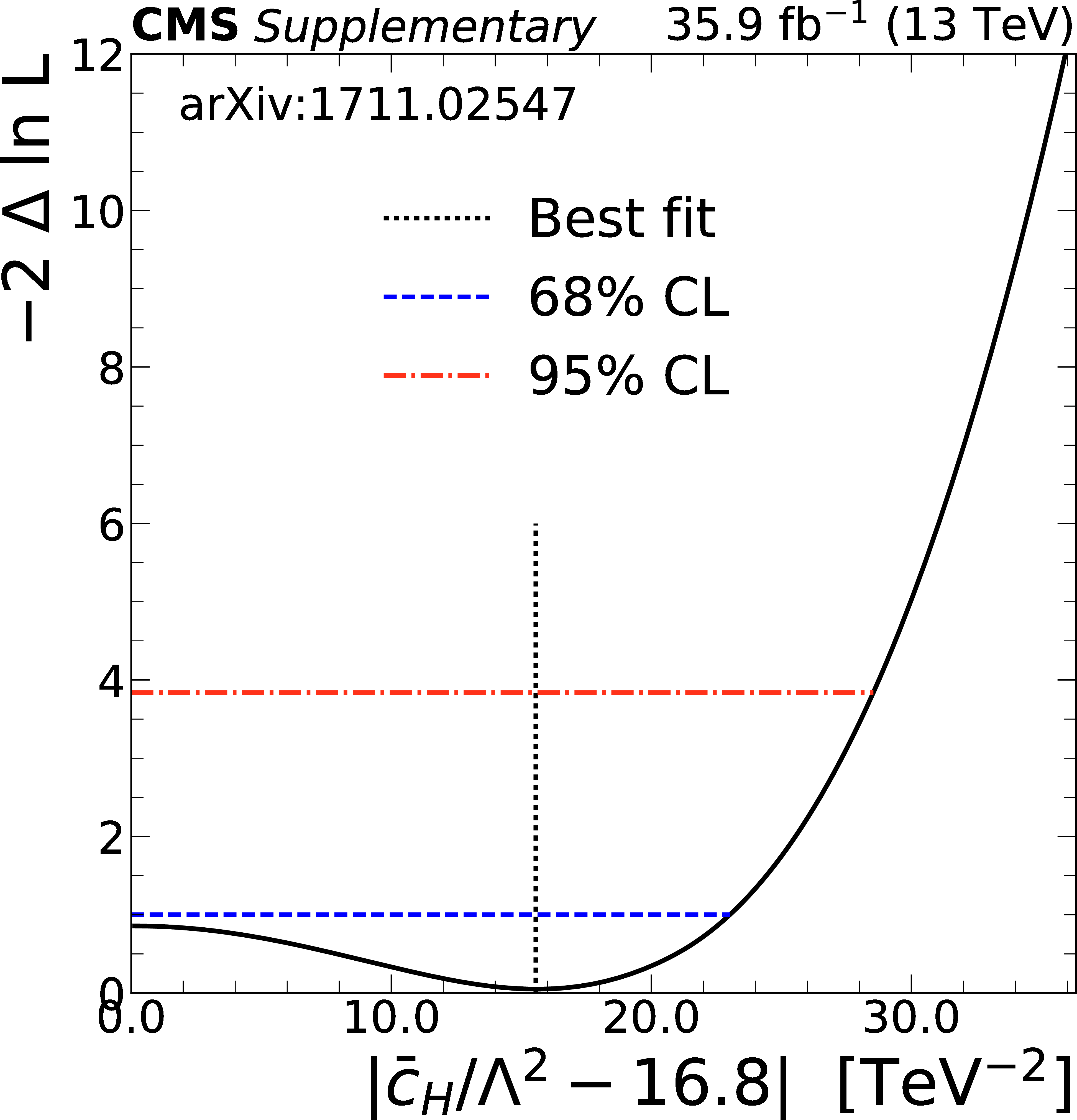
Additional Figure 7-b:
The 1D test statistic $q(\bar{c}_{\text{H}})$ scan as a function of $\bar{c}_{\text{H}}$, profiling all other nuisance parameters. The global best fit value is indicated by a black dotted line. Blue dotted and red dash-dotted lines indicate 68% and 95% CL intervals, respectively. |
png pdf |
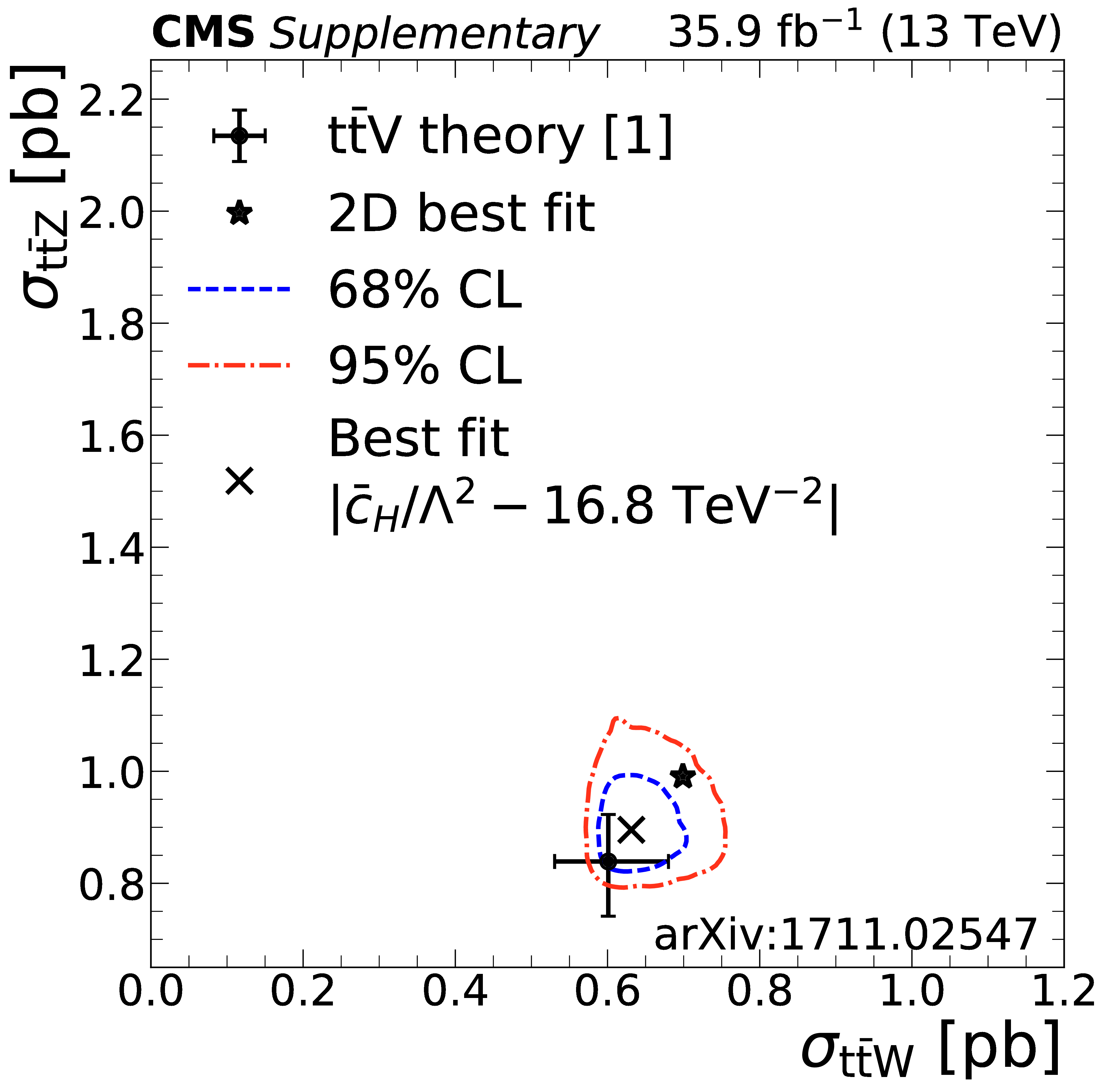
Additional Figure 7-c:
The $ {{{\mathrm {t}\overline {\mathrm {t}}}} {\mathrm {Z}}} $ and $ {{{\mathrm {t}\overline {\mathrm {t}}}} {\mathrm {W}}} $ cross section corresponding to the global best fit $\bar{c}_{\text{H}}$ value is shown as a cross, along with the corresponding 68% (blue) and 95% (red) contours. The two-dimensional best fit to the $ {{{\mathrm {t}\overline {\mathrm {t}}}} {\mathrm {W}}} $ and $ {{{\mathrm {t}\overline {\mathrm {t}}}} {\mathrm {Z}}} $ cross sections is given by the star. |

png pdf |
Additional Figure 7-d:
Signal strength as a function of the $\tilde{c}_{\text{3G}}$ Wilson coefficient for $ { {{\mathrm {t}\overline {\mathrm {t}}}} {\mathrm {W}}} $ (blue crosses), $ {{{\mathrm {t}\overline {\mathrm {t}}}} {\mathrm {Z}}} $ (green pluses), and $ {{{\mathrm {t}\overline {\mathrm {t}}}} \mathrm{H}} $ (red circles). |

png pdf |
Additional Figure 7-e:
The 1D test statistic $q(\tilde{c}_{\text{3G}})$ scan as a function of $\tilde{c}_{\text{3G}}$, profiling all other nuisance parameters. The global best fit value is indicated by a black dotted line. Blue dotted and red dash-dotted lines indicate 68% and 95% CL intervals, respectively. |
png pdf |
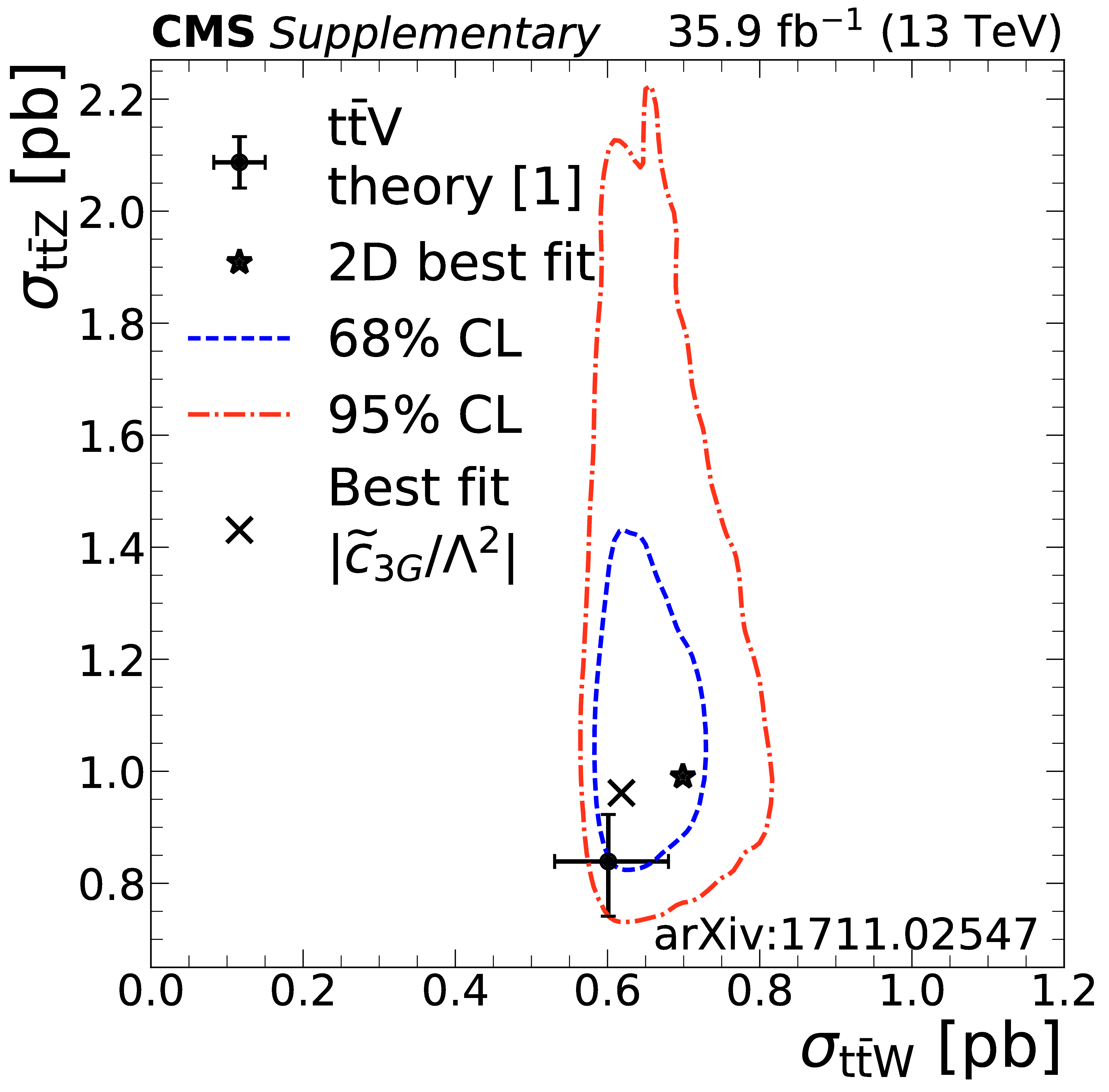
Additional Figure 7-f:
The $ {{{\mathrm {t}\overline {\mathrm {t}}}} {\mathrm {Z}}} $ and $ {{{\mathrm {t}\overline {\mathrm {t}}}} {\mathrm {W}}} $ cross section corresponding to the global best fit $\tilde{c}_{\text{3G}}$ value is shown as a cross, along with the corresponding 68% (blue) and 95% (red) contours. The two-dimensional best fit to the $ {{{\mathrm {t}\overline {\mathrm {t}}}} {\mathrm {W}}} $ and $ {{{\mathrm {t}\overline {\mathrm {t}}}} {\mathrm {Z}}} $ cross sections is given by the star. |

png pdf |
Additional Figure 7-g:
Signal strength as a function of the $\bar{c}_{\text{3G}}$ Wilson coefficient for $ { {{\mathrm {t}\overline {\mathrm {t}}}} {\mathrm {W}}} $ (blue crosses), $ {{{\mathrm {t}\overline {\mathrm {t}}}} {\mathrm {Z}}} $ (green pluses), and $ {{{\mathrm {t}\overline {\mathrm {t}}}} \mathrm{H}} $ (red circles). |
png pdf |
Additional Figure 7-h:
The 1D test statistic $q(\bar{c}_{\text{3G}})$ scan as a function of $\bar{c}_{\text{3G}}$, profiling all other nuisance parameters. The global best fit value is indicated by a black dotted line. Blue dotted and red dash-dotted lines indicate 68% and 95% CL intervals, respectively. |
png pdf |
Additional Figure 7-i:
The $ {{{\mathrm {t}\overline {\mathrm {t}}}} {\mathrm {Z}}} $ and $ {{{\mathrm {t}\overline {\mathrm {t}}}} {\mathrm {W}}} $ cross section corresponding to the global best fit $\bar{c}_{\text{3G}}$ value is shown as a cross, along with the corresponding 68% (blue) and 95% (red) contours. The two-dimensional best fit to the $ {{{\mathrm {t}\overline {\mathrm {t}}}} {\mathrm {W}}} $ and $ {{{\mathrm {t}\overline {\mathrm {t}}}} {\mathrm {Z}}} $ cross sections is given by the star. |
png pdf |
Additional Figure 7-j:
Signal strength as a function of the $\bar{c}_{\text{2G}}$ Wilson coefficient for $ { {{\mathrm {t}\overline {\mathrm {t}}}} {\mathrm {W}}} $ (blue crosses), $ {{{\mathrm {t}\overline {\mathrm {t}}}} {\mathrm {Z}}} $ (green pluses), and $ {{{\mathrm {t}\overline {\mathrm {t}}}} \mathrm{H}} $ (red circles). |
png pdf |
Additional Figure 7-k:
The 1D test statistic $q(\bar{c}_{\text{2G}})$ scan as a function of $\bar{c}_{\text{2G}}$, profiling all other nuisance parameters. The global best fit value is indicated by a black dotted line. Blue dotted and red dash-dotted lines indicate 68% and 95% CL intervals, respectively. |

png pdf |
Additional Figure 7-l:
The $ {{{\mathrm {t}\overline {\mathrm {t}}}} {\mathrm {Z}}} $ and $ {{{\mathrm {t}\overline {\mathrm {t}}}} {\mathrm {W}}} $ cross section corresponding to the global best fit $\bar{c}_{\text{2G}}$ value is shown as a cross, along with the corresponding 68% (blue) and 95% (red) contours. The two-dimensional best fit to the $ {{{\mathrm {t}\overline {\mathrm {t}}}} {\mathrm {W}}} $ and $ {{{\mathrm {t}\overline {\mathrm {t}}}} {\mathrm {Z}}} $ cross sections is given by the star. |

png pdf |
Additional Figure 7-m:
Signal strength as a function of the $\bar{c}_{\text{Hu}}$ Wilson coefficient for $ { {{\mathrm {t}\overline {\mathrm {t}}}} {\mathrm {W}}} $ (blue crosses), $ {{{\mathrm {t}\overline {\mathrm {t}}}} {\mathrm {Z}}} $ (green pluses), and $ {{{\mathrm {t}\overline {\mathrm {t}}}} \mathrm{H}} $ (red circles). |
png pdf |
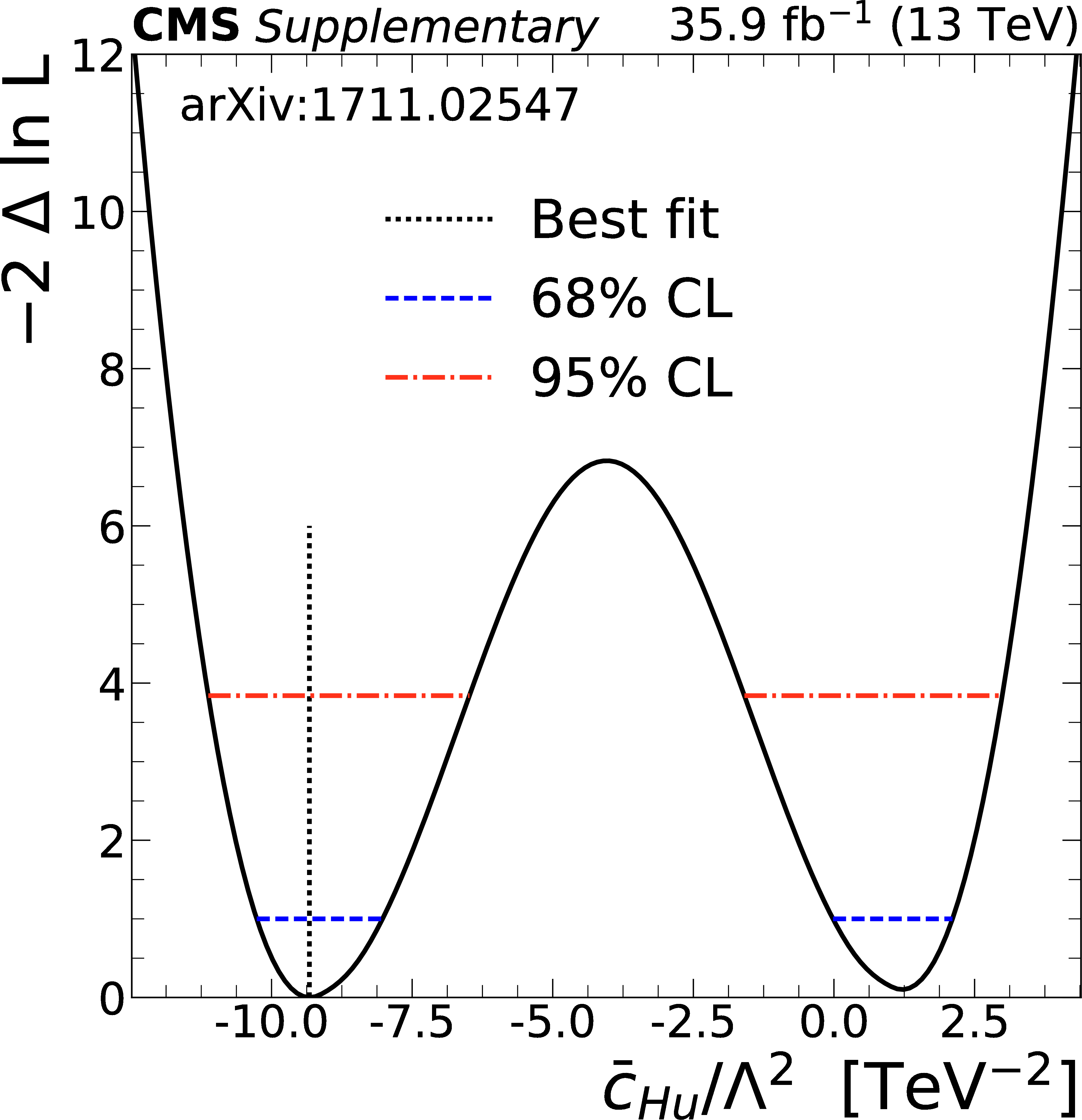
Additional Figure 7-n:
The 1D test statistic $q(\bar{c}_{\text{Hu}})$ scan as a function of $\bar{c}_{\text{Hu}}$, profiling all other nuisance parameters. The global best fit value is indicated by a black dotted line. Blue dotted and red dash-dotted lines indicate 68% and 95% CL intervals, respectively. |

png pdf |
Additional Figure 7-o:
The $ {{{\mathrm {t}\overline {\mathrm {t}}}} {\mathrm {Z}}} $ and $ {{{\mathrm {t}\overline {\mathrm {t}}}} {\mathrm {W}}} $ cross section corresponding to the global best fit $\bar{c}_{\text{Hu}}$ value is shown as a cross, along with the corresponding 68% (blue) and 95% (red) contours. The two-dimensional best fit to the $ {{{\mathrm {t}\overline {\mathrm {t}}}} {\mathrm {W}}} $ and $ {{{\mathrm {t}\overline {\mathrm {t}}}} {\mathrm {Z}}} $ cross sections is given by the star. |
| References | ||||
| 1 | D. de Florian et al. | Handbook of LHC Higgs cross sections: 4. deciphering the nature of the Higgs sector | CERN-2017-002-M | 1610.07922 |
| 2 | O. Bessidskaia Bylund et al. | Probing top quark neutral couplings in the Standard Model Effective Field Theory at NLO in QCD | JHEP 05 (2016) 052 | 1601.08193 |
| 3 | C. Englert, R. Kogler, H. Schulz, and M. Spannowsky | Higgs coupling measurements at the LHC | EPJC 76 (2016) 393 | 1511.05170 |
| 4 | CMS Collaboration | Measurement of associated production of vector bosons and $ \mathrm{t\bar{t}} $ in pp collisions at $ \sqrt{s} = $ 7 TeV | PRL 110 (2013) 172002 | CMS-TOP-12-014 1303.3239 |
| 5 | CMS Collaboration | Measurement of top quark-antiquark pair production in association with a W or Z boson in pp collisions at $ \sqrt{s} = $ 8 TeV | EPJC 74 (2014) 3060 | CMS-TOP-12-036 1406.7830 |
| 6 | CMS Collaboration | Observation of top quark pairs produced in association with a vector boson in pp collisions at $ \sqrt{s} = $ 8 TeV | JHEP 01 (2016) 096 | CMS-TOP-14-021 1510.01131 |
| 7 | ATLAS Collaboration | Measurement of the $ \mathrm{t\bar{t}}\mathrm{W} $ and $ \mathrm{t\bar{t}}\mathrm{Z} $ production cross sections in pp collisions at $ \sqrt{s} = $ 8 TeV with the ATLAS detector | JHEP 11 (2015) 172 | 1509.05276 |
| 8 | ATLAS Collaboration | Measurement of the $ \mathrm{t\bar{t}}\mathrm{Z} $ and $ \mathrm{t\bar{t}}\mathrm{W} $ production cross sections in multilepton final states using 3.2 fb$ ^{-1} $ of pp collisions at $ \sqrt{s} = $ 13 TeV with the ATLAS detector | EPJC 77 (2017) 40 | 1609.01599 |
| 9 | K. G. Wilson | Non-lagrangian models of current algebra | PR179 (1969) 1499 | |
| 10 | CMS Collaboration | The CMS experiment at the CERN LHC | JINST 3 (2008) S08004 | CMS-00-001 |
| 11 | CMS Collaboration | The CMS trigger system | JINST 12 (2017) P01020 | CMS-TRG-12-001 1609.02366 |
| 12 | J. Alwall et al. | The automated computation of tree-level and next-to-leading order differential cross sections, and their matching to parton shower simulations | JHEP 07 (2014) 079 | 1405.0301 |
| 13 | S. Alioli, P. Nason, C. Oleari, and E. Re | A general framework for implementing NLO calculations in shower Monte Carlo programs: the POWHEG BOX | JHEP 06 (2010) 043 | 1002.2581 |
| 14 | H. B. Hartanto, B. Jager, L. Reina, and D. Wackeroth | Higgs boson production in association with top quarks in the POWHEG BOX | PRD 91 (2015) 094003 | 1501.04498 |
| 15 | T. Melia, P. Nason, R. Rontsch, and G. Zanderighi | $ \mathrm{W}^+\mathrm{W}^- $, $ \mathrm{W}\mathrm{Z} $ and $ \mathrm{Z}\mathrm{Z} $ production in the POWHEG BOX | JHEP 11 (2011) 078 | 1107.5051 |
| 16 | P. Nason and G. Zanderighi | $ \mathrm{W}^+\mathrm{W}^- $ , $ \mathrm{W}\mathrm{Z} $ and $ \mathrm{Z}\mathrm{Z} $ production in the POWHEG-BOX-V2 | EPJC 74 (2014) 2702 | 1311.1365 |
| 17 | J. M. Campbell and R. K. Ellis | MCFM for the Tevatron and the LHC | NPPS 205-206 (2010) 10 | 1007.3492 |
| 18 | F. Cascioli et al. | ZZ production at hadron colliders in NNLO QCD | PLB 735 (2014) 311 | 1405.2219 |
| 19 | F. Caola, K. Melnikov, R. Rontsch, and L. Tancredi | QCD corrections to ZZ production in gluon fusion at the LHC | PRD 92 (2015) 094028 | 1509.06734 |
| 20 | NNPDF Collaboration | Parton distributions for the LHC Run II | JHEP 04 (2015) 040 | 1410.8849 |
| 21 | T. Sjostrand, S. Mrenna, and P. Z. Skands | A brief introduction to PYTHIA 8.1 | CPC 178 (2008) 852 | 0710.3820 |
| 22 | T. Sjostrand et al. | An introduction to PYTHIA 8.2 | CPC 191 (2015) 159 | 1410.3012 |
| 23 | P. Skands, S. Carrazza, and J. Rojo | Tuning PYTHIA 8.1: the Monash 2013 tune | EPJC 74 (2014) 3024 | 1404.5630 |
| 24 | CMS Collaboration | Event generator tunes obtained from underlying event and multiparton scattering measurements | EPJC 76 (2016) 155 | CMS-GEN-14-001 1512.00815 |
| 25 | J. Alwall et al. | Comparative study of various algorithms for the merging of parton showers and matrix elements in hadronic collisions | EPJC 53 (2008) 473 | 0706.2569 |
| 26 | R. Frederix and S. Frixione | Merging meets matching in MC@NLO | JHEP 12 (2012) 061 | 1209.6215 |
| 27 | GEANT4 Collaboration | GEANT4 --- a simulation toolkit | NIMA 506 (2003) 250 | |
| 28 | CMS Collaboration | Particle-flow reconstruction and global event description with the CMS detector | JINST 12 (2017) P10003 | CMS-PRF-14-001 1706.04965 |
| 29 | M. Cacciari, G. P. Salam, and G. Soyez | The anti-$ k_t $ jet clustering algorithm | JHEP 04 (2008) 063 | 0802.1189 |
| 30 | M. Cacciari, G. P. Salam, and G. Soyez | FastJet user manual | EPJC 72 (2012) 1896 | 1111.6097 |
| 31 | M. Cacciari and G. P. Salam | Dispelling the $ N^{3} $ myth for the $ k_t $ jet-finder | PLB 641 (2006) 57 | hep-ph/0512210 |
| 32 | CMS Collaboration | Pileup removal algorithms | CMS-PAS-JME-14-001 | CMS-PAS-JME-14-001 |
| 33 | CMS Collaboration | Identification of b-quark jets with the CMS experiment | JINST 8 (2013) P04013 | CMS-BTV-12-001 1211.4462 |
| 34 | CMS Collaboration | Identification of b quark jets at the CMS experiment in the LHC Run 2 | CMS-PAS-BTV-15-001 | CMS-PAS-BTV-15-001 |
| 35 | Particle Data Group | Review of particle physics | CPC 40 (2016) 100001 | |
| 36 | H. Voss, A. Hocker, J. Stelzer, and F. Tegenfeldt | TMVA, the toolkit for multivariate data analysis with ROOT | in XIth International Workshop on Advanced Computing and Analysis Techniques in Physics Research (ACAT), p. 40 2007 | physics/0703039 |
| 37 | CMS Collaboration | Search for new physics in same-sign dilepton events in proton-proton collisions at $ \sqrt{s} = $ 13 TeV | EPJC 76 (2016) 439 | CMS-SUS-15-008 1605.03171 |
| 38 | J. Campbell, R. K. Ellis, and R. Rontsch | Single top production in association with a Z boson at the LHC | PRD 87 (2013) 114006 | 1302.3856 |
| 39 | S. Frixione et al. | Electroweak and QCD corrections to top-pair hadroproduction in association with heavy bosons | JHEP 06 (2015) 184 | 1504.03446 |
| 40 | CMS Collaboration | CMS luminosity measurement for the 2016 data taking period | CMS-PAS-LUM-15-001 | CMS-PAS-LUM-15-001 |
| 41 | ATLAS Collaboration | Measurement of the inelastic proton-proton cross section at $ \sqrt{s} = $ 13 TeV with the ATLAS detector at the LHC | PRL 117 (2016) 182002 | 1606.02625 |
| 42 | CMS Collaboration | Performance of CMS muon reconstruction in pp collision events at $ \sqrt{s} = $ 7 TeV | JINST 7 (2012) P10002 | CMS-MUO-10-004 1206.4071 |
| 43 | CMS Collaboration | Performance of electron reconstruction and selection with the CMS detector in proton-proton collisions at $ \sqrt{s} = $ 8 TeV | JINST 10 (2015) P06005 | CMS-EGM-13-001 1502.02701 |
| 44 | CMS Collaboration | Performance of the CMS missing transverse momentum reconstruction in pp data at $ \sqrt{s} = $ 8 TeV | JINST 10 (2015) P02006 | CMS-JME-13-003 1411.0511 |
| 45 | CMS Collaboration | Performance of missing energy reconstruction in 13 TeV pp collision data using the CMS detector | CMS-PAS-JME-16-004 | CMS-PAS-JME-16-004 |
| 46 | T. Junk | Confidence level computation for combining searches with small statistics | NIMA 434 (1999) 435 | hep-ex/9902006 |
| 47 | A. L. Read | Presentation of search results: the $ CL_s $ technique | in Durham IPPP Workshop: Advanced Statistical Techniques in Particle Physics, p. 2693 Durham, UK, March, 2002 [JPG 28 (2002) 2693] | |
| 48 | ATLAS and CMS Collaborations | Procedure for the LHC Higgs boson search combination in summer 2011 | ATL-PHYS-PUB-2011-011, CMS NOTE-2011/005 | |
| 49 | G. Cowan, K. Cranmer, E. Gross, and O. Vitells | Asymptotic formulae for likelihood-based tests of new physics | EPJC 71 (2011) 1554 | 1007.1727 |
| 50 | W. Buchmuller and D. Wyler | Effective lagrangian analysis of new interactions and flavour conservation | NPB 268 (1986) 621 | |
| 51 | B. Grzadkowski, M. Iskrzynski, M. Misiak, and J. Rosiek | Dimension-six terms in the Standard Model Lagrangian | JHEP 10 (2010) 085 | 1008.4884 |
| 52 | A. Alloul, B. Fuks, and V. Sanz | Phenomenology of the Higgs effective Lagrangian via FeynRules | JHEP 04 (2014) 110 | 1310.5150 |
| 53 | J. Ellis, V. Sanz, and T. You | Complete Higgs sector constraints on dimension-6 operators | JHEP 07 (2014) 036 | 1404.3667 |
| 54 | K. Whisnant, J.-M. Yang, B.-L. Young, and X. Zhang | Dimension-six CP-conserving operators of the third-family quarks and their effects on collider observables | PRD 56 (1997) 467 | hep-ph/9702305 |
| 55 | E. L. Berger, Q.-H. Cao, and I. Low | Model independent constraints among the Wtb, $ \mathrm{Z} \mathrm{ q \bar{q} } $, and $ \mathrm{Z}\mathrm{t\bar{t}} $ couplings | PRD 80 (2009) 074020 | 0907.2191 |
| 56 | R. Rontsch and M. Schulze | Constraining couplings of top quarks to the Z boson in $ \mathrm{t\bar{t}} $+Z production at the LHC | JHEP 07 (2014) 091 | 1404.1005 |
| 57 | E. Malkawi and C. P. Yuan | Global analysis of the top quark couplings to gauge bosons | PRD 50 (1994) 4462 | hep-ph/9405322 |
| 58 | C. Zhang, N. Greiner, and S. Willenbrock | Constraints on nonstandard top quark couplings | PRD 86 (2012) 014024 | 1201.6670 |
| 59 | A. Tonero and R. Rosenfeld | Dipole-induced anomalous top quark couplings at the LHC | PRD 90 (2014) 017701 | 1404.2581 |
| 60 | C. Degrande et al. | Effective field theory: A modern approach to anomalous couplings | Annals Phys. 335 (2013) 21 | 1205.4231 |
| 61 | A. Alloul et al. | FeynRules 2.0 --- A complete toolbox for tree-level phenomenology | CPC 185 (2014) 2250 | 1310.1921 |
| 62 | S. Frixione and B. R. Webber | Matching NLO QCD computations and parton shower simulations | JHEP 06 (2002) 029 | hep-ph/0204244 |
| 63 | J. Ellis | TikZ-Feynman: Feynman diagrams with TikZ | CPC 210 (2017) 103 | 1601.05437 |
|
|
Compact Muon Solenoid LHC, CERN |
|

|

|

|

|

|