

Compact Muon Solenoid
LHC, CERN
| CMS-PAS-HIG-17-006 | ||
| Search for resonant and non-resonant Higgs boson pair production in the $\mathrm{b}\overline{\mathrm{b}} \ell\nu \ell\nu$ final state at $\sqrt{s} = $ 13 TeV | ||
| CMS Collaboration | ||
| March 2017 | ||
| Abstract: Searches for resonant and non-resonant pair-produced Higgs bosons (hh) decaying respectively into $\mathrm{b}\overline{\mathrm{b}}$ and VV (with V either a W or a Z boson), with subsequent VV decays into two leptons and two neutrinos, are presented. The analyses are based on a sample of proton-proton collisions at $\sqrt{s} = $ 13 TeV at the LHC corresponding to an integrated luminosity of 36 fb$^{-1}$. Data and predictions from the standard model are in agreement within uncertainties. For the standard model hh hypothesis, the data are observed (expected) to exclude a production cross-section times branching ratio of 72 (81$^{+42}_{-25}$) fb, corresponding to 79 (89$^{+47}_{-28}$) times the SM cross section. Lack of deviation from the SM predictions in the observations is used to place constraints on different scenarios considering anomalous couplings which could affect the rate and kinematics of hh production. In the case of resonant production of a new particle $\mathrm{X}$, for mass hypotheses from ${\mathrm{m}}_{\mathrm{X}} = $ 300 GeV to ${\mathrm{m}}_{\mathrm{X}} = $ 900 GeV, the data are observed (expected) to exclude a production cross-section times branching ratio of narrow-width spin-0 particles from 434 to 17 (342$^{+135}_{-97}$ to 14$^{+6}_{-4}$) fb and narrow-width spin-2 particles from 448 to 14 (361$^{+140}_{-102}$ to 13$^{+5}_{-4}$) fb. | ||
|
Links:
CDS record (PDF) ;
inSPIRE record ;
CADI line (restricted) ;
These preliminary results are superseded in this paper, JHEP 01 (2018) 054. The superseded preliminary plots can be found here. |
||
| Figures & Tables | Summary | Additional Figures & Tables | References | CMS Publications |
|---|
| Figures | |

png pdf |
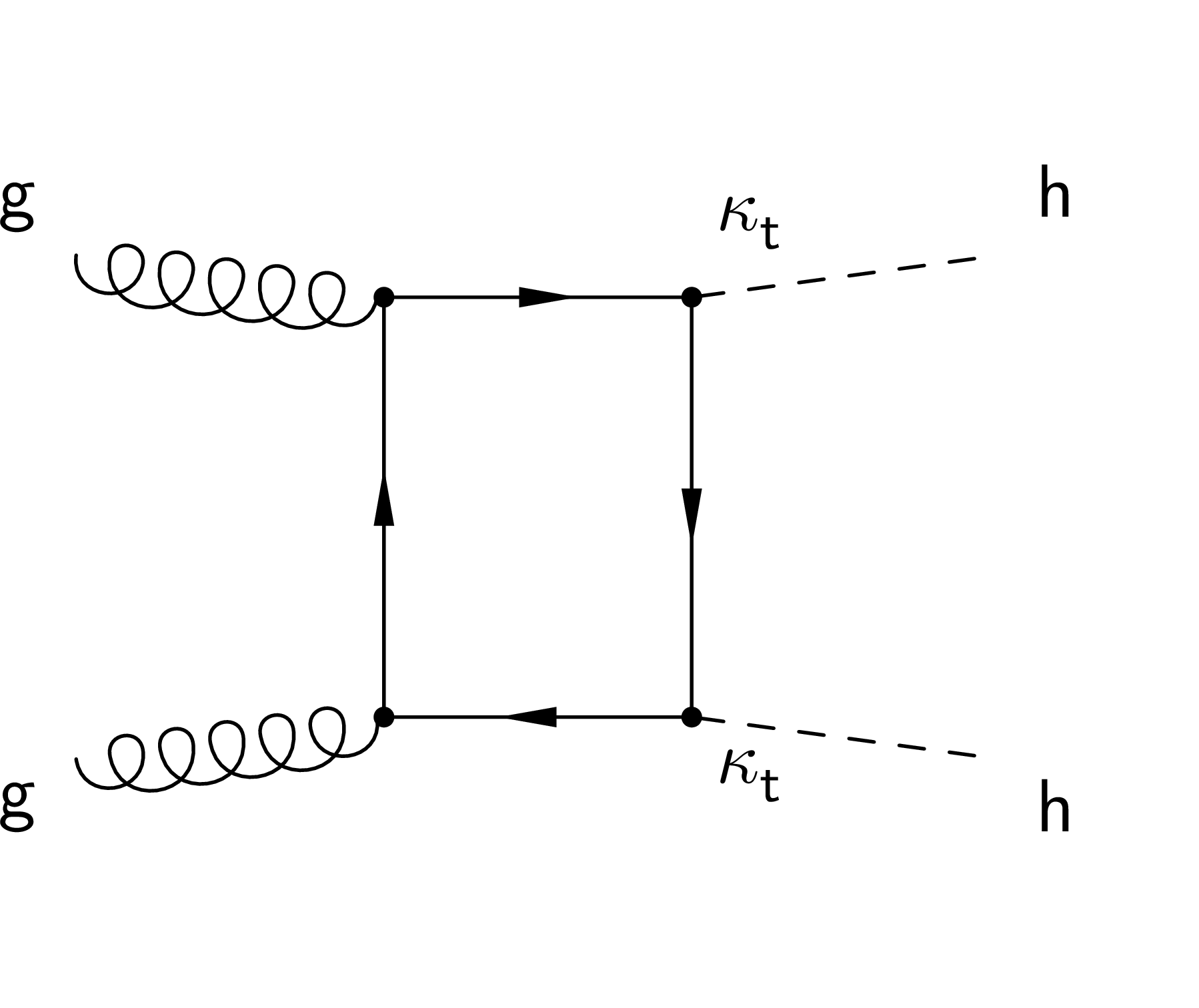
Figure 1:
Higgs pair production diagrams via gluon fusion in the SM. |

png pdf |
Figure 1-a:
Higgs pair production diagram via gluon fusion in the SM. |
png pdf |
Figure 1-b:
Higgs pair production diagram via gluon fusion in the SM. |

png pdf |
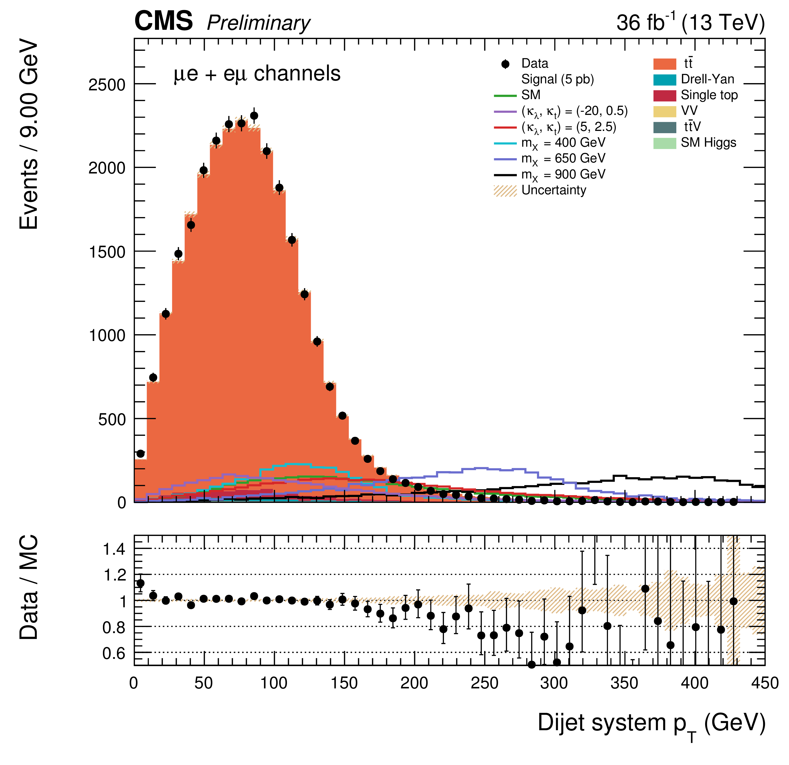
Figure 2:
The di-jet $ {p_{\mathrm {T}}} $ distributions for data and simulated events after requiring two leptons, two b-tagged jets, and $ {m_{\ell \ell }} < {m}_{\mathrm{ Z } } \, - $ 15 GeV, for ee (left), e$\mu $ and $\mu$e (middle), and $\mu \mu $ (right) events. The various signal hypotheses displayed have been scaled to a cross-section of 5 pb. |

png pdf |
Figure 2-a:
The di-jet $ {p_{\mathrm {T}}} $ distributions for data and simulated events after requiring two leptons, two b-tagged jets, and $ {m_{\ell \ell }} < {m}_{\mathrm{ Z } } \, - $ 15 GeV, for ee events. The various signal hypotheses displayed have been scaled to a cross-section of 5 pb. |
png pdf |
Figure 2-b:
The di-jet $ {p_{\mathrm {T}}} $ distributions for data and simulated events after requiring two leptons, two b-tagged jets, and $ {m_{\ell \ell }} < {m}_{\mathrm{ Z } } \, - $ 15 GeV, for e$\mu and $\mu$e events. The various signal hypotheses displayed have been scaled to a cross-section of 5 pb. |

png pdf |
Figure 2-c:
The di-jet $ {p_{\mathrm {T}}} $ distributions for data and simulated events after requiring two leptons, two b-tagged jets, and $ {m_{\ell \ell }} < {m}_{\mathrm{ Z } } \, - $ 15 GeV, for $\mu \mu $ events. The various signal hypotheses displayed have been scaled to a cross-section of 5 pb. |

png pdf |
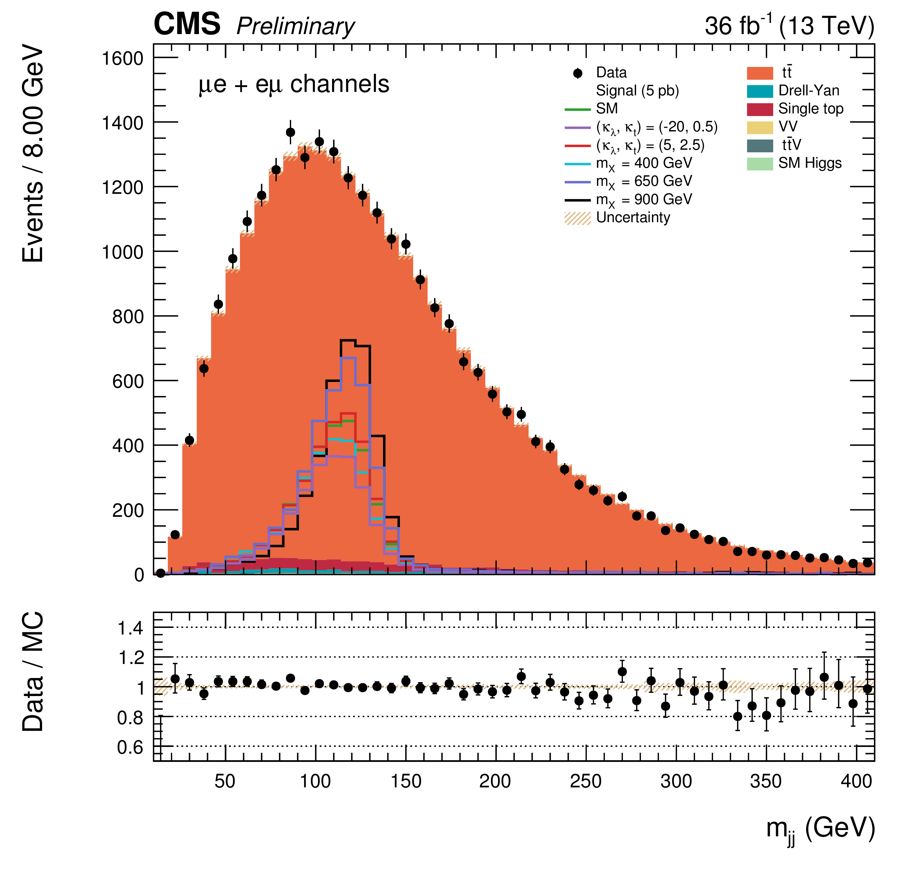
Figure 3:
The $ {m_{ {\mathrm {j}} {\mathrm {j}} }} $ distribution for data and simulated events after requiring all selection cuts in the ee (left), $\mathrm{ e } \mu $ and $\mu \mathrm{ e } $ (middle), and $\mu \mu $ (right) channels. The various signal hypotheses displayed have been scaled to a cross-section of 5 pb. |

png pdf |
Figure 3-a:
The $ {m_{ {\mathrm {j}} {\mathrm {j}} }} $ distribution for data and simulated events after requiring all selection cuts in the ee channel. The various signal hypotheses displayed have been scaled to a cross-section of 5 pb. |
png pdf |
Figure 3-b:
The $ {m_{ {\mathrm {j}} {\mathrm {j}} }} $ distribution for data and simulated events after requiring all selection cuts in the $\mathrm{ e } \mu $ and $\mu \mathrm{ e } $ channel. The various signal hypotheses displayed have been scaled to a cross-section of 5 pb. |

png pdf |
Figure 3-c:
The $ {m_{ {\mathrm {j}} {\mathrm {j}} }} $ distribution for data and simulated events after requiring all selection cuts in the $\mu \mu $ channel. The various signal hypotheses displayed have been scaled to a cross-section of 5 pb. |

png pdf |
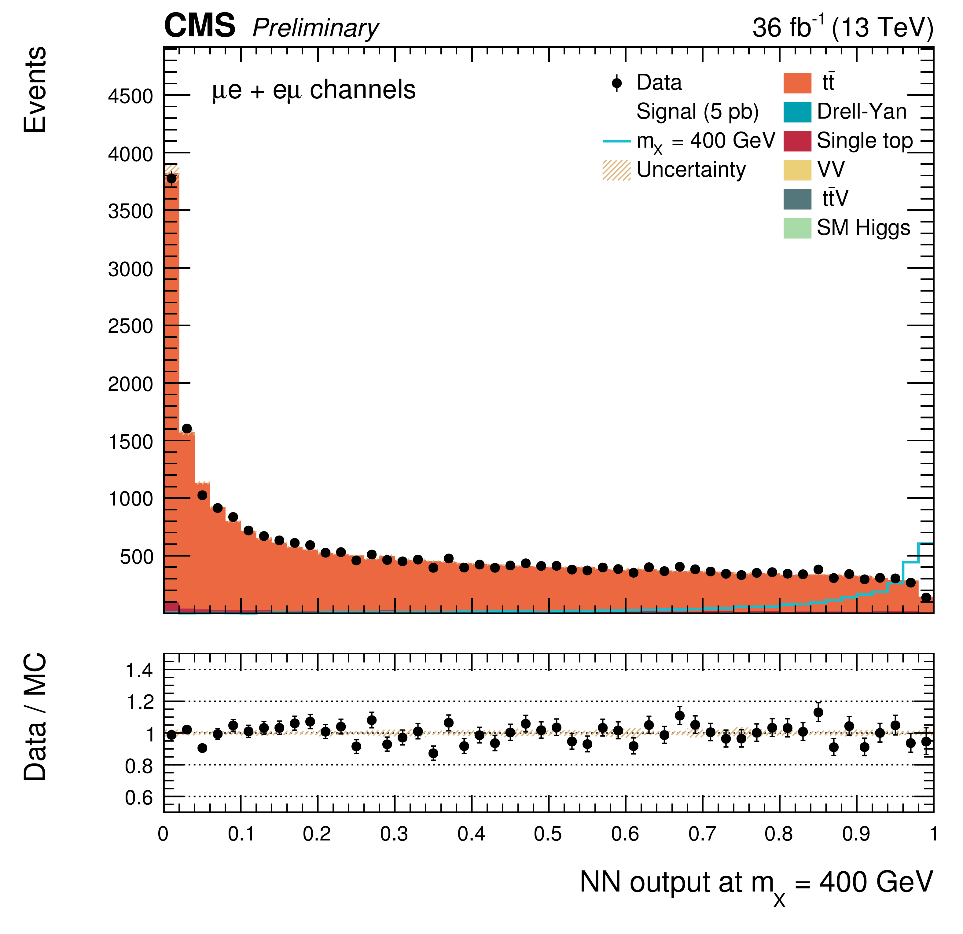
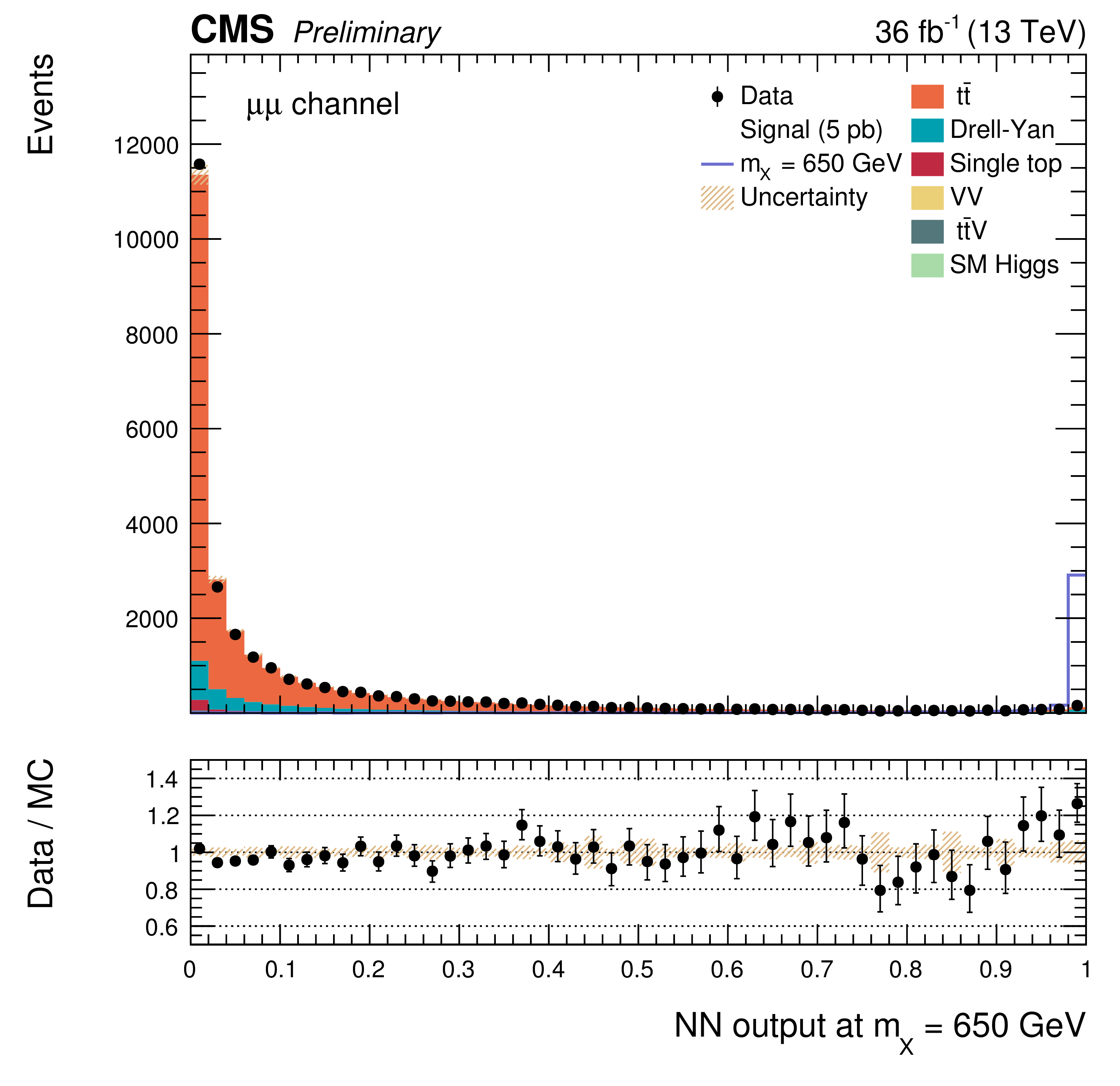
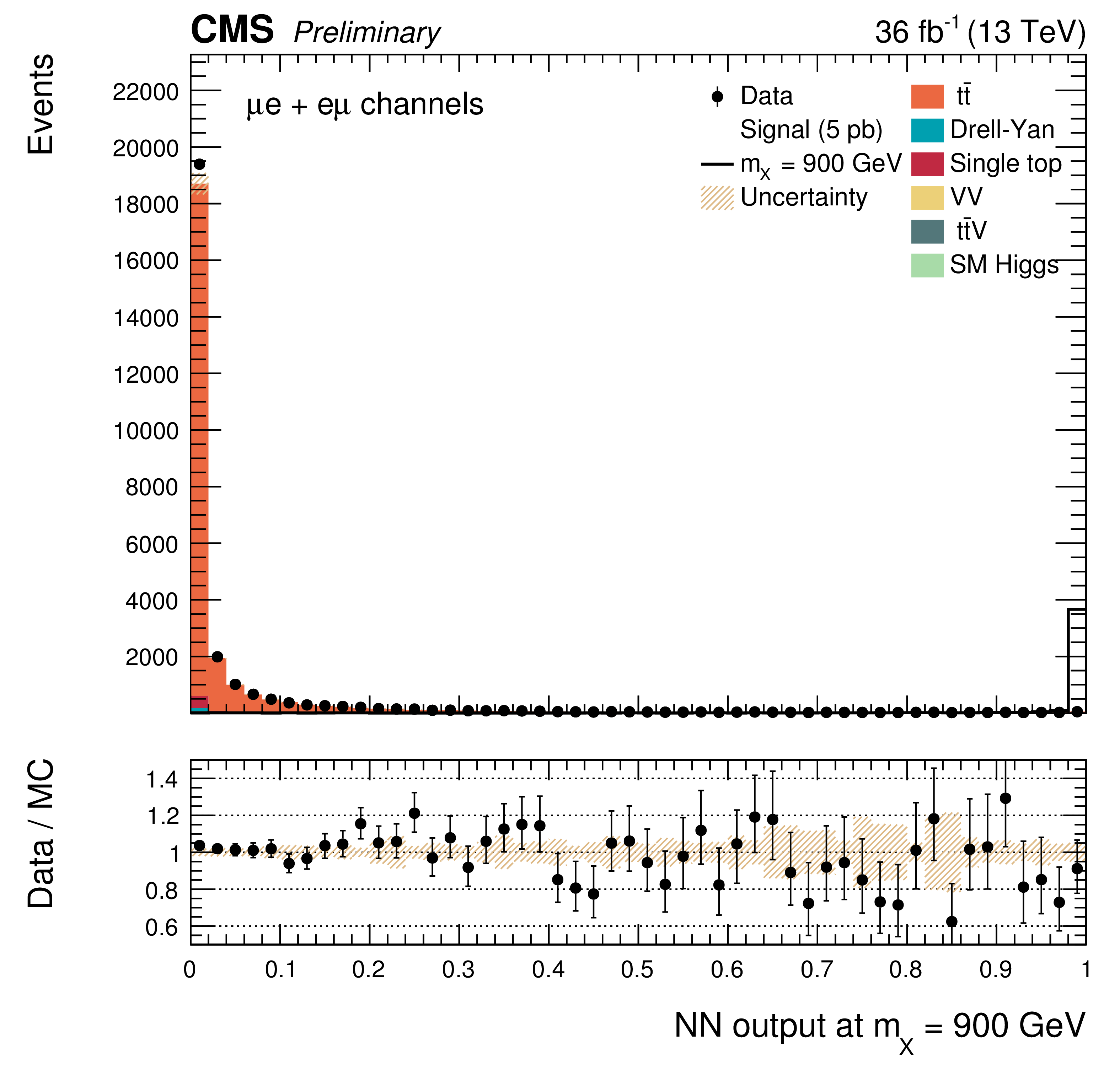
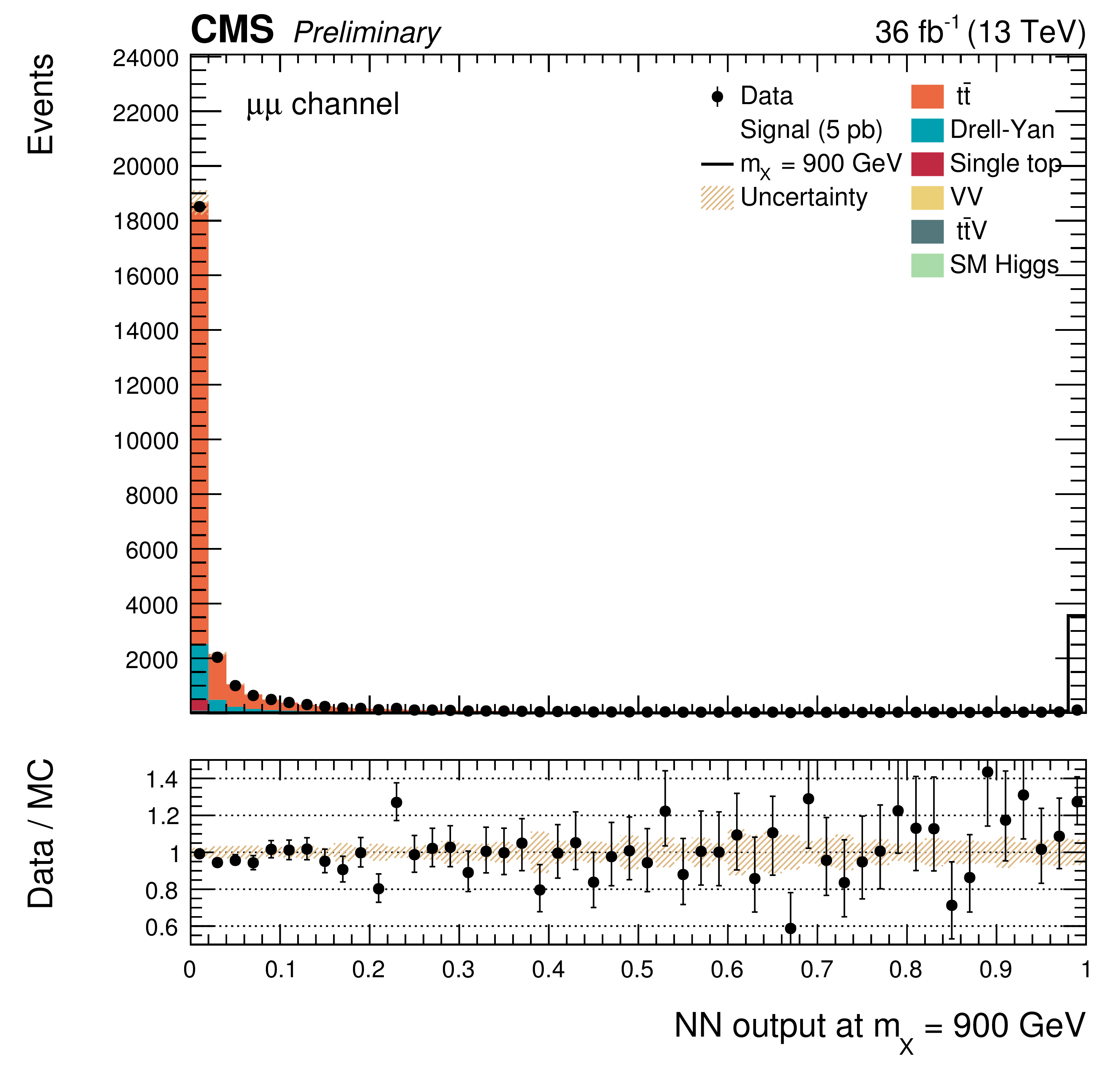
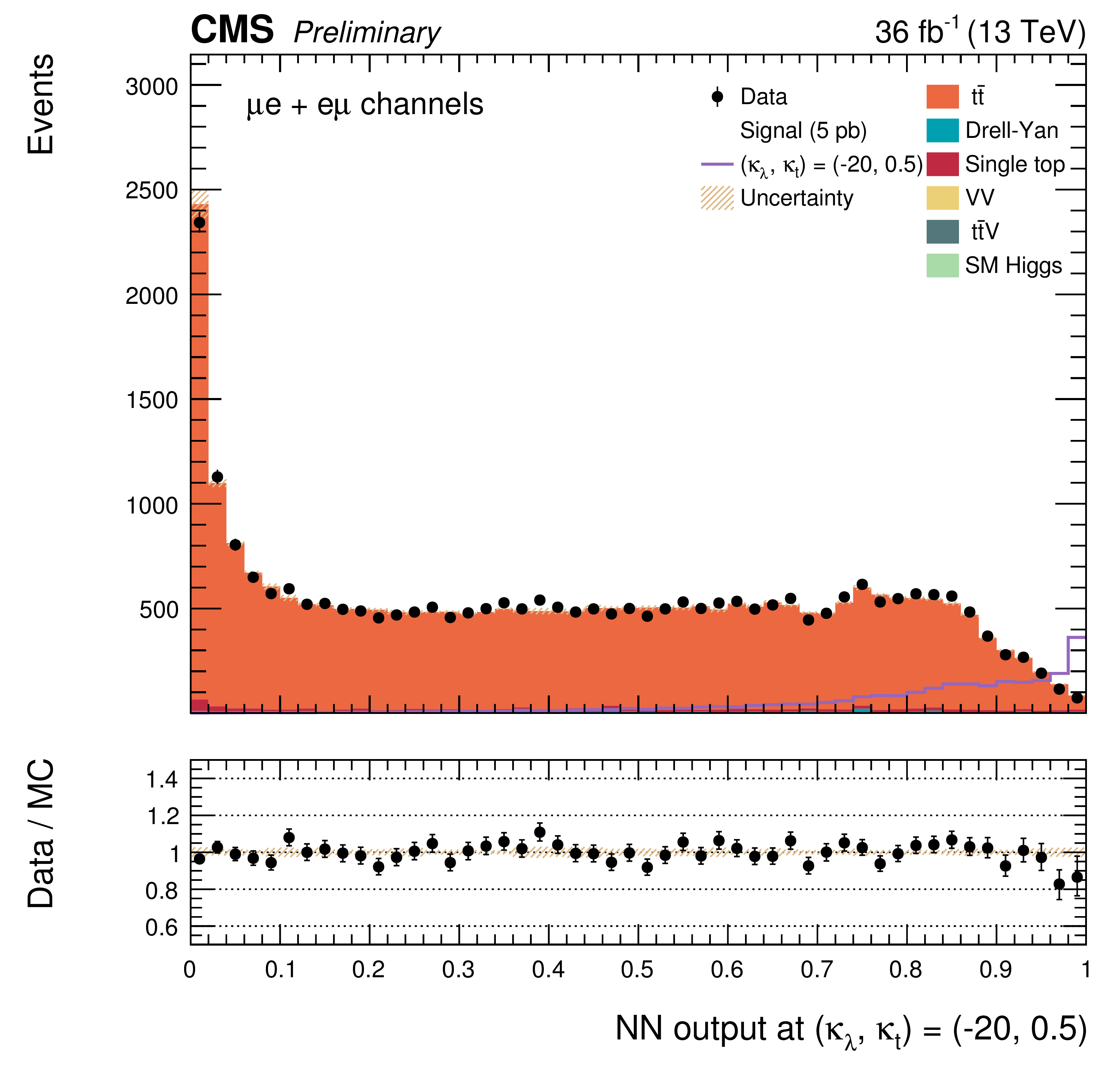
Figure 4:
The DNN output distribution for data and simulated events after requiring all selection cuts, for the $\mu^{+} \mu^{-} $ channel. Output values towards 0 are background-like, while output values towards 1 are signal-like. The resonant DNN output (left) evaluated at $ {m_{\mathrm {X}}} = $ 400 GeV and the non-resonant DNN output (right) evaluated at $\kappa _{\lambda } =$ 1, $\kappa _{\mathrm{ t } } = $ 1. The various signal hypotheses displayed have been scaled to a cross-section of 5 pb. |
png pdf |
Figure 4-a:
The DNN output distribution for data and simulated events after requiring all selection cuts, for the $\mu^{+} \mu^{-} $ channel. Output values towards 0 are background-like, while output values towards 1 are signal-like. The resonant DNN output evaluated at $ {m_{\mathrm {X}}} = $ 400 GeV. The various signal hypotheses displayed have been scaled to a cross-section of 5 pb. |

png pdf |
Figure 4-b:
The DNN output distribution for data and simulated events after requiring all selection cuts, for the $\mu^{+} \mu^{-} $ channel. Output values towards 0 are background-like, while output values towards 1 are signal-like. The non-resonant DNN output evaluated at $\kappa _{\lambda } =$ 1, $\kappa _{\mathrm{ t } } = $ 1. The various signal hypotheses displayed have been scaled to a cross-section of 5 pb. |

png pdf |
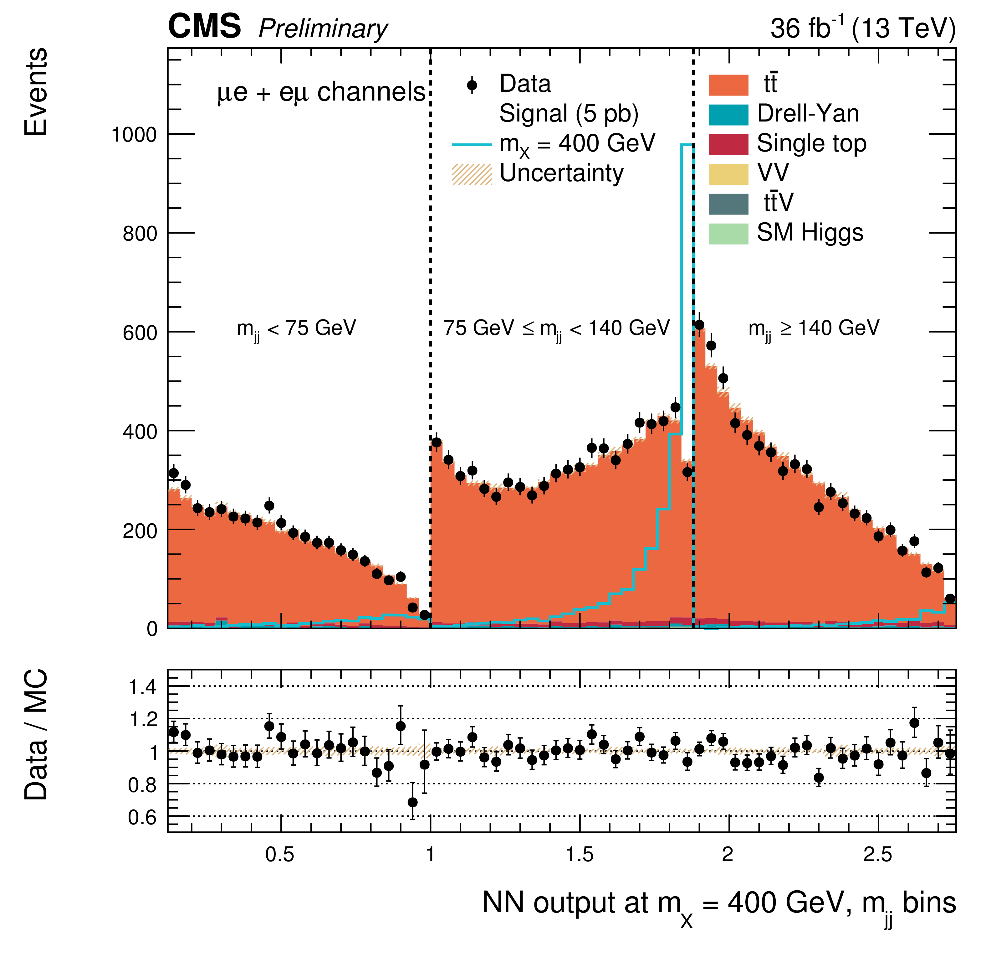
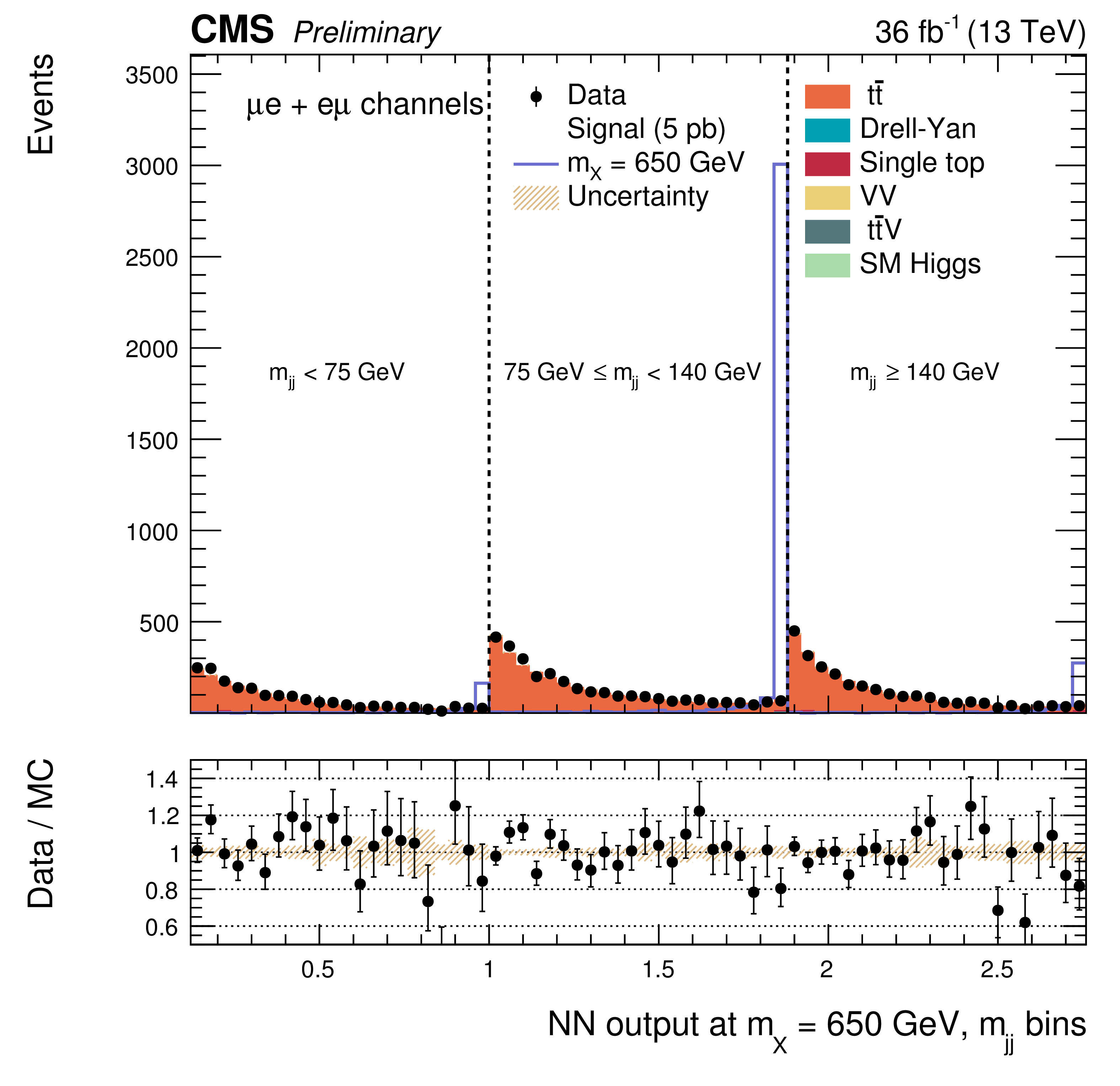
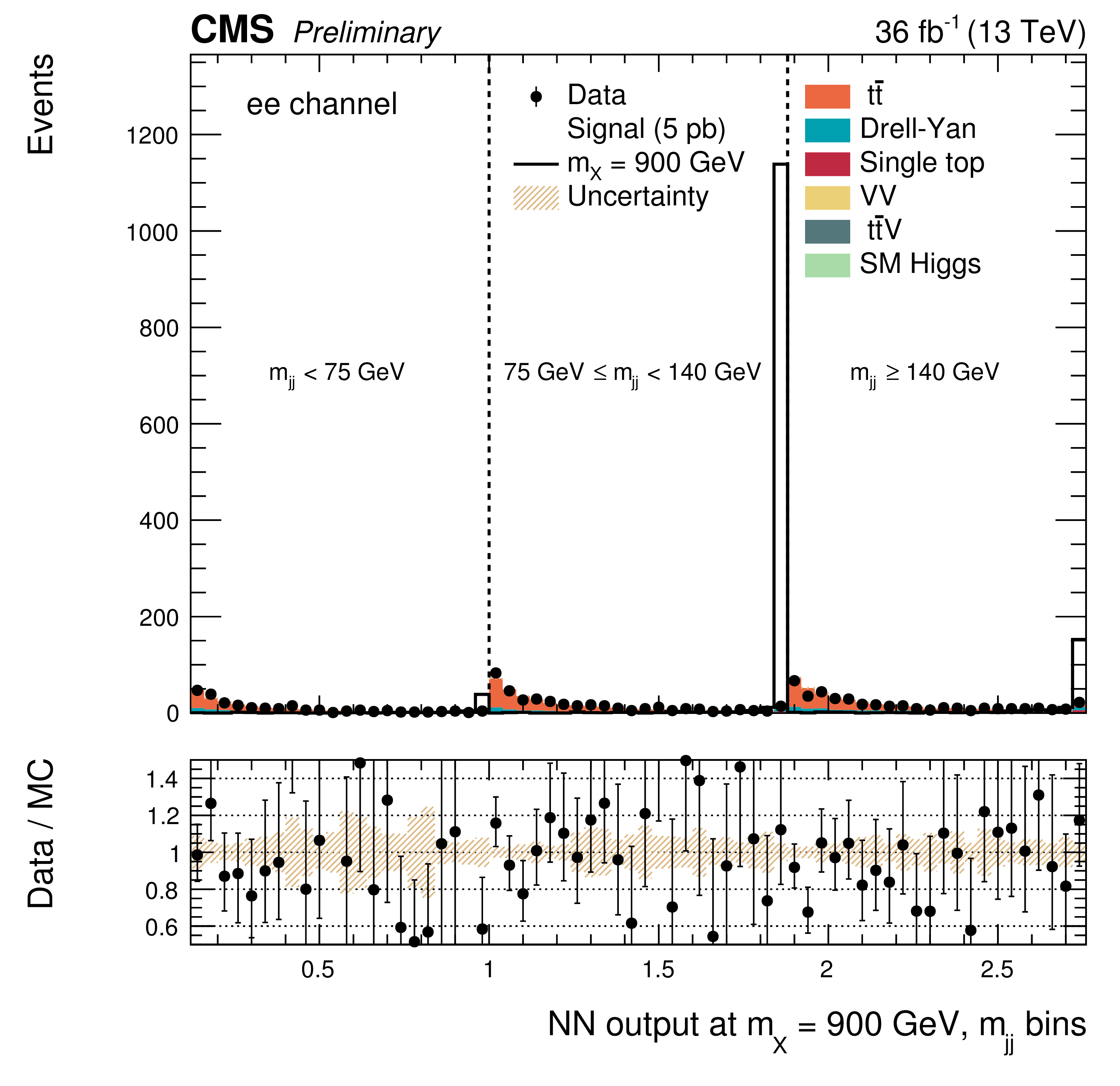
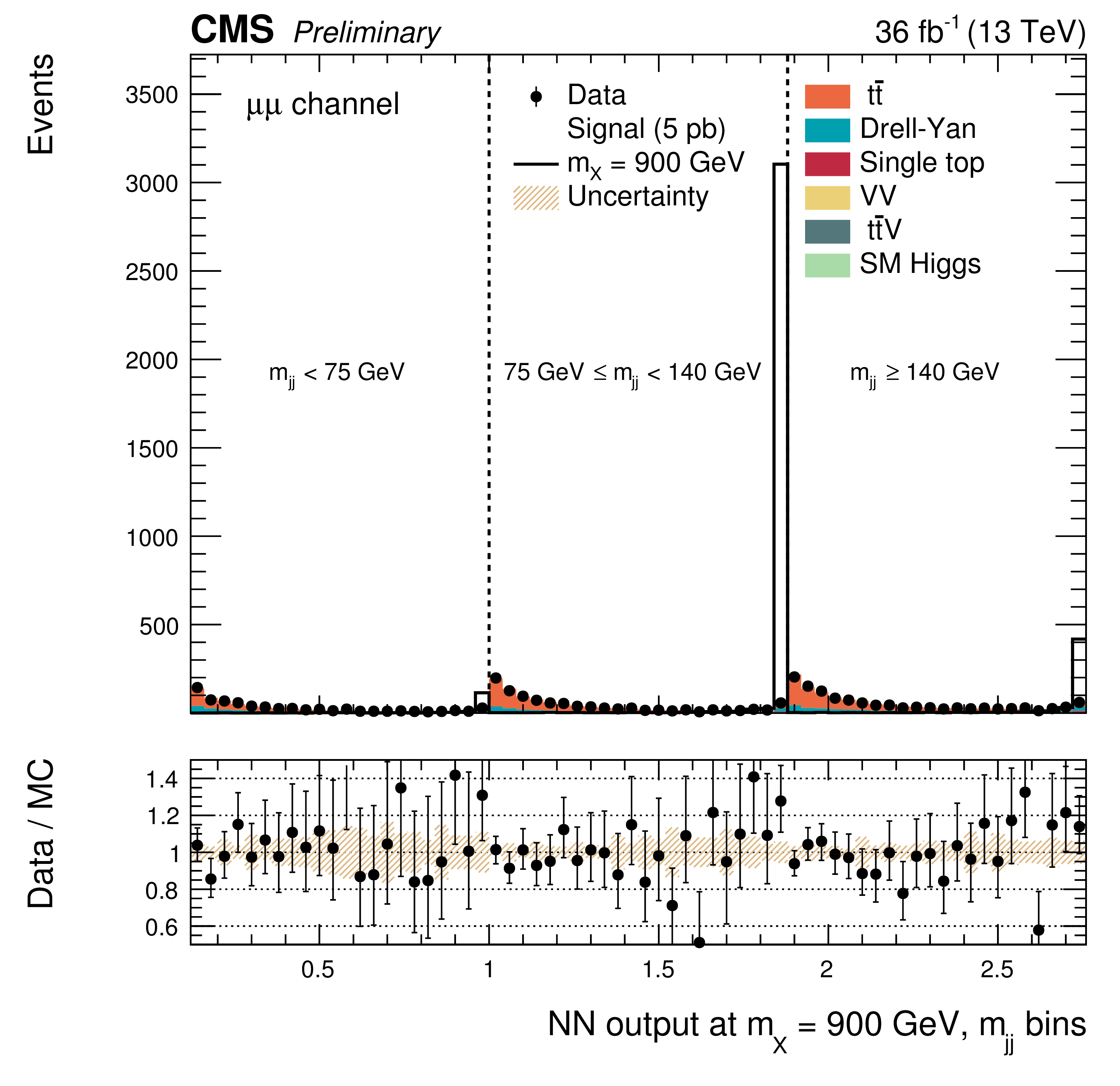
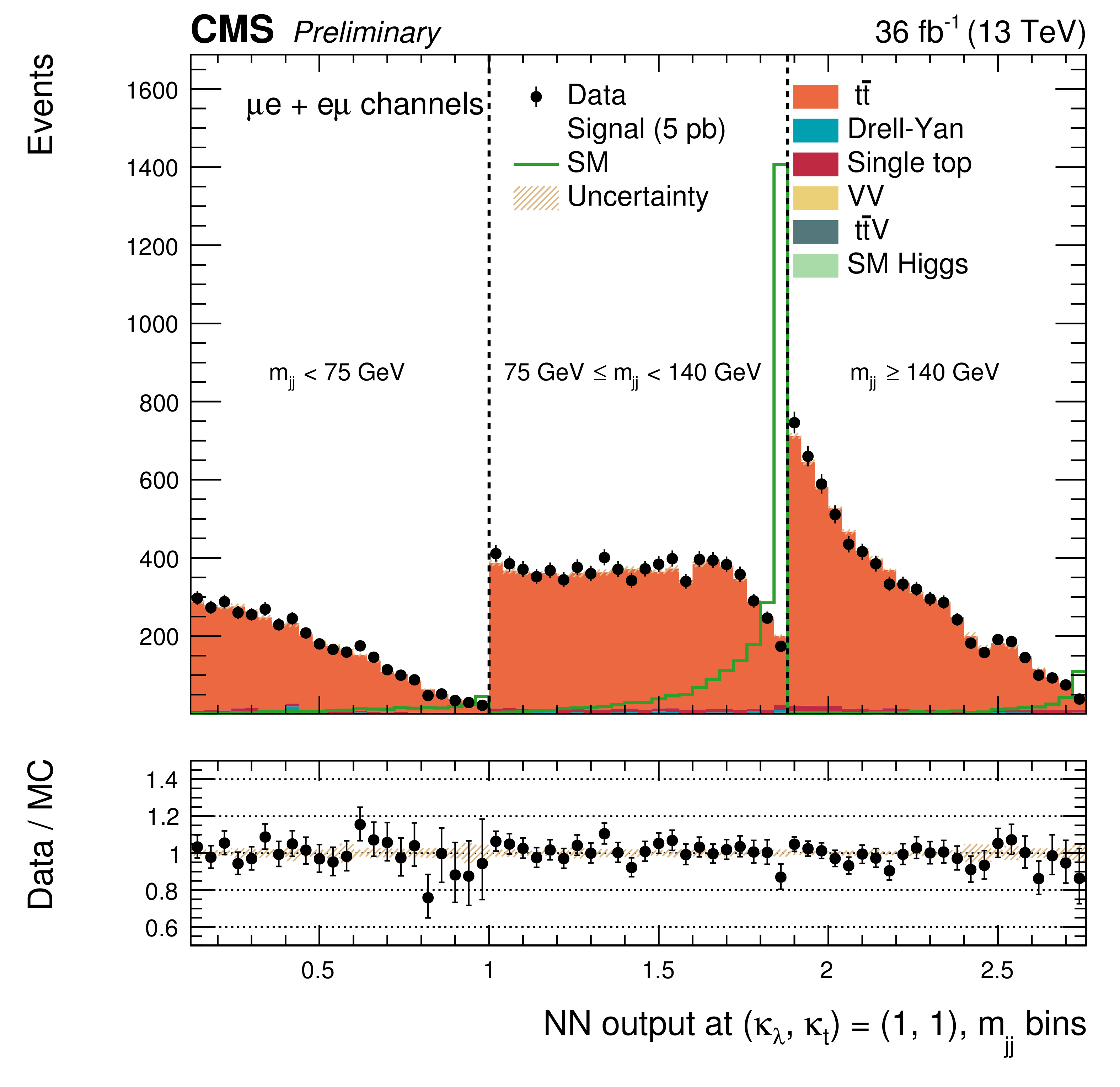
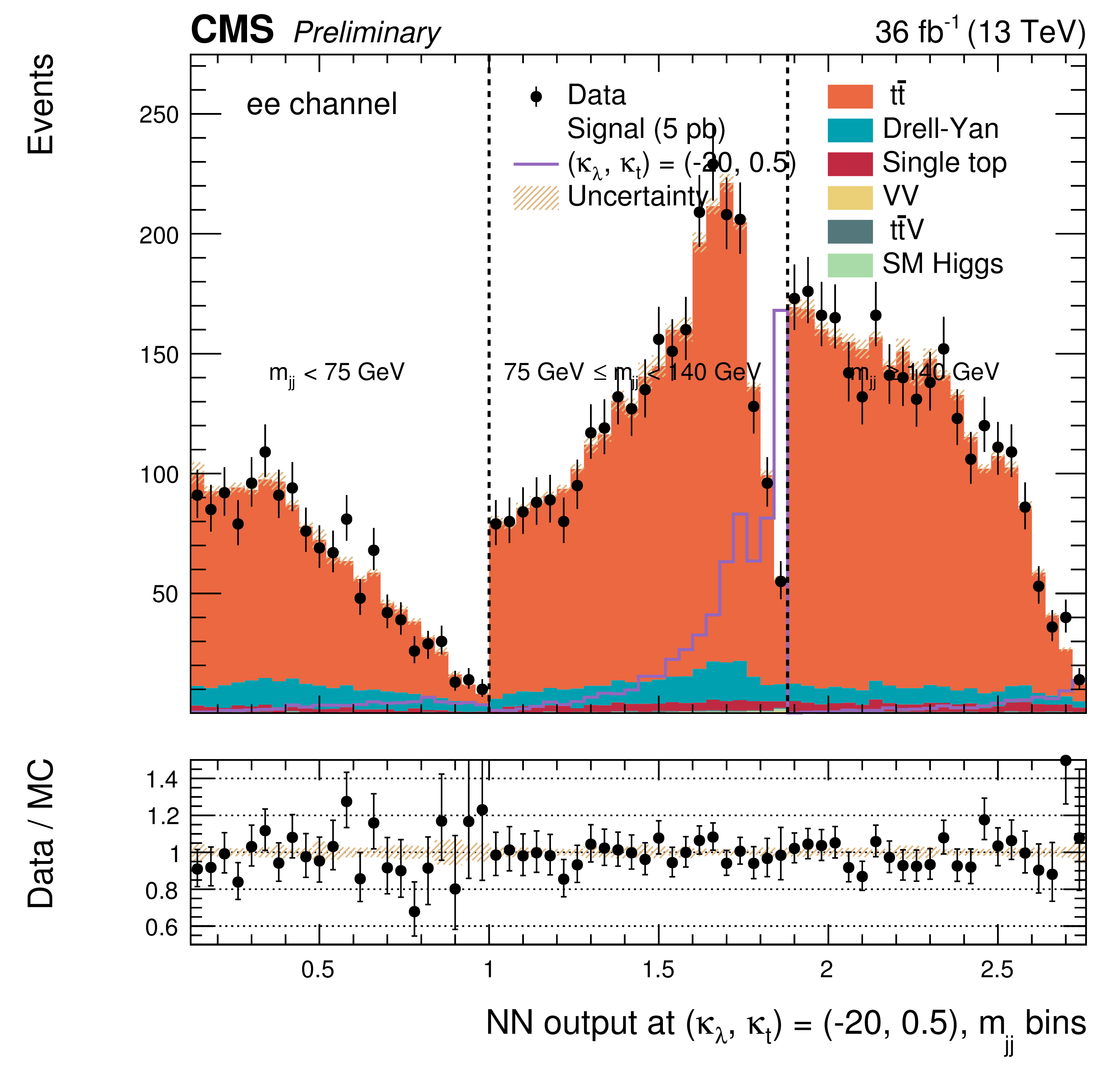
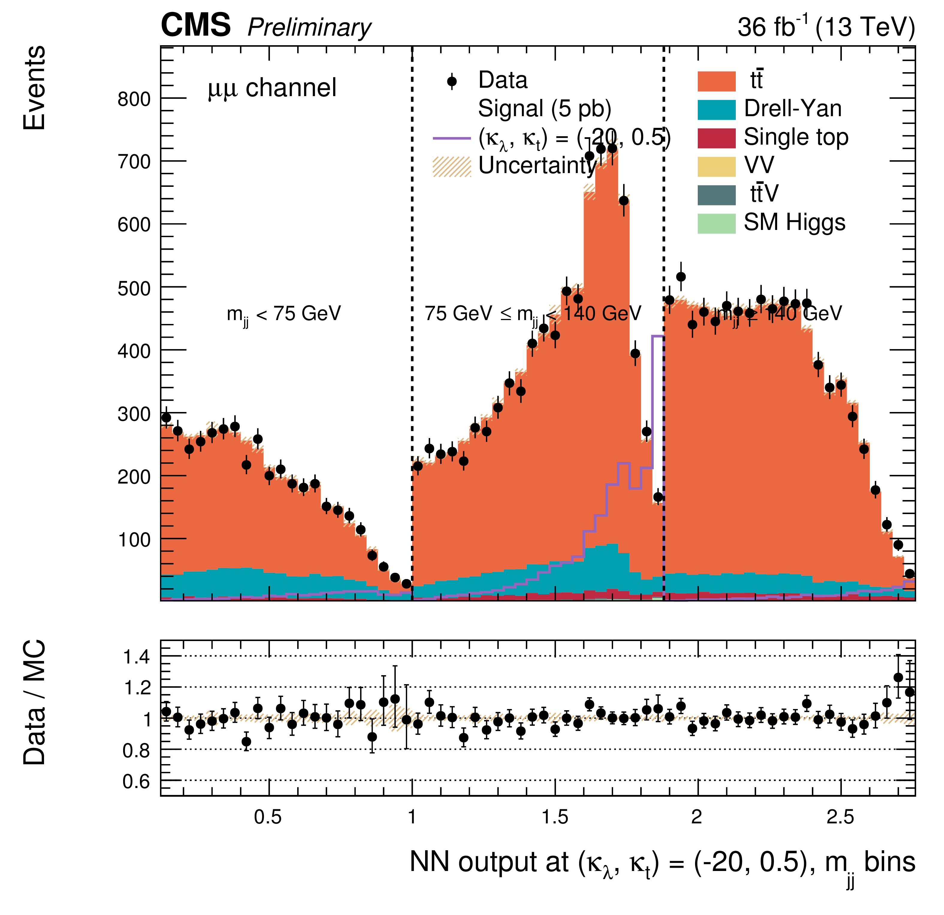
Figure 5:
The DNN output distribution for data and simulated events in three different $ {m_{ {\mathrm {j}} {\mathrm {j}} }} $ regions, for the $\mu^{+} \mu^{-} $ channel: $ {m_{ {\mathrm {j}} {\mathrm {j}} }} < $ 75 GeV, $ {m_{ {\mathrm {j}} {\mathrm {j}} }} \in $ [75, 140[ GeV and $ {m_{ {\mathrm {j}} {\mathrm {j}} }} \geq $ 140 GeV. The resonant DNN output (left) evaluated at $ {m_{\mathrm {X}}} = $ 400 GeV and the non-resonant DNN output (right) evaluated at $\kappa _{\lambda } =$ 1, $\kappa _{\mathrm{ t } } = $ 1. The various signal hypotheses displayed have been scaled to a cross-section of 5 pb. |

png pdf |
Figure 5-a:
The DNN output distribution for data and simulated events in three different $ {m_{ {\mathrm {j}} {\mathrm {j}} }} $ regions, for the $\mu^{+} \mu^{-} $ channel: $ {m_{ {\mathrm {j}} {\mathrm {j}} }} < $ 75 GeV, $ {m_{ {\mathrm {j}} {\mathrm {j}} }} \in $ [75, 140[ GeV and $ {m_{ {\mathrm {j}} {\mathrm {j}} }} \geq $ 140 GeV. The resonant DNN output evaluated at $ {m_{\mathrm {X}}} = $ 400 GeV. The various signal hypotheses displayed have been scaled to a cross-section of 5 pb. |

png pdf |
Figure 5-b:
The DNN output distribution for data and simulated events in three different $ {m_{ {\mathrm {j}} {\mathrm {j}} }} $ regions, for the $\mu^{+} \mu^{-} $ channel: $ {m_{ {\mathrm {j}} {\mathrm {j}} }} < $ 75 GeV, $ {m_{ {\mathrm {j}} {\mathrm {j}} }} \in $ [75, 140[ GeV and $ {m_{ {\mathrm {j}} {\mathrm {j}} }} \geq $ 140 GeV. The non-resonant DNN output (right) evaluated at $\kappa _{\lambda } =$ 1, $\kappa _{\mathrm{ t } } = $ 1. The various signal hypotheses displayed have been scaled to a cross-section of 5 pb. |

png pdf |
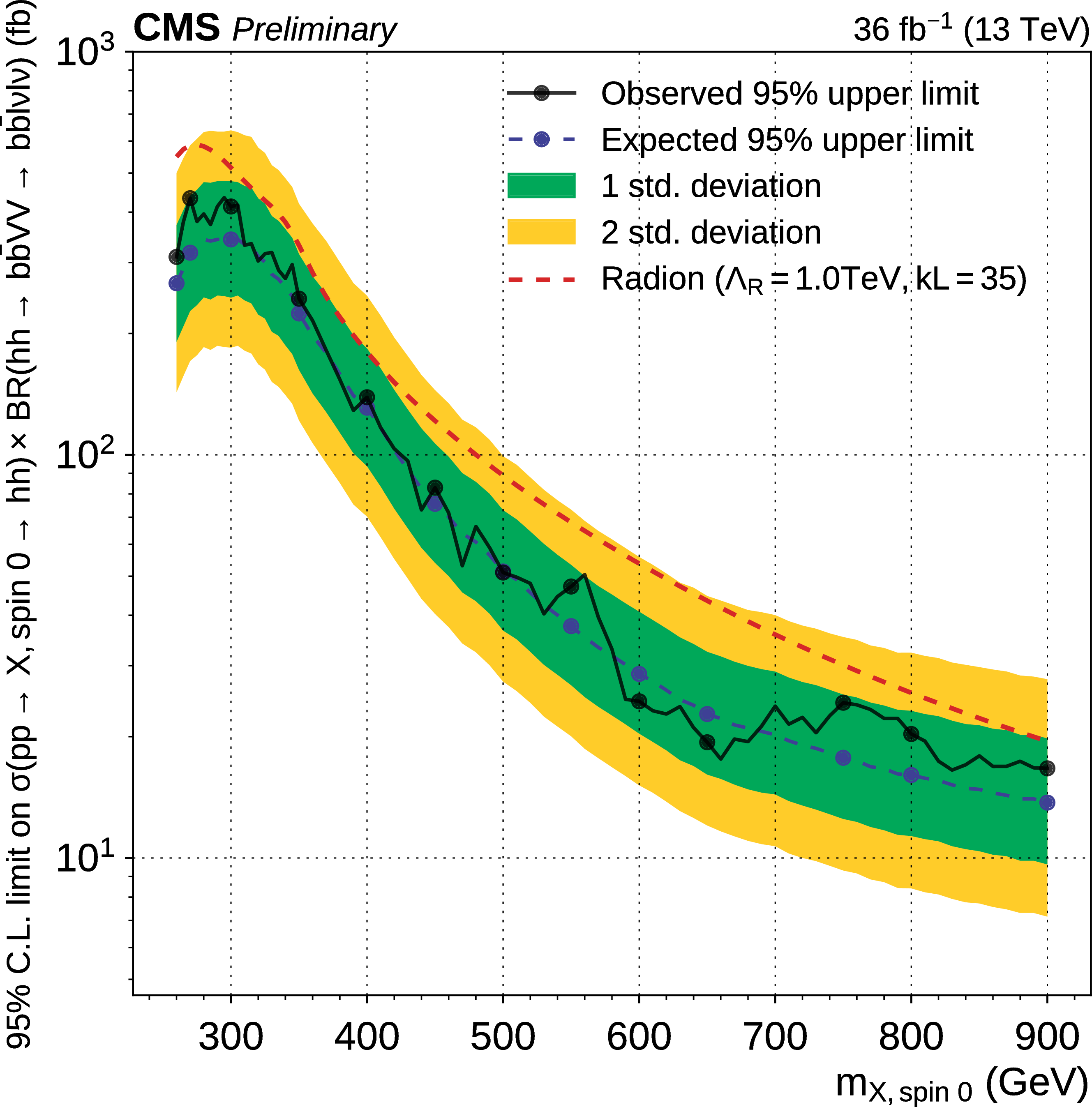
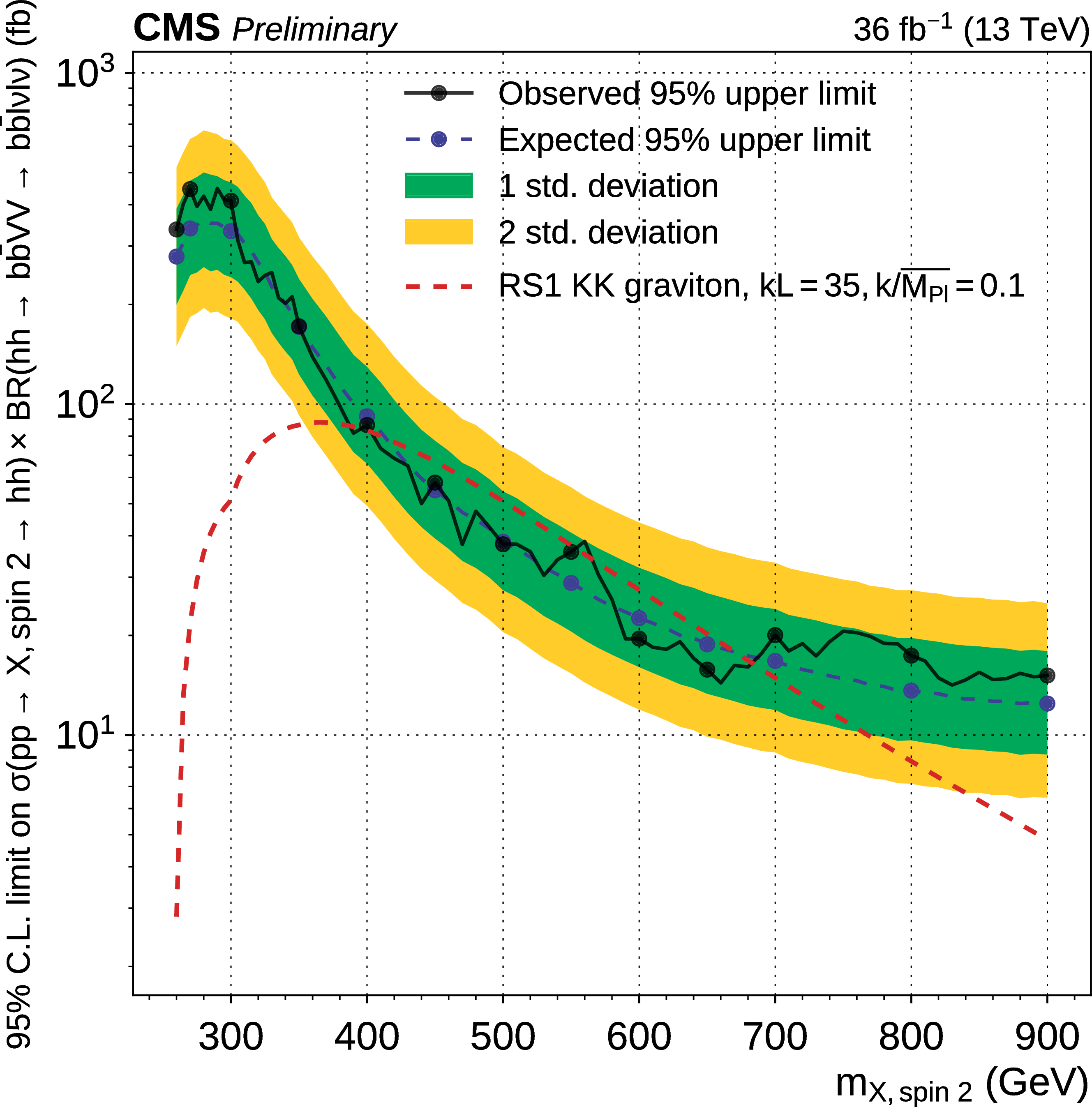
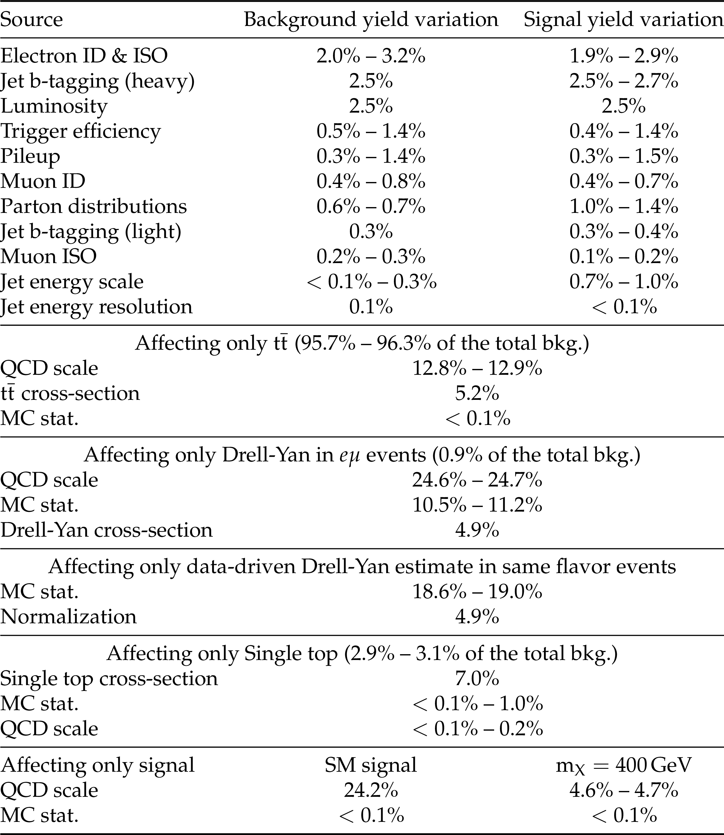
Figure 6:
Expected and observed 95% CL upper limits on Higgs pair production cross section times branching ratio for $\mathrm{h} \mathrm{h} \to {\mathrm{ b \bar{b} } } {\mathrm {V}} {\mathrm {V}} \to {\mathrm{ b \bar{b} } } \ell \nu \ell \nu $ as a function of $ {m_{\mathrm {X}}} $. These limits are computed using the asymptotic CL$_s$ method, combining the $\mathrm{ e }^{+} \mathrm{ e }^{-} $, $\mu^{+} \mu^{-} $ and $\mathrm{ e } ^{\pm }\mu ^{\mp }$ channels, for spin-0 (left) and spin-2 (right) hypotheses. The dashed red lines represent possible expectations for new physics arising from a new spin-0 or spin-2 resonance (see text for details). The irregular behaviour of the observed limit is due to the limited statistics on data and to the parameterised learning technique, which results in a reshuffling of the observed data distributions for each point of the scan. The expected limits are evaluated with the same granularity as the observed limits. The DNN interpolates the expected analysis performance in a smooth fashion between the fully-simulated points. |
png pdf |
Figure 6-a:
Expected and observed 95% CL upper limits on Higgs pair production cross section times branching ratio for $\mathrm{h} \mathrm{h} \to {\mathrm{ b \bar{b} } } {\mathrm {V}} {\mathrm {V}} \to {\mathrm{ b \bar{b} } } \ell \nu \ell \nu $ as a function of $ {m_{\mathrm {X}}} $. These limits are computed using the asymptotic CL$_s$ method, combining the $\mathrm{ e }^{+} \mathrm{ e }^{-} $, $\mu^{+} \mu^{-} $ and $\mathrm{ e } ^{\pm }\mu ^{\mp }$ channels, for the spin-0 hypothesis. The dashed red lines represent possible expectations for new physics arising from a new spin-0 resonance (see text for details). The irregular behaviour of the observed limit is due to the limited statistics on data and to the parameterised learning technique, which results in a reshuffling of the observed data distributions for each point of the scan. The expected limits are evaluated with the same granularity as the observed limits. The DNN interpolates the expected analysis performance in a smooth fashion between the fully-simulated points. |
png pdf |
Figure 6-b:
Expected and observed 95% CL upper limits on Higgs pair production cross section times branching ratio for $\mathrm{h} \mathrm{h} \to {\mathrm{ b \bar{b} } } {\mathrm {V}} {\mathrm {V}} \to {\mathrm{ b \bar{b} } } \ell \nu \ell \nu $ as a function of $ {m_{\mathrm {X}}} $. These limits are computed using the asymptotic CL$_s$ method, combining the $\mathrm{ e }^{+} \mathrm{ e }^{-} $, $\mu^{+} \mu^{-} $ and $\mathrm{ e } ^{\pm }\mu ^{\mp }$ channels, for the spin-2 hypothesis. The dashed red lines represent possible expectations for new physics arising from a new spin-2 resonance (see text for details). The irregular behaviour of the observed limit is due to the limited statistics on data and to the parameterised learning technique, which results in a reshuffling of the observed data distributions for each point of the scan. The expected limits are evaluated with the same granularity as the observed limits. The DNN interpolates the expected analysis performance in a smooth fashion between the fully-simulated points. |

png pdf |
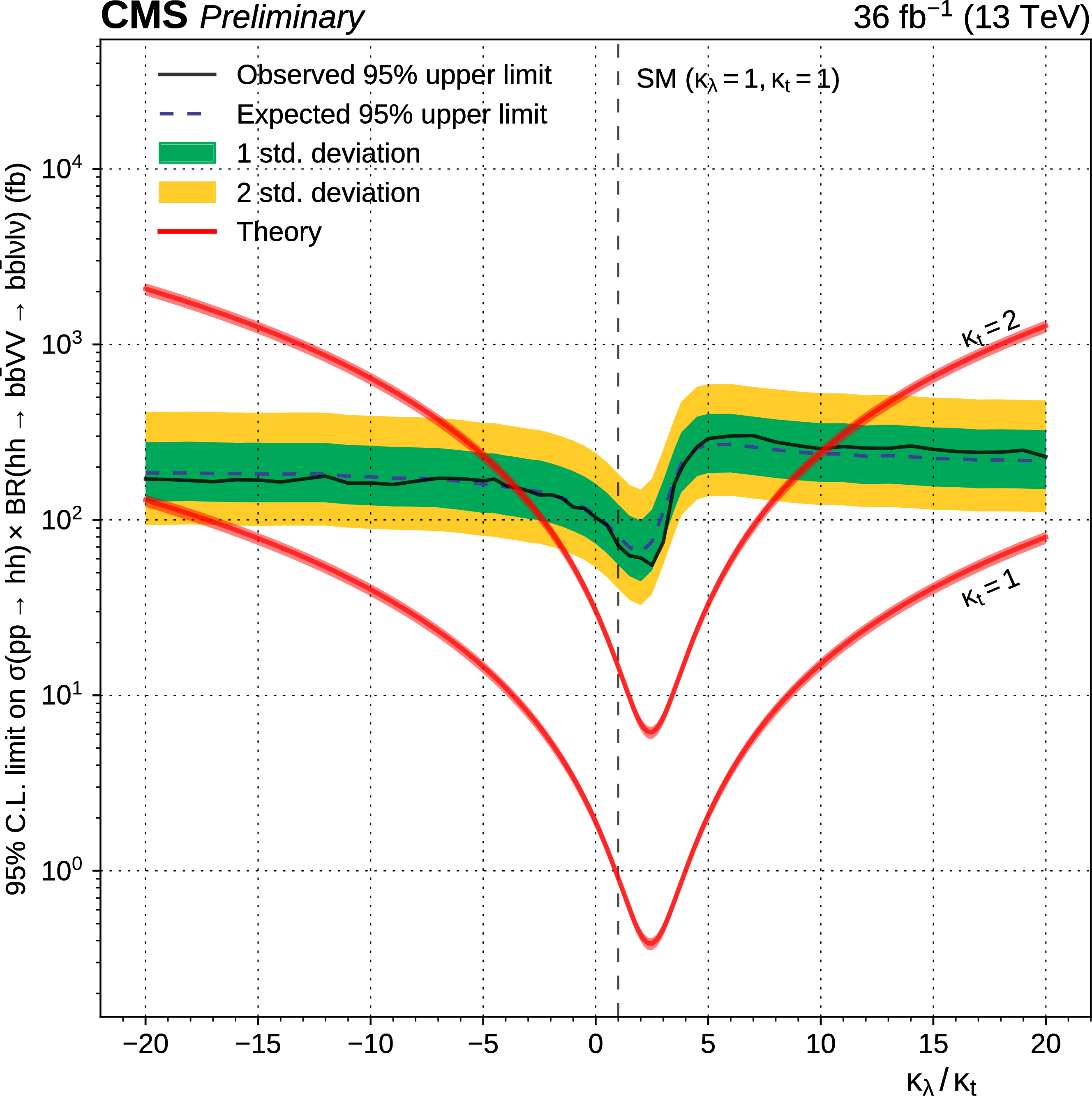
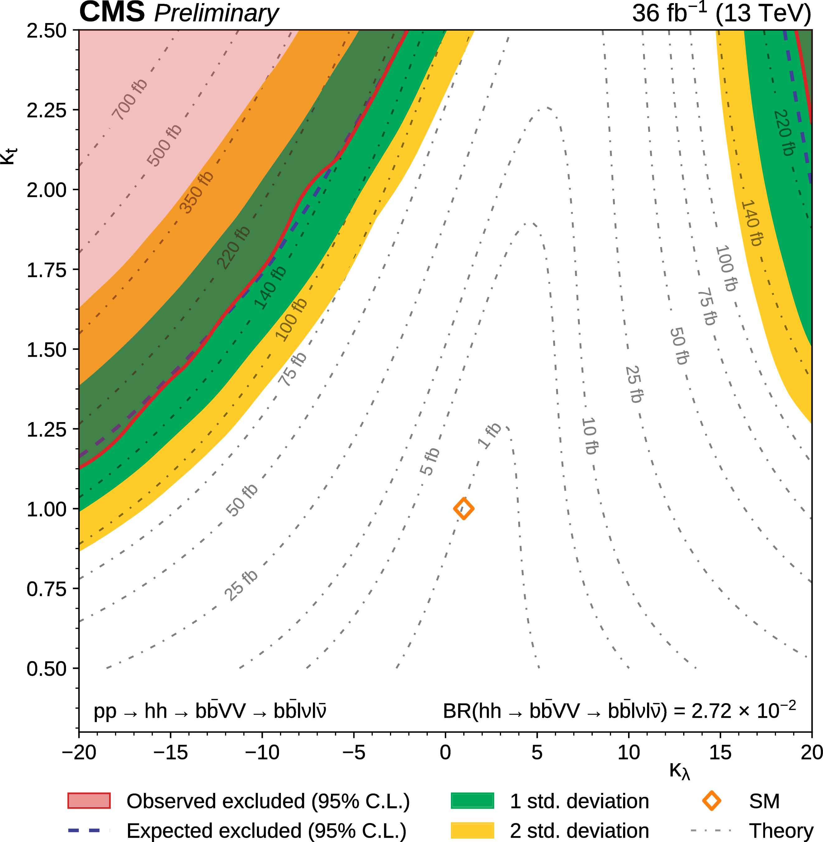
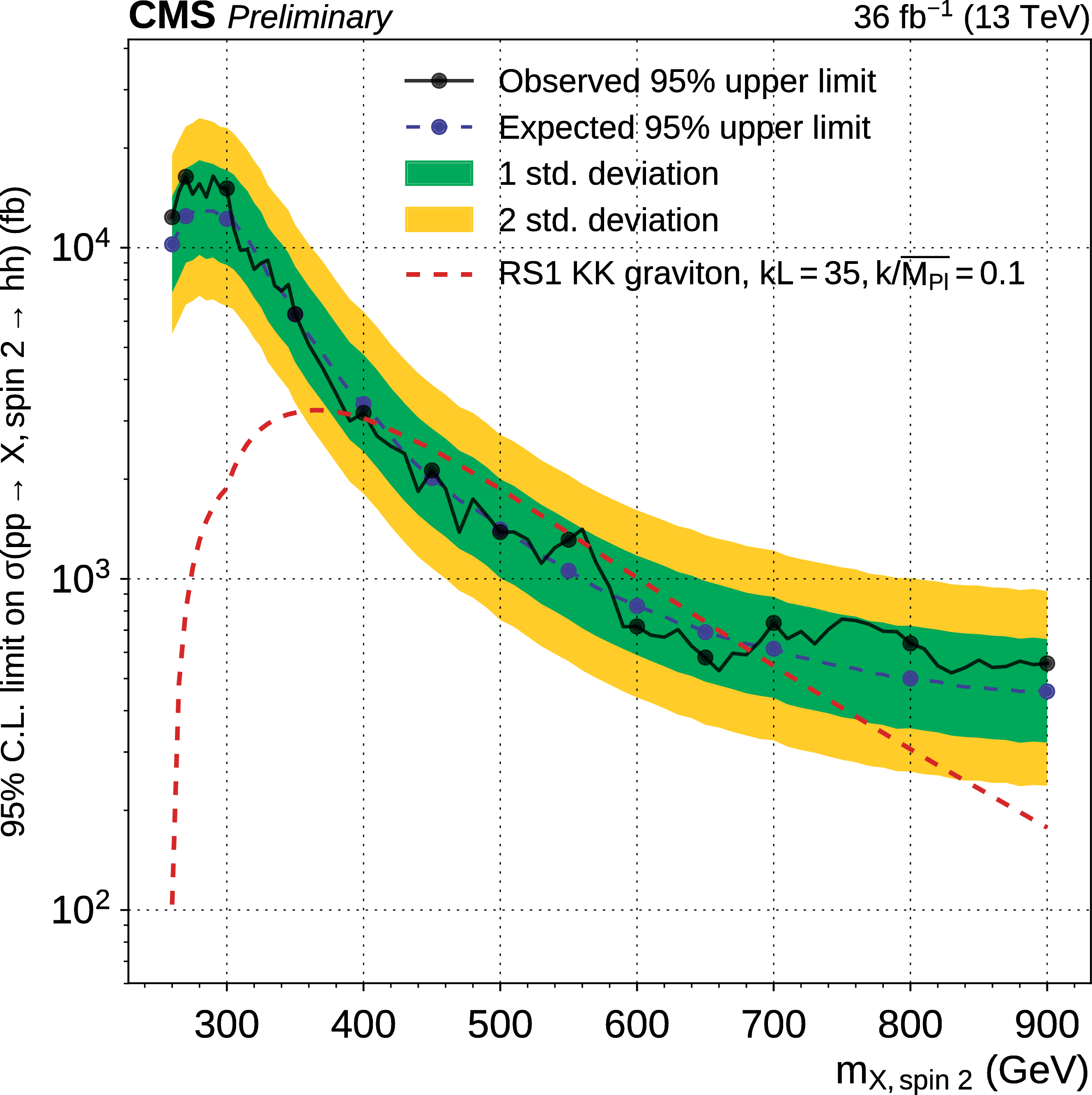
Figure 7:
Expected and observed 95% CL upper limits on Higgs pair production cross section times branching ratio for $\mathrm{h} \mathrm{h} \to {\mathrm{ b \bar{b} } } {\mathrm {V}} {\mathrm {V}} \to {\mathrm{ b \bar{b} } } \ell \nu \ell \nu $ as a function of $\kappa _{\lambda } / \kappa _{\mathrm{ t } }$ (left). Observed (red region) and expected (dashed blue line) exclusion of the BSM parameter space at 95% CL in the $\kappa _{\lambda }$ vs $\kappa _{t}$ plane (right). Theoretical cross-section times branching fraction isolines for $\mathrm{h} \mathrm{h} \to {\mathrm{ b \bar{b} } } {\mathrm {V}} {\mathrm {V}} \to {\mathrm{ b \bar{b} } } \ell \nu \ell \nu $ are shown as dashed lines (right). These limits are computed using the asymptotic CL$_s$ method, combining the $\mathrm{ e }^{+} \mathrm{ e }^{-} $, $\mu^{+} \mu^{-} $ and $\mathrm{ e }^{+}m {\mu ^\mp } $ channels. Theory predictions are extracted from [68,10,11,12,13,14,69]. One can note that both theory predictions, expected and observed limits are symmetric through a $(\kappa _{\lambda } , \kappa _{\mathrm{ t } }) \leftrightarrow (-\kappa _{\lambda } , -\kappa _{\mathrm{ t } })$ transformation. |
png pdf |
Figure 7-a:
Observed (red region) and expected (dashed blue line) exclusion of the BSM parameter space at 95% CL in the $\kappa _{\lambda }$ vs $\kappa _{t}$ plane. Theoretical cross-section times branching fraction isolines for $\mathrm{h} \mathrm{h} \to {\mathrm{ b \bar{b} } } {\mathrm {V}} {\mathrm {V}} \to {\mathrm{ b \bar{b} } } \ell \nu \ell \nu $ are shown as dashed lines. These limits are computed using the asymptotic CL$_s$ method, combining the $\mathrm{ e }^{+} \mathrm{ e }^{-} $, $\mu^{+} \mu^{-} $ and $\mathrm{ e }^{+}m {\mu ^\mp } $ channels. Theory predictions are extracted from [68,10,11,12,13,14,69]. One can note that both theory predictions, expected and observed limits are symmetric through a $(\kappa _{\lambda } , \kappa _{\mathrm{ t } }) \leftrightarrow (-\kappa _{\lambda } , -\kappa _{\mathrm{ t } })$ transformation. |
png pdf |
Figure 7-b:
Expected and observed 95% CL upper limits on Higgs pair production cross section times branching ratio for $\mathrm{h} \mathrm{h} \to {\mathrm{ b \bar{b} } } {\mathrm {V}} {\mathrm {V}} \to {\mathrm{ b \bar{b} } } \ell \nu \ell \nu $ as a function of $\kappa _{\lambda } / \kappa _{\mathrm{ t } }$ (left). Observed (red region) and expected (dashed blue line) exclusion of the BSM parameter space at 95% CL in the $\kappa _{\lambda }$ vs $\kappa _{t}$ plane (right). Theoretical cross-section times branching fraction isolines for $\mathrm{h} \mathrm{h} \to {\mathrm{ b \bar{b} } } {\mathrm {V}} {\mathrm {V}} \to {\mathrm{ b \bar{b} } } \ell \nu \ell \nu $ are shown as dashed lines (right). These limits are computed using the asymptotic CL$_s$ method, combining the $\mathrm{ e }^{+} \mathrm{ e }^{-} $, $\mu^{+} \mu^{-} $ and $\mathrm{ e }^{+}m {\mu ^\mp } $ channels. Theory predictions are extracted from [68,10,11,12,13,14,69]. One can note that both theory predictions, expected and observed limits are symmetric through a $(\kappa _{\lambda } , \kappa _{\mathrm{ t } }) \leftrightarrow (-\kappa _{\lambda } , -\kappa _{\mathrm{ t } })$ transformation. |
| Tables | |
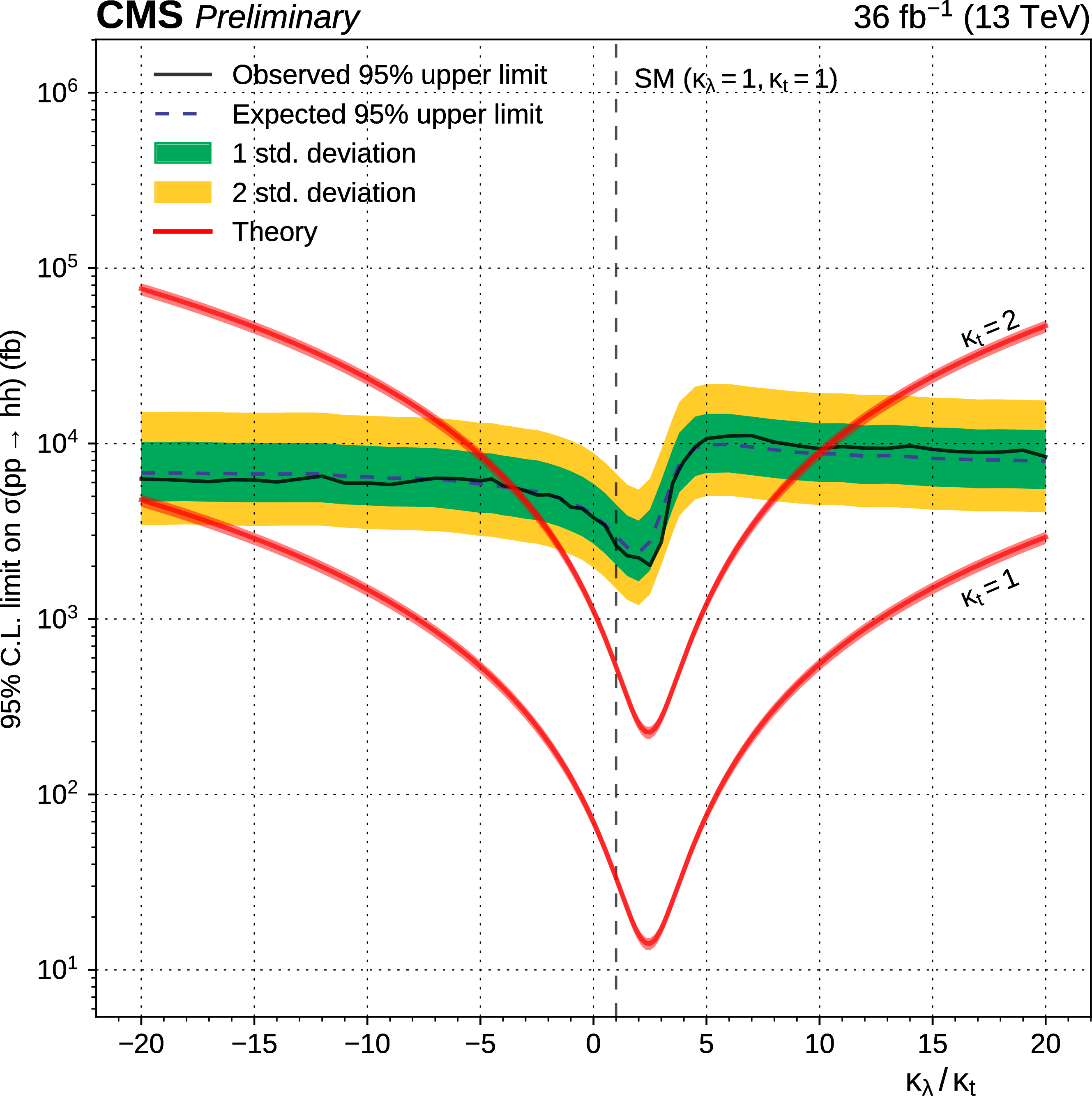
png pdf |
Table 1:
Summary of the systematic uncertainties and their impact range on total background yields and on the SM and $ {m_{\mathrm {X}}} = $ 400 GeV signal hypotheses in the signal region. |
| Summary |
|
We have presented a search for resonant and non-resonant Higgs pair production, where one of the h decays as $\mathrm{h} \to \mathrm{ b \bar{b} }$, and the other as $\mathrm{h} \to \mathrm{ V }\mathrm{ V } \to \ell\nu \ell\nu$ using LHC proton-proton collision data at $\sqrt{s}$ = 13 TeV, corresponding to an integrated luminosity of 36 fb$^{-1}$. Masses are considered in the range between $m_{\mathrm{X}} = $ 260 GeV and 900 GeV for the resonant search, and anomalous couplings $\kappa_{\lambda}$, $\kappa_{\mathrm{ t }}$ are considered in addition to the standard model case for the non-resonant search. The results obtained by the analysis are in agreement with the predictions from the standard model within uncertainties. For mass hypotheses from $m_{\mathrm{X}} = $ 300 GeV to $m_{\mathrm{X}} = $ 900 GeV, the data are observed (expected) to exclude a production cross-section times branching ratio of narrow-width spin-0 particles from 434 to 17 (342$^{+135}_{-97}$ to 14$^{+6}_{-4}$) fb and narrow-width spin-2 particles from 448 to 14 (361$^{+140}_{-102}$ to 13$^{+5}_{-4}$) fb for the resonant search. For the SM hh hypothesis, the data are observed (expected) to exclude a production cross section times branching ratio of 72 (81$^{+42}_{-25}$) fb, corresponding to 79 (89$^{+47}_{-28}$) times the SM cross section. |
| Additional Figures | |

png pdf |
Additional Figure 1:
Expected and observed 95% CL upper limits on Higgs pair production cross section as a function of $ {\mathrm {m}_{\mathrm {X}}} $. These limits are computed using the asymptotic CL$_s$ method, combining the $\mathrm{ e }^{+} \mathrm{ e }^{-} $, $\mu^{+} \mu^{-} $ and $\mathrm{ e } ^{\pm }\mu ^{\mp }$ channels, for spin-0 hypotheses and divided by the branching ratio for $\mathrm{h} \mathrm{h} \to {\mathrm{ b \bar{b} } } {\mathrm {V}} {\mathrm {V}} \to {\mathrm{ b \bar{b} } } \ell \nu \ell \nu $. |
png pdf |
Additional Figure 2:
Expected and observed 95% CL upper limits on Higgs pair production cross section as a function of $ {\mathrm {m}_{\mathrm {X}}} $. These limits are computed using the asymptotic CL$_s$ method, combining the $\mathrm{ e }^{+} \mathrm{ e }^{-} $, $\mu^{+} \mu^{-} $ and $\mathrm{ e } ^{\pm }\mu ^{\mp }$ channels, for spin-2 hypotheses and divided by the branching ratio for $\mathrm{h} \mathrm{h} \to {\mathrm{ b \bar{b} } } {\mathrm {V}} {\mathrm {V}} \to {\mathrm{ b \bar{b} } } \ell \nu \ell \nu $. |
png pdf |
Additional Figure 3:
Expected and observed 95% CL upper limits on Higgs pair production cross section as a function of $\kappa _{\lambda } / \kappa _{\mathrm{ t } }$. These limits are computed using the asymptotic CL$_s$ method, combining the $\mathrm{ e }^{+} \mathrm{ e }^{-} $, $\mu^{+} \mu^{-} $ and $\mathrm{ e }^{+}m {\mu ^\mp } $ channels and divided by the branching ratio for $\mathrm{h} \mathrm{h} \to {\mathrm{ b \bar{b} } } {\mathrm {V}} {\mathrm {V}} \to {\mathrm{ b \bar{b} } } \ell \nu \ell \nu $. |

png pdf |
Additional Figure 4:
The DNN output distribution for data and simulated events after requiring all selection cuts. Output values towards 0 are background-like, while output values towards 1 are signal-like. The resonant DNN output evaluated at $ {\mathrm {m}_{\mathrm {X}}} = $ 400 GeV. $\mathrm{ e }^{+} \mathrm{ e }^{-} $ channel only. The various signal hypotheses displayed have been scaled to a cross-section of 5 pb. |
png pdf |
Additional Figure 5:
The DNN output distribution for data and simulated events after requiring all selection cuts. Output values towards 0 are background-like, while output values towards 1 are signal-like. The resonant DNN output evaluated at $ {\mathrm {m}_{\mathrm {X}}} = $ 400 GeV. $\mathrm{ e }^{+}m {} {\mu ^\mp } $ channel only. The various signal hypotheses displayed have been scaled to a cross-section of 5 pb. |

png pdf |
Additional Figure 6:
The DNN output distribution for data and simulated events after requiring all selection cuts. Output values towards 0 are background-like, while output values towards 1 are signal-like. The resonant DNN output evaluated at $ {\mathrm {m}_{\mathrm {X}}} = $ 650 GeV. $\mathrm{ e }^{+} \mathrm{ e }^{-} $ channel only. The various signal hypotheses displayed have been scaled to a cross-section of 5 pb. |

png pdf |
Additional Figure 7:
The DNN output distribution for data and simulated events after requiring all selection cuts. Output values towards 0 are background-like, while output values towards 1 are signal-like. The resonant DNN output evaluated at $ {\mathrm {m}_{\mathrm {X}}} = $ 650 GeV. $\mathrm{ e }^{+}m {} {\mu ^\mp } $ channel only. The various signal hypotheses displayed have been scaled to a cross-section of 5 pb. |
png pdf |
Additional Figure 8:
The DNN output distribution for data and simulated events after requiring all selection cuts. Output values towards 0 are background-like, while output values towards 1 are signal-like. The resonant DNN output evaluated at $ {\mathrm {m}_{\mathrm {X}}} = $ 650 GeV. $\mu^{+} {}\mu^{-} $ channel only. The various signal hypotheses displayed have been scaled to a cross-section of 5 pb. |

png pdf |
Additional Figure 9:
The DNN output distribution for data and simulated events after requiring all selection cuts. Output values towards 0 are background-like, while output values towards 1 are signal-like. The resonant DNN output evaluated at $ {\mathrm {m}_{\mathrm {X}}} = $ 900 GeV. $\mathrm{ e }^{+} \mathrm{ e }^{-} $ channel only. The various signal hypotheses displayed have been scaled to a cross-section of 5 pb. |
png pdf |
Additional Figure 10:
The DNN output distribution for data and simulated events after requiring all selection cuts. Output values towards 0 are background-like, while output values towards 1 are signal-like. The resonant DNN output evaluated at $ {\mathrm {m}_{\mathrm {X}}} = $ 900 GeV. $\mathrm{ e }^{+}m {} {\mu ^\mp } $ channel only. The various signal hypotheses displayed have been scaled to a cross-section of 5 pb. |
png pdf |
Additional Figure 11:
The DNN output distribution for data and simulated events after requiring all selection cuts. Output values towards 0 are background-like, while output values towards 1 are signal-like. The resonant DNN output evaluated at $ {\mathrm {m}_{\mathrm {X}}} = $ 900 GeV. $\mu^{+} {}\mu^{-} $ channel only. The various signal hypotheses displayed have been scaled to a cross-section of 5 pb. |

png pdf |
Additional Figure 12:
DNN output distribution for data and simulated events in three different $ {\mathrm {m}_{ {\mathrm {j}} {\mathrm {j}} }} $ regions: $ {\mathrm {m}_{ {\mathrm {j}} {\mathrm {j}} }} < $ 75 GeV, $ {\mathrm {m}_{ {\mathrm {j}} {\mathrm {j}} }} \in $ [75, 140 [ GeV and $ {\mathrm {m}_{ {\mathrm {j}} {\mathrm {j}} }} \geq 140$ GeV. The resonant DNN output evaluated at $ {\mathrm {m}_{\mathrm {X}}} = $ 400 GeV. $\mathrm{ e }^{+} \mathrm{ e }^{-} $ channel only. The various signal hypotheses displayed have been scaled to a cross-section of 5 pb. |
png pdf |
Additional Figure 13:
DNN output distribution for data and simulated events in three different $ {\mathrm {m}_{ {\mathrm {j}} {\mathrm {j}} }} $ regions: $ {\mathrm {m}_{ {\mathrm {j}} {\mathrm {j}} }} < $ 75 GeV, $ {\mathrm {m}_{ {\mathrm {j}} {\mathrm {j}} }} \in $ [75, 140 [ GeV and $ {\mathrm {m}_{ {\mathrm {j}} {\mathrm {j}} }} \geq 140$ GeV. The resonant DNN output evaluated at $ {\mathrm {m}_{\mathrm {X}}} = $ 400 GeV. $\mathrm{ e }^{+}m {} {\mu ^\mp } $ channel only. The various signal hypotheses displayed have been scaled to a cross-section of 5 pb. |

png pdf |
Additional Figure 14:
DNN output distribution for data and simulated events in three different $ {\mathrm {m}_{ {\mathrm {j}} {\mathrm {j}} }} $ regions: $ {\mathrm {m}_{ {\mathrm {j}} {\mathrm {j}} }} < $ 75 GeV, $ {\mathrm {m}_{ {\mathrm {j}} {\mathrm {j}} }} \in $ [75, 140 [ GeV and $ {\mathrm {m}_{ {\mathrm {j}} {\mathrm {j}} }} \geq 140$ GeV. The resonant DNN output evaluated at $ {\mathrm {m}_{\mathrm {X}}} = $ 650 GeV. $\mathrm{ e }^{+} \mathrm{ e }^{-} $ channel only. The various signal hypotheses displayed have been scaled to a cross-section of 5 pb. |
png pdf |
Additional Figure 15:
DNN output distribution for data and simulated events in three different $ {\mathrm {m}_{ {\mathrm {j}} {\mathrm {j}} }} $ regions: $ {\mathrm {m}_{ {\mathrm {j}} {\mathrm {j}} }} < $ 75 GeV, $ {\mathrm {m}_{ {\mathrm {j}} {\mathrm {j}} }} \in $ [75, 140 [ GeV and $ {\mathrm {m}_{ {\mathrm {j}} {\mathrm {j}} }} \geq 140$ GeV. The resonant DNN output evaluated at $ {\mathrm {m}_{\mathrm {X}}} = $ 650 GeV. $\mathrm{ e }^{+}m {} {\mu ^\mp } $ channel only. The various signal hypotheses displayed have been scaled to a cross-section of 5 pb. |

png pdf |
Additional Figure 16:
DNN output distribution for data and simulated events in three different $ {\mathrm {m}_{ {\mathrm {j}} {\mathrm {j}} }} $ regions: $ {\mathrm {m}_{ {\mathrm {j}} {\mathrm {j}} }} < $ 75 GeV, $ {\mathrm {m}_{ {\mathrm {j}} {\mathrm {j}} }} \in $ [75, 140 [ GeV and $ {\mathrm {m}_{ {\mathrm {j}} {\mathrm {j}} }} \geq 140$ GeV. The resonant DNN output evaluated at $ {\mathrm {m}_{\mathrm {X}}} = $ 650 GeV. $\mu^{+} {}\mu^{-} $ channel only. The various signal hypotheses displayed have been scaled to a cross-section of 5 pb. |
png pdf |
Additional Figure 17:
DNN output distribution for data and simulated events in three different $ {\mathrm {m}_{ {\mathrm {j}} {\mathrm {j}} }} $ regions: $ {\mathrm {m}_{ {\mathrm {j}} {\mathrm {j}} }} < $ 75 GeV, $ {\mathrm {m}_{ {\mathrm {j}} {\mathrm {j}} }} \in $ [75, 140 [ GeV and $ {\mathrm {m}_{ {\mathrm {j}} {\mathrm {j}} }} \geq 140$ GeV. The resonant DNN output evaluated at $ {\mathrm {m}_{\mathrm {X}}} = $ 900 GeV. $\mathrm{ e }^{+} \mathrm{ e }^{-} $ channel only. The various signal hypotheses displayed have been scaled to a cross-section of 5 pb. |

png pdf |
Additional Figure 18:
DNN output distribution for data and simulated events in three different $ {\mathrm {m}_{ {\mathrm {j}} {\mathrm {j}} }} $ regions: $ {\mathrm {m}_{ {\mathrm {j}} {\mathrm {j}} }} < $ 75 GeV, $ {\mathrm {m}_{ {\mathrm {j}} {\mathrm {j}} }} \in $ [75, 140 [ GeV and $ {\mathrm {m}_{ {\mathrm {j}} {\mathrm {j}} }} \geq 140$ GeV. The resonant DNN output evaluated at $ {\mathrm {m}_{\mathrm {X}}} = $ 900 GeV. $\mathrm{ e }^{+}m {} {\mu ^\mp } $ channel only. The various signal hypotheses displayed have been scaled to a cross-section of 5 pb. |
png pdf |
Additional Figure 19:
DNN output distribution for data and simulated events in three different $ {\mathrm {m}_{ {\mathrm {j}} {\mathrm {j}} }} $ regions: $ {\mathrm {m}_{ {\mathrm {j}} {\mathrm {j}} }} < $ 75 GeV, $ {\mathrm {m}_{ {\mathrm {j}} {\mathrm {j}} }} \in $ [75, 140 [ GeV and $ {\mathrm {m}_{ {\mathrm {j}} {\mathrm {j}} }} \geq 140$ GeV. The resonant DNN output evaluated at $ {\mathrm {m}_{\mathrm {X}}} = $ 900 GeV. $\mu^{+} {}\mu^{-} $ channel only. The various signal hypotheses displayed have been scaled to a cross-section of 5 pb. |

png pdf |
Additional Figure 20:
The DNN output distribution for data and simulated events after requiring all selection cuts. Output values towards 0 are background-like, while output values towards 1 are signal-like. The non-resonant DNN output evaluated at $\kappa _{\lambda } = $ 1, $\kappa _{\mathrm{ t } } = $ 1. $\mathrm{ e }^{+} \mathrm{ e }^{-} $ channel only.The various signal hypotheses displayed have been scaled to a cross-section of 5 pb. |

png pdf |
Additional Figure 21:
The DNN output distribution for data and simulated events after requiring all selection cuts. Output values towards 0 are background-like, while output values towards 1 are signal-like. The non-resonant DNN output evaluated at $\kappa _{\lambda } = $ 1, $\kappa _{\mathrm{ t } } = $ 1. $\mathrm{ e }^{+}m {} {\mu ^\mp } $ channel only.The various signal hypotheses displayed have been scaled to a cross-section of 5 pb. |

png pdf |
Additional Figure 22:
The DNN output distribution for data and simulated events after requiring all selection cuts. Output values towards 0 are background-like, while output values towards 1 are signal-like. The non-resonant DNN output evaluated at $\kappa _{\lambda } = $ 5, $\kappa _{\mathrm{ t } } =2.5$. $\mathrm{ e }^{+} \mathrm{ e }^{-} $ channel only.The various signal hypotheses displayed have been scaled to a cross-section of 5 pb. |

png pdf |
Additional Figure 23:
The DNN output distribution for data and simulated events after requiring all selection cuts. Output values towards 0 are background-like, while output values towards 1 are signal-like. The non-resonant DNN output evaluated at $\kappa _{\lambda } = $ 5, $\kappa _{\mathrm{ t } } =2.5$. $\mathrm{ e }^{+}m {} {\mu ^\mp } $ channel only.The various signal hypotheses displayed have been scaled to a cross-section of 5 pb. |

png pdf |
Additional Figure 24:
The DNN output distribution for data and simulated events after requiring all selection cuts. Output values towards 0 are background-like, while output values towards 1 are signal-like. The non-resonant DNN output evaluated at $\kappa _{\lambda } = $ 5, $\kappa _{\mathrm{ t } } =2.5$. $\mu^{+} {}\mu^{-} $ channel only.The various signal hypotheses displayed have been scaled to a cross-section of 5 pb. |
png pdf |
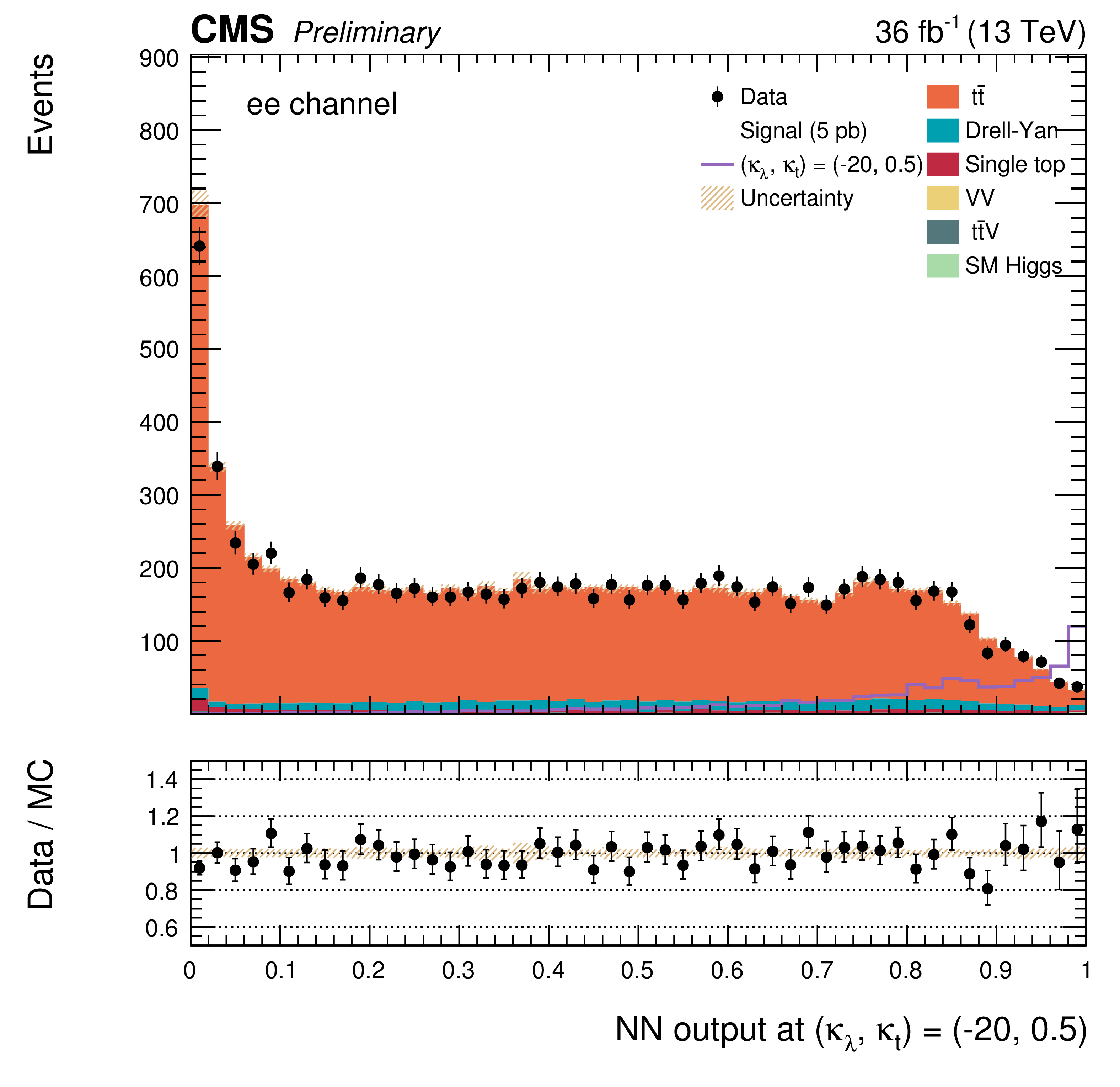
Additional Figure 25:
The DNN output distribution for data and simulated events after requiring all selection cuts. Output values towards 0 are background-like, while output values towards 1 are signal-like. The non-resonant DNN output evaluated at $\kappa _{\lambda } =-20$, $\kappa _{\mathrm{ t } } =0.5$. $\mathrm{ e }^{+} \mathrm{ e }^{-} $ channel only.The various signal hypotheses displayed have been scaled to a cross-section of 5 pb. |
png pdf |
Additional Figure 26:
The DNN output distribution for data and simulated events after requiring all selection cuts. Output values towards 0 are background-like, while output values towards 1 are signal-like. The non-resonant DNN output evaluated at $\kappa _{\lambda } =-20$, $\kappa _{\mathrm{ t } } =0.5$. $\mathrm{ e }^{+}m {} {\mu ^\mp } $ channel only.The various signal hypotheses displayed have been scaled to a cross-section of 5 pb. |

png pdf |
Additional Figure 27:
The DNN output distribution for data and simulated events after requiring all selection cuts. Output values towards 0 are background-like, while output values towards 1 are signal-like. The non-resonant DNN output evaluated at $\kappa _{\lambda } =-20$, $\kappa _{\mathrm{ t } } =0.5$. $\mu^{+} {}\mu^{-} $ channel only.The various signal hypotheses displayed have been scaled to a cross-section of 5 pb. |

png pdf |
Additional Figure 28:
DNN output distribution for data and simulated events in three different $ {\mathrm {m}_{ {\mathrm {j}} {\mathrm {j}} }} $ regions: $ {\mathrm {m}_{ {\mathrm {j}} {\mathrm {j}} }} < $ 75 GeV, $ {\mathrm {m}_{ {\mathrm {j}} {\mathrm {j}} }} \in $ [75, 140 [ GeV and $ {\mathrm {m}_{ {\mathrm {j}} {\mathrm {j}} }} \geq 140$ GeV. The non-resonant DNN output evaluated at $\kappa _{\lambda } = $ 1, $\kappa _{\mathrm{ t } } = $ 1. $\mathrm{ e }^{+} \mathrm{ e }^{-} $ channel only. The various signal hypotheses displayed have been scaled to a cross-section of 5 pb. |
png pdf |
Additional Figure 29:
DNN output distribution for data and simulated events in three different $ {\mathrm {m}_{ {\mathrm {j}} {\mathrm {j}} }} $ regions: $ {\mathrm {m}_{ {\mathrm {j}} {\mathrm {j}} }} < $ 75 GeV, $ {\mathrm {m}_{ {\mathrm {j}} {\mathrm {j}} }} \in $ [75, 140 [ GeV and $ {\mathrm {m}_{ {\mathrm {j}} {\mathrm {j}} }} \geq 140$ GeV. The non-resonant DNN output evaluated at $\kappa _{\lambda } = $ 1, $\kappa _{\mathrm{ t } } = $ 1. $\mathrm{ e }^{+}m {} {\mu ^\mp } $ channel only. The various signal hypotheses displayed have been scaled to a cross-section of 5 pb. |

png pdf |
Additional Figure 30:
DNN output distribution for data and simulated events in three different $ {\mathrm {m}_{ {\mathrm {j}} {\mathrm {j}} }} $ regions: $ {\mathrm {m}_{ {\mathrm {j}} {\mathrm {j}} }} < $ 75 GeV, $ {\mathrm {m}_{ {\mathrm {j}} {\mathrm {j}} }} \in $ [75, 140 [ GeV and $ {\mathrm {m}_{ {\mathrm {j}} {\mathrm {j}} }} \geq 140$ GeV. The non-resonant DNN output evaluated at $\kappa _{\lambda } = $ 5, $\kappa _{\mathrm{ t } } =2.5$. $\mathrm{ e }^{+} \mathrm{ e }^{-} $ channel only. The various signal hypotheses displayed have been scaled to a cross-section of 5 pb. |

png pdf |
Additional Figure 31:
DNN output distribution for data and simulated events in three different $ {\mathrm {m}_{ {\mathrm {j}} {\mathrm {j}} }} $ regions: $ {\mathrm {m}_{ {\mathrm {j}} {\mathrm {j}} }} < $ 75 GeV, $ {\mathrm {m}_{ {\mathrm {j}} {\mathrm {j}} }} \in $ [75, 140 [ GeV and $ {\mathrm {m}_{ {\mathrm {j}} {\mathrm {j}} }} \geq 140$ GeV. The non-resonant DNN output evaluated at $\kappa _{\lambda } = $ 5, $\kappa _{\mathrm{ t } } =2.5$. $\mathrm{ e }^{+}m {} {\mu ^\mp } $ channel only. The various signal hypotheses displayed have been scaled to a cross-section of 5 pb. |

png pdf |
Additional Figure 32:
DNN output distribution for data and simulated events in three different $ {\mathrm {m}_{ {\mathrm {j}} {\mathrm {j}} }} $ regions: $ {\mathrm {m}_{ {\mathrm {j}} {\mathrm {j}} }} < $ 75 GeV, $ {\mathrm {m}_{ {\mathrm {j}} {\mathrm {j}} }} \in $ [75, 140 [ GeV and $ {\mathrm {m}_{ {\mathrm {j}} {\mathrm {j}} }} \geq 140$ GeV. The non-resonant DNN output evaluated at $\kappa _{\lambda } = $ 5, $\kappa _{\mathrm{ t } } =2.5$. $\mu^{+} {}\mu^{-} $ channel only. The various signal hypotheses displayed have been scaled to a cross-section of 5 pb. |
png pdf |
Additional Figure 33:
DNN output distribution for data and simulated events in three different $ {\mathrm {m}_{ {\mathrm {j}} {\mathrm {j}} }} $ regions: $ {\mathrm {m}_{ {\mathrm {j}} {\mathrm {j}} }} < $ 75 GeV, $ {\mathrm {m}_{ {\mathrm {j}} {\mathrm {j}} }} \in $ [75, 140 [ GeV and $ {\mathrm {m}_{ {\mathrm {j}} {\mathrm {j}} }} \geq 140$ GeV. The non-resonant DNN output evaluated at $\kappa _{\lambda } =-20$, $\kappa _{\mathrm{ t } } =0.5$. $\mathrm{ e }^{+} \mathrm{ e }^{-} $ channel only. The various signal hypotheses displayed have been scaled to a cross-section of 5 pb. |

png pdf |
Additional Figure 34:
DNN output distribution for data and simulated events in three different $ {\mathrm {m}_{ {\mathrm {j}} {\mathrm {j}} }} $ regions: $ {\mathrm {m}_{ {\mathrm {j}} {\mathrm {j}} }} < $ 75 GeV, $ {\mathrm {m}_{ {\mathrm {j}} {\mathrm {j}} }} \in $ [75, 140 [ GeV and $ {\mathrm {m}_{ {\mathrm {j}} {\mathrm {j}} }} \geq 140$ GeV. The non-resonant DNN output evaluated at $\kappa _{\lambda } =-20$, $\kappa _{\mathrm{ t } } =0.5$. $\mathrm{ e }^{+}m {} {\mu ^\mp } $ channel only. The various signal hypotheses displayed have been scaled to a cross-section of 5 pb. |
png pdf |
Additional Figure 35:
DNN output distribution for data and simulated events in three different $ {\mathrm {m}_{ {\mathrm {j}} {\mathrm {j}} }} $ regions: $ {\mathrm {m}_{ {\mathrm {j}} {\mathrm {j}} }} < $ 75 GeV, $ {\mathrm {m}_{ {\mathrm {j}} {\mathrm {j}} }} \in $ [75, 140 [ GeV and $ {\mathrm {m}_{ {\mathrm {j}} {\mathrm {j}} }} \geq 140$ GeV. The non-resonant DNN output evaluated at $\kappa _{\lambda } =-20$, $\kappa _{\mathrm{ t } } =0.5$. $\mu^{+} {}\mu^{-} $ channel only. The various signal hypotheses displayed have been scaled to a cross-section of 5 pb. |

png pdf |
Additional Figure 36:
Signal vs background efficiency curve comparing the non resonant DNN parameterised training, evaluated at $\kappa _{\lambda } = -20$, $\kappa _{\mathrm{ t } } = 0.5$ (dashed lines) and $\kappa _{\lambda } = 1$, $\kappa _{\mathrm{ t } } = 1$ (solid lines), with a dedicated non-parameterised training for each of the points. Both approaches show similar performance. |

png pdf |
Additional Figure 37:
Signal vs background efficiency curve showing the resonant DNN parameterised training, evaluated at $ {\mathrm {m}_{\mathrm {X}}} = $ 650 GeV. Blue line shows a parameterised training which includes $ {\mathrm {m}_{\mathrm {X}}} = $ 650 GeV , while the red line shows a parameterised training which does not include $ {\mathrm {m}_{\mathrm {X}}} = $ 650 GeV. |
png pdf |
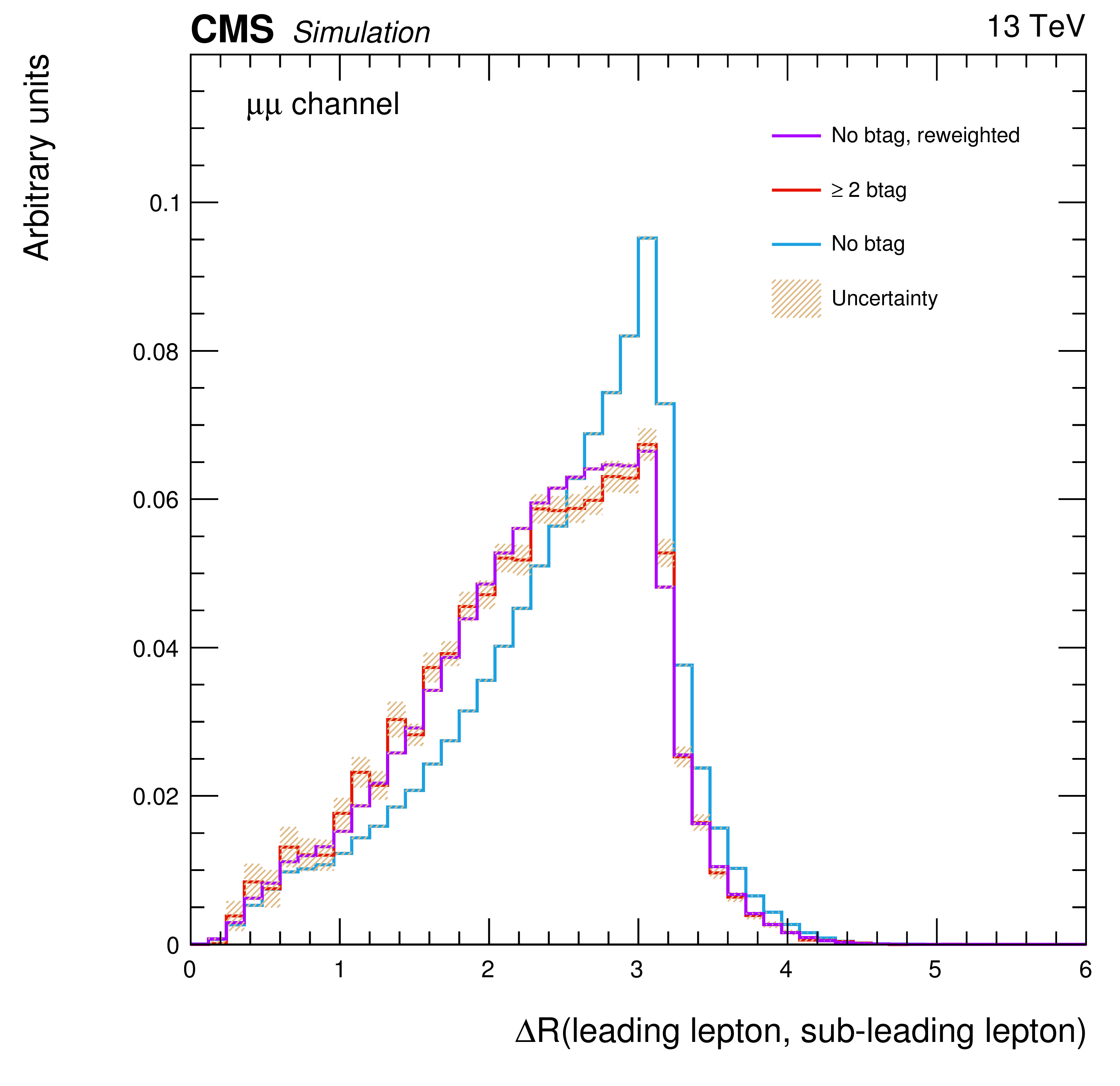
Additional Figure 38:
The $\Delta R_{ll}$ distribution in Drell-Yan Monte Carlo events requiring two leptons and two jets ( blue line), two leptons and two b-tag jets by applying the b-tagging algorithm (red line), and two leptons and two b-tagged using the DY re-weighting method (violet line). |
| Additional Tables | |

png pdf |
Additional Table 1:
Expected and observed 95% CL upper limits on Higgs pair production cross section times branching ratio for $\mathrm{h} \mathrm{h} \to {\mathrm{ b \bar{b} } } {\mathrm {V}} {\mathrm {V}} \to {\mathrm{ b \bar{b} } } \ell \nu \ell \nu $ as a function of $ {\mathrm {m}_{\mathrm {X}}} $. These limits are computed using the asymptotic CL$_s$ method, combining the $\mathrm{ e }^{+} \mathrm{ e }^{-} $, $\mu^{+} \mu^{-} $ and $\mathrm{ e } ^{\pm }\mu ^{\mp }$ channels, for spin-0 hypotheses. |

png pdf |
Additional Table 2:
Expected and observed 95% CL upper limits on Higgs pair production cross section times branching ratio for $\mathrm{h} \mathrm{h} \to {\mathrm{ b \bar{b} } } {\mathrm {V}} {\mathrm {V}} \to {\mathrm{ b \bar{b} } } \ell \nu \ell \nu $ as a function of $ {\mathrm {m}_{\mathrm {X}}} $. These limits are computed using the asymptotic CL$_s$ method, combining the $\mathrm{ e }^{+} \mathrm{ e }^{-} $, $\mu^{+} \mu^{-} $ and $\mathrm{ e } ^{\pm }\mu ^{\mp }$ channels, for spin-2 hypotheses. |
png pdf |
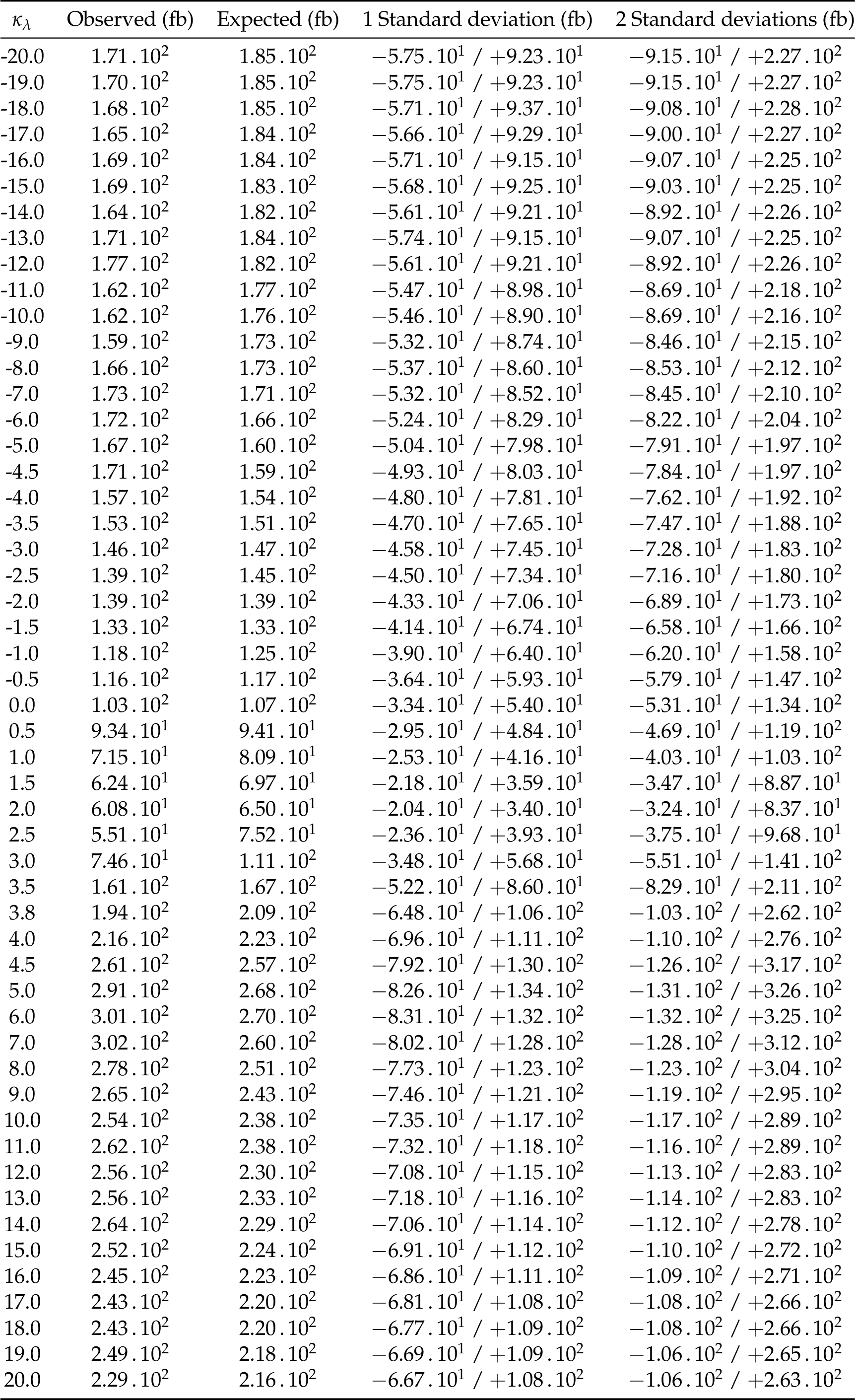
Additional Table 3:
Expected and observed 95% CL upper limits on Higgs pair production cross section times branching ratio for $\mathrm{h} \mathrm{h} \to {\mathrm{ b \bar{b} } } {\mathrm {V}} {\mathrm {V}} \to {\mathrm{ b \bar{b} } } \ell \nu \ell \nu $ as a function of $\kappa _{\lambda }$. These limits are computed using the asymptotic CL$_s$ method, combining the $\mathrm{ e }^{+} \mathrm{ e }^{-} $, $\mu^{+} \mu^{-} $ and $\mathrm{ e } ^{\pm }\mu ^{\mp }$ channels, for $\kappa _{\mathrm{ t } } = 1$. |
| References | ||||
| 1 | F. Englert and R. Brout | Broken Symmetry and the Mass of Gauge Vector Mesons | PRL 13 (1964) 321 | |
| 2 | P. W. Higgs | Broken symmetries, massless particles and gauge fields | PL12 (1964) 132 | |
| 3 | P. W. Higgs | Broken Symmetries and the Masses of Gauge Bosons | PRL 13 (1964) 508 | |
| 4 | G. S. Guralnik, C. R. Hagen, and T. W. B. Kibble | Global conservation laws and massless particles | PRL 13 (1964) 585 | |
| 5 | P. W. Higgs | Spontaneous symmetry breakdown without massless bosons | PR145 (1966) 1156 | |
| 6 | T. W. B. Kibble | Symmetry breaking in non-Abelian gauge theories | PR155 (1967) 1554 | |
| 7 | ATLAS Collaboration | Observation of a new particle in the search for the Standard Model Higgs boson with the ATLAS detector at the LHC | Phys.Lett. B 716 (2012) 129 | |
| 8 | CMS Collaboration | Observation of a new boson at a mass of 125~GeV with the CMS experiment at the LHC | Phys.Lett. B 716 (2012) 3061 | |
| 9 | LHC Higgs Cross Section Working Group Collaboration | Handbook of LHC Higgs Cross Sections: 4. Deciphering the Nature of the Higgs Sector | 1610.07922 | |
| 10 | D. de Florian and J. Mazzitelli | Higgs pair production at next-to-next-to-leading logarithmic accuracy at the LHC | JHEP 09 (2015) 053 | 1505.07122 |
| 11 | D. de Florian and J. Mazzitelli | Higgs Boson Pair Production at Next-to-Next-to-Leading Order in QCD | PRL 111 (2013) 201801 | 1309.6594 |
| 12 | S. Borowka et al. | Higgs boson pair production in gluon fusion at NLO with full top-quark mass dependence | 1604.06447 | |
| 13 | S. Dawson, S. Dittmaier, and M. Spira | Neutral Higgs boson pair production at hadron colliders: QCD corrections | PRD58 (1998) 115012 | hep-ph/9805244 |
| 14 | J. Grigo, K. Melnikov, and M. Steinhauser | Virtual corrections to Higgs boson pair production in the large top quark mass limit | Nucl.Phys. B888 (2014) 17--29 | 1408.2422 |
| 15 | J. Grigo, J. Hoff, and M. Steinhauser | Higgs boson pair production: top quark mass effects at NLO and NNLO | Nucl. Phys. B900 (2015) 412--430 | 1508.00909 |
| 16 | J. Grigo, J. Hoff, K. Melnikov, and M. Steinhauser | On the Higgs boson pair production at the LHC | Nucl. Phys. B875 (2013) 1--17 | 1305.7340 |
| 17 | R. Frederix et al. | Higgs pair production at the LHC with NLO and parton-shower effects | PLB732 (2014) 142--149 | 1401.7340 |
| 18 | F. Maltoni, E. Vryonidou, and M. Zaro | Top-quark mass effects in double and triple Higgs production in gluon-gluon fusion at NLO | JHEP 11 (2014) 079 | 1408.6542 |
| 19 | A. Azatov, R. Contino, G. Panico, and M. Son | Effective field theory analysis of double Higgs boson production via gluon fusion | PRD92 (2015), no. 3, 035001 | 1502.00539 |
| 20 | F. Goertz, A. Papaefstathiou, L. L. Yang, and J. Zurita | Higgs boson pair production in the D=6 extension of the SM | JHEP 04 (2015) 167 | 1410.3471 |
| 21 | B. Hespel, D. Lopez-Val, and E. Vryonidou | Higgs pair production via gluon fusion in the Two-Higgs-Doublet Model | JHEP 09 (2014) 124 | 1407.0281 |
| 22 | G. C. Branco et al. | Theory and phenomenology of two-Higgs-doublet models | PR 516 (2012) 1--102 | 1106.0034 |
| 23 | L. Randall and R. Sundrum | A Large mass hierarchy from a small extra dimension | Phys.Rev.Lett. 83 (1999) 3370–3373 | |
| 24 | W. D. Goldberger and M. S. Wise | Modulus stabilization with bulk fields | Phys.Rev.Lett. 83 (1999) 4922–4925 | |
| 25 | O. DeWolfe, D. Freedman, S. Gubser, and A. Karch | Modeling the fifth-dimension with scalars and gravity | Phys.Rev. D 62 (2000) 046008 | |
| 26 | C. Csaki, M. Graesser, L. Randall, and J. Terning | Cosmology of brane models with radion stabilization | Phys.Rev. D 62 (2000) 045015 | |
| 27 | C. Csaki, J. Hubisz, and S. J. Lee | Radion phenomenology in realistic warped space Model | Phys.Rev. D 76 (2007) 125015 | |
| 28 | H. Davoudiasl, J. Hewett, and T. Rizzo | Phenomenology of the Randall-Sundrum Gauge Hierarchy Model | Phys.Rev.Lett. 84 (2000) 2080 | |
| 29 | C. Csaki, M. L. Graesser, and G. D. Kribs | Radion dynamics and electroweak physics | Phys.Rev. D 63 (2001) 065002 | |
| 30 | CMS Collaboration | Search for two Higgs bosons in final states containing two photons and two bottom quarks in proton-proton collisions at 8 TeV | CMS-PAS-HIG-13-032 | CMS-PAS-HIG-13-032 |
| 31 | CMS Collaboration | Search for pair production of Higgs bosons in the two tau leptons and two bottom quarks final state using proton-proton collisions at $ \sqrt{s} = $ 13 TeV | CDS | |
| 32 | CMS Collaboration | Search for Higgs boson pair production in the $ \mathrm{b}\overline{\mathrm{b}} \mathrm{l}\nu \mathrm{l}\nu $ final state at $ \sqrt{s} = $ 13 TeV | CDS | |
| 33 | CMS Collaboration | Model independent search for Higgs boson pair production in the $ \mathrm{b\overline{b}}\tau^+\tau^- $ final state | CMS-PAS-HIG-15-013 | CMS-PAS-HIG-15-013 |
| 34 | ATLAS Collaboration | Search For Higgs Boson Pair Production in the $ \gamma\gamma b\bar{b} $ Final State using $ pp $ Collision Data at $ \sqrt{s}= $ 8 TeV from the ATLAS Detector | PRL 114 (2015), no. 8, 081802 | 1406.5053 |
| 35 | ATLAS Collaboration | Search for Higgs boson pair production in the $ b\bar{b}b\bar{b} $ final state from pp collisions at $ \sqrt{s} = $ 8 TeV with the ATLAS detector | EPJC75 (2015), no. 9, 412 | 1506.00285 |
| 36 | ATLAS Collaboration | Searches for Higgs boson pair production in the $ hh\to bb\tau\tau, \gamma\gamma WW^*, \gamma\gamma bb, bbbb $ channels with the ATLAS detector | PRD92 (2015) 092004 | 1509.04670 |
| 37 | ATLAS Collaboration | Search for pair production of Higgs bosons in the $ b\bar{b}b\bar{b} $ final state using proton--proton collisions at $ \sqrt{s}= $ 13 TeV with the ATLAS detector | PRD94 (2016), no. 5, 052002 | 1606.04782 |
| 38 | ATLAS Collaboration | Search for Higgs boson pair production in the $ b\bar{b}\gamma\gamma $ final state using pp collision data at $ \sqrt{s}= $ 13 TeV with the ATLAS detector | Technical Report ATLAS-CONF-2016-004, CERN, Geneva, Mar | |
| 39 | ATLAS Collaboration | Search for pair production of Higgs bosons in the $ b\bar{b}b\bar{b} $ final state using proton$ - $proton collisions at $ \sqrt{s}= $ 13 TeV with the ATLAS detector | Technical Report ATLAS-CONF-2016-049, CERN, Geneva, Aug | |
| 40 | ATLAS Collaboration | Search for Higgs boson pair production in the final state of $ \gamma\gamma WW^* $($ \rightarrow l\nu jj $) using 13.3 fb$ ^{-1} $ of $ pp $ collision data recorded at $ \sqrt{s}= $ 13 TeV with the ATLAS detector | Technical Report ATLAS-CONF-2016-071, CERN, Geneva, Aug | |
| 41 | CMS Collaboration | Search for H(bb)H(gammagamma) decays at 13TeV | CDS | |
| 42 | CMS Collaboration | Search for non-resonant pair production of Higgs bosons in the $ \rm{b} \bar{\rm{b}} \rm{b} \bar{\rm{b}} $ final state with 13 TeV CMS data | CDS | |
| 43 | CMS Collaboration | The CMS experiment at the CERN LHC | JINST 0803 (2008) S08004 | |
| 44 | J. Alwall et al. | The automated computation of tree-level and next-to-leading order differential cross sections, and their matching to parton shower simulations | JHEP 07 (2014) 079 | 1405.0301 |
| 45 | P. Nason | A New method for combining NLO QCD with shower Monte Carlo algorithms | JHEP 11 (2004) 040 | hep-ph/0409146 |
| 46 | S. Frixione, P. Nason, and C. Oleari | Matching NLO QCD computations with Parton Shower simulations: the POWHEG method | JHEP 11 (2007) 070 | 0709.2092 |
| 47 | S. Alioli, P. Nason, C. Oleari, and E. Re | A general framework for implementing NLO calculations in shower Monte Carlo programs: the POWHEG BOX | JHEP 06 (2010) 043 | 1002.2581 |
| 48 | S. Alioli, S. Moch, and P. Uwer | Hadronic top-quark pair-production with one jet and parton showering | JHEP 1201 (2012) 137 | |
| 49 | S. Alioli, P. Nason, C. Oleari, and E. Re | Single-top production in the s- and t-channel | JHEP 0909 (2009) 111 | |
| 50 | T. Sjostrand, S. Mrenna, and P. Z. Skands | PYTHIA 6.4 Physics and Manual | JHEP 05 (2006) 026 | hep-ph/0603175 |
| 51 | T. Sjostrand, S. Mrenna, and P. Z. Skands | A Brief Introduction to PYTHIA 8.1 | CPC 178 (2008) 852--867 | 0710.3820 |
| 52 | S. Agostinelli et al. | Geant4—a simulation toolkit | NIM A506 (2003) | |
| 53 | CMS Collaboration | Performance of electron reconstruction and selection with the CMS detector in proton-proton collisions at $ \sqrt{s} $ = 8 TeV | JINST 10 (2015), no. 06, P06005 | CMS-EGM-13-001 1502.02701 |
| 54 | CMS Collaboration | Performance of CMS muon reconstruction in $ pp $ collision events at $ \sqrt{s}= $ 7 TeV | JINST 7 (2012) P10002 | CMS-MUO-10-004 1206.4071 |
| 55 | CMS Collaboration | “Performance of the CMS missing transverse momentum reconstruction in pp data at $ \sqrt{s} $ = 8 TeV | JINST 10 (2015) P02006 | |
| 56 | M. Cacciari, G. P. Salam, and G. Soyez | The anti-$ k_T $ jet clustering algorithm | JHEP 04 (2008) 063 | |
| 57 | M. Cacciari, G. P. Salam, and G. Soyez | FastJet user manual | EPJC 72 (2012) 1896 | |
| 58 | CMS Collaboration | Jet energy scale and resolution in the CMS experiment in pp collisions at 8 TeV | Submitted to: JINST (2016) | CMS-JME-13-004 1607.03663 |
| 59 | CMS Collaboration | Identification of b-quark jets with the CMS experimet | JINST 8 (2013) P04013 | |
| 60 | F. Chollet | |||
| 61 | P. Baldi et al. | Parameterized Machine Learning for High-Energy Physics | Phys. J. C 76: 235 (2016) | hep-ex/1601.07913 |
| 62 | CMS Collaboration | Measurement of the inclusive W and Z production cross sections in pp collisions at $ \sqrt{s}= $ 7 TeV with the CMS experiment | Journal of High Energy Physics 2011 (2011), no. 10, 132 | |
| 63 | NNPDF Collaboration | Parton distributions for the LHC Run II | JHEP 04 (2015) 040 | 1410.8849 |
| 64 | CMS Collaboration | Measurement of the production cross sections for a Z boson and one or more b jets in pp collisions at $ \sqrt{s}= $ 7 TeV | JHEP 06 (2014) 120 | CMS-SMP-13-004 1402.1521 |
| 65 | CMS Collaboration | Measurements of the associated production of a Z boson and b jets in pp collisions at $ \sqrt{s} $ = 8 TeV | Submitted to: EPJC (2016) | CMS-SMP-14-010 1611.06507 |
| 66 | T. Junk | Confidence level computation for combining searches with small statistics | Nucl.Instrum.Meth. A434 (1999) 435 | hep-ex/9902006 |
| 67 | A. L. Read | Presentation of search results: the CLs technique | JPG: Nucl. Part. Phys. 28 (2002) | |
| 68 | B. Mellado Garcia, P. Musella, M. Grazzini, and R. Harlander | CERN Report 4: Part I Standard Model Predictions | ||
| 69 | A. Carvalho Antunes De Oliveira et al. | Analytical parametrization and shape classification of anomalous HH production in EFT approach | Technical Report LHCHXSWG-2016-001, CERN, Geneva, Jul | |
|
|
Compact Muon Solenoid LHC, CERN |
|

|

|

|

|

|