&DRIFT: methods

velocity

The magnitude of the drift velocity vector is taken from the gas tables. Mainly for historic reasons, the tables list the velocity for electrons and the velocity divided by the field (usually called mobility) for ions, a difference that is of a merely formal nature.

The magnitude of the drift velocity of electrons and the mobility of ions can be entered with the TABLE and ADD gas section commands. Electron velocities can in addition be computed with MAGBOLTZ and MIX.

In the presence of a magnetic field, both electrons and ions experience a force which is perpendicular to both the E field and the local velocity. In vacuum, particles will follow a spiraling trajectory. In chamber gases however, both electrons and ions undergo frequent scattering as a result of which they move in a straight line.

This motion can be described in 3 ways in Garfield:

• Programs like Magboltz compute the velocity vector in E and B fields at random relative orientations. Garfield asks Magboltz to compute velocity vectors on a grid of E, B and angle(E,B) values, and interpolates the required vectors in the table.
• Experimental data exists for the angle between the line of motion and the E field vector, an angle usually known as Lorentz angle. This angle can be entered by means of LORENTZ-ANGLE. Since the Lorentz angle is defined for perpendicular E and B fields, Garfield uses the angle to compute a drift vector such that:
  • the angle between the drift velocity vector and E equals the tabulated Lorentz angle for the local electric and magnetic field;
  • the drift velocity vector is located in a plane spanned by E and E\×B;
  • the norm of the vector equals the tabulated velocity entered with DRIFT-VELOCITY.
• If neither complete vectors nor Lorentz angles for electrons are present in the gas tables, then the drift velocity vector is computed with the Langevin formula:

          \μ       /                          \\
  v = ---------- | E  +  \μ E\×B  +  \μ\² B (E.B) |
      1 + (\μ B)\²  \\                          /
  

  where \μ stands for the mobility with the sign of the charge. I.e. \μ is negative for electrons. The mobility is computed by dividing the velocity entered via DRIFT-VELOCITY by the electric field E.

Since the Lorentz angle for ions can currently not be entered in the gas tables, the latter formula is always used for ions.

Runge_Kutta_Fehlberg

• a starting point and the velocity vector (velocity for short) there;
• a time step, conservatively set to the requested accuracy divided by the drift velocity at the starting point.

The method iterates over the following steps:

1. Given a starting point, the velocity at the starting point, and a time step, compute 2 estimates of the next point on the drift-line:
   • z\<SUB\>2\</SUB\>, accurate to 2nd order;
   • z\<SUB\>3\</SUB\>, accurate to 3rd order.
   These 2 estimates are based on the drift velocity at the starting point and the velocity at only 3 new locations.
2. The time step is updated by comparing the 2nd and 3rd order estimates with the requested accuracy:

               accuracy
   dt' =  dt \√ ---------
               |z\<SUB\>2\</SUB\> - z\<SUB\>3\</SUB\>|
   

3. The step is repeated if:
   • the time step shrinks by more than a factor 5;
   • the step size exceeds the maximum_step length allowed.
4. The position is updated with the 2nd order estimate.
5. The velocity is updated according to the end-point velocity of the step, which is one of the 3 velocity vectors that were computed under 1.

The iteration ends when any of the following conditions is satisfied:

• The particle is traced to the nearest electrode if:
  • it enters in the attraction zone of a wire (see TRAP-RADIUS);
  • the evaluation of z\<SUB\>2\</SUB\> or z\<SUB\>3\</SUB\> required a point inside an electrode;
  • the step went through a wire or across a plane.
• The calculations are stopped if the number of steps reaches the maximum number of steps allowed.
• The calculations are abandoned if:
  • kink rejection (REJECT-KINKS) is in effect and there is a kink of more than 90\&deg; in the drift-line;
  • the step size drops below the requested accuracy;
  • the velocity becomes zero or less, usually because the gas tables do not extend to the electric fields encountered near the electrodes;
  • a particle moves away from an electrode that is charged such that it should attract the particle.

The strength of this algorithm is that it takes very long steps in areas where the field is nearly constant and small steps in areas with a varying field. This saves computation time and improves the overall accuracy of the calculation.

The method is well adapted to fields that are smooth, such as analytic potentials. Field maps in contrast are sometimes not even continuous. This algorithm has difficulties coping with such rough maps - the Monte Carlo method is then a better choice.

Monte_Carlo

• a starting point and the drift velocity vector there;
• a time step_size, which is derived from:
  • a user specified time step;
  • a user specified distance step, converted to a time step by dividing by the norm of the velocity vector;
  • an estimate of the time between 2 collisions according to:

    \½ m v\² = t E
    

    then drawing an exponentially distributed time interval with the collision time as mean and multiplying this with a user specified number of collisions to be skipped.

The method iterates over the following steps:

1. From the velocity and the time step, compute a step length, assuming the velocity to be constant over the step.
2. Compute the transverse and longitudinal diffusion coefficients at the starting location, scale with the square root of the step length. Here too, we assume the diffusion is constant over the step.
3. Generate a diffusion step, with 1 longitudinal component in the direction of the drift velocity and 2 transverse components according to 3 uncorrelated Gaussian distributions.
4. Update the location by adding the step due to the velocity and the random step due to diffusion.

The iteration ends when any of the following conditions is satisfied:

• The particle is traced to the nearest electrode if:
  • it enters in the attraction zone of a wire (see TRAP-RADIUS);
  • the step entered an electrode;
  • the step went through a wire or across a plane.
• The calculations are stopped if the number of steps reaches the maximum number of steps allowed.
• The calculations are abandoned if:
  • the velocity becomes zero;
  • a particle moves away from an electrode that is charged such that it should attract the particle.

The most striking difference between Monte Carlo and Runge Kutta integration is that the latter will, for a given starting point, always compute the same path while Monte Carlo integration will lead to different trajectories (provided lateral diffusion is appreciable).

Monte Carlo integration is intrinsically robust and is therefore well suited when integrating non-smooth fields such as those encountered in field maps.

The Monte Carlo method is also to be preferred for very small scale detectors at the scale of the diffusion.

However, care must be taken to adjust the step size. If the steps are too large, the method is inaccurate. If they are too small, the maximum number of steps will be reached before the particle has reached an electrode.

microscopic

This method relies heavily on the Magboltz procedures and should give results which are statistically compatible with Magboltz tables.

Between collisions with gas molecules, the electron follows a vacuum trajectory. The path length between collisions is drawn from an exponential distribution around the mean free path that corresponds to the electron energy. The null-collision technique [H.R. Skullerud, Brit. J. Appl. Phys. series 2 volume 1 (1968) 1567-1577] is used to correct for the variations of the mean free path as a result of the change in electron kinetic energy between collisions.

Each collision is classified as one of the following with one of the molecule species present in the gas:

• elastic: energy is neither lost nor gained;
• inelastic: the electron excites a gas molecule and loses energy while in the process;
• super-elastic: interactions in which the electron gains energy;
• attachment: loss of the electron through attachment;
• ionisation: production of an additional electron.

The choice is made according to the relative cross sections of these processes at the energy of the electron just prior to the collision. Magboltz contains for each gas ingredient separate cross sections for each type of interaction. It is not unusual that several tens or even hundreds of processes take part.

Procedures which perform microscopic tracking include DRIFT_MICROSCOPIC_ELECTRON and MICROSCOPIC_AVALANCHE.

vacuum

Runge-Kutta-Nystr\&ouml;m integration is used to solve the second order equation of motion numerically:

  .    q   /                              \\
  v = --- | E  +  v/c \× B  -  v/c  v/c \⋅ E |
      \γ m  \\                              /

An automatic step size update is performed by comparing the RKN step, accurate to fourth order, with a simple trapezoid estimate. The integration accuracy must therefore be set to a larger value than with RKF integration.

Tracking in vacuum is provided by the procedures DRIFT_ELECTRON_VACUUM and DRIFT_ION_VACUUM.

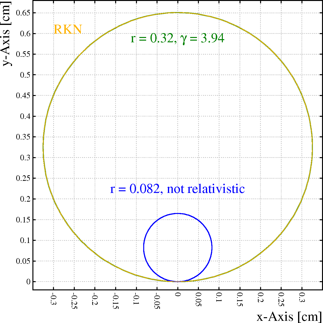
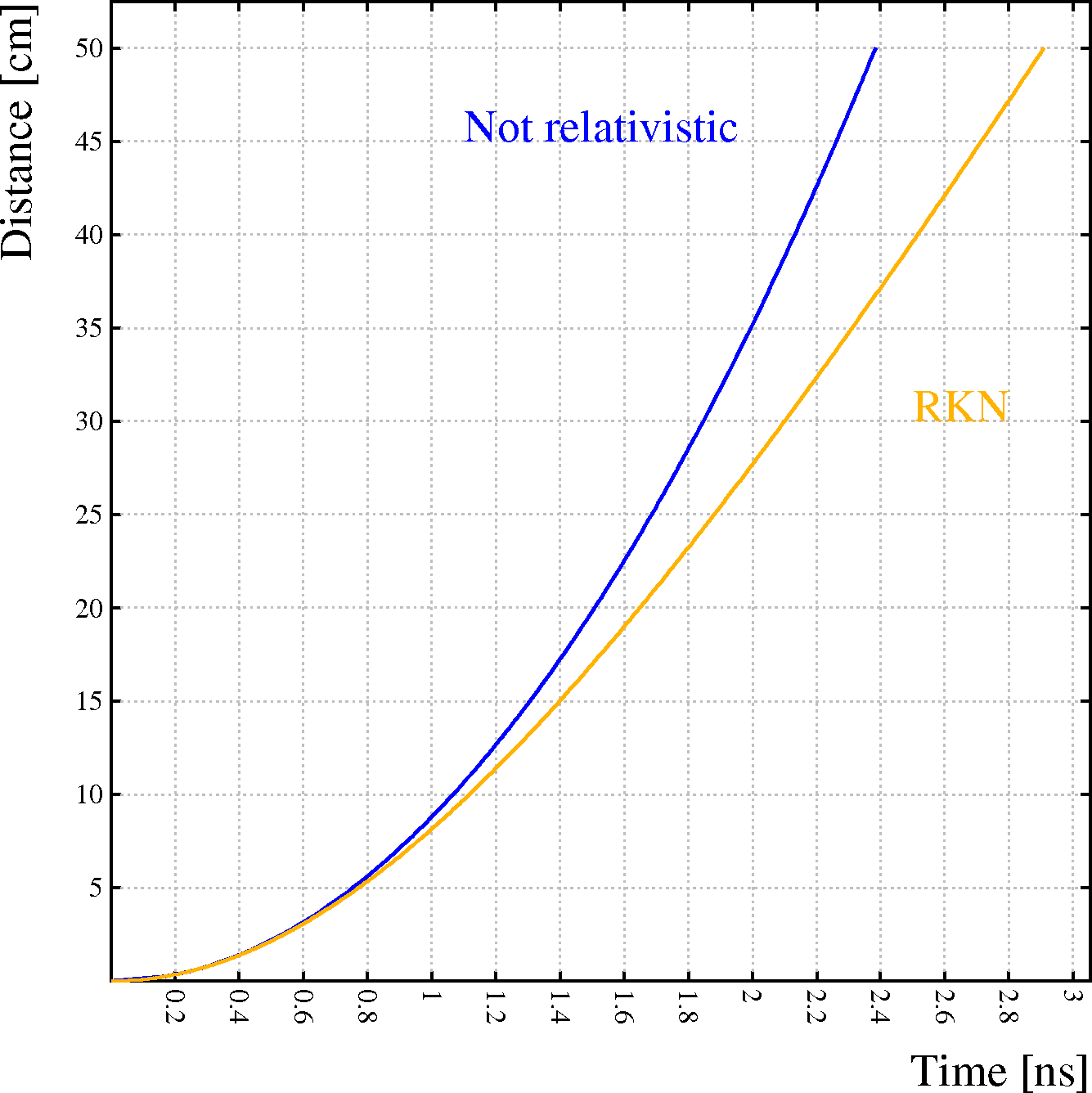
The relativistic character of the calculations is illustrated by the following examples:

Left: the orange line represents a relativistic electron (\&gamma; nearly 4) moving through a uniform B field of 2\&nbsp;T perpendicular to the plane of view. It starts from (0,0) with an initial velocity pointing along the positive x-axis. There is no electric field. The green line (partially hidden by the orange line) is a circle with a radius\&nbsp;=\&nbsp;p/(B\&nbsp;q) where p is the momentum and q the charge. For the blue line, the momentum is replaced by m\&nbsp;v, i.e. this is the result of a non-relativistic calculation.

Right: an electron, initially at rest, accelerates in a uniform electric field of 10\&nbsp;kV/cm over a distance of 50\&nbsp;/cm. As in the figure on the left, the blue line shows the non-relativistic calculation.

diffusion

The transverse component of diffusion, usually the largest of the two, will make a particle follow a trajectory that differs from the mean. Longitudinal diffusion will only have an effect on the drift time.

If diffusion does not cause the particles starting at one and the same point to reach different electrodes, the dominant effect of diffusion is a fluctuation in arrival time. One should note that this fluctuation is not only due to the longitudinal part of diffusion - also the transverse part plays a role.

Garfield offers several methods to estimate the effect of diffusion:

• the spread in arrival time over a given drift path due to longitudinal diffusion only;
• the spread in arrival time over a given drift path due to transverse and longitudinal diffusion, estimated by propagating a probability cloud over the path;
• the spread in arrival point and time due to both longitudinal and transverse diffusion using a Monte Carlo technique.

Additional information on:

multiplication

M = e\<SUP\>\&int; \&alpha; dz\</SUP\>

The integral of the Townsend coefficient over a drift path computed with the Monte_Carlo technique is larger than the integral over a drift path from the same point computed with the Runge_Kutta_Fehlberg method. The reason for this difference is that the path length for Monte Carlo integration is larger than for RKF integration.

Magboltz computes Townsend coefficients which are suitable for use with an Runge-Kutta path. The PROJECTED-PATH-INTEGRATION integration parameter can in certain contexts be used to reduce the step size dependence of the integral over Monte Carlo paths.

Attachment, even at a rate which is orders of magnitude smaller than the gain, profoundly modifies the avalanche fluctuations. Usually, the effect of combined gain and attachment is a loss of energy resolution. The reason for this effect is that the attachment rate, in many gas mixtures, exceeds the gain at the onset of the avalanche. Thus, there is a non-negligible probability that an electron is lost before it can start an avalanche while attachment after the avalanche has reached a certain size has virtually no effect anymore. Fluctuations of the avalanche size can be estimated by using the AVALANCHE and RND_MULTIPLICATION procedures.

attachment

L = e\<SUP\>- \&int; &eta; dz\</SUP\>

The integral of the attachment coefficient over a drift path computed with the Monte_Carlo technique is larger than the integral over a drift path from the same point computed with the Runge_Kutta_Fehlberg method. The reason for this difference is that the path length for Monte Carlo integration is larger than for RKF integration.

Magboltz computes attachment coefficients for use with an RKF path. The PROJECTED-PATH-INTEGRATION integration parameter can in certain contexts be used to reduce the step size dependence of the integral over Monte Carlo paths.

status

When the integration routines are called through commands, the status is, on request, printed as part of the output. If the routines are called via procedures, then the status is usually one of the output arguments.

The status is usually shown or returned as a string, shown in the second column of the table below. Occasionally however, a numeric status code is returned, shown in the third column.

The DRIFT_INFORMATION procedure returns on request the status of the last drift-line that has been computed in either of these 2 formats.

Notes:

1. The drift area is set with the AREA command. When magnetic fields are present, care should be taken to define an appropriate drift area in all 3 dimensions.
2. If a drift-line ends because the calculation requires too many steps, then usually either the integration accuracy or the maximum_step size are poorly chosen. The permitted maximum number of steps MXLIST is set at compilation time.
3. Faults can occur for a variety of reasons specific to the integration technique used (either Runge_Kutta_Fehlberg or Monte_Carlo).
4. The status "Bend sharper than pi/2" only occurs if the REJECT-KINKS integration parameter has been switched on.
5. The status "Energy exceeds E_maximum" only occurs with microscopic electron tracing as a result of an incorrect choice of the e_maximum parameter.
6. When a particle hits an electrode in a finite element field map, it will usually be declared to have "Left the mesh": finite element programs do not normally generate a mesh inside conductors. If SOLIDS have been defined, then Garfield will check whether the last point on the mesh is located inside a solid, in which case it will assign a status code accordingly.
7. The "X" in the status code for wires, replicas of wires and solids is replaced by the corresponding wire label or the corresponding solid label (see SOLIDS). "N" is replaced by the respective sequence number.
8. A further status code, "Started from a line or an edge" (numeric code -20), is used when the REVERSE-ISOCHRONS option has not been used for plotting isochrons in EDGES and TRACK plots. This status code merely indicates that the particle started from an edge or from the track and it does not give information on the end point of the particle.
9. A status "Calculations abandoned" can correspond to any of a large number of situations. Examples include: zero electric field, zero electron velocity, step-size smaller than the accuracy, error computing the rotation matrices or divergence tensors used for Monte Carlo integration, difficulties terminating a drift-line on an electrode, internal inconsistencies.

Formatted on 21/01/18 at 16:55.