

Compact Muon Solenoid
LHC, CERN
| CMS-B2G-12-016 ; CERN-EP-2017-145 | ||
| Search for vector-like light-flavor quark partners in proton-proton collisions at $ \sqrt{s} = $ 8 TeV | ||
| CMS Collaboration | ||
| 8 August 2017 | ||
| Phys. Rev. D 97 (2018) 072008 | ||
| Abstract: A search is presented for heavy vector-like quarks (VLQs) that couple only to light quarks in proton-proton collisions at $ \sqrt{s} = $ 8 TeV at the LHC. The data were collected by the CMS experiment during 2012 and correspond to an integrated luminosity of 19.7 fb$^{-1}$. Both single and pair production of VLQs are considered. The single-production search is performed for down-type VLQs (electric charge of magnitude 1/3), while the pair-production search is sensitive to up-type (charge of magnitude 2/3) and down-type VLQs. Final states with at least one muon or one electron are considered. No significant excess over standard model expectations is observed, and lower limits on the mass of VLQs are derived. The lower mass limits range from 400 to 1800 GeV, depending on the single-production cross section and the VLQ branching fractions $\mathcal{B}$ to W, Z, and Higgs bosons. When considering pair production alone, VLQs with masses below 845 GeV are excluded for $\mathcal{B}(\mathrm{ W }) = $ 1.0, and below 685 GeV for $\mathcal{B}(\mathrm{ W }) = $ 0.5, $\mathcal{B}(\mathrm{ Z }) = \mathcal{B}(\mathrm{ H }) = $ 0.25. The results are more stringent than those previously obtained for single and pair production of VLQs coupled to light quarks. | ||
| Links: e-print arXiv:1708.02510 [hep-ex] (PDF) ; CDS record ; inSPIRE record ; CADI line (restricted) ; | ||
| Figures | |
png pdf |
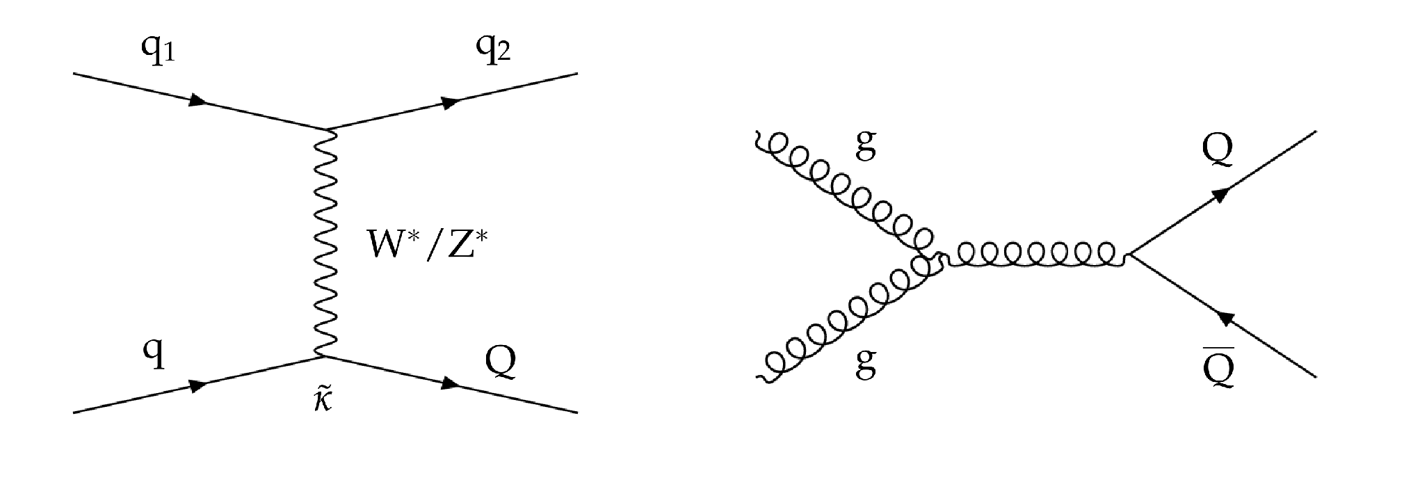
Figure 1:
Vector-like quarks (denoted Q) can be produced in proton-proton collisions either singly through electroweak interactions (the $t$ channel mode (left) is shown as an example), or in pairs via the strong interaction (right). For single production we consider in the present work only vector-like quarks with electric charge of magnitude 1/3 (denoted D). |
png pdf |
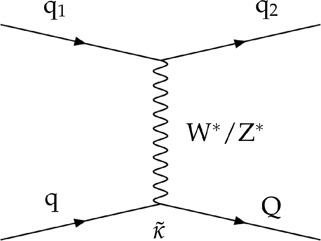
Figure 1-a:
Vector-like quarks (denoted Q) can be produced in proton-proton collisions singly through electroweak interactions (the $t$ channel mode is shown as an example). For single production we consider in the present work only vector-like quarks with electric charge of magnitude 1/3 (denoted D). |
png pdf |
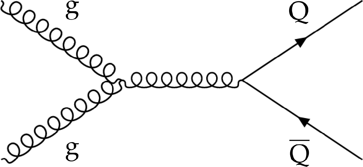
Figure 1-b:
Vector-like quarks (denoted Q) can be produced in proton-proton collisions in pairs via the strong interaction. |
png pdf |
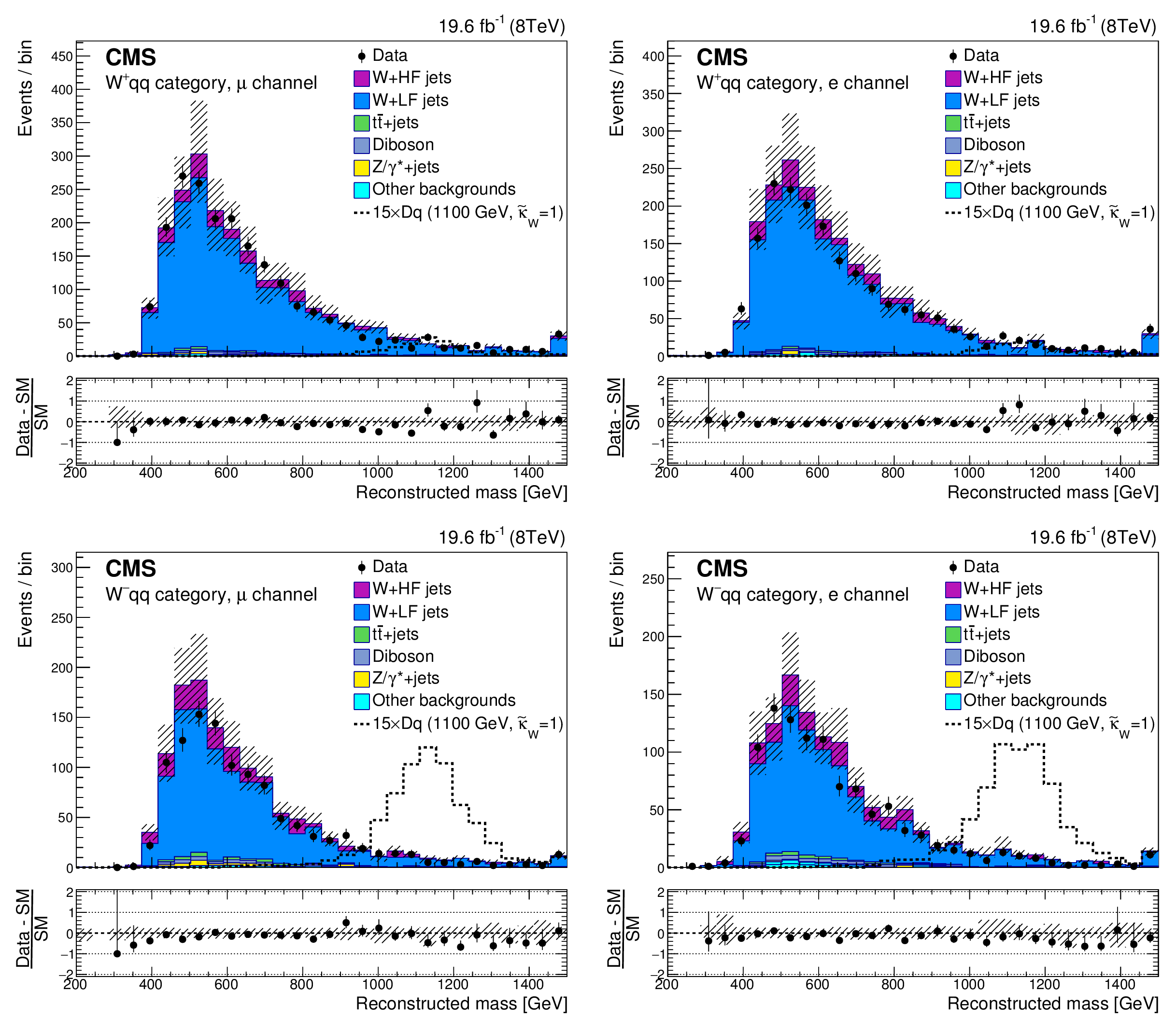
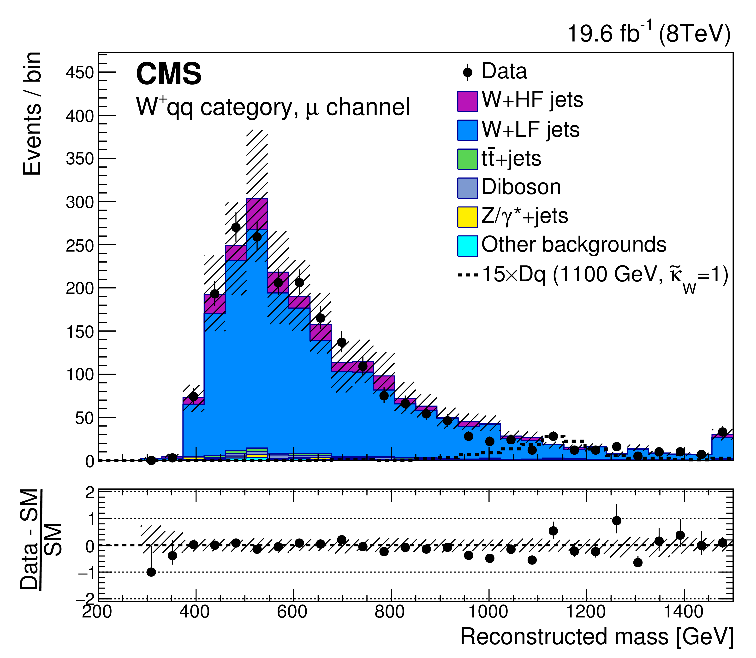
Figure 2:
The reconstructed mass of the VLQ candidate in the $\mathrm{ W^{+} } \mathrm{ q } \mathrm{ q } $ event category (upper) and the $\mathrm{ W^{-} } \mathrm{ q } \mathrm{ q } $ event category (lower), in the muon channel (left) and the electron channel (right). The contributions of simulated events where the W boson is produced in association with light-flavor (LF) jets and heavy-flavor (HF) jets are shown separately. The distribution for a heavy VLQ signal (indicated as D$\mathrm{ q } $ representing a down-type VLQ produced in association with a SM quark) of mass 1100 GeV and $\tilde{\kappa }_\mathrm{ W } = $ 1 (for $\mathcal {B}_\mathrm{ W } = $ 0.5 and $\mathcal {B}_\mathrm{ Z } = \mathcal {B}_\mathrm{ H } = $ 0.25) is scaled up by a factor of 15 for visibility. The enhanced D quark signal contribution in the $\mathrm{ W^{-} } \mathrm{ q } \mathrm{ q } $ event category in comparison to the $\mathrm{ W^{+} } \mathrm{ q } \mathrm{ q } $ event category is clearly shown. The shaded bands represent the combined statistical and systematic uncertainties, and the highest bin contains the overflow. |
png pdf |
Figure 2-a:
The reconstructed mass of the VLQ candidate in the $\mathrm{ W^{+} } \mathrm{ q } \mathrm{ q } $ event category, in the muon channel. The contributions of simulated events where the W boson is produced in association with light-flavor (LF) jets and heavy-flavor (HF) jets are shown separately. The distribution for a heavy VLQ signal (indicated as D$\mathrm{ q } $ representing a down-type VLQ produced in association with a SM quark) of mass 1100 GeV and $\tilde{\kappa }_\mathrm{ W } = $ 1 (for $\mathcal {B}_\mathrm{ W } = $ 0.5 and $\mathcal {B}_\mathrm{ Z } = \mathcal {B}_\mathrm{ H } = $ 0.25) is scaled up by a factor of 15 for visibility. The enhanced D quark signal contribution in the $\mathrm{ W^{-} } \mathrm{ q } \mathrm{ q } $ event category in comparison to the $\mathrm{ W^{+} } \mathrm{ q } \mathrm{ q } $ event category is clearly shown. The shaded bands represent the combined statistical and systematic uncertainties, and the highest bin contains the overflow. |

png pdf |
Figure 2-b:
The reconstructed mass of the VLQ candidate in the $\mathrm{ W^{+} } \mathrm{ q } \mathrm{ q } $ event category, in the electron channel. The contributions of simulated events where the W boson is produced in association with light-flavor (LF) jets and heavy-flavor (HF) jets are shown separately. The distribution for a heavy VLQ signal (indicated as D$\mathrm{ q } $ representing a down-type VLQ produced in association with a SM quark) of mass 1100 GeV and $\tilde{\kappa }_\mathrm{ W } = $ 1 (for $\mathcal {B}_\mathrm{ W } = $ 0.5 and $\mathcal {B}_\mathrm{ Z } = \mathcal {B}_\mathrm{ H } = $ 0.25) is scaled up by a factor of 15 for visibility. The enhanced D quark signal contribution in the $\mathrm{ W^{-} } \mathrm{ q } \mathrm{ q } $ event category in comparison to the $\mathrm{ W^{+} } \mathrm{ q } \mathrm{ q } $ event category is clearly shown. The shaded bands represent the combined statistical and systematic uncertainties, and the highest bin contains the overflow. |
png pdf |
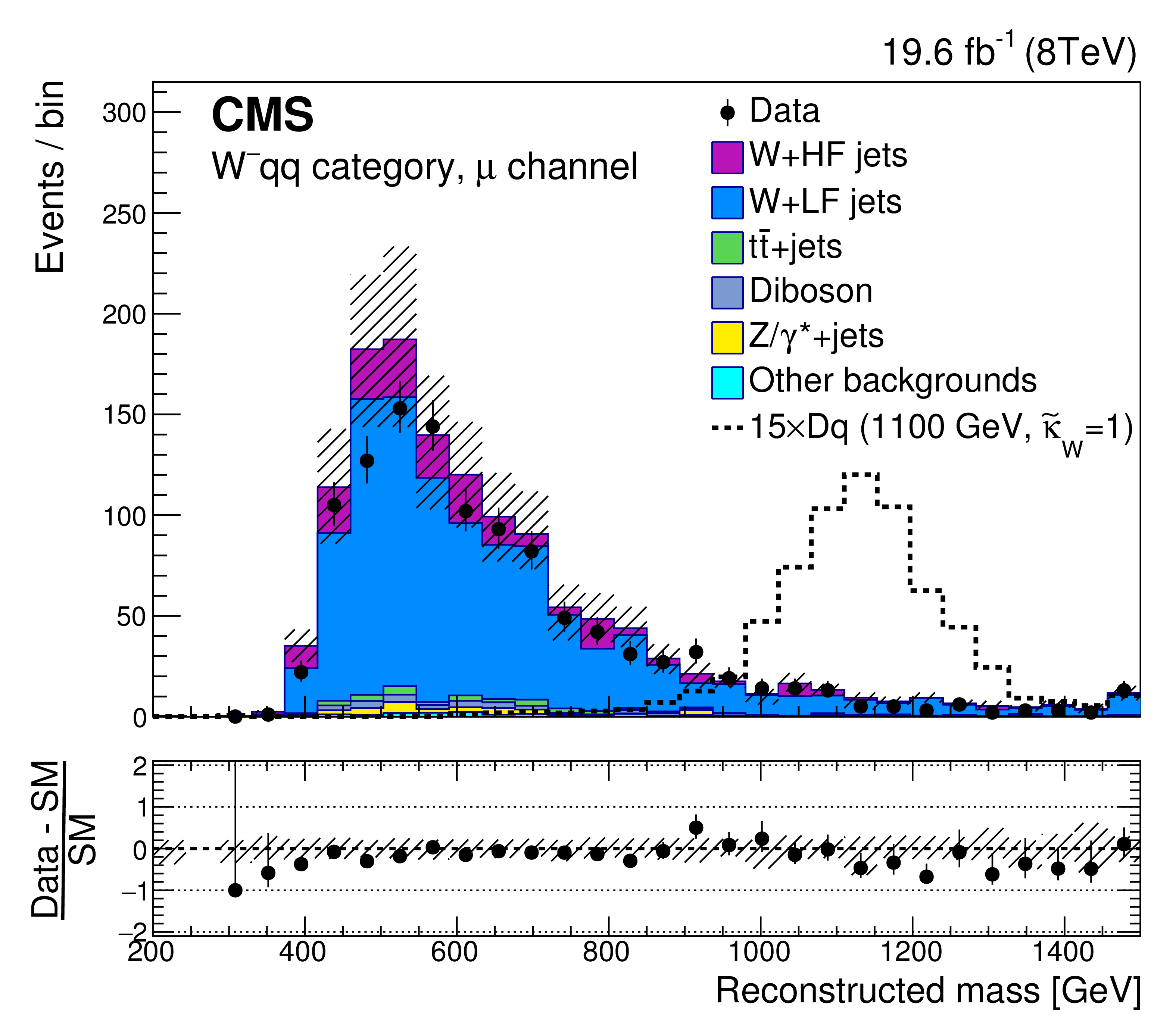
Figure 2-c:
The reconstructed mass of the VLQ candidate in the $\mathrm{ W^{-} } \mathrm{ q } \mathrm{ q } $ event category, in the muon channel. The contributions of simulated events where the W boson is produced in association with light-flavor (LF) jets and heavy-flavor (HF) jets are shown separately. The distribution for a heavy VLQ signal (indicated as D$\mathrm{ q } $ representing a down-type VLQ produced in association with a SM quark) of mass 1100 GeV and $\tilde{\kappa }_\mathrm{ W } = $ 1 (for $\mathcal {B}_\mathrm{ W } = $ 0.5 and $\mathcal {B}_\mathrm{ Z } = \mathcal {B}_\mathrm{ H } = $ 0.25) is scaled up by a factor of 15 for visibility. The enhanced D quark signal contribution in the $\mathrm{ W^{-} } \mathrm{ q } \mathrm{ q } $ event category in comparison to the $\mathrm{ W^{+} } \mathrm{ q } \mathrm{ q } $ event category is clearly shown. The shaded bands represent the combined statistical and systematic uncertainties, and the highest bin contains the overflow. |
png pdf |
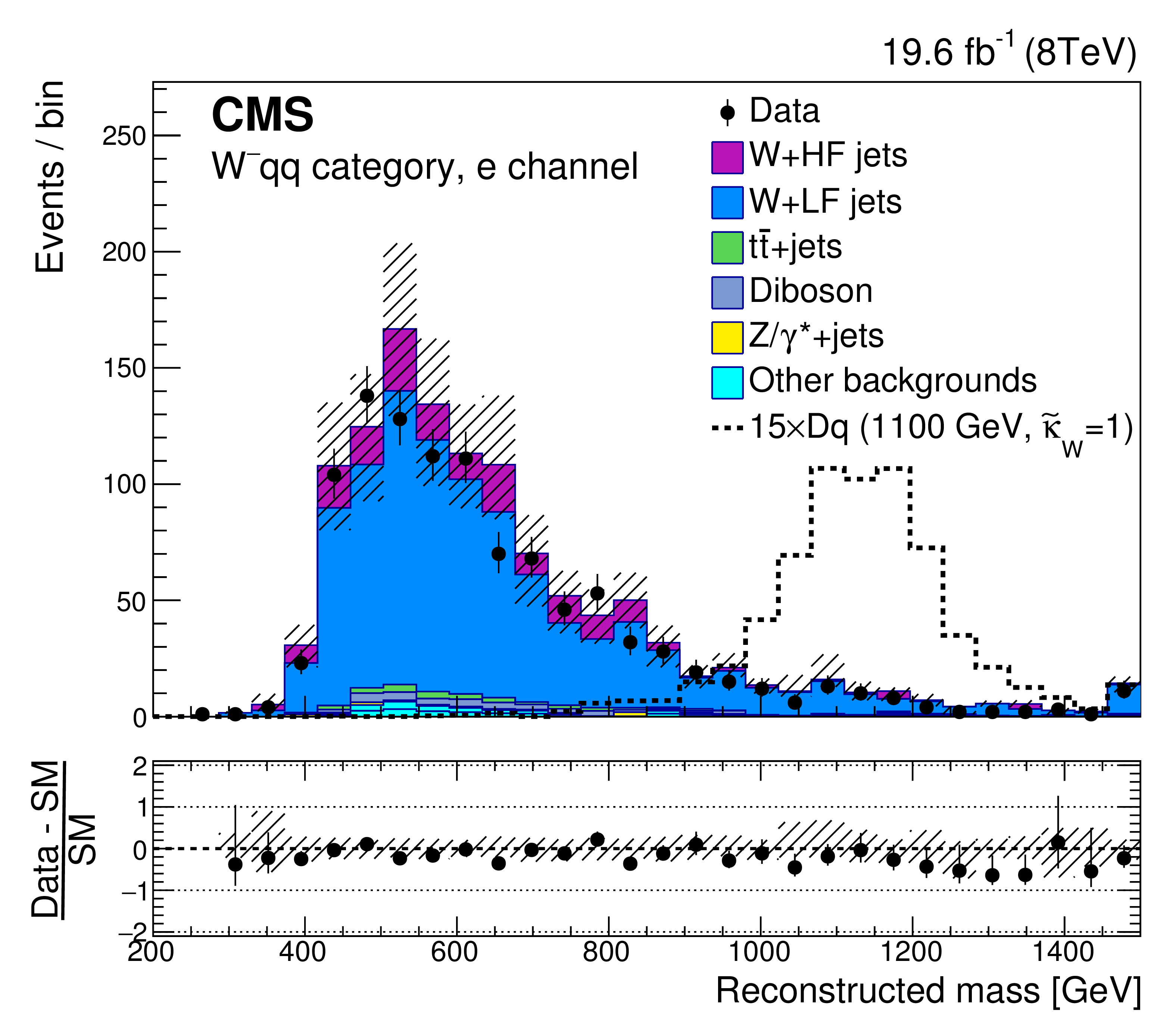
Figure 2-d:
The reconstructed mass of the VLQ candidate in the $\mathrm{ W^{-} } \mathrm{ q } \mathrm{ q } $ event category, in the electron channel. The contributions of simulated events where the W boson is produced in association with light-flavor (LF) jets and heavy-flavor (HF) jets are shown separately. The distribution for a heavy VLQ signal (indicated as D$\mathrm{ q } $ representing a down-type VLQ produced in association with a SM quark) of mass 1100 GeV and $\tilde{\kappa }_\mathrm{ W } = $ 1 (for $\mathcal {B}_\mathrm{ W } = $ 0.5 and $\mathcal {B}_\mathrm{ Z } = \mathcal {B}_\mathrm{ H } = $ 0.25) is scaled up by a factor of 15 for visibility. The enhanced D quark signal contribution in the $\mathrm{ W^{-} } \mathrm{ q } \mathrm{ q } $ event category in comparison to the $\mathrm{ W^{+} } \mathrm{ q } \mathrm{ q } $ event category is clearly shown. The shaded bands represent the combined statistical and systematic uncertainties, and the highest bin contains the overflow. |

png pdf |
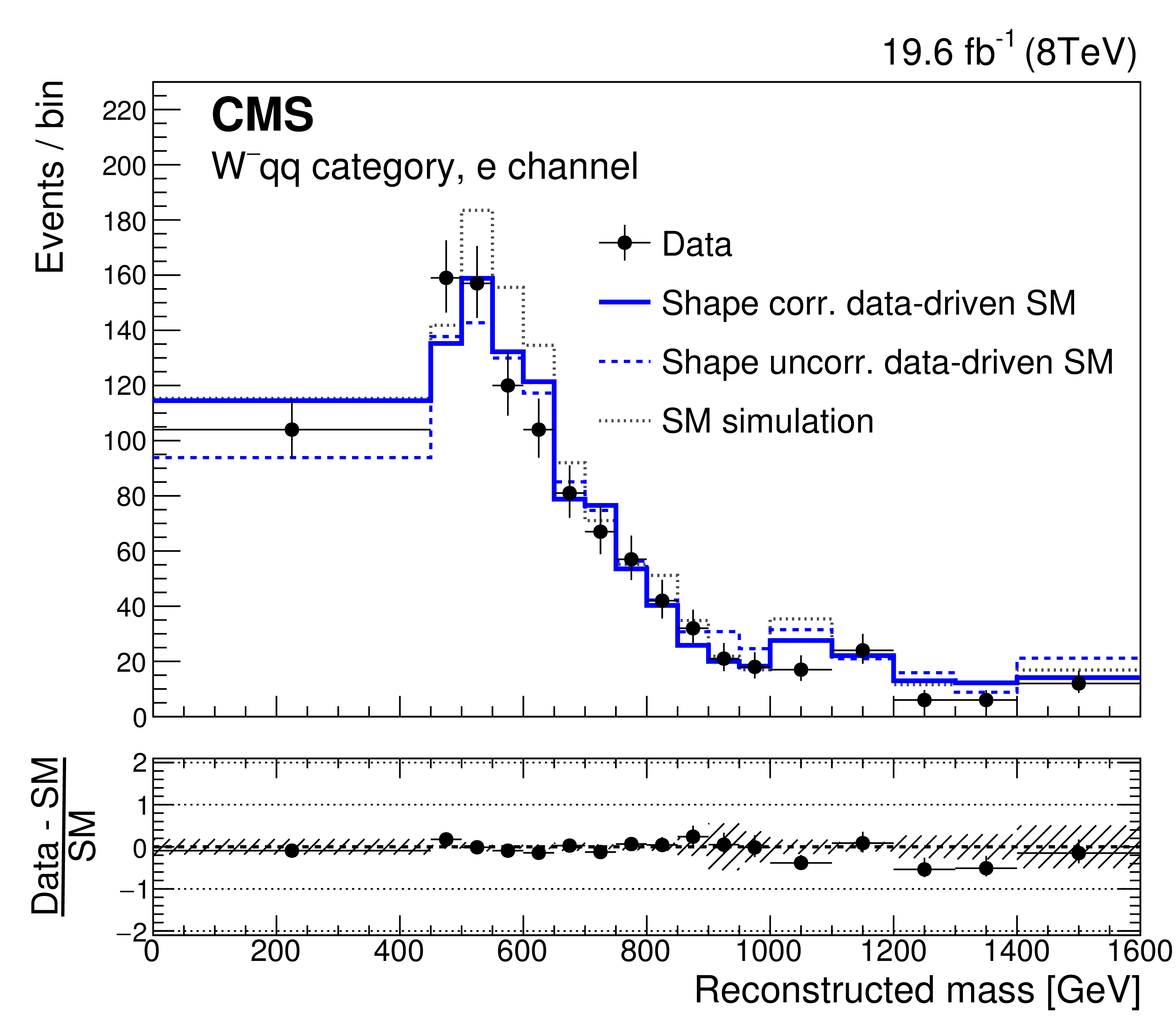
Figure 3:
The reconstructed VLQ candidate mass in the $\mathrm{ W^{-} } \mathrm{ q } \mathrm{ q } $ category for the muon channel (left) and the electron channel (right), for the background prediction and the data. The solid bold (blue) line is the background distribution estimated from data, with a final shape correction that accounts for the difference between the W+jets simulation in the control region and the $\mathrm{ W^{-} } \mathrm{ q } \mathrm{ q } $ signal region. The dashed (blue) line is the same, but without the shape correction. The dotted (grey) line represents the SM prediction from simulation. The lower panel shows the ratio of the data to the data-driven background distribution with shape corrections. For bins from 1000 GeV onwards, a wider bin width is chosen to reduce statistical uncertainties in the background estimation from the data control region. The horizontal error bars on the data points only indicate the bin width. |

png pdf |
Figure 3-a:
The reconstructed VLQ candidate mass in the $\mathrm{ W^{-} } \mathrm{ q } \mathrm{ q } $ category for the muon channel, for the background prediction and the data. The solid bold (blue) line is the background distribution estimated from data, with a final shape correction that accounts for the difference between the W+jets simulation in the control region and the $\mathrm{ W^{-} } \mathrm{ q } \mathrm{ q } $ signal region. The dashed (blue) line is the same, but without the shape correction. The dotted (grey) line represents the SM prediction from simulation. The lower panel shows the ratio of the data to the data-driven background distribution with shape corrections. For bins from 1000 GeV onwards, a wider bin width is chosen to reduce statistical uncertainties in the background estimation from the data control region. The horizontal error bars on the data points only indicate the bin width. |
png pdf |
Figure 3-b:
The reconstructed VLQ candidate mass in the $\mathrm{ W^{-} } \mathrm{ q } \mathrm{ q } $ category for the electron channel, for the background prediction and the data. The solid bold (blue) line is the background distribution estimated from data, with a final shape correction that accounts for the difference between the W+jets simulation in the control region and the $\mathrm{ W^{-} } \mathrm{ q } \mathrm{ q } $ signal region. The dashed (blue) line is the same, but without the shape correction. The dotted (grey) line represents the SM prediction from simulation. The lower panel shows the ratio of the data to the data-driven background distribution with shape corrections. For bins from 1000 GeV onwards, a wider bin width is chosen to reduce statistical uncertainties in the background estimation from the data control region. The horizontal error bars on the data points only indicate the bin width. |

png pdf |
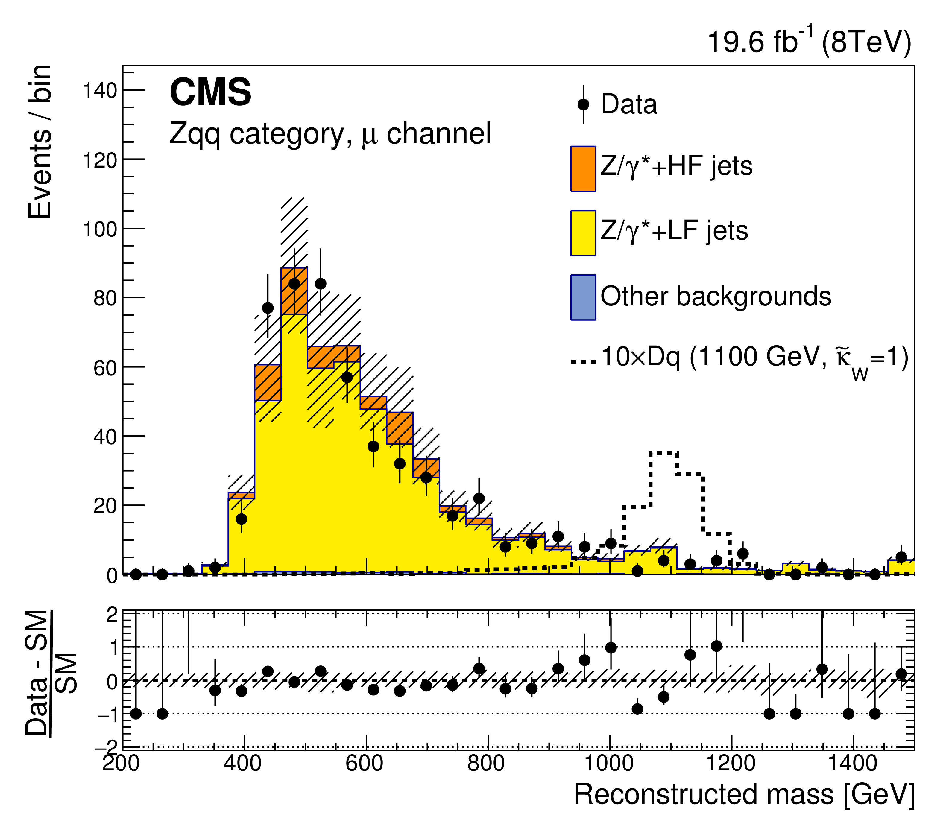
Figure 4:
The reconstructed mass of the VLQ candidate in the Zqq event category, in the muon channel (left) and the electron channel (right). The contributions of simulated events where the Z boson is produced in association with light-flavor (LF) jets and heavy-flavor (HF) jets are shown separately. The distribution for a heavy VLQ signal (indicated as D$\mathrm{ q } $ representing a down-type VLQ produced in association with a SM quark) of mass 1100 GeV and $\tilde{\kappa }_\mathrm{ W } = $ 1 (for $\mathcal {B}_\mathrm{ W } = $ 0.5 and $\mathcal {B}_\mathrm{ Z } = \mathcal {B}_\mathrm{ H } = $ 0.25) is scaled by a factor of 10 for better visibility. The shaded bands represent the combined statistical and systematic uncertainties. |
png pdf |
Figure 4-a:
The reconstructed mass of the VLQ candidate in the Zqq event category, in the muon channel. The contributions of simulated events where the Z boson is produced in association with light-flavor (LF) jets and heavy-flavor (HF) jets are shown separately. The distribution for a heavy VLQ signal (indicated as D$\mathrm{ q } $ representing a down-type VLQ produced in association with a SM quark) of mass 1100 GeV and $\tilde{\kappa }_\mathrm{ W } = $ 1 (for $\mathcal {B}_\mathrm{ W } = $ 0.5 and $\mathcal {B}_\mathrm{ Z } = \mathcal {B}_\mathrm{ H } = $ 0.25) is scaled by a factor of 10 for better visibility. The shaded bands represent the combined statistical and systematic uncertainties. |

png pdf |
Figure 4-b:
The reconstructed mass of the VLQ candidate in the Zqq event category, in the electron channel. The contributions of simulated events where the Z boson is produced in association with light-flavor (LF) jets and heavy-flavor (HF) jets are shown separately. The distribution for a heavy VLQ signal (indicated as D$\mathrm{ q } $ representing a down-type VLQ produced in association with a SM quark) of mass 1100 GeV and $\tilde{\kappa }_\mathrm{ W } = $ 1 (for $\mathcal {B}_\mathrm{ W } = $ 0.5 and $\mathcal {B}_\mathrm{ Z } = \mathcal {B}_\mathrm{ H } = $ 0.25) is scaled by a factor of 10 for better visibility. The shaded bands represent the combined statistical and systematic uncertainties. |
png pdf |
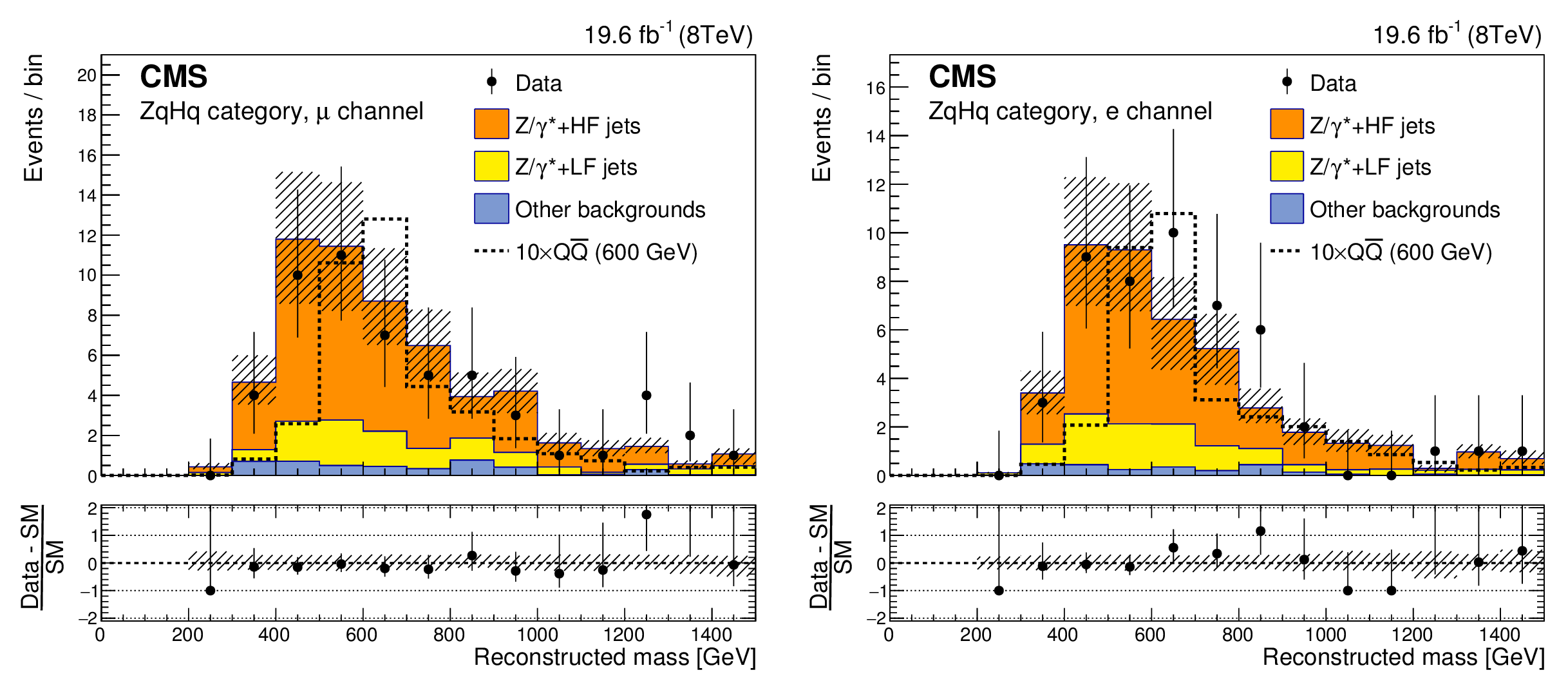
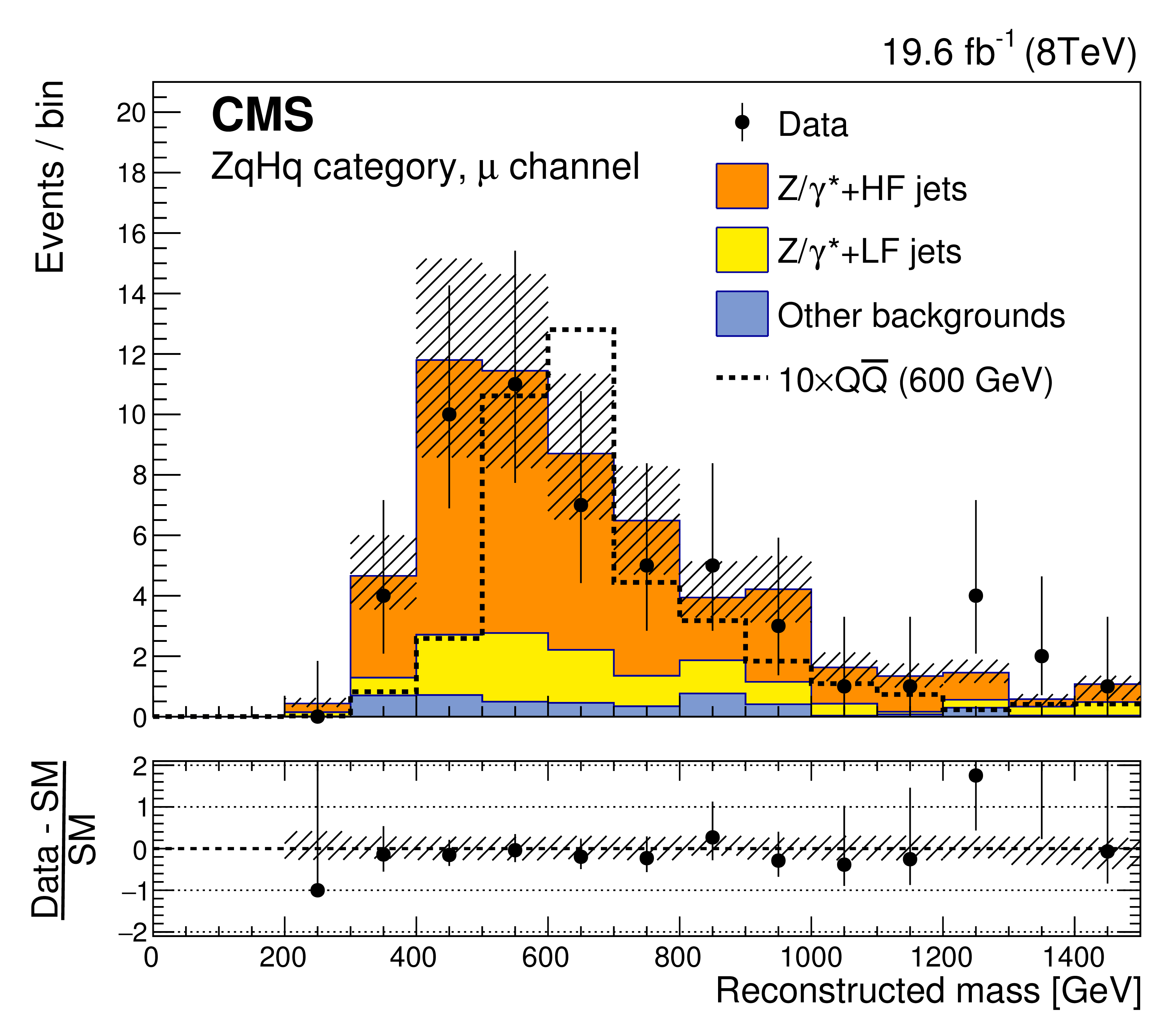
Figure 5:
The reconstructed mass of the VLQ candidate in the ${\mathrm{ Z } } \mathrm{ q } \mathrm{ H } \mathrm{ q } $ event category, in the muon channel (left) and the electron channel (right). The contributions of simulated events where the Z boson is produced in association with light-flavor (LF) jets and heavy-flavor (HF) jets are shown separately. The distribution for a heavy VLQ signal of mass 600 GeV and $\tilde{\kappa }_\mathrm{ W } = $ 0.1 (for $\mathcal {B}_\mathrm{ W } = $ 0.5 and $\mathcal {B}_\mathrm{ Z } = \mathcal {B}_\mathrm{ H } =$ 0.25) is scaled up by a factor of 10 for visibility. The shaded bands represent the combined statistical and systematic uncertainties. |
png pdf |
Figure 5-a:
The reconstructed mass of the VLQ candidate in the ${\mathrm{ Z } } \mathrm{ q } \mathrm{ H } \mathrm{ q } $ event category, in the muon channel. The contributions of simulated events where the Z boson is produced in association with light-flavor (LF) jets and heavy-flavor (HF) jets are shown separately. The distribution for a heavy VLQ signal of mass 600 GeV and $\tilde{\kappa }_\mathrm{ W } = $ 0.1 (for $\mathcal {B}_\mathrm{ W } = $ 0.5 and $\mathcal {B}_\mathrm{ Z } = \mathcal {B}_\mathrm{ H } =$ 0.25) is scaled up by a factor of 10 for visibility. The shaded bands represent the combined statistical and systematic uncertainties. |
png pdf |
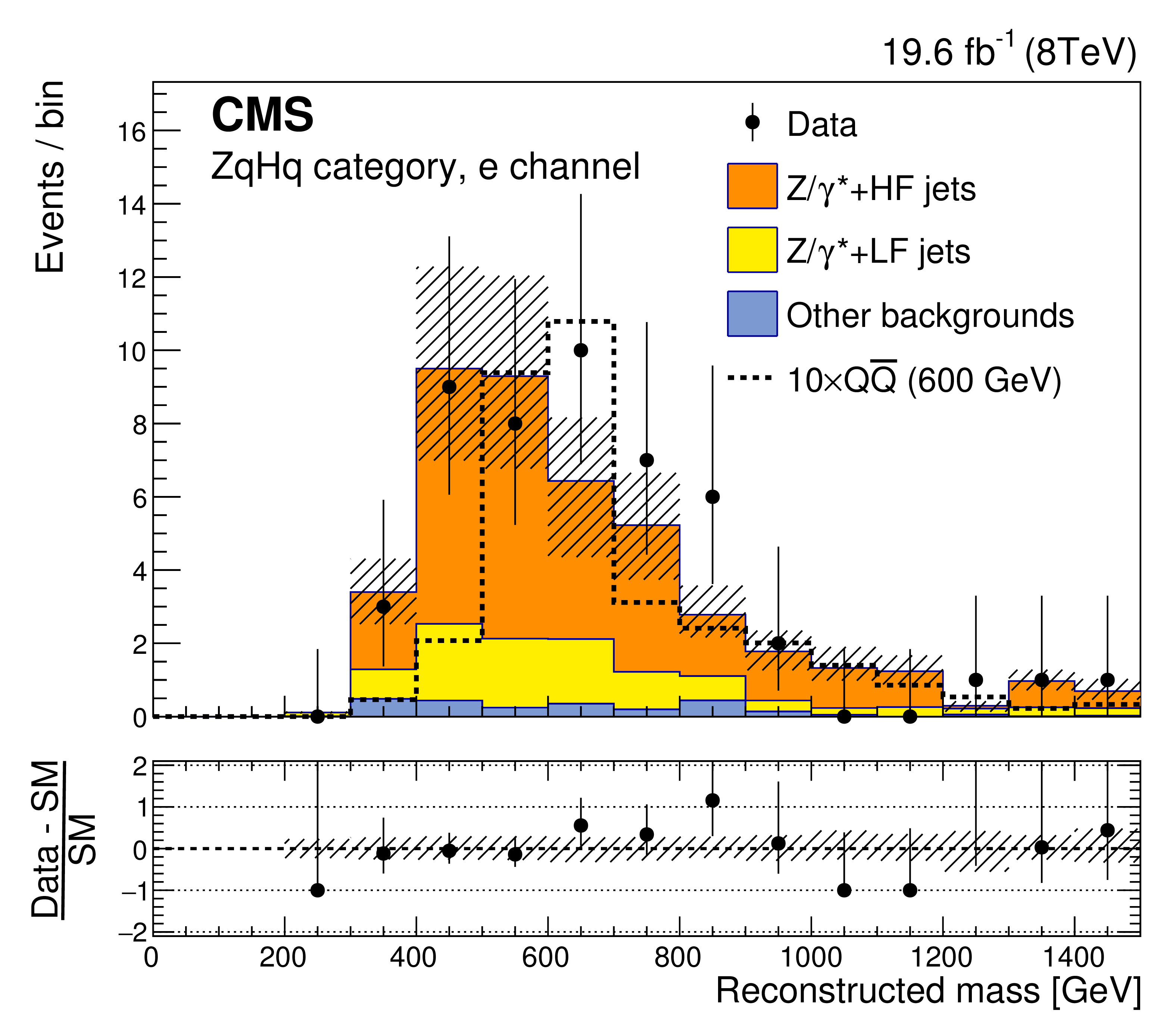
Figure 5-b:
The reconstructed mass of the VLQ candidate in the ${\mathrm{ Z } } \mathrm{ q } \mathrm{ H } \mathrm{ q } $ event category, in the electron channel. The contributions of simulated events where the Z boson is produced in association with light-flavor (LF) jets and heavy-flavor (HF) jets are shown separately. The distribution for a heavy VLQ signal of mass 600 GeV and $\tilde{\kappa }_\mathrm{ W } = $ 0.1 (for $\mathcal {B}_\mathrm{ W } = $ 0.5 and $\mathcal {B}_\mathrm{ Z } = \mathcal {B}_\mathrm{ H } =$ 0.25) is scaled up by a factor of 10 for visibility. The shaded bands represent the combined statistical and systematic uncertainties. |
png pdf |
Figure 6:
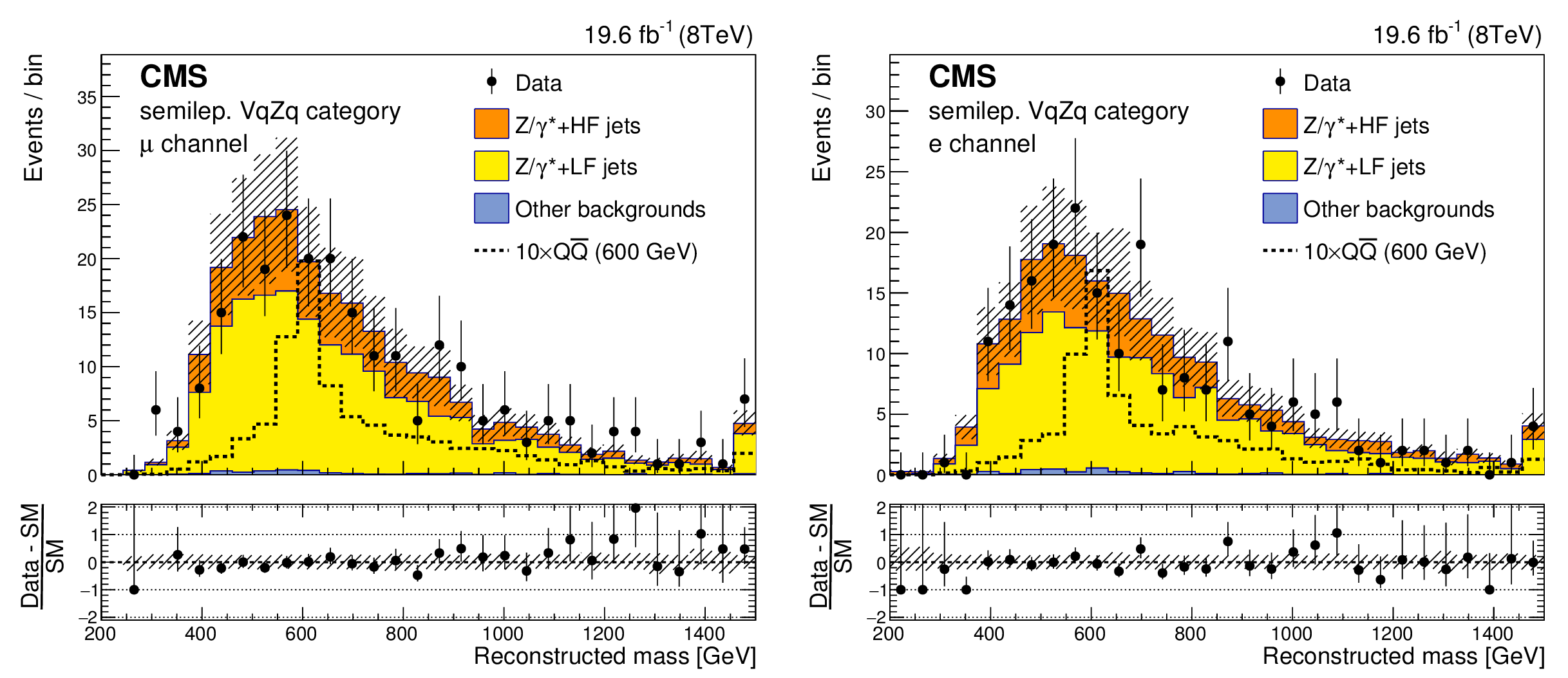
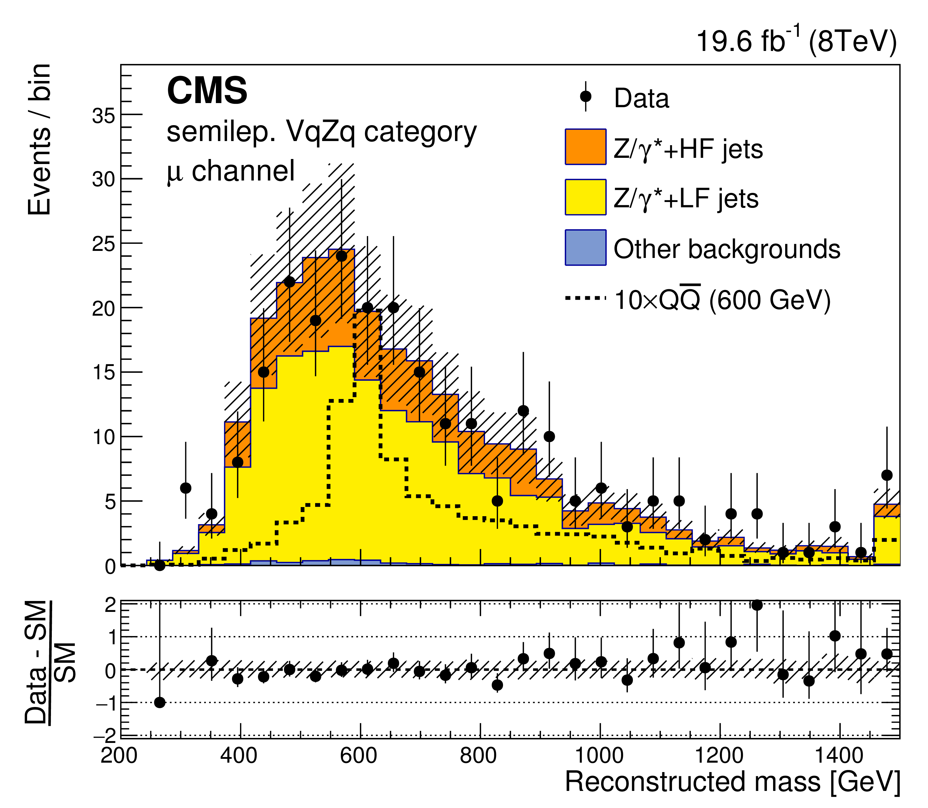
The reconstructed mass of the VLQ candidate in the semileptonic $ {\mathrm {V}} \mathrm{ q } {\mathrm{ Z } } \mathrm{ q } $ event category, in the muon channel (left) and the electron channel (right). The contributions of simulated events where the Z boson is produced in association with light-flavor (LF) jets and heavy-flavor (HF) jets are shown separately. The distribution for a heavy VLQ signal of mass 600 GeV and $\tilde{\kappa }_\mathrm{ W } = $ 0.1 (for $\mathcal {B}_\mathrm{ W } = $ 0.5 and $\mathcal {B}_\mathrm{ Z } = \mathcal {B}_\mathrm{ H } = $ 0.25) is scaled up by a factor of 10 for visibility. The shaded bands represent the combined statistical and systematic uncertainties. |
png pdf |
Figure 6-a:
The reconstructed mass of the VLQ candidate in the semileptonic $ {\mathrm {V}} \mathrm{ q } {\mathrm{ Z } } \mathrm{ q } $ event category, in the muon channel. The contributions of simulated events where the Z boson is produced in association with light-flavor (LF) jets and heavy-flavor (HF) jets are shown separately. The distribution for a heavy VLQ signal of mass 600 GeV and $\tilde{\kappa }_\mathrm{ W } = $ 0.1 (for $\mathcal {B}_\mathrm{ W } = $ 0.5 and $\mathcal {B}_\mathrm{ Z } = \mathcal {B}_\mathrm{ H } = $ 0.25) is scaled up by a factor of 10 for visibility. The shaded bands represent the combined statistical and systematic uncertainties. |

png pdf |
Figure 6-b:
The reconstructed mass of the VLQ candidate in the semileptonic $ {\mathrm {V}} \mathrm{ q } {\mathrm{ Z } } \mathrm{ q } $ event category, in the electron channel. The contributions of simulated events where the Z boson is produced in association with light-flavor (LF) jets and heavy-flavor (HF) jets are shown separately. The distribution for a heavy VLQ signal of mass 600 GeV and $\tilde{\kappa }_\mathrm{ W } = $ 0.1 (for $\mathcal {B}_\mathrm{ W } = $ 0.5 and $\mathcal {B}_\mathrm{ Z } = \mathcal {B}_\mathrm{ H } = $ 0.25) is scaled up by a factor of 10 for visibility. The shaded bands represent the combined statistical and systematic uncertainties. |
png pdf |
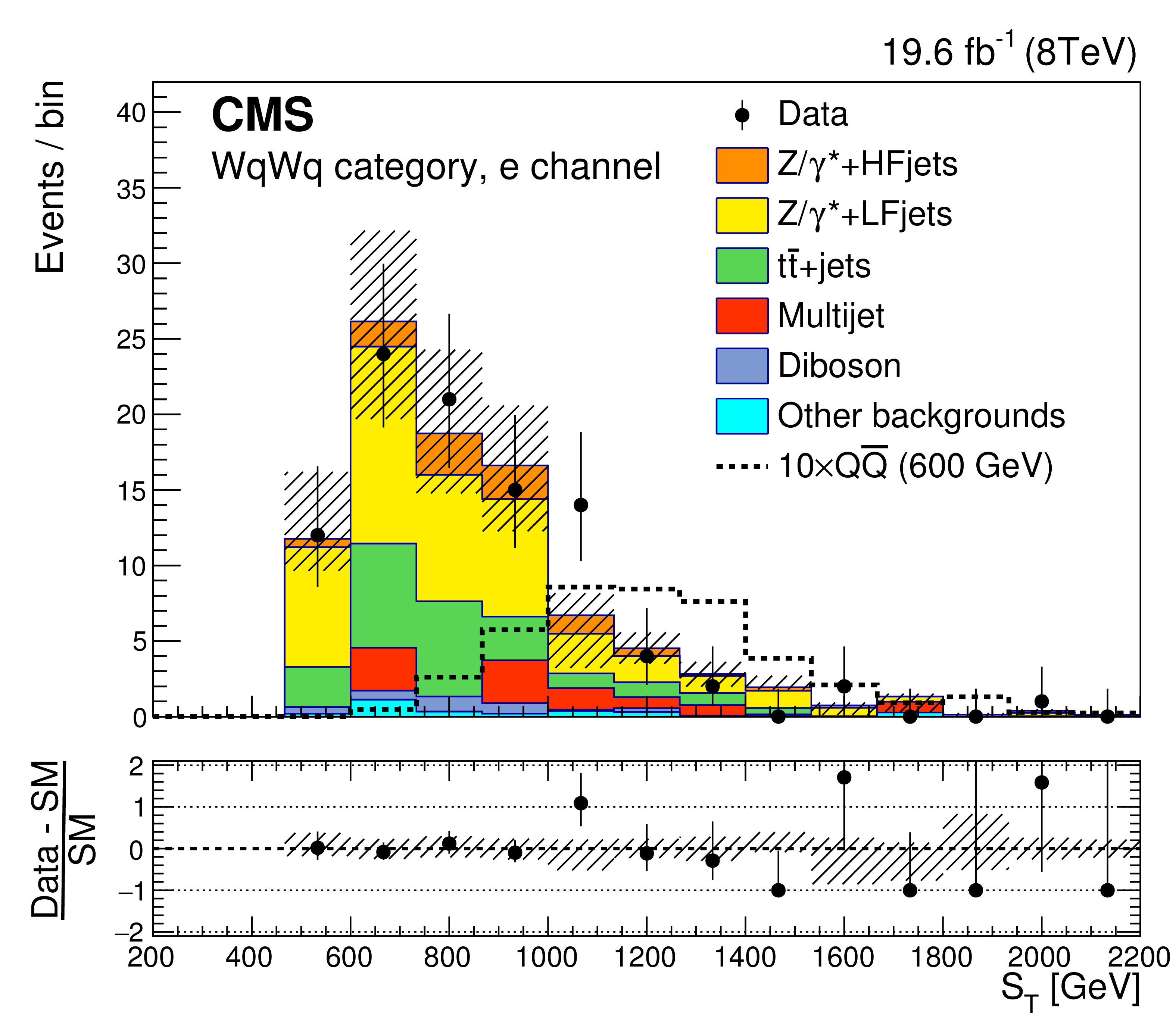
Figure 7:
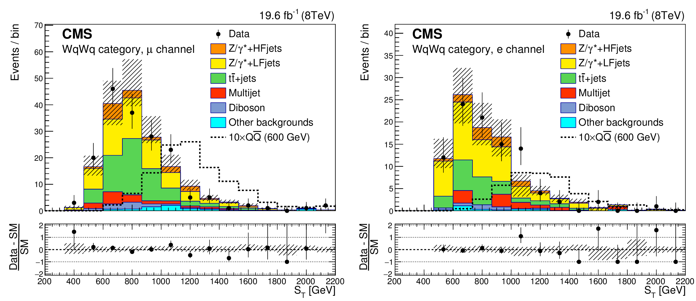
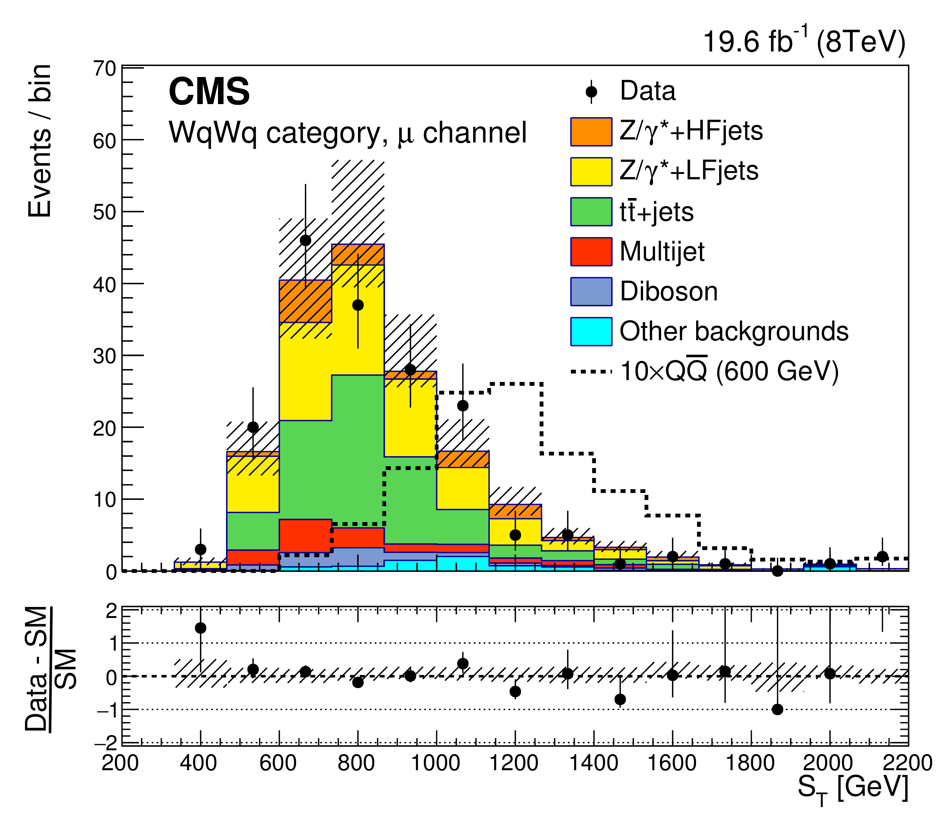
The $S_T$ variable in the $\mathrm{ W } \mathrm{ q } \mathrm{ W } \mathrm{ q } $ event category, in the muon channel (left) and in the electron channel (right). The contributions of simulated events where the Z boson is produced in association with light-flavor (LF) jets and heavy-flavor (HF) jets are shown separately. The distribution for a heavy VLQ signal of mass 600 GeV and $\tilde{\kappa }_\mathrm{ W } = $ 0.1 (for $\mathcal {B}_\mathrm{ W } = $ 0.5 and $\mathcal {B}_\mathrm{ Z } = \mathcal {B}_\mathrm{ H } = $ 0.25) is scaled up by a factor of 10 for visibility. The shaded bands represent the combined statistical and systematic uncertainties. |
png pdf |
Figure 7-a:
The $S_T$ variable in the $\mathrm{ W } \mathrm{ q } \mathrm{ W } \mathrm{ q } $ event category, in the muon channel. The contributions of simulated events where the Z boson is produced in association with light-flavor (LF) jets and heavy-flavor (HF) jets are shown separately. The distribution for a heavy VLQ signal of mass 600 GeV and $\tilde{\kappa }_\mathrm{ W } = $ 0.1 (for $\mathcal {B}_\mathrm{ W } = $ 0.5 and $\mathcal {B}_\mathrm{ Z } = \mathcal {B}_\mathrm{ H } = $ 0.25) is scaled up by a factor of 10 for visibility. The shaded bands represent the combined statistical and systematic uncertainties. |
png pdf |
Figure 7-b:
The $S_T$ variable in the $\mathrm{ W } \mathrm{ q } \mathrm{ W } \mathrm{ q } $ event category, in the electron channel. The contributions of simulated events where the Z boson is produced in association with light-flavor (LF) jets and heavy-flavor (HF) jets are shown separately. The distribution for a heavy VLQ signal of mass 600 GeV and $\tilde{\kappa }_\mathrm{ W } = $ 0.1 (for $\mathcal {B}_\mathrm{ W } = $ 0.5 and $\mathcal {B}_\mathrm{ Z } = \mathcal {B}_\mathrm{ H } = $ 0.25) is scaled up by a factor of 10 for visibility. The shaded bands represent the combined statistical and systematic uncertainties. |

png pdf |
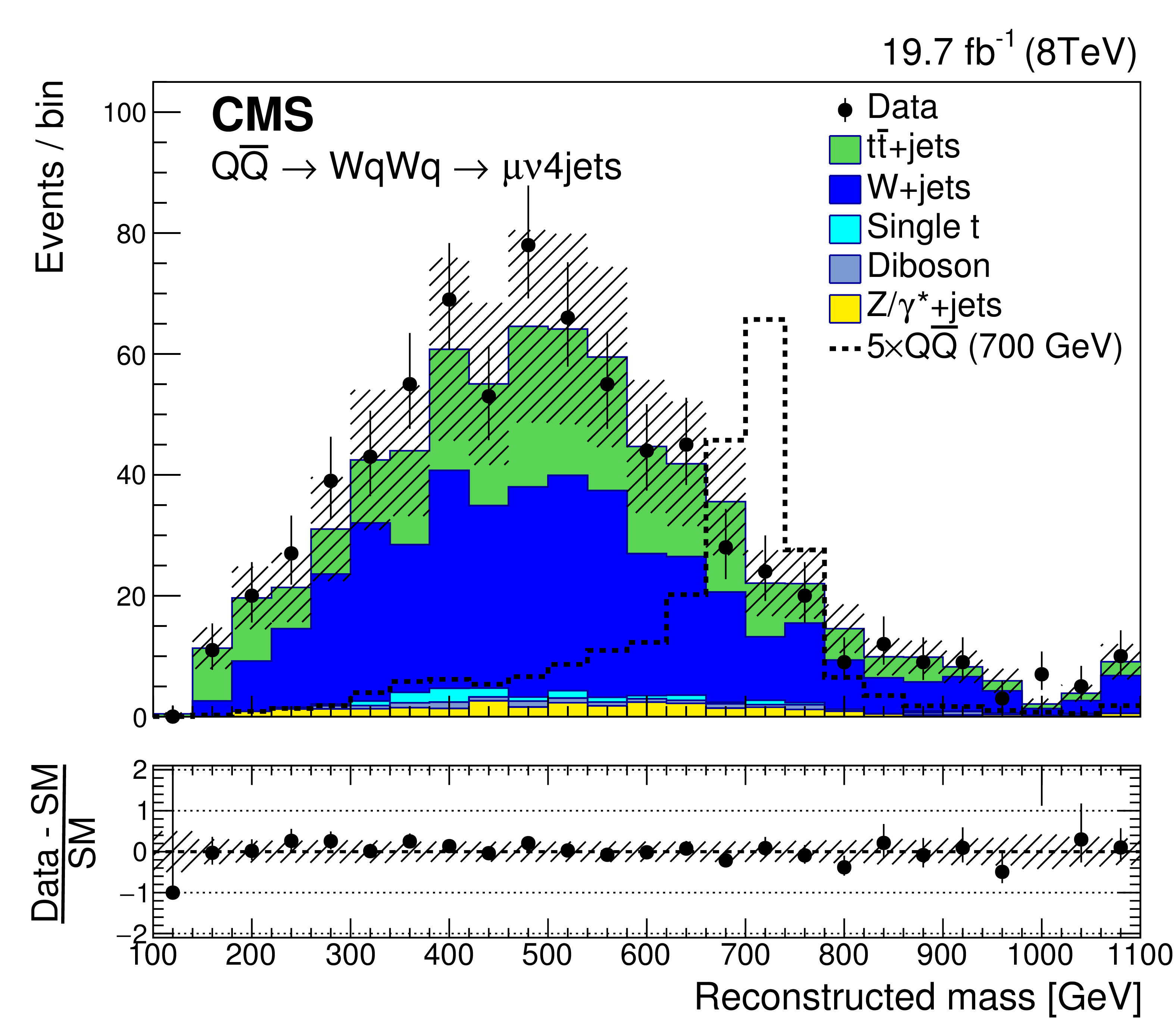
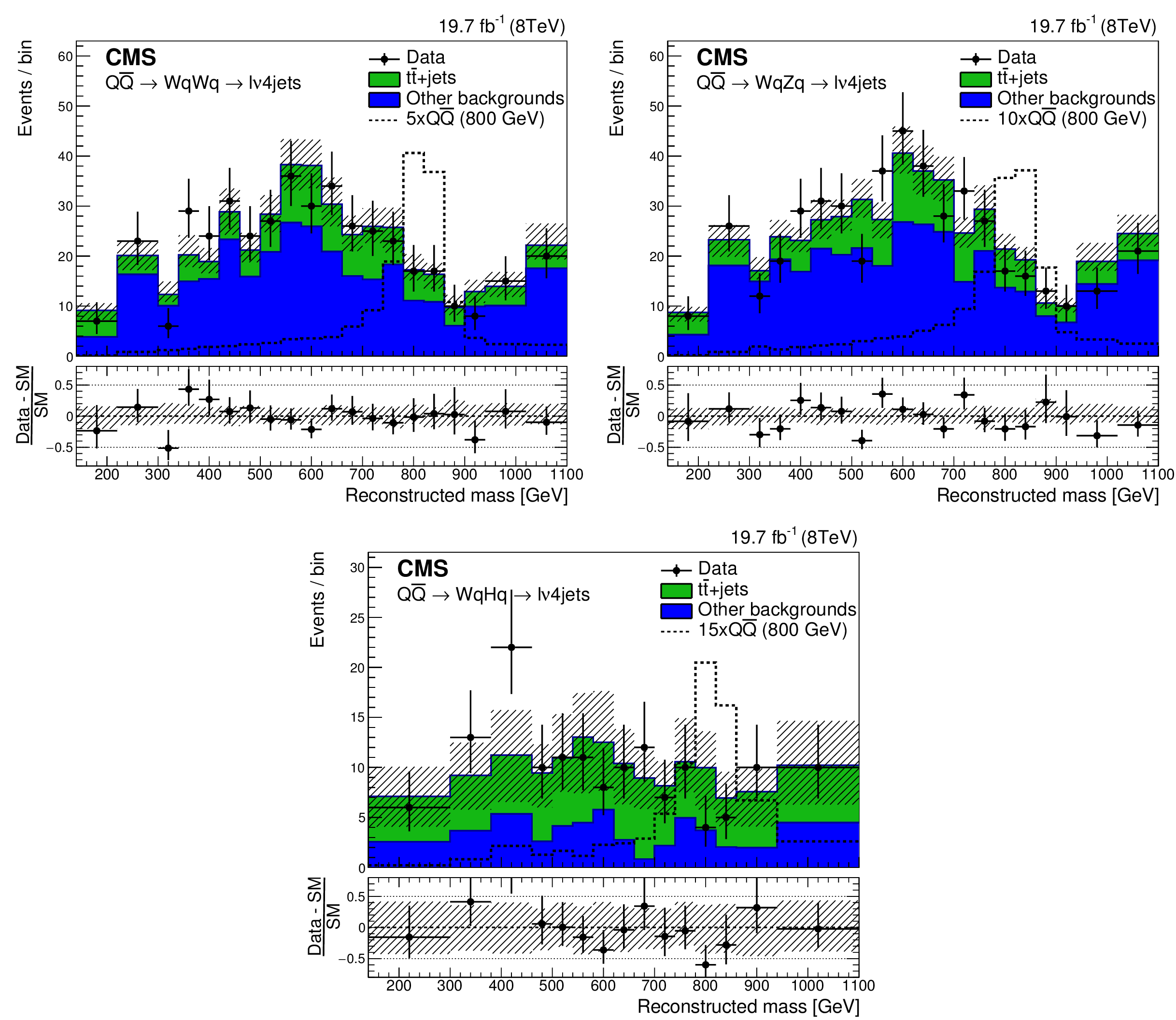
Figure 8:
Reconstructed mass distributions for $\mathrm{ W } \mathrm{ q } \mathrm{ W } \mathrm{ q } $ (uppermost), $\mathrm{ W } \mathrm{ q } {\mathrm{ Z } } \mathrm{ q } $ (middle), and $\mathrm{ W } \mathrm{ q } \mathrm{ H } \mathrm{ q } $ (lowest) reconstruction. Plots on the left are for the $\mu $+jets channel and on the right, for the $\mathrm{ e } $+jets channel. The distribution for pair-produced VLQs of mass 700 GeV for $\mathcal {B}_\mathrm{ W } = $ 1.0 (uppermost), $\mathcal {B}_\mathrm{ W } = \mathcal {B}_\mathrm{ Z } = $ 0.5 (middle) and $\mathcal {B}_\mathrm{ W } = \mathcal {B}_\mathrm{ H } = $ 0.5 (lowest) are scaled up for visibility by a factor of 5, 10 and 5, respectively. The shaded bands represent the combined statistical and systematic uncertainties. |
png pdf |
Figure 8-a:
Reconstructed mass distribution for the $\mathrm{ W } \mathrm{ q } \mathrm{ W } \mathrm{ q } $ reconstruction, for the $\mu $+jets channel. The distribution for pair-produced VLQs of mass 700 GeV for $\mathcal {B}_\mathrm{ W } = $ 1.0 are scaled up for visibility by a factor of 5. The shaded bands represent the combined statistical and systematic uncertainties. |

png pdf |
Figure 8-b:
Reconstructed mass distribution for the $\mathrm{ W } \mathrm{ q } \mathrm{ W } \mathrm{ q } $ reconstruction, for the $\mathrm{ e } $+jets channel. The distribution for pair-produced VLQs of mass 700 GeV for |
png pdf |
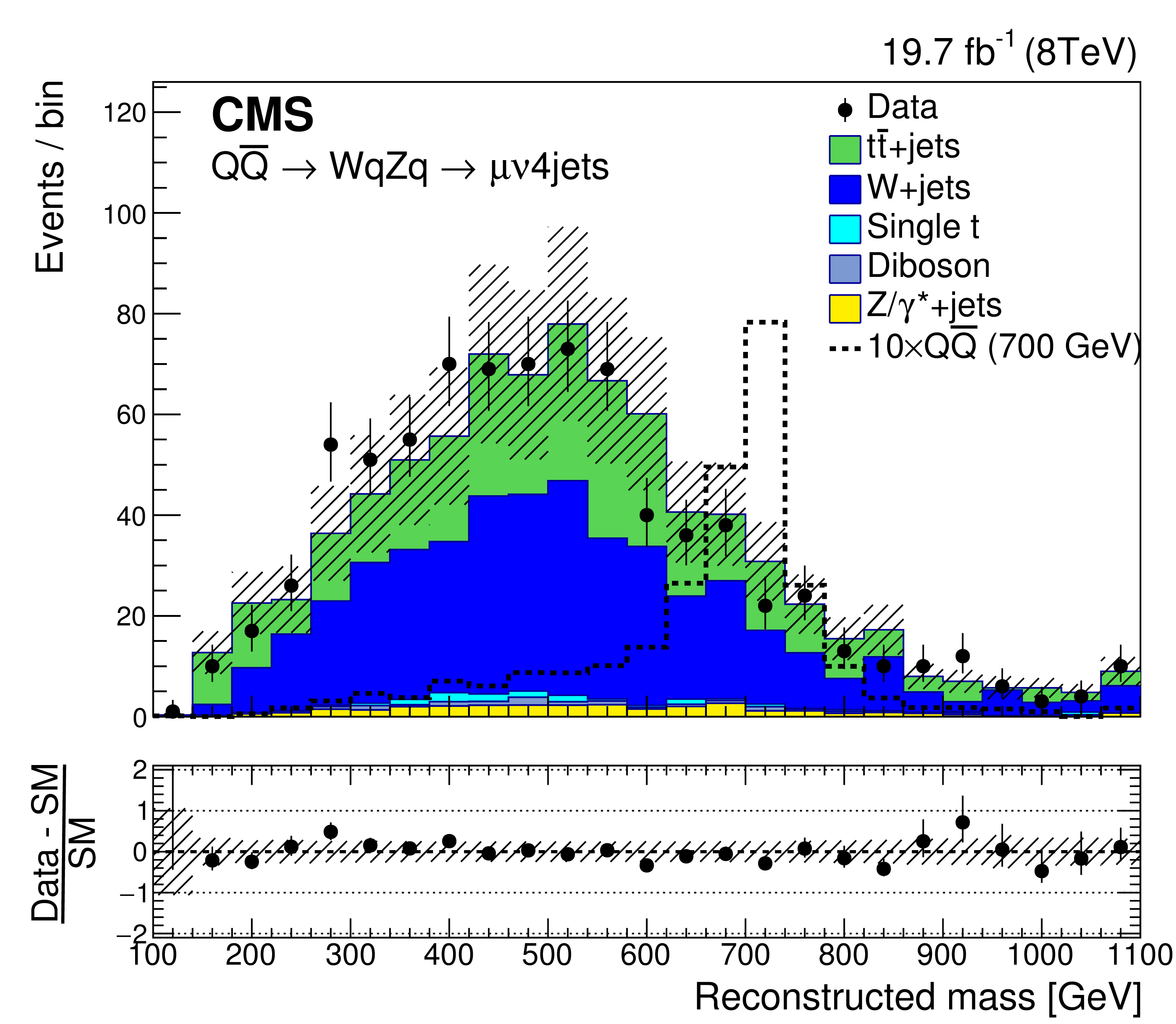
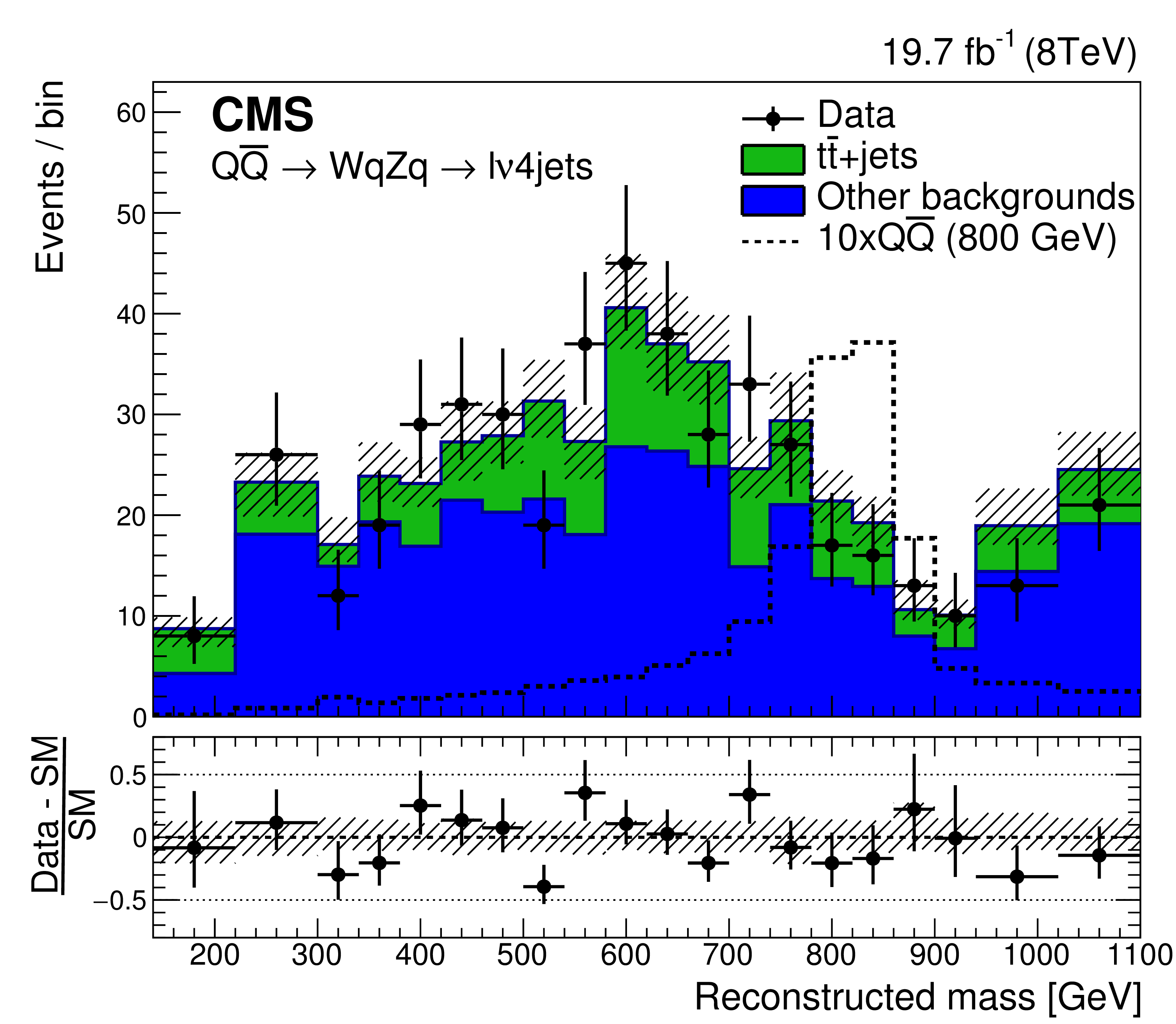
Figure 8-c:
Reconstructed mass distribution for the $\mathrm{ W } \mathrm{ q } {\mathrm{ Z } } \mathrm{ q } $ reconstruction, for the $\mu $+jets channel. The distribution for pair-produced VLQs of mass 700 GeV for $\mathcal {B}_\mathrm{ W } = \mathcal {B}_\mathrm{ Z } = $ 0.5 are scaled up for visibility by a factor of 10. The shaded bands represent the combined statistical and systematic uncertainties. |
png pdf |
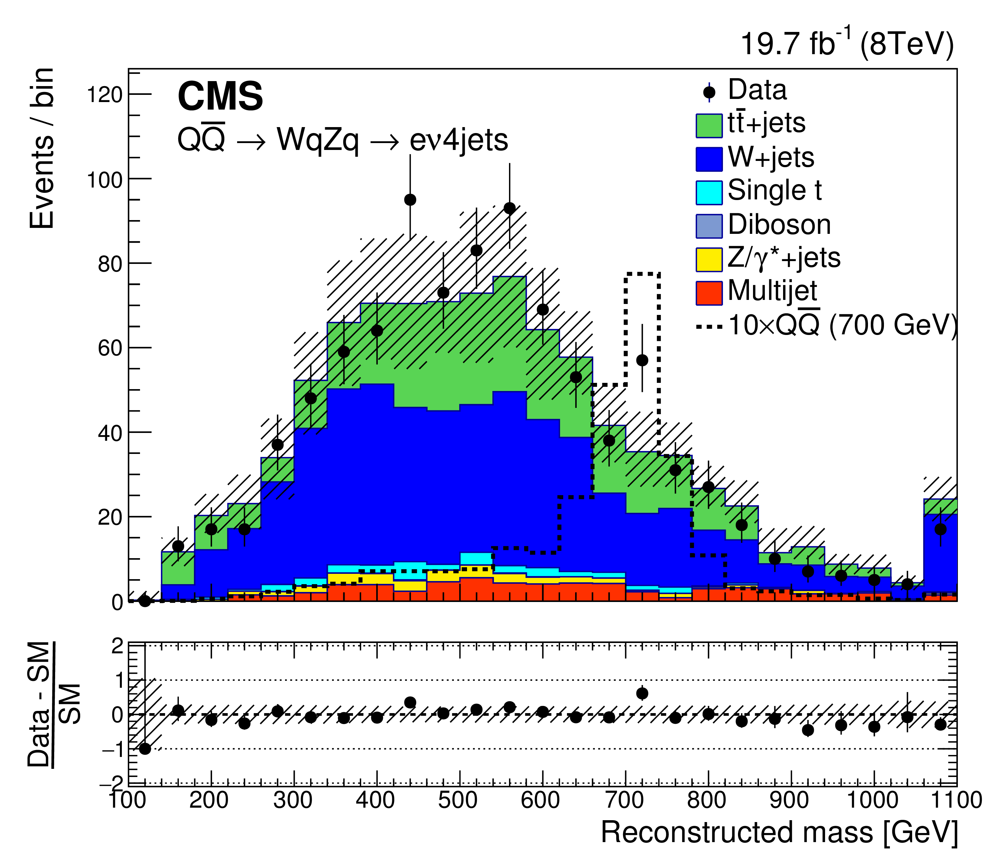
Figure 8-d:
Reconstructed mass distribution for the $\mathrm{ W } \mathrm{ q } {\mathrm{ Z } } \mathrm{ q } $ reconstruction, for the $\mathrm{ e } $+jets channel. The distribution for pair-produced VLQs of mass 700 GeV for $\mathcal {B}_\mathrm{ W } = \mathcal {B}_\mathrm{ Z } = $ 0.5 are scaled up for visibility by a factor of 10. The shaded bands represent the combined statistical and systematic uncertainties. |

png pdf |
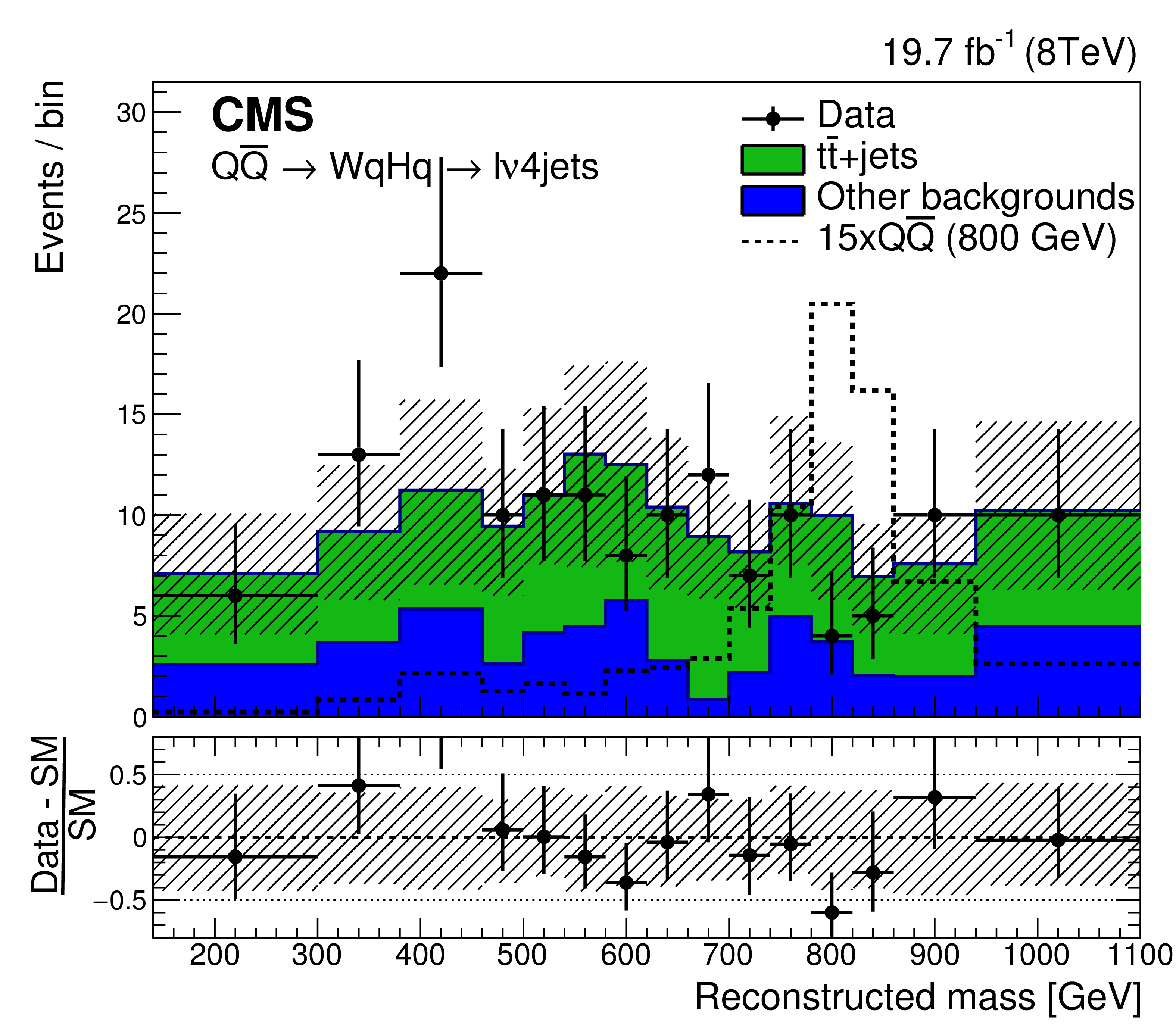
Figure 8-e:
Reconstructed mass distribution for the $\mathrm{ W } \mathrm{ q } \mathrm{ H } \mathrm{ q } $ reconstruction, for the $\mu $+jets channel. The distribution for pair-produced VLQs of mass 700 GeV for $\mathcal {B}_\mathrm{ W } = \mathcal {B}_\mathrm{ H } = $ 0.5 are scaled up for visibility by a factor of 5. The shaded bands represent the combined statistical and systematic uncertainties. |

png pdf |
Figure 8-f:
Reconstructed mass distribution for the $\mathrm{ W } \mathrm{ q } \mathrm{ H } \mathrm{ q } $ reconstruction, for the $\mathrm{ e } $+jets channel. The distribution for pair-produced VLQs of mass 700 GeV for $\mathcal {B}_\mathrm{ W } = \mathcal {B}_\mathrm{ H } = $ 0.5 are scaled up for visibility by a factor of 5. The shaded bands represent the combined statistical and systematic uncertainties. |
png pdf |
Figure 9:
Mass distributions for the $\mathrm{ W } \mathrm{ q } \mathrm{ W } \mathrm{ q } $ (upper left), $\mathrm{ W } \mathrm{ q } {\mathrm{ Z } } \mathrm{ q } $ (upper right), and $\mathrm{ W } \mathrm{ q } \mathrm{ H } \mathrm{ q } $ (lower) reconstructions for the combination of the $\mu $+jets and $\mathrm{ e } $+jets channel, for events with $S_\mathrm {T} >$ 1240 GeV. The distribution for pair-produced VLQs of mass 800 GeV for $\mathcal {B}_\mathrm{ W } = $ 1.0 (upper left), $\mathcal {B}_\mathrm{ W } = \mathcal {B}_\mathrm{ Z } = $ 0.5 (upper right) and $\mathcal {B}_\mathrm{ W } = \mathcal {B}_\mathrm{ H } = $ 0.5 (lower) is scaled up for visibility by a factor of 5, 10 and 15, respectively. The shaded bands represent the combined statistical and systematic uncertainties. The horizontal error bars on the data points only indicate the bin width. |

png pdf |
Figure 9-a:
Mass distribution for the $\mathrm{ W } \mathrm{ q } \mathrm{ W } \mathrm{ q } $ reconstruction for the combination of the $\mu $+jets and $\mathrm{ e } $+jets channel, for events with $S_\mathrm {T} >$ 1240 GeV. The distribution for pair-produced VLQs of mass 800 GeV for $\mathcal {B}_\mathrm{ W } = $ 1.0 is scaled up for visibility by a factor of 5. The shaded bands represent the combined statistical and systematic uncertainties. The horizontal error bars on the data points only indicate the bin width. |
png pdf |
Figure 9-b:
Mass distribution for the $\mathrm{ W } \mathrm{ q } {\mathrm{ Z } } \mathrm{ q } $ $\mathrm{ W } \mathrm{ q } \mathrm{ H } \mathrm{ q } $ reconstruction for the combination of the $\mu $+jets and $\mathrm{ e } $+jets channel, for events with $S_\mathrm {T} >$ 1240 GeV. The distribution for pair-produced VLQs of mass 800 GeV for $\mathcal {B}_\mathrm{ W } = \mathcal {B}_\mathrm{ Z } = $ 0.5 is scaled up for visibility by a factor of 10. The shaded bands represent the combined statistical and systematic uncertainties. The horizontal error bars on the data points only indicate the bin width. |
png pdf |
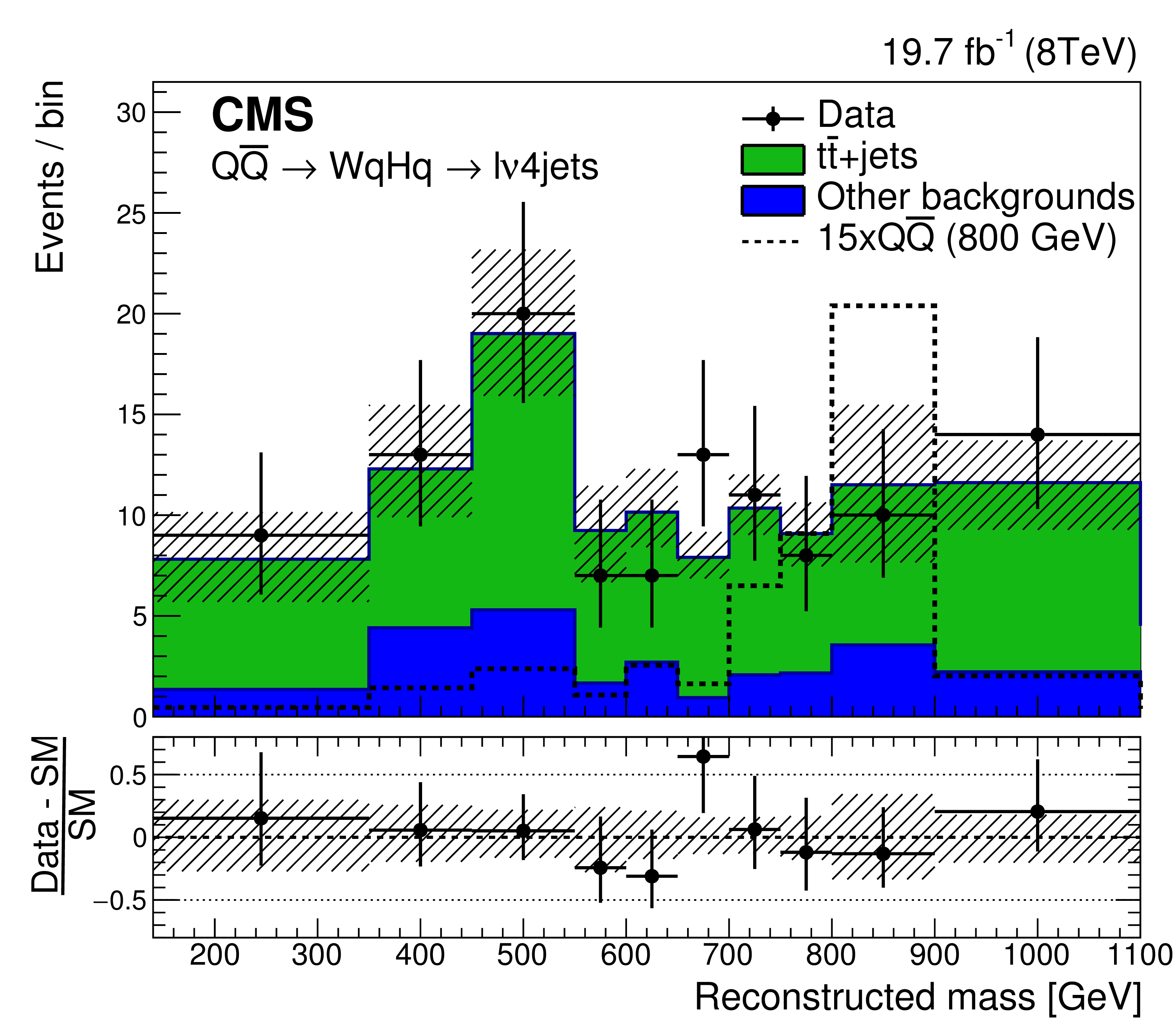
Figure 9-c:
Mass distribution for the $\mathrm{ W } \mathrm{ q } \mathrm{ H } \mathrm{ q } $ reconstruction for the combination of the $\mu $+jets and $\mathrm{ e } $+jets channel, for events with $S_\mathrm {T} >$ 1240 GeV. The distribution for pair-produced VLQs of mass 800 GeV for $\mathcal {B}_\mathrm{ W } = \mathcal {B}_\mathrm{ H } = $ 0.5 is scaled up for visibility by a factor of 15. The shaded bands represent the combined statistical and systematic uncertainties. The horizontal error bars on the data points only indicate the bin width. |
png pdf |
Figure 10:
Mass distribution for the $\mathrm{ W } \mathrm{ q } \mathrm{ H } \mathrm{ q } $ reconstruction, for combined $\mu $+jets and $\mathrm{ e } $+jets channels and for events with $S_\mathrm {T} > $ 1240 GeV. Events appearing also in the $\mathrm{ W } \mathrm{ q } \mathrm{ W } \mathrm{ q } $ sample have been removed. The distribution for pair-produced VLQs of mass 800 GeV for $\mathcal {B}_\mathrm{ W } = \mathcal {B}_\mathrm{ H } = $ 0.5 is scaled up by a factor of 15 for visibility. The shaded band represent the combined statistical and systematic uncertainties. The horizontal error bars on the data points only indicate the bin width. |
png pdf |
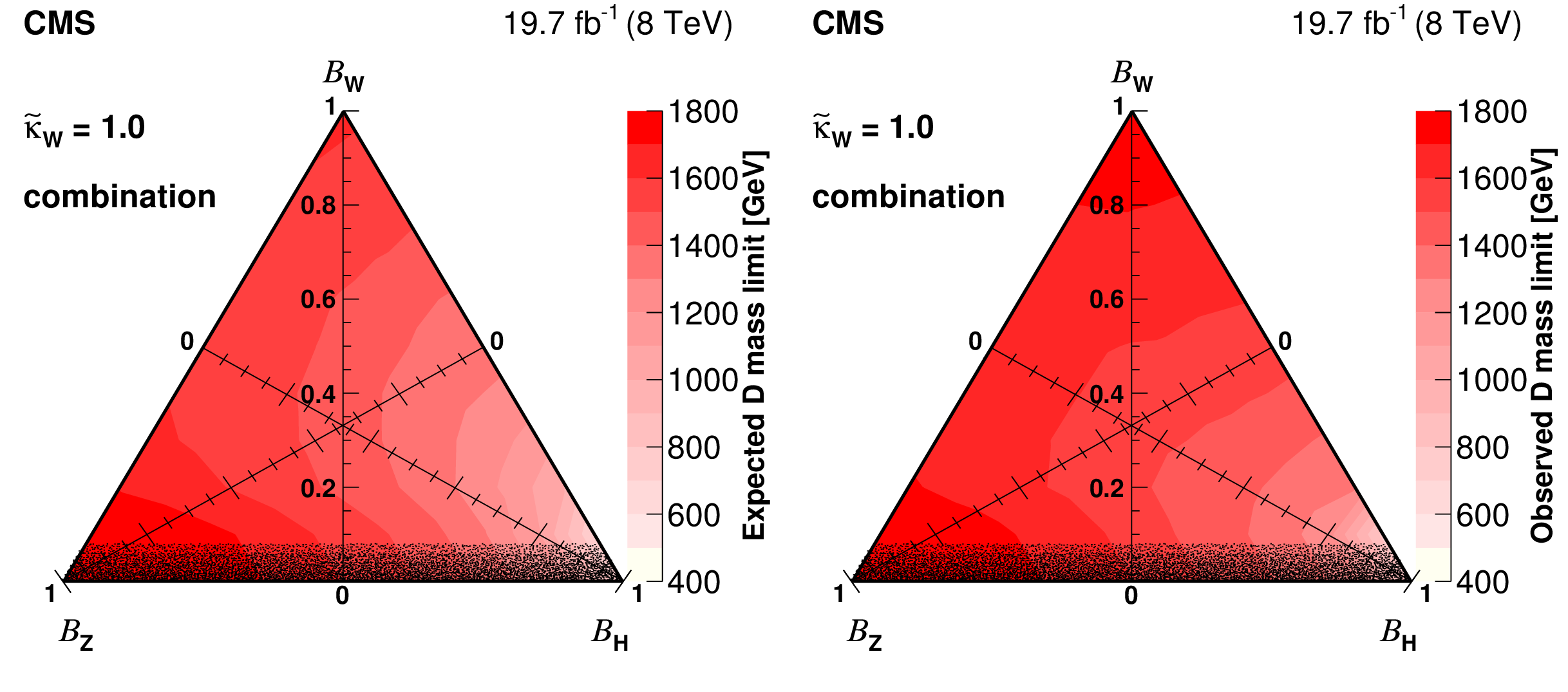
Figure 11:
The median expected (left) and observed (right) combined lower mass limits represented in a triangular form, where each point of the triangle corresponds to a given set of branching fractions for the decay of a VLQ into a boson and a first-generation quark. The limit contours are determined assuming that $\tilde{\kappa }_\mathrm{ W } = $ 1.0, which means that the signal is dominated by electroweak single production. The black shaded band near $\mathcal {B}_\mathrm{ W } = $ 0 shows a region where the results cannot be reliably interpreted because $\tilde{\kappa }_\mathrm{ Z } $ diverges, as explained in the text. |
png pdf |
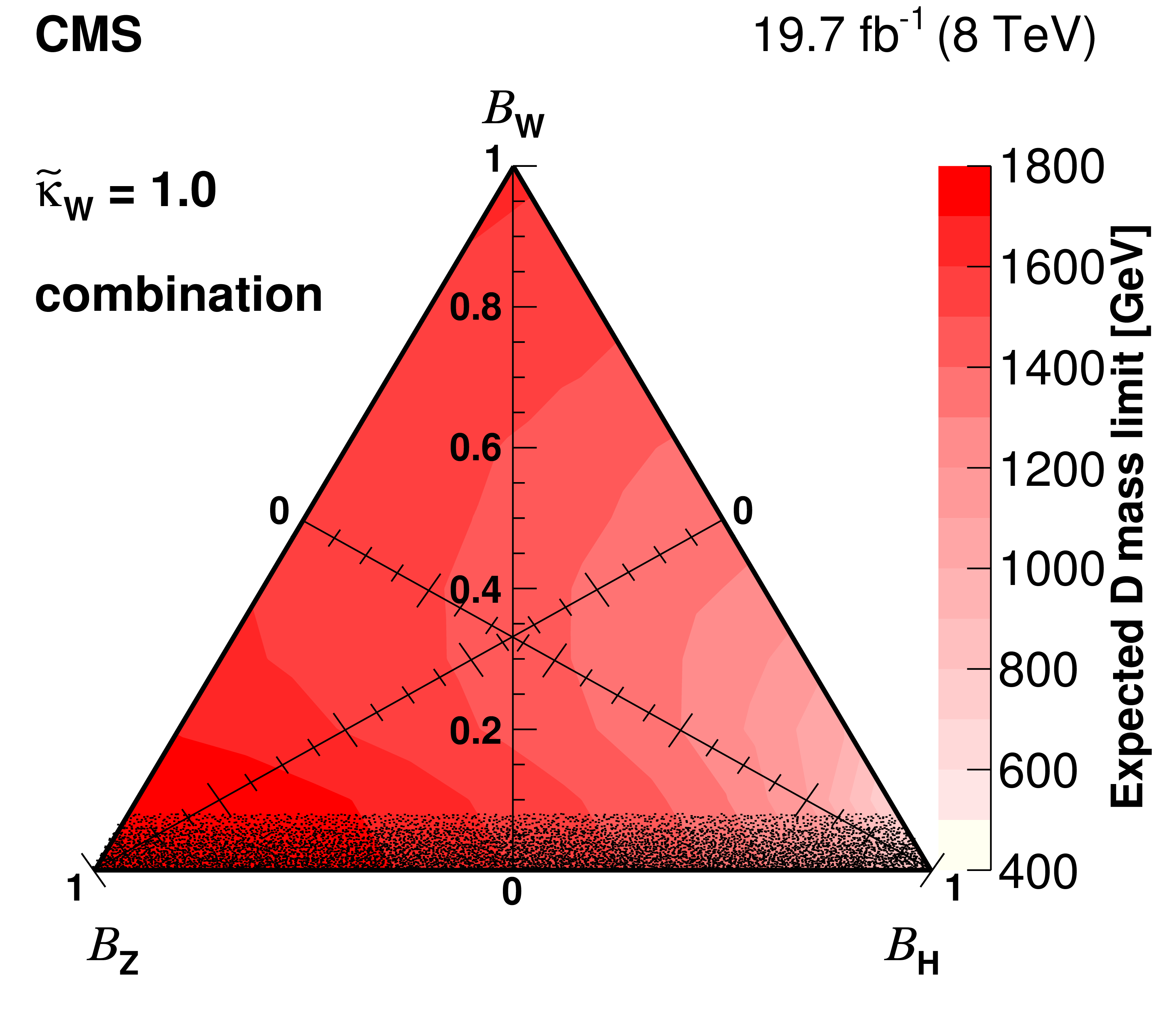
Figure 11-a:
The median expected combined lower mass limits represented in a triangular form, where each point of the triangle corresponds to a given set of branching fractions for the decay of a VLQ into a boson and a first-generation quark. The limit contours are determined assuming that $\tilde{\kappa }_\mathrm{ W } = $ 1.0, which means that the signal is dominated by electroweak single production. The black shaded band near $\mathcal {B}_\mathrm{ W } = $ 0 shows a region where the results cannot be reliably interpreted because $\tilde{\kappa }_\mathrm{ Z } $ diverges, as explained in the text. |
png pdf |
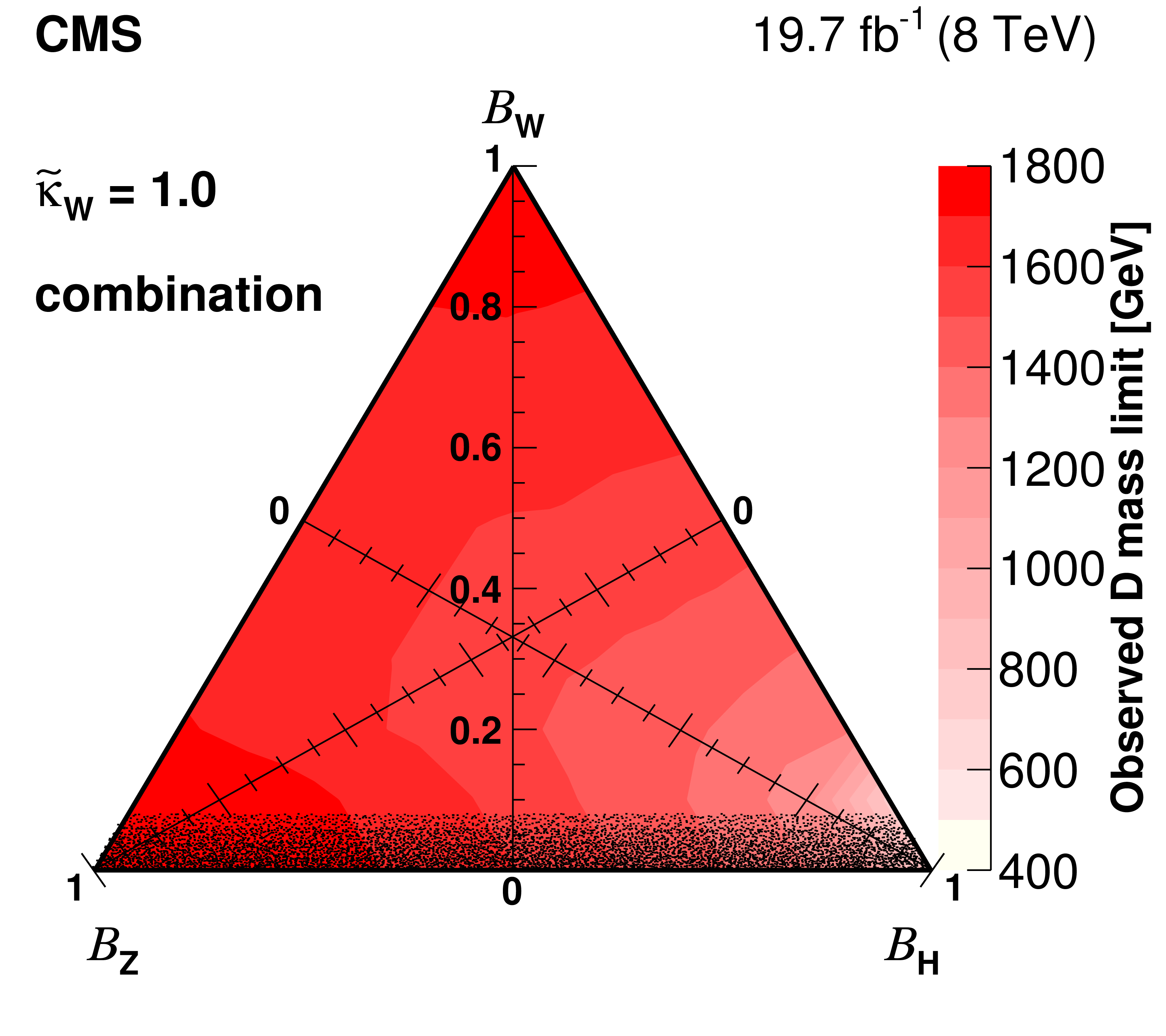
Figure 11-b:
The observed combined lower mass limits represented in a triangular form, where each point of the triangle corresponds to a given set of branching fractions for the decay of a VLQ into a boson and a first-generation quark. The limit contours are determined assuming that $\tilde{\kappa }_\mathrm{ W } = $ 1.0, which means that the signal is dominated by electroweak single production. The black shaded band near $\mathcal {B}_\mathrm{ W } = $ 0 shows a region where the results cannot be reliably interpreted because $\tilde{\kappa }_\mathrm{ Z } $ diverges, as explained in the text. |

png pdf |
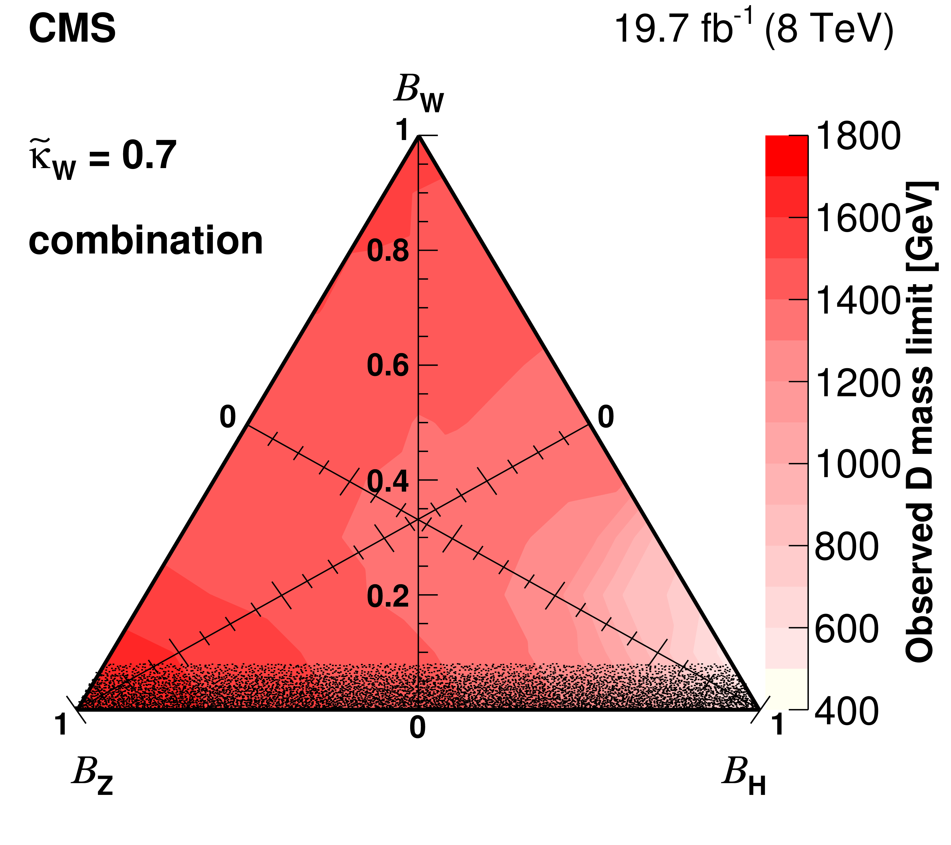
Figure 12:
The median expected (left) and observed (right) combined lower mass limits represented in a triangular form, where each point of the triangle corresponds to a given set of branching fractions for a VLQ decaying into a boson and a first-generation quark. The limit contours are determined assuming $\tilde{\kappa }_\mathrm{ W } = $ 0.7, which means that the signal will be dominated by electroweak single production for most of the parameter space represented by the triangles. The black shaded band near $\mathcal {B}_\mathrm{ W } = $ 0 represents a region where results cannot be reliably interpreted because $\tilde{\kappa }_\mathrm{ Z } $ diverges, as explained in the text. |
png pdf |
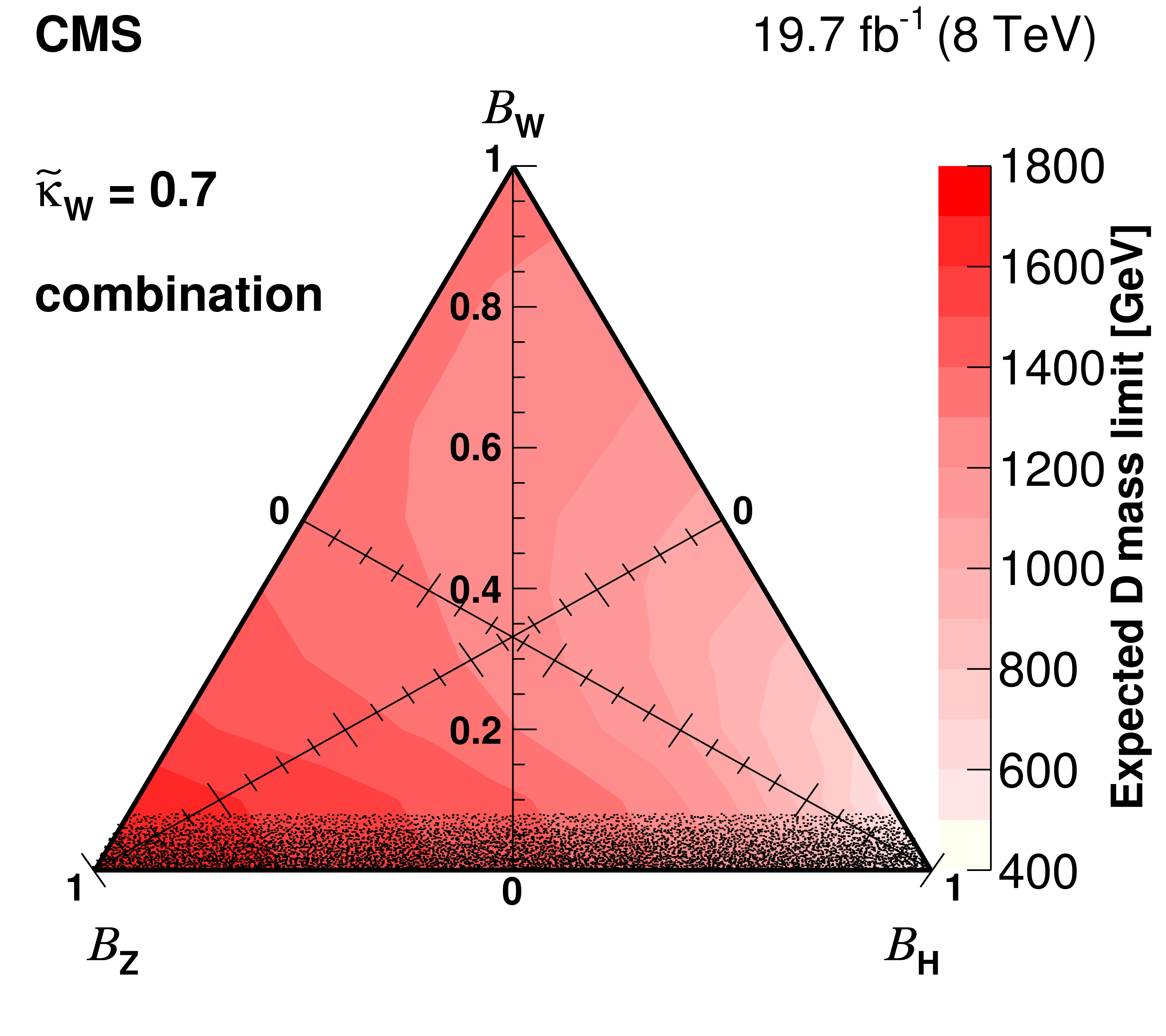
Figure 12-a:
The median expected combined lower mass limits represented in a triangular form, where each point of the triangle corresponds to a given set of branching fractions for a VLQ decaying into a boson and a first-generation quark. The limit contours are determined assuming $\tilde{\kappa }_\mathrm{ W } = $ 0.7, which means that the signal will be dominated by electroweak single production for most of the parameter space represented by the triangles. The black shaded band near $\mathcal {B}_\mathrm{ W } = $ 0 represents a region where results cannot be reliably interpreted because $\tilde{\kappa }_\mathrm{ Z } $ diverges, as explained in the text. |
png pdf |
Figure 12-b:
The observed combined lower mass limits represented in a triangular form, where each point of the triangle corresponds to a given set of branching fractions for a VLQ decaying into a boson and a first-generation quark. The limit contours are determined assuming $\tilde{\kappa }_\mathrm{ W } = $ 0.7, which means that the signal will be dominated by electroweak single production for most of the parameter space represented by the triangles. The black shaded band near $\mathcal {B}_\mathrm{ W } = $ 0 represents a region where results cannot be reliably interpreted because $\tilde{\kappa }_\mathrm{ Z } $ diverges, as explained in the text. |
png pdf |
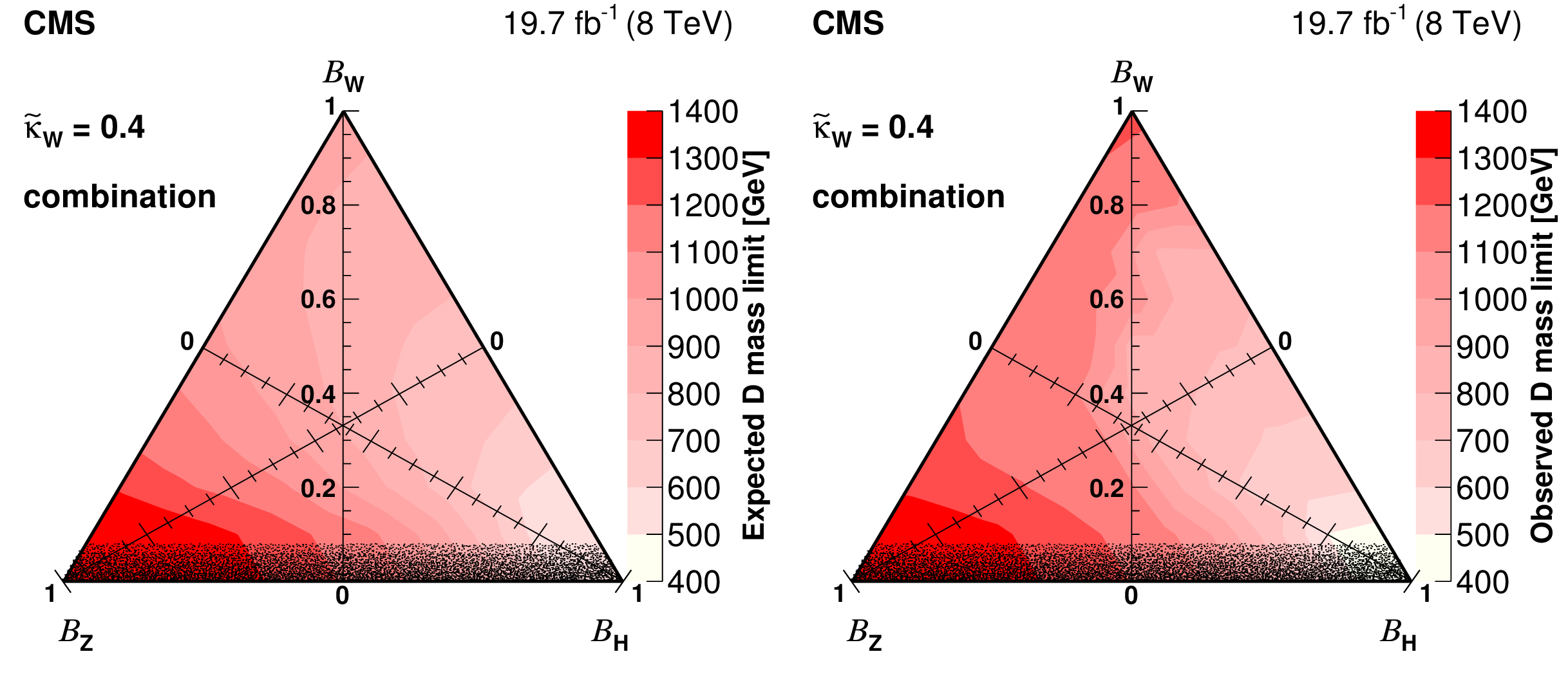
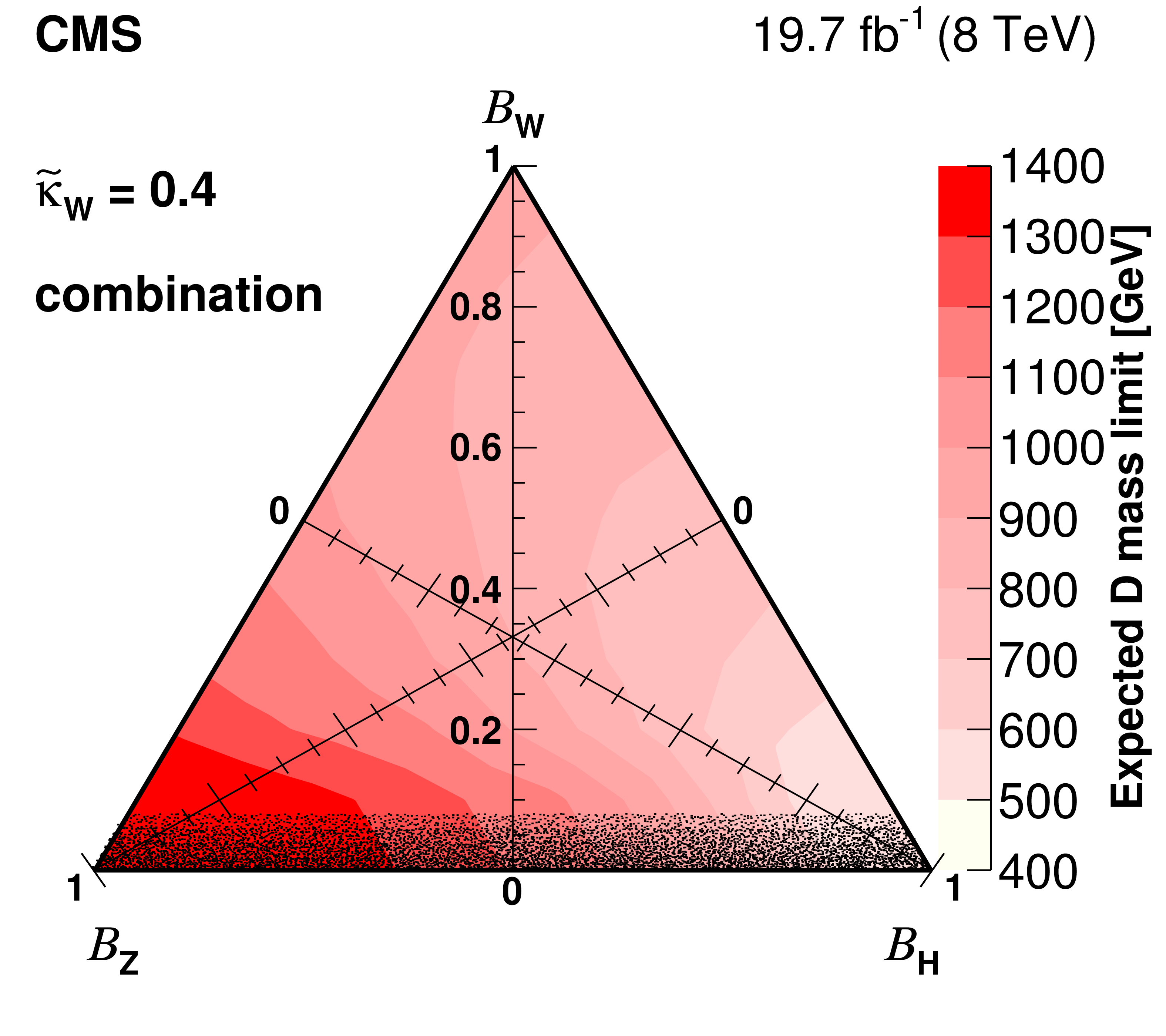
Figure 13:
The median expected (left) and observed (right) combined lower mass limits represented in a triangular form, where each point of the triangle corresponds to a given set of branching fractions for a VLQ decaying into a boson and a first-generation quark. The limit contours were determined assuming $\tilde{\kappa }_\mathrm{ W } = $ 0.4, which means that the signal is dominated by electroweak single production in most of the parameter space represented by the triangles, but in which the relative importance of the pair-produced signal has increased. The black shaded band near $\mathcal {B}_\mathrm{ W } = $ 0 represents a region where results cannot be reliably interpreted because $\tilde{\kappa }_\mathrm{ Z } $ diverges, as explained in the text. |
png pdf |
Figure 13-a:
The median expected combined lower mass limits represented in a triangular form, where each point of the triangle corresponds to a given set of branching fractions for a VLQ decaying into a boson and a first-generation quark. The limit contours were determined assuming $\tilde{\kappa }_\mathrm{ W } = $ 0.4, which means that the signal is dominated by electroweak single production in most of the parameter space represented by the triangles, but in which the relative importance of the pair-produced signal has increased. The black shaded band near $\mathcal {B}_\mathrm{ W } = $ 0 represents a region where results cannot be reliably interpreted because $\tilde{\kappa }_\mathrm{ Z } $ diverges, as explained in the text. |

png pdf |
Figure 13-b:
The observed combined lower mass limits represented in a triangular form, where each point of the triangle corresponds to a given set of branching fractions for a VLQ decaying into a boson and a first-generation quark. The limit contours were determined assuming $\tilde{\kappa }_\mathrm{ W } = $ 0.4, which means that the signal is dominated by electroweak single production in most of the parameter space represented by the triangles, but in which the relative importance of the pair-produced signal has increased. The black shaded band near $\mathcal {B}_\mathrm{ W } = $ 0 represents a region where results cannot be reliably interpreted because $\tilde{\kappa }_\mathrm{ Z } $ diverges, as explained in the text. |
png pdf |
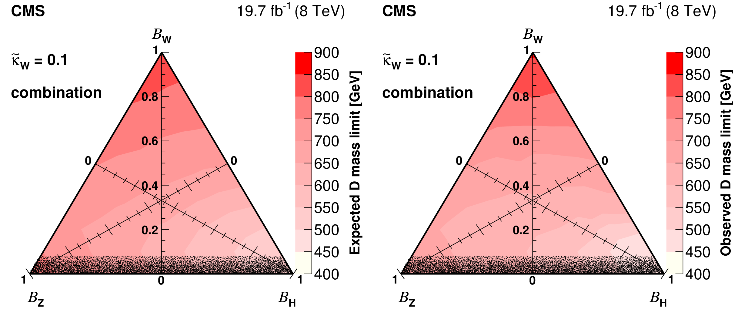
Figure 14:
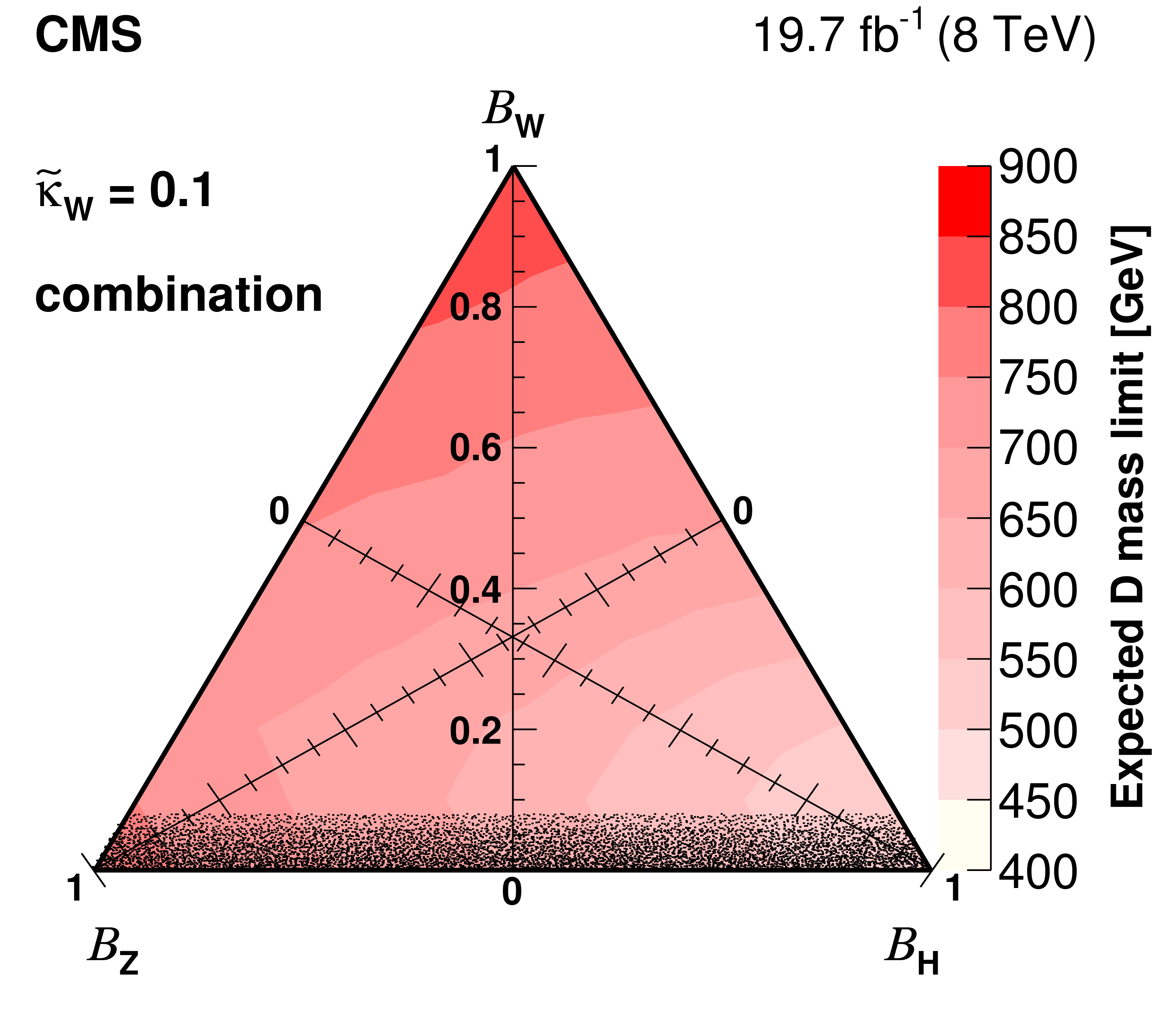
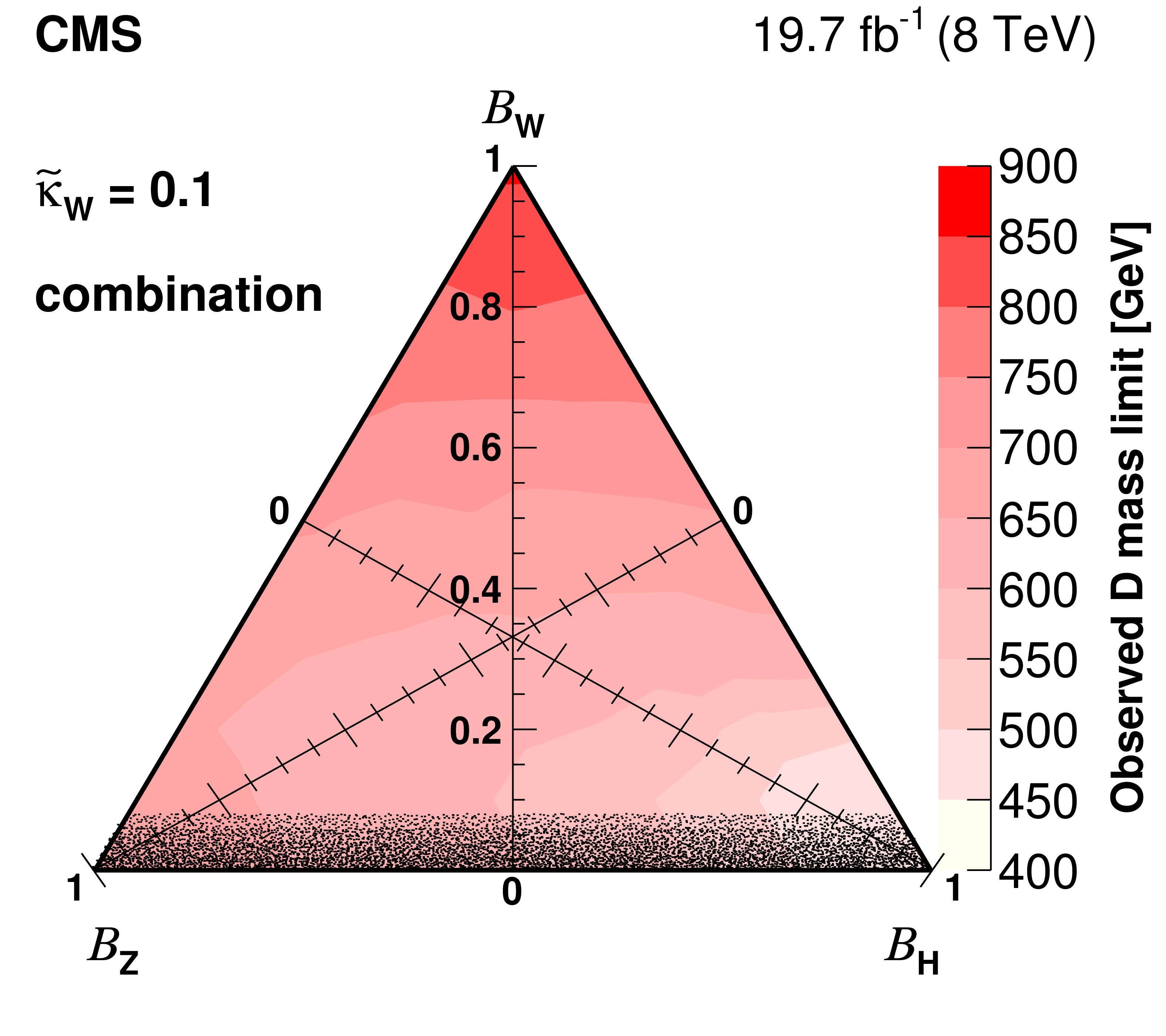
The median expected (left) and observed (right) combined lower mass limits represented in a triangular form, where each point of the triangle corresponds to a given set of branching fractions for a VLQ decaying into a boson and a first-generation quark. The limit contours were determined assuming $\tilde{\kappa }_\mathrm{ W } = $ 0.1, which means that the signal is dominated by strong pair production for most of the parameter space represented by the triangles. The black shaded band near $\mathcal {B}_\mathrm{ W } = $ 0 indicates a region where results cannot be reliably interpreted because $\tilde{\kappa }_\mathrm{ Z } $ diverges, as explained in the text. |
png pdf |
Figure 14-a:
The median expected combined lower mass limits represented in a triangular form, where each point of the triangle corresponds to a given set of branching fractions for a VLQ decaying into a boson and a first-generation quark. The limit contours were determined assuming $\tilde{\kappa }_\mathrm{ W } = $ 0.1, which means that the signal is dominated by strong pair production for most of the parameter space represented by the triangles. The black shaded band near $\mathcal {B}_\mathrm{ W } = $ 0 indicates a region where results cannot be reliably interpreted because $\tilde{\kappa }_\mathrm{ Z } $ diverges, as explained in the text. |
png pdf |
Figure 14-b:
The observed combined lower mass limits represented in a triangular form, where each point of the triangle corresponds to a given set of branching fractions for a VLQ decaying into a boson and a first-generation quark. The limit contours were determined assuming $\tilde{\kappa }_\mathrm{ W } = $ 0.1, which means that the signal is dominated by strong pair production for most of the parameter space represented by the triangles. The black shaded band near $\mathcal {B}_\mathrm{ W } = $ 0 indicates a region where results cannot be reliably interpreted because $\tilde{\kappa }_\mathrm{ Z } $ diverges, as explained in the text. |
png pdf |
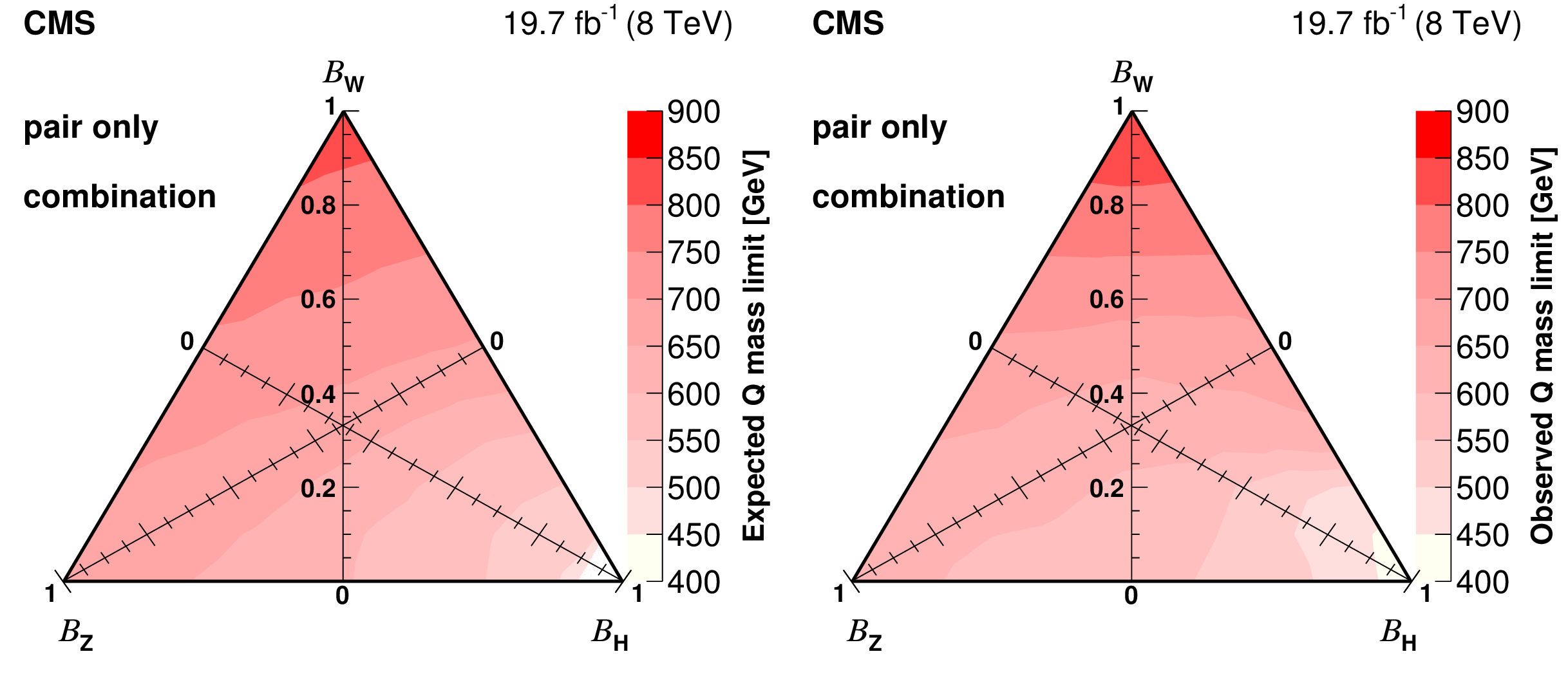
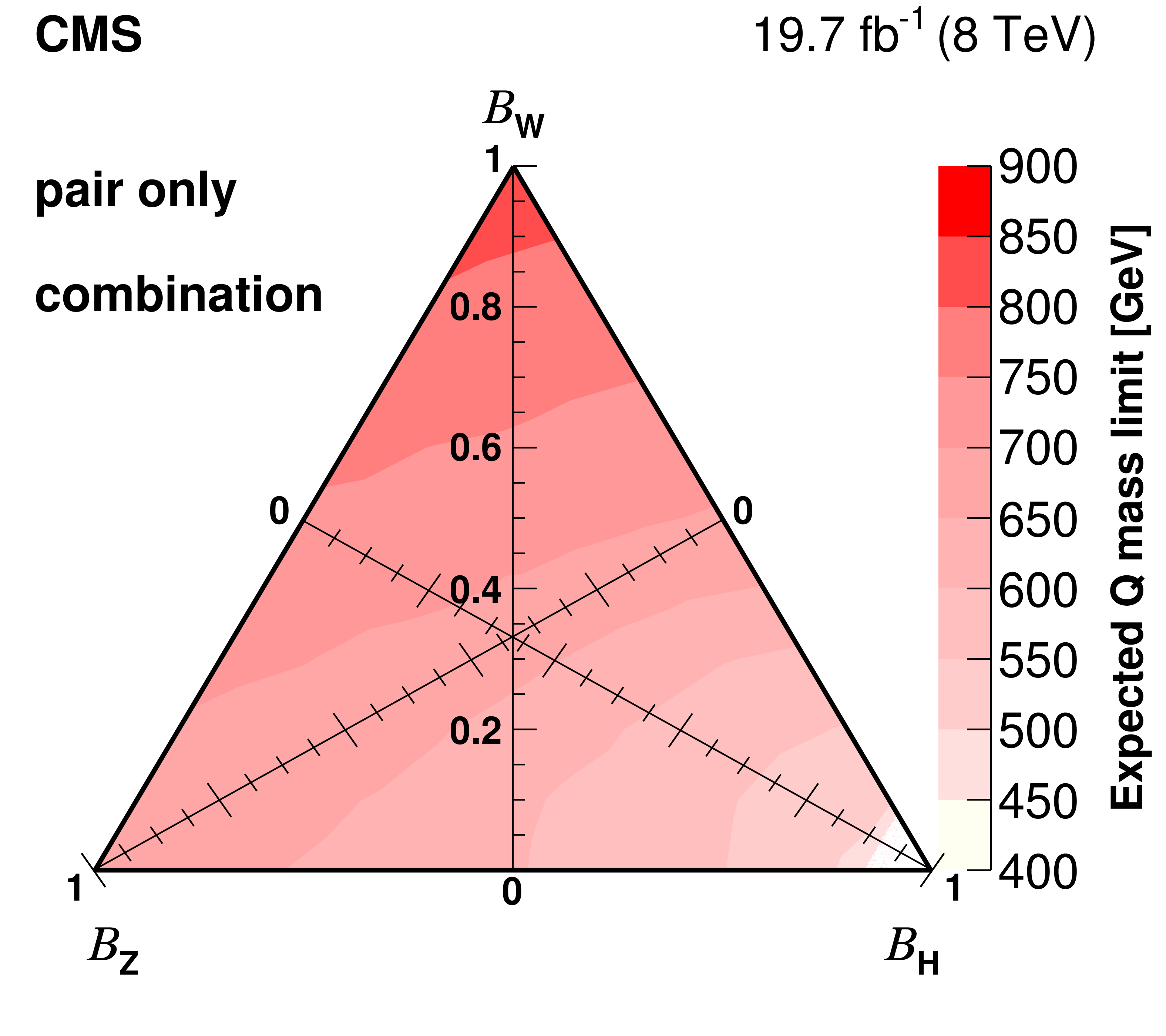
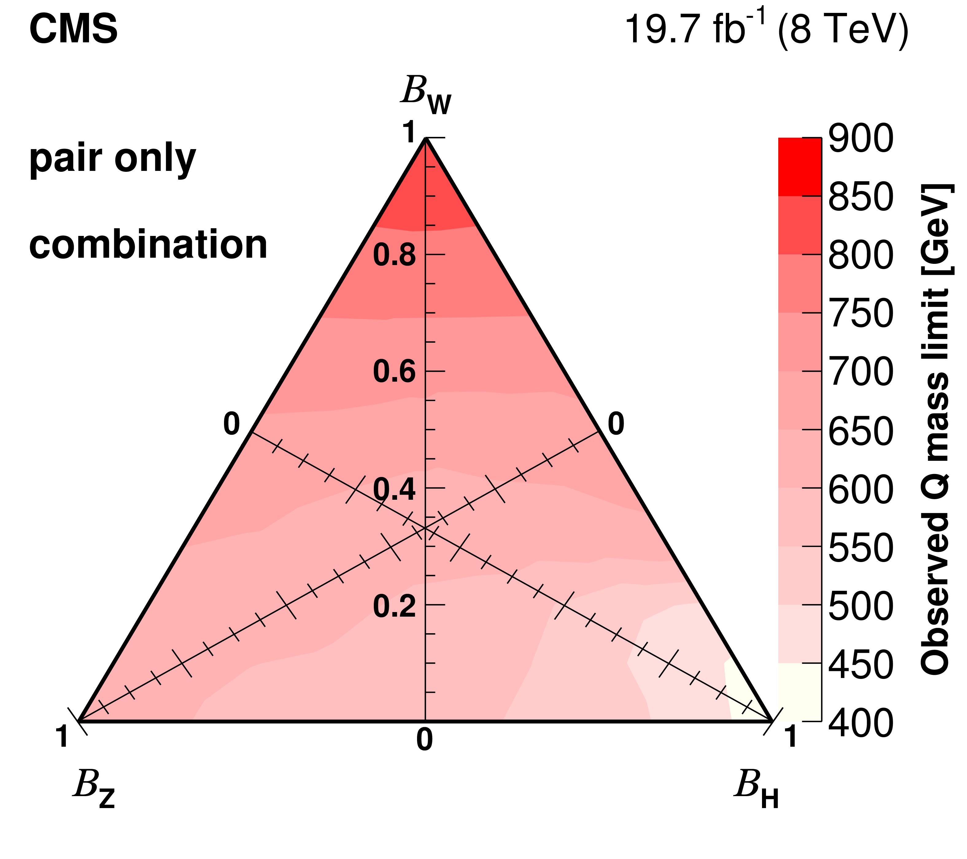
Figure 15:
The median expected (left) and observed (right) combined lower mass limits represented in a triangular form, where each point of the triangle corresponds to a given set of branching fractions for a VLQ decaying into a boson and a first-generation quark. The limit contours were determined assuming that $\tilde{\kappa }_\mathrm{ W } $ and $\tilde{\kappa }_\mathrm{ Z } $ are so small that the single-production modes can be neglected, and therefore that the heavy quarks can only be produced in pairs via strong interaction. The white area in the triangle with expected limits indicates mass limits below 400 GeV. |
png pdf |
Figure 15-a:
The median expected combined lower mass limits represented in a triangular form, where each point of the triangle corresponds to a given set of branching fractions for a VLQ decaying into a boson and a first-generation quark. The limit contours were determined assuming that $\tilde{\kappa }_\mathrm{ W } $ and $\tilde{\kappa }_\mathrm{ Z } $ are so small that the single-production modes can be neglected, and therefore that the heavy quarks can only be produced in pairs via strong interaction. The white area in the triangle with expected limits indicates mass limits below 400 GeV. |
png pdf |
Figure 15-b:
The observed combined lower mass limits represented in a triangular form, where each point of the triangle corresponds to a given set of branching fractions for a VLQ decaying into a boson and a first-generation quark. The limit contours were determined assuming that $\tilde{\kappa }_\mathrm{ W } $ and $\tilde{\kappa }_\mathrm{ Z } $ are so small that the single-production modes can be neglected, and therefore that the heavy quarks can only be produced in pairs via strong interaction. The white area in the triangle with expected limits indicates mass limits below 400 GeV. |
png pdf |
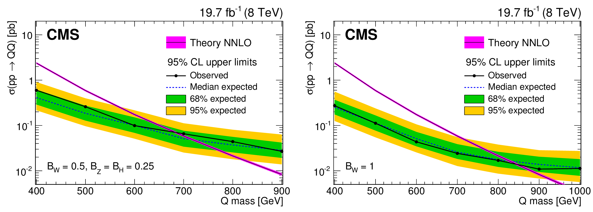
Figure 16:
The 95% CL exclusion limits on the production cross section determined assuming different sets of model parameters ($\mathcal {B}_\mathrm{ W } = $ 0.5, $\mathcal {B}_\mathrm{ Z } = $ 0.25 (left), and $\mathcal {B}_\mathrm{ W } = $ 1 (right)) as a function of the hypothetical VLQ mass, and for the scenario where only strong pair production of the VLQs is considered. The median expected and observed exclusion limits are indicated with a dashed and a solid line, respectively. The inner (green) band and the outer (yellow) band indicate the regions containing 68 and 95%, respectively, of the distribution of limits expected under the background-only hypothesis. The cross section from a full NNLO calculation [24], including uncertainties in the PDF description and the renormalization and factorization scales, is shown by the magenta band. |
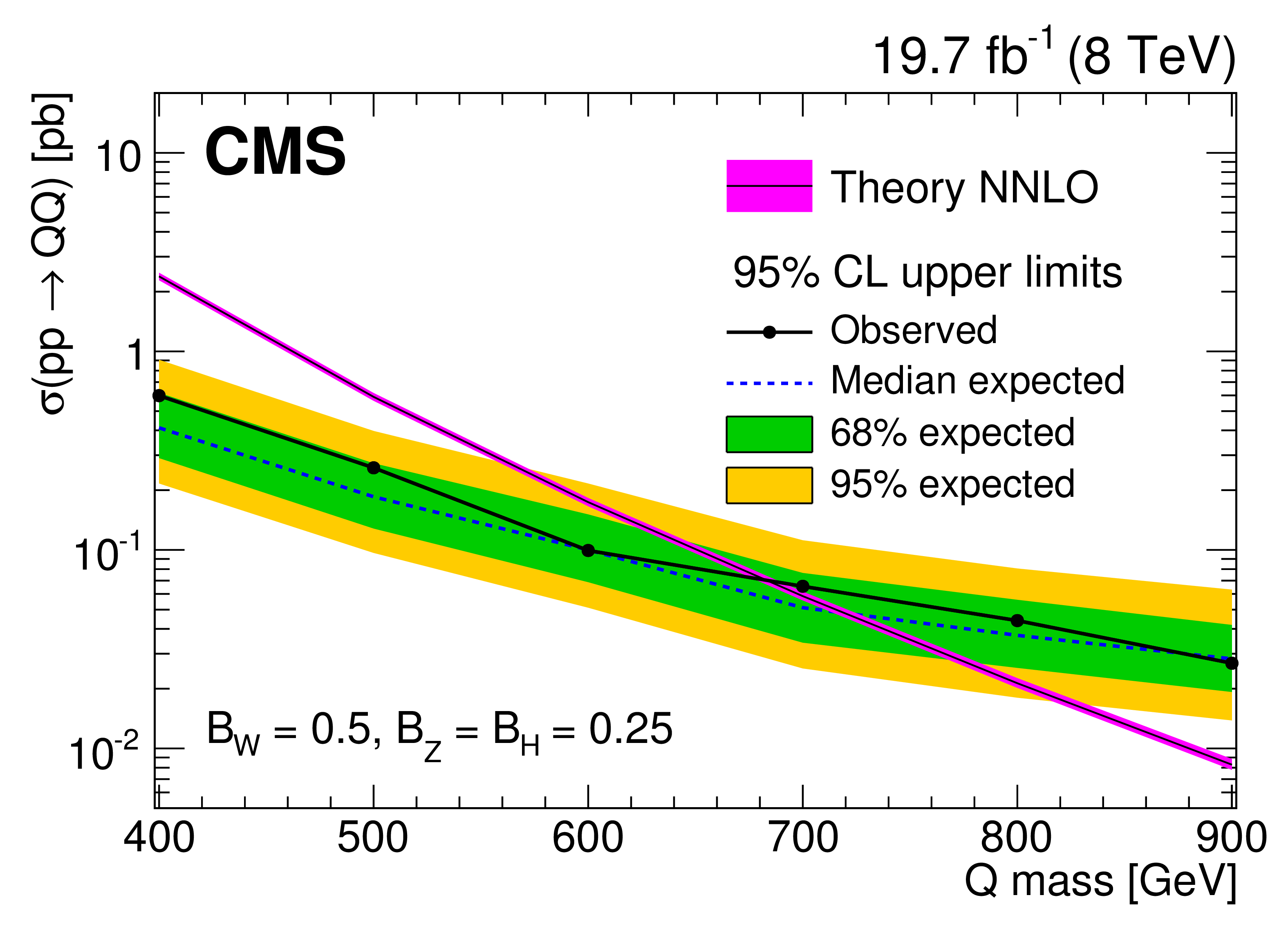
png pdf |
Figure 16-a:
The 95% CL exclusion limits on the production cross section determined assuming different sets of model parameters ($\mathcal {B}_\mathrm{ W } = $ 0.5, $\mathcal {B}_\mathrm{ Z } = $ 0.25) as a function of the hypothetical VLQ mass, and for the scenario where only strong pair production of the VLQs is considered. The median expected and observed exclusion limits are indicated with a dashed and a solid line, respectively. The inner (green) band and the outer (yellow) band indicate the regions containing 68 and 95%, respectively, of the distribution of limits expected under the background-only hypothesis. The cross section from a full NNLO calculation [24], including uncertainties in the PDF description and the renormalization and factorization scales, is shown by the magenta band. |
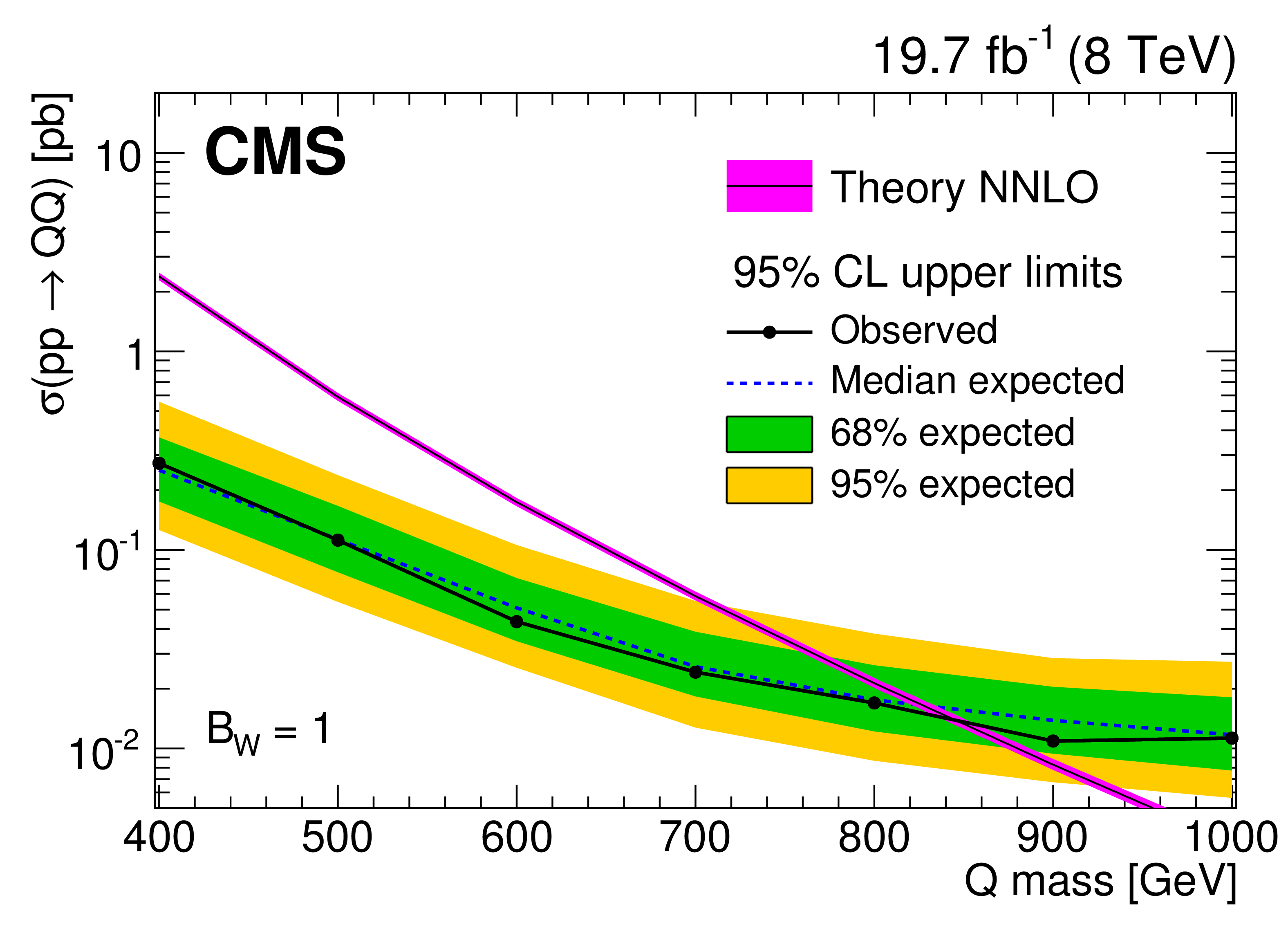
png pdf |
Figure 16-b:
The 95% CL exclusion limits on the production cross section determined assuming different sets of model parameters ($\mathcal {B}_\mathrm{ W } = $ 1) as a function of the hypothetical VLQ mass, and for the scenario where only strong pair production of the VLQs is considered. The median expected and observed exclusion limits are indicated with a dashed and a solid line, respectively. The inner (green) band and the outer (yellow) band indicate the regions containing 68 and 95%, respectively, of the distribution of limits expected under the background-only hypothesis. The cross section from a full NNLO calculation [24], including uncertainties in the PDF description and the renormalization and factorization scales, is shown by the magenta band. |
png pdf |
Figure 17:
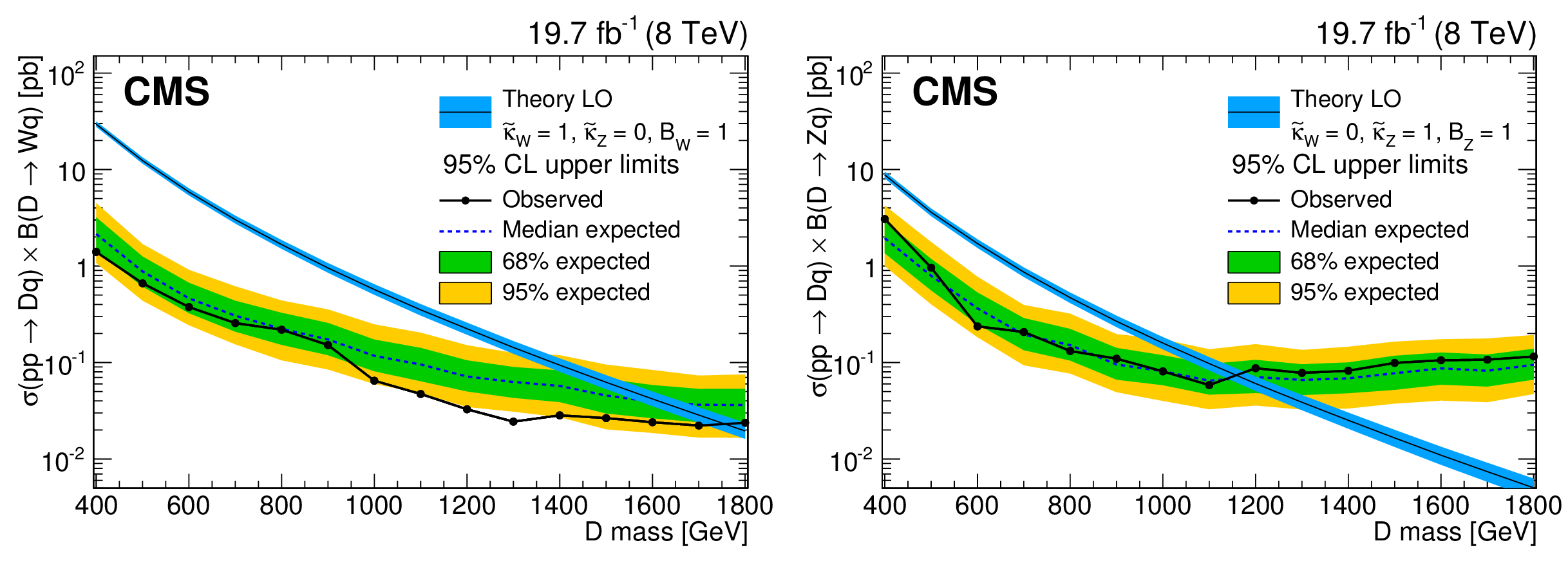
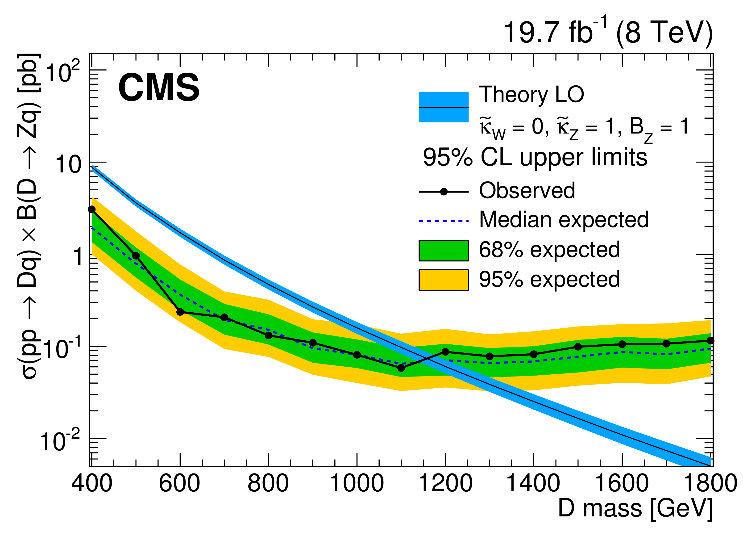
The 95% CL exclusion limits on the product of the production cross section and the branching fraction, considering only single production of down-type VLQs, and assuming a neutral current coupling of zero (left) or a charged current coupling of zero (right). The median expected and observed exclusion limits are indicated with a dashed and a solid line, respectively. The inner (green) band and the outer (yellow) band indicate the regions containing 68 and 95%, respectively, of the distribution of limits expected under the background-only hypothesis. The corresponding LO theory predictions are superimposed. The predictions are represented by a solid black line centered within a blue band, which shows the uncertainty of the calculation. The uncertainties are determined based on the choice of PDF set along with the renormalization and factorization scales. |

png pdf |
Figure 17-a:
The 95% CL exclusion limits on the product of the production cross section and the branching fraction, considering only single production of down-type VLQs, and assuming a neutral current coupling of zero. The median expected and observed exclusion limits are indicated with a dashed and a solid line, respectively. The inner (green) band and the outer (yellow) band indicate the regions containing 68 and 95%, respectively, of the distribution of limits expected under the background-only hypothesis. The corresponding LO theory predictions are superimposed. The predictions are represented by a solid black line centered within a blue band, which shows the uncertainty of the calculation. The uncertainties are determined based on the choice of PDF set along with the renormalization and factorization scales. |
png pdf |
Figure 17-b:
The 95% CL exclusion limits on the product of the production cross section and the branching fraction, considering only single production of down-type VLQs, and assuming a charged current coupling of zero. The median expected and observed exclusion limits are indicated with a dashed and a solid line, respectively. The inner (green) band and the outer (yellow) band indicate the regions containing 68 and 95%, respectively, of the distribution of limits expected under the background-only hypothesis. The corresponding LO theory predictions are superimposed. The predictions are represented by a solid black line centered within a blue band, which shows the uncertainty of the calculation. The uncertainties are determined based on the choice of PDF set along with the renormalization and factorization scales. |
| Tables | |
png pdf |
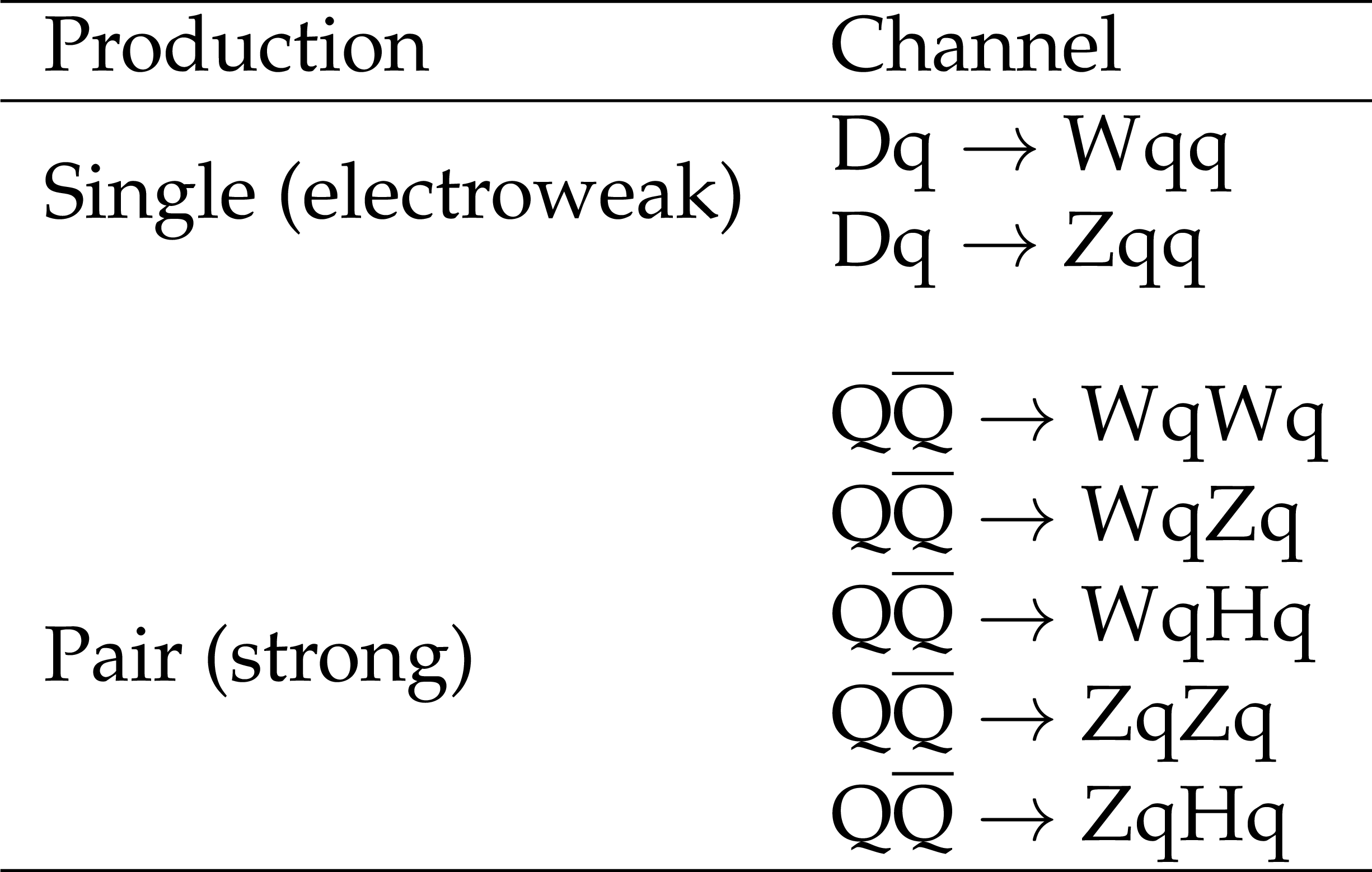
Table 1:
Decay channels of vector-like quarks considered in the analysis. |
png pdf |
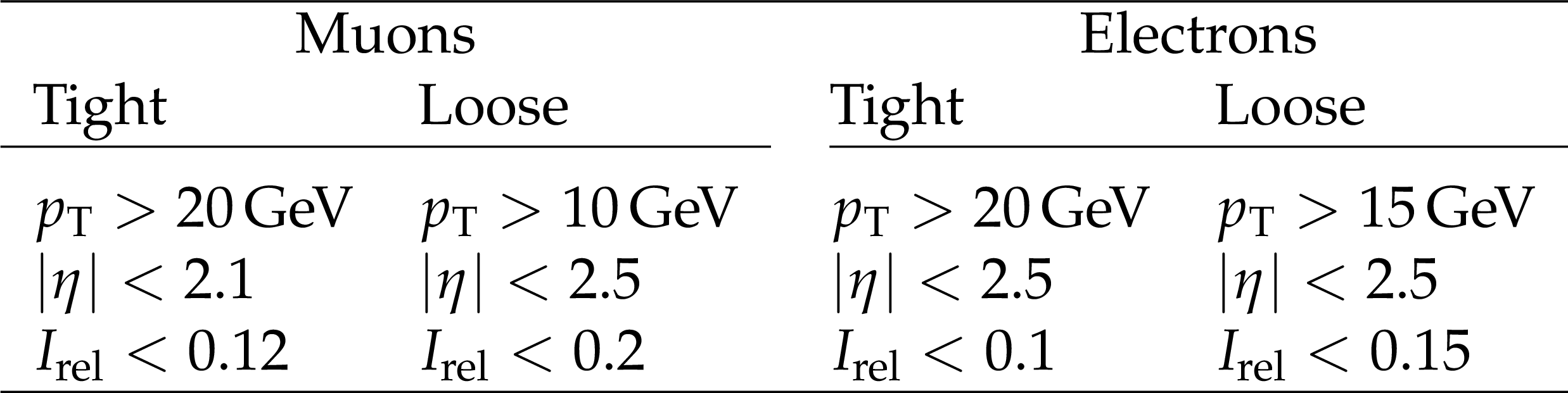
Table 2:
Initial selection requirements for tight and loose leptons. |

png pdf |
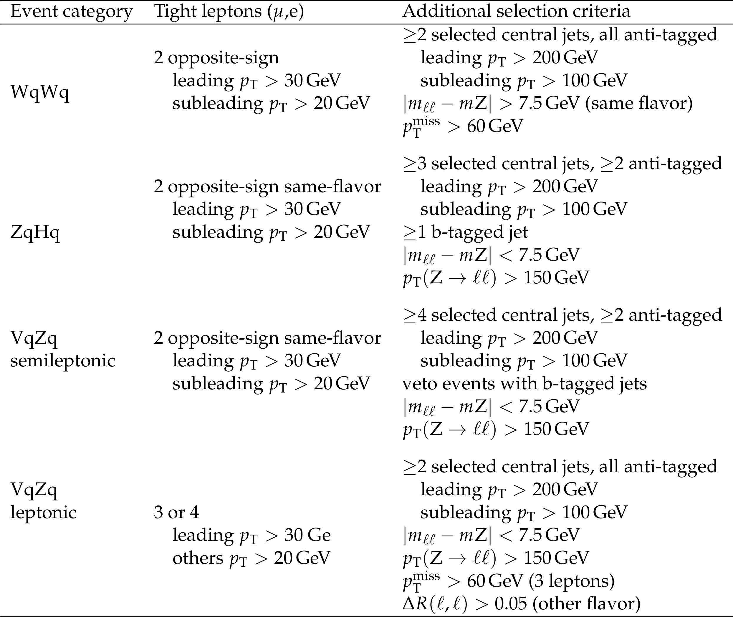
Table 3:
The event categories as optimized for the VLQ single production. The categories are based on the number of tight muons or electrons present in the event, along with additional criteria optimized for specific VLQ topologies. Events containing any additional loose leptons are excluded. |
png pdf |
Table 4:
The event categories as optimized for the VLQ pair production. The categories are based on the number of tight muons or electrons present in the event, along with additional criteria optimized for specific VLQ topologies. Events containing any additional loose leptons are excluded. |
png pdf |
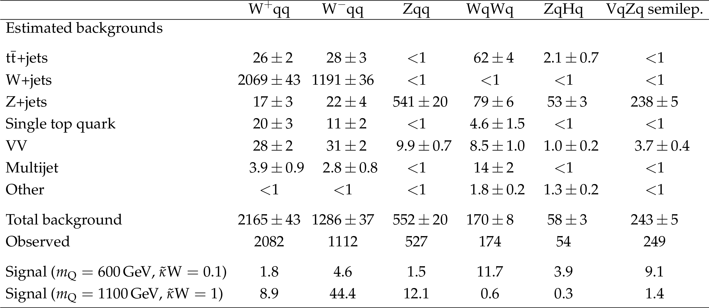
Table 5:
Event yields in the muon channel for the inclusive analysis, for the event categories with one or two isolated leptons. The $\mathrm{ W^{+} } \mathrm{ q } \mathrm{ q } $ event category is not used in the search, but is shown for comparison, in order to demonstrate the expected lepton charge asymmetry. The indicated uncertainties are statistical only, originating from the limited number of MC events. The prediction for the signals is shown assuming branching fractions of $\mathcal {B}_\mathrm{ W } = $ 0.5 and $\mathcal {B}_\mathrm{ Z } = \mathcal {B}_\mathrm{ H } = $ 0.25. The label 'Other' designates the background originating from ${\mathrm{ t } {}\mathrm{ \bar{t} } } \mathrm{ W } $, ${\mathrm{ t } {}\mathrm{ \bar{t} } } \mathrm{ Z } $ and triboson processes. |
png pdf |
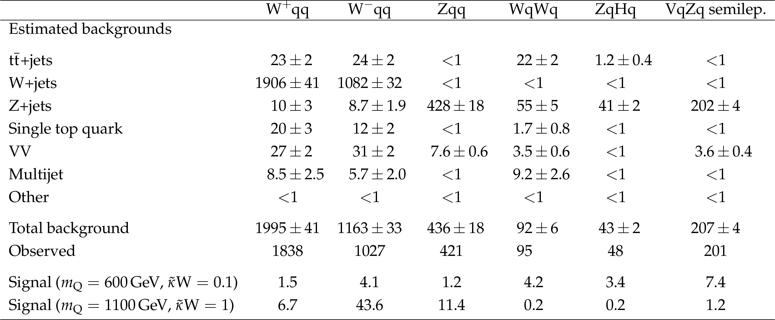
Table 6:
Event yields in the electron channel for the inclusive analysis, for the event categories with one or two isolated leptons. The $\mathrm{ W^{+} } \mathrm{ q } \mathrm{ q } $ event category is not used in the search, but is shown for comparison, in order to demonstrate the expected lepton charge asymmetry. The indicated uncertainties are statistical only, originating from the limited number of MC events. The prediction for the signals is shown assuming branching fractions of $\mathcal {B}_\mathrm{ W } = $ 0.5 and $\mathcal {B}_\mathrm{ Z } = \mathcal {B}_\mathrm{ H } = $ 0.25. The label 'Other' designates the background evaluated to originating from ${\mathrm{ t } {}\mathrm{ \bar{t} } } \mathrm{ W } $, ${\mathrm{ t } {}\mathrm{ \bar{t} } } \mathrm{ Z } $ and triboson processes. |
png pdf |
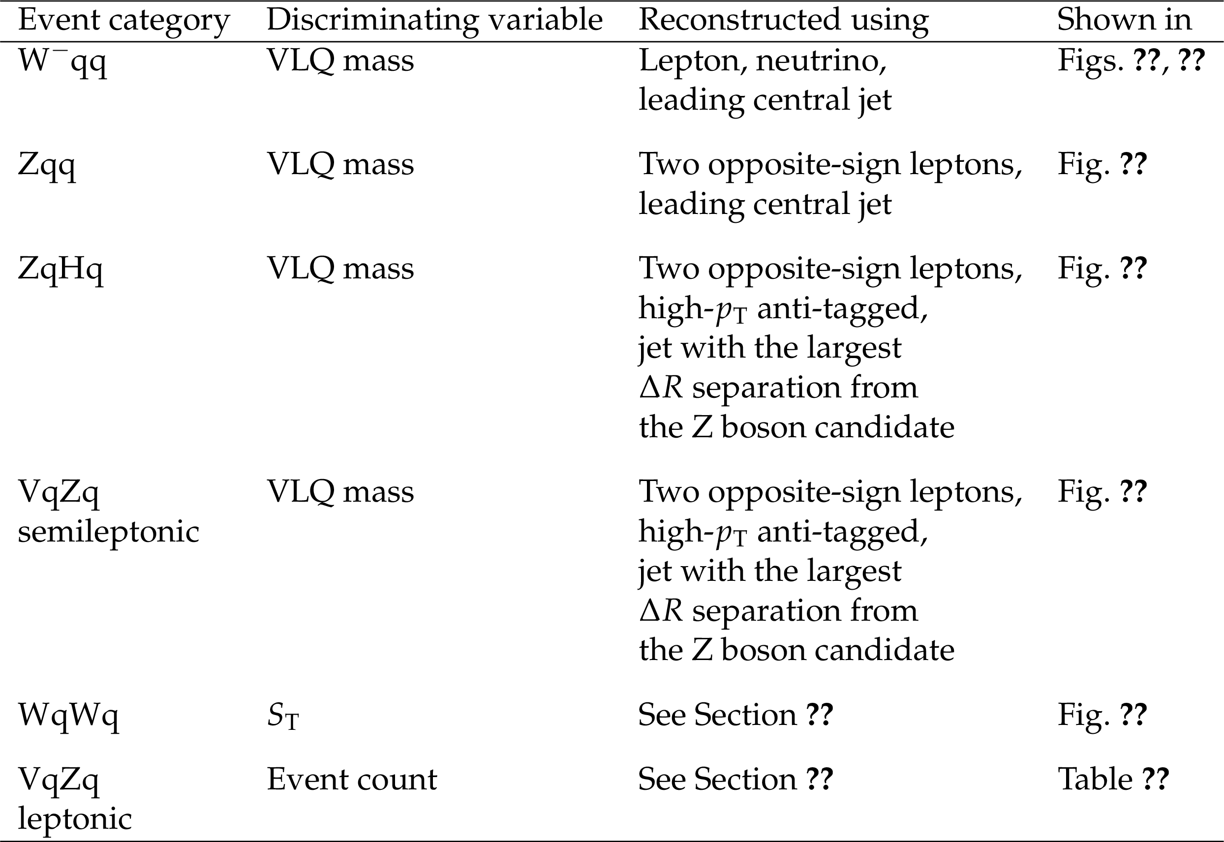
Table 7:
Discriminating variables used for the different event categories. |
png pdf |
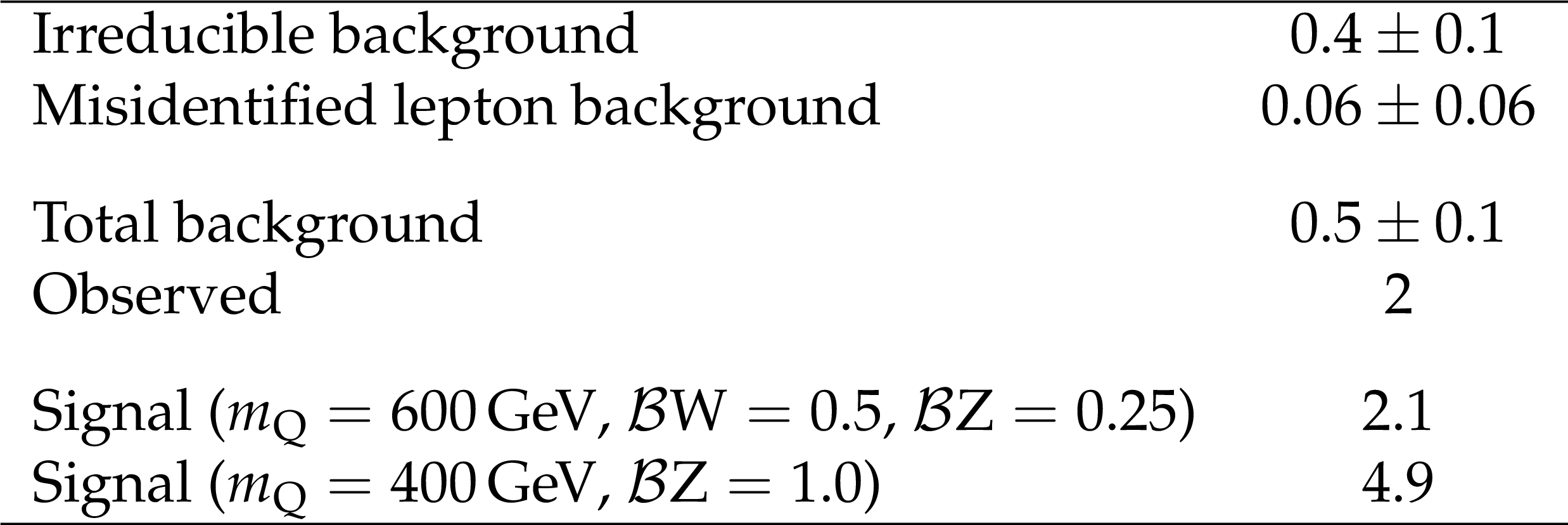
Table 8:
The total number of estimated background events compared to the number of observed events, in the leptonic $ {\mathrm {V}} \mathrm{ q } {\mathrm{ Z } } \mathrm{ q } $ event category, with either 3 or 4 leptons. The numbers of expected signal events for two different signal hypotheses are shown. The indicated uncertainties are statistical only, originating from the limited number of MC events. |
png pdf |
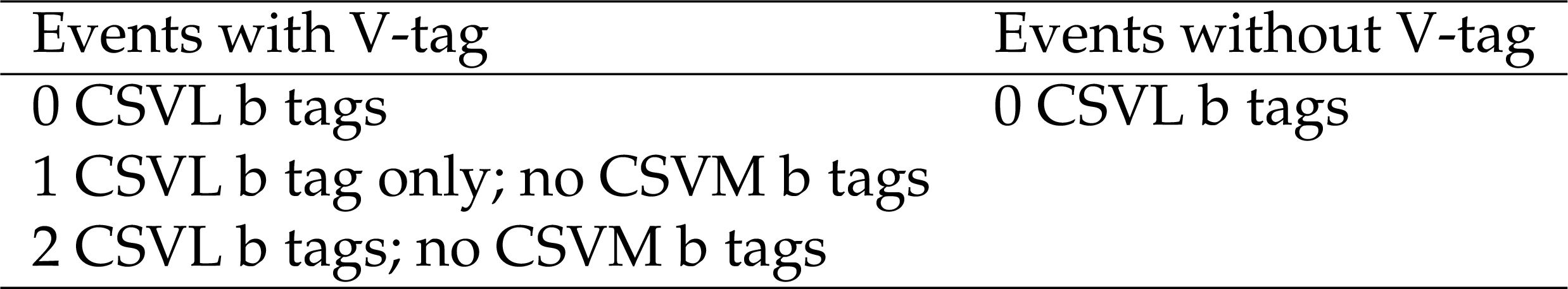
Table 9:
Combinations of pairs of jets that have not been identified as V-jet matches, which can be accepted for matching to the quark pair $\{\mathrm{ q } _\ell, \mathrm{ q } _{\mathrm {h}}\}$. In the left column, the group with the lowest available b-tag content is chosen, and within that group, the combination with the lowest $\chi ^2$ is selected. In the right column, only anti-tagged category is accepted. |
png pdf |
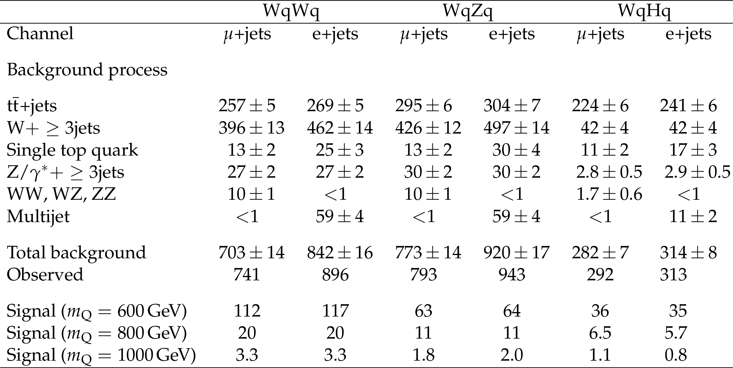
Table 10:
Numbers of expected background events from simulation and of data events in the $\mathrm{ W } \mathrm{ q } \mathrm{ W } \mathrm{ q } $, $\mathrm{ W } \mathrm{ q } {\mathrm{ Z } } \mathrm{ q } $, and $\mathrm{ W } \mathrm{ q } \mathrm{ H } \mathrm{ q } $ channels after applying the event selection. The uncertainties in the estimated backgrounds are statistical only. |
png pdf |
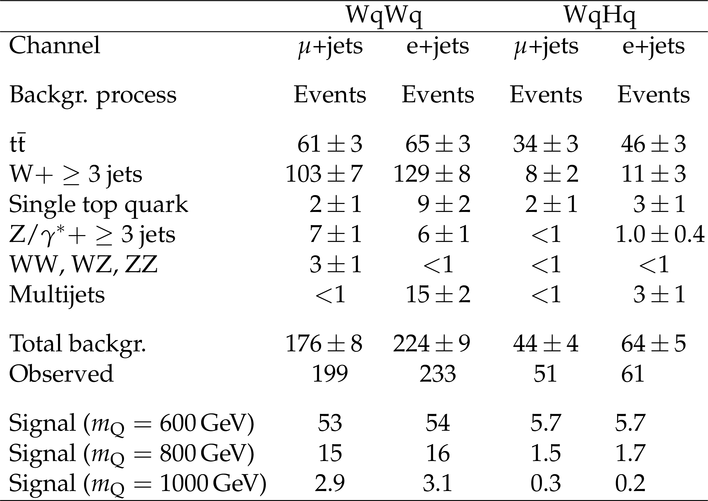
Table 11:
Numbers of expected background events from simulation and of data events in the $\mathrm{ W } \mathrm{ q } \mathrm{ W } \mathrm{ q } $ and $\mathrm{ W } \mathrm{ q } \mathrm{ H } \mathrm{ q } $ channels, after the application of the $S_\mathrm {T} >$ 1240 GeV requirement. Events in the $\mathrm{ W } \mathrm{ q } \mathrm{ H } \mathrm{ q } $ channel that also appear in the $\mathrm{ W } \mathrm{ q } \mathrm{ W } \mathrm{ q } $ channel are excluded. The uncertainties in the estimated backgrounds are statistical only. |
png pdf |
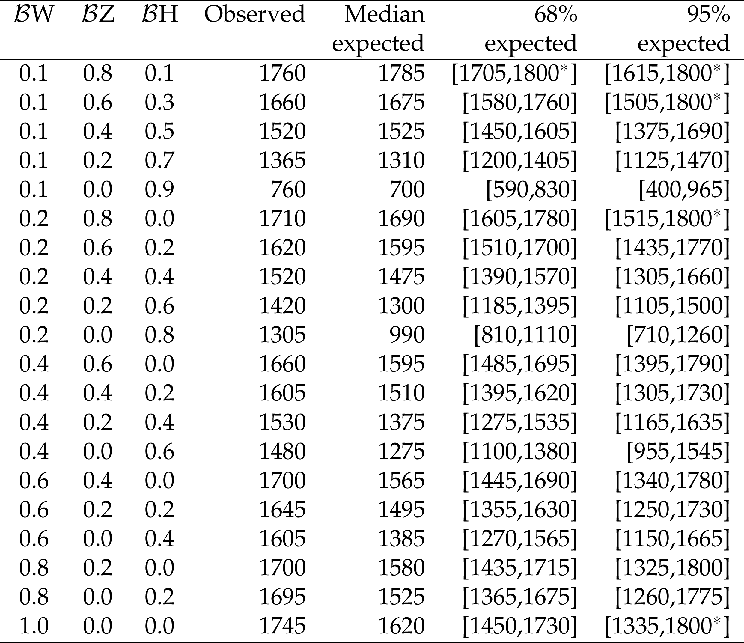
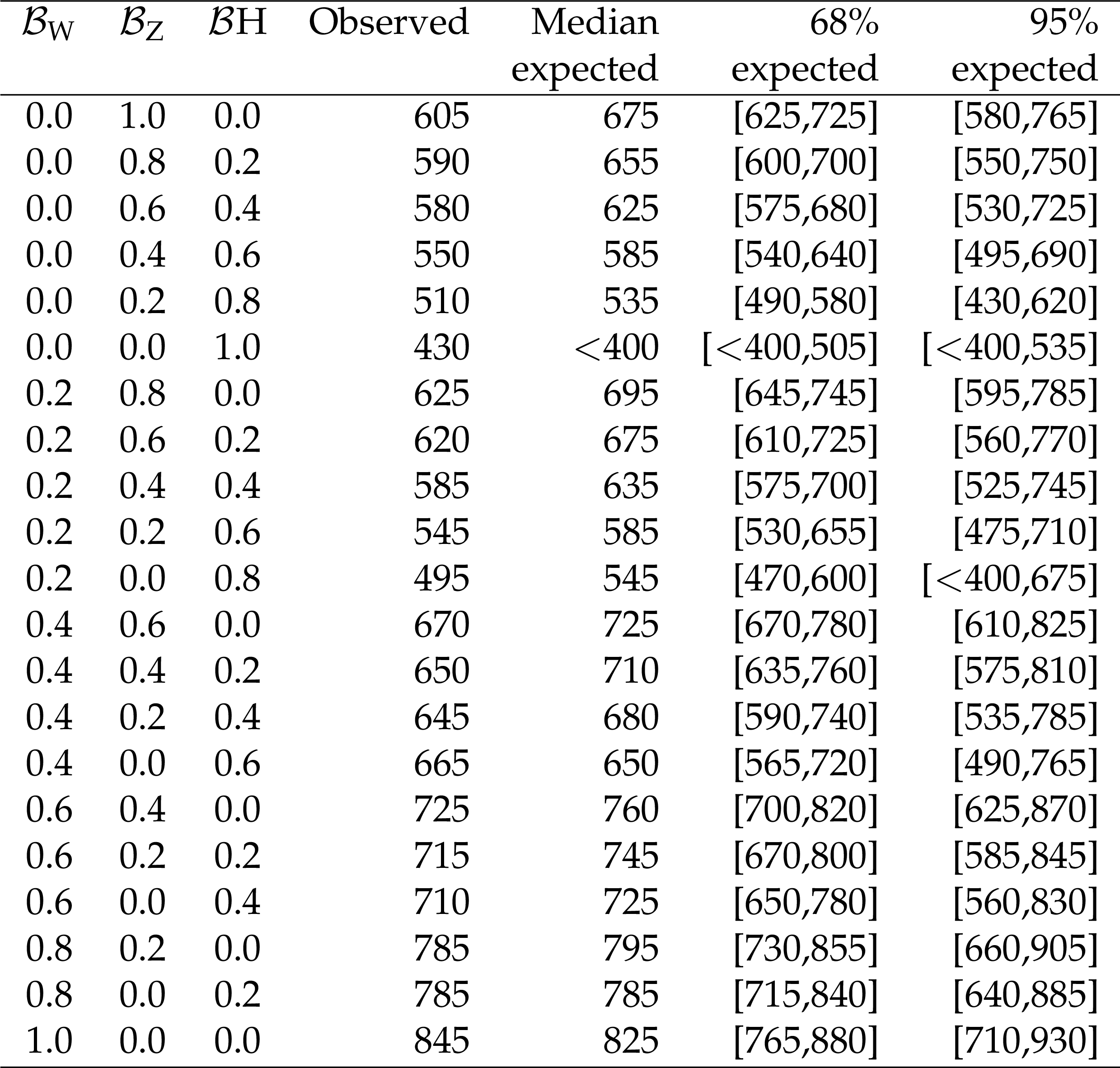
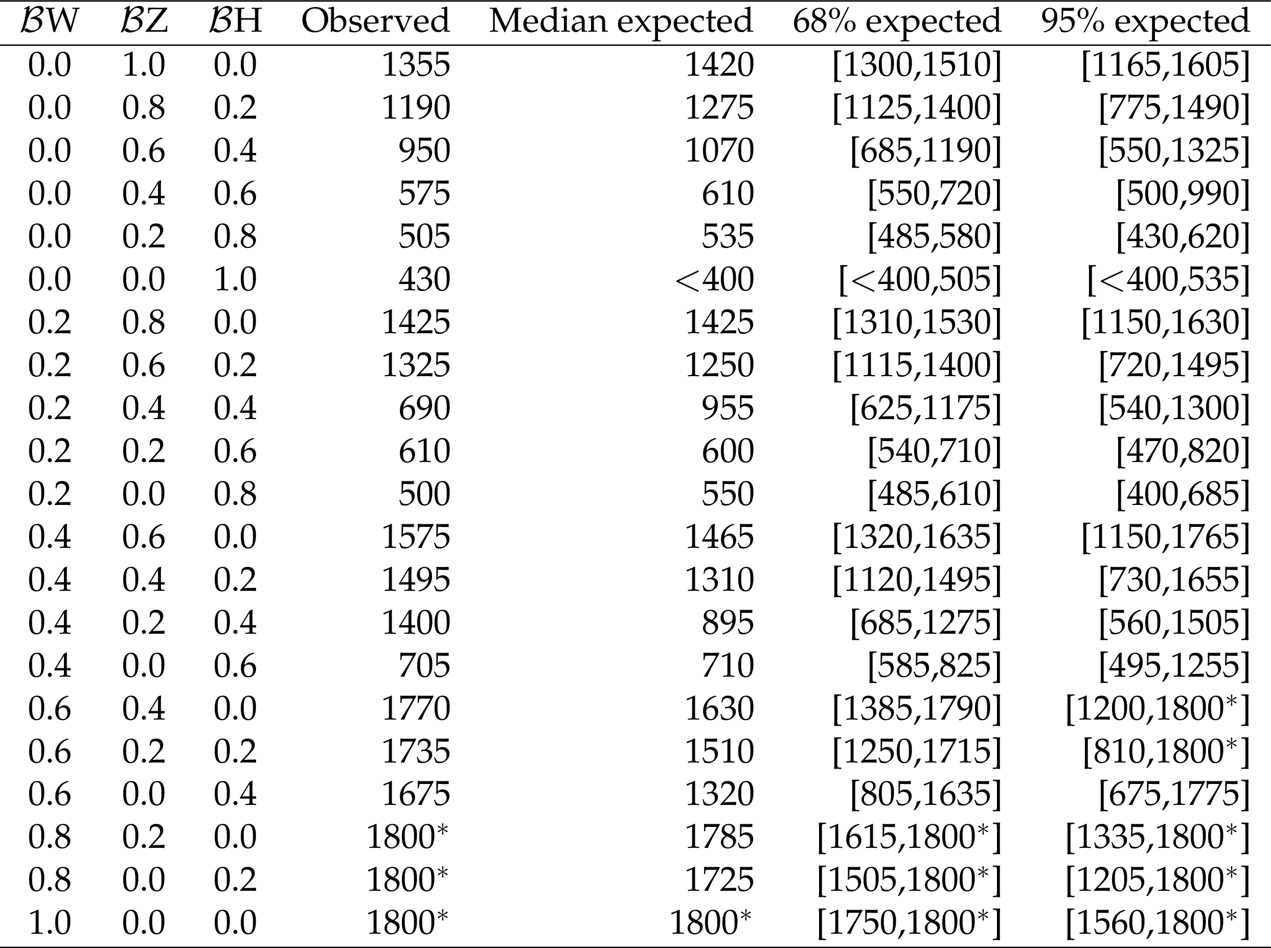
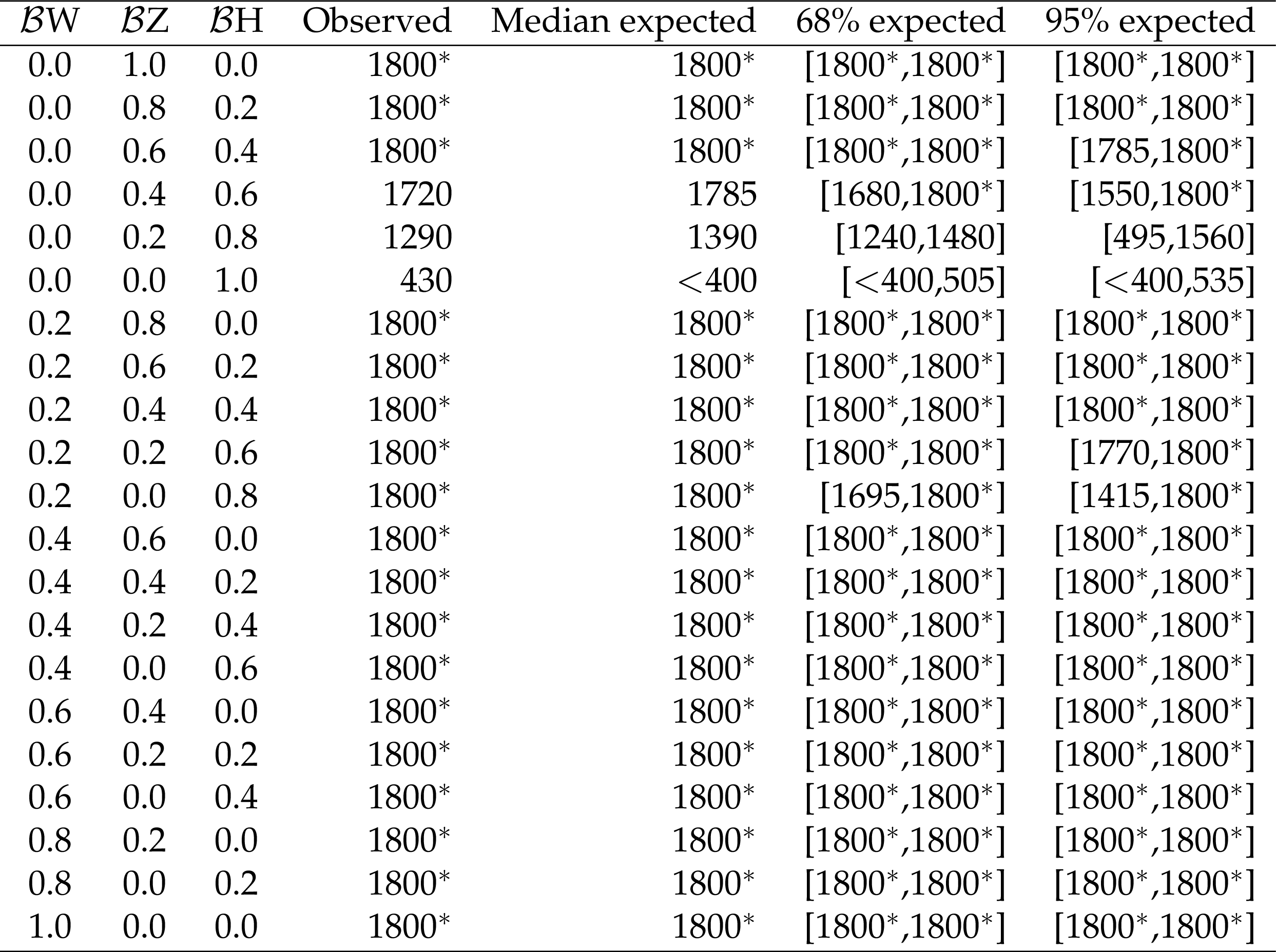
Table 12:
Observed and median expected lower limits on the VLQ mass (in GeV ) at 95% CL, or greater than 95% CL when indicated with $*$, for a range of different combinations of decay branching fractions. The ranges containing 68 and 95%, respectively, of the distribution of limits expected under the background-only hypothesis, are also given. The limits are determined assuming $\tilde{\kappa }_\mathrm{ W } = $ 1.0. |
png pdf |
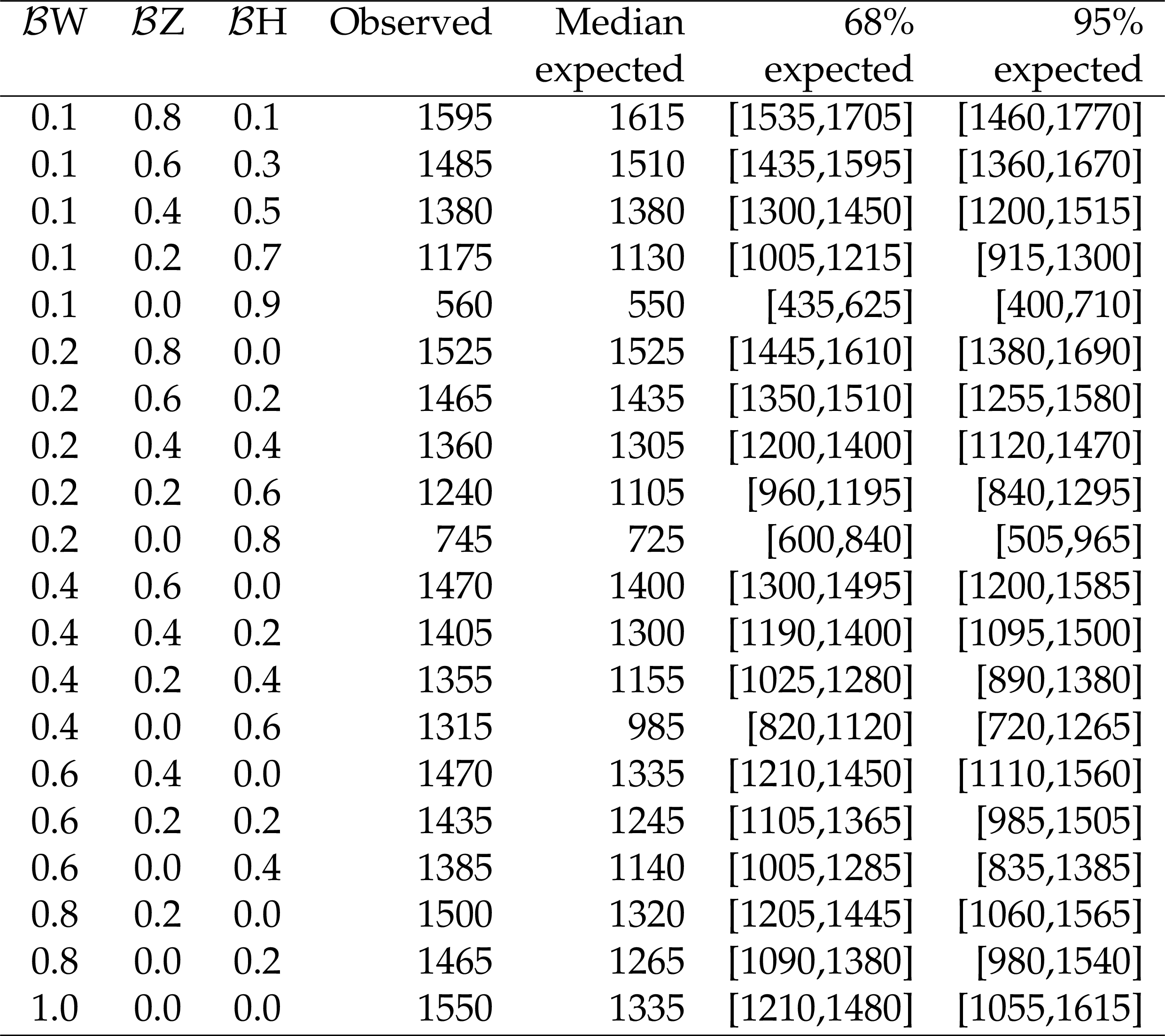
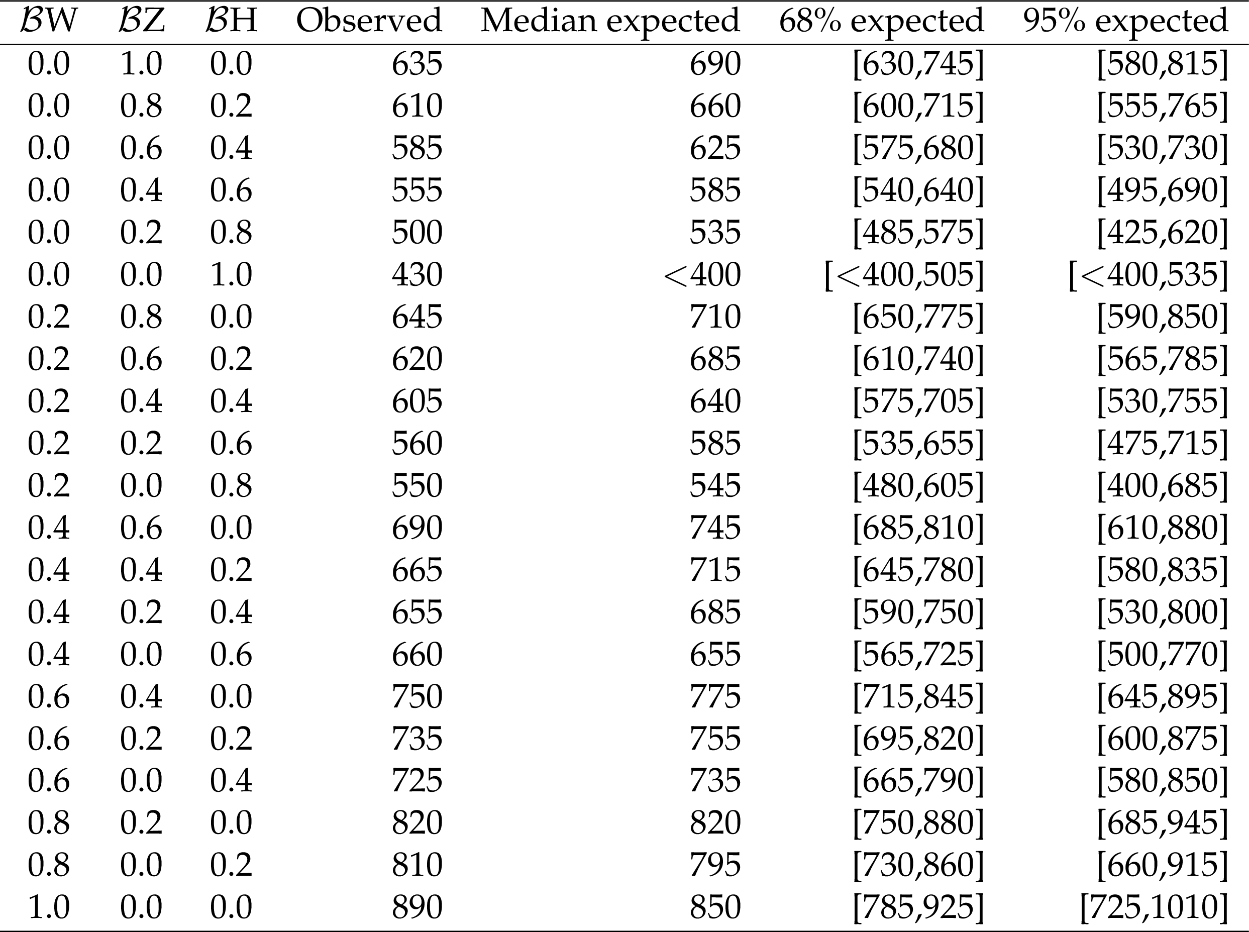
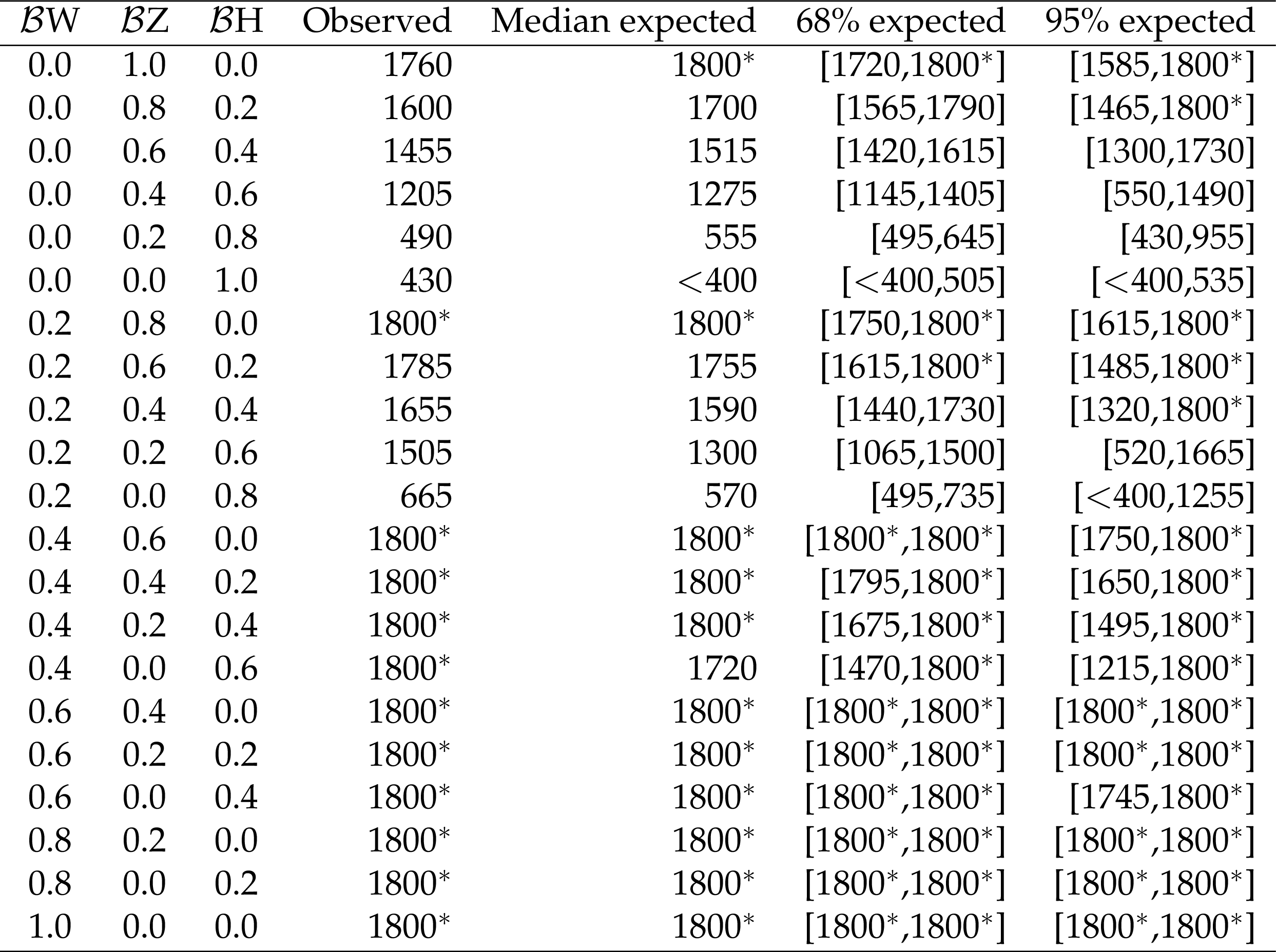
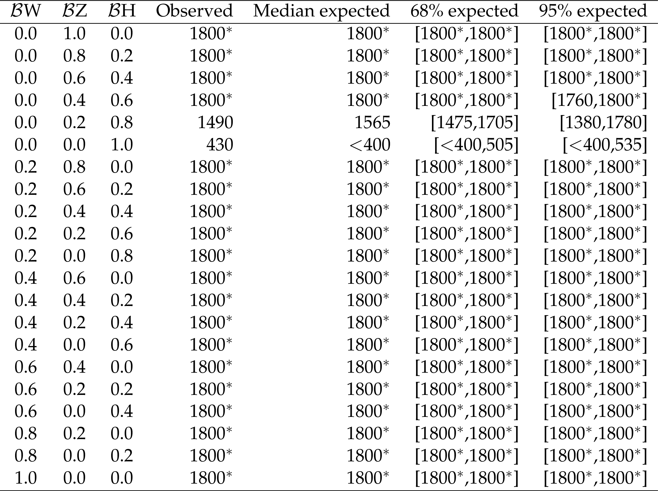
Table 13:
Observed and median expected lower limits on the VLQ mass (in GeV ) at 95% CL, for a range of different combinations of decay branching fractions. The ranges containing 68 and 95%, respectively, of the distribution of limits expected under the background-only hypothesis, are also given. The limits were determined using $\tilde{\kappa }_\mathrm{ W } = $ 0.7. |
png pdf |
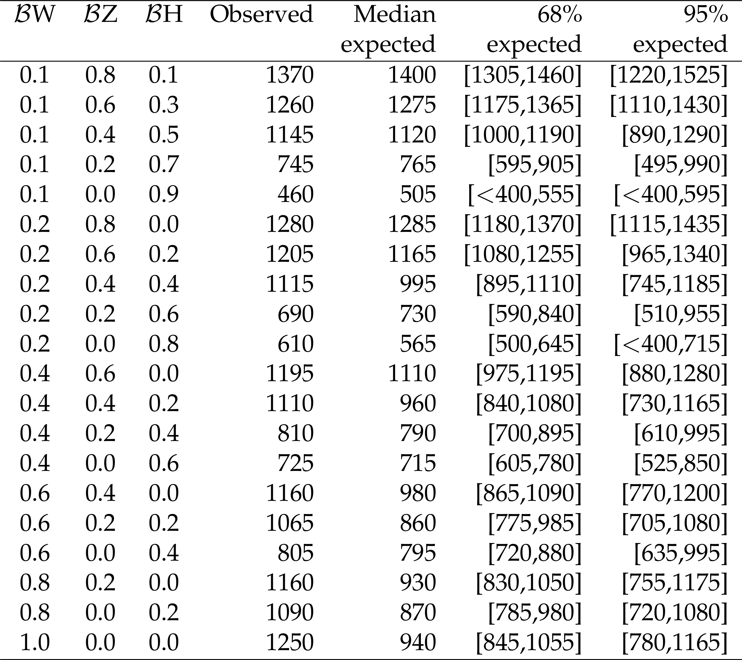
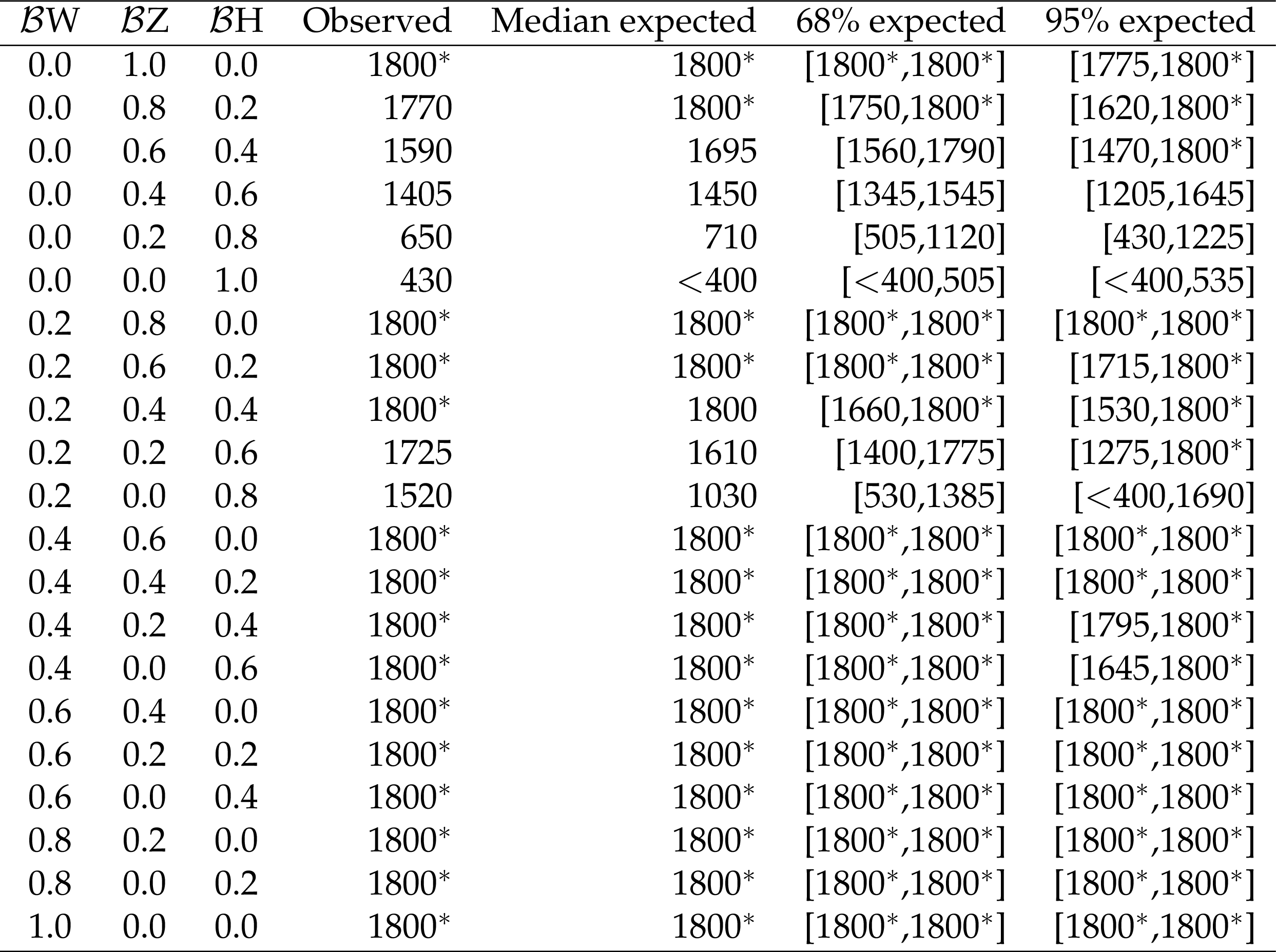
Table 14:
Observed and median expected lower limits on the VLQ mass (in GeV ) at 95% CL, for a range of different combinations of decay branching fractions. The ranges containing 68 and 95%, respectively, of the distribution of limits expected under the background-only hypothesis, are also given. The limits are determined assuming $\tilde{\kappa }_\mathrm{ W } = $ 0.4. |
png pdf |
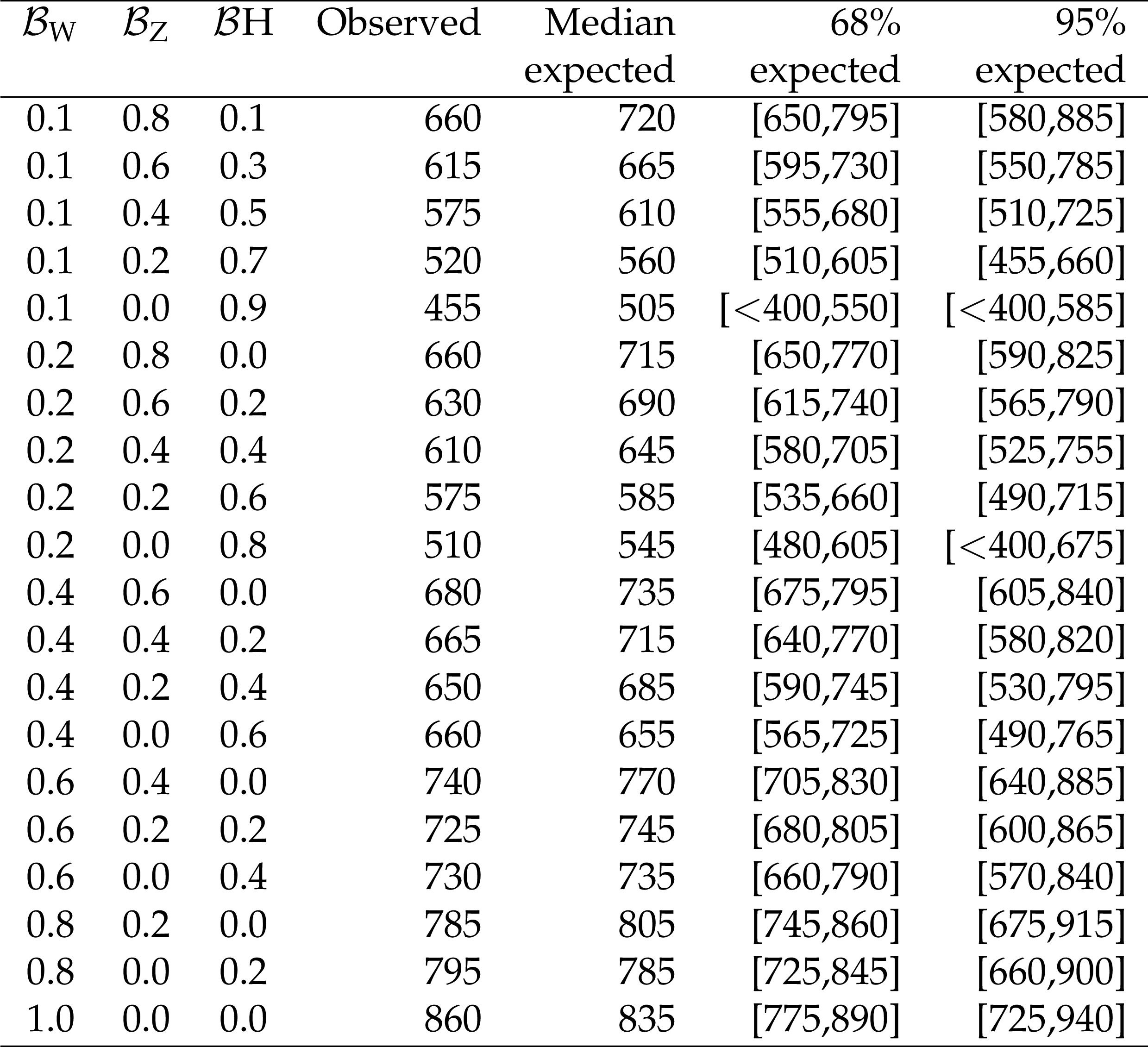
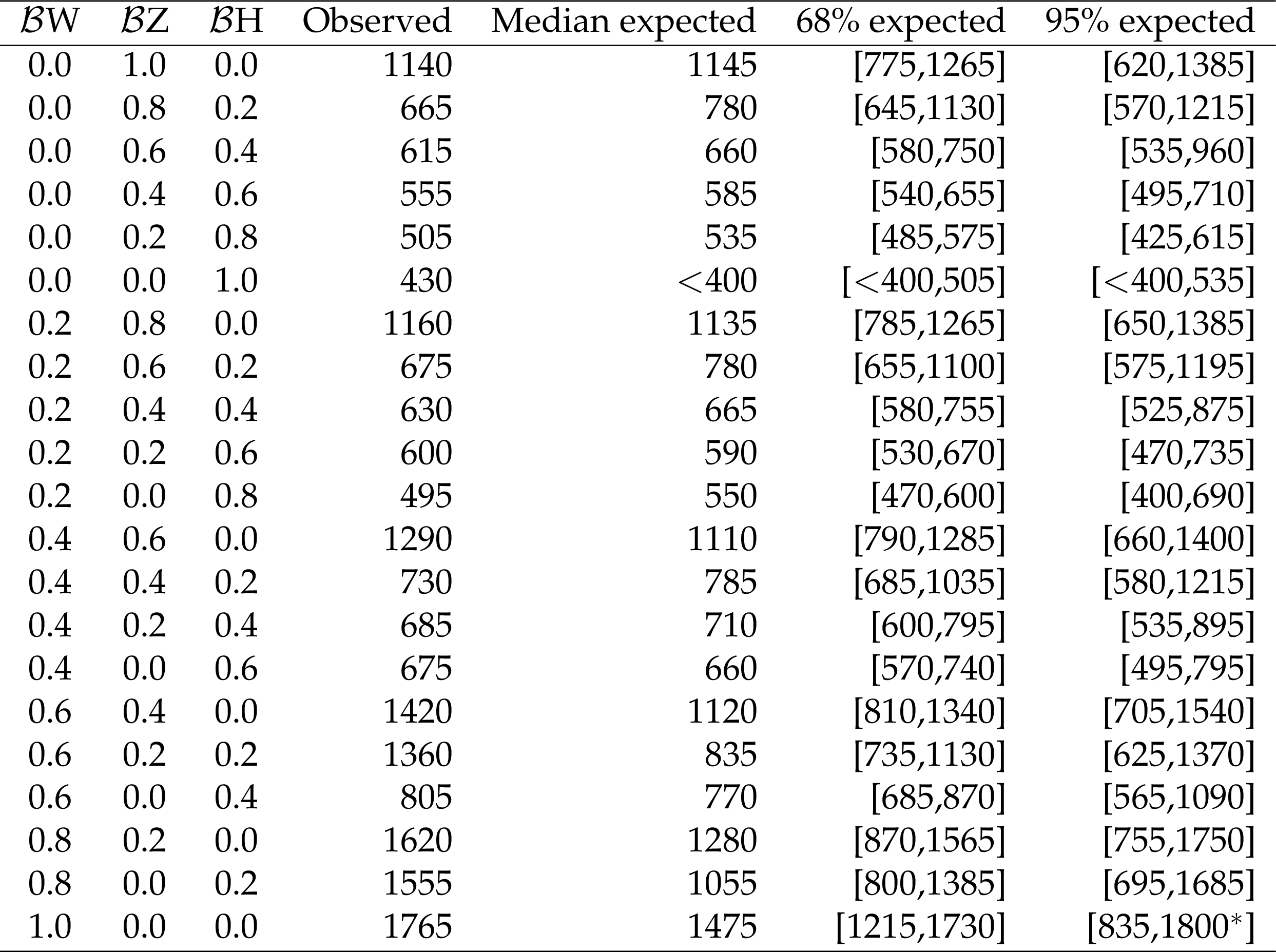
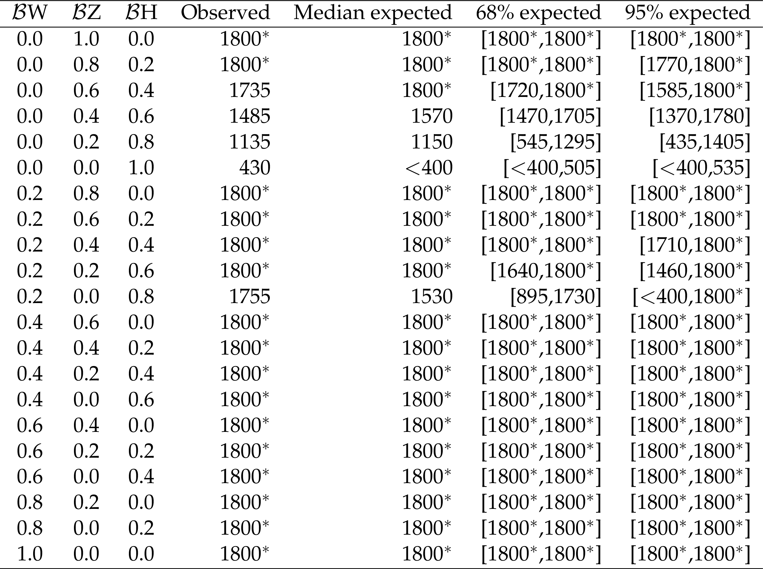
Table 15:
Observed and median expected lower limits on the VLQ mass (in GeV ) at 95% CL, for a range of different combinations of decay branching fractions. The ranges containing 68 and 95%, respectively, of the distribution of limits expected under the background-only hypothesis, are also given. The limits were determined assuming $\tilde{\kappa }_\mathrm{ W } = $ 0.1. |
png pdf |
Table 16:
Observed and median expected lower limits on the VLQ mass (in GeV ) at 95% CL, for a range of different combinations of decay branching fractions. The ranges containing 68 and 95%, respectively, of the distribution of limits expected under the background-only hypothesis, are also given. The limits are determined under the assumption that pair production is the only available VLQ production mechanism. |
png pdf |
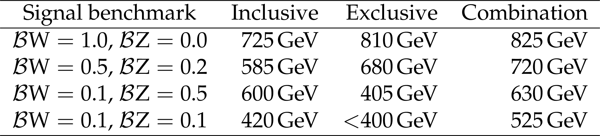
Table 17:
Comparison of several expected 95% CL lower mass limits for signal pair production only, illustrating the added sensitivity of the two analyses in the combination. |
png pdf |
Table A1:
Observed and median expected lower limits on the VLQ mass (in GeV) at 95% CL, or greater than 95% CL when indicated with $*$, for a range of different combinations of decay branching fractions. The ranges containing 68 and 95%, respectively, of the distribution of limits expected under the background-only hypothesis, are also given. The limits are determined assuming $\kappa_{\mathrm{D}}= $ 0.05. |
png pdf |
Table A2:
Observed and median expected lower limits on the VLQ mass (in GeV) at 95% CL, or greater than 95% CL when indicated with $*$, for a range of different combinations of decay branching fractions. The ranges containing 68 and 95%, respectively, of the distribution of limits expected under the background-only hypothesis, are also given. The limits are determined assuming $\kappa_{\mathrm{D}}= $ 0.1. |
png pdf |
Table A3:
Observed and median expected lower limits on the VLQ mass (in GeV) at 95% CL, or greater than 95% CL when indicated with $*$, for a range of different combinations of decay branching fractions. The ranges containing 68 and 95%, respectively, of the distribution of limits expected under the background-only hypothesis, are also given. The limits are determined assuming $\kappa_{\mathrm{D}}= $ 0.15. |

png pdf |
Table A4:
Observed and median expected lower limits on the VLQ mass (in GeV) at 95% CL, or greater than 95% CL when indicated with $*$, for a range of different combinations of decay branching fractions. The ranges containing 68 and 95%, respectively, of the distribution of limits expected under the background-only hypothesis, are also given. The limits are determined assuming $\kappa_{\mathrm{D}}= $ 0.2. |
png pdf |
Table A5:
Observed and median expected lower limits on the VLQ mass (in GeV) at 95% CL, or greater than 95% CL when indicated with $*$, for a range of different combinations of decay branching fractions. The ranges containing 68 and 95%, respectively, of the distribution of limits expected under the background-only hypothesis, are also given. The limits are determined assuming $\kappa_{\mathrm{D}}= $ 0.3. |
png pdf |
Table A6:
Observed and median expected lower limits on the VLQ mass (in GeV) at 95% CL, or greater than 95% CL when indicated with $*$, for a range of different combinations of decay branching fractions. The ranges containing 68 and 95%, respectively, of the distribution of limits expected under the background-only hypothesis, are also given. The limits are determined assuming $\kappa_{\mathrm{D}}= $ 0.4. |
png pdf |
Table A7:
Observed and median expected lower limits on the VLQ mass (in GeV) at 95% CL, or greater than 95% CL when indicated with $*$, for a range of different combinations of decay branching fractions. The ranges containing 68 and 95%, respectively, of the distribution of limits expected under the background-only hypothesis, are also given. The limits are determined assuming $\kappa_{\mathrm{D}}= $ 0.5. |

png pdf |
Table A8:
Observed and median expected lower limits on the VLQ mass (in GeV) at 95% CL, or greater than 95% CL when indicated with $*$, for a range of different combinations of decay branching fractions. The ranges containing 68 and 95%, respectively, of the distribution of limits expected under the background-only hypothesis, are also given. The limits are determined assuming $\kappa_{\mathrm{D}}= $ 0.6. |
png pdf |
Table A9:
Observed and median expected lower limits on the VLQ mass (in GeV) at 95% CL, or greater than 95% CL when indicated with $*$, for a range of different combinations of decay branching fractions. The ranges containing 68 and 95%, respectively, of the distribution of limits expected under the background-only hypothesis, are also given. The limits are determined assuming $\kappa_{\mathrm{D}}= $ 0.7. |

png pdf |
Table A10:
Observed and median expected lower limits on the VLQ mass (in GeV) at 95% CL, or greater than 95% CL when indicated with $*$, for a range of different combinations of decay branching fractions. The ranges containing 68 and 95%, respectively, of the distribution of limits expected under the background-only hypothesis, are also given. The limits are determined assuming $\kappa_{\mathrm{D}}= $ 0.8. |

png pdf |
Table A11:
Observed and median expected lower limits on the VLQ mass (in GeV) at 95% CL, or greater than 95% CL when indicated with $*$, for a range of different combinations of decay branching fractions. The ranges containing 68 and 95%, respectively, of the distribution of limits expected under the background-only hypothesis, are also given. The limits are determined assuming $\kappa_{\mathrm{D}}= $ 0.9. |
png pdf |
Table A12:
Observed and median expected lower limits on the VLQ mass (in GeV) at 95% CL, or greater than 95% CL when indicated with $*$, for a range of different combinations of decay branching fractions. The ranges containing 68 and 95%, respectively, of the distribution of limits expected under the background-only hypothesis, are also given. The limits are determined assuming $\kappa_{\mathrm{D}}= $ 1. |
| Summary |
| A search has been performed for the single and pair production of vector-like quarks, coupled to light quarks, in proton-proton collisions at $\sqrt{s} = $ 8 TeV at the LHC. In the single-production mode the search has been performed for down-type quarks (electric charge of magnitude 1/3), while in the pair-production mode the search is sensitive to decays of vector-like quarks into up, down and strange quarks. Inclusive and exclusive approaches have been used to perform this search. No significant excess over standard model expectations has been observed. Lower limits on the mass of the vector-like quarks have been determined by combining the results from both the single- and pair-production searches. Limits have also been extracted using the data from the pair-production search alone. For all processes considered, including single production, the lower mass limits range from 400 to 1800 GeV, depending on the vector-like quark branching fractions for decays to W, Z, and Higgs bosons and the assumed value of the electroweak single-production strength. When considering pair production alone, vector-like quarks with masses below 845 GeV (825 GeV expected) are excluded for $\mathcal{B}(\mathrm{ W }) = $ 1.0, and with masses below 685 GeV (720 GeV expected), for the widely adopted benchmark with $\mathcal{B}(\mathrm{ W }) = $ 0.5, $\mathcal{B}(\mathrm{ Z }) = \mathcal{B}(\mathrm{ H }) = $ 0.25. These results provide the most stringent mass limits to date on vector-like quarks that couple to light quarks and that are produced either singly or in pairs. |
| References | ||||
| 1 | D. Choudhury, T. M. P. Tait, and C. E. M. Wagner | Beautiful mirrors and precision electroweak data | PRD 65 (2002) 053002 | hep-ph/0109097 |
| 2 | N. Arkani-Hamed, A. G. Cohen, E. Katz, and A. E. Nelson | The littlest Higgs | JHEP 07 (2002) 034 | hep-ph/0206021 |
| 3 | M. Schmaltz | Physics beyond the standard model (theory): Introducing the little Higgs | NPPS 117 (2003) 40 | hep-ph/0210415 |
| 4 | M. Schmaltz and D. Tucker-Smith | Little Higgs review | Ann. Rev. Nucl. Part. Sci 55 (2005) 229 | hep-ph/0502182 |
| 5 | D. Marzocca, M. Serone, and J. Shu | General composite Higgs models | JHEP 08 (2012) 013 | 1205.0770 |
| 6 | H.-C. Cheng, B. A. Dobrescu, and C. T. Hill | Electroweak symmetry breaking and extra dimensions | NPB 589 (2000) 249 | hep-ph/9912343 |
| 7 | J. Kang, P. Langacker, and B. D. Nelson | Theory and phenomenology of exotic isosinglet quarks and squarks | PRD 77 (2008) 035003 | 0708.2701 |
| 8 | D. Guadagnoli, R. N. Mohapatra, and I. Sung | Gauged flavor group with left-right symmetry | JHEP 04 (2011) 093 | 1103.4170 |
| 9 | A. Atre et al. | Model-independent searches for new quarks at the LHC | JHEP 08 (2011) 080 | 1102.1987 |
| 10 | J. A. Aguilar-Saavedra, R. Benbrik, S. Heinemeyer, and M. P\'erez-Victoria | A handbook of vector-like quarks: mixing and single production | PRD 88 (2013) 112003 | 1306.0572 |
| 11 | B. W. Lee, C. Quigg, and H. B. Thacker | Weak interactions at very high-energies: the role of the Higgs boson mass | PRD 16 (1977) 1519 | |
| 12 | ATLAS Collaboration | Search for heavy vector-like quarks coupling to light quarks in proton-proton collisions at $ \sqrt{s} = $ 7 TeV with the ATLAS detector | PLB 712 (2012) 22 | 1112.5755 |
| 13 | ATLAS Collaboration | Search for pair production of a new heavy quark that decays into a $ W $ boson and a light quark in $ pp $ collisions at $ \sqrt{s} = $ 8 TeV with the ATLAS detector | PRD 92 (2015) 112007 | 1509.04261 |
| 14 | M. Buchkremer, G. Cacciapaglia, A. Deandrea, and L. Panizzi | Model-independent framework for searches of top partners | NPB 876 (2013) 376 | 1305.4172 |
| 15 | CMS Collaboration | The CMS experiment at the CERN LHC | JINST 3 (2008) S08004 | CMS-00-001 |
| 16 | J. Alwall et al. | MadGraph 5: going beyond | JHEP 06 (2011) 128 | 1106.0522 |
| 17 | J. Pumplin et al. | New generation of parton distributions with uncertainties from global QCD analysis | JHEP 07 (2002) 012 | hep-ph/0201195 |
| 18 | T. Sjostrand, S. Mrenna, and P. Skands | PYTHIA 6.4 physics and manual | JHEP 05 (2006) 026 | hep-ph/0603175 |
| 19 | CMS Collaboration | Study of the underlying event at forward rapidity in pp collisions at $ \sqrt{s} = $ 0.9 , 2.76, and 7 TeV | JHEP 04 (2013) 072 | CMS-FWD-11-003 1302.2394 |
| 20 | CMS Collaboration | Event generator tunes obtained from underlying event and multiparton scattering measurements | EPJC 76 (2016) 155 | CMS-GEN-14-001 1512.00815 |
| 21 | P. Nason | A new method for combining NLO QCD with shower Monte Carlo algorithms | JHEP 11 (2004) 040 | hep-ph/0409146 |
| 22 | S. Frixione, P. Nason, and C. Oleari | Matching NLO QCD computations with parton shower simulations: the POWHEG method | JHEP 11 (2007) 070 | 0709.2092 |
| 23 | S. Alioli, P. Nason, C. Oleari, and E. Re | A general framework for implementing NLO calculations in shower Monte Carlo programs: the POWHEG BOX | JHEP 06 (2010) 043 | 1002.2581 |
| 24 | M. Czakon, P. Fiedler, and A. Mitov | Total top-quark pair-production cross section at hadron colliders through $ O(\alpha_S^4) $ | PRL 110 (2013) 252004 | 1303.6254 |
| 25 | CMS Collaboration | Measurement of the $ \mathrm{ t \bar{t} } $ production cross section in the dilepton channel in pp collisions at $ \sqrt{s}= $ 8 TeV | JHEP 02 (2014) 024 | CMS-TOP-12-007 1312.7582 |
| 26 | CMS Collaboration | Observation of the associated production of a single top quark and a $ W $ boson in $ pp $ collisions at $ \sqrt{s} = $ 8 TeV | PRL 112 (2014) 231802 | CMS-TOP-12-040 1401.2942 |
| 27 | CMS Collaboration | Measurement of the $ \mathrm{W}^+\mathrm{W}^- $ and ZZ production cross sections in pp collisions at $ \sqrt{s} = $ 8 TeV | PLB 721 (2013) 190 | |
| 28 | CMS Collaboration | Measurement of WZ and zz production in pp collisions at $ \sqrt{s} = $ 8 TeV in final states with b-tagged jets | EPJC 74 (2014) 2973 | CMS-SMP-13-011 1403.3047 |
| 29 | GEANT4 Collaboration | Geant4 -- a simulation toolkit | NIMA 506 (2003) 250 | |
| 30 | CMS Collaboration | Particle-flow reconstruction and global event description with the CMS detector | Submitted to JINST | CMS-PRF-14-001 1706.04965 |
| 31 | CMS Collaboration | Performance of electron reconstruction and selection with the CMS detector in proton-proton collisions at $ \sqrt{s} = $ 8 TeV | JINST 10 (2015) P06005 | CMS-EGM-13-001 1502.02701 |
| 32 | M. Cacciari, G. P. Salam, and G. Soyez | The anti-$ k_t $ jet clustering algorithm | JHEP 04 (2008) 063 | 0802.1189 |
| 33 | Y. L. Dokshitzer, G. D. Leder, S. Moretti, and B. R. Webber | Better jet clustering algorithms | JHEP 08 (1997) 001 | hep-ph/9707323 |
| 34 | M. Cacciari, G. P. Salam, and G. Soyez | FastJet user manual | EPJC 72 (2012) 1896 | 1111.6097 |
| 35 | M. Cacciari and G. P. Salam | Dispelling the $ N^{3} $ myth for the $ k_t $ jet-finder | PLB 641 (2006) 57 | hep-ph/0512210 |
| 36 | CMS Collaboration | Determination of jet energy calibration and transverse momentum resolution in CMS | JINST 6 (2011) P11002 | CMS-JME-10-011 1107.4277 |
| 37 | M. Cacciari, G. P. Salam, and G. Soyez | The catchment area of jets | JHEP 04 (2008) 005 | 0802.1188 |
| 38 | M. Cacciari and G. P. Salam | Pileup subtraction using jet areas | PLB 659 (2008) 119 | 0707.1378 |
| 39 | S. D. Ellis, C. K. Vermilion, and J. R. Walsh | Techniques for improved heavy particle searches with jet substructure | PRD 80 (2009) 051501 | 0903.5081 |
| 40 | S. D. Ellis, C. K. Vermilion, and J. R. Walsh | Recombination algorithms and jet substructure: Pruning as a tool for heavy particle searches | PRD 81 (2010) 094023 | 0912.0033 |
| 41 | CMS Collaboration | Identification of b-quark jets with the CMS experiment | JINST 8 (2013) P04013 | CMS-BTV-12-001 1211.4462 |
| 42 | C. Collaboration | Performance of b tagging at $ \sqrt{s} = $ 8 TeV in multijet, $ \mathrm{ t \bar{t} } $ and boosted topology events | CMS-PAS-BTV-13-001 | CMS-PAS-BTV-13-001 |
| 43 | H. Sumowidagdo | HitFit: A Kinematic Fitter for Complete Reconstruction of Top Quark-Antitop Quark Lepton+Jets Events | link | |
| 44 | S. S. Snyder | Measurement of the top quark mass at D0 | FERMILAB-THESIS-1995-27, State University of New York, Stony Brook | |
| 45 | Particle Data Group, C. Patrignani et al. | Review of Particle Physics | CPC 40 (2016), no. 10, 100001 | |
| 46 | CMS Collaboration | Performance of quark/gluon discrimination using pp collision data at $ \sqrt{s} = $ 8 TeV | CMS-PAS-JME-13-002 | CMS-PAS-JME-13-002 |
| 47 | CMS Collaboration | Search for vector-like charge 2/3 T quarks in proton-proton collisions at $ \sqrt{s} = $ 8 TeV | PRD 93 (2016) 012003 | CMS-B2G-13-005 1509.04177 |
| 48 | CMS Collaboration | Measurement of the differential cross section for top quark pair production in pp collisions at $ \sqrt{s} = $ 8 TeV | EPJC 75 (2015) 542 | CMS-TOP-12-028 1505.04480 |
| 49 | CMS Collaboration | CMS luminosity based on pixel cluster counting -- Summer 2013 update | CMS-PAS-LUM-13-001 | CMS-PAS-LUM-13-001 |
| 50 | P. M. Nadolsky et al. | Implications of CTEQ global analysis for collider observables | PRD 78 (2008) 013004 | 0802.0007 |
|
|
Compact Muon Solenoid LHC, CERN |
|

|

|

|

|

|