

Compact Muon Solenoid
LHC, CERN
| CMS-BPH-18-003 ; CERN-EP-2021-085 | ||
| Measurement of prompt open-charm production cross sections in proton-proton collisions at $\sqrt{s} = $ 13 TeV | ||
| CMS Collaboration | ||
| 3 July 2021 | ||
| JHEP 11 (2021) 225 | ||
| Abstract: The production cross sections for prompt open-charm mesons in proton-proton collisions at a center-of-mass energy of 13 TeV are reported. The measurement is performed using a data sample collected by the CMS experiment corresponding to an integrated luminosity of 29 nb$^{-1}$. The differential production cross sections of the ${{\mathrm{D}^{\ast}(2010)^{\pm}}}$, ${\mathrm{D^{\pm}}}$, and ${\mathrm{D^0}}$ ($\mathrm{\overline{D}{}^{0}}$) mesons are presented in ranges of transverse momentum and pseudorapidity 4 $ < {p_{\mathrm{T}}} < $ 100 GeV and $|{\eta}| < $ 2.1, respectively. The results are compared to several theoretical calculations and to previous measurements. | ||
| Links: e-print arXiv:2107.01476 [hep-ex] (PDF) ; CDS record ; inSPIRE record ; HepData record ; CADI line (restricted) ; | ||
| Figures | |
png pdf |
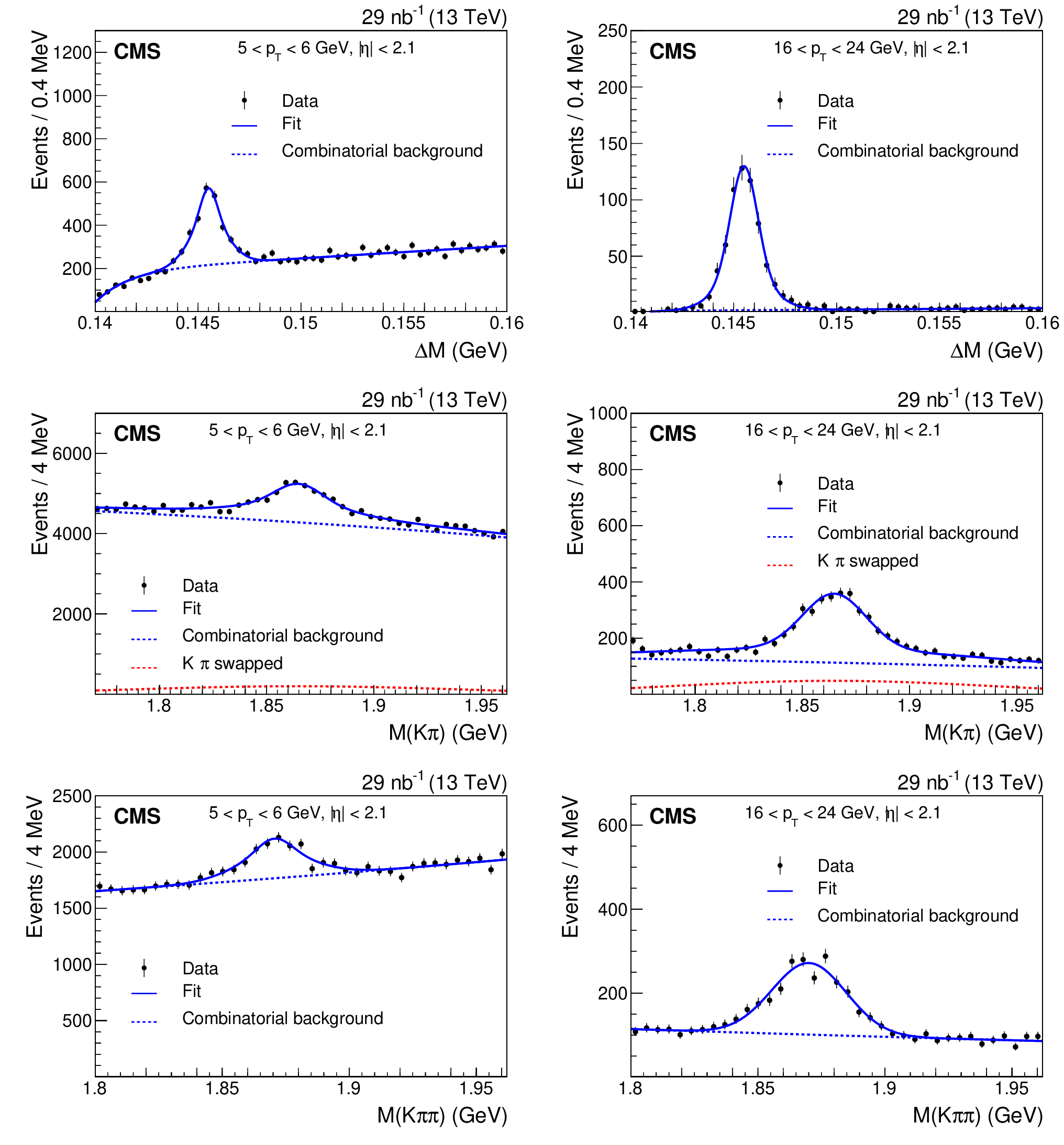
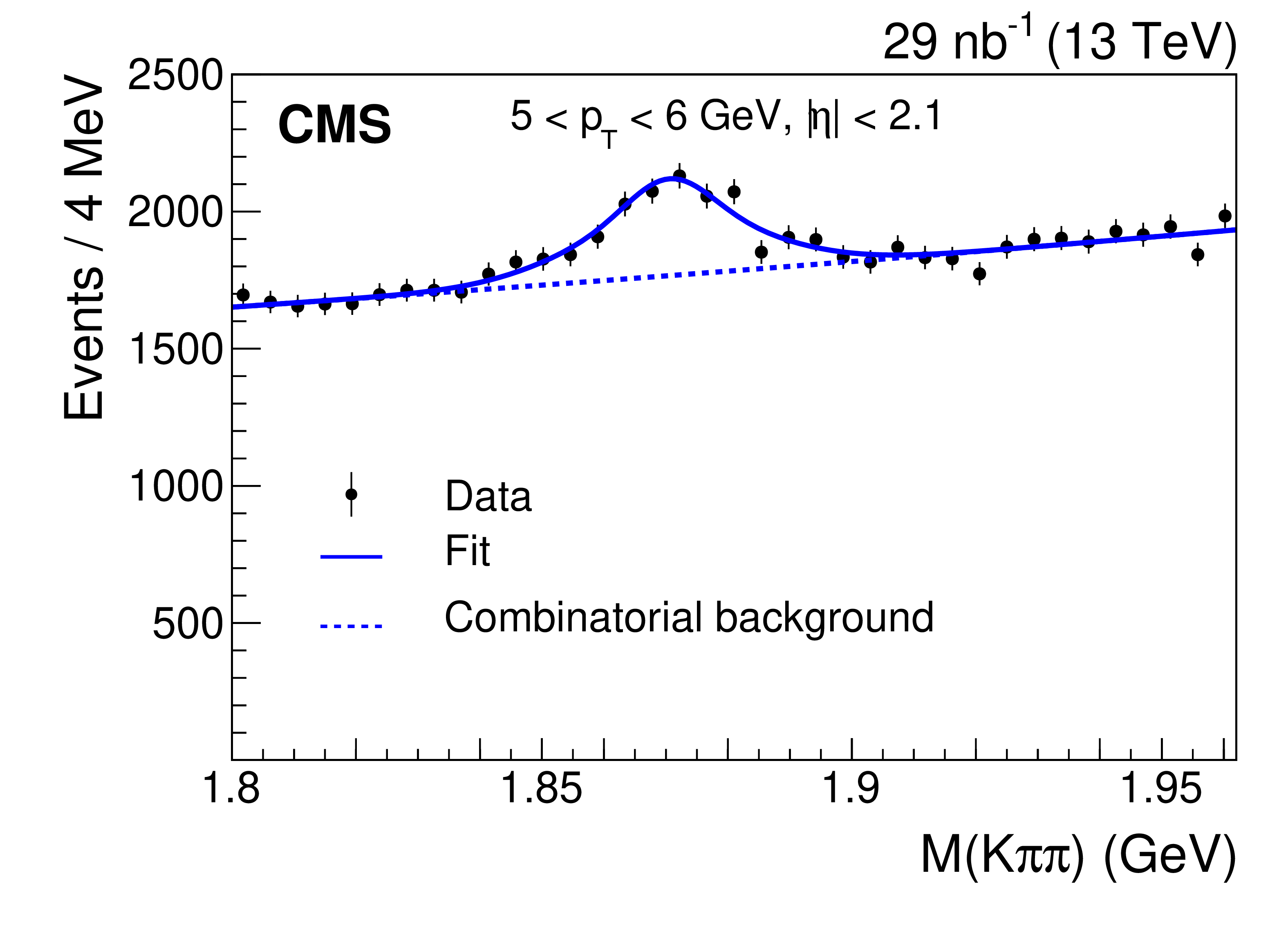
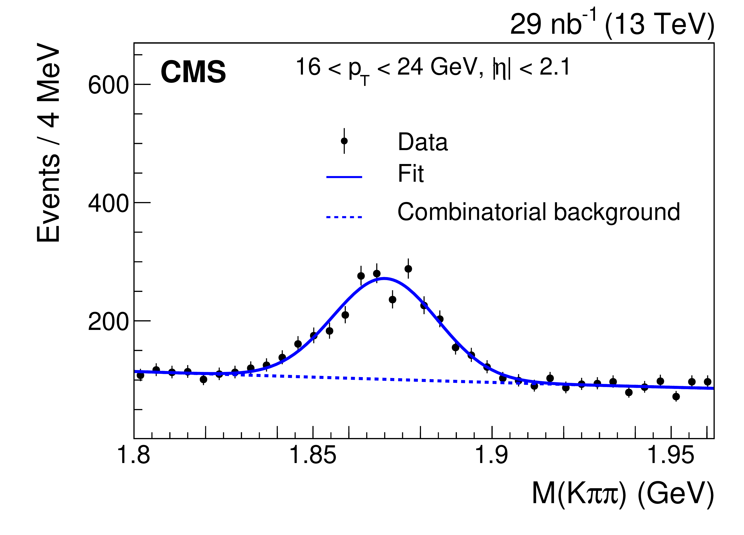
Figure 1:
The invariant mass distributions: $\Delta M = M(\mathrm{K^{-}} \pi^{+} {\pi ^+_{\mathrm {s}}}) - M(\mathrm{K^{-}} \pi^{+})$ (upper), $M(\mathrm{K^{-}} \pi^{+})$ (middle), and $M(\mathrm{K^{-}} \pi^{+} \pi^{+})$ (lower); charge conjugation is implied. Plots in the left column show the 5 $ < {p_{\mathrm {T}}} < $ 6 GeV bin, while the 16 $ < {p_{\mathrm {T}}} < $ 24 GeV bin is shown in the right column. The vertical bars on the points represent the statistical uncertainties in the data. The overall result from the fit is shown by the solid line, the fit to the combinatorial background by the dotted line, and, in the middle plots, the fit to the K/$\pi$ swapped candidates by the red dot-dashed line. |

png pdf |
Figure 1-a:
The $\Delta M = M(\mathrm{K^{-}} \pi^{+} {\pi ^+_{\mathrm {s}}}) - M(\mathrm{K^{-}} \pi^{+})$ invariant mass distribution in the 5 $ < {p_{\mathrm {T}}} < $ 6 GeV bin ; charge conjugation is implied. The vertical bars on the points represent the statistical uncertainties in the data. The overall result from the fit is shown by the solid line, the fit to the combinatorial background by the dotted line. |
png pdf |
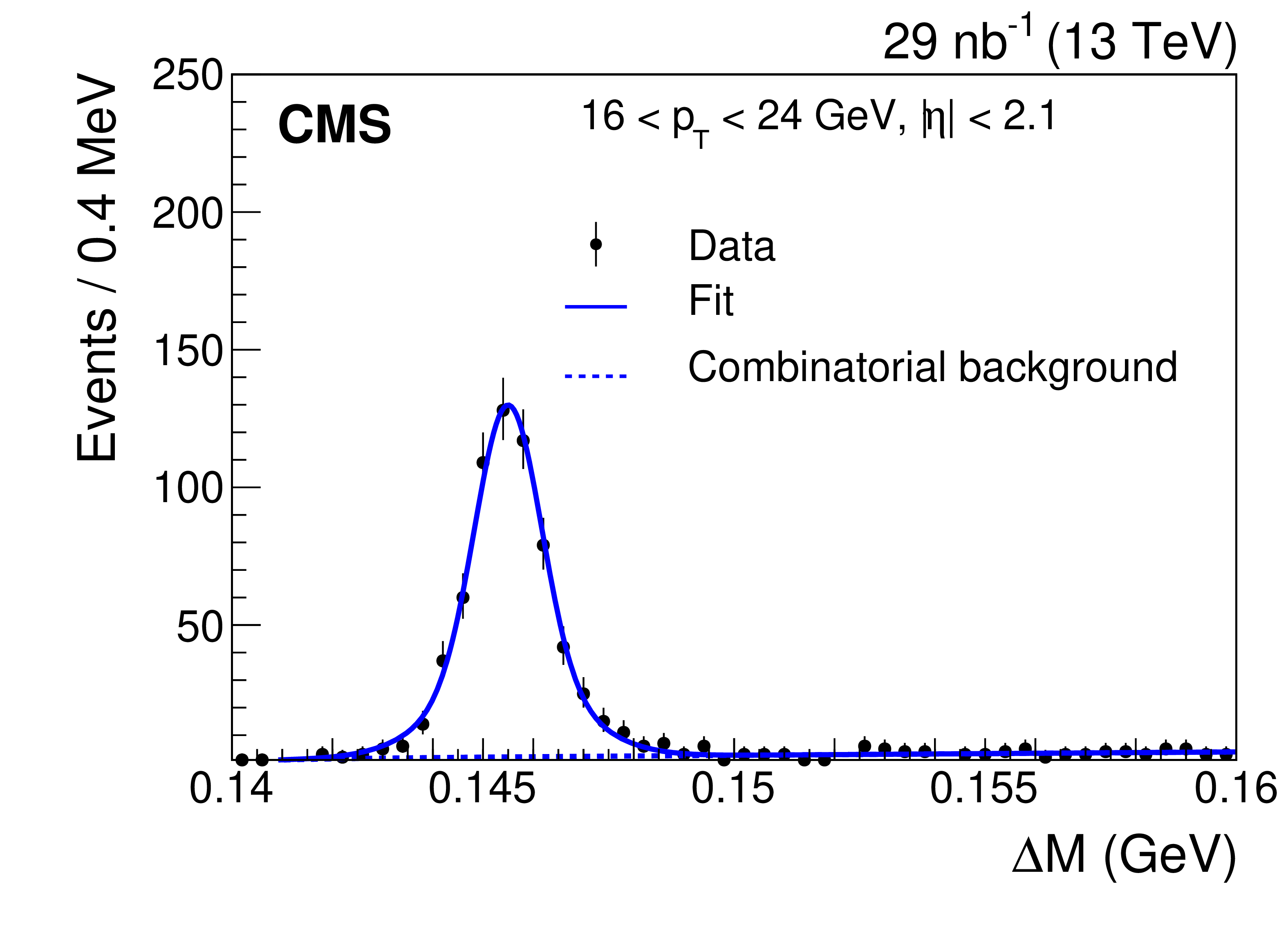
Figure 1-b:
The $\Delta M = M(\mathrm{K^{-}} \pi^{+} {\pi ^+_{\mathrm {s}}}) - M(\mathrm{K^{-}} \pi^{+})$ invariant mass distribution in the 16 $ < {p_{\mathrm {T}}} < $ 24 GeV bin ; charge conjugation is implied. The vertical bars on the points represent the statistical uncertainties in the data. The overall result from the fit is shown by the solid line, the fit to the combinatorial background by the dotted line. |
png pdf |
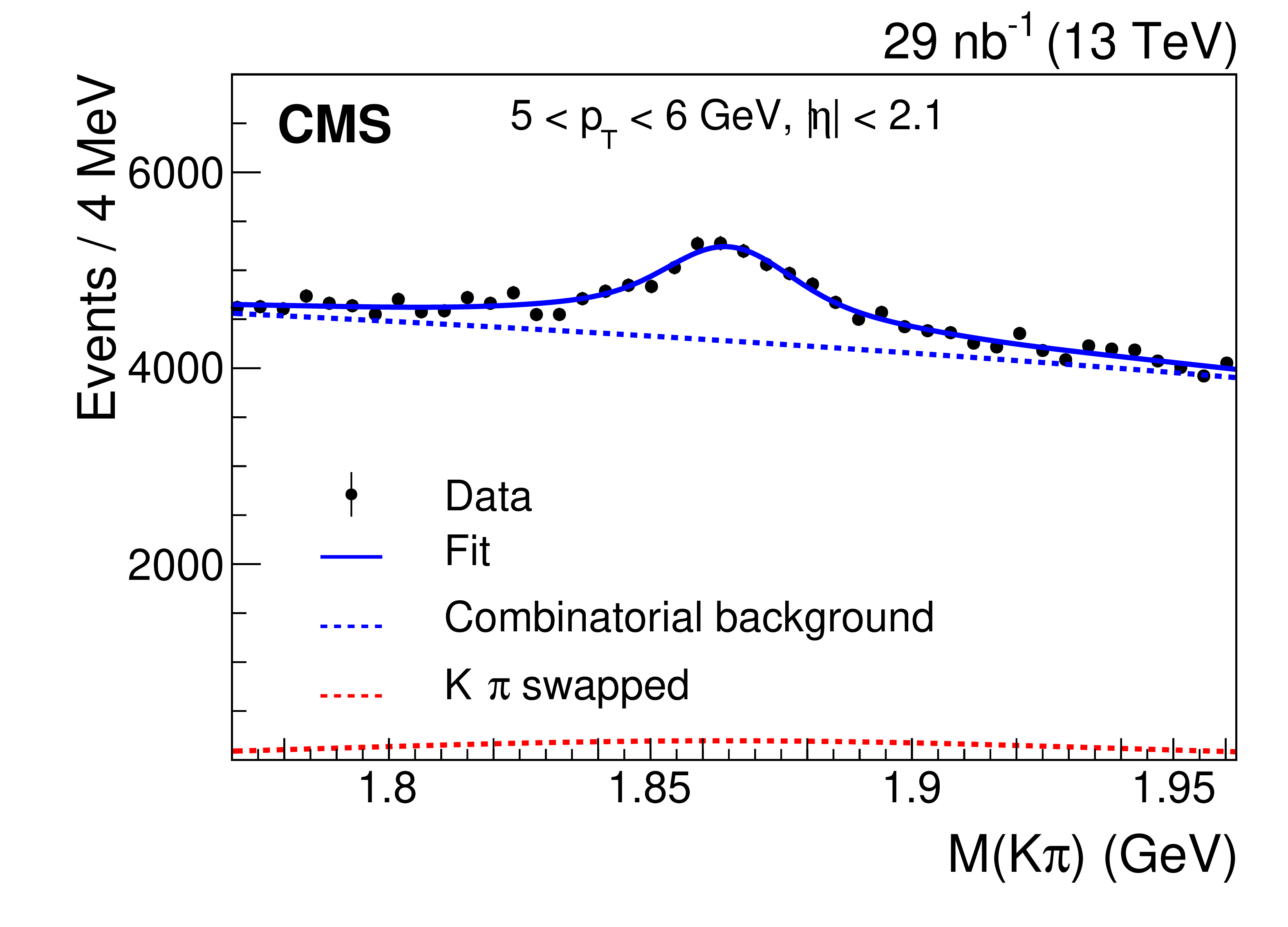
Figure 1-c:
The $M(\mathrm{K^{-}} \pi^{+})$ invariant mass distribution in the 5 $ < {p_{\mathrm {T}}} < $ 6 GeV bin ; charge conjugation is implied. The vertical bars on the points represent the statistical uncertainties in the data. The overall result from the fit is shown by the solid line, the fit to the combinatorial background by the dotted line, and the fit to the K/$\pi$ swapped candidates by the red dot-dashed line. |
png pdf |
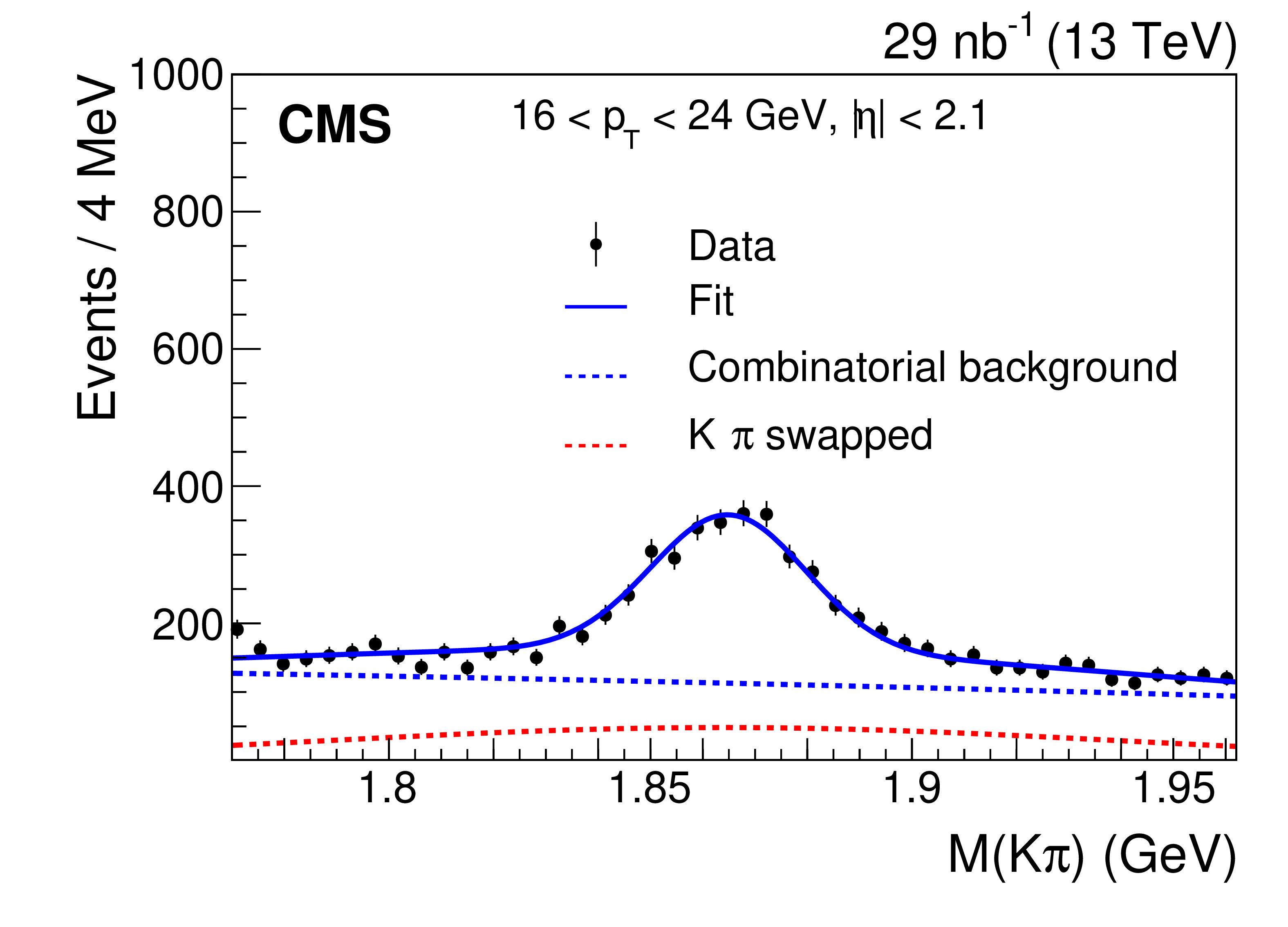
Figure 1-d:
The $M(\mathrm{K^{-}} \pi^{+})$ invariant mass distribution in the 16 $ < {p_{\mathrm {T}}} < $ 24 GeV bin ; charge conjugation is implied. The vertical bars on the points represent the statistical uncertainties in the data. The overall result from the fit is shown by the solid line, the fit to the combinatorial background by the dotted line, and the fit to the K/$\pi$ swapped candidates by the red dot-dashed line. |
png pdf |
Figure 1-e:
The $M(\mathrm{K^{-}} \pi^{+} \pi^{+})$ invariant mass distribution in the 5 $ < {p_{\mathrm {T}}} < $ 6 GeV bin ;charge conjugation is implied. The vertical bars on the points represent the statistical uncertainties in the data. The overall result from the fit is shown by the solid line, the fit to the combinatorial background by the dotted line. |
png pdf |
Figure 1-f:
The $M(\mathrm{K^{-}} \pi^{+} \pi^{+})$ invariant mass distribution in the 16 $ < {p_{\mathrm {T}}} < $ 24 GeV bin ; charge conjugation is implied. The vertical bars on the points represent the statistical uncertainties in the data. The overall result from the fit is shown by the solid line, the fit to the combinatorial background by the dotted line. |
png pdf |
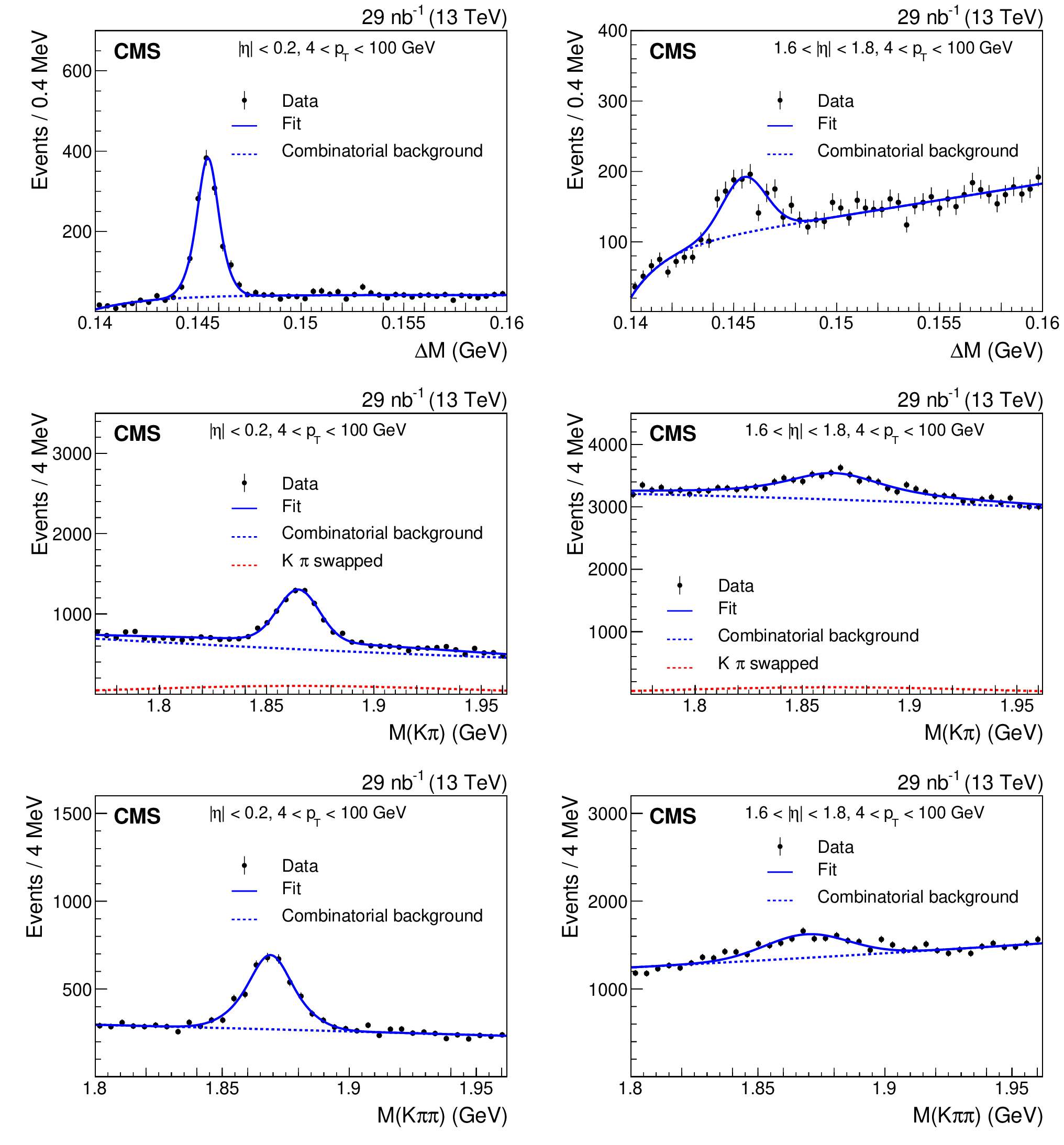
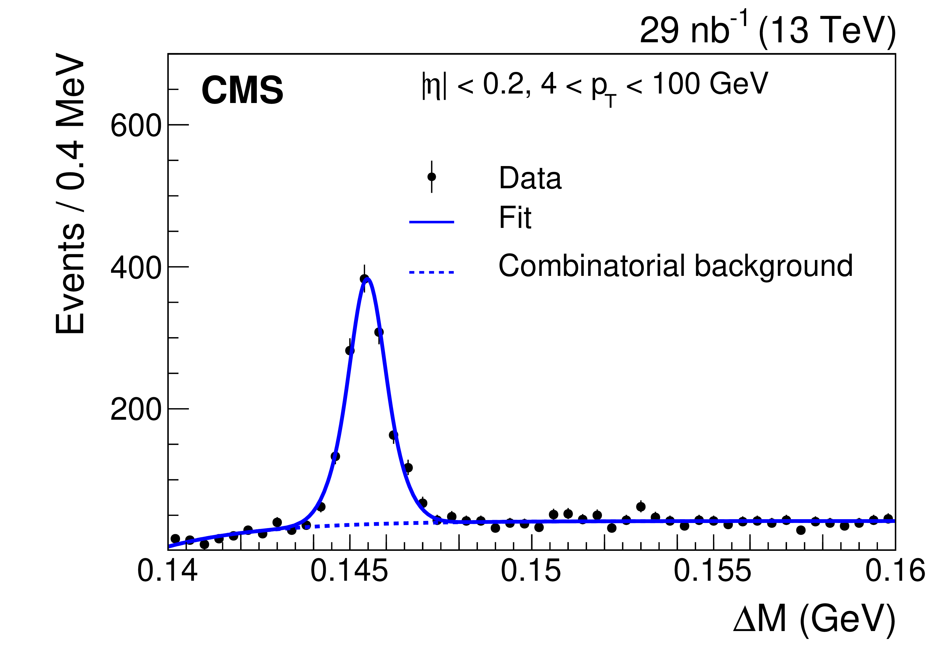
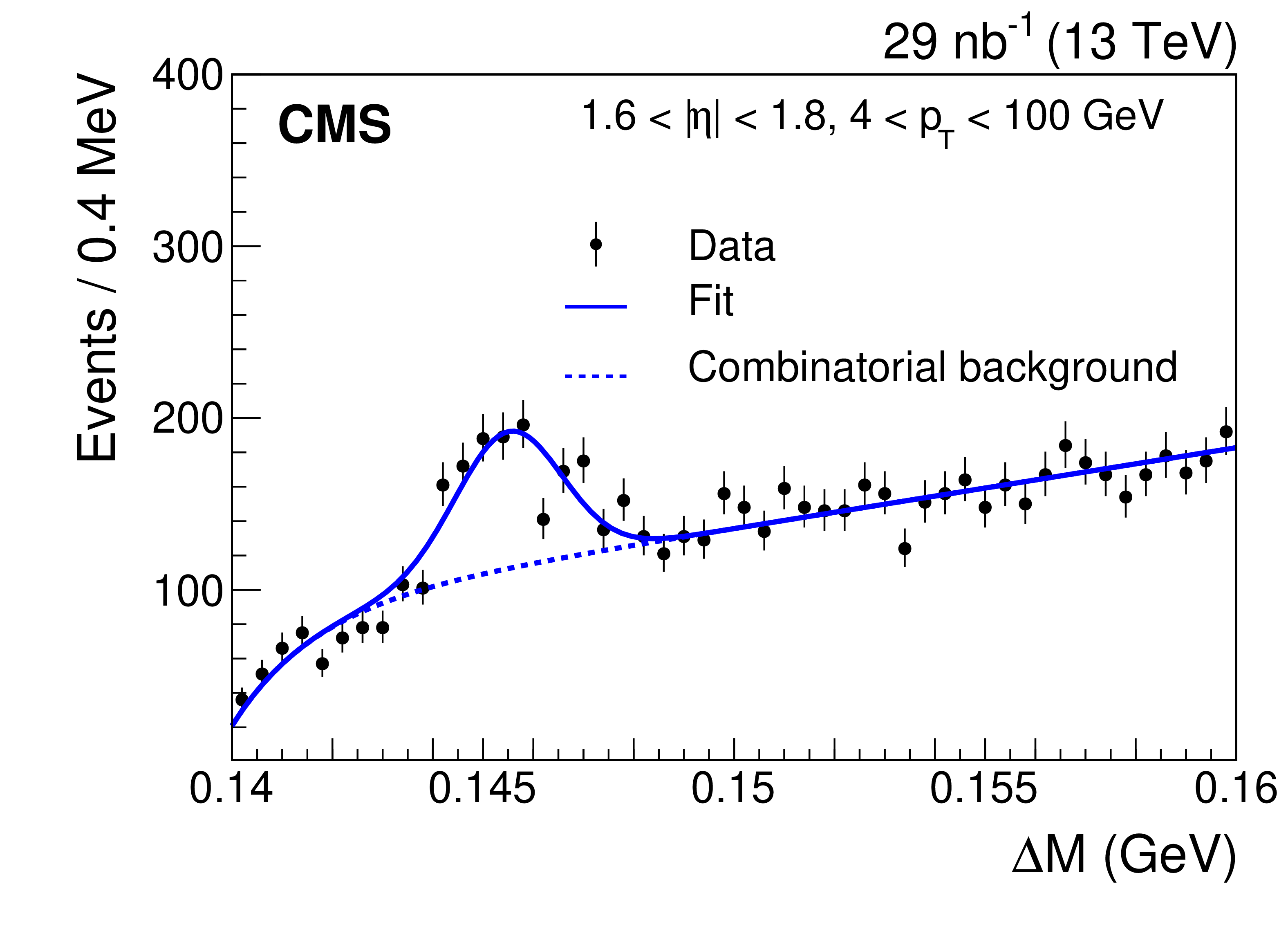
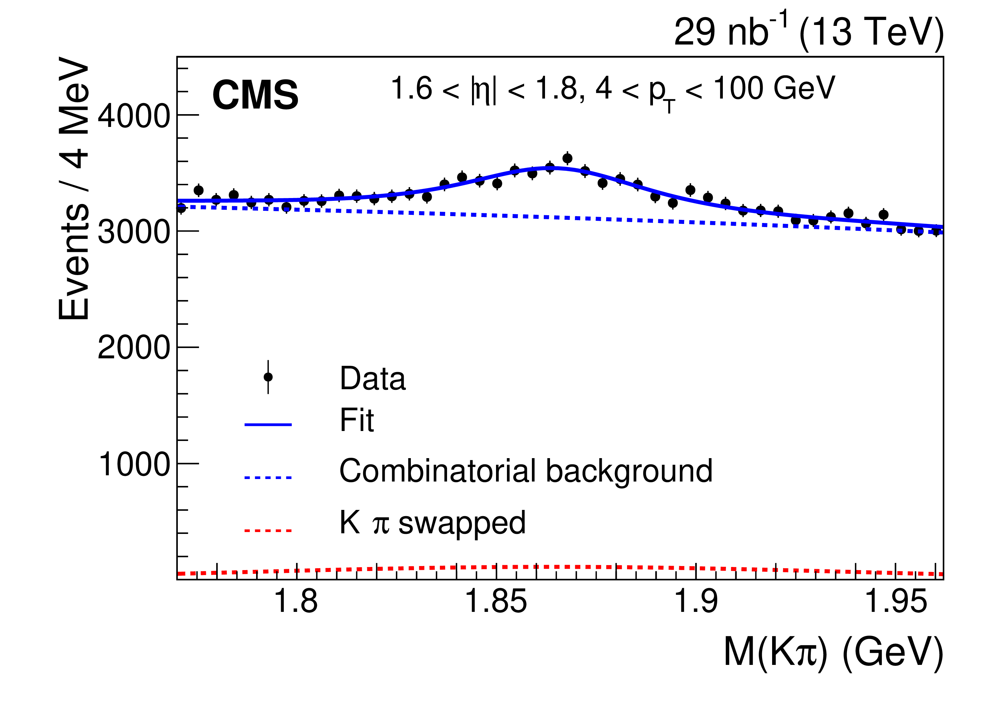
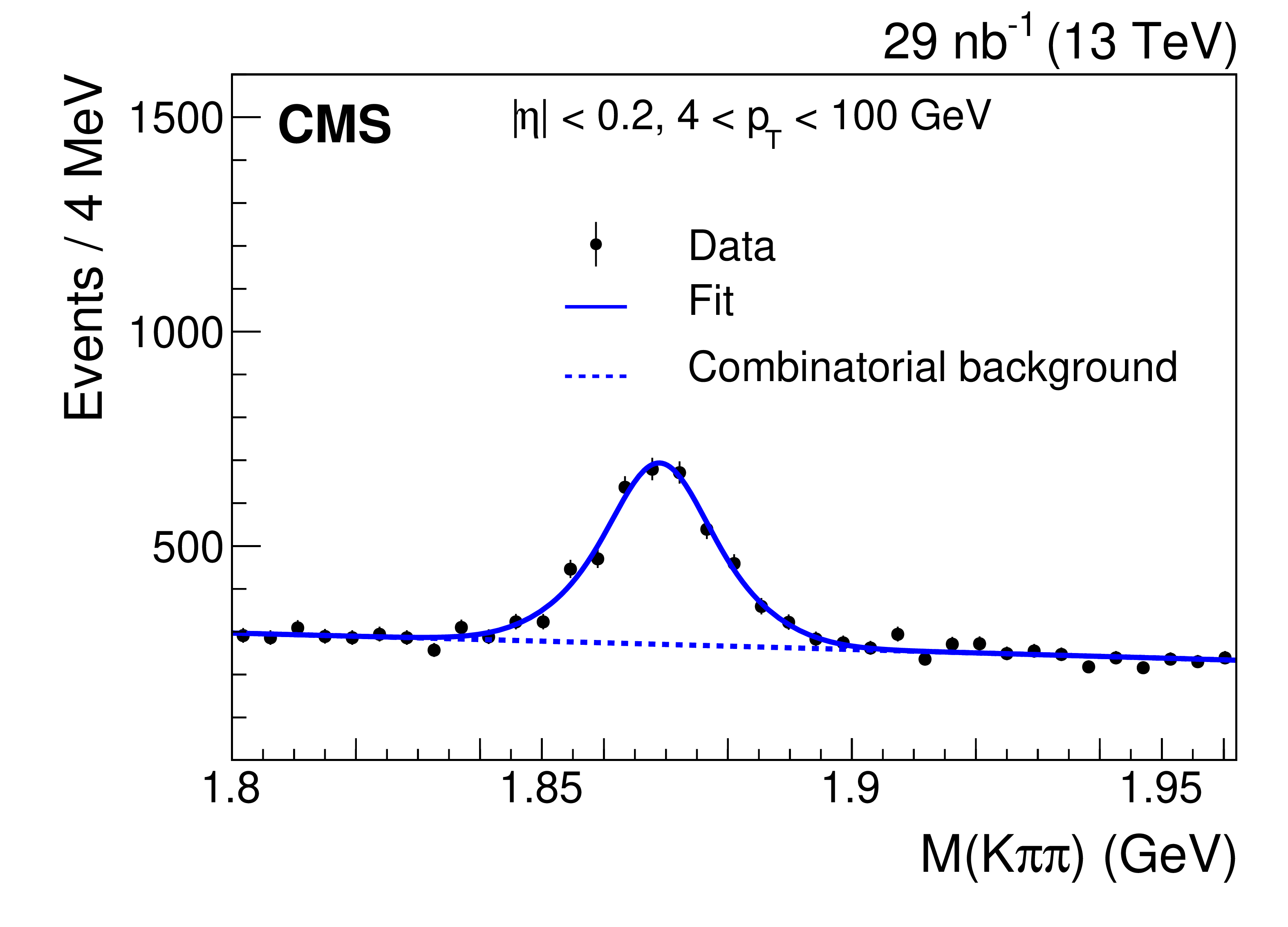
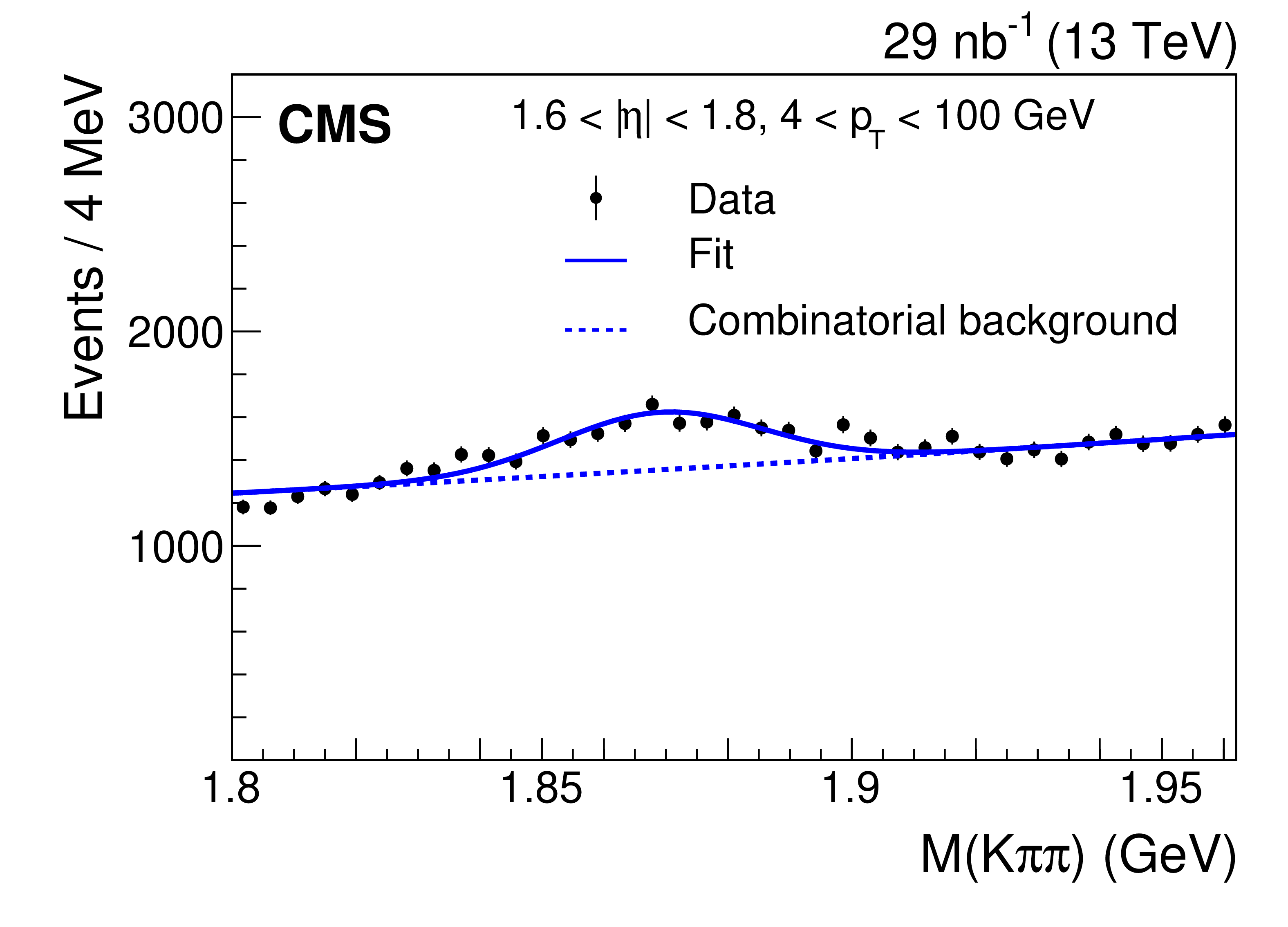
Figure 2:
The invariant mass distributions: $\Delta M = M(\mathrm{K^{-}} \pi^{+} {\pi ^+_{\mathrm {s}}}) - M(\mathrm{K^{-}} \pi^{+})$ (upper), $M(\mathrm{K^{-}} \pi^{+})$ (middle), and $M(\mathrm{K^{-}} \pi^{+} \pi^{+})$ (lower); charge conjugation is implied. Plots in the left column show the $ {| \eta |} < $ 0.2 bin, while the 1.6 $ < {| \eta |} < $ 1.8 bin is shown in the right column. The vertical bars on the points represent the statistical uncertainties in the data. The overall result from the fit is shown by the solid line, and the fit to the combinatorial background by the dotted line, and, in the middle plots, the fit to the K/$\pi$ swapped candidates by the red dot-dashed line. |
png pdf |
Figure 2-a:
The $\Delta M = M(\mathrm{K^{-}} \pi^{+} {\pi ^+_{\mathrm {s}}}) - M(\mathrm{K^{-}} \pi^{+})$ invariant mass distribution in the $ {| \eta |} < $ 0.2 bin ; charge conjugation is implied. The vertical bars on the points represent the statistical uncertainties in the data. The overall result from the fit is shown by the solid line, and the fit to the combinatorial background by the dotted line. |
png pdf |
Figure 2-b:
The $\Delta M = M(\mathrm{K^{-}} \pi^{+} {\pi ^+_{\mathrm {s}}}) - M(\mathrm{K^{-}} \pi^{+})$ invariant mass distribution in the 1.6 $ < {| \eta |} < $ 1.8 bin ; charge conjugation is implied. The vertical bars on the points represent the statistical uncertainties in the data. The overall result from the fit is shown by the solid line, and the fit to the combinatorial background by the dotted line. |

png pdf |
Figure 2-c:
The $M(\mathrm{K^{-}} \pi^{+})$ invariant mass distribution in the $ {| \eta |} < $ 0.2 bin ; charge conjugation is implied. The vertical bars on the points represent the statistical uncertainties in the data. The overall result from the fit is shown by the solid line, and the fit to the combinatorial background by the dotted line, and the fit to the K/$\pi$ swapped candidates by the red dot-dashed line. |
png pdf |
Figure 2-d:
The $M(\mathrm{K^{-}} \pi^{+})$ invariant mass distribution in the 1.6 $ < {| \eta |} < $ 1.8 bin ; charge conjugation is implied. The vertical bars on the points represent the statistical uncertainties in the data. The overall result from the fit is shown by the solid line, and the fit to the combinatorial background by the dotted line, and the fit to the K/$\pi$ swapped candidates by the red dot-dashed line. |
png pdf |
Figure 2-e:
The $M(\mathrm{K^{-}} \pi^{+} \pi^{+})$ invariant mass distribution in the $ {| \eta |} < $ 0.2 bin ; charge conjugation is implied. The vertical bars on the points represent the statistical uncertainties in the data. The overall result from the fit is shown by the solid line, and the fit to the combinatorial background by the dotted line. |
png pdf |
Figure 2-f:
The $M(\mathrm{K^{-}} \pi^{+} \pi^{+})$ invariant mass distribution in the 1.6 $ < {| \eta |} < $ 1.8 bin ; charge conjugation is implied. The vertical bars on the points represent the statistical uncertainties in the data. The overall result from the fit is shown by the solid line, and the fit to the combinatorial background by the dotted line. |
png pdf |
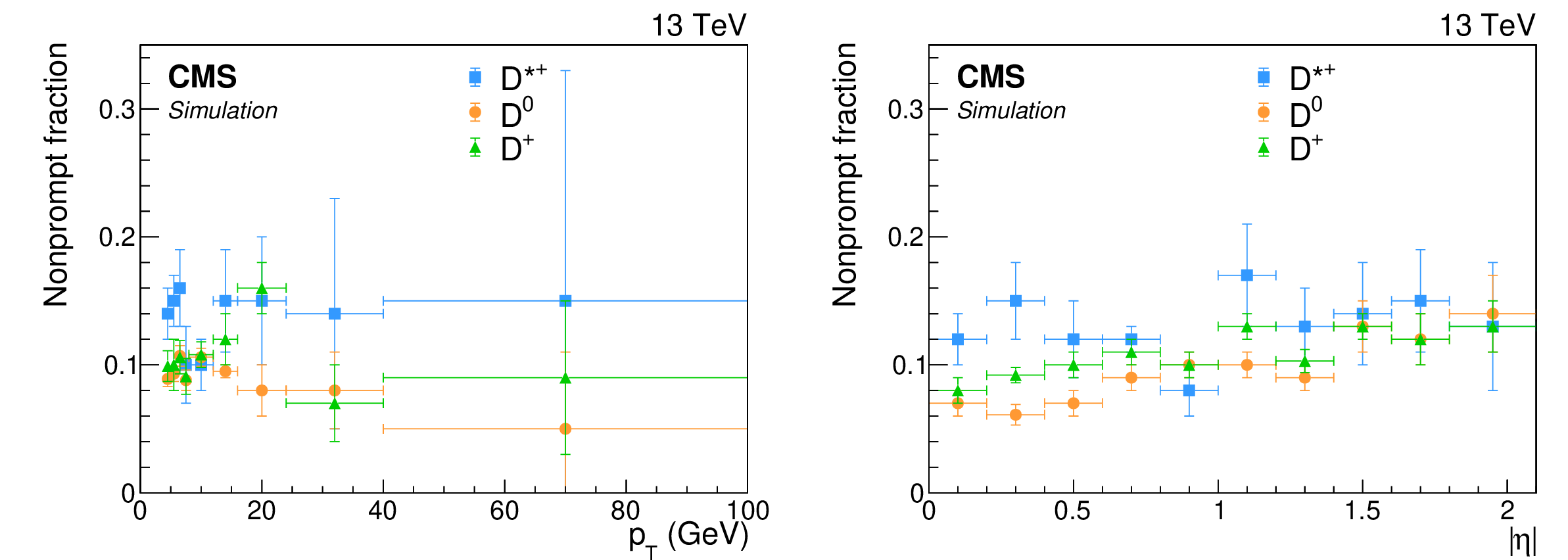
Figure 3:
The nonprompt fractions found from simulation, as a function of ${p_{\mathrm {T}}}$ (left) and $ {| \eta |}$ (right) for $\mathrm{D^{*+}}$ (squares), ${\mathrm{D^0}}$ (circles), and ${\mathrm{D^+}}$ (triangles) mesons. The vertical lines represent the statistical uncertainties and the horizontal lines the bin widths. |
png pdf |
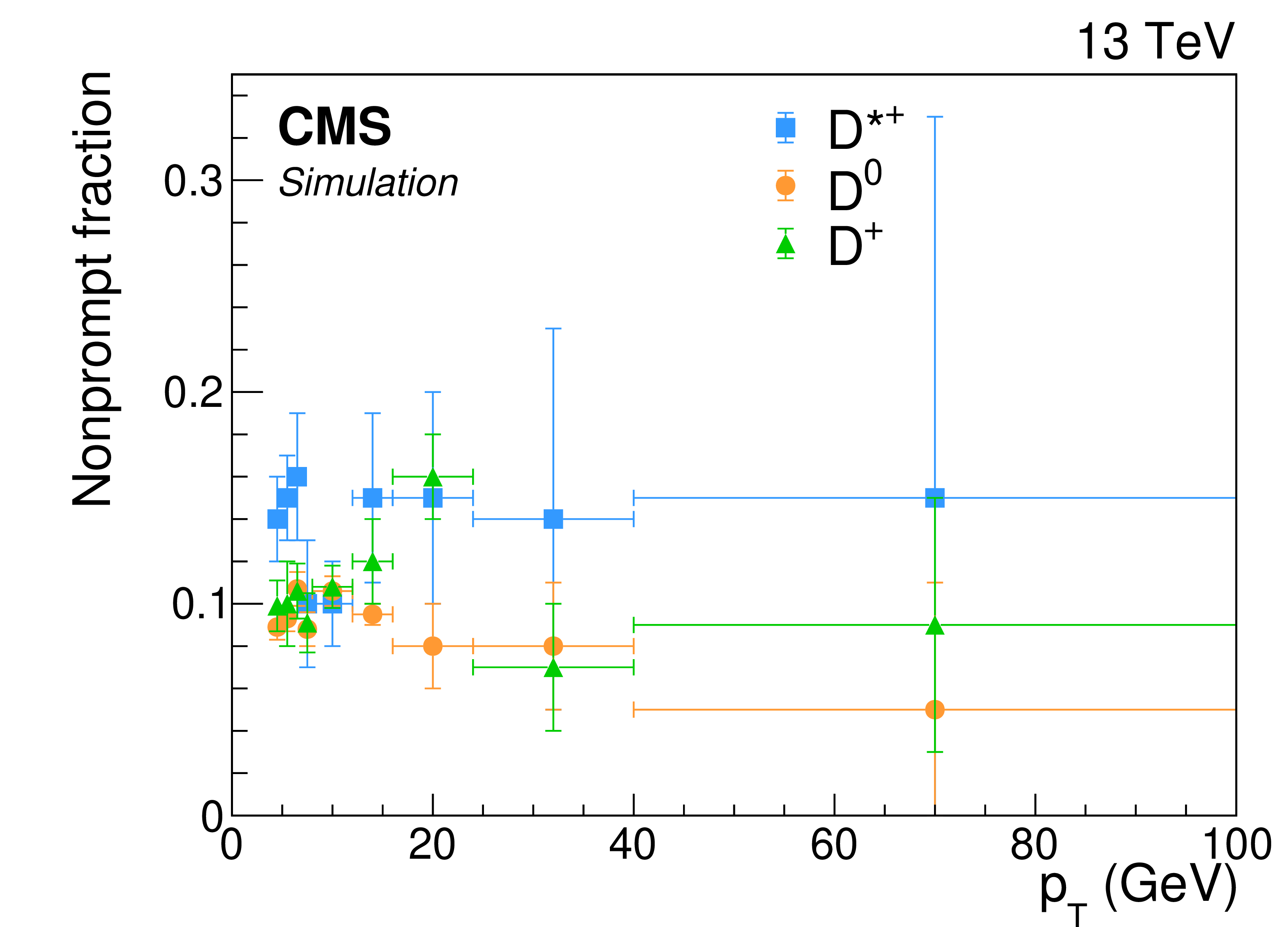
Figure 3-a:
The nonprompt fractions found from simulation, as a function of ${p_{\mathrm {T}}}$ (squares), ${\mathrm{D^0}}$ (circles), and ${\mathrm{D^+}}$ (triangles) mesons. The vertical lines represent the statistical uncertainties and the horizontal lines the bin widths. |
png pdf |
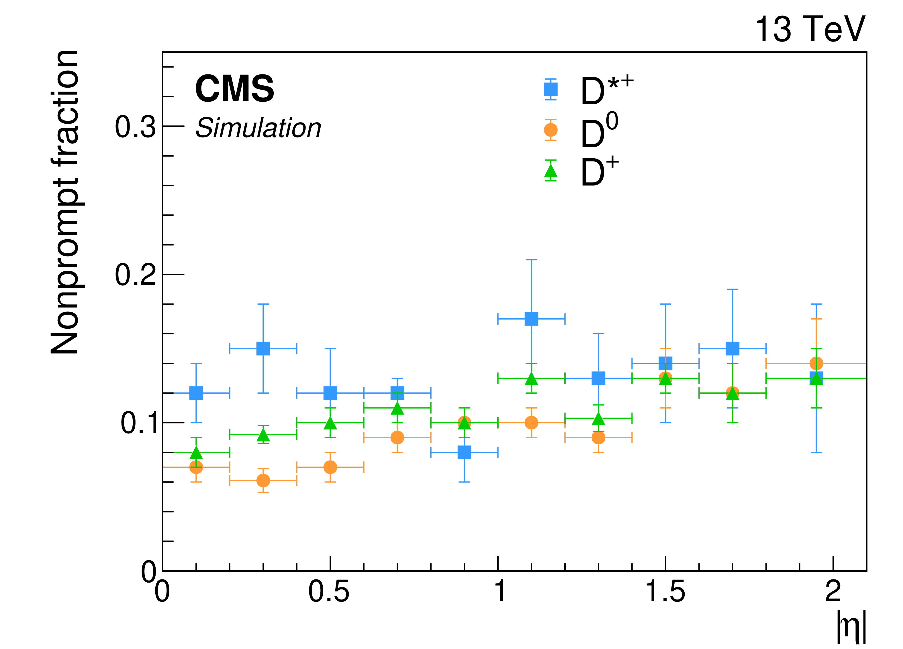
Figure 3-b:
The nonprompt fractions found from simulation, as a function of $ {| \eta |}$ for $\mathrm{D^{*+}}$ (squares), ${\mathrm{D^0}}$ (circles), and ${\mathrm{D^+}}$ (triangles) mesons. The vertical lines represent the statistical uncertainties and the horizontal lines the bin widths. |

png pdf |
Figure 4:
Differential cross sections $ {\mathrm {d}}\sigma / {\mathrm {d}} {p_{\mathrm {T}}} $ (upper) and $ {\mathrm {d}}\sigma / {\mathrm {d}} {| \eta |}$ (lower) for prompt ${{\mathrm{D}^{\ast}(2010)^{\pm}}}$ meson production. Black markers represent the data and are compared with several MC simulation models and theoretical predictions. The statistical and total uncertainties are shown by the inner and outer vertical lines, respectively. The FONLL band represents the standard uncertainties in the prediction as detailed in the text. The lower panel gives the ratios of the predictions to the data. |

png pdf |
Figure 4-a:
Differential cross section $ {\mathrm {d}}\sigma / {\mathrm {d}} {p_{\mathrm {T}}} $ for prompt ${{\mathrm{D}^{\ast}(2010)^{\pm}}}$ meson production. Black markers represent the data and are compared with several MC simulation models and theoretical predictions. The statistical and total uncertainties are shown by the inner and outer vertical lines, respectively. The FONLL band represents the standard uncertainties in the prediction as detailed in the text. The lower panel gives the ratios of the predictions to the data. |
png pdf |
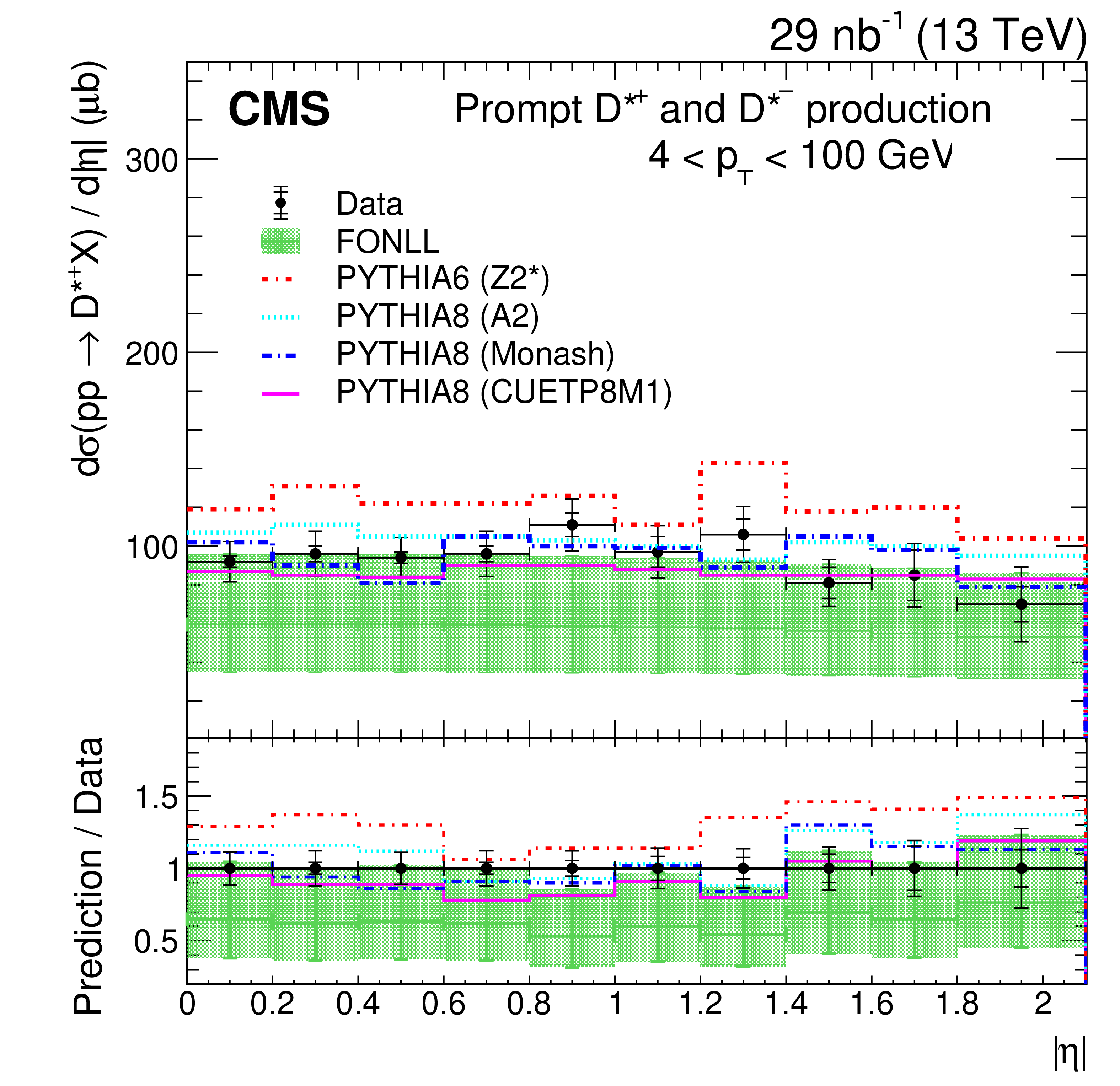
Figure 4-b:
Differential cross section $ {\mathrm {d}}\sigma / {\mathrm {d}} {| \eta |}$ for prompt ${{\mathrm{D}^{\ast}(2010)^{\pm}}}$ meson production. Black markers represent the data and are compared with several MC simulation models and theoretical predictions. The statistical and total uncertainties are shown by the inner and outer vertical lines, respectively. The FONLL band represents the standard uncertainties in the prediction as detailed in the text. The lower panel gives the ratios of the predictions to the data. |
png pdf |
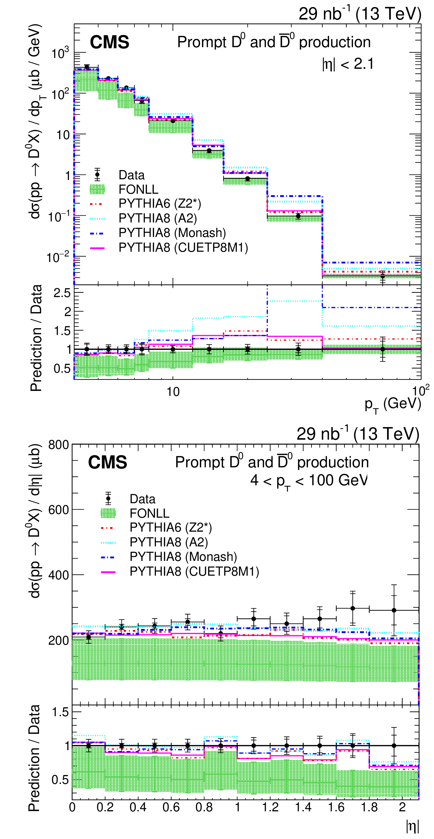
Figure 5:
Differential cross section $ {\mathrm {d}}\sigma / {\mathrm {d}} {p_{\mathrm {T}}} $ (upper) and $ {\mathrm {d}}\sigma / {\mathrm {d}} {| \eta |}$ (lower) for prompt ${\mathrm{D^0}}$ ($\mathrm{\overline{D}{}^{0}}$) meson production. Black markers represent the data and are compared with several MC simulation models and theoretical predictions. The statistical and total uncertainties are shown by the inner and outer vertical lines, respectively. The FONLL band represents the standard uncertainties in the prediction as detailed in the text. The lower panel gives the ratios of the predictions to the data. |

png pdf |
Figure 5-a:
Differential cross section $ {\mathrm {d}}\sigma / {\mathrm {d}} {p_{\mathrm {T}}} $ for prompt ${\mathrm{D^0}}$ ($\mathrm{\overline{D}{}^{0}}$) meson production. Black markers represent the data and are compared with several MC simulation models and theoretical predictions. The statistical and total uncertainties are shown by the inner and outer vertical lines, respectively. The FONLL band represents the standard uncertainties in the prediction as detailed in the text. The lower panel gives the ratios of the predictions to the data. |
png pdf |
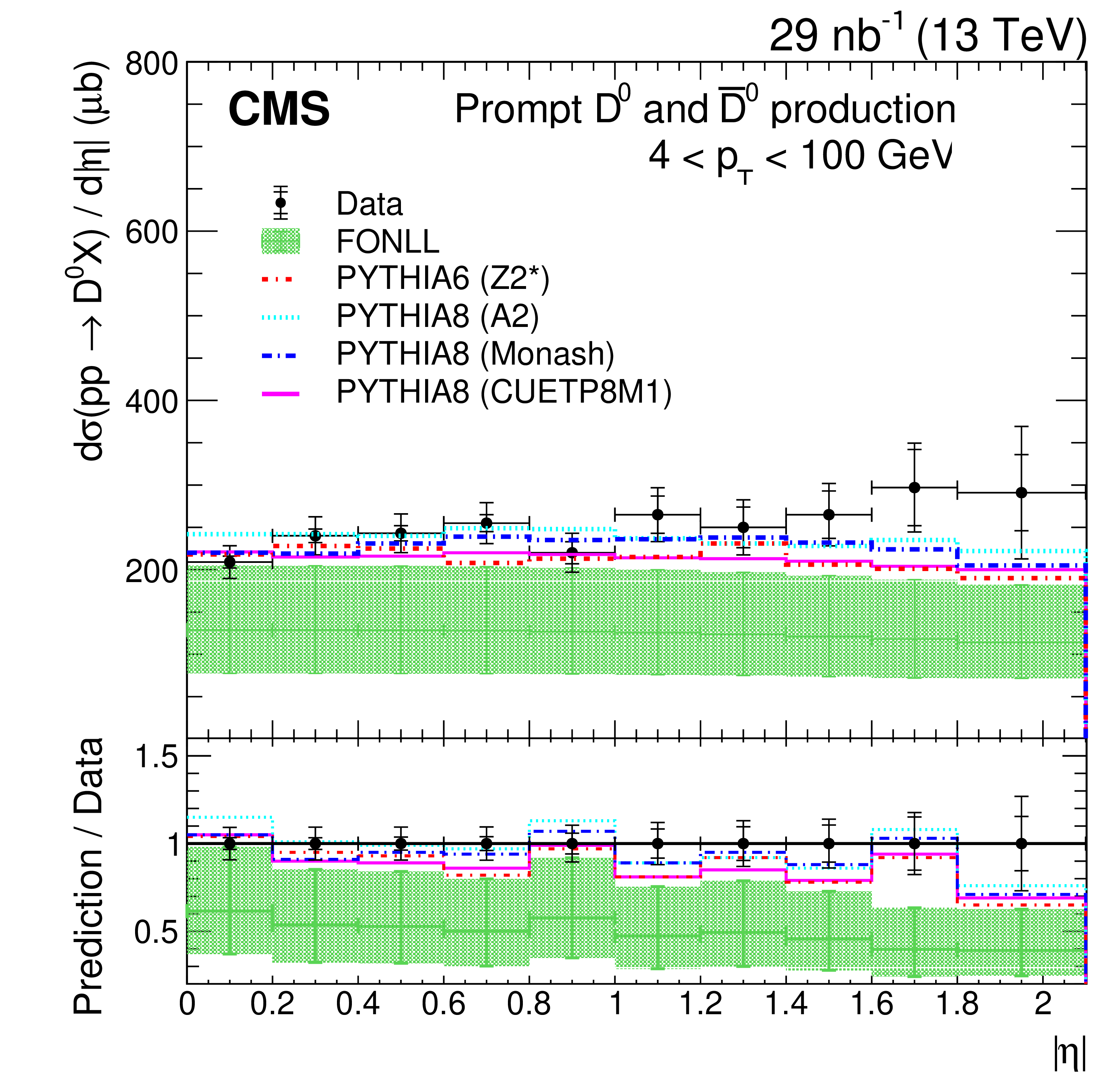
Figure 5-b:
Differential cross section $ {\mathrm {d}}\sigma / {\mathrm {d}} {| \eta |}$ for prompt ${\mathrm{D^0}}$ ($\mathrm{\overline{D}{}^{0}}$) meson production. Black markers represent the data and are compared with several MC simulation models and theoretical predictions. The statistical and total uncertainties are shown by the inner and outer vertical lines, respectively. The FONLL band represents the standard uncertainties in the prediction as detailed in the text. The lower panel gives the ratios of the predictions to the data. |
png pdf |
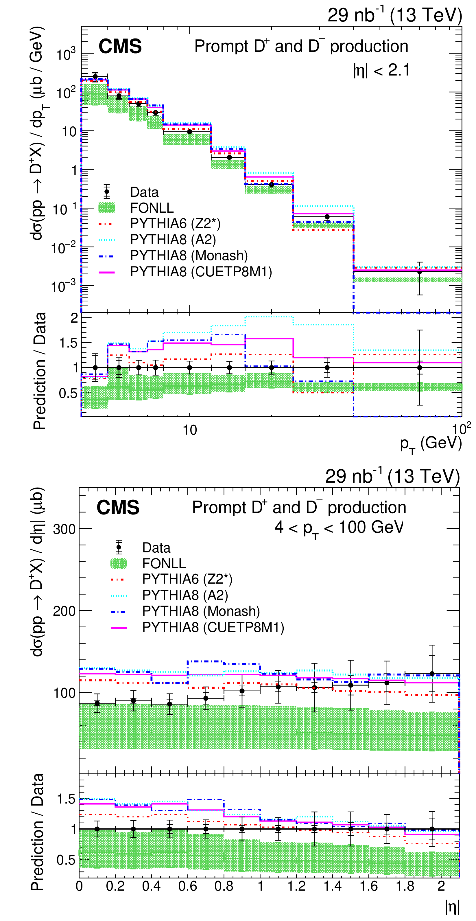
Figure 6:
Differential cross section $ {\mathrm {d}}\sigma / {\mathrm {d}} {p_{\mathrm {T}}} $ (upper) and $ {\mathrm {d}}\sigma / {\mathrm {d}} {| \eta |}$ (lower) for prompt ${\mathrm{D^{\pm}}}$ meson production. Black markers represent the data and are compared with several MC simulation models and theoretical predictions. The statistical and total uncertainties are shown by the inner and outer vertical lines, respectively. The FONLL band represents the standard uncertainties in the prediction as detailed in the text. The lower panel gives the ratios of the predictions to the data. |
png pdf |
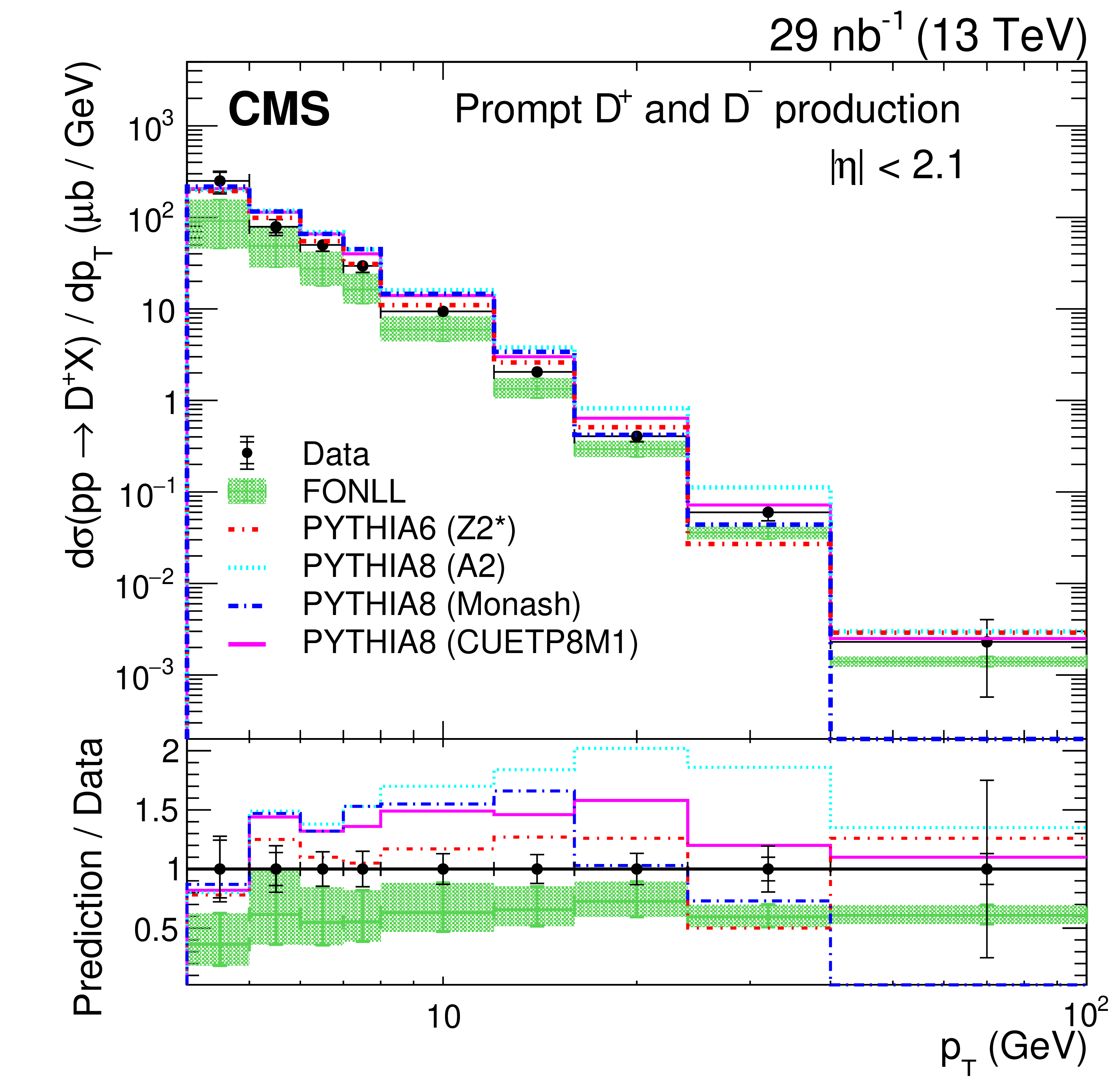
Figure 6-a:
Differential cross section $ {\mathrm {d}}\sigma / {\mathrm {d}} {p_{\mathrm {T}}} $ for prompt ${\mathrm{D^{\pm}}}$ meson production. Black markers represent the data and are compared with several MC simulation models and theoretical predictions. The statistical and total uncertainties are shown by the inner and outer vertical lines, respectively. The FONLL band represents the standard uncertainties in the prediction as detailed in the text. The lower panel gives the ratios of the predictions to the data. |

png pdf |
Figure 6-b:
Differential cross section $ {\mathrm {d}}\sigma / {\mathrm {d}} {| \eta |}$ for prompt ${\mathrm{D^{\pm}}}$ meson production. Black markers represent the data and are compared with several MC simulation models and theoretical predictions. The statistical and total uncertainties are shown by the inner and outer vertical lines, respectively. The FONLL band represents the standard uncertainties in the prediction as detailed in the text. The lower panel gives the ratios of the predictions to the data. |

png pdf |
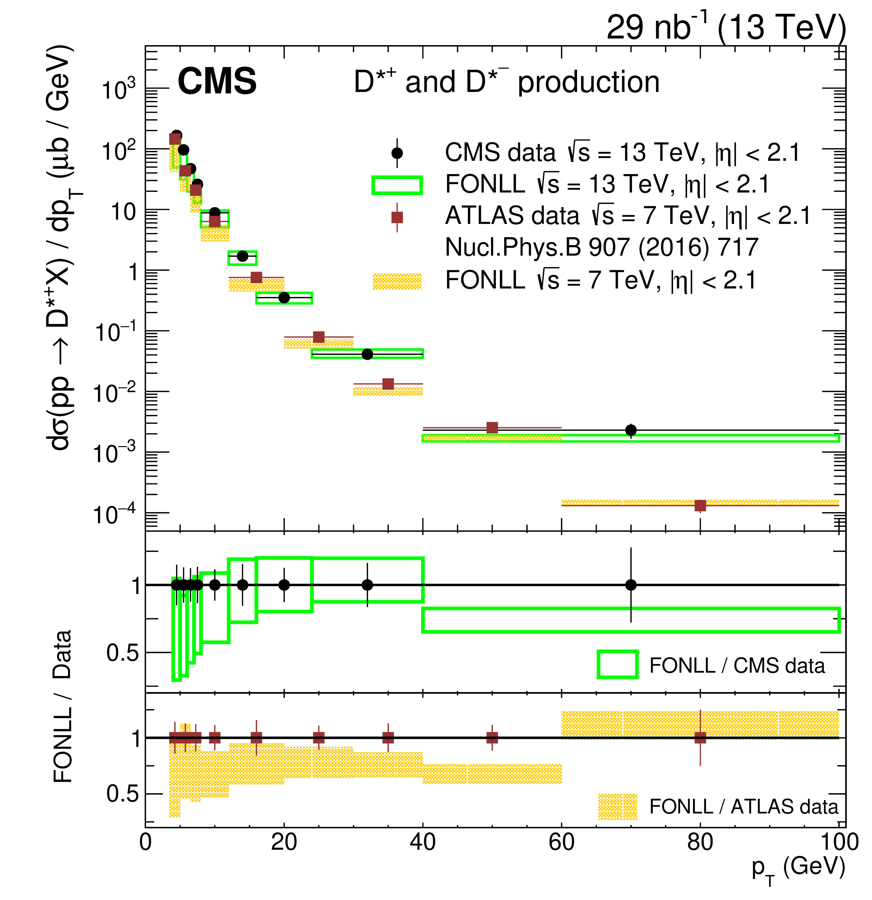
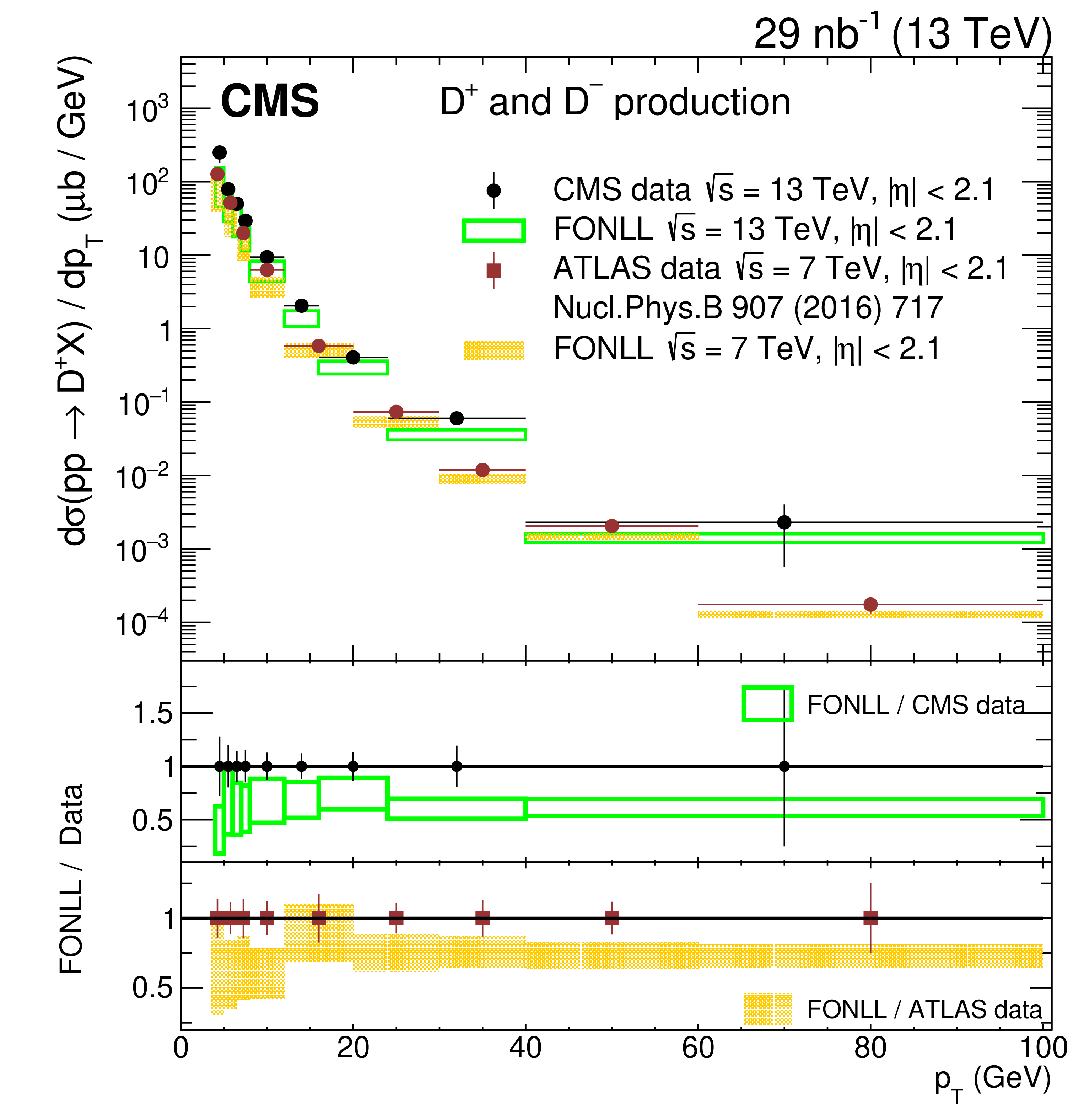
Figure 7:
Differential cross section $ {\mathrm {d}}\sigma / {\mathrm {d}} {p_{\mathrm {T}}} $ for ${{\mathrm{D}^{\ast}(2010)^{\pm}}}$ (left) and ${\mathrm{D^{\pm}}}$ (right) meson production, comparing the production from CMS (black circles, prompt, this paper) at $\sqrt {s} = $ 13 TeV and ATLAS (red squares, prompt $+$ nonprompt) at $\sqrt {s} = $ 7 TeV [5]. The corresponding predictions from FONLL are shown by the unfilled and filled boxes, respectively. The vertical lines on the points give the total uncertainties in the data, and the horizontal lines show the bin widths. The two lower panels in each plot give the ratios of the FONLL predictions to the CMS and ATLAS data, shown by circles and squares, respectively. |
png pdf |
Figure 7-a:
Differential cross section $ {\mathrm {d}}\sigma / {\mathrm {d}} {p_{\mathrm {T}}} $ for ${{\mathrm{D}^{\ast}(2010)^{\pm}}}$ meson production, comparing the production from CMS (black circles, prompt, this paper) at $\sqrt {s} = $ 13 TeV and ATLAS (red squares, prompt $+$ nonprompt) at $\sqrt {s} = $ 7 TeV [5]. The corresponding predictions from FONLL are shown by the unfilled and filled boxes, respectively. The vertical lines on the points give the total uncertainties in the data, and the horizontal lines show the bin widths. The two lower panels give the ratios of the FONLL predictions to the CMS and ATLAS data, shown by circles and squares, respectively. |
png pdf |
Figure 7-b:
Differential cross section $ {\mathrm {d}}\sigma / {\mathrm {d}} {p_{\mathrm {T}}} $ for ${\mathrm{D^{\pm}}}$ meson production, comparing the production from CMS (black circles, prompt, this paper) at $\sqrt {s} = $ 13 TeV and ATLAS (red squares, prompt $+$ nonprompt) at $\sqrt {s} = $ 7 TeV [5]. The corresponding predictions from FONLL are shown by the unfilled and filled boxes, respectively. The vertical lines on the points give the total uncertainties in the data, and the horizontal lines show the bin widths. The two lower panels give the ratios of the FONLL predictions to the CMS and ATLAS data, shown by circles and squares, respectively. |
png pdf |
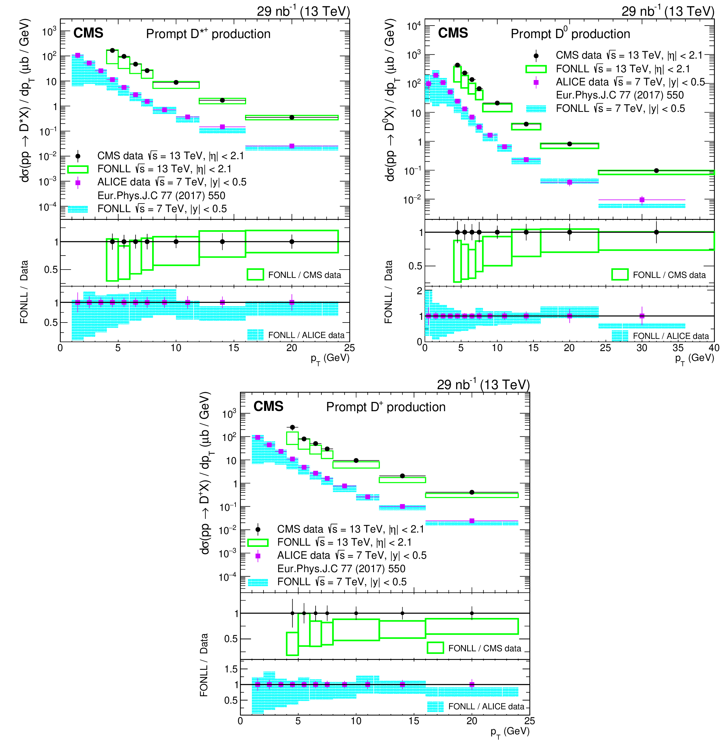
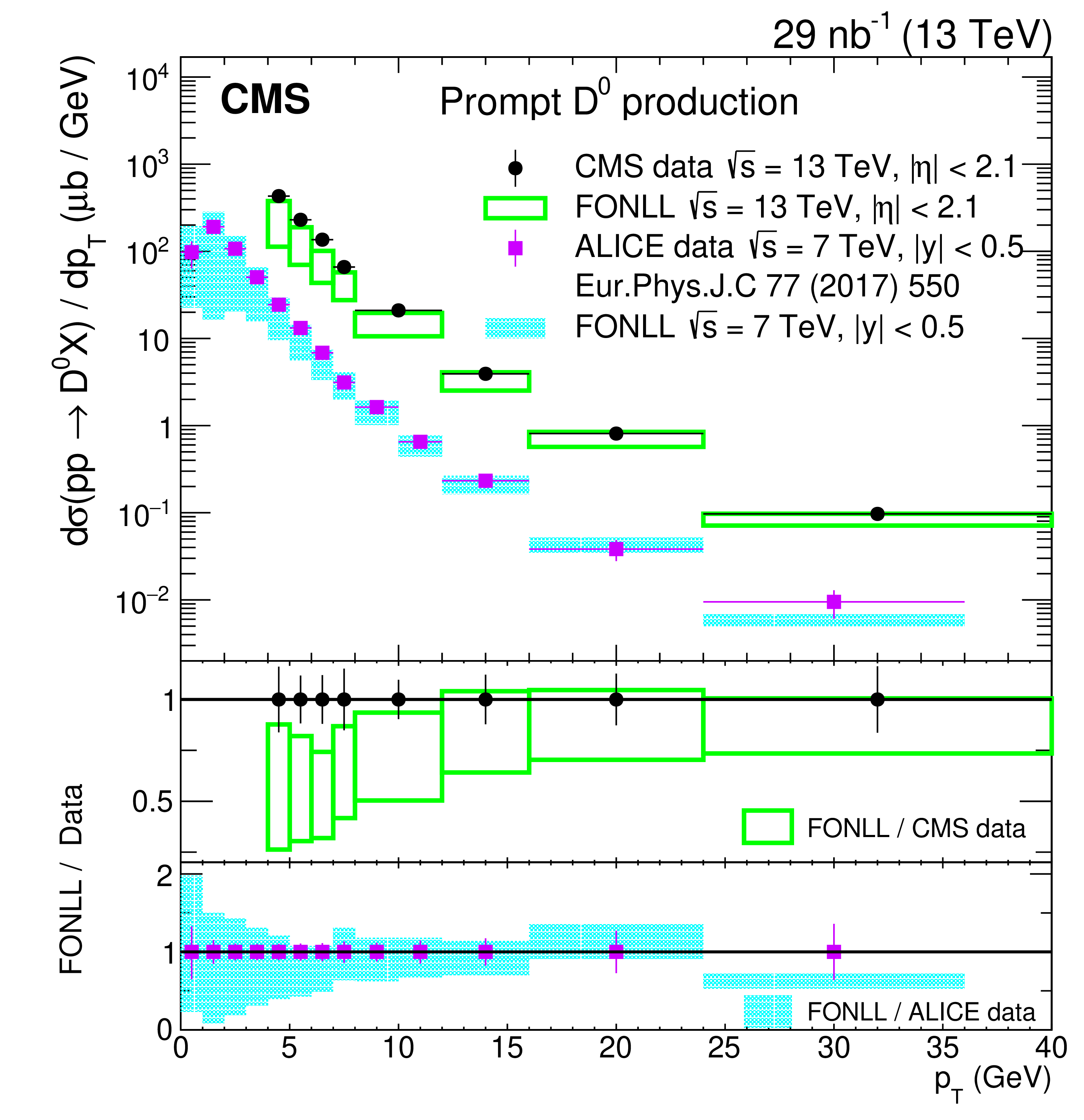
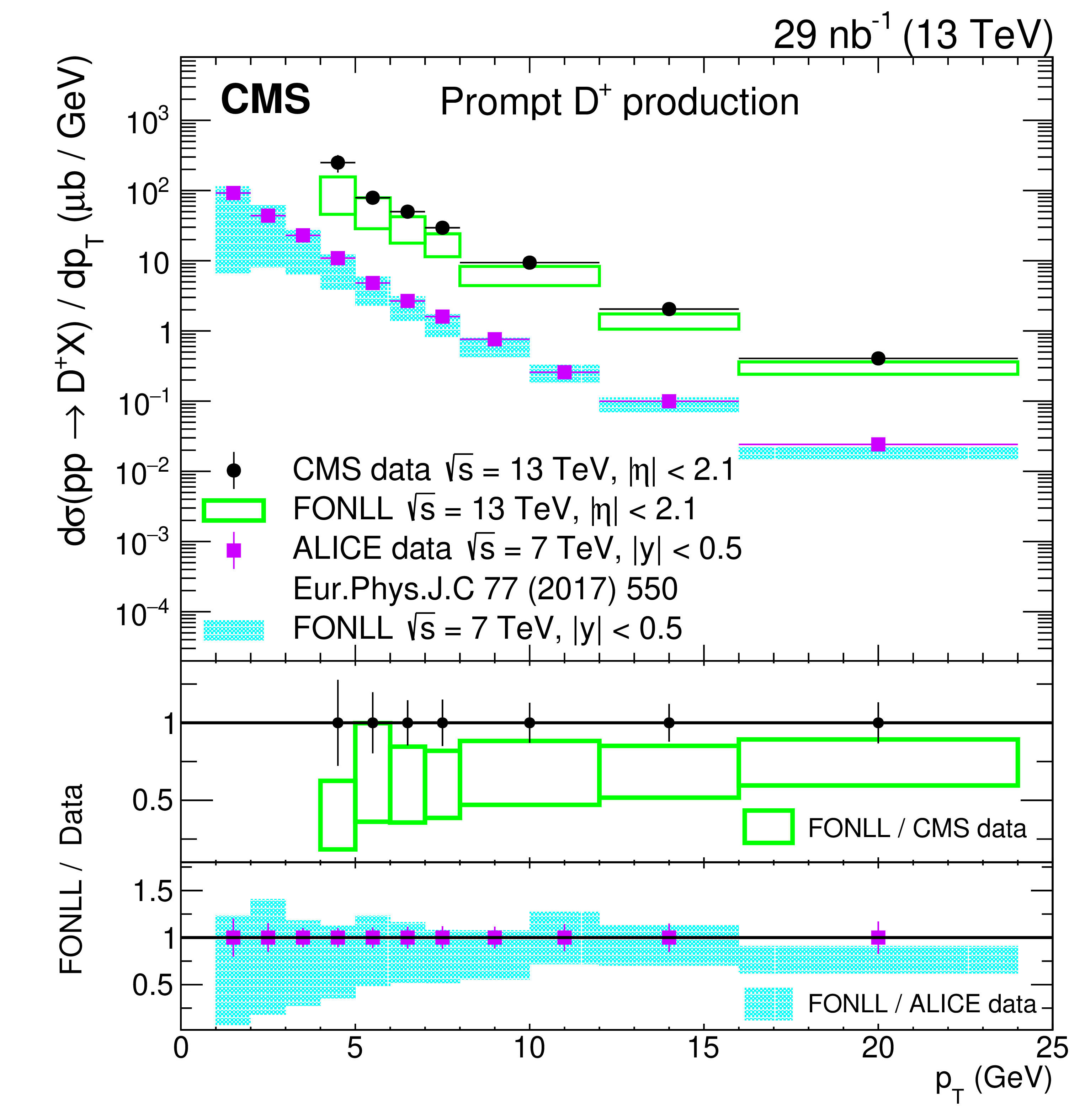
Figure 8:
Differential cross section $ {\mathrm {d}}\sigma / {\mathrm {d}} {p_{\mathrm {T}}} $ for prompt ${{\mathrm{D}^{\ast}(2010)^{\pm}}}$ (upper left), ${\mathrm{D^0}} + \mathrm{\overline{D}{}^{0}}$ (upper right) and ${\mathrm{D^{\pm}}}$ (lower) meson production with $ {p_{\mathrm {T}}} < $ 24 GeV from CMS (black circles, this paper) at $\sqrt {s} = $ 13 TeV and ALICE [7] (magenta squares) at $\sqrt {s} = $ 7 TeV and $ {| y |} < $ 0.5. The corresponding predictions from FONLL are shown by the unfilled and filled boxes, respectively. The cross section definition by ALICE includes a factor of 1/2 that accounts for the fact that the measured yields include particles and antiparticles while the cross sections are given for particles only. The same is true for the corresponding FONLL predictions, as well. The vertical lines on the points give the total uncertainties in the data, and the horizontal lines show the bin widths. The two lower panels in each plot give the ratios of the FONLL predictions to the CMS and ALICE data, shown by circles and squares, respectively. |
png pdf |
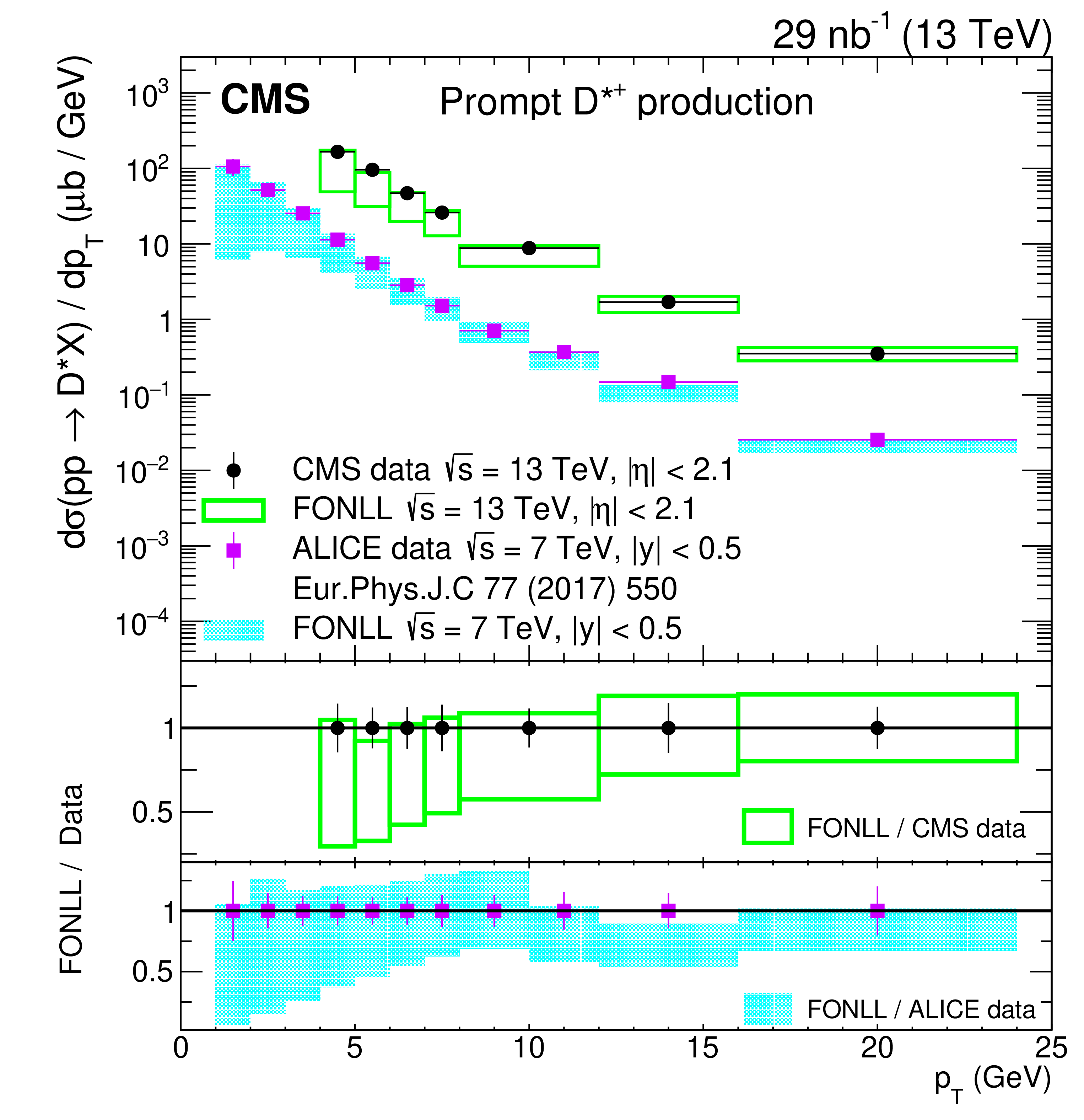
Figure 8-a:
Differential cross section $ {\mathrm {d}}\sigma / {\mathrm {d}} {p_{\mathrm {T}}} $ for prompt ${{\mathrm{D}^{\ast}(2010)^{\pm}}}$ meson production with $ {p_{\mathrm {T}}} < $ 24 GeV from CMS (black circles, this paper) at $\sqrt {s} = $ 13 TeV and ALICE [7] (magenta squares) at $\sqrt {s} = $ 7 TeV and $ {| y |} < $ 0.5. The corresponding predictions from FONLL are shown by the unfilled and filled boxes, respectively. The cross section definition by ALICE includes a factor of 1/2 that accounts for the fact that the measured yields include particles and antiparticles while the cross sections are given for particles only. The same is true for the corresponding FONLL predictions, as well. The vertical lines on the points give the total uncertainties in the data, and the horizontal lines show the bin widths. The two lower panels give the ratios of the FONLL predictions to the CMS and ALICE data, shown by circles and squares, respectively. |
png pdf |
Figure 8-b:
Differential cross section $ {\mathrm {d}}\sigma / {\mathrm {d}} {p_{\mathrm {T}}} $ for prompt ${\mathrm{D^0}} + \mathrm{\overline{D}{}^{0}}$ meson production with $ {p_{\mathrm {T}}} < $ 24 GeV from CMS (black circles, this paper) at $\sqrt {s} = $ 13 TeV and ALICE [7] (magenta squares) at $\sqrt {s} = $ 7 TeV and $ {| y |} < $ 0.5. The corresponding predictions from FONLL are shown by the unfilled and filled boxes, respectively. The cross section definition by ALICE includes a factor of 1/2 that accounts for the fact that the measured yields include particles and antiparticles while the cross sections are given for particles only. The same is true for the corresponding FONLL predictions, as well. The vertical lines on the points give the total uncertainties in the data, and the horizontal lines show the bin widths. The two lower panels give the ratios of the FONLL predictions to the CMS and ALICE data, shown by circles and squares, respectively. |
png pdf |
Figure 8-c:
Differential cross section $ {\mathrm {d}}\sigma / {\mathrm {d}} {p_{\mathrm {T}}} $ for prompt ${\mathrm{D^{\pm}}}$ meson production with $ {p_{\mathrm {T}}} < $ 24 GeV from CMS (black circles, this paper) at $\sqrt {s} = $ 13 TeV and ALICE [7] (magenta squares) at $\sqrt {s} = $ 7 TeV and $ {| y |} < $ 0.5. The corresponding predictions from FONLL are shown by the unfilled and filled boxes, respectively. The cross section definition by ALICE includes a factor of 1/2 that accounts for the fact that the measured yields include particles and antiparticles while the cross sections are given for particles only. The same is true for the corresponding FONLL predictions, as well. The vertical lines on the points give the total uncertainties in the data, and the horizontal lines show the bin widths. The two lower panels give the ratios of the FONLL predictions to the CMS and ALICE data, shown by circles and squares, respectively. |
png pdf |
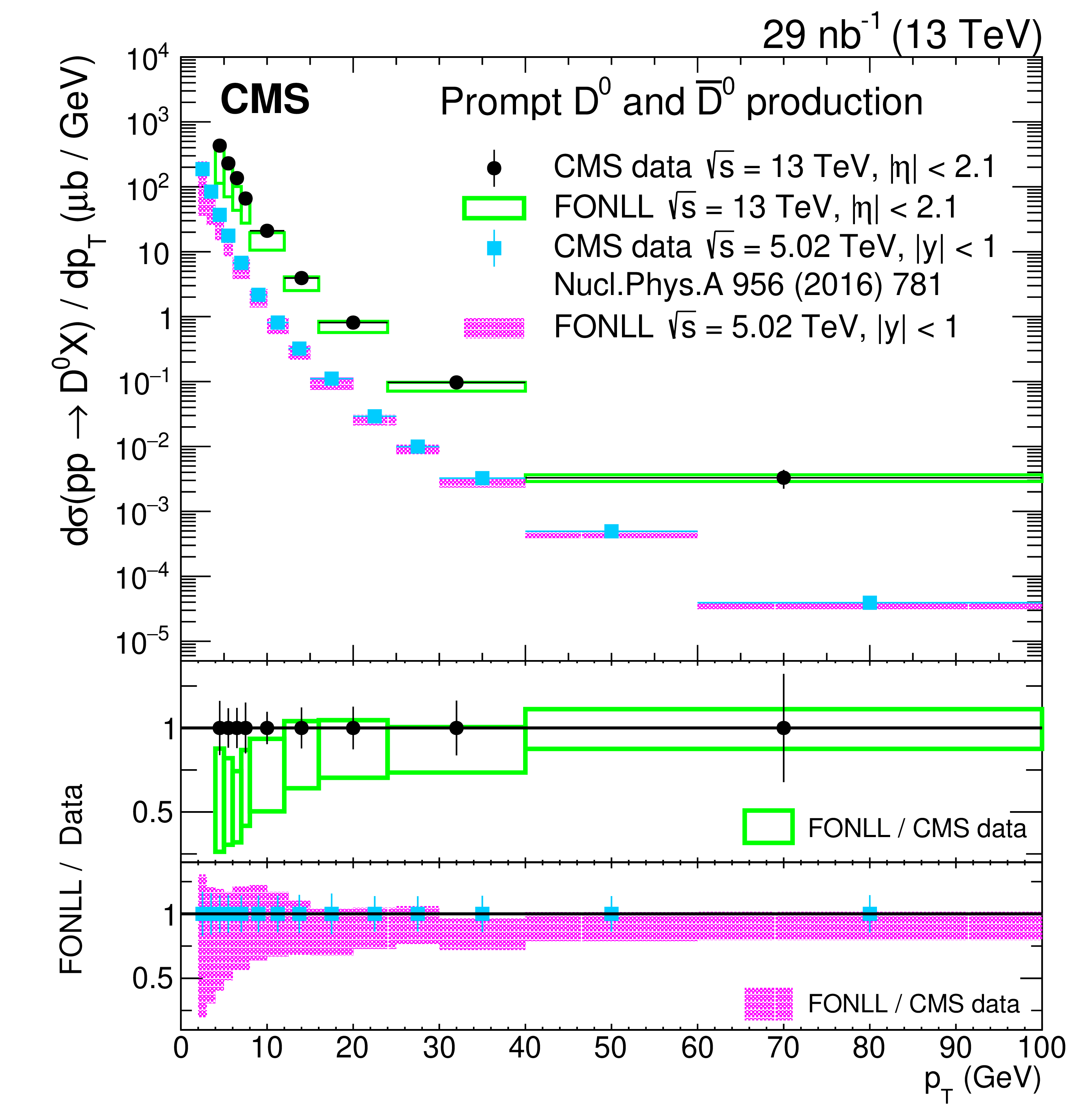
Figure 9:
Differential cross section $ {\mathrm {d}}\sigma / {\mathrm {d}} {p_{\mathrm {T}}} $ for the prompt ${\mathrm{D^0}} +\mathrm{\overline{D}{}^{0}} $ meson production from CMS at $\sqrt {s} = $ 13 TeV (black circles, this paper) and 5.02 TeV [4] (light blue squares) for $ {| y |} < $ 1. The corresponding FONLL predictions are shown by the unfilled and filled boxes, respectively. The vertical lines on the points give the total uncertainty in the data, and the horizontal lines show the bin widths. The two lower panels give the ratios of the FONLL predictions to the CMS data at $\sqrt {s} = $ 13 TeV and 5.02 TeV, shown by circles and squares, respectively. |
png pdf |
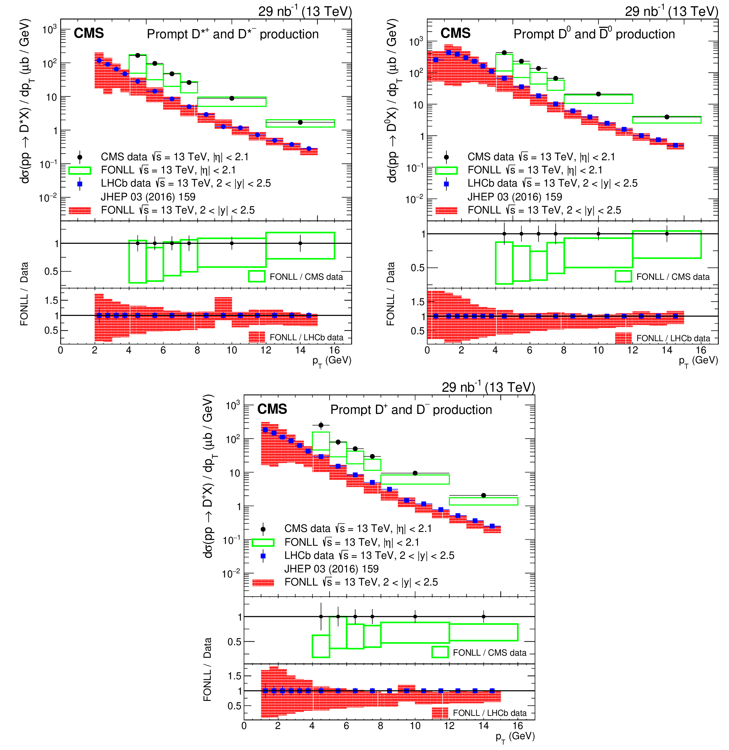
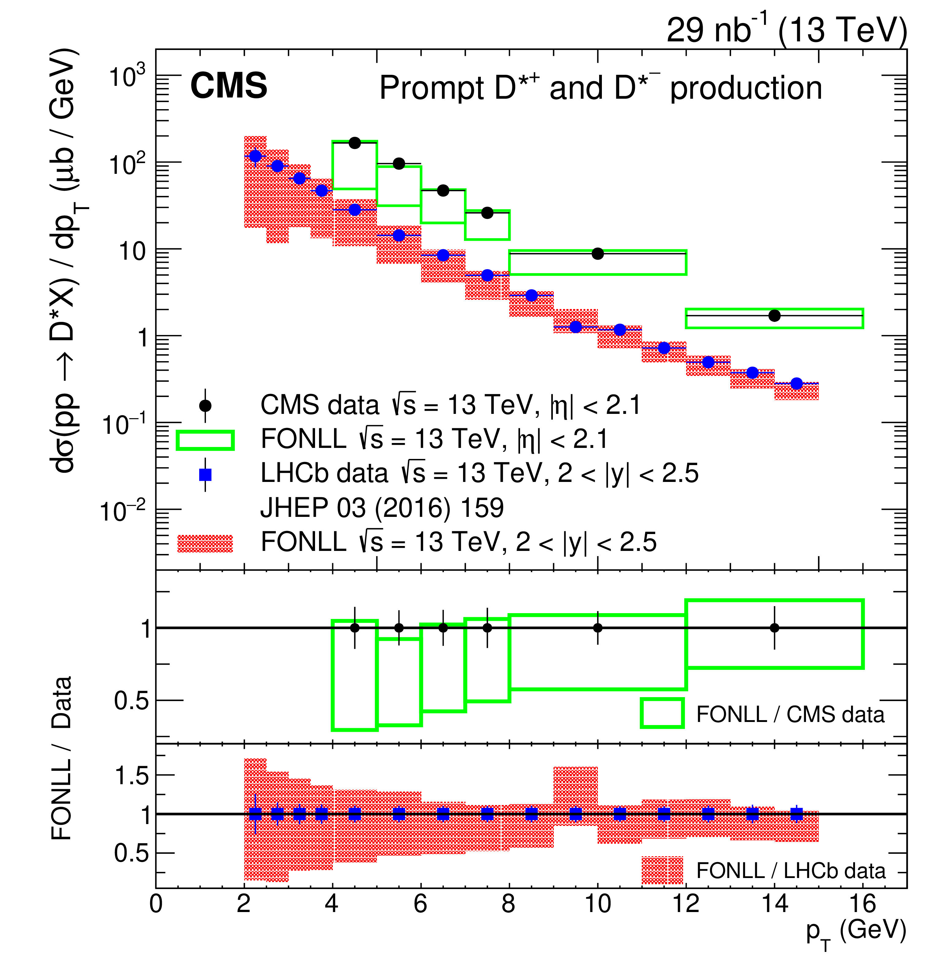
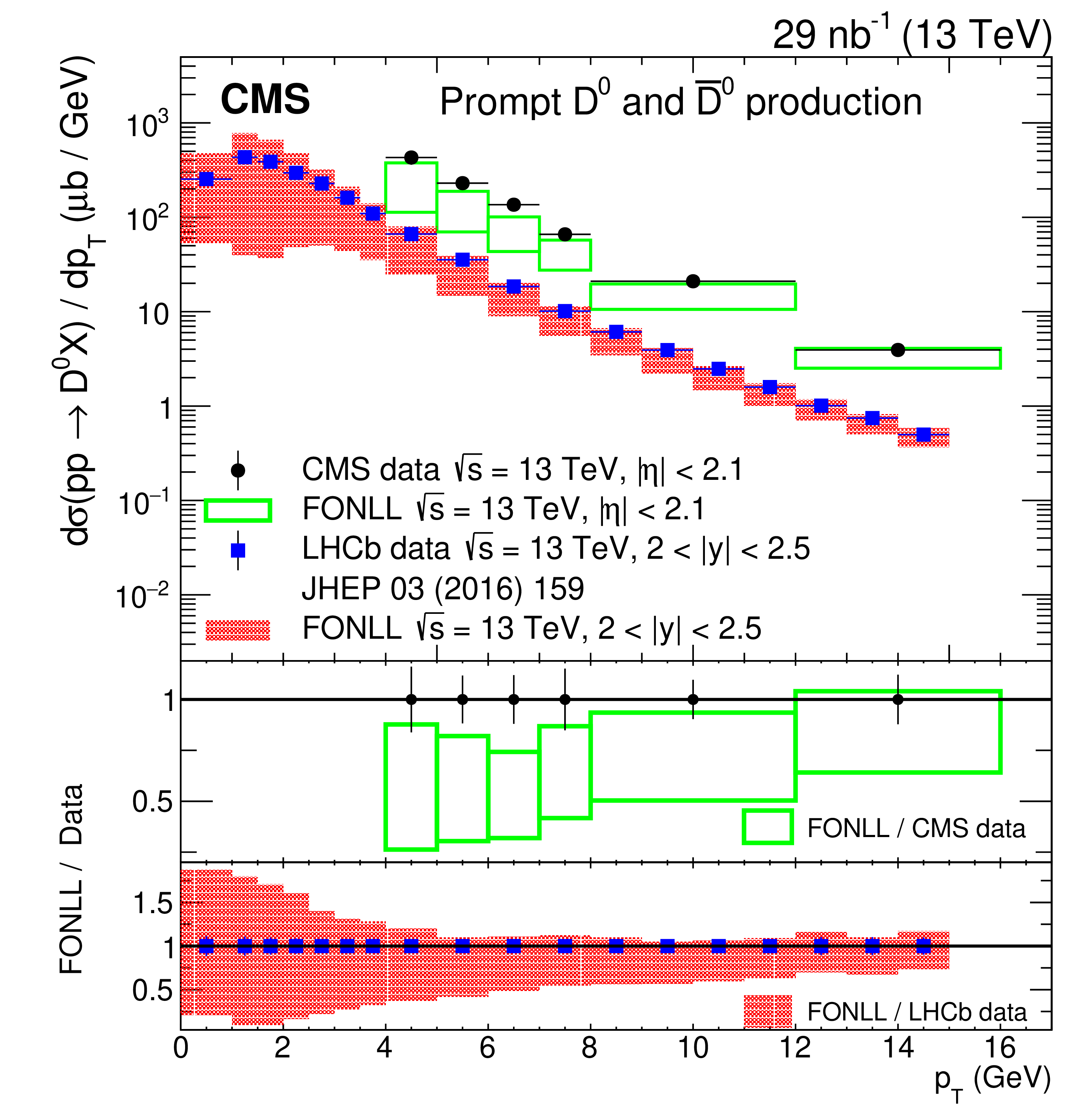
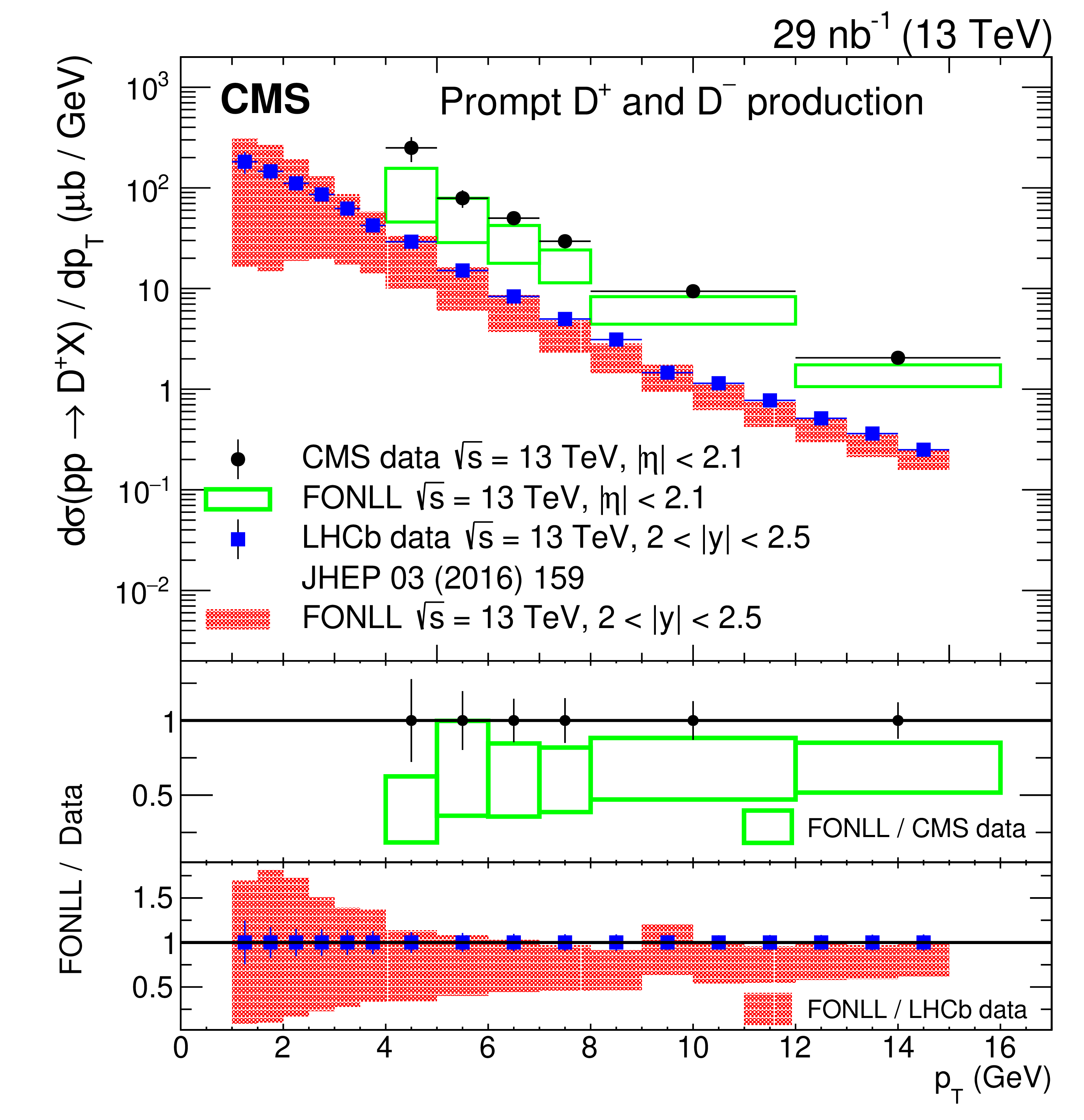
Figure 10:
Differential cross section $ {\mathrm {d}}\sigma / {\mathrm {d}} {p_{\mathrm {T}}} $ for prompt ${{\mathrm{D}^{\ast}(2010)^{\pm}}}$ (upper left), ${\mathrm{D^0}} + \mathrm{\overline{D}{}^{0}}$ (upper right) and ${\mathrm{D^{\pm}}}$ (lower) meson production at $\sqrt {s} = $ 13 TeV with $ {p_{\mathrm {T}}} < $ 16 GeV for CMS (black circles, this paper) for $ {| \eta |} < $ 2.1 and LHCb [11] (blue squares) for 2 $ < {| y |} < $ 2.5. The corresponding FONLL predictions are shown by the unfilled and filled boxes, respectively. To simplify the results representation, the equivalence between $ {\mathrm {d}}\sigma / {\mathrm {d}} {p_{\mathrm {T}}} $ for 2 $ < {| y |} < $ 2.5 and $ {\mathrm {d}}^2\sigma / {\mathrm {d}} {p_{\mathrm {T}}} dy$ for 2 $ < y < $ 2.5, as in the original publication, has been used. The vertical lines on the points give the total uncertainty in the data, and the horizontal lines show the bin widths. The two lower panels in each plot give the ratios of the FONLL predictions to the CMS and LHCb data, shown by circles and squares, respectively. |
png pdf |
Figure 10-a:
Differential cross section $ {\mathrm {d}}\sigma / {\mathrm {d}} {p_{\mathrm {T}}} $ for prompt ${{\mathrm{D}^{\ast}(2010)^{\pm}}}$ meson production at $\sqrt {s} = $ 13 TeV with $ {p_{\mathrm {T}}} < $ 16 GeV for CMS (black circles, this paper) for $ {| \eta |} < $ 2.1 and LHCb [11] (blue squares) for 2 $ < {| y |} < $ 2.5. The corresponding FONLL predictions are shown by the unfilled and filled boxes, respectively. To simplify the results representation, the equivalence between $ {\mathrm {d}}\sigma / {\mathrm {d}} {p_{\mathrm {T}}} $ for 2 $ < {| y |} < $ 2.5 and $ {\mathrm {d}}^2\sigma / {\mathrm {d}} {p_{\mathrm {T}}} dy$ for 2 $ < y < $ 2.5, as in the original publication, has been used. The vertical lines on the points give the total uncertainty in the data, and the horizontal lines show the bin widths. The two lower panels give the ratios of the FONLL predictions to the CMS and LHCb data, shown by circles and squares, respectively. |
png pdf |
Figure 10-b:
Differential cross section $ {\mathrm {d}}\sigma / {\mathrm {d}} {p_{\mathrm {T}}} $ for prompt ${\mathrm{D^0}} + \mathrm{\overline{D}{}^{0}}$ meson production at $\sqrt {s} = $ 13 TeV with $ {p_{\mathrm {T}}} < $ 16 GeV for CMS (black circles, this paper) for $ {| \eta |} < $ 2.1 and LHCb [11] (blue squares) for 2 $ < {| y |} < $ 2.5. The corresponding FONLL predictions are shown by the unfilled and filled boxes, respectively. To simplify the results representation, the equivalence between $ {\mathrm {d}}\sigma / {\mathrm {d}} {p_{\mathrm {T}}} $ for 2 $ < {| y |} < $ 2.5 and $ {\mathrm {d}}^2\sigma / {\mathrm {d}} {p_{\mathrm {T}}} dy$ for 2 $ < y < $ 2.5, as in the original publication, has been used. The vertical lines on the points give the total uncertainty in the data, and the horizontal lines show the bin widths. The two lower panels give the ratios of the FONLL predictions to the CMS and LHCb data, shown by circles and squares, respectively. |
png pdf |
Figure 10-c:
Differential cross section $ {\mathrm {d}}\sigma / {\mathrm {d}} {p_{\mathrm {T}}} $ for prompt ${\mathrm{D^{\pm}}}$ meson production at $\sqrt {s} = $ 13 TeV with $ {p_{\mathrm {T}}} < $ 16 GeV for CMS (black circles, this paper) for $ {| \eta |} < $ 2.1 and LHCb [11] (blue squares) for 2 $ < {| y |} < $ 2.5. The corresponding FONLL predictions are shown by the unfilled and filled boxes, respectively. To simplify the results representation, the equivalence between $ {\mathrm {d}}\sigma / {\mathrm {d}} {p_{\mathrm {T}}} $ for 2 $ < {| y |} < $ 2.5 and $ {\mathrm {d}}^2\sigma / {\mathrm {d}} {p_{\mathrm {T}}} dy$ for 2 $ < y < $ 2.5, as in the original publication, has been used. The vertical lines on the points give the total uncertainty in the data, and the horizontal lines show the bin widths. The two lower panels give the ratios of the FONLL predictions to the CMS and LHCb data, shown by circles and squares, respectively. |
| Tables | |
png pdf |
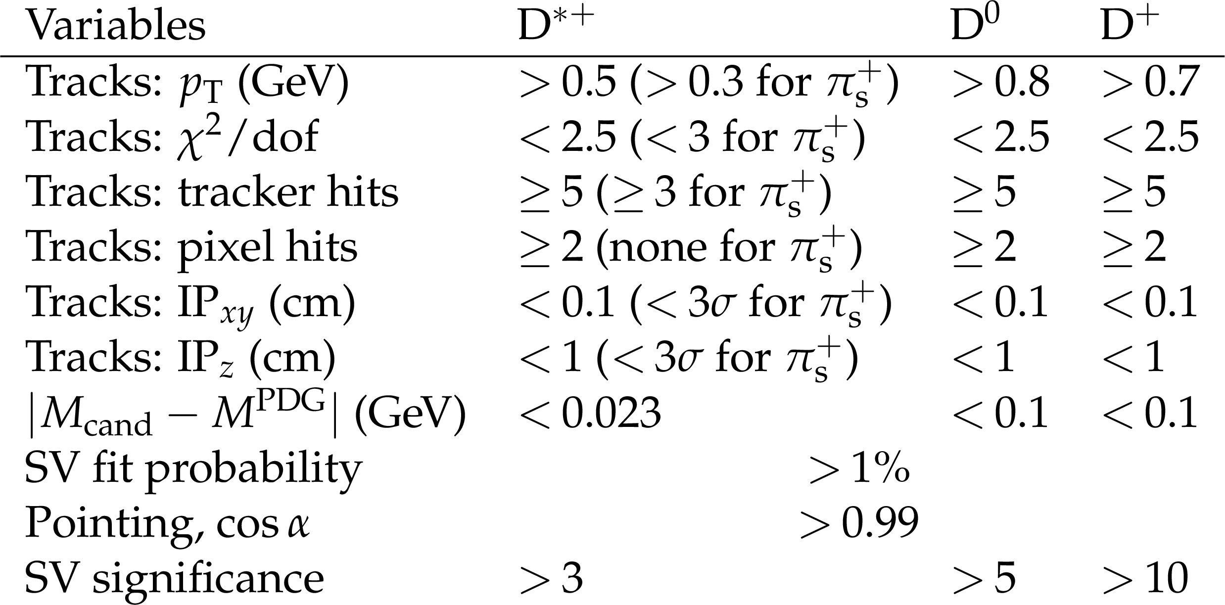
Table 1:
The selection requirements for each charm meson. |

png pdf |
Table 2:
The signal yields in data for $\mathrm{D^{*+}}$, ${\mathrm{D^0}}$, and ${\mathrm{D^+}}$ mesons in ${p_{\mathrm {T}}}$ bins for $ {| \eta |} < $ 2.1. The uncertainties are statistical only. |
png pdf |
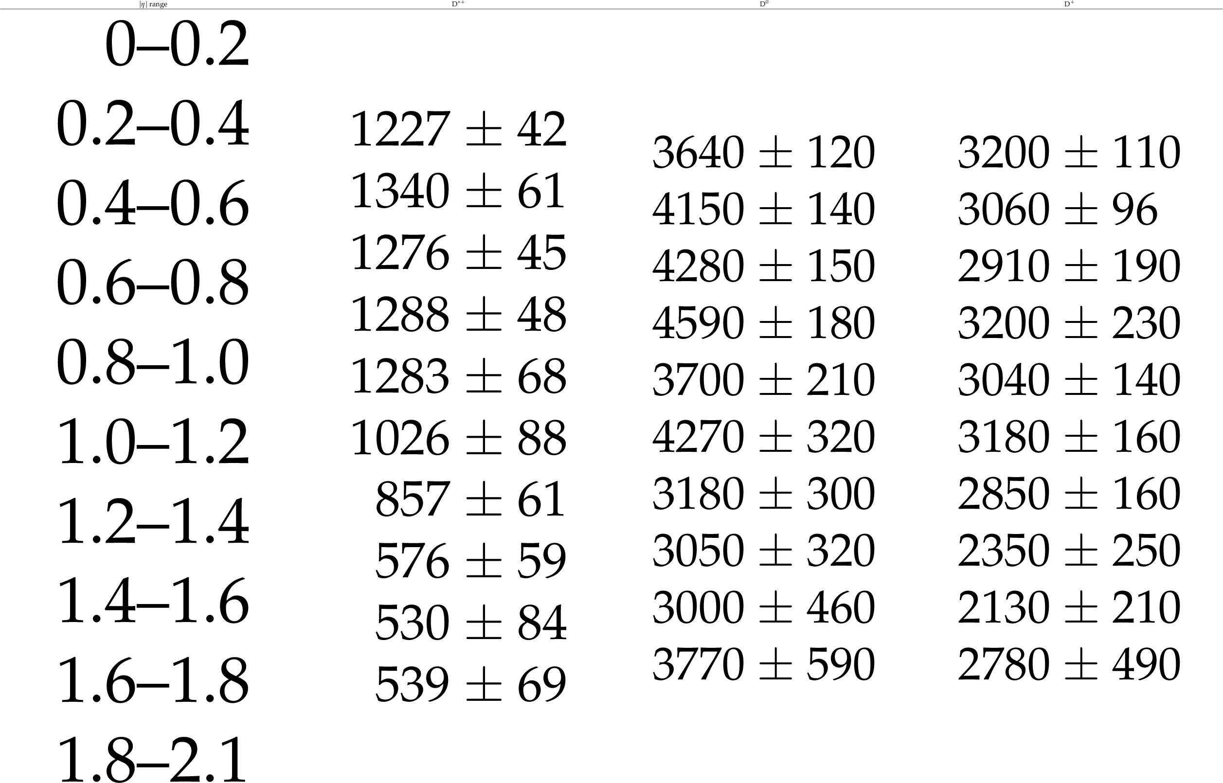
Table 3:
The signal yields in data for $\mathrm{D^{*+}}$, ${\mathrm{D^0}}$, and ${\mathrm{D^+}}$ mesons with 4 $ < {p_{\mathrm {T}}} < $ 100 GeV in $ {| \eta |}$ bins. The uncertainties are statistical only. |
png pdf |
Table 4:
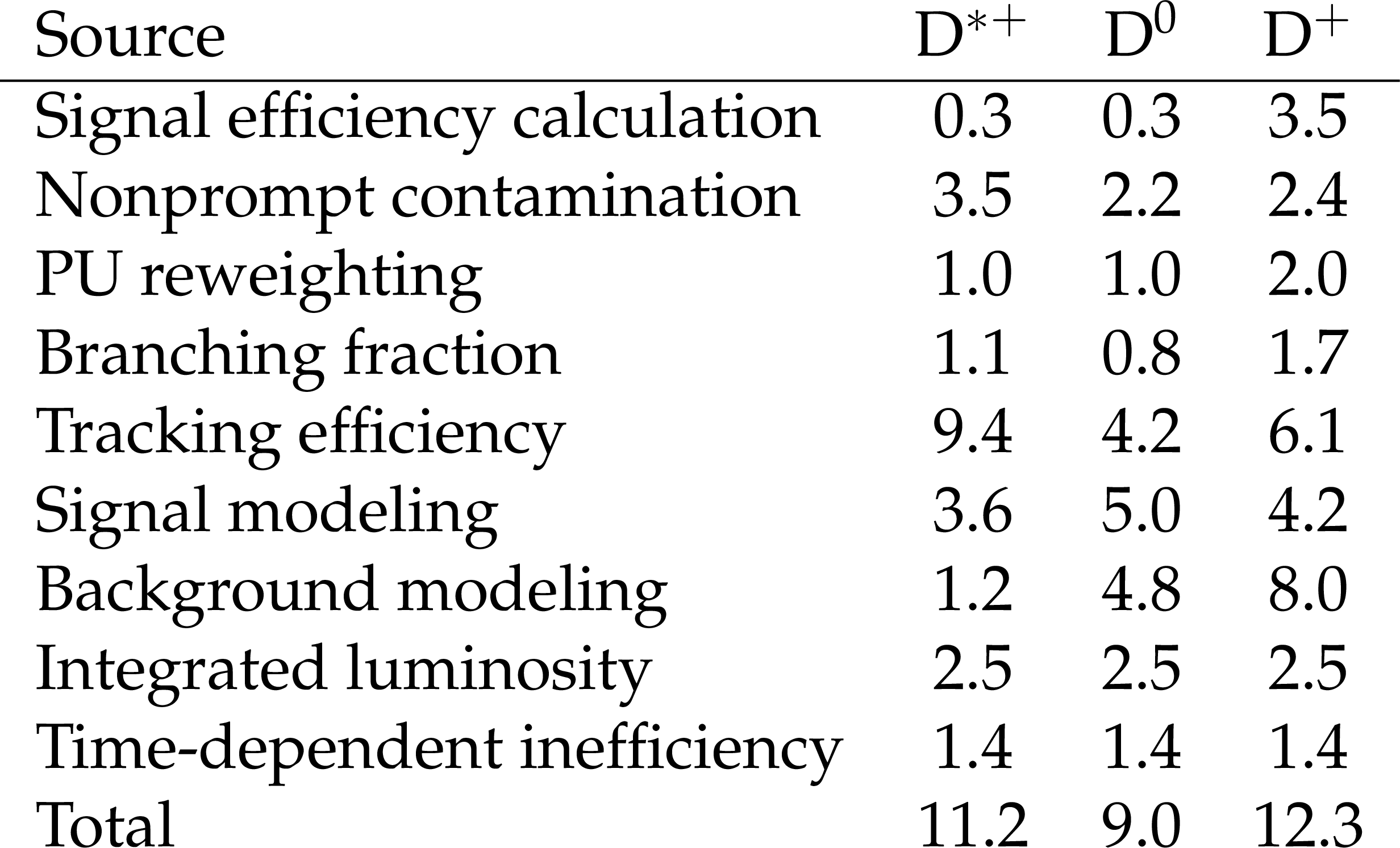
Summary of the systematic uncertainties (%) in the $\mathrm{D^{*+}}$, ${\mathrm{D^0}}$, and ${\mathrm{D^+}}$ meson cross sections. For the bin-dependent systematic uncertainties in the table, the weighted average is shown. The total uncertainty is the sum in quadrature of the individual contributions. |

png pdf |
Table 5:
The differential cross sections of prompt $\mathrm{D^{*+}} + \mathrm{D^{*-}}$, ${\mathrm{D^0}} + \mathrm{\overline{D}{}^{0}}$, and ${\mathrm{D^+}} + \mathrm{D^{-}}$ production in ${p_{\mathrm {T}}}$ bins with $ {| \eta |} < $ 2.1; the first uncertainty is statistical, the second is systematic. |
png pdf |
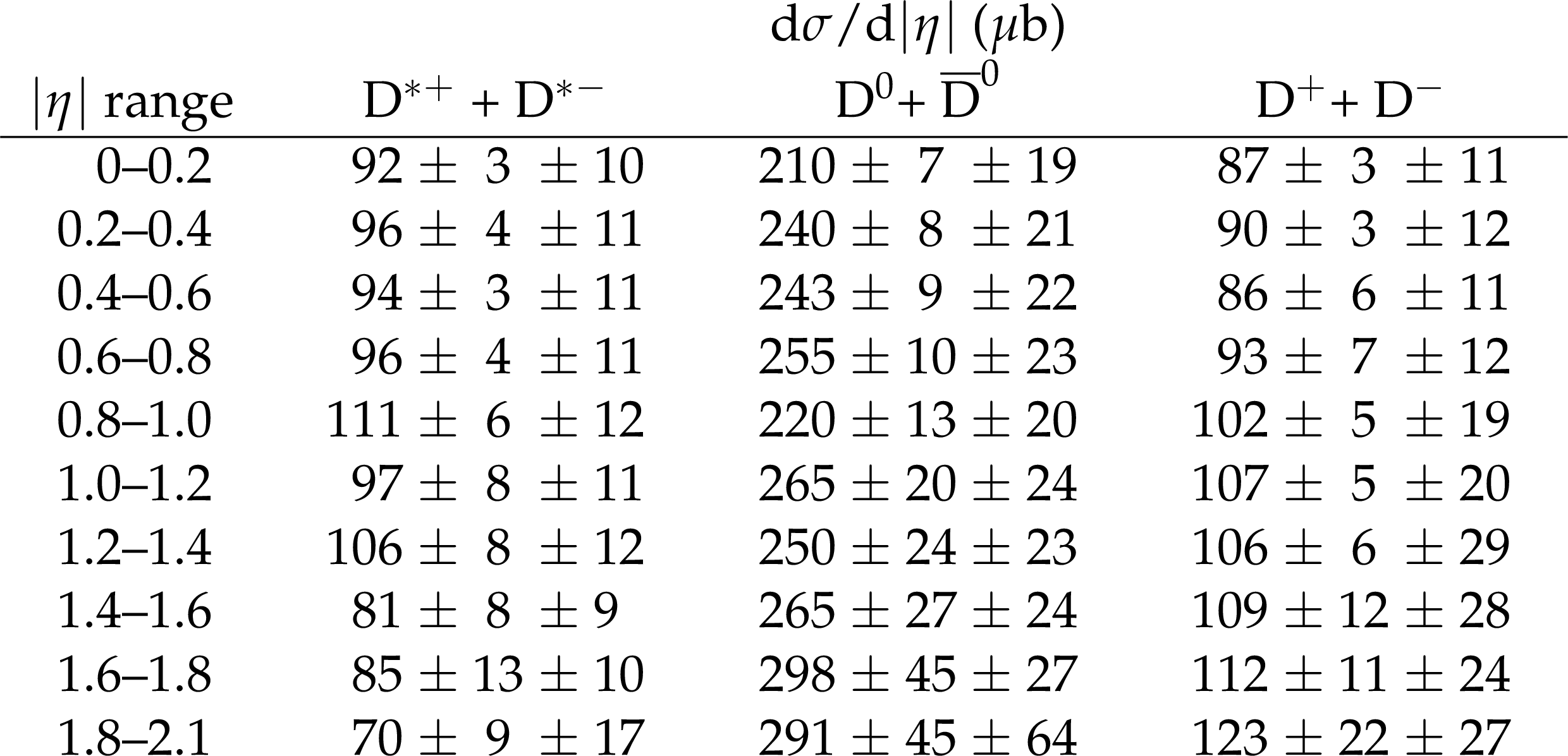
Table 6:
The differential cross sections of prompt $\mathrm{D^{*+}} + \mathrm{D^{*-}}$, ${\mathrm{D^0}} + \mathrm{\overline{D}{}^{0}}$, and ${\mathrm{D^+}} + \mathrm{D^{-}}$ production in $ {| \eta |}$ bins with 4 $ < {p_{\mathrm {T}}} < $ 100 GeV; the first uncertainty is statistical, the second is systematic. |
| Summary |
|
The differential cross sections ${\mathrm{d}}\sigma/{\mathrm{d}}{p_{\mathrm{T}}}$ and ${\mathrm{d}}\sigma/{\mathrm{d}}|{\eta}|$ for prompt charm meson (${{\mathrm{D}^{\ast}(2010)^{\pm}}}$, ${\mathrm{D^0}}$ ($\mathrm{\overline{D}{}^{0}}$), and ${\mathrm{D^{\pm}}}$) production are measured in the transverse momentum range 4 $ < {p_{\mathrm{T}}} < $ 100 GeV and pseudorapidity $|{\eta}| < $ 2.1, using data collected by the CMS experiment in proton-proton collisions in 2016 at $\sqrt{s} = $ 13 TeV, corresponding to an integrated luminosity of 29 nb$^{-1}$. The charm mesons were identified with signal invariant mass peaks of high statistical significance. The contamination arising from nonprompt D mesons originating from b hadron decays was removed using Monte Carlo event simulations, validated by measurements. The measured cross section values are compared to predictions from a theoretical calculation and several different Monte Carlo generators. The agreement with the various models can be considered fair, but no single Monte Carlo simulation or theoretical prediction describes the data well over the entire kinematic range. The measurements tend to favor a higher cross section than predicted by the FONLL calculations [15,16] and lower than estimated by the PYTHIA event generators [13,14]. The cross section predictions from the different PYTHIA tunes differ in both normalization and shape, which confirms that the description of the data provided by the models is sensitive to further model improvements. Overall, the best description is obtained by the upper edge of the FONLL uncertainty band, which could be taken as a reference prediction for background estimations for other processes, over the full kinematic range covered by all the LHC measurements. By confirming this finding in kinematic regions not previously covered, this measurement makes a contribution to the understanding of charm meson production in hadronic collisions, which is still dominated by large uncertainties in the present theoretical models. |
| References | ||||
| 1 | FASER Collaboration | Technical Proposal: FASERnu | technical report, January | 2001.03073 |
| 2 | S. Alekhin et al. | A facility to Search for Hidden Particles at the CERN SPS: the SHiP physics case | Rept. Prog. Phys. 79 (2016), no. CERN-SPSC-2015-017, SPSC-P-350-ADD-1, 124201 | 1504.04855 |
| 3 | SHiP Collaboration | SND@LHC - Scattering and Neutrino Detector at the LHC | CERN-LHCC-2021-003, LHCC-P-016, CERN, Geneva, Jan | |
| 4 | CMS Collaboration | Nuclear modification factor of D$ ^0 $ mesons in PbPb collisions at $ \sqrt{s_\mathrm{NN}} = $ 5.02 TeV | PLB 782 (2018) 474 | CMS-HIN-16-001 1708.04962 |
| 5 | ATLAS Collaboration | Measurement of $ D^{*\pm} $, $ D^\pm $ and $ D_s^\pm $ meson production cross sections in pp collisions at $ \sqrt{s}= $ 7 TeV with the ATLAS detector | NPB 907 (2016) 717 | 1512.02913 |
| 6 | ALICE Collaboration | Measurement of $ {{\mathrm{D}}^0} $ , $ {{\mathrm{D}}^+} $ , $ {{\mathrm{D}}^{*+}} $ and $ {{\mathrm{D}}^+_{\mathrm{s}}} $ production in pp collisions at $ \sqrt{s} = $ 5.02 TeV with ALICE | EPJC 79 (2019) 388 | 1901.07979 |
| 7 | ALICE Collaboration | Measurement of charm production at central rapidity in proton-proton collisions at $ \sqrt{s} = $ 7 TeV | JHEP 01 (2012) 128 | 1111.1553 |
| 8 | ALICE Collaboration | Measurement of D-meson production at mid-rapidity in pp collisions at $ {\sqrt{s}=7} $ TeV | EPJC 77 (2017) 550 | 1702.00766 |
| 9 | LHCb Collaboration | Measurements of prompt charm production cross-sections in pp collisions at $ \sqrt{s}= $ 5 TeV | JHEP 06 (2017) 147 | 1610.02230 |
| 10 | LHCb Collaboration | Prompt charm production in pp collisions at $ \sqrt{s} = $ 7 TeV | NPB 871 (2013) 1 | 1302.2864 |
| 11 | LHCb Collaboration | Measurements of prompt charm production cross-sections in pp collisions at $ \sqrt{s}= $ 13 TeV | JHEP 03 (2016) 159 | 1510.01707 |
| 12 | CMS Collaboration | HEPData record for this analysis | doi | |
| 13 | T. Sjostrand, S. Mrenna, and P. Z. Skands | PYTHIA 6.4 physics and manual | JHEP 05 (2006) 026 | hep-ph/0603175 |
| 14 | T. Sjostrand et al. | An introduction to PYTHIA 8.2 | CPC 191 (2015) 159 | 1410.3012 |
| 15 | M. Cacciari, M. Greco, and P. Nason | The $ p_T $ spectrum in heavy flavor hadroproduction | JHEP 05 (1998) 007 | hep-ph/9803400 |
| 16 | M. Cacciari, M. L. Mangano, and P. Nason | Gluon PDF constraints from the ratio of forward heavy-quark production at the LHC at $ \sqrt{s}= $ 7 and 13 TeV | EPJC 75 (2015) 610 | 1507.06197 |
| 17 | CMS Collaboration | Description and performance of track and primary-vertex reconstruction with the CMS tracker | JINST 9 (2014) P10009 | CMS-TRK-11-001 1405.6569 |
| 18 | CMS Collaboration | The CMS trigger system | JINST 12 (2017) P01020 | CMS-TRG-12-001 1609.02366 |
| 19 | CMS Collaboration | The CMS experiment at the CERN LHC | JINST 3 (2008) S08004 | CMS-00-001 |
| 20 | CMS Collaboration | Precision luminosity measurement in proton-proton collisions at $ \sqrt{s} = $ 13 TeV in 2015 and 2016 at CMS | Submitted to EPJC | CMS-LUM-17-003 2104.01927 |
| 21 | M. Cacciari, G. P. Salam, and G. Soyez | The anti-$ {k_{\mathrm{T}}} $ jet clustering algorithm | JHEP 04 (2008) 063 | 0802.1189 |
| 22 | M. Cacciari, G. P. Salam, and G. Soyez | FastJet user manual | EPJC 72 (2012) 1896 | 1111.6097 |
| 23 | D. J. Lange | The EvtGen particle decay simulation package | NIMA 462 (2001) 152 | |
| 24 | GEANT4 Collaboration | GEANT4--A simulation toolkit | NIMA 506 (2003) 250 | |
| 25 | Particle Data Group, M. Tanabashi et al. | Review of particle physics | PRD 98 (2018) 030001 | |
| 26 | CMS Collaboration | Measurement of tracking efficiency | CDS | |
| 27 | CMS Collaboration | Event generator tunes obtained from underlying event and multiparton scattering measurements | EPJC 76 (2016) 155 | CMS-GEN-14-001 1512.00815 |
| 28 | CMS Collaboration | Studies of beauty suppression via nonprompt $ D^0 $ mesons in Pb-Pb collisions at $ Q^2 = $ 4 GeV$^2 $ | PRL 123 (2019) 022001 | CMS-HIN-16-016 1810.11102 |
| 29 | CMS Collaboration | Tracking POG results for pion efficiency with the D* meson using data from 2016 and 2017 | CDS | |
| 30 | M. J. Oreglia | A study of the reactions $\psi' \to \gamma\gamma \psi$ | PhD thesis, Stanford University, 1980 SLAC Report SLAC-R-236, see A | |
| 31 | J. Gaiser | Charmonium Spectroscopy From Radiative Decays of the $\mathrm{J}/\psi$ | PhD thesis, SLAC | |
| 32 | CMS Collaboration | CMS luminosity measurements for the 2016 data taking period | CMS-PAS-LUM-17-001 | CMS-PAS-LUM-17-001 |
| 33 | M. Lisovyi, A. Verbytskyi, and O. Zenaiev | Combined analysis of charm-quark fragmentation-fraction measurements | EPJC 76 (2016) 397 | 1509.01061 |
| 34 | CMS Collaboration | Study of the underlying event at forward rapidity in pp collisions at $ \sqrt{s} = $ 0.9, 2.76, and 7 TeV | JHEP 04 (2013) 072 | CMS-FWD-11-003 1302.2394 |
| 35 | R. Field | Early LHC underlying event data - findings and surprises | in 22nd Hadron Collider Physics Symposium (HCP 2010), W. Trischuk, ed Toronto | 1010.3558 |
| 36 | ATLAS Collaboration | Summary of ATLAS Pythia 8 tunes | ATL-PHYS-PUB-2012-003, 8 | |
| 37 | R. Corke and T. Sjostrand | Interleaved parton showers and tuning prospects | JHEP 03 (2011) 032 | 1011.1759 |
| 38 | P. Skands, S. Carrazza, and J. Rojo | Tuning PYTHIA 8.1: the Monash 2013 tune | EPJC 74 (2014) 3024 | 1404.5630 |
| 39 | CMS Collaboration | Extraction and validation of a new set of CMS PYTHIA8 tunes from underlying-event measurements | EPJC 80 (2020) 4 | CMS-GEN-17-001 1903.12179 |
|
|
Compact Muon Solenoid LHC, CERN |
|

|

|

|

|

|