

Compact Muon Solenoid
LHC, CERN
| CMS-LUM-17-003 ; CERN-EP-2021-033 | ||
| Precision luminosity measurement in proton-proton collisions at $\sqrt{s}=$ 13 TeV in 2015 and 2016 at CMS | ||
| CMS Collaboration | ||
| 5 April 2021 | ||
| Eur. Phys. J. C 81 (2021) 800 | ||
| Abstract: The measurement of the luminosity recorded by the CMS detector installed at LHC interaction point 5, using proton-proton collisions at $\sqrt{s}=$ 13 TeV in 2015 and 2016, is reported. The absolute luminosity scale is measured for individual bunch crossings using beam-separation scans (the van der Meer method), with a relative precision of 1.3% and 1.0% in 2015 and 2016, respectively. The dominant sources of uncertainty are related to residual differences between the measured beam positions and the ones provided by the operational settings of the LHC magnets, the factorizability of the proton bunch spatial density functions in the coordinates transverse to the beam direction, and the modeling of the effect of electromagnetic interactions among protons in the colliding bunches. When applying the van der Meer calibration to the entire run periods, the integrated luminosities when CMS was fully operational are 2.27 and 36.3 fb$^{-1}$ in 2015 and 2016, with a relative precision of 1.6% and 1.2%, respectively. These are among the most precise luminosity measurements at bunched-beam hadron colliders. | ||
| Links: e-print arXiv:2104.01927 [hep-ex] (PDF) ; CDS record ; inSPIRE record ; CADI line (restricted) ; | ||
| Figures | |

png pdf |
Figure 1:
Schematic cross section through the CMS detector in the $r$-$z$ plane. The main luminometers in Run 2, as described in the text, are highlighted, showing the silicon pixel detector, PLT, BCM1F, DTs, and HF. The two RAMSES monitors used as a luminometer in Run 2 are located directly behind HF. In this view, the detector is symmetric about the horizontal and vertical axes, so only one quarter is shown here. The center of the detector, corresponding to the approximate position of the pp collision point, is located at the origin. Solid lines represent distinct $\eta $ values. |
png pdf |
Figure 2:
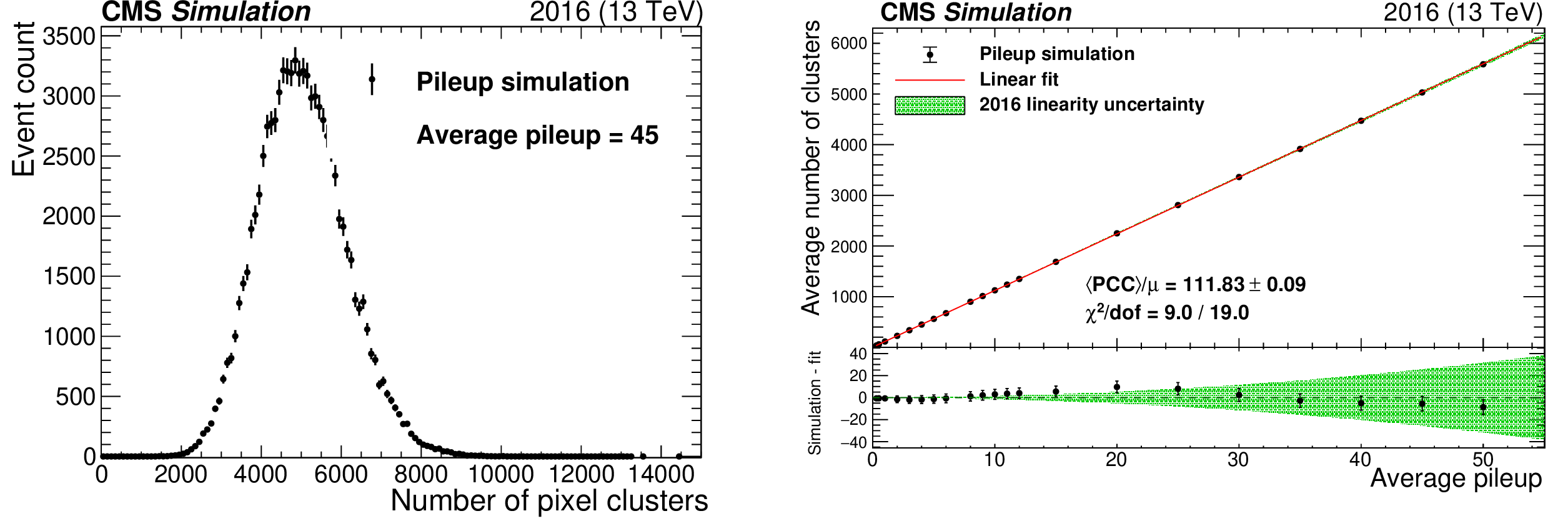
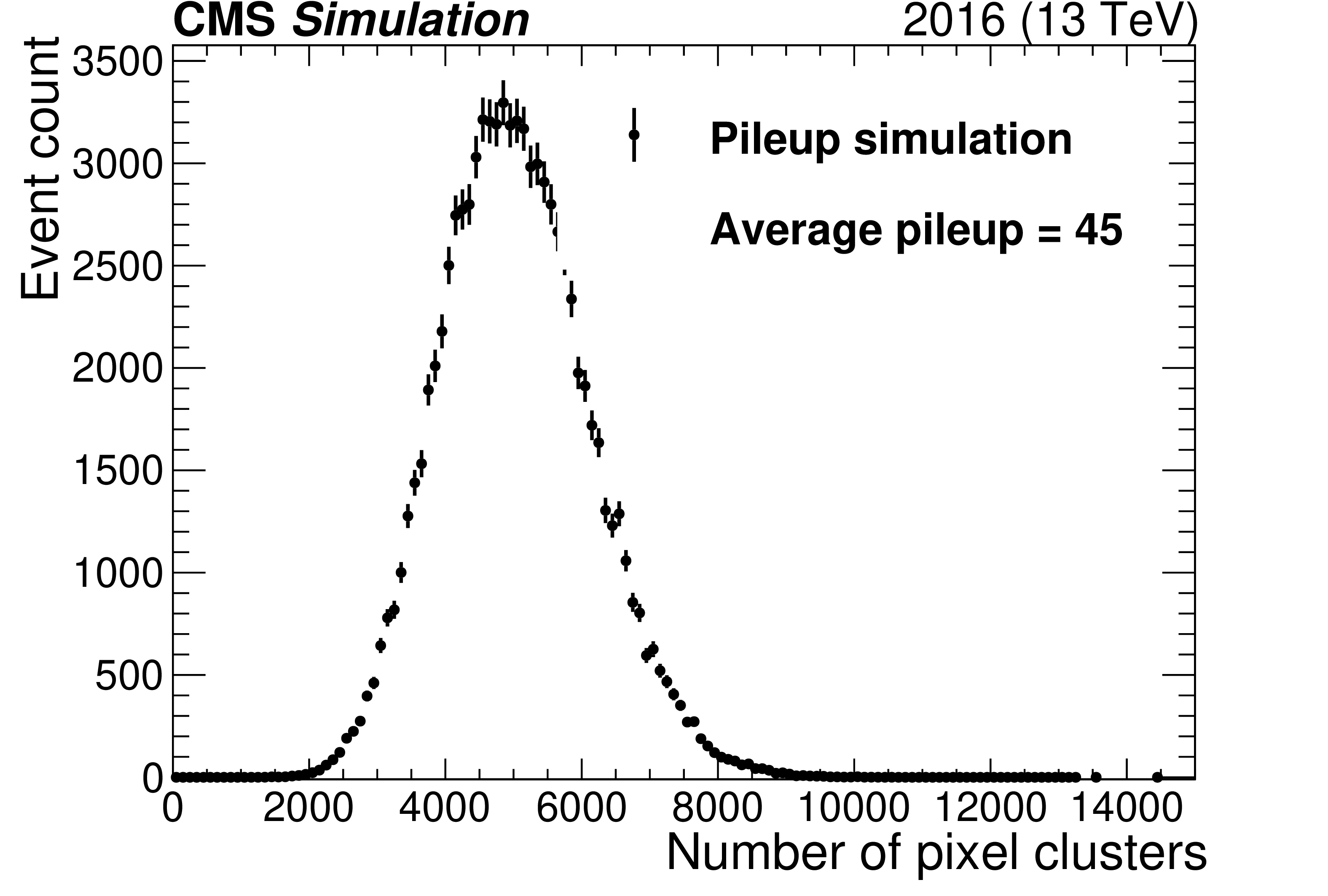
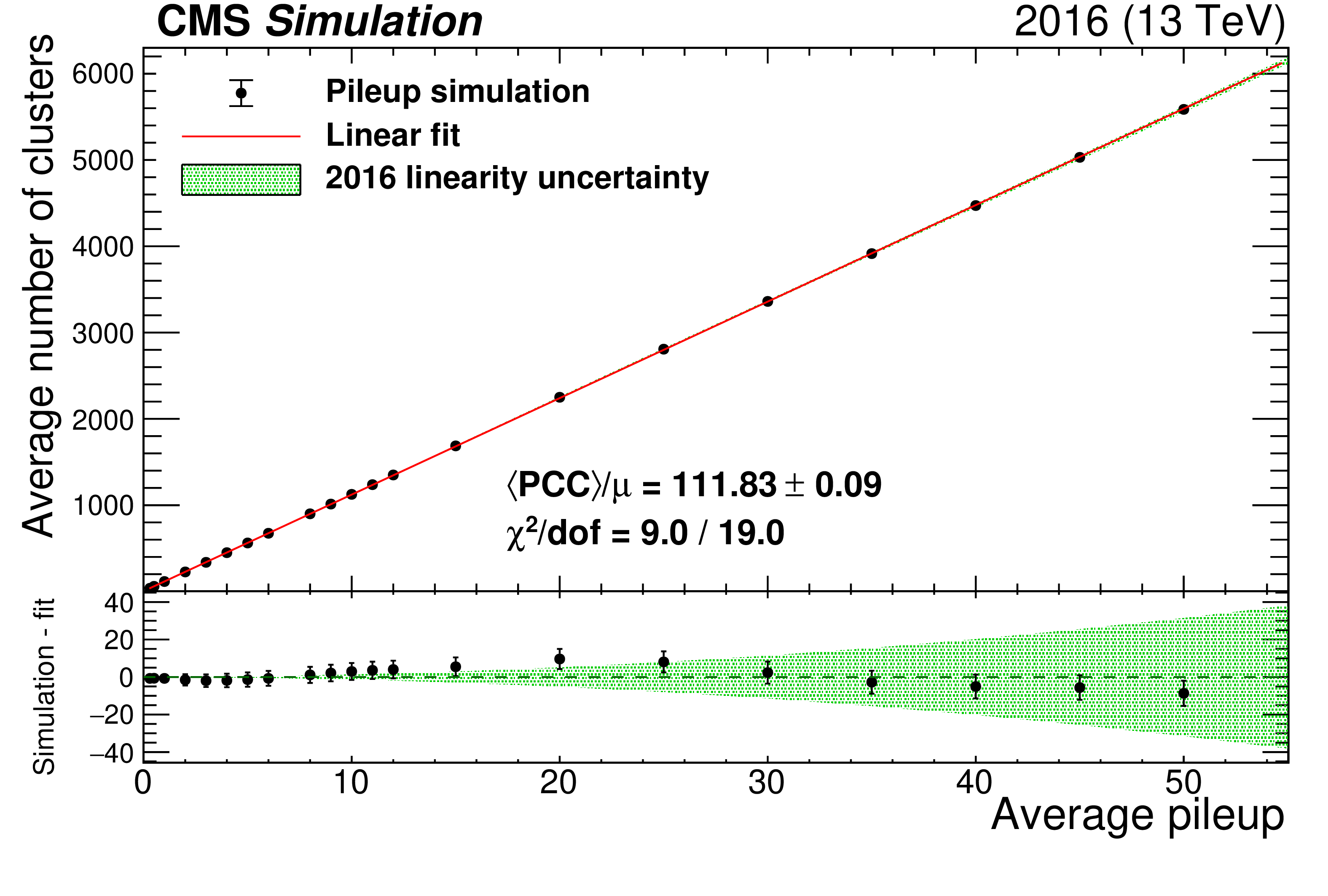
The left plot shows the number of pixel clusters and their statistical uncertainty from simulation of pileup following a Poisson distribution with a mean of 45. The right plot shows the mean number of pixel clusters from simulation as a function of mean pileup. The red curve is a first-order polynomial fit with slope and $\chi ^2/\text {dof}$ values shown in the legend. Only pixel modules considered for the PCC measurement in data are included. The lower panel of the right plot shows the difference between the simulation and the linear fit in black points. The green band is the final linearity uncertainty for the 2016 data set. |
png pdf |
Figure 2-a:
The plot shows the number of pixel clusters and their statistical uncertainty from simulation of pileup following a Poisson distribution with a mean of 45. |
png pdf |
Figure 2-b:
The plot shows the mean number of pixel clusters from simulation as a function of mean pileup. The red curve is a first-order polynomial fit with slope and $\chi ^2/\text {dof}$ values shown in the legend. Only pixel modules considered for the PCC measurement in data are included. The lower panel shows the difference between the simulation and the linear fit in black points. The green band is the final linearity uncertainty for the 2016 data set. |

png pdf |
Figure 3:
Relative change in the positions of beams 1 and 2 measured by the DOROS BPMs during fill 4954 in the horizontal ($x$) or vertical ($y$) directions, as a function of the time elapsed from the beginning of the program. The gray vertical lines delineate vdM, BI, or LSC scans. |
png pdf |
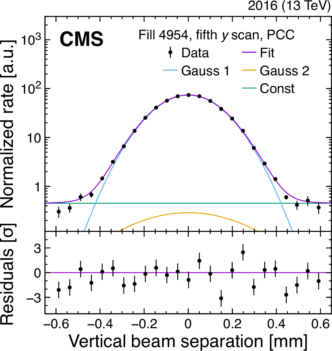
Figure 4:
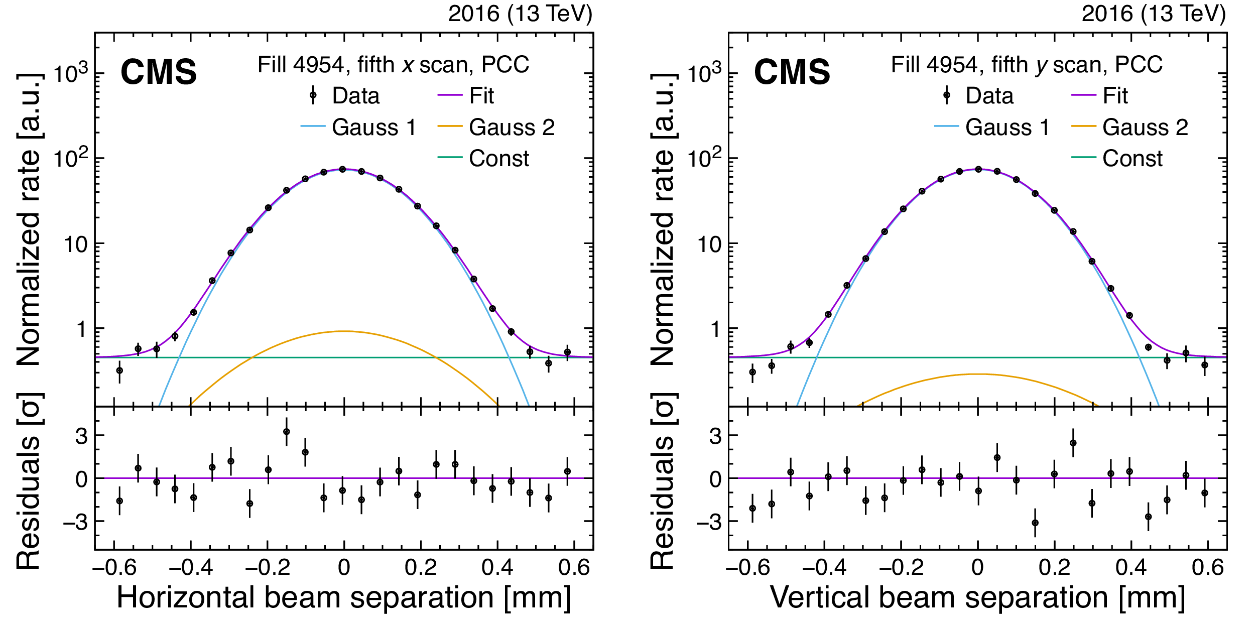
Example vdM scans for PCC for BCID 41, from the last scan pair in fill 4954, showing the rate normalized by the product of beam currents and its statistical uncertainty as a function of the beam separation in the $x$ (left) and $y$ (right) direction, and the fitted curves. The purple curve shows the overall double-Gaussian fit, while the blue, yellow, and green curves show the first and second Gaussian components and the constant component, respectively. All corrections described in Section 4.3 are applied. The lower panels display the difference between the measured and fitted values divided by the statistical uncertainty. |

png pdf |
Figure 4-a:
Example vdM scans for PCC for BCID 41, from the last scan pair in fill 4954, showing the rate normalized by the product of beam currents and its statistical uncertainty as a function of the beam separation in the $x$ direction, and the fitted curves. The purple curve shows the overall double-Gaussian fit, while the blue, yellow, and green curves show the first and second Gaussian components and the constant component, respectively. All corrections described in Section 4.3 are applied. The lower panels display the difference between the measured and fitted values divided by the statistical uncertainty. |
png pdf |
Figure 4-b:
Example vdM scans for PCC for BCID 41, from the last scan pair in fill 4954, showing the rate normalized by the product of beam currents and its statistical uncertainty as a function of the beam separation in the $y$ direction, and the fitted curves. The purple curve shows the overall double-Gaussian fit, while the blue, yellow, and green curves show the first and second Gaussian components and the constant component, respectively. All corrections described in Section 4.3 are applied. The lower panels display the difference between the measured and fitted values divided by the statistical uncertainty. |
png pdf |
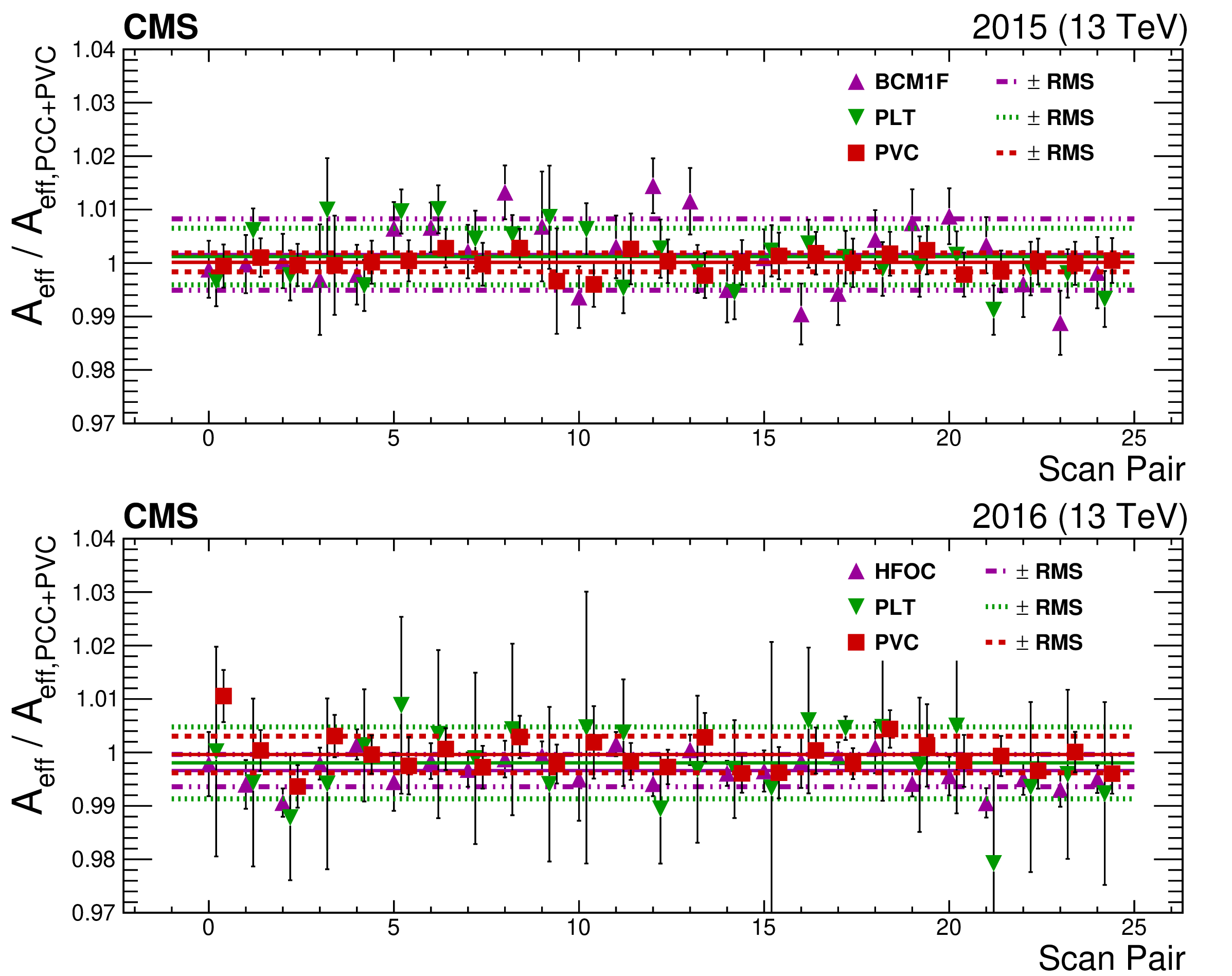
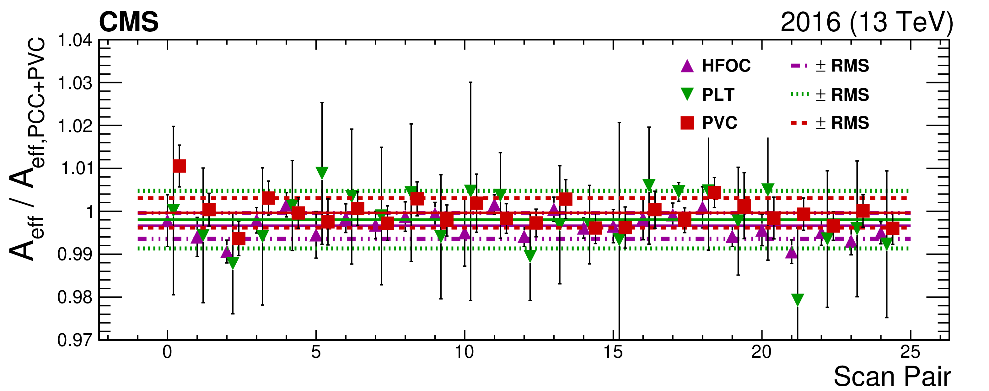
Figure 5:
The two figures above show comparisons of effective area (${A_{\text {eff}}}$) of cross-check luminometers with respect to the nominal PCC+PVC for fills 4266 (upper) and 4954 (lower). The points are the ratio of the ${A_{\text {eff}}}$ of the labeled luminometer to PCC+PVC. There are 25 ${A_{\text {eff}}}$ values because there are five scan pairs with five BCIDs analyzed for each scan pair. The solid lines are the average of all the ${A_{\text {eff}}}$ while the bands are the standard deviations. In both sets of data the average comparison is compatible with unity within or near the standard deviation. |

png pdf |
Figure 5-a:
The two figures above show comparisons of effective area (${A_{\text {eff}}}$) of cross-check luminometers with respect to the nominal PCC+PVC for fill 4266. The points are the ratio of the ${A_{\text {eff}}}$ of the labeled luminometer to PCC+PVC. There are 25 ${A_{\text {eff}}}$ values because there are five scan pairs with five BCIDs analyzed for each scan pair. The solid lines are the average of all the ${A_{\text {eff}}}$ while the bands are the standard deviations. The average comparison is compatible with unity within or near the standard deviation. |
png pdf |
Figure 5-b:
The two figures above show comparisons of effective area (${A_{\text {eff}}}$) of cross-check luminometers with respect to the nominal PCC+PVC for fill 4954. The points are the ratio of the ${A_{\text {eff}}}$ of the labeled luminometer to PCC+PVC. There are 25 ${A_{\text {eff}}}$ values because there are five scan pairs with five BCIDs analyzed for each scan pair. The solid lines are the average of all the ${A_{\text {eff}}}$ while the bands are the standard deviations. The average comparison is compatible with unity within or near the standard deviation. |
png pdf |
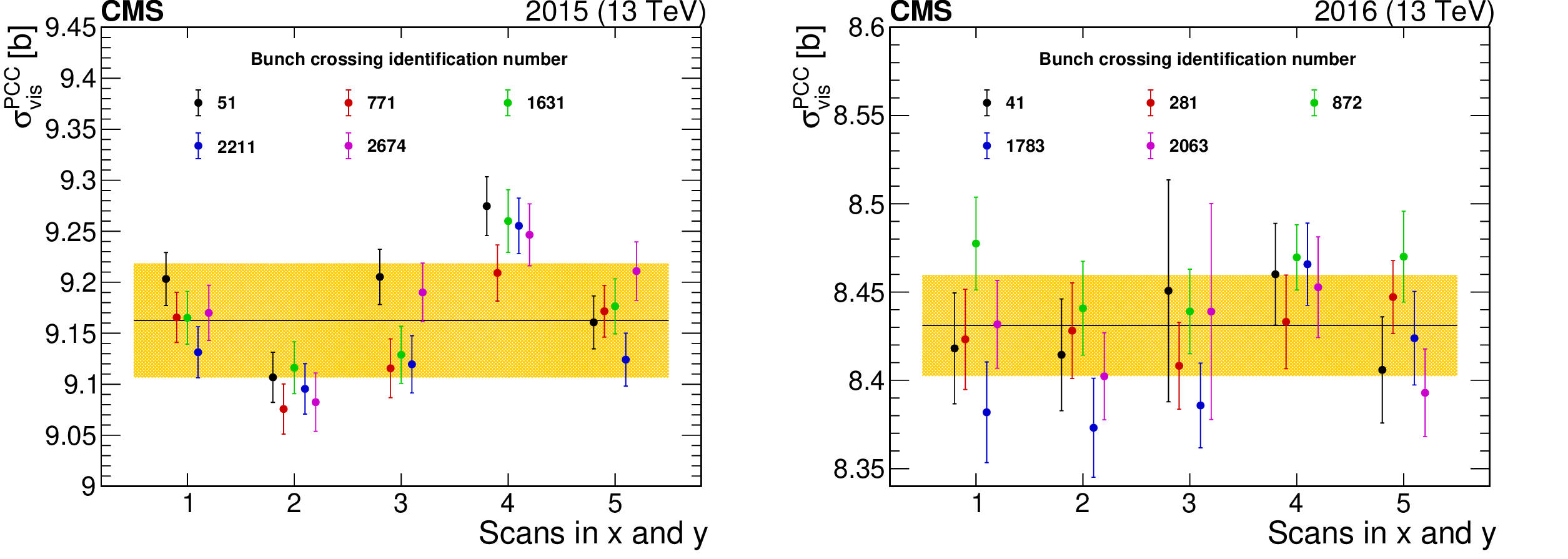
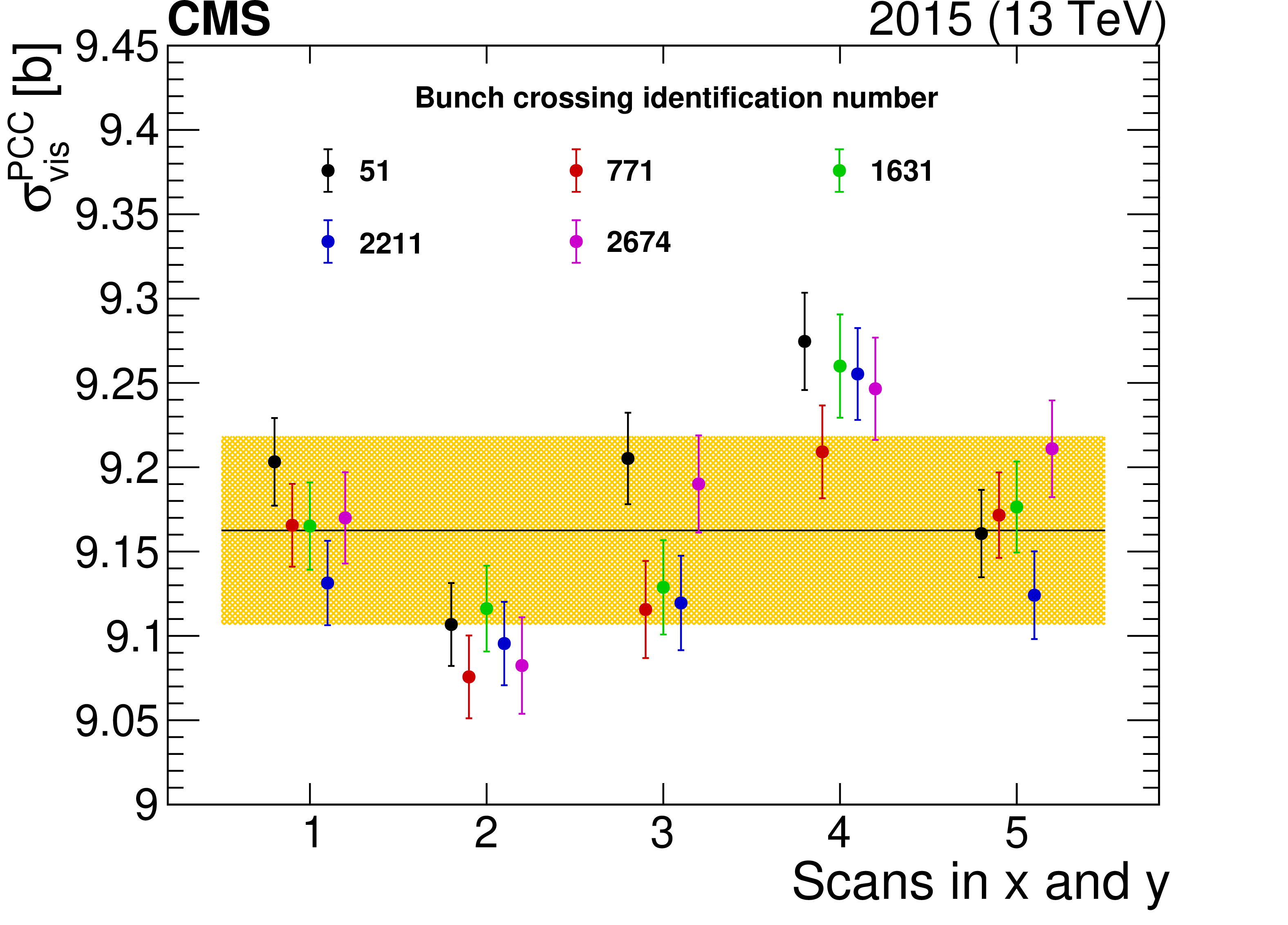
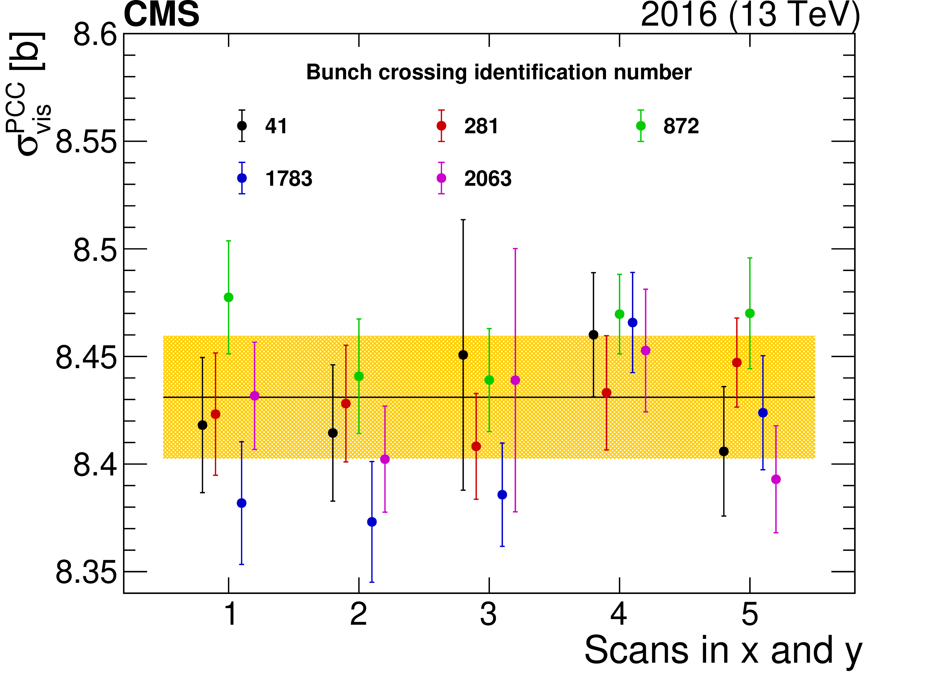
Figure 6:
The measured ${\sigma _{\text {vis}}^{\text {PCC}}}$, corrected for all the effects described in Section 4.3 , shown chronologically for all vdM scan pairs (where 3 and 4 are BI scans) taken in fills 4266 (left) and 4954 (right), respectively. Each of the five colliding bunch pairs is marked with a different color. The error bars correspond to the statistical uncertainty propagated from the vdM fit to ${\sigma _{\text {vis}}^{\text {PCC}}}$. The band is the standard deviation of all fitted ${\sigma _{\text {vis}}^{\text {PCC}}}$ values. |
png pdf |
Figure 6-a:
The measured ${\sigma _{\text {vis}}^{\text {PCC}}}$, corrected for all the effects described in Section 4.3 , shown chronologically for all vdM scan pairs (where 3 and 4 are BI scans) taken in fill 4266. Each of the five colliding bunch pairs is marked with a different color. The error bars correspond to the statistical uncertainty propagated from the vdM fit to ${\sigma _{\text {vis}}^{\text {PCC}}}$. The band is the standard deviation of all fitted ${\sigma _{\text {vis}}^{\text {PCC}}}$ values. |
png pdf |
Figure 6-b:
The measured ${\sigma _{\text {vis}}^{\text {PCC}}}$, corrected for all the effects described in Section 4.3 , shown chronologically for all vdM scan pairs (where 3 and 4 are BI scans) taken in fill 4954. Each of the five colliding bunch pairs is marked with a different color. The error bars correspond to the statistical uncertainty propagated from the vdM fit to ${\sigma _{\text {vis}}^{\text {PCC}}}$. The band is the standard deviation of all fitted ${\sigma _{\text {vis}}^{\text {PCC}}}$ values. |
png pdf |
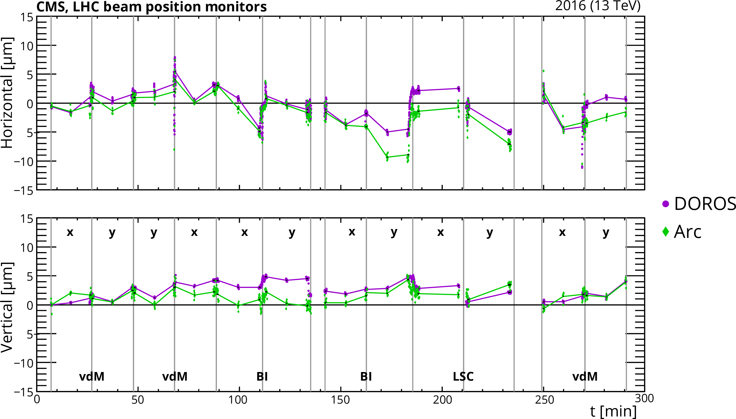
Figure 7:
Effect of orbit drift in the horizontal (upper) and vertical (lower) beam-separation directions during fill 4954. The dots correspond to the beam positions measured by the DOROS or LHC arc BPMs in $\mu $m at times when the beams nominally collide head-on and in three periods per scan (before, during, and after) represented by the vertical lines. First-order polynomial fits are subsequently made to the input from BPMs (dots) and are used to estimate the orbit drift at each scan step. Slow, linear orbit drifts are corrected exactly in this manner, and more discrete discontinuities are corrected on average. |
png pdf |
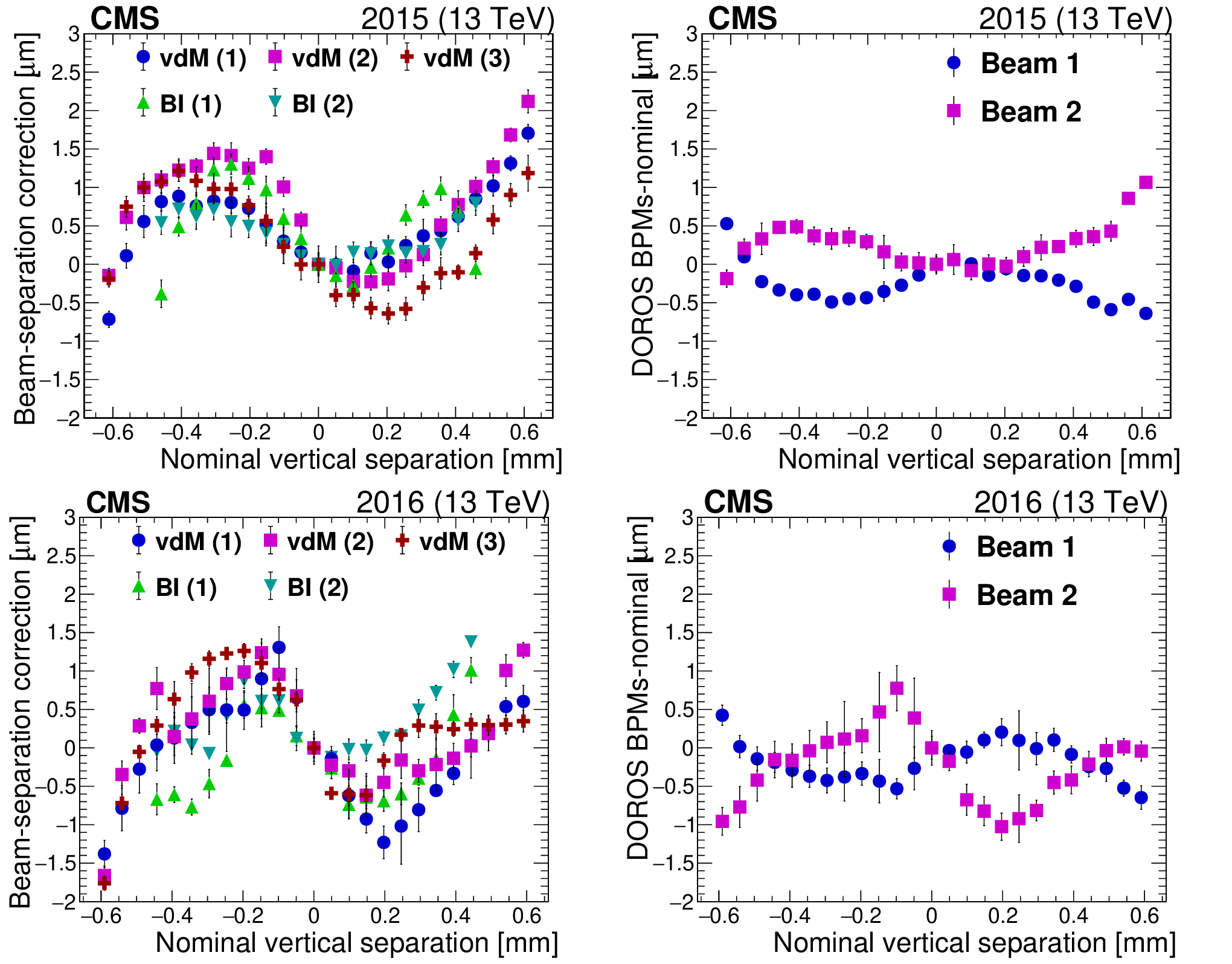
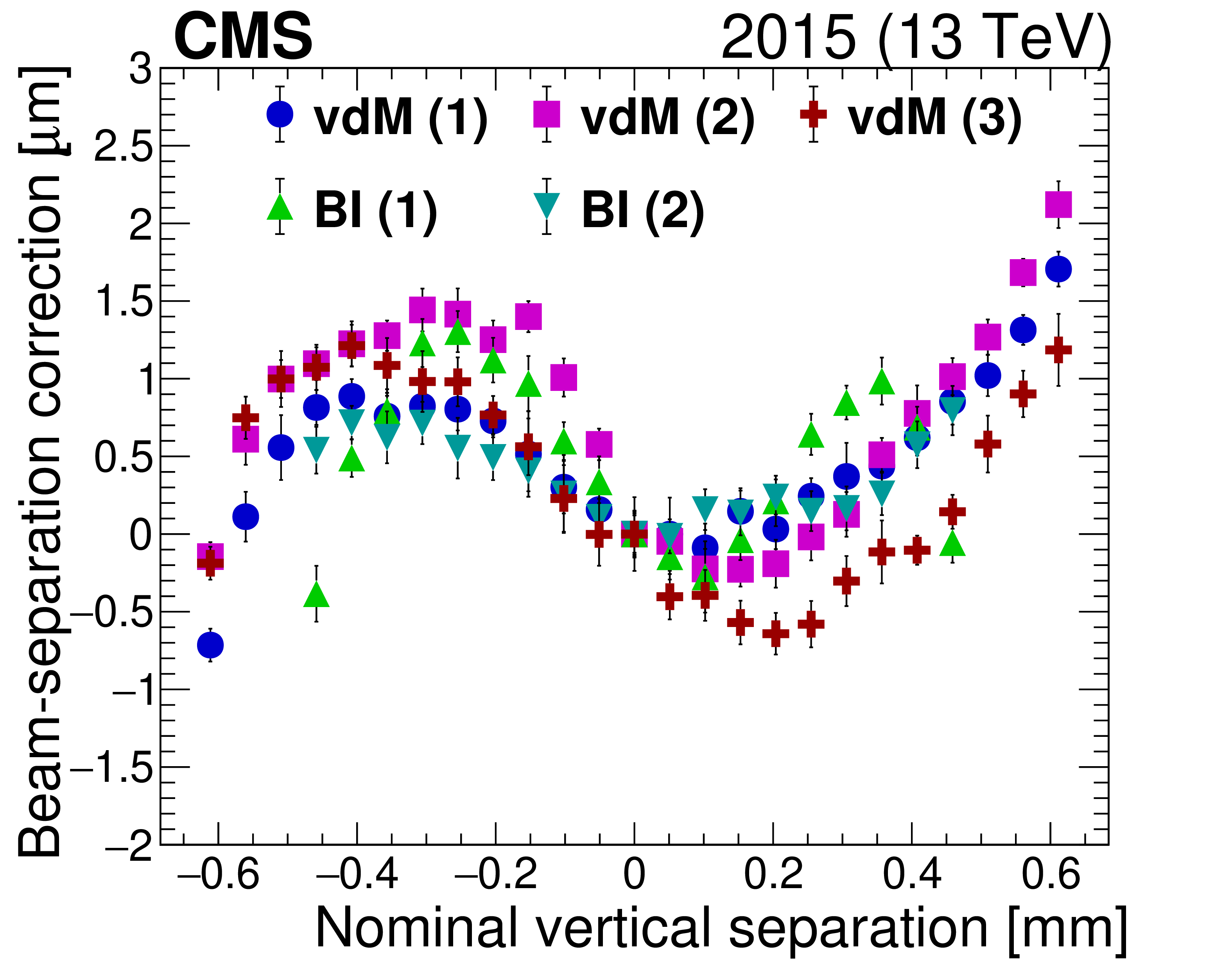
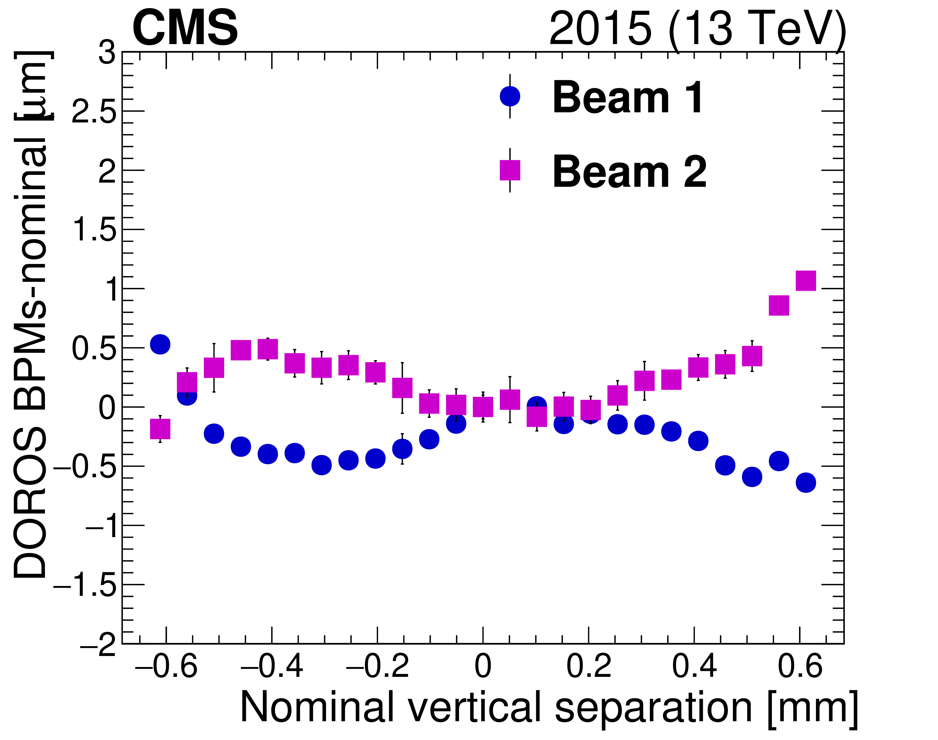
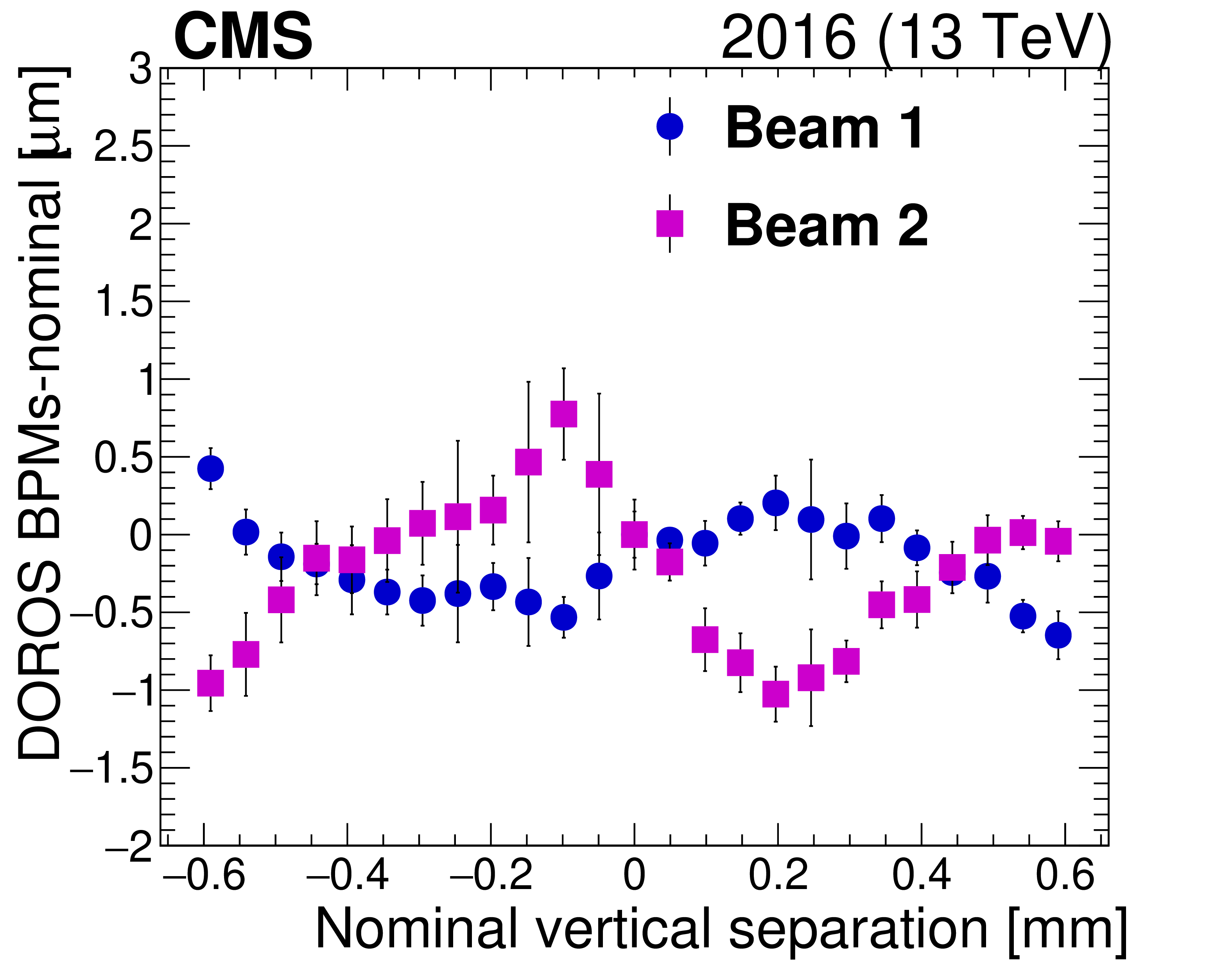
Figure 8:
The beam-separation residuals in $y$ during all scans in fills 4266 (upper) and 4954 (lower) are shown on the left. The dots correspond to the difference (in terms of beam separation in $\mu $m) between the corrected beam positions measured by the DOROS BPMs and the beam separation provided by LHC magnets ("nominal''). The error bars denote the standard deviation in the measurements. The figures on the right show the residual position differences per beam between the DOROS BPMs and LHC positions for the first vdM scans in $y$ in fills 4266 (upper) and 4954 (lower). |
png pdf |
Figure 8-a:
The beam-separation residuals in $y$ during all scans in fill 4266 are shown. The dots correspond to the difference (in terms of beam separation in $\mu $m) between the corrected beam positions measured by the DOROS BPMs and the beam separation provided by LHC magnets ("nominal''). The error bars denote the standard deviation in the measurements. |
png pdf |
Figure 8-b:
The figure shows the residual position differences per beam between the DOROS BPMs and LHC positions for the first vdM scans in $y$ in fill 4266. |

png pdf |
Figure 8-c:
The beam-separation residuals in $y$ during all scans in fill 4954 are shown. The dots correspond to the difference (in terms of beam separation in $\mu $m) between the corrected beam positions measured by the DOROS BPMs and the beam separation provided by LHC magnets ("nominal''). The error bars denote the standard deviation in the measurements. |
png pdf |
Figure 8-d:
The figure shows the residual position differences per beam between the DOROS BPMs and LHC positions for the first vdM scans in $y$ in fill 4954. |
png pdf |
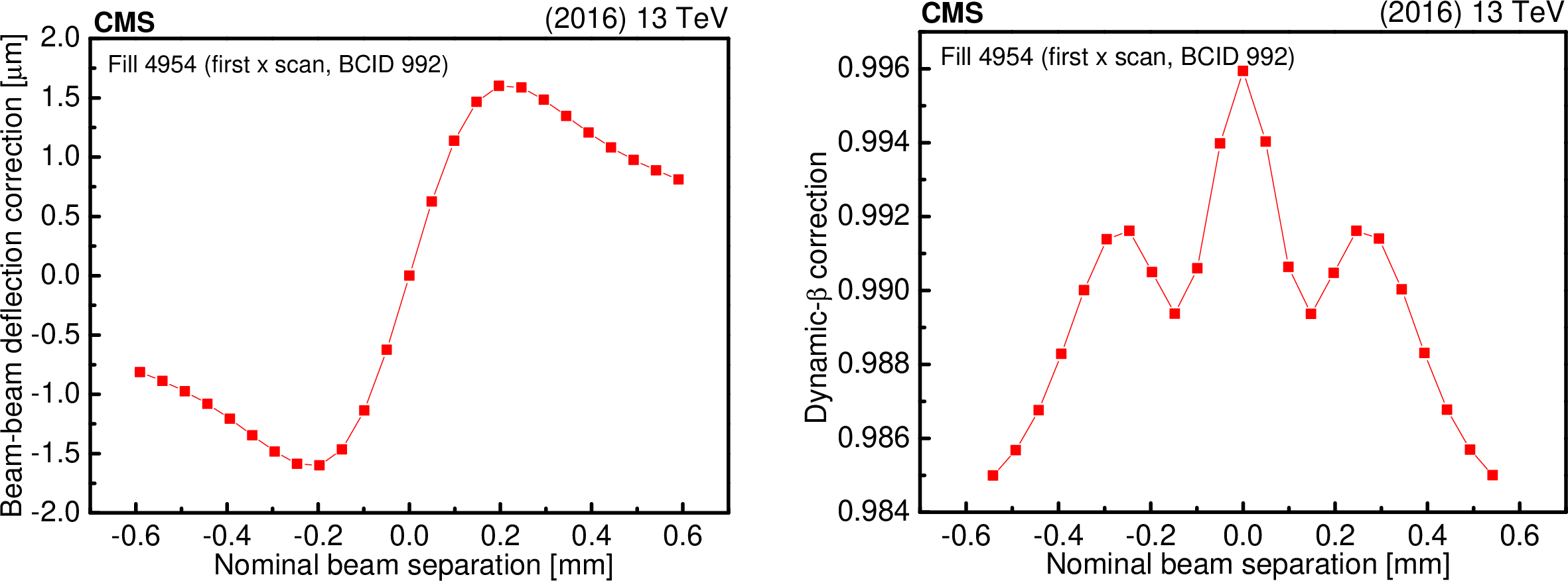
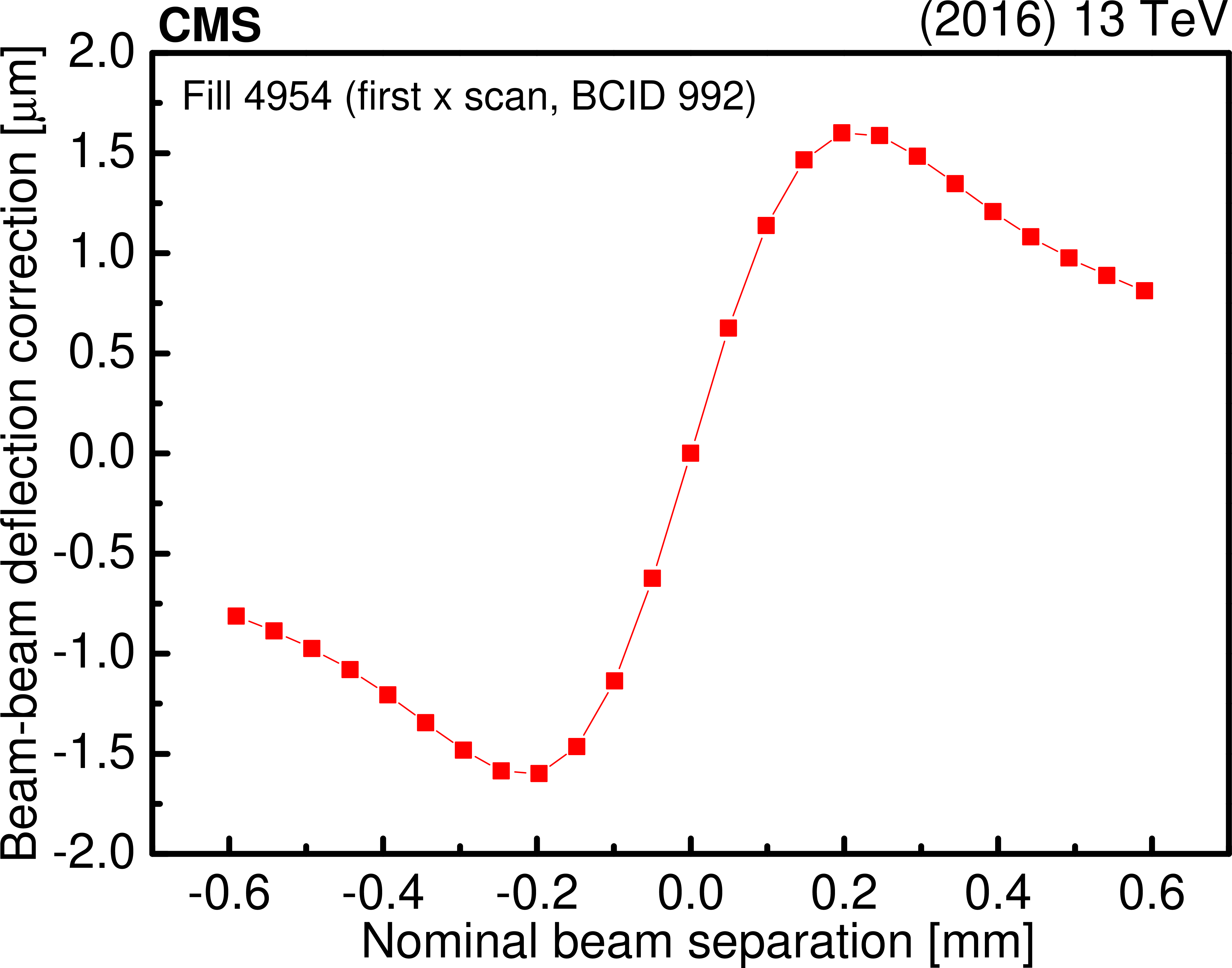
Figure 9:
Calculated beam-beam deflection due to closed-orbit shift (left) and the multiplicative rate correction for PLT due to the dynamic-$\beta $ effect (right) as a function of the nominal beam separation for the beam parameters associated with fill 4954 (first scan, BCID 992). Lines represent first-order polynomial interpolations between any two adjacent values. |
png pdf |
Figure 9-a:
Calculated beam-beam deflection due to closed-orbit shift as a function of the nominal beam separation for the beam parameters associated with fill 4954 (first scan, BCID 992). Lines represent first-order polynomial interpolations between any two adjacent values. |

png pdf |
Figure 9-b:
The multiplicative rate correction for PLT due to the dynamic-$\beta $ effect as a function of the nominal beam separation for the beam parameters associated with fill 4954 (first scan, BCID 992). Lines represent first-order polynomial interpolations between any two adjacent values. |
png pdf |
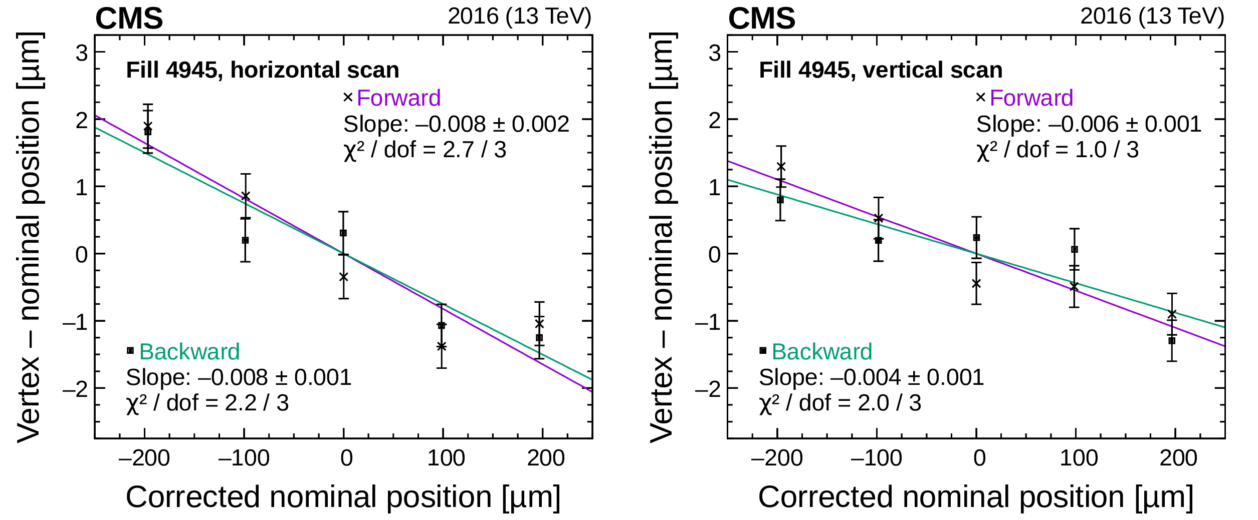
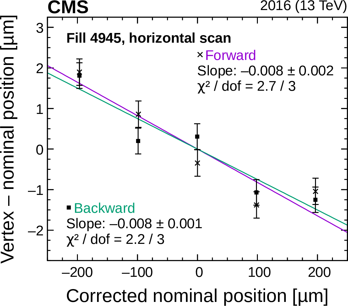
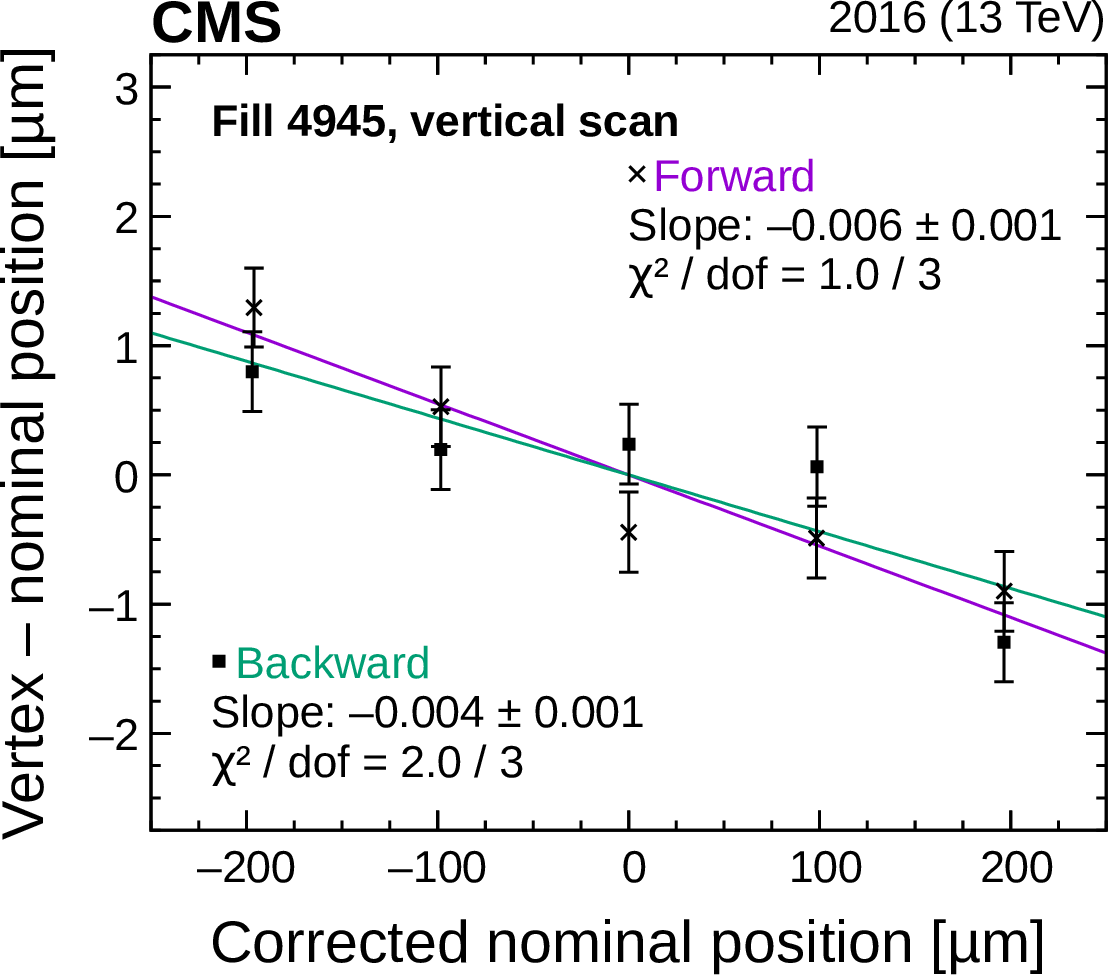
Figure 10:
Fits to LSC forward (purple) and backward (green) scan data for the $x$ (left) and $y$ (right) LSC scans in fill 4945. The error bars denote the statistical uncertainty in the fitted luminous region centroid. |
png pdf |
Figure 10-a:
Fits to LSC forward (purple) and backward (green) scan data for the $x$ LSC scans in fill 4945. The error bars denote the statistical uncertainty in the fitted luminous region centroid. |
png pdf |
Figure 10-b:
Fits to LSC forward (purple) and backward (green) scan data for the $y$ LSC scans in fill 4945. The error bars denote the statistical uncertainty in the fitted luminous region centroid. |
png pdf |
Figure 11:
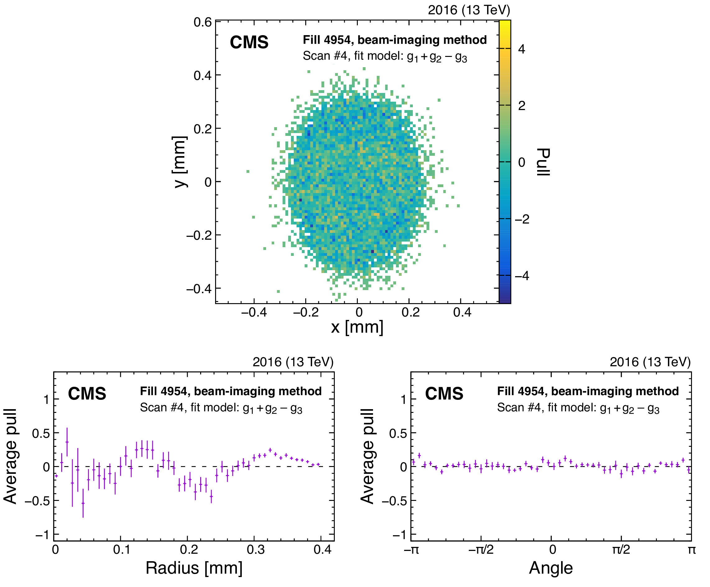
Example of the pull distributions of the fit model of Eq. (22) with respect to the vertex distribution that constrains beam 2 in the $y$ direction recorded in fill 4954. The upper plot shows the two-dimensional pull distributions, and the lower plots show the per-bin pulls averaged over the same radial distance (lower left) or angle (lower right). The error bars in the lower plot denote the standard error in the mean of the pulls in each bin. The fluctuations observed in the radial projection of the residuals are included in the uncertainty estimation. |
png pdf |
Figure 11-a:
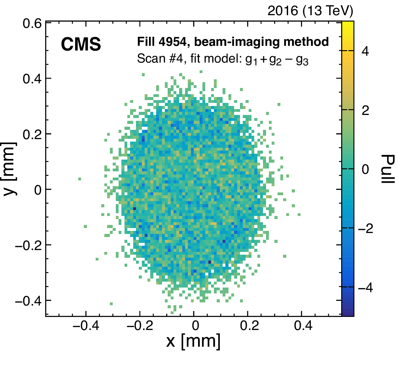
Example of the pull distributions of the fit model of Eq. (22) with respect to the vertex distribution that constrains beam 2 in the $y$ direction recorded in fill 4954. The plot shows the two-dimensional pull distributions. |
png pdf |
Figure 11-b:
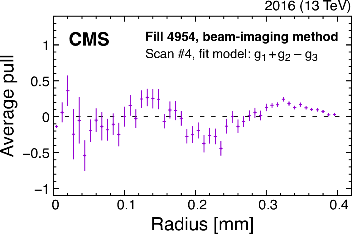
Example of the pull distributions of the fit model of Eq. (22) with respect to the vertex distribution that constrains beam 2 in the $y$ direction recorded in fill 4954. The plot shows the per-bin pulls averaged over the same radial distance. The error bars denote the standard error in the mean of the pulls in each bin. The fluctuations observed in the radial projection of the residuals are included in the uncertainty estimation. |
png pdf |
Figure 11-c:
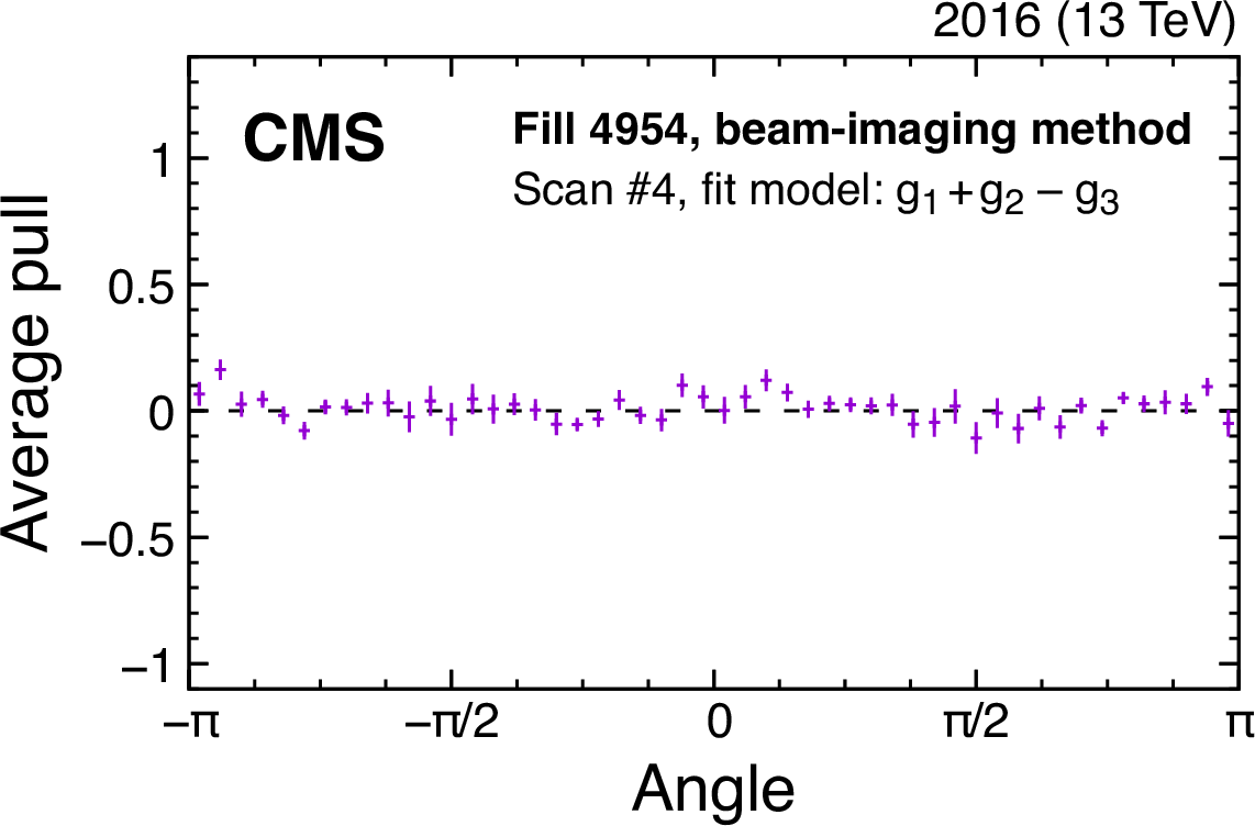
Example of the pull distributions of the fit model of Eq. (22) with respect to the vertex distribution that constrains beam 2 in the $y$ direction recorded in fill 4954. The plot shows the per-bin pulls averaged over the same angle. The error bars denote the standard error in the mean of the pulls in each bin. The fluctuations observed in the radial projection of the residuals are included in the uncertainty estimation. |

png pdf |
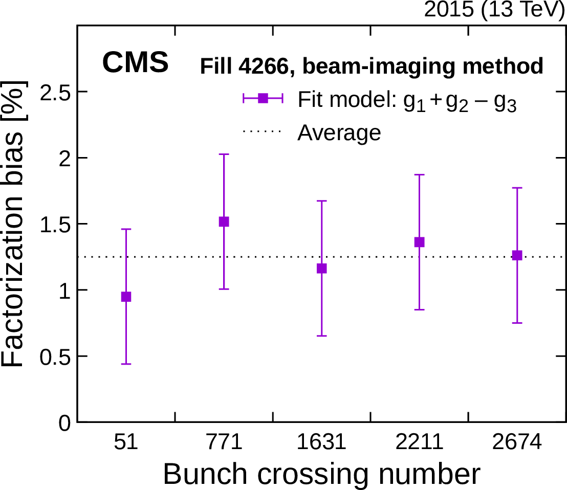
Figure 12:
Factorization bias estimated from the fits to the BI bunch-by-bunch data in fills 4266 (left) and 4954 (right). The error bars denote sources of uncertainty (statistical and systematic), added in quadrature, in the factorization bias estimates. |
png pdf |
Figure 12-a:
Factorization bias estimated from the fits to the BI bunch-by-bunch data in fill 4266. The error bars denote sources of uncertainty (statistical and systematic), added in quadrature, in the factorization bias estimates. |

png pdf |
Figure 12-b:
Factorization bias estimated from the fits to the BI bunch-by-bunch data in fill 4954. The error bars denote sources of uncertainty (statistical and systematic), added in quadrature, in the factorization bias estimates. |

png pdf |
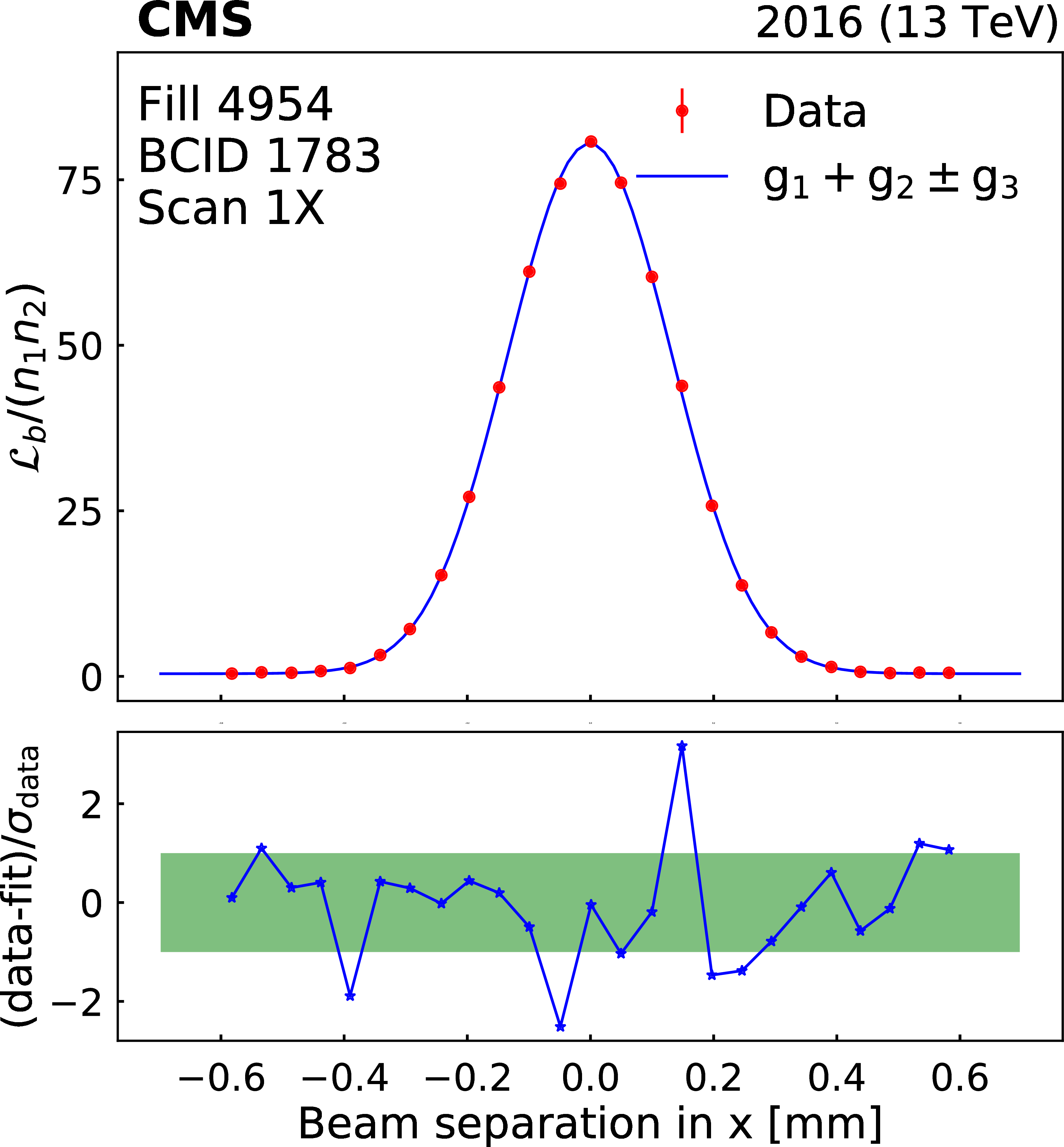
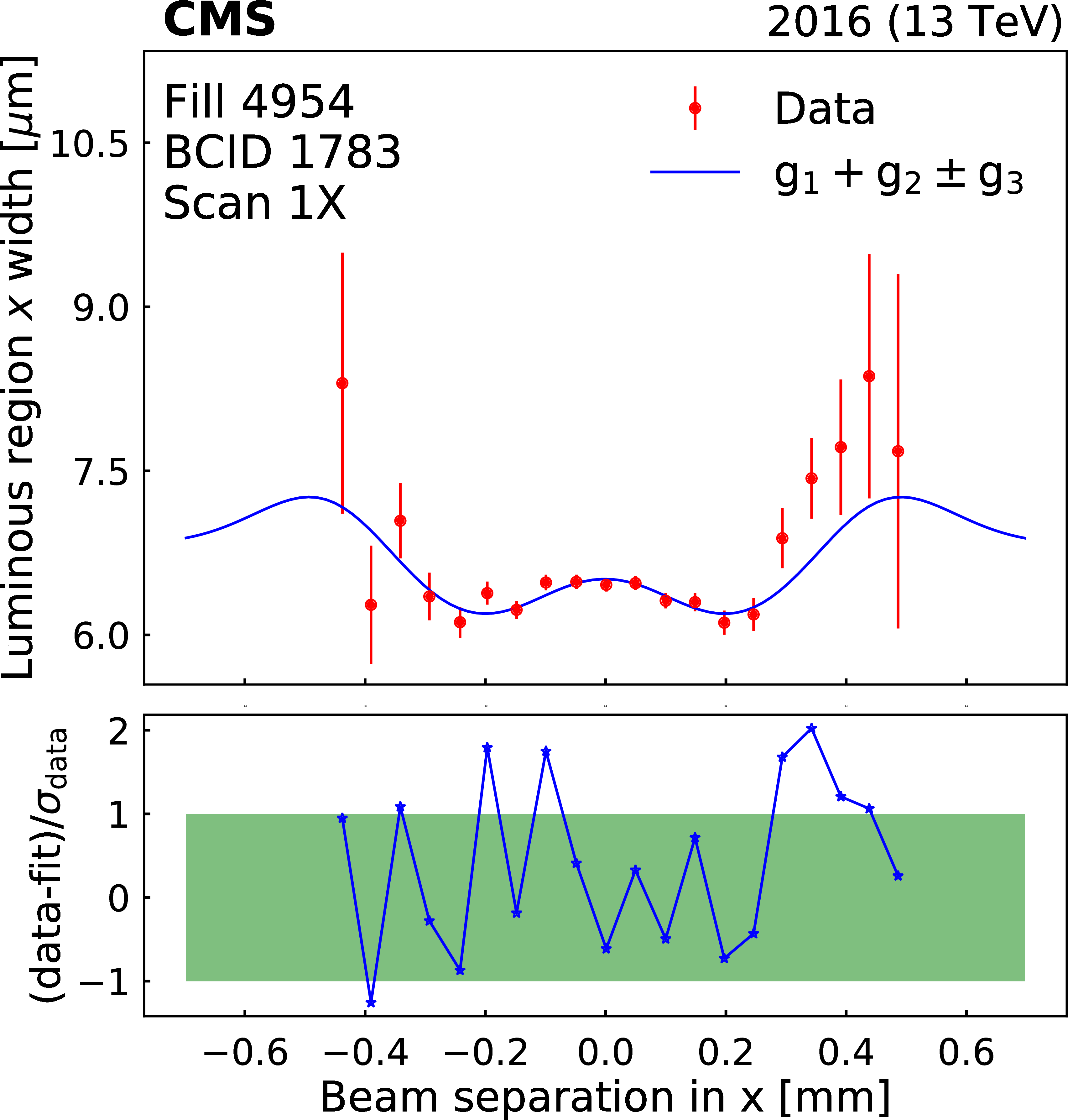
Figure 13:
Beam-separation dependence of the luminosity and some luminous region parameters during the first horizontal vdM scan in fill 4954. The points represent the luminosity normalized by the beam current product (upper left), the horizontal position of the luminous centroid (upper right), and the horizontal and vertical luminous region widths (lower left and right). The error bars represent the statistical uncertainty in the luminosity, and the fit uncertainty in the luminous region parameters. The line is the result of the three-Gaussian ($g_1+g_2\pm g_3$) fit described in the text. In all cases, the lower panels show the one-dimensional pulls. |
png pdf |
Figure 13-a:
Beam-separation dependence of the luminosity and some luminous region parameters during the first horizontal vdM scan in fill 4954. The points represent the luminosity normalized by the beam current product. The error bars represent the statistical uncertainty in the luminosity, and the fit uncertainty in the luminous region parameters. The line is the result of the three-Gaussian ($g_1+g_2\pm g_3$) fit described in the text. The lower panel shows the one-dimensional pulls. |

png pdf |
Figure 13-b:
Beam-separation dependence of the luminosity and some luminous region parameters during the first horizontal vdM scan in fill 4954. The points represent the luminosity normalized by the horizontal position of the luminous centroid. The error bars represent the statistical uncertainty in the luminosity, and the fit uncertainty in the luminous region parameters. The line is the result of the three-Gaussian ($g_1+g_2\pm g_3$) fit described in the text. The lower panel shows the one-dimensional pulls. |
png pdf |
Figure 13-c:
Beam-separation dependence of the luminosity and some luminous region parameters during the first horizontal vdM scan in fill 4954. The points represent the luminosity normalized by the horizontal luminous region width. The error bars represent the statistical uncertainty in the luminosity, and the fit uncertainty in the luminous region parameters. The line is the result of the three-Gaussian ($g_1+g_2\pm g_3$) fit described in the text. The lower panel shows the one-dimensional pulls. |

png pdf |
Figure 13-d:
Beam-separation dependence of the luminosity and some luminous region parameters during the first horizontal vdM scan in fill 4954. The points represent the luminosity normalized by the vertical luminous region width. The error bars represent the statistical uncertainty in the luminosity, and the fit uncertainty in the luminous region parameters. The line is the result of the three-Gaussian ($g_1+g_2\pm g_3$) fit described in the text. The lower panel shows the one-dimensional pulls. |
png pdf |
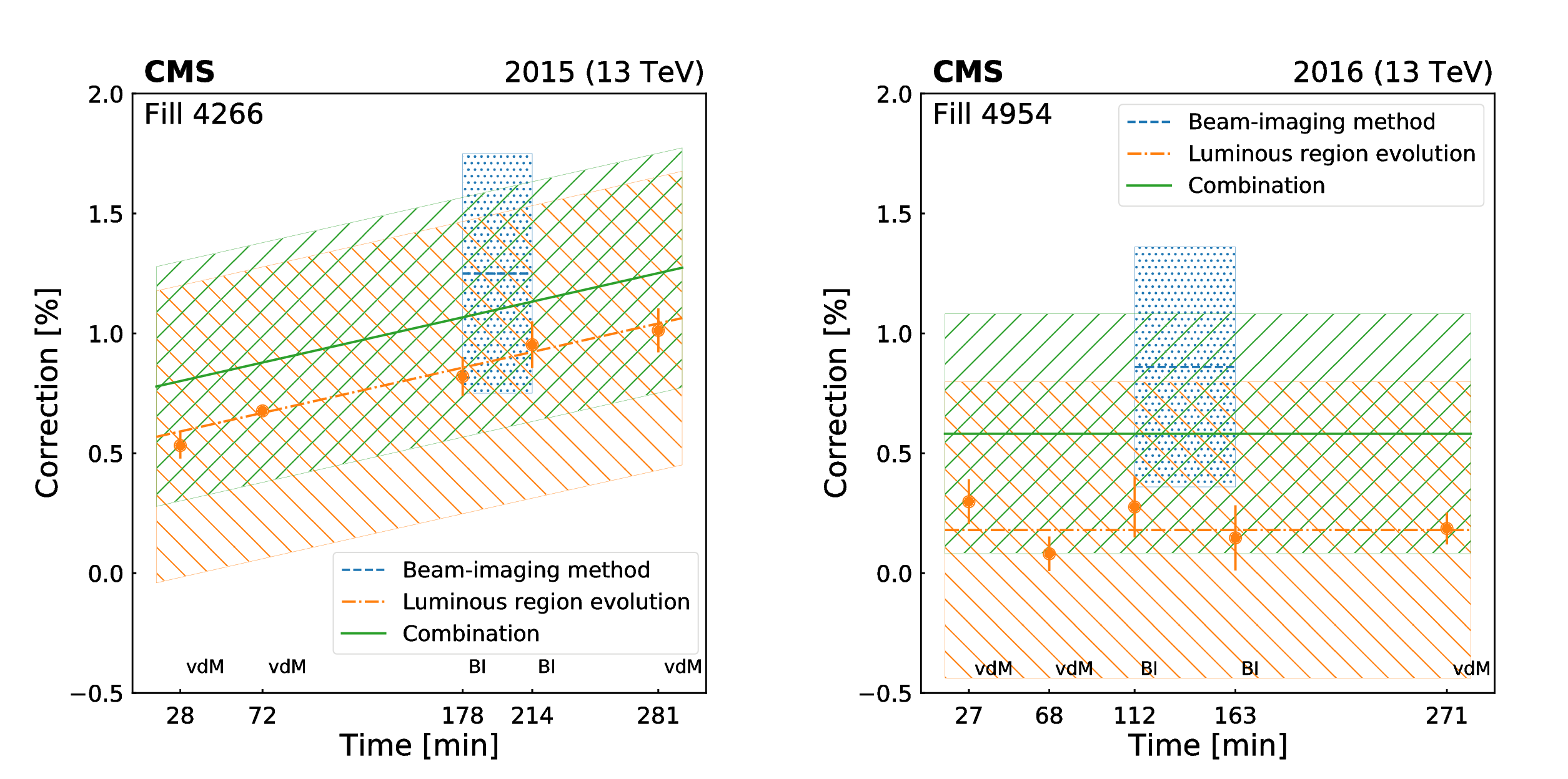
Figure 14:
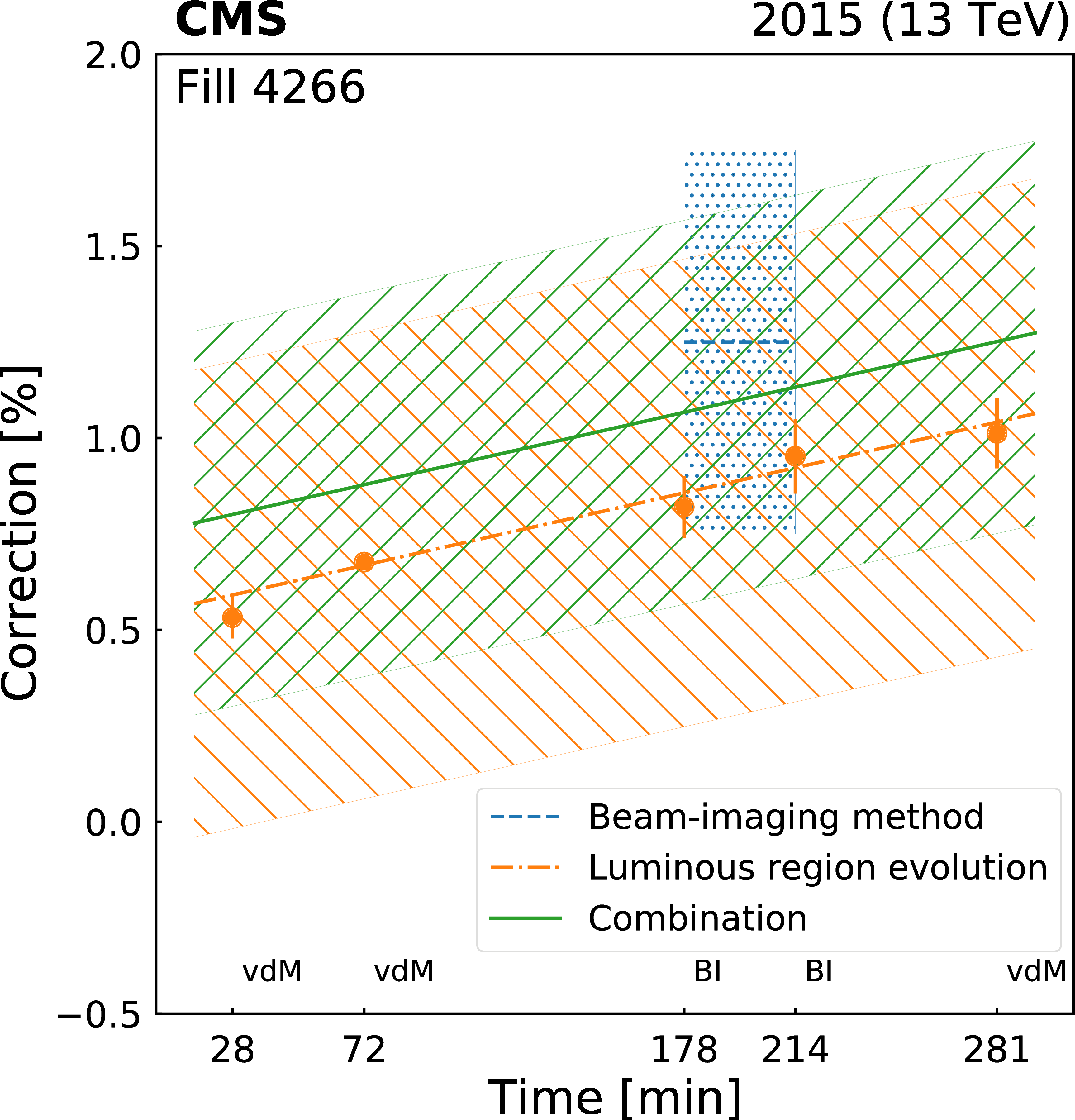
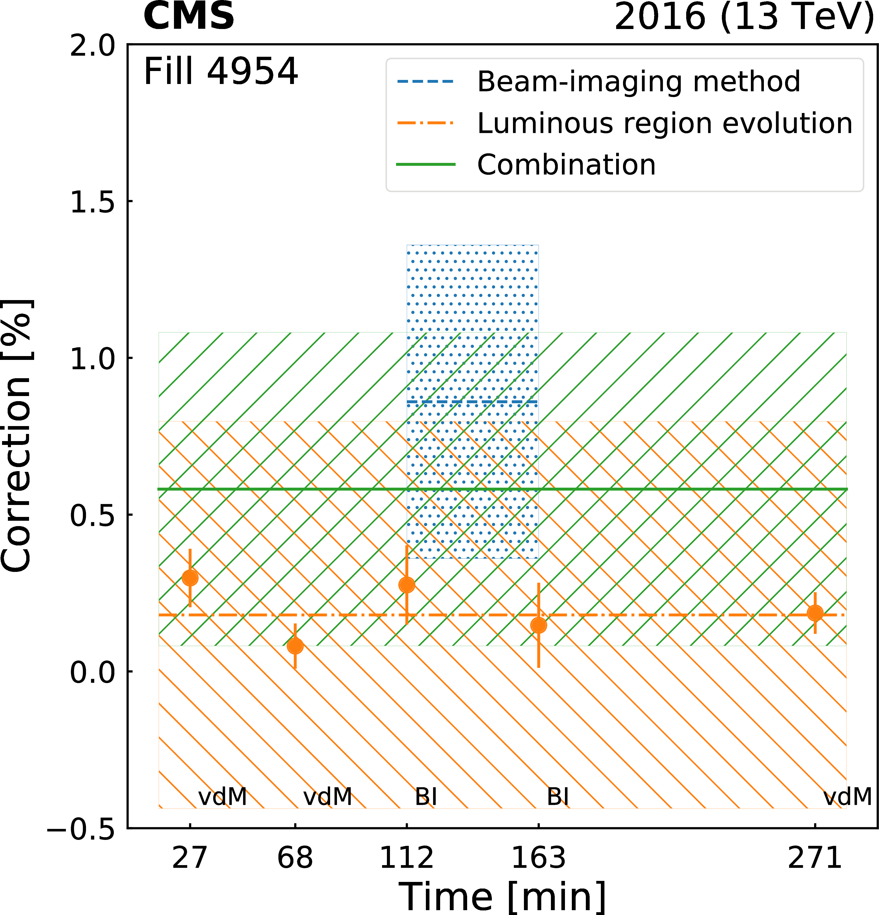
Ratio of the ${\sigma _{\text {vis}}}$ evaluated from the overlap integral of the reconstructed single-bunch profiles in two (BI method) or three (luminous region evolution) spatial dimensions to that determined by the vdM method, assuming factorization, and their combination. The central values are displayed as points or with a line while the corresponding full uncertainties are shown as hatched areas. Different methods (including the combination) are color coded. Each point corresponds to one scan pair in fills 4266 (left) and 4954 (right). The statistical uncertainty is shown by the error bars. |
png pdf |
Figure 14-a:
Ratio of the ${\sigma _{\text {vis}}}$ evaluated from the overlap integral of the reconstructed single-bunch profiles in two (BI method) or three (luminous region evolution) spatial dimensions to that determined by the vdM method, assuming factorization, and their combination. The central values are displayed as points or with a line while the corresponding full uncertainties are shown as hatched areas. Different methods (including the combination) are color coded. Each point corresponds to one scan pair in fill 4266 . The statistical uncertainty is shown by the error bars. |
png pdf |
Figure 14-b:
Ratio of the ${\sigma _{\text {vis}}}$ evaluated from the overlap integral of the reconstructed single-bunch profiles in two (BI method) or three (luminous region evolution) spatial dimensions to that determined by the vdM method, assuming factorization, and their combination. The central values are displayed as points or with a line while the corresponding full uncertainties are shown as hatched areas. Different methods (including the combination) are color coded. Each point corresponds to one scan pair in fill 4954. The statistical uncertainty is shown by the error bars. |
png pdf |
Figure 15:
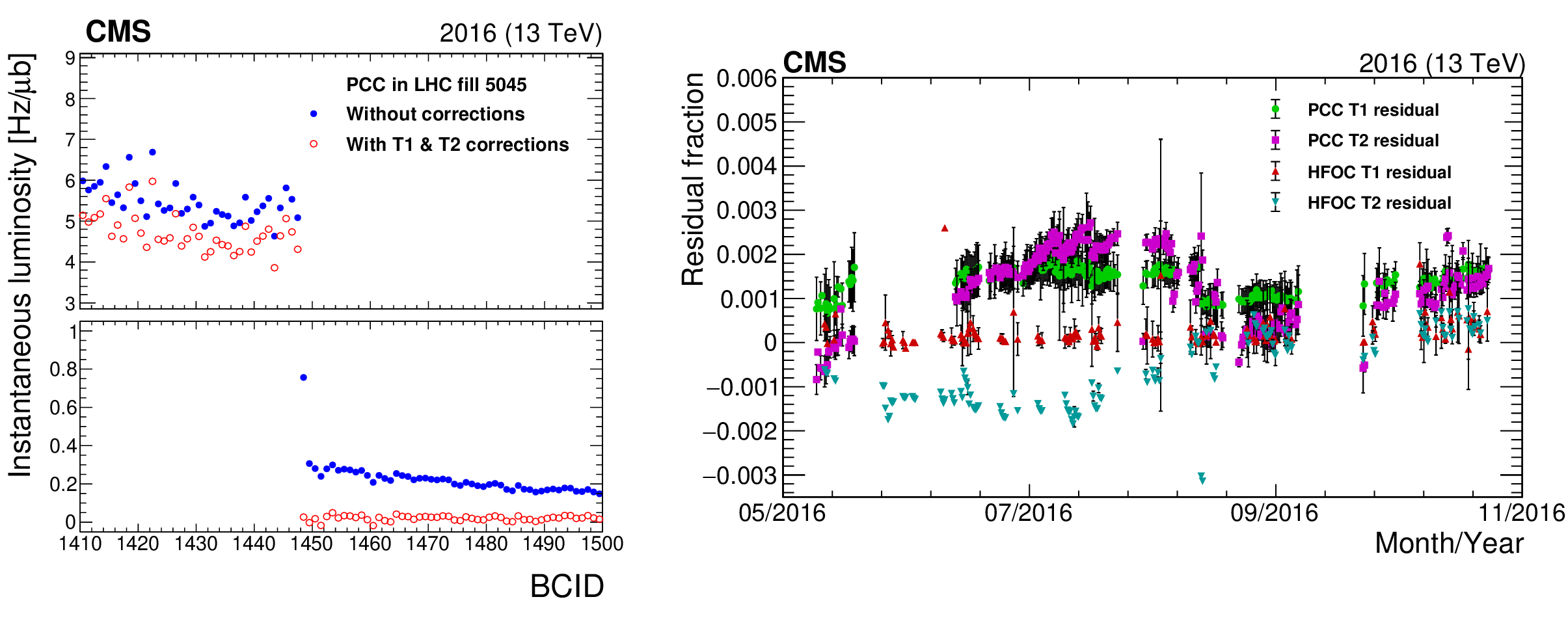
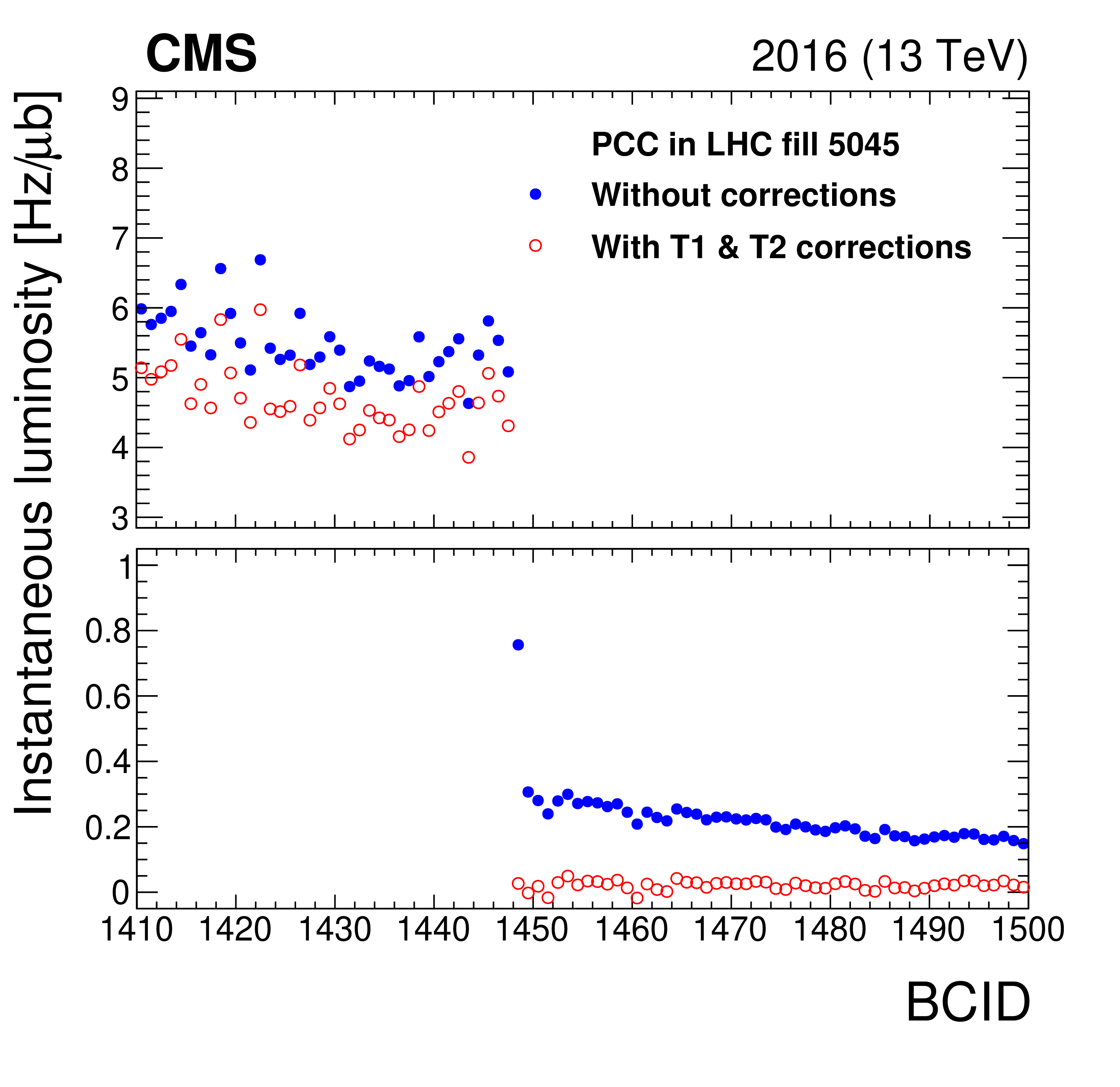
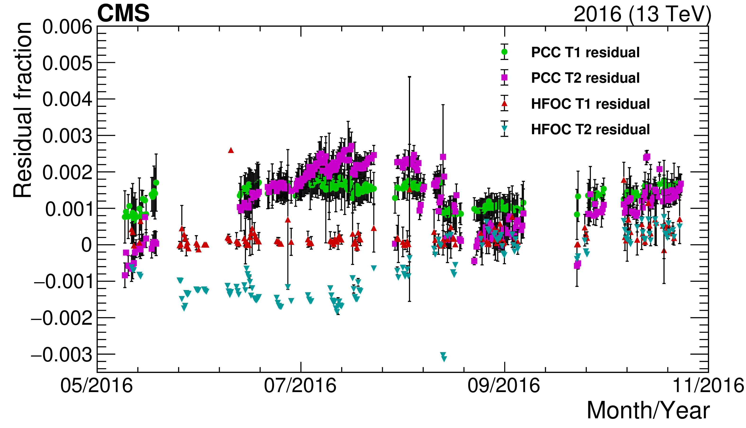
The left plot shows the instantaneous luminosity measured from PCC as a function of BCID before (filled blue points) and after (open red points) afterglow corrections are applied for each colliding bunch. The upper panel shows a subset of bunch crossings colliding at IP 5, and the lower panel shows empty bunch crossings (the scale is different in the two panels to show differences more clearly). The open red points in the lower panel lie close to 0, indicating that any residual PCC response is small in empty bunch slots. The right plot shows the estimated residual T1 and T2 afterglow as a function of time during the full range of 2016 data for both PCC and HFOC, which use the same afterglow subtraction methodology. |
png pdf |
Figure 15-a:
The plot shows the instantaneous luminosity measured from PCC as a function of BCID before (filled blue points) and after (open red points) afterglow corrections are applied for each colliding bunch. The upper panel shows a subset of bunch crossings colliding at IP 5, and the lower panel shows empty bunch crossings (the scale is different in the two panels to show differences more clearly). The open red points in the lower panel lie close to 0, indicating that any residual PCC response is small in empty bunch slots. |
png pdf |
Figure 15-b:
The plot shows the estimated residual T1 and T2 afterglow as a function of time during the full range of 2016 data for both PCC and HFOC, which use the same afterglow subtraction methodology. |
png pdf |
Figure 16:
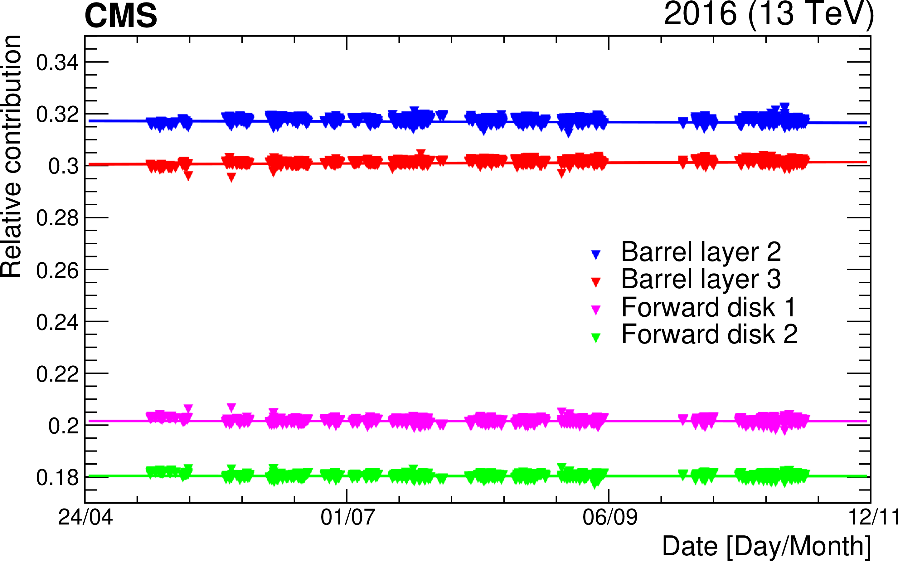
The relative contribution to the total number of observed pixel clusters from the four regions of the pixel detector used in the luminosity measurement (barrel layers 2 and 3, and inner and outer forward pixel disks), as a function of time throughout 2016. The lines represent first-order polynomial fits to the relative contributions from each region. |

png pdf |
Figure 17:
The luminosity measurements from PCC, HFOC, and RAMSES are compared as a function of the integrated luminosity in 2016. Comparison among three luminometers facilitates the identification of periods where a single luminometer suffers from transient stability issues. The ratios that are plotted in red contain invalidated data. The dashed line delineates the vdM calibration (fill 4954). |
png pdf |
Figure 18:
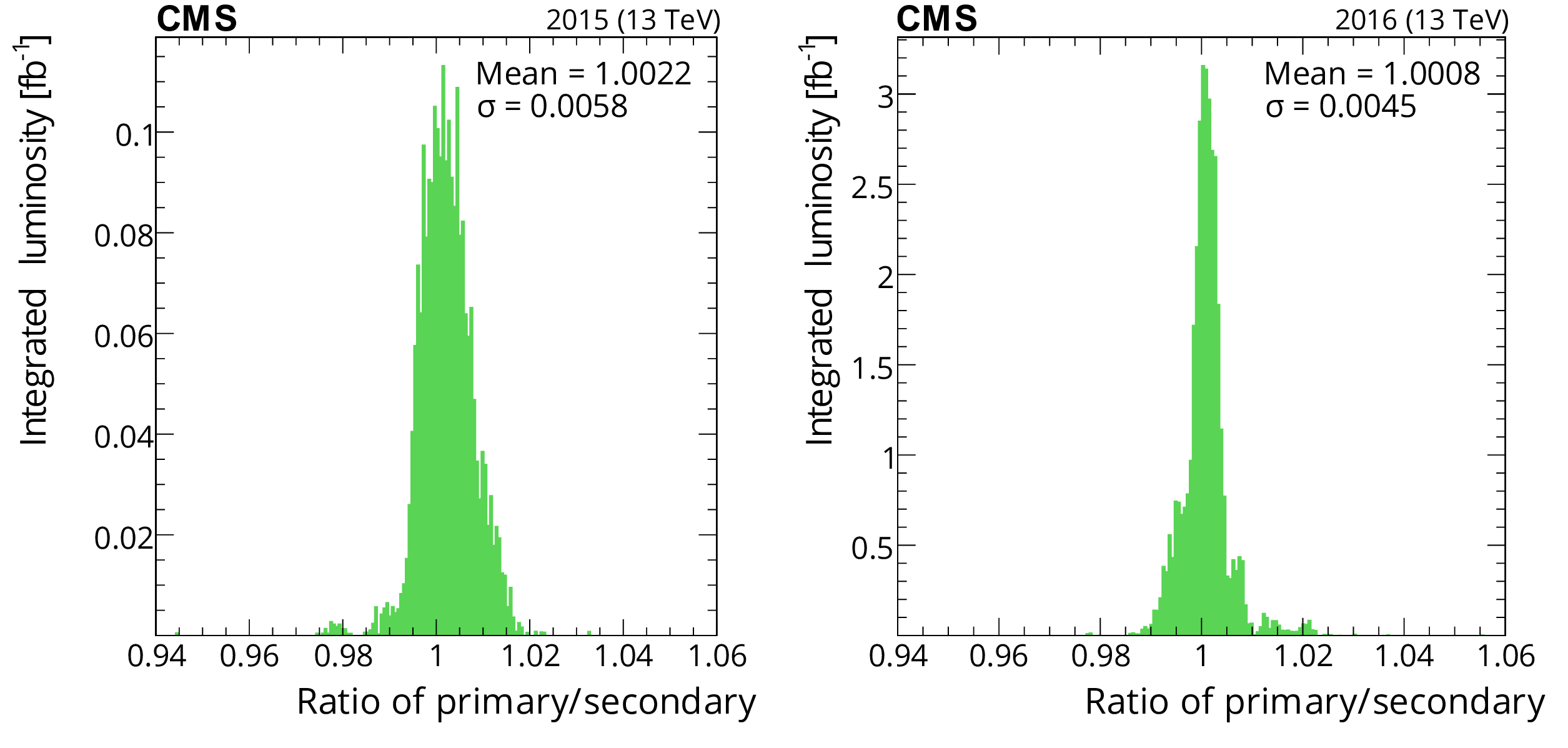
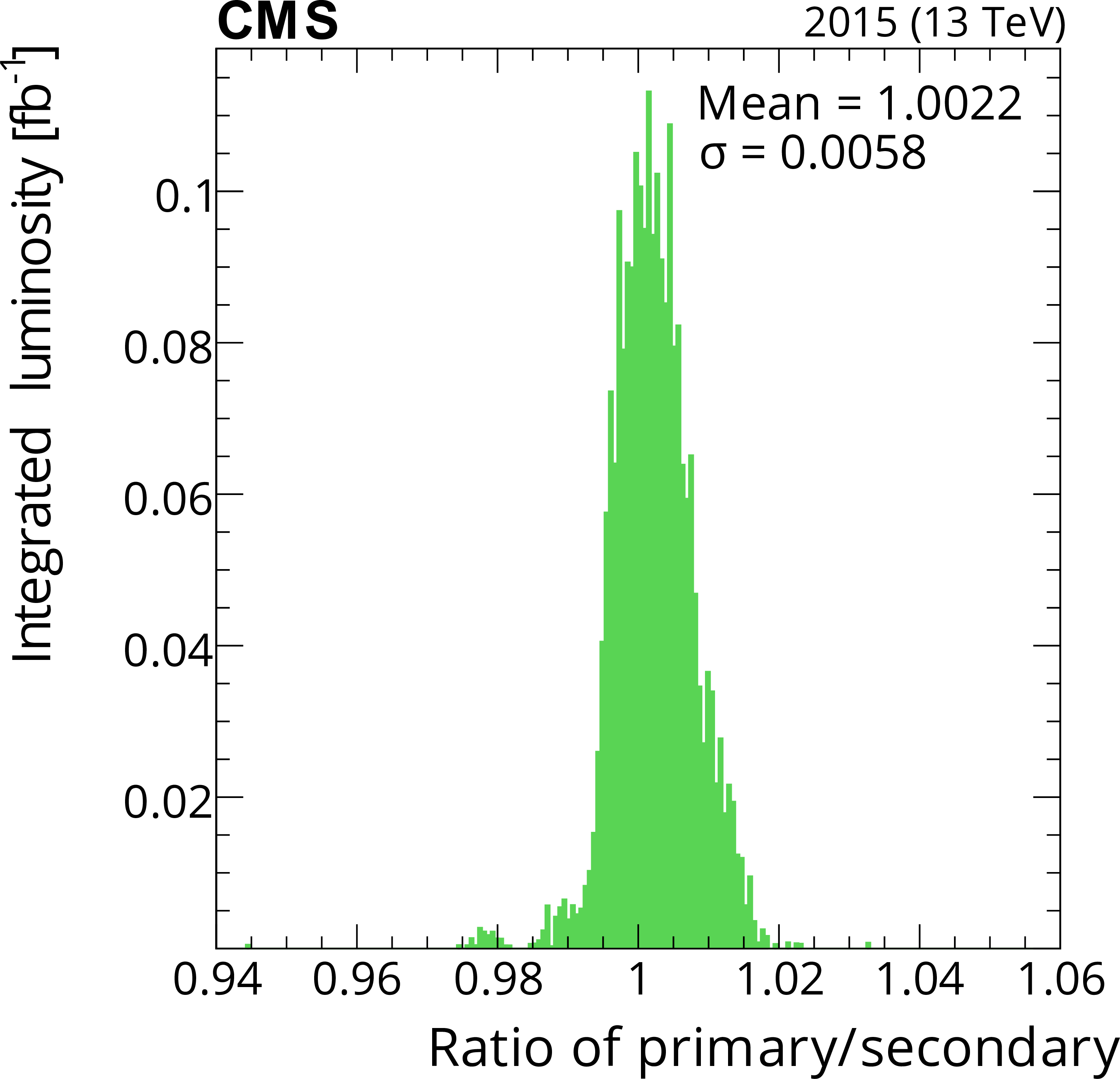
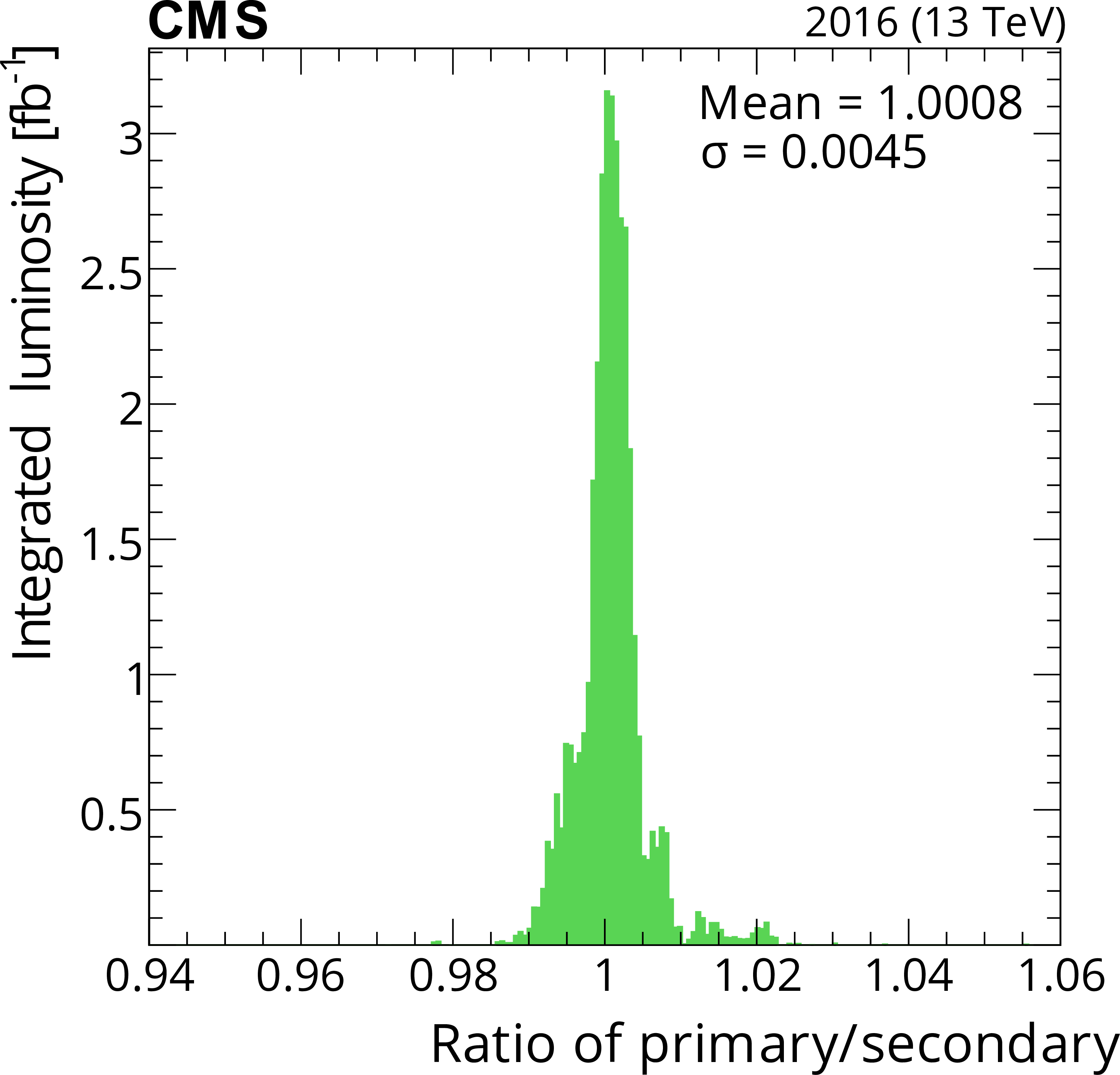
The ratio of the primary (best available) to secondary (next-best available) luminosity as computed in time windows of approximately 20 min each. The left plot shows the 2015 results (principally PCC/RAMSES), and the right plot shows the 2016 results (principally PCC/HFOC). Each entry is weighted by the integrated luminosity for the time period. |
png pdf |
Figure 18-a:
The ratio of the primary (best available) to secondary (next-best available) luminosity as computed in time windows of approximately 20 min each. The plot shows the 2015 results (principally PCC/RAMSES). Each entry is weighted by the integrated luminosity for the time period. |
png pdf |
Figure 18-b:
The ratio of the primary (best available) to secondary (next-best available) luminosity as computed in time windows of approximately 20 min each. The plot shows the 2016 results (principally PCC/HFOC). Each entry is weighted by the integrated luminosity for the time period. |
png pdf |
Figure 19:
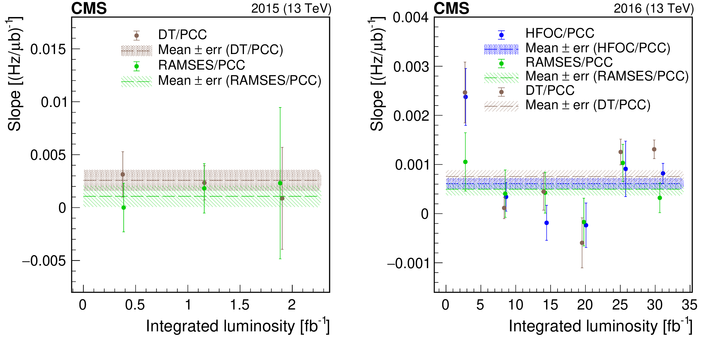
Linearity summary for 2015 (left) and 2016 (right) at $\sqrt {s}= $ 13 TeV. The slopes are plotted for each detector relative to PCC. The markers are averages of fill-by-fill slopes from fits binned in roughly equal fractions of the total integrated luminosity through the year. The error bars on the markers are the propagated statistical uncertainty from fitted slope parameters in each fill, which are weighted by integrated luminosities of each fill. The dashed lines and corresponding hatched areas show the average from the entire data set and its uncertainty. |
png pdf |
Figure 19-a:
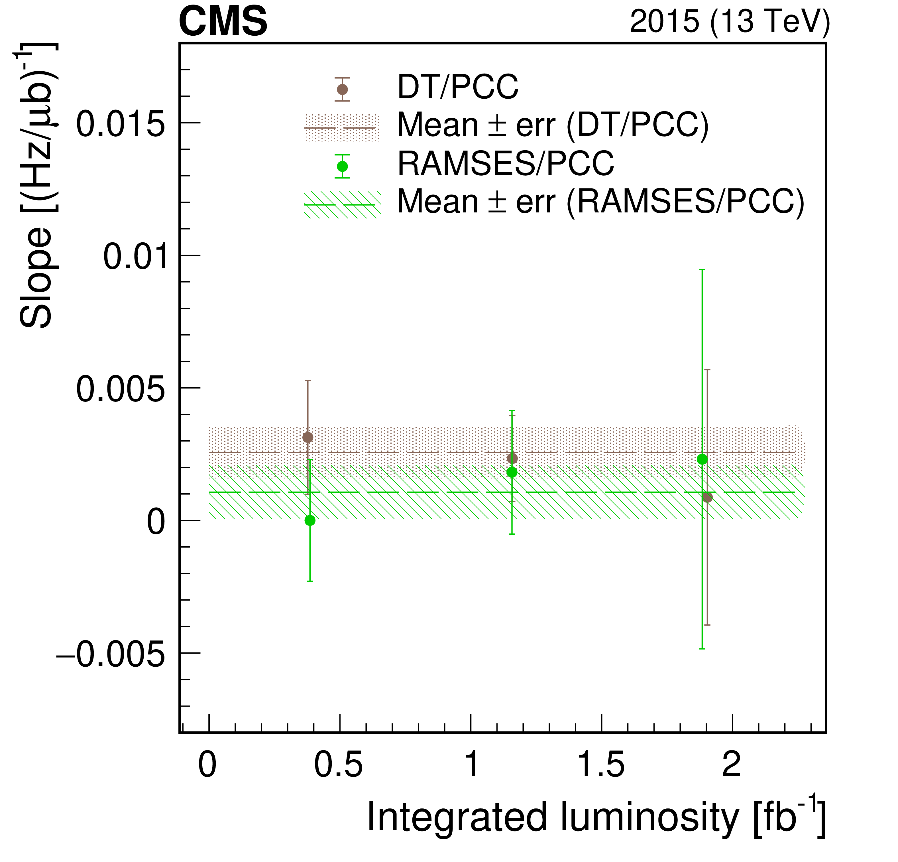
Linearity summary for 2015 at $\sqrt {s}= $ 13 TeV. The slopes are plotted for each detector relative to PCC. The markers are averages of fill-by-fill slopes from fits binned in roughly equal fractions of the total integrated luminosity through the year. The error bars on the markers are the propagated statistical uncertainty from fitted slope parameters in each fill, which are weighted by integrated luminosities of each fill. The dashed lines and corresponding hatched areas show the average from the entire data set and its uncertainty. |
png pdf |
Figure 19-b:
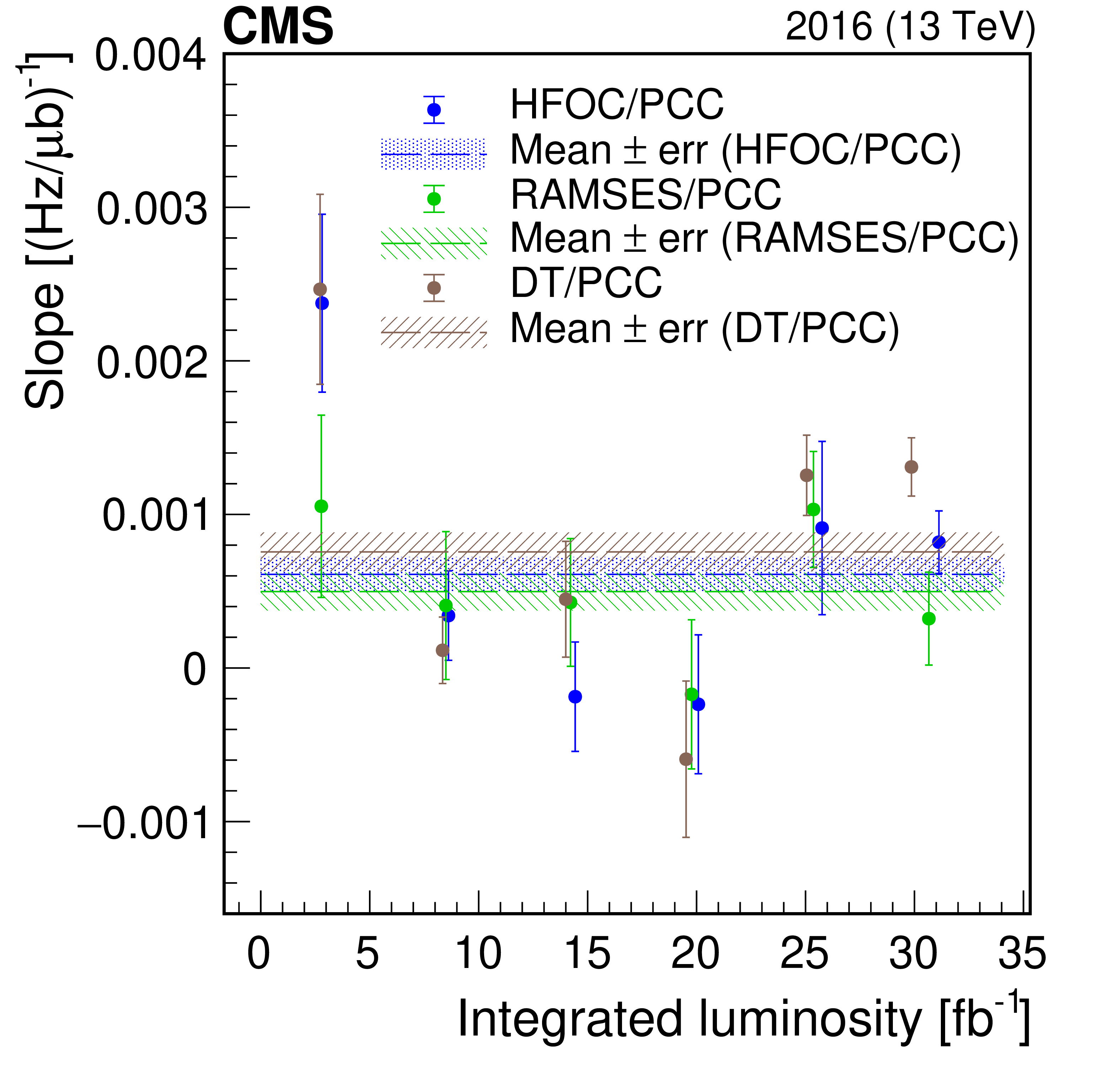
Linearity summary for 2016 at $\sqrt {s}= $ 13 TeV. The slopes are plotted for each detector relative to PCC. The markers are averages of fill-by-fill slopes from fits binned in roughly equal fractions of the total integrated luminosity through the year. The error bars on the markers are the propagated statistical uncertainty from fitted slope parameters in each fill, which are weighted by integrated luminosities of each fill. The dashed lines and corresponding hatched areas show the average from the entire data set and its uncertainty. |
| Tables | |

png pdf |
Table 1:
Summary of the LHC conditions at IP 5 for the scan sessions in pp collisions in 2015 and 2016. The column labeled $\mu $ is the average pileup corresponding to $ {\mathcal {L}} _{\text {init}}$, the latter denoting the initial instantaneous luminosity. The columns corresponding to "No. of scans'' indicate the total number of vdM, BI, and LSC scans that were performed in either transverse coordinate, counting only scans used for analysis. |
png pdf |
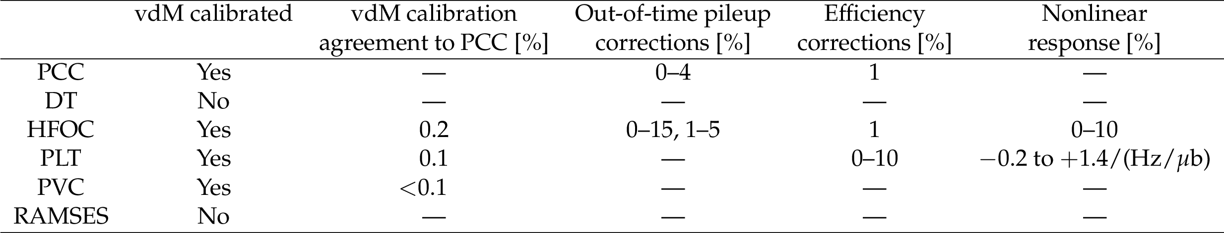
Table 2:
Summary of the rate corrections under physics running conditions in 2016 applied separately to each luminometer. For HFOC, two distinct sources of out-of-time pileup corrections are provided. In the first and second columns, the vdM calibration condition and the relative agreement of the luminometers in terms of ${A_{\text {eff}}}$ relative to PCC during fill 4954 are given, respectively. The DT luminosity is also corrected for a very small additional muon rate from beam halo and cosmic sources, which is treated as a constant per fill. |
png pdf |
Table 3:
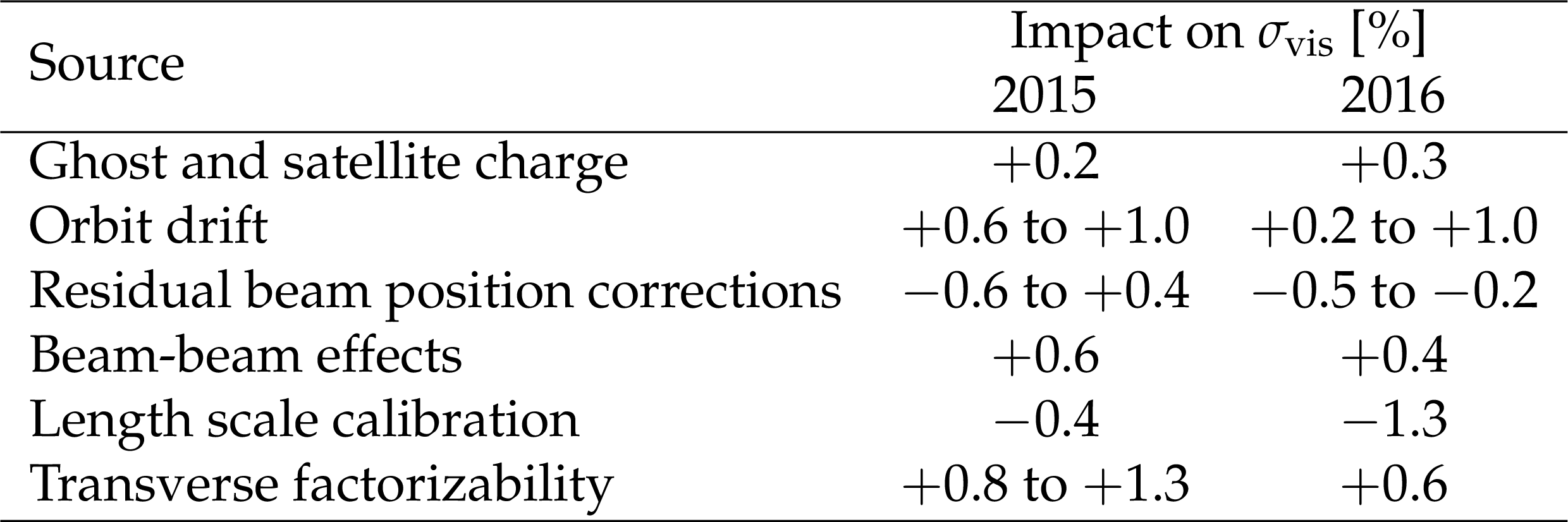
Summary of the BCID-averaged corrections to ${\sigma _{\text {vis}}}$ (in %) obtained with the vdM scan calibrations at $\sqrt {s}= $ 13 TeV in 2015 and 2016. When a range is shown, it is because of possible scan-to-scan variations. To obtain the impact on ${\sigma _{\text {vis}}}$, each correction is consecutively included, the fits are redone following the order below, and the result is compared with the baseline. The impact from transverse factorizability is obtained separately (as discussed in Section 4.4). |
png pdf |
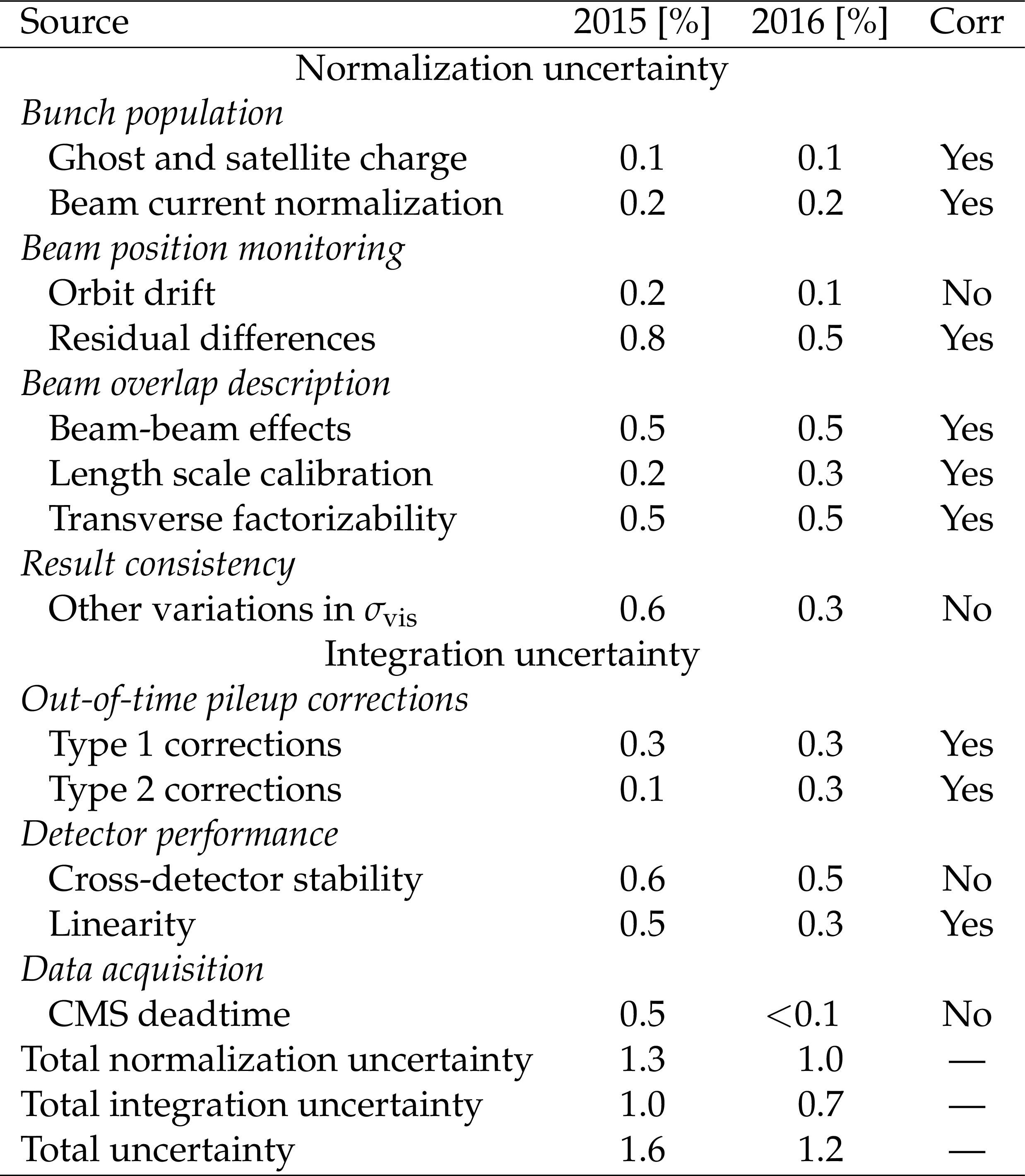
Table 4:
Summary of contributions to the relative systematic uncertainty in ${\sigma _{\text {vis}}}$ (in %) at $\sqrt {s}= $ 13 TeV in 2015 and 2016. The systematic uncertainty is divided into groups affecting the description of the vdM profile and the bunch population product measurement (normalization), and the measurement of the rate in physics running conditions (integration). The fourth column indicates whether the sources of uncertainty are correlated between the two calibrations at $\sqrt {s}= $ 13 TeV. |
| Summary |
|
The luminosity calibration using beam-separation (van der Meer, vdM) scans has been presented for data from proton-proton collisions recorded by the CMS experiment in 2015 and 2016 when all subdetectors were fully operational. The main sources of systematic uncertainty are related to residual differences between the measured beam positions and the ones provided by the operational settings of the LHC magnets, the factorizability of the transverse spatial distributions of proton bunches, and the modeling of effects on the proton distributions due to electromagnetic interactions among protons in the colliding bunches. When applying the vdM calibration to the entire data-taking period, the relative stability and linearity of luminosity subdetectors (luminometers) are included in the uncertainty in the integrated luminosity measurement as well. The resulting relative precision in the calibration from the vdM scans is 1.3 (1.0 )% in 2015 (2016) at $\sqrt{s}=$ 13 TeV ; the integration uncertainty due to luminometer-specific effects contributes 1.0 (0.7 )%, resulting in a total uncertainty of 1.6 (1.2 )%; when applying the vdM calibration to the entire periods, the total integrated luminosity is 2.27 (36.3) fb$^{-1}$. The final precision is among the best achieved at bunched-beam hadron colliders. Advanced techniques are used to estimate and correct for the bias associated with the beam position monitoring at the scale of $\mu$m, the factorizability of the transverse beam distribution, and beam-beam effects. In addition, detailed luminometer rate corrections and the inclusion of novel measurements (such as the data from the Radiation Monitoring System for the Environment and Safety) lead to precise estimates of the stability and linearity over time. In the coming years, a similarly precise calibration of the real-time luminosity delivered to the LHC will become increasingly important for standard operations. Under those conditions, the impact of out-of-time pileup effects is expected to be larger, but in principle they can be mitigated using techniques described in this paper. |
| References | ||||
| 1 | P. Grafstrom and W. Kozanecki | Luminosity determination at proton colliders | Prog. Part. NP 81 (2015) 97 | |
| 2 | ATLAS and CMS Collaborations | Addendum to the report on the physics at the HL-LHC, and perspectives for the HE-LHC: Collection of notes from ATLAS and CMS | CERN (2019) | 1902.10229 |
| 3 | CMS Collaboration | The CMS experiment at the CERN LHC | JINST 3 (2008) S08004 | CMS-00-001 |
| 4 | CMS Collaboration | Measurement of the differential cross sections for the associated production of a W boson and jets in proton-proton collisions at $ \sqrt{s}= $ 13 TeV | PRD 96 (2017) 072005 | CMS-SMP-16-005 1707.05979 |
| 5 | CMS Collaboration | Measurement of the differential Drell--Yan cross section in proton-proton collisions at $ \sqrt{s} = $ 13 TeV | JHEP 12 (2019) 059 | CMS-SMP-17-001 1812.10529 |
| 6 | CMS Collaboration | Measurement of the $ \mathrm{t\bar{t}}\ $ production cross section using events with one lepton and at least one jet in pp collisions at $ \sqrt{s}= $ 13 TeV | JHEP 09 (2017) 051 | CMS-TOP-16-006 1701.06228 |
| 7 | CMS Collaboration | Measurement of the $ \mathrm{t\bar{t}}\ $ production cross section, the top quark mass, and the strong coupling constant using dilepton events in pp collisions at $ \sqrt{s}= $ 13 TeV | EPJC 79 (2019) 368 | CMS-TOP-17-001 1812.10505 |
| 8 | M. Hostettler et al. | Luminosity scans for beam diagnostics | PRAccel. Beams 21 (2018) 102801 | 1804.10099 |
| 9 | F. Antoniou et al. | Can we predict luminosity? | in Proceedings of the 7th Evian Workshop on LHC beam operation, p. 125 2016 | |
| 10 | S. van der Meer | Calibration of the effective beam height in the ISR | ISR Report CERN-ISR-PO-68-31 | |
| 11 | C. Rubbia | Measurement of the luminosity of $ {\mathrm{p}}\mathrm{\bar{p}} $ collider with a (generalized) van der Meer method | CERN $\Pp\PAp$ Note 38 | |
| 12 | LHCb Collaboration | Precision luminosity measurements at LHCb | JINST 9 (2014) P12005 | 1410.0149 |
| 13 | ATLAS Collaboration | Luminosity determination in pp collisions at $ \sqrt{s}= $ 8 TeV using the ATLAS detector at the LHC | EPJC 76 (2016) 653 | 1608.03953 |
| 14 | L. Evans and P. Bryant | LHC machine | JINST 3 (2008) S08001 | |
| 15 | B. Salvachua | Overview of proton-proton physics during Run 2 | in Proceedings of the 9th Evian Workshop on LHC beam operation, p. 7 2019 | |
| 16 | J. Boyd and C. Schwick | Experiments---experience and future | in Proceedings of the 7th Evian Workshop on LHC beam operation, p. 229 2017 | |
| 17 | CMS Collaboration | Measurement of the double-differential inclusive jet cross section in proton-proton collisions at $ \sqrt{s}= $ 13 TeV | EPJC 76 (2016) 451 | CMS-SMP-15-007 1605.04436 |
| 18 | P. Skands, S. Carrazza, and J. Rojo | Tuning PYTHIA 8.1: the Monash 2013 tune | EPJC 74 (2014) 3024 | 1404.5630 |
| 19 | T. Sjostrand et al. | An introduction to PYTHIA 8.2 | CPC 191 (2015) 159 | 1410.3012 |
| 20 | CMS Collaboration | Performance of the CMS muon detector and muon reconstruction with proton-proton collisions at $ \sqrt{s}= $ 13 TeV | JINST 13 (2018) P06015 | CMS-MUO-16-001 1804.04528 |
| 21 | CMS Collaboration | The CMS trigger system | JINST 12 (2017) P01020 | CMS-TRG-12-001 1609.02366 |
| 22 | A. J. Bell | Beam and radiation monitoring for CMS | in Proceedings, 2008 IEEE Nuclear Science Symposium, p. 2322 2008 | |
| 23 | P. Lujan | Performance of the Pixel Luminosity Telescope for luminosity measurement at CMS during Run 2 | PoS 314 (2017) 504 | |
| 24 | M. Hempel | Development of a novel diamond based detector for machine induced background and luminosity measurements | PhD thesis, Brandenburg University of Technology Cottbus-Senftenberg, 2017 DESY-THESIS-2017-030 | |
| 25 | CMS Collaboration | CMS technical design report for the level-1 trigger upgrade | CDS | |
| 26 | CMS Collaboration | Event generator tunes obtained from underlying event and multiparton scattering measurements | EPJC 76 (2016) 155 | CMS-GEN-14-001 1512.00815 |
| 27 | \GEANTfour Collaboration | GEANT4--a simulation toolkit | NIMA 506 (2003) 250 | |
| 28 | W. Verkerke and D. P. Kirkby | The RooFit toolkit for data modeling | in Proceedings of the 13th International Conference for Computing in High-Energy and Nuclear Physics (CHEP03), p. MOLT007 2003 | physics/0306116 |
| 29 | CMS Collaboration | Description and performance of track and primary-vertex reconstruction with the CMS tracker | JINST 9 (2014) P10009 | CMS-TRK-11-001 1405.6569 |
| 30 | G. Segura Millan, D. Perrin, and L. Scibile | RAMSES: the LHC radiation monitoring system for the environment and safety | in Proceedings of the 10th International Conference on Accelerator and Large Experimental Physics Control Systems (ICALEPCS 2005) 2005 TH3B.1-3O | |
| 31 | A. Ledeul et al. | CERN supervision, control, and data acquisition system for radiation and environmental protection | in Proceedings of the 12th International Workshop on Emerging Technologies and Scientific Facilities Controls (PCaPAC'18), p. 248 (FRCC3) 2019 | |
| 32 | J. Salfeld-Nebgen and D. Marlow | Data-driven precision luminosity measurements with Z bosons at the LHC and HL-LHC | JINST 13 (2018) P12016 | 1806.02184 |
| 33 | O. S. Bruning et al. | LHC design report vol. 1: The LHC main ring | CERN (2004) | |
| 34 | M. Hostettler | LHC luminosity performance | PhD thesis, University of Bern, 2018, CERN-THESIS-2018-051 | |
| 35 | C. Barschel et al. | Results of the LHC DCCT calibration studies | CERN-ATS-Note-2012-026 PERF | |
| 36 | D. Belohrad et al. | The LHC fast BCT system: A comparison of design parameters with initial performance | CERN-BE-2010-010 | |
| 37 | A. Jeff et al. | Longitudinal density monitor for the LHC | PRST Accel. Beams 15 (2012) 032803 | |
| 38 | A. Jeff | A longitudinal density monitor for the LHC | PhD thesis, University of Liverpool, 2012, CERN-THESIS-2012-240 | |
| 39 | G. Papotti, T. Bohl, F. Follin, and U. Wehrle | Longitudinal beam measurements at the LHC: The LHC Beam Quality Monitor | in Proceedings, 2nd International Particle Accelerator Conference (IPAC 2011), p. 1852 (TUPZ022) 2011 | |
| 40 | M. Gasior, J. Olexa, and R. Steinhagen | BPM electronics based on compensated diode detectors---results from development systems | in Proceedings of the 2012 Beam Instrumentation Workshop (BIW'12), p. 44 (MOPG010) 2012 | |
| 41 | T. Persson et al. | LHC optics corrections in Run 2 | in Proceedings, 9th Evian Workshop on LHC beam operation, p. 59 2019 | |
| 42 | M. Gasior, G. Baud, J. Olexa, and G. Valentino | First operational experience with the LHC Diode ORbit and OScillation (DOROS) system | in Proceedings of the 5th International Beam Instrumentation Conference (IBIC 2016), p. 43 (MOPG07) 2017 | |
| 43 | H. Bartosik and G. Rumolo | Production of the single bunch for van der Meer scans in the LHC injector chain | CERN Accelerator Note CERN-ACC-NOTE-2013-0008 | |
| 44 | V. Balagura | Van der Meer scan luminosity measurement and beam-beam correction | EPJC 81 (2021) 26 | 2012.07752 |
| 45 | A. Babaev et al. | Impact of beam-beam effects on absolute luminosity calibrations at the CERN Large Hadron Collider | To be submitted to PRST Accel. Beams | |
| 46 | C. Barschel | Precision luminosity measurement at LHCb with beam–gas imaging | PhD thesis, RWTH Aachen University, 2014, CERN-THESIS-2013-301 | |
| 47 | G. Coombs, M. Ferro-Luzzi, and R. Matev | Beam-gas imaging measurements at LHCb | in Proceedings, 7th International Beam Instrumentation Conference (IBIC 2018), p. 459 (WEPB13) 2019 | |
| 48 | W. Kozanecki, T. Pieloni, and J. Wenninger | Observation of beam-beam deflections with LHC orbit data | CERN Accelerator Note CERN-ACC-NOTE-2013-0006 | |
| 49 | S. M. White | Determination of the absolute luminosity at the LHC | PhD thesis, Université Paris-Sud 11, 2010, CERN-THESIS-2010-139, LAL-10-154 | |
| 50 | M. Klute, C. Medlock, and J. Salfeld-Nebgen | Beam imaging and luminosity calibration | JINST 12 (2017) P03018 | 1603.03566 |
| 51 | J. Knolle | Measuring luminosity and the ttZ production cross section with the CMS experiment | PhD thesis, Universität Hamburg, 2020 CERN-THESIS-2020-185, DESY-THESIS-2020-020 | |
|
|
Compact Muon Solenoid LHC, CERN |
|

|

|

|

|

|