

Compact Muon Solenoid
LHC, CERN
| CMS-HIG-14-040 ; CERN-EP-2016-112 | ||
| Search for lepton flavour violating decays of the Higgs boson to $\mathrm{ e }\tau$ and $\mathrm{ e }\mu$ in proton-proton collisions at $\sqrt{s}= $ 8 TeV | ||
| CMS Collaboration | ||
| 13 July 2016 | ||
| Phys. Lett. B 763 (2016) 472 | ||
| Abstract: A direct search for lepton flavour violating decays of the Higgs boson (H) in the $\mathrm{ H } \to \mathrm{ e } \tau$ and $\mathrm{ H } \to \mathrm{ e } \mu$ channels is described. The data sample used in the search was collected in proton-proton collisions at $\sqrt{s}= $ 8 TeV with the CMS detector at the LHC and corresponds to an integrated luminosity of 19.7 fb$^{-1}$. No evidence is found for lepton flavour violating decays in either final state. Upper limits on the branching fractions, $\mathcal{B}(\mathrm{ H } \to \mathrm{ e } \tau )<$ 0.69% and $\mathcal{B}(\mathrm{ H } \to \mathrm{ e } \mu)<$ 0.035%, are set at the 95% confidence level. The constraint set on $\mathcal{B}(\mathrm{ H } \to \mathrm{ e } \tau)$ is an order of magnitude more stringent than the existing indirect limits. The limits are used to constrain the corresponding flavour violating Yukawa couplings, absent in the standard model. | ||
| Links: e-print arXiv:1607.03561 [hep-ex] (PDF) ; CDS record ; inSPIRE record ; CADI line (restricted) ; | ||
| Figures | |
png pdf |
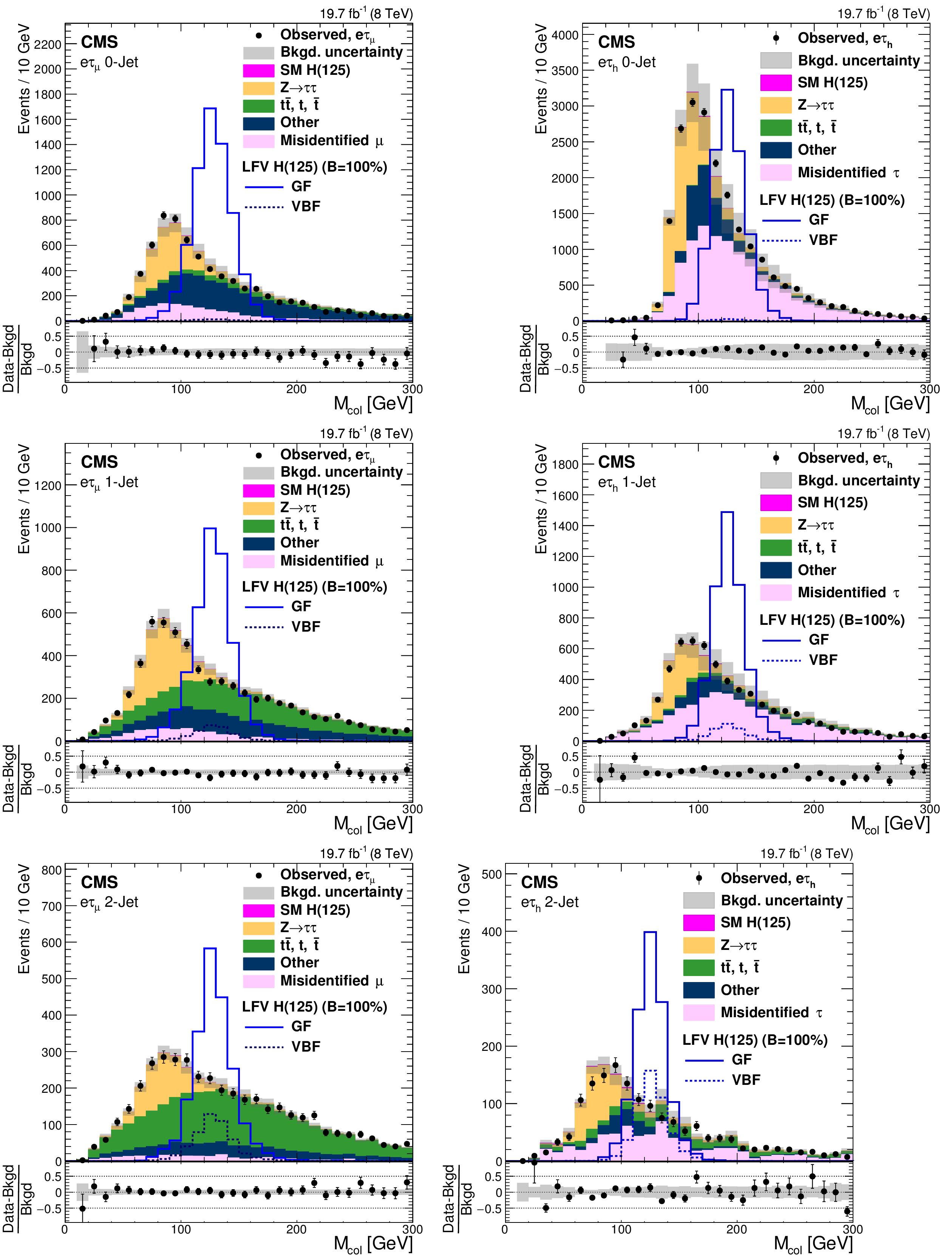
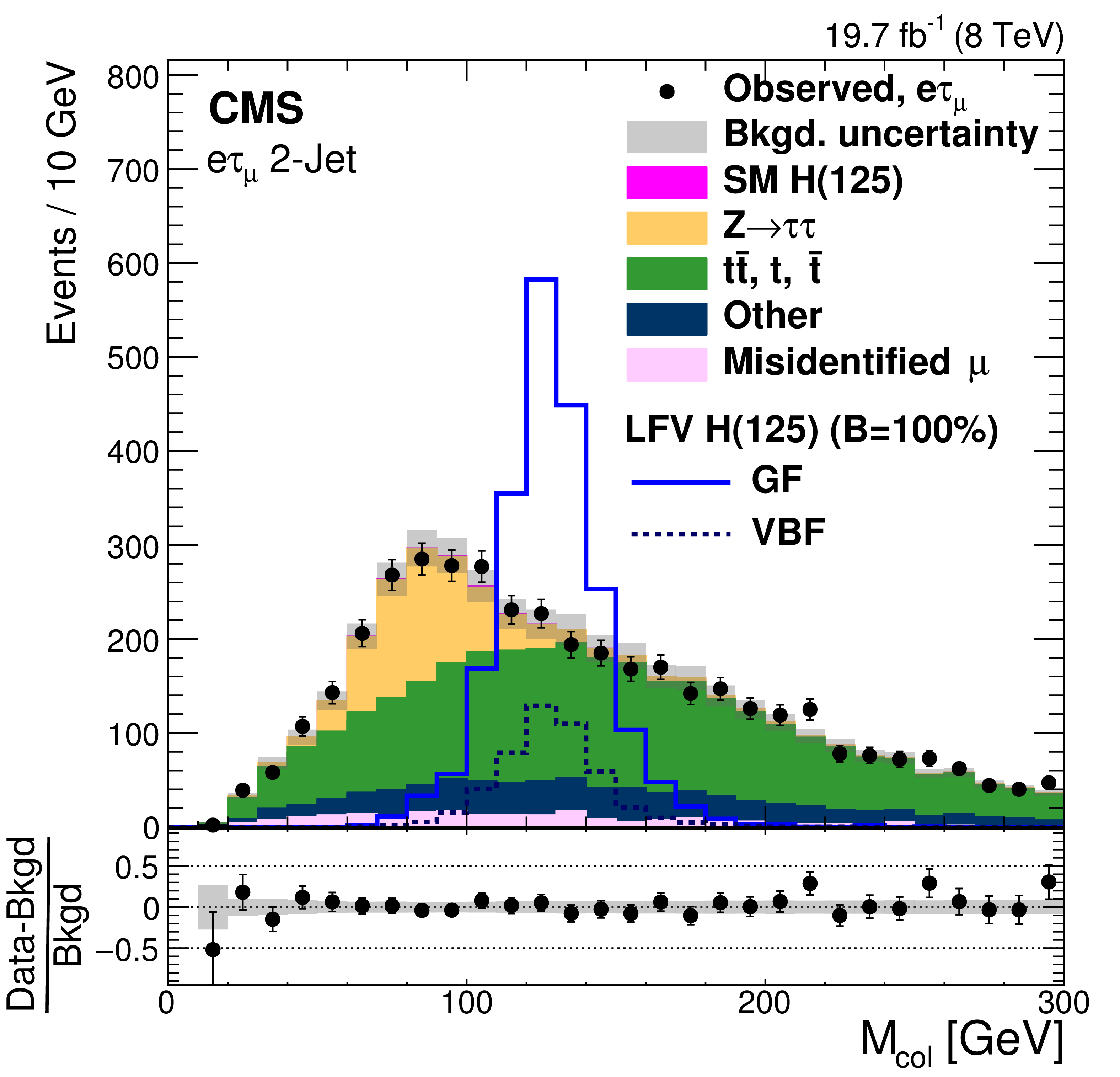
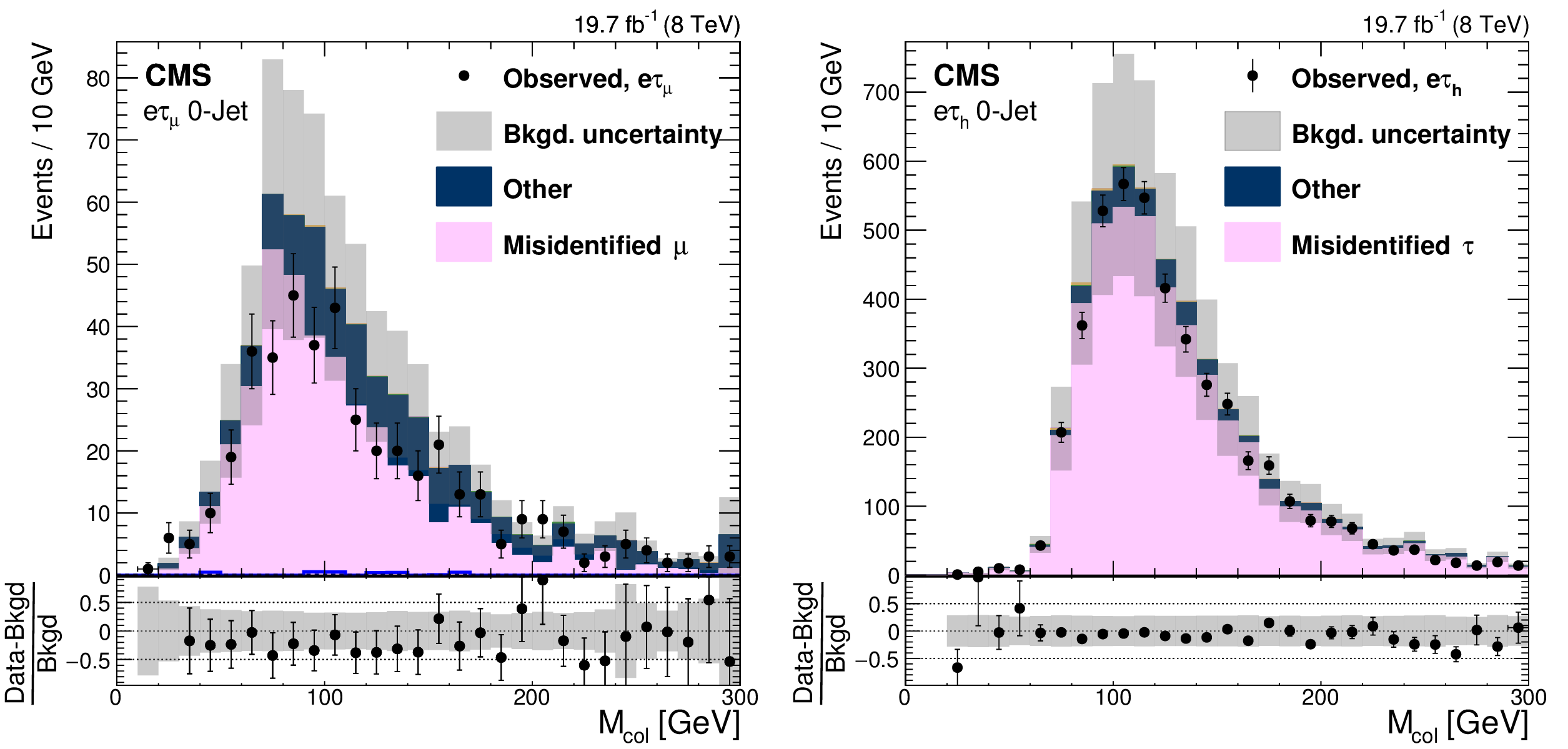
Figure 1:
Comparison of the observed collinear mass distributions with the background expectations after the loose selection requirements. The shaded grey bands indicate the total background uncertainty. The open histograms correspond to the expected signal distributions for $\mathcal {B}(\mathrm{ H } \to \mathrm{ e } \tau )=$ 100%. The (a,c,e) plots are $\mathrm{ H } \to \mathrm{ e } \tau _{\mu }$ and the (b,d,f) plots are $\mathrm{ H } \to \mathrm{ e } {\tau _\mathrm {h}} $; the (a,b), (c,d) and (e,f) plots are the 0-jet, 1-jet and 2-jet categories, respectively. |
png pdf |
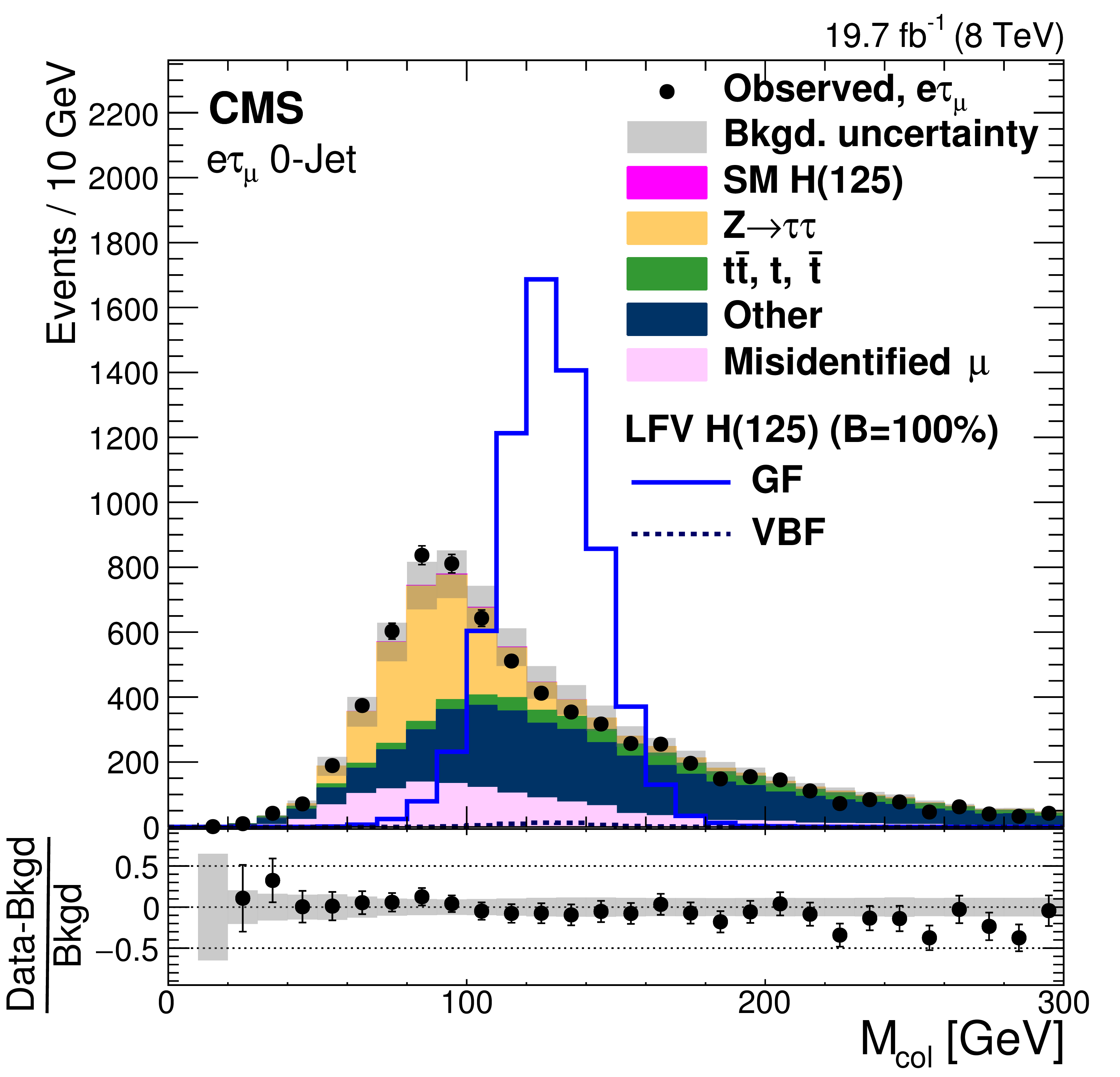
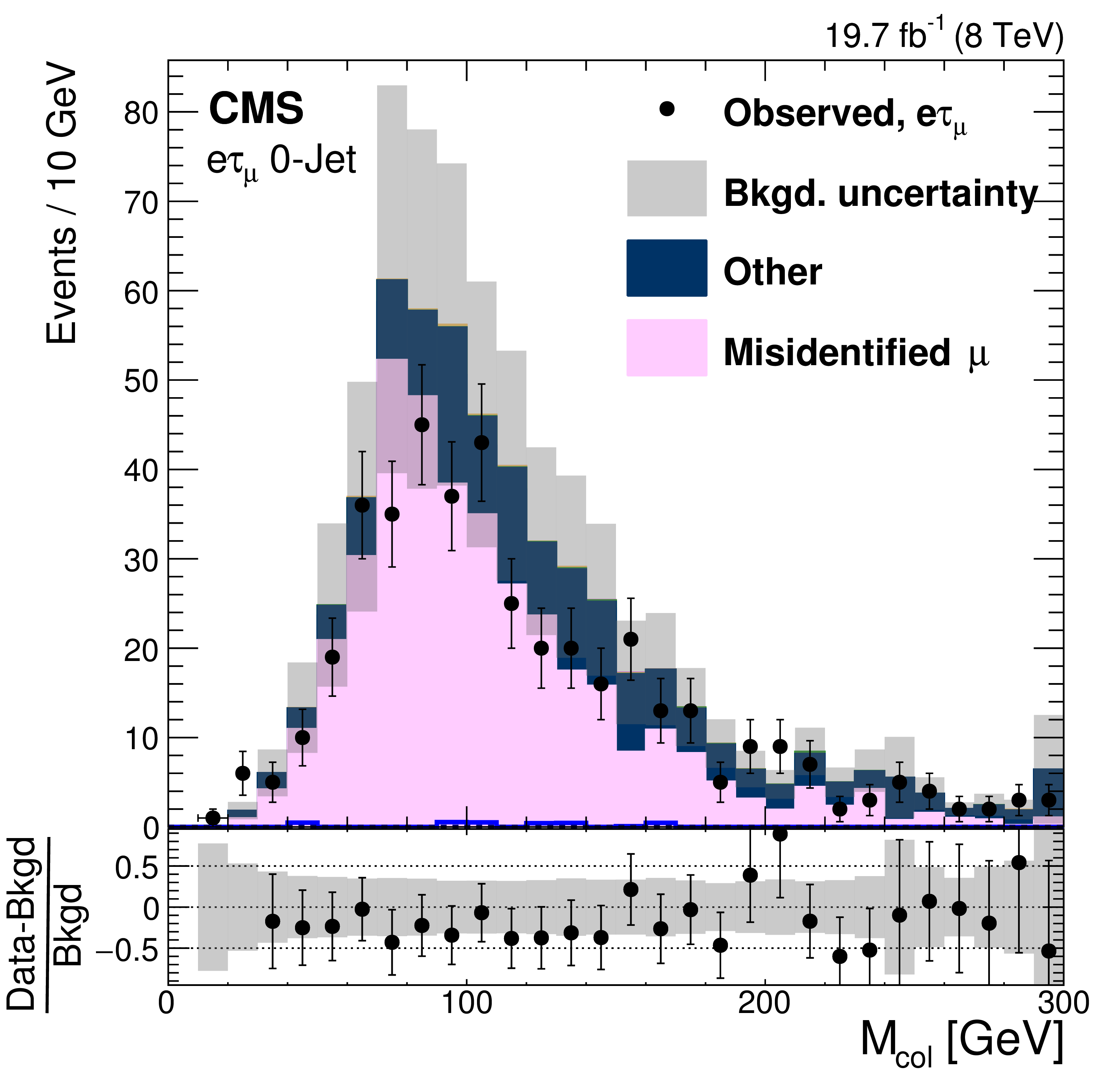
Figure 1-a:
Comparison of the observed collinear mass distributions with the background expectations after the loose selection requirements. The shaded grey bands indicate the total background uncertainty. The open histograms correspond to the expected signal distributions for $\mathcal {B}(\mathrm{ H } \to \mathrm{ e } \tau )=$ 100%. The (a,c,e) plots are $\mathrm{ H } \to \mathrm{ e } \tau _{\mu }$ and the (b,d,f) plots are $\mathrm{ H } \to \mathrm{ e } {\tau _\mathrm {h}} $; the (a,b), (c,d) and (e,f) plots are the 0-jet, 1-jet and 2-jet categories, respectively. |
png pdf |
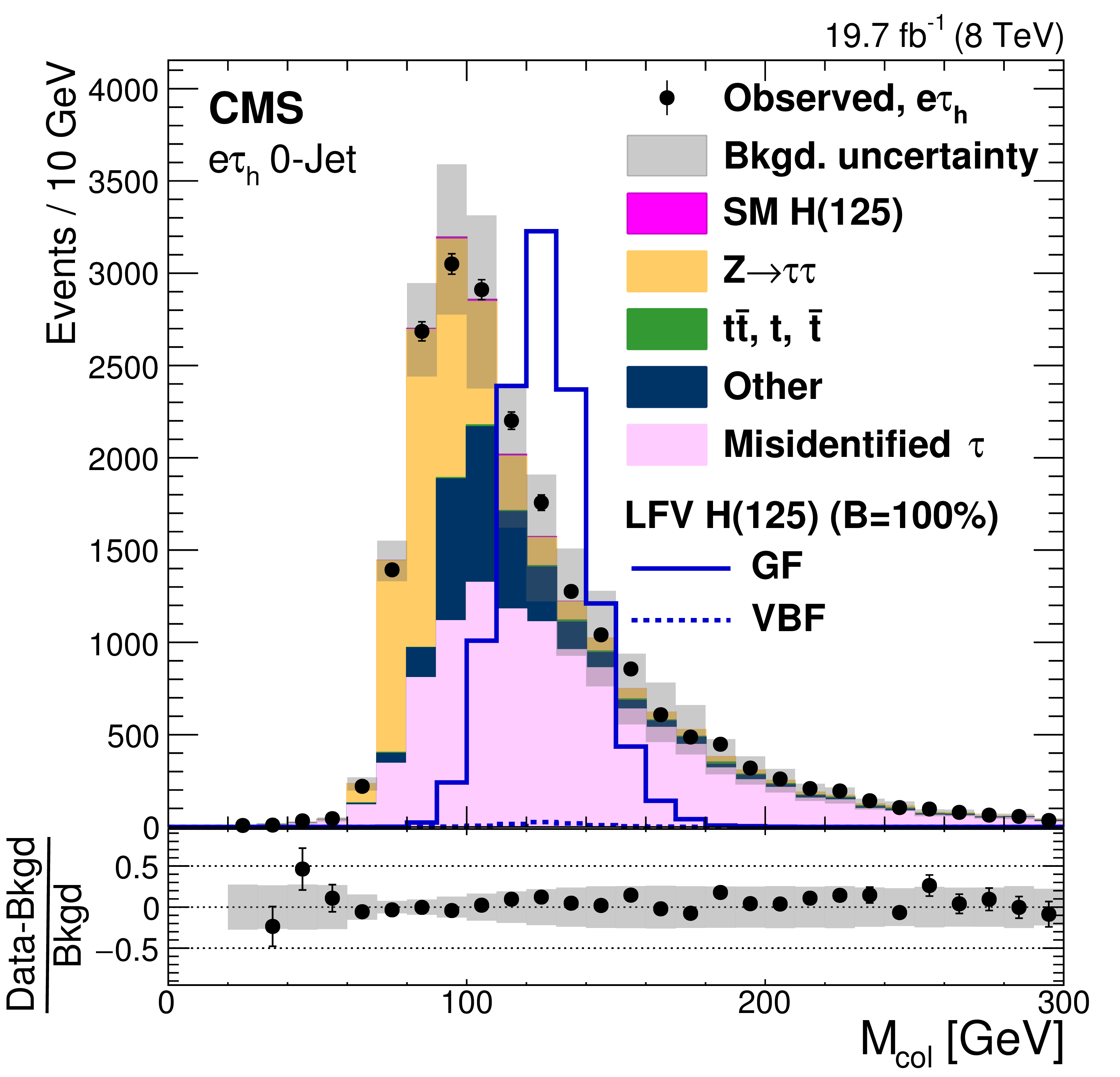
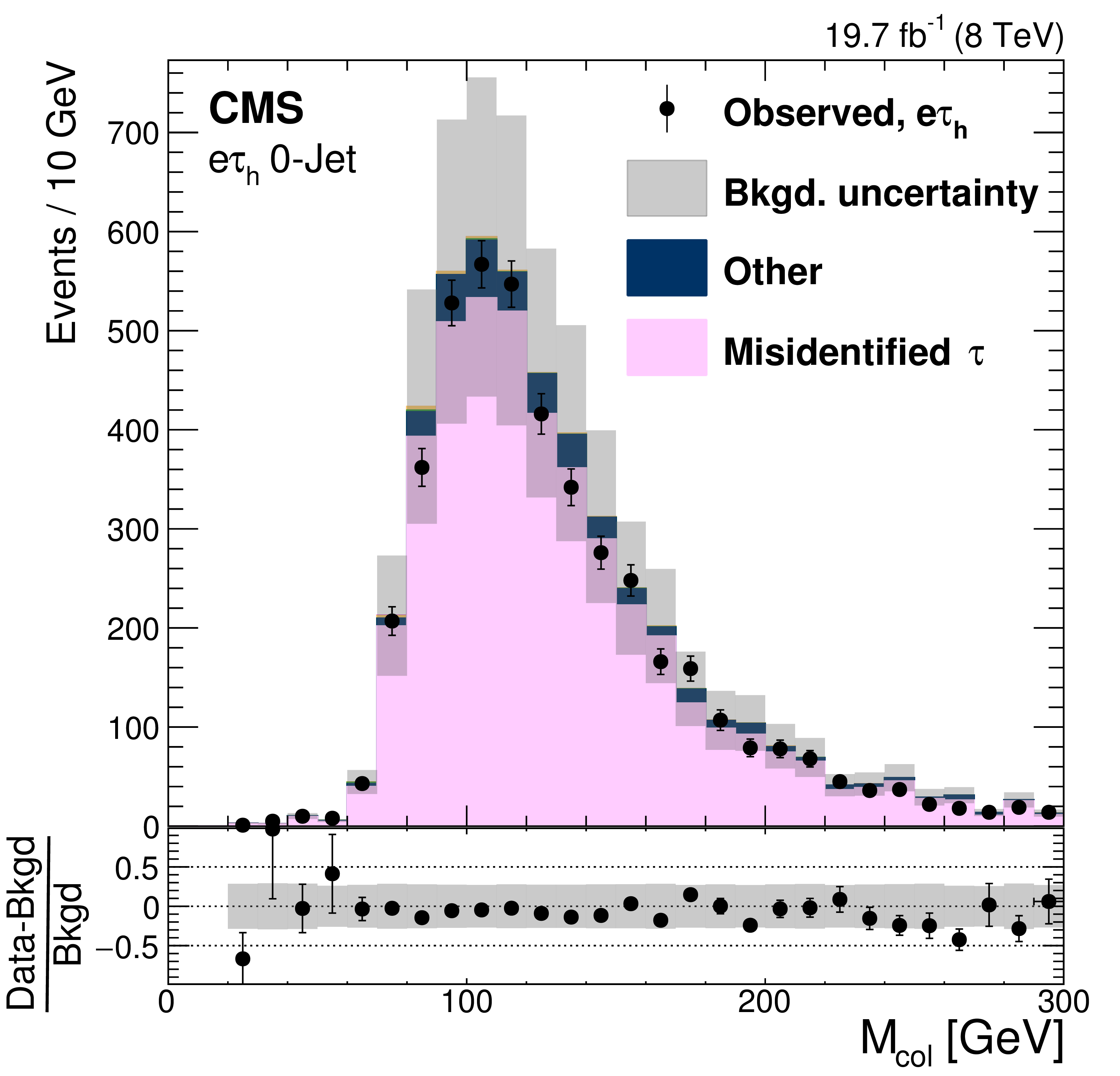
Figure 1-b:
Comparison of the observed collinear mass distributions with the background expectations after the loose selection requirements. The shaded grey bands indicate the total background uncertainty. The open histograms correspond to the expected signal distributions for $\mathcal {B}(\mathrm{ H } \to \mathrm{ e } \tau )=$ 100%. The (a,c,e) plots are $\mathrm{ H } \to \mathrm{ e } \tau _{\mu }$ and the (b,d,f) plots are $\mathrm{ H } \to \mathrm{ e } {\tau _\mathrm {h}} $; the (a,b), (c,d) and (e,f) plots are the 0-jet, 1-jet and 2-jet categories, respectively. |

png pdf |
Figure 1-c:
Comparison of the observed collinear mass distributions with the background expectations after the loose selection requirements. The shaded grey bands indicate the total background uncertainty. The open histograms correspond to the expected signal distributions for $\mathcal {B}(\mathrm{ H } \to \mathrm{ e } \tau )=$ 100%. The (a,c,e) plots are $\mathrm{ H } \to \mathrm{ e } \tau _{\mu }$ and the (b,d,f) plots are $\mathrm{ H } \to \mathrm{ e } {\tau _\mathrm {h}} $; the (a,b), (c,d) and (e,f) plots are the 0-jet, 1-jet and 2-jet categories, respectively. |
png pdf |
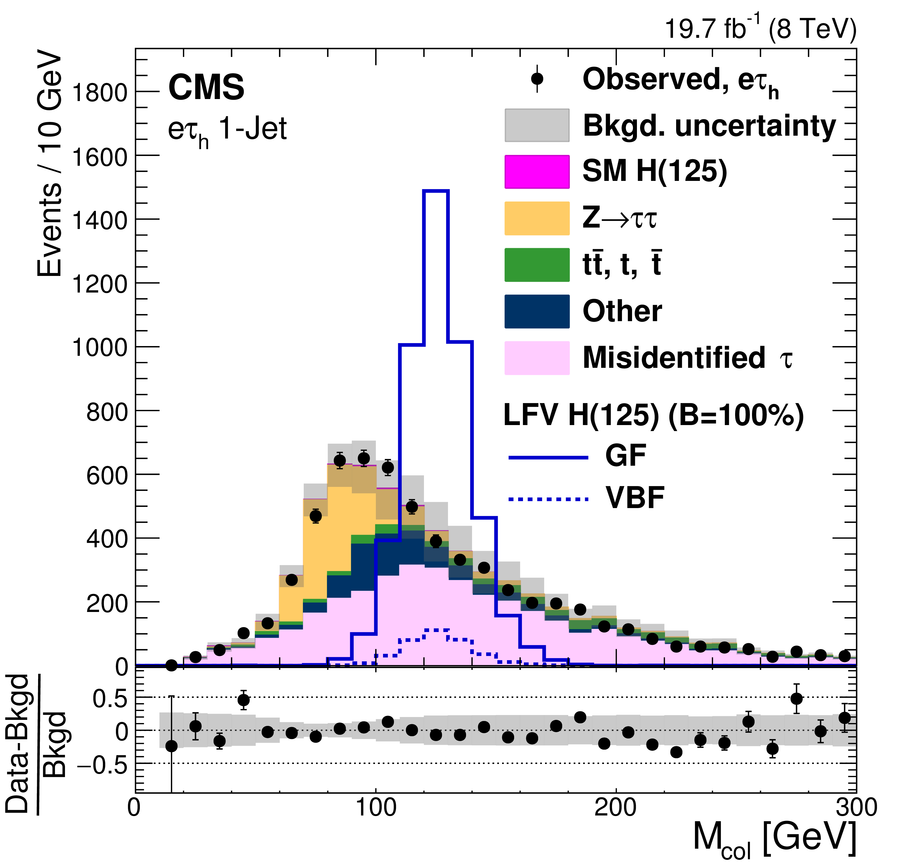
Figure 1-d:
Comparison of the observed collinear mass distributions with the background expectations after the loose selection requirements. The shaded grey bands indicate the total background uncertainty. The open histograms correspond to the expected signal distributions for $\mathcal {B}(\mathrm{ H } \to \mathrm{ e } \tau )=$ 100%. The (a,c,e) plots are $\mathrm{ H } \to \mathrm{ e } \tau _{\mu }$ and the (b,d,f) plots are $\mathrm{ H } \to \mathrm{ e } {\tau _\mathrm {h}} $; the (a,b), (c,d) and (e,f) plots are the 0-jet, 1-jet and 2-jet categories, respectively. |
png pdf |
Figure 1-e:
Comparison of the observed collinear mass distributions with the background expectations after the loose selection requirements. The shaded grey bands indicate the total background uncertainty. The open histograms correspond to the expected signal distributions for $\mathcal {B}(\mathrm{ H } \to \mathrm{ e } \tau )=$ 100%. The (a,c,e) plots are $\mathrm{ H } \to \mathrm{ e } \tau _{\mu }$ and the (b,d,f) plots are $\mathrm{ H } \to \mathrm{ e } {\tau _\mathrm {h}} $; the (a,b), (c,d) and (e,f) plots are the 0-jet, 1-jet and 2-jet categories, respectively. |

png pdf |
Figure 1-f:
Comparison of the observed collinear mass distributions with the background expectations after the loose selection requirements. The shaded grey bands indicate the total background uncertainty. The open histograms correspond to the expected signal distributions for $\mathcal {B}(\mathrm{ H } \to \mathrm{ e } \tau )=$ 100%. The (a,c,e) plots are $\mathrm{ H } \to \mathrm{ e } \tau _{\mu }$ and the (b,d,f) plots are $\mathrm{ H } \to \mathrm{ e } {\tau _\mathrm {h}} $; the (a,b), (c,d) and (e,f) plots are the 0-jet, 1-jet and 2-jet categories, respectively. |
png pdf |
Figure 2:
Distributions of $m_{\text {col}}$ for RegionII. a: $\mathrm{ H } \to \mathrm{ e } \tau _{\mu }$. b: $\mathrm{ H } \to \mathrm{ e } {\tau _\mathrm {h}} $. |
png pdf |
Figure 2-a:
Distributions of $m_{\text {col}}$ for RegionII. a: $\mathrm{ H } \to \mathrm{ e } \tau _{\mu }$. b: $\mathrm{ H } \to \mathrm{ e } {\tau _\mathrm {h}} $. |
png pdf |
Figure 2-b:
Distributions of $m_{\text {col}}$ for RegionII. a: $\mathrm{ H } \to \mathrm{ e } \tau _{\mu }$. b: $\mathrm{ H } \to \mathrm{ e } {\tau _\mathrm {h}} $. |
png pdf |
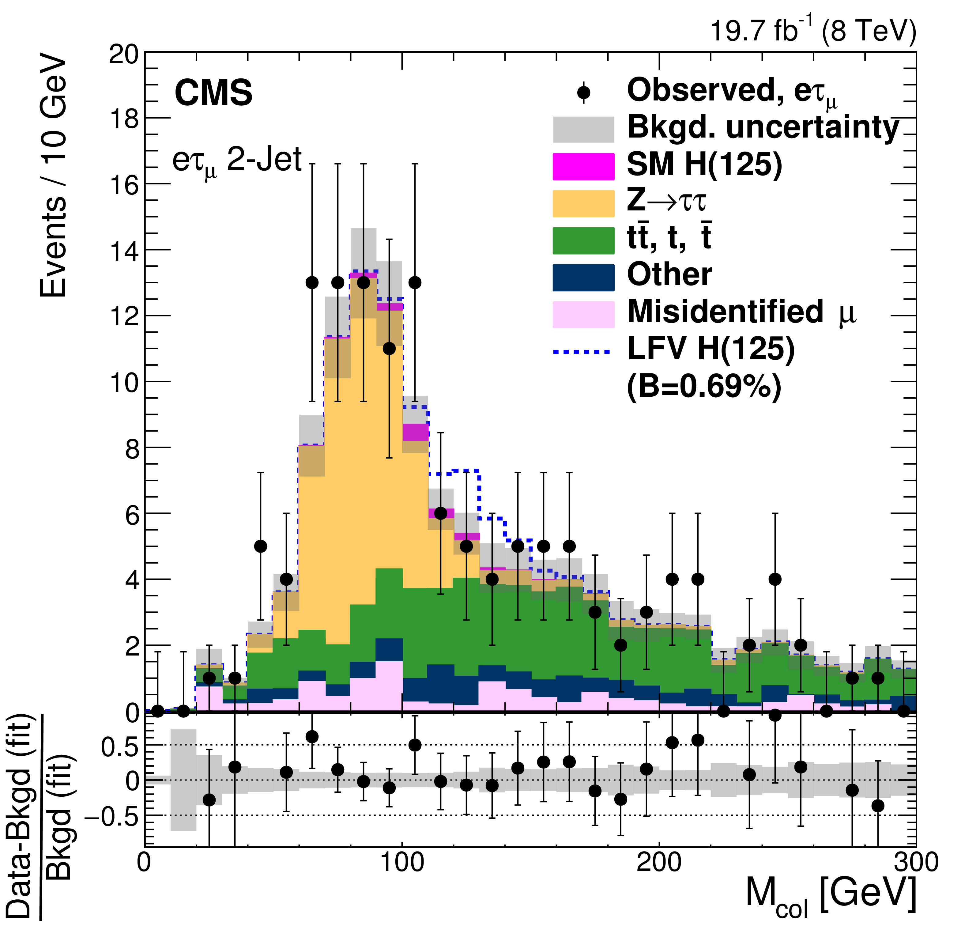
Figure 3:
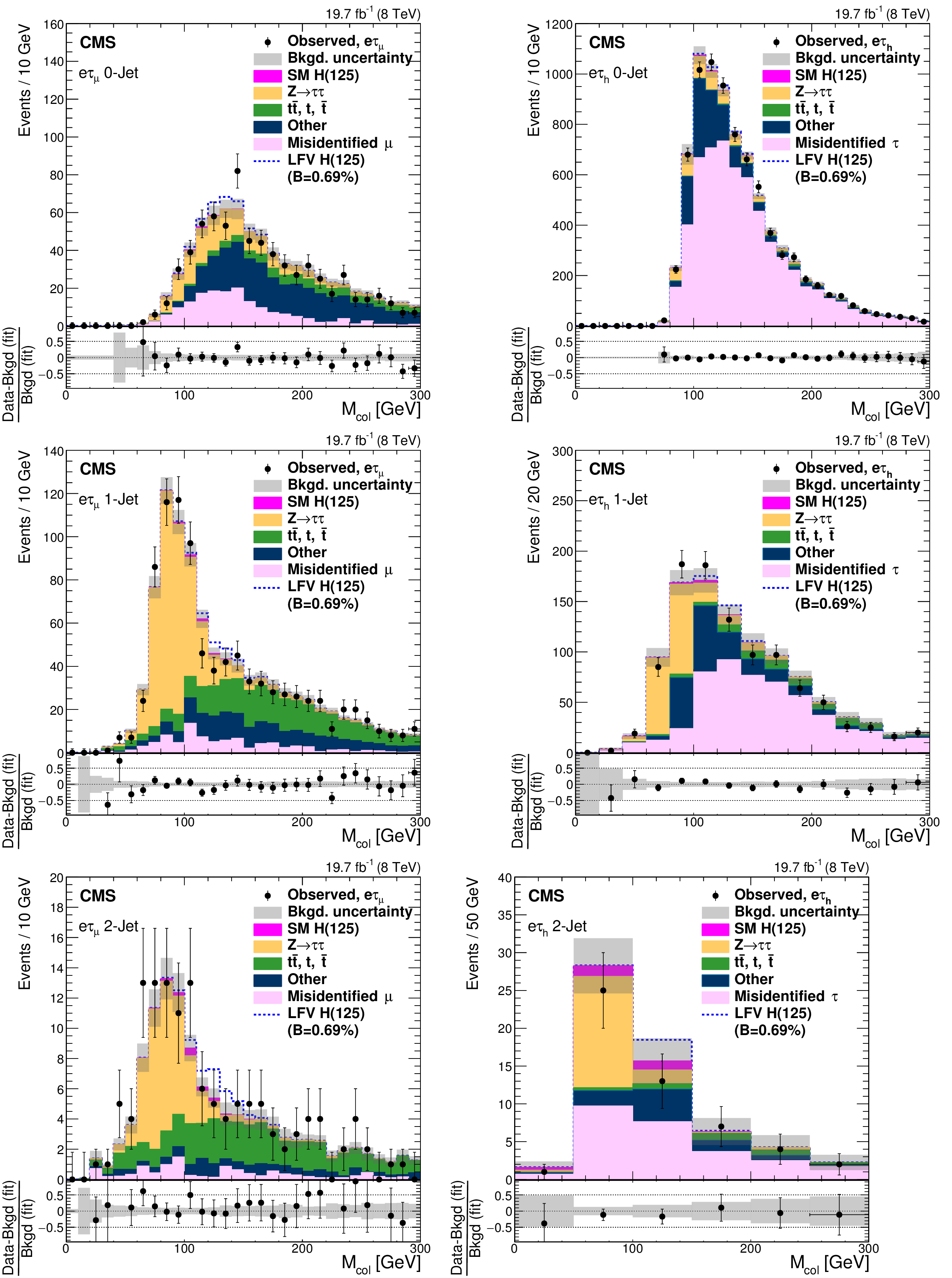
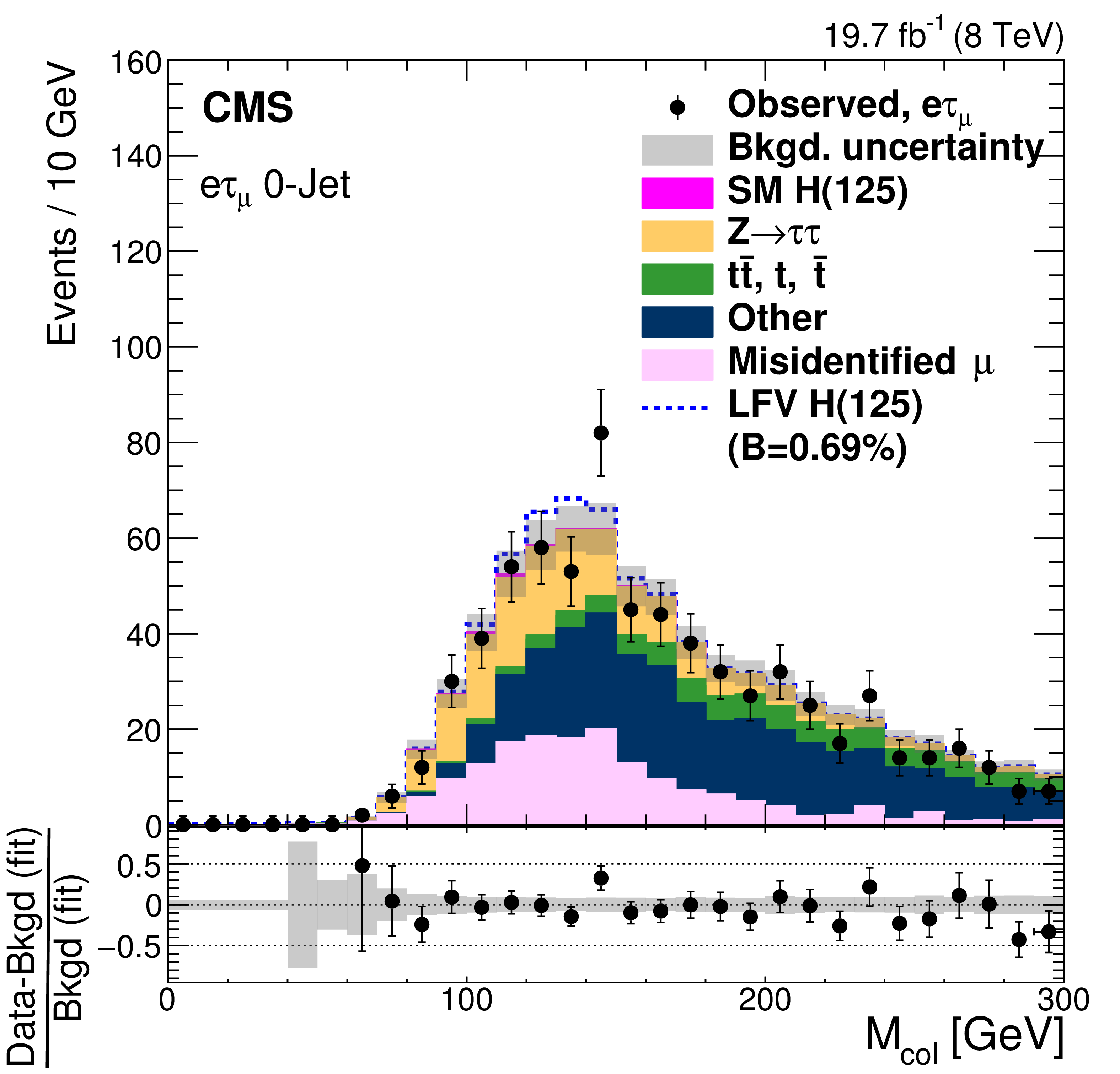
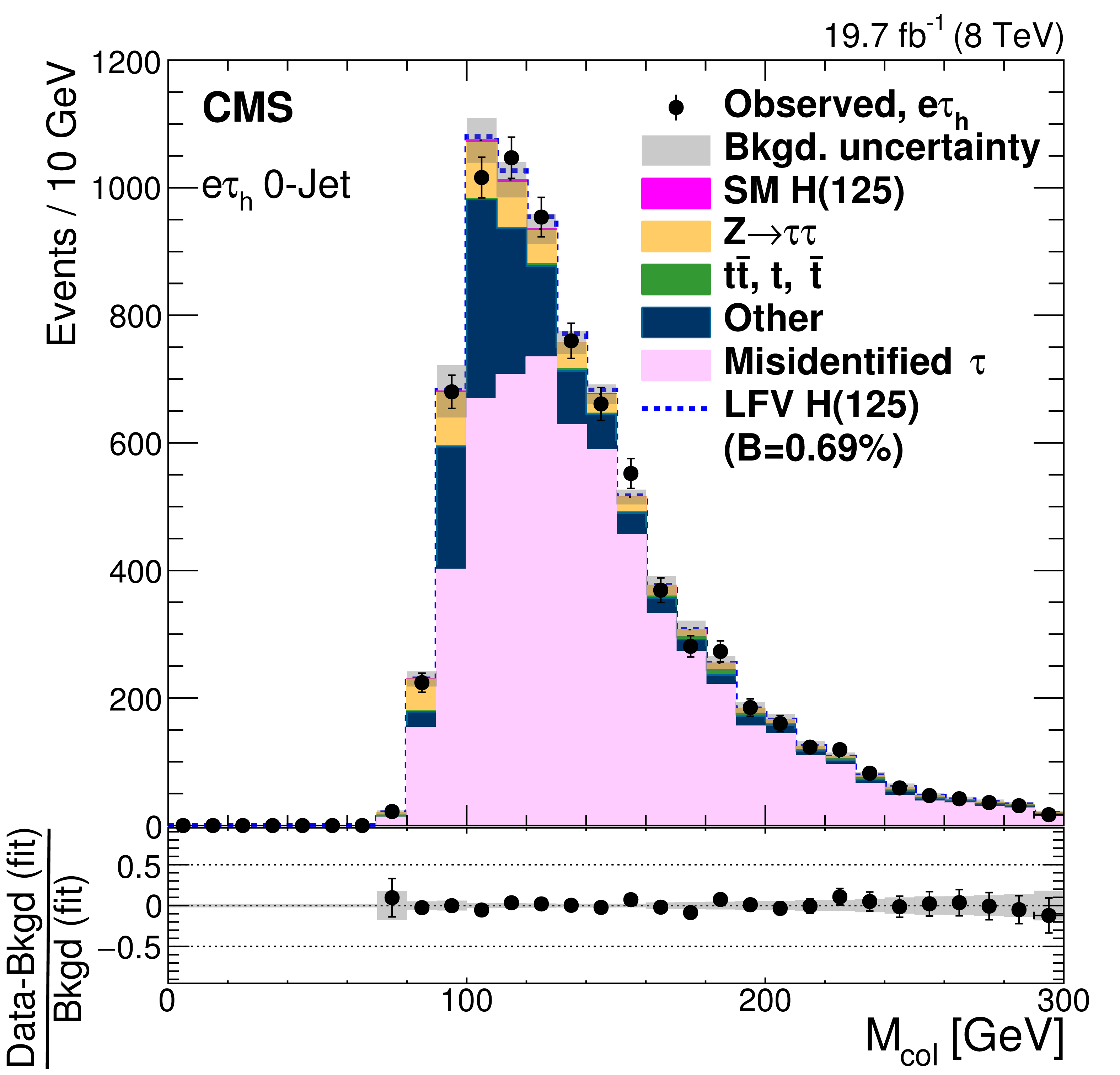
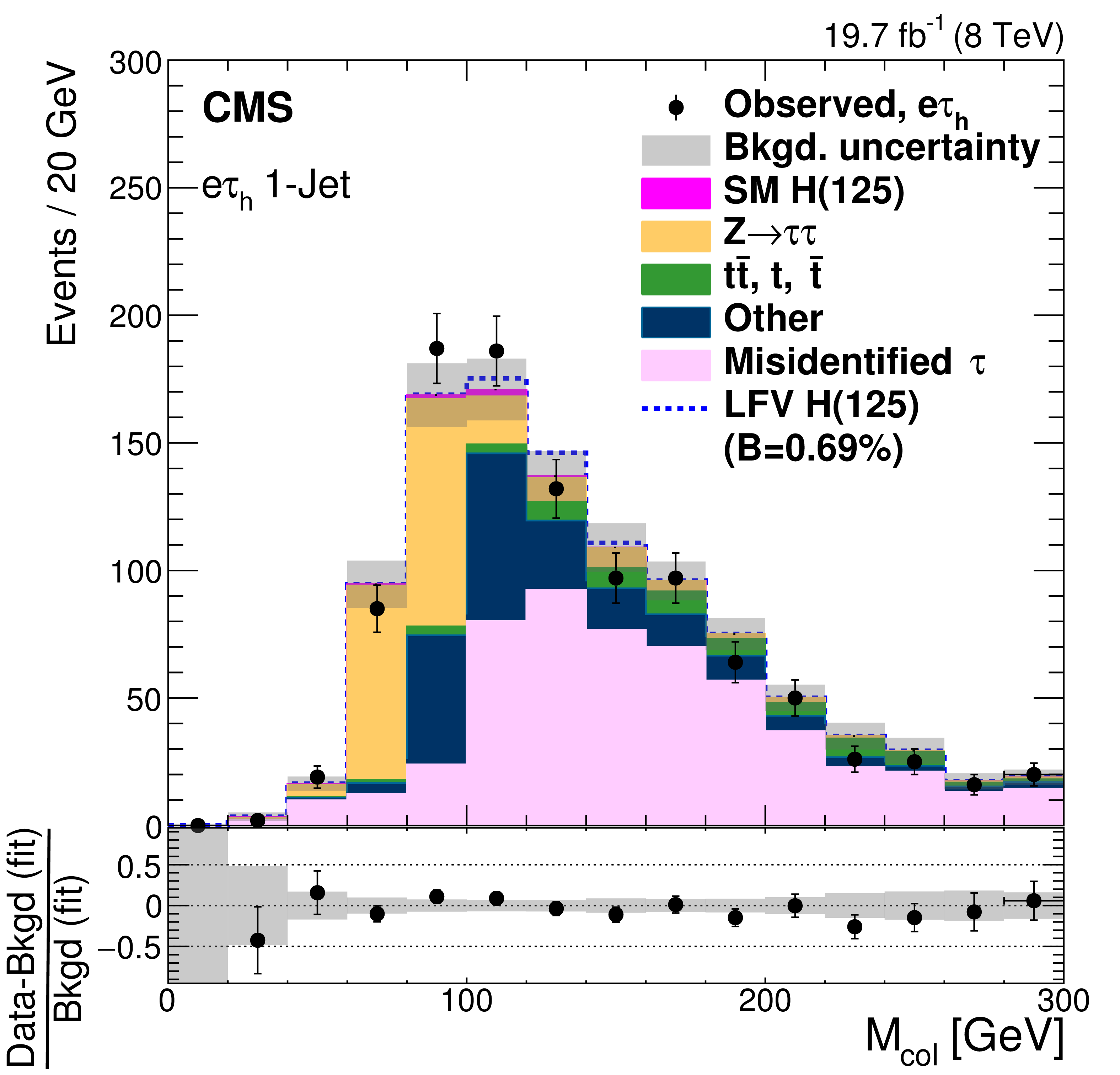
Comparison of the observed collinear mass distributions with the background expectations after the fit. The simulated distributions for the signal are shown for the branching fraction $\mathcal {B}(\mathrm{ H } \to \mathrm{ e } \tau )=$ 0.69%. The (a,c,e) plots are $\mathrm{ H } \to \mathrm{ e } \tau _{\mu }$ and the (b,d,f) plots are $\mathrm{ H } \to \mathrm{ e } {\tau _\mathrm {h}} $; the (a,b), (c,d) and (e,f) plots are the 0-jet, 1-jet and 2-jet categories, respectively. |
png pdf |
Figure 3-a:
Comparison of the observed collinear mass distributions with the background expectations after the fit. The simulated distributions for the signal are shown for the branching fraction $\mathcal {B}(\mathrm{ H } \to \mathrm{ e } \tau )=$ 0.69%. The (a,c,e) plots are $\mathrm{ H } \to \mathrm{ e } \tau _{\mu }$ and the (b,d,f) plots are $\mathrm{ H } \to \mathrm{ e } {\tau _\mathrm {h}} $; the (a,b), (c,d) and (e,f) plots are the 0-jet, 1-jet and 2-jet categories, respectively. |
png pdf |
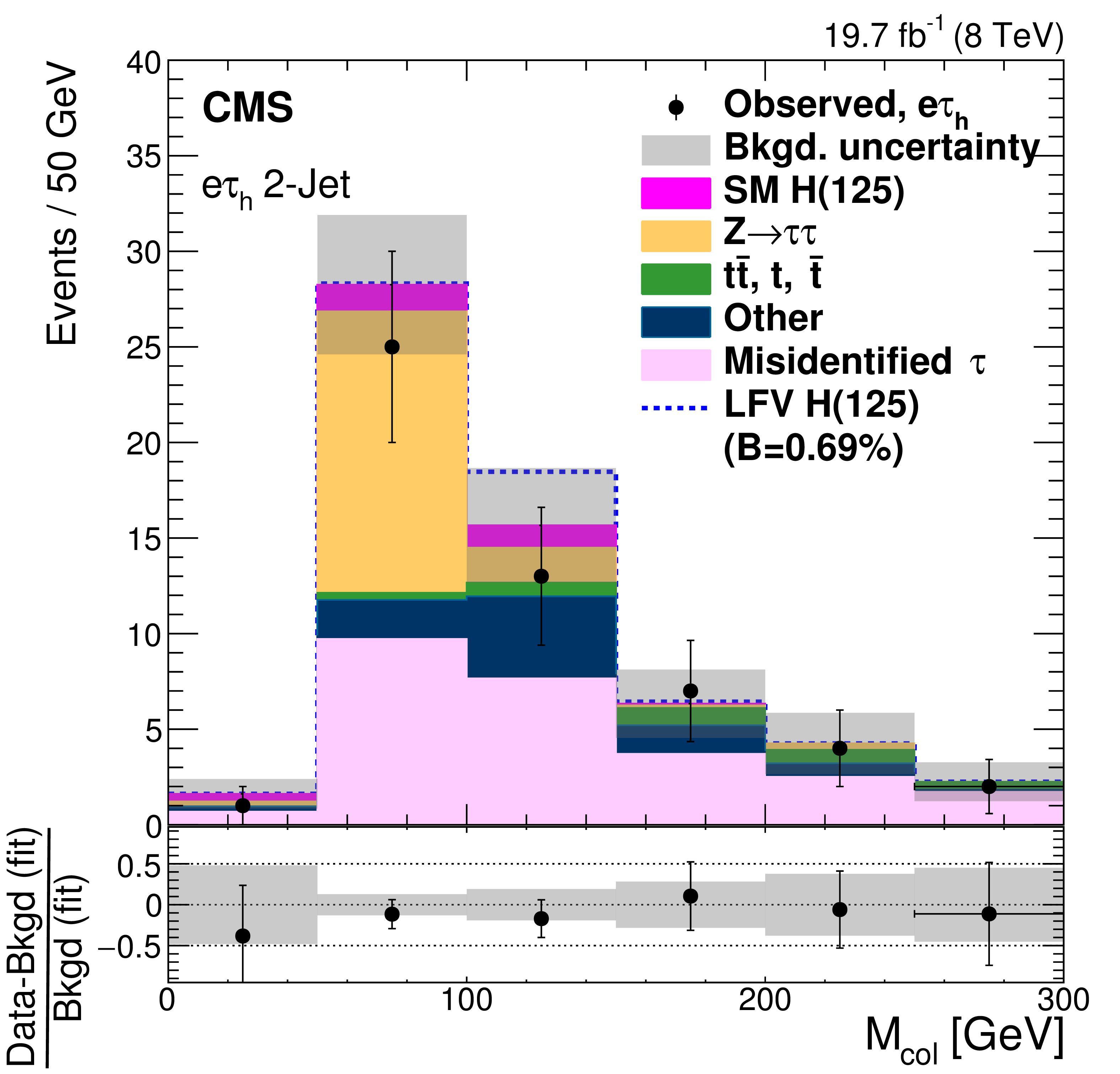
Figure 3-b:
Comparison of the observed collinear mass distributions with the background expectations after the fit. The simulated distributions for the signal are shown for the branching fraction $\mathcal {B}(\mathrm{ H } \to \mathrm{ e } \tau )=$ 0.69%. The (a,c,e) plots are $\mathrm{ H } \to \mathrm{ e } \tau _{\mu }$ and the (b,d,f) plots are $\mathrm{ H } \to \mathrm{ e } {\tau _\mathrm {h}} $; the (a,b), (c,d) and (e,f) plots are the 0-jet, 1-jet and 2-jet categories, respectively. |

png pdf |
Figure 3-c:
Comparison of the observed collinear mass distributions with the background expectations after the fit. The simulated distributions for the signal are shown for the branching fraction $\mathcal {B}(\mathrm{ H } \to \mathrm{ e } \tau )=$ 0.69%. The (a,c,e) plots are $\mathrm{ H } \to \mathrm{ e } \tau _{\mu }$ and the (b,d,f) plots are $\mathrm{ H } \to \mathrm{ e } {\tau _\mathrm {h}} $; the (a,b), (c,d) and (e,f) plots are the 0-jet, 1-jet and 2-jet categories, respectively. |
png pdf |
Figure 3-d:
Comparison of the observed collinear mass distributions with the background expectations after the fit. The simulated distributions for the signal are shown for the branching fraction $\mathcal {B}(\mathrm{ H } \to \mathrm{ e } \tau )=$ 0.69%. The (a,c,e) plots are $\mathrm{ H } \to \mathrm{ e } \tau _{\mu }$ and the (b,d,f) plots are $\mathrm{ H } \to \mathrm{ e } {\tau _\mathrm {h}} $; the (a,b), (c,d) and (e,f) plots are the 0-jet, 1-jet and 2-jet categories, respectively. |
png pdf |
Figure 3-e:
Comparison of the observed collinear mass distributions with the background expectations after the fit. The simulated distributions for the signal are shown for the branching fraction $\mathcal {B}(\mathrm{ H } \to \mathrm{ e } \tau )=$ 0.69%. The (a,c,e) plots are $\mathrm{ H } \to \mathrm{ e } \tau _{\mu }$ and the (b,d,f) plots are $\mathrm{ H } \to \mathrm{ e } {\tau _\mathrm {h}} $; the (a,b), (c,d) and (e,f) plots are the 0-jet, 1-jet and 2-jet categories, respectively. |
png pdf |
Figure 3-f:
Comparison of the observed collinear mass distributions with the background expectations after the fit. The simulated distributions for the signal are shown for the branching fraction $\mathcal {B}(\mathrm{ H } \to \mathrm{ e } \tau )=$ 0.69%. The (a,c,e) plots are $\mathrm{ H } \to \mathrm{ e } \tau _{\mu }$ and the (b,d,f) plots are $\mathrm{ H } \to \mathrm{ e } {\tau _\mathrm {h}} $; the (a,b), (c,d) and (e,f) plots are the 0-jet, 1-jet and 2-jet categories, respectively. |
png pdf |
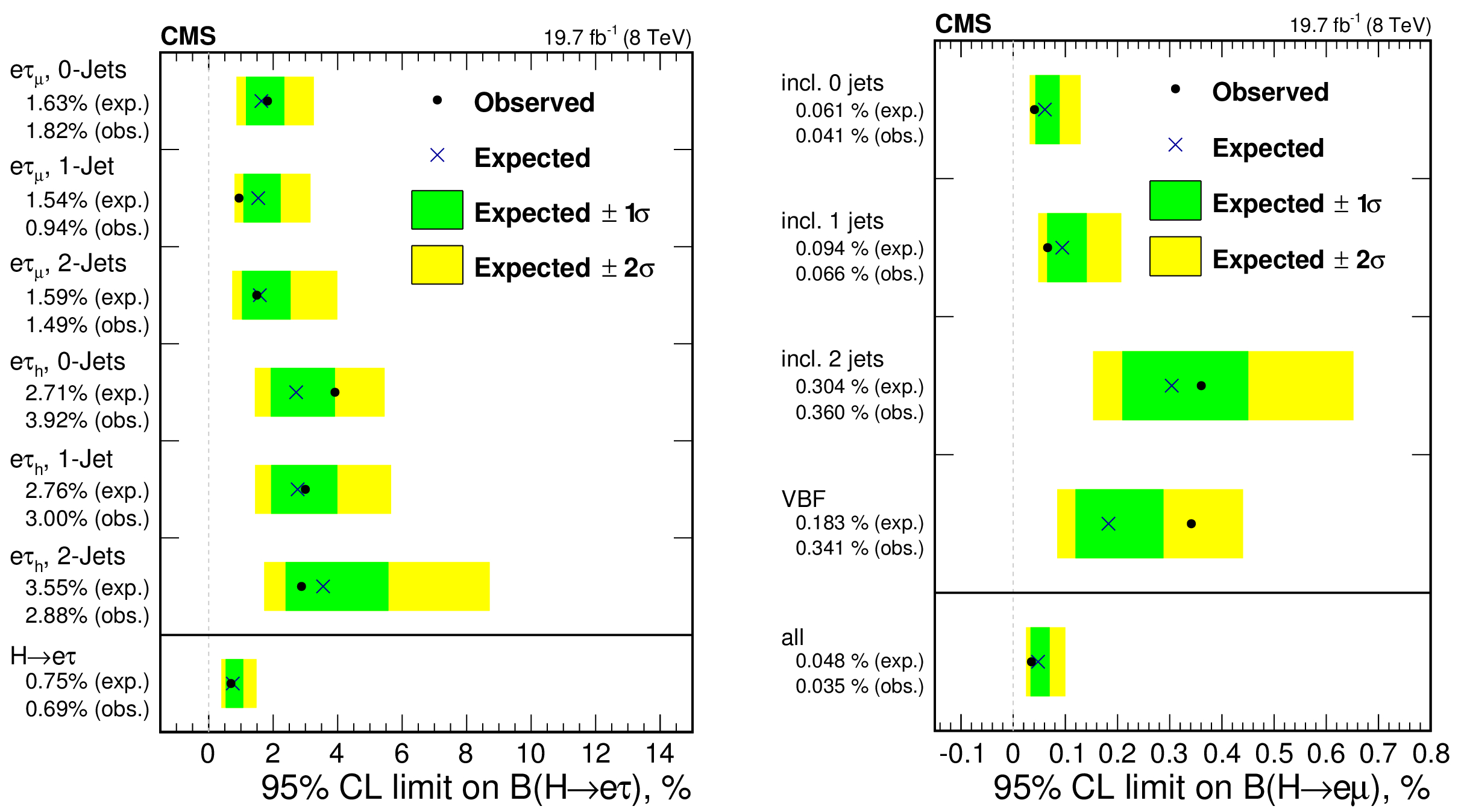
Figure 4:
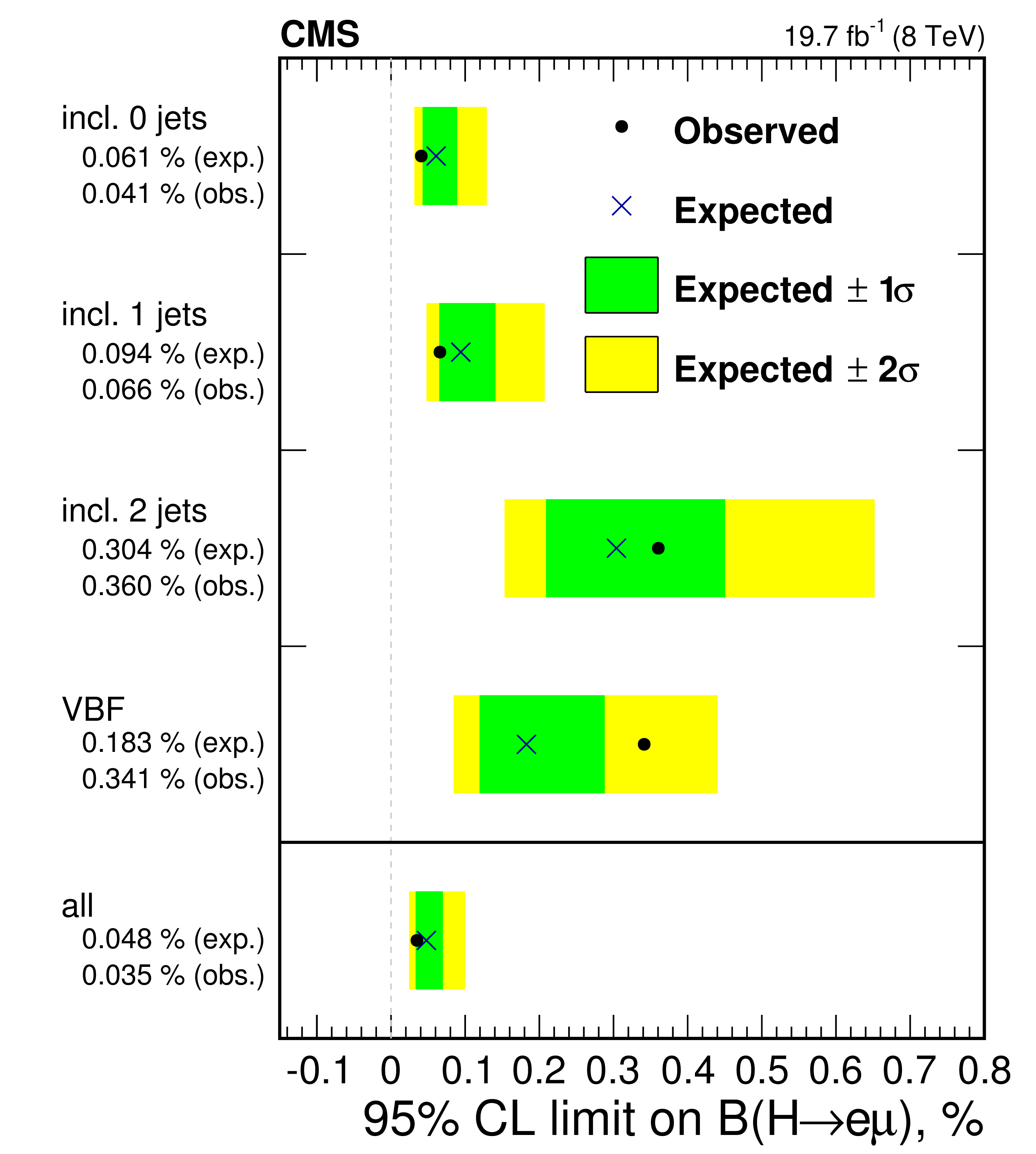
95% CL upper limits by category for the LFV decays for $ {M_{\mathrm{ H } }}= $ 125 GeV. a: $\mathrm{ H } \to \mathrm{ e } \tau $. b: $ {\mathrm{ H } \to \mathrm{ e } \mu } $ for categories combined by number of jets, the VBF categories combined, and all categories combined. |
png pdf |
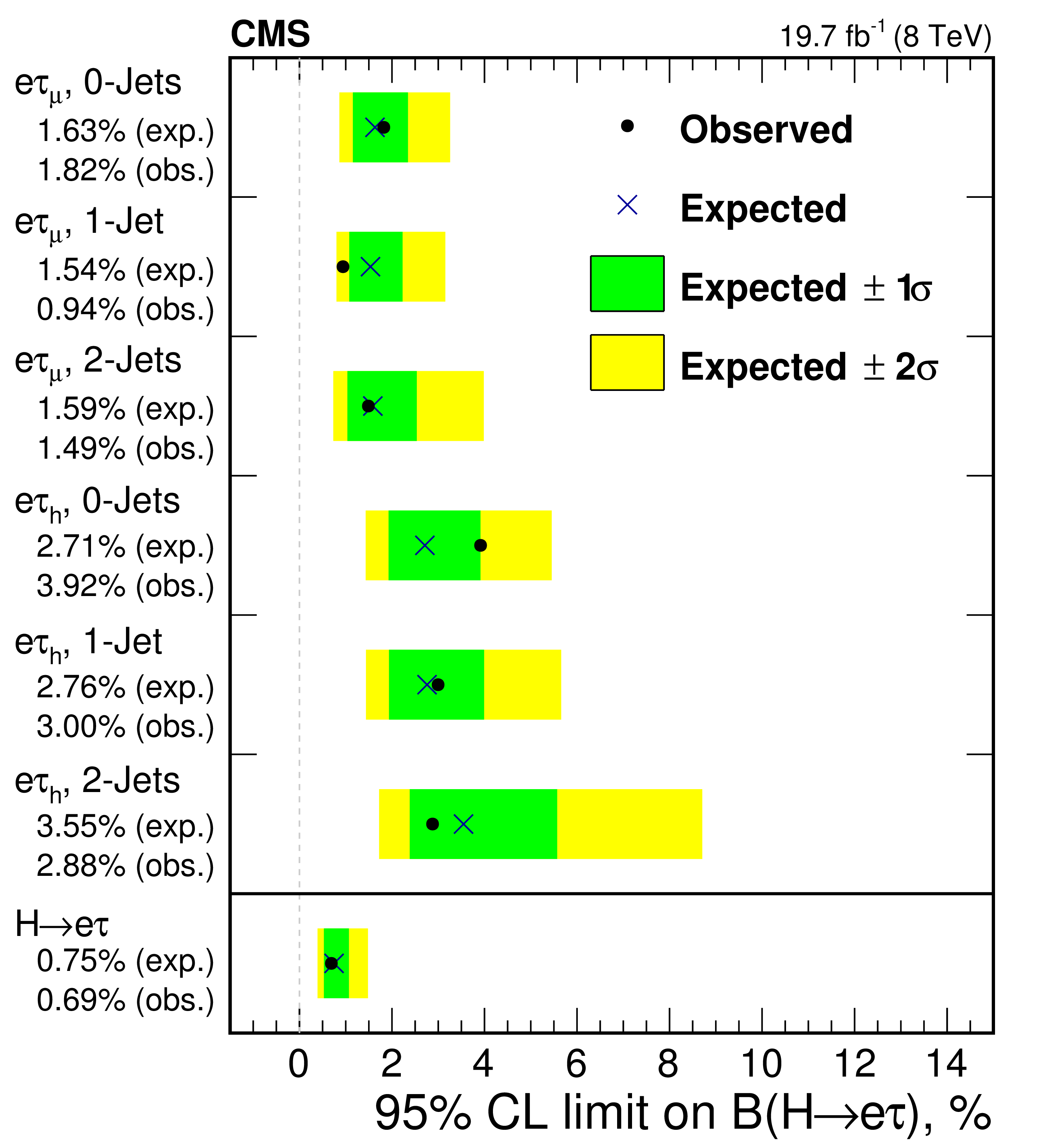
Figure 4-a:
95% CL upper limits by category for the LFV decays for $ {M_{\mathrm{ H } }}= $ 125 GeV. a: $\mathrm{ H } \to \mathrm{ e } \tau $. b: $ {\mathrm{ H } \to \mathrm{ e } \mu } $ for categories combined by number of jets, the VBF categories combined, and all categories combined. |
png pdf |
Figure 4-b:
95% CL upper limits by category for the LFV decays for $ {M_{\mathrm{ H } }}= $ 125 GeV. a: $\mathrm{ H } \to \mathrm{ e } \tau $. b: $ {\mathrm{ H } \to \mathrm{ e } \mu } $ for categories combined by number of jets, the VBF categories combined, and all categories combined. |
png pdf |
Figure 5:
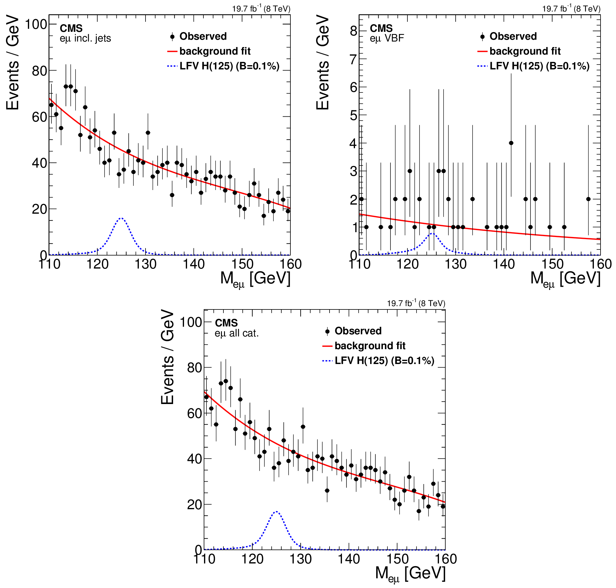
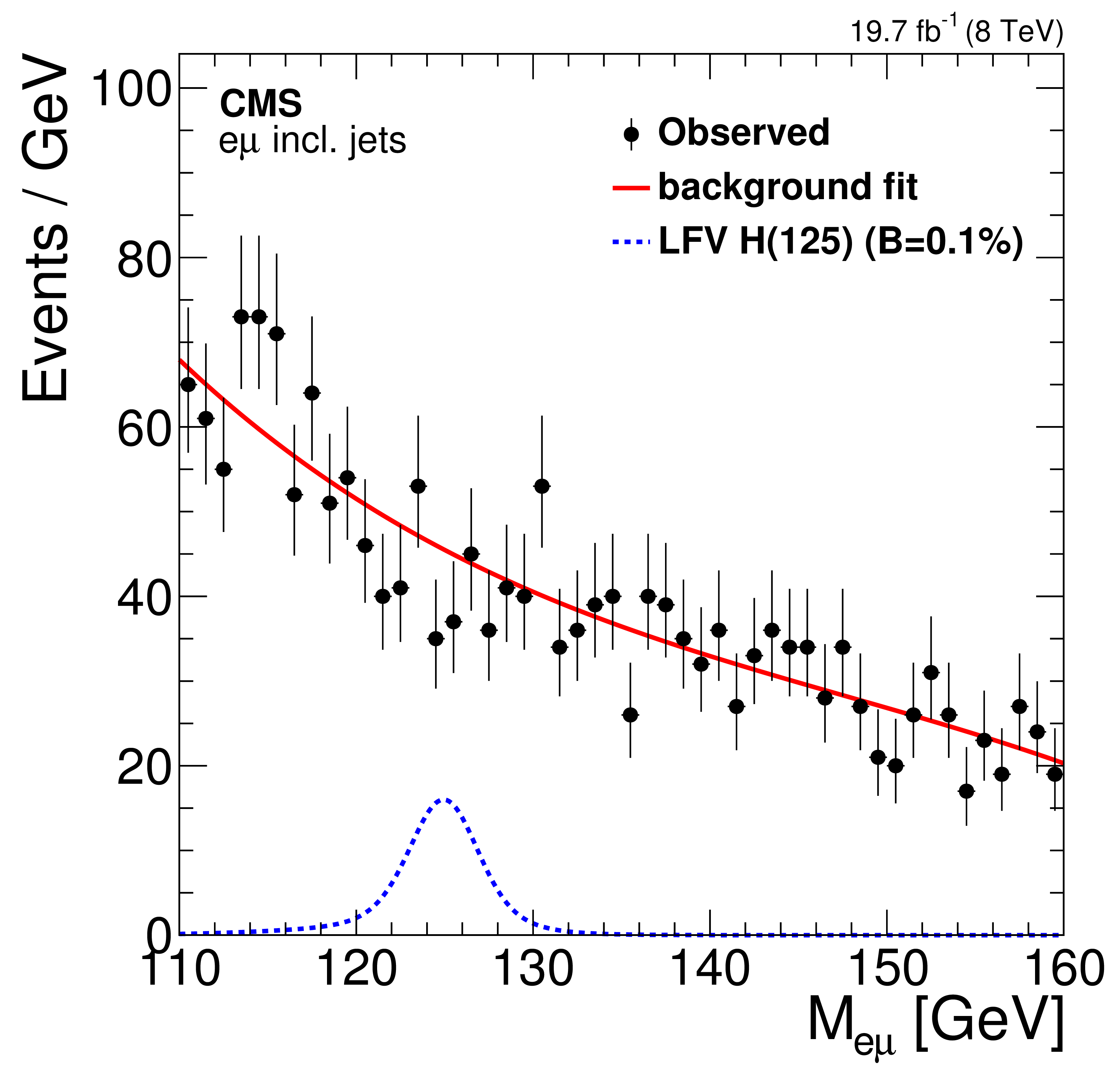
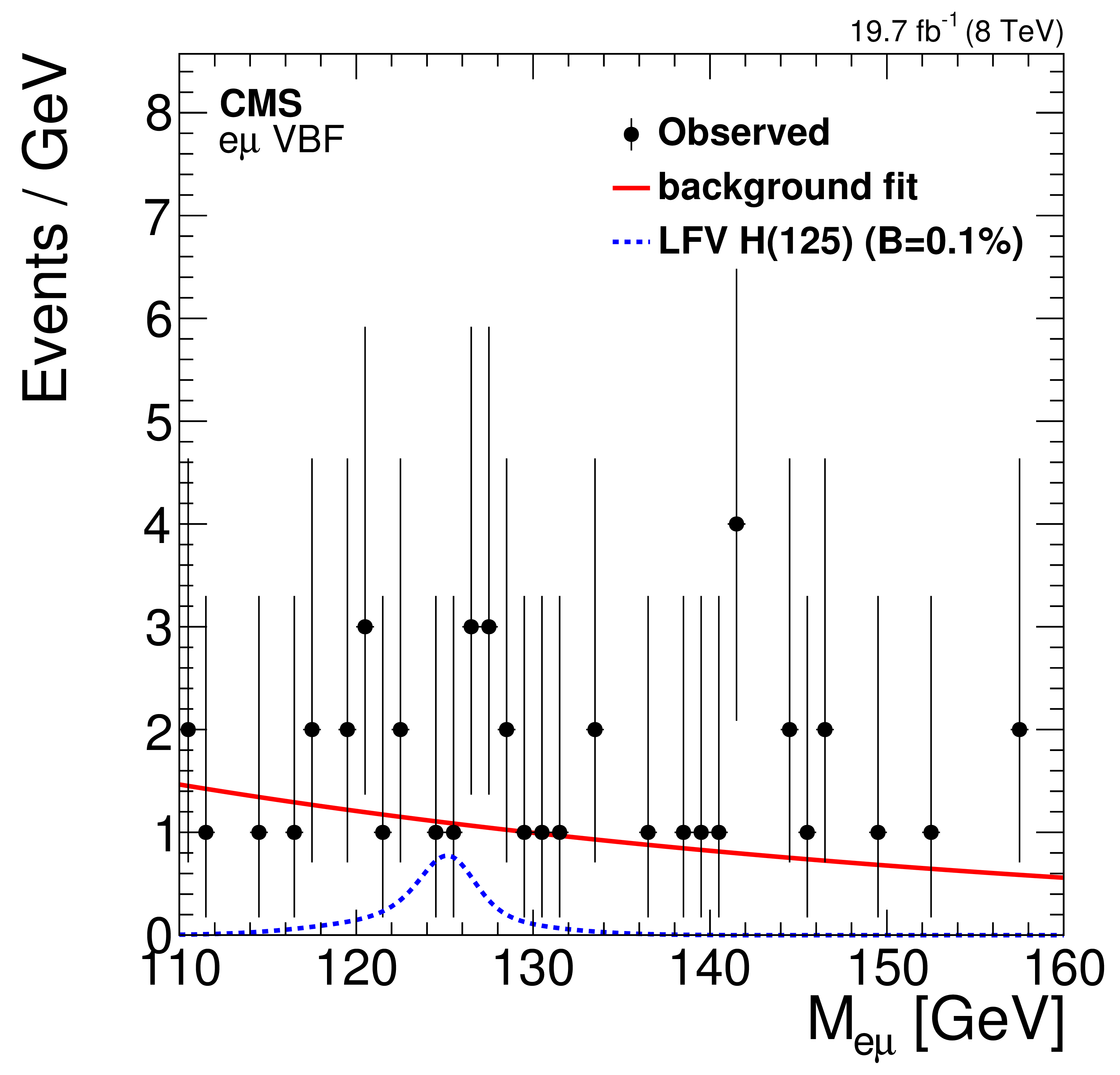
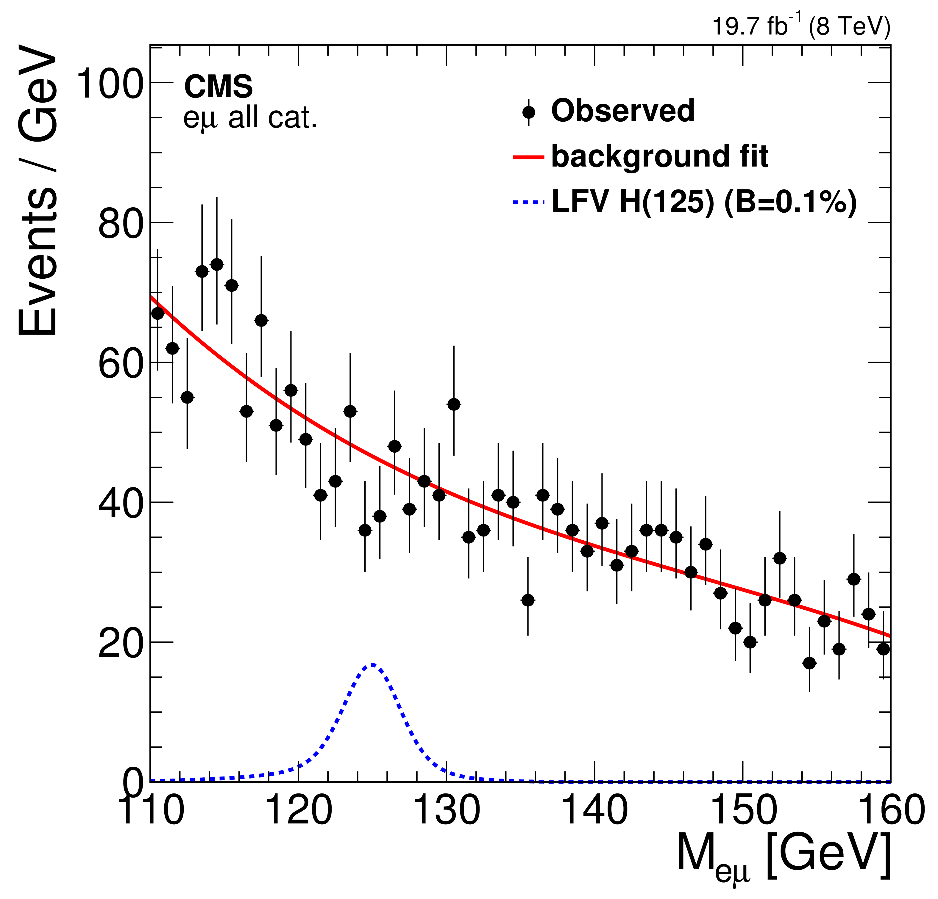
Observed $\mathrm{ e } \mu $ mass spectra (points), background fit (solid line) and signal model (blue dashed line) for $\mathcal {B}( {\mathrm{ H } \to \mathrm{ e } \mu } ) = $ 0.1%. a : inclusive jet categories combined (0-8). b : VBF jet tagged categories combined (9-10). c : all categories combined. |
png pdf |
Figure 5-a:
Observed $\mathrm{ e } \mu $ mass spectra (points), background fit (solid line) and signal model (blue dashed line) for $\mathcal {B}( {\mathrm{ H } \to \mathrm{ e } \mu } ) = $ 0.1%. a : inclusive jet categories combined (0-8). b : VBF jet tagged categories combined (9-10). c : all categories combined. |
png pdf |
Figure 5-b:
Observed $\mathrm{ e } \mu $ mass spectra (points), background fit (solid line) and signal model (blue dashed line) for $\mathcal {B}( {\mathrm{ H } \to \mathrm{ e } \mu } ) = $ 0.1%. a : inclusive jet categories combined (0-8). b : VBF jet tagged categories combined (9-10). c : all categories combined. |
png pdf |
Figure 5-c:
Observed $\mathrm{ e } \mu $ mass spectra (points), background fit (solid line) and signal model (blue dashed line) for $\mathcal {B}( {\mathrm{ H } \to \mathrm{ e } \mu } ) = $ 0.1%. a : inclusive jet categories combined (0-8). b : VBF jet tagged categories combined (9-10). c : all categories combined. |
png pdf |
Figure 6:
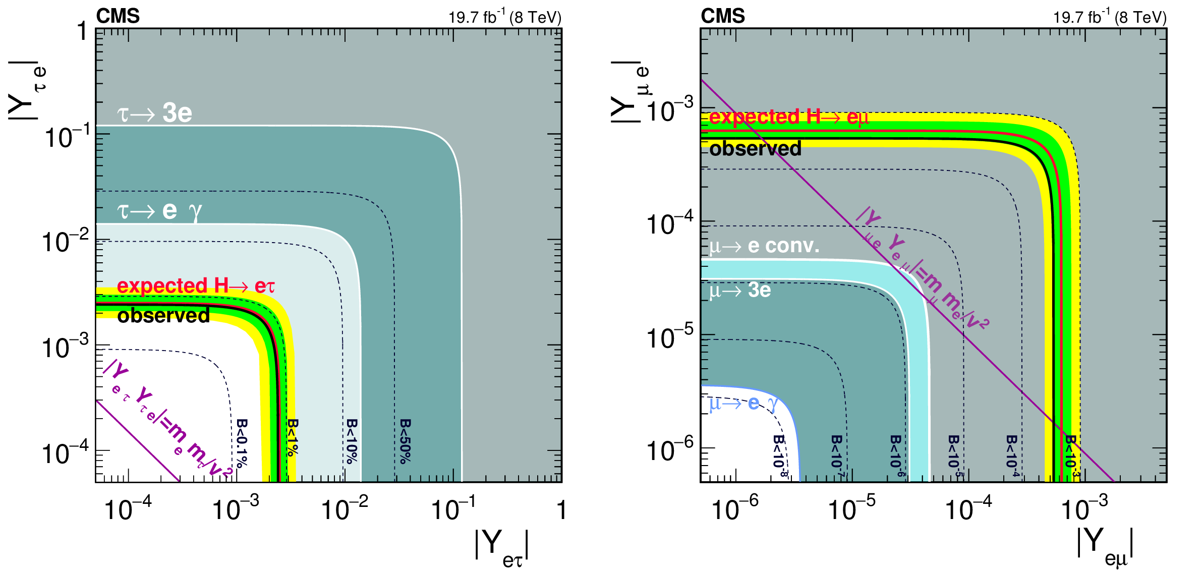
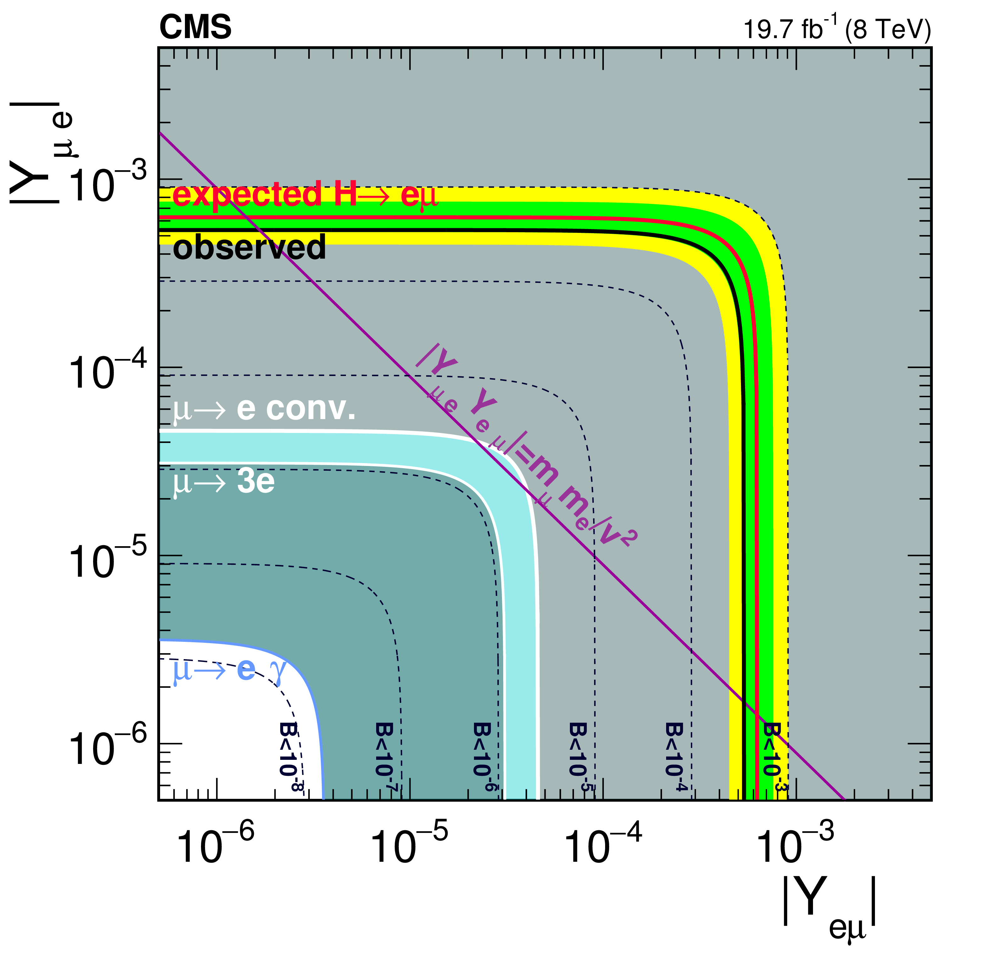
Constraints on the flavour violating Yukawa couplings $ {| Y_{\mathrm{ e } \tau } | }, {| Y_{\tau \mathrm{ e } } | }$ (a) and $ {| Y_{\mathrm{ e } \mu } | }, {| Y_{\mu \mathrm{ e } } | }$ (b). The expected (red solid line) and observed (black solid line) limits are derived from the limits on $\mathcal {B}(\mathrm{ H } \to \mathrm{ e } \tau )$ and $\mathcal {B}(\mathrm{ H } \to \mathrm{ e } \mu )$ from the present analysis. The flavour diagonal Yukawa couplings are approximated by their SM values. The green (yellow) band indicates the range that is expected to contain $68%$ ($95%$) of all observed limit excursions. The shaded regions in the left plot are derived constraints from null searches for $\tau \to 3\mathrm{ e } $ (grey), $\tau \to \mathrm{ e } \gamma $ (dark green) and the present analysis (light blue). The shaded regions in the right plot are derived constraints from null searches for $\mu \to \mathrm{ e } \gamma $ (dark green), $\mu \to 3\mathrm{ e } $ (light blue) and $\mu \to \mathrm{ e } $ conversions (grey). The purple diagonal line is the theoretical naturalness limit $Y_{ij}Y_{ji} \leq m_im_j/v^2$ [28]. |

png pdf |
Figure 6-a:
Constraints on the flavour violating Yukawa couplings $ {| Y_{\mathrm{ e } \tau } | }, {| Y_{\tau \mathrm{ e } } | }$ (a) and $ {| Y_{\mathrm{ e } \mu } | }, {| Y_{\mu \mathrm{ e } } | }$ (b). The expected (red solid line) and observed (black solid line) limits are derived from the limits on $\mathcal {B}(\mathrm{ H } \to \mathrm{ e } \tau )$ and $\mathcal {B}(\mathrm{ H } \to \mathrm{ e } \mu )$ from the present analysis. The flavour diagonal Yukawa couplings are approximated by their SM values. The green (yellow) band indicates the range that is expected to contain $68%$ ($95%$) of all observed limit excursions. The shaded regions in the left plot are derived constraints from null searches for $\tau \to 3\mathrm{ e } $ (grey), $\tau \to \mathrm{ e } \gamma $ (dark green) and the present analysis (light blue). The shaded regions in the right plot are derived constraints from null searches for $\mu \to \mathrm{ e } \gamma $ (dark green), $\mu \to 3\mathrm{ e } $ (light blue) and $\mu \to \mathrm{ e } $ conversions (grey). The purple diagonal line is the theoretical naturalness limit $Y_{ij}Y_{ji} \leq m_im_j/v^2$ [28]. |
png pdf |
Figure 6-b:
Constraints on the flavour violating Yukawa couplings $ {| Y_{\mathrm{ e } \tau } | }, {| Y_{\tau \mathrm{ e } } | }$ (a) and $ {| Y_{\mathrm{ e } \mu } | }, {| Y_{\mu \mathrm{ e } } | }$ (b). The expected (red solid line) and observed (black solid line) limits are derived from the limits on $\mathcal {B}(\mathrm{ H } \to \mathrm{ e } \tau )$ and $\mathcal {B}(\mathrm{ H } \to \mathrm{ e } \mu )$ from the present analysis. The flavour diagonal Yukawa couplings are approximated by their SM values. The green (yellow) band indicates the range that is expected to contain $68%$ ($95%$) of all observed limit excursions. The shaded regions in the left plot are derived constraints from null searches for $\tau \to 3\mathrm{ e } $ (grey), $\tau \to \mathrm{ e } \gamma $ (dark green) and the present analysis (light blue). The shaded regions in the right plot are derived constraints from null searches for $\mu \to \mathrm{ e } \gamma $ (dark green), $\mu \to 3\mathrm{ e } $ (light blue) and $\mu \to \mathrm{ e } $ conversions (grey). The purple diagonal line is the theoretical naturalness limit $Y_{ij}Y_{ji} \leq m_im_j/v^2$ [28]. |
| Tables | |
png pdf |
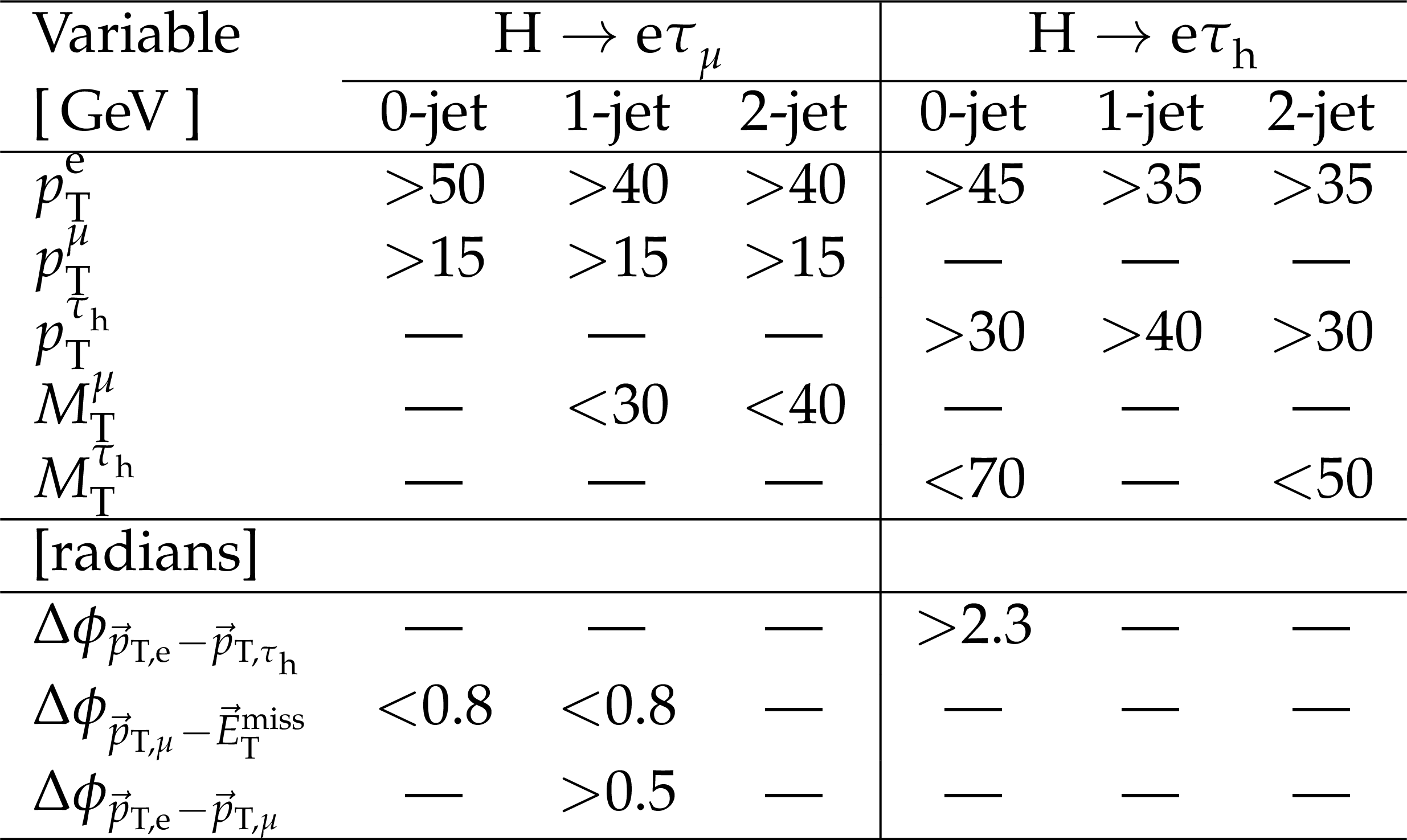
Table 1:
Event selection criteria for the kinematic variables after applying loose selection requirements. |

png pdf |
Table 2:
Definition of the samples used to estimate the misidentified lepton ($\ell $) background. They are defined by the charge of the two leptons and by the isolation requirements on each. |
png pdf |
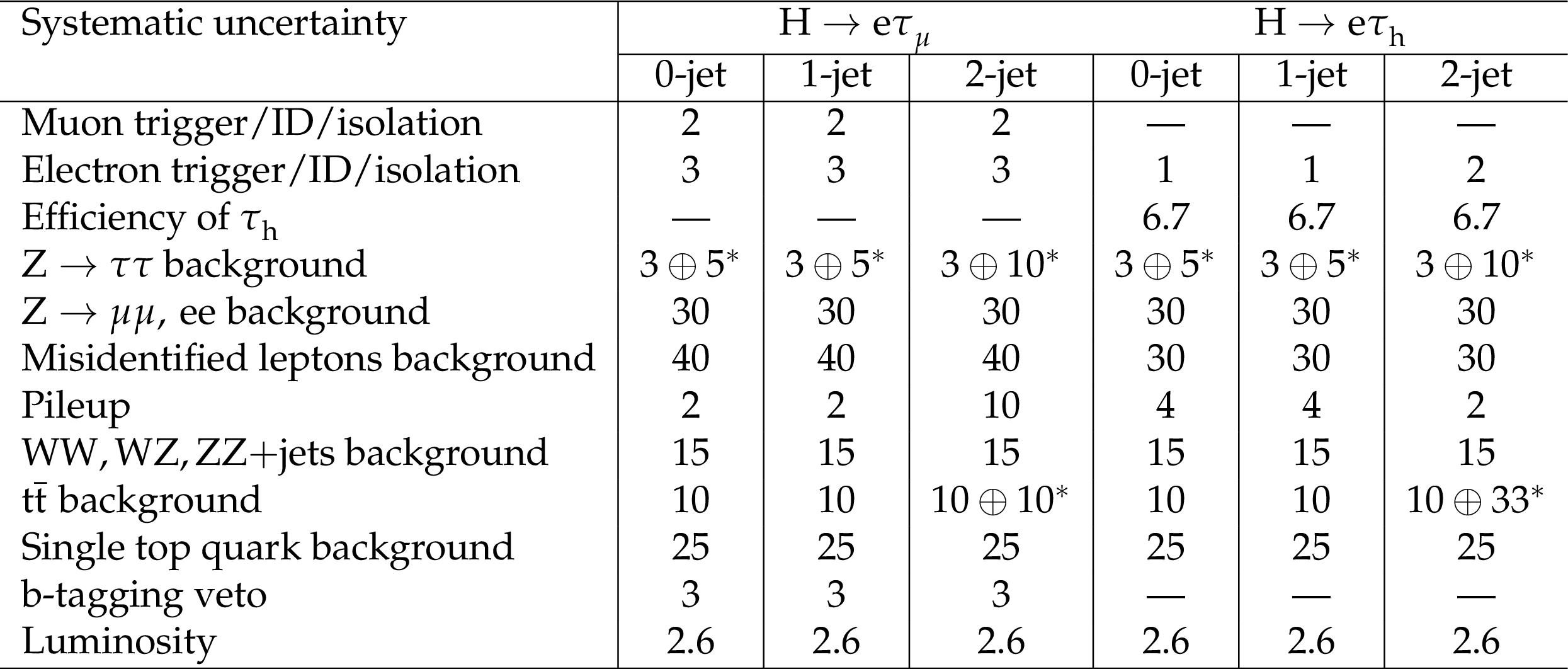
Table 3:
The systematic uncertainties in the expected event yields in percentage for the $\mathrm{ e } {\tau _\mathrm {h}} $ and $\mathrm{ e } \tau _{\mu }$ channels. All uncertainties are treated as correlated between the categories, except when two values are quoted, in which case the number denoted by an asterisk is treated as uncorrelated between categories. |
png pdf |
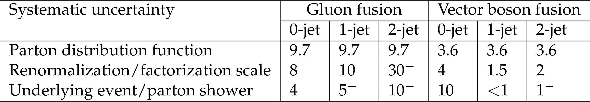
Table 4:
Theoretical uncertainties in percentage for the Higgs boson production cross section for each production process and category. All uncertainties are treated as fully correlated between categories except those denoted by a negative superscript which are fully anticorrelated due to the migration of events. |
png pdf |
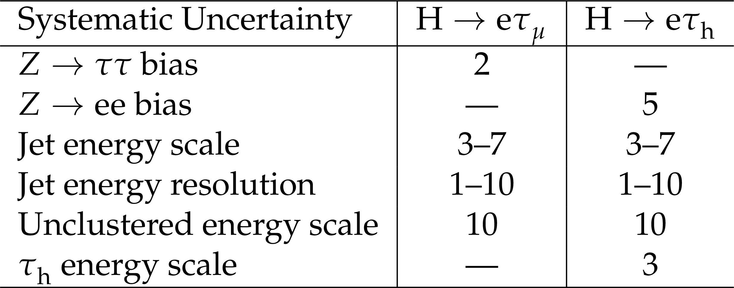
Table 5:
Systematic uncertainties in the shape of the signal and background distributions, expressed in percentage. |

png pdf |
Table 6:
The $\mathrm{ H } \to \mathrm{ e } \mu $ event selection criteria and background model for each event category. The categories are primarily defined according to whether the leptons are detected in the barrel ($\ell _B$) or endcap ($\ell _{EC}$), and the number of jets (N-jets). Requirements are also made on $ {p_{\mathrm {T}}} ^{\ell }$, ${E_{\mathrm {T}}^{\text {miss}}}$ and a veto on jets arising from a b-quark decay. The background model function and order of that function are also given. |

png pdf |
Table 7:
Systematic uncertainties in percentage on the expected yield for $\mathrm{ H } \to \mathrm{ e } \mu $. Ranges are given where the uncertainty varies with production process and category. All uncertainties are treated as correlated between categories. |
png pdf |
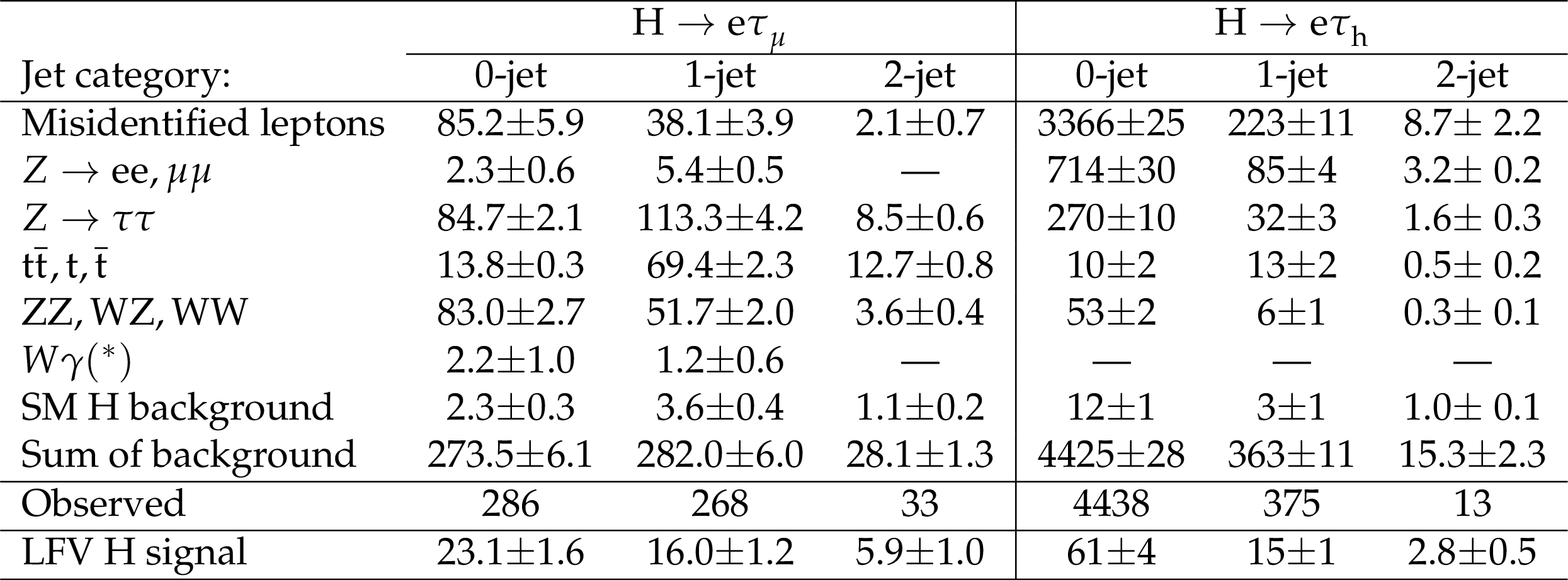
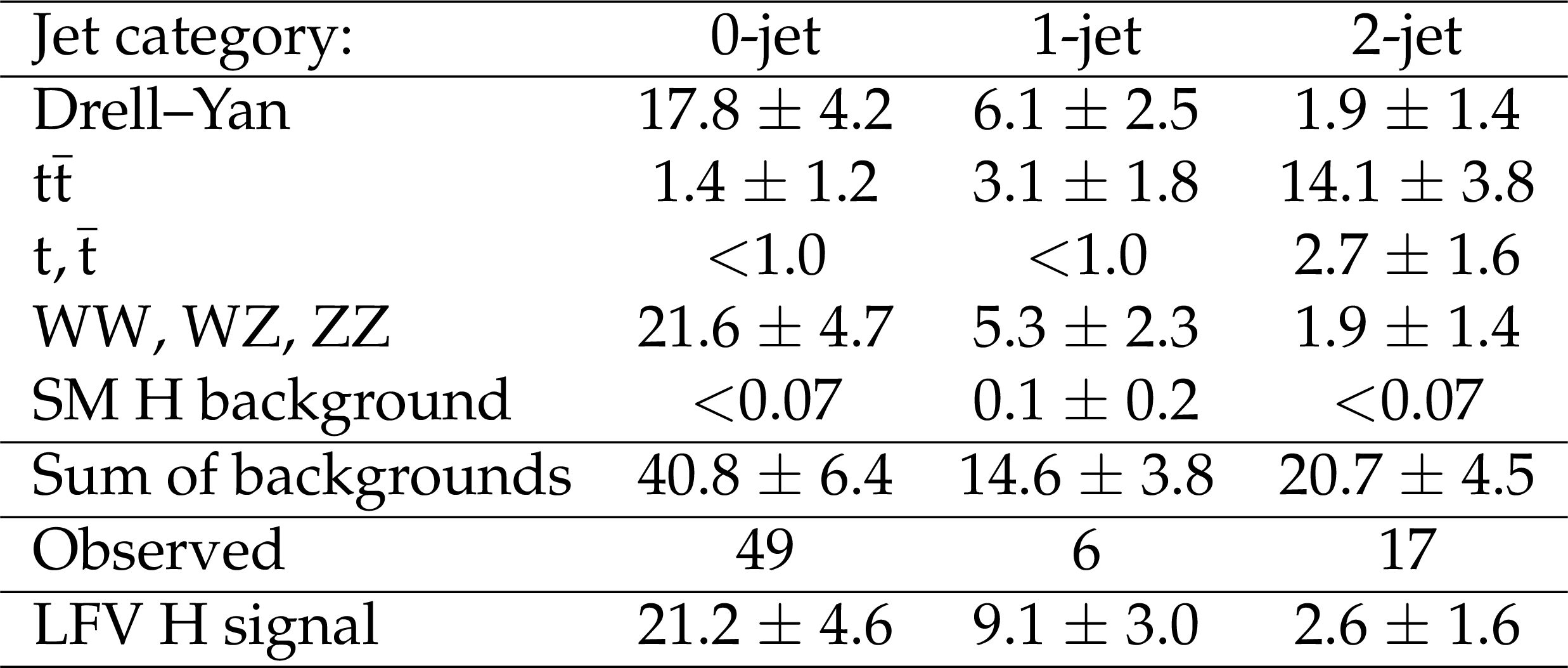
Table 8:
Event yields in the signal region, 100 GeV $ < M_{\text {col}} < $ 150 GeV, after fitting for signal and background for the $\mathrm{ H } \to \mathrm{ e } \tau $ channel, normalized to an integrated luminosity of 19.7 fb$^{-1}$. The LFV Higgs boson signal is the expected yield for $\mathcal {B}(\mathrm{ H } \to \mathrm{ e } \tau )=$ 0.69% assuming the SM Higgs boson production cross section. |
png pdf |
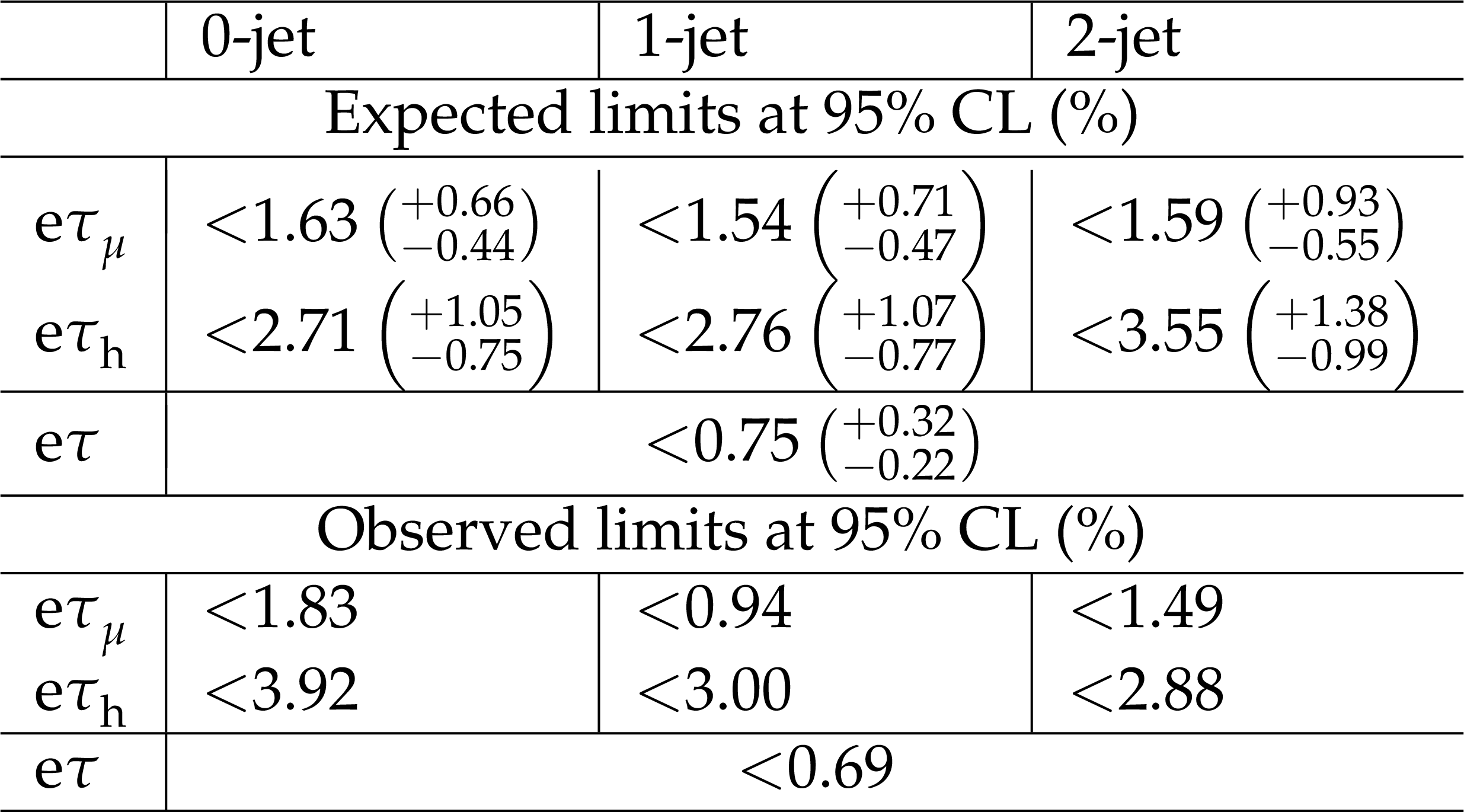
Table 9:
The expected and observed upper limits at 95% CL, and best fit values for the branching fractions $\mathcal {B}(\mathrm{ H } \to \mathrm{ e } \tau )$ for different jet categories and analysis channels. The asymmetric one standard-deviation uncertainties around the expected limits are shown in parentheses. |
png pdf |
Table 10:
Event yields in the mass window 124 GeV $ < M_{\mathrm{ e } \mu } < $ 126 GeV for the ${\mathrm{ H } \to \mathrm{ e } \mu } $channel. The expected contributions, estimated from simulation, are normalized to an integrated luminosity of 19.7 fb$^{-1}$. The LFV Higgs boson signal is the expectation for $\mathcal {B}( {\mathrm{ H } \to \mathrm{ e } \mu } )=$ 0.1% assuming the SM production cross section. Values for background processes are given for information only and are not used for the analysis. The expected number of background events in the VBF categories obtained from simulation are associated with large uncertainties and are therefore not quoted here; we expect 1.5 $\pm$ 1.2 events from signal and observe 2 events. |
| Summary |
| A search for lepton flavour violating decays of the Higgs boson to $\mathrm{ e }\tau$ or $\mathrm{ e }\mu$, based on the full $ \sqrt{s} = $ 8 TeV collision data set collected by the CMS experiment in 2012, is presented. No evidence is found for such decays. Observed upper limits of $\mathcal{B}(\mathrm{ H } \to \mathrm{ e } \tau )<$ 0.69% and $\mathcal{B}(\mathrm{ H }\to\mathrm{ e }\mu )<$ 0.035% at 95% CL are set for $\textrm{M}_{\mathrm{ H }} = $ 125 GeV. These limits are used to constrain the $Y_{\mathrm{ e }\tau}$ and $Y_{\mathrm{ e }\mu}$ Yukawa couplings as follows: $\sqrt{|{Y_{\mathrm{ e }\tau}}|^{2}+|{Y_{\tau\mathrm{ e }}}|^{2}}<2.4\times 10^{-3}$ and $\sqrt{|{Y_{\mathrm{ e }\mu}|}^2 + |{Y_{\mu\mathrm{ e }}}|^2} < 5.4 \times 10^{-4}$ at 95% CL. |
| References | ||||
| 1 | ATLAS Collaboration | Observation of a new particle in the search for the Standard Model Higgs boson with the ATLAS detector at the LHC | PLB 716 (2012) 1 | 1207.7214 |
| 2 | CMS Collaboration | Observation of a new boson at a mass of 125 GeV with the CMS experiment at the LHC | PLB 716 (2012) 30 | CMS-HIG-12-028 1207.7235 |
| 3 | CMS Collaboration | Observation of a new boson with mass near 125 GeV in pp collisions at $ \sqrt{s} = $ 7 and 8 TeV | JHEP 06 (2013) 081 | CMS-HIG-12-036 1303.4571 |
| 4 | J. D. Bjorken and S. Weinberg | Mechanism for nonconservation of muon number | PRL 38 (1977) 622 | |
| 5 | J. L. Diaz-Cruz and J. J. Toscano | Lepton flavor violating decays of Higgs bosons beyond the standard model | PRD 62 (2000) 116005 | hep-ph/9910233 |
| 6 | T. Han and D. Marfatia | $ h \to \mu \tau $ at hadron colliders | PRL 86 (2001) 1442 | hep-ph/0008141 |
| 7 | E. Arganda, A. M. Curiel, M. J. Herrero, and D. Temes | Lepton flavor violating Higgs boson decays from massive seesaw neutrinos | PRD 71 (2005) 035011 | hep-ph/0407302 |
| 8 | A. Arhrib, Y. Cheng, and O. C. W. Kong | Comprehensive analysis on lepton flavor violating Higgs boson to $ \mu\bar{\tau} + \tau \bar{\mu} $ decay in supersymmetry without R parity | PRD 87 (2013) 015025 | 1210.8241 |
| 9 | M. Arana-Catania, E. Arganda, and M. J. Herrero | Non-decoupling SUSY in LFV Higgs decays: a window to new physics at the LHC | JHEP 09 (2013) 160 | 1304.3371 |
| 10 | E. Arganda, M. J. Herrero, R. Morales, and A. Szynkman | Analysis of the $ h, H, A \to\tau\mu $ decays induced from SUSY loops within the Mass Insertion Approximation | JHEP 03 (2016) 055 | 1510.04685 |
| 11 | E. Arganda, M. J. Herrero, X. Marcano, and C. Weiland | Enhancement of the lepton flavor violating Higgs boson decay rates from SUSY loops in the inverse seesaw model | PRD 93 (2016), no. 5, 055010 | 1508.04623 |
| 12 | K. Agashe and R. Contino | Composite Higgs-mediated flavor-changing neutral current | PRD 80 (2009) 075016 | 0906.1542 |
| 13 | A. Azatov, M. Toharia, and L. Zhu | Higgs mediated flavor changing neutral currents in warped extra dimensions | PRD 80 (2009) 035016 | 0906.1990 |
| 14 | H. Ishimori et al. | Non-Abelian discrete symmetries in particle physics | Prog. Theor. Phys. Suppl. 183 (2010) 1 | 1003.3552 |
| 15 | G. Perez and L. Randall | Natural neutrino masses and mixings from warped geometry | JHEP 01 (2009) 077 | 0805.4652 |
| 16 | S. Casagrande et al. | Flavor physics in the Randall-Sundrum model I. Theoretical setup and electroweak precision tests | JHEP 10 (2008) 094 | 0807.4937 |
| 17 | A. J. Buras, B. Duling, and S. Gori | The impact of Kaluza-Klein fermions on Standard Model fermion couplings in a RS model with custodial protection | JHEP 09 (2009) 076 | 0905.2318 |
| 18 | M. Blanke et al. | $ \Delta F= $ 2 observables and fine-tuning in a warped extra dimension with custodial protection | JHEP 03 (2009) 001 | 0809.1073 |
| 19 | G. F. Giudice and O. Lebedev | Higgs-dependent Yukawa couplings | PLB 665 (2008) 79 | 0804.1753 |
| 20 | J. A. Aguilar-Saavedra | A minimal set of top-Higgs anomalous couplings | NPB 821 (2009) 215 | 0904.2387 |
| 21 | M. E. Albrecht et al. | Electroweak and flavour structure of a warped extra dimension with custodial protection | JHEP 09 (2009) 064 | 0903.2415 |
| 22 | A. Goudelis, O. Lebedev, and J. H. Park | Higgs-induced lepton flavor violation | PLB 707 (2012) 369 | 1111.1715 |
| 23 | D. McKeen, M. Pospelov, and A. Ritz | Modified Higgs branching ratios versus CP and lepton flavor violation | PRD 86 (2012) 113004 | 1208.4597 |
| 24 | A. Pilaftsis | Lepton flavour nonconservation in $ \mathrm{ H }^0 $ decays | PLB 285 (1992) 68 | |
| 25 | J. G. Korner, A. Pilaftsis, and K. Schilcher | Leptonic $ \mathrm{CP} $ asymmetries in flavor-changing $ \mathrm{ H }^{0} $ decays | PRD 47 (1993) 1080 | |
| 26 | E. Arganda, M. J. Herrero, X. Marcano, and C. Weiland | Imprints of massive inverse seesaw model neutrinos in lepton flavor violating Higgs boson decays | PRD 91 (2015), no. 1, 015001 | 1405.4300 |
| 27 | CMS Collaboration | Search for lepton-flavour-violating decays of the Higgs boson | PLB 749 (2015) 337 | CMS-HIG-14-005 1502.07400 |
| 28 | ATLAS Collaboration | Search for lepton-flavour-violating $ \mathrm{ H }\to\mu\tau $ decays of the Higgs boson with the ATLAS detector | JHEP 11 (2015) 211 | 1508.03372 |
| 29 | ATLAS Collaboration | Search for lepton-flavour-violating decays of the Higgs and $ Z $ bosons with the ATLAS detector | Submitted to JHEP | 1604.07730 |
| 30 | B. McWilliams and L.-F. Li | Virtual effects of Higgs particles | NPB 179 (1981) 62 | |
| 31 | O. U. Shanker | Flavour violation, scalar particles and leptoquarks | NPB 206 (1982) 253 | |
| 32 | G. Blankenburg, J. Ellis, and G. Isidori | Flavour-changing decays of a 125 GeV Higgs-like particle | PLB 712 (2012) 386 | 1202.5704 |
| 33 | R. Harnik, J. Kopp, and J. Zupan | Flavor violating higgs decays | JHEP 03 (2013) 26 | 1209.1397 |
| 34 | Particle Data Group, J. Beringer et al. | Review of Particle Physics | PRD 86 (2012) 010001 | |
| 35 | A. Celis, V. Cirigliano, and E. Passemar | Lepton flavor violation in the Higgs sector and the role of hadronic tau-lepton decays | PRD 89 (2014) 013008 | 1309.3564 |
| 36 | S. M. Barr and A. Zee | Electric dipole moment of the electron and of the neutron | PRL 65 (1990) 21 | |
| 37 | CMS Collaboration | Evidence for the direct decay of the 125 GeV Higgs boson to fermions | NP 10 (2014) 557 | CMS-HIG-13-033 1401.6527 |
| 38 | CMS Collaboration | Evidence for the 125 GeV higgs boson decaying to a pair of $ \tau $ leptons | JHEP 05 (2014) 104 | CMS-HIG-13-004 1401.5041 |
| 39 | ATLAS Collaboration | Evidence for the Higgs-boson Yukawa coupling to tau leptons with the ATLAS detector | JHEP 04 (2015) 117 | 1501.04943 |
| 40 | CMS Collaboration | The CMS experiment at the CERN LHC | JINST 3 (2008) S08004 | CMS-00-001 |
| 41 | GEANT4 Collaboration | GEANT4 --- a simulation toolkit | NIMA 506 (2003) 250 | |
| 42 | H. M. Georgi, S. L. Glashow, M. E. Machacek, and D. V. Nanopoulos | Higgs bosons from two gluon annihilation in proton proton collisions | PRL 40 (1978) 692 | |
| 43 | R. N. Cahn, S. D. Ellis, R. Kleiss, and W. J. Stirling | Transverse-momentum signatures for heavy Higgs bosons | PRD 35 (1987) 1626 | |
| 44 | S. L. Glashow, D. V. Nanopoulos, and A. Yildiz | Associated production of Higgs bosons and Z particles | PRD 18 (1978) 1724 | |
| 45 | T. Sjostrand, S. Mrenna, and P. Skands | A brief introduction to PYTHIA 8.1 | CPC 178 (2007) 852 | 0710.3820 |
| 46 | T. Sjostrand, S. Mrenna, and P. Skands | PYTHIA 6.4 physics and manual | JHEP 05 (2006) 026 | hep-ph/0603175 |
| 47 | P. M. Nadolsky et al. | Implications of CTEQ global analysis for collider observables | PRD 78 (2008) 013004 | 0802.0007 |
| 48 | P. Nason | A new method for combining NLO QCD with shower Monte Carlo algorithms | JHEP 11 (2004) 040 | hep-ph/0409146 |
| 49 | S. Frixione, P. Nason, and C. Oleari | Matching NLO QCD computations with parton shower simulations: the POWHEG method | JHEP 11 (2007) 070 | 0709.2092 |
| 50 | S. Alioli, P. Nason, C. Oleari, and E. Re | A general framework for implementing NLO calculations in shower Monte Carlo programs: the POWHEG BOX | JHEP 06 (2010) 043 | 1002.2581 |
| 51 | S. Alioli et al. | Jet pair production in POWHEG | JHEP 04 (2011) 081 | 1012.3380 |
| 52 | S. Alioli, P. Nason, C. Oleari, and E. Re | NLO Higgs boson production via gluon fusion matched with shower in POWHEG | JHEP 04 (2009) 002 | 0812.0578 |
| 53 | J. Alwall et al. | MadGraph 5: going beyond | JHEP 06 (2011) 128 | 1106.0522 |
| 54 | R. Field | Early LHC Underlying Event Data - Findings and Surprises | in Hadron collider physics. Proceedings, 22nd Conference, HCP 2010, Toronto, Canada, August 23-27, 2010 2010 | 1010.3558 |
| 55 | CMS Collaboration | Description and performance of track and primary-vertex reconstruction with the CMS tracker | JINST 9 (2014) P10009 | CMS-TRK-11-001 1405.6569 |
| 56 | CMS Collaboration | Particle--flow event reconstruction in CMS and performance for jets, taus, and $ E_{\mathrm{T}}^{\text{miss}} $ | CMS-PAS-PFT-09-001 | |
| 57 | CMS Collaboration | Particle flow reconstruction of 0.9 tev and 2.36 tev collision events in cms | CMS-PAS-PFT-10-002 | |
| 58 | CMS Collaboration | Commissioning of the particle--flow event reconstruction with leptons from j/$ \psi $ and W decays at 7 tev | CMS-PAS-PFT-10-003 | |
| 59 | CMS Collaboration | Performance of the CMS missing transverse momentum reconstruction in pp data at $ \sqrt{s} = $ 8 TeV | JINST 10 (2015) P02006 | CMS-JME-13-003 1411.0511 |
| 60 | CMS Collaboration | Performance of electron reconstruction and selection with the CMS detector in proton-proton collisions at $ \sqrt{s} = $ 8 TeV | JINST 10 (2015) P06005 | CMS-EGM-13-001 1502.02701 |
| 61 | CMS Collaboration | Measurement of the properties of a higgs boson in the four-lepton final state | PRD 89 (2014) 092007 | CMS-HIG-13-002 1312.5353 |
| 62 | CMS Collaboration | Performance of CMS muon reconstruction in pp collision events at $ \sqrt{s} = $ 7 TeV | JINST 7 (2012) P10002 | CMS-MUO-10-004 1206.4071 |
| 63 | CMS Collaboration | Reconstruction and identification of tau lepton decays to hadrons and $ \nu_\tau $ at CMS | JINST 11 (2016) P01019 | CMS-TAU-14-001 1510.07488 |
| 64 | M. Cacciari, G. P. Salam, and G. Soyez | FastJet user manual | EPJC 72 (2012) 1896 | 1111.6097 |
| 65 | M. Cacciari, G. P. Salam, and G. Soyez | The anti-$ k_t $ jet clustering algorithm | JHEP 04 (2008) 063 | 0802.1189 |
| 66 | CMS Collaboration | Determination of jet energy calibration and transverse momentum resolution in CMS | JINST 6 (2011) 11002 | CMS-JME-10-011 1107.4277 |
| 67 | CMS Collaboration | Pile-up jet identification | CMS-PAS-JME-13-005 | CMS-PAS-JME-13-005 |
| 68 | R. K. Ellis, I. Hinchliffe, M. Soldate, and J. J. van der Bij | Higgs Decay to $ \tau^+\tau^- $: A possible signature of intermediate mass Higgs bosons at high energy hadron colliders | NPB 297 (1988) 221 | |
| 69 | CMS Collaboration | Performance of b tagging at $ \sqrt{s} = $ 8 TeV in multijet, ttbar and boosted topology events | CMS-PAS-BTV-13-001 | CMS-PAS-BTV-13-001 |
| 70 | T. Junk | Confidence level computation for combining searches with small statistics | NIMA 434 (1999) 435 | hep-ex/9902006 |
| 71 | A. L. Read | Presentation of search results: the $ CL_s $ technique | JPG 28 (2002) 2693 | |
| 72 | CMS Collaboration | Measurement of the inclusive W and Z production cross sections in pp collisions at $ \sqrt{s}= $ 7 TeV with the CMS experiment | JHEP 10 (2011) 132 | CMS-EWK-10-005 1107.4789 |
| 73 | CMS Collaboration | Measurement of inclusive $ W $ and $ Z $ boson production cross sections in $ pp $ collisions at $ \sqrt{s} = $ 8 TeV | PRL 112 (2014) 191802 | CMS-SMP-12-011 1402.0923 |
| 74 | CMS Collaboration | Measurement of the inelastic proton-proton cross section at $ \sqrt{s} = $ 7 TeV | PLB 722 (2013) 5 | |
| 75 | CMS Collaboration | Measurement of the $ \mathrm{ W }^+\mathrm{ W }^- $ and ZZ production cross sections in pp collisions at $ \sqrt{s}= $ 8 TeV | PLB 721 (2013) 190 | CMS-SMP-12-024 1301.4698 |
| 76 | CMS Collaboration | Observation of the associated production of a single top quark and a $ W $ boson in $ pp $ collisions at $ \sqrt s = $ 8 TeV | PRL 112 (2014), no. 23, 231802 | CMS-TOP-12-040 1401.2942 |
| 77 | CMS Collaboration | Measurement of the $ \mathrm{t \bar t} $ production cross section in pp collisions at $ \sqrt s = $ 8 TeV in dilepton final states containing one $ \tau $ lepton | PLB 739 (2014) 23 | CMS-TOP-12-026 1407.6643 |
| 78 | A. D. Martin, W. J. Stirling, R. S. Thorne, and G. Watt | Parton distributions for the LHC | EPJC 63 (2009) 189 | 0901.0002 |
| 79 | NNPDF Collaboration | A first unbiased global NLO determination of parton distributions and their uncertainties | NPB 838 (2010) 136 | 1002.4407 |
| 80 | M. Botje et al. | The PDF4LHC Working Group Interim Recommendations | 1101.0538 | |
| 81 | CMS Collaboration | CMS Luminosity Based on Pixel Cluster Counting - Summer 2013 Update | CMS-PAS-LUM-13-001 | CMS-PAS-LUM-13-001 |
| 82 | ATLAS and CMS Collaboration | Procedure for the LHC Higgs boson search combination in summer 2011 | CMS-NOTE-2011-005 | |
| 83 | G. Cowan, K. Cranmer, E. Gross, and O. Vitells | Asymptotic formulae for likelihood-based tests of new physics | EPJC 71 (2011) 1554 | 1007.1727 |
| 84 | A. Denner et al. | Standard model Higgs-boson branching ratios with uncertainties | EPJC 71 (2011) 1753 | 1107.5909 |
|
|
Compact Muon Solenoid LHC, CERN |
|

|

|

|

|

|