

Compact Muon Solenoid
LHC, CERN
| CMS-PRO-21-001 ; TOTEM-2022-001 ; CERN-EP-2022-139 | ||
| Proton reconstruction with the CMS-TOTEM Precision Proton Spectrometer | ||
| CMS and TOTEM Collaborations | ||
| 12 October 2022 | ||
| JINST 18 (2023) P09009 | ||
| Abstract: The Precision Proton Spectrometer (PPS) of the CMS and TOTEM experiments collected 107.7 fb$ ^{-1} $ in proton-proton (pp) collisions at the LHC at 13 TeV (Run 2). This paper describes the key features of the PPS alignment and optics calibrations, the proton reconstruction procedure, as well as the detector efficiency and the performance of the PPS simulation. The reconstruction and simulation are validated using a sample of (semi)exclusive dilepton events. The performance of PPS has proven the feasibility of continuously operating a near-beam proton spectrometer at a high luminosity hadron collider. | ||
| Links: e-print arXiv:2210.05854 [hep-ex] (PDF) ; CDS record ; inSPIRE record ; Physics Briefing ; CADI line (restricted) ; | ||
| Figures | |
png pdf |
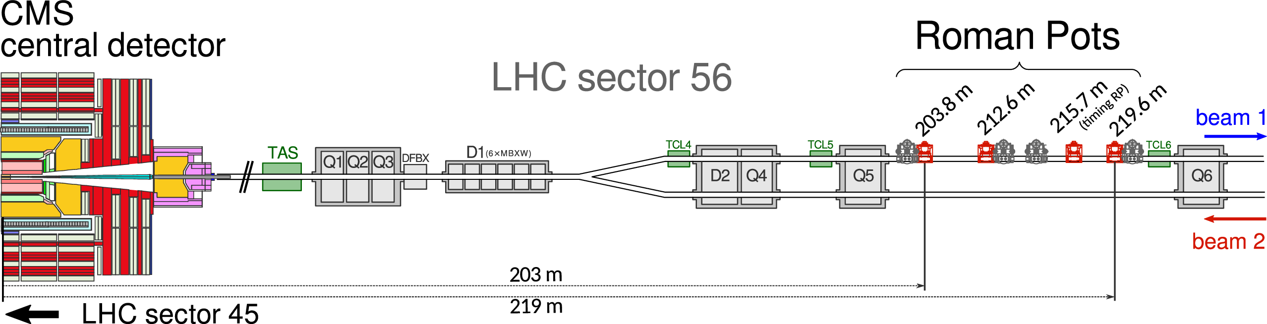
Figure 1:
Schematic layout of the beam line between the interaction point and the RP locations in LHC sector 56, corresponding to the negative $ z $ direction in the CMS coordinate system and the outgoing proton in the clockwise beam direction. The accelerator magnets are indicated in grey and the collimator system elements in green. The horizontal RPs, which constitute PPS, are marked in red. The vertical RPs are indicated in dark grey; they are part of the TOTEM experiment. The vertical RPs are not used during high luminosity data taking; nevertheless, they provide PPS with a reference measurement for the calibration and alignment of the detectors. |
png pdf |
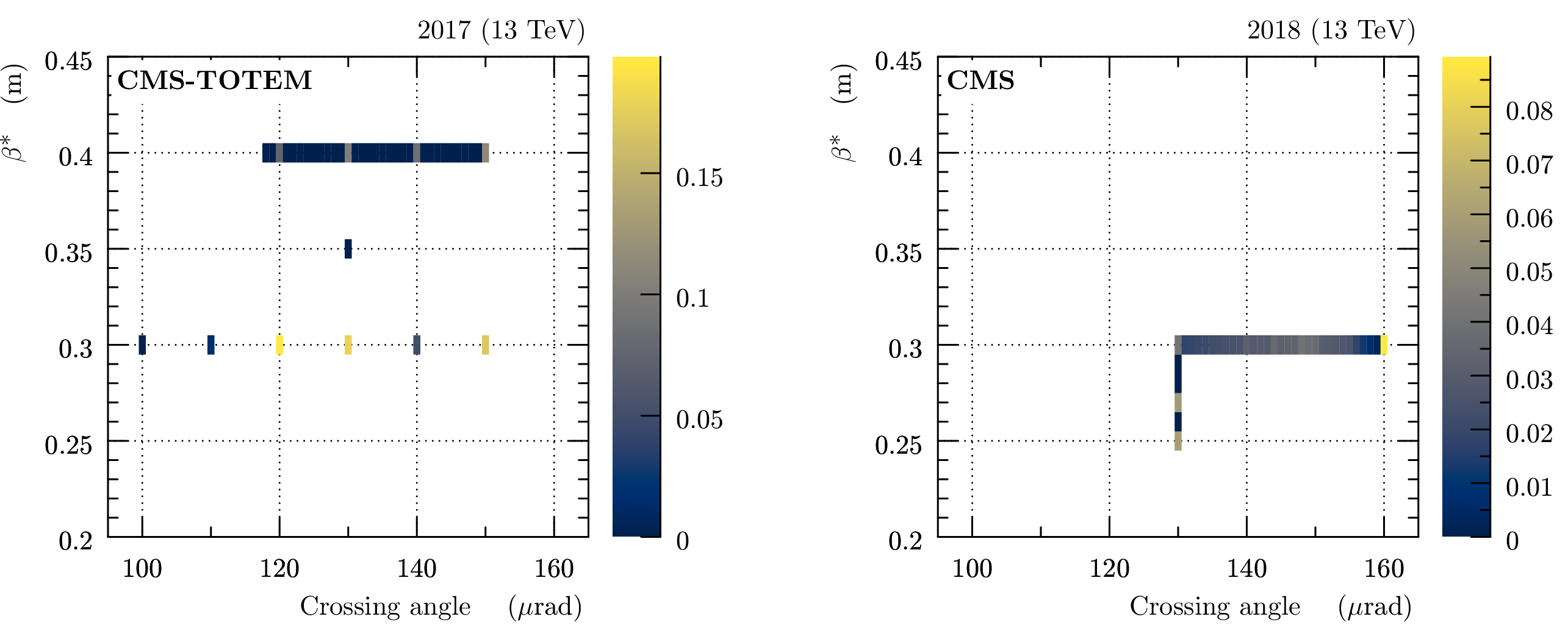
Figure 2:
Frequency distributions of $ \beta^{\ast} $ vs. crossing angle configurations as extracted from data. Left: year 2017. Right: year 2018. |

png pdf |
Figure 3:
Illustration of a proton crossing both the vertical (blue) and the horizontal (green) RPs (overlapping configuration). |

png pdf |
Figure 4:
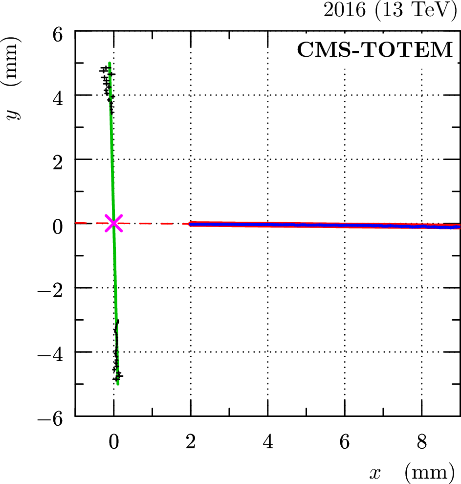
Left: relative alignment between vertical and horizontal RPs (April 2018). The plot shows track impact points in a scoring plane perpendicular to the beam. The points in red represent tracks only reconstructed from vertical RPs, in blue only from horizontal RPs and in green from both vertical and horizontal RPs. The size and position of the RP sensors is schematically indicated by the black (vertical strip RPs) and magenta (horizontal pixel RPs) contours. Right: determination of the beam position with respect to the RPs (September 2016). Black: profile (mean $ x $ as a function of y) of elastic track impact points observed in vertical RPs; green: fit and interpolation. Blue: horizontal profile of minimum bias tracks found in the horizontal RP; red: fit and extrapolation. Magenta cross: the determined beam position. The error bars represent statistical uncertainties. |

png pdf |
Figure 4-a:
Left: relative alignment between vertical and horizontal RPs (April 2018). The plot shows track impact points in a scoring plane perpendicular to the beam. The points in red represent tracks only reconstructed from vertical RPs, in blue only from horizontal RPs and in green from both vertical and horizontal RPs. The size and position of the RP sensors is schematically indicated by the black (vertical strip RPs) and magenta (horizontal pixel RPs) contours. Right: determination of the beam position with respect to the RPs (September 2016). Black: profile (mean $ x $ as a function of y) of elastic track impact points observed in vertical RPs; green: fit and interpolation. Blue: horizontal profile of minimum bias tracks found in the horizontal RP; red: fit and extrapolation. Magenta cross: the determined beam position. The error bars represent statistical uncertainties. |
png pdf |
Figure 4-b:
Left: relative alignment between vertical and horizontal RPs (April 2018). The plot shows track impact points in a scoring plane perpendicular to the beam. The points in red represent tracks only reconstructed from vertical RPs, in blue only from horizontal RPs and in green from both vertical and horizontal RPs. The size and position of the RP sensors is schematically indicated by the black (vertical strip RPs) and magenta (horizontal pixel RPs) contours. Right: determination of the beam position with respect to the RPs (September 2016). Black: profile (mean $ x $ as a function of y) of elastic track impact points observed in vertical RPs; green: fit and interpolation. Blue: horizontal profile of minimum bias tracks found in the horizontal RP; red: fit and extrapolation. Magenta cross: the determined beam position. The error bars represent statistical uncertainties. |
png pdf |
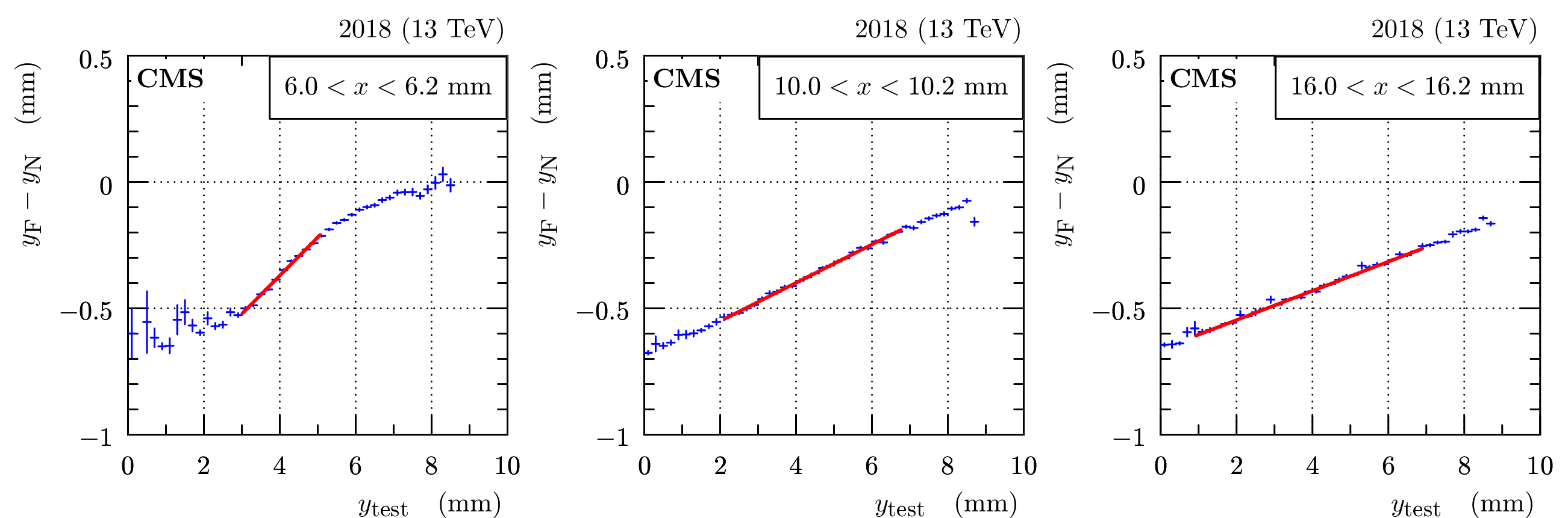
Figure 5:
Illustration of $ y_\mathrm{F} - y_\mathrm{N} $ dependence on $ y $ (fill 7139, 2018, near RP in sector 56). The three plots correspond to three $ x $ selections as indicated in the legends. Blue: profile histogram of the dependence, red: linear fit to the central part. The error bars represent statistical uncertainties. |
png pdf |
Figure 6:
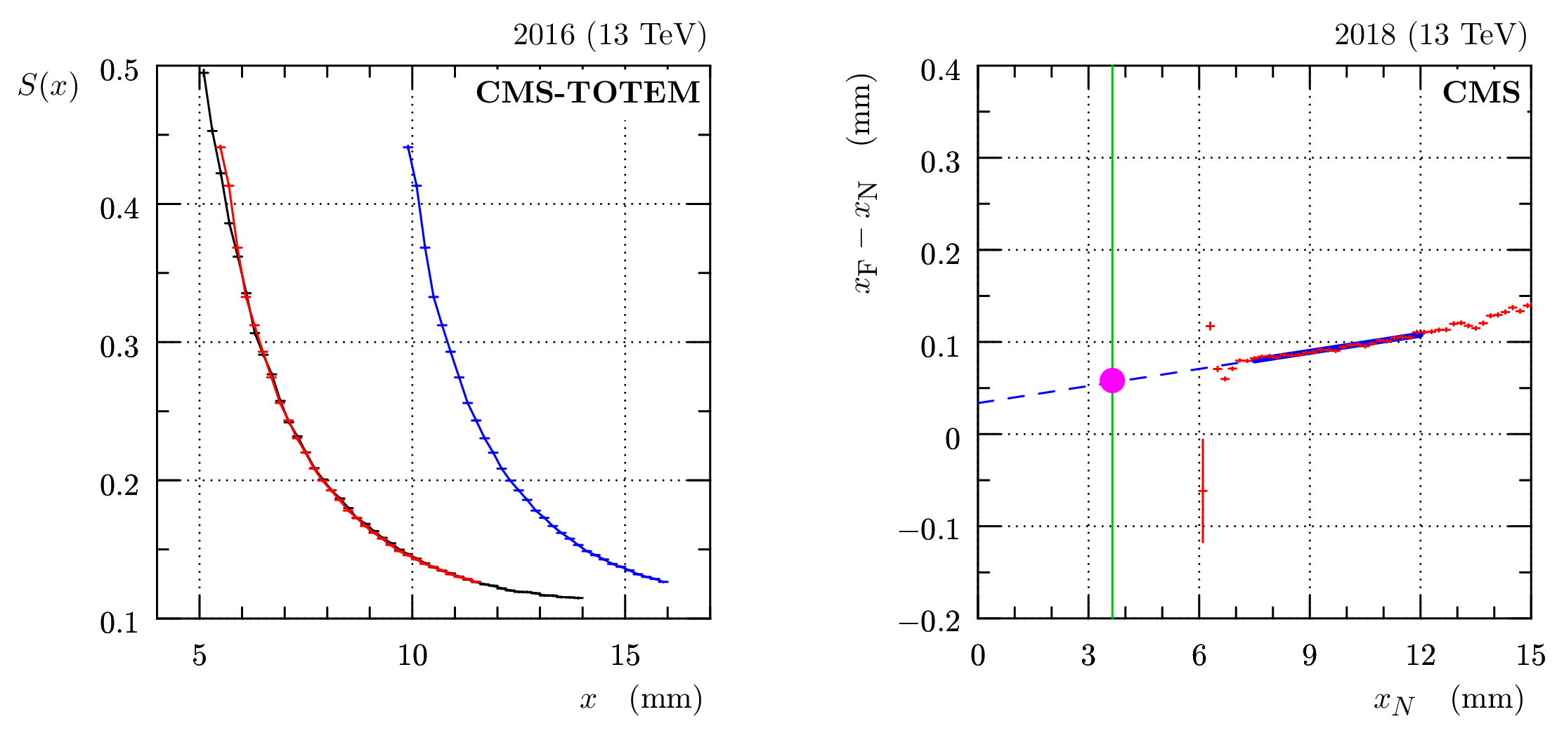
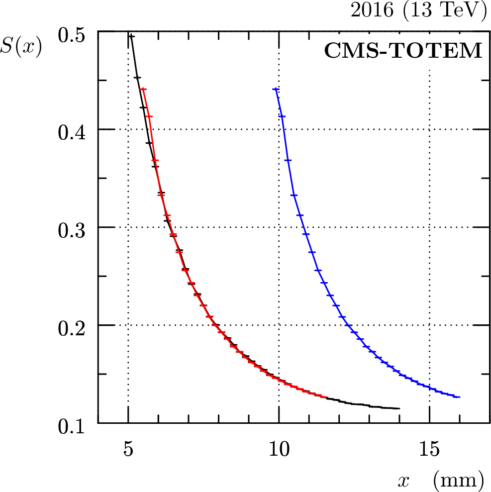
Left: illustration of the absolute horizontal alignment (fill 5424, 2016 post-TS2, far RP in sector 45). Black: data from the reference alignment fill, blue: data from a physics fill before the alignment and red: data from the physics fill, aligned to match with the black reference. The error bars represent the bin sizes (horizontally) and statistical uncertainties (vertically). Right: illustration of horizontal near-far relative alignment (fill 7052, 2018 and sector 45). Red: mean value of $ x_\mathrm{F} - x_\mathrm{N} $ as function of $ x_\mathrm{N} $. Blue: fit and extrapolation to the horizontal beam position (vertical green line, e.g. from the left plot). The value of the relative near-far alignment correction is indicated by the magenta dot. The error bars represent the bin sizes (horizontally) and statistical uncertainties (vertically). |
png pdf |
Figure 6-a:
Left: illustration of the absolute horizontal alignment (fill 5424, 2016 post-TS2, far RP in sector 45). Black: data from the reference alignment fill, blue: data from a physics fill before the alignment and red: data from the physics fill, aligned to match with the black reference. The error bars represent the bin sizes (horizontally) and statistical uncertainties (vertically). Right: illustration of horizontal near-far relative alignment (fill 7052, 2018 and sector 45). Red: mean value of $ x_\mathrm{F} - x_\mathrm{N} $ as function of $ x_\mathrm{N} $. Blue: fit and extrapolation to the horizontal beam position (vertical green line, e.g. from the left plot). The value of the relative near-far alignment correction is indicated by the magenta dot. The error bars represent the bin sizes (horizontally) and statistical uncertainties (vertically). |

png pdf |
Figure 6-b:
Left: illustration of the absolute horizontal alignment (fill 5424, 2016 post-TS2, far RP in sector 45). Black: data from the reference alignment fill, blue: data from a physics fill before the alignment and red: data from the physics fill, aligned to match with the black reference. The error bars represent the bin sizes (horizontally) and statistical uncertainties (vertically). Right: illustration of horizontal near-far relative alignment (fill 7052, 2018 and sector 45). Red: mean value of $ x_\mathrm{F} - x_\mathrm{N} $ as function of $ x_\mathrm{N} $. Blue: fit and extrapolation to the horizontal beam position (vertical green line, e.g. from the left plot). The value of the relative near-far alignment correction is indicated by the magenta dot. The error bars represent the bin sizes (horizontally) and statistical uncertainties (vertically). |
png pdf |
Figure 7:
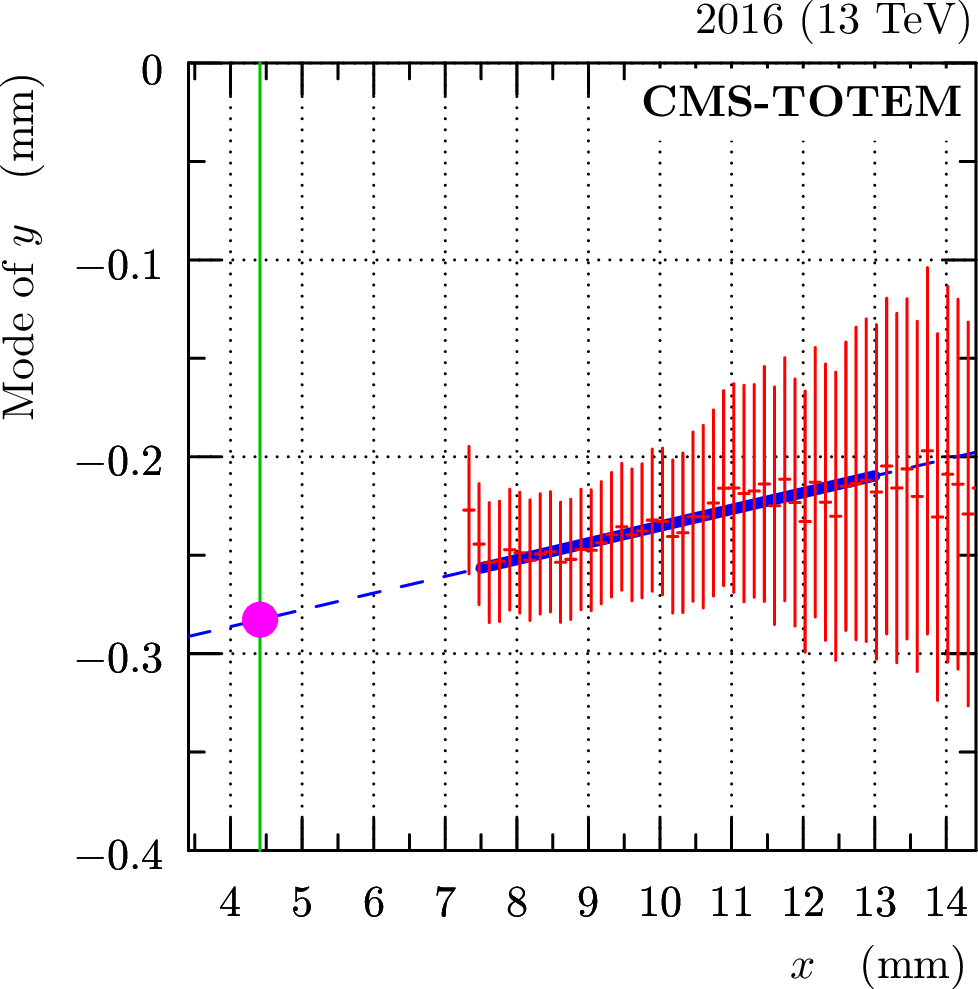
Illustration of the vertical alignment (fill 5424, 2016 post-TS2, far RP in sector 45). Red: mode (most frequent value) of $ y $ as a function of $ x $, Blue: fit and extrapolation to the horizontal beam position (indicated by the vertical green line and extracted from Fig. 6, left). The value of the vertical alignment correction is indicated by the magenta dot. The error bars represent the systematic uncertainties. |
png pdf |
Figure 8:
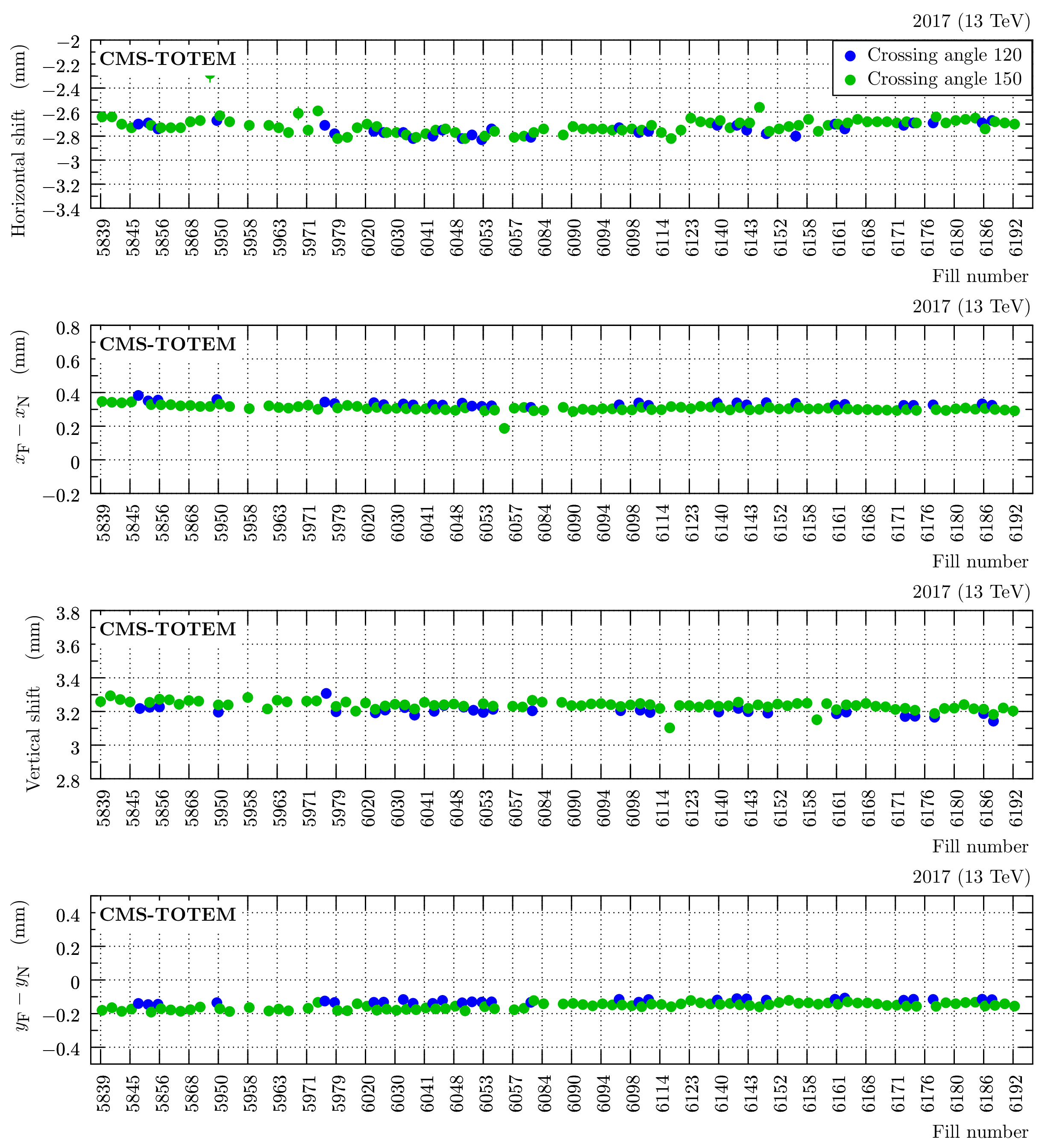
Example of per-fill alignment results (2017 post-TS2, sector 56 or near RP in sector 56). Horizontal axis contains representative LHC fills where PPS was active. The colors indicate two values of crossing angle, 120 $ \mu $rad (blue) and 150 $ \mu $rad (green). Rows from top to bottom: absolute horizontal alignment, near-far relative horizontal alignment, absolute vertical alignment and near-far relative vertical alignment. The error bars (mostly invisible) represent a combination of statistical and systematic uncertainties. |
png pdf |
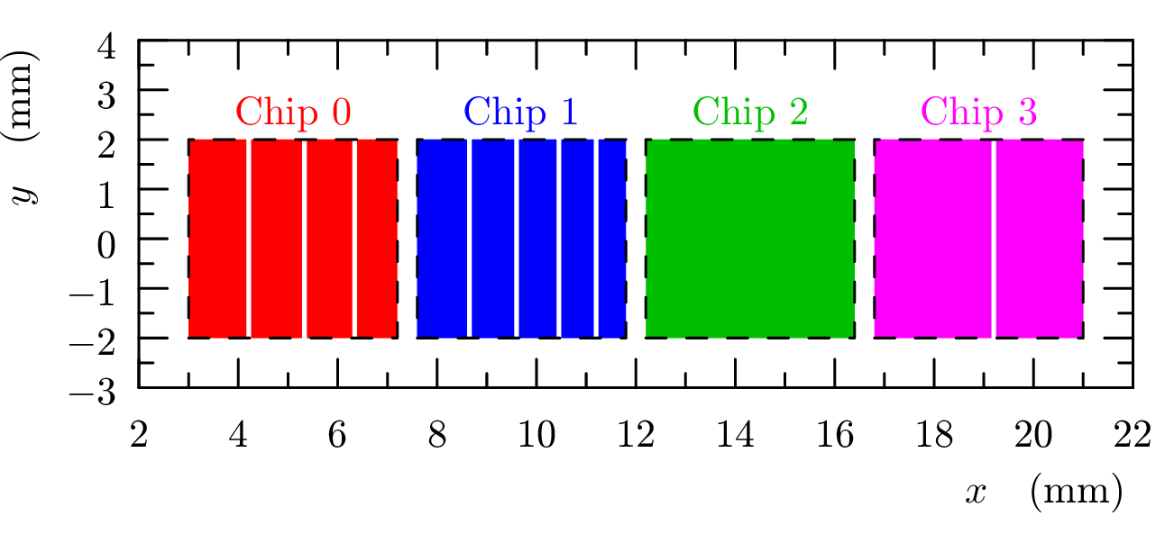
Figure 9:
Example of timing detector segmentation in one plane (plane 1 in 2018 configuration). The beam is at $ x = $ 0 mm. Chip boundaries are drawn as dashed black rectangles. Pads are visualized as thick vertical strips, their colors indicate the chip relation. |
png pdf |
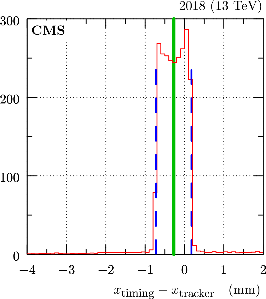
Figure 10:
Illustration of the timing-RP alignment method (fill 7137, 2018, sector 56, plane 1 and pad 9). The red histogram shows the difference between the horizontal track position in the timing sensor, $ x_\text{timing} $, and the track interpolated from the tracking RPs, $ x_\text{tracker} $. The vertical blue dashed lines indicate the identified pad boundaries, the green line the pad center. |
png pdf |
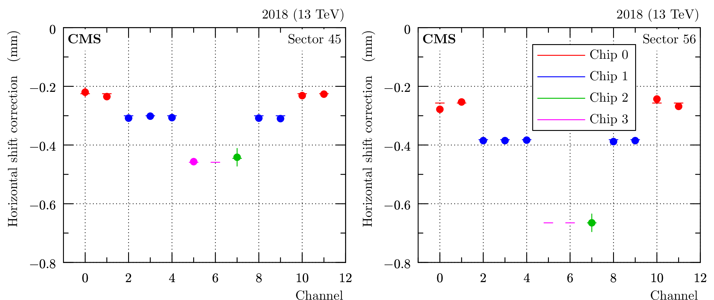
Figure 11:
An example of alignment corrections in a single timing RP sensor plane (fill 7137, 2018, plane 1). Two different markers are used: the dots represent per-channel measurements, while the short horizontal lines represent per-chip averages. The same color is used for channels/pads placed on the same diamond chip, following the scheme in Fig. 9. For chip 3 (most far from the beam) sometimes the track statistics is insufficient for alignment determination. In such cases the magenta thick dot is missing. The error bars represent a combination of statistical and systematic uncertainties reflecting the sharpness of the pad boundaries shown in Fig. 10. Left: sector 45, right: sector 56. |
png pdf |
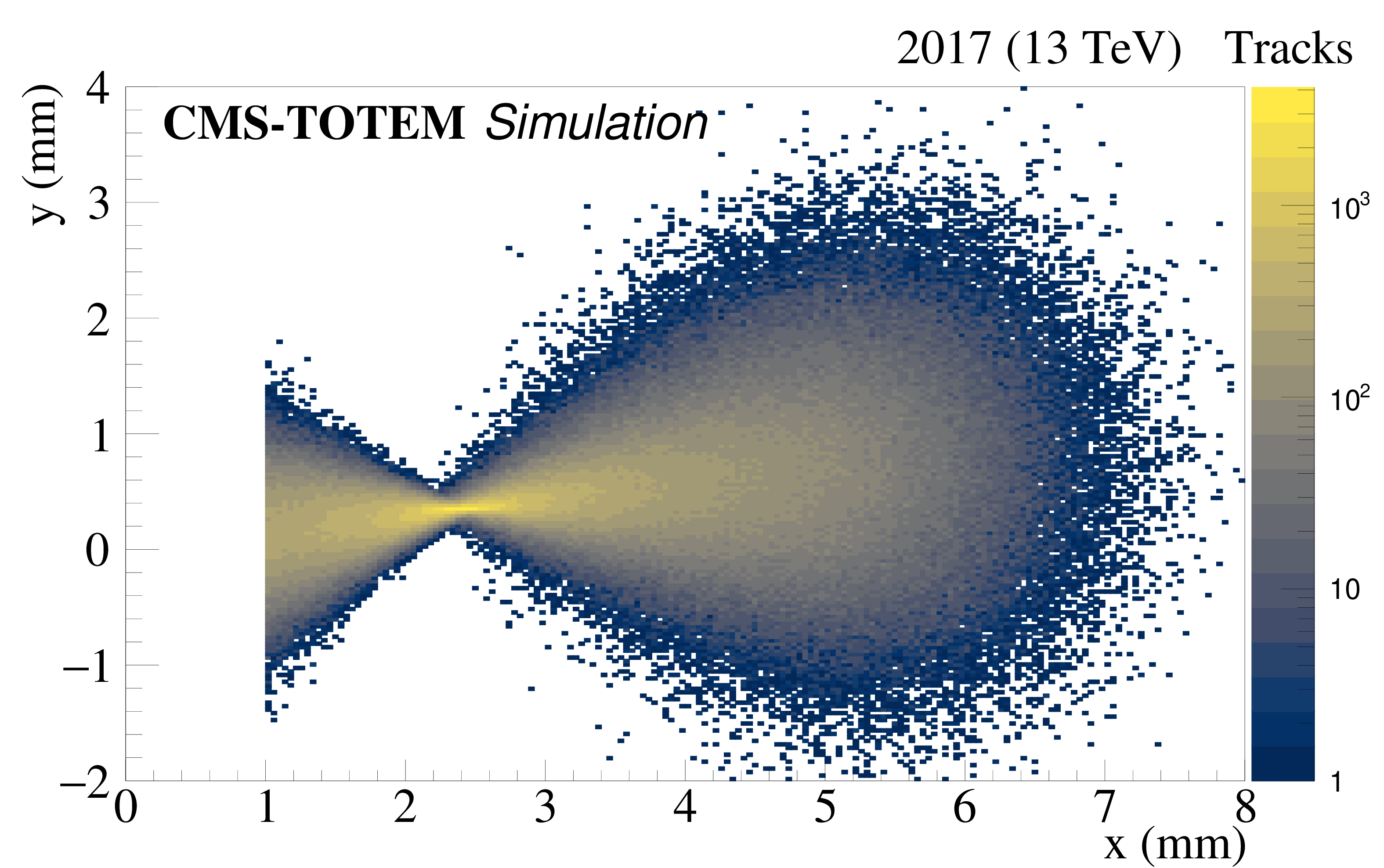
Figure 12:
The $ (x,y) $ distribution of simulated proton tracks in the near RP in sector 56 using MAD-X. It illustrates the ``pinch'' or focal point at $ x = x_\mathrm{F} $ where the vertical effective length vanishes: $ L_{y}(\xi_\mathrm{F}) = $ 0, given the relation $ y \approx {L_{y}(\xi_\mathrm{F})}\cdot \theta_{y}^{*} $. The simulation takes into account that the small vertical dispersion moves particles upward according to $ \Delta y=D_{y}\ \xi $ with increasing $ x $, and $ \xi $. |
png pdf |
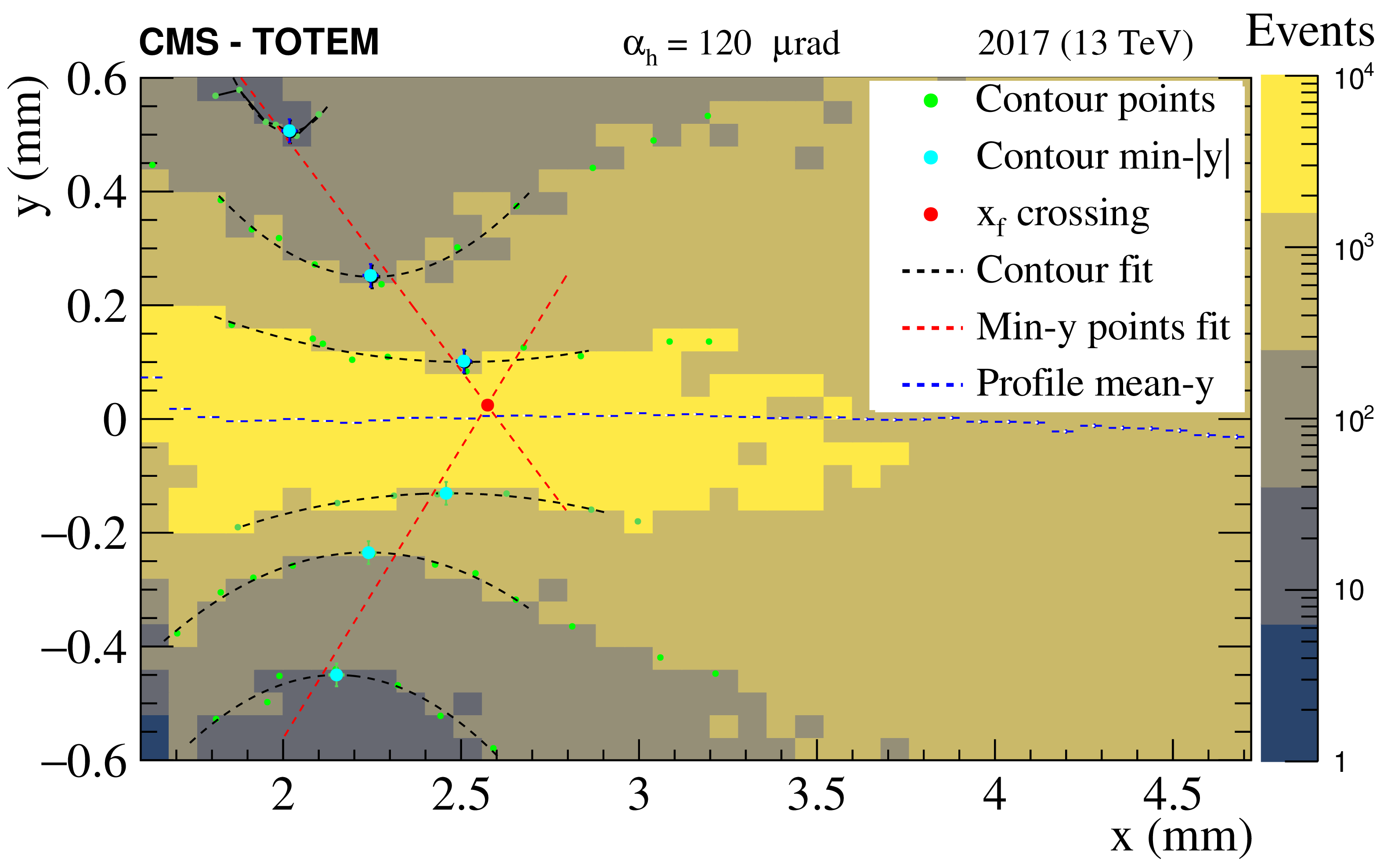
Figure 13:
The $ (x,y) $ distribution of the proton impact points in the near RP detector in sector 45 for 2017 using minimum bias data, along with parabolic fits of the contours around the ``pinch''. The minima of the parabolas are fitted with a straight line. The intersection of the two lines is marked with a red dot, and indicates the estimated focal point coordinate $ x_\mathrm{F} $. To make the contour curves and extrapolation symmetric, the mean of the histogram was aligned to 0 to remove the $ y $ offset created by the vertical dispersion $ \Delta y=D_{y}\ \xi $. The vertical error bar on the contour minima, blue points, represents the statistical uncertainty of the fit. |

png pdf |
Figure 14:
The momentum loss of the protons $ \xi $ as a function of $ x $ in the near RP of sector 45. The dispersion function is $ \xi $ dependent itself and the figure shows directly the nonlinear $ x(\xi)=D({\xi})\cdot \xi $ function. The $ \xi(x) $ function depends on the crossing angle as well; the figure shows the dependence for three reference angles, so the function can be interpolated to arbitrary intermediate angles. |
png pdf |
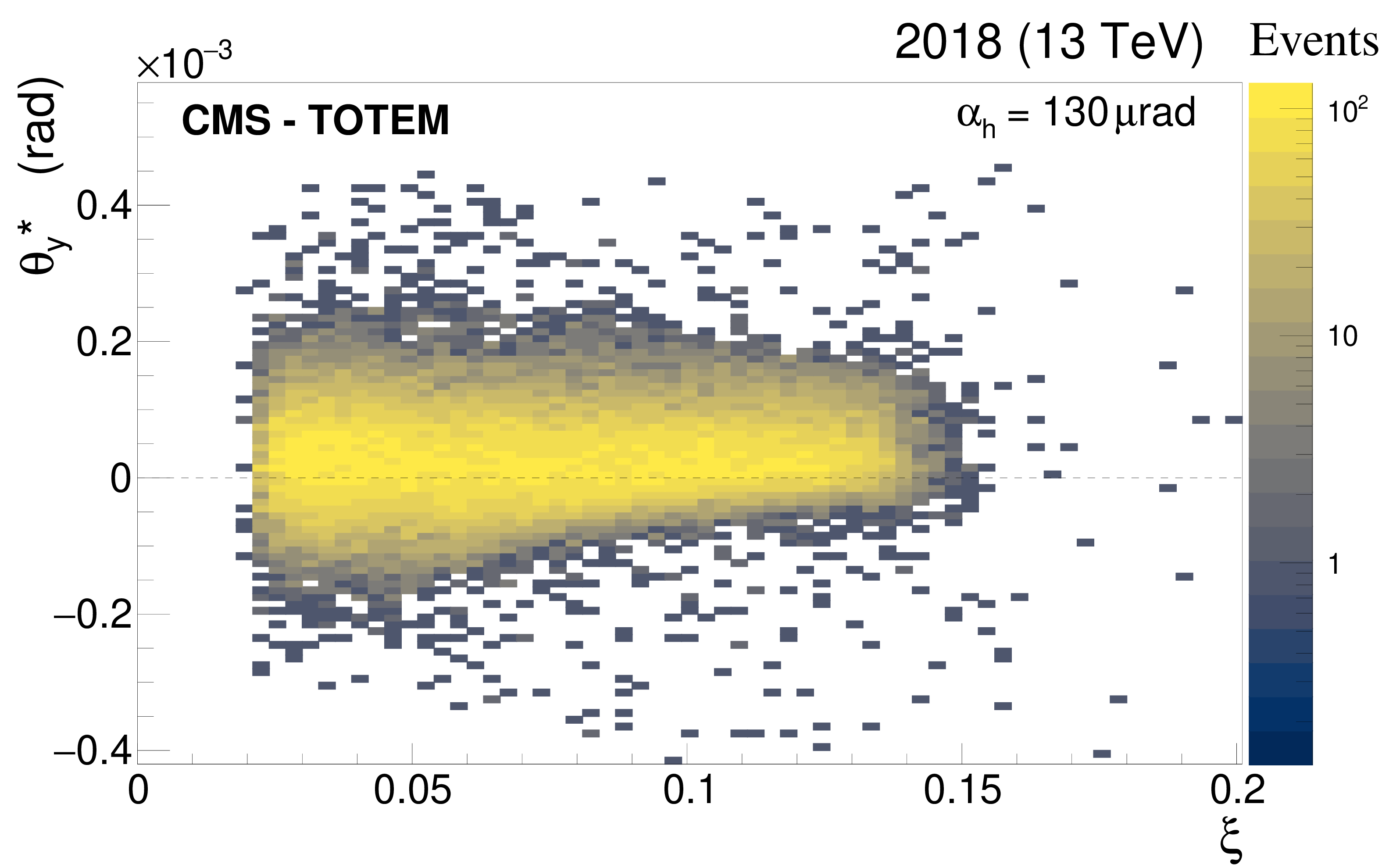
Figure 15:
The vertical scattering angle $ \theta_{y}^{*} $ as a function of $ \xi $ after calibration of the vertical dispersion $ D_{y} $ for sector 45 and fill 6923. The mean of the scattering angle distribution is consistent with 0. The distribution is also affected by the vertical acceptance limitations starting from about $ \xi\approx $ 5% because of the vertical acceptance limits of the detector cf. Fig. 3. |
png pdf |
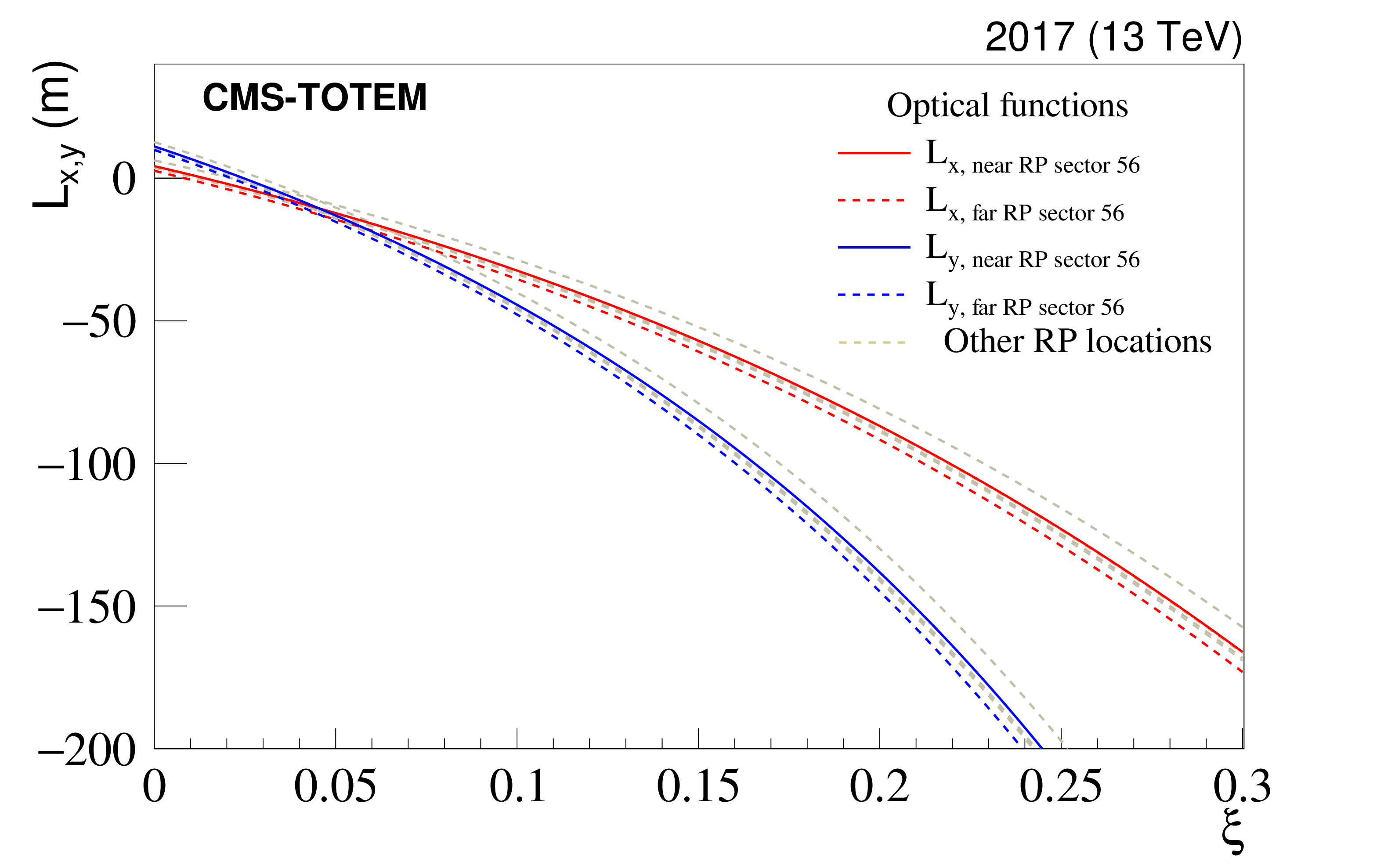
Figure 16:
The horizontal and vertical effective lengths $ L_{x} $ and $ L_{y} $ transport the scattering angle of the proton at IP5 $ \theta_{x}^{*} $ and $ \theta_{y}^{*} $ to the position $ (x,y) $ at the RPs. The figure shows the $ \xi $ dependence of the two functions. The horizontal effective length $ L_{x}(\xi) $ decreases faster than the vertical function $ L_{y} $; both of them cross zero at low $ \xi $, below $ \xi= $ 5%. The grey dashed lines show the effective lengths for the TOTEM RPs used for calibration. |
png pdf |
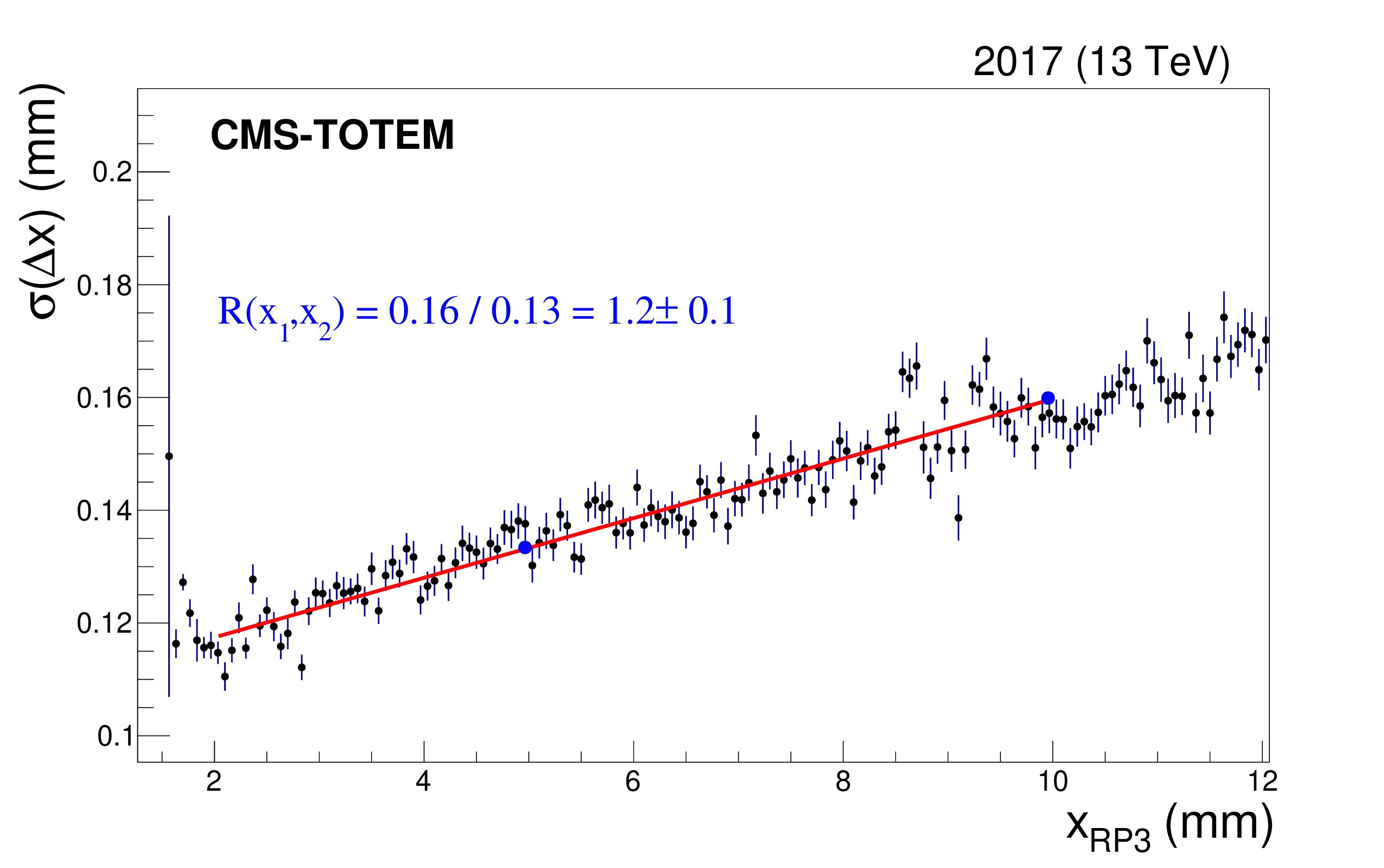
Figure 17:
Fit of $ \sigma(\Delta x) $ as a function of $ x $ for the near RP in sector 45. The fit is used to estimate the uncertainty of the optical function $ \mathrm{d} L_{x}/\mathrm{d} l $. The vertical error bars represent the statistical uncertainties. |
png pdf |
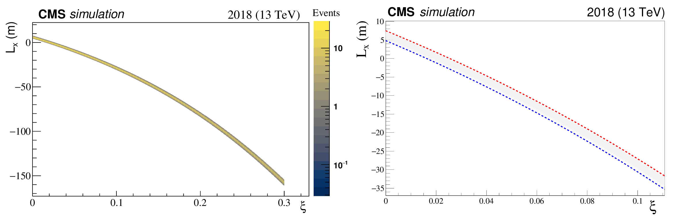
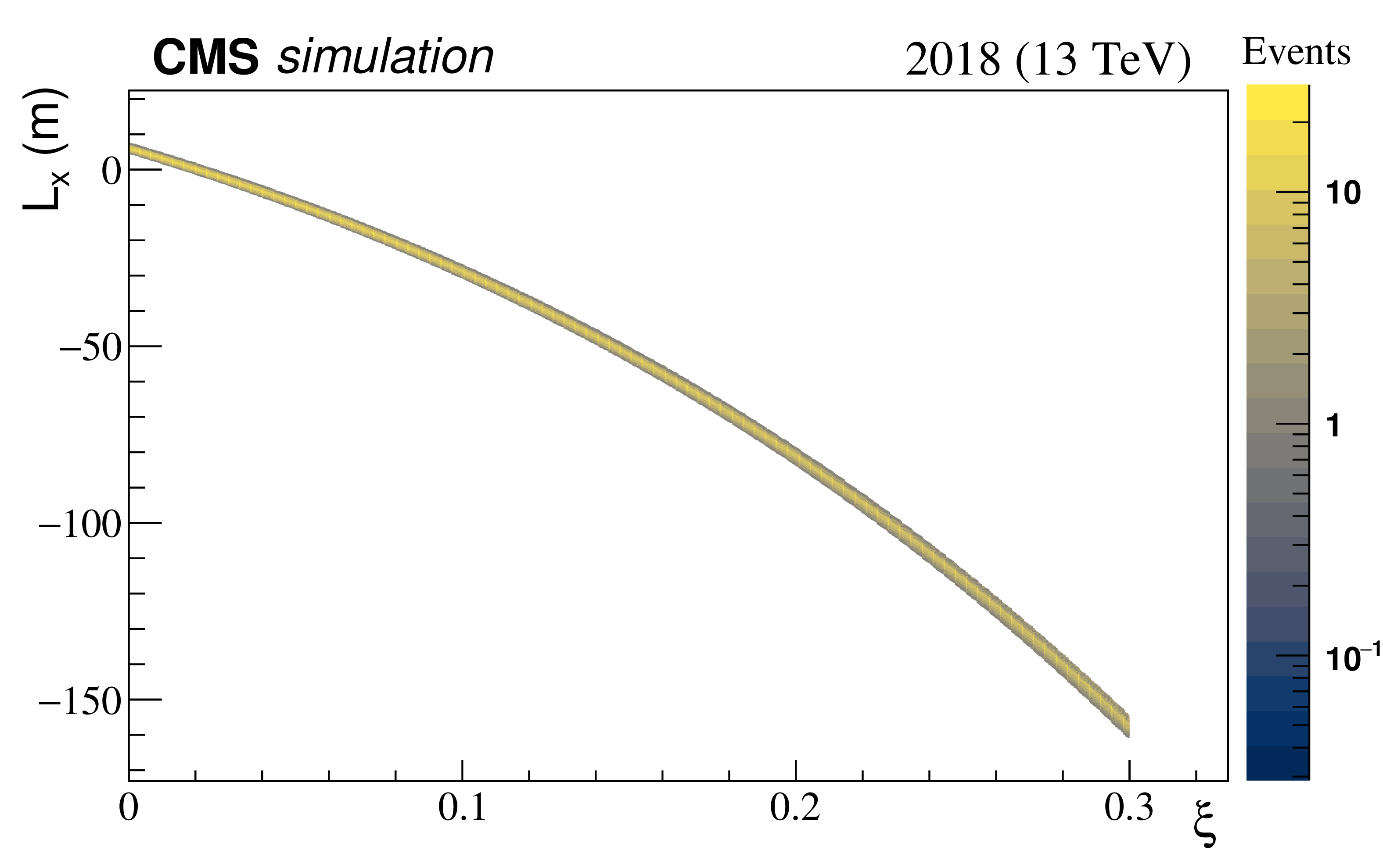
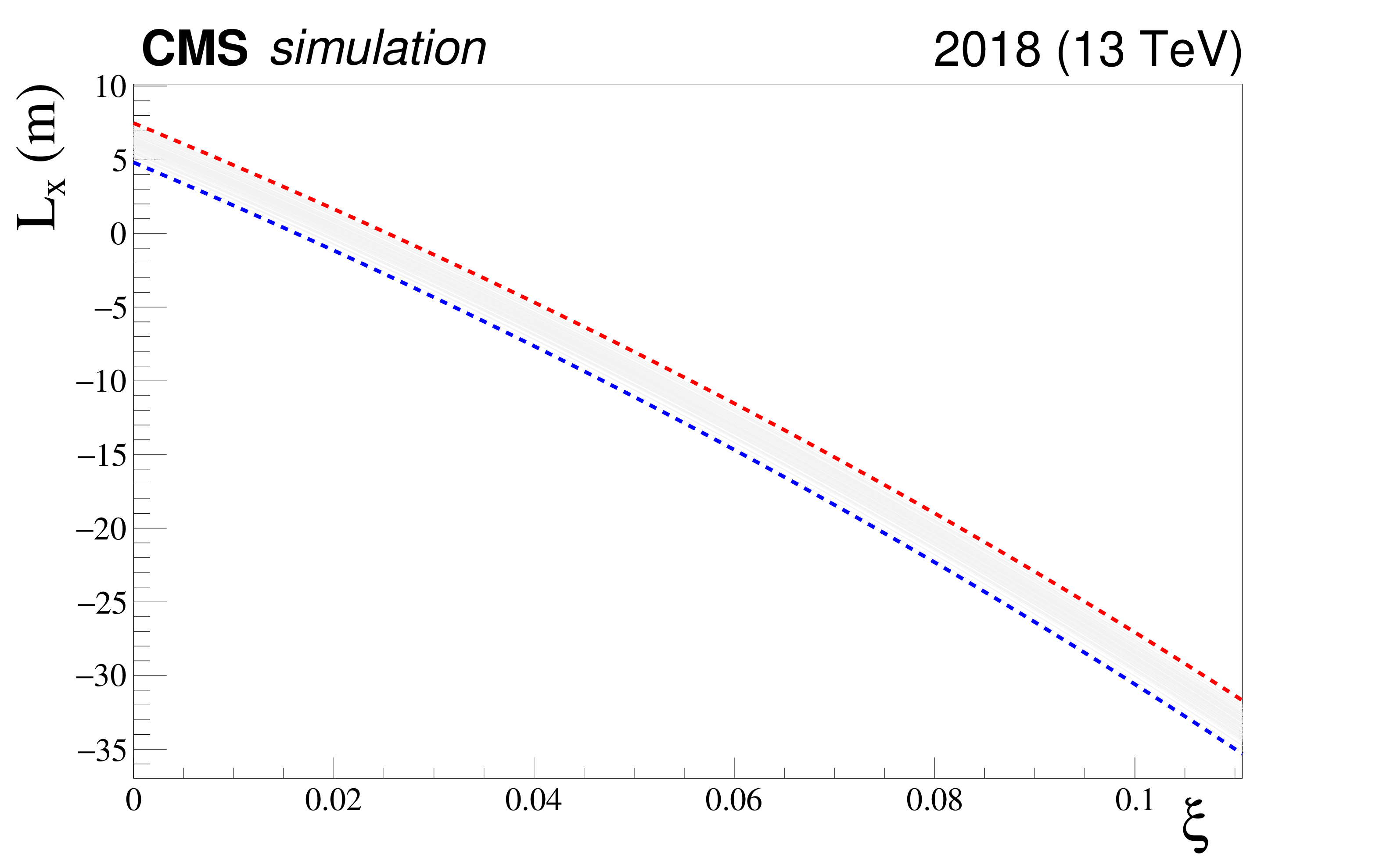
Figure 18:
Left: the distribution of the horizontal effective length $ L_{x}(\xi) $ values as a consequence of perturbations of the magnetic strength. Right: the correlations of the functions; the red and blue dashed curves represent the two extreme $ L_{x}(\xi) $-curves of the Monte Carlo. The upper and lower envelopes demonstrate that the points of the curve move together at different $ \xi $. |
png pdf |
Figure 18-a:
Left: the distribution of the horizontal effective length $ L_{x}(\xi) $ values as a consequence of perturbations of the magnetic strength. Right: the correlations of the functions; the red and blue dashed curves represent the two extreme $ L_{x}(\xi) $-curves of the Monte Carlo. The upper and lower envelopes demonstrate that the points of the curve move together at different $ \xi $. |
png pdf |
Figure 18-b:
Left: the distribution of the horizontal effective length $ L_{x}(\xi) $ values as a consequence of perturbations of the magnetic strength. Right: the correlations of the functions; the red and blue dashed curves represent the two extreme $ L_{x}(\xi) $-curves of the Monte Carlo. The upper and lower envelopes demonstrate that the points of the curve move together at different $ \xi $. |
png pdf |
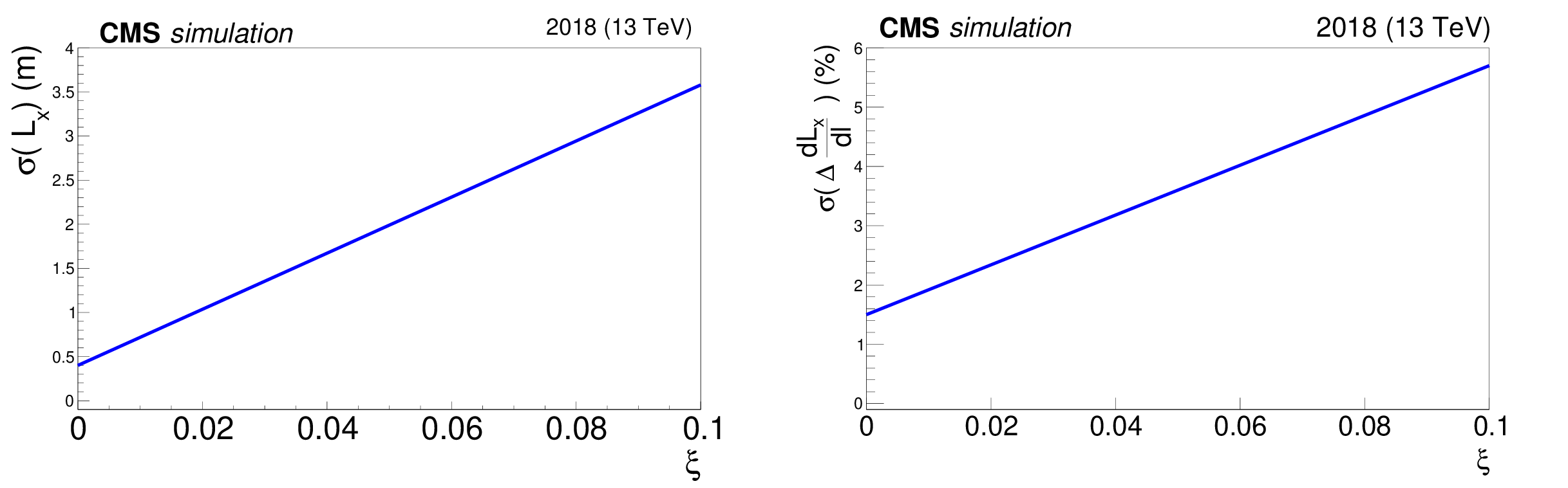
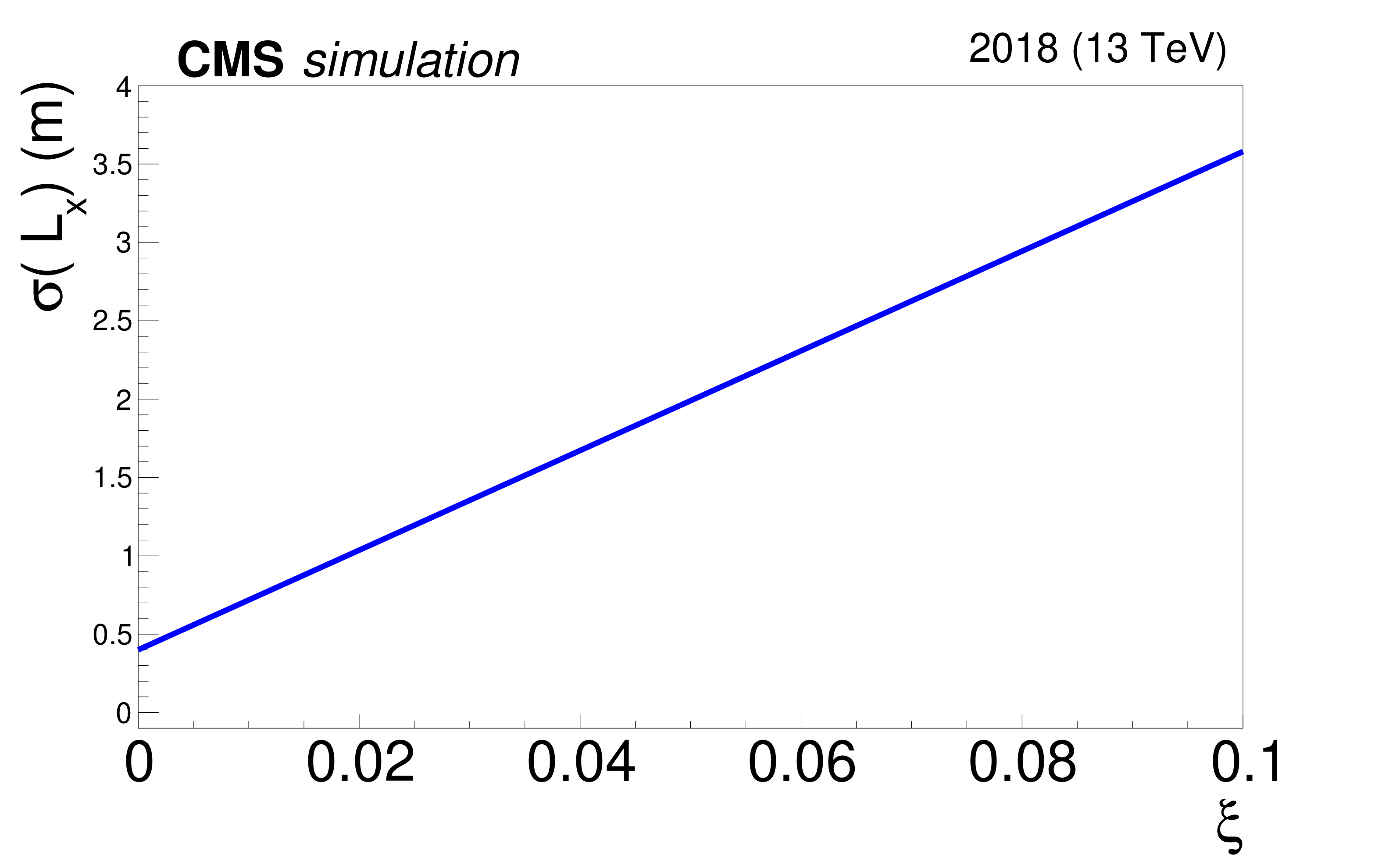
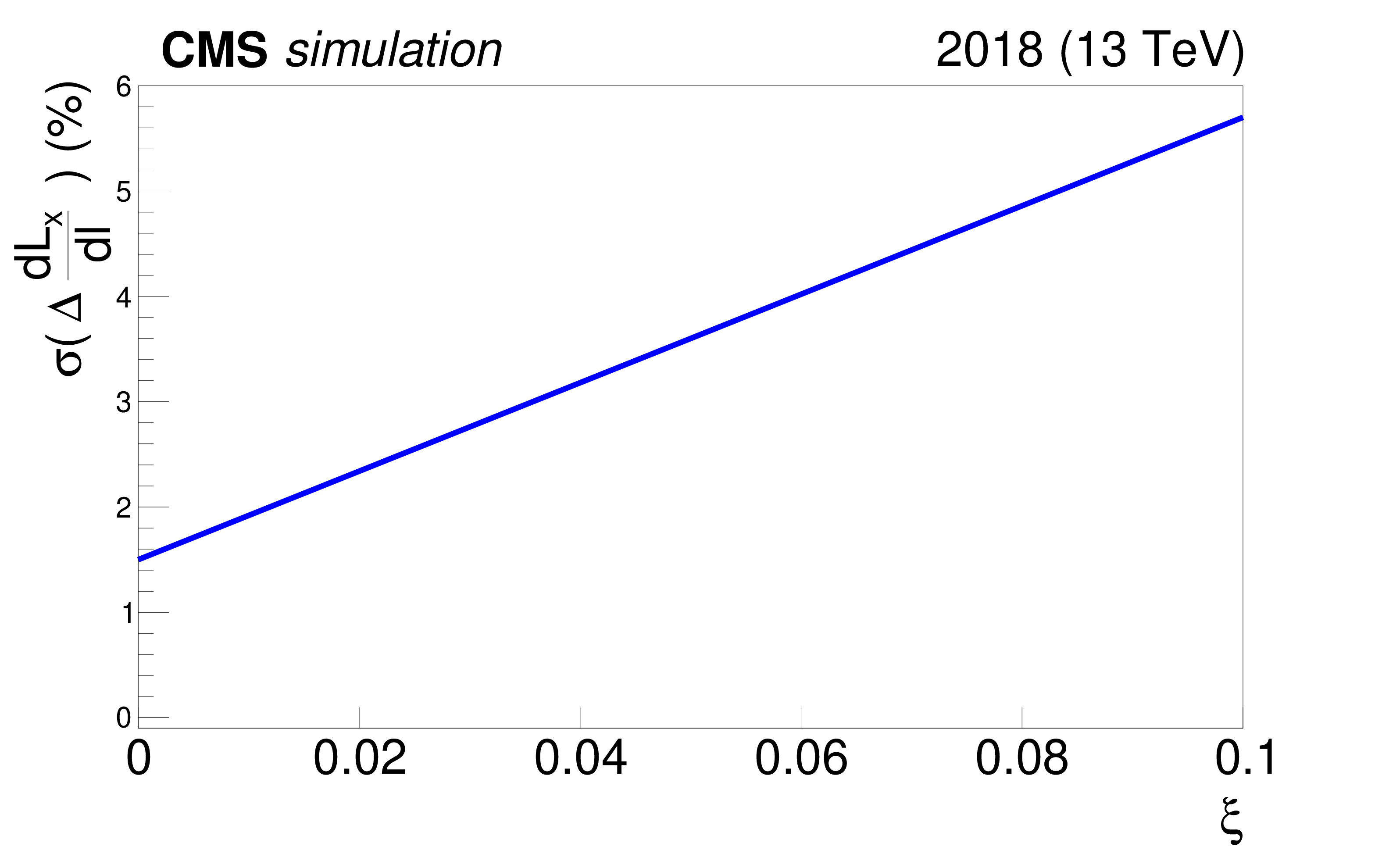
Figure 19:
Left: $ \xi $ dependent uncertainty function of the horizontal effective length $ L_{x}(\xi) $. Right: $ \xi $ dependent uncertainty function of the derivative of the horizontal effective length $ \mathrm{d} L_{x}(\xi)/\mathrm{d} l $. |
png pdf |
Figure 19-a:
Left: $ \xi $ dependent uncertainty function of the horizontal effective length $ L_{x}(\xi) $. Right: $ \xi $ dependent uncertainty function of the derivative of the horizontal effective length $ \mathrm{d} L_{x}(\xi)/\mathrm{d} l $. |
png pdf |
Figure 19-b:
Left: $ \xi $ dependent uncertainty function of the horizontal effective length $ L_{x}(\xi) $. Right: $ \xi $ dependent uncertainty function of the derivative of the horizontal effective length $ \mathrm{d} L_{x}(\xi)/\mathrm{d} l $. |
png pdf |
Figure 20:
Comparison of $ \xi $ reconstructed with the single-RP method from the near and far RP in each arm, presented as a function of $ \xi $ (fill 5849, 2017). The color code represents per-bin event counts. Left: sector 45, right: sector 56. |
png pdf |
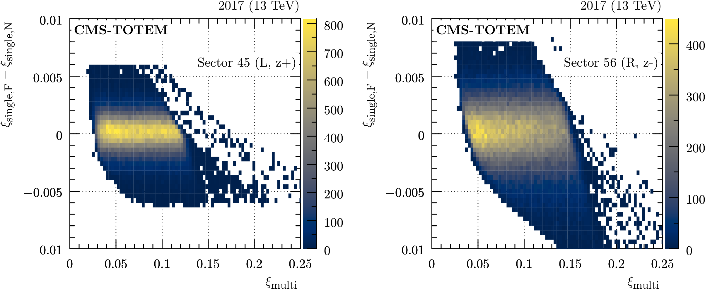
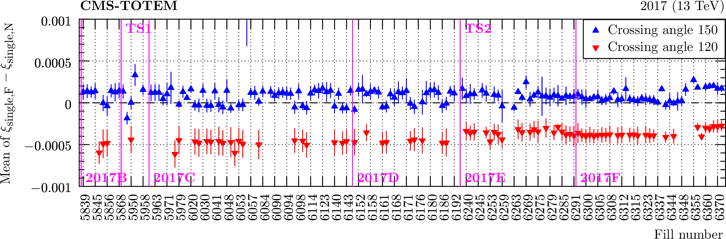
Figure 21:
Mean near-far $ \xi $ difference from single-RP reconstruction (in a safe region far from acceptance limitations) as a function of fill number (2017, sector 56). The different colors represent data taken with different values of the crossing angle. The error bars represent the systematic uncertainty estimated as a difference of means evaluated at two different values of $ \xi_\text{multi} $. |
png pdf |
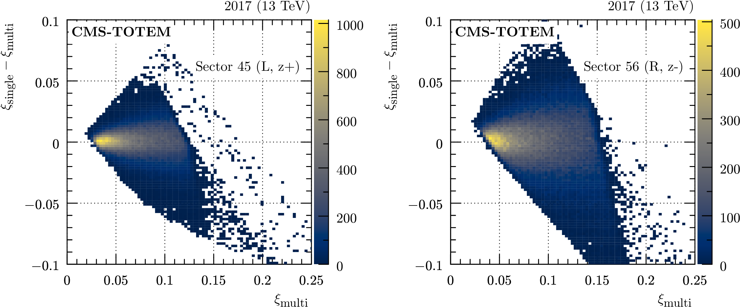
Figure 22:
Comparison of $ \xi $ reconstructed with the single-RP and multi-RP methods, presented as a function of $ \xi $ (LHC fill 5849, 2017, single-RP reconstruction from the near RPs). The color code represents per-bin event counts. Left: sector 45, right: sector 56. |
png pdf |
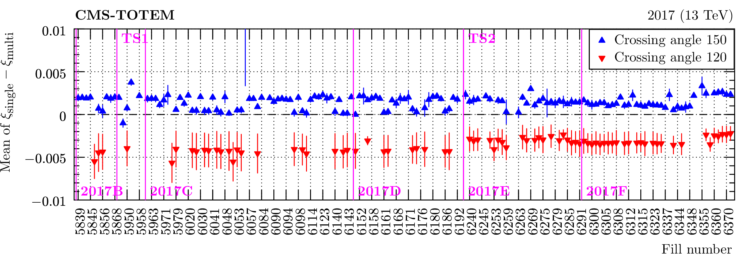
Figure 23:
Mean single-RP vs. multi-RP $ \xi $ difference (in a safe region far from acceptance limitations) as a function of fill number (2017, sector 56, single-RP reconstruction from the near RP). The different colors represent data taken with different values of the crossing angle. The error bars represent the systematic uncertainty estimated as a difference of means evaluated at two different values of $ \xi_\text{multi} $. |
png pdf |
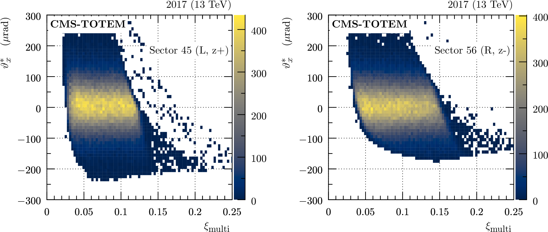
Figure 24:
Histogram of $ \theta^*_x $ vs. $ \xi $ as reconstructed with the multi-RP method (fill 5849, 2017). The color code represents per-bin event counts. Left: sector 45, right: sector 56. |

png pdf |
Figure 25:
Mean value of $ \theta^*_x $ (in a safe region far from acceptance limitations) as a function of fill number (2017, sector 56). The markers in several colors represent data taken with different values of the crossing angle. The error bars represent the systematic uncertainty estimated as a difference of means evaluated at two different values of $ \xi_\text{multi} $. |

png pdf |
Figure 26:
Histogram of $ \theta^*_y $ vs. $ \xi $ as reconstructed with the multi-RP method (fill 5276, 2016). The color code represents per-bin event counts. Left: sector 45, right: sector 56. |

png pdf |
Figure 27:
Mean value of $ \theta^*_y $ (in a safe region far from acceptance limitations) as a function of fill number (2016, sector 45). The markers in different colors represent data taken with different values of the crossing angle. The error bars represent the systematic uncertainty estimated as a difference of means evaluated at two different values of $ \xi_\text{multi} $. |
png pdf |
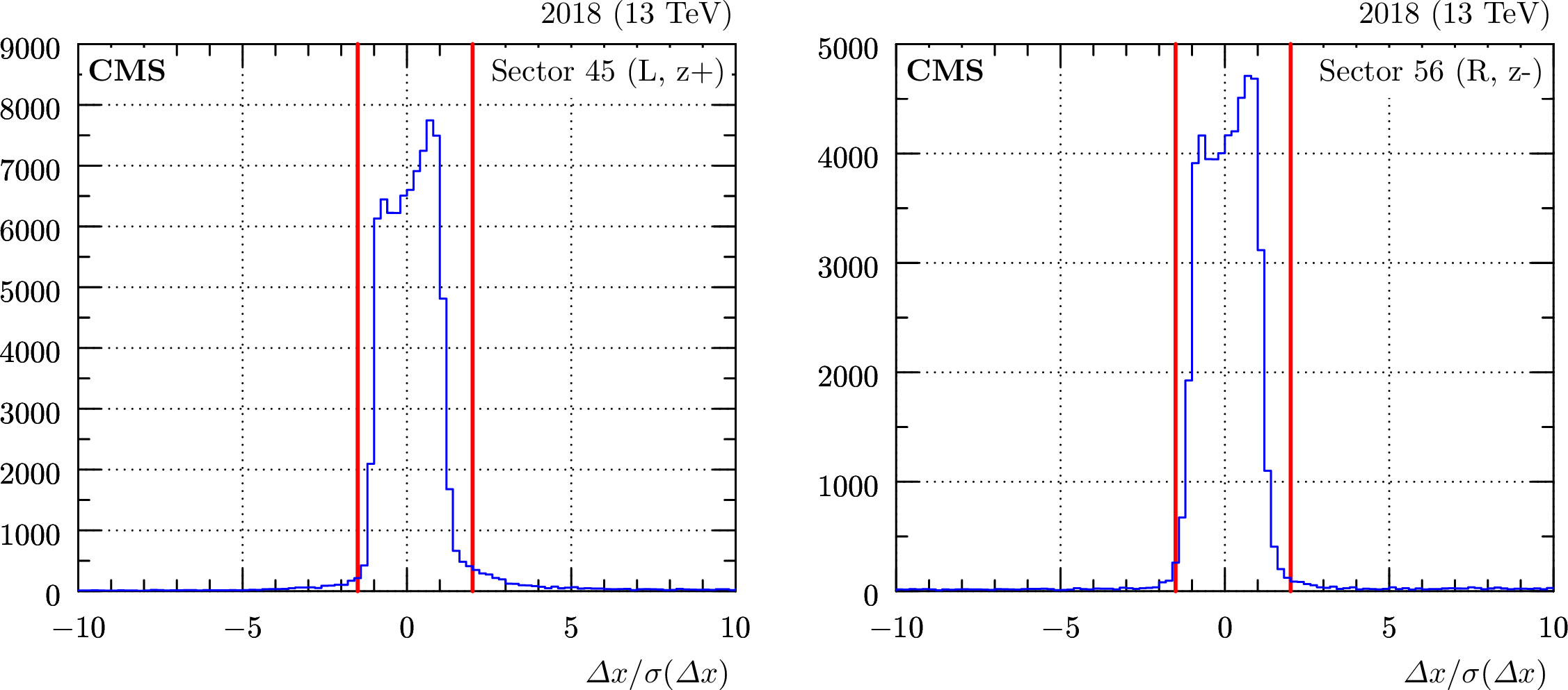
Figure 28:
Association of local tracks from tracking and timing RPs (fill 7039, 2018). $ \Delta x $ refers to horizontal distance between the tracks from tracking and timing RPs, $ \sigma(\Delta x) $ stands for the corresponding uncertainty. The vertical red lines delimit the tolerance window. |
png pdf |
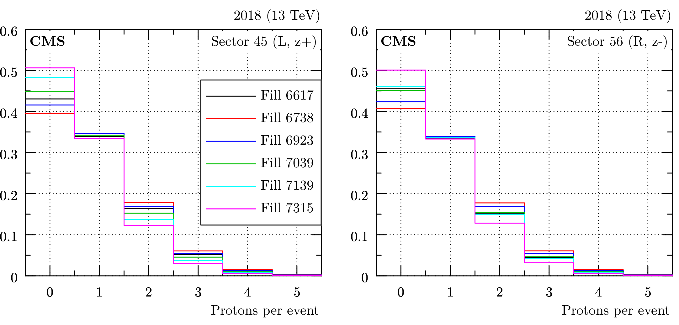
Figure 29:
Multiplicity of reconstructed protons per arm and per event (2018 data). The histograms are normalised to unit area. Different colors correspond to different fills as indicated in the legend. Left: sector 45, right: sector 56. |
png pdf |
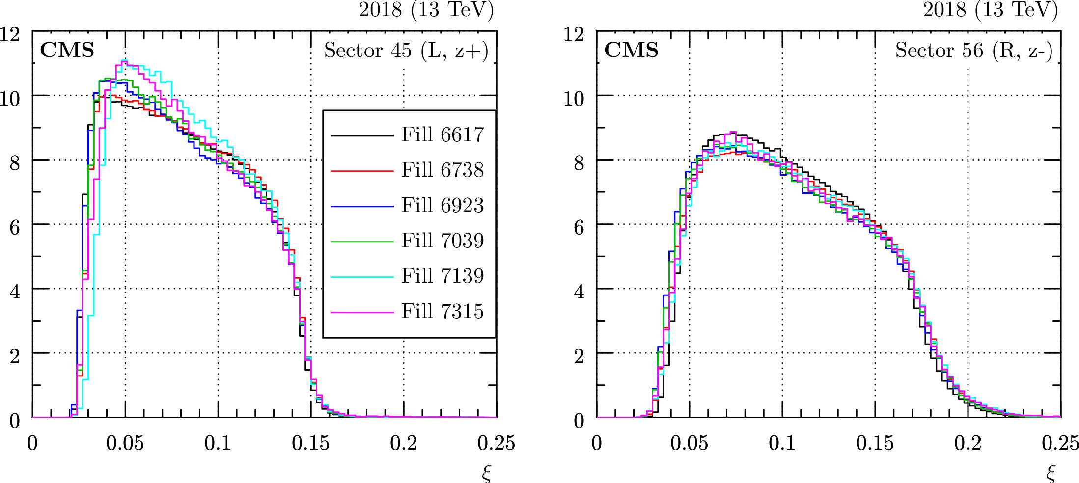
Figure 30:
$ \xi $ distributions as extracted from reconstructed protons with no corrections (acceptance, efficiency, etc.), 2018 data. The histograms are normalised to unit area. Different colors correspond to different fills as indicated in the legend. Left: sector 45, right: sector 56. |
png pdf |
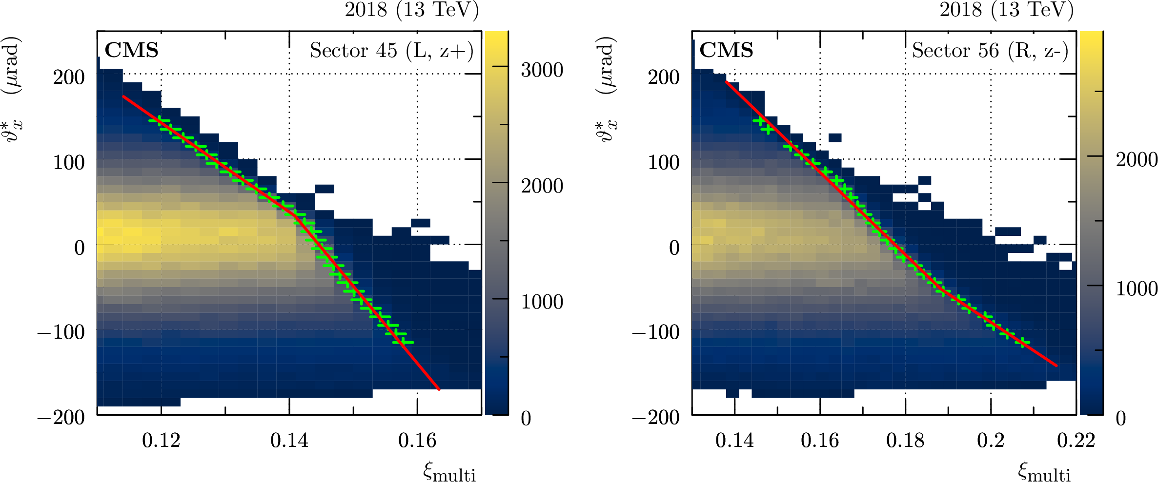
Figure 31:
Distribution of $ \theta^*_x $ vs. $ \xi $ reconstructed with the multi-RP method (fill 6617, 2018), zoomed at high $ \xi $. The color code represents per-bin event counts. The green markers show the identified aperture cutoff, the red line the fit according to Eq. (23). The green error bars vertically represent the bin size, horizontally a combination of statistical and systematic uncertainties. Left: sector 45, right: sector 56. |
png pdf |
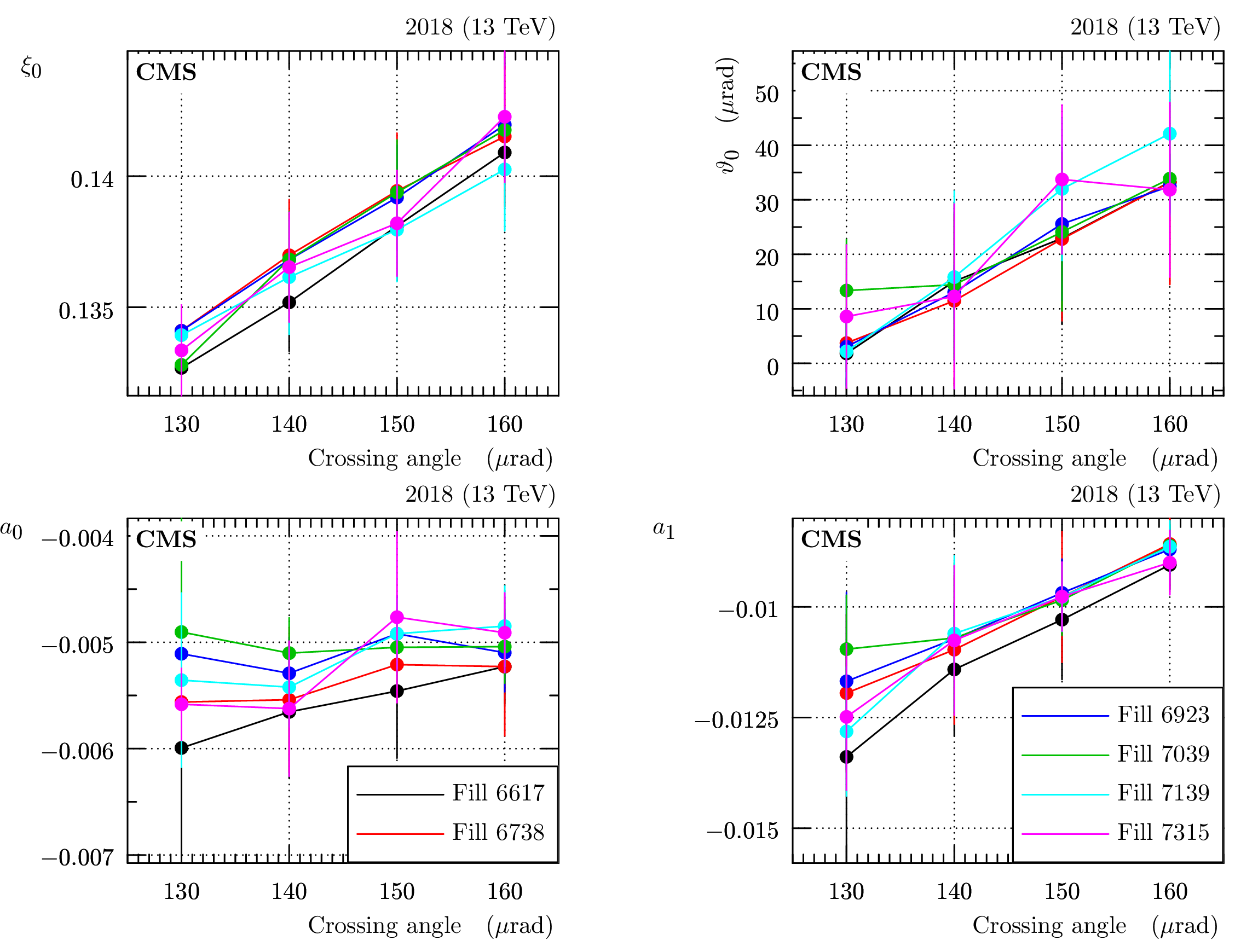
Figure 32:
Summary of aperture-limitation parameters extracted from several LHC fills (different colors, 2018) and several crossing angle values (horizontal axis), for sector 45. The error bars represent a combination of statistical and systematic uncertainties. |

png pdf |
Figure 33:
Comparison of hit distributions from simulation (red) and LHC data (fill 6738, no explicit event/track selection, black), for the 2018 pre-TS1 configuration and the near RP in sector 56. The black error bars represent statistical uncertainties. Left: distribution of horizontal track positions, right: distribution of vertical track positions ($ y $ range limited to the area around the upper sensor edge). |
png pdf |
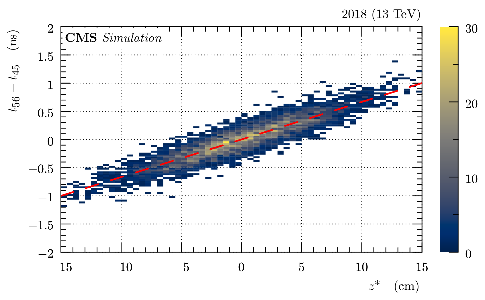
Figure 34:
Simulated correlation between vertex position along the beam, $ z^* $, and the proton timing difference observed in LHC sectors 56 and 45 (2018 pre-TS1 configuration). The color code represents per-bin event counts. Reconstruction resolution of $ z^* $ is not included in this plot. The red dashed line indicates the ideal correlation. |
png pdf |
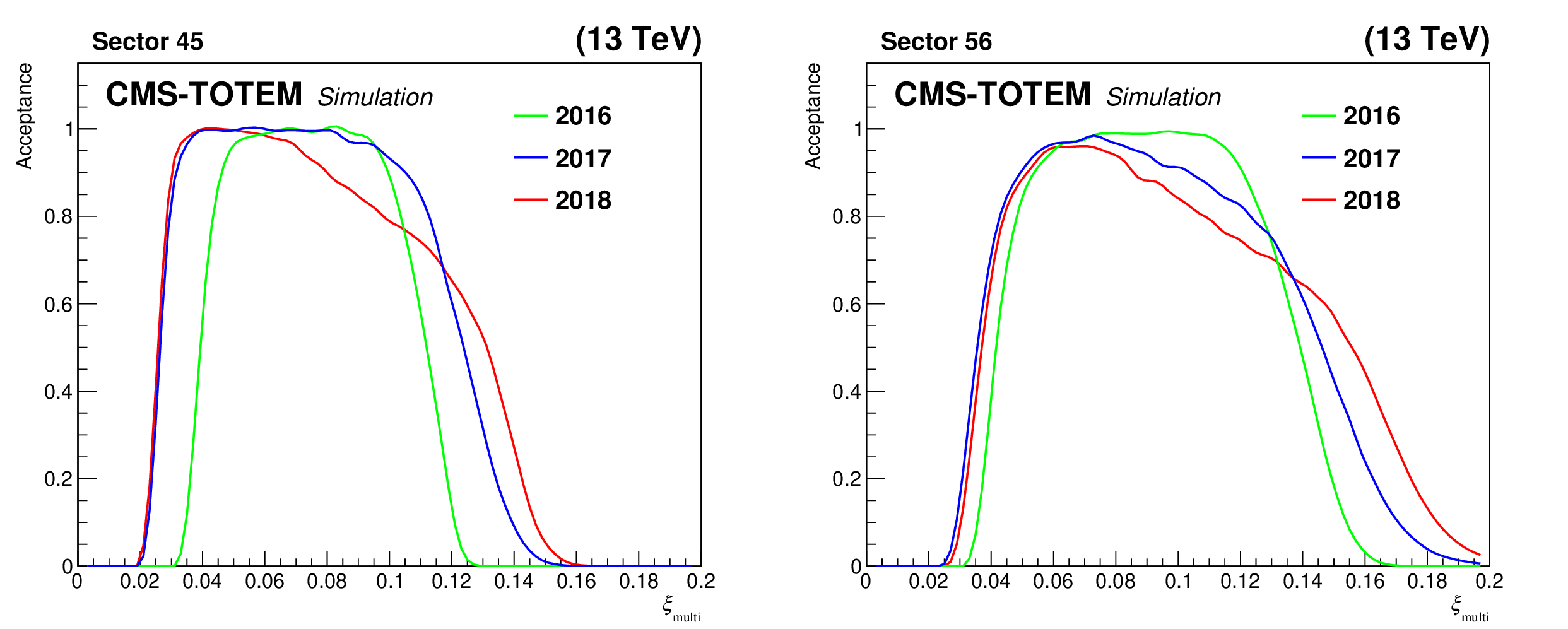
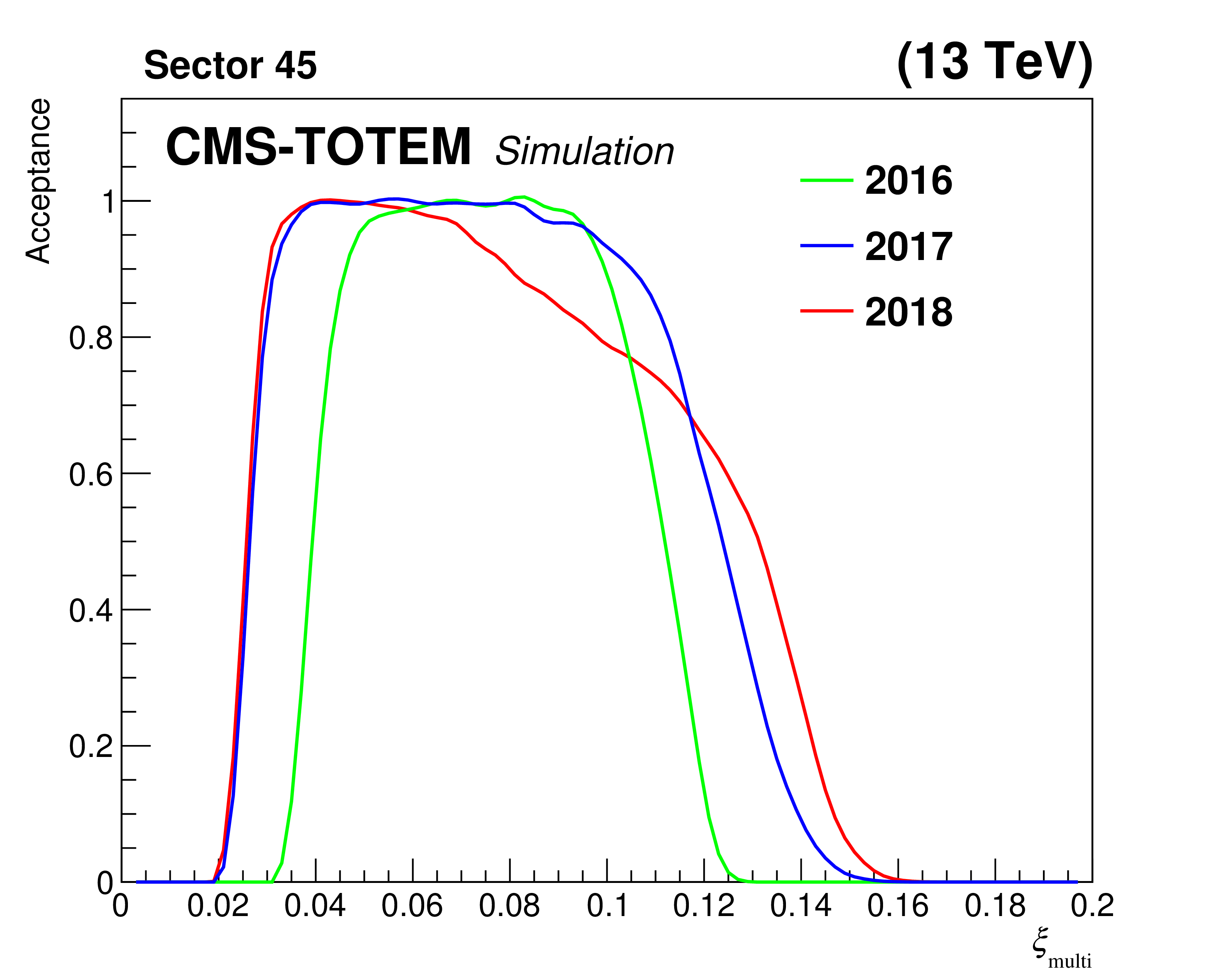
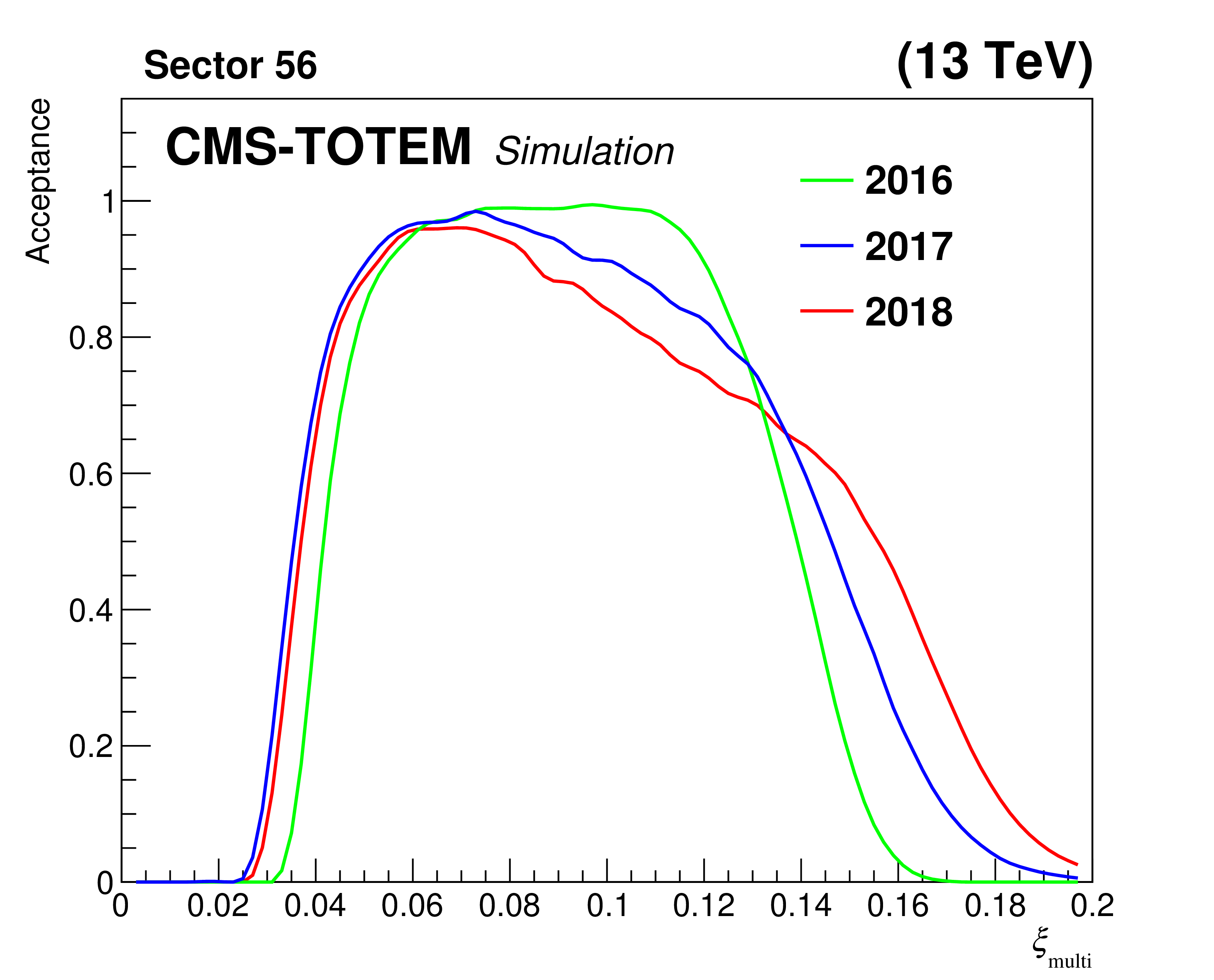
Figure 35:
Fraction of reconstructed multi-RP protons, as a function of $ \xi_\text{multi} $, for a proton sample produced with the PPS direct simulation. Since perfect detector efficiency was assumed in this simulation, the results reflect mostly the geometrical acceptance of the apparatus. |
png pdf |
Figure 35-a:
Fraction of reconstructed multi-RP protons, as a function of $ \xi_\text{multi} $, for a proton sample produced with the PPS direct simulation. Since perfect detector efficiency was assumed in this simulation, the results reflect mostly the geometrical acceptance of the apparatus. |
png pdf |
Figure 35-b:
Fraction of reconstructed multi-RP protons, as a function of $ \xi_\text{multi} $, for a proton sample produced with the PPS direct simulation. Since perfect detector efficiency was assumed in this simulation, the results reflect mostly the geometrical acceptance of the apparatus. |

png pdf |
Figure 36:
Example of resolution studies for $ \xi $ (2018 pre-TS1, sector 56). On the vertical axes, $ \Delta\xi $ refers to the difference between the reconstructed and simulated $ \xi $. On the horizontal axes, $ \xi $ denotes the simulated value. The different colors refer to different smearing effects considered. Black: only vertical vertex smearing, red: in addition also horizontal vertex smearing, blue: in addition also beam divergence, green (the most complete scenario): in addition also detector spatial resolution. The error bars represent statistical uncertainties. Note that some curves are superimposed. Left: single-RP, right: multi-RP reconstruction. |
png pdf |
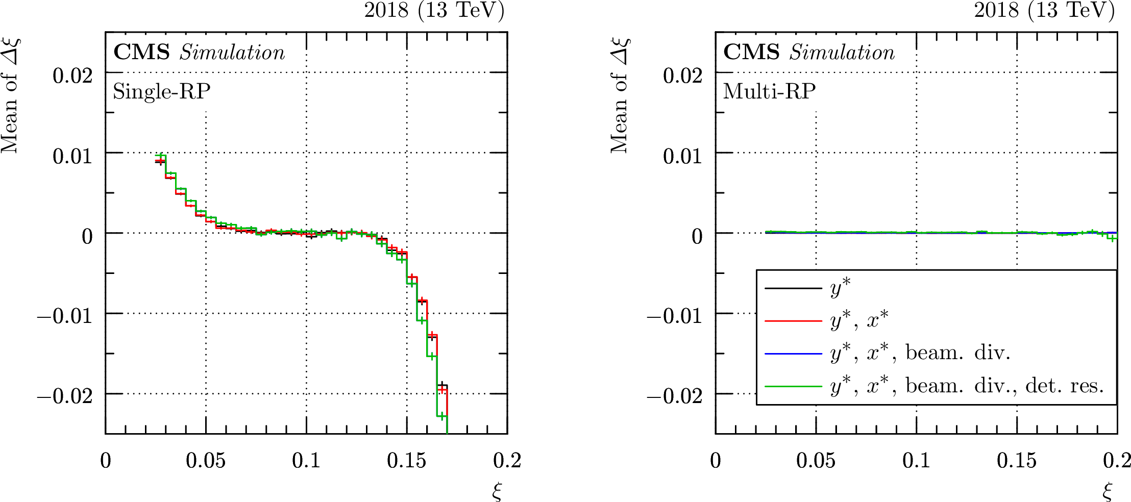
Figure 37:
Example of bias studies for $ \xi $ (2018 pre-TS1, sector 56). The different colors refer to different smearing effects considered (see caption of Fig. 36). The error bars represent statistical uncertainties. Left: single-RP, right: multi-RP reconstruction. |

png pdf |
Figure 38:
Example of systematic studies for $ \xi $ (2018 pre-TS1, sector 56). Each curve corresponds to a perturbation at 1 $ \sigma $ level. The red and blue curves represent alignment variations: in the former both the near and far RP are shifted in the same direction, in the latter opposite directions are considered. The remaining scenarios cover perturbations of the optical functions. The error bars represent statistical uncertainties. Left: single-RP, right: multi-RP reconstruction. |
png pdf |
Figure 39:
Example of combined systematic uncertainties of proton $ \xi $ (2018 pre-TS1, sector 56). The results for the single-RP and multi-RP reconstructions are shown in red and blue, respectively. The error bars represent statistical uncertainties. Left: absolute, right: relative uncertainty. |

png pdf |
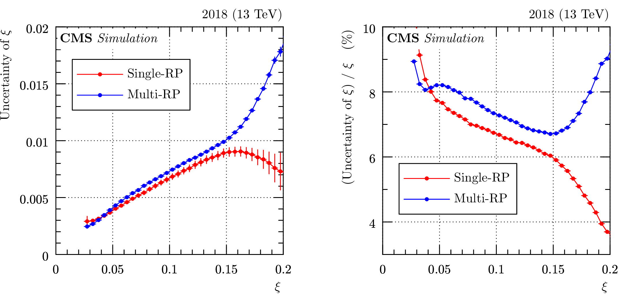
Figure 40:
Comparison of bias, resolution and systematics characteristics (2018 pre-TS1, sector 56). For the bias and resolution curves, all considered smearing effects are included. The systematics curves represent the combination of all contributions. The error bars represent statistical uncertainties. |

png pdf |
Figure 41:
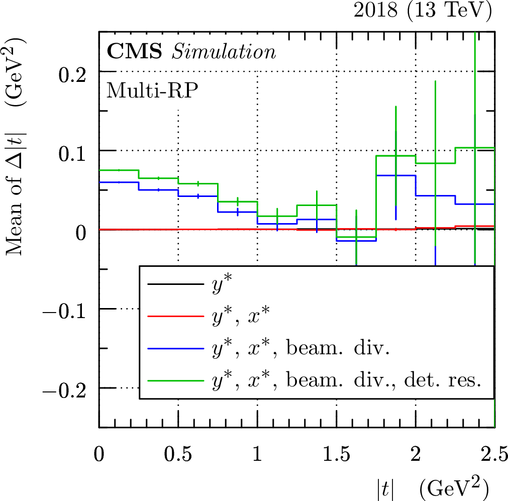
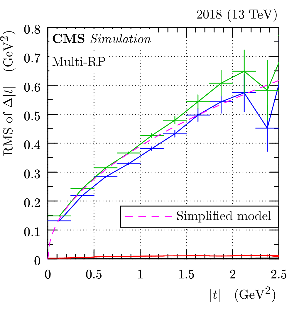
Example of resolution bias (left) and resolution (right) studies for four-momentum transfer squared, $ t $, with multi-RP reconstruction (2018 pre-TS1, sector 56). On the vertical axes, $ \Delta |t| $ refers to the difference between the reconstructed and simulated value of $ |t| $. On the horizontal axes, $ |t| $ denotes the simulated value. The different colors refer to different smearing effects considered. Black: only vertical vertex smearing, red: in addition also horizontal vertex smearing, blue: in addition also beam divergence, green (the most complete scenario): in addition also detector spatial resolution. In the right plot, the dashed magenta curve represents the simplified analytic model from Eq. (26). The error bars represent statistical uncertainties. |
png pdf |
Figure 41-a:
Example of resolution bias (left) and resolution (right) studies for four-momentum transfer squared, $ t $, with multi-RP reconstruction (2018 pre-TS1, sector 56). On the vertical axes, $ \Delta |t| $ refers to the difference between the reconstructed and simulated value of $ |t| $. On the horizontal axes, $ |t| $ denotes the simulated value. The different colors refer to different smearing effects considered. Black: only vertical vertex smearing, red: in addition also horizontal vertex smearing, blue: in addition also beam divergence, green (the most complete scenario): in addition also detector spatial resolution. In the right plot, the dashed magenta curve represents the simplified analytic model from Eq. (26). The error bars represent statistical uncertainties. |
png pdf |
Figure 41-b:
Example of resolution bias (left) and resolution (right) studies for four-momentum transfer squared, $ t $, with multi-RP reconstruction (2018 pre-TS1, sector 56). On the vertical axes, $ \Delta |t| $ refers to the difference between the reconstructed and simulated value of $ |t| $. On the horizontal axes, $ |t| $ denotes the simulated value. The different colors refer to different smearing effects considered. Black: only vertical vertex smearing, red: in addition also horizontal vertex smearing, blue: in addition also beam divergence, green (the most complete scenario): in addition also detector spatial resolution. In the right plot, the dashed magenta curve represents the simplified analytic model from Eq. (26). The error bars represent statistical uncertainties. |

png pdf |
Figure 42:
Diagrams for $ \gamma\gamma\to\mu^{+}\mu^{-} $ production with intact protons. Left: fully exclusive production, with both protons remaining intact. Right: Single proton dissociation, with one of the two protons remaining intact. In the right plot, the three lines labelled $ p^* $ indicate that the proton does not remain intact, but dissociates into an undetected low-mass system. |
png pdf |
Figure 43:
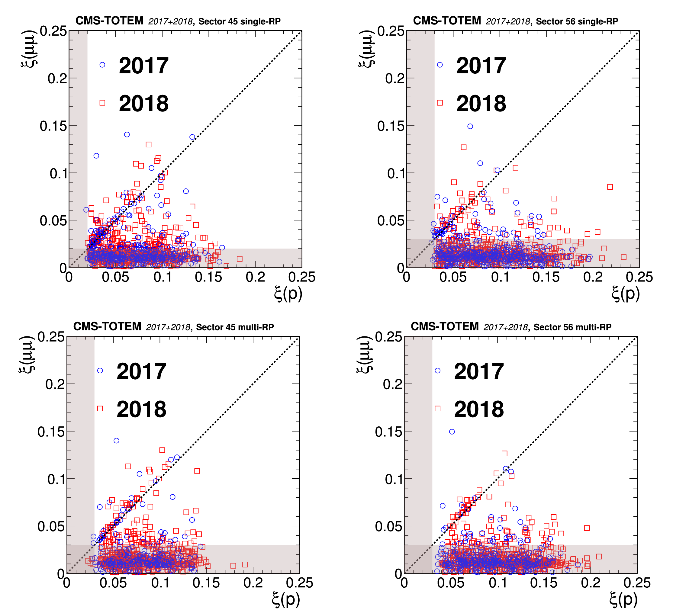
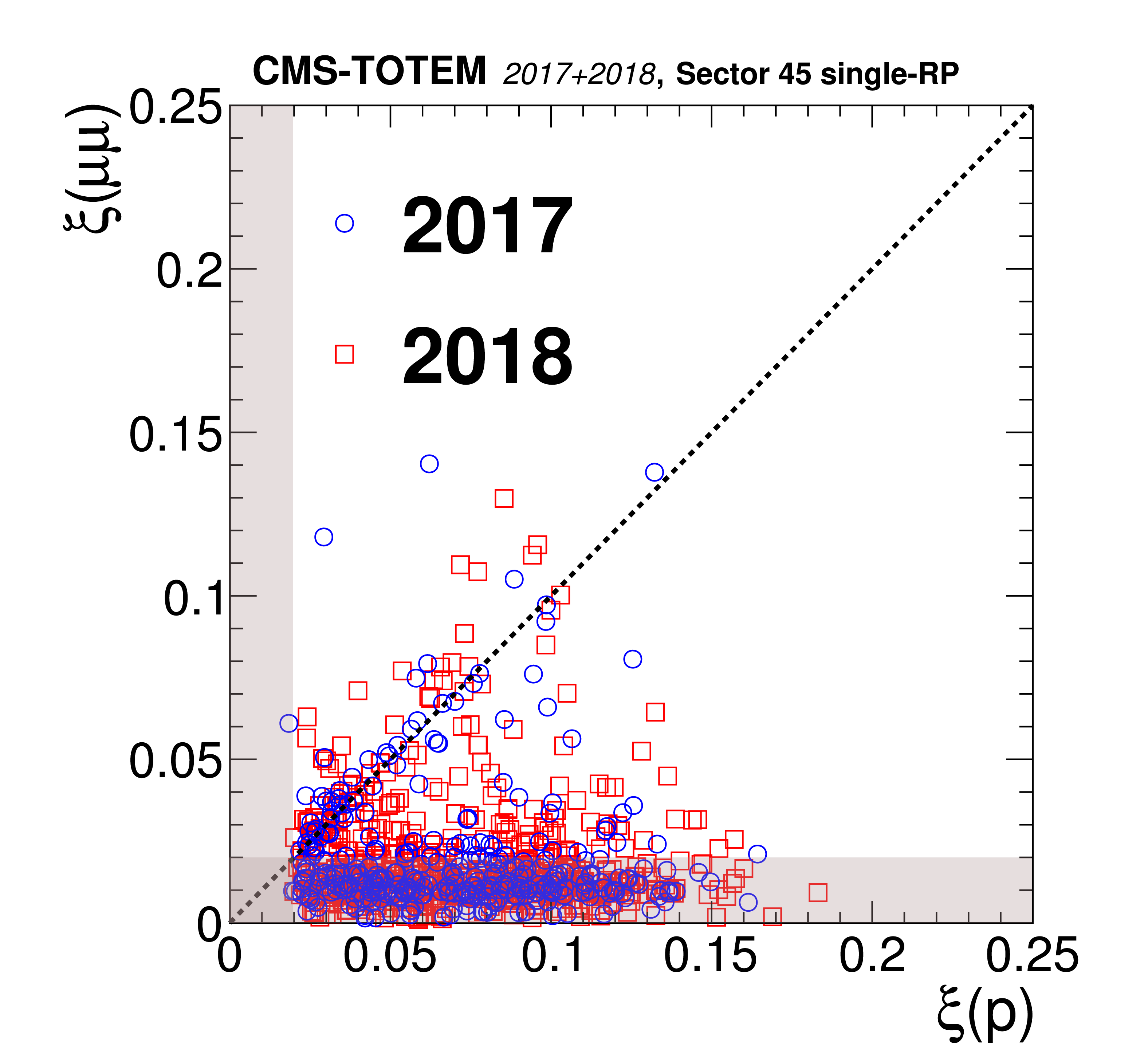
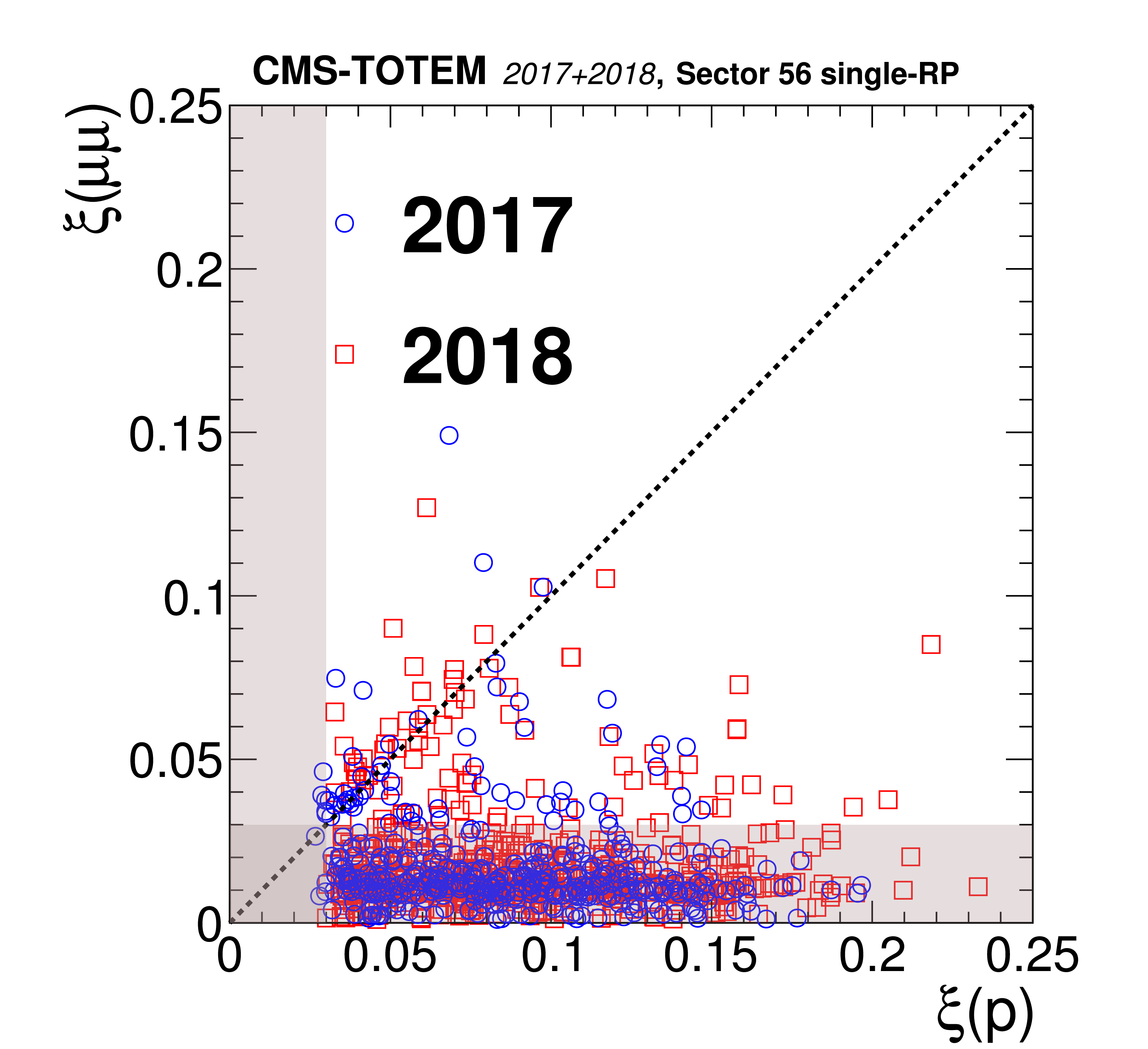
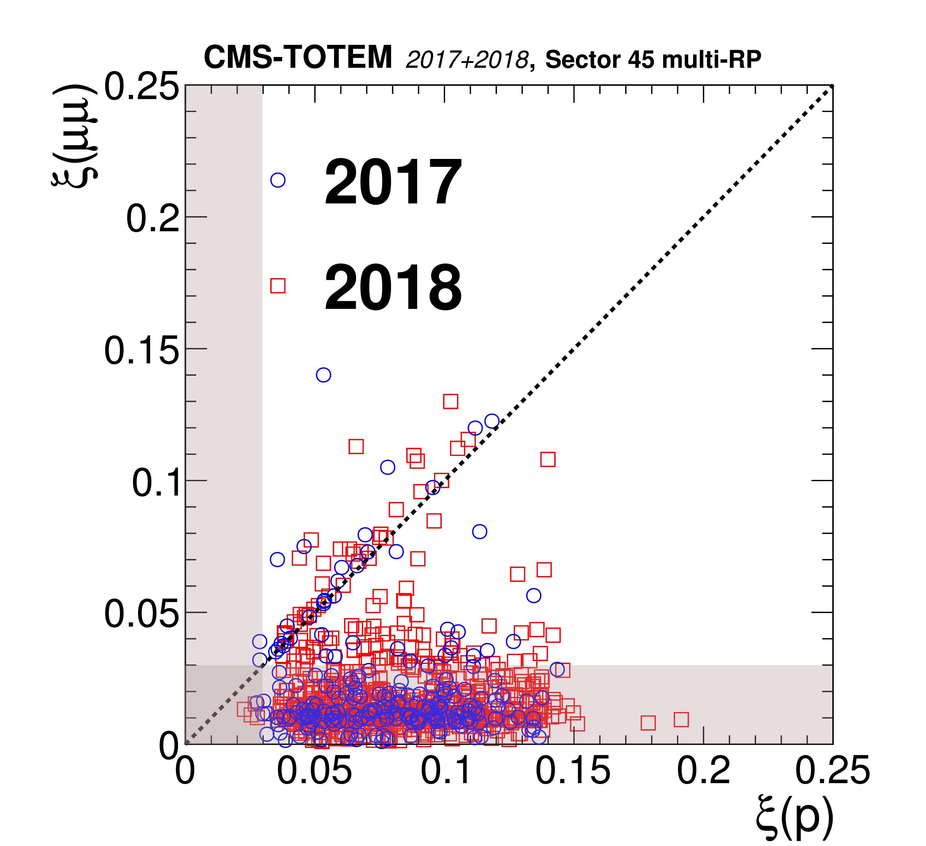
Distribution of $ \xi $(p) vs. $ \xi(\mu^{+}\mu^{-}) $ for the $ z > $ 0 (LHC sector 45) and $ z < $ 0 (LHC sector 56) directions in the CMS coordinate system. The two styles of points represent the data collected during 2017 and 2018. The shaded bands represent the region incompatible with the PPS acceptance for signal events; events in this region are expected to arise from random combinations of muon pairs with protons from pileup interactions. The upper plots show the results of the single-RP reconstruction algorithm, and the lower plots show the multi-RP results. The dotted line illustrates the case of a perfect correlation, where signal events are expected. |
png pdf |
Figure 43-a:
Distribution of $ \xi $(p) vs. $ \xi(\mu^{+}\mu^{-}) $ for the $ z > $ 0 (LHC sector 45) and $ z < $ 0 (LHC sector 56) directions in the CMS coordinate system. The two styles of points represent the data collected during 2017 and 2018. The shaded bands represent the region incompatible with the PPS acceptance for signal events; events in this region are expected to arise from random combinations of muon pairs with protons from pileup interactions. The upper plots show the results of the single-RP reconstruction algorithm, and the lower plots show the multi-RP results. The dotted line illustrates the case of a perfect correlation, where signal events are expected. |
png pdf |
Figure 43-b:
Distribution of $ \xi $(p) vs. $ \xi(\mu^{+}\mu^{-}) $ for the $ z > $ 0 (LHC sector 45) and $ z < $ 0 (LHC sector 56) directions in the CMS coordinate system. The two styles of points represent the data collected during 2017 and 2018. The shaded bands represent the region incompatible with the PPS acceptance for signal events; events in this region are expected to arise from random combinations of muon pairs with protons from pileup interactions. The upper plots show the results of the single-RP reconstruction algorithm, and the lower plots show the multi-RP results. The dotted line illustrates the case of a perfect correlation, where signal events are expected. |
png pdf |
Figure 43-c:
Distribution of $ \xi $(p) vs. $ \xi(\mu^{+}\mu^{-}) $ for the $ z > $ 0 (LHC sector 45) and $ z < $ 0 (LHC sector 56) directions in the CMS coordinate system. The two styles of points represent the data collected during 2017 and 2018. The shaded bands represent the region incompatible with the PPS acceptance for signal events; events in this region are expected to arise from random combinations of muon pairs with protons from pileup interactions. The upper plots show the results of the single-RP reconstruction algorithm, and the lower plots show the multi-RP results. The dotted line illustrates the case of a perfect correlation, where signal events are expected. |

png pdf |
Figure 43-d:
Distribution of $ \xi $(p) vs. $ \xi(\mu^{+}\mu^{-}) $ for the $ z > $ 0 (LHC sector 45) and $ z < $ 0 (LHC sector 56) directions in the CMS coordinate system. The two styles of points represent the data collected during 2017 and 2018. The shaded bands represent the region incompatible with the PPS acceptance for signal events; events in this region are expected to arise from random combinations of muon pairs with protons from pileup interactions. The upper plots show the results of the single-RP reconstruction algorithm, and the lower plots show the multi-RP results. The dotted line illustrates the case of a perfect correlation, where signal events are expected. |
png pdf |
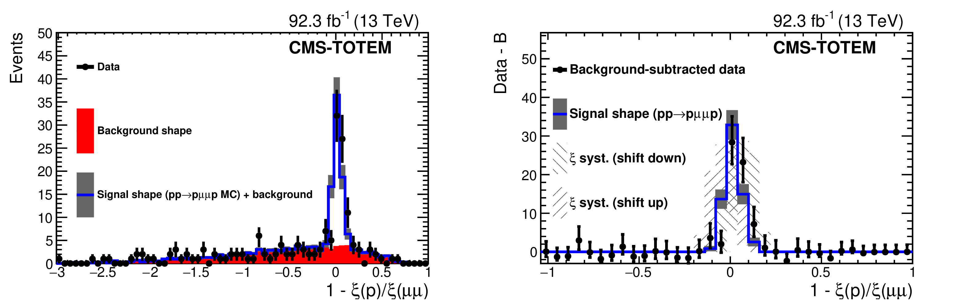
Figure 44:
One-dimensional projections of the correlation between $ \xi $(p) and $ \xi(\mu^{+}\mu^{-}) $, for the full 2017+2018 data sample and both arms combined, using the multi-RP algorithm. A minimum requirement of $ \xi(\mu^{+}\mu^{-}) > $ 0.04 is applied. The left plot shows the data compared with the background shape (solid histogram) estimated from sideband regions, and the signal shape obtained from simulation (open histogram). The right plot shows the data and signal shape in a narrower region, after subtracting the background component from the data. In the right plot the dark bands represent the statistical uncertainty due to the number of simulated events, whereas the two light shaded bands represent the effect of shifting the distribution up or down by the systematic uncertainty of the proton $ \xi $ reconstruction. The vertical bars on the data points represent statistical uncertainties. |
png pdf |
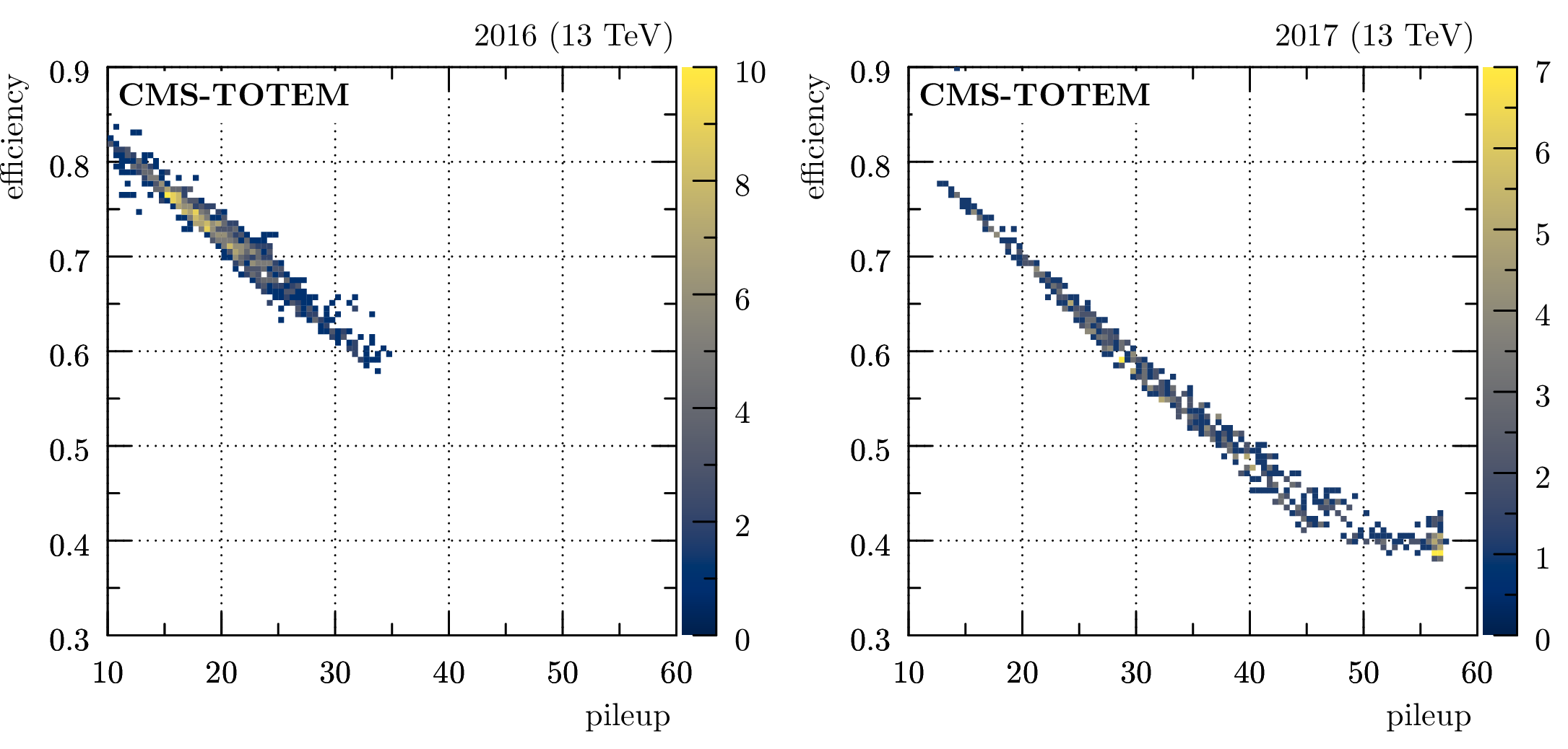
Figure 45:
Strip multiple track efficiency component versus pileup in the sector 45 near RP. The color code represents per-bin counts. Left: data-taking period between the first and the second 2016 Technical Stops. Right: data-taking period between the second and the third 2017 Technical Stops. |
png pdf |
Figure 46:
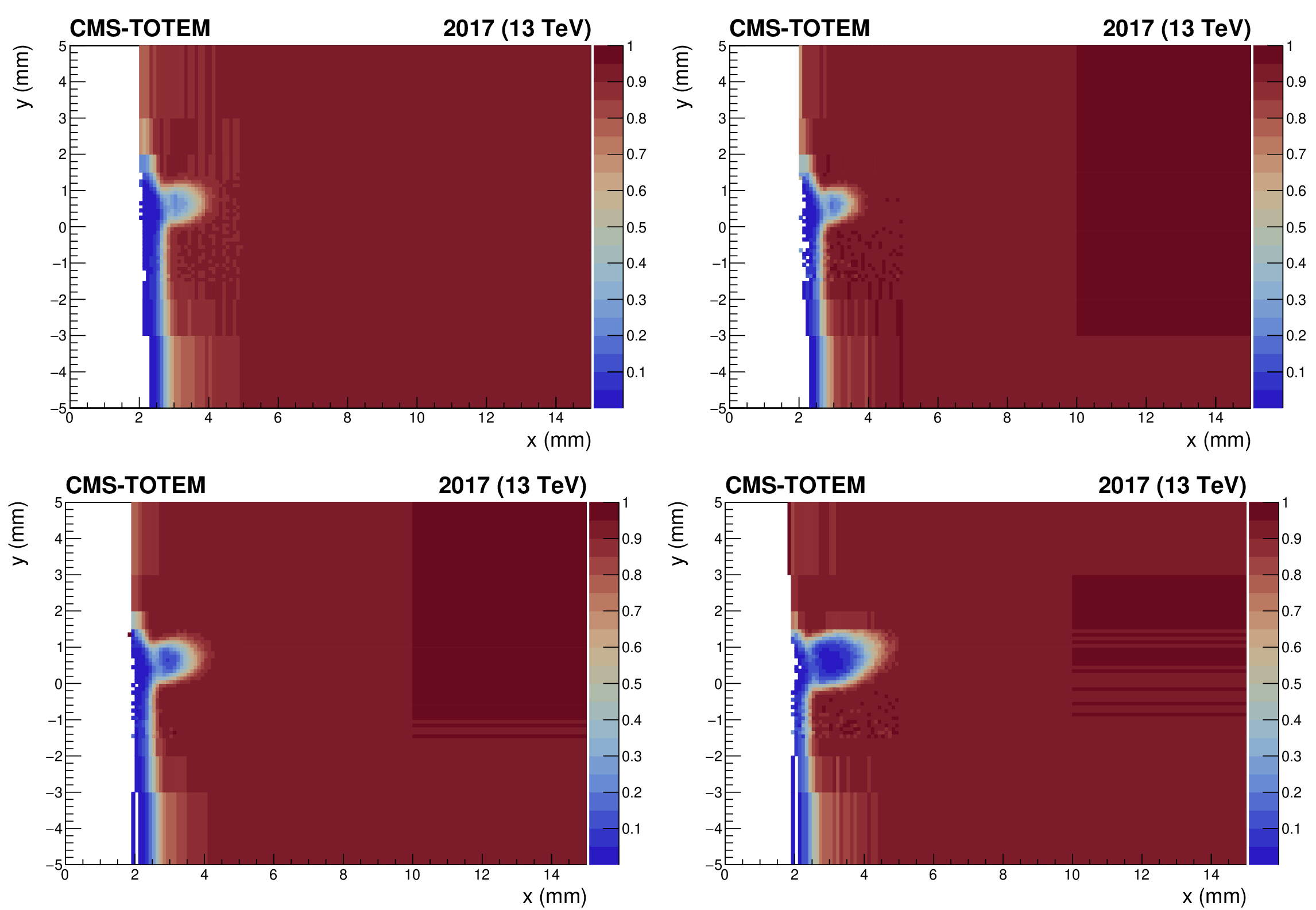
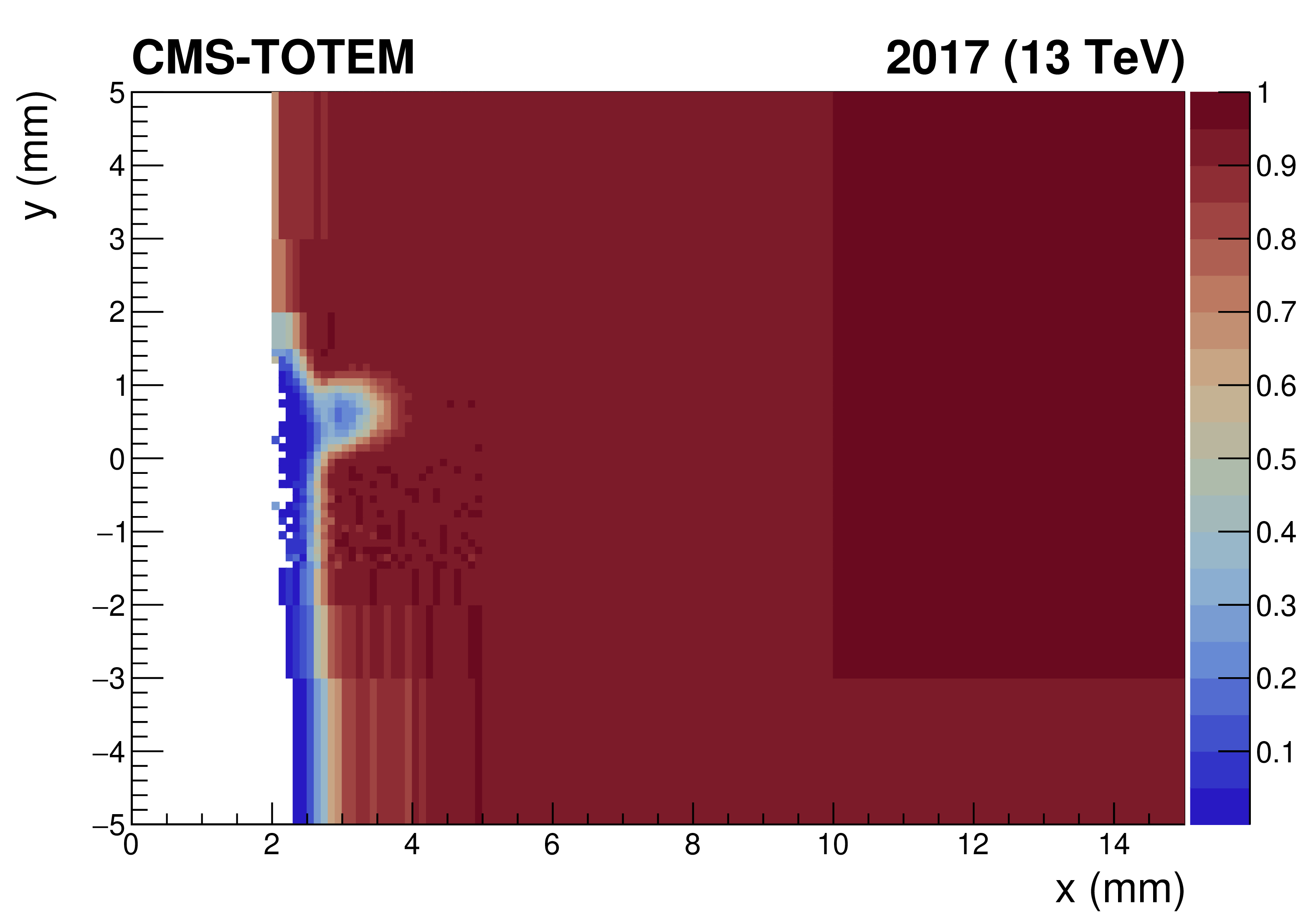
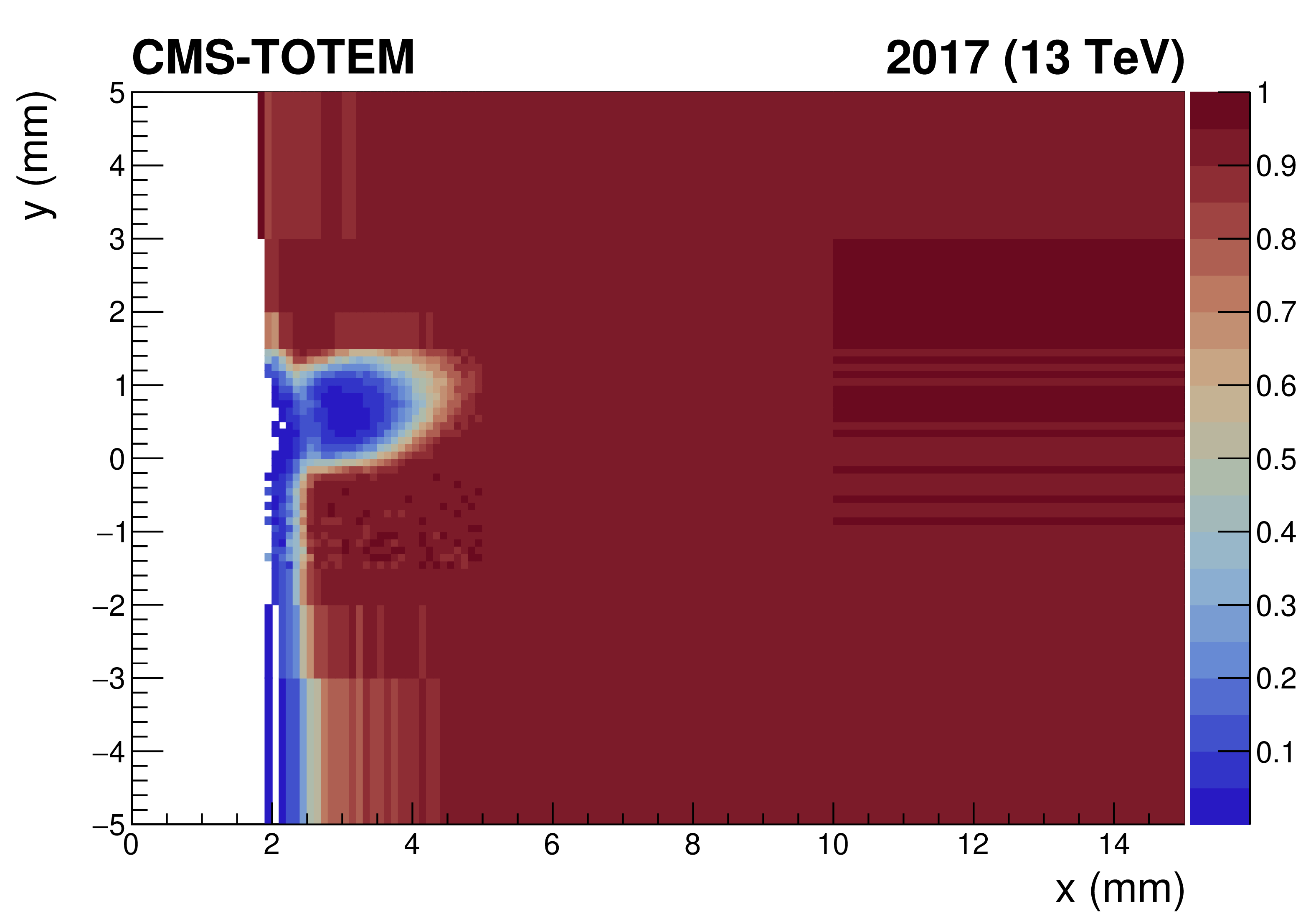
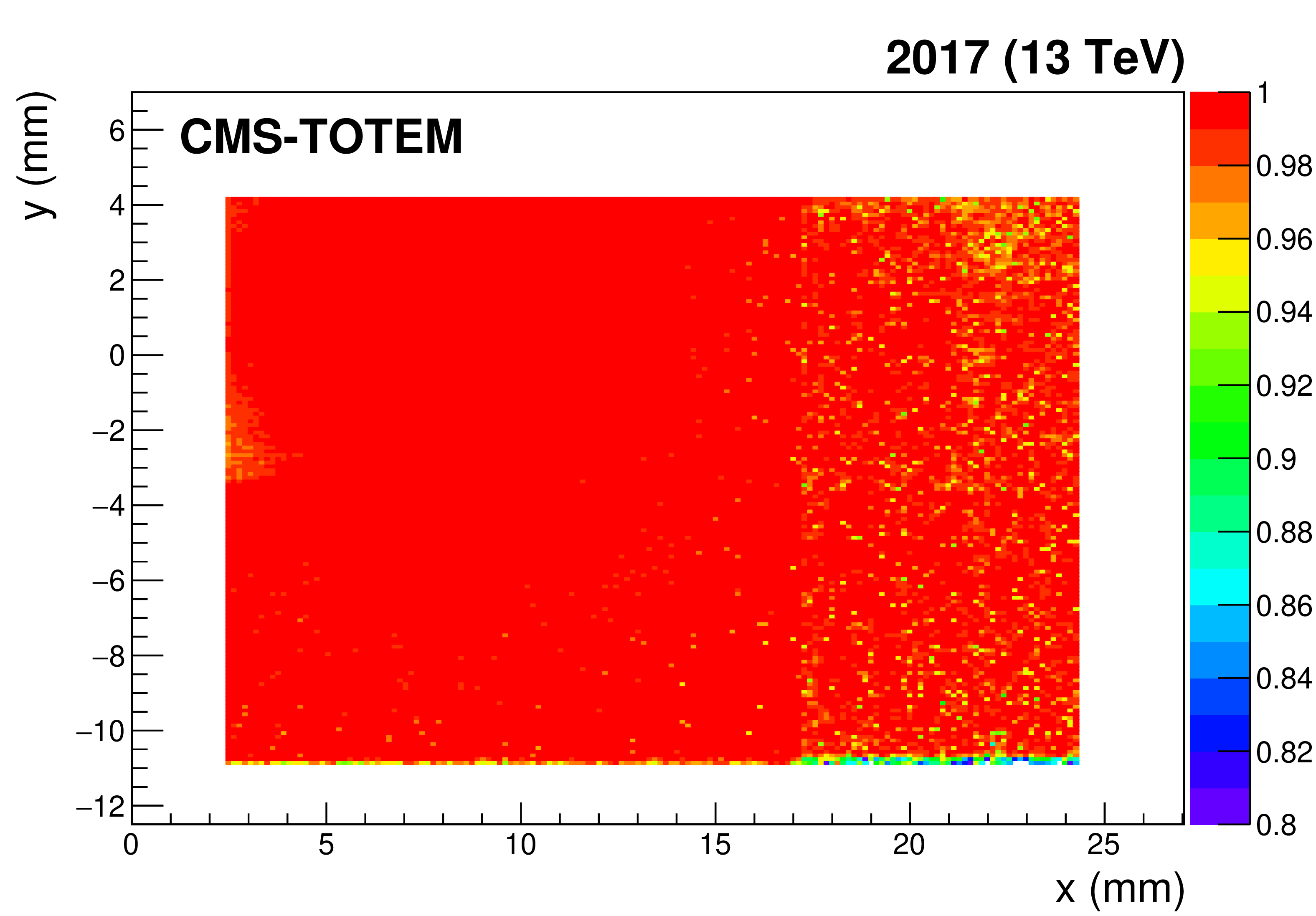
Strip detector tracking efficiency component (in color code) related to radiation effects, computed with data collected in 2017, over different consecutive data-taking periods. The figure shows the results for the sector 56 near station in 2017, as a function of the $ x-y $ coordinates of the track measured in the tagging far station, for different periods. Each period is defined as an interval in integrated luminosity computed since the detector installation. Upper left: $ L_\text{int} = $ 0--9 fb$ ^{-1} $. Upper right: $ L_\text{int} = $ 9--10.7. Lower left: $ L_\text{int} = $ 10.7--18.5 fb$ ^{-1} $. Lower right: $ L_\text{int} = $ 18.5--22.2 fb$ ^{-1} $. |
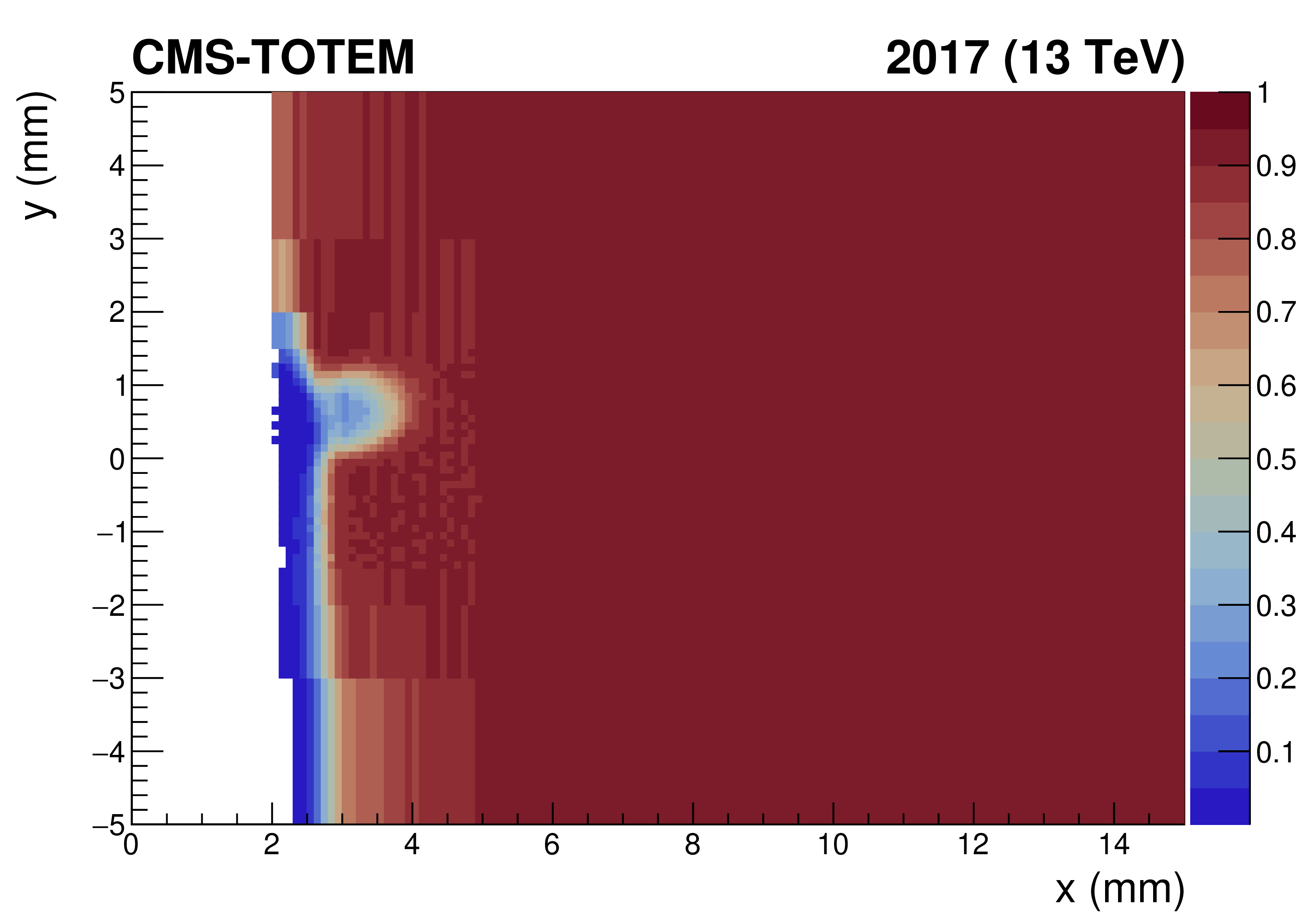
png pdf |
Figure 46-a:
Strip detector tracking efficiency component (in color code) related to radiation effects, computed with data collected in 2017, over different consecutive data-taking periods. The figure shows the results for the sector 56 near station in 2017, as a function of the $ x-y $ coordinates of the track measured in the tagging far station, for different periods. Each period is defined as an interval in integrated luminosity computed since the detector installation. Upper left: $ L_\text{int} = $ 0--9 fb$ ^{-1} $. Upper right: $ L_\text{int} = $ 9--10.7. Lower left: $ L_\text{int} = $ 10.7--18.5 fb$ ^{-1} $. Lower right: $ L_\text{int} = $ 18.5--22.2 fb$ ^{-1} $. |
png pdf |
Figure 46-b:
Strip detector tracking efficiency component (in color code) related to radiation effects, computed with data collected in 2017, over different consecutive data-taking periods. The figure shows the results for the sector 56 near station in 2017, as a function of the $ x-y $ coordinates of the track measured in the tagging far station, for different periods. Each period is defined as an interval in integrated luminosity computed since the detector installation. Upper left: $ L_\text{int} = $ 0--9 fb$ ^{-1} $. Upper right: $ L_\text{int} = $ 9--10.7. Lower left: $ L_\text{int} = $ 10.7--18.5 fb$ ^{-1} $. Lower right: $ L_\text{int} = $ 18.5--22.2 fb$ ^{-1} $. |

png pdf |
Figure 46-c:
Strip detector tracking efficiency component (in color code) related to radiation effects, computed with data collected in 2017, over different consecutive data-taking periods. The figure shows the results for the sector 56 near station in 2017, as a function of the $ x-y $ coordinates of the track measured in the tagging far station, for different periods. Each period is defined as an interval in integrated luminosity computed since the detector installation. Upper left: $ L_\text{int} = $ 0--9 fb$ ^{-1} $. Upper right: $ L_\text{int} = $ 9--10.7. Lower left: $ L_\text{int} = $ 10.7--18.5 fb$ ^{-1} $. Lower right: $ L_\text{int} = $ 18.5--22.2 fb$ ^{-1} $. |
png pdf |
Figure 46-d:
Strip detector tracking efficiency component (in color code) related to radiation effects, computed with data collected in 2017, over different consecutive data-taking periods. The figure shows the results for the sector 56 near station in 2017, as a function of the $ x-y $ coordinates of the track measured in the tagging far station, for different periods. Each period is defined as an interval in integrated luminosity computed since the detector installation. Upper left: $ L_\text{int} = $ 0--9 fb$ ^{-1} $. Upper right: $ L_\text{int} = $ 9--10.7. Lower left: $ L_\text{int} = $ 10.7--18.5 fb$ ^{-1} $. Lower right: $ L_\text{int} = $ 18.5--22.2 fb$ ^{-1} $. |
png pdf |
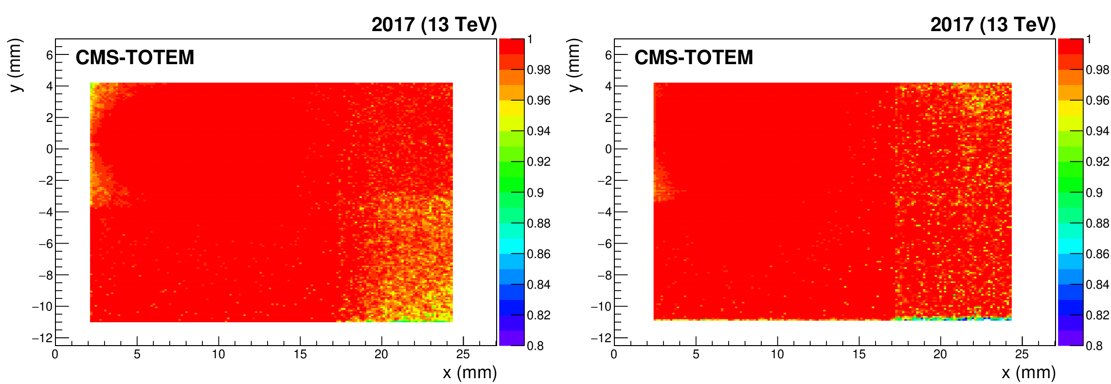
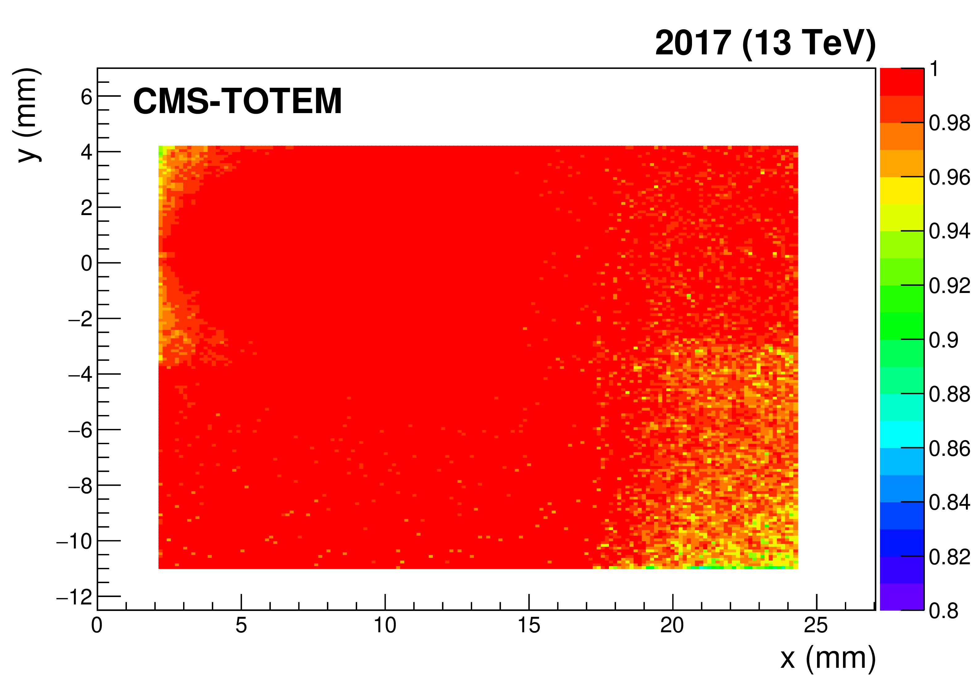
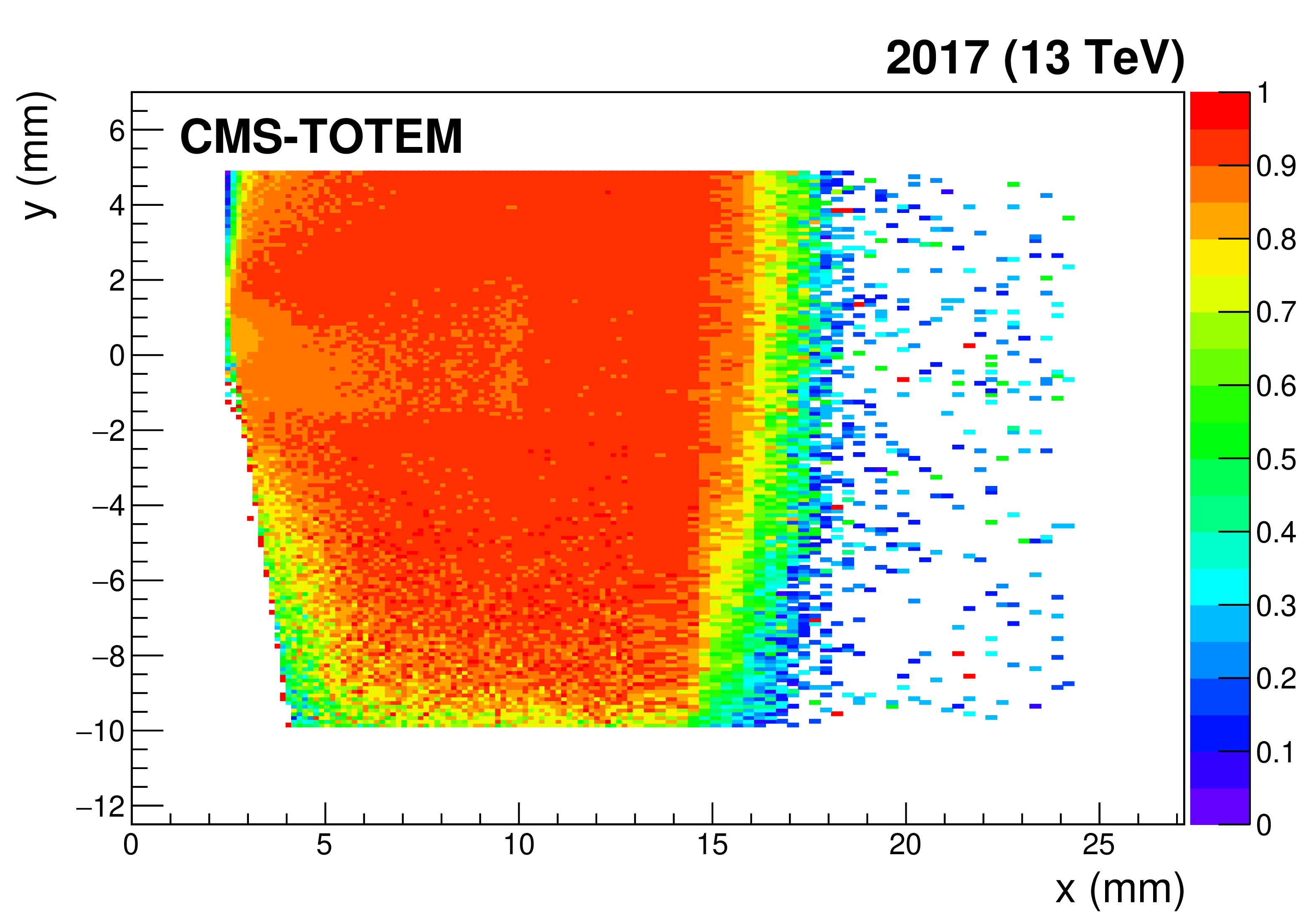
Figure 47:
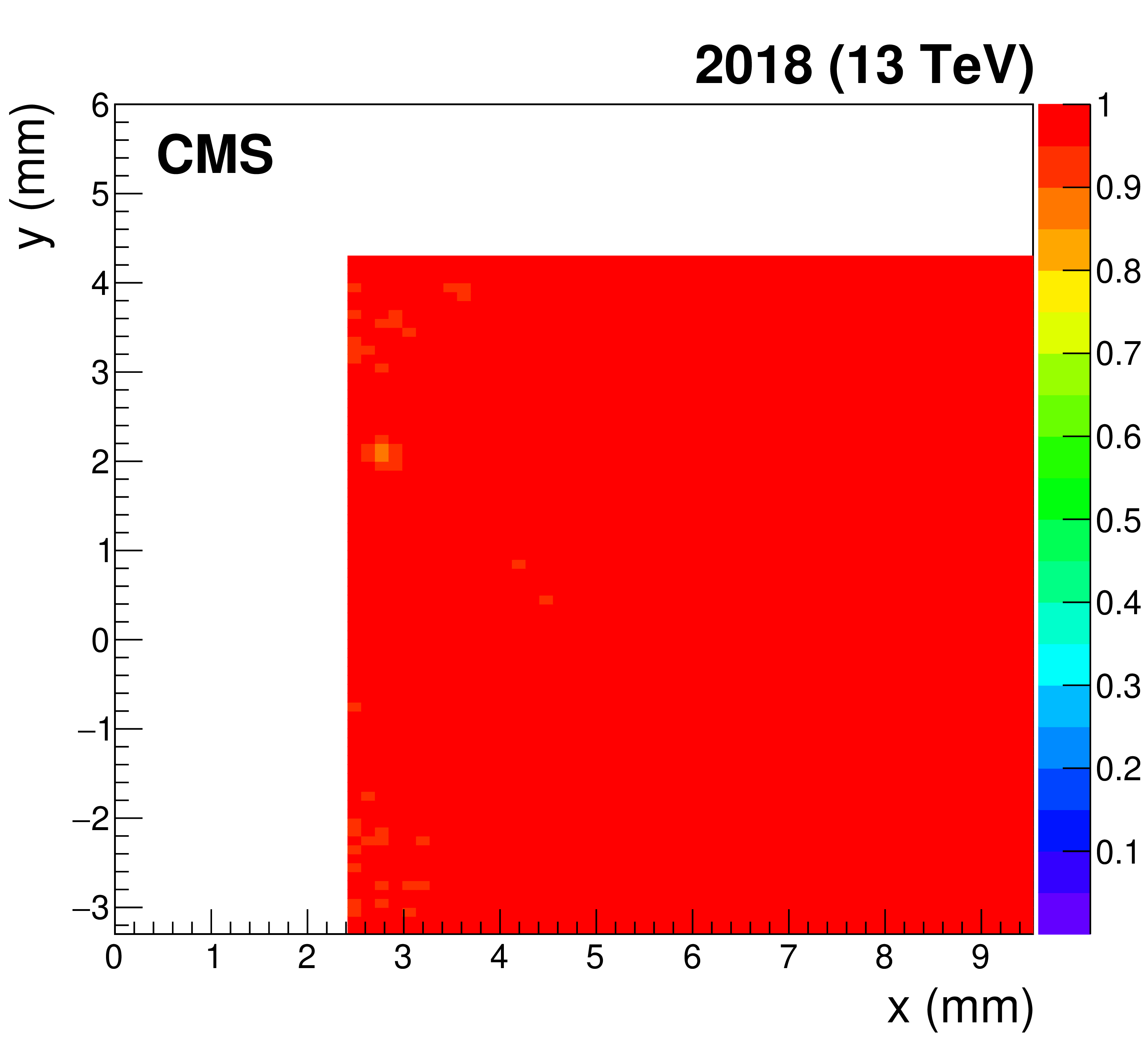
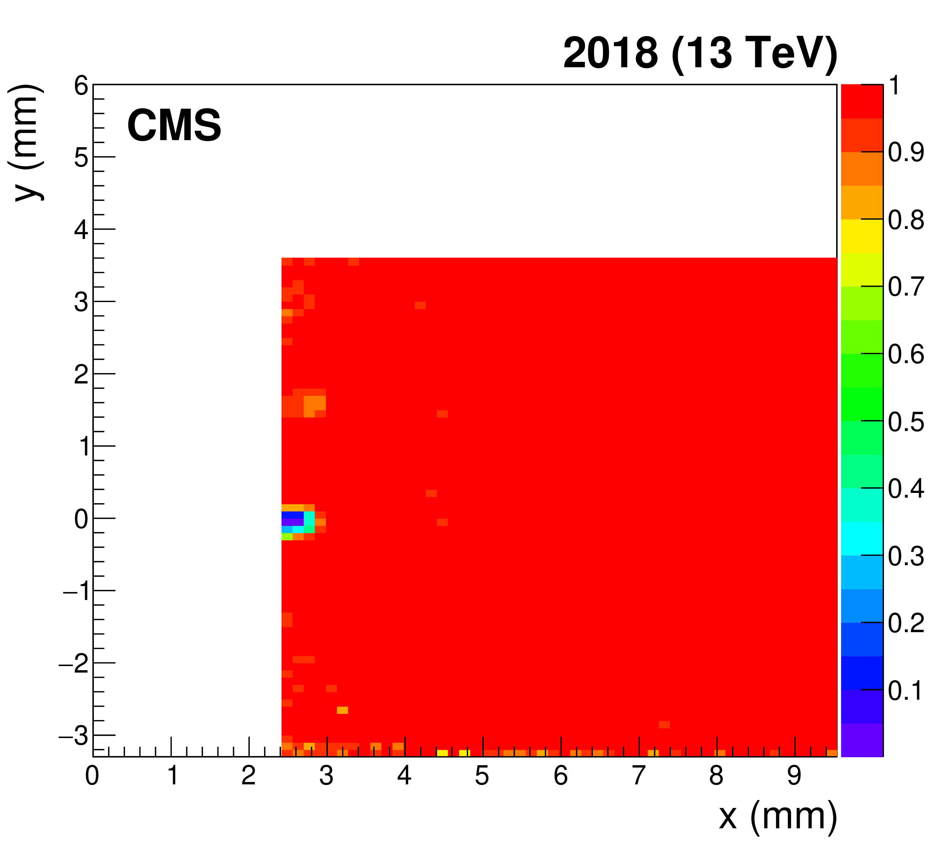
Pixel detector efficiency map, computed on the first data collected in 2017 for sector 45 (left) and 56 (right), and shown as a function of the $ x-y $ coordinates. The color code represents the efficiency value. The slightly lower efficiency on the bottom-right corner of the sector 45 far station is due to suboptimal detector configuration. |
png pdf |
Figure 47-a:
Pixel detector efficiency map, computed on the first data collected in 2017 for sector 45 (left) and 56 (right), and shown as a function of the $ x-y $ coordinates. The color code represents the efficiency value. The slightly lower efficiency on the bottom-right corner of the sector 45 far station is due to suboptimal detector configuration. |
png pdf |
Figure 47-b:
Pixel detector efficiency map, computed on the first data collected in 2017 for sector 45 (left) and 56 (right), and shown as a function of the $ x-y $ coordinates. The color code represents the efficiency value. The slightly lower efficiency on the bottom-right corner of the sector 45 far station is due to suboptimal detector configuration. |
png pdf |
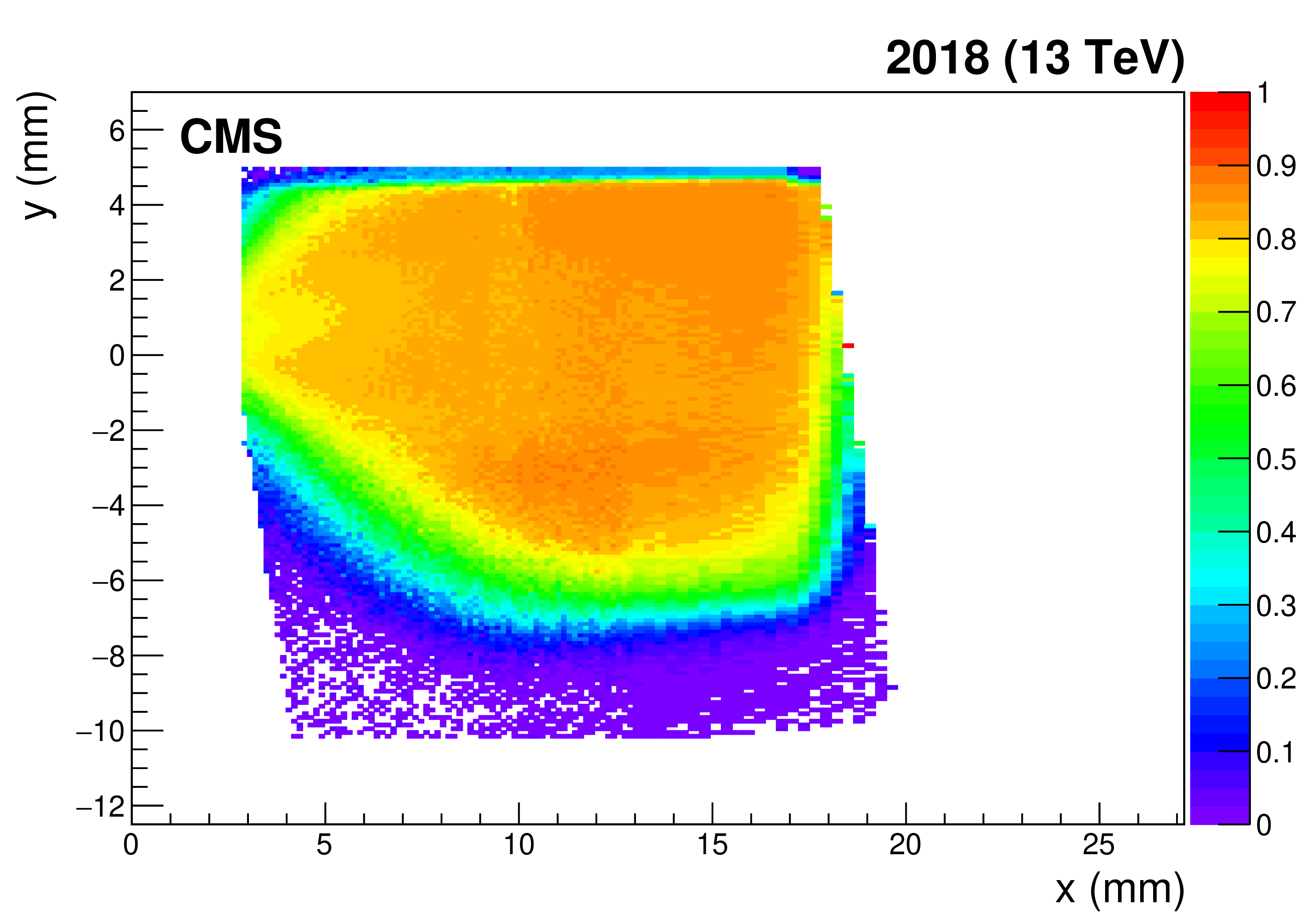
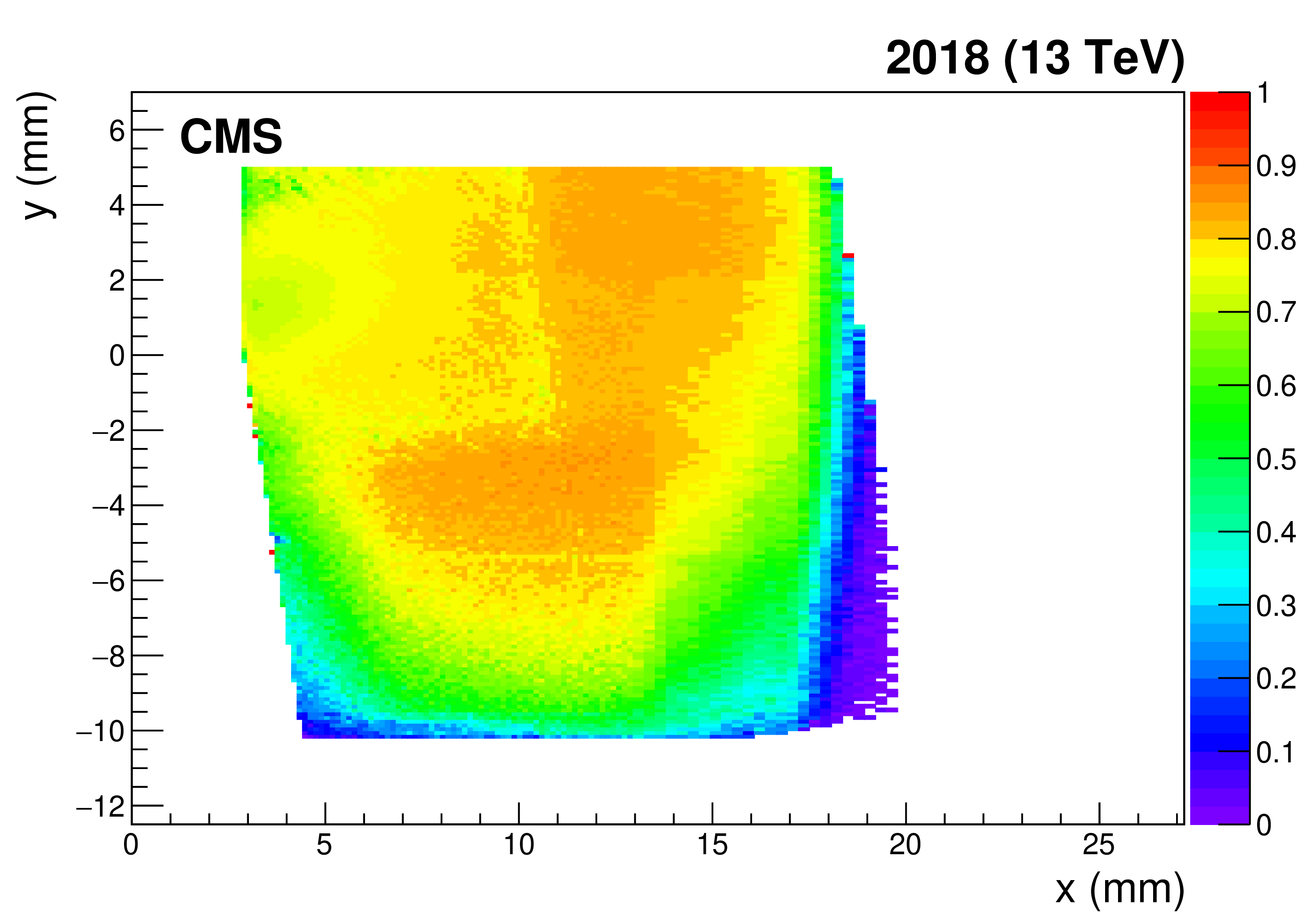
Figure 48:
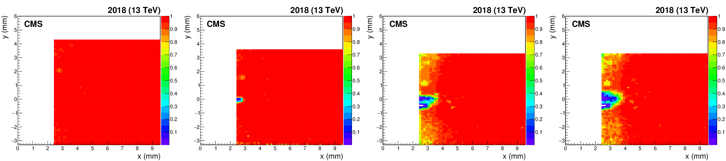
Evolution of the pixel detector package efficiency (in color code) in the detector region closest to the beam for the sector 45 far station, computed with data collected in 2018. During each TS, detectors in both sectors were vertically shifted by 0.5 mm downwards. From left to right: efficiency computed after the detector collected $ L_\text{int} = $, 21.0, 50.3, 57.8 fb$ ^{-1} $, respectively. Each efficiency map is produced using a small data sample of $ \sim $ 0.5 fb$ ^{-1} $. |
png pdf |
Figure 48-a:
Evolution of the pixel detector package efficiency (in color code) in the detector region closest to the beam for the sector 45 far station, computed with data collected in 2018. During each TS, detectors in both sectors were vertically shifted by 0.5 mm downwards. From left to right: efficiency computed after the detector collected $ L_\text{int} = $, 21.0, 50.3, 57.8 fb$ ^{-1} $, respectively. Each efficiency map is produced using a small data sample of $ \sim $ 0.5 fb$ ^{-1} $. |
png pdf |
Figure 48-b:
Evolution of the pixel detector package efficiency (in color code) in the detector region closest to the beam for the sector 45 far station, computed with data collected in 2018. During each TS, detectors in both sectors were vertically shifted by 0.5 mm downwards. From left to right: efficiency computed after the detector collected $ L_\text{int} = $, 21.0, 50.3, 57.8 fb$ ^{-1} $, respectively. Each efficiency map is produced using a small data sample of $ \sim $ 0.5 fb$ ^{-1} $. |

png pdf |
Figure 48-c:
Evolution of the pixel detector package efficiency (in color code) in the detector region closest to the beam for the sector 45 far station, computed with data collected in 2018. During each TS, detectors in both sectors were vertically shifted by 0.5 mm downwards. From left to right: efficiency computed after the detector collected $ L_\text{int} = $, 21.0, 50.3, 57.8 fb$ ^{-1} $, respectively. Each efficiency map is produced using a small data sample of $ \sim $ 0.5 fb$ ^{-1} $. |

png pdf |
Figure 48-d:
Evolution of the pixel detector package efficiency (in color code) in the detector region closest to the beam for the sector 45 far station, computed with data collected in 2018. During each TS, detectors in both sectors were vertically shifted by 0.5 mm downwards. From left to right: efficiency computed after the detector collected $ L_\text{int} = $, 21.0, 50.3, 57.8 fb$ ^{-1} $, respectively. Each efficiency map is produced using a small data sample of $ \sim $ 0.5 fb$ ^{-1} $. |

png pdf |
Figure 49:
Multi-RP efficiency factor as a function of the $ x-y $ coordinates that includes the efficiency of the detectors installed in the far RPs, the efficiency of the multi-RP reconstruction algorithm, and the probability that a proton propagates from the near RPs to the far ones without interacting. The color code represents the efficiency value. Top: multi-RP efficiency in sector 45 (left) and 56 (right) at the beginning of the 2017 data-taking. Bottom: multi-RP efficiency in sector 45 (left) and 56 (right) at the beginning of the 2018 data-taking. |

png pdf |
Figure 49-a:
Multi-RP efficiency factor as a function of the $ x-y $ coordinates that includes the efficiency of the detectors installed in the far RPs, the efficiency of the multi-RP reconstruction algorithm, and the probability that a proton propagates from the near RPs to the far ones without interacting. The color code represents the efficiency value. Top: multi-RP efficiency in sector 45 (left) and 56 (right) at the beginning of the 2017 data-taking. Bottom: multi-RP efficiency in sector 45 (left) and 56 (right) at the beginning of the 2018 data-taking. |
png pdf |
Figure 49-b:
Multi-RP efficiency factor as a function of the $ x-y $ coordinates that includes the efficiency of the detectors installed in the far RPs, the efficiency of the multi-RP reconstruction algorithm, and the probability that a proton propagates from the near RPs to the far ones without interacting. The color code represents the efficiency value. Top: multi-RP efficiency in sector 45 (left) and 56 (right) at the beginning of the 2017 data-taking. Bottom: multi-RP efficiency in sector 45 (left) and 56 (right) at the beginning of the 2018 data-taking. |
png pdf |
Figure 49-c:
Multi-RP efficiency factor as a function of the $ x-y $ coordinates that includes the efficiency of the detectors installed in the far RPs, the efficiency of the multi-RP reconstruction algorithm, and the probability that a proton propagates from the near RPs to the far ones without interacting. The color code represents the efficiency value. Top: multi-RP efficiency in sector 45 (left) and 56 (right) at the beginning of the 2017 data-taking. Bottom: multi-RP efficiency in sector 45 (left) and 56 (right) at the beginning of the 2018 data-taking. |
png pdf |
Figure 49-d:
Multi-RP efficiency factor as a function of the $ x-y $ coordinates that includes the efficiency of the detectors installed in the far RPs, the efficiency of the multi-RP reconstruction algorithm, and the probability that a proton propagates from the near RPs to the far ones without interacting. The color code represents the efficiency value. Top: multi-RP efficiency in sector 45 (left) and 56 (right) at the beginning of the 2017 data-taking. Bottom: multi-RP efficiency in sector 45 (left) and 56 (right) at the beginning of the 2018 data-taking. |

png pdf |
Figure 50:
Fraction of reconstructed multi-RP protons, as a function of $ \xi_\text{multi} $, for a proton sample produced with the PPS direct simulation. Acceptance and efficiency effects are taken into account. The left and right plots show results for sector 45 and 56, respectively. The efficiency systematic uncertainties, computed by combining in quadrature the systematic uncertainties estimated for each efficiency factor, are 10, 2.7, and 2.1% for 2016, 2017, and 2018, respectively. |

png pdf |
Figure 50-a:
Fraction of reconstructed multi-RP protons, as a function of $ \xi_\text{multi} $, for a proton sample produced with the PPS direct simulation. Acceptance and efficiency effects are taken into account. The left and right plots show results for sector 45 and 56, respectively. The efficiency systematic uncertainties, computed by combining in quadrature the systematic uncertainties estimated for each efficiency factor, are 10, 2.7, and 2.1% for 2016, 2017, and 2018, respectively. |

png pdf |
Figure 50-b:
Fraction of reconstructed multi-RP protons, as a function of $ \xi_\text{multi} $, for a proton sample produced with the PPS direct simulation. Acceptance and efficiency effects are taken into account. The left and right plots show results for sector 45 and 56, respectively. The efficiency systematic uncertainties, computed by combining in quadrature the systematic uncertainties estimated for each efficiency factor, are 10, 2.7, and 2.1% for 2016, 2017, and 2018, respectively. |

png pdf |
Figure 51:
Correlation between the z vertex position measured in the central CMS tracker, and the time difference of the protons measured in the PPS detectors. Left: low-pileup data with protons on both arms. Right: mixed background sample, with both protons chosen from a different event than that of the central vertex. The red dashed line indicates the ideal slope of c/2, which would be expected with zero background. The blue points with error bars show the profile of the data, with the mean and RMS of the time difference in each bin of the position z. |
png pdf |
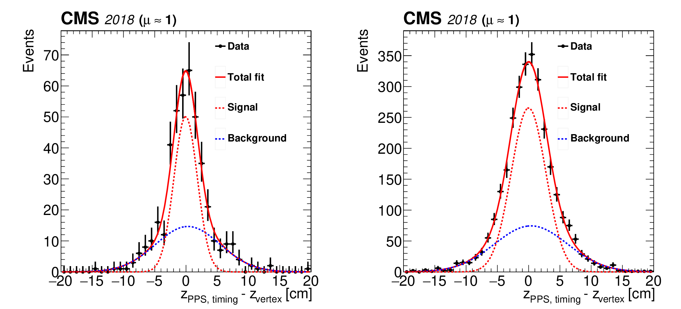
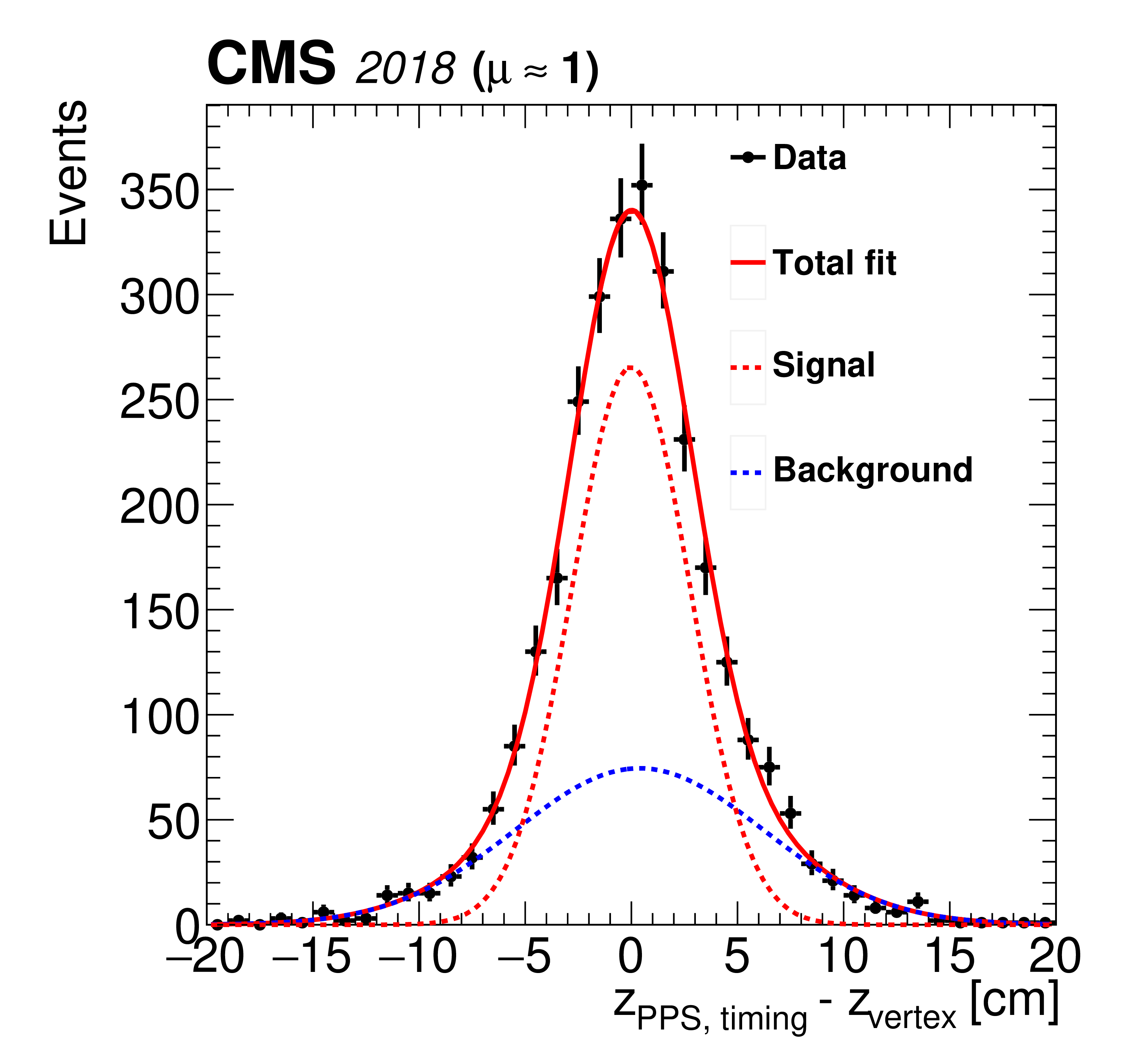
Figure 52:
Vertex resolution obtained from the difference of proton arrival times, using data collected during low-pileup runs. Left: resolution for two-arm multi-RP events, using the subset of events with a predicted resolution $ < $100\,ps for both arms. Right: resolution for two-arm events using all events with exactly one multi-RP proton in each arm. The fitted signal (red dashed line) and background (blue dashed line) are shown separately, with the means and widths of both components treated as free parameters. The bars on the data points indicate the statistical uncertainties. |
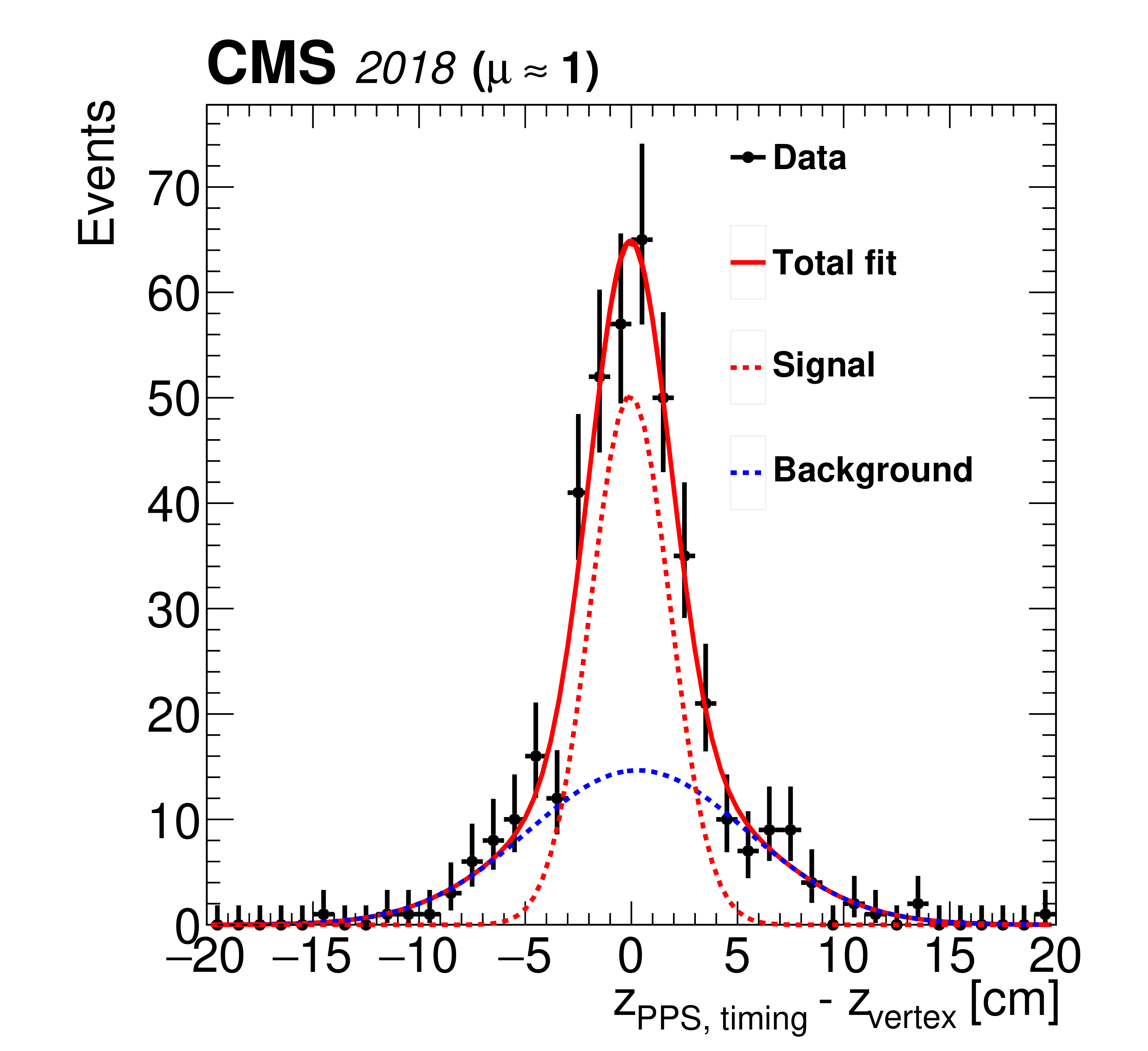
png pdf |
Figure 52-a:
Vertex resolution obtained from the difference of proton arrival times, using data collected during low-pileup runs. Left: resolution for two-arm multi-RP events, using the subset of events with a predicted resolution $ < $100\,ps for both arms. Right: resolution for two-arm events using all events with exactly one multi-RP proton in each arm. The fitted signal (red dashed line) and background (blue dashed line) are shown separately, with the means and widths of both components treated as free parameters. The bars on the data points indicate the statistical uncertainties. |
png pdf |
Figure 52-b:
Vertex resolution obtained from the difference of proton arrival times, using data collected during low-pileup runs. Left: resolution for two-arm multi-RP events, using the subset of events with a predicted resolution $ < $100\,ps for both arms. Right: resolution for two-arm events using all events with exactly one multi-RP proton in each arm. The fitted signal (red dashed line) and background (blue dashed line) are shown separately, with the means and widths of both components treated as free parameters. The bars on the data points indicate the statistical uncertainties. |
| Tables | |
png pdf |
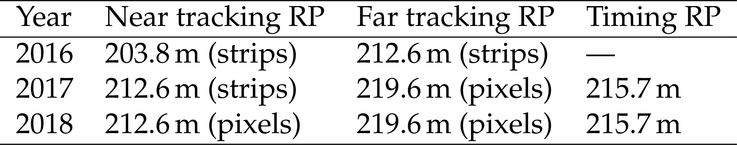
Table 1:
RP configurations in different years. The numbers represent the RP distances from the IP5, the sensor technology is indicated in parentheses. The RP layout was always symmetric about the IP5. There were always two tracking RPs per arm; the one closer to the IP5 is denoted as ``near'', the other as ``far''. In 2016, no timing RPs were used. |
png pdf |
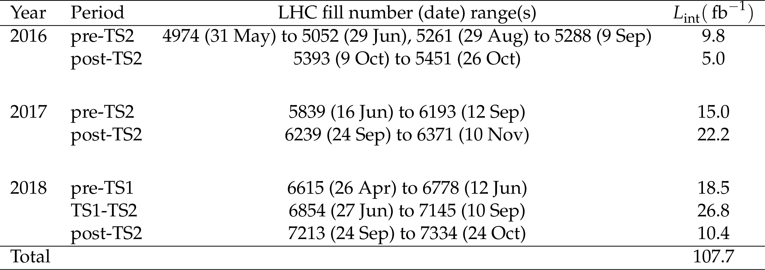
Table 2:
List of the PPS periods with distinct LHC and/or RP settings. The third column from left indicates the time ranges where PPS recorded data. $ L_\text{int} $ corresponds to the integrated luminosity recorded during runs certified for use in physics analysis. |
png pdf |
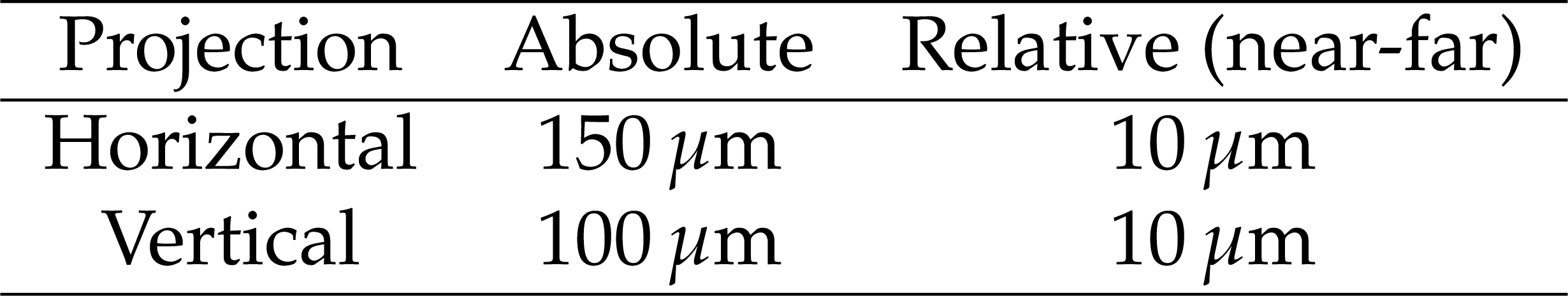
Table 3:
Summary of per-fill alignment uncertainties. |
png pdf |
Table 4:
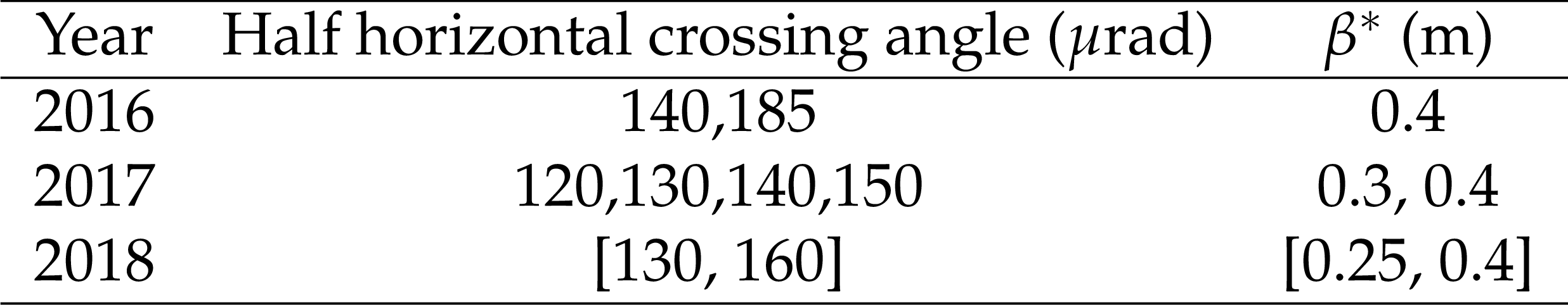
Summary of main beam parameter values, crossing angle and $ \beta^{*} $, during the Run 2 period per year. In 2017 the values changed in discrete steps, whereas in 2018 there was a continuous change within the interval. |

png pdf |
Table 5:
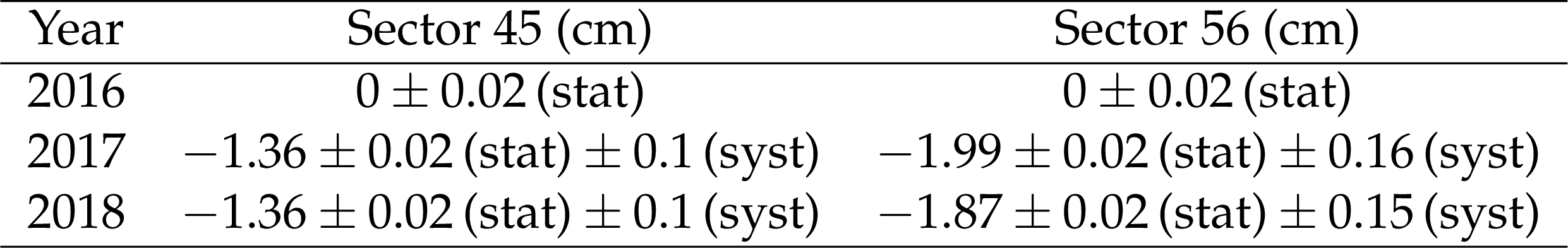
Measured horizontal dispersion values $ D_{x} $ in the near RP at low $ \xi $ between 2% and 4% (the exact $ \xi_\mathrm{F} $ value depends on the detector and the year). The resulting $ D_{x} $ value is the weighted average of the $ L_{y}= $ 0 and (semi)-exclusive $ \mu\mu $ results. The quoted 8% uncertainty in $ D_{x} $ applies to the $ x_{d} $ function as well. |
png pdf |
Table 6:
Final measured vertical dispersion values $ D_{y} $ in the near RP per year. The uncertainty is derived conservatively from the measured $ (D_{y}/D_{x}) $ ratio. |
png pdf |
Table 7:
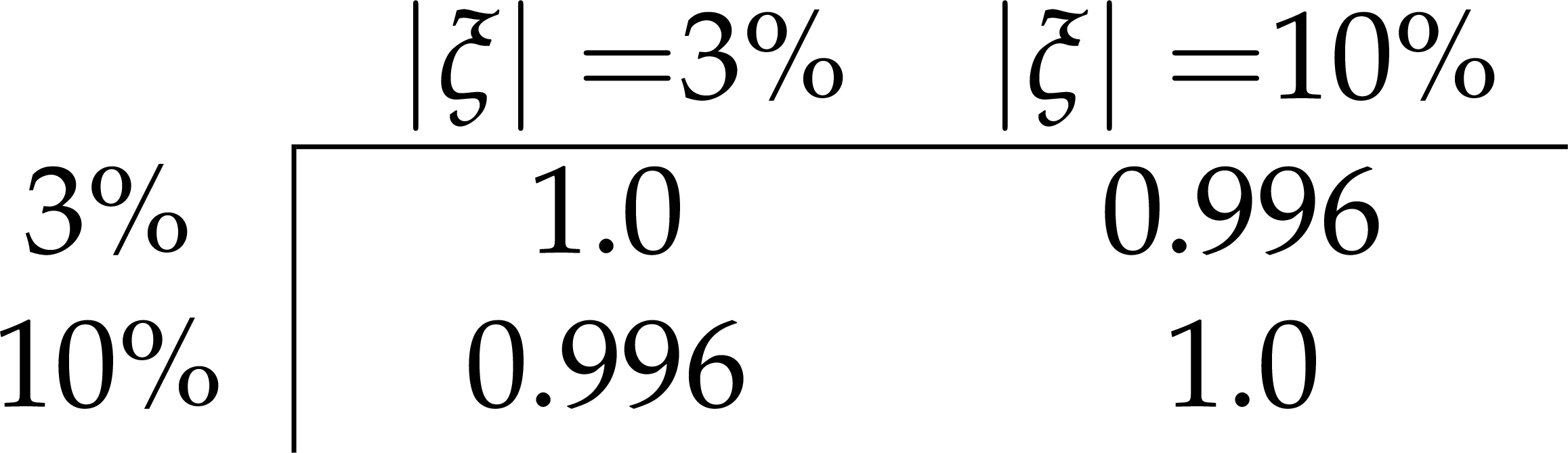
The correlation matrix for $ L_{x} $ between different $ \xi $ values for the detector RP56-220-fr vertical. |
png pdf |
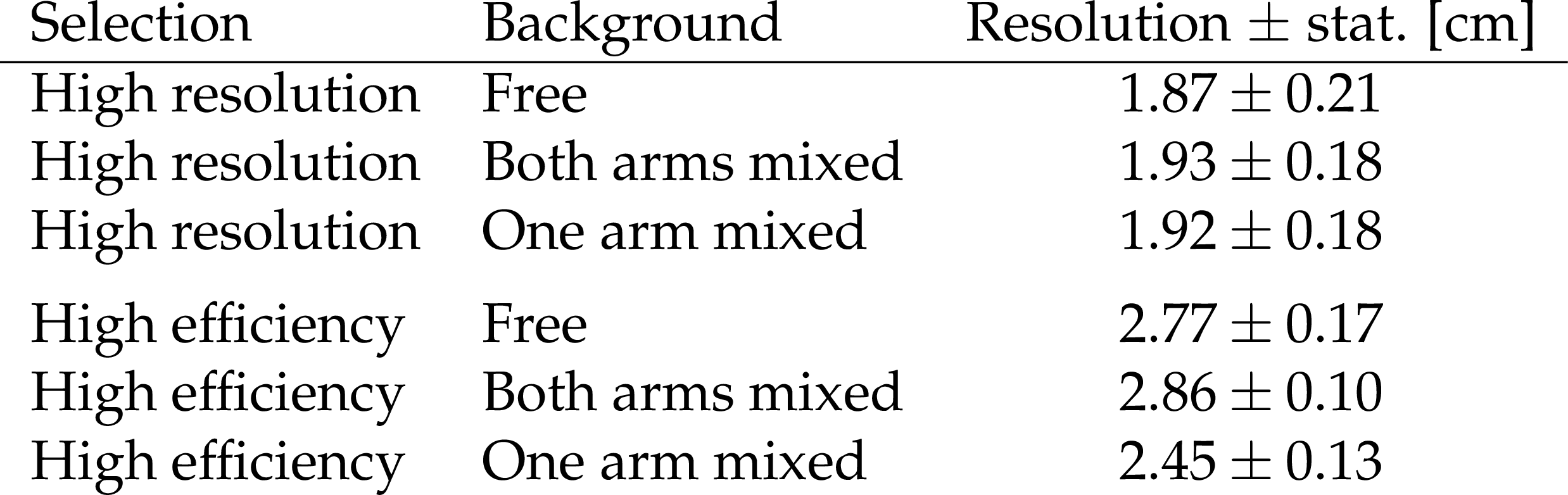
Table 8:
Vertex position resolutions obtained from the proton times measured in the PPS timing detectors, using different selection criteria and background shape assumptions. The sample of events in the high resolution and high efficiency categories is always the same, therefore the statistical uncertainties are highly correlated. |
| Summary |
| The procedures developed to reconstruct the proton tracks from the signals detected in the CMS-TOTEM Precision Proton Spectrometer have been described. The performance of the reconstruction is studied with data from the LHC Run 2 of proton-proton collisions at 13 TeV energy, corresponding to an integrated luminosity of 107.7 fb$ ^{-1} $. A multi-step alignment of the detectors is performed. Alignment with respect to the LHC collimators is followed by relative alignment of the sensor planes within a Roman Pot (RP) and among all RPs. Then, global alignment is performed with respect to the LHC beam with elastic events collected in low luminosity runs, and is extrapolated to the RP's positions in the high luminosity fills. Finally, the timing detectors are aligned with respect to the tracking detectors. The alignment uncertainties are 150 $ \mu $m and 100 $ \mu $m in the horizontal and vertical projections, respectively. The precision of the relative alignment between near and far RPs is better than 10 $ \mu $m. A precise modelling of the LHC optics is a necessary precondition for the reconstruction. The track horizontal and vertical positions at the RPs can be obtained from the proton kinematics at the interaction point via the optical functions. The horizontal dispersion, $ D_x $, is calibrated using the $ L_y $ = 0 constraint from the data and a sample of (semi)exclusive dimuon events. The horizontal dispersion carries information on the dependence of the optics model on the horizontal crossing angle. The parameters of the optics model (half crossing angle, quadrupole positions and magnet strengths) are determined from a fit to the beam position obtained from the beam position monitors and RPs, and the measured horizontal dispersion. The vertical dispersion is estimated from the vertical vertex position and the vertical scattering angle. The effective length and its derivative with respect to the position along the beam are calibrated at $ \xi= $ 0 using elastic events, where $ \xi $ is the relative momentum loss of a forward proton. An approximate determination of $ \xi $ and of the vertical scattering angle can be performed with the information of a single RP. A more accurate and complete determination of the proton kinematics is obtained by combining the information from both tracking RPs in each arm. The two reconstruction methods are referred to as single- and multi-RP. The single-RP reconstruction has significantly lower resolution especially because of the neglected term proportional to the horizontal scattering angle. A large bias at small and large $ \xi $ is hence observed given the asymmetric acceptance in the horizontal scattering angle. The multi-RP reconstruction has a much better resolution, negligible bias and comparable systematic uncertainties at small and intermediate $ \xi $. At large $ \xi $, the effect of the systematic uncertainty in the optics calibration is larger for the multi-RP reconstruction. A fast simulation of the proton propagation along the beam line and of the PPS detectors has been developed. It includes realistic beam parameters and beam smearing effects; the calibrated optics model; the LHC aperture limitations; the simulation of the detector planes and sensor geometry, acceptance and spatial resolution; and a realistic simulation of the proton arrival time. A sample of (semi)exclusive dimuon events has been analyzed in order to validate the proton reconstruction. A good correlation between the measured proton $ \xi $ values and those inferred from the dimuon system is observed. The data are well described by the simulation. As expected, the multi-RP reconstruction shows a better resolution than the single-RP method. The proton reconstruction efficiency has been measured for the different data taking periods. It depends on different multiplicative factors describing the sensor efficiency, the reconstruction algorithm efficiency, and the effect of interactions along the proton path. The silicon pixel detector efficiency is caused by the radiation damage. The silicon strip detector efficiency loss is caused by radiation damage and in addition by multiple tracks in the same event. The effect of radiation damage is studied as a function of the integrated luminosity and is significant in the region closest to the detector edge facing the beam. The efficiency of the multi-RP reconstruction is smaller than that for the single-RP reconstruction, because of the sensor efficiency of the extra RP, and the effect of multiple, ambiguous proton combinations between tracks from the near and far detectors. The correlation between the difference in arrival time of protons in the two detector arms and the $ z $ vertex position has been studied using low pileup data. The width of the $ z $ position residuals is consistent with the single-arm timing resolutions. For part of the data taking period they are better than 100 ps, corresponding to $ \approx $2 cm. The performance of the Precision Proton Spectrometer in Run 2 has proven the feasibility of continuously operating a near-beam proton spectrometer at a high luminosity hadron collider. PPS has had no impact on the operation of LHC in terms of background, heating, or impedance. The success of PPS has been made possible by two independent collaborations, CMS and TOTEM, joining forces to pursue a common physics interest. |
| References | ||||
| 1 | CMS Collaboration | The CMS experiment at the CERN LHC | JINST 3 (2008) S08004 | |
| 2 | TOTEM Collaboration | The TOTEM experiment at the CERN Large Hadron Collider | JINST 3 (2008) S08007 | |
| 3 | CMS and TOTEM Collaborations | CMS-TOTEM Precision Proton Spectrometer | Technical Report CERN-LHCC-2014-021, TOTEM-TDR-003, CMS-TDR-13, 2014 | |
| 4 | LHC Forward Physics Working Group Collaboration | LHC forward physics | JPG 43 (2016) 110201 | 1611.05079 |
| 5 | CMS Collaboration | The CMS Precision Proton Spectrometer at the HL-LHC --- expression of interest | technical report, 2021 | 2103.02752 |
| 6 | E. Chapon, C. Royon, and O. Kepka | Anomalous quartic WW gamma gamma, ZZ gamma gamma, and trilinear WW gamma couplings in two-photon processes at high luminosity at the LHC | PRD 81 (2010) 074003 | 0912.5161 |
| 7 | S. Fichet et al. | Light-by-light scattering with intact protons at the LHC: from Standard Model to New Physics | JHEP 02 (2015) 165 | 1411.6629 |
| 8 | C. Baldenegro, S. Fichet, G. von Gersdorff, and C. Royon | Searching for axion-like particles with proton tagging at the LHC | JHEP 06 (2018) 131 | 1803.10835 |
| 9 | CMS Collaboration | Performance of the CMS Level-1 trigger in proton-proton collisions at $ \sqrt{s} = $ 13 TeV | JINST 15 (2020) P10017 | CMS-TRG-17-001 2006.10165 |
| 10 | CMS Collaboration | The CMS trigger system | JINST 12 (2017) P01020 | CMS-TRG-12-001 1609.02366 |
| 11 | G. Ruggiero et al. | Characteristics of edgeless silicon detectors for the roman pots of the TOTEM experiment at the LHC | NIM A 604 (06) 242, 2009 | |
| 12 | TOTEM Collaboration | Diamond detectors for the TOTEM timing upgrade | JINST 12 (2017) P03007 | 1701.05227 |
| 13 | V. Sola et al. | Ultra-fast silicon detectors for 4D tracking | JINST 12 (2017) C02072 | |
| 14 | O. S. Bruning et al. | LHC design report | CERN Report CERN-2004-003-V-1, 2004 link |
|
| 15 | H. Wiedemann | Particle accelerator physics: Basic principles and linear beam dynamics | ||
| 16 | E. J. N. Wilson | An introduction to particle accelerators | Oxford University Press, Oxford, 2001 | |
| 17 | TOTEM Collaboration | LHC optics measurement with proton tracks detected by the roman pots of the TOTEM experiment | New J. Phys. 16 (2014) 103041 | 1406.0546 |
| 18 | F. Nemes | LHC optics determination with proton tracks measured in the CT-PPS detectors in 2016, before TS2 | Technical Report CERN-TOTEM-NOTE-2017-002, Mar, 2017 | |
| 19 | F. Willeke and G. Ripken | Methods of beam optics | AIP Conf. Proc. 184 (1989) 758 | |
| 20 | TOTEM Collaboration | Performance of the TOTEM detectors at the LHC | International Journal of Modern Physics A 28 (2013) 1330046 | |
| 21 | CMS Collaboration | Precision luminosity measurement in proton-proton collisions at $ \sqrt{s} = $ 13 TeV in 2015 and 2016 at CMS | EPJC 81 (2021) 800 | CMS-LUM-17-003 2104.01927 |
| 22 | CMS Collaboration | CMS luminosity measurement for the 2017 data-taking period at $ \sqrt{s} = $ 13 TeV | CMS Physics Analysis Summary , CERN, Geneva, 2018 CMS-PAS-LUM-17-004 |
CMS-PAS-LUM-17-004 |
| 23 | CMS Collaboration | CMS luminosity measurement for the 2018 data-taking period at $ \sqrt{s} = $ 13 TeV | CMS Physics Analysis Summary , CERN, Geneva, 2019 CMS-PAS-LUM-18-002 |
CMS-PAS-LUM-18-002 |
| 24 | J. Ka | Elastic scattering at the LHC | PhD thesis, Charles U, 2011 link |
|
| 25 | TOTEM Collaboration | Evidence for non-exponential elastic proton-proton differential cross-section at low $ |t| $ and $ \sqrt{s} $=8 TeV by TOTEM | NPB 899 (2015) 527 | 1503.08111 |
| 26 | J. Kaspar | Alignment of CT-PPS detectors in 2016, before TS2 | Technical Report CERN-TOTEM-NOTE-2017-001, Mar, 2017 | |
| 27 | S. Fartoukh | Experience with the ATS optics | in 7th Evian Workshop on LHC beam operation, CERN, 2017 | |
| 28 | W. Herr | Features and implications of different LHC crossing schemes | Technical Report LHC-Project-Report-628, CERN-LHC-Project-Report-628, CERN, Geneva, Feb, 2003 | |
| 29 | H. Grote and F. Schmidt | MAD-X: An upgrade from MAD8 | in Proc. Particle Accelerator Conf., IEEE, 2003 | |
| 30 | R. Billen and C. Roderick | The LHC logging service: capturing, storing and using time-series data for the world's largest scientific instrument | Technical Report AB-Note-2006-046. CERN-AB-Note-2006-046, CERN, Nov, 2006 | |
| 31 | C. Roderick and R. Billen | The LSA database to drive the accelerator settings | in Proc. 12th Int. Conf. on accelerator and large experimental physics control systems. CERN, Geneva, Nov, 2009 | |
| 32 | N. Aquilina et al. | The FiDel model at 7 TeV | in Proc. 5th Int. Particle Accelerator Conf. (IPAC14) 2014 link |
|
| 33 | F. J. Nemes | Elastic scattering of protons at the TOTEM experiment at the LHC | PhD thesis, Eotvos U, 2015 | |
| 34 | CMS and TOTEM Collaborations | Observation of proton-tagged, central (semi)exclusive production of high-mass lepton pairs in pp c ollisions at 13 TeV with the CMS-TOTEM precision proton spectrometer | JHEP 07 (2018) 153 | 1803.04496 |
| 35 | F. James and M. Roos | Minuit: a system for function minimization and analysis of the parameter errors and correlations | Comput. Phys. Commun. 10 (1975) 343 | |
| 36 | H. Niewiadomski | Reconstruction of protons in the TOTEM roman pot detectors at the LHC | PhD thesis, Manchester U, 2008 | |
| 37 | L. Evans and P. Bryant | LHC machine | JINST 3 (2008) S08001 | |
| 38 | ATLAS Collaboration | Observation and Measurement of Forward Proton Scattering in Association with Lepton Pairs Produced via the Photon Fusion Mechanism at ATLAS | PRL 125 (2020) 261801 | 2009.14537 |
| 39 | CMS and TOTEM Collaborations | Efficiency of Si-strips sensors used in Precision Proton Spectrometer | Technical Report CMS-DP-2018-056, CERN, Sep, 2018 | |
| 40 | CMS Collaboration | Efficiency of the Si-strips sensors used in the Precision Proton Spectrometer: radiation damage | Technical Report CMS-DP-2019-035, CERN, Oct, 2019 CDS |
|
| 41 | CMS Collaboration | Efficiency of the Pixel sensors used in the Precision Proton Spectrometer: radiation damage | Technical Report CMS-DP-2019-036, CERN, Oct, 2019 CDS |
|
| 42 | C. J. Clopper and E. S. Pearson | The use of confidence or fiducial limits illustrated in the case of the binomial | Biometrika 26 (1934) 404 | |
| 43 | D. M. Chew and G. F. Chew | Prediction of double-pomeron cross-sections from single-diffraction measurements | PLB 53 (1974) 191 | |
| 44 | CMS Collaboration | Description and performance of track and primary-vertex reconstruction with the CMS tracker | JINST 9 (2014) P10009 | CMS-TRK-11-001 1405.6569 |
| 45 | CMS Collaboration | Time resolution of the diamond sensors used in the Precision Proton Spectrometer | Technical Report CMS-DP-2019-034, CERN, Oct, 2019 CDS |
|
|
|
Compact Muon Solenoid LHC, CERN |
|

|

|

|

|

|