

Compact Muon Solenoid
LHC, CERN
| CMS-TOP-14-007 ; CERN-EP-2016-207 | ||
| Search for anomalous Wtb couplings and flavour-changing neutral currents in $t$-channel single top quark production in pp collisions at $\sqrt{s}= $ 7 and 8 TeV | ||
| CMS Collaboration | ||
| 11 October 2016 | ||
| JHEP 02 (2017) 028 | ||
| Abstract: Single top quark events produced in the $t$ channel are used to set limits on anomalous Wtb couplings and to search for top quark flavour-changing neutral current (FCNC) interactions. The data taken with the CMS detector at the LHC in proton-proton collisions at $\sqrt{s}=$ 7 and 8 TeV correspond to integrated luminosities of 5.0 and 19.7 fb$^{-1}$, respectively. The analysis is performed using events with one muon and two or three jets. A Bayesian neural network technique, used to discriminate between the signal and backgrounds, is found to be consistent with the standard model prediction. The 95% confidence level (CL) exclusion limits on anomalous right-handed vector, and left- and right-handed tensor Wtb couplings are measured to be $ |f_{\rm V}^{\rm R}| < 0.16$, $|f_{\rm T}^{\rm L}| < 0.05 $, and $ -0.049 < f_{\rm T}^{\rm R} < 0.048 $, respectively. For the FCNC couplings $\kappa_{\rm tug}$ and $\kappa_{\rm tcg}$, the 95% CL upper limits on coupling strengths are $|\kappa_{\rm tug}|/\Lambda < 4.1 \times 10^{-3}\,\mathrm{TeV^{-1}}$ and $|\kappa_{\rm tcg}| /\Lambda < 1.8 \times 10^{-2}\,\mathrm{TeV^{-1}}$, where $\Lambda$ is the scale for new physics, and correspond to upper limits on the branching fractions of $ 2.0\times10^{-5} $ and $ 4.1\times10^{-4} $ for the decays $ \rm t\rightarrow ug $ and $ \rm t\rightarrow cg $, respectively. | ||
| Links: e-print arXiv:1610.03545 [hep-ex] (PDF) ; CDS record ; inSPIRE record ; HepData record ; CADI line (restricted) ; | ||
| Figures | |
png pdf |
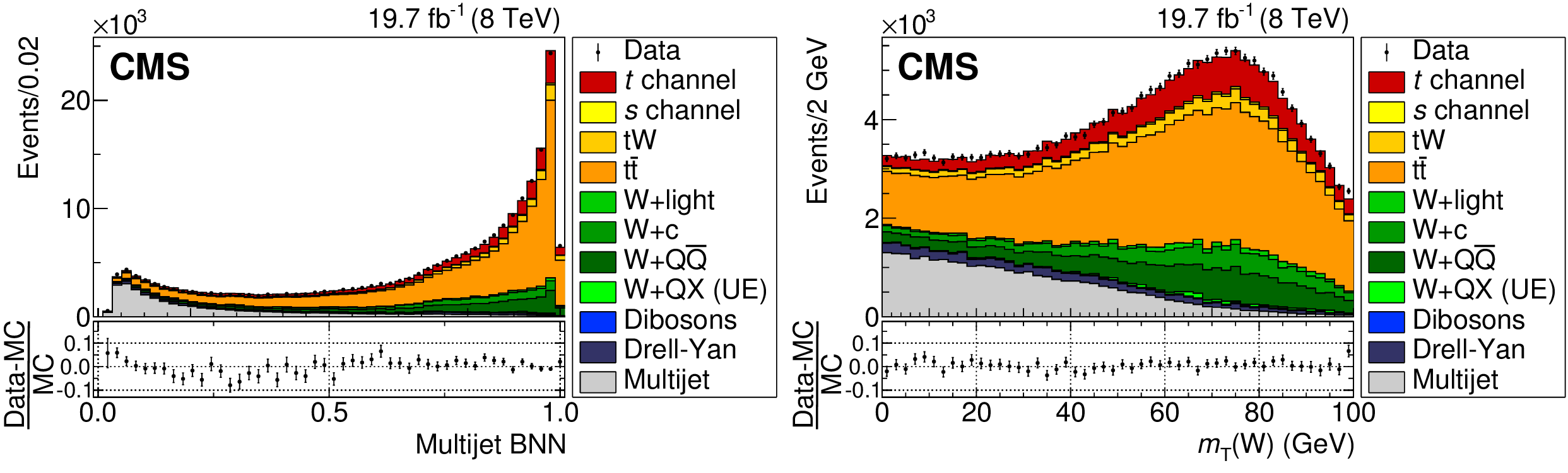
Figure 1:
The distributions of the multijet BNN discriminant used for the QCD multijet background rejection (left) and the reconstructed transverse W boson mass (right) from data (points) and the predicted backgrounds from simulation (filled histograms) for $ \sqrt{s} = $ 8 TeV. The lower part of each plot shows the relative difference between the data and the total predicted background. The vertical bars represent the statistical uncertainties. |
png pdf |
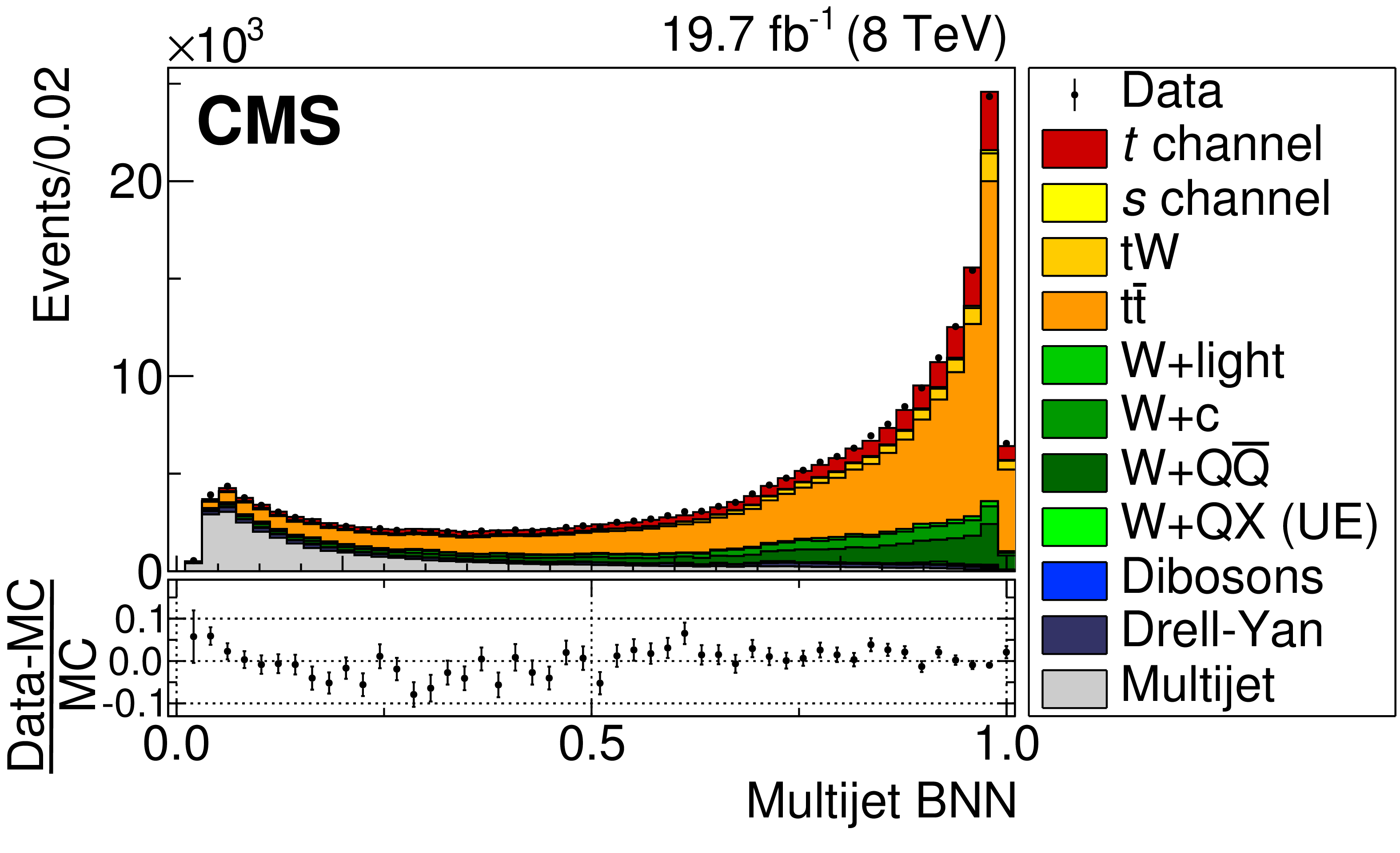
Figure 1-a:
The distributions of the multijet BNN discriminant used for the QCD multijet background rejection from data (points) and the predicted backgrounds from simulation (filled histograms) for $ \sqrt{s} = $ 8 TeV. The lower part of the plot shows the relative difference between the data and the total predicted background. The vertical bars represent the statistical uncertainties. |
png pdf |
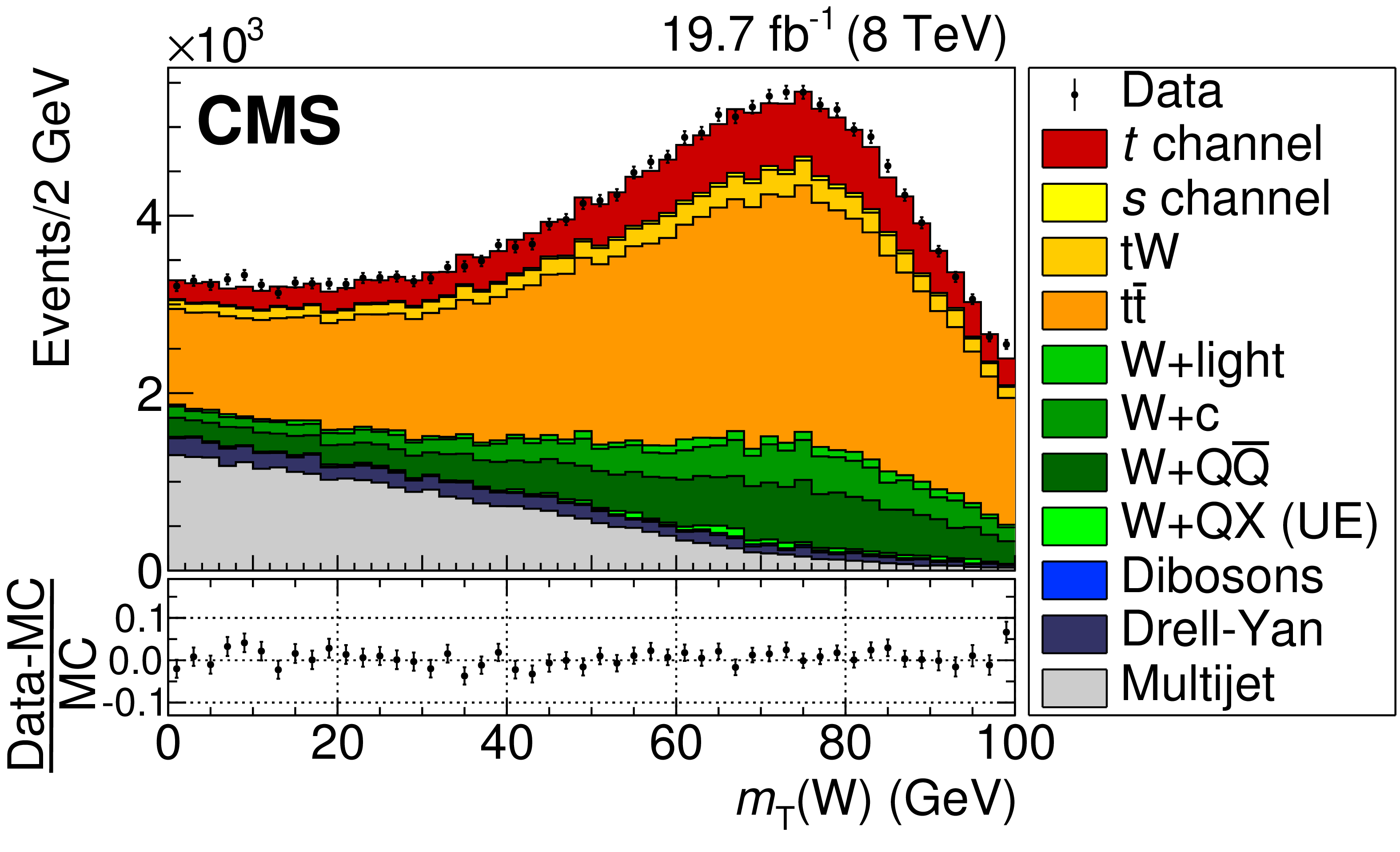
Figure 1-b:
The distributions of the multijet BNN discriminant used for the reconstructed transverse W boson mass from data (points) and the predicted backgrounds from simulation (filled histograms) for $ \sqrt{s} = $ 8 TeV. The lower part of the plot shows the relative difference between the data and the total predicted background. The vertical bars represent the statistical uncertainties. |
png pdf |
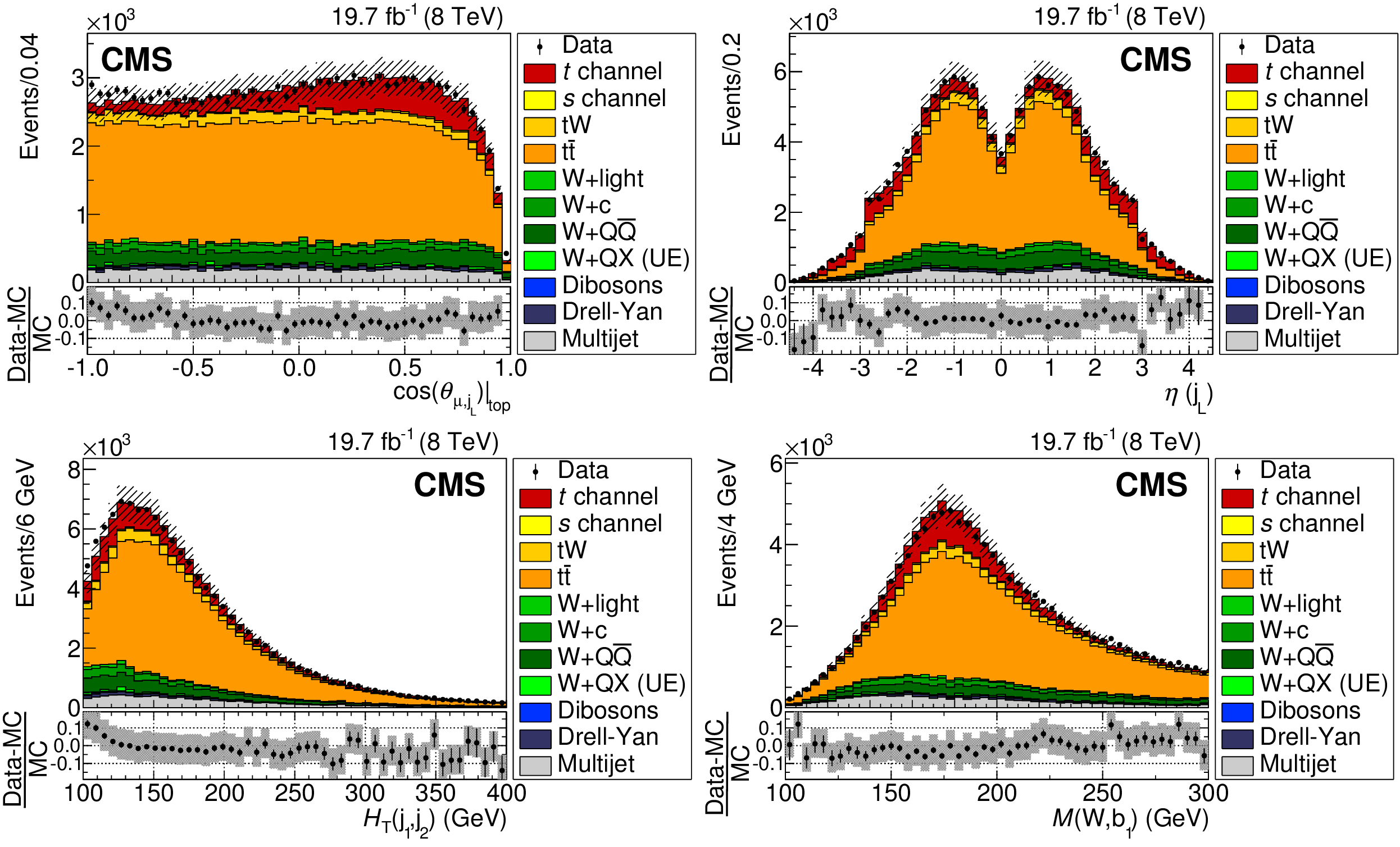
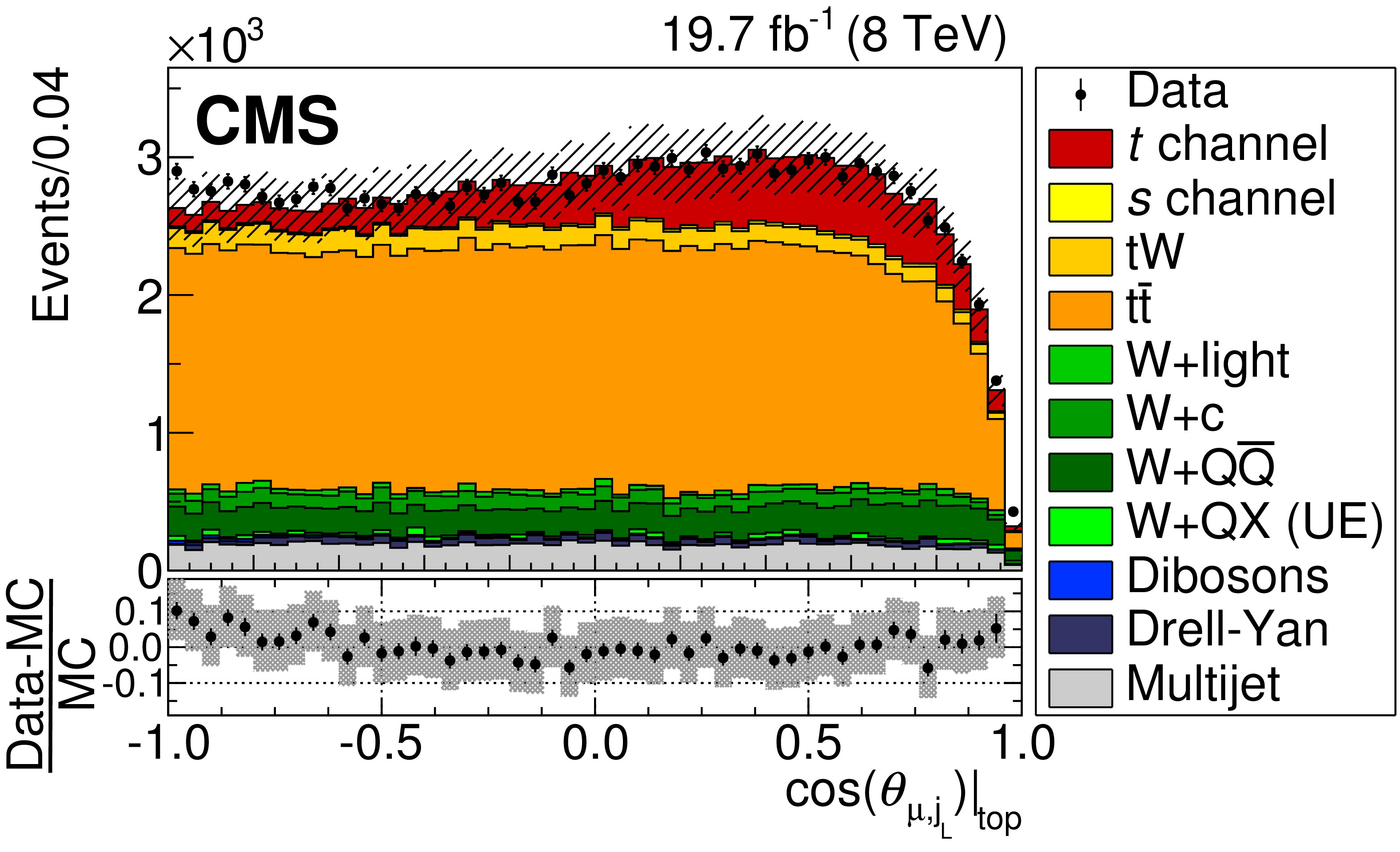
Figure 2:
Comparison of experimental with simulated data of the BNNs input variables $\cos(\theta _{\mu ,\rm {\rm j_L}})|_{\rm top}$, $\eta (\rm j_L)$, $H_{\rm T}(\rm j_1, j_2)$, and $M(\rm W,\rm {b_1})$. The variables are described in Table 2. The lower part of each plot shows the relative difference between the data and the total predicted background. The hatched band corresponds to the total simulation uncertainty. The vertical bars represent the statistical uncertainties. Plots are for the $\sqrt {s}=$ 8 TeV data set. |
png pdf |
Figure 2-a:
Comparison of experimental with simulated data of the BNNs input variable $\cos(\theta _{\mu ,\rm {\rm j_L}})|_{\rm top}$. The variable is described in Table 2. The lower part of the plot shows the relative difference between the data and the total predicted background. The hatched band corresponds to the total simulation uncertainty. The vertical bars represent the statistical uncertainties. Plots are for the $\sqrt {s}=$ 8 TeV data set. |

png pdf |
Figure 2-b:
Comparison of experimental with simulated data of the BNNs input variable $\eta (\rm j_L)$. The variable is described in Table 2. The lower part of the plot shows the relative difference between the data and the total predicted background. The hatched band corresponds to the total simulation uncertainty. The vertical bars represent the statistical uncertainties. Plots are for the $\sqrt {s}=$ 8 TeV data set. |
png pdf |
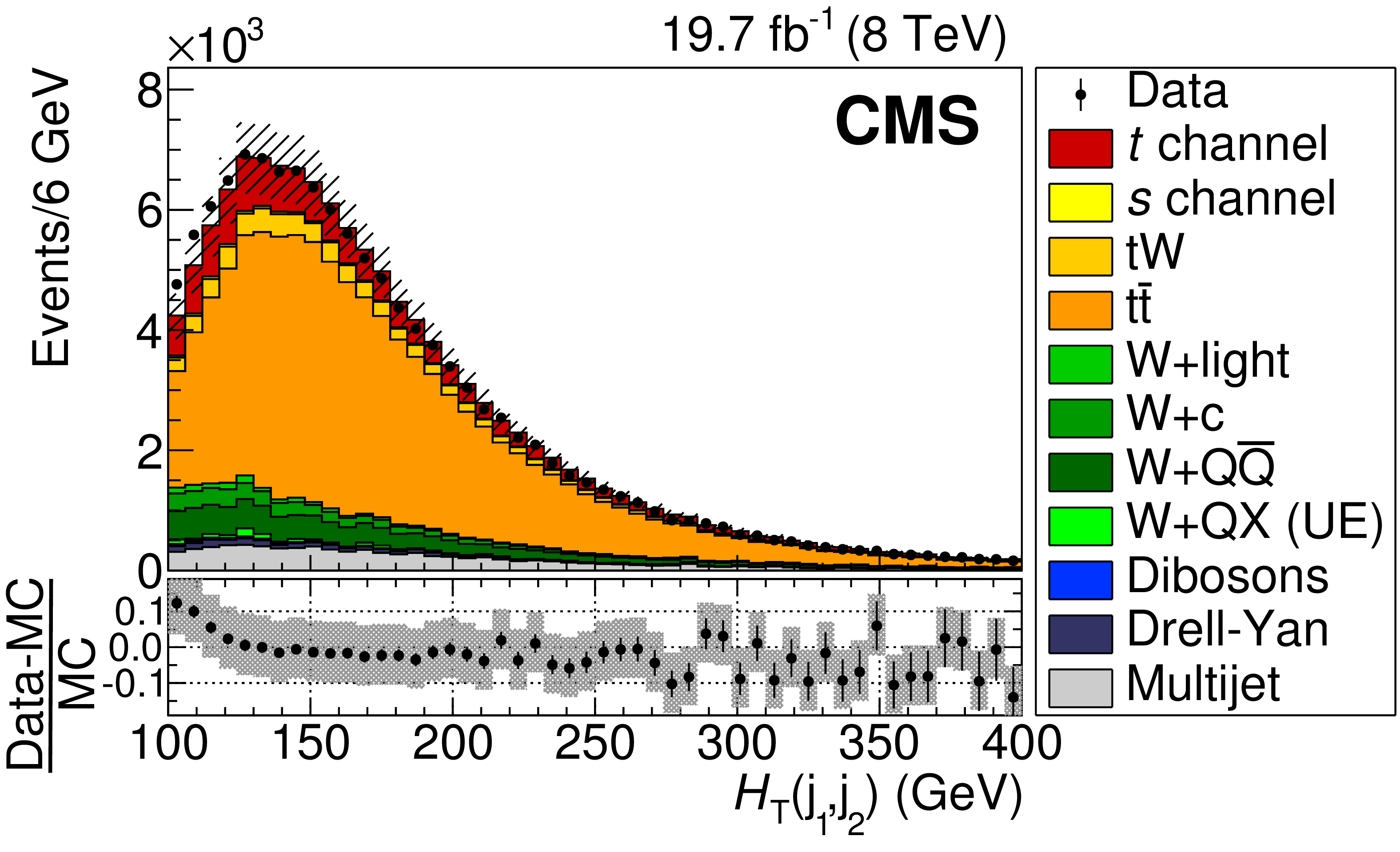
Figure 2-c:
Comparison of experimental with simulated data of the BNNs input variable $H_{\rm T}(\rm j_1, j_2)$. The variable is described in Table 2. The lower part of the plot shows the relative difference between the data and the total predicted background. The hatched band corresponds to the total simulation uncertainty. The vertical bars represent the statistical uncertainties. Plots are for the $\sqrt {s}=$ 8 TeV data set. |
png pdf |
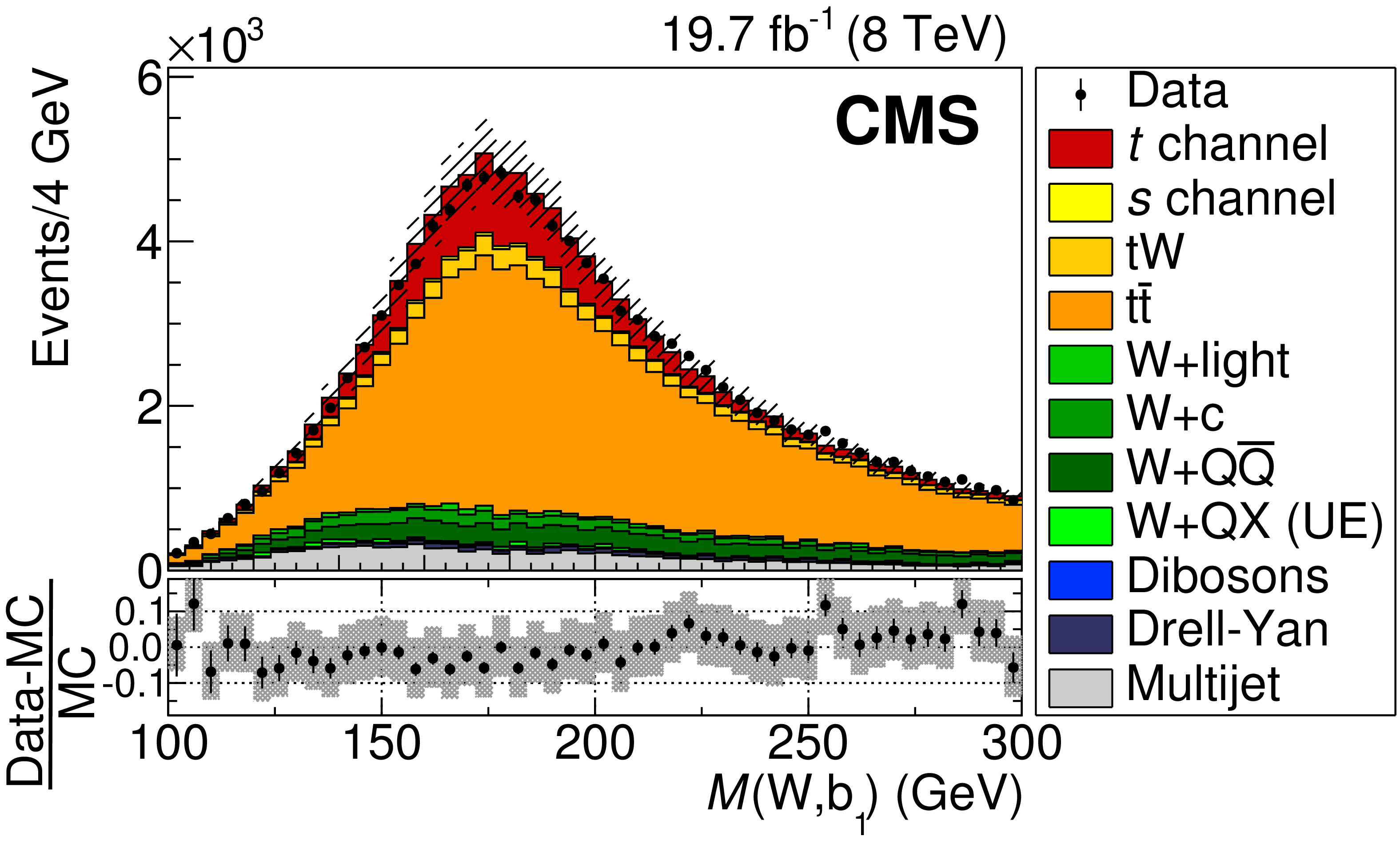
Figure 2-d:
Comparison of experimental with simulated data of the BNNs input variable $M(\rm W,\rm {b_1})$. The variable is described in Table 2. The lower part of the plot shows the relative difference between the data and the total predicted background. The hatched band corresponds to the total simulation uncertainty. The vertical bars represent the statistical uncertainties. Plots are for the $\sqrt {s}=$ 8 TeV data set. |
png pdf |
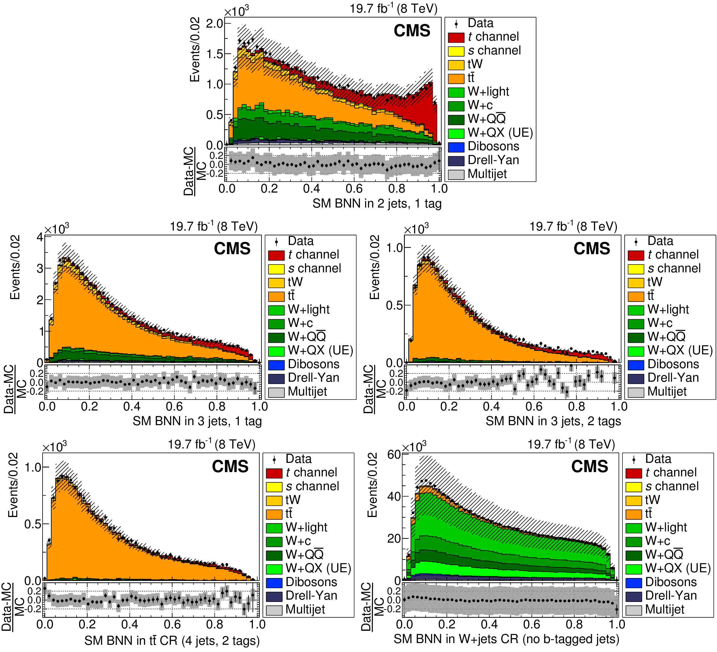
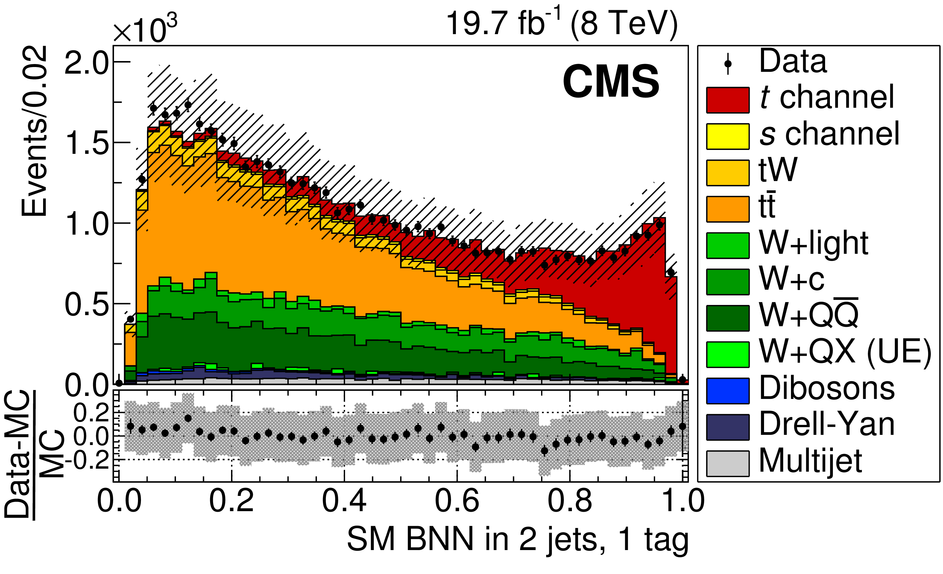
Figure 3:
Comparison of $ \sqrt{s} = $ 8 TeV data and simulation using the SM BNN discriminant in three separate signal regions of two jets with one b-tagged (2 jets, 1 tag) (upper), three jets with one of them b-tagged (3 jets, 1 tag) (middle left), and three jets with two of them b-tagged (3 jets, 2 tags) (middle right), and in ${\mathrm{ t } {}\mathrm{ \bar{t} } }$ (4 jets, 2 tags) (lower left) and W+jets (no b-tagged jets) (lower right) background control regions (CR). The lower part of each plot shows the relative difference between the data and the total predicted background. The hatched band corresponds to the total simulation uncertainty. The vertical bars represent the statistical uncertainties. |
png pdf |
Figure 3-a:
Comparison of $ \sqrt{s} = $ 8 TeV data and simulation using the SM BNN discriminant in the two jets with one b-tagged (2 jets, 1 tag) background control region (CR). The lower part of the plot shows the relative difference between the data and the total predicted background. The hatched band corresponds to the total simulation uncertainty. The vertical bars represent the statistical uncertainties. |
png pdf |
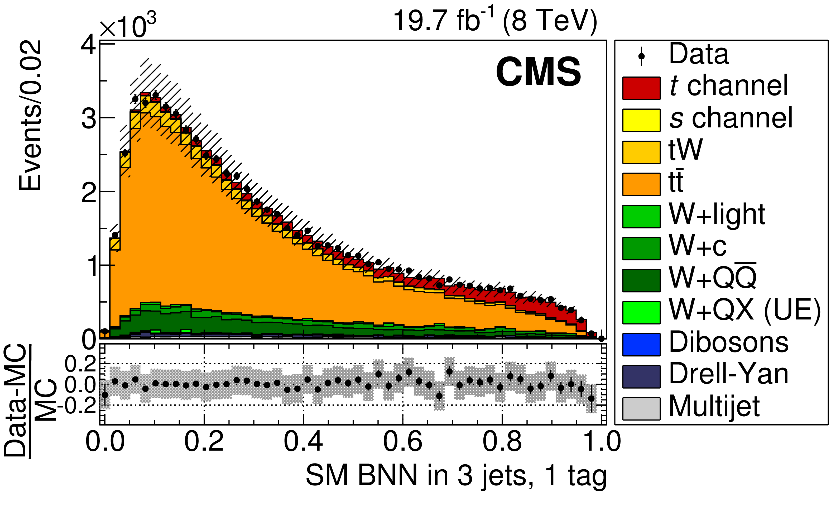
Figure 3-b:
Comparison of $ \sqrt{s} = $ 8 TeV data and simulation using the SM BNN discriminant in the three jets with one of them b-tagged (3 jets, 1 tag) background control region (CR). The lower part of the plot shows the relative difference between the data and the total predicted background. The hatched band corresponds to the total simulation uncertainty. The vertical bars represent the statistical uncertainties. |
png pdf |
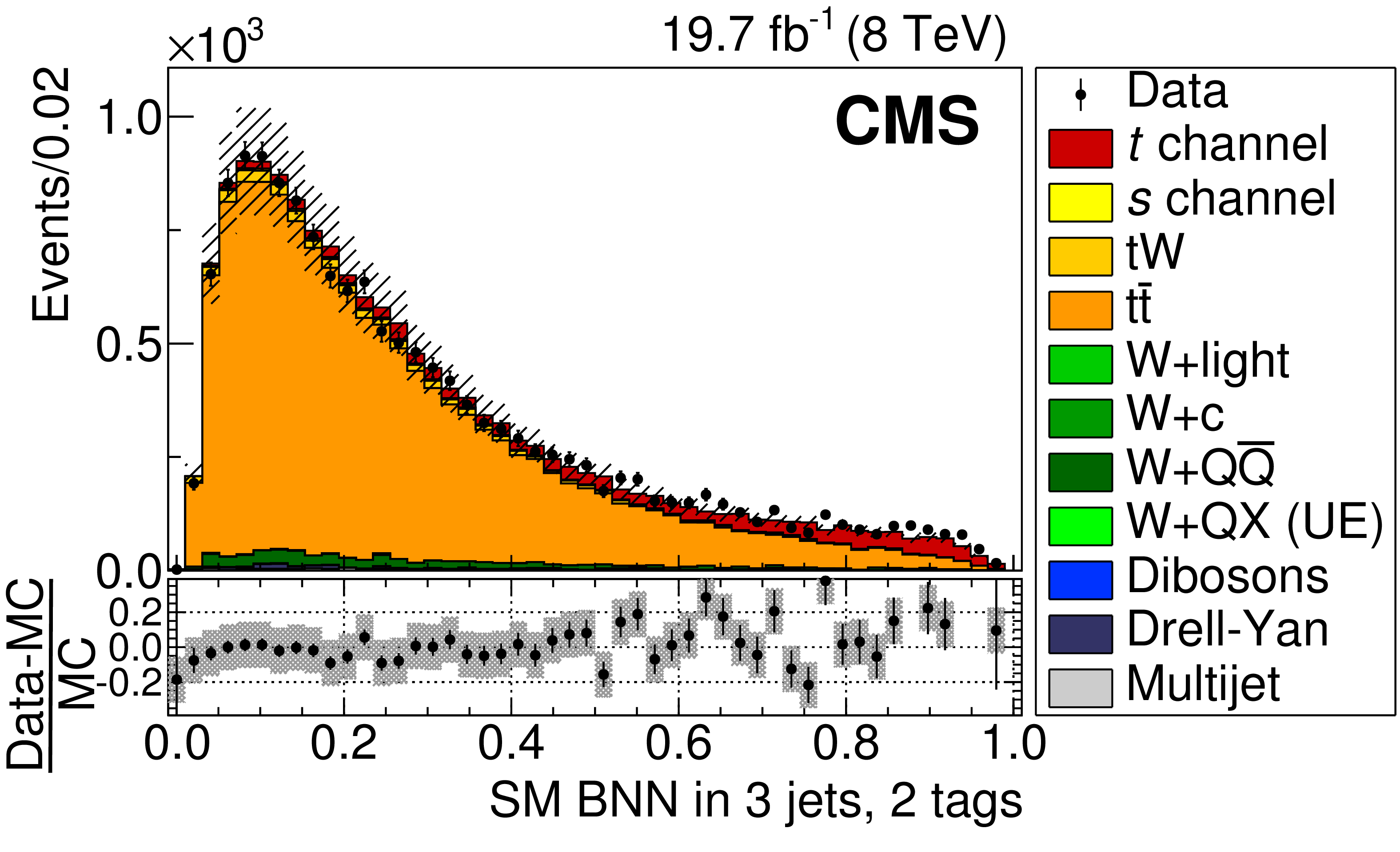
Figure 3-c:
Comparison of $ \sqrt{s} = $ 8 TeV data and simulation using the SM BNN discriminant in the three jets with two of them b-tagged (3 jets, 2 tags) (middle right) background control region (CR). The lower part of the plot shows the relative difference between the data and the total predicted background. The hatched band corresponds to the total simulation uncertainty. The vertical bars represent the statistical uncertainties. |
png pdf |
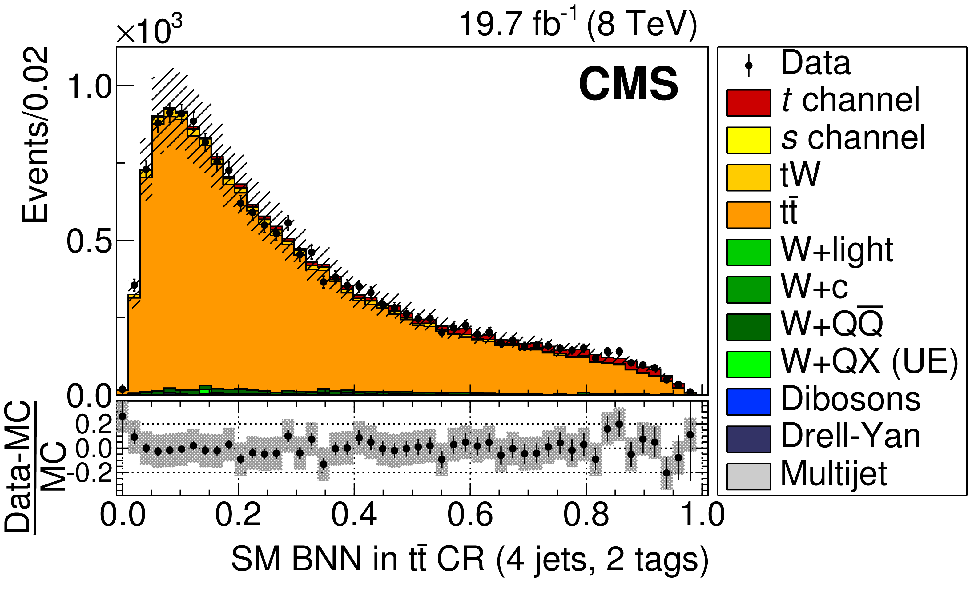
Figure 3-d:
Comparison of $ \sqrt{s} = $ 8 TeV data and simulation using the SM BNN discriminant in the ${\mathrm{ t } {}\mathrm{ \bar{t} } }$ (4 jets, 2 tags) background control region (CR). The lower part of the plot shows the relative difference between the data and the total predicted background. The hatched band corresponds to the total simulation uncertainty. The vertical bars represent the statistical uncertainties. |

png pdf |
Figure 3-e:
Comparison of $ \sqrt{s} = $ 8 TeV data and simulation using the SM BNN discriminant in the W+jets (no b-tagged jets) background control region (CR). The lower part of the plot shows the relative difference between the data and the total predicted background. The hatched band corresponds to the total simulation uncertainty. The vertical bars represent the statistical uncertainties. |
png pdf |
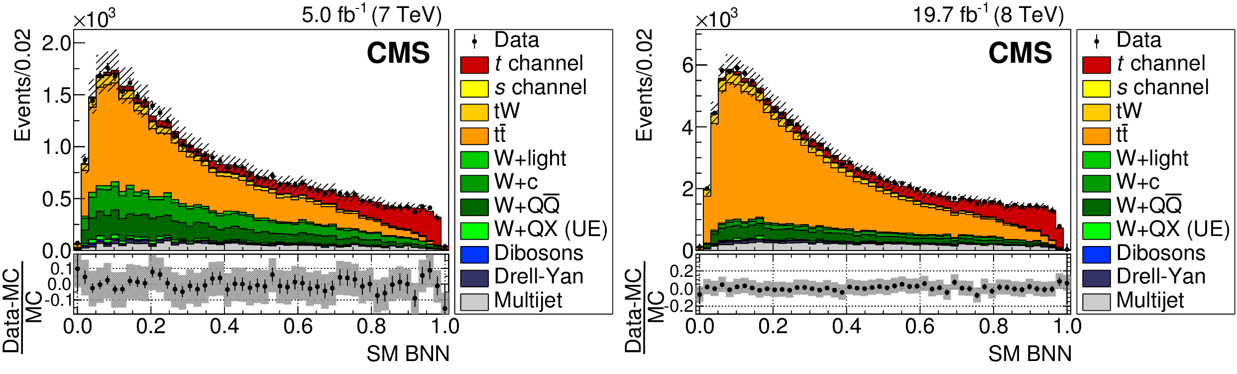
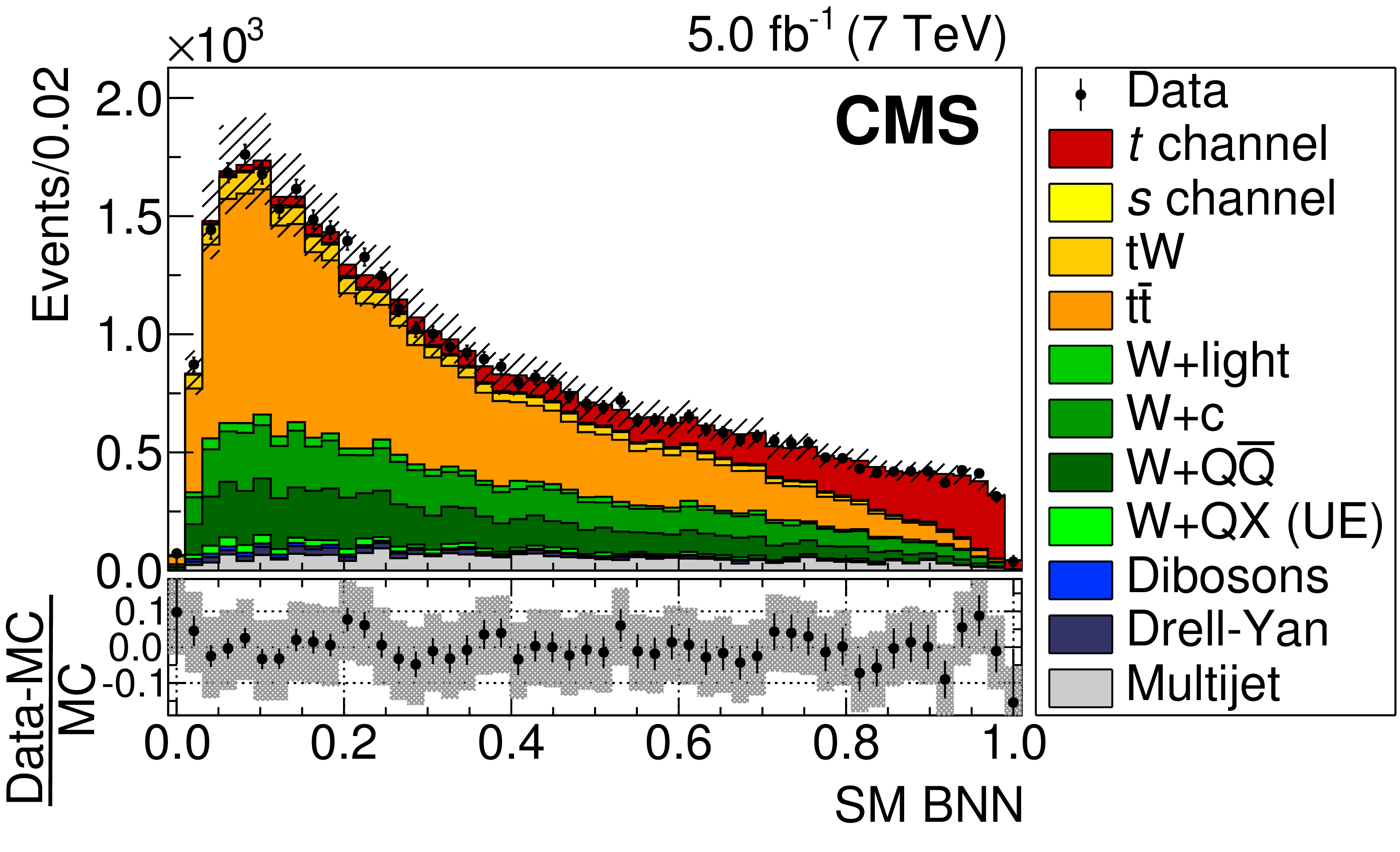
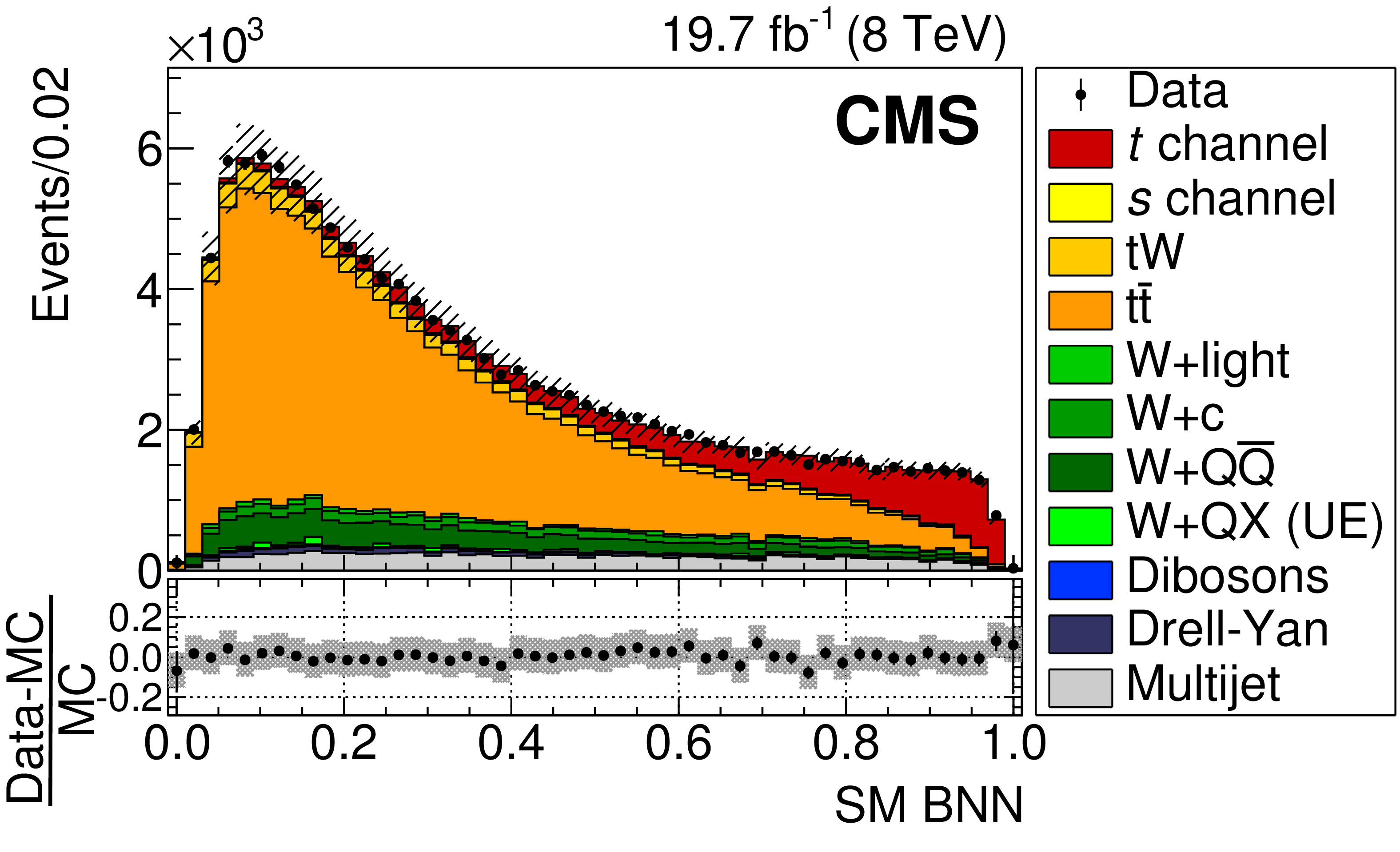
Figure 4:
The SM BNN discriminant distributions after the statistical analysis and evaluation of all the uncertainties. The lower part of each plot shows the relative difference between the data and the total predicted background. The hatched band corresponds to the total simulation uncertainty. The vertical bars represent the statistical uncertainties. The left (right) plot corresponds to $\sqrt {s}=$ 7 (8) TeV . |
png pdf |
Figure 4-a:
The SM BNN discriminant distribution at $\sqrt {s}=$ 7 TeV after the statistical analysis and evaluation of all the uncertainties. The lower part of the plot shows the relative difference between the data and the total predicted background. The hatched band corresponds to the total simulation uncertainty. The vertical bars represent the statistical uncertainties. |
png pdf |
Figure 4-b:
The SM BNN discriminant distribution at $\sqrt {s}=$ 8 TeV after the statistical analysis and evaluation of all the uncertainties. The lower part of the plot shows the relative difference between the data and the total predicted background. The hatched band corresponds to the total simulation uncertainty. The vertical bars represent the statistical uncertainties. |
png pdf |
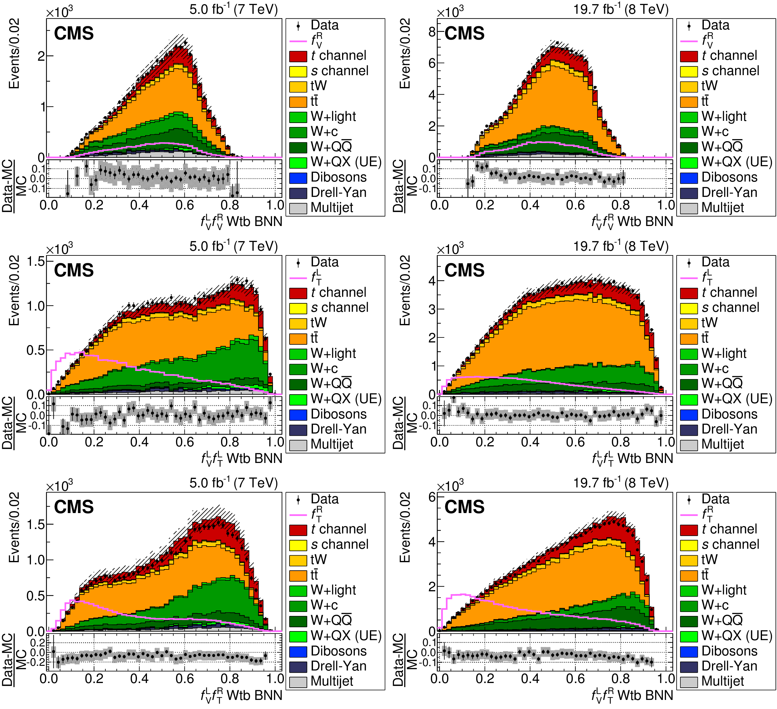
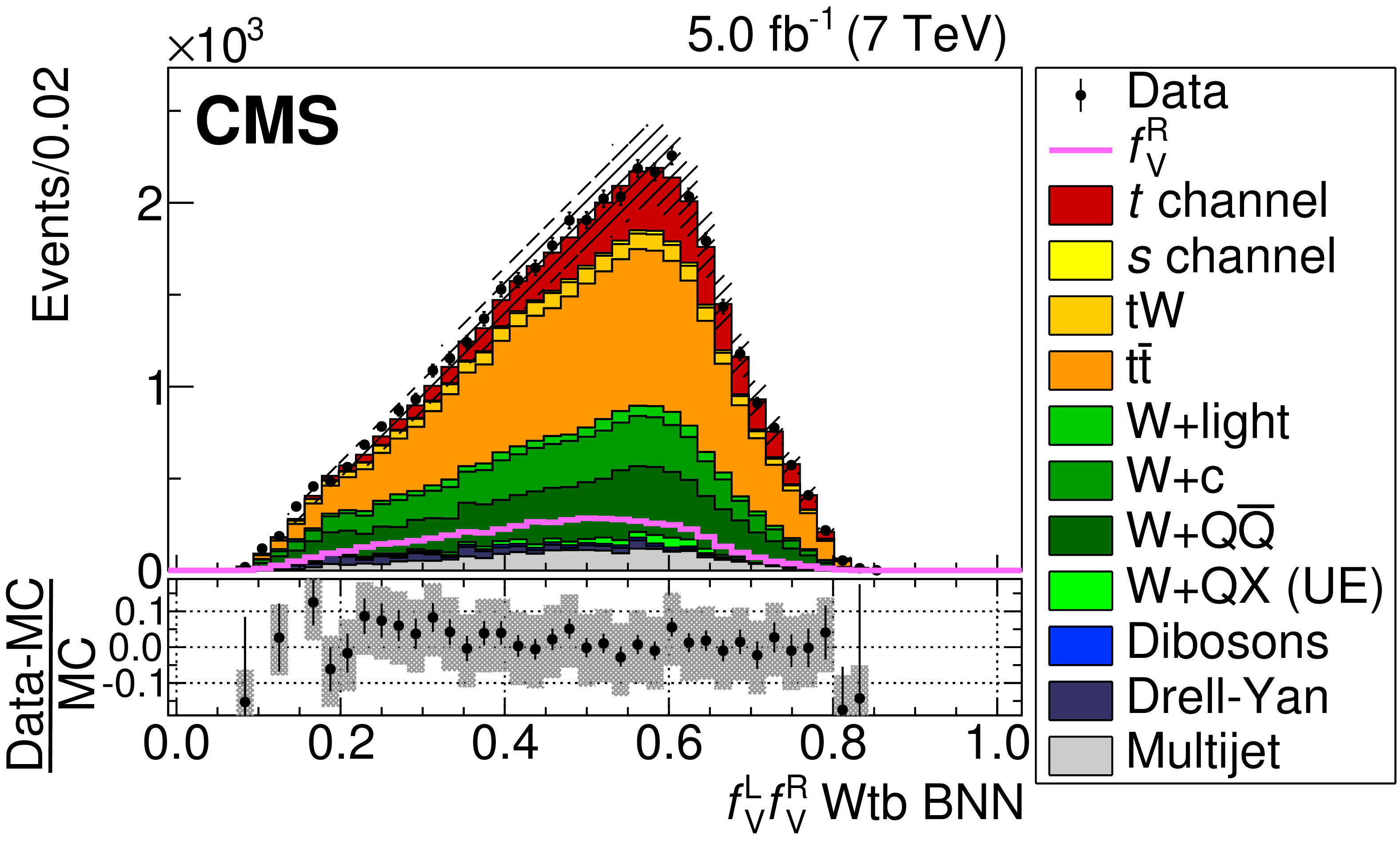
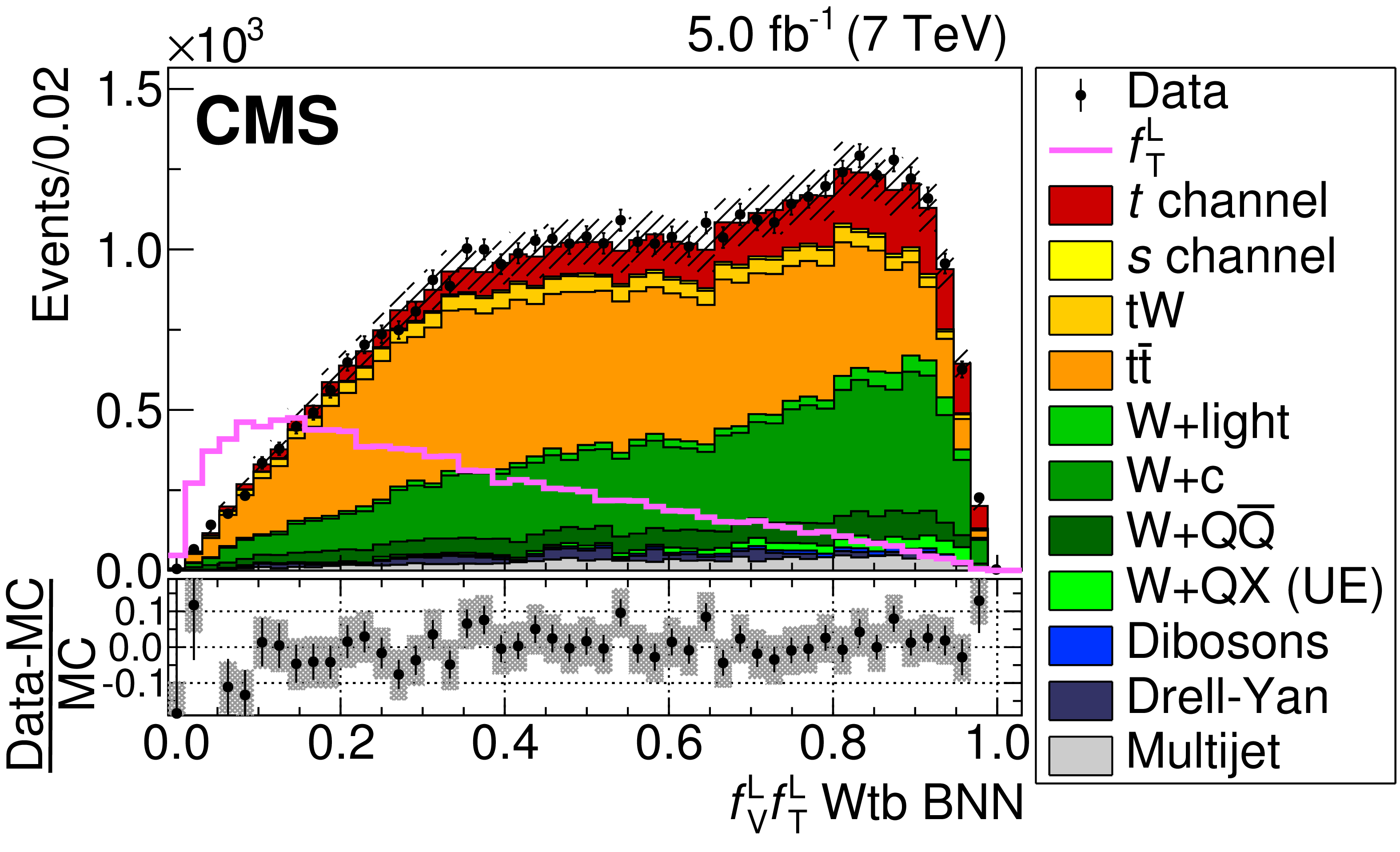
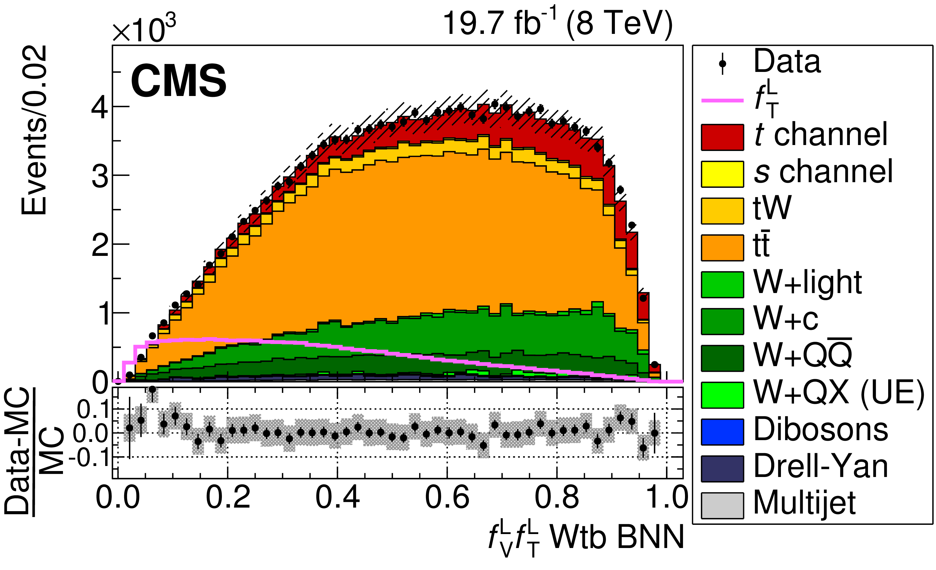
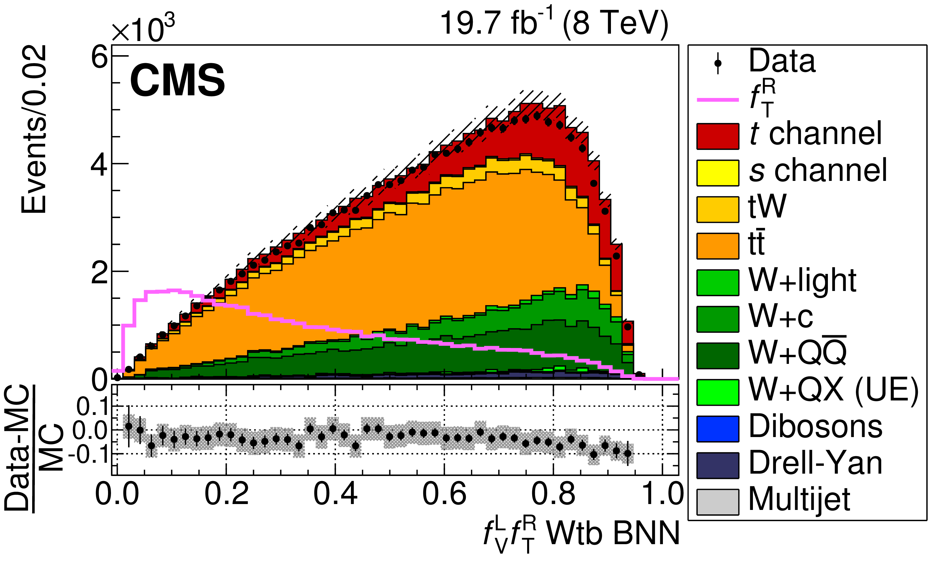
Figure 5:
Distributions of the Wtb BNN discriminants from data (points) and simulation (filled histograms) for the scenarios $(f_{\rm V}^{\rm L}$, $f_{\rm V}^{\rm R})$ (top), $(f_{\rm V}^{\rm L}$, $f_{\rm T}^{\rm L})$ (middle), and $(f_{\rm V}^{\rm L}$, $f_{\rm T}^{\rm R})$ (bottom). The plots on the left (right) correspond to $\sqrt {s}=$ 7 (8) TeV. The Wtb BNNs are trained to separate SM left-handed interactions from one of the anomalous interactions. In each plot, the expected distribution with the corresponding anomalous coupling set to 1.0 is shown by the solid curve. The lower part of each plot shows the relative difference between the data and the total predicted background. The hatched band corresponds to the total simulation uncertainty. The vertical bars represent the statistical uncertainties. |
png pdf |
Figure 5-a:
Distribution of the Wtb BNN discriminant at $\sqrt {s}=$ 7 TeV from data (points) and simulation (filled histograms) for the scenario $(f_{\rm V}^{\rm L}$, $f_{\rm V}^{\rm R})$. In the plot, the expected distribution with the corresponding anomalous coupling set to 1.0 is shown by the solid curve. The lower part of the plot shows the relative difference between the data and the total predicted background. The hatched band corresponds to the total simulation uncertainty. The vertical bars represent the statistical uncertainties. |

png pdf |
Figure 5-b:
Distribution of the Wtb BNN discriminant at $\sqrt {s}=$ 8 TeV from data (points) and simulation (filled histograms) for the scenario $(f_{\rm V}^{\rm L}$, $f_{\rm V}^{\rm R})$. In the plot, the expected distribution with the corresponding anomalous coupling set to 1.0 is shown by the solid curve. The lower part of the plot shows the relative difference between the data and the total predicted background. The hatched band corresponds to the total simulation uncertainty. The vertical bars represent the statistical uncertainties. |
png pdf |
Figure 5-c:
Distribution of the Wtb BNN discriminant at $\sqrt {s}=$ 7 TeV from data (points) and simulation (filled histograms) for the scenario $(f_{\rm V}^{\rm L}$, $f_{\rm T}^{\rm L})$. In the plot, the expected distribution with the corresponding anomalous coupling set to 1.0 is shown by the solid curve. The lower part of the plot shows the relative difference between the data and the total predicted background. The hatched band corresponds to the total simulation uncertainty. The vertical bars represent the statistical uncertainties. |
png pdf |
Figure 5-d:
Distribution of the Wtb BNN discriminant at $\sqrt {s}=$ 8 TeV from data (points) and simulation (filled histograms) for the scenario $(f_{\rm V}^{\rm L}$, $f_{\rm T}^{\rm L})$. In the plot, the expected distribution with the corresponding anomalous coupling set to 1.0 is shown by the solid curve. The lower part of the plot shows the relative difference between the data and the total predicted background. The hatched band corresponds to the total simulation uncertainty. The vertical bars represent the statistical uncertainties. |

png pdf |
Figure 5-e:
Distribution of the Wtb BNN discriminant at $\sqrt {s}=$ 7 TeV from data (points) and simulation (filled histograms) for the scenario$(f_{\rm V}^{\rm L}$, $f_{\rm T}^{\rm R})$. In the plot, the expected distribution with the corresponding anomalous coupling set to 1.0 is shown by the solid curve. The lower part of the plot shows the relative difference between the data and the total predicted background. The hatched band corresponds to the total simulation uncertainty. The vertical bars represent the statistical uncertainties. |
png pdf |
Figure 5-f:
Distribution of the Wtb BNN discriminant at $\sqrt {s}=$ 8 TeV from data (points) and simulation (filled histograms) for the scenario$(f_{\rm V}^{\rm L}$, $f_{\rm T}^{\rm R})$. In the plot, the expected distribution with the corresponding anomalous coupling set to 1.0 is shown by the solid curve. The lower part of the plot shows the relative difference between the data and the total predicted background. The hatched band corresponds to the total simulation uncertainty. The vertical bars represent the statistical uncertainties. |
png pdf |
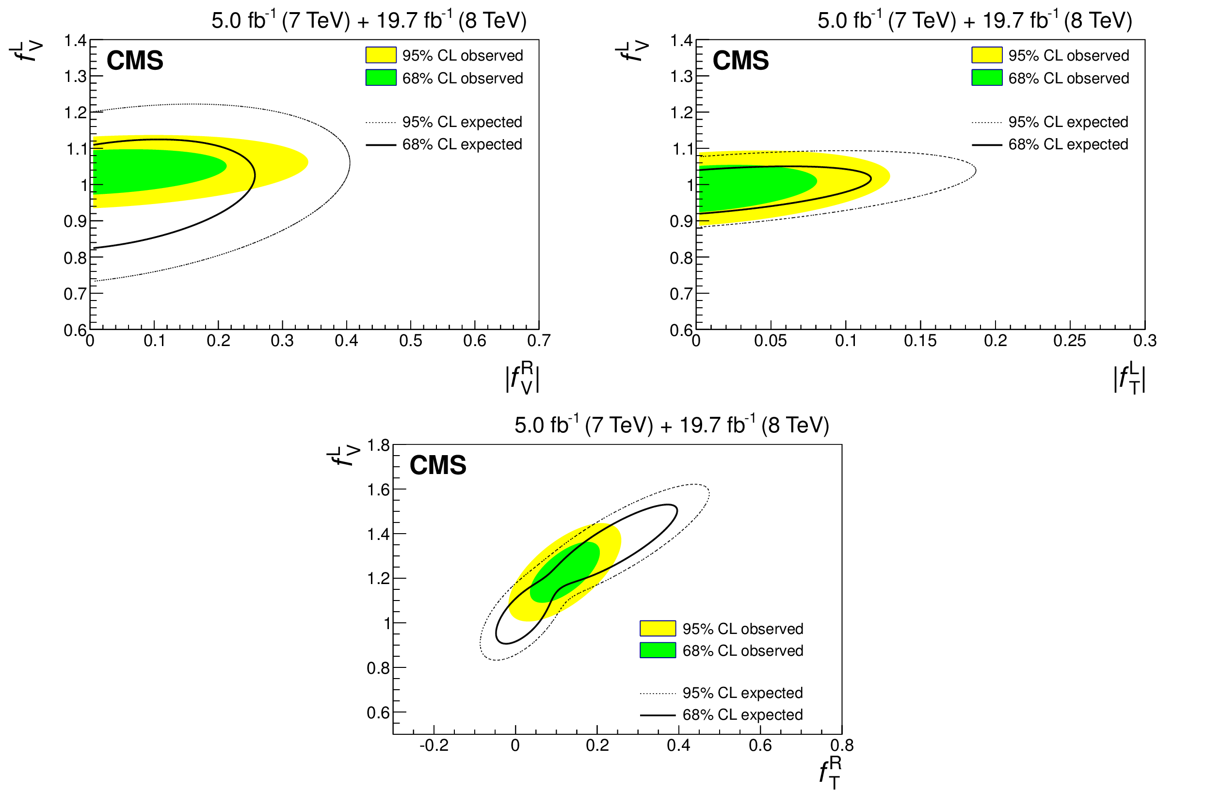
Figure 6:
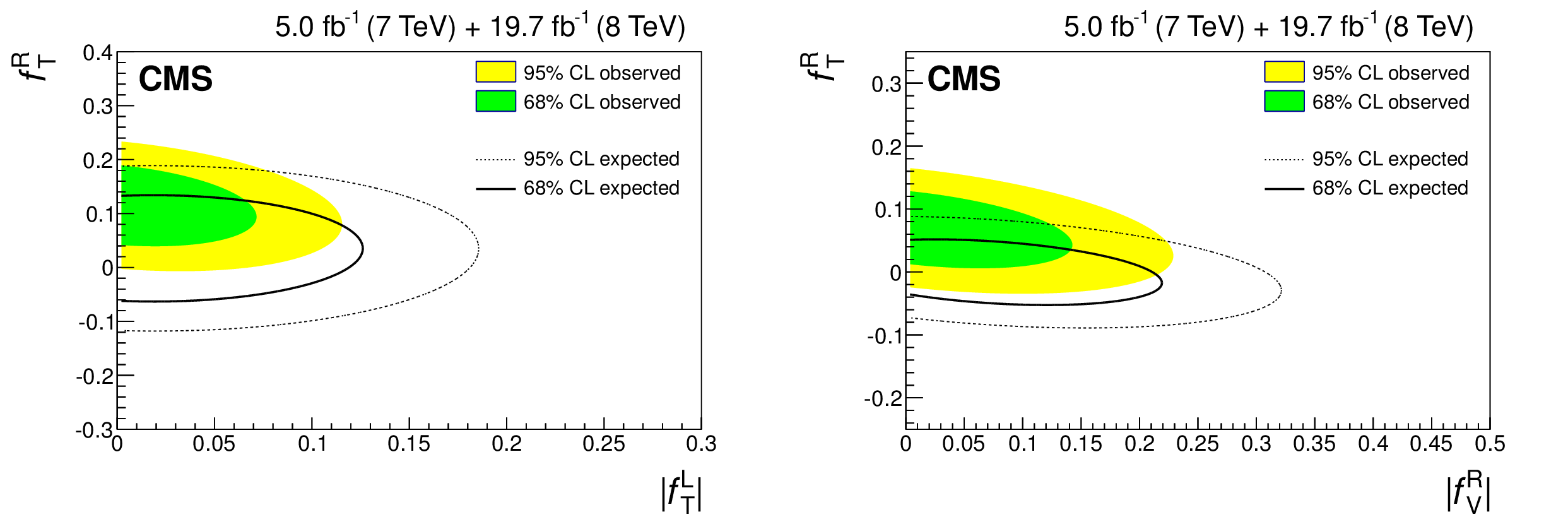
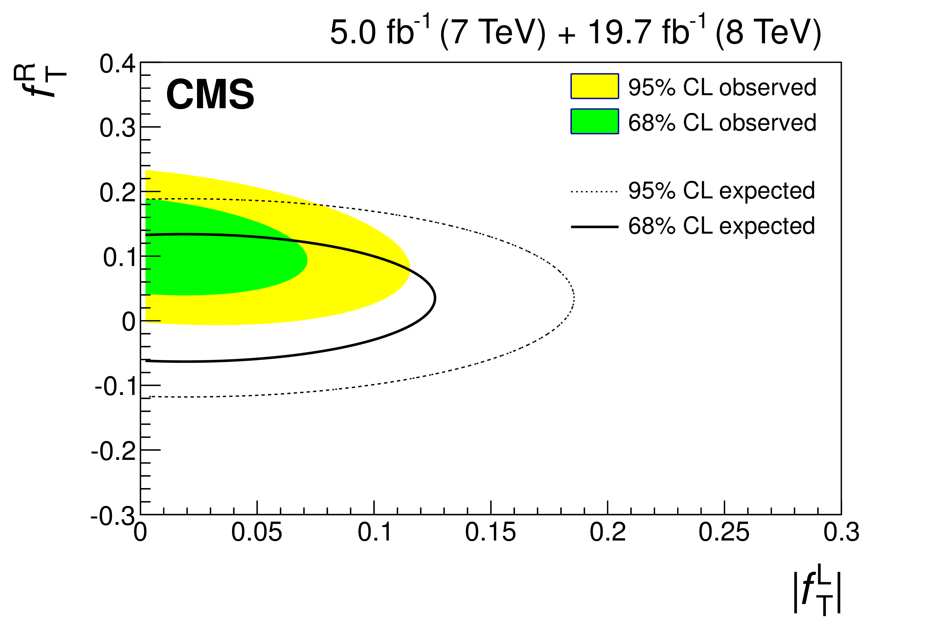
Combined $\sqrt {s}=$ 7 and 8 TeV observed and expected exclusion limits in the two-dimensional planes $(f_{\rm V}^{\rm L}$, $| f_{\rm V}^{\rm R}| )$ (top-left), $(f_{\rm V}^{\rm L}$, $| f_{\rm T}^{\rm L}| )$ (top-right), and $(f_{\rm V}^{\rm L}$, $f_{\rm T}^{\rm R})$ (bottom) at 68% and 95% CL. |
png pdf |
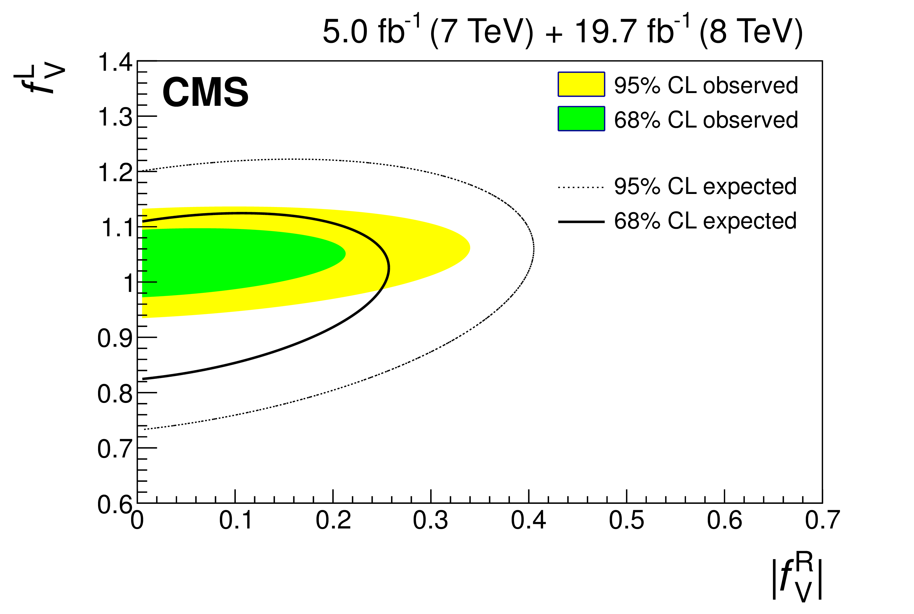
Figure 6-a:
Combined $\sqrt {s}=$ 7 and 8 TeV observed and expected exclusion limits in the two-dimensional plane $(f_{\rm V}^{\rm L}$, $| f_{\rm V}^{\rm R}| )$ at 68% and 95% CL. |
png pdf |
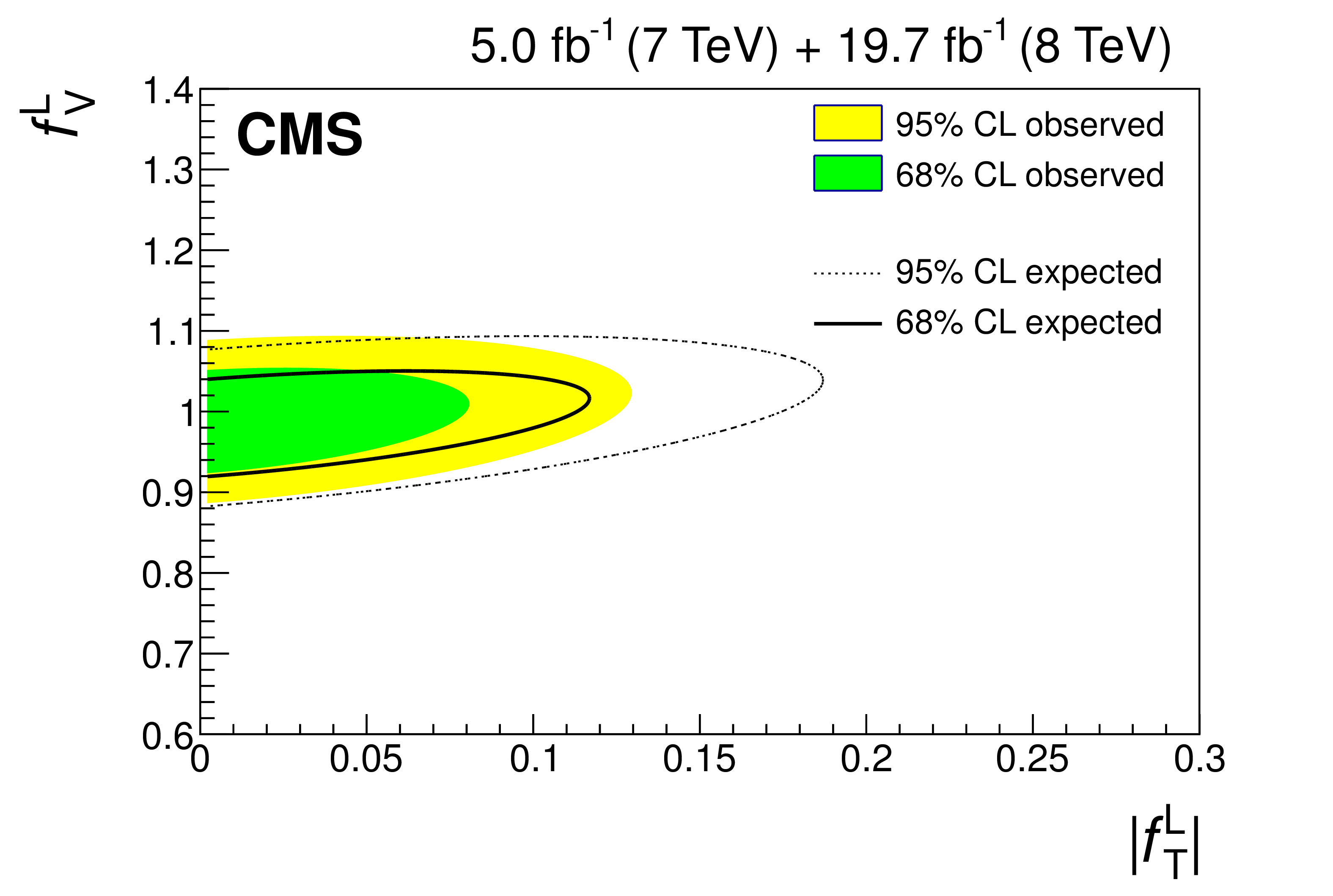
Figure 6-b:
Combined $\sqrt {s}=$ 7 and 8 TeV observed and expected exclusion limits in the two-dimensional plane $(f_{\rm V}^{\rm L}$, $| f_{\rm T}^{\rm L}| )$ at 68% and 95% CL. |
png pdf |
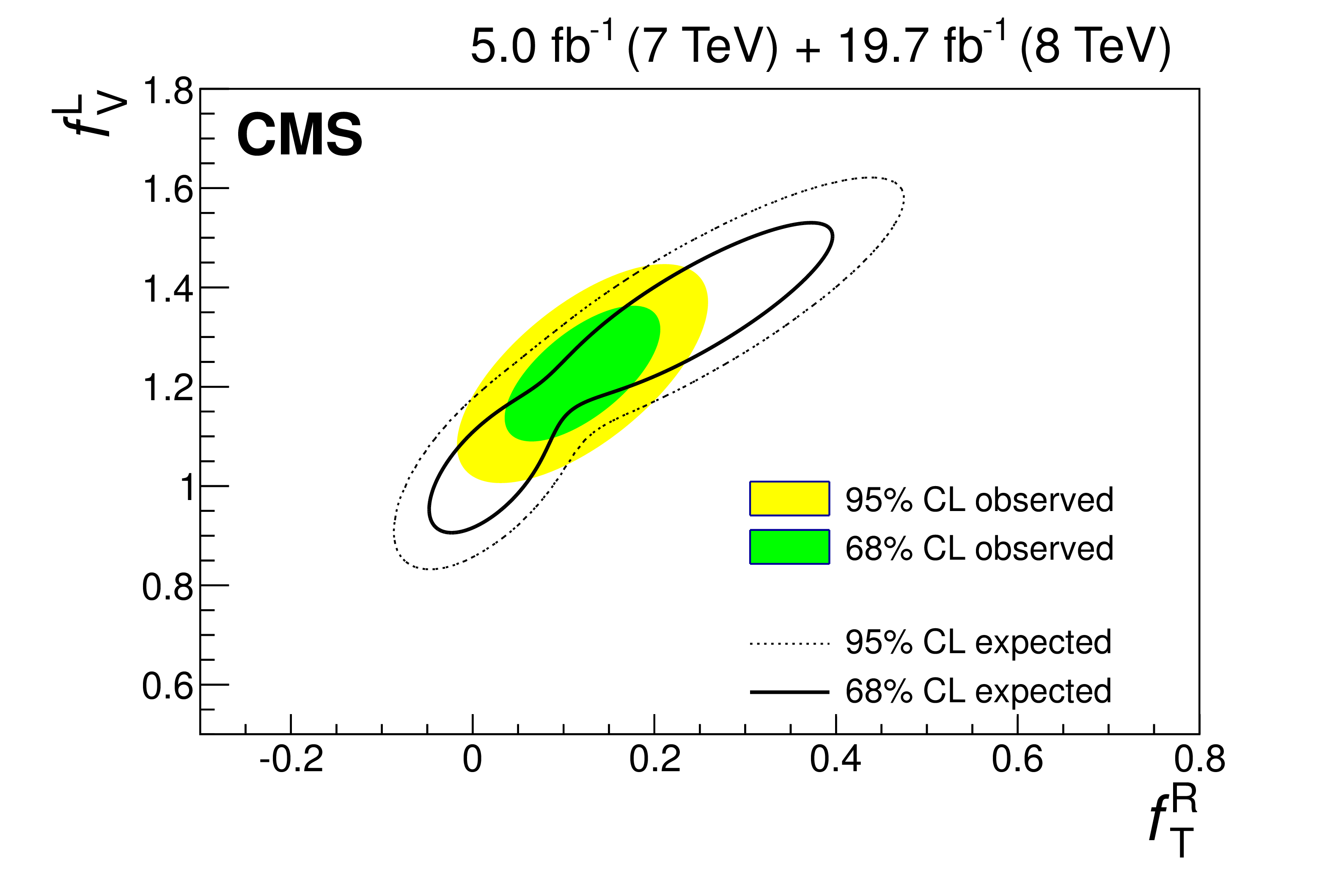
Figure 6-c:
Combined $\sqrt {s}=$ 7 and 8 TeV observed and expected exclusion limits in the two-dimensional plane $f_{\rm T}^{\rm R})$ at 68% and 95% CL. |
png pdf |
Figure 7:
Combined $\sqrt {s}=$ 7 and 8 TeV results from the three-dimensional variation of the couplings of $f_{\rm V}^{\rm L}$, $f_{\rm T}^{\rm L}$, $f_{\rm T}^{\rm R}$ (left), and $f_{\rm V}^{\rm L}$, $f_{\rm V}^{\rm R}$, $f_{\rm T}^{\rm R}$ (right) in the form of observed and expected exclusion limits at 68% and 95% CL in the two-dimension planes $(| f_{\rm T}^{\rm L}| $, $f_{\rm T}^{\rm R})$ (left) and $(| f_{\rm V}^{\rm R}| $, $f_{\rm T}^{\rm R})$ (right). |
png pdf |
Figure 7-a:
Combined $\sqrt {s}=$ 7 and 8 TeV result from the three-dimensional variation of the couplings of $f_{\rm V}^{\rm L}$, $f_{\rm T}^{\rm L}$, $f_{\rm T}^{\rm R}$ in the form of observed and expected exclusion limits at 68% and 95% CL in the two-dimension plane $(| f_{\rm T}^{\rm L}| $, $f_{\rm T}^{\rm R})$. |

png pdf |
Figure 7-b:
Combined $\sqrt {s}=$ 7 and 8 TeV result from the three-dimensional variation of the couplings of $f_{\rm V}^{\rm L}$, $f_{\rm V}^{\rm R}$, $f_{\rm T}^{\rm R}$ in the form of observed and expected exclusion limits at 68% and 95% CL in the two-dimension plane $(| f_{\rm V}^{\rm R}| $, $f_{\rm T}^{\rm R})$. |

png pdf |
Figure 8:
Representative Feynman diagrams for the FCNC processes. |
png pdf |
Figure 9:
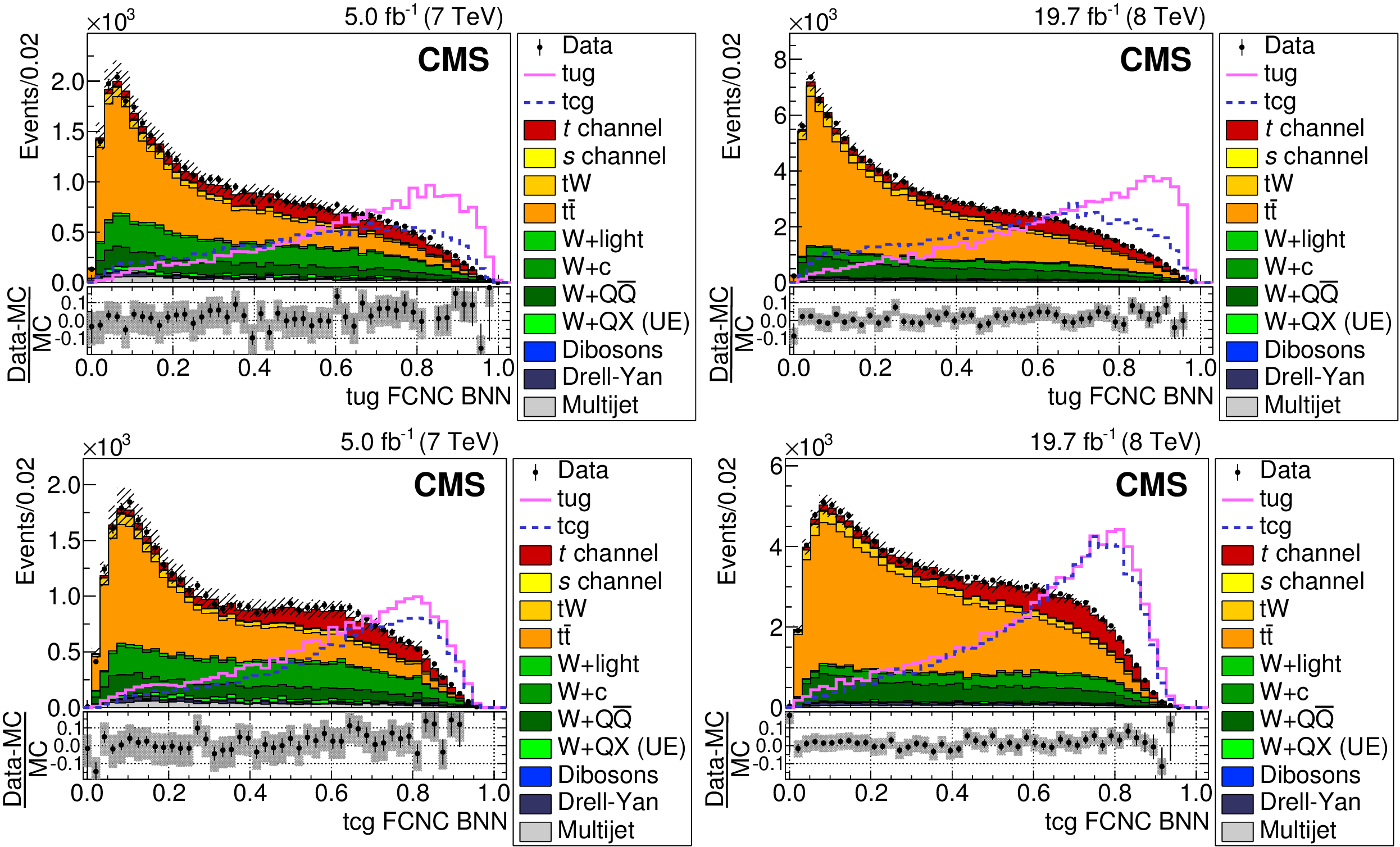
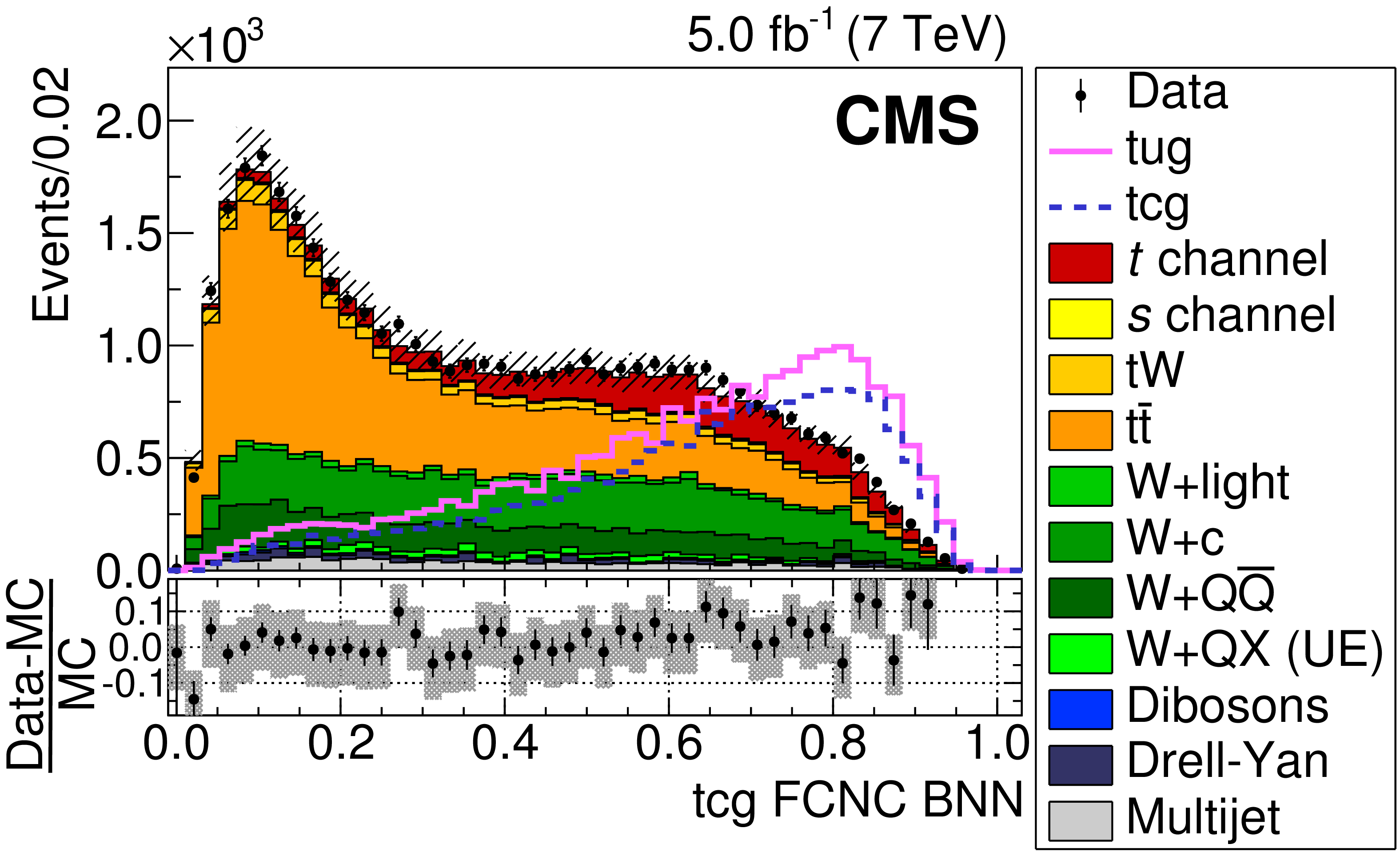
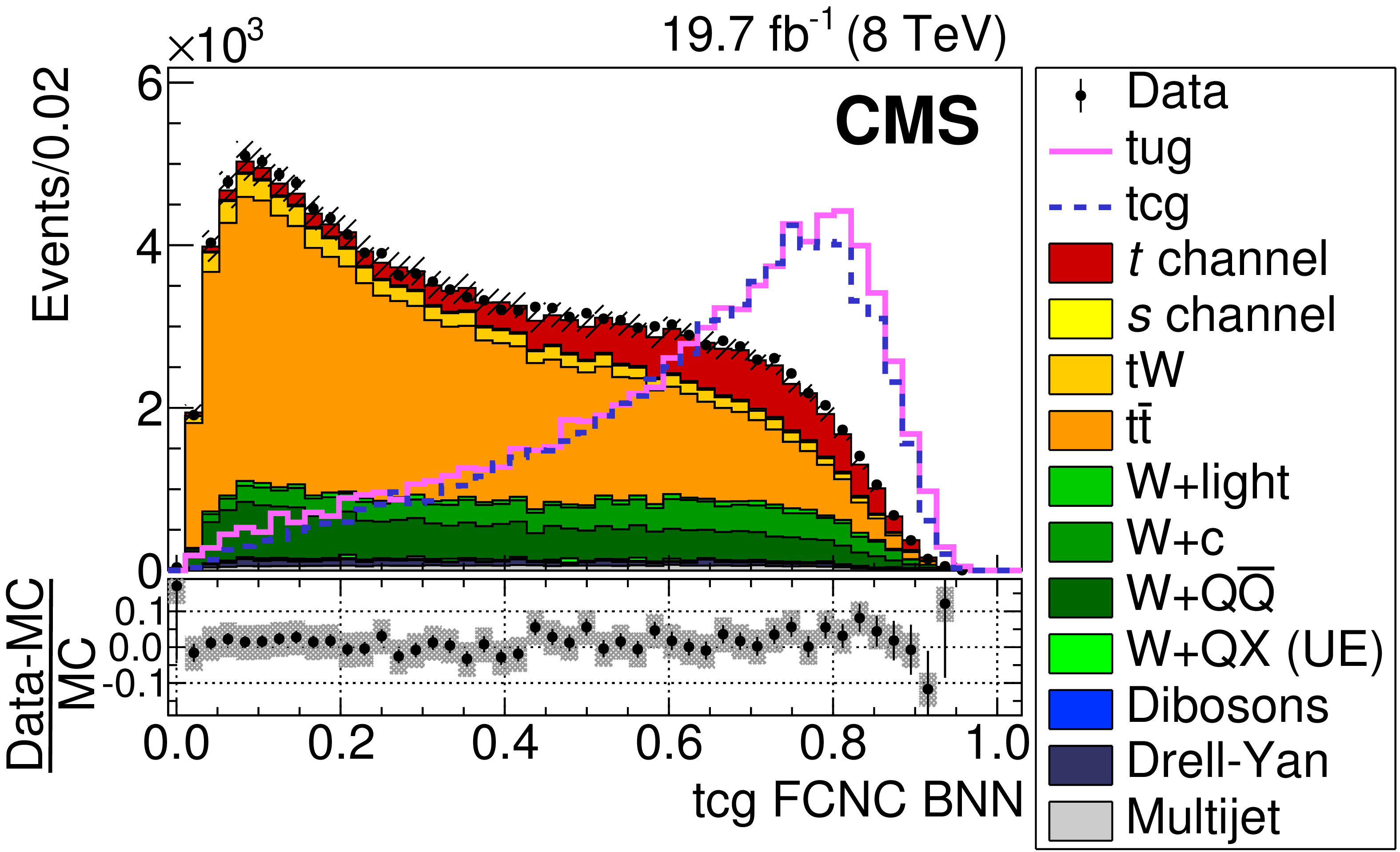
The FCNC BNN discriminant distributions when the BNN is trained to distinguish $\rm t\rightarrow ug$ (upper) or $\rm t\rightarrow cg$ (lower) processes as signal from the SM processes as background. The results from data are shown as points and the predicted distributions from the background simulations by the filled histograms. The plots on the left (right) correspond to the $\sqrt {s} =$ 7 (8) TeV data. The solid and dashed lines give the expected distributions for $\rm t\rightarrow ug$ and $\rm t\rightarrow cg$, respectively, assuming a coupling of $| \kappa _{\rm tug}| /\Lambda = 0.04\ (0.06)$ and $| \kappa _{\rm tcg}| /\Lambda = $ 0.08 (0.12) TeV$ ^{-1}$ on the left (right) plots. The lower part of each plot shows the relative difference between the data and the total predicted background. The hatched band corresponds to the total simulation uncertainty. The vertical bars represent the statistical uncertainties. |

png pdf |
Figure 9-a:
The FCNC BNN discriminant distributions when the BNN is trained to distinguish $\rm t\rightarrow ug$ (upper) or $\rm t\rightarrow cg$ (lower) processes as signal from the SM processes as background. The results from data are shown as points and the predicted distributions from the background simulations by the filled histograms. The plots on the left (right) correspond to the $\sqrt {s} =$ 7 (8) TeV data. The solid and dashed lines give the expected distributions for $\rm t\rightarrow ug$ and $\rm t\rightarrow cg$, respectively, assuming a coupling of $| \kappa _{\rm tug}| /\Lambda = 0.04\ (0.06)$ and $| \kappa _{\rm tcg}| /\Lambda = $ 0.08 (0.12) TeV$ ^{-1}$ on the left (right) plots. The lower part of each plot shows the relative difference between the data and the total predicted background. The hatched band corresponds to the total simulation uncertainty. The vertical bars represent the statistical uncertainties. |

png pdf |
Figure 9-b:
The FCNC BNN discriminant distributions when the BNN is trained to distinguish $\rm t\rightarrow ug$ (upper) or $\rm t\rightarrow cg$ (lower) processes as signal from the SM processes as background. The results from data are shown as points and the predicted distributions from the background simulations by the filled histograms. The plots on the left (right) correspond to the $\sqrt {s} =$ 7 (8) TeV data. The solid and dashed lines give the expected distributions for $\rm t\rightarrow ug$ and $\rm t\rightarrow cg$, respectively, assuming a coupling of $| \kappa _{\rm tug}| /\Lambda = 0.04\ (0.06)$ and $| \kappa _{\rm tcg}| /\Lambda = $ 0.08 (0.12) TeV$ ^{-1}$ on the left (right) plots. The lower part of each plot shows the relative difference between the data and the total predicted background. The hatched band corresponds to the total simulation uncertainty. The vertical bars represent the statistical uncertainties. |
png pdf |
Figure 9-c:
The FCNC BNN discriminant distributions when the BNN is trained to distinguish $\rm t\rightarrow ug$ (upper) or $\rm t\rightarrow cg$ (lower) processes as signal from the SM processes as background. The results from data are shown as points and the predicted distributions from the background simulations by the filled histograms. The plots on the left (right) correspond to the $\sqrt {s} =$ 7 (8) TeV data. The solid and dashed lines give the expected distributions for $\rm t\rightarrow ug$ and $\rm t\rightarrow cg$, respectively, assuming a coupling of $| \kappa _{\rm tug}| /\Lambda = 0.04\ (0.06)$ and $| \kappa _{\rm tcg}| /\Lambda = $ 0.08 (0.12) TeV$ ^{-1}$ on the left (right) plots. The lower part of each plot shows the relative difference between the data and the total predicted background. The hatched band corresponds to the total simulation uncertainty. The vertical bars represent the statistical uncertainties. |
png pdf |
Figure 9-d:
The FCNC BNN discriminant distributions when the BNN is trained to distinguish $\rm t\rightarrow ug$ (upper) or $\rm t\rightarrow cg$ (lower) processes as signal from the SM processes as background. The results from data are shown as points and the predicted distributions from the background simulations by the filled histograms. The plots on the left (right) correspond to the $\sqrt {s} =$ 7 (8) TeV data. The solid and dashed lines give the expected distributions for $\rm t\rightarrow ug$ and $\rm t\rightarrow cg$, respectively, assuming a coupling of $| \kappa _{\rm tug}| /\Lambda = 0.04\ (0.06)$ and $| \kappa _{\rm tcg}| /\Lambda = $ 0.08 (0.12) TeV$ ^{-1}$ on the left (right) plots. The lower part of each plot shows the relative difference between the data and the total predicted background. The hatched band corresponds to the total simulation uncertainty. The vertical bars represent the statistical uncertainties. |

png pdf |
Figure 10:
Combined $\sqrt {s} =$ 7 and 8 TeV observed and expected limits for the 68% and 95% CL on the $| \kappa _{\rm tug}| /\Lambda $ and $| \kappa _{\rm tcg}| /\Lambda $ couplings. |
| Tables | |
png pdf |
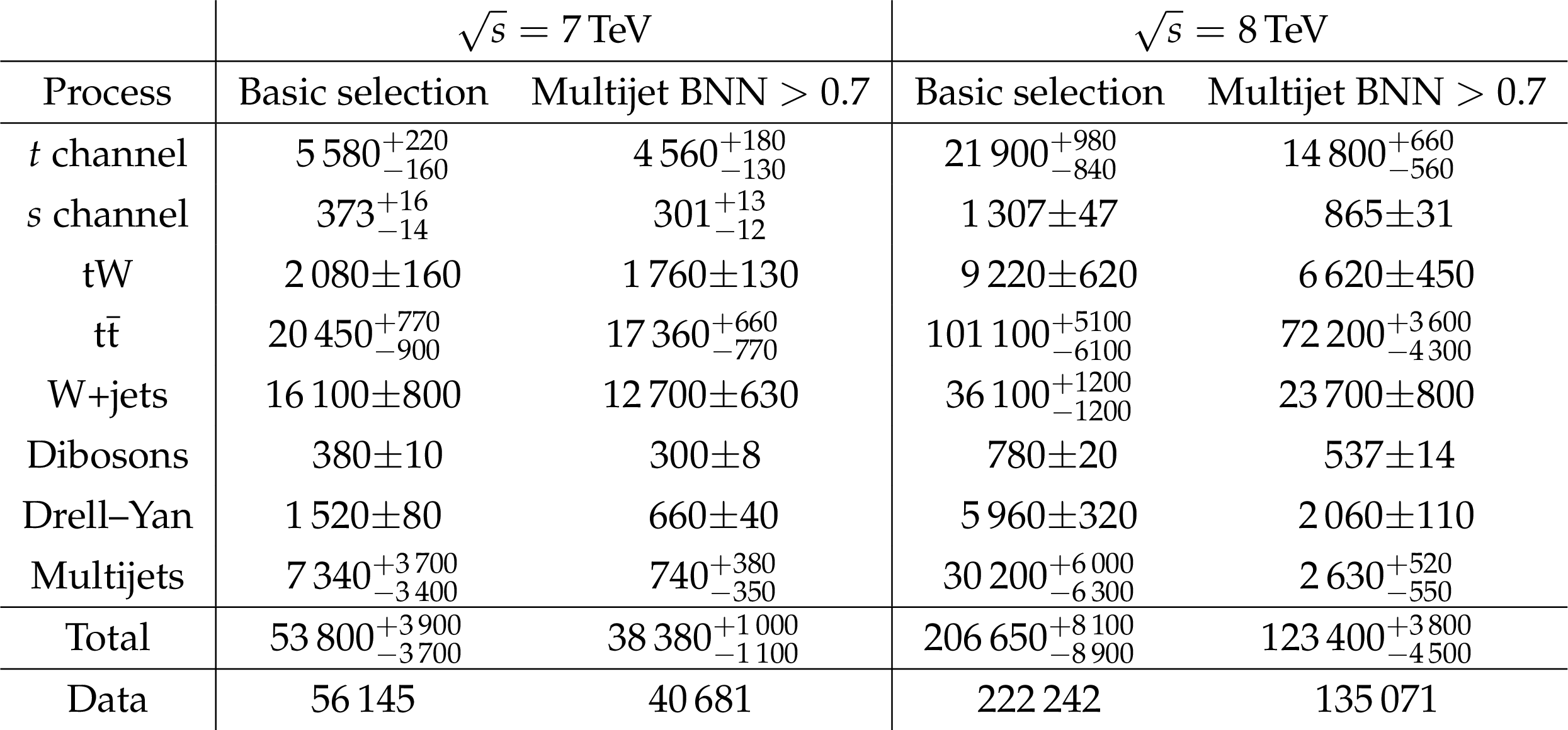
Table 1:
The predicted and observed events yields before and after the multijet BNN selection for the two data sets. The uncertainties include the estimation of the scale and parton distribution function uncertainties. |
png pdf |
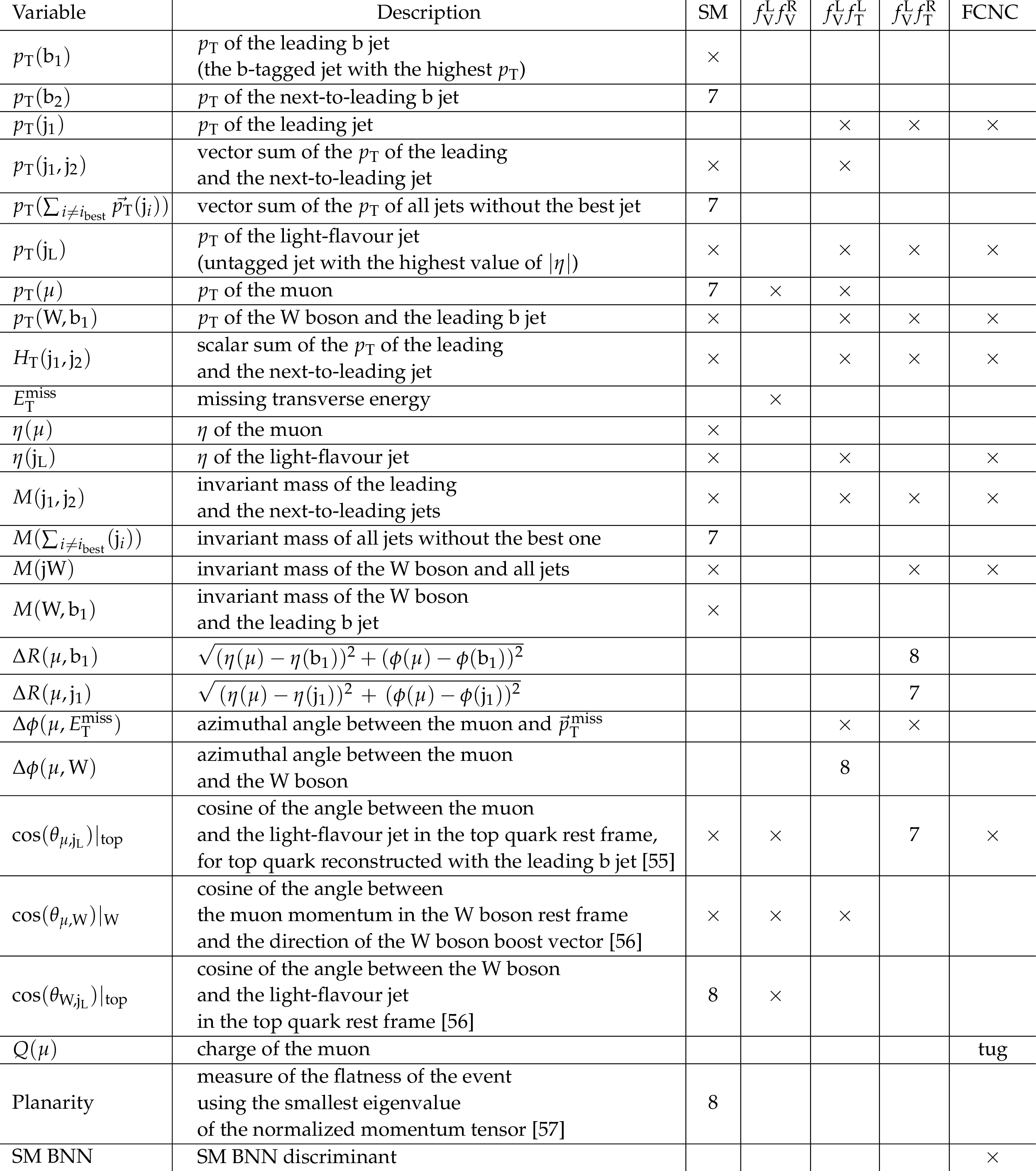
Table 2:
Input variables for the BNNs used in the analysis. The symbol $\times $ represents the variables used for each particular BNN. The number 7 or 8 marks the variables used in just the $\sqrt {s}=$ 7 or 8 TeV analysis. The symbol "tug" marks the variables used just in the training of the tug FCNC BNN. The notations "leading" and "next-to-leading" refer to the highest-$ {p_{\mathrm {T}}}$ and second-highest-$ {p_{\mathrm {T}}}$ jet, respectively. The notation "best" jet is used for the jet that gives a reconstructed mass of the top quark closest to the value of 172.5 GeV , which is used in the MC simulation. |
png pdf |
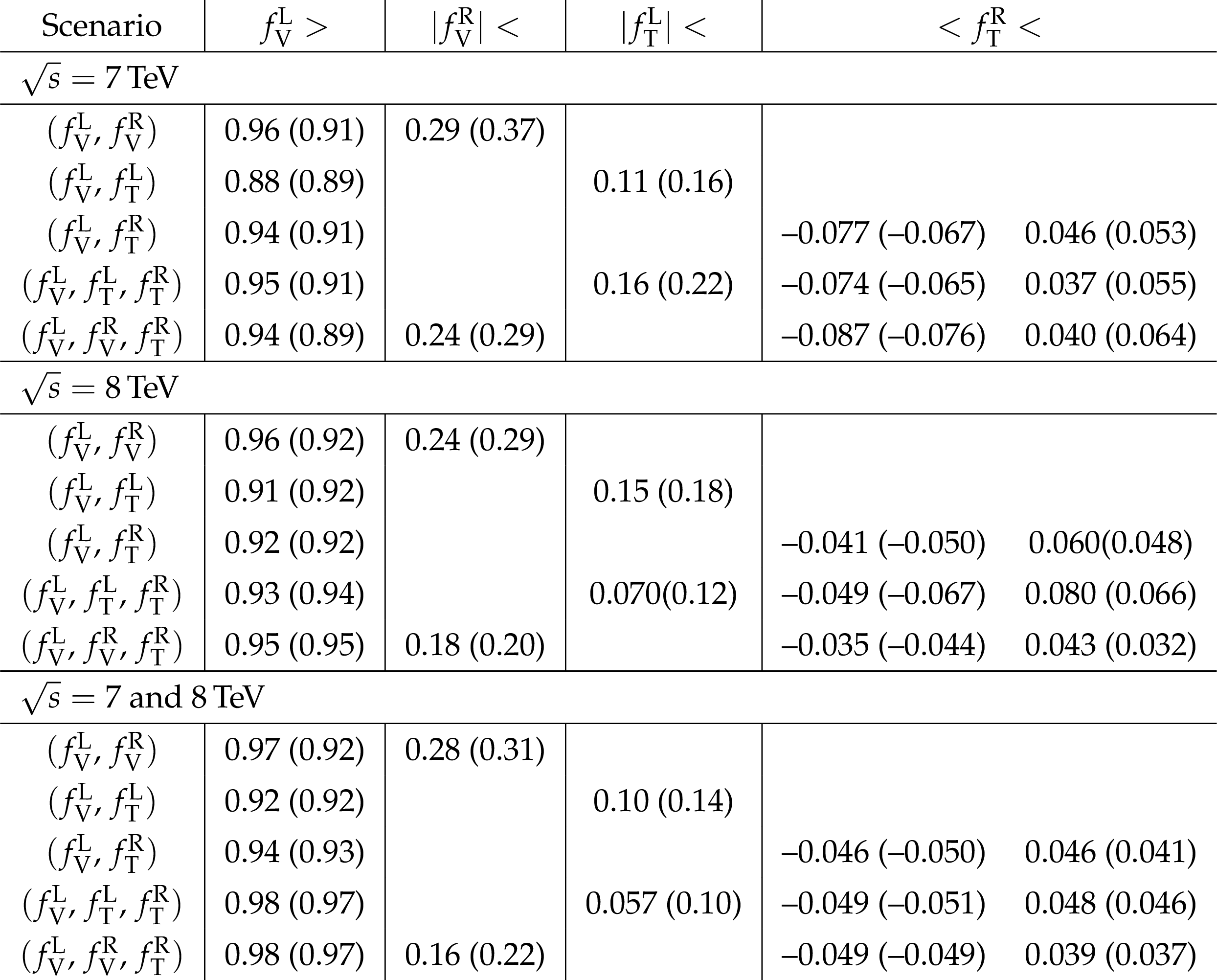
Table 3:
One-dimensional exclusion limits obtained in different two- and three-dimensional fit scenarios. The first column shows the couplings allowed to vary in the fit, with the remaining couplings set to the SM values. The observed (expected) 95% CL limits for each of the two data sets and their combination are given in the following columns. |
png pdf |
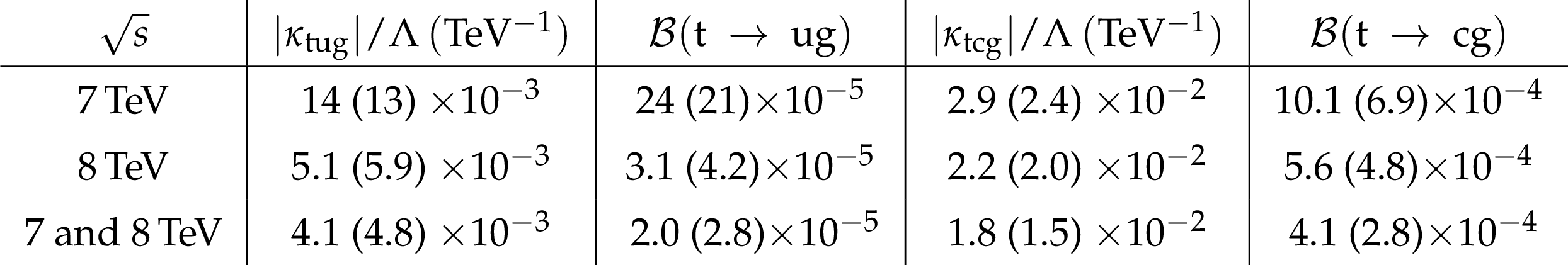
Table 4:
Observed (expected) upper limits at 95% CL for the FCNC couplings and branching fractions obtained using the $\sqrt {s} = $ 7 and 8 TeV data, and their combination. |
| Summary |
| A direct search for model-independent anomalous operators in the Wtb vertex and FCNC couplings has been performed using single top quark $t$-channel production in data collected by the CMS experiment in pp collisions at $\sqrt{s} =$ 7 and 8 TeV. Different possible anomalous contributions are investigated. The observed event rates are consistent with the SM prediction, and exclusion limits are extracted at 95% CL. The combined limits in three-dimensional scenarios on possible Wtb anomalous couplings are $f_{\rm V}^{\rm L} > 0.98$ for the left-handed vector coupling, $| f_{\rm V}^{\rm R}| < 0.16 $ for the right-handed vector coupling, $| f_{\rm T}^{\rm L}| <0.05$ 7 for the left-handed tensor coupling, and $ -0.049 < f_{\rm T}^{\rm R} < 0.048 $ for the right-handed tensor coupling. For FCNC couplings of the gluon to top and up quarks (tug) or top and charm quarks (tcg), the 95% CL exclusion limits on the coupling strengths are $|\kappa_{\rm tug}| /\Lambda < 4.1 \times 10^{-3}\,\mathrm{TeV^{ -1}}$ and $|\kappa_{\rm tcg}| /\Lambda < 1.8 \times 10^{-2}\,\mathrm{TeV^{ -1}}$ or, in terms of branching fractions, $\mathcal{B}(\rm t\rightarrow ug) < 2.0\times 10^{-5}$ and $\mathcal{B}(\rm t \rightarrow cg) < 4.1\times10^{-4}$. |
| References | ||||
| 1 | M. Beneke et al. | Top quark physics | hep-ph/0003033 | |
| 2 | S. S. D. Willenbrock and D. A. Dicus | Production of heavy quarks from W gluon fusion | PRD 34 (1986) 155 | |
| 3 | S. L. Glashow, J. Iliopoulos, and L. Maiani | Weak interactions with lepton-hadron symmetry | PRD 2 (1970) 1285 | |
| 4 | Particle Data Group, K. A. Olive et al. | Review of Particle Physics | CPC 38 (2014) 090001 | |
| 5 | G. Eilam, J. L. Hewett, and A. Soni | Rare decays of the top quark in the standard and two Higgs doublet models | PRD 44 (1991) 1473, .[Erratum: \DOI10.1103/PhysRevD.59.039901 | |
| 6 | D. Atwood, L. Reina, and A. Soni | Probing flavor changing top-charm-scalar interactions in $ {\rm e^{+} e^{-}} $ collisions | PRD 53 (1996) 1199 | hep-ph/9506243 |
| 7 | J. M. Yang, B.-L. Young, and X. Zhang | Flavor-changing top quark decays in R-parity-violating SUSY | PRD 58 (1998) 055001 | hep-ph/9705341 |
| 8 | Y. Grossman | Phenomenology of models with more than two Higgs doublets | Nucl. Phys. B 426 (1994) 355 | hep-ph/9401311 |
| 9 | A. Pich and P. Tuzon | Yukawa alignment in the two-Higgs-doublet model | PRD 80 (2009) 091702 | 0908.1554 |
| 10 | V. Keus, S. F. King, and S. Moretti | Three-Higgs-doublet models: symmetries, potentials and Higgs boson masses | JHEP 01 (2014) 052 | 1310.8253 |
| 11 | J. L. Diaz-Cruz, R. Martinez, M. A. Perez, and A. Rosado | Flavor changing radiative decay of the $ t $ quark | PRD 41 (1990) 891 | |
| 12 | A. Arhrib and W.-S. Hou | Flavor changing neutral currents involving heavy quarks with four generations | JHEP 07 (2006) 009 | hep-ph/0602035 |
| 13 | G. C. Branco and M. N. Rebelo | New physics in the flavour sector in the presence of flavour changing neutral currents | PoS Corfu2012 (2013) 024 | 1308.4639 |
| 14 | H. Georgi, L. Kaplan, D. Morin, and A. Schenk | Effects of top compositeness | PRD 51 (1995) 3888 | hep-ph/9410307 |
| 15 | G. F. Giudice, C. Grojean, A. Pomarol, and R. Rattazzi | The strongly-interacting light Higgs | JHEP 06 (2007) 045 | hep-ph/0703164 |
| 16 | M. K\"onig, M. Neubert, and D. M. Straub | Dipole operator constraints on composite Higgs models | EPJC 74 (2014) 2945 | 1403.2756 |
| 17 | K. Agashe et al. | Warped dipole completed, with a tower of Higgs bosons | JHEP 06 (2015) 196 | 1412.6468 |
| 18 | R. Contino, Y. Nomura, and A. Pomarol | Higgs as a holographic pseudo-Goldstone boson | Nucl. Phys. B 671 (2003) 148 | hep-ph/0306259 |
| 19 | J. A. Aguilar-Saavedra | A minimal set of top anomalous couplings | Nucl. Phys. B 812 (2009) 181 | 0811.3842 |
| 20 | S. Willenbrock and C. Zhang | Effective field theory beyond the Standard Model | Ann. Rev. Nucl. Part. Sci. 64 (2014) 83 | 1401.0470 |
| 21 | CDF Collaboration | Search for top-quark production via flavor-changing neutral currents in $ \mathrm{W} $+1 jet events at CDF | PRL 102 (2009) 151801 | 0812.3400 |
| 22 | D0 Collaboration | Search for flavor changing neutral currents via quark-gluon couplings in single top quark production using 2.3$ fb$^{-1}$ $ of $ \rm {p\bar{p}} $ collisions | PLB 693 (2010) 81 | 1006.3575 |
| 23 | ATLAS Collaboration | Search for single top-quark production via flavour-changing neutral currents at 8$ TeV $ with the ATLAS detector | EPJC 76 (2016) 55 | 1509.00294 |
| 24 | CMS Collaboration | Measurement of the $ t $-channel single-top-quark production cross section and of the $ |V_{\mathrm{tb}}| $ CKM matrix element in pp collisions at $ \sqrt{s} = $ 8$ TeV $ | JHEP 06 (2014) 090 | CMS-TOP-12-038 1403.7366 |
| 25 | CMS Collaboration | Measurement of top quark polarisation in $ t $-channel single top quark production | JHEP 04 (2016) 073 | CMS-TOP-13-001 1511.02138 |
| 26 | ATLAS Collaboration | Comprehensive measurements of $ t $-channel single top-quark production cross sections at $ \sqrt{s} = $ 7$ TeV $ with the ATLAS detector | PRD 90 (2014) 112006 | 1406.7844 |
| 27 | E. Boos et al. | CompHEP 4.4: automatic computations from Lagrangians to events | NIMA 534 (2004) 250 | hep-ph/0403113 |
| 28 | R. M. N. | Bayesian learning for neural networks | Technical Report ISBN 0-387-94724-8, Dept. of Statistics and Dept. of Computer Science, University of Toronto | |
| 29 | P. C. Bhat and H. B. Prosper | Bayesian neural networks | ||
| 30 | R. M. Neal | Software for flexible Bayesian modeling and Markov chain sampling | Technical Report 2004-11-10, Dept. of Statistics and Dept. of Computer Science, University of Toronto | |
| 31 | CMS Collaboration | The CMS experiment at the CERN LHC | JINST 3 (2008) S08004 | CMS-00-001 |
| 32 | CMS Collaboration | Particle--flow event reconstruction in CMS and performance for jets, taus, and $ E_{\mathrm{T}}^{\text{miss}} $ | CDS | |
| 33 | CMS Collaboration | Commissioning of the particle--flow event reconstruction with the first LHC collisions recorded in the CMS detector | CDS | |
| 34 | M. Cacciari, G. P. Salam, and G. Soyez | The anti-$ k_t $ jet clustering algorithm | JHEP 04 (2008) 063 | 0802.1189 |
| 35 | M. Cacciari, G. P. Salam, and G. Soyez | FastJet user manual | EPJC 72 (2012) 1896 | 1111.6097 |
| 36 | E. E. Boos et al. | Method for simulating electroweak top-quark production events in the NLO approximation: SingleTop event generator | Phys. Atom. Nucl. 69 (2006) 1317 | |
| 37 | N. Kidonakis | Next-to-next-to-leading-order collinear and soft gluon corrections for $ t $-channel single top quark production | PRD 83 (2011) 091503 | 1103.2792 |
| 38 | U. L. M. Aliev, H. Lacker et al. | HATHOR: a HAdronic Top and Heavy quarks crOss section calculatoR | CPC 182 (2011) 1034 | 1007.1327 |
| 39 | P. Kant et al. | HatHor for single top-quark production: Updated predictions and uncertainty estimates for single top-quark production in hadronic collisions | CPC 191 (2015) 74 | 1406.4403 |
| 40 | S. Alioli, P. Nason, C. Oleari, and E. Re | A general framework for implementing NLO calculations in shower Monte Carlo programs: the POWHEG BOX | JHEP 06 (2010) 043 | 1002.2581 |
| 41 | J. Alwall et al. | MadGraph 5: going beyond | JHEP 06 (2011) 128 | 1106.0522 |
| 42 | M. Czakon, P. Fiedler, and A. Mitov | Total top-quark pair-production cross section at hadron colliders through $ \mathcal{O}(\alpha^4_S) $ | PRL 110 (2013) 252004 | 1303.6254 |
| 43 | M. Czakon and A. Mitov | Top++: a program for the calculation of the top-pair cross-section at hadron colliders | CPC 185 (2014) 2930 | 1112.5675 |
| 44 | R. Gavin, Y. Li, F. Petriello, and S. Quackenbush | FEWZ 2.0: A code for hadronic Z production at next-to-next-to-leading order | CPC 182 (2011) 2388 | 1011.3540 |
| 45 | J. M. Campbell and R. K. Ellis | MCFM for the Tevatron and the LHC | NPPS 205-206 (2010) 10 | 1007.3492 |
| 46 | T. Sj\"ostrand, S. Mrenna, and P. Z. Skands | PYTHIA 6.4 physics and manual | JHEP 05 (2006) 026 | hep-ph/0603175 |
| 47 | N. Kidonakis | Top quark production | 1311.0283 | |
| 48 | CMS Collaboration | Performance of CMS muon reconstruction in pp collision events at $ \sqrt{s}= $ 7$ TeV $ | JINST 7 (2012) P10002 | CMS-MUO-10-004 1206.4071 |
| 49 | CMS Collaboration | Single muon efficiencies in 2012 Data | CDS | |
| 50 | CMS Collaboration | Identification of b-quark jets with the CMS experiment | JINST 8 (2013) P04013 | CMS-BTV-12-001 1211.4462 |
| 51 | G. Mahlon and S. J. Parke | Improved spin basis for angular correlation studies in single top quark production at the Tevatron | PRD 55 (1997) 7249 | hep-ph/9611367 |
| 52 | J. A. Aguilar-Saavedra and R. V. Herrero-Hahn | Model-independent measurement of the top quark polarisation | PLB 718 (2012) 983 | 1208.6006 |
| 53 | V. D. Barger and R. J. N. Phillips | Collider physics | Redwood City, USA: Addison-Wesley (1987) (Frontiers In Physics, 71)(1987) | |
| 54 | CMS Collaboration | Measurement of the $ t $-channel single top quark production cross section in pp collisions at $ \sqrt{s} = $ 7$ TeV $ | PRL 107 (2011) 091802 | CMS-TOP-10-008 1106.3052 |
| 55 | CMS Collaboration | Measurement of the single-top-quark $ t $-channel cross section in pp collisions at $ \sqrt{s} = $ 7$ TeV $ | JHEP 12 (2012) 035 | CMS-TOP-11-021 1209.4533 |
| 56 | CMS Collaboration | Determination of jet energy calibration and transverse momentum resolution in CMS | JINST 6 (2011) P11002 | CMS-JME-10-011 1107.4277 |
| 57 | CMS Collaboration | Jet energy resolution in CMS at $ \sqrt{s} = $ 7$ TeV $ | CDS | |
| 58 | CMS Collaboration | Absolute calibration of the luminosity measurement at CMS: winter 2012 update | CDS | |
| 59 | CMS Collaboration | CMS luminosity based on pixel cluster counting --- Summer 2013 update | ||
| 60 | CMS Collaboration | Measurement of the inelastic proton-proton cross section at $ \sqrt{s} = $ 7$ TeV $ | PLB 722 (2013) 5 | CMS-FWD-11-001 1210.6718 |
| 61 | J. Alwall, S. de Visscher, and F. Maltoni | QCD radiation in the production of heavy colored particles at the LHC | JHEP 02 (2009) 017 | 0810.5350 |
| 62 | J. Gao et al. | CT10 next-to-next-to-leading order global analysis of QCD | PRD 89 (2014) 033009 | 1302.6246 |
| 63 | S. Alekhin et al. | The PDF4LHC Working Group interim report | 1101.0536 | |
| 64 | CMS Collaboration | Measurement of differential top-quark pair production cross sections in pp collisions at $ \sqrt{s} = $ 7$ TeV $ | EPJC 73 (2013) 2339 | CMS-TOP-11-013 1211.2220 |
| 65 | CMS Collaboration | Measurement of the differential cross section for top quark pair production in pp collisions at $ \sqrt{s} = $ 8$ TeV $ | EPJC 75 (2015) 542 | CMS-TOP-12-028 1505.04480 |
| 66 | R. J. Barlow and C. Beeston | Fitting using finite Monte Carlo samples | CPC 77 (1993) 219 | |
| 67 | W. Buchm\"uller and D. Wyler | Effective lagrangian analysis of new interactions and flavor conservation | Nucl. Phys. B 268 (1986) 621 | |
| 68 | G. L. Kane, G. A. Ladinsky, and C. P. Yuan | Using the top quark for testing Standard Model polarization and CP predictions | PRD 45 (1992) 124 | |
| 69 | D0 Collaboration | Search for anomalous Wtb couplings in single top quark production | PRL 101 (2008) 221801 | 0807.1692 |
| 70 | D0 Collaboration | Search for anomalous Wtb couplings in single top quark production in $ \rm {p\bar{p}} $ collisions at $ \sqrt{s} = $ 1.96$ TeV $ | PLB 708 (2012) 21 | 1110.4592 |
| 71 | E. Boos, V. Bunichev, L. Dudko, and M. Perfilov | Modeling of anomalous Wtb interactions in single top quark events using auxiliary fields | 1607.00505 | |
| 72 | ATLAS Collaboration | Measurement of the W boson polarization in top quark decays with the ATLAS detector | JHEP 06 (2012) 088 | 1205.2484 |
| 73 | CMS Collaboration | Measurement of the W-boson helicity in top-quark decays from $ t\bar{t} $ production in lepton+jets events in pp collisions at $ \sqrt{s} = $ 7$ TeV $ | JHEP 10 (2013) 167 | CMS-TOP-11-020 1308.3879 |
| 74 | CMS Collaboration | Measurement of the W boson helicity in events with a single reconstructed top quark in pp collisions at $ \sqrt{s}= $ 8$ TeV $ | JHEP 01 (2015) 053 | CMS-TOP-12-020 1410.1154 |
| 75 | J. J. Liu, C. S. Li, L. L. Yang, and L. G. Jin | Next-to-leading order QCD corrections to the direct top quark production via model-independent FCNC couplings at hadron colliders | PRD 72 (2005) 074018 | hep-ph/0508016 |
| 76 | J. J. Zhang et al. | Next-to-leading order QCD corrections to the top quark decay via model-independent FCNC couplings | PRL 102 (2009) 072001 | 0810.3889 |
|
|
Compact Muon Solenoid LHC, CERN |
|

|

|

|

|

|