

Compact Muon Solenoid
LHC, CERN
| CMS-PAS-HIG-18-007 | ||
| Search for the standard model Higgs boson decaying to a pair of $\tau$ leptons and produced in association with a W or a Z boson in proton-proton collisions at $\sqrt{s}=$ 13 TeV | ||
| CMS Collaboration | ||
| June 2018 | ||
| Abstract: A search for the standard model Higgs boson produced in association with a W or a Z boson decaying leptonically is performed using a data sample of proton-proton collisions collected at $\sqrt{s} = $ 13 TeV by the CMS experiment at the LHC corresponding to an integrated luminosity of 35.9 fb$^{-1}$. The Higgs boson is sought in its decay to a pair of $\tau$ leptons. A significance of 2.3 standard deviations is observed (1.0 expected) for a Higgs boson mass of 125 GeV. The signal strength, $\mu = $ 2.5$^{+1.4} _{-1.3}$, is measured relative to the expectation for the standard model Higgs boson. These results are combined with a previous analysis performed on the same data set targeting the gluon fusion and vector boson fusion production modes with the Higgs boson decaying to a pair of $\tau$ leptons. The combined results provide increased sensitivity to the Higgs boson couplings to fermions and vector bosons, which are measured to be compatible with standard model predictions within one standard deviation. | ||
|
Links:
CDS record (PDF) ;
inSPIRE record ;
CADI line (restricted) ;
These preliminary results are superseded in this paper, JHEP 06 (2019) 093. The superseded preliminary plots can be found here. |
||
| Figures | |

png pdf |
Figure 1:
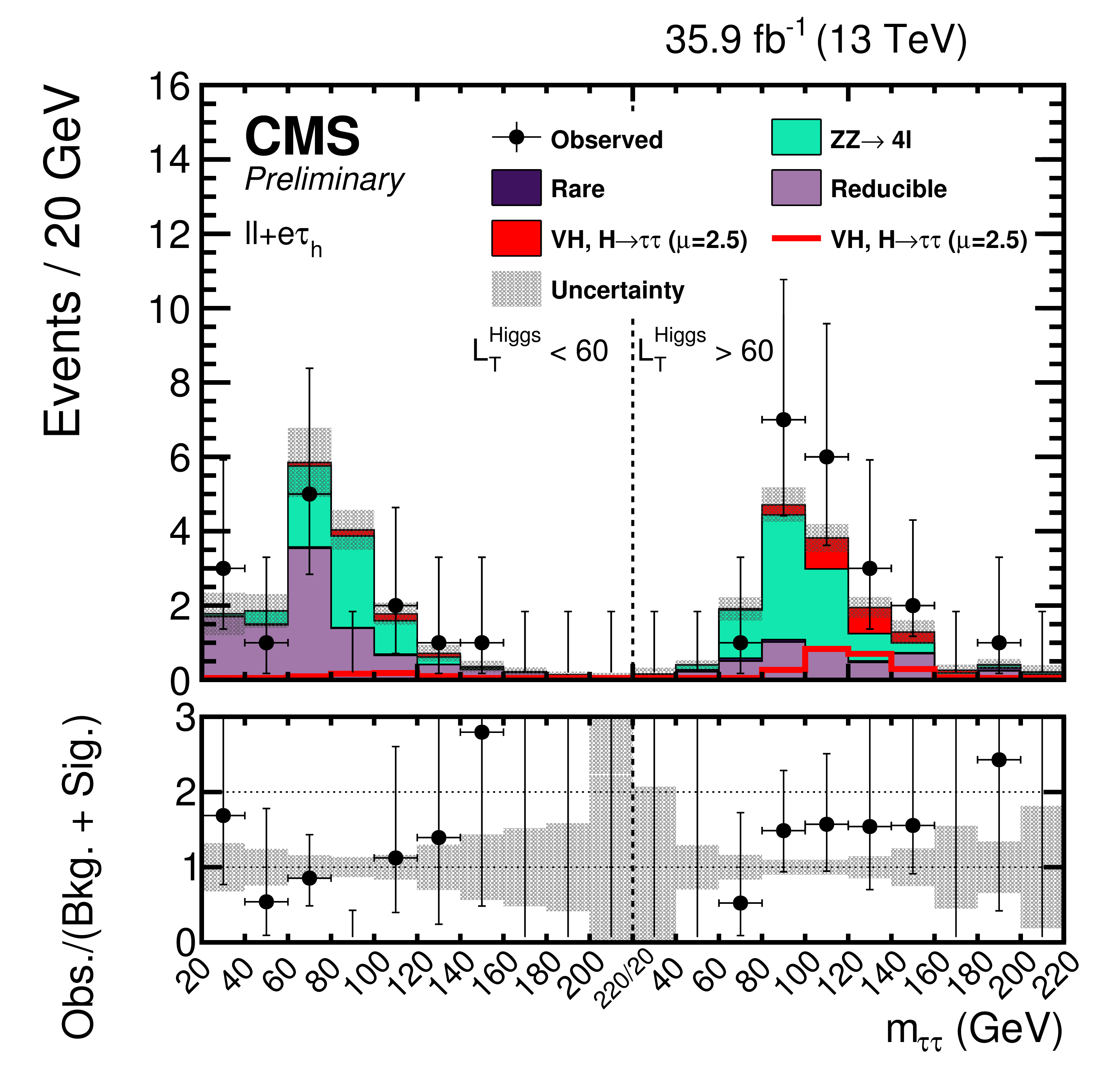
The postfit $ {m_{{\tau} {\tau}}} $ distributions used to extract the signal shown for (top left) $\ell \ell {\mathrm {e}} {{\tau} _\mathrm {h}} $, (top right) $\ell \ell {{\mu}} {{\tau} _\mathrm {h}} $, (bottom left) $\ell \ell {{\tau} _\mathrm {h}} {{\tau} _\mathrm {h}} $, and (bottom right) $\ell \ell {\mathrm {e}} {{\mu}}$. The uncertainties include statistical and systematic sources. The left half of each distribution is the Low-$L_{T}^{\textrm {Higgs}}$ region while the right half of each distribution is the High-$L_{T}^{\textrm {Higgs}}$ region. The $ {\mathrm {W}} {\mathrm {H}} $ and $ {\mathrm {Z}} {\mathrm {H}} $, $ {{\mathrm {H}} \to {\tau} {\tau}} $ signal processes are summed together and shown as $ {\text {VH}} $, $ {{\mathrm {H}} \to {\tau} {\tau}} $ with a best-fit $\mu = 2.5$. $ {\text {VH}} $, $ {{\mathrm {H}} \to {\tau} {\tau}} $ is shown both as a stacked filled histogram and an open overlaid histogram. In these distributions the $ {\mathrm {Z}} {\mathrm {H}} $, $ {{\mathrm {H}} \to {\tau} {\tau}} $ process contributes more than 99% of the total of $ {\text {VH}} $, $ {{\mathrm {H}} \to {\tau} {\tau}} $. |
png pdf |
Figure 1-a:
The postfit $ {m_{{\tau} {\tau}}} $ distributions used to extract the signal shown for (top left) $\ell \ell {\mathrm {e}} {{\tau} _\mathrm {h}} $, (top right) $\ell \ell {{\mu}} {{\tau} _\mathrm {h}} $, (bottom left) $\ell \ell {{\tau} _\mathrm {h}} {{\tau} _\mathrm {h}} $, and (bottom right) $\ell \ell {\mathrm {e}} {{\mu}}$. The uncertainties include statistical and systematic sources. The left half of each distribution is the Low-$L_{T}^{\textrm {Higgs}}$ region while the right half of each distribution is the High-$L_{T}^{\textrm {Higgs}}$ region. The $ {\mathrm {W}} {\mathrm {H}} $ and $ {\mathrm {Z}} {\mathrm {H}} $, $ {{\mathrm {H}} \to {\tau} {\tau}} $ signal processes are summed together and shown as $ {\text {VH}} $, $ {{\mathrm {H}} \to {\tau} {\tau}} $ with a best-fit $\mu = 2.5$. $ {\text {VH}} $, $ {{\mathrm {H}} \to {\tau} {\tau}} $ is shown both as a stacked filled histogram and an open overlaid histogram. In these distributions the $ {\mathrm {Z}} {\mathrm {H}} $, $ {{\mathrm {H}} \to {\tau} {\tau}} $ process contributes more than 99% of the total of $ {\text {VH}} $, $ {{\mathrm {H}} \to {\tau} {\tau}} $. |

png pdf |
Figure 1-b:
The postfit $ {m_{{\tau} {\tau}}} $ distributions used to extract the signal shown for (top left) $\ell \ell {\mathrm {e}} {{\tau} _\mathrm {h}} $, (top right) $\ell \ell {{\mu}} {{\tau} _\mathrm {h}} $, (bottom left) $\ell \ell {{\tau} _\mathrm {h}} {{\tau} _\mathrm {h}} $, and (bottom right) $\ell \ell {\mathrm {e}} {{\mu}}$. The uncertainties include statistical and systematic sources. The left half of each distribution is the Low-$L_{T}^{\textrm {Higgs}}$ region while the right half of each distribution is the High-$L_{T}^{\textrm {Higgs}}$ region. The $ {\mathrm {W}} {\mathrm {H}} $ and $ {\mathrm {Z}} {\mathrm {H}} $, $ {{\mathrm {H}} \to {\tau} {\tau}} $ signal processes are summed together and shown as $ {\text {VH}} $, $ {{\mathrm {H}} \to {\tau} {\tau}} $ with a best-fit $\mu = 2.5$. $ {\text {VH}} $, $ {{\mathrm {H}} \to {\tau} {\tau}} $ is shown both as a stacked filled histogram and an open overlaid histogram. In these distributions the $ {\mathrm {Z}} {\mathrm {H}} $, $ {{\mathrm {H}} \to {\tau} {\tau}} $ process contributes more than 99% of the total of $ {\text {VH}} $, $ {{\mathrm {H}} \to {\tau} {\tau}} $. |

png pdf |
Figure 1-c:
The postfit $ {m_{{\tau} {\tau}}} $ distributions used to extract the signal shown for (top left) $\ell \ell {\mathrm {e}} {{\tau} _\mathrm {h}} $, (top right) $\ell \ell {{\mu}} {{\tau} _\mathrm {h}} $, (bottom left) $\ell \ell {{\tau} _\mathrm {h}} {{\tau} _\mathrm {h}} $, and (bottom right) $\ell \ell {\mathrm {e}} {{\mu}}$. The uncertainties include statistical and systematic sources. The left half of each distribution is the Low-$L_{T}^{\textrm {Higgs}}$ region while the right half of each distribution is the High-$L_{T}^{\textrm {Higgs}}$ region. The $ {\mathrm {W}} {\mathrm {H}} $ and $ {\mathrm {Z}} {\mathrm {H}} $, $ {{\mathrm {H}} \to {\tau} {\tau}} $ signal processes are summed together and shown as $ {\text {VH}} $, $ {{\mathrm {H}} \to {\tau} {\tau}} $ with a best-fit $\mu = 2.5$. $ {\text {VH}} $, $ {{\mathrm {H}} \to {\tau} {\tau}} $ is shown both as a stacked filled histogram and an open overlaid histogram. In these distributions the $ {\mathrm {Z}} {\mathrm {H}} $, $ {{\mathrm {H}} \to {\tau} {\tau}} $ process contributes more than 99% of the total of $ {\text {VH}} $, $ {{\mathrm {H}} \to {\tau} {\tau}} $. |

png pdf |
Figure 1-d:
The postfit $ {m_{{\tau} {\tau}}} $ distributions used to extract the signal shown for (top left) $\ell \ell {\mathrm {e}} {{\tau} _\mathrm {h}} $, (top right) $\ell \ell {{\mu}} {{\tau} _\mathrm {h}} $, (bottom left) $\ell \ell {{\tau} _\mathrm {h}} {{\tau} _\mathrm {h}} $, and (bottom right) $\ell \ell {\mathrm {e}} {{\mu}}$. The uncertainties include statistical and systematic sources. The left half of each distribution is the Low-$L_{T}^{\textrm {Higgs}}$ region while the right half of each distribution is the High-$L_{T}^{\textrm {Higgs}}$ region. The $ {\mathrm {W}} {\mathrm {H}} $ and $ {\mathrm {Z}} {\mathrm {H}} $, $ {{\mathrm {H}} \to {\tau} {\tau}} $ signal processes are summed together and shown as $ {\text {VH}} $, $ {{\mathrm {H}} \to {\tau} {\tau}} $ with a best-fit $\mu = 2.5$. $ {\text {VH}} $, $ {{\mathrm {H}} \to {\tau} {\tau}} $ is shown both as a stacked filled histogram and an open overlaid histogram. In these distributions the $ {\mathrm {Z}} {\mathrm {H}} $, $ {{\mathrm {H}} \to {\tau} {\tau}} $ process contributes more than 99% of the total of $ {\text {VH}} $, $ {{\mathrm {H}} \to {\tau} {\tau}} $. |
png pdf |
Figure 2:
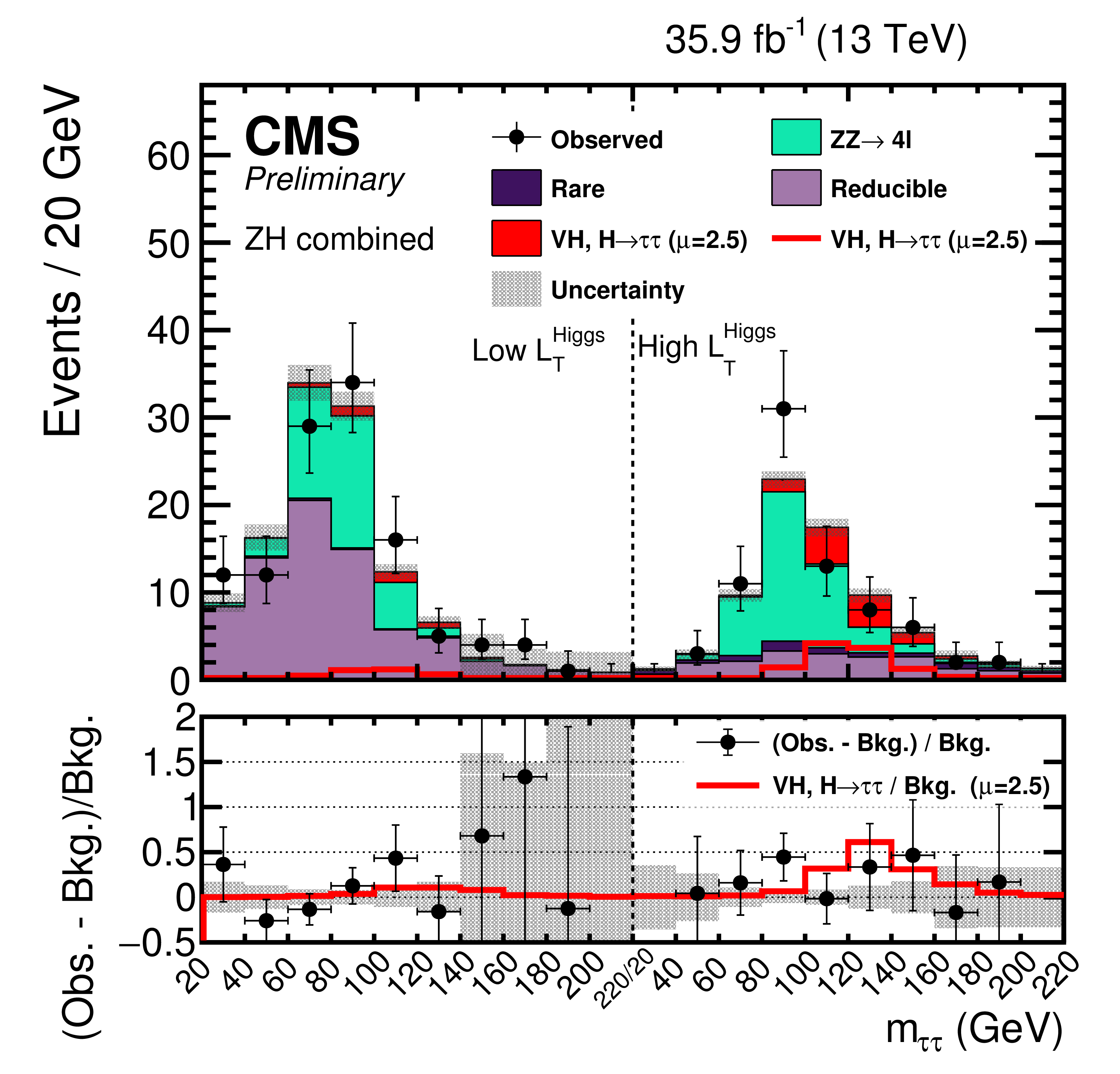
The postfit $ {m_{{\tau} {\tau}}} $ distributions used to extract the signal shown for all 8 $ {\mathrm {Z}} {\mathrm {H}} $ channels combined. The uncertainties include statistical and systematic sources. The left half of the distribution is the Low-$L_{T}^{\textrm {Higgs}}$ region while the right half corresponds to the High-$L_{T}^{\textrm {Higgs}}$ region. The definitions of the $L_{T}^{\textrm {Higgs}}$ regions in this distribution are the same as those used in Fig. 1 and are final state dependent. The $ {\mathrm {W}} {\mathrm {H}} $ and $ {\mathrm {Z}} {\mathrm {H}} $, $ {{\mathrm {H}} \to {\tau} {\tau}} $ signal processes are summed together and shown as $ {\text {VH}} $, $ {{\mathrm {H}} \to {\tau} {\tau}} $ with a best-fit $\mu = 2.5$. $ {\text {VH}} $, $ {{\mathrm {H}} \to {\tau} {\tau}} $ is shown both as a stacked filled histogram and an open overlaid histogram. In this distribution the $ {\mathrm {Z}} {\mathrm {H}} $, $ {{\mathrm {H}} \to {\tau} {\tau}} $ process contributes more than 99% of the total of $ {\text {VH}} $, $ {{\mathrm {H}} \to {\tau} {\tau}} $. |

png pdf |
Figure 3:
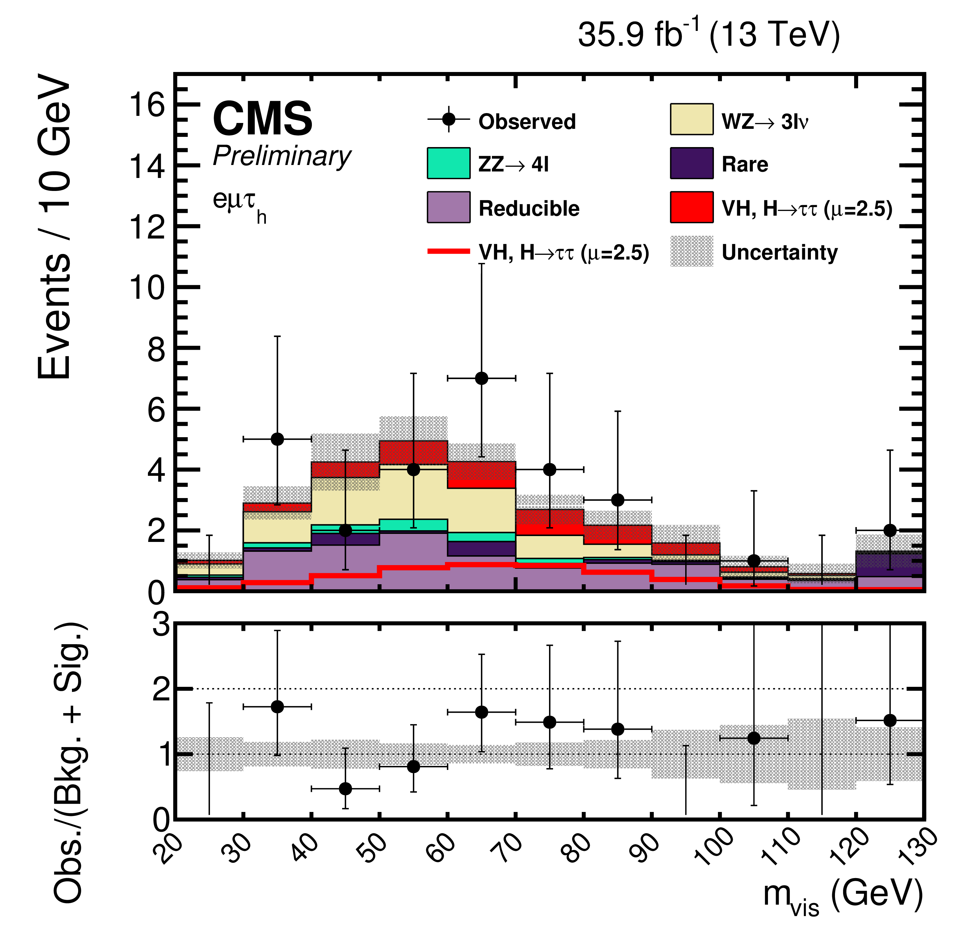
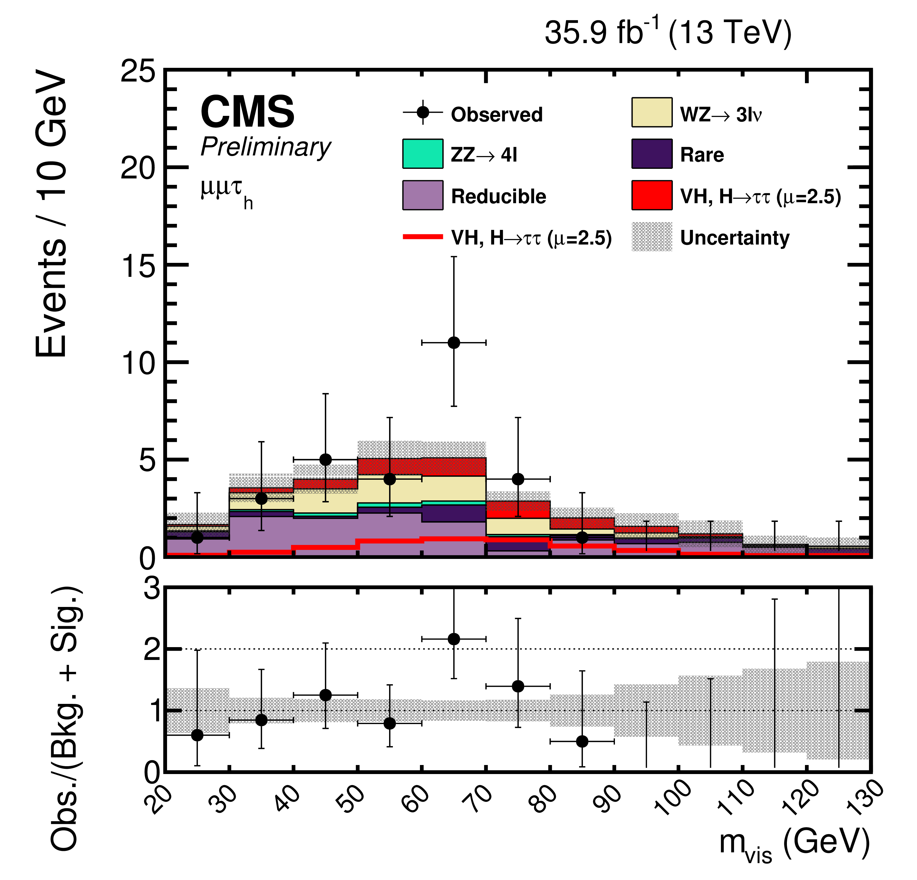
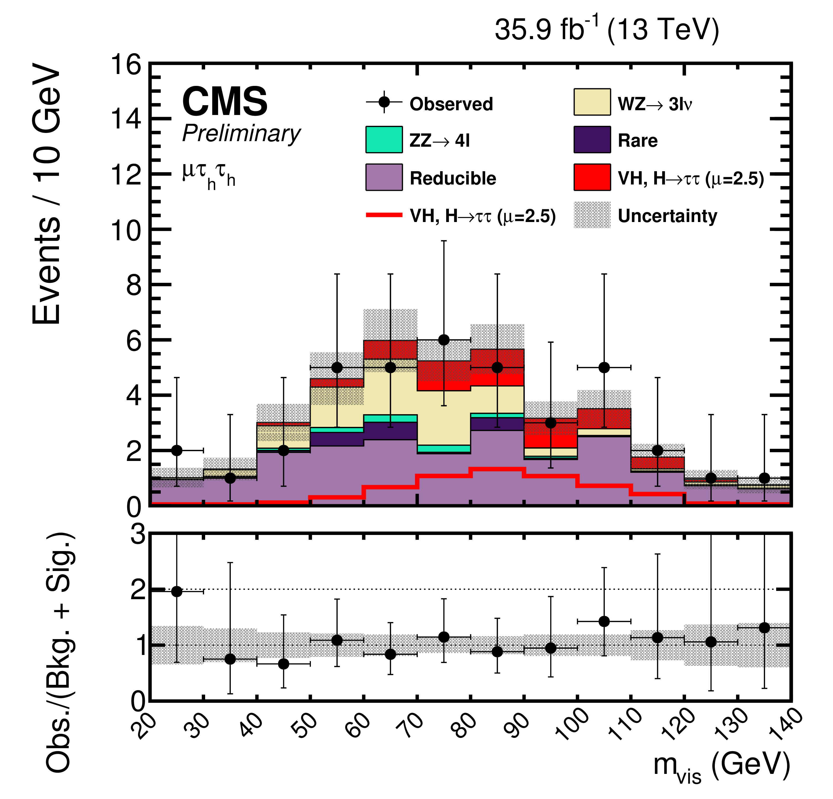
Postfit mass distributions in the $ {\mathrm {e}} {{\mu}} {{\tau} _\mathrm {h}} $ (top left), $ {{\mu}} {{\mu}} {{\tau} _\mathrm {h}} $ (top right), $ {\mathrm {e}} {{\tau} _\mathrm {h}} {{\tau} _\mathrm {h}} $ (bottom left), and $ {{\mu}} {{\tau} _\mathrm {h}} {{\tau} _\mathrm {h}} $ (bottom right) final states. The uncertainties include statistical and systematic sources. The $ {\mathrm {W}} {\mathrm {H}} $ and $ {\mathrm {Z}} {\mathrm {H}} $, $ {{\mathrm {H}} \to {\tau} {\tau}} $ signal processes are summed together and shown as $ {\text {VH}} $, $ {{\mathrm {H}} \to {\tau} {\tau}} $ with a best-fit $\mu = 2.5$. $ {\text {VH}} $, $ {{\mathrm {H}} \to {\tau} {\tau}} $ is shown both as a stacked filled histogram and an open overlaid histogram. In these distribution the $ {\mathrm {W}} {\mathrm {H}} $, $ {{\mathrm {H}} \to {\tau} {\tau}} $ processes contributes between 91-93% of the total of $ {\text {VH}} $, $ {{\mathrm {H}} \to {\tau} {\tau}} $. |
png pdf |
Figure 3-a:
Postfit mass distributions in the $ {\mathrm {e}} {{\mu}} {{\tau} _\mathrm {h}} $ (top left), $ {{\mu}} {{\mu}} {{\tau} _\mathrm {h}} $ (top right), $ {\mathrm {e}} {{\tau} _\mathrm {h}} {{\tau} _\mathrm {h}} $ (bottom left), and $ {{\mu}} {{\tau} _\mathrm {h}} {{\tau} _\mathrm {h}} $ (bottom right) final states. The uncertainties include statistical and systematic sources. The $ {\mathrm {W}} {\mathrm {H}} $ and $ {\mathrm {Z}} {\mathrm {H}} $, $ {{\mathrm {H}} \to {\tau} {\tau}} $ signal processes are summed together and shown as $ {\text {VH}} $, $ {{\mathrm {H}} \to {\tau} {\tau}} $ with a best-fit $\mu = 2.5$. $ {\text {VH}} $, $ {{\mathrm {H}} \to {\tau} {\tau}} $ is shown both as a stacked filled histogram and an open overlaid histogram. In these distribution the $ {\mathrm {W}} {\mathrm {H}} $, $ {{\mathrm {H}} \to {\tau} {\tau}} $ processes contributes between 91-93% of the total of $ {\text {VH}} $, $ {{\mathrm {H}} \to {\tau} {\tau}} $. |
png pdf |
Figure 3-b:
Postfit mass distributions in the $ {\mathrm {e}} {{\mu}} {{\tau} _\mathrm {h}} $ (top left), $ {{\mu}} {{\mu}} {{\tau} _\mathrm {h}} $ (top right), $ {\mathrm {e}} {{\tau} _\mathrm {h}} {{\tau} _\mathrm {h}} $ (bottom left), and $ {{\mu}} {{\tau} _\mathrm {h}} {{\tau} _\mathrm {h}} $ (bottom right) final states. The uncertainties include statistical and systematic sources. The $ {\mathrm {W}} {\mathrm {H}} $ and $ {\mathrm {Z}} {\mathrm {H}} $, $ {{\mathrm {H}} \to {\tau} {\tau}} $ signal processes are summed together and shown as $ {\text {VH}} $, $ {{\mathrm {H}} \to {\tau} {\tau}} $ with a best-fit $\mu = 2.5$. $ {\text {VH}} $, $ {{\mathrm {H}} \to {\tau} {\tau}} $ is shown both as a stacked filled histogram and an open overlaid histogram. In these distribution the $ {\mathrm {W}} {\mathrm {H}} $, $ {{\mathrm {H}} \to {\tau} {\tau}} $ processes contributes between 91-93% of the total of $ {\text {VH}} $, $ {{\mathrm {H}} \to {\tau} {\tau}} $. |

png pdf |
Figure 3-c:
Postfit mass distributions in the $ {\mathrm {e}} {{\mu}} {{\tau} _\mathrm {h}} $ (top left), $ {{\mu}} {{\mu}} {{\tau} _\mathrm {h}} $ (top right), $ {\mathrm {e}} {{\tau} _\mathrm {h}} {{\tau} _\mathrm {h}} $ (bottom left), and $ {{\mu}} {{\tau} _\mathrm {h}} {{\tau} _\mathrm {h}} $ (bottom right) final states. The uncertainties include statistical and systematic sources. The $ {\mathrm {W}} {\mathrm {H}} $ and $ {\mathrm {Z}} {\mathrm {H}} $, $ {{\mathrm {H}} \to {\tau} {\tau}} $ signal processes are summed together and shown as $ {\text {VH}} $, $ {{\mathrm {H}} \to {\tau} {\tau}} $ with a best-fit $\mu = 2.5$. $ {\text {VH}} $, $ {{\mathrm {H}} \to {\tau} {\tau}} $ is shown both as a stacked filled histogram and an open overlaid histogram. In these distribution the $ {\mathrm {W}} {\mathrm {H}} $, $ {{\mathrm {H}} \to {\tau} {\tau}} $ processes contributes between 91-93% of the total of $ {\text {VH}} $, $ {{\mathrm {H}} \to {\tau} {\tau}} $. |
png pdf |
Figure 3-d:
Postfit mass distributions in the $ {\mathrm {e}} {{\mu}} {{\tau} _\mathrm {h}} $ (top left), $ {{\mu}} {{\mu}} {{\tau} _\mathrm {h}} $ (top right), $ {\mathrm {e}} {{\tau} _\mathrm {h}} {{\tau} _\mathrm {h}} $ (bottom left), and $ {{\mu}} {{\tau} _\mathrm {h}} {{\tau} _\mathrm {h}} $ (bottom right) final states. The uncertainties include statistical and systematic sources. The $ {\mathrm {W}} {\mathrm {H}} $ and $ {\mathrm {Z}} {\mathrm {H}} $, $ {{\mathrm {H}} \to {\tau} {\tau}} $ signal processes are summed together and shown as $ {\text {VH}} $, $ {{\mathrm {H}} \to {\tau} {\tau}} $ with a best-fit $\mu = 2.5$. $ {\text {VH}} $, $ {{\mathrm {H}} \to {\tau} {\tau}} $ is shown both as a stacked filled histogram and an open overlaid histogram. In these distribution the $ {\mathrm {W}} {\mathrm {H}} $, $ {{\mathrm {H}} \to {\tau} {\tau}} $ processes contributes between 91-93% of the total of $ {\text {VH}} $, $ {{\mathrm {H}} \to {\tau} {\tau}} $. |
png pdf |
Figure 4:
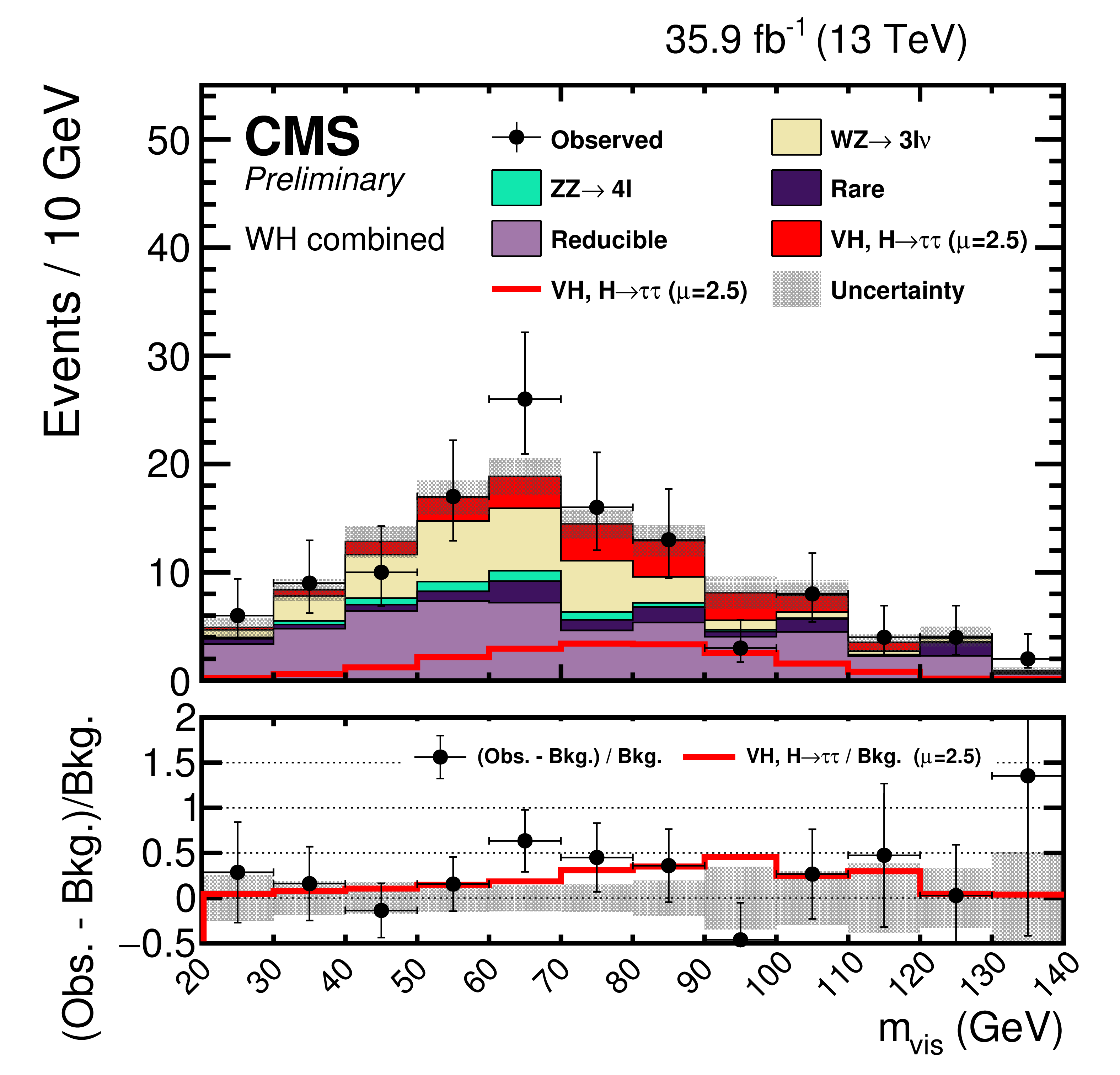
Postfit mass distributions of the four $ {\mathrm {W}} {\mathrm {H}} $ final states combined together. The uncertainties include statistical and systematic sources. The $ {\mathrm {W}} {\mathrm {H}} $ and $ {\mathrm {Z}} {\mathrm {H}} $, $ {{\mathrm {H}} \to {\tau} {\tau}} $ signal processes are summed together and shown as $ {\text {VH}} $, $ {{\mathrm {H}} \to {\tau} {\tau}} $ with a best-fit $\mu = 2.5$. $ {\text {VH}} $, $ {{\mathrm {H}} \to {\tau} {\tau}} $ is shown both as a stacked filled histogram and an open overlaid histogram. In this distribution the $ {\mathrm {W}} {\mathrm {H}} $, $ {{\mathrm {H}} \to {\tau} {\tau}} $ process contributes 92% of the total of $ {\text {VH}} $, $ {{\mathrm {H}} \to {\tau} {\tau}} $. |

png pdf |
Figure 5:
Distribution of the decimal logarithm of the ratio between the expected signal and the sum of expected signal, corresponding to the best fit value $\mu =2.5$, and expected background in each bin of the mass distributions used to extract the results, in all final states combined. The background contributions are separated based on the production process, $ {\mathrm {W}} {\mathrm {H}} $ or $ {\mathrm {Z}} {\mathrm {H}} $. The inset shows the corresponding difference between the observed data and expected background distributions divided by the background expectation, as well as the signal expectation divided by the background expectation. |

png pdf |
Figure 6:
Best-fit signal strength per Higgs boson production process, for $ {m_{{\mathrm {H}}}} = 125.09$ GeV, using a combination of the $ {\mathrm {W}} {\mathrm {H}} $ and $ {\mathrm {Z}} {\mathrm {H}} $ targeted analysis detailed in this paper with the CMS analysis performed in the same data set for the same decay mode but targeting the gluon fusion and vector boson fusion productions [18,19]. The constraints from the combined global fit are used to extract each of the individual best fit signal strengths. The combined best fit signal strength is $\mu = 1.24 ^{+0.29} _{-0.27}$. |

png pdf |
Figure 7:
Scan of the negative log-likelihood difference as a function of $\kappa _V$ and $\kappa _f$, for $ {m_{{\mathrm {H}}}} = 125.09$ GeV. All nuisance parameters are profiled for each point. This scan is a combination of the $ {\mathrm {W}} {\mathrm {H}} $ and $ {\mathrm {Z}} {\mathrm {H}} $ targeted analysis detailed in this paper with the CMS analysis performed in the same data set for the same decay mode but targeting the gluon fusion and vector boson fusion productions [18,19]. The results for the gluon fusion and vector boson fusion analysis are shown as the overlaid dashed lines. For this scan, the included $ {{\mathrm {H}} \to {\mathrm {W}} {\mathrm {W}}} $ and $ {{\mathrm {H}} \to {\mathrm {Z}} {\mathrm {Z}}} $ processes are treated as signal. |
| Tables | |

png pdf |
Table 1:
Kinematic selection requirements for $ {\mathrm {W}} {\mathrm {H}} $ and $ {\mathrm {Z}} {\mathrm {H}} $ events. The trigger requirement is defined by a combination of trigger candidates with ${p_{\mathrm {T}}}$ over a given threshold (in GeV), indicated inside parentheses. The pseudorapidity thresholds come from trigger and object reconstruction constraints. |

png pdf |
Table 2:
Sources of systematic uncertainty. |
png pdf |
Table 3:
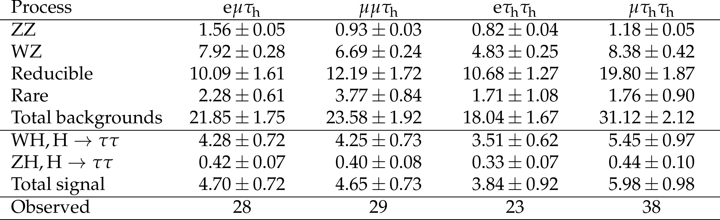
Background and signal expectations for the $ {\mathrm {W}} {\mathrm {H}} $ channels, together with the number of observed events, for the post-fit signal region distributions. The signal yields are the number of expected signal events for a Higgs boson with a mass $ {m_{{\mathrm {H}}}} = $ 125.09 GeV. The background uncertainty accounts for all sources of background uncertainty, systematic as well as statistical, after the global fit. The contribution from "Rare'' includes events from triboson, $ {{\mathrm {t}\overline {\mathrm {t}}}} + {\mathrm {W}}$/$ {\mathrm {Z}} $, $ {{\mathrm {t}\overline {\mathrm {t}}}} {\mathrm {H}} $ production, and other rare processes. |

png pdf |
Table 4:
Background and signal expectations for the $ {\mathrm {Z}} {\mathrm {H}} $ channels, together with the number of observed events, for the post-fit signal region distributions. The $ {\mathrm {Z}} {\mathrm {H}} $ final states are each grouped according to the Higgs boson decay products. $\ell \ell $ covers both $ {\mathrm {Z}} \to {{\mu}} {{\mu}}$ and $ {\mathrm {Z}} \to {\mathrm {e}} {\mathrm {e}}$ events. The signal yields are the number of expected signal events for a Higgs boson with a mass $ {m_{{\mathrm {H}}}} = $ 125.09 GeV. The background uncertainty accounts for all sources of background uncertainty, systematic as well as statistical, after the global fit. The contribution from "Rare'' includes events from triboson, $ {{\mathrm {t}\overline {\mathrm {t}}}} + {\mathrm {W}}$/$ {\mathrm {Z}} $, $ {{\mathrm {t}\overline {\mathrm {t}}}} {\mathrm {H}} $ production, and other rare processes. |
| Summary |
|
A search for the standard model Higgs boson in $\mathrm{W}\mathrm{H}$ and $\mathrm{Z}\mathrm{H}$ associated production processes is presented based on data collected in proton-proton collisions by the CMS detector in 2016 at a center-of-mass energy of 13 TeV. Event categories are split into three-lepton final states targeting $\mathrm{W}\mathrm{H}$ production, and four-lepton final states targeting $\mathrm{Z}\mathrm{H}$ production. The best-fit signal strength is $\mu = $ 2.54$ ^{+1.35} _{-1.26}$ ($\mu = $ 1.00$ ^{+1.08} _{-0.97}$ expected) for a significance of 2.3 standard deviations (1.0 expected). Combining this analysis with the analysis targeting Higgs boson decays to $\tau$ leptons in gluon fusion and vector boson fusion productions performed at a center-of-mass energy of 13 TeV with the CMS experiment, the tightest constraints on the ${\mathrm{H}\to\tau\tau} $ decay are set. The best-fit signal strength is $\mu = $ 1.24$ ^{+0.29} _{-0.27}$, and the observed significance is 5.5 standard deviations (4.8 expected). The combination further constrains the coupling of the Higgs boson to vector bosons resulting in measured couplings which are consistent with SM predictions within one standard deviation. |
| References | ||||
| 1 | S. Weinberg | A model of leptons | PRL 19 (1967) 1264 | |
| 2 | A. Salam | Weak and electromagnetic interactions | in Elementary particle physics: relativistic groups and analyticity, N. Svartholm, ed., p. 367 Almqvist \& Wiksell, Stockholm, 1968 Proceedings of the eighth Nobel symposium | |
| 3 | F. Englert and R. Brout | Broken symmetry and the mass of gauge vector mesons | PRL 13 (1964) 321 | |
| 4 | P. W. Higgs | Broken symmetries, massless particles and gauge fields | PL12 (1964) 132 | |
| 5 | P. W. Higgs | Broken symmetries and the masses of gauge bosons | PRL 13 (1964) 508 | |
| 6 | G. S. Guralnik, C. R. Hagen, and T. W. B. Kibble | Global conservation laws and massless particles | PRL 13 (1964) 585 | |
| 7 | P. W. Higgs | Spontaneous symmetry breakdown without massless bosons | PR145 (1966) 1156 | |
| 8 | T. W. B. Kibble | Symmetry breaking in non-abelian gauge theories | PR155 (1967) 1554 | |
| 9 | ATLAS Collaboration | Observation of a new particle in the search for the standard model Higgs boson with the ATLAS detector at the LHC | PLB 716 (2012) | 1207.7214 |
| 10 | CMS Collaboration | Observation of a new boson at a mass of 125 GeV with the CMS experiment at the LHC | PLB 716 (2012) | CMS-HIG-12-028 1207.7235 |
| 11 | CMS Collaboration | Observation of a new boson with mass near 125 GeV in pp collisions at $ \sqrt{s} = $ 7 and 8 TeV | JHEP 06 (2013) 081 | |
| 12 | CMS Collaboration | Measurements of properties of the Higgs boson decaying into the four-lepton final state in pp collisions at $ \sqrt{s}= $ 13 TeV | JHEP 11 (2017) 047 | CMS-HIG-16-041 1706.09936 |
| 13 | ATLAS and CMS Collaboration | Combined measurement of the Higgs boson mass in pp collisions at $ \sqrt{s}= $ 7 and 8 TeV with the ATLAS and CMS experiments | PRL 114 (2015) 191803 | 1503.07589 |
| 14 | ALEPH Collaboration | Observation of an excess in the search for the standard model Higgs boson at ALEPH | PLB 495 (2000) 1 | hep-ex/0011045 |
| 15 | DELPHI Collaboration | Final results from DELPHI on the searches for SM and MSSM neutral Higgs bosons | EPJC 32 (2004) 145 | hep-ex/0303013 |
| 16 | L3 Collaboration | Standard model Higgs boson with the L3 experiment at LEP | PLB 517 (2001) 319 | hep-ex/0107054 |
| 17 | OPAL Collaboration | Search for the standard model Higgs boson in e$ ^+ $e$ ^- $ collisions at $ \sqrt{s} = $ 192--209 GeV | PLB 499 (2001) 38 | hep-ex/0101014 |
| 18 | CMS Collaboration | Observation of the Higgs boson decay to a pair of $ \tau $ leptons with the CMS detector | PLB 779 (2018) 283 | CMS-HIG-16-043 1708.00373 |
| 19 | CMS Collaboration | Combined measurements of the Higgs boson's couplings at $ \sqrt{s}= $ 13 TeV | CMS-PAS-HIG-17-031 | CMS-PAS-HIG-17-031 |
| 20 | CMS Collaboration | The CMS trigger system | JINST 12 (2017) P01020 | CMS-TRG-12-001 1609.02366 |
| 21 | CMS Collaboration | The CMS experiment at the CERN LHC | JINST 3 (2008) S08004 | CMS-00-001 |
| 22 | P. Nason | A new method for combining NLO QCD with shower Monte Carlo algorithms | JHEP 11 (2004) 040 | hep-ph/0409146 |
| 23 | S. Frixione, P. Nason, and C. Oleari | Matching NLO QCD computations with parton shower simulations: the POWHEG method | JHEP 11 (2007) 070 | 0709.2092 |
| 24 | S. Alioli, P. Nason, C. Oleari, and E. Re | A general framework for implementing NLO calculations in shower Monte Carlo programs: the POWHEG BOX | JHEP 06 (2010) 043 | 1002.2581 |
| 25 | S. Alioli et al. | Jet pair production in POWHEG | JHEP 04 (2011) 081 | 1012.3380 |
| 26 | S. Alioli, P. Nason, C. Oleari, and E. Re | NLO Higgs boson production via gluon fusion matched with shower in POWHEG | JHEP 04 (2009) 002 | 0812.0578 |
| 27 | G. Luisoni, P. Nason, C. Oleari, and F. Tramontano | $ HW^{\pm}/HZ + 0 $ and 1 jet at NLO with the POWHEG BOX interfaced to GoSam and their merging within MiNLO | JHEP 10 (2013) 083 | 1306.2542 |
| 28 | R. D. Ball et al. | Unbiased global determination of parton distributions and their uncertainties at NNLO and at LO | NPB 855 (2012) 153 | 1107.2652 |
| 29 | D. de Florian, G. Ferrera, M. Grazzini, and D. Tommasini | Higgs boson production at the LHC: transverse momentum resummation effects in the $ \mathrm{H}\rightarrow \gamma\gamma $, $ \mathrm{H}\rightarrow ww \rightarrow l\nu l\nu $ and $ \mathrm{H}\rightarrow zz\rightarrow 4l $ decay modes | JHEP 06 (2012) 132 | 1203.6321 |
| 30 | M. Grazzini and H. Sargsyan | Heavy-quark mass effects in Higgs boson production at the LHC | JHEP 09 (2013) 129 | 1306.4581 |
| 31 | D. de Florian et al. | Handbook of LHC Higgs cross sections: 4. deciphering the nature of the Higgs sector | CERN-2017-002-M | 1610.07922 |
| 32 | A. Denner et al. | Standard model Higgs-boson branching ratios with uncertainties | EPJC 71 (2011) 1753 | 1107.5909 |
| 33 | NNPDF Collaboration | Impact of heavy quark masses on parton distributions and LHC phenomenology | NPB 849 (2011) 296 | 1101.1300 |
| 34 | J. M. Campbell and R. K. Ellis | MCFM for the Tevatron and the LHC | NPPS 205-206 (2010) 10 | 1007.3492 |
| 35 | R. Frederix and S. Frixione | Merging meets matching in MC@NLO | JHEP 12 (2012) 061 | 1209.6215 |
| 36 | J. Alwall et al. | Comparative study of various algorithms for the merging of parton showers and matrix elements in hadronic collisions | EPJC 53 (2008) 473 | 0706.2569 |
| 37 | T. Sjostrand et al. | An introduction to PYTHIA 8.2 | CPC 191 (2015) 159 | 1410.3012 |
| 38 | CMS Collaboration | Event generator tunes obtained from underlying event and multiparton scattering measurements | EPJC 76 (2016) 155 | CMS-GEN-14-001 1512.00815 |
| 39 | GEANT4 Collaboration | $ GEANT4--a $ simulation toolkit | NIMA 506 (2003) 250 | |
| 40 | CMS Collaboration | Particle-flow reconstruction and global event description with the CMS detector | JINST 12 (2017) P10003 | CMS-PRF-14-001 1706.04965 |
| 41 | M. Cacciari, G. P. Salam, and G. Soyez | The anti-$ {k_{\mathrm{T}}} $ jet clustering algorithm | JHEP 04 (2008) 063 | 0802.1189 |
| 42 | M. Cacciari, G. P. Salam, and G. Soyez | FastJet user manual | EPJC 72 (2012) 1896 | 1111.6097 |
| 43 | CMS Collaboration | Performance of CMS muon reconstruction in pp collision events at $ \sqrt{s}= $ 7 TeV | JINST 7 (2012) P10002 | CMS-MUO-10-004 1206.4071 |
| 44 | CMS Collaboration | Performance of electron reconstruction and selection with the CMS detector in proton-proton collisions at $ \sqrt{s}= $ 8 TeV | JINST 10 (2015) P06005 | CMS-EGM-13-001 1502.02701 |
| 45 | M. Cacciari and G. P. Salam | Dispelling the $ N^{3} $ myth for the $ {k_{\mathrm{T}}} $ jet-finder | PLB 641 (2006) 57 | hep-ph/0512210 |
| 46 | CMS Collaboration | Identification of heavy-flavour jets with the CMS detector in pp collisions at 13 TeV | JINST (2017) | CMS-BTV-16-002 1712.07158 |
| 47 | CMS Collaboration | Reconstruction and identification of $ \tau $ lepton decays to hadrons and $ \nu_\tau $ at CMS | JINST 11 (2016) P01019 | CMS-TAU-14-001 1510.07488 |
| 48 | CMS Collaboration | Performance of reconstruction and identification of tau leptons in their decays to hadrons and tau neutrino in LHC Run-2 | CMS-PAS-TAU-16-002 | CMS-PAS-TAU-16-002 |
| 49 | H. Voss, A. Hocker, J. Stelzer, and F. Tegenfeldt | TMVA, the toolkit for multivariate data analysis with ROOT | in XI Int. Workshop on Advanced Computing and Analysis Techniques in Physics Research 2007 | physics/0703039 |
| 50 | CMS Collaboration | Measurement of the inclusive $ w $ and $ z $ production cross sections in pp collisions at $ \sqrt{s}= $ 7 TeV | JHEP 10 (2011) 132 | CMS-EWK-10-005 1107.4789 |
| 51 | L. Bianchini, J. Conway, E. K. Friis, and C. Veelken | Reconstruction of the Higgs mass in $ h \to \tau\tau $ events by dynamical likelihood techniques | J. Phys. Conf. Ser. 513 (2014) 022035 | |
| 52 | CMS Collaboration | Performance of missing energy reconstruction in 13 TeV pp collision data using the CMS detector | CMS-PAS-JME-16-004 | CMS-PAS-JME-16-004 |
| 53 | CMS Collaboration | CMS luminosity measurements for the 2016 data taking period | CMS-PAS-LUM-17-001 | CMS-PAS-LUM-17-001 |
| 54 | K. Hamilton, P. Nason, E. Re, and G. Zanderighi | NNLOPS simulation of Higgs boson production | JHEP 10 (2013) 222 | 1309.0017 |
| 55 | CMS Collaboration | Evidence for the 125 GeV Higgs boson decaying to a pair of $ \tau $ leptons | JHEP 05 (2014) 104 | CMS-HIG-13-004 1401.5041 |
|
|
Compact Muon Solenoid LHC, CERN |
|

|

|

|

|

|