Compact Muon Solenoid
LHC, CERN

Visit us: CMS Public Website, CMS Physics ; Contact us: CMS Publications Committee

CMS-SUS-15-007 ; CERN-EP-2016-111

Search for supersymmetry in pp collisions at $ \sqrt{s} = $ 13 TeV in the single-lepton final state using the sum of masses of large-radius jets

CMS Collaboration

15 May 2016

J. High Energy Phys. 08 (2016) 122

Abstract: Results are reported from a search for supersymmetric particles in proton-proton collisions in the final state with a single, high transverse momentum lepton; multiple jets, including at least one b-tagged jet; and large missing transverse momentum. The data sample corresponds to an integrated luminosity of 2.3 fb$^{-1}$ at $ \sqrt{s} = $ 13 TeV, recorded by the CMS experiment at the LHC. The search focuses on processes leading to high jet multiplicities, such as gluino pair production with ${\mathrm{ \tilde g}}\to{\mathrm{ t \bar{t} }}\,{\tilde{\chi}^0_1}$. The quantity $M_J$, defined as the sum of the masses of the large-radius jets in the event, is used in conjunction with other kinematic variables to provide discrimination between signal and background and as a key part of the background estimation method. The observed event yields in the signal regions in data are consistent with those expected for standard model backgrounds, estimated from control regions in data. Exclusion limits are obtained for a simplified model corresponding to gluino pair production with three-body decays into top quarks and neutralinos. Gluinos with a mass below 1600 GeV are excluded at a 95% confidence level for scenarios with low $\tilde{\chi}^0_1$ mass, and neutralinos with a mass below 800 GeV are excluded for a gluino mass of about 1300 GeV. For models with two-body gluino decays producing on-shell top squarks, the excluded region is only weakly sensitive to the top squark mass.

Links: e-print arXiv:1605.04608 [hep-ex] (PDF) ; CDS record ; inSPIRE record ; HepData record ; CADI line (restricted) ;

Figures
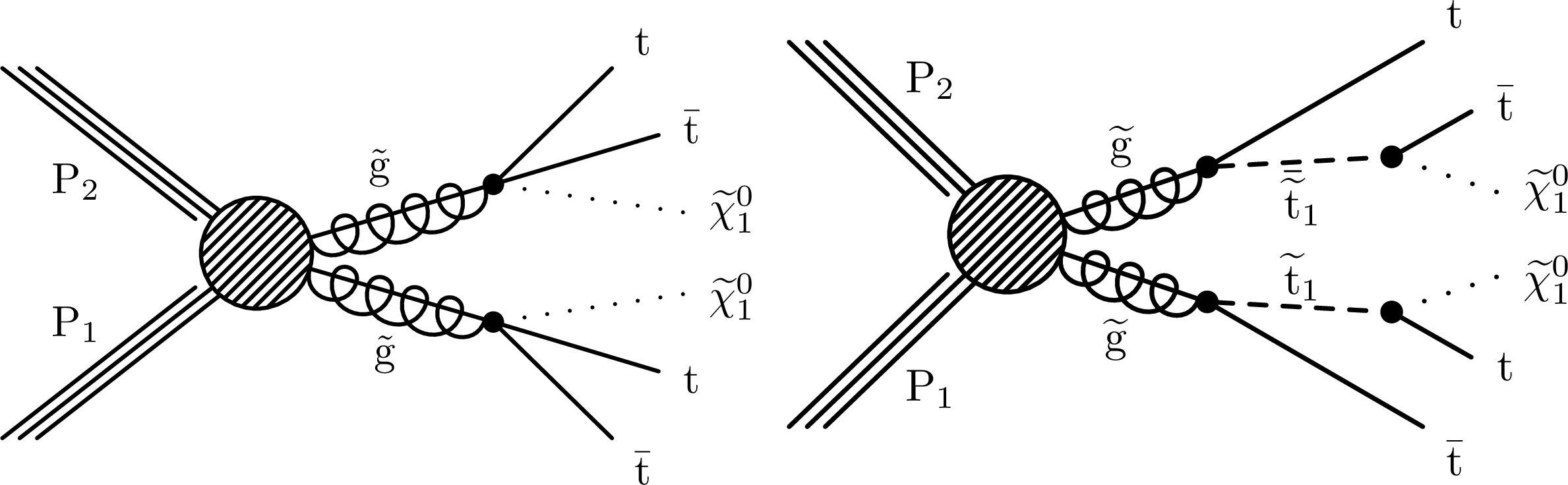
png pdf	Figure 1: Gluino pair production and decay for the simplified models T1tttt (left) and T5tttt (right). In T1tttt, the gluino undergoes three-body decay $\mathrm{ \tilde{g} } \to {\mathrm{ t \bar{t} } } {\tilde{\chi}^0_1} $ via a virtual intermediate top squark. In T5tttt, the gluino decays via the sequential two-body process $\mathrm{ \tilde{g} } \to \tilde{ \mathrm{ t } } _1\mathrm{ \bar{t} } $, $\tilde{ \mathrm{ t } } _1\to \mathrm{ t } {\tilde{\chi}^0_1} $. Because gluinos are Majorana particles, each one can decay to $\tilde{ \mathrm{ t } } _1\mathrm{ \bar{t} } $ and to the charge conjugate final state ${\tilde{ \mathrm{ \bar{t} } } }_1\mathrm{ t } $.
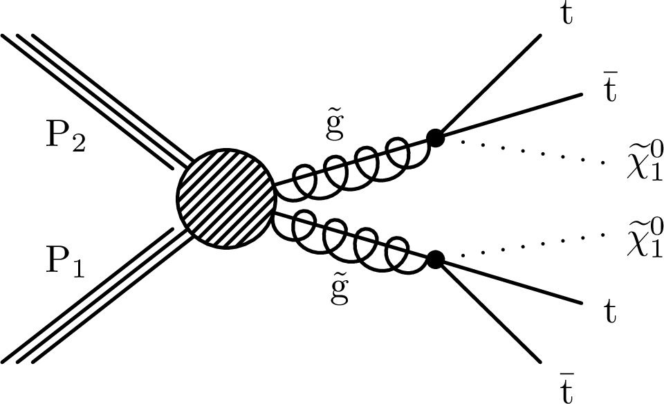
png pdf	Figure 1-a: Gluino pair production and decay for the simplified model T1tttt. The gluino undergoes three-body decay $\mathrm{ \tilde{g} } \to {\mathrm{ t \bar{t} } } {\tilde{\chi}^0_1} $ via a virtual intermediate top squark. Because gluinos are Majorana particles, each one can decay to $\tilde{ \mathrm{ t } } _1\mathrm{ \bar{t} } $ and to the charge conjugate final state ${\tilde{ \mathrm{ \bar{t} } } }_1\mathrm{ t } $.
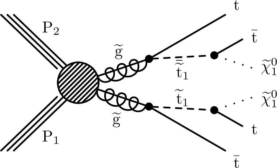
png pdf	Figure 1-b: Gluino pair production and decay for the simplified model T5tttt. In T5tttt, the gluino decays via the sequential two-body process $\mathrm{ \tilde{g} } \to \tilde{ \mathrm{ t } } _1\mathrm{ \bar{t} } $, $\tilde{ \mathrm{ t } } _1\to \mathrm{ t } {\tilde{\chi}^0_1} $. Because gluinos are Majorana particles, each one can decay to $\tilde{ \mathrm{ t } } _1\mathrm{ \bar{t} } $ and to the charge conjugate final state ${\tilde{ \mathrm{ \bar{t} } } }_1\mathrm{ t } $.
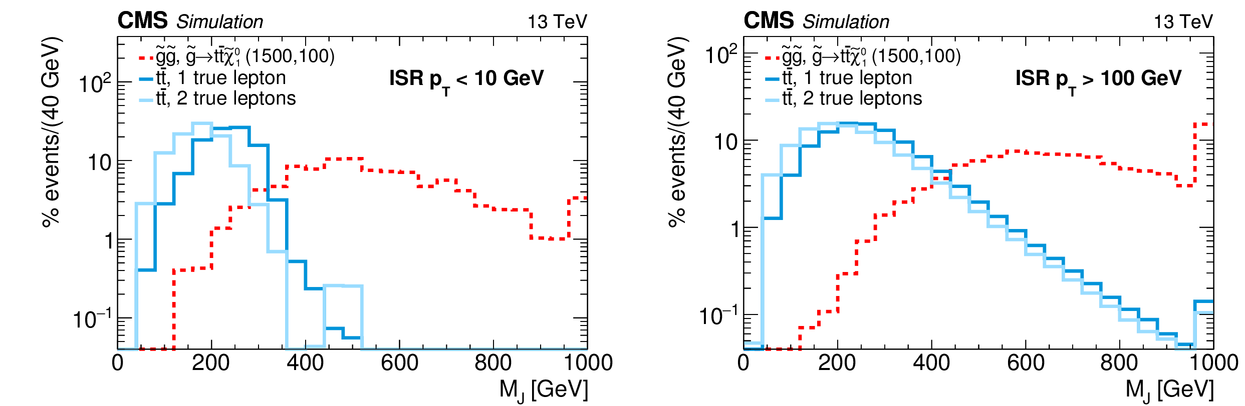
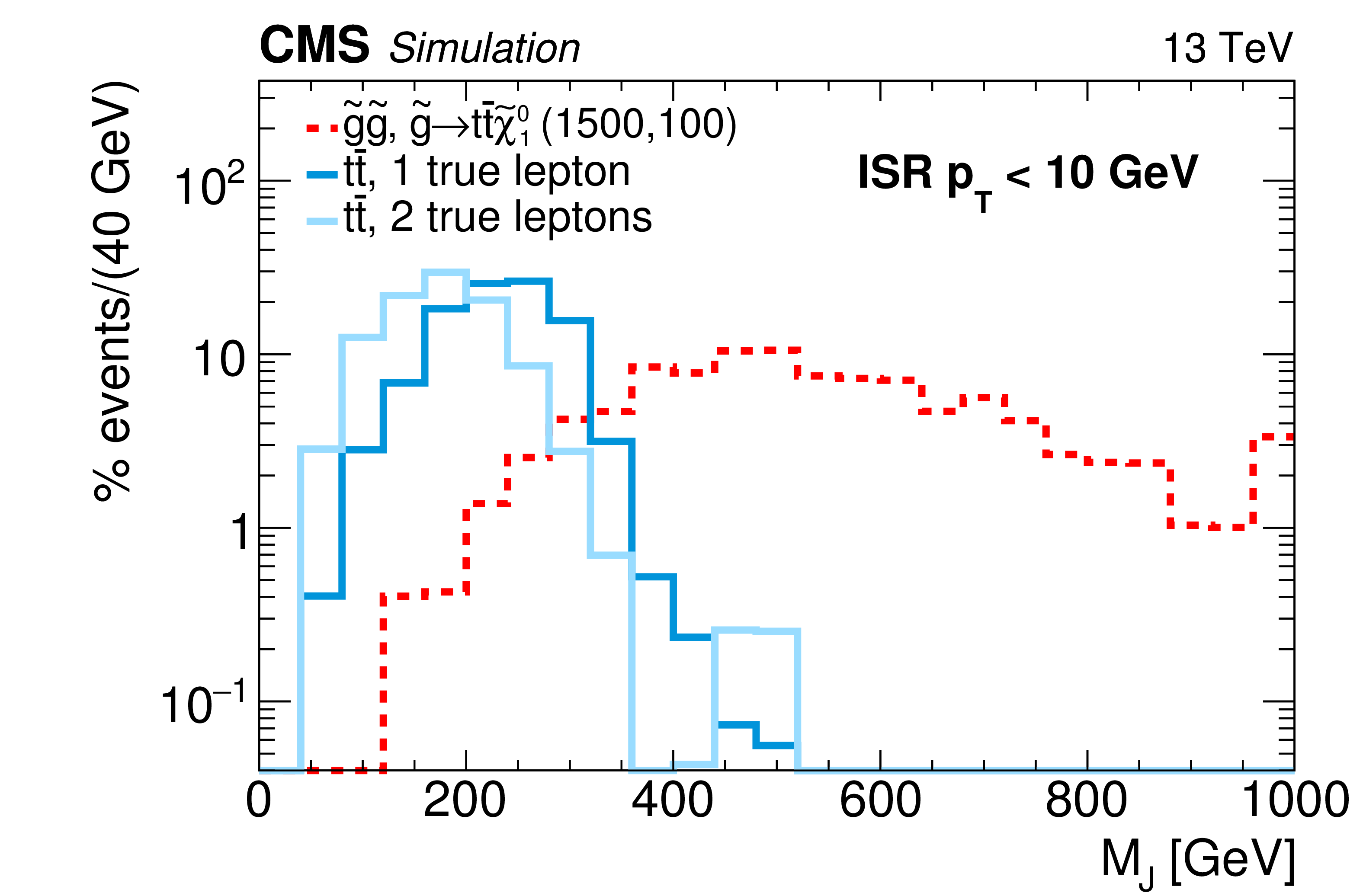
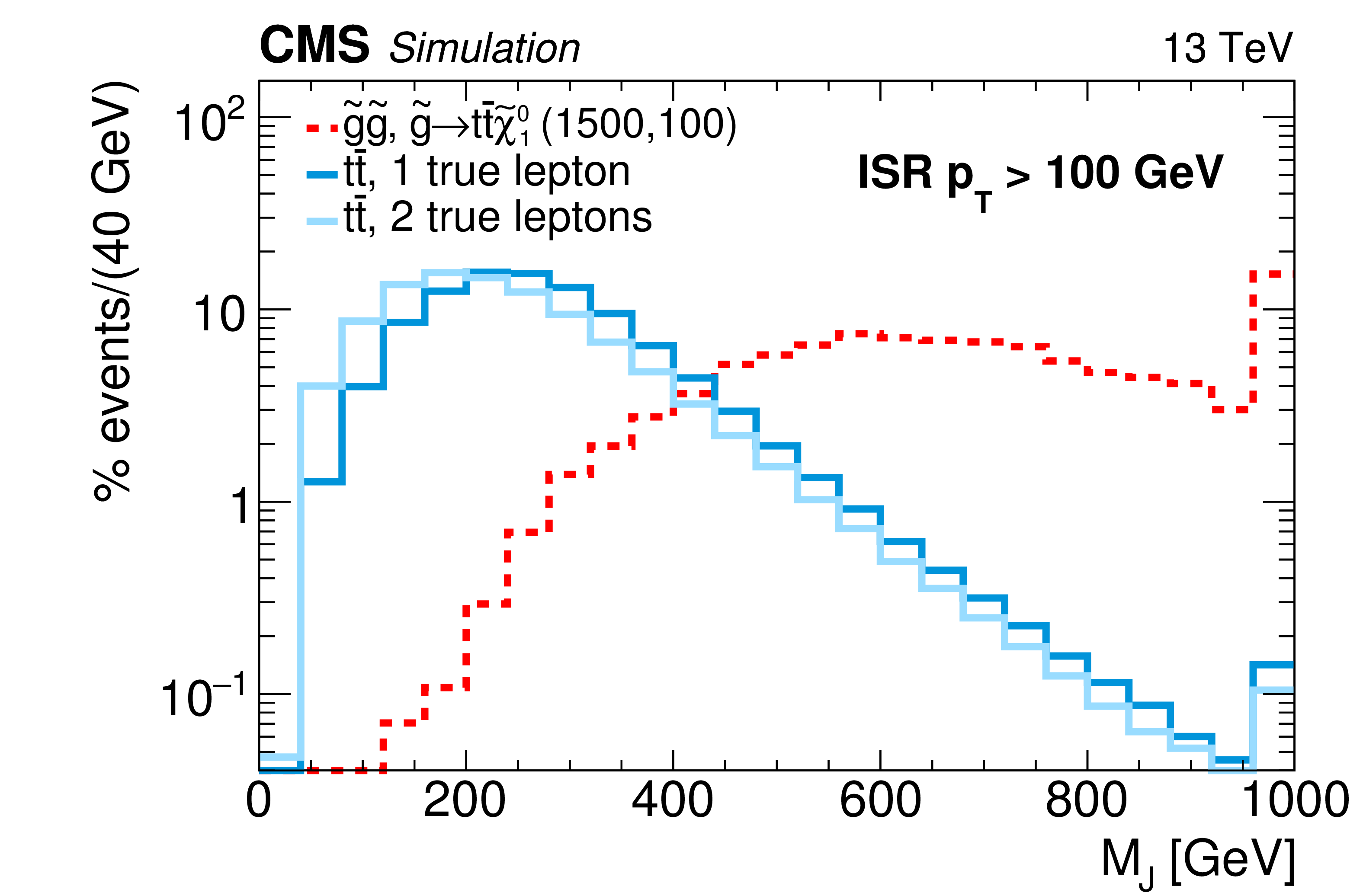
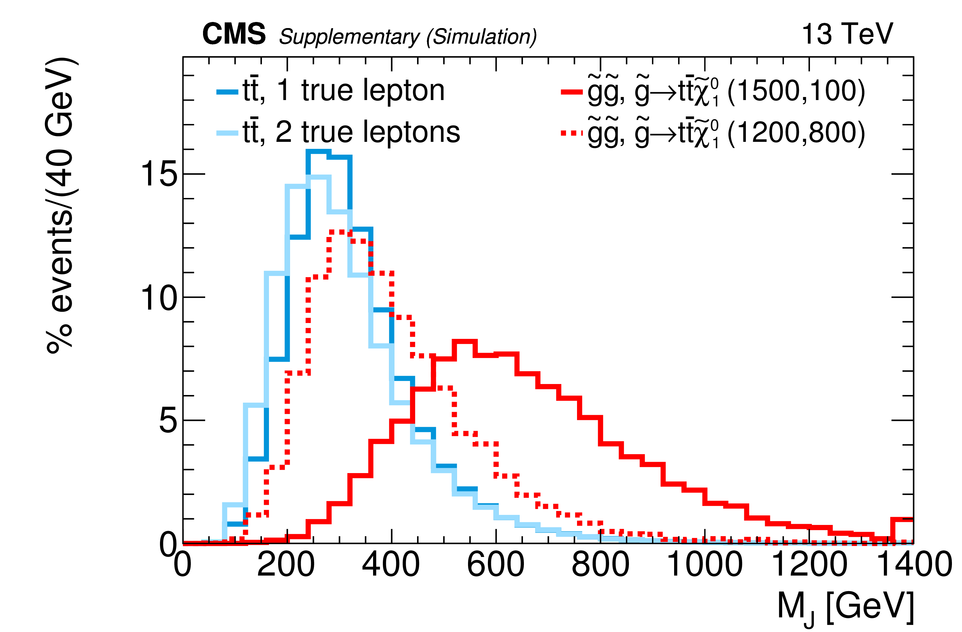
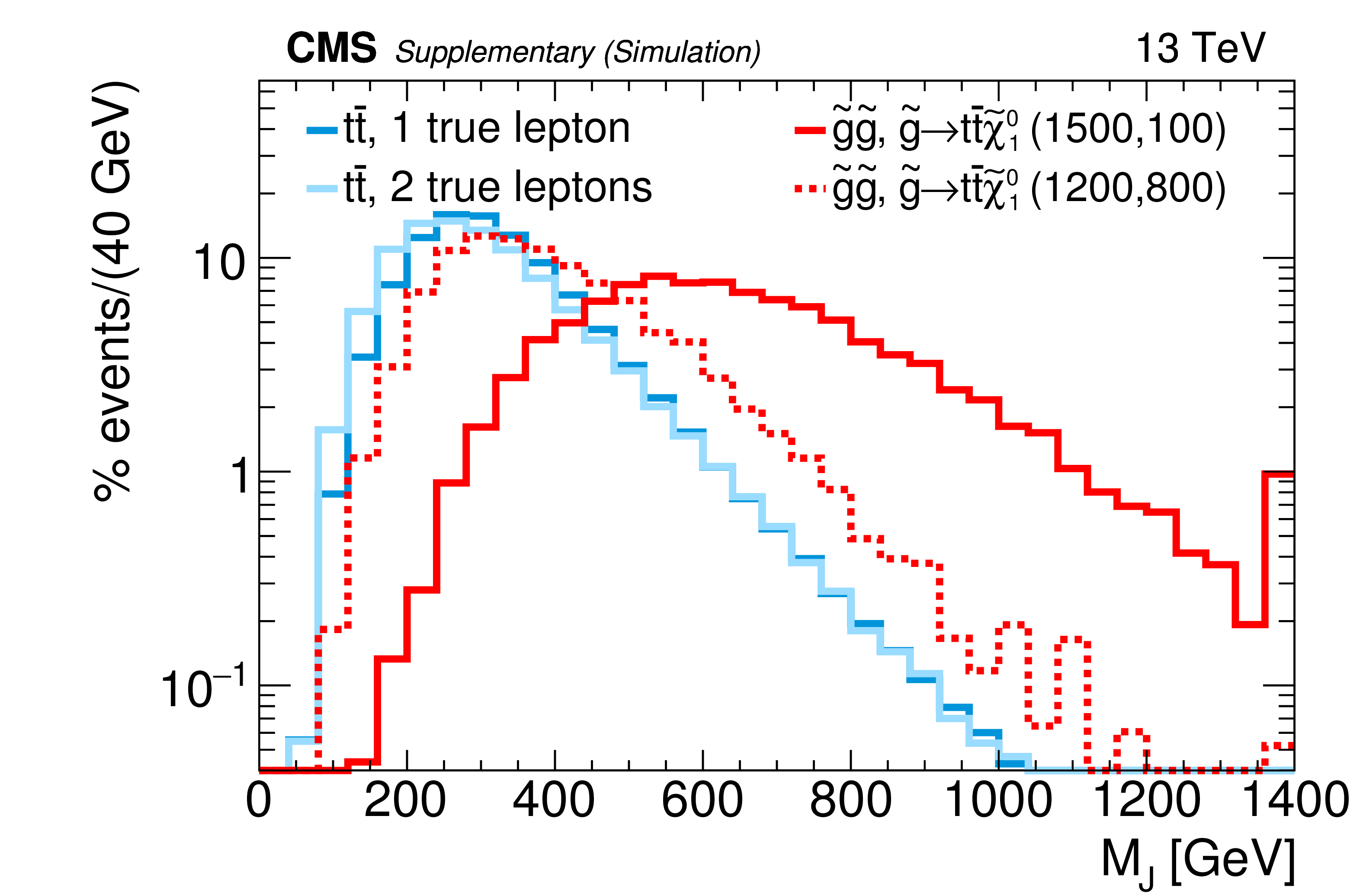
png pdf	Figure 2: Distributions of ${M_J} $, normalized to the same area, from simulated event samples with a small ISR contribution (left) and a significant ISR contribution (right). These components are defined according to whether the $ {p_{\mathrm {T}}} $ of the $ {\mathrm{ t \bar{t} } } $ system (or, in the case of signal events, that of the $\mathrm{ \tilde{g} } \mathrm{ \tilde{g} } $ system) is $< $ 10 GeV or $> $ 100 GeV, respectively. The T1tttt(NC) signal model (dashed red line), is described in Section 3; the first model parameter in parentheses corresponds to ${m_{\mathrm{ \tilde{g} } }}$ and the second to ${m_{ {\tilde{\chi}^0_1} }} $, both in units of GeV. The events satisfy the requirements $ {E_{\mathrm {T}}^{\text {miss}}} > $ 200 GeV and $ {H_{\mathrm {T}}} > $ 500 GeV and have at least one reconstructed lepton.
png pdf	Figure 2-a: Distributions of ${M_J} $, normalized to the same area, from simulated event samples with a small ISR contribution. These components are defined according to whether the $ {p_{\mathrm {T}}} $ of the $ {\mathrm{ t \bar{t} } } $ system (or, in the case of signal events, that of the $\mathrm{ \tilde{g} } \mathrm{ \tilde{g} } $ system) is $< $ 10 GeV or $> $ 100 GeV, respectively. The T1tttt(NC) signal model (dashed red line), is described in Section 3; the first model parameter in parentheses corresponds to ${m_{\mathrm{ \tilde{g} } }}$ and the second to ${m_{ {\tilde{\chi}^0_1} }} $, both in units of GeV. The events satisfy the requirements $ {E_{\mathrm {T}}^{\text {miss}}} > $ 200 GeV and $ {H_{\mathrm {T}}} > $ 500 GeV and have at least one reconstructed lepton.
png pdf	Figure 2-b: Distributions of ${M_J} $, normalized to the same area, from simulated event samples with a significant ISR contribution. These components are defined according to whether the $ {p_{\mathrm {T}}} $ of the $ {\mathrm{ t \bar{t} } } $ system (or, in the case of signal events, that of the $\mathrm{ \tilde{g} } \mathrm{ \tilde{g} } $ system) is $< $ 10 GeV or $> $ 100 GeV, respectively. The T1tttt(NC) signal model (dashed red line), is described in Section 3; the first model parameter in parentheses corresponds to ${m_{\mathrm{ \tilde{g} } }}$ and the second to ${m_{ {\tilde{\chi}^0_1} }} $, both in units of GeV. The events satisfy the requirements $ {E_{\mathrm {T}}^{\text {miss}}} > $ 200 GeV and $ {H_{\mathrm {T}}} > $ 500 GeV and have at least one reconstructed lepton.
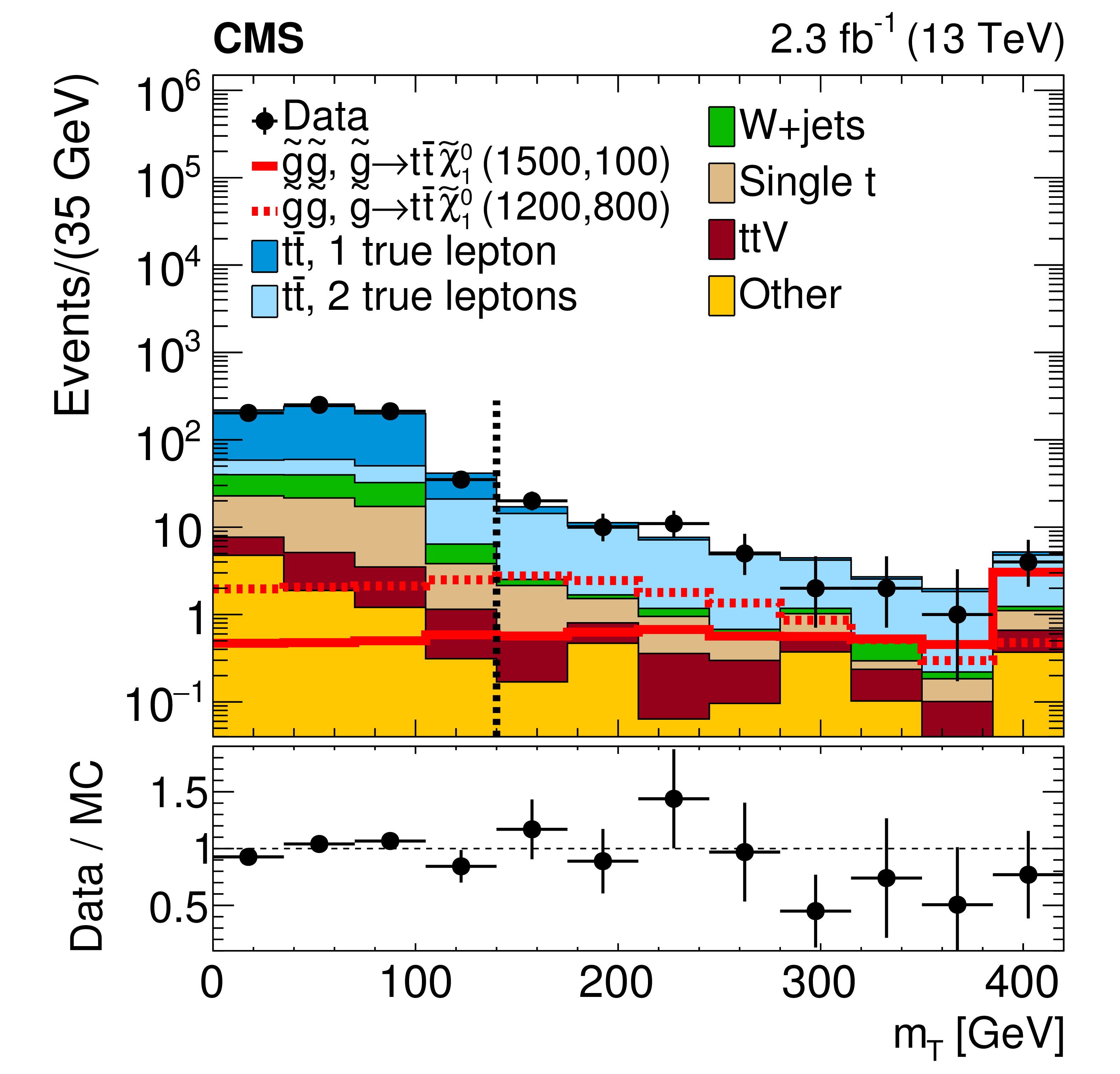
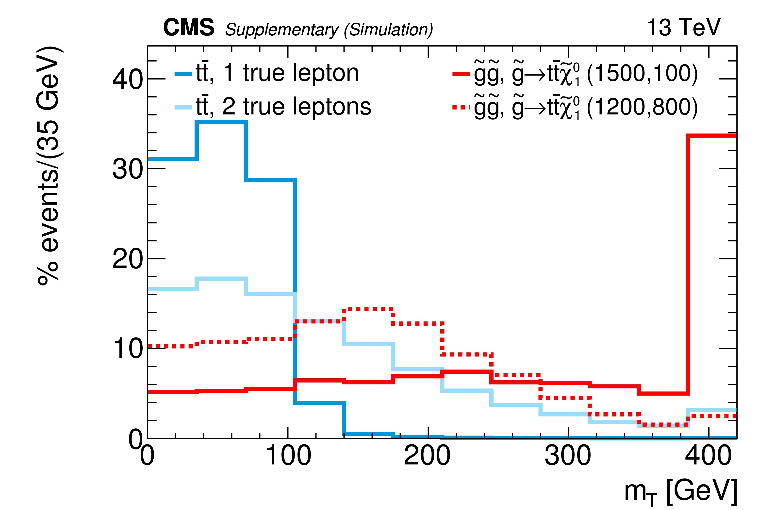
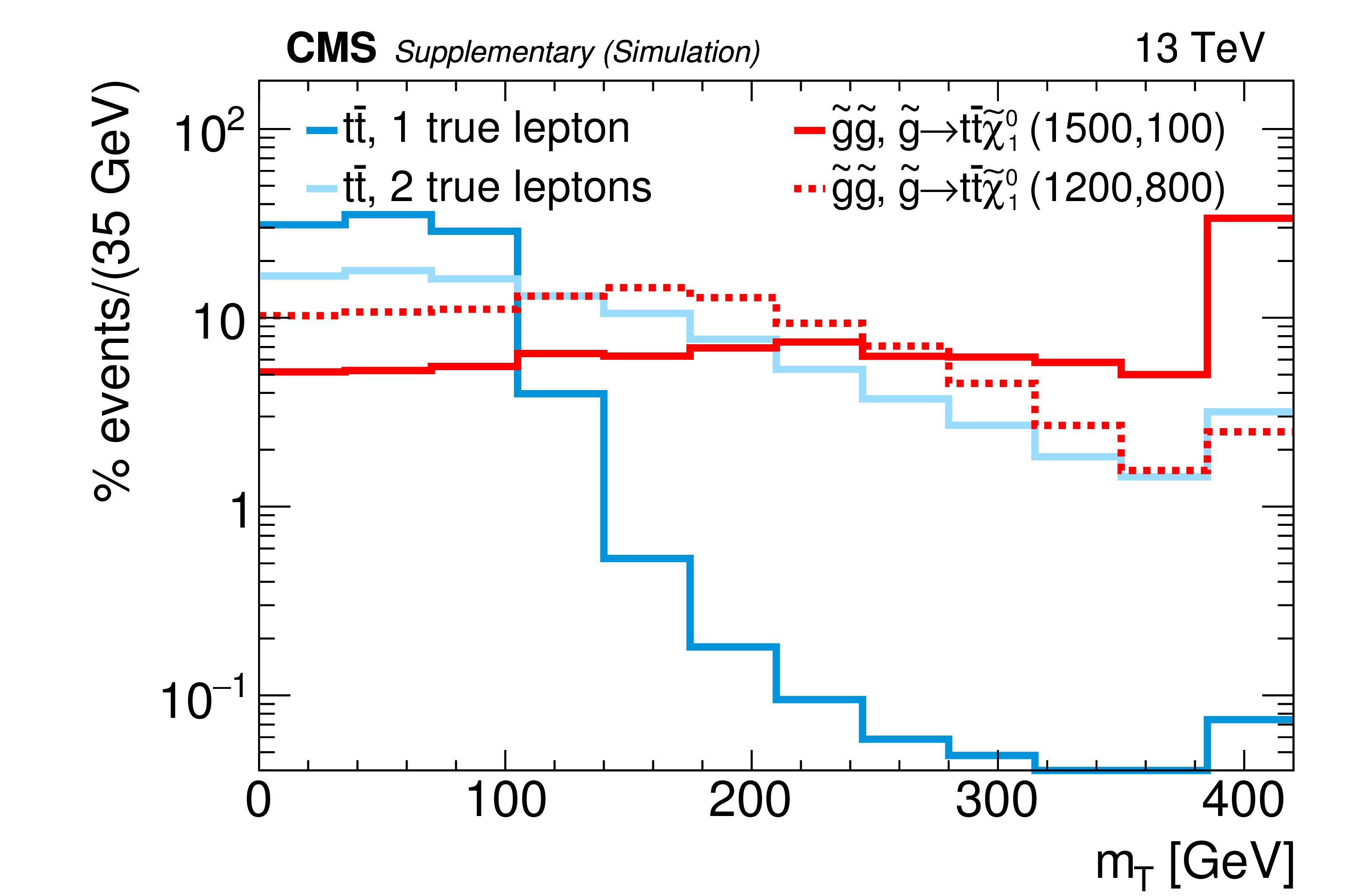
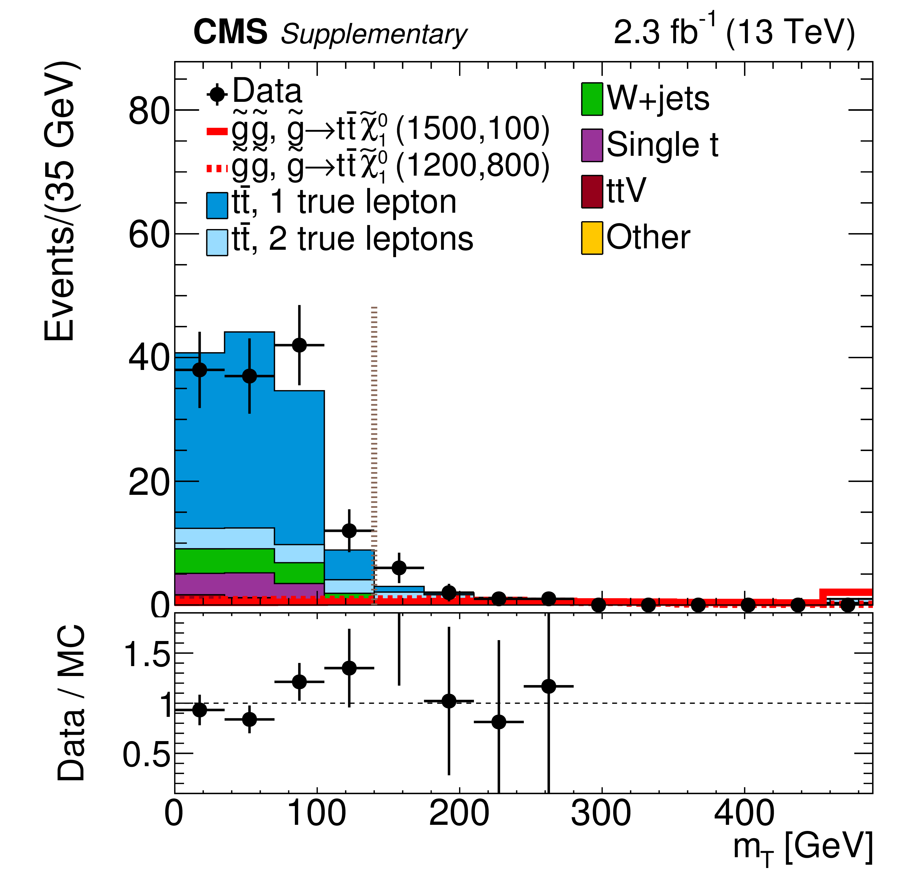
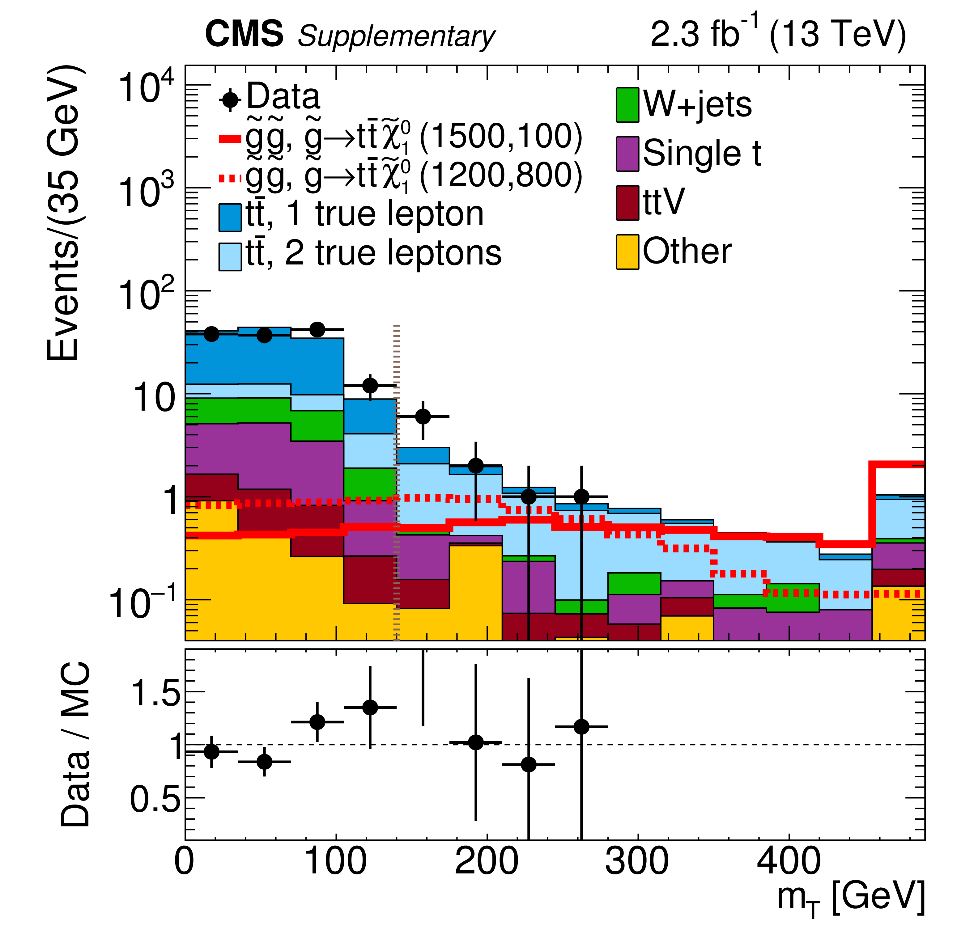
png pdf	Figure 3: Distribution of ${m_{\mathrm {T}}}$ in data and simulated event samples after the baseline selection is applied. The background contributions shown here are from simulation, and their total yield is normalized to the number of events observed in data. The signal distributions are normalized to the expected cross sections. The dashed vertical line indicates the $ {m_{\mathrm {T}}} > $ 140 GeV threshold that separates the signal regions from the control samples.
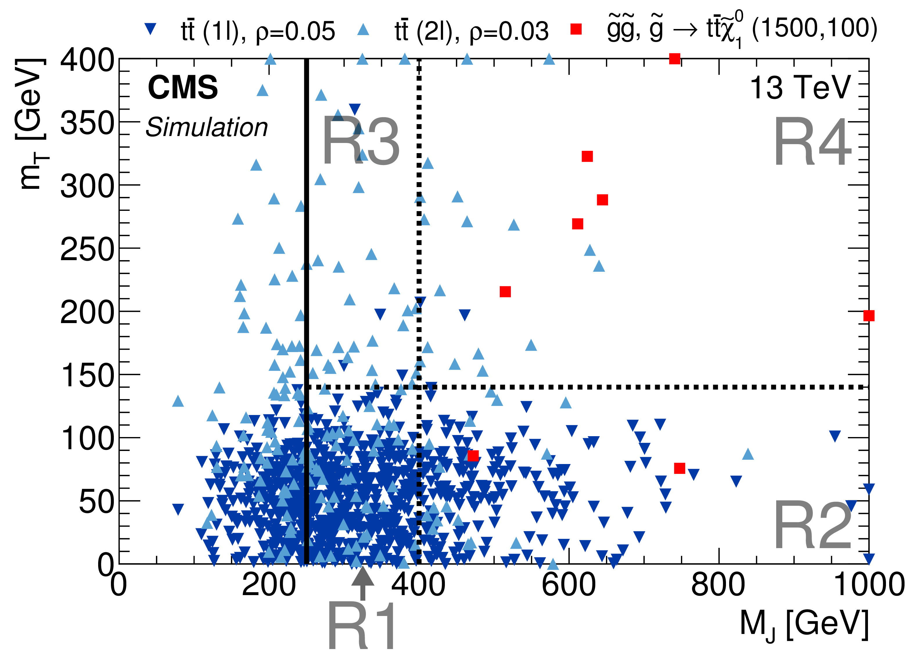
png pdf	Figure 4: Distribution of simulated single-lepton ${\mathrm{ t \bar{t} } }$ events (dark-blue triangles), dilepton ${\mathrm{ t \bar{t} } }$ events (light-blue inverted triangles), and T1tttt(1500,100) events (red squares) in the ${M_J} - {m_{\mathrm {T}}}$ plane after the baseline selection. Each marker represents one expected event at 2.3 fb$^{-1}$. Overflow events are placed on the edge of the plot. The values of the correlation coefficients $\rho $ for each background process are given in the legend. Region R4 is the nominal signal region, while R1, R2, and R3 serve as control regions. The small signal contributions in the control regions are taken into account in one of the global fits, as discussed in the text.
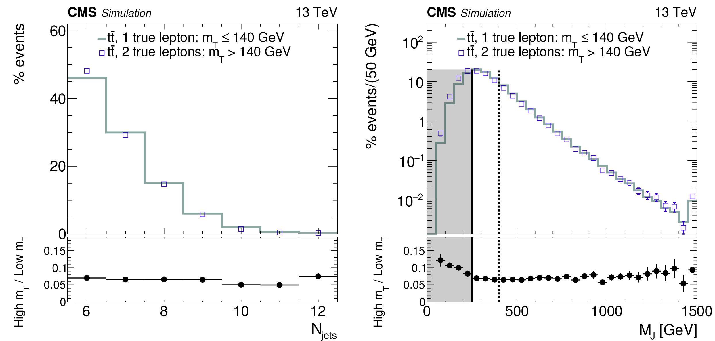
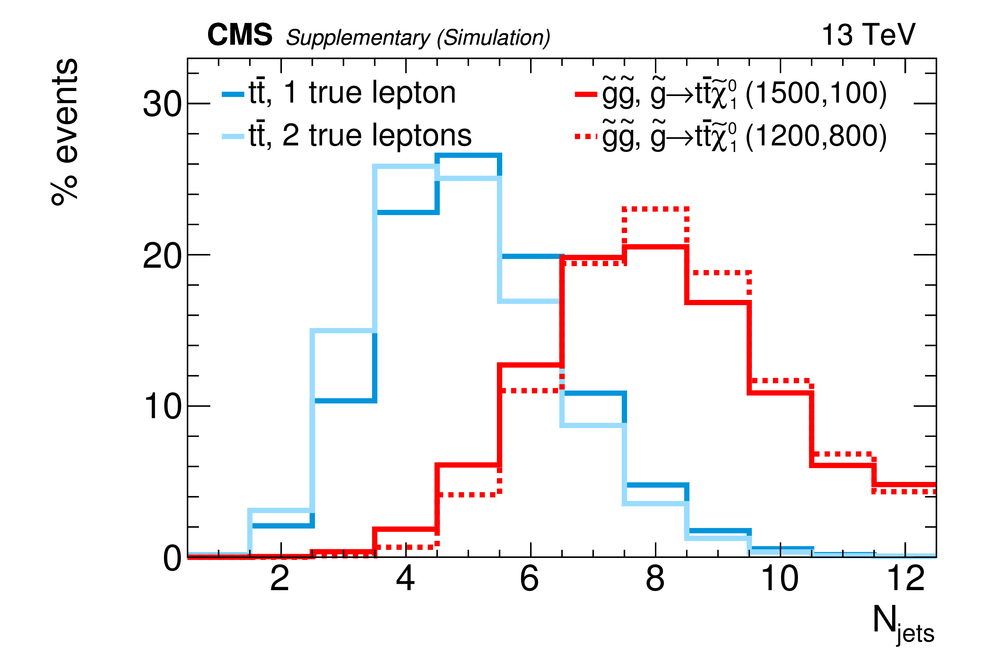
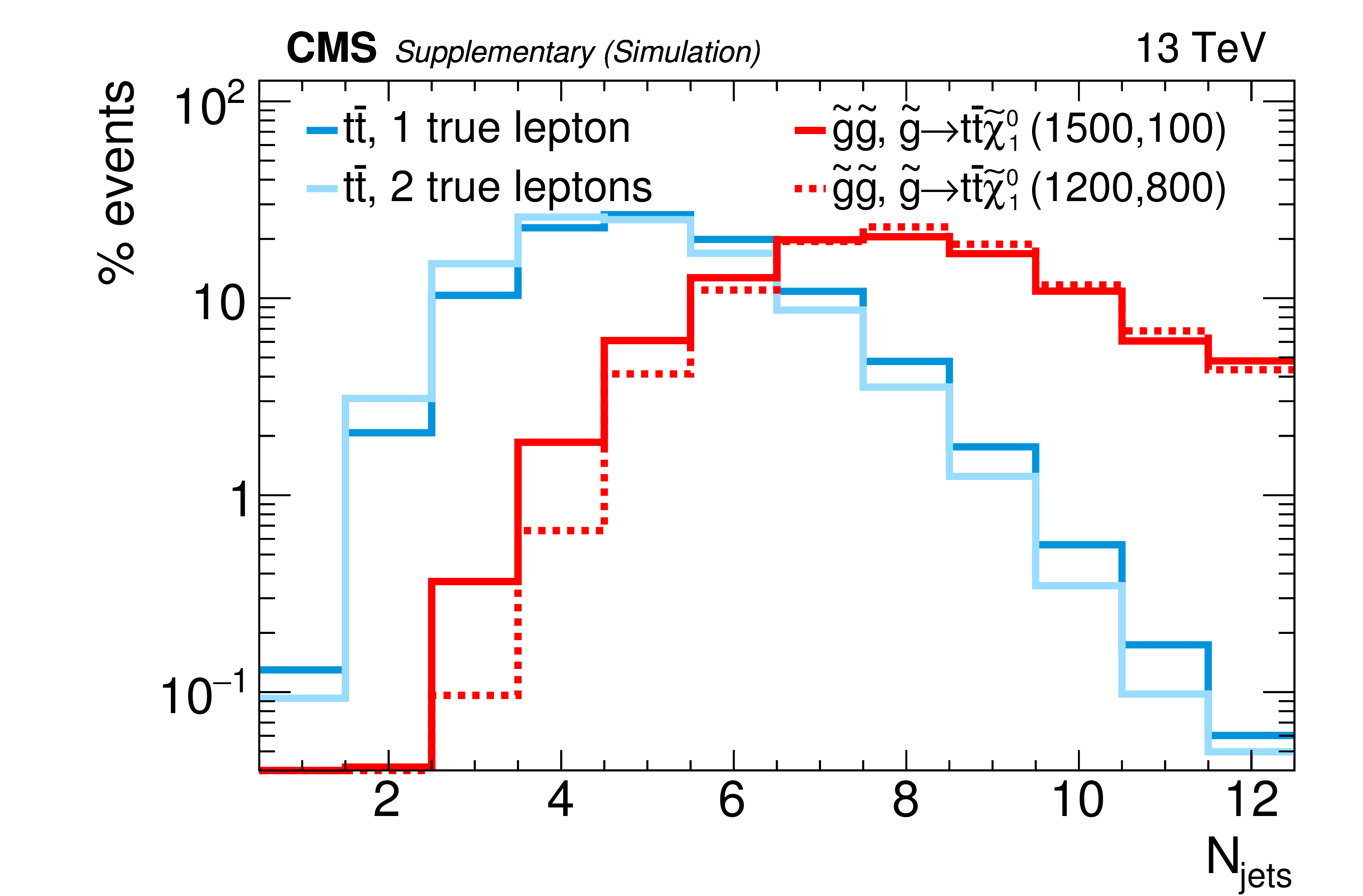
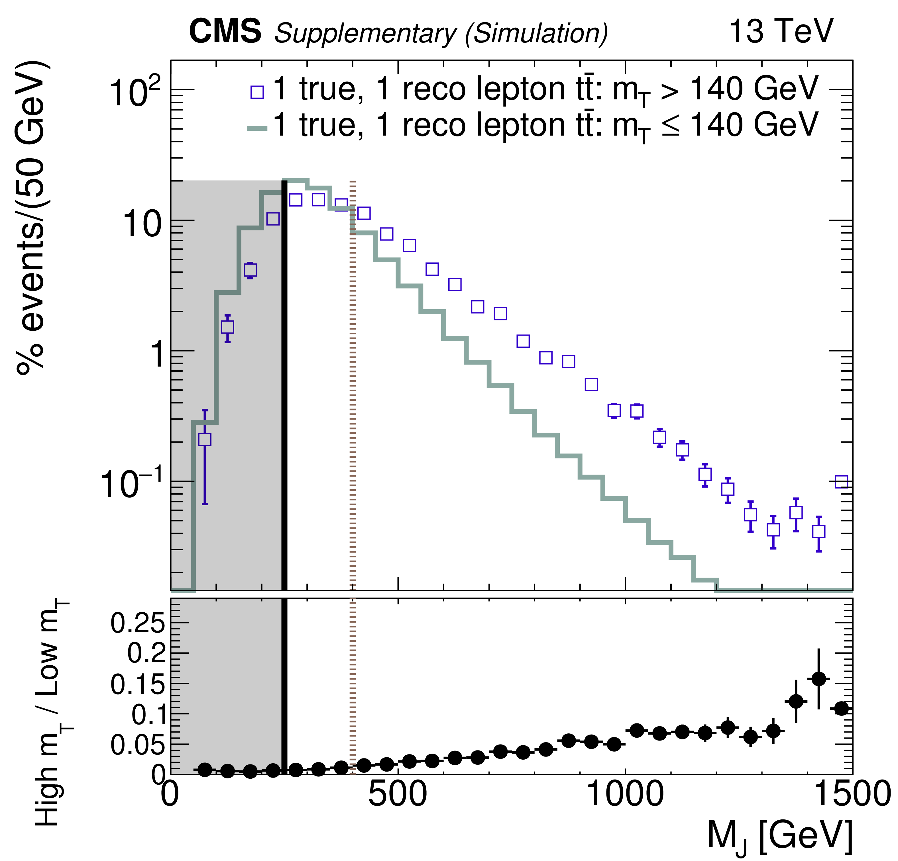
png pdf	Figure 5: Comparison of ${N_{\text {jets}}}$ and ${M_J}$ distributions, normalized to the same area, in simulated ${\mathrm{ t \bar{t} } } $ events with two true leptons at high ${m_{\mathrm {T}}}$ and one true lepton at low ${m_{\mathrm {T}}} $, after the baseline selection is applied. The shapes of these distributions are similar. These two contributions are the dominant backgrounds in their respective ${m_{\mathrm {T}}}$ regions. The dashed vertical line on the (b) plot indicates the $ {M_J} > $ 400 GeV threshold that separates the signal regions from the control samples. The shaded region corresponding to $ {M_J} < $ 250 GeV is not used in the background estimation.
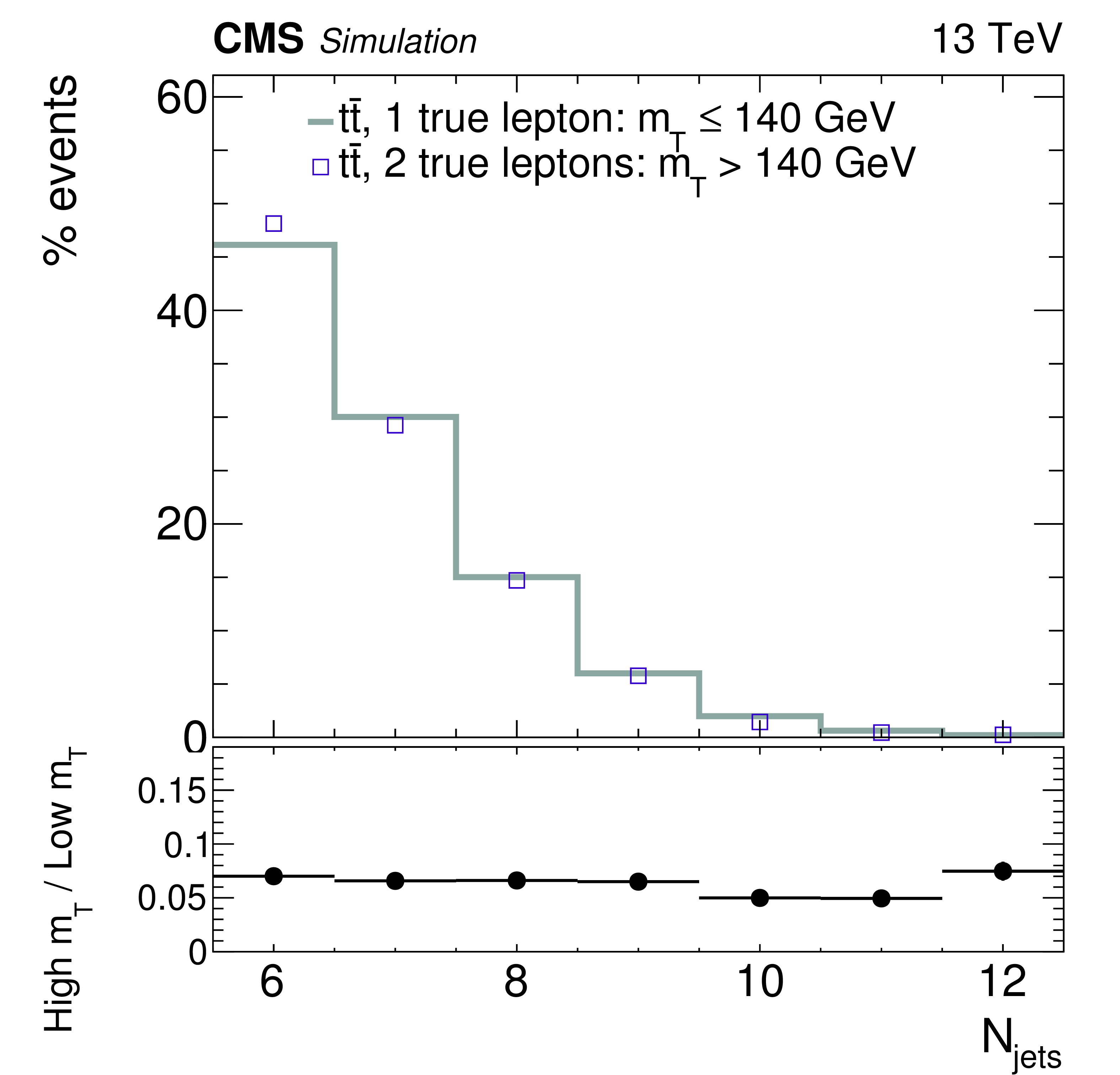
png pdf	Figure 5-a: Comparison of the ${N_{\text {jets}}}$ distribution, normalized to the same area, in simulated ${\mathrm{ t \bar{t} } } $ events with two true leptons at high ${m_{\mathrm {T}}}$ and one true lepton at low ${m_{\mathrm {T}}} $, after the baseline selection is applied. The shapes of these distributions are similar. These two contributions are the dominant backgrounds in their respective ${m_{\mathrm {T}}}$ regions.
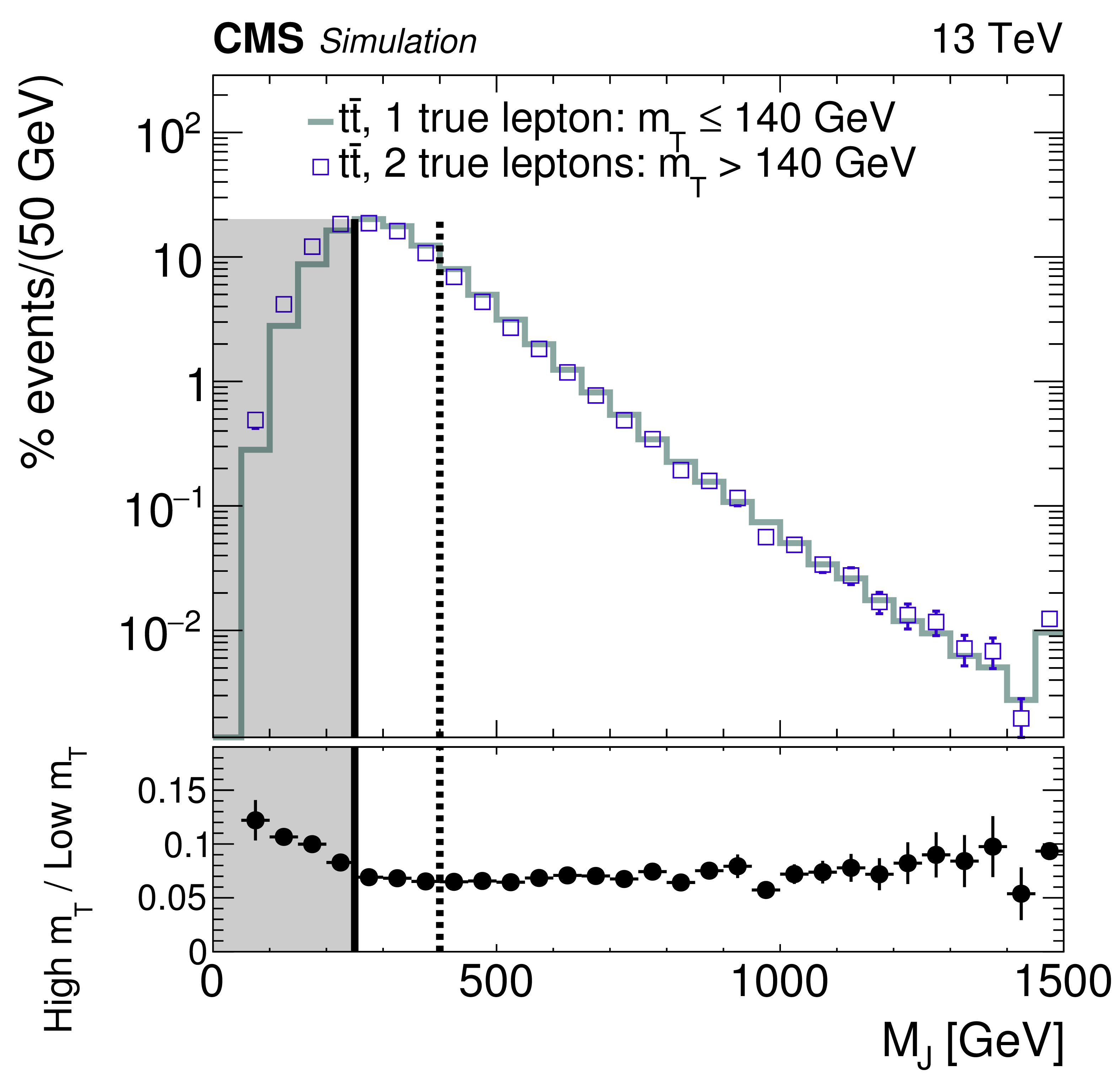
png pdf	Figure 5-b: Comparison of the ${M_J}$ distribution, normalized to the same area, in simulated ${\mathrm{ t \bar{t} } } $ events with two true leptons at high ${m_{\mathrm {T}}}$ and one true lepton at low ${m_{\mathrm {T}}} $, after the baseline selection is applied. The shapes of these distributions are similar. These two contributions are the dominant backgrounds in their respective ${m_{\mathrm {T}}}$ regions. The dashed vertical line on the plot indicates the $ {M_J} > $ 400 GeV threshold that separates the signal regions from the control samples. The shaded region corresponding to $ {M_J} < $ 250 GeV is not used in the background estimation.
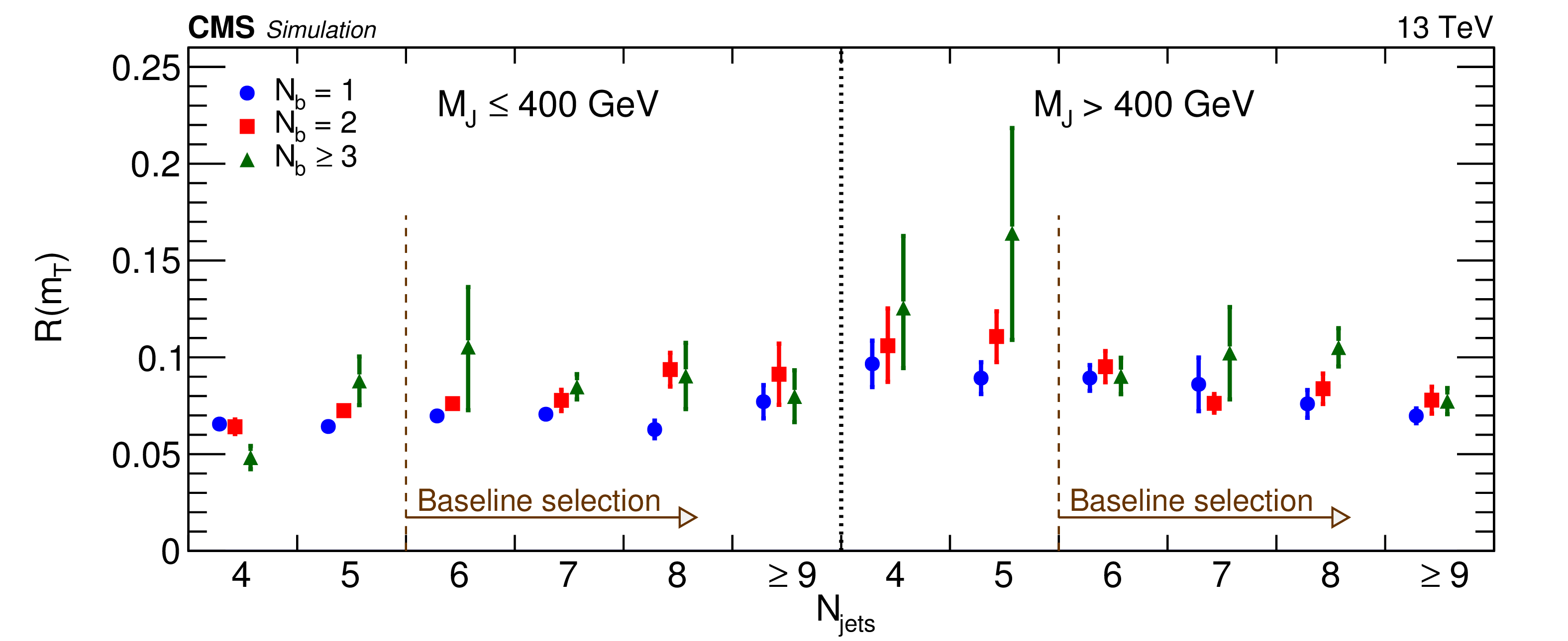
png pdf	Figure 6: The ratio $R( {m_{\mathrm {T}}} )$ of high-$ {m_{\mathrm {T}}}$ (R3+R4) to low-$ {m_{\mathrm {T}}}$ (R1+R2) event yields for the simulated SM background, as a function of ${N_{\text {jets}}}$ and ${N_{\text {b}}} $. The baseline selection requires $ {N_{\text {jets}}} \geq$ 6. The uncertainties shown are statistical only.
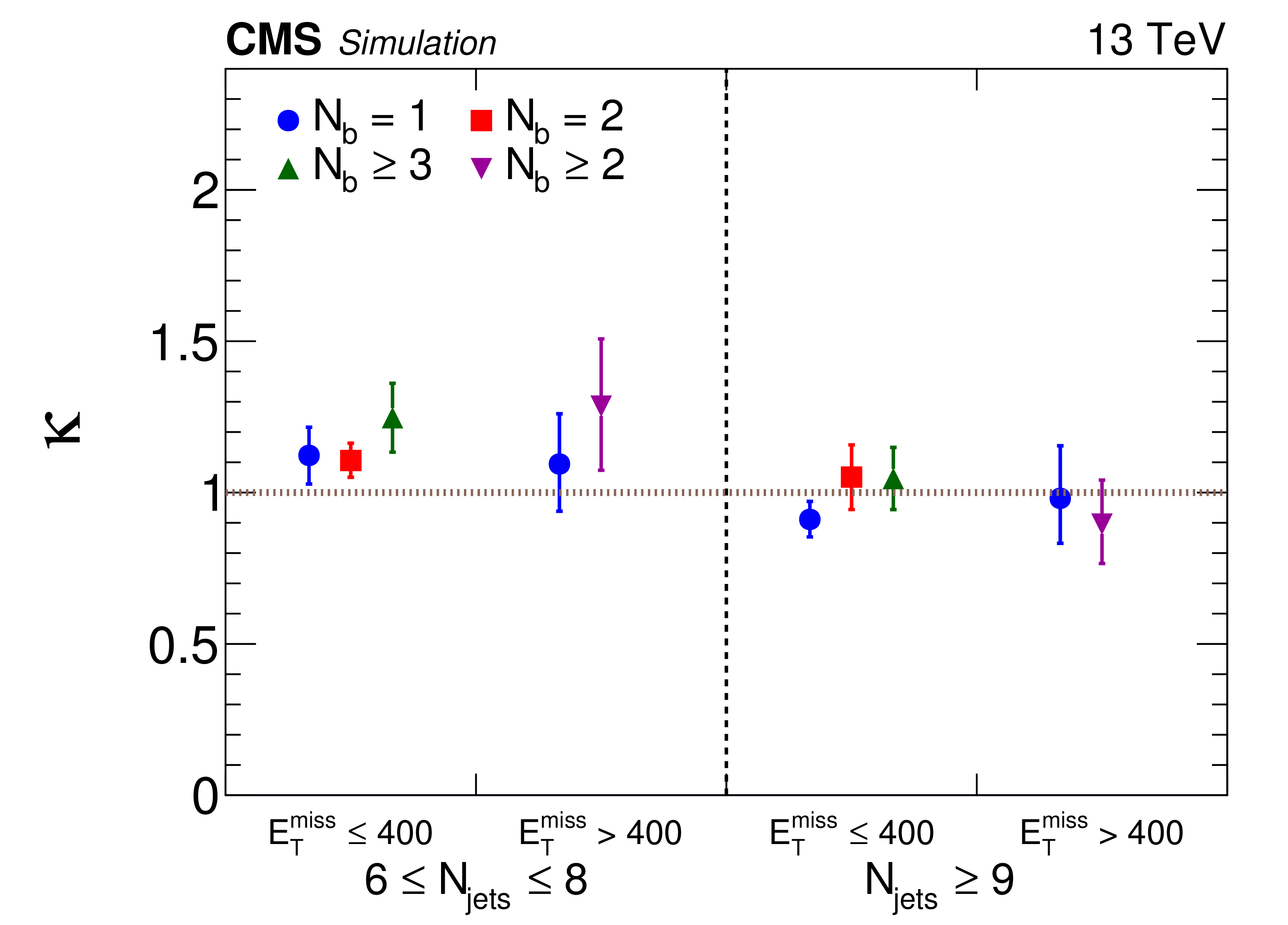
png pdf	Figure 7: Values of the double-ratio $\kappa $ in each of the 10 signal bins, calculated using the simulated SM background. The $\kappa $ factors are close to unity, indicating the small correlation between ${M_J} $ and ${m_{\mathrm {T}}} $. The uncertainties shown are statistical only.
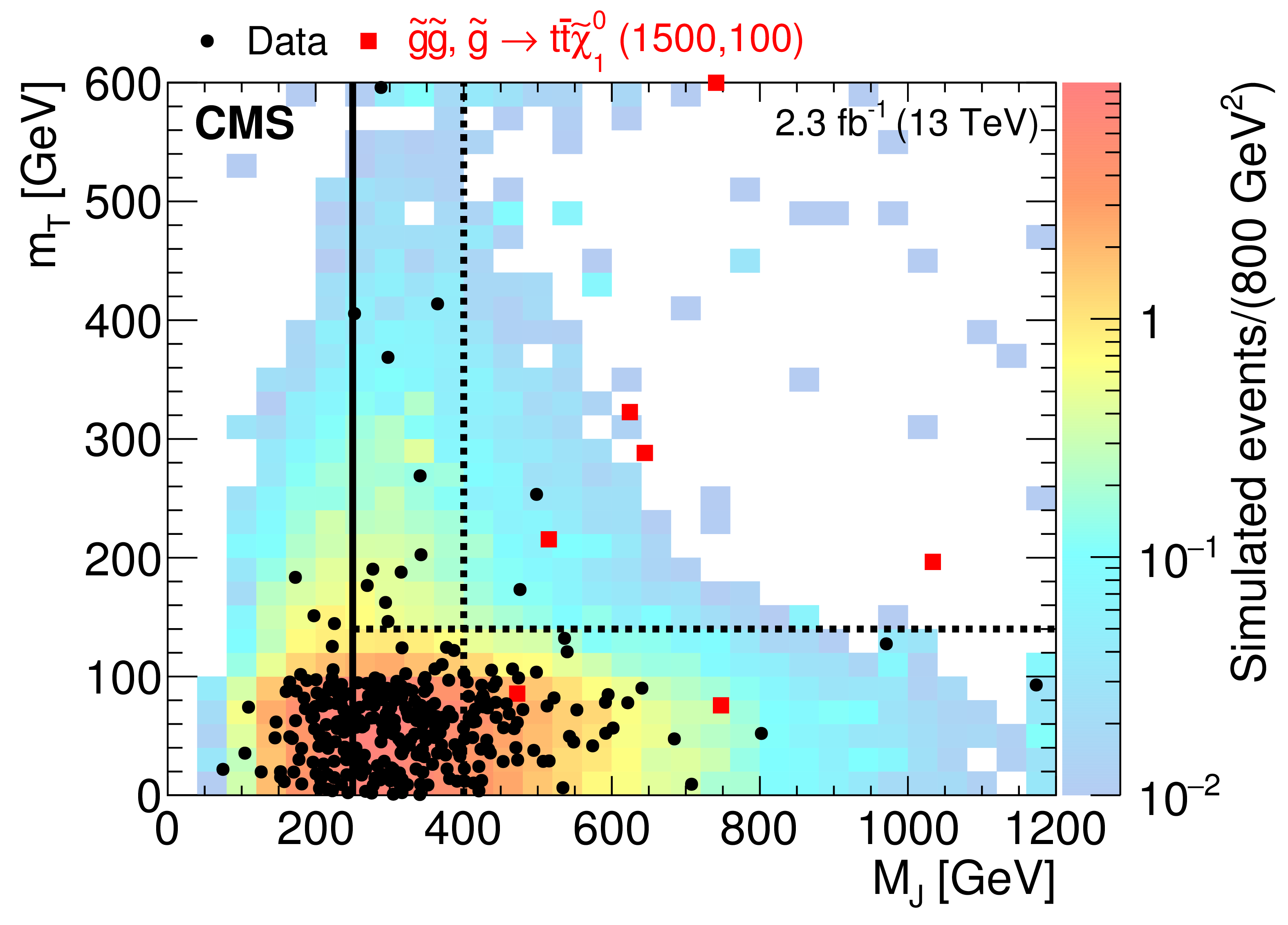
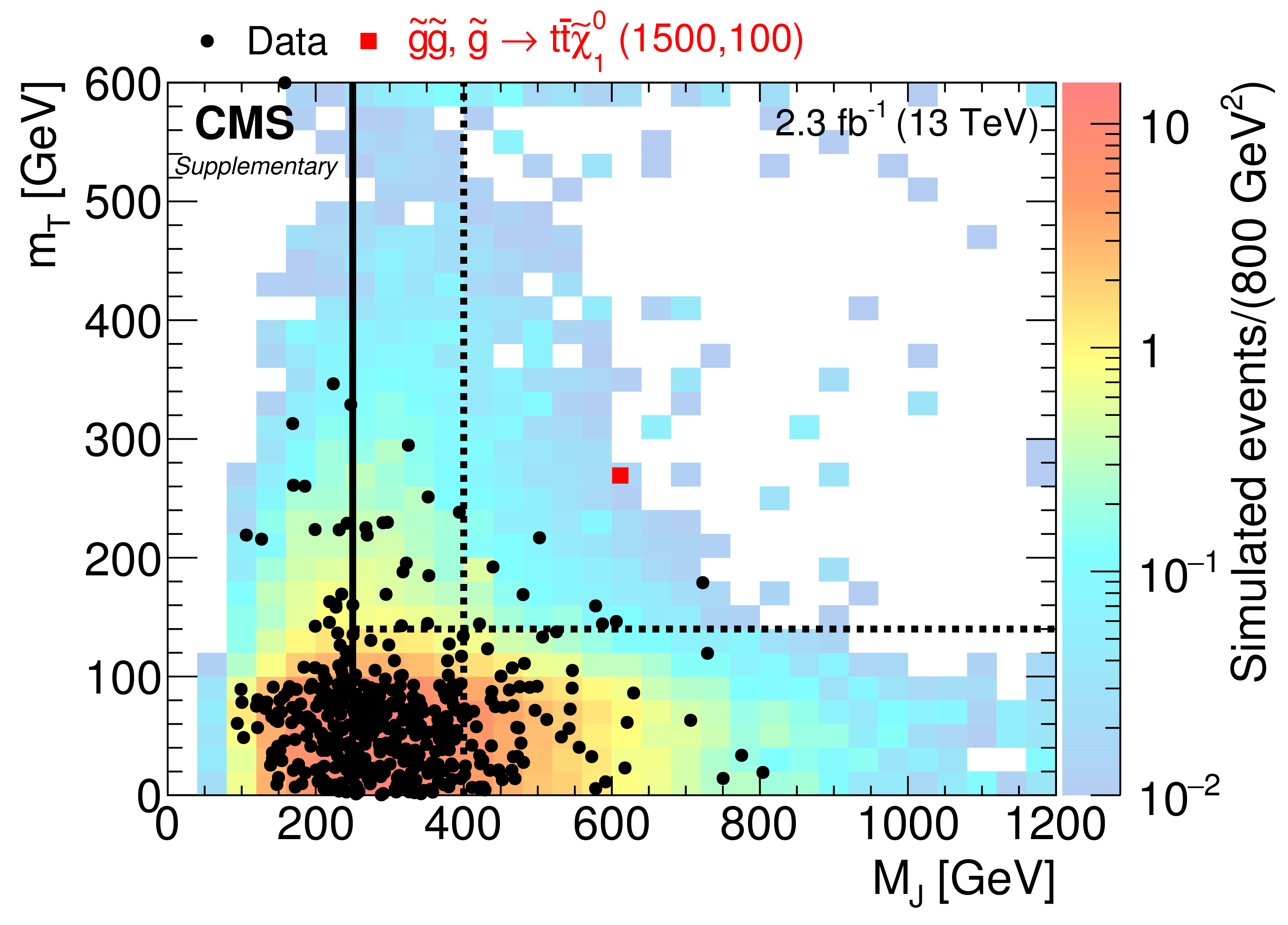
png pdf	Figure 8: Two-dimensional distributions for data and simulated event samples in the variables ${m_{\mathrm {T}}}$ and ${M_J}$ in the $ {N_{\text {b}}} \ge$ 2 region after the baseline selection. The distributions integrate over the ${N_{\text {jets}}}$ and ${E_{\mathrm {T}}^{\text {miss}}}$ bins. The black dots are the data; the colored histogram is the total simulated background, normalized to the data; and the red dots are a particular signal sample drawn from the expected distribution for gluino pair production in the T1tttt model with $ {m_{\mathrm{ \tilde{g} } }} =$ 1500 GeV and $m_{ {\tilde{\chi}^0_1} } = $ 100 GeV for 2.3 fb$^{-1}$. Overflow events are shown on the edges of the plot. The definitions of the signal and control regions are the same as those shown in Fig. 4.
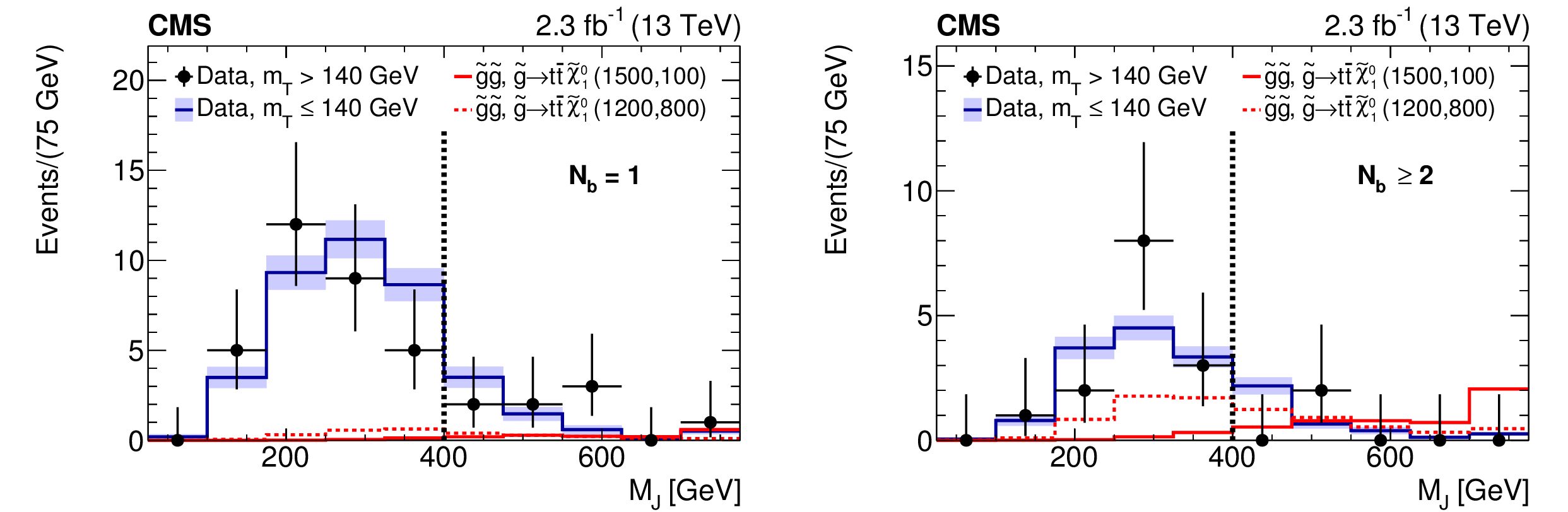
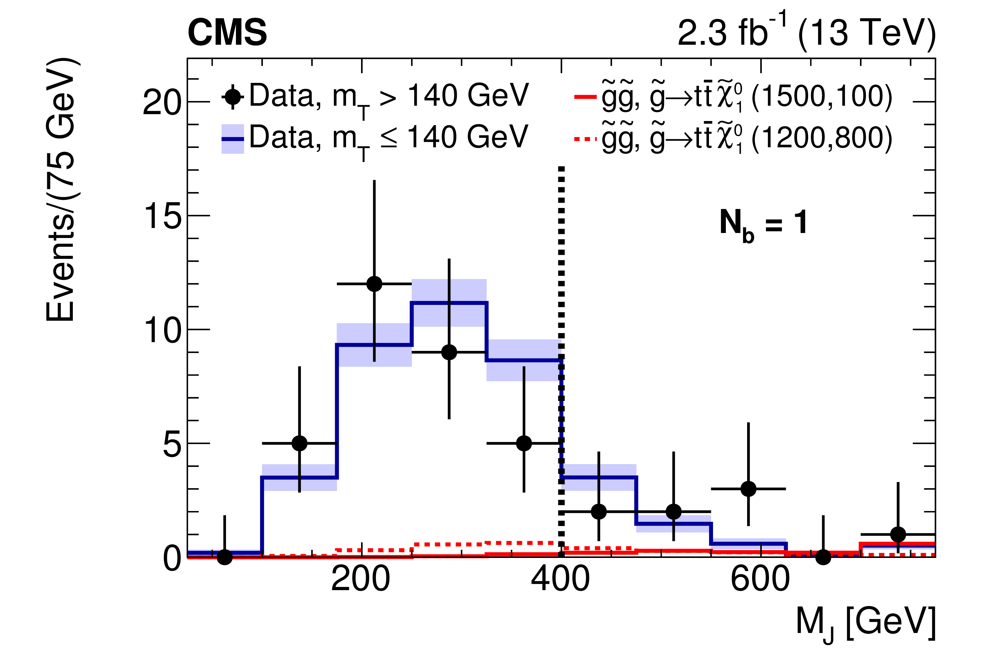
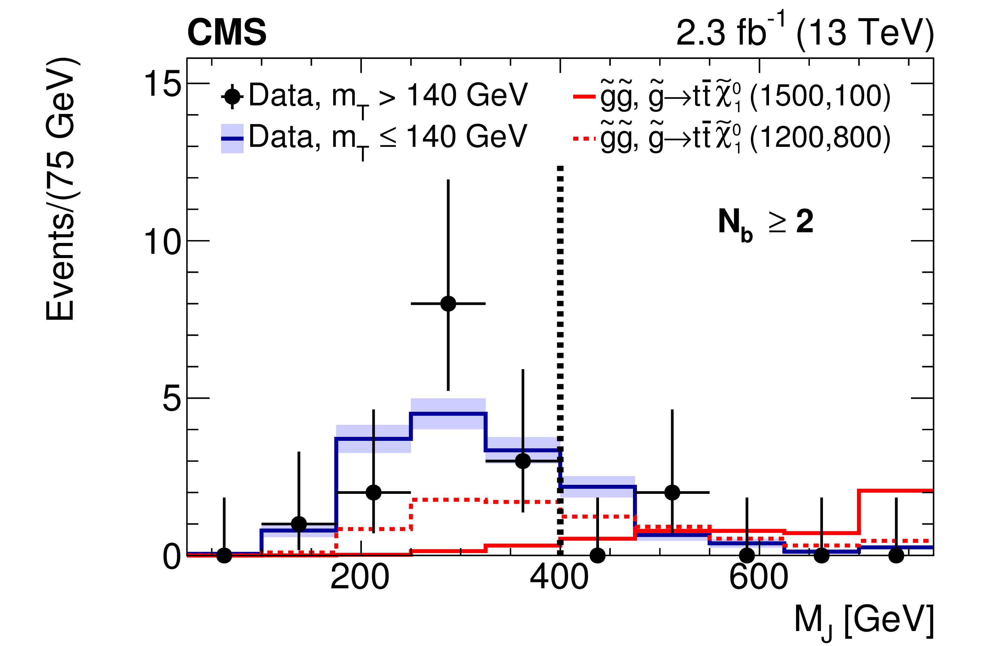
png pdf	Figure 9: Comparison of the ${M_J}$ distributions for low- and high-$ {m_{\mathrm {T}}}$ in data with $ {N_{\text {b}}} = $ 1 (left) and $ {N_{\text {b}}} \ge$ 2 (right) after the baseline selection. The expected ${M_J}$ distributions of the two benchmark T1tttt scenarios for $ {m_{\mathrm {T}}} > $ 140 GeV are overlaid. The distributions integrate over the ${N_{\text {jets}}}$ and ${E_{\mathrm {T}}^{\text {miss}}}$ bins. The low-$ {m_{\mathrm {T}}}$ distribution is normalized to the number of events in the high-$ {m_{\mathrm {T}}}$ region. The dashed vertical lines indicate the $ {M_J} > $ 400 GeV threshold that separates the signal regions from the control samples.
png pdf	Figure 9-a: Comparison of the ${M_J}$ distributions for low- and high-$ {m_{\mathrm {T}}}$ in data with $ {N_{\text {b}}} = $ 1 after the baseline selection. The expected ${M_J}$ distributions of the two benchmark T1tttt scenarios for $ {m_{\mathrm {T}}} > $ 140 GeV are overlaid. The distributions integrate over the ${N_{\text {jets}}}$ and ${E_{\mathrm {T}}^{\text {miss}}}$ bins. The low-$ {m_{\mathrm {T}}}$ distribution is normalized to the number of events in the high-$ {m_{\mathrm {T}}}$ region. The dashed vertical lines indicate the $ {M_J} > $ 400 GeV threshold that separates the signal regions from the control samples.
png pdf	Figure 9-b: Comparison of the ${M_J}$ distributions for low- and high-$ {m_{\mathrm {T}}}$ in data with $ {N_{\text {b}}} \ge$ 2 after the baseline selection. The expected ${M_J}$ distributions of the two benchmark T1tttt scenarios for $ {m_{\mathrm {T}}} > $ 140 GeV are overlaid. The distributions integrate over the ${N_{\text {jets}}}$ and ${E_{\mathrm {T}}^{\text {miss}}}$ bins. The low-$ {m_{\mathrm {T}}}$ distribution is normalized to the number of events in the high-$ {m_{\mathrm {T}}}$ region. The dashed vertical lines indicate the $ {M_J} > $ 400 GeV threshold that separates the signal regions from the control samples.
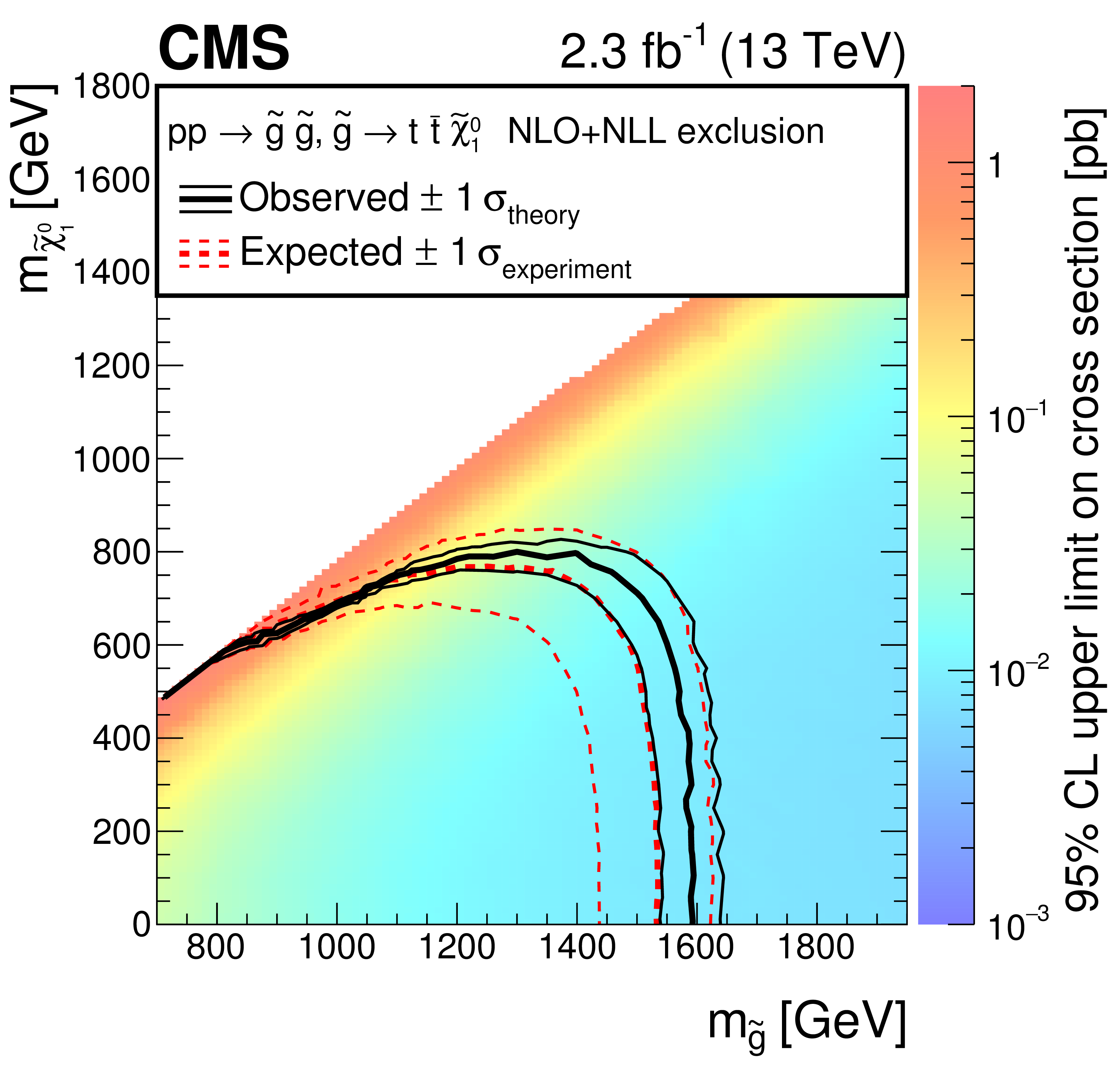
png pdf	Figure 10: Interpretation of results in the T1tttt model. The colored regions show the upper limits (95% CL) on the production cross section for $\mathrm{ p } \mathrm{ p } \rightarrow \mathrm{ \tilde{g} } \mathrm{ \tilde{g} } ,\mathrm{ \tilde{g} } \rightarrow {\mathrm{ t \bar{t} } } {\tilde{\chi}^0_1} $ in the $ {m_{\mathrm{ \tilde{g} } }} $-$ {m_{ {\tilde{\chi}^0_1} }} $ plane. The curves show the expected and observed limits on the corresponding SUSY particle masses obtained by comparing the excluded cross section with theoretical cross sections.
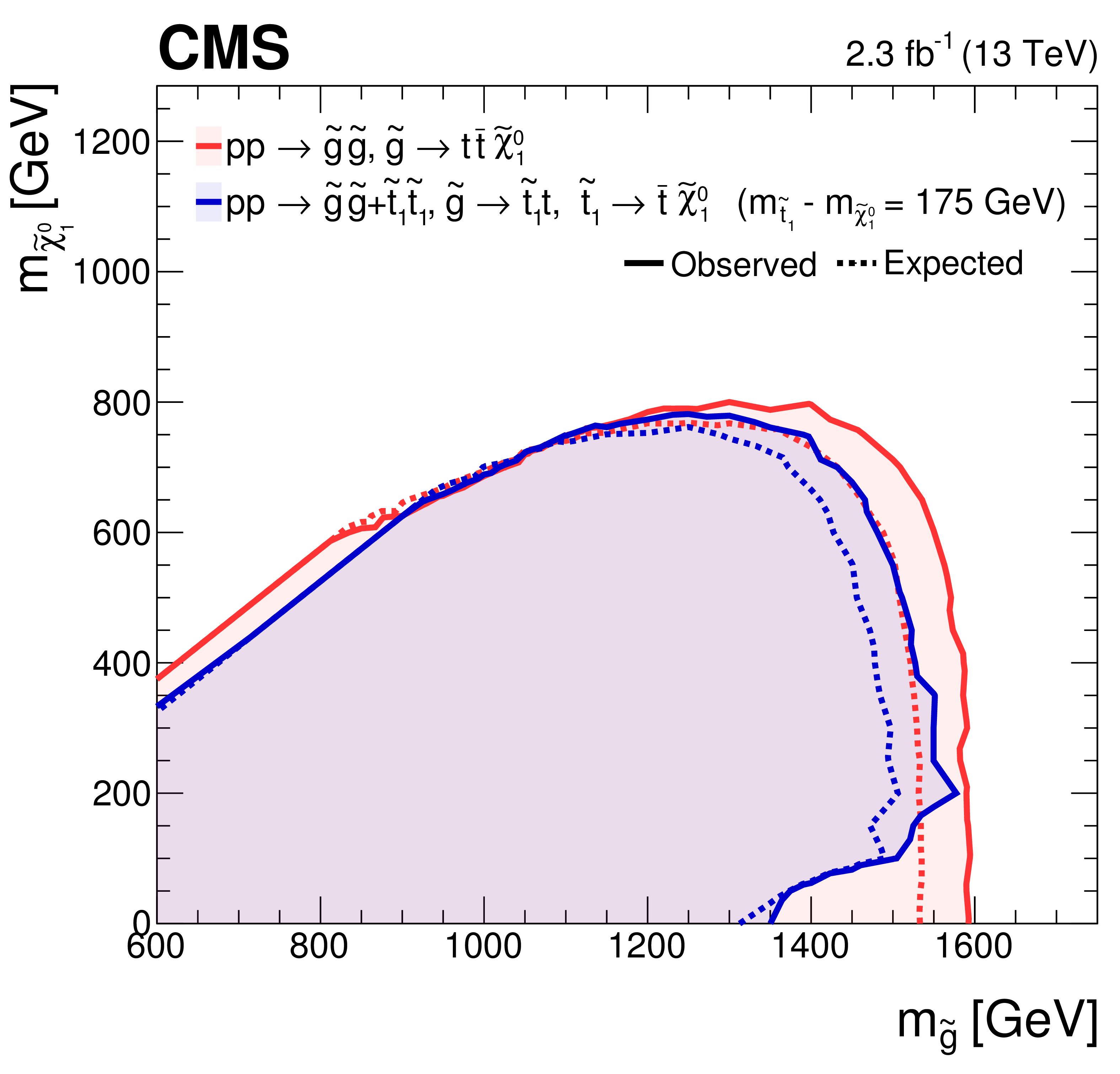
png pdf	Figure 11: Excluded region (95% CL), shown in blue, in the $ {m_{\mathrm{ \tilde{g} } }} $-$ {m_{ {\tilde{\chi}^0_1} }} $ plane for a model combining T5tttt, gluino pair production, followed by gluino decay to an on-shell top squark, together with a model for direct top squark pair production. The top squarks decay via the two-body process $\tilde{ mathrm{ t } } \to \mathrm{ t } {\tilde{\chi}^0_1} $. The neutralino and top squark masses are related by the constraint $ {m_{\tilde{ mathrm{ t } } _1}} = {m_{ {\tilde{\chi}^0_1} }}$ + 175 GeV. For comparison, the excluded region (95% CL) from Fig. 10 for the T1tttt model, which has three-body gluino decay, is shown in red. The small difference between the two boundary curves shows that the limits for the scenarios with two-body gluino decay have only a weak dependence on the top squark mass.

Tables
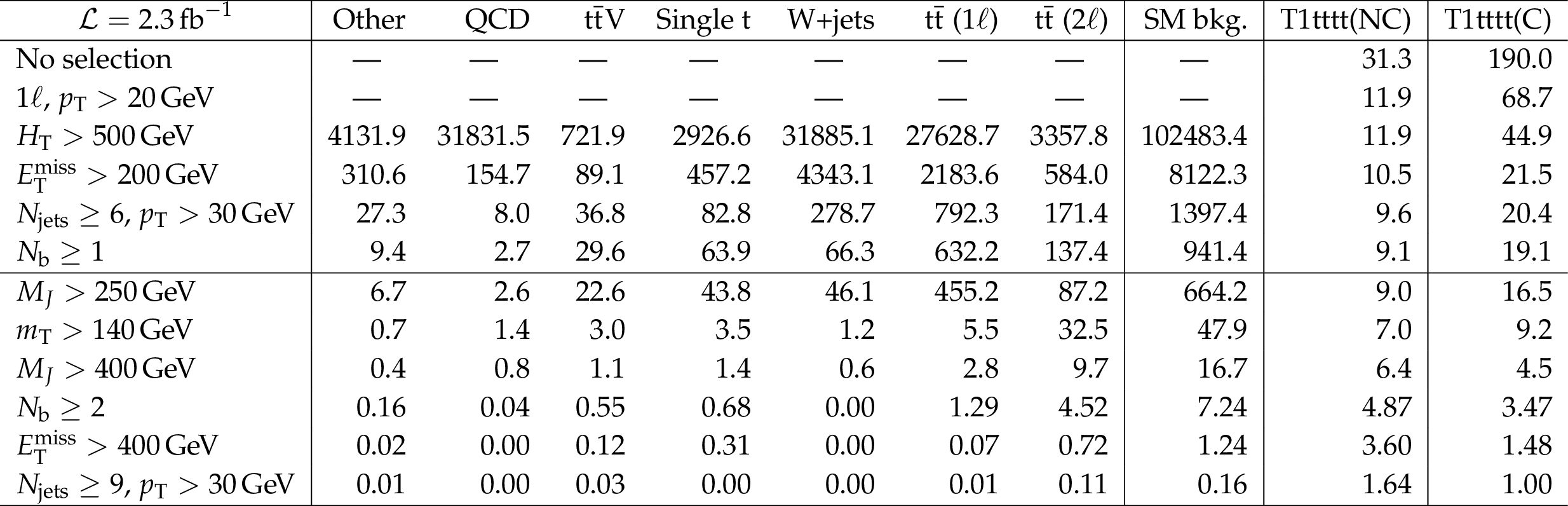
png pdf	Table 1: Event yields obtained from simulated event samples, as the event selection criteria are applied. The category Other includes Drell-Yan, $ {\mathrm{ t \bar{t} } } \mathrm{ H } (\rightarrow {\mathrm{ b \bar{b} } } )$, $ {\mathrm{ t \bar{t} } } {\mathrm{ t \bar{t} } } $, $\mathrm{ W } \mathrm{ Z } $, and $\mathrm{ W } \mathrm{ W } $. The yields for ${\mathrm{ t \bar{t} } }$ events in fully hadronic final states are included in the QCD multijet category. The category $ {\mathrm{ t \bar{t} } } {\rm V}$ includes $ {\mathrm{ t \bar{t} } } \mathrm{ W } $, $ {\mathrm{ t \bar{t} } } \mathrm{ Z } $, and $ {\mathrm{ t \bar{t} } } \gamma $. The benchmark signal models, T1tttt(NC) and T1tttt(C), are described in Section 3. The event selection requirements listed above the horizontal line in the middle of the table are defined as the baseline selection. The background estimates before the $ {H_{\mathrm {T}}} $ requirement are not specified because some of the simulated event samples do not extend to the low $ {H_{\mathrm {T}}} $ region. Given the size of the MC samples described in Section 3, rows with zero yield have statistical uncertainties of at most 0.16 events, and below 0.05 events in most cases.
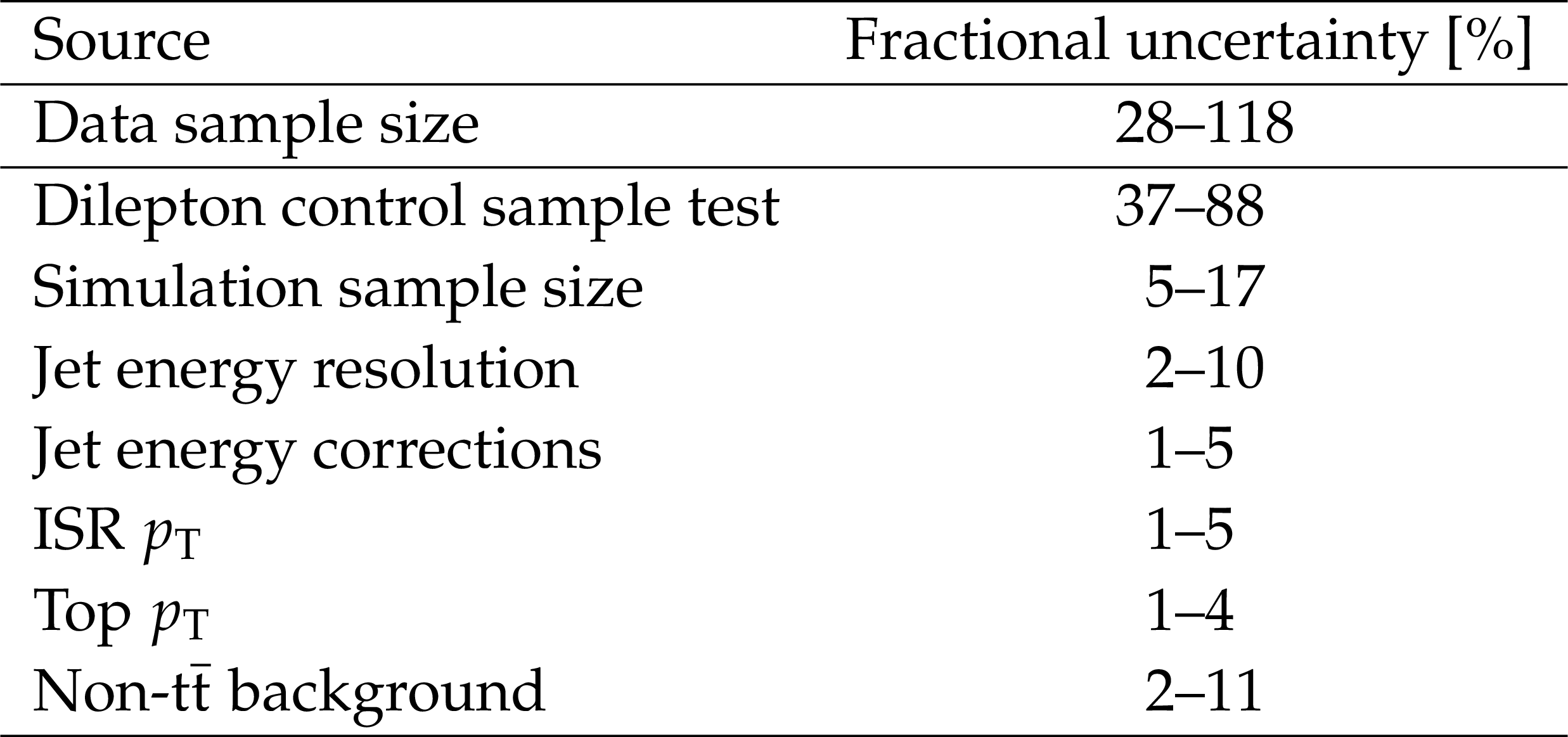
png pdf	Table 2: Summary of uncertainties in the background predictions. All entries in the table except for data sample size correspond to a relative uncertainty on $\kappa $. The ranges indicate the spread of each uncertainty across the signal bins. Uncertainties from a particular source are treated as fully correlated across bins, while uncertainties from different sources are treated as uncorrelated.
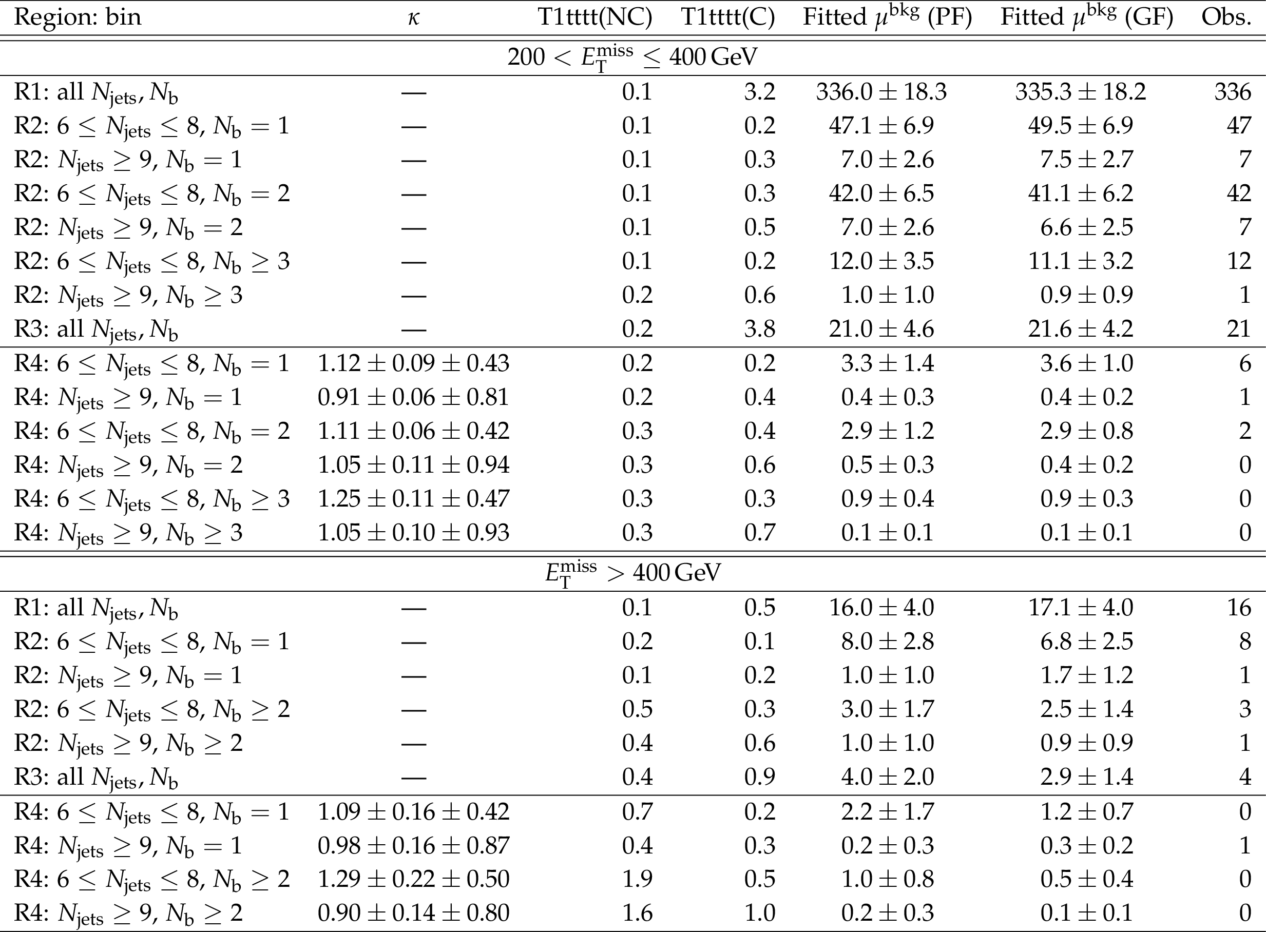
png pdf	Table 3: Observed and predicted event yields for the signal regions (R4) and background regions (R1-R3) in data (2.3 fb$^{-1}$). Expected yields for the two SUSY T1tttt benchmark scenarios are also given. The results from two types of fits are reported: the predictive fit (PF) and the version of the global fit (GF) performed under the assumption of the null hypothesis ($r= $ 0 ). The predictive fit uses the observed yields in regions R1, R2, and R3 only and is effectively just a propagation of uncertainties. The global fit uses all four regions. The values of $\kappa $ obtained from the simulation fit are also listed. The first uncertainty in $\kappa $ is statistical, while the second corresponds to the total systematic uncertainty. The benchmark signal models, T1tttt(NC) and T1tttt(C), are described in Section 3.
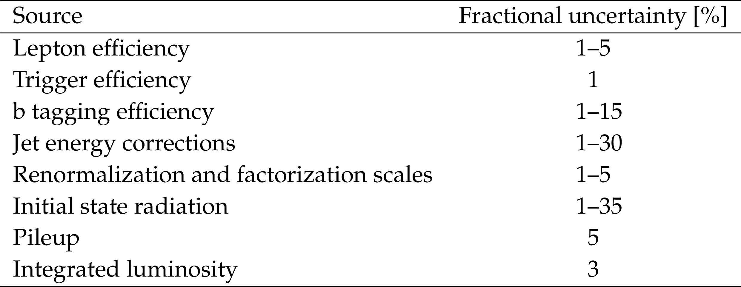
png pdf	Table 4: Typical values of the signal-related systematic uncertainties. Uncertainties due to a particular source are treated as fully correlated between bins, while uncertainties due to different sources are treated as uncorrelated.

Summary

Using a sample of proton-proton collisions at $\sqrt s = $ 13 GeV with an integrated luminosity of 2.3 fb$^{-1}$, a search for supersymmetry is performed in the final state with a single lepton, b-tagged jets, and large missing transverse momentum. The search focuses on final states resulting from the pair production of gluinos, which subsequently decay via $\mathrm{ \tilde{g} }\to\mathrm{ t \bar{t} }{\tilde{\chi}^0_1} $, leading to high jet multiplicities. A key feature of the analysis is the use of the variable ${M_J} $, the sum of the masses of large-$R$ jets, which are formed by clustering anti-$k_{\mathrm{T}}$ $R= $ 0.4 jets and leptons. Used in conjunction with the variable ${m_{\mathrm{T}}} $, the transverse mass of the system consisting of the lepton and the missing transverse momentum vector, ${M_J} $ provides a powerful background estimation method that is well suited to this high jet multiplicity search. After the baseline selection is applied, signal (R4) and control regions (R1, R2, and R3) are defined in the ${M_J} $-${m_{\mathrm{T}}} $ plane, which are further divided into bins of $E_{\mathrm{T}}^{\text{miss}}$, ${N_{\text{jets}}} $, and ${N_{\text{b}}} $ to provide additional sensitivity. In regions R3 and R4, the requirement ${m_{\mathrm{T}}} > $ 140 GeV provides strong suppression of the single-lepton $\mathrm{ t \bar{t} }$ background, so that dilepton $\mathrm{ t \bar{t} }$ events dominate over all other background sources. For these dilepton events to enter a signal region, however, they must contain a substantial amount of initial-state radiation (ISR). For this extreme range of ISR jet momentum and multiplicity, the single-lepton and dilepton $\mathrm{ t \bar{t} }$ events have very similar kinematic properties. The variables ${M_J} $ and ${m_{\mathrm{T}}} $ are nearly uncorrelated, even though different processes dominate the low- and high-${m_{\mathrm{T}}} $ regions. As a consequence, the low-${m_{\mathrm{T}}} $ regions (R1 and R2) can be used to measure the background shape for the ${M_J} $ distribution at high ${m_{\mathrm{T}}} $. A correction factor, near unity, is taken from simulation and is used to account for a possible correlation between ${M_J} $ and ${m_{\mathrm{T}}} $. The observed event yields in the signal regions are consistent with the predictions for the SM background contributions, and exclusion limits are set on the gluino pair production cross sections in the ${m_{\mathrm{ \tilde{g} }}} $-${m_{{\tilde{\chi}^0_1} }} $ plane, as described by the simplified models T1tttt and T5tttt, where the latter is augmented with a model of direct top squark pair production for consistency. In the T1tttt model, gluinos decay via the three-body process $\mathrm{ \tilde{g} }\to\mathrm{ t \bar{t} }{\tilde{\chi}^0_1} $, which proceeds via a virtual top squark in the intermediate state. Under the assumption of a 100% branching fraction to this final state, the cross section limit for each model point is compared with the theoretical cross section to determine the excluded particle masses. Gluinos with a mass below 1600 GeV are excluded at a 95% CL for scenarios with low $\tilde\chi_1^0$ mass, and neutralinos with a mass below 800 GeV are excluded for a gluino mass of about 1300 GeV. In the T5tttt model, the top squark is lighter than the gluino, which therefore decays via a two-body process. The boundary of the excluded region in the ${m_{\mathrm{ \tilde{g} }}} $-${m_{{\tilde{\chi}^0_1} }} $ plane for T5tttt is found to be only weakly sensitive to the top squark mass. These results significantly extend the sensitivity of single-lepton searches based on data at $\sqrt s = $ 8 GeV.

Additional Figures
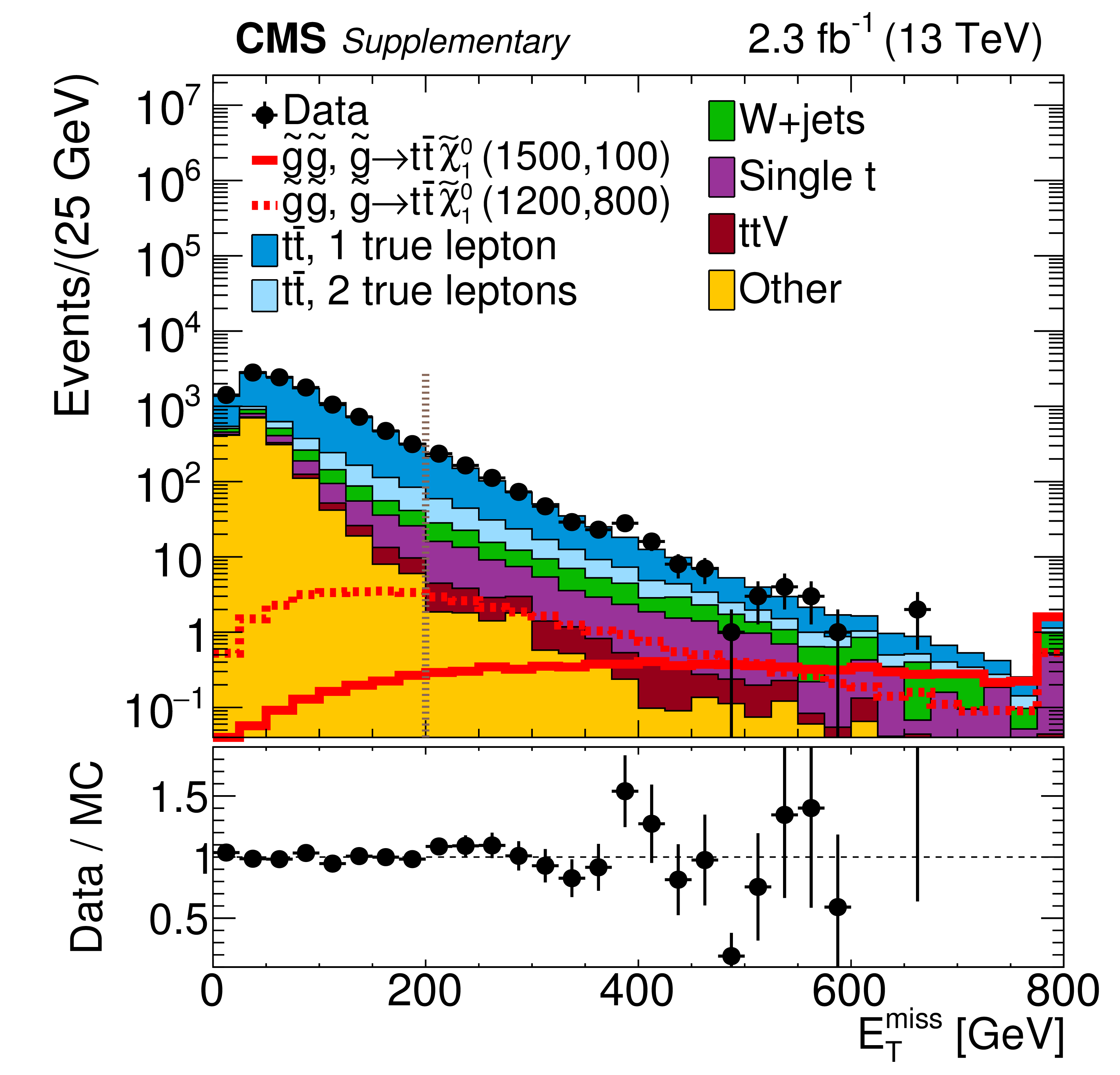
png pdf	Additional Figure 1-a: Distribution of ${E_{\mathrm {T}}^{\text {miss}}}$ in data and simulated event samples after the baseline selection is applied (except for the ${E_{\mathrm {T}}^{\text {miss}}}$ requirement) in linear (a) and logarithmic (b) scales. The background contributions shown here are from simulation, and their total yield is normalized to the number of events observed in data. The signal distributions are normalized to the expected cross sections. The dashed vertical line indicates the $ {E_{\mathrm {T}}^{\text {miss}}} > $ 200 GeV baseline requirement.
png pdf	Additional Figure 1-b: Distribution of ${E_{\mathrm {T}}^{\text {miss}}}$ in data and simulated event samples after the baseline selection is applied (except for the ${E_{\mathrm {T}}^{\text {miss}}}$ requirement) in linear (a) and logarithmic (b) scales. The background contributions shown here are from simulation, and their total yield is normalized to the number of events observed in data. The signal distributions are normalized to the expected cross sections. The dashed vertical line indicates the $ {E_{\mathrm {T}}^{\text {miss}}} > $ 200 GeV baseline requirement.
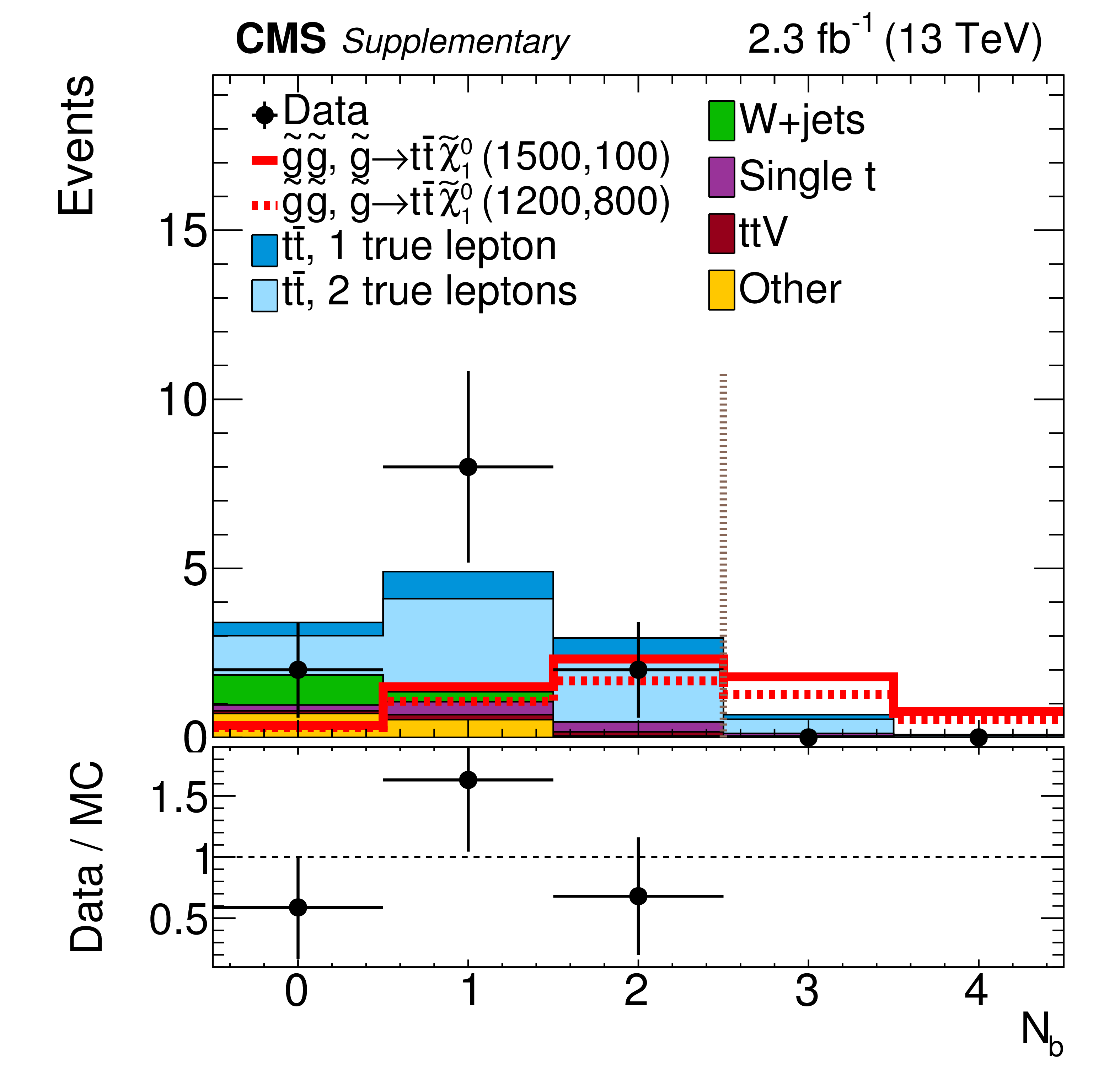
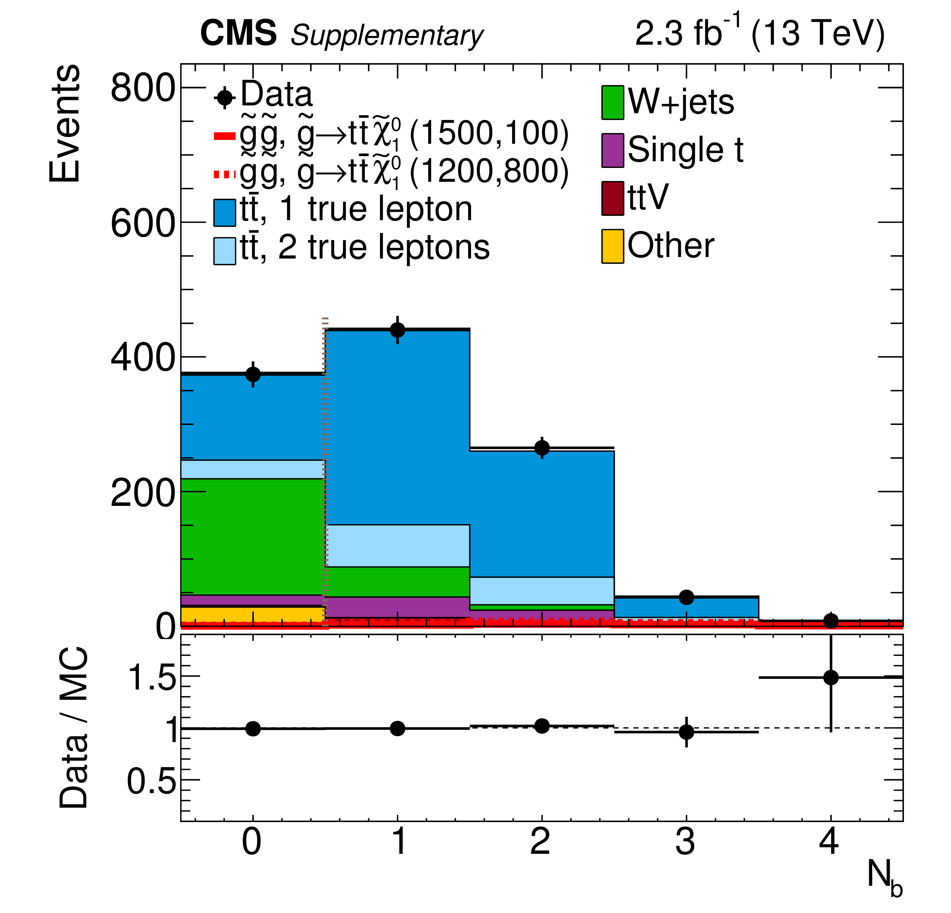
png pdf	Additional Figure 2-a: Distribution of $ {N_{\text {b}}}$ in data and simulated event samples after the baseline selection is applied (except for the $ {N_{\text {b}}}$ requirement) in linear (a) and logarithmic (b) scales. The background contributions shown here are from simulation, and their total yield is normalized to the number of events observed in data. The signal distributions are normalized to the expected cross sections. The dashed vertical line indicates the $ {N_{\text {b}}} \geq 1$ baseline requirement.
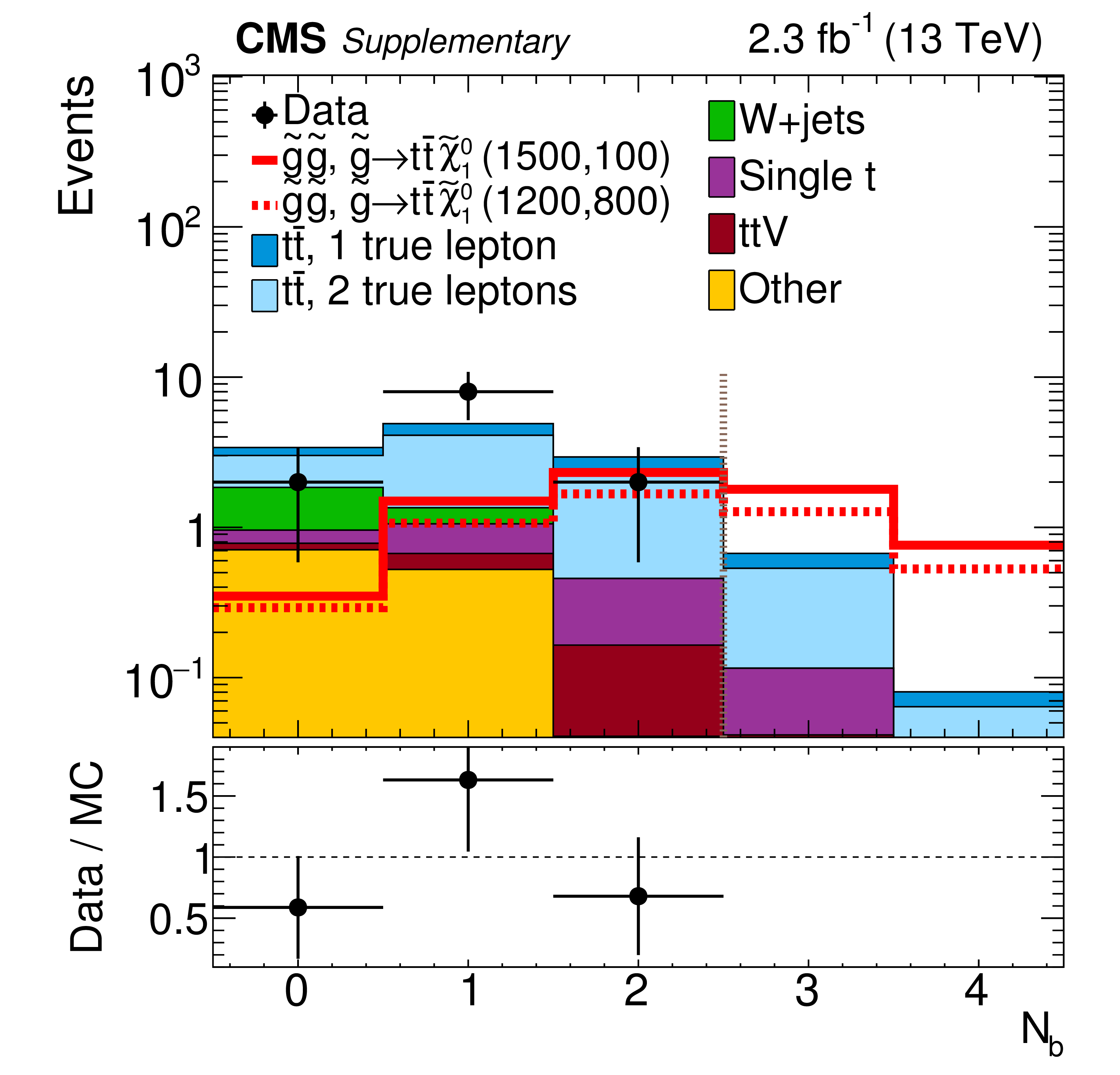
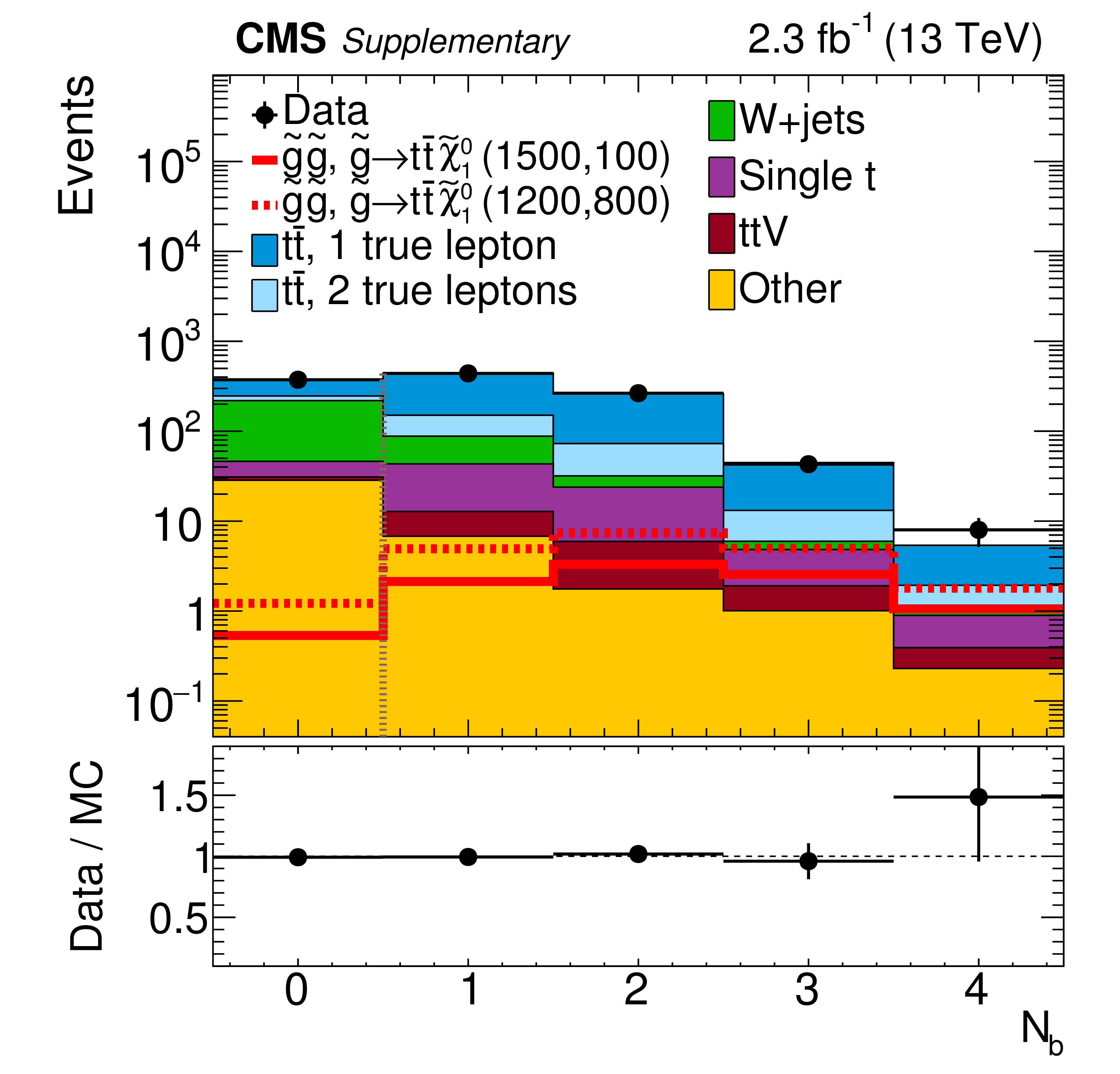
png pdf	Additional Figure 2-b: Distribution of $ {N_{\text {b}}}$ in data and simulated event samples after the baseline selection is applied (except for the $ {N_{\text {b}}}$ requirement) in linear (a) and logarithmic (b) scales. The background contributions shown here are from simulation, and their total yield is normalized to the number of events observed in data. The signal distributions are normalized to the expected cross sections. The dashed vertical line indicates the $ {N_{\text {b}}} \geq 1$ baseline requirement.
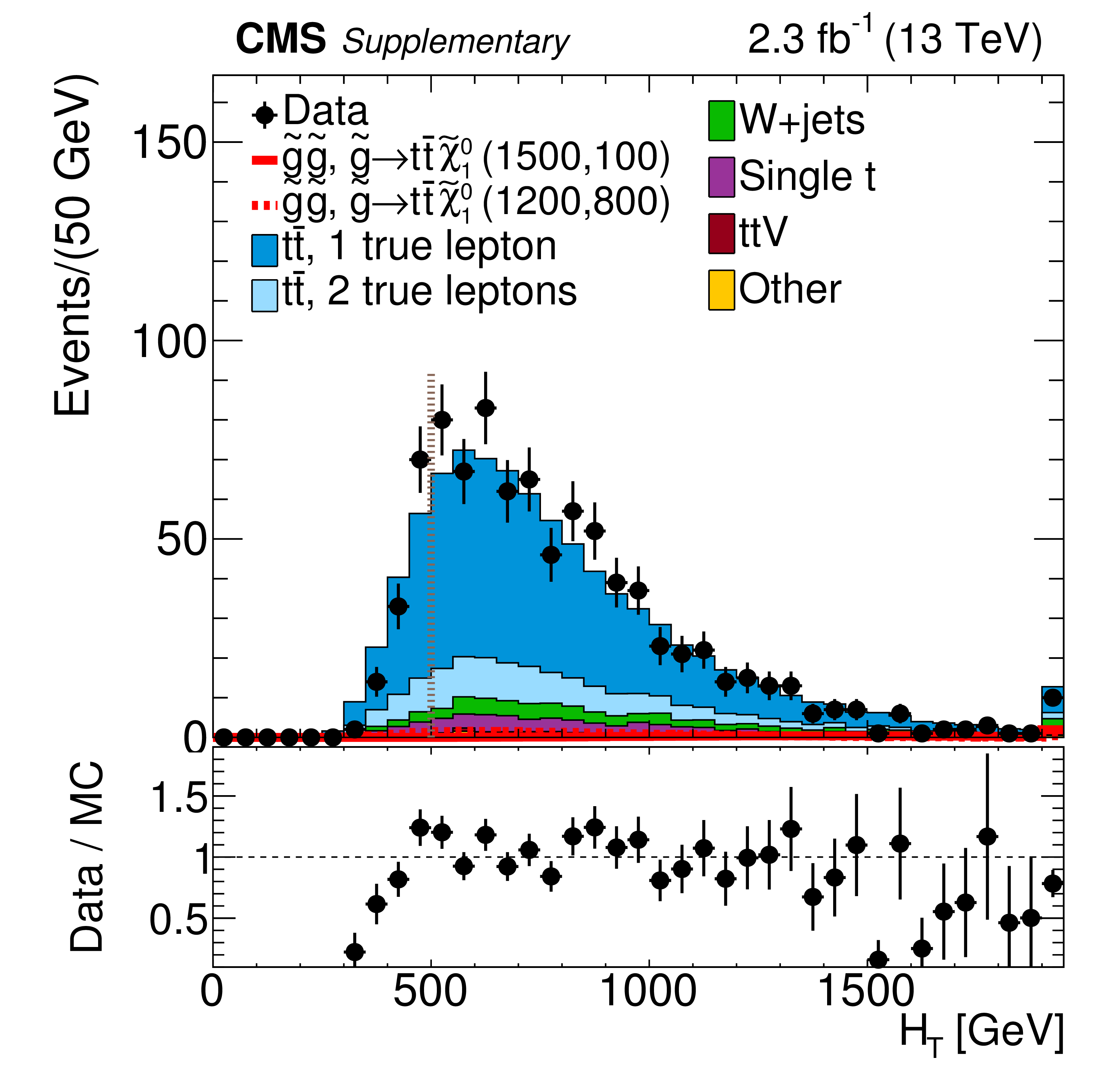
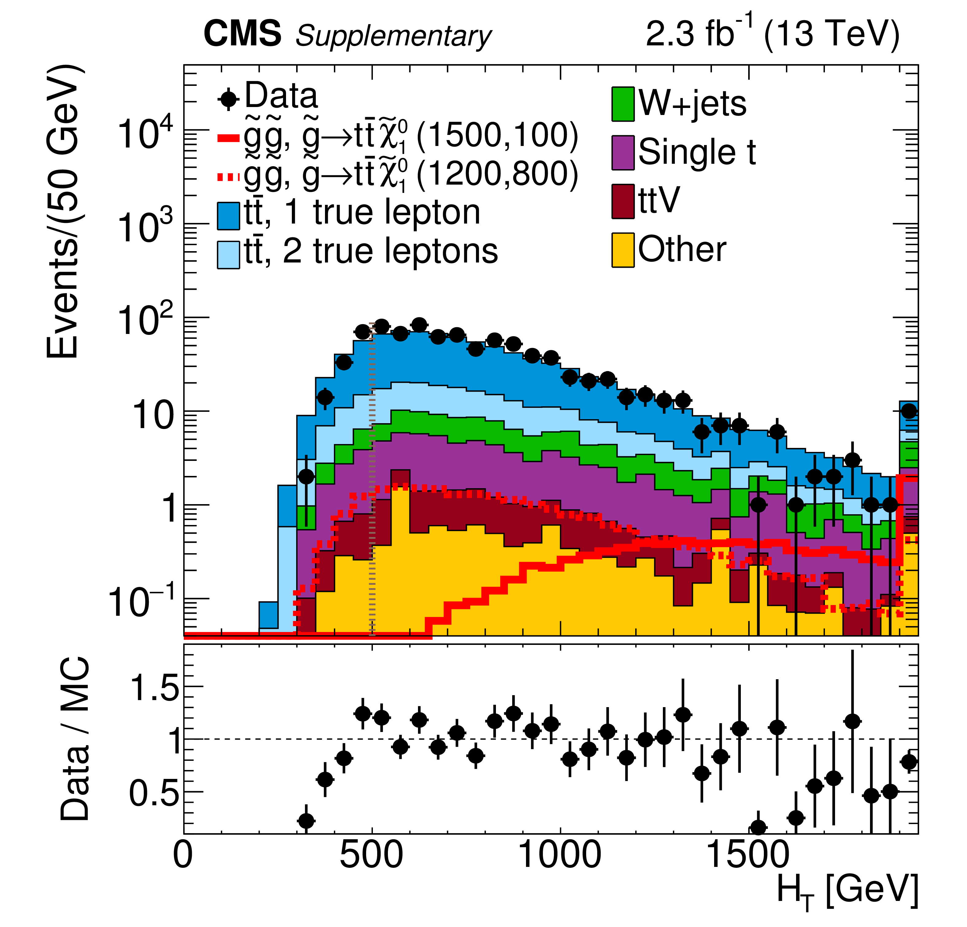
png pdf	Additional Figure 3-a: Distribution of ${H_{\mathrm {T}}}$ in data and simulated event samples after the baseline selection is applied (except for the ${H_{\mathrm {T}}}$ requirement) in linear (a) and logarithmic (b) scales. The background contributions shown here are from simulation, and their total yield is normalized to the number of events observed in data. The signal distributions are normalized to the expected cross sections. For low ${H_{\mathrm {T}}}$, the data points go below the simulation due to trigger inefficiency. The dashed vertical line indicates the $ {H_{\mathrm {T}}} > $ 500 GeV baseline requirement that ensures trigger plateau efficiency.
png pdf	Additional Figure 3-b: Distribution of ${H_{\mathrm {T}}}$ in data and simulated event samples after the baseline selection is applied (except for the ${H_{\mathrm {T}}}$ requirement) in linear (a) and logarithmic (b) scales. The background contributions shown here are from simulation, and their total yield is normalized to the number of events observed in data. The signal distributions are normalized to the expected cross sections. For low ${H_{\mathrm {T}}}$, the data points go below the simulation due to trigger inefficiency. The dashed vertical line indicates the $ {H_{\mathrm {T}}} > $ 500 GeV baseline requirement that ensures trigger plateau efficiency.
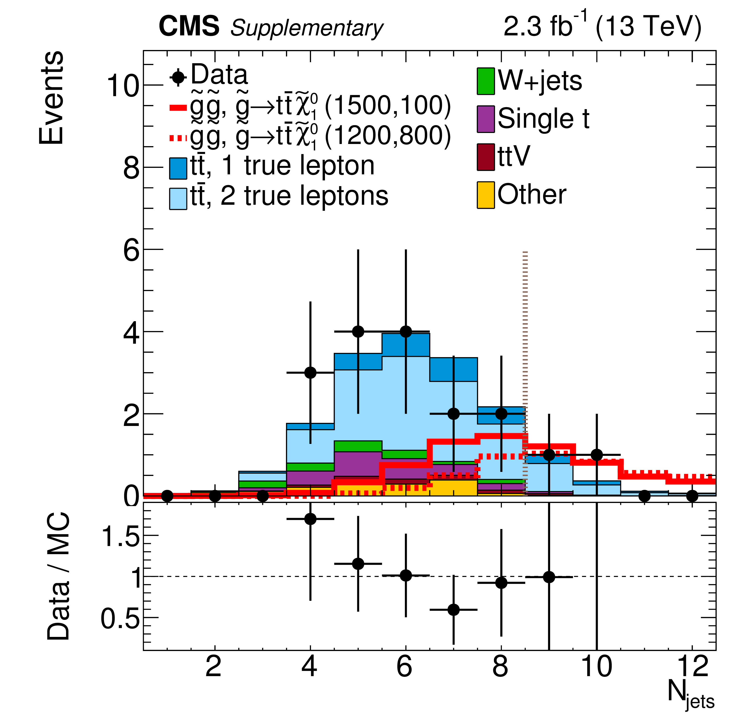
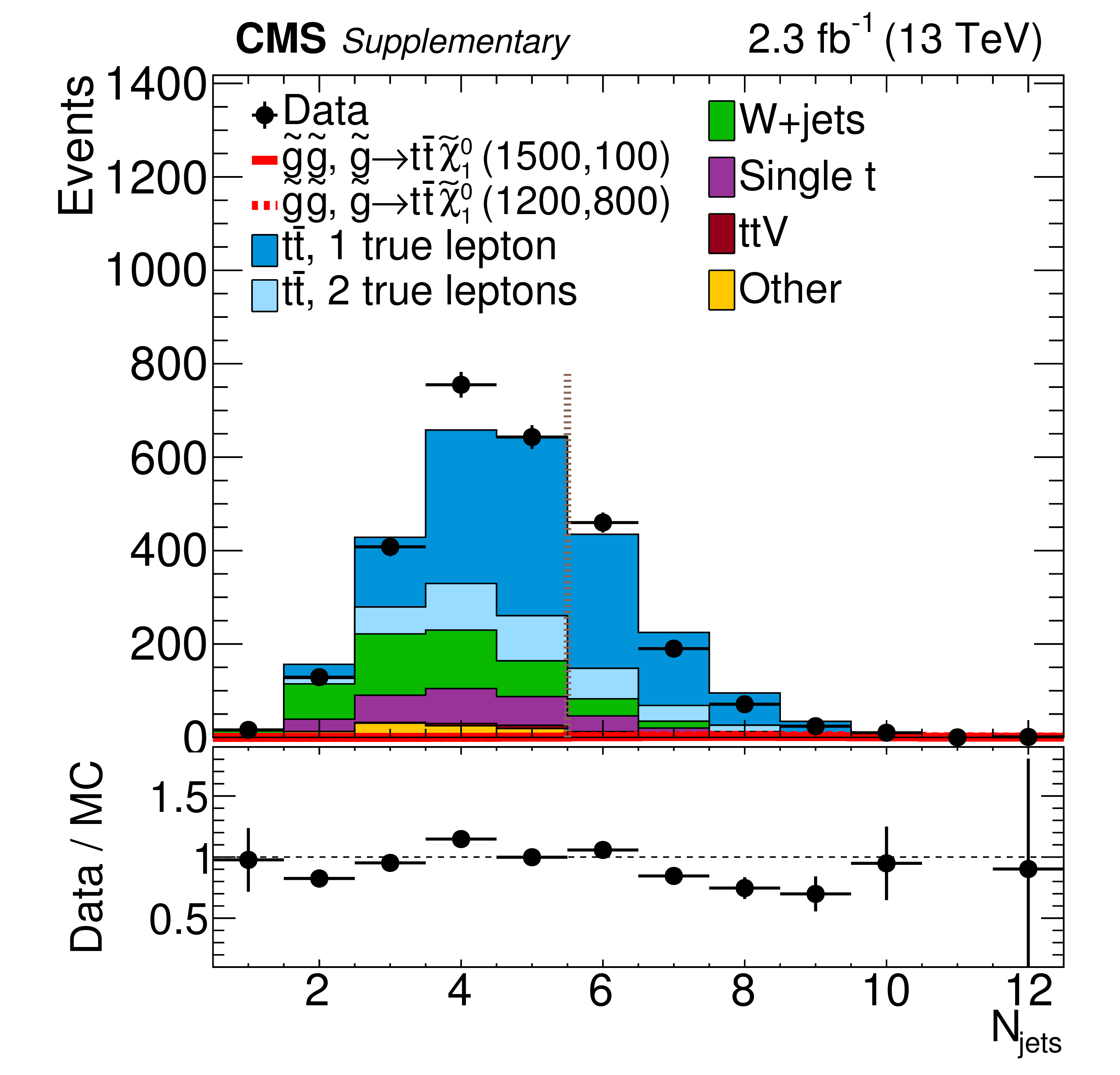
png pdf	Additional Figure 4-a: Distribution of ${N_{\text {jets}}}$ in data and simulated event samples after the baseline selection is applied (except for the ${N_{\text {jets}}}$ requirement) in linear (a) and logarithmic (b) scales. The background contributions shown here are from simulation, and their total yield is normalized to the number of events observed in data. The signal distributions are normalized to the expected cross sections. The dashed vertical line indicates the $ {N_{\text {jets}}} \geq 6$ baseline requirement.
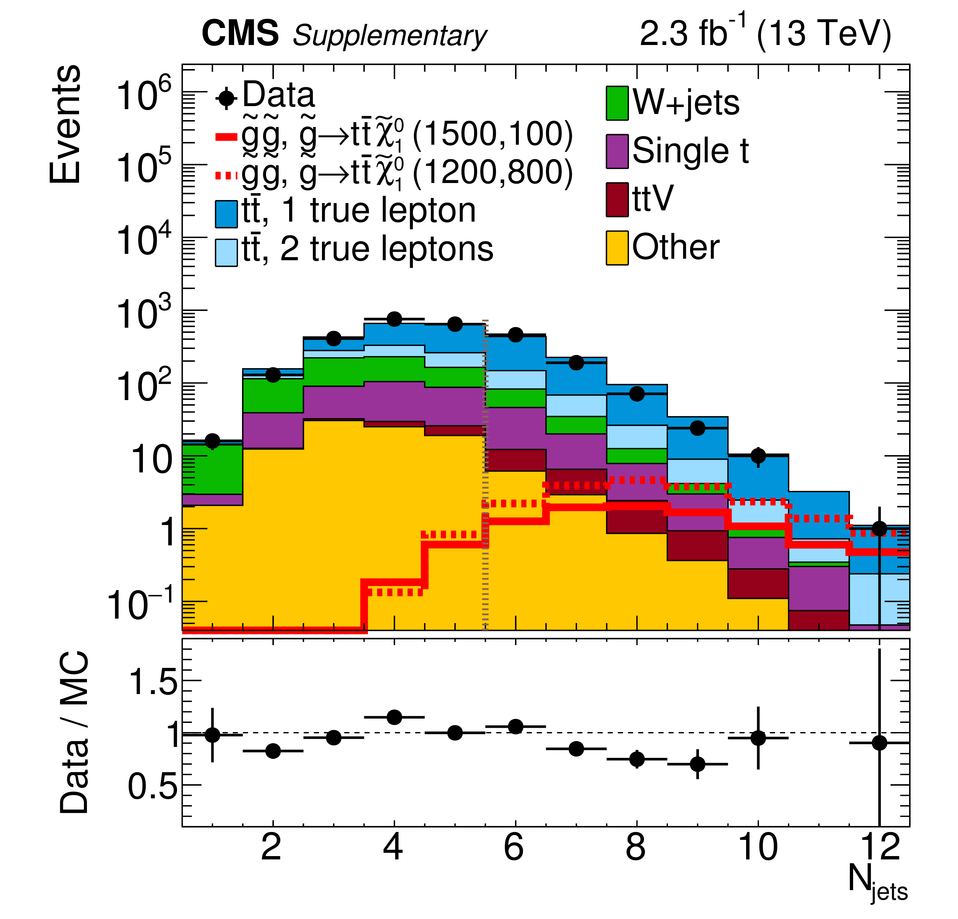
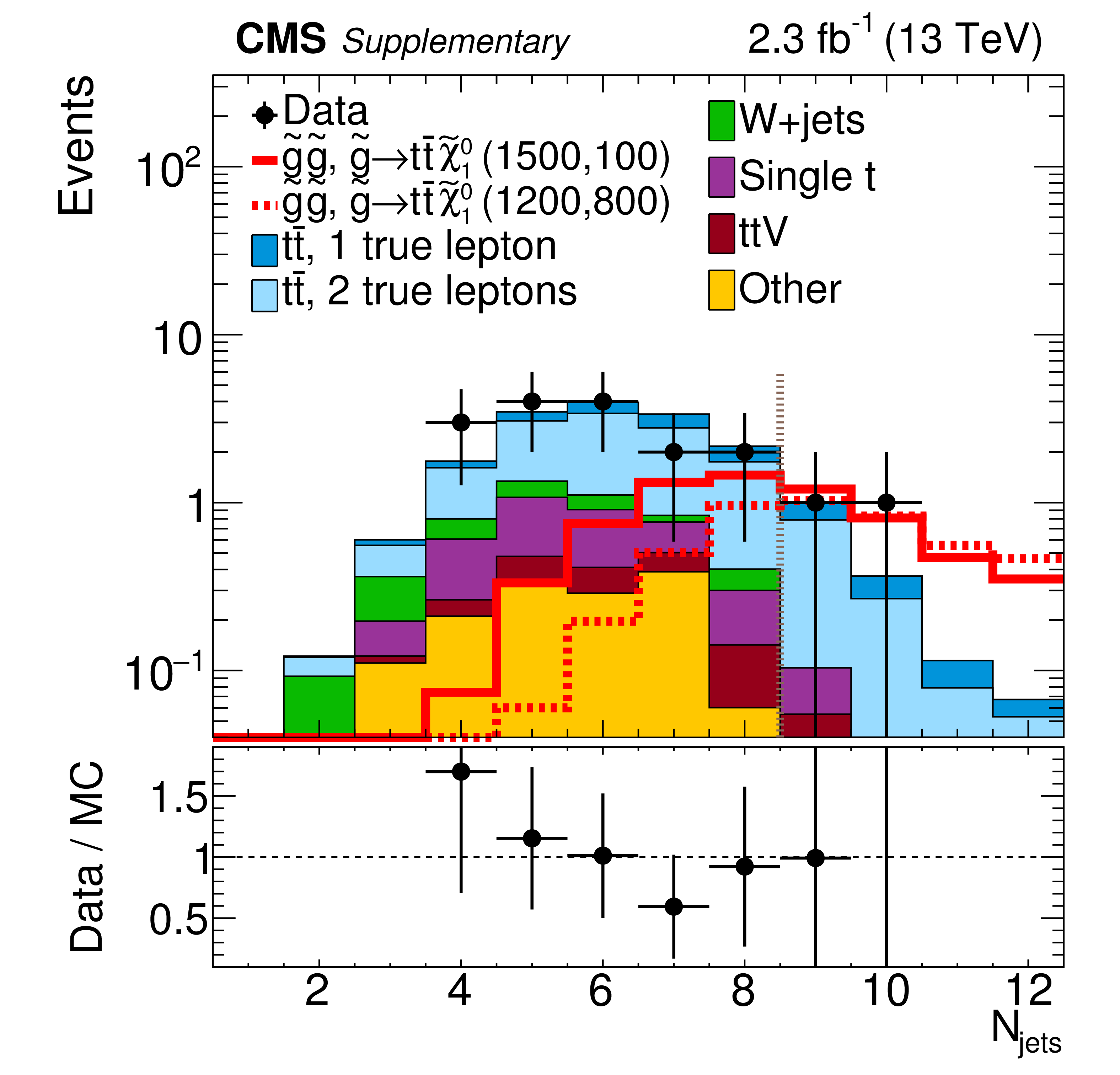
png pdf	Additional Figure 4-b: Distribution of ${N_{\text {jets}}}$ in data and simulated event samples after the baseline selection is applied (except for the ${N_{\text {jets}}}$ requirement) in linear (a) and logarithmic (b) scales. The background contributions shown here are from simulation, and their total yield is normalized to the number of events observed in data. The signal distributions are normalized to the expected cross sections. The dashed vertical line indicates the $ {N_{\text {jets}}} \geq 6$ baseline requirement.
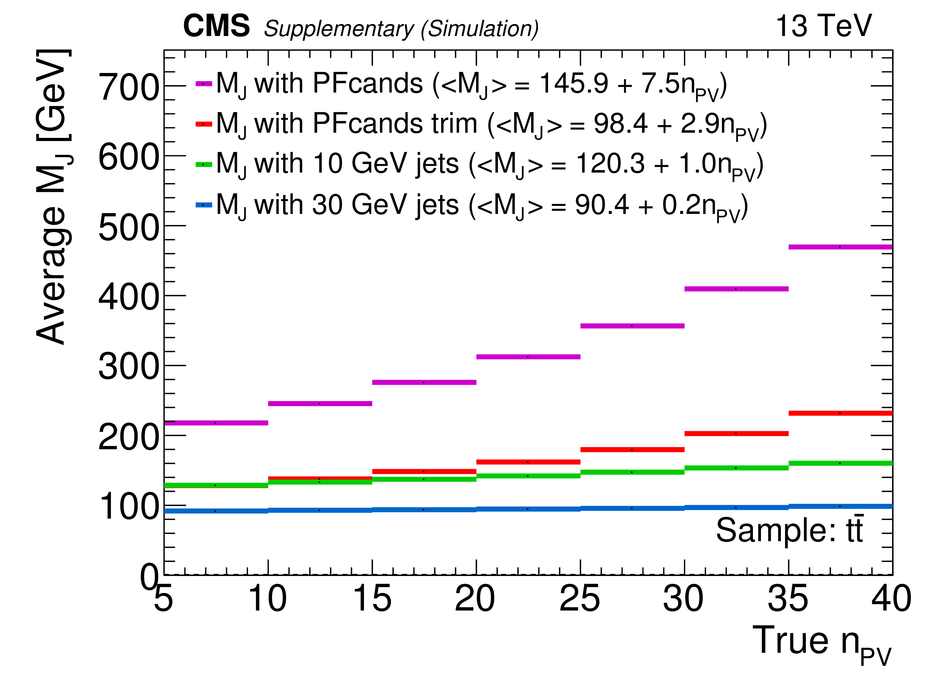
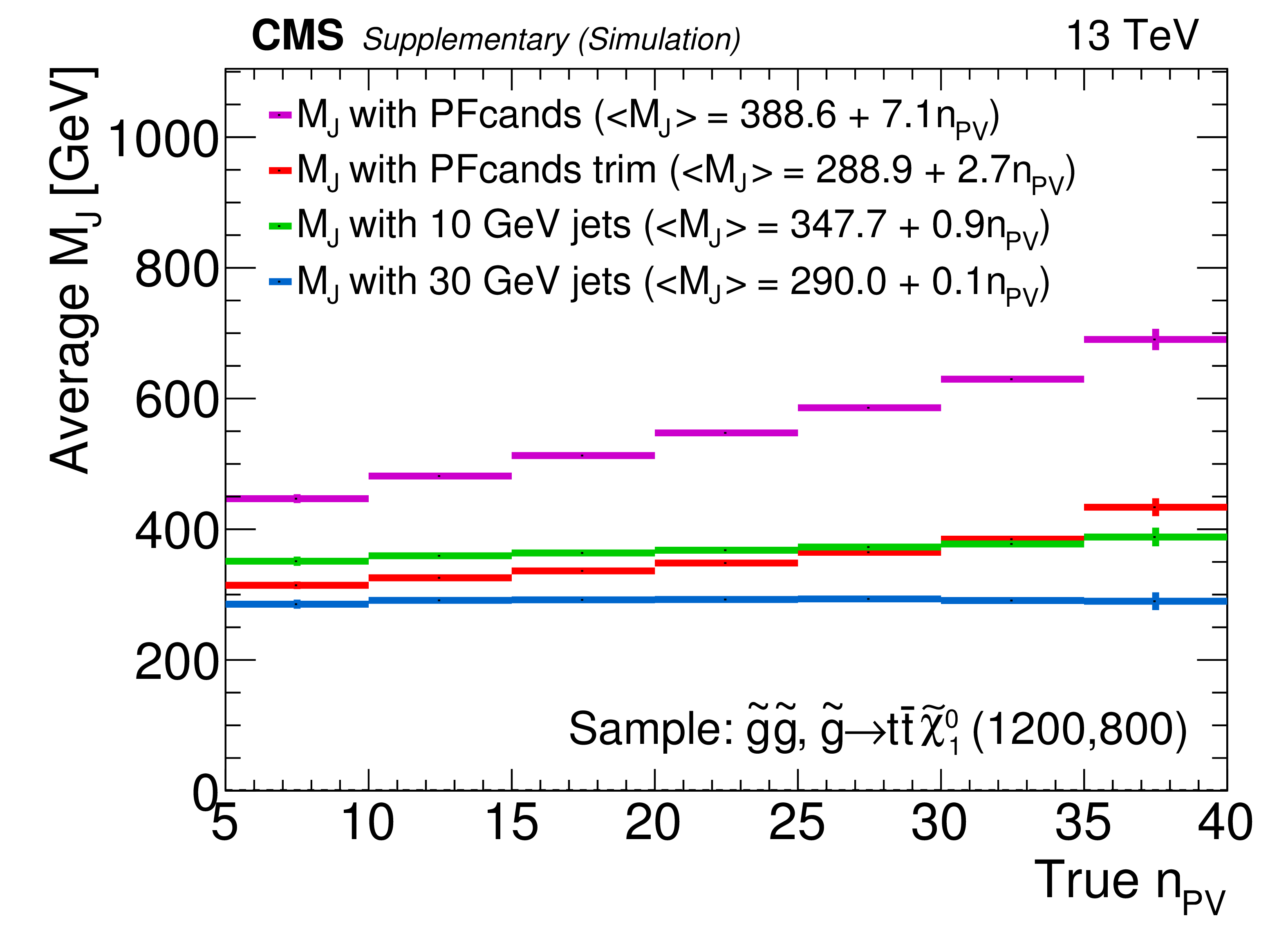
png pdf	Additional Figure 5-a: Average ${M_J}$ as a function of the number of primary vertices for ${\mathrm{ t } \mathrm{ \bar{t} } }$ and a signal model. ${M_J}$ is shown as calculated from all CHS PF candidates (magenta), all CHS PF candidates plus trimming (red), AK4 PF jets with $p_T> $ 10 GeV (green), or AK4 PF jets with $p_T> $ 30 GeV (blue). The legend includes the results of linear fits to each set of points, showing that for the choice of 30 GeV jets, the PU dependence is very small.
png pdf	Additional Figure 5-b: Average ${M_J}$ as a function of the number of primary vertices for ${\mathrm{ t } \mathrm{ \bar{t} } }$ and a signal model. ${M_J}$ is shown as calculated from all CHS PF candidates (magenta), all CHS PF candidates plus trimming (red), AK4 PF jets with $p_T> $ 10 GeV (green), or AK4 PF jets with $p_T> $ 30 GeV (blue). The legend includes the results of linear fits to each set of points, showing that for the choice of 30 GeV jets, the PU dependence is very small.
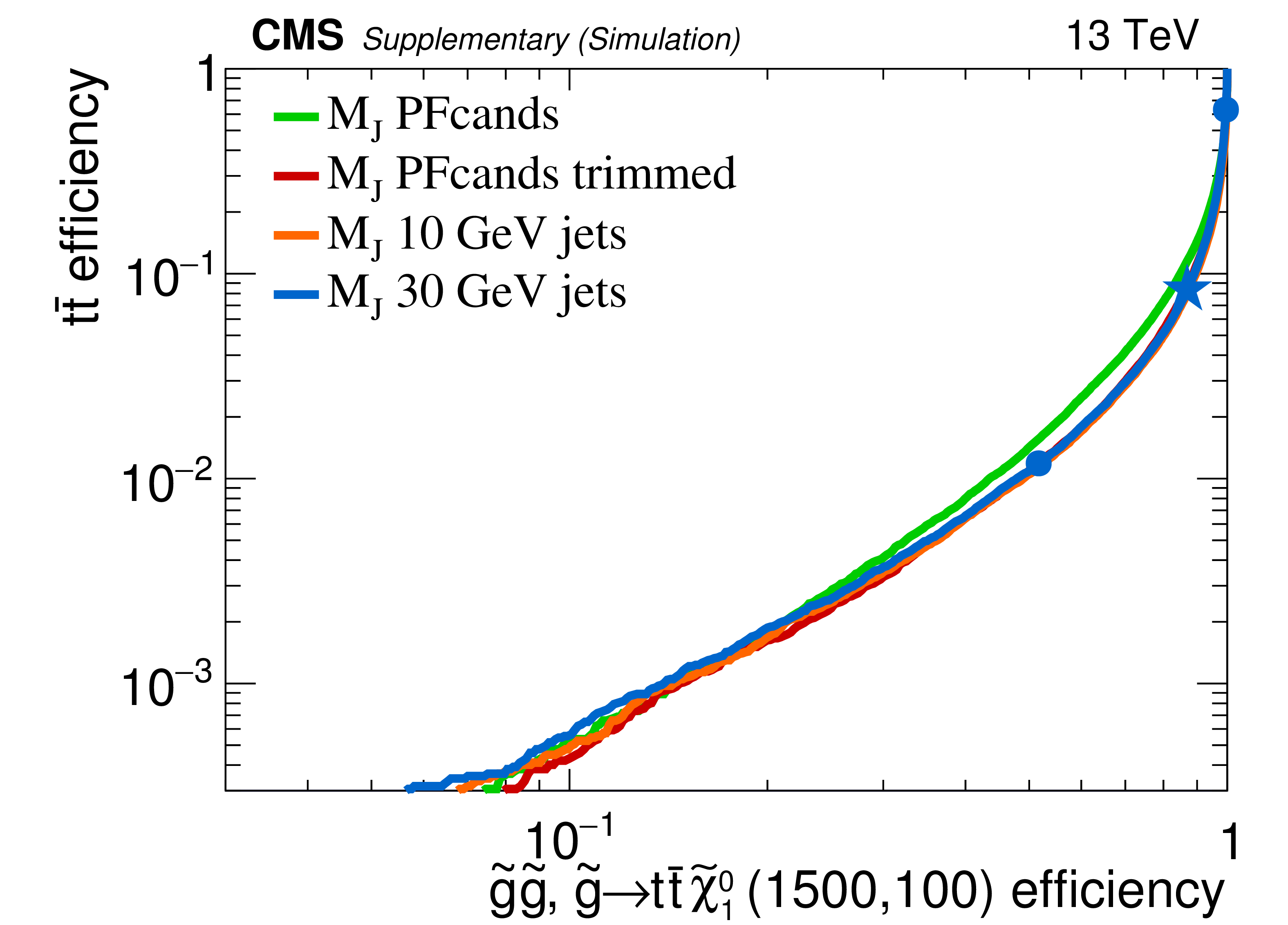
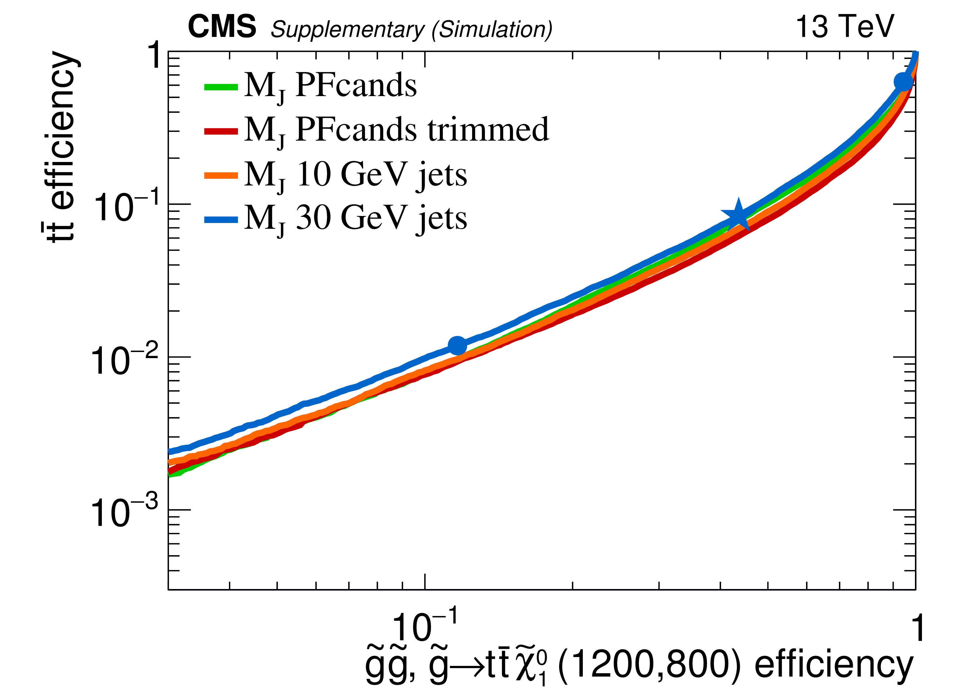
png pdf	Additional Figure 6-a: Comparison of performance (signal and background efficiencies) for ${M_J}$ made with all PF candidates (with and without trimming) and jets (with minimum ${p_{\mathrm {T}}}$ 10 and 30 GeV) after $ {H_{\mathrm {T}}} > $ 500 GeV and $ {E_{\mathrm {T}}^{\text {miss}}} > $ 200 GeV requirements. The performance is similar for all options, so we choose to cluster calibrated 30 GeV jets which have the smallest PU-dependence. The blue star corresponds to $ {M_J} > $ 400 GeV and the blue circles to $ {M_J} > [200,600]$ GeV.
png pdf	Additional Figure 6-b: Comparison of performance (signal and background efficiencies) for ${M_J}$ made with all PF candidates (with and without trimming) and jets (with minimum ${p_{\mathrm {T}}}$ 10 and 30 GeV) after $ {H_{\mathrm {T}}} > $ 500 GeV and $ {E_{\mathrm {T}}^{\text {miss}}} > $ 200 GeV requirements. The performance is similar for all options, so we choose to cluster calibrated 30 GeV jets which have the smallest PU-dependence. The blue star corresponds to $ {M_J} > $ 400 GeV and the blue circles to $ {M_J} > [200,600]$ GeV.
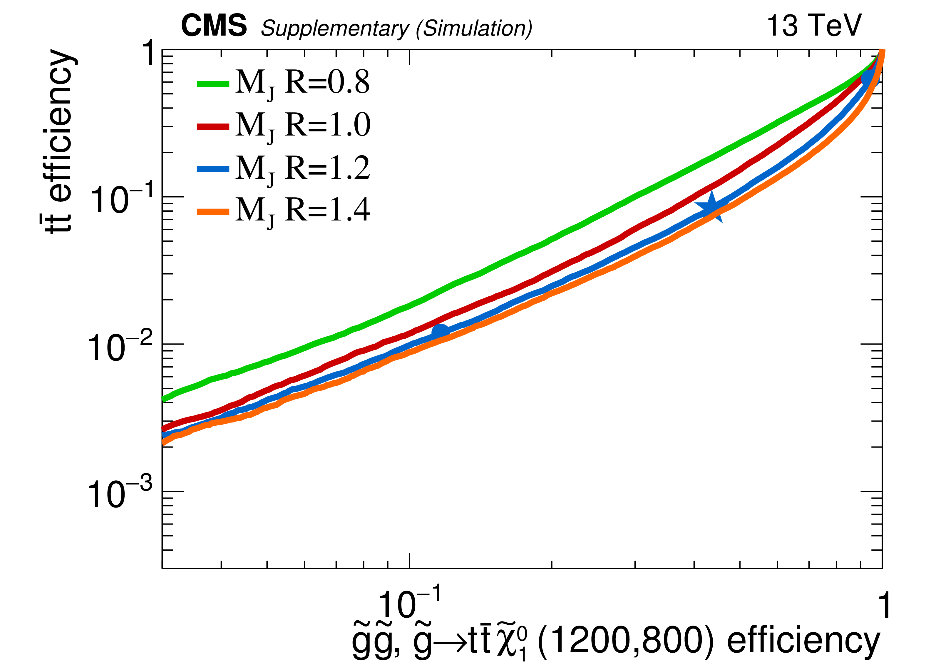
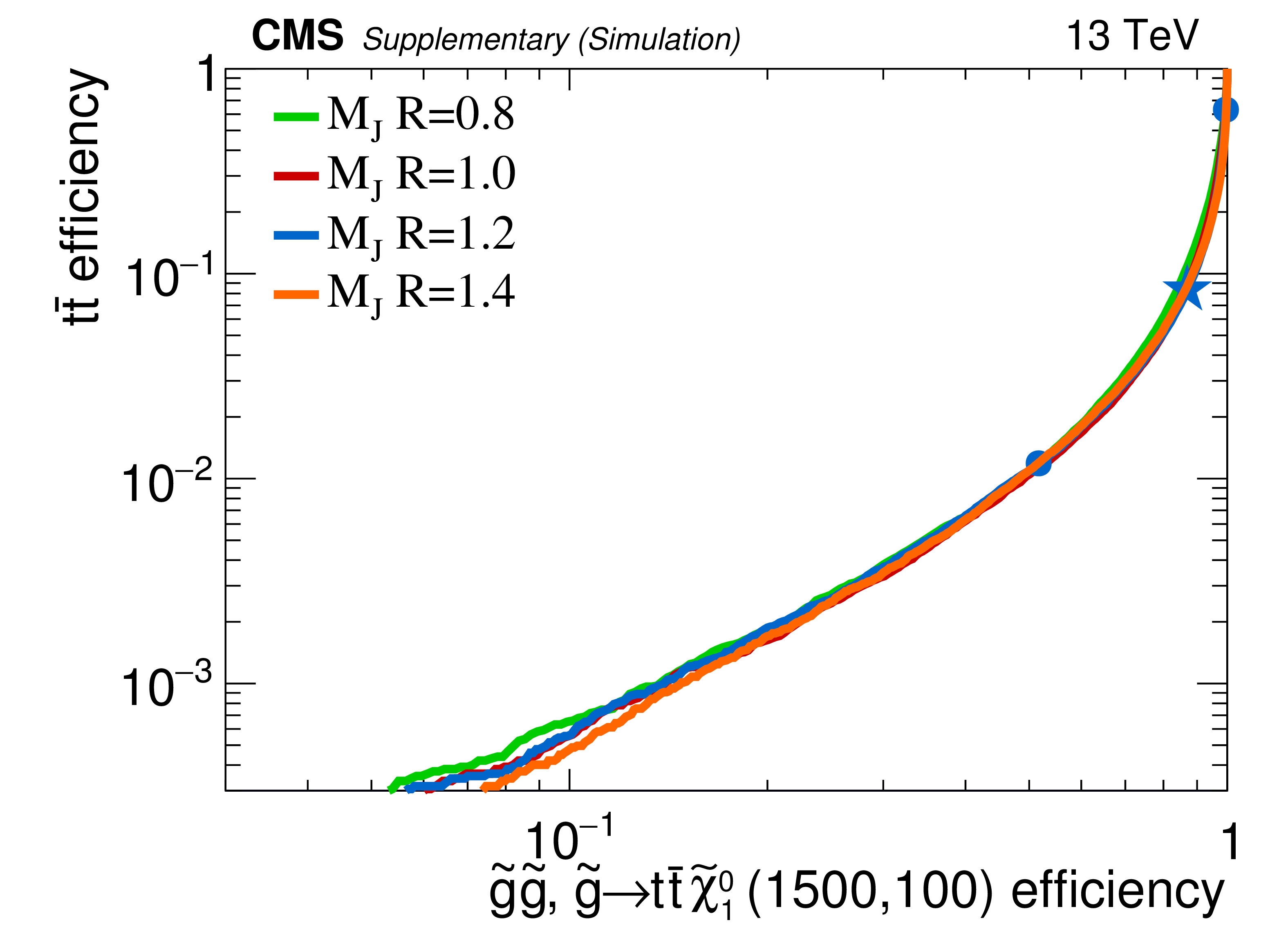
png pdf	Additional Figure 7-a: Comparison of performance (signal and background efficiencies) for ${M_J}$ made of large-$R$ jets for various values of $R$ after $ {H_{\mathrm {T}}} > $ 500 GeV and $ {E_{\mathrm {T}}^{\text {miss}}} > $ 200 GeV requirements. The blue star corresponds to $ {M_J} > $ 400 GeV and the blue circles to $ {M_J} > [200,600]$ GeV. For the compressed point, larger $R$ gives better performance, but it saturates at about $R= $ 1.2.
png pdf	Additional Figure 7-b: Comparison of performance (signal and background efficiencies) for ${M_J}$ made of large-$R$ jets for various values of $R$ after $ {H_{\mathrm {T}}} > $ 500 GeV and $ {E_{\mathrm {T}}^{\text {miss}}} > $ 200 GeV requirements. The blue star corresponds to $ {M_J} > $ 400 GeV and the blue circles to $ {M_J} > [200,600]$ GeV. For the compressed point, larger $R$ gives better performance, but it saturates at about $R= $ 1.2.
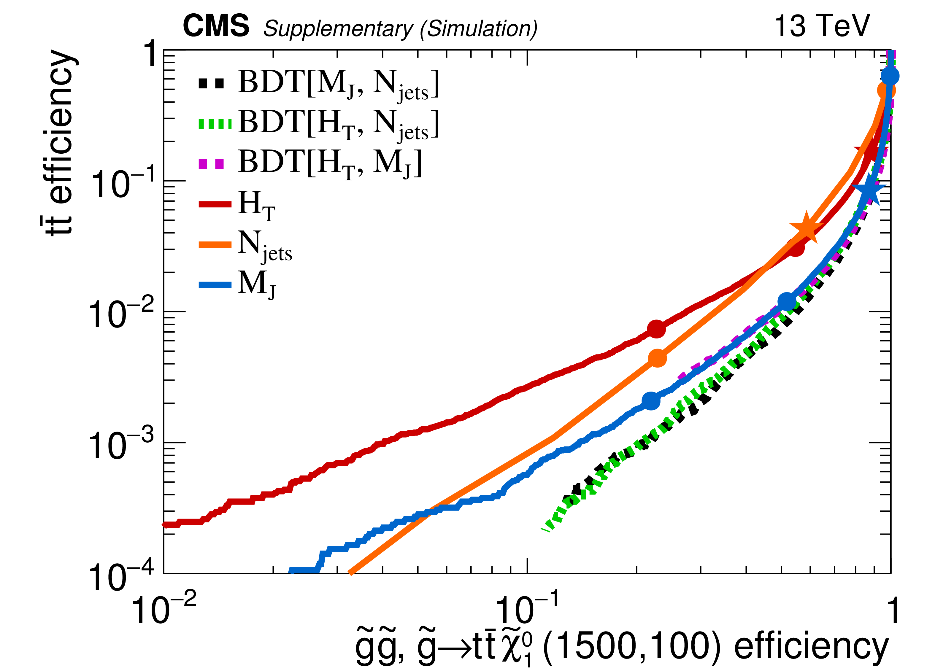
png pdf	Additional Figure 8-a: Comparison of performance (signal and background efficiencies) for ${H_{\mathrm {T}}}$, ${N_{\text {jets}}}$, ${M_J}$, and combination of these variables using boosted decision trees (BDTs) after $ {H_{\mathrm {T}}} > $ 500 GeV and $ {E_{\mathrm {T}}^{\text {miss}}} > $ 200 GeV requirements. The red star corresponds to $ {H_{\mathrm {T}}} > $ 1000 GeV and the red circles to $ {H_{\mathrm {T}}} > [1500,2000]$ GeV. The orange star corresponds to $ {N_{\text {jets}}} \geq 9$ and the orange circles to $ {N_{\text {jets}}} > [6,11]$. The blue star corresponds to $ {M_J} > $ 400 GeV and the blue circles to $ {M_J} > [200,600,800]$ GeV. The BDT curves do not extend all the way to the bottom-left corner due to limited MC statistics for the BDT training. The performance of ${M_J}$ alone is superior to that of ${H_{\mathrm {T}}}$, but the combination of ${M_J}$ and ${N_{\text {jets}}}$ has similar performance as the combination of ${H_{\mathrm {T}}}$ and ${N_{\text {jets}}}$.
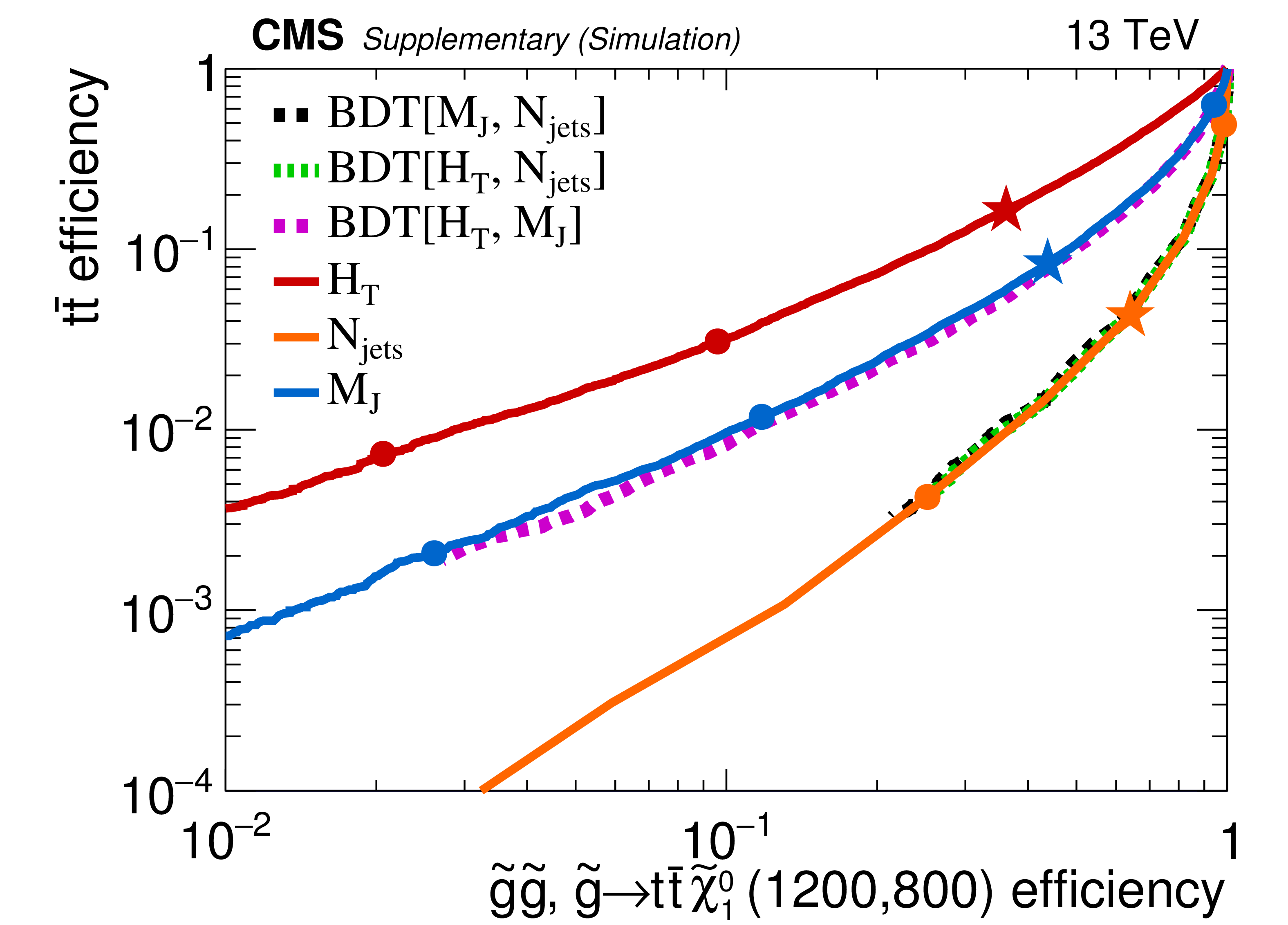
png pdf	Additional Figure 8-b: Comparison of performance (signal and background efficiencies) for ${H_{\mathrm {T}}}$, ${N_{\text {jets}}}$, ${M_J}$, and combination of these variables using boosted decision trees (BDTs) after $ {H_{\mathrm {T}}} > $ 500 GeV and $ {E_{\mathrm {T}}^{\text {miss}}} > $ 200 GeV requirements. The red star corresponds to $ {H_{\mathrm {T}}} > $ 1000 GeV and the red circles to $ {H_{\mathrm {T}}} > [1500,2000]$ GeV. The orange star corresponds to $ {N_{\text {jets}}} \geq 9$ and the orange circles to $ {N_{\text {jets}}} > [6,11]$. The blue star corresponds to $ {M_J} > $ 400 GeV and the blue circles to $ {M_J} > [200,600,800]$ GeV. The BDT curves do not extend all the way to the bottom-left corner due to limited MC statistics for the BDT training. The performance of ${M_J}$ alone is superior to that of ${H_{\mathrm {T}}}$, but the combination of ${M_J}$ and ${N_{\text {jets}}}$ has similar performance as the combination of ${H_{\mathrm {T}}}$ and ${N_{\text {jets}}}$.
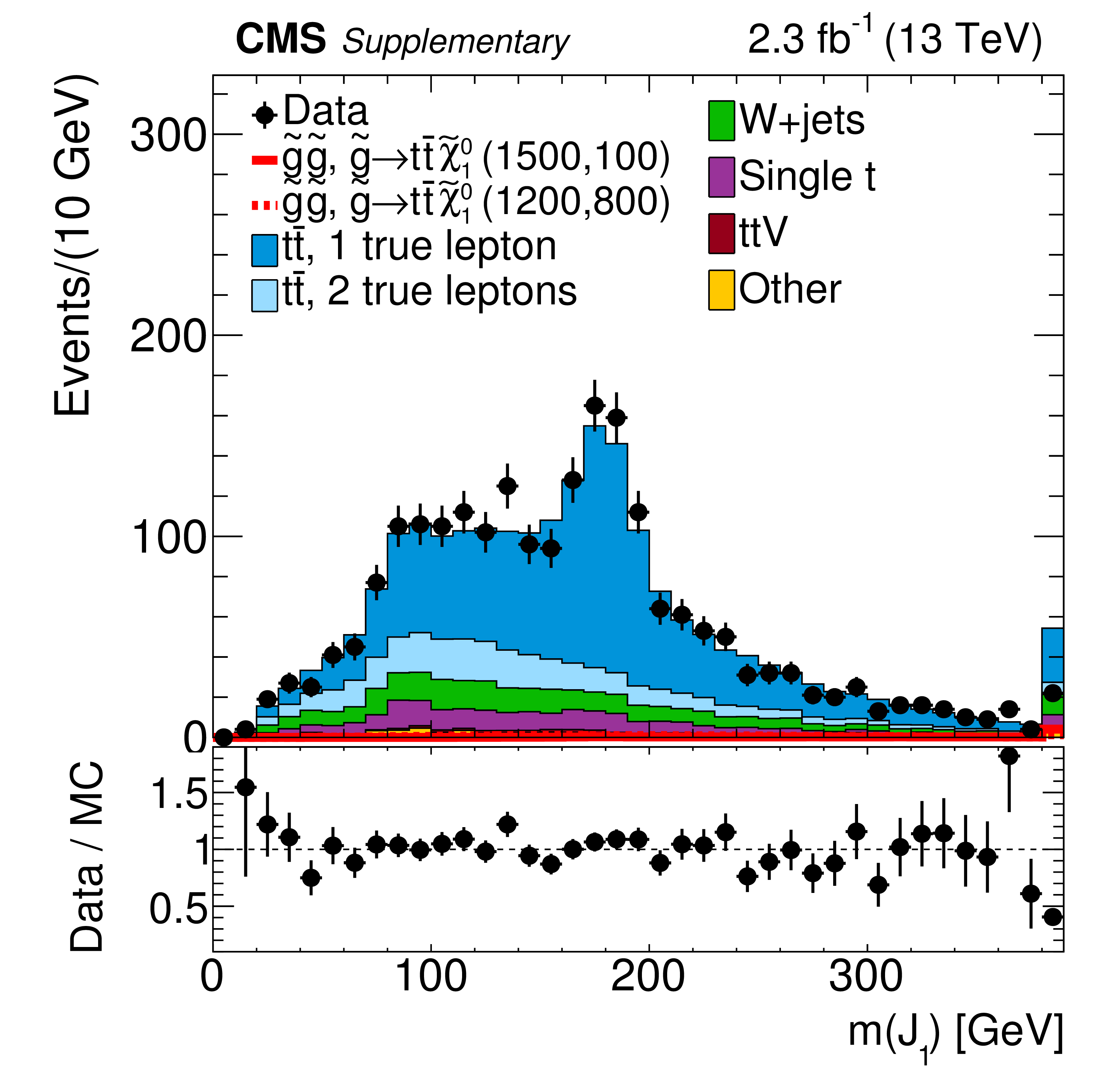
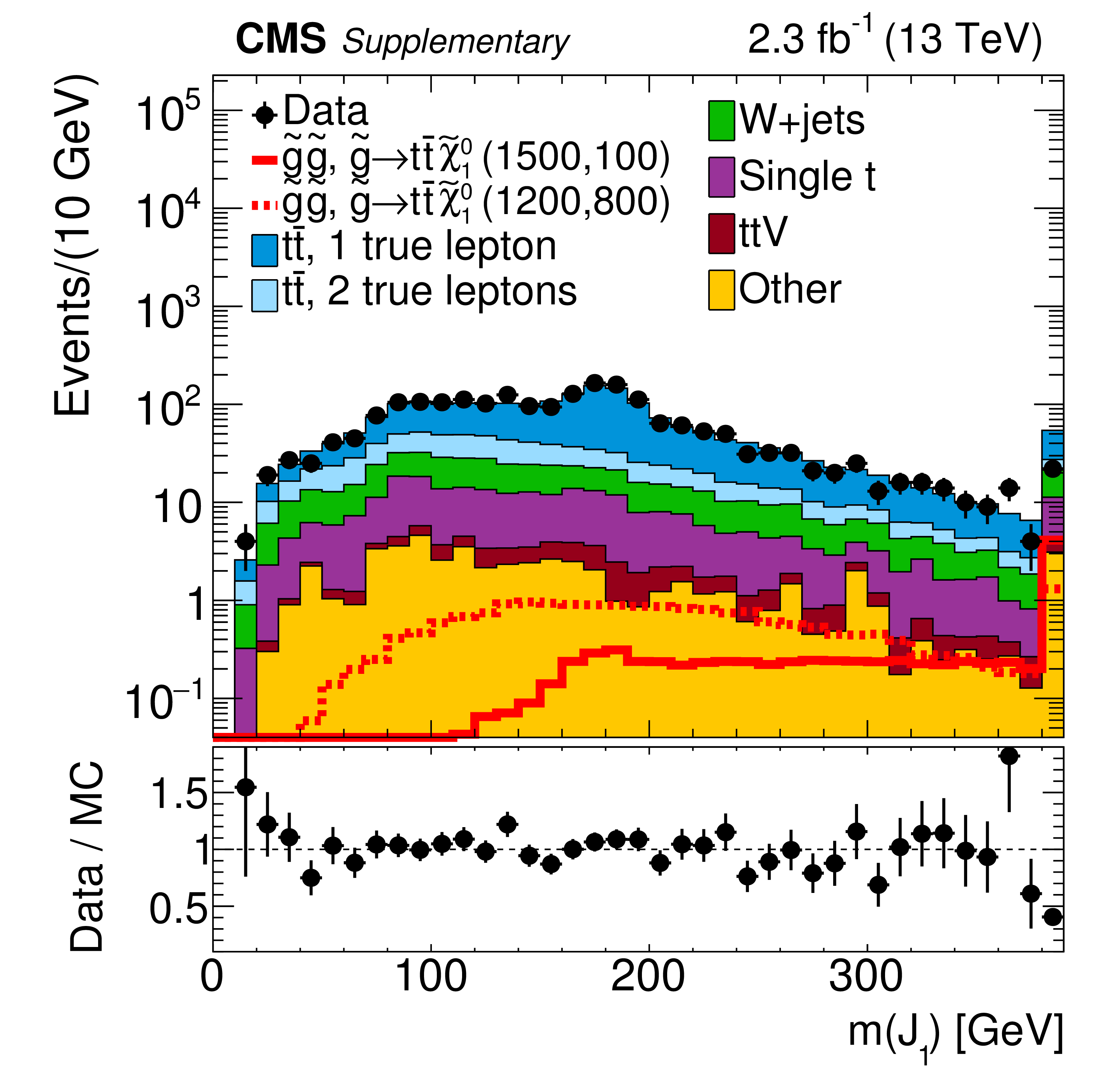
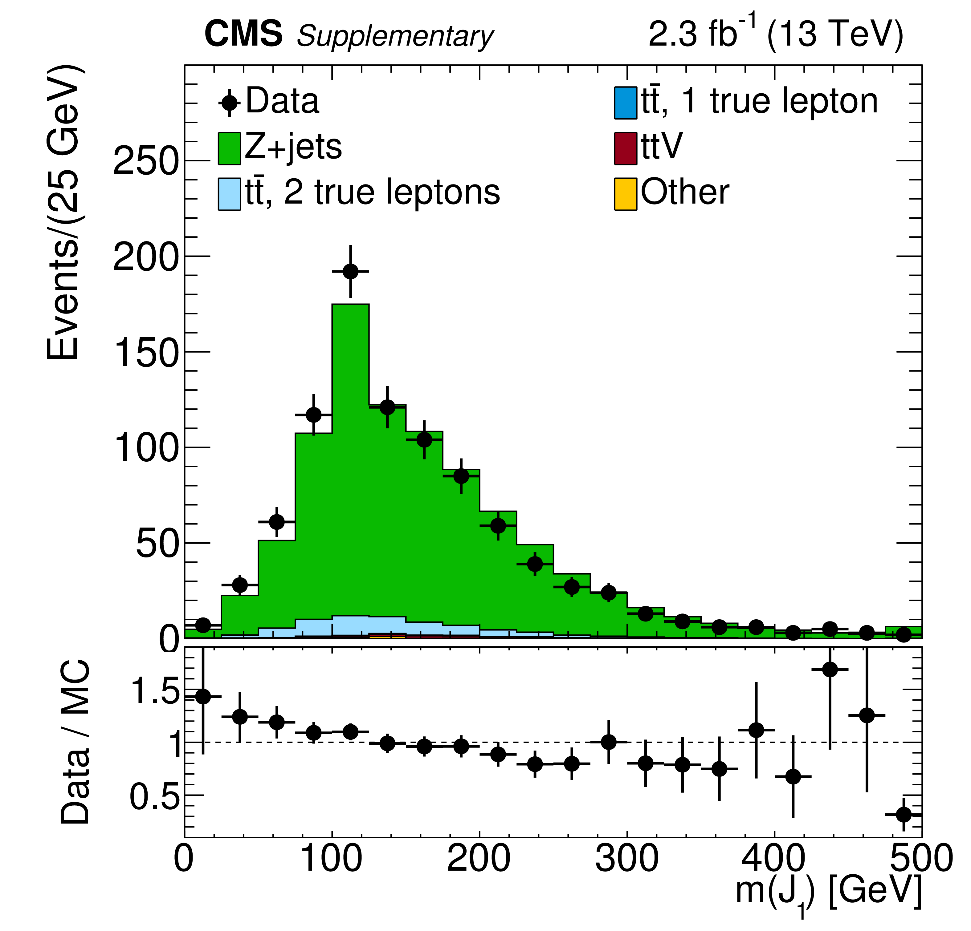
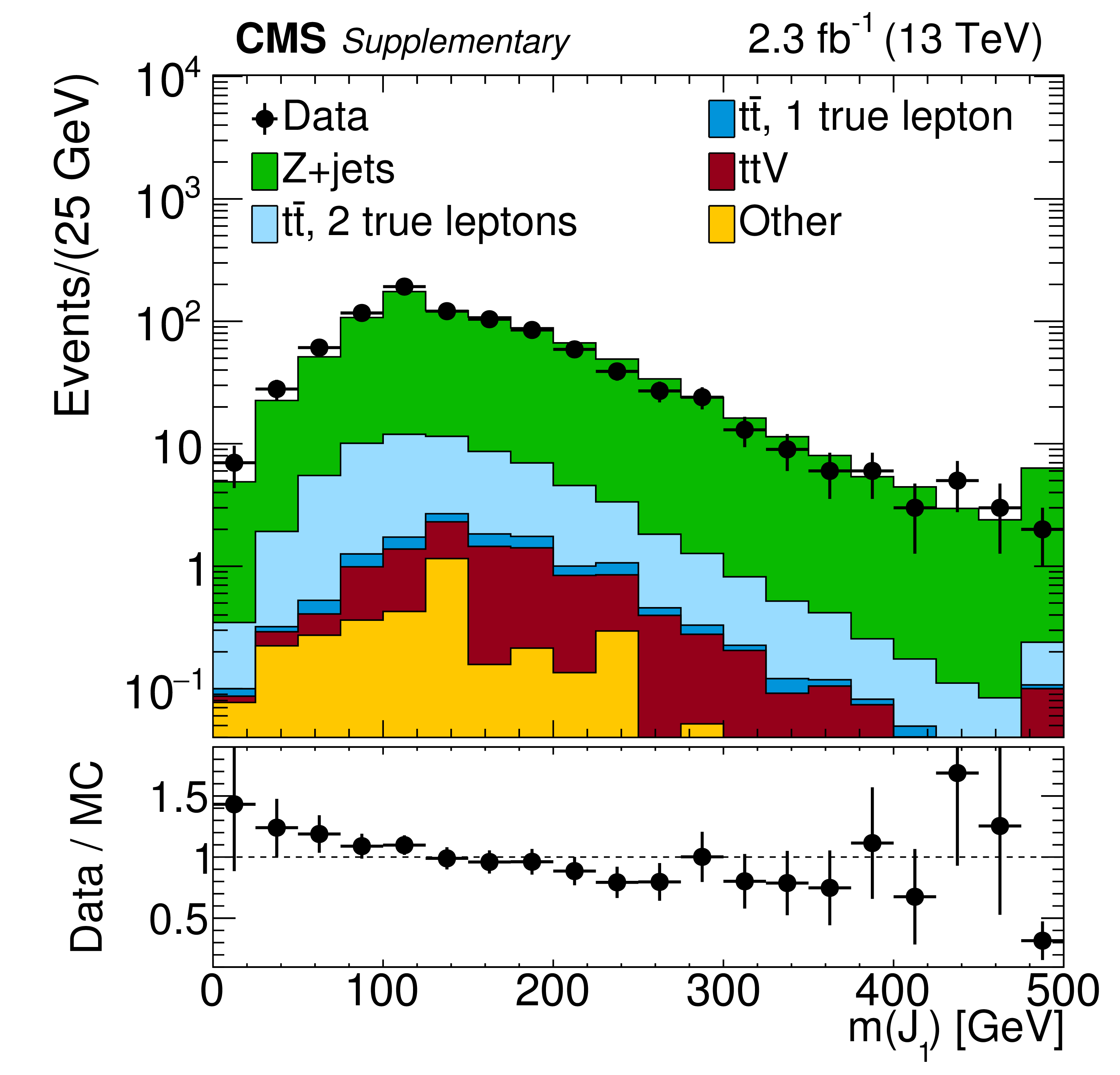
png pdf	Additional Figure 9-a: Distribution of $m(J_{1})$ in data and simulated event samples after the baseline selection (with the ${N_{\text {jets}}}$ requirement relaxed to $ {N_{\text {jets}}} \geq 4$) is applied in linear (a) and logarithmic (b) scales. The background contributions shown here are from simulation, and their total yield is normalized to the number of events observed in data.
png pdf	Additional Figure 9-b: Distribution of $m(J_{1})$ in data and simulated event samples after the baseline selection (with the ${N_{\text {jets}}}$ requirement relaxed to $ {N_{\text {jets}}} \geq 4$) is applied in linear (a) and logarithmic (b) scales. The background contributions shown here are from simulation, and their total yield is normalized to the number of events observed in data.
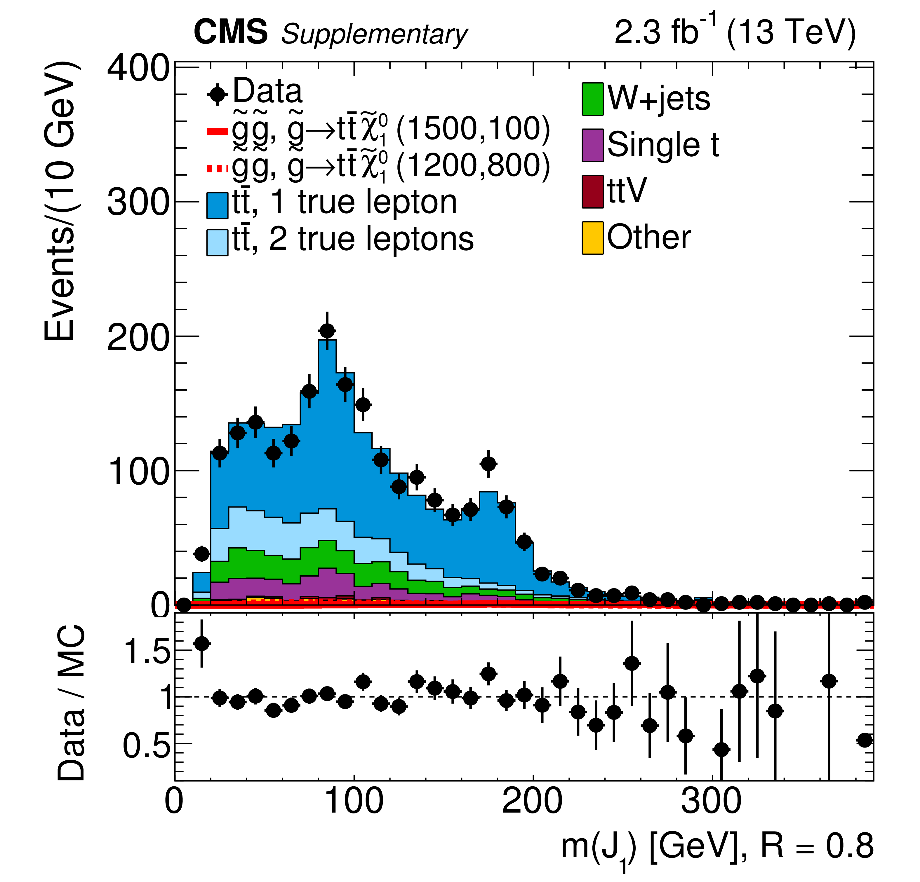
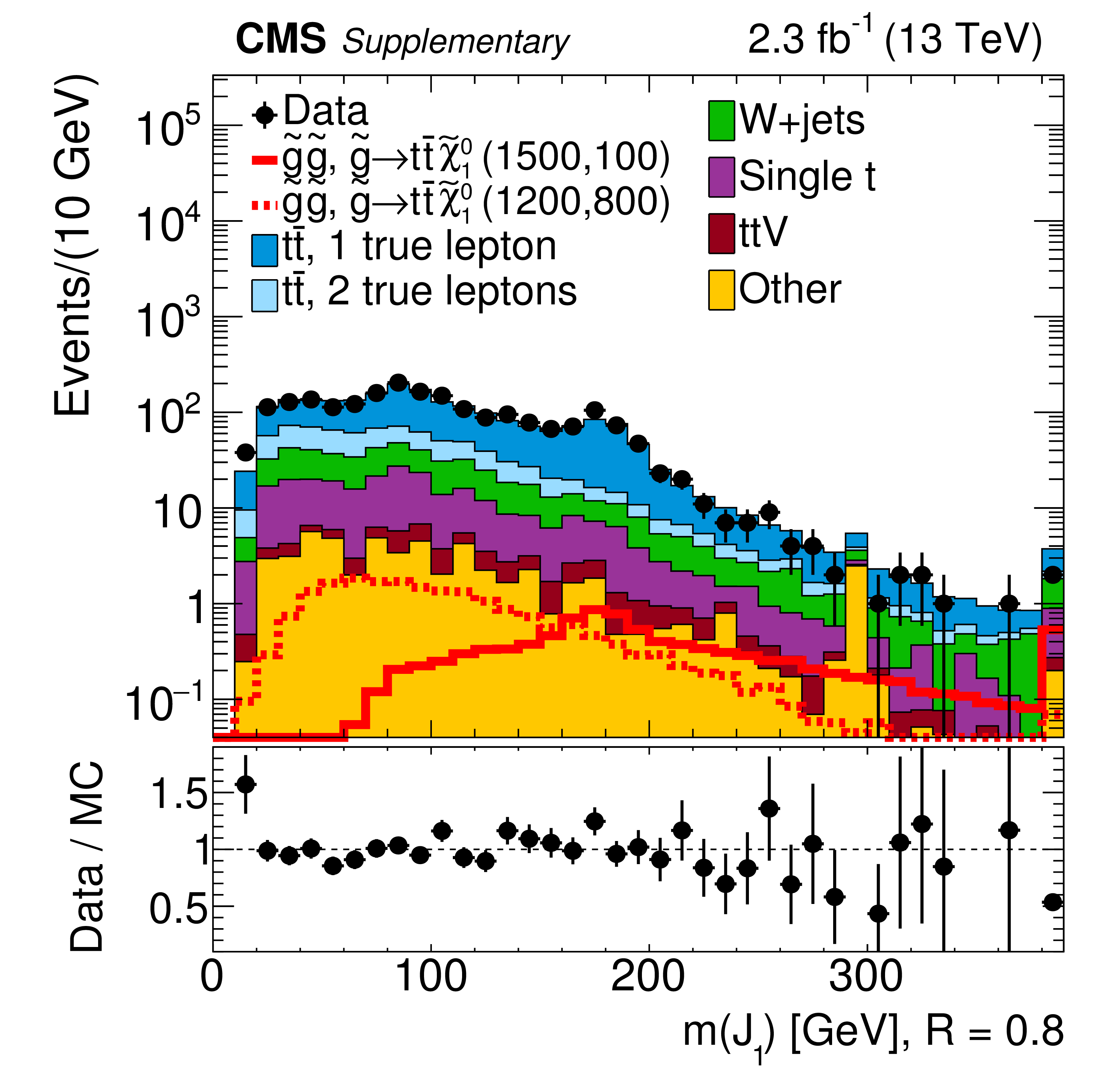
png pdf	Additional Figure 10-a: Distribution of $m(J_{1})$ clustered with radius R = 0.8, in data and simulated event samples after the baseline selection (with the ${N_{\text {jets}}}$ requirement relaxed to $ {N_{\text {jets}}} \geq 4$) is applied in linear (a) and logarithmic (b) scales. The background contributions shown here are from simulation, and their total yield is normalized to the number of events observed in data.
png pdf	Additional Figure 10-b: Distribution of $m(J_{1})$ clustered with radius R = 0.8, in data and simulated event samples after the baseline selection (with the ${N_{\text {jets}}}$ requirement relaxed to $ {N_{\text {jets}}} \geq 4$) is applied in linear (a) and logarithmic (b) scales. The background contributions shown here are from simulation, and their total yield is normalized to the number of events observed in data.
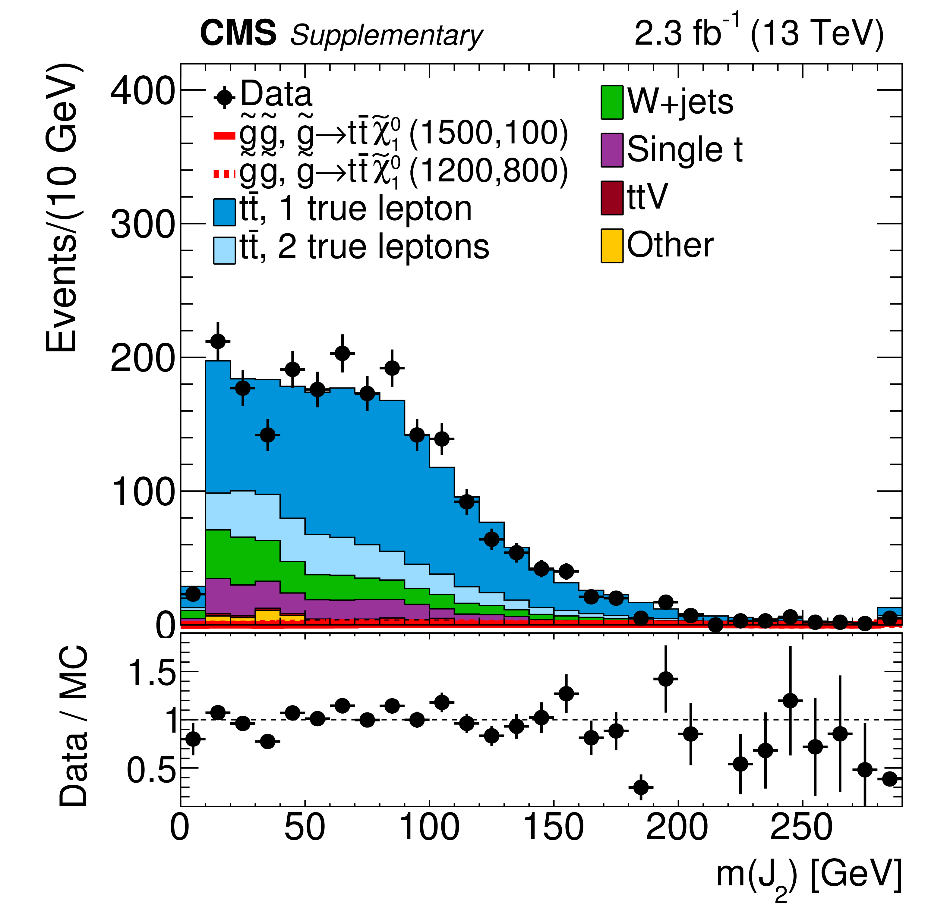
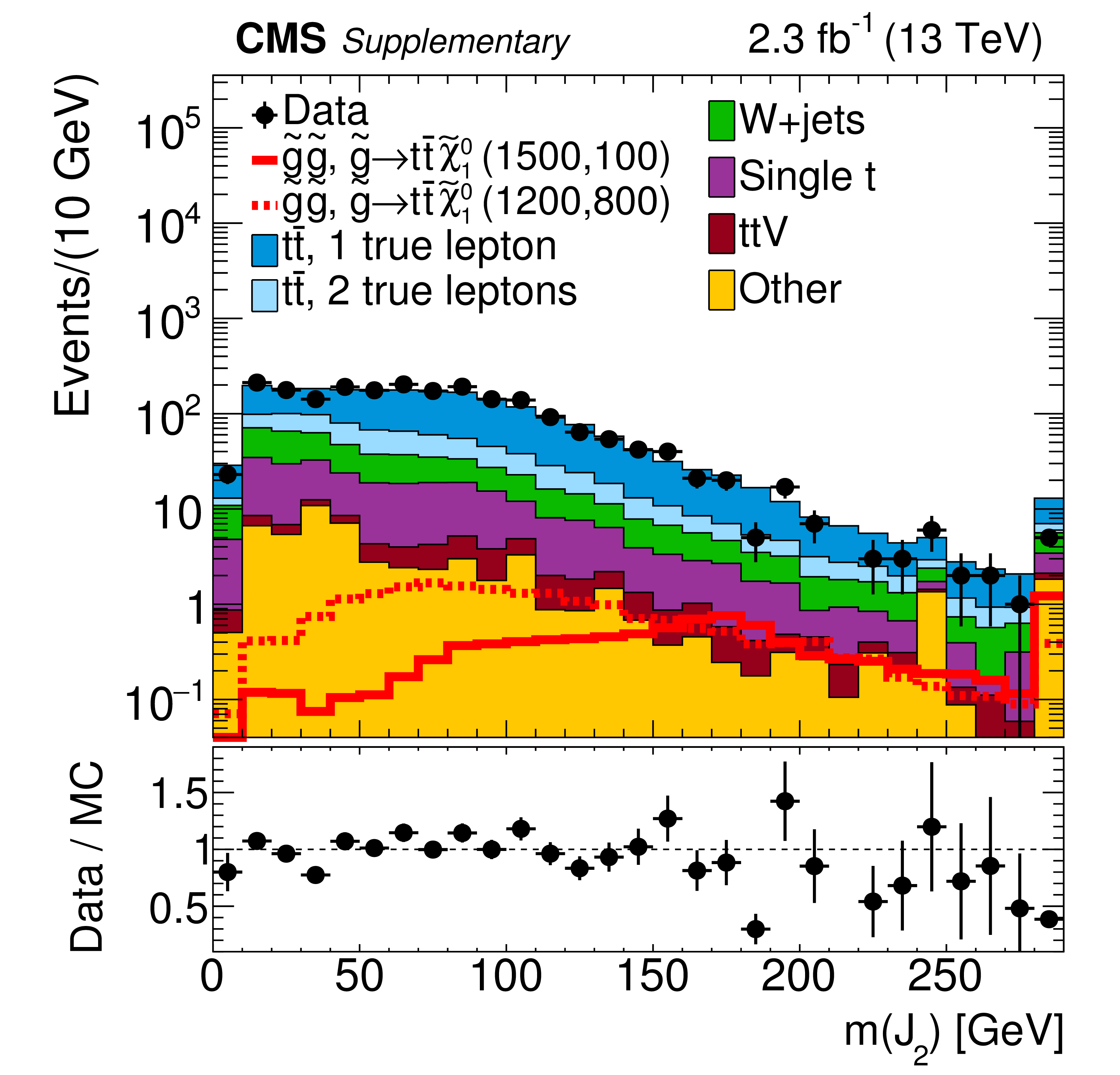
png pdf	Additional Figure 11-a: Distribution of $m(J_{2})$ in data and simulated event samples after the baseline selection (with the ${N_{\text {jets}}}$ requirement relaxed to $ {N_{\text {jets}}} \geq 4$) is applied in linear (a) and logarithmic (b) scales. The background contributions shown here are from simulation, and their total yield is normalized to the number of events observed in data.
png pdf	Additional Figure 11-b: Distribution of $m(J_{2})$ in data and simulated event samples after the baseline selection (with the ${N_{\text {jets}}}$ requirement relaxed to $ {N_{\text {jets}}} \geq 4$) is applied in linear (a) and logarithmic (b) scales. The background contributions shown here are from simulation, and their total yield is normalized to the number of events observed in data.
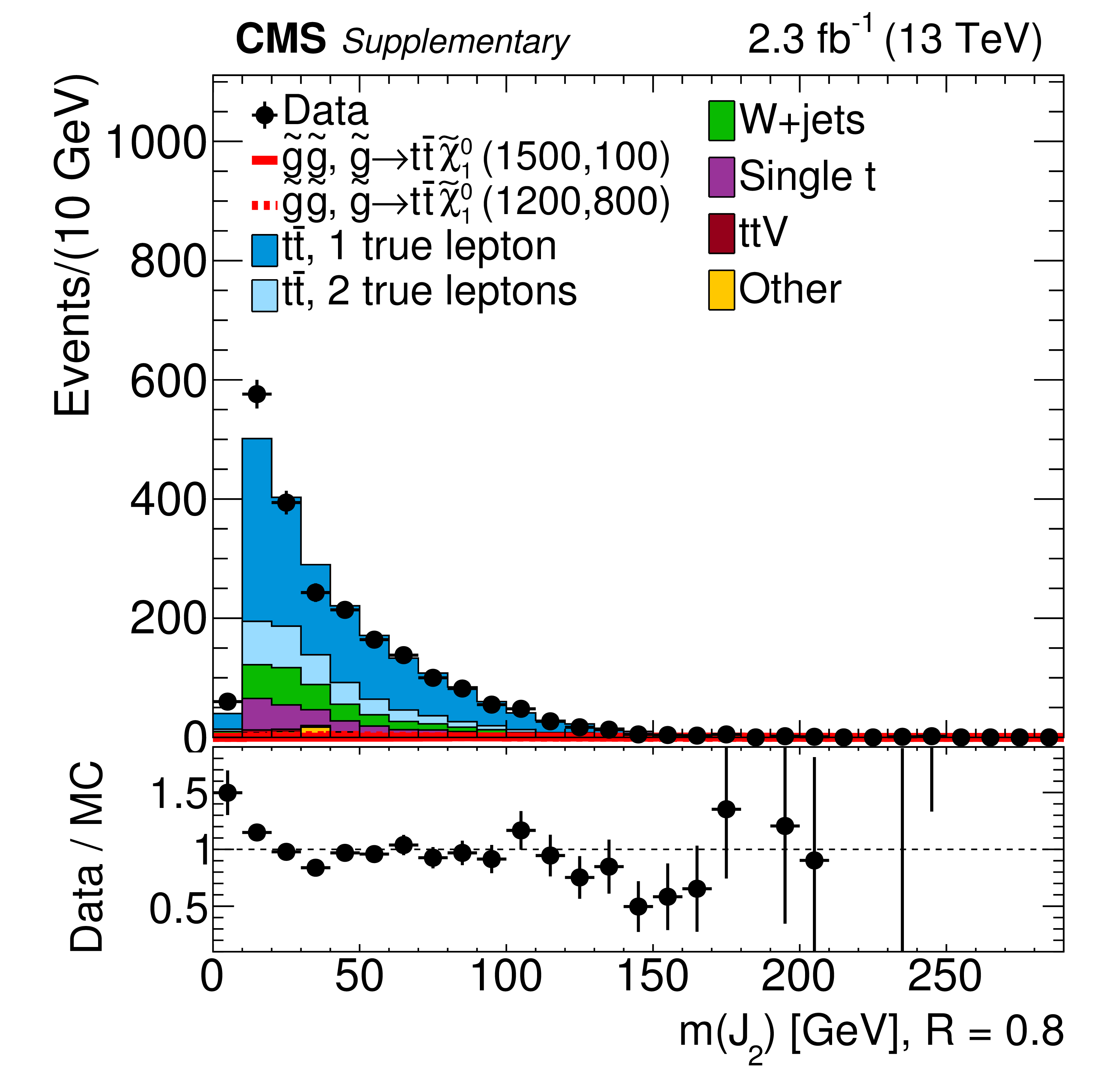
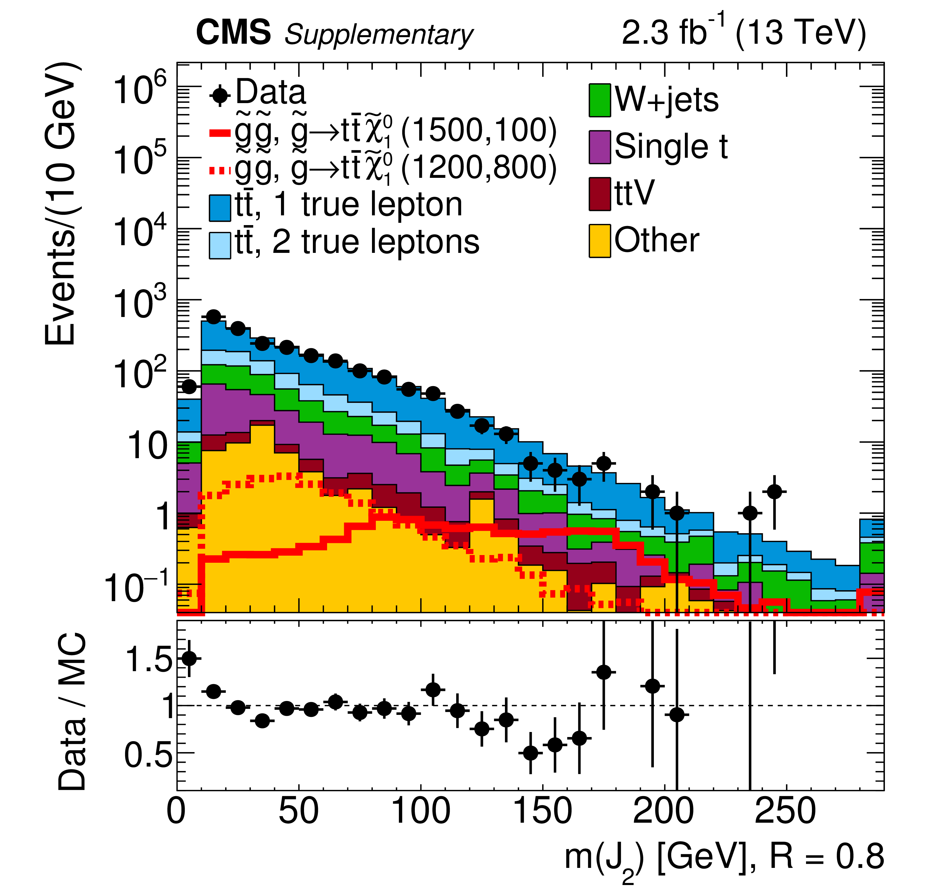
png pdf	Additional Figure 12-a: Distribution of $m(J_{2})$ clustered with radius R = 0.8, in data and simulated event samples after the baseline selection (with the ${N_{\text {jets}}}$ requirement relaxed to $ {N_{\text {jets}}} \geq 4$) is applied in linear (a) and logarithmic (b) scales. The background contributions shown here are from simulation, and their total yield is normalized to the number of events observed in data.
png pdf	Additional Figure 12-b: Distribution of $m(J_{2})$ clustered with radius R = 0.8, in data and simulated event samples after the baseline selection (with the ${N_{\text {jets}}}$ requirement relaxed to $ {N_{\text {jets}}} \geq 4$) is applied in linear (a) and logarithmic (b) scales. The background contributions shown here are from simulation, and their total yield is normalized to the number of events observed in data.
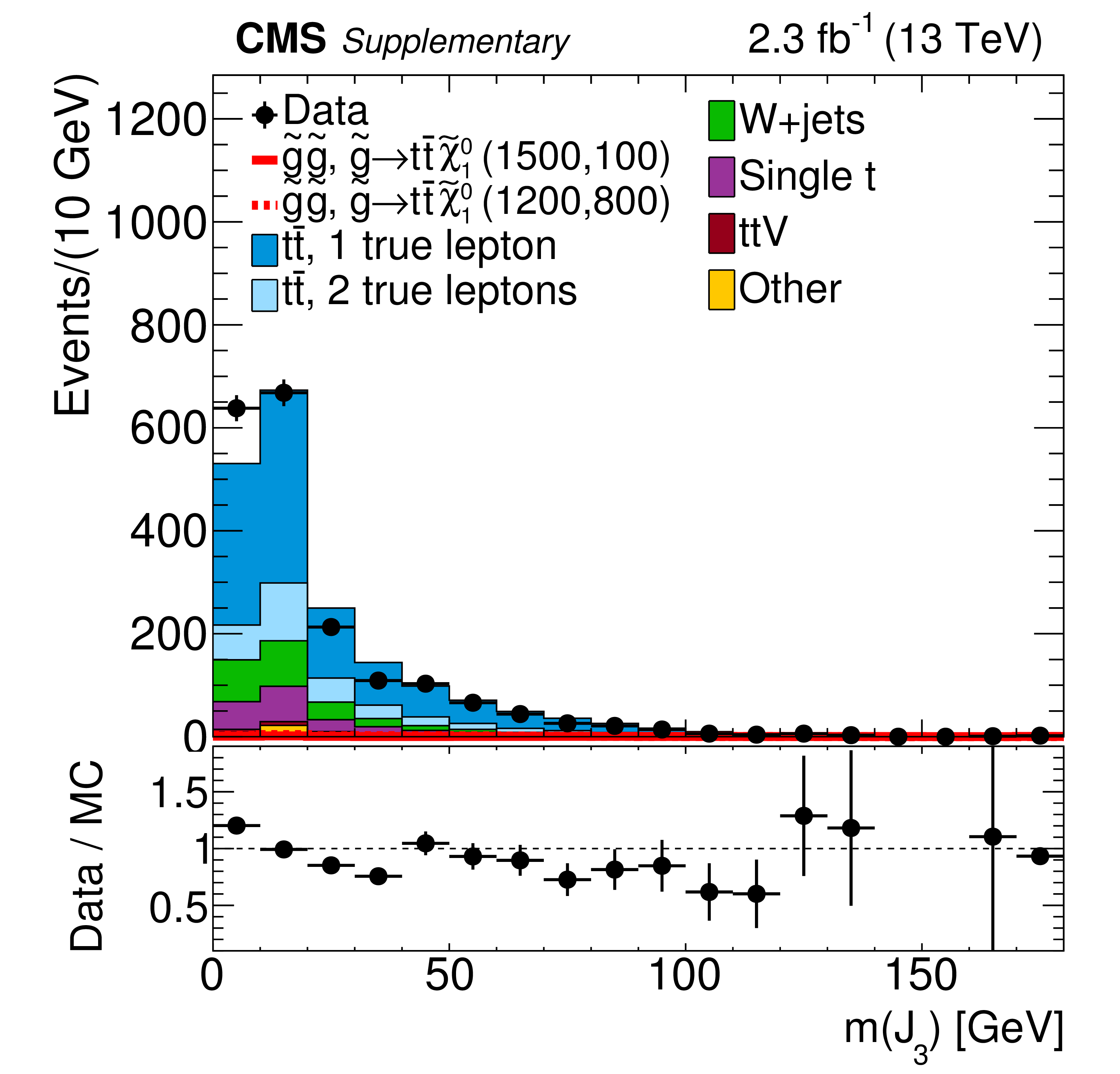
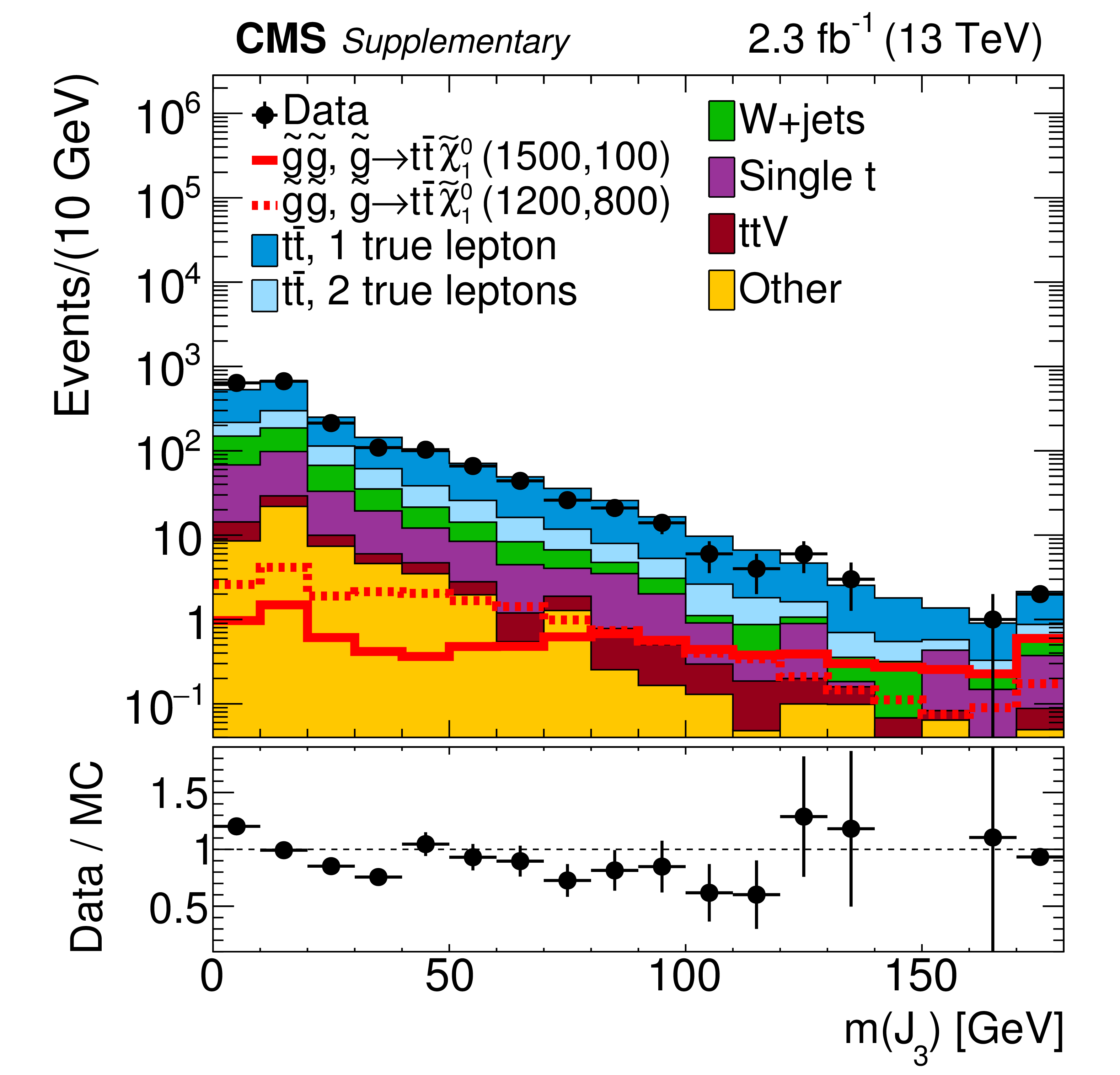
png pdf	Additional Figure 13-a: Distribution of $m(J_{3})$ in data and simulated event samples after the baseline selection (with the ${N_{\text {jets}}}$ requirement relaxed to $ {N_{\text {jets}}} \geq 4$) is applied in linear (a) and logarithmic (b) scales. The background contributions shown here are from simulation, and their total yield is normalized to the number of events observed in data.
png pdf	Additional Figure 13-b: Distribution of $m(J_{3})$ in data and simulated event samples after the baseline selection (with the ${N_{\text {jets}}}$ requirement relaxed to $ {N_{\text {jets}}} \geq 4$) is applied in linear (a) and logarithmic (b) scales. The background contributions shown here are from simulation, and their total yield is normalized to the number of events observed in data.
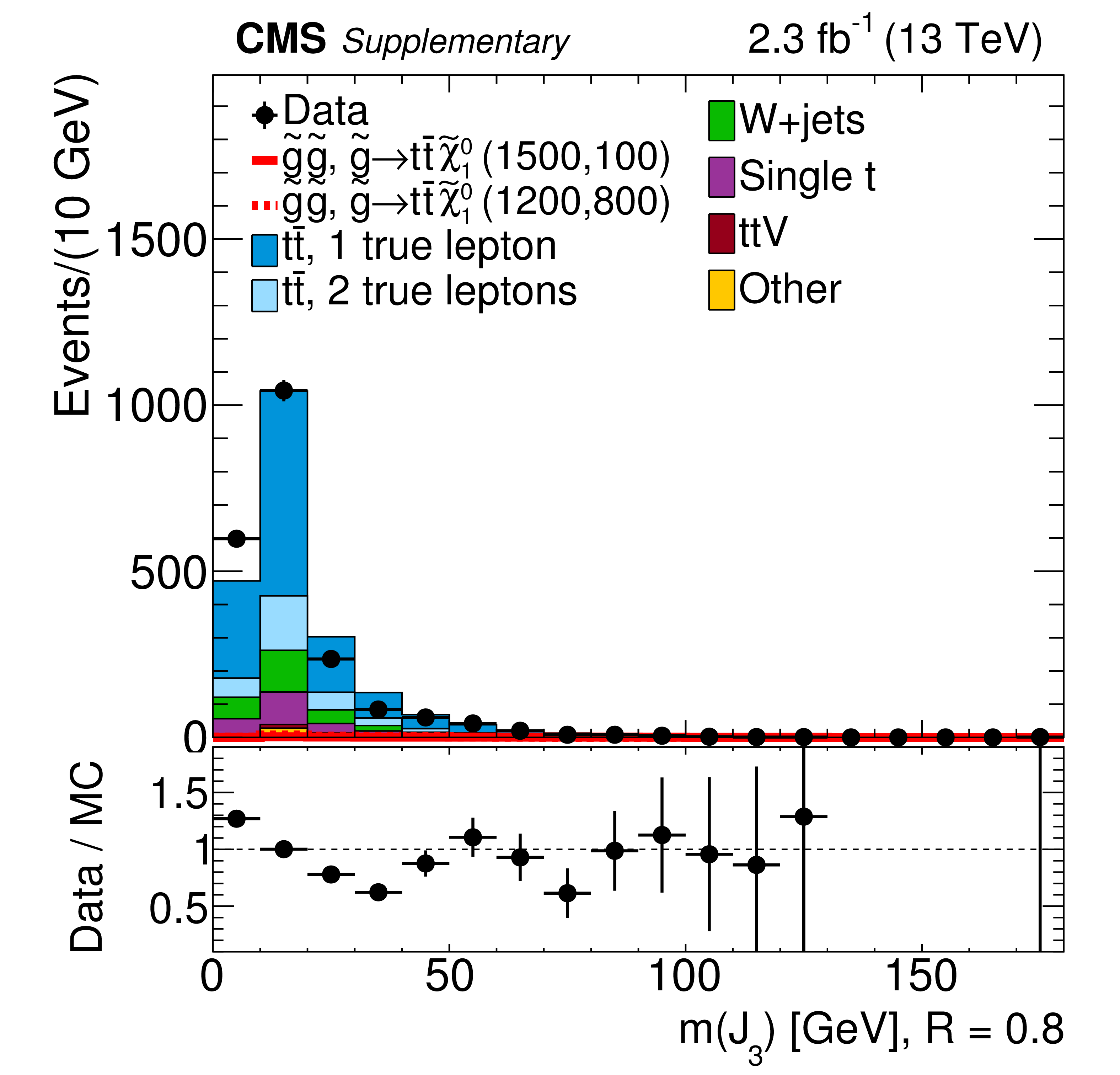
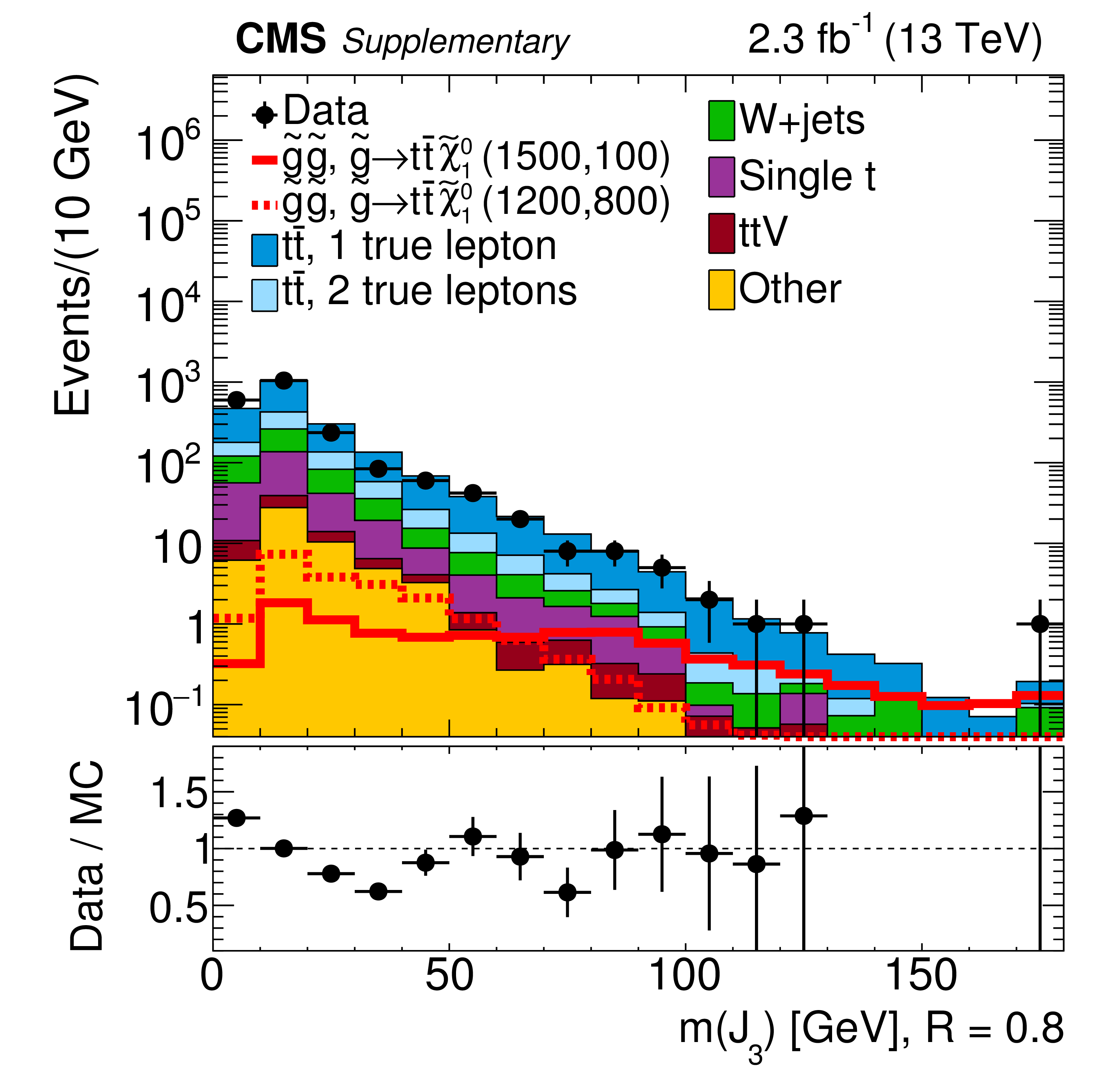
png pdf	Additional Figure 14-a: Distribution of $m(J_{3})$ clustered with radius $R =$ 0.8, in data and simulated event samples after the baseline selection (with the ${N_{\text {jets}}}$ requirement relaxed to $ {N_{\text {jets}}} \geq 4$) is applied in linear (a) and logarithmic (b) scales. The background contributions shown here are from simulation, and their total yield is normalized to the number of events observed in data.
png pdf	Additional Figure 14-b: Distribution of $m(J_{3})$ clustered with radius $R =$ 0.8, in data and simulated event samples after the baseline selection (with the ${N_{\text {jets}}}$ requirement relaxed to $ {N_{\text {jets}}} \geq 4$) is applied in linear (a) and logarithmic (b) scales. The background contributions shown here are from simulation, and their total yield is normalized to the number of events observed in data.
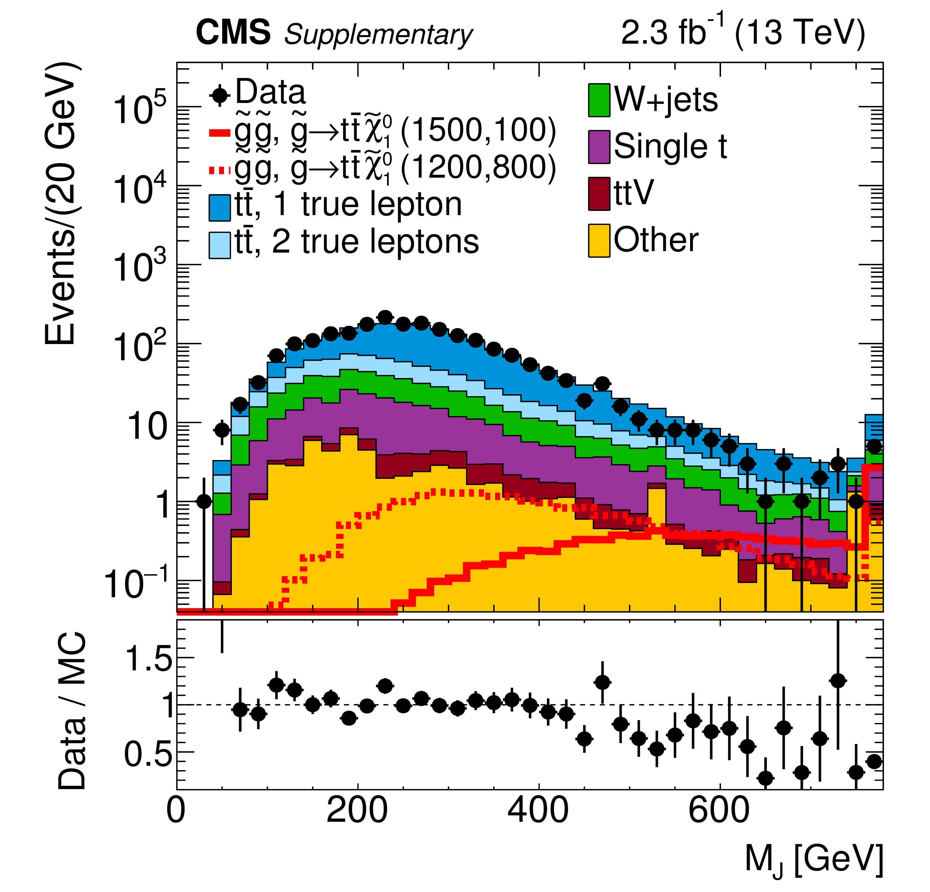
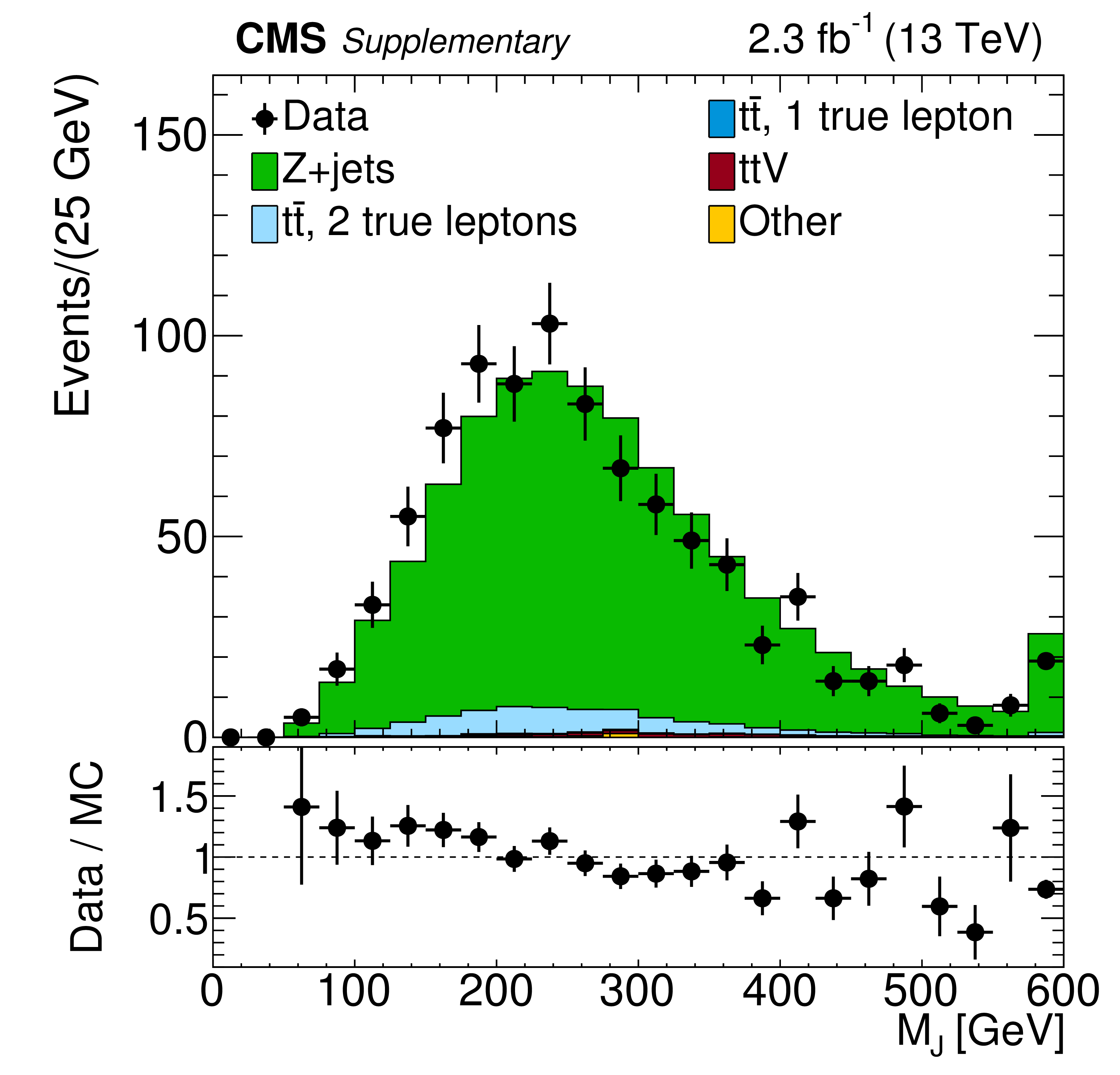
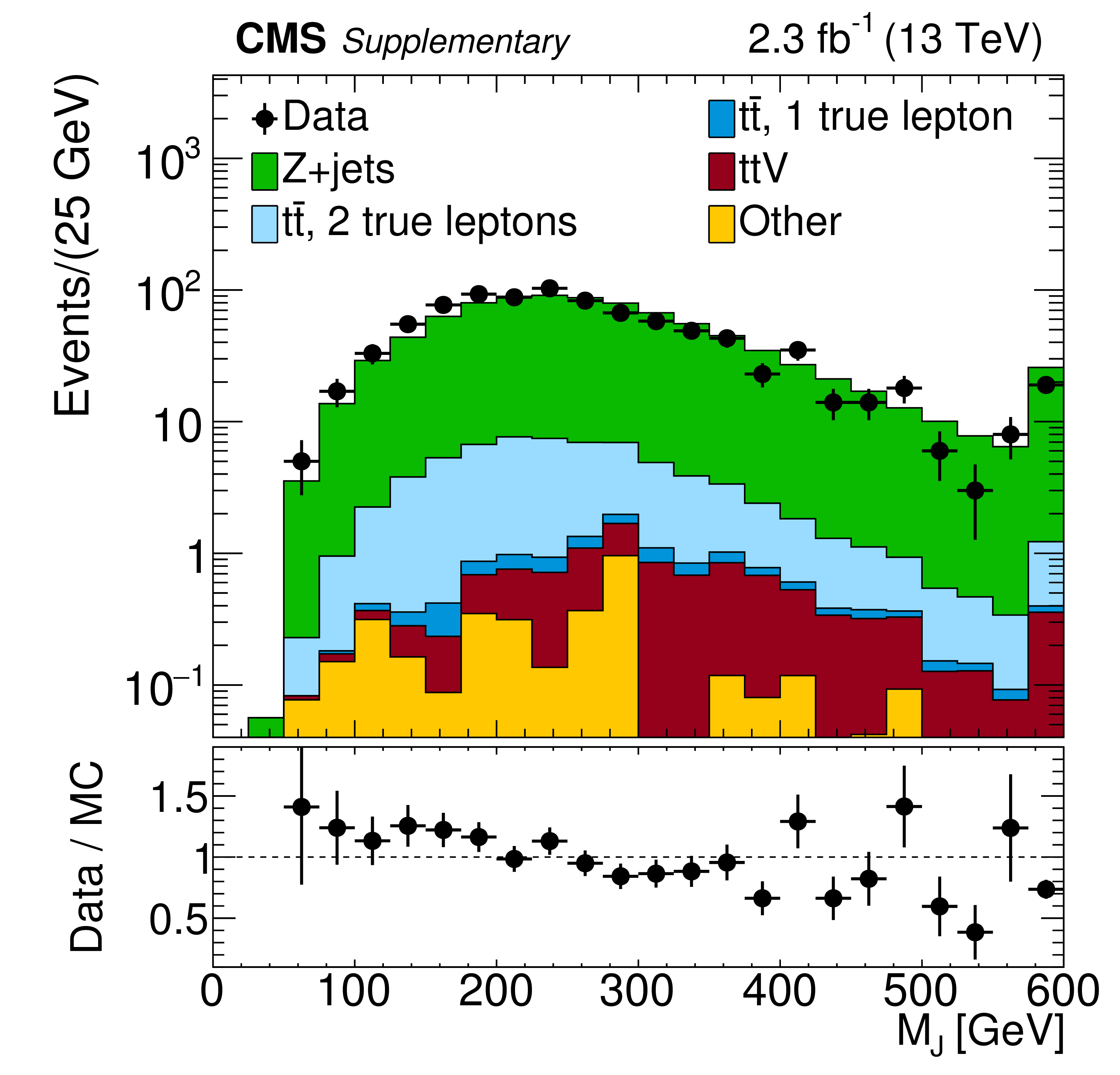
png pdf	Additional Figure 15-a: Distribution of ${M_J}$ in data and simulated event samples after the baseline selection (with the ${N_{\text {jets}}}$ requirement relaxed to $ {N_{\text {jets}}} \geq 4$) is applied in linear (a) and logarithmic (b) scales. The background contributions shown here are from simulation, and their total yield is normalized to the number of events observed in data.
png pdf	Additional Figure 15-b: Distribution of ${M_J}$ in data and simulated event samples after the baseline selection (with the ${N_{\text {jets}}}$ requirement relaxed to $ {N_{\text {jets}}} \geq 4$) is applied in linear (a) and logarithmic (b) scales. The background contributions shown here are from simulation, and their total yield is normalized to the number of events observed in data.
png pdf	Additional Figure 16-a: Distribution of ${M_J}$ in data and simulated event samples after a selection targetting dilepton Z+jets events is applied in linear (a) and logarithmic (b) scales. The selection requires a pair of opposite sign, same flavor leptons with invariant mass between 80 and 100 GeV, as well as $ {H_{\mathrm {T}}} > $ 500 and $ {N_{\text {jets}}} \geq 4$. The background contributions shown here are from simulation, and their total yield is normalized to the number of events observed in data.
png pdf	Additional Figure 16-b: Distribution of ${M_J}$ in data and simulated event samples after a selection targetting dilepton Z+jets events is applied in linear (a) and logarithmic (b) scales. The selection requires a pair of opposite sign, same flavor leptons with invariant mass between 80 and 100 GeV, as well as $ {H_{\mathrm {T}}} > $ 500 and $ {N_{\text {jets}}} \geq 4$. The background contributions shown here are from simulation, and their total yield is normalized to the number of events observed in data.
png pdf	Additional Figure 17-a: Distribution of $m(J_{1})$ in data and simulated event samples after a selection targetting dilepton Z+jets events is applied in linear (a) and logarithmic (b) scales. The selection requires a pair of opposite sign, same flavor leptons with invariant mass between 80 and 100 GeV, as well as $ {H_{\mathrm {T}}} > $ 500 and $ {N_{\text {jets}}} \geq 4$. The background contributions shown here are from simulation, and their total yield is normalized to the number of events observed in data. The peak at around 100 GeV corresponds to the case of the two jets associated with the leptons coming from the Z boson being clustered in the same large-$R$ jet.
png pdf	Additional Figure 17-b: Distribution of $m(J_{1})$ in data and simulated event samples after a selection targetting dilepton Z+jets events is applied in linear (a) and logarithmic (b) scales. The selection requires a pair of opposite sign, same flavor leptons with invariant mass between 80 and 100 GeV, as well as $ {H_{\mathrm {T}}} > $ 500 and $ {N_{\text {jets}}} \geq 4$. The background contributions shown here are from simulation, and their total yield is normalized to the number of events observed in data. The peak at around 100 GeV corresponds to the case of the two jets associated with the leptons coming from the Z boson being clustered in the same large-$R$ jet.
png pdf	Additional Figure 18-a: Distribution of ${m_{\mathrm {T}}}$ in signal (red) and simulated ${\mathrm{ t } \mathrm{ \bar{t} } }$ samples (blue) after the baseline selection is applied in linear (a) and logarithmic (b) scales.
png pdf	Additional Figure 18-b: Distribution of ${m_{\mathrm {T}}}$ in signal (red) and simulated ${\mathrm{ t } \mathrm{ \bar{t} } }$ samples (blue) after the baseline selection is applied in linear (a) and logarithmic (b) scales.
png pdf	Additional Figure 19-a: Distribution of ${M_J}$ in signal (red) and simulated ${\mathrm{ t } \mathrm{ \bar{t} } }$ samples (blue) after the baseline selection is applied in linear (a) and logarithmic (b) scales.
png pdf	Additional Figure 19-b: Distribution of ${M_J}$ in signal (red) and simulated ${\mathrm{ t } \mathrm{ \bar{t} } }$ samples (blue) after the baseline selection is applied in linear (a) and logarithmic (b) scales.
png pdf	Additional Figure 20-a: Distribution of ${N_{\text {jets}}}$ in signal (red) and simulated ${\mathrm{ t } \mathrm{ \bar{t} } }$ samples (blue) after the baseline selection is applied in linear (a) and logarithmic (b) scales.
png pdf	Additional Figure 20-b: Distribution of ${N_{\text {jets}}}$ in signal (red) and simulated ${\mathrm{ t } \mathrm{ \bar{t} } }$ samples (blue) after the baseline selection is applied in linear (a) and logarithmic (b) scales.
png pdf	Additional Figure 21-a: Distribution of $ {N_{\text {b}}}$ in signal (red) and simulated ${\mathrm{ t } \mathrm{ \bar{t} } }$ samples (blue) after the baseline selection is applied in linear (a) and logarithmic (b) scales.
png pdf	Additional Figure 21-b: Distribution of $ {N_{\text {b}}}$ in signal (red) and simulated ${\mathrm{ t } \mathrm{ \bar{t} } }$ samples (blue) after the baseline selection is applied in linear (a) and logarithmic (b) scales.
png pdf	Additional Figure 22-a: Distribution of ${E_{\mathrm {T}}^{\text {miss}}}$ in signal (red) and simulated ${\mathrm{ t } \mathrm{ \bar{t} } }$ samples (blue) after the baseline selection is applied in linear (a) and logarithmic (b) scales.
png pdf	Additional Figure 22-b: Distribution of ${E_{\mathrm {T}}^{\text {miss}}}$ in signal (red) and simulated ${\mathrm{ t } \mathrm{ \bar{t} } }$ samples (blue) after the baseline selection is applied in linear (a) and logarithmic (b) scales.
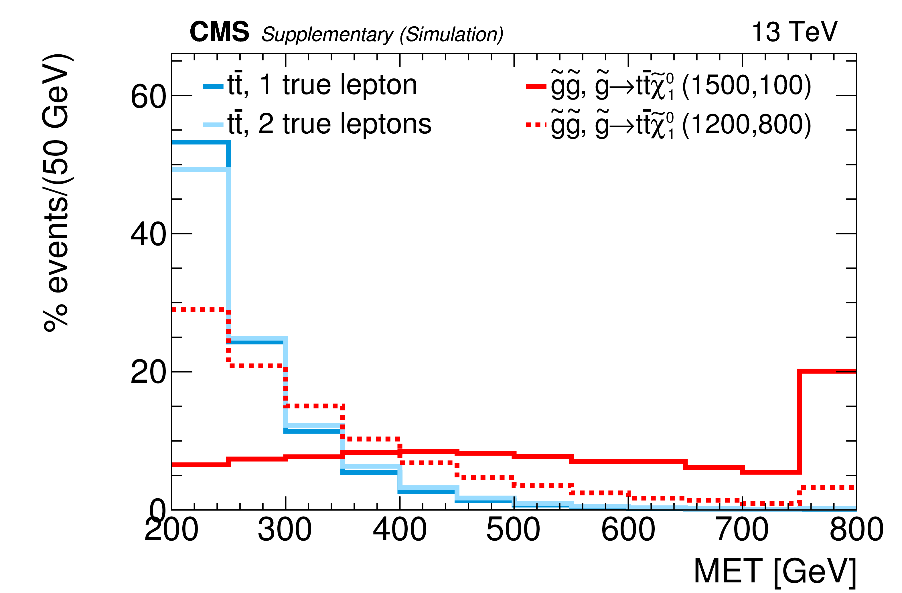
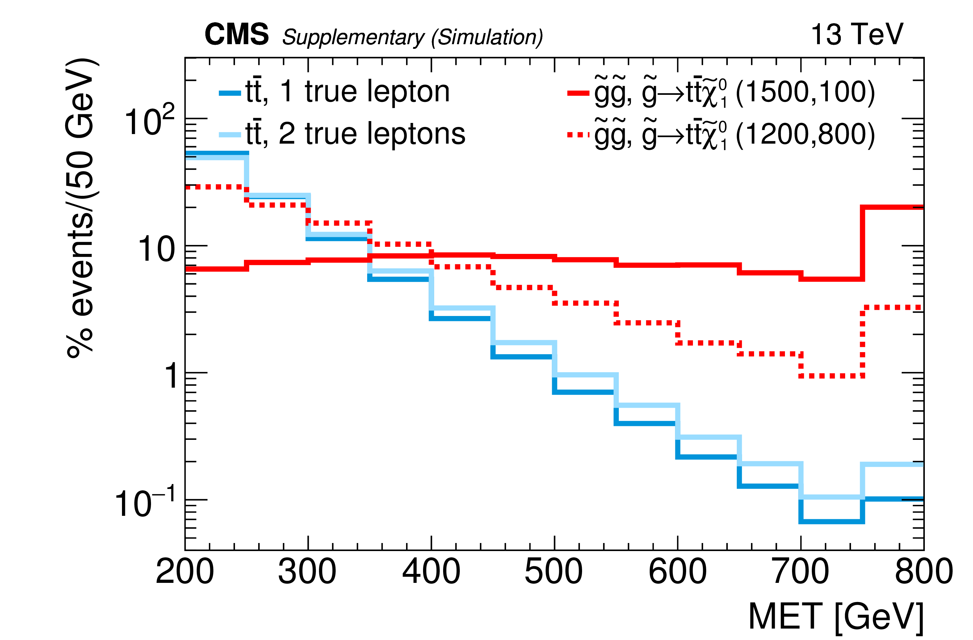
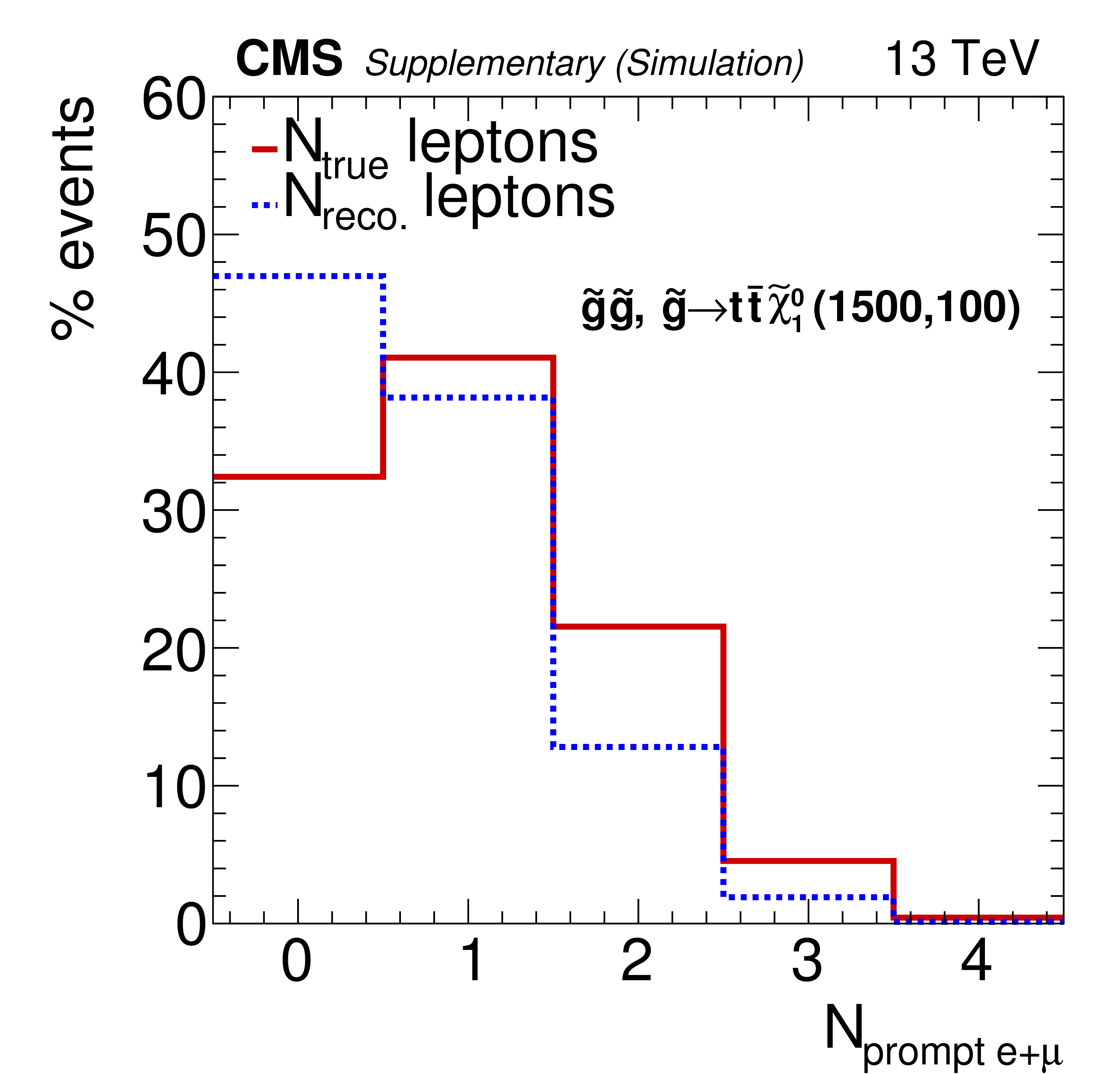
png pdf	Additional Figure 23: Distribution of the number of true e, $\mu $, and $\tau \rightarrow \mathrm{e}/\mu $ coming from W bosons (red) and reconstructed leptons (dashed blue) in gluino pair production events, with $\tilde{\mathrm{g}} \to {\mathrm{ t } \mathrm{ \bar{t} } } \tilde{\chi}^0_1 $, for $ {m_{\tilde{\mathrm{g}} }} = $ 1500 GeV and $ {m_{ \tilde{\chi}^0_1 }} = $ 100 GeV.
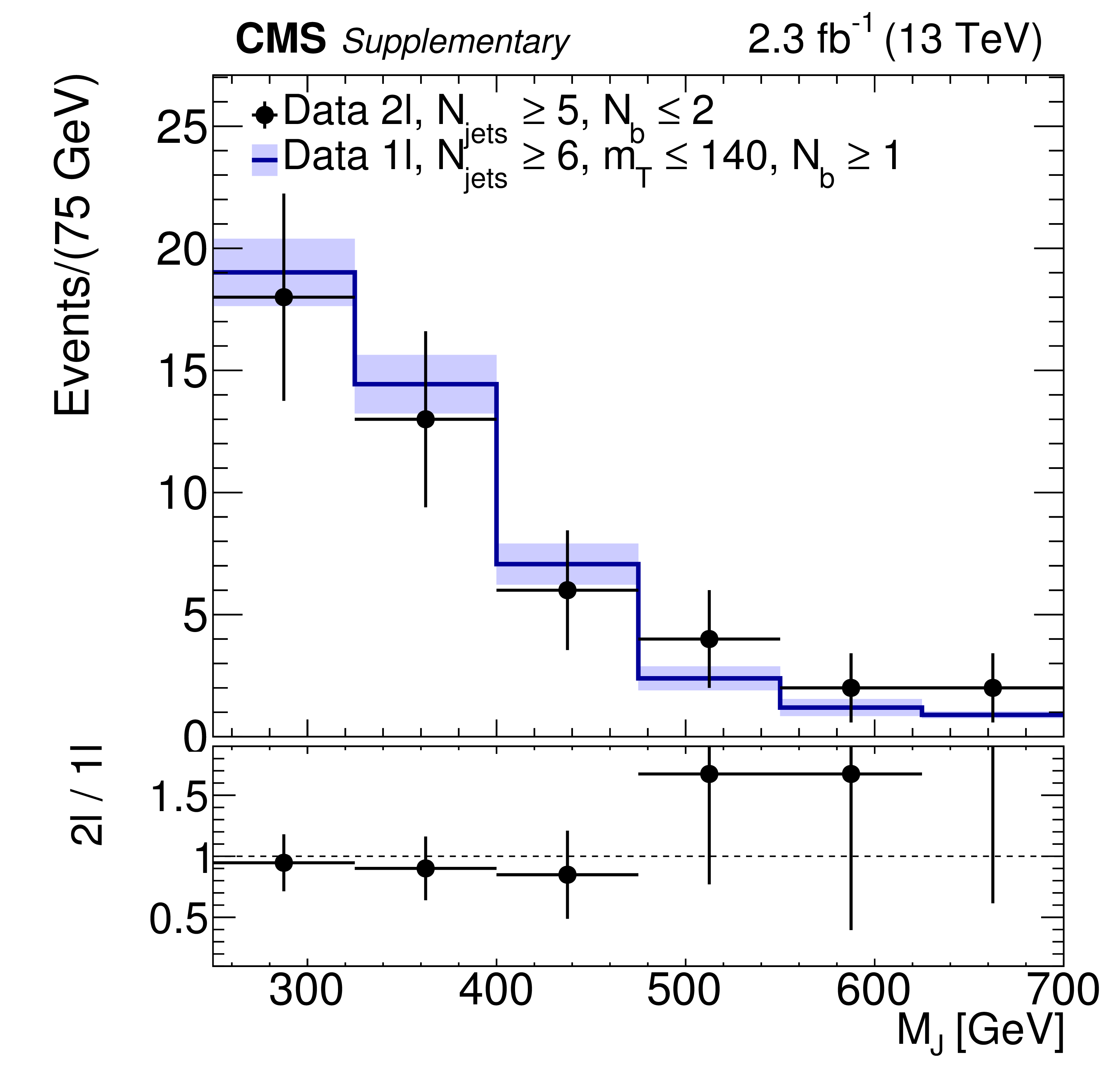
png pdf	Additional Figure 24: Distribution of ${M_J}$ for a single-lepton selection with $ {m_{\mathrm {T}}} < $ 140 GeV (histogram) and a dilepton selection (points). To increase statistics, dilepton events with $ {N_{\text {b}}} = $ 0 are included. To avoid signal contamination, dilepton events with $ {N_{\text {b}}} \geq 3$ are excluded and a cut $ {E_{\mathrm {T}}^{\text {miss}}} < $ 400 is applied to all events. The overall yield from the single-lepton sample is normalized to that for the dilepton sample to compare shapes.
png pdf	Additional Figure 25: Comparison of the ${M_J}$ shape after the baseline selection in ${\mathrm{ t } \mathrm{ \bar{t} } }$ events with 1 true lepton at low and high ${m_{\mathrm {T}}}$. The different ${M_J}$ shape at high ${m_{\mathrm {T}}}$ is produced predominantly from the mismeasurement of jets. While this difference can introduce a correlation between ${M_J}$ and ${m_{\mathrm {T}}}$, single-lepton events at high ${m_{\mathrm {T}}}$ are only a small component (${\sim}$ 15%) of the full high ${m_{\mathrm {T}}}$ background.
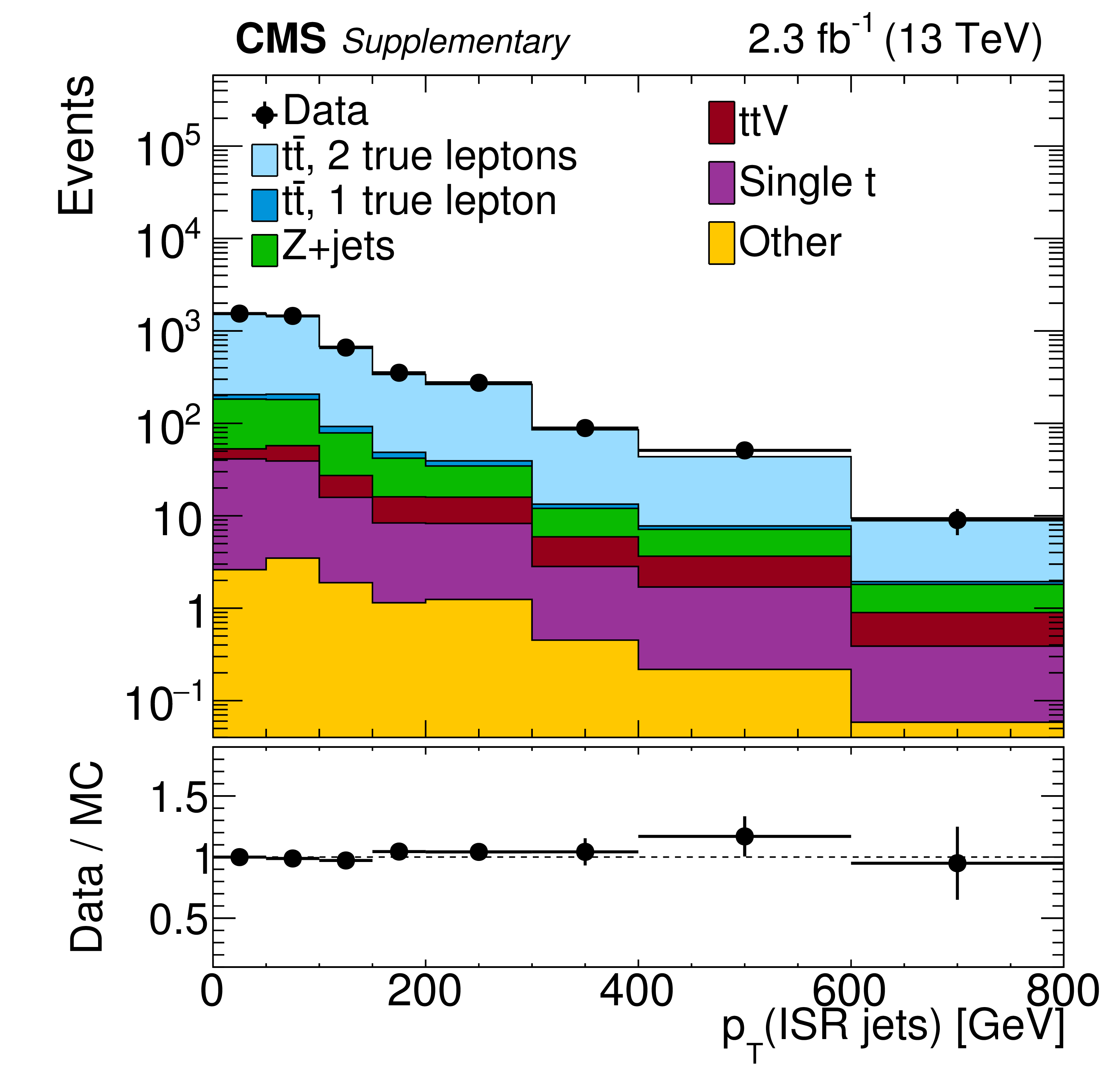
png pdf	Additional Figure 26: The ISR ${p_{\mathrm {T}}}$ distribution in a dilepton ${\mathrm{ t } \mathrm{ \bar{t} } }$ sample. This sample is selected by requiring exactly two leptons and two b-tagged jets. The momenta of the remaining jets are summed vectorially to form the ${p_{\mathrm {T}}}$ of the ISR for the event.
png pdf	Additional Figure 27-a: Distribution of ${m_{\mathrm {T}}}$ in data and simulated event samples in the R2 and R4 region in linear (a) and logarithmic (b) scales. The background contributions shown here are from simulation, and their total yield is normalized to the number of events observed in data. The signal distributions are normalized to the expected cross sections. The dashed vertical line indicates the $ {m_{\mathrm {T}}} > $ 140 GeV requirement for the signal region R4.
png pdf	Additional Figure 27-b: Distribution of ${m_{\mathrm {T}}}$ in data and simulated event samples in the R2 and R4 region in linear (a) and logarithmic (b) scales. The background contributions shown here are from simulation, and their total yield is normalized to the number of events observed in data. The signal distributions are normalized to the expected cross sections. The dashed vertical line indicates the $ {m_{\mathrm {T}}} > $ 140 GeV requirement for the signal region R4.
png pdf	Additional Figure 28-a: Distribution of ${M_J}$ in data and simulated event samples in the R3 and R4 regions in linear (a) and logarithmic (b) scales. The background contributions shown here are from simulation, and their total yield is normalized to the number of events observed in data. The signal distributions are normalized to the expected cross sections. The dashed vertical line indicates the $ {M_J} > $ 400 GeV requirement for the signal region R4.
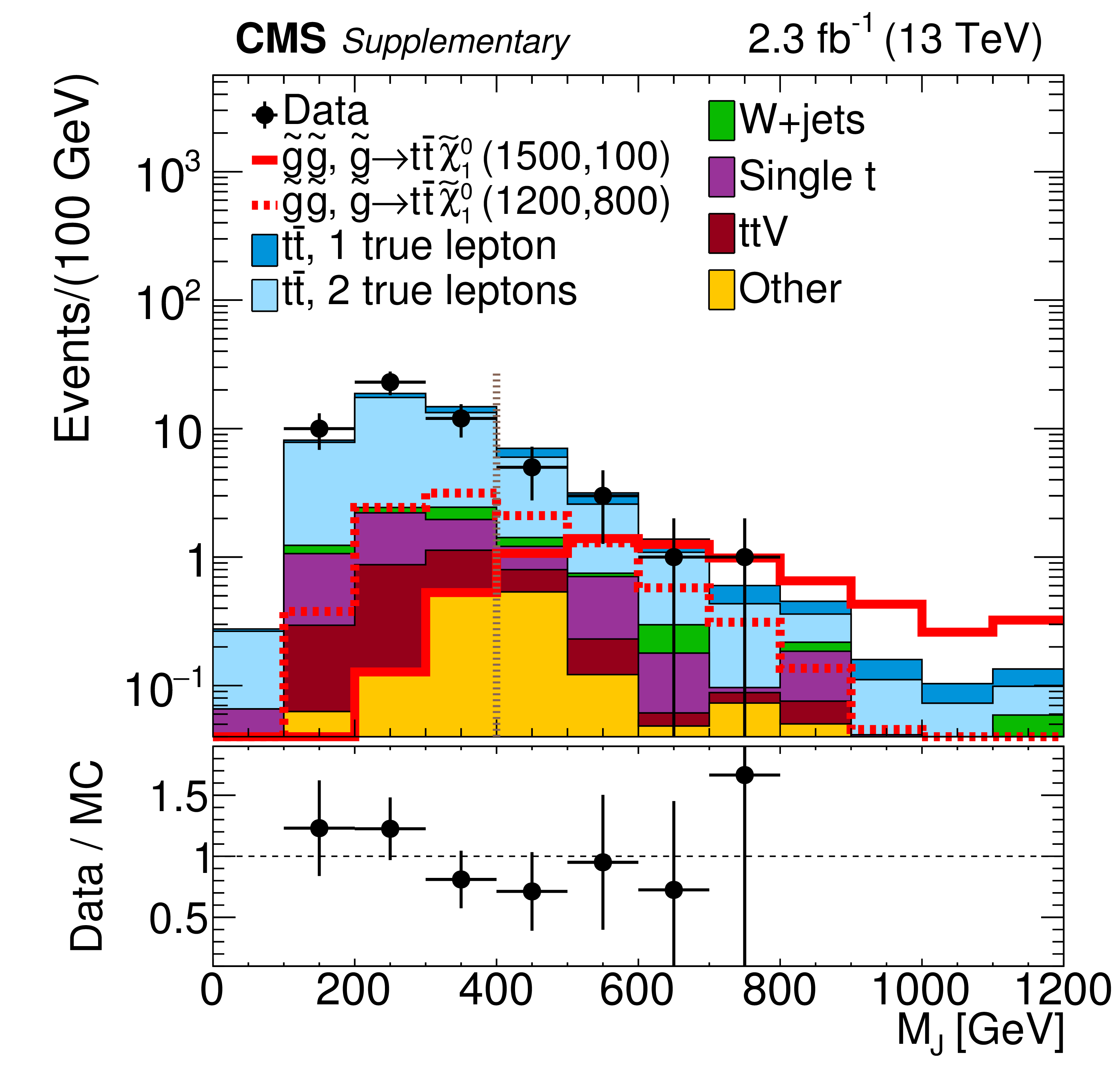
png pdf	Additional Figure 28-b: Distribution of ${M_J}$ in data and simulated event samples in the R3 and R4 regions in linear (a) and logarithmic (b) scales. The background contributions shown here are from simulation, and their total yield is normalized to the number of events observed in data. The signal distributions are normalized to the expected cross sections. The dashed vertical line indicates the $ {M_J} > $ 400 GeV requirement for the signal region R4.
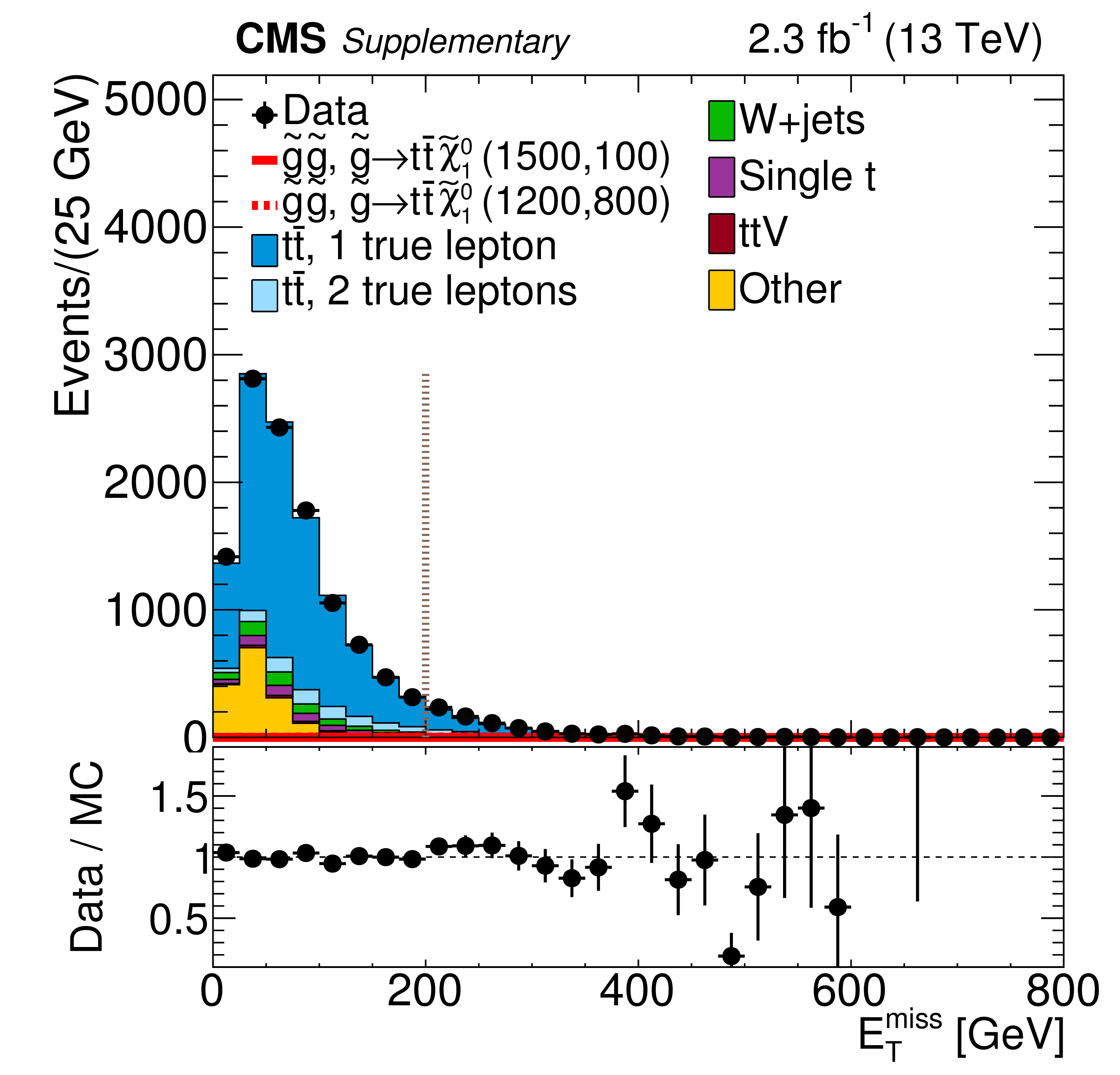
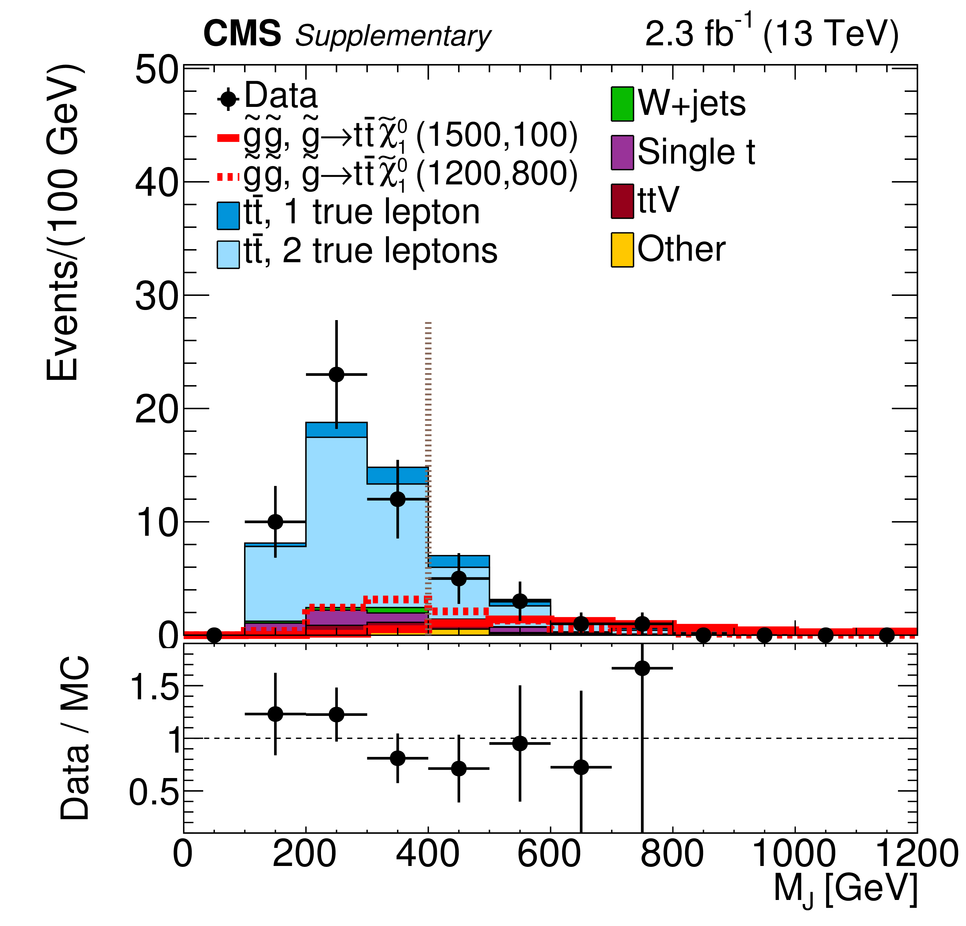
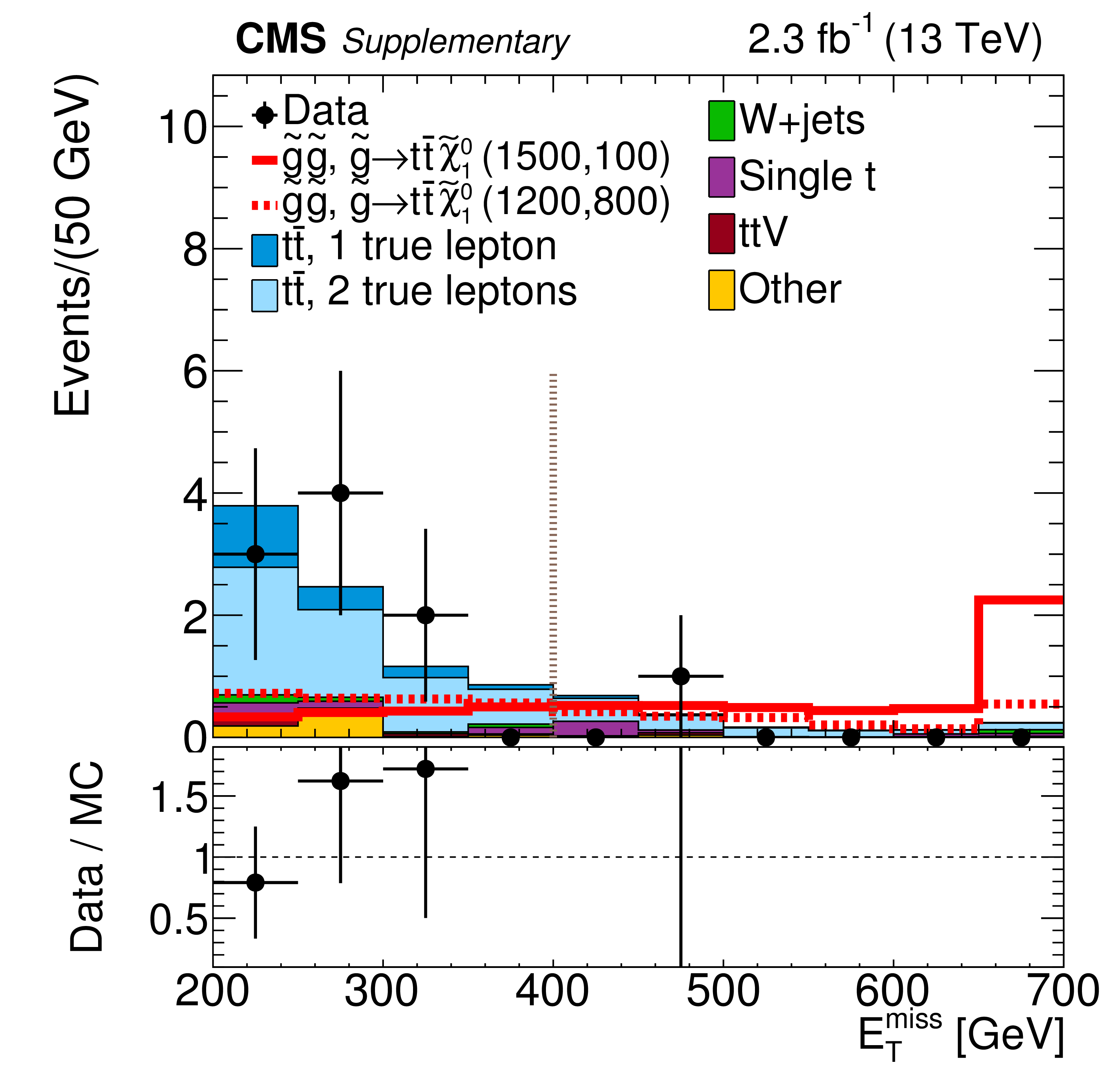
png pdf	Additional Figure 29-a: Distribution of ${E_{\mathrm {T}}^{\text {miss}}}$ in data and simulated event samples in the signal region R4 (baseline selection plus $ {m_{\mathrm {T}}} > $ 140 GeV and $ {M_J} > $ 400 GeV) in linear (a) and logarithmic (b) scales. The background contributions shown here are from simulation, and their total yield is normalized to the number of events observed in data. The signal distributions are normalized to the expected cross sections. The dashed vertical line indicates the $ {E_{\mathrm {T}}^{\text {miss}}} > $ 400 GeV requirement for the tightest ${E_{\mathrm {T}}^{\text {miss}}}$ bin.
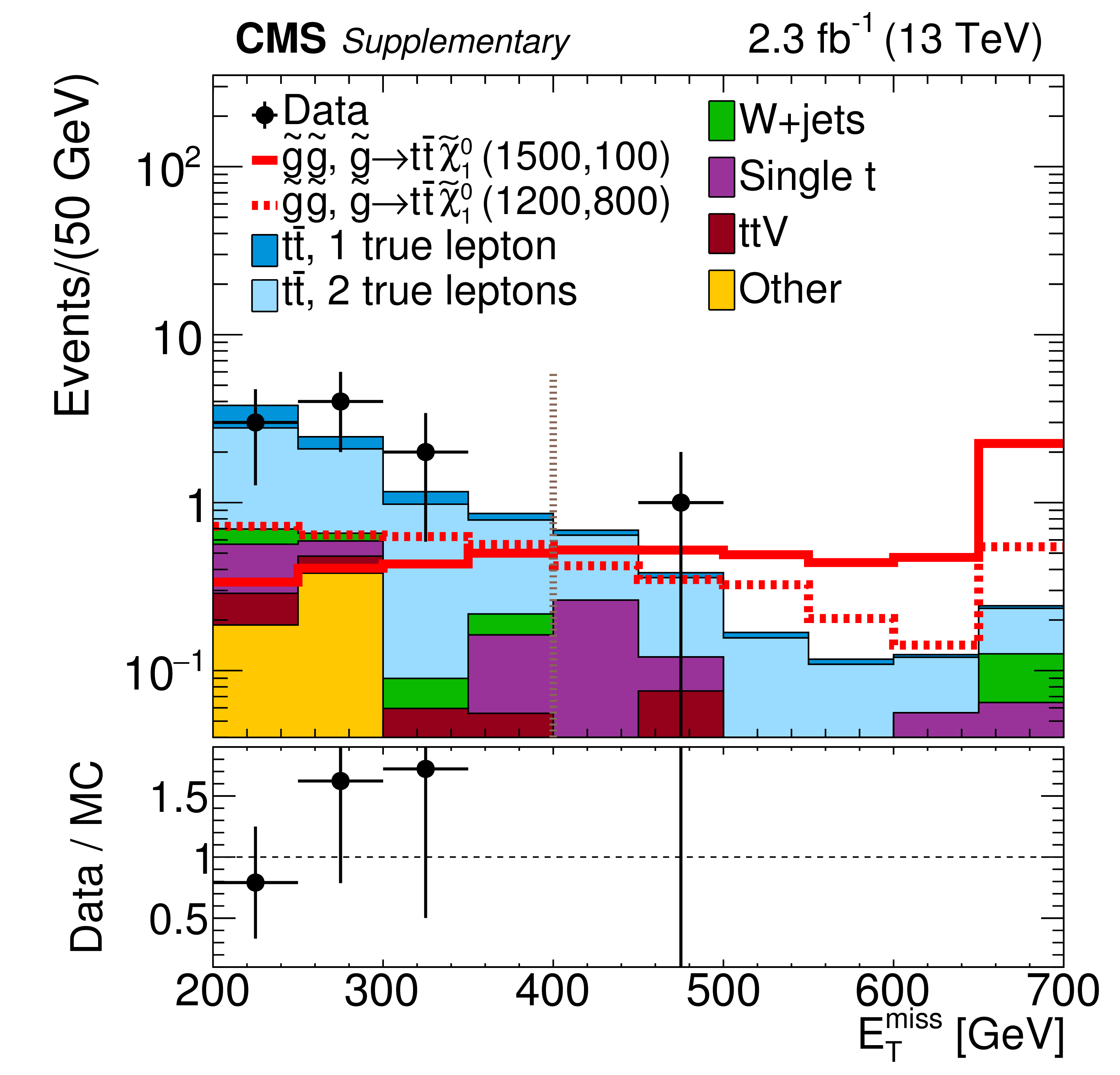
png pdf	Additional Figure 29-b: Distribution of ${E_{\mathrm {T}}^{\text {miss}}}$ in data and simulated event samples in the signal region R4 (baseline selection plus $ {m_{\mathrm {T}}} > $ 140 GeV and $ {M_J} > $ 400 GeV) in linear (a) and logarithmic (b) scales. The background contributions shown here are from simulation, and their total yield is normalized to the number of events observed in data. The signal distributions are normalized to the expected cross sections. The dashed vertical line indicates the $ {E_{\mathrm {T}}^{\text {miss}}} > $ 400 GeV requirement for the tightest ${E_{\mathrm {T}}^{\text {miss}}}$ bin.
png pdf	Additional Figure 30-a: Distribution of $ {N_{\text {b}}}$ in data and simulated event samples in the signal region R4 (baseline selection except for the $ {N_{\text {b}}}$ requirement plus $ {m_{\mathrm {T}}} > $ 140 GeV and $ {M_J} > $ 400 GeV) in linear (a) and logarithmic (b) scales. The background contributions shown here are from simulation, and their total yield is normalized to the number of events observed in data. The signal distributions are normalized to the expected cross sections. The dashed vertical line indicates the $ {N_{\text {b}}} \geq 3$ requirement for the tightest $ {N_{\text {b}}}$ bin.
png pdf	Additional Figure 30-b: Distribution of $ {N_{\text {b}}}$ in data and simulated event samples in the signal region R4 (baseline selection except for the $ {N_{\text {b}}}$ requirement plus $ {m_{\mathrm {T}}} > $ 140 GeV and $ {M_J} > $ 400 GeV) in linear (a) and logarithmic (b) scales. The background contributions shown here are from simulation, and their total yield is normalized to the number of events observed in data. The signal distributions are normalized to the expected cross sections. The dashed vertical line indicates the $ {N_{\text {b}}} \geq 3$ requirement for the tightest $ {N_{\text {b}}}$ bin.
png pdf	Additional Figure 31-a: Distribution of ${N_{\text {jets}}}$ in data and simulated event samples in the signal region R4 (baseline selection except for the ${N_{\text {jets}}}$ requirement plus $ {m_{\mathrm {T}}} > $ 140 GeV and $ {M_J} > $ 400 GeV) in linear (a) and logarithmic (b) scales. The background contributions shown here are from simulation, and their total yield is normalized to the number of events observed in data. The signal distributions are normalized to the expected cross sections. The dashed vertical line indicates the $ {N_{\text {jets}}} \geq 9$ requirement for the tightest ${N_{\text {jets}}}$ bin.
png pdf	Additional Figure 31-b: Distribution of ${N_{\text {jets}}}$ in data and simulated event samples in the signal region R4 (baseline selection except for the ${N_{\text {jets}}}$ requirement plus $ {m_{\mathrm {T}}} > $ 140 GeV and $ {M_J} > $ 400 GeV) in linear (a) and logarithmic (b) scales. The background contributions shown here are from simulation, and their total yield is normalized to the number of events observed in data. The signal distributions are normalized to the expected cross sections. The dashed vertical line indicates the $ {N_{\text {jets}}} \geq 9$ requirement for the tightest ${N_{\text {jets}}}$ bin.
png pdf	Additional Figure 32: Two-dimensional distributions for data and simulated event samples in the variables ${m_{\mathrm {T}}}$ and ${M_J}$ in the $ {N_{\text {b}}} = $ 1 region after the baseline selection. The ${N_{\text {jets}}}$ and the ${E_{\mathrm {T}}^{\text {miss}}}$ bins are integrated over. The black dots are the data; the colored histogram is the total simulated background, normalized to the data; and the red dots are a particular signal sample drawn from the expected distribution for gluino pair production with $\tilde{\mathrm{g}} \to {\mathrm{ t } \mathrm{ \bar{t} } } \tilde{\chi}^0_1 $ $( {m_{\tilde{\mathrm{g}} }} =$1500 GeV and ${m_{ \tilde{\chi}^0_1 }} =$ 100 GeV) for 2.3 fb$^{-1}$. Overflow events are shown on the edges of the plot. The definitions of the signal and control regions are the same as those shown in Fig. 4.
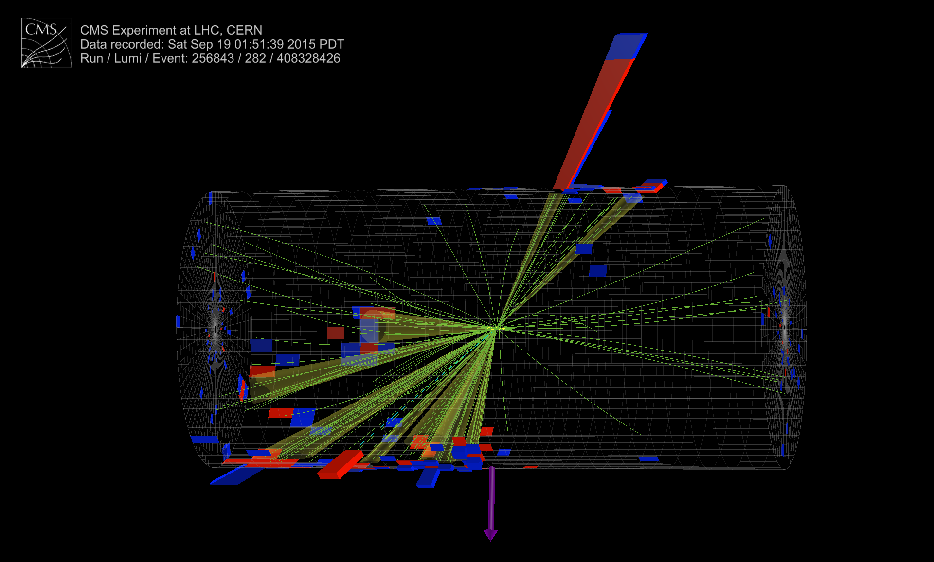
png	Additional Figure 33: Event display showing the highest-${M_J}$ event (256843:282:408328426) in 3D Tower view mode. This event has $ {M_J} = $ 1173 GeV, $ {m_{\mathrm {T}}} = $ 91 GeV, $ {E_{\mathrm {T}}^{\text {miss}}} = $ 347 GeV, $ {N_{\text {jets}}} = $ 9, $ {N_{\text {b}}} = $ 2 with a 172 GeV electron.
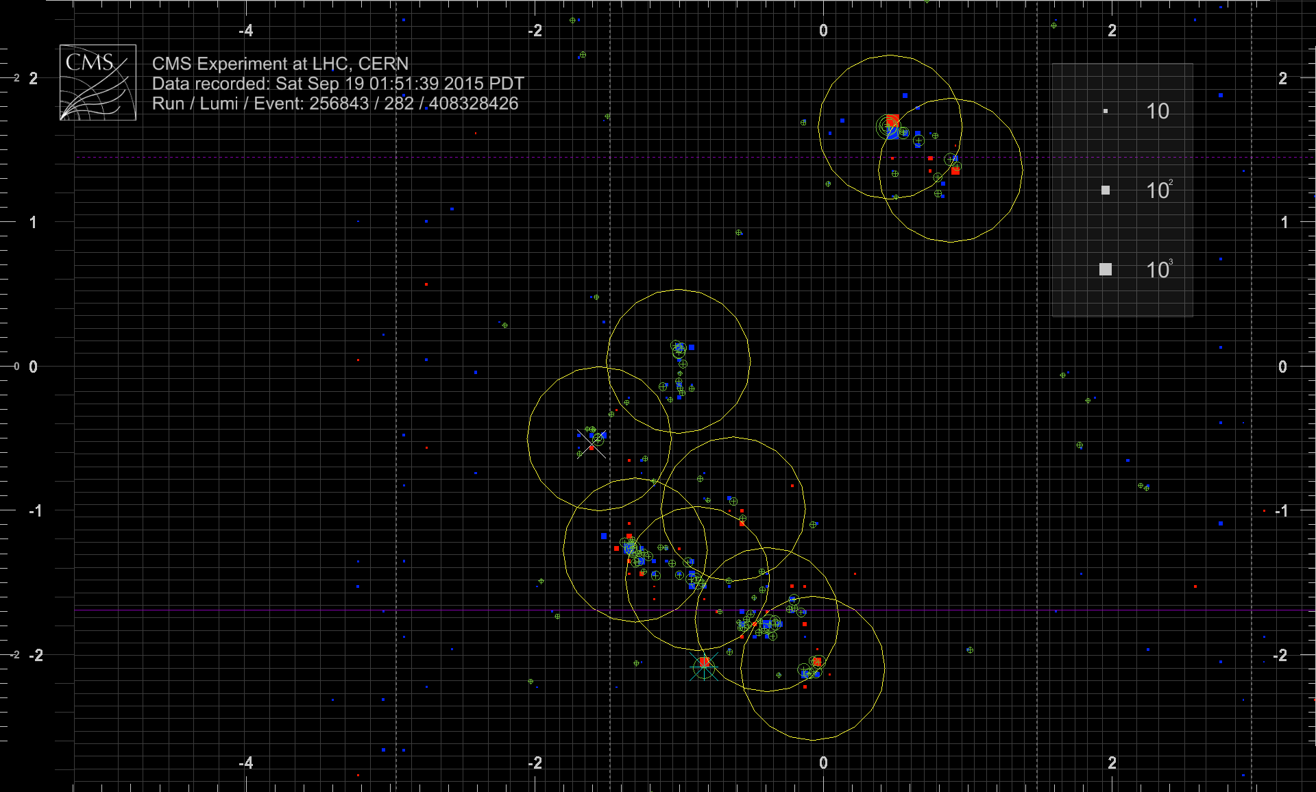
png	Additional Figure 34: Event display showing the highest-${M_J}$ event (256843:282:408328426) in the $z$-$\phi $ plane (lego plot). This event has $ {M_J} = $ 1173 GeV, $ {m_{\mathrm {T}}} = $ 91 GeV, $ {E_{\mathrm {T}}^{\text {miss}}} = $ 347 GeV, $ {N_{\text {jets}}} = $ 9, $ {N_{\text {b}}} = $ 2 with a 172 GeV electron.
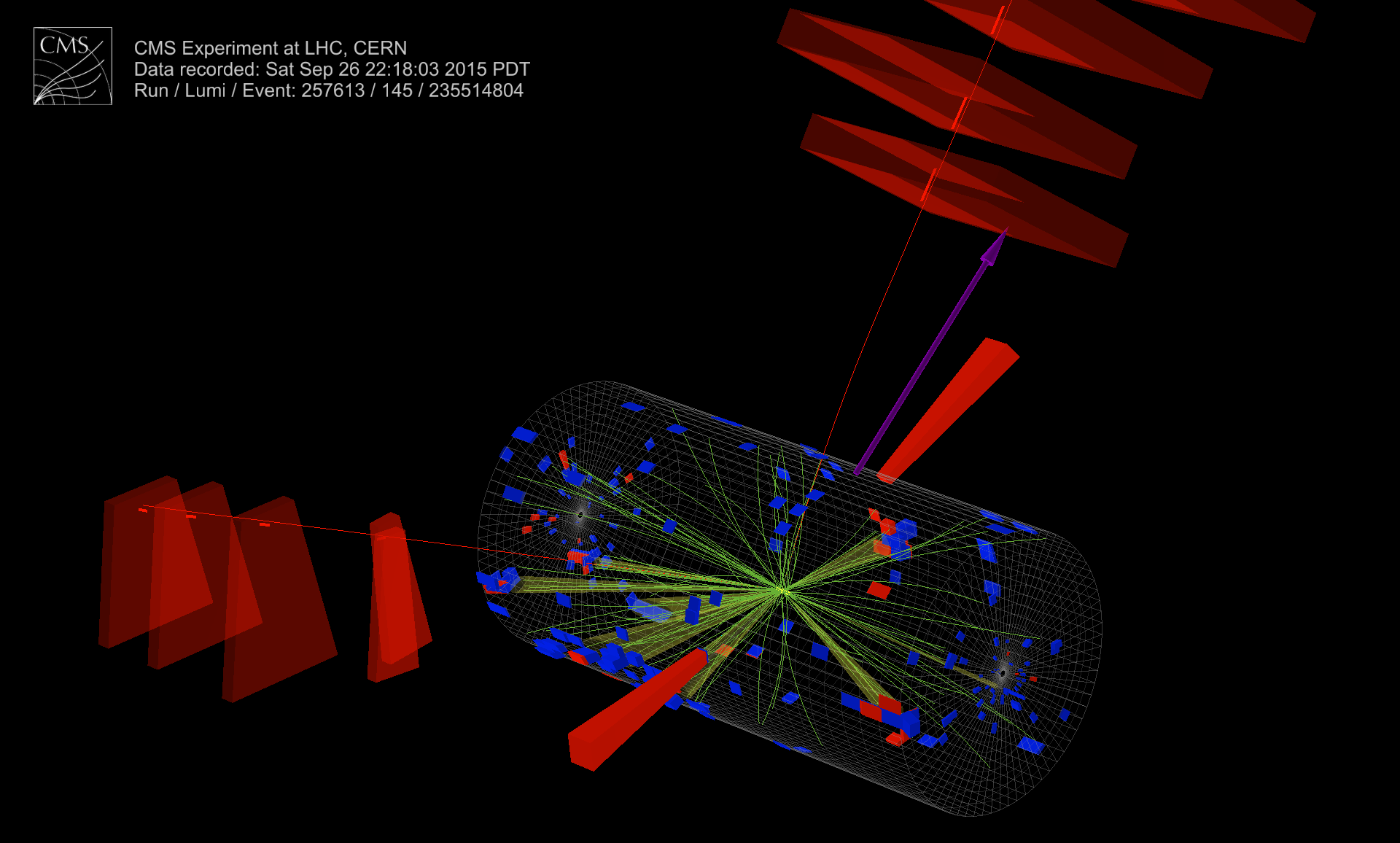
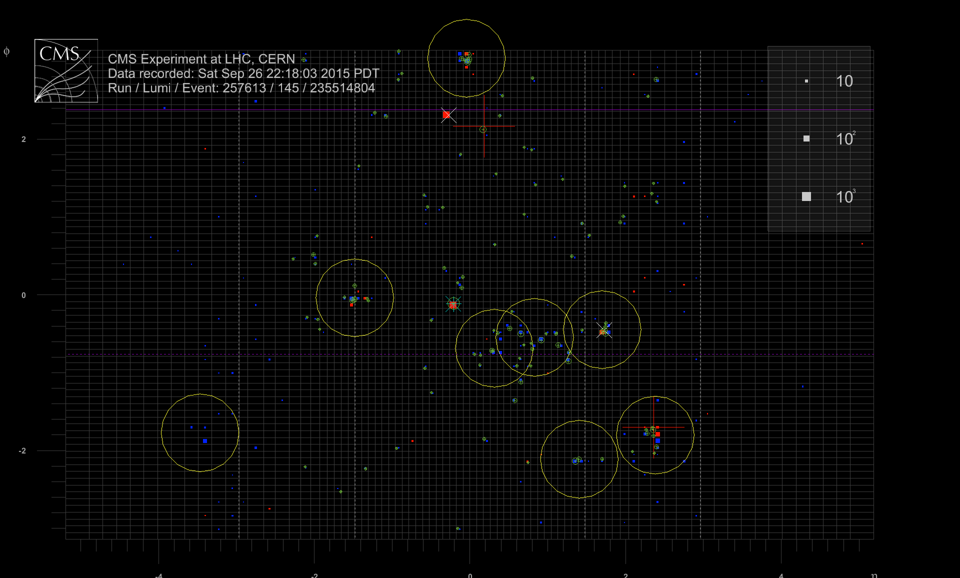
png	Additional Figure 35: Event display showing a high ${m_{\mathrm {T}}}$ event (257613:145:235514804) in 3D Tower view mode compatible with a $2\ell $ ${\mathrm{ t } \mathrm{ \bar{t} } }$ event. This event has $ {M_J} = $ 365 GeV, $ {m_{\mathrm {T}}} = $ 414 GeV, $ {E_{\mathrm {T}}^{\text {miss}}} = $ 266 GeV, $ {N_{\text {jets}}} = $ 8, $ {N_{\text {b}}} = $ 2 with a 181 GeV reconstructed electron and muon with 16 GeV that does not satisfy the minimum ${p_{\mathrm {T}}}$ requirement of 20 GeV (there is an additional 10 GeV non-isolated muon).
png	Additional Figure 36: Event display showing a high ${m_{\mathrm {T}}}$ event (257613:145:235514804) in the $z$-$\phi $ plane (lego plot) compatible with a $2\ell $ ${\mathrm{ t } \mathrm{ \bar{t} } }$ event. This event has $ {M_J} = $ 365 GeV, $ {m_{\mathrm {T}}} = $ 414 GeV, $ {E_{\mathrm {T}}^{\text {miss}}} = $ 266 GeV, $ {N_{\text {jets}}} = $ 8, $ {N_{\text {b}}} = $ 2 with a 181 GeV reconstructed electron and another electron with 16 GeV that does not satisfy the minimum ${p_{\mathrm {T}}}$ requirement of 20 GeV.
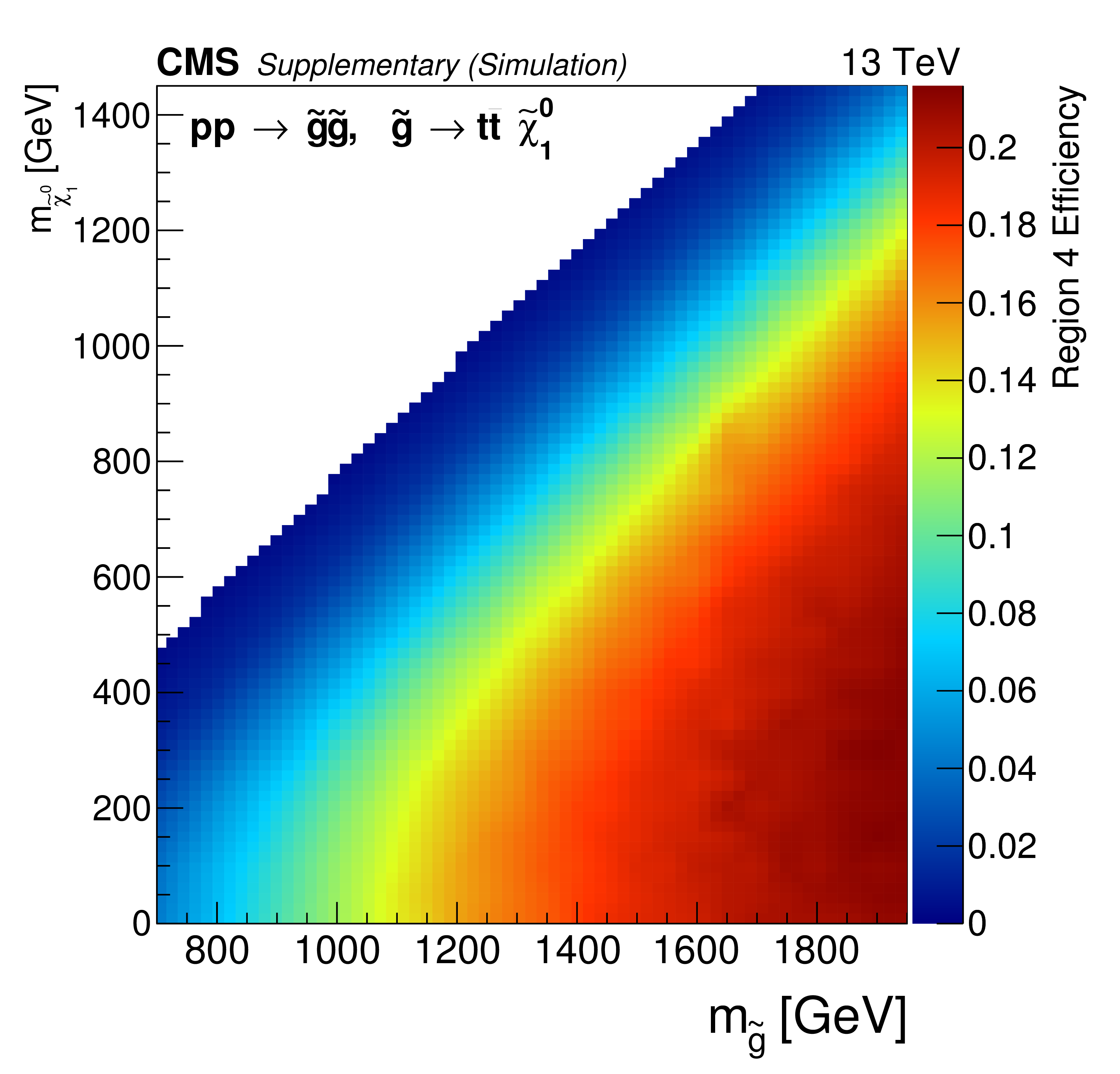
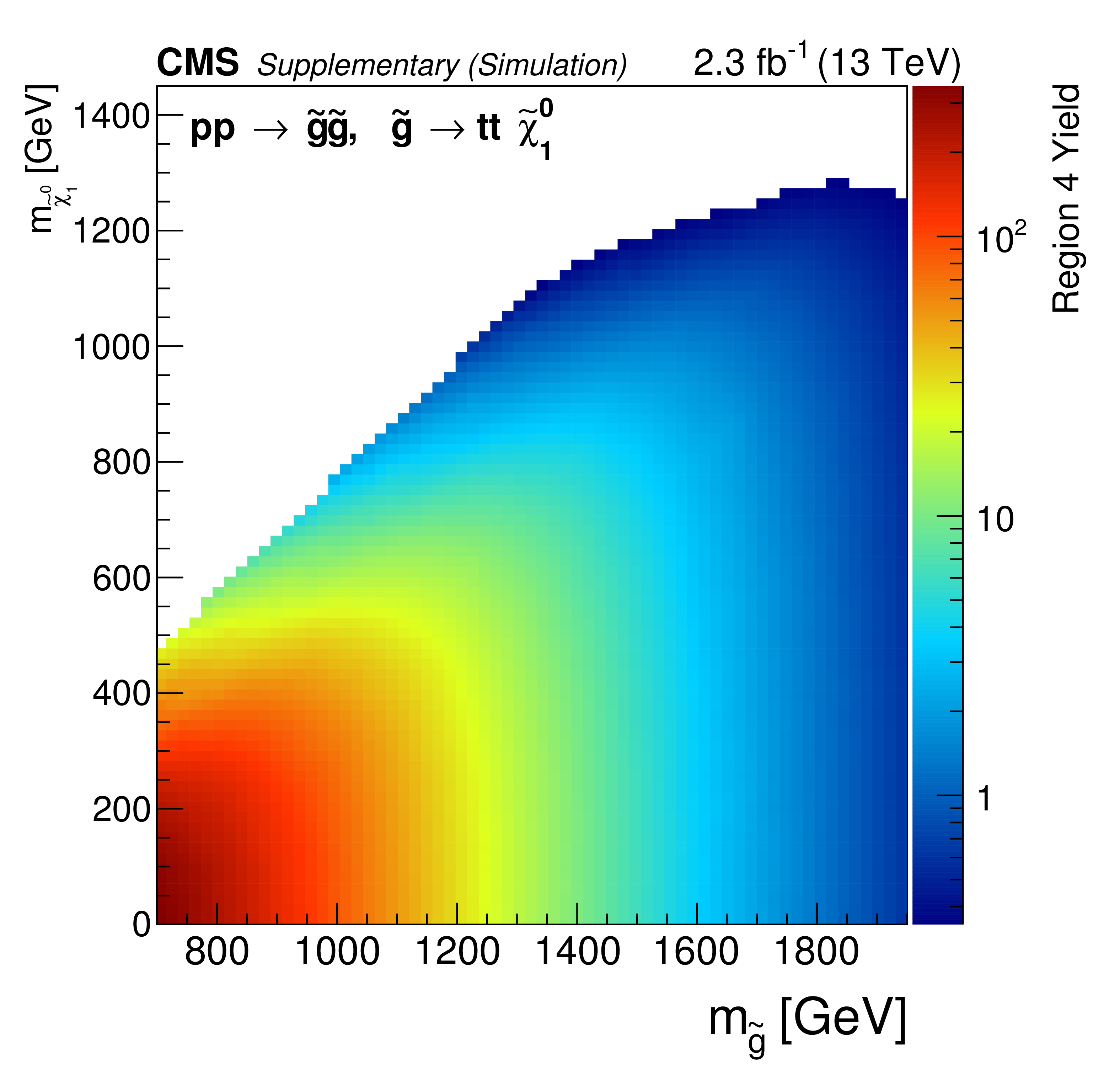
png pdf	Additional Figure 37-a: Signal efficiency (a) and expected yields for 2.3 fb$^{-1}$ (b) in region 4 for the process $\mathrm{ p } \mathrm{ p } \rightarrow \tilde{\mathrm{g}} \tilde{\mathrm{g}},\tilde{\mathrm{g}} \rightarrow {\mathrm{ t } \mathrm{ \bar{t} } } \tilde{\chi}^0_1 $ in the $ {m_{\tilde{\mathrm{g}} }} $-$ {m_{ \tilde{\chi}^0_1 }} $ plane. The efficiency is taken with respect to the total $\mathrm{ p } \mathrm{ p } \rightarrow \tilde{\mathrm{g}} \tilde{\mathrm{g}},\tilde{\mathrm{g}} \rightarrow {\mathrm{ t } \mathrm{ \bar{t} } } \tilde{\chi}^0_1 $ cross section, and therefore includes losses to final states with a different number of leptons.
png pdf	Additional Figure 37-b: Signal efficiency (a) and expected yields for 2.3 fb$^{-1}$ (b) in region 4 for the process $\mathrm{ p } \mathrm{ p } \rightarrow \tilde{\mathrm{g}} \tilde{\mathrm{g}},\tilde{\mathrm{g}} \rightarrow {\mathrm{ t } \mathrm{ \bar{t} } } \tilde{\chi}^0_1 $ in the $ {m_{\tilde{\mathrm{g}} }} $-$ {m_{ \tilde{\chi}^0_1 }} $ plane. The efficiency is taken with respect to the total $\mathrm{ p } \mathrm{ p } \rightarrow \tilde{\mathrm{g}} \tilde{\mathrm{g}},\tilde{\mathrm{g}} \rightarrow {\mathrm{ t } \mathrm{ \bar{t} } } \tilde{\chi}^0_1 $ cross section, and therefore includes losses to final states with a different number of leptons.
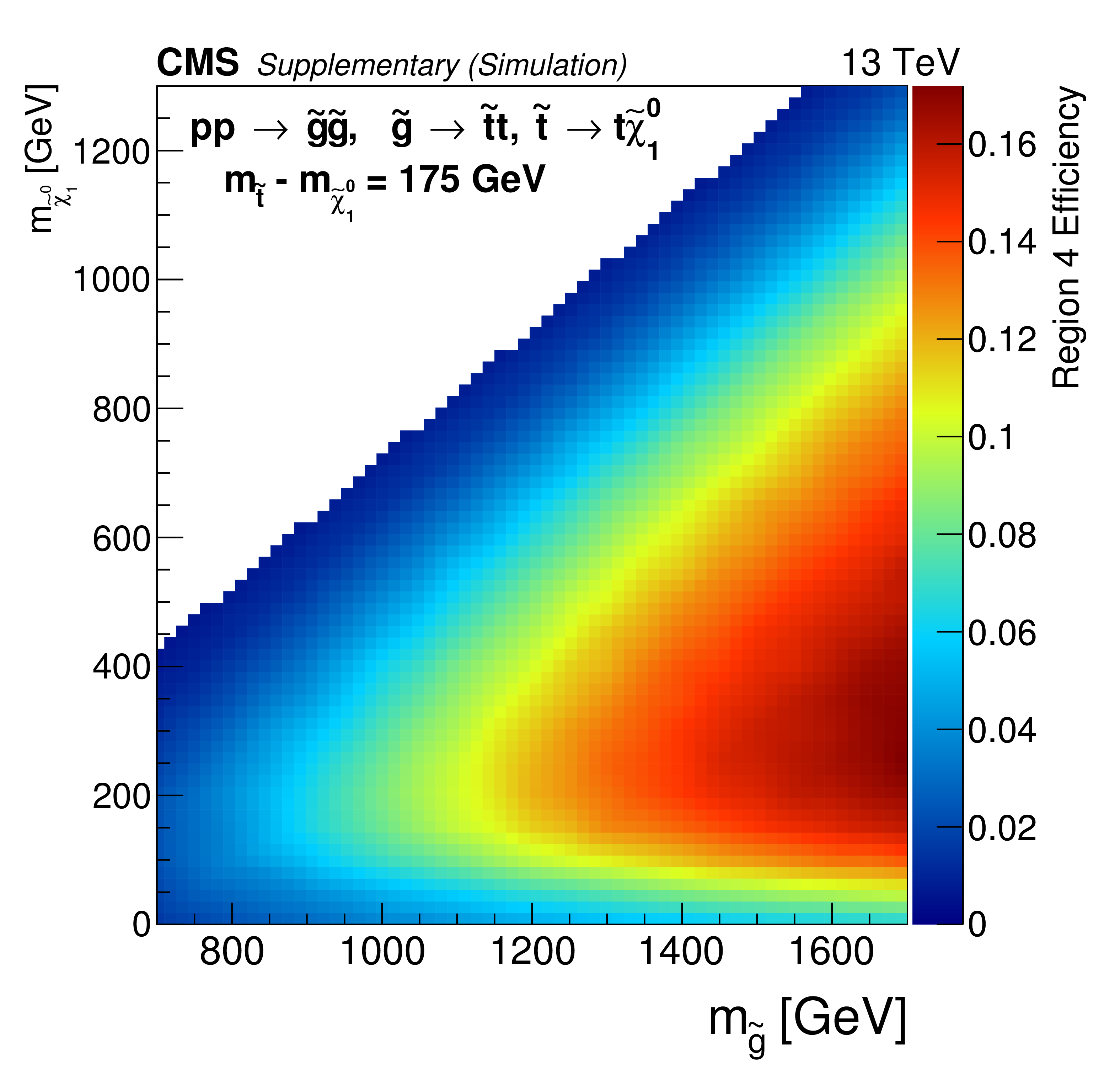
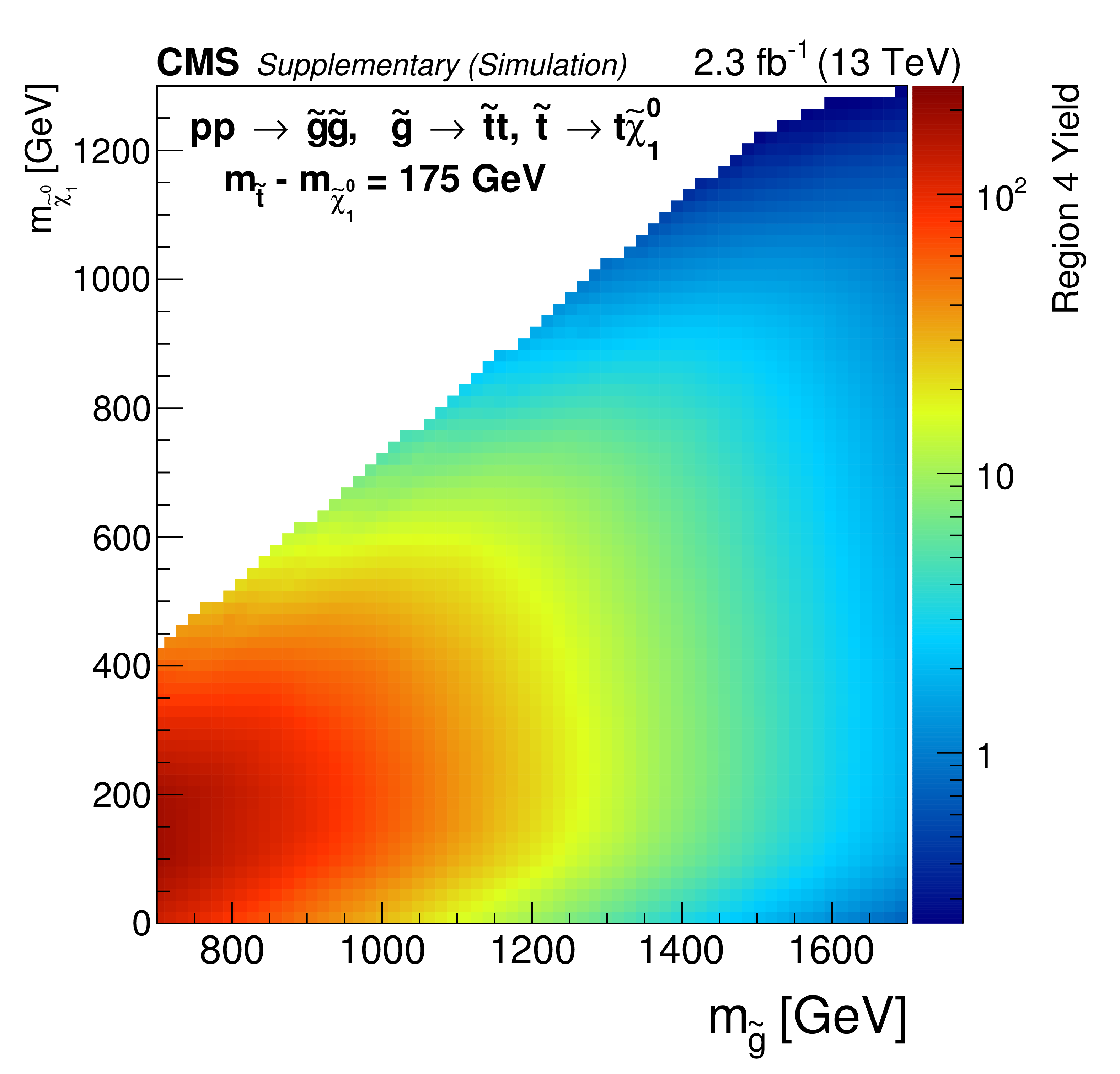
png pdf	Additional Figure 38-a: Signal efficiency (a) and expected yields for 2.3 fb$^{-1}$ (b) in region 4 for the process $\mathrm{ p } \mathrm{ p } \rightarrow \tilde{\mathrm{g}} \tilde{\mathrm{g}},\tilde{\mathrm{g}} \rightarrow \tilde{\mathrm{t}} \tilde{\mathrm{\bar{t}}},\tilde{\mathrm{t}} \rightarrow t \tilde{\chi}^0_1 $ in the $ {m_{\tilde{\mathrm{g}} }} $-$ {m_{ \tilde{\chi}^0_1 }} $ plane. The mass of the top squark is fixed to $ {m_{\tilde{ \mathrm{ t } } _1}} = {m_{ \tilde{\chi}^0_1 }} $ +175 GeV. The efficiency is taken with respect to the total $\mathrm{ p } \mathrm{ p } \rightarrow \tilde{\mathrm{g}} \tilde{\mathrm{g}},\tilde{\mathrm{g}} \rightarrow \tilde{\mathrm{t}} \tilde{\mathrm{\bar{t}}},\tilde{\mathrm{t}} \rightarrow \mathrm{t} \tilde{\chi}^0_1 $ cross section, and therefore includes losses to final states with a different number of leptons.
png pdf	Additional Figure 38-b: Signal efficiency (a) and expected yields for 2.3 fb$^{-1}$ (b) in region 4 for the process $\mathrm{ p } \mathrm{ p } \rightarrow \tilde{\mathrm{g}} \tilde{\mathrm{g}},\tilde{\mathrm{g}} \rightarrow \tilde{\mathrm{t}} \tilde{\mathrm{\bar{t}}},\tilde{\mathrm{t}} \rightarrow t \tilde{\chi}^0_1 $ in the $ {m_{\tilde{\mathrm{g}} }} $-$ {m_{ \tilde{\chi}^0_1 }} $ plane. The mass of the top squark is fixed to $ {m_{\tilde{ \mathrm{ t } } _1}} = {m_{ \tilde{\chi}^0_1 }} $ +175 GeV. The efficiency is taken with respect to the total $\mathrm{ p } \mathrm{ p } \rightarrow \tilde{\mathrm{g}} \tilde{\mathrm{g}},\tilde{\mathrm{g}} \rightarrow \tilde{\mathrm{t}} \tilde{\mathrm{\bar{t}}},\tilde{\mathrm{t}} \rightarrow \mathrm{t} \tilde{\chi}^0_1 $ cross section, and therefore includes losses to final states with a different number of leptons.

References
1	P. Ramond	Dual theory for free fermions	PRD 3 (1971) 2415
2	Y. A. Gol'fand and E. P. Likhtman	Extension of the algebra of Poincar$ \'e $ group generators and violation of P invariance	JEPTL 13 (1971)323
3	A. Neveu and J. H. Schwarz	Factorizable dual model of pions	Nucl. Phys. B 31 (1971) 86
4	D. V. Volkov and V. P. Akulov	Possible universal neutrino interaction	JEPTL 16 (1972) 438
5	J. Wess and B. Zumino	A Lagrangian model invariant under supergauge transformations	PLB 49 (1974) 52
6	J. Wess and B. Zumino	Supergauge transformations in four dimensions	Nucl. Phys. B 70 (1974) 39
7	P. Fayet	Supergauge invariant extension of the Higgs mechanism and a model for the electron and its neutrino	Nucl. Phys. B 90 (1975) 104
8	H. P. Nilles	Supersymmetry, supergravity and particle physics	Phys. Rep. 110 (1984) 1
9	G. 't Hooft	Naturalness, chiral symmetry, and spontaneous chiral symmetry breaking	in Recent Developments in Gauge Theories, G. 't Hooft et al., eds., p. 135 Springer, 1980NATO Advanced Study Institutes Series B
10	E. Witten	Dynamical breaking of supersymmetry	Nucl. Phys. B 188 (1981) 513
11	M. Dine, W. Fischler, and M. Srednicki	Supersymmetric technicolor	Nucl. Phys. B 189 (1981) 575
12	S. Dimopoulos and S. Raby	Supercolor	Nucl. Phys. B 192 (1981) 353
13	S. Dimopoulos and H. Georgi	Softly broken supersymmetry and SU(5)	Nucl. Phys. B 193 (1981) 150
14	R. K. Kaul and P. Majumdar	Cancellation of quadratically divergent mass corrections in globally supersymmetric spontaneously broken gauge theories	Nucl. Phys. B 199 (1982) 36
15	F. Zwicky	Die Rotverschiebung von Extragalaktischen Nebeln	Helv. Phys. Acta 6 (1933)110
16	V. C. Rubin and W. K. Ford Jr	Rotation of the Andromeda nebula from a spectroscopic survey of emission regions	Astrophys. J. 159 (1970) 379
17	Particle Data Group, K. A. Olive et al.	Review of Particle Physics	CPC 38 (2014) 090001
18	S. Dimopoulos, S. Raby, and F. Wilczek	Supersymmetry and the scale of unification	PRD 24 (1981) 1681
19	N. Sakai	Naturalness in supersymmetric GUTS	Z. Phys. C 11 (1981) 153
20	L. E. Ibanez and G. G. Ross	Low-energy predictions in supersymmetric grand unified theories	PLB 105 (1981) 439
21	M. B. Einhorn and D. R. T. Jones	The weak mixing angle and unification mass in supersymmetric SU(5)	Nucl. Phys. B 196 (1982) 475
22	W. J. Marciano and G. Senjanovic	Predictions of supersymmetric grand unified theories	PRD 25 (Jun, 1982) 3092
23	G. R. Farrar and P. Fayet	Phenomenology of the production, decay, and detection of new hadronic states associated with supersymmetry	PLB 76 (1978) 575
24	S. P. Martin	A Supersymmetry Primer	Adv. Ser. Direct. High Energy Phys., vol. 21	hep-ph/9709356
25	ATLAS Collaboration	Observation of a new particle in the search for the Standard Model Higgs boson with the ATLAS detector at the LHC	PLB 716 (2012) 1	1207.7214
26	CMS Collaboration	Observation of a new boson at a mass of 125 GeV with the CMS experiment at the LHC	PLB 716 (2012) 30	CMS-HIG-12-028 1207.7235
27	CMS Collaboration	Observation of a new boson with mass near 125 GeV in pp collisions at $ \sqrt{s} $ = 7 and 8 TeV	JHEP 06 (2013) 081	CMS-HIG-12-036 1303.4571
28	CMS Collaboration	Precise determination of the mass of the Higgs boson and tests of compatibility of its couplings with the standard model predictions using proton collisions at 7 and 8 TeV	EPJC 75 (2015) 212	CMS-HIG-14-009 1412.8662
29	ATLAS Collaboration	Measurement of the Higgs boson mass from the $ \textrm{H}\rightarrow \gamma\gamma $ and $ \textrm{H} \rightarrow \textrm{ZZ}^{*} \rightarrow 4\ell $ channels with the ATLAS detector using 25 fb$ ^{-1} $ of pp collision data	PRD 90 (2014) 052004	1406.3827
30	ATLAS and CMS Collaborations	Combined measurement of the Higgs boson mass in pp collisions at $ \sqrt{s} = 7 $ and 8 TeV with the ATLAS and CMS experiments	PRL 114 (2015) 191803	1503.07589
31	S. Dimopoulos and G. F. Giudice	Naturalness constraints in supersymmetric theories with nonuniversal soft terms	PLB 357 (1995) 573	hep-ph/9507282
32	R. Barbieri and D. Pappadopulo	S-particles at their naturalness limits	JHEP 10 (2009) 061	0906.4546
33	M. Papucci, J. T. Ruderman, and A. Weiler	Natural SUSY endures	JHEP 09 (2012) 035	1110.6926
34	J. L. Feng	Naturalness and the status of supersymmetry	Ann. Rev. Nucl. Part. Sci. 63 (2013) 351	1302.6587
35	N. Craig	The state of supersymmetry after Run I of the LHC	in Beyond the Standard Model after the first run of the LHC, Arcetri, Florence, Italy, May 20-July 12, 2013 2013	1309.0528
36	ATLAS Collaboration	Search for strong production of supersymmetric particles in final states with missing transverse momentum and at least three $ b $-jets at $ \sqrt{s} $= 8 TeV proton-proton collisions with the ATLAS detector	JHEP 10 (2014) 024	1407.0600
37	ATLAS Collaboration	Search for squarks and gluinos in events with isolated leptons, jets and missing transverse momentum at $ \sqrt{s} = $ 8 TeV with the ATLAS detector	JHEP 04 (2015) 116	1501.03555
38	CMS Collaboration	Search for supersymmetry in pp collisions at $ \sqrt{s} = $ 8 TeV in events with a single lepton, large jet multiplicity, and multiple b jets	PLB 733 (2014) 328	CMS-SUS-13-007 1311.4937
39	C. Borschensky et al.	Squark and gluino production cross sections in pp collisions at $ \sqrt{s} = 13 $, 14, 33 and 100 TeV	EPJC 74 (2014) 3174	1407.5066
40	M. Czakon, P. Fiedler, and A. Mitov	The total top quark pair production cross-section at $ \mathcal{O}(\alpha^4_S) $	PRL 110 (2013) 252004	1303.6254
41	CMS Collaboration	Interpretation of searches for supersymmetry with simplified models	PRD 88 (2013) 052017	CMS-SUS-11-016 1301.2175
42	J. Alwall, P. Schuster, and N. Toro	Simplified models for a first characterization of new physics at the LHC	PRD 79 (2009) 075020	0810.3921
43	J. Alwall, M.-P. Le, M. Lisanti, and J. G. Wacker	Model-independent jets plus missing energy searches	PRD 79 (2009) 015005	0809.3264
44	D. Alves et al.	Simplified models for LHC new physics searches	JPG 39 (2012) 105005	1105.2838
45	A. Hook, E. Izaguirre, M. Lisanti, and J. G. Wacker	High multiplicity searches at the LHC using jet masses	PRD 85 (2012) 055029	1202.0558
46	T. Cohen, E. Izaguirre, M. Lisanti, and H. K. Lou	Jet substructure by accident	JHEP 03 (2013) 161	1212.1456
47	S. El Hedri, A. Hook, M. Jankowiak, and J. G. Wacker	Learning how to count: a high multiplicity search for the LHC	JHEP 08 (2013) 136	1302.1870
48	ATLAS Collaboration	Search for massive supersymmetric particles decaying to many jets using the ATLAS detector in pp collisions at $ \sqrt{s} = $ 8 TeV	PRD 91 (2015) 112016	1502.05686
49	ATLAS Collaboration	Search for new phenomena in final states with large jet multiplicities and missing transverse momentum at $ \sqrt{s} = $ 8 TeV proton-proton collisions using the ATLAS experiment	JHEP 10 (2013) 130, , [Erratum: \DOI10.1007/JHEP01(2014)109]	1308.1841
50	CMS Collaboration	Commissioning the performance of key observables used in SUSY searches with the first 13 TeV data	CDS
51	CMS Collaboration	The CMS experiment at the CERN LHC	JINST 3 (2008) S08004	CMS-00-001
52	J. Alwall et al.	The automated computation of tree-level and next-to-leading order differential cross sections, and their matching to parton shower simulations	JHEP 07 (2014) 079	1405.0301
53	S. Alioli, P. Nason, C. Oleari, and E. Re	NLO single-top production matched with shower in POWHEG: $ s $- and $ t $-channel contributions	JHEP 09 (2009) 111, , [Erratum: \DOI10.1007/JHEP02(2010)011]	0907.4076
54	E. Re	Single-top $ \mathrm{ W }\mathrm{ t } $-channel production matched with parton showers using the POWHEG method	EPJC 71 (2011) 1547	1009.2450
55	NNPDF Collaboration	Parton distributions for the LHC Run II	JHEP 04 (2015) 040	1410.8849
56	T. Sjostrand et al.	An Introduction to PYTHIA 8.2	CPC 191 (2015) 159	1410.3012
57	CMS Collaboration	Event generator tunes obtained from underlying event and multiparton scattering measurements	EPJC 76 (2016), no. 3, 155	CMS-GEN-14-001 1512.00815
58	GEANT4 Collaboration	GEANT4---a simulation toolkit	NIMA 506 (2003) 250
59	CMS Collaboration	Measurement of the differential cross section for top quark pair production in pp collisions at $ \sqrt{s} = $ 8 TeV	EPJC 75 (2015) 542	CMS-TOP-12-028 1505.04480
60	CMS Collaboration	The fast simulation of the CMS detector at LHC	J. Phys. Conf. Ser. 331 (2011) 032049
61	W. Beenakker, R. Hopker, M. Spira, and P. M. Zerwas	Squark and gluino production at hadron colliders	Nucl. Phys. B 492 (1997) 51	hep-ph/9610490
62	A. Kulesza and L. Motyka	Threshold resummation for squark-antisquark and gluino-pair production at the LHC	PRL 102 (2009) 111802	0807.2405
63	A. Kulesza and L. Motyka	Soft gluon resummation for the production of gluino-gluino and squark-antisquark pairs at the LHC	PRD 80 (2009) 095004	0905.4749
64	W. Beenakker et al.	Soft-gluon resummation for squark and gluino hadroproduction	JHEP 12 (2009) 041	0909.4418
65	CMS Collaboration	Particle flow event reconstruction in CMS and performance for jets, taus and $ E_{\mathrm{T}}^{\text{miss}} $	CDS
66	CMS Collaboration	Commissioning of the particle-flow event reconstruction with the first LHC collisions recorded in the CMS detector	CDS
67	M. Cacciari, G. P. Salam, and G. Soyez	The anti-$ k_{\rm t} $ jet clustering algorithm	JHEP 04 (2008) 063	0802.1189
68	M. Cacciari, G. P. Salam, and G. Soyez	FastJet user manual	EPJC 72 (2012) 1896	1111.6097
69	M. Cacciari and G. P. Salam	Pileup subtraction using jet areas	PLB 659 (2008) 119	0707.1378
70	CMS Collaboration	Determination of jet energy calibration and transverse momentum resolution in CMS	JINST 6 (2011) P11002	CMS-JME-10-011 1107.4277
71	CMS Collaboration	Identification of $ \mathrm{ b } $-quark jets with the CMS experiment	JINST 8 (2013) P04013	CMS-BTV-12-001 1211.4462
72	CMS Collaboration	Identification of $ \mathrm{ b } $ quark jets at the CMS Experiment in the LHC Run 2	CMS-PAS-BTV-15-001	CMS-PAS-BTV-15-001
73	CMS Collaboration	Performance of electron reconstruction and selection with the CMS detector in proton-proton collisions at $ \sqrt{s} = $ 8 TeV	JINST 10 (2015) P06005	CMS-EGM-13-001 1502.02701
74	CMS Collaboration	Performance of CMS muon reconstruction in pp collision events at $ \sqrt{s} = $ 7 TeV	JINST 7 (2012) P10002	CMS-MUO-10-004 1206.4071
75	K. Rehermann and B. Tweedie	Efficient identification of boosted semileptonic top quarks at the LHC	JHEP 03 (2011) 059	1007.2221
76	ATLAS Collaboration	Search for direct pair production of the top squark in all-hadronic final states in proton-proton collisions at $ \sqrt{s} = $ 8 TeV with the ATLAS detector	JHEP 09 (2014) 015	1406.1122
77	CMS Collaboration	Search for supersymmetry in the multijet and missing transverse momentum final state in pp collisions at 13 TeV	Submitted to PLB	CMS-SUS-15-002 1602.06581
78	CMS Collaboration	CMS luminosity measurement for the 2015 data taking period	CMS-PAS-LUM-15-001	CMS-PAS-LUM-15-001
79	T. Junk	Confidence level computation for combining searches with small statistics	NIMA 434 (1999) 435	hep-ex/9902006
80	A. L. Read	Presentation of search results: the $ \rm CL_s $ technique	JPG 28 (2002) 2693
81	ATLAS Collaboration, CMS Collaboration, LHC Higgs Combination Group	Procedure for the LHC Higgs boson search combination in Summer 2011	CMS-NOTE-2011-005

Compact Muon Solenoid LHC, CERN

© Copyright CERN 2018 for the benefit of the CMS Collaboration