

Compact Muon Solenoid
LHC, CERN
| CMS-B2G-17-014 ; CERN-EP-2018-258 | ||
| Search for top quark partners with charge 5/3 in the same-sign dilepton and single-lepton final states in proton-proton collisions at $\sqrt{s} = $ 13 TeV | ||
| CMS Collaboration | ||
| 8 October 2018 | ||
| JHEP 03 (2019) 082 | ||
| Abstract: A search for the pair production of heavy fermionic partners of the top quark with charge 5/3 (${X_{5/3}} $) is performed in proton-proton collisions at a center-of-mass energy of 13 TeV with the CMS detector at the CERN LHC. The data sample analyzed corresponds to an integrated luminosity of 35.9 fb$^{-1}$. The ${X_{5/3}} $ quark is assumed always to decay into a top quark and a W boson. Both the right-handed and left-handed ${X_{5/3}} $ couplings to the W boson are considered. Final states with either a pair of same-sign leptons or a single lepton are studied. No significant excess of events is observed above the expected standard model background. Lower limits at 95% confidence level on the ${X_{5/3}} $ quark mass are set at 1.33 and 1.30 TeV respectively for the case of right-handed and left-handed couplings to W bosons in a combination of the same-sign dilepton and single-lepton final states. | ||
| Links: e-print arXiv:1810.03188 [hep-ex] (PDF) ; CDS record ; inSPIRE record ; HepData record ; CADI line (restricted) ; | ||
| Figures | |
png pdf |
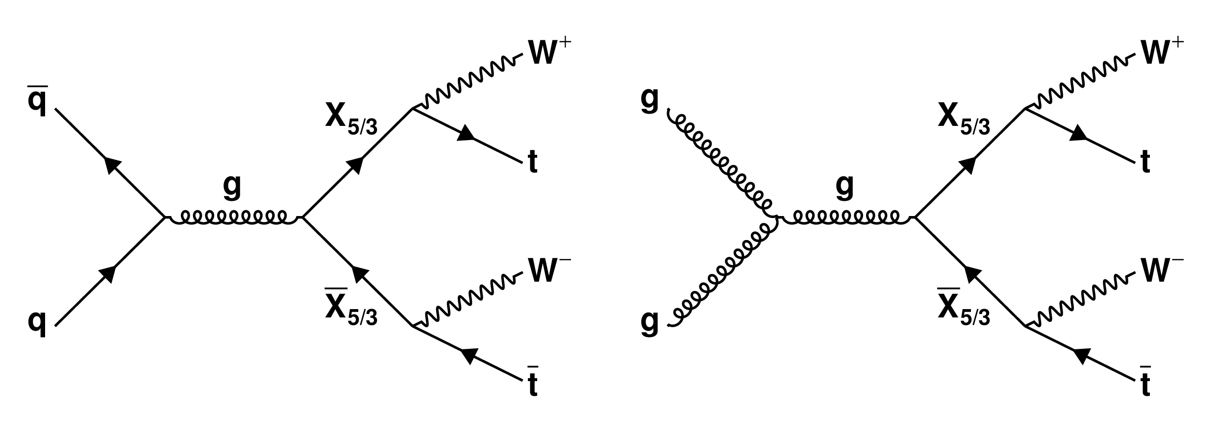
Figure 1:
Leading order Feynman diagrams showing pair production and decays of ${X_{5/3}} $ particles via QCD processes. |
png pdf |
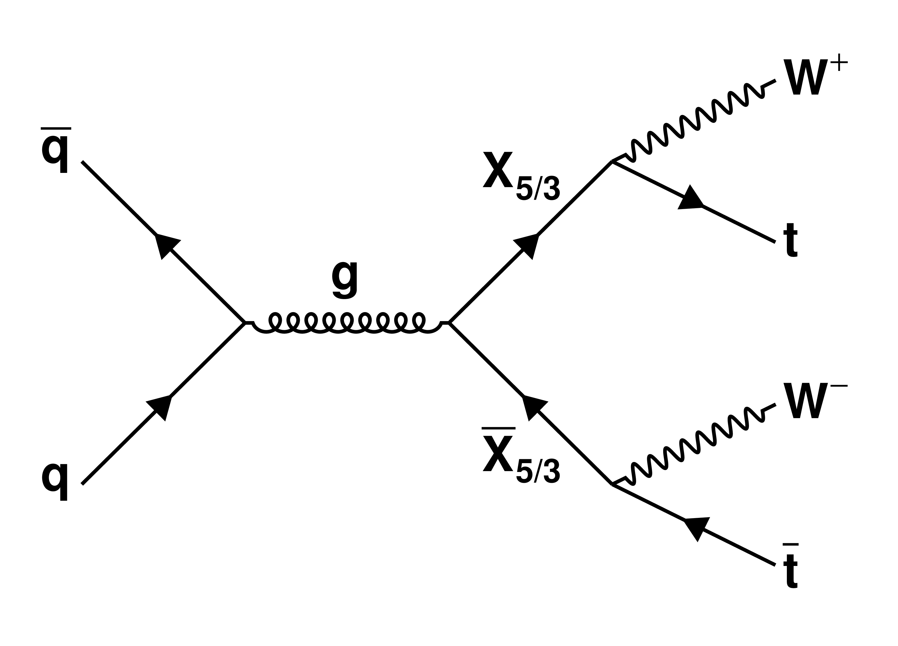
Figure 1-a:
Leading order Feynman diagram showing pair production and decays of ${X_{5/3}} $ particles via a QCD process. |
png pdf |
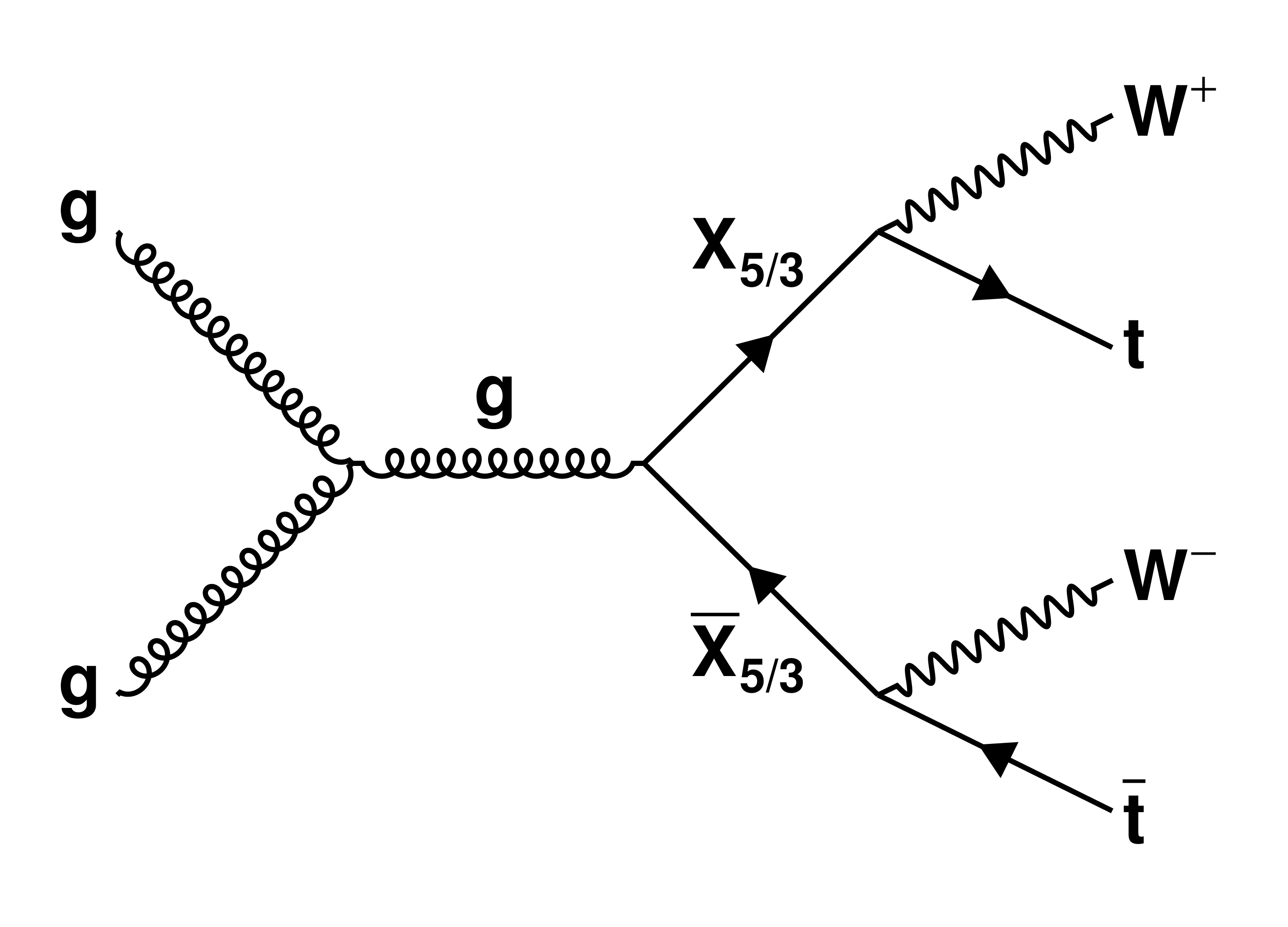
Figure 1-b:
Leading order Feynman diagram showing pair production and decays of ${X_{5/3}} $ particles via a QCD process. |
png pdf |
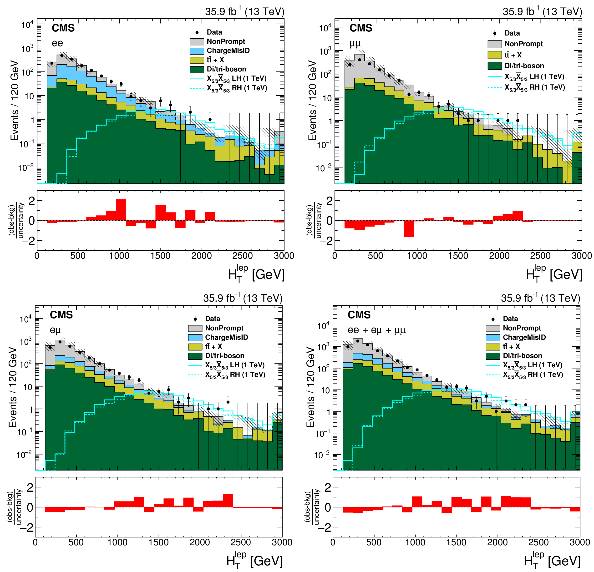
Figure 2:
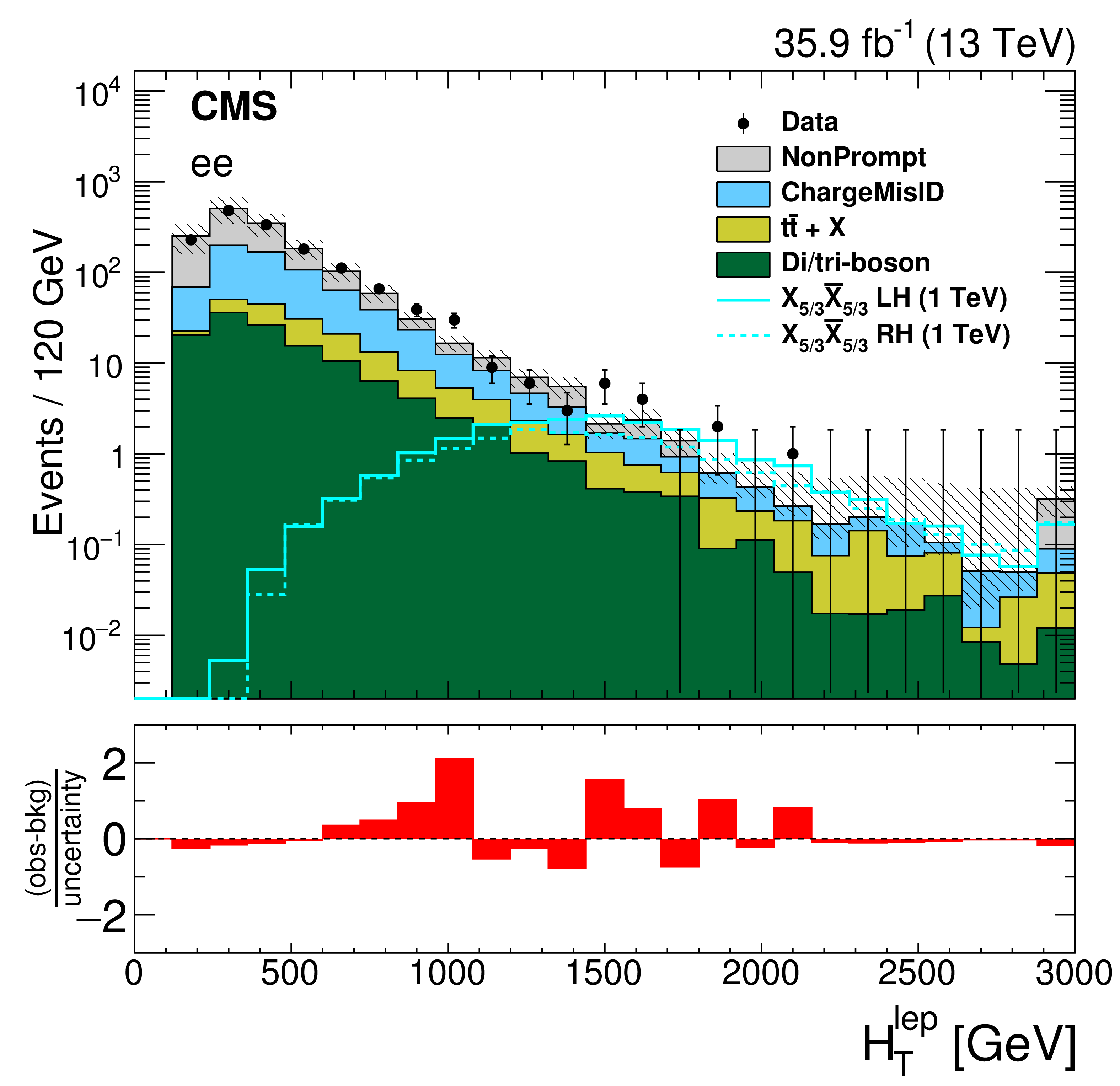
The $ {{H_{\mathrm {T}}} ^{\text {lep}}}$ distributions after the same-sign dilepton requirement, Z boson and quarkonia lepton invariant mass vetoes, and the requirement of at least two AK4 jets in the event, for dielectron (upper left), dimuon (upper right), electron-muon (lower left) final states, and their combination (lower right). The hatched area shows the combined systematic and statistical uncertainty in the background prediction for each bin. The last bin includes overflow events. The lower panel in each plot shows the difference between the observed and the predicted numbers of events divided by the total uncertainty. The total uncertainty is calculated as the sum in quadrature of the statistical uncertainty in the observed measurement and the uncertainty in the background, including both statistical and systematic components. Also shown are the expected signal distributions for a 1 TeV ${X_{5/3}} $ with LH (solid line) and RH (dashed line) couplings. |
png pdf |
Figure 2-a:
The $ {{H_{\mathrm {T}}} ^{\text {lep}}}$ distribution after the same-sign dilepton requirement, Z boson and quarkonia lepton invariant mass vetoes, and the requirement of at least two AK4 jets in the event, for the dielectron final state. The hatched area shows the combined systematic and statistical uncertainty in the background prediction for each bin. The last bin includes overflow events. The lower panel shows the difference between the observed and the predicted numbers of events divided by the total uncertainty. The total uncertainty is calculated as the sum in quadrature of the statistical uncertainty in the observed measurement and the uncertainty in the background, including both statistical and systematic components. Also shown are the expected signal distributions for a 1 TeV ${X_{5/3}} $ with LH (solid line) and RH (dashed line) couplings. |

png pdf |
Figure 2-b:
The $ {{H_{\mathrm {T}}} ^{\text {lep}}}$ distribution after the same-sign dilepton requirement, Z boson and quarkonia lepton invariant mass vetoes, and the requirement of at least two AK4 jets in the event, for the dimuon final state. The hatched area shows the combined systematic and statistical uncertainty in the background prediction for each bin. The last bin includes overflow events. The lower panel shows the difference between the observed and the predicted numbers of events divided by the total uncertainty. The total uncertainty is calculated as the sum in quadrature of the statistical uncertainty in the observed measurement and the uncertainty in the background, including both statistical and systematic components. Also shown are the expected signal distributions for a 1 TeV ${X_{5/3}} $ with LH (solid line) and RH (dashed line) couplings. |

png pdf |
Figure 2-c:
The $ {{H_{\mathrm {T}}} ^{\text {lep}}}$ distribution after the same-sign dilepton requirement, Z boson and quarkonia lepton invariant mass vetoes, and the requirement of at least two AK4 jets in the event, for the electron-muon final state. The hatched area shows the combined systematic and statistical uncertainty in the background prediction for each bin. The last bin includes overflow events. The lower panel shows the difference between the observed and the predicted numbers of events divided by the total uncertainty. The total uncertainty is calculated as the sum in quadrature of the statistical uncertainty in the observed measurement and the uncertainty in the background, including both statistical and systematic components. Also shown are the expected signal distributions for a 1 TeV ${X_{5/3}} $ with LH (solid line) and RH (dashed line) couplings. |
png pdf |
Figure 2-d:
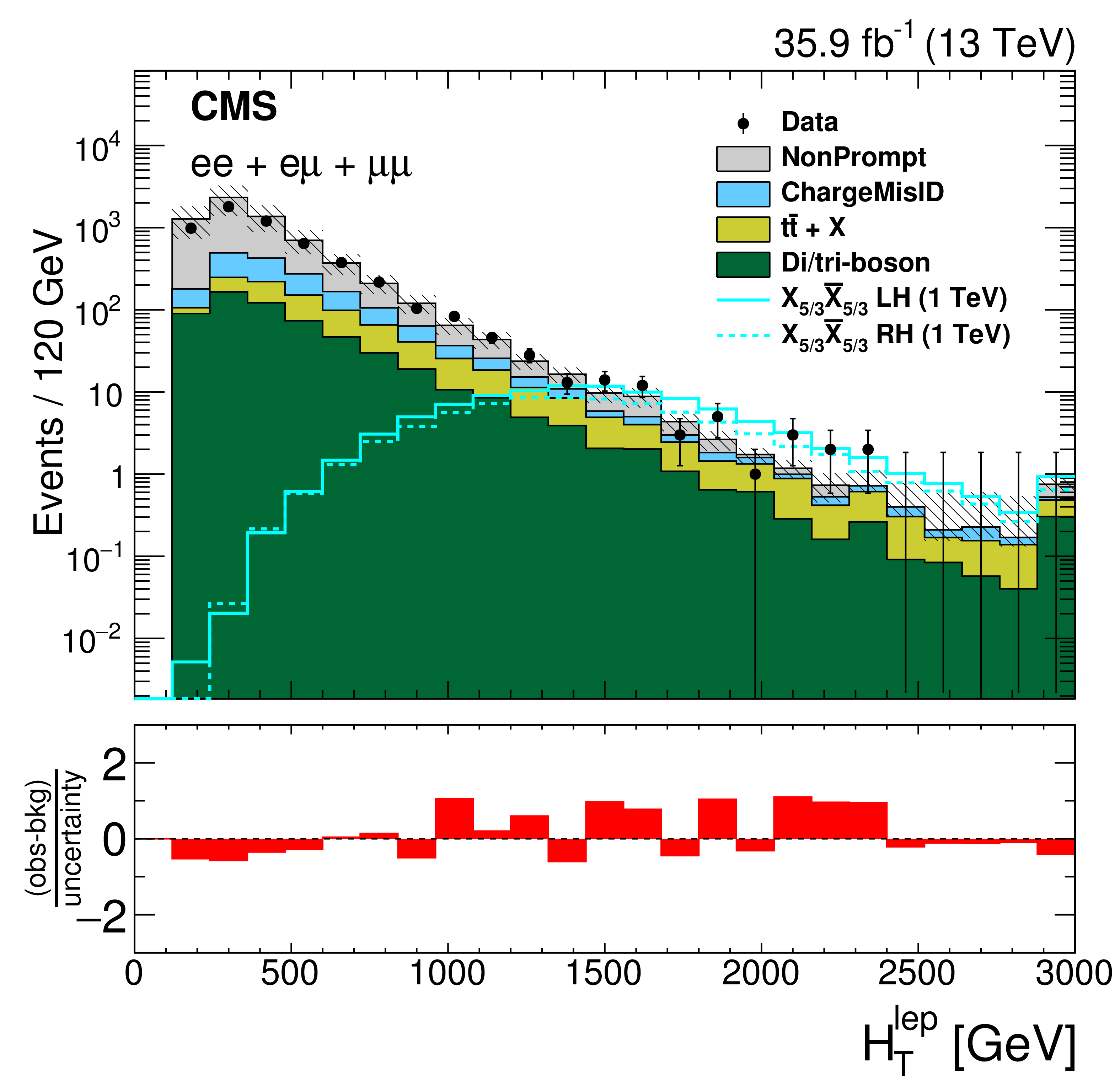
The $ {{H_{\mathrm {T}}} ^{\text {lep}}}$ distribution after the same-sign dilepton requirement, Z boson and quarkonia lepton invariant mass vetoes, and the requirement of at least two AK4 jets in the event, for the combination of dielectron, dimuon and electron-muon final states. The hatched area shows the combined systematic and statistical uncertainty in the background prediction for each bin. The last bin includes overflow events. The lower panel shows the difference between the observed and the predicted numbers of events divided by the total uncertainty. The total uncertainty is calculated as the sum in quadrature of the statistical uncertainty in the observed measurement and the uncertainty in the background, including both statistical and systematic components. Also shown are the expected signal distributions for a 1 TeV ${X_{5/3}} $ with LH (solid line) and RH (dashed line) couplings. |
png pdf |
Figure 3:
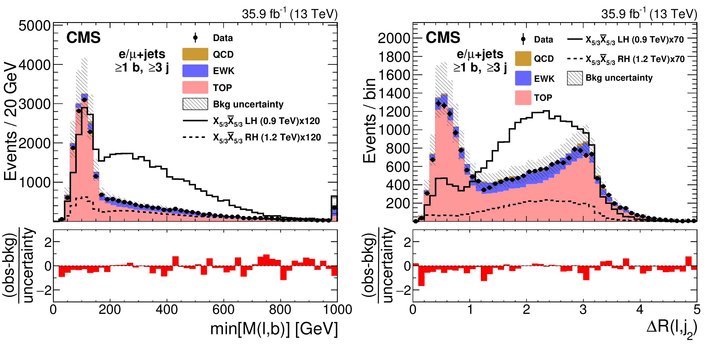
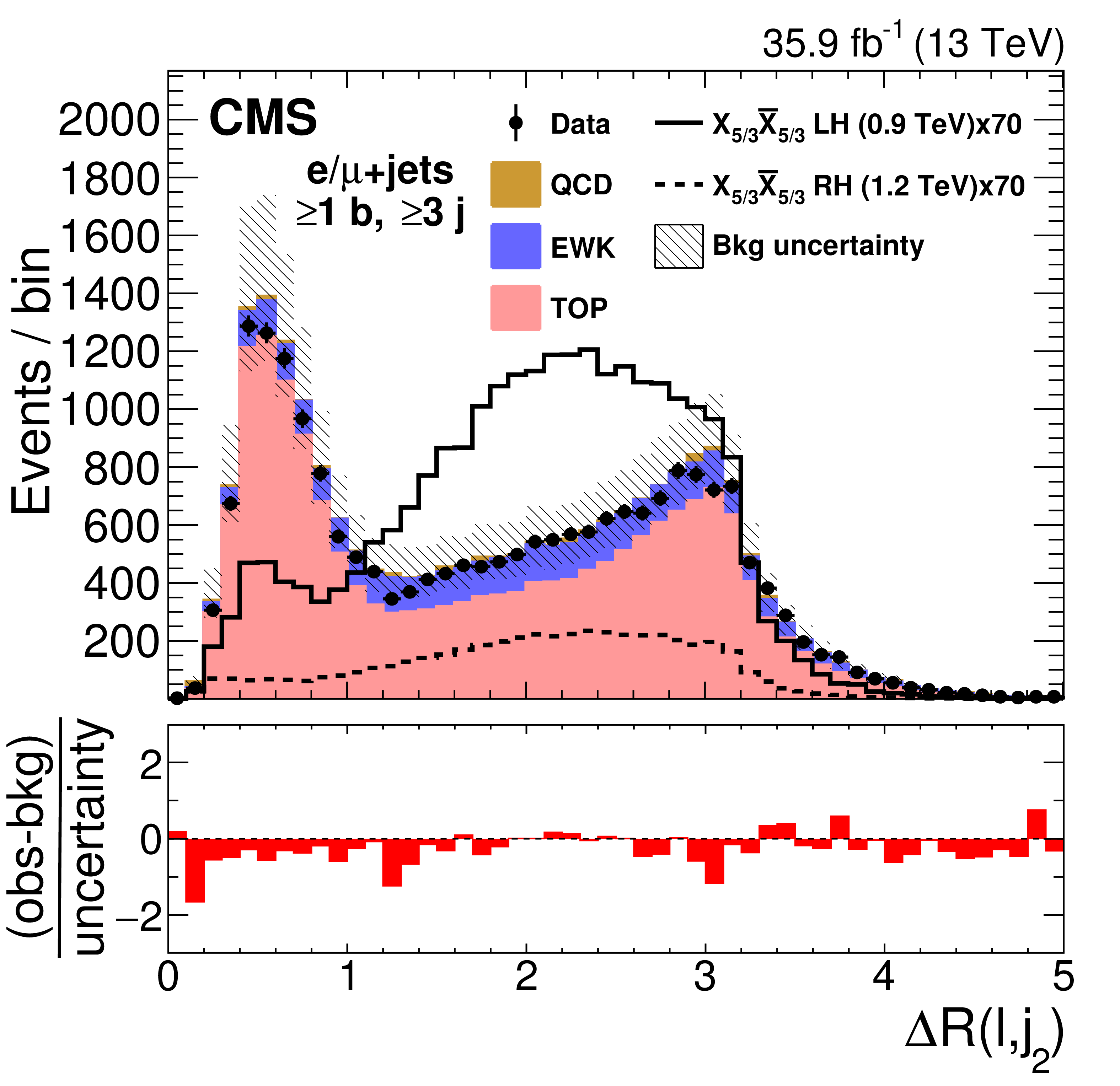
Distributions of ${\text{min}[M(\ell, {\mathrm {b}})]}$ (left) and ${\Delta R(\ell, \mathrm {j_{2})}}$ (right) in data and simulation for events with at least three AK4 jets, including a leading (subleading) jet with $ {p_{\mathrm {T}}} > $ 250 (150) GeV, after combining the electron and muon channels. Example signal distributions are also shown, scaled by a factor of 120 (70) in the ${\text{min}[M(\ell, {\mathrm {b}})]}$ (${\Delta R(\ell, \mathrm {j_{2})}}$) distribution. The last bin includes overflow events. The lower panel in each plot shows the difference between the observed and the predicted numbers of events in that bin divided by the total uncertainty. The total uncertainty is calculated as the sum in quadrature of the statistical uncertainty in the observed measurement and the statistical and systematic uncertainties in the background. |
png pdf |
Figure 3-a:
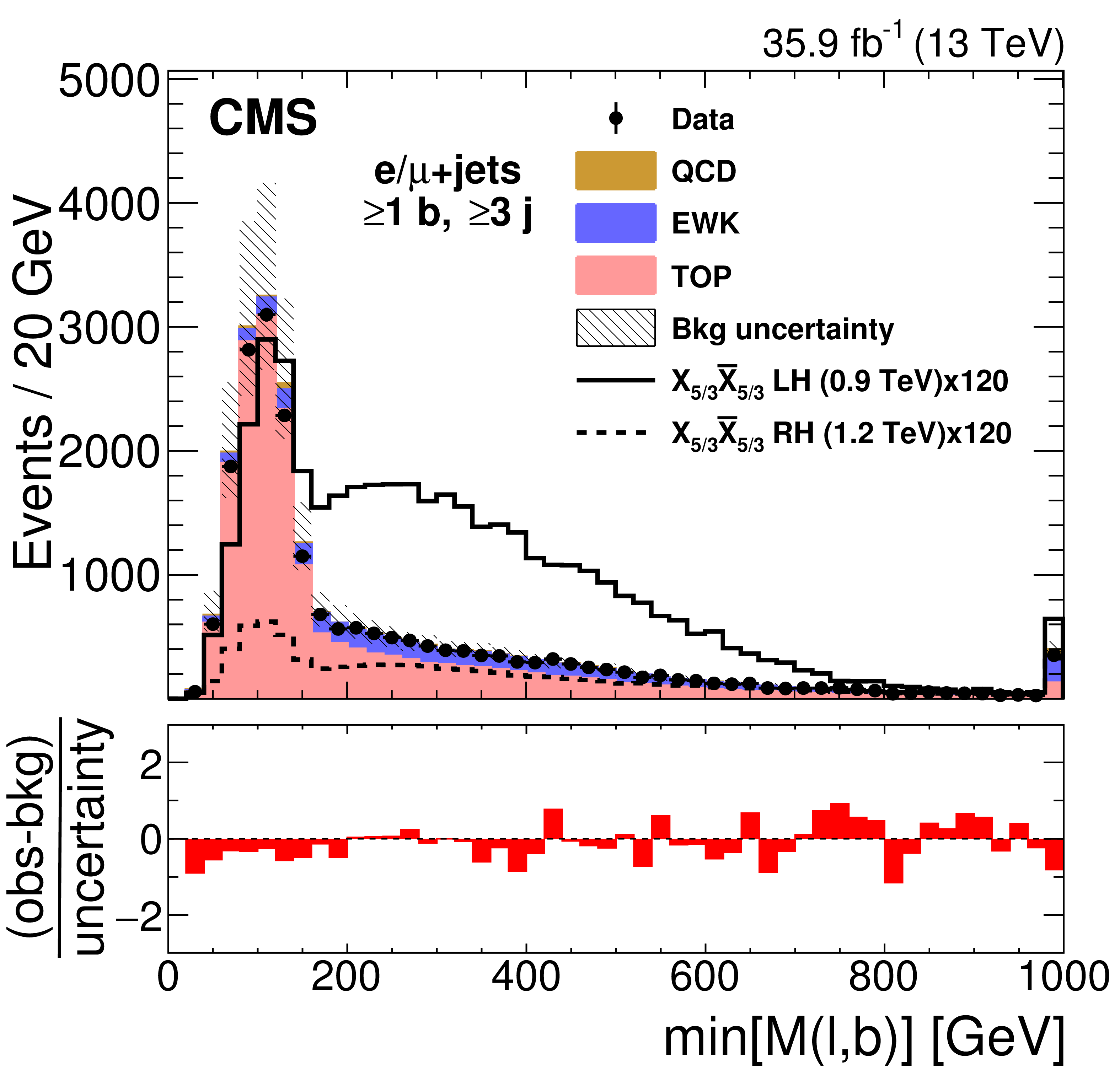
Distribution of ${\text{min}[M(\ell, {\mathrm {b}})]}$ in data and simulation for events with at least three AK4 jets, including a leading (subleading) jet with $ {p_{\mathrm {T}}} > $ 250 (150) GeV, after combining the electron and muon channels. Example signal distributions are also shown, scaled by a factor of 120 in the ${\text{min}[M(\ell, {\mathrm {b}})]}$ distribution. The last bin includes overflow events. The lower panel shows the difference between the observed and the predicted numbers of events in that bin divided by the total uncertainty. The total uncertainty is calculated as the sum in quadrature of the statistical uncertainty in the observed measurement and the statistical and systematic uncertainties in the background. |
png pdf |
Figure 3-b:
Distribution of ${\Delta R(\ell, \mathrm {j_{2})}}$ in data and simulation for events with at least three AK4 jets, including a leading (subleading) jet with $ {p_{\mathrm {T}}} > $ 250 (150) GeV, after combining the electron and muon channels. Example signal distributions are also shown, scaled by a factor of 70 in the ${\Delta R(\ell, \mathrm {j_{2})}}$ distribution. The last bin includes overflow events. The lower panel shows the difference between the observed and the predicted numbers of events in that bin divided by the total uncertainty. The total uncertainty is calculated as the sum in quadrature of the statistical uncertainty in the observed measurement and the statistical and systematic uncertainties in the background. |
png pdf |
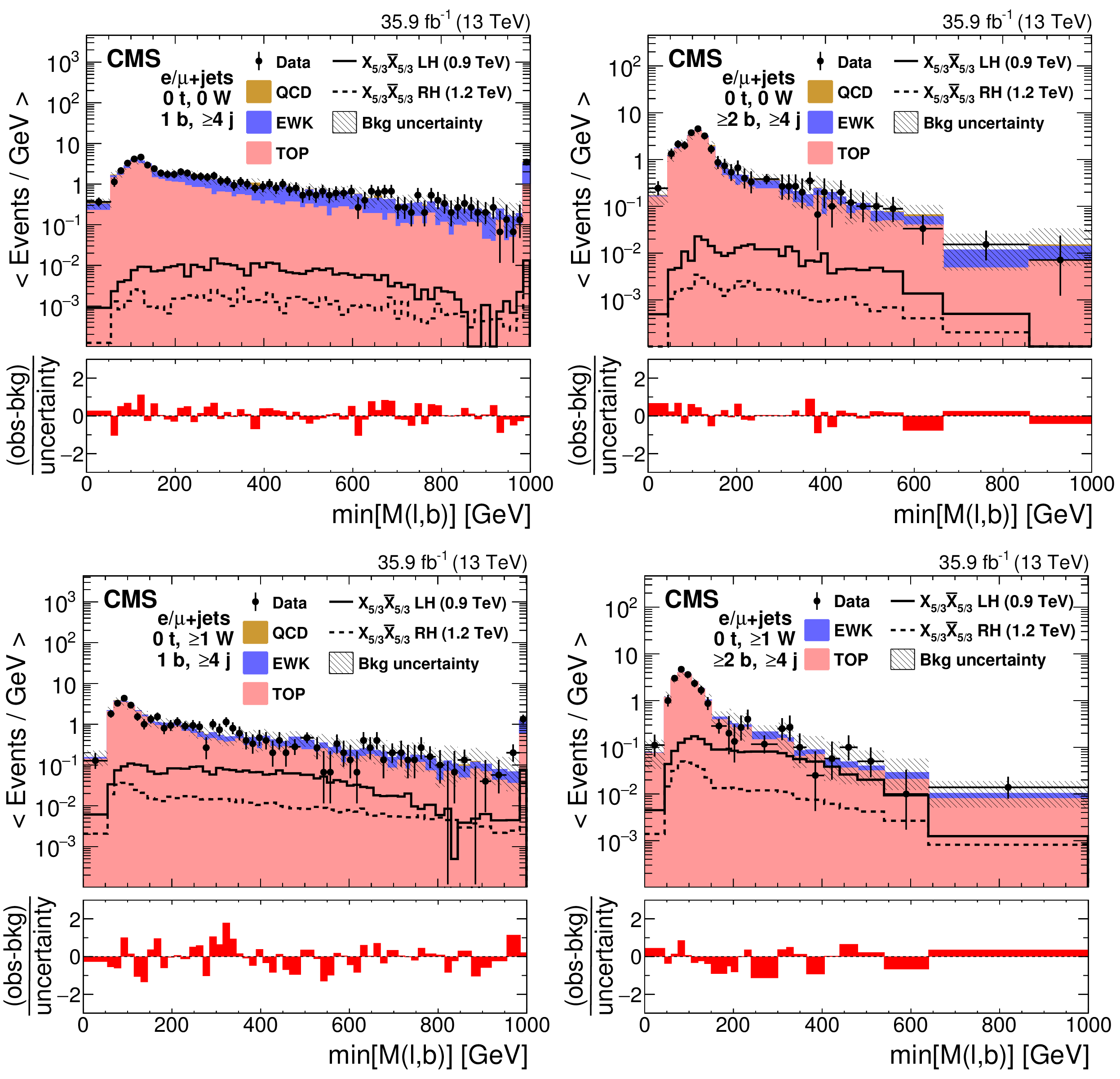
Figure 4:
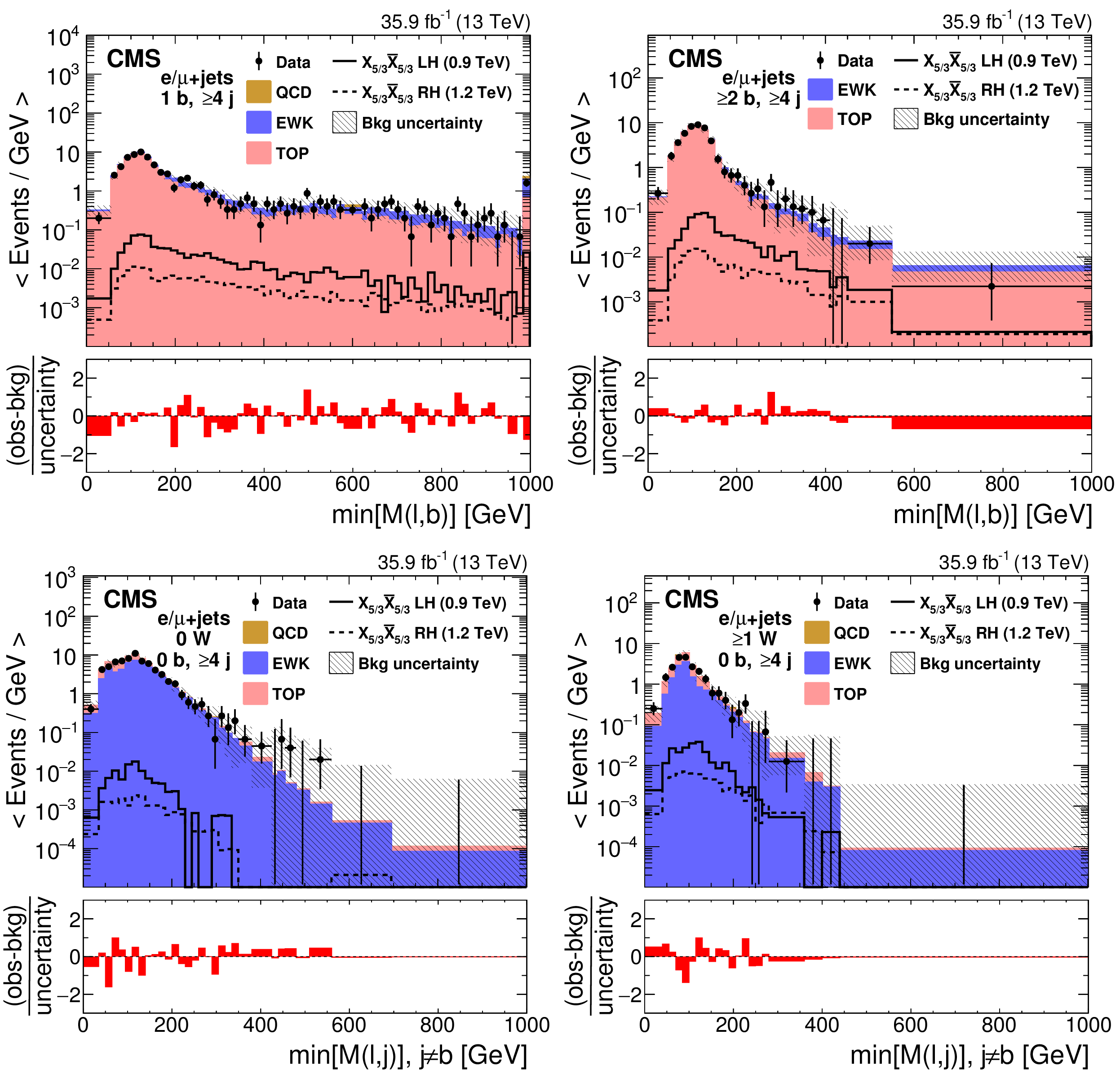
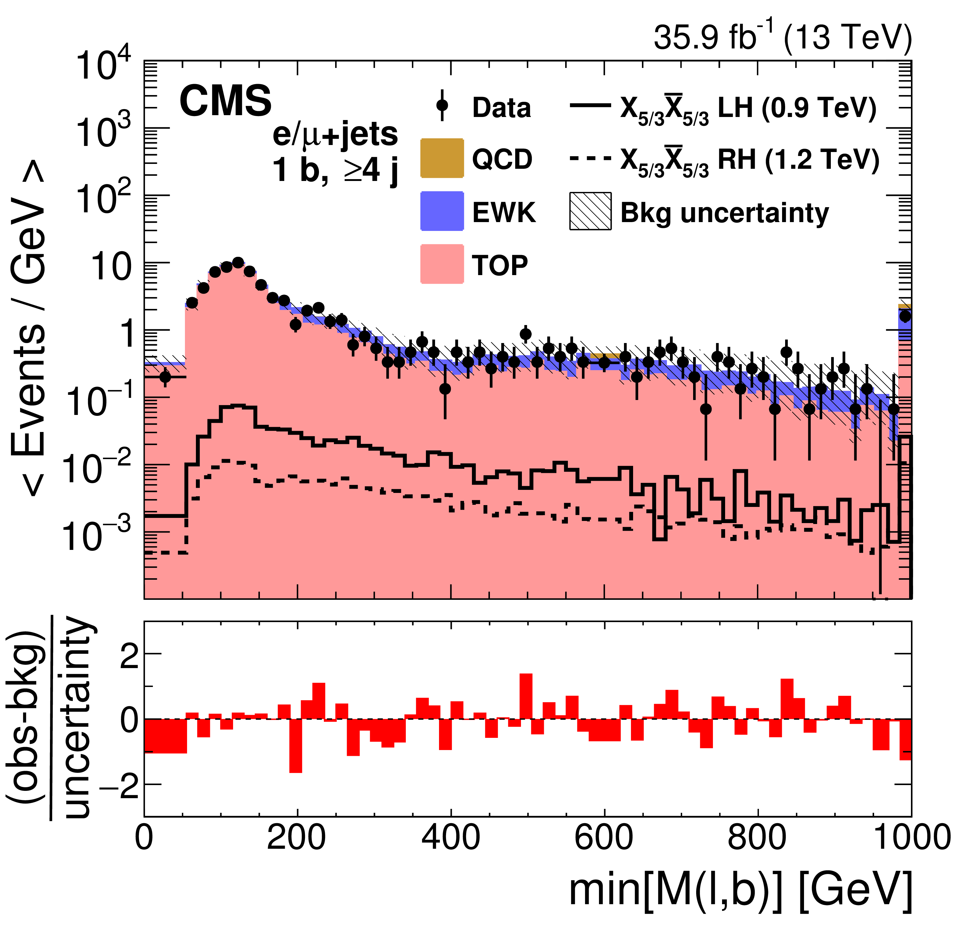
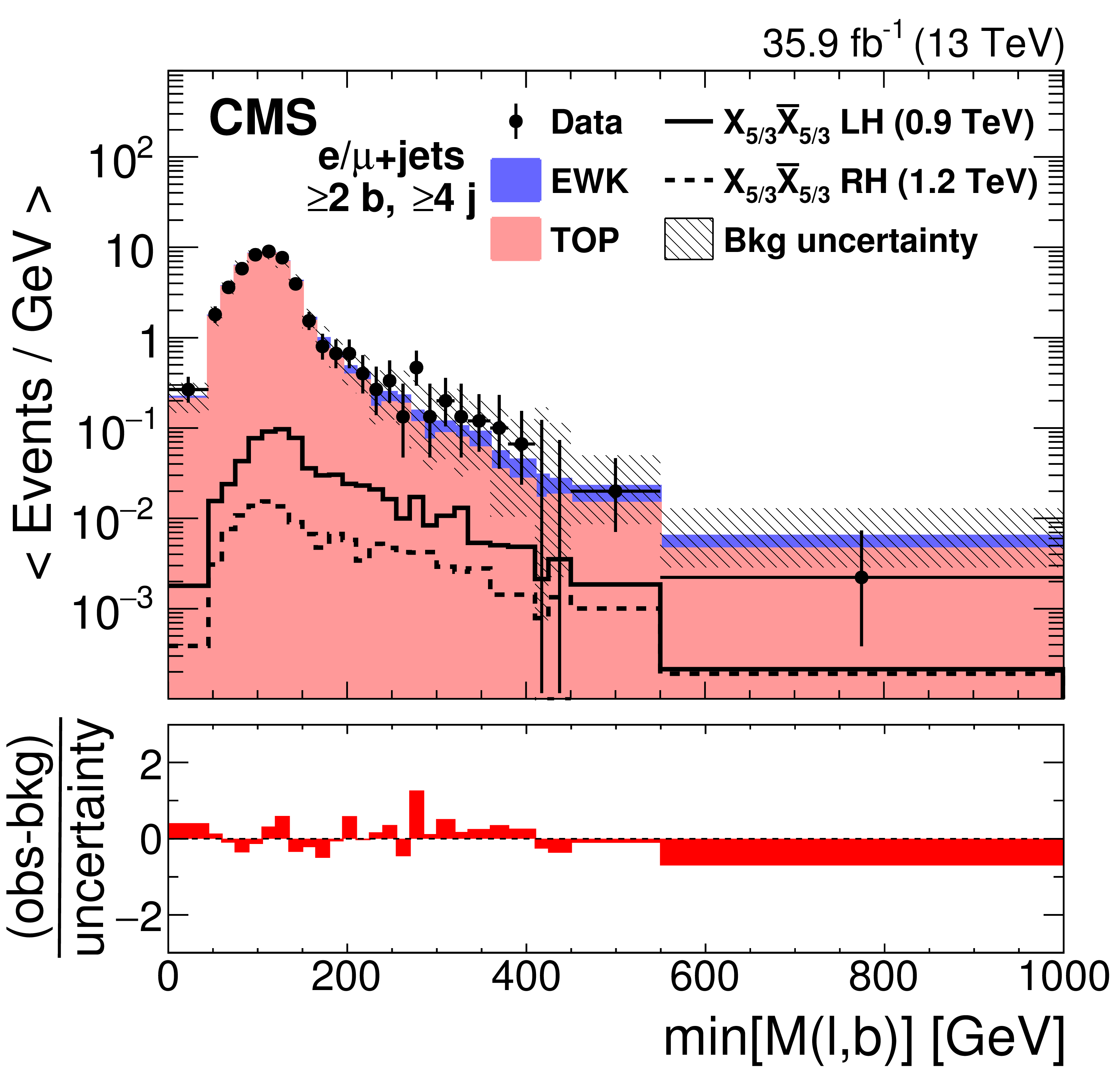
Distributions of ${\text{min}[M(\ell, {\mathrm {b}})]}$ in the $ {{\mathrm {t}\overline {\mathrm {t}}}} $ control region, for 1 b-tagged jet (upper left) and $\ge $2 b-tagged jets (upper right) categories, and of ${\text{min}[M(\ell, {\mathrm {j}})]}$ in the W+jets control region, for 0 W-tagged jets (lower left) and $\ge $1 W-tagged jets (lower right) categories. Example signal distributions are also shown. The background distributions correspond to background-only fit to data while signal distributions are before the fit to data. Electron and muon event samples are combined. The last bin includes overflow events and its content is divided by the bin width. The distributions in each category have variable-size bins, chosen so that the statistical uncertainty in the total background in each bin is less than 30%. The lower panel in each plot shows the difference between the observed and the predicted numbers of events in that bin divided by the total uncertainty. The total uncertainty is calculated as the sum in quadrature of the statistical uncertainty in the observed measurement and the statistical and systematic uncertainties in the background-only fit to data. |
png pdf |
Figure 4-a:
Distribution of ${\text{min}[M(\ell, {\mathrm {b}})]}$ in the $ {{\mathrm {t}\overline {\mathrm {t}}}} $ control region, for the 1 b-tagged jet category. Example signal distributions are also shown. The background distributions correspond to background-only fit to data while signal distributions are before the fit to data. Electron and muon event samples are combined. The last bin includes overflow events and its content is divided by the bin width. The distributions have variable-size bins, chosen so that the statistical uncertainty in the total background in each bin is less than 30%. The lower panel shows the difference between the observed and the predicted numbers of events in that bin divided by the total uncertainty. The total uncertainty is calculated as the sum in quadrature of the statistical uncertainty in the observed measurement and the statistical and systematic uncertainties in the background-only fit to data. |
png pdf |
Figure 4-b:
Distribution of ${\text{min}[M(\ell, {\mathrm {b}})]}$ in the $ {{\mathrm {t}\overline {\mathrm {t}}}} $ control region, for the $\ge $2 b-tagged jets category. Example signal distributions are also shown. The background distributions correspond to background-only fit to data while signal distributions are before the fit to data. Electron and muon event samples are combined. The last bin includes overflow events and its content is divided by the bin width. The distributions have variable-size bins, chosen so that the statistical uncertainty in the total background in each bin is less than 30%. The lower panel shows the difference between the observed and the predicted numbers of events in that bin divided by the total uncertainty. The total uncertainty is calculated as the sum in quadrature of the statistical uncertainty in the observed measurement and the statistical and systematic uncertainties in the background-only fit to data. |
png pdf |
Figure 4-c:
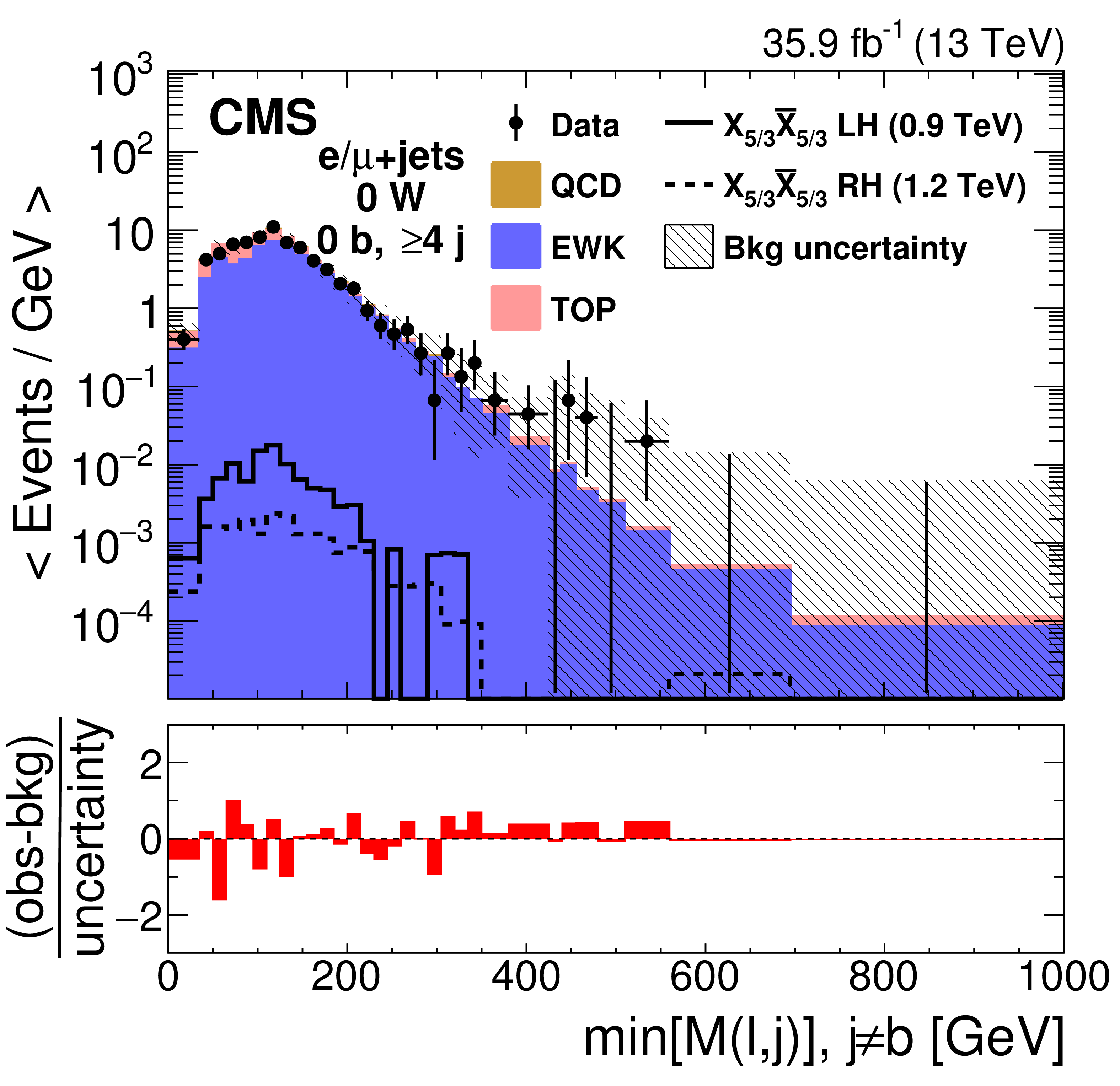
Distribution of ${\text{min}[M(\ell, {\mathrm {j}})]}$ in the W+jets control region, for the 0 W-tagged jet category. Example signal distributions are also shown. The background distributions correspond to background-only fit to data while signal distributions are before the fit to data. Electron and muon event samples are combined. The last bin includes overflow events and its content is divided by the bin width. The distributions have variable-size bins, chosen so that the statistical uncertainty in the total background in each bin is less than 30%. The lower panel shows the difference between the observed and the predicted numbers of events in that bin divided by the total uncertainty. The total uncertainty is calculated as the sum in quadrature of the statistical uncertainty in the observed measurement and the statistical and systematic uncertainties in the background-only fit to data. |

png pdf |
Figure 4-d:
Distribution of ${\text{min}[M(\ell, {\mathrm {j}})]}$ in the W+jets control region, for the $\ge $1 W-tagged jet category. Example signal distributions are also shown. The background distributions correspond to background-only fit to data while signal distributions are before the fit to data. Electron and muon event samples are combined. The last bin includes overflow events and its content is divided by the bin width. The distributions have variable-size bins, chosen so that the statistical uncertainty in the total background in each bin is less than 30%. The lower panel shows the difference between the observed and the predicted numbers of events in that bin divided by the total uncertainty. The total uncertainty is calculated as the sum in quadrature of the statistical uncertainty in the observed measurement and the statistical and systematic uncertainties in the background-only fit to data. |
png pdf |
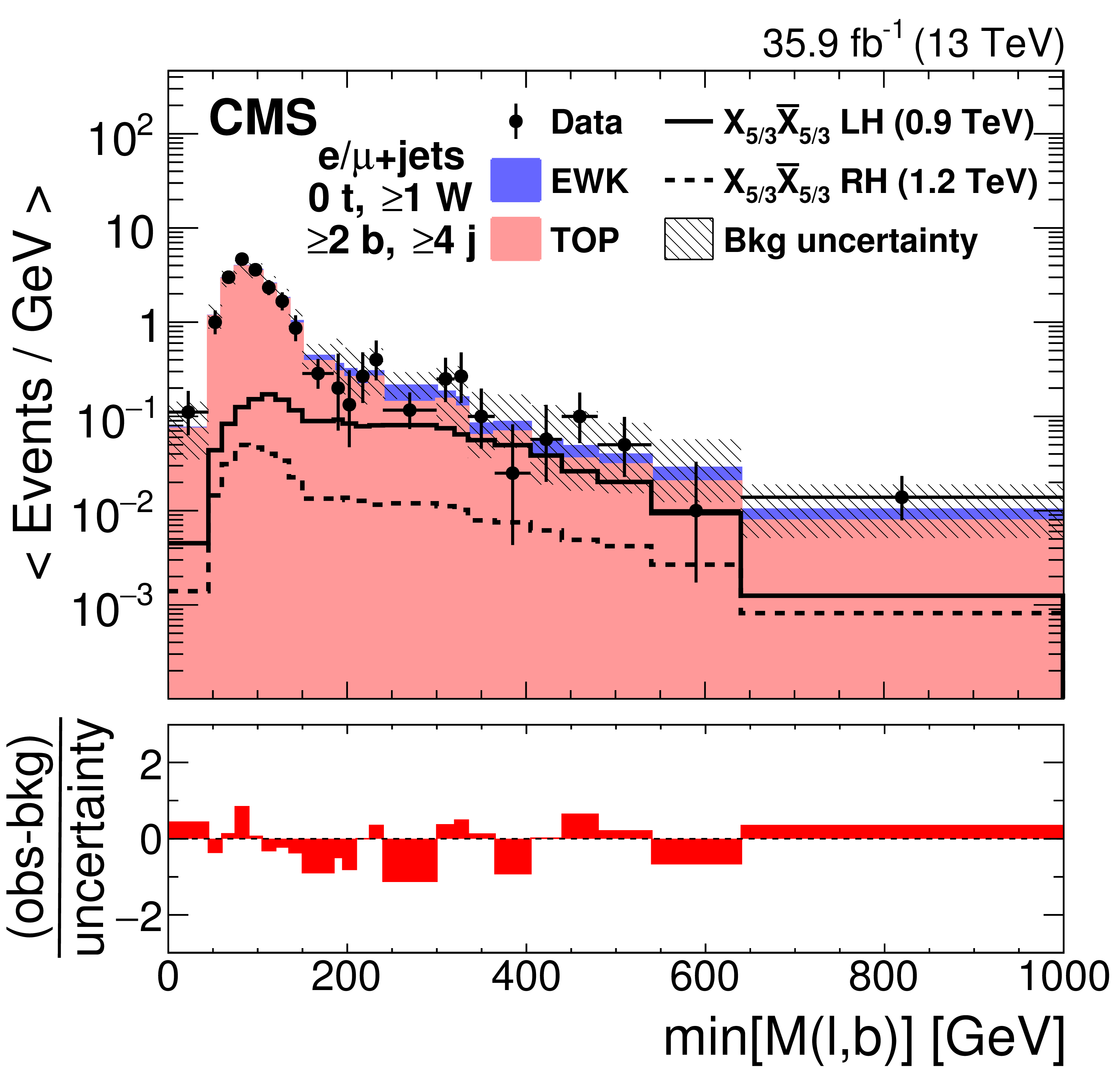
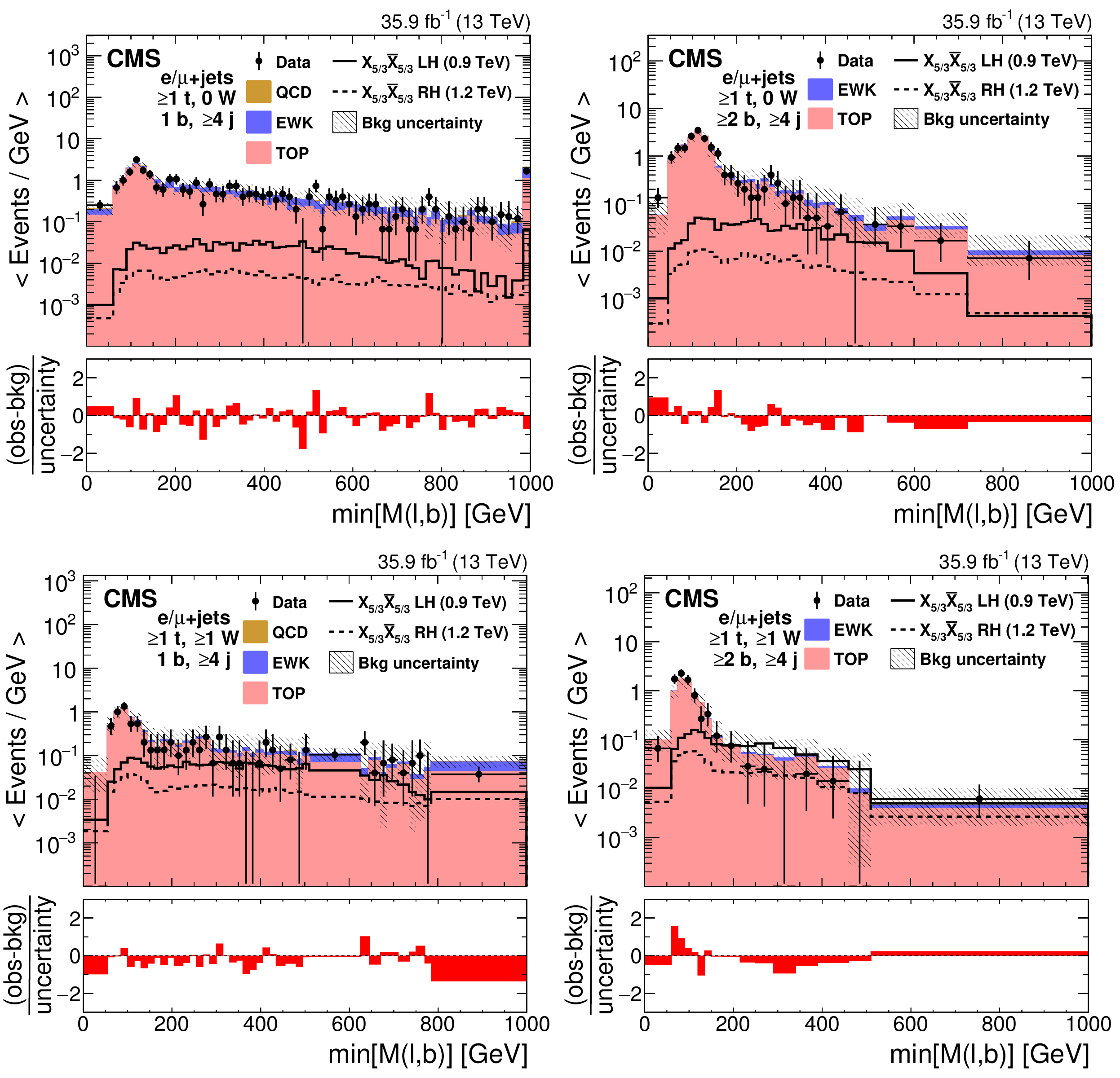
Figure 5:
Distributions of ${\text{min}[M(\ell, {\mathrm {b}})]}$ in events with 0 t-tagged jets, 0 (upper) or $\geq $1 (lower) W-tagged jets, and 1 (left) or $\geq $2 (right) b-tagged jets for the combined electron and muon samples in the signal region. Example signal distributions are also shown. The background distributions correspond to the background-only fit to data, while signal distributions are before the fit to data. The last bin includes overflow events and its content is divided by the bin width. The distributions in each category have variable-size bins, chosen so that the statistical uncertainty in the total background in each bin is less than 30%. The lower panel in each plot shows the difference between the observed and the predicted numbers of events in that bin divided by the total uncertainty. The total uncertainty is calculated as the sum in quadrature of the statistical uncertainty in the observed measurement and the statistical and systematic uncertainties in the background-only fit to data. |
png pdf |
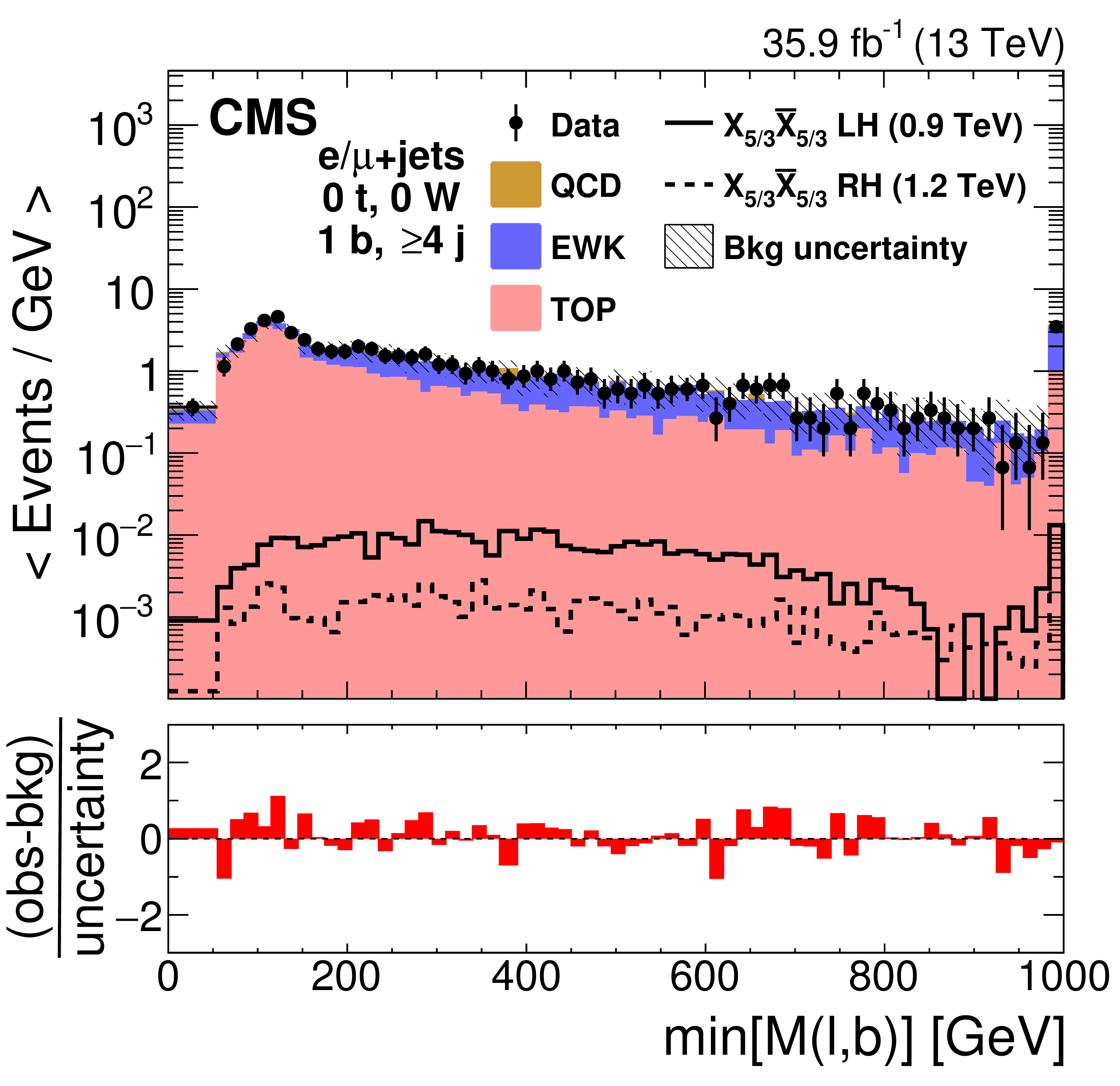
Figure 5-a:
Distribution of ${\text{min}[M(\ell, {\mathrm {b}})]}$ in events with 0 t-tagged jets, 0 W-tagged jet and 1 b-tagged jet, for the combined electron and muon samples in the signal region. Example signal distributions are also shown. The background distributions correspond to the background-only fit to data, while signal distribution is before the fit to data. The last bin includes overflow events and its content is divided by the bin width. The distributions have variable-size bins, chosen so that the statistical uncertainty in the total background in each bin is less than 30%. The lower panel shows the difference between the observed and the predicted numbers of events in that bin divided by the total uncertainty. The total uncertainty is calculated as the sum in quadrature of the statistical uncertainty in the observed measurement and the statistical and systematic uncertainties in the background-only fit to data. |
png pdf |
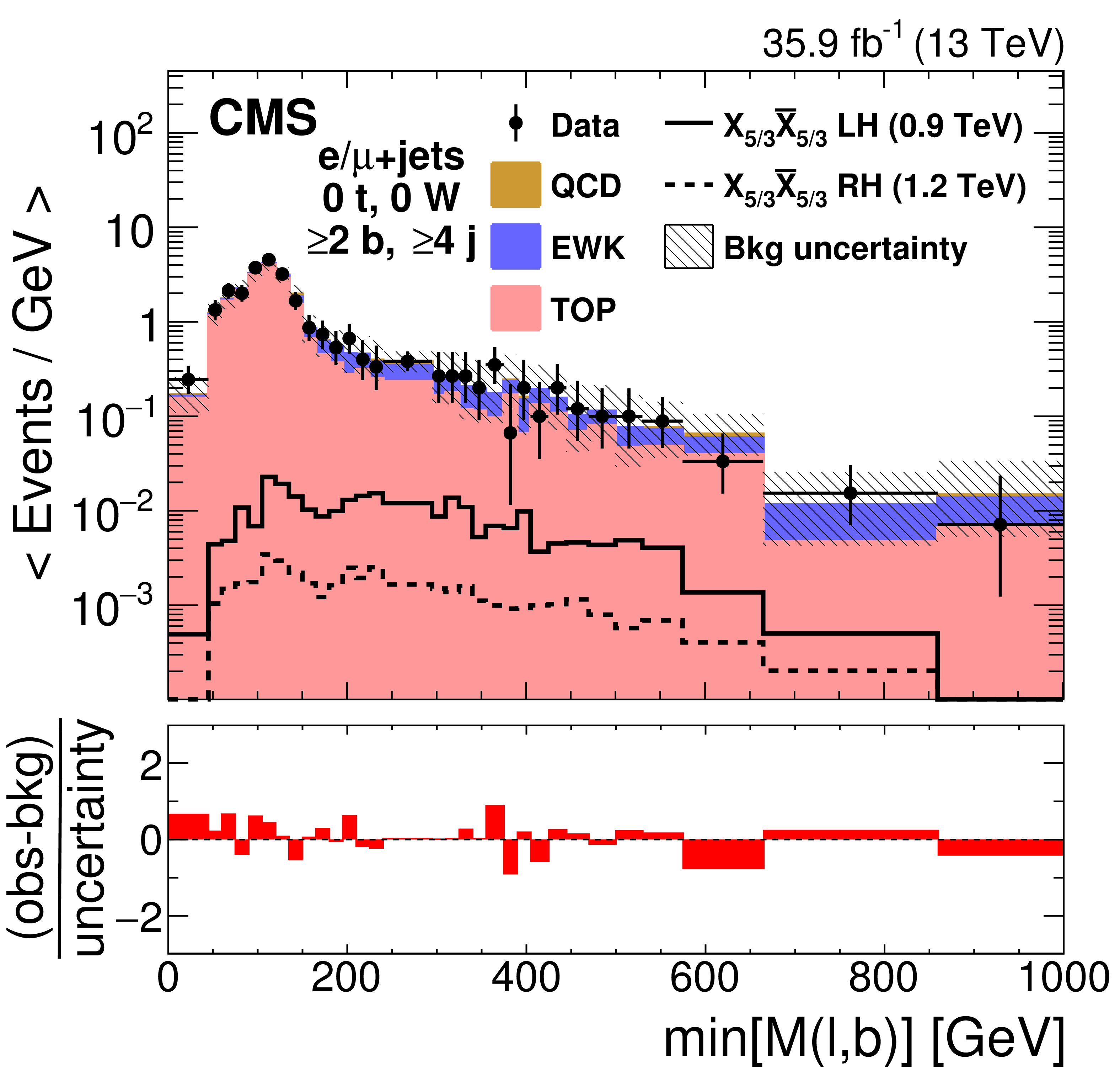
Figure 5-b:
Distribution of ${\text{min}[M(\ell, {\mathrm {b}})]}$ in events with 0 t-tagged jets, 0 W-tagged jet and $\geq $2 b-tagged jets, for the combined electron and muon samples in the signal region. Example signal distributions are also shown. The background distributions correspond to the background-only fit to data, while signal distribution is before the fit to data. The last bin includes overflow events and its content is divided by the bin width. The distributions have variable-size bins, chosen so that the statistical uncertainty in the total background in each bin is less than 30%. The lower panel shows the difference between the observed and the predicted numbers of events in that bin divided by the total uncertainty. The total uncertainty is calculated as the sum in quadrature of the statistical uncertainty in the observed measurement and the statistical and systematic uncertainties in the background-only fit to data. |

png pdf |
Figure 5-c:
Distribution of ${\text{min}[M(\ell, {\mathrm {b}})]}$ in events with 0 t-tagged jets, $\geq $1 W-tagged jet and1 b-tagged jet, for the combined electron and muon samples in the signal region. Example signal distributions are also shown. The background distributions correspond to the background-only fit to data, while signal distribution is before the fit to data. The last bin includes overflow events and its content is divided by the bin width. The distributions have variable-size bins, chosen so that the statistical uncertainty in the total background in each bin is less than 30%. The lower panel shows the difference between the observed and the predicted numbers of events in that bin divided by the total uncertainty. The total uncertainty is calculated as the sum in quadrature of the statistical uncertainty in the observed measurement and the statistical and systematic uncertainties in the background-only fit to data. |
png pdf |
Figure 5-d:
Distribution of ${\text{min}[M(\ell, {\mathrm {b}})]}$ in events with 0 t-tagged jets, $\geq $1 W-tagged jet and $\geq $2 b-tagged jets, for the combined electron and muon samples in the signal region. Example signal distributions are also shown. The background distributions correspond to the background-only fit to data, while signal distribution is before the fit to data. The last bin includes overflow events and its content is divided by the bin width. The distributions have variable-size bins, chosen so that the statistical uncertainty in the total background in each bin is less than 30%. The lower panel shows the difference between the observed and the predicted numbers of events in that bin divided by the total uncertainty. The total uncertainty is calculated as the sum in quadrature of the statistical uncertainty in the observed measurement and the statistical and systematic uncertainties in the background-only fit to data. |
png pdf |
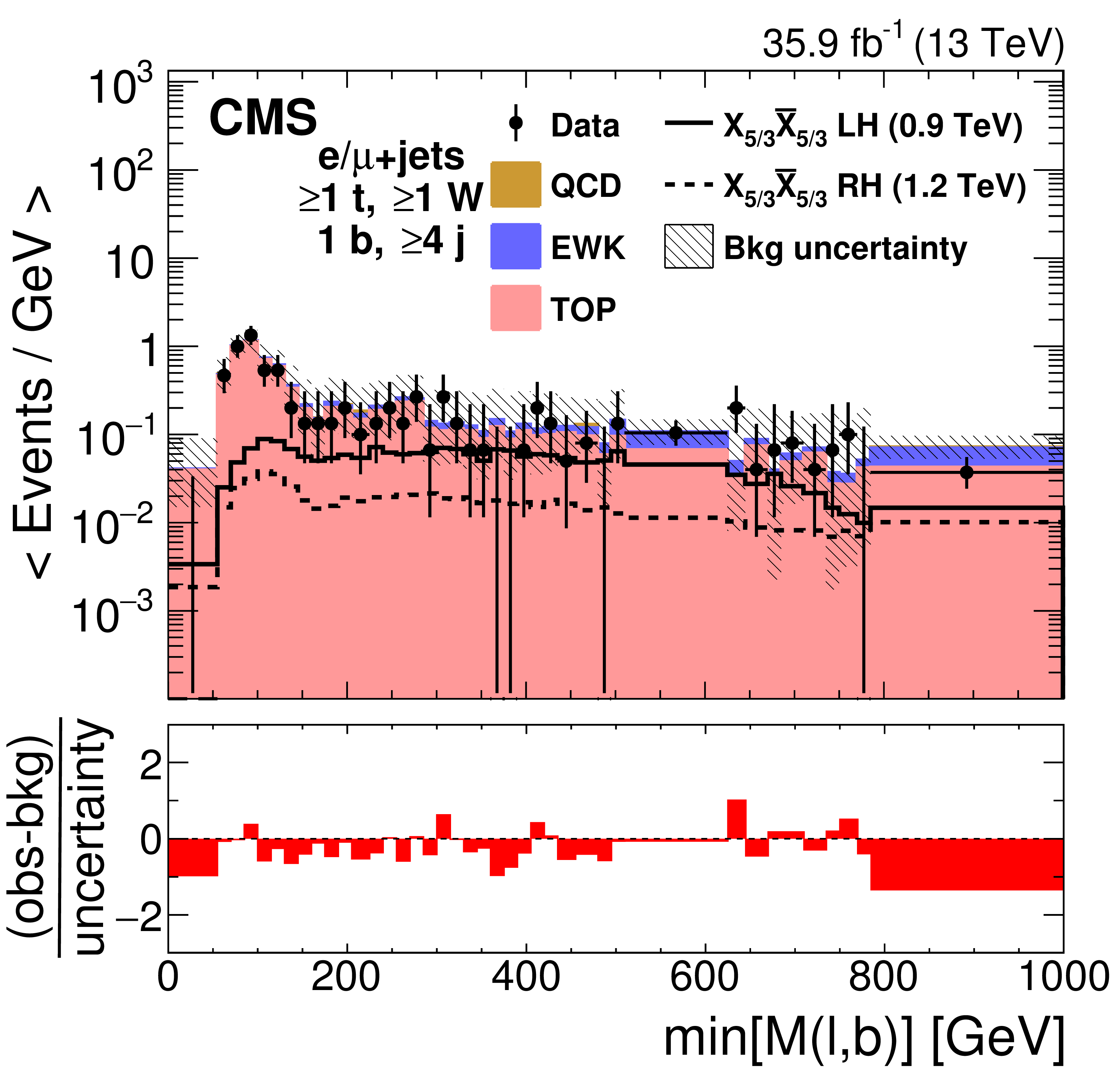
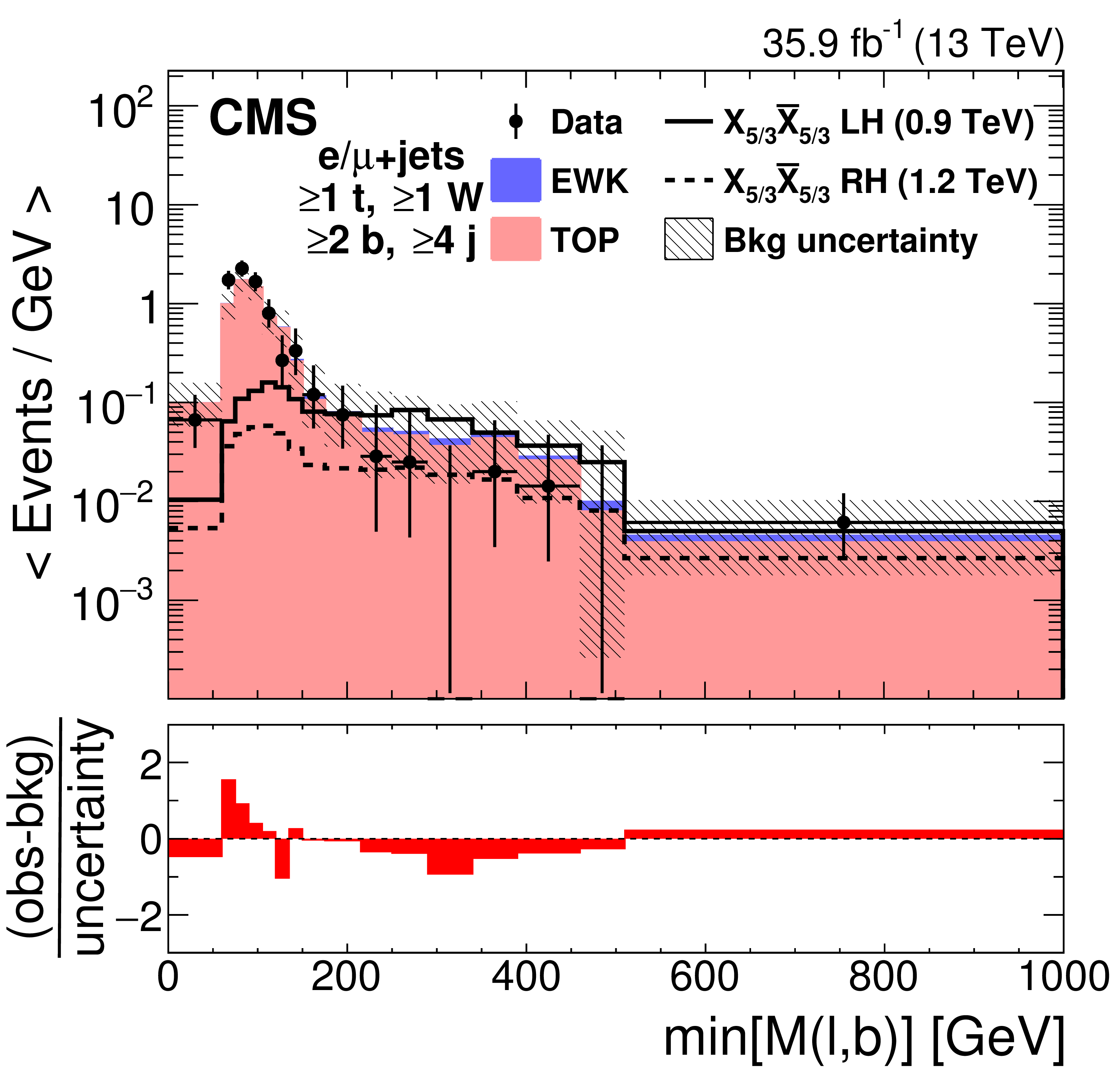
Figure 6:
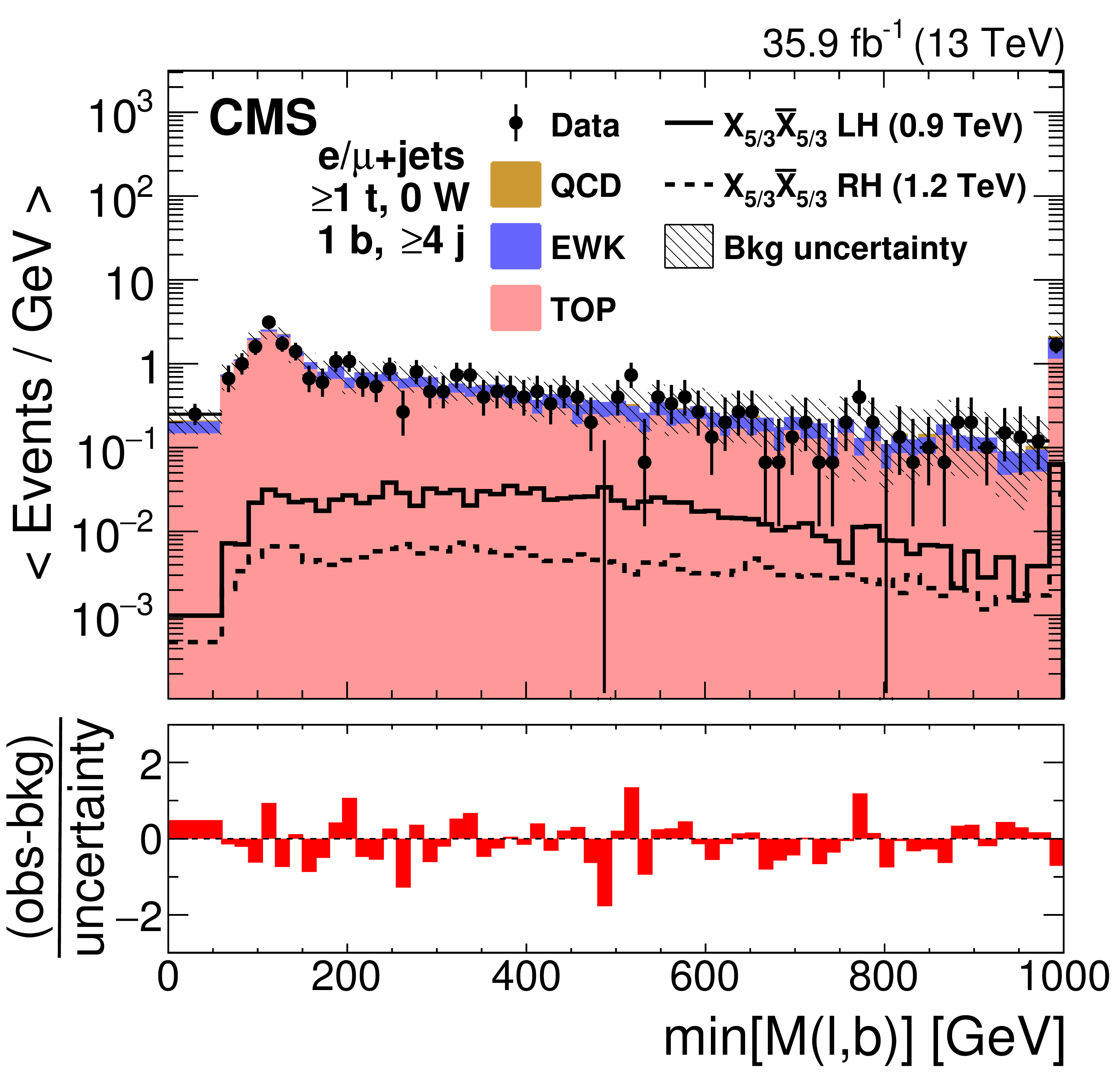
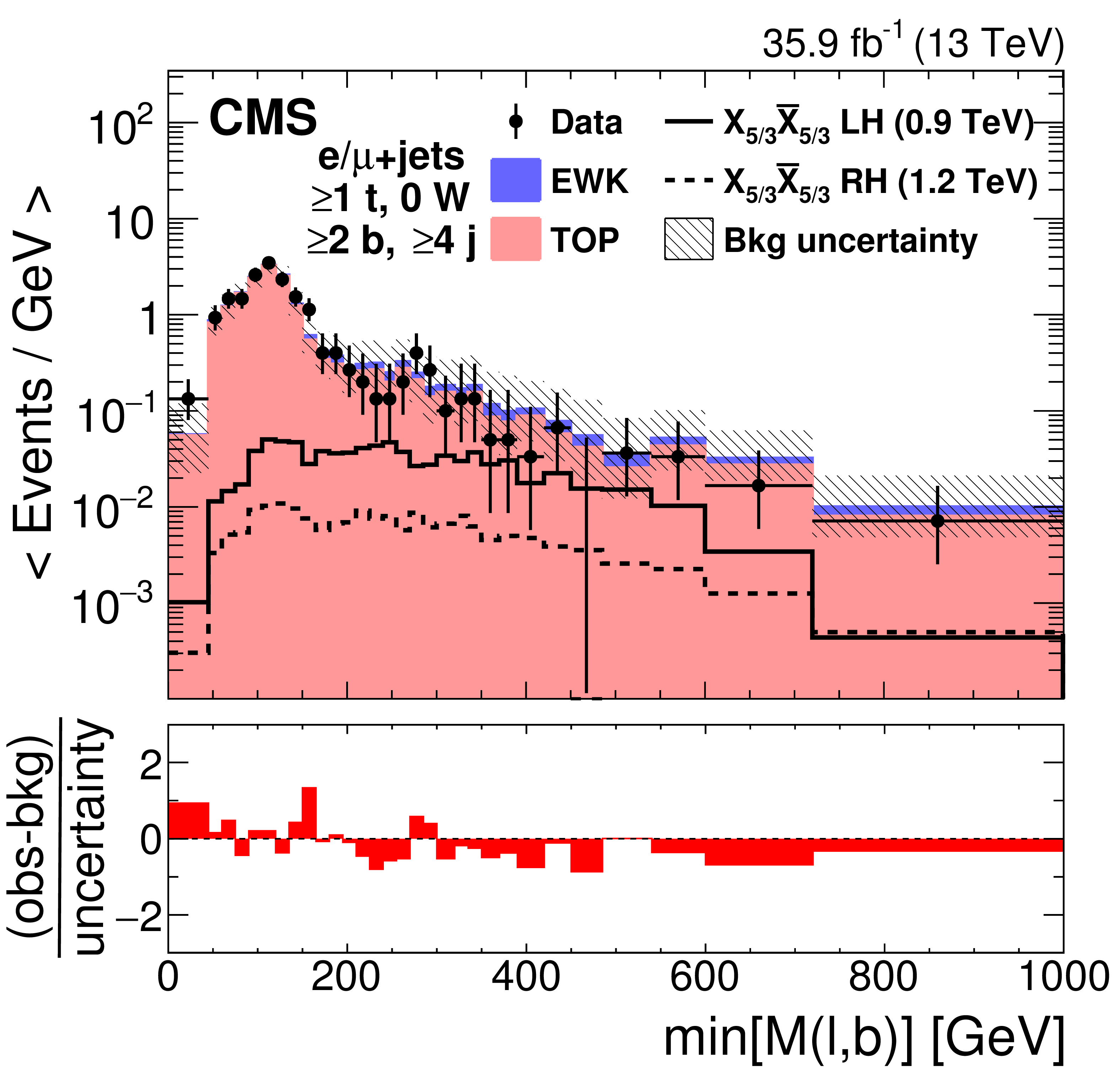
Distributions of ${\text{min}[M(\ell, {\mathrm {b}})]}$ in events with $\geq $1 t-tagged jets, 0 (upper) or $\geq $1 (lower) W-tagged jets, and 1 (left) or $\geq $2 (right) b-tagged jets for the combined electron and muon samples in the signal region. Example signal distributions are also shown. The background distributions correspond to the background-only fit to data, while signal distributions are before the fit to data. The last bin includes overflow events and its content is divided by the bin width. The distributions in each category have variable-size bins, chosen so that the statistical uncertainty in the total background in each bin is less than 30%. The lower panel in each plot shows the difference between the observed and the predicted numbers of events in that bin divided by the total uncertainty. The total uncertainty is calculated as the sum in quadrature of the statistical uncertainty in the observed measurement and the statistical and systematic uncertainties in the background-only fit to data. |
png pdf |
Figure 6-a:
Distribution of ${\text{min}[M(\ell, {\mathrm {b}})]}$ in events with $\geq $1 t-tagged jets, 0 W-tagged jet and 1 b-tagged jet, for the combined electron and muon samples in the signal region. Example signal distributions are also shown. The background distributions correspond to the background-only fit to data, while the signal distribution is before the fit to data. The last bin includes overflow events and its content is divided by the bin width. The distributions have variable-size bins, chosen so that the statistical uncertainty in the total background in each bin is less than 30%. The lower panel shows the difference between the observed and the predicted numbers of events in that bin divided by the total uncertainty. The total uncertainty is calculated as the sum in quadrature of the statistical uncertainty in the observed measurement and the statistical and systematic uncertainties in the background-only fit to data. |
png pdf |
Figure 6-b:
Distribution of ${\text{min}[M(\ell, {\mathrm {b}})]}$ in events with $\geq $1 t-tagged jets, 0 W-tagged jet and $\geq $2 b-tagged jets, for the combined electron and muon samples in the signal region. Example signal distributions are also shown. The background distributions correspond to the background-only fit to data, while the signal distribution is before the fit to data. The last bin includes overflow events and its content is divided by the bin width. The distributions have variable-size bins, chosen so that the statistical uncertainty in the total background in each bin is less than 30%. The lower panel shows the difference between the observed and the predicted numbers of events in that bin divided by the total uncertainty. The total uncertainty is calculated as the sum in quadrature of the statistical uncertainty in the observed measurement and the statistical and systematic uncertainties in the background-only fit to data. |
png pdf |
Figure 6-c:
Distribution of ${\text{min}[M(\ell, {\mathrm {b}})]}$ in events with $\geq $1 t-tagged jets, $\geq $1 W-tagged jet and 1 b-tagged jet, for the combined electron and muon samples in the signal region. Example signal distributions are also shown. The background distributions correspond to the background-only fit to data, while the signal distribution is before the fit to data. The last bin includes overflow events and its content is divided by the bin width. The distributions have variable-size bins, chosen so that the statistical uncertainty in the total background in each bin is less than 30%. The lower panel shows the difference between the observed and the predicted numbers of events in that bin divided by the total uncertainty. The total uncertainty is calculated as the sum in quadrature of the statistical uncertainty in the observed measurement and the statistical and systematic uncertainties in the background-only fit to data. |
png pdf |
Figure 6-d:
Distribution of ${\text{min}[M(\ell, {\mathrm {b}})]}$ in events with $\geq $1 t-tagged jets, $\geq $1 W-tagged jet and $\geq $2 b-tagged jets, for the combined electron and muon samples in the signal region. Example signal distributions are also shown. The background distributions correspond to the background-only fit to data, while the signal distribution is before the fit to data. The last bin includes overflow events and its content is divided by the bin width. The distributions have variable-size bins, chosen so that the statistical uncertainty in the total background in each bin is less than 30%. The lower panel shows the difference between the observed and the predicted numbers of events in that bin divided by the total uncertainty. The total uncertainty is calculated as the sum in quadrature of the statistical uncertainty in the observed measurement and the statistical and systematic uncertainties in the background-only fit to data. |
png pdf |
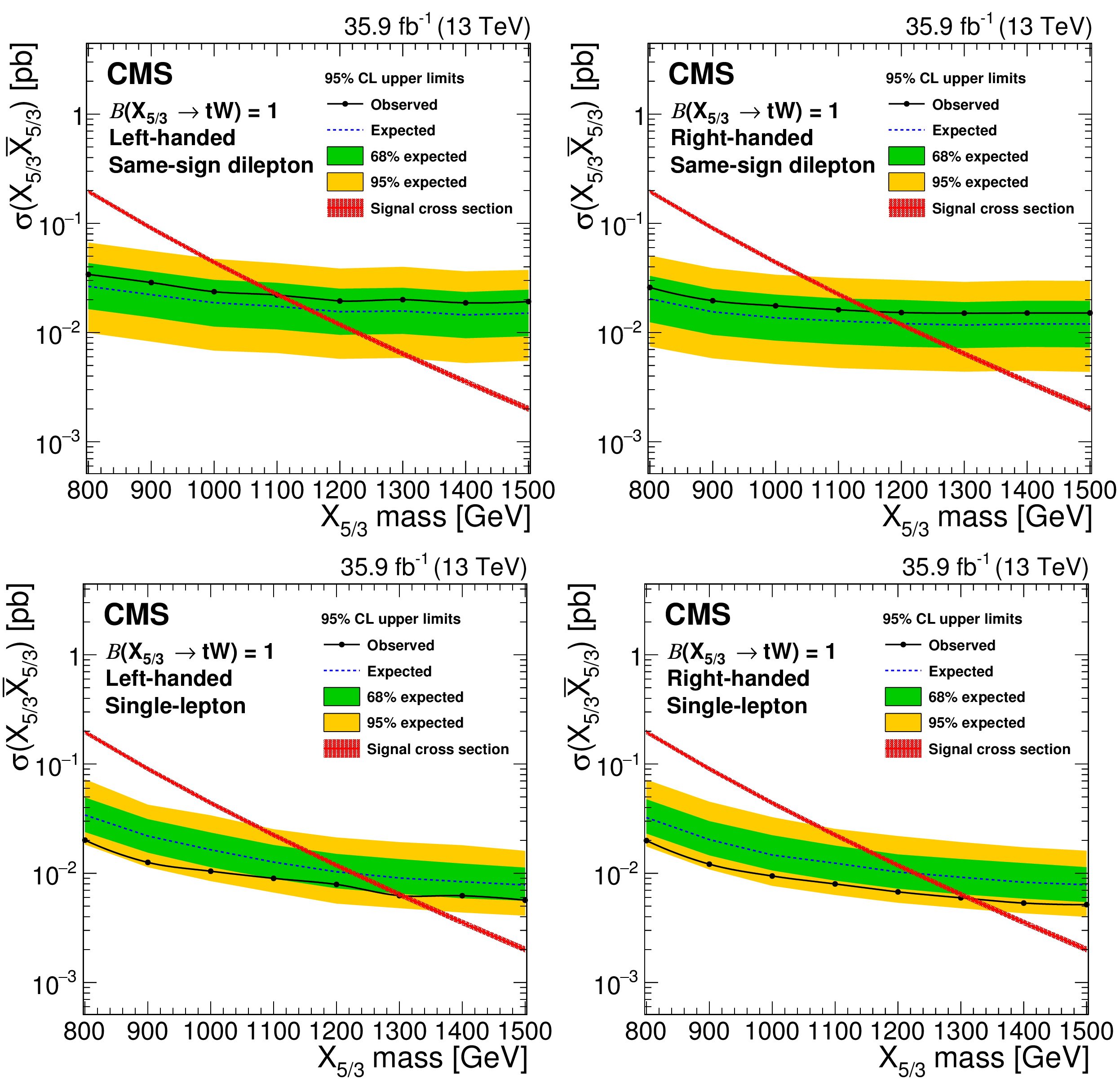
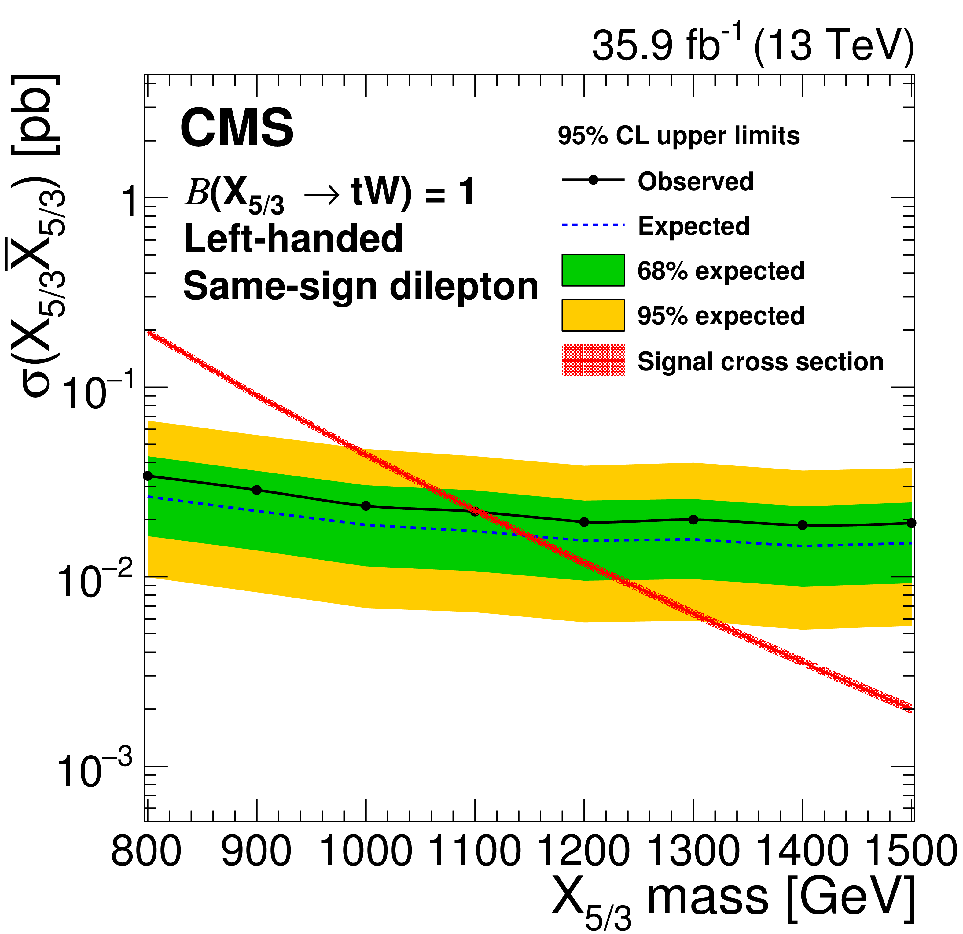
Figure 7:
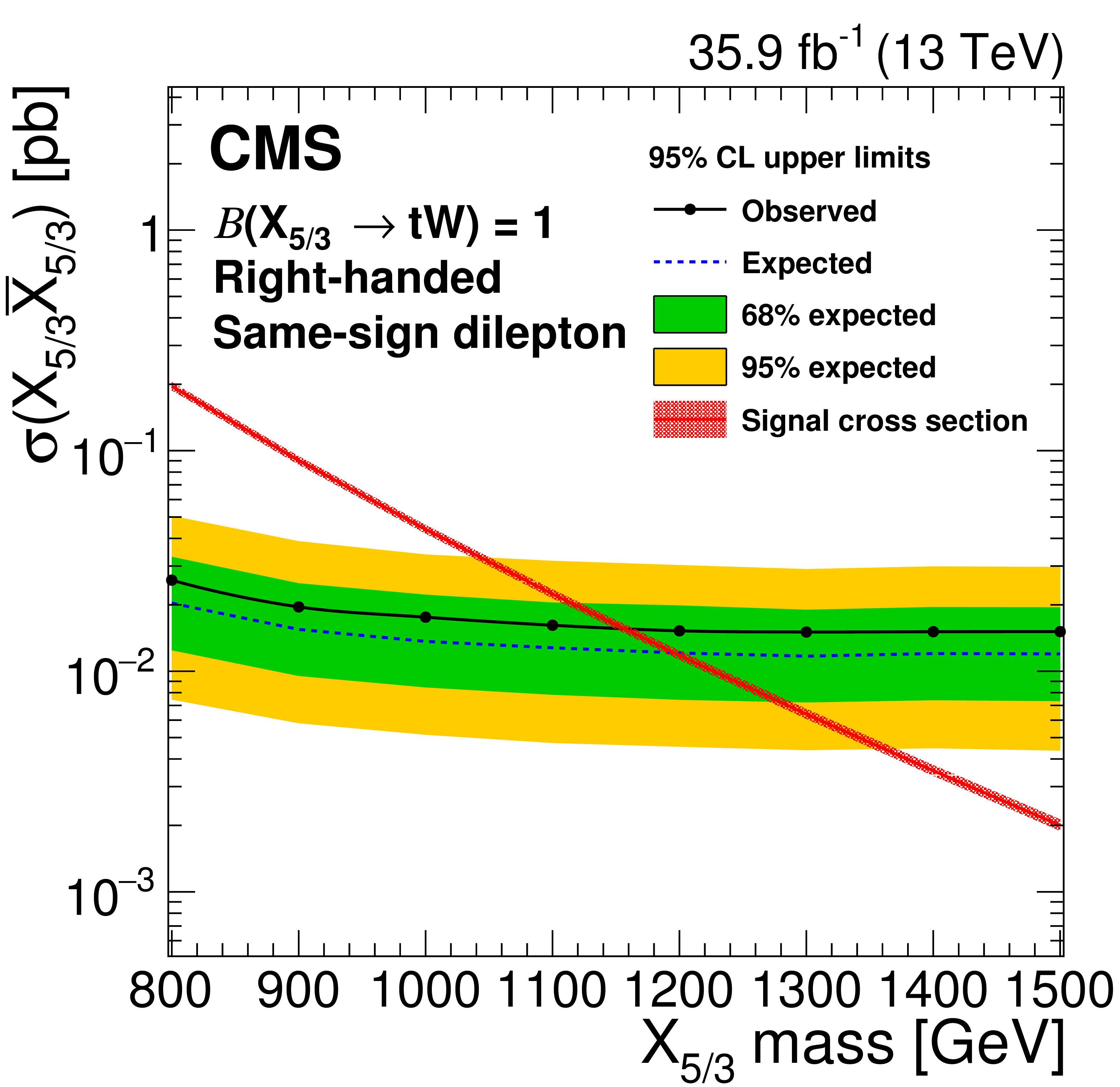
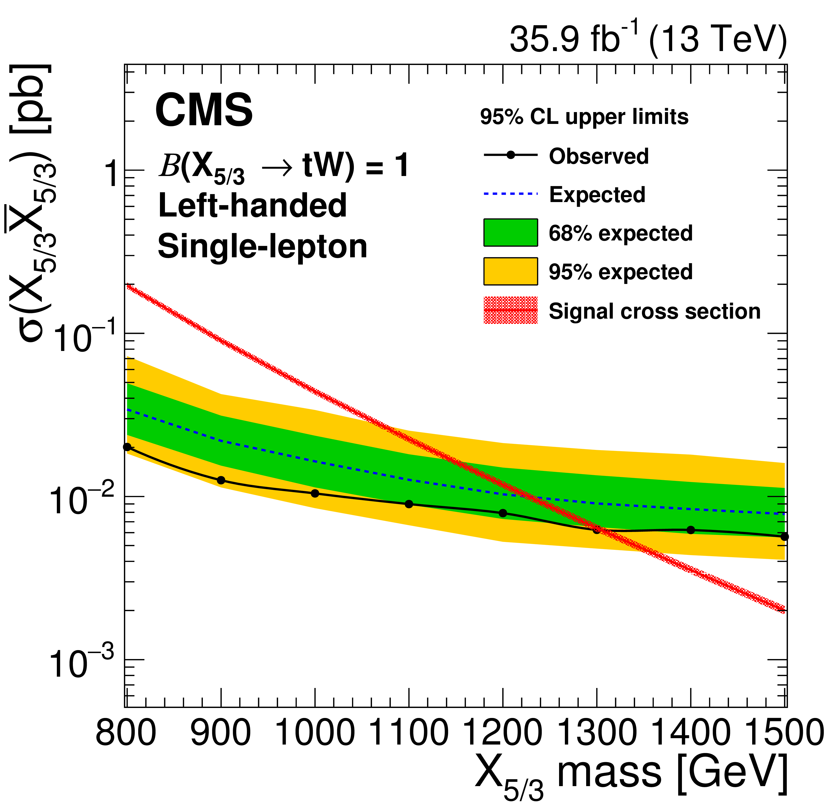
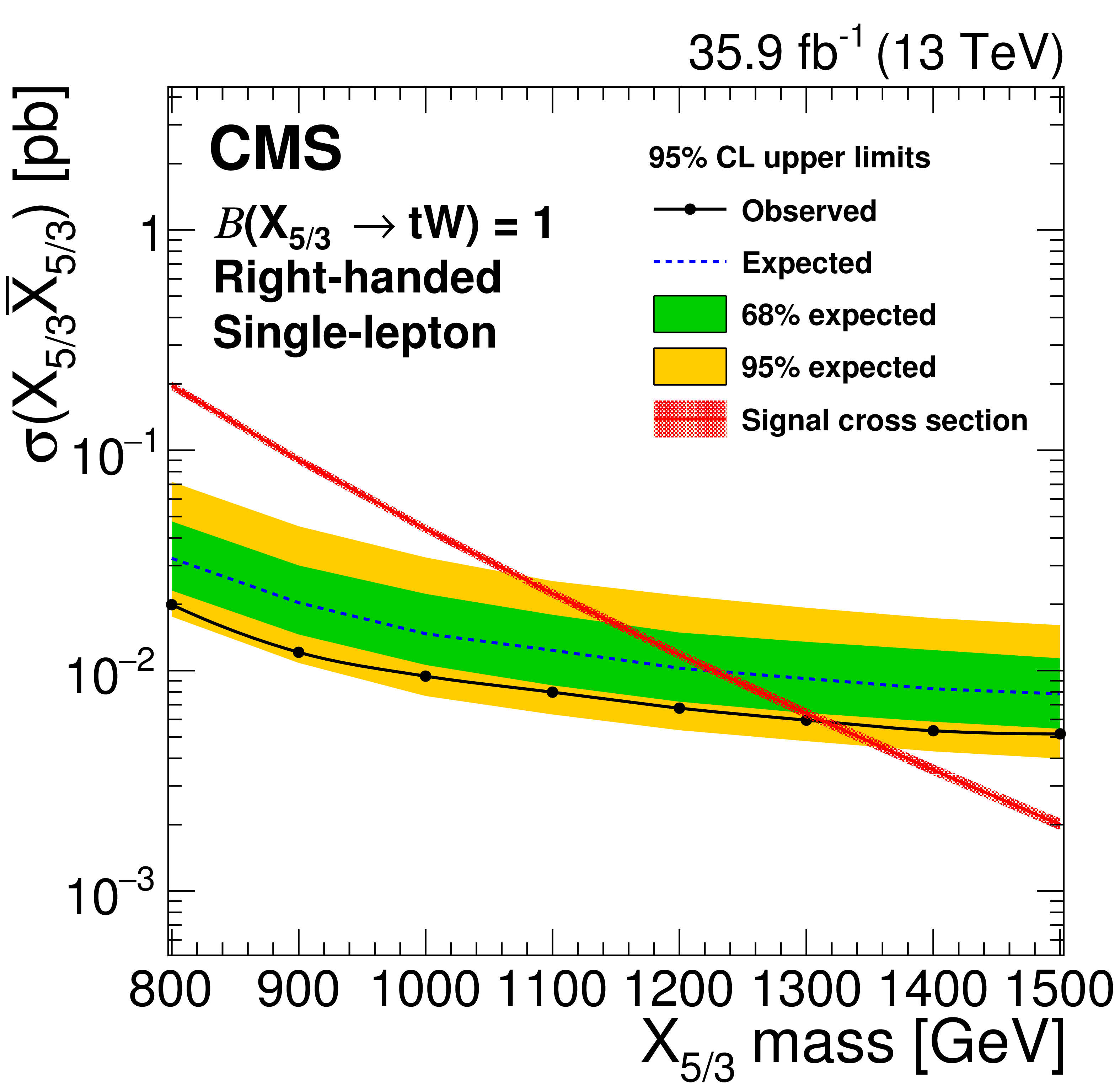
Expected and observed limits at 95% CL for an LH (left) and RH (right) ${X_{5/3}} $ after combining all categories for the same-sign dilepton (upper row) and the single-lepton (lower row) final states. The theoretical uncertainty in the signal cross section is shown as a narrow band around the theoretical prediction. |
png pdf |
Figure 7-a:
Expected and observed limits at 95% CL for an LH ${X_{5/3}} $ after combining all categories for the same-sign dilepton final state. The theoretical uncertainty in the signal cross section is shown as a narrow band around the theoretical prediction. |
png pdf |
Figure 7-b:
Expected and observed limits at 95% CL for an RH ${X_{5/3}} $ after combining all categories for the same-sign dilepton final state. The theoretical uncertainty in the signal cross section is shown as a narrow band around the theoretical prediction. |
png pdf |
Figure 7-c:
Expected and observed limits at 95% CL for an LH ${X_{5/3}} $ after combining all categories for the single-lepton final state. The theoretical uncertainty in the signal cross section is shown as a narrow band around the theoretical prediction. |
png pdf |
Figure 7-d:
Expected and observed limits at 95% CL for an RH ${X_{5/3}} $ after combining all categories for the single-lepton final state. The theoretical uncertainty in the signal cross section is shown as a narrow band around the theoretical prediction. |
png pdf |
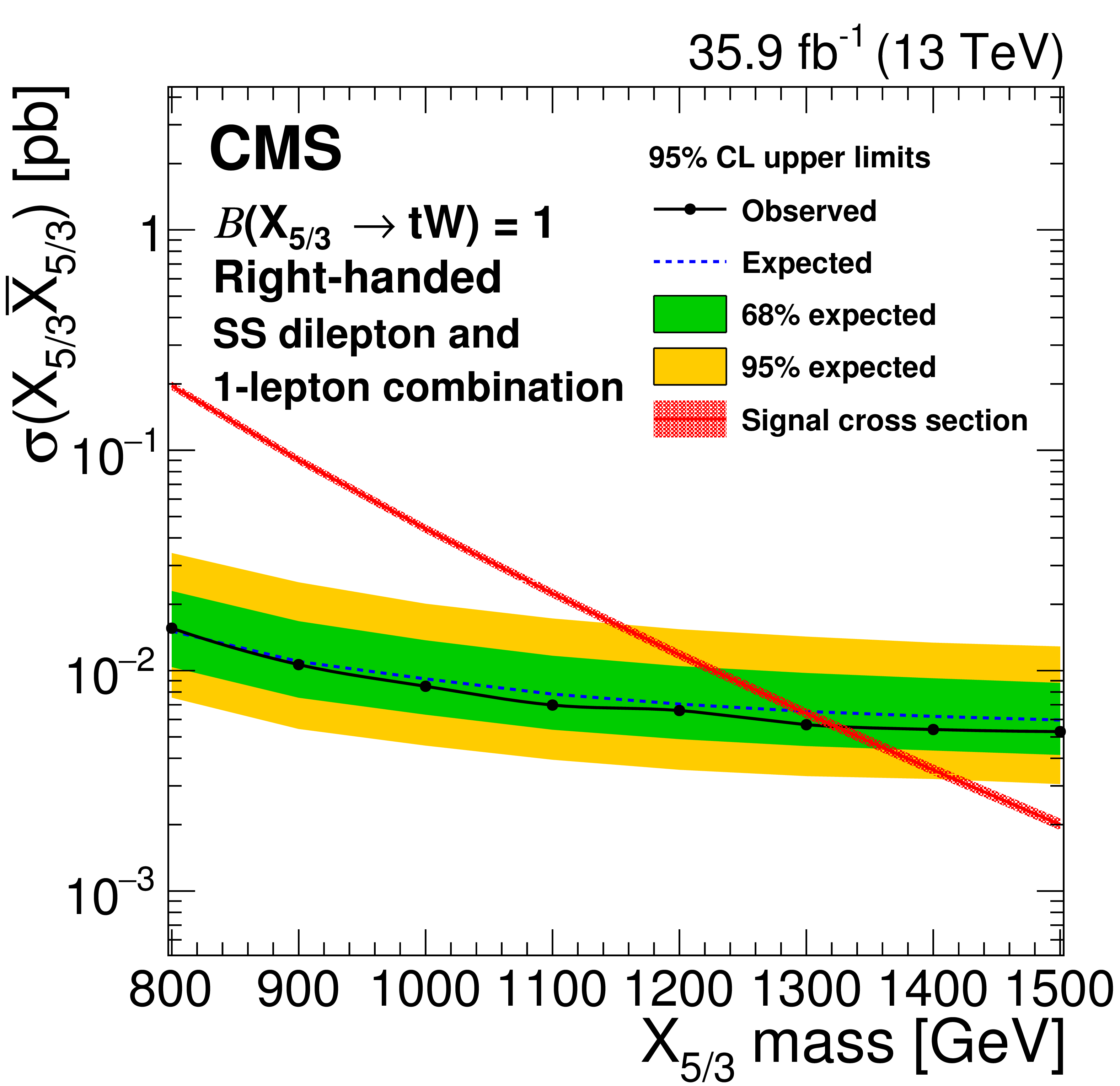
Figure 8:
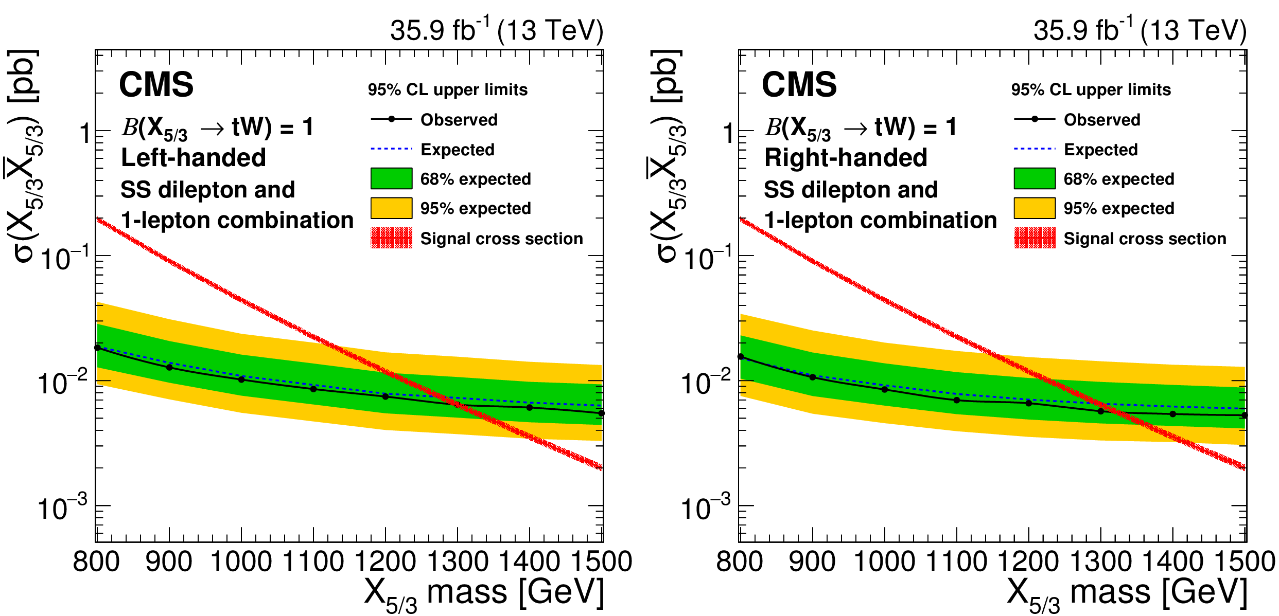
Expected and observed limits at 95% CL for an LH (left) and RH (right) ${X_{5/3}} $ after combining the same-sign dilepton and single-lepton final states. The theoretical uncertainty in the signal cross section is shown as a narrow band around the theoretical prediction. |

png pdf |
Figure 8-a:
Expected and observed limits at 95% CL for an LH ${X_{5/3}} $ after combining the same-sign dilepton and single-lepton final states. The theoretical uncertainty in the signal cross section is shown as a narrow band around the theoretical prediction. |
png pdf |
Figure 8-b:
Expected and observed limits at 95% CL for an RH ${X_{5/3}} $ after combining the same-sign dilepton and single-lepton final states. The theoretical uncertainty in the signal cross section is shown as a narrow band around the theoretical prediction. |
| Tables | |
png pdf |
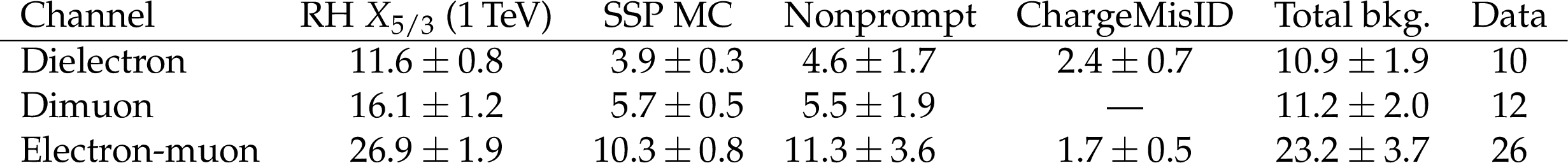
Table 1:
Summary of yields from simulated prompt same-sign dilepton (SSP MC), same-sign nonprompt (Nonprompt), and opposite-sign prompt (ChargeMisID) backgrounds after the full analysis selection. Also shown are the number of expected events for an RH ${X_{5/3}} $ particle with a mass of 1 TeV. The uncertainties include both statistical and all systematic components (as described in Section 8). The number of events and uncertainties correspond to the background-only fit to data for the background, while for the signal they are based on the yields before the fit to data. |
png pdf |
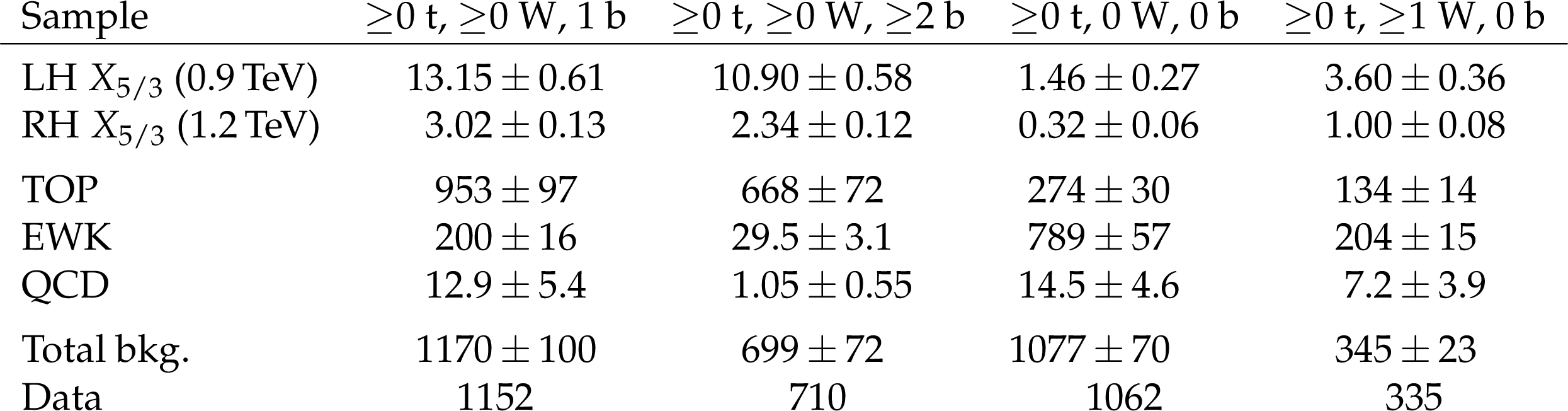
Table 2:
Expected (observed) numbers of background (data) events passing the final selection requirements, in the $ {{\mathrm {t}\overline {\mathrm {t}}}} $ and W+jets control region (0.4 $ < {\Delta R(\ell, \mathrm {j_{2})}} < $ 1.0) categories, after combining the single-electron and single-muon channels. The numbers of events expected from two example signals are also shown. The event yields and their uncertainties correspond to the background-only fit to data for the background, while for the signal they are based on the values before the fit to data. |
png pdf |
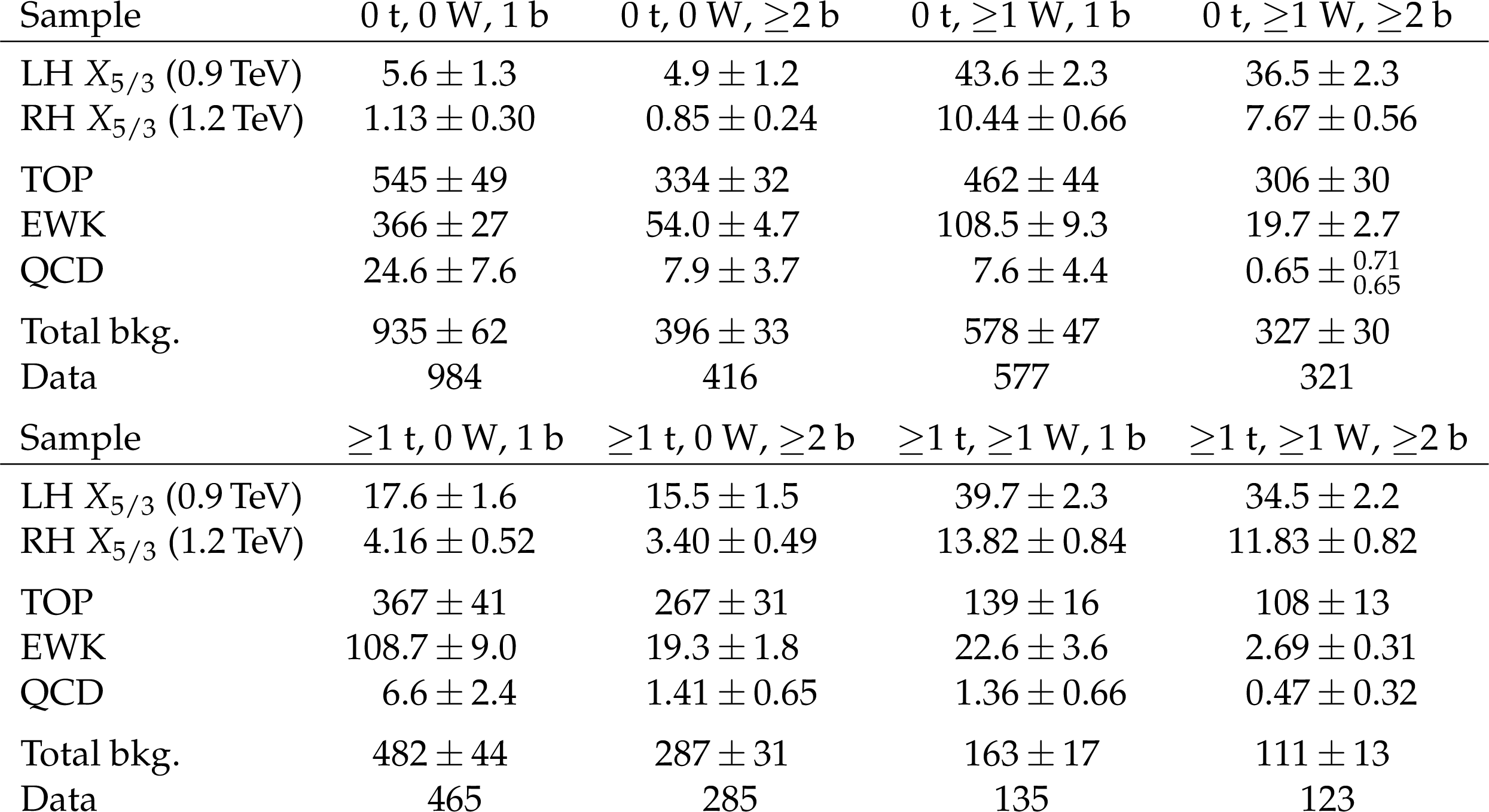
Table 3:
Expected (observed) numbers of background (data) events passing the final selection requirements, in the signal region ($ {\Delta R(\ell, \mathrm {j_{2})}} > $ 1.0) categories, after combining the single-electron and single-muon channels. The numbers of events expected from two example signals are also shown. The event yields and their uncertainties correspond to the background-only fit to data for the background, while for the signal they are based on the values before the fit to data. |
png pdf |
Table 4:
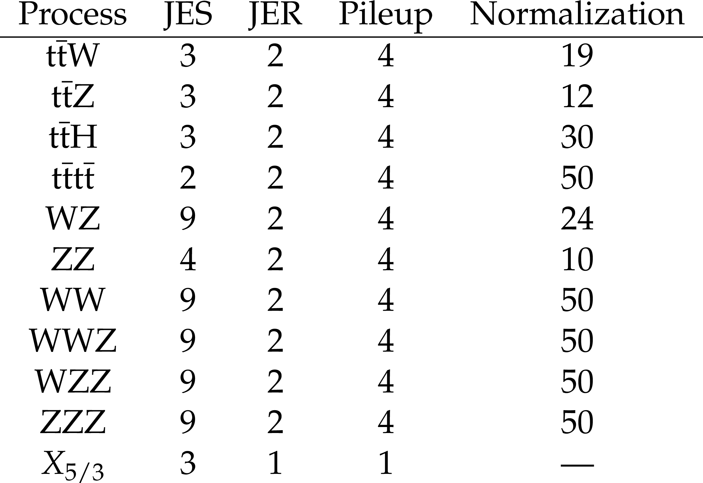
Systematic uncertainties in percentage (%) in the same-sign dilepton final state, associated with the simulated processes. The "Normalization'' column refers to the uncertainties from the cross section normalization and the choice of PDF set. |
png pdf |
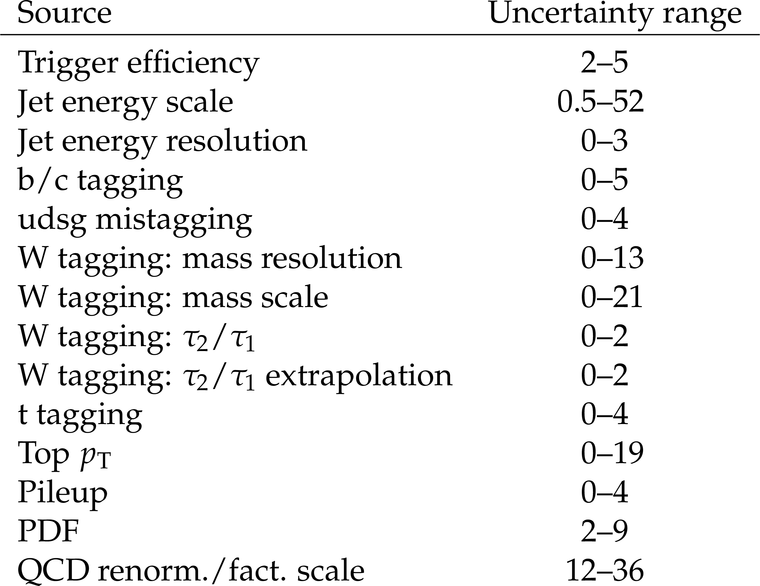
Table 5:
Summary of systematic uncertainties in the single-lepton final state. These uncertainties are included in both signal and all background processes, except for the top ${p_{\mathrm {T}}}$ systematic uncertainty, which is included only in $ {{\mathrm {t}\overline {\mathrm {t}}}} $. The range of uncertainty values in percentage (%) corresponds to the effect on the yields before the fit to data and is given across the relevant background processes and channels for each systematic uncertainty. |
| Summary |
| A search has been performed for a heavy top quark partner with an exotic 5/3 charge (${X_{5/3}} $) using proton-proton collision data collected by the CMS experiment in 2016 at a center-of-mass energy of 13 TeV and corresponding to 35.9 fb$^{-1}$. The ${X_{5/3}} $ quark is assumed always to decay into a top quark and a W boson. Two different final states, same-sign dilepton and single-lepton, are analyzed separately and then combined. No significant excess over the expected standard model backgrounds is seen in data. Lower limits are set on the mass of the ${X_{5/3}} $ particle. The observed (expected) limit is 1.33 (1.30) TeV for an ${X_{5/3}} $ particle with right-handed couplings to W bosons and 1.30 (1.28) TeV for an ${X_{5/3}} $ particle with left-handed couplings to W bosons in a combination of the same-sign dilepton and single-lepton final states. |
| References | ||||
| 1 | R. Contino and G. Servant | Discovering the top partners at the LHC using same-sign dilepton final states | JHEP 06 (2008) 026 | 0801.1679 |
| 2 | A. De Simone, O. Matsedonskyi, R. Rattazzi, and A. Wulzer | A first top partner hunter's guide | JHEP 04 (2013) 004 | 1211.5663 |
| 3 | K. Agashe, R. Contino, and A. Pomarol | The minimal composite Higgs model | NPB 719 (2005) 165 | hep-ph/0412089 |
| 4 | R. Barbieri and G. F. Giudice | Upper bounds on supersymmetric particle masses | NPB 306 (1988) 63 | |
| 5 | D. B. Kaplan | Flavor at SSC energies: A new mechanism for dynamically generated fermion masses | NPB 365 (1991) 259 | |
| 6 | A. Azatov and J. Galloway | Light custodians and Higgs physics in composite models | PRD 85 (2012) 055013 | 1110.5646 |
| 7 | G. Cacciapaglia et al. | Heavy vector-like quark with charge 5/3 at the LHC | JHEP 03 (2013) 004 | 1211.4034 |
| 8 | CMS Collaboration | Search for top-quark partners with charge 5/3 in the same-sign dilepton final state | PRL 112 (2014) 171801 | CMS-B2G-12-012 1312.2391 |
| 9 | CMS Collaboration | Search for top quark partners with charge 5/3 in proton-proton collisions at $ \sqrt{s}= $ 13 TeV | JHEP 08 (2017) 073 | CMS-B2G-15-006 1705.10967 |
| 10 | ATLAS Collaboration | Analysis of events with $ b $-jets and a pair of leptons of the same charge in pp collisions at $ \sqrt{s}= $ 8 TeV with the ATLAS detector | JHEP 10 (2015) 150 | 1504.04605 |
| 11 | ATLAS Collaboration | Search for vector-like $ B $ quarks in events with one isolated lepton, missing transverse momentum and jets at $ \sqrt{s}= $ 8 TeV with the ATLAS detector | PRD 91 (2015) 112011 | 1503.05425 |
| 12 | ATLAS Collaboration | Search for pair production of heavy vector-like quarks decaying to high-p$ _{T} $ W bosons and b quarks in the lepton-plus-jets final state in pp collisions at $ \sqrt{s}= $ 13 TeV with the ATLAS detector | JHEP 10 (2017) 141 | 1707.03347 |
| 13 | ATLAS Collaboration | Search for pair production of heavy vector-like quarks decaying into high-$ {p_{\mathrm{T}}}$ W bosons and top quarks in the lepton-plus-jets final state in pp collisions at $ \sqrt{s}= $ 13 TeV with the ATLAS detector | JHEP 08 (2018) 048 | 1806.01762 |
| 14 | ATLAS Collaboration | Search for new phenomena in events with same-charge leptons and $ b $-jets in pp collisions at $ \sqrt{s}= $ 13 TeV with the ATLAS detector | Submitted to JHEP | 1807.11883 |
| 15 | ATLAS Collaboration | Combination of the searches for pair-produced vector-like partners of the third-generation quarks at $ \sqrt{s}= $ 13 TeV with the ATLAS detector | Submitted to PRLett | 1808.02343 |
| 16 | CMS Collaboration | The CMS trigger system | JINST 12 (2017) P01020 | CMS-TRG-12-001 1609.02366 |
| 17 | CMS Collaboration | The CMS experiment at the CERN LHC | JINST 3 (2008) S08004 | CMS-00-001 |
| 18 | J. Alwall et al. | The automated computation of tree-level and next-to-leading order differential cross sections, and their matching to parton shower simulations | JHEP 07 (2014) 079 | 1405.0301 |
| 19 | P. Artoisenet, R. Frederix, O. Mattelaer, and R. Rietkerk | Automatic spin-entangled decays of heavy resonances in Monte Carlo simulations | JHEP 03 (2013) 015 | 1212.3460 |
| 20 | M. Czakon and A. Mitov | Top++: a program for the calculation of the top-pair cross-section at hadron colliders | CPC 185 (2014) 2930 | 1112.5675 |
| 21 | M. Czakon, P. Fiedler, and A. Mitov | The total top quark pair production cross-section at hadron colliders through $ \mathcal{O}({{\alpha}}_{S}^{4}) $ | PRL 110 (2013) 252004 | 1303.6254 |
| 22 | M. Czakon and A. Mitov | NNLO corrections to top-pair production at hadron colliders: the all-fermionic scattering channels | JHEP 12 (2012) 054 | 1207.0236 |
| 23 | M. Czakon and A. Mitov | NNLO corrections to top pair production at hadron colliders: the quark-gluon reaction | JHEP 01 (2013) 080 | 1210.6832 |
| 24 | P. Barnreuther, M. Czakon, and A. Mitov | Percent level precision physics at the Tevatron: first genuine NNLO QCD corrections to $ q \bar{q} \to t \bar{t} + {X} $ | PRL 109 (2012) 132001 | 1204.5201 |
| 25 | M. Cacciari et al. | Top-pair production at hadron colliders with next-to-next-to-leading logarithmic soft-gluon resummation | PLB 710 (2012) 612 | 1111.5869 |
| 26 | P. Nason | A new method for combining NLO QCD with shower Monte Carlo algorithms | JHEP 11 (2004) 040 | hep-ph/0409146 |
| 27 | S. Frixione, P. Nason, and C. Oleari | Matching NLO QCD computations with parton shower simulations: the POWHEG method | JHEP 11 (2007) 070 | 0709.2092 |
| 28 | S. Alioli, P. Nason, C. Oleari, and E. Re | A general framework for implementing NLO calculations in shower Monte Carlo programs: the POWHEG BOX | JHEP 06 (2010) 043 | 1002.2581 |
| 29 | S. Frixione, P. Nason, and G. Ridolfi | A positive-weight next-to-leading-order Monte Carlo for heavy flavour hadroproduction | JHEP 09 (2007) 126 | 0707.3088 |
| 30 | J. Alwall et al. | Comparative study of various algorithms for the merging of parton showers and matrix elements in hadronic collisions | EPJC 53 (2008) 473 | 0706.2569 |
| 31 | R. Frederix and S. Frixione | Merging meets matching in MC@NLO | JHEP 12 (2012) 061 | 1209.6215 |
| 32 | T. Sjostrand et al. | An introduction to PYTHIA 8.2 | CPC 191 (2015) 159 | 1410.3012 |
| 33 | NNPDF Collaboration | Parton distributions for the LHC Run II | JHEP 04 (2015) 040 | 1410.8849 |
| 34 | CMS Collaboration | Event generator tunes obtained from underlying event and multiparton scattering measurements | EPJC 76 (2016) 155 | CMS-GEN-14-001 1512.00815 |
| 35 | P. Skands, S. Carrazza, and J. Rojo | Tuning PYTHIA 8.1: the Monash 2013 tune | EPJC 74 (2014) 3024 | 1404.5630 |
| 36 | CMS Collaboration | Investigations of the impact of the parton shower tuning in Pythia 8 in the modelling of $ \mathrm{t\overline{t}} $ at $ \sqrt{s}= $ 8 and 13 TeV | CMS-PAS-TOP-16-021 | CMS-PAS-TOP-16-021 |
| 37 | GEANT4 Collaboration | GEANT4--a simulation toolkit | NIMA 506 (2003) 250 | |
| 38 | CMS Collaboration | Measurement of the differential cross section for top quark pair production in pp collisions at $ \sqrt{s}= $ 8 TeV | EPJC 75 (2015) 542 | CMS-TOP-12-028 1505.04480 |
| 39 | CMS Collaboration | Particle-flow reconstruction and global event description with the CMS detector | JINST 12 (2017) P10003 | CMS-PRF-14-001 1706.04965 |
| 40 | M. Cacciari, G. P. Salam, and G. Soyez | The anti-$ {k_{\mathrm{T}}} $ jet clustering algorithm | JHEP 04 (2008) 063 | 0802.1189 |
| 41 | M. Cacciari, G. P. Salam, and G. Soyez | FastJet user manual | EPJC 72 (2012) 1896 | 1111.6097 |
| 42 | CMS Collaboration | Performance of electron reconstruction and selection with the CMS detector in proton-proton collisions at $ \sqrt{s}= $ 8 TeV | JINST 10 (2015) P06005 | CMS-EGM-13-001 1502.02701 |
| 43 | CMS Collaboration | CMS tracking performance results from early LHC operation | EPJC 70 (2010) 1165 | CMS-TRK-10-001 1007.1988 |
| 44 | W. Adam, R. Fruhwirth, A. Strandlie, and T. Todorov | Reconstruction of electrons with the Gaussian-sum filter in the CMS tracker at the LHC | JPG 31 (2005) N9 | physics/0306087 |
| 45 | M. Cacciari and G. P. Salam | Pileup subtraction using jet areas | PLB 659 (2008) 119 | 0707.1378 |
| 46 | CMS Collaboration | Measurement of the inclusive W and Z production cross sections in pp collisions at $ \sqrt{s}= $ 7 TeV | JHEP 10 (2011) 132 | CMS-EWK-10-005 1107.4789 |
| 47 | M. Cacciari, G. P. Salam, and G. Soyez | The catchment area of jets | JHEP 04 (2008) 005 | 0802.1188 |
| 48 | CMS Collaboration | Jet algorithms performance in 13 TeV data | CMS-PAS-JME-16-003 | CMS-PAS-JME-16-003 |
| 49 | CMS Collaboration | Determination of jet energy calibration and transverse momentum resolution in CMS | JINST 6 (2011) P11002 | CMS-JME-10-011 1107.4277 |
| 50 | CMS Collaboration | Jet energy scale and resolution in the CMS experiment in $ {\mathrm{p}}{\mathrm{p}} $ collisions at 8 TeV | JINST 12 (2017) P02014 | CMS-JME-13-004 1607.03663 |
| 51 | CMS Collaboration | Identification of heavy-flavour jets with the CMS detector in pp collisions at 13 TeV | JINST 13 (2018) P05011 | CMS-BTV-16-002 1712.07158 |
| 52 | A. J. Larkoski, S. Marzani, G. Soyez, and J. Thaler | Soft drop | JHEP 05 (2014) 146 | 1402.2657 |
| 53 | J. Thaler and K. Van Tilburg | Maximizing boosted top identification by minimizing $ N $-subjettiness | JHEP 02 (2012) 093 | 1108.2701 |
| 54 | S. D. Ellis, C. K. Vermilion, and J. R. Walsh | Techniques for improved heavy particle searches with jet substructure | PRD 80 (2009) 051501 | 0903.5081 |
| 55 | CMS Collaboration | Search for new physics in same-sign dilepton events in proton-proton collisions at $ \sqrt{s}= $ 13 TeV | EPJC 76 (2016) 439 | CMS-SUS-15-008 1605.03171 |
| 56 | CMS Collaboration | Search for new physics with same-sign isolated dilepton events with jets and missing transverse energy at the LHC | JHEP 06 (2011) 077 | CMS-SUS-10-004 1104.3168 |
| 57 | CMS Collaboration | CMS luminosity measurement for the 2016 data-taking period | CMS-PAS-LUM-17-001 | CMS-PAS-LUM-17-001 |
| 58 | CMS Collaboration | Measurement of the inelastic proton-proton cross section at $ \sqrt{s}= $ 13 TeV | JHEP 07 (2018) 161 | CMS-FSQ-15-005 1802.02613 |
| 59 | Particle Data Group, C. Patrignani et al. | Review of particle physics | CPC 40 (2016) 100001 | |
| 60 | J. Ott | Theta--A framework for template-based modeling and inference | 2010 \url http://www-ekp.physik.uni-karlsruhe.de/\ ott/theta/theta-auto | |
|
|
Compact Muon Solenoid LHC, CERN |
|

|

|

|

|

|