CMS-BTV-16-002

CMS-BTV-16-002 ; CERN-EP-2017-326
Identification of heavy-flavour jets with the CMS detector in pp collisions at 13 TeV
CMS Collaboration
19 December 2017
JINST 13 (2018) P05011
Abstract: Many measurements and searches for physics beyond the standard model at the LHC rely on the efficient identification of heavy-flavour jets, i.e. jets originating from bottom or charm quarks. In this paper, the discriminating variables and the algorithms used for heavy-flavour jet identification during the first years of operation of the CMS experiment in proton-proton collisions at a centre-of-mass energy of 13 TeV, are presented. Heavy-flavour jet identification algorithms have been improved compared to those used previously at centre-of-mass energies of 7 and 8 TeV. For jets with transverse momenta in the range expected in simulated $ \mathrm{t\bar{t}} $ events, these new developments result in an efficiency of 68% for the correct identification of a b jet for a probability of 1% of misidentifying a light-flavour jet. The improvement in relative efficiency at this misidentification probability is about 15%, compared to previous CMS algorithms. In addition, for the first time algorithms have been developed to identify jets containing two b hadrons in Lorentz-boosted event topologies, as well as to tag c jets. The large data sample recorded in 2016 at a centre-of-mass energy of 13 TeV has also allowed the development of new methods to measure the efficiency and misidentification probability of heavy-flavour jet identification algorithms. The heavy-flavour jet identification efficiency is measured with a precision of a few per cent at moderate jet transverse momenta (between 30 and 300 GeV) and about 5% at the highest jet transverse momenta (between 500 and 1000 GeV).
Links: e-print arXiv:1712.07158 [physics.ins-det] (PDF) ; CDS record ; inSPIRE record ; CADI line (restricted) ;

Figures & Tables	Summary	References	CMS Publications

Figures
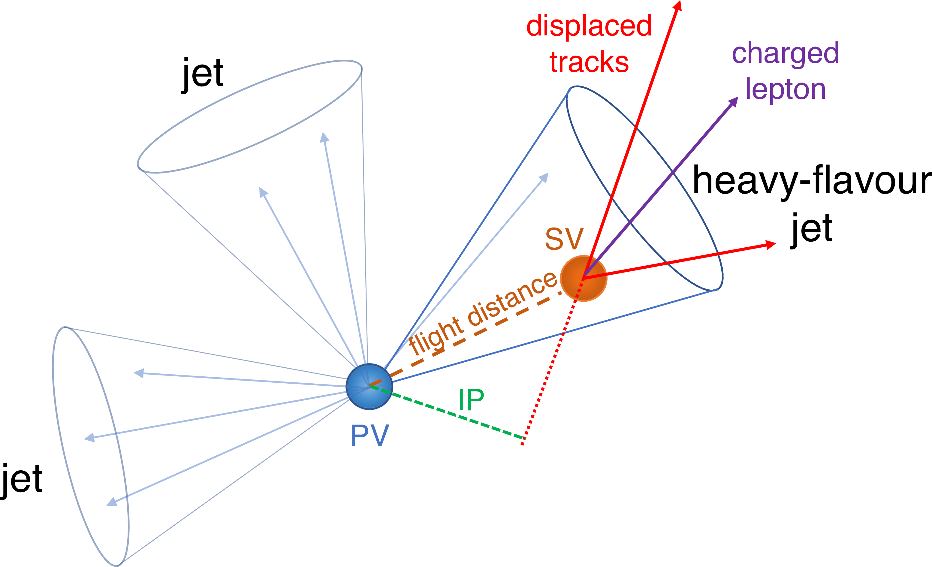
png pdf	Figure 1: Illustration of a heavy-flavour jet with a secondary vertex (SV) from the decay of a b or c hadron resulting in charged-particle tracks (including possibly a soft lepton) that are displaced with respect to the primary interaction vertex (PV), and hence with a large impact parameter (IP) value.
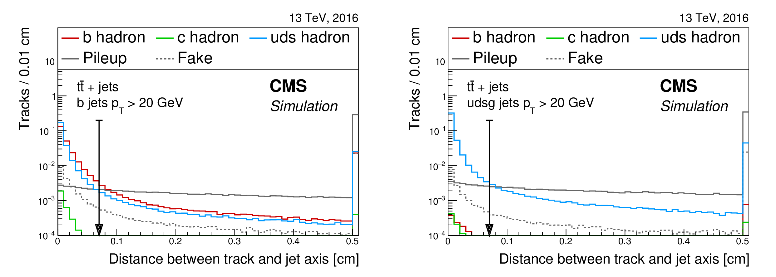
png pdf	Figure 2: Distribution of the distance between a track and the jet axis at their point of closest approach for tracks associated with b (left) and light-flavour (right) jets in $ {\mathrm {t}\overline {\mathrm {t}}} $ events. This distance is required to be smaller than 0.07 cm, as indicated by the arrow. The tracks are divided into categories according to their origin as defined in the text. The distributions are normalized such that their sum has unit area. The last bin includes the overflow entries.
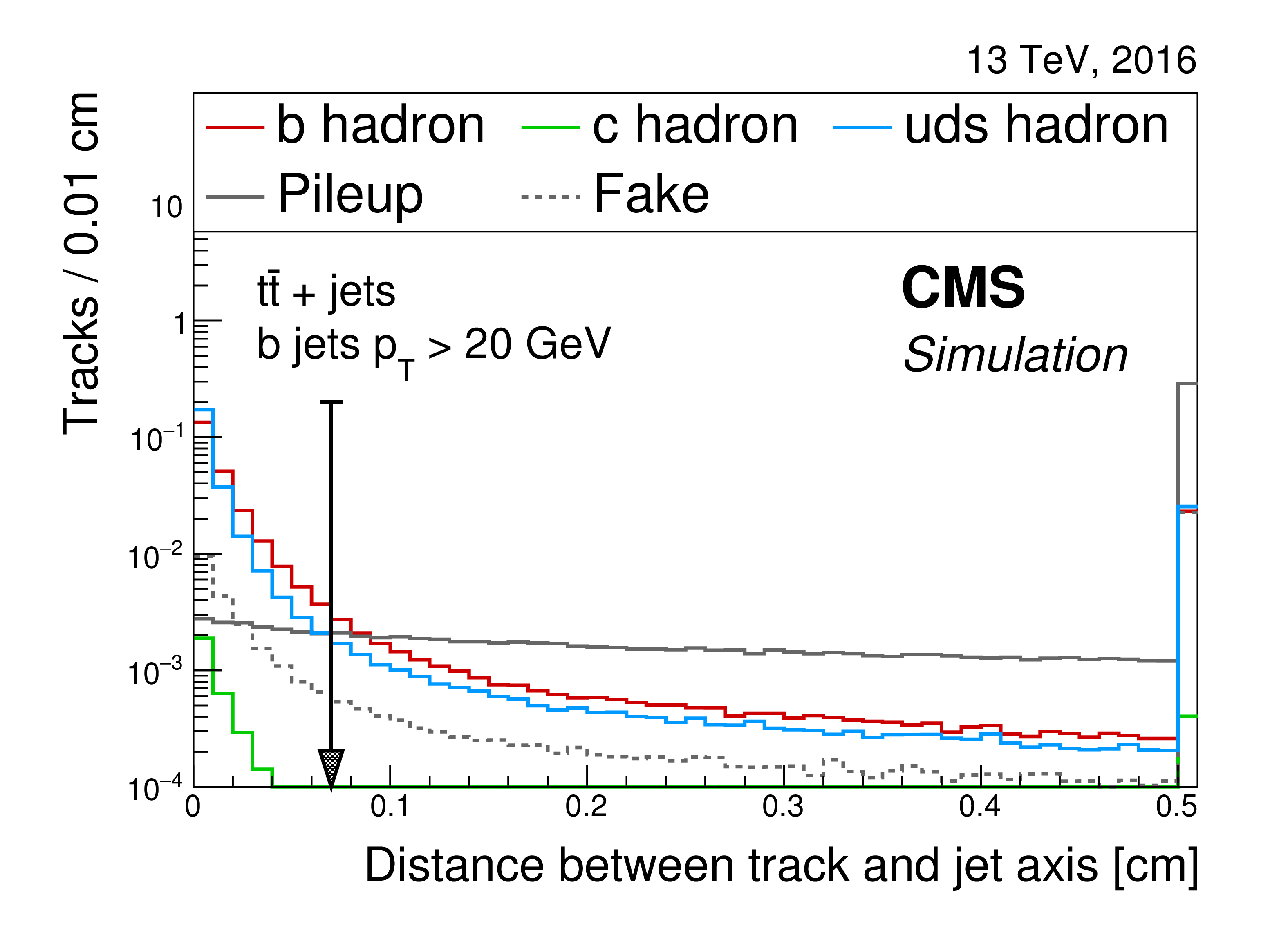
png pdf	Figure 2-a: Distribution of the distance between a track and the jet axis at their point of closest approach for tracks associated with b jets in $ {\mathrm {t}\overline {\mathrm {t}}} $ events. This distance is required to be smaller than 0.07 cm, as indicated by the arrow. The tracks are divided into categories according to their origin as defined in the text. The distributions are normalized such that their sum has unit area. The last bin includes the overflow entries.
png pdf	Figure 2-b: Distribution of the distance between a track and the jet axis at their point of closest approach for tracks associated with light-flavour jets in $ {\mathrm {t}\overline {\mathrm {t}}} $ events. This distance is required to be smaller than 0.07 cm, as indicated by the arrow. The tracks are divided into categories according to their origin as defined in the text. The distributions are normalized such that their sum has unit area. The last bin includes the overflow entries.
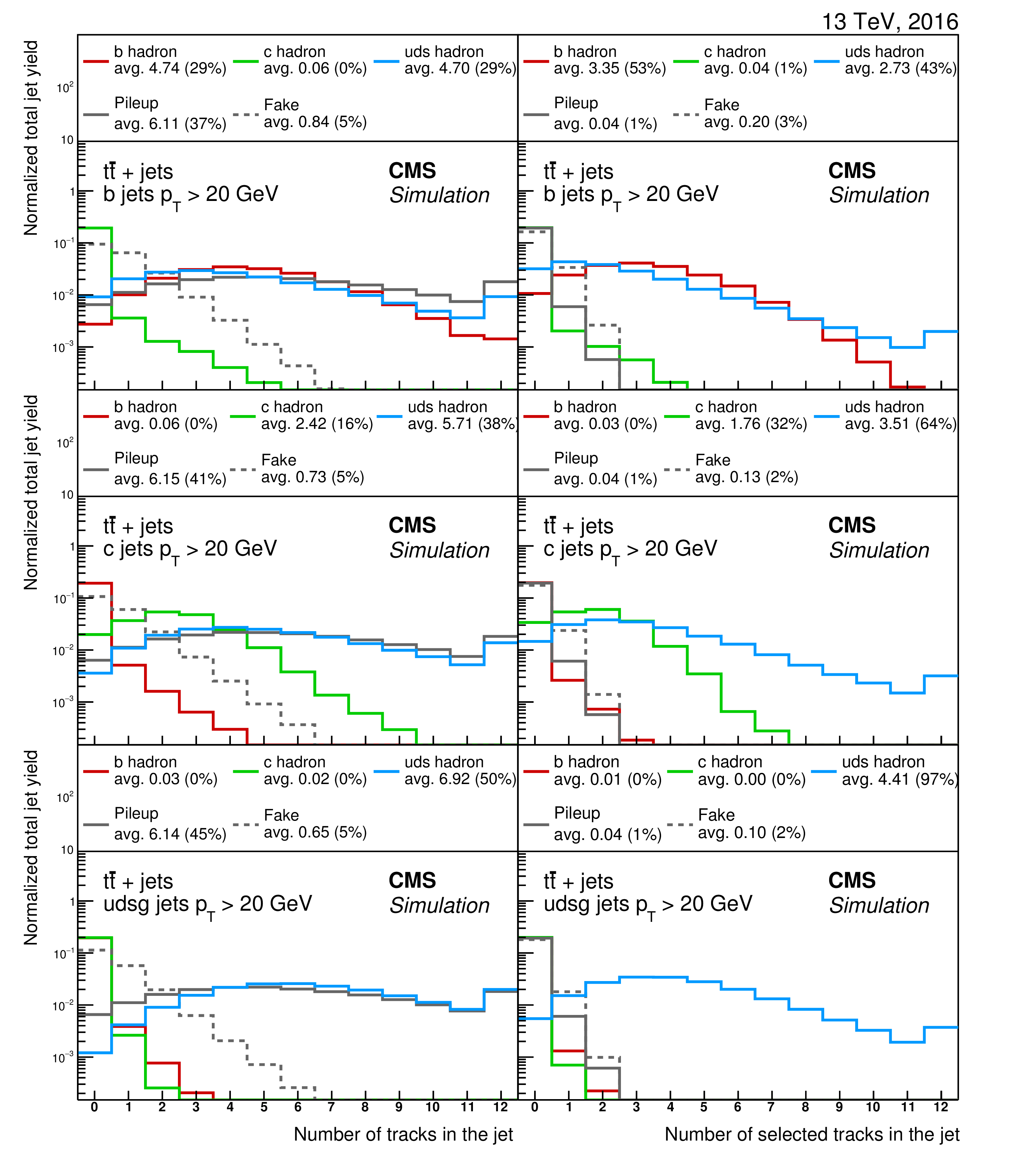
png pdf	Figure 3: Fraction of tracks from different origins before (left) and after (right) applying the track selection requirements on b (upper), c (middle), and light-flavour (lower) jets in $ {\mathrm {t}\overline {\mathrm {t}}} $ events. The average number of tracks of each origin is given in the legend as well as the average fraction of tracks of a certain origin with respect to the total number of tracks in the jet, indicated in per cent. The number of tracks corresponding to pileup vertices or mismeasured tracks is strongly reduced after applying the track selection requirements. The distributions are normalized such that their sum has unit area. The last bin includes the overflow entries.
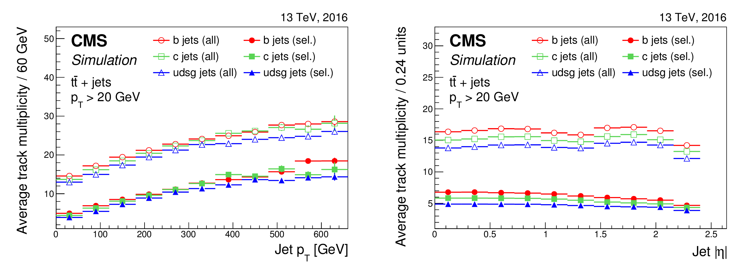
png pdf	Figure 4: Average track multiplicity as a function of the jet $ {p_{\mathrm {T}}} $ (left) and $ { \| \eta \|}$ (right) for jets of different flavours in $ {\mathrm {t}\overline {\mathrm {t}}} $ events before (open symbols) and after (filled symbols) applying the track selection requirements.
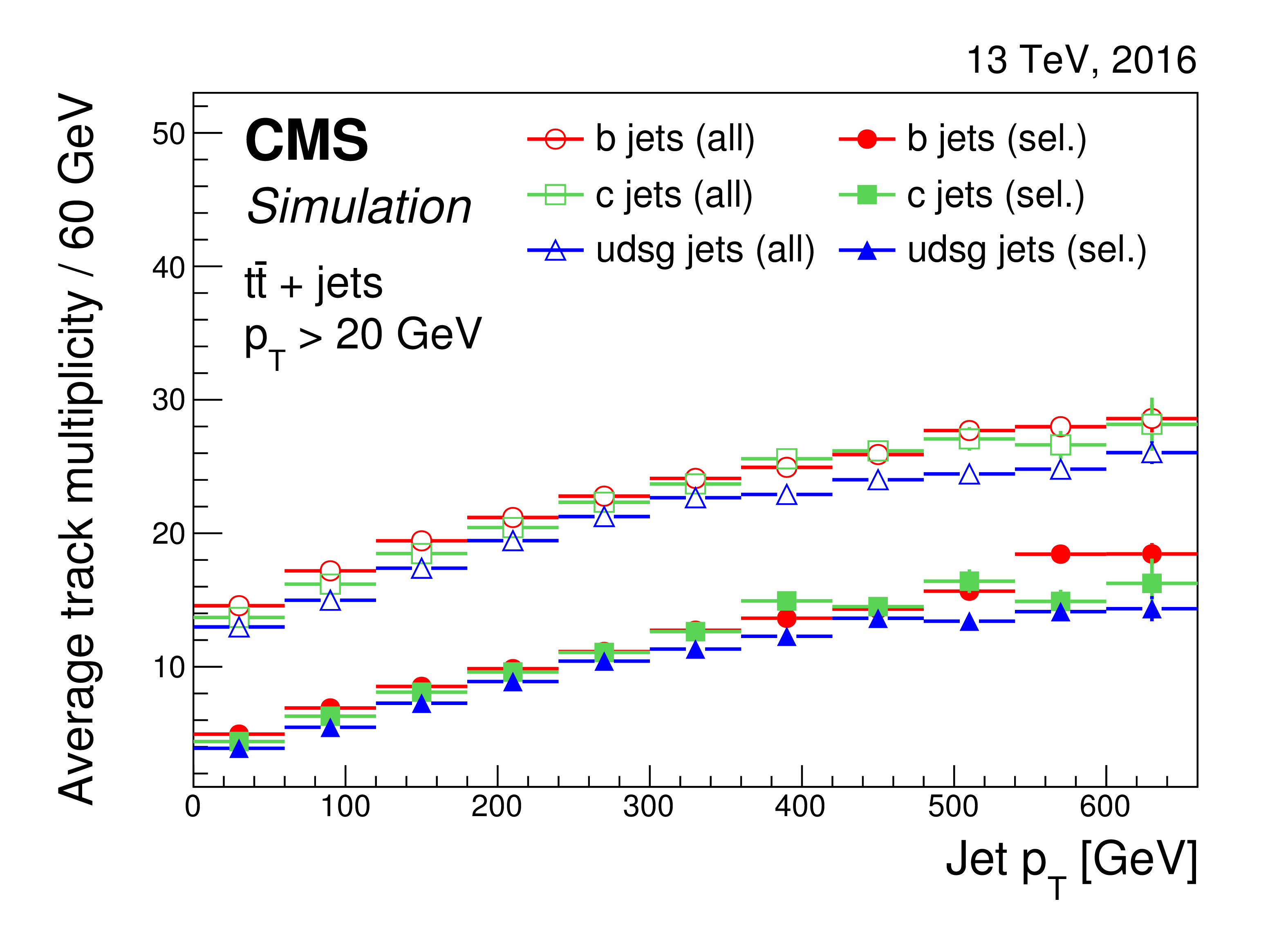
png pdf	Figure 4-a: Average track multiplicity as a function of the jet $ {p_{\mathrm {T}}} $ for jets of different flavours in $ {\mathrm {t}\overline {\mathrm {t}}} $ events before (open symbols) and after (filled symbols) applying the track selection requirements.
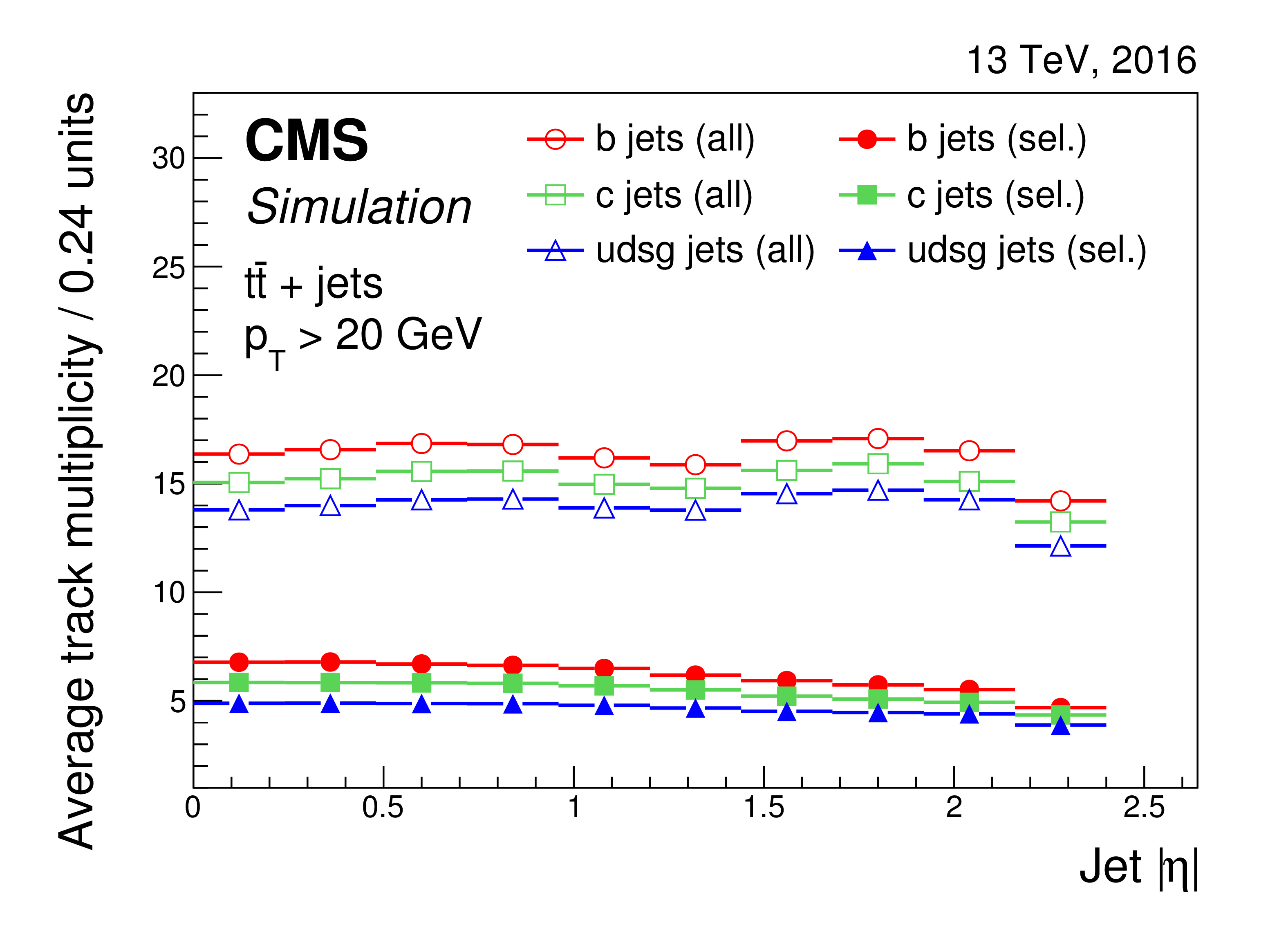
png pdf	Figure 4-b: Average track multiplicity as a function of the jet $ { \| \eta \|}$ for jets of different flavours in $ {\mathrm {t}\overline {\mathrm {t}}} $ events before (open symbols) and after (filled symbols) applying the track selection requirements.
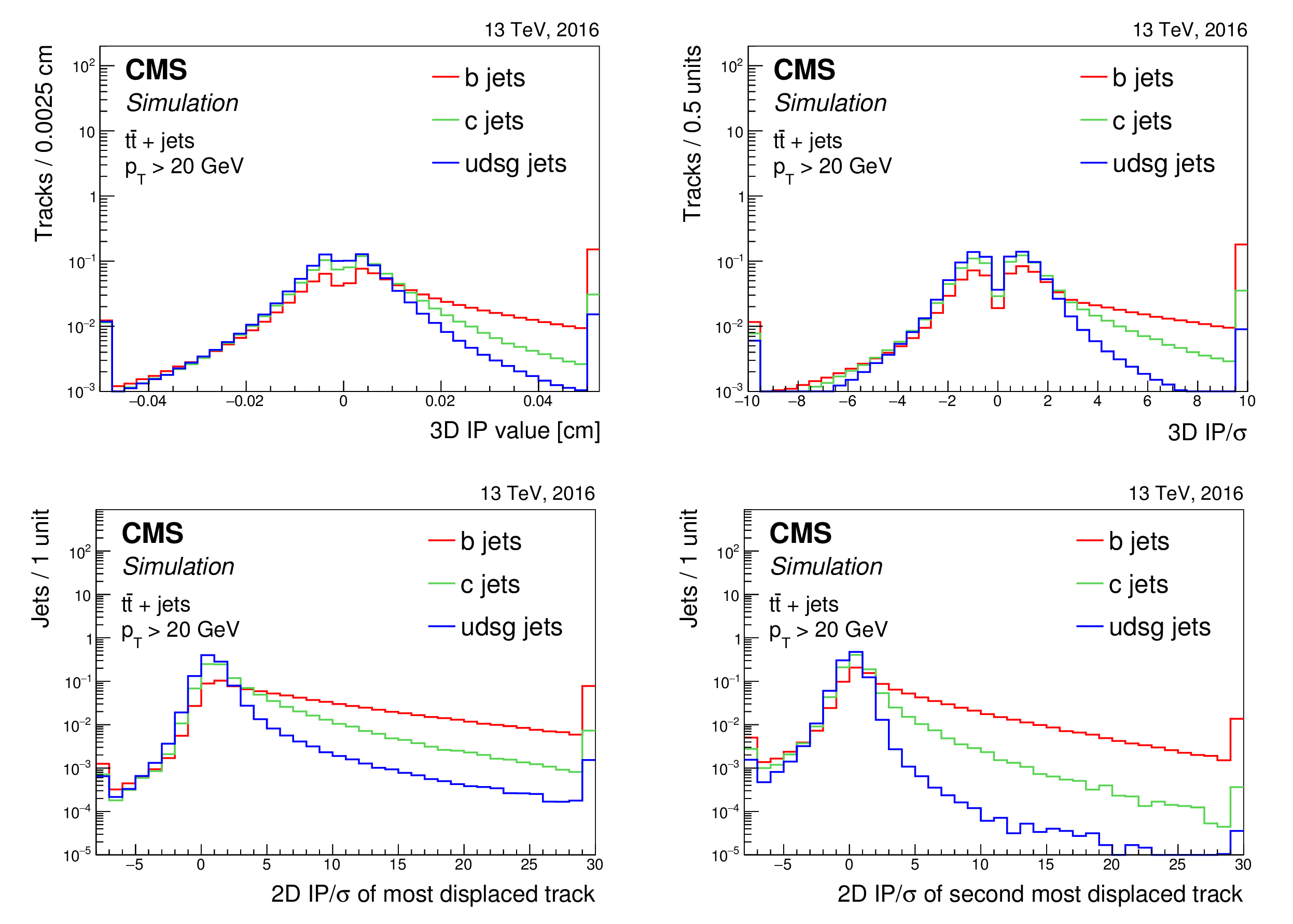
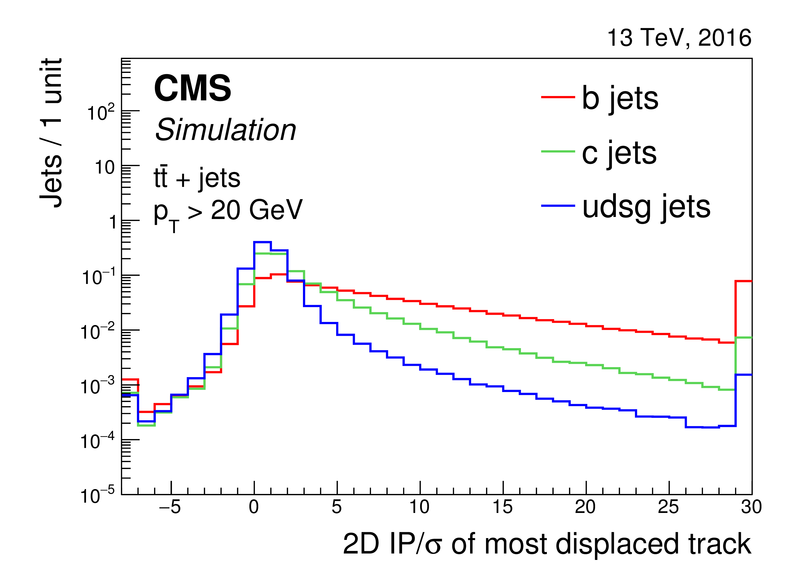
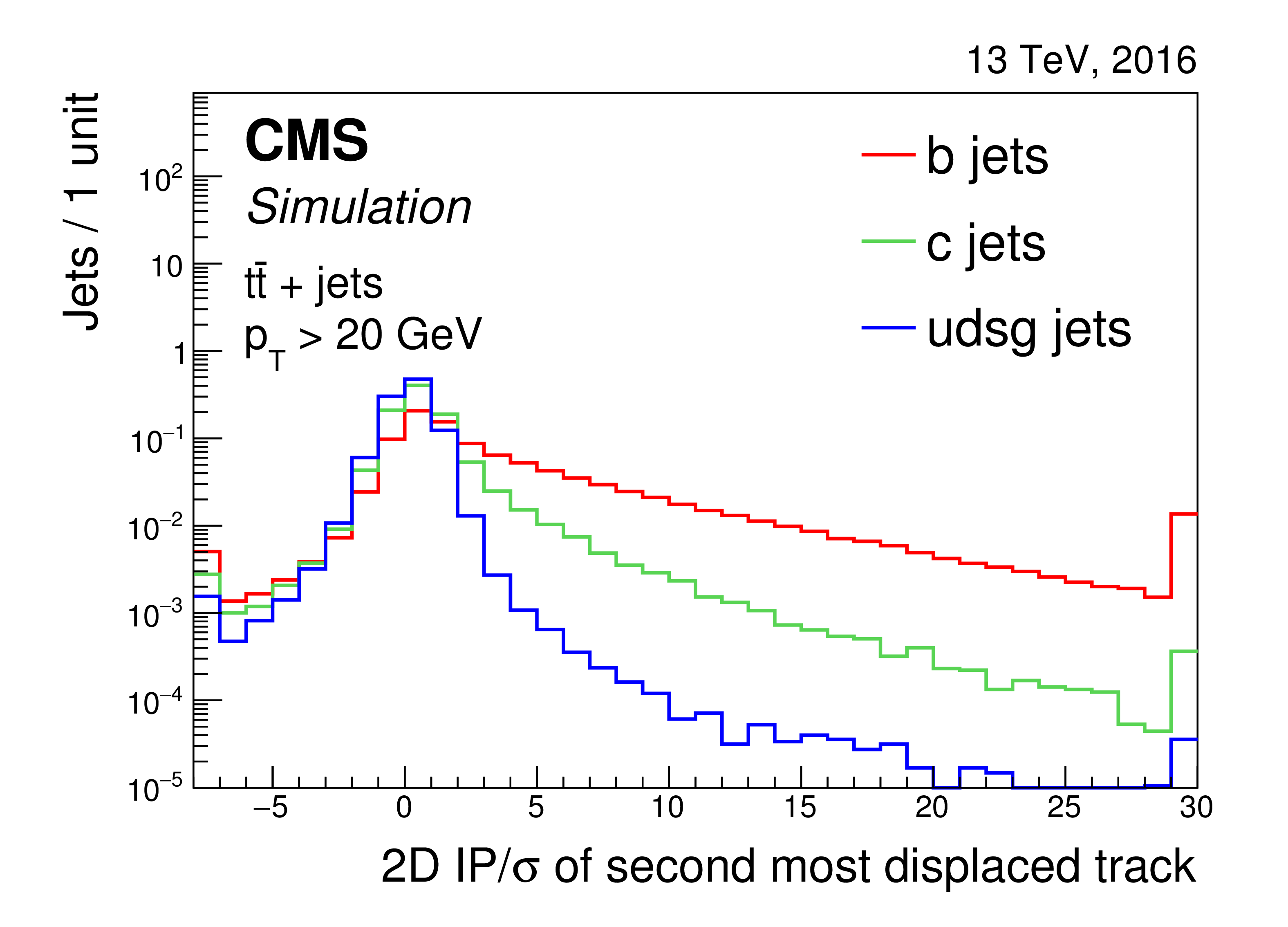
png pdf	Figure 5: Distribution of the 3D impact parameter value (upper left) and significance (upper right) for tracks associated with jets of different flavours in $ {\mathrm {t}\overline {\mathrm {t}}} $ events. Distribution of the 2D impact parameter significance for the track with the highest (lower left) and second-highest (lower right) 2D impact parameter significance for jets of different flavours in $ {\mathrm {t}\overline {\mathrm {t}}} $ events. The distributions are normalized to unit area. The first and last bin include the underflow and overflow entries, respectively.
png pdf	Figure 5-a: Distribution of the 3D impact parameter value for tracks associated with jets of different flavours in $ {\mathrm {t}\overline {\mathrm {t}}} $ events. The distributions are normalized to unit area. The first and last bin include the underflow and overflow entries, respectively.
png pdf	Figure 5-b: Distribution of the 3D significance for tracks associated with jets of different flavours in $ {\mathrm {t}\overline {\mathrm {t}}} $ events. The distributions are normalized to unit area. The first and last bin include the underflow and overflow entries, respectively.
png pdf	Figure 5-c: Distribution of the 2D impact parameter significance for the track with the highest 2D impact parameter significance for jets of different flavours in $ {\mathrm {t}\overline {\mathrm {t}}} $ events. The distributions are normalized to unit area. The first and last bin include the underflow and overflow entries, respectively.
png pdf	Figure 5-d: Distribution of the 2D impact parameter significance for the track with the second-highest 2D impact parameter significance for jets of different flavours in $ {\mathrm {t}\overline {\mathrm {t}}} $ events. The distributions are normalized to unit area. The first and last bin include the underflow and overflow entries, respectively.
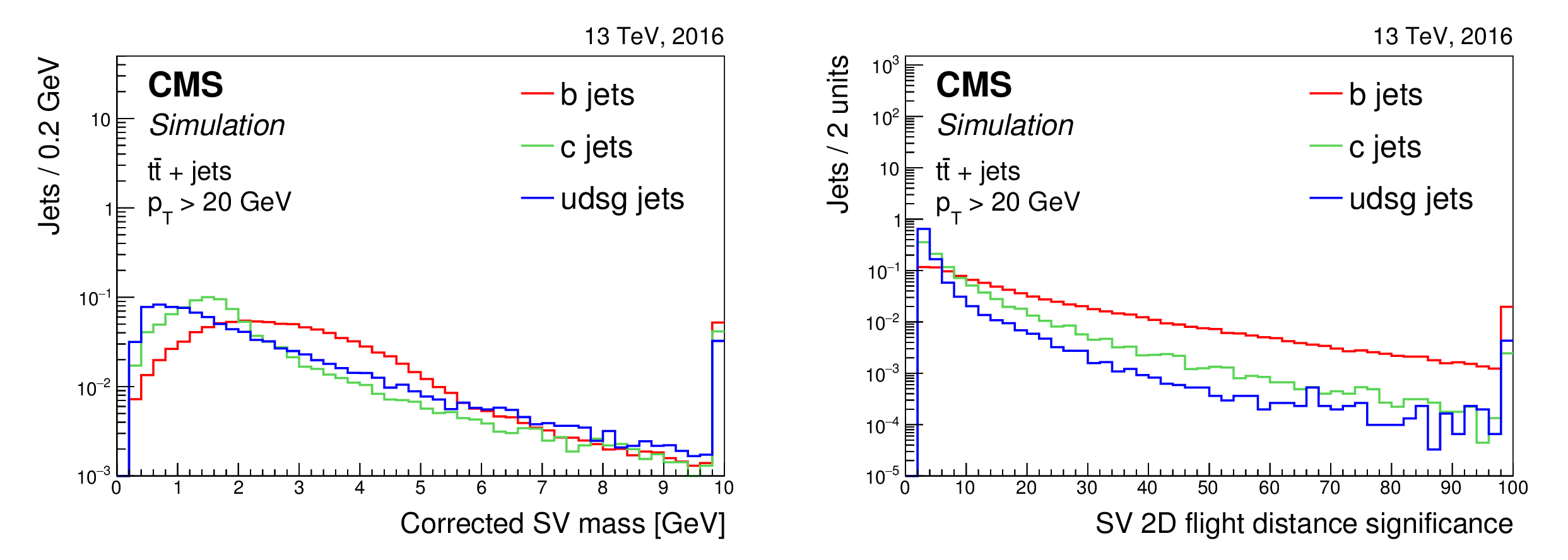
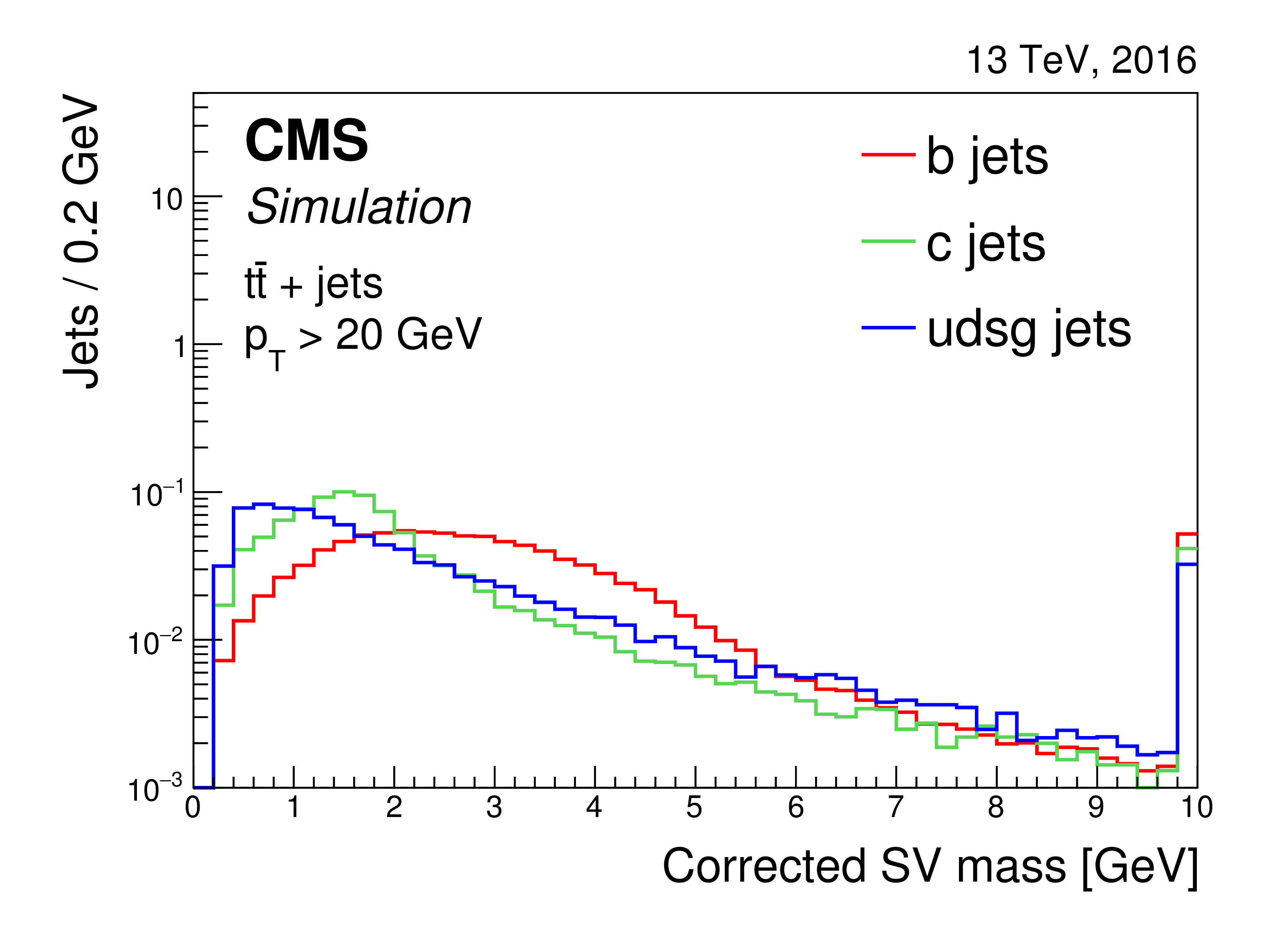
png pdf	Figure 6: Distribution of the corrected secondary vertex mass (left) and of the secondary vertex 2D flight distance significance (right) for jets containing an IVF secondary vertex. The distributions are shown for jets of different flavours in $ {\mathrm {t}\overline {\mathrm {t}}} $ events and are normalized to unit area. The last bin includes the overflow entries.
png pdf	Figure 6-a: Distribution of the corrected secondary vertex mass for jets containing an IVF secondary vertex. The distributions are shown for jets of different flavours in $ {\mathrm {t}\overline {\mathrm {t}}} $ events and are normalized to unit area. The last bin includes the overflow entries.
png pdf	Figure 6-b: Distribution of the secondary vertex 2D flight distance significance for jets containing an IVF secondary vertex. The distributions are shown for jets of different flavours in $ {\mathrm {t}\overline {\mathrm {t}}} $ events and are normalized to unit area. The last bin includes the overflow entries.
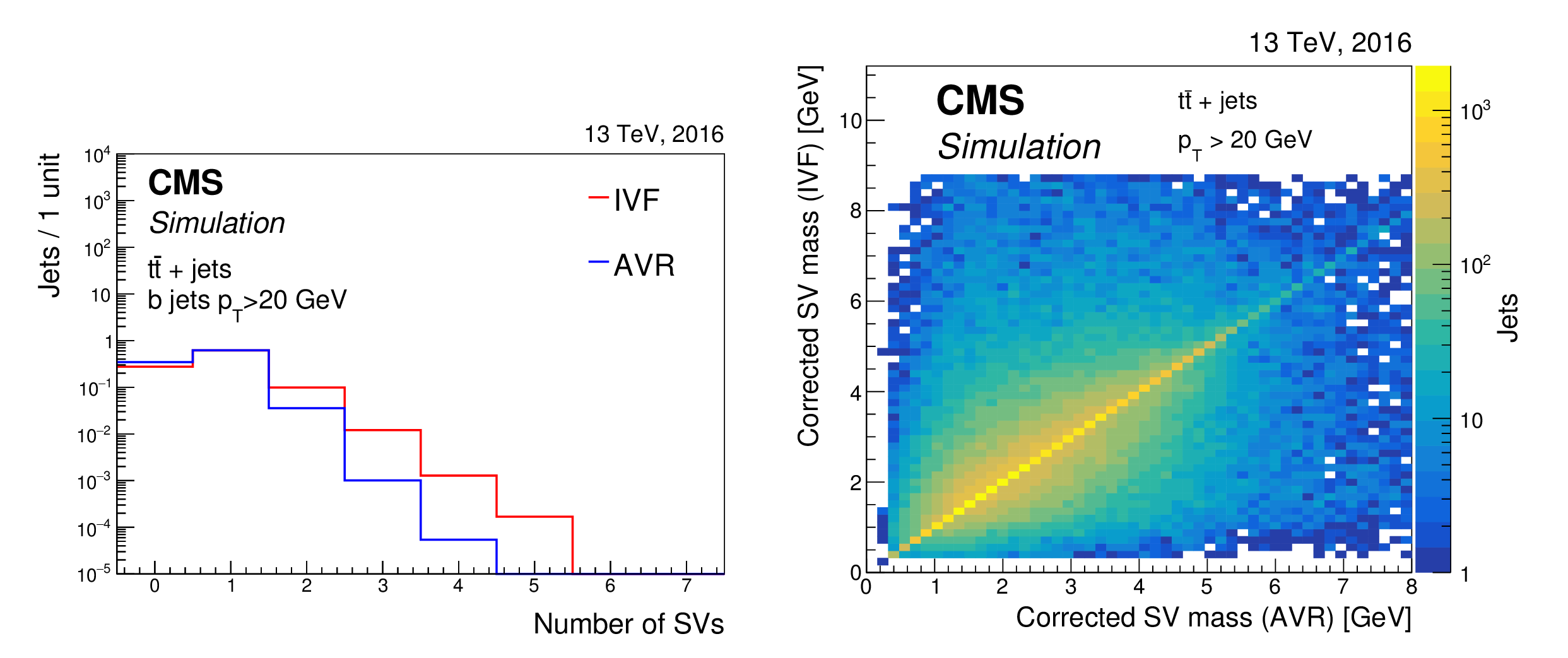
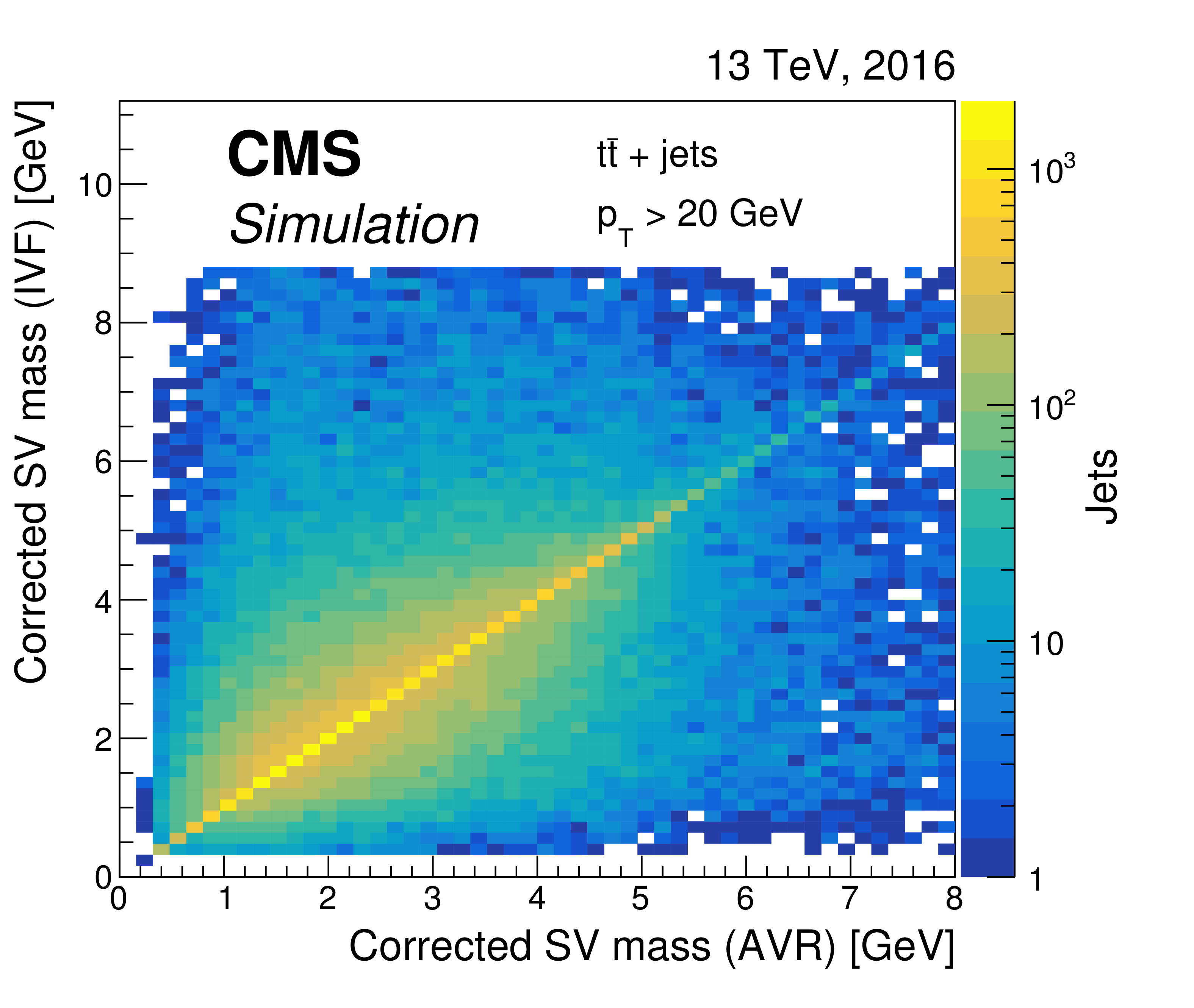
png pdf	Figure 7: Distribution of the number of secondary vertices in b jets for the two vertex finding algorithms described in the text (left). The distributions are normalized to unit area. Correlation between the corrected secondary vertex mass for the vertices obtained with the two vertex finding algorithms (right). Both panels show jets in $ {\mathrm {t}\overline {\mathrm {t}}} $ events.
png pdf	Figure 7-a: Distribution of the number of secondary vertices in b jets for the two vertex finding algorithms described in the text.This panel shows jets in $ {\mathrm {t}\overline {\mathrm {t}}} $ events.
png pdf	Figure 7-b: The distributions are normalized to unit area. Correlation between the corrected secondary vertex mass for the vertices obtained with the two vertex finding algorithms. This panel shows jets in $ {\mathrm {t}\overline {\mathrm {t}}} $ events.
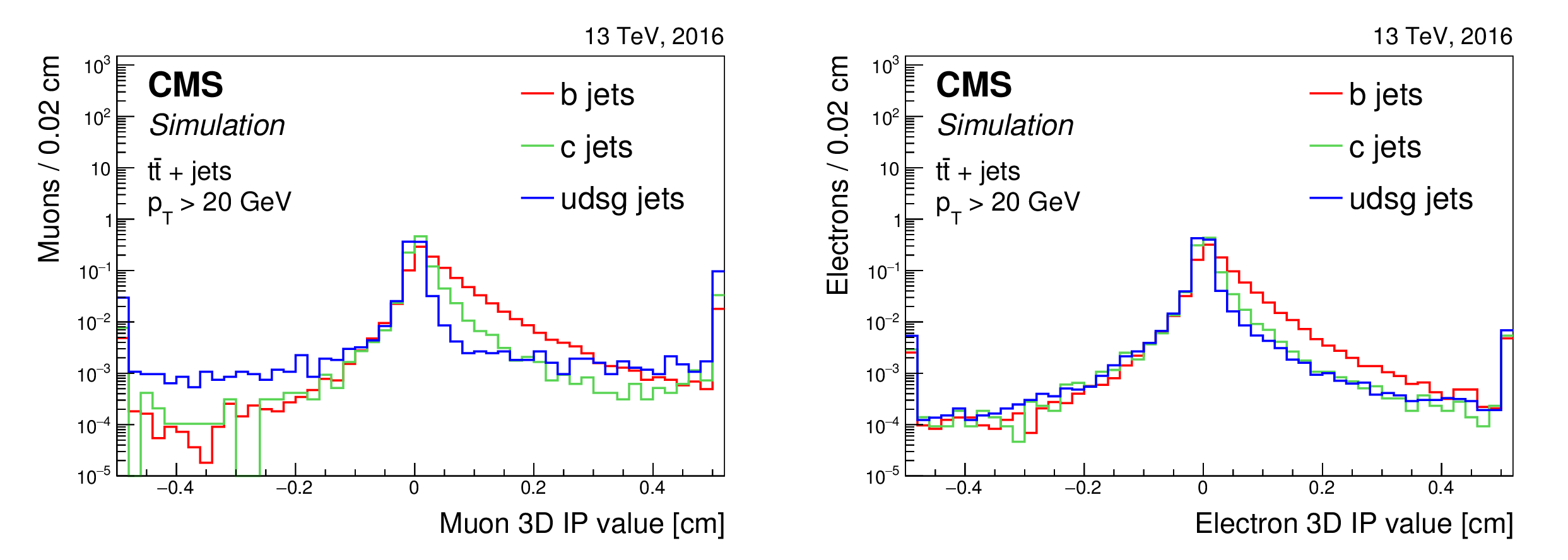
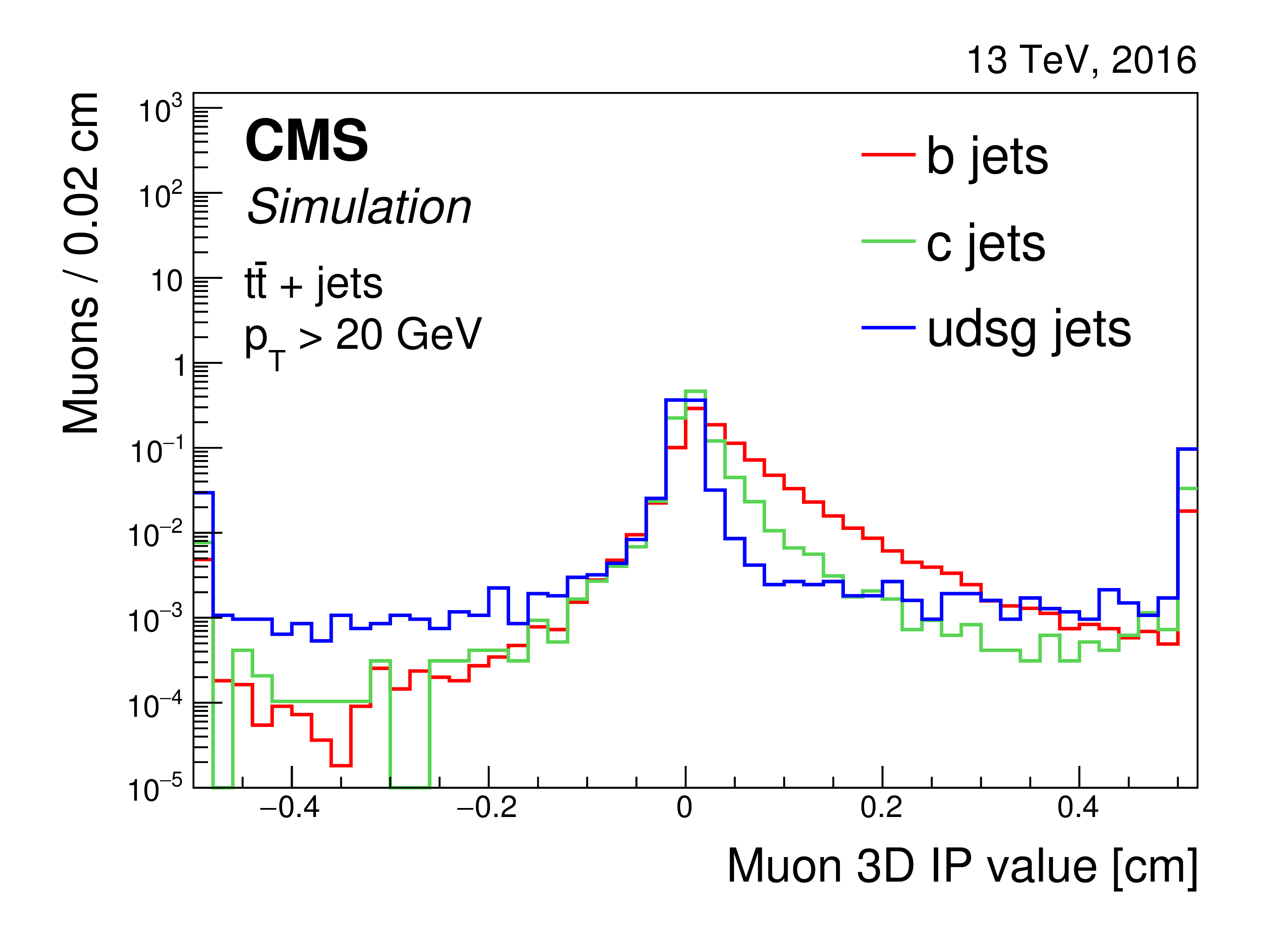
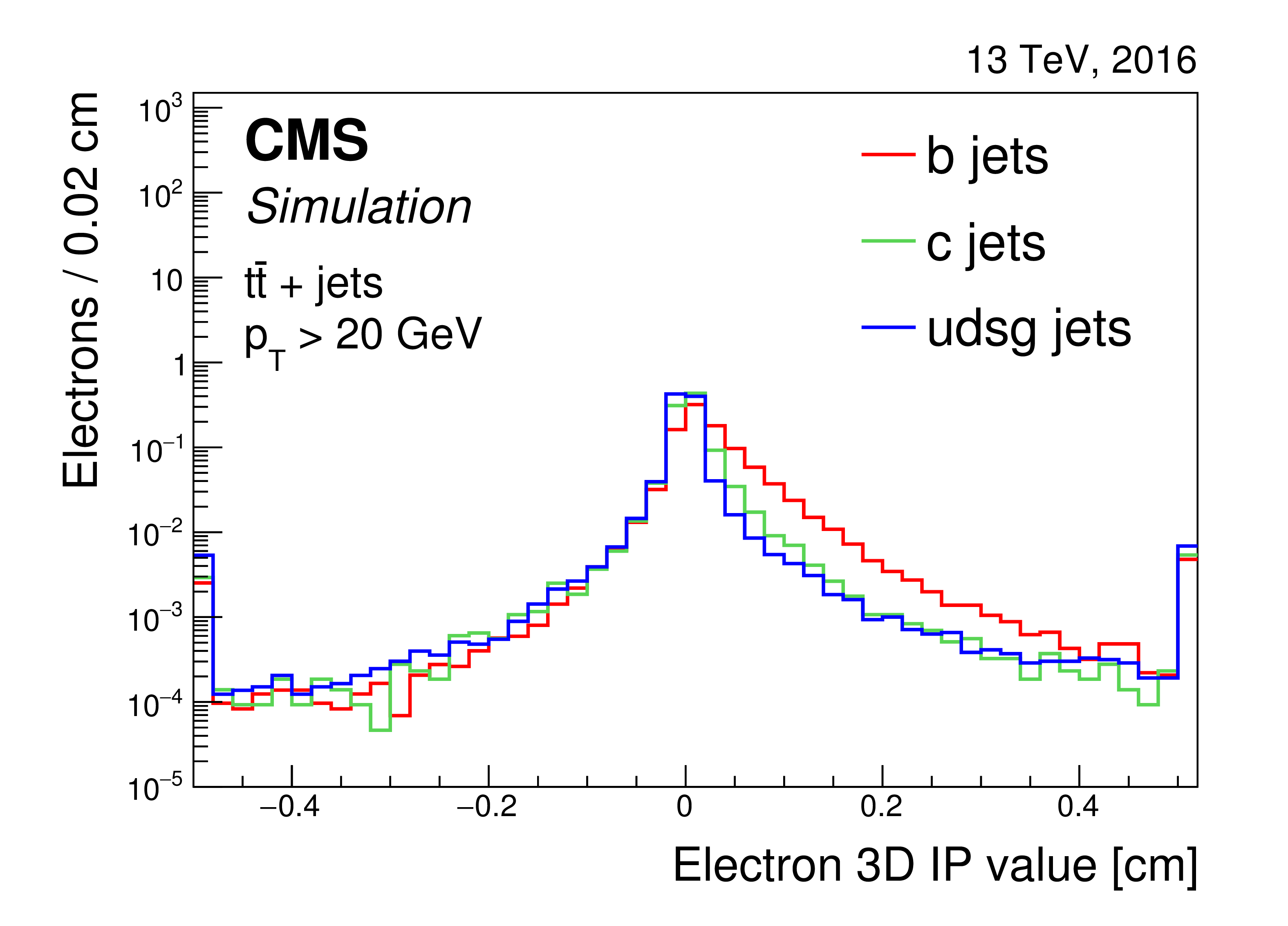
png pdf	Figure 8: Distribution of the 3D impact parameter value for soft muons (left) and soft electrons (right) for jets of different flavours in $ {\mathrm {t}\overline {\mathrm {t}}} $ events. The distributions are normalized to unit area. The first and last bins include the underflow and overflow entries, respectively.
png pdf	Figure 8-a: Distribution of the 3D impact parameter value for soft muons for jets of different flavours in $ {\mathrm {t}\overline {\mathrm {t}}} $ events. The distributions are normalized to unit area. The first and last bins include the underflow and overflow entries, respectively.
png pdf	Figure 8-b: Distribution of the 3D impact parameter value for soft electrons for jets of different flavours in $ {\mathrm {t}\overline {\mathrm {t}}} $ events. The distributions are normalized to unit area. The first and last bins include the underflow and overflow entries, respectively.
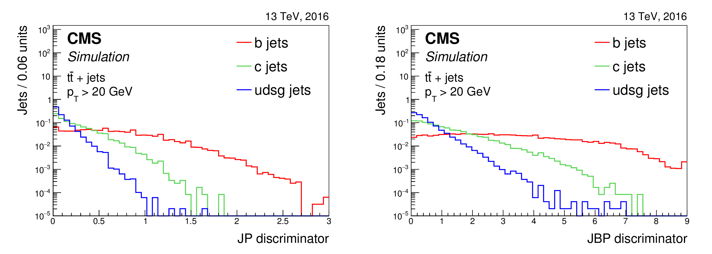
png pdf	Figure 9: Distribution of the JP (left) and JBP (right) discriminator values for jets of different flavours in $ {\mathrm {t}\overline {\mathrm {t}}} $ events. Jets without selected tracks are assigned a negative value. The distributions are normalized to unit area. The first and last bin include the underflow and overflow entries, respectively.
png pdf	Figure 9-a: Distribution of the JP discriminator values for jets of different flavours in $ {\mathrm {t}\overline {\mathrm {t}}} $ events. Jets without selected tracks are assigned a negative value. The distributions are normalized to unit area. The first and last bin include the underflow and overflow entries, respectively.
png pdf	Figure 9-b: Distribution of the JBP discriminator values for jets of different flavours in $ {\mathrm {t}\overline {\mathrm {t}}} $ events. Jets without selected tracks are assigned a negative value. The distributions are normalized to unit area. The first and last bin include the underflow and overflow entries, respectively.
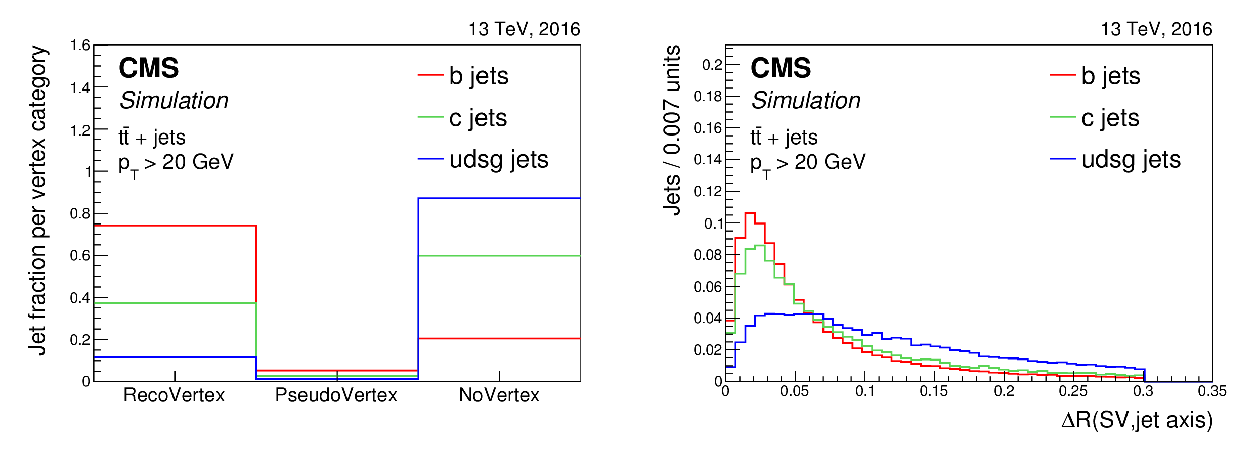
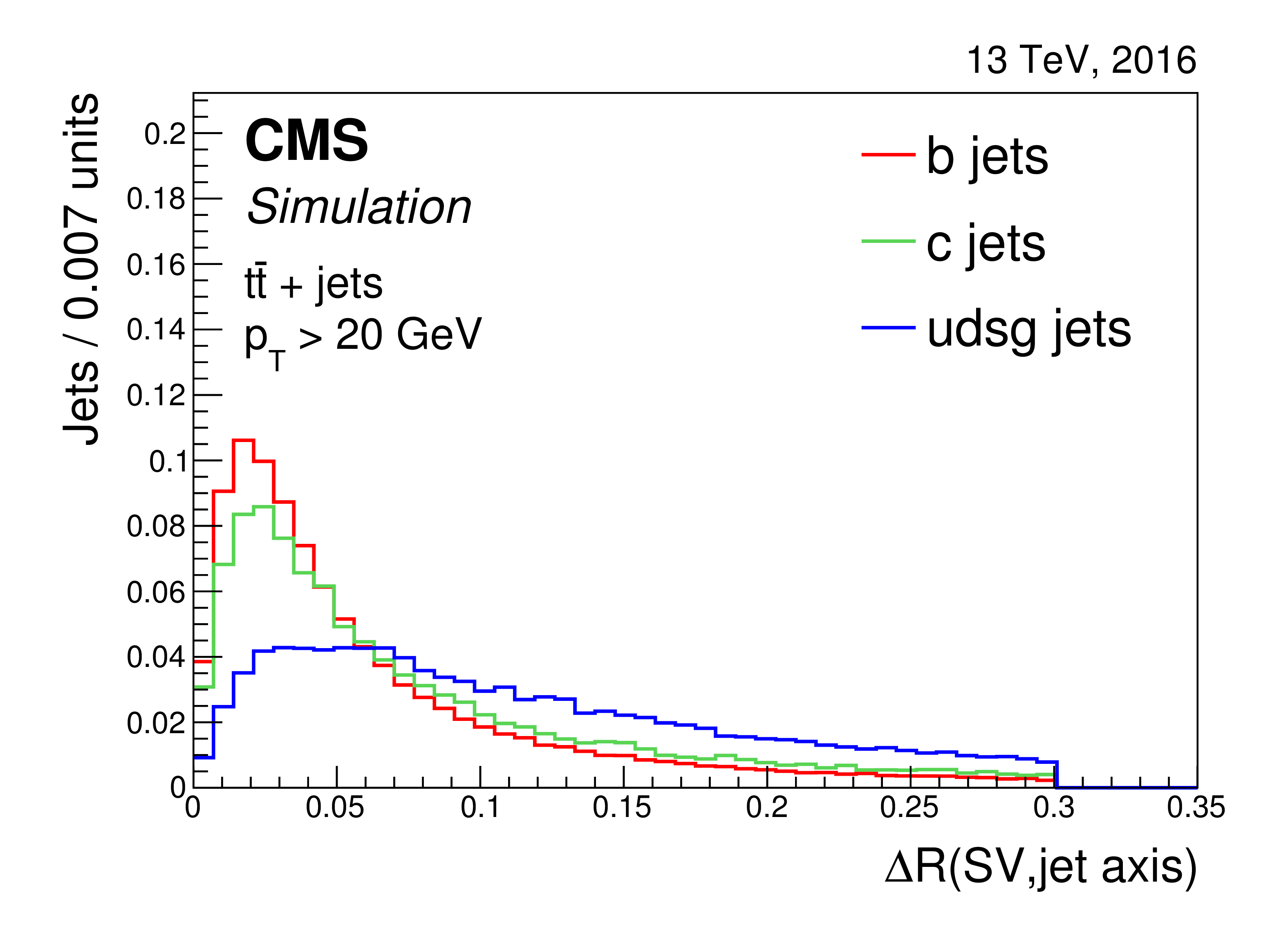
png pdf	Figure 10: Vertex category for secondary vertices reconstructed with the IVF algorithm (left), and the distribution of the angular distance between the IVF secondary vertex flight direction and the jet axis (right) for jets of different flavours in $ {\mathrm {t}\overline {\mathrm {t}}} $ events. The distributions are normalized to unit area.
png pdf	Figure 10-a: Vertex category for secondary vertices reconstructed with the IVF algorithm for jets of different flavours in $ {\mathrm {t}\overline {\mathrm {t}}} $ events. The distributions are normalized to unit area.
png pdf	Figure 10-b: Distribution of the angular distance between the IVF secondary vertex flight direction and the jet axis for jets of different flavours in $ {\mathrm {t}\overline {\mathrm {t}}} $ events. The distributions are normalized to unit area.
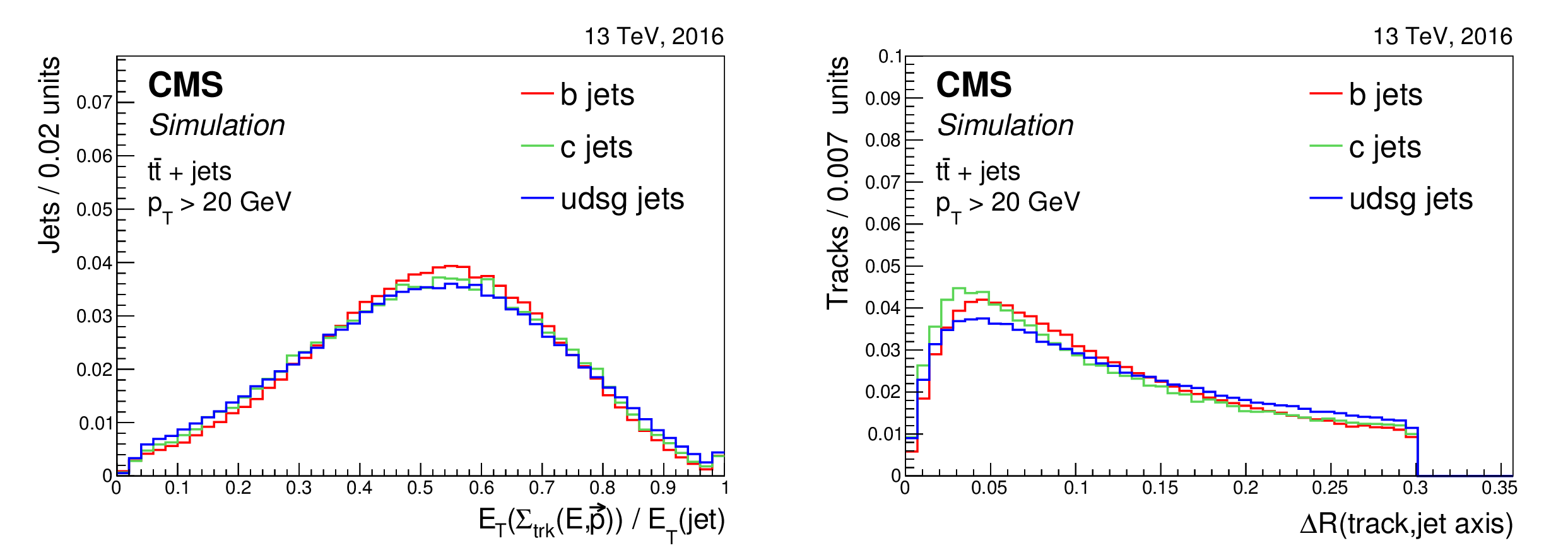
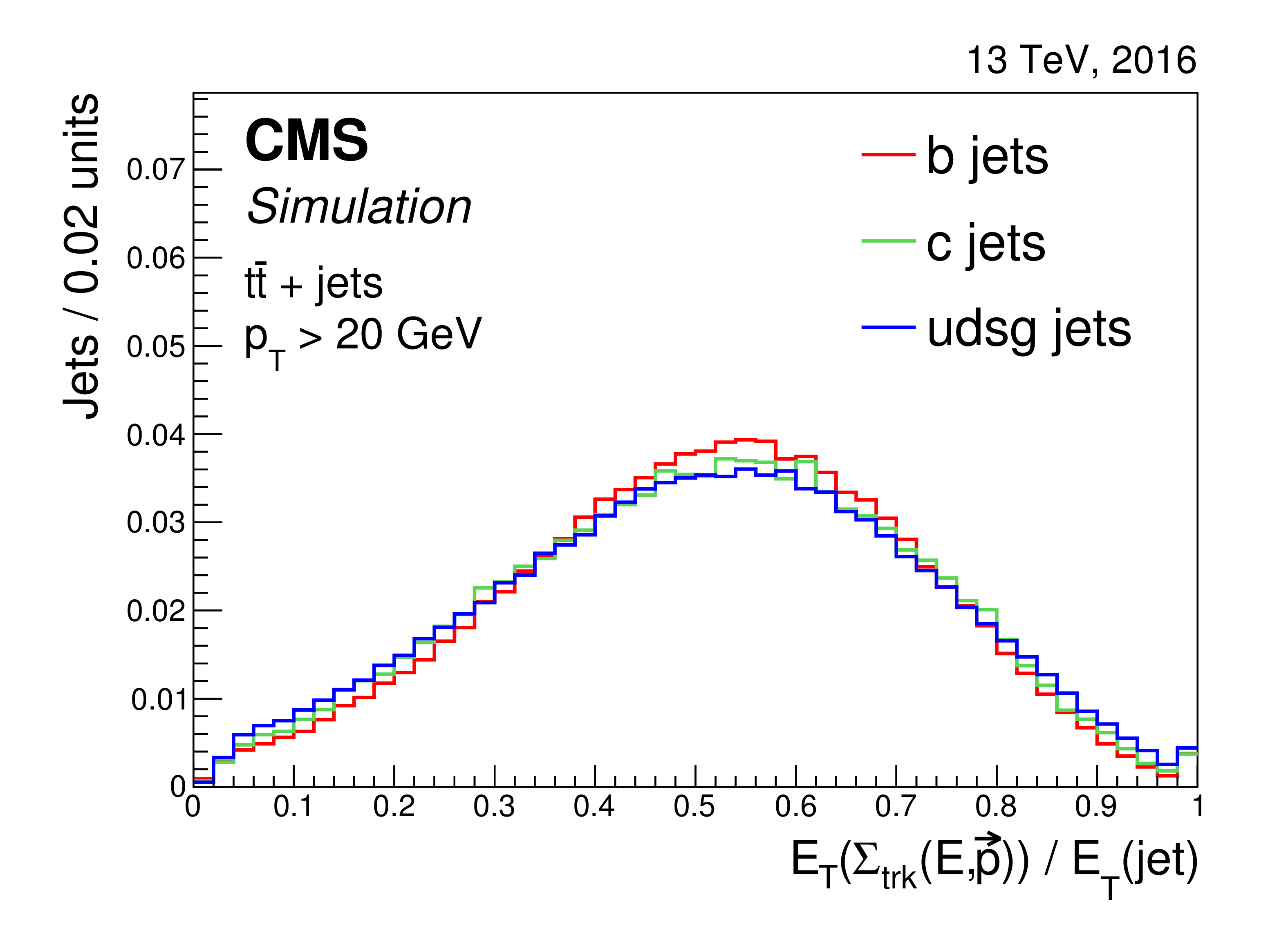
png pdf	Figure 11: Distribution of the transverse energy of the total summed four-momentum vector of the selected tracks divided by the jet transverse energy (left), and angular distance between the track and the jet axis (right) for jets of different flavours in $ {\mathrm {t}\overline {\mathrm {t}}} $ events. The distributions are normalized to unit area. The last bin in the left panel includes the overflow entries.
png pdf	Figure 11-a: Distribution of the transverse energy of the total summed four-momentum vector of the selected tracks divided by the jet transverse energy for jets of different flavours in $ {\mathrm {t}\overline {\mathrm {t}}} $ events. The distributions are normalized to unit area. The last bin includes the overflow entries.
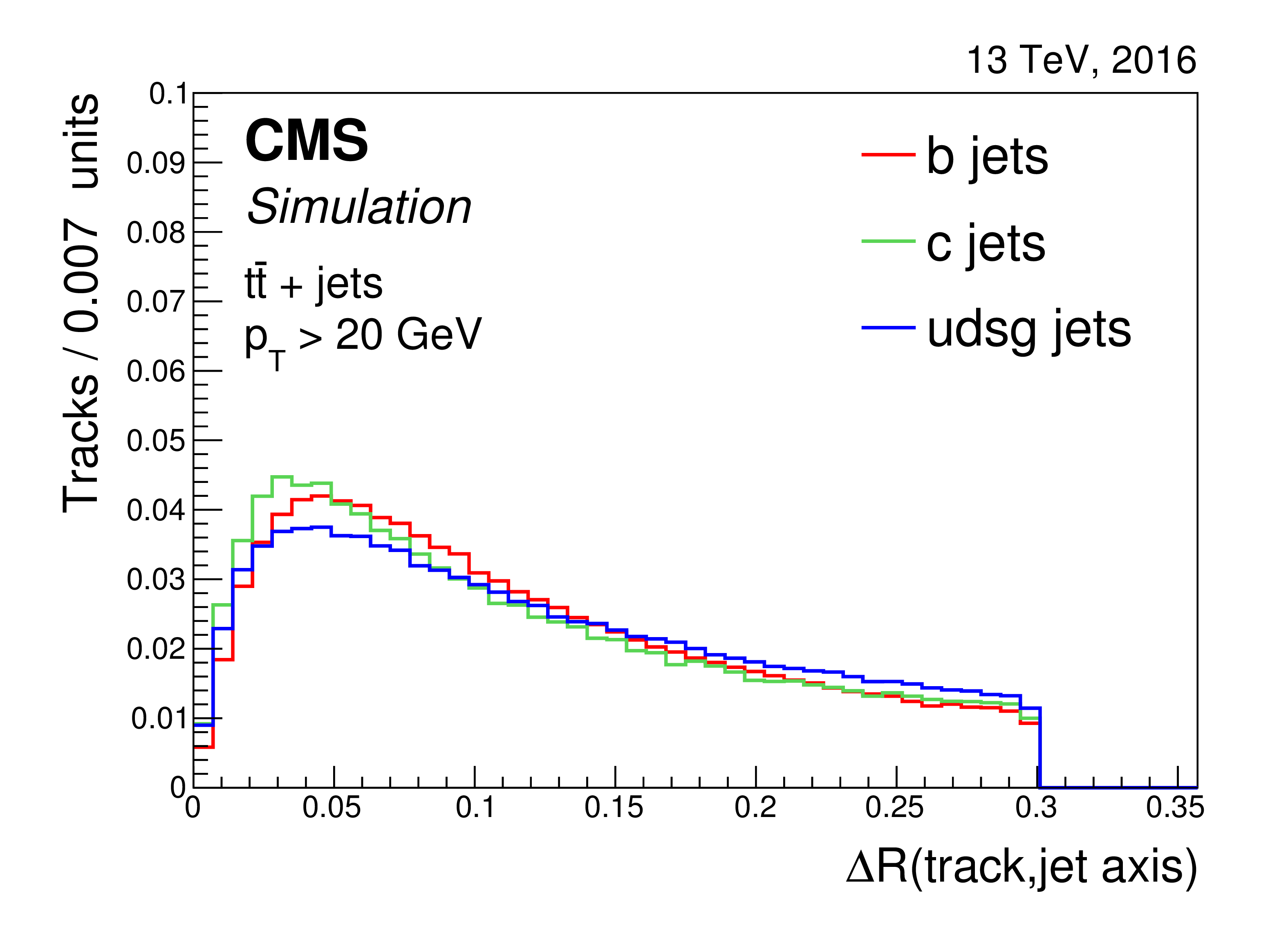
png pdf	Figure 11-b: Distribution of the angular distance between the track and the jet axis for jets of different flavours in $ {\mathrm {t}\overline {\mathrm {t}}} $ events. The distributions are normalized to unit area.
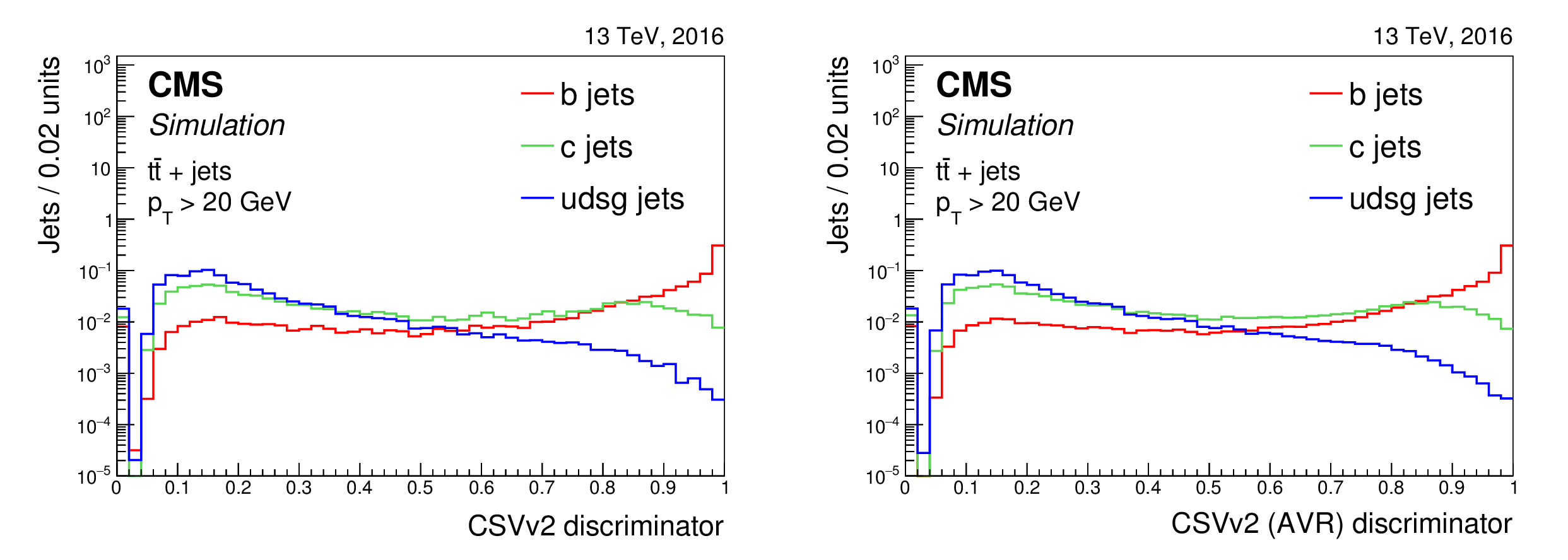
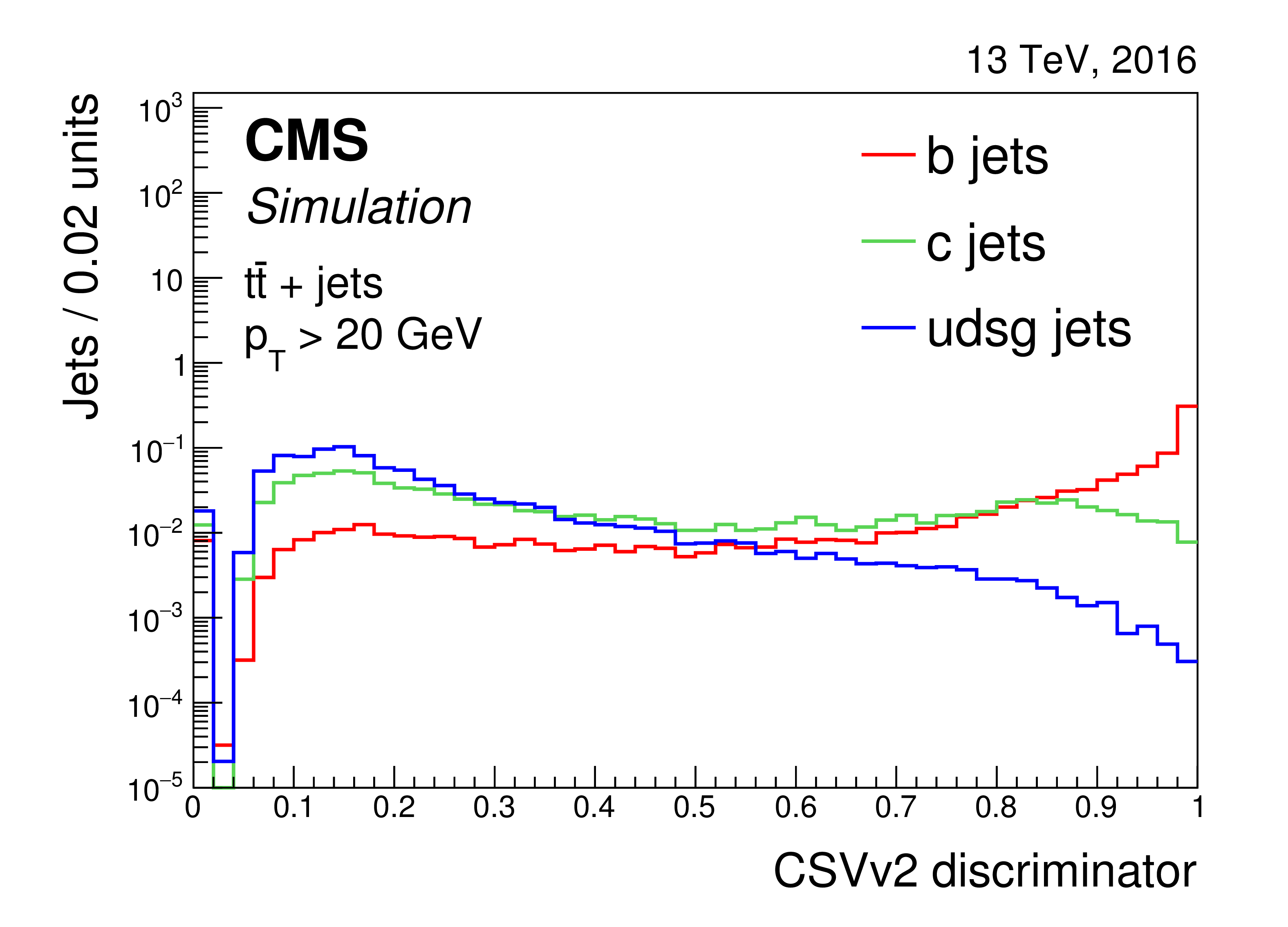
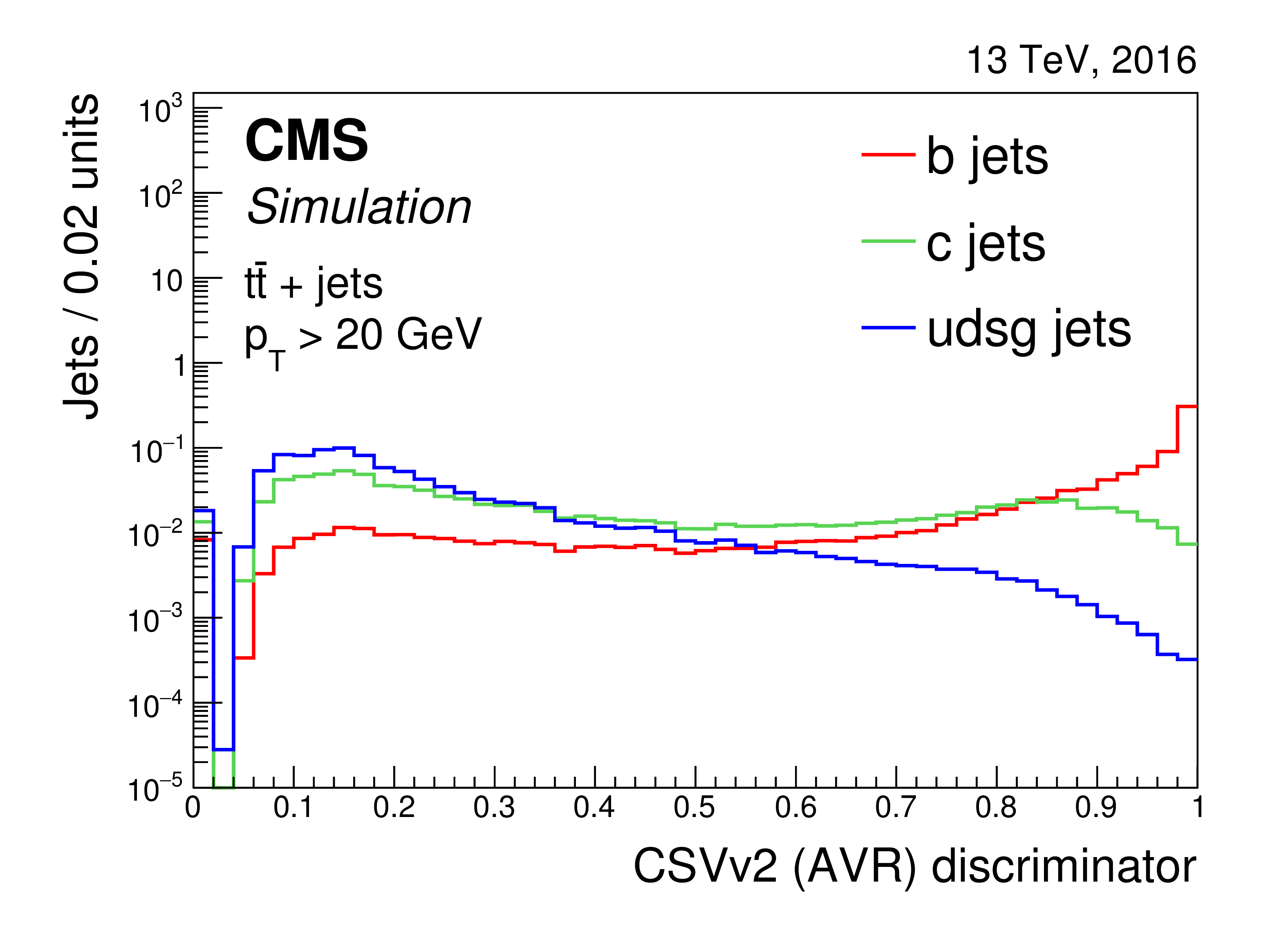
png pdf	Figure 12: Distribution of the CSVv2 (left) and CSVv2(AVR) (right) discriminator values for jets of different flavours in $ {\mathrm {t}\overline {\mathrm {t}}} $ events. The distributions are normalized to unit area. Jets without a selected track and secondary vertex are assigned a negative discriminator value. The first bin includes the underflow entries.
png pdf	Figure 12-a: Distribution of the CSVv2 discriminator values for jets of different flavours in $ {\mathrm {t}\overline {\mathrm {t}}} $ events. The distributions are normalized to unit area. Jets without a selected track and secondary vertex are assigned a negative discriminator value. The first bin includes the underflow entries.
png pdf	Figure 12-b: Distribution of the CSVv2(AVR) discriminator values for jets of different flavours in $ {\mathrm {t}\overline {\mathrm {t}}} $ events. The distributions are normalized to unit area. Jets without a selected track and secondary vertex are assigned a negative discriminator value. The first bin includes the underflow entries.
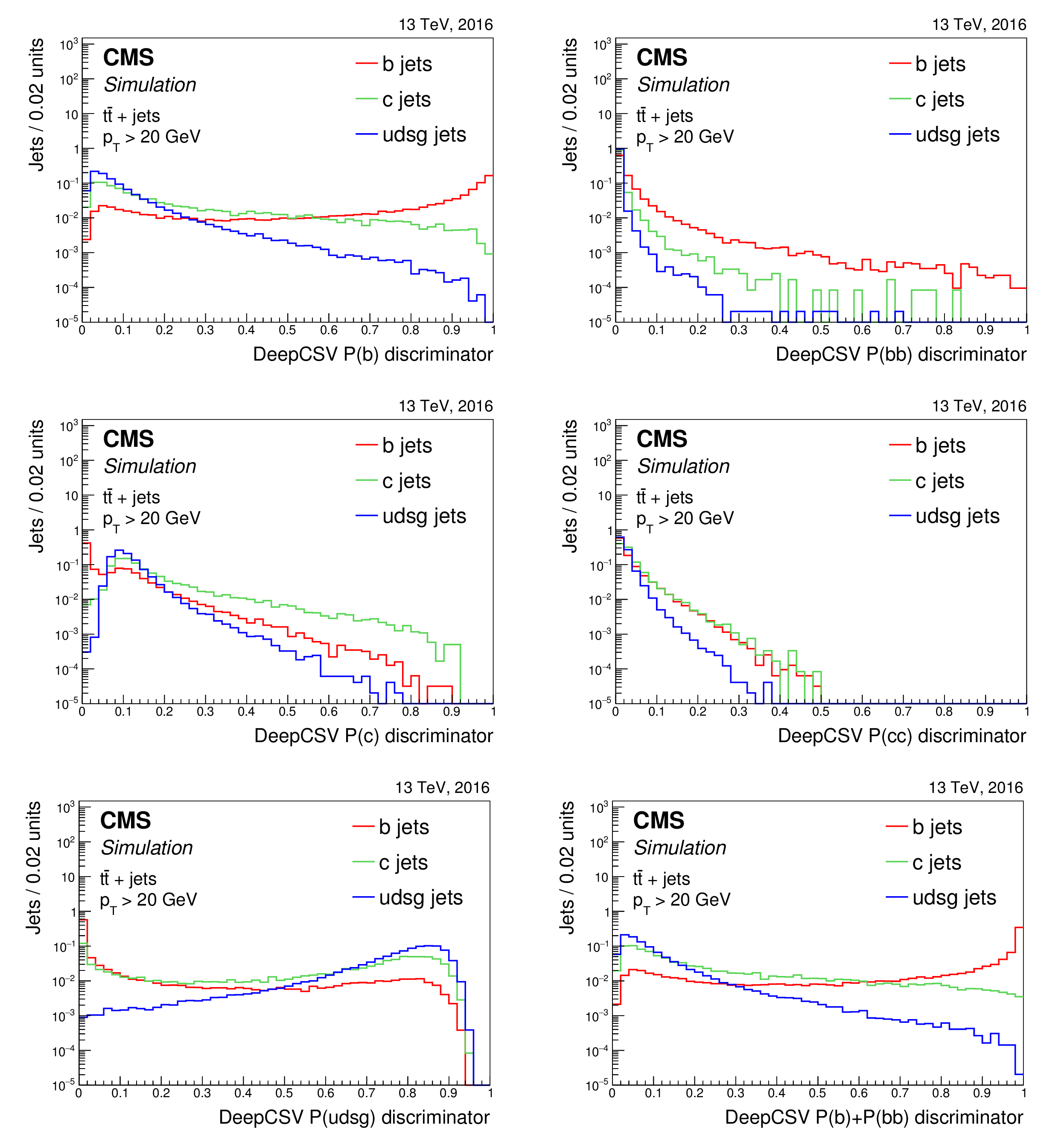
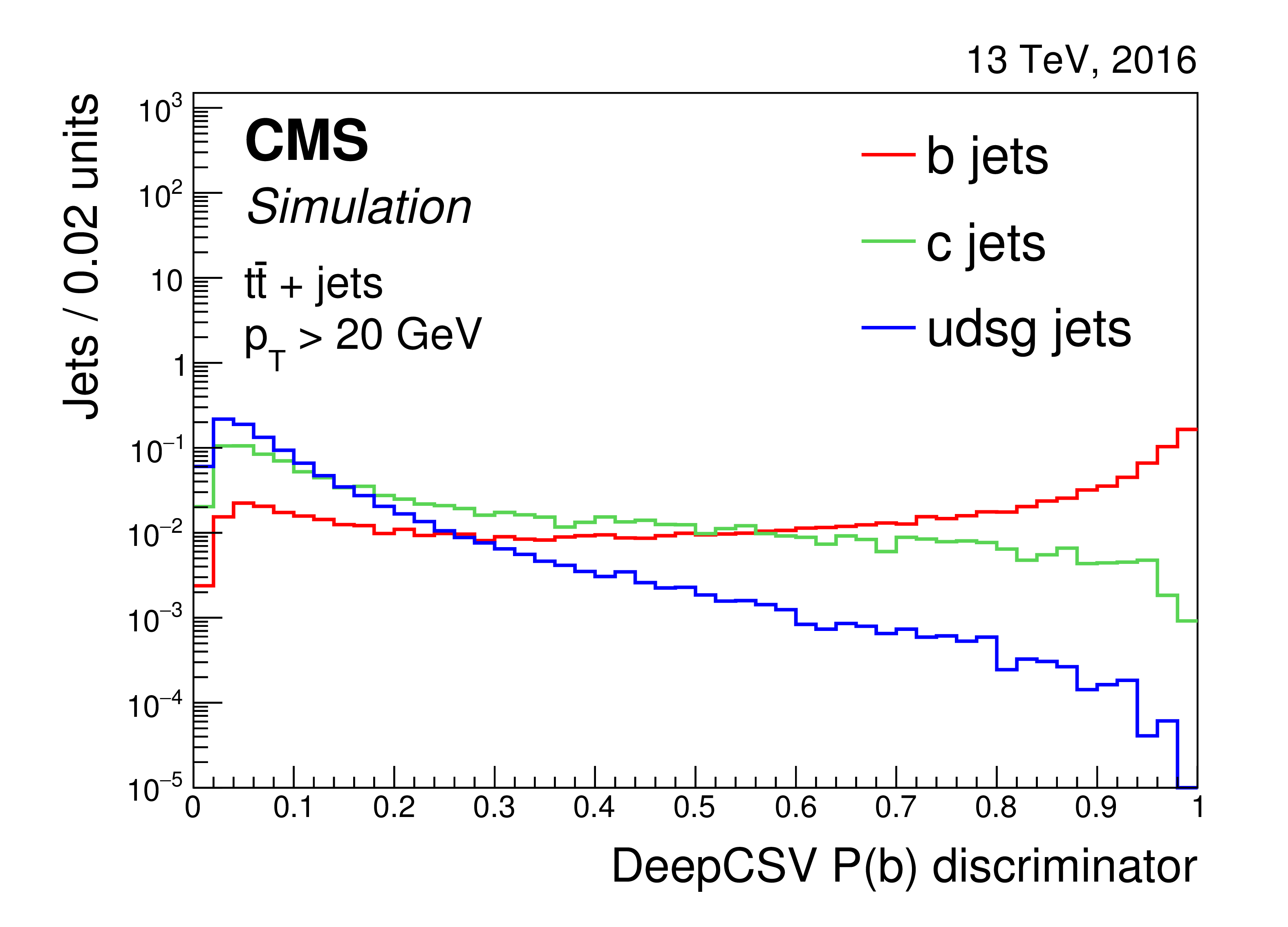
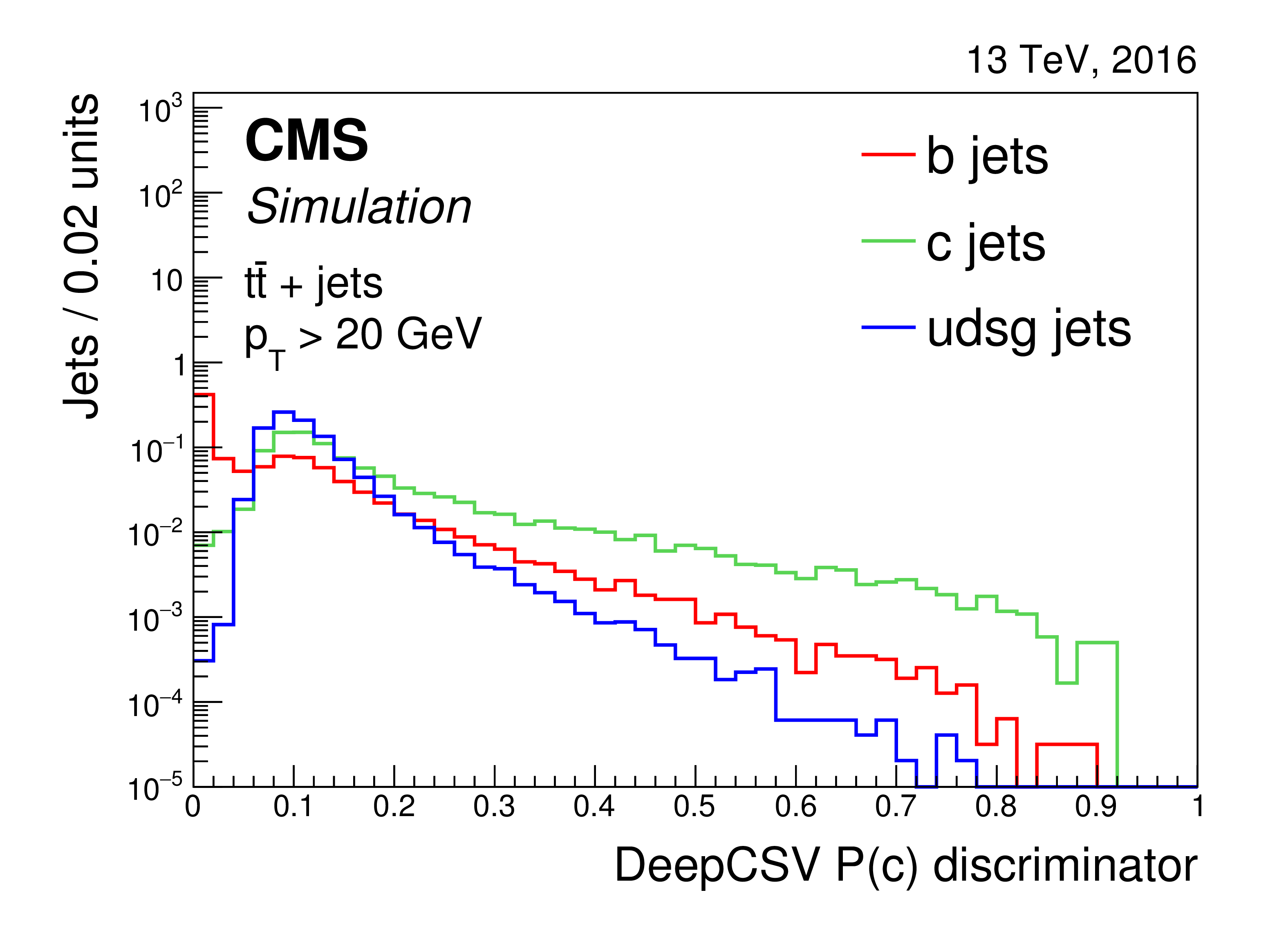
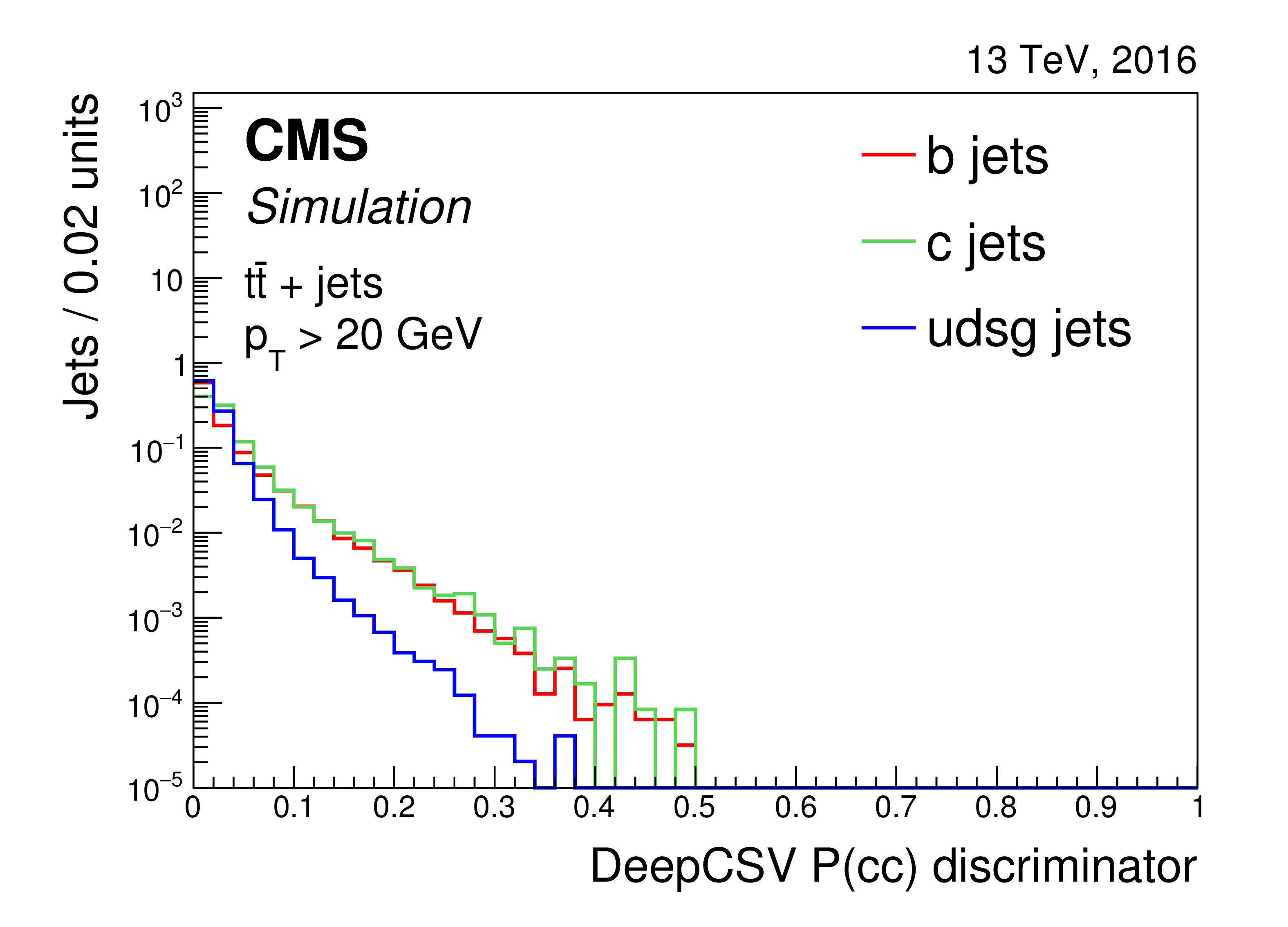
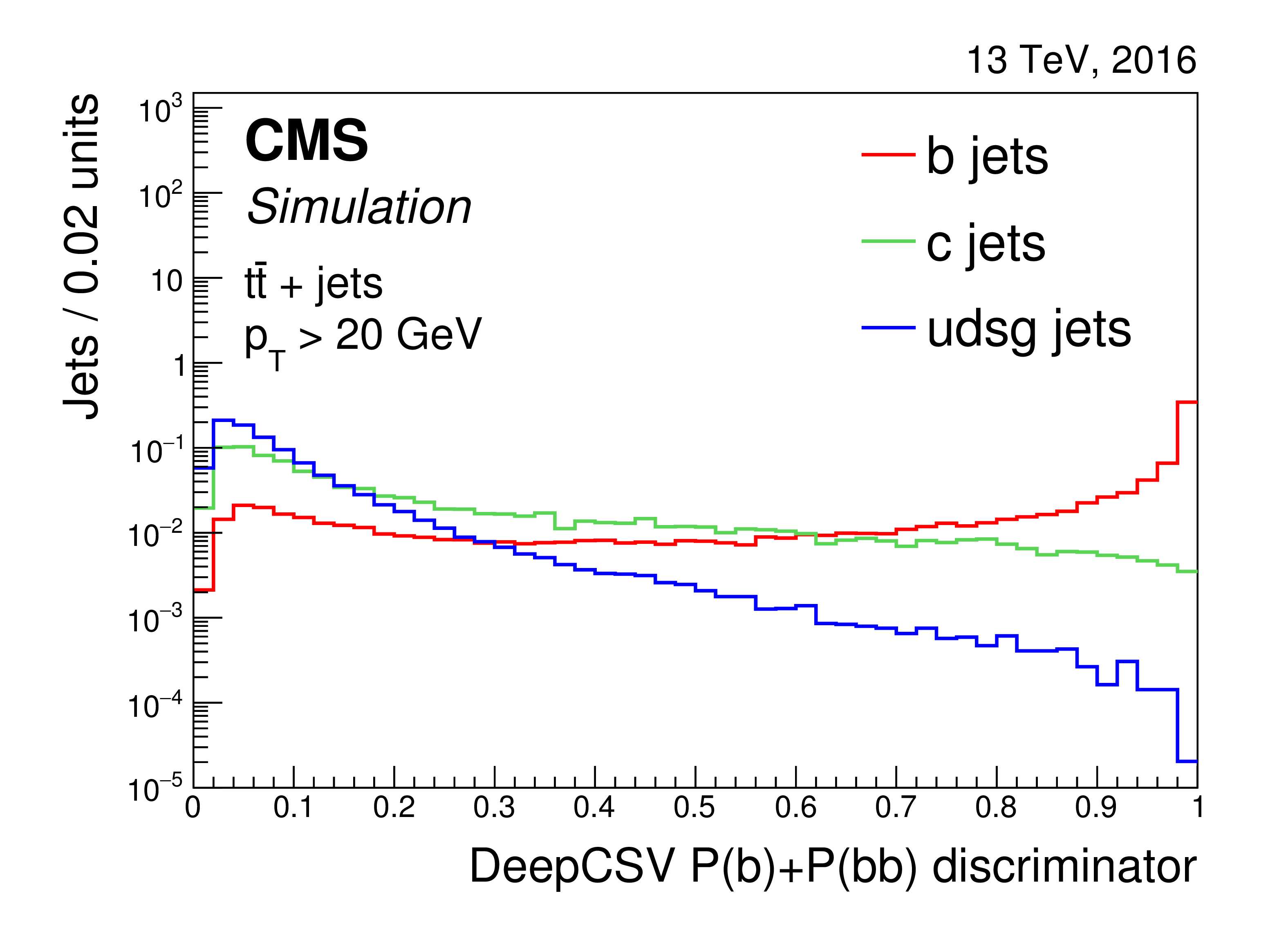
png pdf	Figure 13: Distribution of the DeepCSV $P({\mathrm {b}})$ (upper left), $P({\mathrm {b}} {\mathrm {b}})$ (upper right), $P({\mathrm {c}})$ (middle left), $P({\mathrm {c}} {\mathrm {c}})$ (middle right), $P({\text {udsg}})$ (lower left), and $P({\mathrm {b}})+P({\mathrm {b}} {\mathrm {b}})$ (lower right) discriminator values for jets of different flavours in $ {\mathrm {t}\overline {\mathrm {t}}} $ events. Jets without a selected track and without a secondary vertex are assigned a discriminator value of 0. The distributions are normalized to unit area.
png pdf	Figure 13-a: Distribution of the DeepCSV $P({\mathrm {b}})$ discriminator values for jets of different flavours in $ {\mathrm {t}\overline {\mathrm {t}}} $ events. Jets without a selected track and without a secondary vertex are assigned a discriminator value of 0. The distributions are normalized to unit area.
png pdf	Figure 13-b: Distribution of the $P({\mathrm {b}} {\mathrm {b}})$ discriminator values for jets of different flavours in $ {\mathrm {t}\overline {\mathrm {t}}} $ events. Jets without a selected track and without a secondary vertex are assigned a discriminator value of 0. The distributions are normalized to unit area.
png pdf	Figure 13-c: Distribution of the $P({\mathrm {c}})$ discriminator values for jets of different flavours in $ {\mathrm {t}\overline {\mathrm {t}}} $ events. Jets without a selected track and without a secondary vertex are assigned a discriminator value of 0. The distributions are normalized to unit area.
png pdf	Figure 13-d: Distribution of the $P({\mathrm {c}} {\mathrm {c}})$ discriminator values for jets of different flavours in $ {\mathrm {t}\overline {\mathrm {t}}} $ events. Jets without a selected track and without a secondary vertex are assigned a discriminator value of 0. The distributions are normalized to unit area.
png pdf	Figure 13-e: Distribution of the $P({\text {udsg}})$ discriminator values for jets of different flavours in $ {\mathrm {t}\overline {\mathrm {t}}} $ events. Jets without a selected track and without a secondary vertex are assigned a discriminator value of 0. The distributions are normalized to unit area.
png pdf	Figure 13-f: Distribution of the $P({\mathrm {b}})+P({\mathrm {b}} {\mathrm {b}})$ discriminator values for jets of different flavours in $ {\mathrm {t}\overline {\mathrm {t}}} $ events. Jets without a selected track and without a secondary vertex are assigned a discriminator value of 0. The distributions are normalized to unit area.
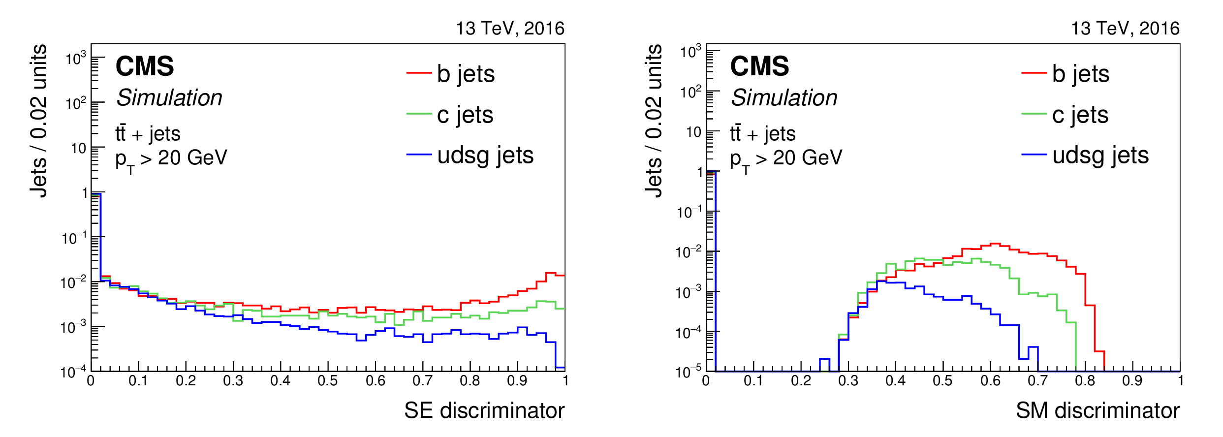
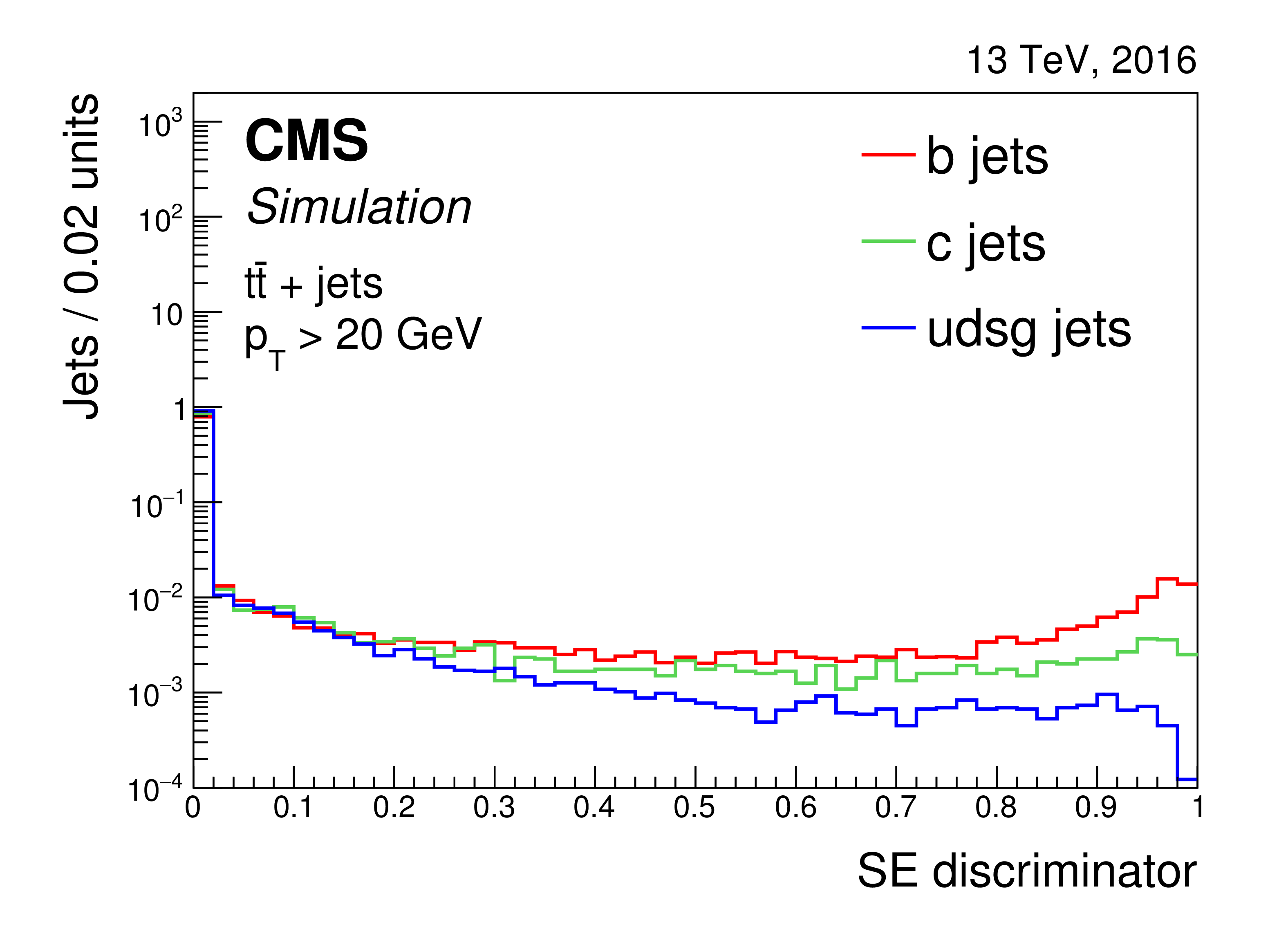
png pdf	Figure 14: Distribution of the soft-electron (left) and soft-muon (right) discriminator values for jets of different flavours in $ {\mathrm {t}\overline {\mathrm {t}}} $ events. Jets without a soft lepton are assigned a discriminator value of 0. The distributions are normalized to unit area.
png pdf	Figure 14-a: Distribution of the soft-electron discriminator values for jets of different flavours in $ {\mathrm {t}\overline {\mathrm {t}}} $ events. Jets without a soft lepton are assigned a discriminator value of 0. The distributions are normalized to unit area.
png pdf	Figure 14-b: Distribution of the soft-muon discriminator values for jets of different flavours in $ {\mathrm {t}\overline {\mathrm {t}}} $ events. Jets without a soft lepton are assigned a discriminator value of 0. The distributions are normalized to unit area.
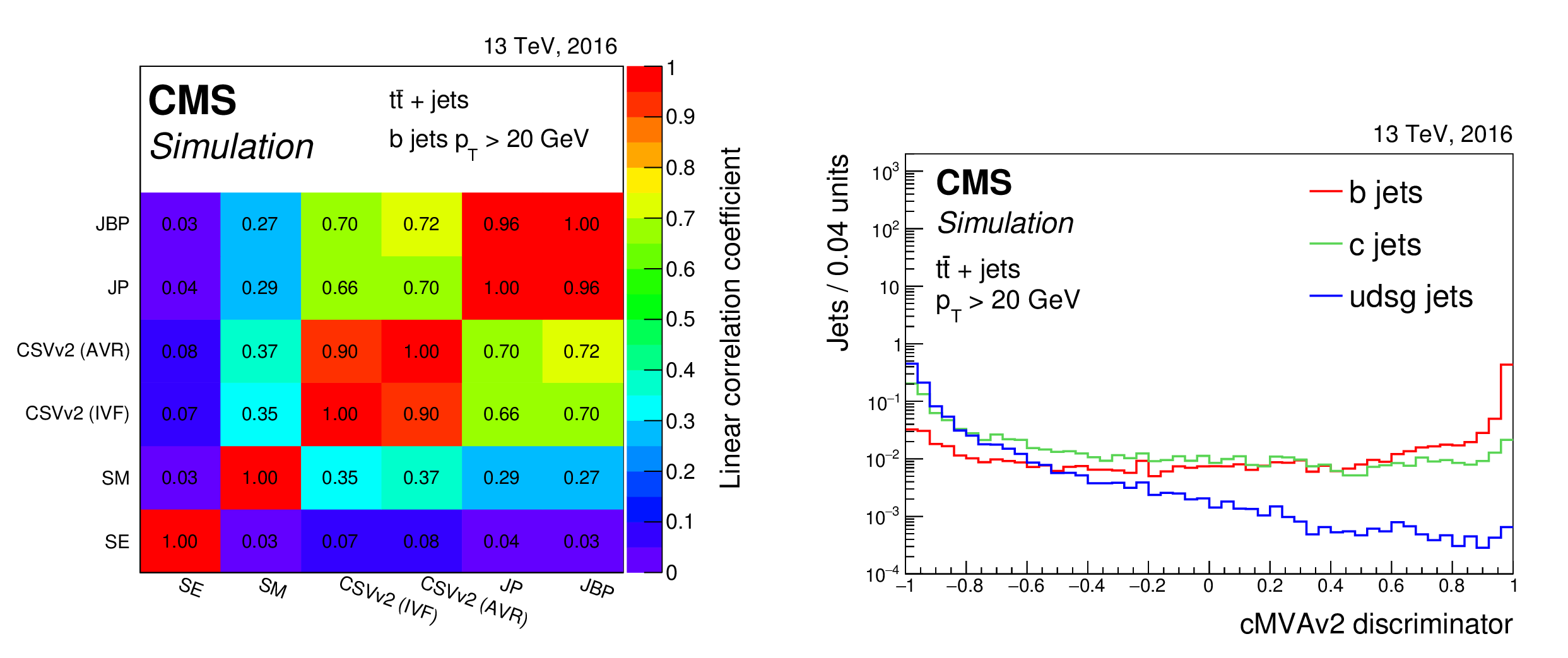
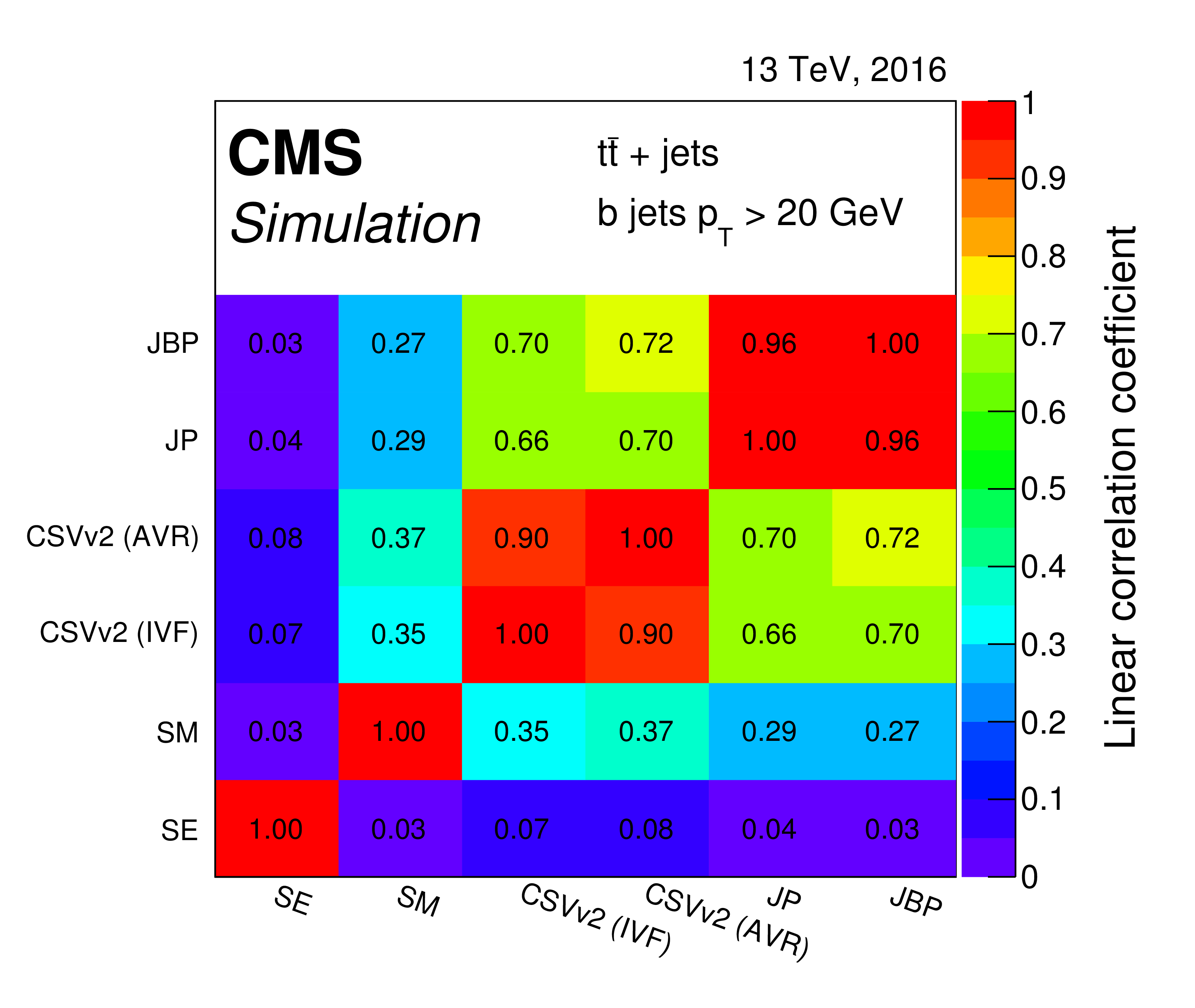
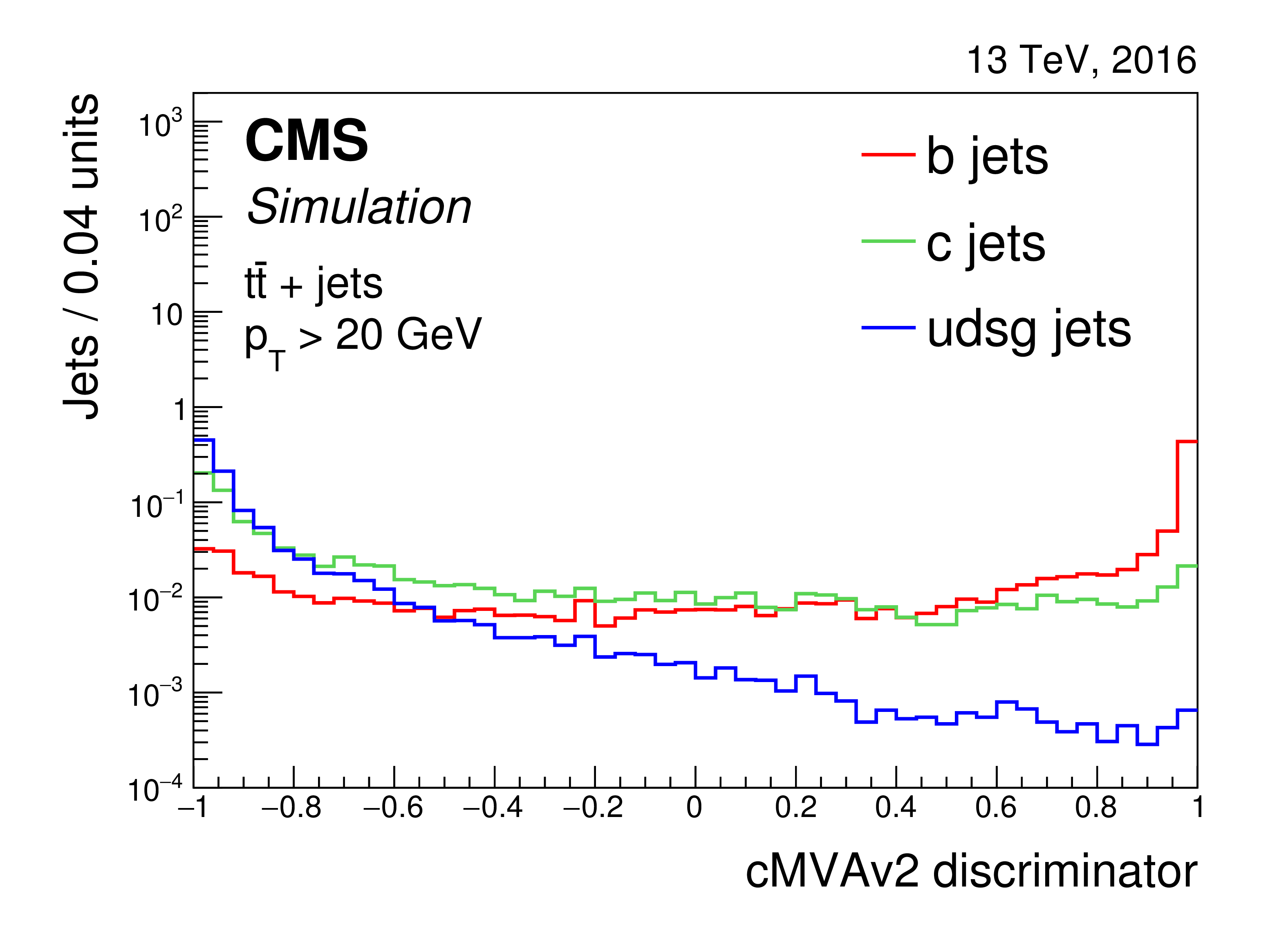
png pdf	Figure 15: Correlation between the different input variables for the cMVAv2 tagger for b jets in $ {\mathrm {t}\overline {\mathrm {t}}} $ events (left), and distribution of the cMVAv2 discriminator values (right), normalized to unit area, for jets of different flavours in $ {\mathrm {t}\overline {\mathrm {t}}} $ events.
png pdf	Figure 15-a: Correlation between the different input variables for the cMVAv2 tagger for b jets in $ {\mathrm {t}\overline {\mathrm {t}}} $ events, normalized to unit area, for jets of different flavours in $ {\mathrm {t}\overline {\mathrm {t}}} $ events.
png pdf	Figure 15-b: Distribution of the cMVAv2 discriminator values, normalized to unit area, for jets of different flavours in $ {\mathrm {t}\overline {\mathrm {t}}} $ events.
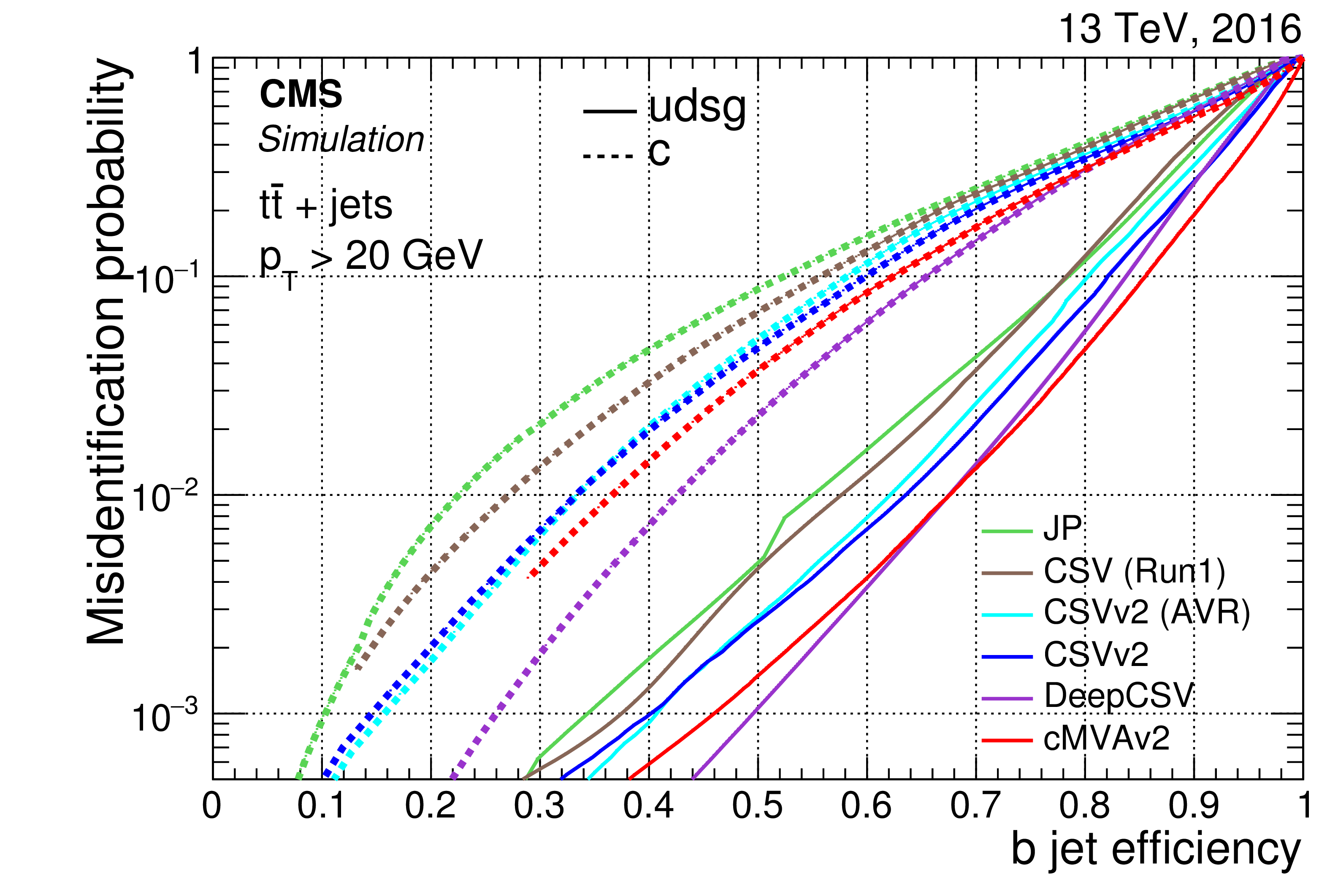
png pdf	Figure 16: Misidentification probability for c and light-flavour jets versus b jet identification efficiency for various b tagging algorithms applied to jets in $ {\mathrm {t}\overline {\mathrm {t}}} $ events.
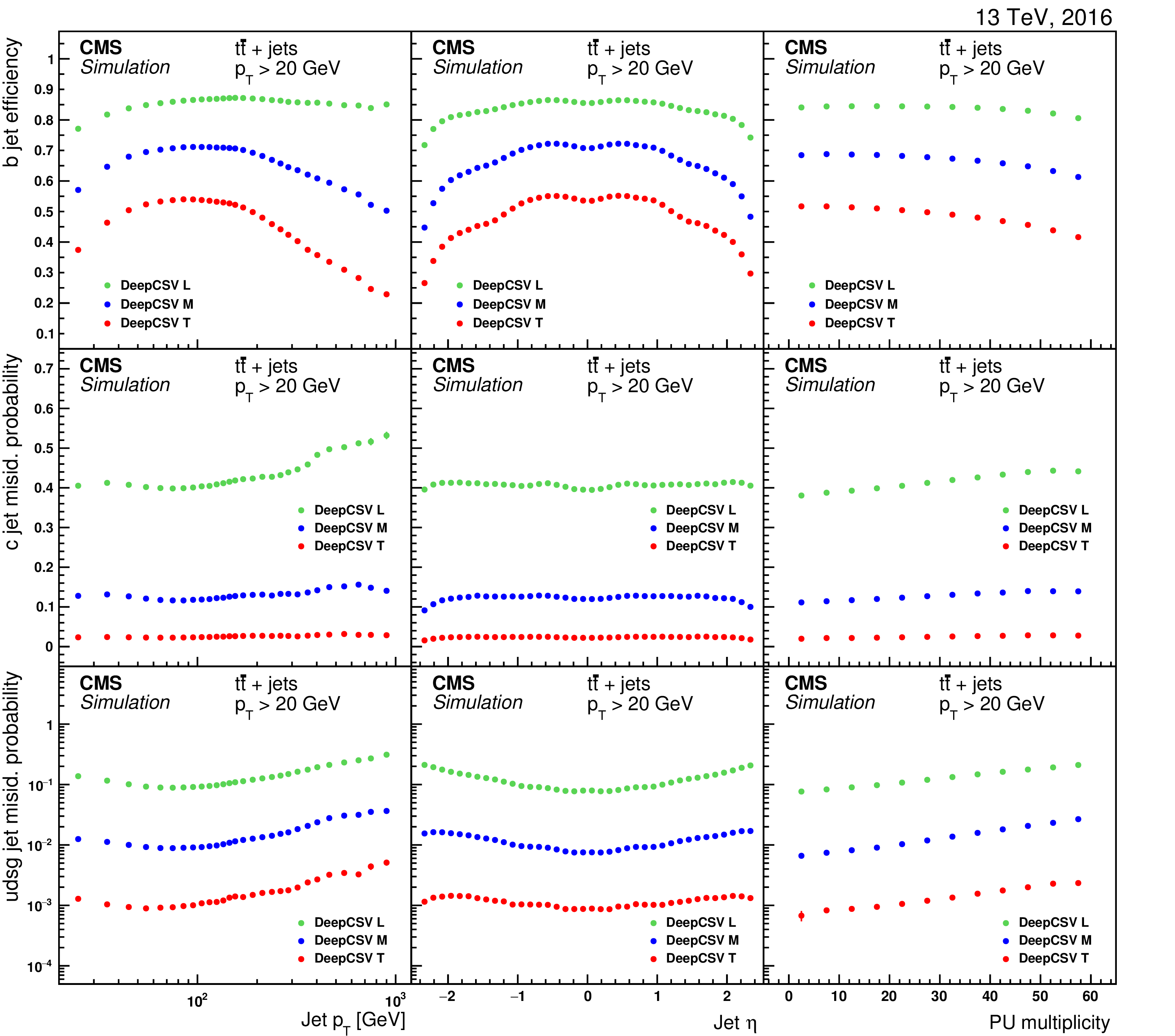
png pdf	Figure 17: Efficiencies and misidentification probabilities for the DeepCSV $P({\mathrm {b}})+P({\mathrm {b}} {\mathrm {b}})$ tagger as a function of the jet $ {p_{\mathrm {T}}} $ (left), jet $\eta $ (middle), and number of pileup interactions in the event (right), for b (upper), c (middle), and light-flavour (lower) jets in $ {\mathrm {t}\overline {\mathrm {t}}} $ events. Each panel shows the efficiency for the three different working points with different colours.
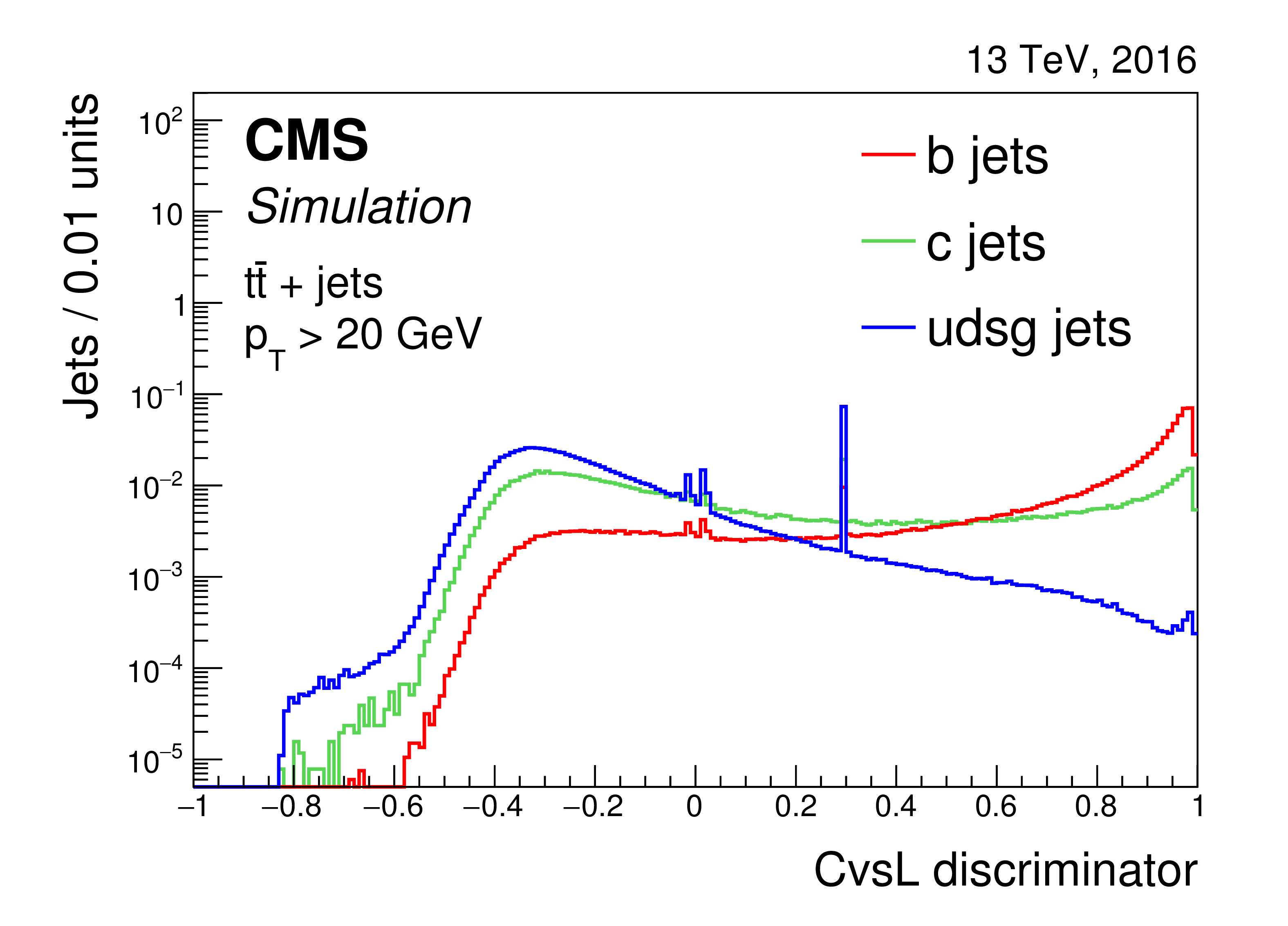
png pdf	Figure 18: Distribution of the CvsL (left) and CvsB (right) discriminator values for jets of different flavours in $ {\mathrm {t}\overline {\mathrm {t}}} $ events. The spikes originate from jets without a track passing the track selection criteria, as discussed in the text. The distributions are normalized to unit area.
png pdf	Figure 18-a: Distribution of the CvsL discriminator values for jets of different flavours in $ {\mathrm {t}\overline {\mathrm {t}}} $ events. The spikes originate from jets without a track passing the track selection criteria, as discussed in the text. The distributions are normalized to unit area.
png pdf	Figure 18-b: Distribution of the CvsB discriminator values for jets of different flavours in $ {\mathrm {t}\overline {\mathrm {t}}} $ events. The spikes originate from jets without a track passing the track selection criteria, as discussed in the text. The distributions are normalized to unit area.
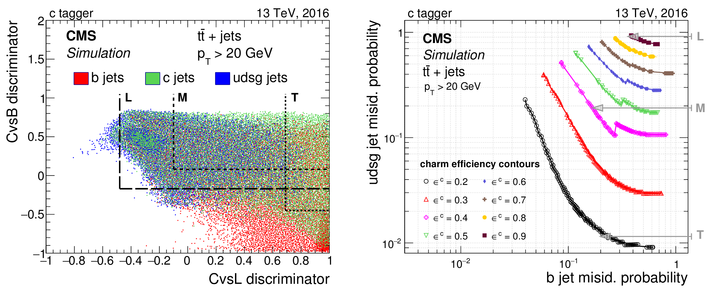
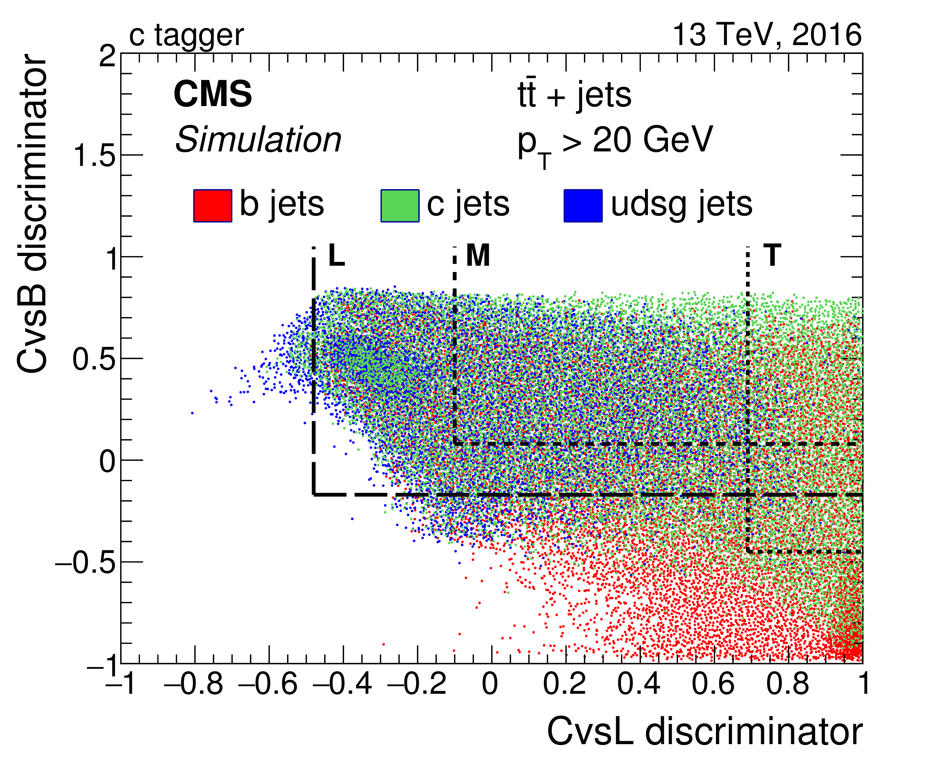
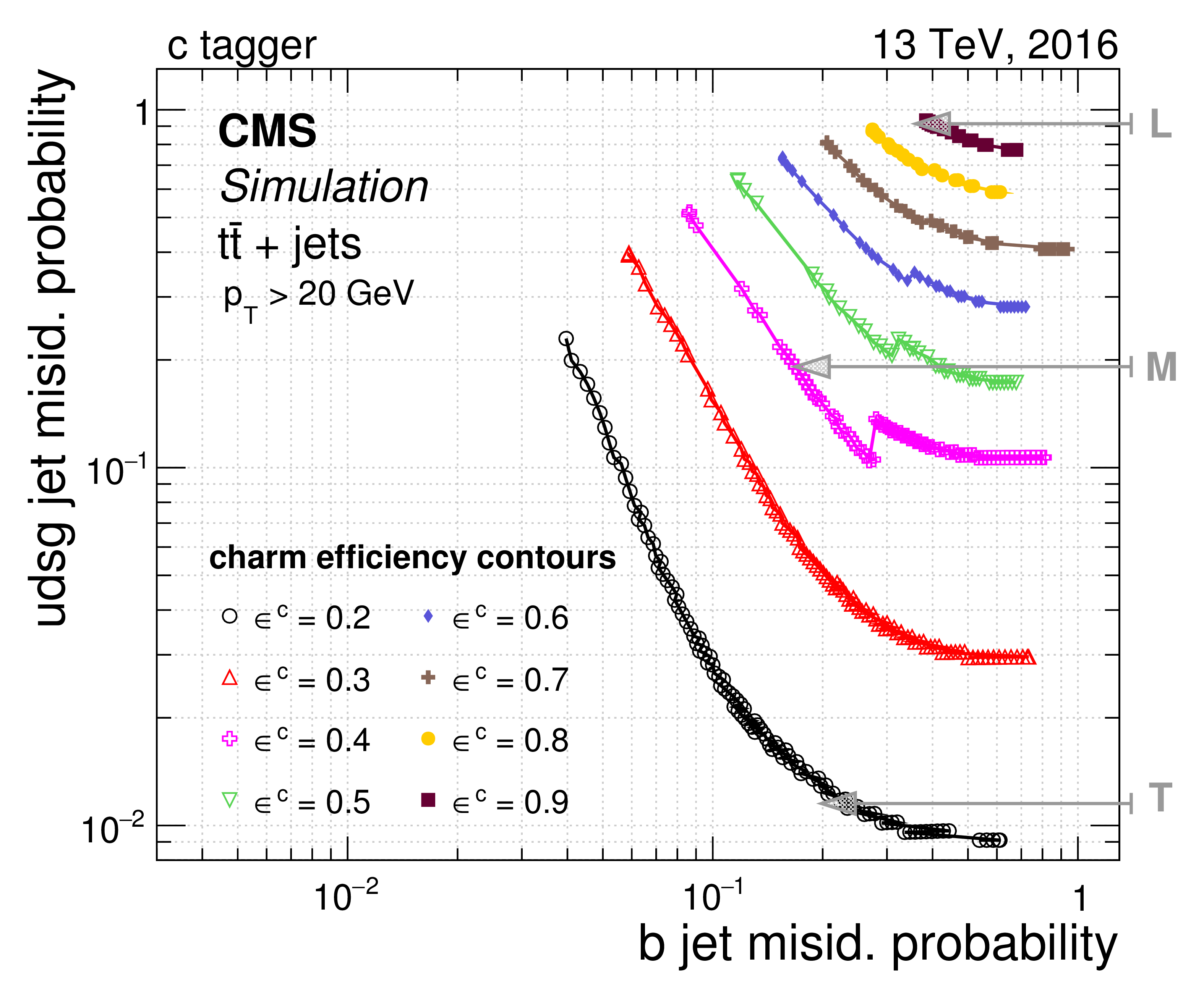
png pdf	Figure 19: Correlation between CvsL and CvsB taggers for the various jet flavours (left), and misidentification probability for light-flavour jets versus misidentification probability for b jets for various constant c jet efficiencies (right) in $ {\mathrm {t}\overline {\mathrm {t}}} $ events. The L, M, and T working points discussed in the text are indicated by the dashed lines (left) or arrows (right). The discontinuity in the curves corresponding to c tagging efficiencies between 0.4 and 0.7 are due to the spike in the CvsL distribution of Figure 19.
png pdf	Figure 19-a: Correlation between CvsL and CvsB taggers for the various jet flavours in $ {\mathrm {t}\overline {\mathrm {t}}} $ events. The L, M, and T working points discussed in the text are indicated by the dashed lines (left) or arrows (right). The discontinuity in the curves corresponding to c tagging efficiencies between 0.4 and 0.7 are due to the spike in the CvsL distribution of Figure 19.
png pdf	Figure 19-b: Misidentification probability for light-flavour jets versus misidentification probability for b jets for various constant c jet efficiencies in $ {\mathrm {t}\overline {\mathrm {t}}} $ events. The L, M, and T working points discussed in the text are indicated by the dashed lines (left) or arrows (right). The discontinuity in the curves corresponding to c tagging efficiencies between 0.4 and 0.7 are due to the spike in the CvsL distribution of Figure 19.
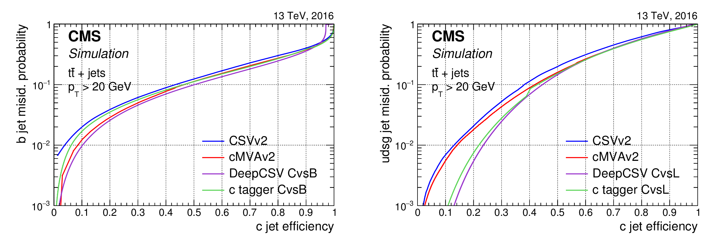
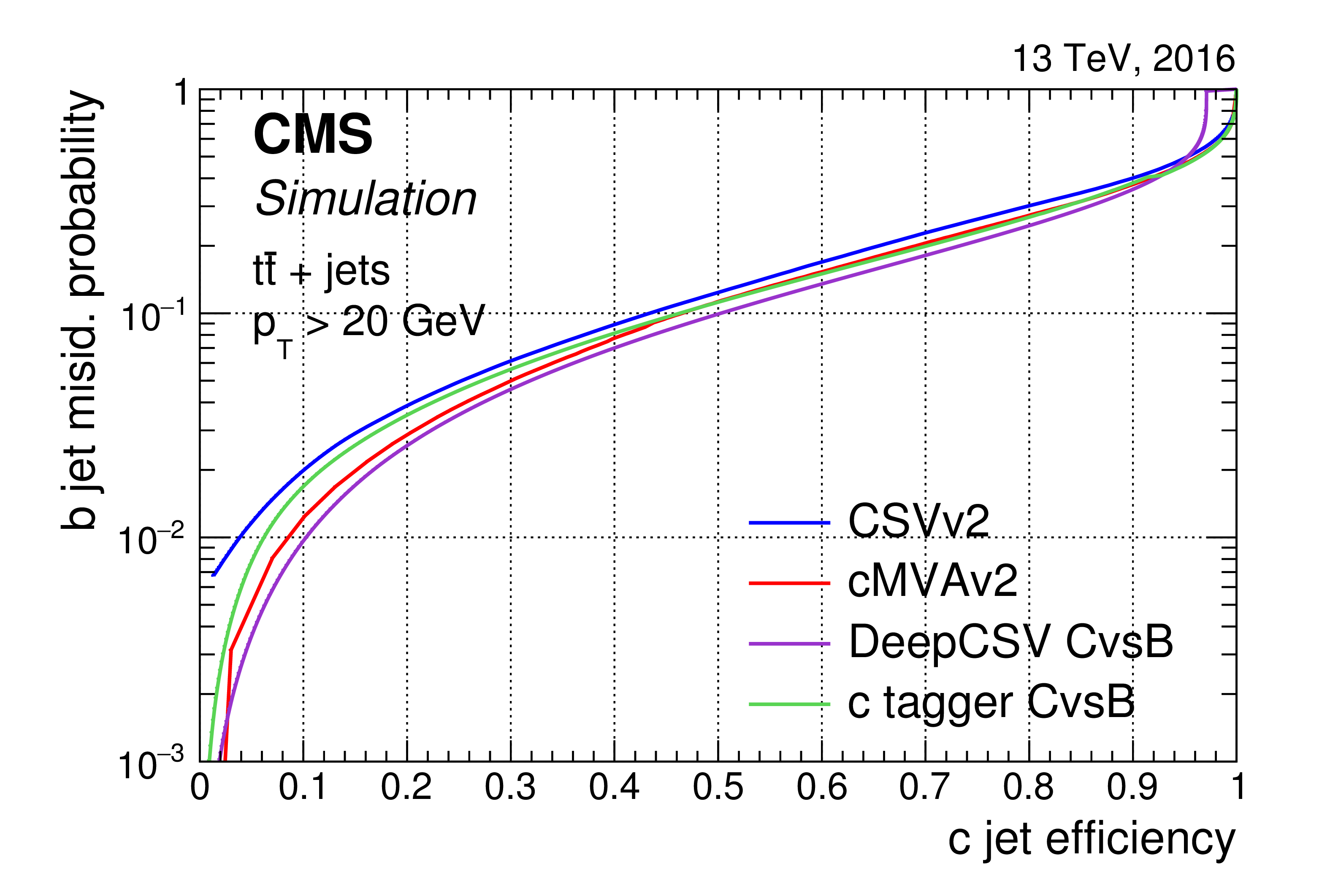
png pdf	Figure 20: Misidentification probability for b jets (left) or light-flavour jets (right) versus c jet identification efficiency for various c tagging algorithms applied to jets in $ {\mathrm {t}\overline {\mathrm {t}}} $ events.
png pdf	Figure 20-a: Misidentification probability for b jets versus c jet identification efficiency for various c tagging algorithms applied to jets in $ {\mathrm {t}\overline {\mathrm {t}}} $ events.
png pdf	Figure 20-b: Misidentification probability for light-flavour jets versus c jet identification efficiency for various c tagging algorithms applied to jets in $ {\mathrm {t}\overline {\mathrm {t}}} $ events.
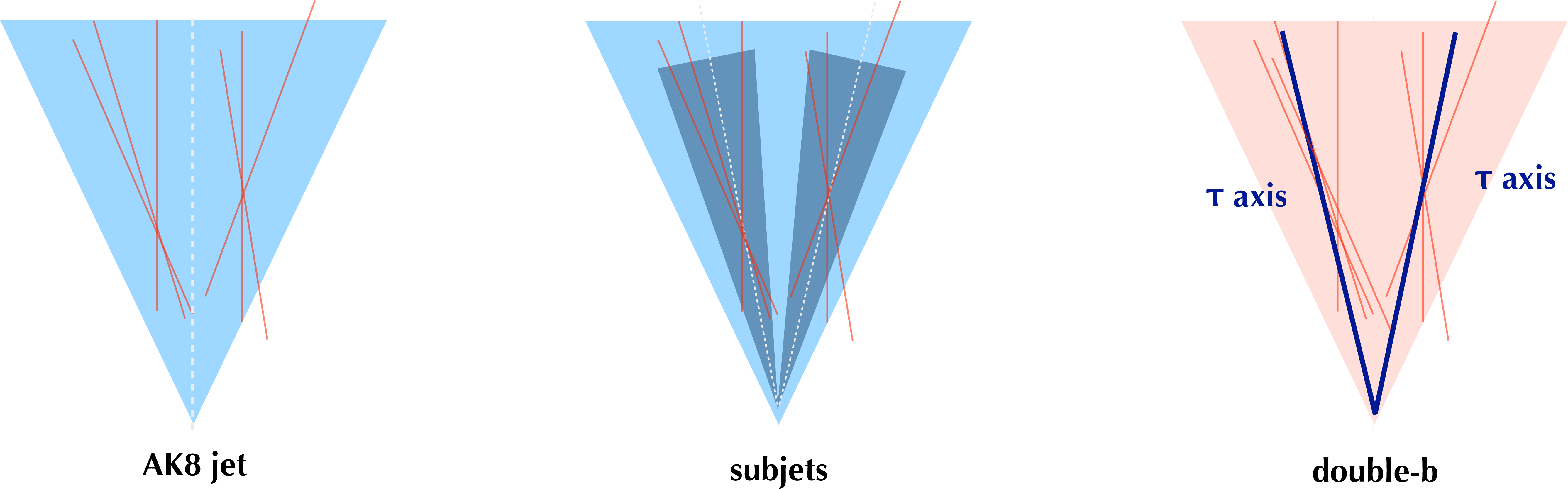
png pdf	Figure 21: Schematic representation of the AK8 jet (left) and subjet (middle) b tagging approaches, and of the double-b tagger approach (right).
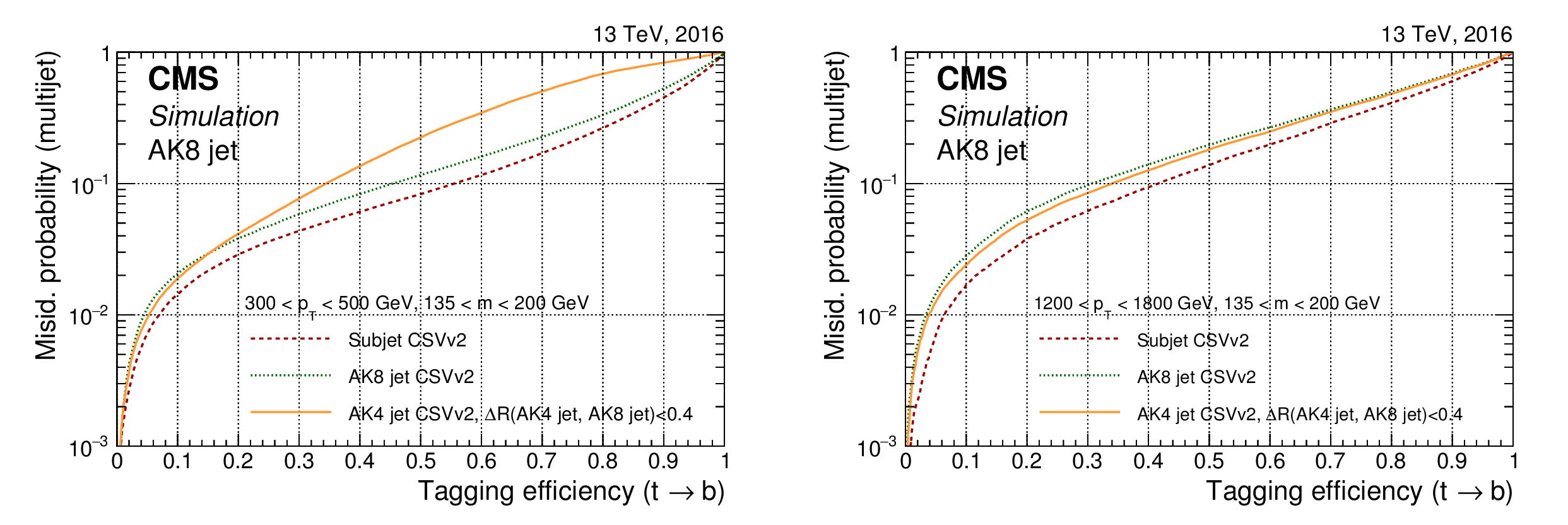
png pdf	Figure 22: Misidentification probability for jets in an inclusive multijet sample versus the efficiency to correctly tag boosted top quark jets. The CSVv2 algorithm is applied to three different types of jets: AK8 jets, their subjets, and AK4 jets matched to AK8 jets. The AK8 jets are selected to have a pruned jet mass between 135 and 200 GeV, and 300 $ < {p_{\mathrm {T}}} < $ 500 GeV (left), or 1.2 $ < {p_{\mathrm {T}}} < $ 1.8 TeV (right).
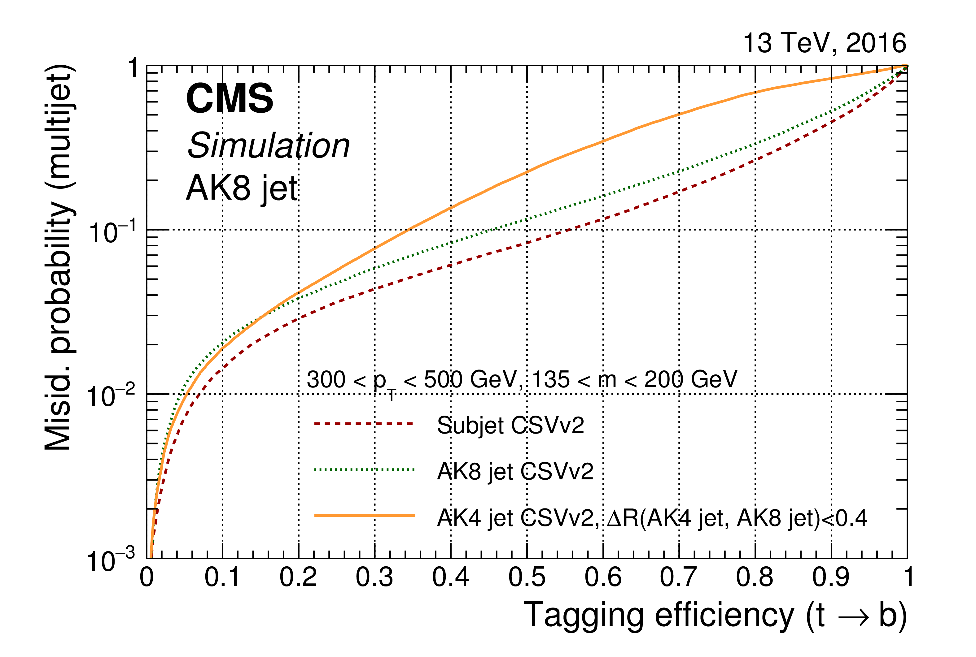
png pdf	Figure 22-a: Misidentification probability for jets in an inclusive multijet sample versus the efficiency to correctly tag boosted top quark jets. The CSVv2 algorithm is applied to three different types of jets: AK8 jets, their subjets, and AK4 jets matched to AK8 jets. The AK8 jets are selected to have a pruned jet mass between 135 and 200 GeV, and 300 $ < {p_{\mathrm {T}}} < $ 500 GeV.
png pdf	Figure 22-b: Misidentification probability for jets in an inclusive multijet sample versus the efficiency to correctly tag boosted top quark jets. The CSVv2 algorithm is applied to three different types of jets: AK8 jets, their subjets, and AK4 jets matched to AK8 jets. The AK8 jets are selected to have a pruned jet mass between 135 and 200 GeV, and 1.2 $ < {p_{\mathrm {T}}} < $ 1.8 TeV.
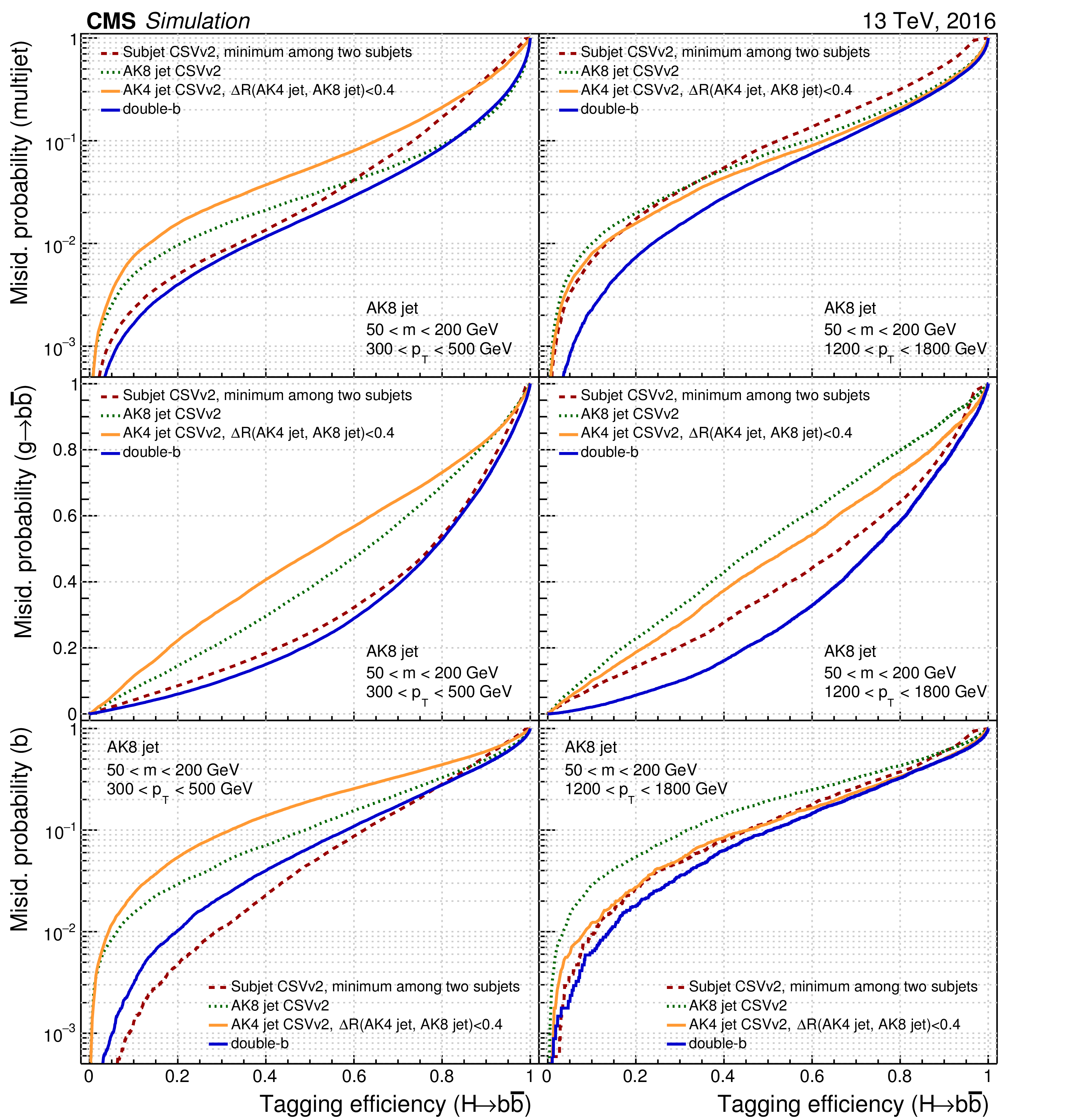
png pdf	Figure 23: Misidentification probability using jets in a multijet sample (upper), for $ {\mathrm {g}} \to {{\mathrm {b}}}{{\overline {\mathrm {b}}}}$ jets (middle), and for single b jets (lower), versus the efficiency to correctly tag $ {\mathrm {H}} \to {{\mathrm {b}}}{{\overline {\mathrm {b}}}}$ jets. The CSVv2 algorithm is applied to three different types of jets: AK8 jets, their subjets, and AK4 jets matched to AK8 jets. For the subjet b tagging curves, both subjets are required to be tagged. The double-b tagger, described in Section yyyyy, is applied to AK8 jets. The AK8 jets are selected to have a pruned jet mass between 50 and 200 GeV, and 300 $ < {p_{\mathrm {T}}} < $ 500 GeV (left), or 1.2 $ < {p_{\mathrm {T}}} < $ 1.8 TeV (right).
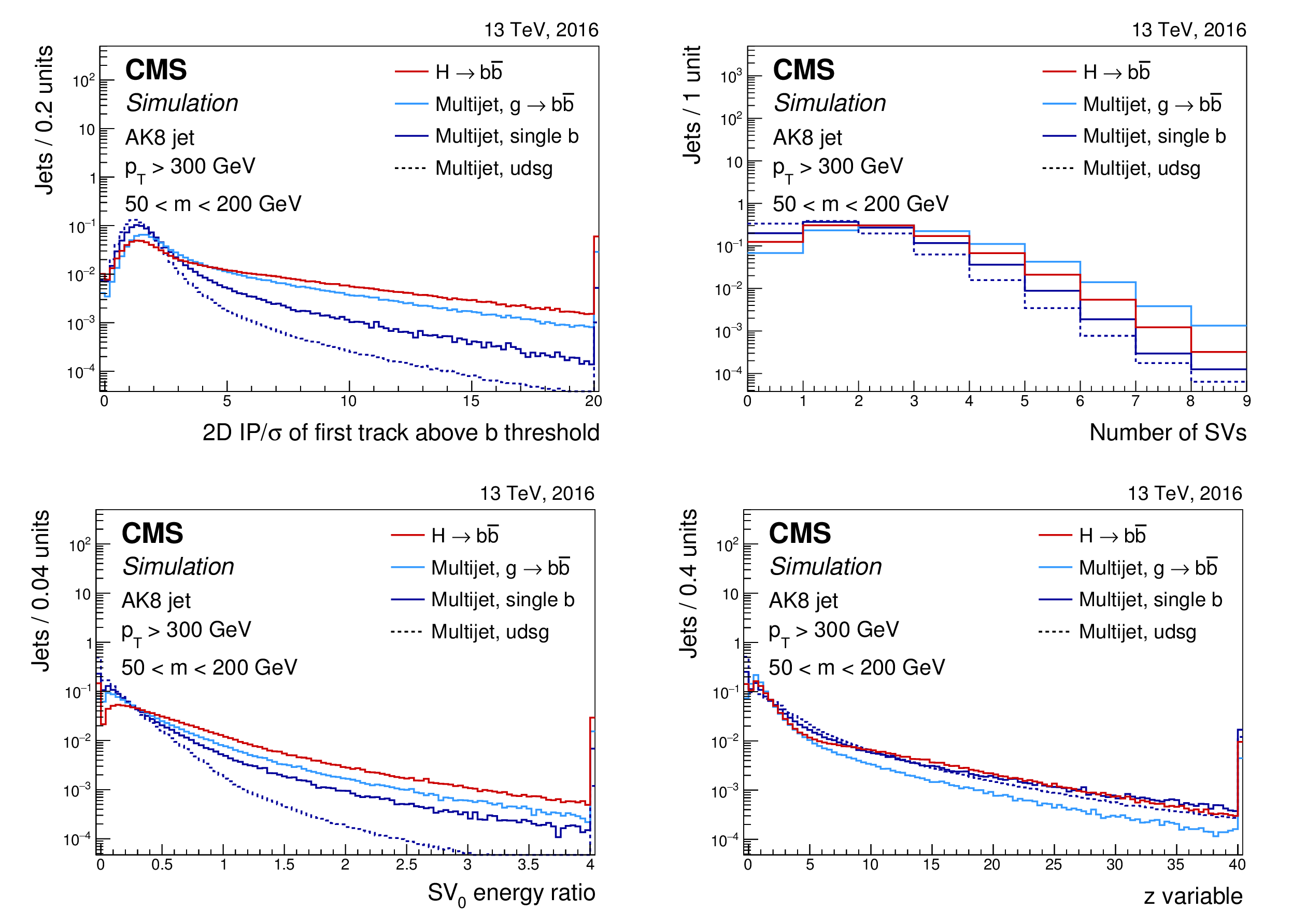
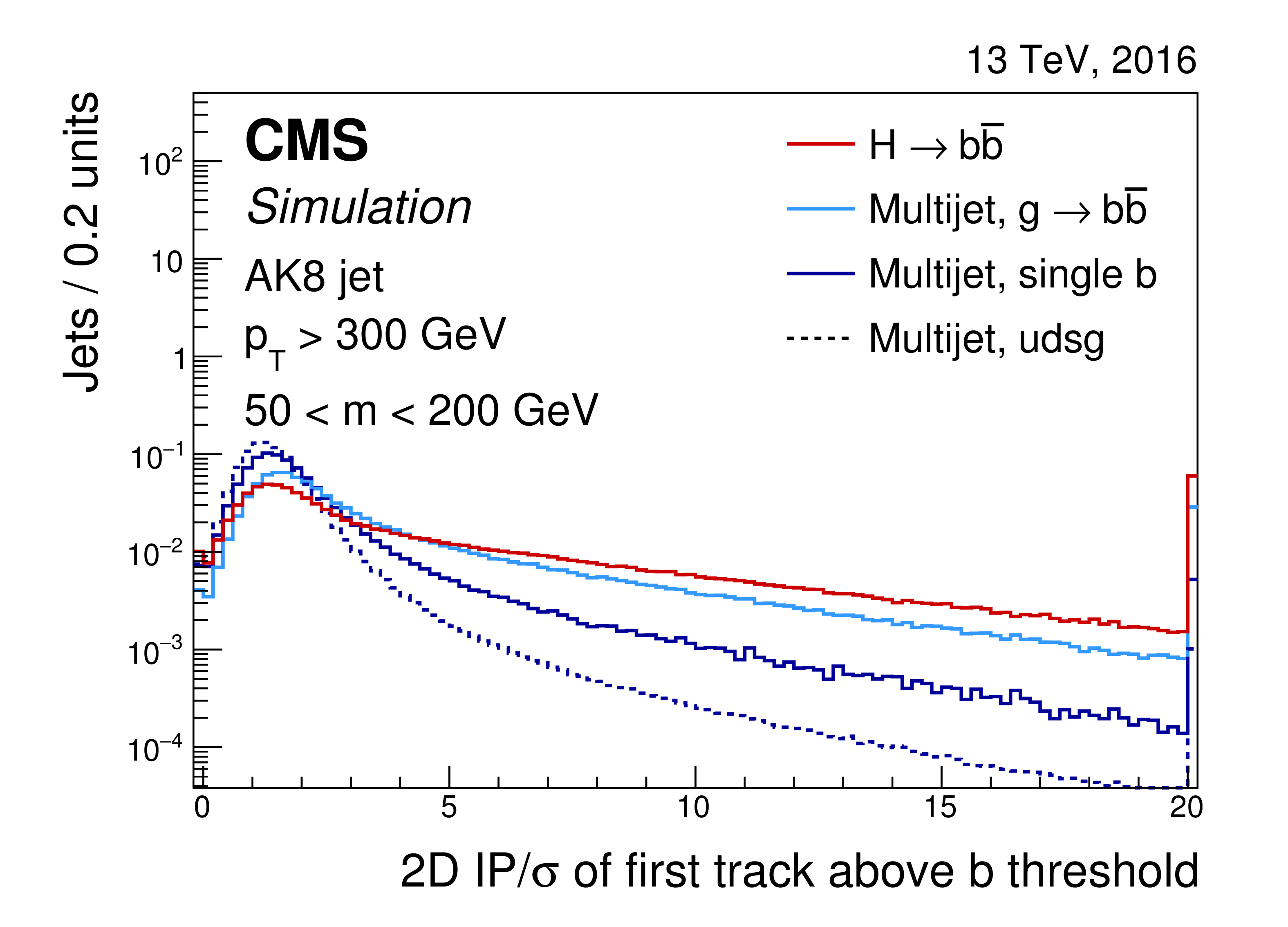
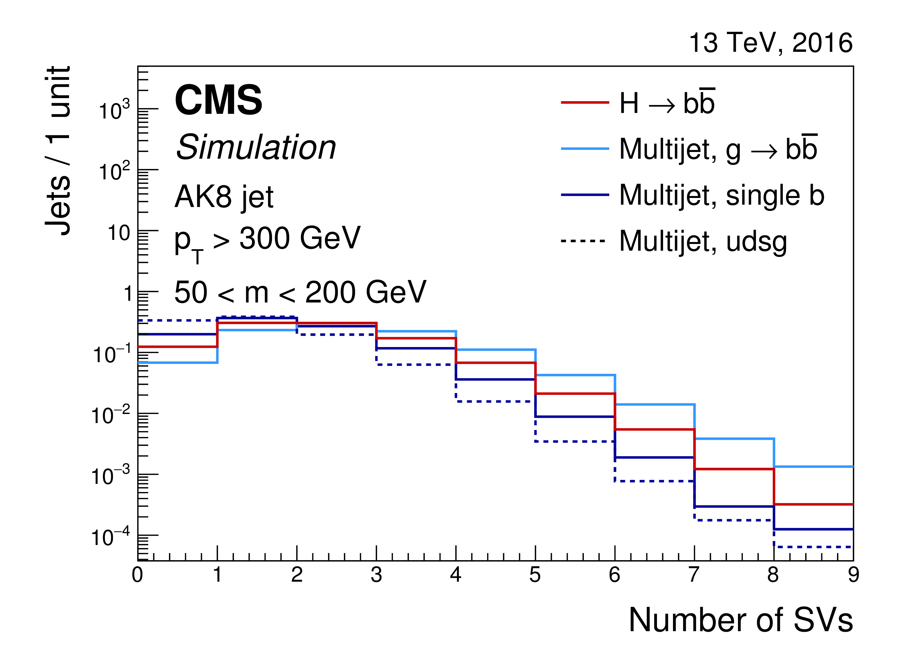
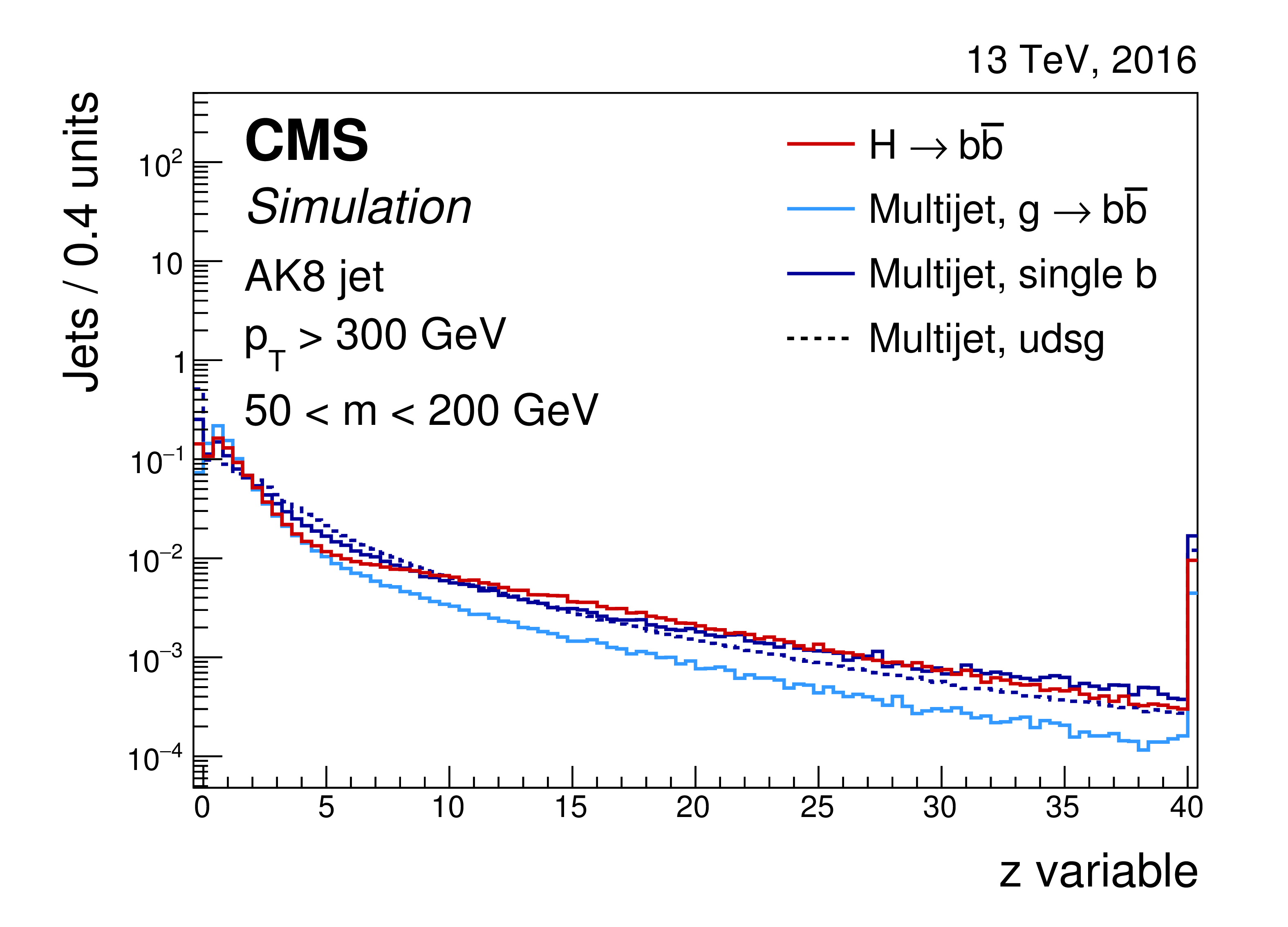
png pdf	Figure 24: Distribution of 2D impact parameter significance for the most displaced track raising the mass above the b hadron mass threshold as described in the text (upper left), number of secondary vertices associated with the AK8 jet (upper right), vertex energy ratio for the secondary vertex with the smallest 3D flight distance uncertainty (lower left), and $z$ variable described in the text (lower right). Comparison between $ {\mathrm {H}} \to {{\mathrm {b}}}{{\overline {\mathrm {b}}}}$ jets from simulated samples of a Kaluza-Klein graviton decaying to two Higgs bosons, and jets in an inclusive multijet sample containing zero, one, or two b quarks. The AK8 jets are selected with $ {p_{\mathrm {T}}} > $ 300 GeV and pruned jet mass between 50 and 200 GeV. The distributions are normalized to unit area. The last bin includes the overflow entries.
png pdf	Figure 24-a: Distribution of the 2D impact parameter significance for the most displaced track raising the mass above the b hadron mass threshold as described in the text. Comparison between $ {\mathrm {H}} \to {{\mathrm {b}}}{{\overline {\mathrm {b}}}}$ jets from simulated samples of a Kaluza-Klein graviton decaying to two Higgs bosons, and jets in an inclusive multijet sample containing zero, one, or two b quarks. The AK8 jets are selected with $ {p_{\mathrm {T}}} > $ 300 GeV and pruned jet mass between 50 and 200 GeV. The distributions are normalized to unit area. The last bin includes the overflow entries.
png pdf	Figure 24-b: Distribution of the number of secondary vertices associated with the AK8 jet. Comparison between $ {\mathrm {H}} \to {{\mathrm {b}}}{{\overline {\mathrm {b}}}}$ jets from simulated samples of a Kaluza-Klein graviton decaying to two Higgs bosons, and jets in an inclusive multijet sample containing zero, one, or two b quarks. The AK8 jets are selected with $ {p_{\mathrm {T}}} > $ 300 GeV and pruned jet mass between 50 and 200 GeV. The distributions are normalized to unit area. The last bin includes the overflow entries.
png pdf	Figure 24-c: Distribution of the vertex energy ratio for the secondary vertex with the smallest 3D flight distance uncertainty. Comparison between $ {\mathrm {H}} \to {{\mathrm {b}}}{{\overline {\mathrm {b}}}}$ jets from simulated samples of a Kaluza-Klein graviton decaying to two Higgs bosons, and jets in an inclusive multijet sample containing zero, one, or two b quarks. The AK8 jets are selected with $ {p_{\mathrm {T}}} > $ 300 GeV and pruned jet mass between 50 and 200 GeV. The distributions are normalized to unit area. The last bin includes the overflow entries.
png pdf	Figure 24-d: Distribution of the $z$ variable described in the text. Comparison between $ {\mathrm {H}} \to {{\mathrm {b}}}{{\overline {\mathrm {b}}}}$ jets from simulated samples of a Kaluza-Klein graviton decaying to two Higgs bosons, and jets in an inclusive multijet sample containing zero, one, or two b quarks. The AK8 jets are selected with $ {p_{\mathrm {T}}} > $ 300 GeV and pruned jet mass between 50 and 200 GeV. The distributions are normalized to unit area. The last bin includes the overflow entries.
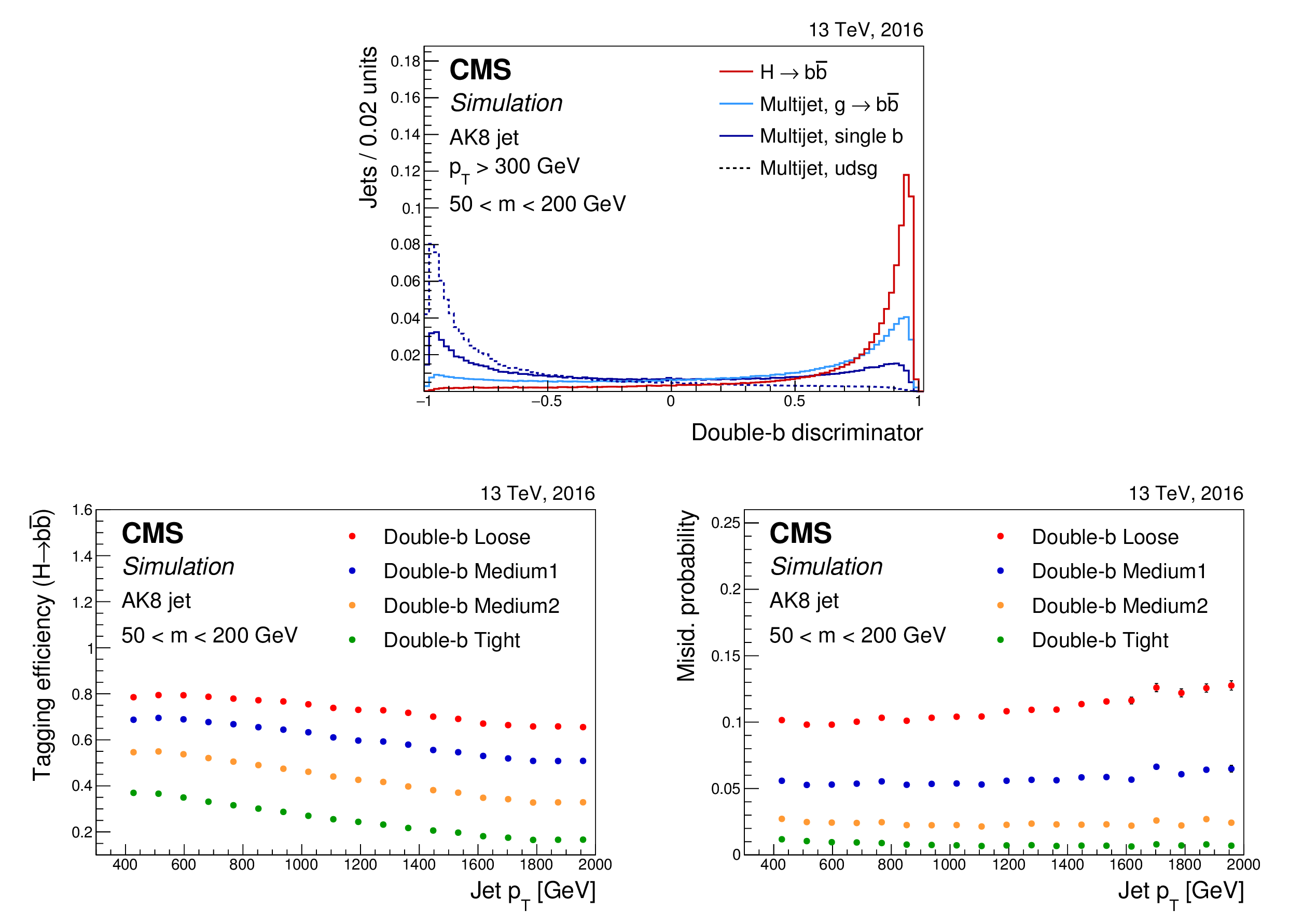
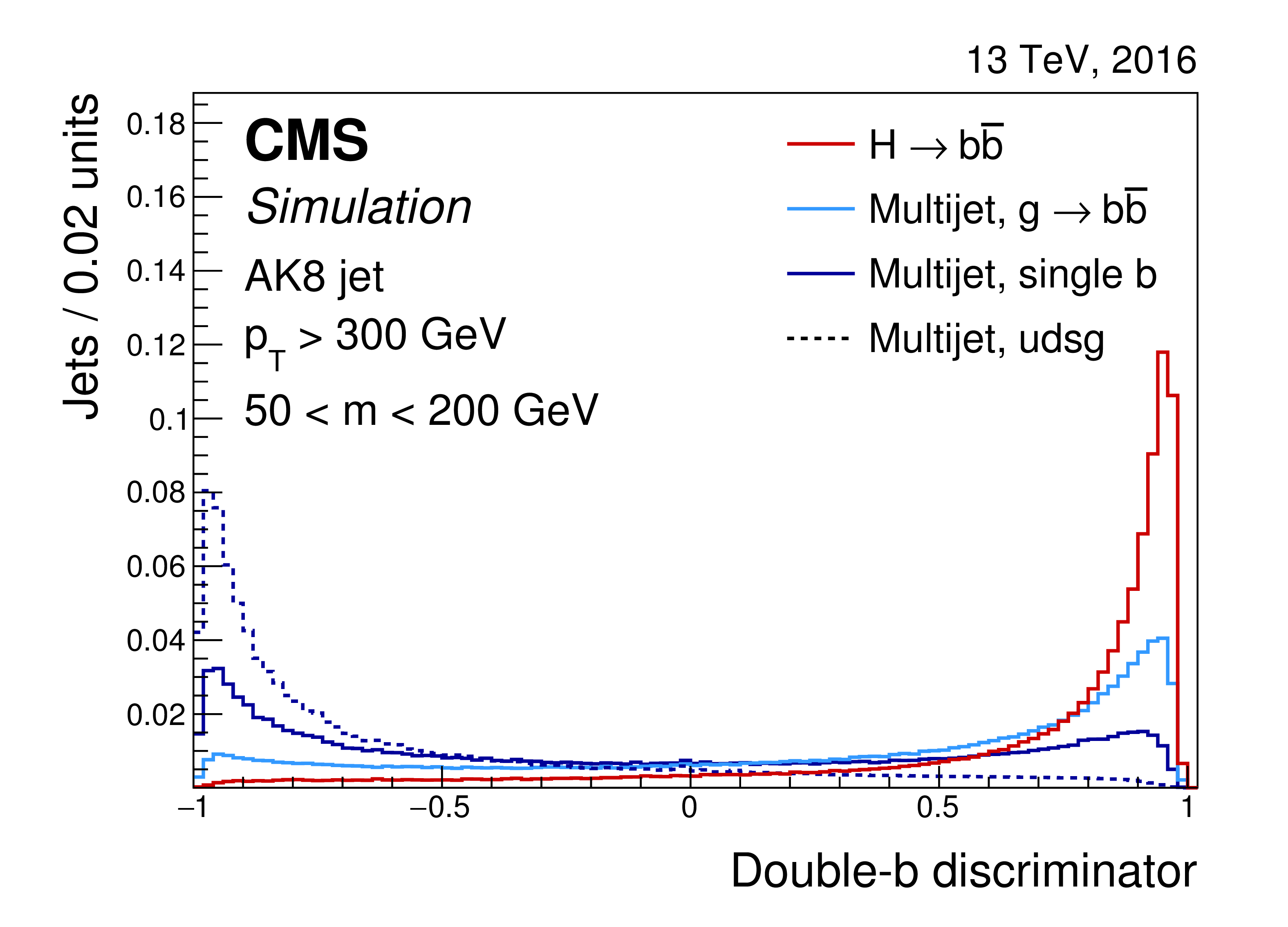
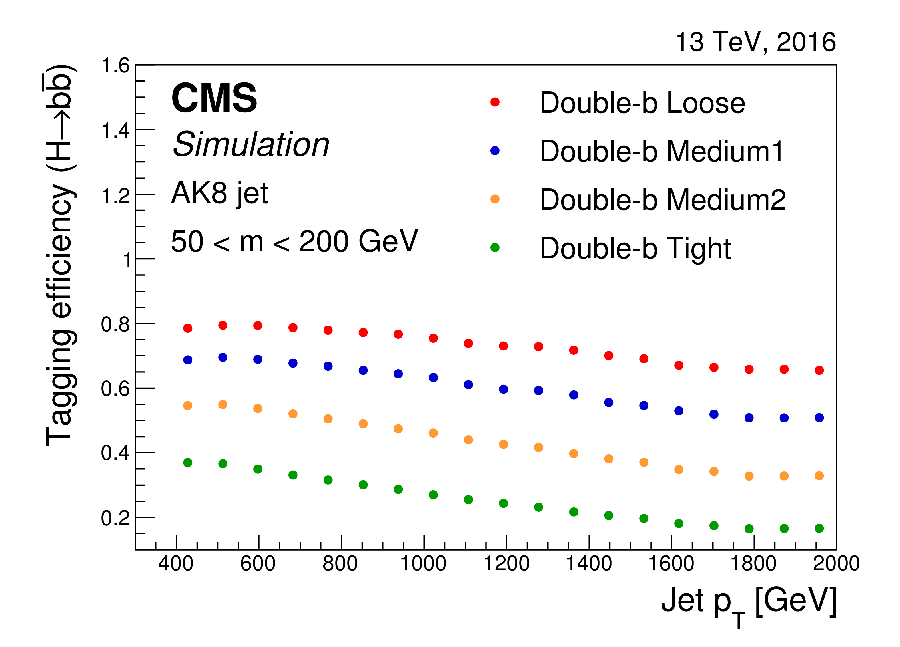
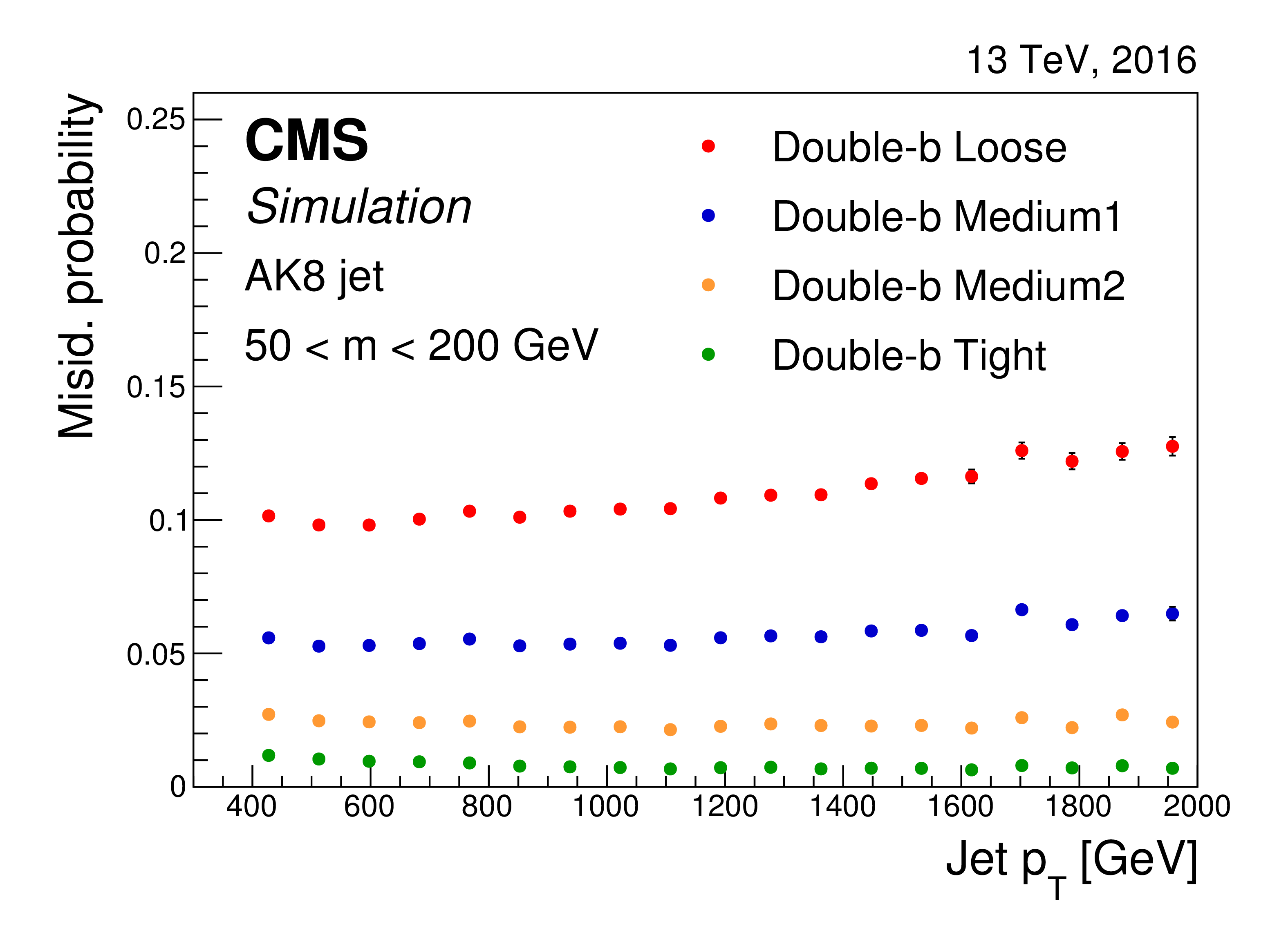
png pdf	Figure 25: Distribution of the double-b tagger discriminator values normalized to unit area for $ {\mathrm {H}} \to {{\mathrm {b}}}{{\overline {\mathrm {b}}}}$ jets in simulated samples of a Kaluza-Klein graviton decaying to two Higgs bosons, and for jets in an inclusive multijet sample containing zero, one, or two b quarks (upper). Efficiency to correctly tag $ {\mathrm {H}} \to {{\mathrm {b}}}{{\overline {\mathrm {b}}}}$ jets (lower left) and misidentification probability using jets in an inclusive multijet sample (lower right) for four working points of the double-b tagger as a function of the jet $ {p_{\mathrm {T}}} $. The AK8 jets are selected with $ {p_{\mathrm {T}}} > $ 300 GeV and pruned jet mass between 50 and 200 GeV.
png pdf	Figure 25-a: Distribution of the double-b tagger discriminator values normalized to unit area for $ {\mathrm {H}} \to {{\mathrm {b}}}{{\overline {\mathrm {b}}}}$ jets in simulated samples of a Kaluza-Klein graviton decaying to two Higgs bosons, and for jets in an inclusive multijet sample containing zero, one, or two b quarks.
png pdf	Figure 25-b: Efficiency to correctly tag $ {\mathrm {H}} \to {{\mathrm {b}}}{{\overline {\mathrm {b}}}}$ jets for four working points of the double-b tagger as a function of the jet $ {p_{\mathrm {T}}} $. The AK8 jets are selected with $ {p_{\mathrm {T}}} > $ 300 GeV and pruned jet mass between 50 and 200 GeV.
png pdf	Figure 25-c: Misidentification probability using jets in an inclusive multijet sample for four working points of the double-b tagger as a function of the jet $ {p_{\mathrm {T}}} $. The AK8 jets are selected with $ {p_{\mathrm {T}}} > $ 300 GeV and pruned jet mass between 50 and 200 GeV.
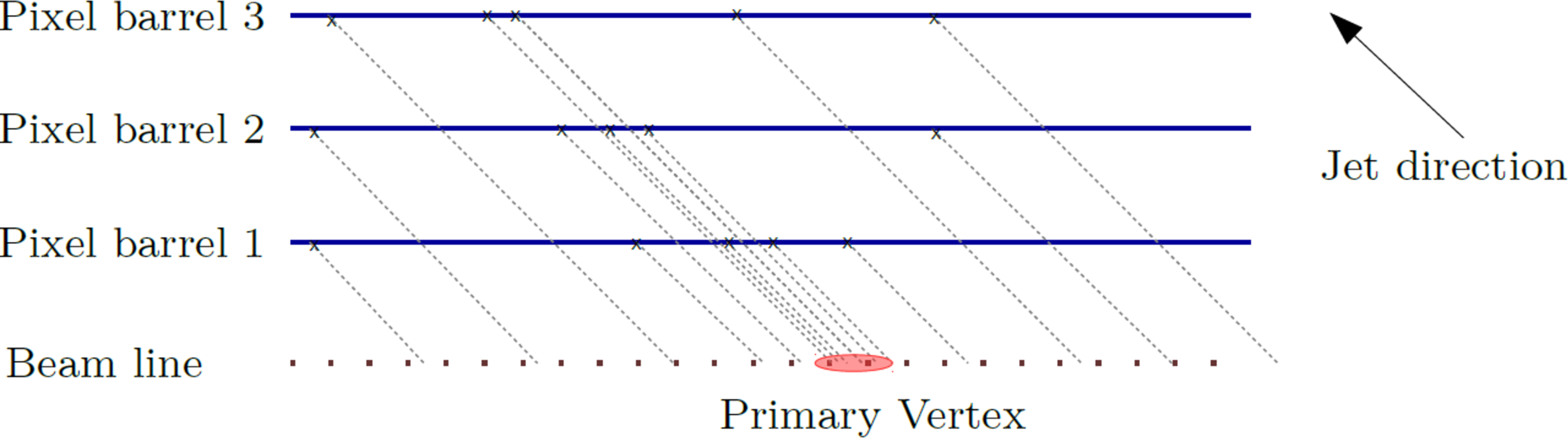
png pdf	Figure 26: Scheme of the fast primary vertex finding algorithm used to determine the position of the vertex along the beam line. The pixel detector hits from the tracks in a jet are projected along the calorimeter jet direction onto the beam line.
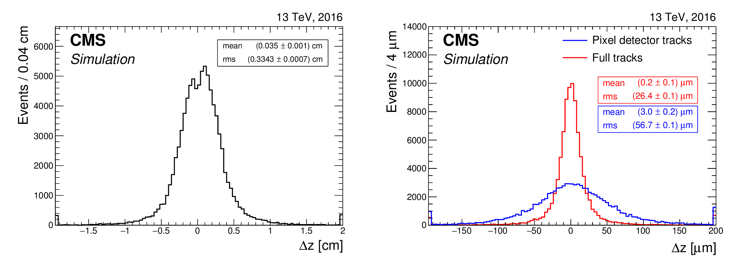
png pdf	Figure 27: Distribution of residuals on the position of the primary vertex along the beam line using the fast primary vertex finding algorithm described in the text (left), and on the position of the primary vertex along the beam line after refitting with the tracks reconstructed at the HLT (right). The distributions are obtained using simulated multijet events with 35 pileup interactions on average and a flat $\hat{p}_{\text {T}}$ spectrum between 15 and 3000 GeV for the leading jet. Events are selected for which the scalar sum of the $ {p_{\mathrm {T}}} $ of the jets is above 250 GeV.
png pdf	Figure 27-a: Distribution of residuals on the position of the primary vertex along the beam line using the fast primary vertex finding algorithm described in the text. The distributions are obtained using simulated multijet events with 35 pileup interactions on average and a flat $\hat{p}_{\text {T}}$ spectrum between 15 and 3000 GeV for the leading jet. Events are selected for which the scalar sum of the $ {p_{\mathrm {T}}} $ of the jets is above 250 GeV.
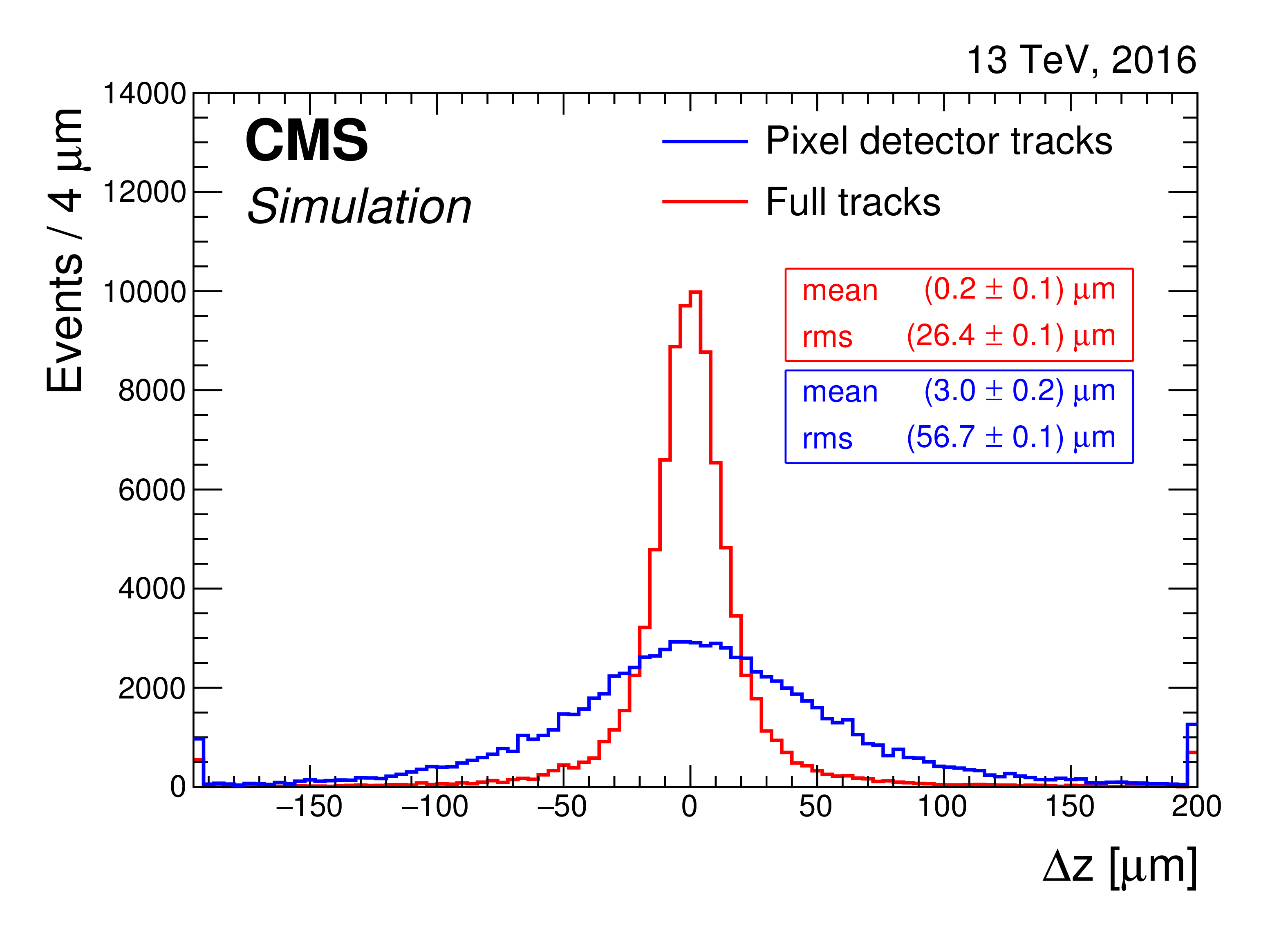
png pdf	Figure 27-b: Distribution of residuals on the position of the primary vertex along the beam line after refitting with the tracks reconstructed at the HLT. The distributions are obtained using simulated multijet events with 35 pileup interactions on average and a flat $\hat{p}_{\text {T}}$ spectrum between 15 and 3000 GeV for the leading jet. Events are selected for which the scalar sum of the $ {p_{\mathrm {T}}} $ of the jets is above 250 GeV.
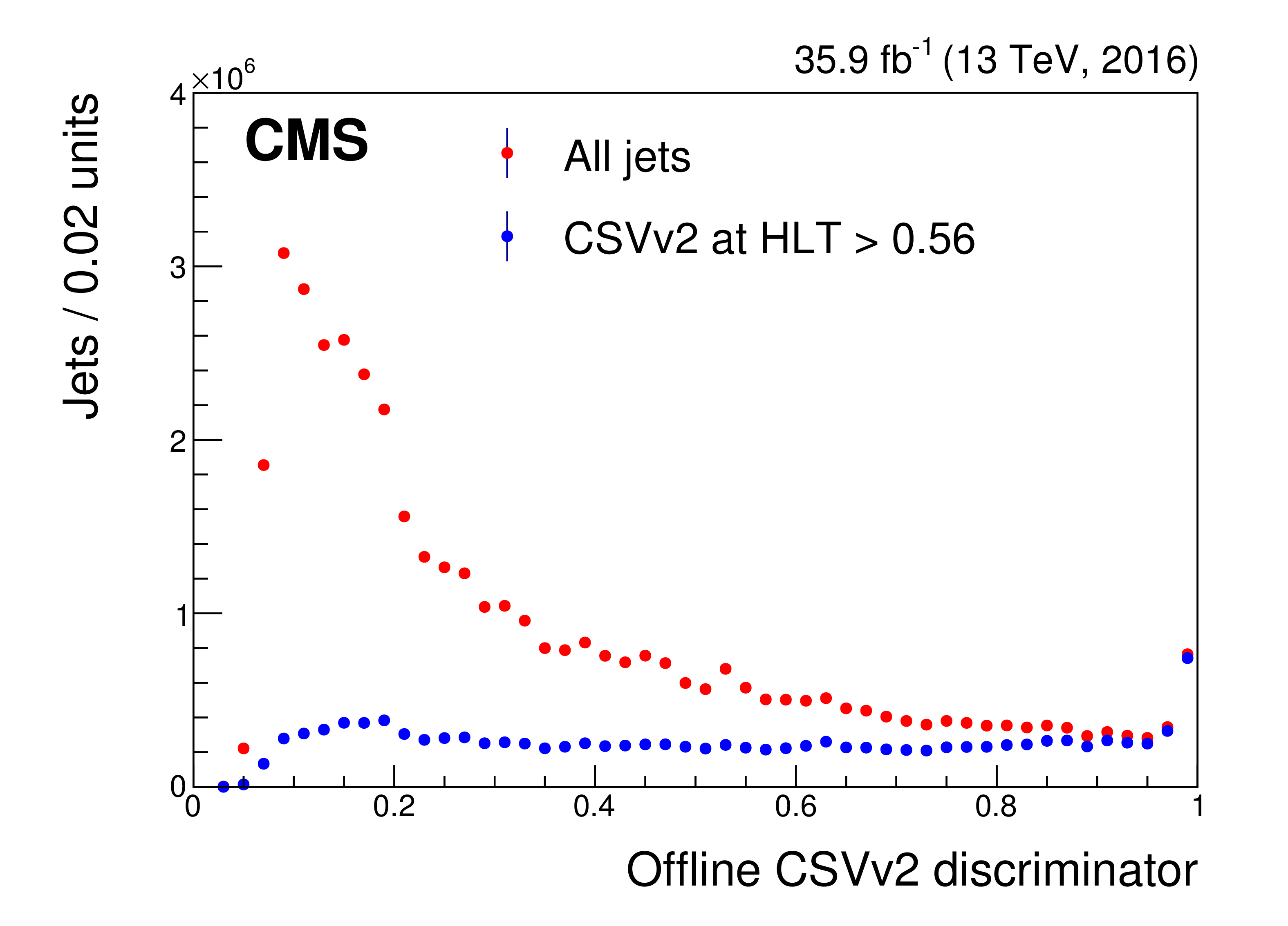
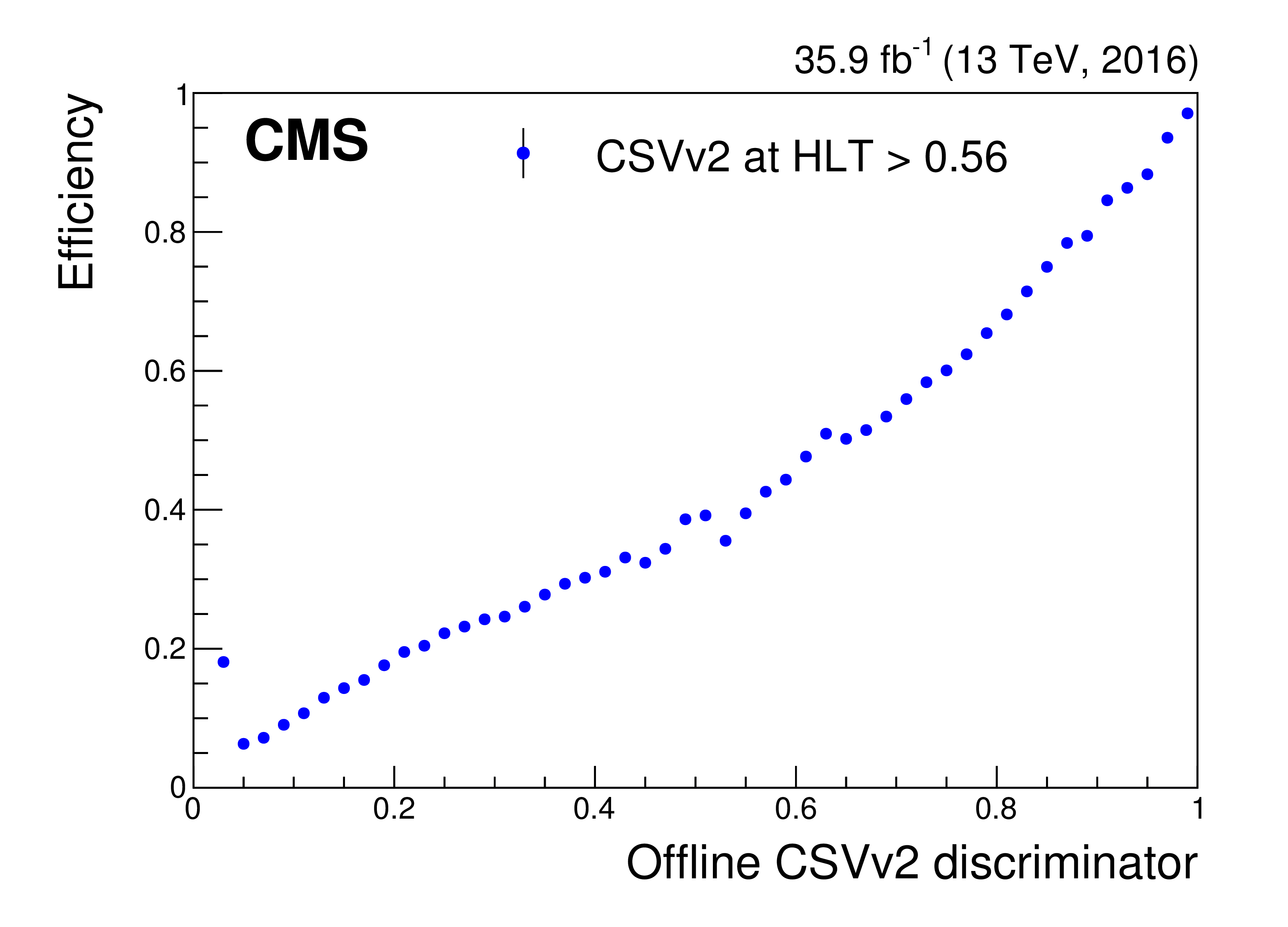
png pdf	Figure 28: Offline CSVv2 discriminator distribution for all jets and for jets with a value of the CSVv2 discriminator at the HLT exceeding 0.56 (left), and b tagging efficiency at the HLT as a function of the offline CSVv2 discriminator value (right).
png pdf	Figure 28-a: Offline CSVv2 discriminator distribution for all jets and for jets with a value of the CSVv2 discriminator at the HLT exceeding 0.56.
png pdf	Figure 28-b: b tagging efficiency at the HLT as a function of the offline CSVv2 discriminator value.
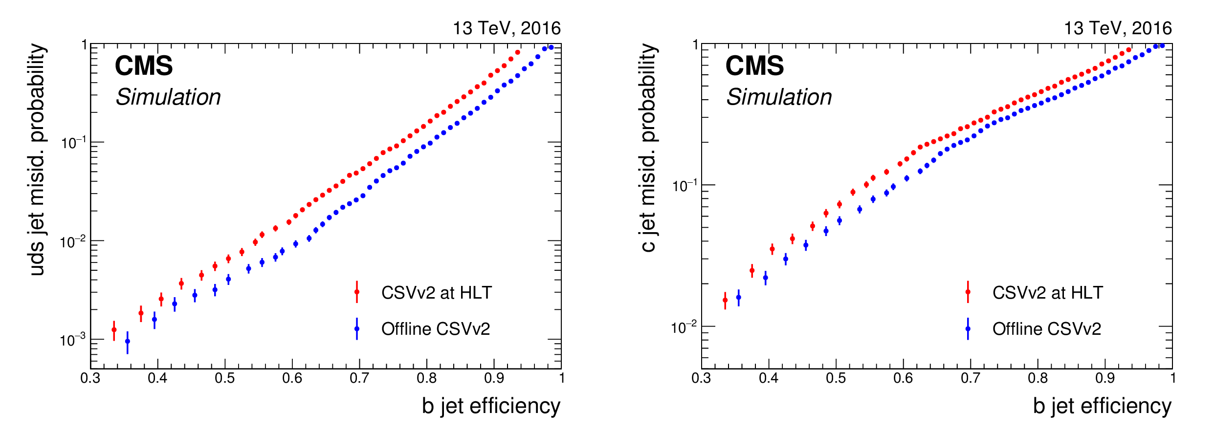
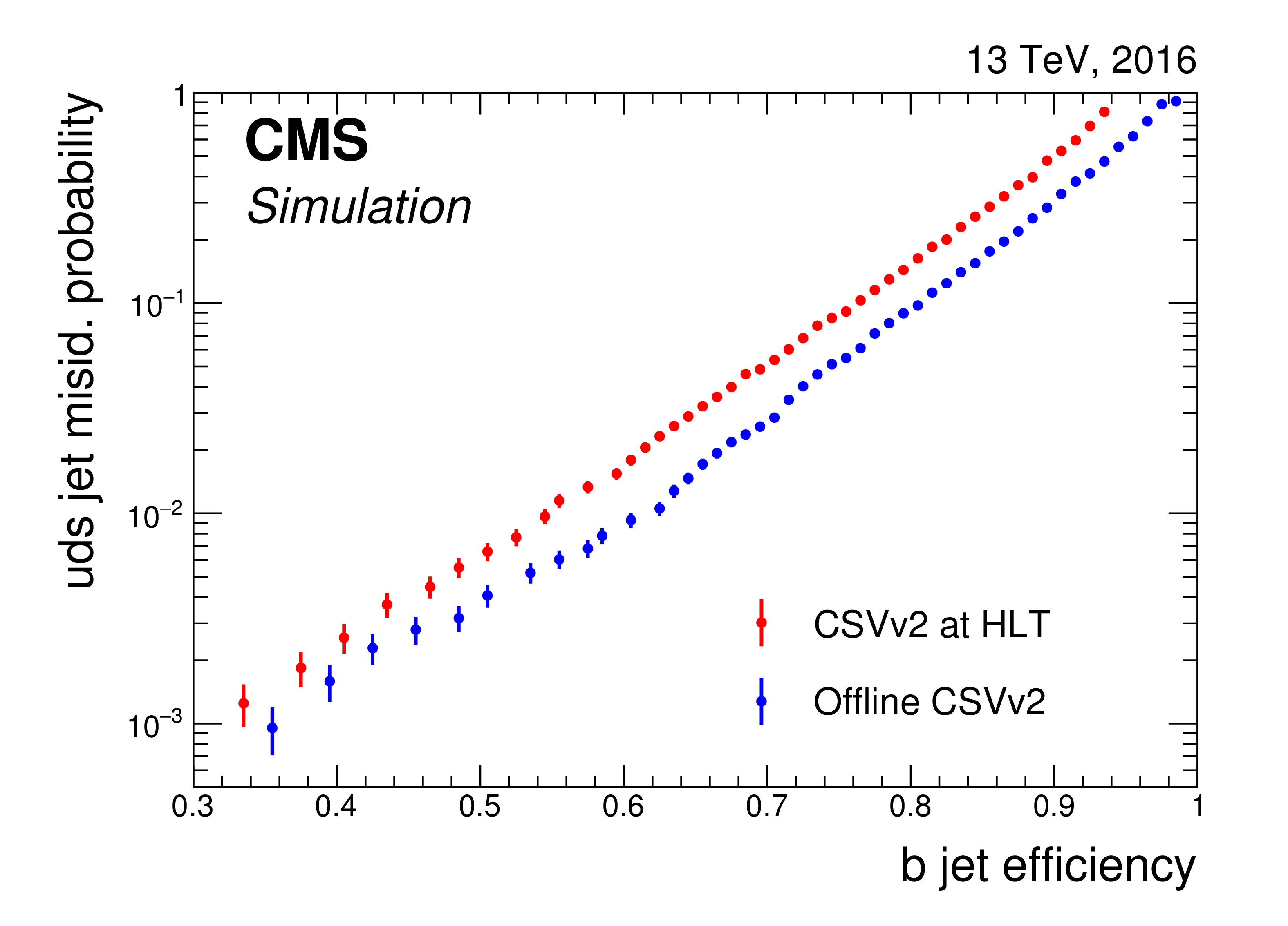
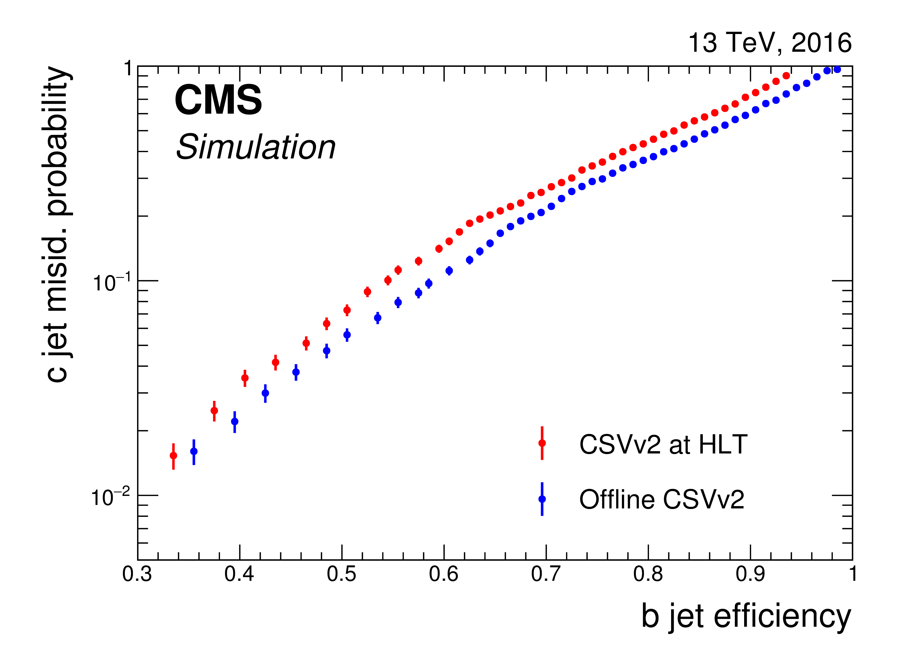
png pdf	Figure 29: Comparison of the misidentification probability for light-flavour jets (left) and c jets (right) versus the b tagging efficiency at the HLT and offline for the CSVv2 algorithm applied on simulated $ {\mathrm {t}\overline {\mathrm {t}}} $ events for which the scalar sum of the jet $ {p_{\mathrm {T}}} $ for all jets in the event exceeds 250 GeV.
png pdf	Figure 29-a: Comparison of the misidentification probability for light-flavour jets versus the b tagging efficiency at the HLT and offline for the CSVv2 algorithm applied on simulated $ {\mathrm {t}\overline {\mathrm {t}}} $ events for which the scalar sum of the jet $ {p_{\mathrm {T}}} $ for all jets in the event exceeds 250 GeV.
png pdf	Figure 29-b: Comparison of the misidentification probability for c jets versus the b tagging efficiency at the HLT and offline for the CSVv2 algorithm applied on simulated $ {\mathrm {t}\overline {\mathrm {t}}} $ events for which the scalar sum of the jet $ {p_{\mathrm {T}}} $ for all jets in the event exceeds 250 GeV.
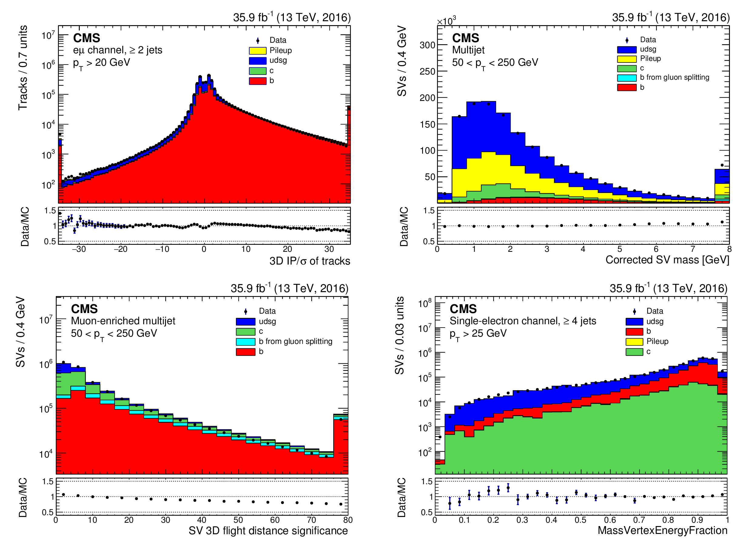
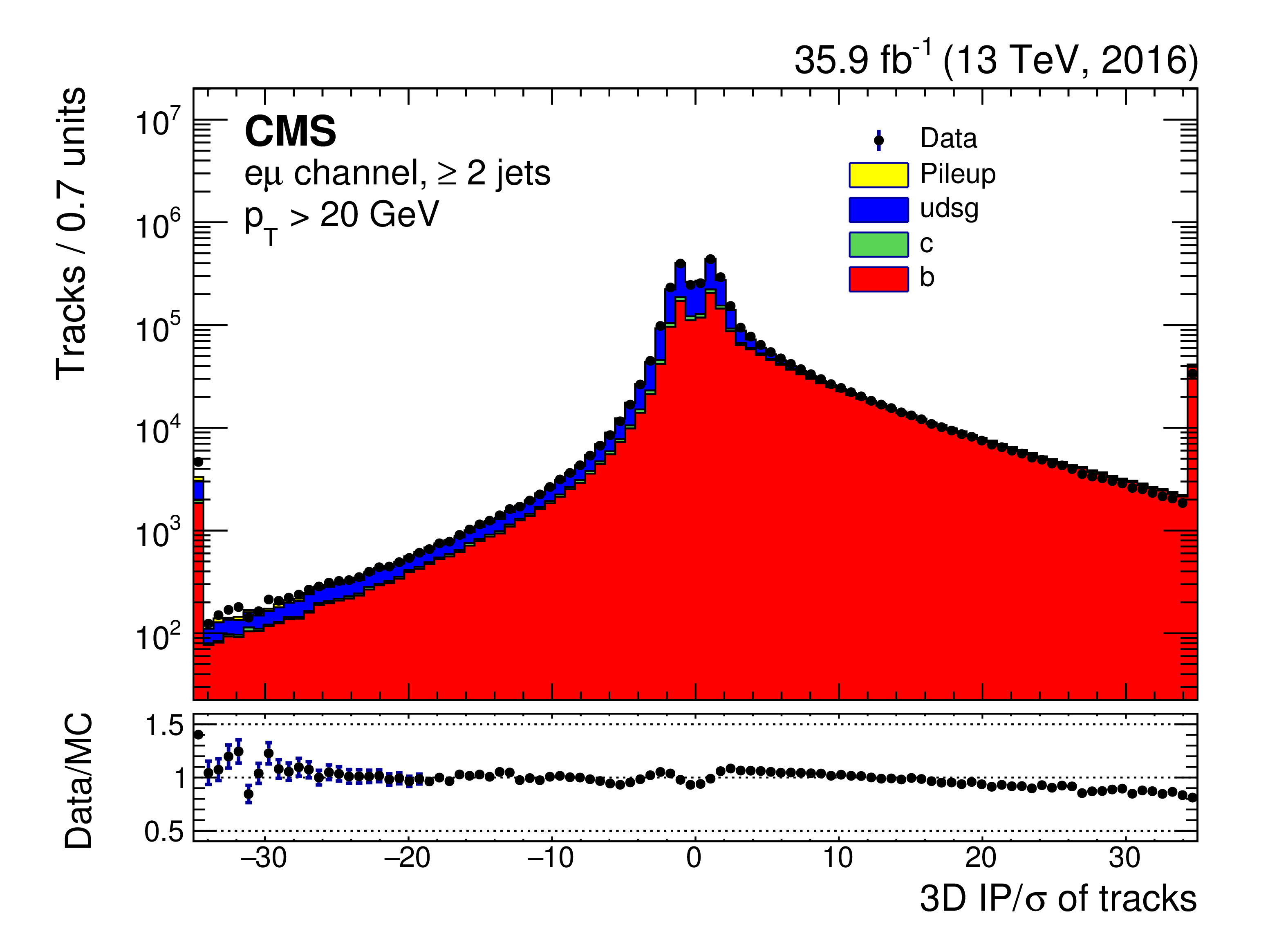
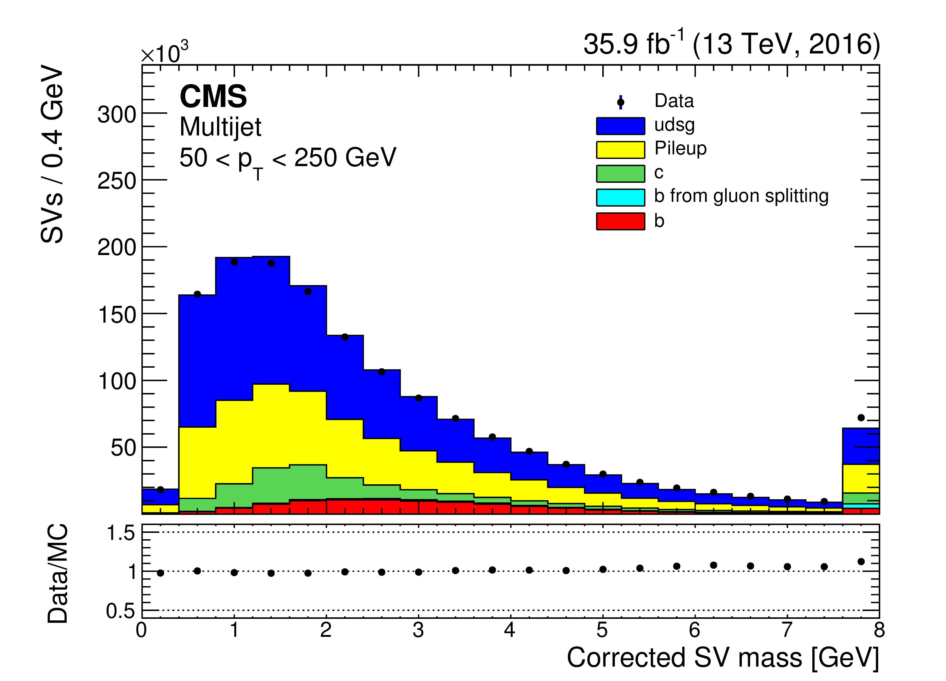
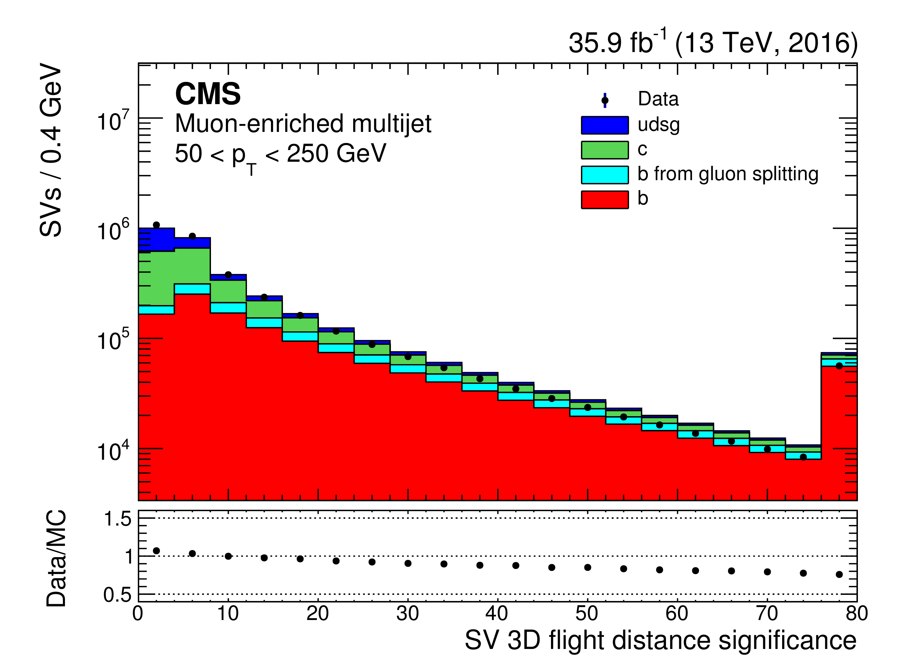
png pdf	Figure 30: Examples of input variables used in heavy-flavour tagging algorithms in data compared to simulation. Impact parameter significance of the tracks in jets from the dilepton $ {\mathrm {t}\overline {\mathrm {t}}} $ sample (upper left), corrected secondary vertex mass for the secondary vertex with the smallest uncertainty in the 3D flight distance for jets in an inclusive multijet sample (upper right), secondary vertex flight distance significance for jets in a muon-enriched jet sample (lower left), and distribution of the massVertexEnergyFraction variable described in the text for jets in the single-lepton $ {\mathrm {t}\overline {\mathrm {t}}} $ sample (lower right). The simulated contributions of each flavour are shown with different colours. The total number of entries in the simulation is normalized to the number of observed entries in data. The first and last bin of each histogram contain the underflow and overflow entries, respectively.
png pdf	Figure 30-a: Impact parameter significance of the tracks in jets from the dilepton $ {\mathrm {t}\overline {\mathrm {t}}} $ sample. The simulated contributions of each flavour are shown with different colours. The total number of entries in the simulation is normalized to the number of observed entries in data. The first and last bin of each histogram contain the underflow and overflow entries, respectively.
png pdf	Figure 30-b: Corrected secondary vertex mass for the secondary vertex with the smallest uncertainty in the 3D flight distance for jets in an inclusive multijet sample. The simulated contributions of each flavour are shown with different colours. The total number of entries in the simulation is normalized to the number of observed entries in data. The first and last bin of each histogram contain the underflow and overflow entries, respectively.
png pdf	Figure 30-c: Secondary vertex flight distance significance for jets in a muon-enriched jet sample. The simulated contributions of each flavour are shown with different colours. The total number of entries in the simulation is normalized to the number of observed entries in data. The first and last bin of each histogram contain the underflow and overflow entries, respectively.
png pdf	Figure 30-d: Distribution of the massVertexEnergyFraction variable described in the text for jets in the single-lepton $ {\mathrm {t}\overline {\mathrm {t}}} $ sample. The simulated contributions of each flavour are shown with different colours. The total number of entries in the simulation is normalized to the number of observed entries in data. The first and last bin of each histogram contain the underflow and overflow entries, respectively.
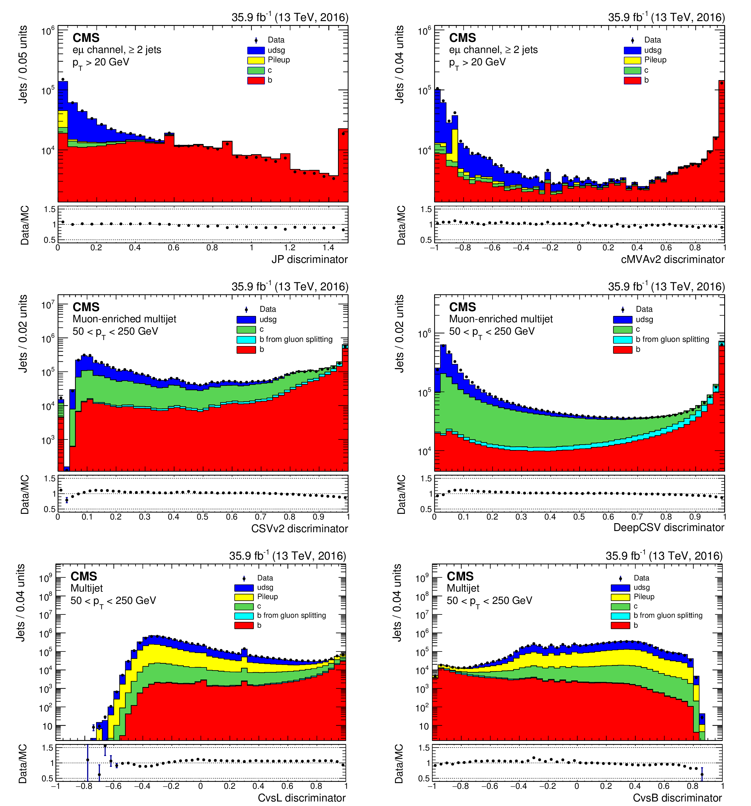
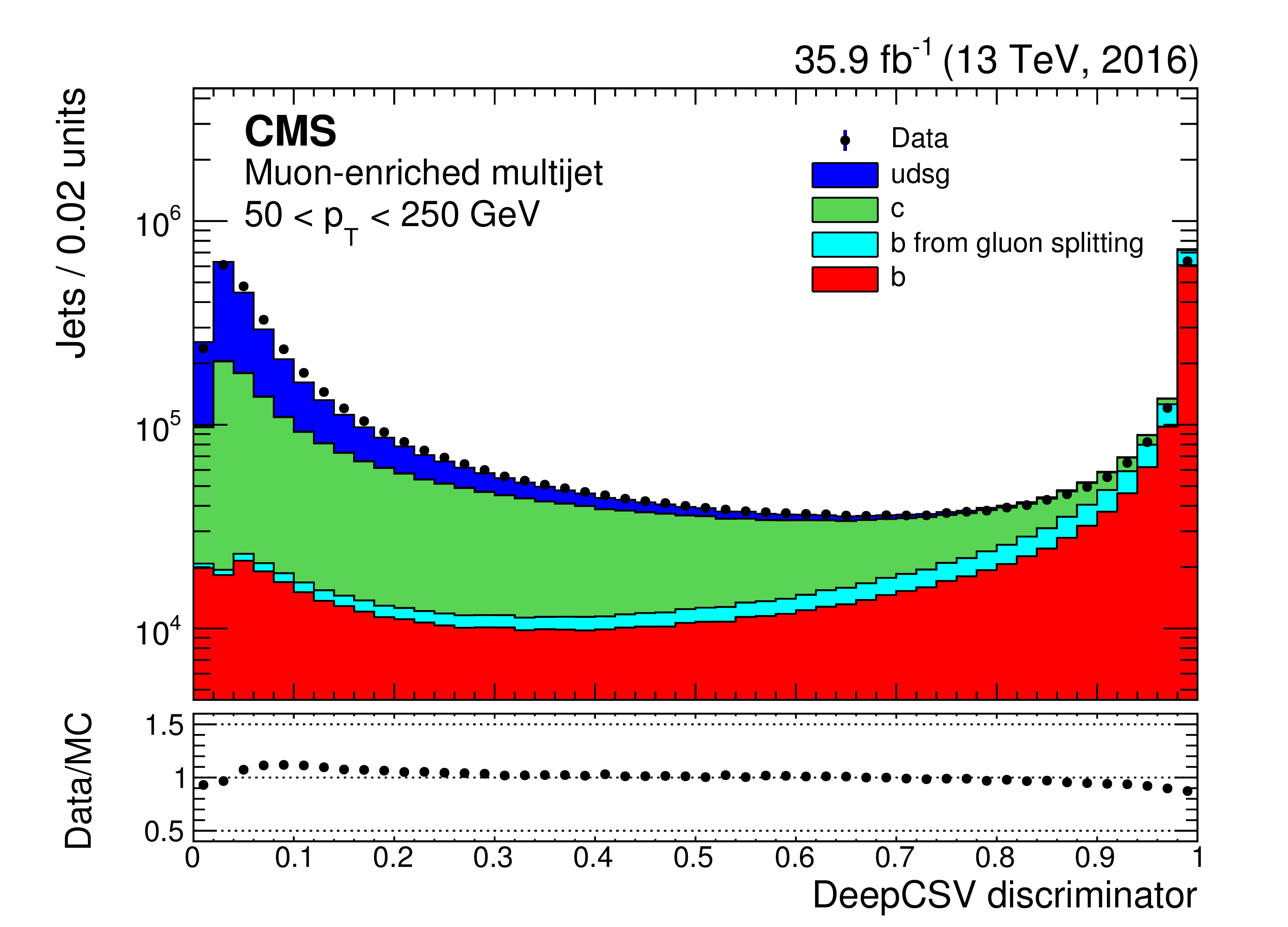
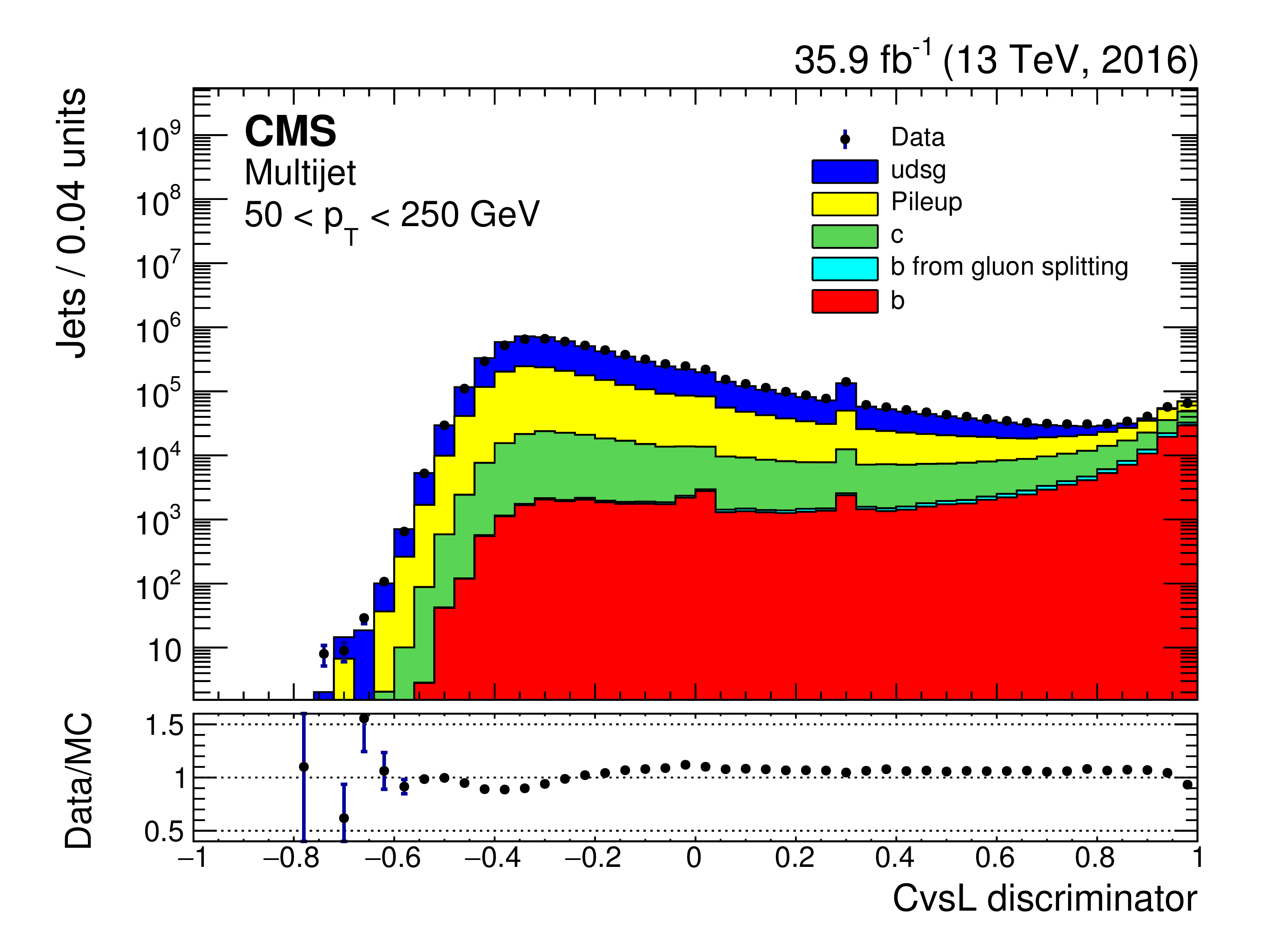
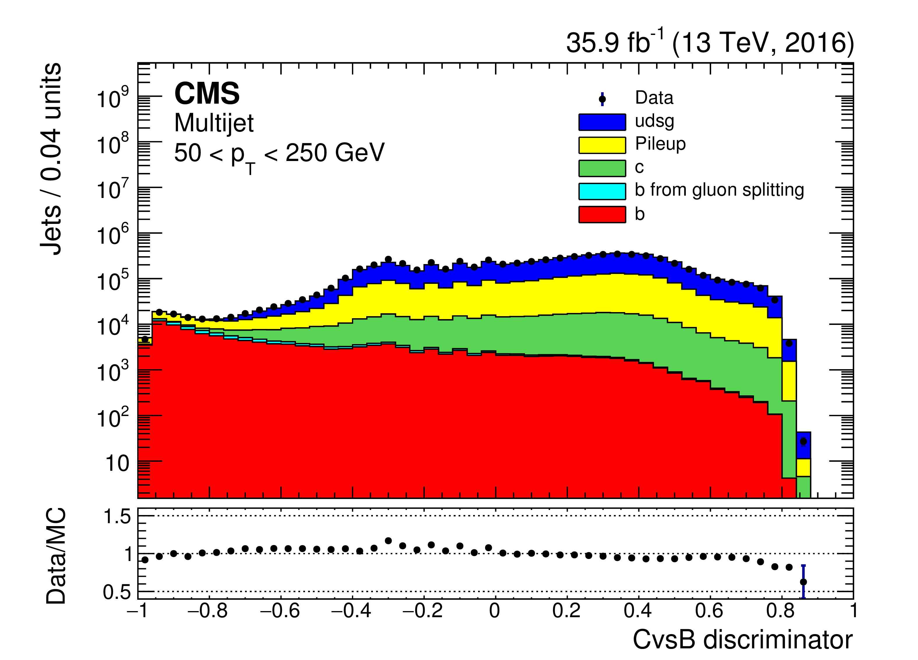
png pdf	Figure 31: Examples of discriminator distributions in data compared to simulation. The JP (upper left) and cMVAv2 (upper right) discriminator values are shown for jets in the dilepton $ {\mathrm {t}\overline {\mathrm {t}}} $ sample, the CSVv2 (middle left) and DeepCSV (middle right) discriminators for jets in the muon-enriched multijet sample, and the CvsL (lower left) and CvsB (lower right) discriminators for jets in the inclusive multijet sample. The simulated contributions of each jet flavour are shown with different colours. The total number of entries in the simulation is normalized to the number of observed entries in data. The first and last bin of each histogram contain the underflow and overflow entries, respectively.
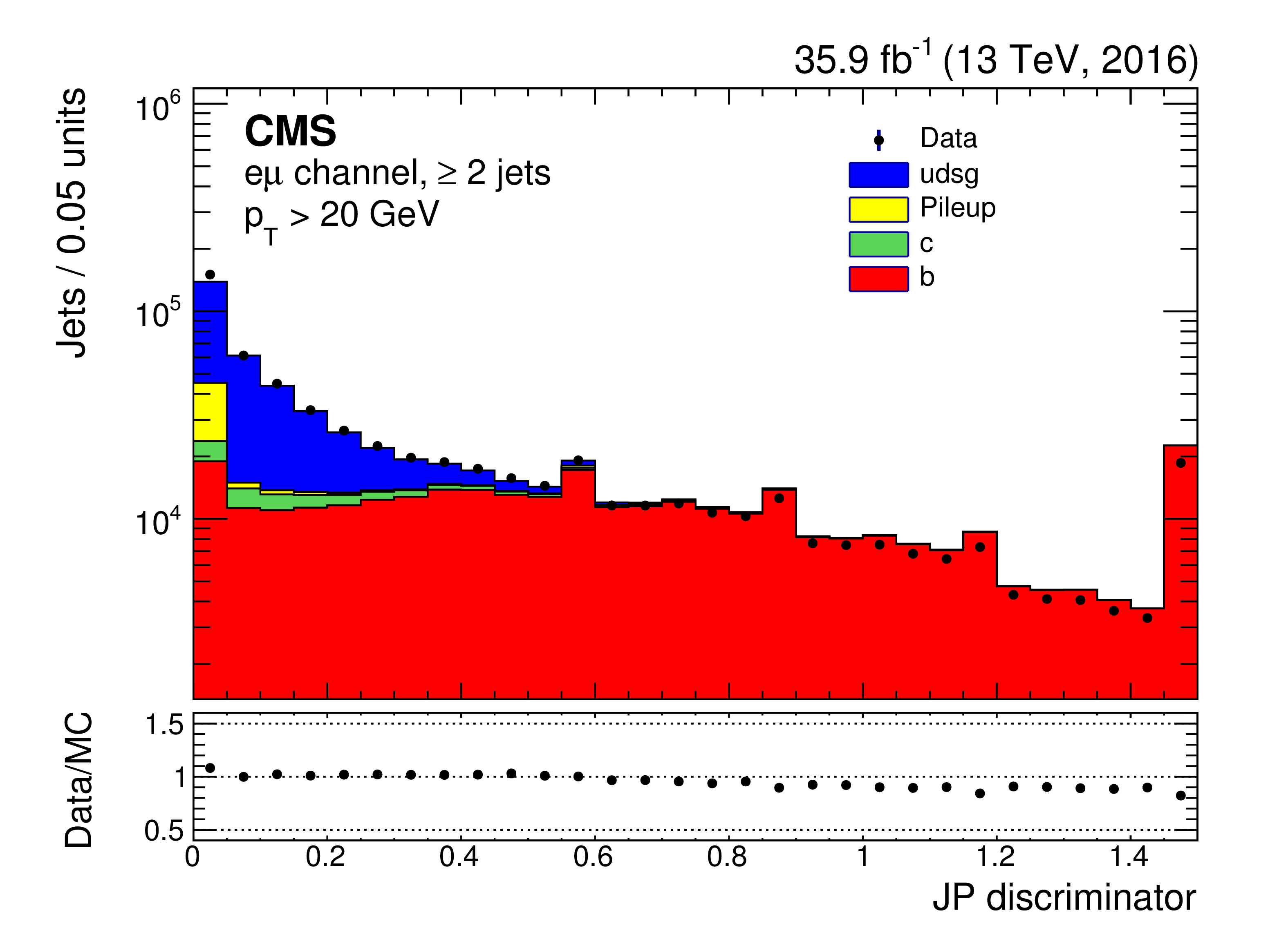
png pdf	Figure 31-a: JP discriminator values are shown for jets in the dilepton $ {\mathrm {t}\overline {\mathrm {t}}} $ sample. The simulated contributions of each jet flavour are shown with different colours. The total number of entries in the simulation is normalized to the number of observed entries in data. The first and last bin of each histogram contain the underflow and overflow entries, respectively.
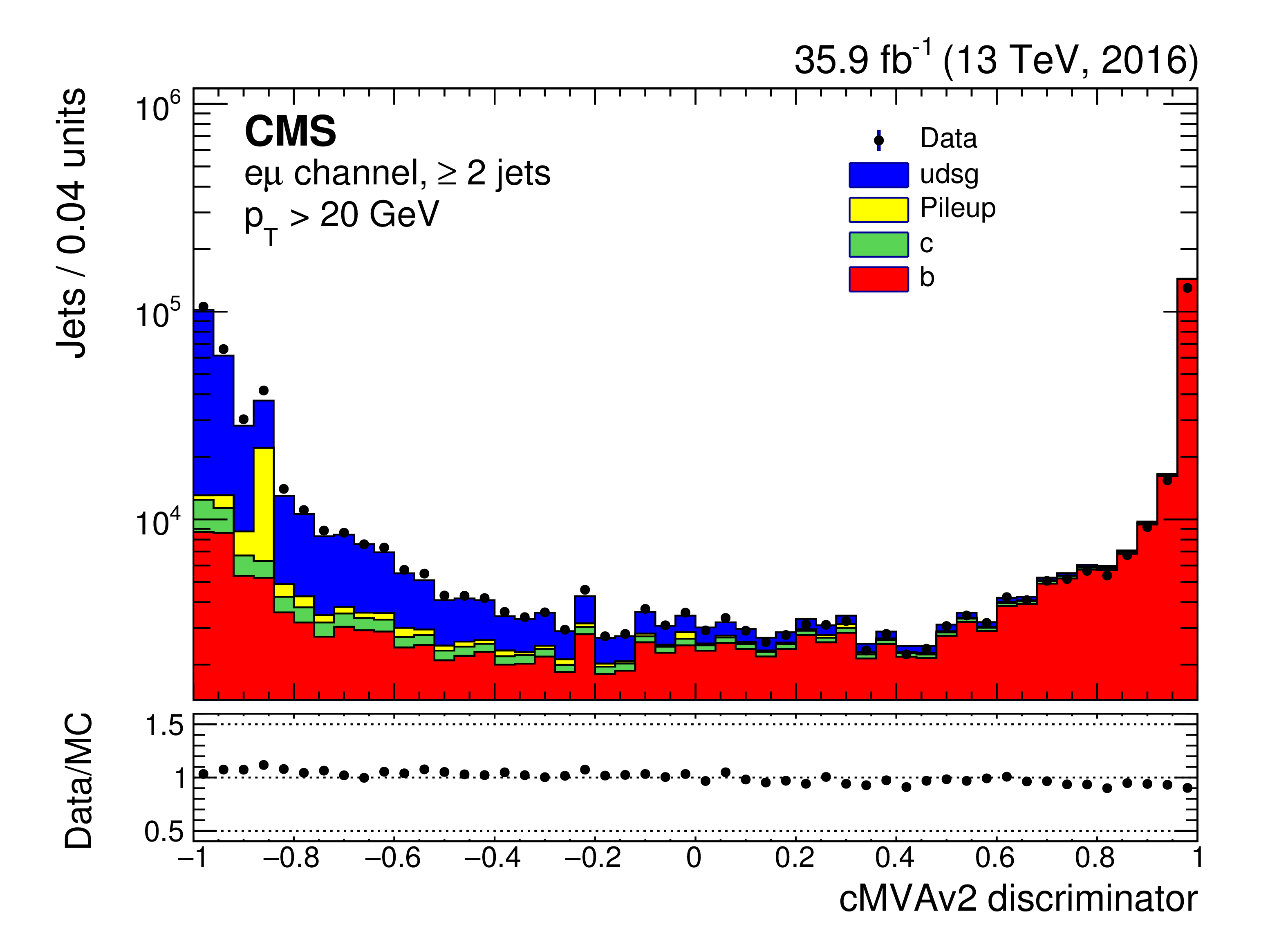
png pdf	Figure 31-b: cMVAv2 discriminator values are shown for jets in the dilepton $ {\mathrm {t}\overline {\mathrm {t}}} $ sample. The simulated contributions of each jet flavour are shown with different colours. The total number of entries in the simulation is normalized to the number of observed entries in data. The first and last bin of each histogram contain the underflow and overflow entries, respectively.
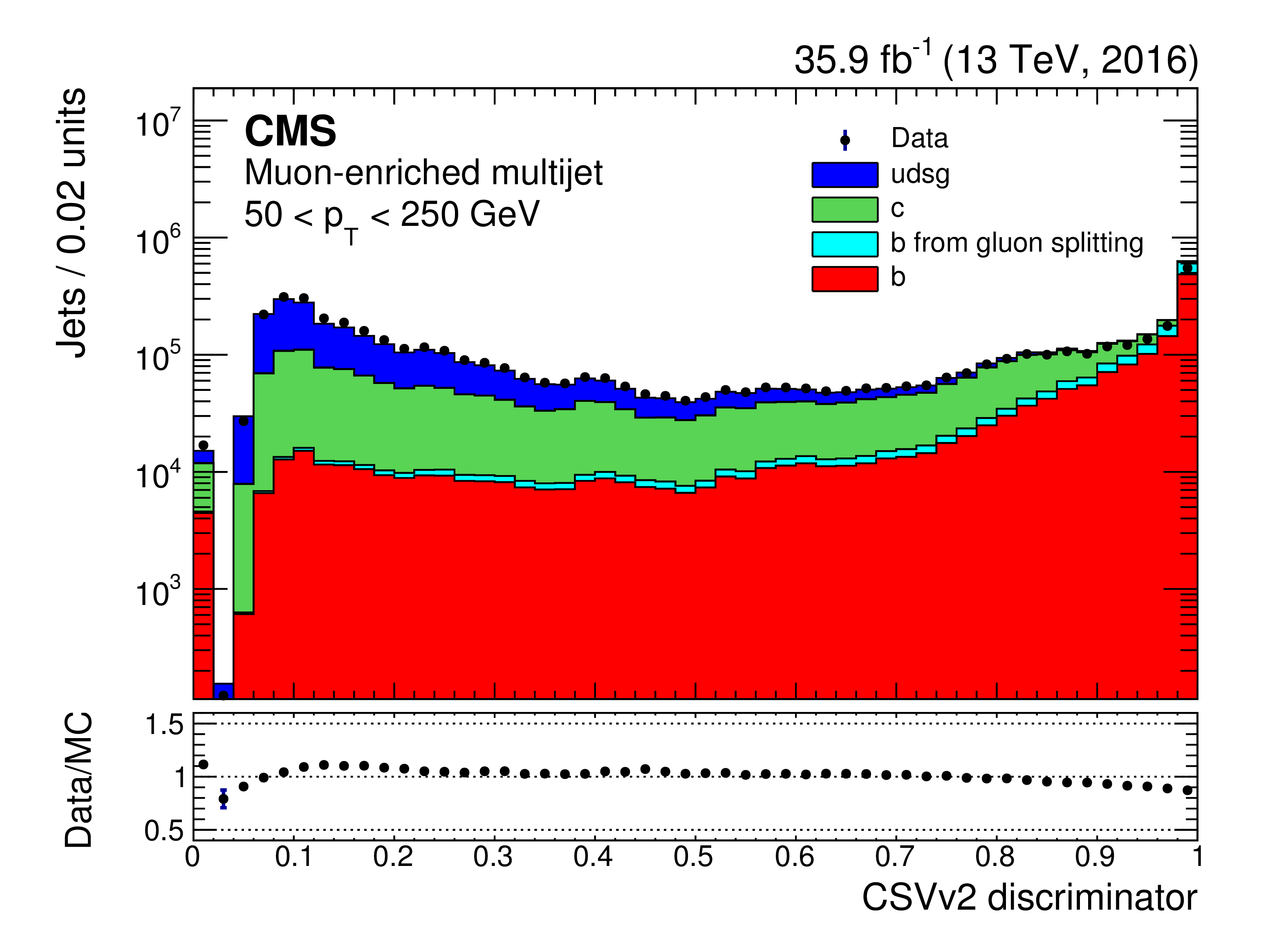
png pdf	Figure 31-c: CSVv2 discriminator for jets in the muon-enriched multijet sample. The simulated contributions of each jet flavour are shown with different colours. The total number of entries in the simulation is normalized to the number of observed entries in data. The first and last bin of each histogram contain the underflow and overflow entries, respectively.
png pdf	Figure 31-d: DeepCSV discriminator for jets in the muon-enriched multijet sample. The simulated contributions of each jet flavour are shown with different colours. The total number of entries in the simulation is normalized to the number of observed entries in data. The first and last bin of each histogram contain the underflow and overflow entries, respectively.
png pdf	Figure 31-e: CvsL discriminator for jets in the inclusive multijet sample. The simulated contributions of each jet flavour are shown with different colours. The total number of entries in the simulation is normalized to the number of observed entries in data. The first and last bin of each histogram contain the underflow and overflow entries, respectively.
png pdf	Figure 31-f: CvsB discriminator for jets in the inclusive multijet sample. The simulated contributions of each jet flavour are shown with different colours. The total number of entries in the simulation is normalized to the number of observed entries in data. The first and last bin of each histogram contain the underflow and overflow entries, respectively.
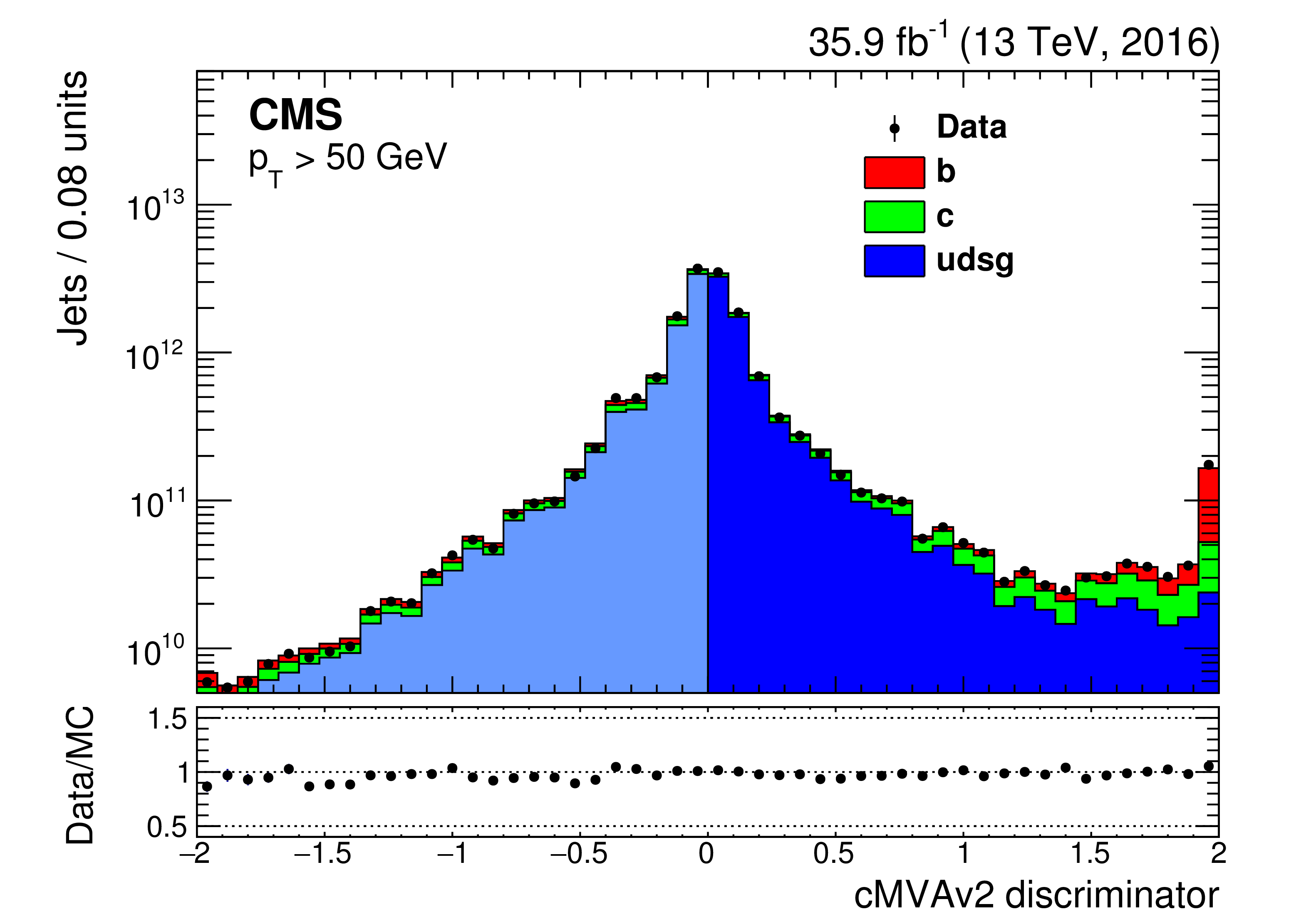
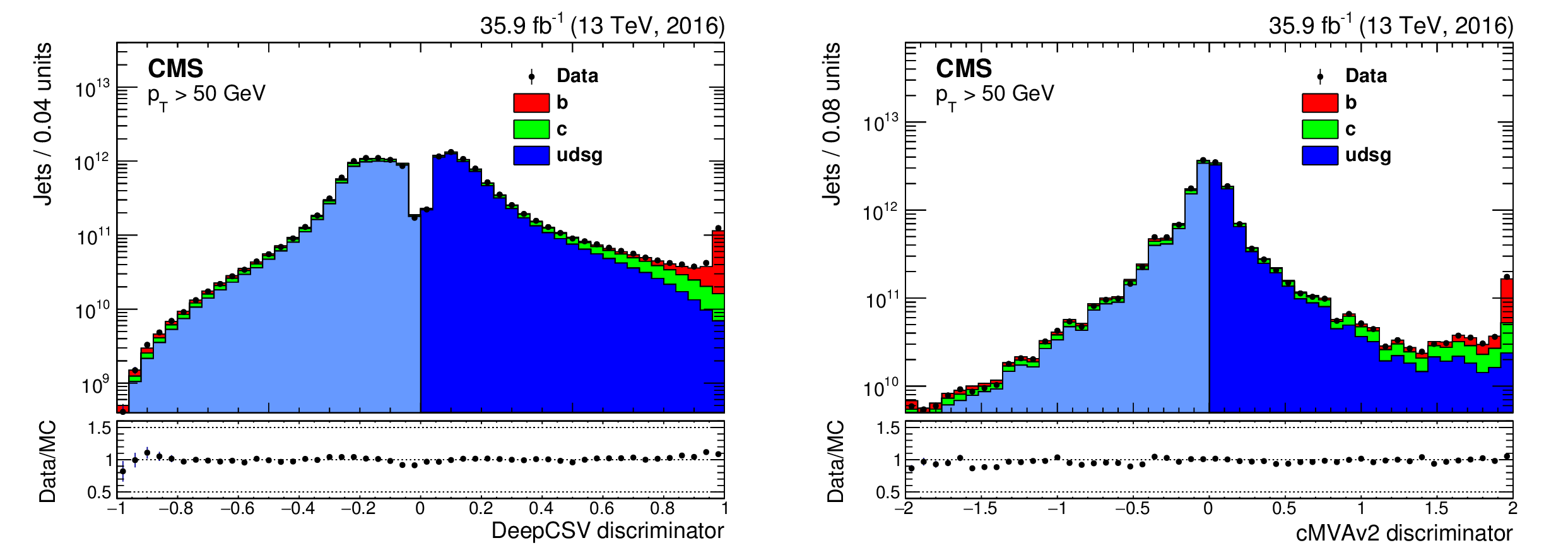
png pdf	Figure 32: Distributions of the DeepCSV (left) and the cMVAv2 (right) discriminators for jets in an inclusive multijet sample. For visualization purposes the discriminator output of the negative DeepCSV tagger is shown with a negative sign. For the cMVAv2 tagger, the discriminator output of the positive tagger is shifted from $[-1,1]$ to $[0,2]$ and the discriminator values of the negative tagger are shown with a negative sign. The simulation is normalized to the number of entries in the data.
png pdf	Figure 32-a: Distribution of the DeepCSV discriminator for jets in an inclusive multijet sample. For visualization purposes the discriminator output of the negative DeepCSV tagger is shown with a negative sign. The simulation is normalized to the number of entries in the data.
png pdf	Figure 32-b: Distribution of the cMVAv2 discriminator for jets in an inclusive multijet sample. The discriminator output of the positive tagger is shifted from $[-1,1]$ to $[0,2]$ and the discriminator values of the negative tagger are shown with a negative sign.
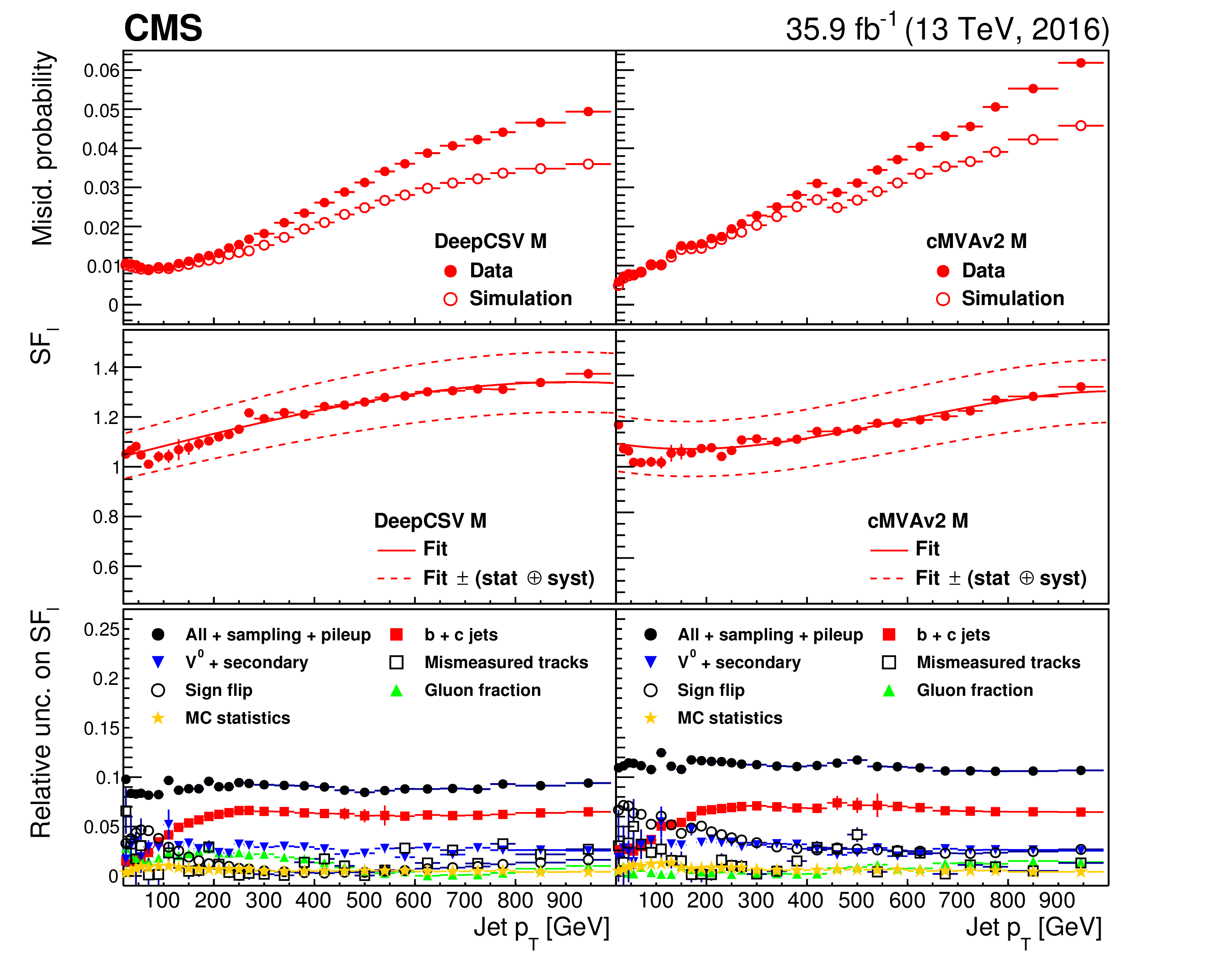
png pdf	Figure 33: Misidentification probability, data-to-simulation scale factors, and relative uncertainty in the scale factors for light-flavour jets for the medium working point of the DeepCSV (left) and cMVAv2 (right) algorithm. The upper panels show the misidentification probability in data and simulation as a function of the jet $ {p_{\mathrm {T}}} $. The middle panels show the scale factors for light-flavour jets, where the solid curve is the result of a fit to the scale factors, and the dashed lines represent the overall statistical and systematic uncertainty in the measurement. The lower panels show the relative systematic uncertainties in the scale factors for light-flavour jets. The sampling and pileup uncertainties are not shown since they are below 1%, but are included in the total systematic uncertainty covered by the black dots.
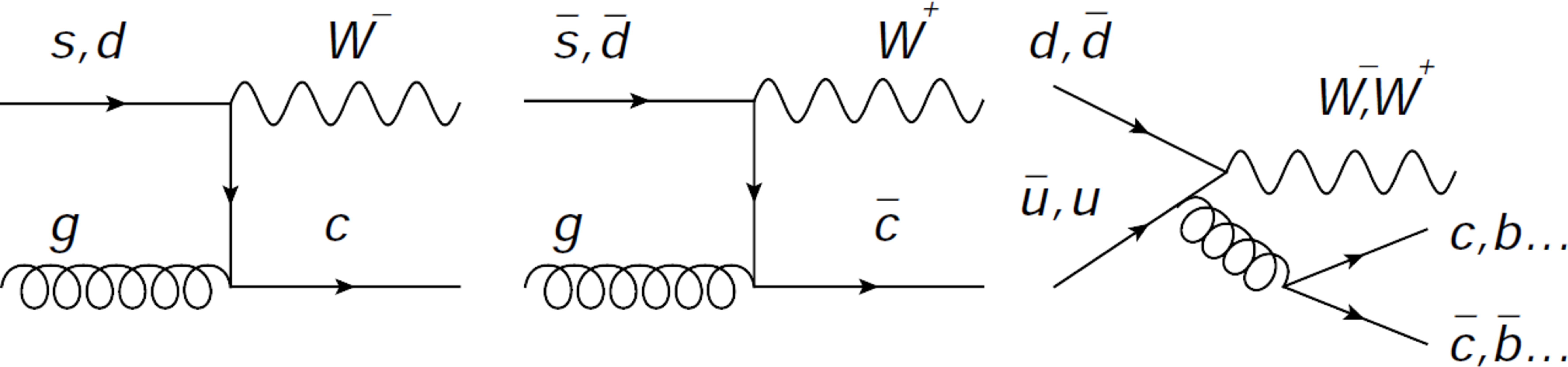
png pdf	Figure 34: Leading order production of W+c with opposite-sign electric charges (left and middle), and of W+${{\mathrm {q}} {\overline {\mathrm {q}}}}$ through gluon splitting (right). In gluon splitting there is an additional c quark with the same sign as the W boson.
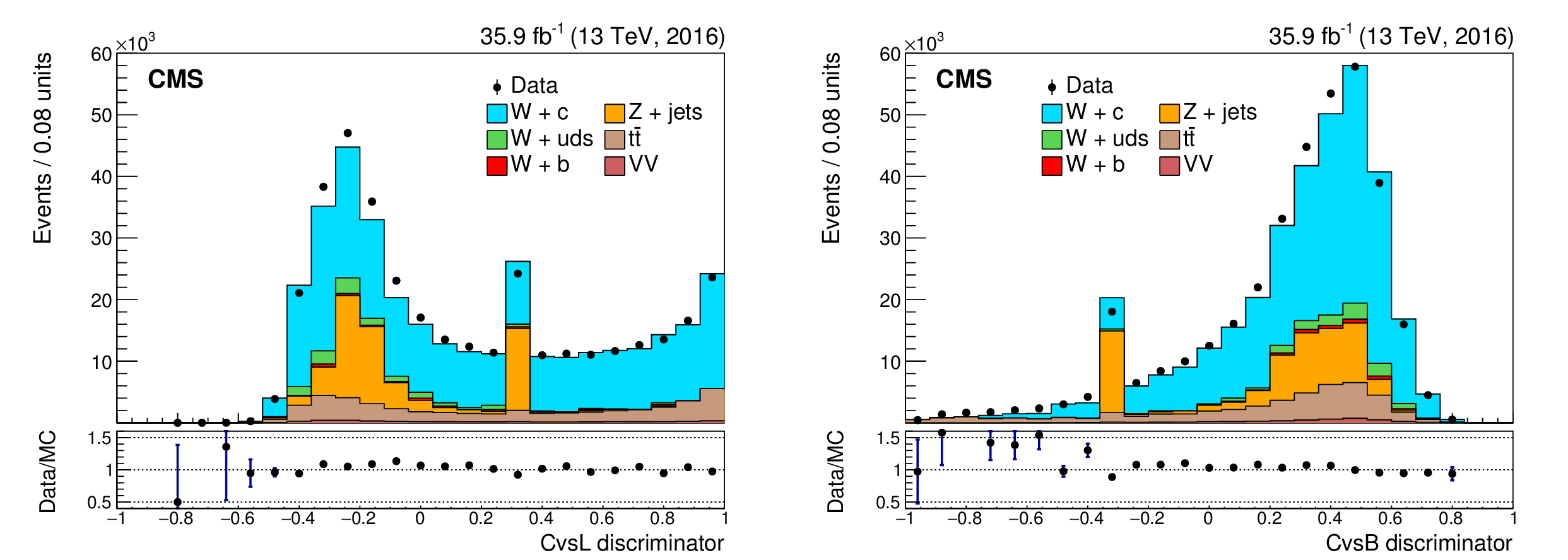
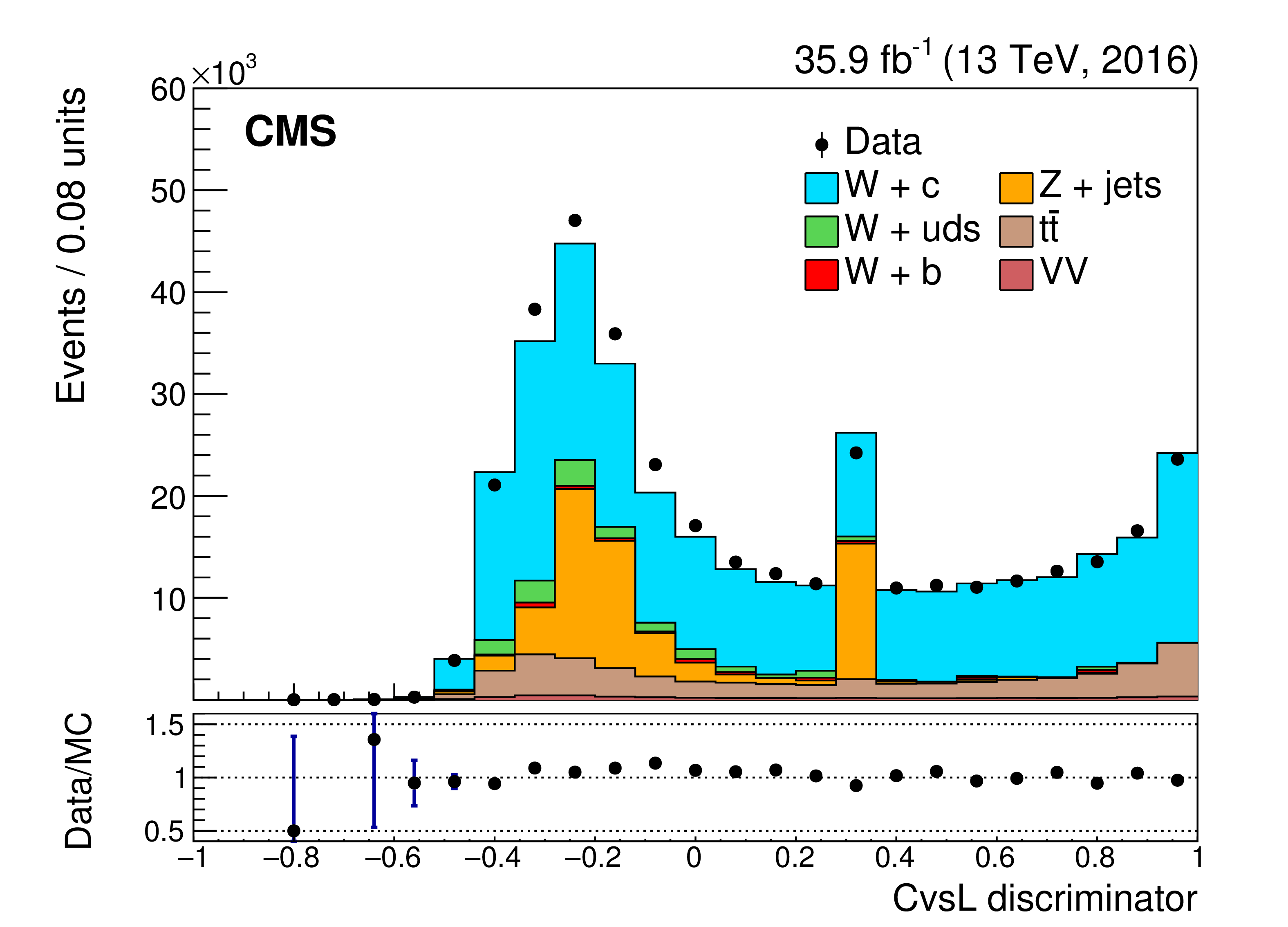
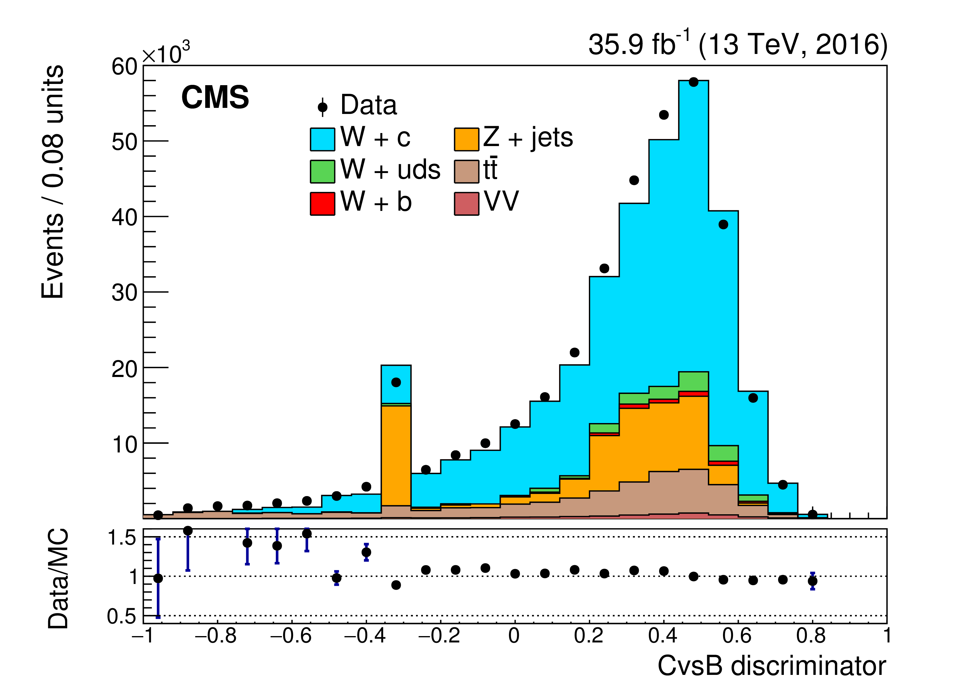
png pdf	Figure 35: Distribution of the CvsL (left) and CvsB (right) discriminators in the $ {\mathrm {W}}\to {{\mu}} {\nu}$ and $ {\mathrm {W}}\to {\mathrm {e}} {\nu}$ channels after the OS-SS subtraction. The spikes originate from jets without a track passing the track selection criteria, as discussed in Section 5.2.1. The last bin includes the overflow entries.
png pdf	Figure 35-a: Distribution of the CvsL discriminator in the $ {\mathrm {W}}\to {{\mu}} {\nu}$ and $ {\mathrm {W}}\to {\mathrm {e}} {\nu}$ channels after the OS-SS subtraction. The spikes originate from jets without a track passing the track selection criteria, as discussed in Section 5.2.1. The last bin includes the overflow entries.
png pdf	Figure 35-b: Distribution of the CvsB discriminator in the $ {\mathrm {W}}\to {{\mu}} {\nu}$ and $ {\mathrm {W}}\to {\mathrm {e}} {\nu}$ channels after the OS-SS subtraction. The spikes originate from jets without a track passing the track selection criteria, as discussed in Section 5.2.1. The last bin includes the overflow entries.
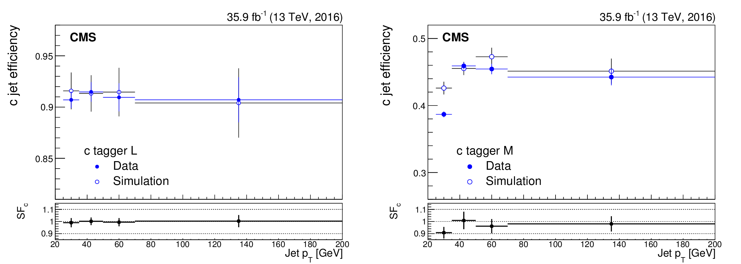
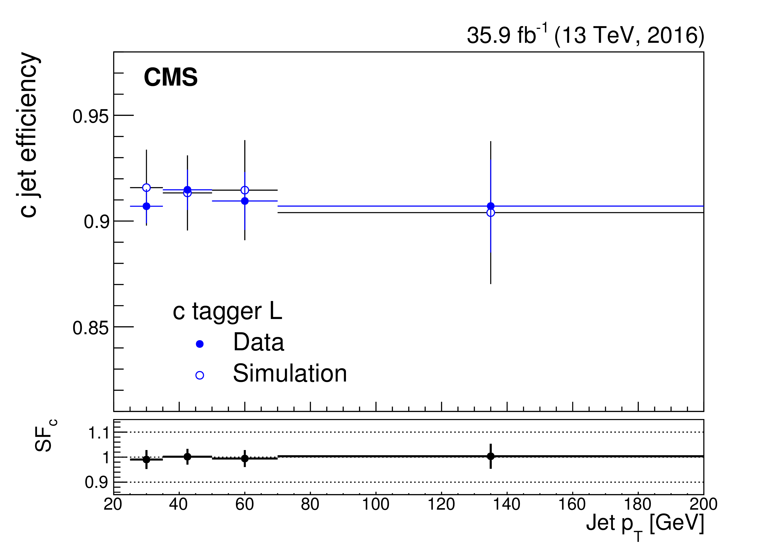
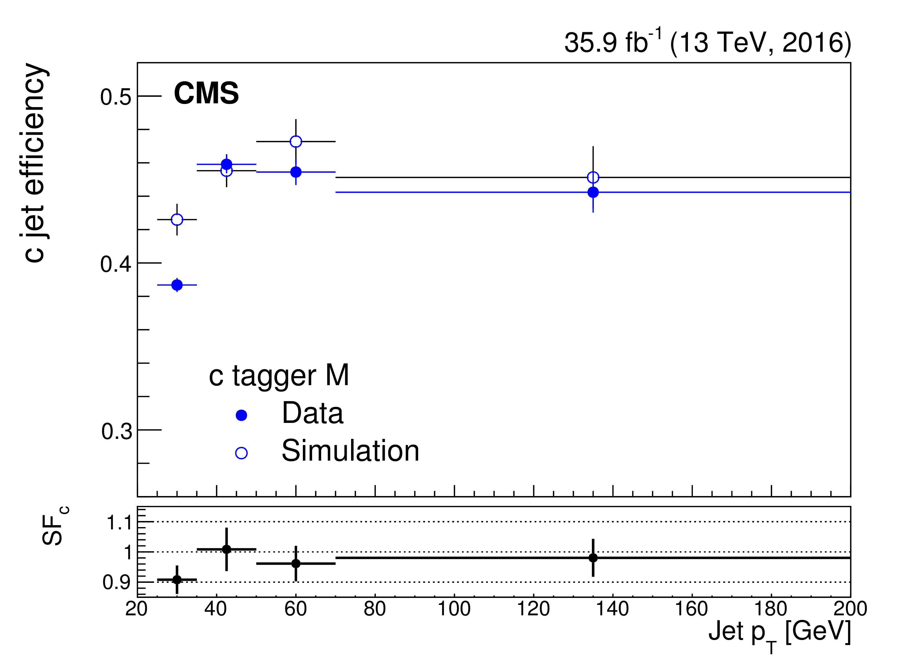
png pdf	Figure 36: Efficiency for tagging c jets in data and simulation as a function of the jet $ {p_{\mathrm {T}}}$, and corresponding data-to-simulation scale factors (bottom panels) for the loose (left) and medium (right) working points of the c tagger.
png pdf	Figure 36-a: Efficiency for tagging c jets in data and simulation as a function of the jet $ {p_{\mathrm {T}}}$, and corresponding data-to-simulation scale factors (bottom panels) for the loose working point of the c tagger.
png pdf	Figure 36-b: Efficiency for tagging c jets in data and simulation as a function of the jet $ {p_{\mathrm {T}}}$, and corresponding data-to-simulation scale factors (bottom panels) for the medium working point of the c tagger.
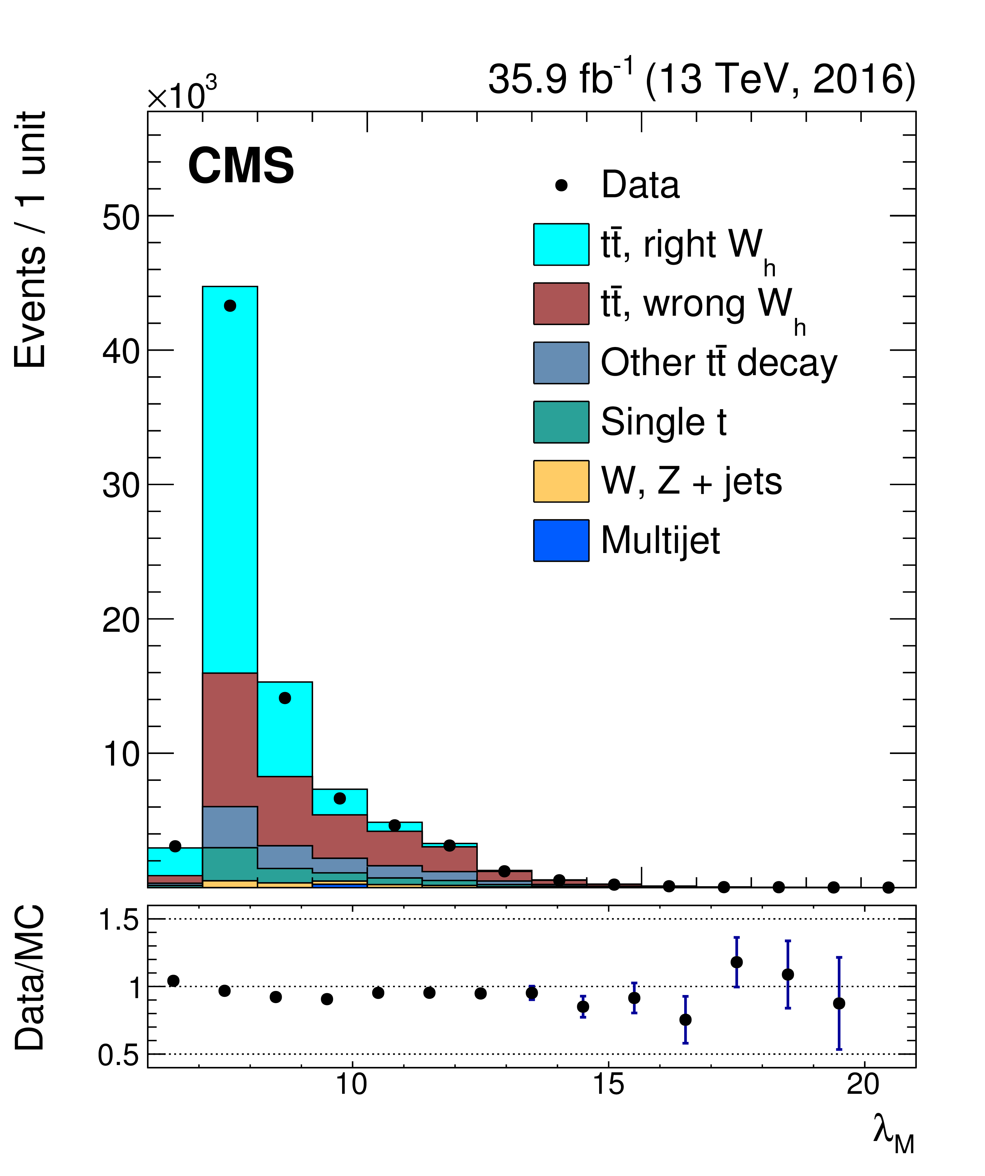
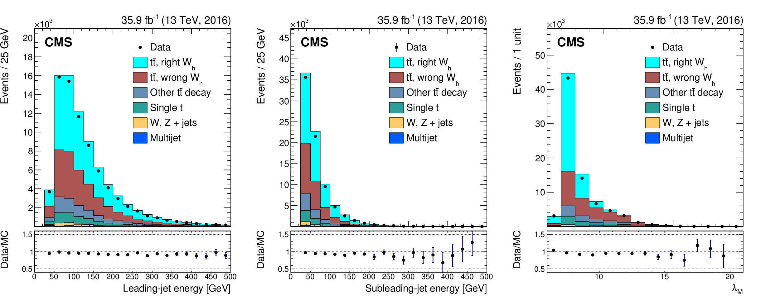
png pdf	Figure 37: Distributions of the leading- (left) and subleading- (middle) jet energy as well as of the mass discriminant $ {\lambda _{M}}$ (right) after the full event selection, jet-quark assignment, and b tagging requirement on the two b jet candidates.
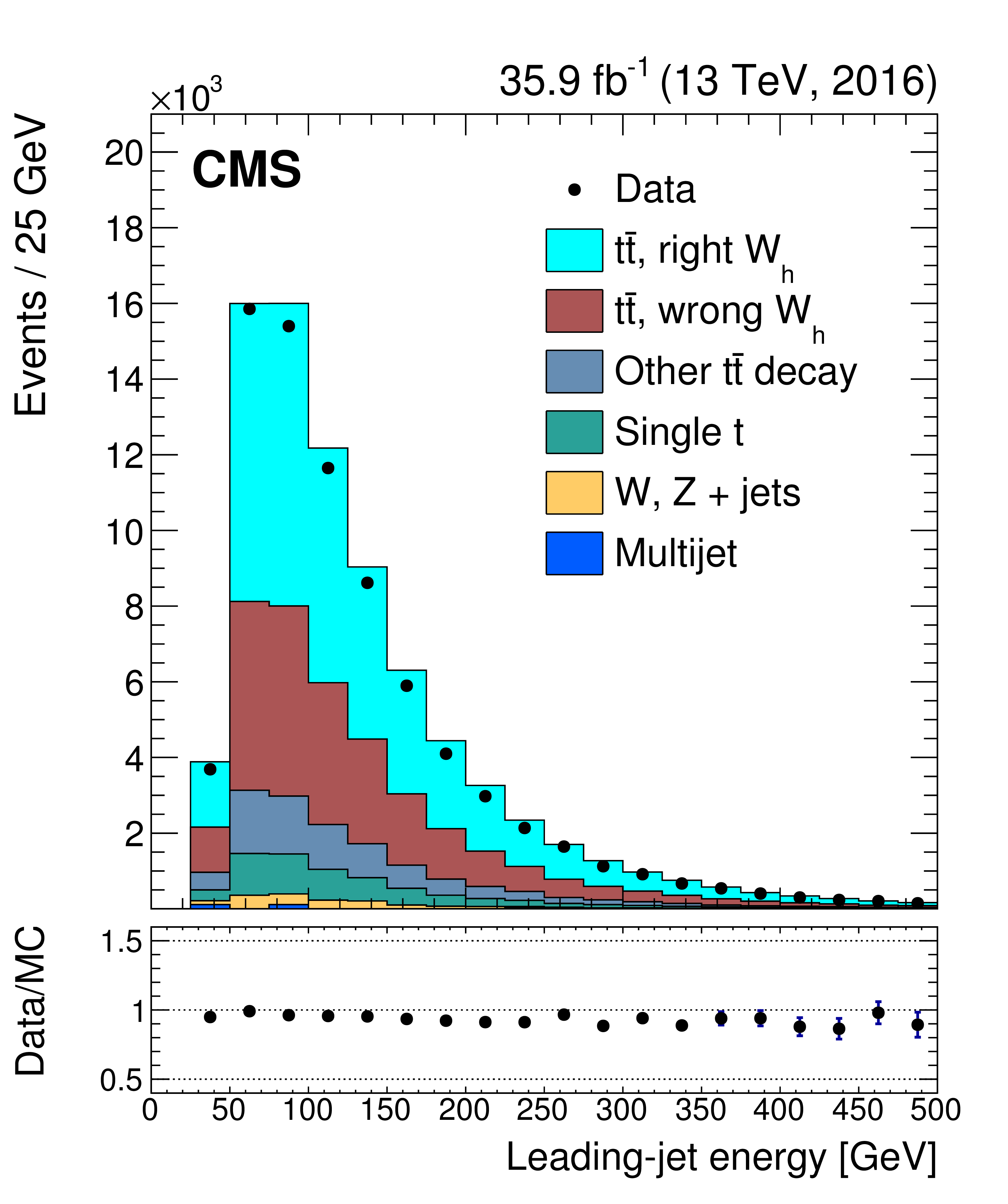
png pdf	Figure 37-a: Distribution of the leading-jet energy after the full event selection, jet-quark assignment, and b tagging requirement on the two b jet candidates.
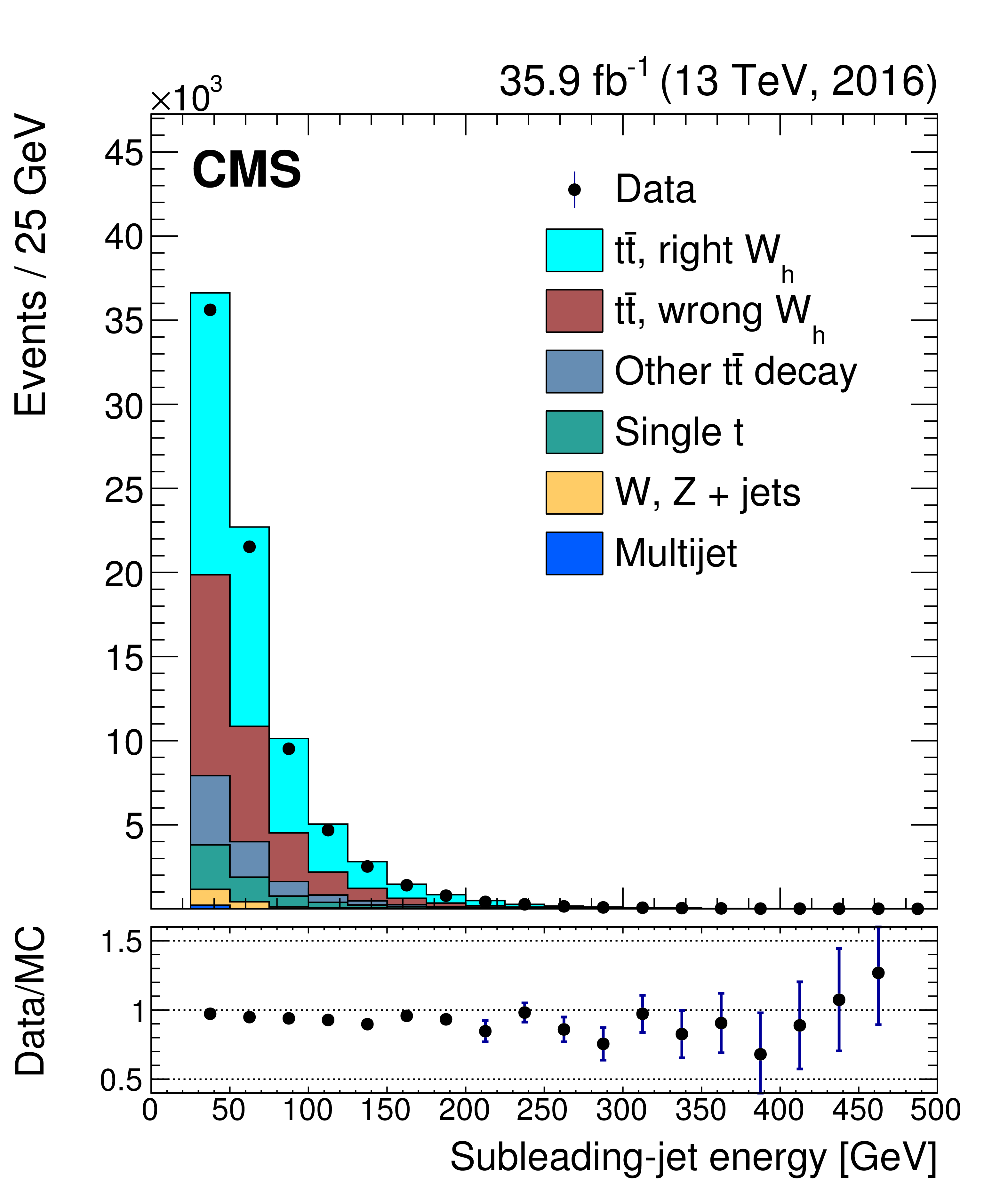
png pdf	Figure 37-b: Distribution of the subleading-jet energy after the full event selection, jet-quark assignment, and b tagging requirement on the two b jet candidates.
png pdf	Figure 37-c: Distribution of the mass discriminant $ {\lambda _{M}}$ after the full event selection, jet-quark assignment, and b tagging requirement on the two b jet candidates.
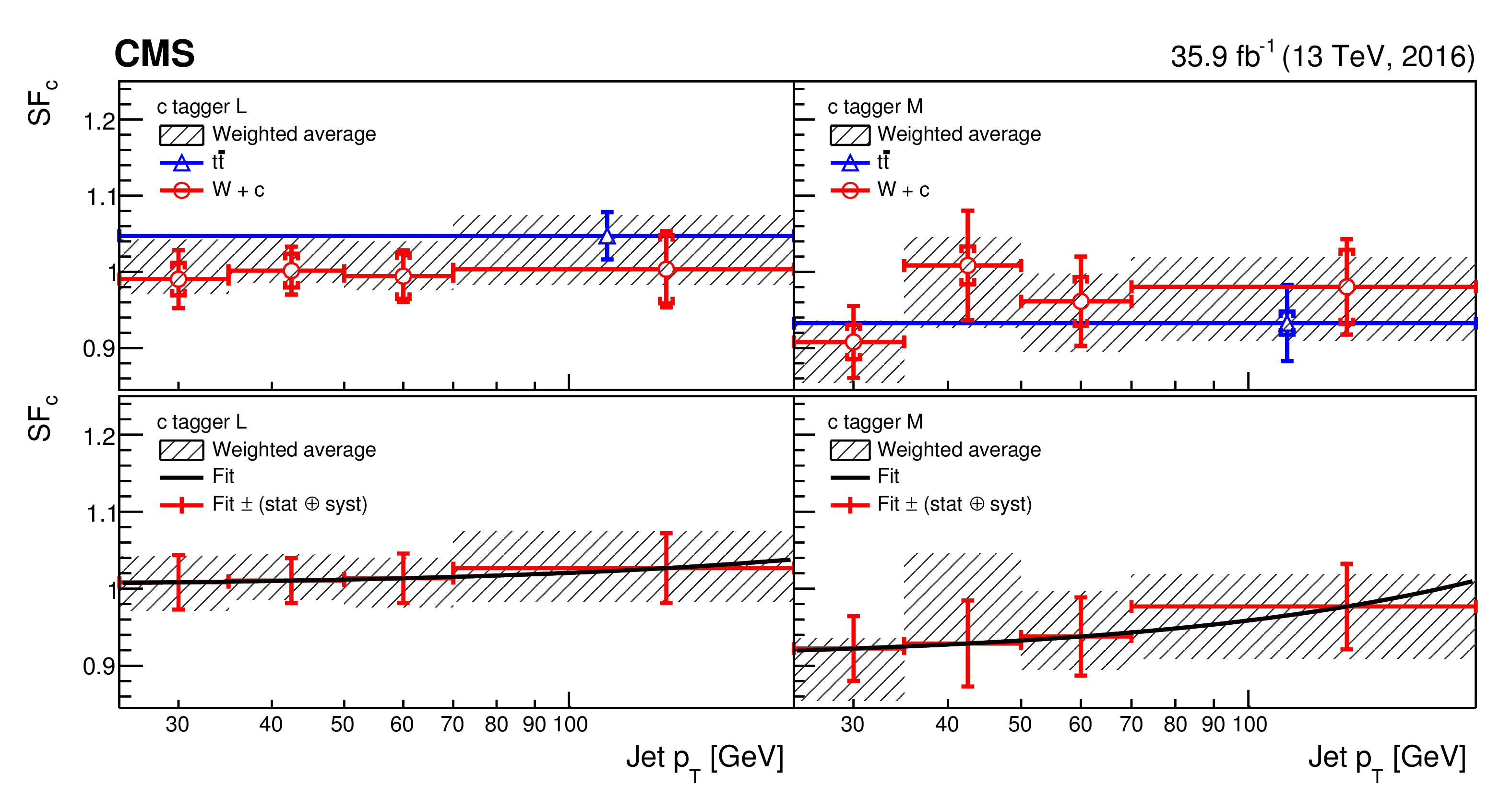
png pdf	Figure 38: Data-to-simulation scale factors for c jets for the loose (left) and medium (right) working points of the c tagger. The upper panels show the scale factors for c jets as a function of the jet $ {p_{\mathrm {T}}} $ obtained with the two methods described in the text. The inner error bars represent the statistical uncertainty and the outer error bars the combined statistical and systematic uncertainty. The combined scale factor values with their overall uncertainty are displayed as a hatched area. The lower panels show the same combined scale factor values with superimposed the result of a fit function represented by the solid curve. The combined statistical and systematic uncertainty is centred around the fit result, represented by the points with error bars. The last bin includes the overflow entries.
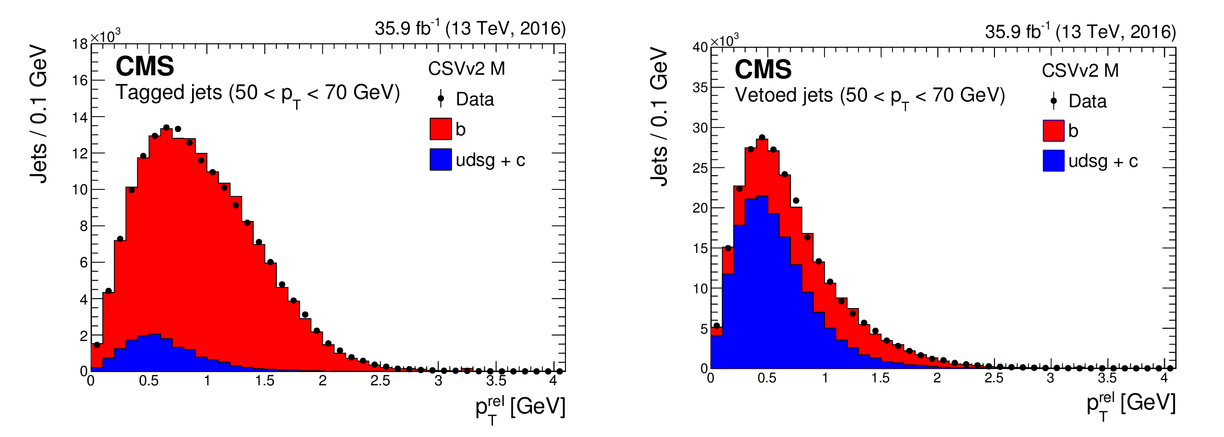
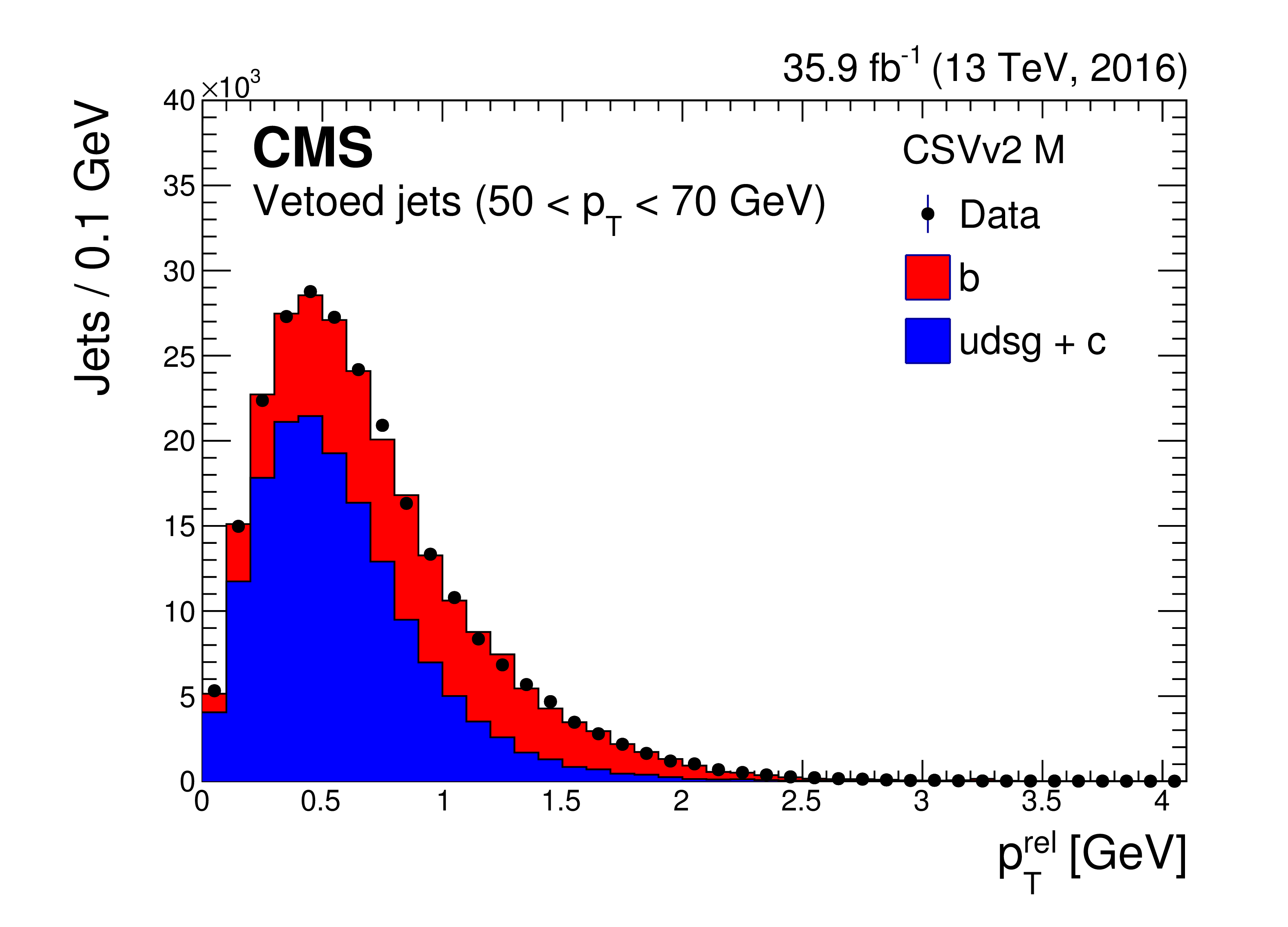
png pdf	Figure 39: Fitted $ {p_{\mathrm {T}}} ^{\text {rel}}$ distribution for muon jets passing (left) and failing (right) the medium working point of the CSVv2 algorithm. The distribution is shown for jets with 50 $ < {p_{\mathrm {T}}} < $ 70 GeV. The simulation is normalized to the observed number of events.
png pdf	Figure 39-a: Fitted $ {p_{\mathrm {T}}} ^{\text {rel}}$ distribution for muon jets passing the medium working point of the CSVv2 algorithm. The distribution is shown for jets with 50 $ < {p_{\mathrm {T}}} < $ 70 GeV. The simulation is normalized to the observed number of events.
png pdf	Figure 39-b: Fitted $ {p_{\mathrm {T}}} ^{\text {rel}}$ distribution for muon jets failing the medium working point of the CSVv2 algorithm. The distribution is shown for jets with 50 $ < {p_{\mathrm {T}}} < $ 70 GeV. The simulation is normalized to the observed number of events.
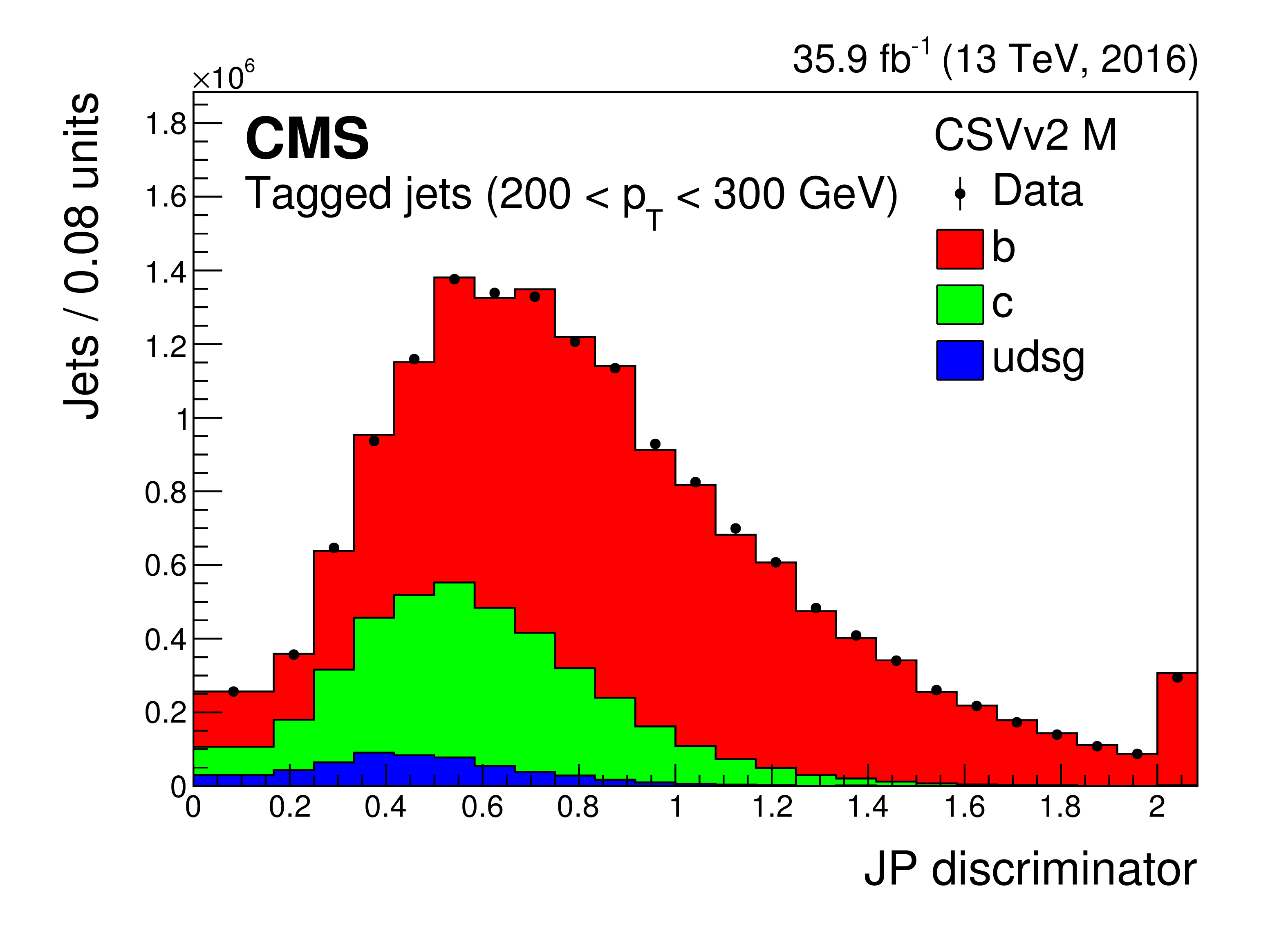
png pdf	Figure 40: Fitted JP distribution for muon jets (left) and for the subsample of those jets passing the medium working point of the CSVv2 algorithm (right). The distribution is shown for jets with 200 $ < {p_{\mathrm {T}}} < $ 300 GeV. The simulation is normalized to the integrated luminosity for the data set. The last bin includes the overflow entries.
png pdf	Figure 40-a: Fitted JP distribution for muon jets. The distribution is shown for jets with 200 $ < {p_{\mathrm {T}}} < $ 300 GeV. The simulation is normalized to the integrated luminosity for the data set. The last bin includes the overflow entries.
png pdf	Figure 40-b: Fitted JP distribution for the subsample of muon jets passing the medium working point of the CSVv2 algorithm. The distribution is shown for jets with 200 $ < {p_{\mathrm {T}}} < $ 300 GeV. The simulation is normalized to the integrated luminosity for the data set. The last bin includes the overflow entries.
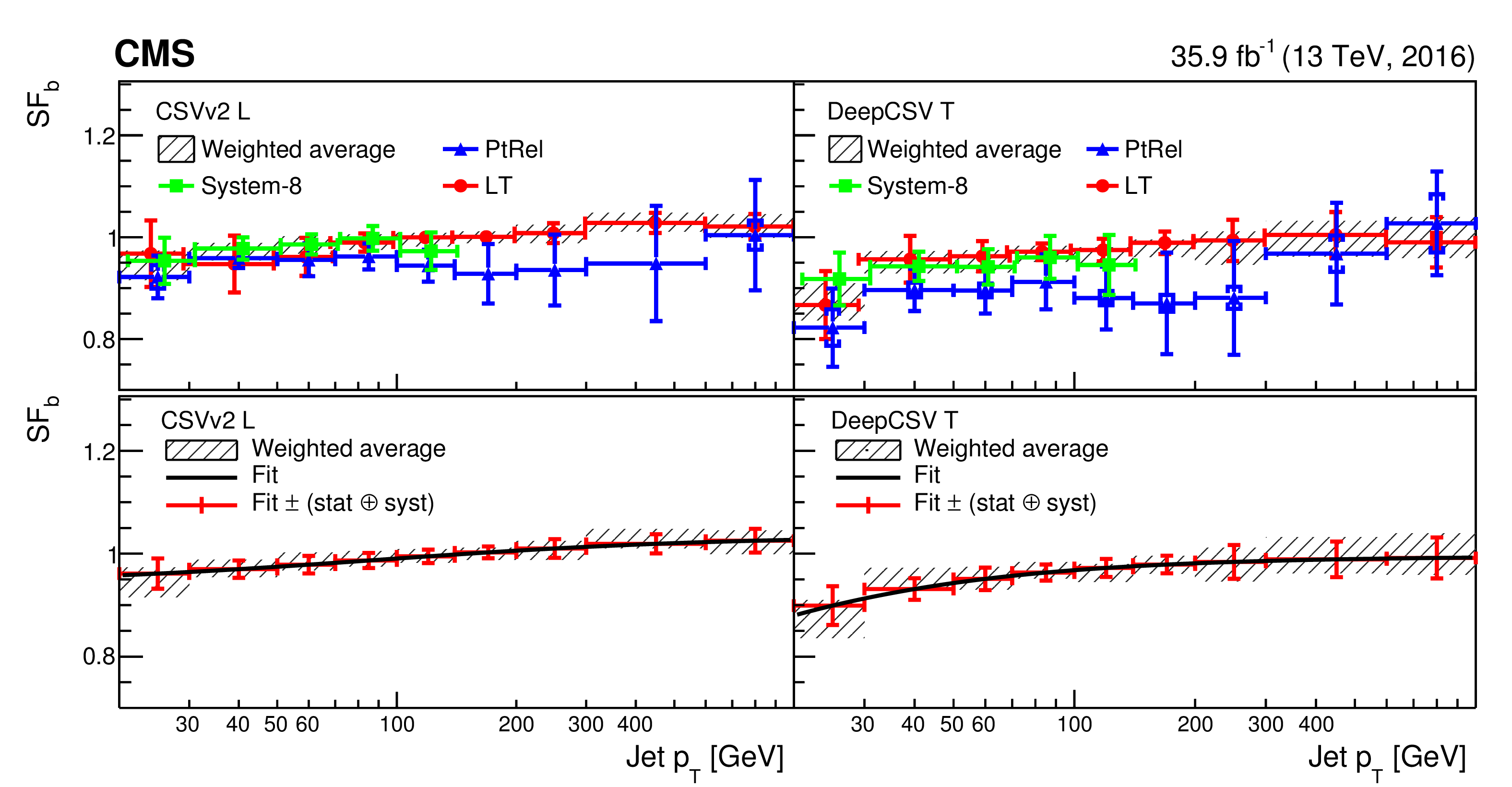
png pdf	Figure 41: Data-to-simulation scale factors for b jets as a function of the jet $ {p_{\mathrm {T}}} $ for the loose CSVv2 (left) and the tight DeepCSV (right) algorithms working points. The upper panels show the scale factors for tagging b as a function of the jet $ {p_{\mathrm {T}}} $ measured with three methods in muon jet events. The inner error bars represent the statistical uncertainty and the outer error bars the combined statistical and systematic uncertainty. The combined scale factors with their overall uncertainty are displayed as a hatched area. The lower panels show the same combined scale factors with the result of a fit function (solid curve) superimposed. The combined scale factors with the overall uncertainty are centred around the fit result. To increase the visibility of the individual measurements, the scale factors obtained with various methods are slightly displaced with respect to the bin centre for which the measurement was performed. The last bin includes the overflow entries.
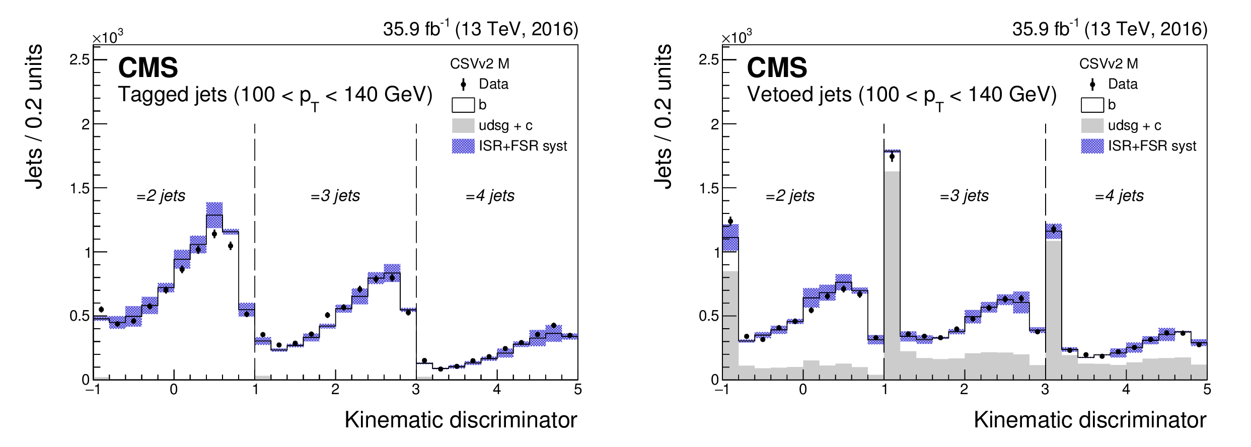
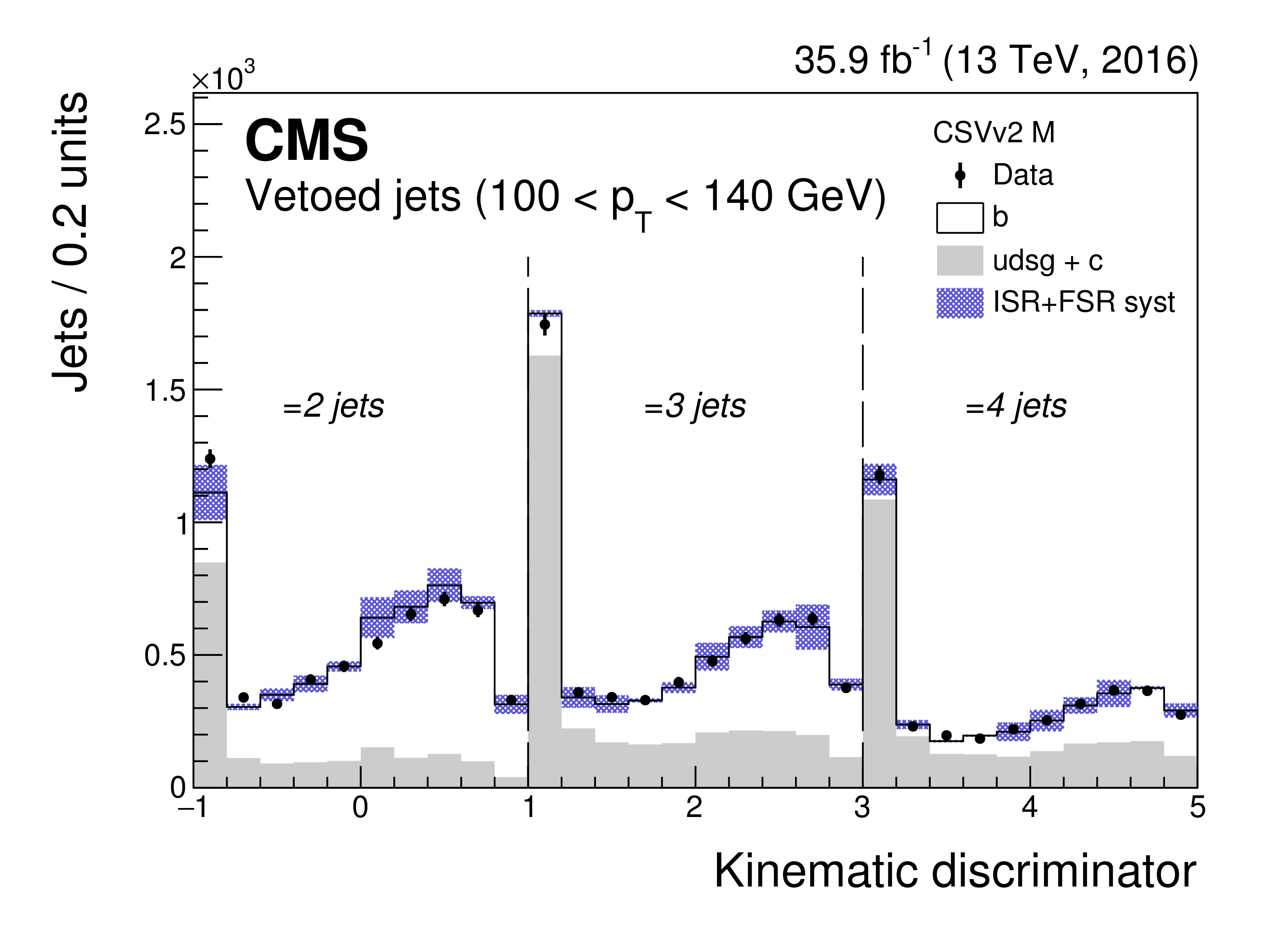
png pdf	Figure 42: Fitted distribution of the kinematic discriminator for jets with 70 $ < {p_{\mathrm {T}}} < $ 100 GeV passing (left) and failing (right) the medium working point of the CSVv2 algorithm. The discriminator distribution is shown in bins of jet multiplicity with the discriminator output transformed from $[-1,1]$ to $[-1,1]+ 2 (N_{\text {jets}}-2)$.
png pdf	Figure 42-a: Fitted distribution of the kinematic discriminator for jets with 70 $ < {p_{\mathrm {T}}} < $ 100 GeV passing the medium working point of the CSVv2 algorithm. The discriminator distribution is shown in bins of jet multiplicity with the discriminator output transformed from $[-1,1]$ to $[-1,1]+ 2 (N_{\text {jets}}-2)$.
png pdf	Figure 42-b: Fitted distribution of the kinematic discriminator for jets with 70 $ < {p_{\mathrm {T}}} < $ 100 GeV failing the medium working point of the CSVv2 algorithm. The discriminator distribution is shown in bins of jet multiplicity with the discriminator output transformed from $[-1,1]$ to $[-1,1]+ 2 (N_{\text {jets}}-2)$.
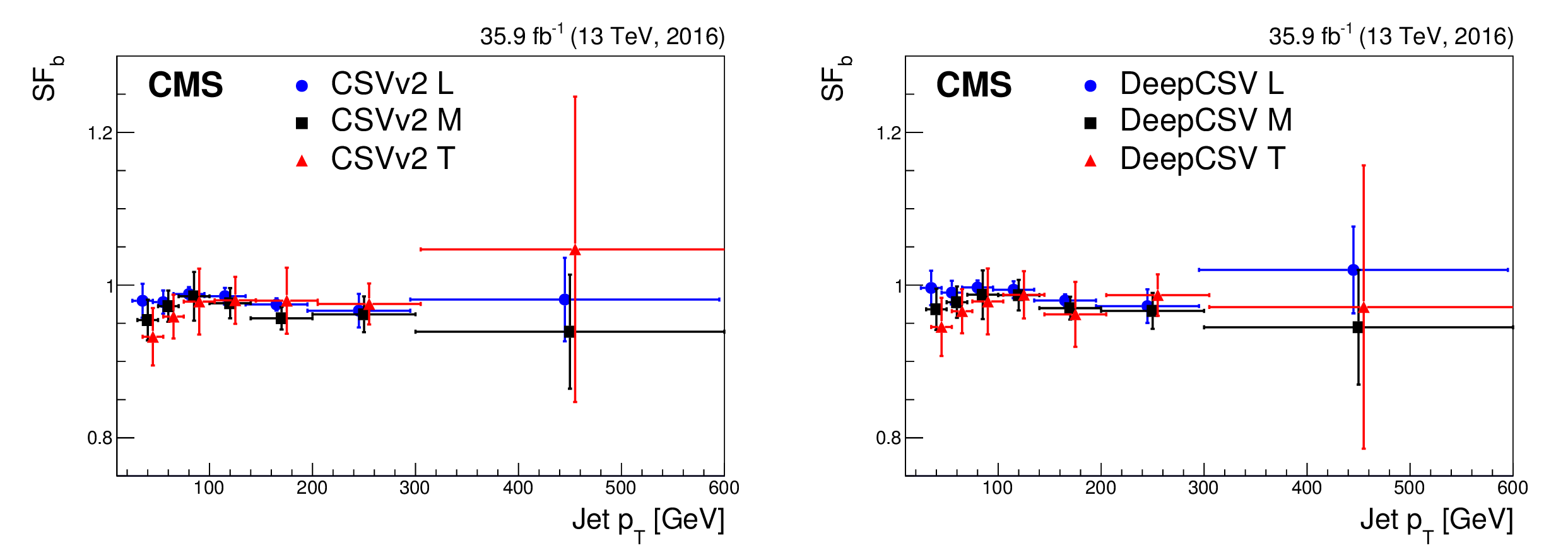
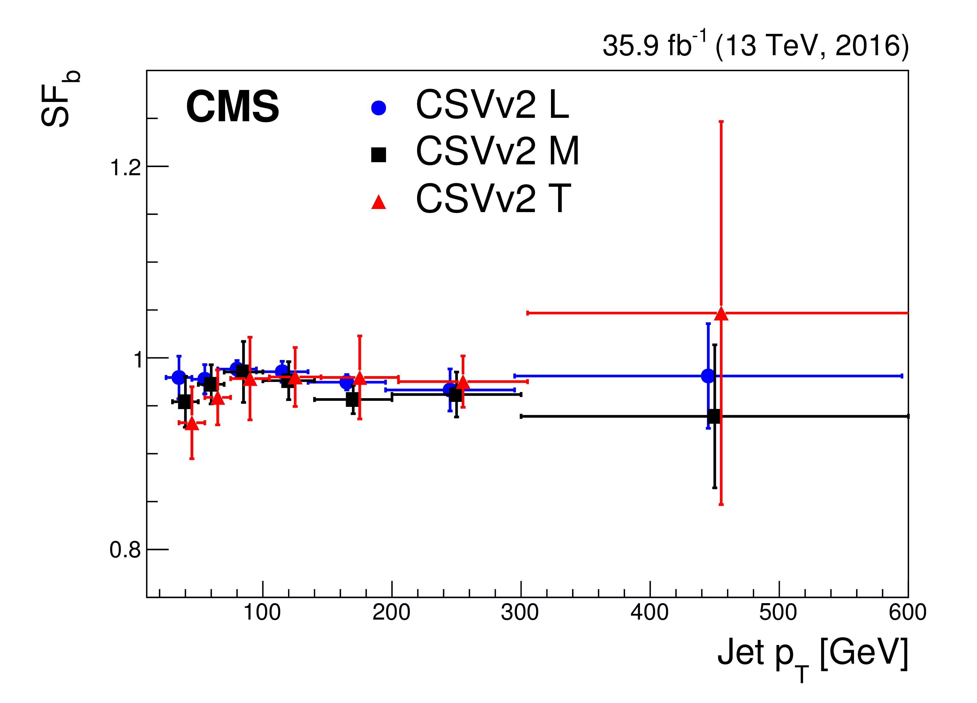
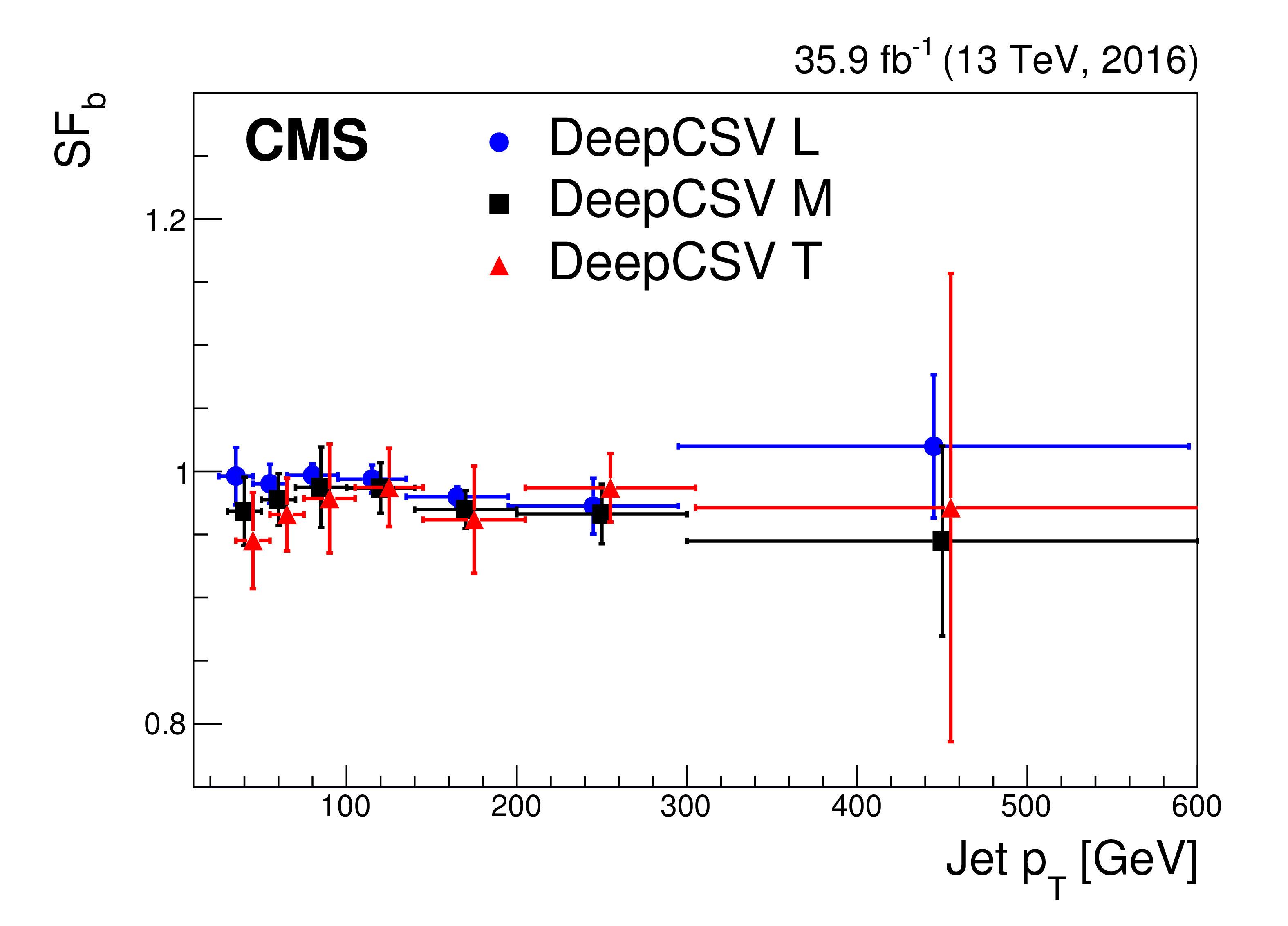
png pdf	Figure 43: Data-to-simulation scale factors for b jets obtained with the Kin method as a function of the jet $ {p_{\mathrm {T}}} $ for the three CSVv2 (left) and the three DeepCSV (right) working points. The uncertainty corresponds to the combined statistical and systematic uncertainty. For clarity, the points for the loose and tight tagging requirement are shifted by $-5$ and $+5$ GeV with respect to the bin centre.
png pdf	Figure 43-a: Data-to-simulation scale factors for b jets obtained with the Kin method as a function of the jet $ {p_{\mathrm {T}}} $ for the three CSVv2 working points. The uncertainty corresponds to the combined statistical and systematic uncertainty. For clarity, the points for the loose and tight tagging requirement are shifted by $-5$ and $+5$ GeV with respect to the bin centre.
png pdf	Figure 43-b: Data-to-simulation scale factors for b jets obtained with the Kin method as a function of the jet $ {p_{\mathrm {T}}} $ for the three DeepCSV working points. The uncertainty corresponds to the combined statistical and systematic uncertainty. For clarity, the points for the loose and tight tagging requirement are shifted by $-5$ and $+5$ GeV with respect to the bin centre.
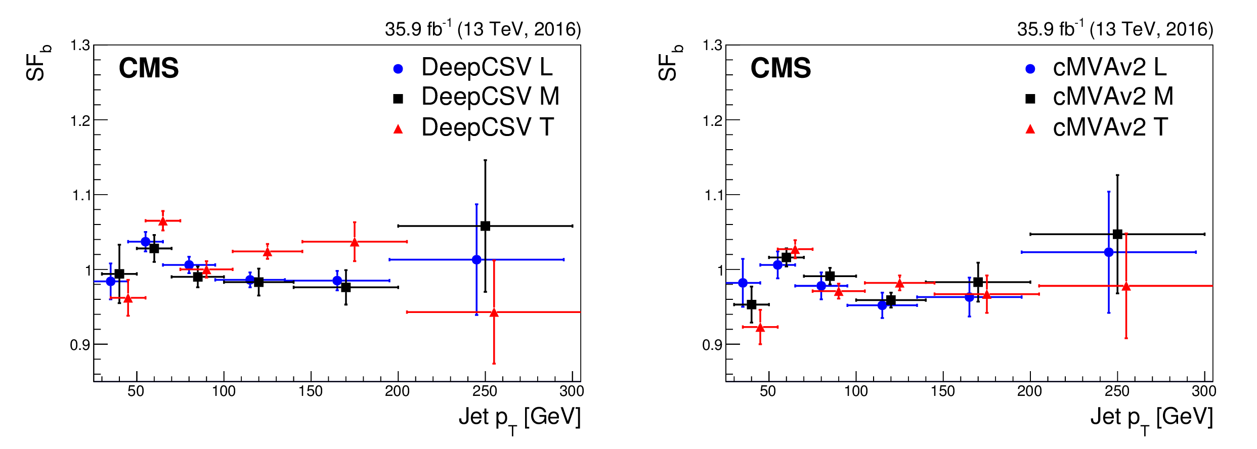
png pdf	Figure 44: Data-to-simulation scale factors for b jets measured with the TagCount method as a function of the jet $ {p_{\mathrm {T}}} $ for the three DeepCSV (left) and cMVAv2 (right) working points. The uncertainty corresponds to the combined statistical and systematic uncertainty. For clarity, the points for the loose and tight tagging requirement are shifted by $-5$ and $+5$ GeV with respect to the bin centre.
png pdf	Figure 44-a: Data-to-simulation scale factors for b jets measured with the TagCount method as a function of the jet $ {p_{\mathrm {T}}} $ for the three DeepCSV working points. The uncertainty corresponds to the combined statistical and systematic uncertainty. For clarity, the points for the loose and tight tagging requirement are shifted by $-5$ and $+5$ GeV with respect to the bin centre.
png pdf	Figure 44-b: Data-to-simulation scale factors for b jets measured with the TagCount method as a function of the jet $ {p_{\mathrm {T}}} $ for the three cMVAv2 working points. The uncertainty corresponds to the combined statistical and systematic uncertainty. For clarity, the points for the loose and tight tagging requirement are shifted by $-5$ and $+5$ GeV with respect to the bin centre.
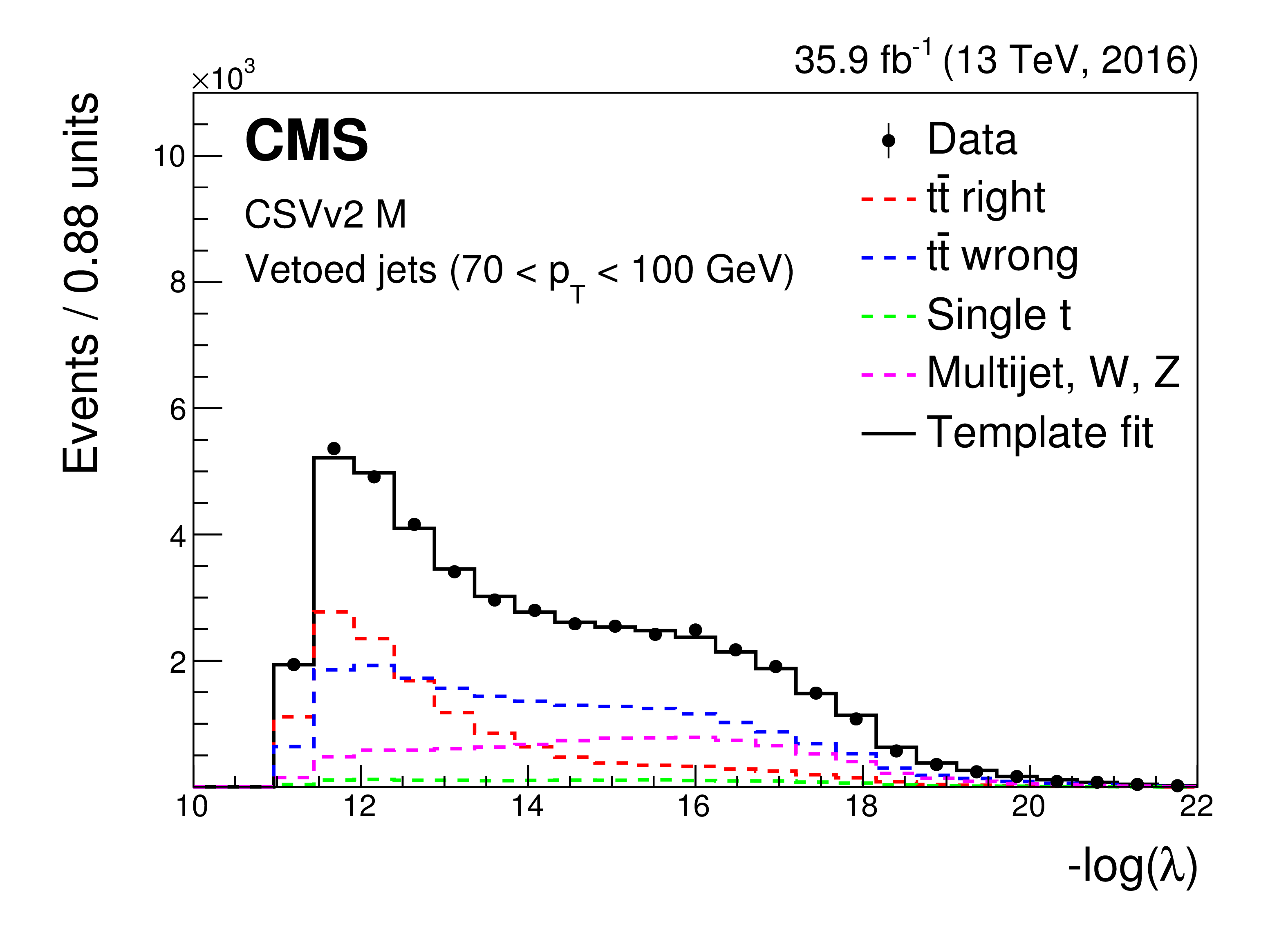
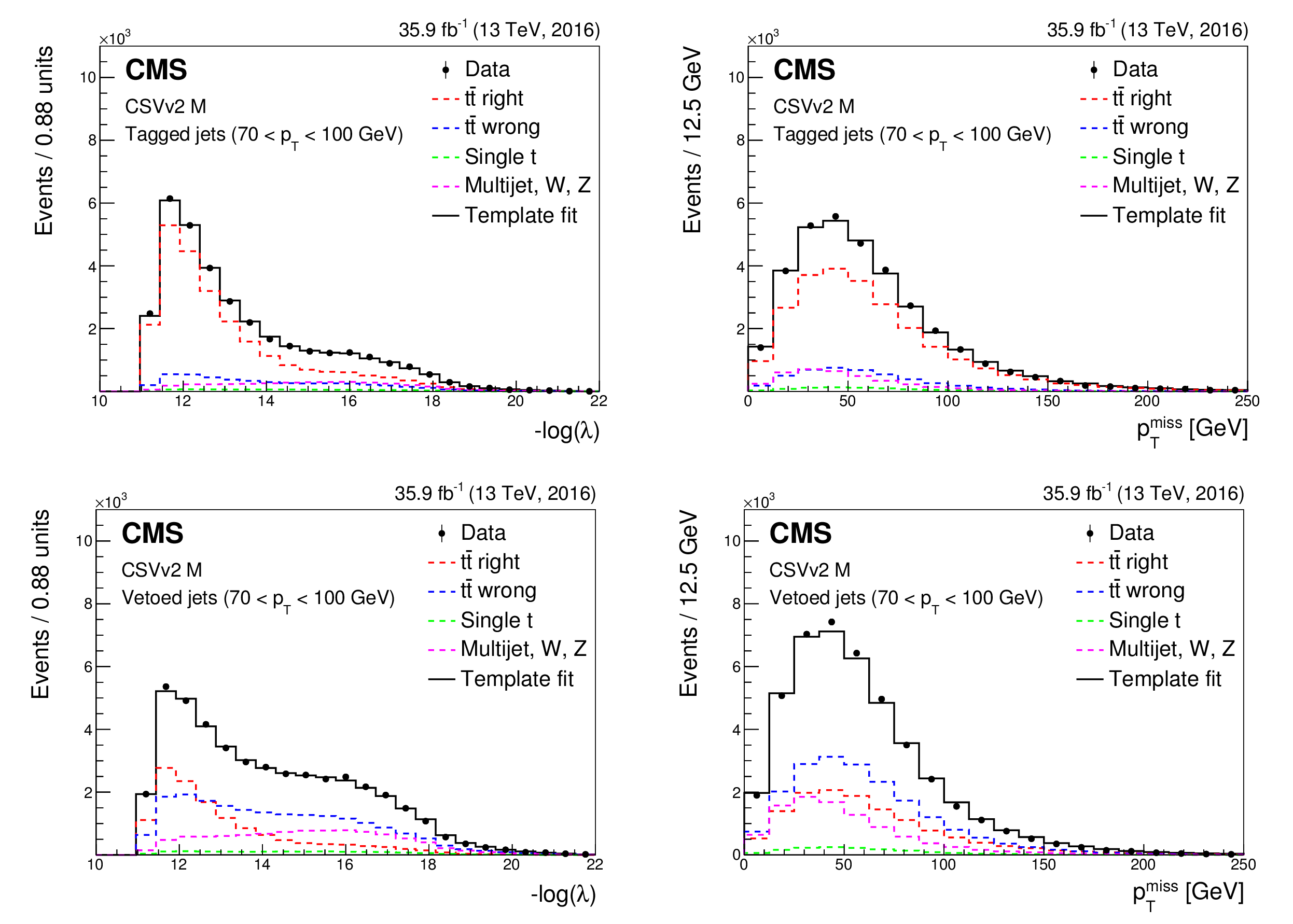
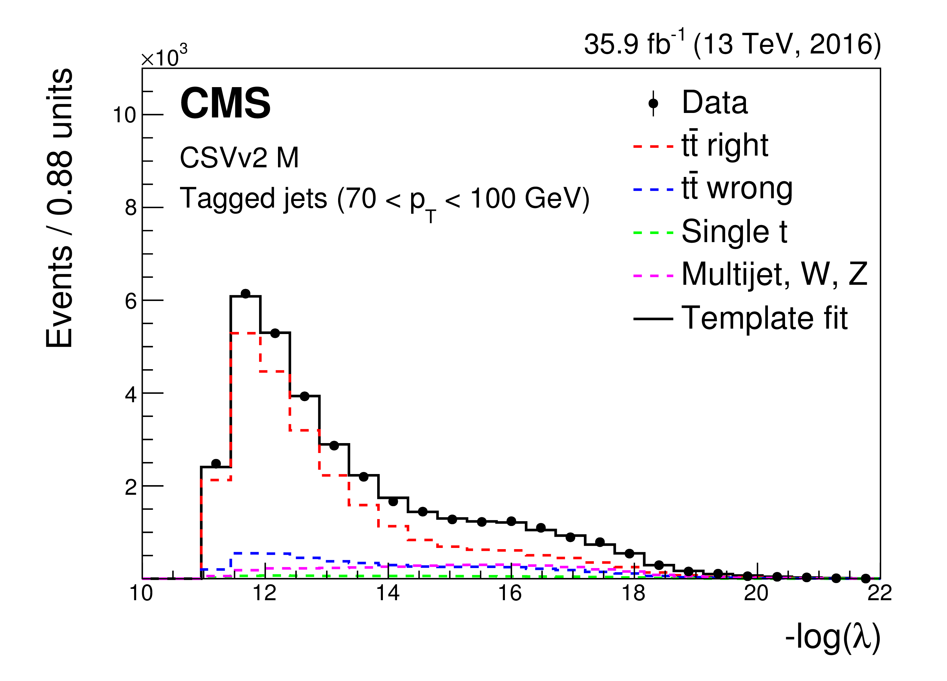
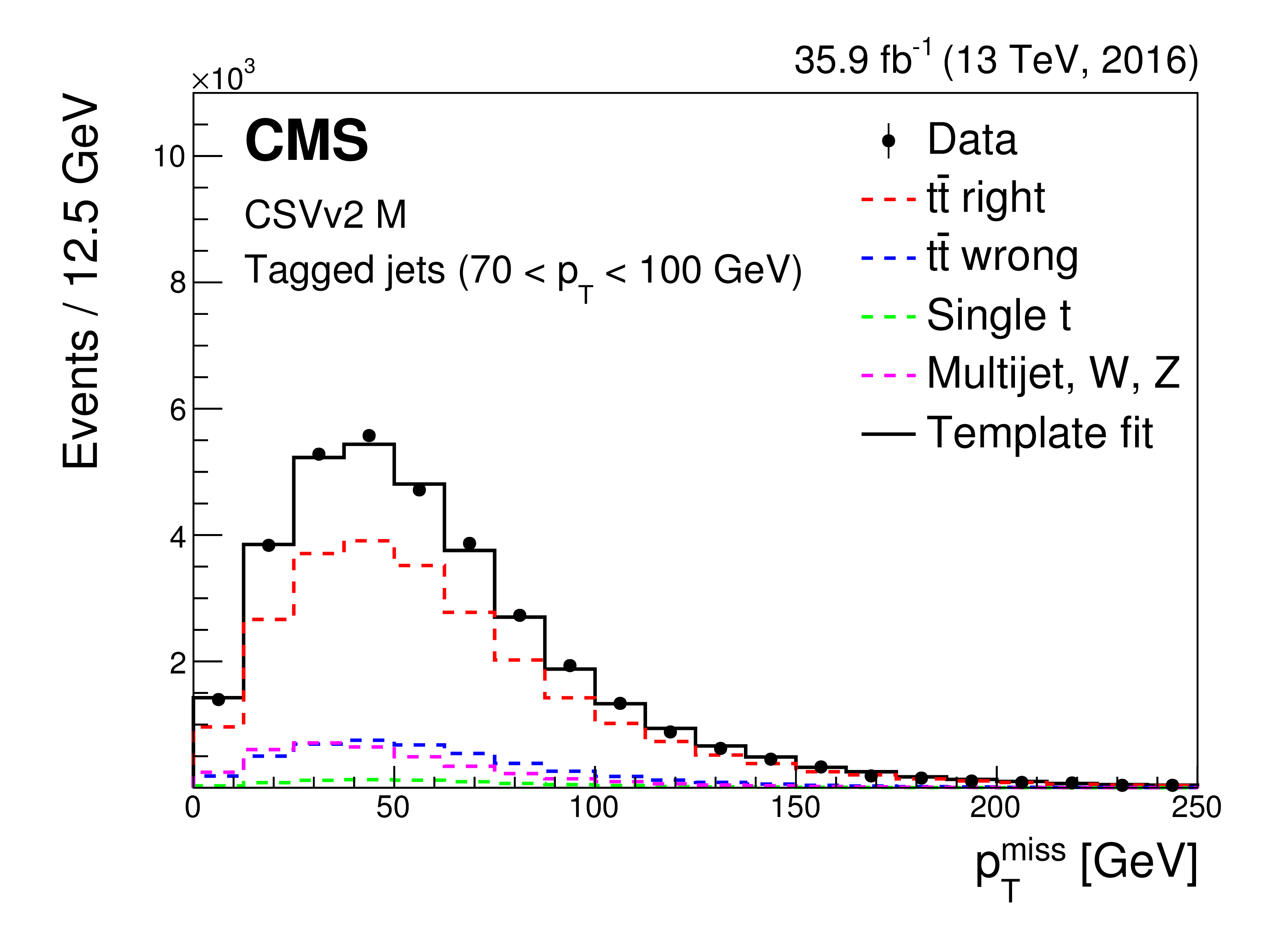
png pdf	Figure 45: Distributions of fitted $-\text {log}(\lambda)$ (left) and ${{{p_{\mathrm {T}}} ^\text {miss}}}$ (right) for jets from the $ {\mathrm {t}\overline {\mathrm {t}}} $ leptonic side with 70 $ < {p_{\mathrm {T}}} < $ 100 GeV passing (upper) and failing (lower) the medium working point of the CSVv2 algorithm.
png pdf	Figure 45-a: Distributions of fitted $-\text {log}(\lambda)$ (left) and ${{{p_{\mathrm {T}}} ^\text {miss}}}$ (right) for jets from the $ {\mathrm {t}\overline {\mathrm {t}}} $ leptonic side with 70 $ < {p_{\mathrm {T}}} < $ 100 GeV passing (upper) and failing (lower) the medium working point of the CSVv2 algorithm.
png pdf	Figure 45-b: Distributions of fitted $-\text {log}(\lambda)$ (left) and ${{{p_{\mathrm {T}}} ^\text {miss}}}$ (right) for jets from the $ {\mathrm {t}\overline {\mathrm {t}}} $ leptonic side with 70 $ < {p_{\mathrm {T}}} < $ 100 GeV passing (upper) and failing (lower) the medium working point of the CSVv2 algorithm.
png pdf	Figure 45-c: Distributions of fitted $-\text {log}(\lambda)$ (left) and ${{{p_{\mathrm {T}}} ^\text {miss}}}$ (right) for jets from the $ {\mathrm {t}\overline {\mathrm {t}}} $ leptonic side with 70 $ < {p_{\mathrm {T}}} < $ 100 GeV passing (upper) and failing (lower) the medium working point of the CSVv2 algorithm.
png pdf	Figure 45-d: Distributions of fitted $-\text {log}(\lambda)$ (left) and ${{{p_{\mathrm {T}}} ^\text {miss}}}$ (right) for jets from the $ {\mathrm {t}\overline {\mathrm {t}}} $ leptonic side with 70 $ < {p_{\mathrm {T}}} < $ 100 GeV passing (upper) and failing (lower) the medium working point of the CSVv2 algorithm.
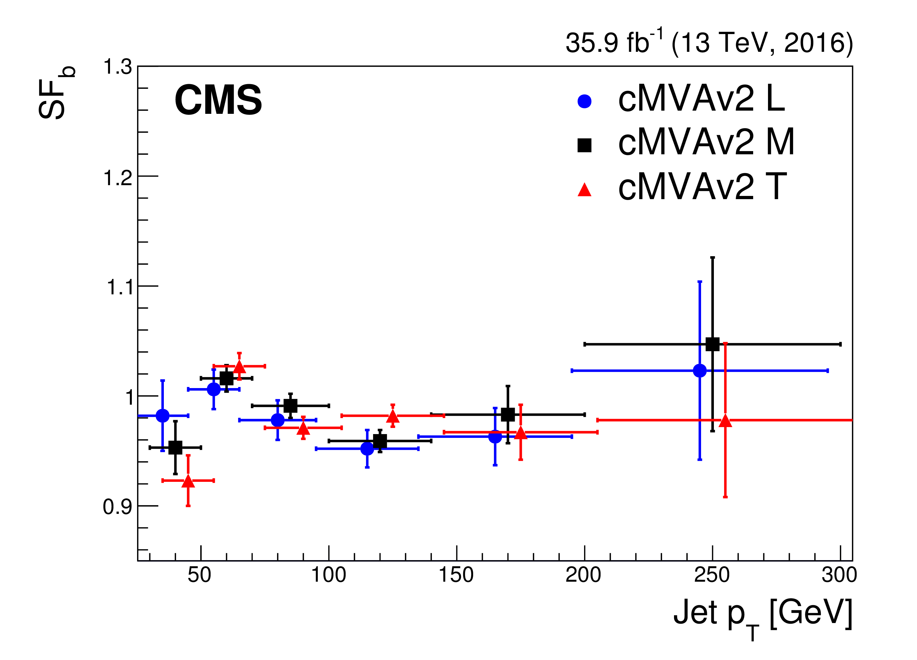
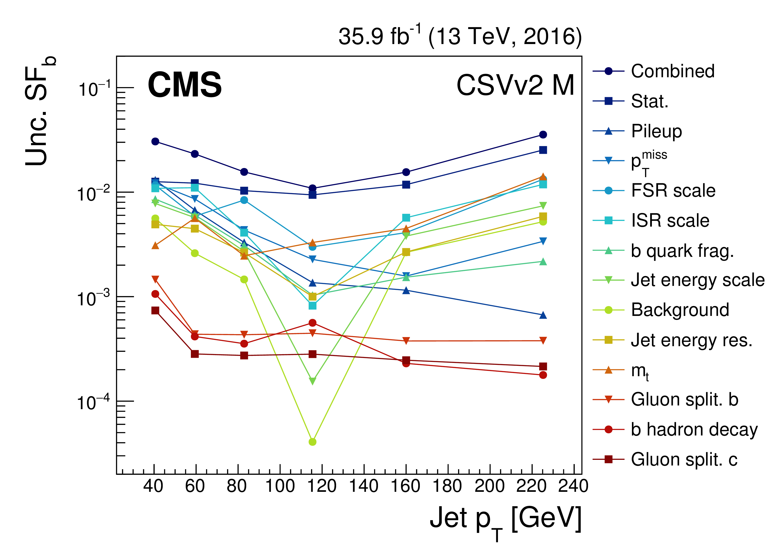
png pdf	Figure 46: Data-to-simulation scale factors for b jets from the hadronic or leptonic side of the single-lepton $ {\mathrm {t}\overline {\mathrm {t}}} $ decay as well as for their combination, as a function of the jet $ {p_{\mathrm {T}}} $ for the medium working of the CSVv2 tagger (left). The error bars represent the combined statistical and systematic uncertainty. Size of the individual uncertainties in the combined scale factors for the CSVv2 medium working point (right).
png pdf	Figure 46-a: Data-to-simulation scale factors for b jets from the hadronic or leptonic side of the single-lepton $ {\mathrm {t}\overline {\mathrm {t}}} $ decay as well as for their combination, as a function of the jet $ {p_{\mathrm {T}}} $ for the medium working of the CSVv2 tagger (left). The error bars represent the combined statistical and systematic uncertainty. Size of the individual uncertainties in the combined scale factors for the CSVv2 medium working point (right).
png pdf	Figure 46-b: Data-to-simulation scale factors for b jets from the hadronic or leptonic side of the single-lepton $ {\mathrm {t}\overline {\mathrm {t}}} $ decay as well as for their combination, as a function of the jet $ {p_{\mathrm {T}}} $ for the medium working of the CSVv2 tagger (left). The error bars represent the combined statistical and systematic uncertainty. Size of the individual uncertainties in the combined scale factors for the CSVv2 medium working point (right).
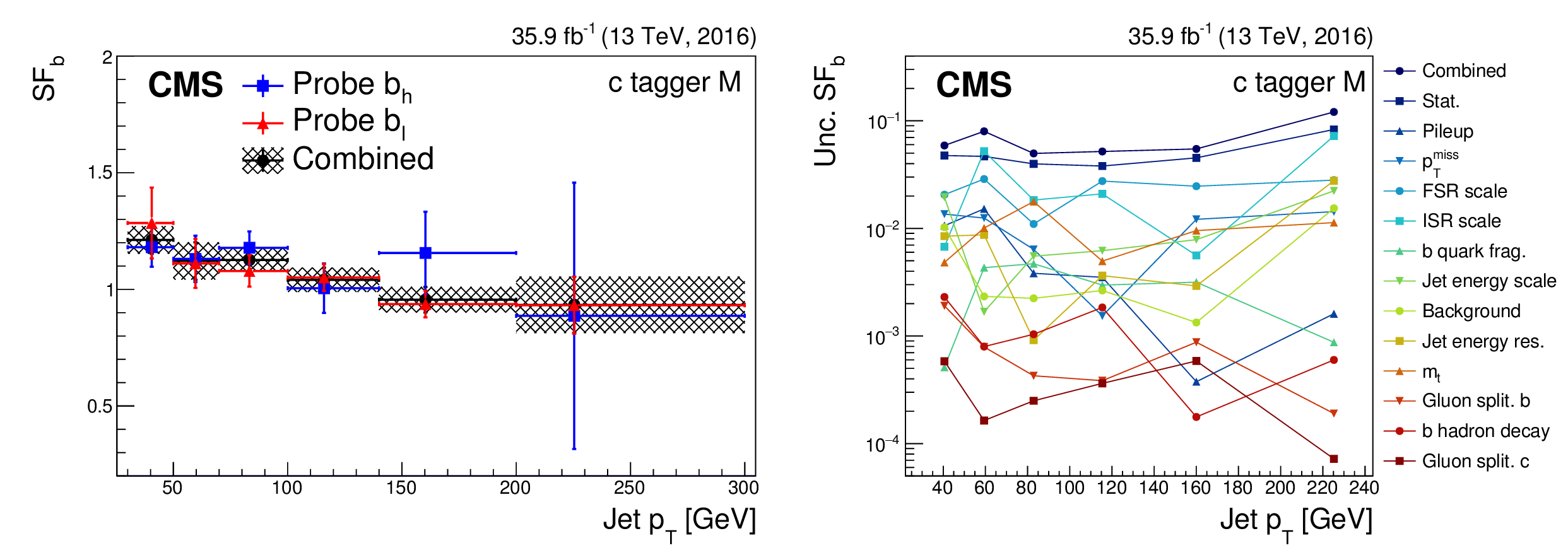
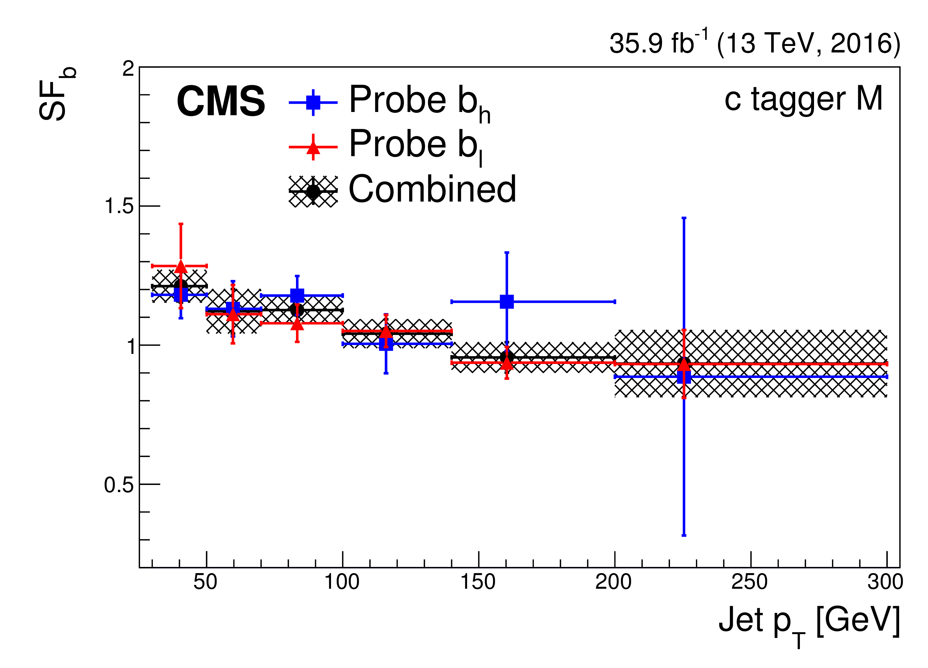
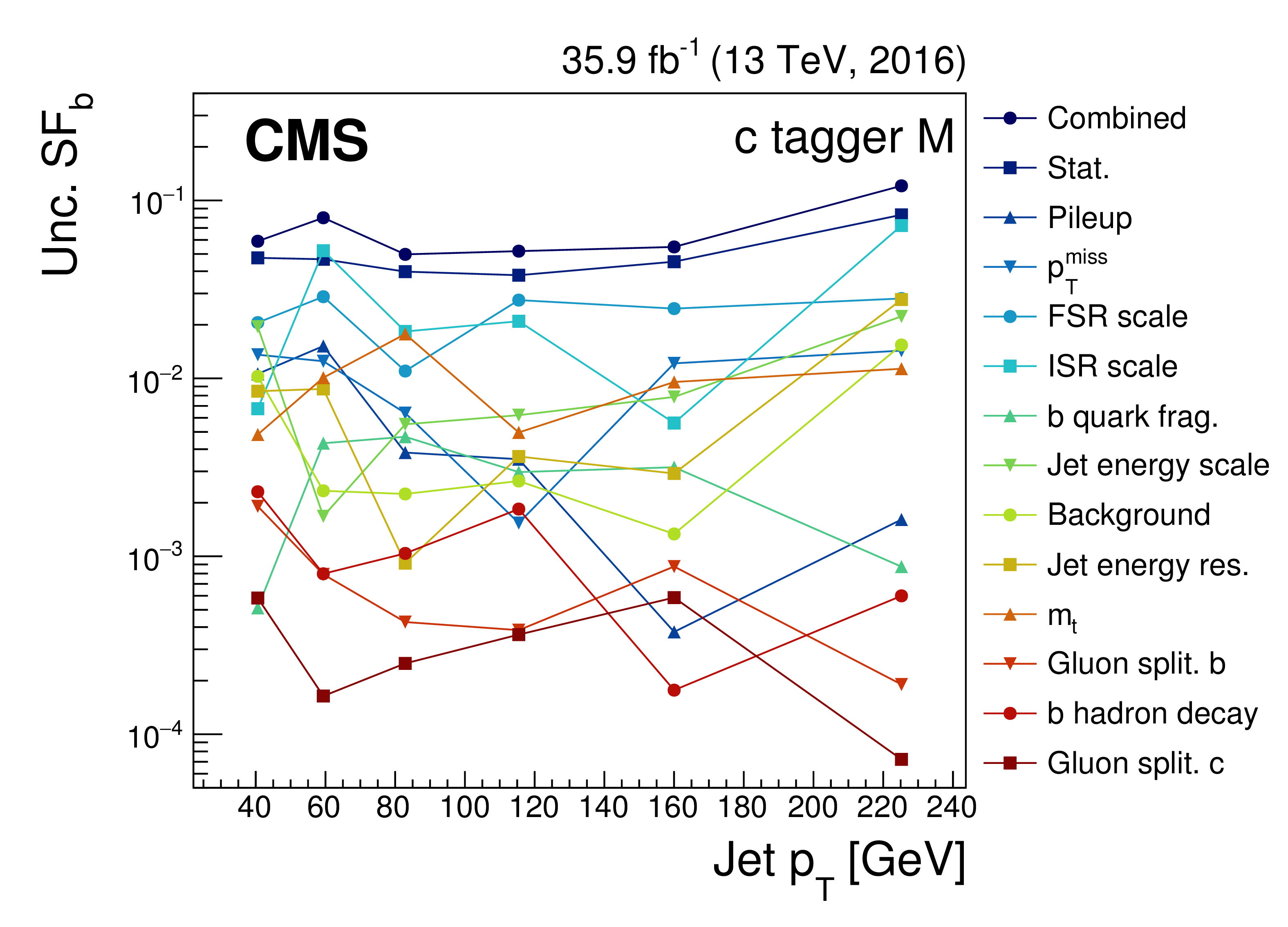
png pdf	Figure 47: Data-to-simulation scale factors for b jets from the hadronic or leptonic side of the single-lepton $ {\mathrm {t}\overline {\mathrm {t}}} $ decay as well as for their combination, as a function of the jet $ {p_{\mathrm {T}}} $ for the medium working of the c tagger (left). The error bars represent the combined statistical and systematic uncertainty. Size of the individual uncertainties in the combined scale factors for the CSVv2 medium working point (right).
png pdf	Figure 47-a: Data-to-simulation scale factors for b jets from the hadronic or leptonic side of the single-lepton $ {\mathrm {t}\overline {\mathrm {t}}} $ decay as well as for their combination, as a function of the jet $ {p_{\mathrm {T}}} $ for the medium working of the c tagger (left). The error bars represent the combined statistical and systematic uncertainty. Size of the individual uncertainties in the combined scale factors for the CSVv2 medium working point (right).
png pdf	Figure 47-b: Data-to-simulation scale factors for b jets from the hadronic or leptonic side of the single-lepton $ {\mathrm {t}\overline {\mathrm {t}}} $ decay as well as for their combination, as a function of the jet $ {p_{\mathrm {T}}} $ for the medium working of the c tagger (left). The error bars represent the combined statistical and systematic uncertainty. Size of the individual uncertainties in the combined scale factors for the CSVv2 medium working point (right).
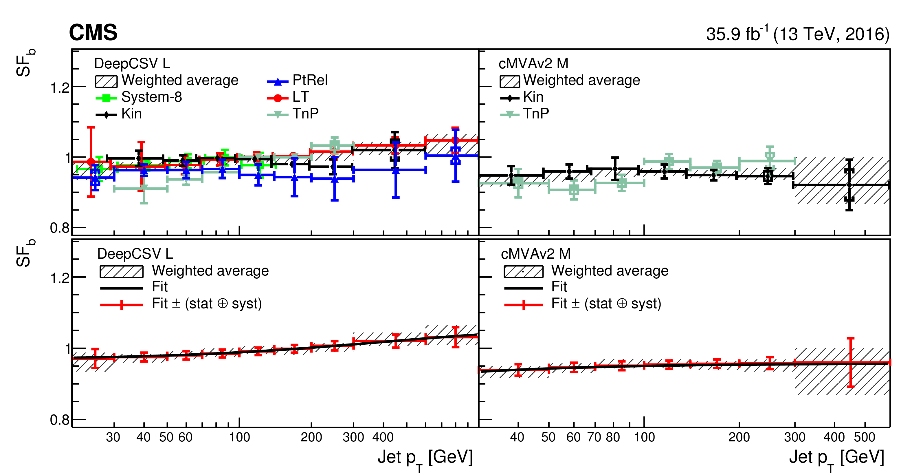
png pdf	Figure 48: Data-to-simulation scale factors for b jets as a function of jet $ {p_{\mathrm {T}}} $ for the loose DeepCSV (left) and the medium cMVAv2 (right) algorithms working points. The upper panels show the scale factors for tagging b as function of jet $ {p_{\mathrm {T}}} $ measured with the various methods. The inner error bars represent the statistical uncertainty, and the outer error bars the combined statistical and systematic uncertainty. The combined scale factors with their overall uncertainty are displayed as a hatched area. The lower panels show the same combined scale factors with the result of a fit function (solid curve) superimposed. The combined scale factors with the overall uncertainty are centred around the fit result. To increase the visibility of the individual measurements, the scale factors obtained with various methods are slightly displaced with respect to the bin centre for which the measurement was performed. The last bin includes the overflow entries.
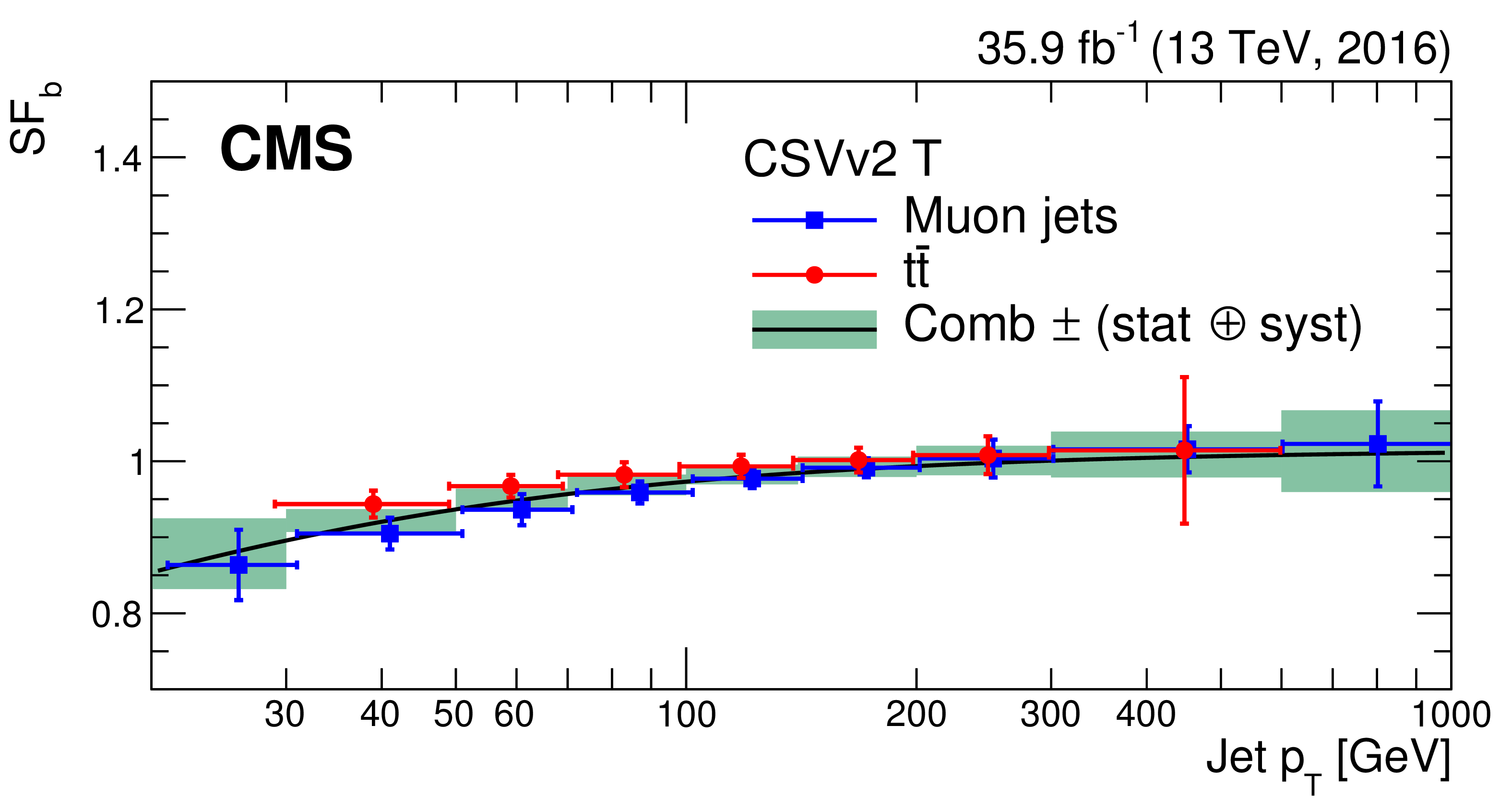
png pdf	Figure 49: Data-to-simulation scale factors for b jets as a function of jet $ {p_{\mathrm {T}}} $ measured in muon-enriched multijet and $ {\mathrm {t}\overline {\mathrm {t}}} $ events for the tight working point of the CSVv2 tagger. The green area shows the combined scale factors with their overall uncertainty, including an additional 1% uncertainty to cover any residual sample dependence, fitted to the superimposed solid curve. For visibility purposes, the scale factors are slightly displaced with respect to the bin centre for which the measurement was performed. The last bin includes the overflow entries.
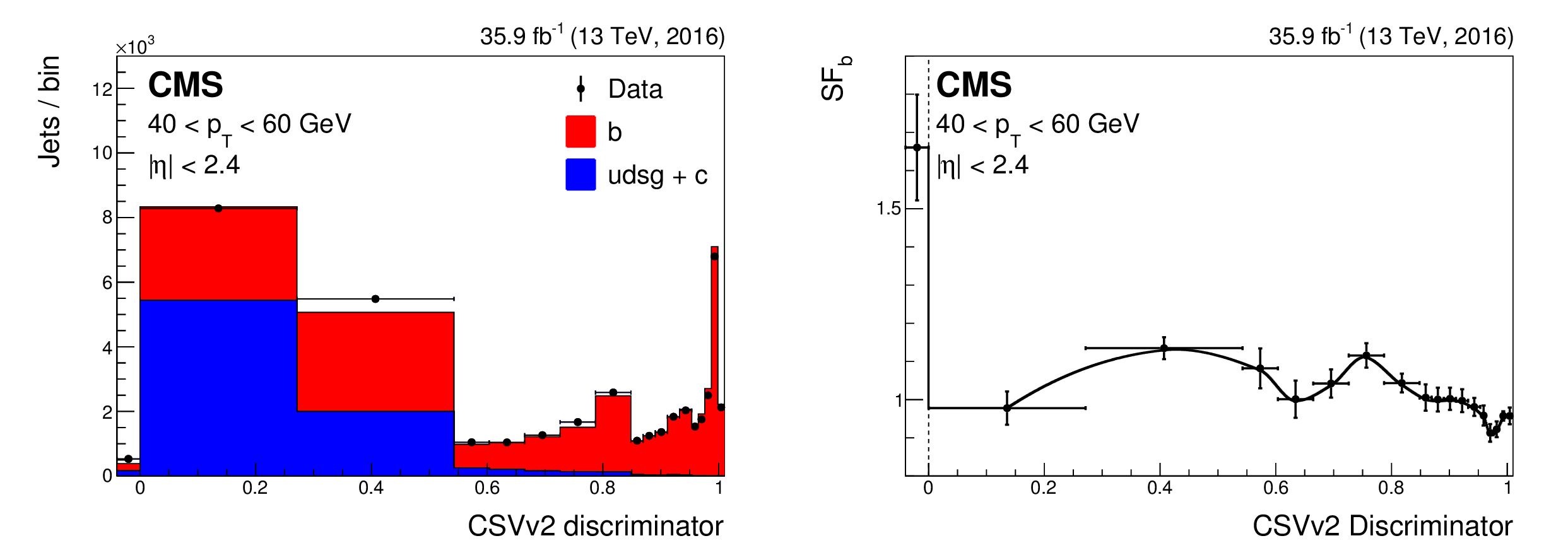
png pdf	Figure 50: Distribution of the CSVv2 discriminator values for jets with 40 $ < {p_{\mathrm {T}}} < $ 60 GeV before the data-to-simulation scale factors are applied in the $ {\mathrm {t}\overline {\mathrm {t}}} $ dilepton sample (left). The simulation is normalized to the number of entries in data. Measured scale factors for b jets as a function of the CSVv2 discriminator value (right). The line is an interpolation between the scale factors measured in each bin of the CSVv2 discriminator distribution. The bin below 0 contains the jets with a default discriminator value.
png pdf	Figure 50-a: Distribution of the CSVv2 discriminator values for jets with 40 $ < {p_{\mathrm {T}}} < $ 60 GeV before the data-to-simulation scale factors are applied in the $ {\mathrm {t}\overline {\mathrm {t}}} $ dilepton sample (left). The simulation is normalized to the number of entries in data. Measured scale factors for b jets as a function of the CSVv2 discriminator value (right). The line is an interpolation between the scale factors measured in each bin of the CSVv2 discriminator distribution. The bin below 0 contains the jets with a default discriminator value.
png pdf	Figure 50-b: Distribution of the CSVv2 discriminator values for jets with 40 $ < {p_{\mathrm {T}}} < $ 60 GeV before the data-to-simulation scale factors are applied in the $ {\mathrm {t}\overline {\mathrm {t}}} $ dilepton sample (left). The simulation is normalized to the number of entries in data. Measured scale factors for b jets as a function of the CSVv2 discriminator value (right). The line is an interpolation between the scale factors measured in each bin of the CSVv2 discriminator distribution. The bin below 0 contains the jets with a default discriminator value.
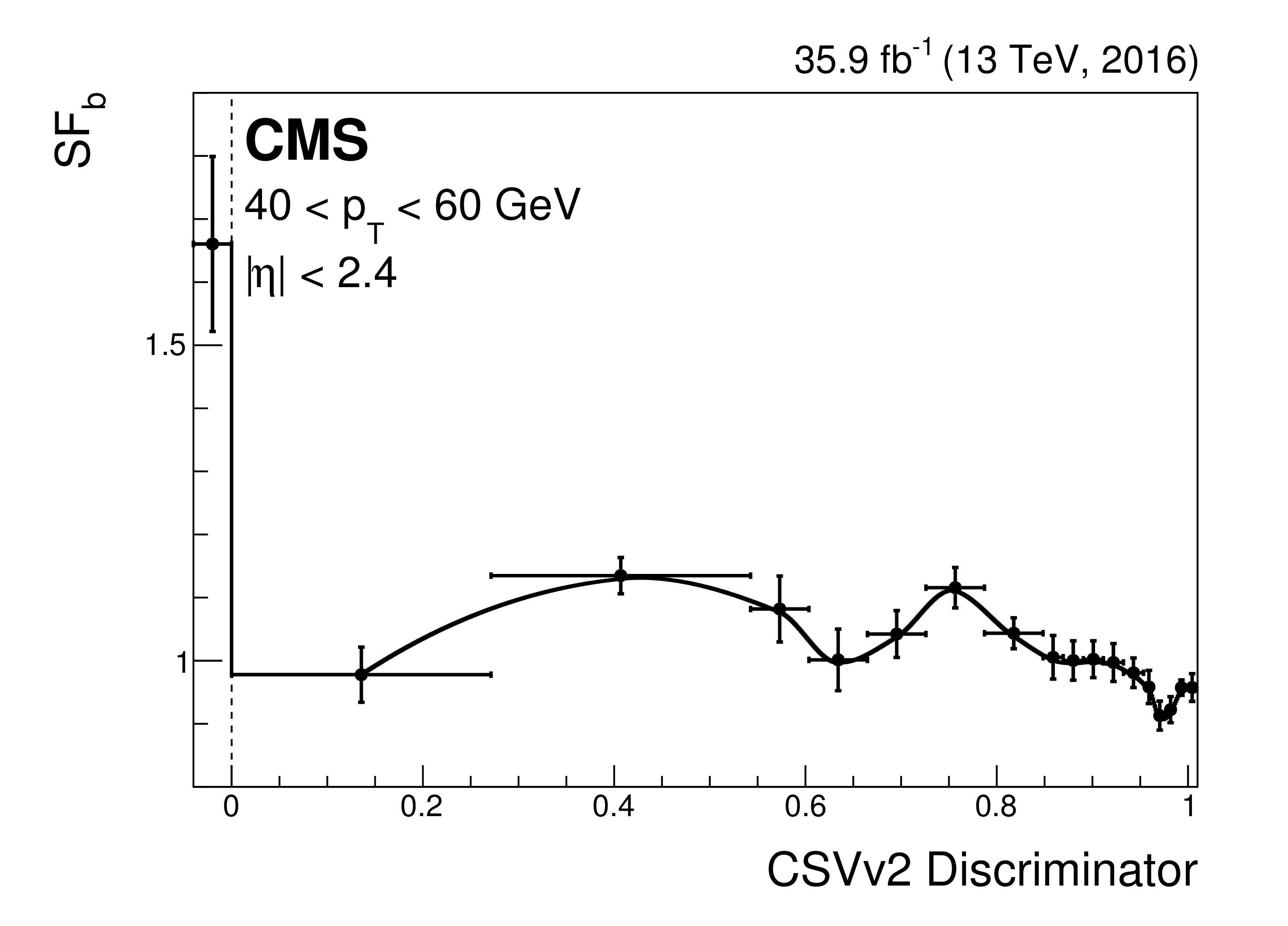
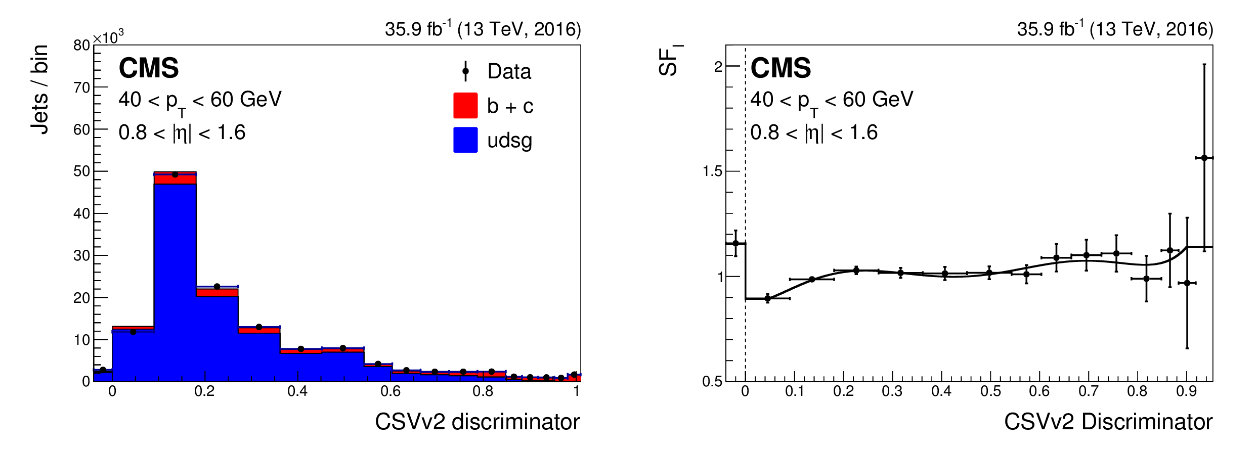
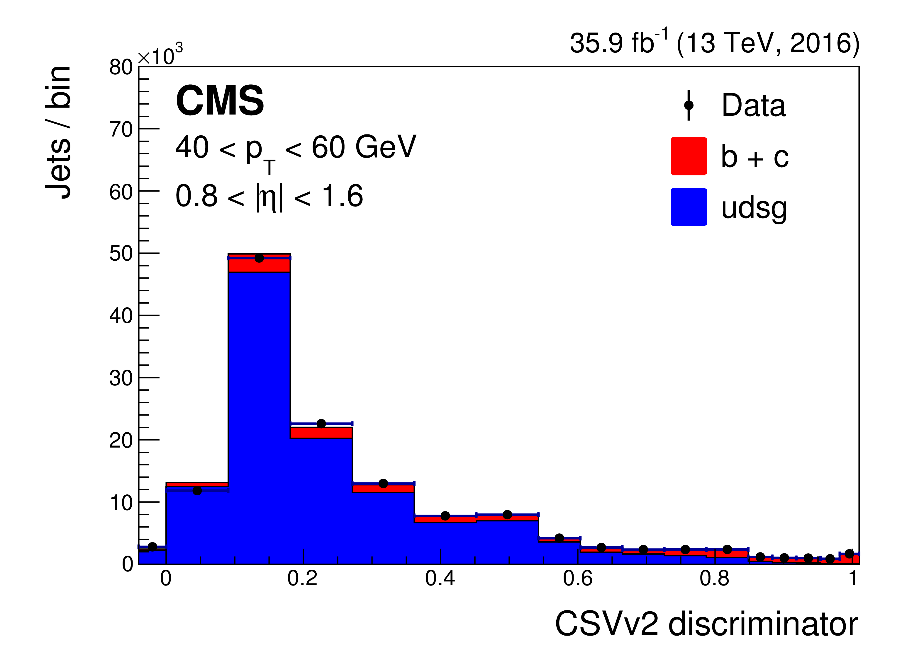
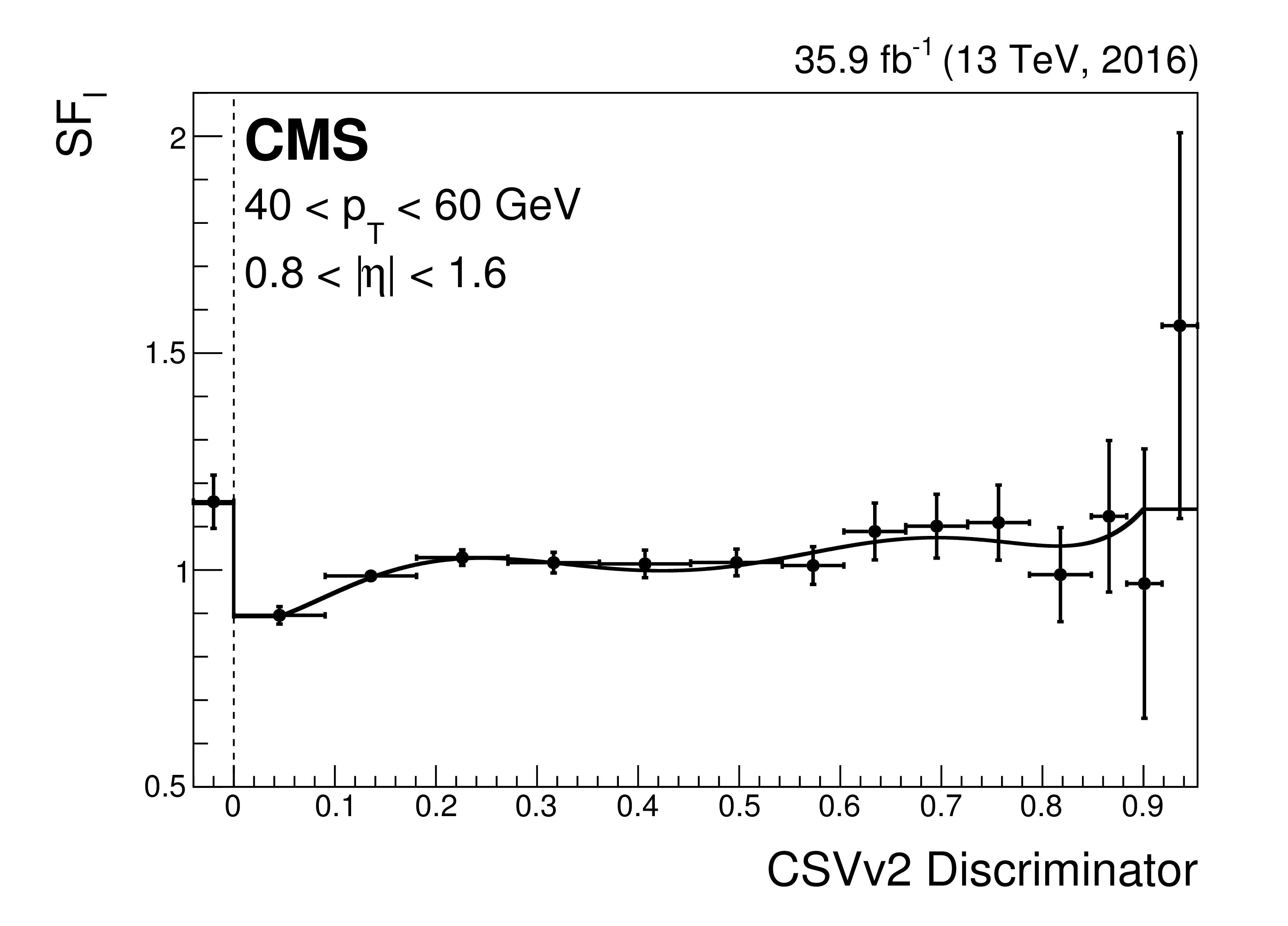
png pdf	Figure 51: Distribution of the CSVv2 discriminator values for jets with 40 $ < {p_{\mathrm {T}}} < $ 60 GeV and 0.8 $ < { \| \eta \|} < 1.6$ before the data-to-simulation scale factors are applied in the Z+jets sample (left). The simulation is normalized to the number of entries for data. Measured scale factors for light-flavour jets as a function of the CSVv2 discriminator value (right). The line represents a polynomial fit to the scale factors measured in each bin of the CSVv2 discriminator distribution. The bin below 0 contains the jets with a default discriminator value.
png pdf	Figure 51-a: Distribution of the CSVv2 discriminator values for jets with 40 $ < {p_{\mathrm {T}}} < $ 60 GeV and 0.8 $ < { \| \eta \|} < 1.6$ before the data-to-simulation scale factors are applied in the Z+jets sample (left). The simulation is normalized to the number of entries for data. Measured scale factors for light-flavour jets as a function of the CSVv2 discriminator value (right). The line represents a polynomial fit to the scale factors measured in each bin of the CSVv2 discriminator distribution. The bin below 0 contains the jets with a default discriminator value.
png pdf	Figure 51-b: Distribution of the CSVv2 discriminator values for jets with 40 $ < {p_{\mathrm {T}}} < $ 60 GeV and 0.8 $ < { \| \eta \|} < 1.6$ before the data-to-simulation scale factors are applied in the Z+jets sample (left). The simulation is normalized to the number of entries for data. Measured scale factors for light-flavour jets as a function of the CSVv2 discriminator value (right). The line represents a polynomial fit to the scale factors measured in each bin of the CSVv2 discriminator distribution. The bin below 0 contains the jets with a default discriminator value.
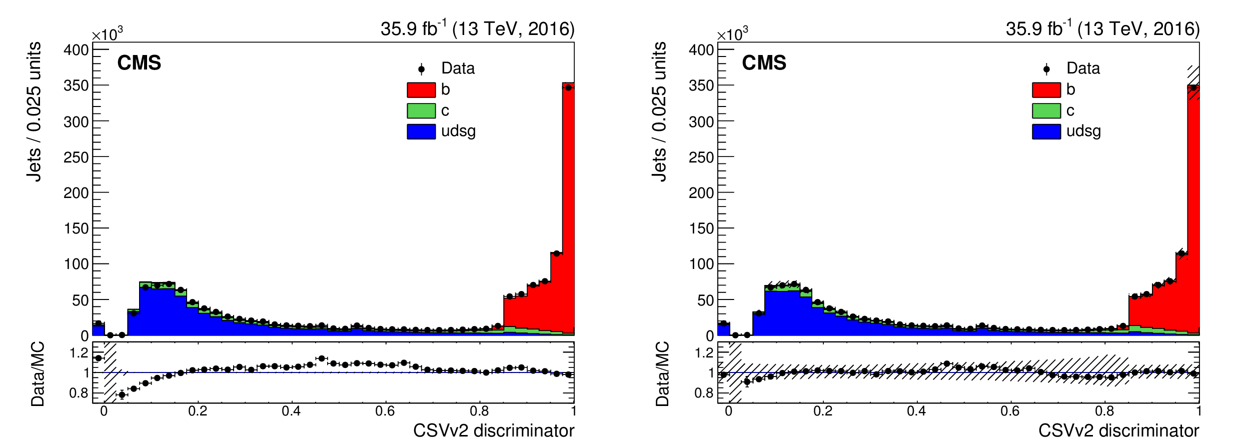
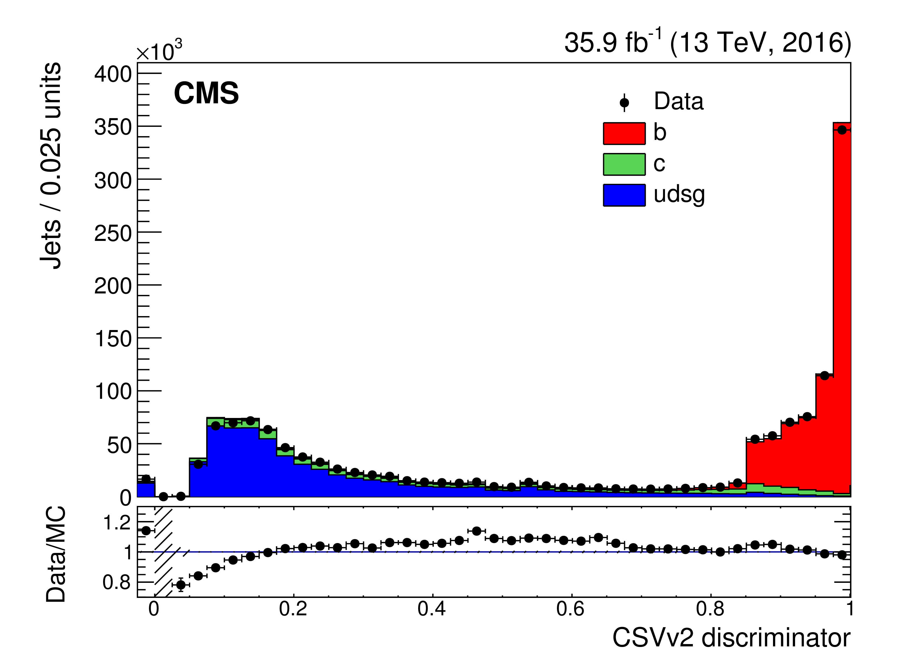
png pdf	Figure 52: Distribution of the CSVv2 discriminator values for the single-lepton $ {\mathrm {t}\overline {\mathrm {t}}} $ sample. Exactly four jets are required, two of which passing the medium working point of the CSVv2 algorithm. The values of the discriminator are shown before (left) and after (right) applying the data-to-simulation scale factors derived with the IterativeFit method. The hatched band around the ratios shows the statistical uncertainty (left), and the total uncertainty (right) in the measured scale factors. The simulation is normalized to the total number of data events. The bin below 0 contains the jets with a default discriminator value.
png pdf	Figure 52-a: Distribution of the CSVv2 discriminator values for the single-lepton $ {\mathrm {t}\overline {\mathrm {t}}} $ sample. Exactly four jets are required, two of which passing the medium working point of the CSVv2 algorithm. The values of the discriminator are shown before (left) and after (right) applying the data-to-simulation scale factors derived with the IterativeFit method. The hatched band around the ratios shows the statistical uncertainty (left), and the total uncertainty (right) in the measured scale factors. The simulation is normalized to the total number of data events. The bin below 0 contains the jets with a default discriminator value.
png pdf	Figure 52-b: Distribution of the CSVv2 discriminator values for the single-lepton $ {\mathrm {t}\overline {\mathrm {t}}} $ sample. Exactly four jets are required, two of which passing the medium working point of the CSVv2 algorithm. The values of the discriminator are shown before (left) and after (right) applying the data-to-simulation scale factors derived with the IterativeFit method. The hatched band around the ratios shows the statistical uncertainty (left), and the total uncertainty (right) in the measured scale factors. The simulation is normalized to the total number of data events. The bin below 0 contains the jets with a default discriminator value.
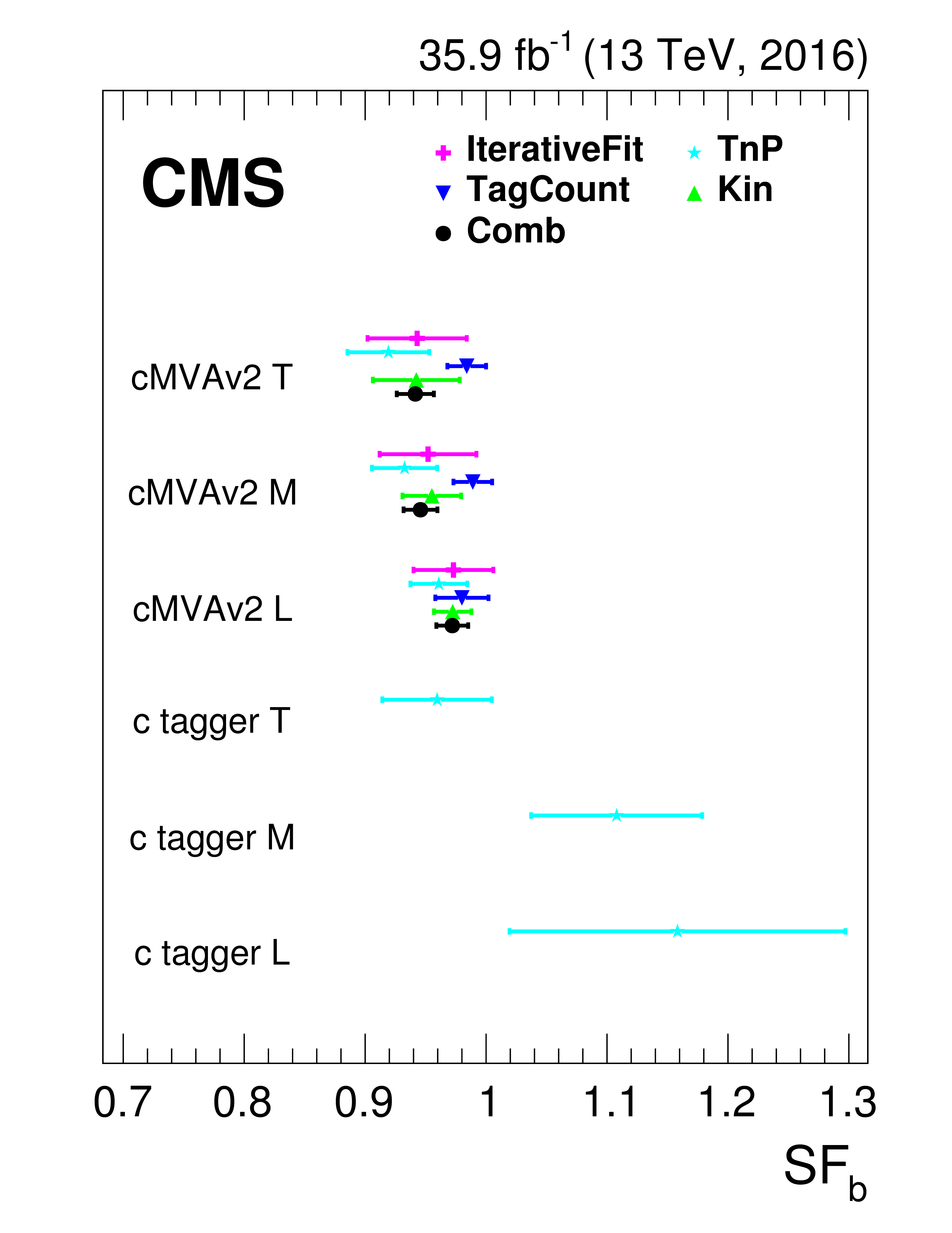
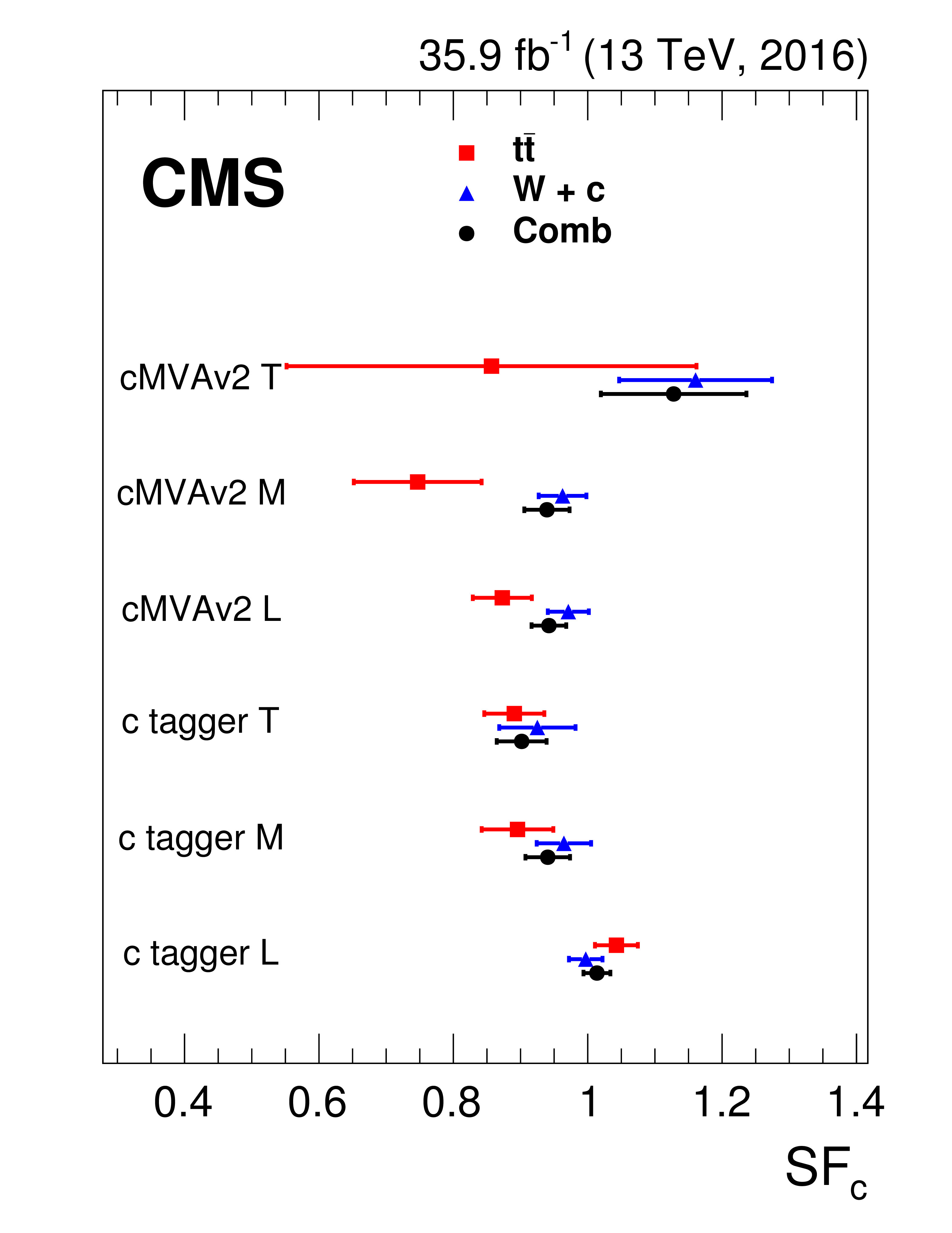
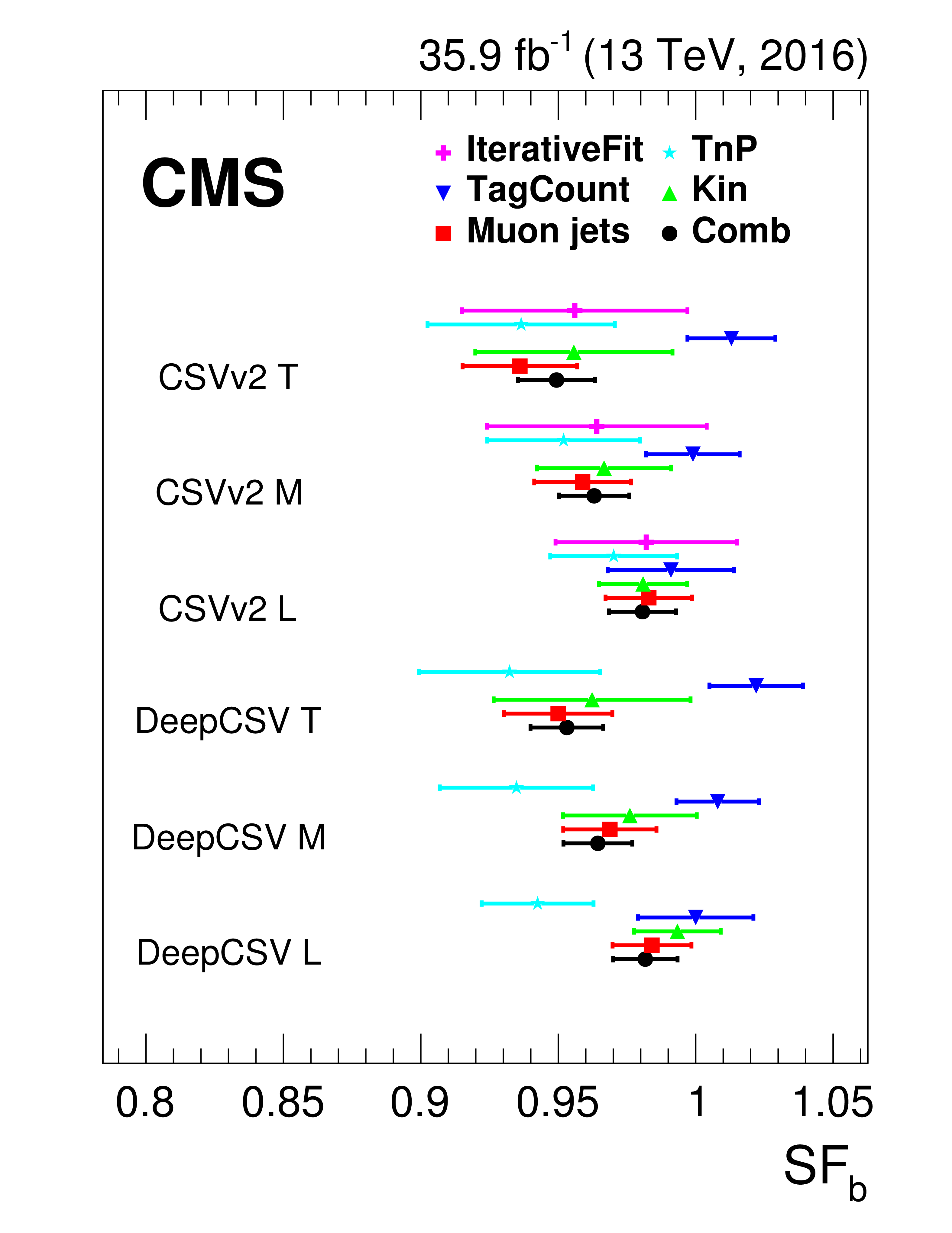
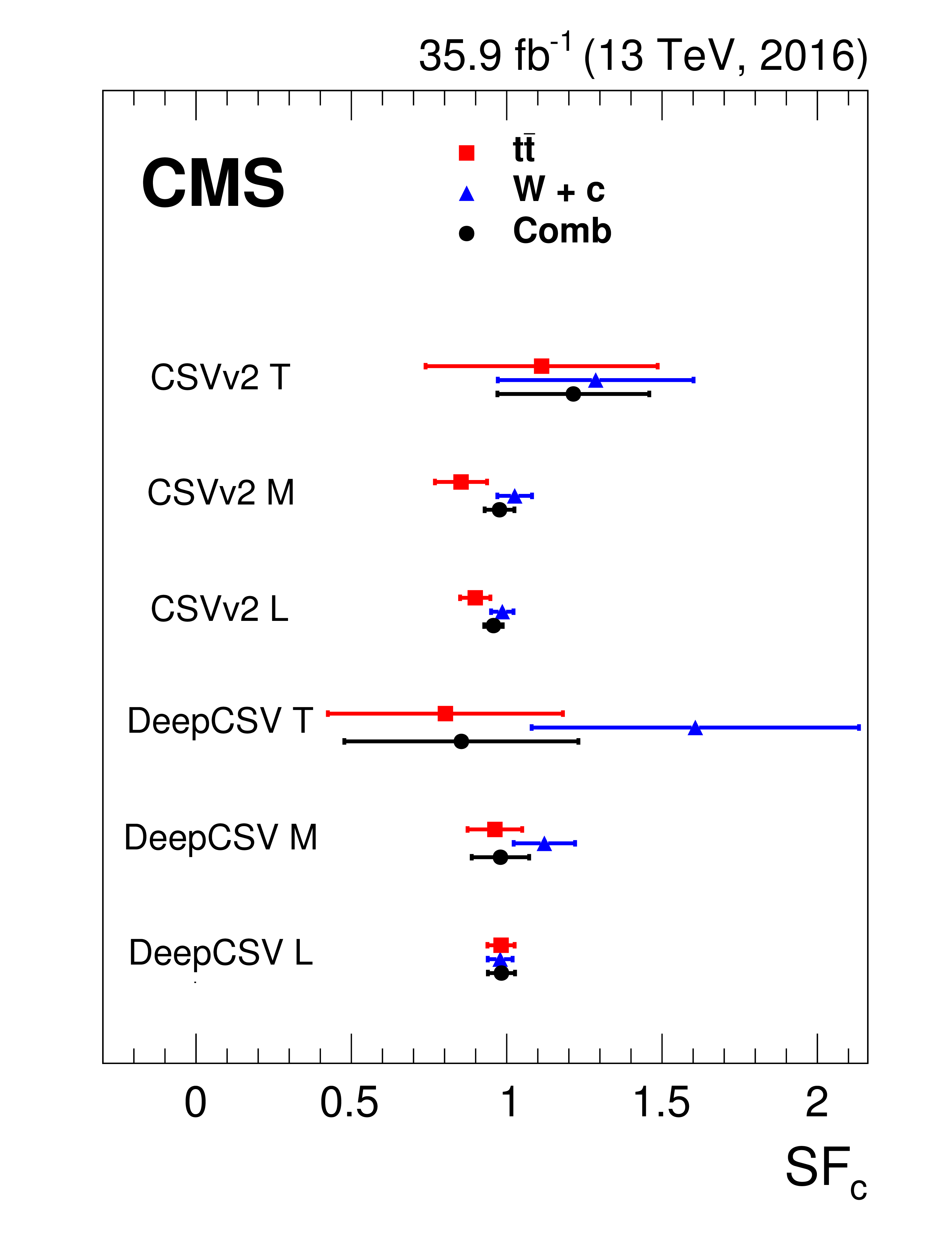
png pdf	Figure 53: Comparison of the data-to-simulation scale factors derived with various methods and their combination, for b (left) and c (right) jets. The scale factors measured with the different methods agree within their uncertainties. For the left panels, the combination includes all measurements with the exception of the IterativeFit and the TagCount methods.
png pdf	Figure 53-a: Comparison of the data-to-simulation scale factors derived with various methods and their combination, for b (left) and c (right) jets. The scale factors measured with the different methods agree within their uncertainties. For the left panels, the combination includes all measurements with the exception of the IterativeFit and the TagCount methods.
png pdf	Figure 53-b: Comparison of the data-to-simulation scale factors derived with various methods and their combination, for b (left) and c (right) jets. The scale factors measured with the different methods agree within their uncertainties. For the left panels, the combination includes all measurements with the exception of the IterativeFit and the TagCount methods.
png pdf	Figure 53-c: Comparison of the data-to-simulation scale factors derived with various methods and their combination, for b (left) and c (right) jets. The scale factors measured with the different methods agree within their uncertainties. For the left panels, the combination includes all measurements with the exception of the IterativeFit and the TagCount methods.
png pdf	Figure 53-d: Comparison of the data-to-simulation scale factors derived with various methods and their combination, for b (left) and c (right) jets. The scale factors measured with the different methods agree within their uncertainties. For the left panels, the combination includes all measurements with the exception of the IterativeFit and the TagCount methods.
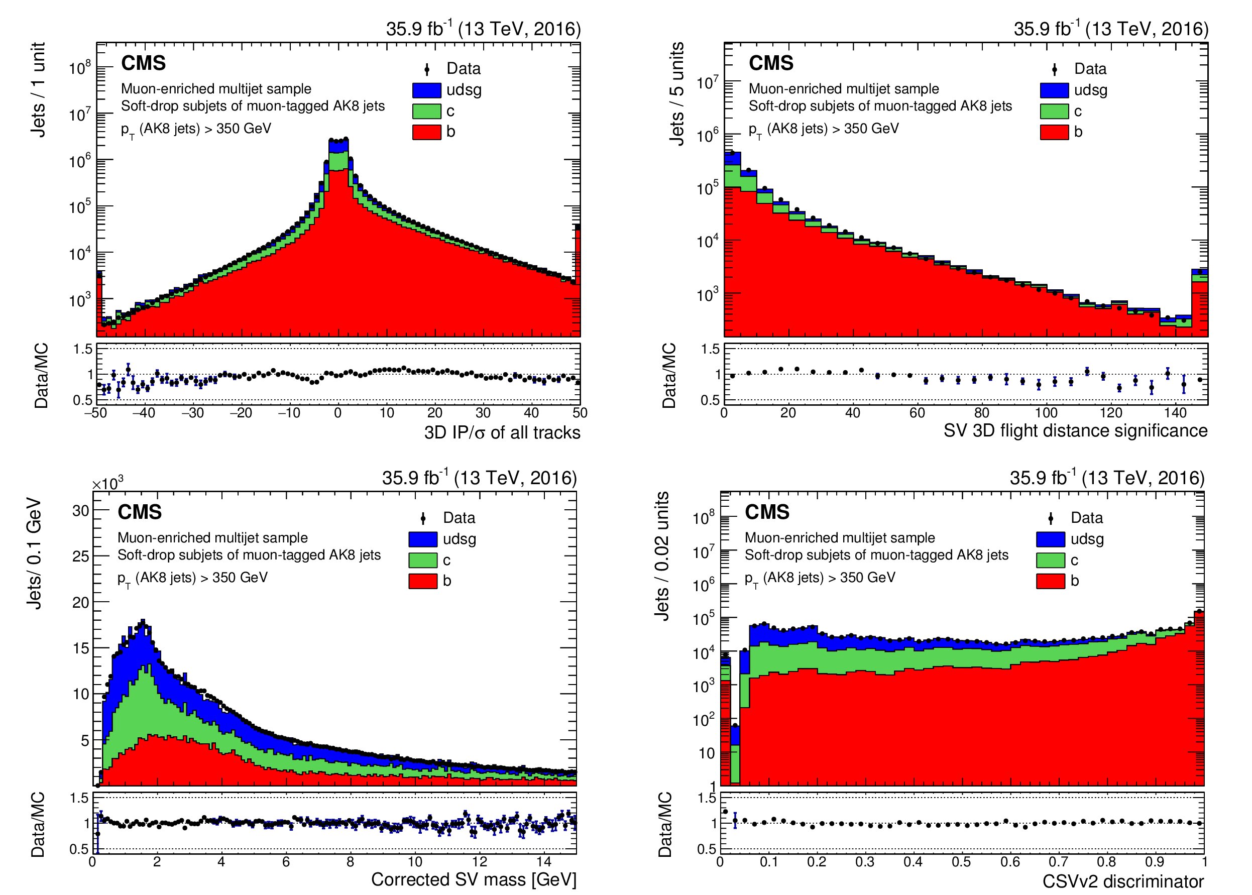
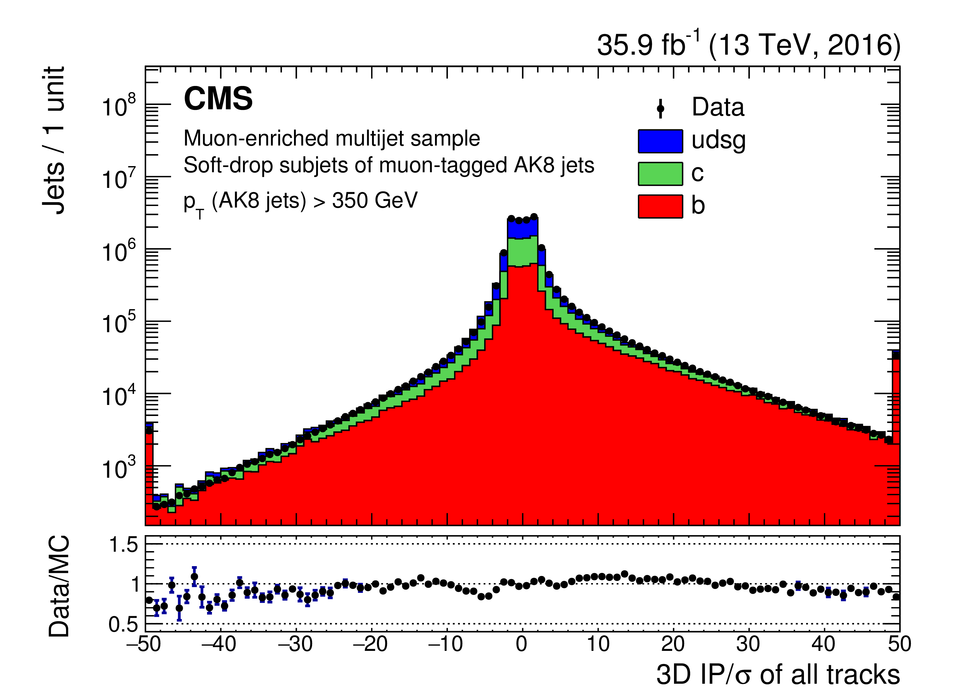
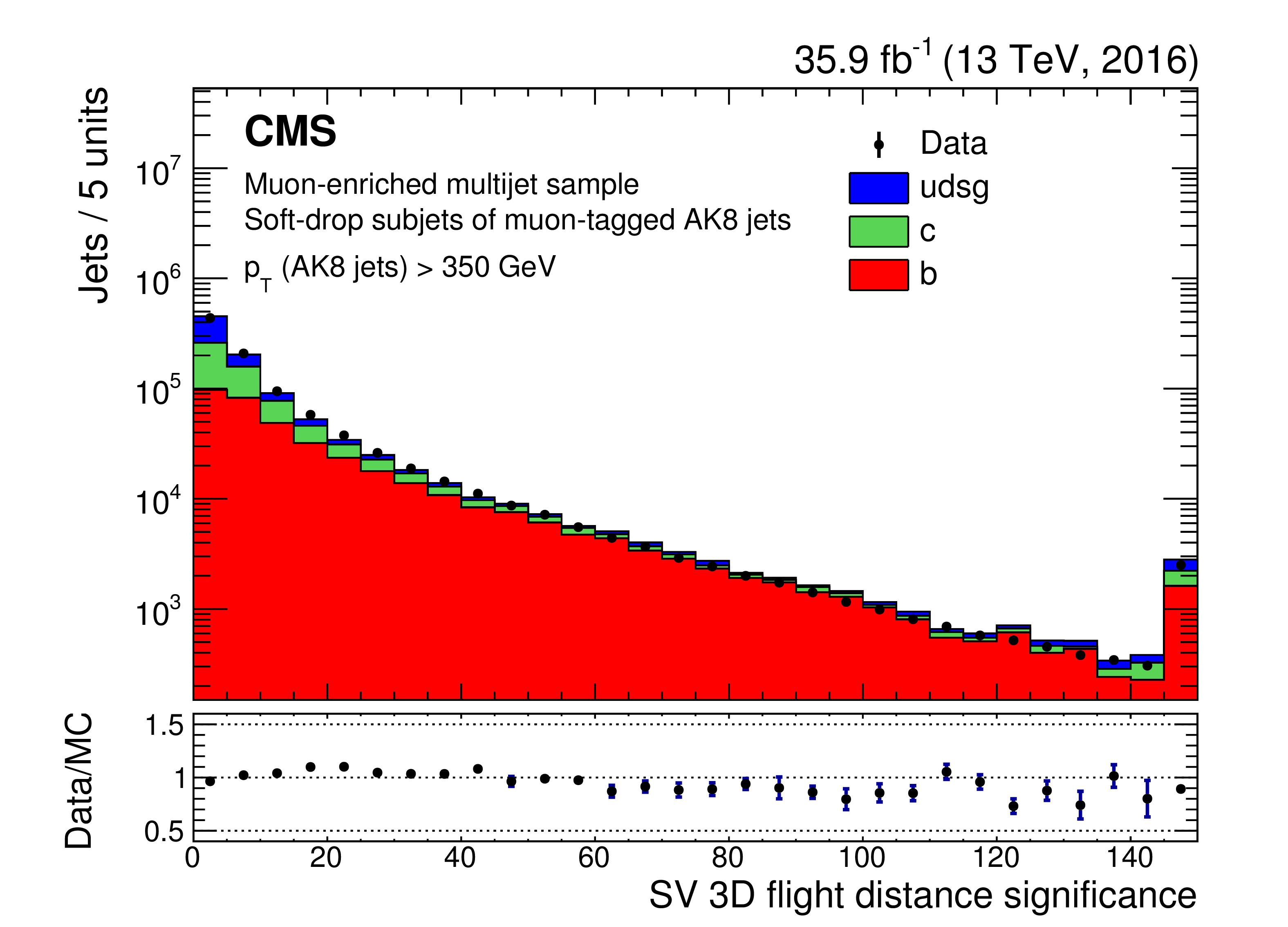
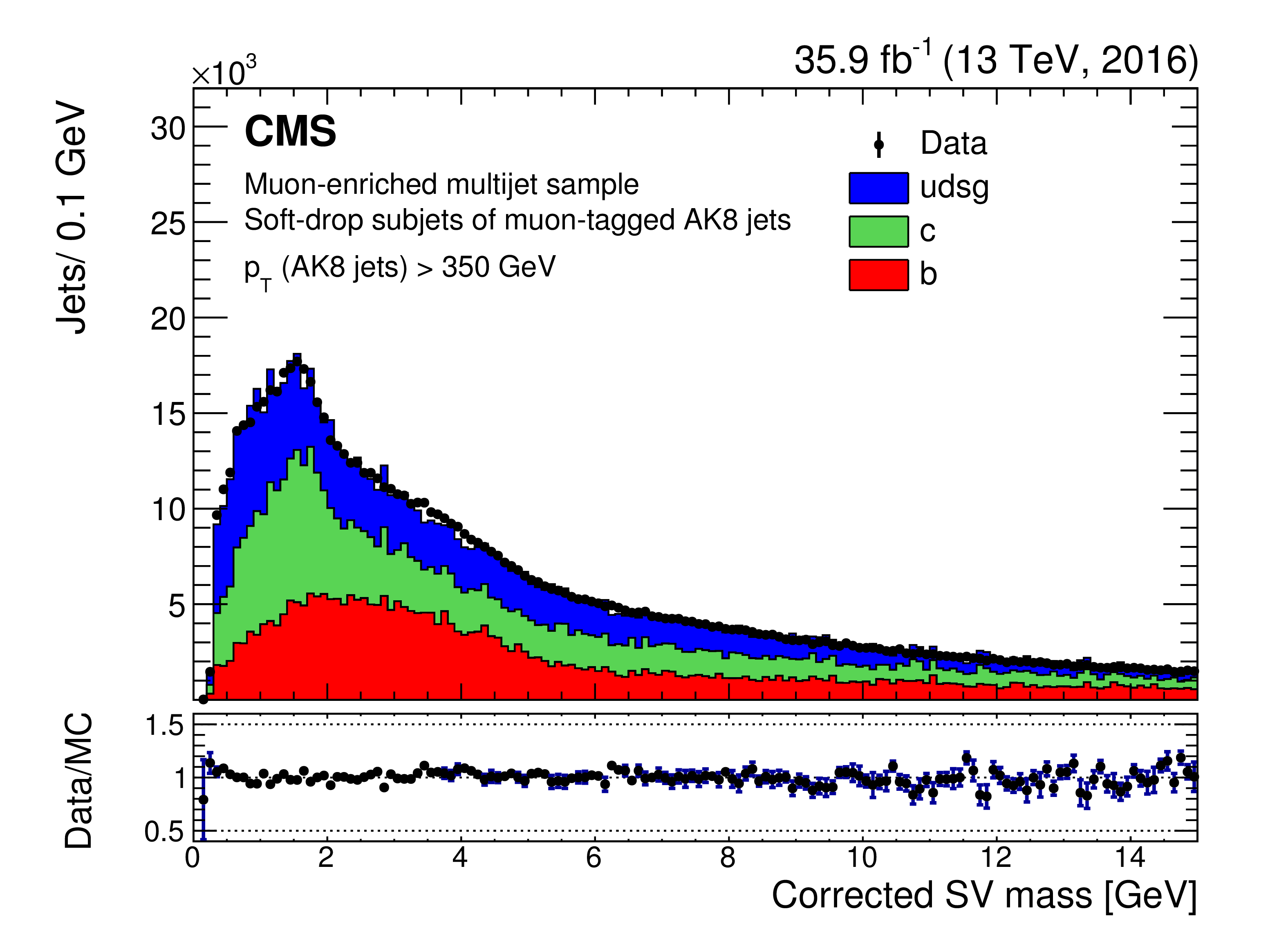
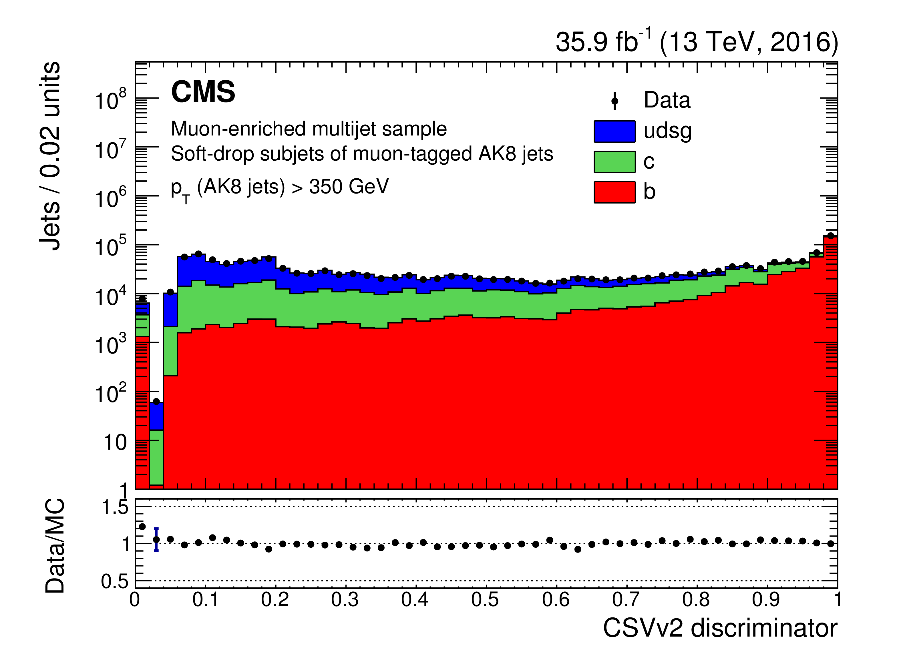
png pdf	Figure 54: Distribution of the 3D impact parameter significance of the tracks (upper left), the secondary vertex 3D flight distance significance (upper right), the corrected secondary vertex mass (lower left), and the CSVv2 discriminator (lower right) for muon-tagged subjets of AK8 jets with $ {p_{\mathrm {T}}} > $ 350 GeV. The simulated contributions of each jet flavour are shown with a different colour. The total number of entries in the simulation is normalized to the number of observed entries in data. The first and last bin of each histogram contain the underflow and overflow entries, respectively.
png pdf	Figure 54-a: Distribution of the 3D impact parameter significance of the tracks (upper left), the secondary vertex 3D flight distance significance (upper right), the corrected secondary vertex mass (lower left), and the CSVv2 discriminator (lower right) for muon-tagged subjets of AK8 jets with $ {p_{\mathrm {T}}} > $ 350 GeV. The simulated contributions of each jet flavour are shown with a different colour. The total number of entries in the simulation is normalized to the number of observed entries in data. The first and last bin of each histogram contain the underflow and overflow entries, respectively.
png pdf	Figure 54-b: Distribution of the 3D impact parameter significance of the tracks (upper left), the secondary vertex 3D flight distance significance (upper right), the corrected secondary vertex mass (lower left), and the CSVv2 discriminator (lower right) for muon-tagged subjets of AK8 jets with $ {p_{\mathrm {T}}} > $ 350 GeV. The simulated contributions of each jet flavour are shown with a different colour. The total number of entries in the simulation is normalized to the number of observed entries in data. The first and last bin of each histogram contain the underflow and overflow entries, respectively.
png pdf	Figure 54-c: Distribution of the 3D impact parameter significance of the tracks (upper left), the secondary vertex 3D flight distance significance (upper right), the corrected secondary vertex mass (lower left), and the CSVv2 discriminator (lower right) for muon-tagged subjets of AK8 jets with $ {p_{\mathrm {T}}} > $ 350 GeV. The simulated contributions of each jet flavour are shown with a different colour. The total number of entries in the simulation is normalized to the number of observed entries in data. The first and last bin of each histogram contain the underflow and overflow entries, respectively.
png pdf	Figure 54-d: Distribution of the 3D impact parameter significance of the tracks (upper left), the secondary vertex 3D flight distance significance (upper right), the corrected secondary vertex mass (lower left), and the CSVv2 discriminator (lower right) for muon-tagged subjets of AK8 jets with $ {p_{\mathrm {T}}} > $ 350 GeV. The simulated contributions of each jet flavour are shown with a different colour. The total number of entries in the simulation is normalized to the number of observed entries in data. The first and last bin of each histogram contain the underflow and overflow entries, respectively.
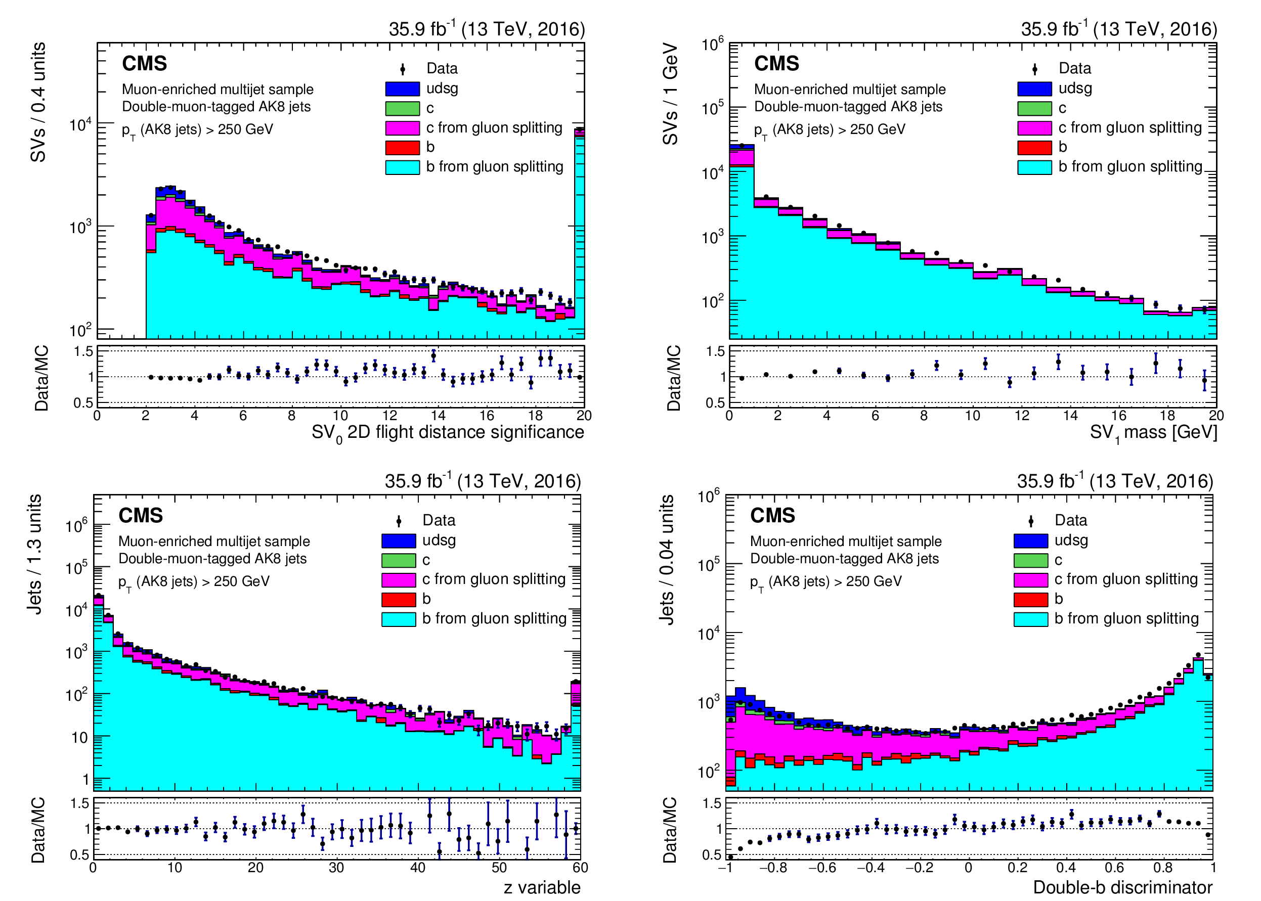
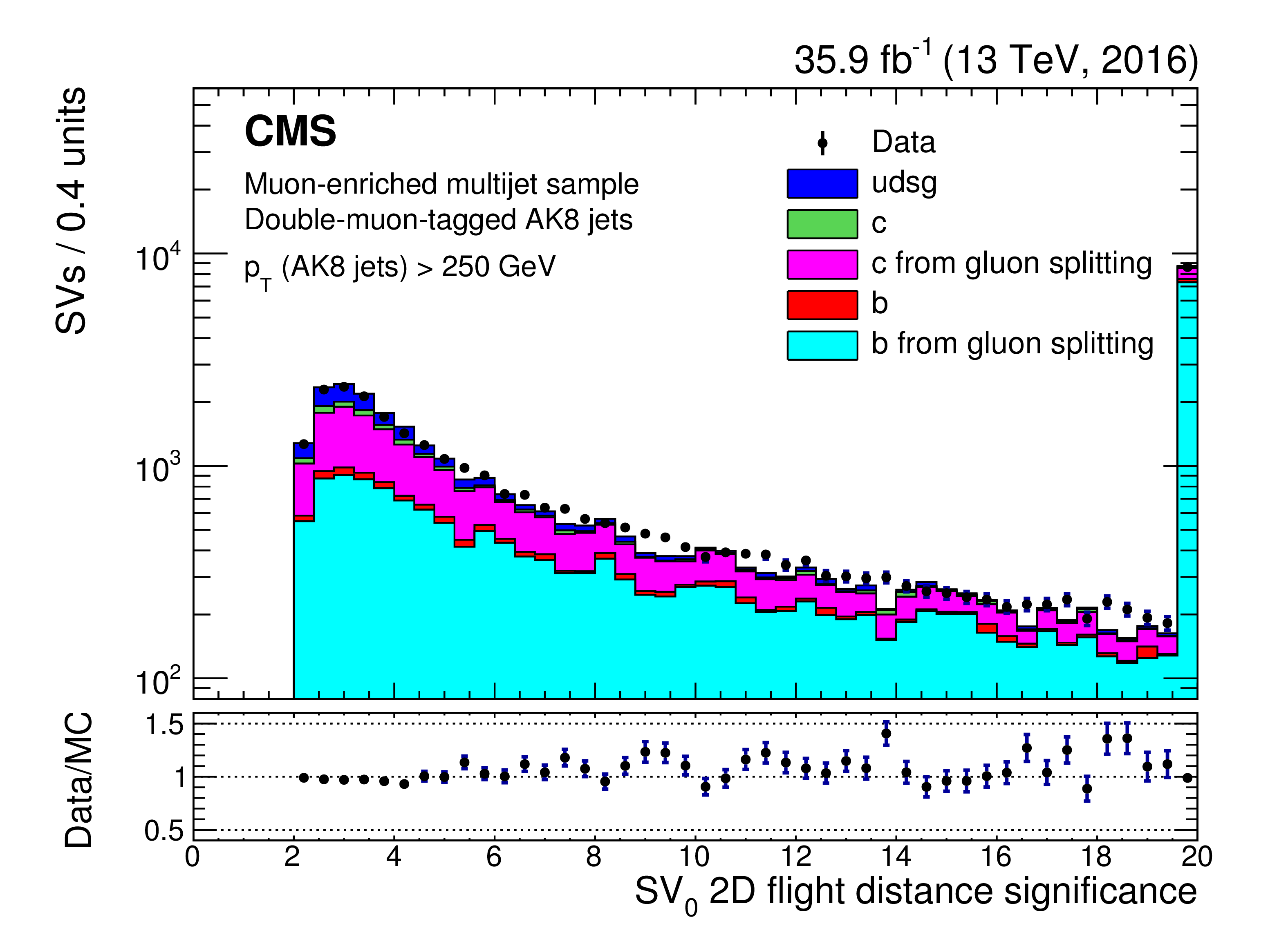
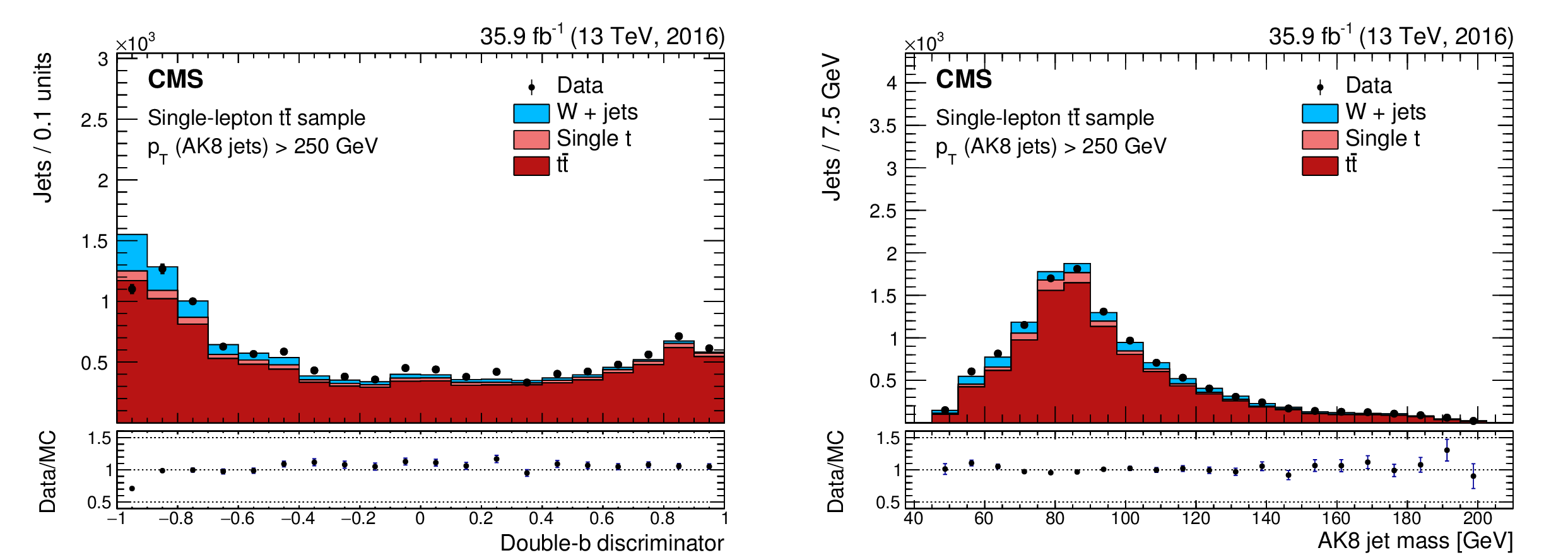
png pdf	Figure 55: Distribution of the 2D flight distance significance of the secondary vertex associated with the first $\tau $ axis (upper left), the mass of the secondary vertex associated with the second $\tau $ axis (upper right), the $z$ variable (lower left), and the double-b discriminator (lower right) for double-muon-tagged AK8 jets with $ {p_{\mathrm {T}}} > $ 250 GeV. The simulated contributions of each jet flavour are shown with a different colour. The total number of entries in the simulation is normalized to the number of observed entries in data. The first and last bin of the upper and lower right histograms contain the underflow and overflow entries, respectively.
png pdf	Figure 55-a: Distribution of the 2D flight distance significance of the secondary vertex associated with the first $\tau $ axis (upper left), the mass of the secondary vertex associated with the second $\tau $ axis (upper right), the $z$ variable (lower left), and the double-b discriminator (lower right) for double-muon-tagged AK8 jets with $ {p_{\mathrm {T}}} > $ 250 GeV. The simulated contributions of each jet flavour are shown with a different colour. The total number of entries in the simulation is normalized to the number of observed entries in data. The first and last bin of the upper and lower right histograms contain the underflow and overflow entries, respectively.
png pdf	Figure 55-b: Distribution of the 2D flight distance significance of the secondary vertex associated with the first $\tau $ axis (upper left), the mass of the secondary vertex associated with the second $\tau $ axis (upper right), the $z$ variable (lower left), and the double-b discriminator (lower right) for double-muon-tagged AK8 jets with $ {p_{\mathrm {T}}} > $ 250 GeV. The simulated contributions of each jet flavour are shown with a different colour. The total number of entries in the simulation is normalized to the number of observed entries in data. The first and last bin of the upper and lower right histograms contain the underflow and overflow entries, respectively.
png pdf	Figure 55-c: Distribution of the 2D flight distance significance of the secondary vertex associated with the first $\tau $ axis (upper left), the mass of the secondary vertex associated with the second $\tau $ axis (upper right), the $z$ variable (lower left), and the double-b discriminator (lower right) for double-muon-tagged AK8 jets with $ {p_{\mathrm {T}}} > $ 250 GeV. The simulated contributions of each jet flavour are shown with a different colour. The total number of entries in the simulation is normalized to the number of observed entries in data. The first and last bin of the upper and lower right histograms contain the underflow and overflow entries, respectively.
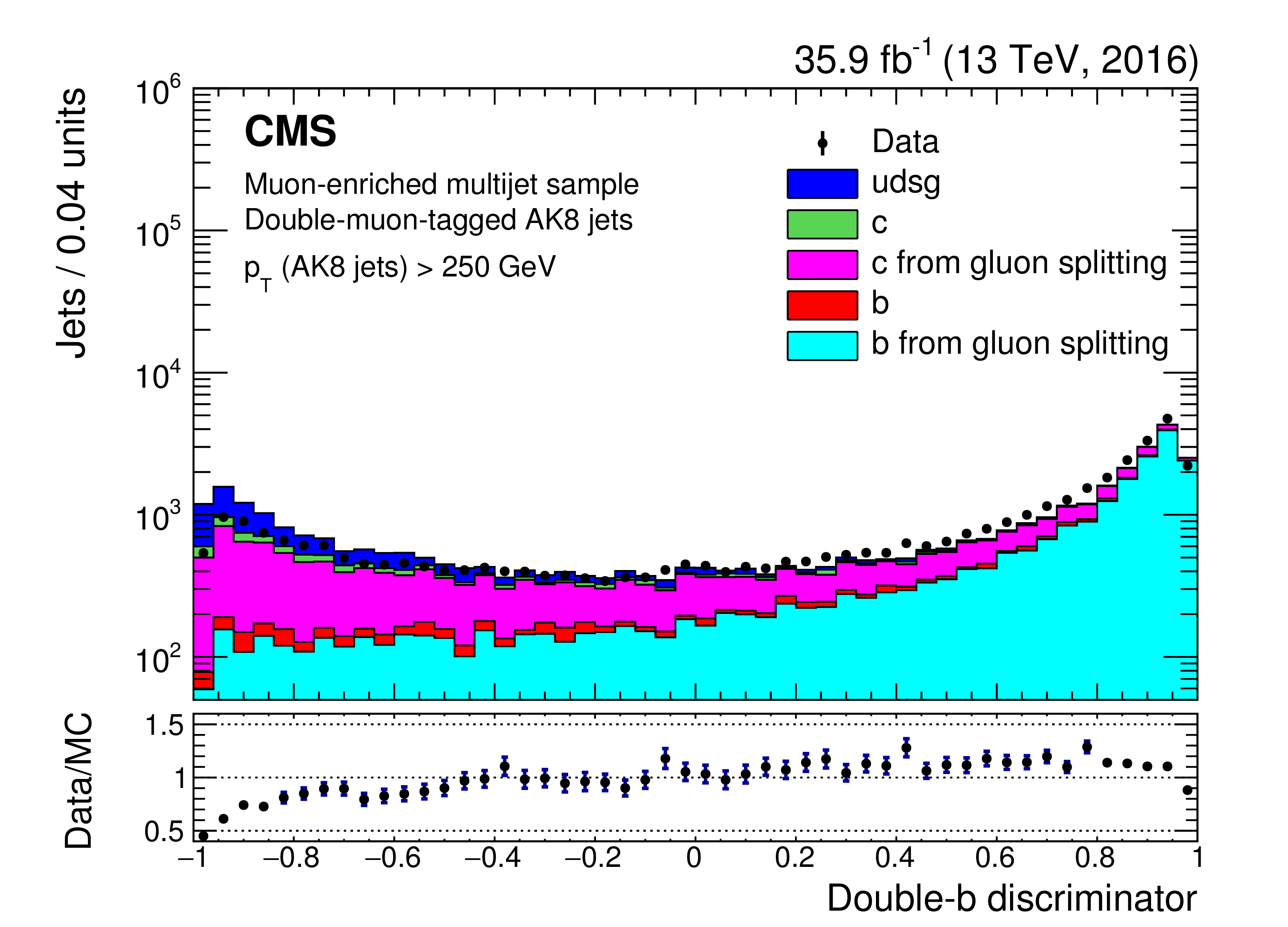
png pdf	Figure 55-d: Distribution of the 2D flight distance significance of the secondary vertex associated with the first $\tau $ axis (upper left), the mass of the secondary vertex associated with the second $\tau $ axis (upper right), the $z$ variable (lower left), and the double-b discriminator (lower right) for double-muon-tagged AK8 jets with $ {p_{\mathrm {T}}} > $ 250 GeV. The simulated contributions of each jet flavour are shown with a different colour. The total number of entries in the simulation is normalized to the number of observed entries in data. The first and last bin of the upper and lower right histograms contain the underflow and overflow entries, respectively.
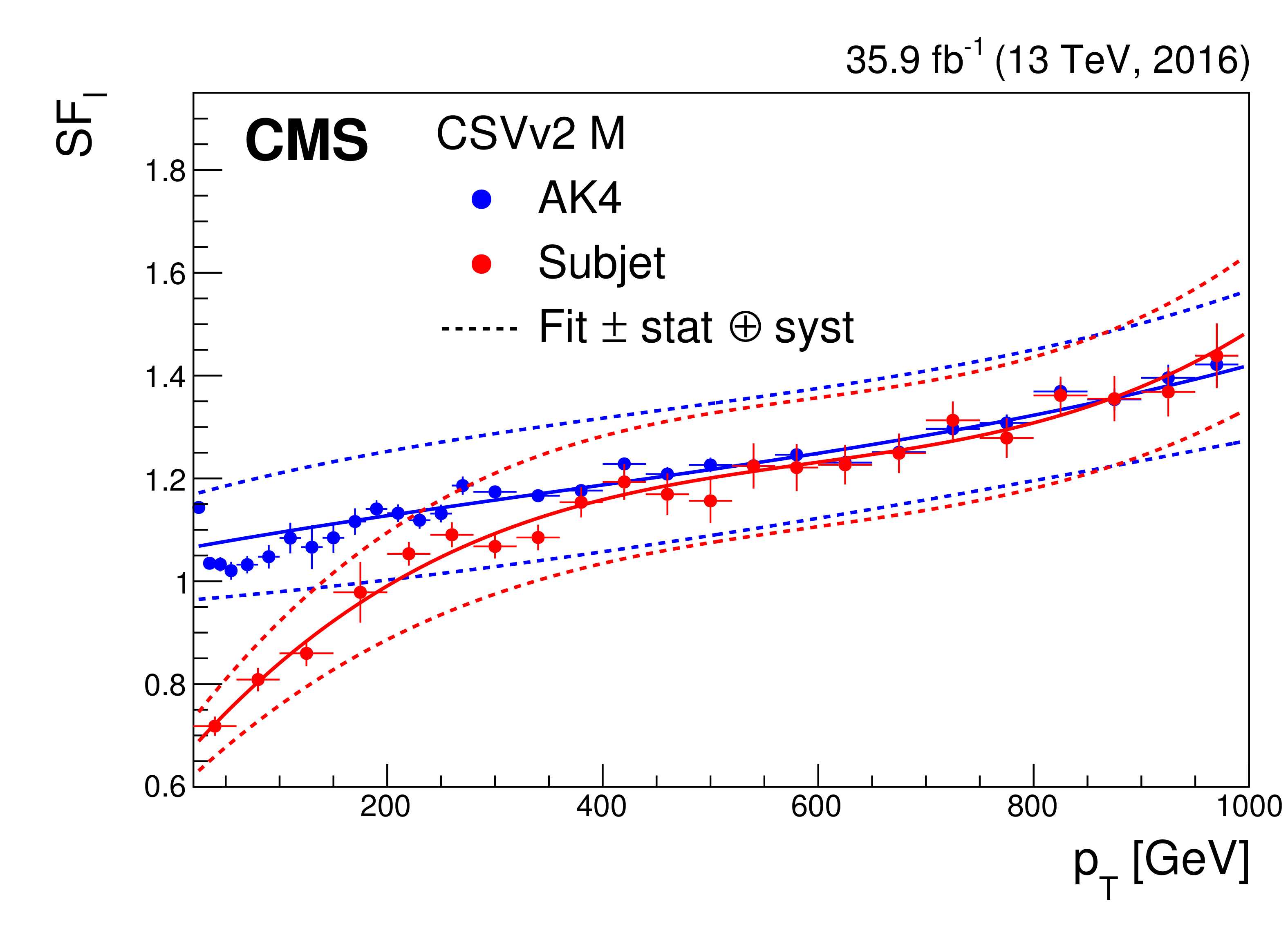
png pdf	Figure 56: Data-to-simulation scale factors for light-flavour subjets of AK8 jets as a function of the subjet ${p_{\mathrm {T}}}$, as well as for AK4 jets as a function of jet ${p_{\mathrm {T}}}$, for the loose (left) and medium (right) working points of the CSVv2 algorithm. The solid curve is the result of a fit to the scale factors, and the dashed lines represent the overall statistical and systematic uncertainty of the measurements.
png pdf	Figure 56-a: Data-to-simulation scale factors for light-flavour subjets of AK8 jets as a function of the subjet ${p_{\mathrm {T}}}$, as well as for AK4 jets as a function of jet ${p_{\mathrm {T}}}$, for the loose (left) and medium (right) working points of the CSVv2 algorithm. The solid curve is the result of a fit to the scale factors, and the dashed lines represent the overall statistical and systematic uncertainty of the measurements.
png pdf	Figure 56-b: Data-to-simulation scale factors for light-flavour subjets of AK8 jets as a function of the subjet ${p_{\mathrm {T}}}$, as well as for AK4 jets as a function of jet ${p_{\mathrm {T}}}$, for the loose (left) and medium (right) working points of the CSVv2 algorithm. The solid curve is the result of a fit to the scale factors, and the dashed lines represent the overall statistical and systematic uncertainty of the measurements.
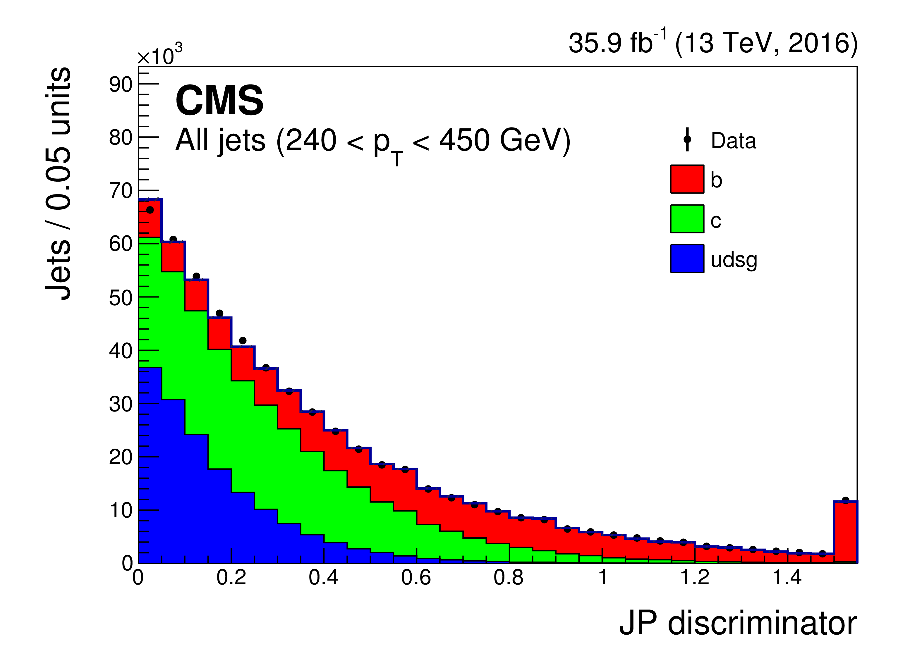
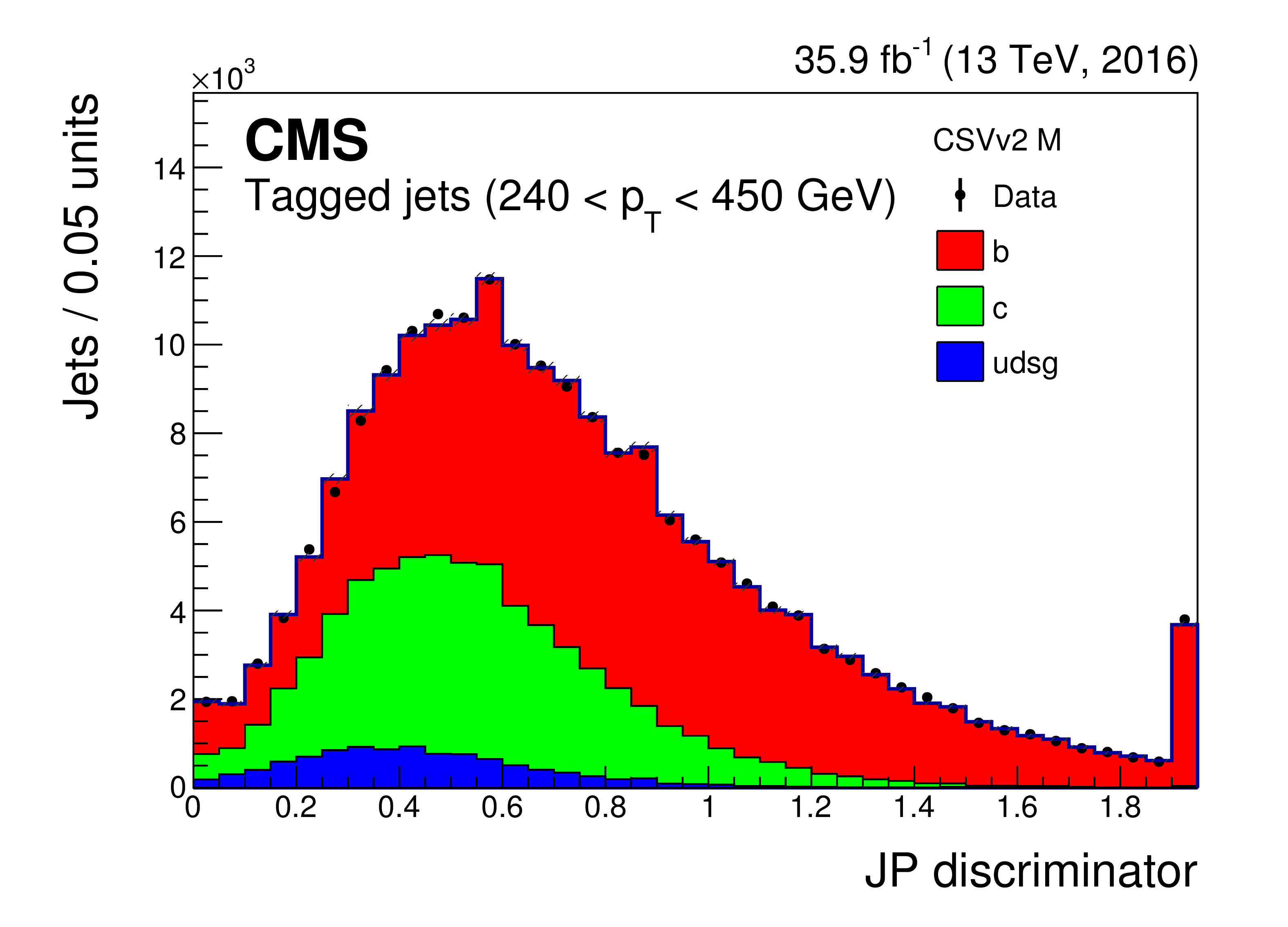
png pdf	Figure 57: Fitted JP discriminator distribution for all soft-drop subjets with 240 $ < {p_{\mathrm {T}}} < $ 450 GeV (left) and for the subsample of those subjets passing the medium working point of the CSVv2 algorithm (right). The last bin contains the overflow entries.
png pdf	Figure 57-a: Fitted JP discriminator distribution for all soft-drop subjets with 240 $ < {p_{\mathrm {T}}} < $ 450 GeV (left) and for the subsample of those subjets passing the medium working point of the CSVv2 algorithm (right). The last bin contains the overflow entries.
png pdf	Figure 57-b: Fitted JP discriminator distribution for all soft-drop subjets with 240 $ < {p_{\mathrm {T}}} < $ 450 GeV (left) and for the subsample of those subjets passing the medium working point of the CSVv2 algorithm (right). The last bin contains the overflow entries.
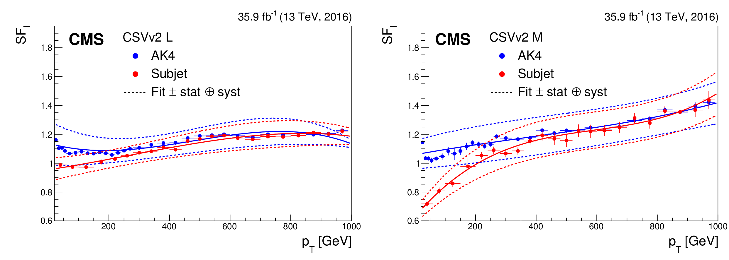
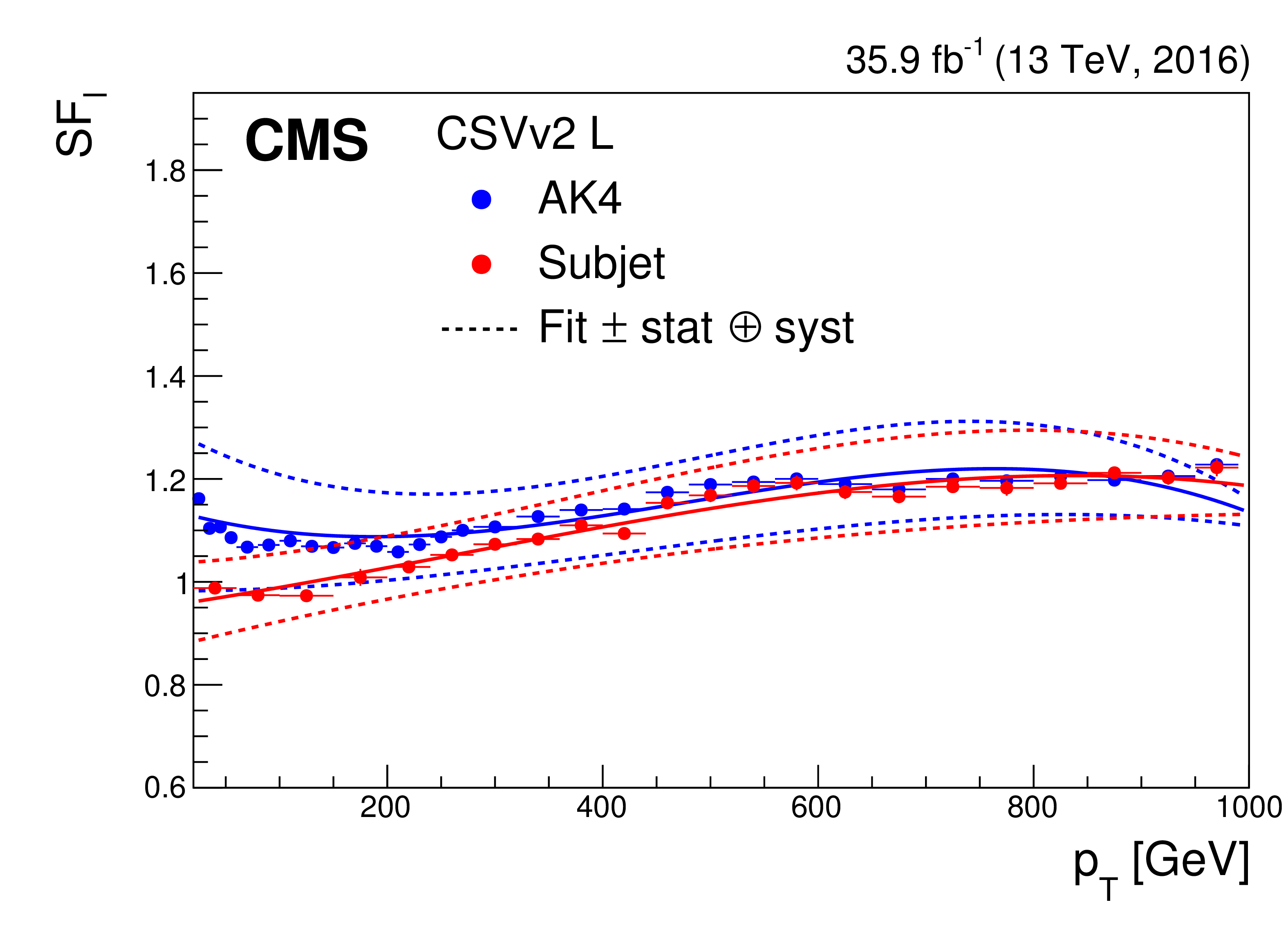
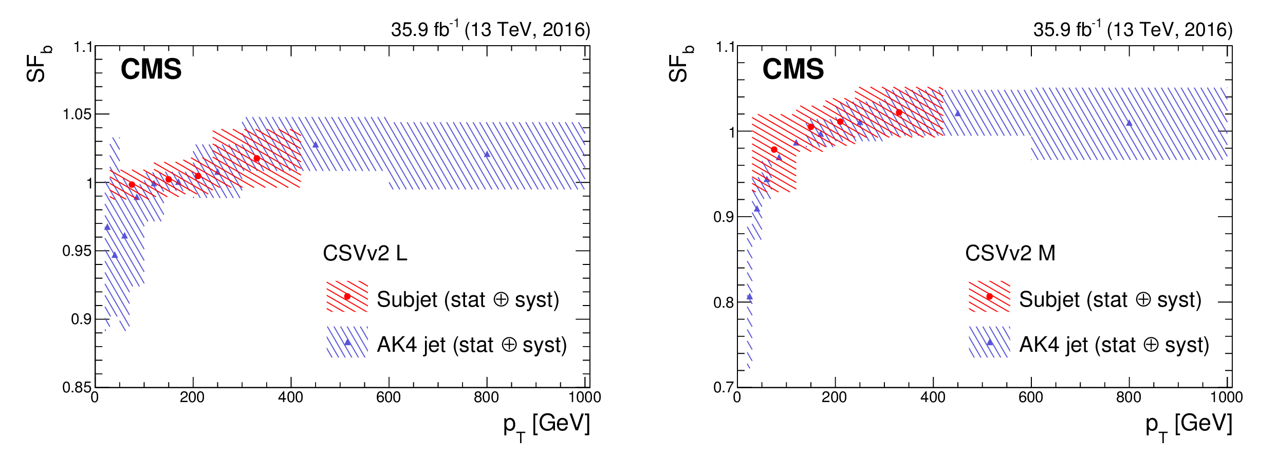
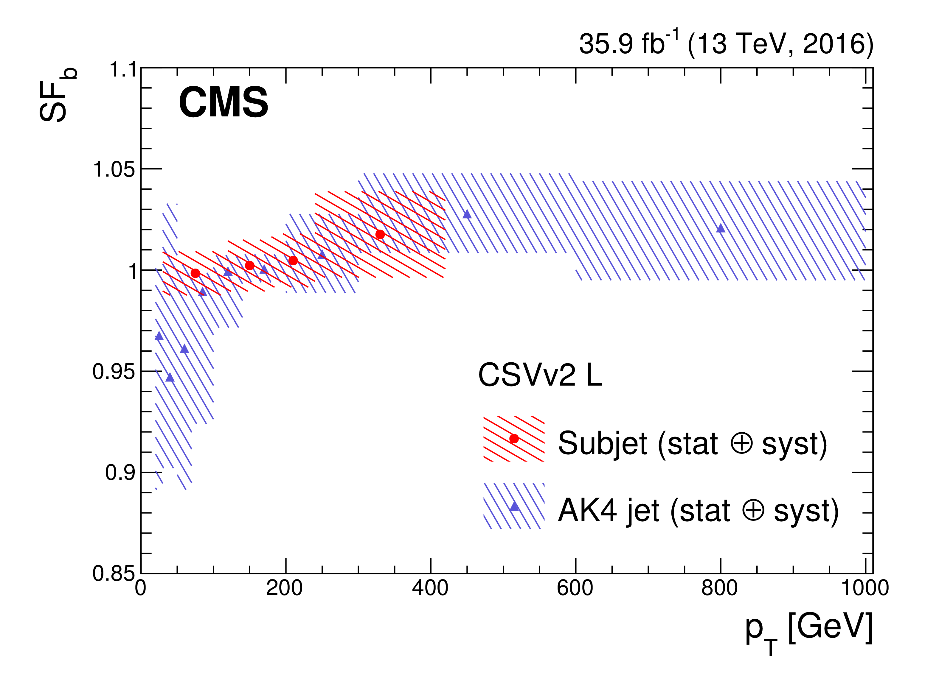
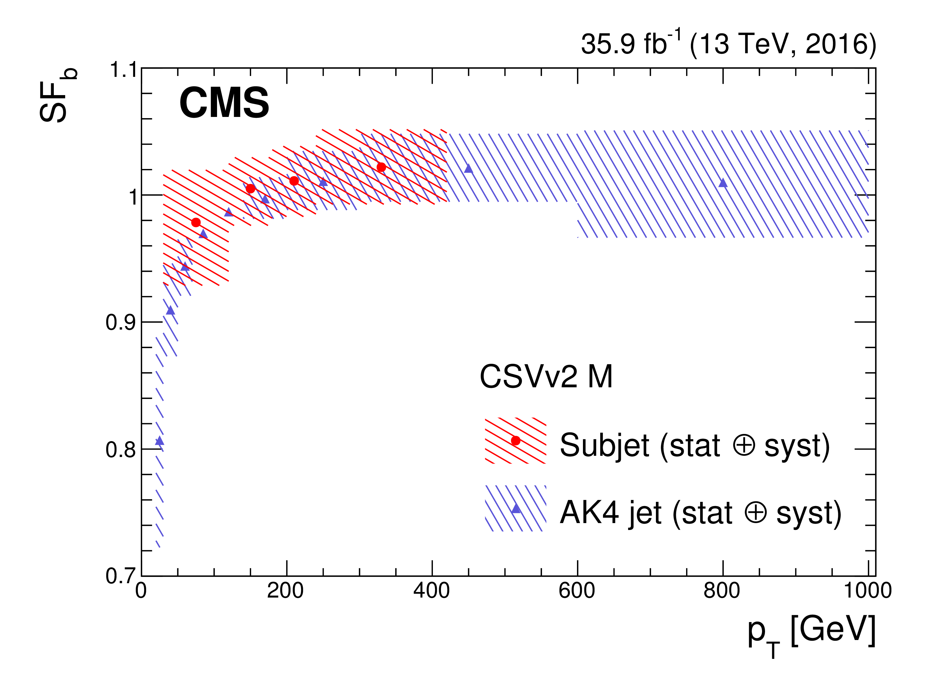
png pdf	Figure 58: Data-to-simulation scale factors for b subjets of AK8 jets as a function of the subjet $ {p_{\mathrm {T}}}$, as well as for AK4 jets as a function of jet $ {p_{\mathrm {T}}}$, for the loose (left) and medium (right) working points of the CSVv2 algorithm. The hatched band around the scale factors represents the overall statistical and systematic uncertainty of the measurements.
png pdf	Figure 58-a: Data-to-simulation scale factors for b subjets of AK8 jets as a function of the subjet $ {p_{\mathrm {T}}}$, as well as for AK4 jets as a function of jet $ {p_{\mathrm {T}}}$, for the loose (left) and medium (right) working points of the CSVv2 algorithm. The hatched band around the scale factors represents the overall statistical and systematic uncertainty of the measurements.
png pdf	Figure 58-b: Data-to-simulation scale factors for b subjets of AK8 jets as a function of the subjet $ {p_{\mathrm {T}}}$, as well as for AK4 jets as a function of jet $ {p_{\mathrm {T}}}$, for the loose (left) and medium (right) working points of the CSVv2 algorithm. The hatched band around the scale factors represents the overall statistical and systematic uncertainty of the measurements.
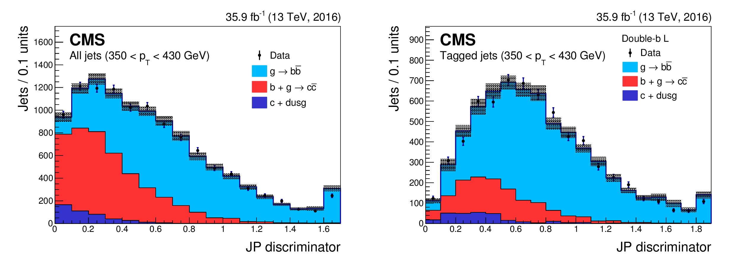
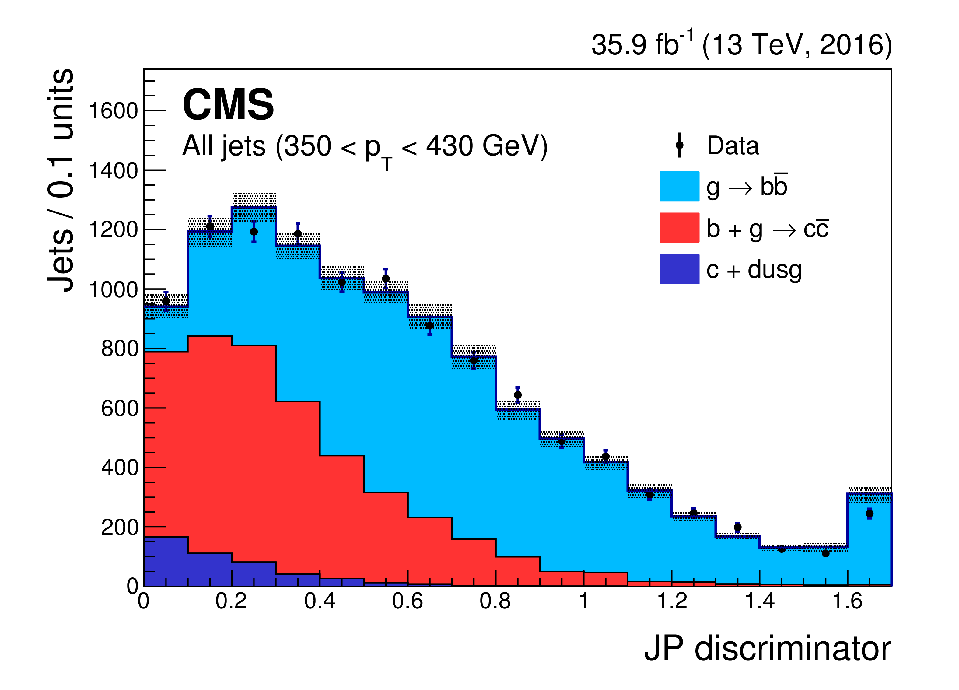
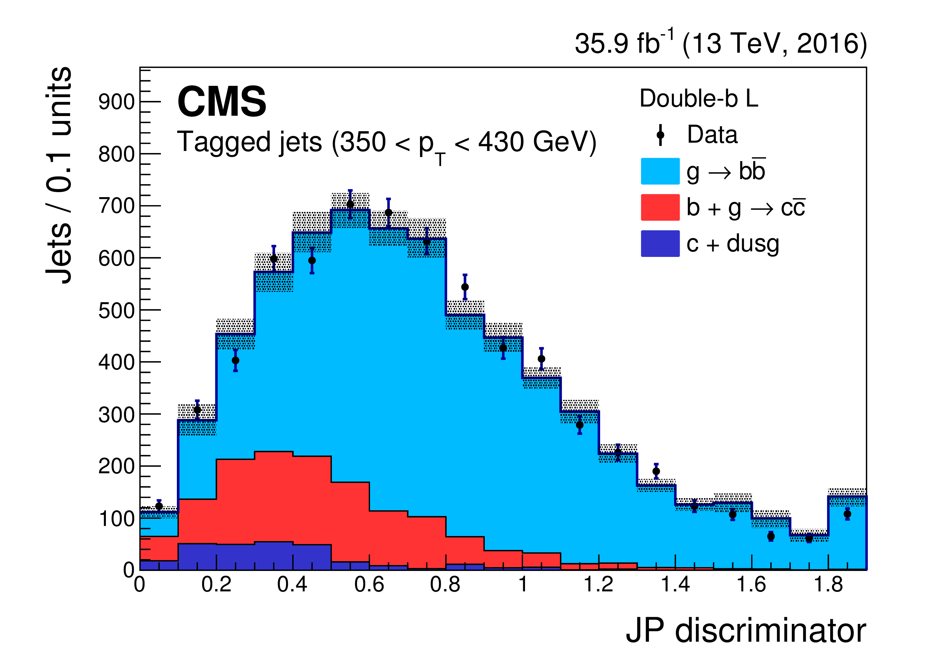
png pdf	Figure 59: Fitted JP discriminator distribution for all soft-drop subjets with 350 $ < {p_{\mathrm {T}}} < $ 430 GeV (left) and for the subsample of those subjets passing the loose working point of the double-b algorithm (right). The shaded area represents the statistical and systematic uncertainties in the templates obtained from simulation. The last bin contains the overflow entries.
png pdf	Figure 59-a: Fitted JP discriminator distribution for all soft-drop subjets with 350 $ < {p_{\mathrm {T}}} < $ 430 GeV (left) and for the subsample of those subjets passing the loose working point of the double-b algorithm (right). The shaded area represents the statistical and systematic uncertainties in the templates obtained from simulation. The last bin contains the overflow entries.
png pdf	Figure 59-b: Fitted JP discriminator distribution for all soft-drop subjets with 350 $ < {p_{\mathrm {T}}} < $ 430 GeV (left) and for the subsample of those subjets passing the loose working point of the double-b algorithm (right). The shaded area represents the statistical and systematic uncertainties in the templates obtained from simulation. The last bin contains the overflow entries.
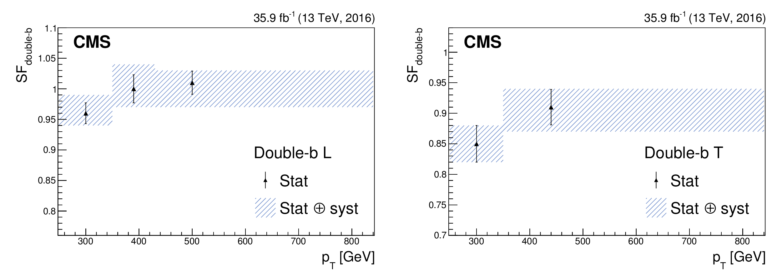
png pdf	Figure 60: Data-to-simulation scale factors for correctly identifying two b jets in an AK8 jet as a function of the jet $ {p_{\mathrm {T}}} $ for the loose (left) and tight (right) working points of the double-b tagger. The hatched band around the scale factors represents the overall statistical and systematic uncertainty in the measurement. Jets with $ {p_{\mathrm {T}}} > $ 840 GeV are included in the last $ {p_{\mathrm {T}}} $ bin.
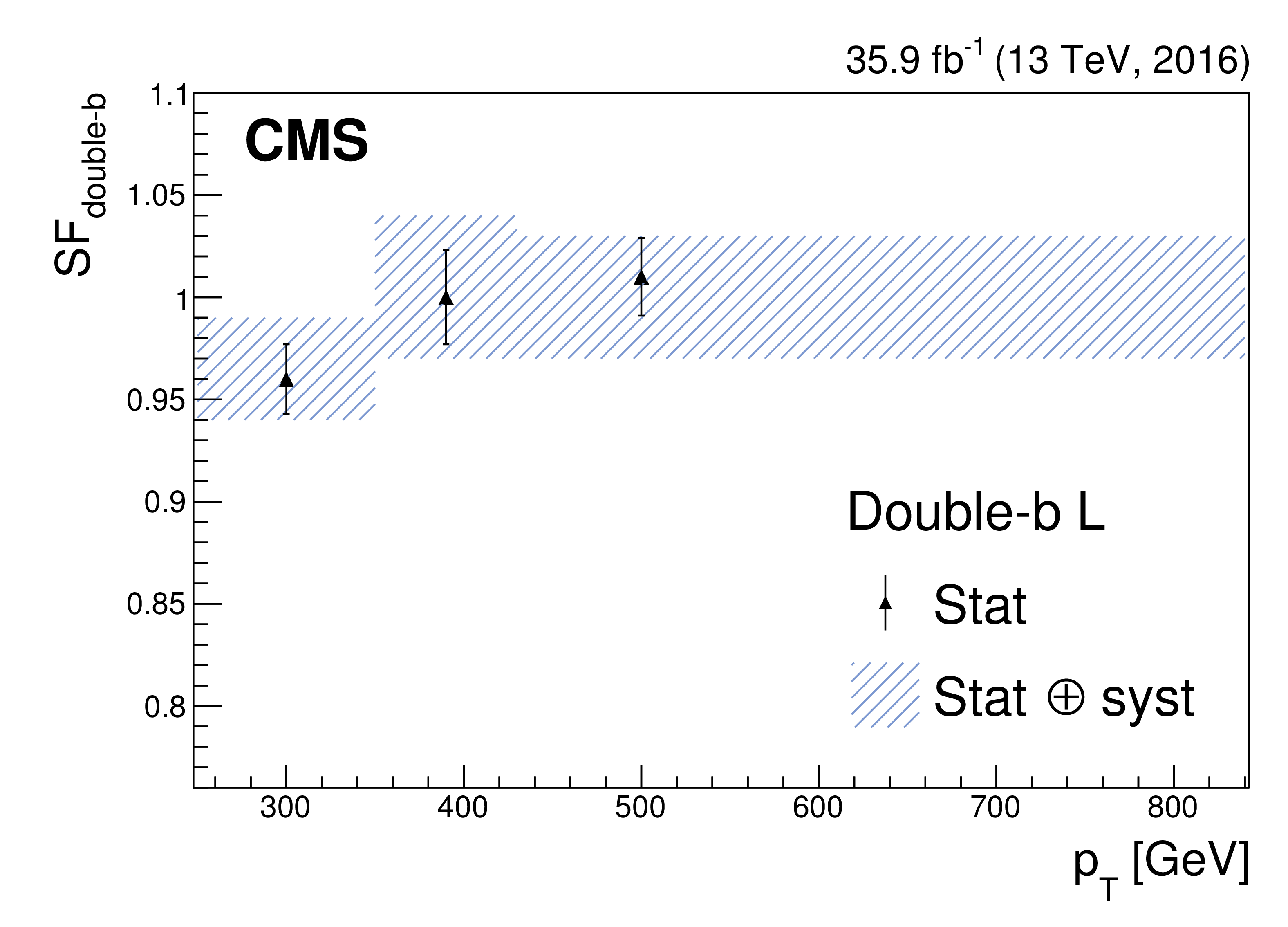
png pdf	Figure 60-a: Data-to-simulation scale factors for correctly identifying two b jets in an AK8 jet as a function of the jet $ {p_{\mathrm {T}}} $ for the loose (left) and tight (right) working points of the double-b tagger. The hatched band around the scale factors represents the overall statistical and systematic uncertainty in the measurement. Jets with $ {p_{\mathrm {T}}} > $ 840 GeV are included in the last $ {p_{\mathrm {T}}} $ bin.
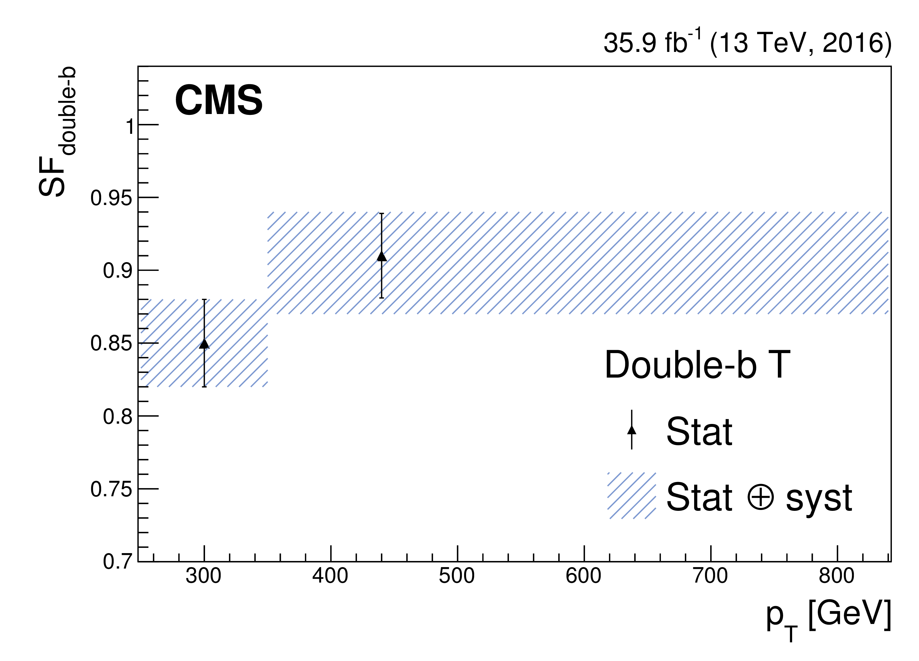
png pdf	Figure 60-b: Data-to-simulation scale factors for correctly identifying two b jets in an AK8 jet as a function of the jet $ {p_{\mathrm {T}}} $ for the loose (left) and tight (right) working points of the double-b tagger. The hatched band around the scale factors represents the overall statistical and systematic uncertainty in the measurement. Jets with $ {p_{\mathrm {T}}} > $ 840 GeV are included in the last $ {p_{\mathrm {T}}} $ bin.
png pdf	Figure 61: Distribution of the double-b tagger discriminator (left) and pruned jet mass (right) for AK8 jets passing the 2-prong event selection as described in the text. The simulation is normalized to the observed number of events.
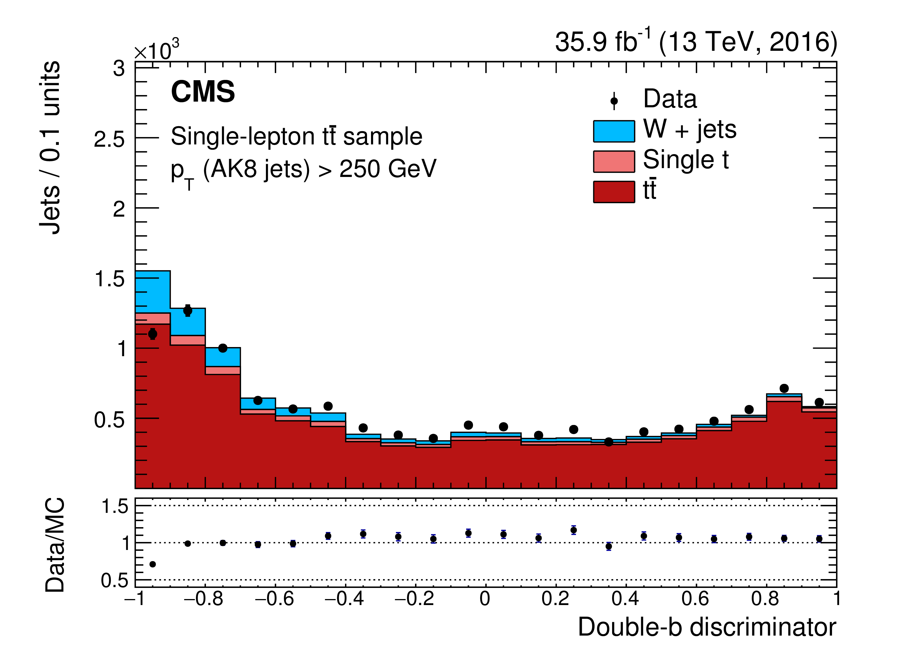
png pdf	Figure 61-a: Distribution of the double-b tagger discriminator (left) and pruned jet mass (right) for AK8 jets passing the 2-prong event selection as described in the text. The simulation is normalized to the observed number of events.
png pdf	Figure 61-b: Distribution of the double-b tagger discriminator (left) and pruned jet mass (right) for AK8 jets passing the 2-prong event selection as described in the text. The simulation is normalized to the observed number of events.
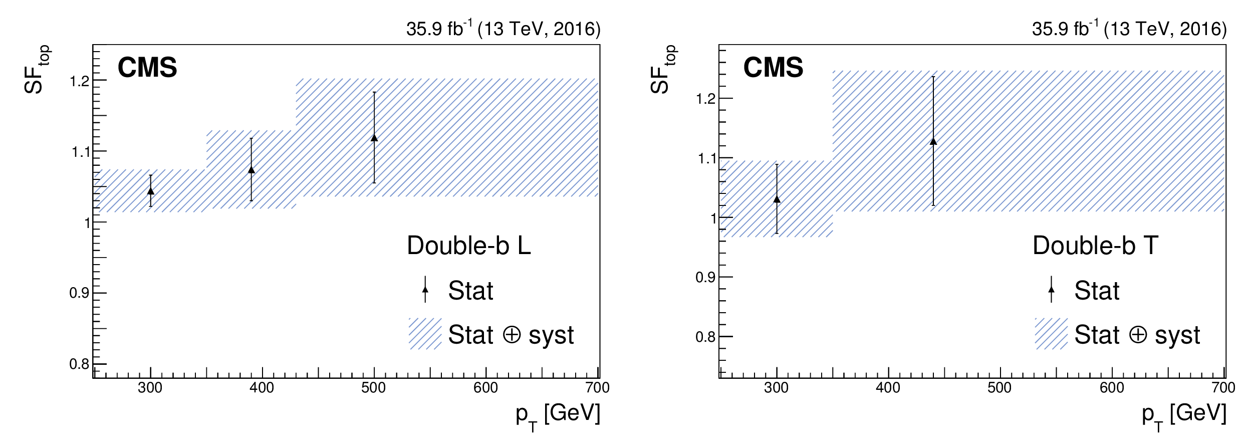
png pdf	Figure 62: Data-to-simulation scale factors for misidentifying a top quark jet as a function of the jet $ {p_{\mathrm {T}}} $ for the loose (left) and tight (right) working points of the double-b tagger. The hatched band around the scale factors represents the overall statistical and systematic uncertainty in the measurement. Jets with $ {p_{\mathrm {T}}} > $ 840 GeV are included in the last $ {p_{\mathrm {T}}} $ bin.
png pdf	Figure 62-a: Data-to-simulation scale factors for misidentifying a top quark jet as a function of the jet $ {p_{\mathrm {T}}} $ for the loose (left) and tight (right) working points of the double-b tagger. The hatched band around the scale factors represents the overall statistical and systematic uncertainty in the measurement. Jets with $ {p_{\mathrm {T}}} > $ 840 GeV are included in the last $ {p_{\mathrm {T}}} $ bin.
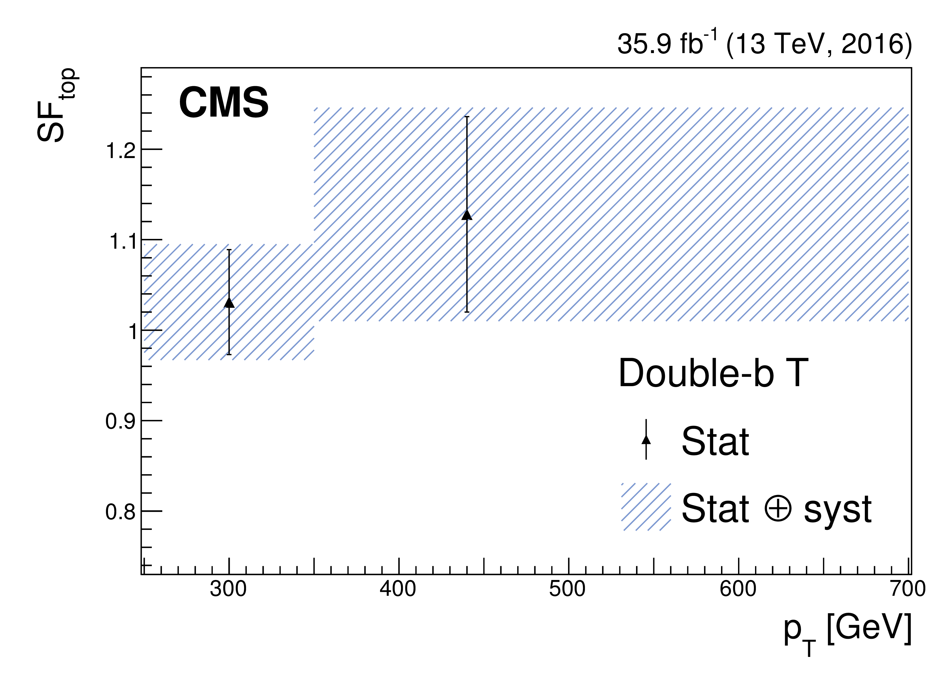
png pdf	Figure 62-b: Data-to-simulation scale factors for misidentifying a top quark jet as a function of the jet $ {p_{\mathrm {T}}} $ for the loose (left) and tight (right) working points of the double-b tagger. The hatched band around the scale factors represents the overall statistical and systematic uncertainty in the measurement. Jets with $ {p_{\mathrm {T}}} > $ 840 GeV are included in the last $ {p_{\mathrm {T}}} $ bin.
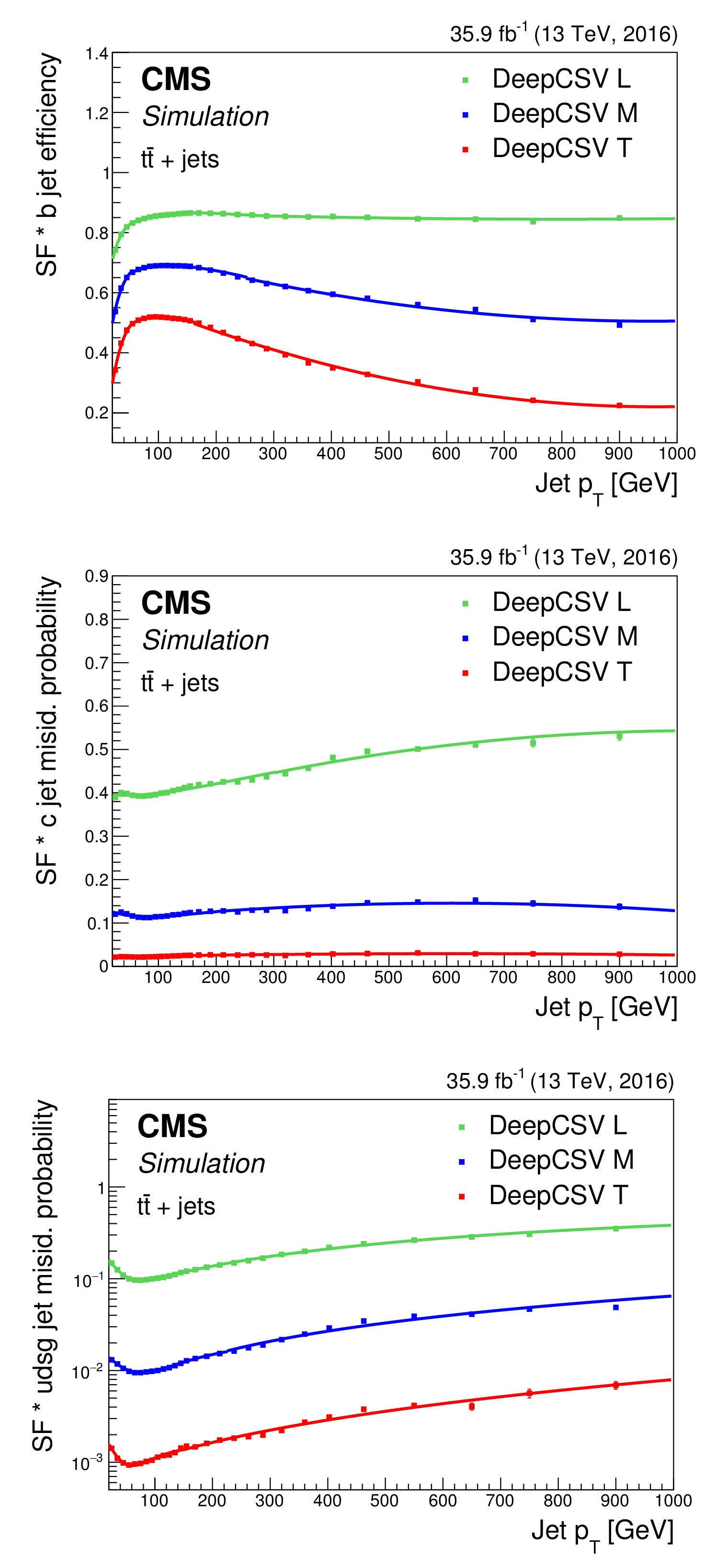
png pdf	Figure 63: Efficiency for b tagging jets for the three different working points of the DeepCSV algorithm multiplied by the measured data-to-simulation scale factor. The efficiencies are shown as a function of the jet $ {p_{\mathrm {T}}} $ using jets with $ {p_{\mathrm {T}}} > $ 20 GeV in $ {\mathrm {t}\overline {\mathrm {t}}} $ events for b jets (upper), c jets (middle), and light-flavour jets (lower). The solid lines represents the functions used to fit the dependence on the jet $ {p_{\mathrm {T}}}$. The last bin includes the overflow.
png pdf	Figure 63-a: Efficiency for b tagging jets for the three different working points of the DeepCSV algorithm multiplied by the measured data-to-simulation scale factor. The efficiencies are shown as a function of the jet $ {p_{\mathrm {T}}} $ using jets with $ {p_{\mathrm {T}}} > $ 20 GeV in $ {\mathrm {t}\overline {\mathrm {t}}} $ events for b jets (upper), c jets (middle), and light-flavour jets (lower). The solid lines represents the functions used to fit the dependence on the jet $ {p_{\mathrm {T}}}$. The last bin includes the overflow.
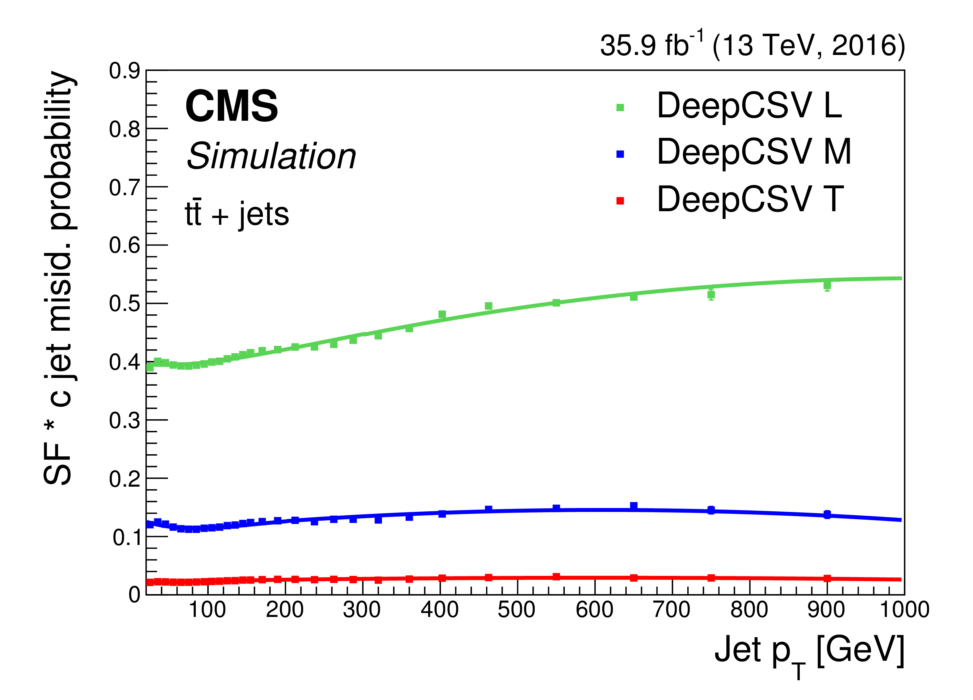
png pdf	Figure 63-b: Efficiency for b tagging jets for the three different working points of the DeepCSV algorithm multiplied by the measured data-to-simulation scale factor. The efficiencies are shown as a function of the jet $ {p_{\mathrm {T}}} $ using jets with $ {p_{\mathrm {T}}} > $ 20 GeV in $ {\mathrm {t}\overline {\mathrm {t}}} $ events for b jets (upper), c jets (middle), and light-flavour jets (lower). The solid lines represents the functions used to fit the dependence on the jet $ {p_{\mathrm {T}}}$. The last bin includes the overflow.
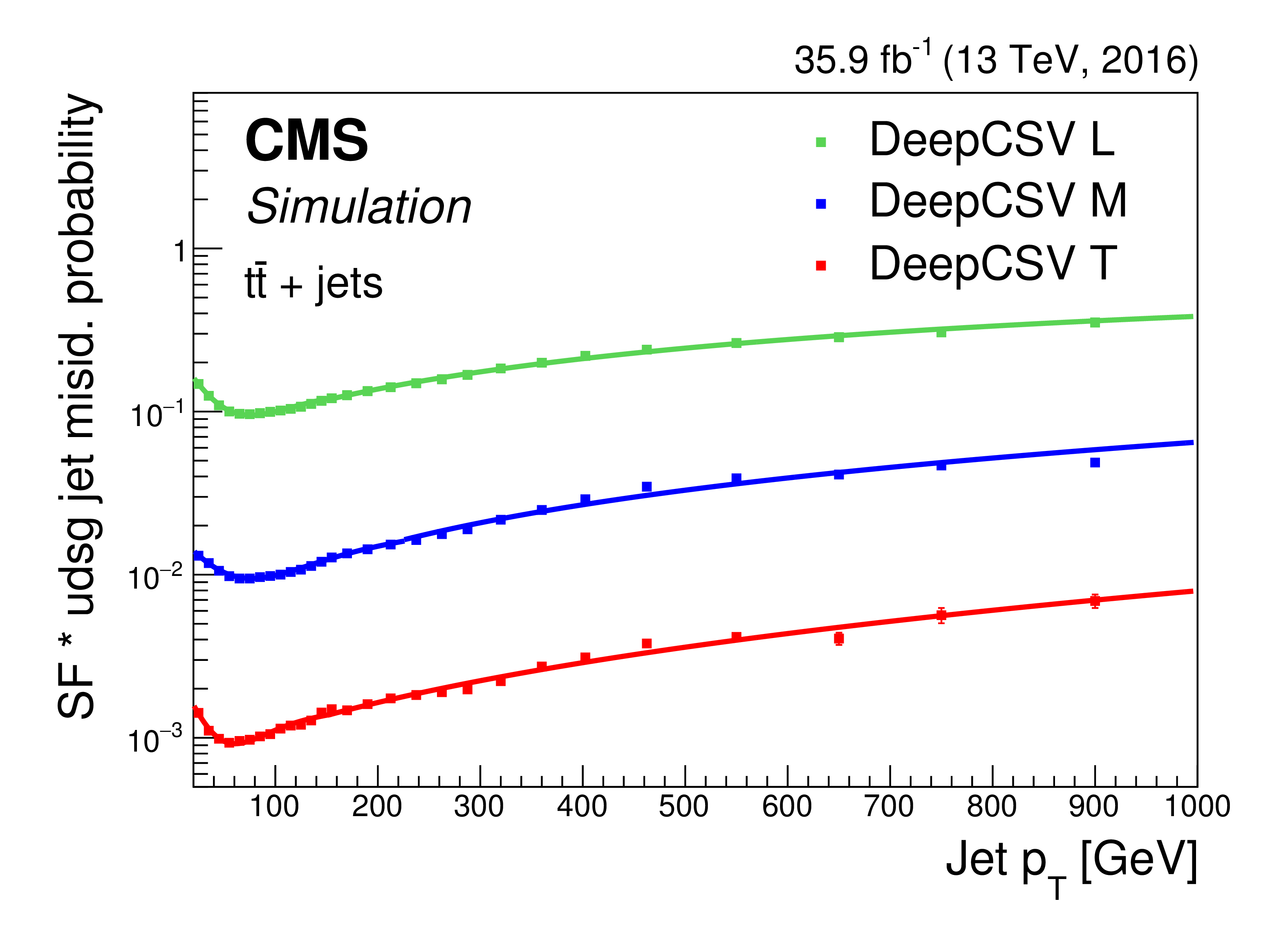
png pdf	Figure 63-c: Efficiency for b tagging jets for the three different working points of the DeepCSV algorithm multiplied by the measured data-to-simulation scale factor. The efficiencies are shown as a function of the jet $ {p_{\mathrm {T}}} $ using jets with $ {p_{\mathrm {T}}} > $ 20 GeV in $ {\mathrm {t}\overline {\mathrm {t}}} $ events for b jets (upper), c jets (middle), and light-flavour jets (lower). The solid lines represents the functions used to fit the dependence on the jet $ {p_{\mathrm {T}}}$. The last bin includes the overflow.

Tables
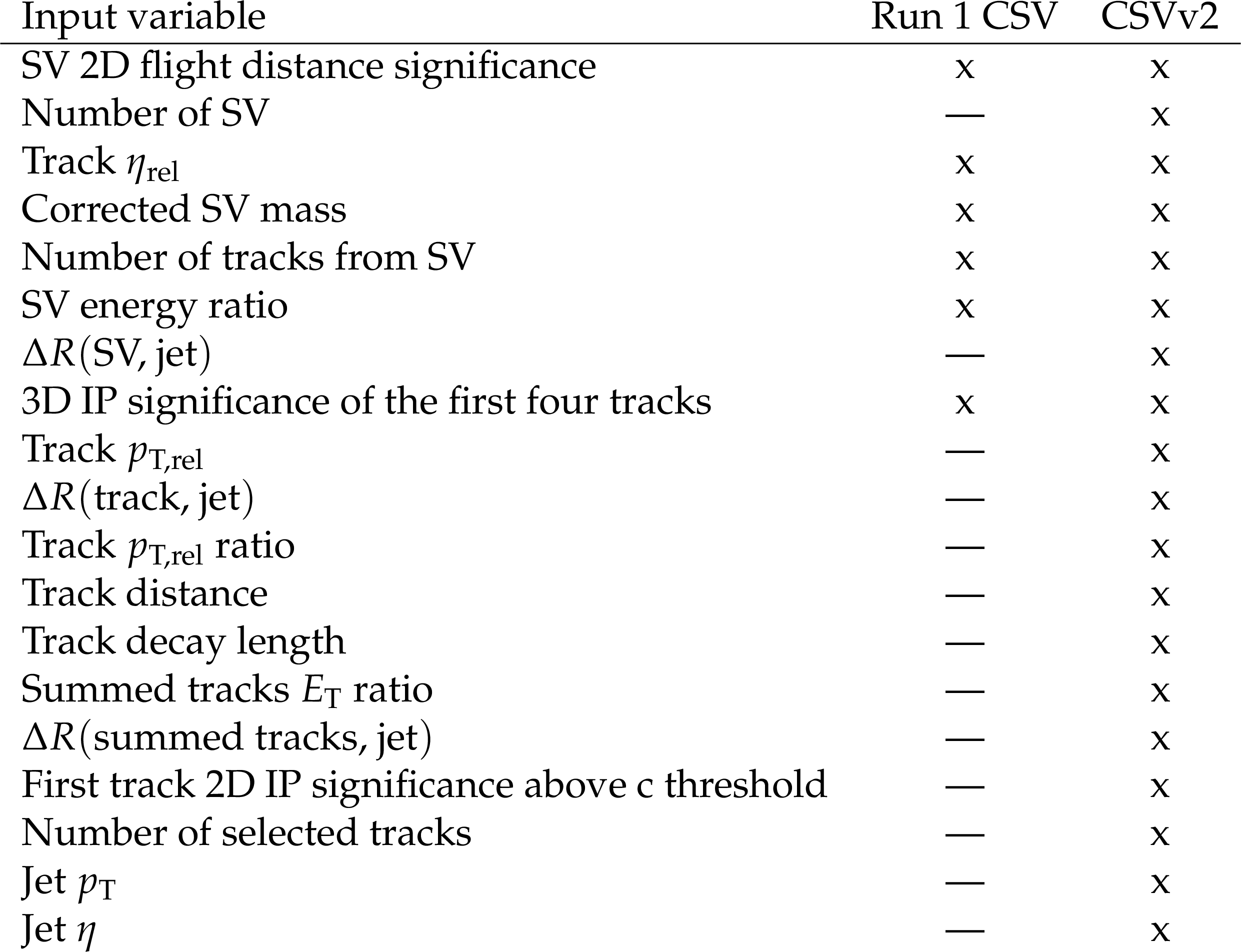
png pdf	Table 1: Input variables used for the Run 1 version of the CSV algorithm and for the CSVv2 algorithm. The symbol "x'' (" {\text {--}}{}'') means that the variable is (not) used in the algorithm
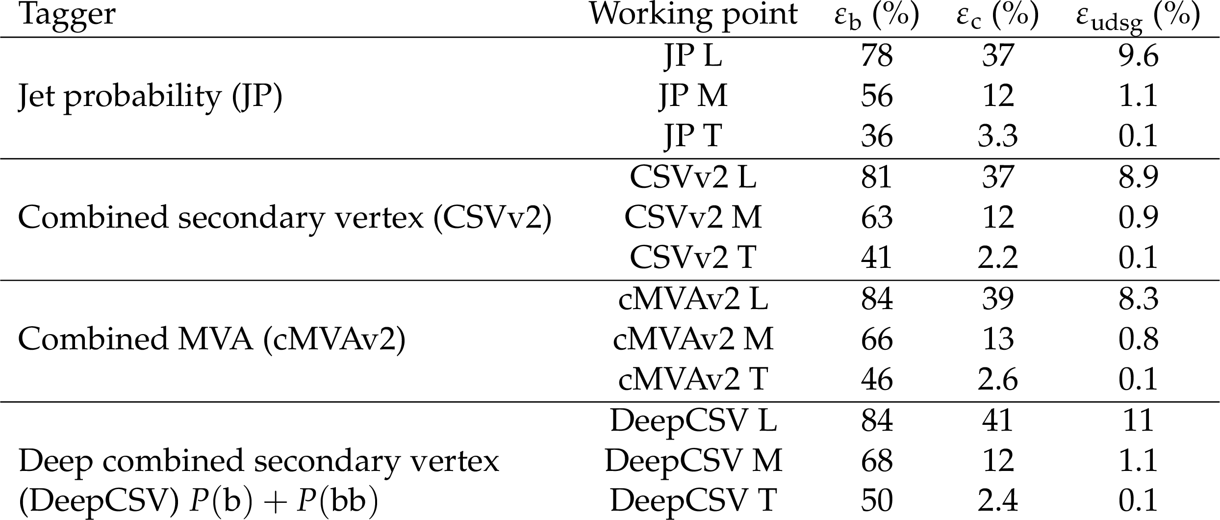
png pdf	Table 2: Taggers, working points, and corresponding efficiency for b jets with $ {p_{\mathrm {T}}} > $ 20 GeV in simulated $ {\mathrm {t}\overline {\mathrm {t}}} $ events. The numbers in this table are for illustrative purposes since the b jet identification efficiency is integrated over the $ {p_{\mathrm {T}}} $ and $\eta $ distributions of jets.
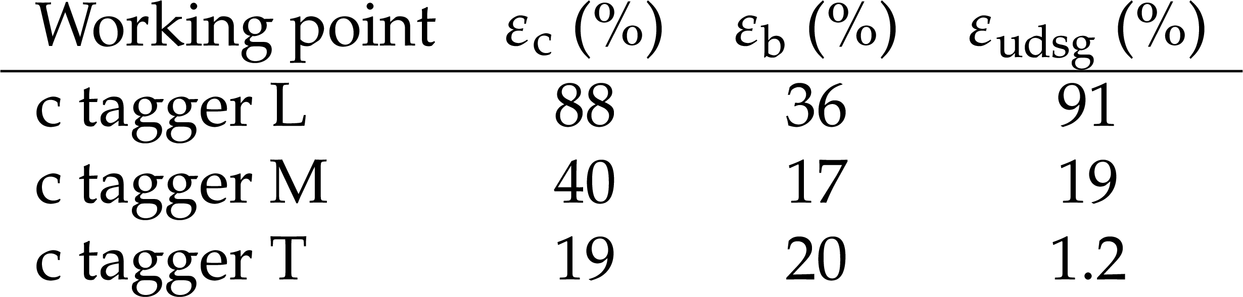
png pdf	Table 3: Efficiency for the working points of the c tagger and corresponding efficiency for the different jet flavours obtained using jets with $ {p_{\mathrm {T}}} > $ 20 GeV in simulated $ {\mathrm {t}\overline {\mathrm {t}}} $ events. The numbers quoted are for illustrative purposes since the efficiency is integrated over the $ {p_{\mathrm {T}}} $ and $\eta $ distributions of the jets.
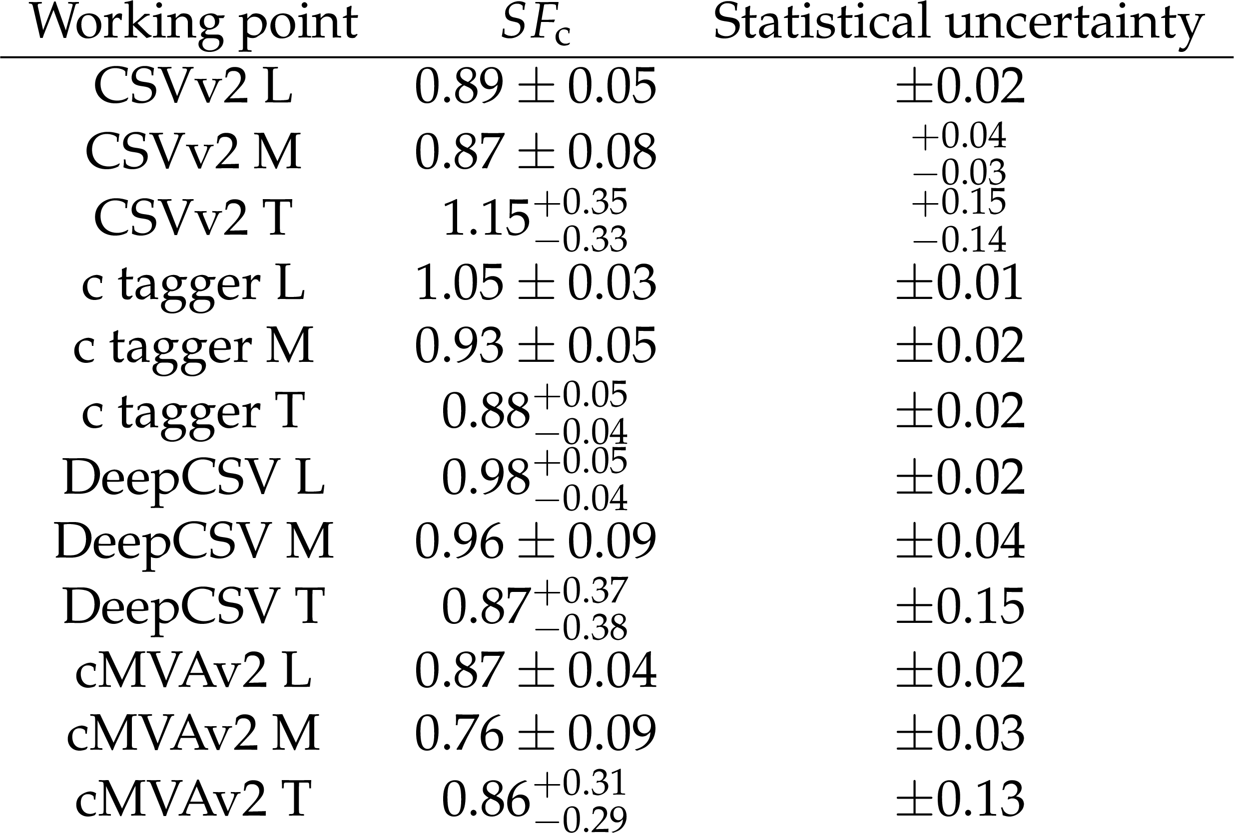
png pdf	Table 4: Measured data-to-simulation scale factors for c jets for various algorithms and working points in single-lepton $ {\mathrm {t}\overline {\mathrm {t}}} $ events. The uncertainty in the scale factor includes both the statistical and systematic uncertainties, while the last column shows the statistical uncertainty alone.
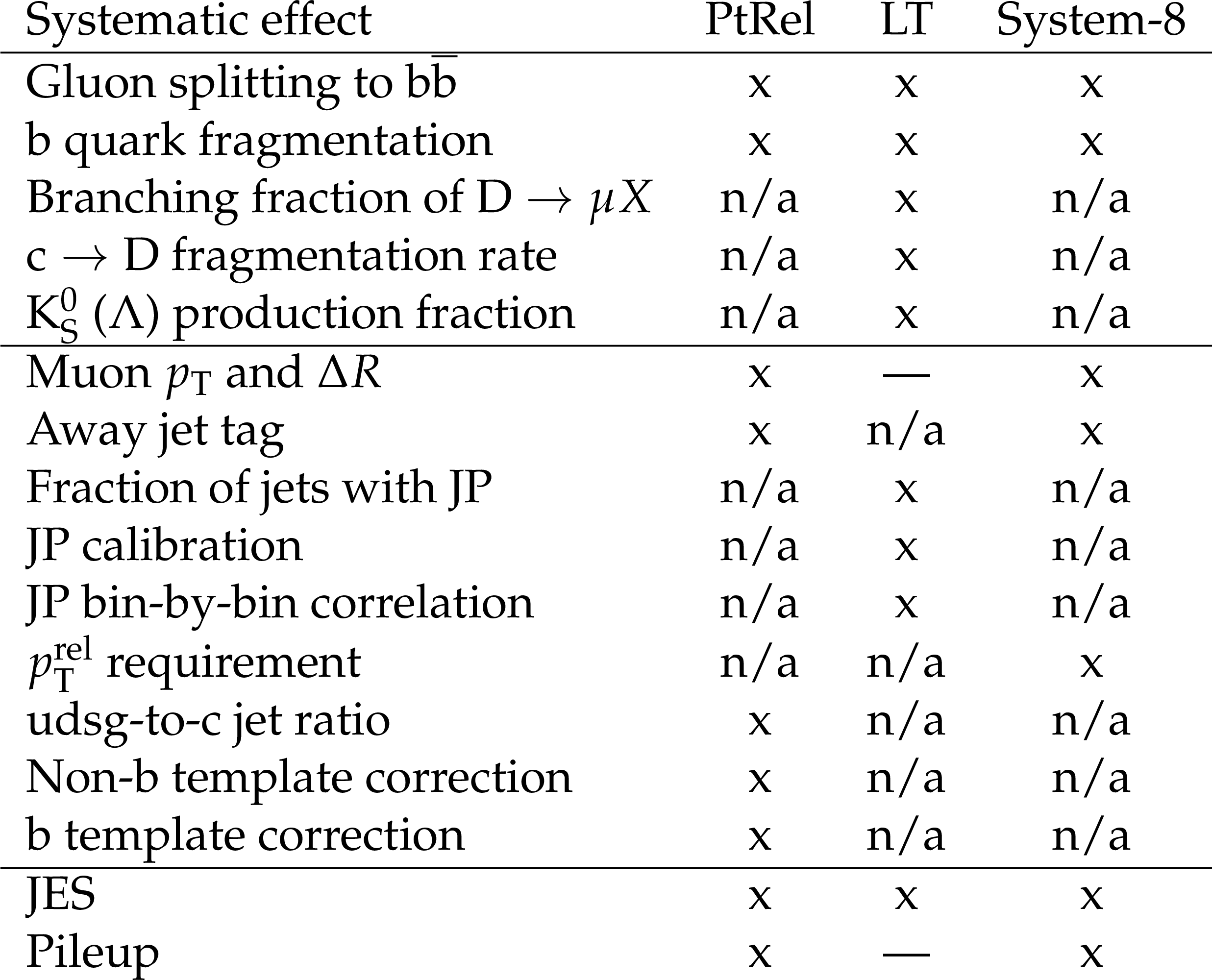
png pdf	Table 5: Summary of the potential sources of systematic effects taken into account for the muon-enriched $SF_{{\mathrm {b}}}$ measurements. The symbol "x'' means that the uncertainty is considered, "--'' means that it is negligible, and "n/a'' that it is not applicable. The systematic effects are separated by horizontal lines according to the type of uncertainty. The first set indicates the modelling uncertainty of heavy-flavour jets in the simulation, the second set are uncertainties related to the selection requirements or to the method that is applied, and the third set covers any other type of uncertainty.
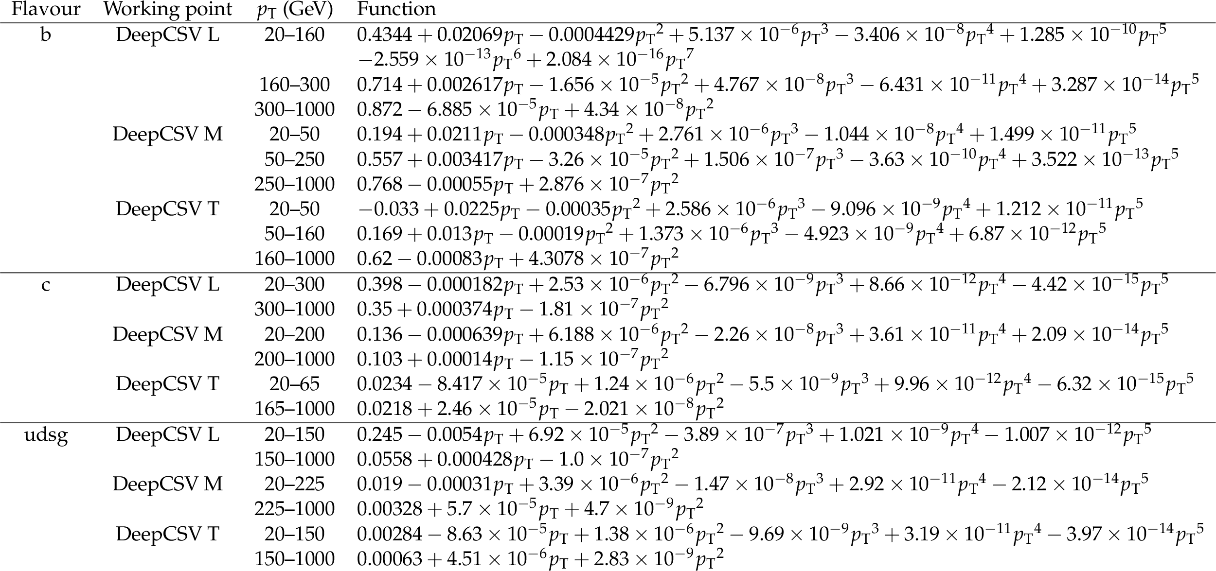
png pdf	Table 6: Polynomial functions used to fit the efficiency of the three working points of the DeepCSV algorithm for the three jet flavours as a function of the jet $ {p_{\mathrm {T}}} $ for jets with 20 $ < {p_{\mathrm {T}}} < $ 1000 GeV.

Summary

A variety of discriminating variables and algorithms used by the CMS experiment for the identification of heavy-flavour (charm and bottom) jets in proton-proton collisions at 13 TeV have been reviewed. Detailed simulation studies have allowed the reoptimization of existing b tagging algorithms and, in addition, new algorithms have been developed for the first time to identify c jets, as well as $ \mathrm{b\bar{b}} $ jets in events with boosted topologies. The performance of these heavy-flavour jet identification algorithms has been studied with simulations of different final states with heavy- and light-flavour quarks. The efficiency to correctly identify b jets in resolved $ \mathrm{t\bar{t}} $ events is 68% at a misidentification probability for light-flavour jets of 1%, which is an improvement of 15% in relative efficiency compared to the best performing algorithm used during LHC Run 1.

The variables and discriminators have been also compared to the data collected by the CMS experiment in 2016 for various event topologies enriched in heavy- or light-flavour jets. Various methods have been presented to determine the data-to-simulation scale factors for the heavy-flavour jet identification efficiency, as well as for the probability to misidentify light-flavour jets. A precision of a few per cent is obtained in the tagging efficiency for b jets with 30 $ < {p_{\mathrm{T}}} < $ 300 GeV. For b jets with ${p_{\mathrm{T}}} > $ 500 GeV, the precision is of the order of 5%. For scale factors measured in boosted topologies and for c jets in resolved topologies, the total uncertainty is 5-10%, and the statistical uncertainty in the tagging efficiency dominates over the full jet $ {p_{\mathrm{T}}} $ range.

With the increasing integrated luminosity delivered by the LHC, the precision of the data-to-simulation scale factors for the specified topologies, jet flavours, and $ {p_{\mathrm{T}}} $ ranges will increase further. Differential studies of the heavy-flavour identification performances as a function of jet pseudorapidity, and of the number of multiple proton-proton interactions in the same bunch crossing, will also become viable.

References
1	CMS Collaboration	Identification of b-quark jets with the CMS experiment	JINST 8 (2013) P04013	CMS-BTV-12-001 1211.4462
2	CMS Collaboration	Description and performance of track and primary-vertex reconstruction with the CMS tracker	JINST 9 (2014) P10009	CMS-TRK-11-001 1405.6569
3	K. Rose	Deterministic annealing for clustering, compression, classification, regression, and related optimization problems	in Proceedings of the IEEE, p. 2210 1998
4	R. Fruhwirth, W. Waltenberger, and P. Vanlaer	Adaptive vertex fitting	JPG 34 (2007) N343
5	CMS Collaboration	Particle-flow reconstruction and global event description with the CMS detector	JINST 12 (2017) P10003	CMS-PRF-14-001 1706.04965
6	M. Cacciari, G. P. Salam, and G. Soyez	The anti-$ k_t $ jet clustering algorithm	JHEP 04 (2008) 063	0802.1189
7	M. Cacciari, G. P. Salam, and G. Soyez	FastJet user manual	EPJC 72 (2012) 1896	1111.6097
8	CMS Collaboration	Jet energy scale and resolution in the CMS experiment in pp collisions at 8 TeV	JINST 12 (2016) P02014	CMS-JME-13-004 1607.03663
9	CMS Collaboration	Performance of electron reconstruction and selection with the CMS detector in proton-proton collisions at $ \sqrt{s} = $ 8 TeV	JINST 10 (2015) P06005	CMS-EGM-13-001 1502.02701
10	CMS Collaboration	Performance of CMS muon reconstruction in pp collision events at $ \sqrt{s} = $ 7 TeV	JINST 7 (2012) P10002	CMS-MUO-10-004 1206.4071
11	CMS Collaboration	The CMS trigger system	JINST 12 (2017) P01020	CMS-TRG-12-001 1609.02366
12	CMS Collaboration	The CMS experiment at the CERN LHC	JINST 3 (2008) S08004	CMS-00-001
13	GEANT4 Collaboration	GEANT4---a simulation toolkit	NIMA 506 (2003) 250
14	GEANT4 Collaboration	Recent developments in GEANT4	NIMA 835 (2016) 186
15	GEANT4 Collaboration	GEANT4 developments and applications	IEEE Transactions on Nuclear Science 53 (2006) 270
16	P. Nason	A new method for combining NLO QCD with shower Monte Carlo algorithms	JHEP 11 (2004) 040	hep-ph/0409146
17	S. Frixione, P. Nason, and C. Oleari	Matching NLO QCD computations with parton shower simulations: the POWHEG method	JHEP 11 (2007) 070	0709.2092
18	S. Alioli, P. Nason, C. Oleari, and E. Re	A general framework for implementing NLO calculations in shower Monte Carlo programs: the POWHEG BOX	JHEP 06 (2010) 043	1002.2581
19	J. M. Campbell, R. K. Ellis, P. Nason, and E. Re	Top-pair production and decay at NLO matched with parton showers	JHEP 04 (2015) 114	1412.1828
20	E. Re	Single-top $ Wt $-channel production matched with parton showers using the POWHEG method	EPJC 71 (2011) 1547	1009.2450
21	S. Alioli, P. Nason, C. Oleari, and E. Re	NLO single-top production matched with shower in POWHEG: $ s $- and $ t $-channel contributions	JHEP 09 (2009) 111	0907.4076
22	J. Alwall et al.	MadGraph 5: going beyond	JHEP 06 (2011) 128	1106.0522
23	P. Artoisenet, R. Frederix, O. Mattelaer, and R. Rietkerk	Automatic spin-entangled decays of heavy resonances in Monte Carlo simulations	JHEP 03 (2013) 015	1212.3460
24	R. Frederix and S. Frixione	Merging meets matching in MC@NLO	JHEP 12 (2012) 061	1209.6215
25	T. Melia, P. Nason, R. Rontsch, and G. Zanderighi	$ W^+W^- $, $ WZ $ and $ ZZ $ production in the POWHEG BOX	JHEP 11 (2011) 078	1107.5051
26	P. Nason and G. Zanderighi	$ W^+ W^- $ , $ W Z $ and $ Z Z $ production in the POWHEG-BOX-V2	EPJC 74 (2014) 2702	1311.1365
27	M. L. Mangano, M. Moretti, F. Piccinini, and M. Treccani	Matching matrix elements and shower evolution for top-pair production in hadronic collisions	JHEP 01 (2007) 013	hep-ph/0611129
28	L. Randall and R. Sundrum	Large mass hierarchy from a small extra dimension	PRL 83 (1999) 3370	hep-ph/9905221
29	T. Sjostrand et al.	An introduction to PYTHIA 8.2	CPC 191 (2015) 159	1410.3012
30	CMS Collaboration	Event generator tunes obtained from underlying event and multiparton scattering measurements	EPJC 76 (2016) 155	CMS-GEN-14-001 1512.00815
31	NNPDF Collaboration	Parton distributions with LHC data	NPB 867 (2013) 244	1207.1303
32	CMS Collaboration	Investigations of the impact of the parton shower tuning in PYTHIA 8 in the modelling of $ \mathrm{t\overline{t}} $ at $ \sqrt{s}= $ 8 and 13 TeV	CDS
33	NNPDF Collaboration	Parton distributions for the LHC Run II	JHEP 04 (2015) 040	1410.8849
34	M. Cacciari and G. P. Salam	Pileup subtraction using jet areas	PLB 659 (2008) 119	0707.1378
35	Particle Data Group Collaboration	Review of particle physics	CPC 40 (2016), no. 10, 100001
36	W. Waltenberger	Adaptive vertex reconstruction	CMS-NOTE-2008-033
37	CMS Collaboration	Measurement of $ B\bar{B} $ angular correlations based on secondary vertex reconstruction at $ \sqrt{s}= $ 7 TeV	JHEP 03 (2011) 136	CMS-BPH-10-010 1102.3194
38	D. Guest et al.	Jet flavor classification in high-energy physics with deep neural networks	PRD 94 (2016) 112002	1607.08633
39	W. S. Sarle	Neural networks and statistical models	in Proceedings of the Nineteenth Annual SAS Users Group International Conference 1994
40	F. Chollet	KERAS	link
41	M. Abadi et al.	TensorFlow: Large-scale machine learning on heterogeneous systems	2015 Software available from tensorflow.org
42	F. Pedregosa et al.	Scikit-learn: Machine learning in Python	J. Machine Learning Research 12 (2011) 2825	1201.0490
43	A. Dominguez et al.	CMS technical design report for the pixel detector upgrade	CMS Technical Design Report CERN-LHCC-2012-016, CMS-TDR-11, CERN
44	M. Lehmacher and N. Wermes	Measurement of the flavour composition of dijet events in proton-proton collisions at $ \sqrt{s} = $ 7 TeV with the ATLAS detector at the LHC	technical report, CERN
45	A. J. Larkoski, S. Marzani, G. Soyez, and J. Thaler	Soft drop	JHEP 05 (2014) 146	1402.2657
46	M. Dasgupta, A. Fregoso, S. Marzani, and G. P. Salam	Towards an understanding of jet substructure	JHEP 09 (2013) 029	1307.0007
47	J. Thaler and K. Van Tilburg	Identifying boosted objects with N-subjettiness	JHEP 03 (2011) 015	1011.2268
48	CMS Collaboration	Jet algorithms performance in 13 TeV data	CMS-PAS-JME-16-003	CMS-PAS-JME-16-003
49	J. M. Butterworth, A. R. Davison, M. Rubin, and G. P. Salam	Jet substructure as a new Higgs search channel at the LHC	in Proceedings, 34th International Conference on High Energy Physics (ICHEP 2008) SLAC, 2008 SLAC-eConf-C080730
50	D. Krohn, J. Thaler, and L.-T. Wang	Jet trimming	JHEP 02 (2010) 84	0912.1342
51	S. D. Ellis, C. K. Vermilion, and J. R. Walsh	Recombination algorithms and jet substructure: Pruning as a tool for heavy particle searches	PRD 81 (2010) 094023	0912.0033
52	H. Voss, A. Hocker, J. Stelzer, and F. Tegenfeldt	TMVA, the toolkit for multivariate data analysis with ROOT	in XIth International Workshop on Advanced Computing and Analysis Techniques in Physics Research (ACAT), p. 40 2007	physics/0703039
53	CMS Collaboration	Inclusive b-jet production in pp collisions at $ \sqrt{s}= $ 7 TeV	JHEP 04 (2012) 084	CMS-BPH-11-022 1202.4617
54	CMS Collaboration	Measurement of the inclusive jet cross section in pp collisions at $ \sqrt{s} = $ 7 TeV	PRL 107 (2011) 132001	CMS-QCD-10-011 1106.0208
55	CMS Collaboration	CMS tracking performance results from early LHC operation	EPJC 70 (2010) 1165	CMS-TRK-10-001 1007.1988
56	CMS Collaboration	Strange particle production in pp collisions at $ \sqrt{s} = $ 0.9 and 7 TeV	JHEP 05 (2011) 064	CMS-QCD-10-007 1102.4282
57	ATLAS Collaboration	Measurement of the inelastic proton-proton cross section at $ \sqrt{s} = $ 13 ~TeV with the ATLAS detector at the LHC	PRL 117 (2016) 182002	1606.02625
58	CMS Collaboration	Measurement of associated W + charm production in pp collisions at $ \sqrt{s} = $ 7 TeV	JHEP 02 (2014) 013	CMS-SMP-12-002 1310.1138
59	L. Gladilin	Fragmentation fractions of $ c $ and $ b $ quarks into charmed hadrons at LEP	EPJC 75 (2015), no. 1, 19	1404.3888
60	CMS Collaboration	Measurement of differential cross sections for top quark pair production using the lepton+jets final state in proton-proton collisions at 13 TeV	PRD 95 (2017) 092001	CMS-TOP-16-008 1610.04191
61	CMS Collaboration	Cross section measurement of $ t $-channel single top quark production in pp collisions at $ \sqrt s = $ 13 TeV	PLB 772 (2017) 752	CMS-TOP-16-003 1610.00678
62	CMS Collaboration	Observation of the associated production of a single top quark and a $ W $ boson in $ pp $ collisions at $ \sqrt s = $ 8 TeV	PRL 112 (2014) 231802	CMS-TOP-12-040 1401.2942
63	CMS Collaboration	Measurement of the differential cross sections for the associated production of a W boson and jets in proton-proton collisions at $ \sqrt{s} = $ 13 TeV	Submitted to PRD	CMS-SMP-16-005 1707.05979
64	CMS Collaboration	Measurement of the production cross section of a W boson in association with two b jets in pp collisions at $ \sqrt{s} = 8{ \mathrm{{TeV}}} $	EPJC 77 (2017) 92	CMS-SMP-14-020 1608.07561
65	CMS Collaboration	CMS luminosity measurements for the 2016 data taking period	CMS-PAS-LUM-17-001	CMS-PAS-LUM-17-001
66	P. Skands, S. Carrazza, and J. Rojo	Tuning $ PYTHIA $ 8.1: the Monash 2013 tune	EPJC 74 (2014) 3024	1404.5630
67	L. Lyons, D. Gibaut, and P. Clifford	How to combine correlated estimates of a single physical quantity	NIMA 270 (1988) 110
68	A. Valassi	Combining correlated measurements of several different physical quantities	NIMA 500 (2003) 391
69	PDG Collaboration	Review of particle physics	PLB 667 (2008) 1
70	G. Mahlon and S. J. Parke	Spin correlation effects in top quark pair production at the LHC	PRD 81 (2010) 074024	1001.3422
71	B. A. Betchart, R. Demina, and A. Harel	Analytic solutions for neutrino momenta in decay of top quarks	NIMA 736 (2014) 169	1305.1878
72	ALEPH Collaboration	A measurement of the gluon splitting rate into $ \mathrm{c \bar{c}} $ pairs in hadronic Z decays	PLB 561 (2003) 213	hep-ex/0302003
73	ALEPH Collaboration	Measurement of the gluon splitting rate into $ \mathrm{b \bar{b}} $ pairs in hadronic Z decays	PLB 434 (1998) 437
74	CMS Collaboration	Search for the associated production of the Higgs boson with a top-quark pair	JHEP 09 (2014) 087	CMS-HIG-13-029 1408.1682
75	CMS Collaboration	Measurement of the $ \mathrm{t}\overline{\mathrm{t}} $ production cross section in the all-jets final state in pp collisions at $ \sqrt{s} = $ 8 TeV	EPJC 76 (2015) 128	CMS-TOP-14-018 1509.06076
76	CMS Collaboration	Measurement of the differential cross section for top quark pair production in pp collisions at $ \sqrt{s} = $ 8 TeV	EPJC 75 (2015) 542	CMS-TOP-12-028 1505.0448