

Compact Muon Solenoid
LHC, CERN
| CMS-EGM-18-002 ; CERN-EP-2024-014 | ||
| Performance of the CMS electromagnetic calorimeter in pp collisions at $ \sqrt{s}= $ 13 TeV | ||
| CMS Collaboration | ||
| 23 March 2024 | ||
| Submitted to J. Instrum. | ||
| Abstract: The operation and performance of the Compact Muon Solenoid (CMS) electromagnetic calorimeter (ECAL) are presented, based on data collected in pp collisions at $ \sqrt{s}= $ 13 TeV at the CERN LHC, in the years from 2015 to 2018 (LHC Run 2), corresponding to an integrated luminosity of 151 fb$ ^{-1} $. The CMS ECAL is a scintillating lead-tungstate crystal calorimeter, with a silicon strip preshower detector in the forward region that provides precise measurements of the energy and the time-of-arrival of electrons and photons. The successful operation of the ECAL is crucial for a broad range of physics goals, ranging from observing the Higgs boson and measuring its properties, to other standard model measurements and searches for new phenomena. Precise calibration, alignment, and monitoring of the ECAL response are important ingredients to achieve these goals. To face the challenges posed by the higher luminosity, which characterized the operation of the LHC in Run 2, the procedures established during the 2011-2012 run of the LHC have been revisited and new methods have been developed for the energy measurement and for the ECAL calibration. The energy resolution of the calorimeter, for electrons from Z boson decays reaching the ECAL without significant loss of energy by bremsstrahlung, was better than 1.8%, 3.0%, and 4.5% in the $ |\eta| $ intervals $ [$0.0, 0.8$] $, $ [$0.8, 1.5$] $, $ [$1.5, 2.5$] $, respectively. This resulting performance is similar to that achieved during Run 1 in 2011-2012, in spite of the more severe running conditions. | ||
| Links: e-print arXiv:2403.15518 [hep-ex] (PDF) ; CDS record ; inSPIRE record ; CADI line (restricted) ; | ||
| Figures | |
png pdf |
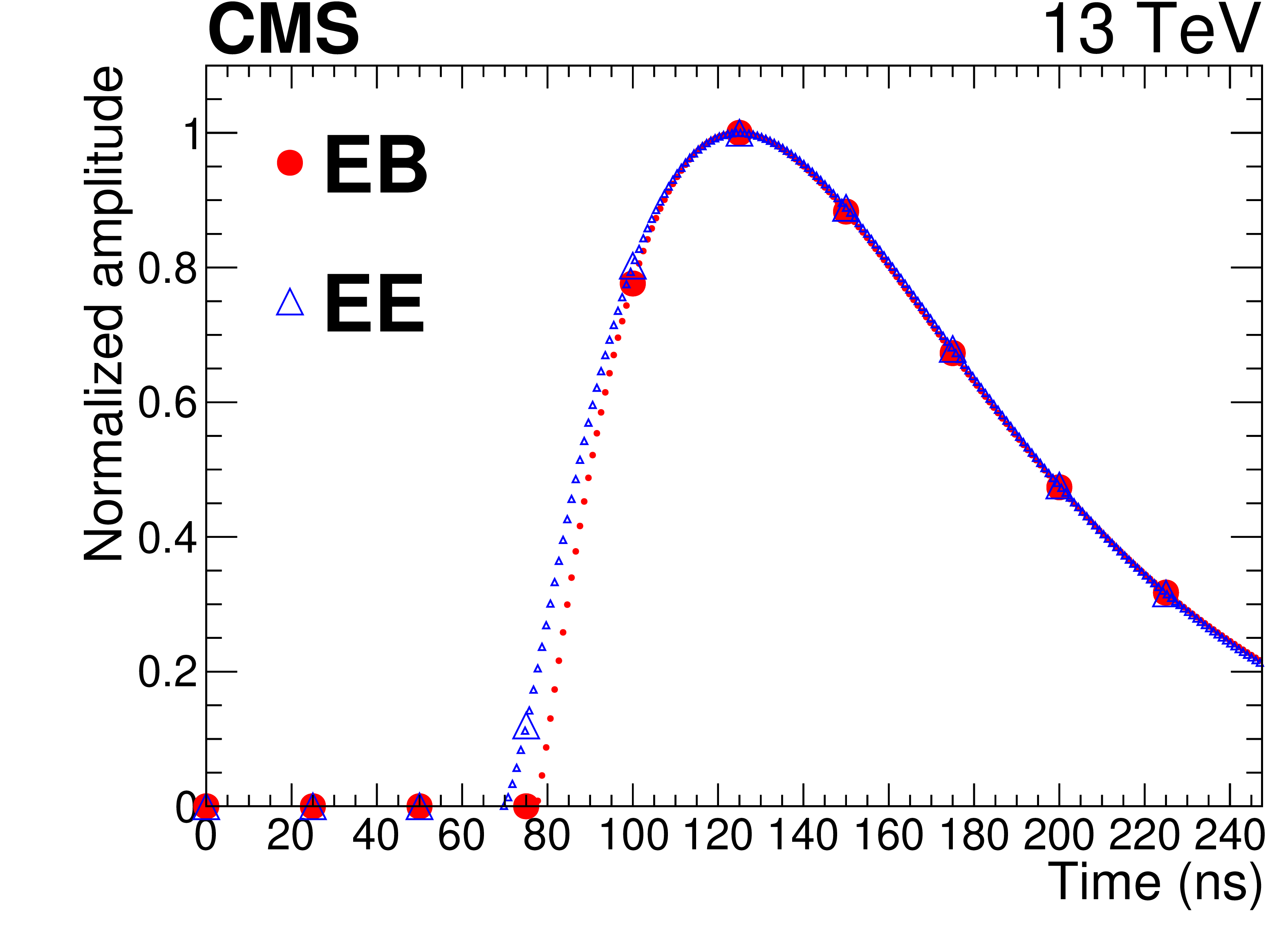
Figure 1:
Average signal pulse shape for a channel for the EB (red filled circles), and the EE (blue hollow triangles), after subtraction of the pedestal. The ten larger markers are an example of a pulse shape sampled once every 25 ns. The dots are the result of a granular timing scan provides a more precise measurement of the pulse. |

png pdf |
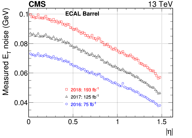
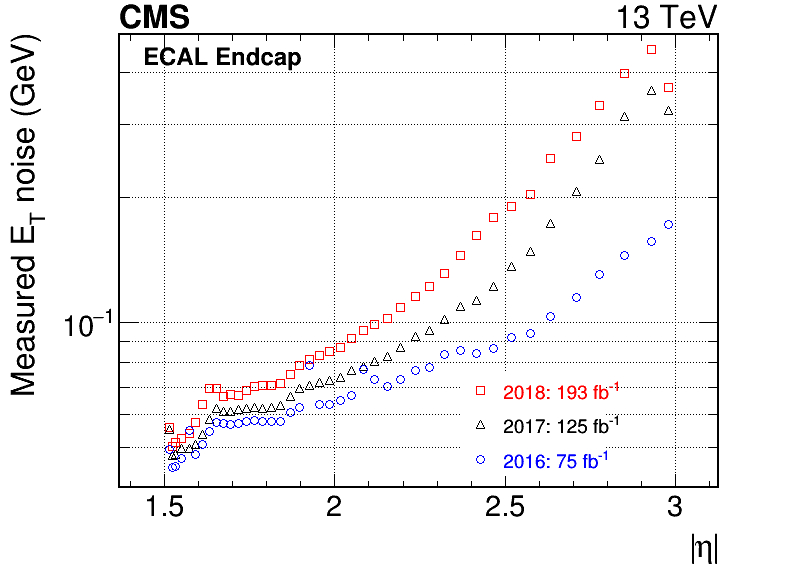
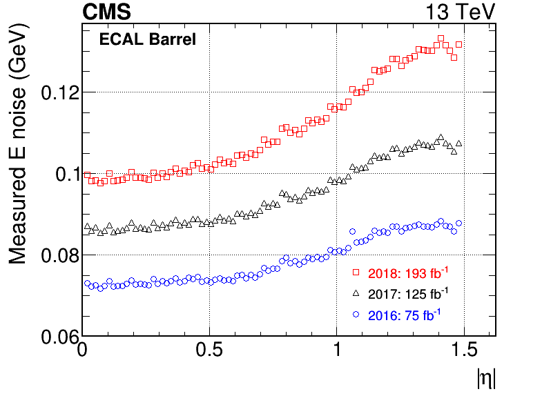
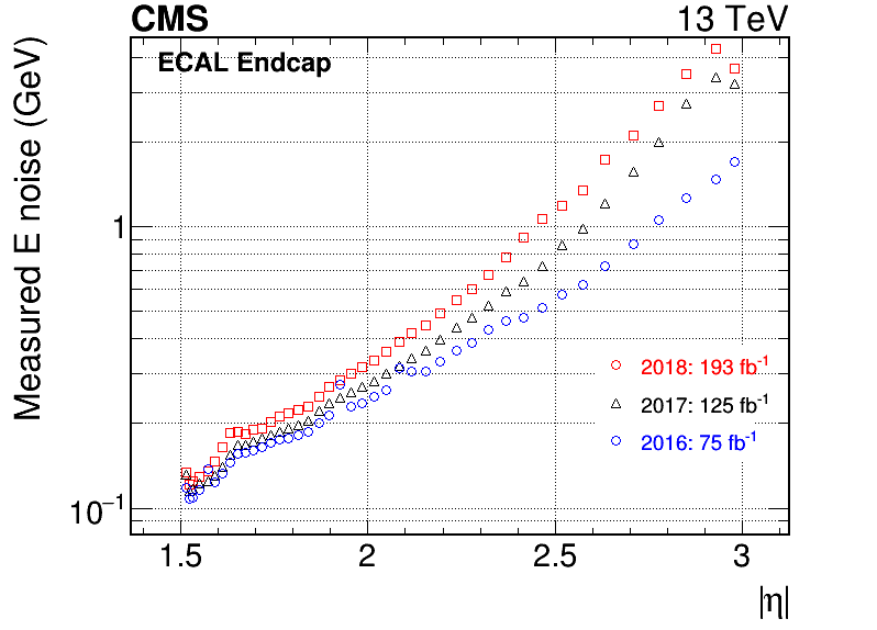
Figure 2:
Average energy-equivalent noise for the EB (left column) and the EE (right column) at the end of 2016, 2017, and 2018, measured as the 1 sigma variation of the pedestal baseline values for each channel and converted into energy using Eq. (1). Both transverse energy (upper row) and energy (lower row) are shown. The integrated luminosity for the different years refers to the cumulated delivered luminosity since the beginning of Run 1. |
png |
Figure 2-a:
Average energy-equivalent noise for the EB (left column) and the EE (right column) at the end of 2016, 2017, and 2018, measured as the 1 sigma variation of the pedestal baseline values for each channel and converted into energy using Eq. (1). Both transverse energy (upper row) and energy (lower row) are shown. The integrated luminosity for the different years refers to the cumulated delivered luminosity since the beginning of Run 1. |
png |
Figure 2-b:
Average energy-equivalent noise for the EB (left column) and the EE (right column) at the end of 2016, 2017, and 2018, measured as the 1 sigma variation of the pedestal baseline values for each channel and converted into energy using Eq. (1). Both transverse energy (upper row) and energy (lower row) are shown. The integrated luminosity for the different years refers to the cumulated delivered luminosity since the beginning of Run 1. |
png |
Figure 2-c:
Average energy-equivalent noise for the EB (left column) and the EE (right column) at the end of 2016, 2017, and 2018, measured as the 1 sigma variation of the pedestal baseline values for each channel and converted into energy using Eq. (1). Both transverse energy (upper row) and energy (lower row) are shown. The integrated luminosity for the different years refers to the cumulated delivered luminosity since the beginning of Run 1. |
png |
Figure 2-d:
Average energy-equivalent noise for the EB (left column) and the EE (right column) at the end of 2016, 2017, and 2018, measured as the 1 sigma variation of the pedestal baseline values for each channel and converted into energy using Eq. (1). Both transverse energy (upper row) and energy (lower row) are shown. The integrated luminosity for the different years refers to the cumulated delivered luminosity since the beginning of Run 1. |
png pdf |
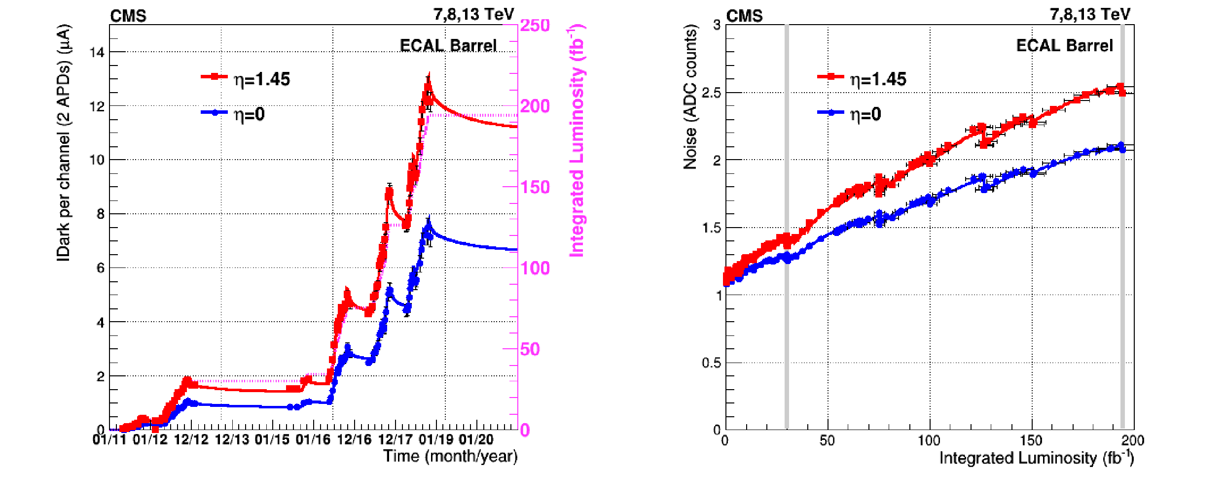
Figure 3:
The APD dark current (IDark) evolution versus time in EB (left), in red for the channels at $ |\eta|= $ 1.45 and in blue for the channels at $ \eta= $ 0, with the continuous lines representing the prediction of the model. The delivered integrated luminosity since the beginning of Run 1 is also shown in purple. The scale of the integrated luminosity axis is chosen such that it tends to overlap with the dark current at $ |\eta|= $ 1.45, in order to emphasize visually the strong correlation between dark current and integrated luminosity. The vertical bars on the points represent the uncertainty in the dark current measurement. On the right, the APD noise estimated from the dark current (continuous line) is compared with the direct noise measurement (data points) for the two $ \eta $ regions. The vertical grey lines in the right plot indicate the region corresponding to Run 2. The horizontal bars on the points represent the uncertainty on the luminosity. |
png |
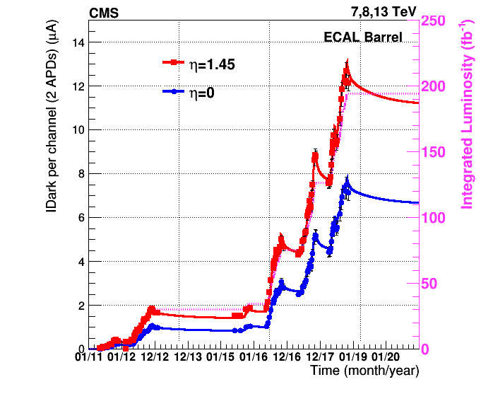
Figure 3-a:
The APD dark current (IDark) evolution versus time in EB (left), in red for the channels at $ |\eta|= $ 1.45 and in blue for the channels at $ \eta= $ 0, with the continuous lines representing the prediction of the model. The delivered integrated luminosity since the beginning of Run 1 is also shown in purple. The scale of the integrated luminosity axis is chosen such that it tends to overlap with the dark current at $ |\eta|= $ 1.45, in order to emphasize visually the strong correlation between dark current and integrated luminosity. The vertical bars on the points represent the uncertainty in the dark current measurement. On the right, the APD noise estimated from the dark current (continuous line) is compared with the direct noise measurement (data points) for the two $ \eta $ regions. The vertical grey lines in the right plot indicate the region corresponding to Run 2. The horizontal bars on the points represent the uncertainty on the luminosity. |
png |
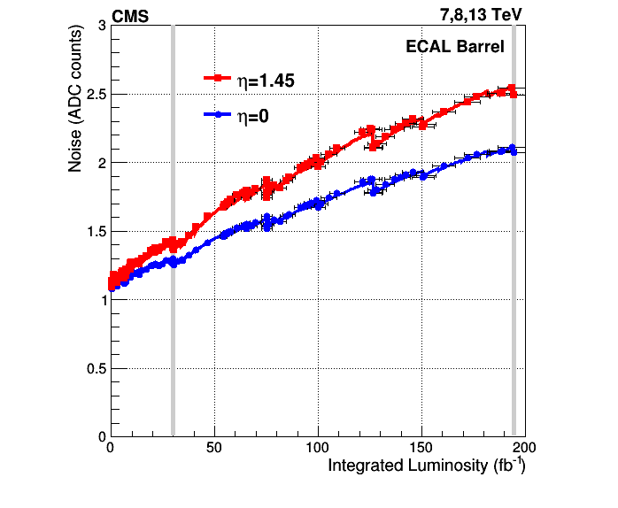
Figure 3-b:
The APD dark current (IDark) evolution versus time in EB (left), in red for the channels at $ |\eta|= $ 1.45 and in blue for the channels at $ \eta= $ 0, with the continuous lines representing the prediction of the model. The delivered integrated luminosity since the beginning of Run 1 is also shown in purple. The scale of the integrated luminosity axis is chosen such that it tends to overlap with the dark current at $ |\eta|= $ 1.45, in order to emphasize visually the strong correlation between dark current and integrated luminosity. The vertical bars on the points represent the uncertainty in the dark current measurement. On the right, the APD noise estimated from the dark current (continuous line) is compared with the direct noise measurement (data points) for the two $ \eta $ regions. The vertical grey lines in the right plot indicate the region corresponding to Run 2. The horizontal bars on the points represent the uncertainty on the luminosity. |

png pdf |
Figure 4:
Relative response to laser light (440 nm in 2011 and 447 nm from 2012 onwards) injected into the ECAL crystals, measured by the ECAL light monitoring system, averaged over all crystals in bins of pseudorapidity ($ |\eta| $). The lower panel shows the instantaneous LHC luminosity as a function of time. |

png pdf |
Figure 5:
The stability of the relative energy scale measured from the invariant mass distribution of $ \pi^{0} \to \gamma \gamma $ decays in the EB as a function of time, over a period of 3 hours during an LHC fill. The plot shows the data with (green points) and without (red points) the light-monitoring corrections applied. The vertical bars on the points represent the statistal uncertainty. The right-hand panel shows the 1D projections of the points in the left panel. The mean value and root-mean-square (RMS) are shown. |

png pdf |
Figure 6:
The stability of the relative energy scale measured from the ratio of the energy of electrons, as measured by the ECAL (EB, $ |\eta| < $ 0.43), and the electron momentum, as measured by the tracker. The stability is shown for a period of 4 consecutive LHC fills, with the limits of the fills delineated with vertical lines. The laser corrections were applied. Each point of the plot is obtained from a fit of the $ E/p $ distribution to approximately one hour of data taking. The vertical bars on the points represent the statistal uncertainty. The origin of the residual scale variation observed can be due to pileup variation and to less accurate measurement of transparency variation at the very beginning of the fill, when the response changes rapidly with time. After the beginning of a fill, the change of scale is less than 0.4%. |
png pdf |
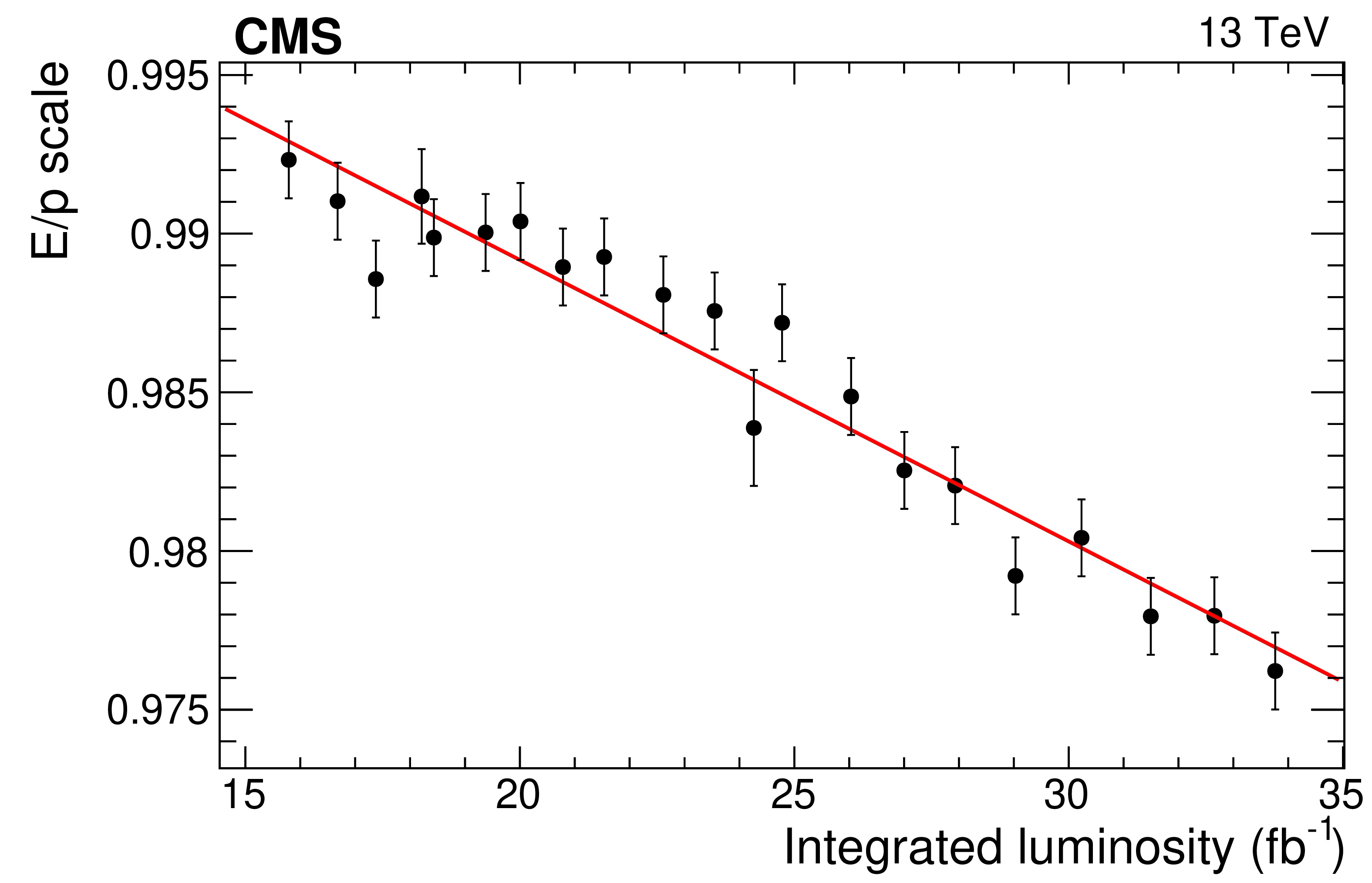
Figure 7:
The average ratio of the ECAL energy to the track momentum for electrons from W boson decays reconstructed in the crystals of one light-monitoring harness, as a function of delivered integrated luminosity during 2018. The vertical bars on the points represent the statistal uncertainty. A linear fit to the data (red line) is superimposed. For this particular light-monitoring harness a drift of 1% every 10 fb$ ^{-1} $ is measured. The dimension of the intervals on the horizontal axis is chosen such that each point is obtained from a sample of about 10000 electrons. This corresponds to about 1-2 days of data taking for the modules in the inner EB ($ |\eta| < $ 0.8), and about 2-3 days for the modules in the outer EB (0.8 $ < |\eta| < $ 1.5). |
png pdf |
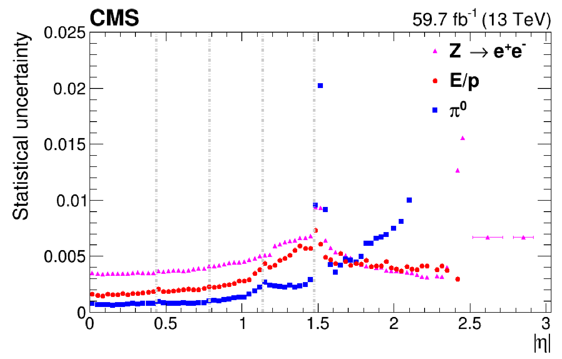
Figure 8:
The statistical uncertainties in the different intercalibration methods for data collected in 2018. The vertical dotted lines mark the boundary between the ECAL modules in the EB and the EB/EE transition. The increase in the statistical uncertainties for the last two points for the $ \mathrm{Z}\to\mathrm{e}^+\mathrm{e}^- $ method close to $ |\eta| = $ 2.5 are due to a reduction in the efficiency of the selection of two electrons since this $ |\eta| $ value corresponds to the end of the tracker coverage. A similar performance is observed for data collected in 2016 and 2017. |
png pdf |
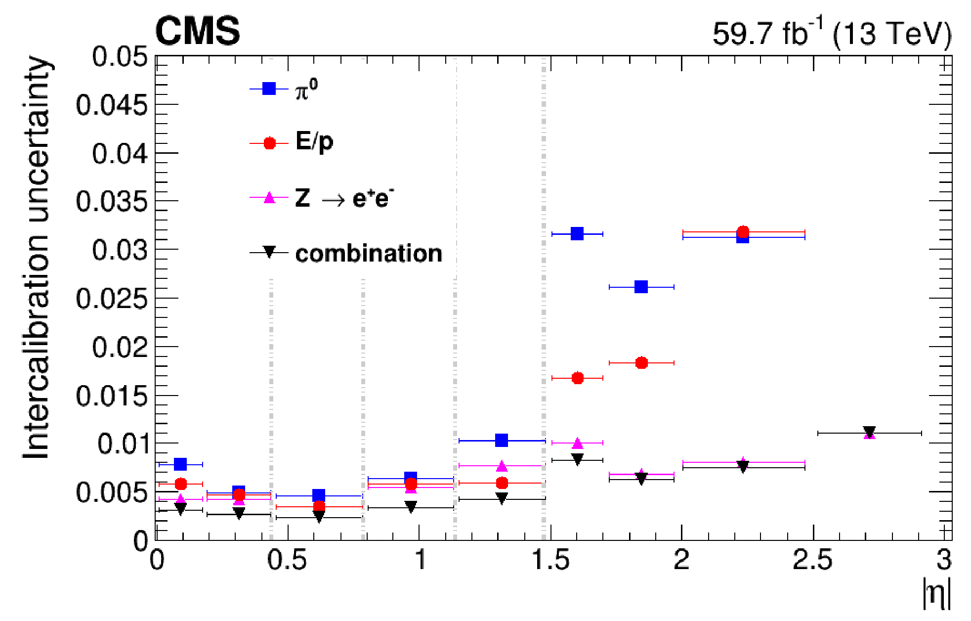
Figure 9:
The precision of the different IC measurement methods, as well as their combination, in 2018. The vertical dotted lines mark the boundary between the ECAL modules in the EB and the EB/EE transition. In the region outside the tracker coverage, $ |\eta| > $ 2.5, only the $ \mathrm{Z}\to\mathrm{e}^+\mathrm{e}^- $ method is available for calibration. Similar performance is observed in data collected in 2016 and 2017. |
png pdf |
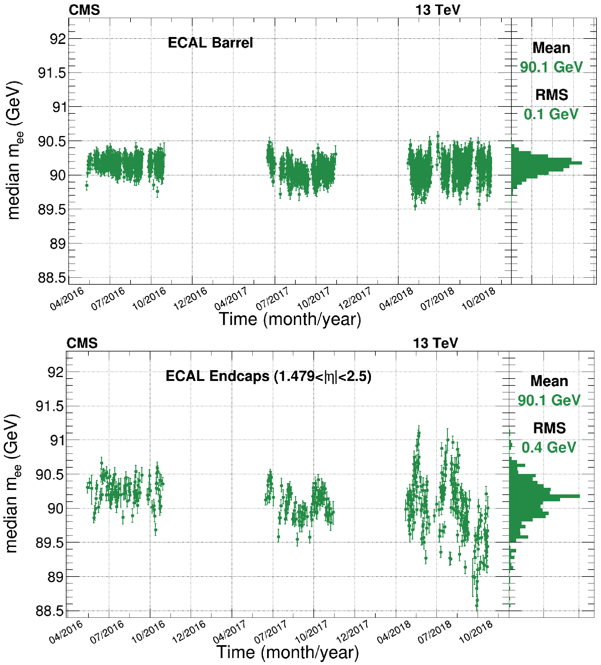
Figure 10:
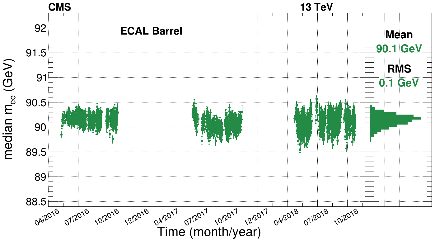
Time stability of the dielectron invariant mass distribution for the Run 2 data-taking period using $ \mathrm{Z}\to\mathrm{e}^+\mathrm{e}^- $ electrons. Both electrons are required to be in the EB (upper) or in the EE (lower). Each time bin contains about ten thousand events. The error bar on the points denotes the statistical uncertainty (at 95% confidence level) on the median. The right panel shows the distribution of the medians. |
png |
Figure 10-a:
Time stability of the dielectron invariant mass distribution for the Run 2 data-taking period using $ \mathrm{Z}\to\mathrm{e}^+\mathrm{e}^- $ electrons. Both electrons are required to be in the EB (upper) or in the EE (lower). Each time bin contains about ten thousand events. The error bar on the points denotes the statistical uncertainty (at 95% confidence level) on the median. The right panel shows the distribution of the medians. |

png |
Figure 10-b:
Time stability of the dielectron invariant mass distribution for the Run 2 data-taking period using $ \mathrm{Z}\to\mathrm{e}^+\mathrm{e}^- $ electrons. Both electrons are required to be in the EB (upper) or in the EE (lower). Each time bin contains about ten thousand events. The error bar on the points denotes the statistical uncertainty (at 95% confidence level) on the median. The right panel shows the distribution of the medians. |
png pdf |
Figure 11:
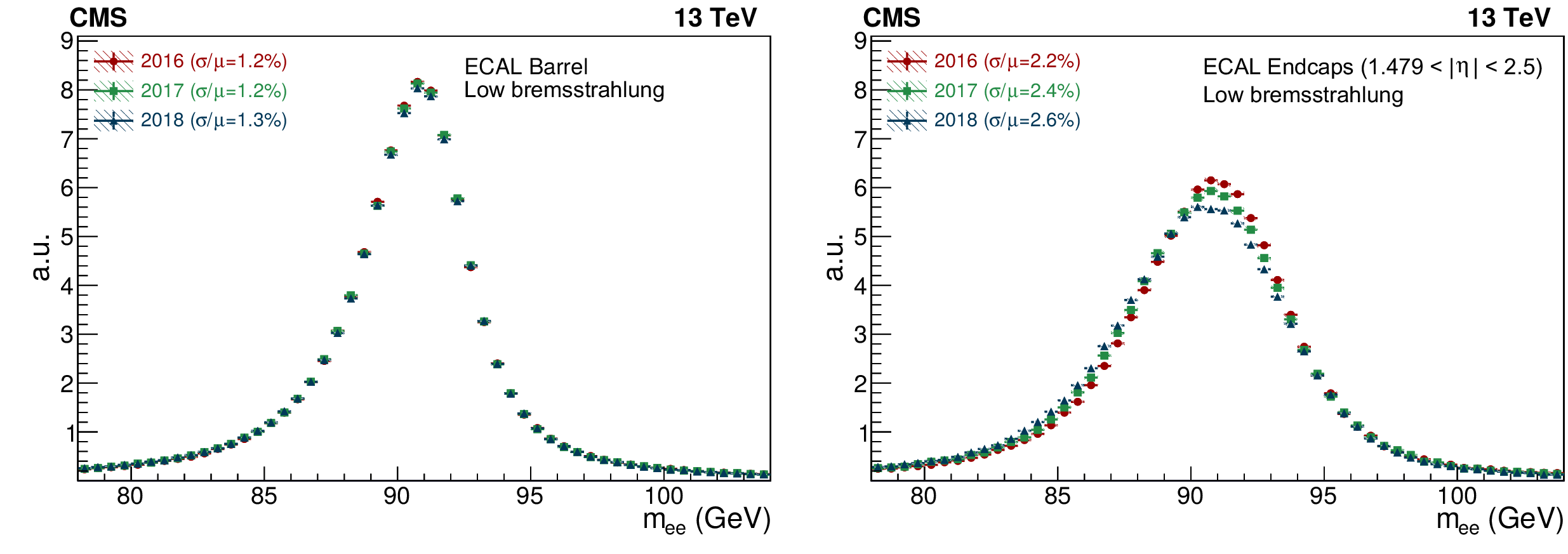
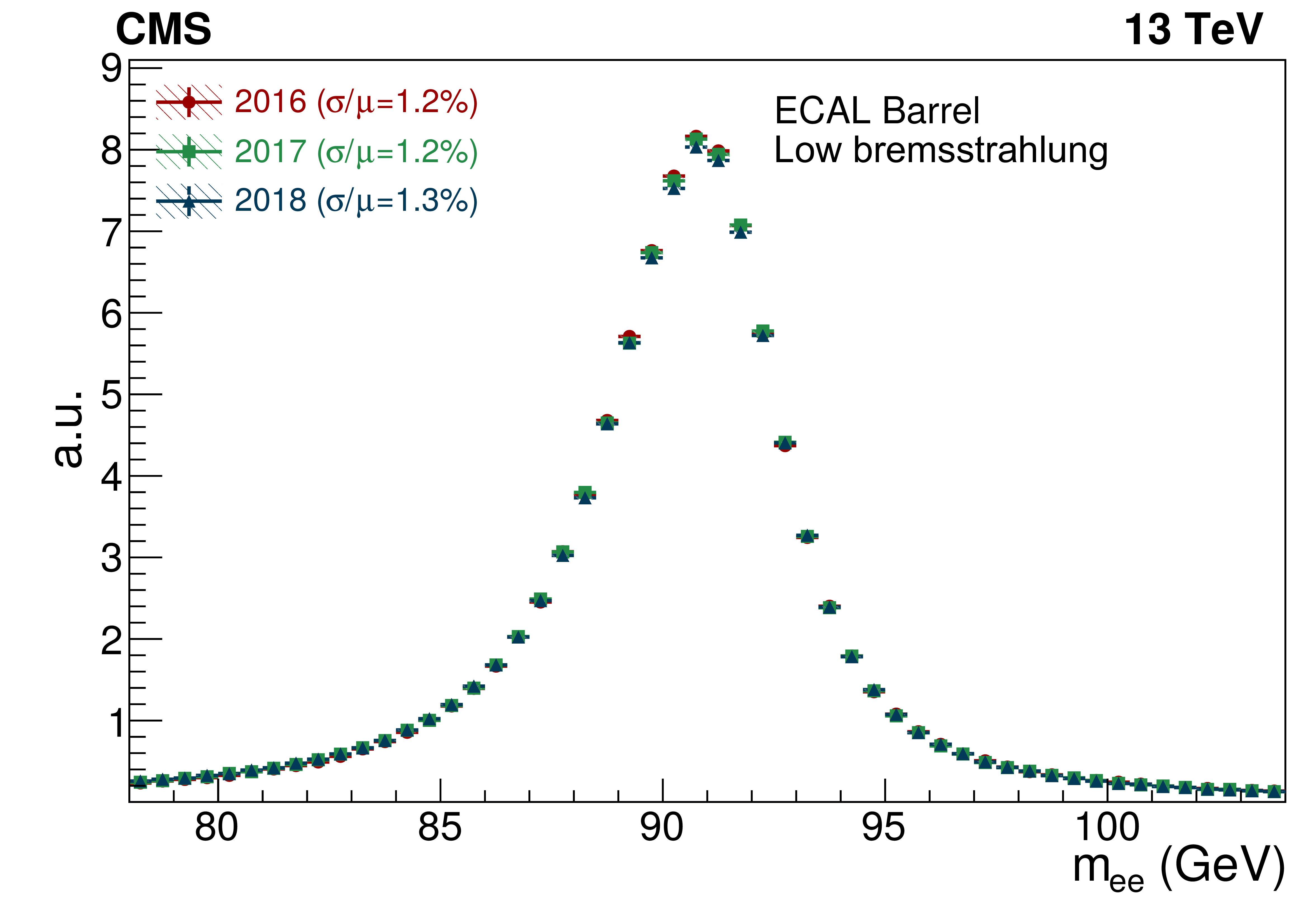
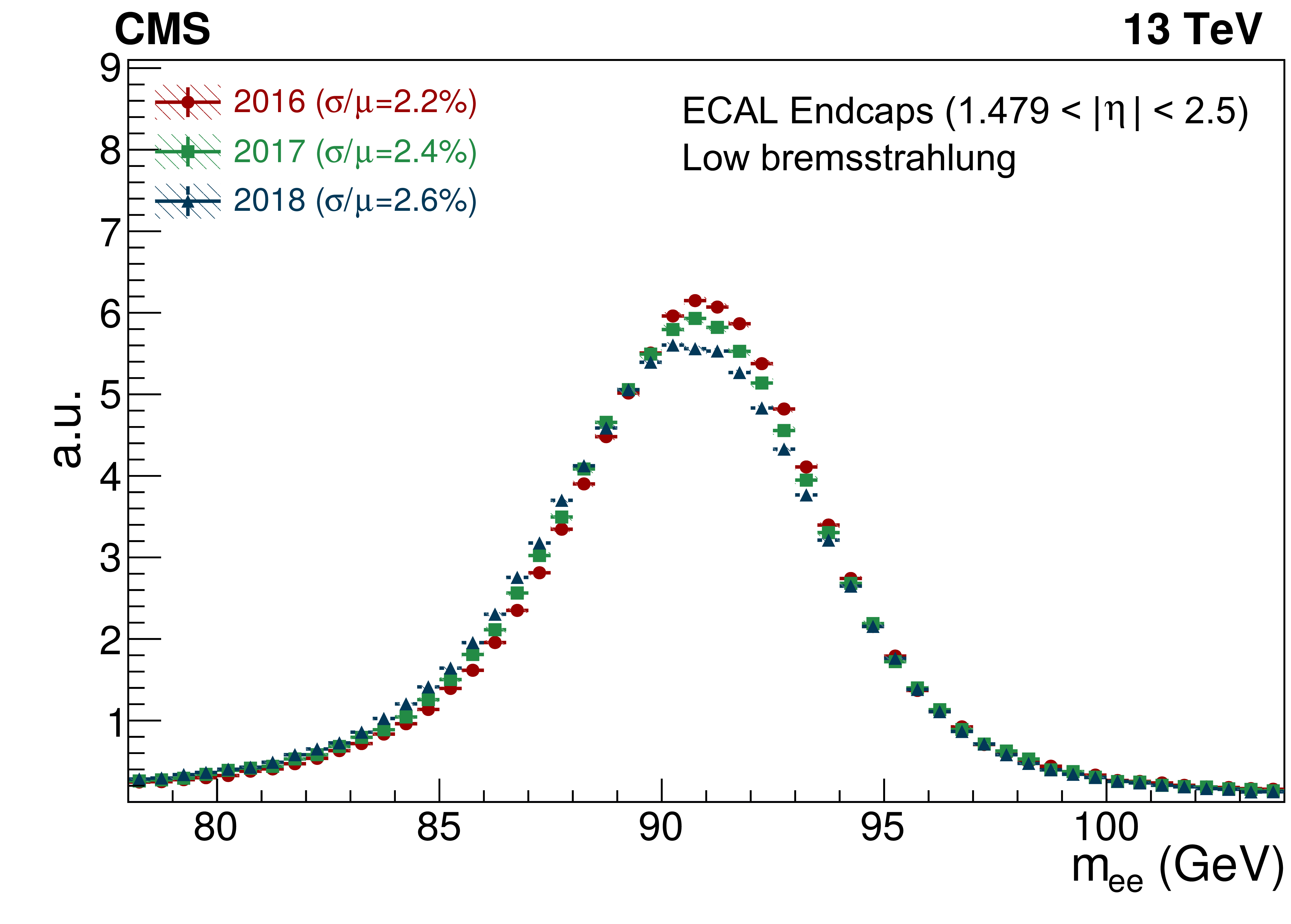
Invariant mass distribution for electron-positron pairs from Z boson decays using low-bremsstrahlung electrons. The distributions from data recorded in 2016, 2017, and 2018 are shown with different colours. The event selection requires two electrons to be in the EB (left) or in the EE within the tracker acceptance (right). The vertical bars on the points represent the statistal uncertainty. |
png pdf |
Figure 11-a:
Invariant mass distribution for electron-positron pairs from Z boson decays using low-bremsstrahlung electrons. The distributions from data recorded in 2016, 2017, and 2018 are shown with different colours. The event selection requires two electrons to be in the EB (left) or in the EE within the tracker acceptance (right). The vertical bars on the points represent the statistal uncertainty. |
png pdf |
Figure 11-b:
Invariant mass distribution for electron-positron pairs from Z boson decays using low-bremsstrahlung electrons. The distributions from data recorded in 2016, 2017, and 2018 are shown with different colours. The event selection requires two electrons to be in the EB (left) or in the EE within the tracker acceptance (right). The vertical bars on the points represent the statistal uncertainty. |
png pdf |
Figure 12:
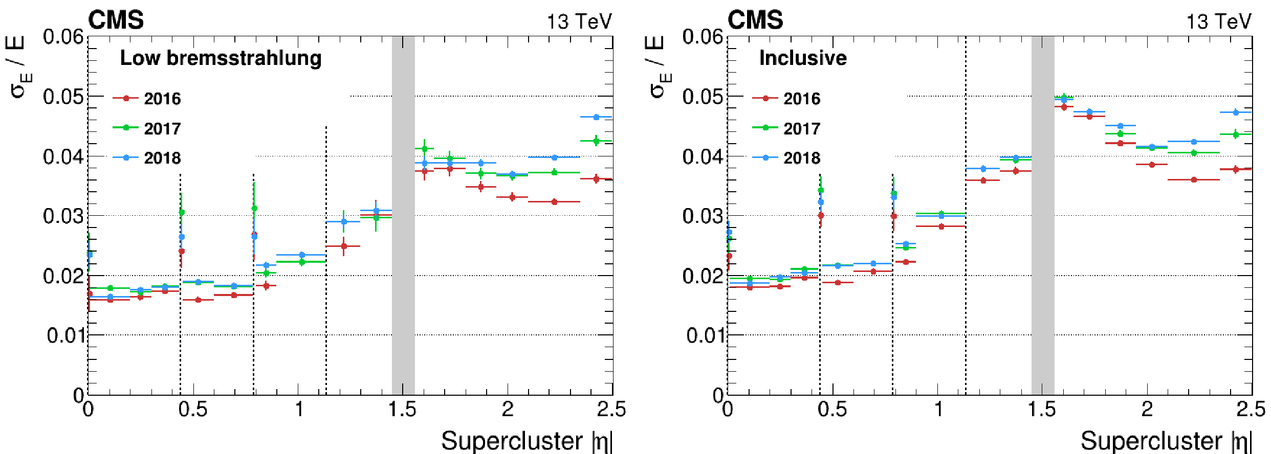
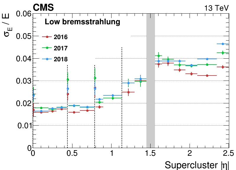
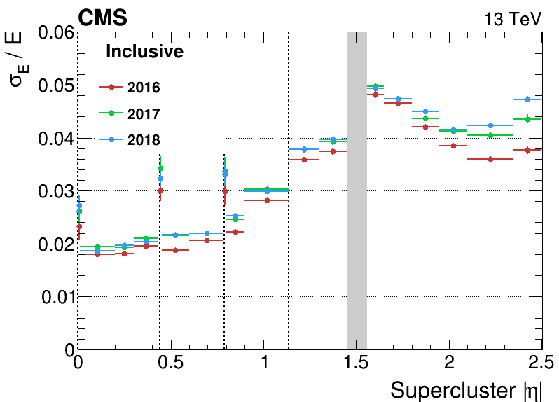
Relative energy resolution for electrons from $ \mathrm{Z}\to\mathrm{e}^+\mathrm{e}^- $ decays as a function of $ |\eta| $. The energy resolution is measured by the method presented in Appendix 13.4 for low-bremsstrahlung electrons (left) and for the inclusive sample (right). The vertical bars on the points represent the statistal uncertainty. The vertical dotted lines mark the boundaries between the ECAL modules in the barrel, where a slight worsening of the resolution is observed due to the material of the mechanical structures. The shaded grey band corresponds to the EB/EE transition. |
png |
Figure 12-a:
Relative energy resolution for electrons from $ \mathrm{Z}\to\mathrm{e}^+\mathrm{e}^- $ decays as a function of $ |\eta| $. The energy resolution is measured by the method presented in Appendix 13.4 for low-bremsstrahlung electrons (left) and for the inclusive sample (right). The vertical bars on the points represent the statistal uncertainty. The vertical dotted lines mark the boundaries between the ECAL modules in the barrel, where a slight worsening of the resolution is observed due to the material of the mechanical structures. The shaded grey band corresponds to the EB/EE transition. |
png |
Figure 12-b:
Relative energy resolution for electrons from $ \mathrm{Z}\to\mathrm{e}^+\mathrm{e}^- $ decays as a function of $ |\eta| $. The energy resolution is measured by the method presented in Appendix 13.4 for low-bremsstrahlung electrons (left) and for the inclusive sample (right). The vertical bars on the points represent the statistal uncertainty. The vertical dotted lines mark the boundaries between the ECAL modules in the barrel, where a slight worsening of the resolution is observed due to the material of the mechanical structures. The shaded grey band corresponds to the EB/EE transition. |

png pdf |
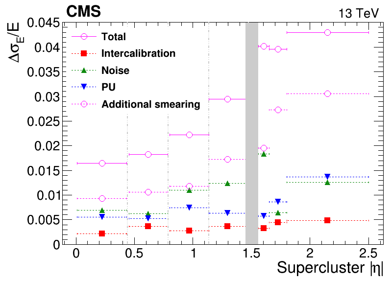
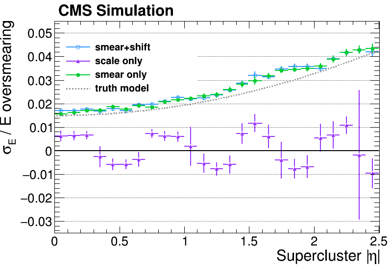
Figure 13:
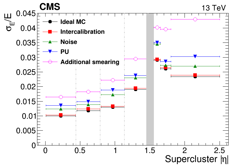
Left: the relative energy resolution for electrons from simulated $ \mathrm{Z}\to\mathrm{e}^+\mathrm{e}^- $ decays. The energy resolution is measured by the method presented in Appendix 13.4 for low-bremsstrahlung electrons. The different simulations correspond to the dedicated scenarios. The label ``Additional smearing'' is the observed resolution in data, corresponding to the ``PU'' scenario with the inclusion of the additional smearing. Right: the contributions of different effects to the resolution (intercalibration accuracy, noise, PU) and the additional smearing. The total resolution, which in the left pane corresponds to the sample labelled ``Additional smearing'' is also reported in the right pane, labelled as ``Total''. The plots are shown as functions of the $ |\eta| $ of the SC. The vertical dotted lines mark the boundaries between the ECAL modules in the EB. The shaded grey band corresponds to the EB/EE transition. |
png |
Figure 13-a:
Left: the relative energy resolution for electrons from simulated $ \mathrm{Z}\to\mathrm{e}^+\mathrm{e}^- $ decays. The energy resolution is measured by the method presented in Appendix 13.4 for low-bremsstrahlung electrons. The different simulations correspond to the dedicated scenarios. The label ``Additional smearing'' is the observed resolution in data, corresponding to the ``PU'' scenario with the inclusion of the additional smearing. Right: the contributions of different effects to the resolution (intercalibration accuracy, noise, PU) and the additional smearing. The total resolution, which in the left pane corresponds to the sample labelled ``Additional smearing'' is also reported in the right pane, labelled as ``Total''. The plots are shown as functions of the $ |\eta| $ of the SC. The vertical dotted lines mark the boundaries between the ECAL modules in the EB. The shaded grey band corresponds to the EB/EE transition. |
png |
Figure 13-b:
Left: the relative energy resolution for electrons from simulated $ \mathrm{Z}\to\mathrm{e}^+\mathrm{e}^- $ decays. The energy resolution is measured by the method presented in Appendix 13.4 for low-bremsstrahlung electrons. The different simulations correspond to the dedicated scenarios. The label ``Additional smearing'' is the observed resolution in data, corresponding to the ``PU'' scenario with the inclusion of the additional smearing. Right: the contributions of different effects to the resolution (intercalibration accuracy, noise, PU) and the additional smearing. The total resolution, which in the left pane corresponds to the sample labelled ``Additional smearing'' is also reported in the right pane, labelled as ``Total''. The plots are shown as functions of the $ |\eta| $ of the SC. The vertical dotted lines mark the boundaries between the ECAL modules in the EB. The shaded grey band corresponds to the EB/EE transition. |
png pdf |
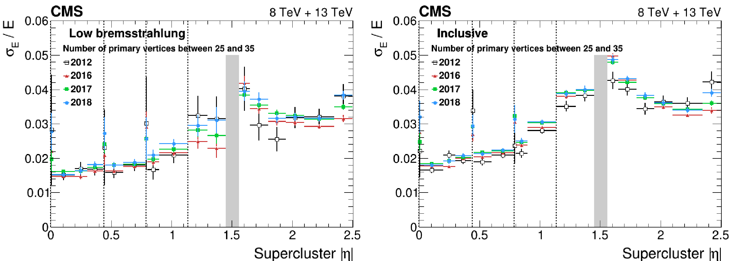
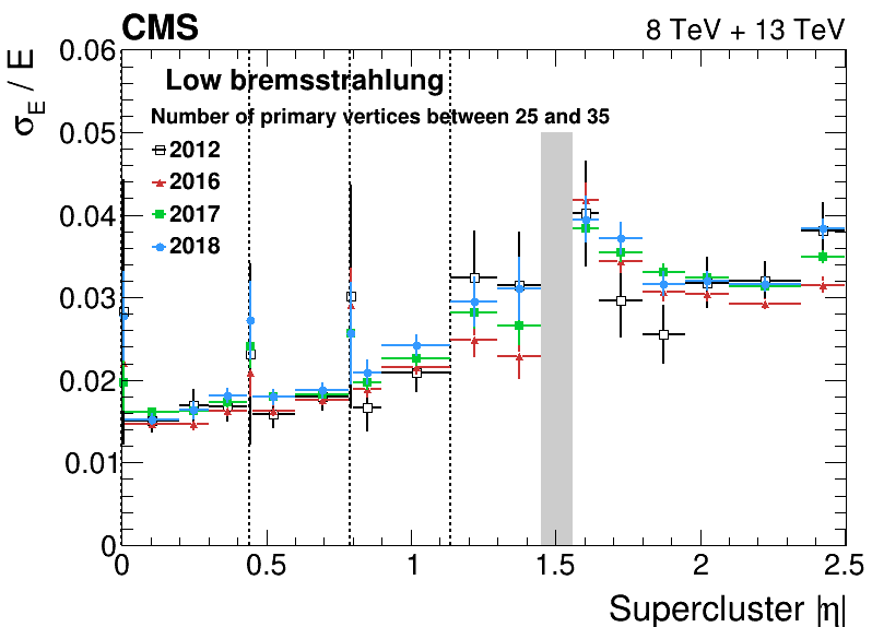
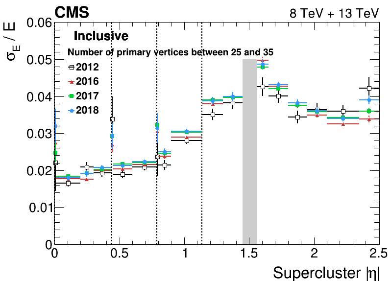
Figure 14:
Relative energy resolution for electrons from $ \mathrm{Z}\to\mathrm{e}^+\mathrm{e}^- $ decays versus $ |\eta| $ for events with low number of vertices and weighted to the Run 1 pileup distribution. The energy resolution is measured by the method presented in Appendix 13.4 for low-bremsstrahlung electrons (left) and for the inclusive sample (right). The vertical bars on the points represent the statistal uncertainty. The vertical dotted lines mark the boundary between the ECAL modules in the barrel, where a slightly worsening of the resolution is observed due to the material of the mechanical structures. The shaded grey band corresponds to the EB/EE transition. |
png |
Figure 14-a:
Relative energy resolution for electrons from $ \mathrm{Z}\to\mathrm{e}^+\mathrm{e}^- $ decays versus $ |\eta| $ for events with low number of vertices and weighted to the Run 1 pileup distribution. The energy resolution is measured by the method presented in Appendix 13.4 for low-bremsstrahlung electrons (left) and for the inclusive sample (right). The vertical bars on the points represent the statistal uncertainty. The vertical dotted lines mark the boundary between the ECAL modules in the barrel, where a slightly worsening of the resolution is observed due to the material of the mechanical structures. The shaded grey band corresponds to the EB/EE transition. |
png |
Figure 14-b:
Relative energy resolution for electrons from $ \mathrm{Z}\to\mathrm{e}^+\mathrm{e}^- $ decays versus $ |\eta| $ for events with low number of vertices and weighted to the Run 1 pileup distribution. The energy resolution is measured by the method presented in Appendix 13.4 for low-bremsstrahlung electrons (left) and for the inclusive sample (right). The vertical bars on the points represent the statistal uncertainty. The vertical dotted lines mark the boundary between the ECAL modules in the barrel, where a slightly worsening of the resolution is observed due to the material of the mechanical structures. The shaded grey band corresponds to the EB/EE transition. |
png pdf |
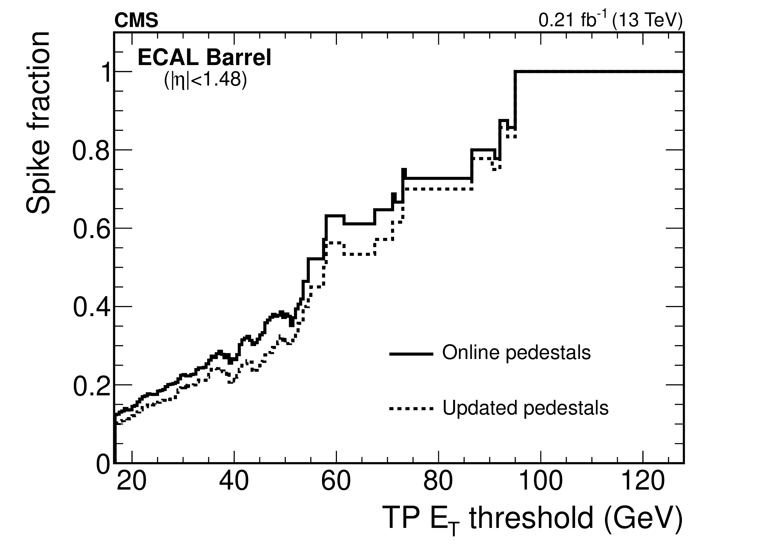
Figure 15:
Fraction of ECAL TPs in the barrel region that are matched to an offline spike, as a function of the trigger primitive $ E_{\mathrm{T}} $ threshold, before and after updated pedestal values are applied. |
png pdf |
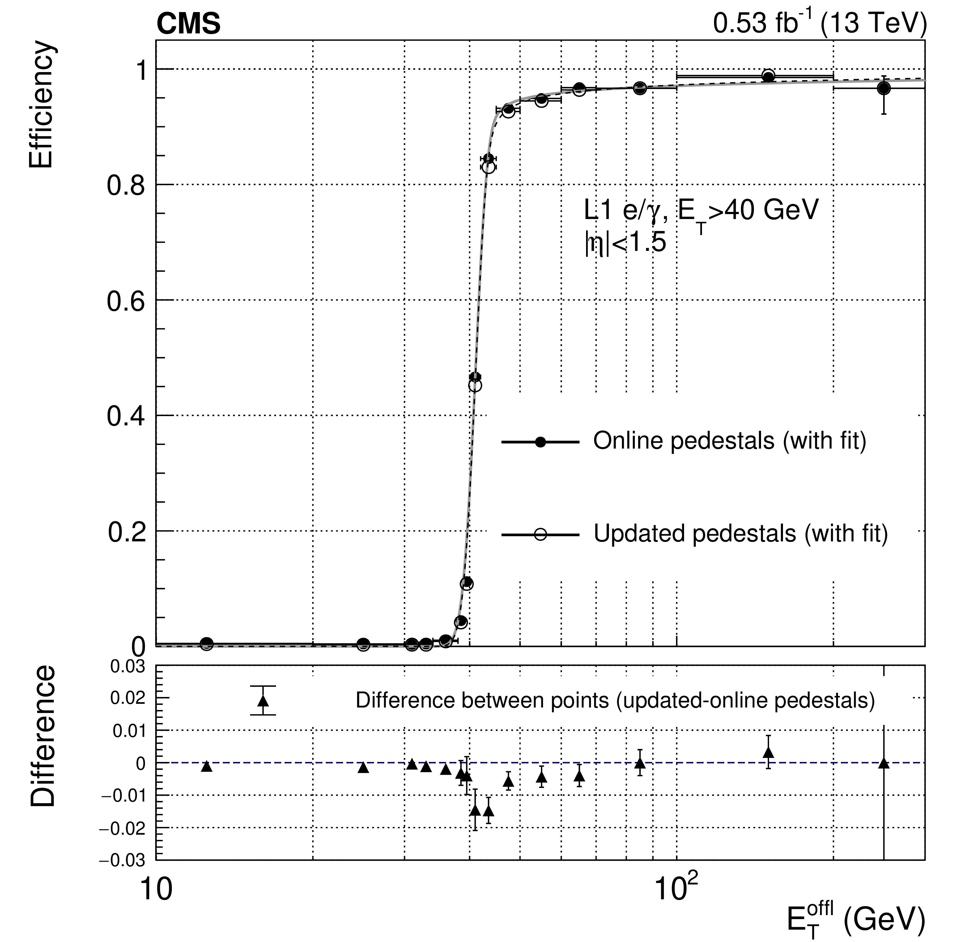
Figure 16:
The efficiency of the L1 electron/photon trigger with a transverse energy threshold of 40 GeV, measured using the ``tag-and-probe'' method on $ \mathrm{Z}\to\mathrm{e}^+\mathrm{e}^- $ events, as a function of the transverse energy of the tag electron, reconstructed offline, before and after updated pedestal values are applied, and fitted with a sigmoid function. The vertical bars on the points represent the statistal uncertainty. In the lower panel the difference between the efficiencies before and after the update of the pedestals is shown. |
png pdf |
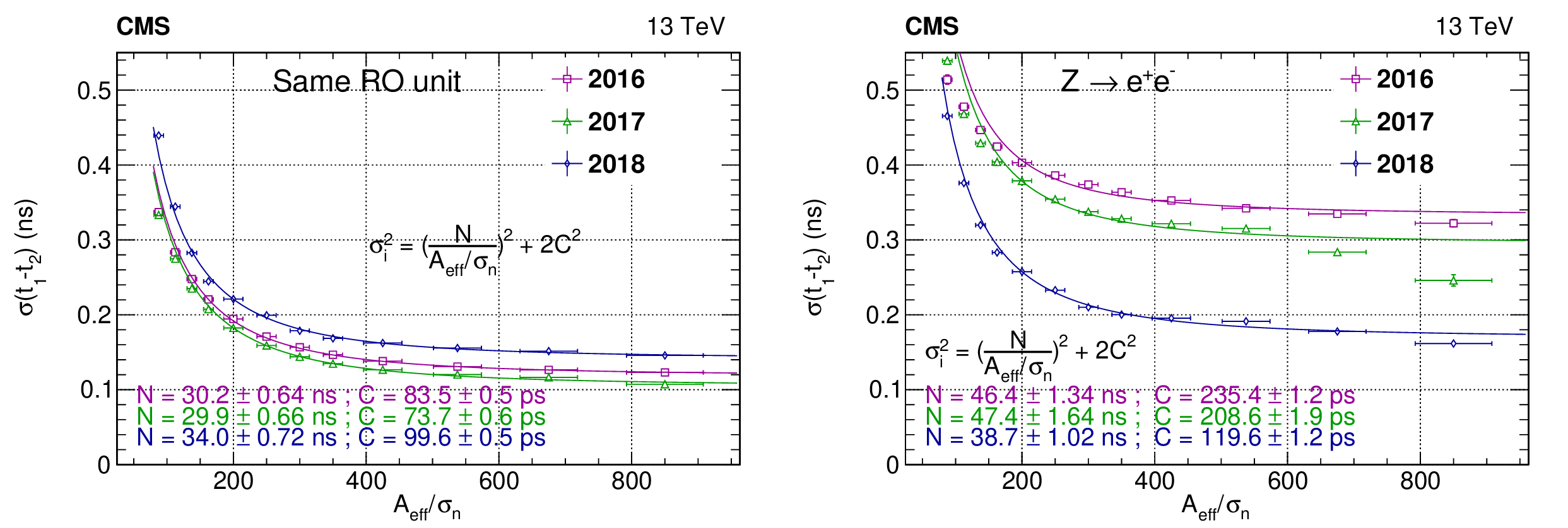
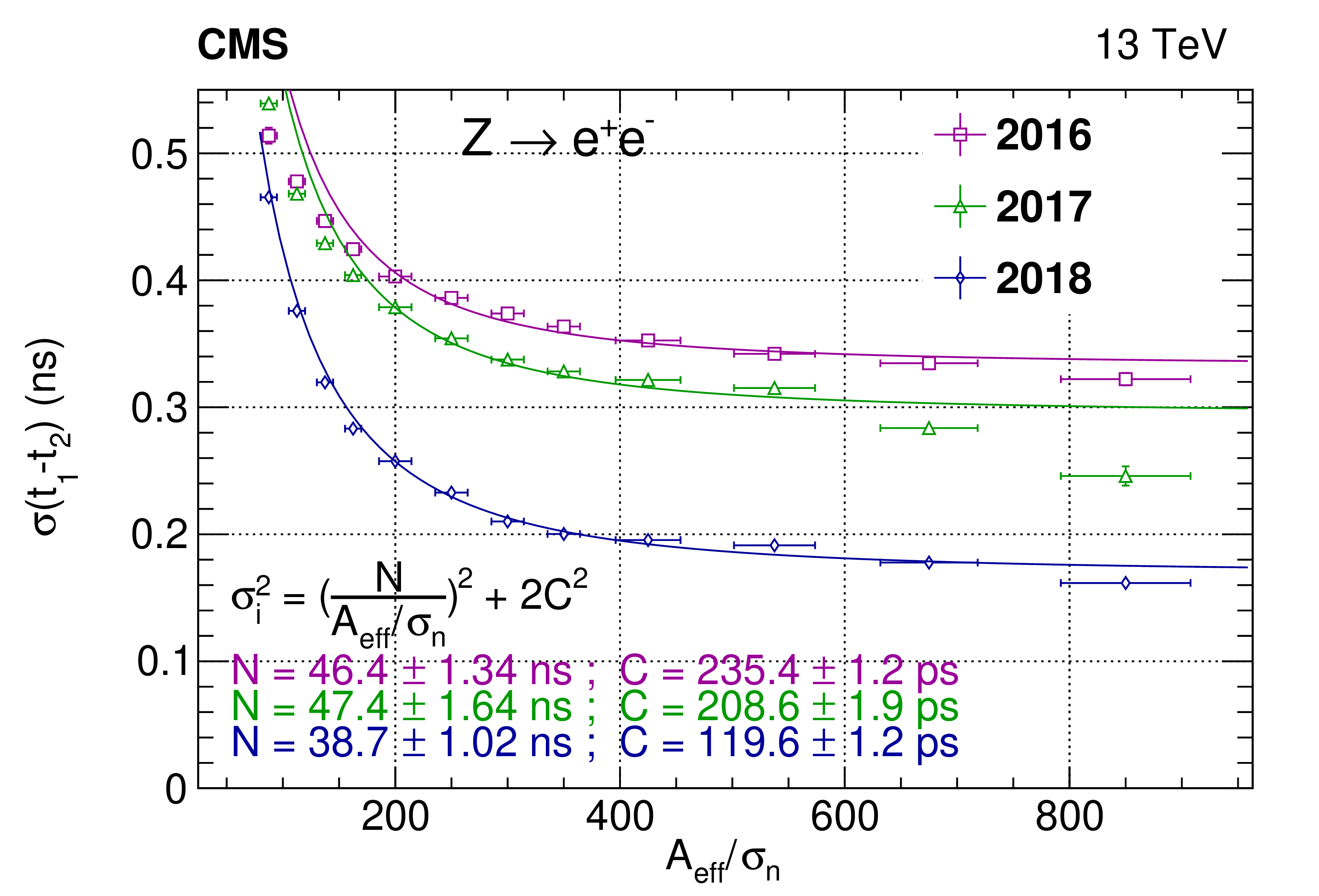
Figure 17:
The ECAL timing precision as measured from adjacent crystals sharing the same electronic readout (left), in 2016, 2017, and 2018 data. The timing precision extracted from $ \mathrm{Z}\to\mathrm{e}^+\mathrm{e}^- $ events comparing the time of flight of the $ \mathrm{e}^+ $ and $ \mathrm{e}^- $ is shown as well (right). The vertical bars on the points represent the statistal uncertainty. |

png pdf |
Figure 17-a:
The ECAL timing precision as measured from adjacent crystals sharing the same electronic readout (left), in 2016, 2017, and 2018 data. The timing precision extracted from $ \mathrm{Z}\to\mathrm{e}^+\mathrm{e}^- $ events comparing the time of flight of the $ \mathrm{e}^+ $ and $ \mathrm{e}^- $ is shown as well (right). The vertical bars on the points represent the statistal uncertainty. |
png pdf |
Figure 17-b:
The ECAL timing precision as measured from adjacent crystals sharing the same electronic readout (left), in 2016, 2017, and 2018 data. The timing precision extracted from $ \mathrm{Z}\to\mathrm{e}^+\mathrm{e}^- $ events comparing the time of flight of the $ \mathrm{e}^+ $ and $ \mathrm{e}^- $ is shown as well (right). The vertical bars on the points represent the statistal uncertainty. |
png pdf |
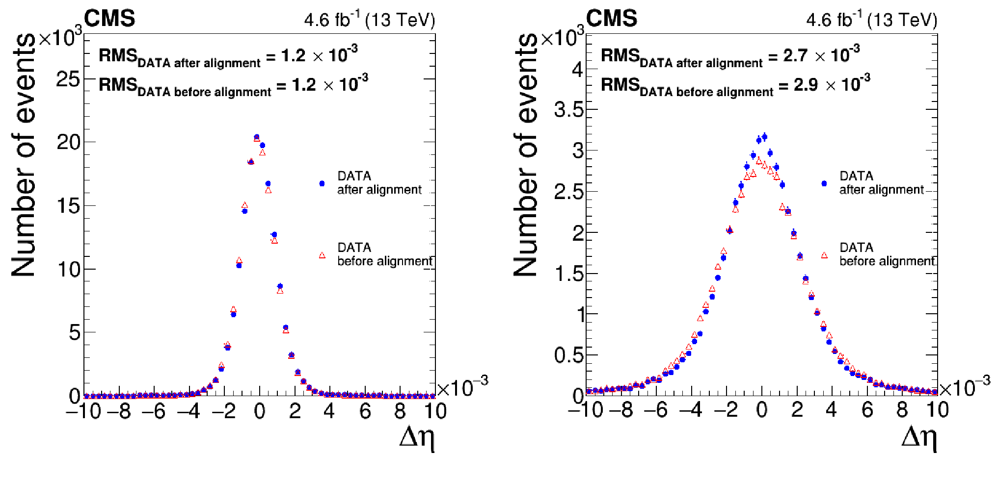
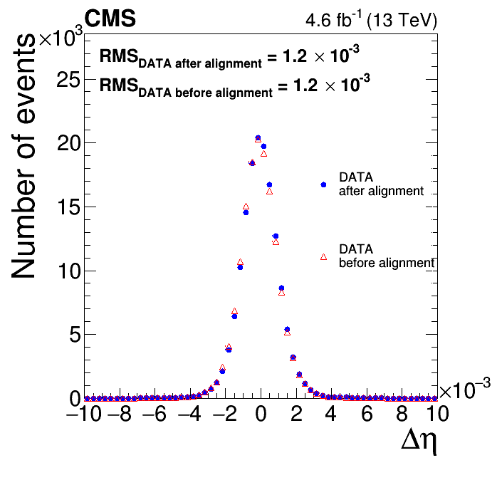
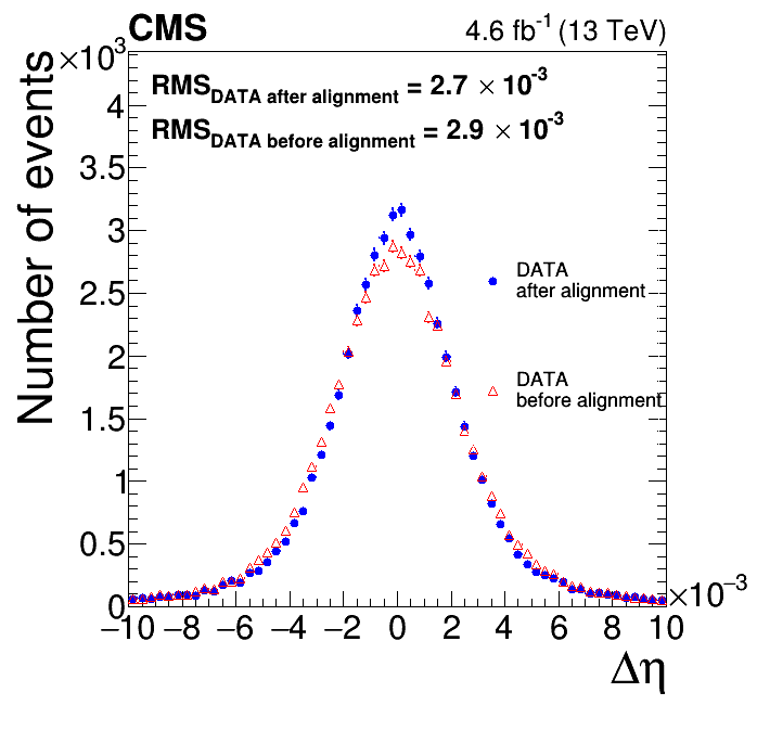
Figure A1:
The $ \Delta\eta $ between the extrapolated tracker position and the position measurement provided by the ECAL, before (red triangles) and after (blue circles) the alignment, for (left) the EB and (right) the EE, measured using electrons at the start of the 2017 data-taking period. The vertical bars on the points represent the statistal uncertainty. |
png |
Figure A1-a:
The $ \Delta\eta $ between the extrapolated tracker position and the position measurement provided by the ECAL, before (red triangles) and after (blue circles) the alignment, for (left) the EB and (right) the EE, measured using electrons at the start of the 2017 data-taking period. The vertical bars on the points represent the statistal uncertainty. |
png |
Figure A1-b:
The $ \Delta\eta $ between the extrapolated tracker position and the position measurement provided by the ECAL, before (red triangles) and after (blue circles) the alignment, for (left) the EB and (right) the EE, measured using electrons at the start of the 2017 data-taking period. The vertical bars on the points represent the statistal uncertainty. |

png pdf |
Figure A2:
Distribution of the residuals between the hits in the ES and the expected hit position from the reconstructed tracks, before (black open squares) and after (red solid circles) the alignment of each ES plane was performed, using the first 0.5 fb$ ^{-1} $ of data recorded in 2017. The upper (lower) row corresponds to the ES detector at positive (negative) z, and the left (right) column corresponds to the front (rear) detector plane. The vertical bars on the points represent the statistal uncertainty. |

png pdf |
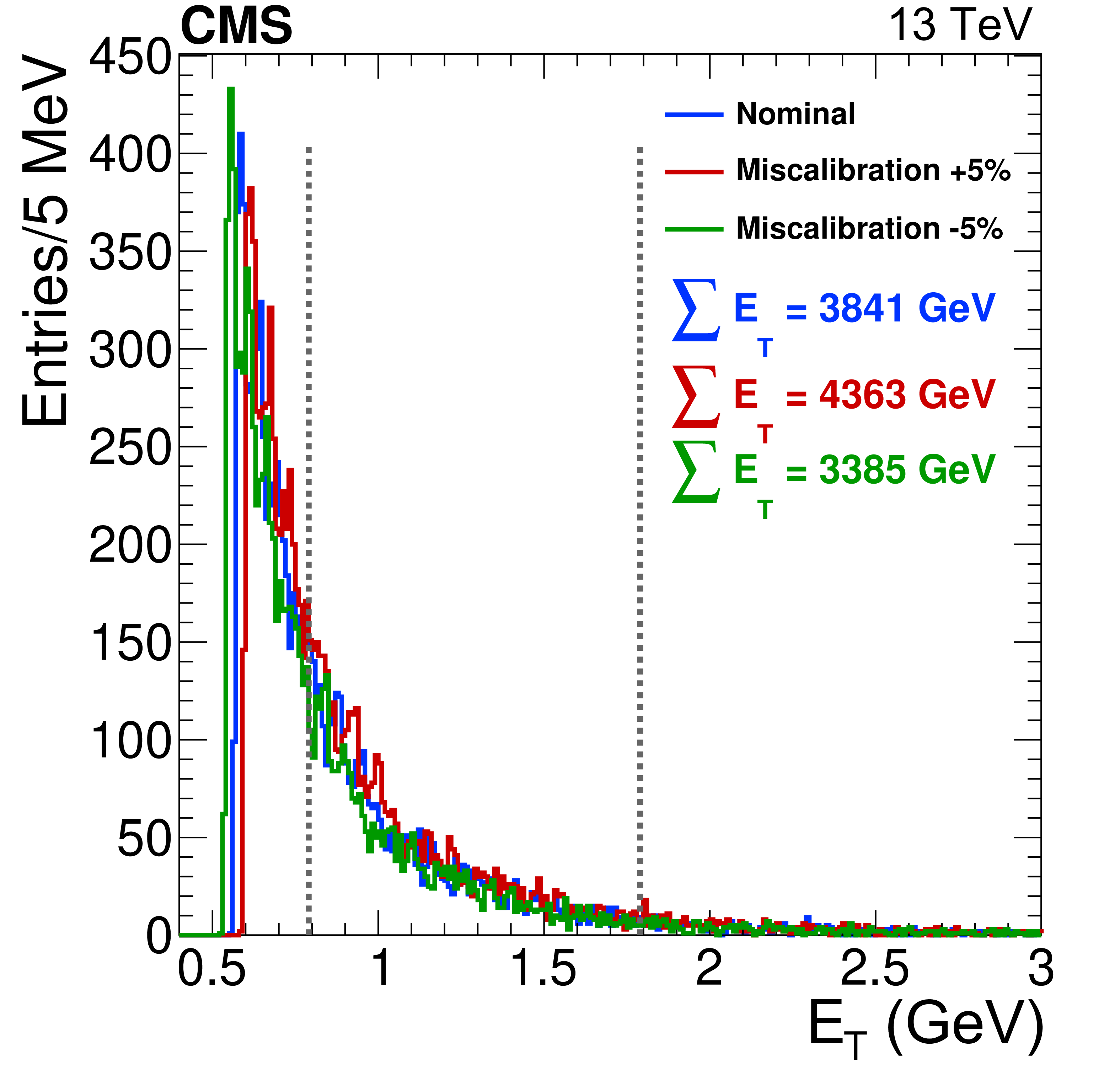
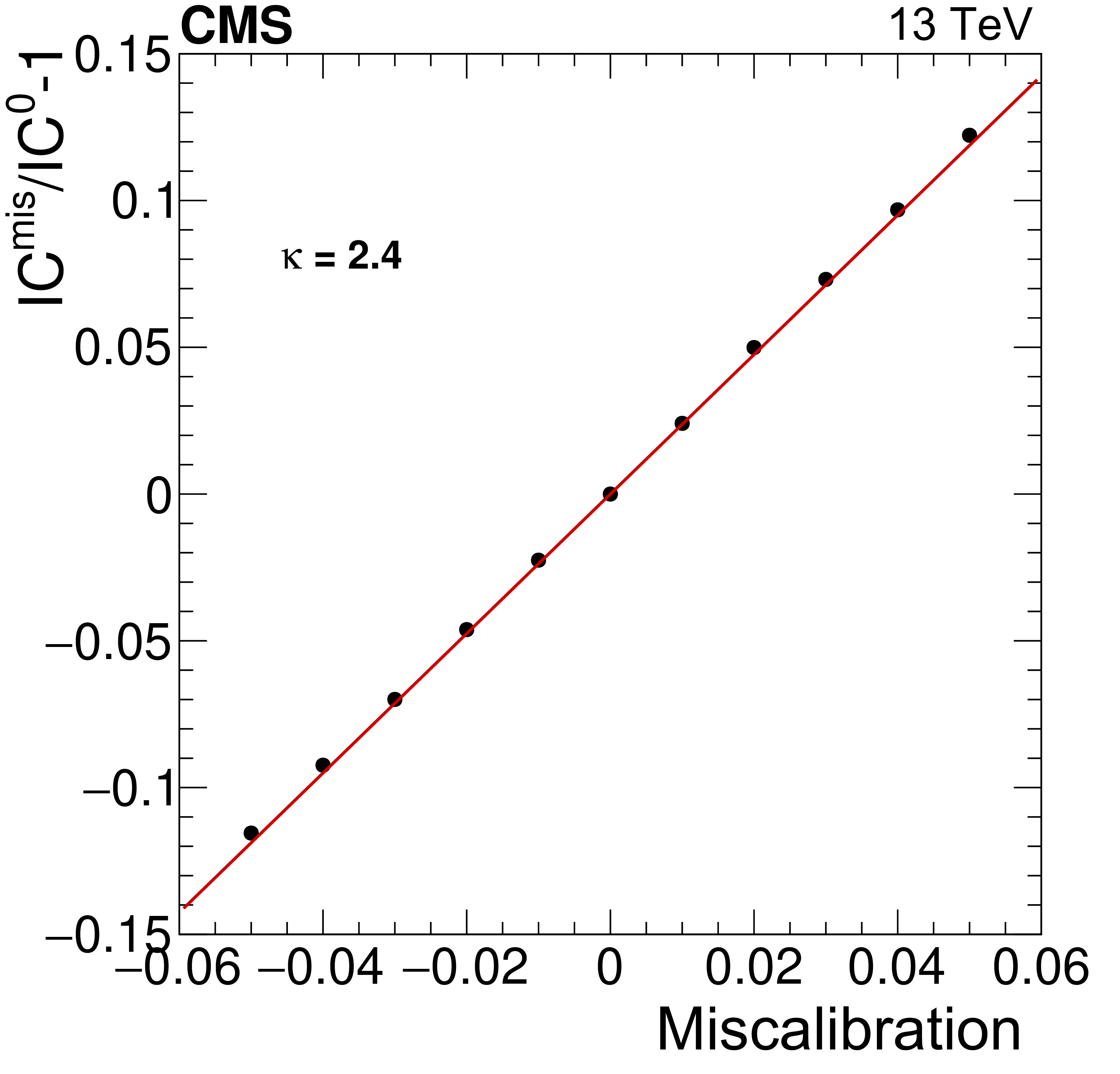
Figure B1:
On the left, the energy spectrum of events selected by the $ \phi $-symmetry HLT path in a chosen crystal in the central EB. The blue histogram corresponds to the measured energy deposition, while the red and green histograms are obtained from the blue histogram by injecting a miscalibration of $ \pm$5%. Vertical lines represent the interval of events selected in that crystal for the calibration. For each histogram, the sum of the energy of the selected events is also reported. On the right, a typical fit to extract the $ \kappa $-factor. The $ x $-axis is the injected miscalibration, while the $ y $-axis is the variation in the IC constant with a given miscalibration minus one. A linear fit is superimposed (red line) and the $ \kappa $-factor is the slope of the line. |
png pdf |
Figure B1-a:
On the left, the energy spectrum of events selected by the $ \phi $-symmetry HLT path in a chosen crystal in the central EB. The blue histogram corresponds to the measured energy deposition, while the red and green histograms are obtained from the blue histogram by injecting a miscalibration of $ \pm$5%. Vertical lines represent the interval of events selected in that crystal for the calibration. For each histogram, the sum of the energy of the selected events is also reported. On the right, a typical fit to extract the $ \kappa $-factor. The $ x $-axis is the injected miscalibration, while the $ y $-axis is the variation in the IC constant with a given miscalibration minus one. A linear fit is superimposed (red line) and the $ \kappa $-factor is the slope of the line. |
png pdf |
Figure B1-b:
On the left, the energy spectrum of events selected by the $ \phi $-symmetry HLT path in a chosen crystal in the central EB. The blue histogram corresponds to the measured energy deposition, while the red and green histograms are obtained from the blue histogram by injecting a miscalibration of $ \pm$5%. Vertical lines represent the interval of events selected in that crystal for the calibration. For each histogram, the sum of the energy of the selected events is also reported. On the right, a typical fit to extract the $ \kappa $-factor. The $ x $-axis is the injected miscalibration, while the $ y $-axis is the variation in the IC constant with a given miscalibration minus one. A linear fit is superimposed (red line) and the $ \kappa $-factor is the slope of the line. |

png pdf |
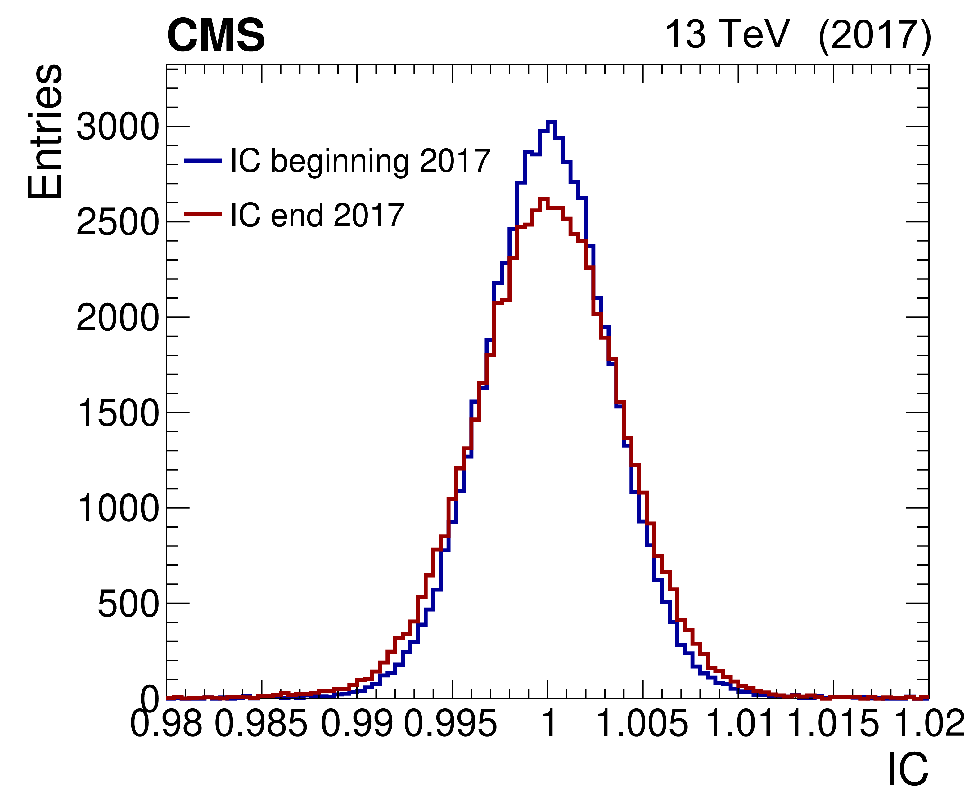
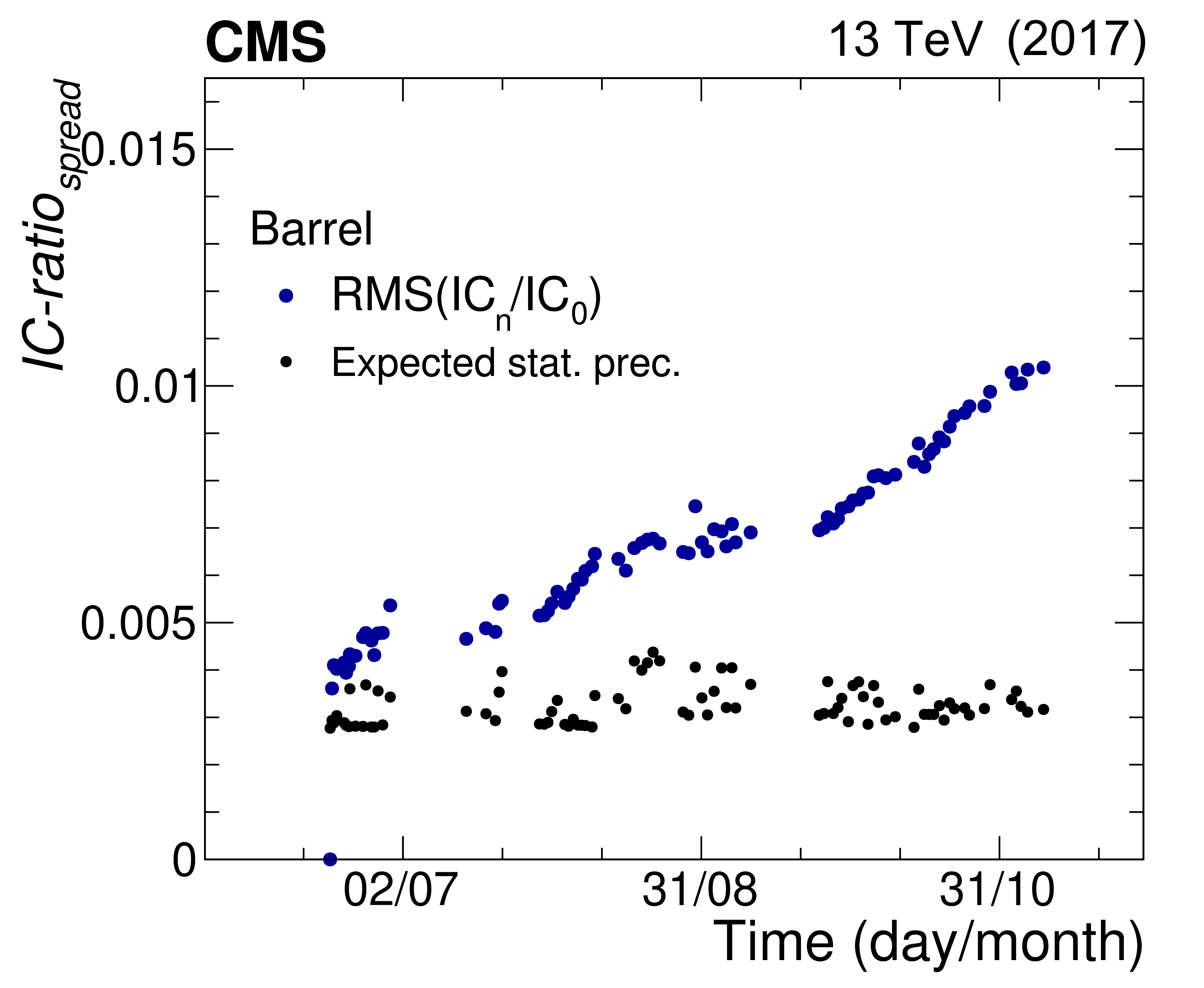
Figure B2:
On the left, the distribution of the normalized IC constants of all EB crystals shown for two time bins, at the beginning (blue) and at the end (red) of the 2017 data-taking period. The IC value is normalised, for each crystal, to the initial value. On the right, the RMS of the distribution of the ratio of the IC constants at a given point in time over the beginning of the year is shown in blue. The black points show the statistical precision of the method, evaluated by randomly splitting the data into two subsets. |
png pdf |
Figure B2-a:
On the left, the distribution of the normalized IC constants of all EB crystals shown for two time bins, at the beginning (blue) and at the end (red) of the 2017 data-taking period. The IC value is normalised, for each crystal, to the initial value. On the right, the RMS of the distribution of the ratio of the IC constants at a given point in time over the beginning of the year is shown in blue. The black points show the statistical precision of the method, evaluated by randomly splitting the data into two subsets. |
png pdf |
Figure B2-b:
On the left, the distribution of the normalized IC constants of all EB crystals shown for two time bins, at the beginning (blue) and at the end (red) of the 2017 data-taking period. The IC value is normalised, for each crystal, to the initial value. On the right, the RMS of the distribution of the ratio of the IC constants at a given point in time over the beginning of the year is shown in blue. The black points show the statistical precision of the method, evaluated by randomly splitting the data into two subsets. |
png pdf |
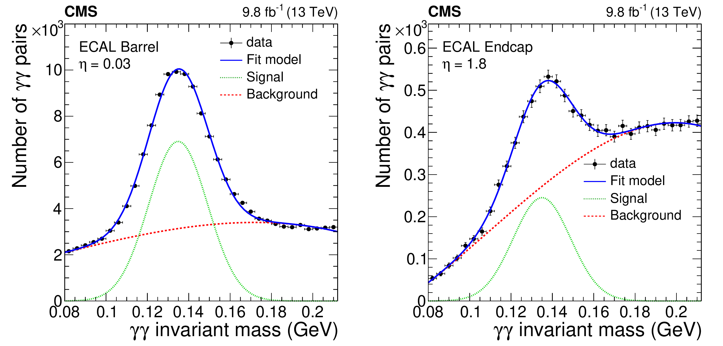
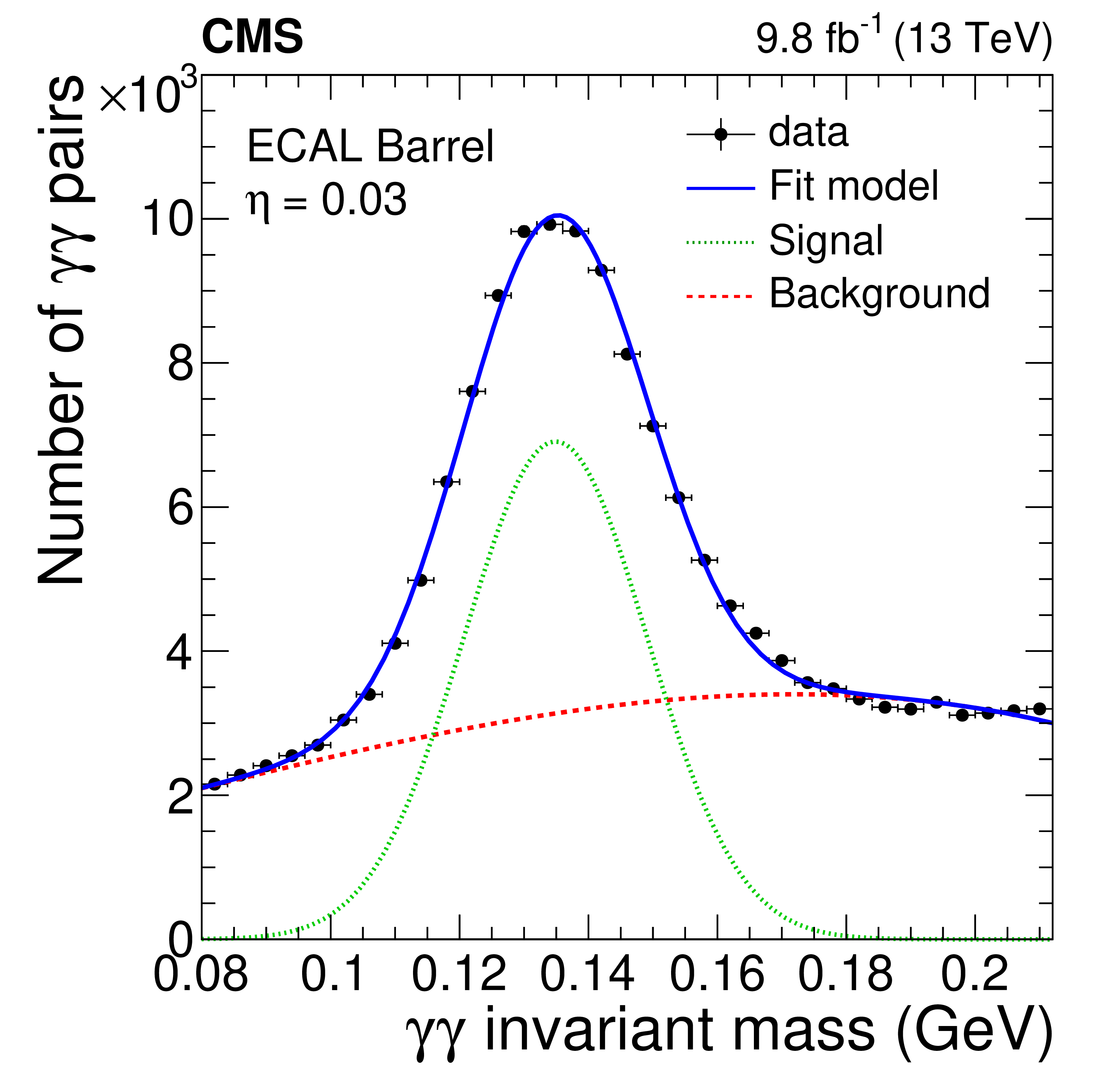
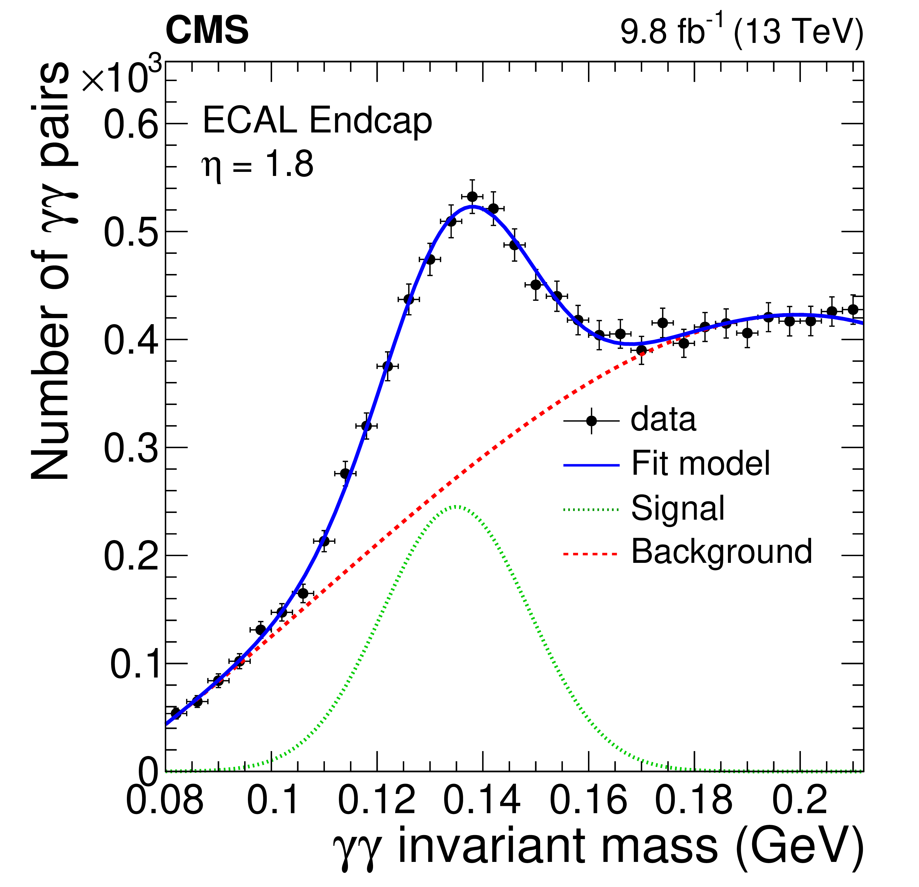
Figure B3:
The invariant mass distribution of photon pairs around the $ \pi^{0} $ mass peak for one crystal in EB (left) and EE (right). Data (black points) are fitted with the sum (solid blue line) of signal (dashed green line) and background components (dotted red line), as detailed in the text. The vertical bars on the points represent the statistal uncertainty. |
png pdf |
Figure B3-a:
The invariant mass distribution of photon pairs around the $ \pi^{0} $ mass peak for one crystal in EB (left) and EE (right). Data (black points) are fitted with the sum (solid blue line) of signal (dashed green line) and background components (dotted red line), as detailed in the text. The vertical bars on the points represent the statistal uncertainty. |
png pdf |
Figure B3-b:
The invariant mass distribution of photon pairs around the $ \pi^{0} $ mass peak for one crystal in EB (left) and EE (right). Data (black points) are fitted with the sum (solid blue line) of signal (dashed green line) and background components (dotted red line), as detailed in the text. The vertical bars on the points represent the statistal uncertainty. |
png pdf |
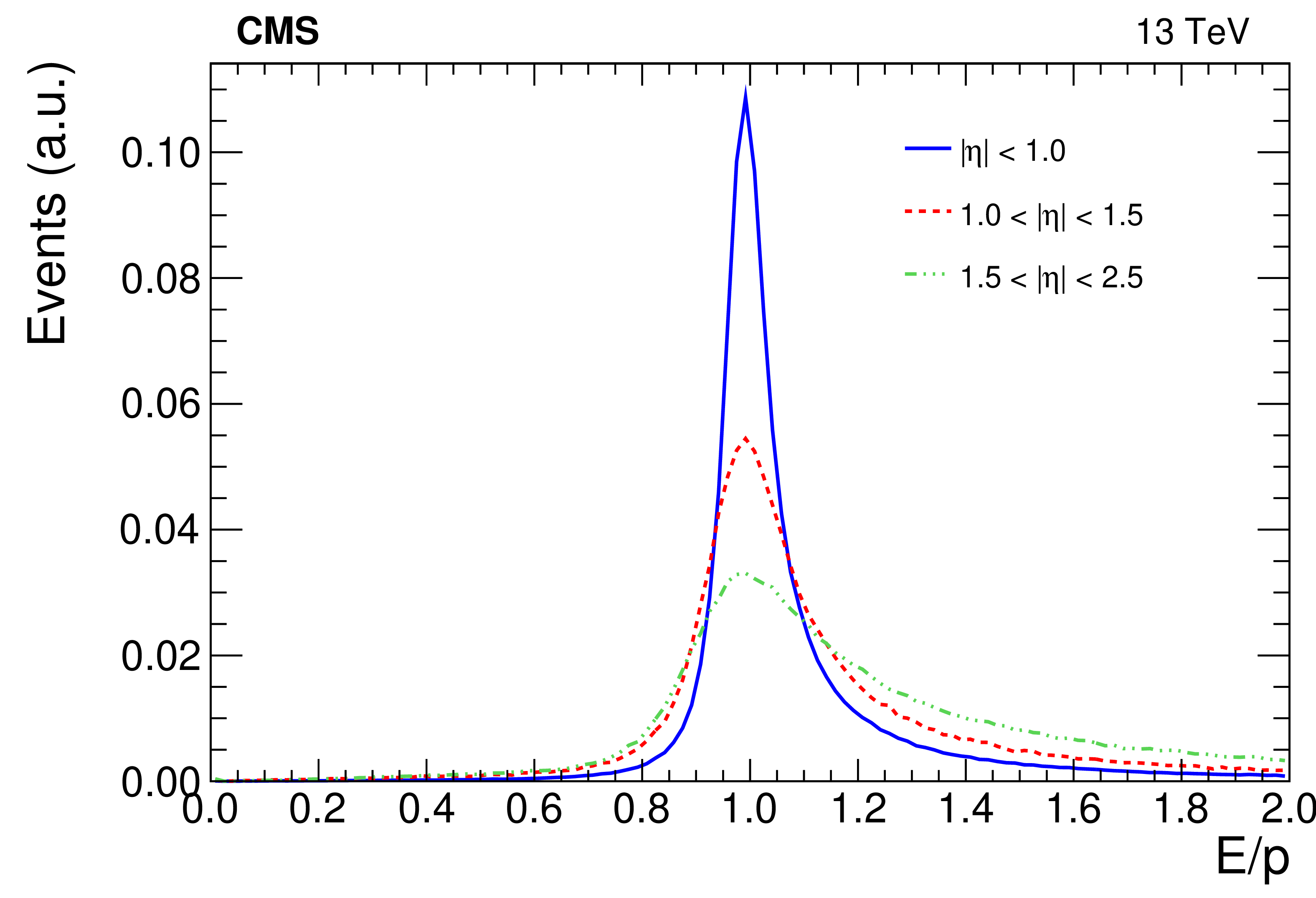
Figure B4:
The $ E/p $ distributions measured from data in different intervals of $ \eta $. Electrons from W and Z boson decays are selected, whose $ E_{\mathrm{T}} $ ranges between 30 and 70 GeV. |
png pdf |
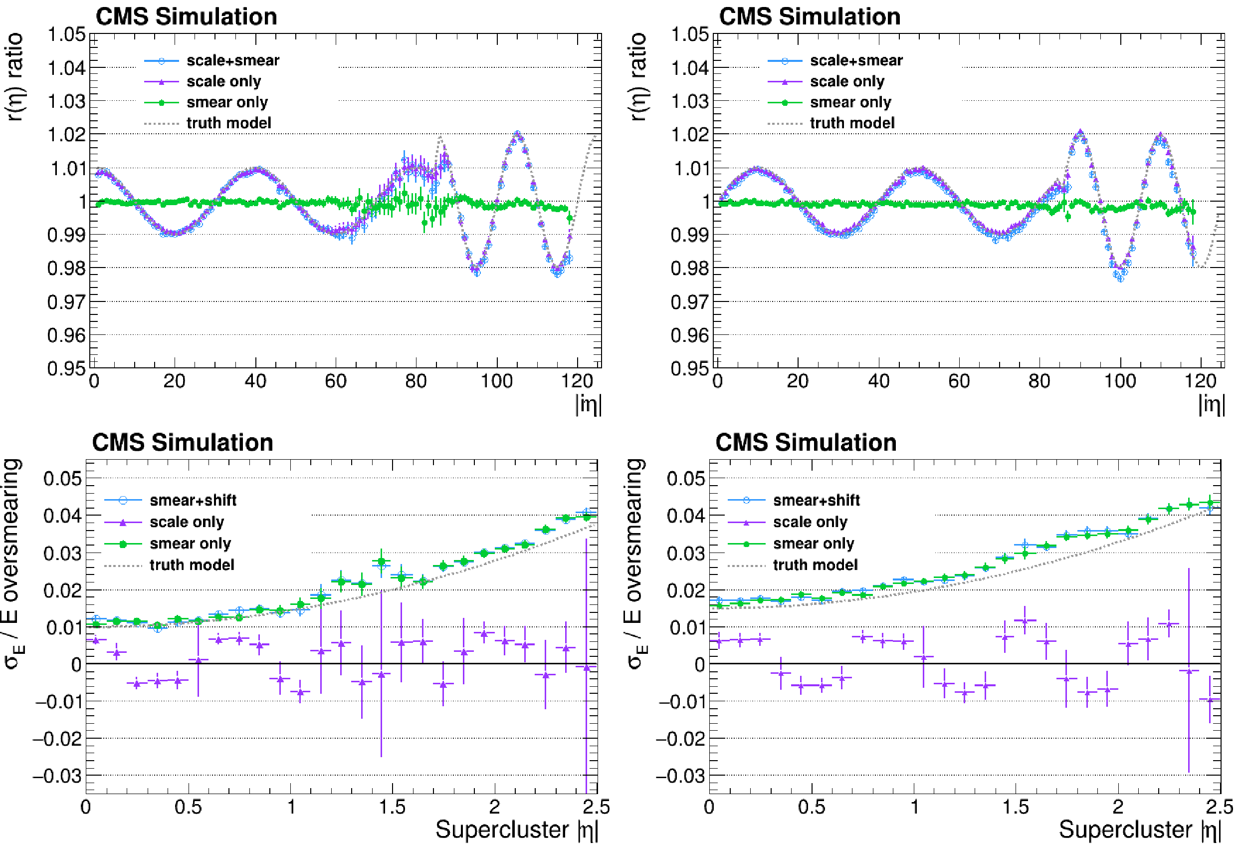
Figure B5:
The result of the $ \mathrm{Z}\to\mathrm{e}^+\mathrm{e}^- $ method validation fit to the four simulations described in the text. The upper row shows the ratio to the original simulation. The lower row corresponds to the resolution quadratic difference between the two simulations. The grey dashed lines correspond to the input parameters used in the simulation, that should be retrieved by the fit. The results for the low- and high-bremsstrahlung electrons are shown, respectively, on the left and on the right. The error bars shown correspond to the uncertainty, as determined from the fit. |

png |
Figure B5-a:
The result of the $ \mathrm{Z}\to\mathrm{e}^+\mathrm{e}^- $ method validation fit to the four simulations described in the text. The upper row shows the ratio to the original simulation. The lower row corresponds to the resolution quadratic difference between the two simulations. The grey dashed lines correspond to the input parameters used in the simulation, that should be retrieved by the fit. The results for the low- and high-bremsstrahlung electrons are shown, respectively, on the left and on the right. The error bars shown correspond to the uncertainty, as determined from the fit. |

png |
Figure B5-b:
The result of the $ \mathrm{Z}\to\mathrm{e}^+\mathrm{e}^- $ method validation fit to the four simulations described in the text. The upper row shows the ratio to the original simulation. The lower row corresponds to the resolution quadratic difference between the two simulations. The grey dashed lines correspond to the input parameters used in the simulation, that should be retrieved by the fit. The results for the low- and high-bremsstrahlung electrons are shown, respectively, on the left and on the right. The error bars shown correspond to the uncertainty, as determined from the fit. |

png |
Figure B5-c:
The result of the $ \mathrm{Z}\to\mathrm{e}^+\mathrm{e}^- $ method validation fit to the four simulations described in the text. The upper row shows the ratio to the original simulation. The lower row corresponds to the resolution quadratic difference between the two simulations. The grey dashed lines correspond to the input parameters used in the simulation, that should be retrieved by the fit. The results for the low- and high-bremsstrahlung electrons are shown, respectively, on the left and on the right. The error bars shown correspond to the uncertainty, as determined from the fit. |
png |
Figure B5-d:
The result of the $ \mathrm{Z}\to\mathrm{e}^+\mathrm{e}^- $ method validation fit to the four simulations described in the text. The upper row shows the ratio to the original simulation. The lower row corresponds to the resolution quadratic difference between the two simulations. The grey dashed lines correspond to the input parameters used in the simulation, that should be retrieved by the fit. The results for the low- and high-bremsstrahlung electrons are shown, respectively, on the left and on the right. The error bars shown correspond to the uncertainty, as determined from the fit. |
| Tables | |

png pdf |
Table 1:
Delivered and recorded integrated luminosity for the Run 2 period [7,none,none]. |
| Summary |
| The challenge of maintaining the same excellent performance of the CMS electromagnetic calorimeter achieved in Run 1 has been met despite the increased levels of radiation damage and pileup. This has included an increase in the transparency loss by the crystals and larger energy-equivalent electronic noise levels. To meet this challenge, a new algorithm has been developed to reconstruct the energy deposited in the crystals; the detector conditions have been monitored using different and complementary methods and updated continuously, and residual time-dependent corrections to the detector have been derived with electrons from the decays of W and Z bosons. Because of these changes in Run 2, the stability of the energy scale was better than 0.1% in the barrel and 0.4% in the endcaps. For electrons from Z boson decays with low bremsstrahlung (for the inclusive sample), the energy resolution was better than 1.8 (2.0)% in the central barrel, 3.0 (4.0)% in the outer barrel, and 4.5 (5.0)% in the endcaps. These techniques and methods will continue to be used and improved to maintain the excellent performance of the CMS electromagnetic calorimeter during the even more challenging operating conditions in the LHC Run 3. |
| References | ||||
| 1 | CMS Collaboration | The CMS experiment at the CERN LHC | JINST 3 (2008) S08004 | |
| 2 | CMS Collaboration | Search for long-lived particles using delayed photons in proton-proton collisions at $ \sqrt{s}= $ 13 TeV | PRD 100 (2019) 112003 | CMS-EXO-19-005 1909.06166 |
| 3 | CMS Collaboration | Performance of the CMS Level-1 trigger in proton-proton collisions at $ \sqrt{s} = $ 13 TeV | JINST 15 (2020) P10017 | CMS-TRG-17-001 2006.10165 |
| 4 | CMS Collaboration | The CMS trigger system | JINST 12 (2017) P01020 | CMS-TRG-12-001 1609.02366 |
| 5 | CMS Collaboration | The CMS electromagnetic calorimeter project: Technical design report | Technical Report CERN-LHCC-97-033, 1997 CDS |
|
| 6 | CMS Collaboration | Changes to CMS ECAL electronics: addendum to the technical design report | Technical Report CERN-LHCC-2002-027, 2002 CDS |
|
| 7 | CMS Collaboration | Precision luminosity measurement in proton-proton collisions at $ \sqrt{s} = $ 13 TeV in 2015 and 2016 at CMS | Eur. Phys. J. 81 (2021) 800 | CMS-LUM-17-003 2104.01927 |
| 8 | CMS Collaboration | CMS luminosity measurement for the 2017 data-taking period at $ \sqrt{s} = $ 13 TeV | CMS Physics Analysis Summary, 2018 CMS-PAS-LUM-17-004 |
CMS-PAS-LUM-17-004 |
| 9 | CMS Collaboration | CMS luminosity measurement for the 2018 data-taking period at $ \sqrt{s} = $ 13 TeV | CMS Physics Analysis Summary, 2019 CMS-PAS-LUM-18-002 |
CMS-PAS-LUM-18-002 |
| 10 | CMS Collaboration | Reconstruction of signal amplitudes in the CMS electromagnetic calorimeter in the presence of overlapping proton-proton interactions | JINST 15 (2020) P10002 | CMS-EGM-18-001 2006.14359 |
| 11 | P. Paganini | CMS electromagnetic trigger commissioning and first operation experiences | J.Phys. Conf. Ser. 160 (2009) 012062 | |
| 12 | CMS Collaboration | CMS TriDAS project: Technical design report, volume 1: The trigger systems | technical report, 2000 CDS |
|
| 13 | D. A. Petyt | Anomalous APD signals in the CMS electromagnetic calorimeter | NIM A 695 (2012) 293 | |
| 14 | N. Almeida et al. | Data filtering in the readout of the CMS electromagnetic calorimeter | P0, 2008 JINST 3 (2008) |
|
| 15 | N. Almeida et al. | The selective read-out processor for the CMS electromagnetic calorimeter | IEEE Trans. Nucl. Sci. 52 (2005) 772 | |
| 16 | CMS Collaboration | New development in the CMS ECAL Level-1 trigger system to meet the challenges of LHC Run 2 | Proceedings of Topical Workshop on Electronics for Particle Physics -- PoS(TWEPP) 343 052, 2019 link |
|
| 17 | M. Anfreville et al. | Laser monitoring system for the CMS lead tungstate crystal calorimeter | NIM A 594 (2008) 292 | |
| 18 | P. Adzic et al. | Reconstruction of the signal amplitude of the CMS electromagnetic calorimeter | EPJC 46 (2006) 23 | |
| 19 | J. Cantarella and M. Piatek | Tsnnls: A solver for large sparse least squares problems with non-negative variables | link | cs/0408029 |
| 20 | CMS Collaboration | Time reconstruction and performance of the CMS electromagnetic calorimeter | JINST 5 (2010) T03011 | |
| 21 | CMS Collaboration | Particle-flow reconstruction and global event description with the CMS detector | JINST 12 (2017) P10003 | CMS-PRF-14-001 1706.04965 |
| 22 | CMS Collaboration | Energy calibration and resolution of the CMS electromagnetic calorimeter in pp collisions at $ \sqrt{s} = $ 7 TeV | JINST 8 (2013) P09009 | CMS-EGM-11-001 1306.2016 |
| 23 | CMS Collaboration | Electron and photon reconstruction and identification with the CMS experiment at the CERN LHC | JINST 16 (2021) P05014 | CMS-EGM-17-001 2012.06888 |
| 24 | L. Zhang et al. | Performance of the monitoring light source for the CMS lead tungstate crystal calorimeter | IEEE Trans. Nucl. Sci. 52 (2005) 1123 | |
| 25 | P. Bonamy and others | The ECAL calibration use of the light monitoring system | Technical Report CMS-NOTE-1998-013, 1998 | |
| 26 | J. Allison | GEANT 4 developments and applications | IEEE Trans. Nucl. Sci. 53 (2006) 270 | |
| 27 | GEANT4 Collaboration | GEANT 4--- a simulation toolkit | NIM A 506 (2003) 250 | |
| 28 | CMS Collaboration | Performance of photon reconstruction and identification with the CMS detector in proton-proton collisions at $ \sqrt{s} = $ 8 TeV | JINST 10 (2015) P08010 | |
| 29 | CMS Collaboration | Measurement of the inclusive W and Z production cross sections in pp collisions at $ \sqrt{s} = $ 7 TeV with the CMS experiment | JHEP 10 (2011) 132 | |
| 30 | D. del Re | Timing performance of the CMS ECAL and prospects for the future | J. Phys. Conf. Ser. 587 (2015) 012003 | |
| 31 | Particle Data Group , M. Tanabashi et al. | Review of particle physics | PRD 98 (2018) 030001 | |
| 32 | P. Meridiani and R. Paramatti | Use of $ \mathrm{Z} \to \mathrm{e}^+\mathrm{e}^- $ events for ECAL calibration | Technical Report CMS-NOTE-2006-039, 2006 | |
| 33 | F. Couderc | Quest for the Higgs boson(s) from D0 to CMS experiments | Habilitation à diriger des recherches, Sorbonne Université, 2018 link |
|
| 34 | B. L. Roberts, R. A. J. Riddle, and G. T. A. Squier | Measurement of Lorentzian linewidths | NIM A 130 (1975) 559 | |
| 35 | T. Czosnyka and A. Trzcińska | Unified analytical approximation of Gaussian and Voigtian lineshapes | NIM A 431 (1999) 548 | |
|
|
Compact Muon Solenoid LHC, CERN |
|

|

|

|

|

|