

Compact Muon Solenoid
LHC, CERN
| CMS-EGM-18-001 ; CERN-EP-2020-105 | ||
| Reconstruction of signal amplitudes in the CMS electromagnetic calorimeter in the presence of overlapping proton-proton interactions | ||
| CMS Collaboration | ||
| 25 June 2020 | ||
| JINST 15 (2020) P10002 | ||
| Abstract: A template fitting technique for reconstructing the amplitude of signals produced by the lead tungstate crystals of the CMS electromagnetic calorimeter is described. This novel approach is designed to suppress the increased out-of-time pileup contribution to the signal following the reduction of the accelerator bunch spacing from 50 to 25 ns at the start of Run 2 of the LHC. Execution of the algorithm is sufficiently fast for it to be employed in the CMS high-level trigger. It is also used in the offline event reconstruction. Results obtained from simulations and from collision data demonstrate a substantial improvement in the energy resolution of the calorimeter over a range of energies extending from a few GeV to several tens of GeV. | ||
| Links: e-print arXiv:2006.14359 [hep-ex] (PDF) ; CDS record ; inSPIRE record ; CADI line (restricted) ; | ||
| Figures | |
png pdf |
Figure 1:
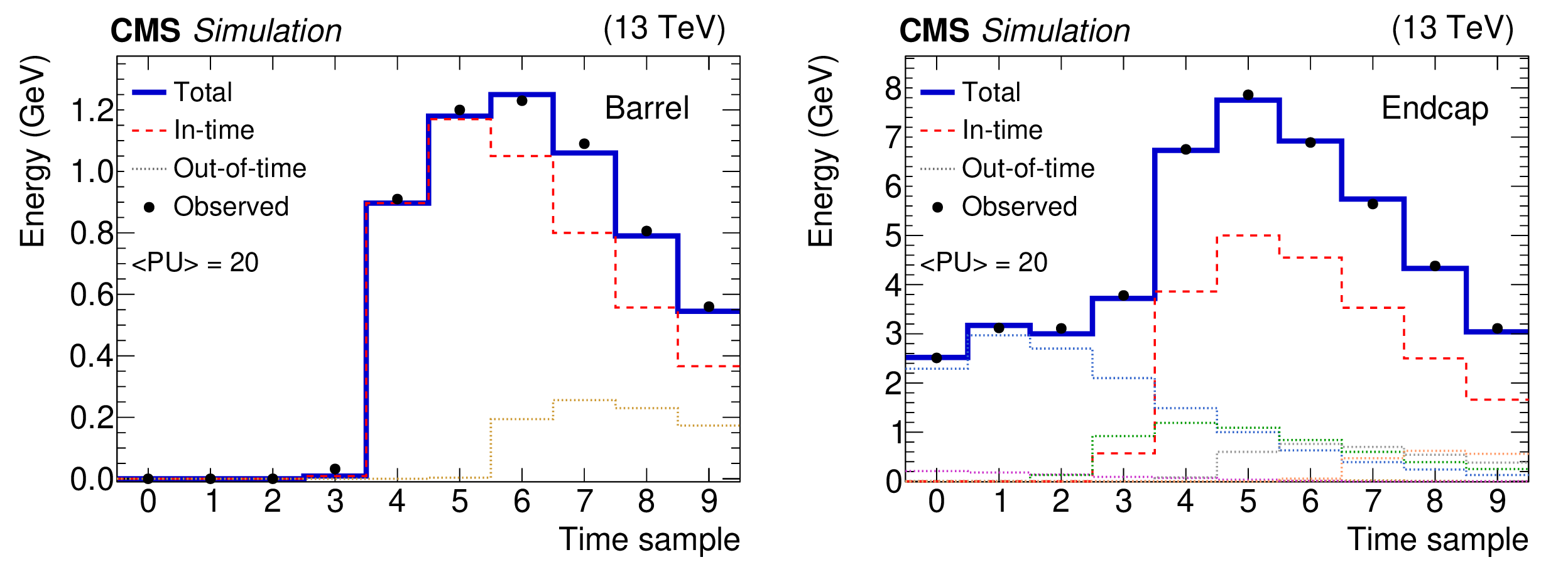
Two examples of fitted pulses for simulated events with 20 average pileup interactions and 25 ns bunch spacing. Signals from individual crystals are shown. They arise from a $ {p_{\mathrm {T}}} = $ 10 GeV photon shower in the barrel (left) and in an endcap (right). Filled circles with error bars represent the 10 digitized samples, the red dashed distributions (dotted multicolored distributions) represent the fitted in-time (out-of time) pulses with positive amplitudes. The solid dark blue histograms represent the sum of all the fitted contributions. Within the dotted distributions, the color distinguishes the fitted out-of-time pulses with different BX, while the legend represent them as a generic gray dotted line. |
png pdf |
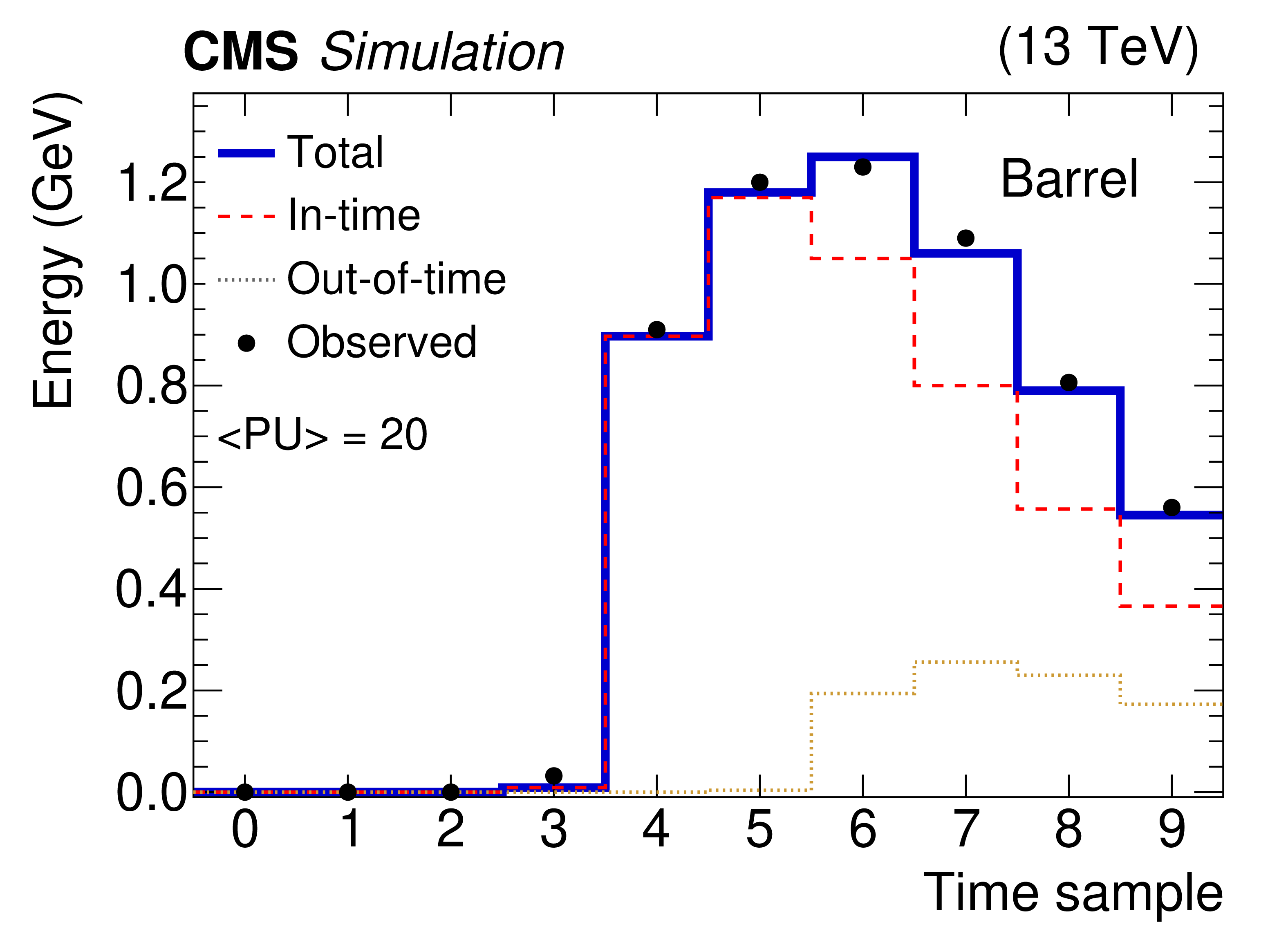
Figure 1-a:
Two examples of fitted pulses for simulated events with 20 average pileup interactions and 25 ns bunch spacing. Signals from individual crystals are shown. They arise from a $ {p_{\mathrm {T}}} = $ 10 GeV photon shower in the barrel. Filled circles with error bars represent the 10 digitized samples, the red dashed distributions (dotted multicolored distributions) represent the fitted in-time (out-of time) pulses with positive amplitudes. The solid dark blue histograms represent the sum of all the fitted contributions. Within the dotted distributions, the color distinguishes the fitted out-of-time pulses with different BX, while the legend represent them as a generic gray dotted line. |
png pdf |
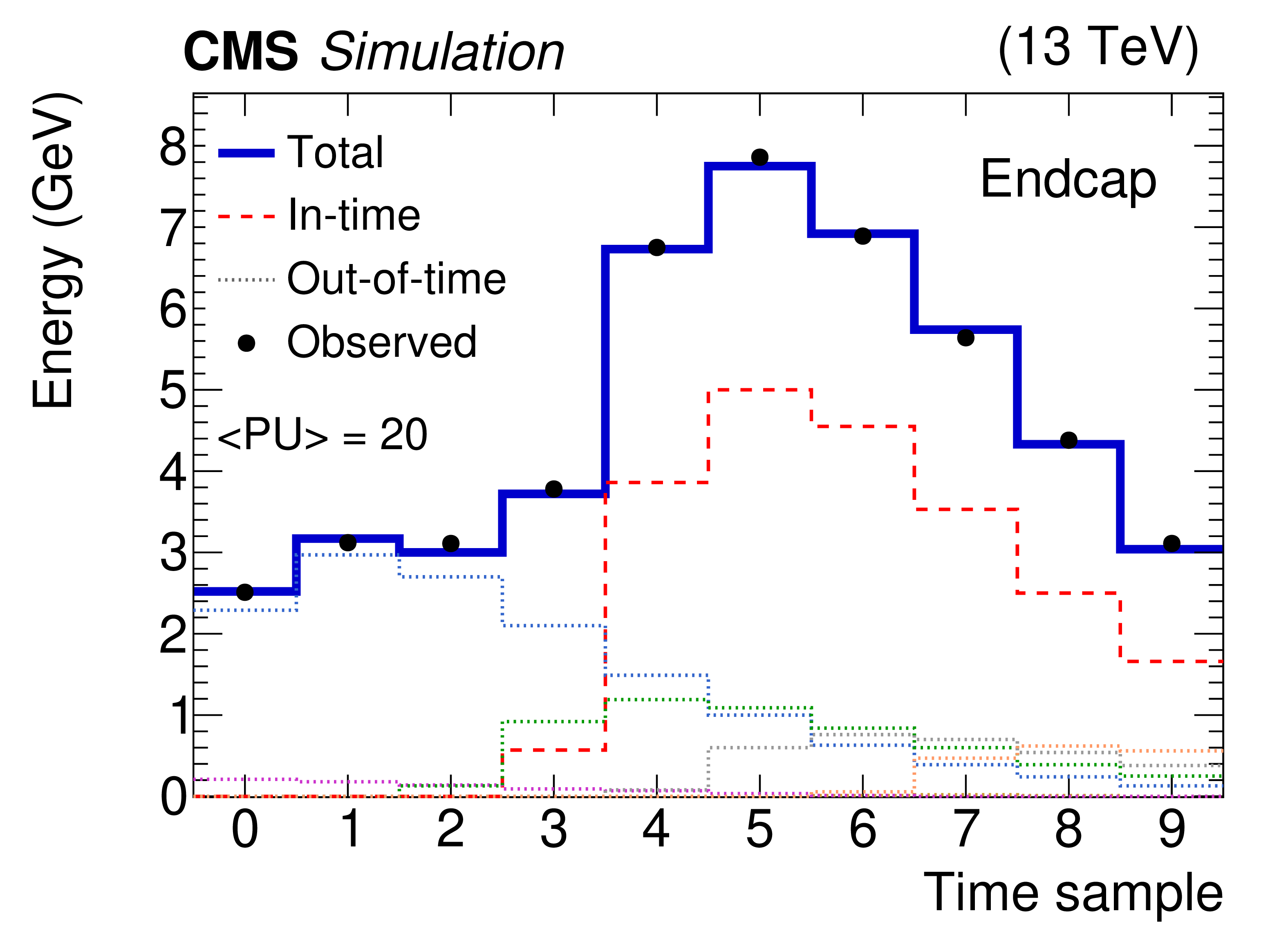
Figure 1-b:
Two examples of fitted pulses for simulated events with 20 average pileup interactions and 25 ns bunch spacing. Signals from individual crystals are shown. They arise from a $ {p_{\mathrm {T}}} = $ 10 GeV photon shower in an endcap. Filled circles with error bars represent the 10 digitized samples, the red dashed distributions (dotted multicolored distributions) represent the fitted in-time (out-of time) pulses with positive amplitudes. The solid dark blue histograms represent the sum of all the fitted contributions. Within the dotted distributions, the color distinguishes the fitted out-of-time pulses with different BX, while the legend represent them as a generic gray dotted line. |
png pdf |
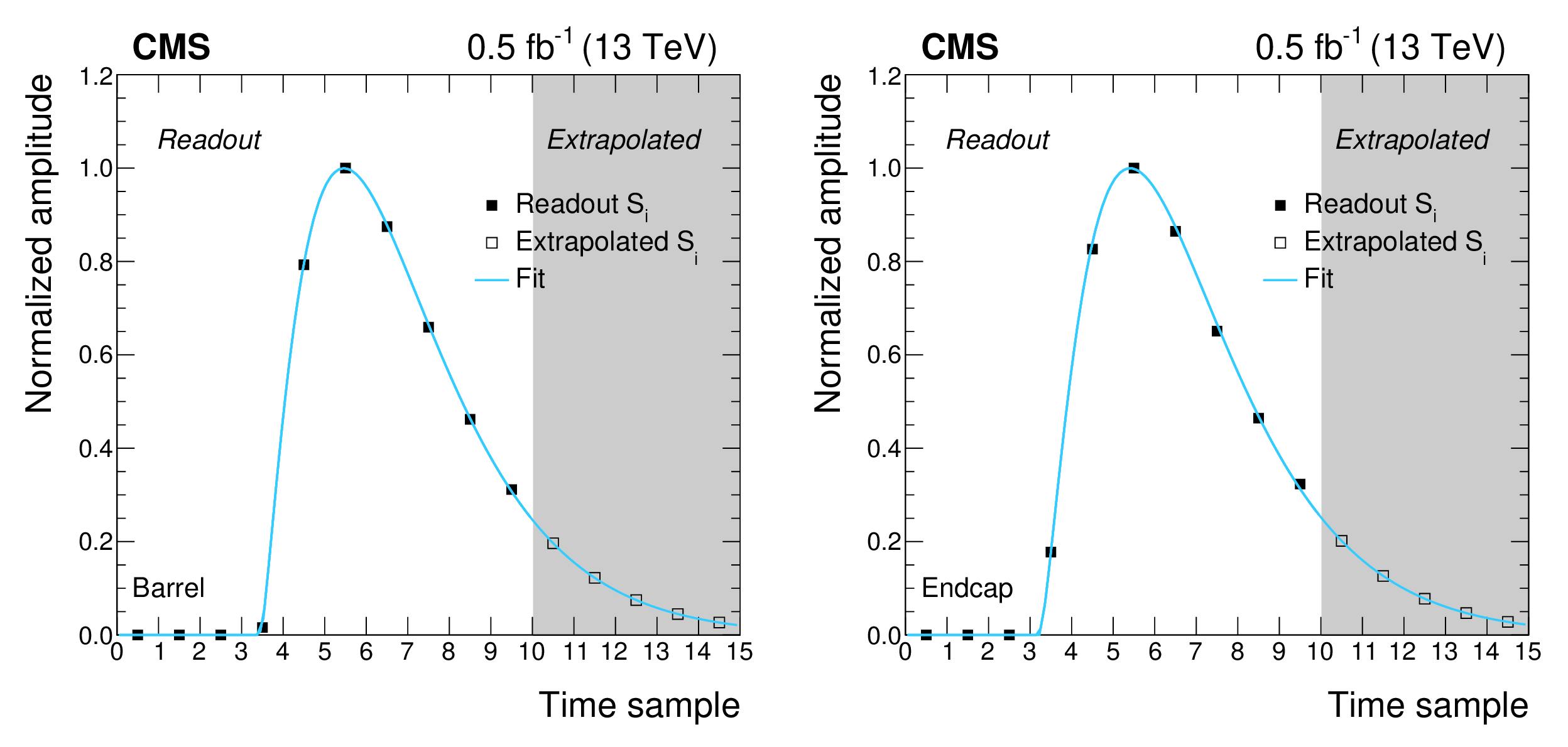
Figure 2:
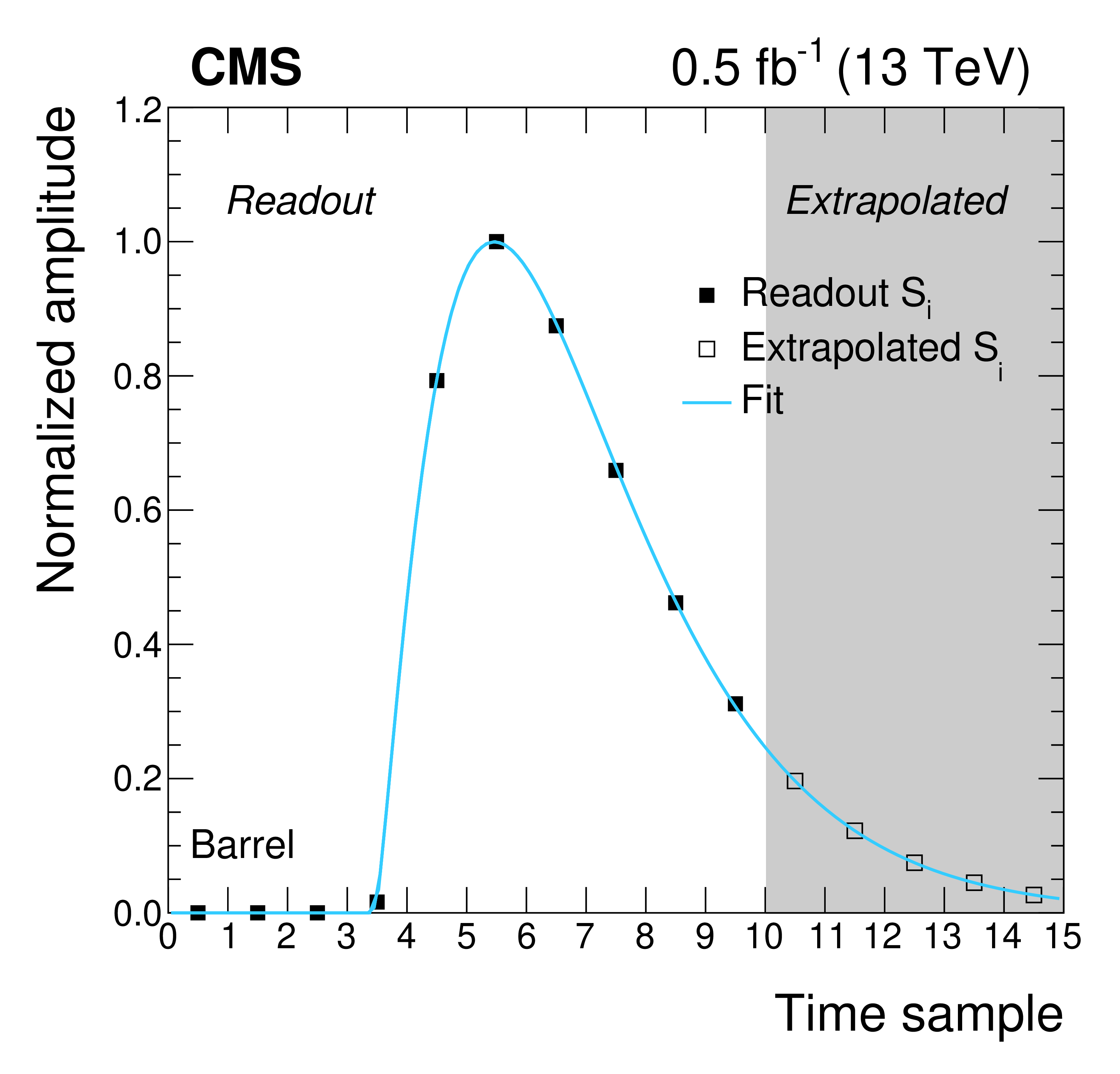
Pulse shape binned templates, measured in collision data recorded during June 2017 in a typical LHC fill, for a channel in the barrel (left) and in an endcap (right). The horizontal error bars represent the bin size. The first 3 bins are the pedestal samples, and their values equal zero by construction. The following 7 bins are estimated from the average of the digitized samples on many hits, while the rightmost 5 bins are estimated by extrapolating the distribution using the function of Eq. (5) (blue solid line). |
png pdf |
Figure 2-a:
Pulse shape binned templates, measured in collision data recorded during June 2017 in a typical LHC fill, for a channel in the barrel. The horizontal error bars represent the bin size. The first 3 bins are the pedestal samples, and their values equal zero by construction. The following 7 bins are estimated from the average of the digitized samples on many hits, while the rightmost 5 bins are estimated by extrapolating the distribution using the function of Eq. (5) (blue solid line). |
png pdf |
Figure 2-b:
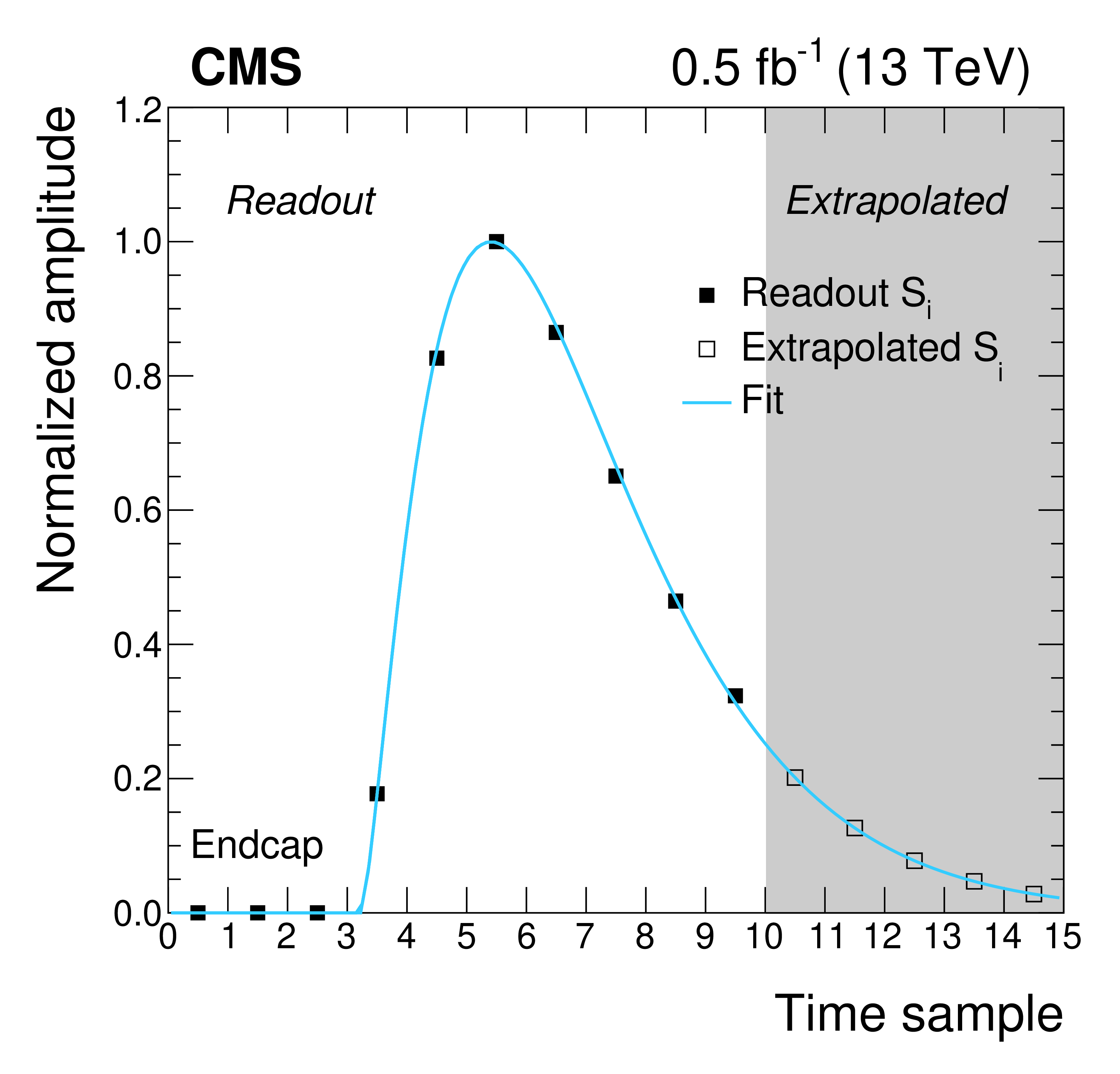
Pulse shape binned templates, measured in collision data recorded during June 2017 in a typical LHC fill, for a channel in an endcap. The horizontal error bars represent the bin size. The first 3 bins are the pedestal samples, and their values equal zero by construction. The following 7 bins are estimated from the average of the digitized samples on many hits, while the rightmost 5 bins are estimated by extrapolating the distribution using the function of Eq. (5) (blue solid line). |
png pdf |
Figure 3:
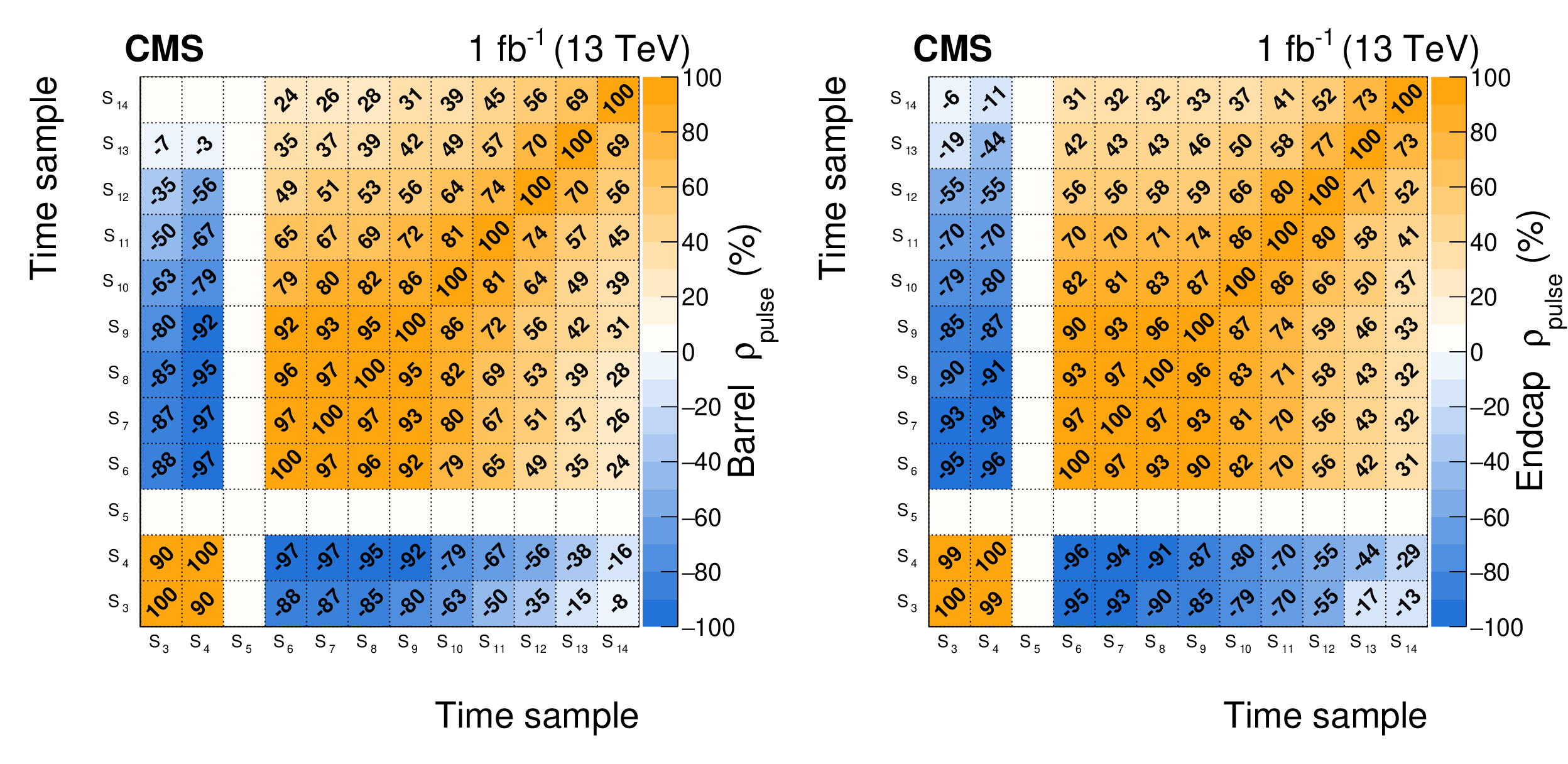
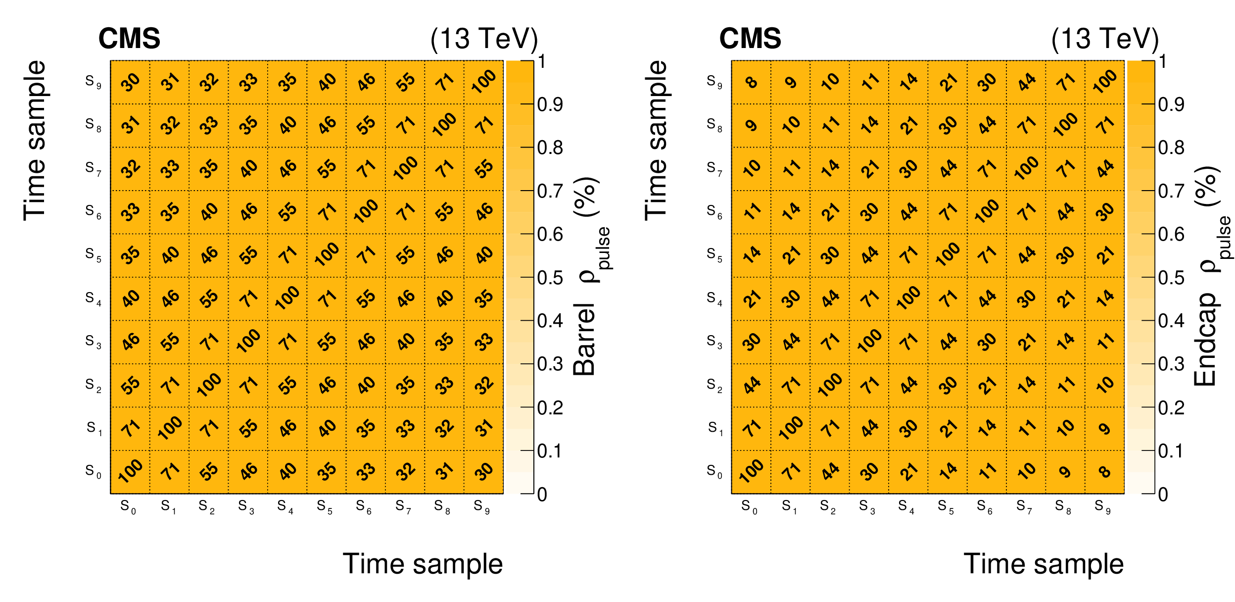
Correlation matrix of the pulse shape binned templates, $ {\rho}_\text {pulse}$, measured in collision data recorded during June 2017 in a typical LHC fill, for one channel in the barrel (left) and in an endcap (right). The elements with $i=$ 5 or $k=$ 5 have zero variance by definition, since $S_5 = 1$ for all the hits. The elements $\rho _\text {pulse}^{i,k}$ with $i < $ 3 or $k < $ 3 are the presamples, where no signal is expected, and are set to zero. Those with $i > $ 9 or $k > $ 9 are estimated from simulations with a shifted BX. The others are measured in collision data, as described in the text. All the values in the figure represent 100$\rho _\text {pulse}^{i,k}$ for readability. |
png pdf |
Figure 3-a:
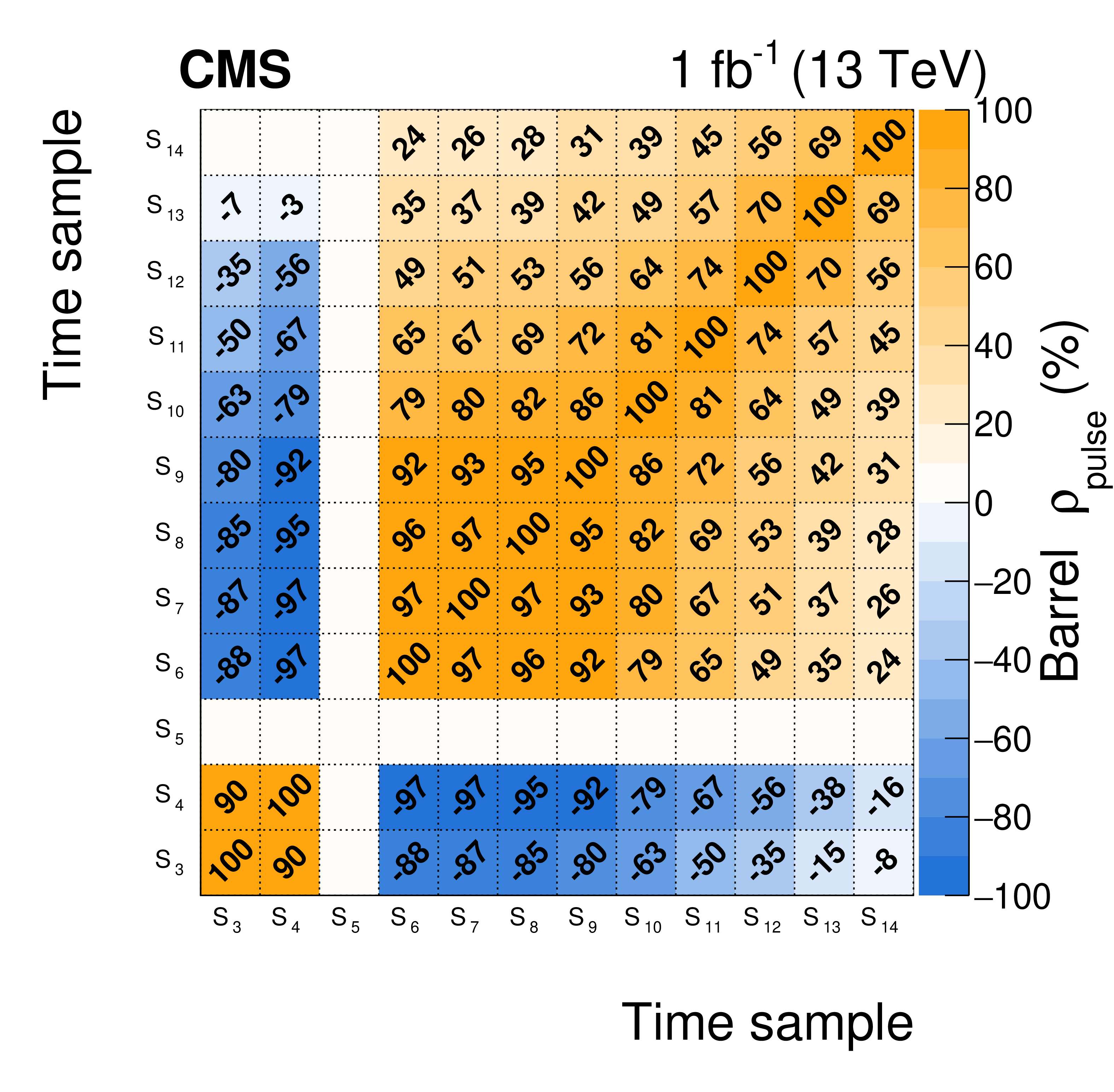
Correlation matrix of the pulse shape binned templates, $ {\rho}_\text {pulse}$, measured in collision data recorded during June 2017 in a typical LHC fill, for one channel in the barrel. The elements with $i=$ 5 or $k=$ 5 have zero variance by definition, since $S_5 = 1$ for all the hits. The elements $\rho _\text {pulse}^{i,k}$ with $i < $ 3 or $k < $ 3 are the presamples, where no signal is expected, and are set to zero. Those with $i > $ 9 or $k > $ 9 are estimated from simulations with a shifted BX. The others are measured in collision data, as described in the text. All the values in the figure represent 100$\rho _\text {pulse}^{i,k}$ for readability. |

png pdf |
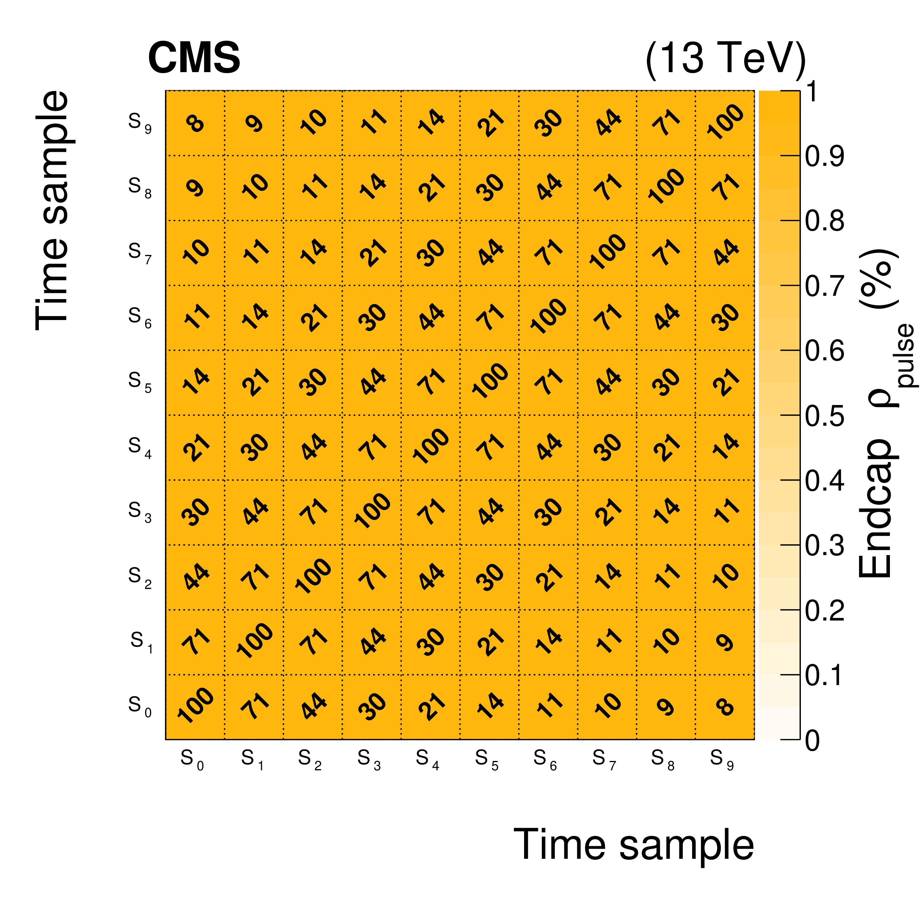
Figure 3-b:
Correlation matrix of the pulse shape binned templates, $ {\rho}_\text {pulse}$, measured in collision data recorded during June 2017 in a typical LHC fill, for one channel in an endcap. The elements with $i=$ 5 or $k=$ 5 have zero variance by definition, since $S_5 = 1$ for all the hits. The elements $\rho _\text {pulse}^{i,k}$ with $i < $ 3 or $k < $ 3 are the presamples, where no signal is expected, and are set to zero. Those with $i > $ 9 or $k > $ 9 are estimated from simulations with a shifted BX. The others are measured in collision data, as described in the text. All the values in the figure represent 100$\rho _\text {pulse}^{i,k}$ for readability. |
png pdf |
Figure 4:
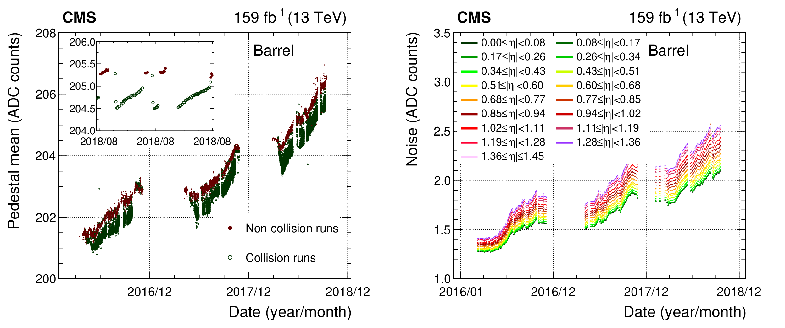
History of the pedestal mean value for the ECAL barrel (left) and its noise (right), measured for the highest MGPA gain in collision or noncollision runs taken during the 2016-2018 data taking period. The inset in the left panel shows an enlargement of two days in August 2018, to show in more detail the variation of the pedestal mean during LHC fills. |
png pdf |
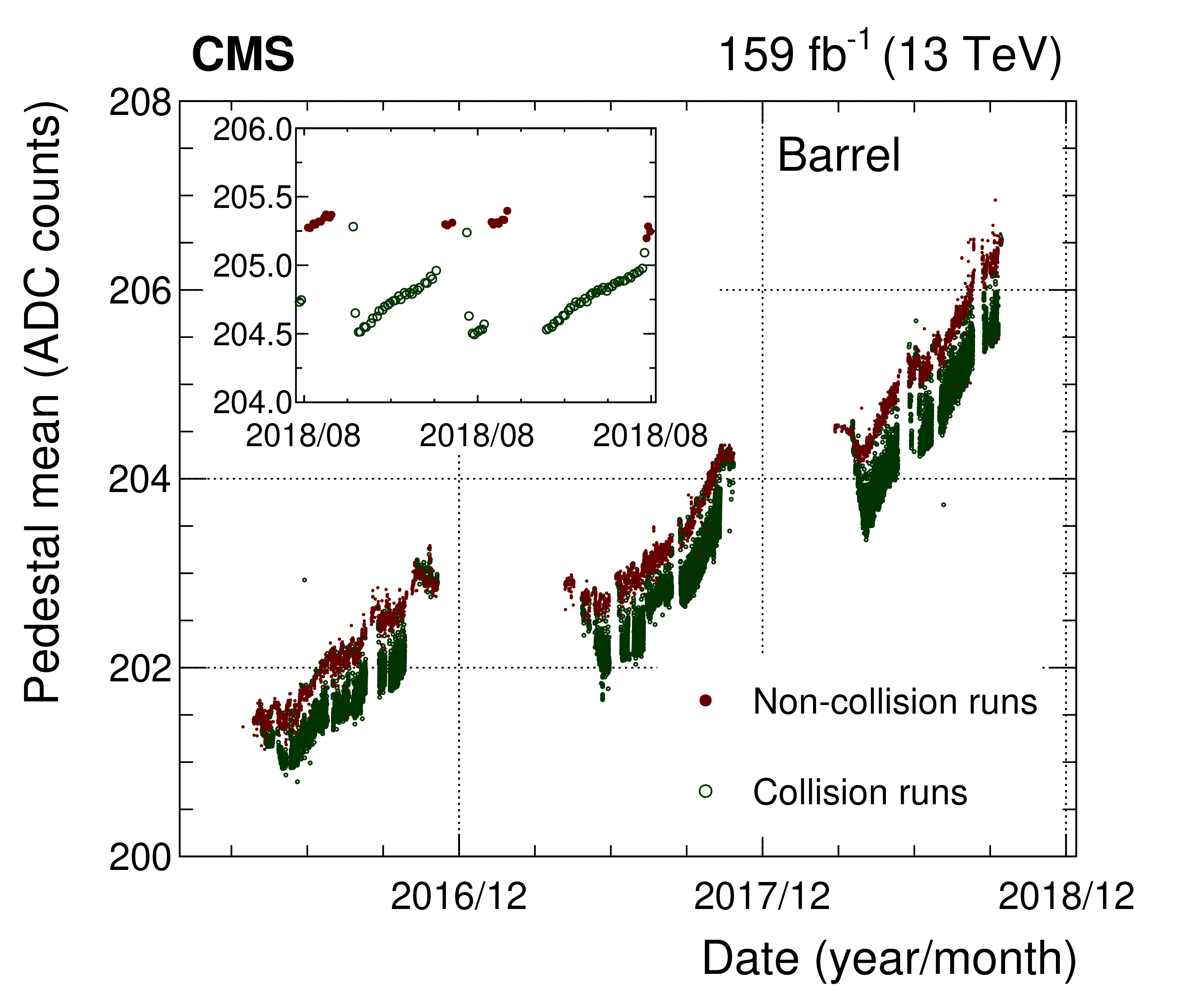
Figure 4-a:
History of the pedestal mean value for the ECAL barrel, measured for the highest MGPA gain in collision or noncollision runs taken during the 2016-2018 data taking period. The inset shows an enlargement of two days in August 2018, to show in more detail the variation of the pedestal mean during LHC fills. |

png pdf |
Figure 4-b:
History of the noise for the ECAL barrel, measured for the highest MGPA gain in collision or noncollision runs taken during the 2016-2018 data taking period. |
png pdf |
Figure 5:
Correlation matrix of the electronics noise, $ {\rho}_\text {noise}$, measured in dedicated pedestal runs in Run 2, averaged over all the channels of the barrel (left) or endcaps (right). All the values in the figure represent 100$ {\rho}_\text {noise}$ for readability. |

png pdf |
Figure 5-a:
Correlation matrix of the electronics noise, $ {\rho}_\text {noise}$, measured in dedicated pedestal runs in Run 2, averaged over all the channels of the barrel (left) or endcaps (right). All the values in the figure represent 100$ {\rho}_\text {noise}$ for readability. |
png pdf |
Figure 5-b:
Correlation matrix of the electronics noise, $ {\rho}_\text {noise}$, measured in dedicated pedestal runs in Run 2, averaged over all the channels of the barrel (left) or endcaps (right). All the values in the figure represent 100$ {\rho}_\text {noise}$ for readability. |

png pdf |
Figure 6:
Reconstructed amplitude bias for the IT amplitude, $< A > -A_\text {true}$, as a function of pedestal shifts $\Delta P$, for a single-crystal pulse of $E = $ 50 GeV the EB. |
png pdf |
Figure 7:
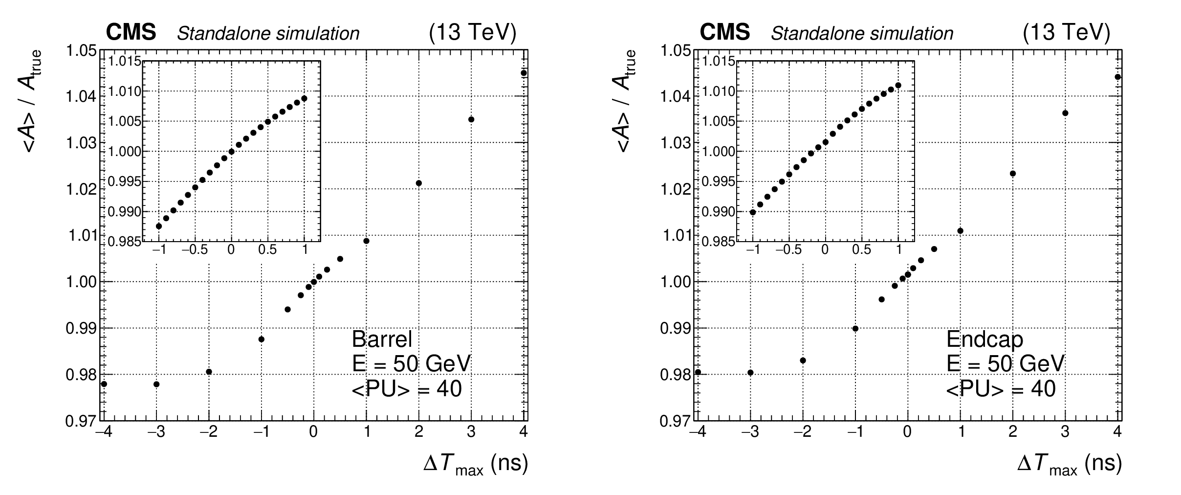
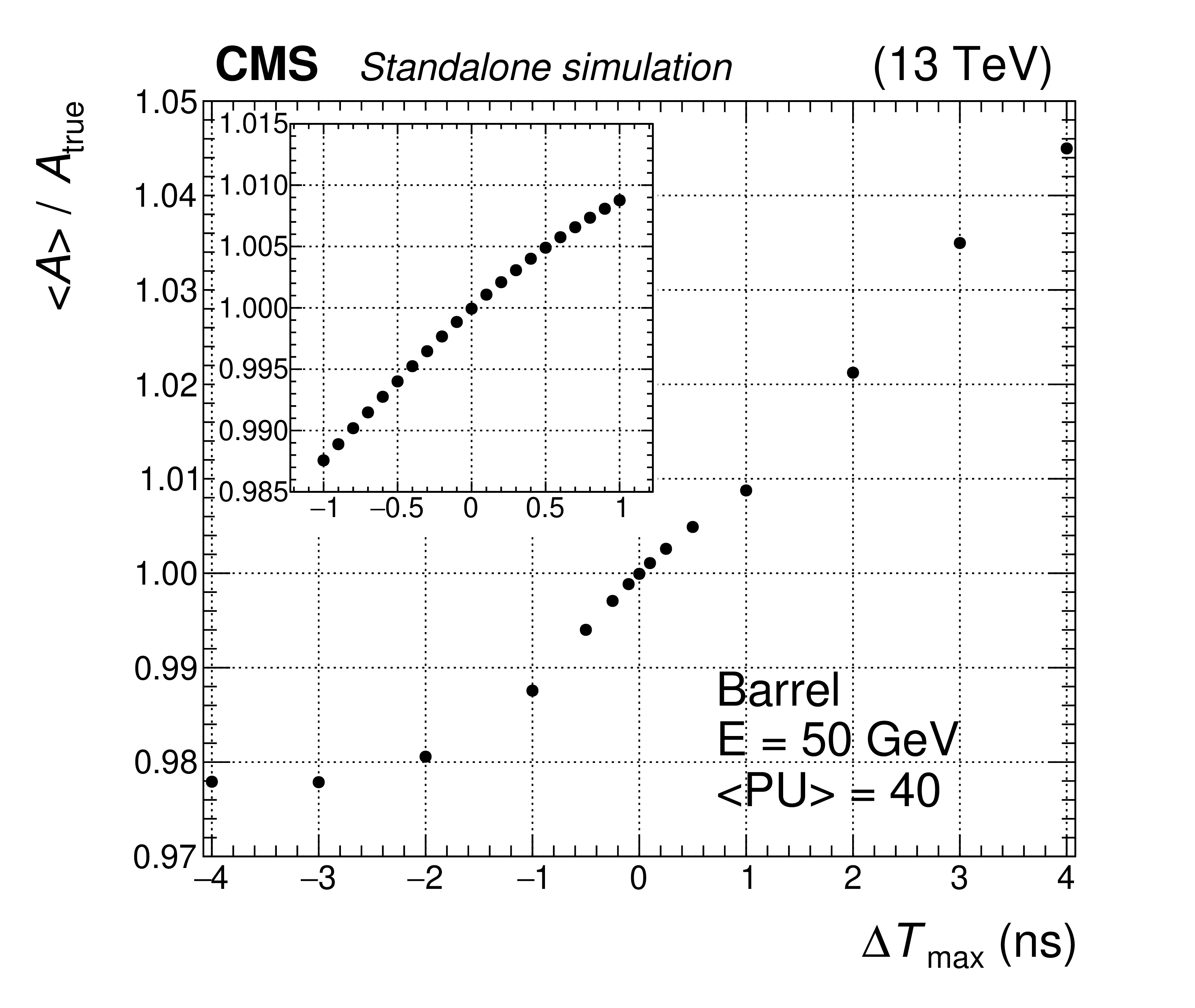
Reconstructed amplitude over true amplitude, $< A > /A_\text {true}$, as a function of the timing shift of the pulse template, $\Delta T_\text {max}$, for a single-crystal pulse of $E = $ 50 GeV in the EB (left) and EE (right). The insets show an enlargement in the $ \pm $1 ns range with a finer $\Delta T_\text {max}$ granularity. |
png pdf |
Figure 7-a:
Reconstructed amplitude over true amplitude, $< A > /A_\text {true}$, as a function of the timing shift of the pulse template, $\Delta T_\text {max}$, for a single-crystal pulse of $E = $ 50 GeV in the EB (left) and EE (right). The insets show an enlargement in the $ \pm $1 ns range with a finer $\Delta T_\text {max}$ granularity. |

png pdf |
Figure 7-b:
Reconstructed amplitude over true amplitude, $< A > /A_\text {true}$, as a function of the timing shift of the pulse template, $\Delta T_\text {max}$, for a single-crystal pulse of $E = $ 50 GeV in the EB (left) and EE (right). The insets show an enlargement in the $ \pm $1 ns range with a finer $\Delta T_\text {max}$ granularity. |
png pdf |
Figure 8:
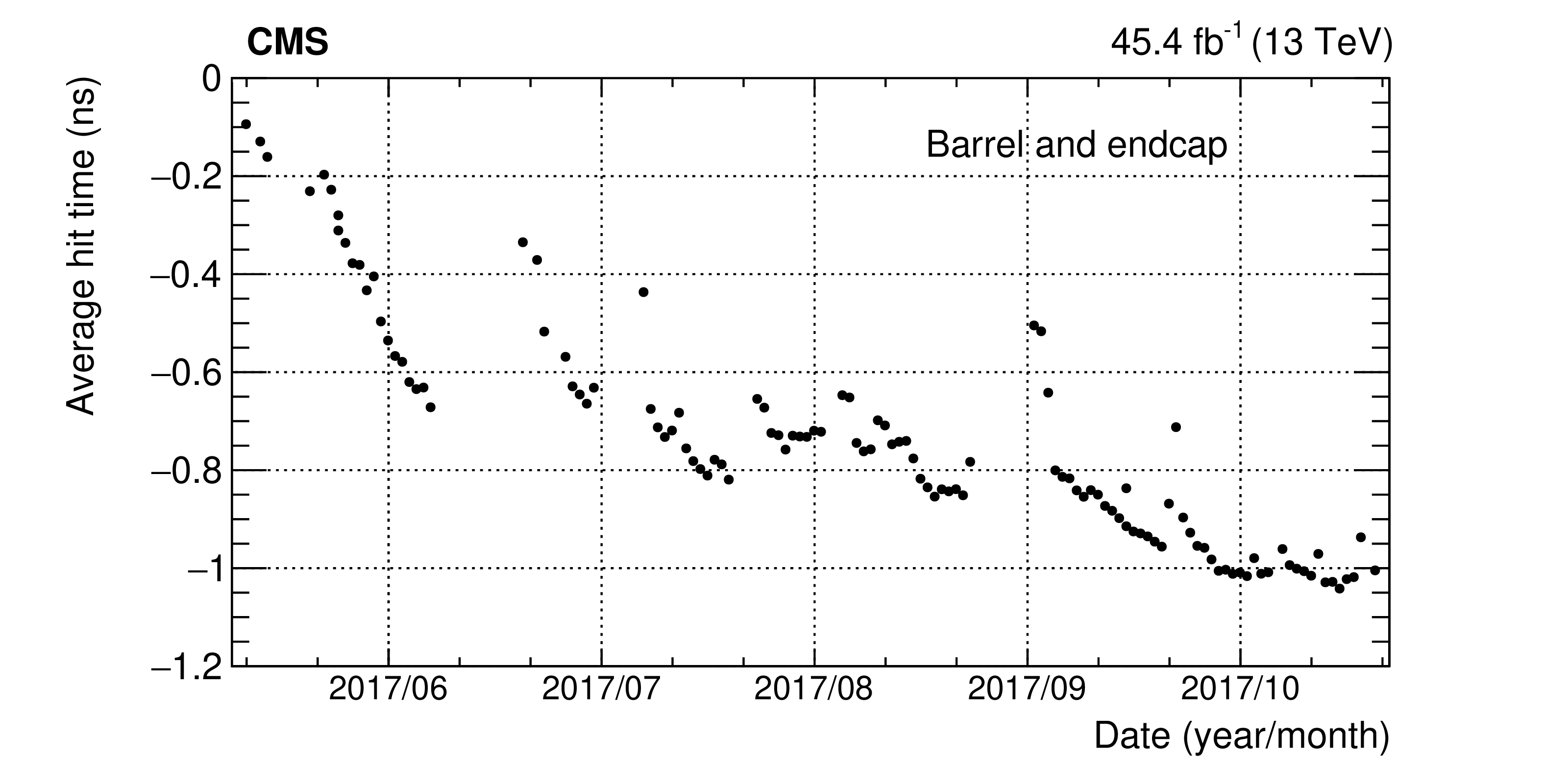
Average timing of ECAL pulses in proton-proton collisions collected in 2017, as measured in Ref. [21]. For each point, the average of the hits reconstructed in all barrel and endcaps channels is used. The sharp changes in $T_\text {max}$ correspond to restarts of data taking following LHC technical stops, as discussed in the text. At the beginning of the yearly data taking, the timing is calibrated so that the average $T_\text {max}=$ 0. |
png pdf |
Figure 9:
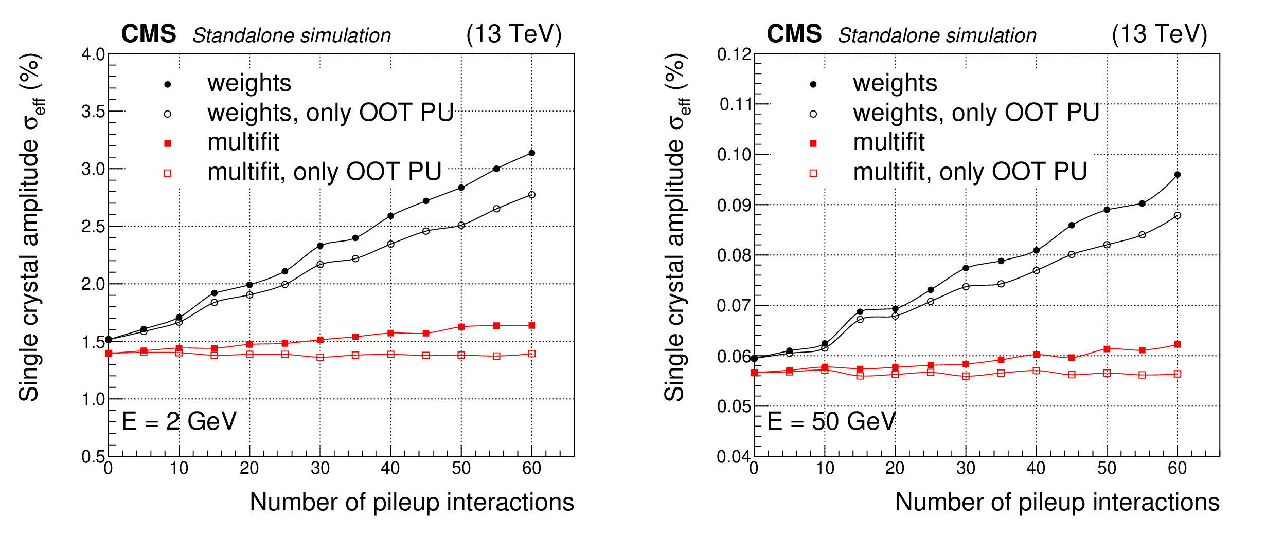
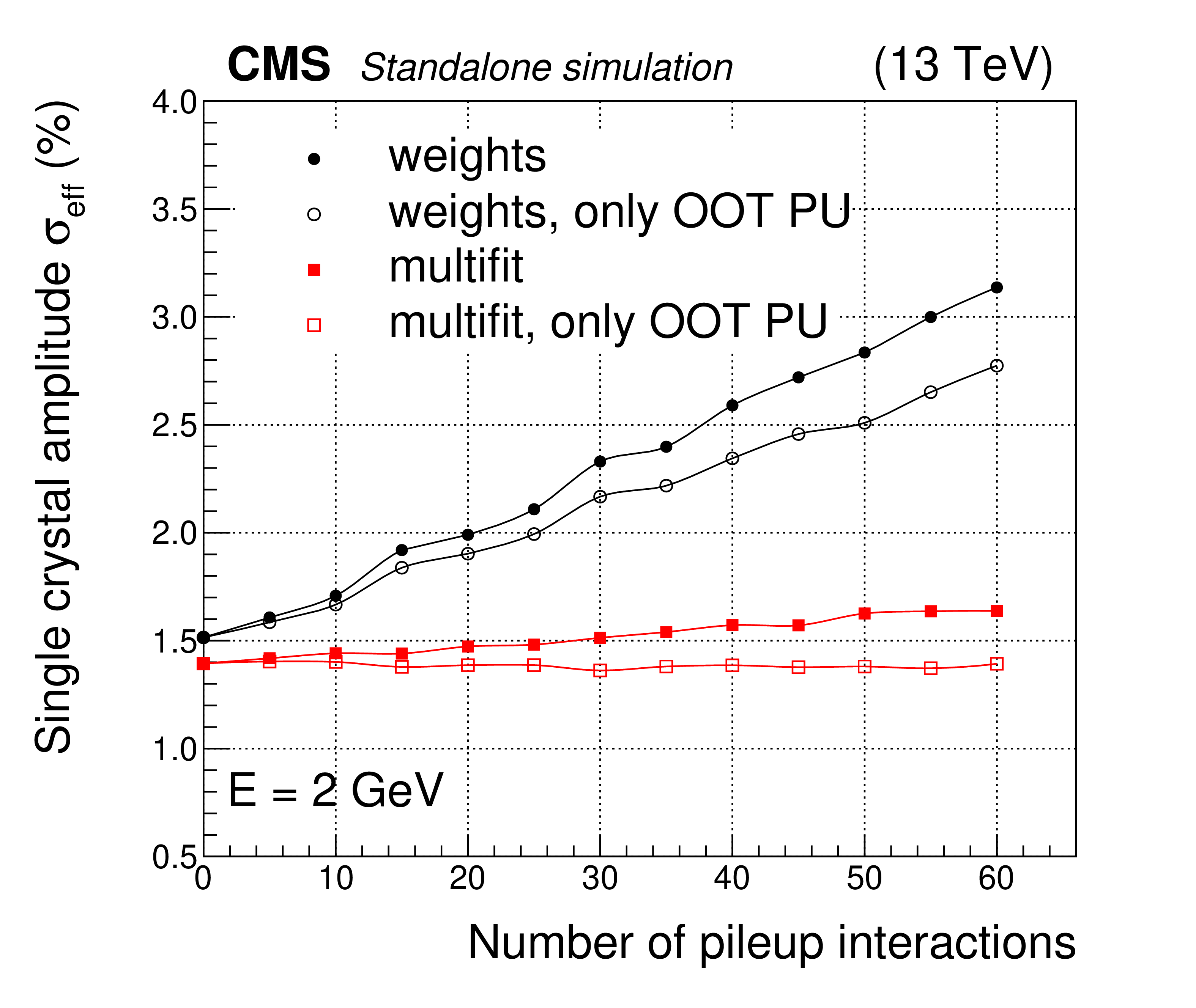
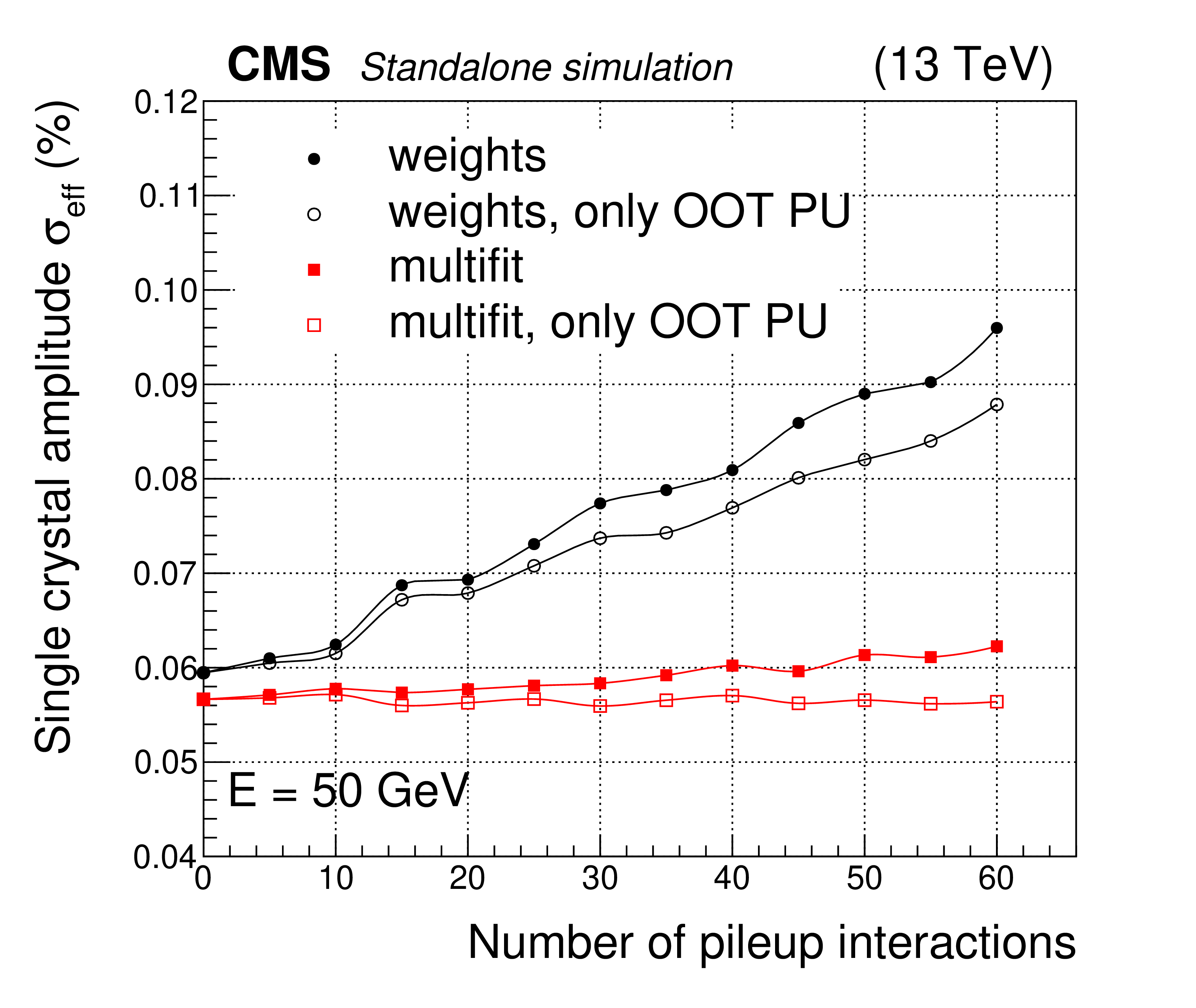
Measured amplitude resolution for two generated energy deposits ($E = $ 2 GeV or $E = $ 50 GeV) in a single ECAL barrel crystal, at $\eta =$ 0, reconstructed with either the multifit or the weights algorithm. Filled points show the effective resolution expressed as the difference between the reconstructed energy and the true energy, divided by the true energy. Open points show the percentage resolution estimated when the true energy is replaced with the sum of the true energy and the in-time pileup energy. |
png pdf |
Figure 9-a:
Measured amplitude resolution for two generated energy deposits ($E = $ 2 GeV or $E = $ 50 GeV) in a single ECAL barrel crystal, at $\eta =$ 0, reconstructed with either the multifit or the weights algorithm. Filled points show the effective resolution expressed as the difference between the reconstructed energy and the true energy, divided by the true energy. Open points show the percentage resolution estimated when the true energy is replaced with the sum of the true energy and the in-time pileup energy. |
png pdf |
Figure 9-b:
Measured amplitude resolution for two generated energy deposits ($E = $ 2 GeV or $E = $ 50 GeV) in a single ECAL barrel crystal, at $\eta =$ 0, reconstructed with either the multifit or the weights algorithm. Filled points show the effective resolution expressed as the difference between the reconstructed energy and the true energy, divided by the true energy. Open points show the percentage resolution estimated when the true energy is replaced with the sum of the true energy and the in-time pileup energy. |

png pdf |
Figure 10:
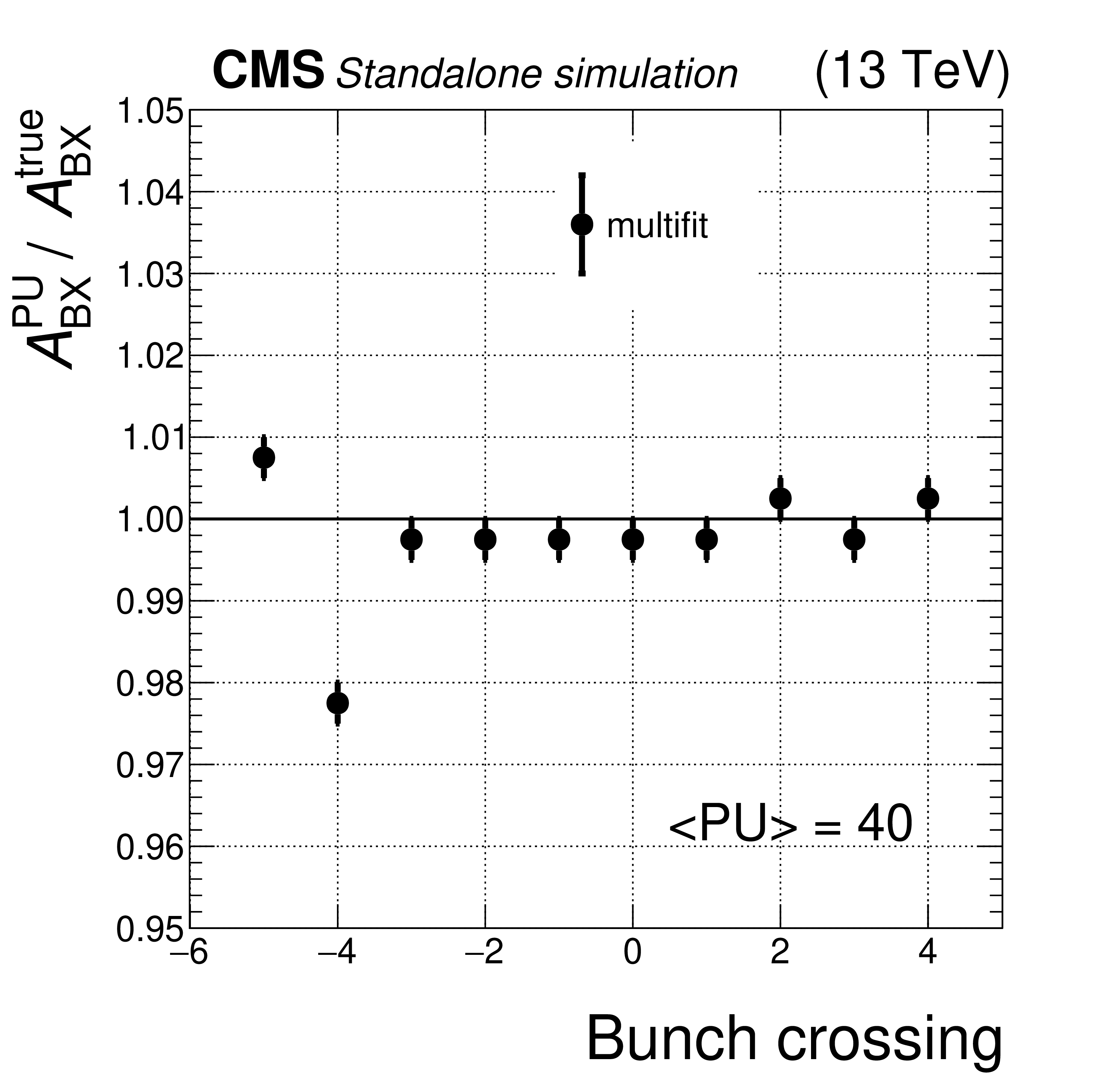
Left: bias in the out-of-time amplitude estimated by the multifit algorithm as a function of BX, for the bunch crossings $-5\le \mathrm {BX}\le +4$. The in-time interaction corresponds to BX $=$ 0 in the figure. The bias is estimated as the mode of the distribution of the ratio between the measured and the true energy. Only statistical uncertainties are shown. Right: energy spectrum in an ECAL barrel crystal, at $\eta \approx $ 0. |
png pdf |
Figure 10-a:
Left: bias in the out-of-time amplitude estimated by the multifit algorithm as a function of BX, for the bunch crossings $-5\le \mathrm {BX}\le +4$. The in-time interaction corresponds to BX $=$ 0 in the figure. The bias is estimated as the mode of the distribution of the ratio between the measured and the true energy. Only statistical uncertainties are shown. Right: energy spectrum in an ECAL barrel crystal, at $\eta \approx $ 0. |

png pdf |
Figure 10-b:
Left: bias in the out-of-time amplitude estimated by the multifit algorithm as a function of BX, for the bunch crossings $-5\le \mathrm {BX}\le +4$. The in-time interaction corresponds to BX $=$ 0 in the figure. The bias is estimated as the mode of the distribution of the ratio between the measured and the true energy. Only statistical uncertainties are shown. Right: energy spectrum in an ECAL barrel crystal, at $\eta \approx $ 0. |
png pdf |
Figure 11:
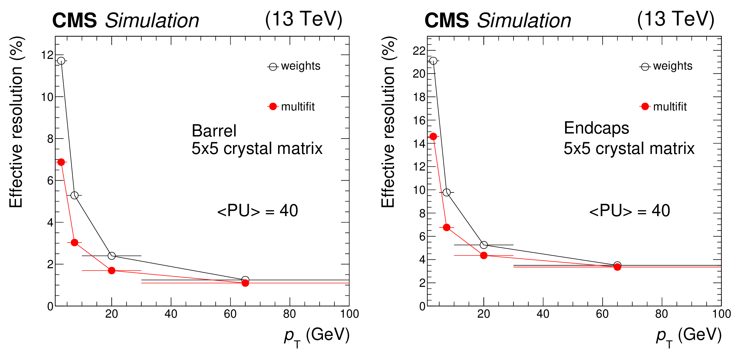
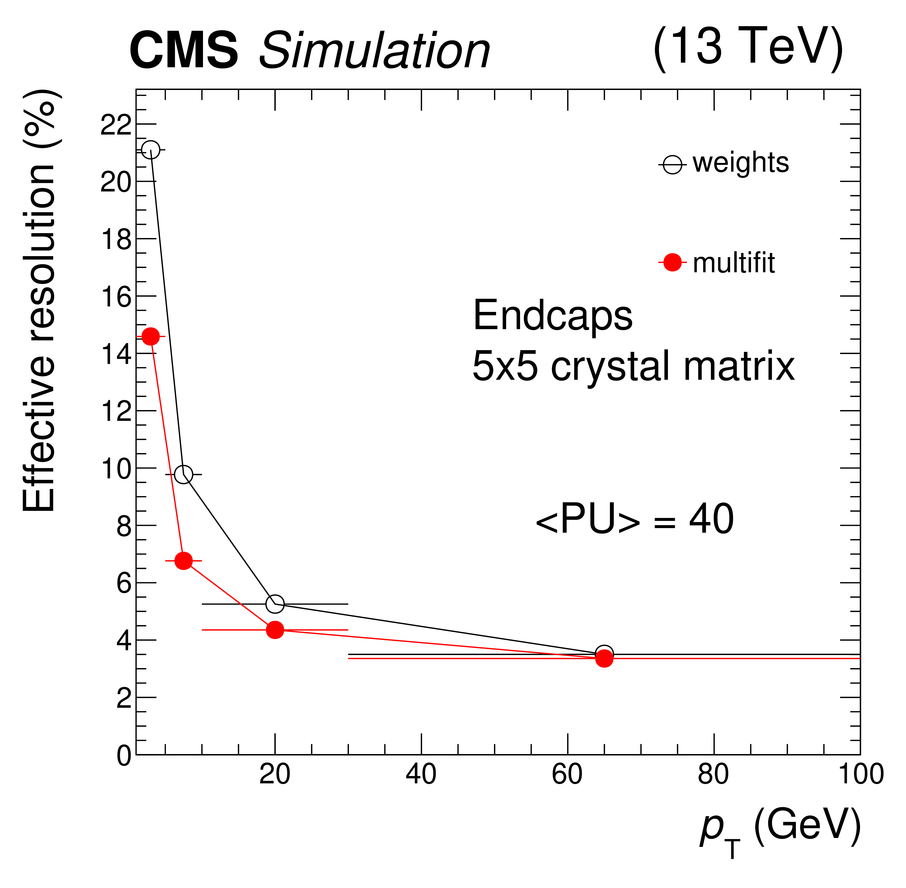
Effective energy resolutions for nonconverted photons in barrel (left) and endcaps (right) as a function of the generated ${p_{\mathrm {T}}}$ of the photon. The photons are generated with a uniform ${p_{\mathrm {T}}}$ distribution and their interaction is obtained with the full detector simulation. The average number of PU interactions is 40. The horizontal error bars represent the bin width. The statistical uncertainties are too small to be displayed. |

png pdf |
Figure 11-a:
Effective energy resolutions for nonconverted photons in barrel (left) and endcaps (right) as a function of the generated ${p_{\mathrm {T}}}$ of the photon. The photons are generated with a uniform ${p_{\mathrm {T}}}$ distribution and their interaction is obtained with the full detector simulation. The average number of PU interactions is 40. The horizontal error bars represent the bin width. The statistical uncertainties are too small to be displayed. |
png pdf |
Figure 11-b:
Effective energy resolutions for nonconverted photons in barrel (left) and endcaps (right) as a function of the generated ${p_{\mathrm {T}}}$ of the photon. The photons are generated with a uniform ${p_{\mathrm {T}}}$ distribution and their interaction is obtained with the full detector simulation. The average number of PU interactions is 40. The horizontal error bars represent the bin width. The statistical uncertainties are too small to be displayed. |
png pdf |
Figure 12:
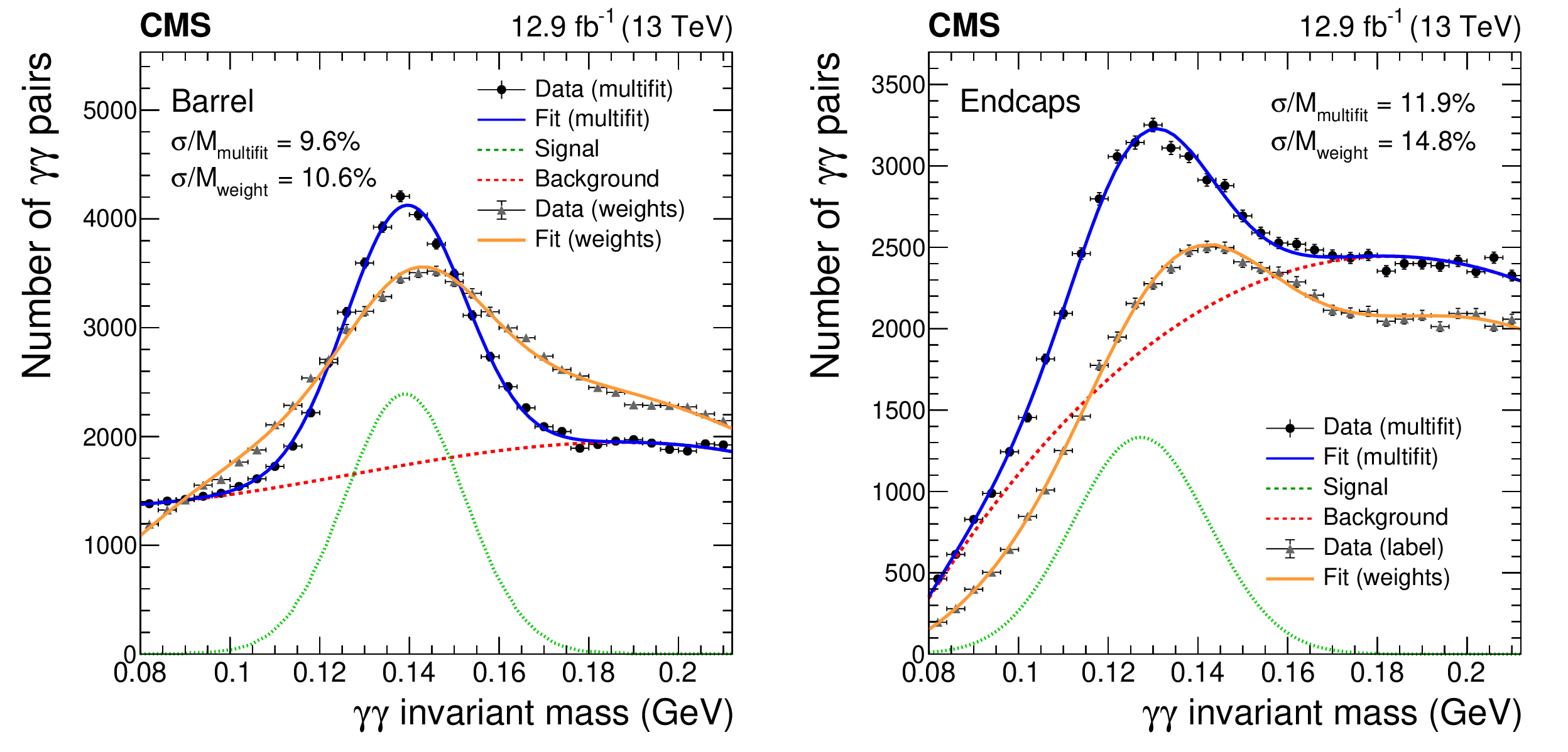
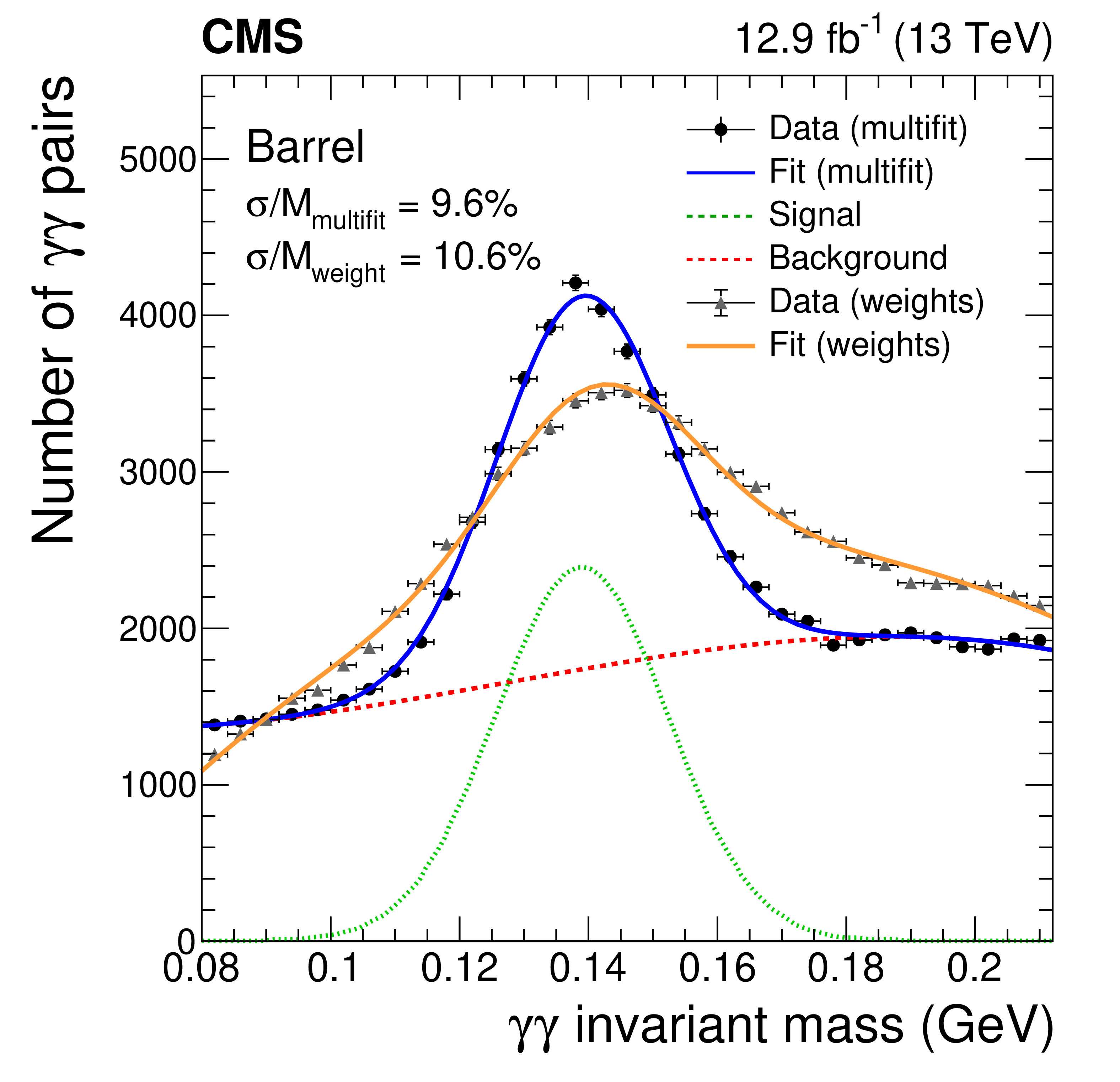
Examples of the $\pi ^0$-meson peak reconstructed from the invariant mass of photon pairs in the barrel (left) and endcaps (right), for the single-crystal amplitudes measured with either the weights or the multifit reconstruction. A portion of collision data with typical Run 2 conditions, recorded during July 2018, is used. Error bars represent the statistical uncertainty. The result of the fit with a Gaussian distribution (green dotted line) plus a polynomial function (red dashed line) is superimposed on the measured distributions for the multifit case (dark blue solid line). For the weights case the same model is used, but only the total likelihood is shown superimposed (light orange solid line). |
png pdf |
Figure 12-a:
Examples of the $\pi ^0$-meson peak reconstructed from the invariant mass of photon pairs in the barrel (left) and endcaps (right), for the single-crystal amplitudes measured with either the weights or the multifit reconstruction. A portion of collision data with typical Run 2 conditions, recorded during July 2018, is used. Error bars represent the statistical uncertainty. The result of the fit with a Gaussian distribution (green dotted line) plus a polynomial function (red dashed line) is superimposed on the measured distributions for the multifit case (dark blue solid line). For the weights case the same model is used, but only the total likelihood is shown superimposed (light orange solid line). |

png pdf |
Figure 12-b:
Examples of the $\pi ^0$-meson peak reconstructed from the invariant mass of photon pairs in the barrel (left) and endcaps (right), for the single-crystal amplitudes measured with either the weights or the multifit reconstruction. A portion of collision data with typical Run 2 conditions, recorded during July 2018, is used. Error bars represent the statistical uncertainty. The result of the fit with a Gaussian distribution (green dotted line) plus a polynomial function (red dashed line) is superimposed on the measured distributions for the multifit case (dark blue solid line). For the weights case the same model is used, but only the total likelihood is shown superimposed (light orange solid line). |
png pdf |
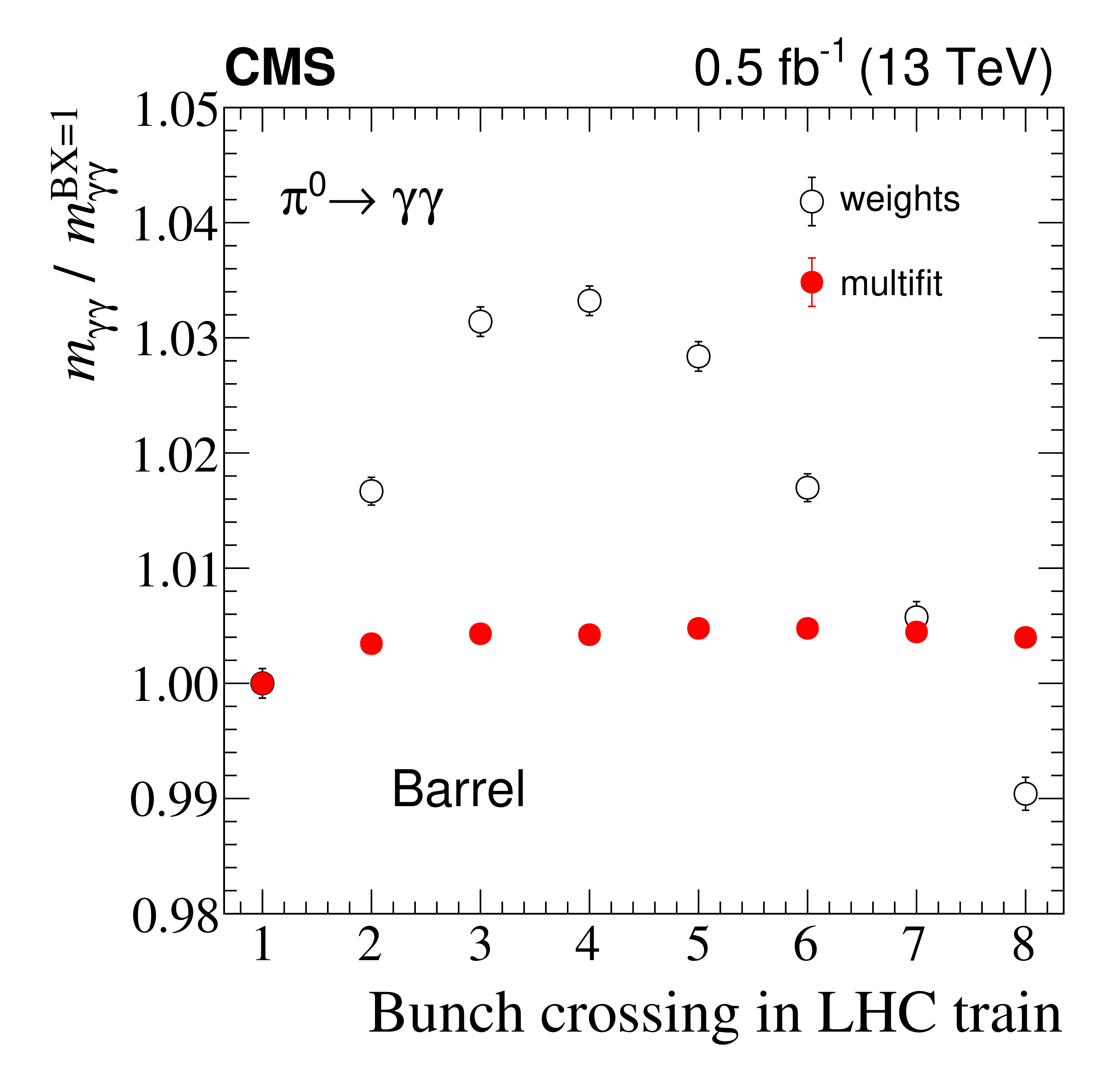
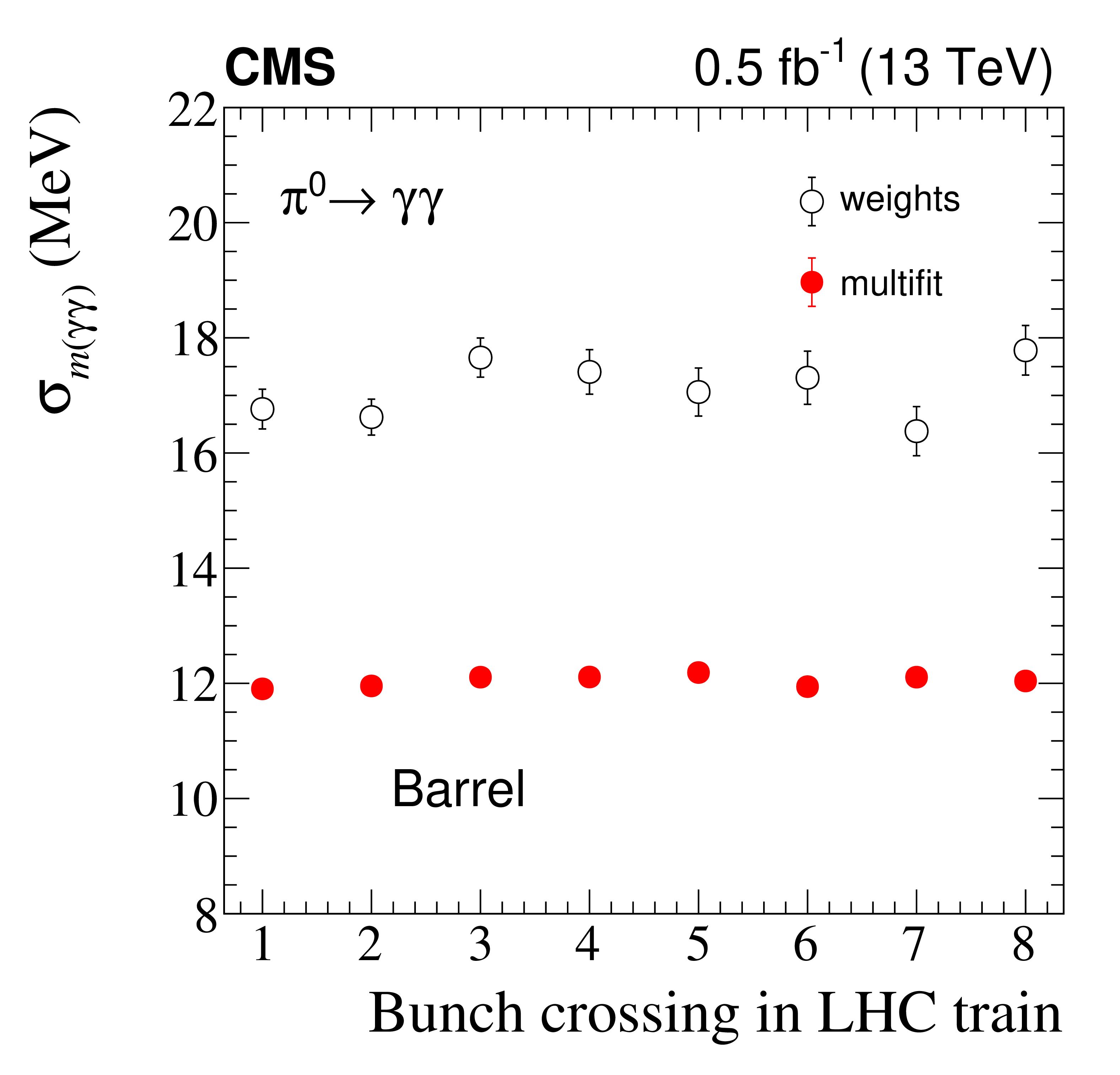
Figure 13:
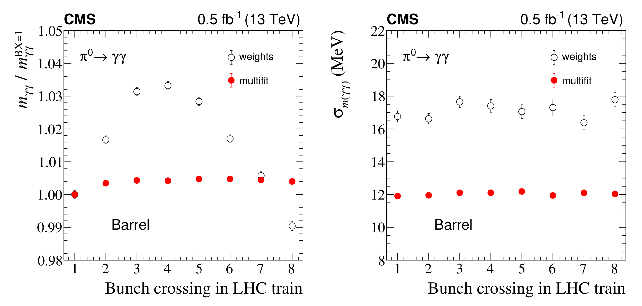
Peak position, normalized to the mass measured in the first BX of the train, (left) and Gaussian resolution $\sigma _{m({\gamma \gamma})}$ (right) of the invariant mass distribution of $\pi ^0\to \gamma \gamma $ decays with both photons in the EB, within a bunch train of 8 colliding bunches from an LHC fill in October 2017. Error bars represent the statistical uncertainty. The single-crystal energy is reconstructed either with the weights method (open circles) or with the multifit method (filled circles). Each point is obtained by fitting the diphoton invariant mass distribution in collisions selected from a single BX of the train. |
png pdf |
Figure 13-a:
Peak position, normalized to the mass measured in the first BX of the train, (left) and Gaussian resolution $\sigma _{m({\gamma \gamma})}$ (right) of the invariant mass distribution of $\pi ^0\to \gamma \gamma $ decays with both photons in the EB, within a bunch train of 8 colliding bunches from an LHC fill in October 2017. Error bars represent the statistical uncertainty. The single-crystal energy is reconstructed either with the weights method (open circles) or with the multifit method (filled circles). Each point is obtained by fitting the diphoton invariant mass distribution in collisions selected from a single BX of the train. |
png pdf |
Figure 13-b:
Peak position, normalized to the mass measured in the first BX of the train, (left) and Gaussian resolution $\sigma _{m({\gamma \gamma})}$ (right) of the invariant mass distribution of $\pi ^0\to \gamma \gamma $ decays with both photons in the EB, within a bunch train of 8 colliding bunches from an LHC fill in October 2017. Error bars represent the statistical uncertainty. The single-crystal energy is reconstructed either with the weights method (open circles) or with the multifit method (filled circles). Each point is obtained by fitting the diphoton invariant mass distribution in collisions selected from a single BX of the train. |
png pdf |
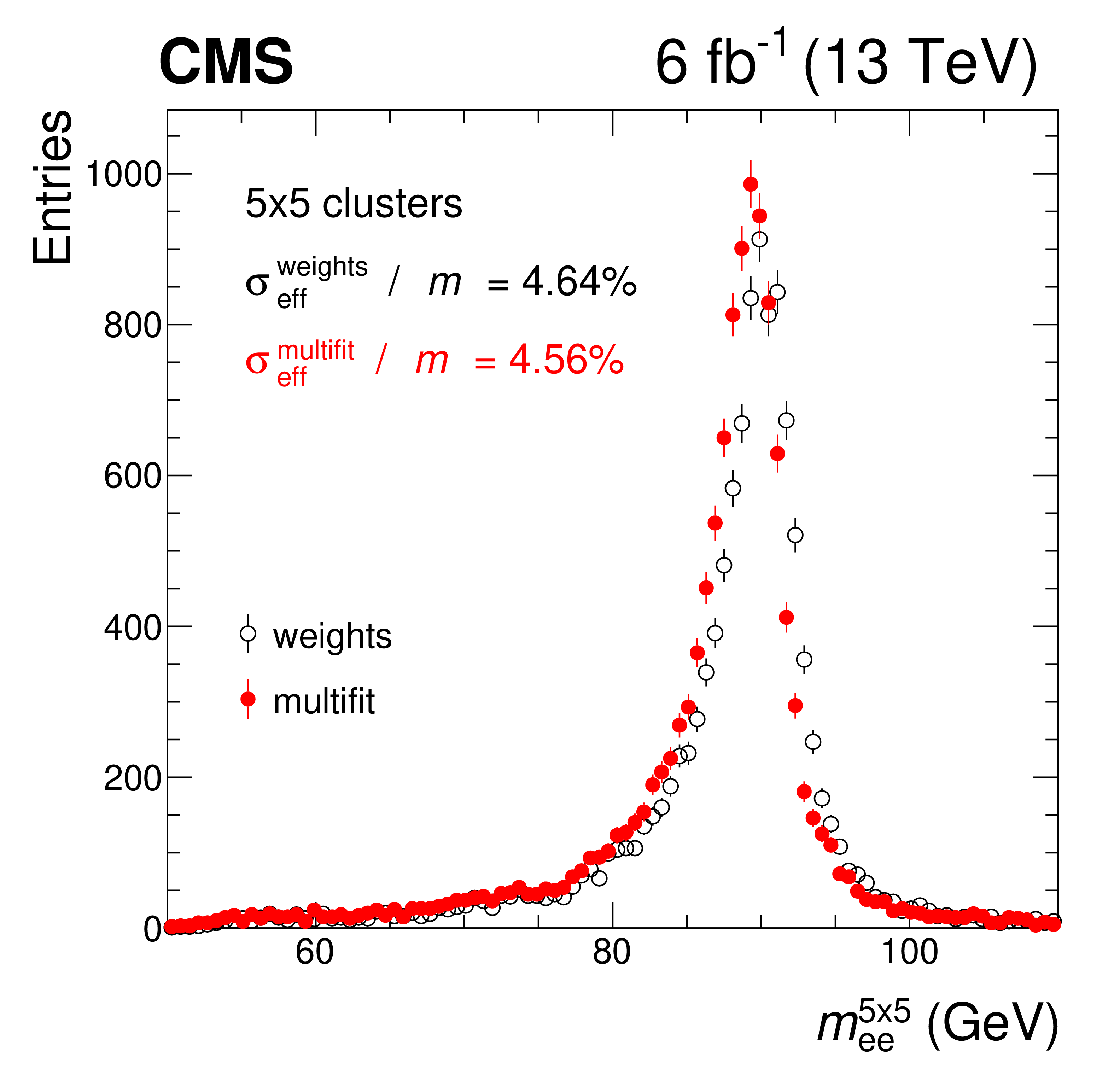
Figure 14:
Example of the $\mathrm{Z} \to \mathrm{e^{+}} \mathrm{e^{-}} $ invariant mass distribution in a central region of the barrel (0.200 $ < \text {max}({| \eta _1 |}, {| \eta _2 |}) < $ 0.435) with the single-crystal amplitude estimated using either the weights or the multifit method. A portion of collision data with typical Run 2 conditions, recorded during October 2016, is used. Error bars represent the statistical uncertainty. The energy is summed over a 5${\times}$5 crystal matrix. The reported values of $\sigma _\text {eff}$ include the natural width of the Z boson, and are expressed as a percentage of the position of the peak, $m$, of the corresponding invariant mass distribution. |
png pdf |
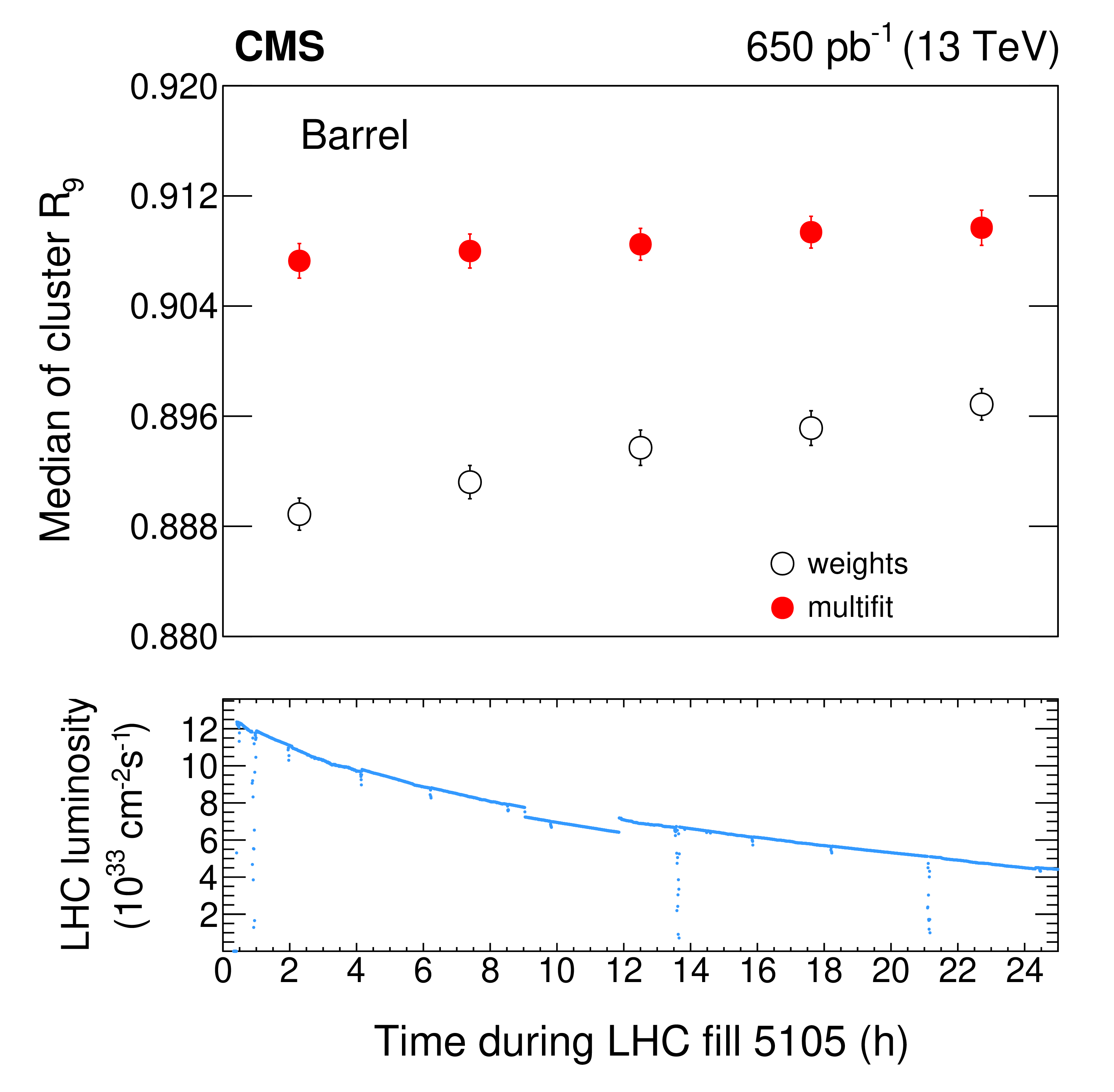
Figure 15:
History of the median of the $R_9$ cluster shape for electrons from $\mathrm{Z} \to \mathrm{e^{+}} \mathrm{e^{-}} $ decays during one typical LHC fill in 2016. Hits are reconstructed with either the multifit (filled circles) or the weights algorithm (open circles). Each point represents the median of the distribution for a 5 hour period during the considered LHC fill. Error bars represent the statistical uncertainty on the median. The bottom panel shows the instantaneous luminosity delivered by the LHC as a function of time. |
| Summary |
|
A multifit algorithm that uses a template fitting technique to reconstruct the energy of single hits in the CMS electromagnetic calorimeter has been presented. This algorithm was implemented before the start of the Run 2 data taking period of the LHC, replacing the weights method used in Run 1. The change was motivated by the reduction of the LHC bunch spacing from 50 to 25 ns, and by the higher instantaneous luminosity delivered in Run 2, which led to a substantial increase in both the in-time and out-of-time pileup. Procedures have been developed to provide regular updates of input parameters to ensure the stability of energy reconstruction over time. Studies based on control samples in data show that the energy resolution for deposits ranging from a few to several tens of GeV is improved, using $\pi^0\to\gamma\gamma$ and $\mathrm{Z}\to\mathrm{e^{+}}\mathrm{e^{-}}$ decays. The gain is more significant for lower energy electromagnetic deposits, for which the relative contribution of pileup is larger. This enhances the reconstruction of jets and missing transverse energy with the particle-flow algorithm used in CMS. These results have been reproduced with simulation studies, which show that an improvement relative to the weights method is obtained at all energies, including those relevant for photons from Higgs boson decays. Simulation studies show that the new algorithm will perform successfully at the high-luminosity LHC, where a peak pileup of about 200 interactions per bunch crossing, with 25 ns bunch spacing, is expected. |
| References | ||||
| 1 | CMS Collaboration | The CMS experiment at the CERN LHC | JINST 3 (2008) S08004 | CMS-00-001 |
| 2 | CMS Collaboration | The CMS electromagnetic calorimeter project: technical design report | CDS | |
| 3 | P. Adzic et al. | Reconstruction of the signal amplitude of the CMS electromagnetic calorimeter | EPJC 46 (2006) 23 | |
| 4 | CMS Collaboration | The CMS trigger system | JINST 12 (2017) P01020 | CMS-TRG-12-001 1609.02366 |
| 5 | S. Gadomski et al. | The deconvolution method of fast pulse shaping at hadron colliders | NIMA 320 (1992) 217 | |
| 6 | CMS Collaboration | CMS tracking performance results from early LHC operation | EPJC 70 (2010) 1165 | |
| 7 | F. James and M. Roos | MINUIT: a system for function minimization and analysis of the parameter errors and correlations | CPC 10 (1975) 343 | |
| 8 | D. Chen and R. J. Plemmons | Nonnegativity constraints in numerical analysis | in The Birth of Numerical Analysis, p. 109 2009 | |
| 9 | C. L. Lawson and R. J. Hanson | Solving least squares problems | Society for Industrial and Applied Mathematics, 1995 | |
| 10 | GEANT4 Collaboration | GEANT4 --- a simulation toolkit | NIMA 506 (2003) 250 | |
| 11 | G. Guennebaud and B. Jacob | Eigen v3 | 2010 \url http://eigen.tuxfamily.org | |
| 12 | C. Richardson | CMS high level trigger timing measurements | J. Phys. Conf. Ser. 664 (2015) 082045 | |
| 13 | CMS Collaboration | Energy calibration and resolution of the CMS electromagnetic calorimeter in pp collisions at $ \sqrt{s} = $ 7 TeV | JINST 8 (2013) P09009 | CMS-EGM-11-001 1306.2016 |
| 14 | CMS Collaboration | Anomalous APD signals in the CMS electromagnetic calorimeter | NIMA 695 (2012) 293 | |
| 15 | CMS Collaboration | Performance and operation of the CMS electromagnetic calorimeter | JINST 5 (2010) T03010 | CMS-CFT-09-004 0910.3423 |
| 16 | CMS Collaboration | CMS luminosity based on pixel cluster counting --- Summer 2013 update | CMS-PAS-LUM-13-001 | CMS-PAS-LUM-13-001 |
| 17 | M. Anfreville et al. | Laser monitoring system for the CMS lead tungstate crystal calorimeter | NIMA 594 (2008) 292 | |
| 18 | L.-Y. Zhang et al. | Performance of the monitoring light source for the CMS lead tungstate crystal calorimeter | IEEE Trans. Nucl. Sci. 52 (2005) 1123 | |
| 19 | S. D. Guida et al. | The CMS condition database system | in Proceedings, 21st International Conference on Computing in High Energy and Nuclear Physics (CHEP 2015) | |
| 20 | Z. Antunovic et al. | Radiation hard avalanche photodiodes for the CMS detector | NIMA 537 (2005) 379 | |
| 21 | CMS Collaboration | Time reconstruction and performance of the CMS electromagnetic calorimeter | JINST 5 (2010) T03011 | CMS-CFT-09-006 0911.4044 |
| 22 | G. Apollinari et al. | High-Luminosity Large Hadron Collider (HL-LHC) | CERN Yellow Rep. Monogr. 4 (2017) 1 | |
| 23 | CMS Collaboration | The Phase-2 upgrade of the CMS barrel calorimeters | CMS-PAS-TDR-17-002 | CMS-PAS-TDR-17-002 |
| 24 | CMS Collaboration | Performance of photon reconstruction and identification with the CMS detector in proton-proton collisions at $ \sqrt{s} = $ 8 TeV | JINST 10 (2015) P08010 | CMS-EGM-14-001 1502.02702 |
| 25 | CMS Collaboration | Performance of electron reconstruction and selection with the CMS detector in proton-proton collisions at $ \sqrt{s} = $ 8 TeV | JINST 10 (2015) P06005 | CMS-EGM-13-001 1502.02701 |
| 26 | CMS Collaboration | Particle-flow reconstruction and global event description with the CMS detector | JINST 12 (2017) P10003 | CMS-PRF-14-001 1706.04965 |
| 27 | CMS Collaboration | Jet energy scale and resolution in the CMS experiment in pp collisions at 8 TeV | JINST 12 (2017) P02014 | CMS-JME-13-004 1607.03663 |
| 28 | CMS Collaboration | Jet energy scale and resolution performance with 13 TeV data collected by CMS in 2016 | CDS | |
| 29 | CMS Collaboration | Performance of missing transverse momentum reconstruction in proton-proton collisions at $ \sqrt{s} = $ 13 TeV using the CMS detector | JINST 14 (2019) P07004 | CMS-JME-17-001 1903.06078 |
|
|
Compact Muon Solenoid LHC, CERN |
|

|

|

|

|

|