

Compact Muon Solenoid
LHC, CERN
| CMS-EGM-17-001 ; CERN-EP-2020-219 | ||
| Electron and photon reconstruction and identification with the CMS experiment at the CERN LHC | ||
| CMS Collaboration | ||
| 12 December 2020 | ||
| JINST 16 (2021) P05014 | ||
| Abstract: The performance is presented of the reconstruction and identification algorithms for electrons and photons with the CMS experiment at the LHC. The reported results are based on proton-proton collision data collected at a center-of-mass energy of 13 TeV and recorded in 2016-2018, corresponding to an integrated luminosity of 136 fb$^{-1}$. Results obtained from lead-lead collision data collected at ${\sqrt {\smash [b]{s_{_{\mathrm {NN}}}}}} = $ 5.02 TeV are also presented. Innovative techniques are used to reconstruct the electron and photon signals in the detector and to optimize the energy resolution. Events with electrons and photons in the final state are used to measure the energy resolution and energy scale uncertainty in the recorded events. The measured energy resolution for electrons produced in Z boson decays in proton-proton collision data ranges from 2 to 5%, depending on electron pseudorapidity and energy loss through bremsstrahlung in the detector material. The energy scale in the same range of energies is measured with an uncertainty smaller than 0.1 (0.3)% in the barrel (endcap) region in proton-proton collisions and better than 1 (3)% in the barrel (endcap) region in heavy ion collisions. The timing resolution for electrons from Z boson decays with the full 2016-2018 proton-proton collision data set is measured to be 200 ps. | ||
| Links: e-print arXiv:2012.06888 [hep-ex] (PDF) ; CDS record ; inSPIRE record ; CADI line (restricted) ; | ||
| Figures | |
png pdf |
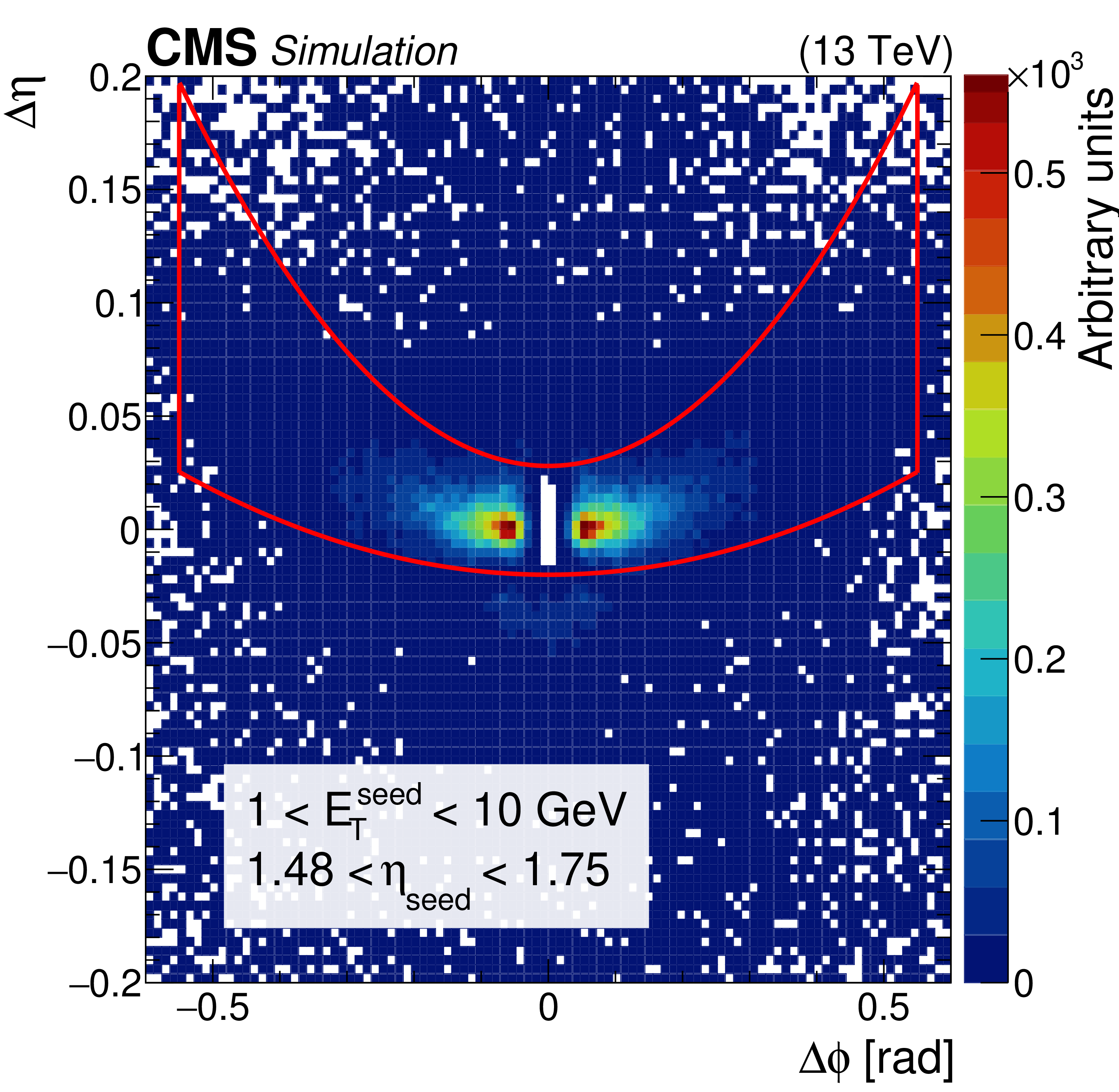
Figure 1:
Distribution of $\Delta \eta =\eta _{\text {seed-cluster}}-\eta _{\text {cluster}}$ versus $\Delta \phi =\phi _{\text {seed-cluster}}-\phi _{\text {cluster}}$ for simulated electrons with 1 $ < {E_{\mathrm {T}}} ^{\text {seed}} < $ 10 GeV and 1.48 $ < \eta _{\text {seed}} < $ 1.75. The $z$ axis represents the occupancy of the number of PF clusters matched with the simulation (requiring to share at least 1% of the simulated electron energy) around the seed. The red line contains approximately the set of clusters selected by the mustache algorithm. The white region at the centre of the plot represents the $\eta $-$\phi $ footprint of the seed cluster. |
png pdf |
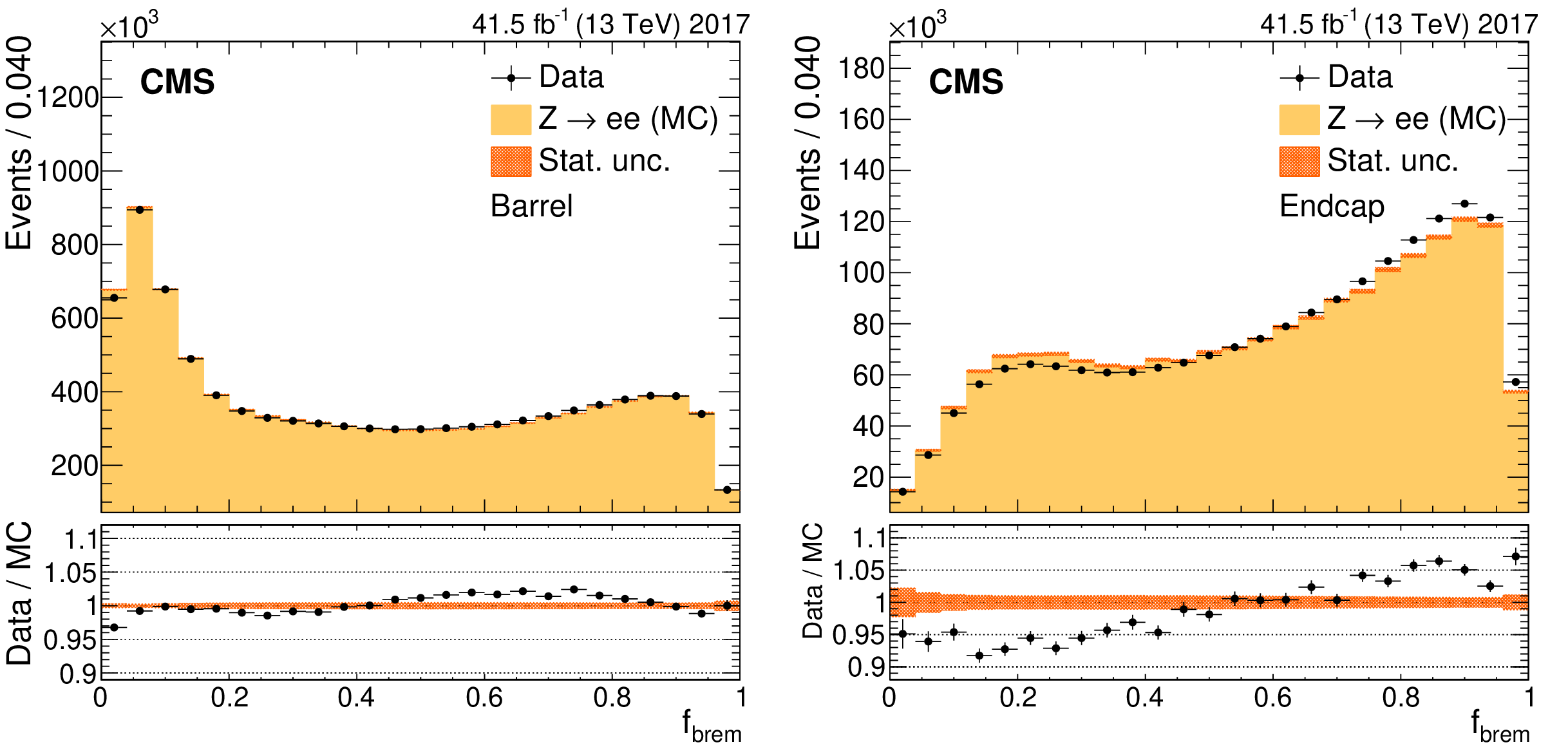
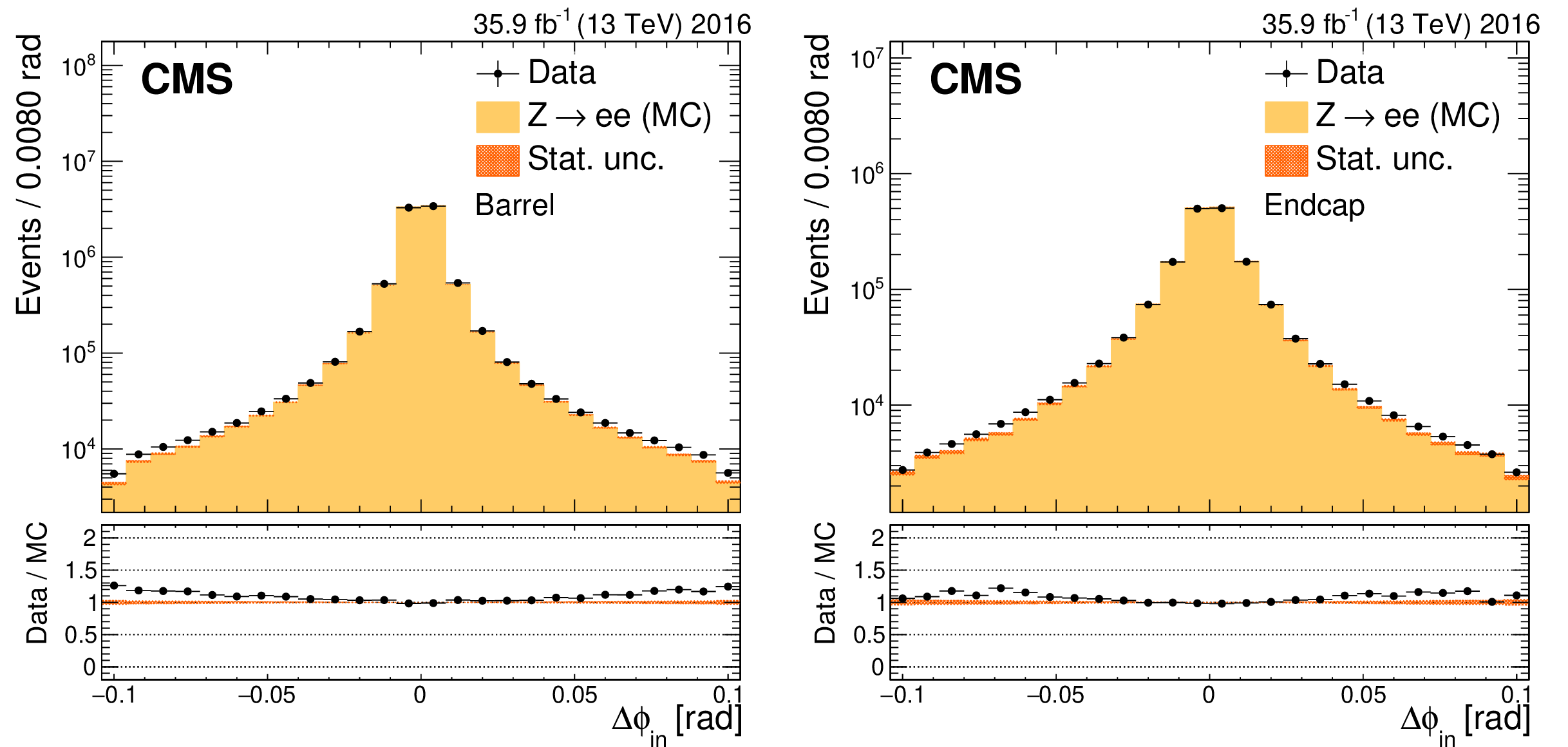
Figure 2:
Fraction of the momentum lost by bremsstrahlung between the inner and outer parts of the tracker for electrons from Z boson decays in the barrel (left) and in the endcaps (right). The upper panels show the comparison between data and simulation. The simulation is shown with the filled histograms and data are represented by the markers. The vertical bars on the markers represent the statistical uncertainties in data. The hatched regions show the statistical uncertainty in the simulation. The lower panels show the data-to-simulation ratio. |
png pdf |
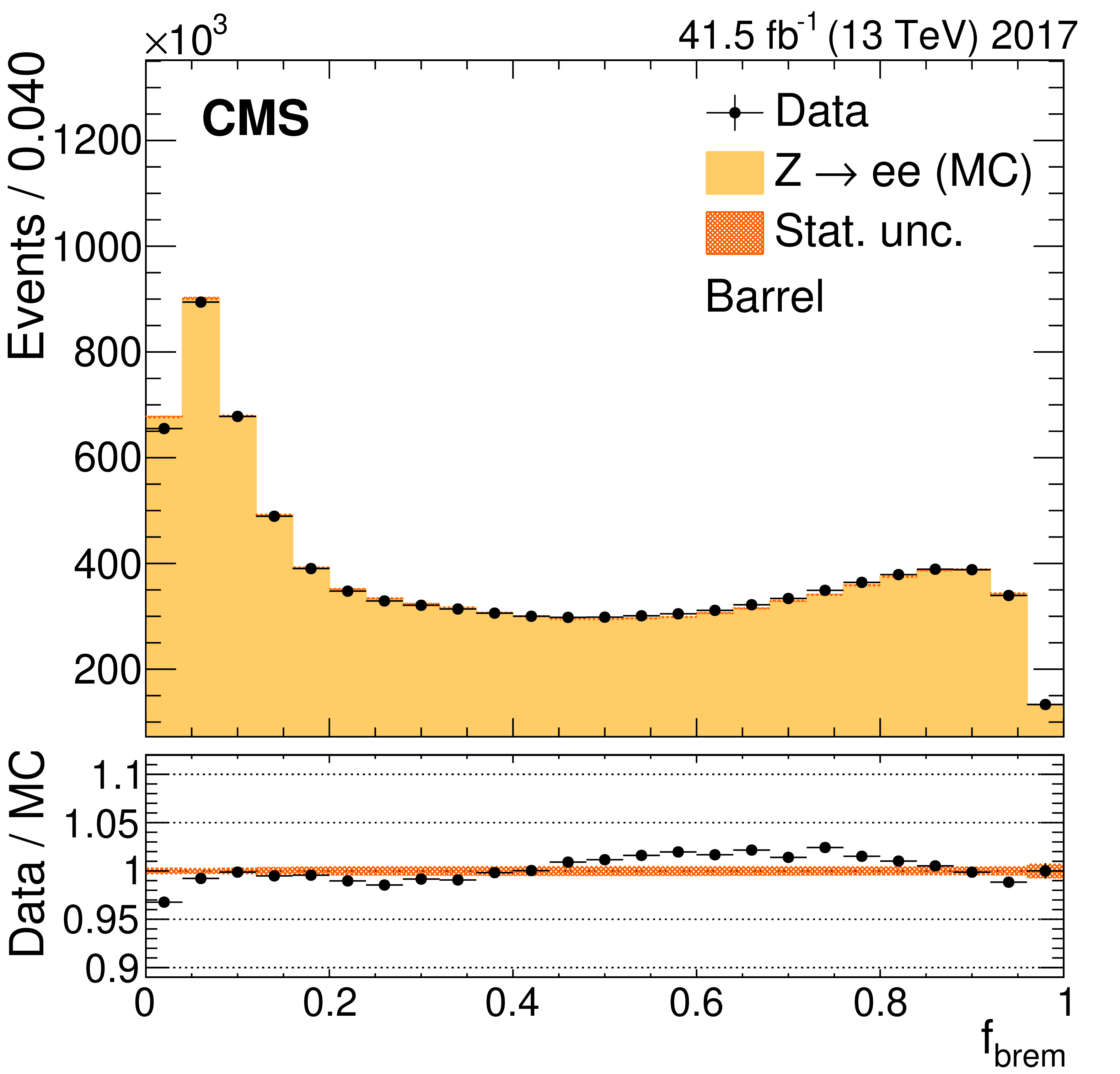
Figure 2-a:
Fraction of the momentum lost by bremsstrahlung between the inner and outer parts of the tracker for electrons from Z boson decays in the barrel. The upper panels show the comparison between data and simulation. The simulation is shown with the filled histograms and data are represented by the markers. The vertical bars on the markers represent the statistical uncertainties in data. The hatched regions show the statistical uncertainty in the simulation. The lower panels show the data-to-simulation ratio. |
png pdf |
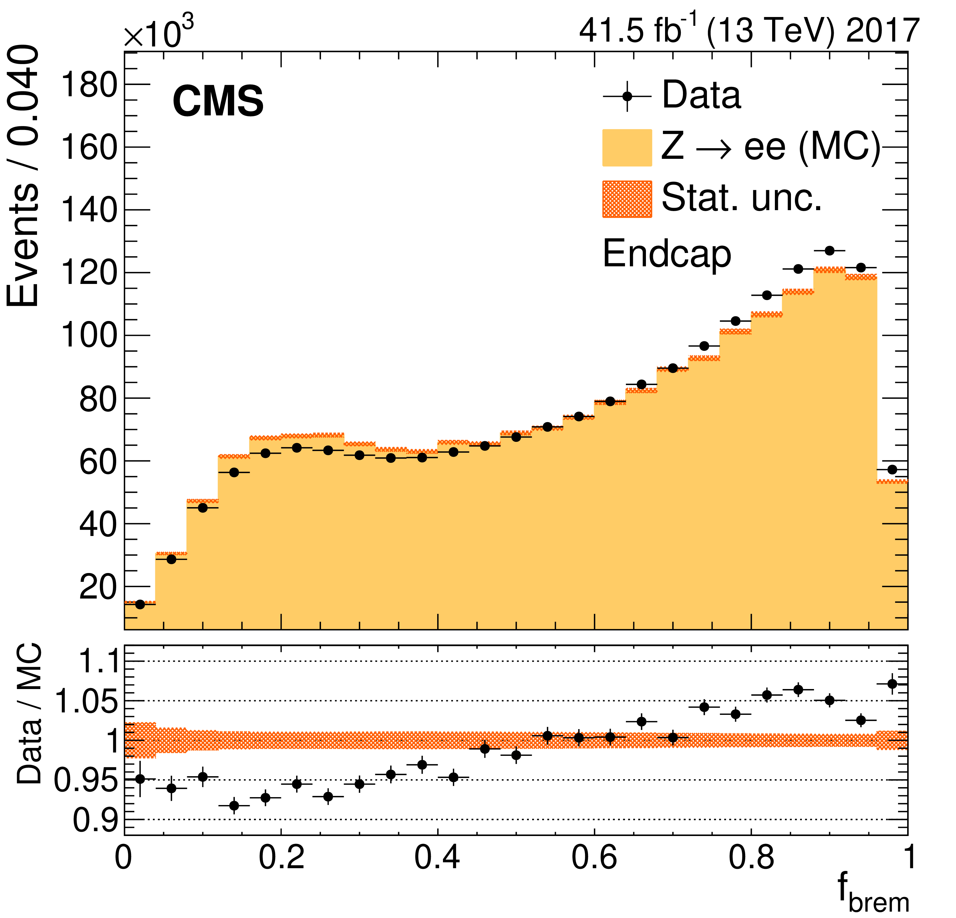
Figure 2-b:
Fraction of the momentum lost by bremsstrahlung between the inner and outer parts of the tracker for electrons from Z boson decays in the endcaps. The upper panels show the comparison between data and simulation. The simulation is shown with the filled histograms and data are represented by the markers. The vertical bars on the markers represent the statistical uncertainties in data. The hatched regions show the statistical uncertainty in the simulation. The lower panels show the data-to-simulation ratio. |
png pdf |
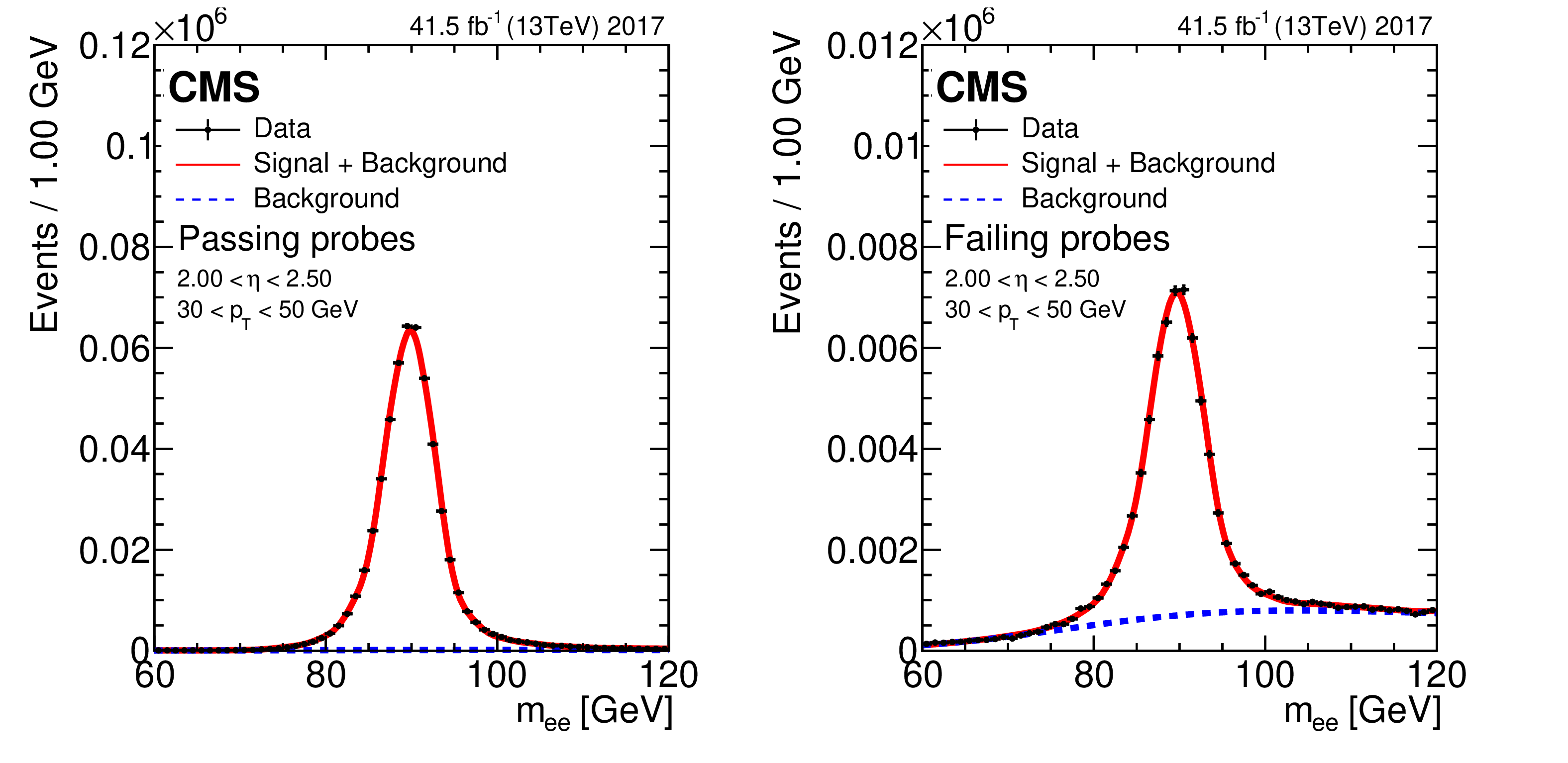
Figure 3:
Example $\mathrm{Z} \to \mathrm{ee} $ invariant mass fits for passing (left) and failing (right) probes. Black markers show data while red solid lines show the signal + background fitting model and the blue dotted lines represent the background only component. The vertical bars on the markers represent the statistical uncertainties of the data. |
png pdf |
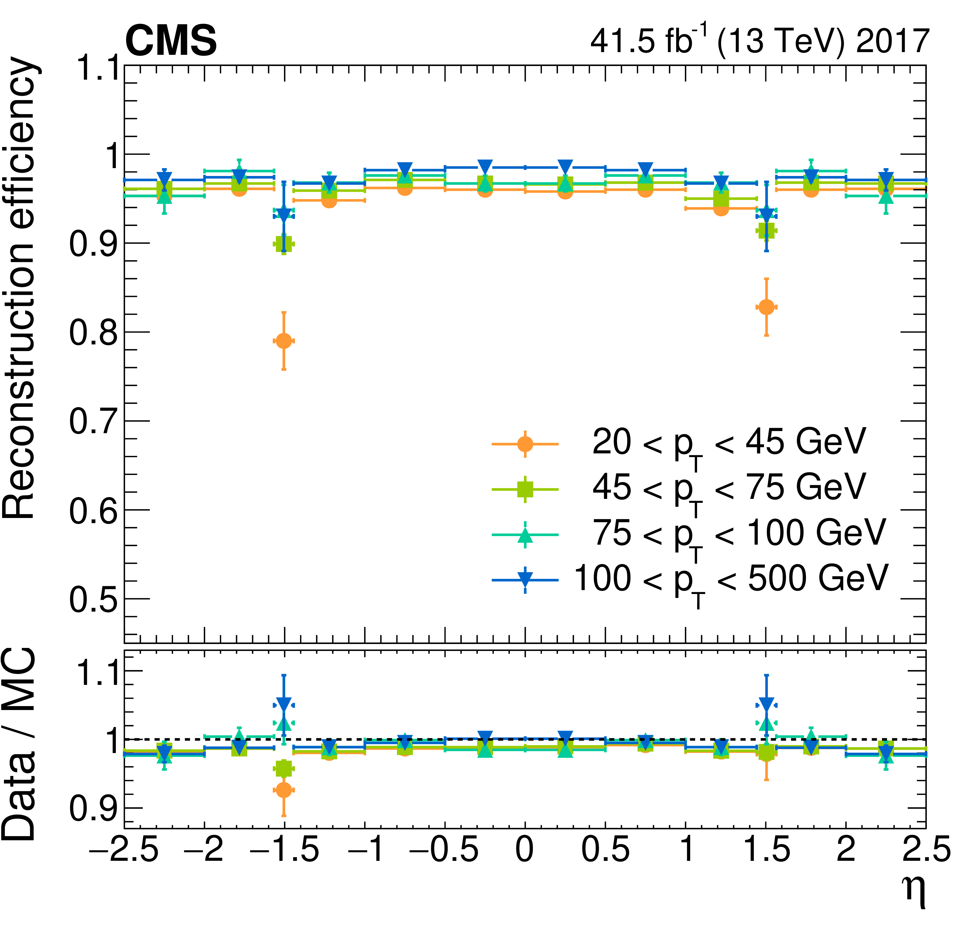
Figure 4:
Electron reconstruction efficiency versus $\eta $ in data (upper panel) and data-to-simulation efficiency ratios (lower panel) for the 2017 data taking period. The vertical bars on the markers represent the combined statistical and systematic uncertainties. The region 1.44 $ < {| \eta |} < $ 1.57 corresponds to the transition region between the barrel and endcap regions of ECAL and is not considered in physics analyses. |
png pdf |
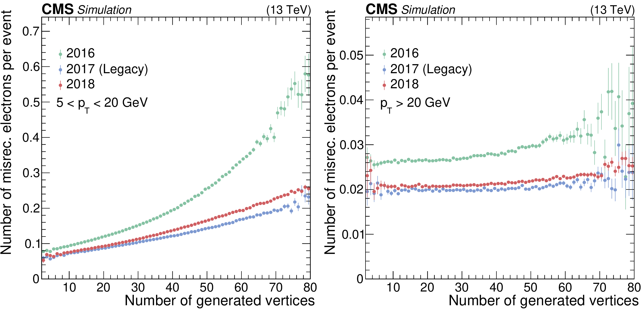
Figure 5:
Number of misidentified electron candidates per event as a function of the number of generated vertices in DY + jets MC events simulated with the different detector conditions of the Run 2 data taking period. Results are shown for electrons with ${p_{\mathrm {T}}}$ in the range 5-20 GeV (left) and electrons with $ {p_{\mathrm {T}}} > $ 20 GeV (right) without further selection. The vertical bars on the markers represent the statistical uncertainties of the MC sample. |
png pdf |
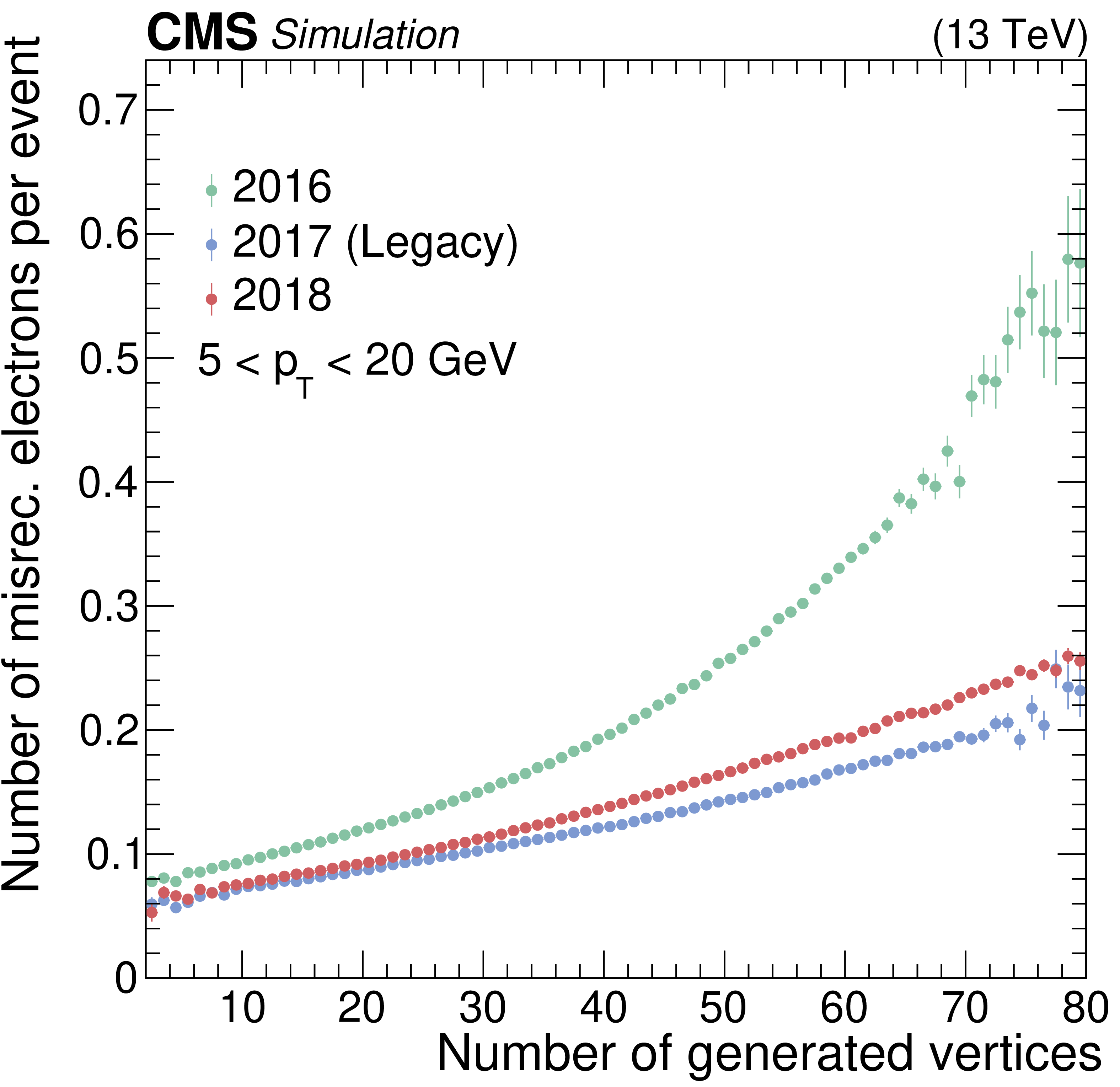
Figure 5-a:
Number of misidentified electron candidates per event as a function of the number of generated vertices in DY + jets MC events simulated with the different detector conditions of the Run 2 data taking period. Results are shown for electrons with ${p_{\mathrm {T}}}$ in the range 5-20 GeV without further selection. The vertical bars on the markers represent the statistical uncertainties of the MC sample. |
png pdf |
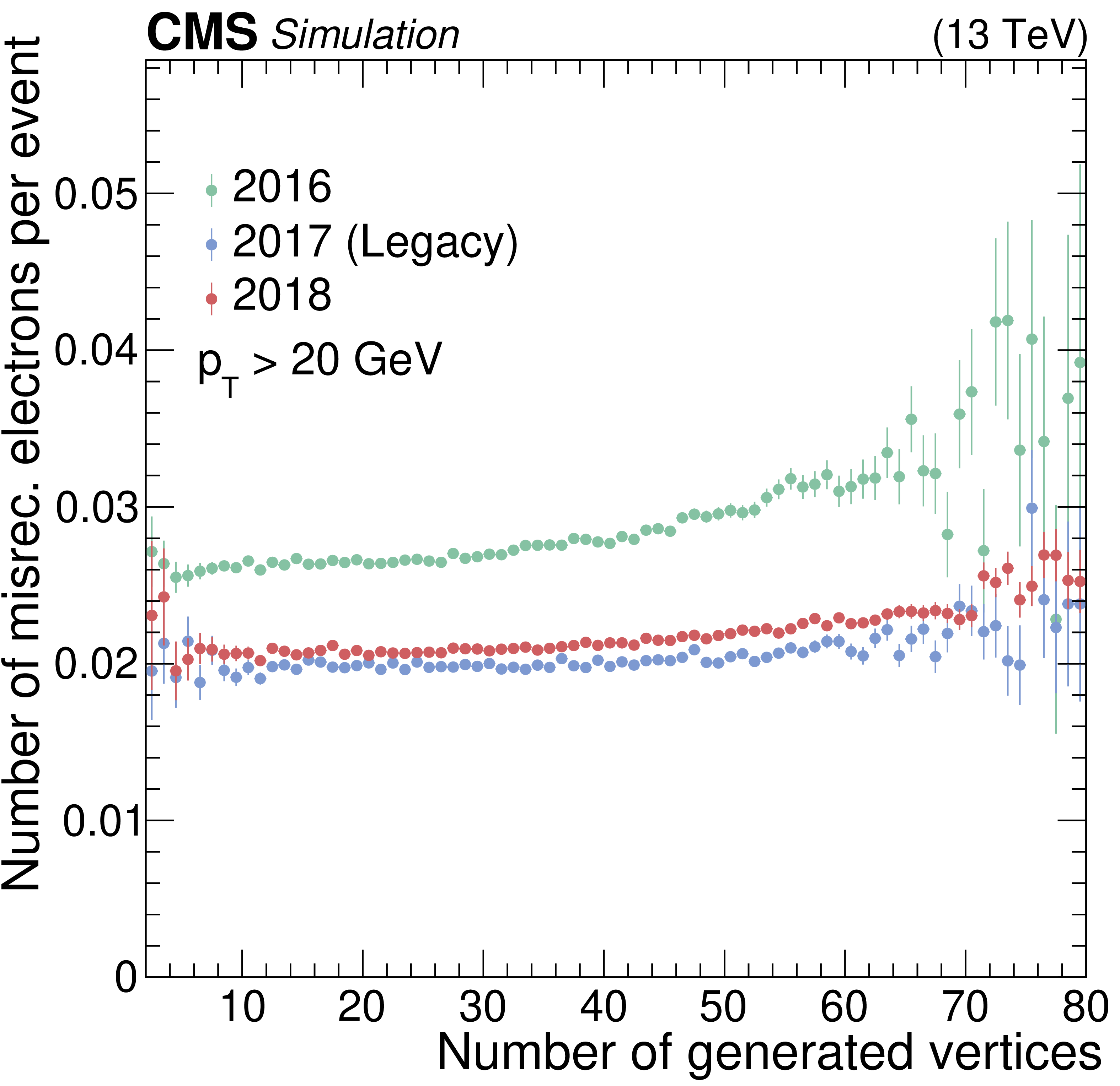
Figure 5-b:
Number of misidentified electron candidates per event as a function of the number of generated vertices in DY + jets MC events simulated with the different detector conditions of the Run 2 data taking period. Results are shown for electrons with $ {p_{\mathrm {T}}} > $ 20 GeV without further selection. The vertical bars on the markers represent the statistical uncertainties of the MC sample. |

png pdf |
Figure 6:
Efficiency of the selective method for the electron charge sign measurement as a function of ${p_{\mathrm {T}}}$ for electrons in the barrel and endcap regions, as measured using simulated $\mathrm{Z} \to \mathrm{ee} $ events. Electrons are required to satisfy the loose identification requirements described in Section 7.3. The uncertainties assigned to the points are statistical only. |
png pdf |
Figure 7:
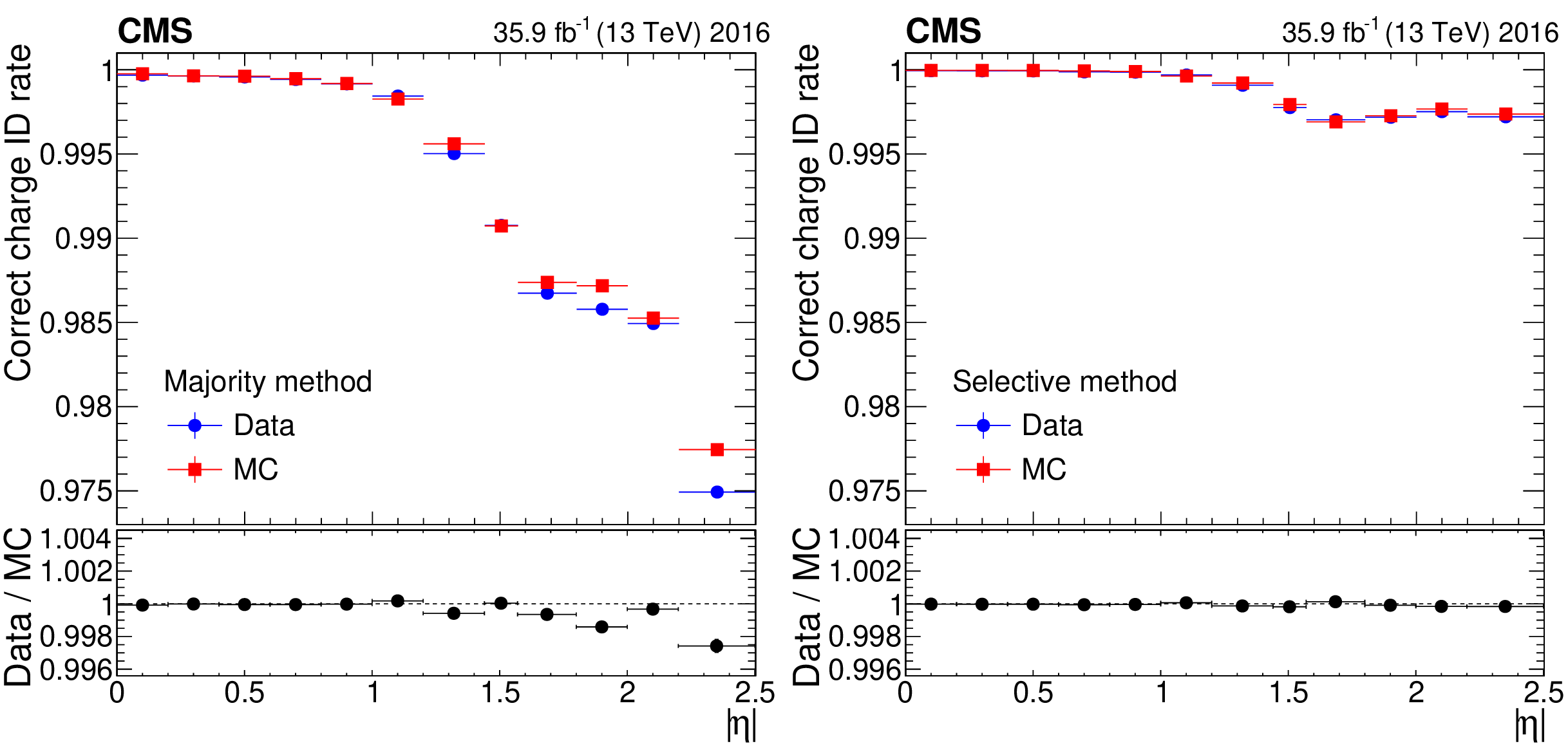
Correct charge identification probability for electrons using the majority method (left) and the selective method (right), as measured in the 2016 data set and in simulated $\mathrm{Z} \to \mathrm{ee} $ events. The electrons are required to satisfy the loose identification requirements described in Section 7.3. The uncertainties assigned to the points are statistical only. |
png pdf |
Figure 7-a:
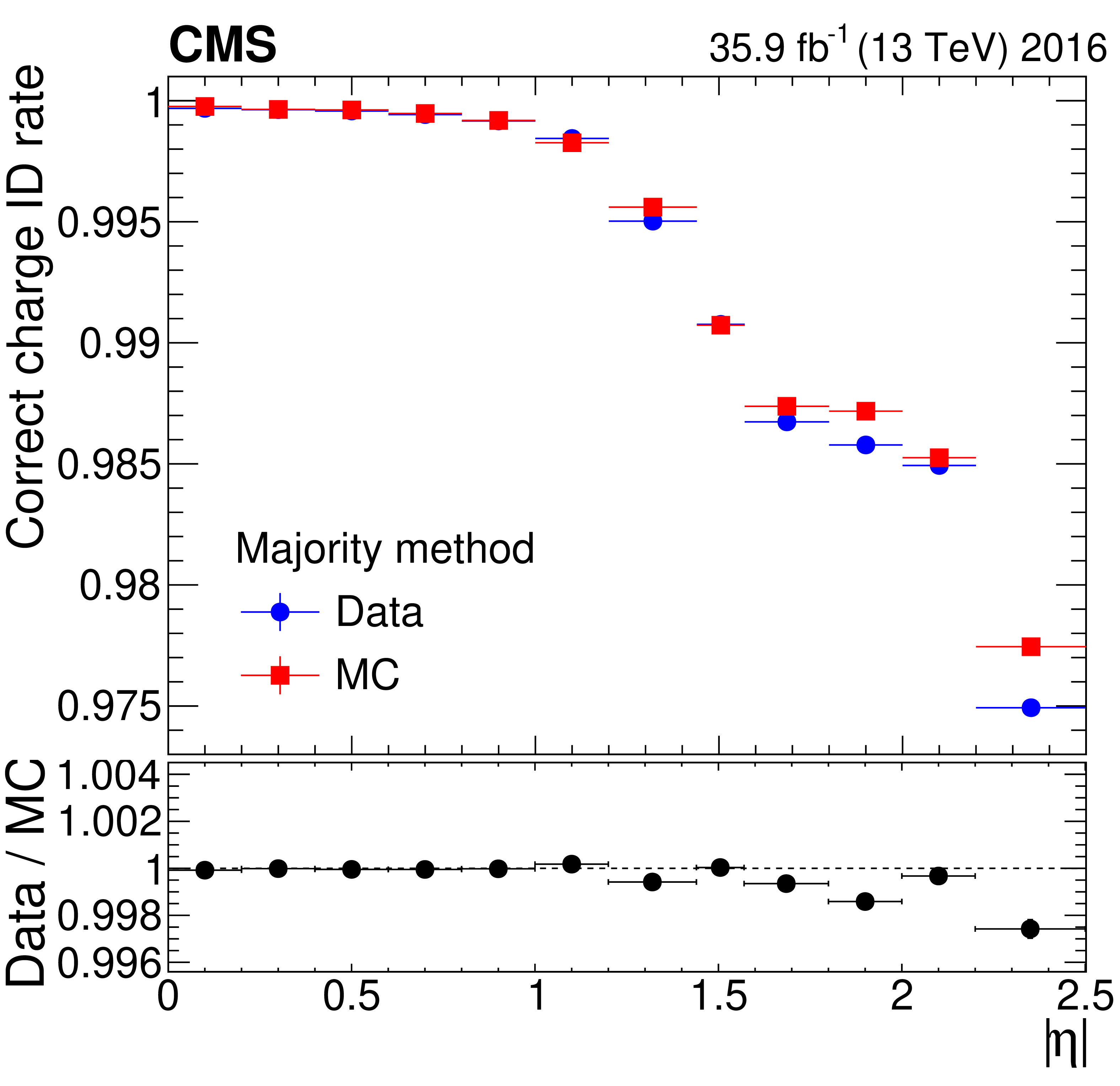
Correct charge identification probability for electrons using the majority method, as measured in the 2016 data set and in simulated $\mathrm{Z} \to \mathrm{ee} $ events. The electrons are required to satisfy the loose identification requirements described in Section 7.3. The uncertainties assigned to the points are statistical only. |

png pdf |
Figure 7-b:
Correct charge identification probability for electrons using the selective method, as measured in the 2016 data set and in simulated $\mathrm{Z} \to \mathrm{ee} $ events. The electrons are required to satisfy the loose identification requirements described in Section 7.3. The uncertainties assigned to the points are statistical only. |

png pdf |
Figure 8:
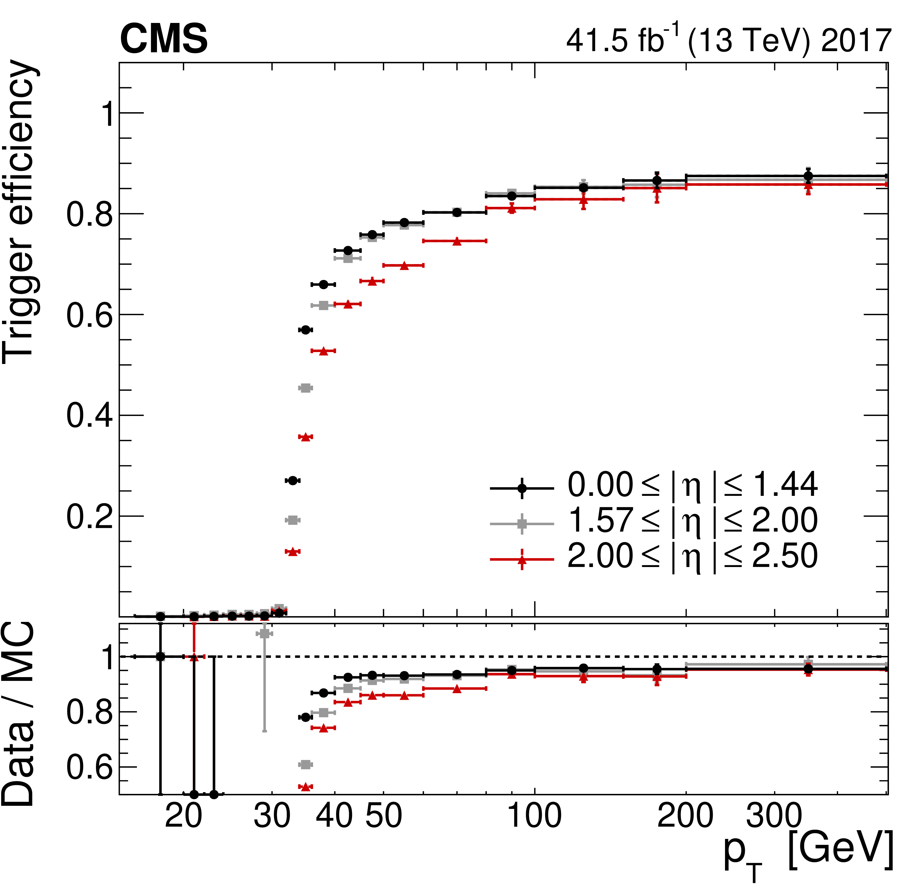
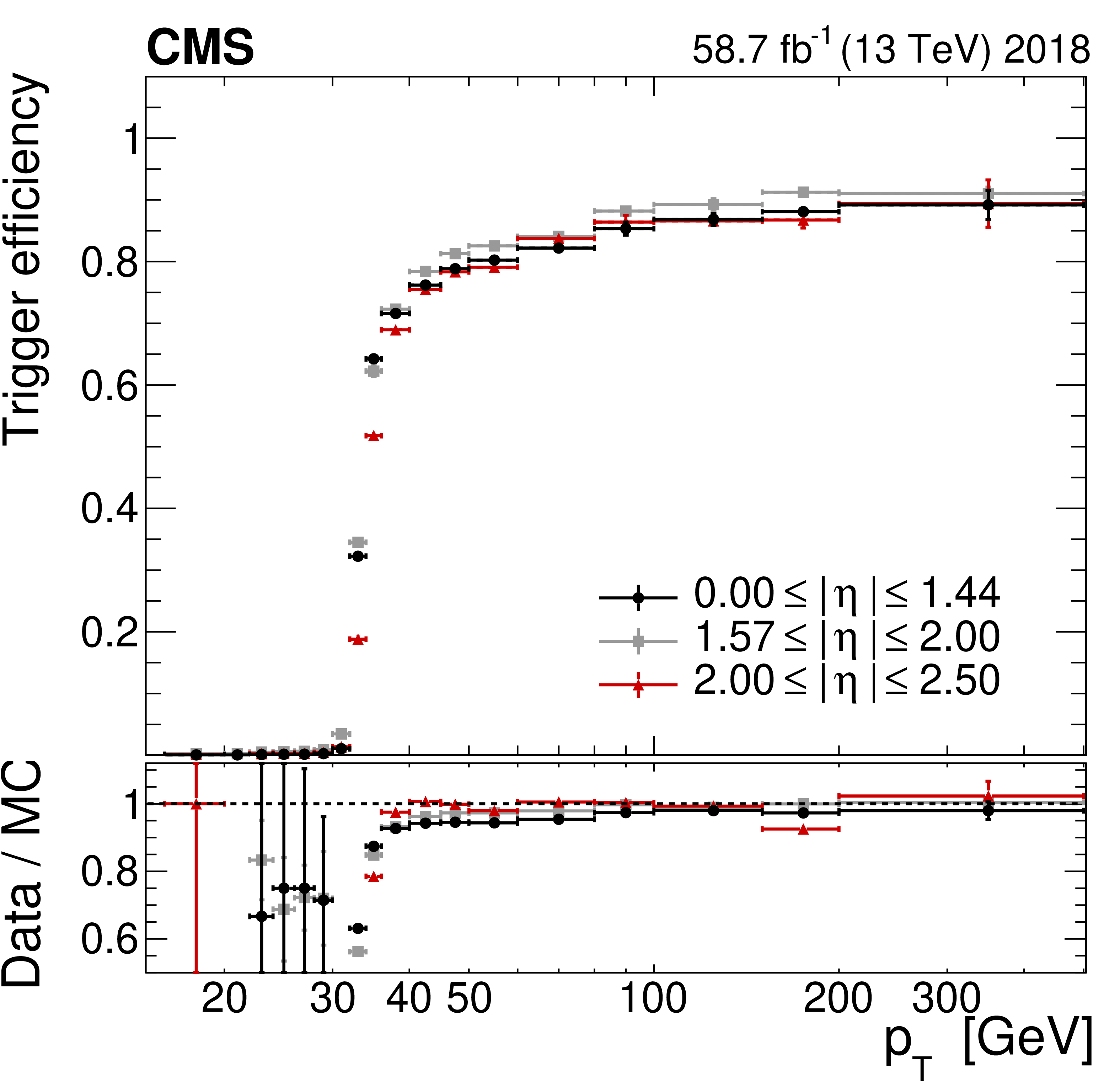
Efficiency of the lowest unprescaled single-electron HLT path (HLT_Ele27_WPTight_Gsf in 2016, HLT_Ele32_WPTight_Gsf in 2017-2018), with respect to the offline reconstruction, as a function of the electron ${p_{\mathrm {T}}}$, for different $\eta $ regions using the 2016 (upper left), 2017 (upper right) and 2018 (lower) data sets. The bottom panel shows the data-to-simulation ratio. The efficiency measurements combine the effects of the L1 and HLT triggers. The vertical bars on the markers represent combined statistical and systematic uncertainties. |
png pdf |
Figure 8-a:
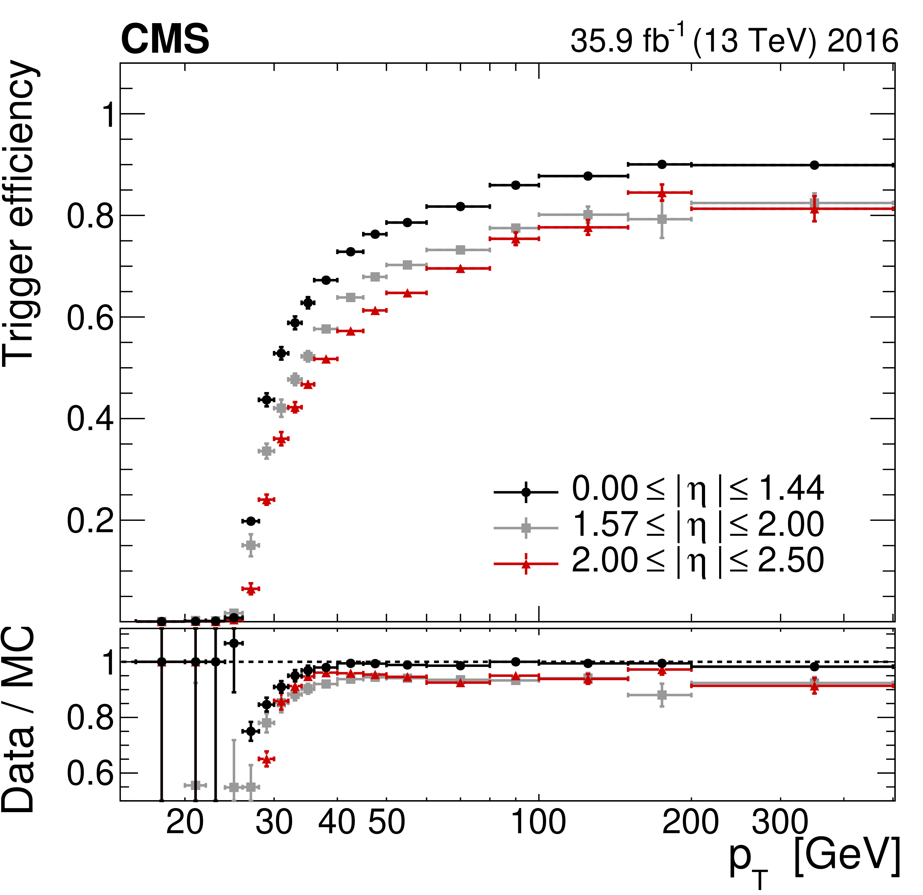
Efficiency of the lowest unprescaled single-electron HLT path (HLT_Ele27_WPTight_Gsf in 2016, HLT_Ele32_WPTight_Gsf in 2017-2018), with respect to the offline reconstruction, as a function of the electron ${p_{\mathrm {T}}}$, for different $\eta $ regions using the 2016 data set. The bottom panel shows the data-to-simulation ratio. The efficiency measurements combine the effects of the L1 and HLT triggers. The vertical bars on the markers represent combined statistical and systematic uncertainties. |
png pdf |
Figure 8-b:
Efficiency of the lowest unprescaled single-electron HLT path (HLT_Ele27_WPTight_Gsf in 2016, HLT_Ele32_WPTight_Gsf in 2017-2018), with respect to the offline reconstruction, as a function of the electron ${p_{\mathrm {T}}}$, for different $\eta $ regions using the 2017 data set. The bottom panel shows the data-to-simulation ratio. The efficiency measurements combine the effects of the L1 and HLT triggers. The vertical bars on the markers represent combined statistical and systematic uncertainties. |
png pdf |
Figure 8-c:
Efficiency of the lowest unprescaled single-electron HLT path (HLT_Ele27_WPTight_Gsf in 2016, HLT_Ele32_WPTight_Gsf in 2017-2018), with respect to the offline reconstruction, as a function of the electron ${p_{\mathrm {T}}}$, for different $\eta $ regions using the 2018 data set. The bottom panel shows the data-to-simulation ratio. The efficiency measurements combine the effects of the L1 and HLT triggers. The vertical bars on the markers represent combined statistical and systematic uncertainties. |
png pdf |
Figure 9:
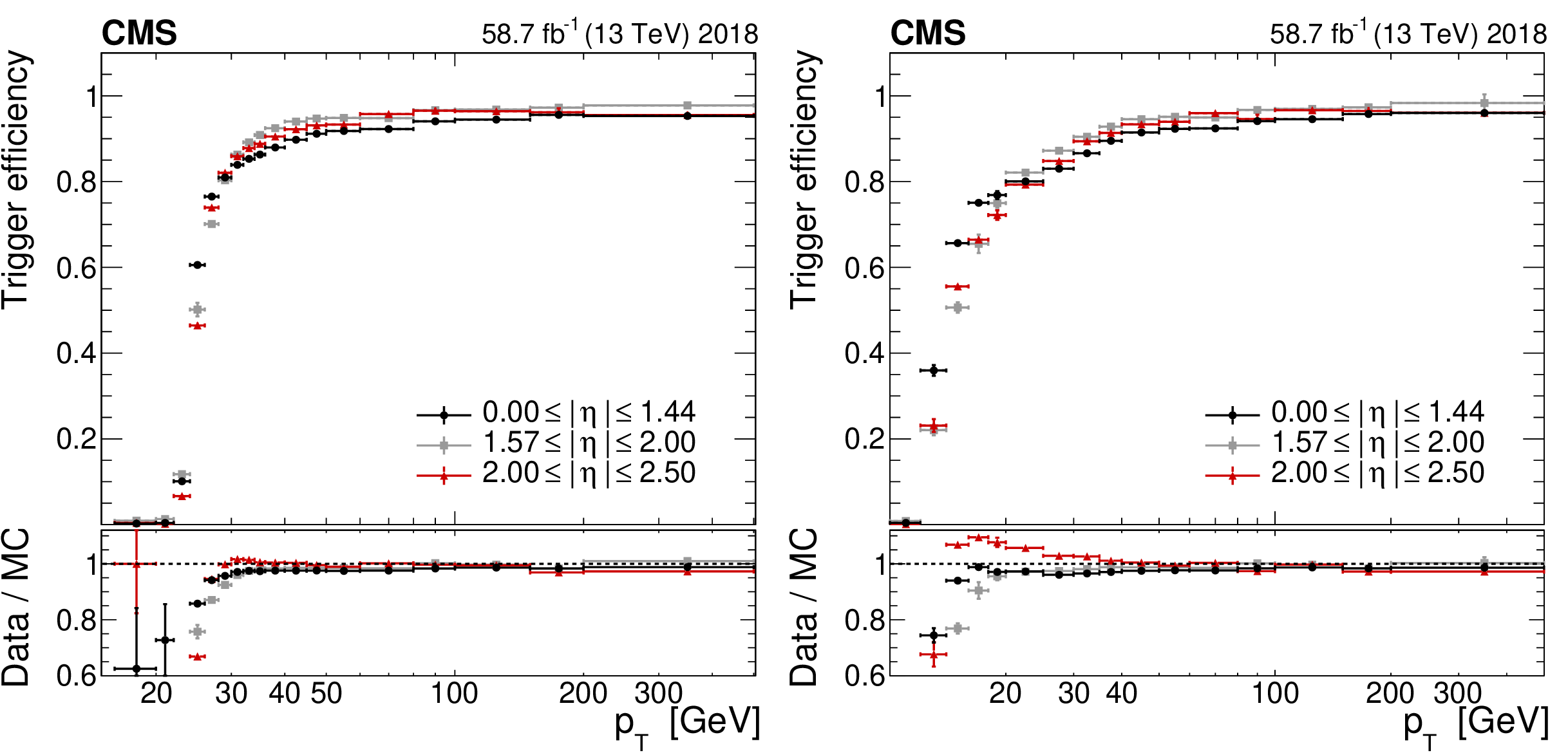
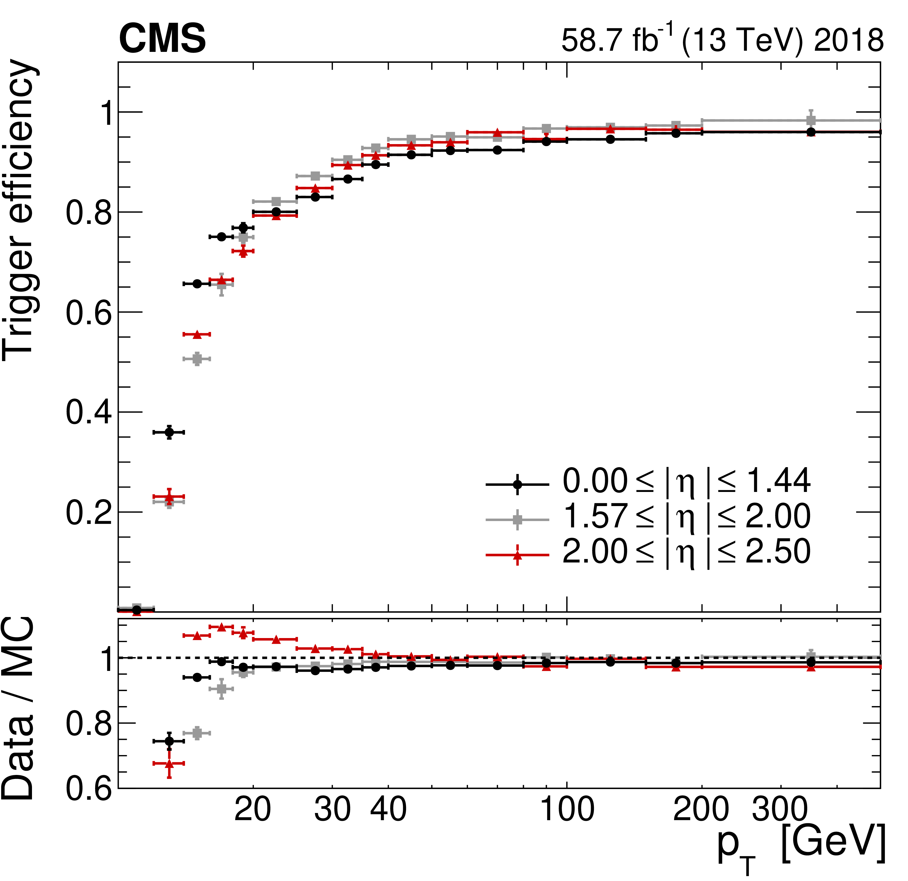
Efficiency of the Ele23 object (left) and Ele12 object (right) of the HLT_Ele23_Ele12 trigger, with respect to an offline reconstructed electron, as a function of the electron ${p_{\mathrm {T}}}$, obtained for different $\eta $ regions using the 2018 data set. The Ele23 efficiency includes the requirement of passing the leading electron threshold of the asymmetric L1_DoubleEG seed. The bottom panel shows the data-to-simulation ratio. The efficiency measurements combine the effects of the L1 and HLT triggers. The vertical bars on the markers represent combined statistical and systematic uncertainties. |

png pdf |
Figure 9-a:
Efficiency of the Ele23 object of the HLT_Ele23_Ele12 trigger, with respect to an offline reconstructed electron, as a function of the electron ${p_{\mathrm {T}}}$, obtained for different $\eta $ regions using the 2018 data set. The bottom panel shows the data-to-simulation ratio. The efficiency measurements combine the effects of the L1 and HLT triggers. The vertical bars on the markers represent combined statistical and systematic uncertainties. |
png pdf |
Figure 9-b:
Efficiency of the Ele12 object of the HLT_Ele23_Ele12 trigger, with respect to an offline reconstructed electron, as a function of the electron ${p_{\mathrm {T}}}$, obtained for different $\eta $ regions using the 2018 data set. The efficiency includes the requirement of passing the leading electron threshold of the asymmetric L1_DoubleEG seed. The bottom panel shows the data-to-simulation ratio. The efficiency measurements combine the effects of the L1 and HLT triggers. The vertical bars on the markers represent combined statistical and systematic uncertainties. |
png pdf |
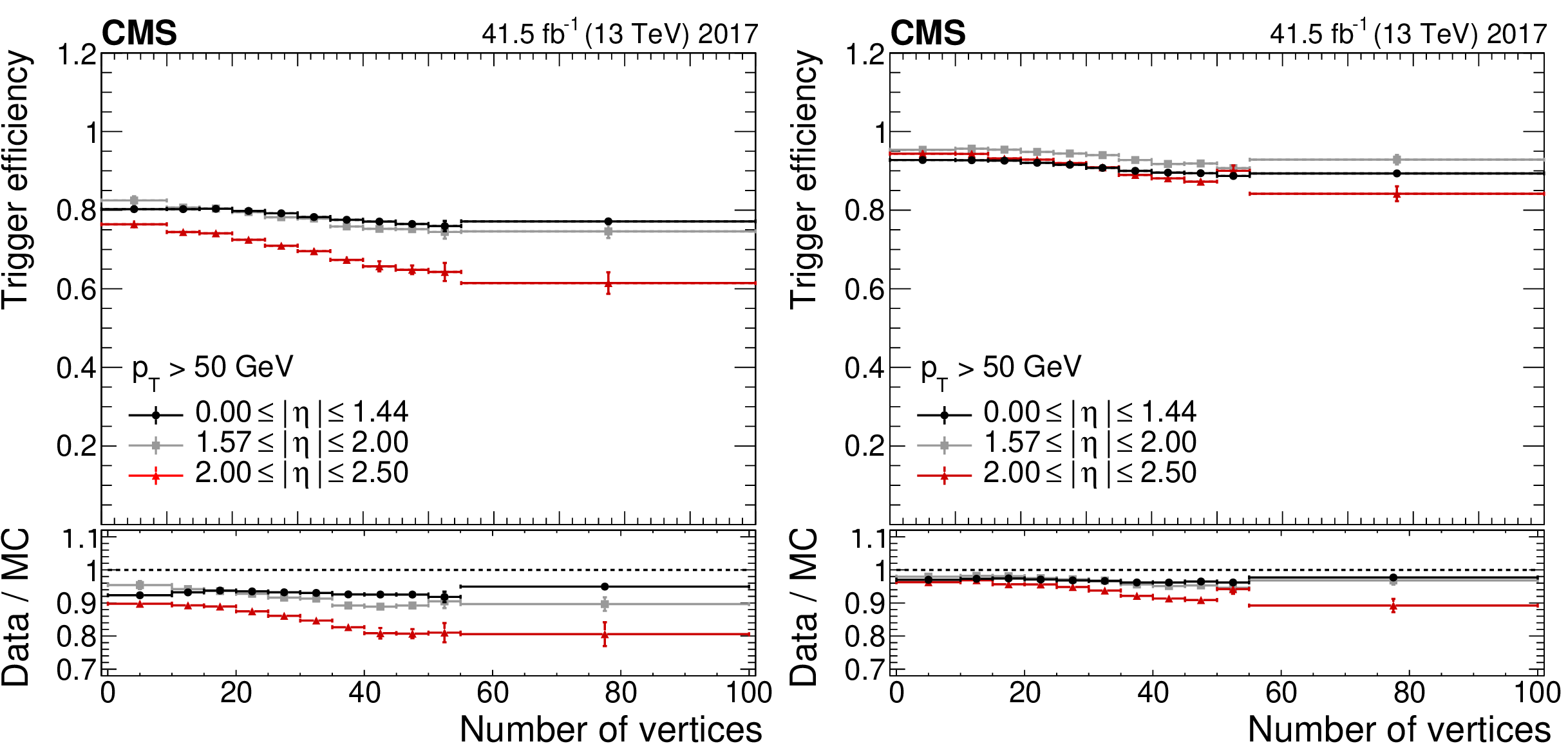
Figure 10:
Efficiency of HLT_Ele32_WPTight_Gsf (left) and HLT_Ele23_Ele12 (right) trigger, with respect to an offline reconstructed electron, as a function of the number of reconstructed primary vertices, obtained for different $\eta $ regions using the 2017 data set. Electron $ {E_{\mathrm {T}}} $ is required to be $ > $50 GeV. The bottom panel shows the data-to-simulation ratio. The efficiency measurements combine the effects of the L1 and HLT triggers. The vertical bars on the markers represent combined statistical and systematic uncertainties. In 2017 the majority of the high-pileup data was recorded at the end of the year, the same time the pixel DC-DC convertors exhibited efficiency losses. Thus the efficiency loss versus number of vertices in the event is not solely due to the pileup. However the efficiency loss is significant only for 2.0 $ < {| \eta |} < $ 2.5. |
png pdf |
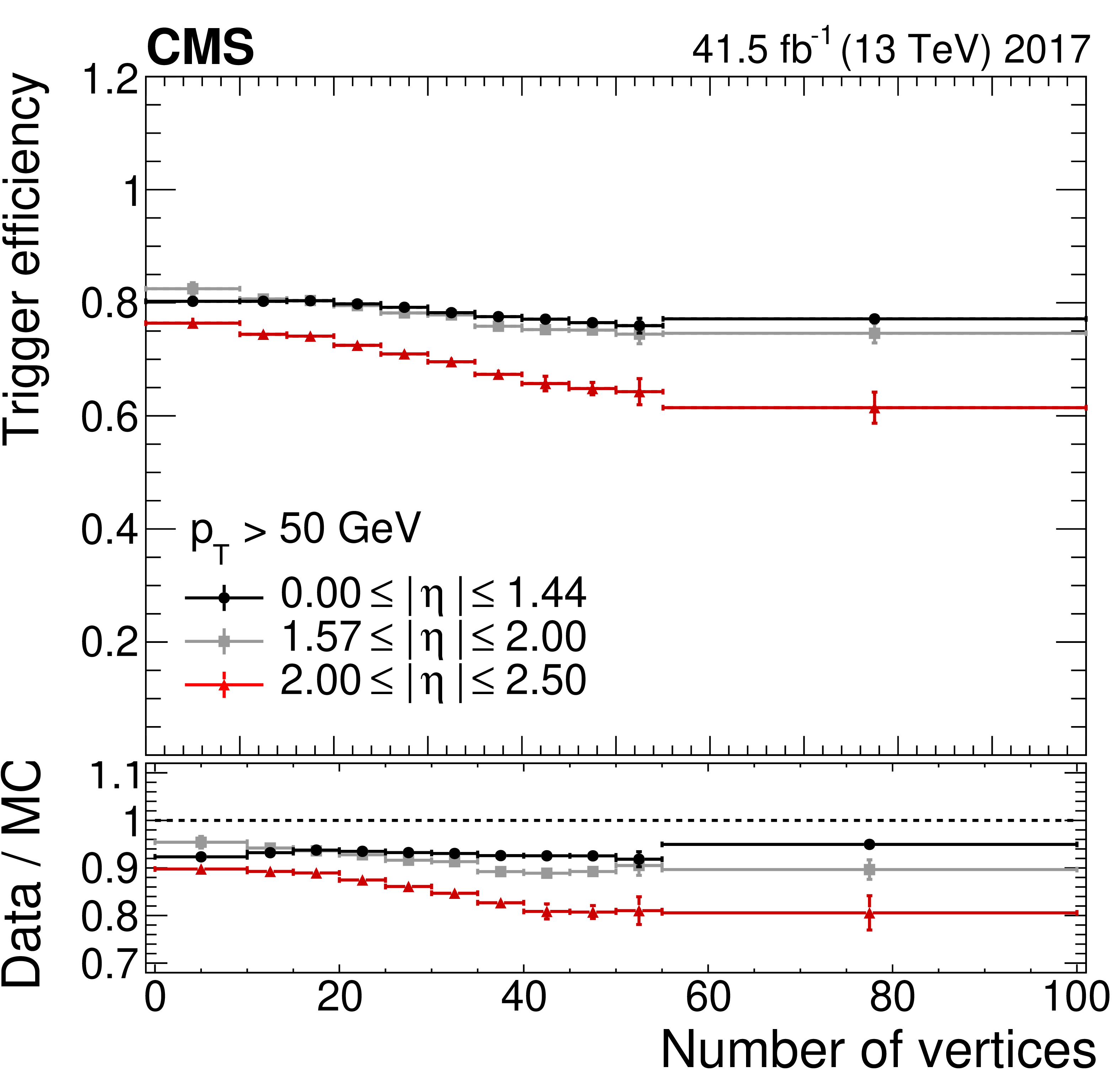
Figure 10-a:
Efficiency of HLT_Ele32_WPTight_Gsf trigger, with respect to an offline reconstructed electron, as a function of the number of reconstructed primary vertices, obtained for different $\eta $ regions using the 2017 data set. Electron $ {E_{\mathrm {T}}} $ is required to be $ > $50 GeV. The bottom panel shows the data-to-simulation ratio. The efficiency measurements combine the effects of the L1 and HLT triggers. The vertical bars on the markers represent combined statistical and systematic uncertainties. In 2017 the majority of the high-pileup data was recorded at the end of the year, the same time the pixel DC-DC convertors exhibited efficiency losses. Thus the efficiency loss versus number of vertices in the event is not solely due to the pileup. However the efficiency loss is significant only for 2.0 $ < {| \eta |} < $ 2.5. |
png pdf |
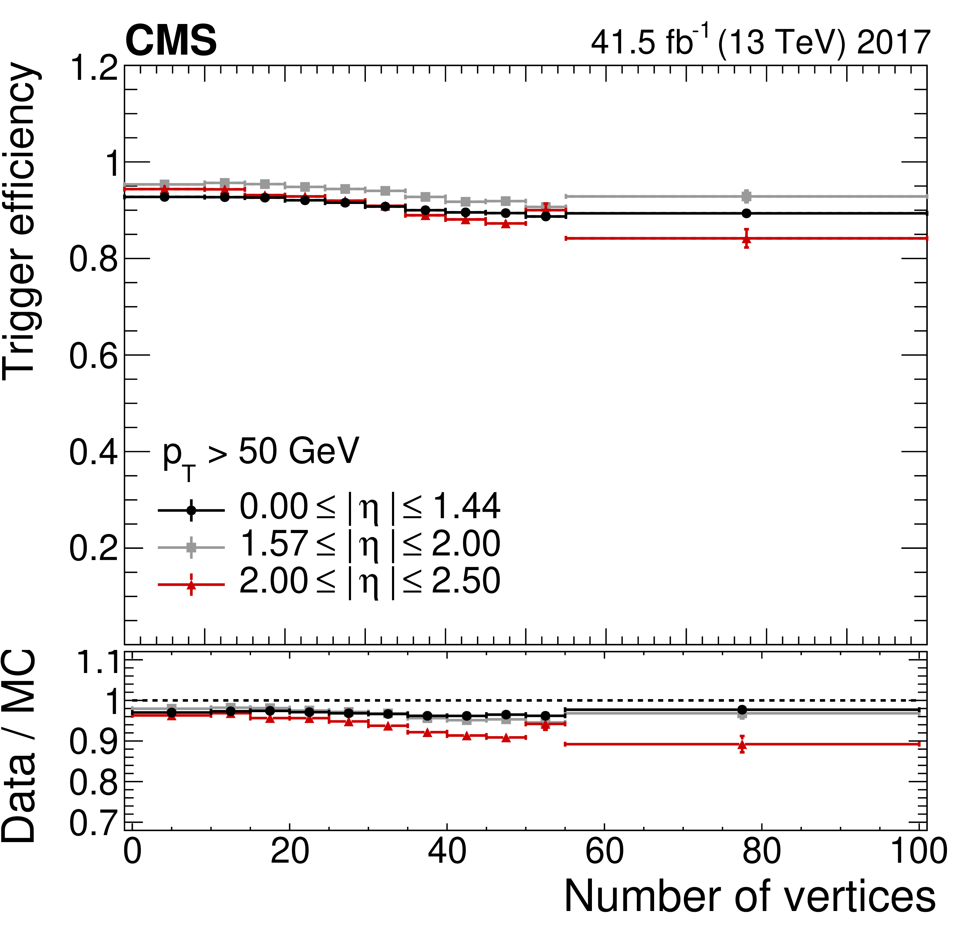
Figure 10-b:
Efficiency of HLT_Ele23_Ele12 trigger, with respect to an offline reconstructed electron, as a function of the number of reconstructed primary vertices, obtained for different $\eta $ regions using the 2017 data set. Electron $ {E_{\mathrm {T}}} $ is required to be $ > $50 GeV. The bottom panel shows the data-to-simulation ratio. The efficiency measurements combine the effects of the L1 and HLT triggers. The vertical bars on the markers represent combined statistical and systematic uncertainties. In 2017 the majority of the high-pileup data was recorded at the end of the year, the same time the pixel DC-DC convertors exhibited efficiency losses. Thus the efficiency loss versus number of vertices in the event is not solely due to the pileup. However the efficiency loss is significant only for 2.0 $ < {| \eta |} < $ 2.5. |
png pdf |
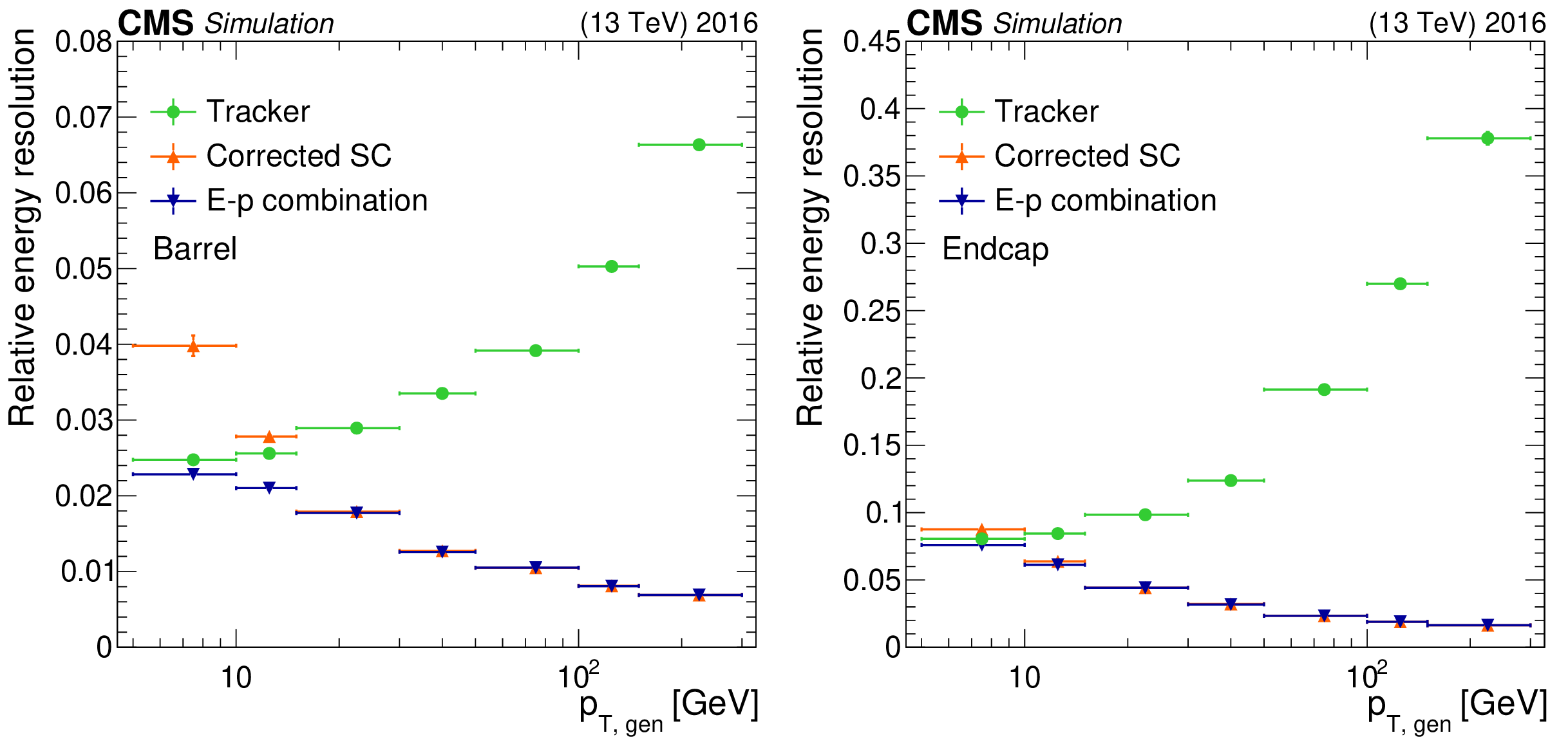
Figure 11:
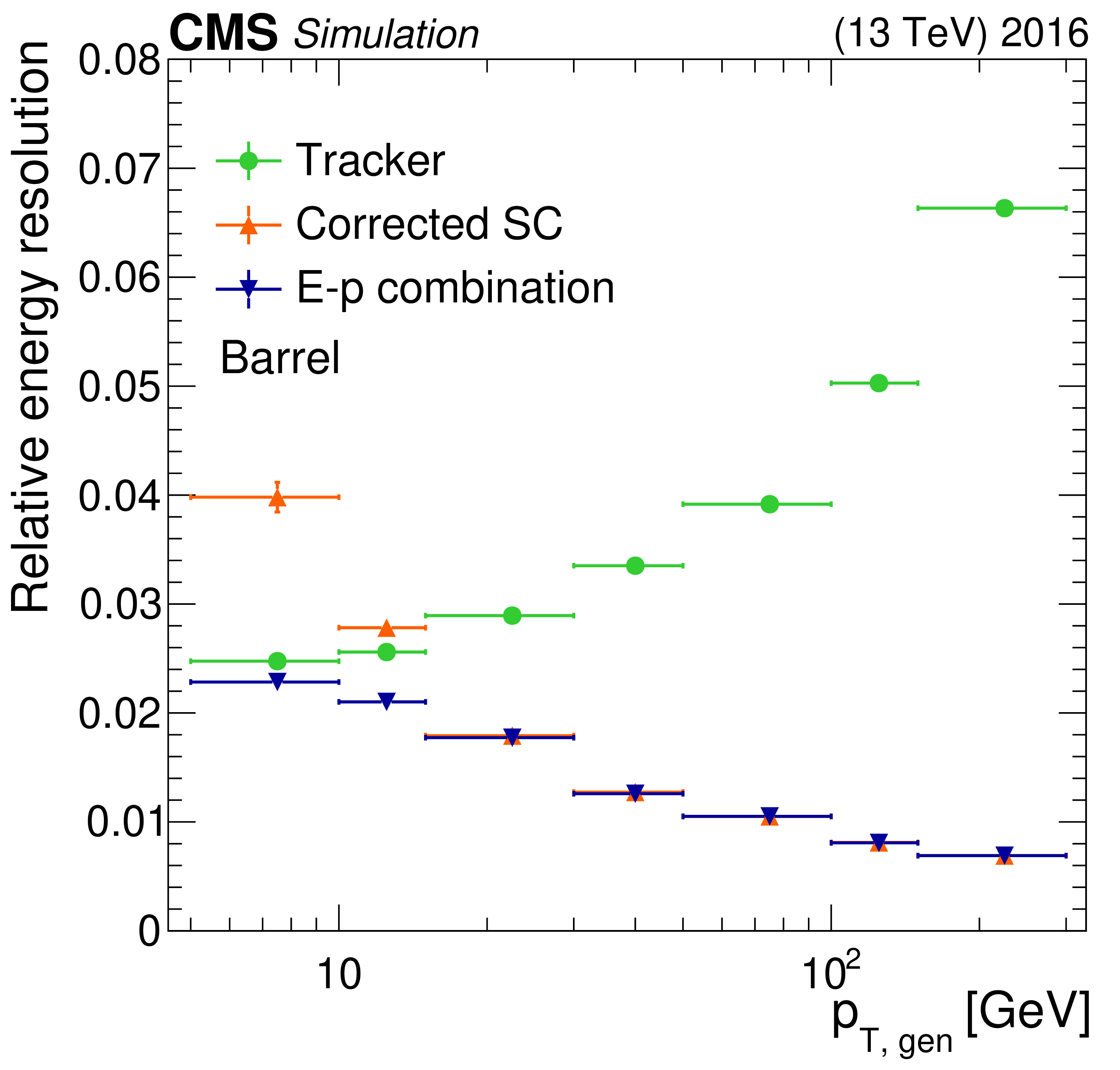
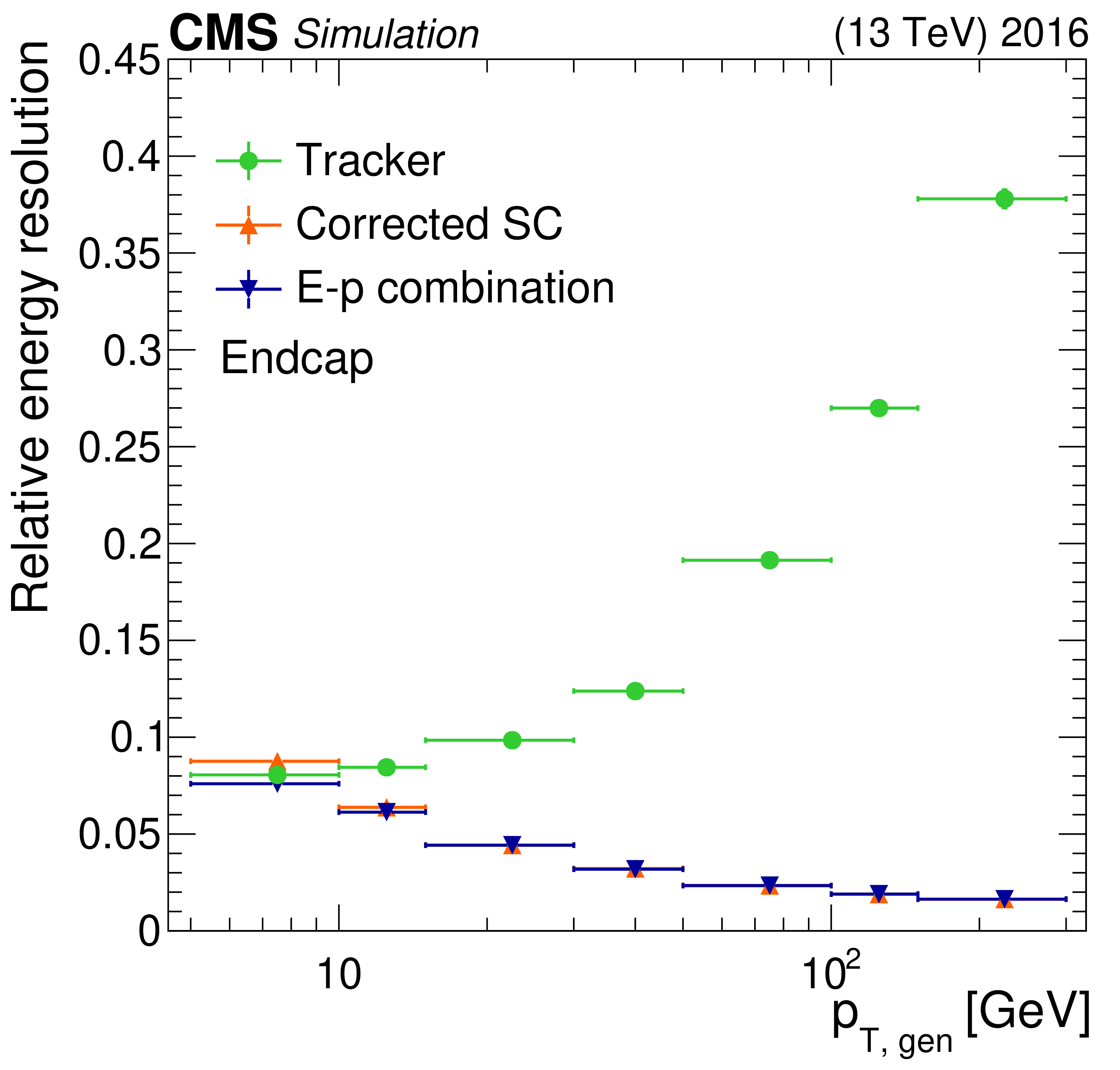
Relative electron resolution versus electron $ {p_{\mathrm {T}}} $, as measured by the ECAL ("corrected SC''), by the tracker, and seen in the $E$-$p$ combination, as found in 2016 MC samples for barrel (left) and endcap (right) electrons. Vertical bars on the markers represent the uncertainties coming from the fit procedure. |
png pdf |
Figure 11-a:
Relative electron resolution versus electron $ {p_{\mathrm {T}}} $, as measured by the ECAL ("corrected SC''), by the tracker, and seen in the $E$-$p$ combination, as found in 2016 MC samples for barrel electrons. Vertical bars on the markers represent the uncertainties coming from the fit procedure. |
png pdf |
Figure 11-b:
Relative electron resolution versus electron $ {p_{\mathrm {T}}} $, as measured by the ECAL ("corrected SC''), by the tracker, and seen in the $E$-$p$ combination, as found in 2016 MC samples for endcap electrons. Vertical bars on the markers represent the uncertainties coming from the fit procedure. |
png pdf |
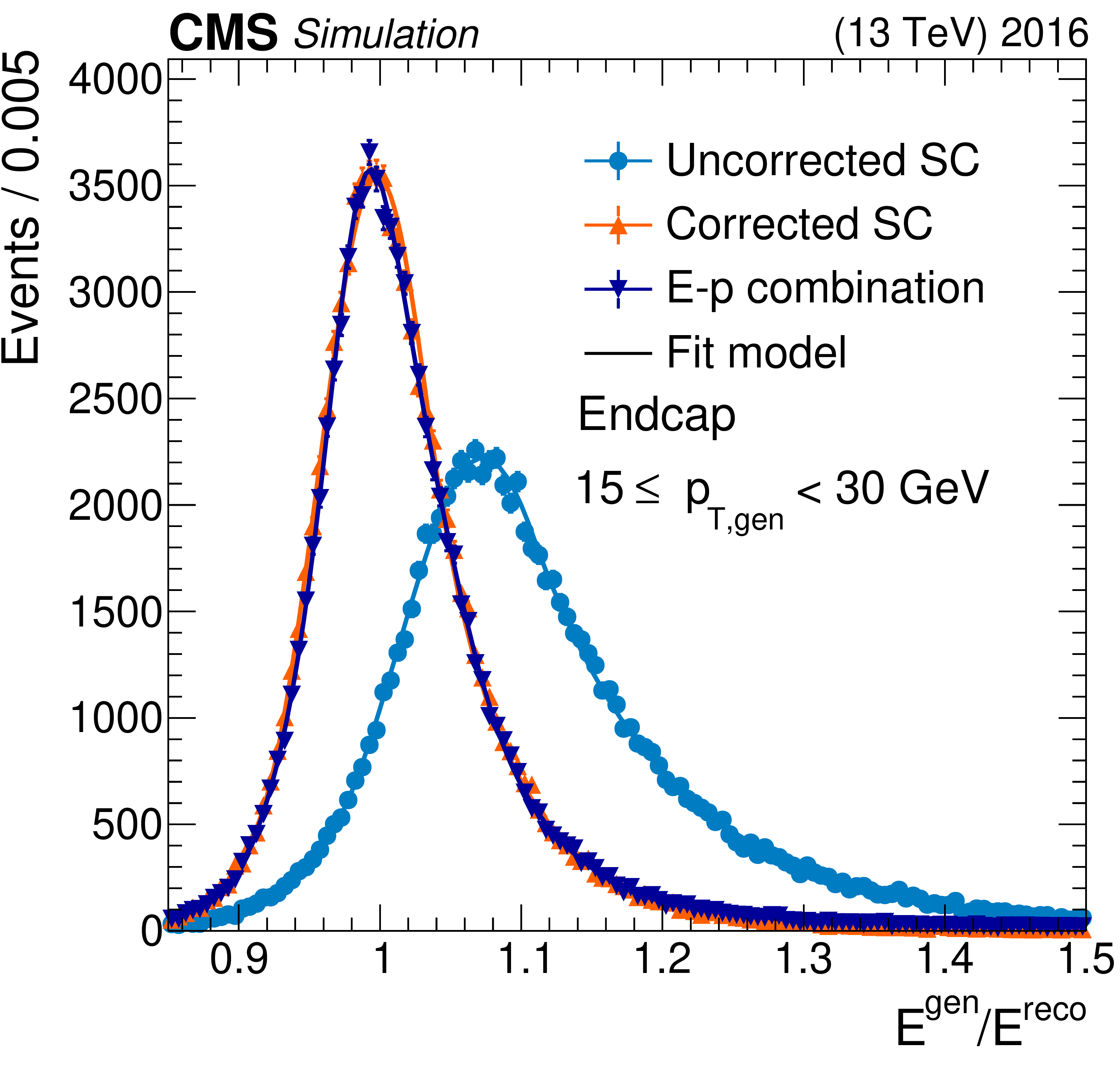
Figure 12:
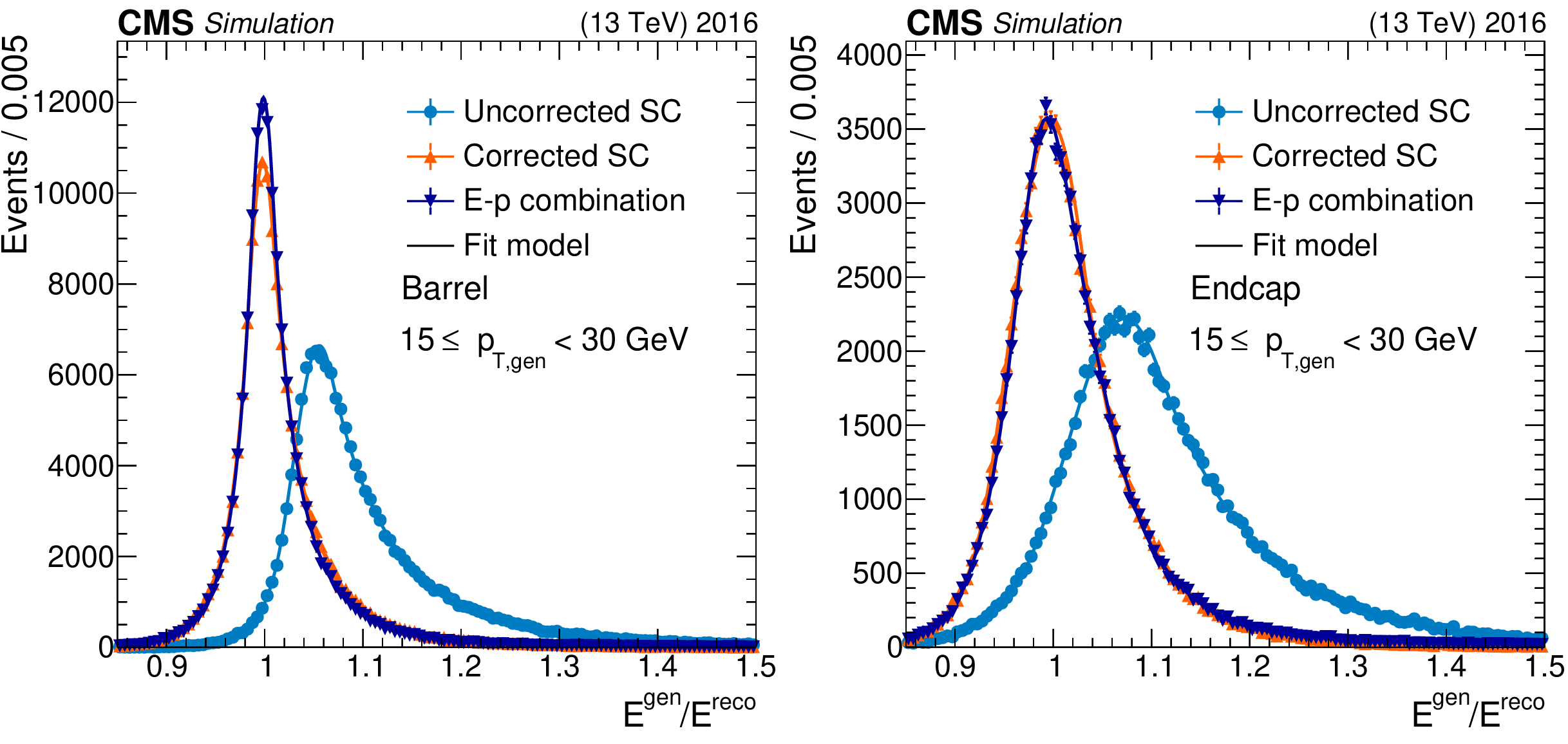
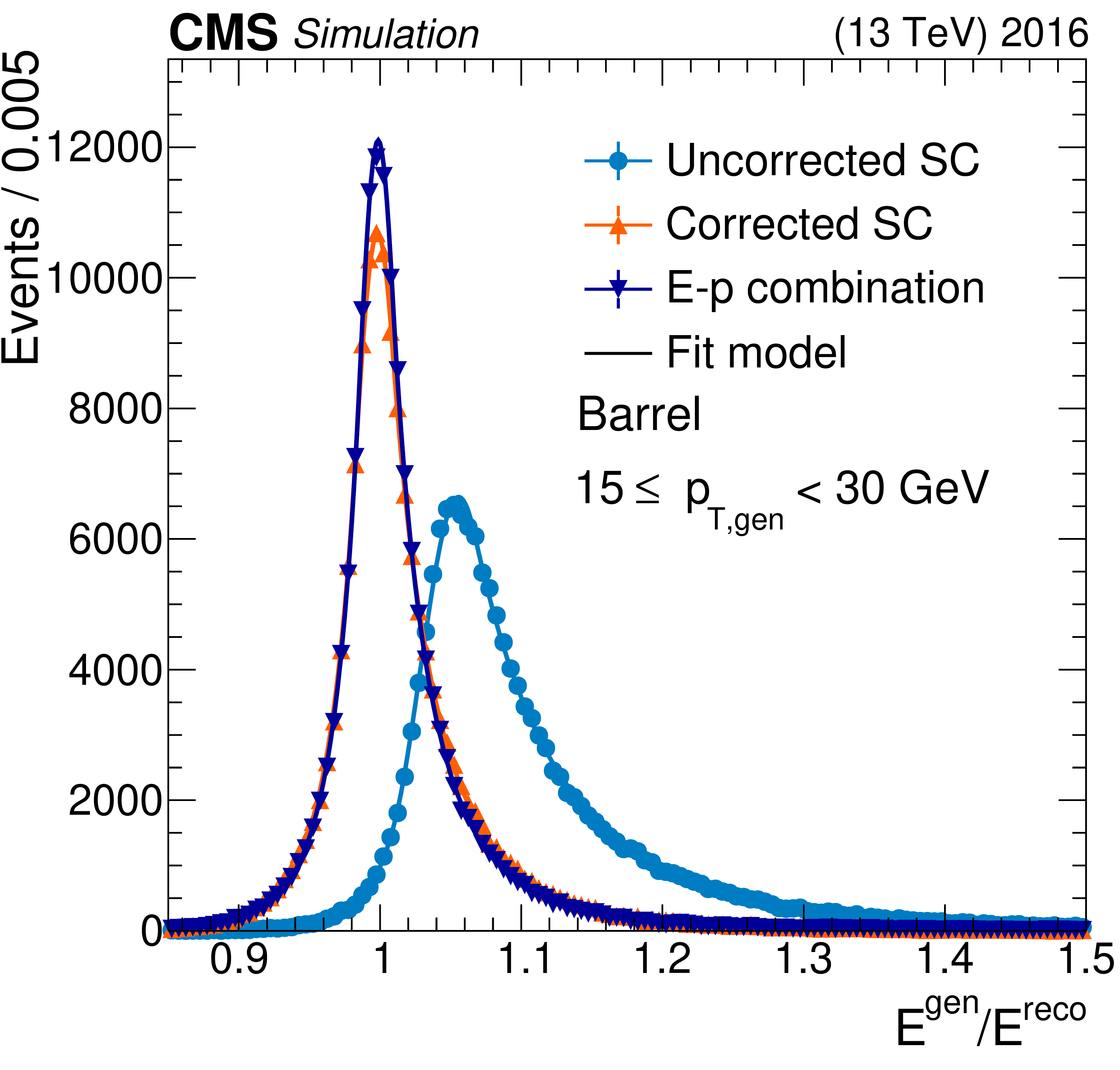
Ratio of the true to the reconstructed electron energy in the ${p_{\mathrm {T}}}$ range 15-30 GeV with and without regression corrections, with a DSCB function fit overlaid, in 2016 MC samples for barrel (left) and endcap (right) electrons. Vertical bars on the markers represent the statistical uncertainties of the MC samples. |
png pdf |
Figure 12-a:
Ratio of the true to the reconstructed electron energy in the ${p_{\mathrm {T}}}$ range 15-30 GeV with and without regression corrections, with a DSCB function fit overlaid, in 2016 MC samples for barrel electrons. Vertical bars on the markers represent the statistical uncertainties of the MC samples. |
png pdf |
Figure 12-b:
Ratio of the true to the reconstructed electron energy in the ${p_{\mathrm {T}}}$ range 15-30 GeV with and without regression corrections, with a DSCB function fit overlaid, in 2016 MC samples for endcap electrons. Vertical bars on the markers represent the statistical uncertainties of the MC samples. |
png pdf |
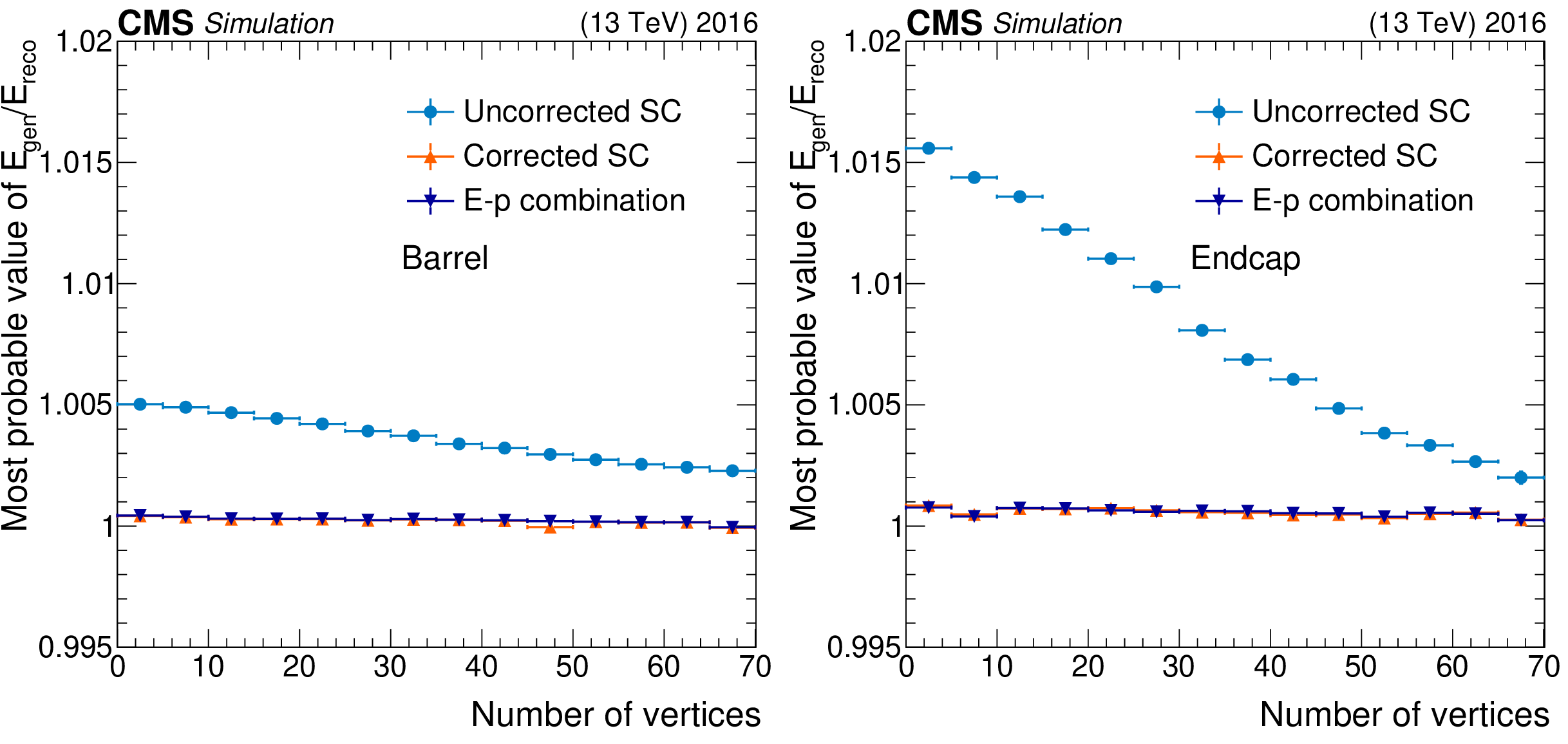
Figure 13:
Most probable value of the ratio of true to reconstructed electron energy, as a function of pileup, with and without regression corrections in 2016 MC samples for barrel (left) and endcap (right) electrons. Vertical bars on the markers represent the uncertainties coming from the fit procedure and are too small to be observed from the plot. |
png pdf |
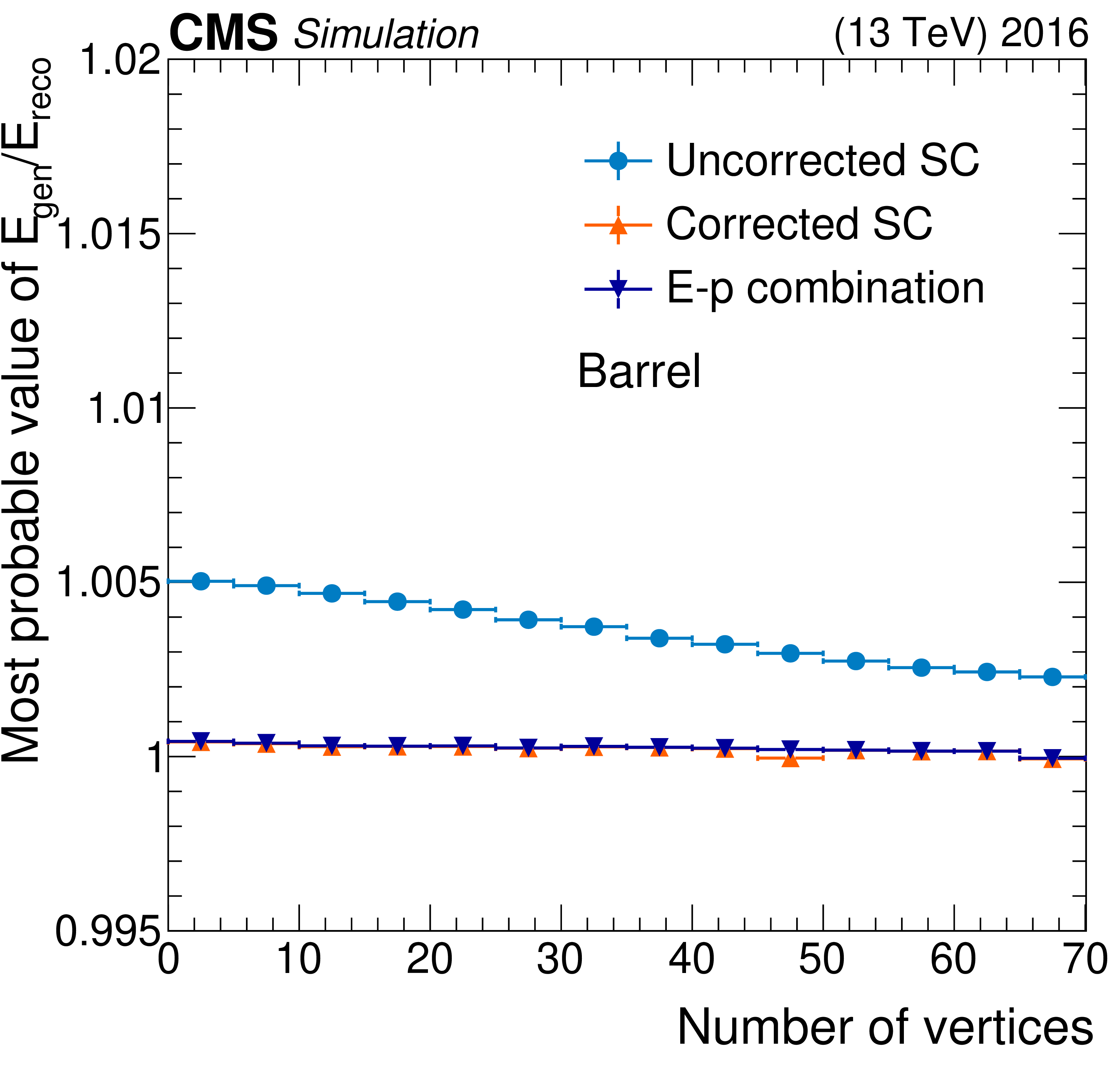
Figure 13-a:
Most probable value of the ratio of true to reconstructed electron energy, as a function of pileup, with and without regression corrections in 2016 MC samples for barrel electrons. Vertical bars on the markers represent the uncertainties coming from the fit procedure and are too small to be observed from the plot. |
png pdf |
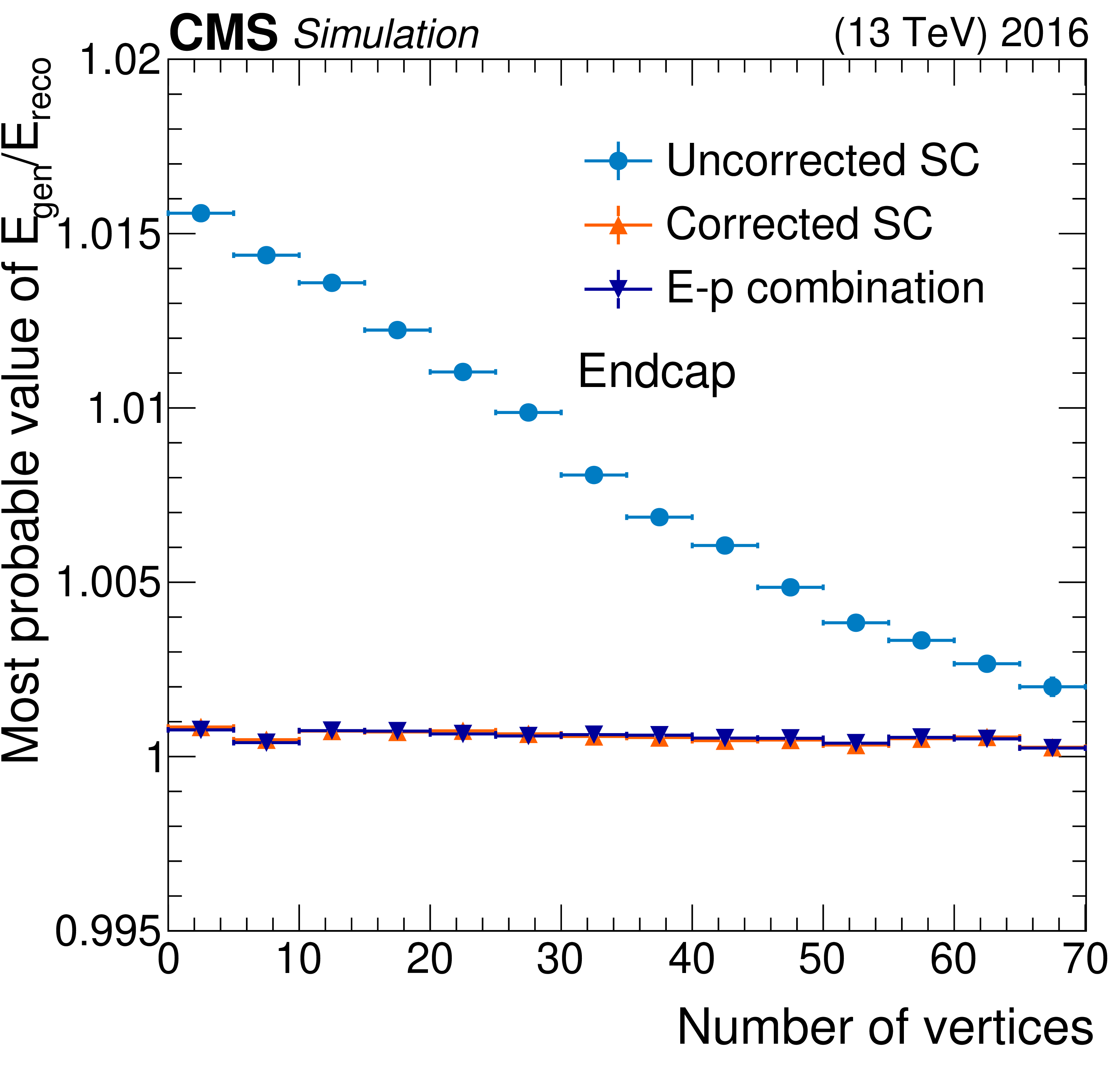
Figure 13-b:
Most probable value of the ratio of true to reconstructed electron energy, as a function of pileup, with and without regression corrections in 2016 MC samples for endcap electrons. Vertical bars on the markers represent the uncertainties coming from the fit procedure and are too small to be observed from the plot. |

png pdf |
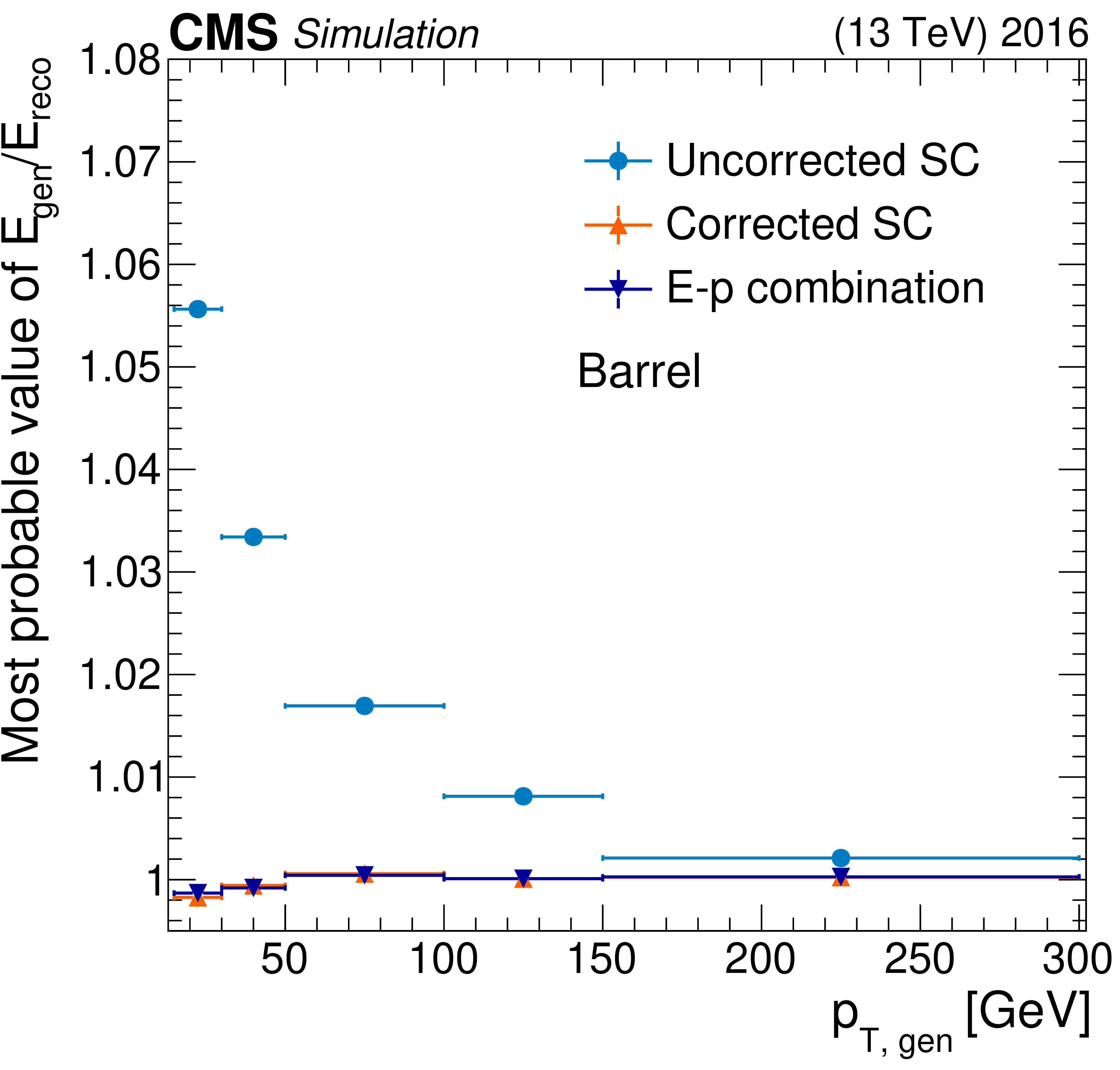
Figure 14:
Most probable value of the ratio of true to reconstructed electron energy, as a function of the electron ${p_{\mathrm {T}}}$ with and without the regression corrections, evaluated using 2016 MC samples for barrel (left) and endcap (right) electrons. Vertical bars on the markers represent the uncertainties coming from the fit procedure and are too small to be observed from the plot. |
png pdf |
Figure 14-a:
Most probable value of the ratio of true to reconstructed electron energy, as a function of the electron ${p_{\mathrm {T}}}$ with and without the regression corrections, evaluated using 2016 MC samples for barrel electrons. Vertical bars on the markers represent the uncertainties coming from the fit procedure and are too small to be observed from the plot. |
png pdf |
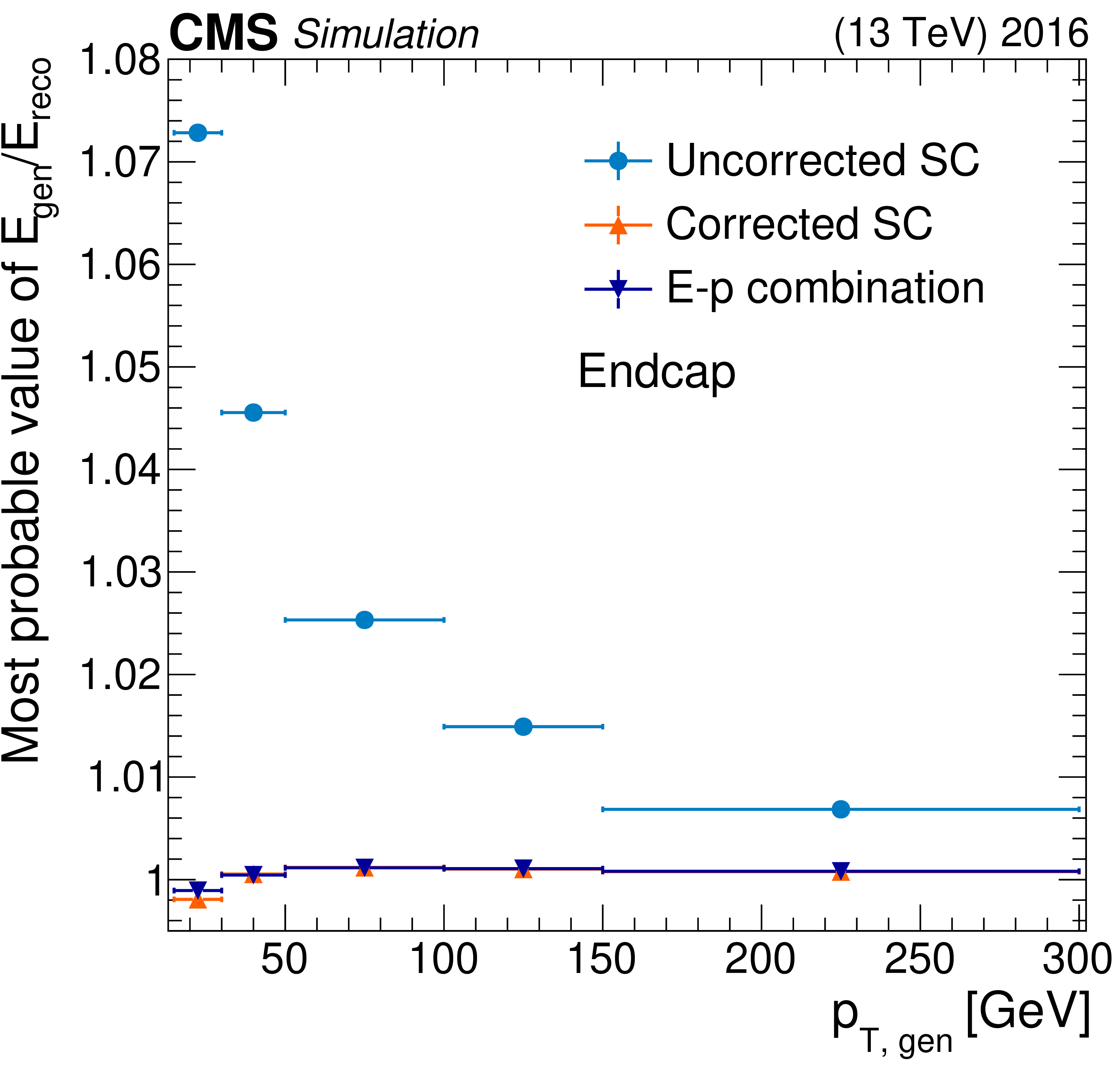
Figure 14-b:
Most probable value of the ratio of true to reconstructed electron energy, as a function of the electron ${p_{\mathrm {T}}}$ with and without the regression corrections, evaluated using 2016 MC samples for endcap electrons. Vertical bars on the markers represent the uncertainties coming from the fit procedure and are too small to be observed from the plot. |
png pdf |
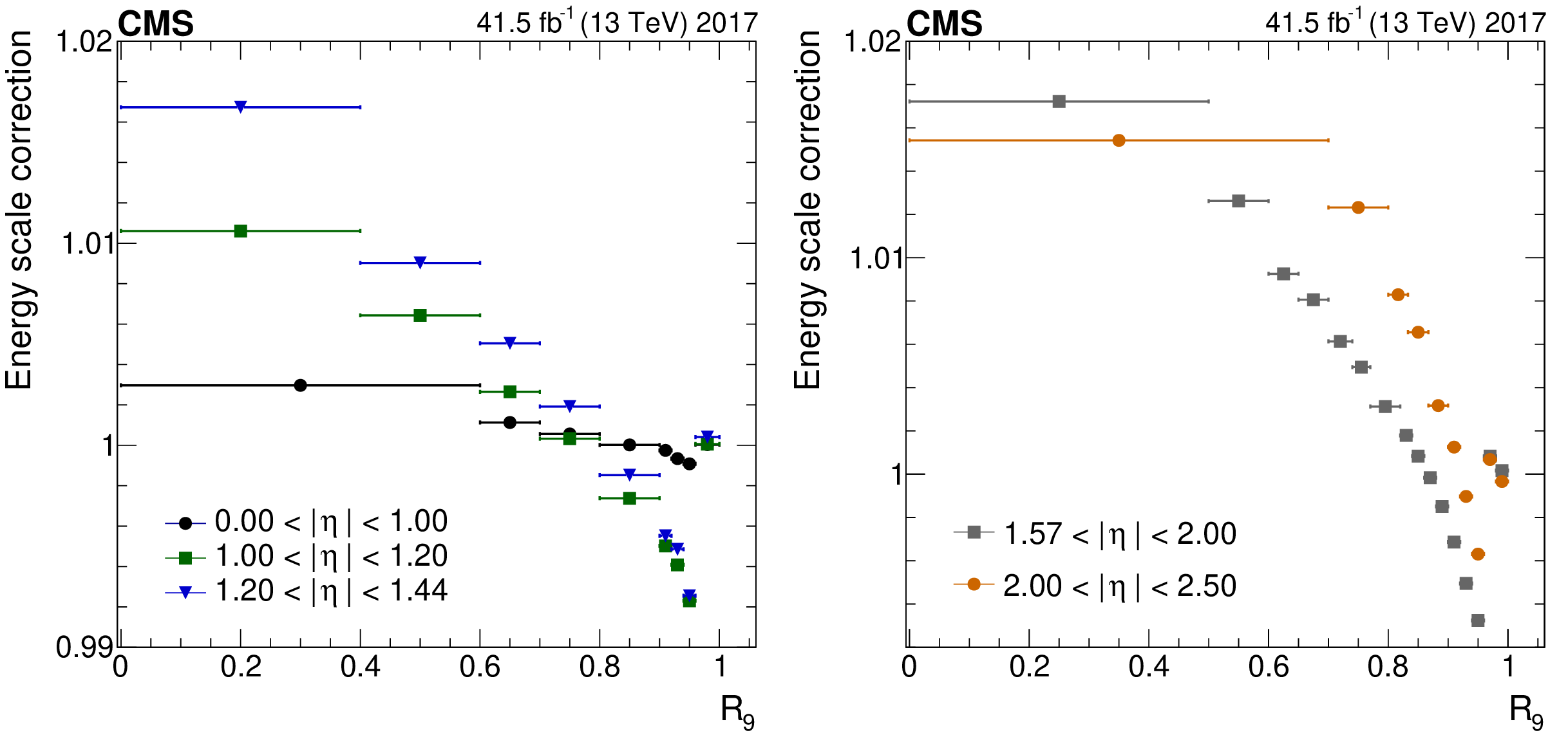
Figure 15:
Energy scale corrections for the 2017 data-taking period, as function of $R_9$, for different $ {| \eta |}$ ranges, in the barrel (left) and for the endcap (right). The error bars represent the statistical uncertainties in the derived correction and are too small to be observed from the plot. |
png pdf |
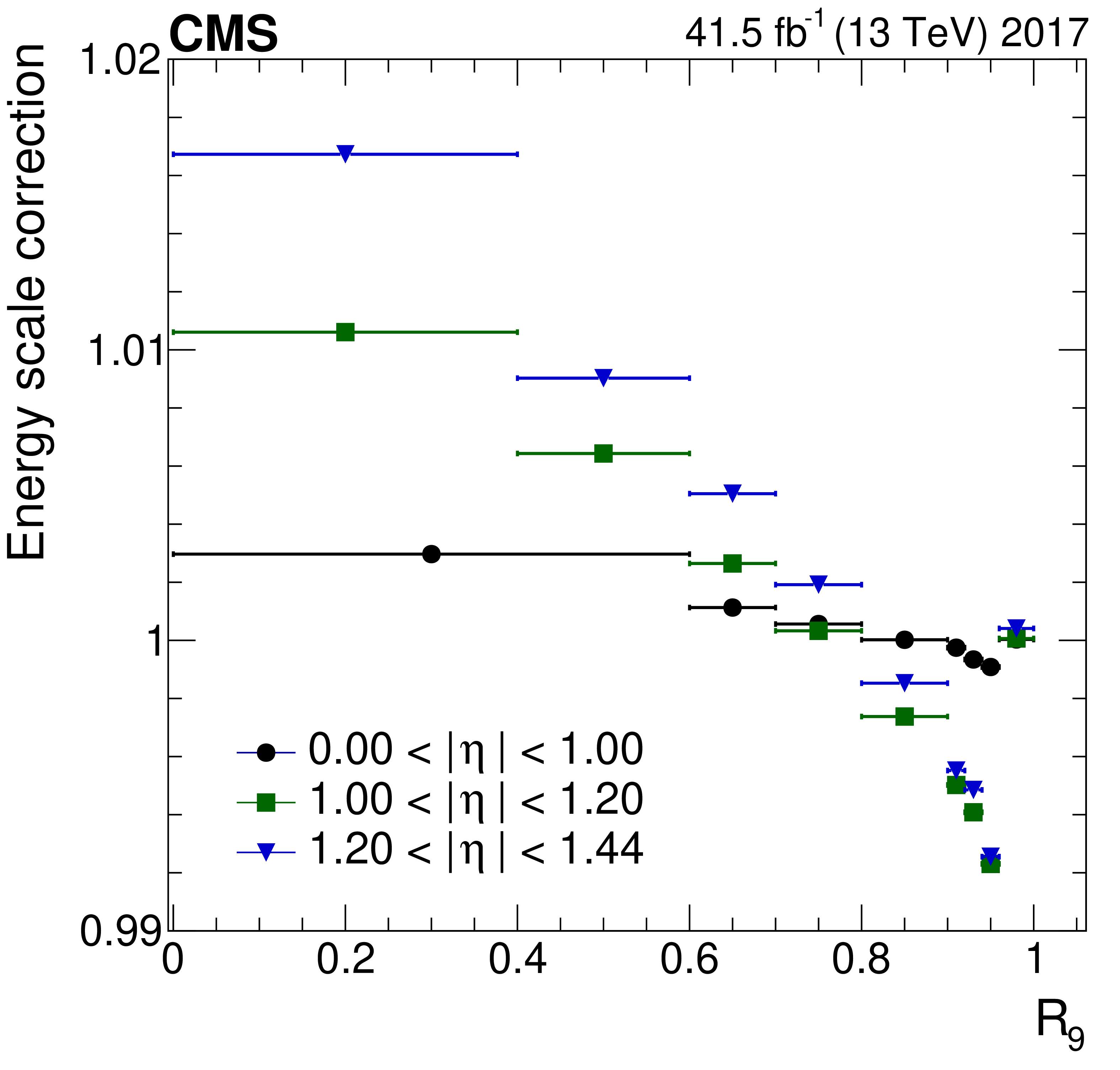
Figure 15-a:
Energy scale corrections for the 2017 data-taking period, as function of $R_9$, for different $ {| \eta |}$ ranges, in the barrel. The error bars represent the statistical uncertainties in the derived correction and are too small to be observed from the plot. |

png pdf |
Figure 15-b:
Energy scale corrections for the 2017 data-taking period, as function of $R_9$, for different $ {| \eta |}$ ranges, in the endcap. The error bars represent the statistical uncertainties in the derived correction and are too small to be observed from the plot. |
png pdf |
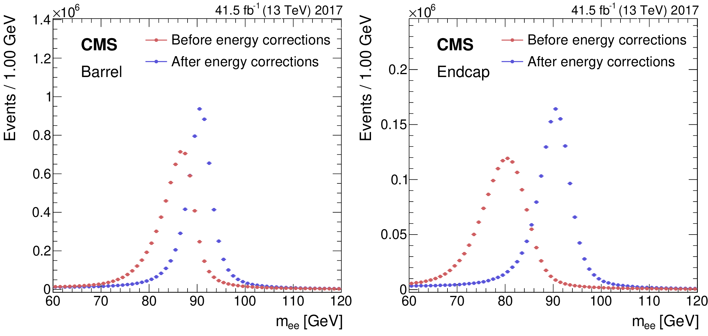
Figure 16:
Dielectron invariant mass distribution before and after all the energy corrections (regression and scale corrections) for barrel (left) and endcap (right) electrons for $\mathrm{Z} \to \mathrm{ee} $ events. The error bars represent the statistical uncertainties in data and are too small to be observed from the plot. |

png pdf |
Figure 16-a:
Dielectron invariant mass distribution before and after all the energy corrections (regression and scale corrections) for barrel electrons for $\mathrm{Z} \to \mathrm{ee} $ events. The error bars represent the statistical uncertainties in data and are too small to be observed from the plot. |
png pdf |
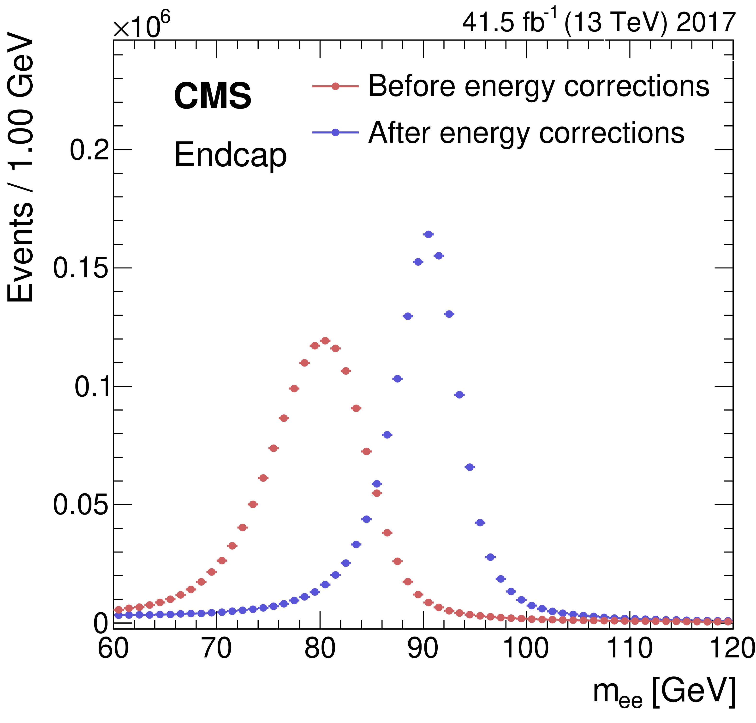
Figure 16-b:
Dielectron invariant mass distribution before and after all the energy corrections (regression and scale corrections) for endcap electrons for $\mathrm{Z} \to \mathrm{ee} $ events. The error bars represent the statistical uncertainties in data and are too small to be observed from the plot. |

png pdf |
Figure 17:
Invariant mass distribution of $\mathrm{Z} \to \mathrm{ee} $ events, after spreading is applied to simulation and scale corrections to data. The results are shown for barrel (left) and endcap (right) electrons. The simulation is shown with the filled histograms and data are shown by the markers. The vertical bars on the markers represent the statistical uncertainties in data. The hatched regions show the combined statistical and systematic uncertainties in the simulation. The lower panels display the ratio of the data to the simulation with the bands representing the uncertainties in the simulation. |
png pdf |
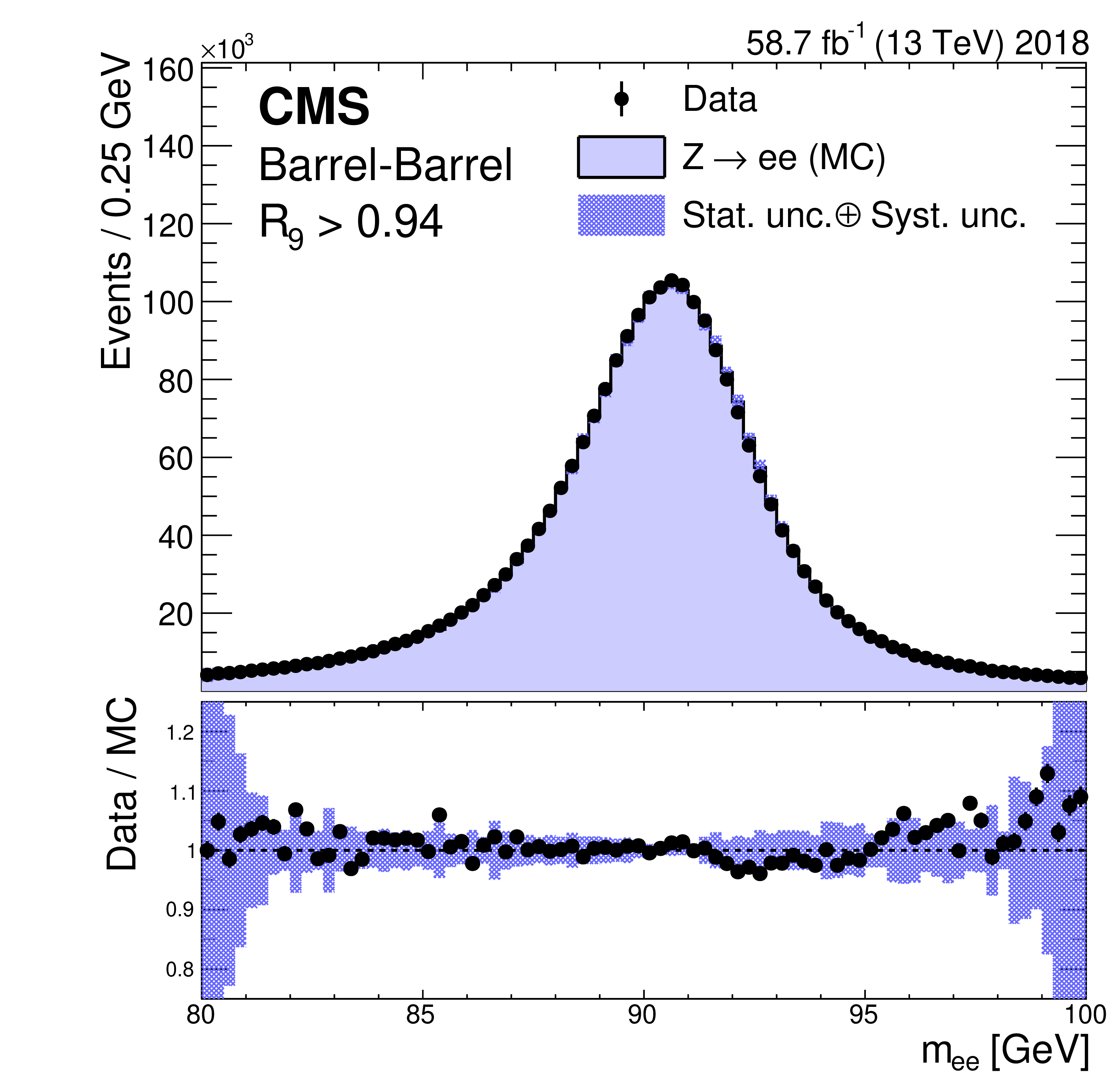
Figure 17-a:
Invariant mass distribution of $\mathrm{Z} \to \mathrm{ee} $ events, after spreading is applied to simulation and scale corrections to data. The results are shown for barrel electrons. The simulation is shown with the filled histograms and data are shown by the markers. The vertical bars on the markers represent the statistical uncertainties in data. The hatched regions show the combined statistical and systematic uncertainties in the simulation. The lower panel displays the ratio of the data to the simulation with the bands representing the uncertainties in the simulation. |
png pdf |
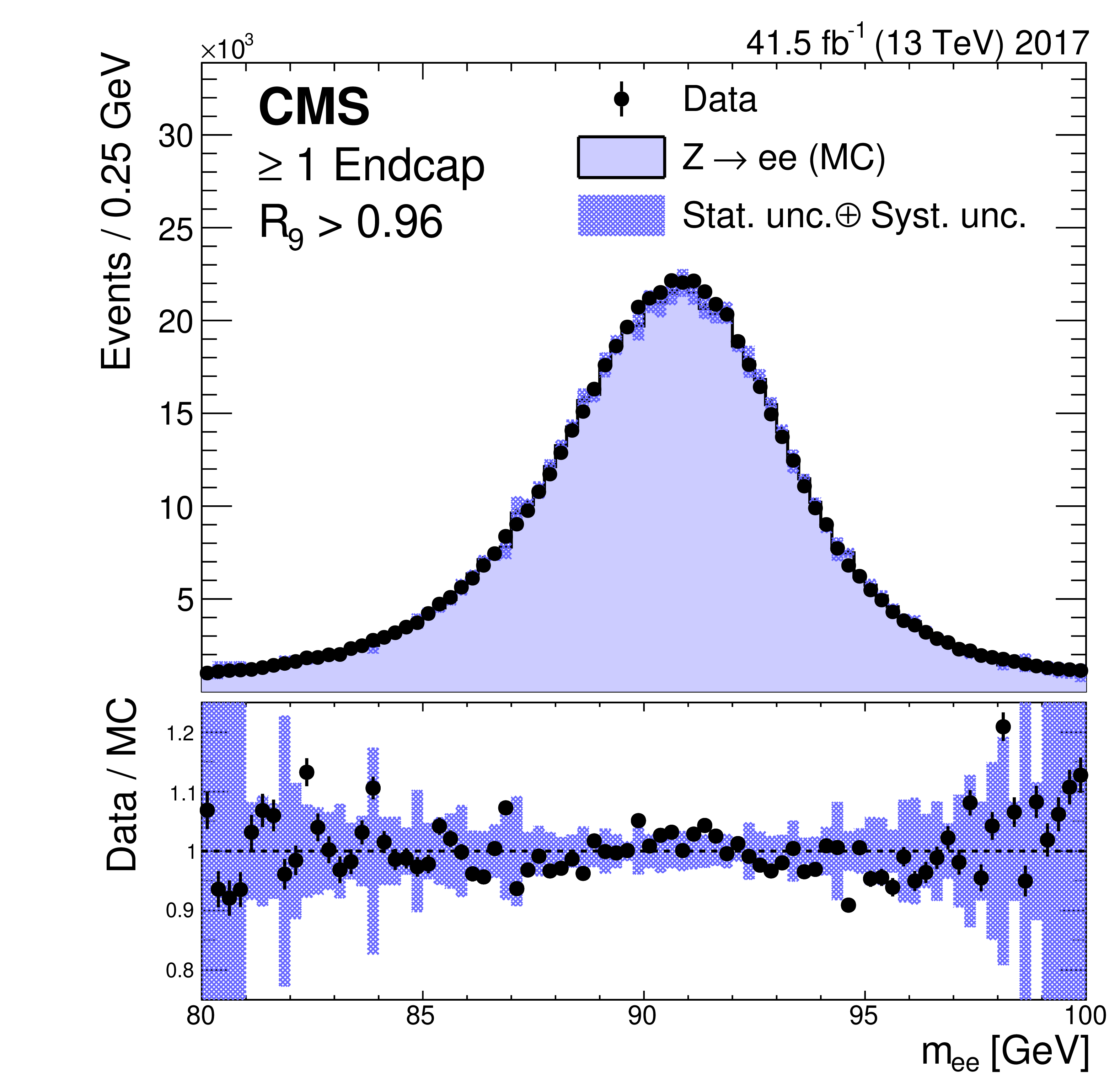
Figure 17-b:
Invariant mass distribution of $\mathrm{Z} \to \mathrm{ee} $ events, after spreading is applied to simulation and scale corrections to data. The results are shown for endcap electrons. The simulation is shown with the filled histograms and data are shown by the markers. The vertical bars on the markers represent the statistical uncertainties in data. The hatched regions show the combined statistical and systematic uncertainties in the simulation. The lower panel displays the ratio of the data to the simulation with the bands representing the uncertainties in the simulation. |
png pdf |
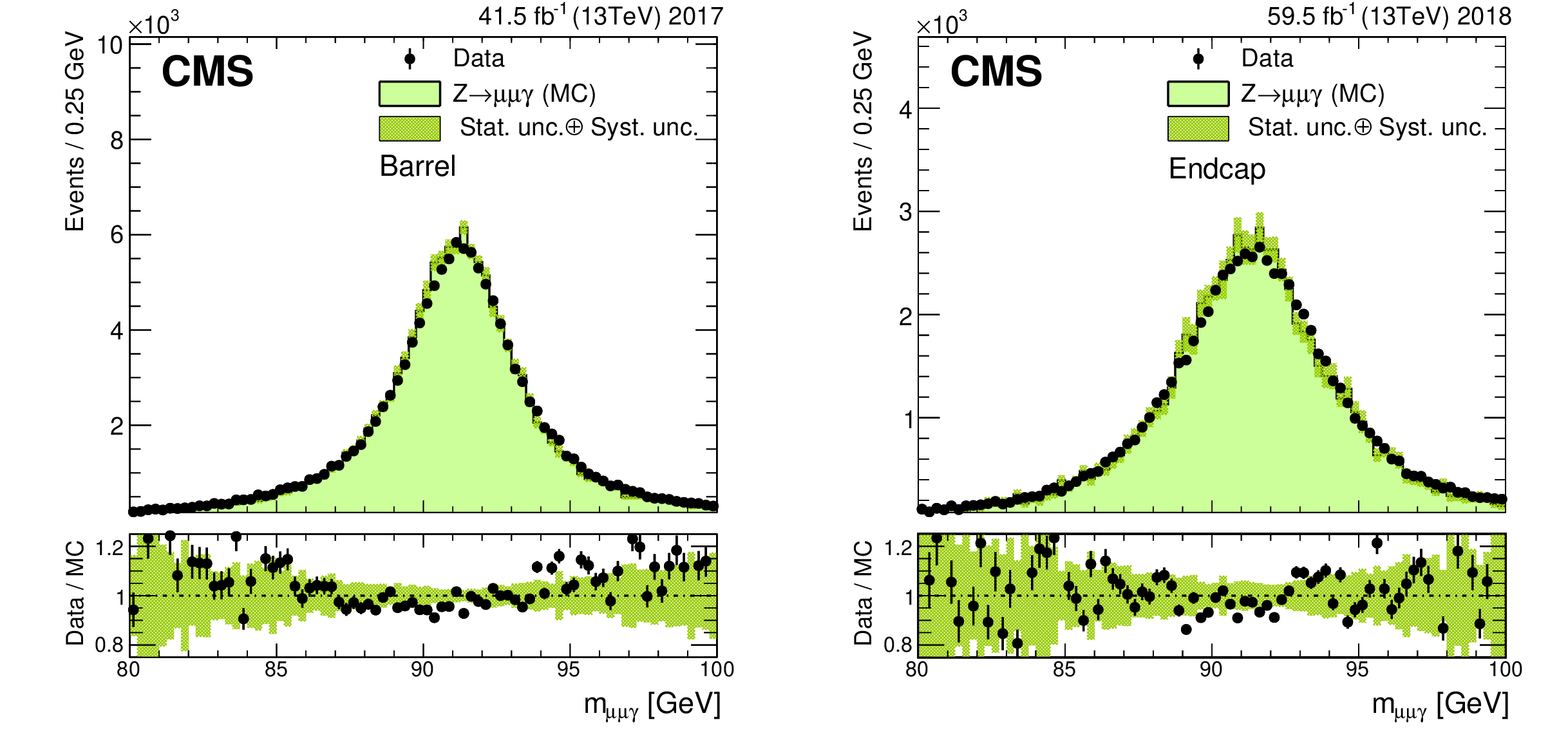
Figure 18:
Invariant mass distributions of $\mathrm{Z} \to \mu \mu \gamma $ shown for barrel (left) and endcap (right) photons selected from 2017 data and simulation (left), 2018 data and simulation (right). The simulation is shown with the filled histograms and data are shown by the markers. The vertical bars on the markers represent the statistical uncertainties in data. The hatched regions show the sum of statistical and systematic uncertainties in the simulation. The lower panels display the ratio of the data to the simulation with bands representing the uncertainties in the simulation. |
png pdf |
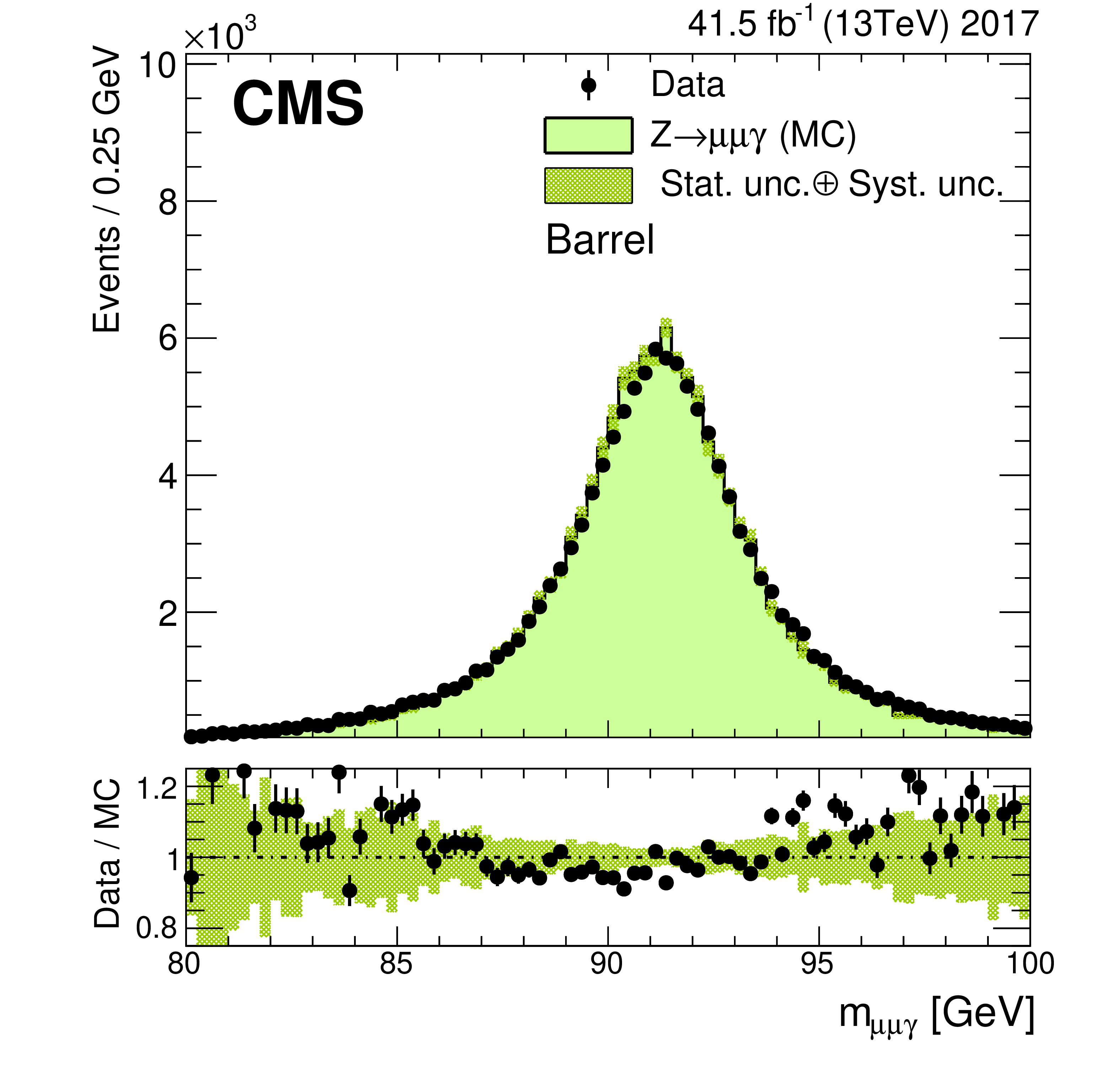
Figure 18-a:
Invariant mass distributions of $\mathrm{Z} \to \mu \mu \gamma $ shown for barrel photons selected from 2017 data and simulation. The simulation is shown with the filled histograms and data are shown by the markers. The vertical bars on the markers represent the statistical uncertainties in data. The hatched regions show the sum of statistical and systematic uncertainties in the simulation. The lower panels display the ratio of the data to the simulation with bands representing the uncertainties in the simulation. |
png pdf |
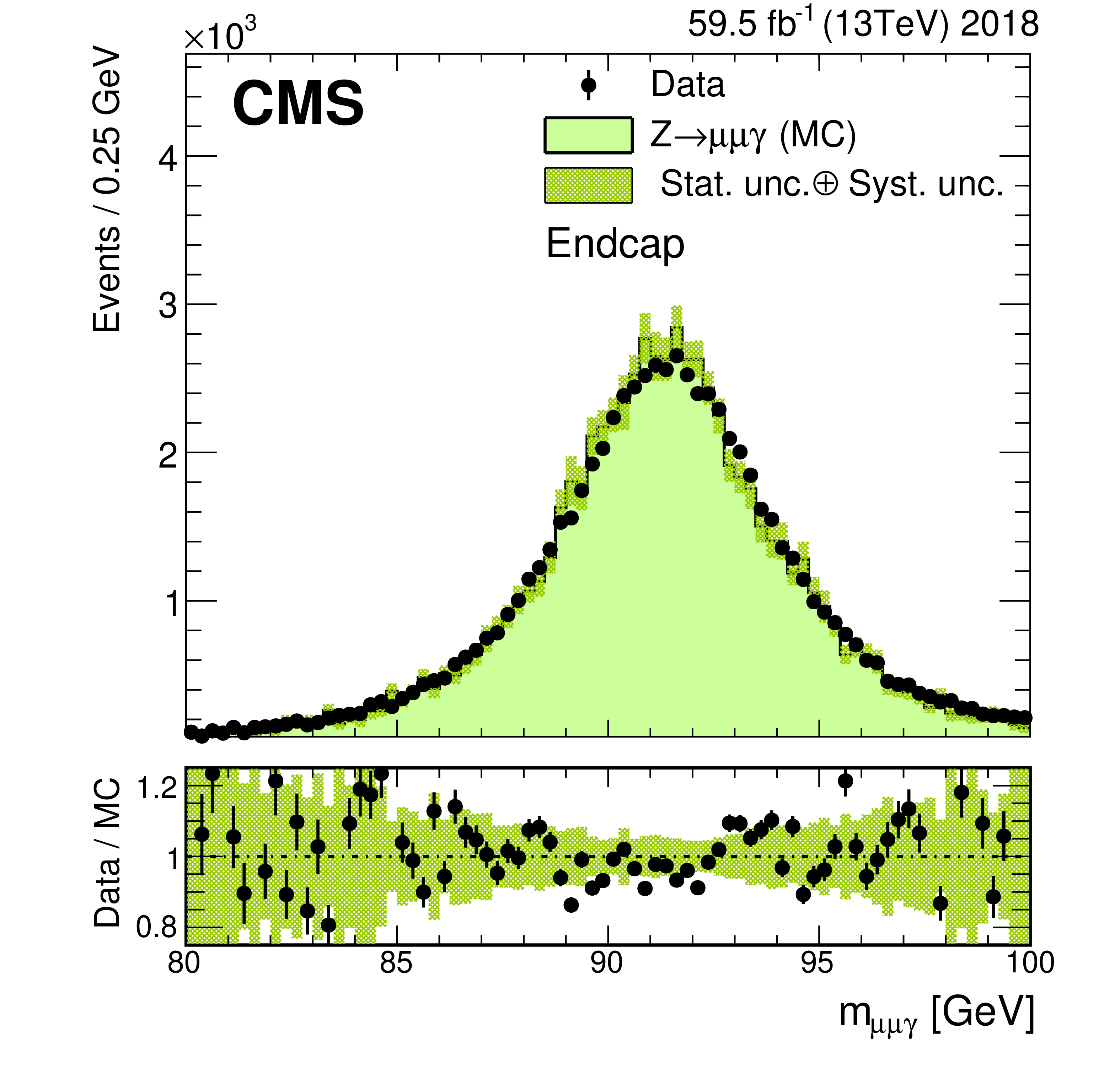
Figure 18-b:
Invariant mass distributions of $\mathrm{Z} \to \mu \mu \gamma $ shown for endcap photons selected from 2018 data and simulation. The simulation is shown with the filled histograms and data are shown by the markers. The vertical bars on the markers represent the statistical uncertainties in data. The hatched regions show the sum of statistical and systematic uncertainties in the simulation. The lower panels display the ratio of the data to the simulation with bands representing the uncertainties in the simulation. |
png pdf |
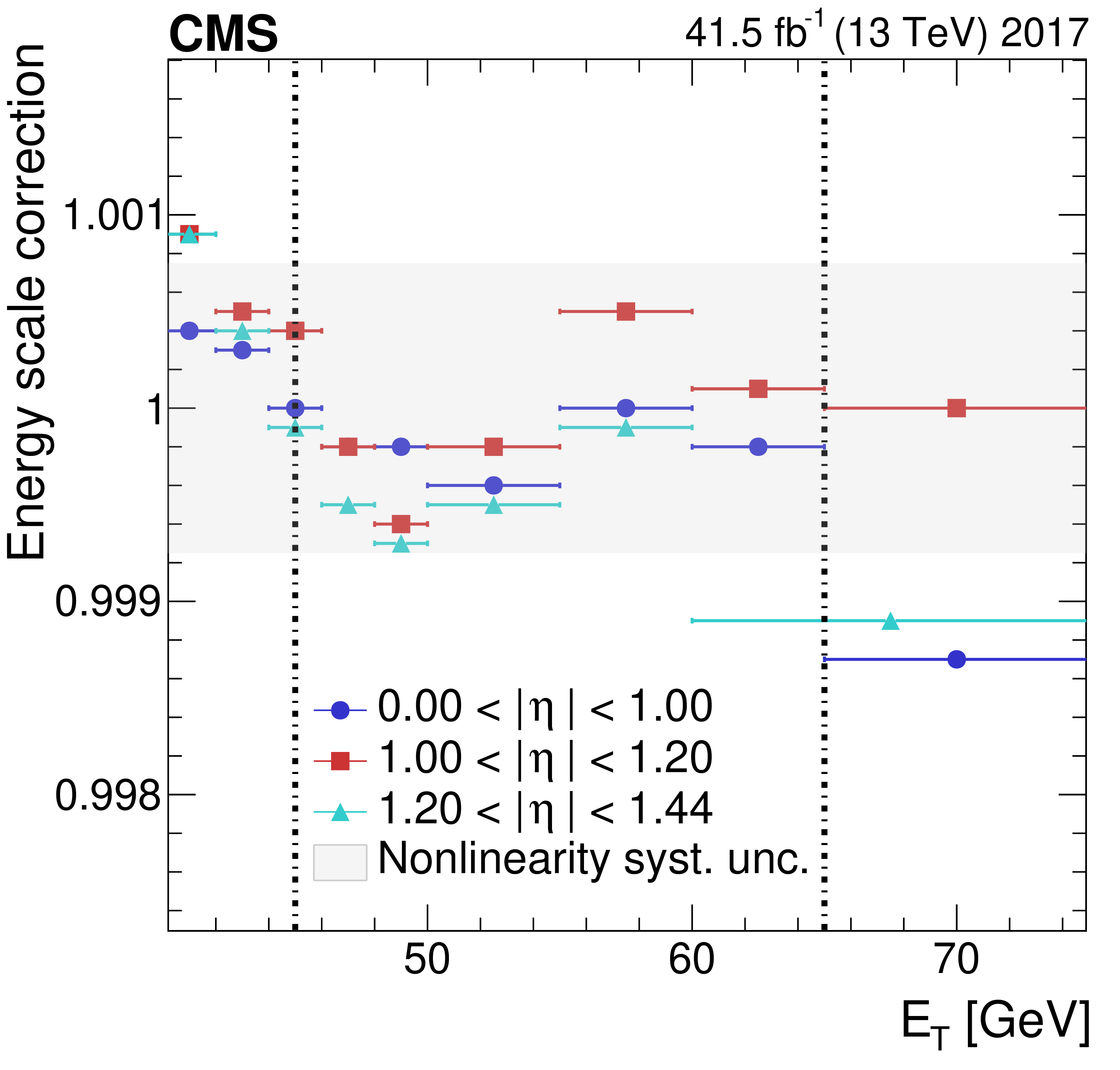
Figure 19:
Energy scale corrections as a function of the photon $ {E_{\mathrm {T}}} $. The horizontal bars represent the variable bin width. The systematic uncertainty associated with this correction is approximately the maximum deviation observed in the $ {E_{\mathrm {T}}} $ range between 45 and 65 GeV for electrons in the barrel. |
png pdf |
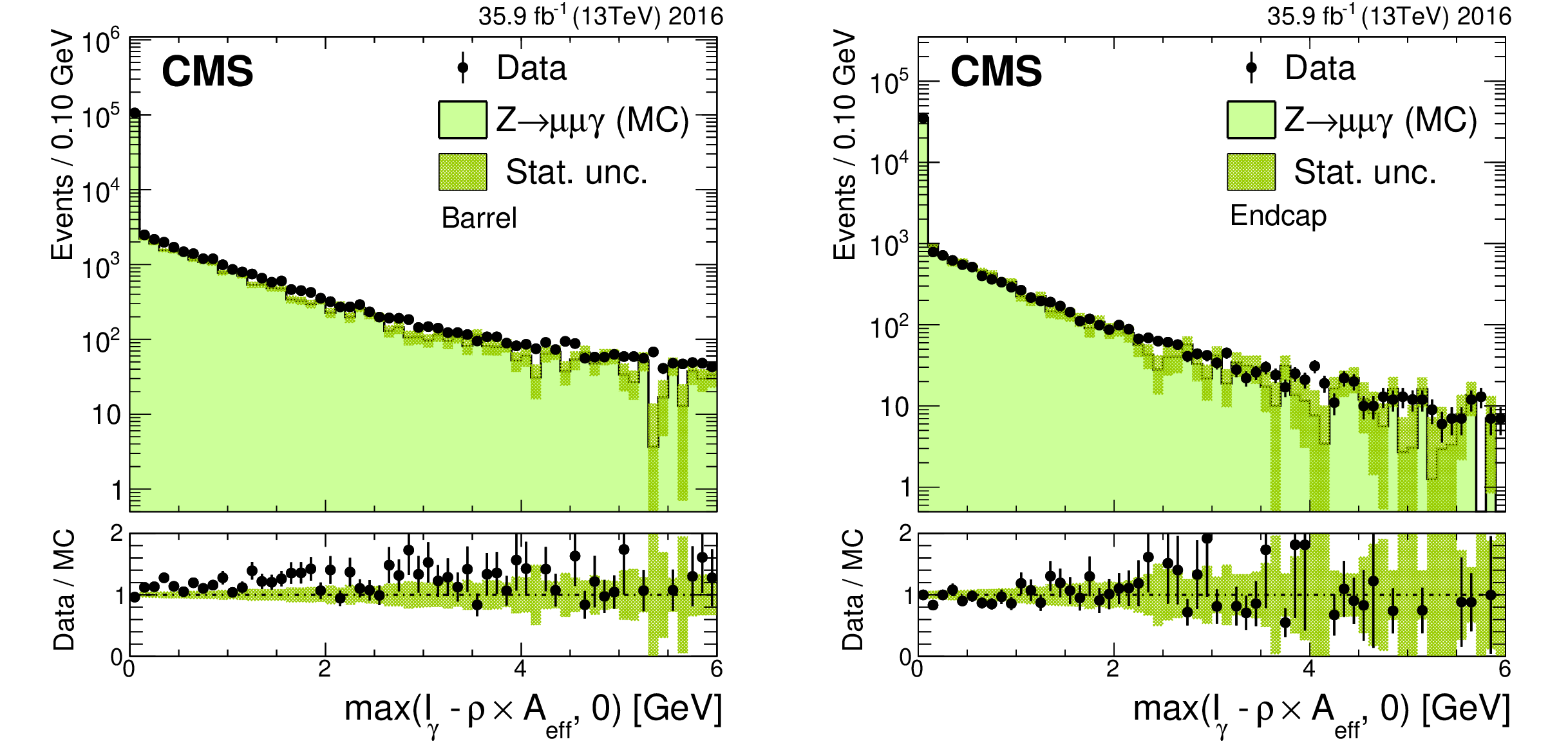
Figure 20:
The $\rho $-corrected PF photon isolation in a cone defined by $\Delta R = $ 0.3 for photons in $\mathrm{Z} \to \mu \mu \gamma $ events in the EB (left) and in the EE (right). Photons are selected from 2016 data and simulation. The simulation is shown with the filled histograms and data are represented by the markers. The vertical bars on the markers represent the statistical uncertainties in data. The hatched regions show the statistical uncertainty in the simulation. The lower panels display the ratio of the data to the simulation, with the bands representing the uncertainties in the simulation. |
png pdf |
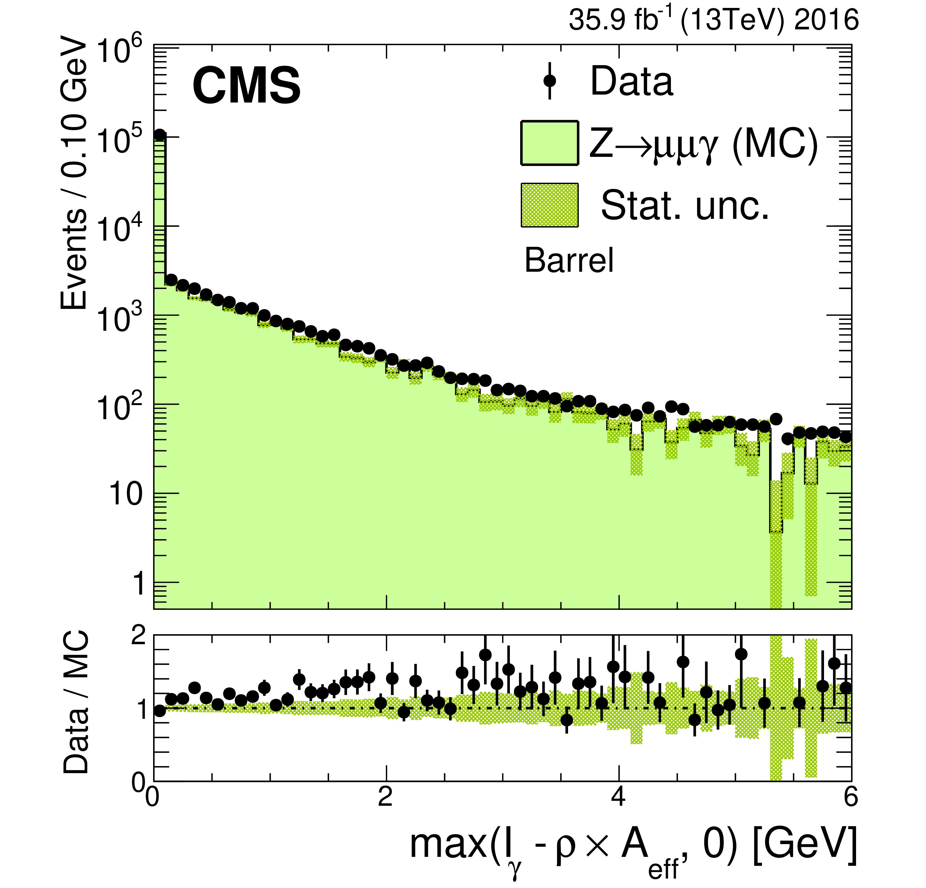
Figure 20-a:
The $\rho $-corrected PF photon isolation in a cone defined by $\Delta R = $ 0.3 for photons in $\mathrm{Z} \to \mu \mu \gamma $ events in the EB. Photons are selected from 2016 data and simulation. The simulation is shown with the filled histograms and data are represented by the markers. The vertical bars on the markers represent the statistical uncertainties in data. The hatched regions show the statistical uncertainty in the simulation. The lower panel displays the ratio of the data to the simulation, with the bands representing the uncertainties in the simulation. |
png pdf |
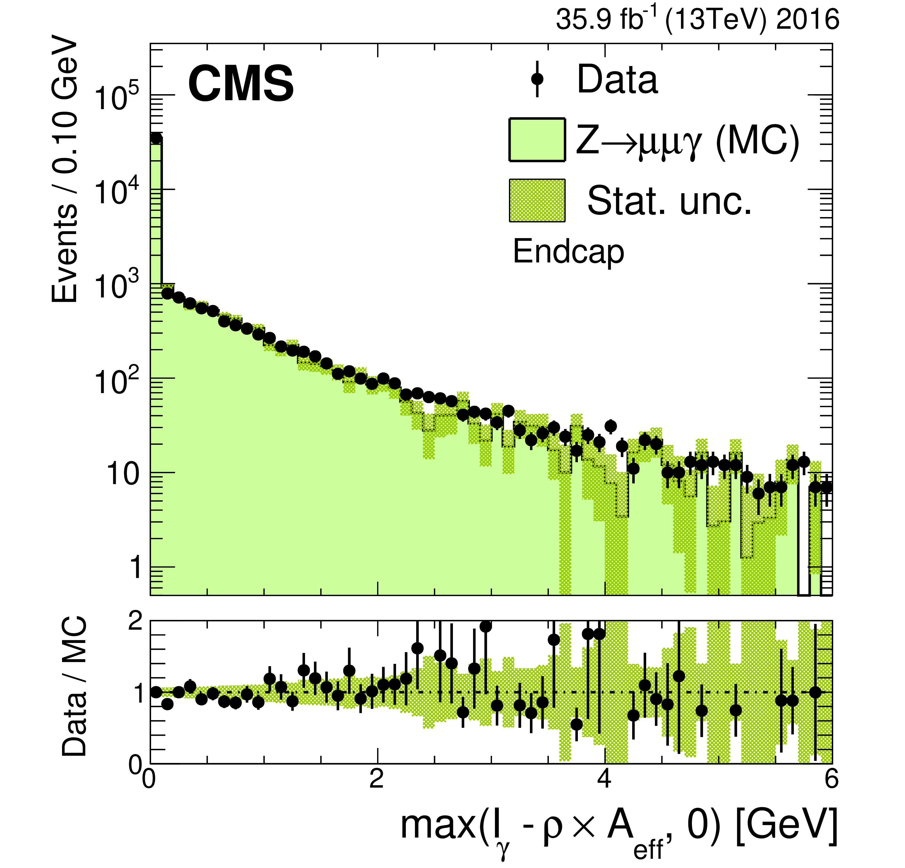
Figure 20-b:
The $\rho $-corrected PF photon isolation in a cone defined by $\Delta R = $ 0.3 for photons in $\mathrm{Z} \to \mu \mu \gamma $ events in the EE. Photons are selected from 2016 data and simulation. The simulation is shown with the filled histograms and data are represented by the markers. The vertical bars on the markers represent the statistical uncertainties in data. The hatched regions show the statistical uncertainty in the simulation. The lower panel displays the ratio of the data to the simulation, with the bands representing the uncertainties in the simulation. |
png pdf |
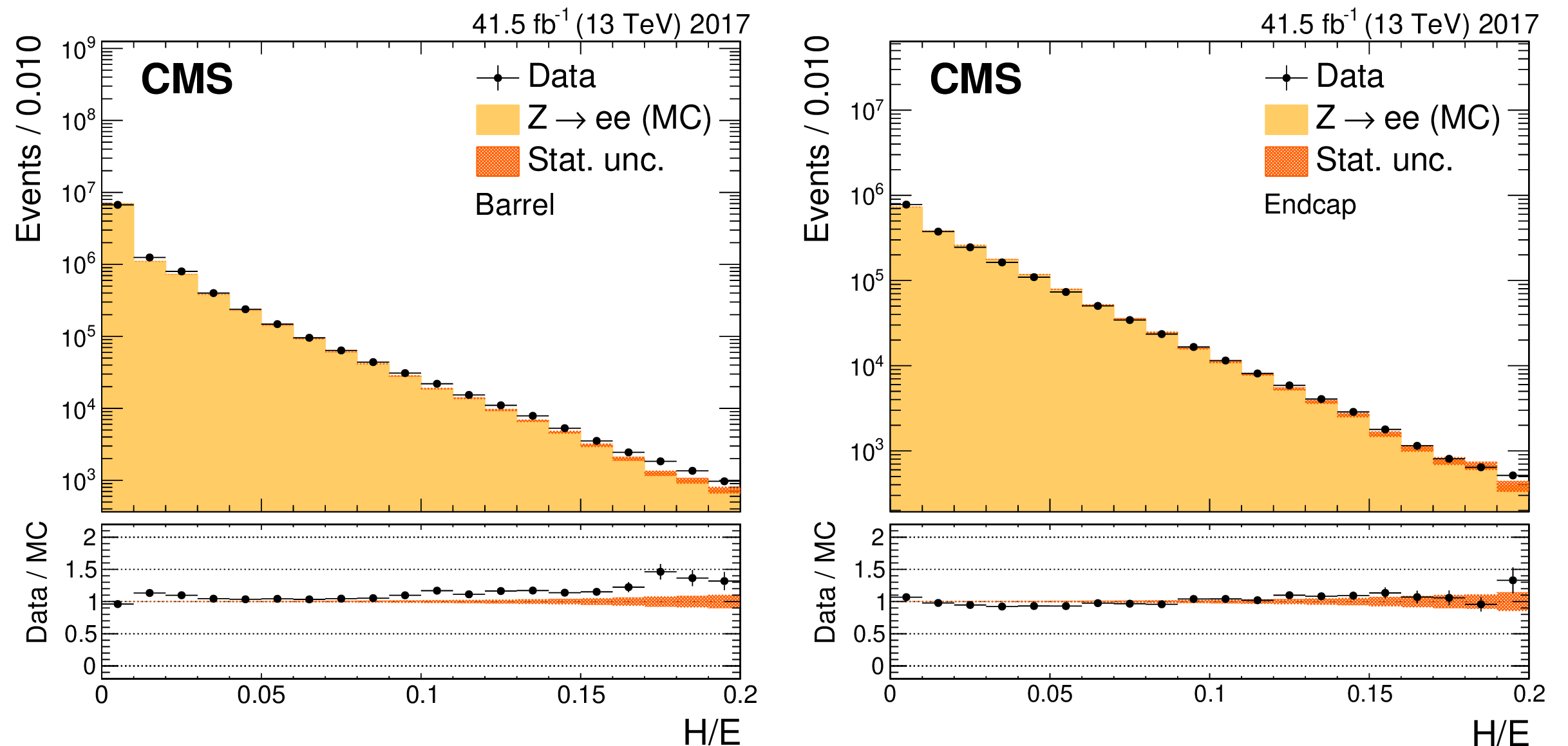
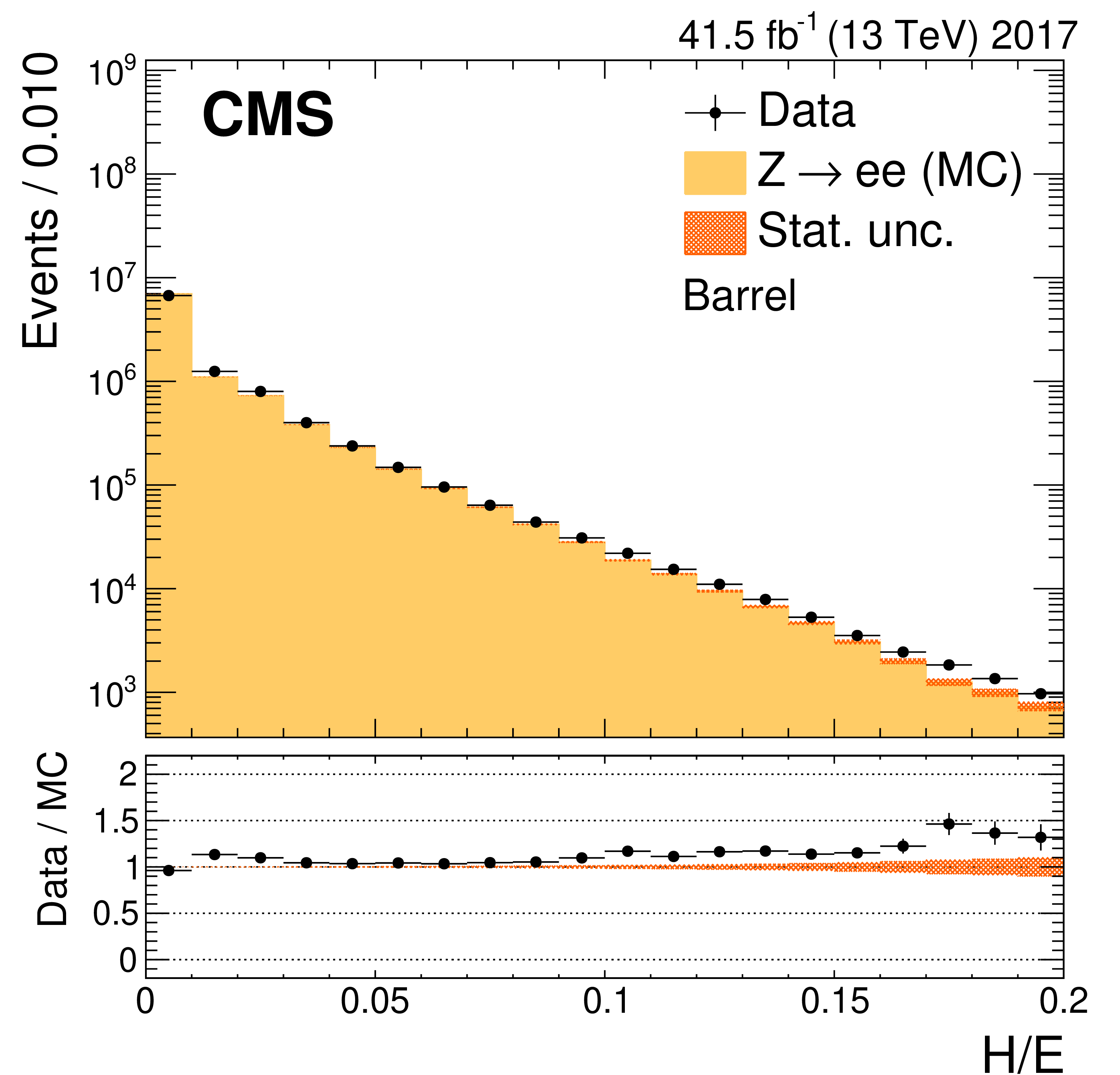
Figure 21:
Distribution of $H/E$ for electrons in the barrel (left) and in the endcaps (right). The simulation is shown with the filled histograms and data are represented by the markers. The vertical bars on the markers represent the statistical uncertainties in data. The hatched regions show the statistical uncertainty in the simulation. The lower panels display the ratio of the data to the simulation, with the bands representing the uncertainties in the simulation. |
png pdf |
Figure 21-a:
Distribution of $H/E$ for electrons in the barrel. The simulation is shown with the filled histograms and data are represented by the markers. The vertical bars on the markers represent the statistical uncertainties in data. The hatched regions show the statistical uncertainty in the simulation. The lower panel displays the ratio of the data to the simulation, with the bands representing the uncertainties in the simulation. |

png pdf |
Figure 21-b:
Distribution of $H/E$ for electrons in the endcaps. The simulation is shown with the filled histograms and data are represented by the markers. The vertical bars on the markers represent the statistical uncertainties in data. The hatched regions show the statistical uncertainty in the simulation. The lower panel displays the ratio of the data to the simulation, with the bands representing the uncertainties in the simulation. |
png pdf |
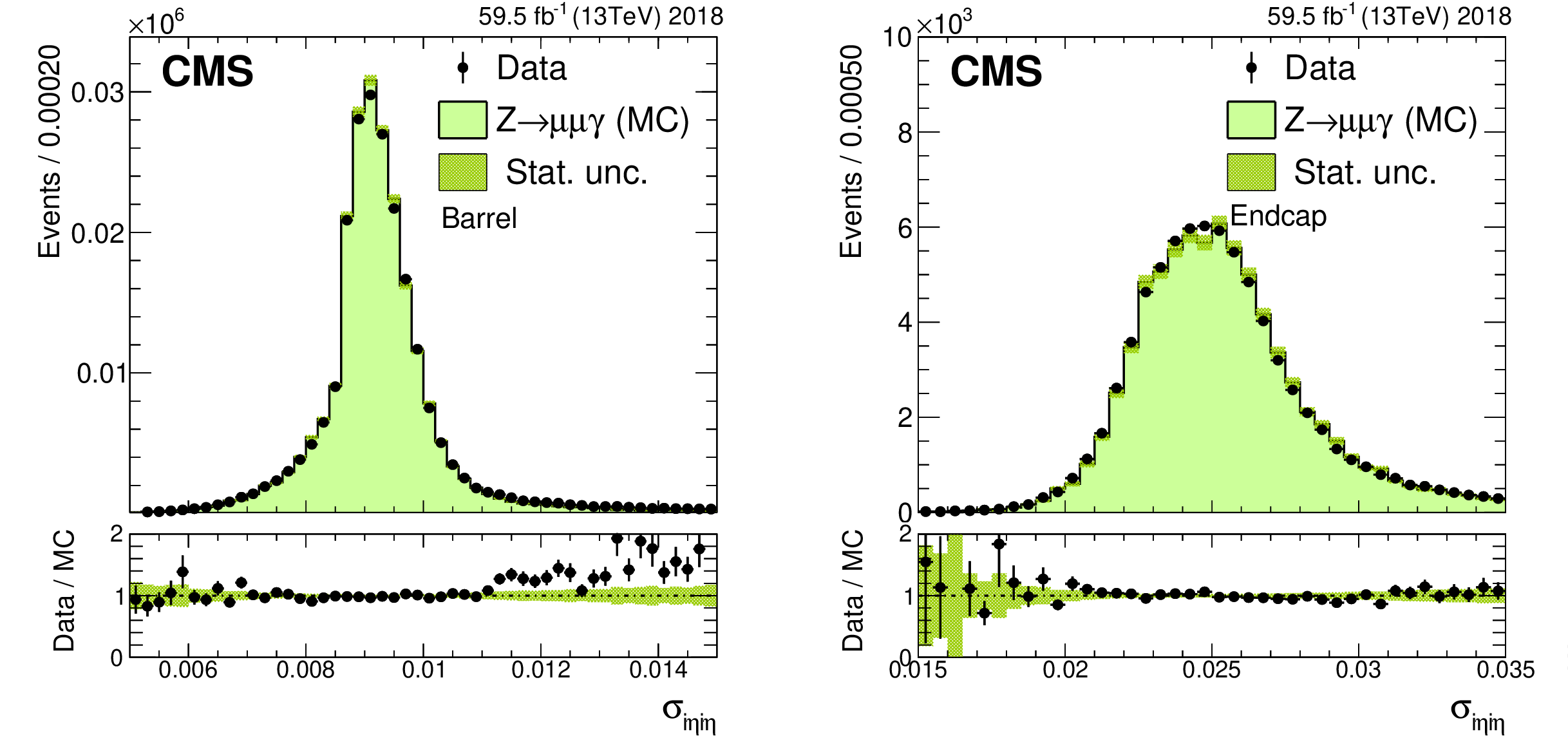
Figure 22:
Distribution of $\sigma _{i \eta i \eta}$ for photons from $\mathrm{Z} \to \mu \mu \gamma $ events in the barrel (left) and in the endcaps (right). Photons are selected from 2018 data and simulation. The simulation is shown with the filled histograms and data are represented by the markers. The vertical bars on the markers represent the statistical uncertainties in data. The hatched regions show the statistical uncertainty in the simulation. The lower panels display the ratio of the data to the simulation, with the bands representing the uncertainties in the simulation. |
png pdf |
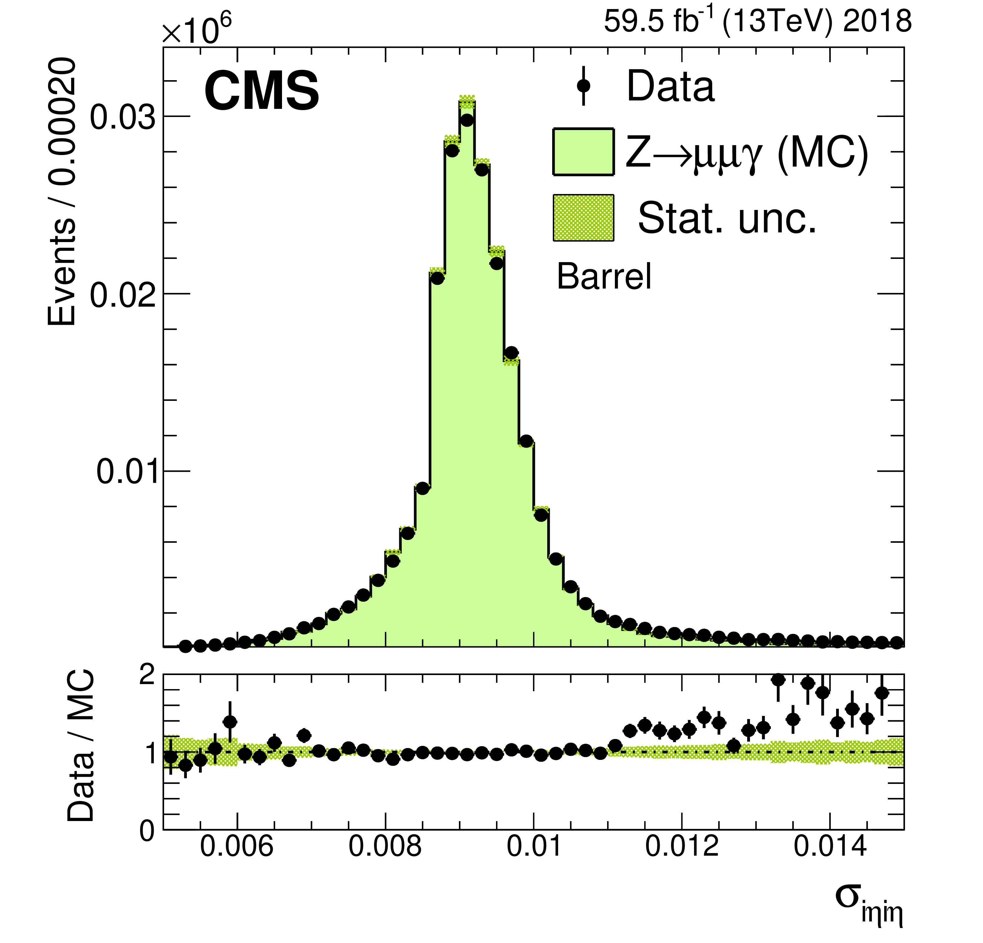
Figure 22-a:
Distribution of $\sigma _{i \eta i \eta}$ for photons from $\mathrm{Z} \to \mu \mu \gamma $ events in the barrel. Photons are selected from 2018 data and simulation. The simulation is shown with the filled histograms and data are represented by the markers. The vertical bars on the markers represent the statistical uncertainties in data. The hatched regions show the statistical uncertainty in the simulation. The lower panel displays the ratio of the data to the simulation, with the bands representing the uncertainties in the simulation. |
png pdf |
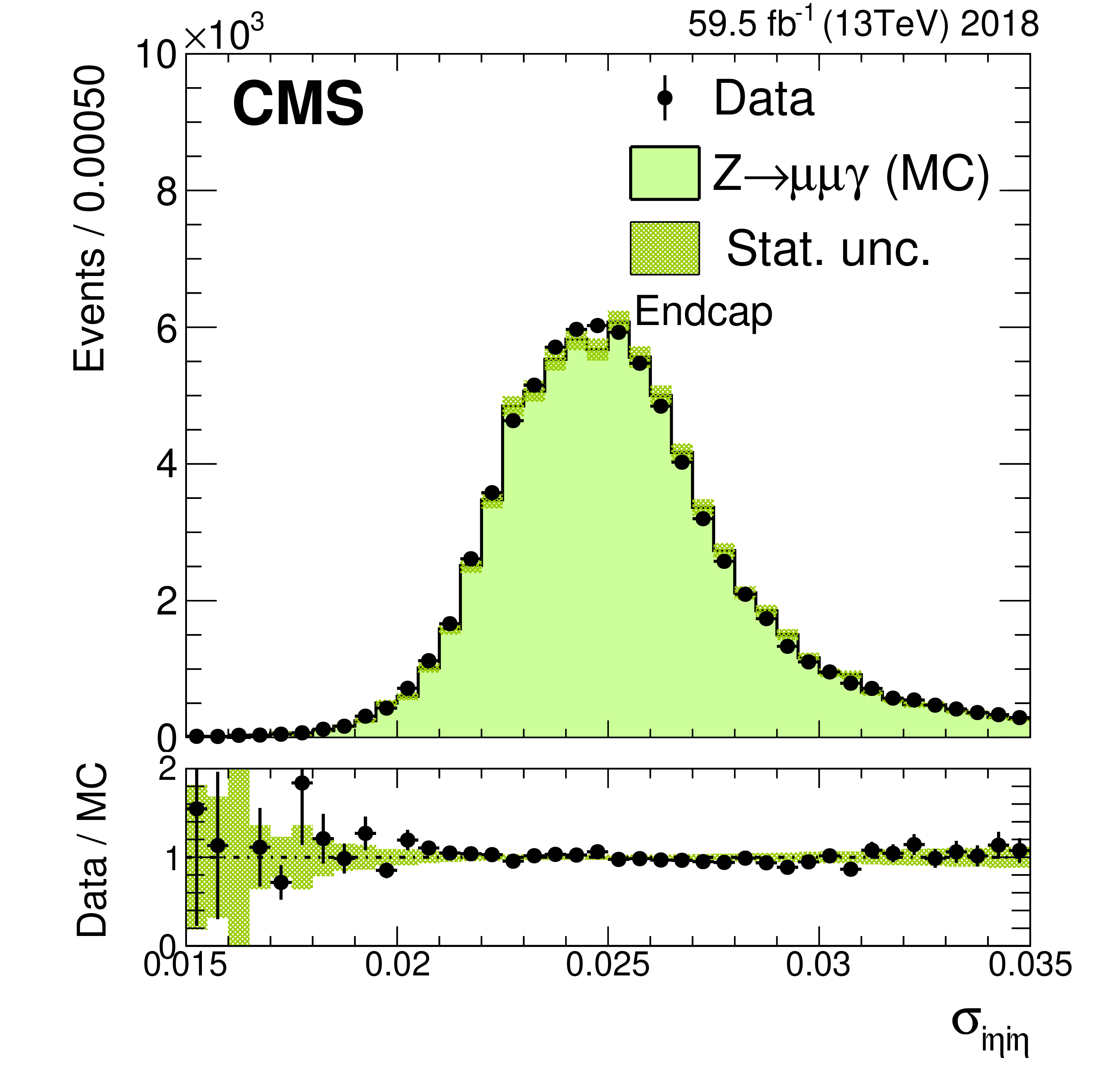
Figure 22-b:
Distribution of $\sigma _{i \eta i \eta}$ for photons from $\mathrm{Z} \to \mu \mu \gamma $ events in the endcaps. Photons are selected from 2018 data and simulation. The simulation is shown with the filled histograms and data are represented by the markers. The vertical bars on the markers represent the statistical uncertainties in data. The hatched regions show the statistical uncertainty in the simulation. The lower panel displays the ratio of the data to the simulation, with the bands representing the uncertainties in the simulation. |
png pdf |
Figure 23:
Distribution of $\Delta \phi _{\text {in}}$ for electrons in the barrel (left) and endcaps (right). For the cut-based identification, selection requirements on this variable are listed in Table 5. The simulation is shown with the filled histograms and data are represented by the markers. The vertical bars on the markers represent the statistical uncertainties in data. The hatched regions show the statistical uncertainty in the simulation. The lower panels display the ratio of the data to the simulation, with the bands representing the uncertainties in the simulation. |

png pdf |
Figure 23-a:
Distribution of $\Delta \phi _{\text {in}}$ for electrons in the barrel. For the cut-based identification, selection requirements on this variable are listed in Table 5. The simulation is shown with the filled histograms and data are represented by the markers. The vertical bars on the markers represent the statistical uncertainties in data. The hatched regions show the statistical uncertainty in the simulation. The lower panel displays the ratio of the data to the simulation, with the bands representing the uncertainties in the simulation. |
png pdf |
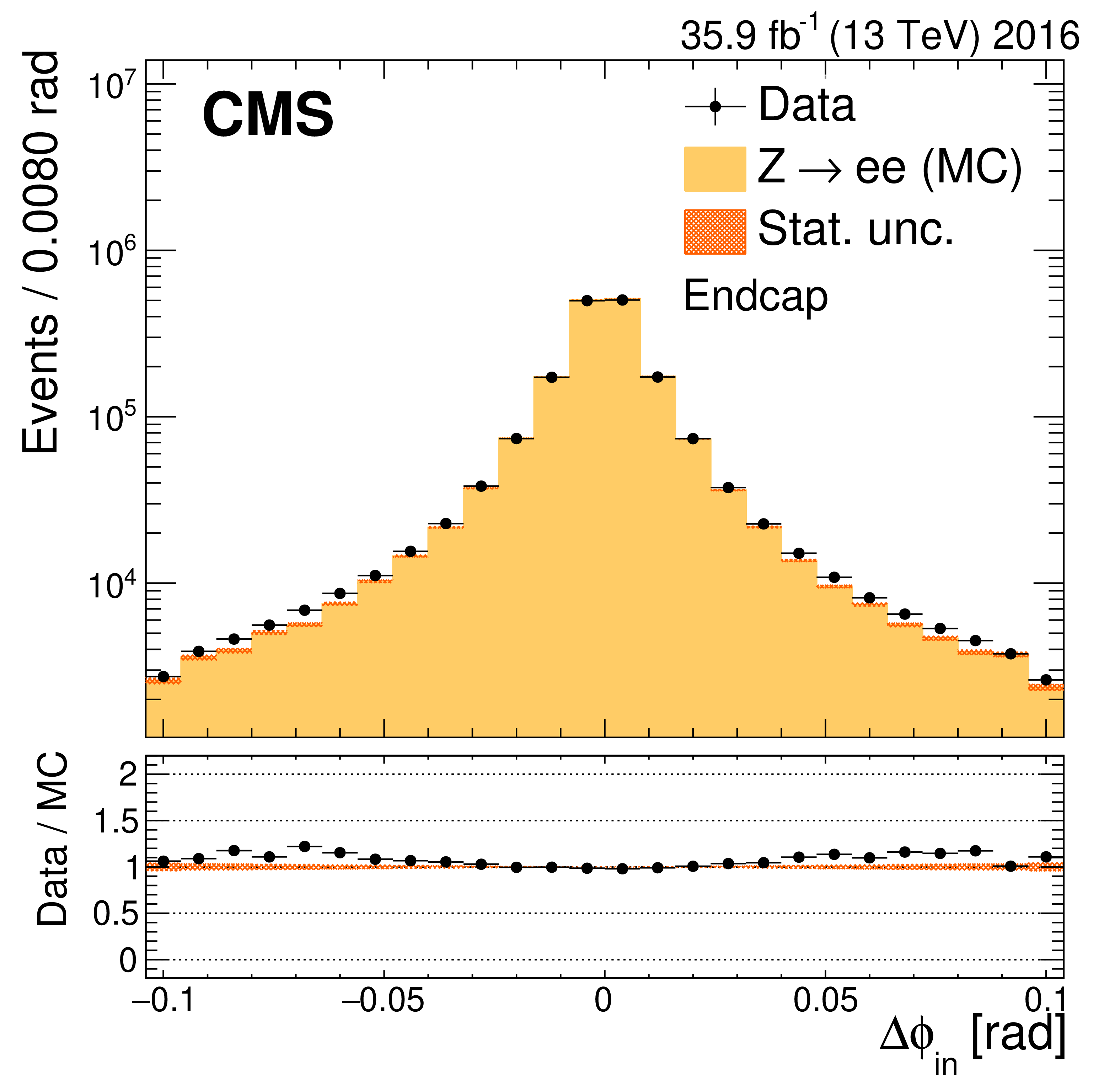
Figure 23-b:
Distribution of $\Delta \phi _{\text {in}}$ for electrons in the endcaps. For the cut-based identification, selection requirements on this variable are listed in Table 5. The simulation is shown with the filled histograms and data are represented by the markers. The vertical bars on the markers represent the statistical uncertainties in data. The hatched regions show the statistical uncertainty in the simulation. The lower panel displays the ratio of the data to the simulation, with the bands representing the uncertainties in the simulation. |

png pdf |
Figure 24:
Performance of the photon BDT and cut-based identification algorithms in 2017. Cut-based identification is shown for three different working points, loose, medium and tight. |
png pdf |
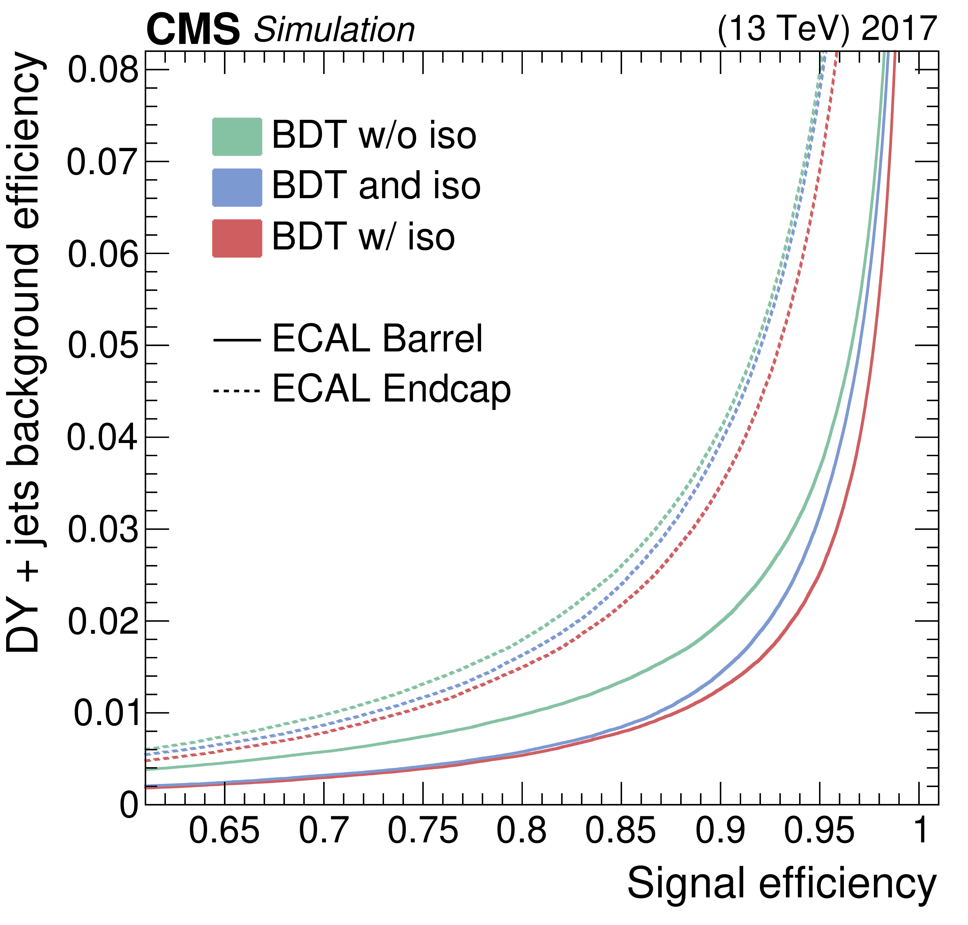
Figure 25:
Performance of the electron BDT-based identification algorithm with (red) and without (green) the isolation variables, compared to an optimized sequential selection using the BDT without the isolations followed by a selection requirement on the combined isolation (blue). Electrons are selected for the BDT training with an $ {E_{\mathrm {T}}} $ of at least 20 GeV. |
png pdf |
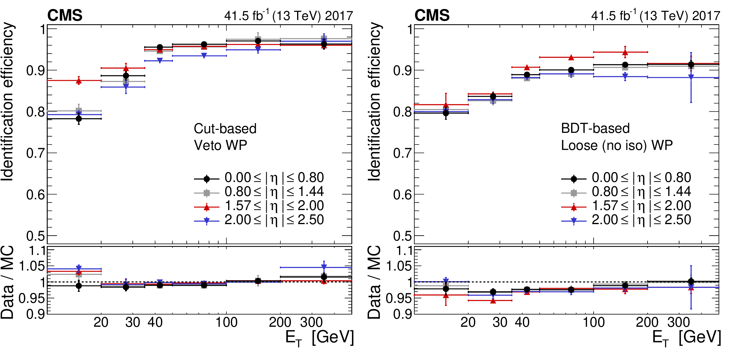
Figure 26:
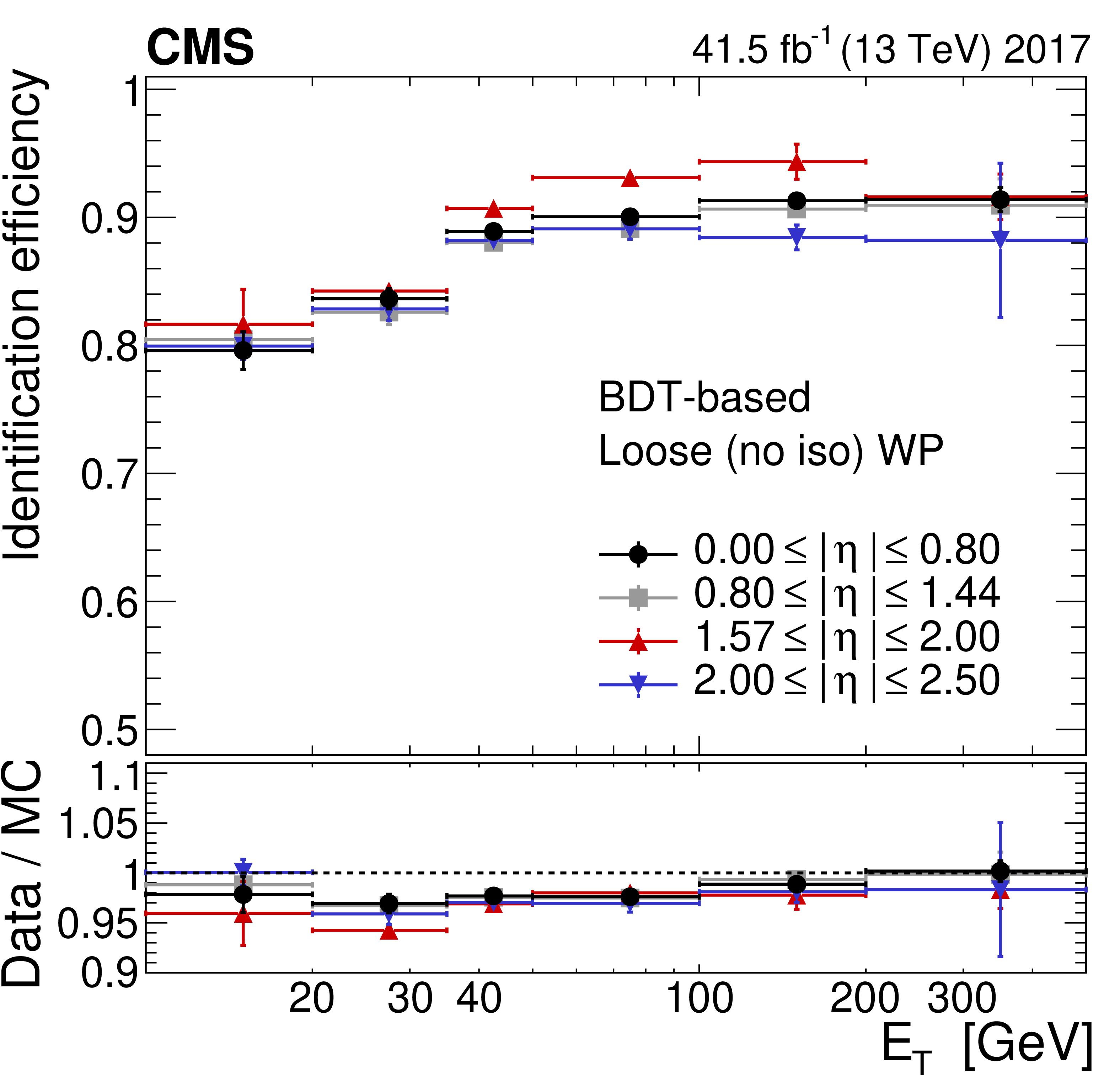
Electron identification efficiency measured in data (upper panels) and data-to-simulation efficiency ratios (lower panels), as a function of the electron $ {E_{\mathrm {T}}} $, for the cut-based identification veto working point (left) and the BDT-based (without isolation) loosest working point (right). The vertical bars on the markers represent combined statistical and systematic uncertainties. |

png pdf |
Figure 26-a:
Electron identification efficiency measured in data (upper panels) and data-to-simulation efficiency ratios (lower panels), as a function of the electron $ {E_{\mathrm {T}}} $, for the cut-based identification veto working point. The vertical bars on the markers represent combined statistical and systematic uncertainties. |
png pdf |
Figure 26-b:
Electron identification efficiency measured in data (upper panels) and data-to-simulation efficiency ratios (lower panels), as a function of the electron $ {E_{\mathrm {T}}} $, for the BDT-based (without isolation) loosest working point. The vertical bars on the markers represent combined statistical and systematic uncertainties. |
png pdf |
Figure 27:
Photon identification efficiency in data (upper panels) and data-to-simulation efficiency ratios (lower panels) for the loose cut-based (left) and loosest BDT-based (right) identification working points, as functions of the photon $ {E_{\mathrm {T}}} $. The vertical bars on the markers represent combined statistical and systematic uncertainties. |

png pdf |
Figure 27-a:
Photon identification efficiency in data and data-to-simulation efficiency ratios (lower panel) for the loose cut-based identification working point, as functions of the photon $ {E_{\mathrm {T}}} $. The vertical bars on the markers represent combined statistical and systematic uncertainties. |
png pdf |
Figure 27-b:
Photon identification efficiency in data and data-to-simulation efficiency ratios (lower panel) for the loosest BDT-based identification working point, as functions of the photon $ {E_{\mathrm {T}}} $. The vertical bars on the markers represent combined statistical and systematic uncertainties. |

png pdf |
Figure 28:
Dielectron mass resolution from $\mathrm{Z} \to \mathrm{ee} $ events as a function of the $\eta $ of the electron for the Legacy calibration (green filled markers) and the EOY calibration (pink empty markers) of the 2017 data set. The grey vertical band represents the region 1.44 $ < {| \eta |} < $ 1.57 and it is not included since it corresponds to the transition between barrel and endcap electromagnetic calorimeters. |
png pdf |
Figure 29:
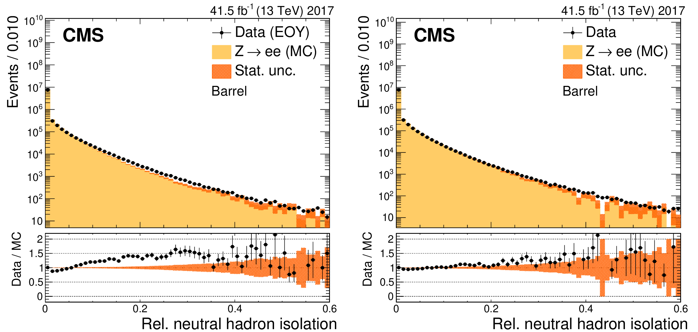
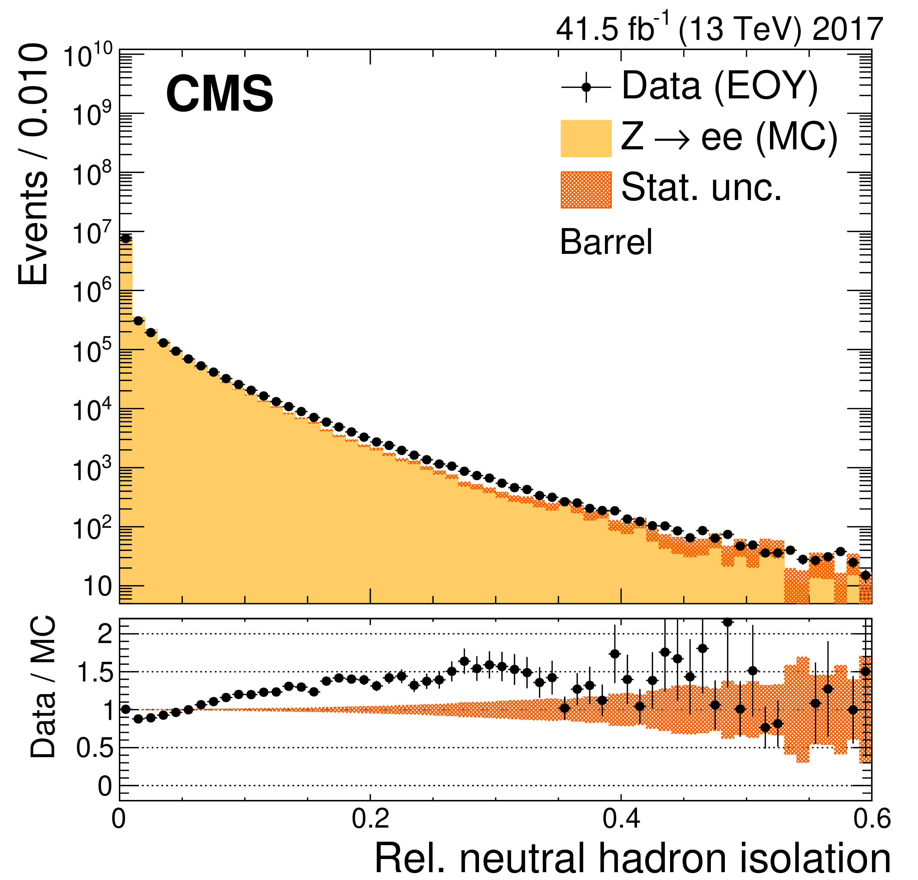
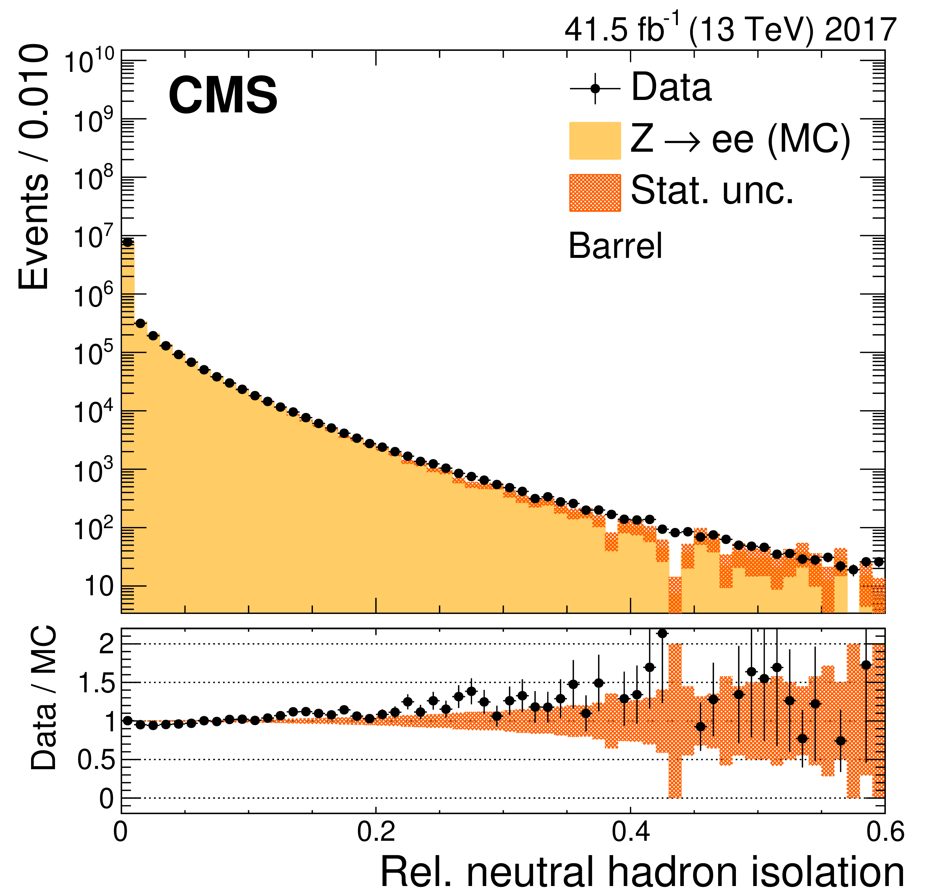
The PF-based neutral hadron isolation in the barrel. The left plot is from the EOY calibration and the right plot is from the Legacy calibration 2017 data set. The simulation is shown with the filled histograms and data are represented by the markers. The vertical bars on the markers represent combined statistical uncertainty in data. The hatched regions show the statistical uncertainty in the simulation. The lower panels display the ratio of the data to the simulation, with the bands representing the uncertainties in the simulation, and show an improvement for the Legacy calibration compared to the EOY calibration. |
png pdf |
Figure 29-a:
The PF-based neutral hadron isolation in the barrel. The plot is from the EOY calibration. The simulation is shown with the filled histograms and data are represented by the markers. The vertical bars on the markers represent combined statistical uncertainty in data. The hatched regions show the statistical uncertainty in the simulation. The lower panel displays the ratio of the data to the simulation, with the bands representing the uncertainties in the simulation. |
png pdf |
Figure 29-b:
The PF-based neutral hadron isolation in the barrel. The plot is from the Legacy calibration 2017 data set. The simulation is shown with the filled histograms and data are represented by the markers. The vertical bars on the markers represent combined statistical uncertainty in data. The hatched regions show the statistical uncertainty in the simulation. The lower panel displays the ratio of the data to the simulation, with the bands representing the uncertainties in the simulation. |
png pdf |
Figure 30:
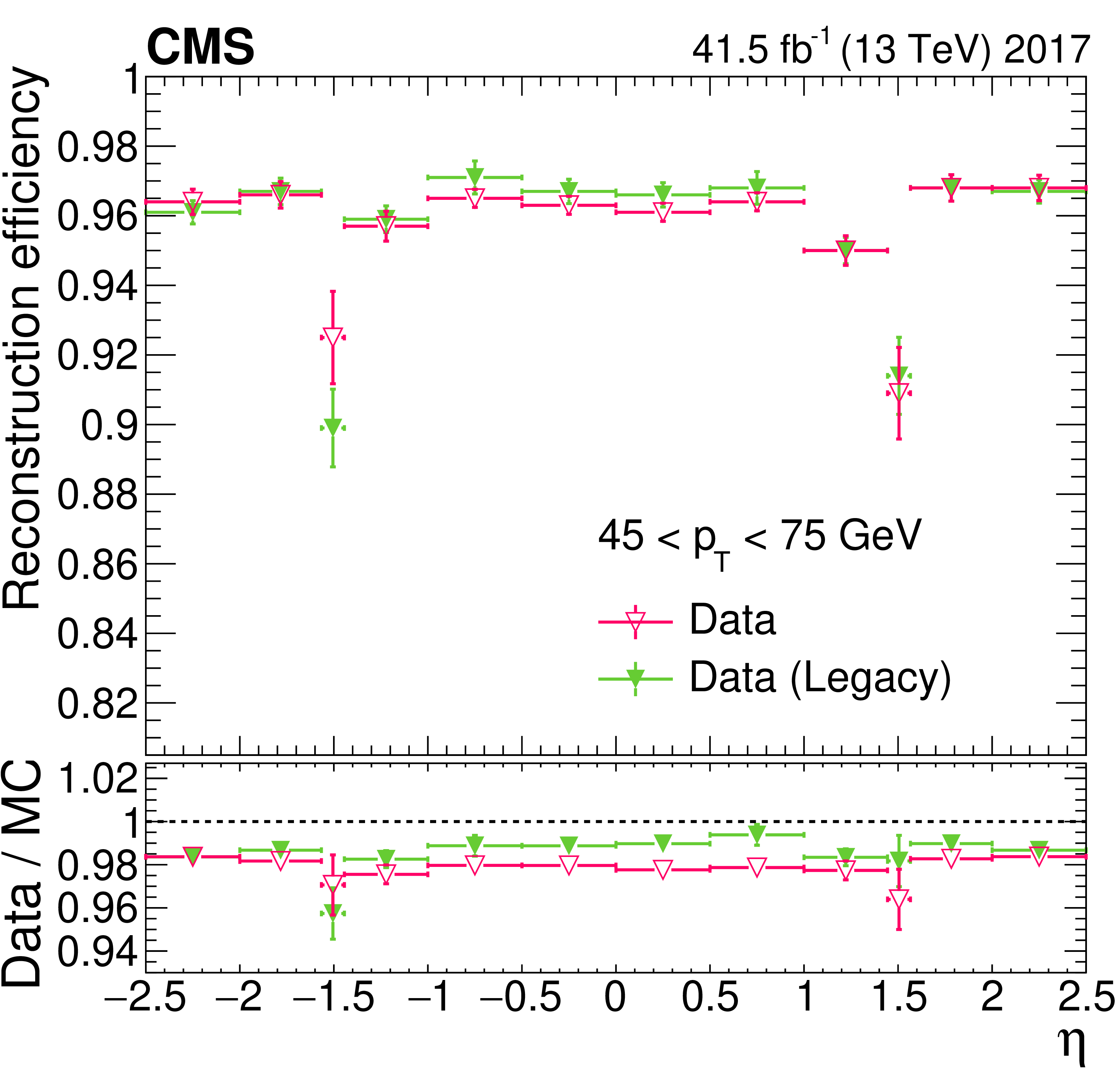
Electron reconstruction efficiency (upper panel) and data-to-simulation correction factors (lower panel) comparing the Legacy and the EOY calibrations of the 2017 data set for electrons from $\mathrm{Z} \to \mathrm{ee} $ decays with $ {E_{\mathrm {T}}} $ between 45 and 75 GeV. The vertical bars on the markers represent combined statistical and systematic uncertainties. |

png pdf |
Figure 31:
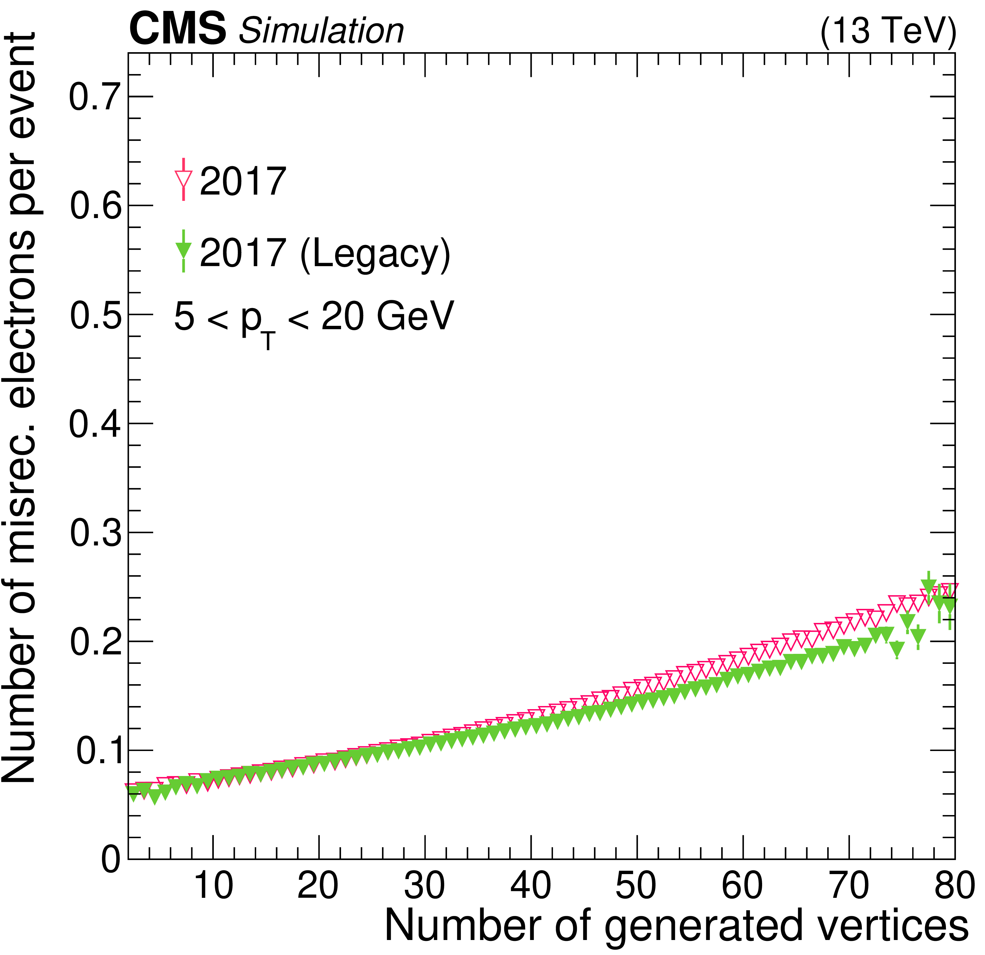
Number of misreconstructed electron candidates per event as a function of pileup in DY + jets MC events simulated with the Legacy and the EOY detector conditions of 2017. Results are shown for electrons with ${p_{\mathrm {T}}}$ within the 5-20 GeV range (left) and $ {p_{\mathrm {T}}} > $ 20 GeV (right) before any selection criteria. Electrons in the region 1.44 $ < {| \eta |} < $ 1.57 are discarded. The vertical bars on the markers represent combined statistical uncertainties of the MC sample. |
png pdf |
Figure 31-a:
Number of misreconstructed electron candidates per event as a function of pileup in DY + jets MC events simulated with the Legacy and the EOY detector conditions of 2017. Results are shown for electrons with ${p_{\mathrm {T}}}$ within the 5-20 GeV range before any selection criteria. Electrons in the region 1.44 $ < {| \eta |} < $ 1.57 are discarded. The vertical bars on the markers represent combined statistical uncertainties of the MC sample. |

png pdf |
Figure 31-b:
Number of misreconstructed electron candidates per event as a function of pileup in DY + jets MC events simulated with the Legacy and the EOY detector conditions of 2017. Results are shown for electrons with $ {p_{\mathrm {T}}} > $ 20 GeV before any selection criteria. Electrons in the region 1.44 $ < {| \eta |} < $ 1.57 are discarded. The vertical bars on the markers represent combined statistical uncertainties of the MC sample. |
png pdf |
Figure 32:
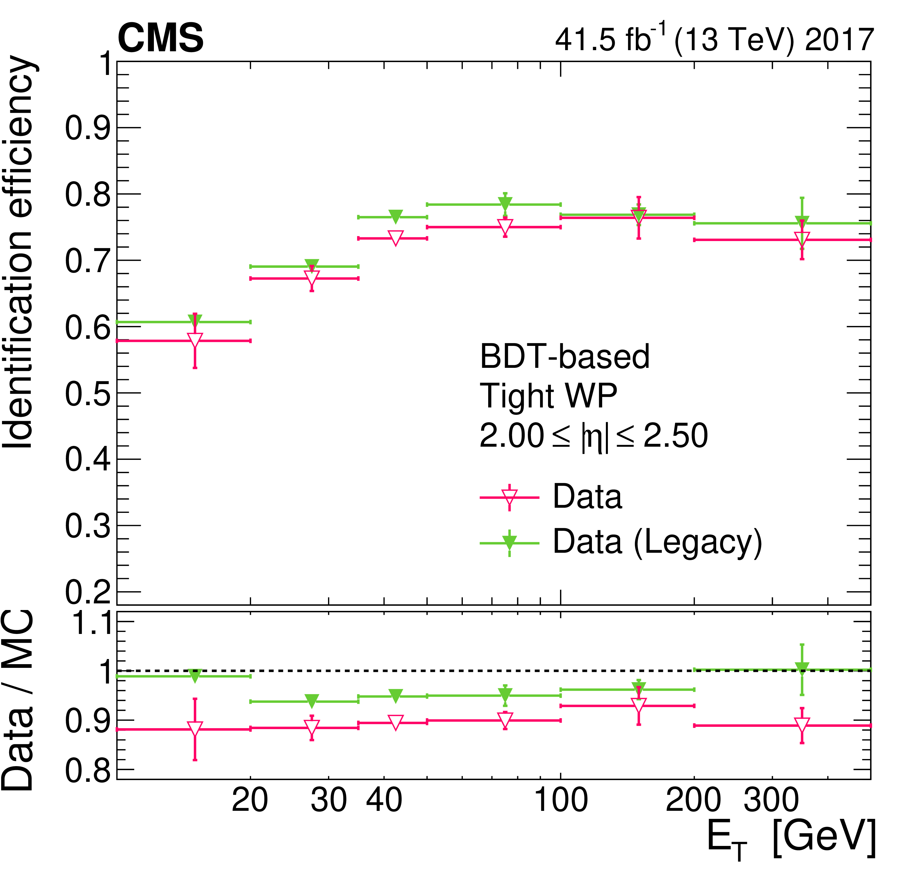
Tight BDT-based electron identification efficiency (upper panel) and data-to-simulation correction factors (lower panel) comparing the Legacy to the EOY calibration of the 2017 data set for electrons from $\mathrm{Z} \to \mathrm{ee} $ decays with $\eta $ between 2.00 and 2.50. The vertical bars on the markers represent combined statistical and systematic uncertainties. |

png pdf |
Figure 33:
The relative Z mass resolution from $\mathrm{Z} \to \mathrm{ee} $ decays in bins of $\eta $ for the barrel and endcaps. Electrons from $\mathrm{Z} \to \mathrm{ee} $ decays are used and the resolution is shown for low-bremsstrahlung electrons. The plot compares the resolution achieved for the data collected at 13 TeV during Run 2 in 2016, 2017, and 2018. The 2016 and 2018 data are reconstructed with an initial calibration whereas the 2017 data are reconstructed with refined calibrations. The resolution is estimated after all the corrections are applied, as described in Section 6.3.1, including the scale and spreading corrections of Section 6.2. The grey vertical band represents the region 1.44 $ < {| \eta |} < $ 1.57 and it is not included since it corresponds to the transition between barrel and endcap electromagnetic calorimeters. |
png pdf |
Figure 34:
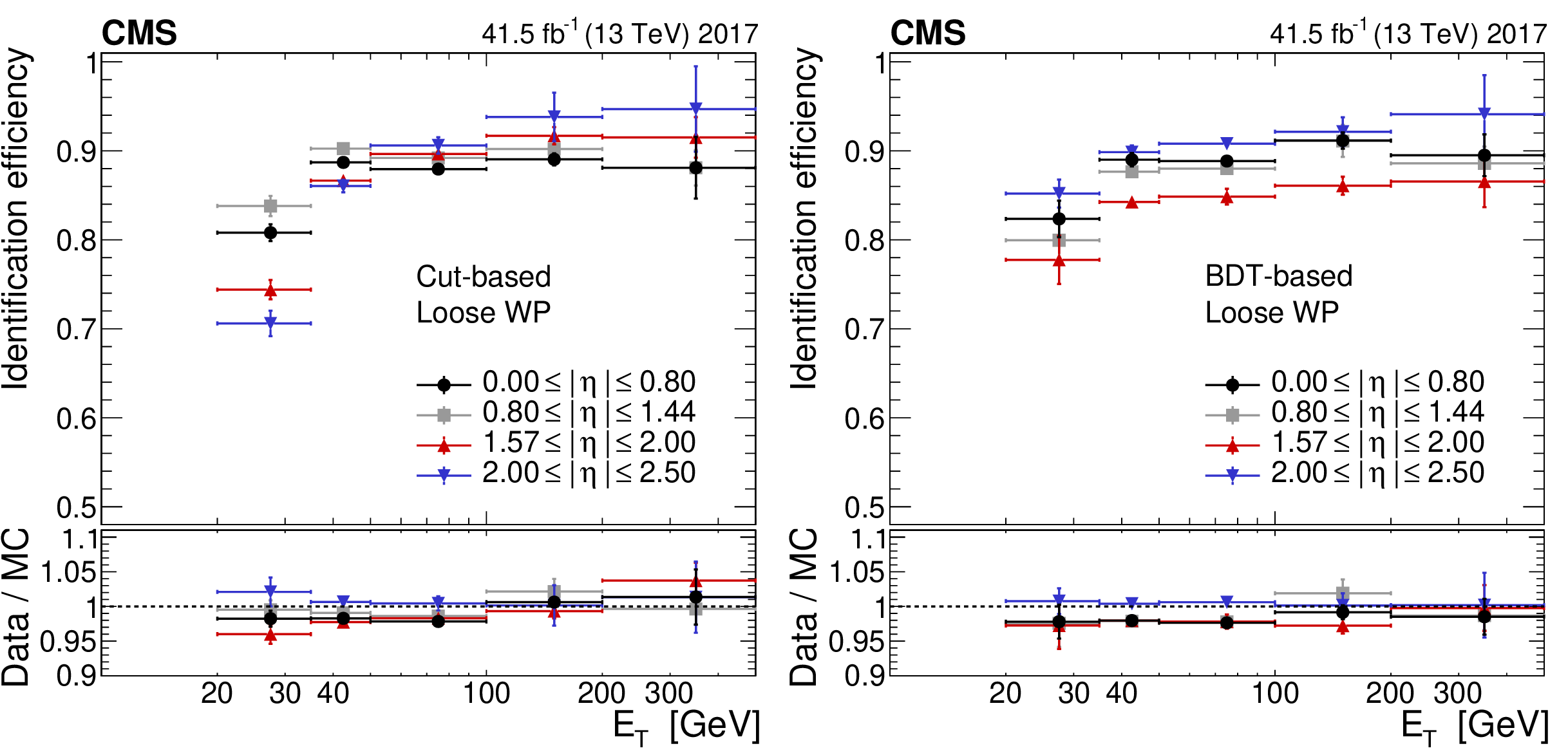
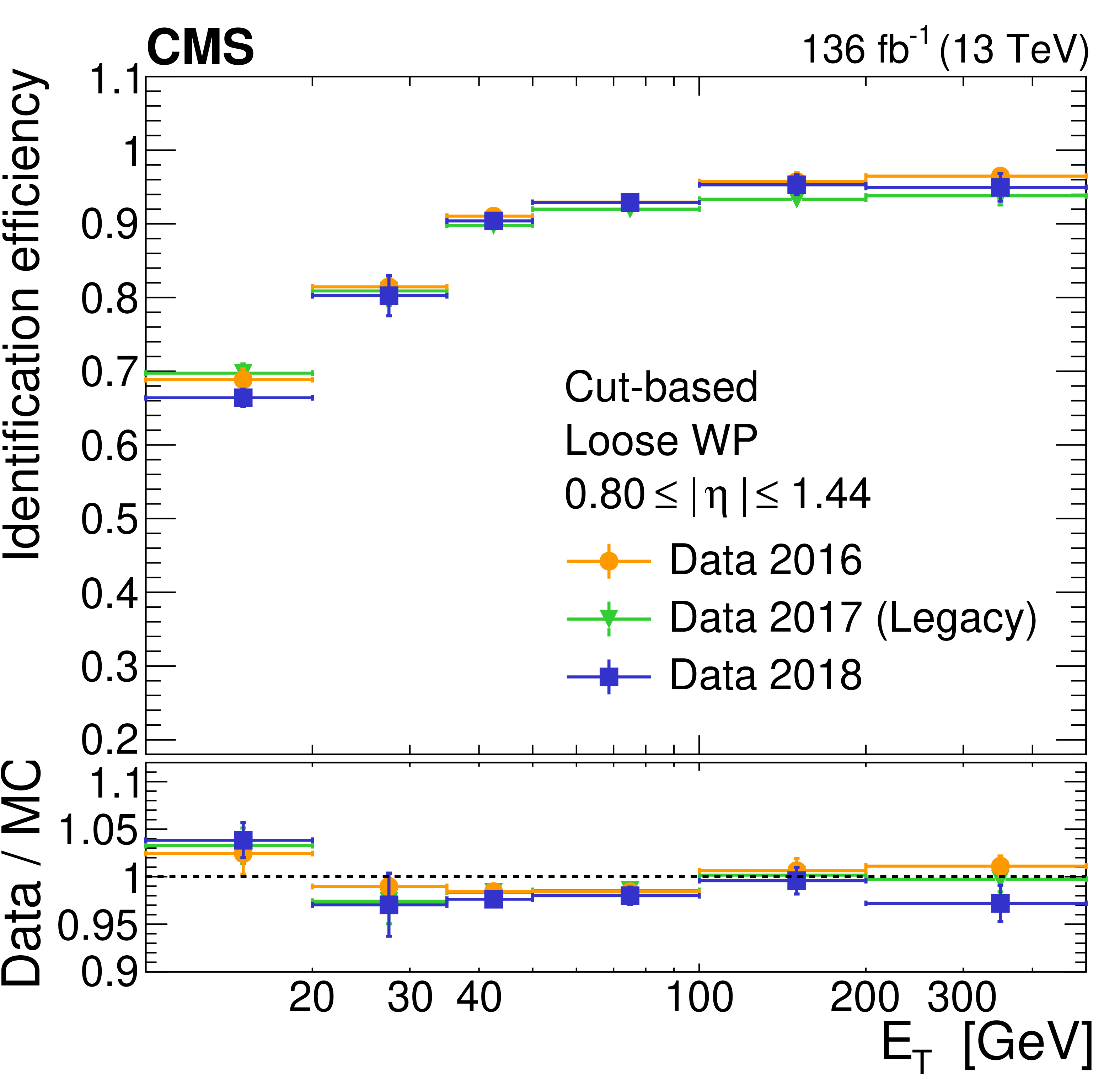
Cut-based loose electron identification efficiency in data (upper panel) and data-to-simulation efficiency ratios (lower panel) as a function of the electron ${p_{\mathrm {T}}}$ shown for 2016, 2017 "Legacy'', and 2018 data-taking periods. The vertical bars on the markers represent combined statistical and systematic uncertainties. |
png pdf |
Figure 35:
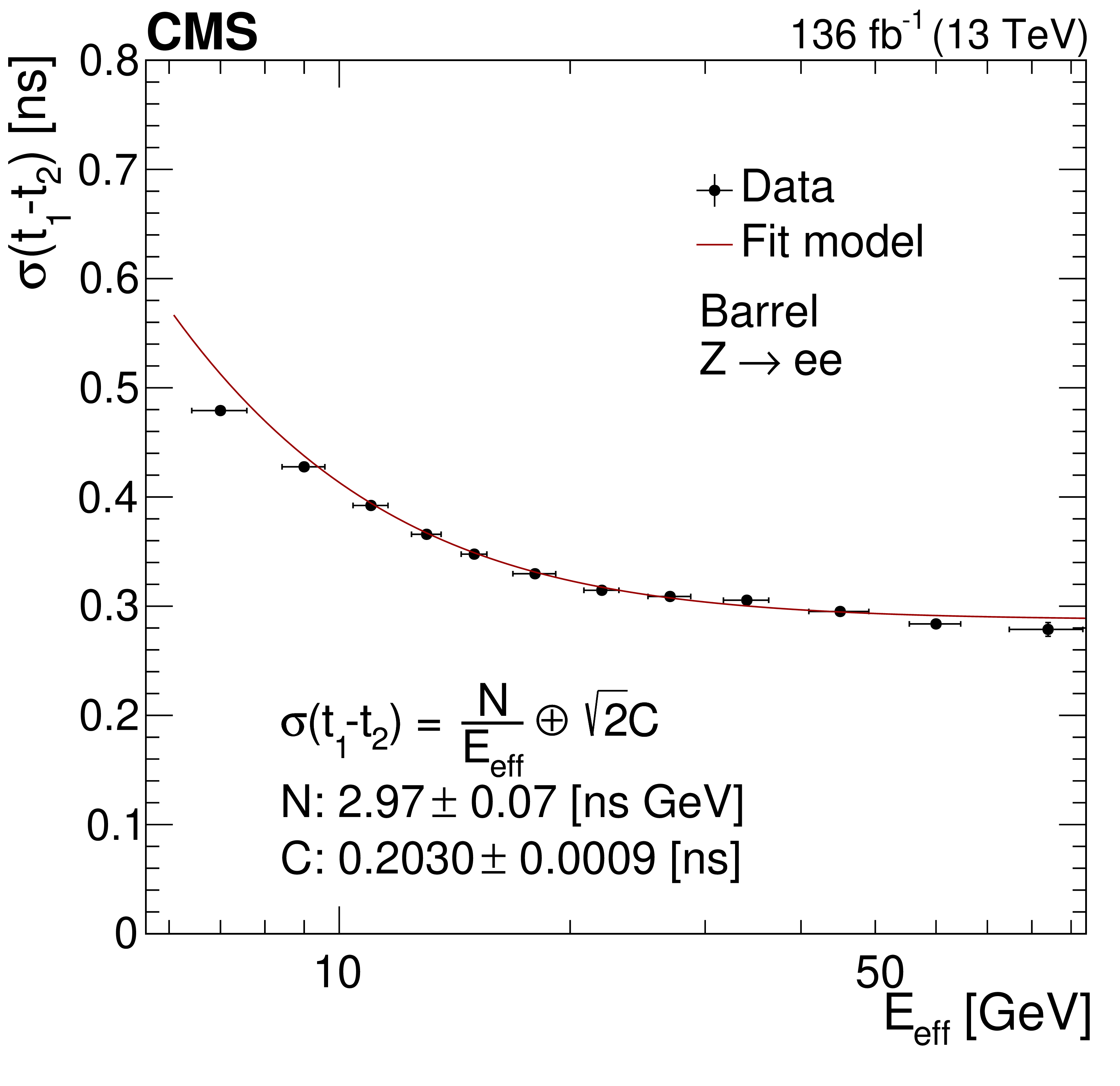
ECAL timing resolution as a function of the effective energy of the electron pairs as measured in 2016, 2017 (Legacy), and 2018 data. Vertical bars on the markers represent the uncertainties coming from the fit procedure used to determine the $\sigma (t_1-t_2)$ parameters. |
png pdf |
Figure 36:
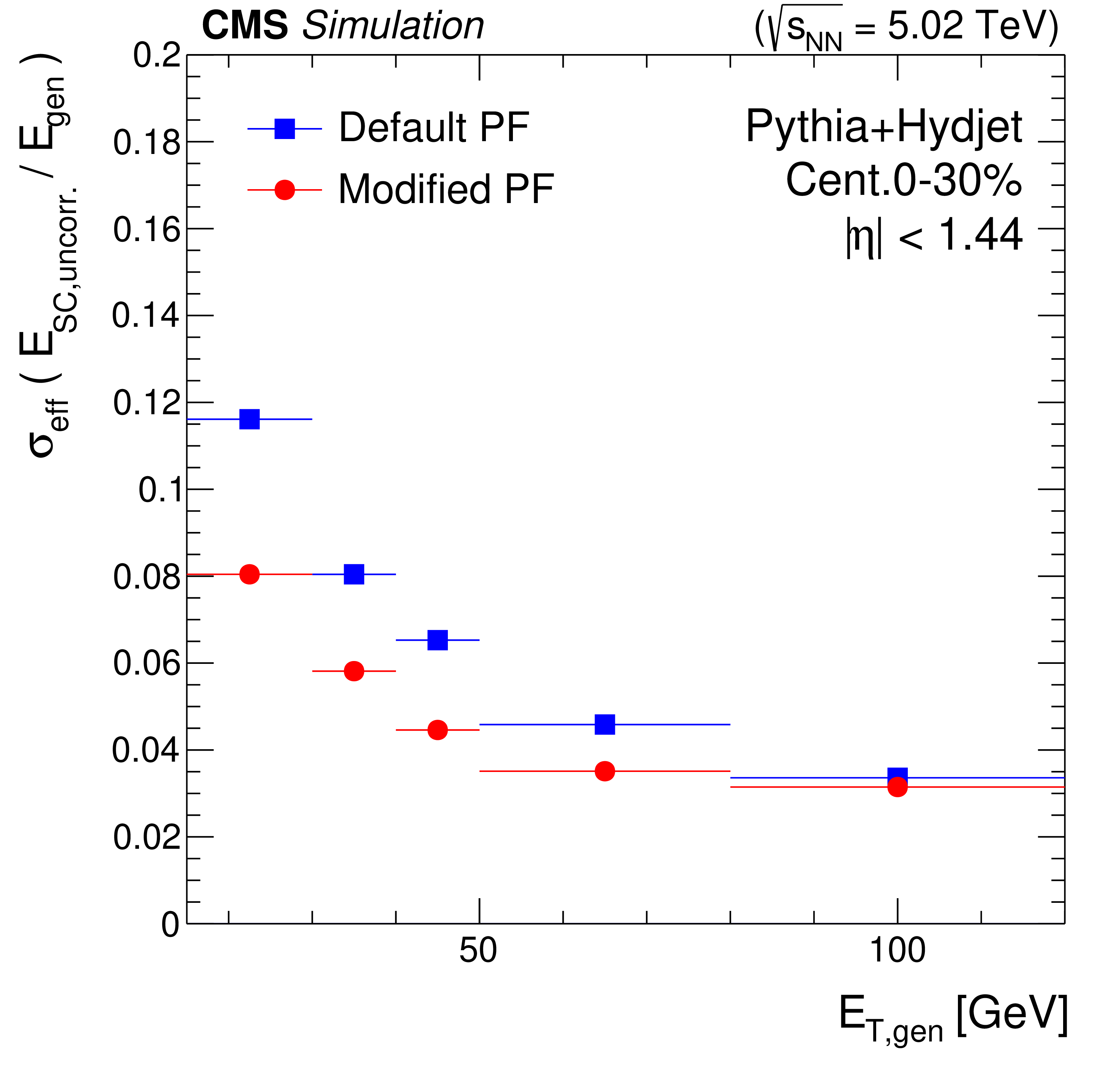
Photon energy resolution comparison in simulation for different PF clustering algorithms in PbPb collisions as a function of the generated photon $ {E_{\mathrm {T}}} $. The default algorithm (in blue) has a dynamic $\eta $-$\phi $ window, and is compared to the modified PF clustering algorithm with an upper bound on the SC extent in the $\phi $ direction (in red). Barrel photons ($ {| \eta |} < 1.44$) are used in simulated PbPb events within the 0-30% centrality range. |

png pdf |
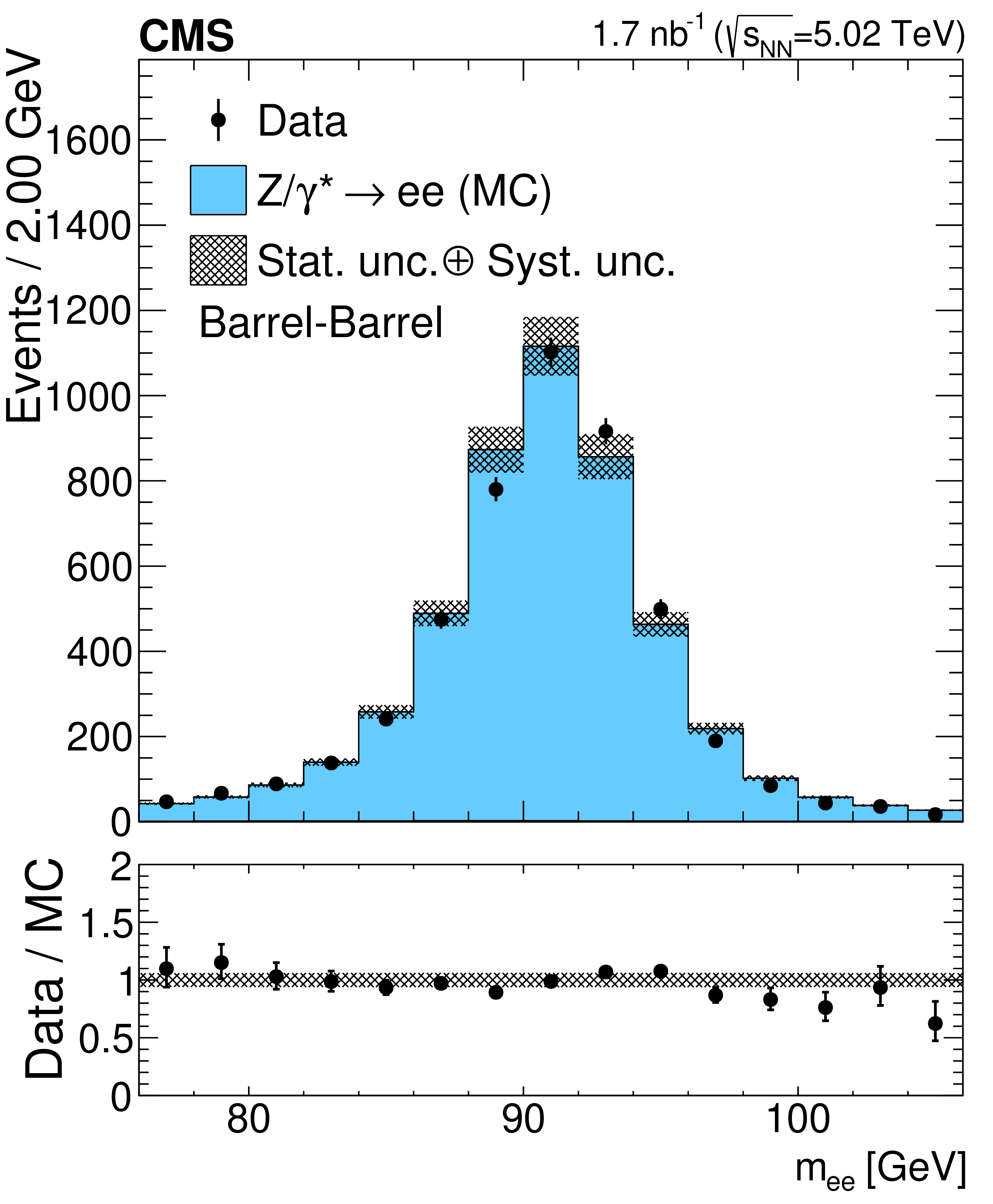
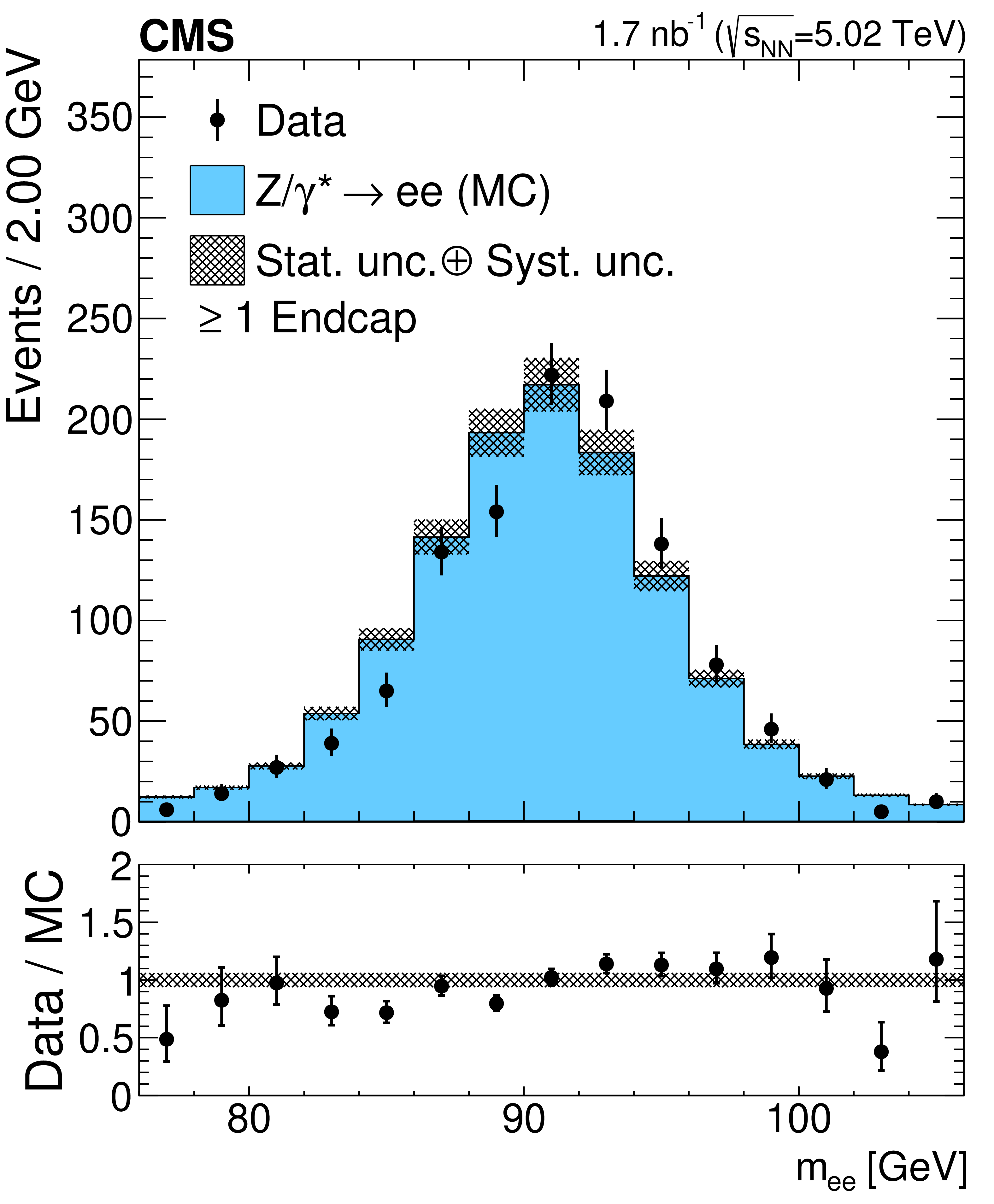
Figure 37:
Invariant mass distributions of the electron pairs from $\mathrm{Z} \to \mathrm{ee} $ decays selected in PbPb collisions, for the barrel-barrel electrons on the left, and with at least one electron in the endcaps on the right. The simulation is shown with the filled histograms and data are represented by the markers. The vertical bars on the markers represent the statistical uncertainties in data. The hatched regions show the combined statistical and systematic uncertainties in the simulation. The lower panels display the ratio of data to simulation, with bands representing the initial estimation of the uncertainties in the simulation, with the PDF uncertainty being the main contributor. |
png pdf |
Figure 37-a:
Invariant mass distributions of the electron pairs from $\mathrm{Z} \to \mathrm{ee} $ decays selected in PbPb collisions, for the barrel-barrel electrons. The simulation is shown with the filled histograms and data are represented by the markers. The vertical bars on the markers represent the statistical uncertainties in data. The hatched regions show the combined statistical and systematic uncertainties in the simulation. The lower panel displays the ratio of data to simulation, with bands representing the initial estimation of the uncertainties in the simulation, with the PDF uncertainty being the main contributor. |
png pdf |
Figure 37-b:
Invariant mass distributions of the electron pairs from $\mathrm{Z} \to \mathrm{ee} $ decays selected in PbPb collisions, with at least one electron in the endcaps. The simulation is shown with the filled histograms and data are represented by the markers. The vertical bars on the markers represent the statistical uncertainties in data. The hatched regions show the combined statistical and systematic uncertainties in the simulation. The lower panel displays the ratio of data to simulation, with bands representing the initial estimation of the uncertainties in the simulation, with the PDF uncertainty being the main contributor. |
| Tables | |
png pdf |
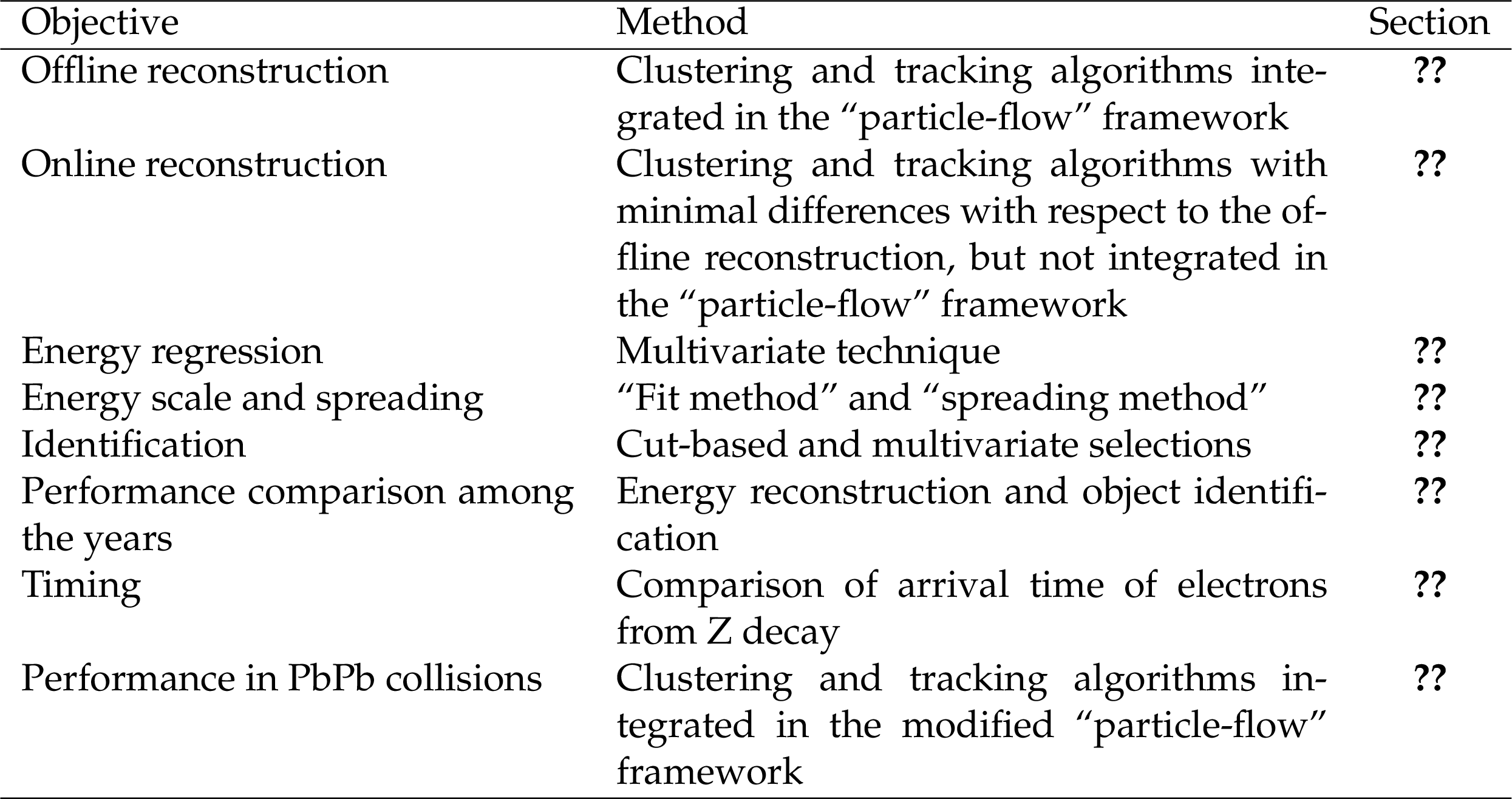
Table 1:
List of the main objectives described in the paper concerning electrons and photons, a summary of the methods used to achieve them, and a reference to the section where they are detailed. |
png pdf |
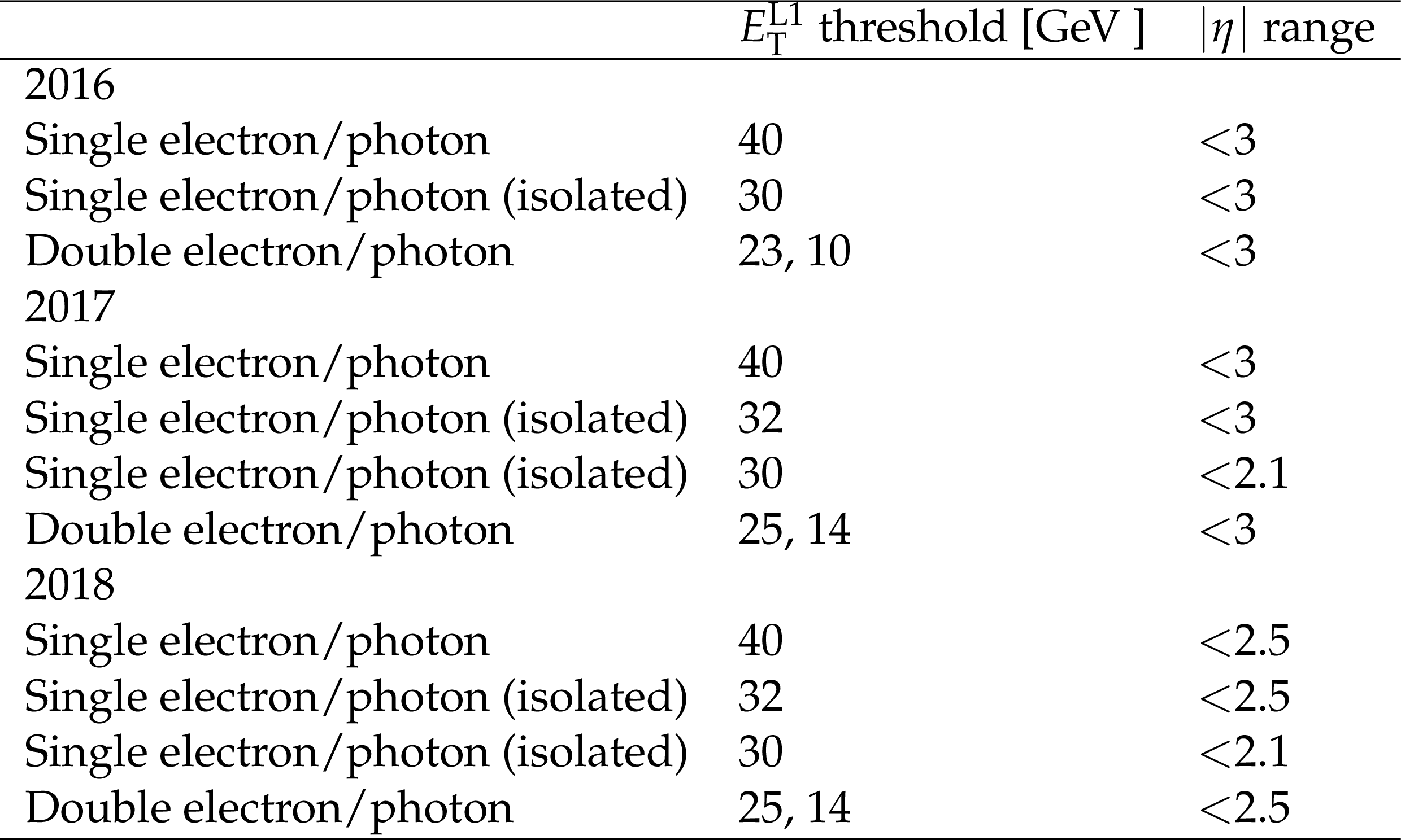
Table 2:
Lowest unprescaled $ {E_{\mathrm {T}}} ^\text {L1}$ thresholds and the corresponding seed names, for the three years of Run 2. |

png pdf |
Table 3:
Lowest unprescaled $ {E_{\mathrm {T}}} ^\text {HLT}$ thresholds and the corresponding path names, for the three years of Run 2 data-taking. The electrons are always required to be within the L1 $ {| \eta |}$ requirement and always within $ {| \eta |} < $ 2.65. |
png pdf |
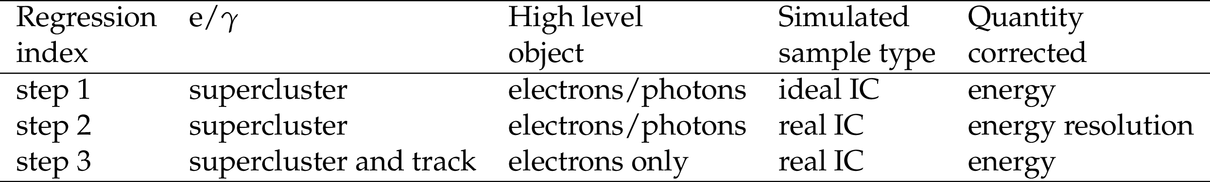
Table 4:
Details of the three energy regression steps used in electron and photon energy reconstruction. |
png pdf |
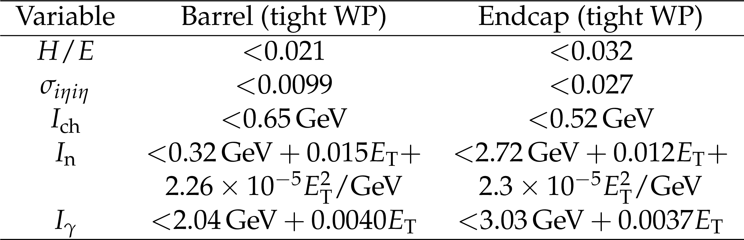
Table 5:
Cut-based photon identification requirements for the tight working point in the EB and EE. |
png pdf |
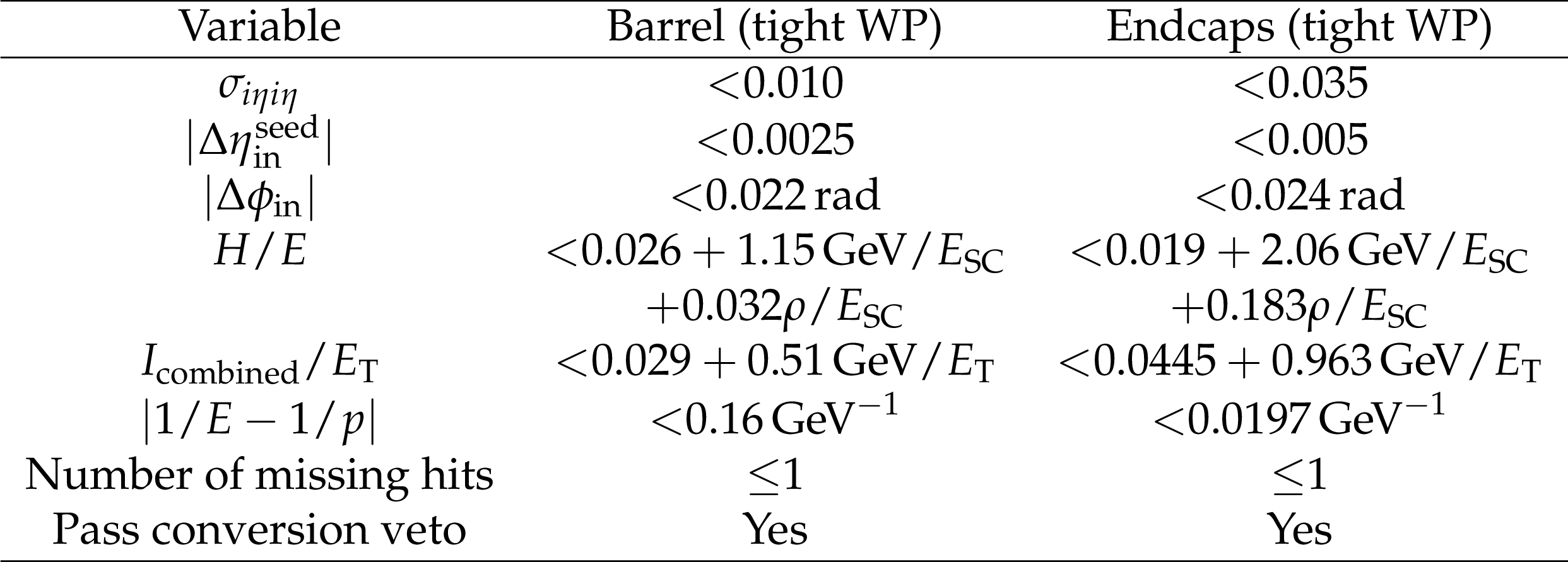
Table 6:
Cut-based electron identification requirements for the tight working point in the barrel and in the endcaps. |

png pdf |
Table 7:
Identification requirements for high-$ {E_{\mathrm {T}}} $ electrons in the barrel and in the endcaps. |
| Summary |
|
The performance of electron and photon reconstruction and identification in CMS during LHC Run 2 was measured using data collected in proton-proton collisions at $\sqrt{s}=$ 13 TeV in 2016-2018 corresponding to a total integrated luminosity of 136 fb$^{-1}$. A clustering algorithm developed to cope with the increasing pileup conditions is described, together with the use of the new pixel detector with one more layer and a reduced material budget. These are major changes in electron and photon performance with respect to Run 1. Multivariate algorithms are used to correct the electron and photon energy measured in the electromagnetic calorimeter (ECAL), as well as to estimate the electron momentum by combining independent measurements in the ECAL and in the tracker. The overall energy scale and resolution are both calibrated using electrons from $\mathrm{Z} \to \mathrm{ee}$ decays. The uncertainty in the electron and photon energy scale is within 0.1% in the barrel, and 0.3% in the endcaps in the transverse energy (${E_{\mathrm{T}}}$) range from 10 to 50 GeV. The stability of this correction is estimated to be within 2-3% for higher energies. The measured energy resolution for electrons produced in Z boson decays ranges from 2 to 5%, depending on electron pseudorapidity and energy loss through bremsstrahlung in the detector material. Energy scale and resolution corrections have been checked also for photons using $\mathrm{Z}\to \mu\mu\gamma$ events and found stable within the assigned systematic uncertainties. The performance of electron and photon reconstruction and identification algorithms in data is studied with a tag-and-probe method using $\mathrm{Z}\to \mathrm{ee}$ events. Good agreement is observed between data and simulation for most of the variables relevant to both reconstruction and identification. The reconstruction efficiency in data is better than 95% in the ${E_{\mathrm{T}}}$ range from 10 to 500 GeV. The data-to-simulation efficiency ratios, both for electron reconstruction and for the various electron and photon selections, are compatible with unity within 2% over the full ${E_{\mathrm{T}}}$ range, down to an ${E_{\mathrm{T}}}$ as low as 10 (20) GeV for electrons (photons). Identification efficiencies target three working points with selection efficiencies of 70, 80, and 90%, respectively. The energy resolution and energy scale measurements, together with the relevant identification efficiencies, remain stable throughout the full Run 2 data-taking period (2016-2018). For the 2017 data-taking period, the dedicated Legacy calibration brings an improvement of up to 50% in terms of relative energy resolution in the ECAL, as well as an improved agreement between data and simulation, leading to smaller reconstruction and identification efficiency correction over the entire ${E_{\mathrm{T}}}$ and $\eta$ ranges. As a result of these calibrations the electron and photon reconstruction and identification performance at Run 2 are similar to that of Run 1, despite the increased pileup and radiation damage. The evident success of the dedicated Legacy calibration of 2017 data motivates a plan to pursue the same techniques for the 2016 and 2018 data. The ECAL timing resolution is crucial at CMS to suppress noncollision backgrounds, as well as to perform dedicated searches for delayed photons or jets predicted in several models of physics beyond the standard model. A global timing resolution of 200 ps is measured for electrons from Z decays with the full Run 2 collision data. Excellent performance in electron and photon reconstruction and identification has also been achieved in the case of lead-lead collisions at ${\sqrt {\smash [b]{s_{_{\mathrm {NN}}}}}} = $ 5.02 TeV in 2018 corresponding to a total integrated luminosity of 1.7 nb$^{-1}$. Reconstruction, identification, and energy correction algorithms have been revised and optimized to perform in the extreme conditions of high underlying event activity in central lead-lead collisions. For electrons and photons reconstructed in lead-lead collisions, the uncertainty on the energy scale is estimated to be better than 1 (3)% in the barrel (endcap) region. |
| References | ||||
| 1 | CMS Collaboration | Observation of a new boson with mass near 125 GeV in pp collisions at $ \sqrt{s} = $ 7 and 8 TeV | JHEP 06 (2013) 081 | CMS-HIG-12-036 1303.4571 |
| 2 | ATLAS Collaboration | Observation of a new particle in the search for the standard model Higgs boson with the ATLAS detector at the LHC | PLB 716 (2012) 1 | 1207.7214 |
| 3 | CMS Collaboration | Performance of electron reconstruction and selection with the CMS detector in proton-proton collisions at $ \sqrt{s} = $ 8 TeV | JINST 10 (2015) P06005 | CMS-EGM-13-001 1502.02701 |
| 4 | CMS Collaboration | Performance of photon reconstruction and identification with the CMS detector in proton-proton collisions at $ \sqrt{s} = $ 8 TeV | JINST 10 (2015) P08010 | CMS-EGM-14-001 1502.02702 |
| 5 | CMS Collaboration | CMS luminosity measurements for the 2016 data-taking period | CMS-PAS-LUM-17-001 | CMS-PAS-LUM-17-001 |
| 6 | CMS Collaboration | CMS luminosity measurement for the 2017 data-taking period at $ \sqrt{s} = $ 13 TeV | CMS-PAS-LUM-17-004 | CMS-PAS-LUM-17-004 |
| 7 | CMS Collaboration | CMS luminosity measurement for the 2018 data-taking period at $ \sqrt{s} = $ 13 TeV | CMS-PAS-LUM-18-002 | CMS-PAS-LUM-18-002 |
| 8 | CMS Collaboration | The CMS experiment at the CERN LHC | JINST 3 (2008) S08004 | CMS-00-001 |
| 9 | CMS Collaboration | CMS technical design report for the pixel detector upgrade | CDS | |
| 10 | CMS Collaboration | Description and performance of track and primary-vertex reconstruction with the CMS tracker | JINST 9 (2014) P10009 | CMS-TRK-11-001 1405.6569 |
| 11 | CMS Collaboration | The CMS electromagnetic calorimeter project: technical design report | CDS | |
| 12 | CMS Collaboration | Particle-flow reconstruction and global event description with the CMS detector | JINST 12 (2017) P10003 | CMS-PRF-14-001 1706.04965 |
| 13 | M. Cacciari, G. P. Salam, and G. Soyez | The anti-$ {k_{\mathrm{T}}} $ jet clustering algorithm | JHEP 04 (2008) 063 | 0802.1189 |
| 14 | M. Cacciari, G. P. Salam, and G. Soyez | FastJet user manual | EPJC 72 (2012) 1896 | 1111.6097 |
| 15 | CMS Collaboration | The CMS trigger system | JINST 12 (2017) P01020 | CMS-TRG-12-001 1609.02366 |
| 16 | A. Perrotta | Performance of the CMS high level trigger | J. Phys. Conf. Ser. 664 (2015) 082044 | |
| 17 | CMS Collaboration | Pileup mitigation at CMS in 13 TeV data | JINST 15 (2020) P09018 | CMS-JME-18-001 2003.00503 |
| 18 | CMS Collaboration | Energy calibration and resolution of the CMS electromagnetic calorimeter in pp collisions at $ \sqrt{s} = $ 7 TeV | JINST 8 (2013) P09009 | CMS-EGM-11-001 1306.2016 |
| 19 | CMS Collaboration | Alignment of the CMS tracker with LHC and cosmic ray data | JINST 9 (2014) P06009 | CMS-TRK-11-002 1403.2286 |
| 20 | J. Alwall et al. | The automated computation of tree-level and next-to-leading order differential cross sections, and their matching to parton shower simulations | JHEP 07 (2014) 079 | 1405.0301 |
| 21 | T. Sjostrand et al. | An introduction to PYTHIA 8.2 | CPC 191 (2015) 159 | 1410.3012 |
| 22 | CMS Collaboration | Event generator tunes obtained from underlying event and multiparton scattering measurements | EPJC 76 (2016) 155 | CMS-GEN-14-001 1512.00815 |
| 23 | CMS Collaboration | Extraction and validation of a new set of CMS PYTHIA8 tunes from underlying-event measurements | EPJC 80 (2020), no. 1, 4 | CMS-GEN-17-001 1903.12179 |
| 24 | R. Frederix and S. Frixione | Merging meets matching in MC@NLO | JHEP 12 (2012) 061 | 1209.6215 |
| 25 | NNPDF Collaboration | Parton distributions for the LHC Run II | JHEP 04 (2015) 040 | 1410.8849 |
| 26 | NNPDF Collaboration | Parton distributions with LHC data | NPB 867 (2013) 244 | 1207.1303 |
| 27 | GEANT4 Collaboration | GEANT4 --- a simulation toolkit | NIMA 506 (2003) 250 | |
| 28 | CMS Collaboration | Reconstruction of signal amplitudes in the CMS electromagnetic calorimeter in the presence of overlapping proton-proton interactions | JINST 15 (2020) P10002 | CMS-EGM-18-001 2006.14359 |
| 29 | W. Adam, R. Fruhwirth, A. Strandlie, and T. Todorov | Reconstruction of electrons with the Gaussian-sum filter in the CMS tracker at the LHC | JPG 31 (2005) 9 | physics/0306087 |
| 30 | H. Voss, A. Hocker, J. Stelzer, and F. Tegenfeldt | TMVA, the toolkit for multivariate data analysis with ROOT | in XIth International Workshop on Advanced Computing and Analysis Techniques in Physics Research, 2007 | physics/0703039 |
| 31 | J. R. Quinlan | Simplifying decision trees | Int. J. Man-Mach. Stud. 27 (1987) 221 | |
| 32 | H. A. Bethe and L. C. Maximon | Theory of bremsstrahlung and pair production. I. differential cross section | PR93 (1954) 768 | |
| 33 | CMS Collaboration | Measurements of inclusive $ W $ and $ Z $ cross sections in pp collisions at $ \sqrt{s}= $ 7 TeV | JHEP 01 (2011) 080 | CMS-EWK-10-002 1012.2466 |
| 34 | A. R. Bohm and Y. Sato | Relativistic resonances: their masses, widths, lifetimes, superposition, and causal evolution | PRD 71 (2005) 085018 | hep-ph/0412106 |
| 35 | Particle Data Group, P. A. Zyla et al. | Review of particle physics | Prog. Theor. Exp. Phys. 2020 (2020) 083C01 | |
| 36 | M. J. Oreglia | A study of the reactions $\psi' \to \gamma\gamma \psi$ | PhD thesis, Stanford University, 1980 SLAC Report SLAC-R-236, see Appendix D | |
| 37 | CMS Collaboration | Performance of the CMS Level-1 trigger in proton-proton collisions at $ \sqrt{s} = $ 13 TeV | JINST 15 (2020) P10017 | CMS-TRG-17-001 2006.10165 |
| 38 | CMS Collaboration | Observation of the diphoton decay of the Higgs boson and measurement of its properties | EPJC 74 (2014) 3076 | CMS-HIG-13-001 1407.0558 |
| 39 | CMS Collaboration | Performance of the CMS muon detector and muon reconstruction with proton-proton collisions at $ \sqrt{s}= $ 13 TeV | JINST 13 (2018) P06015 | CMS-MUO-16-001 1804.04528 |
| 40 | CMS Collaboration | A measurement of the Higgs boson mass in the diphoton decay channel | PLB 805 (2020) 135423 | |
| 41 | T. Chen and C. Guestrin | XGBoost: a scalable tree boosting system | 1603.02754 | |
| 42 | CMS Collaboration | Search for contact interactions and large extra dimensions in the dilepton mass spectra from proton-proton collisions at $ \sqrt{s} = $ 13 TeV | JHEP 04 (2019) 114 | CMS-EXO-17-025 1812.10443 |
| 43 | CMS Collaboration | Time reconstruction and performance of the CMS electromagnetic calorimeter | JINST 5 (2010) T03011 | CMS-CFT-09-006 0911.4044 |
| 44 | CMS Collaboration | Search for long-lived charged particles in proton-proton collisions at $ \sqrt{s}= $ 13 TeV | PRD 94 (2016) 112004 | CMS-EXO-15-010 1609.08382 |
| 45 | CMS Collaboration | Search for long-lived particles decaying to photons and missing energy in proton-proton collisions at $ \sqrt{s}= $ 7 TeV | PLB 722 (2013) 273 | CMS-EXO-11-035 1212.1838 |
| 46 | CMS Collaboration | Search for long-lived particles using delayed photons in proton-proton collisions at $ \sqrt{s}= $ 13 TeV | PRD 100 (2019) 112003 | CMS-EXO-19-005 1909.06166 |
| 47 | J. D. Bjorken | Energy loss of energetic partons in quark-gluon plasma: possible extinction of high p$ _{T} $ jets in hadron-hadron collisions | FERMILAB-PUB-82-59-THY | |
| 48 | D. d'Enterria | Jet quenching | in Relativistic Heavy Ion Physics, Springer Berlin Heidelberg | |
| 49 | PHENIX Collaboration | Formation of dense partonic matter in relativistic nucleus-nucleus collisions at RHIC: Experimental evaluation by the PHENIX collaboration | NP A 757 (2005) 184 | nucl-ex/0410003 |
| 50 | STAR Collaboration | Experimental and theoretical challenges in the search for the quark gluon plasma: The STAR collaboration critical assessment of the evidence from RHIC collisions | NP A 757 (2005) 102 | nucl-ex/0501009 |
| 51 | PHOBOS Collaboration | The PHOBOS perspective on discoveries at RHIC | NP A 757 (2005) 28 | nucl-ex/0410022 |
| 52 | BRAHMS Collaboration | Quark gluon plasma and color glass condensate at RHIC? The perspective from the BRAHMS experiment | NP A 757 (2005) 1 | nucl-ex/0410020 |
| 53 | CMS Collaboration | Study of high-$ {p_{\mathrm{T}}} $ charged particle suppression in PbPb compared to pp collisions at $ {\sqrt {\smash [b]{s_{_{\mathrm {NN}}}}}} = $ 5.02 TeV | Euro. Phys. J. C 72 (2012) 1945 | CMS-HIN-10-005 1202.2554 |
| 54 | ATLAS Collaboration | Measurement of charged particle spectra in PbPb collisions at $ {\sqrt {\smash [b]{s_{_{\mathrm {NN}}}}}} = $ 5.02 TeV with the ATLAS detector at the LHC | JHEP 09 (2015) 050 | 1504.04337 |
| 55 | ALICE Collaboration | Suppression of charged particle production at large transverse momentum in central PbPb collisions at $ {\sqrt {\smash [b]{s_{_{\mathrm {NN}}}}}} = $ 5.02 TeV | PLB 696 (2011) 30 | 1012.1004 |
| 56 | ATLAS Collaboration | Observation of a centrality-dependent dijet asymmetry in lead-lead collisions $ {\sqrt {\smash [b]{s_{_{\mathrm {NN}}}}}} = $ 5.02 TeV with the ATLAS detector at the LHC | PRL 105 (2010) 252303 | 1011.6182 |
| 57 | CMS Collaboration | Observation and studies of jet quenching in PbPb collisions at $ {\sqrt {\smash [b]{s_{_{\mathrm {NN}}}}}} = $ 5.02 TeV | PRC 84 (2011) 024906 | CMS-HIN-10-004 1102.1957 |
| 58 | I. P. Lokhtin and A. M. Snigirev | A model of jet quenching in ultrarelativistic heavy ion collisions and high-$ {p_{\mathrm{T}}} $ hadron spectra at RHIC | EPJC 45 (2006) 211 | hep-ph/0506189 |
| 59 | C. Loizides, J. Kamin, and D. d'Enterria | Improved Monte Carlo Glauber predictions at present and future nuclear colliders | PRC 97 (2018) 054910 | 1710.07098 |
|
|
Compact Muon Solenoid LHC, CERN |
|

|

|

|

|

|